Influences of the anti-aliasing filter damping factor in an active power filtering environment

Influences of the Anti-Aliasing Filter DampingFactor in an Active Power Filtering Environment

Joao Marcos Kanieski∗ and Rafael Scapini† and Hilton Abılio Grundling† and Rafael Cardoso∗∗Universidade Tecnologica Federal do Parana - Campus Pato Branco

Grupo de Pesquisa em Automacao IndustrialVia do Conhecimento, Km 1, CEP: 85503-390, Pato Branco, PR, Brazil

†Universidade Federal de Santa MariaCentro de Tecnologia

Grupo de Eletronica de Potencia e ControleAv. Roraima S/N, Camobi, CEP: 97105-900, Santa Maria, RS, Brazil

e-mails:[email protected], [email protected], [email protected],[email protected]

Abstract—This paper presents the performance influences ofthe damping factor of a second order anti-aliasing filter in anactive power filtering (APF) environment. For the studied plant,due to the significative changes in the system response, it isshown that is very important the appropriated choice of thisparameter. To analyze the differences among responses, when theanti-aliasing filter damping factor is varied, the APF systems areimplemented using a proportional integral (PI) controller. Thepaper shows the low-pass filtering effect for two APF’s topologies:The first topology uses a mono-phase shunt Voltage SourceInverter (VSI) to compensate a non-linear inductive/capacitiveload; The second one uses a three-phase/three-legs active powerfilter, considering a three-phase rectified inductive load. At theend of the text, simulation results are presented in order tocompare the performance of using different analog filter dampingfactors for the two APF systems, verifying their responses underhigh harmonic content.

Index Terms—Aliasing, Damping Factor, Instrumentation, Ac-tive Power Filter, Power quality.

I. I NTRODUCTION

The widespread use of power electronic devices had aknown growth in the last decades. Due to the inherent nonlin-ear characteristics of the most types of industrial devices (ad-justable speed drives, furnaces, cycloconverters...), as well asresidences devices (television sets, computer power supplies,microwave ovens...), power quality degradation problems haveincreased in the utility. Active power filters (APF) are apossible alternative to minimize the nonlinear loads effectson the power system, such as voltage distortion, heating,misoperation of protective equipment, power losses amongother effects [1], [2]. They permit to compensate the harmonicsgenerated by nonlinear loads and can be helpful to compensateasymmetries and power factor of the load.

Static converters, which are inherent to the APF system, hasthe characteristic of insert high frequency PWM harmonics onthe signals of interest. Due to the existence of this and otherkind of high frequency signals, which may be coupled to theinstrumentation system, and, depending on the sampling rate,a signal effect called by aliasing distortion, or simply aliasing,may affect the system. Such a distortion can bring serious

consequences to the control system, harming its performanceand/or even its stability.

Instrumentation and signal acquisition are key words incontrol of processes. Measuring and instrumentation problemshave to be analyzed, from the beginning, in research anddevelopment stages. Signal acquisition has to be seen as theguarantee of a good product [3]. In this way, the projectof feedback system has to dedicate special attention to anappropriated measuring of quantities. Therefore, in this work,the main task is to mitigate the aliasing effect caused by highfrequency harmonic content, sampled by low frequencies rates,and analyze the closed loop response behavior due to theinsertion of second order low-pass filters, differentiated by itsdamping factors, into the control system.

The references for the APF output currents are extracted bya recent algorithm proposed in [4], based on optimum filteringtheory. To control the plant, it was chosen the proportionalintegral PI compensating approach.

The paper is structured as follows: In section II, the plantsare presented and modeled; The reference generation methodusing Kalman filter is briefly referenced in section III. SectionIV describes the proportional integral controller, applied toboth cases in study; The aliasing distortion, as well as itsoccurrence in APF systems, and the low-pass filtering aliasingmitigation approach are presented in section ; Section VI refersto the impact of choosing different values of the dampingfactor parameter; Section VII presents the results obtained byuse of the developed approach; and Section VIII concludes thework.

II. M ODEL OF THESHUNT APF SYSTEMS

A. Mono-phase APF system Model

The schematic diagram of the considered shunt mono-phasevoltage source PWM inverter, is presented at Fig. 1. Basedon that figure and considering the Kirchoff’s laws for voltageand current, at the connection point, it is easy to derive thefollowing equation, which represents the mono-phase activepower filter behavior:

VF − VN = iF ·RF + Lfd

dtiF (1)

Considering the PCC voltage as a disturbance,VN = 0, theLaplace transformation of equation (1) give us a frequency-domain interpretation for the before-mentioned system. The

iL

RF

LF

Vdc

Vs

is

iF RL

LL

CL

VN

VF

Fig. 1. APF system connected in parallel to the grid.

result of transforming equation (1) by Laplace transformationis given in equation (2) below,

GP (s) =iF (s)VF (s)

=1

LF

s + RF

LF

(2)

whereGP (s) is the mono-phase APF system transfer functionands = σ + jω is a complex variable.

B. Three-phase/Three-legs APF system Model

Figure 2 presents the schematic diagram of the three-phases/three-legs shunt voltage source PWM inverter.

vS

N

Lf

iL1

v1N

S1

S2

S3

iL2

v3 N

Vdc

M

iL3

v2N

S1

S2

Load

Rf

iS 1

iS 2

iS 3

iF 3

iF 1

iF 2

S3v

1 M v2 M

v2 M

Fig. 2. APF system connected in parallel to the grid.

The Kirchoff’s laws for voltage and current, applied at theconnection point, lead us to write the 3 following differentialequations in the ’abc’ frame,

v1N = LfdiF1

dt+ Rf iF1 + v1M + vMN , (3)

v2N = LfdiF2

dt+ Rf iF2 + v2M + vMN , (4)

v3N = LfdiF3

dt+ Rf iF3 + v3M + vMN , (5)

The state space variables in the ’abc’ frame have sinusoidalsteady state waveforms, at the grid frequencyω. Aiming tofacilitate the state variable control of this system, the modelmay be transformed to the rotating reference frame ’dq’,because, in this frame, the positive sequence componentsof the fundamental frequency become constants, such framechanging is made by the Park’s transformation, given by (6).

C123dqO =

23

sin ωt sin(ωt− 2π

3

)sin

(ωt− 4π

3

)cosωt cos

(ωt− 2π

3

)cos

(ωt− 4π

3

)32

32

32

,

(6)The state space variables model represented in the ’dq’ is givenby equation (7)

d

dt[idq] = A [idq] + B [ddq] + E [vdq] , (7)

where,

A = −[

Rf

Lf−ω

ωRf

Lf

],

B = −[

vdc

Lf0

0 vdc

Lf

]E =

[1

Lf0

0 1Lf

],

and ”ddq” is the commutation function [5].

III. C URRENT REFERENCEGENERATION

Using the same approach as presented in [6], the harmoniccomponents of a distorted signal can be optimally extractedusing a Kalman filter with an appropriate mathematical modeldescribing the evolution of such a signal. The algorithm pro-posed is used to generate the current references by measuringthe load currents and the voltage at the connection point toextract the references from it. The references are used in thePI controller which computes the control actionu for the plant.

IV. PI CONTROLLER

A. Mono-phase APF system case

For the mono-phase case the PI controller is applied directlyto the output error, so,

VF = kp1phe + ki1ph

∫edt (8)

wheree = i∗F − iF is the current error, andi∗F the referencefor iF . kp1ph andki1ph are the proportional and integral gains,respectively.

B. Three-phase APF system case

In the three-phase/three-legs APF system, there is a couplingbetween the ”dq” variables. In order to facilitate the controlstrategy, it is possible to rewrite equation (7) as

Lfdid

dt + Rf id = Lfωiq − vdcdnd + vd

Lfdiq

dt + Rf iq = −Lfωid − vdcdnq + vq(9)

Defining, the equivalent input as in equation (10)

ud = Lfωiq − vdcdnd + vd

uq = −Lfωid − vdcdnq + vq(10)

the tracking problem with coupled dynamics was transformedin a problem with decoupled dynamics. Thus, currentsid andiq may be controlled independently by acting on the inputsud e uq, respectively. So, the equations presented in (11) areobtained for the PI controller

ud = kp3phed + ki3ph

∫eddt

uq = kp3pheq + ki3ph

∫eqdt

(11)

whereed = i∗d − id and eq = i∗q − iq are the current errors,and i∗d and i∗q are the current references forid and iq. kp3ph

andki3ph are the proportional and integral gains, respectively.

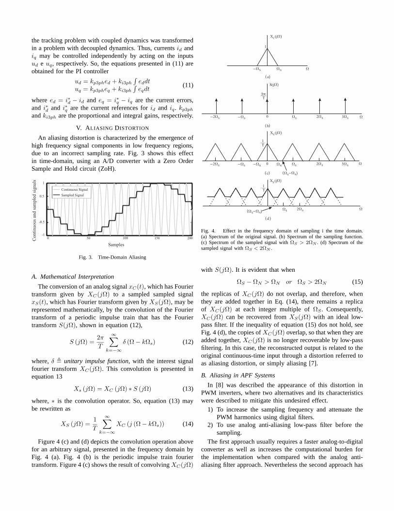
V. A LIASING DISTORTION

An aliasing distortion is characterized by the emergence ofhigh frequency signal components in low frequency regions,due to an incorrect sampling rate. Fig. 3 shows this effectin time-domain, using an A/D converter with a Zero OrderSample and Hold circuit (ZoH).

0 50 100 150 200-1

-0.5

0

0.5

1

Samples

Conti

nuous

and s

ample

d s

ignal

s

Continuous Signal

Sampled Signal

Fig. 3. Time-Domain Aliasing

A. Mathematical Interpretation

The conversion of an analog signalxC(t), which has Fouriertransform given byXC(jΩ) to a sampled sampled signalxS(t), which has Fourier transform given byXS(jΩ), may berepresented mathematically, by the convolution of the Fouriertransform of a periodic impulse train that has the FouriertransformS(jΩ), shown in equation (12),

S (jΩ) =2π

T

∞∑

k=−∞δ (Ω− kΩs) (12)

where,δ , unitary impulse function, with the interest signalfourier transformXC(jΩ). This convolution is presented inequation 13

Xs (jΩ) = XC (jΩ) ∗ S (jΩ) (13)

where,∗ is the convolution operator. So, equation (13) maybe rewritten as

XS (jΩ) =1T

∞∑

k=−∞XC (j (Ω− kΩs)) (14)

Figure 4 (c) and (d) depicts the convolution operation abovefor an arbitrary signal, presented in the frequency domain byFig. 4 (a). Fig. 4 (b) is the periodic impulse train fouriertransform. Figure 4 (c) shows the result of convolvingXC(jΩ)

Ω-Ω ΩN N

Ω-ΩS S2ΩS 3ΩS-2ΩS Ω0

X (jΩ)C

S(jΩ)

X (jΩ)S

X (jΩ)S

Ω-ΩS S2ΩS 3ΩS-2ΩS

Ω0

ΩS2ΩS Ω

Ω-ΩN N

ΩS-ΩN( )

ΩS-ΩN( )

d( )

c( )

b( )

a( )

1

2πT

T1

T1

Fig. 4. Effect in the frequency domain of sampling i the time domain.(a) Spectrum of the original signal. (b) Spectrum of the sampling function.(c) Spectrum of the sampled signal withΩS > 2ΩN . (d) Spectrum of thesampled signal withΩS < 2ΩN .

with S(jΩ). It is evident that when

ΩS − ΩN > ΩN or ΩS > 2ΩN (15)

the replicas ofXC(jΩ) do not overlap, and therefore, whenthey are added together in Eq. (14), there remains a replicaof XC(jΩ) at each integer multiple ofΩS . Consequently,XC(jΩ) can be recovered fromXS(jΩ) with an ideal low-pass filter. If the inequality of equation (15) dos not hold, seeFig. 4 (d), the copies ofXC(jΩ) overlap, so that when they areadded together,XC(jΩ) is no longer recoverable by low-passfiltering. In this case, the reconstructed output is related to theoriginal continuous-time input through a distortion referred toas aliasing distortion, or simply aliasing [7].

B. Aliasing in APF Systems

In [8] was described the appearance of this distortion inPWM inverters, where two alternatives and its characteristicswere described to mitigate this undesired effect.

1) To increase the sampling frequency and attenuate thePWM harmonics using digital filters.

2) To use analog anti-aliasing low-pass filter before thesampling.

The first approach usually requires a faster analog-to-digitalconverter as well as increases the computational burden forthe implementation when compared with the analog anti-aliasing filter approach. Nevertheless the second approach has

being not to much used because of the fact that the low-passfilter inserts additional dynamics in the loop. There was akind of compromise between mitigation of the high frequencyunwanted signals and the impact of the anti-aliasing filter overthe control system. But, there also wasn’t until today a worryconcerned to the low-pass filter project unless to the cut-offfrequency, chosen through the Nyquist criteria.

Therefore the text that follows is centered on the secondproject parameter of the analog anti-aliasing filter, the ”damp-ing factor”.

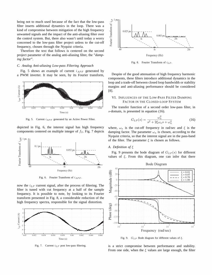
C. Analog Anti-aliasing Low-pass Filtering Approach

Fig. 5 shows an example of currentiAPF generated bya PWM inverter. It may be seen, by its Fourier transform,

0.05 0.052 0.054 0.056 0.058 0.06 0.062 0.064 0.066-6

-4

-2

0

2

4

6

Time (s)

i

C

urr

ent

(A)

AP

F

Fig. 5. CurrentiAPF generated by an Active Power Filter.

depicted in Fig. 6, the interest signal has high frequencycomponents centered on multiple integer offS . Fig. 7 depicts

1 pu

Frequency (Hz)

fs 2fs

fs

0.1 pu

0.052 pu

2fs

60

Fou

rier

Tra

nsfo

rm o

fi A

PF

Fig. 6. Fourier Transform ofiAPF .

now theiLP current signal, after the process of filtering. Thefilter is tuned with cut frequency at a half of the samplefrequency. It is possible to note, by looking to its Fouriertransform presented in Fig. 8, a considerable reduction of thehigh frequency spectra, responsible for the signal distortion.

0.05 0.052 0.054 0.056 0.058 0.06 0.062 0.064 0.066-6

-4

-2

0

2

4

6

Time (s)

i

C

urr

ent

(A)

LP

Fig. 7. CurrentiLP post low-pass filtering.

fs 2fs

Fou

rier

Tra

nsfo

rm o

fi

1 pu

Frequency (Hz)

60

fs

0.025 pu

0.003 pu2fs

LP

Fig. 8. Fourier Transform ofiLP .

Despite of the good attenuation of high frequency harmoniccomponents, these filters introduce additional dynamics in theloop and a trade-off between closed loop bandwidth or stabilitymargins and anti-aliasing performance should be considered[8].

VI. I NFLUENCES OF THELOW-PASS FILTER DAMPING

FACTOR IN THE CLOSED-LOOP SYSTEM

The transfer function of a second order low-pass filter, ins-domain, is presented in equation (16).

GLP (s) =ω2

n

s2 + 2ξωns + ω2n

(16)

where, ωn is the cut-off frequency in rad/sec andξ is thedamping factor. The parameterωn is chosen, according to theNyquist criteria, so that the interest signal are in the pass-bandof the filter. The parameterξ is chosen as follows.

A. Definition ofξ

Fig. 9 presents the bode diagram ofGLP (s) for differentvalues of ξ. From this diagram, one can infer that there

-60

-40

-20

0

20

40

Mag

nit

ude

(dB

)

103

104

105

106

-180

-135

-90

-45

0

Phas

e (d

eg)

Bode Diagram

Frequency (rad/sec)

ξ = 1.00ξ = 0.70ξ = 0.07ξ = 0.01

Fig. 9. GLP Bode diagram for different values ofξ.

is a strict compromise between performance and stability.From one side, when theξ values are large enough, the filter

dynamics have a great affect on the system, what can be seenthrough the phase deviation in the interest band. From theother side, decreasing the values ofξ, a resonance at thecut-off frequency comes on so a stability problem emerges.Nevertheless, for systems which the references also comesfrom measured signals, as in the case of the studied activepower filter, the system performance and stability issues haveto be differently analyzed.

Consider the whole APF model presented in Fig. 10 (a),which depicts the analogGLP (s) s-domain anti-aliasing filter,the Kalman filter block, the digitalGPI(Z) Z-domain PIcontroller and the analogGP (s) s-domain plant model. Asit can be seen, the low-pass filter is found at two positions(the reference and output signals are measured).

In order to have the control system expressed in a uniquedomain, see Fig. 10 (d), first of all, it is considered that Kalmanfilter extracts the references without inserting any dynamicsinto the system, so there is a reference signal in thes-domain,which is just affected by the anti-aliasing filter, as depictsFig. 10 (b). From Fig. 10 (b) to Fig. 10 (c) a block diagramproperty is used to consider the analog filter as part of thedirect loop. Finally, the PWM modulation followed by thecontrolled system plus the anti-aliasing transfer function andthe sample and hold circuit are replaced by itsZ-transform,GP GLP (Z) = Z(GP (s)GLP (s)).

G (s)LP

G (s)LP

G (Z)PI

G (s)P

KalmanFilter

R(s)G (s)

LPG (Z)

PI

G (Z)PI

G (s)P

R(Z) Y(Z)

R (Z) Y(s)PWM

(b)

(a)

c)(

KF

G (s)P

G (s)LP

Y(s)PWM

PWM

G (Z)PI

GP

R(Z) Y(Z)

d)(

G (Z)LP

G (s)LP

Y(s)

Fig. 10. Block diagram of the considered closed-loop system.

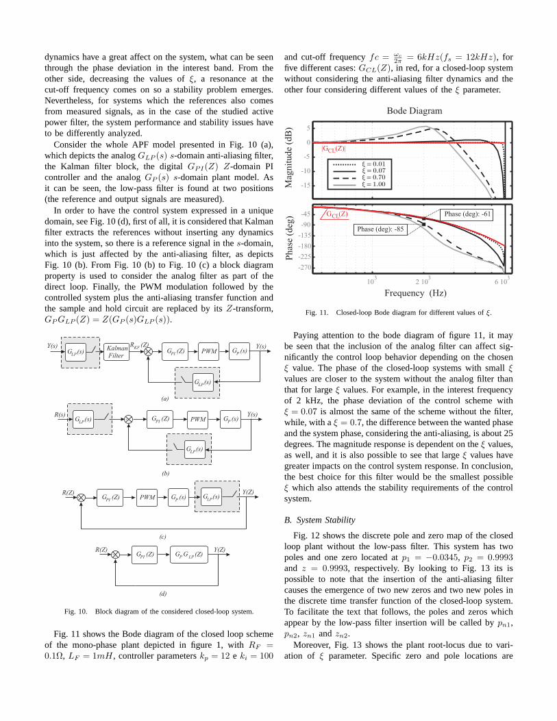
Fig. 11 shows the Bode diagram of the closed loop schemeof the mono-phase plant depicted in figure 1, withRF =0.1Ω, LF = 1mH, controller parameterskp = 12 e ki = 100

and cut-off frequencyfc = ωc

2π = 6kHz(fs = 12kHz), forfive different cases:GCL(Z), in red, for a closed-loop systemwithout considering the anti-aliasing filter dynamics and theother four considering different values of theξ parameter.

Mag

nit

ude

(dB

)P

has

e (d

eg)

Bode Diagram

Frequency (Hz)

|G (Z)|CL

-15

-10

-5

0

5

-270

-225

-180

-135

-90

-45

ξ = 1.00ξ = 0.70ξ = 0.07ξ = 0.01

103

6 103

G (Z)CL

Phase (deg): -85

2 103

Phase (deg): -61

Fig. 11. Closed-loop Bode diagram for different values ofξ.

Paying attention to the bode diagram of figure 11, it maybe seen that the inclusion of the analog filter can affect sig-nificantly the control loop behavior depending on the chosenξ value. The phase of the closed-loop systems with smallξvalues are closer to the system without the analog filter thanthat for largeξ values. For example, in the interest frequencyof 2 kHz, the phase deviation of the control scheme withξ = 0.07 is almost the same of the scheme without the filter,while, with aξ = 0.7, the difference between the wanted phaseand the system phase, considering the anti-aliasing, is about 25degrees. The magnitude response is dependent on theξ values,as well, and it is also possible to see that largeξ values havegreater impacts on the control system response. In conclusion,the best choice for this filter would be the smallest possibleξ which also attends the stability requirements of the controlsystem.

B. System Stability

Fig. 12 shows the discrete pole and zero map of the closedloop plant without the low-pass filter. This system has twopoles and one zero located atp1 = −0.0345, p2 = 0.9993and z = 0.9993, respectively. By looking to Fig. 13 its ispossible to note that the insertion of the anti-aliasing filtercauses the emergence of two new zeros and two new poles inthe discrete time transfer function of the closed-loop system.To facilitate the text that follows, the poles and zeros whichappear by the low-pass filter insertion will be called bypn1,pn2, zn1 andzn2.

Moreover, Fig. 13 shows the plant root-locus due to vari-ation of ξ parameter. Specific zero and pole locations are

pointed on that figure in order to explain some importantregions of the control system root-locus.

Real Axis

Imag

inar

yA

xis

-1 -0.5 0 0.5 1

-1

-0.8

-0.6

-0.4

-0.2

0

0.2

0.4

0.6

0.8

1

: -0.0345 : 0.9993: 0.9993

Pole-Zero Map

1p2p

z

Fig. 12. Pole and zero mapping closed-loop plant without anti-aliasing filter.

Firstly the zeros and poles, in red, are depicted to showthat, for to small values ofξ, the system is unstable, it isnoted through the polepn1 located outside the unit circle. Thealready existent plant zeros and poles located atp2 = 0.9993andz = 0.9993 does not change its location and the polep1 isreplaced fromp1 = −0.0345 to p1 = −0.00177. The barrierof stability is crossed whenξ ≈ 0.0005.

Real Axis

Root Locus

Imag

inar

yA

xis

-1 -0.5 0 0.5 1

-1

-0.8

-0.6

-0.4

-0.2

0

0.2

0.4

0.6

0.8

1

ξ = 1.00ξ = 0.07ξ = 0.04ξ = 0

Non minimum phase zero

-1

pn1 pn2

zn1 zn2

Fig. 13. Root locus of the closed loop system due to theξ variation

The second point, zero and poles in dashed gray, is catchedwhen theξ parameter is equal0.04. It is possible to verify thatthis system is now stable, there is a small contribution of theimaginary axis to the polespn1 andpn2, which are, followedby the zerozn1, tending to the center of the circle, while thezerozn2 is tending to left side. The existent polep1 also tendsto left side of the circle (p1 = −0.062).

Whenξ = 0.07, pn1, pn2 andzn1, in black, are still tendingto the center of the circle, but sinceξ ≈ 0.052 there is no more

contribution of the imaginary axis,zn2 is still tending to theleft, and the polep1 tending to right (p1 = −0.13).

When ξ = 1, see the zeros and poles in gray, the polesp1

and pn2 formed a complex conjugate pair of poles, tendingas shows Fig. 13.pn1 and zn1 keep tending to the center ofthe circle.zn1, which is outside the unit circle (non-minimumphase zero), is still tending to left. The barrier of minimumphase to non-minimum phase was broken whenξ ≈ 0.09 andthe boundary which separates the complex pair of poles isfound whenξ ≈ 0.101.

VII. S IMULATION RESULTS

The simulation of the mono-phase and three-phase/three-legs PWM inverters, depicted in Fig. 1 and 2 respectively, wasmade to verify the consistence of the developed approach. Thesimulation was carried out by using MATLABr and PSIMenvironments, which offer an advanced platform of functionsthat can be used to simulate the APF systems in study. Themono-phase load is as presented in section II and the three-phase load is presented at Fig. 14. Tab. I shows the projectparameters of both APF systems.

LL

RL

V1N

V2N

V3 N

3

Fig. 14. Load under study.

Table IPROJECTPARAMETERS

MONO-PHASE PLANT

Grid Voltage 127V (RMS) Rf 0.1Ω

ω 376.9911rad/s Lf 1mH

fs 12kHz Vdc 200V

LOAD

RL 30Ω LL 1mH

CL 75µF

CONTROLLER

kp1ph 20 ki1ph 100

THREE-PHASE PLANT

Grid Voltage 127V (RMS) Rf 0.1Ω

ω 376.9911rad/s Lf 1mH

fs 12kHz Vdc 350V

LOAD

RL 30Ω LL 50uH

CONTROLLER

kp3ph 1 ki3ph 10

Fig. 15 and 16 bellow depict, respective to the mono-phaseand three-phase cases, the current references,i∗F and i∗F1, theoutput currents,iF andiF1, and the compensated grid currents,iS and iS1: Fig. 15 and 16 (a) for a system without anti-aliasing filter; Fig. 15 and 16 (b) for a system with the lowpass filter tuned withξ = 0.03; Fig. 15 and 16 (c) present theresults for aξ = 0.07; Fig. 15 and 16 (d) show the case whenξ = 0.7; and, finally, Fig. 15 and 16 (d) present theξ = 1case.

-10

0

10

-10

0

10

-10

0

10

-10

0

10

0.034 0.036 0.038 0.04 0.042 0.044 0.046 0.048 0.05-10

0

10

ξ=

0.0

7ξ

= 0

.03

ξ=

0.7

ξ=

1W

ith

ou

tF

ilte

r

Reference Output Current Grid Current

Time (s)

(e)

(d)

(c

(b)

(a)

)

Fig. 15. Mono-phase case: References, outputs and compensated currentsfor different ξ values.

From the case without the filter it is possible to notethat sometimes the references outline the output signals, inother words, they have different fundamental currents in itsspectrum, what is one of the characteristics of the aliasingproblem in static converters. For aξ = 0.03, it is shownthat the output signals track the references, however, as theyhave poles in the imaginary axis near to the unit circle, theoutput signals oscillate around the references and the trackingperformance is harmed, specially in the three-phase case, asshows Fig. 16 (b). Withξ = 0.07 it is noted that thereis no more fundamental difference between reference andoutput, moreover the tracking performance is relatively good,presenting very small oscillations around the references. Whenξ = 0.7, there is a pair of complex conjugate poles (p1 andpn2) and one non-minimum phase zero (zn2) in the closed-loop transfer function, see Fig. 13. It makes the trackingperformance to be worst than the case forξ = 0.07 and itmay seen by the output current oscillations that arise aroundthe references. Finally, for aξ = 1, the system is not to muchaffected in comparison to theξ = 0.7 case, it is explained bythe fact of the zero and poles of the plant does not change

significantly its position in the complex plane so the result isa small difference between these two cases in respect to thetracking performance.

-10

0

10

-10

0

10

-10

0

10

-10

0

10

0.034 0.036 0.038 0.04 0.042 0.044 0.046 0.048 0.05-20

0

20

ξ=

0.0

7ξ

= 0

.03

ξ=

0.7

ξ=

1W

ith

ou

tF

ilte

r

Reference Output Current Grid Current

Time (s)

(e)

(d)

(b)

(a)

(c)

Fig. 16. Three-phase case: References, outputs and compensated currentsfor different ξ values.

VIII. C ONCLUSION

The paper has shown the effect of choosing different valuesfor the anti-aliasing filter damping factor parameter. By look-ing to the presented results, it is verified the importance of aright ξ choice because it influences directly on the closed loopsystem behavior. Paying attention to section IV, it is possible toconclude that there is an optimal region for theξ values, wherethe control response is not to much impacted. In the studiedcase, the optimalξ region is found in betweenξ = 0.052and ξ = 0.9, these points are considered as performanceboundaries based on the zero and pole placement.

Furthermore, in APF systems, in order to avoid problemsrelated with high harmonic signals coupled to the interestsignals, the data acquisition are often made in instants whenthere is no commutation of the switches, however it brings aproblem called by transport delay. As the low-pass filteringapproach attenuates reasonably the high frequency harmoniccontent of the signals and as the right projected low-pass filterdoes not insert significative dynamics to the whole system,the approach presented in this paper, may have its maincontribution as a step forward the mitigation of the transportdelay.

ACKNOWLEDGMENT

The authors would like to thank to CAPES, CNPq andFundacao Araucaria for the financial support.

REFERENCES

[1] A. E. Emanuel, J. A. Orr, D. Cyganski, and E. M. Gulachenski, “Asurvey of harmonic voltages and currents at distribution substations,”IEEE Transactions on Power Delivery, vol. v. 6, no. 4, pp. 1883–1890,Oct. 1991.

[2] P. Verdelho and G. D. Marques, “An active power filter and unbalancedcurrent compensator,”IEEE Transactions on Industrial Electronics, vol.v. 44, no. 3, pp. 321–328, Jun. 1997.

[3] H. Hellwig, “The importance of measurement in technology-basedcompetition,” IEEE Transactions on instrumentation and measurement,vol. 39, no. 5, pp. 685–688, October 1990.

[4] R. Cardoso, J. M. Kanieski, H. Pinheiro, and H. A. Grundling, “Referencegeneration for shunt active power filters based on optimum filteringtheory,” Industry Applications Conference, IAS Annual meetting, vol. 42,September 2007.

[5] B. Kedjar and K. Al-Haddad, “Dsp-based implementation of an lqr withintegral action for a three-phase three-wire shunt active power filter,”IEEE Trans. on Industrial Electronics, vol. 56, August 2009.

[6] R. Cardoso, “Algoritmos para sincronismo, analise da qualidade deenergia e geracao de referencias para filtros ativos de potencia: Umaabordagem estocastica,” Ph.D. dissertation, Universidade Federal de SantaMaria, 2008.

[7] A. V. Oppenheim, R. W. Schafer, and J. R. Buck,Discrete-Time SignalProcessing, 2nd ed., D. D. Pasquale, Ed. Prentice-Hall,Inc, 1998.

[8] H. Pinheiro, “On discrete controllers for static converters,”9th BrazilianPower Electronics Conference, vol. 1, 2007.