Influences of shifts in climate, landscape, and permafrost on terrestrial hydrology

Influences of shifts in climate, landscape, and permafroston terrestrial hydrology

Emma Bosson,1,2,3 Ulrika Sabel,4 Lars-Göran Gustafsson,4 Mona Sassner,4

and Georgia Destouni1,2

Received 20 June 2011; revised 19 January 2012; accepted 20 January 2012; published 9 March 2012.

[1] This study has simulated the terrestrial hydrology associated with different climate,landscape, and permafrost regime scenarios for the field case example of the relativelywell characterized coastal catchment of Forsmark, Sweden. The regime scenarios wereselected from long-term simulation results of climate, topographical, shoreline, andassociated Quaternary deposit and vegetation development in this catchment with a timeperspective of 100,000 years or more and were used as drivers for hydrological simulationswith the three-dimensional model MIKE SHE. The hydrological simulations quantifythe responses of different water flow and water storage components of terrestrial hydrologyto shifts from the present cool temperate climate landscape regime in Forsmark to apossible future Arctic periglacial landscape regime with or without permafrost. The resultsshow complexity and nonlinearity in the runoff responses to precipitation changes due toparallel changes in evapotranspiration, along with changes in surface and subsurfacewater storage dynamics and flow pathways through the landscape. The results furtherilluminate different possible perspectives of what constitutes wetter/drier landscapeconditions, in contrast to the clearer concept of what constitutes a warmer/colder climate.

Citation: Bosson, E., U. Sabel, L.-G. Gustafsson, M. Sassner, and G. Destouni (2012), Influences of shifts in climate, landscape,and permafrost on terrestrial hydrology, J. Geophys. Res., 117, D05120, doi:10.1029/2011JD016429.

1. Introduction

[2] Changes in the terrestrial water cycle are integral partsof ongoing climate change [Rodriguez-Iturbe et al., 2007;Bengtsson, 2010] and of climate-driven changes in the inlandcryosphere [Dyurgerov et al., 2010; Lyon and Destouni,2010; Frampton et al., 2011] and ecosystems [Hodkinsonet al., 1999; Rodriguez-Iturbe et al., 2009; Karlsson et al.,2011]. The climate-driven presence of and changes in per-mafrost may also influence hydrology, such as the seasonalvariability and amount of surface water discharge, and thesoil water–groundwater flow system above and below thepermafrost [Bense et al., 2009; Frampton et al., 2011]. Inaddition to climate change there are also other drivers forchanges in terrestrial hydrology, such as topography, andland-water cover and use changes. Topography dynamics,determined by erosion processes, and isostatic and eustaticchanges affect the networks of surface water drainage[Rinaldo et al., 1992; Tucker and Bras, 1998] and the con-ditions for groundwater flow [Lemieux et al., 2008]. Land

cover, and land and water use dynamics affect evapotrans-piration [Shibuo et al., 2007; Asokan et al., 2010] as well asregional climate [Boucher et al., 2004; Destouni et al., 2010;Degu et al., 2011] and atmospheric circulation [Lee et al.,2011].[3] Hence, the inland water integrates and further pro-

pagates and distributes the effects of different causes ofchange. It is then unclear what are the hydrological effectsof climate change and those of other, parallel changes. Toinvestigate, distinguish and quantify the drivers of differenthydrological changes, and not least those related to perma-frost change, the present study utilizes available results fromscenario simulations of the possible long-term climate, land-scape, and permafrost development in the catchment areaof Forsmark, situated on the Baltic Sea coast, approximately120 km north of Stockholm in central Sweden [SvenskKärnbränslehantering AB (SKB), 2010a, 2010b]. TheSwedish Nuclear Fuel and Waste Management Company(SKB) conducted these scenario simulations as part of theirsafety assessment of a geological storage concept for high-level nuclear waste, with Forsmark being the proposed finalrepository site for such waste in Sweden [SKB, 2011]. Thepresent study does not address the specific nuclear wasterepository problem but uses the reported simulation resultsof future climate-landscape-permafrost changes in Forsmark[SKB, 2010a, 2010b] as drivers in detailed hydrologicalmodeling with the general aim to understand, distinguish,and quantify the hydrological responses to the differentchange drivers.

1Department of Physical Geography and Quaternary Geology, StockholmUniversity, Stockholm, Sweden.

2Bert Bolin Centre for Climate Research, Stockholm University,Stockholm, Sweden.

3Swedish Nuclear Fuel and Waste Management Company, Stockholm,Sweden.

4DHI Sweden AB, Göteborg, Sweden.

Copyright 2012 by the American Geophysical Union.0148-0227/12/2011JD016429

JOURNAL OF GEOPHYSICAL RESEARCH, VOL. 117, D05120, doi:10.1029/2011JD016429, 2012

D05120 1 of 12

[4] The hydrological simulations in this study are carriedout with the distributed three-dimensional (3-D) modelMIKE SHE [Graham and Butts, 2005; Refsgaard et al.,2010] and with the current conditions and simulated futurescenarios of climate-landscape-permafrost states in Forsmark[SKB, 2010a, 2010b] as driving boundary conditions. Thedriving states differ in surface climate (surface temperatureand precipitation), subsurface climate (permafrost existenceand thickness), and landscape conditions (topography abovesea level and associated shoreline extent, Quaternary deposits,and vegetation). The main objective of the hydrologicalsimulations is to investigate and quantify the effects of thesedifferent driving states, and in particular to distinguish thepermafrost effects, on the different water flow and waterstorage components of the terrestrial water cycle in perma-frost environments.

2. Materials and Methods

2.1. The Forsmark Catchment and Climate-Landscape-Permafrost States[5] The Forsmark catchment has a flat topography, with the

present study area being almost entirely below 20 m abovethe present sea level (m asl). There are no major water-courses, and only small streams connect the lakes, which aregenerally small and shallow, in this coastal catchment. Fine-grained, low permeable sediments underlie most of the lakes.Approximately 70% of the catchment area is covered byforest, and till is the dominating type of the mostly shallowQuaternary deposits (QD). The site measurements indicate astrong correlation between surface topography and thegroundwater table in the QD and an anisotropic hydraulicconductivity in the till, with the vertical hydraulic conduc-tivity being generally smaller than the horizontal conductiv-ity and with a decrease in conductivity with depth. Graniticrock is the dominating bedrock type in the area. The upper!200 m of the bedrock is, in some areas within the catch-ment, highly fractured compared to the deeper bedrock.Horizontal sheet joints are present in the upper bedrock,which are interconnected hydraulically over long distances[Follin, 2008]. The horizontal hydraulic conductivity of thefractures/sheet joints in the upper bedrock is very high,leading to relatively fast, essentially horizontal groundwaterflow.[6] As the proposed final repository site for spent nuclear

fuel in Sweden, the hydrological state of the Forsmarkcatchment is well investigated and characterized under cur-rent climate and landscape conditions [Johansson, 2008;Johansson and Öhman, 2008; Jarsjö et al., 2008; Destouni

et al., 2008a]. However, the time perspective that must beconsidered in the safety assessment of such a repository is100 kyr and more into the future. Over this time the climate,as well as the landscape, and with them also the hydrologyand water-ice manifestations in the catchment will change.The landscape, for instance, will change as a net result ofboth isostatic and eustatic changes [Påsse, 2001; Brydstenand Strömgren, 2010]. To account for this and other changeaspects, SKB has conducted long-term scenario simulationsof future climate and landscape change in Forsmark; detaileddescriptions of these simulations are reported by SKB[2010b]. A basic reference scenario assumes then onlynatural climate variability and change, with no influencefrom human activity. This scenario is based on a simulatedrepetition of reconstructed climate conditions for the lastglacial cycle, and yields a first periglacial climate period withpermafrost occurring at Forsmark at around 10,000 AD[SKB, 2010b]. An alternative climate scenario considersalso effects of anthropogenic global warming and yields thefirst period of periglacial conditions occurring at around60,000 AD.[7] For the present study, scenario results with system-

atic differences in their surface climate (temperature andprecipitation), landscape and permafrost conditions wereselected from SKB’s different long-term change simulationsfor Forsmark [SKB, 2010a, 2010b]. This selection includes arange of different climate-landscape-permafrost states, fromthe present, cool temperate climate-landscape regime at theForsmark site, to potential future Arctic periglacial climate-landscape regimes, with or without continuous permafrostof various possible thickness (Table 1). The selection wasmade with regard to this study’s main objective to investi-gate and quantify the (separate and combined) climate-landscape-permafrost state effects on different water flow andwater storage components. The selected climate-landscape-permafrost scenarios were used as boundary and internalpermafrost conditions for hydrological simulations with thedistributed 3D hydrological model MIKE SHE [Graham andButts, 2005; Refsgaard et al., 2010], which includes bothgroundwater and surface water flow, and soil-atmosphereexchange of water (see further model description in theauxiliary material Text S1, section 1).1

2.2. Hydrological Simulations[8] Figure 1 shows the hydrological model area, which is

in total 180 km2, and the landscape conditions associated

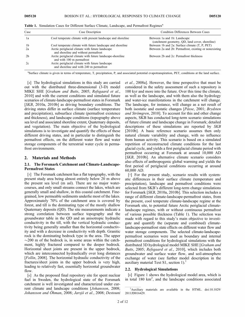
Table 1. Simulation Cases for Different Surface Climate, Landscape, and Permafrost Regimesa

Case Case Description Condition Differences Between Cases

1a Cool temperate climate with present landscape and shoreline Between 1a and 1b: Landscape(catchment geometry, QD, land cover, shoreline)

1b Cool temperate climate with future landscape and shoreline Between 1b and 2a: Surface climate (T, P, PET)2a Arctic periglacial climate with future landscape

and shoreline and without permafrostBetween 2a and 2b: Permafrost, existing or nonexisting

2b Arctic periglacial climate with future landscape-shorelineand with 100 m permafrost

Between 2b and 2c: Permafrost thickness

2c Arctic periglacial climate with future landscapeand shoreline and with 240 m permafrost

aSurface climate is given in terms of temperature, T, precipitation, P, and associated potential evapotranspiration, PET, conditions at the land surface.

1Auxiliary materials are available in the HTML. doi:10.1029/2011JD016429.

BOSSON ET AL.: HYDROLOGICAL RESPONSES TO CLIMATE CHANGE D05120D05120

2 of 12

with the different simulation cases in Table 1. Case 1aregards the present landscape and its shoreline, while allother cases regard the future landscape and its associatedshoreline [Påsse, 2001; Brydsten and Strömgren, 2010],developed QD (erosion and sedimentation processes) and landuse (e.g., lake terrestrialization) [Brydsten and Strömgren,2010], and vegetation with related model properties influ-encing evapotranspiration (ET) [Löfgren, 2010; Bosson et al.,2010].[9] When evaluating the results, and in the calculations of

water fractionation into different water balance componentsonly the part of the model area that constitutes land (green

for the present landscape, green and yellow for the futurelandscape in Figure 1) is considered in each case. In case 1aonly the mainland part (with land area of 34 km2) of theForsmark catchment is considered, i.e., the island (greencolor) to the right in Figure 1 is not a part of the resultevaluation. Currently, the dominating part of the model areais covered by the Baltic Sea (case 1a, with sea and islandarea of 146 km2), while in the future landscape cases(cases 1b–2c), large parts of the model area are locatedabove the present sea level (with land area of 178 km2,and sea area of 2 km2). The shoreline, i.e., the part of themodel land area that is exposed to the sea, is then 66 km in

Figure 1. The hydrological model area in cases 1a–2c (Table 1). In case 1a the green area is land and seacovers the remaining area. In cases 1b–2c the green and yellow areas are land, and sea covers only the bluearea part. The shoreline in case 1a is 66 km, and in cases 1b–2c it is only 8 km. The locations of throughtaliks in cases 2b and 2c are marked; the taliks in case 2c (permafrost thickness 240 m) are also taliks incase 2b (permafrost thickness 100 m).

BOSSON ET AL.: HYDROLOGICAL RESPONSES TO CLIMATE CHANGE D05120D05120

3 of 12

case 1a (only the mainland considered) whereas it is only8 km in the other cases.[10] To simulate the present hydrology at the site

(case 1a), the current cool temperate climate regime (withsurface temperature and precipitation as shown by red linesin Figure 2) was used as driver, and all relevant availabledata from the SKB site investigations were included in thesimulation and calibration, and the testing of the calibratedMIKE SHE model. The testing was made against indepen-dent data, not used in the calibration process, as described inmore detail by Bosson et al. [2008, 2010] (see also detaileddescription in Text S1, section 2). Generally, simulatedgroundwater and surface water levels, as well as surfacewater discharges agreed well with local measurements at thesite.[11] The model of the present hydrological state (case 1a)

was further used as initial condition for the simulation ofthe future regime scenarios (cases 1b–2c). In case 1b, thepresent cool temperate climate was used as driver, while apossible future Arctic periglacial surface climate was used

in cases 2a–2c; Figure 2 shows the characteristics of bothsurface climate regimes. The surface climate data used inthe MIKE SHE simulations are time varying T, P andpotential evapotranspiration (PET). Actual evapotranspira-tion, ET, and its different components (snow sublimation,interception, evaporation from soil and ponded water,transpiration) are calculated in the simulations.[12] For the hydrological simulations of the cool temperate

surface climate we used measured meteorological data from aselected year of the SKB site investigation period, consideredto represent the current long-term average situation at the site[Bosson et al., 2010]. The mean annual air temperature(MAAT) for the selected year of the current cool temperateclimate regime is +6.4°C and the annual P is 583 mm. Thecorresponding meteorological time series used to representthe possible future Arctic periglacial surface climate was thatsimulated for such a climate regime at Forsmark byKjellström et al. [2009], with resulting MAAT of "7°C andannual P of 412 mm. In all simulation cases, the representa-tive driving climatic year for each case was repeated until a

Figure 2. Time series of air temperature at the surface, T, precipitation, P, and P minus potential evapo-transpiration (P-ET) at the Forsmark site for the present cool temperate climate (driving cases 1a and 1b,Table 1) and the potential future Arctic periglacial climate (driving cases 2a–2c, Table 1). Statistics foreach climate regime are also given in terms of mean annual air temperature (MAAT), minimum and max-imum T, and annual precipitation, P.

BOSSON ET AL.: HYDROLOGICAL RESPONSES TO CLIMATE CHANGE D05120D05120

4 of 12

long-term annual hydrological steady state was reached. Thesimulation results for all cases 1a–2c are transient over theyear, and describe the seasonal and smaller temporal scaledynamics throughout the representative resulting hydrolog-ical year.[13] The offshore sea-covered areas in each simulation case

were accounted for by a prescribed time-varying hydraulichead, representative for the locally measured sea level fluc-tuations of today. The bottom boundary of the model domain,placed at 600 m depth below the present sea level, constituteda no flow boundary. The groundwater divides were assumedto coincide with the surface water divides, thus a no flowboundary was applied along the land parts of the modelboundary (catchment water divide), and a time varying headboundary, representing the sea level fluctuation, along theshoreline of each simulation case (Figure 1). In cases 1b–2c,representing a possible future landscape, the shoreline issituated at "31.42 m asl relative to today’s shoreline.

2.3. Permafrost Representation in the HydrologicalSimulations[14] Even though MIKE SHE does not support thermal

modeling, simulation scenarios were also set up to investi-gate the hydrological effects of the possible existence ofcontinuous permafrost with different thickness in cases 2band 2c. The approach to account for permafrost effects inMIKE SHE simulations has been described in more detail byBosson et al. [2010] and is shortly summarized here. Severalmodel parameters important for the description of freezeand thaw processes, as well as permafrost conditions, havebeen identified. Hydraulic properties are then chosen tomimic a low-permeable permafrost layer, with the hydraulicconductivities in both the saturated and unsaturated zonereduced so that water cannot infiltrate or flow through thepermafrost. The Manning number at the surface is furtherchanged so that water on the land surface becomes immobilewhen the air temperature is below 0°C.[15] In the present simulations, an active layer of 1 m depth

was assumed to overlie the permafrost, with its freezing andthawing depending on the weather conditions during theyear. The hydrological year was divided into seven parts,starting with two periods of freezing, when the hydraulicconductivity and other permafrost related parameters wereof the stepwise changed toward fully frozen conditions[Bosson et al., 2010]. These parameters values were appliedthroughout the frozen period, followed by three thawingperiods when the hydraulic conductivities were increased ina stepwise way toward representing unfrozen conditions,and finally, an entirely unfrozen period was simulated at theend of the hydrological year.[16] In case 2b, the thickness of the permafrost layer was

set to 100 m and in case 2c to 240 m. According to Forsmark-specific permafrost simulations for the SKB safety assess-ment [SKB, 2010b], with the same driving periglacial climateregime as in the present cases 2a–2c [Kjellström et al., 2009],the permafrost thickness for an average ground surface tem-perature of "4°C would be on the order of 240 m at theForsmark site, as assumed here in case 2c. The 100 m thickpermafrost case 2b is considered as an additional compara-tive case, in order to investigate the hydrological effects ofpermafrost thickness.

[17] Permafrost thickness influences in particular thepotential for through taliks, unfrozen areas in the permafrost[French, 2007], to form in the landscape. The thicker thepermafrost the fewer through taliks can be maintained, asreported for instance from Forsmark-specific, detailed per-mafrost simulations [SKB, 2006; Hartikainen et al., 2010].Site-specific simulations performed in particular to study therelation between lake geometry, permafrost thickness andtalik formation [SKB, 2006] considered two types of circularlakes with flat bathymetry as representative for (1) shallowlakes with bottom temperature above 0°C and (2) deep lakeswith bottom temperature above 4°C. The depth of the sim-ulated representative shallow lake was then set to 2 m andthe depth of the representative deep lake was set to 8 m. Inthe present study, the Forsmark-specific permafrost simula-tion results from SKB [2006] were used so that lakes withmean depth of 0.5–4 m were considered as shallow (bottomtemperature above 0°C for the Arctic periglacial climatewith MAAT of "7°C), and lakes with mean depth >4 mwere considered as deep (bottom temperature above 4°Cunder the periglacial climate). SKB [2006] showed that athrough talik can develop beneath the lakes if (1) the radiusof a shallow lake (with its surface area interpreted as a circle)exceeded the thickness of the surrounding permafrost and(2) the radius of a deep lake (interpreted as for a shallowlake) was !0.6 times the thickness of the surroundingpermafrost.[18] If a lake in the case 1b landscape fulfilled condition 1

or 2 relative to the different permafrost thickness in cases 2band 2c, an unfrozen column was simulated in the QD andbedrock under the lake to represent a talik. These talik for-mation conditions in the MIKE SHE modeling of Forsmarkhave also been used and described previously by Bossonet al. [2010, Appendix 1]. The area under the sea bay wasassumed unfrozen; that is, the hydraulic properties for seabottom sediments and underlying bedrock were kept thesame in cases 2b and 2c as in case 2a.

3. Results

[19] Table 2 summarizes some mean annual hydrologicalresults for all simulation cases (as outlined in Table 1), whileFigure 1 shows the resulting number of through taliks inthe permafrost cases 2b and 2c. In the following, we discussthe results further in relation to different water storage andwater flow components, and their dynamics over an averageyear at the different climate, landscape and permafrost statesrepresented by the different simulation cases.

3.1. Water in the Landscape[20] Table 2 shows that the landscape shift from case 1a to

case 1b decreases the relative lake and wetland area in thelandscape from 15% to 13.1%. The added shifts in climateand permafrost, from case 1b to cases 2a, 2b, and 2c, thenincrease the surface water area up to a range of 16–18.5%,with the higher values applying to the permafrost cases 2band 2c (Table 2).[21] Regarding the climate shift from case 1b to case 2a,

the mean surface temperature (T) clearly determines case 2aas representing a colder climate than case 1b. However, withregard to water, case 2a could be viewed as both wetter and

BOSSON ET AL.: HYDROLOGICAL RESPONSES TO CLIMATE CHANGE D05120D05120

5 of 12

drier than case 1b. There are multiple hydrological para-meters that determine different wetness and dryness aspects,with complex relations between them. Case 2a has greatersurface water storage (in lakes and wetlands), as well asgreater mean annual runoff (R) than case 1b, mainly due tothe smaller mean annual evapotranspiration (ET), both inabsolute terms and in relation to P, in case 2a than in case 1b(Table 2). The greater P and ET fluxes, which link thelandscape and atmospheric water, may be a basis for con-sidering case 1b as wetter than case 2a from an atmosphericperspective. The greater water storage (lakes and wetlands)and R in 2a, however, mean that this case can be viewed aswetter than 1b from a landscape perspective.[22] The surface water storage in lakes and wetlands, and

R are even greater in the permafrost cases 2b and 2c than inthe nonpermafrost case 2a. This is both because ET issmaller and because less water can infiltrate due to the per-mafrost, with more water then remaining at the ground sur-face, in cases 2b and 2c than in case 2a. The two permafrostcases 2b and 2c, with essentially the same P, ET, R and meanannual groundwater recharge (Rgw), but different permafrostthickness, have similar surface water storage in lakes andwetlands (17.9–18.5%). The main permafrost thickness effectis to regulate the number of through taliks, and through themthe amount and direction of water exchange between thesurface and the deeper groundwater under the permafrost.The total net flow contribution through the inland throughtaliks is then a relatively small (about 1 mm in 2b and 0.1 mmin 2c) net recharge flux into the deep groundwater below thepermafrost. This contribution is greater in 2b because it hasmore inland through taliks than 2c (Figure 1). The inlandsurface water bodies that form through taliks in case 2b arealso present at the land surface in case 2c, but they do not in 2c,with its thicker permafrost, fulfill the conditions for throughtalik formation. Also the sea bay constitutes a through talikin the permafrost simulation cases 2b and 2c, yielding atotal net discharge flux contribution (of about 1 mm in 2band 0.1 mm in 2c) from the deep groundwater to the sea.

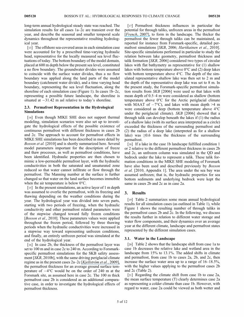
3.2. Water Storage Dynamics[23] Regarding the temporal pattern of both surface and

subsurface water storage dynamics, Figure 3 (top) showsthat it is essentially the same for the different landscapes ofthe two warmer climate cases, 1a and 1b. Groundwaterstorage increases during the autumn rains, with increasinggroundwater table and saturated zone (SZ) extent, and cor-respondingly decreasing unsaturated zone (UZ) extent, as

consequences. Also the surface water storage increasessomewhat during this period. In spring, after the snowmelt,the groundwater storage and level decrease again and theUZ (SZ) extent increases (decreases), primarily due toincreasing ET as the vegetation grows.[24] The main water storage effect of the landscape shift

from case 1a to case 1b is that the autumn increase ingroundwater (SZ) storage is smaller in 1b, and as a conse-quence the groundwater table is lower during the wholeperiod October–June in case 1b than in case 1a. The changein groundwater storage over the year is then also smaller incase 1b, even though Rgw is somewhat greater in this casethan in case 1a (Table 2).[25] Comparison between Figure 3 (top) and Figure 3

(bottom) shows that the shift in surface climate from case 1bto case 2a fundamentally changes the seasonal pattern ofwater storage dynamics. The low temperatures during autumnand winter in case 2a lead to continuous snow accumulationfrom October to the end of April. The groundwater level andstorage, and the associated SZ and UZ extents are almostconstant over this period, and exhibit only relatively smallchanges in response to the snowmelt in spring. The surfacewater storage exhibits greater increase in response to thesnowmelt.[26] The presence of permafrost in cases 2b and 2c has

some, relatively small influence on the water storagedynamics, regarding details in the UZ and SZ relation aftersnowmelt compared to the corresponding nonpermafrostcase 2a. Since the active layer is only 1 m thick in the presentpermafrost case simulations, and no water can infiltrate belowthis level, the available depth extent for UZ and correspondingSZ/groundwater storage changes are quite limited in cases 2band 2c. The active layer becomes fully saturated much faster,almost directly after the snowmelt starts, and the surfacewater storage exhibits a larger snowmelt response in cases 2band 2c than in case 2a. Less water can infiltrate and morewater is therefore present at the ground surface, which con-tributes to the greater lake and wetland area in cases 2b and2c than in case 2a (Table 2). However, the permafrostthickness (case 2b or 2c) has no water storage influence.

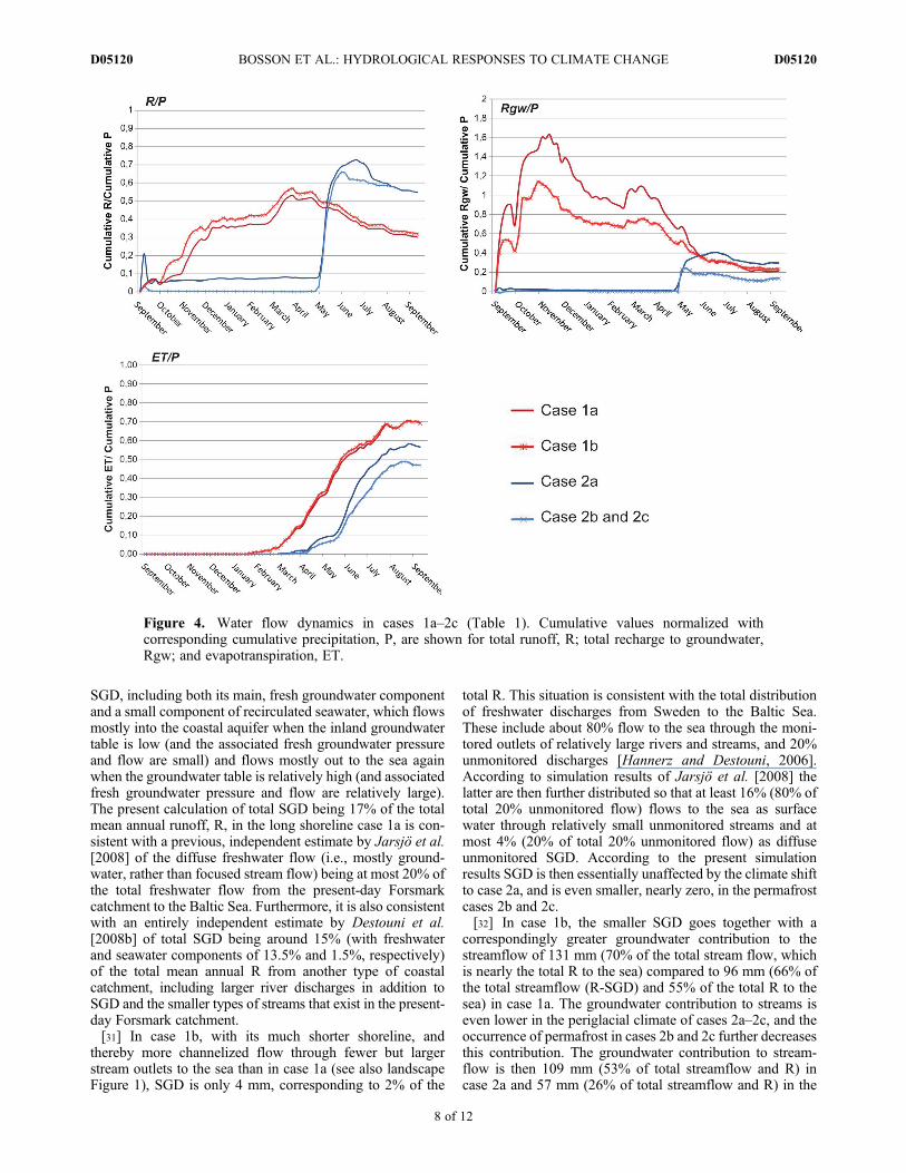
3.3. Water Flux Partitioning at the Land Surface[27] Figure 4 shows that the transience of the main water

fluxes ET, R and Rgw, and their partitioning at the landsurface over the year are strongly influenced by the climateshift from cases 1a and 1b to cases 2a–2c. The main differencebetween the cases is due to the larger snow accumulation

Table 2. Driving Climate and Resulting Hydrological Variables for the Simulation Cases in Table 1a

Case

Climate Conditions Water in Landscapeas Percent Wetlands

and Lakesb

Absolute Hydrological FlowsRelative Hydrological

Coefficients

T (°C) PET (mm/yr) P (mm/yr) ET (mm/yr) R (mm/yr) Rgw (mm/yr) ET/P R/P Rgw/P

1a 6.4 420 583 15 405 175 124 0.69 0.30 0.211b 6.4 420 583 13.1 403 186 136 0.69 0.32 0.232a "7 216 412 16 211 204 109 0.51 0.50 0.262b "7 216 412 18.5 194 217 56 0.47 0.53 0.142c "7 216 412 17.9 193 217 55 0.47 0.53 0.13

aThe listed variables are temperature, T; potential evapotranspiration, PET; precipitation, P; evapotranspiration, ET; runoff, R; and groundwater rechargeRgw. The percent values for wetlands and lakes refer to their surface area in relation to the total land area.

bWater in storage is at the end of each simulation, when the storage change is zero. Wetlands are areas with surface water depth (D) 0.01 m " D < 0.3 m,and lakes are areas with surface water depth (D) D ! 0.3 m.

BOSSON ET AL.: HYDROLOGICAL RESPONSES TO CLIMATE CHANGE D05120D05120

6 of 12

over a much longer period of time in the periglacial climateof cases 2a–2c than in the cool temperate climate of cases 1aand 1b. In cases 2a–2c, it is mainly only after the snow hasmelted in May that water becomes available for flow by ET,R and Rgw. The rate of snowmelt exceeds then largely thesoil infiltration capacity and water flows mostly out fromthe catchment in more or less equal amounts by ET and Rin the colder climate cases 2a–2c, whereas the outflow byET is about twice that by R in the warmer climate cases 1aand 1b.[28] Also the mean (and total cumulative) annual ET – both

in absolute terms and relative to P –shifts mainly due to theshift in climate from case 1b to case 2a (Table 2 andFigure 4). In contrast, the absolute mean (and total cumu-lative) R shifts more or less similarly in all case shifts, butthe relative runoff coefficient R/P shifts mostly, as doesET/P, in the climate shift from case 1b to case 2a. Themean (and cumulative) annual Rgw, however, shifts mostconsiderably (decreasing) in the permafrost shift from case2a to cases 2b and 2c, even though it is to somewhat smallerdegree also affected by the climate shift from 1b to 2a(decreasing Rgw), and the landscape shift from 1a to 1b case

(increasing Rgw). However, the shift in permafrost thick-ness between 2b and 2c does not affect Rgw much.[29] Regarding the 192 mm smaller ET output flux in

case 2a than in case 1b, most of the difference is due tothe 171 mm smaller P input flux in 2a than in 1b, whilethe remaining 21 mm difference is due to the much longerperiod with snow, which allows less time for relativelyhigh ET to occur in 2a than in 1b. The 21 mm smaller netoutput flux, ET-P, implies that so much more water is thenavailable for R, which is also about that much greater (18 mm)in case 2a than in case 1b.

3.4. Pathways of Water Flow Through the Landscapeto the Sea[30] Figure 5 shows that the change in landscape from

case 1a to case 1b notably affects the distribution ofpathways followed by different parts of the total runoff, R,to the sea. In case 1a, with its long shoreline and associatedlarge exposure to the sea, about 30 mm of water (17% oftotal R) leaves the model area and flows into the sea assubmarine groundwater discharge, SGD, occurring mostly inthe uppermost QD layers. This quantification regards total

Figure 3. Water storage dynamics in cases 1a–2c. The snow storage, the subsurface storage in theunsaturated zone, UZ, and as groundwater in the saturated zone, SZ; and the surface water storage areshown as cumulative values. Cases 2b and 2c exhibit the same results, and only case 2b is shown.

BOSSON ET AL.: HYDROLOGICAL RESPONSES TO CLIMATE CHANGE D05120D05120

7 of 12

SGD, including both its main, fresh groundwater componentand a small component of recirculated seawater, which flowsmostly into the coastal aquifer when the inland groundwatertable is low (and the associated fresh groundwater pressureand flow are small) and flows mostly out to the sea againwhen the groundwater table is relatively high (and associatedfresh groundwater pressure and flow are relatively large).The present calculation of total SGD being 17% of the totalmean annual runoff, R, in the long shoreline case 1a is con-sistent with a previous, independent estimate by Jarsjö et al.[2008] of the diffuse freshwater flow (i.e., mostly ground-water, rather than focused stream flow) being at most 20% ofthe total freshwater flow from the present-day Forsmarkcatchment to the Baltic Sea. Furthermore, it is also consistentwith an entirely independent estimate by Destouni et al.[2008b] of total SGD being around 15% (with freshwaterand seawater components of 13.5% and 1.5%, respectively)of the total mean annual R from another type of coastalcatchment, including larger river discharges in addition toSGD and the smaller types of streams that exist in the present-day Forsmark catchment.[31] In case 1b, with its much shorter shoreline, and

thereby more channelized flow through fewer but largerstream outlets to the sea than in case 1a (see also landscapeFigure 1), SGD is only 4 mm, corresponding to 2% of the

total R. This situation is consistent with the total distributionof freshwater discharges from Sweden to the Baltic Sea.These include about 80% flow to the sea through the moni-tored outlets of relatively large rivers and streams, and 20%unmonitored discharges [Hannerz and Destouni, 2006].According to simulation results of Jarsjö et al. [2008] thelatter are then further distributed so that at least 16% (80% oftotal 20% unmonitored flow) flows to the sea as surfacewater through relatively small unmonitored streams and atmost 4% (20% of total 20% unmonitored flow) as diffuseunmonitored SGD. According to the present simulationresults SGD is then essentially unaffected by the climate shiftto case 2a, and is even smaller, nearly zero, in the permafrostcases 2b and 2c.[32] In case 1b, the smaller SGD goes together with a

correspondingly greater groundwater contribution to thestreamflow of 131 mm (70% of the total stream flow, whichis nearly the total R to the sea) compared to 96 mm (66% ofthe total streamflow (R-SGD) and 55% of the total R to thesea) in case 1a. The groundwater contribution to streams iseven lower in the periglacial climate of cases 2a–2c, and theoccurrence of permafrost in cases 2b and 2c further decreasesthis contribution. The groundwater contribution to stream-flow is then 109 mm (53% of total streamflow and R) incase 2a and 57 mm (26% of total streamflow and R) in the

Figure 4. Water flow dynamics in cases 1a–2c (Table 1). Cumulative values normalized withcorresponding cumulative precipitation, P, are shown for total runoff, R; total recharge to groundwater,Rgw; and evapotranspiration, ET.

BOSSON ET AL.: HYDROLOGICAL RESPONSES TO CLIMATE CHANGE D05120D05120

8 of 12

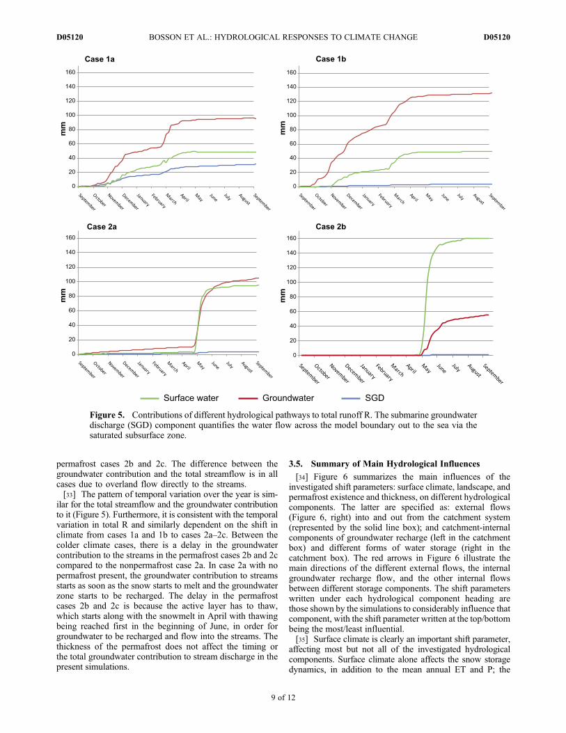
permafrost cases 2b and 2c. The difference between thegroundwater contribution and the total streamflow is in allcases due to overland flow directly to the streams.[33] The pattern of temporal variation over the year is sim-

ilar for the total streamflow and the groundwater contributionto it (Figure 5). Furthermore, it is consistent with the temporalvariation in total R and similarly dependent on the shift inclimate from cases 1a and 1b to cases 2a–2c. Between thecolder climate cases, there is a delay in the groundwatercontribution to the streams in the permafrost cases 2b and 2ccompared to the nonpermafrost case 2a. In case 2a with nopermafrost present, the groundwater contribution to streamsstarts as soon as the snow starts to melt and the groundwaterzone starts to be recharged. The delay in the permafrostcases 2b and 2c is because the active layer has to thaw,which starts along with the snowmelt in April with thawingbeing reached first in the beginning of June, in order forgroundwater to be recharged and flow into the streams. Thethickness of the permafrost does not affect the timing orthe total groundwater contribution to stream discharge in thepresent simulations.

3.5. Summary of Main Hydrological Influences[34] Figure 6 summarizes the main influences of the

investigated shift parameters: surface climate, landscape, andpermafrost existence and thickness, on different hydrologicalcomponents. The latter are specified as: external flows(Figure 6, right) into and out from the catchment system(represented by the solid line box); and catchment-internalcomponents of groundwater recharge (left in the catchmentbox) and different forms of water storage (right in thecatchment box). The red arrows in Figure 6 illustrate themain directions of the different external flows, the internalgroundwater recharge flow, and the other internal flowsbetween different storage components. The shift parameterswritten under each hydrological component heading arethose shown by the simulations to considerably influence thatcomponent, with the shift parameter written at the top/bottombeing the most/least influential.[35] Surface climate is clearly an important shift parameter,

affecting most but not all of the investigated hydrologicalcomponents. Surface climate alone affects the snow storagedynamics, in addition to the mean annual ET and P; the

Figure 5. Contributions of different hydrological pathways to total runoff R. The submarine groundwaterdischarge (SGD) component quantifies the water flow across the model boundary out to the sea via thesaturated subsurface zone.

BOSSON ET AL.: HYDROLOGICAL RESPONSES TO CLIMATE CHANGE D05120D05120

9 of 12

relatively small evaporation from snow is illustrated with adashed red arrow in Figure 6. Landscape alone, and in par-ticular its shoreline length, affects mostly the SGD pathway,and through that the general distribution of freshwater path-ways to the sea.[36] The SGD, which can be relatively large in catchments

with long shorelines, bypasses entirely the surface waterpathway to the sea and SGD quantification is difficult[Prieto and Destouni, 2011]. The present results clarify thewater balance links between the different flow pathwaysto the sea, which can be used for bounding SGD quan-tifications. In general, consideration of water balances onproblem-relevant catchment scales can bound and provideimportant reality checks for both historic reconstructions andfuture projections of hydrological flows and their changes ina changing climate [Shibuo et al., 2007; Destouni et al.,2010; Asokan et al., 2010; Jarsjö et al., 2011]. The presentresults emphasize that such checks must also account forthe subsurface components and surface-subsurface links ofterrestrial water change.[37] Surface (lake-wetland) and subsurface (UZ-SZ) water

storage, groundwater recharge (Rgw), and total runoff (R)with its different pathway components all collect, integrate,and through their changes propagate further through thelandscape the effects of different shift parameters. Amongthese, not only the surface but also the subsurface climate,expressed here in terms of permafrost existence (as perma-frost thickness was found to have only small effect on the

investigated hydrological components), is an essential con-trol parameter for terrestrial hydrology.

4. Conclusion

[38] This study has distinguished and quantified separateand combined influences of surface climate, landscape andpermafrost conditions on different water flow and water stor-age components, through a scenario simulation and analysisapproach applied to the Swedish Forsmark catchment area.The latter represents a relatively well characterized field caseexample. The results show complexity in the connectionsbetween different hydrological flow and storage components,and as a consequence in the responses of these components toshifts in climate, landscape and permafrost regimes. Forinstance, both R and water storage may increase in a catch-ment where P decreases if ET decreases even more than P.[39] Nonintuitive R responses to P change have been found

in different studies of hydroclimatic change, for catchmentsof different scales and in different parts of the world.Reported earlier findings include R change in the oppositedirection than P due to concurrent natural or anthropogenicET changes [Shibuo et al., 2007], in the same direction butconsiderably more than P due to concurrent water storagechanges, e.g., in the terrestrial cryosphere [Bring andDestouni, 2011], or entirely unrelated to P change due tovarious parallel land and water use changes on differentunresolved local regional scales [Koutsouris et al., 2010].

Figure 6. The influence of investigated shift parameters on different hydrological components. The shiftparameters are landscape, surface climate, and permafrost (PF) existence and thickness (Table 1).The hydrological components are external flows (right side) into and out from the catchment system(represented by the solid line box); and catchment-internal groundwater recharge (left in the catchment box)and different forms of water storage (right in the catchment box). The red arrows show the main flowdirections. The shift parameters under each hydrological component heading are those influencing thatcomponent, with that at the top/bottom being the most/least influential.

BOSSON ET AL.: HYDROLOGICAL RESPONSES TO CLIMATE CHANGE D05120D05120

10 of 12

Hence, linear assumptions of a projected P increase(decrease) leading directly to correspondingly wetter (drier)landscape conditions may in many cases be too simplistic.[40] Furthermore, the present results show that the defini-

tion of what actually constitutes a wetter or drier climate ina landscape may be problematic. Specifically, for smaller Pand ET, which may be viewed as drier conditions from anatmospheric perspective, the present simulations yieldedgreater R and surface water extent, which may be viewed aswetter conditions from a landscape perspective. Projectionsand assessments of climate-driven water changes must con-sider such different perspectives and their implications forwhat water changes society should expect and try to mitigateor adapt to.[41] Landscape changes can further affect the shoreline-

dependent SGD, which links to another water perspectiveproblem: highly different SGD quantifications are reportedfrom inland-based (hydrological) and marine-based SGDestimation methodologies [Prieto and Destouni, 2011]. Thepresent results are consistent with other hydrological SGDquantifications, and further emphasize the need to seriouslyconsider the SGD quantification gaps and allocate relevantresearch efforts toward bridging them. In general, the resultsof this study have illuminated the need to account for andlink subsurface hydrology, and not least its permafrostcomponent in cold regions, to changes at the surface in orderto accurately understand and assess hydrological changepropagation through the whole inland water system.

[42] Acknowledgment. G.D. acknowledges financial support fromthe Swedish Research Council (VR; project 311-2007-8393, contract70839301).

ReferencesAsokan, S. M., J. Jarsjö, and G. Destouni (2010), Vapor flux by evapo-transpiration: Effects of changes in climate, land use, and water use,J. Geophys. Res., 115, D24102, doi:10.1029/2010JD014417.

Bengtsson, L. (2010), The global atmospheric water cycle, Environ. Res.Lett., 5, 025202, doi:10.1088/1748-9326/5/2/025202.

Bense, V. F., G. Ferguson, and H. Kooi (2009), Evolution of shallowgroundwater flow systems in areas of degrading permafrost, Geophys.Res. Lett., 36, L22401, doi:10.1029/2009GL039225.

Bosson, E., L. G. Gustafsson, and M. Sassner (2008), Numerical modellingof surface hydrology and near-surface hydrogeology at Forsmark: Sitedescriptive modelling, SDM-site Forsmark, SKB Rapp. 08-09, Sven.Kärnbränslehantering AB, Stockholm.

Bosson, E., M. Sassner, U. Sabel, and L. G. Gustafsson (2010), Modellingof present and future hydrology and solute transport at Forsmark, SR-site biosphere, SKB Rapp. 10-20, Sven. Kärnbränslehantering AB,Stockholm.

Boucher, O., G. Myhre, and A. Myhre (2004), Direct human influenceof irrigation on atmospheric water vapor and climate, Clim. Dyn., 22,597–603, doi:10.1007/s00382-004-0402-4.

Bring, A., and G. Destouni (2011), Relevance of hydro-climatic changeprojection and monitoring for assessment of water cycle changes in theArctic, Ambio, 40, 361–369, doi:10.1007/s13280-010-0109-1.

Brydsten, L., and M. Strömgren (2010), A coupled regolith-lake develop-ment model applied to the Forsmark site, Tech. Rep. Sven. Kaernbraen-slehantering AB, TR-10-56, 49 pp.

Degu, A. M., F. Hossain, D. Niyogi, R. Pielke, J. M. Shepherd, N. Voisin,and T. Chronis (2011), The influence of large dams on surrounding climateand precipitation patterns, Geophys. Res. Lett., 38, L04405, doi:10.1029/2010GL046482.

Destouni, G., Y. Shibuo, and J. Jarsjö (2008a), Freshwater flows to thesea: Spatial variability, statistics and scale dependence along coastlines,Geophys. Res. Lett., 35, L18401, doi:10.1029/2008GL035064.

Destouni, G., F. Hannerz, C. Prieto, J. Jarsjö, and Y. Shibuo (2008b), Smallunmonitored near-coastal catchment areas yielding large mass loadingto the sea, Global Biogeochem. Cycles, 22, GB4003, doi:10.1029/2008GB003287.

Destouni, G., S. M. Asokan, and J. Jarsjö (2010), Inland hydro-climaticinteraction: Effects of human water use on regional climate, Geophys.Res. Lett., 37, L18402, doi:10.1029/2010GL044153.

Dyurgerov, M., A. Bring, and G. Destouni (2010), Integrated assessment ofchanges in freshwater inflow to the Arctic Ocean, J. Geophys. Res., 115,D12116, doi:10.1029/2009JD013060.

Follin, S. (2008), Bedrock hydrogeology Forsmark: Site descriptive model-ling, SDM-site Forsmark, SKB Rapp. 08-95, Sven. KärnbränslehanteringAB, Stockholm.

Frampton, A., S. Painter, S. W. Lyon, and G. Destouni (2011), Non-isothermal, three-phase simulations of near-surface flows in a modelpermafrost system under seasonal variability and climate change,J. Hydrol., 403, 352–359, doi:10.1016/j.jhydrol.2011.04.010.

French, H. M. (2007), The Periglacial Environment, 3rd ed., John Wiley,Chichester, U. K.

Graham, D. N., and M. B. Butts (2005), Flexible, integrated watershedmodelling with MIKE SHE, in Watershed Models, edited by V. P. Singhand D. K. Frevert, pp. 245–272, CRC Press, Boca Raton, Fla.

Hannerz, F., and G. Destouni (2006), Spatial characterization of theBaltic Sea drainage basin and its unmonitored catchments, Ambio,35, 214–219, doi:10.1579/05-A-022R.1.

Hartikainen, J., R. Kouhia, and T. Wallroth (2010), Permafrost simulationsat Forsmark using a numerical 2D thermo-hydro-chemical model, Tech.Rep. Sven. Kaernbraenslehantering AB, TR-09-17, 142 pp.

Hodkinson, I. D., N. R. Webb, J. S. Bale, and W. Block (1999), Hydrology,water availability and tundra ecosystem function in a changing climate:The need for a closer integration of ideas?, Global Change Biol., 5,359–369, doi:10.1046/j.1365-2486.1999.00229.x.

Jarsjö, J., Y. Shibuo, and G. Destouni (2008), Spatial distribution ofunmonitored inland water discharges to the sea, J. Hydrol., 348, 59–72,doi:10.1016/j.jhydrol.2007.09.052.

Jarsjö, J., S. M. Asokan, C. Prieto, A. Bring, and G. Destouni (2011),Hydrological responses to climate change conditioned by historic altera-tions of land-use and water-use, Hydrol. Earth Syst. Sci. Discuss., 8, 1–26,doi:10.5194/hessd-8-1-2011.

Johansson, P. O. (2008), Description of surface hydrology and near surfacehydrogeology at Forsmark: Site descriptive modelling, SDM-site Forsmark,SKB Rapp. 08-08, Sven. Kärnbränslehantering AB, Stockholm.

Johansson, P. O., and J. Öhman (2008), Presentation of meteorological,hydrological and hydrogeological monitoring data from Forsmark: Sitedescriptive modelling, SDM-site Forsmark, SKB Rapp. 08-10, Sven.Kärnbränslehantering AB, Stockholm.

Karlsson, M. J., A. Bring, G. D. Peterson, L. J. Gordon, and G. Destouni(2011), Opportunities and limitations to detect climate-related regimeshifts in inland Arctic ecosystems through eco-hydrological monitoring,Environ. Res. Lett., 6, 014015, doi:10.1088/1748-9326/6/1/014015.

Kjellström, E., G. Strandberg, J. Brandefelt, J. O. Näslund, B. Smith, andB. Wohlfarth (2009), Climate conditions in Sweden in a 100,000-yeartime perspective, Tech. Rep. Sven. Kaernbraenslehantering AB, TR-09-04,140 pp.

Koutsouris, A. J., G. Destouni, J. Jarsjö, and S. W. Lyon (2010), Hydro-climatic trends and water resource management implications based onmulti-scale data for the Lake Victoria region, Kenya, Environ. Res.Lett., 5, 034005, doi:10.1088/1748-9326/5/3/034005.

Lee, E., W. J. Sacks, T. N. Chase, and J. A. Foley (2011), Simulatedimpacts of irrigation on the atmospheric circulation over Asia, J. Geo-phys. Res., 116, D08114, doi:10.1029/2010JD014740.

Lemieux, J. M., E. A. Sudicky, W. R. Peltier, and L. Tarasov (2008), Simu-lating the impact of glaciations on continental groundwater flow systems:2. Model application to the Wisconsinian glaciation over the Canadianlandscape, J. Geophys. Res., 113, F03018, doi:10.1029/2007JF000929.

Löfgren, A. (Ed.) (2010), The terrestrial ecosystems at Forsmark andLaxemar-Simpevarp: SR-site biosphere, Tech. Rep. Sven. Kaernbraen-slehantering AB, TR-10-01, 434 pp.

Lyon, S., and G. Destouni (2010), Changes in catchment-scale recessionflow properties in response to permafrost thawing in the Yukon RiverBasin, Int. J. Climatol., 30, 2138–2145, doi:10.1002/joc.1993.

Påsse, T. (2001), An empirical model of glacio-isostatic movements andshore-level displacement in Fennoscandia, SKB Rapp. 01-41, Sven.Kärnbränslehantering AB, Stockholm.

Prieto, C., and G. Destouni (2011), Is submarine groundwater discharge pre-dictable?, Geophys. Res. Lett., 38, L01402, doi:10.1029/2010GL045621.

Refsgaard, J. C., B. Storm, and T. Clausen (2010), Systèm HydrologiqueEuropeén (SHE): Review and perspectives after 30 years developmentin distributed physically-based hydrological modeling, Hydrol. Res., 41,355–377, doi:10.2166/nh.2010.009.

Rinaldo A., I. Rodriguez-Iturbe, R. Rigon, R. L. Bras, E. Ijjaszvasquez,and A. Marani (1992), Minimum energy and fractal structures of drainagenetworks,Water Resour. Res., 28, 2183–2195, doi:10.1029/92WR00801.

BOSSON ET AL.: HYDROLOGICAL RESPONSES TO CLIMATE CHANGE D05120D05120

11 of 12

Rodriguez-Iturbe, I., P. D’Odorico, F. Laio, L. Ridolfi, and S. Tamea(2007), Challenges in humid land ecohydrology: Interactions of watertable and unsaturated zone with climate, soil, and vegetation, WaterResour. Res., 43, W09301, doi:10.1029/2007WR006073.

Rodriguez-Iturbe, I., R. Muneepeerakul, E. Bertuzzo, S. A. Levin, andA. Rinaldo (2009), River networks as ecological corridors: A complexsystems perspective for integrating hydrologic, geomorphologic, andecologic dynamics, Water Resour. Res., 45, W01413, doi:10.1029/2008WR007124.

Shibuo, Y., J. Jarsjö, and G. Destouni (2007), Hydrological responses toclimate change and irrigation in the Aral Sea drainage basin, Geophys.Res. Lett., 34, L21406, doi:10.1029/2007GL031465.

Svensk Kärnbränslehantering AB (SKB) (2006), Climate and climate-related issues for the safety assessment SR-Can, Tech. Rep. Sven.Kaernbraenslehantering AB, TR-06-23, 183 pp.

Svensk Kärnbränslehantering AB (SKB) (2010a), Biosphere analyses forthe safety assessment SR-site—Synthesis and summary of results, Tech.Rep. Sven. Kaernbraenslehantering AB, TR-10-09, 170 pp.

Svensk Kärnbränslehantering AB (SKB) (2010b), Climate and climate-related issues for the safety assessment SR-site, Tech. Rep. Sven.Kaernbraenslehantering AB, TR-10-49, 160 pp.

Svensk Kärnbränslehantering AB (SKB) (2011), Long-term safety for thefinal repository for spent nuclear fuel at Forsmark, Tech. Rep. Sven.Kaernbraenslehantering AB, TR-11-01, 893 pp.

Tucker, G. E., and R. L. Bras (1998), Hillslope processes, drainage density,and landscape morphology, Water Resour. Res., 34, 2751–2764,doi:10.1029/98WR01474.

E. Bosson and G. Destouni, Department of Physical Geography andQuaternary Geology, Stockholm University, SE-10691 Stockholm, Sweden.([email protected])L.-G. Gustafsson, U. Sabel, and M. Sassner, DHI Sweden AB, Lilla

Bommen 1, SE-41104 Göteborg, Sweden.

BOSSON ET AL.: HYDROLOGICAL RESPONSES TO CLIMATE CHANGE D05120D05120

12 of 12