Influence of the intrapulse Raman scattering on the localized pulsating solutions of generalized complex-quintic Ginzburg-Landau equation

Final variant of this manuscript is published in: Uzunov I.M. and Zh. D. Georgiev, Influence of the intrapulse Raman scattering on the localized pulsating solutions of generalized complex-quintic Ginzburg-Landau equation, in Th. E. Simos, Z. Kalogitaru, Th. Monovasilis, AIP Proceedings of 10-th International Conference of Computational Methods in Science and Engineering - ICCMSE, Athens, Greece, vol. 1618, 2014, pp. 405-414.

Influence of the Intrapulse Raman Scattering on the

Localized Pulsating Solutions of Generalized Complex-

Quintic Ginzburg-Landau Equation

Ivan M. Uzunova , Zhivko D. Georgiev

b

aDepartment of Applied Physics, Technical University Sofia,

8 Kl. Ohridski Blvd., Sofia 1000, Bulgaria, e-mail: [email protected] bDepartment of Theoretical Electrical Engineering, Technical University Sofia,

8 Kl. Ohridski Blvd., Sofia 1000, Bulgaria

Abstract. We study the dynamics of the localized pulsating solutions of generalized complex cubic– quintic Ginzburg-

Landau equation (CCQGLE) in the presence of intrapulse Raman scattering (IRS). We present an approach for identification

of periodic attractors of the generalized CCQGLE. At first using ansatz of the travelling wave, and fixing some relations

between the material parameters, we derive the strongly nonlinear Lienard - Van der Pol equation for the amplitude of the

nonlinear wave. Next, we apply the Melnikov method to this equation to analyze the possibility of existence of limit cycles.

For a set of fixed material parameters we show the existence of limit cycle that arises around a closed phase trajectory of the

unperturbed system and prove its stability.

Keywords: nonlinear fiber optics, fiber lasers, soliton transmission systems, intrapulse Raman scattering, cubic– quintic

complex Ginzburg-Landau equation, Melnikov’s method, limit cycle.

PACS: 05.45.-a 42.65.Tg 42.65.Dr .

INTRODUCTION

As is well known the complex cubic-quintic Ginzburg - Landau equation (CCQGLE) – a canonical equation

governing the weakly nonlinear behavior of dissipative systems has been used to describe a variety of phenomena

including second-order phase transitions, superconductivity, superfluidity, Bose-Einstein condensation, liquid

crystals, and string theory [1,2]. It has been recently established that in optics the CCQGLE can model soliton

transmission lines [3-4] as well as passively mode-locked laser systems [5-6].

CCQGLE has exact chirped solitary wave solutions [7-8, 9-10]. Their mathematical nature and the consistent

way of derivation have been deeply discussed in [10]. Numerical solutions of CCQGLE generally could be divided

in two groups: localized fixed–shape solutions and localized pulsating solutions. Novel numerical pulsating

solutions of the CCQGLE, namely pulsating, creeping, snaking and erupting solutions have been reported in [11].

Chaotic pulsating solutions and period doubling were reported in [12]. Detailed review of the analytical and

numerical solutions of CCQGLE can be found in [13-15].

A theoretical approach for analysis of observed solutions of CCQGLE using the variational method has been

reported [16-17]. The resulting Euler-Lagrange equations have been analyzed for existence of periodic,

quasiperiodic and chaotic attractors [16-17]. It has been shown that the different numerically observed solutions of

CCQGLE (dissipative solitons) may be related to the stable periodic attractors of the Euler-Lagrange equations [16-

17].

The influence of the higher order effects, namely the third-order of dispersion (TOD), intrapulse Raman

scattering (IRS) and self-steeping effect (see for detailed description these effects [19-21]) on the description of fiber

laser operation has been studied in [18]. In order to perform this analysis we consider a generalized CCQGLE that

includes the higher-order effects [18]. The existence of the exact chirped solitary solution of this generalized

CCQGLE has been reported for the first time in [22]. Very recently, the influence of these high order effects on the

dynamics of pulsating, erupting and creeping solutions using the generalized CCQGLE has been studied in [23-24].

Generally, it has been shown that these higher-order effects can have strong impact on these solutions. It was

established that under the influence of IRS and TOD, the plain pulsating and the creeping solutions can lose their

pulsating behavior [23]. A further observation was made that in the presence of all higher-order effects the

explosions of an erupting soliton can be reduced and even eliminated [23-24]. Numerical findings of [23], suggest

that in the presence of IRS there is stabilization in the pulsating regime (see Fig. 2(a) and Fig. 2(d) in [16]), or in

other words appearance of periodic attractor in the Eq. (1) is observed.

The main aim of this article is to examine analytically the influence of the intrapulse Raman scattering on the

localized pulsating solutions of the generalized CCQGLE in an attempt to explain the very recent numerical results

of [23]. In fact we propose a theoretical approach for identification of periodic attractors of Eq. (1). We introduce

dynamical system with finite degrees of freedom or system of ordinary differential equations (SODE) related to

generalized CCQGLE. We next identify the periodic attractors of this SODE. The last step of this approach is by the

numerical investigation of the generalized CCQGLE to connect periodic attractors of SODE with those of CCQGLE

(the last step will be the subject of further work.)

In order to introduce SODE, we use ansatz of the travelling wave. Fixing some relations between the material

parameters of the Eq. (1), we succeeded to derive the equation of strongly nonlinear Lienard – Van der Pol oscillator

(see Eq. (10)) for the amplitude of the nonlinear wave. After identifying the possible equilibrium points of the Eq.

(10) in the general case, we had to fix some values of his coefficients in order to demonstrate our approach. The

simpler version of the equation of strongly nonlinear Lienard – Van der Pol oscillator, namely the equation of

strongly nonlinear Duffing – Van der Pol oscillator has been the object of intensive study by means of different

perturbation methods [25]. Interestingly enough, even for the large values (larger than 1) of the small parameter,

appearance of stable periodic attractors - limit cycles were observed [25]. Here we apply the Melnikov method [26-

29] to analyze the possibility of existence of limit cycles in the equation of strongly nonlinear Lienard – Van der Pol

oscillator (Sec. V) and the equation of strongly nonlinear Duffing – Van der Pol oscillator (Sec.VI). For the fixed

values of the coefficients of the equation of strongly nonlinear Lienard – Van der Pol oscillator we prove the

existence of a single limit cycle that arises around a closed phase trajectory of the unperturbed system. We could

then expect that the observed limit cycle will be related to the corresponding periodical attractor of Eq. (1).

BASIC EQUATION

The propagation of ultra-short pulses in the presence of spectral filtering, linear and nonlinear gain/loss, as well

as intrapulse Raman scattering is described by the following generalized CCQGLE [23-24]:

2 2

2 2 4 4 2

2 2

1

2

U U Ui U U i U i i U U U U i U U U U

x t t t

(1)

where U is the normalized envelope of the electric field, x is the normalized propagation distance, t is the retarded

time, is the linear gain or loss coefficient, describes spectral filtering (gain dispersion), is related to

nonlinear gain-absorption process, , if negative, accounts for the saturation of the nonlinear gain, , if negative,

corresponds to the saturation of the nonlinear refractive index. The last term in Eq.(1) describes the intrapulse

Raman scattering (IRS). As is well known IRS, which is the object of the investigation in this article is one of the

most important physical effects which has to be taken into account when femtosecond optical pulses propagate in

optical fibers. It is related to the first moment of the nonlinear response function (the slope of the Raman gain

spectrum) and has been an object of comprehensive study by many authors. The review of these results can be found

in [19-21]. The intrapulse Raman scattering leads to a new physical effect namely soliton self-frequency shift, but

also to the break up of the N-soliton bound states. The last term added to the CCQGLE (see Eq. (1)) is responsible

for the Intrapulse Raman scattering and describes these phenomena.

Eq. (1) has been used to model the solving of the problem of linear-wave growth in bandwidth-limited-amplified

soliton transmission systems [3-4]. In the context of solid state lasers, the Eq. (1) ( 0 ) has been

proposed as a master equation for a fast saturable absorber and additive pulse mode-locking [5] and later has been

used ( 0 ) as a model for self-limited additive pulse mode-locking [30]. It turns out that Eq. (1)

( 0 ) is also applicable as a master equation for the mode-locked fiber lasers [31]. Recently the all-

normal-dispersion passively mode-locked fiber lasers have been successfully described by means of Eq. (1)

( 0 ) [32-33]. Generally, the CCQGLE ( 0 ) has proved to be a good model for the real mode-locked

lasers (for detailed review see [34-35]). As a result of intensive numerical investigation of CCQGLE, some areas in

the space of physical parameters ,,,, have been established in which the stable localized solutions of

CCQGLE exist [14, Chapter 13].

DERIVATION OF LIENARD –VAN DER POL EQUATION

Now I will look for the stationary pulse solutions of Eq. (1) in the form:

, expU x t u i f Kx (2)

where Mxt , and M and K are real numbers. M has a meaning of the unknown inverse equilibrium

velocity. Inserting Eq. (2) into Eq.(1) the following nonlinear system of ordinary differential equations for the

amplitude and phase functions u and f is obtained:

2 3 5

22 3 5

1 2 0

1 2 2 2 1 2 0

u f u M u u u f u f u u

u u f u u Ku Mu f u f u f u u

(3a-3b)

Summing up Eq. 3(a) multiplied with 1 2 and Eq. 3(b) we obtain:

2 2 2 3 52 4 4 1 4 2 1 4 2 8 4 2 (4 2 ) 0K u Muf uf u f M u u u u

(4)

Multiplying Eq. (4) with u we get:

2 2 2 4 2 2 4 61 4 2 2 4 4 4 2 4 2 0d

u f Mu u K u Mu f u ud

(5)

Assuming that the following conditions are satisfied

21 4 4 ; 2 2 ; 2 ; 2M M K , (6)

and introducing the function

2 221 4 2u M f u

(7)

Eq.(5) can be written in the form: 0 , with corresponding solution: 0 0,e const .

The phase function f then is completely determined by the amplitude one u :

20

22 2 2

2

1 4 1 4 1 4

M ef d u d

u

(8)

If we replace f with Eq. (8) in Eq. 3(a), the following equation for the amplitude function u is obtained:

2 22 2 23 50 0

2 2 2 2 2 32 2 2 2 2

2

2

4 4 4 1

1 4 1 4 1 4 1 4 1 4

4

1 4

e eM Mu u u u

u

M u u

(9)

Till this point no restrictions on the value of the parameters have been mentioned. Let us now pay attention to the

fact in Eq. (9) there are terms proportional to the 0e

and 2 2

0 e . As the constant 0 can be freely chosen we

will assume it for a number much smaller than 1. Solving Eq. (9), and increasing , obviously the role of the terms

proportional to 0e

and 2 2

0 e will decrease. Having this in mind, we will neglect these terms in Eq. (9). Then

replacing K and M as well as and by the Eq. (6) we obtain:

3 5 2

1 3 5 1u c u c u c u u u , (10)

where the coefficients 1c , 3c , 5c and are given by the relations

1 2

1 16

16c

,

2

3 2

42

1 4c

,

2 2

5 22

4

1 4c

and

2

4

1 4

. (11)

Eq. (10) is the equation of strongly nonlinear Lienard – Van der Pol oscillator. In order to confirm the correctness of

the transition from Eq. (9) to the Eq. (10), we numerically solved these equations for some fixed values of physical

parameters and compare their phase portraits. We have established that for a properly long time both systems give

the same results. The difference appears at the initial stage and it is proportional to the value of 0 . But for small

values of 0 ( 10 ), this difference is so small that it can be neglected. So we believe that the neglecting of

terms proportional to e0 and

22

0

e in Eq. (9) is acceptable. From the definition of 0 there follows

that 03 c and 0 . The coefficients 1c and 5c can be positive or negative. Consider equation (10) under the

following conditions: 01 c , 03 c and 05 c .

MELNIKOV METHOD FOR LIMIT CYCLES ANALYSIS IN LIENARD–VAN DER

POL EQUATION

In this section we will rewrite Eq. (10) in the form:

uuucucucu 25

5

3

31 1 , (12)

where 1 and . In what follows we will consider as a small quantity. In the end we will recover

the value of 1 .

Our goal is to establish that equation (13) can have a single stable limit cycle, which corresponds to stable

periodic oscillations. We will also give the conditions under which the limit cycle arises as well as the parameters

and localization of this limit cycle.

An important point should be mentioned here. Independently of the fact that in eq. (12) 1 , we intend to

apply for its analysis typical perturbation theory like the Melnikov theory [19,27-28], which requires the existence

of a small parameter. The existence of the limit cycles in the equations like Eq. (12), for example the equation of

strongly nonlinear Duffing – Van der Pol oscillator, has been the object of intensive study by means of different

perturbation methods (see for example [36]). It has been found by means of different perturbation methods that even

for values larger than 1 of the “small parameters”, the limit cycles continue to exist. Of course, an increase of the

small parameter modifies the shape of the limit cycle, but does not destroy it [36]. So, we believe that we can apply

the Melnikov theory in the study of Eq. (12).

For the sake of convenience in the computations we choose 25~3 c . The analysis will be made by using the

Melnikov theory [19,27-28]. Eq.(12) can be written in the form:

vuucucucv

vu25

5

3

31 1

. (13)

The perturbation functions in this system are , 0g u v , 2, (1 )q u v u v . The unperturbed Hamiltonian

system (i.e. system (13) with )0 is given by

5

5

3

31 ucucucv

vu

. (14)

The last system has Hamiltonian function hucucucvvuH 6

5

4

3

2

1

2 )61()41()21(2, , where

the parameter h corresponds to a constant Hamiltonian level.

For the sake of convenience in the computations, we choose the following values of the coefficients:

11 c , 253 c , 15 c . (15)

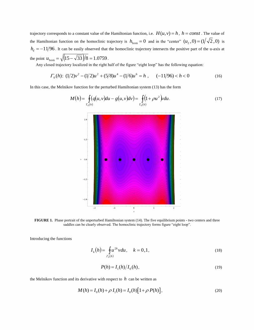
In this case system (14) has the following singular points: )0,0( , which is a “saddle”,

2( ,0) ( 1 2 ,0)u are “centers”, and 4( ,0) ( 2 ,0)u are “saddles”. The phase portrait of the system

(6) is symmetrical concerning x - and y -axis and is shown in Fig. 1.

According to the theory of Melnikov, limit cycles can arise around a closed phase trajectory of the unperturbed

system. Further we are only interested in the family of closed trajectories in the right half of the figure “eight loop”,

i.e. the closed trajectories localized between the center 2( ,0) (1 2 ,0)u and the homoclinic loop. Each phase

trajectory corresponds to a constant value of the Hamiltonian function, i.e. ( , )H u v h , consth . The value of

the Hamiltonian function on the homoclinic trajectory is 0hom h and in the “center” 2( ,0) (1 2 ,0)u is

9611ch . It can be easily observed that the homoclinic trajectory intersects the positive part of the u-axis at

the point 0759.183315hom u .

Any closed trajectory localized in the right half of the figure “eight loop” has the following equation:

huuuvh 6422

0 )61()85()21()21(:)( , 0)9611( h (16)

In this case, the Melnikov function for the perturbed Hamiltonian system (13) has the form

vduudvvugduvuqhMhh

00

21,, . (17)

FIGURE 1. Phase portrait of the unperturbed Hamiltonian system (14). The five equilibrium points - two centers and three

saddles can be clearly observed. The homoclinic trajectory forms figure “eight loop”.

Introducing the functions

h

k

k vduuhI

0

2

, 1,0k , (18)

)()()( 01 hIhIhP , (19)

the Melnikov function and its derivative with respect to h can be written as

0 1 0( ) ( ) ( ) ( ) 1 ( )M h I h I h I h P h , (20)

0 0( ) ( ) 1 ( ) ( ) ( )M h I h P h I h P h . (21)

Note that )(0 hI and )(1 hI are Abelian integrals.

We will look for the zeros of )(hM with 0)9611( h . To find these zeros we need additional

investigations of the functions )(0 hI , )(1 hI and )(hP , the results of which are shortly presented by Lemma 1 in

APPENDIX.

Let is a given negative constant, i.e. 0 . Then taking into account that )(hP is a monotone decreasing

function, a given zero of the Melnikov function 0h satisfies the equations

0)( 0 hM and . 01 ( ) 0P h (22)

The range of variation of the coefficient , so that the system (13) to have a limit cycle, is:

1 (0) 1 ( )cP P h , or 22686.2 (23)

This means that system (13) has a limit cycle 0( )h , which is localized in ( )O -neighborhood of the closed

curve )( 00 h .

According to the Melnikov theory, the stability of the limit cycle is determined by the sign of quantity

0( )M h . It follows from equation (22) and Lemma 1 in APPENDIX, that

0 0 0 0( ) ( ) ( ) 0M h I h P h (24)

and in our case the limit cycle 0( )h is stable when 0 .

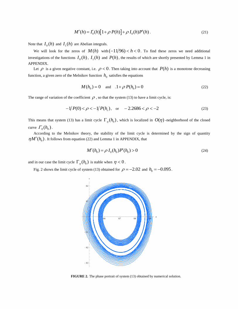
Fig. 2 shows the limit cycle of system (13) obtained for 2.02 and 0 0.095h .

0.6 0.7 0.8 0.9u

0.3

0.2

0.1

0.1

0.2

v

FIGURE 2. The phase portrait of system (13) obtained by numerical solution.

The results of the calculation of three different initial conditions for the time 100 are presented in Fig.2.

One of the initial conditions 0.865,0 coincides with the limit cycle and the corresponding phase trajectory stays

the same during the calculation. Another initial condition 0.815,0 is inside the limit cycle and with the increase

of time it approaches the limit cycle from inside. The last initial condition 0.915,0 is outside the limit cycle and

with the increase of time it approaches the limit cycle from outside. Fig. 2 demonstrates the stability of the observed

limit cycle.

The presented theory allows us to synthesize a system of the type (13), having an advance assigned limit cycle.

Assuming 0hh is the Hamiltonian level around which a limit cycle will arise, then after computing )( 0hP , we

obtain from (24)

01 ( )P h , 0)9611( 0 h , (25)

The obtained value of provides system (13) with the desired limit cycle.

DISCUSSION

As Eq. (10) is derived from Eq. (1), we expect that the existence of this single limit cycle of Eq. (10) which

arises around a closed phase trajectory of the unperturbed system will lead to the existence of periodical attractor of

Eq. (1). As in this case the emerging limit cycle has a finite period, we expect that the corresponding periodic

attractors of the generalized CCQGLE will represent the localized pulsating solutions of this equation.

The values of parameters , 1,3,5jc j fixed in Eq. (16), lead to the following values of the parameters of Eq.

(1): 37375.0;371895.0;49504.1;497519.0;371895.0 . The application of the

method of Melnikov leads to additional condition for given by Eq. (26). Our values of the parameters of Eq. (1)

; ; ; are in these regions for which stable localized fixed–shape solutions and localized pulsating solutions of

Eq. (1) are identified [14].

The module of our 371895.0 , as well as the value of the parameter 005.1 however, are larger than the

usual values [14, 16]. So, in order to confirm our idea, we plan to perform the numerical investigation of the

CCQGLE with the parameters provided by our approach.

As the dynamical system given by Eq. (14) possesses many equilibrium points for different possible relations

between the parameters jc , we may expect the existence of different limit cycles of Eq. (10). Even in the case

considered here the other limit cycles could be found in the region between homoclinic and heteroclinic trajectories,

or in the neighborhood of a homoclinic or heteroclinic trajectory of the unperturbed system. It is clear that the

question of how many limit cycles exist in Eq. (10) and the question of their type will require further systematic

mathematical investigation.

CONCLUSION

We have studied the dynamics of the localized pulsating solutions of generalized cubic– quintic complex

Ginzburg-Landau equation (CCQGLE) in the presence of intrapulse Raman scattering.

The main result of this work is a proposal of an approach for identification of periodic attractors of the

generalized CCQGLE. At first we use ansatz of the travelling wave, and determine some conditions of the material

parameters, we derive the strongly nonlinear Lienard - Van der Pol equation for the amplitude of the nonlinear

wave. Next we apply the Melnikov method to this equation and we show that for a set of fixed material parameters a

limit cycle arises around a closed phase trajectory of the unperturbed system exists. We next prove its stability. Due

to the complexity of the strongly nonlinear Lienard - Van der Pol equation, however, it is clear that the question of

how many limit cycles exist as well as the question of their type will require further systematic mathematical

investigation.

APPENDIX: ANALYSIS OF THE AUXILIARY FUNCTIONS )(0 hI , )(1 hI AND )(hP

The basic properties of the functions )(0 hI , )(1 hI and )(hP are collected in the following Lemma.

Lemma 1: The following statements are valid:

a) 0)(0 hI , 0)(1 hI ; (A1)

b) 0)(0 hI ; (A2)

c) 6973.011

358ln

128

311

16

15)0(0

I ; (A3)

d) 3074.011

358ln

1024

3165

128

97)0(1

I ; (A4)

e) 5.0)9611()( PhP c ; (A5)

f) 4408.0)0()0()0( 01 IIP ; (A6)

g) The function )(hP is strictly monotone decreasing in the interval 0)9611( h , whereupon its

derivative is negative, i.e. 0)( hP for 0)9611( h , and therefore 0)0()()( PhPhP c .

The proof of this lemma will be presented in a future more extended publication.

REFERENCES

1. M.C. Cross, and P.C. Hohenberg, Reviews of Modern Physics, 65, pp.854-1112 (1993).

2. I.S. Aranson, and L. Kramer, Reviews of Modern Physics, 74, pp. 100-143 (2002).

3. Matsumoto M., Ikeda H., Uda T., Hasegawa A., Journal of Lightwave Technology, 13, 658-665 (1995).

4. Y. Kodama, M. Romagnoli, S. Wabnitz , Electronics Letters, 28, 1981-1982 (1992).

5. H.A. Haus, J.G. Fujimoto, and E. P. Ippen, J. Opt. Soc. Am. B8, 2068-2076 (1991).

6. F. X. Kärtner, J. Ausder Au, U. Keller, IEEE J. of Selected Topics in Quantum Electron., 4, 159 (1998).

7. N.R. Pereira and L. Stenflo, Phys. Fluids, 20, 1733 (1977).

8. P.-A. Bélanger, L. Gagnon, and C. Pare, Opt. Lett. 14, 943-945 (1989).

9. R. Conte, and M. Musette, Pure Appl. Opt. 4, 315-320 (1995).

10. R. Conte, and M. Musette, in: N. Akhmediev and A.Ankievicz (eds.), Dissipative solitons, Lect. Notes.

11. J. M. Soto-Crespo, N. Akhmediev, and A. Ankiewicz, Phys. Rev. Lett. 85, 2937-2940 (2000).

12. N. Akhmediev, J. M. Soto-Crespo, G. Town, Phys. Rev. E 63, 056602 (2001).

13. N. N. Akhmediev and A. Ankiewicz (eds.), “Dissipative solitons”, Springer, Berlin (2005).

14. N.N. Akhmediev and Ankiewicz A., “Solitons. Nonlinear Pulses and Beams” (Chapman and Hall, 1997).

15. W. Chang, A. Ankiewicz , N. N. Akhmediev and J. M. Soto-Crespo, Phys. Rev. E 76, 016607 (2007).

16. S. C. Mancas, S. R. Choudhury, Chaos, Solitons & Fractals, 01/2009.

17. S. C. Mancas, S. R. Choudhury, Theoretical and Mathematical Physics 04/2012; 152(2):1160-1172.

18. P.-A. Bélanger, Opt. Express 14, 12174-12182 (2006).

19. A. Hasegawa and Y. Kodama, “Solitons in Optical Communications” (Clarendon Press, 1995).

20. G.P. Agrawal, “Nonlinear Fiber Optics” (Academic Press, third edition, 2001).

21. G.P. Agrawal, “Applications of Nonlinear Fiber Optics” (Academic Press, 2001).

22. Z.Li, L.Li, G. Zhiu, and K.H. Spatschek, Phys. Rev. Lett. 89, 263901 (2002).

23. S. C.V. Latas, M.F.S. Ferreira, M. V. Facao, Appl. Phys. B (2011) 104: 131-137

24. S. C.V. Latas, M.F.S. Ferreira, Opt. Lett. 37, 3897-3898 (2012)

25. Andronov A. A., E. A. Leontovich, I. I. Gordon, A. G. Maier, “Theory of Bifurcations of Dynamical Systems on the

Plane”, Nauka, Moscow, 1967 (in Russian) and Wiley, New York, 1973.

26. Bautin N. M., E. E. Leontovich, “Methods and Tools for Qualitative Analysis of Dynamical Systems on the Plane”,

Nauka, Moscow, 1976 (in Russian).

27. J. Guckenheimer, P. Holmes, Nonlinear Oscillations. Dynamical systems and Bifurcations of vector fields, Springer-

Verlag, (1983).

28. L. Perko, Differential Equations and Dynamical Systems, Springer-Verlag, New York, Third Edition, 2001.

29. I. M. Uzunov, Phys. Rev. E 82, 066603 (2010).

30. F.I. Khatri, J. D. Moores,G. Lenz, H. A. Haus, Opt. Communications 114 (1995) 447-452

31. L.E. Nelson, D. J. Jones, K. Tamura, H. A. Haus, E. P. Ippen, Appl. Phys. B 65 277-294 (1997).

32. W. H. Renniger, A. Chong, and F. W. Wise, Phys. Rev. A 77, 023814 (2008).

33. F. W. Wise, A. Chong, and W. H. Renniger, Laser&Phot. Rev. 2 58-73 (2008).

34. J. Nathan Kutz, SIAM Review, vol. 48, 629-678 (2006).

35. E. Ding, W. H. Renniger, F. W. Wise,F. Grelu, E. Shilizerman, and J. Nathan Kutz, International Journal of Optics, vol.

2012, article ID 354156.

36. S. H. Chen and Y. K. Cheung, “An elliptic perturbation method for certain strongly nonlinear oscillators”, Journal of

Sound and Vibration (1996) 192 (2), 453-464.