Influence of rheology on debris-flow simulation

Nat. Hazards Earth Syst. Sci., 6, 519–528, 2006www.nat-hazards-earth-syst-sci.net/6/519/2006/© Author(s) 2006. This work is licensedunder a Creative Commons License.

Natural Hazardsand Earth

System Sciences

Influence of rheology on debris-flow simulation

M. Arattano 1, L. Franzi2, and L. Marchi 3

1CNR-IRPI, Strada delle Cacce,73, 10135 Torino, Italy2Regione Piemonte, Corso Tortona, 12, 10183 Torino, Italy3CNR-IRPI, C.so Stati Uniti, 4, 35127 Padova, Italy

Received: 1 August 2005 – Revised: 21 February 2005 – Accepted: 6 March 2006 – Published: 12 June 2006

Part of Special Issue “Documentation and monitoring of landslides and debris flows for mathematical modelling and design ofmitigation measures”

Abstract. Systems of partial differential equations that in-clude the momentum and the mass conservation equationsare commonly used for the simulation of debris flow initia-tion, propagation and deposition both in field and in labora-tory research. The numerical solution of the partial differ-ential equations can be very complicated and consequentlymany approximations that neglect some of their terms havebeen proposed in literature. Many numerical methods havebeen also developed to solve the equations. However weshow in this paper that the choice of a reliable rheologicalmodel can be more important than the choice of the bestapproximation or the best numerical method to employ. Asimulation of a debris flow event that occurred in 2004 in anexperimental basin on the Italian Alps has been carried out toinvestigate this issue. The simulated results have been com-pared with the hydrographs recorded during the event. Therheological parameters that have been obtained through thecalibration of the mathematical model have been also com-pared with the rheological parameters obtained through thecalibration of previous events, occurred in the same basin.The simulation results show that the influence of the inertialterms of the Saint-Venant equation is much more negligiblethan the influence of the rheological parameters and the ge-ometry. A methodology to quantify this influence has beenproposed.

1 Introduction

Land-use planning and design of structural countermeasuresfor debris flows are generally carried out on the basis of theanalysis of past events or using the results obtained by theapplication of mathematical models. The first approach cangive useful indication on the possible effects of future debris

Correspondence to:M. Arattano([email protected])

flow events, but it cannot give more detailed predictions oftheir effects (Suwa and Yamakoshi, 2000; Ayotte and Hungr,2000). The application of mathematical models is employedto obtain more quantitative estimations of the dynamic char-acteristics of debris flows (velocity, flow depth, discharge,flow duration, etc.). The estimation of the dynamic character-istics of debris flows is in fact needed by administrators, deci-sion makers and practitioners who have to protect the life, theproperty and the economical activities of people who live indebris flows prone areas and to forbid anthropic activities inthese latter (Regione Piemonte, 2002; Petrascheck and Kien-holz, 2003). Sometimes different boundary conditions (e.g.water-sediment hydrograph, peak discharge) are taken intoaccount in order to test the sensitivity of the results and theadequacy of the designed/existing countermeasures. When amore detailed hazard assessment is needed, especially for re-location of settlements and human activities, more complexmathematical models can be used (2-D models, two phasemodels, movable bed models that can incorporate deposi-tions and erosions along the torrent) (Ghilardi and Natale,2000; Pudasaini et al., 2003, 2005). However the estimationof the parameters to be used in the simulations is often notstraightforward and the choice of the more apt rheologicalmodel can be very difficult. In this paper the simulation of adebris flow event occurred in 2004 in an instrumented torrentwill be presented and the influence on results of the rheolog-ical parameters will be discussed. A one-phase Saint-Venantmodel has been used for the simulation because the avail-able field data allowed to calibrate only 2 parameters: thecalibration of 2-D models would have required more param-eters. At the moment, in the field practice, 1-D models arestill more commonly employed than 2-D models. This papershould offer an help to practitioners to better understand theperformances of 1-D models.

Published by Copernicus GmbH on behalf of the European Geosciences Union.

520 M. Arattano et al.: Influence of rheology on debris-flow simulation

Monitored reach

Fig. 1. The Moscardo basin and its geographical location.

2 The simulated debris flow event

The Moscardo torrent is a small torrent, located in the East-ern Italian Alps, that has been affected in the past by severaldebris flows (Marchi et al., 2002). It drains an overall areaof about 4 km2 ranging in elevation from 890 m to 2043 mabove the sea level (Fig. 1).

In 1989 two ultrasonic sensors were placed on the fan ofthe torrent where the bed slope is approximately 10% andthe torrent reach is quite straight. These sensors measured

the stage performing three measurements each second with aprecision of about 1cm and allowed the recording of an hy-drograph that show the stage variation in time. In 1996 a thirdsensor was added upstream of the previously installed sen-sors and was maintained active until 1998. Nowadays onlytwo ultrasonic sensors are installed along the torrent, 75 mapart. The cross section width of the torrent reach is about8 m. This cross section can be modelled as a broad rectangu-lar section.

Nat. Hazards Earth Syst. Sci., 6, 519–528, 2006 www.nat-hazards-earth-syst-sci.net/6/519/2006/

M. Arattano et al.: Influence of rheology on debris-flow simulation 521

A debris flow event occurred on 23 July 2004 that wascharacterised by a first water-sediment surge that lasted about400 s, followed by a second surge which lasted about 100 s.The first wave had a steeper front and greater flow depthsthat decreased after the peak. The second wave was shorter,with a lower gradient in the front part. A superposition ofthe upstream and downstream hydrographs reveals that noevident modification of the shape of the debris flow waveoccurred between the two stations. The event duration is alsothe same in the two hydrographs. Since the geometry of thechannel does not change along the torrent reach between theultrasonic gauges, the absence of a significant hydrographdeformation suggests that no significant deposition/erosionprocesses occurred between the two sites.

3 The mathematical model

The mathematical model employed is the same 1-D model al-ready proposed and discussed in Arattano and Franzi (2003,2004). A 2-D model would have actually allowed to con-sider, for instance, the boundary effects due to the side of thechannel; however, as mentioned before, the available fielddata would have not allowed to calibrate it.

Applying the momentum and mass conservation laws tothe mixture of a debris flow, a system of two partial differ-ential equations is obtained, namely the Momentum equa-tion and the Mass conservation equation (Cunge et al., 1980;Abbott, 1966), that can be solved with an implicit finite-difference scheme, according to Preismann (Cunge et al.,1980; Abbott, 1966):

∂Q∂t

+ gA ∂h∂x

cosθ +∂∂x

(Q2

A) + gASf − gA tanθ=0,

∂h∂t

+1b

∂Q∂x

= 0,

(1)

whereQ is the water-sediment discharge,A is the cross sec-tion area occupied by the debris flow,b is the free debrisflow surface width in the cross section,h is the flow depth,θis the bed slope angle (assumed constant),Sf is the frictionterm that accounts for internal and external friction,x is thedownstream coordinate (positive downstream),g is the grav-ity acceleration. The effects of the centrifugal forces (Puda-saini and Hutter, 2003) are not taken into account becausethe investigated reach of the Moscardo Torrent is straight.

The first term on the left side of the first equation of thesystem (1) represents the effects of the local inertia, the sec-ond term the pressure effects, the third the convective iner-tia, the fourth the effects of internal and external friction andthe fifth the gravity effects. According to the different topo-graphic and dynamic conditions, different terms can play dif-ferent roles in the simulation. In particular the inertia termscan be considered to be predominant in time and space vary-ing processes, such as floods due to dam breaks. The fourthterm can be expressed in different ways, according to the dif-ferent rheological behaviors of the water-sediment current.

A detailed discussion of this latter issue can be found inArattano and Franzi (2003). The rheological properties ofthe water sediment mixture must be specified to solve thesystem (1). The following closure equation has been used,following Honda and Egashira (1997):

τ = τo + ρghU2

c2h2n, (2)

whereτ o is the yield stress,c andn are two rheological pa-rameters,ρ is the fluid density andU is the mean flow ve-locity in the cross section. Equation (2) is one of the mostgeneric equation for debris flows simulation as it takes intoaccount the presence of a yield strength and a stress. Theterm Sf in (1) is linked toτ through the following relation-ship:

Sf =τ

ρgh(3)

The debris flows of the Moscardo Torrent have a heteroge-neous grain size: transported particles range from silt andclay to boulders (Arattano et al., 1997). On the basis ofthe video recorded images of some events (Deganutti et al.,1998) we have assumed that the coarse fraction gives to theoverall mixture a rather high drainage capability, although noexperimental measurements are available on this aspect. Wethus deem that the effect due to the excess-pore fluid pres-sure (Hungr, 1995; Hutter et al., 1996; Iverson, 1997) can beneglected. This hypothesis is equivalent to state that the ex-cess pore pressure, if present, dissipates in time-scales muchsmaller than the time scale of the water-sediment propaga-tion. Actually, as far as the debris flow front is concerned,this latter sustains generally little pore pressure and exertsmuch frictional resistance because it is composed by a wedgeof coarse particles with a high hydraulic diffusivity. The is-sue about the role of pore pressure would therefore concernonly the debris flow body; in the tail in fact non-hydrostaticpore-pressure dissipates more rapidly than in the body (Iver-son et al., 2000). The large dimensions of coarse particlesin the 2004 debris flow and the little amount of clay in themixture suggests the existence of a very high hydraulic dif-fusivity also in the debris flow body and thus a ready dissi-pation of the non-hydrostatic pore pressures. In these condi-tions the total stress on the bed would be equal to the hydro-static stresses plus the static/dispersive stresses due to con-tacts/collisions among particles. In these conditions the term(∂pbed /∂x) (Iverson, 1997, 2000; Jin and Fread, 1999) tendsto be equal to zero and the pore pressure distribution tendsto be hydrostatic. A hydrostatic distribution of the pore pres-sure is a basic assumption of many rheological models (Taka-hashi, 1991; Egashira et al., 1997) that imply resistance toflow formulas similar to Eq. (2).

Different values have been proposed for the rheologicalparametersc and n by different authors, as sumarized inTable 1.

www.nat-hazards-earth-syst-sci.net/6/519/2006/ Nat. Hazards Earth Syst. Sci., 6, 519–528, 2006


Table 1. Some proposed values for the rheological parameterscandn. Thec dimensions depend on the value ofn.

Author Simulation parameters

n c

[–] [m1−n/s]

Rickenmann 1/3, 1/2 c depends on the parametern and on(1999) the debris flow peak discharge

Takahashi 3/2 For dilatant flow behaviourc depends on(1991) the sediment concentrationC, by volume,

Takahashi and Nakagawa (theoretical and laboratory the interstitial fluid density and the mean grain size(1993) results)

Coussot(1994) 3 muddy debris flows and mudflows

(Herschel-Bulkley model)

0

0.5

1

1.5

2

2.5

0 100 200 300 400 500 600 700 800

time (s)

fow

dep

th (m

)

Recorded Simulated

Fig. 2. Water sediment flow depths in the upstream cross section.

The value of the parametern depends on the rheologi-cal behavior of the debris flow mixture, as summarized byPierson and Costa (1987). The termτo in (2) is responsiblefor the presence of a rigid plug in the flowing mixture anda critical thickness for the flow, below which motion shouldstop and the debris flow should deposit. Previous researchesin the Moscardo torrent have shown that a rigid plug flow isnot always observed for the debris flows in this torrent (De-ganutti et al., 1998) while many of the hydrographs recordedso far show a descending limb that does not show any criti-cal thickness below which a stop of the motion is observed(Marchi et al., 2002; Arattano and Franzi, 2004). Therefore(2) was implemented in the simulation withτ o=0 (Nsom etal., 1998). The resulting equation is often used in practicalapplications (Rickenmann, 1999). It probably works betterwhen the torrent is incised and the banks allow the mainte-nance of a high water content, particularly behind the frontand in the tail of the debris flow: a high water content main-tain the mixture less dense and more fluid reducing the ef-fects or even eliminating the presence of a yield stress. Note

that Eq. (2) withτ o=0 approximates the Herschel-Bulkley orthe Bingham model for small yield stress.

In the simulation the values ofc andn have been adoptedthat allowed best fit to the upstream hydrograph. A steadyflow has been assumed for the initial conditions along theentire torrent reach in order to solve the system of Eqs. (1).The assumed upstream boundary conditions forh are givenby the upstream recorded hydrograph (Fig. 2). Therefore theinitial and boundary conditions are, respectively, the follow-ing:{

t = 0U = U(x, 0);h = h(x, 0) for 0<x<L steady flow

(4)

{x = 0U=f [h(0, t)]=chn

√Sf ; h=h(0, t) for )<t<800 s

(5)

where:

– L is the length of the torrent reach, equal to the distancebetween the first and the second gauging station (75 m),

– U=U(x, 0) and h=h (x, 0)have been obtained by solv-ing system (1) where all the time derivative terms havebeen set equal to zero (steady flow conditions);

– h(0, t) is the hydrogram in the upstream cross section.

As indicated before, theU (0, t)=f [h(0,t)] relationship inthe upstream reach depends on the choice of the simulationparameters. Since theh (0, t) values in Eq. (5) are thoserecorded in the upstream hydrograph, the uncertainty in theestimation ofU and consequently in the estimation of thedebris flow discharge is much smaller than in other simula-tions where both the upstream conditions,h andU , had to beestimated (Honda and Egashira, 1997; Hirano et al., 1997).The assumption of uniform flow conditions in the upstreamboundary can be found in other models (e.g. Hirano et al.,



0

0.5

1

1.5

2

2.5

0 100 200 300 400 500 600 700 800

time (s)

fow

dep

th (m

)

Recorded Simulated

Fig. 3. Comparison between the recorded and simulate hydrographin the downstream cross section (70 m downstream). Notice thatthe different flow depths for t<270 s occur because the rheologicalparameters have been used also in the simulation for t<270 s whenthe flow consisted mostly of clear water.

1997; Suzuky et al., 1993; Arattano and Savage, 1994). Forsteep bed slopes the assumption of uniform flow conditionscan be the most reasonable, because there is a predominanceof the gravity and friction terms in Eq. (1) (Cunge, et al.,1980). For the examined debris flow the assumed initial andboundary conditions are reliable and reasonable and they cer-tainly do not produce a strong influence on the results. Infact, as the discussion that follow will put into light, the un-steady terms in system (1) are far less than the other terms.

Different simulations have been performed for differentc

andn values maintaining the same boundary and initial con-ditions. The best fit between the recorded and the simulatedhydrographs was obtained forc=4 m0.8/s andn=1.2. Thecomparison between the recorded downstream hydrographh′, t and the simulated hydrographh′′, t is quite satisfactory(Fig. 3). Notice that the higher flow depth in the simulatedresults of Fig. 3, before the surge reaches the gauge, is dueto the fact that we have applied the rheological parametersfound in the simulation to the entire wave as if it were madeof the same mixture. Actually the flow preceding the surgewas entirely different and consisted mostly of clear water.

The recorded hydrograph (Fig. 3) shows oscillations dueto the irregularities of the debris flow profile. These are dueto the pebbles, cobbles, stones, trees and smaller pieces ofvegetation that are transported on the surface of the debrisflow itself and to splashes and other turbulences, includingsmall waves, that take place on the debris flow surface. Therelative error in the measured hydrograph is also due to theerror of the instrumental recording device and to the value ofthe time interval of the measurement (one second).

The recorded hydrographs allow to compute the total vol-ume of debris flowing through the two cross sections, as de-scribed in Arattano (2000). The coincidence of the curvesrepresenting the total volumes of debris flows at the twogauging stations (Fig. 4) seems in agreement with one of

0

2000

4000

6000

8000

10000

12000

14000

0 100 200 300 400 500 600 700 800 900

time (s)

volu

me

(m3 )

upstream

downstream

Fig. 4. Comparison between estimated volumes upstream anddownstream.

the basic assumption of the model: the absence of deposi-tion/erosion processes along the monitored torrent reach.

4 Debris flow rheology

The simulation results have been obtained for an unsteadyone-dimensional model with initial and boundary conditionsdeduced from recordings or from empirical evaluations. Ifa reliable estimation of the initial and boundary conditionsis possible, the higher uncertainties in the simulation resultsare either due to the uncertainties in the assumption of therheological behavior or to other aspects of the modeling ofthe debris flow. In the following this point will be discussedin a greater detail. It will also be shown that, for the studiedcase, a simple model that neglects the inertial terms of theSaint-Venant equation can give good simulation results.

4.1 Rheological behaviour of the debris flow – discussion

The rheological properties of a debris flow affect its dynamiccharacteristics and, therefore, the amount of the dynamicimpact against defence structures. The impact forces ex-erted on levees or dams are generally obtained and quanti-fied through the application of the momentum transfer prin-ciple or through the energy conservation theorem. The pre-diction of the rheological behaviour usually relies on obser-vations of past events occurred in the same area. The fielddata collected in the Moscardo Torrent, since the inceptionof the monitoring activities, have provided important infor-mation regarding this latter issue. Following the same proce-dure employed in this paper the debris flows that occurred on20 July 1993, 22 June 1996, 8 July 1996 and 4 August 2002have been previously modelled (Arattano and Franzi, 2003,2004). Table 2 summarises the values ofc andn found forthese events.

As far as the July 2004 event is concerned, the valuesfound for the parameters of the model are similar to the pa-rameters found for the event occurred on 4 August 2002. The



Table 2. Comparison of the simulation parameters for the 1993, 1996, 2002 and 2004 Moscardo events.

20.07.1993 22.06.1996 08.07.1996 04.08.2002 23.07.2004

c (*) 14 14 14 5 4

n (-) 0.2 0.2 0.66 1.3 1.2

(*) unit of c depend onn value, according to the relationship [c]=m(1−n)/s.

deposits of this latter event, surveyed few days after its oc-currence (Arattano and Franzi, 2004), appeared to be quitecoarse and with a very small fine fraction. These field evi-dences led to interpret this debris flow as a stony debris flow.Therefore the value ofn that resulted from the simulationof the 4 August 2002 event was considered as indicative of aflow behaviour of the dilatant type, as that proposed by Taka-hashi (1978, 1980, 1991) (Arattano and Franzi, 2004). Thesame behaviour can be hypothesized for the July 2004 event.

The large variation of thec and n values shown in Ta-ble 2 suggests that the rheological coefficients are not con-stant, even for debris flows taking place in the same torrent.This implies that, for purposes of hazard prediction and as-sessment on a debris fan, different simulations have to beperformed assuming different rheological behaviors and ex-ploring the related consequences. Bothc andn have a stronginfluence on the dynamics: therefore, for practical applica-tions of the proposed methodology, a sensitivity analysis ofthe results for different [n, c] pairs should also be performed.In SEct. 4.3 this point will be further discussed.

4.2 Influence on simulation results of the terms of theSaint-Venant equation

A numerical scheme is needed to solve the partial differen-tial equations (1) for given initial and boundary conditions.Many schemes have been proposed in literature (Jan, 1997;Hashimoto et al., 2000; Cunge at al., 1980), either implicit orexplicit, either one step or multisteps. In general the great-est difficulties in the numerical solutions are represented bythe non linear terms (e.g the convective term) and by the ne-cessity to simulate dam-break like hydrographs with rapidlyvarying flow depths, discharges and velocities. Different nu-merical methods have been proposed to obtain stable math-ematical algorithms and consistent schemes (Cunge at al.,1980; Abbott, 1992). In general, some simplifications ofsystem (1) may apply if the boundary and geometrical con-ditions allow to neglect some of the terms in the momen-tum equation. However it is often not easy to choose whichterm can be neglected, because the influence of the differen-tial terms cannot be evaluated “a priori”, given their strongvariation in time and space during the simulation.

Here a comparison has been carried out of the values andthe related influence of the different terms in system (1). Asstated before, for steep bed slopes, the influence of the fourth

and fifth term in the momentum equation can be predomi-nant on the other terms so that the propagation model canbe strongly simplified. The resulting model is the so-called“kinematic model” (Arattano and Savage, 1994). The mo-mentum equation holds in this case:

Sf = tanθ (6)

Computing the difference between the bed slope, tanθ , andSf , that is the computed value of the energy gradient, it ispossible to obtain an estimation of the error due to the ap-proximation introduced in the computation with the neglect-ing of the differential terms in system (1) and thus evaluatetheir influence:

−1

gA

[∂Q

∂t+ gA

∂h

∂xcosθ +

∂

∂x(Q2

A)

]= Sf − tanθ (7)

The relative error,εk, due to the neglecting of the differentialterms in system (1) will be given by:

εk =Sf − tanθ

tanθ(8)

The relative error,εk, is linked to the relative error in theestimation of the flow heighth. In fact rewriting Eq. (2),with τ o=0 holds:

h =2n

√U2

Sf c2(9)

Recalling that the termSf is given by:

Sf =τ

ρgh

and differentiating Eq. (9) with respect toSf for a constantdischarge, the following equation can be obtained (see ap-pendix):

∂h

h= −

1

2(n + 1)

∂Sf

Sf

. (10)

The term ∂Sf /Sf can be assumed as an estimation of therelative error in the evaluation ofSf . Equation (6) states thatSf can be approximately assumed equal to tanθ , thus theerror∂ Sf will be given bySf –tanθ and the relative error∂Sf / Sf will be given by:

∂Sf

Sf

=Sf − tanθ

Sf

. (11)


M. Arattano et al.: Influence of rheology on debris-flow simulation 525 Figure 5 has to be substituted by the following.

∂h/h; ∂h/h;

-0.15

-0.1

-0.05

0

0.05

0.1

0.15

0 100 200 300 400 500 600 700 800

time (s)

0

1

2

3

4

5

6

7

8

9

10

flow

dep

th (m

)

a

a

debris flow profile

∂ h/h

εi

∂ h/

h; ε

i

Fig. 5. Variation of∂h/h in Eq. (10) andεi in time. The relative er-ror εi has been plotted only for t> 270 s (see Fig. 2). The simulateddebris flow profile has been shown.

Considering that, for steep bed slopes,Sf is actually veryclose to tanθ , the denominator of Eq. (11) can be substitutedby tanθ , and thus ∂ Sf / Sf is approximately equal toεk

(Eq. 8). Equations (8), (10) and (11) thus shows then thatthe relative error,εk, due to the neglecting of the differentialterms in system (1) is directly related to the relative error,∂

h/h, in the evaluation ofh. The relative errorεk can thus beassumed as an indicator of the relative error in the estimationof h made with the kinematic simplification given by Eq. (6).

Since the value of the right-hand-side term in Eq. (11) andconsequently the value of∂ Sf /Sf , can be calculated bymeans of the results of the simulation, the relative errorεk

made in our simulation can be obtained from Eq. (10) (sub-stituting the value of∂ Sf / Sf obtained through the simu-lation and assumingn=1.2). We calculated the value ofεk

following this procedure and we found that, for the largerdebris flow wave of the July 2004 event,εk was generallyless than 1%. It resulted higher than 1% only twice, for 6and 5 s, respectively. In the latter time interval,εk reacheda maximum value of 2.96%. This shows that the approxi-mated assumption made in Eq. (6) affects the results, as faras the estimation of flow depth is concerned, only by somepercentages. This influence appears even more negligible ifthe irregularities in the debris flow profile that are due to thepresence of pebbles, cobbles, wood debris and superficialwaves are taken into account. These irregularities impedea good match between the simulated hydrograph{h′, t} andthe recorded one{h′′, t}. Actually the relative error made inthe estimation ofh, given by Eq. (8), is much smaller thanthe relative errorεi produced by the inadequacy of the modelto reproduce the irregularities of the real debris flow profile:

εi =h′

− h′′

h′′(12)

as shown in Fig. 5. Notice that the large value ofεi ispredominantly due to the complexity of the examined phe-nomenon with its irregular profile. This irregularity of profile

-8

-6

-4

-2

0

2

4

6

8

0 100 200 300 400 500 600 700 800

time (s)

term

s in

Sai

nt V

enan

t equ

atio

n

-0.04

-0.03

-0.02

-0.01

0

0.01

0.02

0.03

0.04

tan θ

-Sf

gAdh/dx cosq dQ/(dt)

d(Q2/A)/dx tan(q)- Sf

debris flow profile

d(Q2/A)/dx tan(θ)- S f

gAdh/dx cos(θ)

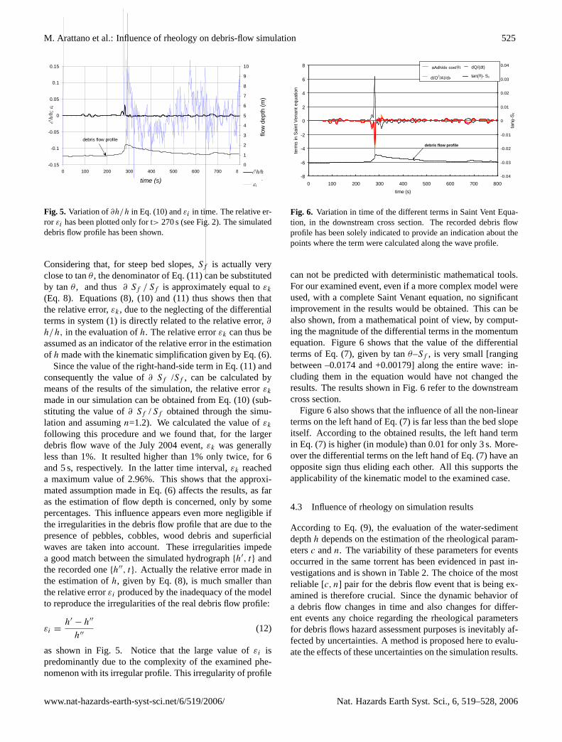
Fig. 6. Variation in time of the different terms in Saint Vent Equa-tion, in the downstream cross section. The recorded debris flowprofile has been solely indicated to provide an indication about thepoints where the term were calculated along the wave profile.

can not be predicted with deterministic mathematical tools.For our examined event, even if a more complex model wereused, with a complete Saint Venant equation, no significantimprovement in the results would be obtained. This can bealso shown, from a mathematical point of view, by comput-ing the magnitude of the differential terms in the momentumequation. Figure 6 shows that the value of the differentialterms of Eq. (7), given by tanθ–Sf , is very small [rangingbetween –0.0174 and +0.00179] along the entire wave: in-cluding them in the equation would have not changed theresults. The results shown in Fig. 6 refer to the downstreamcross section.

Figure 6 also shows that the influence of all the non-linearterms on the left hand of Eq. (7) is far less than the bed slopeitself. According to the obtained results, the left hand termin Eq. (7) is higher (in module) than 0.01 for only 3 s. More-over the differential terms on the left hand of Eq. (7) have anopposite sign thus eliding each other. All this supports theapplicability of the kinematic model to the examined case.

4.3 Influence of rheology on simulation results

According to Eq. (9), the evaluation of the water-sedimentdepthh depends on the estimation of the rheological param-etersc andn. The variability of these parameters for eventsoccurred in the same torrent has been evidenced in past in-vestigations and is shown in Table 2. The choice of the mostreliable [c, n] pair for the debris flow event that is being ex-amined is therefore crucial. Since the dynamic behavior ofa debris flow changes in time and also changes for differ-ent events any choice regarding the rheological parametersfor debris flows hazard assessment purposes is inevitably af-fected by uncertainties. A method is proposed here to evalu-ate the effects of these uncertainties on the simulation results.



-0.3

-0.25

-0.2

-0.15

-0.1

-0.05

0

0.05

0.1

-0.01 -0.005 0 0.005 0.01 0.015 0.02 0.025 0.03εk

εn\

Fig. 7. Dispersion ofεk andεn in time, in correspondence to theupstream cross section, forn=0.75. dn=.55.

By simply differentiating Eq. (9) with respect ton the fol-lowing formula can be obtained for a constant discharge (seeappendix for derivation):

εn =∂h

h= −

1

n + 1ln h · ∂n (13)

which shows that the relative error in the estimation of theflow depth is proportional to the uncertainty in the estima-tion of the parametern. This means that the relative error inthe estimation of the flow depth depends on the uncertaintiesin determining the rheological behavior of the debris flowmixture. If no measurements were available for the studiedcase, a practitioner or a technician who had to chose a valuefor n would probably assumen equal to the mean value ofthe maximum (n=1.3) and minimum (n=0.2) values obtainedin past simulations, that isn=0.75. In this case the∂ n termwould result equal to about 0.55. The relative errorεn hasbeen therefore computed assuming∂ n=0.55 andn=0.75. InFig. 7 εn is compared withεk. Each plotted point refers tothe sameh(t) recorded value at the downstream cross sec-tion. From this comparison it is shown that the order of mag-nitude ofεnfalls in the range [–0.27; 0.062;] and it is muchgreater than the range of variation ofεk.

It would also be possible for a practitioner to decide to as-sume, for safety purposes, then value that leads to the high-esth value. In this case the uncertainty in the estimation ofh,due to the assumption of the value ofn in the range [0.2; 1.3]that causes the largesth, would be much higher than in theprevious case and (13) could not be used to estimate it, sinceEq. (13) is obtained with an infinitesimal approach. Alterna-tively, the first term in Eq. (13) can be calculated by meansof a finite difference equation, so thatεn transforms into:

εn∼=

hn1 − hn2

h̄=

(Q

αc√

Sf

) 1n1+β

−

(Q

αc√

Sf

) 1n2+β

h̄(14)

-0.8

-0.7

-0.6

-0.5

-0.4

-0.3

-0.2

-0.1

0

0.1

0.2

0.3

-0.01 -0.005 0 0.005 0.01 0.015 0.02 0.025 0.03εk

εn

Fig. 8. Dispersion ofεk andεn in time, in correspondence to theupstream cross section, forn1=1.3 andn2=0.2

wheren1=1.3 andn2=0.2 and

h̄ =

(Q

αc√

Sf

) 1n1+β

+

(Q

αc√

Sf

) 1n2+β

2(15)

In Fig. 8 Eq. (14) has been plotted versusεk for the debrisflow discharges computed in the upstream cross section. Inthis case the relative error is of course higher than in Fig. 7.

All this shows that the uncertainties in the determinationof the rheology have a greater influence on the simulationresults than the approximations made neglecting the differ-ential terms of the Saint Venant equation. This shows thatfor our examined event if the complete Saint Venant equa-tion were employed no significant improvement in the resultswould have been obtained.

5 Conclusions

The rheological parameters of a debris flow that occurredin the Summer 2004 in an instrumented basin on the Ital-ian Alps have been estimated by means of a mathematicalmodel, imposing the best fit between simulated results andthe recorded hydrograph. The analysis shows: (i) the rheo-logical behaviour of this debris flow event is different fromother debris flows previously occurred in the same torrent;(ii) the analysis of the relative influence of the different termsof the Saint Venant equation reveals the predominance of theresistance term over the remaining terms; (iii) the value ofthe error made neglecting these latter is much smaller thanthe error made simulating the complex and very irregular de-bris flow profile with a deterministic model; this suggests theuse of a very simple and approximated mathematical model(the kinematic model) to simulate the debris flow propaga-tion; (iv) since the resistance terms are closely related tothe rheological behaviour of the mixture, it is more impor-tant to reliably estimate the rheological parameters used inthe simulation than focusing on the choice of the most suit-able mathematical and numerical schemes needed to solve



the complete Saint Venant equation system. This latter con-sequence has been also evidenced by a comparison betweenthe relative error due to uncertainties in determining the rhe-ology and the relative errors due to the kinematic approxi-mation. These conclusions are valid for a debris flow thatoccurred in a relatively simple torrent, with straight channeland without erosion and deposition.

Appendix A

Derivation of Eq. (10)

The momentum equation in uniform flow conditions holds:

Q = AU = Achn√

Sf (A1)

For a rectangular cross section it is:

A = bh (A2)

while in general, it is (ifA is approximated by a monomialfunction):

A = αhβ (A3)

whereα andβ are parameters that depend on the shape ofthe cross section.

Using Eq. (A3) in Eq. (A1), one obtains:

h =

(Q

αc√

Sf

) 1n+β

(A4)

For a given discharge, Eq. (A4) can be used to calculate thedebris flow depth, for given cross section geometry, rough-ness and bed slope.

Differentiating Eq. (A4) with respect toSf , holds

∂h

∂Sf

=

(1

n+β

)(Q

αc√

Sf

) 1n+β

−1Q

αc

(−

1

2

) (Sf

)−3/2 (A5)

Dividing Eq. (A5) by Eq. (A4), holds:

∂h

h∂Sf

=

(1

n + β

)(Q

αc√

Sf

)−1Q

αc

(−

1

2

) (Sf

)−3/2 (A6)

and therefore

∂h

h= −

1

2(n + β)

∂Sf

Sf

(A7)

For a rectangular (β=1) cross section, Eq. (10) holds.

Appendix B

Derivation of Eq. (13)

Differentiating Eq. (A4) with respect ton holds:

dh

dn=

(Q

αc√

Sf

) 1n+β (

−1

(n + β)2

)ln

(Q

αc√

Sf

)=

h

(−

1

(n + β)2

)ln(hn+β

)(B1)

From Eq. (B1) one obtains:

∂h

h=

(−

1

n + β

)ln (h) · ∂n (B2)

For a rectangular (β=1) cross section, Eq. (13) holds:Notations:b: cross section widthA cross section areah: water sediment depthn: rheological parameterQ: debris flow dischargeα, β: parameters depending on the shape

of the cross section

Acknowledgements.The authors wish to thank the reviewers fortheir suggestions to improve the quality of the paper, particularlyS. P. Pudasaini for the useful discussion on the several aspects ofdebris flow modelling.

Edited by: G. LollinoReviewed by: S. P. Pudasaini and another referee

References

Abbott, M. B.: An introduction to the method of characteristics,American Elsevier, New York, 1966.

Abbott M. B.: Computational hydraulics: elements of the theory offree surface flows, Ashgate, Vermont, 1992.

Arattano, M. and Savage, W. Z.: Modelling debris flows as kine-matic waves, Bulletin of the IAEG, 49, 95–105, 1994.

Arattano, M., Deganutti, A. M. and Marchi, L.: Debris flow mon-itoring activities in an instrumented watershed on the Italianalps, Proceedings of the First International ASCE Conferenceon Debris-Flow Hazard Mitigation: Mechanics, Prediction andAssessment, San Francisco, Ca, August 7–9, 506–515, 1997.

Arattano, M.: On debris flow front evolution along a torrent,Physics and Chemistry of the Earth Part B 25(9), Elsevier Sci-ence Ltd., 733–740, 2000.

Arattano, M. and Franzi L.: On the evaluation of debris flows dy-namics by means of mathematical models, Nat. Hazards EarthSyst. Sci., 3, 539–544, 2003.

Arattano, M. and Franzi, L.: Analysis of different water-sedimentflow processes in a mountain torrent, Nat. Hazards Earth Syst.Sci., 4, 783–791, 2004.



Ayotte, D. and Hungr, O.: Calibration of runout prediction modelfor debris flows avalanches, Proceedings of the Second Interna-tional Congress on Debris Flows Hazard Mitigation: mechanics,prediction and assessment, A.A. Balkema, Rotterdam, 505–514,2000.

Coussot, P.: Steady, laminar, flow of concentrated mud suspensionsin open channel, J. Hydr. Res. 32, 535–539, 1994.

Cunge, J. A., Holly Jr., F. M., and Verwey, A.: Practical aspectof computational River hydraulics, Pitman Publishing Limited,Boston, 1980.

Deganutti, A. M., Arattano, M., and Marchi, L.: Debris flows inthe Moscardo Torrent. National Research Council of Italy, Insti-tute for Hydrological Protection (IRPI) Internal Report (video-cassette), 1998.

Egashira, S., Miyamoto, K., and Itoh, T.: Constitutive equationsof debris flows and their applicability, First int. conference ondebris flows hazard mitigation, 340–349, 1997.

Ghilardi, P. and Natale, L.: Debris flow propagation on urbanizedalluvial fans, Proceedings of the Second International Congresson Debris Flows Hazard Mitigation: mechanics, prediction andassessment, A.A. Balkema, Rotterdam, 471–477, 2000.

Hashimoto, H., Park, K., and Hirano, M.: Numerical Simulation ofsmall debris flows at Mt. Unzendake, Proceedings of the SecondInternational Congress on Debris Flows Hazard Mitigation: me-chanics, prediction and assessment, Balkema, Rotterdam, 177–183, 2000.

Hirano, M., Harada, T., Banuhabib, M. E., and Kawahara, K.: Esti-mation of hazard area due to debris flow. Proceedings of the FirstInternational ASCE Conference on Debris-Flow Hazard Mitiga-tion: Mechanics, Prediction and Assessment, San Francisco, CA,August 7–9, 697–706, 1997.

Honda, N. and Egashira, S.: Prediction of debris flow characteris-tics in mountain torrents, Proceedings of the First InternationalASCE Conference on Debris-Flow Hazard Mitigation: Mechan-ics, Prediction and Assessment, San Francisco, CA, August 7–9,707–716, 1997.

Hungr, O.: A model for the runout analysis of rapid flow slides,debris flows, and avalanches, Canadian Geotechnical Journal 32,610–623, 1995.

Hutter, K., Svendsen, B., and Rickenmann, D.: Debris flow model-ing: a review, Continuum Mech. Thermodyn, 1–35, 1996.

Iverson, R. M.: The physics of debris flows, Reviews of Geo-physics, 35(1), 245–296, 1997.

Iverson R. M., Denliger R. P., LaHusen R. G., and Logan, M.: Twophase debris flow across 3-D Terrain: Model predictions and ex-perimental tests, Second International conference on debris flowshazard mitigation, edited by: Wieczorek, G. F. and Naeser N. D.,521–529, 2000.

Jan, C. D. J.: A study on the numerical modelling of deris flows,Proceedings of the First International Congress on Debris FlowsHazard Mitigation: mechanics, prediction and assessment, SanFrancisco, CA, August 7–9, 717–725, 1997.

Jin, M. and Fread, D. L.: 1D Modelling of mud/debris unsteadyflows, Journal of hydraulic engineering, 125, 8, 827–834, 1999.

Marchi, L., Arattano, M., and Deganutti, A. M.: Ten years of debrisflows monitoring in the Moscardo Torrent (Italian Alps), Geo-morphology, 46 (1/2), 1–17, 2002.

Nsom, B., Longo, S., Laigle, D., and Arattano, M.: Debris flow rhe-ology and flow resistance, Thematic Report, U.E. contract DebrisFlow Risk no ENV4–CT96–0253, Institute for Hydrological Pro-tection (IRPI) Internal Report, 1–49, 1998.

Petrascheck, A. and Kienholz, H.: Hazard assessment and hazardmapping of mountain risks – example of Switzerland, in: Debris-Flow Hazards Mitigation: Mechanics, Prediction, and Assess-ment, edited by: Rickenmann, D. and Chen C. L., Proceed-ings 3rd International DFHM Conference, Davos, Switzerland,September 10–12, Rotterdam, Millpress, 25–38, 2003.

Pierson, T. C. and Costa, J. E.: A rheological classification of sub-aerial sediment water flow, Geol. Soc. of America, Rev. in Engi-neering and Geology, 7, 1–12, 1987.

Pudasaini, S. P. and Hutter, K.: Granular avalanche model in arbi-trarily curved and twisted mountain terrain: a basis for the ex-tension for debris flows, Proceedings of the Third InternationalCongress on Debris Flows Hazard Mitigation: mechanics, pre-diction and assessment, Millpress, Rotterdam, 491–502, 2003.

Pudasaini, S. P. and Hutter, K.: Rapid Shear Flows of Dry GranularMasses Down Curved and twisted Channels, J. Fluid Mech., 495,193–208, 2003.

Pudasaini, S. P., Wang, Y., and Hutter, K.: Modelling Debris FlowsDown General Channels, Nat. Hazards Earth Syst. Sci., 5, 799–819, 2005.

Regione Piemonte, 2002: Deliberazione 45–6656, Indirizzi perl’attuazione del PAI nel settore Urbanistico, Bollettino Ufficialen. 30, 2002.

Rickenmann, D.: Empirical Relationship for debris flows, NaturalHazards, Kluver Academic Publisher, 47–77, 1999.

Suzuky, K., Watanabe, M., Kurihara, T., and Segawa, T.: Fieldstudy on debris and sediment flows in a small mountain tor-rent, Proceedings of the XXV IAHR Congress, Tokyo, 102–108,1993.

Suwa, H. and Yamakoshi, T.: Estimation of debris flow motion byfield survey. Proceedings of the Second International Congresson Debris Flows Hazard Mitigation: mechanics, prediction andassessment, Rotterdam, A.A. Balkema, 293–299, 2000.

Takahashi, T.: Mechanical characteristics of Debris Flow, J. Hydr.Division, ASCE, Vol. 104, No. HY8, 1153–1169, 1978.

Takahashi T.: Debris Flow on prismatic open channel, J. Hydr. Di-vision, ASCE, Vol. 106, No. HY3, 381–396, 1980.

Takahashi, T.: Debris Flows: IAHR/AIRH monograph,A.A. Balkema, Rotterdam, 1991.

Takahashi, T. and Nakagawa, H.: Estimation of flood/debris flowcaused by overtopping of a landslide dam, Proceedings of theXXV IAHR Congress, Tokyo, 117–124, 1993.


Influence of rheology on debris-flow simulation

Documents