Influence of ionospheric perturbations in GPS time and frequency transfer

arX

iv:0

908.

1905

v1 [

phys

ics.

spac

e-ph

] 1

3 A

ug 2

009

Influence of ionospheric perturbations in GPS

time and frequency transfer

Sophie Pireaux, ∗

Pascale Defraigne, Laurence Wauters,

Nicolas Bergeot, Quentin Baire, Carine Bruyninx

Royal Observatory of Belgium, 3 Avenue Circulaire, B-1180 Brussels, Belgium

Abstract

The stability of GPS time and frequency transfer is limited by the fact thatGPS signals travel through the ionosphere. In high precision geodetic time transfer(i.e. based on precise modeling of code and carrier phase GPS data), the so-calledionosphere-free combination of the code and carrier phase measurements made onthe two frequencies is used to remove the first-order ionospheric effect. In this paper,we investigate the impact of residual second- and third-order ionospheric effects ongeodetic time transfer solutions i.e. remote atomic clock comparisons based on GPSmeasurements, using the ATOMIUM software developed at the Royal Observatoryof Belgium (ROB). The impact of third-order ionospheric effects was shown to benegligible, while for second-order effects, the tests performed on different time linksand at different epochs show a small impact of the order of some picoseconds, on aquiet day, and up to more than 10 picoseconds in case of high ionospheric activity.The geomagnetic storm of the 30th October 2003 is used to illustrate how spaceweather products are relevant to understand perturbations in geodetic time andfrequency transfer.

Key words: GNSS, Time and Frequency Transfer, Space Weather

∗ Corresponding authorEmail addresses: [email protected] (Sophie Pireaux, ),

[email protected], [email protected] (Pascale Defraigne,Laurence Wauters, ),[email protected],[email protected],[email protected]

(Nicolas Bergeot, Quentin Baire, Carine Bruyninx ).

Preprint submitted to Elsevier 13 August 2009

1 Introduction

Time and frequency transfer (TFT) using GPS (Global Positioning Sys-tem, (Leick, 2004)) or equivalently GNSS (Global Navigation Satellite System)satellites consists in comparing two remote atomic clocks to the reference timescale of the GPS system (or to another post-processed time scale based on aGPS or GNSS network). From the differences between these comparisons, onegets the synchronization error between the two remote clocks and its timeevolution.GPS TFT is widely used within the time community, for example for the re-alization of TAI (Temps Atomique International), the basis of the legal timeUTC (Universal Time Coordinated), computed by the Bureau Internationaldes Poids et Mesures (BIPM). TFT is characterized by its very good reso-lution (1 observation point/30s or possibly 1 point per second) and a highprecision and frequency stability thanks to the carrier phases (uncertainty uAof about 0.1 ns). The present uncertainty in GPS equipment calibration is 5ns (uncertainty uB -systematic, hence calibration errors- in the BIPM circularT).

The solar activity varies according to the famous 11-year solar cycle, alsocalled sunspot cycle. An indicator of the solar activity is the number and in-tensity of solar flare events, as large flares are less frequent than smaller onesand as the frequency of occurrence varies. Solar flares are violent explosions inthe Sun’s atmosphere that can release as much energy as 6 · 1025 Joules (moredetails can be found in (Berghmans et al., 2005)). The X-rays and UV radi-ation emitted by the strongest solar flares can affect the Earth’s ionosphere,modifying the density and the distribution of the electrons within it.Some solar flares give rise to Coronal Mass Ejections (CMEs), i.e. ejections ofplasma (mainly electrons and protons) from the solar corona, carrying a mag-netic field and travelling at speeds from about 20 km/s to 2700 km/s, with anaverage speed of about 500 km/s. Some CMEs reach the Earth as an Inter-planetary CME (ICME) perturbing the Earth’s magnetosphere and hence theEarth’s ionosphere. Consequently, solar flares and associated CMEs stronglyinfluence our terrestrial environment which has an impact on GPS/GNSS sig-nals.

Since ionospheric influence on electromagnetic waves is frequency depen-dent and since GPS signals are broadcasted in two different frequencies, iono-spheric effects are commonly removed through a given combination (namedionosphere-free) of the signals in the two frequencies f1 and f2. However, itis well known that this combination removes only first-order perturbations,which correspond to about 99.9% of the total perturbation. The present studyaims at evaluating the impact of the remaining part, concentrating on second-and third-order effects. While Fritsche et al. (2005) and Hernandez-Pajares et al.

2

(2007) investigated the higher-order ionospheric impact on GPS receiver po-sition, GPS satellite clock or GPS satellite position estimates, in the presentpaper, we focus on the impact on precise time and frequency transfer usingGPS signals.Second- and third-order ionospheric terms are therefore implemented in thesoftware ATOMIUM (Defraigne et al., 2008), developed at the Royal Obser-vatory of Belgium. ATOMIUM is based on a least-square analysis of dual-frequency carrier phase and code measurements and is able to provide clocksolutions in Precise-Point-Positioning (PPP) as well as in single-difference(also called Common-View, CV) mode.

The present paper is organized as follows. The next section recalls theprinciples of GPS TFT and the ionosphere-free analysis in Precise-Point-Positioning or Common-View mode. In Section 3, the ionosphere-free analysis,as implemented in the ATOMIUM software, is reviewed. In Section 4, the se-lected method used to implement higher-order ionospheric corrections in theATOMIUM ionosphere-free analysis is described. Our corresponding resultsare presented in Section 5, in terms of ionospheric delays of second and thirdorders compared to first-order ionospheric effects, and then in terms of theimpact of higher-order ionospheric delays in the receiver clock solution com-puted with ATOMIUM. In Section 6, we put our results in perspective withsome investigations on related solar flare events and K-index considerations.Conclusions are finally presented in Section 7.Numerical values in the equations of this paper are provided in SI units.

2 GPS time and frequency transfer

High precision geodetic GPS receivers can lock their internal oscillator onan external frequency, given by a stable atomic clock. The GPS measurementsare then based on the clock frequency. Using post-processed satellite orbits andsatellite clock products computed by the International GNSS Service (IGS),one can deduce the synchronization error between the external clock and eitherthe GPS time scale or the reference time scale of the IGS, named IGST. Theuse of GPS measurements made in two stations p and q gives then access tothe synchronization error between the two atomic clocks in these stations pand q.

For a station p or similarly q, the GPS measurements, relative to observedsatellite i, on the signal code Pk and phase Lk, at frequency k (1 for f1 =1575.42 MHz or 2 for f2 = 1227.6 MHz) with corresponding wavelength λk,can be written in length units as

3

(Pk=1,2)i

p= ρi

p + c∆tp + c∆τ i + ∆rip + (εPk

)i

p+ (+I1k + 2 · I2k + 3 · I3k)

i

p

(Lk=1,2)i

p= ρi

p + c∆tp + c∆τ i + ∆rip + N i

pλk + (εLk)i

p+ (−I1k − I2k − I3k)

i

p

(1)

following Bassiri & Hajj (1993) who considered separately the different ordersof the ionosphere impact on GPS code and phase measurements. There, ρi

p

is the geometric distance i-p ; ∆tp is the station clock synchronization error;∆τ i is the satellite clock synchronization error; ∆ri

p is the tropospheric pathdelay for path i-p; I1k (∝ 1/f 2

k ), I2k (∝ 1/f 3

k ) and I3k (∝ 1/f 4

k ) are the first-,second- and third-order ionospheric delays on frequency k; N i

p are the phase

ambiguities; (εPk)i

pand (εLk

)i

pare the error terms in code P and phase L,

respectively, containing noise such as unmodeled multipath, hardware delays(biases from the electronic of the satellite or the station receiver) on the prop-agation of the modulation/carrier of the signal. In their most general form,the different orders of ionospheric delays (I1 ,I2, I3) are expressed as inte-grals along the true path of the signal (including a bending, which is functionof the signal frequency, in the dispersive ionosphere), in terms of the signalfrequency, of the local electron density in the ionosphere and of the local ge-omagnetic field along the trajectory (Bassiri & Hajj, 1993).When a dual frequency GPS receiver is available at station p, the so-calledionosphere-free combination (k = 3) is used. This combination is defined as(Leick, 2004):

P3 ≡

f 2

1

(f 21 − f 2

2 )P1 −

f 2

2

(f 21 − f 2

2 )P2

L3 ≡

f 2

1

(f 21 − f 2

2 )L1 −

f 2

2

(f 21 − f 2

2 )L2 (2)

with f1 and f2 the two GPS carrier frequencies. This combination removes,from the GPS signal, the first-order ionospheric effect, I1, since the latteris proportional to the inverse of the square frequency. The correspondingionosphere-free observation equations therefore do not contain any first-orderionospheric term, but contain new factors for second- and third-order iono-spheric effects (Fritsche et al., 2005) with respect to previous Equation 1:

(P3)i

p = ρip + c∆tp + c∆τ i + ∆ri

p + (εP3)i

p + (+2 · I23 − 3 · I33)i

p

(L3)i

p = ρip + c∆tp + c∆τ i + ∆ri

p + N ipλ3 + (εL3

)i

p + (−I23 + I33)i

p (3)

Note that about 99.9% (Hernandez-Pajares et al., 2008) of ionospheric per-turbations are removed with I1 in the so-called ionosphere-free combination.Note also that while the first order has the same magnitude on GPS phase andcode measurements (but with opposite sign), the impact of second- and third-order effects is larger on code than on phase observations (twice for I2, three

4

times for I3). The GPS observation equations given by 3 are directly used inPrecise Point Positioning. The clock solution obtained is the synchronizationerror between the receiver clock and the GPS or IGS Time scale.

For Common-View analysis, one uses the single differences between simul-taneous observations of a same satellite i in two remote stations p and q inorder to determine directly the synchronization error between the two remoteclocks: the observation equations for receivers p and q with satellite i aresubtracted. This single difference removes the satellite clock bias in the GPSsignal, assuming that the nominal times of observation of the satellite by thetwo stations are the same. When forming ionosphere-free combinations, thesingle-difference code and carrier phase equations are:

(P3)i

pq = ρipq + c∆tpq + ∆ri

pq + (εP3)i

pq + (+2 · I23 − 3 · I33)i

pq

(L3)i

pq = ρipq + c∆tpq + ∆ri

pq + N ipqλ3 + (εL3

)i

pq + (−I23 + I33)i

pq (4)

where, for any quantity X,

Xpq ≡ Xp − Xq

Now, all the terms in above Equations 1, 3 or 4 can be estimated via aninversion procedure using some a priori precise satellite orbits and satelliteclock products. This finally provides the solution for either ∆tp in PPP, i.e.the clock synchronization error between the atomic clock connected to the GPSreceiver and the GPS or IGS Time scale at each epoch, or ∆tpq in CommonView, i.e. the synchronization error between the remote clocks connected totwo GPS receivers. In parallel, the station position and tropospheric zenithdelays are estimated as a by-product.

3 The ATOMIUM software

The present study on ionospheric higher-order perturbations in TFT isbased on the ATOMIUM software (Defraigne et al., 2008), which uses a weightedleast-square approach with ionosphere-free combinations of dual-frequencyGPS code (P3) and carrier phase (L3) observations. ATOMIUM was initiallydeveloped to perform GPS PPP, as described in (Kouba & Heroux, 2001), andlater adapted to single differences, or Common View (CV), of GPS code andcarrier phase observations. In the paragraphs below, we describe ATOMIUM,following the diagram presented in Figure 1. First, GPS ionosphere-free codeand phase combinations are constructed according to Equations 2 from L1, P1,

5

L2, P2 observations read in RINEX observation files. By default, the ATOM-IUM software uses as a priori the IGS products (IGS data and products,2009). IGS satellite clocks (tabulated with a 5-minute interval) are used toobtain ∆τ i at the same sampling rate as provided. IGS satellite orbits (tabu-lated with a 15-minute interval) are used to estimate ρi

p (or ρipq ) via a 12-points

Neville interpolation of the satellite position every 5 minutes. The station po-sition is corrected for its time variations due to degree 2 and 3 solid Earthtides as recommended by the IERS conventions (McCarthy & Petit, 2003, Ch.7) and for ocean loading according to the FES2004 model (Lyard et al., 2004).The relative (if GPS observations were made before GPS week 1400) or ab-solute (if after) elevation (no azimuth) and nadir dependant corrections forreceiver and satellite antenna phase center variations are read from the IGSatx file available at (IGS atx, 2009). Prior to the least-square inversion, thecomputed geometric distance is removed from both phase and code ionosphere-free combinations. Those are also corrected for a relativistic (periodic only)delay and an hydrostatic tropospheric delay. Tropospheric delays are modeledas the sum of a hydrostatic and a wet delay, resulting from the product of agiven mapping function and of the corresponding hydrostatic or wet zenithpath delay (zpd). For the hydrostatic part, we use the Saastamoien a priorimodel (Saastamoinen, 1972) and the dry Niell mapping function (Niell, 1996).For the wet part, we use the wet Niell mapping function (Niell, 1996) while thewet zpd is estimated as one point every 2 hour, and modeled by linear interpo-lation between these points. Carrier phase measurements are further correctedfor phase windup (Wu et al., 1993) taking into account satellite attitude andeclipse events. The implementation of additional higher-order ionospheric cor-rections on phase and code is done at this level, as corrections applied on thecode and phase measurements (see Section 4).

The least-square analysis used in ATOMIUM is detailed in (Defraigne et al.,2008). As output, ATOMIUM provides the station p (or relative p-q) positionfor the whole day, the receiver clock p (or relative p-q) synchronization errorevery 5 minutes, tropospheric wet zenith path delays p (and q) at a given rate(2 hours in our case).

4 Corrections for ionospheric delays

First-, second- and third-order ionospheric terms are function of the SlantTotal Electron Content (STEC), which is the integrated electron density in-side a cylinder column of unit base area between Earth ground and satellitealtitude, along the satellite i- station p direction. STEC is function not onlyof the satellite elevation or station position, but also of the time of the day,of the time of the year, of the solar cycle, and of the particular ionosphericconditions. As the I1 term contains 99.9% of the ionospheric perturbations on

6

the GNSS signal, it can be used to estimate STEC. The second- and third-order terms are then computed using this estimated STEC. The STEC in I1can be determined using the geometry-free combinations of the measurementsmade on the two GPS frequencies, defined as P4 and L4 (Leick, 2004):

P4 ≡−P1 + P2

L4 ≡L1 − L2 (5)

The quantities (P4L4) only contain a given combination of ionospheric delayson the signals of frequency f1 and f2, plus some constant terms associatedwith the differential hardware delays (between f1 and f2) in the satellite andin the receiver, and the phase ambiguities.

In the following, for a practical and efficient implementation of higher-orderionospheric terms in ATOMIUM, we work in the no-bending approximation,meaning that the trajectory considered to compute those ionospheric correc-tions on GPS observations is a straight line from satellite i to station p (andq). Indeed, from analytical estimations based on results of Hoque & Jakowski(2008, formula (31)) and Jakowski et al. (1994, formulas (12-13)), we quan-tified the bending effects in the dispersive ionosphere on the ionosphere-freecombinations of GPS measurements. These effects are due to the excess pathlength for a curved trajectory and to the difference in effective STEC for thetwo GPS frequencies. Under extreme conditions, i.e. a highly ionized iono-sphere together with very low satellite elevations, ionospheric bending effectsmight reach the level of the third-order ionosphere correction, which turns outto be in the TFT noise as we will show in the following.We furthermore assume the ionosphere Single Layer Model (SLM) (Bassiri & Hajj,1993), reducing the whole ionosphere layer through which the GPS signal trav-els to a single effective sheet at a given height with the equivalent electroncontent (see Figure 3).The above assumptions allow to reduce the general integrals for the ionosphericdelays to the easily implemented equations given in the following subsections.

4.1 First-order ionospheric delays

The first-order ionospheric effect, is given by (Bassiri & Hajj, 1993)

I1k = α1k · STEC (6)

with the factor for GPS frequencies 1 and 2 being

7

α11,2 =+40.3

f 21,2

(7)

This implies that the corresponding factors for the ionosphere-free (k = 3) orgeometry-free (k = 4) combinations are

α13 =0

α14 =−40.3

(

1

f 21

−

1

f 22

)

(8)

As announced here above, for each pair of code or phase measurements (onf1 and f2), the geometry-free combination can be used to compute the STEC,which is needed in higher-order ionospheric corrections. Neglecting the I2 andI3 contributions inducing errors in estimated STEC of the order of 0.1 TECUat the most, one gets (Hernandez-Pajares et al., 2007):

(STEC)i

p =1

α14

[

(L4)i

p −

⟨

(L4)i

p − (P4)i

p

⟩

arc without

cycle slips− c · DCBp − c · DCBi

]

(9)

In the above formula, P1 − P2 Differential Code Biases (DCB) are assumedconstant during a day, and we read them from the CODE (IGS AnalysisCenter) IONEX files; <> means taking the average.Alternatively, STEC can be computed using P1P2 codes that have first beensmoothed with the corresponding phase (Dach et al., 2007),

(STEC)i

p =1

α14

[

{

(P2)i

p − (P1)i

p

}

smoothed

with phase− c · DCBp − c · DCBi

]

(10)

This leads to similar results as those obtained from Equation 9 with respectto the same DCB product.Within ATOMIUM, STEC is computed, using formula 9, for each satellite-station pair with a sampling rate of 5 minutes. Figure 2 illustrates STECcomputed via ATOMIUM for stations BRUS, i.e. Brussels, at latitude 50◦28’and longitude 4◦12’, TLSE, i.e. Toulouse at latitude 43◦20’ and longitude1◦17’, ONSA i.e. Onsala at latitude 57◦14’ and longitude 11◦33’. Figure 2afeatures a quiet-ionosphere day (around a minimum of solar activity), 11thMarch 2007, with its normal local-noon diurnal maximum of STEC. Figure2b shows the ionospheric storm of October 30, 2003 and the STEC sensitivityto perturbed ionospheric conditions as induced by solar activity (see Section6). Since ionospheric effects in GPS are function of STEC, we understand thationosphere-induced errors will increase in the next few years due to the increas-ing solar activity associated with the ascending phase of the 24th sunspot cycle(maximum forecast around 2011-2012 depending on the models).

8

4.2 Second-order ionospheric delays

Whereas the magnitude of I1 for a given frequency depends solely on STECand is always positive, the magnitude and sign of I2 depend on the geomag-netic field B values, on STEC and on the i-p signal direction via the anglebetween B and the Line of Sight (LOS), θB−LOS (Figure 3). We used thefollowing integrated formula (Hernandez-Pajares et al., 2007)

I2k = α2k · BIPP · cos θB−LOS · STEC (11)

with frequency factors

α23 =−

7527 · c

2 · f1f2 (f1 + f2)(12)

α21,2 =−

7527 · c

f 31,2

(13)

STEC is obtained from L4P4 (Equation 9) and BIPP is computed using the ac-curate International Geomagnetic Reference (IGR) model (Tsyganenko, 2005),as the latter allows to reduce errors in I2 up to 60% with respect to a dipolarmodel (Hernandez-Pajares et al., 2007, 2008).

4.3 Third-order ionospheric delays

In the third-order ionospheric contribution, the magnetic field term can besafely neglected at sub-millimeter error level, leading to the simple formula(Fritsche et al., 2005)

I3k = α3k · STEC (14)

with frequency factors also being functions of the electron distribution in theionosphere:

α31,2 =−

2437 · Nmax · η

f 41,2

(15)

α33 =−

2437 · Nmax · η

3 · f 21 · f 2

2

(16)

9

where the shape factor η is taken around 0.66 and the peak electron densityalong the signal propagation path, Nmax, can be determined by a linear in-terpolation between a typical ionospheric situation and a solar maximum one(Fritsche et al., 2005, formula 14 corrected according to a private communi-cation from M. Fritsche, November 2008), using, as interpolation coefficients,the numerical values suggested by Brunner & M. Gu (1991):

Nmax =[(20 − 6) · 1012]

[(4.55 − 1.38) · 1018]·

(

V TEC − 4.55 · 1018)

+ 20 · 1012 (17)

The Vertical TEC (VTEC), which is TEC along a vertical trajectory belowthe satellite, is taken as the projection, via the Modified Single Layer Modelionosphere mapping function, of (STEC)i

p from Equation 9 with αMSLM =0.9782, REarth = 6371 · 103 m, H = 506.7 · 103 m as in (Dach et al., 2007):

STEC = fMSLM(z) · V TEC (18)

fMSLM(z) ≡ 1/

√

√

√

√1 −

(

REarth

REarth + H

)2

· cos2 (αMSLM · z) (19)

Finally, using the above equations for the first-, second- and third-order iono-spheric effects on GPS signal propagation, one finds the orders of magnitudeof their impact on the code and carrier phase measurements given in Table 1.

5 Quantifying ionospheric effects on TFT

The I2 and I3 corrections computed according the procedure describedabove were applied to the ionosphere-free combinations P3 and L3 used inATOMIUM. The present section shows some preliminary results: estimatedsecond- and third-order delays on GPS signals (and on combinations of theirmeasurements) and the impact of these on the time and frequency transfersolutions.

5.1 Ionospheric delays

The first results concern the ionospheric delays as computed with ATOM-IUM according to the models detailed in previous section.Firstly, recall that the Total Electron Content of the ionosphere reaches its

10

maximal value at local noon, on a normal day (Figure 2). Since I1, I2 and I3are proportional to Slant TEC, the amplitude of ionospheric perturbations inGPS signal reflect this daily variation of TEC.Secondly, the diurnal TEC maximum is function of the station latitude, so theionospheric delays in GPS signals follow accordingly.And finally, for any observed satellite, as the ionospheric thickness crossed bythe signal is proportional to the inverse of the sine of the satellite elevation,the STEC during one satellite track, as well as the ionospheric delays, takesthe shape of a concave curve.Figures 6, 7 and 8 illustrate I12, I23 and I33 respectively on a quiet (left)versus an ionosphere-stormy day, the ionospheric storm of October 30, 2003(right). The selected station in this illustration is Onsala (ONSA). Each pointof the curves corresponds to an ionospheric correction on a GPS phase mea-surement for an observed satellite. The first-order ionospheric perturbationsin L2 can reach about 100 nanoseconds during the storm (Figures 6 a and b),while it is less than 50 nanoseconds in normal times. I1 in L1 is slightly smalleraccording to factor f 2

2/f 2

1. The I1 effect is removed from the ionosphere-free

combination.The second-order ionospheric perturbation in the ionosphere-free combination(Figure 7 a) is about 3 to 4 orders of magnitude smaller than the first orderin L2. I23 can reach about 15 picoseconds during the storm, about the doubleof its maximum value during a quiet day (Figure 7b compared to 7a). We alsorecall that, in the ionosphere-free combination, the second-order ionosphericperturbation, I23, affects twice more the codes than the phases, as seen inEquation 3.Figure 8 illustrates the third-order ionospheric perturbation which is again anorder of magnitude smaller than the second order. Here the effect of the stormis also clear, as the third-order effect in the ionosphere-free combination canreach about 2 picoseconds during the storm (Figure 8b), while its maximumvalue on a non-stormy day is about 0.14 picoseconds (Figure 8a). Again, thecontribution of I33 is three times more important for codes than for phases, asseen in Equation 3, but remains negligible with respect to the present precisionof GPS time and frequency transfer.

5.2 Ionospheric impact on receiver clock estimates from a L3P3 analysis

Table 1 and the results presented in the above paragraph illustrate theneed to take second-order ionospheric corrections into account in P and Lmeasurements for TFT. However, to be coherent, in addition to the I2 (andI3) correction(s) on GPS code and phase data, we should also use satelliteorbit and clock products computed with I2 (and I3) correction(s) in orderto estimate the impact of the ionosphere on station clock synchronization er-rors via ATOMIUM. Indeed, Hernandez-Pajares et al. (2007) estimated that

11

second-order ionospheric effects in satellite clocks were the largest and couldbe more than 1 centimeter (i.e. ∼ 30 picoseconds); the same authors men-tioned that the second-order ionospheric effects on the satellite position areof the order of several millimeters only, and consist in a global southwardshift of the constellation. Current IGS products do not take I2 nor I3 intoaccount, this is why we present here the impact of our ionospheric correctionson clock solutions via ATOMIUM in Common-View mode (Figures 9 and 10),as the satellite clock is eliminated in CV. We choose the link BRUS-ONSA,i.e. Brussels-Onsala (Sweden), the day of an ionospheric storm, October 30,2003, and used GPS observations with a satellite elevation cutoff of 5 degrees.Figure 9 shows the effect of applying the I2 corrections on GPS P3L3 analysis.We see an effect up to more than 10 picoseconds during the ionospheric stormon the link BRUS-ONSA.The I3 effect shown in Figure 10 is at the present noise level of GPS observa-tions.Consequently, the residual ionospheric errors in P3L3 (when P3L3 is not cor-rected for higher-order effects) are mainly due to the contribution of I23. AI2 delay of 15 picoseconds peak to peak during the storm (Figure 7b) for agiven station A induces a variation with the corresponding differential I23A -I23B amplitude in CV frequency transfer with station B, as the shape of thecurve is determined by the GPS phases for which the I2 correction is appliedwith a factor 1. Furthermore, I2 induces twice as much an offset on the ab-solute time synchronization error (Figure 9), as the calibration of the curveis determined by the code data for which the I2 correction is applied with afactor 2 (Equation 3). However, this of course is still well below the presentcalibration capabilities of GPS equipment.Note that the results presented here correspond to the time link BRUS-ONSA.It is therefore the differential ionospheric effect between those two stations thatmatters for the clock solution in Common-View mode. The impact of I2 on aclock solution in PPP could therefore be higher and induce larger effects onintercontinental time links. This will be investigated in further studies, whenconsistent satellite orbits and clock products computed with I2 (and I3) willbe available.

6 Space weather

Solar activity was initially monitored thanks to ground observations (sunspotgroup evolution). Since recent decades, the Sun is observed via satellites. Thisopened the field to space weather studies, characterizing the conditions of theSun, of the space between the Sun and Earth, and on the Earth.The Geostationary Operational Environmental Satellite (GOES, orbiting theEarth at 35790 km) measures solar flares as X-rays from 100 to 800 picometers

12

and classifies them as A, B, C, M or X according to their peak flux (in wattsper square meter) on a logarithmic scale. Each class has a peak flux ten timesgreater than the preceding one, with X ones of the order of 10−4 W/m2. Thereis an additional linear scale from 1 to 9 inside each class.

Furthermore, the magnetic field of the Earth is characterized (accordingto Earth latitude) by several indexes. The K index quantifies disturbancesin the horizontal component of the Earth’s magnetic field with an integerin the range 0-9. K index is derived from the maximum fluctuations of theEarth geomagnetic field horizontal component observed on a magnetome-ter during a three-hour interval. The conversion table from maximum fluc-tuation (in nanoTesla) to K-index, varies from observatory to observatory(NOAA Space Weather Prediction Center, 2009). Hence, the official planetaryKp index is derived by calculating a weighted average of K-indices from a net-work of geomagnetic observatories. Values of K from 5 and higher indicate ageomagnetic storm which may hamper GPS/GNSS TFT as we shall see.

The previous solar maximum was around 2001. The year 2003 was thusan active period for the Sun, compared to year 2007. For the sake of com-parison, we selected a quiet day, March 11 2007, and the very active day of30th October 2003. Around our quiet test-day, no X and no M flares wereobserved; only four B-type X-ray events were detected during March 2007.On the other side, the solar activity and Earth geomagnetic conditions wereat exceptionally high levels around the 30th October 2003, as can be seenfrom Figure 4, which lists the solar flare events according to their intensity,together with the Earth geomagnetic index K from Wingst Observatory (KW

in the text) in Germany (at geographic latitude 53.74◦ and longitude 9.07◦,close to Onsala’s latitude). Those events were mostly due to two large solaractive regions named NOAA0486 and NOAA0484, which produced numeroussolar M-flares and several X-flares. Further insight for Figure 4 can be gainedwhen reading the corresponding SIDC (Solar Influences Data Center) weeklybulletins (SIDC, 2009) on solar activity for weeks 148 and 149 of 2003, corre-sponding to the range of our plots. We focus on the X-flares accompanied byCME.On October 28, a X17.2 (thus extremely strong) solar flare occurred from thesolar active region NOAA0486 peaking at 11:10 UT. It was accompanied by aCME directed towards the Earth with an estimated plane-of-the-sky speed ofabout 2125 km/s, first detected at 10:54 UT in the LASCO C2 field of viewof the SOHO spacecraft (located at about 1.5 · 106 km from the Earth). Asthe CME was extremely fast, the shock arrived to the Earth around 06:00 UTon October 29. It produced a severe magnetic storm with KW index reaching9. The intensity of the storm decreased slightly to KW = 7 during October29 as the arriving magnetic cloud was of the north-south type. The main por-tion of the negative the north-south interplanetary magnetic field componentBz arrived in the trailing part of the cloud at the end of October 29. Bz was

13

strongly negative during around 8 hours producing the second peak in the KW

index which reached 9 again during 18:00 - 24:00 UT. The KW index settleddown to minor storm conditions (KW = 5) on October 30.On October 29, the solar active region NOAA0486 produced an X10.1 flarepeaking at 20:49 UT, as observed by GOES. It was associated with a CMEobserved by SOHO/LASCO C2 at 20:54 UT that developed to a full haloCME directed towards the Earth with an estimated plane-of-the-sky speed ofabout 1950 km/s. The electromagnetic shock of the CME was registered byACE/MAG around 16:00 UT on October 30. This time the magnetic cloudwas of south-north type, so the severe geomagnetic storm started right afterthe arrival of the shock: the KW index reached 9 again and stayed at thatlevel during two 3-hour intervals (18:00 - 24:00). The geomagnetic storm fi-nally ended on October 31 - November 1 when the KW index dropped to 4.From October 30 to November 5 included, several X- and M-class flares oc-curred in solar active regions NOAA0484, NOAA0486 and NOAA0488.On November 2, an X8.3 flare was observed by GOES, peaking at 17:25 UT,from the solar active region NOAA0486. A halo CME with estimated plane-of-the-sky speed of about 2100 - 2200 km/s followed. The shock of the arrivingCME was recorded in the solar wind on November 4, at 05:53UT. The associ-ated interplanetary magnetic field pointed southward between 07:00 and 9:30UT. This triggered a geomagnetic storm (KW=6-7), but only for a limitedduration: thereafter, the geomagnetic field remained quiet to unsettled.On November 4, came from NOAA0486 an extreme X17 flare (peaking at19:53UT), later estimated to have reached an X28 peak flux that saturatedthe GOES detectors, together with a full halo CME. The shock, correspond-ing to this CME which arrived sideways on November 6 at 19:37 UT, wasrelatively weak and only led to a minor storm that lasted until November 7,00:00 UT. The magnetosphere then remained quiet to unsettled.By contrast, during the end of the week, the Sun had a very low activity.However, an existing large solar coronal hole gave rise to minor geomagneticstorm (KW = 6) episodes on November 9.

We now come back to our STEC at station Onsala on the 30th October2003 (Figure 5), estimated using the software ATOMIUM and GPS data. Weunderstand that the huge solar flare event X17.2 of October 28 2003, that wasassociated with a CME, through the Earth geomagnetic storm it triggered onthe 29th October 2003, is responsible for the abnormally high level of STEC atOnsala (and Brussels as well) at early hours of October 30 2003. This explainsthe correspondingly high first-, second- and third-order ionospheric perturba-tions computed in Figures 6, 7 and 8, in the first hours of October 30 2003. Asmall corresponding impact can be seen on the ATOMIUM clock solution inFigure 9.The major Earth geomagnetic storm that occurred on the 30th October 2003,however, is most probably due to the solar flare event X10.1 of October 292003, associated with a CME. This time, the strong signature present in the

14

STEC estimated with ATOMIUM for Onsala (Figure 5) (and Brussels as well)and computed corresponding first-, second- and third-order ionospheric pertur-bations on GPS signals (Figures 6, 7 and 8) is clearly visible in the estimatedCommon-View clock solution of ATOMIUM (Figure 9). This emphasizes theneed for higher-order ionospheric corrections on GPS signals in precise timeand frequency transfer, as we need to prepare for the next solar maximum.

15

7 Conclusions

This study aimed at quantifying the impact of second- and third-orderionospheric delays on precise time and frequency transfer using GPS signals.

We used the ATOMIUM software, in which we implemented higher-orderionospheric contributions (second and third orders) in the so-called ionosphere-free combination of GPS codes and phases. We then compared these iono-spheric contributions with the first-order ionospheric effect on the GPS dualfrequency signal, which is cancelled in ionosphere-free combination. It wasshown that the first-order ionospheric delay of several tens of nanosecondson an ionosphere-quiet day, is doubled in case of ionospheric storms. Thoughsecond-order delays in the ionosphere-free combination are about 3 to 4 or-ders of magnitude smaller than the first-order delays, they can reach about 15picoseconds on a stormy day, which is significant when performing geodetictime and frequency transfer with very stable clocks. Third-order delays in theionosphere-free combination are yet an order of magnitude smaller, and areat the level of present noise of GPS observations. The impact of those higher-order delays on ionosphere-free time and frequency transfer clock solutions wasestimated for the time link BRUS-ONSA. It reaches more than 10 picosecondsduring the ionospheric storm of October 30 2003. Finally, we illustrated thecorrelations between space weather data (strong solar events, disturbances ofthe Earth geomagnetic field) and time/frequency transfer performed with GPSsignals.

16

Acknowledgements

This work has been supported by the Solar and Terrestrial Center of Ex-cellence (STCE, 2009). The authors also acknowledge the IGS for their dataand products (IGS data and products, 2009), and the Solar Influences DataAnalysis Center (SIDC) (SIDC, 2009) for their space weather weekly bulletinproducts and for their archives on solar events and related indexes.

References

Dach, R., Hugentobler, U., Fridez, P., & Meindl, M., Bernese GPS software

version 5.0, 1-612, 2007.Defraigne, P., Guyennon, N., & Bruyninx, C., GPS Time and Frequency Trans-

fer: PPP and Phase-Only Analysis, International Journal of Navigation andObservation, Vol. 2008, Article ID 175468, 1-7, 2008.

Bassiri, S. , & Hajj, G. A., Higher-order ionospheric effects on the globalpositioning system observables and means of modeling them, ManuscriptaGeodetica 18, 280-289, 1993.

Berghmans, D., Van der Linden, R.A.M., Vanlommel, P., Warnant, R.,Zhukov, A.N.,Robbrecht, E., Clette, F., Podladchikova, O., Nicula, B.,Hochedez, J.-F., Wauters, L., & Willems, S., Solar activity: nowcasting andforcasting at SIDC, Annales Geophysicae, 23(9), 3115-3128, 2005.

Brunner, F. K., & Gu, M., An improved model for the dual frequency iono-spheric correction of GPS observations, Manuscripta Geodetica, 16, 205-214,1991.

Fritsche, M. , Dietrich, R., Knofel, C., Rulke, A., & Vey, S., Impact of higher-order ionospheric terms on GPS estimates, Geophysical Research Letters32, L23311, 1-5, Formula (14), 2005.

Hernandez-Pajares, M., Juan, J. M., Sanz, J., & Oruz, R., Second-order iono-spheric term in GPS: Implementation and impact on geodetic estimates,Journal of Geophysical Research, 112, B08417, 1-16, 2007.

Hernandez-Pajares, M., Fritsche, M., Hoque, M.M., Jakowski, N., Juan, J.M.,Kedar, S., Krankowski, A., Petrie, E., & Sanz, J., Methods and other con-siderations to correct for higher-order ionospheric delay terms in GNSS, IGSworkshop, Miami, USA, 2008, oral presentation.

Hoque, M. M., & Jakowski, N., Estimate of higher order iono-spheric errors in GNSS positioning, Radio Science, 43, 1-15, RS5008,doi:10.1029/2007RS003817, 2008.

IGS satellite antenna phase center variations files igs01.atx and igs05.atx,ftp://igscb.jpl.nasa.gov/pub/station/general/

IGS data and products. ftp://igscb.jpl.nasa.gov/

17

Jakowski, N., Porsch, F., & Mayer, G., Ionosphere - Induced -Ray-Path Bend-ing Effects in Precision Satellite Positioning Systems, SPN 1/94, 6-13, 1994

Kouba, J., & Heroux, P., GPS Precise Point Positioning using GPS orbitproducts, GPS solutions, 5, 12-28, 2001

Leick, A., GPS satellite surveying, 3rd Edition, John Wiley and Sons INC,2004

Lyard, F., Lefevre, F., Letellier, T., & Francis, O, Modelling the global oceantides: modern insights from FES2004, Ocean Dynamics, 56, 394415, 2006

McCarthy, D., & Petit, G., IERS Conventions 2003: IERS Tech-

nical Note 32, Frankfurt am Main: Verlag des Bundesamts furKartographie und Geodasie, 1-127,2004, ISBN 3-89888-884-3,http://www.iers.org/documents/publications/tn/tn32/tn32.pdf

Niell, A. E., Global mapping functions for the atmospheric delay at radiowavelengths, Journal of Geophysical Research, 101(B2), 3227-3246,1996.

NOAA Space Weather Prediction Center, the K index,http://www.swpc.noaa.gov/info/Kindex.html

Saastamoinen, J., Atmospheric corrections for the troposphere and strato-sphere in radio ranging of satellites, Geophysical Monograph 15, Use ofArtificial Satellites for Geodesy, 247-251, AGU 1972, 1972.

Solar Influences Data Analysis Center (SIDC), http://sidc.oma.be/, hostedby the Royal Observatory of Belgium; SIDC space weather weekly bulletin:http://www.sidc.be/products/bul/index.php, bulletins 307 and 314.

Solar- Terrestrial Center of Excellence (STCE),http://www.stce.be/index.php

Tsyganenko, N.A., A set of FORTRAN subroutines for computations of the ge-omagnetic field in the Earth’s magnetosphere, version of May 4, 2005, avail-able on http://modelweb.gsfc.nasa.gov/magnetos/tsygan.html, as geopack-2005.doc and full fortran routines.

Wu, J.T. , Wu, S. C., Hajj, G.A., Bertiger, W.I., & Lichten, S.M., Effectsof antenna orientation on GPS carrier phase, Manuscripta Geodetica 18,91-98, 1993.

18

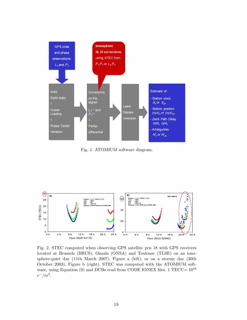
Fig. 1. ATOMIUM software diagram.

Fig. 2. STEC computed when observing GPS satellite prn 18 with GPS receiverslocated at Brussels (BRUS), Onsala (ONSA) and Toulouse (TLSE) on an iono-sphere-quiet day (11th March 2007), Figure a (left), or on a stormy day (30thOctober 2003), Figure b (right). STEC was computed with the ATOMIUM soft-ware, using Equation (9) and DCBs read from CODE IONEX files. 1 TECU= 1016

e−/m2.

19

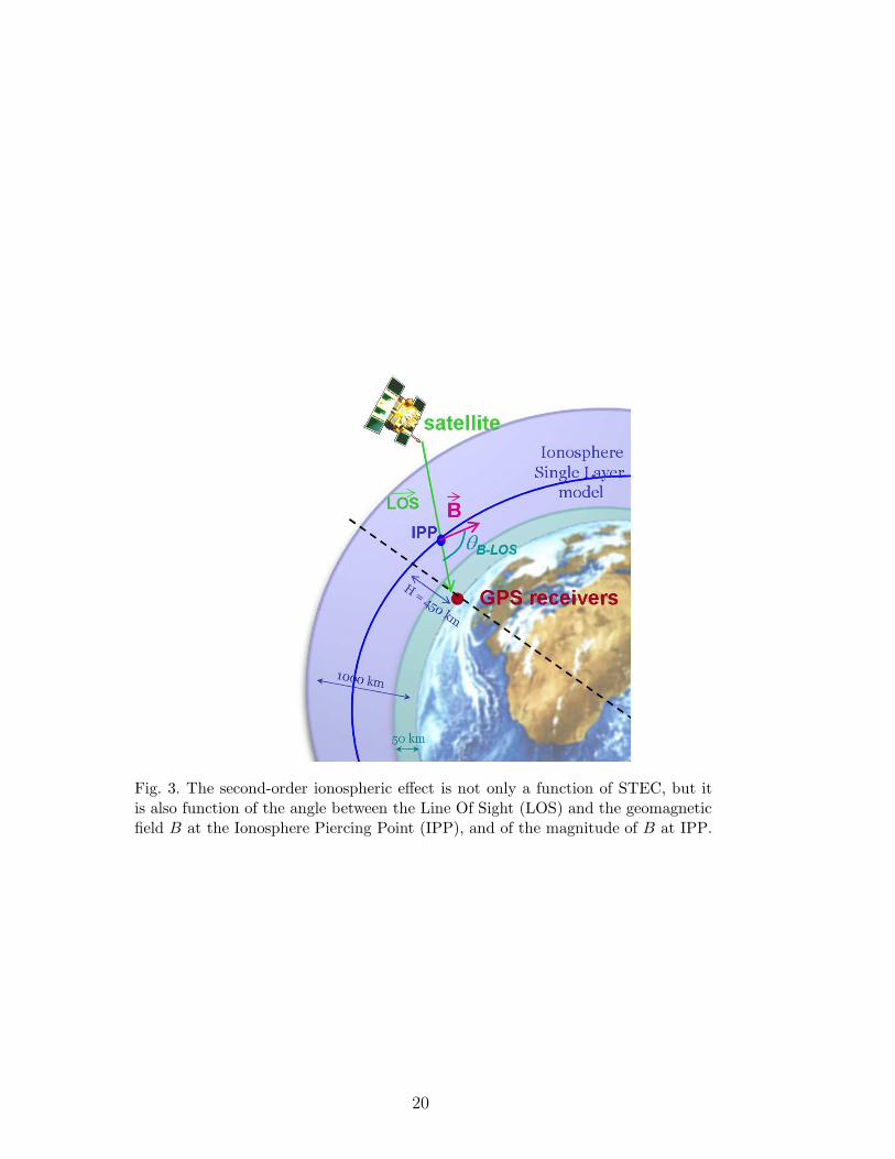
Fig. 3. The second-order ionospheric effect is not only a function of STEC, but itis also function of the angle between the Line Of Sight (LOS) and the geomagneticfield B at the Ionosphere Piercing Point (IPP), and of the magnitude of B at IPP.

20

Fig. 4. Time series of the noticeable solar events (X and M X-ray flares) and geo-magnetic K index from Wingst Observatory (KW in the text). The notation usedis the following. Labels i and j are linked to the classification of flares. M flares arerepresented by a line peaking between 10 and 20 (e.g. M2.5 by a line from 0 to 12.5),while X flares are represented between 20 and 30, at their respective peak-intensitytime. Note that X flares bigger than X9.9 saturate the scale and are represented bya line peaking at 30.

21

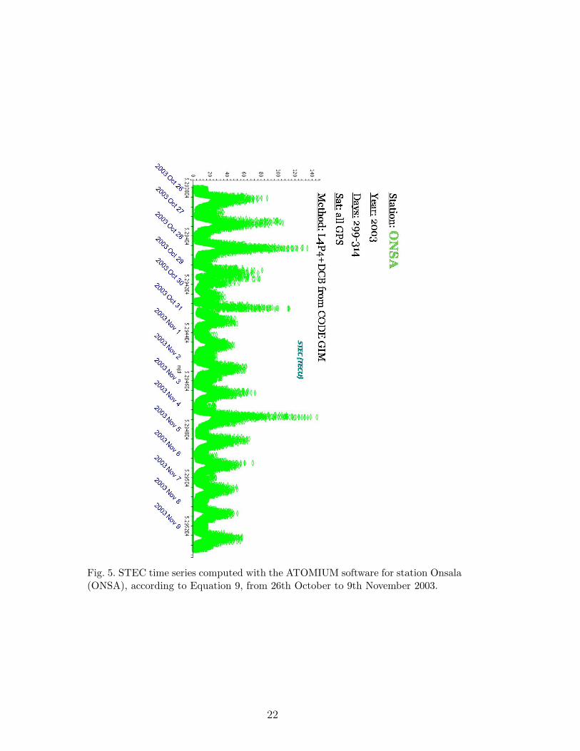
Fig. 5. STEC time series computed with the ATOMIUM software for station Onsala(ONSA), according to Equation 9, from 26th October to 9th November 2003.

22

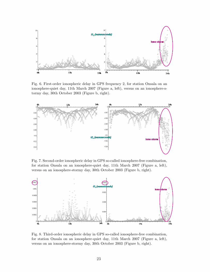
Fig. 6. First-order ionospheric delay in GPS frequency 2, for station Onsala on anionosphere-quiet day, 11th March 2007 (Figure a, left), versus on an ionosphere-s-tormy day, 30th October 2003 (Figure b, right).

Fig. 7. Second-order ionospheric delay in GPS so-called ionosphere-free combination,for station Onsala on an ionosphere-quiet day, 11th March 2007 (Figure a, left),versus on an ionosphere-stormy day, 30th October 2003 (Figure b, right).

Fig. 8. Third-order ionospheric delay in GPS so-called ionosphere-free combination,for station Onsala on an ionosphere-quiet day, 11th March 2007 (Figure a, left),versus on an ionosphere-stormy day, 30th October 2003 (Figure b, right).

23

Fig. 9. Effect of taking second-order ionospheric effects, or not, into account in theL3P3 GPS measurements for the Brussels-Onsala link, on the ionosphere-stormyday 30th October 2003. The difference is taken between two ATOMIUM estimatedstation clock solutions, both using IGS products.

Fig. 10. Effect of taking third-order ionospheric effect, or not, into account in theL3P3 GPS measurements for the Brussels-Onsala link, on the ionosphere-stormyday 30th October 2003. The difference is taken between two ATOMIUM estimatedstation clock solutions, both using IGS products.

24

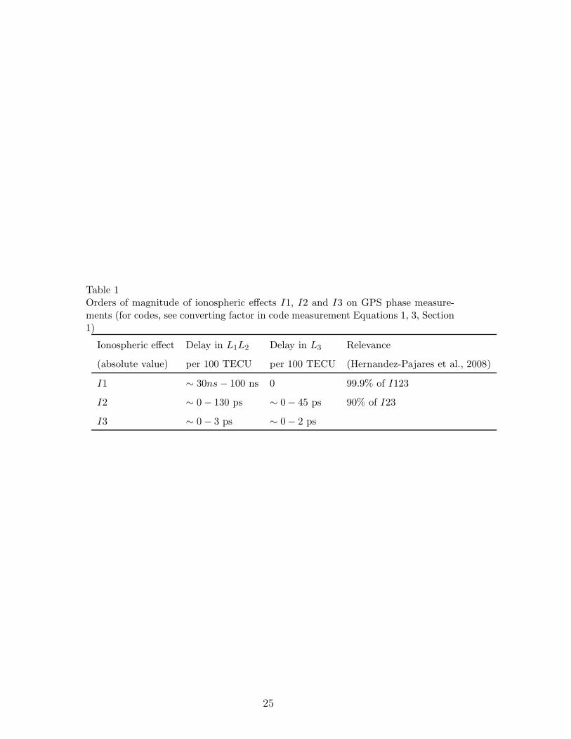
Table 1Orders of magnitude of ionospheric effects I1, I2 and I3 on GPS phase measure-ments (for codes, see converting factor in code measurement Equations 1, 3, Section1)

Ionospheric effect Delay in L1L2 Delay in L3 Relevance

(absolute value) per 100 TECU per 100 TECU (Hernandez-Pajares et al., 2008)

I1 ∼ 30ns − 100 ns 0 99.9% of I123

I2 ∼ 0 − 130 ps ∼ 0 − 45 ps 90% of I23

I3 ∼ 0 − 3 ps ∼ 0 − 2 ps

25