Influence of constant torque on equilibria of satellite in circular orbit

INFLUENCE OF CONSTANT TORQUE ON EQUILIBRIAOF SATELLITE IN CIRCULAR ORBIT

V. A. SARYCHEV1,2, A. GUERMAN2 and P. PAGLIONE3

1Keldysh Institute of Applied Mathematics, Moscow, Russia2Universidade da Beira Interior, Covilhã, Portugal

3Instituto Tecnológico de Aeronáutica, São José dos Campos, SP, Brazil

(Received: 11 October 2001; revised: 19 December 2002; accepted: 19 February 2003)

Abstract. We consider the equilibria of a satellite in a circular orbit under the action of gravitationaland constant torques. The number of equilibria depending on the parameters of the problem is foundby the analysis of an algebraic equation of order 6. The domains with different numbers of equilibriaare specified, and the equations of boundary curves are determined in function of values of thecomponents of constant torque. Classification of different distributions of number of equilibria ismade for arbitrary values of the parameters.

Key words: satellite, attitude motion, gravitation torque, constant torque, equilibria

1. Introduction

Determination of equilibrium orientations of a satellite under the action ofexternal torques constitutes one of the basic problems of astrodynamics. Suchequilibria are used as a nominal motion in the design of rather simple, cheapand long-living passive attitude control systems. Rarely can such a problem be re-solved analytically. For satellite-rigid body it was done by Sarychev (1965), Likinsand Roberson (1966) and Beletsky (1975). Equilibrium orientations of satellite-gyrostat were studied by Roberson (1966), Longman and Roberson (1966),Longman (1975) and Sarychev and Mirer (2001). Equilibria of a satellite subjectedto gravitational and aerodynamic torques were examined by Sarychev and Mirer(2000).

The problem to be analyzed here is related to the behavior of a satellite actedupon by the gravity gradient and constant torques. The constant torque may beproduce actively or caused, for example, by gas or fuel escape from the satellite.The influence of a small constant torque on the satellite dynamics is analogous tothe action of a non-conservative component of aerodynamic torque (Nurre, 1968;Frik, 1970; Sazonov, 1989).

Celestial Mechanics and Dynamical Astronomy 87: 219–239, 2003.© 2003 Kluwer Academic Publishers. Printed in the Netherlands.

220 V. A. SARYCHEV ET AL.

We investigate here the relative equilibria of a satellite with respect to the orbitframe. The analysis is based upon the following assumptions:

— the gravity field of the Earth is central and Newtonian;— the satellite is a triaxial rigid body;— the satellite’s center of mass moves along a circular orbit;— the satellite is subject to the gravity gradient torque and a torque that is fixed

with respect to the body of satellite, so the components of this torque in thebody-fixed frame are constant.

Relative equilibrium in the orbital frame correspond, in an inertial frame, toprecession of the satellite, that is, rotation of the satellite about the normal to theorbit plane with constant orbital angular velocity. This motion exists when the totaltorque acting on the satellite causes the proper change of its angular momentum.For each specific equilibrium orientation, the corresponding constant torque can befound from the angular momentum equation. To solve the inverse problem, that is,to determine a number of equilibria corresponding to a given vector of the constanttorque, one has to examine the general equations of motion. This study is donehere.

In the absence of constant torque, there are 24 equilibrium orientations of satel-lite (Sarychev, 1965; Likins and Roberson, 1966; Beletsky, 1975). Obviously, theaction of some constant torque change these orientations and can destroy some oreven all these equilibria. Garber (1963) indicated the existence of equilibria for asatellite under the action of the gravity gradient and constant disturbing torquesin some particular cases. For general values of constant torque this problem wasstudied by Sarychev and Gutnik (1994). It was shown that for small constant torquethere exist 24 equilibria, and the number of equilibria decreases with the increaseof the constant torque. A different method to solve this problem was suggested bySarychev et al. (1997).

The goal of the present investigation is to obtain the classification of differentdistributions of the number of equilibria (NE) in a function of the parameters of theproblem, namely, the components of the constant torque, the inertial parameters ofthe satellite and the angular velocity of its orbital motion. We complete the analysisof NE developing the approach of Sarychev and Gutnik (1994).

2. Statement of the Problem

We use two right-hand Cartesian reference frames related to the center of mass ofthe satellite O:

— OX1X2X3 is the orbital coordinate system; OX1 is directed along the velocityof the satellite, OX3 axis is directed along the radius-vector of the point O withrespect to the Earth’s center, and OX2 is normal to the orbit plane;

INFLUENCE OF CONSTANT TORQUE ON EQUILIBRIA OF SATELLITE 221

— Ox1x2x3 is the frame connected with the satellite. Ox1,Ox2 and Ox3 are itscentral principal axes. The respective moments of inertia are A, B and C, andthey are supposed to be not equal: A �= B, B �= C, and C �= A.

Mutual orientation of these frames can be described by the matrix A = ‖aij‖,whose elements are direction cosines of the axes of theOx1x2x3 frame with respectto the OX1X2X3 frame:

Ox1 Ox2 Ox3

OX1 a11 a12 a13

OX2 a21 a22 a23

OX3 a31 a32 a33

The direction cosines satisfy the following orthogonality conditions

ai1aj1 + ai2aj2 + ai3aj3 = δij , i, j = 1, 3, (1)

where δij is the Kronecker symbol. The transition from OX1X2X3 system toOx1x2x3 can be realized by three Euler rotations about axes 2, 3, and 1 with therespective matrices

A1 =

cos α 0 sinα0 1 0

− sinα 0 cos α

, A2 =

cos β − sin β 0sin β cos β 0

0 0 1

,

A3 =

1 0 00 cos γ − sin γ0 sin γ cos γ

.

The resulting orientation matrix is the product A = A1 · A2 · A3, and in termsof orientation angles, α (pitch), β (yaw) and γ (roll), the direction cosines aij arerepresented by the formulae

a11 = cos α cos β, a12 = sinα sin γ − cos α sin β cos γ,

a13 = sinα cos γ + cos α sin β sin γ, a21 = sin β,

a22 = cos β cos γ, a23 = − cos β sin γ,

a31 = − sinα cos β, a32 = cos α sin γ + sin α sin β cos γ,

a33 = cos α cos γ − sinα sin β sin γ. (2)

Evidently, the two sets of orientation angles (α, β, γ ) and (α + π, π − β, γ + π)correspond to the same orientation matrix. So it suffices to analyze only the angleswithin the intervals

0 �α < 2π, −π2

�β � π2, 0 � γ < 2π. (3)


It is also worthy of note that for β = ±π/2 the indicated system of orientationangles degenerates, and the orientation of the satellite can be described by therespective combinations of the two remaining angles α ± γ .

Under the above assumptions, one can use the well-known approximation forthe gravitation potential and write down the equations of attitude motion of thesatellite as follows (Sarychev and Gutnik, 1994):

Ap + (C − B)qr = 3ω20(C − B)a32a33 + a,

Bq + (A− C)rp = 3ω20(A− C)a33a31 + b,

Cr + (B − A)pq = 3ω20(B − A)a31a32 + c,

p = αa21 + γ + ω0a21,

q = αa22 + β sin γ + ω0a22,

r = αa23 + β cos γ + ω0a23. (4)

Here ω0 is the angular velocity of the orbital motion of the satellite, p, q and r arethe projections of the angular velocity of the satellite onto the axes of Ox1x2x3

frame, while a, b, and c are the components of the constant torque in the sameframe.

Equilibrium orientations α = const, β = const, γ = const of system (4)correspond to solutions of the system

a22a23 − 3a32a33 = a, a23a21 − 3a33a31 = b, a21a22 − 3a31a32 = c,a2

21 + a222 + a2

23 = 1, a231 + a2

32 + a233 = 1,

a21a31 + a22a32 + a23a33 = 0. (5)

Here

a = a

ω20(C − B), b = b

ω20(A− C), c = c

ω20(B − A)

are the constants that characterize the dimensionless components of the constanttorque.1 System (5) includes six equations for six unknown values a21, a22, a23,a31, a32, and a33. After a21, a22, a23, a31, a32 and a33 are found, the direction cosinesa11, a12 and a13 can be determined from the conditions of orthogonality.

3. Determination of Equilibria

We will study equilibrium orientations of the satellite substituting the directioncosines (2) to Equations (5). This yields the system which describes the equilibrium

1If the satellite possesses any kind of dynamical symmetry, equilibria exist only for some specialconditions imposed on the constant torque; this case is beyond the scope of this paper.


orientations of the satellite through the orientation angles α, β, and γ :

3(cos α sin γ + sinα sin β cos γ )(sinα sin β sin γ − cos α cos γ )−− cos2 β sin γ cos γ = a,

3 sin α cos α cos β cos γ − sin β cos β(1 + 3 sin2 α) sin γ = b,sin β cos β(1 + 3 sin2 α) cos γ + 3 sin α cos α cos β sin γ = c. (6)

System (6) shows that for arbitrary values of α, β, and γ (i.e. for any orientation ofthe satellite) there exists only one set of values a, b, and c that corresponds to theequilibrium orientation.

Since the last two equations in (6) form a system of linear equations with respectto sin γ and cos γ , the proceeding analysis should be performed for two differentsituations: b = c = 0 and b2 + c2 �= 0.

3.1. SPECIAL CASE b = c = 0

If b = c = 0, the solution of (6) exists only if

� = [9 sin2 α cos2 α + sin2 β(1 + 3 sin2 α)2] cos2 β = 0. (7)

For α, β, and γ within the intervals (3), Equation (7) is satisfied in the followingcases:

β = π

2and β = −π

2, (8)

β = 0 and α = 0 or α = π, (9)

β = 0 and α = π

2or α = 3π

2. (10)

In case (8) the first equation of system (6) can be transformed to the equation

sin 2(α + γ ) = −2a

3or sin 2(α − γ ) = −2a

3,

respectively. When |a| < 3/2 each one of these equations has four solutions0 �α ± γ < 2π which describe completely the orientation of the satellite becausethe considered values of β correspond to degeneration of the accepted system oforientation angles. So for these values of a there are eight equilibrium orientationsthat correspond to case (8). In case (9) the first equation of (6) turns to be

sin 2γ = −a2,

it has four solutions satisfying 0 � γ < 2π whenever |a| < 2. Hence we geteight different sets of α, β, and γ , that correspond to eight different equilibriumorientations. Finally, case (10) results in the equation

sin 2γ = −2a,


and for |a| < 1/2 there are eight different sets of angles (α, β, γ ) (and eightdifferent equilibrium orientations of the satellite) of this type. Hence for |a| < 1/2there are 24 equilibria, for 1/2 < |a| < 3/2 there are 16 equilibria, and for3/2 < |a| < 2 there exist eight equilibrium orientations of the satellite.

3.2. CASE b2 + c2 �= 0

If b2 + c2 �= 0, the last two equations of (6) permit us to determine sin γ and cos γ :

sin γ = 1

�[3c sinα cos α − b sin β(1 + 3 sin2 α)] sin β,

cos γ = 1

�[3b sinα cos α + c sin β(1 + 3 sin2 α)] sin β. (11)

Here � = [9 sin2 α cos2 α + sin2 β(1 + 3 sin2 α)2] cos2 β does not vanish when αand β differ from (8)–(10). Since sin2 γ + cos2 γ = 1, one gets

(1 + 3 sin2 α)2 sin4 β − [(1 + 3 sin2 α)2 − 9 sin2 α cos2 α

]sin2 β +

+ b2 + c2 − 9 sin2 α cos2 α = 0. (12)

Let

x = 1 + 3 sin2 α, y = sin β, z = 3 sin α cos α. (13)

Using this notation, it is possible to transform Equation (12) to the form

x2y4 + (z2 − x2)y2 + b2 + c2 − z2 = 0. (14)

One can also exclude γ from the first equation in (6) using (11) and obtain

bcx3y4 + [bcx(2z2 − 4)+ a(b2 + c2)x2]y2 − 4(b2 − c2)yz ++[a(b2 + c2)+ bc(5 − x)]z2 = 0. (15)

Excluding now y4 from (15) by means of (14), one comes to

[bc(5x − 8)+ a(b2 + c2)x]xy2 − 4(b2 − c2)yz −−bc(b2 + c2)x + [5bc + a(b2 + c2)]z2 = 0. (16)

These equations should be completed by the obvious relationship

z2 = −x2 + 5x − 4. (17)

Eliminating y from system (14), (16) by the method of resultant (Kurosh, 1975)and substituting z2 from (17), one gets the following equation:

x2(b2 + c2)2(p0x6 + p1x

5 + p2x4 + p3x

3 + p4x2 + p5x + p6) = 0. (18)


Here the coefficients pj(j = 0; 6) are

p0 = a4r4 + 10a3qr3 − 80a3qr2 + 2a2q2r3 + 57a2q2r2 −− 544a2q2r − 32a2r3 + 400a2r2 + 10aq3r2 + 80aq3r −− 720aq3 − 480aqr2 + 2720aqr + q4r2 + 32q4r − 144q4 ++ 32q2r2 − 1088q2r + 3600q2 + 256r2,

p1 = 8(−3a3qr3 + 58a3qr2 − 40a2q2r2 + 420a2q2r ++ 50a2r3 − 580a2r2 − 3aq3r2 − 83aq3r + 522aq3 −− 8aqr3 + 716aqr2 − 4072aqr − 25q4r + 90q4 −− 70q2r2 + 1690q2r − 5220q2 − 480r2),

p2 = 16(−40a3qr2 + 21a2q2r2 − 336a2q2r − 95a2r3 ++ 1241a2r2 + 90aq3r − 360aq3 + 20aqr3 − 1440aqr2 ++ 9130aqr + 12q4r − 27q4 + 169q2r2 −− 3769q2r + 11169q2 + 16r3 + 1392r2),

p3 = 128(2a3qr2 + 20a2q2r + 15a2r3 − 310a2r2 − 8aq3r ++ 18aq3 − 2aqr3 + 291aqr2 − 2436aqr − 35q2r2 ++ 960q2r − 2790q2 − 20r3 − 490r2),

p4 = 256(−3a2r3 + 158a2r2 − 100aqr2 + 1340aqr ++ 9q2r2 − 509q2r + 1422q2 + 33r3 + 348r2),

p5 = 2048(−10a2r2 + 3aqr2 − 92aqr ++ 35q2r − 90q2 − 5r3 − 30r2),

p6 = 4096(a2r2 + 10aqr − 4q2r + 9q2 + r3 + 4r2).

(The notations used are r = b2 + c2, and q = bc.)Let us show now that no real root of (18) corresponds to more than four equi-

librium orientations of the satellite. If a real value of x satisfies (18), than in accor-dance with the properties of the resultant there exists exactly one common solutiony of system (14), (16). Returning to (13), we get at most four different combinationsα and β within intervals (3). Each of them can be completed by the unique valueof γ calculated by (11). These four different sets of α, β, and γ correspond tofour different sets of orientation cosines aij , that is, to four different equilibriumorientations of the satellite. Taking into account (13), one can see that x �= 0. HenceEquation (18) has at most six real roots, and the satellite possesses no more than24 equilibrium orientations.


4. Special Case b = c �= 0b = c �= 0b = c �= 0

We proceed with the analysis of the special case b = c �= 0. In this case system(14), (16) is equivalent to

x2y4 + (z2 − x2)y2 + 2b2 − z2 = 0,

(5x − 8 + 2ax)xy2 + 5z2 − 2b2x + 2az2 = 0. (19)

Substituting z2 from (17) and eliminating y, one obtains

Q(x) = (−34 − 20a + 8b2 + 5ab2 + 2a2b2 + b4)x3 ++ (210 + 116a − 50b2 − 12ab2)x2 ++ (−336 − 160a + 48b2)x + 160 + 64a = 0. (20)

Equation (20) has at most three real roots. For each of them, there exist no morethan two different values of y that can be found by the formula

y2 = 2b2x + (5 + 2a)(x2 − 5x + 4)

(5 + 2a)x2 − 8x. (21)

So we still have no more than six different solutions (x, y), that correspond to atmost 24 equilibrium orientations. The exact NE can be determined by studying thecondition of changing the number of solutions of (19).

In accordance with (13), there are natural restrictions on the variables x and y,namely, 1 � x� 4 and 0 � y2 � 1. So the necessary conditions for changing the NEare the following:

(a) appearance of a double root of (20);(b) x = 1;(c) x = 4;(d) y2 = 0;(e) y2 = 1.

Examining these conditions one by one, we get the following equations of thecurves in the plane (a, b) where the necessary conditions (a)–(e) are satisfied.

Case (a): Eliminating x from the system Q(x) = Q′(x) = 0, one gets4a2 + 4b2 − 9 = 0 (22)

or27b6 + 27a2b4 − 117b4 + 70ab2 + 169b2 − 36 = 0. (23)

Case (b): Substituting x = 1 to (20), one obtainsb2 + 2a2 − 7a + 6 = 0. (24)

Case (c): Substituting x = 4 to (20), one arrives at2b2 + 4a2 + 4a − 3 = 0. (25)


Case (d): Elimination x from (20) and (21) for y2 = 0 leads tob2 + 2a2 + 5a + 2 = 0 (26)

orb8 + 2a2b6 + 5ab6 + 20b6 + 12a2b4 − 40ab4 − 109b4 +

+ 24a2b2 + 150ab2 + 185b2 + 16a2 − 36 = 0. (27)Case (e): Eliminating x from (20) and (21) for y2 = 1 one concludes that this

condition is never satisfied for b �= 0.

Now the question is whether crossing these curves really changes NE. To detectthe change it suffices to calculate NE at a single point in each domain. Unfortu-nately, the points of a-axis, where NE were found analytically, cannot be used forthis purpose, the case b = c = 0 being special for the provided analysis. The regionof the (a, b, c)-space where equilibria exist is limited by the inequalities (Sarychevand Gutnik, 1994) a2 + b2 + c2 � 5 and b2 + c2 � 4, c2 + a2 � 4, a2 + b2 � 4.Obviously, in general case it is enough to study the equilibria within the cube

|a|� 2, |b|� 2, |c|� 2, (28)

and for the particular case under consideration,

|a|� 2, |b|� √2. (29)

We have calculated NE numerically at one point in each of the domains limited bycurves (22)–(27) in the rectangular |a|� 2, |b|� √

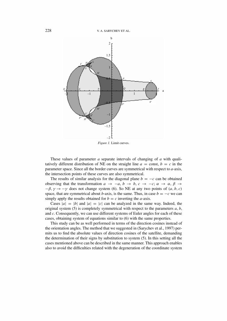
2 of (a, b)-plane, concludingthat only curves (23), (24), (25), and (26) separate regions with different numberof solutions of the original system of equations. Figure 1 shows these regions andthe boundary curves on the plane (a, b). Shaded regions correspond to existenceof equilibria. The intensity of shading indicates their number: the lightest shadowcorresponds to NE = 16, the darkest to NE = 24, and the intermediate grey marksthe regions with NE = 8. On a boundary curve, NE equals the average of its valuesin the adjoining regions because the fusion of solutions occurs there.

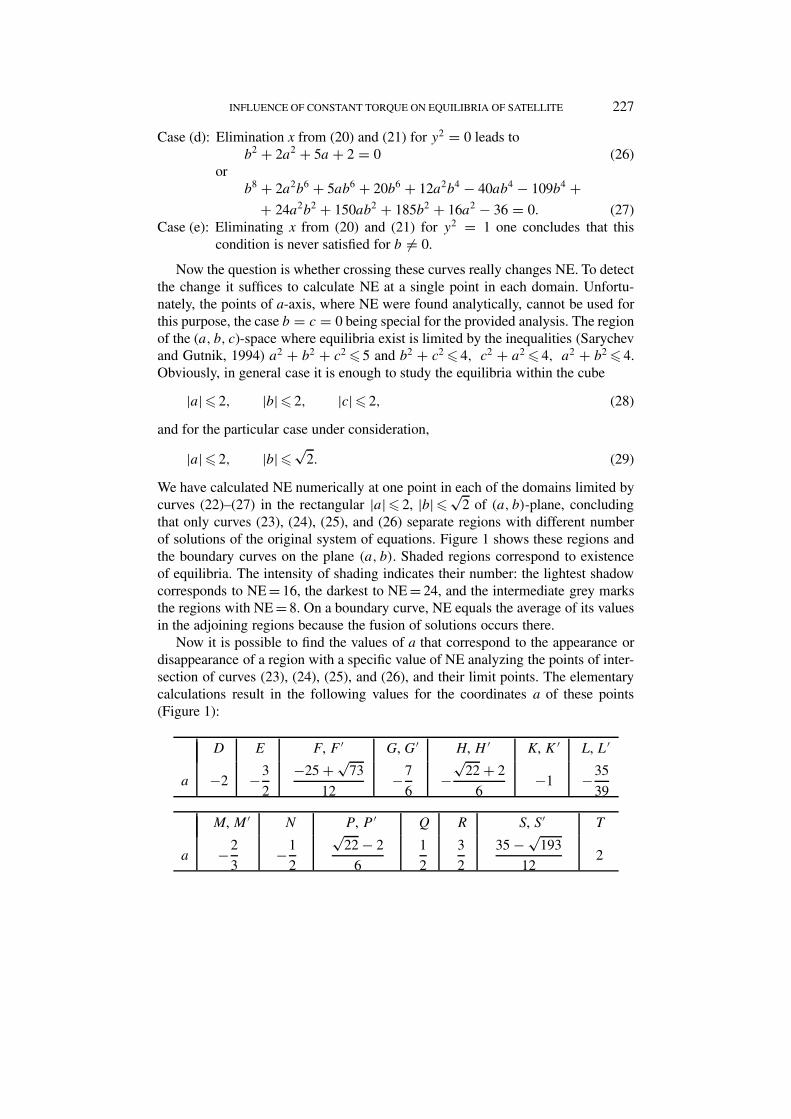
Now it is possible to find the values of a that correspond to the appearance ordisappearance of a region with a specific value of NE analyzing the points of inter-section of curves (23), (24), (25), and (26), and their limit points. The elementarycalculations result in the following values for the coordinates a of these points(Figure 1):

D E F, F ′ G, G′ H, H ′ K, K ′ L, L′

a −2 −3

2

−25 + √73

12−7

6−

√22 + 2

6−1 −35

39

M,M ′ N P, P ′ Q R S, S ′ T

a −2

3−1

2

√22 − 2

6

1

2

3

2

35 − √193

122


Figure 1. Limit curves.

These values of parameter a separate intervals of changing of a with quali-tatively different distribution of NE on the straight line a = const, b = c in theparameter space. Since all the border curves are symmetrical with respect to a-axis,the intersection points of these curves are also symmetrical.

The results of similar analysis for the diagonal plane b = −c can be obtainedobserving that the transformation a → −a, b → b, c → −c; α → α, β →−β, γ →−γ does not change system (6). So NE at any two points of (a, b, c)space, that are symmetrical about b-axis, is the same. Thus, in case b = −c we cansimply apply the results obtained for b = c inverting the a-axis.

Cases |a| = |b| and |a| = |c| can be analyzed in the same way. Indeed, theoriginal system (5) is completely symmetrical with respect to the parameters a, b,and c. Consequently, we can use different systems of Euler angles for each of thesecases, obtaining system of equations similar to (6) with the same properties.

This study can be as well performed in terms of the direction cosines instead ofthe orientation angles. The method that we suggested in (Sarychev et al., 1997) per-mits us to find the absolute values of direction cosines of the satellite, demandingthe determination of their signs by substitution to system (5). In this setting all thecases mentioned above can be described in the same manner. This approach enablesalso to avoid the difficulties related with the degeneration of the coordinate system


for β = ±π/2. Its one disadvantage is the necessity of selecting the solution froma larger number of versions.

5. General Case

When the parameters of the problem do not possess any kind of symmetry de-scribed above, it is possible to find the equations of the boundary surfaces betweenthe regions with different NE. The method used in the special cases |a| = |b|,|a| = |c|, and |b| = |c| is also applicable for arbitrary values of the parameters a,b, and c.

New solutions of system (14), (16) can appear when

(a) Equation (18) has double roots;(b) x = 1;(c) x = 4;(d) y = 1;(e) y = −1.

Examining these conditions we describe the boundaries between the domains witha specific NE in the parameter space. All these conditions are only necessary, sowe have to control the change of NE when crossing these surfaces.

Condition (a) determines a surface in (a, b, c)-space that satisfies the followingsystem of equations:

P(x) = p0x6 + p1x

5 + p2x4 + p3x

3 + p4x2 + p5x + p6 = 0,

P ′(x) = 0. (30)

The variable x can be eliminated from (30) using the method of resultant. Finallyone gets the equation of the surface (a) in the form

(b − c)6(b + c)6'(2) = 0.

Here '(a, b, c), ((a, b, c), and )(a, b, c) are rather cumbersome functions ob-tained using the Mathematica 3.1 package.

In cases (b)–(e) the equations of the respective surfaces can be found substitut-ing the corresponding values of x or y into system (14), (16).

(b) This condition is realized on the following surfaces:a2 + b2 = 0, or b2 + c2 = 0, or c2 + a2 = 0, or

a2bc(−10b4 − 20b2c2 − 10c4)+ a3(b6 + 3b4c2 + 3b2c4 + c6)

= b3c3(36 − b4 − 2b2c2 − c4).

(c) This condition corresponds to the equationsa2 + b2 = 0, or b2 + c2 = 0, or c2 + a2 = 0, or

a2bc(20b4 + 40b2c2 + 20c4)+ a3(4b6 + 12b4c2 + 12b2c4 + 4c6)

= b3c3(36 − b4 − 2b2c2 − c4).


(d) After substituting y = 1 to system (14), (16), the variable x should be excludedby the method of resultant, and we come to the following equations:

b = 0, or c = 0, or ab2 + b2 + 5bc − c2 + ac2 = 0, or

*1 = 0.

(e) Finally, the condition y = −1 is studied similarly to (d). It corresponds to thesurfaces

b = 0, or c = 0, or ab2 − b2 + 5bc + c2 + ac2 = 0, or

*2 = 0.

Now we have to verify whether NE really changes when we cross one of thesurfaces (a)–(e). This can be done directly, finding NE numerically at a singlepoint on each one of the domains in (a, b, c)-space limited by these surfaces. Thisanalysis showed that only the surface

) = 0 (31)

separates domains with different number of equilibrium orientations. (As the ex-pressions that we have obtained for ', (, ), *1, and *2 are rather complicated,in Appendix A we represent in details only ).)

The numerical analysis of the boundary curve (31) as well as the direct calcula-tions of NE within the cube (28) resulted in numerous pictures of the distributionof NE in the plane (b, c) for a = const (some of them are represented below).It was found that most of the regions with specific values of NE arise or vanishon the diagonal of the square |b|� 2, |c|� 2, that is, when |b| = |c|. In thiscase we use the results of Section 4 to calculate analytically the critical valuesof a which correspond to qualitative changes of the distribution of NE as well asthe coordinates (b, c) of points giving rise to new region (or ones where regionsdisappear). Besides, there are some regions that arise outside the diagonals. In thiscase the critical values of a were found numerically.

Figures 2–26 represent all the possible essentially different distributions of thenumber of equilibrium orientations in the planes a = const for negative a. Theclassification was made for −2 � a� 0, because the transformation a → −a leadsto a distribution of NE symmetric with respect to either b- or c-axis. Each figurecorresponds to a specific value of a and shows the regions with different NE in(b, c) plane (b-axis is horizontal and c-axis is vertical) and boundary curves ob-tained as a cross-section of surface (31) by the plane a = const. The value of a iseither critical (bifurcational) or belongs to some interval where the picture changesonly quantitatively, maintaining the number of regions with specific values of NEas well as their mutual disposition. Here also the darkest grey designates regionswith NE = 24, the lightest corresponds to NE = 16, and intermediate grey indicatesregions with NE = 8. We represent the whole square |b|� 2, |c|� 2 or only thefragment where the principal changes appear.


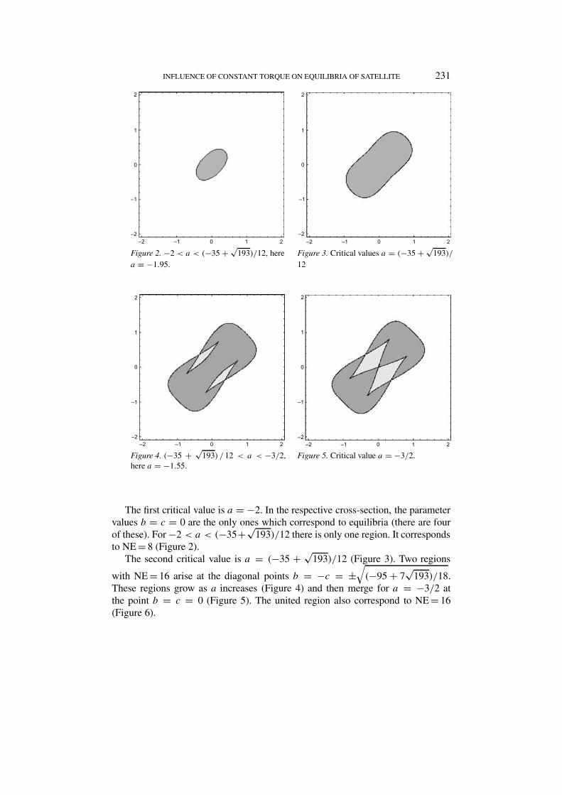
Figure 2. −2 < a < (−35 + √193)/12, here Figure 3. Critical values a = (−35 + √

193)/a = −1.95. 12

Figure 4. (−35 + √193) / 12 < a < −3/2, Figure 5. Critical value a = −3/2.

here a = −1.55.

The first critical value is a = −2. In the respective cross-section, the parametervalues b = c = 0 are the only ones which correspond to equilibria (there are fourof these). For −2 < a < (−35+√

193)/12 there is only one region. It correspondsto NE = 8 (Figure 2).

The second critical value is a = (−35 + √193)/12 (Figure 3). Two regions

with NE = 16 arise at the diagonal points b = −c = ±√(−95 + 7

√193)/18.

These regions grow as a increases (Figure 4) and then merge for a = −3/2 atthe point b = c = 0 (Figure 5). The united region also correspond to NE = 16(Figure 6).


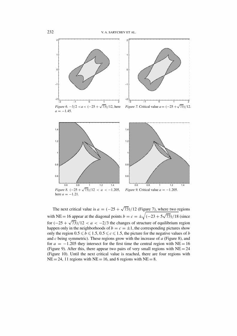
Figure 6. −3/2 <a< (−25 + √73)/12, here Figure 7. Critical value a= (−25 +√

73)/12.a = −1.45.

Figure 8. (−25 + √73)/12 < a < −1.205, Figure 9. Critical value a = −1.205.

here a = −1.21.

The next critical value is a = (−25 + √73)/12 (Figure 7), where two regions

with NE = 16 appear at the diagonal points b = c = ±√(−23 + 5

√73)/18 (since

for (−25 + √73)/12 < a < −2/3 the changes of structure of equilibrium region

happen only in the neighborhoods of b = c = ±1, the corresponding pictures showonly the region 0.5 � b� 1.5, 0.5 � c� 1.5, the picture for the negative values of band c being symmetric). These regions grow with the increase of a (Figure 8), andfor a = −1.205 they intersect for the first time the central region with NE = 16(Figure 9). After this, there appear two pairs of very small regions with NE = 24(Figure 10). Until the next critical value is reached, there are four regions withNE = 24, 11 regions with NE = 16, and 6 regions with NE = 8.


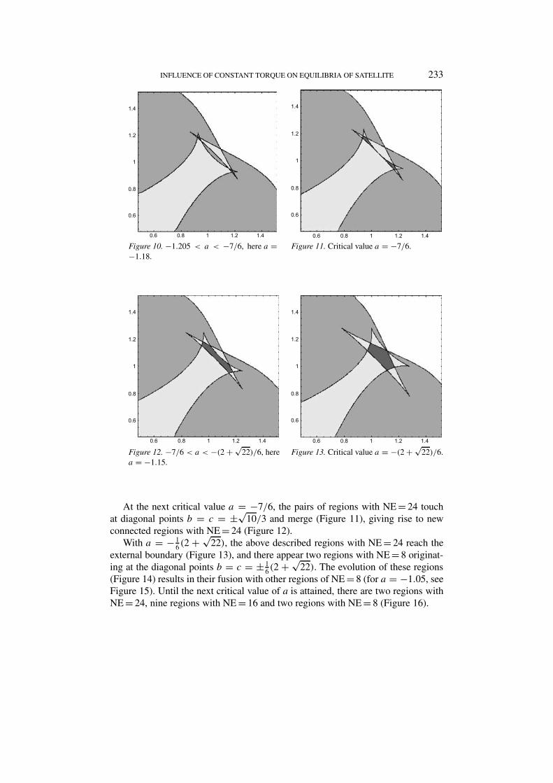
Figure 10. −1.205 < a < −7/6, here a = Figure 11. Critical value a = −7/6.−1.18.

Figure 12. −7/6 < a < −(2 + √22)/6, here Figure 13. Critical value a = −(2 + √

22)/6.a = −1.15.

At the next critical value a = −7/6, the pairs of regions with NE = 24 touchat diagonal points b = c = ±√

10/3 and merge (Figure 11), giving rise to newconnected regions with NE = 24 (Figure 12).

With a = − 16 (2 + √

22), the above described regions with NE = 24 reach theexternal boundary (Figure 13), and there appear two regions with NE = 8 originat-ing at the diagonal points b = c = ± 1

6(2 + √22). The evolution of these regions

(Figure 14) results in their fusion with other regions of NE = 8 (for a = −1.05, seeFigure 15). Until the next critical value of a is attained, there are two regions withNE = 24, nine regions with NE = 16 and two regions with NE = 8 (Figure 16).


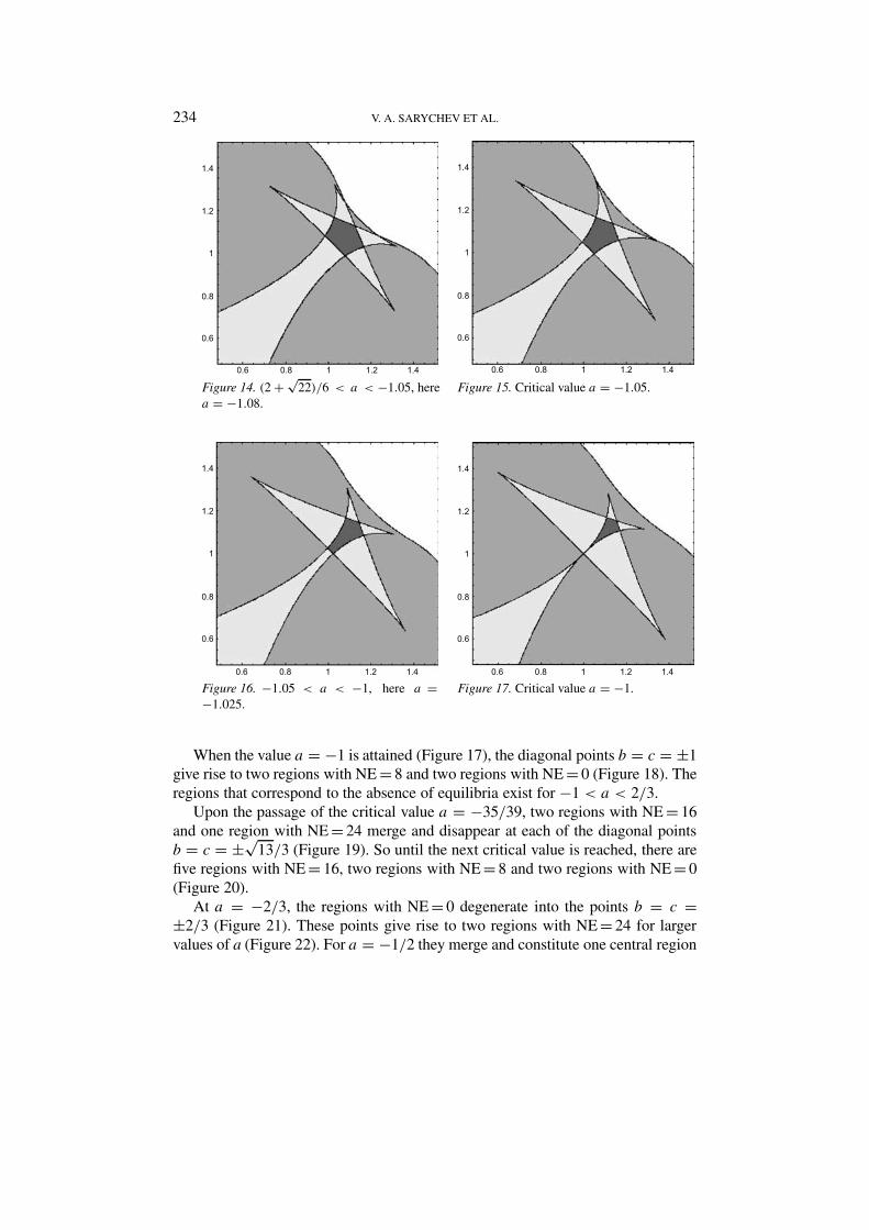
Figure 14. (2 + √22)/6 < a < −1.05, here Figure 15. Critical value a = −1.05.

a = −1.08.

Figure 16. −1.05 < a < −1, here a = Figure 17. Critical value a = −1.−1.025.

When the value a = −1 is attained (Figure 17), the diagonal points b = c = ±1give rise to two regions with NE = 8 and two regions with NE = 0 (Figure 18). Theregions that correspond to the absence of equilibria exist for −1 < a < 2/3.

Upon the passage of the critical value a = −35/39, two regions with NE = 16and one region with NE = 24 merge and disappear at each of the diagonal pointsb = c = ±√

13/3 (Figure 19). So until the next critical value is reached, there arefive regions with NE = 16, two regions with NE = 8 and two regions with NE = 0(Figure 20).

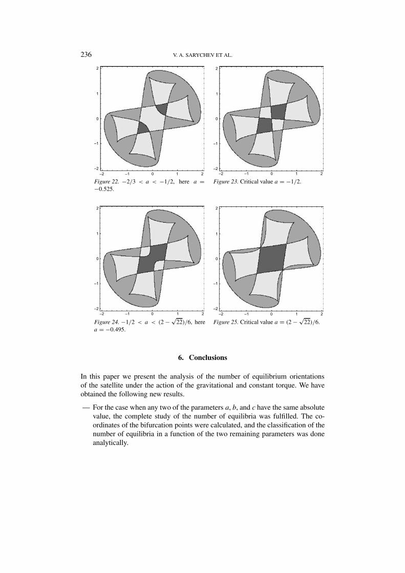
At a = −2/3, the regions with NE = 0 degenerate into the points b = c =±2/3 (Figure 21). These points give rise to two regions with NE = 24 for largervalues of a (Figure 22). For a = −1/2 they merge and constitute one central region


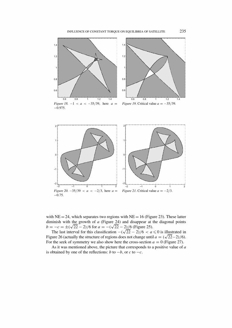
Figure 18. −1 < a < −35/39, here a = Figure 19. Critical value a = −35/39.−0.975.

Figure 20. −35/39 < a < −2/3, here a = Figure 21. Critical value a = −2/3.−0.75.

with NE = 24, which separates two regions with NE = 16 (Figure 23). These latterdiminish with the growth of a (Figure 24) and disappear at the diagonal pointsb = −c = ±(√22 − 2)/6 for a = −(√22 − 2)/6 (Figure 25).

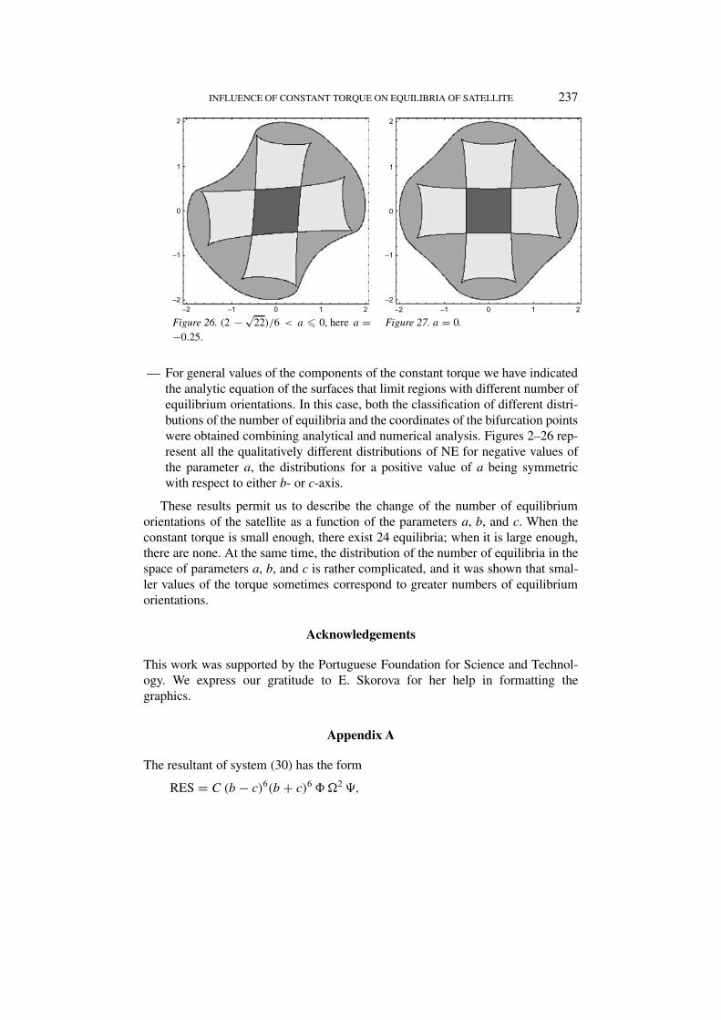
The last interval for this classification −(√22 − 2)/6 < a� 0 is illustrated inFigure 26 (actually the structure of regions does not change until a = (√22−2)/6).For the seek of symmetry we also show here the cross-section a = 0 (Figure 27).

As it was mentioned above, the picture that corresponds to a positive value of ais obtained by one of the reflections: b to −b, or c to −c.


Figure 22. −2/3 < a < −1/2, here a = Figure 23. Critical value a = −1/2.−0.525.

Figure 24. −1/2 < a < (2 − √22)/6, here Figure 25. Critical value a = (2 − √

22)/6.a = −0.495.

6. Conclusions

In this paper we present the analysis of the number of equilibrium orientationsof the satellite under the action of the gravitational and constant torque. We haveobtained the following new results.

— For the case when any two of the parameters a, b, and c have the same absolutevalue, the complete study of the number of equilibria was fulfilled. The co-ordinates of the bifurcation points were calculated, and the classification of thenumber of equilibria in a function of the two remaining parameters was doneanalytically.


Figure 26. (2 − √22)/6 < a � 0, here a = Figure 27. a = 0.

−0.25.

— For general values of the components of the constant torque we have indicatedthe analytic equation of the surfaces that limit regions with different number ofequilibrium orientations. In this case, both the classification of different distri-butions of the number of equilibria and the coordinates of the bifurcation pointswere obtained combining analytical and numerical analysis. Figures 2–26 rep-resent all the qualitatively different distributions of NE for negative values ofthe parameter a, the distributions for a positive value of a being symmetricwith respect to either b- or c-axis.

These results permit us to describe the change of the number of equilibriumorientations of the satellite as a function of the parameters a, b, and c. When theconstant torque is small enough, there exist 24 equilibria; when it is large enough,there are none. At the same time, the distribution of the number of equilibria in thespace of parameters a, b, and c is rather complicated, and it was shown that smal-ler values of the torque sometimes correspond to greater numbers of equilibriumorientations.

Acknowledgements

This work was supported by the Portuguese Foundation for Science and Technol-ogy. We express our gratitude to E. Skorova for her help in formatting thegraphics.

Appendix A

The resultant of system (30) has the form

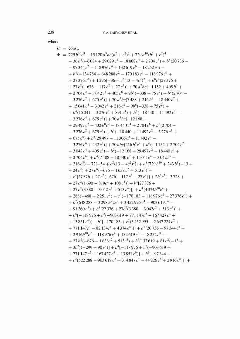
RES = C (b − c)6(b + c)6'(2),


where

C = const,

) = 729 b10c8 + 15 120 a9bc(b2 + c2)2 + 729 a10(b2 + c2)4 −− 36 b2(−6 084 + 29 029 c2 − 18 008 c4 + 2 704 c6)+ b6(20 736 −− 97 344 c2 − 118 976 c4 + 132 619 c6 − 18 252 c8)++ b4(−134 784 + 648 288 c2 − 170 183 c4 − 118 976 c6 ++ 27 376 c8)+ 1 296[−36 + c2(13 − 4c2)2] + b8c4[27 376 ++ 27 c2(−676 − 117 c2 + 27 c4)] + 70 a7bc[−1 152 + 405 b6 ++ 2 704 c2 − 3 042 c4 + 405 c6 + 9b4(−338 + 75 c2)+ b2(2 704 −− 3 276 c2 + 675 c4)] + 70 a5bc[7 488 + 216 b8 − 18 440 c2 ++ 15 041 c4 − 3 042 c6 + 216 c8 + 9b6(−338 + 75 c2)++ b4(15 041 − 3 276 c2 + 891 c4)+ b2(−18 440 + 11 492 c2 −− 3 276 c4 + 675 c6)] + 70 a3bc[−12 168 ++ 29 497 c2 + 432 b8c2 − 18 440 c4 + 2 704 c6 + b6(2 704 −− 3 276 c2 + 675 c4)+ b4(−18 440 + 11 492 c2 − 3 276 c4 ++ 675 c6)+ b2(29 497 − 11 306 c2 + 11 492 c4 −− 3 276 c6 + 432 c8)] + 70 abc{216 b8c4 + b6(−1 152 + 2 704 c2 −− 3 042 c4 + 405 c6)+ b2(−12 168 + 29 497 c2 − 18 440 c4 ++ 2 704 c6)+ b4(7 488 − 18 440 c2 + 15 041c4 − 3 042 c6 ++ 216 c8)− 72[−54 + c2(13 − 4c2)2]} + a8{729 b10 + 243 b8(−13 ++ 24 c2)+ 27 b6(−676 − 1 638 c2 + 513 c4)++ c4[27 376 + 27 c2(−676 − 117 c2 + 27 c4)] + 2b2c2[−3 728 ++ 27 c2(1 690 − 819c2 + 108 c4)] + b4[27 376 ++ 27 c2(3 380 − 3 042 c2 + 513 c4)]} + a4{4 374b10c4 ++ 288(−468 + 2 251 c2)+ c4(−170 183 − 118 976 c2 + 27 376 c4)++ b2(648 288 − 3 298 542c2 + 3 452 995 c4 − 903 619 c6 ++ 91 260 c8)+ b8[27 376 + 27c2(3 380 − 3 042c2 + 513 c4)] ++ b6[−118 976 + c2(−903 619 + 771 147c2 − 167 427 c4 ++ 13 851 c6)] + b4[−170 183 + c2(3 452 995 − 2 647 224 c2 ++ 771 147c4 − 82 134c6 + 4 374 c8)]} + a6{20 736 − 97 344 c2 ++ 2 916b10c2 − 118 976 c4 + 132 619 c6 − 18 252 c8 ++ 27 b8(−676 − 1 638c2 + 513c4)+ b6[132 619 + 81 c2(−13 ++ 3c2)(−299 + 90 c2)] + b4[−118 976 + c2(−903 619 ++ 771 147 c2 − 167 427 c4 + 13 851 c6)] + b2[−97 344 ++ c2(522 288 − 903 619 c2 + 314 847 c4 − 44 226 c6 + 2 916 c8)]} +


+ a2{2 916 b10c6 − 36(−6 084 + 29 029 c2 − 18 008 c4 + 2 704 c6)++ b4(648 288 − 3 298 542 c2 + 3 452 995 c4 − 903 619 c6 ++ 91 260 c8)+ 2b8c2[−3 728 + 27 c2(1 690 − 819 c2 + 108 c4)] ++ b2[−1 045 044 + c2(4 826 593 − 3 298 542 c2 + 522 288 c4 −− 7 456 c6)] + b6[−97 344 + c2(522 288 − 903 619 c2 ++ 314 847 c4 − 44 226 c6 + 2 916 c8)]}.

References

Beletsky, V. V.: 1975, Attitude Motion of Satellite in Gravitational Field, MGU Press, Moscow.Frik, M. A.: 1970, ‘Attitude stability of satellite subjected to gravity gradient and aerodynamic

torques’, AIAA J. 8(10), 1780–1785.Garber, T. B.: 1963, ‘Influence of constant disturbing torques on the motion of gravity-gradient

stabilized satellites’, AIAA J. 1(4), 968–969.Kurosh, A. G.: 1975, Superior Algebra. Nauka, Moscow.Likins, P. W. and Roberson, R. E.: 1966, ‘Uniqueness of equilibrium attitudes for earth-pointing

satellites’, J. Astronaut. Sci. 13(2), 87–88.Longman, R. W.: 1975, ‘Attitude equilibria and stability of arbitrary gyrostat satellites under

gravitational torques’, J. Br. Interplanet. Sci. 28(1), 38–46.Longman, P. W. and Roberson, R. E.: 1966, ‘General solution for the equilibria of orbiting gyrostat

subject to gravitational torques’, J. Astronaut. Sci. 16(2), 49–58.Nurre, G. S.: 1968, ‘Effects of aerodynamic torque on an asymmetric gravity-stabilized satellite’, J.

Spacecraft Rockets 5(9), 1046–1050.Roberson, R. E.: 1966, ‘Equilibria of orbiting gyrostats’, J. Astronaut. Sci. 15(5), 242–248.Sarychev, V. A.: 1965, ‘Asymptotically stable stationary rotational motion of a satellite’, In: Proc.

1st IFAC Symp. on Automatic Control in Space, Stavanger, Norway.Sarychev, V. A. and Gutnik, S. A.: 1994, ‘Equilibria of a satellite subject to gravitational and constant

torques’, Cosmic Res. 32(4–5), 43–50.Sarychev, V. A. and Mirer, S. A.: 2000, ‘Relative equilibria of a satellite subjected to gravitational

and aerodynamic torques’, Celest. Mech. & Dyn. Astr. 76(1), 55–68.Sarychev, V. A. and Mirer, S. A.: 2001, ‘Relative equilibria of a gyrostat satellite with internal angular

momentum along a principal axis’, Acta Astronaut 49(11), 641–644.Sarychev, V. A., Paglione, P. and Guerman, A.: 1997, ‘Equilibria of a satellite in a circular orbit:

the influence of a constant torque’, In: Proc. 48th International Astronautical Congress, PaperIAF-95-A.3.09, Turin, Italy.

Sazonov, V. V.: 1989, ‘On a mechanism of loss of stability in gravity-oriented satellite’, Cosmic Res.27(6), 836–848.

Influence of constant torque on equilibria of satellite in circular orbit

Documents