Influence of an unfavourable pressure gradient on the breakdown of boundary layer streaks

©2007 The Visualization Society of Japan Journal of Visualization, Vol. 10, No. 2 (2007)217-225

Influence of an Unfavourable Pressure Gradient

on the Breakdown of Boundary Layer Streaks

Chernoray, V. G.*1, Kozlov, V. V.*

2, Lee, I.*

3 and Chun, H. H.*

3

*1 Applied Mechanics, Chalmers University of Technology, SE-412 96, Gothenburg, Sweden. *2 Institute of Theoretical and Applied Mechanics SB RAS, 630090, Novosibirsk, Russia.

E-mail: [email protected] *3 Naval Architecture & Ocean Engineering, Pusan National University, 609-735, Pusan, Korea.

Received 8 August 2006 Revised 15 November 2006

Abstract : Breakdown of boundary layer streaks is studied experimentally and compared at zero and adverse (positive) streamwise pressure gradients on a wing under fully controlled experimental conditions. The varicose mode of streak breakdown is found to be a dominant mode in the case of the adverse pressure gradient. A strong influence of pressure gradient upon the development of the streak and the secondary instability is revealed. The unfavourable pressure gradient is shown to alter the critical streak amplitude, the dispersion properties of the streak and the secondary disturbance, as well as attained maximum amplitudes for both the streak and the secondary disturbance.

Keywords : Visualization, hot-wire anemometry, wing flow, sinusoidal and varicose instabilities, streaks.

1. Introduction As is known (Boiko et al., 2002), the laminar breakdown in wall-bounded shear flows is often associated with

transverse modulations of a flow by either steady streamwise vortices (e.g., Görtler vortices, crossflow

vortices) or unsteady streamwise structures (boundary-layer streaks at high free-stream turbulence, -, -,

and hairpin vortices). These structures create spatial velocity modulations providing favourable conditions for

appearance of secondary instabilities, which, in turn, promote the flow breakdown and lead to turbulence in

such flows.

Two fundamental secondary instability modes of the flows modulated by the streaky structures are

the varicose mode (also symmetric, horseshoe, or ‘y’-mode), and the sinusoidal mode (antisymmetric,

meandering, ‘z’-mode). It is agreed that the reason for the secondary instabilities is an inviscid local

mechanism caused by the inflections in the instantaneous velocity profiles both in the wall-normal (varicose

mode) and in the transverse directions (sinusoidal mode). For example, such two different modes were

observed in flow visualizations of Görtler vortex breakdown (Ito, 1985), where it was shown that the

secondary travelling waves are created either in the form of the periodic meandering of the vortices in the

transverse direction or in the form of the horseshoe bunching. The choice of the secondary instability mode

excited first and growing most rapidly depends on the stability properties of the resulted distorted flow. The

strength of the spanwise and the wall-normal gradients of the streamwise velocity as well as a spacing

between the streamwise perturbations are particularly important for the mode selection. Typically, the

varicose instability mode prevails during the breakdown of long-wave vortices, whereas the sinusoidal mode

is most often observed on short-wave disturbances, see Li and Malik (1995), Bottaro and Klingmann (1996).

These two modes of the streak breakdown are examined under controlled experimental conditions by

Asai et al. (2002) and by Chernoray et al. (2006) in the Blasius boundary layer. The first of these studies is

focused on the linear and weakly nonlinear evolution of the secondary instabilities, while the latter work

218 Influence of an Unfavourable Pressure Gradient on the Breakdown of Boundary Layer Streaks

reveals details on the nonlinear breakdown stages. In particular, Asai et al. (2002) have proved that the

streak width is an important parameter for the mode competition and for the growth rate of the secondary

disturbances. Also, the study has highlighted various aspects of the mode development based on hot-wire

measurements and smoke visualizations. Chernoray et al. (2006) have performed detailed visualizations by

hot-wires, which demonstrate that the two instability modes are remarkably similar during the late

nonlinear stages of their development. Both instability modes are revealed to contribute to the horseshoe-like

activity in the outer part of the boundary layer, and the generation of -shaped vortices is shown to take

place in both mode cases.

Current study is a natural continuation of work by Chernoray et al. (2006), and employs the same

experimental techniques of the detailed flow mapping and visualization by hot-wires. The focus of present

study is on flows with non-zero streamwise pressure gradient which are of importance in various technical

applications such as, for example, turbo engines. An attempt is made to reveal how the streak breakdown is

changed due to an external pressure gradient variation, aiming to deepen insight into the late stages of the

laminar-turbulent transition for the flows of a practical importance. To achieve this goal, a spatio-temporal

evolution of the perturbed flow was reconstructed under controlled experimental conditions and the

development and dynamics of the streak breakdown was elucidated in detail.

2. Experimental Arrangement Experiments were performed in a subsonic low-turbulent wind tunnel at the oncoming flow velocity 0U

8.35 m/s and the turbulence level 0/Uu 0.04 %. A wing model (Fig. 1) with chord length c 500 mm and

span 1000 mm was mounted in the middle of the wind tunnel test section. The flow Reynolds number based

on the wing chord was 5103Re c .

The coordinate system is defined in Fig. 1: x is directed streamwise and measured from the wing

leading edge, z is directed spanwise and measured from the wing centreline, and y is normal to the

),( zx -plane with y 0 on the model surface.

A constant-temperature hot-wire anemometer was used to measure the streamwise component of the

flow velocity u . The hot-wire probe was equipped with a gold-plated tungsten wire of 1.2 mm active length

and 5 m in diameter. The probe was calibrated prior every experimental run and the maximum relative

error of the calibration was within 1% for all calibration points. Flow measurements were performed in an

automated mode with use of a traversing system moving the probe in 3D space by a specially developed

software. In each spatial point 100 periods of the disturbance were collected with resolution of 50

points/period. About 6000 and 14000 spatial points were mapped for zero pressure gradient and adverse

pressure gradient cases correspondingly. The spatial resolution of the obtained velocity maps is )( szsysx

= (30.250.5) mm in both cases. Obtained data are post-processed using the Matlab software package.

The ensemble averaged velocity ),,,( tzyxuave is decomposed into the time-mean U , and fluctuation u~

components such that uUuave~ . Subtraction of the 2D base undisturbed flow ),( yxU B gives a total

disturbance velocity Bavetot Uuu , and the disturbance of the mean BUU . Note also that we use

}){min}{max(5.0,,

5.0 Bzy

Bzy

UUUUU to characterize the amplitude of the mean disturbance.

Fig. 1. Experimental setup.

Chernoray, V. G., Kozlov, V. V., Lee, I. and Chun, H. H. 219

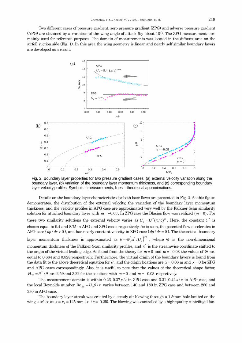
Two different cases of pressure gradient, zero pressure gradient (ZPG) and adverse pressure gradient

(APG) are obtained by a variation of the wing angle of attack (by about 10). The ZPG measurements are

mainly used for reference purposes. The domain of measurements was located in the diffuser area on the

airfoil suction side (Fig. 1). In this area the wing geometry is linear and nearly self-similar boundary layers

are developed as a result.

0 0.1 0.2 0.3 0.4 0.5

0

0.1

0.2

0.3

0.4

0.5

0.6

0.7

x/c

,

mm

0 0.2 0.4 0.6 0.8 10

2

4

6

8

10

U/Ue

y/

Details on the boundary layer characteristics for both base flows are presented in Fig. 2. As this figure

demonstrates, the distribution of the external velocity, the variation of the boundary layer momentum

thickness, and the velocity profiles in APG case are approximated very well by the Falkner-Scan similarity

solution for attached boundary layer with 08.0m . In ZPG case the Blasius flow was realized )0( m . For

these two similarity solutions the external velocity varies as m

e cxUU )/(* . Here, the constant *U is

chosen equal to 9.4 and 8.75 in APG and ZPG cases respectively. As is seen, the potential flow decelerates in

APG case ( 0/ dxdp ), and has nearly constant velocity in ZPG case ( 0/ dxdp ). The theoretical boundary

layer momentum thickness is approximated as 2/1* / eUx , where is the non-dimensional

momentum thickness of the Falkner-Scan similarity profiles, and *x is the streamwise coordinate shifted to

the origin of the virtual leading edge. As found from the theory for 0m and 08.0m the values of are

equal to 0.664 and 0.828 respectively. Furthermore, the virtual origin of the boundary layers is found from

the data fit to the above theoretical equation for , and the origin locations are x 0.06 m and x 0 for ZPG

and APG cases correspondingly. Also, it is useful to note that the values of the theoretical shape factor,

/*

12 H are 2.59 and 3.22 for the solutions with 0m and 08.0m respectively.

The measurement domain is within 0.26–0.37 cx / in ZPG case and 0.31–0.42 cx / in APG case, and

the local Reynolds number /Re eloc U varies between 140 and 180 in ZPG case and between 260 and

330 in APG case.

The boundary layer streak was created by a steady air blowing through a 1.5-mm hole located on the

wing surface at 1xx 125 mm ( cx /1 0.25). The blowing was controlled by a high-quality centrifugal fan.

7

8

9

10

11

12

13

0.00 0.10 0.20 0.30 0.40 0.50

x/c

Ue, m

/s

75.8eU

08.0)/(4.9 cxU e

ZPG

APG

Fig. 2. Boundary layer properties for two pressure gradient cases: (a) external velocity variation along the boundary layer, (b) variation of the boundary layer momentum thickness, and (c) corresponding boundary layer velocity profiles. Symbols – measurements, lines – theoretical approximations.

APG

ZPG

APG

m = –0.08

ZPG

m = 0

(b) (c)

(a)

220 Influence of an Unfavourable Pressure Gradient on the Breakdown of Boundary Layer Streaks

In addition, a loudspeaker was attached to the same pneumatic line and was used to modulate the streak by

high-frequency oscillations. The excitation frequency f was set equal to 333 Hz. The nondimensional

frequency, eS Uf /2 , is within the range 0.055-0.075 in ZPG case and 0.075-0.1 in APG case. The

boundary layer momentum thickness 1 at the location of the hole was 0.22 and 0.36 mm in ZPG and APG

case.

3. Results and Discussion 3.1 Nonlinear Varicose Instability at Zero Pressure Gradient

A localized continuous blowing creates a low-speed streak in the boundary layer due to the lift-up of a

low-speed fluid from the wall into the boundary layer. Figure 3 shows the streak development for ZPG case

in detail. The blue contours and isosurfaces are used to represent the low-speed streak. The coordinates are

scaled by the momentum thickness 1 . The red arc of 1-mm radius which is depicted in Fig. 3(a) gives an

additional reference to the dimensional units. Figure 3(a) shows that the central low-speed streak is

non-dispersive, it has a constant spanwise scale (width) equal to 10 1 (2.2 mm) at all streamwise stations.

The streak is located close to the upper boundary layer edge, with its centre being above the boundary layer

middle. Initially the centre of the streak is located at the constant height 1/y 6 and moves to 1/y 7.5

at the most downstream station. This happens when the horseshoe vortices generated by the periodic

modulation of the streak reach large amplitudes. There are some indications in this and other our studies

showing that initially the dimensions of the streak scale with the hole diameter and not with the boundary

layer thickness. Also, the initial streak location with respect to the wall seems to scale with the blowing

velocity. Thus, blowing a jet with a higher vertical velocity creates a streak located farther from the wall.

Therefore, two zones of the streak development may be distinguished, the field near the source and the

far-field. In the near-field the streak dimensions appear virtually independent of the boundary layer scale

and dependant on the scale of the generator. A very small relative size of the steak generator (blowing hole)

can be a reason of this. Our observations show that generators of a larger relative size can also generate

other scales in the very near field, which are related to the boundary layer thickness.

Both diagrams in Fig. 3 show clearly that the streak experiences the breakdown of the varicose type.

It is seen that the introduced periodic disturbance causes the bulging of the streak, the bulges grow in

amplitude as they convected downstream and form a train of the horseshoe vortices. Figure 3(a) shows that

the oscillations (shaded contours) are spatially localized inside of the streak, and this fact supports for the

local character of the instability. Furthermore, the perturbation maximum amplitudes are located near the

critical layer in the upper part of the low-speed streak where the local velocity gradients are high in the

wall-normal direction.

The development of the streak breakdown is remarkably similar to the development of the varicose

Fig. 3. Breakdown of streak via varicose instability in ZPG case. (a) Contours of mean disturbance velocity

BUU , and r.m.s. velocity u (shading). Negative contours are shown by blue lines; depicted red arc has

diameter of 2 mm. Contour step is 0.2 5.0U for BUU , and 0.02 eU for u . (b) Instantaneous spatial

distribution of velocity totu , iso-levels are +3.5 % eU (grey) and –3.5 % eU (blue).

(a) (b) (x-x1 )/1= 173

(x-x1 )/1= 119

(x-x1 )/1= 79 (x-x1 )/1

z/1

y/

1

z/1

y/

1

y/

1

y/

1

Chernoray, V. G., Kozlov, V. V., Lee, I. and Chun, H. H. 221

streak breakdown reproduced numerically by Skote et al. (2002). The streak location with respect to the wall,

and the width of the horseshoe vortices are identical as well. The wavelength of the secondary perturbation is

different since the nondimensional frequency was about 3 times higher in their simulation. In our study the

initial wavelength of the secondary disturbance is 80 1 and the disturbance phase velocity is 0.68 eU .

Corresponding values from their study are 20 1 and 0.53 0U (for 50/ * x ). Such change of the

wavelength and the phase speed with frequency is in a good agreement with predictions of the inviscid

theory (Monkewitz and Huerre, 1982). It should be noted that the phase of the periodic disturbance was

obtained using the Fourier transform, and the wavelength and the phase speed were found from the linear

approximations of the phase distributions in the initial part of the streamwise region.

From Fig. 3 we can observe that the secondary vortical motion on the disturbance sides leads to the

streak multiplication and formation of two additional streaks. This is an indication that the vortex loops,

typical for the horseshoe vortices, are formed on the each bulging of the streak. At 1xx 150 1 a first

ejection of the horseshoe vortex occurs. Also, two additional high-speed streaks are formed underneath of the

low-speed streaks as a result of the vortex multiplication in the lateral direction, as seen in Fig. 3(b) at

1xx 270 1 . The ‘primary’ high-speed streaks change as well. At the most downstream streamwise

station in Fig 3(a) (top) they merge with each other and form a layer of the accelerated fluid underneath of

the low-speed streak. The wall-normal velocity profiles, thus, approaching the shape of the turbulent profile.

Notice also that the steady disturbance reaches an equilibrium state from the station 11 /)( xx 120.

From this stage the viscous dissipation of the primary disturbance seems to compensate by the energy

production coming from the secondary periodic disturbance. There are some indications that such an

equilibrium state is present in Skote et al. (2002) even though this was not emphasized in their paper.

Our previous investigations have shown that the consideration of the spatial distributions of the

fluctuating velocity component can be very useful for the disturbance analysis. The periodical disturbance is

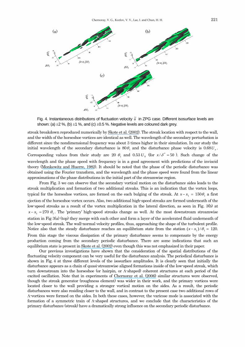
shown in Fig. 4 at three different levels of the isosurface amplitudes. It is clearly seen that initially the

disturbance appears as a chain of quasi-streamwise aligned formations inside of the low-speed streak, which

turn downstream into the horseshoe (or hairpin, or -shaped) coherent structures at each period of the

excited oscillation. Note that in experiments of Chernoray et al. (2006) similar structures were observed,

though the streak generator (roughness element) was wider in their work, and the primary vortices were

located closer to the wall providing a stronger vortical motion on the sides. As a result, the periodic

disturbances were also residing closer to the wall, and in contrast to the present case two additional rows of

-vortices were formed on the sides. In both these cases, however, the varicose mode is associated with the

formation of a symmetric train of -shaped structures, and we conclude that the characteristics of the

primary disturbance (streak) have a dramatically strong influence on the secondary periodic disturbance.

(a) (b)

Fig. 4. Instantaneous distributions of fluctuation velocity u~ in ZPG case. Different isosurface levels are

shown: (a) 2 %, (b) 1 %, and (c) 0.5 %. Negative levels are coloured dark grey.

(c)

(x-x1 )/1

y/

1

z/1

(x-x1 )/1

y/

1

z/1

(x-x1 )/1

y/

1

z/1

222 Influence of an Unfavourable Pressure Gradient on the Breakdown of Boundary Layer Streaks

3.2 Nonlinear Varicose Instability at Positive Pressure Gradient An adverse pressure gradient can be considered as an external force acting against the flow in the

streamwise direction. As a result, the flow decelerates and shows a tendency to spread out in the lateral

directions preserving the continuity. However, the pressure gradient effects become significantly more

complex when the nonlinear interactions of the disturbances during the varicose streak breakdown are

considered.

A comparison of Fig. 5 with Fig. 3 helps to reveal the influence of the pressure gradient on the streak

breakdown. In particular, as in ZPG case, we observe that the initial development of the low-speed streak is

non-dispersive. The streak has the same initial width of about 2.2 mm and its minimum is located at the

same distance (1.4 mm) from the wall. Both these values however differ when scaled by 1 , and this fact

supports the above comments on the initial streak scaling by the hole diameter and the blowing velocity. In

APG case the nondimensional position of the streak centre is closer to the wall and the disturbance stays

lower within the boundary layer until the most downstream stations. The centre of the streak gradually

moves from the wall, from 1/y 4 to 1/y 5 and to 1/y 6.5, as is seen in three contour plots of Fig.

5(a). The secondary low-speed streaks formed on the sides approach the same height as well. In contrary to

ZPG case, the high-speed streaks in APG case are very weak from the beginning, and this is most probably

caused by the lower streak location in the boundary layer in this case. On the other hand, a very broad and

strong high-speed region is formed very quickly as the disturbance evolves 140 1 downstream from the

source and this seems to happen due to the action of the pressure gradient, namely due to the stronger

vertical velocity of the base blow in APG case. Note that the nondimensional streamwise range shown in Fig.

5(b) is shorter than in Fig. 3(b). Nevertheless, later breakdown stages can be seen in Fig. 5(b) since the

breakdown progresses faster in APG case. Also, one can note that the ejection of the horseshoe vortex occurs

in a different way as compared to ZPG case, and is accompanied by the formation of the rib-like structures.

These rib-like vortices penetrate towards the wall, as clearly visible in subsequent Fig.6(a) at 11 /)( xx

200, and are very similar to the structures observed in the free shear layer type flows, see e.g., Levin et al.

(2005) for comparison. The streak breakdown occurs approximately 50 streamwise units closer to the source

than in ZPG case, at 11 /)( xx 200. Also, the equilibrated state which was seen in ZPG case does not

appear in APG case.

As seen from Fig. 5 (a) the secondary low-speed streaks are located at the same spanwise position

1/z 10 in both APG and ZPG cases for 11 /)( xx 167. This indicates that the steady disturbances in

the far-field of the disturbance generator are scaled with the boundary layer scale. The Fourier transform of

the periodic disturbance revealed that its initial wavelength equals to about 50 1 and the phase speed

equals to 0.58 eU . The trend of the variation of these parameters again agrees with the inviscid theory by

Monkewitz and Huerre (1982).

The enhanced lateral spread of the mean disturbance is accompanied by a stronger spread of the

periodic disturbance due to the action of the pressure gradient. This is clearly seen from a comparison of

Fig. 5. Breakdown of streak via varicose instability in APG case. (a) Contours of mean disturbance velocity

BUU , and r.m.s. velocity u (shading). Negative contours are shown by blue lines; depicted red arc has

diameter of 2 mm. Contour step is 0.2 5.0U for BUU , and 0.02 eU for u . (b) Instantaneous spatial

distributions of totu , isosurface levels are +2 % (grey) and –2 % (blue).

(a) (b) (x-x1 )/1= 167

(x-x1 )/1= 125

(x-x1 )/1= 83

z/1

y/

1

y/

1

y/

1

(x-x1 )/1 z/1

y/

1

Chernoray, V. G., Kozlov, V. V., Lee, I. and Chun, H. H. 223

Fig. 6 with Fig. 4. The estimations show that the spreading half-angle in APG case exceeds 11, while in ZPG

case this angle is less than 6. Results of Chernoray et al. (2006) show the value of the half-angle near 5.

From analysis of results of Asai et al. (2002) and Skote et al. (2002) we found values close to 5 as well.

It is remarkable that the topology of the varicose breakdown in APG case reveals closer similarity to

the varicose breakdown in Chernoray et al. (2006) as compared to ZPG breakdown case presented here. In

particular, the spatial velocity distributions of the periodic disturbance are remarkably similar. Three rows of

the -structures are formed. The -structures are asymmetric in the central row and asymmetric on the

sides. The asymmetric -structures have the second ‘leg’ at the stage of the formation and this leg resides

closer to the wall. In addition, Fig. 6 shows that the periodic disturbance forms a very typical staggered

pattern. Thus, our previous conclusion that the primary disturbance has a very strong influence on the

development of the secondary periodic disturbance is supported again.

4. Further Comments and Conclusions The streamwise development of disturbances during the varicose streak breakdown is compared in Fig. 7 for

two cases of pressure gradient. Figure 7(a) shows the development of the steady part of the disturbance and

Fig. 7(b) shows the development of two main harmonics of the disturbance fluctuation. Initially, for both

gradient cases the steady disturbances experience a decay, which is typical for streaks and occurs after the

transient growth (see e.g. Andersson et al., 2001). In our case the decay takes place within 120 streamwise

units from the vortex generator, as Fig. 7(a) demonstrates. The initial streak amplitudes in both cases were

chosen above the threshold for the secondary instability to obtain growing secondary periodic disturbances

behind the source. However, because of the abovementioned decay of streaks, the streaks arrive at

amplitudes below the secondary instability threshold inhibiting the secondary instability growth. This effect

is clearly seen in Fig. 7(a) where the threshold amplitudes are additionally emphasized by dashed horizontal

lines. Particularly, in ZPG case the threshold value is reached at 11 50 xx and is slightly below 0.4 eU .

From this position the periodic disturbance becomes neutrally stable, as seen in top graph of Fig. 7(b). In

APG case the main harmonic of the periodic disturbance becomes neutrally stable for the first station shown

in graphs of Fig. 7, which means that the critical streak amplitude in APG case is approximately 0.1 eU . The

mentioned value of 0.4 eU is a typical threshold amplitude for the varicose instability in the Blasius

boundary layer. Andersson et al. (2001) report the threshold amplitude of 37%. For the reason that the

threshold amplitude is so high, it is usually considered that the varicose mode is unlikely. Nevertheless in

APG case under consideration the situation is opposite: the varicose mode is more likely to develop

Fig. 6. Instantaneous distributions of fluctuation velocity u~ in APG case. Different isosurface levels are

shown: (a) 7 %, (b) 3 %, and (c) 1 %. Negative levels are coloured dark grey.

(a) (b)

(c)

(x-x1 )/1

y/

1

(x-x1 )/1

y/

1

z/1 (x-x1 )/1

y/

1

z/1

z/1

224 Influence of an Unfavourable Pressure Gradient on the Breakdown of Boundary Layer Streaks

comparing to the sinuous mode. Significantly lower streak amplitudes are required as a threshold for the

varicose secondary instability, since the base flow velocity profiles are inflectional. This can be a reason why

we have found only the varicose mode to be unstable in case of the adverse pressure gradient. Even if the

sinuous mode was triggered, it was dumped and transformed to the varicose mode during the streamwise

development.

50 100 150 200 2500

0.1

0.2

0.3

0.4

0.5

(x-x1)/

1

U

0.5

/ U

e

As Fig. 7 shows the disturbances reveal the continuation of the growth from 11 135 xx in both

cases. Which mechanisms drive this subsequent growth is not completely clear. Most probably this is the

stage from which the dissipation of the mean velocity disturbance and the associated shear layer is

compensated by the nonlinear production of the shear by the secondary disturbance due to the wave

break-up. Particularly, the enhanced growth of the second harmonic indicates occurrence of the first

harmonic break-up at this station. The streak amplitudes at this position are 0.23 eU in ZPG case and only

0.06 eU in APG case. Thus, the ‘nonlinear threshold’ is also decreased.

Fig. 7(b) demonstrates that the nonlinear growth rate is higher in APG case than in ZPG case.

Moreover, the nonlinear interactions are advanced as well, which is evidenced by a very rapid growth of the

second harmonic and the stationary disturbance. The nonlinear feed from the periodic disturbance results in

the increase of the amplitude of the steady disturbance to 35 % of eU prior the breakdown. The growth rate

of the first harmonic at the nonlinear stage for APG case is about 4 times higher compared to ZPG case, and

2-3 times higher compared to nonlinear growth in Asai et al. (2002) and Chernoray et al. (2006). The

accelerated growth in APG case results in shift of the transition point about 50 1 upstream compared to

ZPG case. Furthermore, as is seen, the periodic disturbance attains much higher amplitude prior the

breakdown (29 % of eU ). For the Blasius flow the maximum amplitude seems never exceed 25 % (Skote et al.,

2002; Asai et al., 2002; Chernoray et al. 2006).

To conclude, we emphasize the following findings of the present study.

The breakdown of the boundary layer streaks is studied experimentally and compared at zero and adverse

(positive) streamwise pressure gradients under controlled experimental conditions.

Comparison of current results for zero pressure gradient case with results of Asai et al. (2002), Skote et al.

(2002), and Chernoray et al. (2006) revealed that the spatial distribution of the primary steady disturbance

has a dramatic influence on the spatial topology of the secondary periodic disturbance. Depending on

which, the secondary disturbance can be composed either of one or several rows of the -shaped

structures.

In case of adverse pressure gradient only the varicose mode was found to be unstable. Even if the sinuous

mode was triggered, it decayed rapidly and transformed into the varicose mode during the streamwise

development.

A strong influence of the pressure gradient upon the development of the streak and its secondary instability

is revealed. The unfavourable pressure gradient is shown to alter the critical streak amplitude necessary

for triggering the secondary instability. The critical streak amplitude is found to decrease to 10% of eU in

APG boundary layer (compared to 25-40% in zero pressure gradient boundary layers).

Fig. 7. Streamwise variations of: (a) stationary disturbance amplitude 5.0U , and (b) maximum amplitude of

first and second harmonics of fluctuating component. Comparison of two pressure gradient cases is shown. Symbols – experiment, lines – fitting polynomials.

(a) (b) APG

ZPG

1.0)( 5.0 critU

15.0

29.04.0)( 5.0 critU

0

0.1

0.2

0.3

u1 /

Ue

50 100 150 200 2500

0.1

(x-x1)/

1

u2 /

Ue

Chernoray, V. G., Kozlov, V. V., Lee, I. and Chun, H. H. 225

The dispersion properties of the mean disturbance and the periodic disturbance are changed due to the

action of the adverse pressure gradient. The spreading half-angle increased almost twice (11 compared to

5-6 in zero-pressure-gradient flows).

The attained maximum amplitudes for the streak and the periodic disturbance are increased due to

adverse pressure gradient. The amplitude of the secondary disturbance is found to reach about 30% of eU

prior the breakdown, which is significantly higher than that in zero-pressure-gradient flows.

Acknowledgments

This work was supported by the Ministry of Education and Science of the Russian Federation, grants No.

RNP.2.1.2.3370, RFBR grant No. 05-01-034, the ERC program (Advanced Ship Engineering Research

Center) of MOST/KOSEF, grant No. R11-2002-104-05001-0, and the Korea Research Foundation grant

funded by the Korea Government (MOEHRD), grant No. KRF-2005-212-D00024.

References

Andersson, P., Brandt, L., Bottaro, A. and Henningson D. S. On the breakdown of boundary layer streaks, J. Fluid Mech. 428 (2001), 29-60. Asai, M., Minagawa, M. and Nishioka, M. The stability and breakdown of near-wall low-speed streak, J. Fluid Mech., 455 (2002), 289-314. Boiko, A. V., Grek, G. R., Dovgal, A. V. and Kozlov, V. V. The origin of turbulence in near-wall flows, (2002), Springer-Verlag, Berlin. Bottaro, A. and Klingmann, B. G. B. On the linear breakdown of Görtler vortices, Eur. J. Mech. B/Fluids., 15-3 (1996), 301-330. Chernoray, V. G., Kozlov, V. V., Löfdahl, L. and Chun, H. H. Visualization of sinusoidal and varicose instabilities of streaks in a boundary

layer, J. Vis., 9-4 (2006), 437-444. Ito, A. Breakdown structure of longitudinal vortices along a concave wall, J. Japan Soc. Aero. Space Sci., 33 (1985), 166-173. Levin, O., Chernoray V. G., Löfdahl L., Henningson D. S. A study of the Blasius wall jet, J. Fluid Mech. 539 (2005), 313-347. Li, F. and Malik, M. R. Fundamental and subharmonic secondary instabilities of Görtler vortices, J. Fluid Mech., 82 (1995), 77-100. Monkewitz, P. A. and Huerre, P. Influence of the velocity ratio on the spatial instability of mixing layers., Phys. Fluids, 25 (1982),

1137–1143. Skote M., Haritonidis, J. H. and Henningson, D. S., Varicose instabilities in turbulent boundary layers, Phys. Fluids, 4-7 (2002),

23092323.

Author Profile

Valery G. Chernoray: He received his Ph.D. in Physics-Mathematics in 2002 from the Institute of Theoretical and Applied Mechanics of Russian Academy of Sciences. He worked as a full-time research fellow in the Institute of Theoretical and Applied Mechanics. He works in the department of Applied Mechanics at Chalmers University of Technology in Gothenburg, Sweden as an Assistant Professor since 2005. In August 16, 2004 he was awarded the Top National Prize in Science (State Prize of Russian Federation), which was given for outstanding work in science. His current research interests are transitional and turbulent flows, and various techniques of flow control. Victor V. Kozlov: He is a Head of Laboratory of Aero-Physics Researches at ITAM, Novosibirsk, Russia, Professor at the Novosibirsk State University. Prof. Kozlov obtained his Ph.D. in Physics-Mathematics from the Institute of Theoretical and Applied Mechanics of Russian Academy of Sciences in 1976 and defended his Academic Professor's Thesis in 1987. He was awarded the Silver Zhukovsky Medal for great contribution to the aviation theory from the Russian Academy of Sciences in 1993. His main research interests are the experimental studies of flow stability and transition to turbulence.

Inwon Lee: He is an Assistant Professor in the Advanced Ship Engineering Research Center (ASERC) of Pusan National University. Prof. Lee obtained his Ph.D. from KAIST (Korea Advanced Institute of Science and Technology), Korea, in 2000. His research interests include: drag reduction, turbulent flow control, flow visualization and PIV (Particle Image Velocimetry). Ho Hwan Chun: He is a Professor in the Department of Naval Architecture & Ocean Engineering and director of Advanced Ship Engineering Research Center (ASERC). Prof. Chun obtained his Ph.D from University of Glasgow, UK., in 1988. His research interests include: ship hydrodynamics, computational fluid dynamics, high speed ship designs, towing tankery problems, fluid mechanics and drag reduction.