Inflexion Points on Plane Algebraic Curves

Inflexion Points on Plane Algebraic Curves

Bachelor Thesis of Andreas SteigerSupervised by Prof. Richard Pink and Patrik Hubschmid

November 18, 2008

In this thesis we will have a look at algebraic curves in the projective planeover an arbitrary algebraically closed field k. Using the resultant of polyno-mial rings over k we define intersection multiplicities and prove Bezout’sTheorem for effective divisors. We define singularities and inflexion pointsand count their number depending on the degree of the curve, using theHessian of a curve.

0 Introduction

Algebraic geometry is a very active branch in modern mathematics. The language ofschemes, introduced by Grothendieck in the middle of the twentieth century, is enor-mously powerful and allows the mathematician to get geometric insight into facts fromdifferent fields such as algebra and number theory, where there are no obvious analogiesat the first glance. However, a concept which opens a vast amount of possibilities oftendemands its tribute by being difficult to understand, and beginners often struggle. Thisis the case for the language of schemes.

As important as schemes are in current research, one can still use classical algebraicgeometry to understand the basic concepts. One can even try to work with algebraicgeometry with using as little algebra as possible.

When I started to write this thesis, I felt shiftless with the algebra involved in algebraicgeometry. Thus the thesis turned out to use only very basic concepts of commutativealgebra.

In the first chapter we introduce the projective plane over a field and define alge-braic curves in the plane. This concept is easily generalised to projective varieties. Theimportant results are the properties that curves over algebraically closed fields containinfinitely many points (Theorem 1.11), and the equivalence of topological and algebraicirreducibility (Theorem 1.16), as well as its consequence that there exists a unique de-composition into irreducible components. (Theorem 1.17)

In the second chapter we study intersections of curves. The crucial point is the intro-duction of intersection multiplicities, which allows us to prove Bezout’s famous Theorem.

1

1 PROJECTIVE ALGEBRAIC CURVES IN THE PLANE

The intersection multiplicity is introduced via the resultant (Definition 2.9), which sim-plifies the proof of Bezout’s Theorem (Theorem 2.14) greatly. However, this definitionhas its drawbacks: At first glance, the only purpose of this definition seems to be thesimplification mentioned above. It looks arbitrary, and it is not easy to calculate inter-section multiplicities of complicated curves. Nevertheless it has the properties that areknown for the definition using local rings. Unfortunately, we were not able to find aproof for the very important independence of the choice of coordinates, Theorem 2.10.A proof for the case k = C can be found in Fischer [1].

The next topic are then singularities and tangents. We give two equivalent definitionsof the order of a point on a curve, using the Taylor expansion for an algebraic insight(Definition 3.1) and observing intersection multiplicities of lines in that point to geta geometric intuition (Proposition 3.5). The second notion is closely related to thetangents at that point (Corollary 3.7). Two very important tools, the Euler Formula(Proposition 3.11) and the Jacobi Criterion (Proposition 3.12), will be proven. The firstapplication is the proof that a curve only has finitely many singularities (Proposition3.15). This result can be improved to an upper bound depending on the degree of thecurve (Proposition 3.21 and Corollary 3.22).

The fourth chapter then finally deals with the main topic, inflexion points of curves.Nearly all results proven before are required to prove that the Hessian of a curve (Defi-nition 4.4) intersects the curve exactly in flexes and singular points (Theorem 4.8). Asa conclusion we give examples where and how the theorem works, and that it can bewrong in fields of non-zero characteristic.

1 Projective Algebraic Curves in the Plane

Let k be an algebraically closed field and k[X0, X1, X2] be the polynomial algebra overk with variables in X0, X1, X2. Throughout this thesis we will mostly be working inthe projective plane P2

k over the field k. The reason for this choice is that there are alot of theorems which show their full beauty only if we can use the so-called “points atinfinity”.

Definition 1.1. The projective r-space Prk over k of dimension r is given by the set of(r + 1)-tuples (x0, . . . , xr) ∈ kr+1 \ {0} modulo the equivalence relation

(x0, . . . , xr) ∼ (y0, . . . , yr) :⇐⇒ ∃α ∈ k∗ : α · (y0, . . . , yr) = (x0, . . . , xr).

Note that Prk actually describes the lines in kr+1 through the origin.

Definition 1.2. A polynomial F ∈ k[X0, X1, X2] is called homogeneous of degree n ifit is a linear combination of monomials in k[X0, X1, X2] of degree n <∞.

Remark 1.3. The zero polynomial is a polynomial of every degree.

Remark 1.4. If F is a homogeneous polynomial of degree n, then

F (λX0, λX1, λX2) = λnF (X0, X1, X2) ∀λ ∈ k.

2


Therefore, if P = (x0 : x1 : x2) ∈ P2k, the property F (x0, x1, x2) = 0 does not depend

on the particular representing element, but only on the equivalence class of P . We willwrite F (P ) = 0 in these cases.

Definition 1.5. The variety or zero set of a homogeneous polynomial F ∈ k[X0, X1, X2]is the set

V (F ) := {P ∈ P2k | F (P ) = 0}.

Definition 1.6. A subset C ⊂ P2k is called a plane projective algebraic curve if there

is a non-zero homogeneous polynomial F ∈ k[X0, X1, X2] with degF ≥ 1, such thatC = V (F ). A polynomial of least degree defining C is called a minimal polynomial forC, and its degree is called the degree of C.

From now on, a curve shall be a plane projective algebraic curve.Note that the minimal polynomial is not uniquely defined, as multiplication of a

constant λ ∈ k∗ with a polynomial gives a different polynomial with the same variety. Weshall see later that up to multiplication with a constant factor, the minimal polynomialis actually unique.

Example. The curves of degree 1 are called projective lines. One sees immediately thatthey are defined by a linear equation

a0X0 + a1X1 + a2X2 = 0, (a0 : a1 : a2) ∈ P2k.

Two projective lines always intersect. The intersection consists of one point if and onlyif the lines are different, as the equation(

a0 a1 a2

b0 b1 b2

)X0

X1

X2

= 0

has exactly one non-trivial solution up to a constant factor if and only if the coefficientmatrix has rank 2. Otherwise, (a0 : a1 : a2) = (b0 : b1 : b2) and the intersection is thewhole line.

Definition 1.7. A mapping τ : P2k → P2

k is called a projective coordinate transformationif there is a matrix T ∈ GL3(k), such that

τ(x0 : x1 : x2) = (x0 : x1 : x2) · T, ∀(x0 : x1 : x2) ∈ P2k.

Note that T is uniquely determined by its induced mapping τ , up to a constant factorλ ∈ k∗:

Proof. Suppose that both S and T ∈ GL3(k) give the same transformation τ . Then

τ(x0 : x1 : x2) = (x0 : x1 : x2)S = (x0 : x1 : x2)T, ∀(x0 : x1 : x2) ∈ P2k.

Multiplication by T−1 gives

(x0 : x1 : x2)ST−1 = (x0 : x1 : x2), ∀(x0 : x1 : x2) ∈ P2k.

3


By explicit calculation we get

(1, 0, 0)ST−1 = (λ1, 0, 0), (0, 0, 1)ST−1 = (0, λ2, 0), (0, 0, 1)ST−1 = (0, 0, λ3)

for some λ1, λ2, λ3 ∈ k∗. Furthermore,

(1, 1, 1)ST−1 = (1, 0, 0)ST−1 + (0, 1, 0)ST−1 + (0, 0, 1)ST−1 = (λ1, λ2, λ3).

This point is in the same equivalence class in P2k as (1, 1, 1) if and only if λ1 = λ2 = λ3.

Thus ST−1 = λ · E, where λ ∈ k∗ and E denotes the unit matrix, and furthermoreS = λT . Obviously, multiplication of the matrix with a constant factor does not changethe equivalence class of a point in the image.

From now on, any coordinate transformation τ shall be identified with its matrix, i.e.τ itself is a matrix.

If a curve C is given by the homogeneous polynomial F and T is a projective coordinatetransformation, then

F T (X0, X1, X2) := F ((X0, X1, X2) · T−1)

is a homogeneous polynomial with degF T = degF . This gives us the transformed curve

T (C) = V (F T ),

which has the same degree as C. We often will transform curves such that our objectsof interest satisfy special conditions to simplify calculations.

Until now, we have used P2k as a somewhat independent space, i.e. with no relations

other than to the field k. But actually, it is an extension of the affine plane A2k by the

canonical embeddingi : A2

k → P2k

(x1, x2) 7→ (1 : x1 : x2).

We identify A2k with its image under i. Note that P2

k \ i(A2k) is a projective line V (X0) =

{(0 : x1 : x2) ∈ P2k}, called the line at infinity of P2

k. Its points are called points atinfinity . The primary usage of this embedding lies in the homogenisation of polynomialsin two variables:

Definition 1.8. Given a polynomial f ∈ k[X,Y ] with deg f = n, the homogenisationf ∈ k[X0, X1, X2] of f is given by

f(X0, X1, X2) := Xn0 · f

(X1

X0,X2

X0

).

Then f is a homogeneous polynomial of degree n. Conversely, to any homogeneouspolynomial F ∈ k[X0, X1, X2] we associate the dehomogenisation f ∈ k[X,Y ] of F withrespect to X0, by

f(X,Y ) := F (1, X, Y ).

If X0 is not a factor of F , then degF = deg f .

4


Remark 1.9. Let f ∈ k[X,Y ] be a polynomial defining an affine algebraic curve C byits zero set. Then i(V (f)) ⊂ V (f), and the only missing points of the embedding in theprojective space are those at infinity, i.e. i(V (f)) = V (f) ∩ i(A2

k).

Theorem 1.10 (Homogeneous form of the Fundamental Theorem of Algebra). Everynon-zero homogeneous polynomial F ∈ k[X,Y ] has a decomposition into linear factors.

Proof. Let F =∑n

i=0 ciXiY n−i be any non-zero homogeneous polynomial in two vari-

ables X,Y of degree d over k. Let e be the highest power of X dividing F , and letG =

∏di=e ciX

i−eY n−i, i.e. F = Xe · G. Dehomogenising G with respect to X gives apolynomial in Y :

g =n−e∑i=0

ci+eYn−e−i.

By the Fundamental Theorem of Algebra, g has the (not necessarily different) zerosbe+1, . . . , bn ∈ k. Then we can write g as

g = c′ ·n−e∏i=1

(Y − bi+e).

for some c′ ∈ k∗. Homogenising each factor gives

G = g = c′ ·n∏

i=e+1

(Y − biX)⇒ F =n∏i=1

(aiY − biX),

for some ai ∈ k with a1 = . . . = ae = 0.

Theorem 1.11. Every curve C consists of infinitely many points.

Proof. Let C = V (F ), degF =: n, and write F as

F = A0 +A1X2 + . . .+ApXp2 ,

where Ai ∈ k[X0, X1] are homogeneous polynomials of degree n− i and Ap 6= 0.

• p = 0:

Then F = A0 =∑n

i=0 ciXi0X

d−i1 for some ci ∈ k. By Theorem 1.10, there exists a

decomposition into linear factors F =∏ni=1(aiX1− biX0). For each pair (ai, bi) we

get the solution set Li = {(ai : bi : x) | x ∈ k}, which is a projective line. Since weare working in algebraically closed field each line consists of infinitely many points.

• p 6= 0:

The polynomial Ap has at most finitely many zeros in P1k. Thus there exist infinitely

many points P ∈ P1k, such that Ap(P ) 6= 0. For each such point P , the polynomial

F is nonconstant in X2, and thus has at least one zero. Hence we have foundinfinitely many zeros and C consists of infinitely many points.

5


Definition 1.12. The ideal I(C) ⊂ k[X0, X1, X2] of a curve C is the ideal generated byall homogeneous polynomials that vanish at all points of C.

Therefore, it is a homogeneous ideal.

Theorem 1.13 (Hilbert’s Nullstellensatz, homogeneous form). Let k be an algebraicallyclosed field and a ⊆ k[X0, . . . , Xr] be a homogeneous ideal. Let V (a) = {P ∈ Prk | ∀F ∈a : F (P ) = 0}, then I(V (a)) =

√a.

Proof. See Zariski–Samuel [3], Theorem VII.4.15, page 171f.

Theorem 1.14. The minimal polynomial of a curve C is uniquely determined by C upto a constant factor λ ∈ k∗. It generates the ideal I(C).

Proof. Assume C = V (F ) = V (G) for two minimal polynomials F , G of C. Obviously,V ((F )) = V (F ) = V (G) = V ((G)). Thus, by the homogeneous form of Hilbert’sNullstellensatz,

√(G) = I(V (G)) = I(V (F )) =

√(F ). Since F and G are minimal

polynomials for their zero sets, there are no polynomials of lower degree, having thesame zero sets. Thus, (F ) =

√(F ) = I(C) =

√(G) = (G), and I(C) is generated by

any minimal polynomial. Thus F and G have the same degree, and so (F ) = (G) is onlypossible if there is a constant factor λ ∈ k∗, such that F = λG.

From now on, if we say a curve C is given by a polynomial F , we always choose F tobe the minimal polynomial.

Definition 1.15. A curve C is called irreducible if every decomposition C = C1 ∪ C2

into two curves implies C = C1 or C = C2, i.e. C is not the union of two different curves.

Theorem 1.16. The following three statements are equivalent:

i. C is irreducible.

ii. The minimal polynomial of C is irreducible.

iii. I(C) is a homogeneous prime ideal.

Proof. We show i. ⇒ ii. ⇒ iii. ⇒ i.

i. ⇒ ii. Let C be irreducible and F be a minimal polynomial of C. Suppose that F =F1F2 for some Fi ∈ k[X0, X1, X2]. Then the Fi are homogeneous. Furthermore,V (F1) ∪ V (F2) = V (F ) = C, because F (P ) = 0 ⇐⇒ F1(P ) = 0 or F2(P ) = 0for any P ∈ P2

k. But C is irreducible, hence without loss of generality assumeV (F1) = C. We get that degF = degF1, since degF1 ≤ degF by F = F1F2 anddegF1 ≥ degF by minimality of F . This yields degF2 = degF − degF1 = 0 andF2 is constant. Hence, F is irreducible.

ii. ⇒ iii. By Theorem 1.14, I(C) is generated by the minimal polynomial, which is irre-ducible and homogeneous. Hence I(C) is a homogeneous prime ideal.

6


iii. ⇒ i. Let C = C1∪C2 be a decomposition into two curves with minimal polynomials F1

and F2, respectively. Write F := F1F2, then F ∈ I(C), since F is homogeneousand vanishes at all points of C. Furthermore, since I(C) is a prime ideal, withoutloss of generality suppose F1 ∈ I(C). But then F1 vanishes at all points of C, soC ⊂ V (F1) = C1 and we get C = C1.

Theorem 1.17. Every curve C has a unique (up to order) representation

C = C1 ∪ · · · ∪ Cl,

where the Ci are pairwise distinct irreducible curves. They are in one-to-one-correspon-dence with the irreducible factors of a minimal polynomial for C.

Proof. Let F be the minimal polynomial of C and let F = F1·. . .·Fl be the decompositioninto irreducible factors, which is unique up to constant factors and ordering. ThenF (P ) = 0 if and only if there is a polynomial Fi such that Fi(P ) = 0. Thus, C = V (F ) =V (F1) ∪ · · · ∪ V (Fl). Since each Fi is irreducible, they are minimal polynomials of theirrespective varieties. By Theorem 1.16 an irreducible minimal polynomial determines anirreducible curve, thus Ci = V (Fi) gives a decomposition

C = C1 ∪ · · · ∪ Cl

of of C into irreducible curves.Let

C = D1 ∪ . . . ∪D′lbe any decomposition of C into distinct irreducible curves. Then the respective minimalpolynomials Gi, such that Di = V (Gi), are irreducible. But then V (G1 · . . . · G′l) =V (F ). This is only possible if G1 · . . . · G′l is the minimal polynomial itself. Since thedecomposition of a polynomial into irreducible factors is unique, l equals l′ and the Giare just a permutation of the Fj .

This leads us to an algebraic structure on the set of curves:

Definition 1.18. The divisor group D of P2k is the free abelian group on the set of all

irreducible curves. An element D of D is called a divisor . It is represented as a formallinear combination

D =∑

C irred.

nC · C, nC ∈ Z, nC 6= 0 for only finitely many C.

A divisor is an effective divisor if nC ≥ 0 for all irreducible curves C. The degree of aneffective divisor is given by degD =

∑C irred. nC · degC. For an effective divisor, the

support of D is the setSuppD :=

⋃nC>0

C.

If D 6= 0 this is a curve. An effective divisor is a reduced curve, if furthermore nC ≤ 1for all irreducible curves C.

7

2 INTERSECTIONS OF CURVES

2 Intersections of Curves

With the basic properties of curves we are now able to work towards one of the mostimportant results of elementary curve theory, namely Bezout’s Theorem. It relates thenumber of intersections of two curves with their degrees.

Let us first consider the most simple case, the intersection of a curve with a line.

Proposition 2.1. Let C = V (F ) be a curve of degree n and L be a line in P2k. If L does

not completely in C, then the number of intersections C ∩ L is at most n.

Proof. By coordinate transformation, choose L to be given by X2 = 0. Thus, for anypoint P = (x0 : x1 : x2) in the intersection, we need F (P ) = 0 and x2 = 0, which isequivalent to solving F (x0, x1, 0) = 0.

Decompose F in terms of X2, i.e.

F (X0, X1, X2) = F0Xn2 + F1X

n−12 + · · ·+ Fn,

where Fi ∈ k[X0, X1] and Fi is homogeneous of degree i. Then F (x0, x1, 0) = 0 isequivalent to Fn(x0, x1) = 0. If Fn is the zero polynomial, then F is a multiple of X2

and L ⊂ C. Otherwise, degFn = n and by the homogeneous form of the FundamentalTheorem of Algebra Fn has a decomposition

Fn = (b1X0 − a1X1)k1 · . . . · (bmX0 − amX1)km , kj ∈ N∗, (aj : bj) ∈ P1k,

where all (aj : bj) are distinct and m ≤ n. Thus, Fn has at most d zeros.

Note that powers kj do not depend on the particular choice of coordinates, but onlyon C and L. Thus, the intersection multiplicity defined below is indeed well-defined:

Definition 2.2. Let C be a curve and L be a line, which intersect at a point P . Usingthe construction in the proof above, let k = kj for P = (aj : bj : 0) after a coordinatetransformation. Then the intersection multiplicity of C and L at P is given by

µP (C,L) := k.

Corollary 2.3. A line L which is not contained in a curve C of degree n has exactly nintersection points with C, counted with multiplicity.

Of course we want to generalise this result to arbitrary curves. As curves are justzero sets of polynomials, we can use the resultant, which relates the coefficients of twopolynomials with its common zeros. We present the following results, following Fischer[1]:

Definition 2.4. Let A be a commutative ring with unit, and

f = a0Xm + · · ·+ am, g = b0X

n + · · ·+ bn, f, g ∈ A[X],

8


with a0 6= 0 and b0 6= 0. The resultant of f and g is defined by

Rf,g = det

a0 · · · · · · am. . . . . .

a0 · · · · · · amb0 · · · · · · bn

. . . . . .

b0 · · · · · · bn

∈ A.

n rows

m rows

Lemma 2.5. If A is an integral domain and f, g ∈ A[X], then Rf,g = 0 in A if andonly if there exist polynomials ϕ,ψ ∈ A[X], not both zero, with degϕ < deg f anddegψ < deg g, such that ψf + ϕg = 0.

Proof. In the vector space V of polynomials in K[X] of degree < n+m, we look at theelements

Xn−1f, . . . ,Xf, f,Xm−1g, . . . , Xg, g.

Then each row of the resultant matrix is the linear representation in the base Xm+n−1,Xm+n−2, . . . , X, 1 of V . Thus, Rf,g = 0 if and only if the vectors are linearly dependent,i.e. there exists a non-trivial relation

0 = µ0Xn−1f + · · ·+ µn−1f +λ0X

m−1g + . . .+ λm−1g

= (µ0Xn−1 + · · ·+ µn−1)f +(λ0X

m−1 + . . .+ λm−1)g= ψf +ϕg.

It is possible that ψ or ϕ do not have coefficients in A itself, but only in its quotientfield K. If this is the case, we simply multiply ψ and ϕ with the common denominatorof their coefficients, giving coefficients in A.

Proposition 2.6. Let A be a factorial ring and f, g ∈ A[X] as above, with a0 6= 0 andb0 6= 0. Then, the following are equivalent:

i) f and g have a common divisor in A[X] of degree ≥ 1,

ii) Rf,g = 0 in A.

Proof. By Lemma 2.5, Rf,g = 0 if and only if there exist ϕ,ψ of the above form withψf + ϕg = 0.

• i) ⇒ ii):

Let h be common factor of f and g. Then f = f1h and g = g1h. Choose ϕ := f1 andψ := −g1. Then degϕ < deg f, degψ < deg g, and not both are zero. Furthermore,ψf + ϕg = −g1f1h+ f1g1h = 0. Thus Rf,g = 0.

9


• ii) ⇒ i):

Decompose fψ = −gϕ into prime factors

f1 · . . . · fr · ψ1 · . . . · ψk = −g1 · . . . · gs · ϕ1 · . . . · ϕl,

where factors of degree zero in X can show up. Up to units, each factor gi mustshow up on the left hand side of the equation. Since degψ < deg g, at least onefactor gσ of degree ≥ 1 is a prime factor of f , thus f and g have a common factorof degree ≥ 1.

Proposition 2.7. Let k be a field, A = k[Y1, . . . , Yr], and f, g ∈ A[X] with

f = a0Xm + · · ·+ am, g = b0X

n + · · ·+ bn,

where a0 6= 0, b0 6= 0, all ai, bj homogeneous of degree i and j, respectively. Then Rf,gis in A, homogeneous of degree m · n, or Rf,g = 0.

Proof. A polynomial a ∈ k[Y1, . . . , Yr] is homogeneous of degree d if and only if

a(TY1, . . . , TYr) = T da(Y1, . . . , Yr) in k[Y1, . . . , Yr, T ].

If we calculate Rf,g(TY1, . . . , TYr), then the entries of the matrix are multiplied by thefollowing powers of T : ∣∣∣∣∣∣∣∣∣∣∣∣∣∣∣∣∣∣∣∣∣

0 1 m0 m

. . . . . .0 m

0 1 n0 n

. . . . . .. . . . . .

0 n

∣∣∣∣∣∣∣∣∣∣∣∣∣∣∣∣∣∣∣∣∣If we further multiply each row with the power of T given on the left, we get the followingpowers of T :

1 :2 :...n :1 :2 :......m :

∣∣∣∣∣∣∣∣∣∣∣∣∣∣∣∣∣∣∣∣∣

1 2 m2 m+ 1

. . . . . .n m+ n

1 2 n+ 12 n+ 2

. . . . . .. . . . . .

m n+m

∣∣∣∣∣∣∣∣∣∣∣∣∣∣∣∣∣∣∣∣∣

.

10


We can get this result in a different way, namely by multiplying the i-th column of Rf,gwith T i. Thus, with p = (1 + · · ·+ n) + (1 + · · ·+m) and q = (1 + . . .+ (m+ n)),

T pRf,g(TY ) = T qRf,g(Y ).

But q − p = m · n, thus Rf,g is homogeneous of degree m · n, if it is not zero.

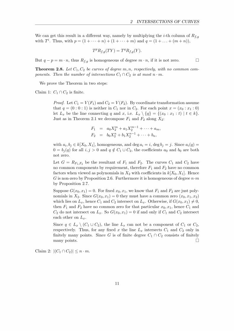
Theorem 2.8. Let C1, C2 be curves of degree m,n, respectively, with no common com-ponents. Then the number of intersections C1 ∩ C2 is at most n ·m.

We prove the Theorem in two steps:

Claim 1: C1 ∩ C2 is finite.

Proof. Let C1 = V (F1) and C2 = V (F2). By coordinate transformation assumethat q = (0 : 0 : 1) is neither in C1 nor in C2. For each point x = (x0 : x1 : 0)let Lx be the line connecting q and x, i.e. Lx \ {q} = {(x0 : x1 : t) | t ∈ k}.Just as in Theorem 2.1 we decompose F1 and F2 along X2:

F1 = a0Xm2 + a1X

m−12 + · · ·+ am,

F2 = b0Xn2 + b1X

n−12 + · · ·+ bn,

with ai, bj ∈ k[X0, X1], homogeneous, and deg ai = i, deg bj = j. Since ai(q) =0 = bj(q) for all i, j > 0 and q /∈ C1 ∪ C2, the coefficients a0 and b0 are bothnot zero.

Let G = RF1,F2 be the resultant of F1 and F2. The curves C1 and C2 haveno common components by requirement, therefore F1 and F2 have no commonfactors when viewed as polynomials in X2 with coefficients in k[X0, X1]. HenceG is non-zero by Proposition 2.6. Furthermore it is homogeneous of degree n·mby Proposition 2.7.

Suppose G(x0, x1) = 0. For fixed x0, x1, we know that F1 and F2 are just poly-nomials in X2. Since G(x0, x1) = 0 they must have a common zero (x0, x1, x2)which lies on Lx, hence C1 and C2 intersect on Lx. Otherwise, if G(x0, x1) 6= 0,then F1 and F2 have no common zero for that particular x0, x1, hence C1 andC2 do not intersect on Lx. So G(x0, x1) = 0 if and only if C1 and C2 intersecteach other on Lx.

Since q ∈ Lx \ (C1 ∪ C2), the line Lx can not be a component of C1 or C2,respectively. Thus, for any fixed x the line Lx intersects C1 and C2 only infinitely many points. Since G is of finite degree C1 ∩ C2 consists of finitelymany points.

Claim 2: |(C1 ∩ C2)| ≤ n ·m.

11


Proof. Between finitely many intersection points, there are only finitely manylines connecting such points. By coordinate transformation, choose q such thatnone of these lines contains q. Then, by the same construction, each line Lxcontains at most one intersection point. Thus C1 ∩ C2 cannot consist of morethan degG = n ·m points.

Again, we want to improve the result by counting multiplicities.

Definition 2.9. Let C1 = V (F1), C2 = V (F2) be two curves without common compo-nents, such that they do not contain q = (0 : 0 : 1), and each line through q contains atmost one intersection point of C1 and C2. Let G = RF1,F2 . If P = (p0 : p1 : p2) ∈ C1∩C2

is an intersection point, let P ′ := (p0 : p1), and define the intersection multiplicity of C1

and C2 at P , µP (C1, C2), to be the order of the zero of G in P ′.

Note that this definition is consistent with the definition of intersection multiplicity ofa curve and a line. If C2 = V (X2), then the resultant is just G = ±am, using the samenotation as above.

Obviously, for each pair of curves C1, C2, there exist several coordinate transforma-tions, such that the transformed curves fulfill the conditions of the definition of inter-section multiplicity. However, it is not clear at all that every transformation yields thesame multiplicities:

Theorem 2.10. If C1 and C2 are curves satisfying the conditions of 2.9 and T is acoordinate transformation, such that the transformed curves T (C1), T (C2) also satisfythese conditions, then

µP (C1, C2) = µPT (T (C1), T (C2)) ∀P ∈ C1 ∩ C2.

In particular, for any two curves not satisfying the conditions of 2.9, any coordinatetransformation, such that the transformed curves do satisfy the conditions, yields thesame intersection multiplicities.

As mentioned in the introduction, we did not succeed in finding a proof within rea-sonable time, and thus decided to leave this gap open.

With a further result about the resultant, we are even able to calculate intersectionmultiplicities of effective divisors:

Proposition 2.11. Let A be an integral ring and let f, g ∈ A[X], such that there existc1, . . . , cm, d1, . . . , dn ∈ A satisfying

f =m∏i=1

(X − ci), g =n∏j=1

(X − dj).

Then

Rf,g =m∏i=1

n∏j=1

(ci − dj) =m∏i=1

g(ci)

= (−1)mnn∏j=1

f(dj) = (−1)mn ·Rg,f .

12


Proof. Let B = Z[Y1, . . . , Ym, Z1, . . . , Zn], and define the polynomials F,G ∈ B[X] by

F :=m∏i=1

(X − Yi) =m∑i=0

FiXm−i,

G :=n∏j=1

(X − Zj) =n∑j=0

GjXn−j ,

where Fi and Gj are the elementary symmetric polynomials of Y1, . . . , Ym and Z1, . . . , Znrespectively. Each of them is homogeneous if degree i or j, respectively. Define

R := RF,G ∈ B, S :=m∏i=1

n∏j=1

(Yi − Zj) ∈ B.

Both R and S are homogeneous polynomials of degree n ·m.We need to show that R = S. Fortunately, we do not need to calculate the determi-

nant: If we substitute Zj by Yi in G, then F and G have a common linear factor. ThusR is zero for Zj = Yi, and (Yi −Zj) must be a divisor of R. We can do this for any pair(i, j), thus S is a divisor of R. Since both have the same degree, there is a factor a ∈ Zsuch that R = aS.

To show that a = 1 we have a look at the summand (−1)mn(Z1 · . . . ·Zn)m of R. Thisis the diagonal of the resultant matrix, and can not appear otherwise in its determinant.But it also is a summand of S, thus a = 1.

If we now substitute Yi and Zj by the constant polynomials Yi = ci and Zj = dj , thestatement follows.

Corollary 2.12. Let f1, f2, g ∈ A[X] be polynomials. Then

Rf1·f2,g = Rf1,g ·Rf2,g ∈ A.

Proof. If all 3 polynomials are monic, then applying Proposition 2.11 in the commonsplitting field of f1, f2, g over the quotient field of A gives the result.

Any polynomial is a multiple of a monic polynomial in its splitting field. By takingthe polynomials to the algebraic closure, we can write the polynomials as f1 = a1h1,f2 = a2h2 and g = bh′, i.e.

f1 = a1

(m1∑i=0

f1iXm1−i

), a1 6= 0,

f2 = a2

(m2∑i=0

f2iXm2−i

), a2 6= 0,

g = b

n∑j=0

gjXn−j

, b 6= 0.

13

3 SINGULARITIES AND TANGENTS

Then the resultants become

Rf1,g = an1bm1Rh1,h′

Rf2,g = an2bm2Rh2,h′

Rf1f2,g = (a1a2)nbm1+m2Rh1h2,h′ .

Thus the formula holds for every polynomial in A[X].

Proposition 2.13. Let C = V (F ), C ′ = V (F ′) and D = V (G) be curves, all containingthe point P , such that P does not lie on a common component of C + C ′ := V (F · F ′)and D. Then

µP (C + C ′, D) = µP (C,D) + µP (C ′, D).

Proof. By Corollary 2.12, the resultant is multiplicative, thus zero orders are additive.

Theorem 2.14 (Bezout’s Theorem). For effective divisors C1 and C2 of degree m andn, respectively, with no common components,∑

P∈C1∩C2

µP (C1, C2) = m · n.

Proof. By the Proposition 2.13 it suffices to show the theorem for reduced curves.Using the same construction as in Theorem 2.8, if necessary via coordinate transfor-

mation, we get at most m · n lines through q, containing intersection points. But sincewe count intersection multiplicities in exactly the same way as we count zeros of G withmultiplicities, those numbers must be equal. Thus,∑

P∈C1∩C2

µP (C1, C2) = degG = m · n.

3 Singularities and Tangents

The notion of counting intersection multiplicities is clearly a local matter. We can studylocal properties more easily if we reduce to the affine case. Let C = V (F ), and letf ∈ k[X,Y ] be the dehomogenisation of F , and let P = (1 : x : y) be a finite point (i.e.not on the line at infinity). Then we can substitute X = x+(X−x) and Y = y+(Y −y),resulting in a new representation of f(X,Y ):

f(X,Y ) =degF∑m=0

f(m), where f(m) =∑

µ+ν=m

aµν(X − x)µ(Y − y)ν ,

where aµν = (DµXD

νY f)(x, y) and DX , DY are the k-linear Hasse differentials

DµX : k[X,Y ] → k[X,Y ]

Xm 7→(mµ

)Xm−µ,

Y 7→ Y,

DνY : k[X,Y ] → k[X,Y ]

X 7→ X,Y n 7→

(nν

)Y n−ν .

14


Definition 3.1. We define the order of P = (1 : x : y) ∈ P2k with respect to C to be

mP (C) := min{m : f(m) 6= 0}.

Definition 3.2. A point P ∈ C is called a simple or regular point of C if mP (C) = 1.Then the curve C is called smooth or regular at P . If mP (C) > 1, then P is called amultiple or singular point or a singularity of C. A curve that has no singularities iscalled smooth or nonsingular . We denote the set of all singular points with Sing(C),and the set of all regular points with Reg(C).

Remark 3.3. Obviously, projective coordinate transformations do not change the orderof a point. Thus we can define the order of a point at infinity independently of thechosen projective coordinates.

Lemma 3.4. Let C be a curve and P a point in P2k.

1. 0 ≤ mP (C) ≤ degC,

2. mP (C) = 0 ⇐⇒ P /∈ C.

Proof. 1. This is obvious from the definition of mP (C).

2. mP (C) = 0 ⇐⇒ f(0) = f(x, y) 6= 0 ⇐⇒ P /∈ C.

Proposition 3.5. The order of a point P ∈ C = V (F ) is also given by

mP (C) = min{µP (C,L) | L is a line through P}.

Proof. Let m := mP (C) and n := degC. Without loss of generality, reduce to thefollowing, affine case: Let L be a line through P , given by L = V (pX0 + qX1 + rX2).Apply a coordinate transformation, such that P maps to (1 : 0 : 0) and L = V (aX1−X2)for some a ∈ k. Now dehomogenise F with respect to X0, i.e. f(X,Y ) = F (1, X, Y ).Hence L is now given by V (Y − aX).

If we write f as the sum of its homogeneous components, f = f0 + . . .+ fn, we knowthat fi = 0 for i < m, because in that case fi = f(i) = 0. Thus

f(X, aX) = Xmn∑

i=m

Xi−mfi(1, a).

By embedding the curve into the projective space again, we see that µP (C,L) ≥ m bydefinition 2.2. Furthermore, fm(1, a) is a non-zero polynomial in a, thus there exists aline L′ = V (Y − a′X) with µP (C,L′) = m.

Definition 3.6. A line L through a point P of a curve C is called a tangent if

µP (C,L) > mP (C).

15


This definition is due to Kunz [2], and we shall see immediately how useful the defi-nition is.

Corollary 3.7. A point P on a curve C = V (F ) of order m := mP (C) has at least oneand at most m tangents. If P = (1 : 0 : 0), they are given by the linear decomposition

f(m) =m∏j=1

(ajX − bjY ).

Proof. We know that fm(1, a) from the proof of 3.5 is a polynomial of degree m in a,thus has, counted with multiplicity, m zeros.

Let aj be a zero of fm(1, a). Thus the line V (Y − ajX) is tangent to P . SinceP = (1 : 0 : 0), the projective coordinate tansformation that we applied in the proof isonly necessary if the line V (X) is tangent to C. Thus we get that the collection of alltangents in P is given by the zero set of

m∏j=1

(ajX − bjY ) = f(m).

Corollary 3.8. If C = V (F ) and F =∏nk=1 Fk, where each Fk is irreducible, then

mP (C) =n∑k=1

mP (V (Fk)).

Proof. Assuming P = (0, 0) and the line at infinity is not contained in C, the deho-mogenisation f of F has a factorisation f =

∏nk=1 fk. Let mk := mP (Fk). Applying the

procedure of the proof of Proposition 3.5 to the factors fk of f , we get

f(X, aX) =n∏k=1

Xmk

deg fk∑l=mk

X l−mkfk,l(1, a)

= X

Pnk=1mk ·

n∏k=1

deg fk∑l=mk

fk,l(1, a)

.

Thus, mP (C) =∑n

k=1mP (V (Fk)).

Corollary 3.9. A simple point P on C does not lie on two distinct components of C.

Proof. By corollary 3.8, a point that lies on two components C1 6= C2 must have

mP (C) ≥ mP (C1) +mP (C2) ≥ 2.

16


Corollary 3.10. Every smooth plane projective curve is irreducible.

Proof. A reducible curve consists of at least two components. By Bezout’s Theorem,these must intersect, thus the curve has a multiple point.

Proposition 3.11 (Euler Formula). Any homogeneous polynomial F satisfies

X0∂F

∂X0+X1

∂F

∂X1+X2

∂F

∂X2= F · degF.

Proof. Decompose F into all its summands Fi = aiXbi0 X

ci1 X

di2 , with bi+ ci+di = degF .

Then

X0∂Fi∂X0

+X1∂Fi∂X1

+X2∂Fi∂X2

= ai · (bi + ci + di) ·Xbi0 X

ci1 X

di2

= Fi · degF.

Proposition 3.12 (Jacobi Criterion). A point P = (x0 : x1 : x2) ∈ C = V (F ) issingular if and only if

FXi(P ) :=∂F

∂Xi(x0, x1, x2) = 0, for all i = 0, 1, 2.

Proof. By coordinate transformation, assume x0 = 1. Now consider the Taylor series ofF at (1 : x1 : x2):

F = F (1, x1, x2) + (X0 − 1)FX0(P ) + (X1 − x1)FX1(P ) + (X2 − x2)FX2(P ) + · · ·

The first summand vanishes, since F (P ) = 0. Dehomogenise with respect to X0, andset X := X1 − x1, Y := X2 − x2. Then we get an affine polynomial corresponding to F ,in a coordinate system where P = (0, 0). It has the form

X · FX1(P ) + Y · FX2(P ) + (terms of higher order).

By definition 3.1, mP (C) > 1 if and only if FX1(P ) = FX2(P ) = 0. Furthermore, theEuler Formula tells us that

1 · FX0(P ) + x1 · FX1(P ) + x2 · FX2(P ) = F (1, x1, x2) · degF = 0,

thus mP (C) > 1 ⇐⇒ FX0(P ) = FX1(P ) = FX2(P ) = 0.

Proposition 3.13. If two curves C, C ′ intersect at a point P , we have

µP (C,C ′) ≥ mP (C) ·mP (C ′).

Equality holds if and only if the curves do not have common tangents in P .

17


The proof of this strong statement requires a large set of local methods. Instead ofproviding these methods, we prove a weaker version, which satisfies our needs.

Lemma 3.14. If P is a singular point on C = V (F ), any intersection at P with adifferent curve C ′ = V (G) has a multiplicity of at least 2.

Proof. Let n be the degree of C, m the degree of C ′, and by a coordinate transformationassume P = (1 : 0 : 0). Write F and G in terms of X2, i.e.

F (X0, X1, X2) = a0Xn2 + a1X

n−12 + . . .+ an,

G(X0, X1, X2) = b0Xm2 + b1X

m−12 + . . .+ am.

Since F (P ) = G(P ) = 0, we know that an(1, 0) = bm(1, 0) = 0. Furthermore, by theJacobi Criterion, ∂F

∂X2(P ) = an−1(1, 0) = 0 and ∂an

∂X0(1, 0) = ∂an

∂X1(1, 0) = 0 and (1, 0) is a

double zero of an. Thus the resultant matrix looks like

RF,G = det

a0 · · · · · · an−2 0 0. . . . . . . . . . . .

. . . . . . an−1 ana0 · · · an−2 an−1 an

b0 · · · bm−1 bm

. . . . . . . . .bm−1 bm 0

b0 · · · bm−1 bm

The last two columns guarantee, that every summand in the determinant has one ofthe factors an or bm · an−1. Thus we get at least a double zero at the point (1, 0), i.e.µP (C,C ′) ≥ 2.

Proposition 3.15. A curve C = V (F ) has only finitely many singularities.

By the Jacobi Criterion and Bezout’s Theorem we only need to prove that F and itspartial derivatives do not vanish and have no common factors.

Claim 1: F has at least one non-vanishing partial derivative.

Proof. If char k = 0, this obviously holds, since F has a positive degree.

If char k = p and all three partial derivatives vanish, then every appearingpower of X0, X1 and X2 must be a multiple of p. Thus

F (X0, X1, X2) = G(Xp0 , X

p1 , X

p2 ) = G(X0, X1, X2)p,

contradicting the minimality of F .

Claim 2: F and its non-vanishing partial derivatives have no common factors.

18


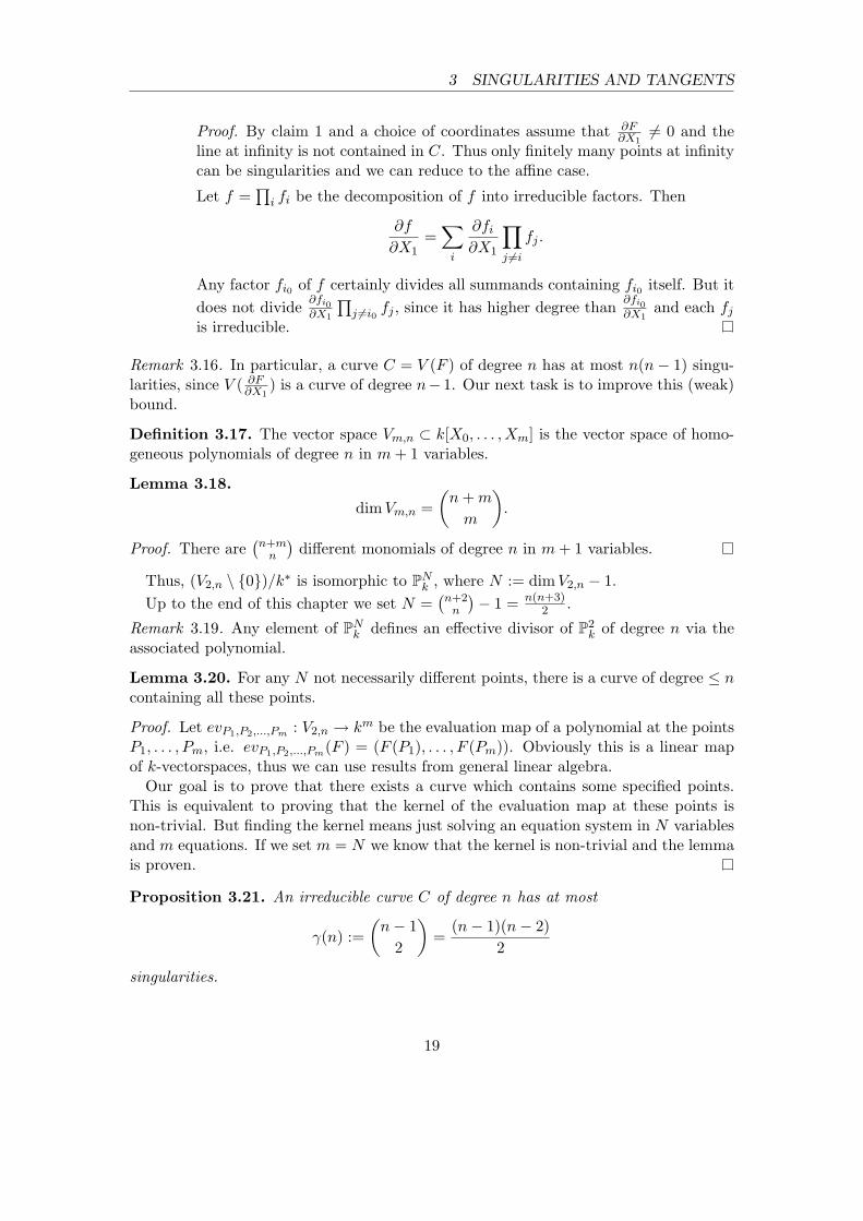
Proof. By claim 1 and a choice of coordinates assume that ∂F∂X16= 0 and the

line at infinity is not contained in C. Thus only finitely many points at infinitycan be singularities and we can reduce to the affine case.

Let f =∏i fi be the decomposition of f into irreducible factors. Then

∂f

∂X1=∑i

∂fi∂X1

∏j 6=i

fj .

Any factor fi0 of f certainly divides all summands containing fi0 itself. But itdoes not divide ∂fi0

∂X1

∏j 6=i0 fj , since it has higher degree than ∂fi0

∂X1and each fj

is irreducible.

Remark 3.16. In particular, a curve C = V (F ) of degree n has at most n(n− 1) singu-larities, since V ( ∂F

∂X1) is a curve of degree n− 1. Our next task is to improve this (weak)

bound.

Definition 3.17. The vector space Vm,n ⊂ k[X0, . . . , Xm] is the vector space of homo-geneous polynomials of degree n in m+ 1 variables.

Lemma 3.18.

dimVm,n =(n+m

m

).

Proof. There are(n+mn

)different monomials of degree n in m+ 1 variables.

Thus, (V2,n \ {0})/k∗ is isomorphic to PNk , where N := dimV2,n − 1.Up to the end of this chapter we set N =

(n+2n

)− 1 = n(n+3)

2 .

Remark 3.19. Any element of PNk defines an effective divisor of P2k of degree n via the

associated polynomial.

Lemma 3.20. For any N not necessarily different points, there is a curve of degree ≤ ncontaining all these points.

Proof. Let evP1,P2,...,Pm : V2,n → km be the evaluation map of a polynomial at the pointsP1, . . . , Pm, i.e. evP1,P2,...,Pm(F ) = (F (P1), . . . , F (Pm)). Obviously this is a linear mapof k-vectorspaces, thus we can use results from general linear algebra.

Our goal is to prove that there exists a curve which contains some specified points.This is equivalent to proving that the kernel of the evaluation map at these points isnon-trivial. But finding the kernel means just solving an equation system in N variablesand m equations. If we set m = N we know that the kernel is non-trivial and the lemmais proven.

Proposition 3.21. An irreducible curve C of degree n has at most

γ(n) :=(n− 1

2

)=

(n− 1)(n− 2)2

singularities.

19

4 THE HESSIAN OF A CURVE

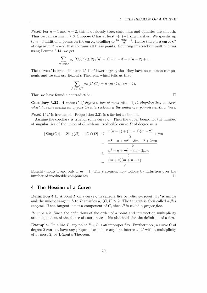
Proof. For n = 1 and n = 2, this is obviously true, since lines and quadrics are smooth.Thus we can assume n ≥ 3. Suppose C has at least γ(n)+1 singularities. We specifiy upto n−3 additional points on the curve, totalling to (n−2)(n+1)

2 . Hence there is a curve C ′

of degree m ≤ n− 2, that contains all these points. Counting intersection multiplicitiesusing Lemma 3.14, we get∑

P∈C∩C′

µP (C,C ′) ≥ 2(γ(n) + 1) + n− 3 = n(n− 2) + 1.

The curve C is irreducible and C ′ is of lower degree, thus they have no common compo-nents and we can use Bezout’s Theorem, which tells us that∑

P∈C∩C′

µP (C,C ′) = n ·m ≤ n · (n− 2).

Thus we have found a contradiction.

Corollary 3.22. A curve C of degree n has at most n(n− 1)/2 singularities. A curvewhich has this maximum of possible intersections is the union of n pairwise distinct lines.

Proof. If C is irreducible, Proposition 3.21 is a far better bound.Assume the corollary is true for some curve C. Then the upper bound for the number

of singularities of the union of C with an irreducible curve D of degree m is

|Sing(C)|+ |Sing(D)|+ |C ∩D| ≤ n(n− 1) + (m− 1)(m− 2)2

+mn

=n2 − n+m2 − 3m+ 2 + 2mn

2

≤ n2 − n+m2 −m+ 2mn2

=(m+ n)(m+ n− 1)

2.

Equality holds if and only if m = 1. The statement now follows by induction over thenumber of irreducible components.

4 The Hessian of a Curve

Definition 4.1. A point P on a curve C is called a flex or inflexion point , if P is simpleand the unique tangent L to P satisfies µP (C,L) > 2. The tangent is then called a flextangent . If the tangent is not a component of C, then P is called a proper flex .

Remark 4.2. Since the definitions of the order of a point and intersection multiplicityare independent of the choice of coordinates, this also holds for the definition of a flex.

Example. On a line L, any point P ∈ L is an improper flex. Furthermore, a curve C ofdegree 2 can not have any proper flexes, since any line intersects C with a multiplicityof at most 2, by Bezout’s Theorem.

20


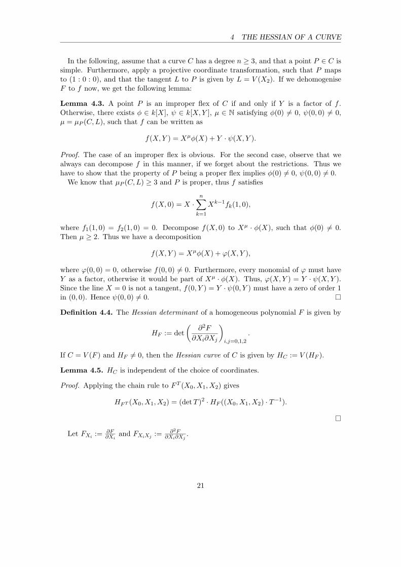
In the following, assume that a curve C has a degree n ≥ 3, and that a point P ∈ C issimple. Furthermore, apply a projective coordinate transformation, such that P mapsto (1 : 0 : 0), and that the tangent L to P is given by L = V (X2). If we dehomogeniseF to f now, we get the following lemma:

Lemma 4.3. A point P is an improper flex of C if and only if Y is a factor of f .Otherwise, there exists φ ∈ k[X], ψ ∈ k[X,Y ], µ ∈ N satisfying φ(0) 6= 0, ψ(0, 0) 6= 0,µ = µP (C,L), such that f can be written as

f(X,Y ) = Xµφ(X) + Y · ψ(X,Y ).

Proof. The case of an improper flex is obvious. For the second case, observe that wealways can decompose f in this manner, if we forget about the restrictions. Thus wehave to show that the property of P being a proper flex implies φ(0) 6= 0, ψ(0, 0) 6= 0.

We know that µP (C,L) ≥ 3 and P is proper, thus f satisfies

f(X, 0) = X ·n∑k=1

Xk−1fk(1, 0),

where f1(1, 0) = f2(1, 0) = 0. Decompose f(X, 0) to Xµ · φ(X), such that φ(0) 6= 0.Then µ ≥ 2. Thus we have a decomposition

f(X,Y ) = Xµφ(X) + ϕ(X,Y ),

where ϕ(0, 0) = 0, otherwise f(0, 0) 6= 0. Furthermore, every monomial of ϕ must haveY as a factor, otherwise it would be part of Xµ · φ(X). Thus, ϕ(X,Y ) = Y · ψ(X,Y ).Since the line X = 0 is not a tangent, f(0, Y ) = Y · ψ(0, Y ) must have a zero of order 1in (0, 0). Hence ψ(0, 0) 6= 0.

Definition 4.4. The Hessian determinant of a homogeneous polynomial F is given by

HF := det(

∂2F

∂Xi∂Xj

)i,j=0,1,2

.

If C = V (F ) and HF 6= 0, then the Hessian curve of C is given by HC := V (HF ).

Lemma 4.5. HC is independent of the choice of coordinates.

Proof. Applying the chain rule to F T (X0, X1, X2) gives

HFT (X0, X1, X2) = (detT )2 ·HF ((X0, X1, X2) · T−1).

Let FXi := ∂F∂Xi

and FXiXj := ∂2F∂Xi∂Xj

.

21


Lemma 4.6. For n := degF we always have

X20 ·HF =

∣∣∣∣∣∣n(n− 1)F (n− 1)FX1 (n− 1)FX2

(n− 1)FX1 FX1X1 FX1X2


∣∣∣∣∣∣ .Proof. Multiplying the first row of HF by X0 and adding X1 times the second row andX2 times the third row gives

X0 ·HF =

∣∣∣∣∣∣X0 ·

∑2j=0 FX0Xj X1 ·

∑2j=0 FX1Xj X2 ·

∑2j=0 FX2Xj

FX0X1 FX1X1 FX1X2

FX0X2 FX1X2 FX2X2

∣∣∣∣∣∣ .Euler’s Formula now tells us, that

(n− 1)FXi =2∑j=0

FXiXj ·Xj , i = 0, 1, 2.

Thus we get

X0 ·HF =

∣∣∣∣∣∣(n− 1)FX0 (n− 1)FX1 (n− 1)FX2

FX0X1 FX1X1 FX1X2

FX0X2 FX1X2 FX2X2

∣∣∣∣∣∣ .Applying the same procedure to columns instead of rows finally results in

X20 ·HF =

∣∣∣∣∣∣n(n− 1)F (n− 1)FX1 (n− 1)FX2



∣∣∣∣∣∣ .

Corollary 4.7. Every singular point P of C = V (F ) lies on its intersection with HC .Also, HF = 0 if char k divides n− 1.

The following Theorem tells us, how we can compute inflexion points easily:

Theorem 4.8. Let C = V (F ) be a curve of degree n ≥ 3. Let p be the characteristicof k, and assume that either p = 0 or p > n. Then HF and HC have the followingproperties:

1. HF is a multiple of F if and only if C is a union of lines.

2. If HF is not a multiple of F , then the intersection of C with its Hessian HC consistsof the singular points of C and the flexes of C.

3. For every point P of C whose tangent L is not a component of C we have

µP (C,L) = µP (C,HC) + 2.

22


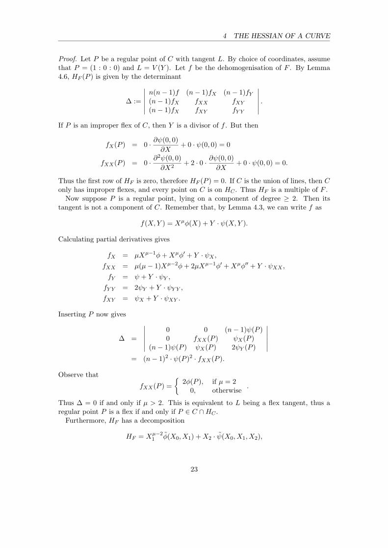
Proof. Let P be a regular point of C with tangent L. By choice of coordinates, assumethat P = (1 : 0 : 0) and L = V (Y ). Let f be the dehomogenisation of F . By Lemma4.6, HF (P ) is given by the determinant

∆ :=

∣∣∣∣∣∣n(n− 1)f (n− 1)fX (n− 1)fY(n− 1)fX fXX fXY(n− 1)fX fXY fY Y

∣∣∣∣∣∣ .If P is an improper flex of C, then Y is a divisor of f . But then

fX(P ) = 0 · ∂ψ(0, 0)∂X

+ 0 · ψ(0, 0) = 0

fXX(P ) = 0 · ∂2ψ(0, 0)∂X2

+ 2 · 0 · ∂ψ(0, 0)∂X

+ 0 · ψ(0, 0) = 0.

Thus the first row of HF is zero, therefore HF (P ) = 0. If C is the union of lines, then Conly has improper flexes, and every point on C is on HC . Thus HF is a multiple of F .

Now suppose P is a regular point, lying on a component of degree ≥ 2. Then itstangent is not a component of C. Remember that, by Lemma 4.3, we can write f as

f(X,Y ) = Xµφ(X) + Y · ψ(X,Y ).

Calculating partial derivatives gives

fX = µXµ−1φ+Xµφ′ + Y · ψX ,fXX = µ(µ− 1)Xµ−2φ+ 2µXµ−1φ′ +Xµφ′′ + Y · ψXX ,fY = ψ + Y · ψY ,fY Y = 2ψY + Y · ψY Y ,fXY = ψX + Y · ψXY .

Inserting P now gives

∆ =

∣∣∣∣∣∣0 0 (n− 1)ψ(P )0 fXX(P ) ψX(P )

(n− 1)ψ(P ) ψX(P ) 2ψY (P )

∣∣∣∣∣∣= (n− 1)2 · ψ(P )2 · fXX(P ).

Observe that

fXX(P ) ={

2φ(P ), if µ = 20, otherwise

.

Thus ∆ = 0 if and only if µ > 2. This is equivalent to L being a flex tangent, thus aregular point P is a flex if and only if P ∈ C ∩HC .

Furthermore, HF has a decomposition

HF = Xµ−21 φ(X0, X1) +X2 · ψ(X0, X1, X2),

23


where φ(1, 0) 6= 0. Thus µP (HC , L) < µP (C,L), hence P lies on a component of C,which is not in HC . Thus HF is not a multiple of F .

By calculating the resultat RF,HF, we see that each summand has the factor Xµ−2

1 .But there is also a summand of the form Xµ−2

1 · (an−1)3n(n−2)bn−10 , and since mP (C) = 1

we have an−1(P ) 6= 0. Thus there is a zero of order µ − 2, and the third part of thetheorem is proven.

Example. The assumption about the characteristic of k can not be dropped easily.Suppose char k = 3, and let F = X2

0X2−X31 define the curve C. This curve is irreducible,

its only point at infinity is the singularity (0 : 0 : 1), and HF = 0. The regular pointsare all at finite distance and satisfy Y = X3. Thus we have a proper flex at (0, 0). Buteven more, any point (a, b) on the curve at finite distance satisfies

Y −X3 = Y −X3 − (b− a3) = Y − b− (X − a)3.

Therefore, any regular point is a flex.

Corollary 4.9. Unter the assumptions of 4.8 let C be irreducible of degree n with ssingularities. Then C has at most 3n(n− 2)− 2s flexes.

Proof. By 4.8, the Hessian HC is non-empty and has no common component with C.Thus Bezout’s Theorem tells us that∑

P

µP (C,HC) = degC · degHC = 3n(n− 2).

But in this sum, s terms come from singularities, and by Lemma 3.14 each intersectionat a singularity has a multiplicity of at least two.

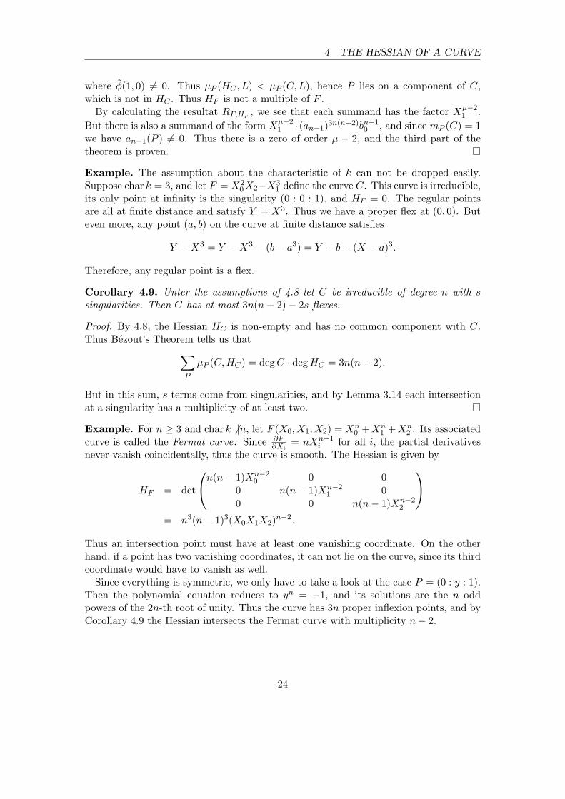
Example. For n ≥ 3 and char k 6 |n, let F (X0, X1, X2) = Xn0 +Xn

1 +Xn2 . Its associated

curve is called the Fermat curve. Since ∂F∂Xi

= nXn−1i for all i, the partial derivatives

never vanish coincidentally, thus the curve is smooth. The Hessian is given by

HF = det

n(n− 1)Xn−20 0 0

0 n(n− 1)Xn−21 0

0 0 n(n− 1)Xn−22

= n3(n− 1)3(X0X1X2)n−2.

Thus an intersection point must have at least one vanishing coordinate. On the otherhand, if a point has two vanishing coordinates, it can not lie on the curve, since its thirdcoordinate would have to vanish as well.

Since everything is symmetric, we only have to take a look at the case P = (0 : y : 1).Then the polynomial equation reduces to yn = −1, and its solutions are the n oddpowers of the 2n-th root of unity. Thus the curve has 3n proper inflexion points, and byCorollary 4.9 the Hessian intersects the Fermat curve with multiplicity n− 2.

24

References References

References

[1] Gerd Fischer. Ebene algebraische Kurven. vieweg, 1994.

[2] Ernst Kunz. Introduction to Plane Algebraic Curves. Birkhauser, 2005.

[3] Oscar Zariski and Pierre Samuel. Commutative Algebra, Volume II. Van Nostrand,1960.

25

Inflexion Points on Plane Algebraic Curves

Documents