Inflationary potentials in DBI models

arX

iv:0

907.

1311

v2 [

gr-q

c] 5

Aug

200

9

Inflationary potentials in DBI models

Dennis Bessada1,2,∗ William H. Kinney1,†, and Konstantinos Tzirakis1,‡

1Dept. of Physics, University at Buffalo, the State University of New York, Buffalo, NY 14260-1500, United States2INPE - Instituto Nacional de Pesquisas Espaciais - Divisao de Astrofısica, Sao Jose dos Campos, 12227-010 SP, Brazil

(Dated: August 5, 2009)

We study DBI inflation based upon a general model characterized by a power-law flow parameterǫ(φ) ∝ φα and speed of sound cs(φ) ∝ φβ, where α and β are constants. We show that in theslow-roll limit this general model gives rise to distinct inflationary classes according to the relationbetween α and β and to the time evolution of the inflaton field, each one corresponding to a specificpotential; in particular, we find that the well-known canonical polynomial (large- and small-field),hybrid and exponential potentials also arise in this non-canonical model. We find that these non-canonical classes have the same physical features as their canonical analogs, except for the factthat the inflaton field evolves with varying speed of sound; also, we show that a broad class ofcanonical and D-brane inflation models are particular cases of this general non-canonical model.Next, we compare the predictions of large-field polynomial models with the current observationaldata, showing that models with low speed of sound have red-tilted scalar spectrum with low tensor-to-scalar ratio, in good agreement with the observed values. These models also show a correlationbetween large non-gaussianity with low tensor amplitudes, which is a distinct signature of DBIinflation with large-field polynomial potentials.

PACS numbers: 98.80.Cq

I. INTRODUCTION

With the advent of the Five-year WMAP data [1] theinflationary paradigm [2–5] (henceforth called canonical

inflation) has been confirmed as the most successful can-didate for explaining the physics of the very early uni-verse [6]. The very rapid acceleration period generatedby canonical inflation has solved some of the puzzles ofthe standard cosmological model, such as the horizon,flatness and entropy problems. However, existing mod-els for inflation are phenomenological in character, anda fundamental explanation of inflation is still missing.Also, the scalar field responsible for the inflationary ex-pansion - the inflaton - is generically highly fine-tuned.

Over the past few years developments in string theoryhave shed new light on these two problems of canon-ical inflation. String theory predicts a broad class ofscalar fields associated with the compactification of extradimensions and the configuration of lower-dimensionalbranes moving in a higher-dimensional bulk space. Thisfact gave rise to some phenomenologically viable inflationmodels, such as the KKLMMT scenario [7], RacetrackInflation [8], Roulette Inflation [9], and the Dirac-Born-Infeld (DBI) scenario [10]. In particular, from a phe-nomenological point of view, the DBI scenario has a veryinteresting and far-reaching feature: being a special caseof a larger class of inflationary models with non-canonicalLagrangians called k-inflation [11], the DBI model pos-sesses a varying speed of sound. This is a far-reachingfeature because, in this case, slow-roll can be achieved

∗[email protected],† [email protected],‡ [email protected]

via a low sound speed instead of from dynamical frictiondue to expansion which, in turn, leads to substantial non-Gaussianity [12–16]. Also, DBI inflation admits severalexact solutions to the flow equations (first introduced in[17] for the canonical case, and generalized in [18] for DBIinflation), as discussed in [14, 19–22].

In this paper we derive a family of non-canonical mod-els characterized by a power-law in the inflaton field φfor the speed of sound cs and the flow parameter ǫ. Wethen derive the forms of the associated inflationary po-tentials, and group them according to the classificationscheme introduced in Ref. [23], in order to have a bet-ter physical picture of the solutions obtained. We latershow that some particular cases possess spectral indicesin agreement with the current observational values, andestablish the limits for the speed of sound in order thattheir tensor-to-scalar ratio correspond to the observedvalues. The outline of the paper is as follows: in sectionII we review the DBI inflation and the flow formalism fornon-canonical inflation with time-varying speed of sound.In section III we review the tools needed to calculate thescalar and tensor spectral indices for slow-roll. In sectionIV we introduce the main features of our model and de-rive general solutions, postponing the discussion of theirphysical properties to section V, where we extend theconcept of large-field, small-field, hybrid and exponen-tial potentials of canonical inflation to the non-canonicalcase. In section VI we compare the observational pre-dictions of a set of non-canonical large-field models withWMAP5 data, and show that there is a generic corre-lation between small sound speed (and therefore signifi-cant non-Gaussianity) and a low tensor/scalar ratio. Wepresent conclusions in VII.

2

II. DBI INFLATION - AN OVERVIEW

In warped D-brane inflation (see [24] and [25] for areview), inflation is regarded as the motion of a D3-branein a six-dimensional “throat” characterized by the metric[26]

ds210 = h2 (r) ds2

4 + h−2 (r)(dr2 + r2ds2

X5

), (1)

where h is the warp factor, X5 is a Sasaki-Einstein five-manifold which forms the base of the cone, and r is theradial coordinate along the throat. In this case, the in-flaton field φ is identified with r as φ =

√T3r, where T3

is the brane tension. The dynamics of the D3-brane inthe warped background (1) is then dictated by the DBILagrangian

L = −f−1 (φ)√

1 − 2f (φ) X − f−1 (φ) − V (φ) , (2)

where gµν is the background spacetime metric, f−1(φ) =T3h(φ)4 is the inverse brane tension, V (φ) is an arbitrarypotential, and X = (1/2)gµν∂µφ∂νφ is the kinetic term.We assume that the background cosmological modelis described by the flat Friedmann-Robertson-Walker(FRW) metric, gµν = diag

{1,−a2(t),−a2(t),−a2(t)

}.

DBI inflation is a special case of k-inflation, character-ized by a varying speed of sound cs, whose expression isgiven by

c2s =

(

1 + 2XL,XX

L,X

)−1

, (3)

where the subscript “, X” indicates a derivative with re-spect to the kinetic term. It is straightforward to see thatin the model (2) the speed of sound is given by

cs(φ) =√

1 − 2f(φ)X. (4)

In those models it is convenient to introduce an analogof the Lorentz factor, related to cs(φ) by:

γ(φ) =1

cs(φ). (5)

We next introduce the generalization of the inflation-ary flow hierarchy for k-inflation models [18]. The twofundamental flow parameters are

ǫ (φ) =2M2

P

γ (φ)

(H ′ (φ)

H (φ)

)2

, (6a)

s (φ) =2M2

P

γ (φ)

H ′ (φ)

H (φ)

γ′ (φ)

γ (φ), (6b)

where the prime indicates a derivative with respect toφ. An infinite hierarchy of additional flow parameterscan be generated by differentiation, and are defined asfollows:

η (φ) =2M2

P

γ (φ)

H ′′ (φ)

H (φ),

...

ℓλ (φ) =

(2M2

P

γ (φ)

)ℓ (H ′ (φ)

H (φ)

)ℓ−11

H (φ)

dℓ+1H (φ)

dφℓ+1,

ρ (φ) =2M2

P

γ (φ)

γ′′ (φ)

γ (φ),

...

ℓα (φ) =

(2M2

P

γ (φ)

)ℓ (H ′ (φ)

H (φ)

)ℓ−11

γ (φ)

dℓ+1γ (φ)

dφℓ+1, (7)

where ℓ = 2, . . . ,∞ is an integer index. It is convenientto express the flow parameters (7) in terms of the numberof e-folds before the end of inflation, which is defined inthe following way:

N = −∫

Hdt =1

√

2M2P

∫ φ

φe

√

γ (φ)

ǫ (φ)dφ, (8)

where φe indicates the value of the inflaton field at theend of inflation. The definition above indicates that thenumber of e-folds increases as we go backward in time,so that it is zero at the end of inflation. We can alsodetermine the scale factor, a, in terms of N in a straight-forward way: since da/a = dtH = −dN , we simply have

a(N) = aee−N . (9)

In terms of N , it is easy to see that the key flow pa-rameters ǫ and s, as defined in (6a) and (6b), assume thefollowing equivalent form

ǫ =1

H

dH

dN, (10a)

s =1

γ

dγ

dN, (10b)

so that we may derive a set of first-order differential equa-tions

dǫ

dN= ǫ (2η − 2ǫ − s) ,

dη

dN= −η (ǫ + s) + 2λ,

...dℓλ

dN= −ℓλ [ℓ (s + ǫ) − (ℓ − 1) η] + ℓ+1λ,

ds

dN= −s (2s + ǫ − η) + ǫρ,

dρ

dN= −2ρs + 2α,

...dℓα

dN= −ℓα [(ℓ + 1) s + (ℓ − 1) (ǫ − η)] + ℓ+1α. (11)

The dynamics of the inflaton field can be completely de-scribed by this hierarchy of equations, which are equiva-lent to the Hamilton-Jacobi equations [27]

φ = −2M2P

γ(φ)H ′(φ), (12a)

3M2P H2(φ) − V (φ) =

γ(φ) − 1

f(φ), (12b)

3

where MP = 1/√

8πG is the reduced Planck mass, and

γ(φ) =

√

1 + 4M4P f(φ) [H ′(φ)]

2. (13)

In terms of the flow parameter ǫ, the potential, V (φ),and the inverse brane tension, f(φ), can be written as

V (φ) = 3M2P H2

(

1 − 2ǫ

3

γ

γ + 1

)

, (14)

and

f (φ) =1

2M2P H2ǫ

(γ2 − 1

γ

)

, (15)

respectively. Our strategy in this paper is to generateinflationary solutions by ansatz for the flow parametersǫ and s, for which the forms of the functions V (φ) andf (φ) are determined.

In the next section, we briefly review the generation ofperturbations in non-canonical inflation models.

III. POWER SPECTRA

Scalar and tensor perturbations in k-inflation were firststudied in Ref. [28], where it was shown that the quan-tum mode function uk obeys the equation of motion

u′′k +

(

c2sk

2 − z′′

z

)

uk = 0, (16)

where k is the comoving wave number, a prime denotesa derivative with respect to conformal time dτ ≡ dt/a,and z is a variable given by

z =a√

ρ + p

csH=

aγ3/2φ

H= −Mpaγ

√2ǫ. (17)

It is convenient to change the conformal time, τ , to

y ≡ k

γaH, (18)

so that

d2

dτ2= a2H2

[

(1 − ǫ − s)2y2 d2

dy2+ G (ǫ, η, s, ρ) y

d

dy

]

,

(19)where

G = −s + 3ǫs − 2ǫη − ηs + 2ǫ2 + 3s2 − ǫρ. (20)

We can also show that

z′′

z= a2H2F

(ǫ, η, s, ρ, 2λ

), (21)

where [29]

F = 2 + 2ǫ − 3η − 3

2s − 4ǫη +

1

2ηs + 2ǫ2

+η2 − 3

4s2 + 2λ +

1

2ǫρ. (22)

Substituting (19) and (21) into (16), we find

(1 − ǫ − s)2y2 d2uk

dy2+ Gy

duk

dy+

[y2 − F

]uk = 0, (23)

which is an exact equation, without any assumption ofslow-roll.

We now proceed to solve equation (23) to first-orderin slow-roll. In this case, this equation takes the form

(1 −2ǫ −2s)y2 d2uk

dy2− sy

duk

dy

+

[

y2 − 2(1 + ǫ − 3

2η − 3

4s)

]

uk = 0, (24)

whose solution is [21]

uk(y) =1

2

√π

csk

√y

1 − ǫ − sHν

(y

1 − ǫ − s

)

, (25)

where Hν is a Hankel function, and

ν =3

2+ 2ǫ − η + s. (26)

The power spectra for scalar and tensor perturbationsare given respectively by

PR =1

8π2

H2

M2P csǫ

∣∣∣∣csk=aH

,

PT =2

π2

H2

M2P

∣∣∣∣k=aH

, (27)

so that, for the solution (25),

P1/2R = [(1 − ǫ − s)

+(2 − ln 2 − γ)(2ǫ − η + s)]H2

2πφ

∣∣∣∣k=γaH

(28)

where γ ≈ 0.577 is Euler’s constant. From the definitionsof the scalar and tensor spectral indices,

ns − 1 ≡ d(ln PR)

d(ln k),

nT ≡ d(ln PT )

d(ln k), (29)

we find

ns − 1 = −4ǫ + 2η − 2s,

nT = −2ǫ, (30)

valid to first-order in the slow-roll limit. The tensor-to-scalar ratio is given by [30]

r = 16ǫc1+ǫ

1−ǫ

s , (31)

4

which, to first-order in slow-roll, gives the well-knownresult

r = 16csǫ, (32)

Since in this paper we will work only to the first-order inslow-roll approximation, we make use of expression (32)to compute the tensor/scalar ratio. It is immediatelyclear from this expression that small cs has the genericeffect of suppressing the tensor/scalar ratio.

IV. THE MODEL

A. The General Setting

The usual approach to the construction of a model ofinflation normally starts with a choice of the inflaton po-tential, V (φ); then, all the flow parameters are derived,and the dynamical analysis is performed. In this work weadopt the reverse procedure: we first look for the solu-tions to the differential equation satisfied by the Hubbleparameter H(φ),

H ′(φ)

H(φ)= ±

√

ǫ(φ)γ(φ)

2M2P

, (33)

and only afterwards derive the form of the potential.Equation (33) can be easily derived from the definition ofthe flow parameter ǫ, given by (6a), and the sign ambigu-ity indicates in which direction the field is rolling. Noticethat in order to solve equation (33) we must know theform of the functions ǫ(φ) and γ(φ); we choose them tobe power-law functions of the inflaton field,

ǫ(φ) =

(φ

φe

)α

, (34a)

γ(φ) = γe

(φ

φe

)β

, (34b)

where γe is the value of the Lorentz factor at the endof inflation1, and α and β are constants. Another caseworth studying appears when ǫ is constant, so that

ǫ(φ) = ǫ = const., (35)

with the same parametrization for γ. We have kept φe forthe following reason: in the IR DBI model the inflatonfield rolls down from the tip of the throat toward thebulk of the manifold with increasing speed of sound; then,when the field enters the bulk cs becomes equal to 1, andthen inflation “ends”. In the UV case the behavior is theopposite, that is, the field evolves away from the bulk and

1 Henceforth all the variables with a subscript e are evaluated atthe end of inflation.

reaches the tip when cs = 1. To reproduce both cases wecould have set γe = 1 from the onset, so that cs(φe) = 1,as required; also, cs(φ) = 1 in the canonical limit, thatis, when β = 0. However, by taking γe arbitrary, wealso reproduce the non-canonical models with constantspeed of sound introduced by Spalinski [20]. It is clearthat in the latter case γe does not refer necessarily to theend of inflation, so that if we take γe ≫ 1 it does notmean a superluminal propagation (as would be the caseif β 6= 0). Bearing this distinction in mind we can usethe same notation unambiguously.

When α 6= 0, substituting (34a) and (34b) into (33),we see that the Hubble parameter takes the form

H(φ) = He exp

σ

√

γe

2M2P φα+β

e

I(φ)

, (36)

where we have defined

I(φ) ≡∫ φ

φe

dφ′φ′(α+β)/2, (37)

and σ accounts for the sign ambiguity appearing in (33).When ǫ is constant, the solution to (33) reads

H(φ) = He exp

σ

√

ǫγe

2Mβ+2P

I(φ)

, (38)

where the integral I(φ) is the same as in (37).It is clear that the integral (37) admits two distinct

solutions: a logarithmic one when α+β = −2, and power-law for α + β 6= −2. These two solutions will give rise todifferent classes of inflationary potentials, which we shalladdress in the next subsections.

To conclude this section we derive the general formulafor the number of e-folds. For α 6= 0 this expression canbe determined by equations (8), (34a), and (34b), so that

N(φ) = σ

√

γeφα−βe

2M2P

J(φ), (39)

where

J(φ) =

∫ φ

φe

dφ′φ′(β−α)/2; (40)

if α = 0 we must use the parametrization (35), so thatexpression (39) changes to

N(φ) = σ

√

γe

2M2P ǫφβ

e

J(φ), (41)

where

J(φ) =

∫ φ

φe

dφ′φ′β/2. (42)

In the next section, we discuss particular cases of thisgeneral class of solutions.

5

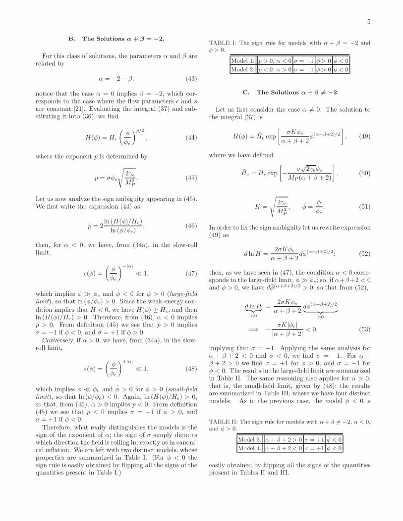
B. The Solutions α + β = −2.

For this class of solutions, the parameters α and β arerelated by

α = −2 − β; (43)

notice that the case α = 0 implies β = −2, which cor-responds to the case where the flow parameters ǫ and sare constant [21]. Evaluating the integral (37) and sub-stituting it into (36), we find

H(φ) = He

(φ

φe

)p/2

, (44)

where the exponent p is determined by

p = σφe

√

2γe

M2P

. (45)

Let us now analyze the sign ambiguity appearing in (45).We first write the expression (44) as

p = 2ln (H(φ)/He)

ln (φ/φe); (46)

then, for α < 0, we have, from (34a), in the slow-rolllimit,

ǫ(φ) =

(φ

φe

)−|α|

≪ 1, (47)

which implies φ ≫ φe and φ < 0 for φ > 0 (large-field

limit), so that ln (φ/φe) > 0. Since the weak-energy con-

dition implies that H < 0, we have H(φ) ≥ He, and thenln (H(φ)/He) > 0. Therefore, from (46), α < 0 impliesp > 0. From definition (45) we see that p > 0 impliesσ = −1 if φ < 0, and σ = +1 if φ > 0.

Conversely, if α > 0, we have, from (34a), in the slow-roll limit,

ǫ(φ) =

(φ

φe

)+|α|

≪ 1, (48)

which implies φ ≪ φe and φ > 0 for φ > 0 (small-field

limit), so that ln (φ/φe) < 0. Again, ln (H(φ)/He) > 0,so that, from (46), α > 0 implies p < 0. From definition(45) we see that p < 0 implies σ = −1 if φ > 0, andσ = +1 if φ < 0.

Therefore, what really distinguishes the models is thesign of the exponent of α; the sign of σ simply dictateswhich direction the field is rolling in, exactly as in canoni-cal inflation. We are left with two distinct models, whoseproperties are summarized in Table I. (For φ < 0 thesign rule is easily obtained by flipping all the signs of thequantities present in Table I.)

TABLE I: The sign rule for models with α + β = −2 andφ > 0.

Model 1. p > 0, α < 0 σ = +1 φ > 0 φ < 0

Model 2. p < 0, α > 0 σ = +1 φ > 0 φ < 0

C. The Solutions α + β 6= −2

Let us first consider the case α 6= 0. The solution tothe integral (37) is

H(φ) = He exp

[σKφe

α + β + 2φ(α+β+2)/2

]

, (49)

where we have defined

He = He exp

[

− σ√

2γeφe

MP (α + β + 2)

]

, (50)

K =

√

2γe

M2P

, φ =φ

φe. (51)

In order to fix the sign ambiguity let us rewrite expression(49) as

d lnH =2σKφe

α + β + 2dφ(α+β+2)/2; (52)

then, as we have seen in (47), the condition α < 0 corre-sponds to the large-field limit, φ ≫ φe; so, if α+β+2 < 0and φ > 0, we have dφ(α+β+2)/2 > 0, so that from (52),

d ln H︸ ︷︷ ︸

<0

=2σKφe

α + β + 2dφ(α+β+2)/2

︸ ︷︷ ︸

>0

=⇒ − σK|φe||α + β + 2| < 0, (53)

implying that σ = +1. Applying the same analysis forα + β + 2 < 0 and φ < 0, we find σ = −1. For α +β + 2 > 0 we find σ = +1 for φ > 0, and σ = −1 forφ < 0. The results in the large-field limit are summarizedin Table II. The same reasoning also applies for α > 0,that is, the small-field limit, given by (48); the resultsare summarized in Table III, where we have four distinctmodels: As in the previous case, the model φ < 0 is

TABLE II: The sign rule for models with α + β 6= −2, α < 0,and φ > 0.

Model 3. α + β + 2 > 0 σ = +1 φ < 0

Model 4. α + β + 2 < 0 σ = +1 φ < 0

easily obtained by flipping all the signs of the quantitiespresent in Tables II and III.

6

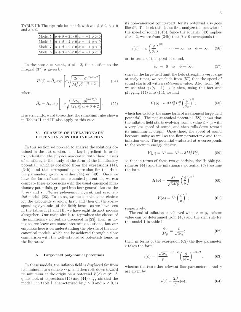
TABLE III: The sign rule for models with α + β 6= 0, α > 0and φ > 0.

Model 5. α + β + 2 > 0 σ = −1 φ > 0

Model 6. α + β + 2 > 0 σ = +1 φ < 0

Model 7. α + β + 2 < 0 σ = −1 φ > 0

Model 8. α + β + 2 < 0 σ = +1 φ < 0

In the case ǫ = const., β 6= −2, the solution to theintegral (37) is given by

H(φ) = He exp

[

σ

√

2ǫγe

M2P φβ

e

φ(β+2)/2

β + 2

]

, (54)

where

He = He exp

[

−σ

√

2ǫγe

M2P φβ

e

φ(β+2)/2e

α + β + 2

]

. (55)

It is straightforward to see that the same sign rules shownin Tables II and III also apply to this case.

V. CLASSES OF INFLATIONARY

POTENTIALS IN DBI INFLATION

In this section we proceed to analyze the solutions ob-tained in the last section. The key ingredient, in orderto understand the physics associated with these classesof solutions, is the study of the form of the inflationarypotential, which is obtained from the expressions (14),(34b), and the corresponding expression for the Hub-ble parameter, given by either (44) or (49). Once wehave the form of such non-canonical potentials, we cancompare these expressions with the usual canonical infla-tionary potentials, grouped into four general classes: thelarge- and small-field polynomial, hybrid, and exponen-

tial models [23]. To do so, we must make some choicesfor the exponents α and β first, and then on the corre-sponding dynamics of the field; hence, as we have seenin the tables I, II and III, we have eight distinct modelsaltogether. Our main aim is to reproduce the classes ofthe inflationary potentials discussed in [23]; then, in do-ing so, we leave out some interesting solutions, but ouremphasis here is on understanding the physics of the non-canonical models, which can be achieved through a closecomparison with the well-established potentials found inthe literature.

A. Large-field polynomial potentials

In these models, the inflaton field is displaced far fromits minimum to a value φ ∼ µ, and then rolls down towardits minimum at the origin on a potential V (φ) ∝ φp. Aquick look at expressions (14) and (44) suggests that themodel 1 in table I, characterized by p > 0 and α < 0, is

its non-canonical counterpart, for its potential also goeslike φp. To check this, let us first analyze the behavior ofthe speed of sound (34b). Since the equality (43) impliesβ > −2, we see from (34b) that β > 0 corresponds to

γ(φ) = γe

(φ

φe

)|β|

=⇒ γ → ∞ as φ → ∞, (56)

or, in terms of the speed of sound,

cs → 0 as φ → ∞; (57)

since in the large-field limit the field strength is very largeat early times, we conclude from (57) that the speed ofsound starts off with a subluminal value. Also, from (56),we see that γ/(γ + 1) → 1; then, using this fact andplugging (44) into (14), we find

V (φ) ∼ 3M2P H2

e

(φ

φe

)p

, (58)

which has exactly the same form of a canonical large-fieldpotential. The non-canonical potential (58) shows thatthe inflaton field starts evolving from a value φ ∼ µ witha very low speed of sound, and then rolls down towardits minimum at origin. Once there, the speed of soundbecomes unity as well as the flow parameter ǫ and theninflation ends. The potential evaluated at µ correspondsto the vacuum energy density,

V (µ) = Λ4 =⇒ Λ4 ∼ 3M2P H2

e , (59)

so that in terms of these two quantities, the Hubble pa-rameter (44) and the inflationary potential (58) assumethe form

H(φ) =Λ2

√

3M2P

(φ

µ

)p/2

(60)

V (φ) = Λ4

(φ

µ

)p

, (61)

respectively.The end of inflation is achieved when φ = φe, whose

value can be determined from (45) and the sign rule forthe model 1 in table I:

φe

MP=

p√2γe

; (62)

then, in terms of the expression (62) the flow parameterǫ takes the form

ǫ(φ) =

[√2γe

p

]−β−2 (φ

MP

)−β−2

, (63)

whereas the two other relevant flow parameters s and ηare given by

s(φ) =2β

pǫ(φ), (64)

7

η(φ) =p − 2

pǫ(φ), (65)

where we have used (6b), the first expression of (7), plus(34b), (60) and (62). The expression for the number ofe-folds is obtained from expressions (39), (40) and (43)for α 6= 0, so that

N(φ) =p

2 (β + 2)

[1

ǫ(φ)− 1

]

. (66)

In the analysis performed above we have consideredsolely models with α < 0 and β > 0; the case α = 0 hasbeen studied in the paper [21], and leads to potentialslike (61) in the UV limit s < 0. The case β = 0, γe = 1,corresponds to canonical large-field models; in this limit,the expressions for the flow parameters ǫ and η, given by(63) and (65), give

ǫ(φ) =p2

2

M2P

φ2, (67)

η(φ) =p(p − 2)

2

M2P

φ2, (68)

which coincides with the results in section III.A of ref-erence [23]. Also in this limit, from (62) we see thatinflation ends when

φce

MP=

p√2, (69)

which coincides with the analogous expression found in[23]2. Hence, all large-field polynomial models with p > 2are particular cases of this non-canonical version. Also,if γe 6= 1, we recover the Spalinski model [20] with apolynomial potential as well. Another particular caseof this general class is isokinetic inflation, proposed in[22]. For this model, we can show that by setting α =−p/2−1 and β = p/2−1, we reproduce all the expressionsderived in [22] up to a redefinition of the exponent of thepotential3.

Therefore, we have a completely well-defined D-braneinflationary scenario with large-field potentials like (61),a flow parameter ǫ given by (34a) with α < 0, and a smallspeed of sound characterized by (34b) with β ≥ 0, repro-ducing not only the canonical large-field polynomial po-tentials, but also other models discussed in the literature.For these reasons we will call this class non-canonical

large-field polynomial models.In particular, as we will see in section VI, these models

predict values for the scalar spectral index and tensor-to-scalar ratio which agree very well with WMAP5 obser-vations.

2 Our notation differs from that adopted in [23]; our MP is relatedto mpl in that reference by MP = mpl/

√8π.

3 In isokinetic inflation the potential has the form V (φ) ∝ φ2piso

[22], whereas in our model we have defined the exponent p (ex-pression (45)) such that V (φ) ∝ φp. Then p = 2piso.

B. Small-field polynomial potentials

Small-field polynomial potentials in canonical inflationarise from a spontaneous symmetry breaking in the pres-ence of a “false” vacuum in unstable equilibrium withnonzero vacuum energy density and a “physical” vacuum,for which the classical expectation value of the scalar fieldis nonzero, 〈φ〉 6= 0 [31]. These models are characterizedby an effective symmetry-breaking scale µ ∝ 〈φ〉 suchthat φ ≪ µ ≪ MP , the field rolls down from an unstableequilibrium at the origin toward µ; hence, for positive φwe have always φ > 0.

For non-canonical models we can express the small-field limit φ ≪ µ by choosing α > 0; also, as we havederived in section IVC, the condition φ > 0 for φ > 0is satisfied when σ = −1 and α + β + 2 > 0, whichcorresponds to the model 5 in table III. In this case, theHubble parameter (49) takes the form

H(φ) = He exp

[

− Kφe

α + β + 2φ(α+β+2)/2

]

; (70)

where K and φe are given by (51); since φ = φ/φe inthe small-field limit, and α + β + 2 > 0, we can expandexpression (70) to first-order in φ, so that

H(φ) = He exp

[

1 − Kφe

α + β + 2φ(α+β+2)/2

]

. (71)

Since β > −2 − α and α > 0, we see that β can takeeither sign; in particular, for β > 0, from (34b) we havethe following relation

γ(φ) = γe

(φ

φe

)−|β|

=⇒ γ → ∞ as φ → 0, (72)

or, in terms of the speed of sound,

cs → 0 as φ → 0. (73)

In the small-field limit, we have always φ ≪ φe, so thatφ → 0 corresponds to early times; then, from (73) weconclude that the field propagates with subluminal speedof sound at early times. Also, property (72) implies thatγ/(γ + 1) → 1, so that by using this fact and plugging(71) into (14), we find

V (φ) ∼ 3M2P H2

e

[

1 − 2

3φα − 2Kφe

α + β + 2φ(α+β+2)/2

]

(74)in the slow-roll limit. It is clear that we can derive outof expression (74) different sort of potentials, dependingon the relations between the exponents. Let us analyzeone of such possible choices; we define first the exponent

p =α + β + 2

2, (75)

and we choose α and β such that p is always integer.Then, if α ≥ p, we see that α ≥ β + 2, and the potential

8

(74) takes the form

V (φ) ∼ 3M2P H2

e

[

1 − Kφe

pφp

]

, α ≥ β + 2. (76)

In the canonical small-field scenario the initial unstableequilibrium state is characterized by the vacuum energydensity Λ4, which is the height of the potential at the ori-gin, Λ4 = V (0), whereas the effective symmetry-breakingscale is given by [31]

µ =

[(m − 1)!V (φ)

|dmV/dφm|

]1/m∣∣∣∣∣φ=0

, (77)

where m is the order of the lowest nonvanishing derivativeof the potential at the origin. In the non-canonical case,the vacuum energy density is given by

Λ4 = 3M2P H2

e , (78)

whereas the effective symmetry-breaking scale (77) reads

1

µp=

√

2γe

M2P φα+β

e

; (79)

then, in terms of these two quantities, the inflationarypotential (74) becomes, in the small-field limit,

V (φ) = Λ4

[

1 − 1

p

(φ

µ

)p]

, (80)

as expected. Then, in the non-canonical case the fieldalso rolls down from an unstable vacuum state whoseenergy density is given by (78) with very low speed ofsound, and evolves toward a minimum characterized bya scale µ given by (79) for α ≥ p ≥ 2, and such behavioris exactly the same as the canonical case.

From (79) we see that inflation ends when

φe

µ=

[µ

MP

√

2γe

]1/(p−1)

, (81)

so that the flow parameters are given by

ǫ(φ) =

[MP

µ√

2γe

](p−1)/α (φ

µ

)α

, (82)

s(φ) = −β

√

2M2P

γeφ2e

, (83)

η(φ) = (α + β)

√

M2P

2γeφ2e

φ(α−β−2)/2 + ǫ(φ), (84)

where we have used (6b), the first expression of (7), plus(34a), (34b), (70) and (81).

In particular, in the canonical limit β = 0, γe = 1 wehave α ≥ 2, so that for even values of α all the potentialswith p ≥ 2 are reproduced. In this limit, from (75) wesee that α = 2(p−1); then, from (82) the flow parameterǫ assumes the form

ǫ(φ) =MP

µ√

2

(φ

µ

)2(p−1)

, (85)

whereas from (81) we see that inflation ends at

φe

µ=

[µ

MP

√2

]1/(p−1)

. (86)

Expressions (85) and (86) agree with the correspondingexpressions (3.25) and (3.26) in [31] derived for canonicalsmall-field potentials.

Therefore, in the slow-roll limit all canonical small-fieldpolynomial models with p ≥ 2 are particular solutions tothe non-canonical model described in this section whenβ = 0, γe = 1 and α even; hence, we have again a well-defined D-brane inflationary scenario with a small-fieldpotential like (80), a flow parameter ǫ given by (34a)with α > 0, and a small speed of sound characterized by(34b) with β ≤ 0, reproducing all the canonical small-field polynomial potentials when β = 0. For these reasonswe will call this class non-canonical small-field polynomial

models.

C. Hybrid potentials

In the last two sections we have discussed the small-field models characterized by φ > 0 for positive φ, givenby the model 5 in table III. Let us now examine a similarmodel, with α + β + 2 > 0 but with φ < 0 for positiveφ. In this case, σ = +1, (model 6 in table III); then, theHubble parameter (49) takes the form

H(φ) = He exp

[Kφe

α + β + 2φ(α+β+2)/2

]

, (87)

where the constant K and variable φ are given by thedefinitions (51). Since φ ≪ 0 and p > 0, where p is givenby (75), we expand expression (87) to first-order in φ,

H(φ) = He exp

[

1 +Kφe

2pφp

]

. (88)

The analysis leading to the sign of β is identical to thatmade in section VB since, as in that case, β > −2 − αand α > 0; then, using the same arguments we find thatthe field rolls down the potential with a subluminal speedof sound. Also, since γ/(γ + 1) → 1 at early times, wehave, plugging (88) into (14), that

V (φ) ∼ 3M2P H2

e

[

1 − 2

3φα +

Kφe

pφp

]

(89)

9

in the slow-roll limit. As in the model derived in sectionVB, we choose α and β such that p is always integer;then, for α > p, the potential (89) takes the form

V (φ) ∼ 3M2P H2

e

[

1 +Kφe

pφp

]

. (90)

In this case, the minimum of the potential is at the origin,as in the small-field polynomial case, but now V (φ) >V (0) around φ = 0. Therefore, the field rolls toward theminimum with nonzero vacuum energy, Λ4 = V (0). Thisis exactly the behavior of the canonical hybrid potentials[33, 34]. Then, we may write the potential (87) as

V (φ) ∼ Λ4

[

1 +

(φ

µ

)p]

, (91)

where we have defined

1

µp=

1

p

√

2γe

M2P φ

2(p−1)e

. (92)

D. Exponential potentials

Along with the models discussed above, there is afourth type whose Hubble parameter and potential areexponentials [23]. Since the general expression for theHubble parameter derived in section IVC is of a expo-nential form, we focus on its large-field limit solution,given by the model 4 in table II. In this case φ < 0for positive φ, so that σ = +1. The expression for theHubble parameter (49) for α < 0, is given by

H(φ) = He exp

√

1

2p

(φ

MP

)α+β+2

, (93)

where we have defined

p =(α + β + 2)

2

4γe

(φe

MP

)α+β

. (94)

Since α + β + 2 > 0, the exponent of the speed ofsound is restricted to the values β > −α − 2; then, forβ > 0, we have that γ → ∞ as φ → ∞, and then cs → 0at early times since φ is in the large-field limit. Hence,the field propagates with a subluminal speed of soundat early times, and γ/(γ + 1) → 1. Using this fact andsubstituting (93) into (14) we find

V (φ) ∼ 3M2P H2

e exp

√

2

p

(φ

MP

)α+β+2

. (95)

Then, the field rolls down the potential toward the min-imum at origin, characterized by a nonzero vacuum en-ergy V (0) = Λ4 with a subluminal speed of sound. Thisis similar to the behavior of exponential potentials in

canonical models, except for the fact that cs = 1. SinceΛ4 = 3MP H2

e , the final form of the non-canonical poten-tial (95) is

V (φ) ∼ Λ4 exp

√

2

p

(φ

MP

)α+β+2

. (96)

Before we study the non-canonical limit of the poten-tial (96), let us have a look first at the flow-parameterǫ. We have used the parametrization associated withα 6= 0, given by (34a), but we can make it general asfollows: substituting and (34b) and (94) into (34a), wefind

ǫ(φ) =(α + β + 2)

2

4pγ(φ)

(φ

MP

)α+β

. (97)

which holds even when α = 0, for ǫ(φ) = ǫ = const. inthat case. The other two flow parameters s and η aregiven respectively by

s(φ) = β

(φ

MP

)−1√

2ǫ(φ)

γ(φ), (98)

η(φ) =α + β√

2

(φ

MP

)−1√

ǫ(φ)

γ(φ)+ ǫ(φ), (99)

where we have used (6b), the first expression of (7), plus(34b) and (93).

Then, with the parametrization defined by (97), we seethat in the canonical case α = β = 0, γe = 1, expressions(97) and (99) give

ǫ(φ) = η(φ) =1

p, (100)

which matches the results derived for the canonical caseas shown in [23]. Expression (100) shows that we haveto restrict the values of (94) to be p > 1, so that we getǫ ≤ 1 in the canonical limit.

Therefore, we have a completely well-defined D-braneinflationary scenario with exponential potentials like(96), a flow parameter ǫ given by (97) with α ≤ 0, and asmall speed of sound characterized by (34b) with β ≥ 0,which reproduces the corresponding canonical model. Wewill call this class non-canonical exponential models.

The four distinct non-canonical classes obtained so farare summarized in Table IV below.

VI. AN APPLICATION OF NON-CANONICAL

LARGE-FIELD POLYNOMIAL MODELS

In this section we study some applications of the large-field models derived in section VA. We choose this classof non-canonical potentials because the expressions forthe scalar spectral index, the tensor/scalar ratio and the

10

TABLE IV: A summary of the distinct models discussed in this work.

model α β p V (φ)

Large-field α = −β − 2 β ≥ 0 φe

q

2γe

M2P

a Λ4“

φ

µ

”p

Small-field α ≥ p β ≤ 0 α+β+22

b Λ4h

1 − 1p

“

φ

µ

”pi

Hybrid α ≥ p β ≤ 0 α+β+22

c Λ4h

1 +“

φ

µ

”pi

Exponential α ≤ 0 β ≥ 0 (α+β+2)2

4γe

“

φe

MP

”α+βd Λ4 exp

"

r

2p

“

φ

MP

”α+β+2#

aCorresponds to model 1 in table I.bp is integer. Corresponds to model 5 in table III.cp is integer. Corresponds to model 6 in table III.dp > 1. Corresponds to model 4 in table II.

level of non-gaussianity are particularly simple, depend-ing on two parameters solely, p and β. Let us first derivean expression for the flow parameter ǫ in terms of N .From (63) and (66) we find

ǫ(N) =p

p + 2 (β + 2)N. (101)

The other two flow parameters s and η are given by

s(N) =2β

p + 2 (β + 2)N, (102)

η(N) =p − 2

p + 2 (β + 2)N; (103)

where we have used (6b), the first expression of (7), plus(34b), (60) and (101). Inserting (101), (102) and (103)into (30), we find, in the slow-roll limit,

ns = 1 − 2(p + 2β + 2)

p + 2 (β + 2)N. (104)

The expression for the speed of sound in terms of Ncan be calculated in the same way: we use (34a), (34b)and (66), so that

cs(N) =1

γe

[p

p + 2 (β + 2)N

]β/(β+2)

. (105)

Through the use of (32), (101) and (105) we can derivea general expression for the tensor/scalar ratio, which isgiven by

r(N) =16

γe

[p

p + 2 (β + 2)N

]2(β+1)/(β+2)

. (106)

The expression for the level of non-gaussianity fNL isgiven by [18]

fNL = − 35

108

(1

c2s

− 1

)

, (107)

which can be easily evaluated by using expression (105).Therefore, the tensor/scalar ratio will have a power-

law dependence as well, with exponent 2(β + 1)/(β + 2),which means that, for a given value of p, a larger β cor-responds to a smaller r. Since β ≥ 0 for non-canonicallarge-field models, we have, from (5) and (34b), thatcs ∝ φ−β ; then, fields rolling with slower speed ofsound would produce lower tensor/scalar ratios. How-ever, from (107), we see that fNL depends on c−2

s , andthen a low speed of sound would produce a larger level ofnon-gaussianity; then, for large-field models low-r tensormodes are strongly correlated with the amplitude of non-gaussianity, as has been discussed in the reference [22]for isokinetic inflation. Then, the suppression of tensormodes by a large amount of non-gaussianity is a featureshared by all non-canonical models with large-field poly-nomial potentials.

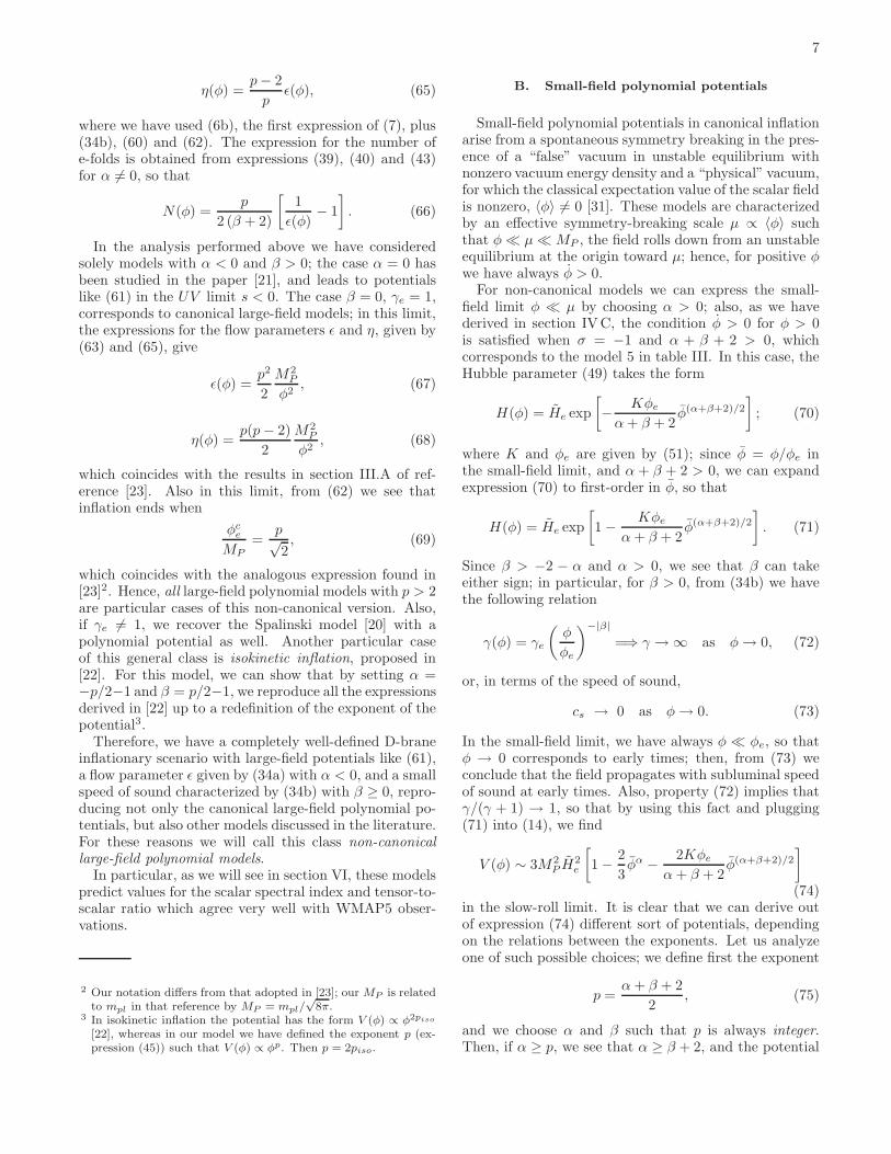
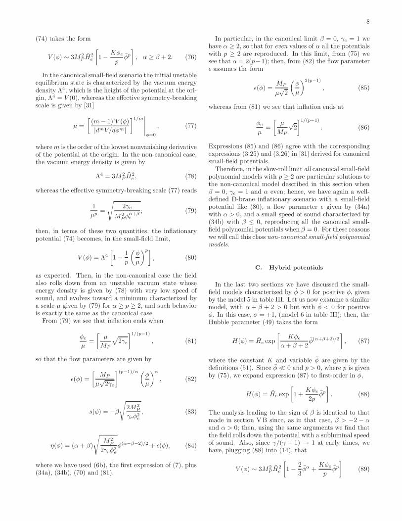
Let us next make some predictions on the values of ns,r and fNL through expressions (104), (106) and (107)respectively, when the modes cross the horizon 46 or 60e-folds before the end of inflation. As we have discussedin section IVA, we have set γe = 1, which characterizesthe end of inflation; the results are depicted in figures1 and 2. In both figures, the top left plots refer to thevariation of the scalar index in terms of β for each valueof p. The top right plots in Figs. 1 and 2 show thecorresponding tensor/scalar ratio. In these plots we seethat for larger values of p and small β the modes havelarge values of r (the observable lower bound is r < 0.22);

11

0 0.5 1 1.5 2 2.5 30.925

0.93

0.935

0.94

0.945

0.95

0.955

0.96

0.965Scalar spectral index for N=46

n s

β

p=2p=3p=4p=5

0 0.5 1 1.5 2 2.5 30

0.05

0.1

0.15

0.2

0.25

0.3

0.35

0.4

0.45Tensor−to−scalar ratio for N=46

r

β

p=2p=3p=4p=5

0 0.5 1 1.5 2 2.5 3−250

−200

−150

−100

−50

0Level of non−gaussianity for N=46

f NL

β

p=2p=3p=4p=5

10−3

10−2

10−1

100

−250

−200

−150

−100

−50

0Level of non−gaussianity x Tensor−to−scalar ratio for N=46

f NL

r

p=2p=3p=4p=5

FIG. 1: The observables ns (top left), r (top right) and fNL (bottom left) as a function of the exponent of the speed of soundβ for each value of p (V (φ) ∝ φp) for N = 46. On bottom right is depicted the behavior of fNL compared to r.

then, as β increases, the speed of sound gets lower and, inconsequence, the tensor/scalar ratio as well. However, asshown in (107), a field rolling very slowly produces a largeamount of non-gaussianity, as can be seen in the bottomleft plots of figures 1 and 2. Therefore, as was first dis-cussed in the particular case of isokinetic inflation [22],the production of large non-gaussianity is strictly cor-related with low tensor amplitudes, and this is a featurecommon to all large-field polynomial potentials. This be-havior is shown in the bottom right plots of figures 1 and2.

We next compare the results obtained with the cur-rent WMAP5 data [1], [6]. The results are depicted inFig. 3 for different values of p. Straight lines indicatethe different values of β, with the left (right) extrem-ity indicating the value of (ns, r) evaluated at N = 46(N = 60). As shown in [6], all canonical models withp > 2 are ruled out by WMAP5 data alone; however,in the non-canonical case, figure 3 shows that the mod-els with p ≤ 5 are also consistent with the observabledata. A field evolving with slow-varying speed of soundproduces low-amplitude tensors, then pushing the val-ues (ns, r) inwards the observable region. However, alarge amount of non-gaussianity is produced, which is adistinct signature of non-canonical large-field polynomialmodels and can be a powerful observable to discriminate

among inflationary models.

VII. CONCLUSIONS

In this paper we propose a general DBI model char-acterized by a power-law flow-parameter power-law flowparameter ǫ(φ) ∝ φα and speed of sound cs(φ) ∝ φβ ,where α and β are constants. We show that this generalmodel has distinct classes of solutions depending on therelation between α and β, and on the time evolution ofthe inflaton field. These classes of solutions are summa-rized in tables I, II and III. In particular, we show thatin the slow-roll limit the four well-known canonical po-tentials arise naturally in this general DBI model, havingsimilar properties to their canonical counterparts, exceptthat the speed of sound in general varies with time. Wealso show that this general DBI model encompasses notonly all the canonical models with the mentioned po-tentials, but other D-brane scenarios as well: the DBImodel with constant speed of sound [20], with constantflow parameters [21], and isokinetic inflation [22]. Thefour non-canonical models are summarized in table IV.

We also derive the expressions for the spectral index,tensor/scalar ratio and the amplitude of non-gaussianityfor large-field potentials in the slow-roll limit. We show

12

0 0.5 1 1.5 2 2.5 30.94

0.945

0.95

0.955

0.96

0.965

0.97

0.975Scalar spectral index for N=60

n s

β

p=2p=3p=4p=5

0 0.5 1 1.5 2 2.5 30

0.05

0.1

0.15

0.2

0.25

0.3

0.35Tensor−to−scalar ratio for N=60

r

β

p=2p=3p=4p=5

0 0.5 1 1.5 2 2.5 3−350

−300

−250

−200

−150

−100

−50

0Level of non−gaussianity for N=60

f NL

β

p=2p=3p=4p=5

10−3

10−2

10−1

100

−350

−300

−250

−200

−150

−100

−50

0Level of non−gaussianity x Tensor−to−scalar ratio for N=60

f NL

r

p=2p=3p=4p=5

FIG. 2: The observables ns (top left), r (top right) and fNL (bottom left) as a function of the exponent of the speed of soundβ for each value of p (V (φ) ∝ φp) for N = 60. On bottom right is depicted the behavior of fNL compared to r.

that a low speed of sound suppresses the tensor/scalar ra-tio r and produces a large amount of non-gaussianity, afeature already explored in the case of isokinetic inflation,and shown to be a general property of all large-field DBImodels with polynomial potentials. Unlike canonical in-flation, where all polynomial models with p > 2 are ruledout, the suppression of tensor modes in the non-canonicalversion allows a larger class of polynomial potentials tolie within the observable range; also, the production oflarge amount of non-gaussianity is a distinct signature

of these DBI large-field models, which can be a powerfulobservable to discriminate among inflationary models.

Acknowledgments

DB thanks Brazilian agency CAPES for financial sup-port. This research is supported in part by the NationalScience Foundation under grant NSF-PHY-0757693.

[1] E. Komatsu et al, Astrophys. J. Suppl.Ser., 180, 330(2009)

[2] A. A. Starobinskii, JETP Lett., 30, 682 (1979)[3] A. H. Guth, Phys. Rev. D 23, 347 (1981).[4] A. D. Linde, Phys. Lett. B 108, 389 (1982).[5] A. Albrecht and P. J. Steinhardt, Phys. Rev. Lett. 48,

1220 (1982).[6] W. H. Kinney, E. W. Kolb, A. Melchiorri, & A. Riotto,

Phys. Rev. D 78, 087302 (2008) [arXiv:0805.2966].[7] S. Kachru, R. Kallosh, A. Linde, J. M. Maldacena,

L. McAllister and S. P. Trivedi, JCAP 0310 (2003) 013[arXiv:hep-th/0308055].

[8] J. J. Blanco-Pillado et al., JHEP 0411, 063 (2004)

[arXiv:hep-th/0406230].[9] J. R. Bond, L. Kofman, S. Prokushkin and P. M. Vau-

drevange, Phys. Rev. D 75, 123511 (2007) [arXiv:hep-th/0612197].

[10] E. Silverstein and D. Tong, Phys. Rev. D 70, 103505(2004) [arXiv:hep-th/0310221].

[11] C. Armendariz-Picon, T. Damour and V. F. Mukhanov,Phys. Lett. B 458, 209 (1999) [arXiv:hep-th/9904075].

[12] M. Alishahiha, E. Silverstein and D. Tong, Phys. Rev. D70, 123505 (2004) [arXiv:hep-th/0404084].

[13] X. Chen, M. X. Huang, S. Kachru and G. Shiu, JCAP0701, 002 (2007) [arXiv:hep-th/0605045].

[14] M. Spalinski, Phys. Lett. B 650, 313 (2007) [arXiv:hep-

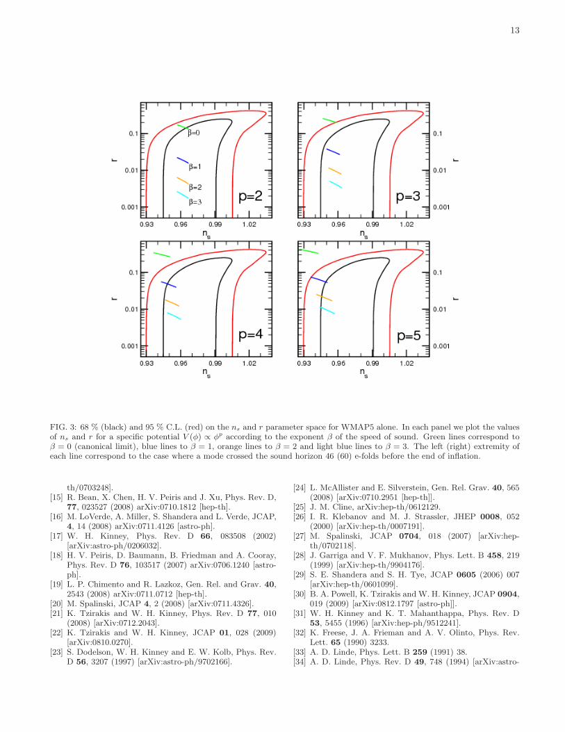
13

FIG. 3: 68 % (black) and 95 % C.L. (red) on the ns and r parameter space for WMAP5 alone. In each panel we plot the valuesof ns and r for a specific potential V (φ) ∝ φp according to the exponent β of the speed of sound. Green lines correspond toβ = 0 (canonical limit), blue lines to β = 1, orange lines to β = 2 and light blue lines to β = 3. The left (right) extremity ofeach line correspond to the case where a mode crossed the sound horizon 46 (60) e-folds before the end of inflation.

th/0703248].[15] R. Bean, X. Chen, H. V. Peiris and J. Xu, Phys. Rev. D,

77, 023527 (2008) arXiv:0710.1812 [hep-th].[16] M. LoVerde, A. Miller, S. Shandera and L. Verde, JCAP,

4, 14 (2008) arXiv:0711.4126 [astro-ph].[17] W. H. Kinney, Phys. Rev. D 66, 083508 (2002)

[arXiv:astro-ph/0206032].[18] H. V. Peiris, D. Baumann, B. Friedman and A. Cooray,

Phys. Rev. D 76, 103517 (2007) arXiv:0706.1240 [astro-ph].

[19] L. P. Chimento and R. Lazkoz, Gen. Rel. and Grav. 40,2543 (2008) arXiv:0711.0712 [hep-th].

[20] M. Spalinski, JCAP 4, 2 (2008) [arXiv:0711.4326].[21] K. Tzirakis and W. H. Kinney, Phys. Rev. D 77, 010

(2008) [arXiv:0712.2043].[22] K. Tzirakis and W. H. Kinney, JCAP 01, 028 (2009)

[arXiv:0810.0270].[23] S. Dodelson, W. H. Kinney and E. W. Kolb, Phys. Rev.

D 56, 3207 (1997) [arXiv:astro-ph/9702166].

[24] L. McAllister and E. Silverstein, Gen. Rel. Grav. 40, 565(2008) [arXiv:0710.2951 [hep-th]].

[25] J. M. Cline, arXiv:hep-th/0612129.[26] I. R. Klebanov and M. J. Strassler, JHEP 0008, 052

(2000) [arXiv:hep-th/0007191].[27] M. Spalinski, JCAP 0704, 018 (2007) [arXiv:hep-

th/0702118].[28] J. Garriga and V. F. Mukhanov, Phys. Lett. B 458, 219

(1999) [arXiv:hep-th/9904176].[29] S. E. Shandera and S. H. Tye, JCAP 0605 (2006) 007

[arXiv:hep-th/0601099].[30] B. A. Powell, K. Tzirakis and W. H. Kinney, JCAP 0904,

019 (2009) [arXiv:0812.1797 [astro-ph]].[31] W. H. Kinney and K. T. Mahanthappa, Phys. Rev. D

53, 5455 (1996) [arXiv:hep-ph/9512241].[32] K. Freese, J. A. Frieman and A. V. Olinto, Phys. Rev.

Lett. 65 (1990) 3233.[33] A. D. Linde, Phys. Lett. B 259 (1991) 38.[34] A. D. Linde, Phys. Rev. D 49, 748 (1994) [arXiv:astro-

14

ph/9307002].