INFLATIONARY COSMOLOGY: PROGRESS AND PROBLEMS …rhb/sample/inflation.pdf · INFLATIONARY COSMOLOGY: PROGRESS AND PROBLEMS ... it is shown how the basic idea of inﬂation can solve

arX

iv:h

ep-p

h/99

1041

0 v1

20

Oct

199

9

INFLATIONARY COSMOLOGY: PROGRESS AND PROBLEMS

ROBERT H. BRANDENBERGER

Physics Department, Brown University

Providence, RI, 02912, USA

Abstract. These lecture notes 1 intend to form a short pedagogical in-troduction to inflationary cosmology, highlighting selected areas of recentprogress such as reheating and the theory of cosmological perturbations.Problems of principle for inflationary cosmology are pointed out, and somenew attempts at solving them are indicated, including a nonsingular Uni-verse construction by means of higher derivative terms in the gravitationalaction, and the study of back-reaction of cosmological perturbations.

1. Introduction

Inflationary cosmology [1] has become one of the cornerstones of moderncosmology. Inflation was the first theory which made predictions aboutthe structure of the Universe on large scales based on causal physics. Thedevelopment of the inflationary Universe scenario has opened up a newand extremely promising avenue for connecting fundamental physics withexperiment.

These lectures form a short pedagogical introduction to inflation, focus-ing more on the basic principles than on detailed particle physics modelbuilding. Section 2 outlines some of the basic problems of standard cos-mology which served as a motivation for the development of inflationarycosmology, especially the apparent impossibility of having a causal theoryof structure formation within the context of standard cosmology.

In Section 3, it is shown how the basic idea of inflation can solve thehorizon and flatness problems, and can lead to a causal theory of structureformation. It is shown that when trying to implement the idea of infla-

1Brown preprint BROWN-HET-1196, invited lectures at the International School onCosmology, Kish Island, Iran, Jan. 22 - Feb. 4 1999, to be publ. in the proceedings(Kluwer, Dordrecht, 2000)

2 ROBERT H. BRANDENBERGER

tion, one is automatically driven to consider the interplay between particlephysics / field theory and cosmology. The section ends with a brief surveyof some models of inflation.

Section 4 reviews two areas in which there has been major progresssince the early days of inflation. The first topic is reheating. It is shownthat parametric resonance effects may play a crucial role in reheating theUniverse at the end of inflation. The second topic is the quantum theoryof the generation and evolution of cosmological perturbations which hasbecome a cornerstone for precision calculations of observable quantities.

In spite of the remarkable success of the inflationary Universe paradigm,there are several serious problems of principle for current models of infla-tion, specifically potential-driven models. These problems are discussed inSection 5.

Section 6 is a summary of some new approaches to solving the problemsof potential-driven inflation. An attempt to obtain inflation from conden-sates is discussed, a nonsingular Universe construction making use of higherderivative terms in the gravitational action is explained, and a frameworkfor calculating the back-reaction of cosmological perturbations is summa-rized.

As indicated before, this review focuses on the principles and problemsof inflationary cosmology. Readers interested in comprehensive reviews ofinflation are referred to [2, 3, 4]. A recent review focusing on inflationarymodel building in the context of supersymmetric models can be found in[5]. For a review at a similar level to this one but with a different bias see[6].

2. Successes and Problems of Standard Cosmology

2.1. FRAMEWORK OF STANDARD COSMOLOGY

The standard big bang cosmology rests on three theoretical pillars: thecosmological principle, Einstein’s general theory of relativity and a classicalperfect fluid description of matter.

The cosmological principle states that on large distance scales the Uni-verse is homogeneous. This implies that the metric of space-time can bewritten in Friedmann-Robertson-Walker (FRW) form:

ds2 = dt2 − a(t)2[

dr2

1 − kr2+ r2(dϑ2 + sin2 ϑdϕ2)

]

, (1)

where the constant k determines the topology of the spatial sections. Inthe following, we shall usually set k = 0, i.e. consider a spatially flat Uni-verse. In this case, we can set the scale factor a(t) to be equal to 1 at the

INFLATIONARY COSMOLOGY 3

present time t0, i.e. a(t0) = 1, without loss of generality. The coordinatesr, ϑ and ϕ are comoving spherical coordinates. World lines with constantcomoving coordinates are geodesics corresponding to particles at rest. Ifthe Universe is expanding, i.e. a(t) is increasing, then the physical distance∆xp(t) between two points at rest with fixed comoving distance ∆xc grows:

∆xp = a(t)∆xc . (2)

The dynamics of an expanding Universe is determined by the Einsteinequations, which relate the expansion rate to the matter content, specif-ically to the energy density ρ and pressure p. For a homogeneous andisotropic Universe and setting the cosmological constant to zero, they re-duce to the Friedmann-Robertston-Walker (FRW) equations

(

a

a

)2

− k

a2=

8πG

3ρ (3)

a

a= −4πG

3(ρ+ 3p) . (4)

These equations can be combined to yield the continuity equation (withHubble constant H = a/a)

ρ = −3H(ρ+ p) . (5)

The third key assumption of standard cosmology is that matter is de-scribed by a classical ideal gas with an equation of state

p = wρ . (6)

For cold matter (dust), pressure is negligible and hence w = 0. From (5) itfollows that

ρm(t) ∼ a−3(t) , (7)

where ρm is the energy density in cold matter. For radiation we have w =1/3 and hence it follows from (5) that

ρr(t) ∼ a−4(t) , (8)

ρr(t) being the energy density in radiation.

2.2. SUCCESSES OF STANDARD COSMOLOGY

The three classic observational pillars of standard cosmology are Hubble’slaw, the existence and black body nature of the nearly isotropic cosmic


microwave background (CMB), and the abundances of light elements (nu-cleosynthesis). These successes are discussed in detail in many textbooks(see e.g. [7, 8, 9] for some recent ones) on cosmology, and also in the lecturesby Blanchard and Sarkar at this school, and will therefore not be reviewedhere.

Let us just recall two important aspects of the thermal history of theearly Universe. Since the energy density in radiation redshifts faster thanthe matter energy density, it follows that although the energy density of theUniverse is now mostly in cold matter, it was initially dominated by radia-tion. The transition occurred at a time denoted by teq, the “time of equalmatter and radiation”. As discussed in the lectures by Padmanabhan at thisschool, teq is the time when perturbations can start to grow by gravitationalclustering. The second important time is trec, the “time of recombination”when photons fell out of equilibrium (since ions and electrons had by thencombined to form electrically neutral atoms). The photons of the CMBhave travelled without scattering from trec to the present. Their spatialdistribution is predicted to be a black body since the cosmological redshiftpreserves the black body nature of the initial spectrum (simply redshiftingthe temperature) which was in turn determined by thermal equilibrium.CMB anisotropies probe the density fluctuations at trec (see the lecturesby Zadellariaga at this school for a detailed analysis). Note that for theusual values of the cosmological parameters, teq < trec.

2.3. PROBLEMS OF STANDARD COSMOLOGY

Standard Big Bang cosmology is faced with several important problems.None represents an actual conflict with observations. The problems I willfocus on here – the homogeneity, flatness and formation of structure prob-lems (see e.g. [1]) – are questions which have no answer within the theoryand are therefore the main motivation for inflationary cosmology.

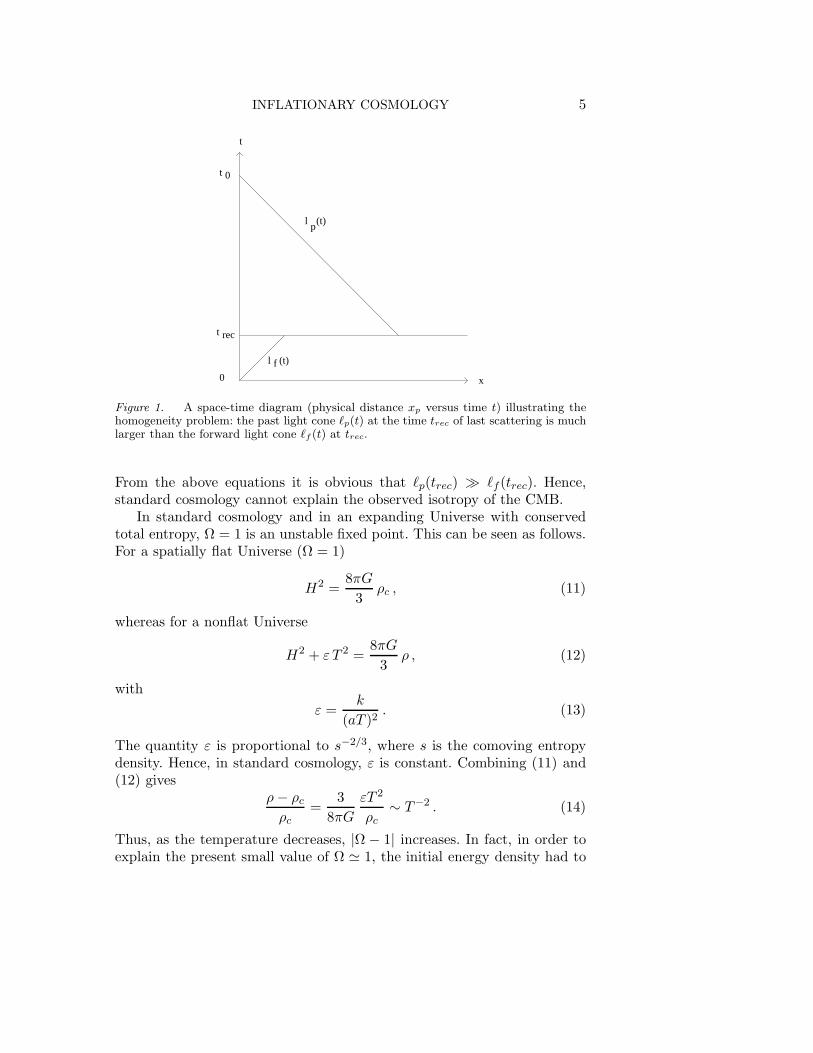
The “horizon problem” is illustrated in Fig. 1. As is sketched, the co-moving region ℓp(trec) over which the CMB is observed to be homogeneousto better than one part in 104 is much larger than the comoving forwardlight cone ℓf (trec) at trec, which is the maximal distance over which micro-physical forces could have caused the homogeneity:

ℓp(trec) =

t0∫

trec

dt a−1(t) ≃ 3 t0

(

1 −(

trec

t0

)1/3)

(9)

ℓf (trec) =

trec∫

0

dt a−1(t) ≃ 3 t2/30 t1/3

rec . (10)


t

x

t 0

t rec

0

l p

l f

(t)

(t)

Figure 1. A space-time diagram (physical distance xp versus time t) illustrating thehomogeneity problem: the past light cone ℓp(t) at the time trec of last scattering is muchlarger than the forward light cone ℓf (t) at trec.

From the above equations it is obvious that ℓp(trec) ≫ ℓf (trec). Hence,standard cosmology cannot explain the observed isotropy of the CMB.

In standard cosmology and in an expanding Universe with conservedtotal entropy, Ω = 1 is an unstable fixed point. This can be seen as follows.For a spatially flat Universe (Ω = 1)

H2 =8πG

3ρc , (11)

whereas for a nonflat Universe

H2 + ε T 2 =8πG

3ρ , (12)

with

ε =k

(aT )2. (13)

The quantity ε is proportional to s−2/3, where s is the comoving entropydensity. Hence, in standard cosmology, ε is constant. Combining (11) and(12) gives

ρ− ρc

ρc=

3

8πG

εT 2

ρc∼ T−2 . (14)

Thus, as the temperature decreases, |Ω − 1| increases. In fact, in order toexplain the present small value of Ω ≃ 1, the initial energy density had to


t

xcdc

t0

t eq

0

H-1 (t)

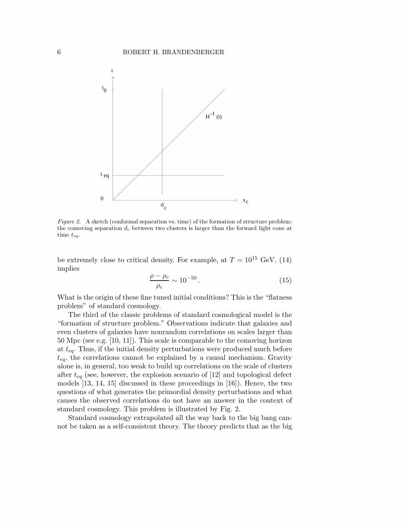
Figure 2. A sketch (conformal separation vs. time) of the formation of structure problem:the comoving separation dc between two clusters is larger than the forward light cone attime teq.

be extremely close to critical density. For example, at T = 1015 GeV, (14)implies

ρ− ρc

ρc∼ 10−50 . (15)

What is the origin of these fine tuned initial conditions? This is the “flatnessproblem” of standard cosmology.

The third of the classic problems of standard cosmological model is the“formation of structure problem.” Observations indicate that galaxies andeven clusters of galaxies have nonrandom correlations on scales larger than50 Mpc (see e.g. [10, 11]). This scale is comparable to the comoving horizonat teq. Thus, if the initial density perturbations were produced much beforeteq, the correlations cannot be explained by a causal mechanism. Gravityalone is, in general, too weak to build up correlations on the scale of clustersafter teq (see, however, the explosion scenario of [12] and topological defectmodels [13, 14, 15] discussed in these proceedings in [16]). Hence, the twoquestions of what generates the primordial density perturbations and whatcauses the observed correlations do not have an answer in the context ofstandard cosmology. This problem is illustrated by Fig. 2.

Standard cosmology extrapolated all the way back to the big bang can-not be taken as a self-consistent theory. The theory predicts that as the big


0 t i t R

a(t) ~ t1/2 a(t) = e tH a(t) ~ t1/2

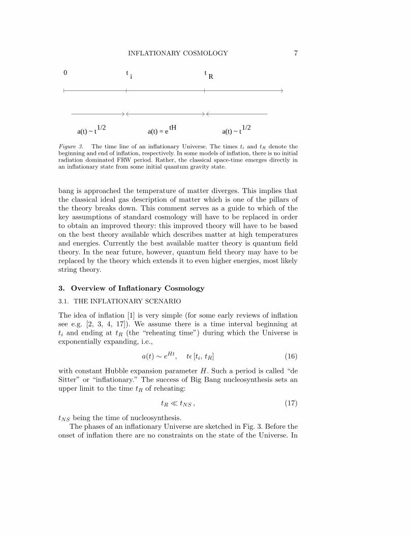
Figure 3. The time line of an inflationary Universe. The times ti and tR denote thebeginning and end of inflation, respectively. In some models of inflation, there is no initialradiation dominated FRW period. Rather, the classical space-time emerges directly inan inflationary state from some initial quantum gravity state.

bang is approached the temperature of matter diverges. This implies thatthe classical ideal gas description of matter which is one of the pillars ofthe theory breaks down. This comment serves as a guide to which of thekey assumptions of standard cosmology will have to be replaced in orderto obtain an improved theory: this improved theory will have to be basedon the best theory available which describes matter at high temperaturesand energies. Currently the best available matter theory is quantum fieldtheory. In the near future, however, quantum field theory may have to bereplaced by the theory which extends it to even higher energies, most likelystring theory.

3. Overview of Inflationary Cosmology

3.1. THE INFLATIONARY SCENARIO

The idea of inflation [1] is very simple (for some early reviews of inflationsee e.g. [2, 3, 4, 17]). We assume there is a time interval beginning atti and ending at tR (the “reheating time”) during which the Universe isexponentially expanding, i.e.,

a(t) ∼ eHt, tǫ [ti, tR] (16)

with constant Hubble expansion parameter H. Such a period is called “deSitter” or “inflationary.” The success of Big Bang nucleosynthesis sets anupper limit to the time tR of reheating:

tR ≪ tNS , (17)

tNS being the time of nucleosynthesis.The phases of an inflationary Universe are sketched in Fig. 3. Before the

onset of inflation there are no constraints on the state of the Universe. In


t

xp

t0

trec

t R

ti

a(t) = e tH

l p(t)

l f (t)

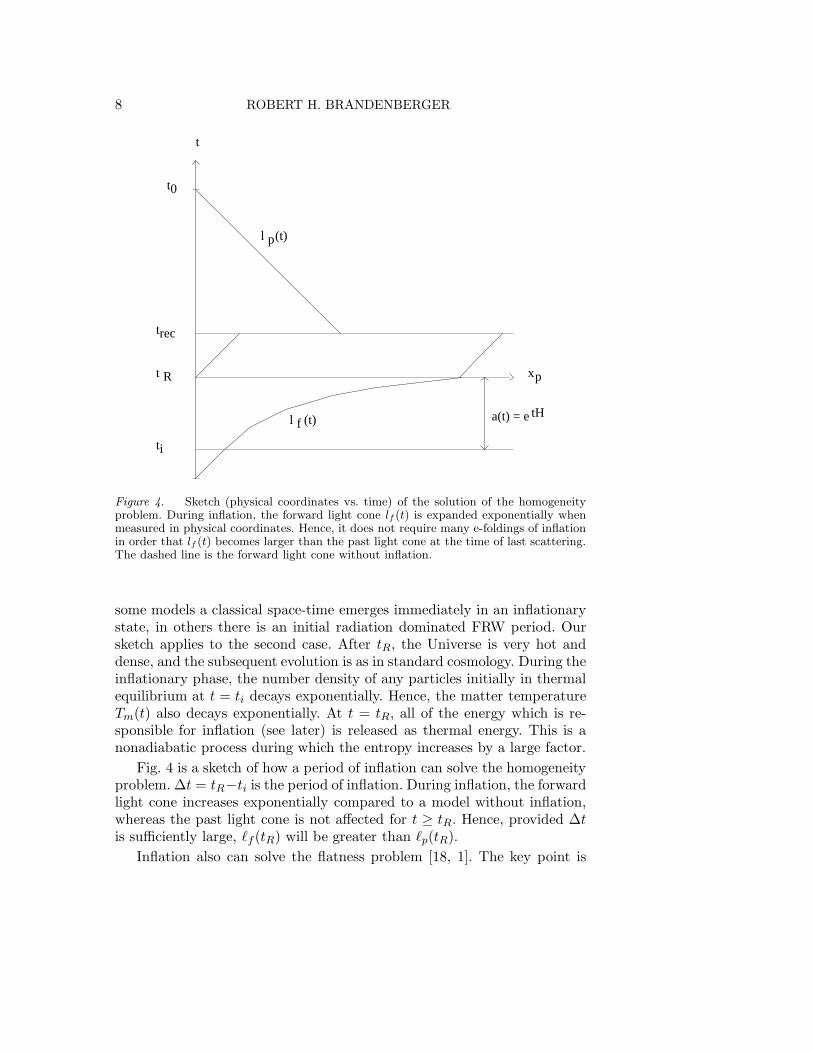
Figure 4. Sketch (physical coordinates vs. time) of the solution of the homogeneityproblem. During inflation, the forward light cone lf (t) is expanded exponentially whenmeasured in physical coordinates. Hence, it does not require many e-foldings of inflationin order that lf (t) becomes larger than the past light cone at the time of last scattering.The dashed line is the forward light cone without inflation.

some models a classical space-time emerges immediately in an inflationarystate, in others there is an initial radiation dominated FRW period. Oursketch applies to the second case. After tR, the Universe is very hot anddense, and the subsequent evolution is as in standard cosmology. During theinflationary phase, the number density of any particles initially in thermalequilibrium at t = ti decays exponentially. Hence, the matter temperatureTm(t) also decays exponentially. At t = tR, all of the energy which is re-sponsible for inflation (see later) is released as thermal energy. This is anonadiabatic process during which the entropy increases by a large factor.

Fig. 4 is a sketch of how a period of inflation can solve the homogeneityproblem. ∆t = tR−ti is the period of inflation. During inflation, the forwardlight cone increases exponentially compared to a model without inflation,whereas the past light cone is not affected for t ≥ tR. Hence, provided ∆tis sufficiently large, ℓf (tR) will be greater than ℓp(tR).

Inflation also can solve the flatness problem [18, 1]. The key point is


that the entropy density s is no longer constant. As will be explained later,the temperatures at ti and tR are essentially equal. Hence, the entropyincreases during inflation by a factor exp(3H∆t). Thus, ǫ decreases by afactor of exp(−2H∆t). Hence, ρ and ρc can be of comparable magnitude atboth ti and the present time. In fact, if inflation occurs at all, then rathergenerically, the theory predicts that at the present time Ω = 1 to a highaccuracy (now Ω < 1 requires special initial conditions or rather specialmodels [19]).

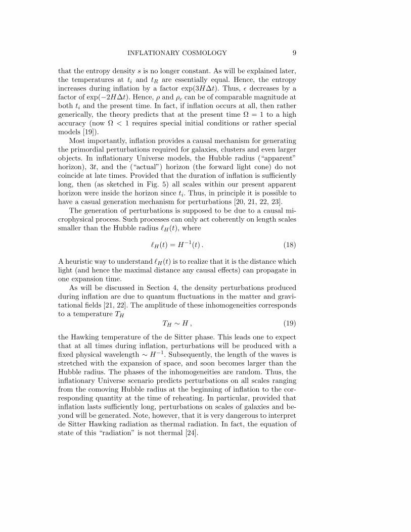
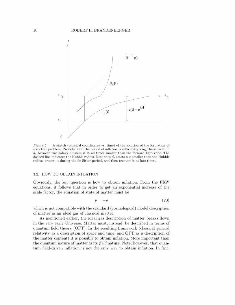
Most importantly, inflation provides a causal mechanism for generatingthe primordial perturbations required for galaxies, clusters and even largerobjects. In inflationary Universe models, the Hubble radius (“apparent”horizon), 3t, and the (“actual”) horizon (the forward light cone) do notcoincide at late times. Provided that the duration of inflation is sufficientlylong, then (as sketched in Fig. 5) all scales within our present apparenthorizon were inside the horizon since ti. Thus, in principle it is possible tohave a casual generation mechanism for perturbations [20, 21, 22, 23].

The generation of perturbations is supposed to be due to a causal mi-crophysical process. Such processes can only act coherently on length scalessmaller than the Hubble radius ℓH(t), where

ℓH(t) = H−1(t) . (18)

A heuristic way to understand ℓH(t) is to realize that it is the distance whichlight (and hence the maximal distance any causal effects) can propagate inone expansion time.

As will be discussed in Section 4, the density perturbations producedduring inflation are due to quantum fluctuations in the matter and gravi-tational fields [21, 22]. The amplitude of these inhomogeneities correspondsto a temperature TH

TH ∼ H , (19)

the Hawking temperature of the de Sitter phase. This leads one to expectthat at all times during inflation, perturbations will be produced with afixed physical wavelength ∼ H−1. Subsequently, the length of the waves isstretched with the expansion of space, and soon becomes larger than theHubble radius. The phases of the inhomogeneities are random. Thus, theinflationary Universe scenario predicts perturbations on all scales rangingfrom the comoving Hubble radius at the beginning of inflation to the cor-responding quantity at the time of reheating. In particular, provided thatinflation lasts sufficiently long, perturbations on scales of galaxies and be-yond will be generated. Note, however, that it is very dangerous to interpretde Sitter Hawking radiation as thermal radiation. In fact, the equation ofstate of this “radiation” is not thermal [24].


a(t) = e tHl f (t)

H -1 (t)

dc(t)

t

xpt R

t i

0

Figure 5. A sketch (physical coordinates vs. time) of the solution of the formation ofstructure problem. Provided that the period of inflation is sufficiently long, the separationdc between two galaxy clusters is at all times smaller than the forward light cone. Thedashed line indicates the Hubble radius. Note that dc starts out smaller than the Hubbleradius, crosses it during the de Sitter period, and then reenters it at late times.

3.2. HOW TO OBTAIN INFLATION

Obviously, the key question is how to obtain inflation. From the FRWequations, it follows that in order to get an exponential increase of thescale factor, the equation of state of matter must be

p = −ρ (20)

which is not compatible with the standard (cosmological) model descriptionof matter as an ideal gas of classical matter.

As mentioned earlier, the ideal gas description of matter breaks downin the very early Universe. Matter must, instead, be described in terms ofquantum field theory (QFT). In the resulting framework (classical generalrelativity as a description of space and time, and QFT as a description ofthe matter content) it is possible to obtain inflation. More important thanthe quantum nature of matter is its field nature. Note, however, that quan-tum field-driven inflation is not the only way to obtain inflation. In fact,


before the seminal paper by Guth [1], Starobinsky [43] proposed a modelwith exponential expansion of the scale factor based on higher derivativecurvature terms in the gravitational action.

Current quantum field theories of matter contain three types of fields:spin 1/2 fermions (the matter fields) ψ, spin 1 bosons Aµ (the gauge bosons)and spin 0 bosons, the scalar fields ϕ (the Higgs fields used to spontaneouslybreak internal gauge symmetries). The Lagrangian of the field theory isconstrained by gauge invariance, minimal coupling and renormalizability.The Lagrangian of the bosonic sector of the theory is thus constrained tohave the form

Lm(ϕ,Aµ) =1

2DµϕD

µϕ− V (ϕ) +1

4FµνF

µν , (21)

where in Minkowski space-time Dµ = ∂µ−igAµ denotes the (gauge) covari-ant derivative, g being the gauge coupling constant, Fµν is the field strengthtensor, and V (ϕ) is the Higgs potential. Renormalizability plus assumingsymmetry under ϕ→ −ϕ constrains V (ϕ) to have the form

V (ϕ) =1

2m2ϕ2 +

1

4λϕ4 , (22)

where m is the mass of the excitations of ϕ about ϕ = 0, and λ is a self-coupling constant. For spontaneous symmetry breaking, m2 < 0 is required.

Given the Lagrangian (21), the action for matter is

Sm =

∫

d4x√−gLm , (23)

where g here denotes the determinant of the metric tensor, and now thecovariant derivative Dµ in (21) is a gauge and metric covariant derivative.The energy-momentum tensor is obtained by varying this action with re-spect to the metric. The contributions of the scalar fields to the energydensity ρ and pressure p are

ρ(ϕ) =1

2ϕ2 +

1

2a−2(∇ϕ)2 + V (ϕ) (24)

p(ϕ) =1

2ϕ2 − 1

6a−2(∇ϕ)2 − V (ϕ) . (25)

It thus follows that if the scalar field is homogeneous and static, but thepotential energy positive, then the equation of state p = −ρ necessaryfor exponential inflation results. This is the idea behind potential-driveninflation.

Note that given the restrictions imposed by minimal coupling, gaugeinvariance and renormalizability, scalar fields with nonvanishing potentials


are required in order to obtain inflation. Mass terms for fermionic andgauge fields are not compatible with gauge invariance, and renormalizabilityforbids nontrivial potentials for fermionic fields. The initial hope of theinflationary Universe scenario [1] was that the Higgs field required for gaugesymmetry breaking in “grand unified” (GUT) models would serve the roleof the inflaton, the field generating inflation. As will be seen in the followingsubsection, this hope cannot be realized.

Most of the current realizations of potential-driven inflation are basedon satisfying the conditions

ϕ2, a−2(∇ϕ)2 ≪ V (ϕ) , (26)

via the idea of slow rolling [31, 32]. Consider the equation of motion of thescalar field ϕ which can be obtained by varying the action Sm with respectto ϕ:

ϕ+ 3Hϕ− a−2 2 ϕ = −V ′(ϕ) . (27)

If the scalar field starts out almost homogeneous and at rest, if the Hubbledamping term (the second term on the l.h.s. of (27) is large), and if thepotential is quite flat (so that the term on the r.h.s. of (27) is small), thenϕ2 may remain small compared to V (ϕ), in which case the slow rollingconditions (26) are satisfied and exponential inflation will result. If thespatial gradient terms are initially negligible, they will remain negligiblesince they redshift.

To illustrate the slow-roll inflationary scenario, consider the simplestmodel, a toy model with quadratic potential

V (ϕ) =1

2m2ϕ2 . (28)

Consider initial conditions for which ϕ≫ mpl and ϕ = 0. At the beginningof the evolution, ϕ will be rolling slowly and one finds approximate solutionsby neglecting the ϕ term (the self-consistency of this approximation needsto be checked in every model independently!). In this simple model, thesystem of approximate equations

3Hϕ = −V ′(ϕ) (29)

and

H2 =8π

3GV (ϕ) (30)

can be solved exactly, yielding

ϕ = − 1√12π

mmpl . (31)


t

T(t)(t)

t i t R t i t R

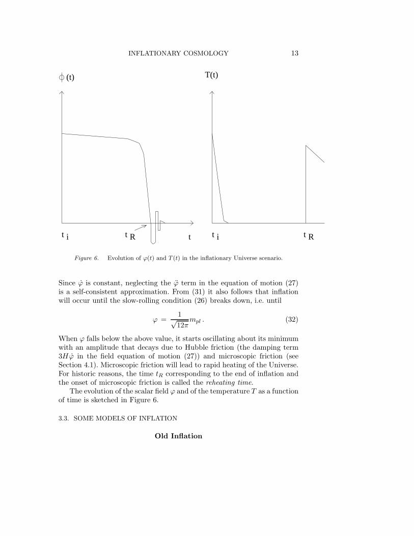
Figure 6. Evolution of ϕ(t) and T (t) in the inflationary Universe scenario.

Since ϕ is constant, neglecting the ϕ term in the equation of motion (27)is a self-consistent approximation. From (31) it also follows that inflationwill occur until the slow-rolling condition (26) breaks down, i.e. until

ϕ =1√12π

mpl . (32)

When ϕ falls below the above value, it starts oscillating about its minimumwith an amplitude that decays due to Hubble friction (the damping term3Hϕ in the field equation of motion (27)) and microscopic friction (seeSection 4.1). Microscopic friction will lead to rapid heating of the Universe.For historic reasons, the time tR corresponding to the end of inflation andthe onset of microscopic friction is called the reheating time.

The evolution of the scalar field ϕ and of the temperature T as a functionof time is sketched in Figure 6.

3.3. SOME MODELS OF INFLATION

Old Inflation


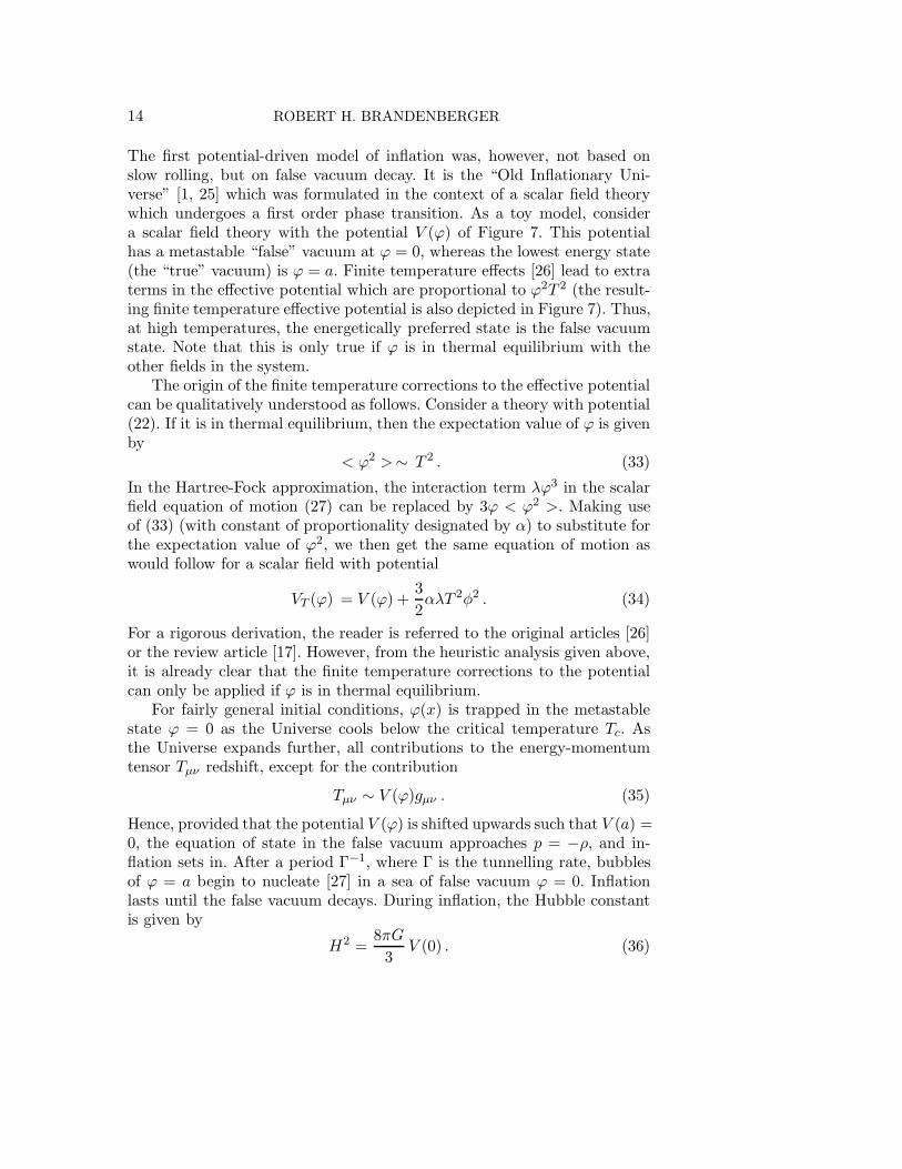
The first potential-driven model of inflation was, however, not based onslow rolling, but on false vacuum decay. It is the “Old Inflationary Uni-verse” [1, 25] which was formulated in the context of a scalar field theorywhich undergoes a first order phase transition. As a toy model, considera scalar field theory with the potential V (ϕ) of Figure 7. This potentialhas a metastable “false” vacuum at ϕ = 0, whereas the lowest energy state(the “true” vacuum) is ϕ = a. Finite temperature effects [26] lead to extraterms in the effective potential which are proportional to ϕ2T 2 (the result-ing finite temperature effective potential is also depicted in Figure 7). Thus,at high temperatures, the energetically preferred state is the false vacuumstate. Note that this is only true if ϕ is in thermal equilibrium with theother fields in the system.

The origin of the finite temperature corrections to the effective potentialcan be qualitatively understood as follows. Consider a theory with potential(22). If it is in thermal equilibrium, then the expectation value of ϕ is givenby

< ϕ2 >∼ T 2 . (33)

In the Hartree-Fock approximation, the interaction term λϕ3 in the scalarfield equation of motion (27) can be replaced by 3ϕ < ϕ2 >. Making useof (33) (with constant of proportionality designated by α) to substitute forthe expectation value of ϕ2, we then get the same equation of motion aswould follow for a scalar field with potential

VT (ϕ) = V (ϕ) +3

2αλT 2φ2 . (34)

For a rigorous derivation, the reader is referred to the original articles [26]or the review article [17]. However, from the heuristic analysis given above,it is already clear that the finite temperature corrections to the potentialcan only be applied if ϕ is in thermal equilibrium.

For fairly general initial conditions, ϕ(x) is trapped in the metastablestate ϕ = 0 as the Universe cools below the critical temperature Tc. Asthe Universe expands further, all contributions to the energy-momentumtensor Tµν redshift, except for the contribution

Tµν ∼ V (ϕ)gµν . (35)

Hence, provided that the potential V (ϕ) is shifted upwards such that V (a) =0, the equation of state in the false vacuum approaches p = −ρ, and in-flation sets in. After a period Γ−1, where Γ is the tunnelling rate, bubblesof ϕ = a begin to nucleate [27] in a sea of false vacuum ϕ = 0. Inflationlasts until the false vacuum decays. During inflation, the Hubble constantis given by

H2 =8πG

3V (0) . (36)


TV (O )

T >> T c

T = Tc

T << Tc

O

Figure 7. The finite temperature effective potential in a theory with a first order phasetransition.

The condition V (a) = 0, which looks rather unnatural, is required to avoid alarge cosmological constant today (none of the present inflationary Universemodels manage to circumvent or solve the cosmological constant problem).

It was immediately realized that old inflation has a serious “gracefulexit” problem [1, 28]. The bubbles nucleate after inflation with radiusr ≪ 2tR. Even if the bubble walls expand with the speed of light, the bub-bles would at the present time be much smaller than our apparent horizon.Thus, unless bubbles percolate, the model predicts extremely large inho-mogeneities inside the Hubble radius, in contradiction with the observedisotropy of the microwave background radiation.

For bubbles to percolate, a sufficiently large number must be producedso that they collide and homogenize over a scale larger than the presentHubble radius. However, because of the exponential expansion of the re-gions still in the false vacuum phase, the volume between bubbles expandsexponentially whereas the volume inside bubbles expands only with a lowpower. This prevents percolation. One way to overcome this problem is byrealizing old inflation in the context of Brans-Dicke gravity [29, 30].

New Inflation

Because of the graceful exit problem, old inflation never was consideredto be a viable cosmological model. However, soon after the seminal paperby Guth, Linde [31] and Albrecht and Steinhardt [32] independently putforwards a modified scenario, the “New Inflationary Universe”.

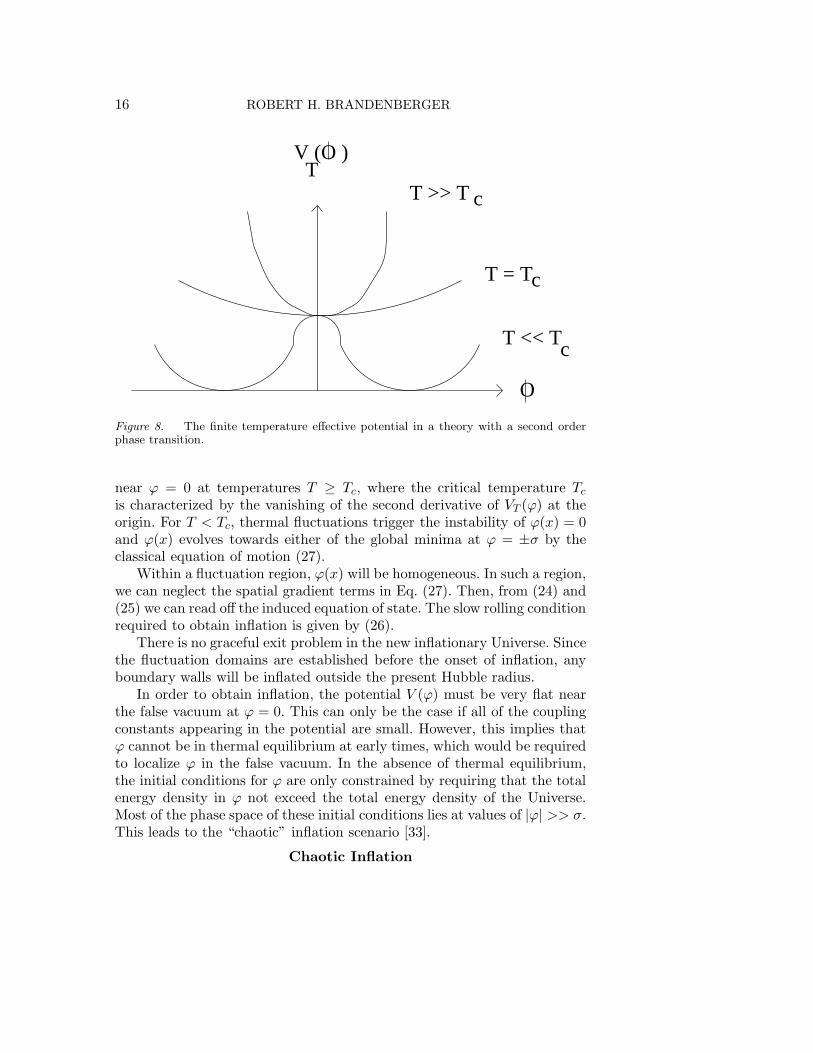
The starting point is a scalar field theory with a double well potentialwhich undergoes a second order phase transition (Fig. 8). V (ϕ) is symmetricand ϕ = 0 is a local maximum of the zero temperature potential. Onceagain, it was argued that finite temperature effects confine ϕ(x) to values


TV (O )

T >> T c

T = Tc

T << Tc

O

Figure 8. The finite temperature effective potential in a theory with a second orderphase transition.

near ϕ = 0 at temperatures T ≥ Tc, where the critical temperature Tc

is characterized by the vanishing of the second derivative of VT (ϕ) at theorigin. For T < Tc, thermal fluctuations trigger the instability of ϕ(x) = 0and ϕ(x) evolves towards either of the global minima at ϕ = ±σ by theclassical equation of motion (27).

Within a fluctuation region, ϕ(x) will be homogeneous. In such a region,we can neglect the spatial gradient terms in Eq. (27). Then, from (24) and(25) we can read off the induced equation of state. The slow rolling conditionrequired to obtain inflation is given by (26).

There is no graceful exit problem in the new inflationary Universe. Sincethe fluctuation domains are established before the onset of inflation, anyboundary walls will be inflated outside the present Hubble radius.

In order to obtain inflation, the potential V (ϕ) must be very flat nearthe false vacuum at ϕ = 0. This can only be the case if all of the couplingconstants appearing in the potential are small. However, this implies thatϕ cannot be in thermal equilibrium at early times, which would be requiredto localize ϕ in the false vacuum. In the absence of thermal equilibrium,the initial conditions for ϕ are only constrained by requiring that the totalenergy density in ϕ not exceed the total energy density of the Universe.Most of the phase space of these initial conditions lies at values of |ϕ| >> σ.This leads to the “chaotic” inflation scenario [33].

Chaotic Inflation


Consider a region in space where at the initial time ϕ(x) is very large,homogeneous and static. In this case, the energy-momentum tensor will beimmediately dominated by the large potential energy term and induce anequation of state p ≃ −ρ which leads to inflation. Due to the large Hubbledamping term in the scalar field equation of motion, ϕ(x) will only roll veryslowly towards ϕ = 0. The kinetic energy contribution to Tµν will remainsmall, the spatial gradient contribution will be exponentially suppresseddue to the expansion of the Universe, and thus inflation persists. Note thatin contrast to old and new inflation, no initial thermal bath is required.Note also that the precise form of V (ϕ) is irrelevant to the mechanism. Inparticular, V (ϕ) need not be a double well potential. This is a significantadvantage, since for scalar fields other than GUT Higgs fields used forspontaneous symmetry breaking, there is no particle physics motivation forassuming a double well potential, and the inflaton (the field which givesrise to inflation) cannot be a conventional Higgs field, due to the severe finetuning constraints.

The field and temperature evolution in a chaotic inflation model is sim-ilar to what is depicted in Figure 8, except that ϕ is rolling towards thetrue vacuum at ϕ = σ from the direction of large field values.

Chaotic inflation is a much more radical departure from standard cos-mology than old and new inflation. In the latter, the inflationary phasecan be viewed as a short phase of exponential expansion bounded at bothends by phases of radiation domination. In chaotic inflation, a piece of theUniverse emerges with an inflationary equation of state immediately afterthe quantum gravity (or string) epoch.

The chaotic inflationary Universe scenario has been developed in greatdetail (see e.g. [34] for a recent review). One important addition is the in-clusion of stochastic noise [35] in the equation of motion for ϕ in order toaccount for the effects of quantum fluctuations. In fact, it can be shownthat for sufficiently large values of |ϕ|, the stochastic force terms are moreimportant than the classical relaxation force V ′(ϕ). There is thus equalprobability for the quantum fluctuations to lead to an increase or decreaseof |ϕ|. Hence, in a substantial fraction of the comoving volume, the field ϕclimbs up the potential. This leads to the conclusion that chaotic inflationis eternal. At all times, a large fraction of the physical space will be in-flating. Another consequence of including stochastic terms is that on largescales (much larger than the present Hubble radius), the Universe will lookextremely inhomogeneous.

It is difficult to realize chaotic inflation in conventional supergravitymodels since gravitational corrections to the potential of scalar fields typ-ically render the potential steep for values of |ϕ| of the order of mpl andlarger. This prevents the slow rolling condition (26) from being realized.


Even if this condition can be met, there are constraints from the amplitudeof produced density fluctuations which are much harder to satisfy (see Sec-tion 5). Note that it is not impossible to obtain single field potential-driveninflation in supergravity models. For examples which show that is possiblesee e.g. [36, 37].

Hybrid Inflation

Hybrid inflation [38] is a solution to the above-mentioned problem ofchaotic inflation. Hybrid inflation requires at least two scalar fields to playan important role in the dynamics of the Universe. As a toy model, considerthe potential of a theory with two scalar fields ϕ and ψ:

V (ϕ,ψ) =1

4λ(M2 − ψ2)2 +

1

2m2ϕ2 +

1

2λ

′

ψ2ϕ2 . (37)

For values of |ϕ| larger than ϕc

ϕc = (λ

λ′M2)1/2 (38)

the minimum of ψ is ψ = 0, whereas for smaller values of ϕ the symmetryψ → −ψ is broken and the ground state value of |ψ| tends to M . The ideaof hybrid inflation is that ϕ is slowly rolling, like the inflaton field in chaoticinflation, but that the energy density of the Universe is dominated by ψ,i.e. by the contribution

V0 =1

4λM4 (39)

to the potential. Inflation terminates once |ϕ| drops below the critical valueϕc, at which point ψ starts to move (and is not required to move slowly).

Note that in hybrid inflation ϕc can be much smaller than mpl and henceinflation without super-Planck scale values of the fields is possible. It is pos-sible to implement hybrid inflation in the context of supergravity (see e.g.[39]. For a detailed discussion of inflation in the context of supersymmetricand supergravity models, the reader is referred to [5].

Comments

At the present time there are many realizations of potential-driven in-flation, but there is no canonical theory. A lot of attention is being devotedto implementing inflation in the context of unified theories, the prime can-didate being superstring theory or M-theory. String theory or M-theorylive in 10 or 11 space-time dimensions, respectively. When compactified to4 space-time dimensions, there exist many moduli fields, scalar fields whichdescribe flat directions in the complicated vacuum manifold of the theory.


A lot of attention is now devoted to attempts at implementing inflationusing moduli fields (see e.g. [40] and references therein).

Recently, it has been suggested that our space-time is a brane in ahigher-dimensional space-time (see [41] for the basic construction). Waysof obtaining inflation on the brane are also under active investigation (seee.g. [42]).

It should also not be forgotten that inflation can arise from the purelygravitational sector of the theory, as in the original model of Starobinsky[43] (see also Section 5), or that it may arise from kinetic terms in aneffective action as in pre-big-bang cosmology [44] or in k-inflation [45].

3.4. FIRST PREDICTIONS OF INFLATION

Theories with (almost) exponential inflation generically predict an (al-most) scale-invariant spectrum of density fluctuations, as was first realizedin [20, 21, 22, 23] and then studied more quantitatively in [46, 47, 48].Via the Sachs-Wolfe effect [49], these density perturbations induce CMBanisotropies with a spectrum which is also scale-invariant on large angularscales.

The heuristic picture is as follows (see Fig. 5). If the inflationary periodwhich lasts from ti to tR is almost exponential, then the physical effectswhich are independent of the small deviations from exponential expan-sion are time-translation-invariant. This implies, for example, that quan-tum fluctuations at all times have the same strength when measured on thesame physical length scale.

If the inhomogeneities are small, they can described by linear theory,which implies that all Fourier modes k evolve independently. The exponen-tial expansion inflates the wavelength of any perturbation. Thus, the wave-length of perturbations generated early in the inflationary phase on lengthscales smaller than the Hubble radius soon becomes equal to (“exits”) theHubble radius (this happens at the time ti(k)) and continues to increaseexponentially. After inflation, the Hubble radius increases as t while thephysical wavelength of a fluctuation increases only as a(t). Thus, eventu-ally the wavelength will cross the Hubble radius again (it will “enter” theHubble radius) at time tf (k). Thus, it is possible for inflation to generatefluctuations on cosmological scales by causal physics.

Any physical process which obeys the symmetry of the inflationaryphase and which generates perturbations will generate fluctuations of equalstrength when measured when they cross the Hubble radius:

δM

M(k, ti(k)) = const (40)


(independent of k). Here, δM (k, t) denotes the r.m.s. mass fluctuation ona length scale k−1 at time t.

It is generally assumed that causal physics cannot affect the amplitudeof fluctuations on super-Hubble scales (see, however, the comments at theend of Section 4.1). Therefore, the magnitude of δM

M can change only by afactor independent of k, and hence it follows that

δM

M(k, tf (k)) = const , (41)

which is the definition of a scale-invariant spectrum [50]. In terms of quan-tities usually used by astronomers, (41) corresponds to a power spectrum

P (k) ∼ k . (42)

Analyses from galaxy redshift surveys (see e.g. [51, 52]) give a powerspectrum of density fluctuations which is consistent with a scale-invariantprimordial spectrum as given by (41). The COBE observations of CMBanisotropies [53] are also in good agreement with the scale-invariant pre-dictions from exponential inflation models, and in fact already give somebounds on possible deviations from scale-invariance. This agreement be-tween the inflationary paradigm and observations is without doubt a ma-jor success of inflationary cosmology. However, it is worth pointing out (see[13, 14, 15] for recent reviews) that topological defect models also generi-cally predict a scale-invariant spectrum of density fluctuations and CMBanisotropies. Luckily, the predictions of defect models and of inflationarytheories differ in important ways: the small-scale CMB anisotropies arevery different (see e.g. the lectures by Mageuijo in these proceedings [16]),and the relative normalization of density and CMB fluctuations also differs.Observations will in the near future be able to discriminate between thepredictions of inflationary cosmology and those of defect models.

4. Progress in Inflationary Cosmology

4.1. PARAMETRIC RESONANCE AND REHEATING

Reheating is an important stage in inflationary cosmology. It determines thestate of the Universe after inflation and has consequences for baryogenesis,defect formation and other aspects of cosmology.

After slow rolling, the inflaton field begins to oscillate uniformly in spaceabout the true vacuum state. Quantum mechanically, this corresponds to acoherent state of k = 0 inflaton particles. Due to interactions of the inflatonwith itself and with other fields, the coherent state will decay into quantaof elementary particles. This corresponds to post-inflationary particle pro-duction.


Reheating is usually studied using simple scalar field toy models. Theone we will adopt here consists of two real scalar fields, the inflaton ϕ withLagrangian

Lo =1

2∂µϕ∂

µϕ− 1

4λ(ϕ2 − σ2)2 (43)

interacting with a massless scalar field χ representing ordinary matter. Theinteraction Lagrangian is taken to be

LI =1

2g2ϕ2χ2 . (44)

Self interactions of χ are neglected.By a change of variables

ϕ = ϕ+ σ , (45)

the interaction Lagrangian can be written as

LI = g2σϕχ2 +1

2g2ϕ2χ2 . (46)

During the phase of coherent oscillations, the field ϕ oscillates with a fre-quency

ω = mϕ = λ1/2σ , (47)

neglecting the expansion of the Universe, although this can be taken intoaccount [54, 55]).

In the elementary theory of reheating (see e.g. [56] and [57]), the decayof the inflaton is calculated using first order perturbation theory. Accordingto the Feynman rules, the decay rate ΓB of ϕ (calculated assuming thatthe cubic coupling term dominates) is given by

ΓB =g2σ2

8πmφ. (48)

The decay leads to a decrease in the amplitude of ϕ (from now on we willdrop the tilde sign) which can be approximated by adding an extra dampingterm to the equation of motion for ϕ:

ϕ+ 3Hϕ+ ΓBϕ = −V ′(ϕ) . (49)

From the above equation it follows that as long as H > ΓB , particle produc-tion is negligible. During the phase of coherent oscillation of ϕ, the energydensity and hence H are decreasing. Thus, eventually H = ΓB, and at thatpoint reheating occurs (the remaining energy density in ϕ is very quicklytransferred to χ particles.


The temperature TR at the completion of reheating can be estimatedby computing the temperature of radiation corresponding to the value ofH at which H = ΓB. From the FRW equations it follows that

TR ∼ (ΓBmpl)1/2 . (50)

If we now use the “naturalness” constraint2

g2 ∼ λ (51)

in conjunction with the constraint on the value of λ from (85), it followsthat for σ < mpl,

TR < 1010GeV . (52)

This would imply no GUT baryogenesis, no GUT-scale defect production,and no gravitino problems in supersymmetric models with m3/2 > TR,where m3/2 is the gravitino mass. As we shall see, these conclusions changeradically if we adopt an improved analysis of reheating.

As was first realized in [58], the above analysis misses an essential point.To see this, we focus on the equation of motion for the matter field χ coupledto the inflaton ϕ via the interaction Lagrangian LI of (46). Considering onlythe cubic interaction term, the equation of motion becomes

χ+ 3Hχ− ((∇a

)2 −m2χ − 2g2σϕ)χ = 0 . (53)

Since the equation is linear in χ, the equations for the Fourier modes χk

decouple:χk + 3Hχk + (k2

p +m2χ + 2g2σϕ)χk = 0, (54)

where kp = k/a is the time-dependent physical wavenumber.Let us for the moment neglect the expansion of the Universe. In this

case, the friction term in (54) drops out and kp is time-independent, andEquation (54) becomes a harmonic oscillator equation with a time-dependentmass determined by the dynamics of ϕ. In the reheating phase, ϕ is un-dergoing oscillations. Thus, the mass in (54) is varying periodically. In themathematics literature, this equation is called the Mathieu equation. It iswell known that there is an instability. In physics, the effect is known asparametric resonance (see e.g. [59]). At frequencies ωn corresponding tohalf integer multiples of the frequency ω of the variation of the mass, i.e.

ω2k = k2

p +m2χ = (

n

2ω)2 n = 1, 2, ..., (55)

2At one loop order, the cubic interaction term will contribute to λ by an amount∆λ ∼ g2. A renormalized value of λ smaller than g2 needs to be finely tuned at eachorder in perturbation theory, which is “unnatural”.


there are instability bands with widths ∆ωn. For values of ωk within theinstability band, the value of χk increases exponentially:

χk ∼ eµt with µ ∼ g2σϕ0

ω, (56)

with ϕ0 being the amplitude of the oscillation of ϕ. Since the widths of theinstability bands decrease as a power of the (small) coupling constant g2

with increasing n, for practical purposes only the lowest instability band isimportant. Its width is

∆ωk ∼ gσ1/2ϕ1/20 . (57)

Note, in particular, that there is no ultraviolet divergence in computing thetotal energy transfer from the ϕ to the χ field due to parametric resonance.

It is easy to include the effects of the expansion of the Universe (seee.g. [58, 54, 55]). The main effect is that the value of ωk can become time-dependent. Thus, a mode may enter and leave the resonance bands. Inthis case, any mode will lie in a resonance band for only a finite time.This can reduce the efficiency of parametric resonance, but the amountof reduction is quite dependent on the specific model. This behavior of themodes, however, also has positive aspects: it implies [58] that the calculationof energy transfer is perfectly well-behaved and no infinite time divergencesarise.

It is now possible to estimate the rate of energy transfer, whose orderof magnitude is given by the phase space volume of the lowest instabilityband multiplied by the rate of growth of the mode function χk. Using asan initial condition for χk the value χk ∼ H given by the magnitude of theexpected quantum fluctuations, we obtain

ρ ∼ µ(ω

2)2∆ωkHe

µt . (58)

From (58) it follows that provided that the condition

µ∆t >> 1 (59)

is satisfied, where ∆t < H−1 is the time a mode spends in the instabilityband, then the energy transfer will procede fast on the time scale of theexpansion of the Universe. In this case, there will be explosive particleproduction, and the energy density in matter at the end of reheating willbe approximately equal to the energy density at the end of inflation.

The above is a summary of the main physics of the modern theoryof reheating. The actual analysis can be refined in many ways (see e.g.[54, 55, 60]). First of all, it is easy to take the expansion of the Universe intoaccount explicitly (by means of a transformation of variables), to employ an


exact solution of the background model and to reduce the mode equationfor χk to a Hill equation, an equation similar to the Mathieu equation whichalso admits exponential instabilities.

The next improvement consists of treating the χ field quantum me-chanically (keeping ϕ as a classical background field). At this point, thetechniques of quantum field theory in a curved background can be applied.There is no need to impose artificial classical initial conditions for χk. In-stead, we may assume that χ starts in its initial vacuum state (excitationof an initial thermal state has been studied in [61]), and the Bogoliubovmode mixing technique (see e.g. [62]) can be used to compute the numberof particles at late times.

Using this improved analysis, we recover the result (58) [55]. Thus,provided that the condition (59) is satisfied, reheating will be explosive.Working out the time ∆t that a mode remains in the instability band forour model, expressing H in terms of ϕ0 and mpl, and ω in terms of σ, andusing the naturalness relation g2 ∼ λ, the condition for explosive particleproduction becomes

ϕ0mpl

σ2>> 1 , (60)

which is satisfied for all chaotic inflation models with σ < mpl (recall thatslow rolling ends when ϕ ∼ mpl and that therefore the initial amplitude ϕ0

of oscillation is of the order mpl).We conclude that rather generically, reheating in chaotic inflation mod-

els will be explosive. This implies that the energy density after reheatingwill be approximately equal to the energy density at the end of the slowrolling period. Therefore, as suggested in [63, 64] and [65], respectively,GUT scale defects may be produced after reheating and GUT-scale baryo-genesis scenarios may be realized, provided that the GUT energy scale islower than the energy scale at the end of slow rolling.

Note that the state of χ after parametric resonance is not a thermalstate. The spectrum consists of high peaks in distinct wave bands. An im-portant question which remains to be studied is how this state thermalizes.For some interesting work on this issue see [66]. As emphasized in [63] and[64], the large peaks in the spectrum may lead to symmetry restoration andto the efficient production of topological defects (for a differing view on thisissue see [67, 68]). Since the state after explosive particle production is nota thermal state, it is useful to follow [54] and call this process “preheating”instead of reheating.

Note that the details of the analysis of preheating are quite model-dependent. In fact[54, 60], in most models one does not get the kind of“narrow-band” resonance discussed here, but “wide-band” resonance. Inthis case, the energy transfer is even more efficient.


Many important questions, e.g. concerning thermalization and back-reaction effects during and after preheating (or parametric resonance) re-main to be fully analyzed. Recently [69] it has been argued that parametricresonance may lead to resonant amplification of super-Hubble-scale cos-mological perturbations and might possibly even modify some of the firstpredictions of inflation mentioned in Section 3.4. The point is that in thepresence of an oscillating inflaton field, the equation of motion for the cos-mological perturbations takes on a similar form to the Mathieu equationdiscussed above (54). In some models of inflation, the first resonance bandincluded modes with wavelength larger than the Hubble radius, leading tothe apparent amplification of super-Hubble-scale modes which will destroythe scale-invariance of the fluctuations. Such a process would not violatecausality [70] since it is driven by the inflaton field which is coherent onsuper-Hubble scales at the end of inflation as a consequence of the causaldynamics of an inflationary Universe. However, careful analyses for simplesingle-field [70, 71] and double-field [72, 73] models demonstrated that thereis no net growth of the physical amplitude of gravitational fluctuations be-yond what the usual theory of cosmological perturbations (see the followingsubsection) predicts. It is still possible, however, that in more complicatedmodel a net physical effect of parametric resonance of gravitational fluctu-ations persists [74].

4.2. QUANTUM THEORY OF COSMOLOGICAL PERTURBATIONS

On scales larger than the Hubble radius (λ > t) the Newtonian theory ofcosmological perturbations obviously is inapplicable, and a general rela-tivistic analysis is needed. On these scales, matter is essentially frozen incomoving coordinates. However, space-time fluctuations can still increasein amplitude.

In principle, it is straightforward to work out the general relativistictheory of linear fluctuations [75]. We linearize the Einstein equations

Gµν = 8πGTµν (61)

(where Gµν is the Einstein tensor associated with the space-time metric gµν ,and Tµν is the energy-momentum tensor of matter) about an expanding

FRW background (g(0)µν , ϕ(0)):

gµν(x, t) = g(0)µν (t) + hµν(x, t) (62)

ϕ(x, t) = ϕ(0)(t) + δϕ(x, t) (63)

and pick out the terms linear in hµν and δϕ to obtain

δGµν = 8πGδTµν . (64)


In the above, hµν is the perturbation in the metric and δϕ is the fluctuationof the matter field ϕ. We have denoted all matter fields collectively by ϕ.

In practice, there are many complications which make this analysishighly nontrivial. The first problem is “gauge invariance” [76] Imagine start-ing with a homogeneous FRW cosmology and introducing new coordinateswhich mix x and t. In terms of the new coordinates, the metric now looksinhomogeneous. The inhomogeneous piece of the metric, however, must bea pure coordinate (or ”gauge”) artefact. Thus, when analyzing relativisticperturbations, care must be taken to factor out effects due to coordinatetransformations.

There are various methods of dealing with gauge artefacts. The simplestand most physical approach is to focus on gauge invariant variables, i.e.,combinations of the metric and matter perturbations which are invariantunder linear coordinate transformations.

The gauge invariant theory of cosmological perturbations is in principlestraightforward, although technically rather tedious. In the following I willsummarize the main steps and refer the reader to [78] for the details andfurther references (see also [78] for a pedagogical introduction and [79, 80,81, 82, 83, 84, 85, 86] for other approaches).

We consider perturbations about a spatially flat Friedmann-Robertson-Walker metric

ds2 = a2(η)(dη2 − dx2) (65)

where η is conformal time (related to cosmic time t by a(η)dη = dt). Atthe linear level, metric perturbations can be decomposed into scalar modes,vector modes and tensor modes (gravitational waves). In the following, wewill focus on the scalar modes since they are the only ones which coupleto energy density and pressure. A scalar metric perturbation (see [87] fora precise definition) can be written in terms of four free functions of spaceand time:

δgµν = a2(η)

(

2φ −B,i

−B,i 2(ψδij + E,ij)

)

. (66)

The next step is to consider infinitesimal coordinate transformationswhich preserve the scalar nature of δgµν , and to calculate the induced trans-formations of φ,ψ,B and E. Then we find invariant combinations to linearorder. (Note that there are in general no combinations which are invariantto all orders [88].) After some algebra, it follows that

Φ = φ+ a−1[(B − E′)a]′ (67)

Ψ = ψ − a′

a(B − E′) (68)

are two invariant combinations (a prime denotes differentiation with respectto η).


Perhaps the simplest way [78] to derive the equations of motion for gaugeinvariant variables is to consider the linearized Einstein equations (64) andto write them out in the longitudinal gauge defined by B = E = 0, in whichΦ = φ and Ψ = ψ, to directly obtain gauge invariant equations.

For several types of matter, in particular for scalar field matter, δT ij ∼ δi

j

which implies Φ = Ψ. Hence, in this case the scalar-type cosmologicalperturbations can be described by a single gauge invariant variable. Theequation of motion takes the form [48, 89, 83, 90, 91]

ξ = O

(

k

aH

)2

Hξ (69)

where

ξ =2

3

H−1Φ + Φ

1 + w+ Φ . (70)

The variable w = p/ρ (with p and ρ background pressure and energydensity respectively) is a measure of the background equation of state. Inparticular, on scales larger than the Hubble radius, the right hand side of(69) is negligible, and hence ξ is constant.

If the equation of state of matter is constant, i.e., w = const, thenξ = 0 implies that the relativistic potential is time-independent on scaleslarger than the Hubble radius, i.e. Φ(t) = const. During a transition froman initial phase with w = wi to a phase with w = wf , Φ changes. In manycases, a good approximation to the dynamics given by (69) is

Φ

1 + w(ti) =

Φ

1 + w(tf ) , (71)

In order to make contact with matter perturbations and Newtonian in-tuition, it is important to remark that, as a consequence of the Einsteinconstraint equations, at Hubble radius crossing Φ is a measure of the frac-tional density fluctuations:

Φ(k, tH(k)) ∼ δρ

ρ(k, tH(k)) . (72)

As mentioned earlier, the primordial fluctuations in an inflationary cos-mology are generated by quantum fluctuations. What follows is a very briefdescription of the unified analysis of the quantum generation and evolutionof perturbations in an inflationary Universe (for a detailed review see [78]).The basic point is that at the linearized level, the equations describingboth gravitational and matter perturbations can be quantized in a con-sistent way. The use of gauge invariant variables makes the analysis bothphysically clear and computationally simple.


The first step of this analysis is to consider the action for the linearperturbations in a background homogeneous and isotropic Universe, i.e. toexpand the gravitational and matter action S(gµν , ϕ) to quadratic order inthe fluctuation variables hµν , δϕ

S(gµν , ϕ) = S0(g(0)µν , ϕ

(0)) + S2(hµν , δϕ; g(0)µν , ϕ

(0)) , (73)

where S2 is quadratic in the perturbation variables. Focusing on the scalarperturbations, it turns out that one can express the resulting S2 in termsof the joint metric and matter gauge invariant variable

v = a(δϕ+ϕ(0),′

H Φ) (74)

describing the fluctuations. In the above, a prime denotes the derivativewith respect to conformal time, and H = a′/a. It turns out that, after alot of algebra, the action S2 reduces to the action of a single gauge invariantfree scalar field (namely v) with a time dependent mass [92, 93] (the timedependence reflects the expansion of the background space-time)

S2 =1

2

∫

dtd3x(v′2 − (∇v)2 +z′′

zv2) , (75)

with

z =aϕ′

0

H . (76)

This result is not surprising. Based on the study of classical cosmologicalperturbations, we know that there is only one field degree of freedom forthe scalar perturbations. Since at the linearized level there are no modeinteractions, the action for this field must be that of a free scalar field.

The action thus has the same form as the action for a free scalar matterfield in a time dependent gravitational or electromagnetic background, andwe can use standard methods to quantize this theory (see e.g. [62]). Ifwe employ canonical quantization, then the mode functions of the fieldoperator obey the same classical equations as we derived in the gauge-invariant analysis of relativistic perturbations.

The time dependence of the mass is reflected in the nontrivial form of thesolutions of the mode equations. The mode equations have growing modeswhich correspond to particle production or equivalently to the generationand amplification of fluctuations. We can start the system off (e.g. at thebeginning of inflation) in the vacuum state (defined as a state with noparticles with respect to a local comoving observer). The state defined thisway will not be the vacuum state from the point of view of an observerat a later time. The Bogoliubov mode mixing technique (see e.g. [62] for a


detailed exposition) can be used to calculate the number density of particlesat a later time. In particular, expectation values of field operators such asthe power spectrum can be computed.

The resulting power spectrum gives the following result for the massperturbations at time ti(k):

(

δM

M

)2

(k, ti(k)) ∼ k3(

V ′(ϕ0)δϕ(k, ti(k))

ρ0

)2

∼(

V ′(ϕ0)H

ρ0

)2

. (77)

If the background scalar field is rolling slowly, then

V ′(ϕ0(ti(k))) = 3H|ϕ0(ti(k))| . (78)

and(1 + p/ρ)(ti(k)) ≃ ρ−1

0 ϕ20(ti(k)) . (79)

Combining (71), (77), (78) and (79) and we get

δM

M(k, tf (k)) ∼ 3H2|ϕ0(ti(k))|

ϕ20(ti(k))

=3H2

|ϕ0(ti(k))|(80)

This result can now be evaluated for specific models of inflation to find theconditions on the particle physics parameters which give a value

δM

M(k, tf (k)) ∼ 10−5 (81)

which is required if quantum fluctuations from inflation are to provide theseeds for galaxy formation and agree with the CMB anisotropy limits.

For chaotic inflation with a potential

V (ϕ) =1

2m2ϕ2 , (82)

we can solve the slow rolling equations for the inflaton to obtain

δM

M(k, tf (k)) ∼ 102 m

mpl(83)

which implies that m ∼ 1013 GeV to agree with (81).Similarly, for a quartic potential

V (ϕ) =1

4λϕ4 (84)

we obtainδM

M(k, tf (k)) ∼ 102 · λ1/2 (85)


which requires λ ≤ 10−12 in order not to conflict with observations.Demanding that (83) and (85) yield the observed amplitude of the den-

sity perturbations requires the presence of small parameters in the particlephysics models. It has been shown [94] that, quite generally, small parame-ters are required in any particle physics model if potential-driven inflationis to solve the fluctuation problem.

To summarize the main results of the analysis of density fluctuations ininflationary cosmology:

1. Quantum vacuum fluctuations in the de Sitter phase of an inflationaryUniverse are the source of perturbations.

2. As a consequence of the change in the background equation of state,the evolution outside the Hubble radius produces a large amplificationof the perturbations. In fact, unless the particle physics model containsvery small coupling constants, the predicted fluctuations are in excessof those allowed by the bounds on cosmic microwave anisotropies.

3. The quantum generation and classical evolution of fluctuations can betreated in a unified manner. The formalism is no more complicatedthat the study of a free scalar field in a time dependent background.

4. Inflationary Universe models generically produce an approximatelyscale invariant Harrison-Zel’dovich spectrum

δM

M(k, tf (k)) ≃ const. (86)

It is not hard to construct models which give a different spectrum. Allthat is required is a significant change in H during the period of inflation.

5. Problems of Inflationary Cosmology

5.1. FLUCTUATION PROBLEM

A generic problem for all realizations of potential-driven inflation studiedup to now concerns the amplitude of the density perturbations which areinduced by quantum fluctuations during the period of exponential expan-sion [47, 48]. From the amplitude of CMB anisotropies measured by COBE,and from the present amplitude of density inhomogeneities on length scalesof clusters of galaxies, it follows that the amplitude of the mass fluctuationsδM/M on a length scale given by the comoving wavenumber k at the timetH(k) when that scale crosses the Hubble radius in the FRW period is ofthe order 10−4.

However, as was discussed in detail in the previous section, the presentrealizations of inflation based on scalar quantum field matter generically[94] predict a much larger value of these fluctuations, unless a parameterin the scalar field potential takes on a very small value. For example, in


a single field chaotic inflationary model with potential given by (84) themass fluctuations generated are of the order 102λ1/2 (see (85)). Thus, inorder not to conflict with observations, a value of λ smaller than 10−12 isrequired. There have been many attempts to justify such small parametersbased on specific particle physics models, but no single convincing modelhas emerged.

5.2. SUPER-PLANCK-SCALE PHYSICS PROBLEM

In many models of inflation, in particular in chaotic inflation, the periodof inflation is so long that comoving scales of cosmological interest todaycorresponded to a physical wavelength much smaller than the Planck lengthat the beginning of inflation. In extrapolating the evolution of cosmologicalperturbations according to linear theory to these very early times, we areimplicitly making the assumption that the theory remains perturbativeto arbitrarily high energies. If there were completely new physics at thePlanck scale, the predictions might change. For example, if there were asharp ultraviolet cutoff in the theory, then, if inflation lasts many e-folding,the modes which represent fluctuations on galactic scales today would notbe present in the theory since their wavelength would have been smallerthan the cutoff length at the beginning of inflation. A similar concern aboutblack hole Hawking radiation has been raised in [95].

As an example of how Planck-scale physics may dramatically alterthe usual predictions of inflation, consider “Pre-big-bang Cosmology” [44]which can be viewed as a toy model for how to include some effects of stringtheory in cosmological considerations. The pre-big-bang scenario is basedon a dilaton-dominated super-exponentially expanding Universe smoothlyconnecting to an expanding FRW Universe dominated by matter and ra-diation. In this model of the early Universe, scalar metric perturbationson large scales are highly suppressed [96] in the absence of excited axionicdegrees of freedom [97].

5.3. SINGULARITY PROBLEM

Scalar field-driven inflation does not eliminate singularities from cosmol-ogy. Although the standard assumptions of the Penrose-Hawking theoremsbreak down if matter has an equation of state with negative pressure, as isthe case during inflation, nevertheless it can be shown that an initial singu-larity persists in inflationary cosmology [98]. This implies that the theory isincomplete. In particular, the physical initial value problem is not defined.


5.4. COSMOLOGICAL CONSTANT PROBLEM

Since the cosmological constant acts as an effective energy density, its valueis bounded from above by the present energy density of the Universe. InPlanck units, the constraint on the effective cosmological constant Λeff is(see e.g. [99])

Λeff

m4pl

≤ 10−122 . (87)

This constraint applies both to the bare cosmological constant and to anymatter contribution which acts as an effective cosmological constant.

The true vacuum value of the potential V (ϕ) acts as an effective cosmo-logical constant. Its value is not constrained by any particle physics require-ments (in the absence of special symmetries). The cosmological constantproblem is thus even more acute in inflationary cosmology than it usually is.The same unknown mechanism which must act to shift the potential suchthat inflation occurs in the false vacuum must also adjust the potential tovanish in the true vacuum. Supersymmetric theories may provide a resolu-tion of this problem, since unbroken supersymmetry forces V (ϕ) = 0 in thesupersymmetric vacuum. However, supersymmetry breaking will induce anonvanishing V (ϕ) in the true vacuum after supersymmetry breaking.

6. New Avenues

In the light of the problems of potential-driven inflation discussed in theprevious sections, many cosmologists have begun thinking about new av-enues towards early Universe cosmology which, while maintaining (someof) the successes of inflation, address and resolve some of its difficulties.One approach which has received a lot of recent attention is pre-big-bangcosmology [44]. A nice feature of this theory is that the mechanism of in-flation is completely independent of a potential and thus independent ofthe cosmological constant issue. The scenario, however, is confronted witha graceful exit problem [100], and the initial conditions need to be veryspecial [101] (see, however, the discussion in [102]). String theory may leadto a natural resolution of some of the puzzles of inflationary cosmology.This is an area of active research. The reader is referred to [40] for a re-view of recent studies of obtaining inflation with moduli fields, and to [42]for attempts to obtain inflation with branes. Below, three more conven-tional approaches to addressing some of the problems of inflation will besummarized.


6.1. INFLATION FROM CONDENSATES

At the present time there is no direct observational evidence for the exis-tence of fundamental scalar fields in nature (in spite of the fact that mostattractive unified theories of nature require the existence of scalar fields inthe low energy effective Lagrangian). Scalar fields were initially introducedin particle physics to yield an order parameter for the symmetry breakingphase transition. Many phase transitions exist in nature; however, in allcases, the order parameter is a condensate. Hence, it is useful to considerthe possibility of obtaining inflation using condensates, and in particularto ask if this would yield a different inflationary scenario.

The analysis of a theory with condensates is intrinsically non-perturbative.The expectation value of the Hamiltonian 〈H〉 of the theory contains termswith arbitrarily high powers of the expectation value 〈ϕ〉 of the conden-sate. A recent study of the possibility of obtaining inflation in a theorywith condensates was undertaken in [103] (see also [104] for some earlierwork). Instead of truncating the expansion of 〈H〉 at some arbitrary or-der, the assumption was made that the expansion of 〈H〉 in powers of 〈ϕ〉is asymptotic and, specifically, Borel summable (on general grounds oneexpects that the expansion will be asymptotic - see e.g. [105])

〈H〉 =∞∑

n=0

n!(−1)nan〈ϕn〉

=

∫

∞

0ds

f(s)

s(smpl + 〈ϕ〉)e−1/s . (88)

The cosmological scenario is as follows: the expectation value 〈ϕ〉 van-ishes at times before the phase transition when the condensate forms. Af-terwards, 〈ϕ〉 evolves according to the classical equations of motion withthe potential given by (88) (we have no information about the form of thekinetic term but will assume that it takes the standard form). Hence, theinitial conditions for the evolution of 〈ϕ〉 are like those of new inflation. Itcan be easily checked that the slow rolling conditions are satisfied. However,the slow roll conditions remain satisfied for all values of 〈ϕ〉, thus leadingto a graceful exit problem - inflation will never terminate.

However, we have neglected the fact that correlation functions, in par-ticular 〈φ2〉, are in general infrared divergent in the de Sitter phase of anexpanding Universe. It is natural to introduce a phenomenological cutoffparameter ǫ(t) into the vacuum expectation value (VEV), and to replace〈ϕ〉 by 〈ϕ〉 / ǫ. It is natural to expect that ǫ(t) ∼ H(t) (see e.g. [106, 107]).Hence, the dynamical system consists of two coupled functions of time 〈ϕ〉and ǫ. A careful analysis shows that a graceful exit from inflation occursprecisely if 〈H〉 tends to zero when 〈ϕ〉 tends to large values.


As is evident, the scenario for inflation in this composite field model isvery different from the standard potential-driven inflationary scenario. Itis particularly interesting that the graceful exit problem from inflation islinked to the cosmological constant problem.

6.2. NONSINGULAR UNIVERSE CONSTRUCTION

A natural approach to resolving the singularity problem of general relativityis to consider an effective theory of gravity which contains higher orderterms, in addition to the Ricci scalar of the Einstein action. This approachis well motivated, since any effective action for classical gravity obtainedfrom string theory, quantum gravity, or by integrating out matter fields,will contain higher derivative terms. Thus, it is quite natural to considerhigher derivative effective gravity theories when studying the properties ofspace-time at large curvatures.

Most higher derivative gravity theories have much worse singularityproblems than Einstein’s theory. However, it is not unreasonable to expectthat in the fundamental theory of nature, be it string theory or some othertheory, the curvature of space-time is limited. In Ref. [108] the hypothe-sis was made that when the limiting curvature is reached, the geometrymust approach that of a maximally symmetric space-time, namely de Sit-ter space. The question now becomes whether it is possible to find a classof higher derivative effective actions for gravity which have the propertythat at large curvatures the solutions approach de Sitter space. A nonsin-

gular Universe construction which achieves this goal was proposed in Refs.[109, 110]. It is based on adding to the Einstein action a particular com-bination of quadratic invariants of the Riemann tensor chosen such thatthe invariant vanishes only in de Sitter space-times. This invariant is cou-pled to the Einstein action via a Lagrange multiplier field in a way thatthe Lagrange multiplier constraint equation forces the invariant to zero athigh curvatures. Thus, the metric becomes de Sitter and hence explicitlynonsingular.

If successful, the above construction will have some very appealing con-sequences. Consider, for example, a collapsing spatially homogeneous Uni-verse. According to Einstein’s theory, this Universe will collapse in a finiteproper time to a final “big crunch” singularity. In the new theory, however,the Universe will approach a de Sitter model as the curvature increases.If the Universe is closed, there will be a de Sitter bounce followed by re-expansion. Similarly, spherically symmetric vacuum solutions of the newequations of motion will presumably be nonsingular, i.e., black holes wouldhave no singularities in their centers. This would have interesting conse-quences for the black hole information loss problem. In two dimensions,


this construction has been successfully realized [111].The nonsingular Universe construction of [109, 110] and its applications

to dilaton cosmology [112, 113] are reviewed in an accompanying article inthese proceedings [114]. Here is just a very brief summary of the pointsrelevant to the problems listed in Section 5.

The procedure for obtaining a nonsingular Universe theory [109] is basedon a Lagrange multiplier construction. Starting from the Einstein action,one can introduce a Lagrange multiplier ϕ1 coupled to the Ricci scalar Rto obtain a theory with bounded R:

S =

∫

d4x√−g(R+ ϕ1R+ V1(ϕ1)) , (89)

where the potential V1(ϕ1) satisfies the asymptotic conditions coming fromdemanding that at small values of ϕ1 (small curvature), the Einstein theoryis recovered, and that at large values of ϕ1 the Ricci scalar tends to aconstant.

However, this action is insufficient to obtain a nonsingular gravity the-ory. For example, singular solutions of the Einstein equations with R = 0are not affected at all. The minimal requirements for a nonsingular theoryare that all curvature invariants remain bounded and the space-time man-ifold is geodesically complete. It is possible to achieve this by a two-stepprocedure. First, we choose one curvature invariant I1(gµν) (e.g. I1 = Rin (89)) and demand that it be explicitely bounded by the constructionof (89). In a second step, we demand that as I1(gµν) approaches its lim-iting value, the metric gµν approach the de Sitter metric gDS

µν , a definitenonsingular metric with maximal symmetry. In this case, all curvature in-variants are automatically bounded (they approach their de Sitter values),and the space-time can be extended to be geodesically complete. The sec-ond step can be implemented by another Lagrange multiplier construction[109]. Consider a curvature invariant I2(gµν) with the property that

I2(gµν) = 0 ⇔ gµν = gDSµν . (90)

Next, introduce a second Lagrange multiplier field ϕ2 which couples to I2and choose a potential V2(ϕ2) which forces I2 to zero at large |ϕ2|:

S =

∫

d4x√−g[R+ ϕ1I1 + V1(ϕ1) + ϕ2I2 + V2(ϕ2)] , (91)

with asymptotic conditions

V2(ϕ2) ∼ const as |ϕ2| → ∞ (92)

V2(ϕ2) ∼ ϕ22 as |ϕ2| → 0 , (93)


for V2(ϕ2). The first constraint forces I2 to zero, the second is required inorder to obtain the correct low curvature limit.

The invariantI2 = (4RµνR

µν −R2 +C2)1/2 , (94)

singles out the de Sitter metric among all homogeneous and isotropic met-rics (in which case adding C2, the Weyl tensor square, is superfluous), allhomogeneous and anisotropic metrics, and all radially symmetric metrics.

As a specific example one can consider the action [109, 110]

S =

∫

d4x√−g

[

R+ ϕ1R− (ϕ2 +3√2ϕ1)I

1/22 + V1(ϕ1) + V2(ϕ2)

]

(95)

with

V1(ϕ1) = 12H20

ϕ21

1 + ϕ1

(

1 − ln(1 + ϕ1)

1 + ϕ1

)

(96)

V2(ϕ2) = −2√

3H20

ϕ22

1 + ϕ22

. (97)

It can be shown that all solutions of the equations of motion which followfrom this action are nonsingular. They are either periodic about Minkowskispace-time (ϕ1, ϕ2) = (0, 0) or else asymptotically approach de Sitter space(|ϕ2| → ∞).

One of the most interesting properties of this theory is asymptotic free-dom [110], i.e., the coupling between matter and gravity goes to zero athigh curvatures. It is easy to add matter (e.g., dust, radiation or a scalarfield) to the gravitational action in the standard way. One finds that in theasymptotic de Sitter regions, the trajectories of the solutions projected ontothe (ϕ1, ϕ2) plane are unchanged by adding matter. This applies, for exam-ple, in a phase of de Sitter contraction when the matter energy density isincreasing exponentially but does not affect the metric. The physical reasonfor asymptotic freedom is obvious: in the asymptotic regions of phase space,the space-time curvature approaches its maximal value and thus cannot bechanged even by adding an arbitrarily high matter energy density. Hence,there is the possibility that this theory will admit a natural suppressionmechanism for cosmological fluctuations. If this were the case, then thesolution of the singularity problem would simultaneously help resolve thefluctuation problem of potential-driven inflationary cosmology.

6.3. BACK-REACTION OF COSMOLOGICAL PERTURBATIONS

The linear theory of cosmological perturbations in inflationary cosmology iswell studied. However, effects beyond linear order have received very little


attention. Beyond linear order, perturbations can effect the backgroundin which they propagate, an effect well known from early studies [115]of gravitational waves. As will be summarized below, the back-reaction ofcosmological perturbations in an exponentially expanding Universe acts likea negative cosmological constant, as first realized in the context of studiesof gravitational waves in de Sitter space in [116].

Gravitational back-reaction of cosmological perturbations concerns it-self with the evolution of space-times which consist of small fluctuationsabout a symmetric Friedmann-Robertson-Walker space-time with metric

g(0)µν . The goal is to study the evolution of spatial averages of observables in

the perturbed space-time. In linear theory, such averaged quantities evolvelike the corresponding variables in the background space-time. However, be-yond linear theory perturbations have an effect on the averaged quantities.In the case of gravitational waves, this effect is well known [115]: gravita-tional waves carry energy and momentum which affect the background inwhich they propagate. Here, we shall focus on scalar metric perturbations.

The analysis of gravitational back-reaction [117] is related to early workby Brill, Hartle and Isaacson [115], among others. The idea is to expandthe Einstein equations to second order in the perturbations, to assume thatthe first order terms satisfy the equations of motion for linearized cosmo-logical perturbations [78] (hence these terms cancel), to take the spatialaverage of the remaining terms, and to regard the resulting equations as

equations for a new homogeneous metric g(0,br)µν which includes the effect of

the perturbations to quadratic order:

Gµν(g(0,br)αβ ) = 8πG

[

T (0)µν + τµν

]

(98)

where the effective energy-momentum tensor τµν of gravitational back-reaction contains the terms resulting from spatial averaging of the secondorder metric and matter perturbations:

τµν =< T (2)µν − 1

8πGG(2)

µν > , (99)

where pointed brackets stand for spatial averaging, and the superscriptsindicate the order in perturbations.

As formulated in (98) and (99), the back-reaction problem is not inde-pendent of the choice of coordinates in space-time and hence is not well de-fined. It is possible to take a homogeneous and isotropic space-time, choosedifferent coordinates, and obtain a nonvanishing τµν . This “gauge” problemis related to the fact that in the above prescription, the hypersurface overwhich the average is taken depends on the choice of coordinates.


The key to resolving the gauge problem is to realize that to secondorder in perturbations, the background variables chage. A gauge indepen-dent form of the back-reaction equation (98) can hence be derived [117]by defining background and perturbation variables Q = Q(0) + δQ whichdo not change under linear coordinate transformations. Here, Q representscollectively both metric and matter variables. The gauge-invariant formof the back-reaction equation then looks formally identical to (98), exceptthat all variables are replaced by the corresponding gauge-invariant ones.We will follow the notation of [78], and use as gauge-invariant perturbationvariables the Bardeen potentials [79] φ and Ψ which in longitudinal gaugecoincide with the actual metric perturbations δgµν . Calculations hence sim-plify greatly if we work directly in longitudinal gauge. Recently, these cal-culations have been confirmed [118] by working in a completely differentgauge, making use of the covariant approach.

In [119], the effective energy-momentum tensor τµν of gravitationalback-reaction was evaluated for long wavelength fluctuations in an infla-tionary Universe in which the matter responsible for inflation is a scalarfield ϕ with the potential

V (ϕ) =1

2m2ϕ2 . (100)

Since there is no anisotropic stress in this model, in longitudinal gaugethe perturbed metric can be written [78] in terms of a single gravitationalpotential φ

ds2 = (1 + 2φ)dt2 − a(t)2(1 − 2φ)δijdxidxj , (101)

where a(t) is the cosmological scale factor.

It is now straightforward to compute G(2)µν and T

(2)µν in terms of the

background fields and the metric and matter fluctuations φ and δϕ, Bytaking averages and making use of (99), the effective energy-momentumtensor τµν can be computed [119].

The general expressions for the effective energy density ρ(2) = τ00 and

effective pressure p(2) = −13τ

ii involve many terms. However, they greatly

simplify if we consider perturbations with wavelength greater than the Hub-ble radius. In this case, all terms involving spatial gradients are negligible.From the theory of linear cosmological perturbations (see e.g. [78]) it fol-lows that on scales larger than the Hubble radius the time derivative of φis also negligible as long as the equation of state of the background doesnot change. The Einstein constraint equations relate the two perturbationvariables φ and δϕ, enabling scalar metric and matter fluctuations to bedescribed in terms of a single gauge-invariant potential φ. During the slow-rolling period of the inflationary Universe, the constraint equation takes on


a very simple form and implies that φ and δϕ are proportional. The upshotof these considerations is that τµν is proportional to the two point func-tion < φ2 >, with a coefficient tensor which depends on the backgrounddynamics. In the slow-rolling approximation we obtain [119]

ρ(2) ≃ −4V < φ2 > (102)

and

p(2) = −ρ(2) . (103)

This demonstrates that the effective energy-momentum tensor of long-wavelength cosmological perturbations has the same form as a negative cos-mological constant. This back-reaction mechanism may thus relate closelyto the cosmological constant problem [120].

7. Conclusions

Inflationary cosmology is an attractive scenario. It solves some problemsof standard cosmology and leads to the possibility of a causal theory ofstructure formation. The specific predictions of an inflationary model ofstructure formation, however, depend on the specific realization of inflation,which makes the idea of inflation hard to verify or falsify. Many models ofinflation have been suggested, but at the present time none are sufficientlydistinguished to form a “standard” inflationary theory.

There has been a lot of recent progress in inflationary cosmology. Asexplained in Section 4.1, a new theory of inflationary reheating (preheat-ing) has been developed based on parametric resonance. Preheating hasdramatic consequences for baryogenesis and for the production of parti-cles and solitons at the end of inflation. A consistent quantum theory ofthe generation and evolution of linear cosmological perturbations has beendeveloped (see Section 4.2). At the present time, a lot of work is beingdevoted to extend the analysis of cosmological perturbations beyond linearorder. A third area of dramatic progress in inflationary cosmology has beenthe development of precision calculations of the power spectrum of densityfluctuations and of CMB anisotropies which will allow detailed comparisonsbetween current and upcoming observations and inflationary models.

However, there are important unsolved problems of principle in infla-tionary cosmology. Four such problems discussed in these lectures (in Sec-tion 5) are the fluctuation problem, the super-Planck-scale physics problem,the singularity problem and the cosmological constant problem, the last ofwhich is probably the Achilles heel of inflationary cosmology.

It may be that a convincing realization of inflation will have to wait foran improvement in our understanding of fundamental physics. In Section 6,


we described some promising but incomplete avenues which address someof the above problems, while still yielding an inflationary epoch.

References

1. A. Guth, Phys. Rev. D23, 347 (1981).2. A. Linde, ‘Particle Physics and Inflationary Cosmology’ (Harwood, Chur, 1990).3. S. Blau and A. Guth, ‘Inflationary Cosmology,’ in ‘300 Years of Gravitation’ ed. by

S. Hawking and W. Israel (Cambridge Univ. Press, Cambridge, 1987).4. K. Olive, Phys. Rep. 190, 307 (1990).5. D. Lyth and A. Riotto, Phys. Rept. 314, 1 (1999).6. A. Liddle, “An Introduction to Cosmological Inflation”, astro-ph/9901124.7. P.J.E. Peebles, ‘Principles of Physical Cosmology’ (Princeton Univ. Press, Prince-

ton, 1993).8. T. Padmanabhan, ‘Structure Formation in the Universe’ (Cambridge Univ. Press,

Cambridge, 1993).9. J. Peacock, ‘Cosmological Physics’ (Cambridge Univ. Press, Cambridge, 1999).

10. V. de Lapparent, M. Geller and J. Huchra, Ap. J. (Lett) 302, L1 (1986).11. S. Landy, S. Shectman, H. Lin, R. Kirschner, A. Oemler and D. Tucker, Ap. J.

(Lett.) 456, 1L (1996);H. Lin, R. Kirshner, S. Shectman, S. Landy, A. Oemler, D. Tucker and P. Schechter,Ap. J. (Lett.) 464, 60L (1996);S. Shectman, S. Landy, A. Oemler, D. Tucker, H. Lin, R. Kirshner and P. Schechter,Ap. J. (Suppl.) 470, 172S (1996).

12. J. Ostriker and L. Cowie, Ap. J. (Lett.) 243, L127 (1981).13. A. Vilenkin and E.P.S. Shellard, ‘Strings and Other Topological Defects’ (Cambridge

Univ. Press, Cambridge, 1994).14. M. Hindmarsh and T.W.B. Kibble, Rept. Prog. Phys. 58, 477 (1995).15. R. Brandenberger, Int. J. Mod. Phys. A9, 2117 (1994).16. J. Magueijo and R. Brandenberger, these proceedings.17. R. Brandenberger, Rev. Mod. Phys. 57, 1 (1985).18. D. Kazanas, Ap. J. 241, L59 (1980).19. J. Gott III and T. Statler, Phys. Lett. 136B, 157 (1984);

M. Bucher, A. Goldhaber and N. Turok, Phys. Rev. D52, 3314 (1995);A. Linde, Phys. Lett. B351, 99 (1995).

20. W. Press, Phys. Scr. 21, 702 (1980).21. G. Chibisov and V. Mukhanov, ‘Galaxy Formation and Phonons,’ Lebedev Physical

Institute Preprint No. 162 (1980);G. Chibisov and V. Mukhanov, Mon. Not. R. Astron. Soc. 200, 535 (1982).

22. V. Lukash, Pis’ma Zh. Eksp. Teor. Fiz. 31, 631 (1980).23. K. Sato, Mon. Not. R. Astron. Soc. 195, 467 (1981).24. R. Brandenberger, Phys. Lett. 129B, 397 (1983).25. A. Guth and S.-H. Tye, Phys. Rev. Lett. 44, 631 (1980).26. D. Kirzhnits and A. Linde, Pis’ma Zh. Eksp. Teor. Fiz. 15, 745 (1972);

D. Kirzhnits and A. Linde, Zh. Eksp. Teor. Fiz. 67, 1263 (1974);C. Bernard, Phys. Rev. D9, 3313 (1974);L. Dolan and R. Jackiw, Phys. Rev. D9, 3320 (1974);S. Weinberg, Phys. Rev. D9, 3357 (1974).

27. S. Coleman, Phys. Rev. D15, 2929 (1977);C. Callan and S. Coleman, Phys. Rev. D16, 1762 (1977);M. Voloshin, Yu. Kobzarev and L. Okun, Sov. J. Nucl. Phys. 20, 644 (1975);M. Stone, Phys. Rev. D14, 3568 (1976);M. Stone, Phys. Lett. 67B, 186 (1977);P. Frampton, Phys. Rev. Lett., 37, 1380 (1976);

http://arxiv.org/abs/astro-ph/9901124


S. Coleman, in ‘The Whys of Subnuclear Physics’ (Erice 1977), ed by A. Zichichi(Plenum, New York, 1979).

28. A. Guth and E. Weinberg, Nucl. Phys. B212, 321 (1983).29. C. Mathiazhagan and V. Johri, Class. Quant. Grav. 1, L29 (1984).30. D. La and P. Steinhardt, Phys. Rev. Lett. 62, 376 (1989).31. A. Linde, Phys. Lett. 108B, 389 (1982).32. A. Albrecht and P. Steinhardt, Phys. Rev. Lett. 48, 1220 (1982).33. A. Linde, Phys. Lett. 129B, 177 (1983).34. A. Linde, D. Linde and A. Mezhlumian, Phys. Rev. D49, 1783 (1994);

A. Linde, ‘Lectures on Inflationary Cosmology’, Stanford preprint SU-ITP-94-36,hep-th/9410082 (1994).

35. A. Starobinski, in ‘Current Trends in Field Theory, Quantum Gravity, and Strings’,Lecture Notes in Physics, ed. by H. de Vega and N. Sanchez (Springer, Heidelberg,1986).

36. E. Stewart, Phys. Rev. D51, 6847 (1995).37. J. Adams, G. Ross and S. Sarkar, Phys. Lett. B391, 271 (1997).38. A. Linde, Phys. Rev. D49, 748 (1994).39. P. Binetruy and G. Dvali, Phys. Lett. D388, 241 (1996);

E. Halyo, Phys. Lett. B387, 43 (1996);A. Linde and A. Riotto, Phys. Rev. D56, R1844 (1997).

40. T. Banks, ‘Remarks on M Theoretic Cosmology’, hep-th/9906126.41. P. Horava and E. Witten, Nucl. Phys. B460, 506 (1996).42. G. Dvali and S. Tye, Phys. Lett. B450, 72 (1999);

N. Kaloper and A. Linde, Phys. Rev. D59, 101303 (1999).43. A. Starobinsky, Phys. Lett. 91B, 99 (1980).44. M. Gasperini and G. Veneziano, Astropart. Phys. 1, 317 (1993).45. T. Damour and V. Mukhanov, Phys. Rev. Lett. 80, 3440 (1998).46. V. Mukhanov and G. Chibisov, JETP Lett. 33, 532 (1981).47. A. Guth and S.-Y. Pi, Phys. Rev. Lett. 49, 110 (1982);

S. Hawking, Phys. Lett. 115B, 295 (1982);A. Starobinski, Phys. Lett. 117B, 175 (1982);V. Mukhanov, JETP Lett. 41, 493 (1985).

48. J. Bardeen, P. Steinhardt and M. Turner, Phys. Rev. D28, 1809 (1983).49. R. Sachs and A. Wolfe, Astrophys. J. 147, 73 (1967).50. E. Harrison, Phys. Rev. D1, 2726 (1970);

Ya.B. Zel’dovich, Mon. Not. R. astron. Soc. 160, 1p (1972).51. C. Baugh and G. Efstathiou, Mon. Not. R. astr. Soc. 267, 323 (1994).52. H. Lin et al., Astrophys. J. 471, 617 (1996).53. G. Smoot et al., Astrophys. J. (Lett.) 396, L1 (1992).54. L. Kofman, A. Linde and A. Starobinski, Phys. Rev. Lett. 73, 3195 (1994).55. Y. Shtanov, J. Traschen and R. Brandenberger, Phys. Rev. D51, 5438 (1995).56. A. Dolgov and A. Linde, Phys. Lett. 116B, 329 (1982).57. L. Abbott, E. Farhi and M. Wise, Phys. Lett. 117B, 29 (1982).58. J. Traschen and R. Brandenberger, Phys. Rev. D42, 2491 (1990).59. L. Landau and E. Lifshitz, ‘Mechanics’ (Pergamon, Oxford, 1960);

V. Arnold, ‘Mathematical Methods of Classical Mechanics’ (Springer, New York,1978).

60. L. Kofman, A. Linde and A. Starobinski, Phys. Rev. D56, 3258 (1997).61. M. Hotta, I. Joichi, S. Matsumoto and M. Yoshimura, Phys. Rev. D55, 4614 (1997).62. N. Birrell and P. Davies, ‘Quantum Fields in Curved Space’ (Cambridge Univ. Press,

Cambridge, 1982).63. L. Kofman, A. Linde and A. Starobinski, Phys. Rev. Lett. 76, 1011 (1996).64. I. Tkachev, Phys. Lett. B376, 35 (1996).65. E. Kolb, A. Linde and A. Riotto, Phys. Rev. Lett. 77, 4290 (1996).66. S. Khlebnikov and I. Tkkachev, Phys. Rev. Lett. 77, 219 (1996);

http://arxiv.org/abs/hep-th/9410082



S. Khlebnikov and I. Tkachev, Phys. Lett. B390, 80 (1997);T. Prokopec and T. Roos, Phys. Rev. D55, 3768 (1997);B. Greene, T. Prokopec and T. Roos, Phys. Rev. D56, 6484 (1997).

67. S. Kasuya and M. Kawasaki, Phys. Rev. D56, 7597 (1997);S. Kasuya and M. Kawasaki, Phys. Rev. D58, 083516 (1998).

68. M. Parry and A. Sornborger, ‘Domain wall production during inflationary reheat-ing’, hep-ph/9805211.

69. B. Bassett, D. Kaiser and R. Maartens, Phys. Lett. B455, 84 (1999).70. F. Finelli and R. Brandenberger, Phys. Rev. Lett. 82, 1362 (1999).71. M. Parry and R. Easther, Phys. Rev. D59, 061301 (1999).72. K. Jedamzik and G. Sigl, ‘On metric preheating’, hep-ph/9906287.73. P. Ivanov, ‘On generation of metric perturbations during preheating’, astro-

ph/9906415.74. B. Bassett, F. Tamburini, D. Kaiser and R. Maartens, ‘Metric preheating and lim-

itations of linearized gravity 2’, hep-ph/9901319.75. E. Lifshitz, Zh. Eksp. Teor. Fiz. 16, 587 (1946);

E. Lifshitz and I. Khalatnikov, Adv. Phys. 12, 185 (1963).76. W. Press and E. Vishniac, Ap. J. 239, 1 (1980).77. V. Mukhanov, H. Feldman and R. Brandenberger, Phys. Rep. 215, 203 (1992).78. R. Brandenberger, H. Feldman, V. Mukhanov and T. Prokopec, ‘Gauge Invari-

ant Cosmological Perturbations: Theory and Applications,’ publ. in “The Originof Structure in the Universe,” eds. E. Gunzig and P. Nardone (Kluwer, Dordrecht,1993).

79. J. Bardeen, Phys. Rev. D22, 1882 (1980).80. R. Brandenberger, R. Kahn and W. Press, Phys. Rev. D28, 1809 (1983).81. H. Kodama and M. Sasaki, Prog. Theor. Phys. Suppl. No. 78, 1 (1984).82. R. Durrer and N. Straumann, Helvet. Phys. Acta 61, 1027 (1988);

R. Durrer, Fund. Cosmic Phys. 15, 209 (1994), astro-ph/9311040.83. D. Lyth, Phys. Rev. D31, 1792 (1985);

D. Lyth and M. Mukherjee, Phys. Rev. D38, 485 (1988).84. J. Hwang and E. Vishniac, Ap. J. 353, 1 (1990).85. G.F.R. Ellis and M. Bruni, Phys. Rev. D40, 1804 (1989);

G.F.R. Ellis, J. Hwang and M. Bruni, Phys. Rev. D40, 1819 (1989).86. D. Salopek and J. Stewart, Phys. Rev. D51, 517 (1995).87. J. Stewart, Class. Quantum Grav. 7, 1169 (1990).88. J. Stewart and M. Walker, Proc. R. Soc. A341, 49 (1974).89. R. Brandenberger and R. Kahn, Phys. Rev. D28, 2172 (1984).90. R. Brandenberger, “Modern Cosmology and Structure Formation”, in ‘CP Violation

and the Limits of the Standard Model (TASI 94)’, ed. J. Donoghue (World Scientific,Singapore, 1995), astro-ph/9411049;R. Brandenberger, in ‘Physics of the Early Universe,’ proc. of the 1989 ScottishUniv. Summer School in Physics, ed. by J. Peacock, A. Heavens and A. Davies(SUSSP Publ., Edinburgh, 1990);R. Brandenberger, ‘Lectures on Modern Cosmology and Structure Formation’, in‘Particles and Fields’, ed. by O. Eboli and V. Ribelles (World Scientific, Singapore1994).

91. J. Martin and D. Schwarz, Phys. Rev. D57, 3302 (1998);M. Gotz, Mon. Not. Roy. Astron. Soc. 295, 873 (1998), astro-ph/9704271.

92. V. Mukhanov, Zh. Eksp. Teor. Fiz. 94, 1 (1988).93. M. Sasaki, Prog. Theor. Phys. 76, 1036 (1986).94. F. Adams, K. Freese and A. Guth, Phys. Rev. D43, 965 (1991).95. T. Jacobson, ‘Black Hole Evaporation: An Open Question’, in Brighton 1990, Rel-

ativistic Astrophysics, Cosmology, and Fundamental Physics, Proc. of the 1990TEXAS/ESO-CERN symposium, ed. by J. Barrow, L. Mestel and P. Thomas (NewYork Acad. Sci., New York, 1991).

http://arxiv.org/abs/hep-ph/9805211









96. R. Brustein, M. Gasperini, M. Giovannini, V. Mukhanov and G. Veneziano, Phys.Rev. D51, 6744 (1995).

97. E. Copeland, R. Easther and D. Wands, Phys. Rev. D56, 874 (1997).98. A. Borde and A. Vilenkin, Phys. Rev. Lett. 72, 3305 (1993).99. S. Weinberg, Rev. Mod. Phys. 61, 1 (1989);

S. Carroll, W. Press and E. Turner, Ann. Rev. Astron. Astrophys. 30, 499 (1992).100. R. Brustein and G. Veneziano, Phys. Lett. B329, 429 (1994);

R. Easther, K. Maeda and D. Wands, Phys. Rev. D53, 4247 (1996);N. Kaloper, R. Madden and K. Olive, Phys. Lett. B371, 34 (1995).

101. N. Kaloper, A. Linde and R. Bousso, Phys. Rev. D59, 043508 (1999).102. A. Buonanno, T. Damour and G. Veneziano, Nucl. Phys. B543, 275 (1999).103. R. Brandenberger and A. Zhitnitsky, Phys. Rev. D55, 4640 (1997).104. R. Ball and A. Matheson, Phys. Rev. D45, 2647 (1992);

A. Matheson, R. Ball, A.-C. Davis and R. Brandenberger, Nucl. Phys. B328, 223(1989).

105. A. Zhitnitsky, Phys. Rev. D54, 5148 (1996).106. A. Linde, Phys. Lett. 116B, 335 (1982).107. A. Vilenkin and L. Ford, Phys. Rev. D25, 2569 (1982).108. M. Markov, Pis’ma Zh. Eksp. Theor. Fiz. 36, 214 (1982);

M. Markov, Pis’ma Zh. Eksp. Theor. Fiz. 46, 342 (1987);V. Ginsburg, V. Mukhanov and V. Frolov, Pis’ma Zh. Eksp. Theor. Fiz. 94, 3(1988);V. Frolov, M. Markov and V. Mukhanov, Phys. Rev. D41, 383 (1990).

109. V. Mukhanov and R. Brandenberger, Phys. Rev. Lett. 68, 1969 (1992).110. R. Brandenberger, V. Mukhanov and A. Sornborger, Phys. Rev. D48, 1629 (1993).111. M. Trodden, V. Mukhanov and R. Brandenberger, Phys. Lett. B316, 483 (1993).112. R. Brandenberger, R. Easther and J. Maia, JHEP 9808, 7 (1998), gr-qc/9806111.113. D. Easson and R. Brandenberger, JHEP 9909 3 (1999), hep-th/9905175.114. R. Brandenberger and J. Magueijo, ‘Imaginative cosmology’, these proceedings.115. D. Brill and J. Hartle, Phys. Rev. 135 B271-278 (1964); R. Isaacson, Phys. Rev.

166, 1263 and 1272 (1968).116. N. Tsamis and R. Woodard, Phys. Lett. B292, 269 (1993); Phys. Rev. D54, 2621

(1996); Nucl. Phys. B474, 235 (1996); Ann. Phys. 253, 1 (1997).117. V. Mukhanov, L.R.W. Abramo and R. Brandenberger, Phys. Rev. Lett. 78, 1624

(1997).118. L.R.W. Abramo and R. Woodard, Phys. Rev. D60, 044010 (1999), astro-

ph/9811430.119. L.R.W. Abramo, R. Brandenberger and V. Mukhanov, Phys. Rev. D56, 3248

(1997), gr-qc/9704037.120. R. Brandenberger, contribution to the 19th Texas Symposium on Relativistic As-

trophysics, Paris, France, Dec. 14 - 18 1998, to be publ. in the proceedings (CD-ROM, Nucl. Phys. B, Suppl.), Brown preprint BROWN-HET-1180.

http://arxiv.org/abs/gr-qc/9806111




http://arxiv.org/abs/gr-qc/9704037

INFLATIONARY COSMOLOGY: PROGRESS AND PROBLEMS …rhb/sample/inflation.pdf · INFLATIONARY COSMOLOGY: PROGRESS AND PROBLEMS ... it is shown how the basic idea of inﬂation can solve

Documents