Inflation Inequality in Europe

Department Economics and Politics

Inflation Inequality in Europe Roberta Colavecchio Ulrich Fritsche Michael Graff DEP Discussion Papers Macroeconomics and Finance Series 2/2011 Hamburg, 2011

Inflation Inequality in Europe§

Roberta Colavecchio∗ Ulrich Fritsche∗∗ Michael Graff‡‡

February 23, 2011

Abstract

We analyze cross-household inflation dispersion in Europe using “fictitious” monthly infla-tion rates for several household categories (grouped according to income levels, householdsize, socio-economic status, age) for the period from 1997 to 2008. Our analysis is carriedout on a panel of 23 up to 27 household-specific inflation rates per country for 15 countries.In the first part of the paper, we employ time series and related non-stationary panel ap-proaches to shed light on cross-country differences in inflation inequality with respect to thenumber of driving forces in the panel. In particular, we focus on the degree of persistenceof the household-specific inflation rates and their the adjustment behaviour towards the in-flation rate of a “representative household”. In the second part of the paper, we pool overthe full sample of all countries and test if and by how much certain household categoriesacross Europe are more prone to significant inflation differentials and significant differencesin the volatility of inflation. Furthermore we search for the presence of clusters with re-spect to inflation susceptibility. On the national level, we find evidence for the existence ofone main driving factor driving the non-stationarity of the panel and evidence for a singleco-integration vector. Persistence of deviations, however, is high, and the adjustment speedtowards the “representative household” is low. Even if there is no concern about a long-runstable distribution, at least in the short- to medium run deviations tend to last. On the Eu-ropean level, we find small but significant differences (mainly along income levels), we canseparate 5 clusters and two main driving forces for the differences in the overall panel. Allin all, even if differences are relatively small, they are not negligible and persistent enoughto represent a serious matter of debate for economic and social policy.

Keywords: Inflation, Inequality, Heterogeneity, Time Series, PanelJEL classification: E31, C22, C23

§The positions do not necessarily reflect those of other persons in the institutions the authors might be affiliated

with. Thanks to Ingrid Grossl and seminar participants at DG-ECFIN for helpful comments. Thanks to Daniel Triet,

Artur Tarassow and Phillip Poppitz for outstanding research assistance. All remaining errors are ours.∗University Hamburg, Faculty Economics and Social Sciences, Department Socioeconomics, Welckerstr. 8, D-

20354 Hamburg, [email protected]∗∗Corresponding author, University Hamburg, Faculty Economics and Social Sciences, Department Socioeconomics,

Welckerstr. 8, D-20354 Hamburg, and KOF Swiss Economic Institute, Department of Management, Technology

and Economics (D-MTEC), Eidgenossische Technische Hochschule Zurich (ETHZ) (Federal Institute of Technology

Zurich), Weinbergstrasse 35, CH-8092 Zurich, [email protected]‡‡KOF Swiss Economic Institute, Department of Management, Technology and Economics (D-MTEC), Eidgenossis-

che Technische Hochschule Zurich (ETHZ) (Federal Institute of Technology Zurich), Weinbergstrasse 35, CH-8092

Zurich, and Jacobs University, Bremen, [email protected]

I

Inflation Inequality in Europe

1 Introduction

1 Introduction

Inflation is a macroeconomic phenomenon, and in standard models the consumer price inflation

rate is seen as a variable faced by all households. Empirical measures of inflation are conse-

quently based on a price index (typically a consumer price index, CPI) constructed to measure

inflation for a “representative” consumer. National consumer price indices therefore measure

the “continously changing cost of the basket of goods and services purchased by [a] ‘typical’ (...)

household” (Hobijn and Lagakos, 2005, p. 581). Most European countries use the “harmonized

consumer price index“ (HICP) these days. During the last couple of years the dispersion of HICP-

based inflation rates across EMU member states received some attention.1 Much less attention,

however, was devoted to the cross-household dispersion of inflation rates in Europe. There are,

however, reasons why such kind of inflation inequality across types of households matters.

First of all, poverty reduction and income redistribution measures are mostly aimed at stabi-

lizing real income for the people at the lower income percentiles. For as much as those house-

holds face a significantly different consumption pattern – e.g. because Engel’s law applies – and

furthermore certain product groups are more prone to price increases and/ or higher volatility

of price changes, those households might be hit much harder by price changes (Michael, 1979;

Hagemann, 1982; Hobijn and Lagakos, 2005). Second, elderly people often show rather dif-

ferent spending patterns compared to the median household. In aging societies, the relative

importance of the elderly continues to increase further (Amble and Stewart, 1994). Third, as

savings rates surely differ across age and income groups, inflation rates might differ as well.

As households are concerned about their real consumption and savings possibilities, differing

inflation rates give raise to a possible amplification of wealth effects in the economy as a whole

(Lettau and Ludvigson, 2001; Carroll et al., 2006; Slacalek, 2006).2 Fourth, inflationary pro-

cesses in itself lead to macroeconomic redistributions (Easterly and Fischer, 2001; Blank and

Blinder, 1985; Cutler and Katz, 1991; Romer and Romer, 1998). This in turn might amplify

inflation inequality across households.

Our paper tries to fill a gap in the literature as – to the best of our knowledge – the question

of inflation inequality has not yet been deeply analyzed for a sample of EU/ EMU member states

over the recent decade. There is a variety of studies mostly dealing with US and UK experience

in the 1970s and 1980s as well as some cross-country comparisons (see section 2 for a detailed

literature survey) but – to the best of our knowledge – there is no up-to-date paper dealing with

a panel of EU/ EMU countries. In our paper we are going to address a number of questions:

First of all, what are specific properties of individual inflation rates for a variety of household

types and what is the relation to a “representative consumer inflation” on a national level. Are

deviations persistent? If this is not the case, how long do the deviations last? How large is the

volatility? Are different types of households across different countries more prone to systematic

differences with respect to the level of inflation and the volatility of inflation in comparison to a

“representative” household? Can we identify clusters of household according to socio-economic

categories which are prone to (statistically) similar rates of inflation?

To answer these and other related questions, we constructed “fictitious” monthly inflation

rates applicable to a number of different households (grouped according to income levels, house-

hold size, socio-economic status, age) for the time span from 1997 to 2008 – insofar as the

respective consumption basket data were available from Eurostat.3

1Papers are inter alia (Allsopp and Artis, 2003; Altissimo et al., 2006; Campolmi and Faia, 2006; Dullien and

Fritsche, 2008, 2009; Dullien and Schwarzer, 2009; Eichengreen, 2007; European Central Bank, 2005; European

Commission, 2008; Fritsche et al., 2005; Gros, 2006; Lane, 2006)2Another relevant argument, which we cannot follow rigorously due to lack of data, goes as follows: since house-

holds at the lower end of the income distribution typically show lower savings rates and the substitutability of their

consumption goods might be low, they are much harder hit by rising prices.3Detailed information is provided in the appendix, section 5.

1

Inflation Inequality in Europe

2 Literature Survey

This resulted in a panel of 23 up to 27 inflation rates per country for 15 countries (besides

the countries forming the first stage of EMU (EU 12) we included Denmark, Sweden and United

Kingdom as control countries). We used a two-fold investigation strategy. In the first part of the

empirical analysis, we mainly used time series and related non-stationary panel approaches to

shed light on cross-country differences with respect to the number of driving forces in the panel,

with respect to the persistence of inflation rates and with respect to the adjustment behaviour

towards the “representative” households. We applied a number of tests, namely panel unit root

tests – including the PANIC approach – as well as individual cointegration tests. Furthermore we

estimated bivariate ECMs as in Cecchetti and Moessner (2008) to analyze the the adjustment

speed towards “representative household’s” inflation. In the second part of the empirical inves-

tigation, we used the full sample of all countries and tested if and by how much certain types

of households were more prone to significant inflation differentials and significant differences

in the volatility of inflation. Furthermore we performed cluster analyses to check for systematic

similarities.

The main findings of our paper can be summarized as follows: On the national level, we

report evidence for the existence of one main factor driving the non-stationarity of the panel.

We also find evidence for a single co-integration vector between individual household inflation

rates and a “representative household inflation rate” on the national level. The persistence of

deviations from the inflation rate faced by the representative household, however, is high and the

adjustment speed towards this “representative inflation rate” is low. Even if there is no concern

about a long-run stable distribution, at least in the short- to medium run, deviations tend to be

quite lasting. In the full panel, we can find small but significant lasting differences (mainly along

income levels) between individual inflation rates and the respective “representative” inflation

rate. We can furthermore identify 5 clusters across the household types in the panel, and we

find two main driving forces for the differences in the overall panel. All in all, even if differences

are found to be quite small in general, they are not negligible and persistent enough to be a

serious concern for economic and social policy.

The paper is organized as follows: Section 2 discusses the state of the literature. Section 3

describes the data we used (additional details are provided in section 5). Section 4 is devoted

to the methods employed and the presentation of results. Section 5 discusses the results and

concludes.

2 Literature Survey

The fact that inflation affects subgroups of consumers in different ways was documented in a

number of seminal papers in the late 1970s and early 1980s for the United States. Michael

(1979) showed that between 1967 and 1974, US households with low incomes, low levels

of education as well older-aged households experienced higher than average inflation. Yet,

according to this study, the differences were not persistent, suggesting that “in the long run no

particular group of consumers suffers disproportionately from inflation” (Michael, 1979, p. 45).

Hagemann (1982) updated the study of Michael (1979) for the period from 1972 to 1982,

i.e. the period of the two oil price shocks. He found that some components of consumption,

especially food-at-home, energy as well as medical services, had price increases higher than

average, implying that groups of consumers that devote a relatively large share of their expendi-

ture on these items, experienced higher than average inflation. Based on this result, Hagemann

(1982) identified a number of population groups partitioned by various socio-economic vari-

ables (income, age, family type and size, education, ethnicity as well as location) that experi-

enced group-specific price increases. Though Hagemann (1982) – as Michael (1979) before him

– found that within-group differences are generally more pronounced than differences in inflation

between groups, he also provided evidence for persistence in deviations, i.e. some household

2

Inflation Inequality in Europe

2 Literature Survey

types faced systematically different inflation than others.

Based on the seminal results of Michael (1979) and Hagemann (1982), a few years ago, the

US Bureau of Labor Statistics constructed experimental price indices for elderly as well as for

poor people. According to that, for elderly people consumer prices rose somewhat faster than

the average from 1987 to 1993, which is due to their larger share of expenditure for medical

care (Amble and Stewart, 1994), whereas the poor faced very similar trends as the general

population (Garner et al., 1996)

More recently, Hobijn and Lagakos (2005) dived under the skin of the CPI and computed

group-specific US inflation rates for different parts of the population, e.g. poor vs. non-poor,

whites vs. blacks and younger vs. elderly people. Like Amble and Stewart (1994), they found

that the cost of living has increased above average for elderly people due to above average

price increases for health expenditures. Moreover, poorer households appeared to be negatively

affected by increasing prices for petrol, which represents a relatively large share of their total

expenditure. Finally, Hobijn and Lagakos (2005) showed that household-specific inflation is

characterised by a low degree of persistence. As a result, they argued that the CPI remains a

useful measure for the cost of living for all groups, which confirms the earlier conclusion in

Michael (1979) and Hagemann (1982).

Idson and Miller (1997) exploited US Consumer Expenditure Surveys reaching back to 1960

and found that household inflation is falling with the level of education. This result appeared

to be reasonably robust and is mainly dued to the different shares of expenditure for fuel and

energy, where price increases have been larger than overall CPI inflation. Two other recent

studies by Chiru (2005a,b) compare group-specific inflation rates in Canada between 1992 and

2004, experienced by (a) the top and the bottom household income quintiles and (b) seniors

aged 65 and above vs. the rest of the population. The studies indicate that the low-income group

was facing slightly higher inflation over this time interval. Yet, a decomposition of relative price

changes over time reveals considerable differences. Initially, the low-income group experienced

lower inflation. Thereafter, however, the group-specific price increases started to accelerate and

exceed those for better-off households. With respect to age, Chiru (2005a,b) finds that seniors

were confronted with price increases slightly larger than for the rest of the population.

Apart from the abovementioned analyses related to evidence from the US and Canada, a

small number of empirical studies has been conducted for European countries. Livada (1990)

focussed on household-specific inflation rates in Greece between 1981 and 1987 and found that

well-off single households as well as childless couples experienced the highest inflation during

this period. Crawford and Smith (2002) computed group-specific inflation rates for the UK

between 1976 and 2000. They argued that headline inflation did not adequately reflect the

experience of the majority of households. In particular, over the full period, inflation rates for

only 13 of the households fell into a range of 1 percentage point around the average rate, while

in 1989, the share was as low as 9 per cent. Moreover, their results imply persistent differences in

inflation, where non-pensioners, mortgage-payers as well as employed and childless households

are affected by above-average inflation. This finding of persistence is in stark contrast to most

other studies; it is particularly noteworthy since Crawford and Smith (2002) analysis covers a

relatively long time period.

Brewer et al. (2006) conducted a country study on the UK experience. They analysed the

distribution of income along with inequality in spending. While their focus is mainly on poverty,

Brewer et al. (2006) also report an interesting observation, finding a significant difference be-

tween household expenditures and imputed consumption of housing. More specifically, they

found that in countries where many retired people live in owner-occupied dwellings (like the

UK) with no outstanding mortgages, expenditure for and consumption of housing may differ

considerably. This implies that inflation experienced by individuals is related to their life cycle

since housing prices are likely to affect the elderly less than other age groups.

3

Inflation Inequality in Europe

3 Data

In a study about Germany, Noll and Weick (2006) examine data from the 2002 wave of the

German Socioeconomic Panel (SOEP) to identify some typical characteristics of elderly people.

For our purposes, the most notable result is that – unsurprisingly – elderly people are less likely

to own a car; on the other hand, seniors are devoting a larger share of their income to health-

related expenditures. Noll and Weick (2006, 2007) exploit data from the 1983, 1993, 1998

and 2003 waves of the German Income and Expenditure Survey to analyse income and expen-

diture patterns. They find that inequality is more pronounced in income than in consumption

and report a narrowing gap between income groups as well as between former East and West

Germany over time. Still, there remain differences with regard to age, income position and

household type. Moreover, Noll and Weick confirm Engel’s law by showing that, in the long run,

households that are growing wealthier devote a diminishing share of their expenditure to food,

clothing and the like, while housing, transport, communication and expenses related to leisure

time gain more weight.

Rippin (2006) also utilises data from the German Income and Expenditure Survey. Drawing

on the 1998 and 2003 waves, she finds that group-specific inflation was lowest for families with

one and more children, students, persons under the age of 25 as well as for higher income

groups. She concludes that this result is mainly driven by relatively low tobacco consumption

and the relatively low share of energy in the group-specific consumption baskets as well as by

large shares for IT related expenditure. Rippin (2006) emphasizes, however, that these findings

may vary considerably across time and space. As a result, it would not be justified to claim that

inflation in Germany is a (persistent) group-specific phenomenon.

3 Data

Our analysis aims at exploring the features of the proper changes in the cost of living for each

household; hence, at its core lies the concept of a “household-specific inflation rate”. In the

appendix (see section 5) we provide the details of our definition of this concept and show how

this indicator is related to the definition of inflation based on Eurostat’s Harmonised Index of

Consumer Prices (HICP).

We consider a panel of 15 European countries (Austria, Belgium, Denmark, Finland, France,

Germany, Greece, Ireland, Italy, Luxemburg, the Netherlands, Portugal, Spain, Sweden, United

Kingdom), and Euro area.4

The data we employ are provided by Eurostat and are drawn from two sources. Data

on household expenditures broken down by household characteristics such as income, socio-

economic characteristics, size and composition are obtained from the Household Budget Surveys

(HBSs). Data on the spending structure on the aggregate level consist in the annual weights for

the HICP sub-indices on a national level. Finally, monthly price data are obtained from the

HICP series for the good categories according to the Classification of individual consumption by

purpose (COICOP), level 2. Further details on the dataset, such as the list of the household char-

acteristics considered in our analysis as well as the list of the COICOP 2 categories, are provided

in the appendix.

The data described above are combined to obtain monthly household-specific inflation rates,

spanning from January 1997 through December 2008.5 This fictitious gauge represents the

4Nine of the considered countries have adopted the euro from the start of the currency union, one before the

changeover (Greece), and three (Denmark, Sweden and the United Kingdom) still maintain their national currencies

up to this date.5Pooling the household-specific inflation data across the 15 countries results in a panel of 53,625 observations,

i.e. 143 monthly observations times 25 household categories across 15 countries. As there are no data on household-

specific consumption baskets and hence inflation rates for a limited number of categories in Germany, Italy and the

Netherlands, we can compute household specific deviations from country inflation for 52,910 observations, which is

4

Inflation Inequality in Europe

3 Data

change in the price, over the past year, of the goods basket that a household bought a year

earlier and its dynamic can be affected by (1) the deviation of household-group specific weights

from the average basket (i.e. HICP item weights); (2) the evolution of goods prices via the

differing weighting schemes; (3) changes in the average basket over time. We shed some light

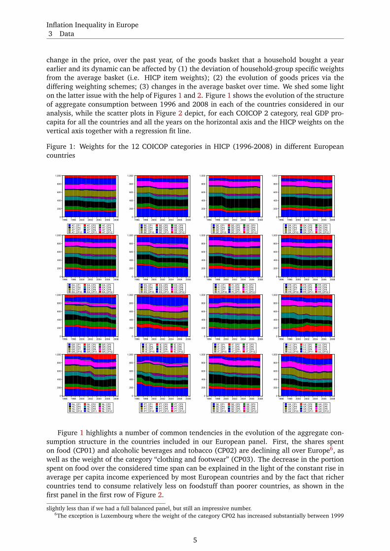
on the latter issue with the help of Figures 1 and 2. Figure 1 shows the evolution of the structure

of aggregate consumption between 1996 and 2008 in each of the countries considered in our

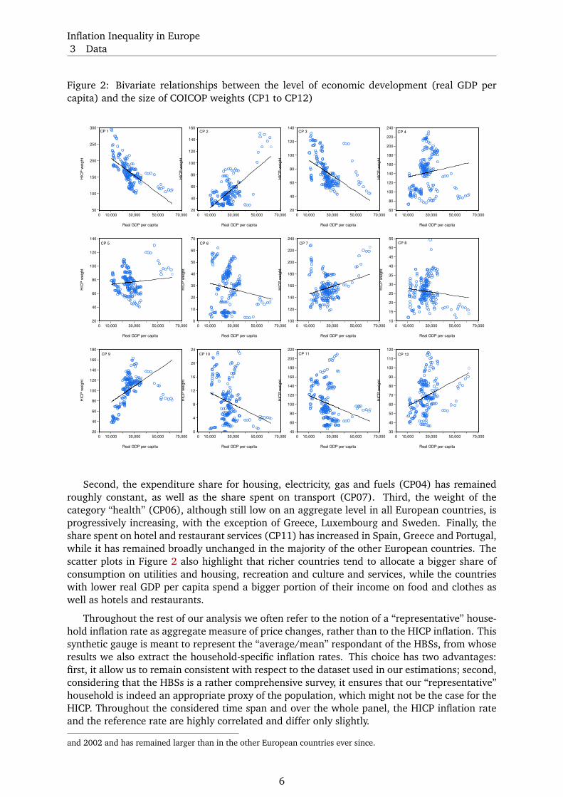
analysis, while the scatter plots in Figure 2 depict, for each COICOP 2 category, real GDP pro-

capita for all the countries and all the years on the horizontal axis and the HICP weights on the

vertical axis together with a regression fit line.

Figure 1: Weights for the 12 COICOP categories in HICP (1996-2008) in different European

countries

0

200

400

600

800

1,000

1996 1998 2000 2002 2004 2006 2008

AT_CP1 AT_CP2 AT_CP3AT_CP4 AT_CP5 AT_CP6AT_CP7 AT_CP8 AT_CP9AT_CP10 AT_CP11 AT_CP12

0

200

400

600

800

1,000

1996 1998 2000 2002 2004 2006 2008

BE_CP1 BE_CP2 BE_CP3BE_CP4 BE_CP5 BE_CP6BE_CP7 BE_CP8 BE_CP9BE_CP10 BE_CP11 BE_CP12

0

200

400

600

800

1,000

1996 1998 2000 2002 2004 2006 2008

DE_CP1 DE_CP2 DE_CP3DE_CP4 DE_CP5 DE_CP6DE_CP7 DE_CP8 DE_CP9DE_CP10 DE_CP11 DE_CP12

0

200

400

600

800

1,000

1996 1998 2000 2002 2004 2006 2008

DK_CP1 DK_CP2 DK_CP3DK_CP4 DK_CP5 DK_CP6DK_CP7 DK_CP8 DK_CP9DK_CP10 DK_CP11 DK_CP12

0

200

400

600

800

1,000

1996 1998 2000 2002 2004 2006 2008

EA_CP1 EA_CP2 EA_CP3EA_CP4 EA_CP5 EA_CP6EA_CP7 EA_CP8 EA_CP9EA_CP10 EA_CP11 EA_CP12

0

200

400

600

800

1,000

1996 1998 2000 2002 2004 2006 2008

ES_CP1 ES_CP2 ES_CP3ES_CP4 ES_CP5 ES_CP6ES_CP7 ES_CP8 ES_CP9ES_CP10 ES_CP11 ES_CP12

0

200

400

600

800

1,000

1996 1998 2000 2002 2004 2006 2008

FI_CP1 FI_CP2 FI_CP3FI_CP4 FI_CP5 FI_CP6FI_CP7 FI_CP8 FI_CP9FI_CP10 FI_CP11 FI_CP12

0

200

400

600

800

1,000

1996 1998 2000 2002 2004 2006 2008

FR_CP1 FR_CP2 FR_CP3FR_CP4 FR_CP5 FR_CP6FR_CP7 FR_CP8 FR_CP9FR_CP10 FR_CP11 FR_CP12

0

200

400

600

800

1,000

1996 1998 2000 2002 2004 2006 2008

GR_CP1 GR_CP2 GR_CP3GR_CP4 GR_CP5 GR_CP6GR_CP7 GR_CP8 GR_CP9GR_CP10 GR_CP11 GR_CP12

0

200

400

600

800

1,000

1996 1998 2000 2002 2004 2006 2008

IE_CP1 IE_CP2 IE_CP3IE_CP4 IE_CP5 IE_CP6IE_CP7 IE_CP8 IE_CP9IE_CP10 IE_CP11 IE_CP12

0

200

400

600

800

1,000

1996 1998 2000 2002 2004 2006 2008

IT_CP1 IT_CP2 IT_CP3IT_CP4 IT_CP5 IT_CP6IT_CP7 IT_CP8 IT_CP9IT_CP10 IT_CP11 IT_CP12

0

200

400

600

800

1,000

1996 1998 2000 2002 2004 2006 2008

LU_CP1 LU_CP2 LU_CP3LU_CP4 LU_CP5 LU_CP6LU_CP7 LU_CP8 LU_CP9LU_CP10 LU_CP11 LU_CP12

0

200

400

600

800

1,000

1996 1998 2000 2002 2004 2006 2008

NL_CP1 NL_CP2 NL_CP3NL_CP4 NL_CP5 NL_CP6NL_CP7 NL_CP8 NL_CP9NL_CP10 NL_CP11 NL_CP12

0

200

400

600

800

1,000

1996 1998 2000 2002 2004 2006 2008

PT_CP1 PT_CP2 PT_CP3PT_CP4 PT_CP5 PT_CP6PT_CP7 PT_CP8 PT_CP9PT_CP10 PT_CP11 PT_CP12

0

200

400

600

800

1,000

1996 1998 2000 2002 2004 2006 2008

SE_CP1 SE_CP2 SE_CP3SE_CP4 SE_CP5 SE_CP6SE_CP7 SE_CP8 SE_CP9SE_CP10 SE_CP11 SE_CP12

0

200

400

600

800

1,000

1996 1998 2000 2002 2004 2006 2008

UK_CP1 UK_CP2 UK_CP3UK_CP4 UK_CP5 UK_CP6UK_CP7 UK_CP8 UK_CP9UK_CP10 UK_CP11 UK_CP12

Figure 1 highlights a number of common tendencies in the evolution of the aggregate con-

sumption structure in the countries included in our European panel. First, the shares spent

on food (CP01) and alcoholic beverages and tobacco (CP02) are declining all over Europe6, as

well as the weight of the category “clothing and footwear” (CP03). The decrease in the portion

spent on food over the considered time span can be explained in the light of the constant rise in

average per capita income experienced by most European countries and by the fact that richer

countries tend to consume relatively less on foodstuff than poorer countries, as shown in the

first panel in the first row of Figure 2.

slightly less than if we had a full balanced panel, but still an impressive number.6The exception is Luxembourg where the weight of the category CP02 has increased substantially between 1999

5

Inflation Inequality in Europe

3 Data

Figure 2: Bivariate relationships between the level of economic development (real GDP per

capita) and the size of COICOP weights (CP1 to CP12)

50

100

150

200

250

300

0 10,000 30,000 50,000 70,000

Real GDP per capita

HIC

P w

eig

ht

CP 1

20

40

60

80

100

120

140

160

0 10,000 30,000 50,000 70,000

Real GDP per capita

HIC

P w

eig

ht

CP 2

20

40

60

80

100

120

140

0 10,000 30,000 50,000 70,000

Real GDP per capita

HIC

P w

eig

ht

CP 3

60

80

100

120

140

160

180

200

220

240

0 10,000 30,000 50,000 70,000

Real GDP per capita

HIC

P w

eig

ht

CP 4

20

40

60

80

100

120

140

0 10,000 30,000 50,000 70,000

Real GDP per capita

HIC

P w

eig

ht

CP 5

0

10

20

30

40

50

60

70

0 10,000 30,000 50,000 70,000

Real GDP per capita

HIC

P w

eig

ht

CP 6

100

120

140

160

180

200

220

240

0 10,000 30,000 50,000 70,000

Real GDP per capita

HIC

P w

eig

ht

CP 7

10

15

20

25

30

35

40

45

50

55

0 10,000 30,000 50,000 70,000

Real GDP per capita

HIC

P w

eig

ht

CP 8

20

40

60

80

100

120

140

160

180

0 10,000 30,000 50,000 70,000

Real GDP per capita

HIC

P w

eig

ht

CP 9

0

4

8

12

16

20

24

0 10,000 30,000 50,000 70,000

Real GDP per capita

HIC

P w

eig

ht

CP 10

40

60

80

100

120

140

160

180

200

220

0 10,000 30,000 50,000 70,000

Real GDP per capita

HIC

P w

eig

ht

CP 11

30

40

50

60

70

80

90

100

110

120

0 10,000 30,000 50,000 70,000

Real GDP per capita

HIC

P w

eig

ht

CP 12

Second, the expenditure share for housing, electricity, gas and fuels (CP04) has remained

roughly constant, as well as the share spent on transport (CP07). Third, the weight of the

category “health” (CP06), although still low on an aggregate level in all European countries, is

progressively increasing, with the exception of Greece, Luxembourg and Sweden. Finally, the

share spent on hotel and restaurant services (CP11) has increased in Spain, Greece and Portugal,

while it has remained broadly unchanged in the majority of the other European countries. The

scatter plots in Figure 2 also highlight that richer countries tend to allocate a bigger share of

consumption on utilities and housing, recreation and culture and services, while the countries

with lower real GDP per capita spend a bigger portion of their income on food and clothes as

well as hotels and restaurants.

Throughout the rest of our analysis we often refer to the notion of a “representative” house-

hold inflation rate as aggregate measure of price changes, rather than to the HICP inflation. This

synthetic gauge is meant to represent the “average/mean” respondant of the HBSs, from whose

results we also extract the household-specific inflation rates. This choice has two advantages:

first, it allow us to remain consistent with respect to the dataset used in our estimations; second,

considering that the HBSs is a rather comprehensive survey, it ensures that our “representative”

household is indeed an appropriate proxy of the population, which might not be the case for the

HICP. Throughout the considered time span and over the whole panel, the HICP inflation rate

and the reference rate are highly correlated and differ only slightly.

and 2002 and has remained larger than in the other European countries ever since.

6

Inflation Inequality in Europe

4 Empirical Analysis

4 Empirical Analysis

In the course of the paper, we test several hypotheses which in turn define the methods we use.

Specifically, we are interested in the following questions:

1. Are the original household-specific inflation rates in general stationary or non-stationary?

To test this aspect, we refer to panel unit root tests (see subsection 4.1.1).

2. Are the different household-specific inflation rates driven by one or more common trends?

Here we apply the PANIC approach (see Bai and Ng (2001, 2004) for the theory, and the

detailed exposition in subsection 4.1.2).

3. Under the aspect of economic-policy making on a national level, a stable relation or mean-

reversion between the “representative households inflation rate” and individual inflation

rates faced by different types of households, is more relevant than a mean-reversion to-

wards a unknown but assessable common trend. To answer this question we apply panel

co-integration tests on a national level (see subsection 4.1.2).

4. To shed further light on convergence properties of the household-specific inflation rates

on a national level, we explore two additional aspects. First, we calculate the speed of

adjustment of household-specific inflation rates towards the “representative” households

inflation. We address this issue by estimating a set of individual error correction models

(ECMs) and evaluating the distributions of the estimated loading coefficients (see sub-

section 4.1.2) in each country. Second, we investigate the persistence of the deviations

of the household-specific inflation rates from the inflation faced by the “representative”

household.

5. Apart from the investigations on the national level, we formed a huge panel across all

countries and all available inflation rates and used a cross-section of household-specific

inflation differentials calculated from the pooled data. In particular, we address the fol-

lowing questions (see subsection 4.2):

(a) Are there any group-specific inflation rates that differ significantly from the respective

(country-specific) overall mean?

(b) Are there clusters of households sharing common household specific inflation rate

patterns in terms of differences from a reference rate or volatility across Europe?

(c) Can we identify common driving processes behind household specific inflation rate

patterns across Europe?

4.1 Country-specific time series and panel results

4.1.1 Persistence patterns of inflation rates

First of all, we were interested if all household-specific inflation rates show the same pattern

of persistence as measured by the respective unit root properties of the process. Panel unit

root tests are the first choice for a data set like ours. Specifically, we applied the following

tests: A panel test based on the assumption of a common unit root process using the method

proposed in Levin et al. (2002) and a test based on the assumption of individual unit roots using

an augmented version of the Dickey and Fuller (1979a) test in a panel version proposed by

Maddala and Wu (1999a) and Choi (2001).7

7The panel unit root tests were performed using EViews 6 and the respective standard settings with regard to lag

length (BIC) and bandwidth selection (Newey-West using Bartlett kernel) were taken.

7

Inflation Inequality in Europe

4 Empirical Analysis

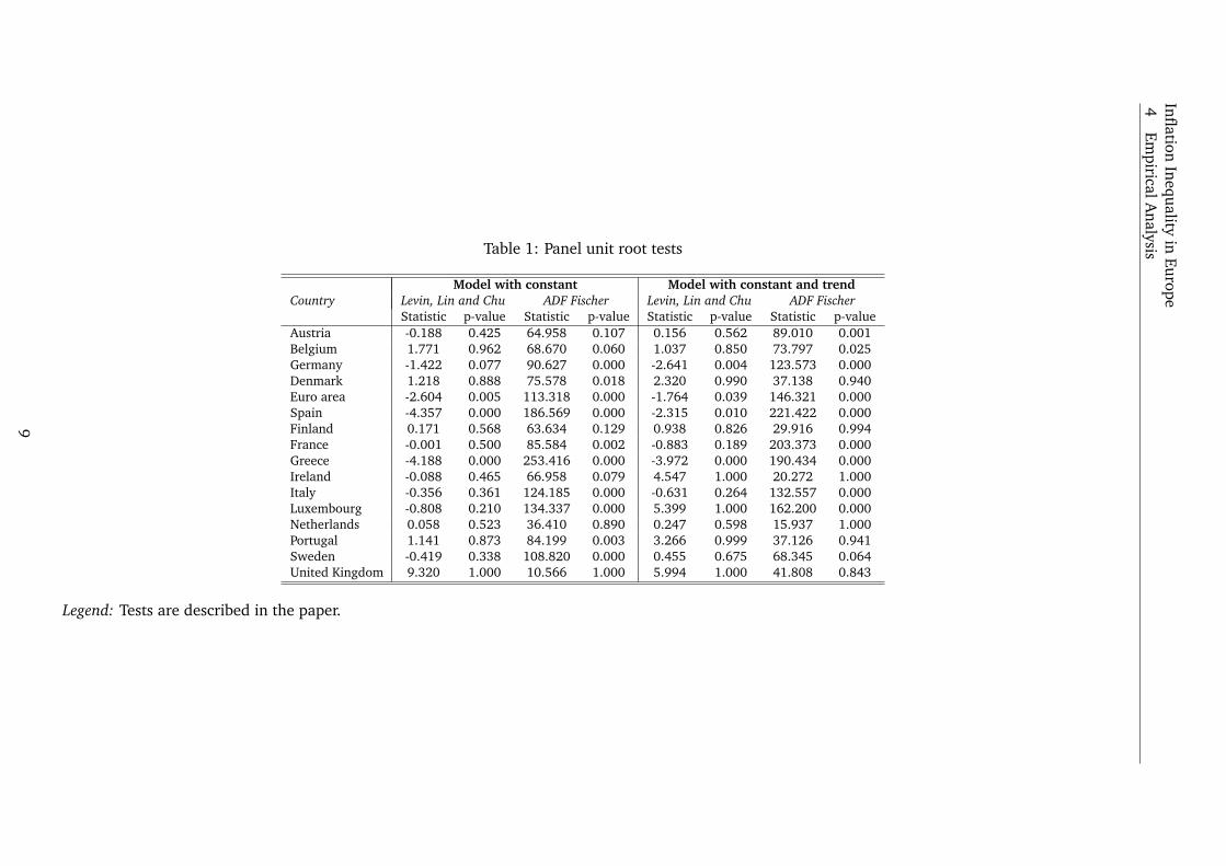
The results are given in Table 1. For the majority of countries – irrespective from the as-

sumption on the deterministic part – the tests fail to reject the hypothesis of a common unit root

process. On the other hand, the hypothesis of an individual unit root process is rejected in the

overwhelming majority of cases. From that result we can infer that the persistence over time is

high in our data set and that there is probably a single common source driving the persistent

part in the time series in each country.

4.1.2 Convergence issues

Following the investigation of the stochastic properties of our dataset by means of a set of panel

unit root tests, this section explores the issue of convergence of the household-specific inflation

rates from a number of different angles. We employ the PANIC approach Bai and Ng (2001,

2004) and panel co-integration tests. Finally, in a country-specific setting, we estimate a set of

bivariate ECMs to shed light on the adjustment process.

PANIC approach A useful approach to test for panel unit roots in the presence of either station-

ary or non-stationary common components is based on a factor representation of the differenced

time series in the panel (Bai and Ng, 2001, 2004). The approach is known by its acronym as

PANIC.8 The approach allows both idiosyncratic and common components to be integrated of

order one, which makes it a very flexible procedure when it comes to test for panel unit roots.

Since we investigate growth rates, we assume a model with an intercept but without linear

trend. Following the notation of Bai and Ng (2004) our model is given by:

Xit = ci + λ′iFt + eit (1)

where Xit are i = 1, . . . , N observed growth rates, Ft is an unobserved vector of common factors

and eit are unit specific idiosyncratic components. Both Ft and eit are allowed to be I(1). To

guarantee consistent estimates of the factors the model has to be estimated in differences, where

xit = ∆Xit, ft = ∆Ft and zit = ∆eit.

In the end, we estimate the following model:

xit = λ′ift + zit (2)

employing the method of principal components. However, we standardize the first differences

before estimating in order to avoid possible distortions by volatile series in calculating principal

components, see Bai and Ng (2001). In particular, we divide differenced time series by their

cross empirical cross-sectional standard deviations. Estimated common factors and idiosyncratic

components are then obtained via cumulating for t = 2, . . . , T and i = 1, . . . , N . Therefore:

eit =t∑

s=2

zis (3)

Fit =t∑

s=2

fs (4)

where zit = xit−λ′ifi are estimated residuals. Bai and Ng (2004) show that estimated factors and

idiosyncratic components are consistent, in particular T−1/2eit = T−1/2eit+op(1) and T−1/2Ft =T−1/2HFt+op(1), where H is a full rank matrix. The rate of convergence is fast enough to leave

8Panel Analysis of Nonstationarity in the Idiosyncratic and Common components.

8

Infl

atio

nIn

equ

ality

inE

uro

pe

4E

mpirica

lA

naly

sisTable 1: Panel unit root tests

Model with constant Model with constant and trend

Country Levin, Lin and Chu ADF Fischer Levin, Lin and Chu ADF Fischer

Statistic p-value Statistic p-value Statistic p-value Statistic p-value

Austria -0.188 0.425 64.958 0.107 0.156 0.562 89.010 0.001

Belgium 1.771 0.962 68.670 0.060 1.037 0.850 73.797 0.025

Germany -1.422 0.077 90.627 0.000 -2.641 0.004 123.573 0.000

Denmark 1.218 0.888 75.578 0.018 2.320 0.990 37.138 0.940

Euro area -2.604 0.005 113.318 0.000 -1.764 0.039 146.321 0.000

Spain -4.357 0.000 186.569 0.000 -2.315 0.010 221.422 0.000

Finland 0.171 0.568 63.634 0.129 0.938 0.826 29.916 0.994

France -0.001 0.500 85.584 0.002 -0.883 0.189 203.373 0.000

Greece -4.188 0.000 253.416 0.000 -3.972 0.000 190.434 0.000

Ireland -0.088 0.465 66.958 0.079 4.547 1.000 20.272 1.000

Italy -0.356 0.361 124.185 0.000 -0.631 0.264 132.557 0.000

Luxembourg -0.808 0.210 134.337 0.000 5.399 1.000 162.200 0.000

Netherlands 0.058 0.523 36.410 0.890 0.247 0.598 15.937 1.000

Portugal 1.141 0.873 84.199 0.003 3.266 0.999 37.126 0.941

Sweden -0.419 0.338 108.820 0.000 0.455 0.675 68.345 0.064

United Kingdom 9.320 1.000 10.566 1.000 5.994 1.000 41.808 0.843

Legend: Tests are described in the paper.

9

Inflation Inequality in Europe

4 Empirical Analysis

the asymptotic distribution of an Augmented Dickey-Fuller-test (ADF-test, see Dickey and Fuller

(1979b)) unchanged, if applied to estimated series Ft and eit. So we can apply any version of

the univariate ADF-test as well as pooled unit root tests to estimated factors and idiosyncratic

components, respectively. In case of estimated factors we allow for a constant in a test regression

and test without any deterministic terms in the panel case of idiosyncratic components.

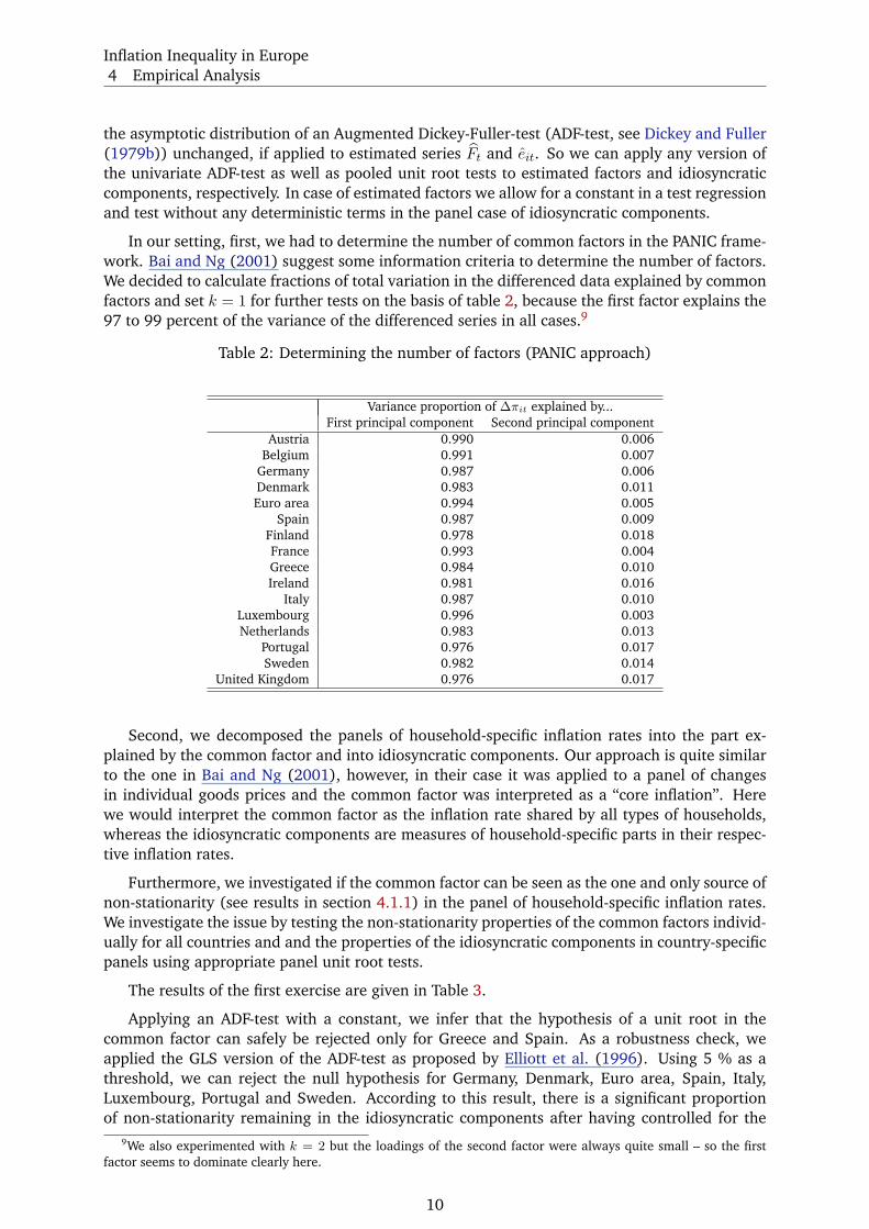
In our setting, first, we had to determine the number of common factors in the PANIC frame-

work. Bai and Ng (2001) suggest some information criteria to determine the number of factors.

We decided to calculate fractions of total variation in the differenced data explained by common

factors and set k = 1 for further tests on the basis of table 2, because the first factor explains the

97 to 99 percent of the variance of the differenced series in all cases.9

Table 2: Determining the number of factors (PANIC approach)

Variance proportion of ∆πit explained by...

First principal component Second principal component

Austria 0.990 0.006

Belgium 0.991 0.007

Germany 0.987 0.006

Denmark 0.983 0.011

Euro area 0.994 0.005

Spain 0.987 0.009

Finland 0.978 0.018

France 0.993 0.004

Greece 0.984 0.010

Ireland 0.981 0.016

Italy 0.987 0.010

Luxembourg 0.996 0.003

Netherlands 0.983 0.013

Portugal 0.976 0.017

Sweden 0.982 0.014

United Kingdom 0.976 0.017

Second, we decomposed the panels of household-specific inflation rates into the part ex-

plained by the common factor and into idiosyncratic components. Our approach is quite similar

to the one in Bai and Ng (2001), however, in their case it was applied to a panel of changes

in individual goods prices and the common factor was interpreted as a “core inflation”. Here

we would interpret the common factor as the inflation rate shared by all types of households,

whereas the idiosyncratic components are measures of household-specific parts in their respec-

tive inflation rates.

Furthermore, we investigated if the common factor can be seen as the one and only source of

non-stationarity (see results in section 4.1.1) in the panel of household-specific inflation rates.

We investigate the issue by testing the non-stationarity properties of the common factors individ-

ually for all countries and and the properties of the idiosyncratic components in country-specific

panels using appropriate panel unit root tests.

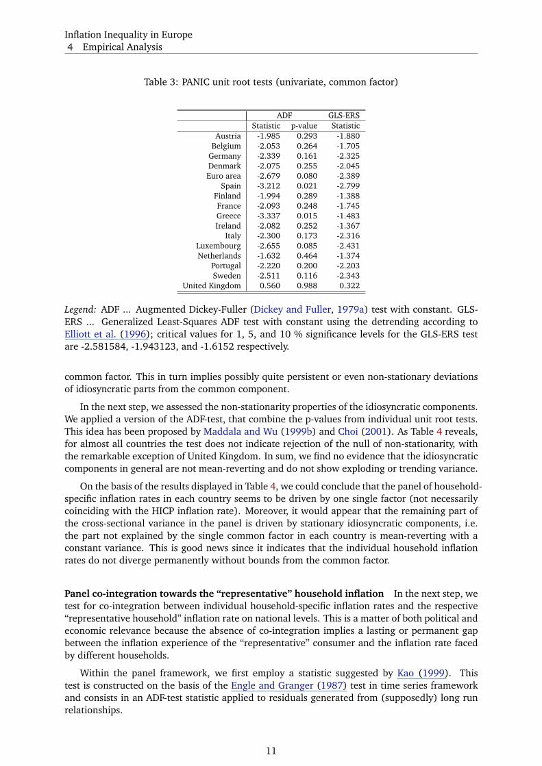
The results of the first exercise are given in Table 3.

Applying an ADF-test with a constant, we infer that the hypothesis of a unit root in the

common factor can safely be rejected only for Greece and Spain. As a robustness check, we

applied the GLS version of the ADF-test as proposed by Elliott et al. (1996). Using 5 % as a

threshold, we can reject the null hypothesis for Germany, Denmark, Euro area, Spain, Italy,

Luxembourg, Portugal and Sweden. According to this result, there is a significant proportion

of non-stationarity remaining in the idiosyncratic components after having controlled for the

9We also experimented with k = 2 but the loadings of the second factor were always quite small – so the first

factor seems to dominate clearly here.

10

Inflation Inequality in Europe

4 Empirical Analysis

Table 3: PANIC unit root tests (univariate, common factor)

ADF GLS-ERS

Statistic p-value Statistic

Austria -1.985 0.293 -1.880

Belgium -2.053 0.264 -1.705

Germany -2.339 0.161 -2.325

Denmark -2.075 0.255 -2.045

Euro area -2.679 0.080 -2.389

Spain -3.212 0.021 -2.799

Finland -1.994 0.289 -1.388

France -2.093 0.248 -1.745

Greece -3.337 0.015 -1.483

Ireland -2.082 0.252 -1.367

Italy -2.300 0.173 -2.316

Luxembourg -2.655 0.085 -2.431

Netherlands -1.632 0.464 -1.374

Portugal -2.220 0.200 -2.203

Sweden -2.511 0.116 -2.343

United Kingdom 0.560 0.988 0.322

Legend: ADF ... Augmented Dickey-Fuller (Dickey and Fuller, 1979a) test with constant. GLS-

ERS ... Generalized Least-Squares ADF test with constant using the detrending according to

Elliott et al. (1996); critical values for 1, 5, and 10 % significance levels for the GLS-ERS test

are -2.581584, -1.943123, and -1.6152 respectively.

common factor. This in turn implies possibly quite persistent or even non-stationary deviations

of idiosyncratic parts from the common component.

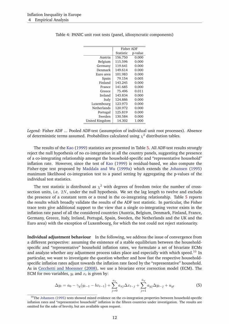
In the next step, we assessed the non-stationarity properties of the idiosyncratic components.

We applied a version of the ADF-test, that combine the p-values from individual unit root tests.

This idea has been proposed by Maddala and Wu (1999b) and Choi (2001). As Table 4 reveals,

for almost all countries the test does not indicate rejection of the null of non-stationarity, with

the remarkable exception of United Kingdom. In sum, we find no evidence that the idiosyncratic

components in general are not mean-reverting and do not show exploding or trending variance.

On the basis of the results displayed in Table 4, we could conclude that the panel of household-

specific inflation rates in each country seems to be driven by one single factor (not necessarily

coinciding with the HICP inflation rate). Moreover, it would appear that the remaining part of

the cross-sectional variance in the panel is driven by stationary idiosyncratic components, i.e.

the part not explained by the single common factor in each country is mean-reverting with a

constant variance. This is good news since it indicates that the individual household inflation

rates do not diverge permanently without bounds from the common factor.

Panel co-integration towards the “representative” household inflation In the next step, we

test for co-integration between individual household-specific inflation rates and the respective

“representative household” inflation rate on national levels. This is a matter of both political and

economic relevance because the absence of co-integration implies a lasting or permanent gap

between the inflation experience of the “representative” consumer and the inflation rate faced

by different households.

Within the panel framework, we first employ a statistic suggested by Kao (1999). This

test is constructed on the basis of the Engle and Granger (1987) test in time series framework

and consists in an ADF-test statistic applied to residuals generated from (supposedly) long run

relationships.

11

Inflation Inequality in Europe

4 Empirical Analysis

Table 4: PANIC unit root tests (panel, idiosyncratic components)

Fisher ADF

Statistic p-value

Austria 156.750 0.000

Belgium 115.596 0.000

Germany 119.641 0.000

Denmark 149.614 0.000

Euro area 101.983 0.000

Spain 79.154 0.005

Finland 143.245 0.000

France 141.685 0.000

Greece 75.496 0.011

Ireland 143.834 0.000

Italy 124.886 0.000

Luxembourg 123.973 0.000

Netherlands 120.972 0.000

Portugal 125.819 0.000

Sweden 130.584 0.000

United Kingdom 14.302 1.000

Legend: Fisher ADF ... Pooled ADF-test (assumption of individual unit root processes). Absence

of deterministic terms assumed. Probabilites calculated using χ2 distribution tables.

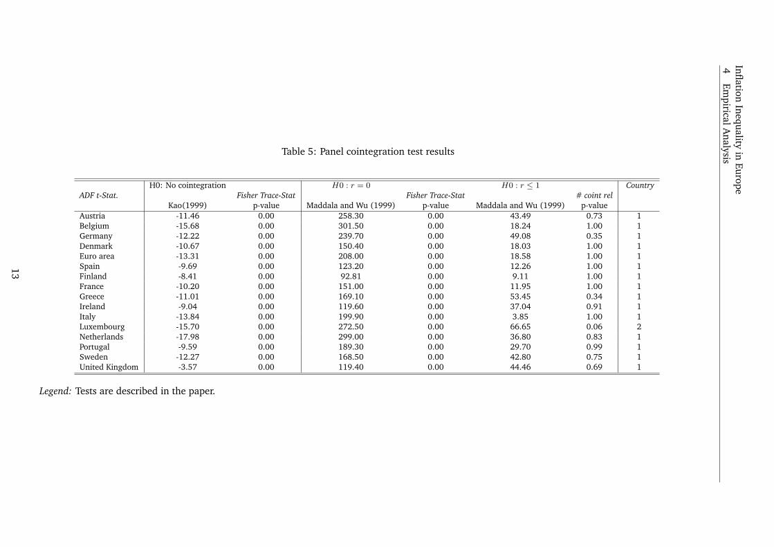
The results of the Kao (1999) statistics are presented in Table 5. All ADF-test results strongly

reject the null hypothesis of no co-integration in all the country panels, suggesting the presence

of a co-integrating relationship amongst the household-specific and “representative household”

inflation rate. However, since the test of Kao (1999) is residual-based, we also compute the

Fisher-type test proposed by Maddala and Wu (1999a) which extends the Johansen (1995)

maximum likelihood co-integration test to a panel setting by aggregating the p-values of the

individual test statistics.

The test statistic is distributed as χ2 with degrees of freedom twice the number of cross-

section units, i.e. 2N , under the null hypothesis. We set the lag length to twelve and exclude

the presence of a constant term or a trend in the co-integrating relationship. Table 5 reports

the results which broadly validate the results of the ADF test statistic. In particular, the Fisher

trace tests give additional support to the view that a single co-integrating vector exists in the

inflation rate panel of all the considered countries (Austria, Belgium, Denmark, Finland, France,

Germany, Greece, Italy, Ireland, Portugal, Spain, Sweden, the Netherlands and the UK and the

Euro area) with the exception of Luxembourg, for which the test could not reject stationarity.

Individual adjustment behaviour In the following, we address the issue of convergence from

a different perspective: assuming the existence of a stable equilibrium between the household-

specific and “representative” household inflation rates, we formulate a set of bivariate ECMs

and analyze whether any adjustment process takes place and especially with which speed.10 In

particular, we want to investigate the question whether and how fast the respective household-

specific inflation rates adjust towards the inflation rate faced by the “representative” household.

As in Cecchetti and Moessner (2008), we use a bivariate error correction model (ECM). The

ECM for two variables, yt and xt is given by:

∆yt = a0 − γy(yt−1 − bxt−1) +

nx∑

j=0

axj∆xt−j +

ny∑

j=1

ayj∆yt−j + uyt (5)

10The Johansen (1995) tests showed mixed evidence on the co-integration properties between household-specific

inflation rates and “representative household” inflation in the fifteen countries under investigation. The results are

omitted for the sake of brevity, but are available upon request.

12

Infl

atio

nIn

equ

ality

inE

uro

pe

4E

mpirica

lA

naly

sis

Table 5: Panel cointegration test results

H0: No cointegration H0 : r = 0 H0 : r ≤ 1 Country

ADF t-Stat. Fisher Trace-Stat Fisher Trace-Stat # coint rel

Kao(1999) p-value Maddala and Wu (1999) p-value Maddala and Wu (1999) p-value

Austria -11.46 0.00 258.30 0.00 43.49 0.73 1

Belgium -15.68 0.00 301.50 0.00 18.24 1.00 1

Germany -12.22 0.00 239.70 0.00 49.08 0.35 1

Denmark -10.67 0.00 150.40 0.00 18.03 1.00 1

Euro area -13.31 0.00 208.00 0.00 18.58 1.00 1

Spain -9.69 0.00 123.20 0.00 12.26 1.00 1

Finland -8.41 0.00 92.81 0.00 9.11 1.00 1

France -10.20 0.00 151.00 0.00 11.95 1.00 1

Greece -11.01 0.00 169.10 0.00 53.45 0.34 1

Ireland -9.04 0.00 119.60 0.00 37.04 0.91 1

Italy -13.84 0.00 199.90 0.00 3.85 1.00 1

Luxembourg -15.70 0.00 272.50 0.00 66.65 0.06 2

Netherlands -17.98 0.00 299.00 0.00 36.80 0.83 1

Portugal -9.59 0.00 189.30 0.00 29.70 0.99 1

Sweden -12.27 0.00 168.50 0.00 42.80 0.75 1

United Kingdom -3.57 0.00 119.40 0.00 44.46 0.69 1

Legend: Tests are described in the paper.

13

Inflation Inequality in Europe

4 Empirical Analysis

∆xt = b0 − γx(yt−1 − bxt−1) +

kx∑

j=1

bxj∆xt−j +

ky∑

j=0

byj∆yt−j + uxt (6)

where yt and xt indicate the household-specific and the “representative household” inflation

series, respectively.

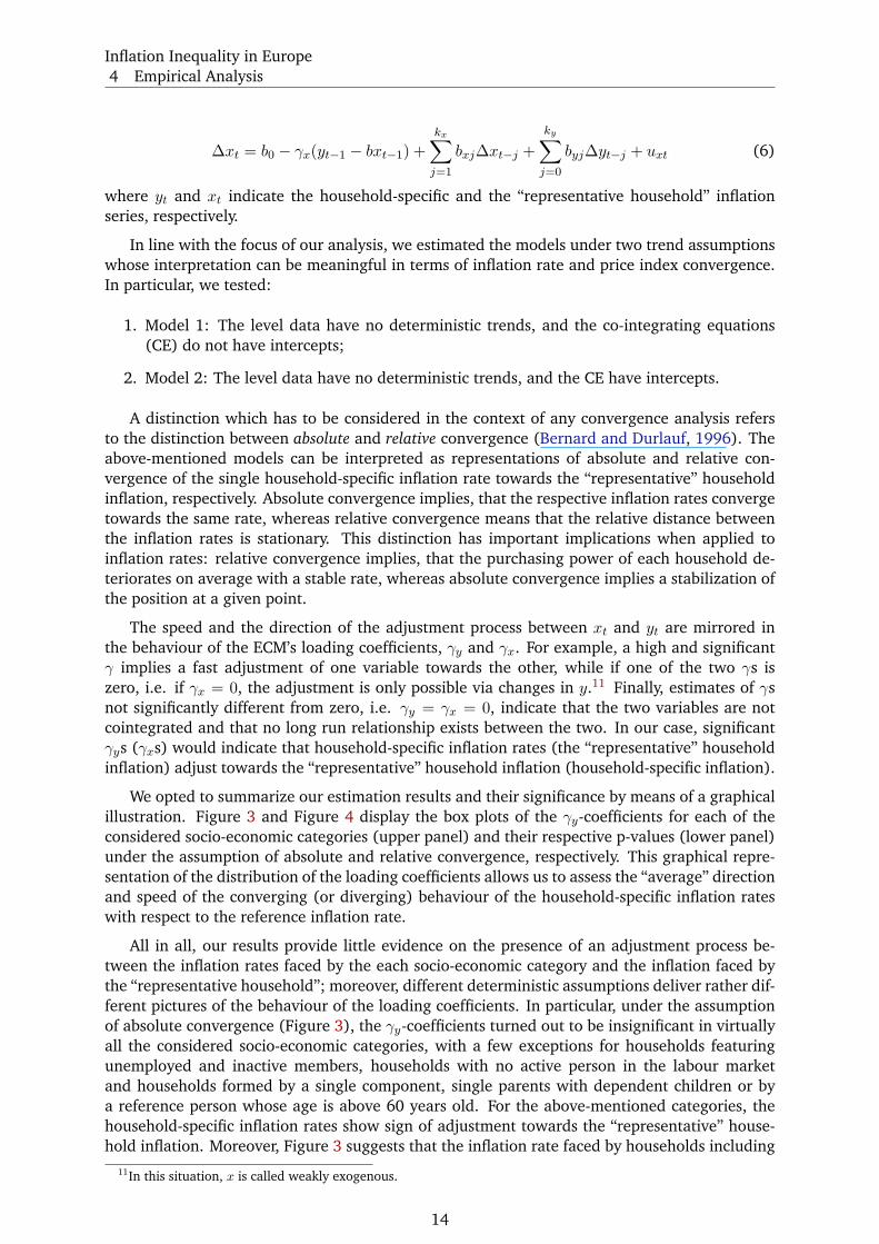
In line with the focus of our analysis, we estimated the models under two trend assumptions

whose interpretation can be meaningful in terms of inflation rate and price index convergence.

In particular, we tested:

1. Model 1: The level data have no deterministic trends, and the co-integrating equations

(CE) do not have intercepts;

2. Model 2: The level data have no deterministic trends, and the CE have intercepts.

A distinction which has to be considered in the context of any convergence analysis refers

to the distinction between absolute and relative convergence (Bernard and Durlauf, 1996). The

above-mentioned models can be interpreted as representations of absolute and relative con-

vergence of the single household-specific inflation rate towards the “representative” household

inflation, respectively. Absolute convergence implies, that the respective inflation rates converge

towards the same rate, whereas relative convergence means that the relative distance between

the inflation rates is stationary. This distinction has important implications when applied to

inflation rates: relative convergence implies, that the purchasing power of each household de-

teriorates on average with a stable rate, whereas absolute convergence implies a stabilization of

the position at a given point.

The speed and the direction of the adjustment process between xt and yt are mirrored in

the behaviour of the ECM’s loading coefficients, γy and γx. For example, a high and significant

γ implies a fast adjustment of one variable towards the other, while if one of the two γs is

zero, i.e. if γx = 0, the adjustment is only possible via changes in y.11 Finally, estimates of γs

not significantly different from zero, i.e. γy = γx = 0, indicate that the two variables are not

cointegrated and that no long run relationship exists between the two. In our case, significant

γys (γxs) would indicate that household-specific inflation rates (the “representative” household

inflation) adjust towards the “representative” household inflation (household-specific inflation).

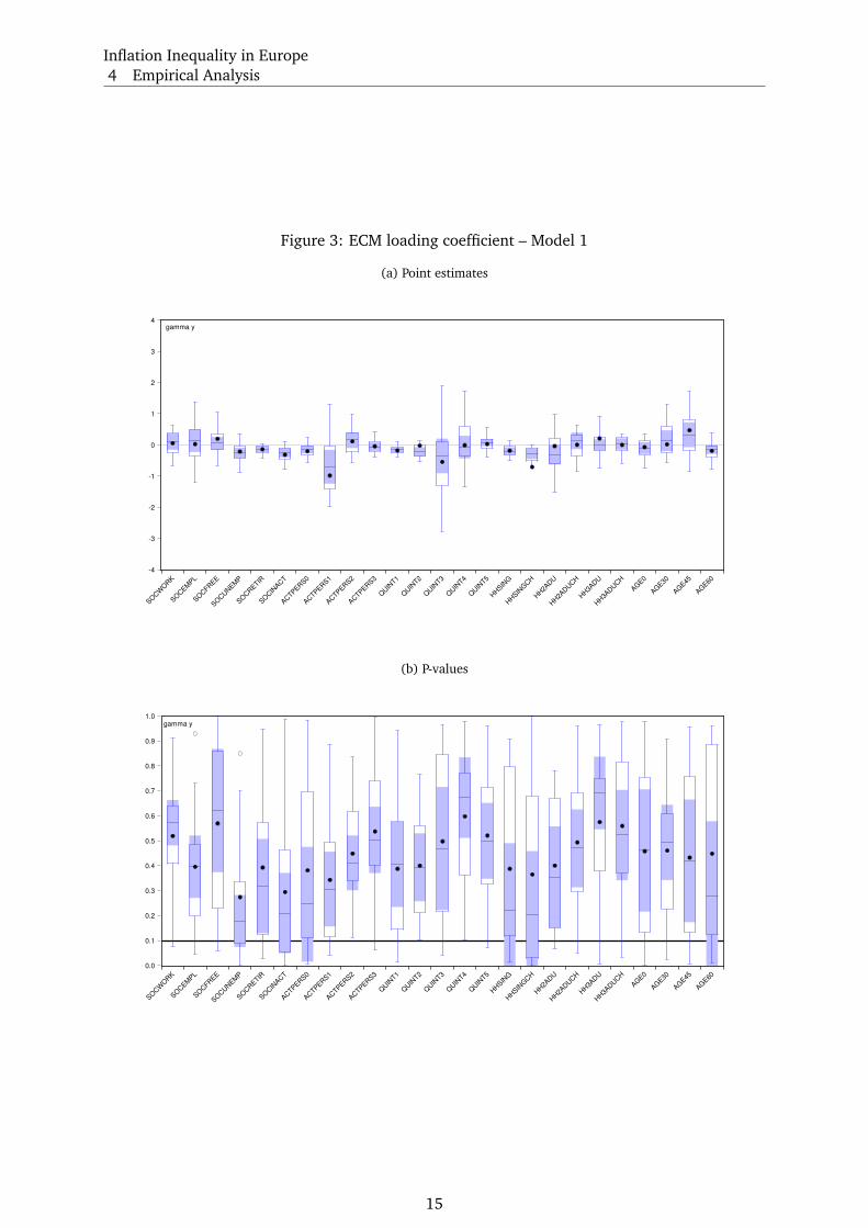
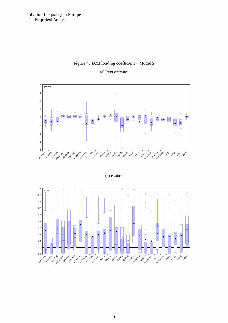
We opted to summarize our estimation results and their significance by means of a graphical

illustration. Figure 3 and Figure 4 display the box plots of the γy-coefficients for each of the

considered socio-economic categories (upper panel) and their respective p-values (lower panel)

under the assumption of absolute and relative convergence, respectively. This graphical repre-

sentation of the distribution of the loading coefficients allows us to assess the “average” direction

and speed of the converging (or diverging) behaviour of the household-specific inflation rates

with respect to the reference inflation rate.

All in all, our results provide little evidence on the presence of an adjustment process be-

tween the inflation rates faced by the each socio-economic category and the inflation faced by

the “representative household”; moreover, different deterministic assumptions deliver rather dif-

ferent pictures of the behaviour of the loading coefficients. In particular, under the assumption

of absolute convergence (Figure 3), the γy-coefficients turned out to be insignificant in virtually

all the considered socio-economic categories, with a few exceptions for households featuring

unemployed and inactive members, households with no active person in the labour market

and households formed by a single component, single parents with dependent children or by

a reference person whose age is above 60 years old. For the above-mentioned categories, the

household-specific inflation rates show sign of adjustment towards the “representative” house-

hold inflation. Moreover, Figure 3 suggests that the inflation rate faced by households including

11In this situation, x is called weakly exogenous.

14

Inflation Inequality in Europe

4 Empirical Analysis

Figure 3: ECM loading coefficient – Model 1

(a) Point estimates

-4

-3

-2

-1

0

1

2

3

4

SOCW

ORK

SOCEM

PL

SOCFR

EE

SOCUNEM

P

SOCRETIR

SOCIN

ACT

ACTPER

S0

ACTPER

S1

ACTPER

S2

ACTPER

S3

QUIN

T1

QUIN

T2

QUIN

T3

QUIN

T4

QUIN

T5

HHSIN

G

HHSIN

GCH

HH2A

DU

HH2A

DUCH

HH3A

DU

HH3A

DUCH

AGE0

AGE30

AGE45

AGE60

gamma y

(b) P-values

0.0

0.1

0.2

0.3

0.4

0.5

0.6

0.7

0.8

0.9

1.0

SOCW

ORK

SOCEM

PL

SOCFR

EE

SOCUNEM

P

SOCRETIR

SOCIN

ACT

ACTPER

S0

ACTPER

S1

ACTPER

S2

ACTPER

S3

QUIN

T1

QUIN

T2

QUIN

T3

QUIN

T4

QUIN

T5

HHSIN

G

HHSIN

GCH

HH2A

DU

HH2A

DUCH

HH3A

DU

HH3A

DUCH

AGE0

AGE30

AGE45

AGE60

gamma y

15

Inflation Inequality in Europe

4 Empirical Analysis

Figure 4: ECM loading coefficient – Model 2

(a) Point estimates

-4

-3

-2

-1

0

1

2

3

4

SOCW

ORK

SOCEM

PL

SOCFR

EE

SOCUNEM

P

SOCRETIR

SOCIN

ACT

ACTPER

S0

ACTPER

S1

ACTPER

S2

ACTPER

S3

QUIN

T1

QUIN

T2

QUIN

T3

QUIN

T4

QUIN

T5

HHSIN

G

HHSIN

GCH

HH2A

DU

HH2A

DUCH

HH3A

DU

HH3A

DUCH

AGE0

AGE30

AGE45

AGE60

gamma y

(b) P-values

0.0

0.1

0.2

0.3

0.4

0.5

0.6

0.7

0.8

0.9

1.0

SOCW

ORK

SOCEM

PL

SOCFR

EE

SOCUNEM

P

SOCRETIR

SOCIN

ACT

ACTPER

S0

ACTPER

S1

ACTPER

S2

ACTPER

S3

QUIN

T1

QUIN

T2

QUIN

T3

QUIN

T4

QUIN

T5

HHSIN

G

HHSIN

GCH

HH2A

DU

HH2A

DUCH

HH3A

DU

HH3A

DUCH

AGE0

AGE30

AGE45

AGE60

gamma y

16

Inflation Inequality in Europe

4 Empirical Analysis

single parents with dependent children adjusts towards the “representative” household inflation

relatively faster than for other categories, such as households featuring unemployed or young

(below 30 years old) members, which all tend to deviate quite persistently from the “represen-

tative” household inflation rate.

The number of significant loading coefficients increases substantially under the assumption

of relative convergence (Figure 4). In particular, evidence of the presence of an adjustment pro-

cess between household-specific and “representative” household inflation emerges in numerous

socio economic categories, where the γy are found to be - on average - significant.12 Figure

4 confirms that households with one active person display, on average, the largest (in abso-

lute value) loading coefficients, together with households belonging to the fourth quartile of

the income distribution. In addition to that, the inflation rates faced by households including

two adults with dependent children and by households with reference person between 45 and

59 years old also seem to adjust relatively fast towards the reference inflation rate. For the

majority of the remaining categories, the adjustment speed towards equilibrium is rather low,

indicating a tendency of the household-specific inflations to deviate quite persistently from the

“representative household” inflation.

4.2 Pooled Panel Analysis of Inflation Differentials

For the 52,910 observations of our panel, the bivariate correlation of the pooled country-specific

headline inflation rates with the household-specific inflation rates amounts to 0.95, which is

high, but at the same time still significantly below unity. Nevertheless, the correlation is so close

that we can assume a common driving force behind the household specific inflation rates. On

the country-level, such an assumption is in line with the results of the PANIC approach (see

section 4.1.2).

Statistically, this amounts to the hypothesis that a singly data-generating process dominates

the variation in our panel. To illustrate this, we run two principal components extractions,

where the variables are the household specific inflation rates; one for the aggregate of the EU-

15 countries and the other for the aggregate of the initial 11 Euro area member countries.13

The EA principal components extraction covers 22 out of 25 household specific rates.14 For

the EA aggregate, the first component already represents 99.6% of the sample variance, the

second component only 0.07%. The finding is very similar for the EU-15 aggregate, where 21

household-specific inflation rates can be computed.15 The first component picks up 99.2 percent

of the sample variance and the second only 0.13%. These are clearly one-dimensional solutions

in statistical terms. This finding on our two aggregate levels also holds for all the 15 coun-

tries individually.16 There is one major data generating process reflected by the “representative

household” inflation that affects all household categories and without exception represents most

of the inflationary variation across time.

Yet, while the inflation generating process appears to be one-dimensional, there still may

exist second or lower order inflationary processes affecting more than one household type only.

12In particular, this holds for: households where the reference person is a manual or a non-manual worker or

unemployed, households featuring up to three active persons, households belonging to the poorest 20 percent or

to the richest 60 percent of the population, households including up to two adults with dependent children and

households where the age of the reference person is less than thirty years old or between 45 and 59 years old.13Austria, Belgium, Finland, France, Germany, Ireland, Italy, Luxembourg, Netherlands, Portugal, and Spain;

henceforth EA.14No EA aggregate household-specific inflation rates are available for the self-employed, unemployed and retired

categories.15Household specific inflation rates for the EU-15 are unavailable for the non-manual worker, unemployed, retired

and three or more adults with dependent children categories.16The country results are not presented here for space reasons, but they are available from the corresponding

author upon request.

17

Inflation Inequality in Europe

4 Empirical Analysis

These should become visible in the deviations of the household specific inflation rates from

the “representative household” inflation in the same country or country group. To assess this

possibility, we compute these differences for all observations in the panel.

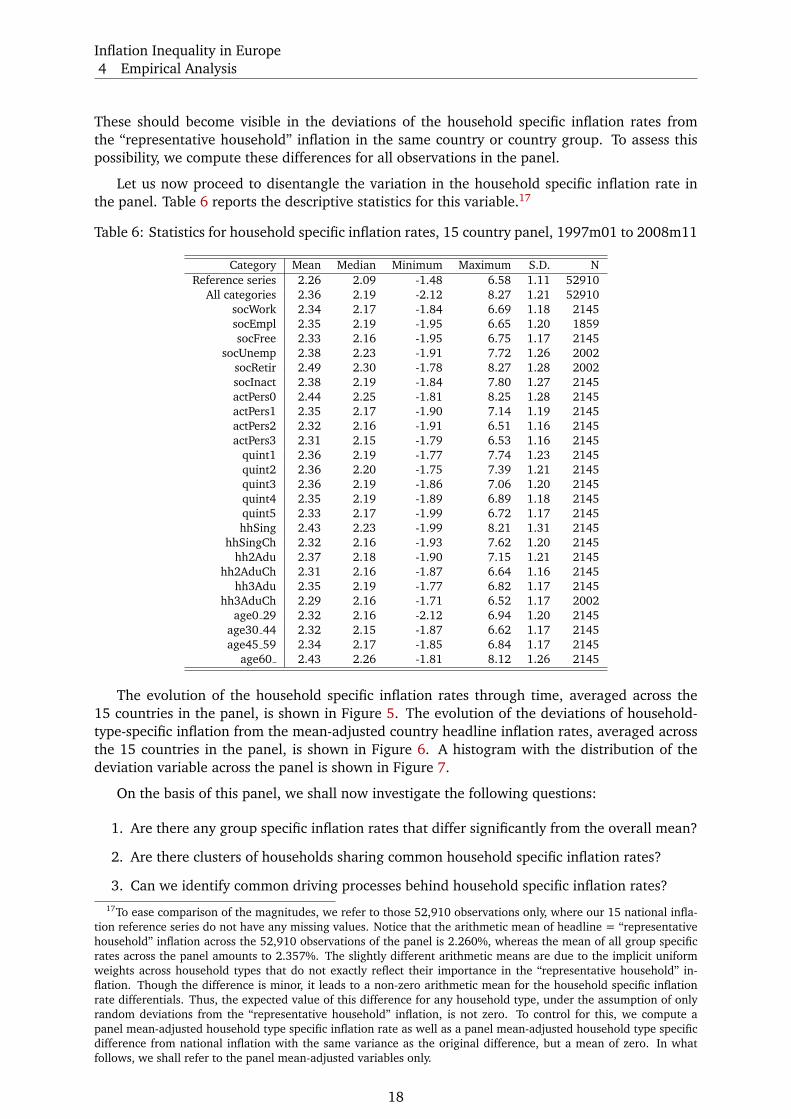
Let us now proceed to disentangle the variation in the household specific inflation rate in

the panel. Table 6 reports the descriptive statistics for this variable.17

Table 6: Statistics for household specific inflation rates, 15 country panel, 1997m01 to 2008m11

Category Mean Median Minimum Maximum S.D. N

Reference series 2.26 2.09 -1.48 6.58 1.11 52910

All categories 2.36 2.19 -2.12 8.27 1.21 52910

socWork 2.34 2.17 -1.84 6.69 1.18 2145

socEmpl 2.35 2.19 -1.95 6.65 1.20 1859

socFree 2.33 2.16 -1.95 6.75 1.17 2145

socUnemp 2.38 2.23 -1.91 7.72 1.26 2002

socRetir 2.49 2.30 -1.78 8.27 1.28 2002

socInact 2.38 2.19 -1.84 7.80 1.27 2145

actPers0 2.44 2.25 -1.81 8.25 1.28 2145

actPers1 2.35 2.17 -1.90 7.14 1.19 2145

actPers2 2.32 2.16 -1.91 6.51 1.16 2145

actPers3 2.31 2.15 -1.79 6.53 1.16 2145

quint1 2.36 2.19 -1.77 7.74 1.23 2145

quint2 2.36 2.20 -1.75 7.39 1.21 2145

quint3 2.36 2.19 -1.86 7.06 1.20 2145

quint4 2.35 2.19 -1.89 6.89 1.18 2145

quint5 2.33 2.17 -1.99 6.72 1.17 2145

hhSing 2.43 2.23 -1.99 8.21 1.31 2145

hhSingCh 2.32 2.16 -1.93 7.62 1.20 2145

hh2Adu 2.37 2.18 -1.90 7.15 1.21 2145

hh2AduCh 2.31 2.16 -1.87 6.64 1.16 2145

hh3Adu 2.35 2.19 -1.77 6.82 1.17 2145

hh3AduCh 2.29 2.16 -1.71 6.52 1.17 2002

age0 29 2.32 2.16 -2.12 6.94 1.20 2145

age30 44 2.32 2.15 -1.87 6.62 1.17 2145

age45 59 2.34 2.17 -1.85 6.84 1.17 2145

age60 2.43 2.26 -1.81 8.12 1.26 2145

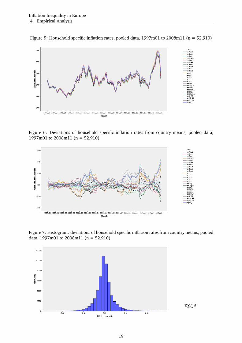
The evolution of the household specific inflation rates through time, averaged across the

15 countries in the panel, is shown in Figure 5. The evolution of the deviations of household-

type-specific inflation from the mean-adjusted country headline inflation rates, averaged across

the 15 countries in the panel, is shown in Figure 6. A histogram with the distribution of the

deviation variable across the panel is shown in Figure 7.

On the basis of this panel, we shall now investigate the following questions:

1. Are there any group specific inflation rates that differ significantly from the overall mean?

2. Are there clusters of households sharing common household specific inflation rates?

3. Can we identify common driving processes behind household specific inflation rates?

17To ease comparison of the magnitudes, we refer to those 52,910 observations only, where our 15 national infla-

tion reference series do not have any missing values. Notice that the arithmetic mean of headline = “representative

household” inflation across the 52,910 observations of the panel is 2.260%, whereas the mean of all group specific

rates across the panel amounts to 2.357%. The slightly different arithmetic means are due to the implicit uniform

weights across household types that do not exactly reflect their importance in the “representative household” in-

flation. Though the difference is minor, it leads to a non-zero arithmetic mean for the household specific inflation

rate differentials. Thus, the expected value of this difference for any household type, under the assumption of only

random deviations from the “representative household” inflation, is not zero. To control for this, we compute a

panel mean-adjusted household type specific inflation rate as well as a panel mean-adjusted household type specific

difference from national inflation with the same variance as the original difference, but a mean of zero. In what

follows, we shall refer to the panel mean-adjusted variables only.

18

Inflation Inequality in Europe

4 Empirical Analysis

Figure 5: Household specific inflation rates, pooled data, 1997m01 to 2008m11 (n = 52,910)

Figure 6: Deviations of household specific inflation rates from country means, pooled data,

1997m01 to 2008m11 (n = 52,910)

Figure 7: Histogram: deviations of household specific inflation rates from country means, pooled

data, 1997m01 to 2008m11 (n = 52,910)

19

Inflation Inequality in Europe

4 Empirical Analysis

4.2.1 Are there any group specific inflation rates that differ significantly from the overall

mean?

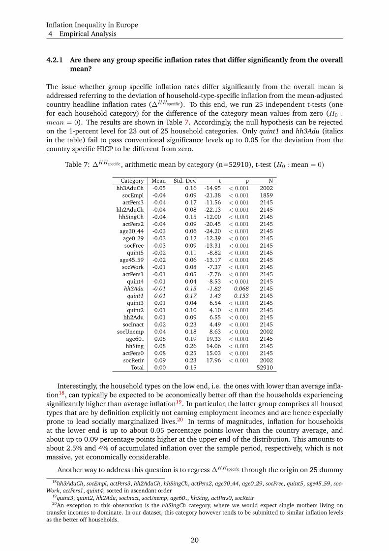
The issue whether group specific inflation rates differ significantly from the overall mean is

addressed referring to the deviation of household-type-specific inflation from the mean-adjusted

country headline inflation rates (∆HHspecific). To this end, we run 25 independent t-tests (one

for each household category) for the difference of the category mean values from zero (H0 :mean = 0). The results are shown in Table 7. Accordingly, the null hypothesis can be rejected

on the 1-percent level for 23 out of 25 household categories. Only quint1 and hh3Adu (italics

in the table) fail to pass conventional significance levels up to 0.05 for the deviation from the

country specific HICP to be different from zero.

Table 7: ∆HHspecific , arithmetic mean by category (n=52910), t-test (H0 : mean = 0)

Category Mean Std. Dev. t p N

hh3AduCh -0.05 0.16 -14.95 < 0.001 2002

socEmpl -0.04 0.09 -21.38 < 0.001 1859

actPers3 -0.04 0.17 -11.56 < 0.001 2145

hh2AduCh -0.04 0.08 -22.13 < 0.001 2145

hhSingCh -0.04 0.15 -12.00 < 0.001 2145

actPers2 -0.04 0.09 -20.45 < 0.001 2145

age30 44 -0.03 0.06 -24.20 < 0.001 2145

age0 29 -0.03 0.12 -12.39 < 0.001 2145

socFree -0.03 0.09 -13.31 < 0.001 2145

quint5 -0.02 0.11 -8.82 < 0.001 2145

age45 59 -0.02 0.06 -13.17 < 0.001 2145

socWork -0.01 0.08 -7.37 < 0.001 2145

actPers1 -0.01 0.05 -7.76 < 0.001 2145

quint4 -0.01 0.04 -8.53 < 0.001 2145

hh3Adu -0.01 0.13 -1.82 0.068 2145

quint1 0.01 0.17 1.43 0.153 2145

quint3 0.01 0.04 6.54 < 0.001 2145

quint2 0.01 0.10 4.10 < 0.001 2145

hh2Adu 0.01 0.09 6.55 < 0.001 2145

socInact 0.02 0.23 4.49 < 0.001 2145

socUnemp 0.04 0.18 8.63 < 0.001 2002

age60 0.08 0.19 19.33 < 0.001 2145

hhSing 0.08 0.26 14.06 < 0.001 2145

actPers0 0.08 0.25 15.03 < 0.001 2145

socRetir 0.09 0.23 17.96 < 0.001 2002

Total 0.00 0.15 52910

Interestingly, the household types on the low end, i.e. the ones with lower than average infla-

tion18, can typically be expected to be economically better off than the households experiencing

significantly higher than average inflation19. In particular, the latter group comprises all housed

types that are by definition explicitly not earning employment incomes and are hence especially

prone to lead socially marginalized lives.20 In terms of magnitudes, inflation for households

at the lower end is up to about 0.05 percentage points lower than the country average, and

about up to 0.09 percentage points higher at the upper end of the distribution. This amounts to

about 2.5% and 4% of accumulated inflation over the sample period, respectively, which is not

massive, yet economically considerable.

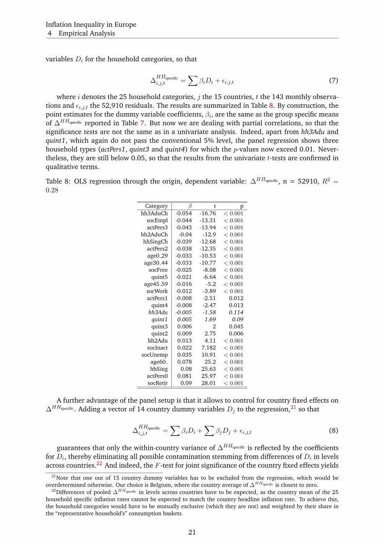
Another way to address this question is to regress ∆HHspecific through the origin on 25 dummy

18hh3AduCh, socEmpl, actPers3, hh2AduCh, hhSingCh, actPers2, age30 44, age0 29, socFree, quint5, age45 59, soc-

Work, actPers1, quint4; sorted in ascendant order19quint3, quint2, hh2Adu, socInact, socUnemp, age60 , hhSing, actPers0, socRetir20An exception to this observation is the hhSingCh category, where we would expect single mothers living on

transfer incomes to dominate. In our dataset, this category however tends to be submitted to similar inflation levels

as the better off households.

20

Inflation Inequality in Europe

4 Empirical Analysis

variables Di for the household categories, so that

∆HHspecific

i,j,t =∑

βiDi + ǫi,j,t (7)

where i denotes the 25 household categories, j the 15 countries, t the 143 monthly observa-

tions and ǫi,j,t the 52,910 residuals. The results are summarized in Table 8. By construction, the

point estimates for the dummy variable coefficients, βi, are the same as the group specific means

of ∆HHspecific reported in Table 7. But now we are dealing with partial correlations, so that the

significance tests are not the same as in a univariate analysis. Indeed, apart from hh3Adu and

quint1, which again do not pass the conventional 5% level, the panel regression shows three

household types (actPers1, quint3 and quint4) for which the p-values now exceed 0.01. Never-

theless, they are still below 0.05, so that the results from the univariate t-tests are confirmed in

qualitative terms.

Table 8: OLS regression through the origin, dependent variable: ∆HHspecific , n = 52910, R2 =0.28

Category β t p

hh3AduCh -0.054 -16.76 < 0.001

socEmpl -0.044 -13.31 < 0.001

actPers3 -0.043 -13.94 < 0.001

hh2AduCh -0.04 -12.9 < 0.001

hhSingCh -0.039 -12.68 < 0.001

actPers2 -0.038 -12.35 < 0.001

age0 29 -0.033 -10.53 < 0.001

age30 44 -0.033 -10.77 < 0.001

socFree -0.025 -8.08 < 0.001

quint5 -0.021 -6.64 < 0.001

age45 59 -0.016 -5.2 < 0.001

socWork -0.012 -3.89 < 0.001

actPers1 -0.008 -2.51 0.012

quint4 -0.008 -2.47 0.013

hh3Adu -0.005 -1.58 0.114

quint1 0.005 1.69 0.09

quint3 0.006 2 0.045

quint2 0.009 2.75 0.006

hh2Adu 0.013 4.11 < 0.001

socInact 0.022 7.182 < 0.001

socUnemp 0.035 10.91 < 0.001

age60 0.078 25.2 < 0.001

hhSing 0.08 25.63 < 0.001

actPers0 0.081 25.97 < 0.001

socRetir 0.09 28.01 < 0.001

A further advantage of the panel setup is that it allows to control for country fixed effects on

∆HHspecific . Adding a vector of 14 country dummy variables Dj to the regression,21 so that

∆HHspecific

i,j,t =∑

βiDi +∑

βjDj + ǫi,j,t (8)

guarantees that only the within-country variance of ∆HHspecific is reflected by the coefficients

for Di, thereby eliminating all possible contamination stemming from differences of Di in levels

across countries.22 And indeed, the F -test for joint significance of the country fixed effects yields

21Note that one out of 15 country dummy variables has to be excluded from the regression, which would be

overdetermined otherwise. Our choice is Belgium, where the country average of ∆HHspecific is closest to zero.22Differences of pooled ∆

HHspecific in levels across countries have to be expected, as the country mean of the 25

household specific inflation rates cannot be expected to match the country headline inflation rate. To achieve this,

the household categories would have to be mutually exclusive (which they are not) and weighted by their share in

the “representative household’s” consumption baskets.

21

Inflation Inequality in Europe

4 Empirical Analysis

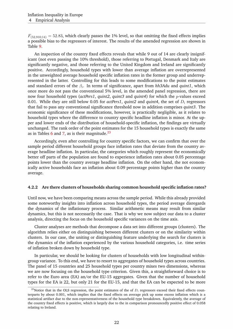
F(52,910;14) = 52.83, which clearly passes the 1% level, so that omitting the fixed effects implies

a possible bias to the regressors of interest. The results of the amended regression are shown in

Table 9.

An inspection of the country fixed effects reveals that while 9 out of 14 are clearly insignif-

icant (not even passing the 10% threshold), those referring to Portugal, Denmark and Italy are

significantly negative, and those referring to the United Kingdom and Ireland are significantly

positive. Accordingly, household types with lower than average inflation are overrepresented

in the unweighted average household specific inflation rates in the former group and underrep-

resented in the latter. Controlling for this leads to some modifications to the point estimates

and standard errors of the βi. In terms of significance, apart from hh3Adu and quint1, which

once more do not pass the conventional 5% level, in the amended panel regression, there are

now four household types (actPers1, quint2, quint3 and quint4) for which the p-values exceed

0.01. While they are still below 0.05 for actPers1, quint2 and quint4, the set of Di regressors

that fail to pass any conventional significance threshold now in addition comprises quint3. The

economic significance of these modifications, however, is practically negligible, as it relates to

household types where the difference to country specific headline inflation is minor. At the up-

per and lower ends of the distribution of household-specific inflation, the findings are virtually

unchanged. The rank order of the point estimates for the 15 household types is exactly the same

as in Tables 6 and 7, as is their magnitude.23

Accordingly, even after controlling for country specific factors, we can confirm that over the

sample period different household groups face inflation rates that deviate from the country av-

erage headline inflation. In particular, the categories which roughly represent the economically

better off parts of the population are found to experience inflation rates about 0.05 percentage

points lower than the country average headline inflation. On the other hand, the not econom-

ically active households face an inflation about 0.09 percentage points higher than the country

average.

4.2.2 Are there clusters of households sharing common household specific inflation rates?

Until now, we have been comparing means across the sample period. While this already provided

some noteworthy insights into inflation across household types, the period average disregards

the dynamics of the inflationary process. Similar arithmetic means may result from similar

dynamics, but this is not necessarily the case. That is why we now subject our data to a cluster

analysis, directing the focus on the household specific variances on the time axis.

Cluster analyses are methods that decompose a data set into different groups (clusters). The

algorithm relies either on distinguishing between different clusters or on the similarity within

clusters. In our case, the uniting or distinguishing feature underlying the search for clusters is

the dynamics of the inflation experienced by the various household categories, i.e. time series

of inflation broken down by household type.

In particular, we should be looking for clusters of households with low longitudinal within-

group variance. To this end, we have to resort to aggregates of household types across countries.

The panel of 15 countries and 25 household types per country mixes two dimensions, whereas

we are now focusing on the household type criterion. Given this, a straightforward choice is to

refer to the Euro area (EA) an/or the EU-15 aggregates. Given that the number of household

types for the EA is 22, but only 21 for the EU-15, and that the EA can be expected to be more

23Notice that in the OLS regression, the point estimates of the of Di regressors exceed their fixed effects coun-

terparts by about 0.001, which implies that the fixed effects on average pick up some excess inflation which is a

statistical artifact due to the non-representativeness of the household type breakdown. Equivalently, the average of

the country fixed effects is positive, which is largely due to the in comparison pronouncedly positive effect of 0.058

relating to Ireland.

22

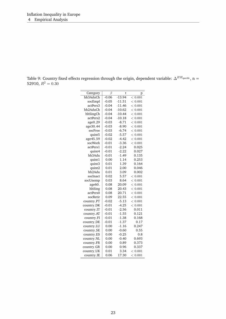
Inflation Inequality in Europe

4 Empirical Analysis

Table 9: Country fixed effects regression through the origin, dependent variable: ∆HHspecific , n =

52910, R2 = 0.30

Category β t p

hh3AduCh -0.06 -13.94 < 0.001

socEmpl -0.05 -11.51 < 0.001

actPers3 -0.04 -11.46 < 0.001

hh2AduCh -0.04 -10.62 < 0.001

hhSingCh -0.04 -10.44 < 0.001

actPers2 -0.04 -10.18 < 0.001

age0 29 -0.03 -8.71 < 0.001

age30 44 -0.03 -8.90 < 0.001

socFree -0.03 -6.74 < 0.001

quint5 -0.02 -5.57 < 0.001

age45 59 -0.02 -4.42 < 0.001

socWork -0.01 -3.36 < 0.001

actPers1 -0.01 -2.24 0.025

quint4 -0.01 -2.22 0.027

hh3Adu -0.01 -1.49 0.135

quint1 0.00 1.14 0.253

quint3 0.01 1.39 0.164

quint2 0.01 2.00 0.046

hh2Adu 0.01 3.09 0.002

socInact 0.02 5.57 < 0.001

socUnemp 0.03 8.64 < 0.001

age60 0.08 20.09 < 0.001

hhSing 0.08 20.43 < 0.001

actPers0 0.08 20.71 < 0.001

socRetir 0.09 22.55 < 0.001

country PT -0.02 -5.13 < 0.001

country DK -0.01 -4.25 < 0.001

country IT -0.01 -2.56 0.011

country AT -0.01 -1.55 0.121

country FI -0.01 -1.38 0.168

country DE -0.01 -1.37 0.17

country LU 0.00 -1.16 0.247

country SE 0.00 -0.60 0.55

country ES 0.00 -0.25 0.8

country NL 0.00 -0.40 0.693

country FR 0.00 0.89 0.373

country GR 0.00 0.96 0.337

country UK 0.01 3.34 < 0.001

country IE 0.06 17.30 < 0.001

23

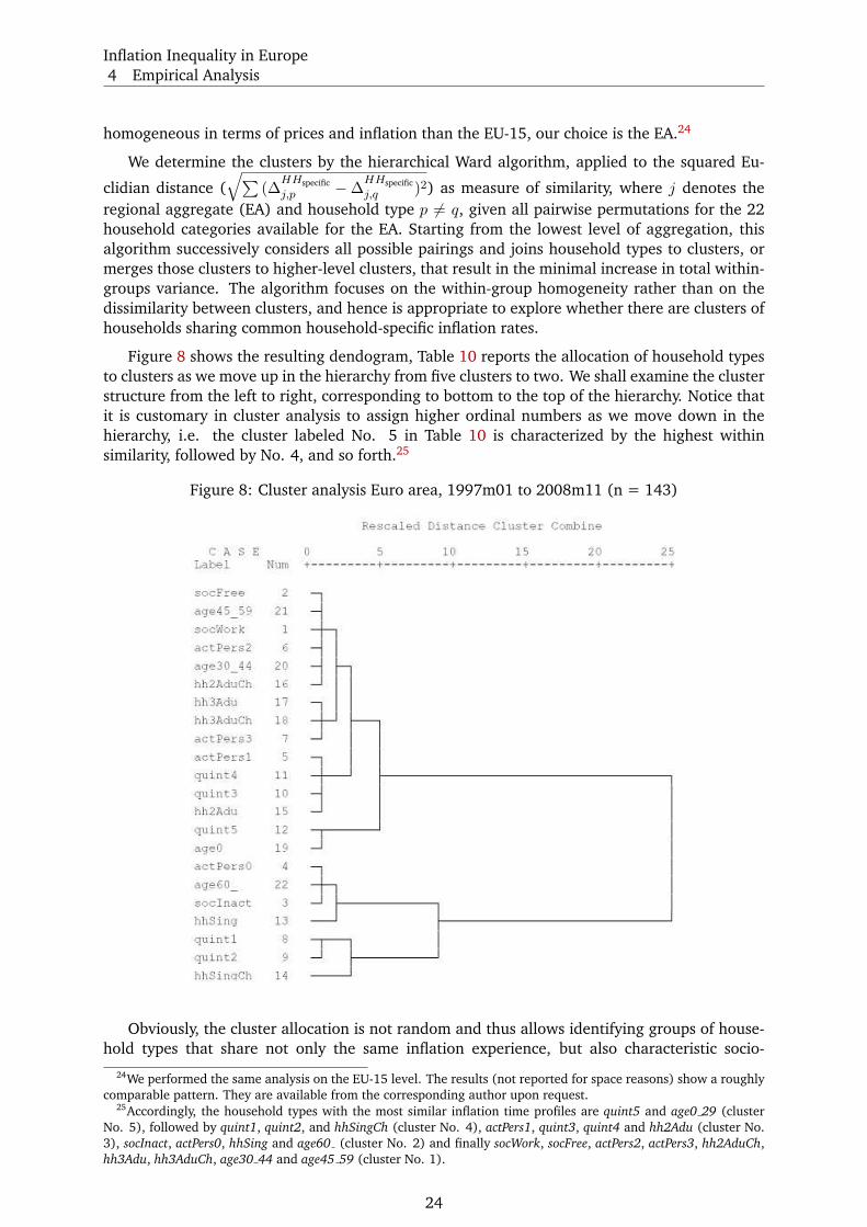
Inflation Inequality in Europe

4 Empirical Analysis

homogeneous in terms of prices and inflation than the EU-15, our choice is the EA.24

We determine the clusters by the hierarchical Ward algorithm, applied to the squared Eu-

clidian distance (

√∑(∆

HHspecific

j,p −∆HHspecific

j,q )2) as measure of similarity, where j denotes the

regional aggregate (EA) and household type p 6= q, given all pairwise permutations for the 22

household categories available for the EA. Starting from the lowest level of aggregation, this

algorithm successively considers all possible pairings and joins household types to clusters, or

merges those clusters to higher-level clusters, that result in the minimal increase in total within-

groups variance. The algorithm focuses on the within-group homogeneity rather than on the

dissimilarity between clusters, and hence is appropriate to explore whether there are clusters of

households sharing common household-specific inflation rates.

Figure 8 shows the resulting dendogram, Table 10 reports the allocation of household types

to clusters as we move up in the hierarchy from five clusters to two. We shall examine the cluster

structure from the left to right, corresponding to bottom to the top of the hierarchy. Notice that

it is customary in cluster analysis to assign higher ordinal numbers as we move down in the

hierarchy, i.e. the cluster labeled No. 5 in Table 10 is characterized by the highest within

similarity, followed by No. 4, and so forth.25

Figure 8: Cluster analysis Euro area, 1997m01 to 2008m11 (n = 143)

Obviously, the cluster allocation is not random and thus allows identifying groups of house-

hold types that share not only the same inflation experience, but also characteristic socio-

24We performed the same analysis on the EU-15 level. The results (not reported for space reasons) show a roughly

comparable pattern. They are available from the corresponding author upon request.25Accordingly, the household types with the most similar inflation time profiles are quint5 and age0 29 (cluster

No. 5), followed by quint1, quint2, and hhSingCh (cluster No. 4), actPers1, quint3, quint4 and hh2Adu (cluster No.

3), socInact, actPers0, hhSing and age60 (cluster No. 2) and finally socWork, socFree, actPers2, actPers3, hh2AduCh,

hh3Adu, hh3AduCh, age30 44 and age45 59 (cluster No. 1).

24

Inflation Inequality in Europe

4 Empirical Analysis

Table 10: Cluster membership

Variable 5 Clusters 4 Clusters 3 Clusters 2 Clusters

socWork 1 1 1 1

socFree 1 1 1 1

actPers2 1 1 1 1

actPers3 1 1 1 1

hh2AduCh 1 1 1 1

hh3Adu 1 1 1 1

hh3AduCh 1 1 1 1

age30 44 1 1 1 1

age45 59 1 1 1 1

socInact 2 2 2 2

actPers0 2 2 2 2

hhSing 2 2 2 2

age60 2 2 2 2

actPers1 3 1 1 1

quint3 3 1 1 1

quint4 3 1 1 1

hh2Adu 3 1 1 1

quint1 4 3 3 2

quint2 4 3 3 2

hhSingCh 4 3 3 2

quint5 5 4 1 1

age0 29 5 4 1 1

economic features leading to the former. Cluster 5 – the tightest – comprises the young an

rich; we might dub it the “yuppies”. Cluster 4 bundles the low socio-economic status (SES)

households. Middle class income earners are sharing the Cluster 3 inflation experience. Clus-

ter 2 mainly consist of the economically inactive and elderly. Finally, cluster 1 – the loosest –

comprises “classical” role model households with children, mostly middle-aged, actively earning

incomes as employees or self employed.

Notably, the clusters can to some degree be associated with a ranking according to the pre-

vailing SES (tentatively, in ascending order: No. 5 → No. 3 → No. 1 → No. 2 → No. 4).

Moving up the hierarchy implies lumping together household types that are increasingly dissim-

ilar in terms of the inflation dynamics experienced during the sample period. As Table 10 shows,

the four cluster solution merges the “middle class” cluster with the “classical” household types.

Reducing the number of clusters to three adds the “yuppie” cluster to the former merger. With

only two clusters, the low SES cluster is merged with the socially inactive/elderly cluster. Ac-

cordingly, the top-level dichotomization draws a dividing line between the low SES and socially

inactive/ elderly households (clusters No. 2 and 5 down the hierarchy) on the one side, and the

rest of the population on the other. Thus, similarity in experienced inflation dynamics tends to

correspond to similarity in SES.

The answer to the question whether there are clusters of households sharing common house-

hold specific inflation rates, is hence affirmative. This allows us to link the findings from the

cluster analysis with the main results from the previous section. In particular, in section 4.2.1

we showed that, over the considered time span, lower SES and otherwise socially marginalized

households were exposed to higher average inflation than more elevated SES households. On

the basis of the analysis carried out in this section, we can conclude that clusters of similar

SES display similar dynamics: households within the same cluster experience similar deviations

between their own inflation and the average process.

25

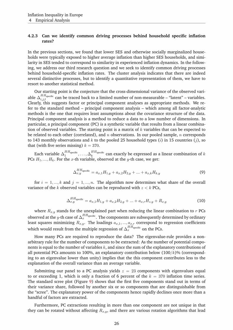
Inflation Inequality in Europe

4 Empirical Analysis

4.2.3 Can we identify common driving processes behind household specific inflation

rates?

In the previous sections, we found that lower SES and otherwise socially marginalized house-

holds were typically exposed to higher average inflation than higher SES households, and simi-

larity in SES tended to correspond to similarity in experienced inflation dynamics. In the follow-

ing, we address our third research question and we seek to identify common driving processes

behind household-specific inflation rates. The cluster analysis indicates that there are indeed

several distinctive processes, but to identify a quantitative representation of them, we have to

resort to another statistical method.

Our starting point is the conjecture that the cross-dimensional variance of the observed vari-

able ∆HHspecific

i,j,t can be traced back to a limited number of non-measurable – “latent” – variables.

Clearly, this suggests factor or principal component analyses as appropriate methods. We re-

fer to the standard method – principal component analysis – which among all factor-analytic

methods is the one that requires least assumptions about the covariance structure of the data.

Principal component analysis is a method to reduce a data to a low number of dimensions. In

particular, a principal component (PC) is a synthetic variable that results from a linear combina-

tion of observed variables. The starting point is a matrix of k variables that can be expected to

be related to each other (correlated), and n observations. In our pooled sample, n corresponds

to 143 monthly observations and k to the pooled 25 household types (i) in 15 countries (j), so

that (with five series missing) k = 370.

Each variable ∆HHspecific

1 , . . . ,∆HHspecific

k can exactly be expressed as a linear combination of kPCs H1, ..., Hk. For the x-th variable, observed at the y-th case, we get:

∆HHspecificx,y = ax,1H1,y + ax,2H2,y + ...+ ax,kHk,y (9)

for i = 1, ..., k and j = 1, ..., n. The algorithm now determines what share of the overall

variance of the k observed variables can be reproduced with z < k PCs,

∆HHspecificx,y = ax,1H1,y + ax,2H2,y + ...+ ax,rHz,y +Rx,y (10)

where Rx,y stands for the unexplained part when reducing the linear combination to r PCs

observed at the y-th case of ∆HHspecificx . The components are subsequently determined by ordinary

least squares minimizing Rx,y. The loadings ax,1, ..., ax,r correspond to regression coefficients

which would result from the multiple regression of ∆HHspecificx on the PCs.

How many PCs are required to reproduce the data? The eigenvalue-rule provides a non-

arbitrary rule for the number of components to be extracted: As the number of potential compo-

nents is equal to the number of variables k, and since the sum of the explanatory contributions of

all potential PCs amounts to 100%, an explanatory contribution below (100/k)% (correspond-

ing to an eigenvalue lower than unity) implies that the this component contributes less to the

explanation of the overall variance than an average variable.

Submitting our panel to a PC analysis yields z = 23 components with eigenvalues equal

to or exceeding 1, which is only a fraction of 6 percent of the k = 370 inflation time series.

The standard scree plot (Figure 9) shows that the first five components stand out in terms of

their variance share, followed by another six or so components that are distinguishable from

the “scree”. The explanatory power of the components hence rapidly declines once more than a

handful of factors are extracted.

Furthermore, PC extractions resulting in more than one component are not unique in that

they can be rotated without affecting Rx,y, and there are various rotation algorithms that lead

26

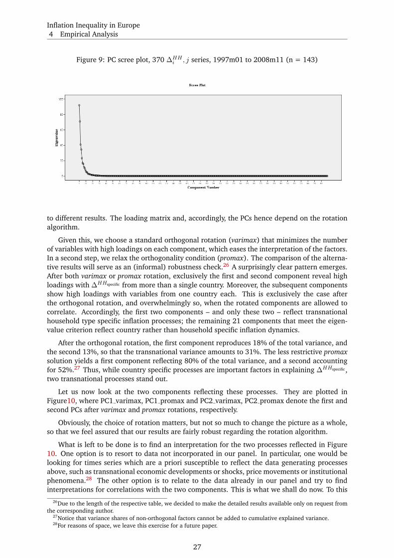
Inflation Inequality in Europe

4 Empirical Analysis

Figure 9: PC scree plot, 370 ∆HHi , j series, 1997m01 to 2008m11 (n = 143)

to different results. The loading matrix and, accordingly, the PCs hence depend on the rotation

algorithm.

Given this, we choose a standard orthogonal rotation (varimax) that minimizes the number

of variables with high loadings on each component, which eases the interpretation of the factors.

In a second step, we relax the orthogonality condition (promax). The comparison of the alterna-

tive results will serve as an (informal) robustness check.26 A surprisingly clear pattern emerges.

After both varimax or promax rotation, exclusively the first and second component reveal high

loadings with ∆HHspecific from more than a single country. Moreover, the subsequent components

show high loadings with variables from one country each. This is exclusively the case after

the orthogonal rotation, and overwhelmingly so, when the rotated components are allowed to

correlate. Accordingly, the first two components – and only these two – reflect transnational

household type specific inflation processes; the remaining 21 components that meet the eigen-

value criterion reflect country rather than household specific inflation dynamics.

After the orthogonal rotation, the first component reproduces 18% of the total variance, and

the second 13%, so that the transnational variance amounts to 31%. The less restrictive promax

solution yields a first component reflecting 80% of the total variance, and a second accounting

for 52%.27 Thus, while country specific processes are important factors in explaining ∆HHspecific ,

two transnational processes stand out.

Let us now look at the two components reflecting these processes. They are plotted in

Figure10, where PC1 varimax, PC1 promax and PC2 varimax, PC2 promax denote the first and

second PCs after varimax and promax rotations, respectively.

Obviously, the choice of rotation matters, but not so much to change the picture as a whole,

so that we feel assured that our results are fairly robust regarding the rotation algorithm.

What is left to be done is to find an interpretation for the two processes reflected in Figure

10. One option is to resort to data not incorporated in our panel. In particular, one would be

looking for times series which are a priori susceptible to reflect the data generating processes

above, such as transnational economic developments or shocks, price movements or institutional

phenomena.28 The other option is to relate to the data already in our panel and try to find

interpretations for correlations with the two components. This is what we shall do now. To this

26Due to the length of the respective table, we decided to make the detailed results available only on request from

the corresponding author.27Notice that variance shares of non-orthogonal factors cannot be added to cumulative explained variance.28For reasons of space, we leave this exercise for a future paper.

27

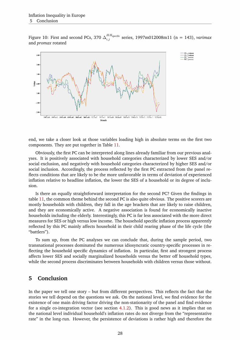
Inflation Inequality in Europe

5 Conclusion

Figure 10: First and second PCs, 370 ∆HHspecific

i,j series, 1997m012008m11 (n = 143), varimax

and promax rotated

end, we take a closer look at those variables loading high in absolute terms on the first two

components. They are put together in Table 11.

Obviously, the first PC can be interpreted along lines already familiar from our previous anal-

yses. It is positively associated with household categories characterized by lower SES and/or

social exclusion, and negatively with household categories characterized by higher SES and/or

social inclusion. Accordingly, the process reflected by the first PC extracted from the panel re-

flects conditions that are likely to be the more unfavorable in terms of deviation of experienced

inflation relative to headline inflation, the lower the SES of a household or its degree of inclu-

sion.

Is there an equally straightforward interpretation for the second PC? Given the findings in

table 11, the common theme behind the second PC is also quite obvious. The positive scorers are

mostly households with children, they fall in the age brackets that are likely to raise children,

and they are economically active. A negative association is found for economically inactive

households including the elderly. Interestingly, this PC is far less associated with the more direct

measures for SES or high versus low income. The household specific inflation process apparently

reflected by this PC mainly affects household in their child rearing phase of the life cycle (the

“battlers”).

To sum up, from the PC analyses we can conclude that, during the sample period, two

transnational processes dominated the numerous idiosyncratic country-specific processes in re-

flecting the household specific dynamics of inflation. In particular, first and strongest process

affects lower SES and socially marginalized households versus the better off household types,

while the second process discriminates between households with children versus those without.

5 Conclusion

In the paper we tell one story – but from different perspectives. This reflects the fact that the

stories we tell depend on the questions we ask. On the national level, we find evidence for the

existence of one main driving factor driving the non-stationarity of the panel and find evidence

for a single co-integration vector (see section 4.1.2). This is good news as it implies that on

the national level individual household’s inflation rates do not diverge from the “representative

rate” in the long-run. However, the persistence of deviations is rather high and therefore the

28

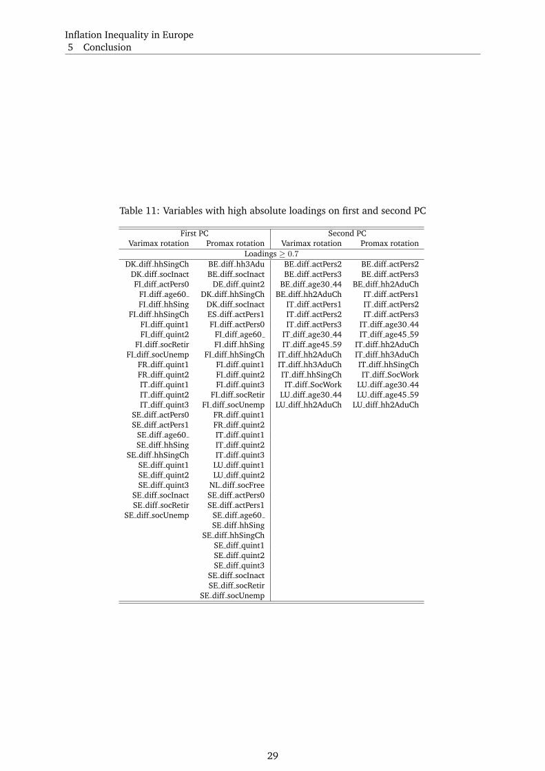
Inflation Inequality in Europe

5 Conclusion

Table 11: Variables with high absolute loadings on first and second PC

First PC Second PC

Varimax rotation Promax rotation Varimax rotation Promax rotation

Loadings ≥ 0.7

DK diff hhSingCh BE diff hh3Adu BE diff actPers2 BE diff actPers2

DK diff socInact BE diff socInact BE diff actPers3 BE diff actPers3

FI diff actPers0 DE diff quint2 BE diff age30 44 BE diff hh2AduCh

FI diff age60 DK diff hhSingCh BE diff hh2AduCh IT diff actPers1

FI diff hhSing DK diff socInact IT diff actPers1 IT diff actPers2

FI diff hhSingCh ES diff actPers1 IT diff actPers2 IT diff actPers3

FI diff quint1 FI diff actPers0 IT diff actPers3 IT diff age30 44

FI diff quint2 FI diff age60 IT diff age30 44 IT diff age45 59

FI diff socRetir FI diff hhSing IT diff age45 59 IT diff hh2AduCh

FI diff socUnemp FI diff hhSingCh IT diff hh2AduCh IT diff hh3AduCh

FR diff quint1 FI diff quint1 IT diff hh3AduCh IT diff hhSingCh

FR diff quint2 FI diff quint2 IT diff hhSingCh IT diff SocWork

IT diff quint1 FI diff quint3 IT diff SocWork LU diff age30 44

IT diff quint2 FI diff socRetir LU diff age30 44 LU diff age45 59

IT diff quint3 FI diff socUnemp LU diff hh2AduCh LU diff hh2AduCh

SE diff actPers0 FR diff quint1

SE diff actPers1 FR diff quint2

SE diff age60 IT diff quint1

SE diff hhSing IT diff quint2

SE diff hhSingCh IT diff quint3

SE diff quint1 LU diff quint1

SE diff quint2 LU diff quint2

SE diff quint3 NL diff socFree

SE diff socInact SE diff actPers0

SE diff socRetir SE diff actPers1

SE diff socUnemp SE diff age60

SE diff hhSing

SE diff hhSingCh

SE diff quint1

SE diff quint2

SE diff quint3

SE diff socInact

SE diff socRetir

SE diff socUnemp

29

Inflation Inequality in Europe

5 Conclusion

adjustment speed towards the “representative household” is low. From a policy perspective, this

means that even if there is no concern about a long-run stable distribution of inflation rates,

over a short- to medium term horizon, deviations tend to be lasting.

On the aggregate level, we can find small but significant differences in the deviations of

household-specific inflation rates from the reference rate – mainly along income and education

levels. We can separate five clusters and we identify two main driving forces for the differences in

the overall panel. These “driving forces” are related to low-income households and households

with children. All in all, even if differences in the deviations of household-specific inflation rates

from the reference rate are small in general, they are not negligible and persistent enough to

be a serious topic of economic and social policy. Uncomfortably, our results suggest that some

of the economically more vulerable parts of the population may be subject to group-specific

inflation dynamics resulting in higher-than-average inflation. To the extent that the cumulative

effects wipe out purchasing power of the economically disadvanteged, welfare payments aiming

at provoding the subsistence level of income must be monitored carefully to avoid letting the

recepints slide into absoltue poverty.

Further research should concentrate on the quality of data. We approximated the distribution

of different types of households in a unweighted manner. This is of course not the only way to

deal with the data. We could weight the households in the panel according to their income level

to get a more appropriate view on what is going on if the data were available (which was not

the case). Further research should focus on micro-data to identify the driving factors behind

differences more clearly. Furthermore, techniques like the σ-convergence test by Quah (1997)

as used in Hobijn and Lagakos (2005) could be applied if micro-data were available.

30

Inflation Inequality in Europe

References

References

Allsopp, C. and M. Artis, “The Assessment: EMU, Four Years On,” Oxford Review of Economic Policy, 2003, 19 (1),

1–29.

Altissimo, F., M. Ehrmann, and Frank Smets, “Inflation persistence and price setting behaviour in the Euro area. A

summary of the IPN evidence.,” Occasional Paper Series 46, European Central Bank 2006.

Amble, Nathan and Kenneth J. Stewart, “Experimental Price Index for Elderly Consumers,” Monthly Labor Review,

May 1994, 117 (5), 11–16.

Bai, J. and S. Ng, “A PANIC attack on unit roots and cointegration,” Econometrica, 2004, 72, 1127–1177.

Bai, Juchan and Serena Ng, “A PANIC Attack on Unit Roots and Cointegration,” Boston College Working Paper in

Economics, December 2001, 519.

Bernard, A. B. and S. N. Durlauf, “Interpreting tests of the convergence hypothesis,” Journal of Econometrics, 1996,

71, 161–173.

Blank, Rebecca M. and Alan M. Blinder, “Macroeconomics, Income Distribution, and Poverty?,” Technical Report,

NBER 1985.

Brewer, Mike, Alissa Goodman, and Andrew Leicester, Household Spending in Britain - What Can It Teach Us About

Poverty?, 1 ed., Bristol: The Policy Press, April 2006.

Campolmi, A. and E. Faia, “Cyclical inflation divergence and different labor market institutions in the EMU.,”

Working Paper Series 619, European Central Bank 2006.

Carroll, Christopher D., Misuzu Otsuka, and Jiri Slacalek, “What Is the Wealth Effect on Consumption? A New

Approach,” mimeo, Johns Hopkins University 2006.

Cecchetti, S. and R. Moessner, “Commodity prices and inflation dynamics,” BIS Quarterly Review, December 2008,

34 (4), 55–66.

Chiru, Radu, “Does Inflation Vary With Income?,” Statistics Canada Analytical Paper, June 2005, Catalogue no. 11-

621-MIE – No. 030.

, “Is Inflation Higher for Seniors?,” Statistics Canada Analytical Paper, May 2005, Catalogue no. 11-621-MIE – No.

027.

Choi, In, “Unit Root Tests for Panel Data,” Journal for International Money and Finance, April 2001, 20 (2), 249–272.

Crawford, Ian and Zoe Smith, “Distributional Aspects of Inflation,” IFS (Institute for Fiscal Studies) Commentary,

June 2002, 90.

Cutler, David M. and Lawrence F. Katz, “Macroeconomic Performance and the Disadvantaged,” Brookings Papers

on Economic Activity, 1991, 22 (1991-2), 1–74.

Dickey, D.A. and W.A. Fuller, “Distribution of the Estimators for Autoregressive Time Series with a Unit Root,”

Journal of the American Statistical Association, 1979, 74, 427–431.

Dickey, David A. and Wayne A. Fuller, “Distribution of the Estimators for Autoregressive Time Series With a Unit

Root,” Journal of the American Statistical Association, June 1979, 74 (366), 427–431.

Dullien, S. and U. Fritsche, “How bad is divergence in the euro zone? Lessons from the United States and Germany,”

Journal of Post Keynesian Economics, 2009, 31, 431–459.

Dullien, Sebastian and Daniela Schwarzer, “Bringing Macroeconomics into the EU Budget Debate: Why and

How?,” Journal of Common Market Studies, 2009, 47 (1), 153–174.

and Ulrich Fritsche, “Does the Dispersion of Unit Labor Cost Dynamics in the EMU Imply Long-run Divergence?

Results from a Comparison with the United States of America and Germany.,” Journal of International Economics

and Economic Policy, November 2008, 5 (3), 269–295.

Easterly, William and Stanley Fischer, “Inflation and the Poor,” Journal of Money, Credit and Banking, May 2001,

33 (2), 160–78.

Eichengreen, B., “The Breakup of the Euro Area,” NBER Working Paper 13393, NBER 2007.

31

Inflation Inequality in Europe

References

Elliott, Graham, Thomas J. Rothenberg, and James H. Stock, “Efficient Tests for an Autoregressive Root,” Econo-

metrica, 1996, 64, 813–836.

Engle, R. and C. W. Granger, “Co-integration and Error Correction: Representation, Estimation, and Testing,”

Econometrica, 1987, 55, 251–276.

European Central Bank, “Inflation Persistence and Price Setting Behaviour in the Euro Area,” report 2005. available

at http://www.ecb.int/home/pdf/research/inflationpersistencepricesettingreport.pdf.

European Commission, “EMU@10: successes and challenges after 10 years of Economic and Monetary Union,”

European Economy 2 2008.

Fritsche, U., C. Logeay, K. Lommatzsch, K. Rietzler, S. Stephan, R. Zwiener, C. Kiziltepe, and Ch. Proano Acosta,

“Auswirkungen von landerspezifischen Differenzen in der Lohn-, Preisniveau und Produktivitatsentwicklung auf

Wachstum und Beschaftigung in den Landern des Euroraums,” Politikberatung kompakt 08/2005, Deutsches In-

stitut fur Wirtschaftsforschung (DIW Berlin) 2005.

Garner, Thesia I., David S. Johnson, and Mary F. Kokoski, “An Experimental Consumer Price Index for the Poor,”

Monthly Labor Review, September 1996, 119 (9), 32–42.

Gros, D., “Will EMU survive 2010?,” Technical Report, Centre for European Policy Studies 2006.

Hagemann, Robert P., “The Variability of Inflation Rates across Household Types,” Journal of Money, Credit and

Banking, November 1982, 14 (4 (1)), 494–510.

Hobijn, Bart and David Lagakos, “Inflation Inequality in the United States,” Review of Income and Wealth, December

2005, 51 (4), 581–606.

Idson, Todd and Cynthia Miller, “The Implications of Demographic-Specific Inflation Rates for Trends in Real

Educational Wage Differentials,” Journal of Business and Economic Statistics, October 1997, 15 (4), 464–469.

Johansen, S., Likelihood-based Inference in Cointegrated Vector Autoregressive Models, Oxford: Oxford University

Press, 1995.

Kao, C., “Spurious Regression and Residual-Based Tests for Cointegration in Panel Data,” Journal of Econometrics,

1999, 90, 1–44.

Lane, Ph., “The real effects of EMU,” Discussion Paper Series 5536, CEPR 2006.

Lettau, Martin and Sydney Ludvigson, “Consumption, Aggregate Wealth, and Expected Stock Returns,” Journal of

Finance, 2001, 56 (3), 815–849.

Levin, A., C.-F. Lin, and C.-S. Chu, “Unit root tests in panel data: Asymptotic and finite sample properties,” Journal

of Econometrics, 2002, 108, 1–24.

Livada, Alexandra, “The Distribution of Household Inflation Rates: The Greek Experience,” Bulletin of Economic

Research, July 1990, 42 (3), 175–196.

Maddala, G. S. and S. Wu, “A Comparative Study of Unit Root Tests with Panel Data and A New Simple Test,” Oxford

Bulletin of Economics and Statistics, 1999, 61, 631–52.

and Shaowen Wu, “A Comparative Study of Unit Root Tests with Panel Data and a New Simple Test,” Oxford

Bulletin of Economics and Statistics, November 1999, 61 (Special Issue), 631–652.

Michael, Robert T., “Variation Across Households in the Rate of Inflation,” Journal of Money, Credit and Banking,

February 1979, 11 (1), 32–46.

Noll, Heinz-Herbert and Stefan Weick, Soziale Ungleichheit, Kulturelle Unterschiede - Verhandlungen des 32. Kon-

gresses der Deutschen Gesellschaft fr Soziologie in Mnchen 2004, 1 ed., Vol. Teilband 1, Frankfurt am Main: Campus,

August

and , “Einkommensarmut und Konsumarmut - unterschiedliche Perspektiven und Diagnosen,” ZUMA Informa-

tionsdienst Soziale Indikatoren (ISI), January 2007, 37, 1–6.

Quah, D. T., “Empirics for Growth and Distribution: Stratification, Polarization, and Convergence Clubs,” Journal of

Economic Growth, 1997, 2, 27–59.

Rippin, Franziska, “Gibt es gruppenspezifische Inflation? Eine Sensitivitatsanalyse mit Hilfe der Einkommens- und

Verbrauchsstichprobe,” Master’s thesis, University of Erfurt 2006.

32

Inflation Inequality in Europe

Appendix

Romer, Christina D. and David H. Romer, “Monetary policy and the well-being of the poor,” Proceedings, 1998,

pp. 159–201.

Slacalek, J., “What Drives Personal Consumption? The Role of Housing and Financial Wealth,” DIW Berlin Discussion

Paper 647, DIW Berlin 2006.

Appendix

Construction of Household-Specific Inflation Rates

The inflation rate in period t is defined as the ratio of weighted averages of the percentage price

changes of each of the goods categories between period t and a base period in the numerator

and between period t − 1 and a base period in the denominator. Let pj,t be the price index

for good category j at time t, and let t = b denote the base period. Furthermore, let wj,b be

the aggregate expenditure share of goods category j in the base period. Using this notation,

inflation is defined as follows:

πt =

m∑j=1

wj,bpj,tpj ,b

m∑j=1

wj,bpj,t−1

pj ,b

− 1 (11)

In other words, the inflation rate gauges the percentage change in the price of the base-

period goods basket between t − 1 and t. Nonetheless, the updates of the base period and of

the expenditure weights are rather infrequent, which is the main source of a substitution bias

in the index. This means that an inflation rate measured as described above does not properly

account for people substituting goods that become relatively cheaper for more expensive goods.

In order to minimize this drawback our inflation rates are calculated as chain-weighted indices,

i.e. updating the expenditure weights in every time period, rather than use weights from some

base period. By setting b = t− 1 in (11), we obtain an alternative measure of inflation

πIt =

m∑

j=1

wj,t−1pj,t

pj, t− 1− 1 =

m∑

j=1

wj,t−1

(pj,tpj,t−1

− 1

)=

m∑

j=1

wj,t−1πj,t (12)

Employing monthly price data that are not seasonally adjusted results in inflation rates fea-

turing seasonal fluctuations. We overcome this issue by considering annual inflation rates, i.e.

we compare current prices with those twelve months earlier.29

So far, our definition of household-specific inflation rate does not contain any household-

specific dimension. In principle, we would need both household-specific expenditure weights

and household-specific price changes. For each household, which we will index by i, we observe

its specific expenditure shares, wi,j,t for each of the m goods categories. 30 However, the specific

prices that households pay for the goods categories are unknown. Therefore, we assumed that

all households face the same price increases, pj,t, for each goods category. The idea behind

29The methods leads in turn to a negative moving average effect in the residuals. As much as possible we are

taking this into consideration when we do our econometric analysis.30Throughout the time span considered in our analysis, Eurostat collected the household-specific expenditure

weights only in t = 1999 and t = 2005, whereas the usual consumer price index item weights according to the

COICOP 2 level, which provides information about the changes in the aggregate (representative, median) basket,

are adjusted and published on yearly basis. In order to cope with this missing data problem and obtain yearly

household-specific expenditure weights, we tracked the evolution of the consumer price index expenditure weights

over time and apply the observed changes to the 1999 weights of the characteristics group, keeping the relative

distance between the household-specific baskets and the consumer price index basket constant at the 1999 level.

33

Inflation Inequality in Europe

Appendix

this assumption is that for any particular goods category at each point in time each household

faces the same price increase as all other households, but the expenditure profiles they chose in

response to these prices are different. This is a common assumption when constructing group

price indices, as in Amble and Stewart (1994)and Garner et al. (1996)Garner et al. (1996).

Plugging the household-specific expenditure shares in the annual inflation rate as calculated in

(12) we arrive at our definition of a household inflation rate, πi,t for household i in month t:

πi,t =1

m∑j=1

w1999i,j,t−1

m∑

j=1

πj,tw1999i,j,t−1 (13)

Here πj,t is the inflation in goods category j over the year preceding month t and wi,j,t−1 is

household i’s expenditure share on good category j defined as:

w1999i,j,t−1 =

wHICPj,t−1

wHICPj,1999

w1999i,j,1999 (14)

where wHICPj,1999 and wHICP

j,t−1 refer to the HICP weights for item j in 1999 and (t−1), respectively,

while w1999i,j,1999 indicate the 1999 household-specific expenditure weight for good category j and

socio-economic category i.

The data are drawn from two sources. Data on household expenditures are obtained from

the Household Budget Surveys (HBSs). The HBSs are national surveys whose purpose is to

give a picture of living conditions of private households by looking at their total consumption

expenditure broken down by household characteristics such as income, socio-economic char-

acteristics, size and composition, degree of urbanisation and region.31 Two thirds of the EU

Member States carry out annual surveys and the remainder have five-yearly or longer intervals

between surveys. For this reason, throughout the considered time span the household-specific

consumption baskets are available only for 1999 and 2005. Data collection in the HBS involves

a combination of (a) interviews, and (b) diaries maintained by households and/or individuals,

generally on a daily basis. The basic unit of data collection and analysis in HBSs is the house-

hold. A crucial issue in the survey is the identification of the reference person (often the head of

the household) whose personal characteristics can be used in the classification and analysis of

information on the household. The socio-economic group, occupation and employment status,

income, sex and age of the reference person is often used to classify and present results. In

our analysis, we considered the following categories of household characteristics: employment

status of the reference person (manual workers in industry and services, non-manual workers

in industry and services, self-employed, unemployed, retired, inactive population); number of

active persons (0, 1, 2, 3 and more); income quintile (1 to 5); type of households (single person,

single parent with dependent children, two adults, two adults with dependent children, three or

more adults, three or more adults with dependent children); age of reference person (less than

30, 30 to 44 years, 45 to 59 years, 60 years and older).

Data on the spending structure on the aggregate level consist in the annual weights for

the HICP sub-indices on a national level. They represent the aggregate expenditure on any

goods category covered by the HICP, expressed as a proportion of the total expenditure on all

goods within the HICP coverage. Monthly price data are obtained from the HICP series for the

good categories according to the Classification of individual consumption by purpose (COICOP),

level 232, which includes: Food, Alcohol and Tobacco, Clothing, Utilities, Household Equipment,

31Due to lack of data availability, we discarded the categories “degree of urbanization” and “household’s primary

income source” from our analysis.32More disaggregated data are not available for all EU15 countries.

34

Inflation Inequality in Europe

Appendix

Health, Transport, Communications, Recreation and Culture, Education, Hotels and Restaurants,

and Miscellaneous.

To keep the headers of the time series short, we use a system of descriptors where the first

part (SOC, ACT, QUINT, HH, ...) refers to the household categories we use, whereas the second

part refers to subcategories. A complete overview of all time series, country abbreviations and a

list of descriptors can be found in Tables 12 to 14.

Table 12: Description of COICOP Categories

Category Description

cp1 Food, and non-alcoholic beverages

cp2 Alcoholic beverages and tobacco

cp3 Clothing and footwear

cp4 Housing, water, electricity, gas and other fuels

cp5 Furnishings, household equipment and maintenance of house

cp6 Health

cp7 Transport

cp8 Communication

cp9 Recreation and culture

cp10 Education

cp11 Hotels, cafes and restaurants

cp12 Miscellaneous goods and services

Table 13: Country Codes

Code Country

AT Austria

BE Belgium

DE Germany

DK Denmark

EA Euro Area

ES Spain

FI Finland

FR France

GR Greece

IE Ireland

IT Italy

LU Luxemburg

NL Netherlands

PT Portugal

SE Sweden

UK United Kingdom

35

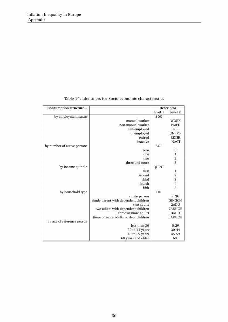
Inflation Inequality in Europe

Appendix

Table 14: Identifiers for Socio-economic characteristics

Consumption structure... Descriptor

level 1 level 2

by employment status SOC

manual worker WORK

non-manual worker EMPL

self-employed FREE

unemployed UNEMP

retired RETIR

inactive INACT

by number of active persons ACT

zero 0

one 1

two 2

three and more 3

by income quintile QUINT

first 1

second 2

third 3

fourth 4

fifth 5

by household type HH

single person SING

single parent with dependent children SINGCH

two adults 2ADU

two adults with dependent children 2ADUCH

three or more adults 3ADU

three or more adults w. dep. children 3ADUCH

by age of reference person

less than 30 0 29

30 to 44 years 30 44

45 to 59 years 45 59

60 years and older 60

36