Inflation and Unemloyment-DONE

1

Inflation and Unemployment

2

Inflation, Unemployment and the Phillips Curve

Two goals of economic policymakers are low inflation and low unemployment, but often these goals conflict.

Suppose that policymakers were to use monetary or fiscal policy to expand aggregate demand. This policy would move the economy along the short-run aggregate supply (SRAS) curve to a point of higher output and a higher price level. Higher output means lower unemployment, because firms employ more workers when they produce more. A higher price level, given the previous (year’s) price level, means higher inflation.

Thus, when policymakers move the economy up along the SRAS curve, they reduce the unemployment rate and raise inflation rate. In other words, in the short run, society faces a trade-off between inflation and unemployment.

3

Inflation, Unemployment and the Phillips Curve

Phillips curve: shows the short-run trade-off between inflation and unemployment

1958: New Zealand born economist A.W. Phillips showed that nominal wage growth was negatively correlated with unemployment in the U.K.

1960: Paul Samuelson & Robert Solow found a negative correlation between U.S. inflation & unemployment, named it “the Phillips Curve.”

4

Inflation, Unemployment and the Phillips Curve

The Phillips curve that economists use today differs in three ways from the relationship Phillips examined.

a) The modern Phillips curve substitutes price inflation for wage inflation. This difference is trivial, since price inflation and wage inflation are closely related. In periods when wages are rising quickly, prices are rising quickly as well.

b) The modern Phillips curve includes expected inflation. This addition is due to the work of Milton Friedman and Edmund Phelps, who during the 1960s have emphasized the importance of expectations for aggregate supply.

c) The modern Phillips curve includes supply shocks. Credit for this addition goes to OPEC, which in 1970s caused large increases in the world price of oil, which made economists more aware of the importance of shocks to aggregate supply.

5

Inflation, Unemployment and the Phillips Curve

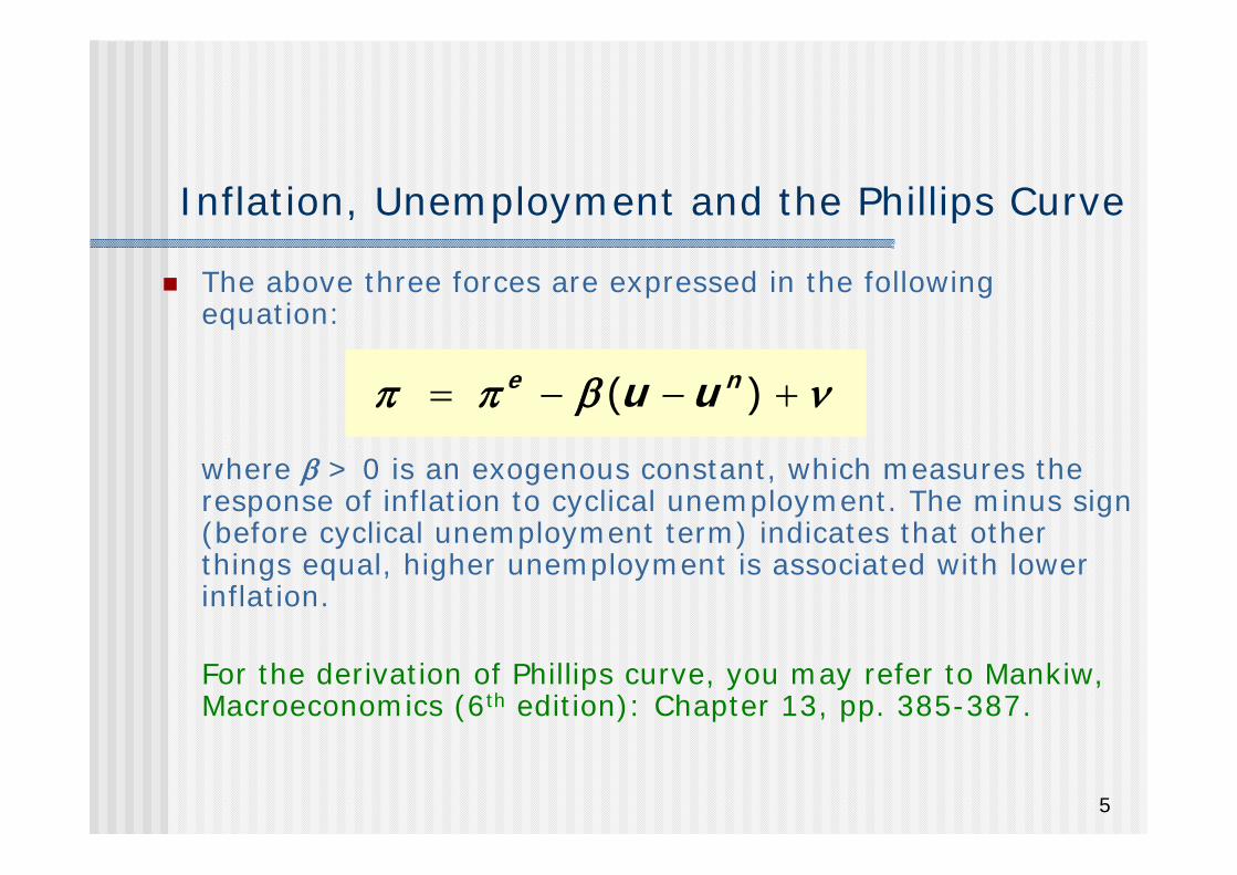
The above three forces are expressed in the following equation:

where > 0 is an exogenous constant, which measures the response of inflation to cyclical unemployment. The minus sign (before cyclical unemployment term) indicates that other things equal, higher unemployment is associated with lower inflation.

For the derivation of Phillips curve, you may refer to Mankiw, Macroeconomics (6th edition): Chapter 13, pp. 385-387.

( ) e nu u ( ) e nu u

6

Adaptive Expectations and Inflation Inertia

What determines expected inflation?

A simple and plausible assumption is that people form their expectations of inflation based on recently observed inflation. This assumption is called adaptive expectations.

A simple example: Expected inflation = last year’s actual inflation, i.e., 1

e

Then, the Phillips curve becomes

1 ( )nu u

When the Phillips curve is written in this form, the natural rate of unemployment is sometimes called the Non-Accelerating Rate of Unemployment, or NAIRU

7

Adaptive Expectations and Inflation Inertia

In this form, the Phillips curve implies that inflation has inertia:

In the absence of supply shocks or cyclical unemployment, inflation will continue indefinitely at its current rate, unless something acts to stop it. In particular, if unemployment is at the NAIRU and if there are no supply shocks, the continued rise in the price level neither speeds up nor slows down.

Past inflation influences expectations of current inflation, which in turn influences the wages & prices that people set.

8

Supply Shock supply shock: an event that directly alters firms’ costs and

prices, shifting the economy’s aggregate-supply curve and thus the Phillips curve.

Examples of adverse supply shocks:

Bad weather reduces crop yields, pushing up food prices

Workers unionize, negotiate wage increases

New environmental regulations require firms to reduce emissions. Firms charge higher prices to help cover the costs of compliance

Graphically, we could represent these supply shocks as a shift in the short-run aggregate-supply curve to the left

The decrease in equilibrium output and the increase in the price level left the economy with stagflation (high inflation with low output and employment).

9

Supply Shock

Given this turn of events, policymakers are left with a less favorable short-run trade-off between unemployment and inflation.

If they increase aggregate demand to fight unemployment, they will raise inflation further.

If they lower aggregate demand to fight inflation, they will raise unemployment further.

10

The 1970s Oil Shock OPEC (Organization of Petroleum Exporting Countries) is a cartel,

which is an organization of suppliers that coordinate production levels and prices.

OPEC first demonstrated its muscle in 1974: in the aftermath of a war in the Middle East (Yom Kippur War), several OPEC producers limited their output - referred to as Arab Oil embargo.

Oil prices rose11% in 197368% in 197416% in 1975

Such sharp oil price increases are supply shocks because they significantly impact production costs and prices (Oil is required to heat the factories in which goods are produced, and to fuel the trucks that transport the goods from the factories to the warehouses to Retail stores. A sharp increase in the price of oil, therefore, has a substantial effect on production costs).

11

The 1970s Oil Shock

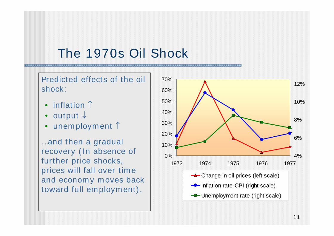
Predicted effects of the oil shock:

• inflation • output • unemployment

…and then a gradual recovery (In absence of further price shocks, prices will fall over time and economy moves back toward full employment).

0%

10%

20%

30%

40%

50%

60%

70%

1973 1974 1975 1976 19774%

6%

8%

10%

12%

Change in oil prices (left scale)

Inflation rate-CPI (right scale)

Unemployment rate (right scale)

12

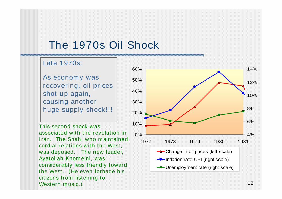
The 1970s Oil ShockLate 1970s:

As economy was recovering, oil prices shot up again, causing another huge supply shock!!!

0%

10%

20%

30%

40%

50%

60%

1977 1978 1979 1980 19814%

6%

8%

10%

12%

14%

Change in oil prices (left scale)

Inflation rate-CPI (right scale)

Unemployment rate (right scale)

This second shock was associated with the revolution in Iran. The Shah, who maintained cordial relations with the West, was deposed. The new leader, Ayatollah Khomeini, was considerably less friendly toward the West. (He even forbade his citizens from listening to Western music.)

13

The 1980s Oil EuphoriaBy the mid-1980s, however, there was a growing glut of oil on world markets, and cheating by cash-short OPEC members became widespread. The result, in 1985, was that producers who had tried to play by the rules – especially Saudi Arabia, the largest producer – got fed up, and collusion collapsed.

As the model predicts, inflation and unemployment fell

-50%-40%-30%-20%-10%

0%10%20%30%40%

1982 1983 1984 1985 1986 19870%

2%

4%

6%

8%

10%

Change in oil prices (left scale)

Inflation rate-CPI (right scale)

Unemployment rate (right scale)

14

Two causes of rising & falling inflation cost-push inflation: inflation resulting from supply shocks

Adverse supply shocks typically raise production costs and induce firms to raise prices, “pushing” inflation up.

demand-pull inflation: inflation resulting from demand shocks

Positive shocks to aggregate demand cause unemployment to fall below its natural rate, which “pulls” the inflation rate up.

Of course, a favorable supply shock that lowers production costs will “push” inflation down, and a negative demand shock which raises cyclical unemployment will “pull” inflation down.

15

Graphing the Phillips Curve

In the short run, policymakers face a tradeoff between and u.

In the short run, policymakers face a tradeoff between and u.

( )e nu u

The short-run Phillips curve

Here, the “short run” is the period until people adjust their expectations of inflation

16

Shifting the Phillips Curve

u

nu

1e

( )e nu u

2e

People adjust their expectations over time, so the tradeoff only holds in the short run.

People adjust their expectations over time, so the tradeoff only holds in the short run.

E.g., an increase in e shifts the short-run P.C. upward.

E.g., an increase in e shifts the short-run P.C. upward.

17

Shifting the Phillips Curve

Show what happens to the Phillips Curve in the face of an increase in the natural rate of unemployment

At any given value of actual unemployment, an increase in the natural rate implies a decrease in cyclical unemployment, which increases inflation by increasing pressures for wages to rise. Thus, each value of unemployment has a higher value of inflation than before.

Try Yourself! What happens to the Phillips Curve in the face of an adverse supply shock?

18

The Sacrifice Ratio To reduce inflation, policymakers can contract aggregate

demand, causing unemployment to rise above the natural rate. The sacrifice ratio measures the percentage of a year’s real GDP

that must be foregone to reduce inflation by 1 percentage point. A typical estimate of the ratio for the US economy is 5.

Example: To reduce inflation from 6 to 2 percent, must sacrifice 20 percent of one year’s GDP:GDP loss = (inflation reduction) x (sacrifice ratio)

= 4 x 5

This loss could be incurred in one year or spread over several, e.g., 5% loss for each of four years.

The cost of disinflation is lost GDP.

19

Rational ExpectationsWays of modeling the formation of expectations:

adaptive expectations: People base their expectations of future inflation on recently observed inflation.

rational expectations: People base their expectations on all available information, including information about current and prospective future policies.

Suppose the RBI announces a shift in priorities, from maintaining low inflation to maintaining low unemployment w/o regard to inflation; this shift will start affecting policy next week

• If expectations are adaptive, then expected inflation will not change, because it is based on past inflation. The RBI’s announcement pertains to the future, and has no impact on past inflation.

• If expectations are rational, then expected inflation will increase right away, as people factor this announcement into their forecasts.

20

Painless disinflation Proponents of rational expectations believe that the sacrifice

ratio may be very small.

They believe if policymakers are credibly committed to reducing inflation, rational people will understand the commitment and will quickly lower their expectations. Workers will demand lower wages while entering into a labour contract and firms that must announce prices in advance will announce lower prices than if they expected higher inflation; thereby reducing the wage-price spiral. Inflation can then come down without a rise in unemployment and fall in output.

Central banks that are politically independent are typically more credible than those that are “puppets” to elected officials. Hence, in countries with central banks that are NOT politically independent, it is usually far costlier to reduce inflation. A very worthwhile reform, therefore, would be for governments to give their central banks independence.

21

Painless disinflation In the most extreme case, one can imagine reducing the rate of

inflation without causing any recession at all.

A painless disinflation has two requirements:

First, the plan to reduce inflation must be announced before workers and firms that set wages and prices have formed their expectations.

Second, the workers and firms must believe the announcement; otherwise, they will not reduce their expectations of inflations.

If both requirements are met, the announcement will immediately shift the short-run tradeoff between inflation and unemployment downward, permitting a lower rate of inflation without higher unemployment.

Almost all economists agree that expectations of inflation influence the short-run tradeoff between inflation and unemployment. The credibility of a policy to reduce inflation is therefore one determinant of how costly the policy will be. Unfortunately, it is often difficult to predict whether the public will view the announcement of the policy as credible.

22

Case 1: Volcker Disinflation

1981: = 9.7%1985: = 3.0%

Total disinflation = 6.7%

23

Case 2: Volcker Disinflation From previous slide: Inflation fell by 6.7%, total cyclical

unemployment was 9.5%. Okun’s law:

1% of unemployment = 2% of lost output. So, 9.5% cyclical unemployment = 19.0% of a year’s real GDP. Sacrifice ratio = (lost GDP)/(total disinflation)

= 19/6.7 = 2.8 percentage points of GDP were lost for each 1 percentage point reduction in inflation.

The sacrifice ratio was smaller than earlier estimates. One explanation is that Volcker’s tough stand was credible enough to influence expectations of inflation directly. Yet the change in expectations was not large enough to make the disinflation painless: in 1982 unemployment reached its highest level since the Great Depression.

24

Case 2: Recovery of Japanese SlumpAttempts to stimulate the economy with monetary expansion were too slow to avoid deflation, leaving Japan in a liquidity trap. Japan’s nominal interest rate was near zero from 1999 until 2003. As a result, conventional monetary policy was powerless to stimulate the economy.

Government spending increased, mainly in the form of public works projects. Fiscal stimulus presumably had some positive effect on output, but not enough to overturn the deflation. Moreover, government deficits increased Japan's government debt to GDP ratio to 85% in 2004. This created the potential for a substantial debt service burden if the interest rate on government debt increases in the future. In this situation, Japanese officials were reluctant to attempt additional fiscal expansion.

25

Case 2: Recovery of Japanese Slump

Output growth has been higher since 2003, and most economists cautiously predict that the recovery will continue.

What are the factors behind the current recovery?

Japan had some good luck – in particular an increase in export demand from China – but also some good policy, which Japan appears to have adopted since 2003.

26

Case 2: Recovery of Japanese SlumpIt is suggested that even if the nominal interest rate is already equal to zero and thus cannot be reduced further, the central bank might still be able to lower the real interest rate by increasing inflation expectations.

To increase expected inflation, the Bank of Japan would have to convince the public that it planned to generate inflation in the future, perhaps by announcing target inflation rates. The success of such a policy depends on whether it is believed.

In 2003, the Bank of Japan announced that it would keep nominal interest rates at 0% until there was strong evidence of sustained inflation. This announcement was taken as a signal of the Bank of Japan’s intention to create the necessary inflation to pull the economy out of its slump. Although inflation remains negative, expected inflation is positive, and the long term real interest rate has fallen, a factor that has probably contributed to the increase in investment spending since 2003.