Inferential Statistics Confidence Intervals and Hypothesis Testing.

Inferential Statistics

Confidence Intervals and Hypothesis Testing

Samples vs. Populations

• Population– All of the objects that belong to a

class (e.g. all Darl projectile points, all Americans, all pollen grains)

– A theoretical distribution• Sample

– Some of the objects in a class– Observations drawn from a

distribution

Two Distributions

• The sample distribution is the distribution of the values of a sample – exactly what we get plotting a histogram or a kernel density plot

• The sampling distribution is the distribution of a statistic that we have computed from the sample (e.g. a mean)

Confidence Intervals

• Given a sample statistic estimating a population parameter, what is the parameter’s actual value?

• Standard Error of the Estimate provides the standard deviation for the sample statistic:

n

ssX

Example 1

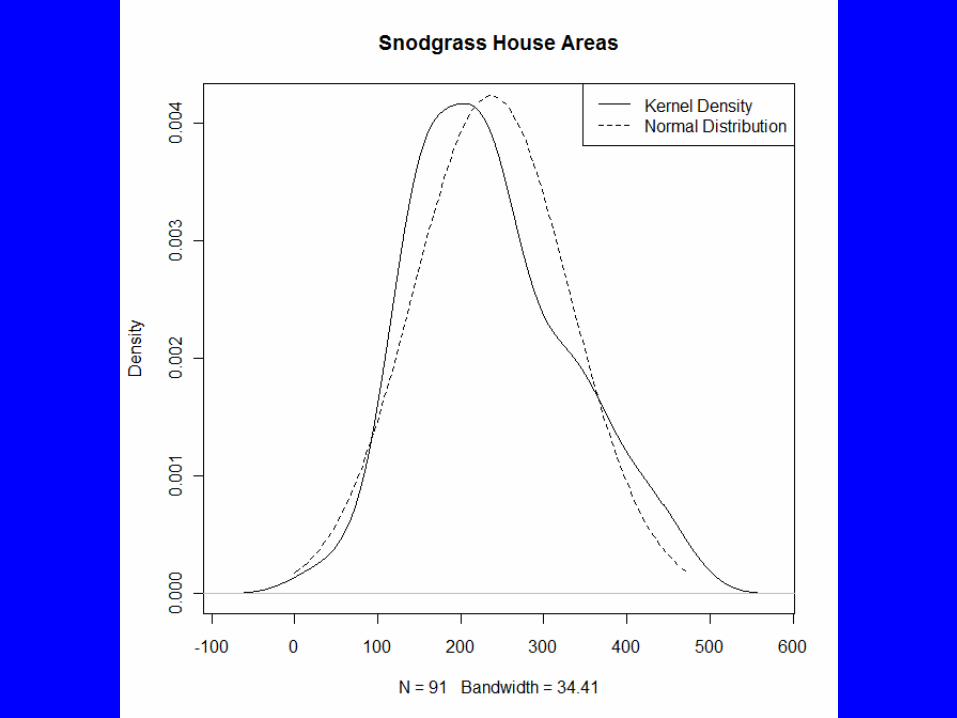
• Snodgrass house size. Mean area is 236.8 with a standard deviation of 94.25 based on 91 houses.

• Area is slightly asymmetrical• Can we use these data to predict

house sizes at other Mississippian sites?

Example 1 (cont)

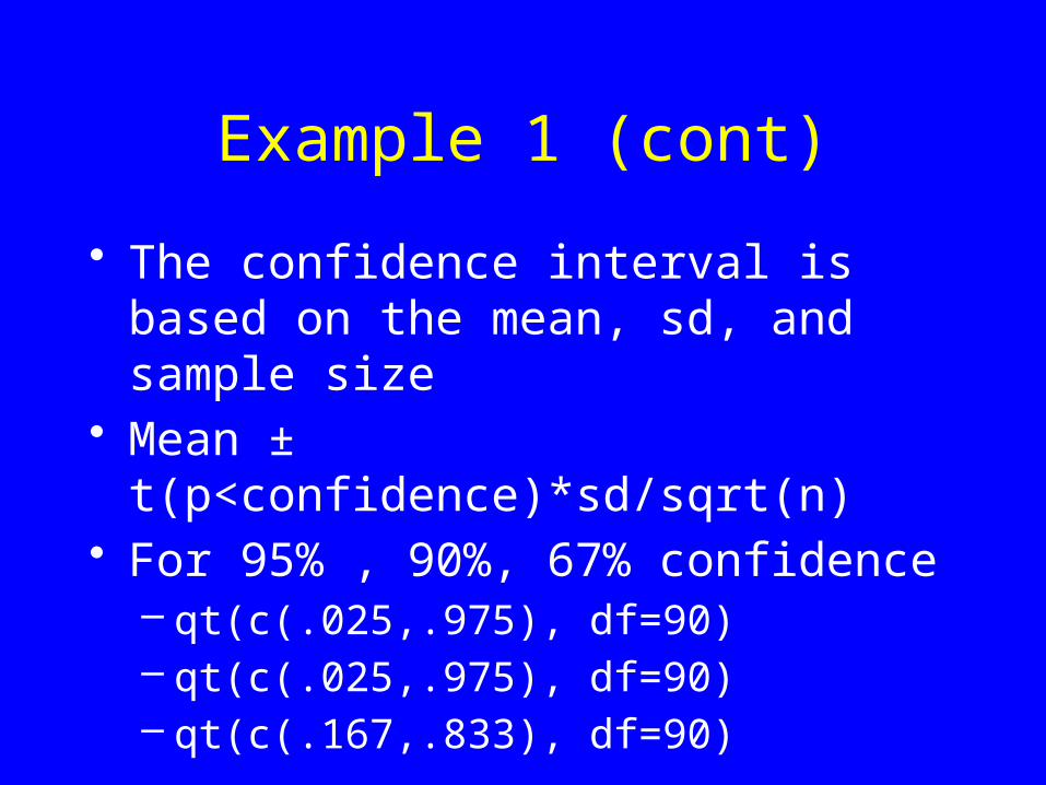
• The confidence interval is based on the mean, sd, and sample size

• Mean ± t(p<confidence)*sd/sqrt(n)• For 95% , 90%, 67% confidence

– qt(c(.025,.975), df=90)– qt(c(.025,.975), df=90)– qt(c(.167,.833), df=90)

# Distributionsx <- seq(10, 40, length.out=200)y1 <- dnorm(x, mean=25, sd=4)y2 <- dnorm(x, mean=25, sd=1)max(y2)plot(x, y1, type="l", ylim=c(0, .4), col="red")lines(x, y2, col="blue")text(c(28, 26.3), c(.08, .30), c("Sample Distribution\n mean=25, sd=4", "Sampling Distribution\n m=25, sd=1, n=16)"), col=c("red", "blue"), pos=4)

# Snodgrass House Areasplot(density(Snodgrass$Area), main="Snodgrass House Areas")lines(seq(0, 475, length.out=100), dnorm(seq(0, 475, length.out=100), mean=236.8, sd=94.2), lty=2)abline(v=mean(Snodgrass$Area))legend("topright", c("Kernel Density", "Normal Distribution"), lty=c(1, 2))

# Confidence interval functionconf <- function(x, conf) {

conf <- ifelse(conf>1, conf/100, conf)tail <- (1-conf)/2mean(x)+qt(c(tail, 1-tail), df=length(x)-1)*sd(x)/sqrt(length(x))

}

Bootstrapping

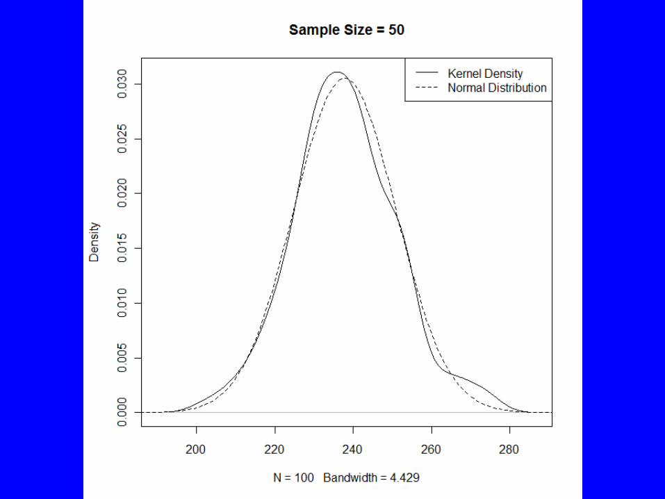
• Confidence intervals depend on a normal sampling distribution

• This will generally be a reasonable assumption if the sample size is moderately large

• We can draw multiple samples of house areas to get some idea

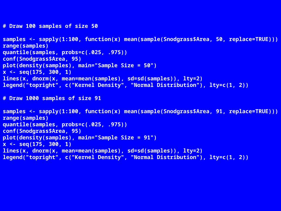
# Draw 100 samples of size 50

samples <- sapply(1:100, function(x) mean(sample(Snodgrass$Area, 50, replace=TRUE)))range(samples)quantile(samples, probs=c(.025, .975))conf(Snodgrass$Area, 95)plot(density(samples), main="Sample Size = 50")x <- seq(175, 300, 1)lines(x, dnorm(x, mean=mean(samples), sd=sd(samples)), lty=2)legend("topright", c("Kernel Density", "Normal Distribution"), lty=c(1, 2))

# Draw 1000 samples of size 91

samples <- sapply(1:100, function(x) mean(sample(Snodgrass$Area, 91, replace=TRUE)))range(samples)quantile(samples, probs=c(.025, .975))conf(Snodgrass$Area, 95)plot(density(samples), main="Sample Size = 91")x <- seq(175, 300, 1)lines(x, dnorm(x, mean=mean(samples), sd=sd(samples)), lty=2)legend("topright", c("Kernel Density", "Normal Distribution"), lty=c(1, 2))

Example 2• Radiocarbon Ages are presented as

an age estimate and a standard error: 2810 ± 110 B.P.

• The probability that the true age is between 2700 and 2920 B.P. is .6826 or .3174 that it is outside that range

• The probability that the true age is between 2590 and 3030 B.P. is .9546 or .0545 that it is outside that range

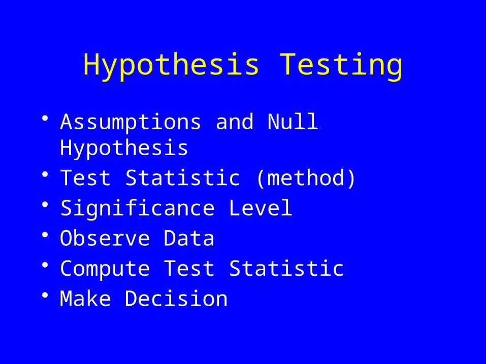
Hypothesis Testing

• Assumptions and Null Hypothesis• Test Statistic (method)• Significance Level• Observe Data• Compute Test Statistic• Make Decision

Assumptions

• Data are a random sample– Every combination is equally likely

• Appropriate sampling distribution

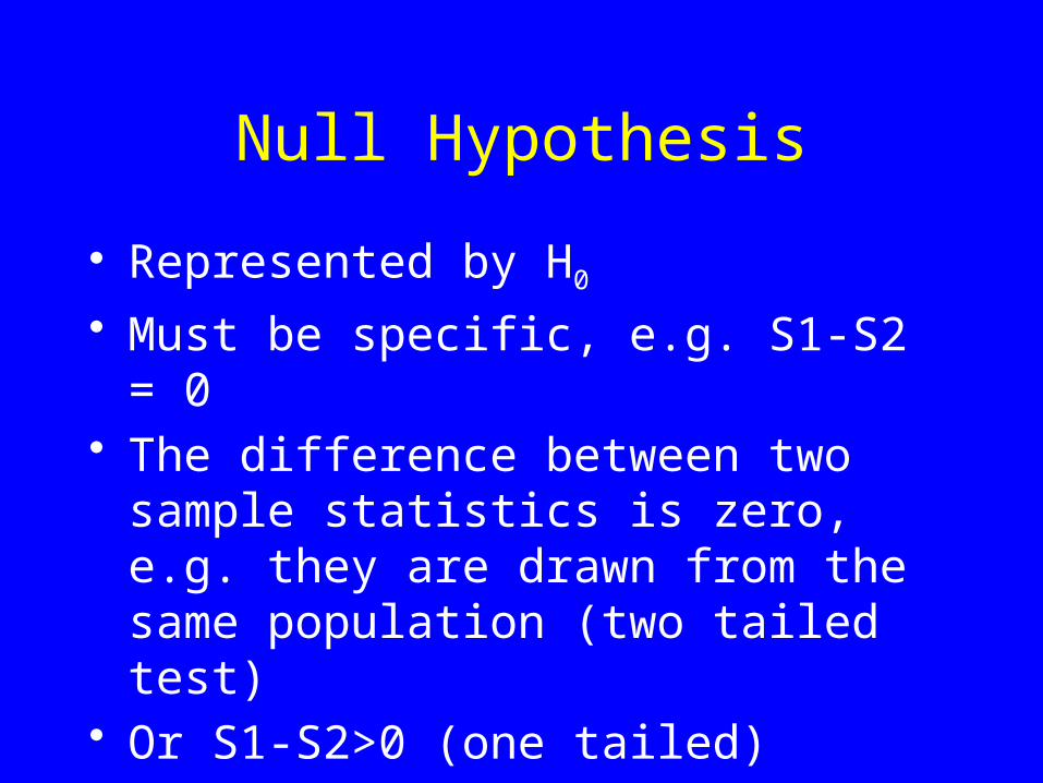
Null Hypothesis

• Represented by H0

• Must be specific, e.g. S1-S2 = 0• The difference between two

sample statistics is zero, e.g. they are drawn from the same population (two tailed test)

• Or S1-S2>0 (one tailed)

Test Statistic

• Measurement Levels• Number of groups• Dependent vs. Independent• Power

Significance Level

• Nothing is absolute in probability• Select probability of making

certain kinds of errors• Cannot minimize both kinds of

errors• Social scientists often use p ≤ 0.05• Consider how many tests

Errors in Hypothesis Testing

Null Hypothesis (H0) is

True False

Research Decision Reject H0

ErrorType I, α

Correct Decision

Accept H0 (fail to reject)

Correct Decision

ErrorType II, β

Difference of Means (t-test)

• Independent random samples of normally distributed variates

• Samples: 1, 2 independent, 2 related

• If 2 independent – variances equal or unequal

• Sample statistics follow the t-distribution

Example

• Snodgrass site is a Mississippian site in Missouri that was occupied about A.D. 1164

Using Rcmdr• Snodgrass Site – House sizes inside

and outside are the same• Check normality - shapiro.test()• Check equal variances – var.test()

or bartlett.test()• Compute statistic and make

decision – t.test()

Wilcoxon Test

• If data do not follow a normal distribution or are ranks not interval/ratio scale

• Nonparametric test that is similar to the t-test but not as powerful

• Tests for equality of medians– wilcox.test()

Difference of Proportions

• Uses the normal distribution to approximate the binomial distribution to test differences between proportions (probabilities)

• This approximation is accurate as long as N x (min(p,(1-p))>5 where N is the sample size, p is the proportion, and min() is the minimum

Using Rcmdr• Must have two or more variables

defined as factors, eg, – Create ProjPts to be equal to

as.factor(ifelse(Points>0, 1, 0)) using Data | Manage variables . . . | Compute new variable

– Statistics | Proportions | Two sample . . .

– prop.test()– Are the % Absent equal inside and

outside the wall?