Aalto University School of Electrical Engineering Department of Electrical Engineering and Automation Teemu Alonen Inference with a neural network in digital signal processing under hard real-time constraints Master’s Thesis Espoo, 31.12.2019 Supervisor: Prof. Themistoklis Charalambous Advisors: Prof. Risto Wichman PhD Jean-Luc Olives MSc Marko Hassinen

Welcome message from author
This document is posted to help you gain knowledge. Please leave a comment to let me know what you think about it! Share it to your friends and learn new things together.
Transcript
Aalto UniversitySchool of Electrical EngineeringDepartment of Electrical Engineering and Automation
Teemu Alonen
Inference with a neural network in digitalsignal processing under hard real-timeconstraints
Master’s ThesisEspoo, 31.12.2019
Supervisor: Prof. Themistoklis CharalambousAdvisors: Prof. Risto Wichman
PhD Jean-Luc OlivesMSc Marko Hassinen
Aalto UniversitySchool of Electrical EngineeringDepartment of Electrical Engineering and Automation
ABSTRACT OFMASTER’S THESIS
Author: Teemu AlonenTitle: Inference with a neural network in digital signal processing
under hard real-time constraintsDate: 31.12.2019 Pages: viii + 75Professorship: Automation Engineering Code: ELEC0007Supervisor: Prof. Themistoklis CharalambousAdvisors: Prof. Risto Wichman
PhD Jean-Luc OlivesMSc Marko Hassinen
The main objective of this thesis is to investigate how neural network inferencecan be efficiently implemented on a digital signal processor under hard real-timeconstraints from the execution speed point of view. Theories on digital signalprocessors and software optimization as well as neural networks are discussed. Aneural network model for the specific use case is designed and a digital signalprocessor implementation is created based on the neural network model.
A neural network model for the use case is created based on the data from theMatlab simulation model. The neural network model is trained and validated usingthe Python programming language with the Keras package. The neural networkmodel is implemented on the CEVA-XC4500 digital signal processor. The digitalsignal processor implementation is written in C++ language with the processorspecific vector-processing intrinsics. The neural network model is evaluated basedon the model accuracy, precision, recall and f1-score. The model performanceis compared to the conventional use case implementation by calculating 3GPPspecified metrics of misdetection probability, false alarm rate and bit error rate.The execution speed of the digital signal processor implementation is evaluatedwith the CEVA integrated development environment profiling tool and also withthe Lauterbach PowerTrace profiling module attached to the real base stationproduct.
Through this thesis, an optimized CEVA-XC4500 digital signal processor imple-mentation was created for the specific neural network architecture. The optimizedimplementation showed to consume 88 percent less cycles than the conventionalimplementation. Also, the neural network model performance fulfills the 3GPPspecification requirements.Keywords: neural networks, machine learning, digital signal processors,
digital signal processing, 5GLanguage: English
ii
Aalto-yliopistoSähkötekniikan korkeakouluAutomaatio- ja systeemitekniikan laitos
DIPLOMITYÖNTIIVISTELMÄ
Tekijä: Teemu AlonenTyön nimi: Neuroverkon inferenssi digitaalisessa signaalikäsittelyssä kovien
reaaliaikavaatimusten alaisuudessaPäiväys: 31.12.2019 Sivumäärä: viii + 75Professuuri: Automaatio- ja systeemitekniikka Koodi: ELEC0007Valvoja: Prof. Themistoklis CharalambousOhjaajat: Prof. Risto Wichman
TkT Jean-Luc OlivesFM Marko Hassinen
Tämän diplomityön tarkoituksena on tutkia miten neuroverkon inferenssi voidaantoteuttaa tehokkaasti digitaalisella signaaliprosessorilla suoritusnopeuden näkökul-masta, kun sovelluksella on kovat reaaliaikavaatimukset. Työssä käsitellään teoriaadigitaalisista signaaliprosessoreista, ohjelmistojen optimoinnista ja neuroverkoista.Työssä kehitetään neuroverkkomalli tiettyyn käyttötapaukseen, ja mallin pohjaltaluodaan toteutus digitaaliselle signaaliprosessorille.
Neuroverkkomalli luodaan Matlab-simulointimallin avulla kerätystä datasta.Neuroverkkomalli opetetaan ja varmennetaan Python-ohjelmointikiellellä jaKeras-paketilla. Neuroverkkomalli toteutetaan CEVA-XC4500 digitaaliselle sig-naaliprosessorille. Digitaalisen signaaliprosessorin toteutus kirjoitetaan C++-ohjelmointikielellä ja prosessorikohtaisilla vektorilaskentaoperaatioilla. Neuroverk-komalli varmennetaan mallin tarkkuuden, precision-arvon, recall-arvon ja f1-arvonperusteella. Mallin suorituskykyä verrataan käyttötapauksen tavanomaiseen to-teutukseen laskemalla 3GPP-spesifikaation mukaiset mittarit virhehavaintoto-dennäköisyys, väärien hälytysten lukumäärä ja bittivirhemäärä. Suoritusnopeusmääritetään sekä CEVA ohjelmointiympäristön profilointityökalulla että tukiase-matuotteeseen kytketyllä Lauterbach PowerTrace-yksiköllä.
Työn tuloksena luotiin optimoitu CEVA-XC4500 digitaalinen signaaliprosessori-toteutus valitulle neuroverkkoarkkitehtuurille. Optimoitu toteutus kulutti 88%vähemmän laskentasyklejä kuin tavanomainen toteutus. Neuroverkkomalli täytti3GPP-spesifikaation mukaiset vaatimukset.Asiasanat: neuroverkot, koneoppiminen, digitaalinen signaalin käsittely,
digitaalinen signaaliprosessori, 5GKieli: Englanti
iii

Preface
This thesis was written in 2019 at Nokia in Espoo headquartes, Finland.I would like to thank Nokia for giving me this opportunity and such an inte-
resting and motivating topic for this thesis. I want to give a special thanks to myadvisors Jean-Luc Olives and Marko Hassinen as well as other colleagues in the L1machine learning and the L1 development teams for supporting my work and brains-torming new ideas. I also want to thank my supervising professors ThemistoklisCharalambous and Risto Wichman for their great support.
I am also thankful for my family and friends, who have always supported methrough my whole academic journey.
Espoo, 31.12.2019
Teemu Alonen
iv

Symbols and abbreviations
Symbols
t time [s]c cycle countf frequency [Hz]I total number of instructionsa accumulatorw neural network weight coefficientW neural network weight coefficient matrixx neural network input valueX neural network input vectorb neural network bias coefficienty actual neural network output valueY actual neural network output vectord desired neural network output valuev induced local field of a neuronη learning ratee error valueC cost functionλ regularization factor
v
Abbreviations
AD Analog-to-digitalAGA Adaptive gradient algorithmANN Artificial neural networkASIC Application-specific integrated circuitBER Bit error rateCISA Configurable instruction set architectureCPI Clock cycles per instructionCPU Central processing unitDAAU Data address and arithmetic unitDMA Direct memory accessDSP Digital signal processorDTX Discontinuous transmissionFAR False alarm rateFFT Fast fourier transformGCU General computation unitHLL High level languageMAC Multiply-accumulateMDP Misdetection propabilityMPN McCulloch-Pitts NeuronMLP Multilayer perceptronNN Neural networkPCU Program control unitPSU Power scaling unitReLU Rectified linear unitRISC Reduced instruction set computerRMSP Root mean square propagationRNN Recurrent neural networkSIMD Single instruction multiple dataSNR Signal-to-noise ratioSOP Sum of productsVCU Vector computation unitVLIW Very long instruction wordVRF Vector register file
vi

Contents
Abstract ii
Tiivistelmä iii
Preface iv
Symbols and abbreviations v
Contents vii
1 Introduction 11.1 Background . . . . . . . . . . . . . . . . . . . . . . . . . . . . . . . 11.2 Research Problem . . . . . . . . . . . . . . . . . . . . . . . . . . . . 11.3 Methods and Materials . . . . . . . . . . . . . . . . . . . . . . . . . 21.4 Outline of the thesis . . . . . . . . . . . . . . . . . . . . . . . . . . 3
2 Digital signal processor 42.1 Overview . . . . . . . . . . . . . . . . . . . . . . . . . . . . . . . . . 42.2 Definitions for real-time . . . . . . . . . . . . . . . . . . . . . . . . 52.3 DSP architecture . . . . . . . . . . . . . . . . . . . . . . . . . . . . 7
2.3.1 Performance metrics . . . . . . . . . . . . . . . . . . . . . . 72.3.2 Representation of numbers . . . . . . . . . . . . . . . . . . . 82.3.3 Data path . . . . . . . . . . . . . . . . . . . . . . . . . . . . 102.3.4 Memory architecture . . . . . . . . . . . . . . . . . . . . . . 11
2.4 General optimization methods . . . . . . . . . . . . . . . . . . . . . 142.4.1 Optimization algorithms . . . . . . . . . . . . . . . . . . . . 152.4.2 Effective use of DSP architecture . . . . . . . . . . . . . . . 172.4.3 Compiler optimization . . . . . . . . . . . . . . . . . . . . . 17
2.5 CEVA-XC4500 DSP . . . . . . . . . . . . . . . . . . . . . . . . . . 21
vii
3 Artificial neural networks 253.1 Introduction . . . . . . . . . . . . . . . . . . . . . . . . . . . . . . . 25
3.1.1 McCulloch-Pitts neuron . . . . . . . . . . . . . . . . . . . . 273.1.2 Rosenblatt’s perceptron . . . . . . . . . . . . . . . . . . . . 28
3.2 Multilayer perceptrons . . . . . . . . . . . . . . . . . . . . . . . . . 333.3 Training procedure . . . . . . . . . . . . . . . . . . . . . . . . . . . 34
3.3.1 Cost function . . . . . . . . . . . . . . . . . . . . . . . . . . 363.3.2 Backpropagation of errors . . . . . . . . . . . . . . . . . . . 373.3.3 Optimization algorithms . . . . . . . . . . . . . . . . . . . . 383.3.4 Regularization . . . . . . . . . . . . . . . . . . . . . . . . . . 40
4 Implementation 414.1 Use case . . . . . . . . . . . . . . . . . . . . . . . . . . . . . . . . . 414.2 Neural network model . . . . . . . . . . . . . . . . . . . . . . . . . 44
4.2.1 Data . . . . . . . . . . . . . . . . . . . . . . . . . . . . . . . 464.2.2 Model architecture and training . . . . . . . . . . . . . . . . 464.2.3 Activation functions . . . . . . . . . . . . . . . . . . . . . . 49
4.3 DSP implementation . . . . . . . . . . . . . . . . . . . . . . . . . . 494.3.1 Fixed point format . . . . . . . . . . . . . . . . . . . . . . . 504.3.2 Induced local field of a neuron . . . . . . . . . . . . . . . . . 534.3.3 Bias . . . . . . . . . . . . . . . . . . . . . . . . . . . . . . . 564.3.4 Activation functions . . . . . . . . . . . . . . . . . . . . . . 57
5 Evaluation 605.1 Neural network model . . . . . . . . . . . . . . . . . . . . . . . . . 60
5.1.1 Evaluation metrics . . . . . . . . . . . . . . . . . . . . . . . 605.1.2 Evaluation . . . . . . . . . . . . . . . . . . . . . . . . . . . . 61
5.2 DSP implementations . . . . . . . . . . . . . . . . . . . . . . . . . . 635.2.1 Evaluation metrics . . . . . . . . . . . . . . . . . . . . . . . 645.2.2 Evaluation . . . . . . . . . . . . . . . . . . . . . . . . . . . . 65
5.3 Evaluation summary . . . . . . . . . . . . . . . . . . . . . . . . . . 68
6 Conclusions 69
References 71
viii
Chapter 1
Introduction
1.1 Background
This thesis is examining CEVA-XC4500 digital signal processor (DSP), whichis part of the Nokia ReefShark chipset. ReefShark chipset is Nokia’s in-housesystem-on-chip (SOC) module developed for Nokia baseband products. ReefSharkchipset is based on 3GPP specifications for 4G and 5G New Radio (NR), and it isdelivered as plug-in unit for the commercially available Nokia AirScale basebandmodule. AirScale module is based on the idea of software-defined system modules,and it supports all radio technologies from 2G to 5G, and all network architecturesfrom distributed radio-access networks (RAN) to centraliced RAN, including alsocloud RAN capability.
1.2 Research Problem
Mobile network requirements are getting more demanding in the 2020s due tomassively increasing data rates. 5G is planned to meet new requirements, but itbrings more engineering challenges due to aggregated data rates, higher edge datarates and peak rates, increasing amount of supported simultaneous user equipment,tighter latency requirements and unknown channel models [1]. Because these newfeatures challenge conventional communication theories, machine learning is one ofthe proposed solutions to solve them. Machine learning has been widely applied tothe upper layer of wireless communication systems for various purposes, and it isincreasingly recognized also in the physical layer development [2] [3].
Most of the high-speed processing in the physical layer is done by digital signalprocessors or specialized hardware units. Machine learning could be optimallyprocessed using special ML processing chip, but if none is available, ML-based
1
CHAPTER 1. INTRODUCTION 2
processing needs to be done on a digital signal processor. Digital signal processorsare optimized for multiply-accumulate (MAC) operations, as many of the moderndigital signal processing algorithms, such as convolution, are based on those op-erations. There is fundamental similarity to feedforward neural networks, whoseforward propagation is mostly processed by multiplications and additions.
Basically, the research problem is defined as follows: how a machine learningalgorithm can be efficiently implemented on a digital signal processing embeddedsystem for real-time applications. This question includes identifying methods, anddesigning the machine learning algorithm from the DSP architecture and operationspoint-of-view. In addition, an important research question is to cover what arethe advantages, limitations and concerns when utilizing digital signal processorarchitecture and operations for machine learning purposes.
1.3 Methods and Materials
Methods of developing execution speed-optimised software for digital signal pro-cessors is reviewed by using available literature. Theory behind neural networks,especially in the context of physical layer software development, is presented as abasis for this research.
Since this thesis work is closely related to Nokia R&D project to utilize machinelearning in physical layer software, specific information about the use case algorithmis deliberately concealed. All the relevant information including input and outputdata dimensions and precision regarding to the machine learning algorithm areshared, but the specific use case description and absolute performance metrics arenot presented.
The neural network inference algorithm is implemented in C++ programminglanguage with CEVA-provided header files containing CEVA XC-specific macrosfor vectorized processing. The implementation is compiled with CEVA-providedcompiler. The implementation is run on a CEVA-XC4500 digital signal processor.Real-time profiling data of the implementation performance is collected using theLauterbach PowerTrace module attached to the digital signal processor. Data forthe neural network model training and validation is collected using Nokia’s 5Gsimulator, which is built by Matlab software. The neural network model itselfis constructed and trained using python programming language with Keras andTensorflow modules.
CHAPTER 1. INTRODUCTION 3
1.4 Outline of the thesis
The aim of this thesis is to apply machine learning techniques in physical layer soft-ware development by implementing computationally speed-efficient neural networkinference for CEVA-XC4500 digital signal processor. The purpose is also to applythe implementation for physical layer control bit decoding use case, and compareits performance against the implementation based on the stochastic mathematicalmodels. The thesis work is divided into 6 chapters. Chapter 2 provides backgroundrelated to digital signal processors in general. It also describes most commonly usedmethods to optimize digital-signal processor applications, and defines the conceptof real-time. Chapter 3 covers a machine learning related algorithm called neuralnetworks. The neural network model itself, network training and network inferenceare discussed. After introduction and theoretical recap, chapter 4 describes howneural network architecture and digital signal processor implementation are tiedtogether on experimental level. Different CEVA-XC4500 digital signal processorrelated optimization methods are explained, and how neural network model is bestfitted to both CEVA-XC4500 specifications and application purposes. Chapter 5presents evaluation and results how implemented neural network inference comparesagainst stochastic model based implementation. Chapter 6 includes the reviewof the implementation and discusses the future improvements and requirementsrelated to machine learning in physical layer development.
Chapter 2
Digital signal processor
2.1 Overview
Digital signal processing refers to a set of mathematical operations to digitallyrepresent signals [4]. The goal of the digital signal processing is to determinespecific information content by transforming, enhancing and modifying the signal.Digital signal processing involves the processing of analog signals that are convertedand represented digitally by sequence of numbers. The term ’digital’ refers to thisnumerical representation, which also implies quantization of some of the signalproperties. [4]. The term ’signal’ refers to a variable parameter, which is treatedas information as it flows through an electronic circuit [4]. The signal is essentiallya voltage that varies within some range of values [4]. The term ’processing’ relatesto the processing of data using software based applications [4].
General-purpose processors (GPPs) are designed to provide broad functionalityfor a wide variety of different kind of applications [4]. From the performancepoint of view, the goal of GPPs is to maximize performance over a broad rangeof applications. Specialized processors instead, are designed to take maximumadvantage of the limited functionality required by their special applications. [4].Digital signal processor (DSP) is a processor specialized for digital signal processing.Its hardware is shaped by the digital signal processing algorithms, and thus it isspecialized to perform them inexpensively and efficiently. Inexpensive and efficientrefers to different DSP performance metrics, which are usually the processing timerequired to accomplish a defined task, memory usage and energy consumption. [5].In the literature, the acronym DSP can refer to both ’digital signal processing’ and’digital signal processor’. In this thesis, DSP refers to the ’digital signal processor’.
The strict role between GPP and DSP is blurring, because many so-calledGPPs have some DSP functionalities, and many DSPs have traditional general-purpose processing functionalities on board [6]. Strictly speaking, any processor
4
CHAPTER 2. DIGITAL SIGNAL PROCESSOR 5
that operates on digitally presented signals can be called DSP. In practise, however,DSP refers to a processor specifically designed for digital signal processing [5]. Inthis thesis, DSP refers to the latter. Distinguishing between DSPs and GPPs byapplication is perhaps not the best way forward. The main difference betweenthose two lies inside the devices themselves, in the internal chip architecture [6].
This chapter introduces the basics of DSPs from the application optimizationpoint of view. Especially, optimization from application speed point of view isdiscussed, as the purpose of this thesis is to produce as fast neural network real-timeinference as possible. The term real-time is defined and discussed in section 2.2.DSP architecture overview is discussed in section 2.3, and DSP memory architectureis discussed more in detail in section 2.3.4. Section 2.3.3 explains the meaningof data path, and why it is important aspect in DSP architecture. Section 2.4discusses some of the most common methods to optimize DSP applications, andhow to utilize DSP architecture efficiently. Lastly, section 2.5 discusses in detailabout the architecture of the CEVA-XC4500 DSP, as the implementation of thereal-time neural network inference is implemented on that chip.
2.2 Definitions for real-time
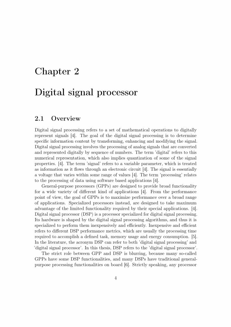
In order to define the term real-time, it is necessary to define a system. Based onthe definition in [7], a system is a mapping of a set of inputs into a set of outputs.When internal details are out of interest, the mapping function can be considered asa black box. Different system definitions may include some other requirements fora system, like system must have purpose [8], but for practical engineering definitionof real-time, input-output mapping is the key concept [7]. Every real-world entitycan be modeled as a system [7]. In computing systems, like DSPs, the inputs andoutputs represent digital or analog data. In embedded systems, inputs may beassociated with sensors, and outputs may be connected to the actuators. Figure2.1 represents the general model of a system with input-output mapping.
Figure 2.1: A general system with inputs and outputs [7].
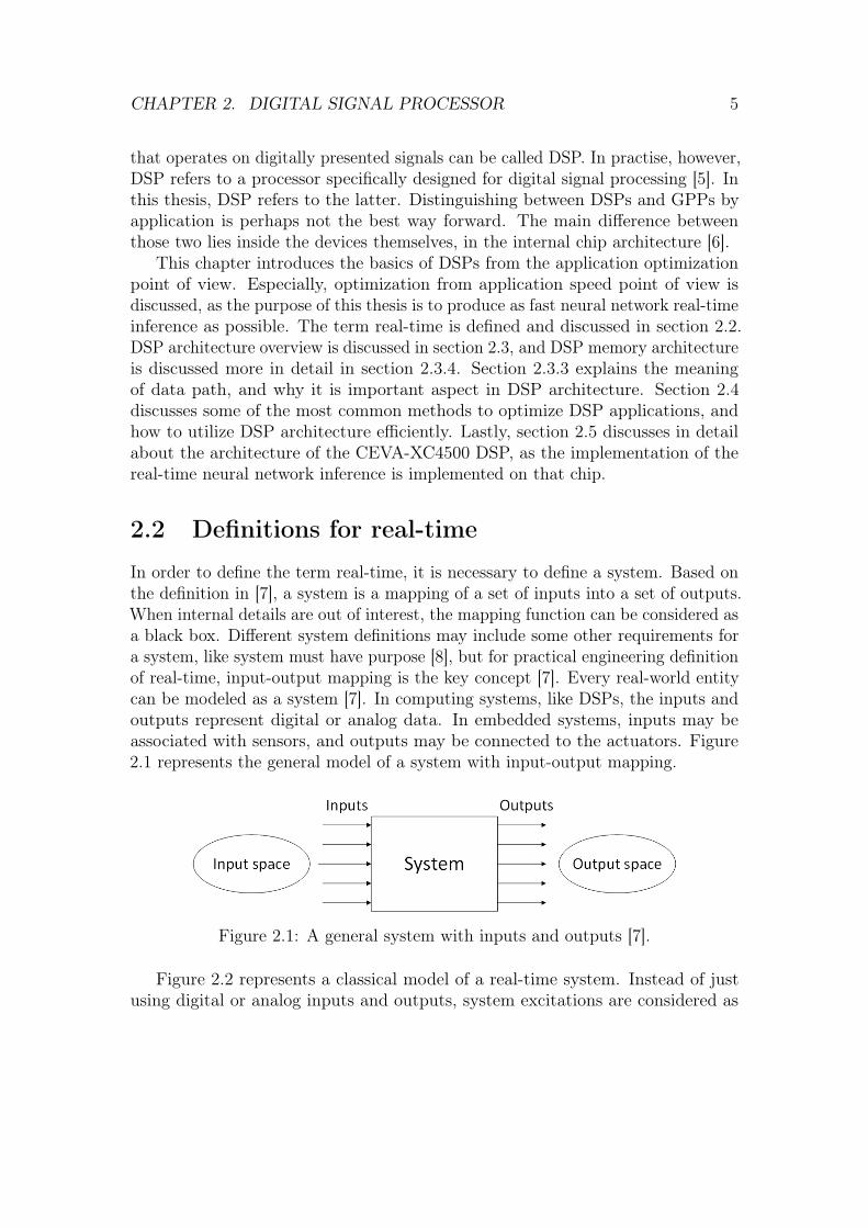
Figure 2.2 represents a classical model of a real-time system. Instead of justusing digital or analog inputs and outputs, system excitations are considered as
CHAPTER 2. DIGITAL SIGNAL PROCESSOR 6
a sequence of jobs to be scheduled. Also, the performance of the jobs can bepredicted [7]. It is still notable that this real-time model ignores the fact that thesystem inputs and the controlled hardware may be very complex, but it it stillgood representation of a real-time system.
Figure 2.2: A real-time system as a sequence of jobs [7].
Both in general system model and in real-time system model, there exists a delaybetween presentation of inputs and appearance of the output [7]. This is one ofthe key reasons why definition of real-time is not just instantaneous response. Thisdelay is called as a response time of the system [7]. The response time of the systemis defined as "the time between the presentation of a set of inputs to a system andthe realization of the required behavior, including the availability of all associatedoutputs" [7]. System response-time differs from one application to another, and therequirements for response-time solely depends on the characteristics and the purposeof the system. However, the response-time requirement defines the term real-timesystem. A real-time system must satisfy bounded response-time constraints orrisk severe consequences, including failure [7]. A failure in a system means thatthe system cannot satisfy one or more of the requirements defined in the systemrequirements specification [7]. Because of this definition of failure, system operationcriteria and timing constraints must be defined in order to discuss about a real-timesystem. Because of existing timing criterion, the real-time system logical correctnessis evaluated based on the correctness of the outputs and the fullfilled response timeconstraints. It is notable that a real-time system does not have to process datainstantaneously, it just need to have response times that are satisfied under definedconstrains.
One important aspect is also the fact that some applications may accept differentamount of failures without catastrophic consequences. The affect of failure in anuclear reactor cooling system response time has a very different consequence thanflight ticket reservation system. Real-time systems are traditionally divided intothree categories [7] based on the effect of missed real-time constraints; soft real-timesystems, hard real-time systems and firm real-time systems. In a soft real-time
CHAPTER 2. DIGITAL SIGNAL PROCESSOR 7
system the performance is degraded if the response time constraints are not met,but the system is not completely destroyed [7]. In a hard real-time system instead,even a single missed response-time constraint may lead to a complete system failure[7]. In a firm real-time system, a few missed response-time constraints will not leadto a system failure, but missing more than a few may destroy the system [7].
2.3 DSP architecture
Architectural choices vary between different DSP vendors, but some characteristicsare common to all DSPs. Typically, the DSP hardware is designed to supportfast arithmetic by utilizing large accumulators, implementing single cycle multiply-accumulate (MAC) instructions, and supporting pipelined and parallell computationand data movement [4]. Parallel data movement is typically enabled by havingmultiple-access memories, which allows the processor to load and store multipleoperands simultaneously and even in parallel with an instruction execution [9]. Highbandwidth memory subsystems enable constant flow of operands available. DSPstypically feature also hardware support for low overhead loop control, and specializedinstructions and addressing modes that reduce the total number of instructionsrequired to describe a typical DSP algorithm [6]. Different memory-addressingmodes and program-flow controls speed the execution of repetitive operations[9]. Also, special on-chip peripherals or input-output interfaces are included, sothat the processor can interface efficiently with other system components, such asanalog-to-digital (AD) converters and memory [9].
2.3.1 Performance metrics
One of the key performance measures discussed throughout this thesis is theprocessing time t required to process an algorithm. As discussed in section 2.2,response-time constraints need to be defined in real-time systems in order to evalu-ate system performance. Instead of discussing about the absolute time the DSPsystem consumes, DSP cycle count is discussed instead. Cycle count means theamount of central processing unit (CPU) clock ticks some measured instant takes.If the DSP main clock runs on a constant frequency within algorithm execution,the absolute time consumed by the algorithm can be determined from the cyclecount according the equation 2.1
t =c
f(2.1)
where t is the absolute CPU time consumed, c is the total cycle count, and f isthe (constant) CPU clock frequency during execution. Because processing time
CHAPTER 2. DIGITAL SIGNAL PROCESSOR 8
can be estimated from the cycle count, the cycle count is discussed in this thesis asan indicator for processing speed.
The required processing time can also be estimated from the total amount ofinstructions the algorithm includes, without knowing the consumed cycle amount.In equation 2.2, I refers to the total amount of instruction in the algorithm, andCPI refers to the average number of cycles each instruction takes to execute, clockcycles per instruction [10].
t =I × CPI
f(2.2)
DSP performance can also be measured in DSP memory usage and powerconsumption. In some applications, those metrics might be as important, or evenmore important than processing speed. An ideal technique for measuring overallperformance of the DSP system would yield data from on execution time, memoryusage and power consumption. However, processing speed is commonly the primarymeasure of performance, with memory consumption and power usage as secondaryconsiderations [9].
It is important to differentiate the DSP clock cycle count from instructioncycle count. Instruction cycle means processing of one CPU instruction. Theinstruction cycle consists of five different phases in a classic reduced instructionset computer (RISC) pipeline: fetch instruction, decode instruction, load operand,execute arithmetic function, and store the result [7]. These different instructioncycle phases may take different amount of CPU clock cycles depending on theinstruction itself. In a DSP processor, one multiply-accumulate (MAC) instructionmay take only one CPU clock cycle [9], but other instructions typically take multipleCPU clock cycles. DSP cycle count means the CPU clock cycle count, not thenumber of consumed instruction cycles.
2.3.2 Representation of numbers
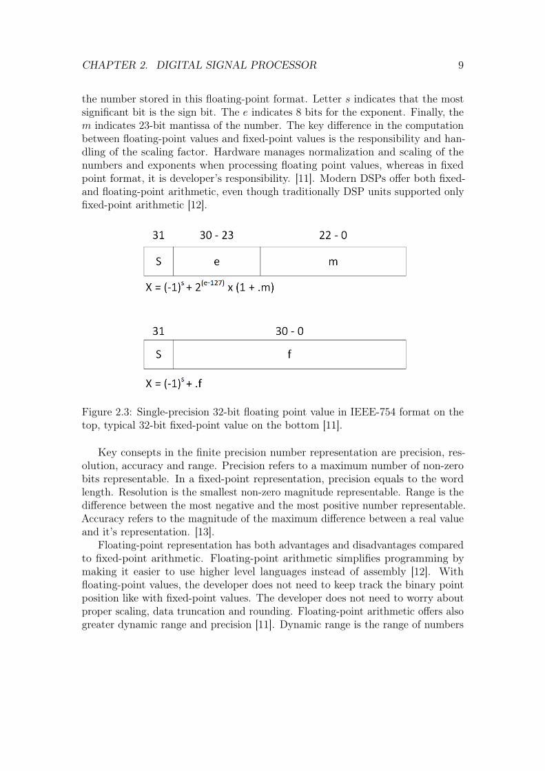
Digital signal processing can be separated into fixed-point processing and floating-point processing. These designations refer to the format used to store and manipu-late numeric representations of data, especially to the representation of decimalnumbers. The difference between those two processing methods is in the contentof stored information about the number. In a floating point format, the processorknows everything about the number. The processor knows how the number isstored, and what is the magnitude of it. In a fixed-point format, the scaling factor,or exponent, needs to be stored separately. [11]. It is the developer’s responsibilityto take care of the scaling factor. Figure 2.3 represents how floating-point andfixed-point values are stored on 32-bit format. In the figure, floating-point value isrepresented in IEEE-754 single-precision format. The letters indicate the parts of
CHAPTER 2. DIGITAL SIGNAL PROCESSOR 9
the number stored in this floating-point format. Letter s indicates that the mostsignificant bit is the sign bit. The e indicates 8 bits for the exponent. Finally, them indicates 23-bit mantissa of the number. The key difference in the computationbetween floating-point values and fixed-point values is the responsibility and han-dling of the scaling factor. Hardware manages normalization and scaling of thenumbers and exponents when processing floating point values, whereas in fixedpoint format, it is developer’s responsibility. [11]. Modern DSPs offer both fixed-and floating-point arithmetic, even though traditionally DSP units supported onlyfixed-point arithmetic [12].
Figure 2.3: Single-precision 32-bit floating point value in IEEE-754 format on thetop, typical 32-bit fixed-point value on the bottom [11].
Key consepts in the finite precision number representation are precision, res-olution, accuracy and range. Precision refers to a maximum number of non-zerobits representable. In a fixed-point representation, precision equals to the wordlength. Resolution is the smallest non-zero magnitude representable. Range is thedifference between the most negative and the most positive number representable.Accuracy refers to the magnitude of the maximum difference between a real valueand it’s representation. [13].
Floating-point representation has both advantages and disadvantages comparedto fixed-point arithmetic. Floating-point arithmetic simplifies programming bymaking it easier to use higher level languages instead of assembly [12]. Withfloating-point values, the developer does not need to keep track the binary pointposition like with fixed-point values. The developer does not need to worry aboutproper scaling, data truncation and rounding. Floating-point arithmetic offers alsogreater dynamic range and precision [11]. Dynamic range is the range of numbers
CHAPTER 2. DIGITAL SIGNAL PROCESSOR 10
that can be presented before an overflow occurs. Precision measures the number ofbits to represent numbers. Precision can be used to estimate the impact of errorsdue to integer truncation and rounding [12].
Floating-point arithmetic has some disadvantages also. Some algorithms donot need floating-point scaling and range precision, and thus are better to beimplemented on fixed-point values. Floating-point arithmetic is slower to processdue to larger device size and more complex operations and more limited parallelism[12], which might also be a major performance drawback. Floating point operationshardware is typically larger, requiring more hardware space for the DSP. This alsorequires more power to operate. Added complexity also makes the hardware moreexpensive than pure fixed-point device [12]. Of course, the trade-off should bemade regarding device cost compared to the software development cost on moredemanding fixed-point arithmetic.
As discussed in section 2.4, optimization of the DSP application is usually trade-off between multiple metrics. Choosing between fixed-point and floating-pointarithmetic is also trade-off between application speed and precision. This trade-offsolely depends on the application requirements.
2.3.3 Data path
Data path refers to a set of functional units, such as multipliers, accumulators,registers and specialized units, which carry out all the arithmetic processing [14].
Multiplication is one of the key operations in digital-signal processing appli-cations. Hence all DSPs have a multiplier that can multiply two data units ina single instruction cycle [14]. In some DSPs, the adder unit is separated fromthe multiplication unit, but in most of the DSPs, the adder is integrated withthe multiplication unit. When adder and multiplier are integrated, they formsingle-cycle MAC-unit. If the units are separated, the result of the multiplicationis first kept in a separate product result register before sending it to the adder foraccumulation. This adds delay of at least one instruction to the processing [14].The product of two n-bit fixed-point values will need 2n bits to store the resultin order to avoid any accuracy lost. Most fixed-point multipliers produce a resultthat is twice the word-length of their operands [14], so the multiplier itself doesnot introduce any error. If the result of the multiplication is truncated, so that forexample 32-bit result is truncated to 24-bits, some accuracy will be lost.
Pipelining is also utilized in some DSP multipliers. Pipelining is a techniquethat allows operations to overlap during program execution [6]. The task is splitinto multiple sub-tasks, which are overlapped. This increases the overall speed, eventhough there is delay between time the inputs are presented to the multiplier tothe time that results are available. Single multiplication might have worse latencycompared to non-pipelined multiplication, but long series of multiplications are
CHAPTER 2. DIGITAL SIGNAL PROCESSOR 11
more effective. [14].In addition to the multipliers, also accumulators are a fundamental part of
digital-signal processing [14]. If there is only one accumulator available in the DSParchitecture, and it is used as one of the source operands and also as the destinationof the calculation, it can become the bottleneck of the processing. However, manyDSPs offer more than one accumulator [14], and they are in many cases mergedwith the multiplication unit [6]. Accumulating two n-bit fixed-point values requiren+1-bits for the resulting operand. Therefore, the size of the accumulator should belarger than the multiplier word by several bits, called guardian bits [14]. Guardianbits allow the accumulation of a number of results without overflow. Some DSPsthat do not offer guard bits, allow scaling of the output register by shifting thevalue by a few bits. The scaling usually happens within a single instructions and isperformed before adding the value to the accumulator. Guard bits are still morepreferable, because they do not lost any precision. [14].
2.3.4 Memory architecture
The overall structure and the architecture of the memory is very important issueaddressed in the design of the DSPs. Memory can be roughly divided into twotypes: internal memory and external memory. Internal memory referes to the DSP’son-chip memory [12], whereas external memory refers to peripheral off-chip memory[15]. Internal memory is much faster than off-chip external memory, thereforebeing the preferred storage for the processing data. Internal memory is sometimesinterpret as sort of developer managed cache type of memory, as many DSPs donot have actual cache [12].
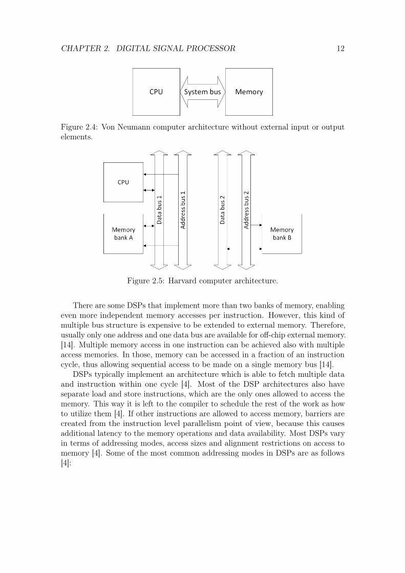
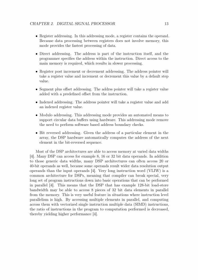
Most of the microprocessors are using memory design around the Von Neumannarchitecture [14], in which program instructions and program data are sharing thesame memory space [6]. Figure 2.4 represents the Von Neumann based memoryarchitecture. Because the memory space is shared, instructions and data are alsoaccessed using the same buses, which makes the systems slower. Because of theshared bus, CPU needs to fetch both program instructions and data, before it canstart processing itself. In Harvard architecture instead, which is used in most ofthe DSPs, program instructions and data are stored in separate and independentmemory areas, and they are also accessed through separate buses [14]. Figure 2.5represents the Harvard architecture with two separate banks of memory, whichcan be accessed in parallel. Because both instructions and data can be accessedsimultaneously, speed advantage is gained compared to conventional Von Neumannbased microprocessor architecture [6]. Also, the so called multi-port memoriesallows simultaneous memory access for data and instructions. Those memorieshave multiple independent sets of address and data lines, which allows multipleindependent memory accesses [14].
CHAPTER 2. DIGITAL SIGNAL PROCESSOR 12
Figure 2.4: Von Neumann computer architecture without external input or outputelements.
Figure 2.5: Harvard computer architecture.
There are some DSPs that implement more than two banks of memory, enablingeven more independent memory accesses per instruction. However, this kind ofmultiple bus structure is expensive to be extended to external memory. Therefore,usually only one address and one data bus are available for off-chip external memory.[14]. Multiple memory access in one instruction can be achieved also with multipleaccess memories. In those, memory can be accessed in a fraction of an instructioncycle, thus allowing sequential access to be made on a single memory bus [14].
DSPs typically implement an architecture which is able to fetch multiple dataand instruction within one cycle [4]. Most of the DSP architectures also haveseparate load and store instructions, which are the only ones allowed to access thememory. This way it is left to the compiler to schedule the rest of the work as howto utilize them [4]. If other instructions are allowed to access memory, barriers arecreated from the instruction level parallelism point of view, because this causesadditional latency to the memory operations and data availability. Most DSPs varyin terms of addressing modes, access sizes and alignment restrictions on access tomemory [4]. Some of the most common addressing modes in DSPs are as follows[4]:
CHAPTER 2. DIGITAL SIGNAL PROCESSOR 13
• Register addressing. In this addressing mode, a register contains the operand.Because data processing between registers does not involve memory, thismode provides the fastest processing of data.
• Direct addressing. The address is part of the instruction itself, and theprogrammer specifies the address within the instruction. Direct access to themain memory is required, which results in slower processing.
• Register post increment or decrement addressing. The address pointer willtake a register value and increment or decrement this value by a default stepvalue.
• Segment plus offset addressing. The addrss pointer will take a register valueadded with a predefined offset from the instruction.
• Indexed addressing. The address pointer will take a register value and addan indexed register value.
• Modulo addressing. This addressing mode provides an automated means tosupport circular data buffers using hardware. This addressing mode removethe need to perform software based address boundary checks.
• Bit reversed addressing. Given the address of a particular element in thearray, the DSP hardware automatically computes the address of the nextelement in the bit-reversed sequence.
Most of the DSP architectures are able to access memory at varied data widths[4]. Many DSP can access for example 8, 16 or 32 bit data operands. In additionto those generic data widths, many DSP architectures can often access 20 or40-bit operands as well, because some operands result wider data resolution outputoperands than the input operands [4]. Very long instruction word (VLIW) is acommon architecture for DSPs, meaning that compiler can break special, verylong set of program instructions down into basic operations that can be performedin parallel [4]. This means that the DSP that has example 128-bit load-storebandwidth may be able to access 8 pieces of 32 bit data elements in parallelfrom the memory. This is very useful feature in situations where instruction levelparallelism is high. By accessing multiple elements in parallel, and computingacross them with vectorized single instruction multiple data (SIMD) instructions,the ratio of instructions in the program to computation performed is decreased,thereby yielding higher performance [4].
CHAPTER 2. DIGITAL SIGNAL PROCESSOR 14
Program caches
A program cache is a small amount of memory for storing program instructionswithin the processor core [14]. Computations can be executed faster when theinstruction is available at the processor core, without fetching it from the programmemory. However, all of the DSPs does not have cache memory, because it causesdeterminism unpredictability in the calculations [12].
There are differences between processors how much the developer is able tocontrol the cache memory usage. In some processors, the developer is able to lockthe contents of the cache memory, or even disable its usage. This kind of manualcontrol adds determinism, as it helps the developer to ensure that the programswill meet time constraints. [14].
If physical cache memory is not available in the processor, a similar type of ideacan be utilized with internal and external memories. In a process called manualcaching, the programmer can manually move some section of the code from slowexternal memory to the fast internal memory for execution. [14].
Direct memory access
Direct memory access (DMA) is the process of transferring data without theinvolvement of the processor itself [14]. Modern DSPs can often compute resultsfaster that the memory system can supply new operands. The bottleneck is keepingthe processor unit fed with data fast enough to prevent the system being idlewaiting for new operands to be available. This situation is called as data starvation[12]. DMA is a solution to that problem. It is often used for transferring databetween core and peripheral devices [14], such as external memory, which is veryslow compared to the internal memory. External memory refers to a memoryunit, which is located outside the chip. In DMA, a separate DMA controller isused for data transfer. The DMA controller is actually another CPU, who is onlyresponsible of moving data around very quickly [12]. When the DMA controller isready for a data transfer, it notifies the DSP, which in turn relinquishes its externalmemory bus control to the DMA controller. The DMA controller transfers thedata independently from the DSP, and notifies the processors after completion ofthe transfer. [14]. DMA is most useful when transferring large block of data, as thesetup and overhead time for the DMA transfer makes it faster just to use regularDSP control for smaller data blocks [12].
2.4 General optimization methods
Optimization is a procedure that seeks to maximize or minimize one or moreperformance indices without changing the meaning of the program output. In
CHAPTER 2. DIGITAL SIGNAL PROCESSOR 15
the context of a real-time application, these performance indices typically includethroughput, memory usage, external input and output bandwidths and powerdissipation [12]. However, it is typically difficult or even impossible to optimizeall of the performance indices at the same time. For example, the speed of theDSP algorithm is usually inversely proportional to the memory usage and powerconsumption of the algorithm, so that making the application faster requires morememory usage and more heat dissipation. The art of the optimization is knowingthe different optimization options, understanding the trade-off between variousperformance indices, and without forgetting the overall goal of the application,creating the application based on those [12]. As many of the modern DSP applica-tions are subject to real-time constraints, it is important to be aware of the generalDSP optimization techniques. As discussed in the chapter 2.2, the definition of thereal-time system is to be able to perform tasks in predetermined time intervals. AsCPU power, memory size and power resources are valuable assets from the costpoint of view, it is usually more cost-efficient trying to compress the application touse as little resources as possible. Therefore, the application should be as optimizedas possible. Sometimes optimization may speed up the application by order ofmagnitudes [12]. Of course, DSPs differ from one to another, but due to limitedspecial functionality requirements by the common signal processing applications,DSPs include some common key features to perform those tasks. Optimization ofthe DSP application is highly related to the efficient usage of DSP architecture,algorithms and the compiler [16]. Optimization methods represented in this chapterare common methods to improve the performance of a DSP application in terms ofcycle count and memory usage.
2.4.1 Optimization algorithms
Algorithm optimization is the highest level of DSP software optimization. Beforeimplementing and optimizing the code, one should try to optimize the algorithmitself and try to make it as efficient as possible [16]. It should be optimized especiallyfrom the DSP point of view, so that DSP architecture and compiler are taken intoaccount while formulating the algorithm. Also, data size to be processed needto be minimized [16], as it generally decreases the amount of required processing.Choosing the right data structure for the right application will provide an efficientway of accessing data and therefore improve the performance [16]. Some datastructures, like classes, might be harder for the compiler to optimize. Some commonprogramming related code optimization techniques [12], which also help in compileroptimization, are:
• Code rearrangement. Changing the order of code execution might save time,if memory read is triggered little bit earlier than the operands are needed.
CHAPTER 2. DIGITAL SIGNAL PROCESSOR 16
Some other code can be executed between the read and execution.
• Minimize branching. Branching is typically harmful from the pipelining pointof view. As pipelining allows sequential instruction to be executed simul-taneously, there should be knowledge about the instruction to be executednext. Branching brokes this determinism, as the forecoming path is unknown.As discussed in the chapter 2.5, vector predicates is a method to executeconditional operations without conditional branching.
• Elimination of recalculations. If it is possible to avoid calculating somethingagain, for example moving code to the outside of the loop, both speed andcode size are optimized.
• Combining equivalent constants and substituting operations. It is suitableto combine constant operations beforehand, so that execution time does notneed to be used for it. Also, if two constants have equal values, they shouldbe replaced by a single constant for memory saving purposes.
• Eliminating unused code and storage of unreferenced values. All of the unusedcode should be removed, as it consumes memory.
• Inlining or replacing function calls with program code. Inlining refers to amethod in which the compiler replaces part of the code, for example functioncall, with the copy of the source code. This prevents the execution jumpingfrom one code section to another, enabling pipelining possibilities, It canspeed up the execution of the software by not having to perform functioncalls with the associated overhead. However, inlining increases code size. [12].
• Loop unrolling. Loop unrolling is a technique in which the body of a suitableloop is replaced with multiple copies of itself, and the control logic of the loopis updated accordingly [17]. Loop unrolling attempts to minimize the thecost of loop overhead, such as branching on the termination condition andupdating counter variables [12]. The loop unrolling manually adds multiplecopies of the code body, and ads updates and counter increments accordingly.This increases code size, but the speed performance is potentially improved.The performance benefit comes from the reduced loop overhead, because lessiterations are performed, and code is potentially pipelined more [12].
• Loop invariant code motion. If a variable within a loop is not altered, thecalculation should be performed outside of the loop body [12].
CHAPTER 2. DIGITAL SIGNAL PROCESSOR 17
2.4.2 Effective use of DSP architecture
DSP is essentially an application-specific microprocessor. DSP was developed toinclude hardware architectures that allow the efficient execution of signal processingspecific algorithms [12]. As discussed previously in this chapter, some of the specificarchitectural features of DSPs include special instructions, large accumulators,specialized loop checking and multiaccess memories [12]. Special hardware-basedinstructions speed up the instruction execution and large accumulators allow accu-mulating a large number of elements [12]. Multiaccess memories allows accessingtwo or more data elements in the same cycle, and special loop checking hardwareperforms much faster than software-based loop checking [12].
As discussed in section 2.3, many DSP applications are composed from astandard set of DSP building blocks, such as filters, FFT and convolutions [12].What is common to these algorithms, they all perform series of multiplies andadds, which is commonly referred to as sum of products (SOP). One of the mostcommon operation, which is encountered in all of these major DSP functions, isthe multiply-accumulate (MAC) operation [12, 14]. MAC operation is representedin equation (2.3), in which w and x are operands to be first multiplied, and thenaccumulated to an accumulator a. MAC operation computes the product of twonumbers, and adds that product to an accumulator. Many DSP related algorithms,like FFT, perform multiple of those operations within a tight loop. As shown in[12], the saving of calculating MAC as a hardware-dedicated operation is four cyclescompared to the software or microcode based operation. The saving becomes moreand more significant, when multiple of MAC operations are performed millions oftimes in an application.
a = a+ (w × x) (2.3)
2.4.3 Compiler optimization
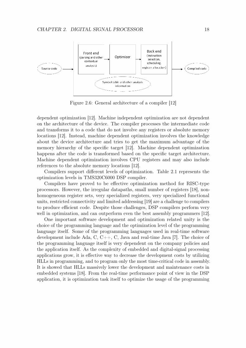
Compiler is a computer program that translates computer code written in oneprogramming language into another programming language [12], usually intomachine code. Compilers are used to translate the source code from higher levellanguage to lower level language to create an executable program. Figure 2.6represents the general architecture of a modern compiler [12]. The front end ofthe compiler reads in the source code, report errors and creates an intermediaterepresentation of the source code [12]. The intermediate stage is the optimizer. Theback end of the compiler generates the target code from the optimized intermediatecode, performs target machine specific optimizations, and finally outputs the objectcode to be run on the target machine [12].
Compilers perform two types of optimization: machine independent and machine
CHAPTER 2. DIGITAL SIGNAL PROCESSOR 18
Figure 2.6: General architecture of a compiler [12]
dependent optimization [12]. Machine independent optimization are not dependenton the architecture of the device. The compiler processes the intermediate codeand transforms it to a code that do not involve any registers or absolute memorylocations [12]. Instead, machine dependent optimization involves the knowledgeabout the device architecture and tries to get the maximum advantage of thememory hierarchy of the specific target [12]. Machine dependent optimizationhappens after the code is transformed based on the specific target architecture.Machine dependent optimization involves CPU registers and may also includereferences to the absolute memory locations [12].
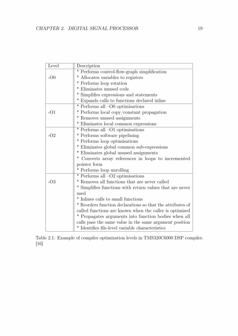
Compilers support different levels of optimization. Table 2.1 represents theoptimization levels in TMS320C6000 DSP compiler.
Compilers have proved to be effective optimization method for RISC-typeprocessors. However, the irregular datapaths, small number of registers [18], non-homogeneous register sets, very specialized registers, very specialized functionalunits, restricted connectivity and limited addressing [19] are a challenge to compilersto produce efficient code. Despite those challenges, DSP compilers perform verywell in optimization, and can outperform even the best assembly programmers [12].
One important software development and optimization related unity is thechoice of the programming language and the optimization level of the programminglanguage itself. Some of the programming languages used in real-time softwaredevelopment include Ada, C, C++, C, Java and real-time Java [7]. The choice ofthe programming language itself is very dependent on the company policies andthe application itself. As the complexity of embedded and digital-signal processingapplications grow, it is effective way to decrease the development costs by utilizingHLLs in programming, and to program only the most time-critical code in assembly.It is showed that HLLs massively lower the development and maintenance costs inembedded systems [18]. From the real-time performance point of view in the DSPapplication, it is optimization task itself to optimize the usage of the programming
CHAPTER 2. DIGITAL SIGNAL PROCESSOR 19
Level Description
-O0* Performs control-flow-graph simplification* Allocates variables to registers* Performs loop rotation* Eliminates unused code* Simplifies expressions and statements* Expands calls to functions declared inline
-O1* Performs all –O0 optimisations* Performs local copy/constant propagation* Removes unused assignments* Eliminates local common expressions
-O2* Performs all –O1 optimisations* Performs software pipelining* Performs loop optimisations* Eliminates global common sub-expressions* Eliminates global unused assignments* Converts array references in loops to incrementedpointer form* Performs loop unrolling
-O3* Performs all –O2 optimisations* Removes all functions that are never called* Simplifies functions with return values that are neverused* Inlines calls to small functions* Reorders function declarations so that the attributes ofcalled functions are known when the caller is optimised* Propagates arguments into function bodies when allcalls pass the same value in the same argument position* Identifies file-level variable characteristics
Table 2.1: Example of compiler optimization levels in TMS320C6000 DSP compiler.[16]
CHAPTER 2. DIGITAL SIGNAL PROCESSOR 20
language. The three states of the programming language optimization are theeffective usage of the language itself, the usage of the DSP-specific programminglanguage extensions, and the usage of the machine level code [20]. All of the levelshave their own advantages and disadvantages.
Implementing the algorithm using only the core language C without using anymachine level code or language extensions is the fastest to implement and theeasiest to reach bit exact results. It also retains the code portability across differentplatforms, even though it might not be necessary in embedded DSP applications.However, without any DSP-specific language extensions or machine level code, thecompiler behaviour might be unexpected, leading to very inefficient performance.It might also waste some DSP resources, leading to non-optimal utilization of thecore features. The problem is that HLLs, such C, are not expressive enough forspecial purpose processors, as they are designed for common architectures. Thoseregular architectures did not have multiple memories, fixed point computationrequirement or modulo addressing modes, so compilers had insufficient informationin the source code in order to generate optimal code for target. [21]. That was thereason for the development of the language extension.
If language extensions, like DSP related C-intrinsics are embedded into thesoftware, the performance will be much more optimized. Language extensionscan usually be utilized on the core language level without requiring to dive intomachine level code, which makes it easier for the developer to utilize them. Also,the compiler is responsible for local frame, register allocation and parallelism whenutilising language extensions, which enables higher core functionality utilization,and also makes them a rather simple optimization method for the developer. Eventhough the compiler makes the optimization, developer has some control over howthe compiler will optimize programs [21]. However, language extensions most likelydamage the code portability, and they require some knowledge of the instructionset and architecture of the platform. Even though language extensions can be usedon the higher language level, it still also slows down the development process.
Machine level code optimization is the only guaranteed way to reach the optimalperformance. It makes it possible to fully utilize all the core features. However, thecode portability and reusability is certainly damaged, it requires very expert anddeep knowledge of instruction set and architecture of the platform, and requireslot of time and perseverance to develop. From the business point of view, itmight not be the optimal way of develop DSP software, if adequate performancecan be reached using only language extensions. [20]. Of course, some of the keyfunctionalities can be programmed using machine code sequences, and rest of thefunctionalities can be programmed using language extensions.
Because compilers do not perfectly optimize code generated in HLLs, andbecause software development is a matter of time and cost, it is becoming com-
CHAPTER 2. DIGITAL SIGNAL PROCESSOR 21
mon practice to develop the full algorithm in HLLs and then rewrite the mostperformance-critical routines in assembly [22]. This results tight in a couplingbetween the HLL and assembly portions, and makes a mixed programming envi-ronment attractive.
As studied in [21], DSP-specific language extensions can significantly improvecompiler optimization, and thereby improve the overall application performance,both in the name of the code size and the execution speed.
2.5 CEVA-XC4500 DSP
CEVA-XC4500 is a DSP based on a very-long instruction word (VLIW) modelcombined with single instruction multiple data (SIMD) concept. This benefits theCEVA-XC4500 with a high level of parallelism and a high code density. CEVA-XC4500 architecture is based on a load and store computer architecture utilizingRISC operations and instructions only. The architecture has dedicated load andstore and load units responsible for loading and storing data from and to the datamemory directly to and from the registers. All other computation instructionsalways utilize those registers as sources and destinations. CEVA-XC4500 instructionset is designed with 16 bits, 32 bits, 48 bits and 64 bits wide. [23].
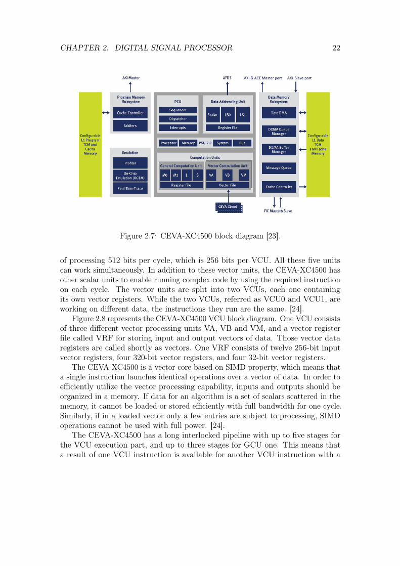
Figure 2.7 represents a block diagram of the CEVA-XC4500 DSP. It consists ofgeneral computation unit (GCU), the data address and arithmetic unit (DAAU),the program control unit (PCU), two vector computation units (VCUs), powerscaling unit (PSU), memory subsystem and emulation interface. The PCU isresponsible for aligning the instructions from the program memory and dispatchingthem to the different units. It is also responsible for the correct program flow,manages the program counter and various mechanisms for different types of non-continuous instructions. The PCU also supports core emulation and profilingthrough a standard JTAG-interface. The GCU is responsible for all of the generalcomputations and bit-manipulation operations which are non-vectorized digital-signal processing operations. The DAAU controls all data memory accesses. It hastwo separate units capable of loading and storing from and to the data memoryusing different kind of addressing modes. Two VCUs are responsible for all vectorcomputation and vector bit-manipulation operations.
The CEVA-XC4500 has three vector processing units, VA, VB and VM, andtwo load and store units LS0 and LS1 that are capable of loading and storing vectordata. The VA Unit is dedicated mostly to multiply operations and permutationsThe VB Unit is mainly used for shifts, min and max operations, transposingand bit manipulations. It supports scaling, normalization and packing. It alsosupports addition and substraction operations. The VM unit is mainly used forpost-processing for the output of the VA unit. Load and store units are capable
CHAPTER 2. DIGITAL SIGNAL PROCESSOR 22
Figure 2.7: CEVA-XC4500 block diagram [23].
of processing 512 bits per cycle, which is 256 bits per VCU. All these five unitscan work simultaneously. In addition to these vector units, the CEVA-XC4500 hasother scalar units to enable running complex code by using the required instructionon each cycle. The vector units are split into two VCUs, each one containingits own vector registers. While the two VCUs, referred as VCU0 and VCU1, areworking on different data, the instructions they run are the same. [24].
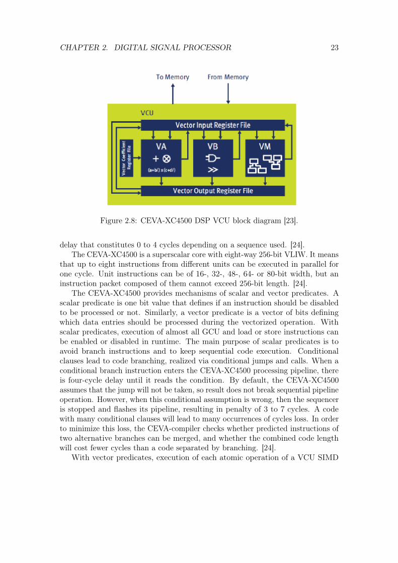
Figure 2.8 represents the CEVA-XC4500 VCU block diagram. One VCU consistsof three different vector processing units VA, VB and VM, and a vector registerfile called VRF for storing input and output vectors of data. Those vector dataregisters are called shortly as vectors. One VRF consists of twelve 256-bit inputvector registers, four 320-bit vector registers, and four 32-bit vector registers.
The CEVA-XC4500 is a vector core based on SIMD property, which means thata single instruction launches identical operations over a vector of data. In order toefficiently utilize the vector processing capability, inputs and outputs should beorganized in a memory. If data for an algorithm is a set of scalars scattered in thememory, it cannot be loaded or stored efficiently with full bandwidth for one cycle.Similarly, if in a loaded vector only a few entries are subject to processing, SIMDoperations cannot be used with full power. [24].
The CEVA-XC4500 has a long interlocked pipeline with up to five stages forthe VCU execution part, and up to three stages for GCU one. This means thata result of one VCU instruction is available for another VCU instruction with a
CHAPTER 2. DIGITAL SIGNAL PROCESSOR 23
Figure 2.8: CEVA-XC4500 DSP VCU block diagram [23].
delay that constitutes 0 to 4 cycles depending on a sequence used. [24].The CEVA-XC4500 is a superscalar core with eight-way 256-bit VLIW. It means
that up to eight instructions from different units can be executed in parallel forone cycle. Unit instructions can be of 16-, 32-, 48-, 64- or 80-bit width, but aninstruction packet composed of them cannot exceed 256-bit length. [24].
The CEVA-XC4500 provides mechanisms of scalar and vector predicates. Ascalar predicate is one bit value that defines if an instruction should be disabledto be processed or not. Similarly, a vector predicate is a vector of bits definingwhich data entries should be processed during the vectorized operation. Withscalar predicates, execution of almost all GCU and load or store instructions canbe enabled or disabled in runtime. The main purpose of scalar predicates is toavoid branch instructions and to keep sequential code execution. Conditionalclauses lead to code branching, realized via conditional jumps and calls. When aconditional branch instruction enters the CEVA-XC4500 processing pipeline, thereis four-cycle delay until it reads the condition. By default, the CEVA-XC4500assumes that the jump will not be taken, so result does not break sequential pipelineoperation. However, when this conditional assumption is wrong, then the sequenceris stopped and flashes its pipeline, resulting in penalty of 3 to 7 cycles. A codewith many conditional clauses will lead to many occurrences of cycles loss. In orderto minimize this loss, the CEVA-compiler checks whether predicted instructions oftwo alternative branches can be merged, and whether the combined code lengthwill cost fewer cycles than a code separated by branching. [24].
With vector predicates, execution of each atomic operation of a VCU SIMD
CHAPTER 2. DIGITAL SIGNAL PROCESSOR 24
instruction can be controlled in runtime. Atomic operation refers to a single opera-tion in a vector of operations of multiple data elements. For example, V CU_addintrinsics explained in the Table 4.5 in section 4 performs 16 atomic operations for16 data pairs from vectors a and b.
Each VCU instruction can be conditioned on a 16-bit predicate register, whosebits will control every atomic operation of the instruction A zero predicate bit doesnot prevent execution of the atomic operation itself, but merely blocks writingits result to the destination register. Thus, a word or double-word part of thedestination vector is defended by a zero predicate bit and the part preserves itsinput value. [24]. A word in the context of CEVA-XC4500 refers to a signed orunsigned 16-bit value, and double-word refers to a signed or unsigned 32-bit value.A word part, defined as LOW or HIGH in the intrinsics explanations in the Tables4.5 and 4.6 in the chapter 4, refers to the most significant (HIGH) or to the lesssignificant (LOW) bits of a double-word.
In the CEVA-XC4500, a generic loop construction requires code and cyclesfor managing the loop condition and branching. The for–loop is a special casewhen the maximum number of iterations is known beforehand, and there is anexplicit loop counter. The CEVA-XC4500 core’s sequencer is equipped with theso called block repeat mechanism, which supports zero-overhead for-loops. In thezero-overhead loops, the loop counter and branching is managed by the hardware,and it does not cost cycles and code. CEVA compiler also supports loop unrollingmechanism. [24].
Chapter 3
Artificial neural networks
This chapter introduces the basics of artificial neural networks. The purpose ofthis thesis is to produce speed-efficient neural network implementation on a digital-signal processor. Therefore, the comprehensive understanding of neural networkarchitecture is necessary. Section 3.1.1 introduces McCulloch-Pitts neuron, whichwas one of the first artificial neuron models, trying to mimic the behaviour of abiological neuron. Section 3.1.2 discuss about Rosenblatt’s perceptron, which isthe most common artificial neuron model today. Multilayer perceptrons (MLPs),including their training and optimization methods, are discussed in section 3.2.
3.1 Introduction
An artificial neural network (ANN) is a massively parallel distributed processor,which can store experimental knowledge and utilize it later [25]. It employs amassive inter-connection units called neurons. Knowledge is obtained by learningfrom the input data presented to the network. Inter-neuron connection strengthsare known as synaptic weights, or shortly as weights. Synaptic weights are used tostore the knowledge.
Artificial neural networks are usually defined by the following four parameters[26]:
• Type of neurons
• Neuron connection architecture
• Learning algorithm
• Recall algorithm
25
CHAPTER 3. ARTIFICIAL NEURAL NETWORKS 26
Type of neurons defines which kind of intra-network calculation units neuralnetwork consists of. These calculation units are called as neurons or nodes [26].One of the most widely used neuron type is Rosenblatt’s perceptron, discussed insection 3.1.2. Rosenblatt’s perceptron is commonly referred as a perceptron. Othercommonly used neuron types are perceptron’s simple predecessor McCulloch-Pittsneuron, introduced in section 3.1.1, and fuzzy neuron discussed in [27]. Common toall of these neurons is that they all originated from the model of a biological neuron,even though neural networks have gradually evolved into purely engineering toolshaving less and less meaning for real biological neurons [25].
Connection architecture defines the connections between neurons, which is thetopology of the ANN. Neurons in the network can be fully connected or partiallyconnected. Fully connected neuron is connected to every neuron in the previouslayer, and each connection has it’s own weight coefficient. Partially connectedneuron is connected to only a few neurons in the previous layer. Fully connectednetworks are typically utilized with MLPs, discussed in section 3.2, while partiallyconnected neurons are typical in convolutional neural networks. Convolutionalneural networks are not discussed in this thesis, as they are typically applied inimage recognition applications. In addition to the connection type of the neurons,the connection architecture can be distinguished depending on the number ofinput and output neurons, and depending on the types of layers used. Connectionarchitecture can be [26]:
• Autoassociative or heteroassociative architecture
• Feedforward or feedback architecture
In an autoassociative network architecture, input neuron of the network arealso output neurons. Autoassociative refers to a memory system, which is capableof restoring full piece of data, even when only a tiny portion of that piece of data isreprented. One example of autoassociative network is Hopfield network, popularizedby J. Hopfield in [28], as it is capable of remembering data by observing only aportion of it. In a heteroassociative network architecture, there are separate inputand output neurons. MLPs and Kohonen networks [29] are type of networks withheteroassociative neurons.
Furthermore, depending on the existence of feedback from the neuron outputback to the input, architecture can be determined to be feedforward or feedback ar-chitecture. In feedforward architecture, there are no feedback connections involved,and neurons do not remember their previous output values or states. MLPs aretype of feedforward networks. In a feedback architecture, there exists connectionsback from the output to the input, and such network holds in memory its previousstates [26]. The next state depends on the current input and the previous states
CHAPTER 3. ARTIFICIAL NEURAL NETWORKS 27
of the network. Hopfield network [28] is type of network with feedback loops.Feedback neural networks are often called recurrent neural networks (RNNs) [26].
Learning algorithm is an algorithm which trains the network. The fundamentalfeature of neural networks is their ability to learn knowledge from input data, andthis would not be possible without learning algorithms. Learning algorithms aretypically classified into supervised learning, unsupervised learning and reinforcementlearning [26]. Learning algorithms are further discussed in section 3.3.
Recall algorithm is an algorithm, which extracts learned knowledge from theneural network [26]. When new data is fed to the trained neural network, therecall algorithm provides the corresponding output based on the learned knowledge.Recall of the neural network is often called as a neural network inference.
3.1.1 McCulloch-Pitts neuron
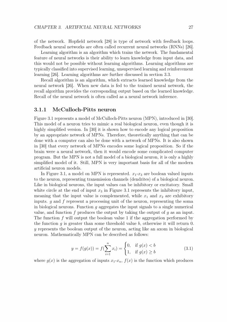
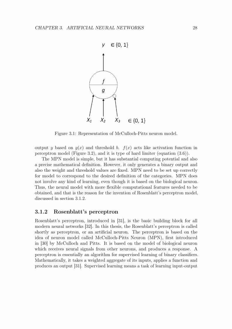
Figure 3.1 represents a model of McCulloch-Pitts neuron (MPN), introduced in [30].This model of a neuron tries to mimic a real biological neuron, even though it ishighly simplified version. In [30] it is shown how to encode any logical propositionby an appropriate network of MPNs. Therefore, theoretically anything that can bedone with a computer can also be done with a network of MPNs. It is also shownin [30] that every network of MPNs encodes some logical proposition. So if thebrain were a neural network, then it would encode some complicated computerprogram. But the MPN is not a full model of a biological neuron, it is only a highlysimplified model of it. Still, MPN is very important basis for all of the modernartificial neuron models.
In Figure 3.1, a model on MPN is represented. x1-x3 are boolean valued inputsto the neuron, representing transmission channels (dendrites) of a biological neuron.Like in biological neurons, the input values can be inhibitory or excitatory. Smallwhite circle at the end of input x3 in Figure 3.1 represents the inhibitory input,meaning that the input value is complemented, while x1 and x2 are exhibitoryinputs. g and f represent a processing unit of the neuron, representing the somain biological neurons. Function g aggregates the input signals to a single numericalvalue, and function f produces the output by taking the output of g as an input.The function f will output the boolean value 1 if the aggregation performed bythe function g is greater than some threshold value b, otherwise it will return 0.y represents the boolean output of the neuron, acting like an axom in biologicalneuron. Mathematically MPN can be described as follows:
y = f(g(x)) = f(n∑
i=1
xi) =
{0, if g(x) < b
1, if g(x) ≥ b(3.1)
where g(x) is the aggregation of inputs x1-xn, f(x) is the function which produces
CHAPTER 3. ARTIFICIAL NEURAL NETWORKS 28
Figure 3.1: Representation of McCulloch-Pitts neuron model.
output y based on g(x) and threshold b. f(x) acts like activation function inperceptron model (Figure 3.2), and it is type of hard limiter (equation (3.6)).
The MPN model is simple, but it has substantial computing potential and alsoa precise mathematical definition. However, it only generates a binary output andalso the weight and threshold values are fixed. MPN need to be set up correctlyfor model to correspond to the desired definition of the categories. MPN doesnot involve any kind of learning, even though it is based on the biological neuron.Thus, the neural model with more flexible computational features needed to beobtained, and that is the reason for the invention of Rosenblatt’s perceptron model,discussed in section 3.1.2.
3.1.2 Rosenblatt’s perceptron
Rosenblatt’s perceptron, introduced in [31], is the basic building block for allmodern neural networks [32]. In this thesis, the Rosenblatt’s perceptron is calledshortly as perceptron, or an artificial neuron. The perceptron is based on theidea of neuron model called McCulloch-Pitts Neuron (MPN), first introducedin [30] by McCulloch and Pitts. It is based on the model of biological neuronwhich receives neural signals from other neurons, and produces a response. Aperceptron is essentially an algorithm for supervised learning of binary classifiers.Mathematically, it takes a weighted aggregate of its inputs, applies a function andproduces an output [31]. Supervised learning means a task of learning input-output
CHAPTER 3. ARTIFICIAL NEURAL NETWORKS 29
mapping from example input-output pairs. A binary classifier is a function whichcan decide if an input vector belongs to a some specific class or not. A fully trainedperceptron can perfectly classify input patterns if they are linearly separable [25].A single perceptron is the most simplest version of ANNs, as it consist only oneneuron on a single layer, the perceptron itself.
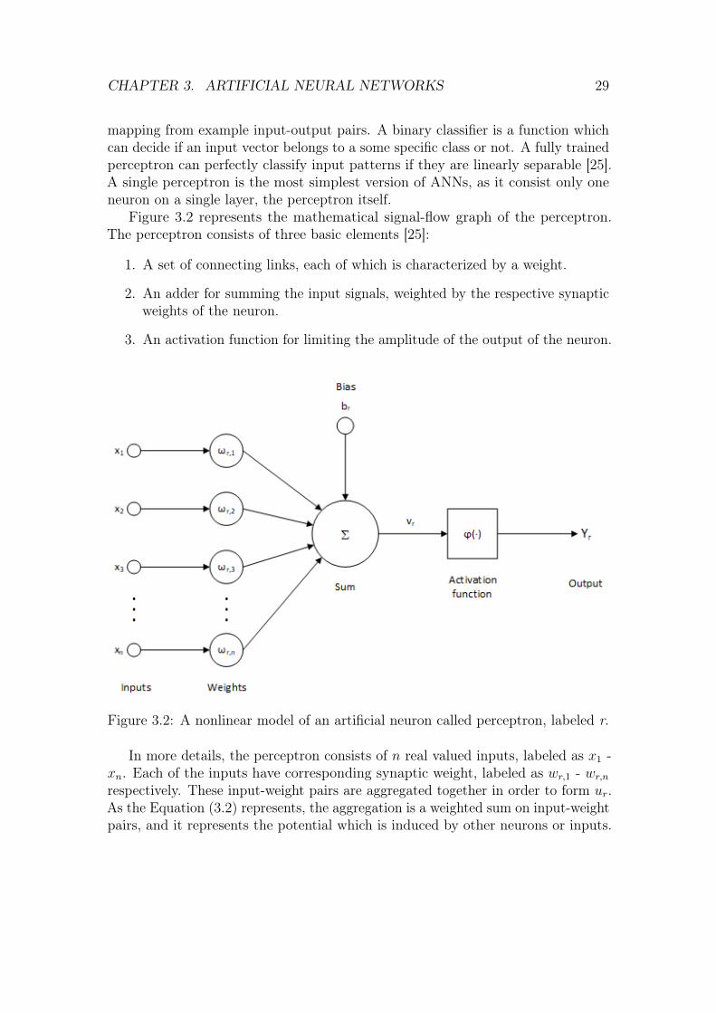
Figure 3.2 represents the mathematical signal-flow graph of the perceptron.The perceptron consists of three basic elements [25]:
1. A set of connecting links, each of which is characterized by a weight.
2. An adder for summing the input signals, weighted by the respective synapticweights of the neuron.
3. An activation function for limiting the amplitude of the output of the neuron.
Figure 3.2: A nonlinear model of an artificial neuron called perceptron, labeled r.
In more details, the perceptron consists of n real valued inputs, labeled as x1 -xn. Each of the inputs have corresponding synaptic weight, labeled as wr,1 - wr,n
respectively. These input-weight pairs are aggregated together in order to form ur.As the Equation (3.2) represents, the aggregation is a weighted sum on input-weightpairs, and it represents the potential which is induced by other neurons or inputs.
CHAPTER 3. ARTIFICIAL NEURAL NETWORKS 30
ur =n∑
i=1
ωr,ixi (3.2)
In the perceptron model, there is also one special input called bias b [26]. Biashas a constant weight value of 1. It can be also considered in a way that theperceptron has one constant input of 1, which is weighted by the bias coefficientb. Mathematically speaking, the purpose of the bias is to adjust the activationthreshold of the perceptron, thereby increasing the flexibility of the perceptronmodel. Bias represents the background potential of the neuron. ur and bias btogether form the induced local field of the neuron vr, represented in Equation(3.3).
vr = ur + br (3.3)
As mentioned earlier, this one special input value can also be considered asconstant input value of 1, paired with the weight b. In many cases this constantinput can be considered to be input x0, and the bias b can be similarly assignedto be wr,0. In this case, br can be embedded to the aggregation, as Equation (3.4)illustrates.
vr =n∑
i=1
ωr,ixi + br =n∑
i=1
ωr,ixi + ωr,0x0 =n∑
i=0
ωr,ixi (3.4)
Activation
In order to produce the final output yr of the perceptron, the induced local field vris activated with a function called activation function [32] or squash function, ϕ(.):
yr = ϕ(vr) (3.5)
The purpose of the activation is to limit the amplitude of the neuron output, andto add non-linearity to the inference [32]. If linear activation function, like identityactivation ϕ(v) = v is used, multiple perceptron layers (discussed in section 3.2)are equivalent to single perceptron layer. In the case of linear activation, extralayers do not add free parameters to the network. In addition to non-linearity, theactivation function is desirably continuously differentiable. Without continuousdifferentiablity, gradient-based learning methods (discussed in section 3.3) are notpossible, or they might have problems to progress with learning. Few of the mostcommonly used activation functions are:
CHAPTER 3. ARTIFICIAL NEURAL NETWORKS 31
• Threshold function or hard limiter
ϕ(v) =
{+1 if v ≥ 0
0 if v < 0(3.6)
Threshold function outputs only two values, either +1 or 0. It is symmetricfunction, and its breakpoint can be easily moved with bias. However, itis neither continuous or continuously differentiable. It was used in manyearly neural network models, and is fundamental part of the McCulloch-Pittsneuron model [30], discussed in section 3.1.1.
• Rectified linear unit (ReLU)
ϕ(v) = max{0, v} (3.7)
The rectified linear unit outputs the input itself, if the input value is positive,and zero otherwise. Therefore, it is linear for half of the input domain, andnon-linear for the other half. Linear property make it easy to optimize withgradient based methods [33]. The gradient is 1 for all positive values, and0 for negative values. This means that during backpropagation training,discussed in section 3.3.2, negative gradient will not be used to update theweights. Because the gradient is 1 for all positive values, the training speedis very good compared to other non-linear functions due to good gradientflow. ReLU also preserves many of the properties that make linear modelgeneralize well [33]. It has become the default activation function for manytypes of neural networks, as it is easy to optimize, it typically convergencesfast, and it has high computation speed [34].
• Sigmoid function
ϕ(v) =1
1 + e−av, a ∈ R (3.8)
The sigmoid function is commonly used S-shaped nonlinear activation function.It is commonly used on the output layer neurons, as it produces restrictedoutput between 0 and 1. This outcome can be interpreted as probability of thatoutput. Using design parameter a, the shape of the sigmoid curve can be tuned.One advantage of the sigmoid function is that its gradient is well-defined,which is probably one of the reasons for its popularity. Sigmoid functionscan be used also on the hidden layer neurons, however, the gradient of thefunction is very close to zero over a large portion of its domain, which makesit harder and slower for the learning algorithm to learn. This unfavourablefeature is often called as gradient vanishing problem [35]. Vanishing gradientmake it difficult to know which direction the parameter should move in order
CHAPTER 3. ARTIFICIAL NEURAL NETWORKS 32
to imporve the model performance [33]. Other commonly identified problemwith the sigmoid function is the saturation. The saturation means thatlarge input values snap to sigmoids maximum output value of 1, and smallvalues similarly snap to the 0. Furthermore, the function is very sensitive onlyaround the mid-point of the input, around 0.5 [33]. The limited sensitivity andsaturation problem happen whether the input contains useful informationor not, and once saturated, it becomes very challenging for the learningalgorithm to continue improving the model performance.
• Softmaxϕ(v)i =
evi∑j e
vj(3.9)
Softmax is utilized in the output layer of the neural network to detectmulticlass classification probabilities. It squashes output vector in the range(0, 1), and all the resulting elements add up to 1. The Softmax functioncannot be applied independently to each element, as it’s value depends onall elements of the output vector. If the classification probability is notimportant in the inference, the softmax activation can be replaced withargmax activation.
Learning
Learning is fundamental property of perceptron and ANNs. Perceptron can acquireknowledge from the training set, and store it in its weight coefficients. Via learning,perceptrons are suitable both for classification and regression problems.
The perceptron rule is a sequential learning procedure for updating the percep-tron weights. In other words, it is the way of learning perceptron input-output map-ping for a classification problem. The learning rule is an example of supervised train-ing, in which the learning rule is provided with a set of examples of proper networkbehavior called a training set S = {X(0), d(0)}, {X(1), d(1)}, ... {X(n), d(n)},where X(n) is the example input vector and d(n) is the corresponding output value.
The Perceptron convergence theorem [36] states that for any data set which islinearly separable, the perceptron learning rule is guaranteed to find a solution in afinite number of steps. In other words, the perceptron learning rule is guaranteedto converge to a weight vector that correctly classifies the examples provided.However, it is important to understand that the converged weight vector W ′ isnot necessarily unique, and it depends on the initial weight vector W . Also, theconverged weight vector W ′ is not necessarily same as the optimal solution W∗,even though it correctly classifies the learning examples. A function is said to belinearly separable when its outputs can be discriminated by a function which isa linear combination of features. The convergence theorem also states that the
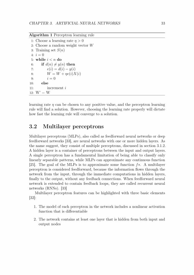
CHAPTER 3. ARTIFICIAL NEURAL NETWORKS 33
Algorithm 1 Perceptron learning rule1: Choose a learning rate η > 02: Choose a random weight vector W3: Training set S(n)4: i = 05: while i < n do6: if d(n) 6= y(n) then7: e(i) = d(i)− y(i)8: W = W + ηe(i)X(i)9: i = 0
10: else11: increment i12: W’ = W
learning rate η can be chosen to any positive value, and the perceptron learningrule will find a solution. However, choosing the learning rate properly will dictatehow fast the learning rule will converge to a solution.
3.2 Multilayer perceptrons
Multilayer perceptrons (MLPs), also called as feedforward neural networks or deepfeedforward networks [33], are neural networks with one or more hidden layers. Asthe name suggest, they consist of multiple perceptrons, discussed in section 3.1.2.A hidden layer is a container of perceptrons between the input and output layers.A single perceptron has a fundamental limitation of being able to classify onlylinearly separable patterns, while MLPs can approximate any continuous function[25]. The goal of the MLPs is to approximate some function f∗. A multilayerperceptron is considered feedforward, because the information flows through thenetwork from the input, through the immediate computations in hidden layers,finally to the output, without any feedback connections. When feedforward neuralnetwork is extended to contain feedback loops, they are called recurrent neuralnetworks (RNNs). [33]
Multilayer perceptron features can be highlighted with three basic elements[32]:
1. The model of each perceptron in the network includes a nonlinear activationfunction that is differentiable
2. The network contains at least one layer that is hidden from both input andoutput nodes
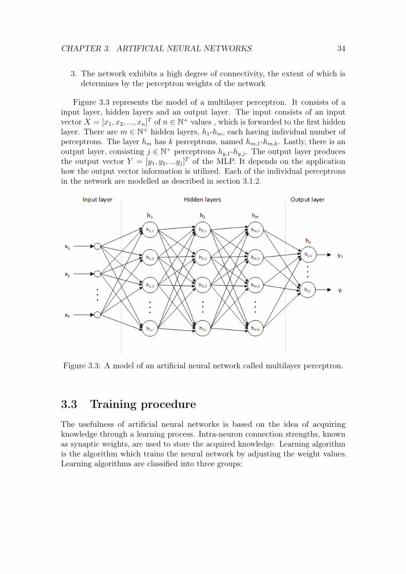
CHAPTER 3. ARTIFICIAL NEURAL NETWORKS 34
3. The network exhibits a high degree of connectivity, the extent of which isdetermines by the perceptron weights of the network
Figure 3.3 represents the model of a multilayer perceptron. It consists of ainput layer, hidden layers and an output layer. The input consists of an inputvector X = [x1, x2, ..., xn]T of n ∈ N+ values , which is forwarded to the first hiddenlayer. There are m ∈ N+ hidden layers, h1-hm, each having individual number ofperceptrons. The layer hm has k perceptrons, named hm,1-hm,k. Lastly, there is anoutput layer, consisting j ∈ N+ perceptrons hy,1-hy,j. The output layer producesthe output vector Y = [y1, y2, ...yj]
T of the MLP. It depends on the applicationhow the output vector information is utilized. Each of the individual perceptronsin the network are modelled as described in section 3.1.2.
Figure 3.3: A model of an artificial neural network called multilayer perceptron.
3.3 Training procedure
The usefulness of artificial neural networks is based on the idea of acquiringknowledge through a learning process. Intra-neuron connection strengths, knownas synaptic weights, are used to store the acquired knowledge. Learning algorithmis the algorithm which trains the neural network by adjusting the weight values.Learning algorithms are classified into three groups:
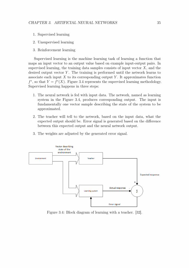
CHAPTER 3. ARTIFICIAL NEURAL NETWORKS 35
1. Supervised learning
2. Unsupervised learning
3. Reinforcement learning
Supervised learning is the machine learning task of learning a function thatmaps an input vector to an output value based on example input-output pairs. Insupervised learning, the training data samples consists of input vector X, and thedesired output vector Y . The training is performed until the network learns toassociate each input X to its corresponding output Y . It approximates functionf ∗, so that Y = f ∗(X). Figure 3.4 represents the supervised learning methodology.Supervised learning happens in three steps:
1. The neural network is fed with input data. The network, named as learningsystem in the Figure 3.4, produces corresponding output. The input isfundamentally one vector sample describing the state of the system to beapproximated.
2. The teacher will tell to the network, based on the input data, what theexpected output should be. Error signal is generated based on the differencebetween this expected output and the neural network output.
3. The weights are adjusted by the generated error signal.
Figure 3.4: Block diagram of learning with a teacher. [32].
CHAPTER 3. ARTIFICIAL NEURAL NETWORKS 36
Unsupervised learning is a training method, in which only training input X issupplied to the network. The network learns some internal feature of the whole setof all data inputs, but there are not any desired output. Unsupervised algorithmsare usually further divided into competitive and non-competitive algorithms.
Reinforcement learning is a method, in which the input vector X is presentedto the network, and it is allowed to determine corresponding output. If the outputis good in the names of cost function C, the existing neural weights are increased(rewarded), otherwise they are decreased (punished).
3.3.1 Cost function
Cost function C is a function that measures the performanse of a machine learningmodel for given data. Cost function quantifies the error between predicted outputand expected output values. Cost function presents this error in the form of a singlereal valued number. The purpose of the cost function is to be either minimizedor maximized. If the cost function is to be minimized, the returned value of thefunction is usually called cost, lost or error. The goal of the training is to find amodel which minimizes the value returned by the cost function. If the purpose ofthe cost function is be maximized, the return value is typically called a reward. Inthis case, the purpose of the training is to find a model for which the returned costfunction value is as large as possible. [25].
Two very commonly used cost functions are mean absolute error (MAE) andmean squared error (MSE). Equation (3.10) represents the cost value C in MAEfunction, and equation (3.11) represents the cost value in MSE. C states for thereturn value of a cost function, n is the total number of data samples, d(i) is theexpected output for the ith data sample, and y(i) is the model output for the ithdata sample.
C =1
n
n∑i=1
|d(i)− y(i)| (3.10)
C =1
2n
n∑i=1
(d(i)− y(i))2 (3.11)
Each cost function treats the difference between observations and expectedoutcome in a unique way. The distance between ideal result and predictions arehaving attached a penalty by metric, based on the magnitude and direction inthe coordinate system. For example, MAE does not add any additional weight tothe error distance, so the error growth is linear. In MSE instead, the error growsexponentially with larger error distances. It adds a massive penalty for predictionthat are war away from expectation, and minimal penalty for close predictions.
CHAPTER 3. ARTIFICIAL NEURAL NETWORKS 37
Binary cross-entropy (BCE) is a loss function used on problems involving binarydecisions [37], such as one hot encoding problems. Equation 3.12 represents the lossin BCE. In multilabel problems, where an example can belong to multiple classesat the same time, the model tries to decide for each class whether the examplebelongs to that class or not. BCE measures how far away from the true binaryvalue the prediction is for each of the classes, and then averages these classwiseerrors to obtain the final loss.
Cbce = − 1
N
N∑i=1
[yilog(p(yi)) + (1− yi)log(1− p(yi))] (3.12)
3.3.2 Backpropagation of errors
Backpropagation of errors, or simply backpropagation algorithm, is the most pop-ular learning algorithm rule for performing supervised learning tasks for MLP.Backpropagation algorithm uses a gradient-search technique to minimize a costfunction between the desired output and the actual MLP output. The gradientsignifies how the error of the network changes with the changes to the network’sweights. Backpropagation makes it possible to extend MLP to many layers. Themodern version of the backpropagation, also called the reverse mode of automaticdifferentiation, was first published in [38] without NN context. In [39] the backprop-agation algorithm is attached to several different NNs, making them to learn muchfaster than previous learning approaches, solving problems which had previouslybeen insolvable.
Algorithm 2 describes the backpropagation on pseudocode level. The basicprinciple is that backpropagation algorithm propagates backwards the error betweenNN output and desired output through the network. After providing an inputpattern, the forward propagated output of the network, the inference, is thencompared with a given target pattern, and the error of each output unit is calculated.This error signal e(n), difference between desired output d(n) pattern and inferredoutput y(n), is propagated backward, and a closed-loop control system is thusestablished. At the heart of backpropagation is an expression for the partialderivative ∂C
∂wof the cost function C with respect to any weight w in the network.
The partial derivative express how quickly the value of the cost function changeswhen weights are changed.
The backpropagation requires two assumptions from the cost function. The firstis that the cost function can be written as an average C = 1
n
∑xCx over individual
cost functions Cx for individual training examples x. The second assumption isthat the cost function is a function of the outputs from the NN, C = f(y)
The adjustments of the synaptic weights depends upon the information of the
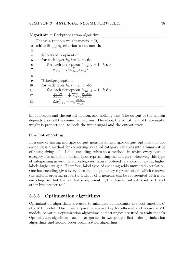
CHAPTER 3. ARTIFICIAL NEURAL NETWORKS 38
Algorithm 2 Backpropagation algorithm1: Choose a random weight matrix w(0)2: while Stopping criterion is not met do3:4: %Forward propagation5: for each layer hi, i = 1...m do6: for each perceptron hm,j, j = 1...k do7: yhm,j
= ϕ(wThm,j
xhm,j)
8:9: %Backpropagation
10: for each layer hi, i = 1...m do11: for each perceptron hm,j, j = 1...k do12: ∂C(w)
∂wi,i+1= 1
N
∑Nd=1
∂C(w)d∂wi,i+1
13: ∆whii,i+1 = −η ∂C(w)
∂wi,i+1
input neuron and the output neuron, and nothing else. The output of the neurondepends upon all the connected neurons. Therefore, the adjustment of the synapticweight is proportional to both the input signal and the output error.
One hot encoding
In a case of having multiple output neurons for multiple output options, one hotencoding is a method for converting so called category variables into a binary-styleof categorizing [40]. Label encoding refers to a method, in which every outputcategory has unique numerical label representing the category. However, this typeof categorizing gives different categories natural ordered relationship, giving higherlabels higher weight. Therefore, label type of encoding adds unwanted correlation.One hot encoding gives every outcome unique binary representation, which removesthe natural ordering property. Output of n neurons can be represented with n-bitencoding, so that the bit that is representing the desired output is set to 1, andother bits are set to 0.
3.3.3 Optimization algorithms
Optimization algorithms are used to minimize or maximise the cost function Cof a ML model. The internal parameters are key for efficient and accurate MLmodels, so various optimization algorithms and strategies are used to train models.Optimization algorithms can be categorised in two groups: first order optimizationalgorithms and second order optimization algorithms.
CHAPTER 3. ARTIFICIAL NEURAL NETWORKS 39
The goal with first order optimization algorithms is to minimize or maximizecost function C based on the gradient of the C respect to a certain model variableθ [41]. In the case of NNs, the model variable θ is the weight vector W of the NN.Gradient of the cost function tells whether the function is increasing or decreasingat a particular value of θ.
Similarly, the goal of the second order optimization algorithms is to minimizeor maximize the cost function C based on the second gradient of the C respect tothe certain model variable θ. The second order derivative of the C tells wheterthe gradient of the C is increasing or decreasing at a particular value of θ. Thesecond order derivative is computational heavy to calculate, therefore, the secondorder optimizations are not as widely used methods as the first order optimizationalgorithms.
Gradient descent is a first order optimization algorithm commonly used in NNmodels. Gradient descent minimizes the cost function by moving iteratively tothe direction of the steepest descent as defined by the negative of the gradient.Equation (3.13) represents the weight update rule of the MLP with gradient descent.η is called as learning rate, which defines how big steps are taken when updatingthe weights based on the gradient of the cost function.
w(n+ 1) = w(n)− η∇C(w(n)) (3.13)
An advanced form of the gradient descent, stochastic gradient descent (SGD), isthe most used optimization algorithms for ML in general [33]. SGD have also lotsof variants, for example Adam optimizer, adaptive gradient algorithm, and rootmean square propagation [42]. In the gradient descent algorithm, all the samplesin the training set are run in order to do a single update for a parameter in aparticular iteration, whereas in SGD, only one sample or subset of training sampleof the training are used to do the update for a parameter in a particular iteration.If a subset of samples are used, the method is called minibatch stochastic gradientdescent [33]. As gradient descent is based on the derivative of the cost function, inorder to optimize cost function with it, also activation functions in the NN mustbe differentiable.
Adam optimizer is one extension of SGD based optimization algorithms. Itcombines properties of the adaptive gradient algorithm (AGA) and root meansquare propagation (RMSP) to provide an optimization algorithm that can handlesparse gradients on noisy problems.[43] It computes adaptive learning rates foreach parameter. Adam uses both the average of the first moment and average ofthe the second moment of the gradient when adapting learning rates. The Adamcalculates an exponential moving average of the gradient and the squared gradient,and two tuning parameters control the decay rates of these moving averages. [42].
CHAPTER 3. ARTIFICIAL NEURAL NETWORKS 40
3.3.4 Regularization
Regularization is a technique to penalize the size of the weights of a NN. Regular-ization penalizes strong weight values, so that strong output confidence cannot beachieved from the output of just single single neuron. The strong output confidencecan be achieved only from the consensus of multiple neurons. Since many neuronshave to agree to achieve a strong output value, the output value is less likely tobiased just by a single neuron. It especially helps to prevent overfitting, as adjustingthe model to be more complex requires bigger weight values, and that is penalized.
There are two commonly used regularization methods, L1 and L2 regularization.A regression model that uses L1 regularization is called Lasso Regression [44], andmodel which uses L2 regression is called Ridge Regression [45].
The L1 regularization penalizes the absolute size of the weight. Equation (3.14)represents the L1 regularization element. Here λ is the tuning parameter thatdecides how much the flexibility of the model is penalized. w represents a weightcoefficient of the model. In L1 regularization, most of the weights will be zero, andonly some medium or large size weights remain [44]. Because L1 regularization tendsto produce sparse weights values, it naturally does a feature selection. Insignificantinput features are assigned with zero weights, and significant features are assignedwith large weight value.
R = λ∑i
|wi| (3.14)
The L2 regularization penalizes the squared size of the weight. Equation 3.15represents the L2 regularization element. Here λ is the tuning parameter thatdecides how much the flexibility of the model is penalized. w represents a weightcoefficient of the model. L2 regularization encourages very small, but non-zeroweights. The inference is established by almost all weights, thus reducing the modelbias. There are no neurons that can turn around model output by themselves. AsL2 regularization does not tend to make weights zero, it is not robust to the outlierdata samples.
R = λ∑i
w2i (3.15)
Chapter 4
Implementation
In this thesis, fully-connected feedforward neural network inference is implementedon the CEVA-XC4500 DSP. The feedforward neural network architecture is potentialML algorithm for an DSP application due to the parallelization potential, and dueto promising results in various classification problems. For the design of advancedneural network based real-time ML application, it is essential to understand thetheory behind neural networks, how to collect suitable data for the model trainingand validation, how to create a working model, and how DSP architecture canbe efficiently utilized. As discussed earlier in this thesis, the first and the mostimportant optimization for an DSP algorithm is to design the algorithm itself fromthe DSP architecture point of view. For that reason, it is important to keep theDSP in mind when creating the neural network model itself.
Theory behind feedforward neural networks, supervised learning, and DSPalgorithm development and optimization methods are explained in previous chapters,while this chapter focuses on the neural network model creation and the DSPimplementation for a specific use case on a specific DSP. At first, the use caseis shortly explained. Next, NN model creation is discussed including the datacollection, the use case specific data-analysis, hyperparameter tuning, and themodel validation. Later, DSP related implementation and optimization methods arediscussed for the specific use case. Evaluation of the implementation is representedin the chapter 5.
Because the source codes of the NN model and the DSP implementation areconfidential property of Nokia, only pseudocodes are represented in this thesis.
4.1 Use case
The use case is to implement NN-based real-time symbol decoder for the 5G uplinkcontrol information. The implementation is executed on the Nokia 5G baseband
41
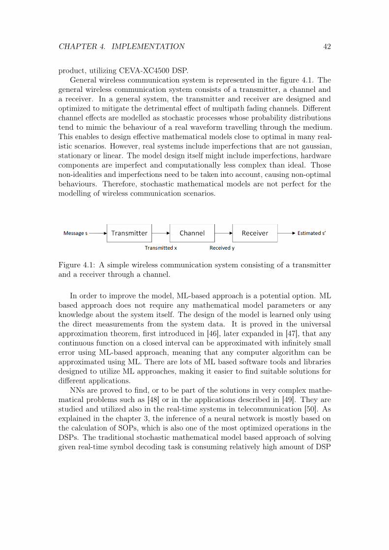
CHAPTER 4. IMPLEMENTATION 42
product, utilizing CEVA-XC4500 DSP.General wireless communication system is represented in the figure 4.1. The
general wireless communication system consists of a transmitter, a channel anda receiver. In a general system, the transmitter and receiver are designed andoptimized to mitigate the detrimental effect of multipath fading channels. Differentchannel effects are modelled as stochastic processes whose probability distributionstend to mimic the behaviour of a real waveform travelling through the medium.This enables to design effective mathematical models close to optimal in many real-istic scenarios. However, real systems include imperfections that are not gaussian,stationary or linear. The model design itself might include imperfections, hardwarecomponents are imperfect and computationally less complex than ideal. Thosenon-idealities and imperfections need to be taken into account, causing non-optimalbehaviours. Therefore, stochastic mathematical models are not perfect for themodelling of wireless communication scenarios.
Figure 4.1: A simple wireless communication system consisting of a transmitterand a receiver through a channel.
In order to improve the model, ML-based approach is a potential option. MLbased approach does not require any mathematical model parameters or anyknowledge about the system itself. The design of the model is learned only usingthe direct measurements from the system data. It is proved in the universalapproximation theorem, first introduced in [46], later expanded in [47], that anycontinuous function on a closed interval can be approximated with infinitely smallerror using ML-based approach, meaning that any computer algorithm can beapproximated using ML. There are lots of ML based software tools and librariesdesigned to utilize ML approaches, making it easier to find suitable solutions fordifferent applications.
NNs are proved to find, or to be part of the solutions in very complex mathe-matical problems such as [48] or in the applications described in [49]. They arestudied and utilized also in the real-time systems in telecommunication [50]. Asexplained in the chapter 3, the inference of a neural network is mostly based onthe calculation of SOPs, which is also one of the most optimized operations in theDSPs. The traditional stochastic mathematical model based approach of solvinggiven real-time symbol decoding task is consuming relatively high amount of DSP
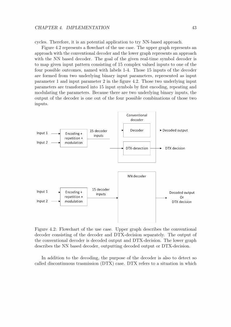
CHAPTER 4. IMPLEMENTATION 43
cycles. Therefore, it is an potential application to try NN-based approach.Figure 4.2 represents a flowchart of the use case. The upper graph represents an
approach with the conventional decoder and the lower graph represents an approachwith the NN based decoder. The goal of the given real-time symbol decoder isto map given input pattern consisting of 15 complex valued inputs to one of thefour possible outcomes, named with labels 1-4. Those 15 inputs of the decoderare formed from two underlying binary input parameters, represented as inputparameter 1 and input parameter 2 in the figure 4.2. Those two underlying inputparameters are transformed into 15 input symbols by first encoding, repeating andmodulating the parameters. Because there are two underlying binary inputs, theoutput of the decoder is one out of the four possible combinations of those twoinputs.
Figure 4.2: Flowchart of the use case. Upper graph describes the conventionaldecoder consisting of the decoder and DTX-decision separately. The output ofthe conventional decoder is decoded output and DTX-decision. The lower graphdescribes the NN based decoder, outputting decoded output or DTX-decision.
In addition to the decoding, the purpose of the decoder is also to detect socalled discontinuous trasmission (DTX) case. DTX refers to a situation in which
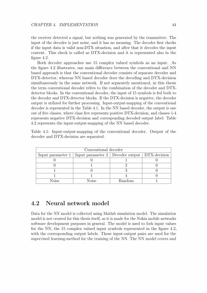
CHAPTER 4. IMPLEMENTATION 44
the receiver detected a signal, but nothing was generated by the transmitter. Theinput of the decoder is just noise, and it has no meaning. The decoder first checksif the input data is valid non-DTX situation, and after that it decodes the inputcontent. This check is called as DTX-decision and it is represented also in thefigure 4.2.
Both decoder approaches use 15 complex valued symbols as an input. Asthe figure 4.2 illustrates, one main difference between the conventional and NNbased approach is that the conventional decoder consists of separate decoder andDTX-detector, whereas NN based decoder does the decoding and DTX-decisionsimultaneously in the same network. If not separately mentioned, in this thesisthe term conventional decoder refers to the combination of the decoder and DTX-detector blocks. In the conventional decoder, the input of 15 symbols is fed both tothe decoder and DTX-detector blocks. If the DTX-decision is negative, the decoderoutput is utilized for further processing. Input-output-mapping of the conventionaldecoder is represented in the Table 4.1. In the NN based decoder, the output is oneout of five classes, where class five represents positive DTX-decision, and classes 1-4represents negative DTX-decision and corresponding decoded output label. Table4.2 represents the input-output-mapping of the NN based decoder.
Table 4.1: Input-output-mapping of the conventional decoder. Output of thedecoder and DTX-decision are separated.
Conventional decoderInput parameter 1 Input parameter 2 Decoder output DTX-decision
0 0 1 00 1 2 01 0 3 01 1 4 0
Noise Noise Random 1
4.2 Neural network model
Data for the NN model is collected using Matlab simulation model. The simulationmodel is not created for this thesis itself, as it is made for the Nokia mobile networkssoftware development purposes in general. The model is used to fork input valuesfor the NN, the 15 complex valued input symbols represented in the figure 4.2,with the corresponding output labels. Those input-output pairs are used for thesupervised learning-method for the training of the NN. The NN model covers and
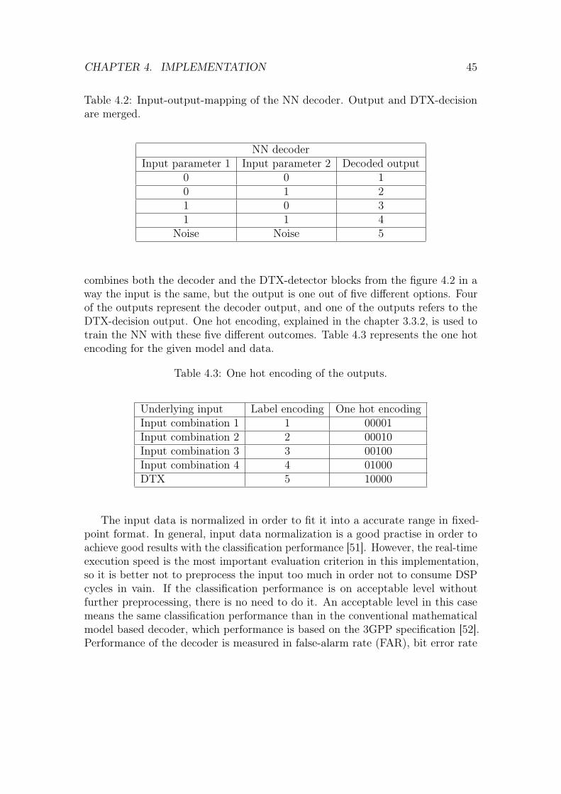
CHAPTER 4. IMPLEMENTATION 45
Table 4.2: Input-output-mapping of the NN decoder. Output and DTX-decisionare merged.
NN decoderInput parameter 1 Input parameter 2 Decoded output
0 0 10 1 21 0 31 1 4
Noise Noise 5
combines both the decoder and the DTX-detector blocks from the figure 4.2 in away the input is the same, but the output is one out of five different options. Fourof the outputs represent the decoder output, and one of the outputs refers to theDTX-decision output. One hot encoding, explained in the chapter 3.3.2, is used totrain the NN with these five different outcomes. Table 4.3 represents the one hotencoding for the given model and data.
Table 4.3: One hot encoding of the outputs.
Underlying input Label encoding One hot encodingInput combination 1 1 00001Input combination 2 2 00010Input combination 3 3 00100Input combination 4 4 01000DTX 5 10000
The input data is normalized in order to fit it into a accurate range in fixed-point format. In general, input data normalization is a good practise in order toachieve good results with the classification performance [51]. However, the real-timeexecution speed is the most important evaluation criterion in this implementation,so it is better not to preprocess the input too much in order not to consume DSPcycles in vain. If the classification performance is on acceptable level withoutfurther preprocessing, there is no need to do it. An acceptable level in this casemeans the same classification performance than in the conventional mathematicalmodel based decoder, which performance is based on the 3GPP specification [52].Performance of the decoder is measured in false-alarm rate (FAR), bit error rate
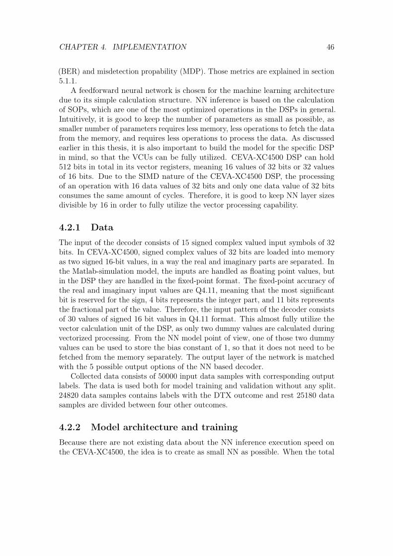
CHAPTER 4. IMPLEMENTATION 46
(BER) and misdetection propability (MDP). Those metrics are explained in section5.1.1.
A feedforward neural network is chosen for the machine learning architecturedue to its simple calculation structure. NN inference is based on the calculationof SOPs, which are one of the most optimized operations in the DSPs in general.Intuitively, it is good to keep the number of parameters as small as possible, assmaller number of parameters requires less memory, less operations to fetch the datafrom the memory, and requires less operations to process the data. As discussedearlier in this thesis, it is also important to build the model for the specific DSPin mind, so that the VCUs can be fully utilized. CEVA-XC4500 DSP can hold512 bits in total in its vector registers, meaning 16 values of 32 bits or 32 valuesof 16 bits. Due to the SIMD nature of the CEVA-XC4500 DSP, the processingof an operation with 16 data values of 32 bits and only one data value of 32 bitsconsumes the same amount of cycles. Therefore, it is good to keep NN layer sizesdivisible by 16 in order to fully utilize the vector processing capability.
4.2.1 Data
The input of the decoder consists of 15 signed complex valued input symbols of 32bits. In CEVA-XC4500, signed complex values of 32 bits are loaded into memoryas two signed 16-bit values, in a way the real and imaginary parts are separated. Inthe Matlab-simulation model, the inputs are handled as floating point values, butin the DSP they are handled in the fixed-point format. The fixed-point accuracy ofthe real and imaginary input values are Q4.11, meaning that the most significantbit is reserved for the sign, 4 bits represents the integer part, and 11 bits representsthe fractional part of the value. Therefore, the input pattern of the decoder consistsof 30 values of signed 16 bit values in Q4.11 format. This almost fully utilize thevector calculation unit of the DSP, as only two dummy values are calculated duringvectorized processing. From the NN model point of view, one of those two dummyvalues can be used to store the bias constant of 1, so that it does not need to befetched from the memory separately. The output layer of the network is matchedwith the 5 possible output options of the NN based decoder.
Collected data consists of 50000 input data samples with corresponding outputlabels. The data is used both for model training and validation without any split.24820 data samples contains labels with the DTX outcome and rest 25180 datasamples are divided between four other outcomes.
4.2.2 Model architecture and training
Because there are not existing data about the NN inference execution speed onthe CEVA-XC4500, the idea is to create as small NN as possible. When the total
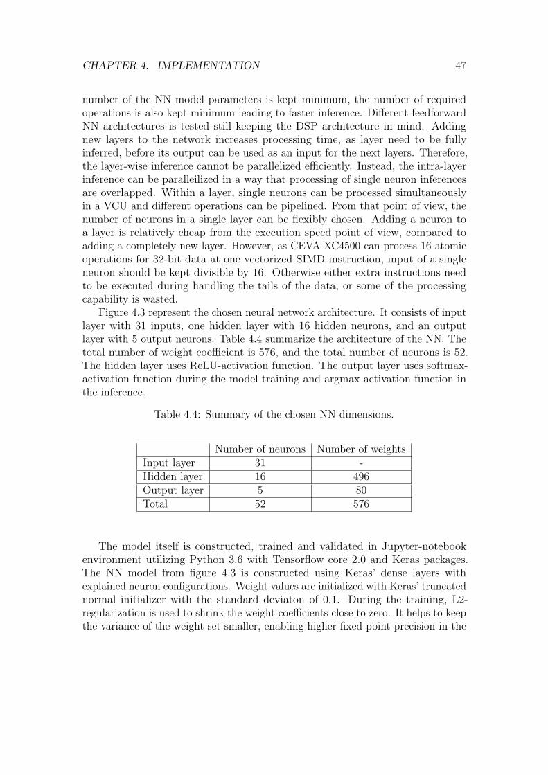
CHAPTER 4. IMPLEMENTATION 47
number of the NN model parameters is kept minimum, the number of requiredoperations is also kept minimum leading to faster inference. Different feedforwardNN architectures is tested still keeping the DSP architecture in mind. Addingnew layers to the network increases processing time, as layer need to be fullyinferred, before its output can be used as an input for the next layers. Therefore,the layer-wise inference cannot be parallelized efficiently. Instead, the intra-layerinference can be paralleilized in a way that processing of single neuron inferencesare overlapped. Within a layer, single neurons can be processed simultaneouslyin a VCU and different operations can be pipelined. From that point of view, thenumber of neurons in a single layer can be flexibly chosen. Adding a neuron toa layer is relatively cheap from the execution speed point of view, compared toadding a completely new layer. However, as CEVA-XC4500 can process 16 atomicoperations for 32-bit data at one vectorized SIMD instruction, input of a singleneuron should be kept divisible by 16. Otherwise either extra instructions needto be executed during handling the tails of the data, or some of the processingcapability is wasted.
Figure 4.3 represent the chosen neural network architecture. It consists of inputlayer with 31 inputs, one hidden layer with 16 hidden neurons, and an outputlayer with 5 output neurons. Table 4.4 summarize the architecture of the NN. Thetotal number of weight coefficient is 576, and the total number of neurons is 52.The hidden layer uses ReLU-activation function. The output layer uses softmax-activation function during the model training and argmax-activation function inthe inference.
Table 4.4: Summary of the chosen NN dimensions.
Number of neurons Number of weightsInput layer 31 -Hidden layer 16 496Output layer 5 80Total 52 576
The model itself is constructed, trained and validated in Jupyter-notebookenvironment utilizing Python 3.6 with Tensorflow core 2.0 and Keras packages.The NN model from figure 4.3 is constructed using Keras’ dense layers withexplained neuron configurations. Weight values are initialized with Keras’ truncatednormal initializer with the standard deviaton of 0.1. During the training, L2-regularization is used to shrink the weight coefficients close to zero. It helps to keepthe variance of the weight set smaller, enabling higher fixed point precision in the
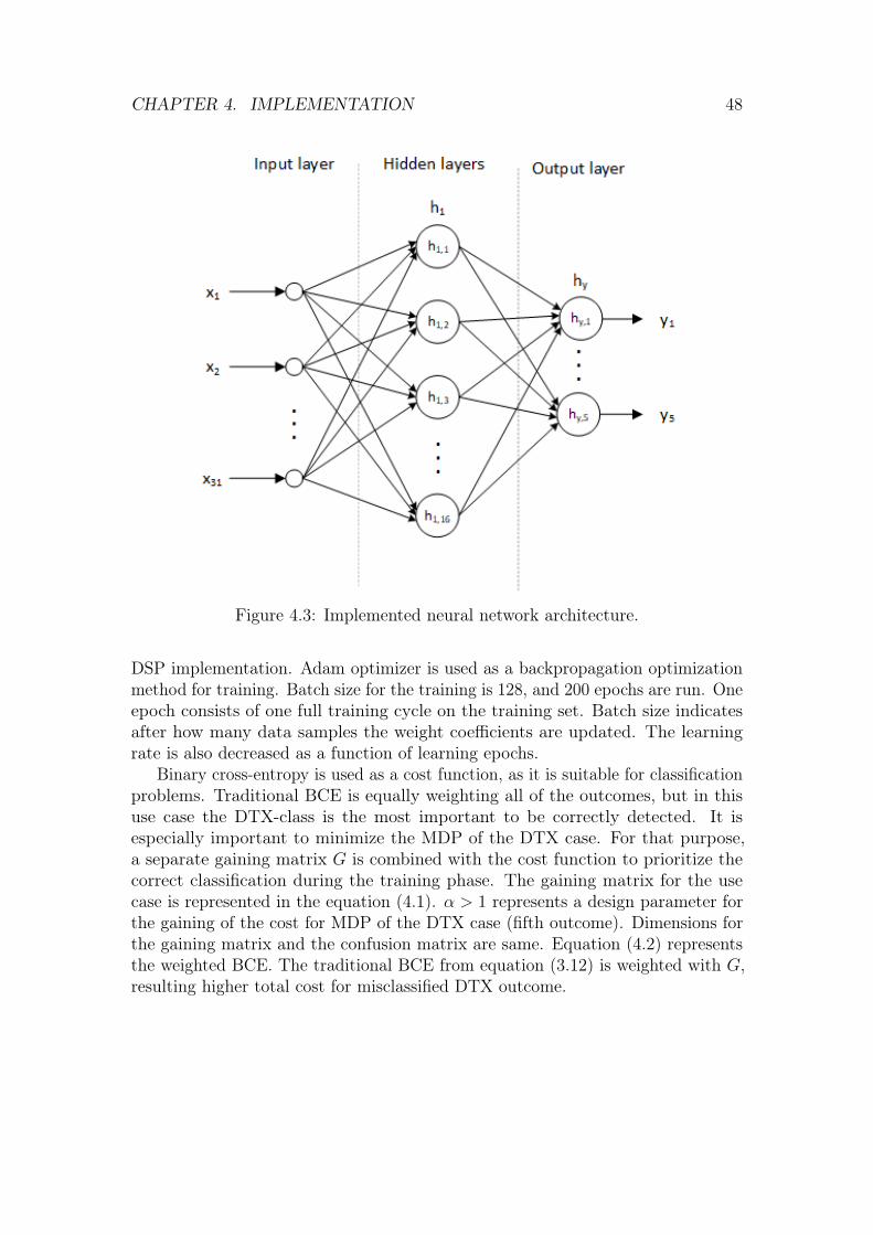
CHAPTER 4. IMPLEMENTATION 48
Figure 4.3: Implemented neural network architecture.
DSP implementation. Adam optimizer is used as a backpropagation optimizationmethod for training. Batch size for the training is 128, and 200 epochs are run. Oneepoch consists of one full training cycle on the training set. Batch size indicatesafter how many data samples the weight coefficients are updated. The learningrate is also decreased as a function of learning epochs.
Binary cross-entropy is used as a cost function, as it is suitable for classificationproblems. Traditional BCE is equally weighting all of the outcomes, but in thisuse case the DTX-class is the most important to be correctly detected. It isespecially important to minimize the MDP of the DTX case. For that purpose,a separate gaining matrix G is combined with the cost function to prioritize thecorrect classification during the training phase. The gaining matrix for the usecase is represented in the equation (4.1). α > 1 represents a design parameter forthe gaining of the cost for MDP of the DTX case (fifth outcome). Dimensions forthe gaining matrix and the confusion matrix are same. Equation (4.2) representsthe weighted BCE. The traditional BCE from equation (3.12) is weighted with G,resulting higher total cost for misclassified DTX outcome.
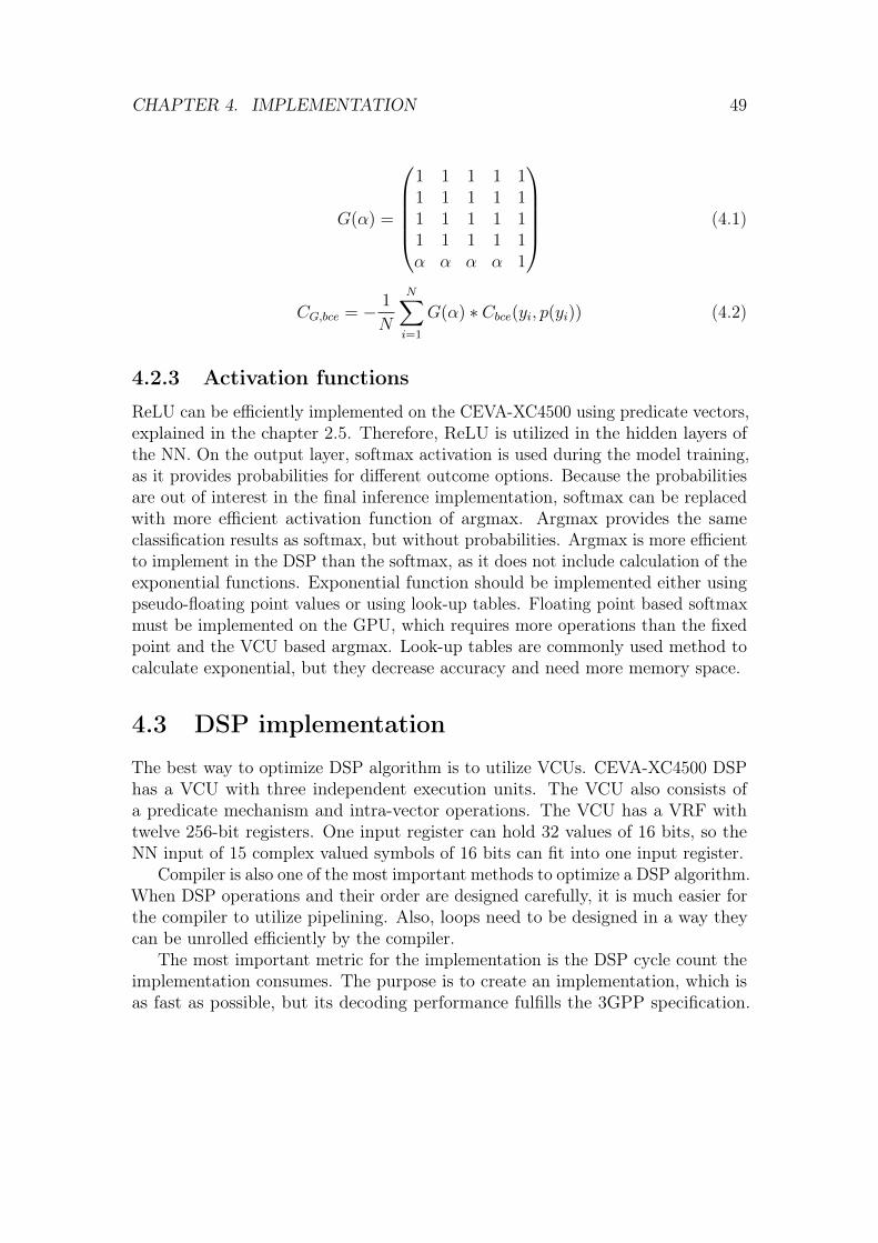
CHAPTER 4. IMPLEMENTATION 49
G(α) =
1 1 1 1 11 1 1 1 11 1 1 1 11 1 1 1 1α α α α 1
(4.1)
CG,bce = − 1
N
N∑i=1
G(α) ∗ Cbce(yi, p(yi)) (4.2)
4.2.3 Activation functions
ReLU can be efficiently implemented on the CEVA-XC4500 using predicate vectors,explained in the chapter 2.5. Therefore, ReLU is utilized in the hidden layers ofthe NN. On the output layer, softmax activation is used during the model training,as it provides probabilities for different outcome options. Because the probabilitiesare out of interest in the final inference implementation, softmax can be replacedwith more efficient activation function of argmax. Argmax provides the sameclassification results as softmax, but without probabilities. Argmax is more efficientto implement in the DSP than the softmax, as it does not include calculation of theexponential functions. Exponential function should be implemented either usingpseudo-floating point values or using look-up tables. Floating point based softmaxmust be implemented on the GPU, which requires more operations than the fixedpoint and the VCU based argmax. Look-up tables are commonly used method tocalculate exponential, but they decrease accuracy and need more memory space.
4.3 DSP implementation
The best way to optimize DSP algorithm is to utilize VCUs. CEVA-XC4500 DSPhas a VCU with three independent execution units. The VCU also consists ofa predicate mechanism and intra-vector operations. The VCU has a VRF withtwelve 256-bit registers. One input register can hold 32 values of 16 bits, so theNN input of 15 complex valued symbols of 16 bits can fit into one input register.
Compiler is also one of the most important methods to optimize a DSP algorithm.When DSP operations and their order are designed carefully, it is much easier forthe compiler to utilize pipelining. Also, loops need to be designed in a way theycan be unrolled efficiently by the compiler.
The most important metric for the implementation is the DSP cycle count theimplementation consumes. The purpose is to create an implementation, which isas fast as possible, but its decoding performance fulfills the 3GPP specification.
CHAPTER 4. IMPLEMENTATION 50
The execution speed of the implementation is measured in DSP cycles, and thedecoding detection performance is measured with FAR, BER and MDP. The NNmodel accuracy is measured and validated already in the mode training phase, butthe DSP model accuracy need to be validated separately. Rounding the floatingpoint weights to the fixed point weights and also shifting the fixed point precisionduring multiplications loses accuracy of the inference.
Even thought the execution speed and the decoding accuracy are the onlyinteresting metrics in this implementation, the memory consumption still needto be concerned as a design constraint. The total code size must be less thanthe internal instruction memory size, and the data must also fit into the internalmemory data section. Without the memory size constraint, the model becomesmuch slower, as the external memory access is very cycle consuming. Also, withoutthe memory size constraint it is not possible to profile the implementation in theCEVA IDE, as the IDE does not simulate external memory.
Implemented NN architecture is represented in figure 4.3 Even though NNarchitecture is fixed, there are multiple ways how different parts of the implemen-tation can be done differently. In this implementation, software development andoptimization is divided into three parts: calculation of induced local fields from theequation (3.3), adding the bias constant and performing neural activations. Twodifferent approaches of the calculation of the induced local field are discussed insection 4.3.2. Comparison between adding the bias in the VCU and in the GCUis explained in the chapter 4.3.3. VCU implementations for ReLU and argmaxactivations are discussed in section 4.3.4. Fixed point precision of the data isdiscussed in section 4.3.1.
Tables 4.5 and 4.6 represent explanations for the CEVA intrinsics used in thepseudo-code representations of the implemented algorithms 3-8.
4.3.1 Fixed point format
As the CEVA-XC4500 is optimized for fixed point operations, also the implementa-tion operates purely on fixed point values. The chosen fixed point format dependson the range of the data values. The input symbols of the network come as a resultfrom the different algorithm with the fixed point format of Q4.11. Therefore, theinput of the implementation has a fixed point format of Q4.11.
Because L2-regularization is used in the training phase of the network, varianceof the weight coefficient remains small. Also, the mean of the weight set is close tozero. Therefore, fixed point format of Q1.15 is enough to cover all possible weightcoefficient values. Equation (4.3) represents the range of signed value τ in Qa.bformat [13]. According to the equation, the range of the weight coefficients in theimplementation in Q1.15 format is [−2, 1.9999694].
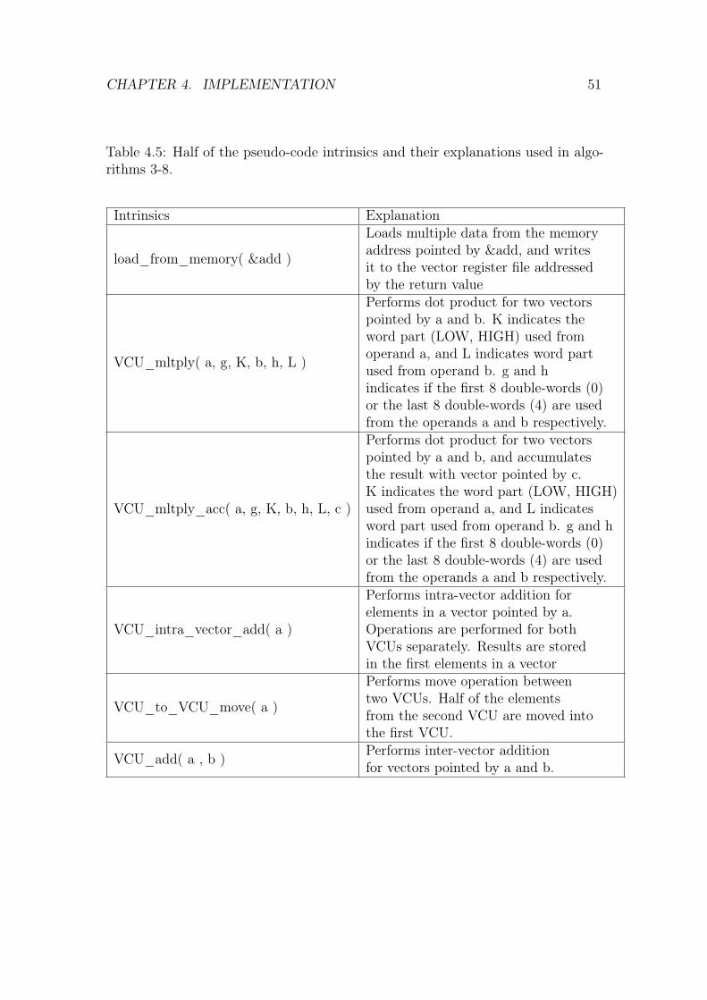
CHAPTER 4. IMPLEMENTATION 51
Table 4.5: Half of the pseudo-code intrinsics and their explanations used in algo-rithms 3-8.
Intrinsics Explanation
load_from_memory( &add )
Loads multiple data from the memoryaddress pointed by &add, and writesit to the vector register file addressedby the return value
VCU_mltply( a, g, K, b, h, L )
Performs dot product for two vectorspointed by a and b. K indicates theword part (LOW, HIGH) used fromoperand a, and L indicates word partused from operand b. g and hindicates if the first 8 double-words (0)or the last 8 double-words (4) are usedfrom the operands a and b respectively.
VCU_mltply_acc( a, g, K, b, h, L, c )
Performs dot product for two vectorspointed by a and b, and accumulatesthe result with vector pointed by c.K indicates the word part (LOW, HIGH)used from operand a, and L indicatesword part used from operand b. g and hindicates if the first 8 double-words (0)or the last 8 double-words (4) are usedfrom the operands a and b respectively.
VCU_intra_vector_add( a )
Performs intra-vector addition forelements in a vector pointed by a.Operations are performed for bothVCUs separately. Results are storedin the first elements in a vector
VCU_to_VCU_move( a )
Performs move operation betweentwo VCUs. Half of the elementsfrom the second VCU are moved intothe first VCU.
VCU_add( a , b ) Performs inter-vector additionfor vectors pointed by a and b.
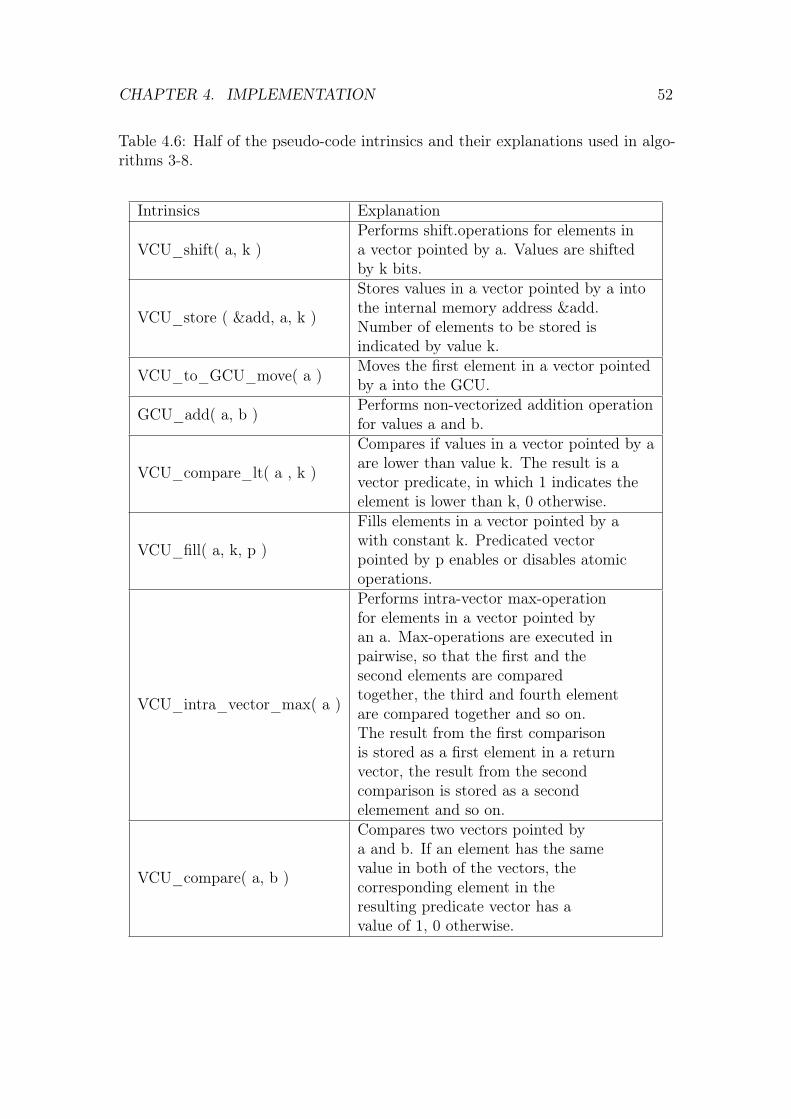
CHAPTER 4. IMPLEMENTATION 52
Table 4.6: Half of the pseudo-code intrinsics and their explanations used in algo-rithms 3-8.
Intrinsics Explanation
VCU_shift( a, k )Performs shift.operations for elements ina vector pointed by a. Values are shiftedby k bits.
VCU_store ( &add, a, k )
Stores values in a vector pointed by a intothe internal memory address &add.Number of elements to be stored isindicated by value k.
VCU_to_GCU_move( a ) Moves the first element in a vector pointedby a into the GCU.
GCU_add( a, b ) Performs non-vectorized addition operationfor values a and b.
VCU_compare_lt( a , k )
Compares if values in a vector pointed by aare lower than value k. The result is avector predicate, in which 1 indicates theelement is lower than k, 0 otherwise.
VCU_fill( a, k, p )
Fills elements in a vector pointed by awith constant k. Predicated vectorpointed by p enables or disables atomicoperations.
VCU_intra_vector_max( a )
Performs intra-vector max-operationfor elements in a vector pointed byan a. Max-operations are executed inpairwise, so that the first and thesecond elements are comparedtogether, the third and fourth elementare compared together and so on.The result from the first comparisonis stored as a first element in a returnvector, the result from the secondcomparison is stored as a secondelemement and so on.
VCU_compare( a, b )
Compares two vectors pointed bya and b. If an element has the samevalue in both of the vectors, thecorresponding element in theresulting predicate vector has avalue of 1, 0 otherwise.
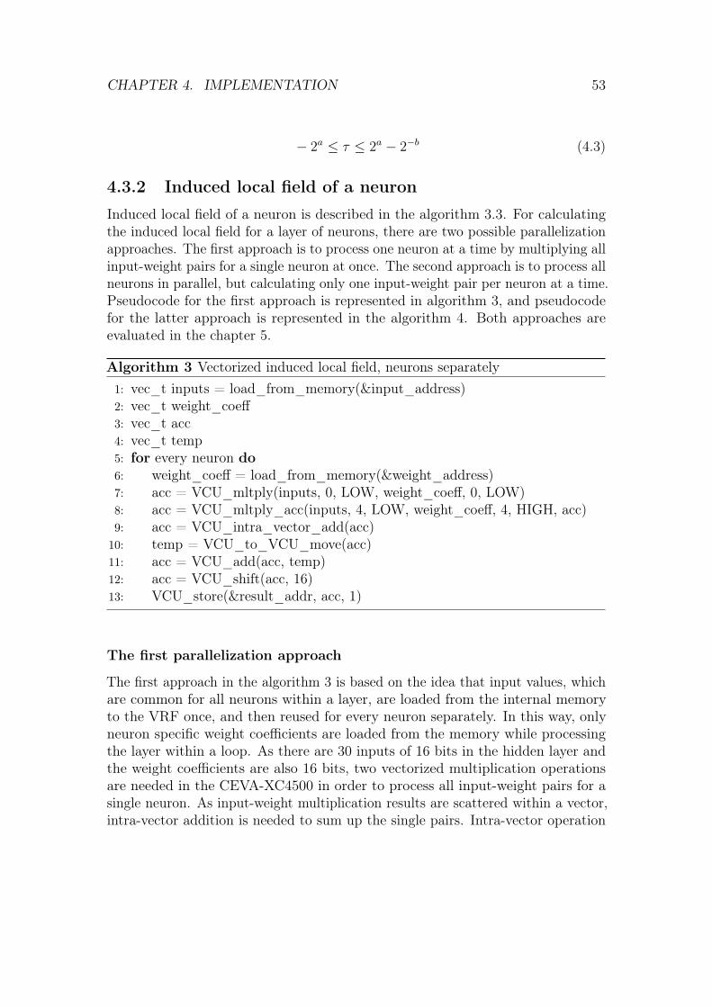
CHAPTER 4. IMPLEMENTATION 53
− 2a ≤ τ ≤ 2a − 2−b (4.3)
4.3.2 Induced local field of a neuron
Induced local field of a neuron is described in the algorithm 3.3. For calculatingthe induced local field for a layer of neurons, there are two possible parallelizationapproaches. The first approach is to process one neuron at a time by multiplying allinput-weight pairs for a single neuron at once. The second approach is to process allneurons in parallel, but calculating only one input-weight pair per neuron at a time.Pseudocode for the first approach is represented in algorithm 3, and pseudocodefor the latter approach is represented in the algorithm 4. Both approaches areevaluated in the chapter 5.
Algorithm 3 Vectorized induced local field, neurons separately1: vec_t inputs = load_from_memory(&input_address)2: vec_t weight_coeff3: vec_t acc4: vec_t temp5: for every neuron do6: weight_coeff = load_from_memory(&weight_address)7: acc = VCU_mltply(inputs, 0, LOW, weight_coeff, 0, LOW)8: acc = VCU_mltply_acc(inputs, 4, LOW, weight_coeff, 4, HIGH, acc)9: acc = VCU_intra_vector_add(acc)
10: temp = VCU_to_VCU_move(acc)11: acc = VCU_add(acc, temp)12: acc = VCU_shift(acc, 16)13: VCU_store(&result_addr, acc, 1)
The first parallelization approach
The first approach in the algorithm 3 is based on the idea that input values, whichare common for all neurons within a layer, are loaded from the internal memoryto the VRF once, and then reused for every neuron separately. In this way, onlyneuron specific weight coefficients are loaded from the memory while processingthe layer within a loop. As there are 30 inputs of 16 bits in the hidden layer andthe weight coefficients are also 16 bits, two vectorized multiplication operationsare needed in the CEVA-XC4500 in order to process all input-weight pairs for asingle neuron. As input-weight multiplication results are scattered within a vector,intra-vector addition is needed to sum up the single pairs. Intra-vector operation
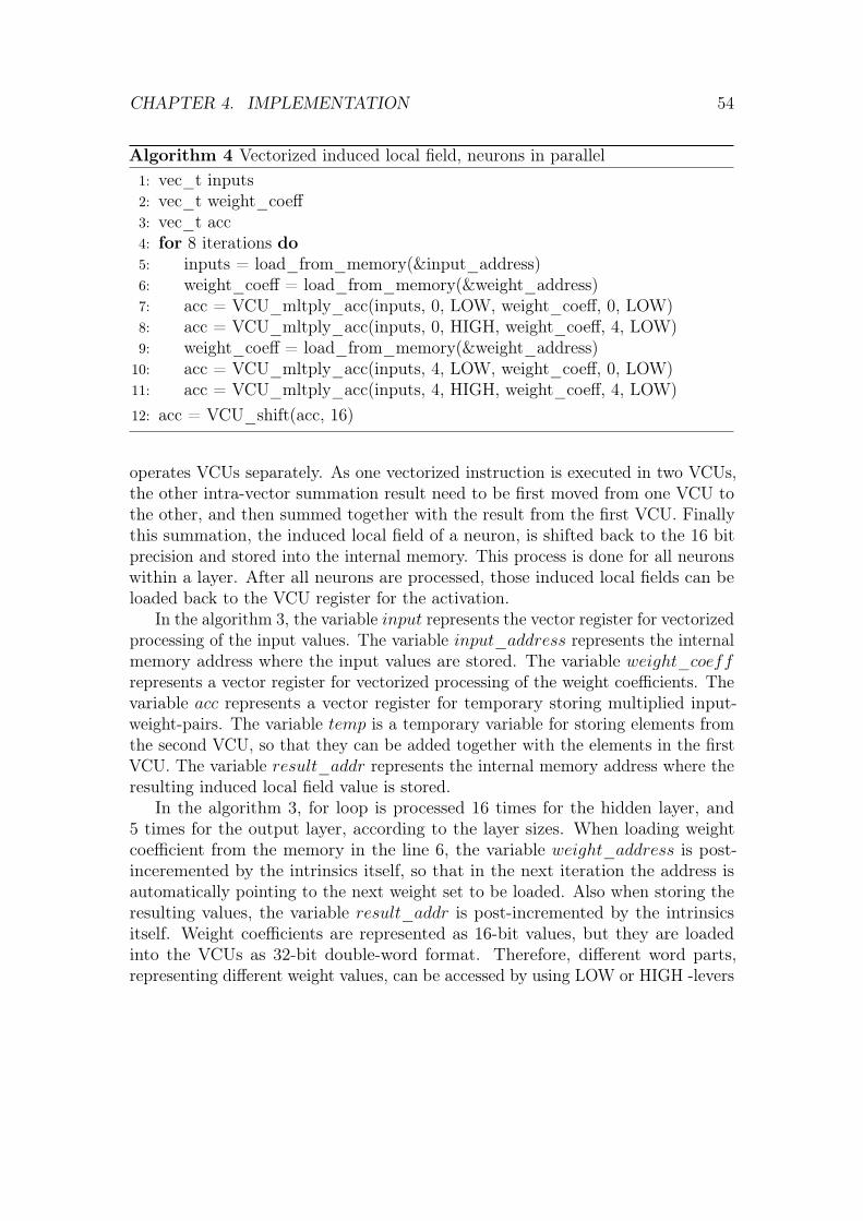
CHAPTER 4. IMPLEMENTATION 54
Algorithm 4 Vectorized induced local field, neurons in parallel1: vec_t inputs2: vec_t weight_coeff3: vec_t acc4: for 8 iterations do5: inputs = load_from_memory(&input_address)6: weight_coeff = load_from_memory(&weight_address)7: acc = VCU_mltply_acc(inputs, 0, LOW, weight_coeff, 0, LOW)8: acc = VCU_mltply_acc(inputs, 0, HIGH, weight_coeff, 4, LOW)9: weight_coeff = load_from_memory(&weight_address)
10: acc = VCU_mltply_acc(inputs, 4, LOW, weight_coeff, 0, LOW)11: acc = VCU_mltply_acc(inputs, 4, HIGH, weight_coeff, 4, LOW)12: acc = VCU_shift(acc, 16)
operates VCUs separately. As one vectorized instruction is executed in two VCUs,the other intra-vector summation result need to be first moved from one VCU tothe other, and then summed together with the result from the first VCU. Finallythis summation, the induced local field of a neuron, is shifted back to the 16 bitprecision and stored into the internal memory. This process is done for all neuronswithin a layer. After all neurons are processed, those induced local fields can beloaded back to the VCU register for the activation.
In the algorithm 3, the variable input represents the vector register for vectorizedprocessing of the input values. The variable input_address represents the internalmemory address where the input values are stored. The variable weight_coeffrepresents a vector register for vectorized processing of the weight coefficients. Thevariable acc represents a vector register for temporary storing multiplied input-weight-pairs. The variable temp is a temporary variable for storing elements fromthe second VCU, so that they can be added together with the elements in the firstVCU. The variable result_addr represents the internal memory address where theresulting induced local field value is stored.
In the algorithm 3, for loop is processed 16 times for the hidden layer, and5 times for the output layer, according to the layer sizes. When loading weightcoefficient from the memory in the line 6, the variable weight_address is post-inceremented by the intrinsics itself, so that in the next iteration the address isautomatically pointing to the next weight set to be loaded. Also when storing theresulting values, the variable result_addr is post-incremented by the intrinsicsitself. Weight coefficients are represented as 16-bit values, but they are loadedinto the VCUs as 32-bit double-word format. Therefore, different word parts,representing different weight values, can be accessed by using LOW or HIGH -levers
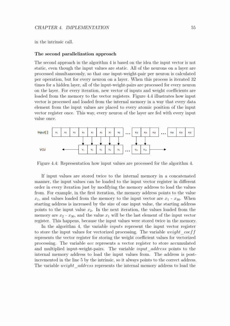
CHAPTER 4. IMPLEMENTATION 55
in the intrinsic call.
The second parallelization approach
The second approach in the algorithm 4 is based on the idea the input vector is notstatic, even though the input values are static. All of the neurons on a layer areprocessed simultaneously, so that one input-weight-pair per neuron is calculatedper operation, but for every neuron on a layer. When this process is iterated 32times for a hidden layer, all of the input-weight-pairs are processed for every neuronon the layer. For every iteration, new vector of inputs and weight coefficients areloaded from the memory to the vector registers. Figure 4.4 illustrates how inputvector is processed and loaded from the internal memory in a way that every dataelement from the input values are placed to every atomic position of the inputvector register once. This way, every neuron of the layer are fed with every inputvalue once.
Figure 4.4: Representation how input values are processed for the algorithm 4.
If input values are stored twice to the internal memory in a concatenatedmanner, the input values can be loaded to the input vector register in differentorder in every iteration just by modifying the memory address to load the valuesfrom. For example, in the first iteration, the memory address points to the valuex1, and values loaded from the memory to the input vector are x1 - x30. Whenstarting address is increased by the size of one input value, the starting addresspoints to the input value x2. In the next iteration, the values loaded from thememory are x2 - x30, and the value x1 will be the last element of the input vectorregister. This happens, because the input values were stored twice in the memory.
In the algorithm 4, the variable inputs represent the input vector registerto store the input values for vectorized processing. The variable weight_coeffrepresents the vector register for storing the weight coefficient values for vectorizedprocessing. The variable acc represents a vector register to store accumulatedand multiplied input-weight-pairs. The variable input_address points to theinternal memory address to load the input values from. The address is post-incremented in the line 5 by the intrinsic, so it always points to the correct address.The variable weight_address represents the internal memory address to load the
CHAPTER 4. IMPLEMENTATION 56
weight coefficient values from, and it is also post-incremented in the lines 6 and 9by the intrinsic.
With levers g and h described in the Table 4.5 for the V CU_multply_acc, theinput vector can be used four different ways per one for-loop-iteration. Therefore,the input vector need to be loaded from the memory only 8 times in order to use allof the 30 inputs and one bias in every atomic position in the input vector register.However, the output layer processing also needs 8 iterations, even though the layersize is smaller. Otherwise all of the 16 input values are not placed into every atomicposition in the input vector register. The g and h levers give the possibility tochoose the offset for the first double-word value to be used from the VCU, and thisway the first 16 values or latter 16 values can be used. Also, it can be chosen if themost significant (HIGH) or less significant (LOW) part of the double-word is usedfirst.
Even though the input vector can be utilized in four different ways, the resultfrom the MAC-intrinsic can be stored only two different ways. The result value canbe stored into the HIGH or LOW part of the resulting double-word. Because oneweight vector can contain only two set of 16-bit weights, weight coefficient vectorneed to be loaded twice in one loop iteration.
The second parallelization approach consumes more memory and does morememory operations than the first parallelization approach, but most of the opera-tions are efficient hardware-based MAC-operations. After 8 iterations, accumulatorcontains the induced local fields of every neuron in the layer. Compared to thefirst parallelization approach represented in the algorithm 3, all intra-vector opera-tions, moves from VCU to VCU, and temporary storage of the induced local fieldvalues are removed. It is much easier for the compiler to pipeline and to optimizeoperations, as the main processing contains only MAC-operations and memoryaccesses.
4.3.3 Bias
As discussed in chapter 3.1.2, the bias constant can be embedded into weightcoefficient vector by adding additional constant to the input vector. This is usefulfeature also for this use case. The input has a length of 30, and there are 2 dummyinput values available in the input vector register. One of those can be utilized asbias input without extra computational cost.
Algorithm 5 represents pseudocode of the CEVA-XC4500 implementation ofadding the bias separately in a GCU. Algorithm 6 represents pseudocode of addingthe bias during the vectorized processing in the VCU. The variable input_addressrepresents a pointer to the internal memory address for the input values. Thevariable weight_address represents a pointer to the internal memory addressfor the weight coefficient values. In the algorithm 5, the variable bias_address
CHAPTER 4. IMPLEMENTATION 57
represents a pointer to the address containing the bias constant. In the algorithm6, the bias is included into the content pointed by the input_address and theweight_address. Those memory contents are loaded into the internal memorybefore any DSP processing. Therefore, no extra processing steps are needed to addthe bias to the inference. In algorithm 5 instead, the bias is located in completelydifferent memory location than the weight coefficients. For that reason, the biasneeds to be loaded separately from the memory. Because the result from theintra-vector addition in the line 4 is stored within vector registers, the result needsto be moved from the VCU to the GCU before the bias can be added to it.
Algorithm 5 Adding bias constant in the GCU1: vec_t input_features = load_from_memory(&input_address)2: vec_t weight_coeff = load_from_memory(&weight_address)3: vec_t product = VCU_multiply(input_features, weight_coeff)4: vec_t sum = VCU_intravector_multiply(product)5:6: int sum = VCU_to_GCU_move(sum)7: int bias_coeff =load_from_memory(&bias_address)8: int output = GCU_add(sum, bias_coeff)9:
10: return output
Algorithm 6 Adding bias constant in the VCU1: vec_t input_features = load_from_memory(&input_address)2: vec_t weight_coeff = load_from_memory(&weight_address)3: vec_t product = VCU_multiply(input_features, weight_coeff)4: vec_t sum = VCU_intravector_multiply(product)5:6: return sum
4.3.4 Activation functions
As discussed earlier in this chapter, ReLU is chosen as an activation functionfor the hidden layer of the chosen NN architecture. The output layer utilizessoftmax activation function in the NN model, but it is replaced with argmaxactivation for the DSP inference. Outcome probabilities are out of interest in thereal-time inference and only the outcome with the highest probability is interesting.Therefore, the computationally more expensive softmax activation can be replacedwith the argmax activation.
CHAPTER 4. IMPLEMENTATION 58
ReLU implementation
Algorithm 7 represents pseudocode for vectorized ReLU implementation for thehidden layer. ReLU is a activation function for a single neuron, but all of theactivations can be computed in parallel for a layer. In order to avoid branching,vector predicate method explained in the chapter 2.5 is utilized to replace allnegative induced local field values with zero. The variable input represents a vectorregister containing induced local fields of a layer. The variable negative_values isa vector predicate containing information about all of the negative elements in theinput vector after the compare-intrinsic is processed. The variable result representa vector register containing ReLU-activated inputs.
Algorithm 7 Vectorized ReLU for CEVA-XC45001: %Process induced local field for all neurons in a layer2: % vector register "input" contains all of the induced local fields3:4: vpred_t negative_values = VCU_compare_lt(input, 0)5: vec_t result = VCU_fill(input, 0, negative_values)6:7: return result
In the algorithm 7, the precondition is that all of the induced local fields for thelayer are processed and stored in the vector register file input. In this use case, theyare stored as 32-bit values. VCU’s comparison intrinsic, V CU_compare_lt(), isutilized to compare content of the input with constant zero, which is the thresholdvalue in the ReLU. The comparison result is stored into vector predicate registercontaining binary 1 for the elements in the input vector having value less than zero,and binary 0 otherwise. The VCU intrinsic V CU_fill() replaces values from inputwith zeros, according to the predicate vector negative_values. The fill operationis executed for every atomic value in the input, but the result is stored to thevector register result only for the values marked by 1 in the predicate vector.
Argmax implementation
Algorithm 8 represents pseudocode for vectorised argmax implementation. Similarythan in algorithm 7, the vector register file input contains the induced local fieldsfor all of the neurons in a layer. In this use case, the input contains 16-bit values.The variable output represents the vector register for storing maximum valuesreturned by the intrinsic V CU_intravector_max(). As explained in the Table 4.6,the intrinsic V CU_intravector_max() performs intra-vector maximum operationbetween 16-bit wide sources that are located in the same vector. Figure 4.5
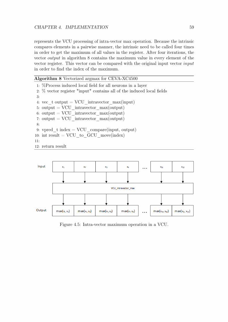
CHAPTER 4. IMPLEMENTATION 59
represents the VCU processing of intra-vector max operation. Because the intrinsiccompares elements in a pairwise manner, the intrinsic need to be called four timesin order to get the maximum of all values in the register. After four iterations, thevector output in algorithm 8 contains the maximum value in every element of thevector register. This vector can be compared with the original input vector inputin order to find the index of the maximum.
Algorithm 8 Vectorized argmax for CEVA-XC45001: %Process induced local field for all neurons in a layer2: % vector register "input" contains all of the induced local fields3:4: vec_t output = VCU_intravector_max(input)5: output = VCU_intravector_max(output)6: output = VCU_intravector_max(output)7: output = VCU_intravector_max(output)8:9: vpred_t index = VCU_compare(input, output)
10: int result = VCU_to_GCU_move(index)11:12: return result
Figure 4.5: Intra-vector maximum operation in a VCU.
Chapter 5
Evaluation
The objective of this thesis was to implement optimal neural network inference forCEVA-XC4500 digital signal processor under hard real-time constraints. The usecase, neural network model and the model’s DSP implementation was described inchapter 4. In this chapter, the trained NN model performance and different DSPimplementations are evaluated. At first, the NN model evaluation metrics and theevaluation results are discussed. After that, the DSP implementation metrics andthe implementation results are evaluated.
As absolute cycle counts are confidential property of Nokia, the measuredcycle counts in section 5.2.2 are represented as a relative count to the optimized,conventional stochastic model based decoder with compiler optimization level -O3. However, the purpose was to study if a neural network based model couldimprove the system performance from an execution speed point of view withoutcompromising accuracy requirements. For that purpose, the relative cycle count isactually an even more interesting metric than absolute cycle values.
5.1 Neural network model
5.1.1 Evaluation metrics
The neural network model described in chapter 4 is evaluated by different metrics.The NN model is evaluated based on the accuracy, precision, recall and f1-scoreof individual classes or the whole dataset. The NN model is compared to theconvectional decoder by calculating the misdetection probability (MDP), false-alarm rate (FAR) and bit-error rate (BER). As described in chapter 4.1, classes 1-4represent different decoder outcomes based on the combination of the two inputsand class 5 represents the DTX outcome.
Accuracy of the model describes how many samples from the data set are
60
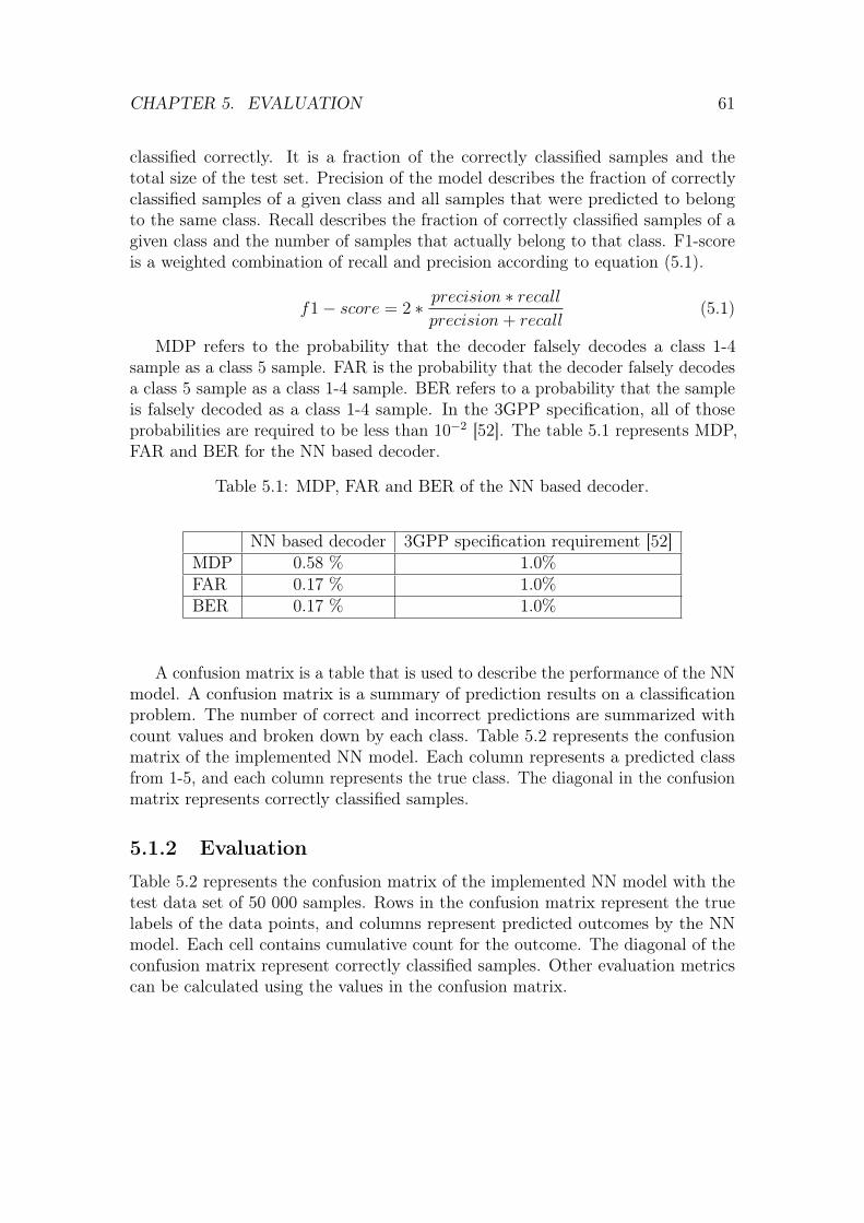
CHAPTER 5. EVALUATION 61
classified correctly. It is a fraction of the correctly classified samples and thetotal size of the test set. Precision of the model describes the fraction of correctlyclassified samples of a given class and all samples that were predicted to belongto the same class. Recall describes the fraction of correctly classified samples of agiven class and the number of samples that actually belong to that class. F1-scoreis a weighted combination of recall and precision according to equation (5.1).
f1− score = 2 ∗ precision ∗ recallprecision+ recall
(5.1)
MDP refers to the probability that the decoder falsely decodes a class 1-4sample as a class 5 sample. FAR is the probability that the decoder falsely decodesa class 5 sample as a class 1-4 sample. BER refers to a probability that the sampleis falsely decoded as a class 1-4 sample. In the 3GPP specification, all of thoseprobabilities are required to be less than 10−2 [52]. The table 5.1 represents MDP,FAR and BER for the NN based decoder.
Table 5.1: MDP, FAR and BER of the NN based decoder.
NN based decoder 3GPP specification requirement [52]MDP 0.58 % 1.0%FAR 0.17 % 1.0%BER 0.17 % 1.0%
A confusion matrix is a table that is used to describe the performance of the NNmodel. A confusion matrix is a summary of prediction results on a classificationproblem. The number of correct and incorrect predictions are summarized withcount values and broken down by each class. Table 5.2 represents the confusionmatrix of the implemented NN model. Each column represents a predicted classfrom 1-5, and each column represents the true class. The diagonal in the confusionmatrix represents correctly classified samples.
5.1.2 Evaluation
Table 5.2 represents the confusion matrix of the implemented NN model with thetest data set of 50 000 samples. Rows in the confusion matrix represent the truelabels of the data points, and columns represent predicted outcomes by the NNmodel. Each cell contains cumulative count for the outcome. The diagonal of theconfusion matrix represent correctly classified samples. Other evaluation metricscan be calculated using the values in the confusion matrix.
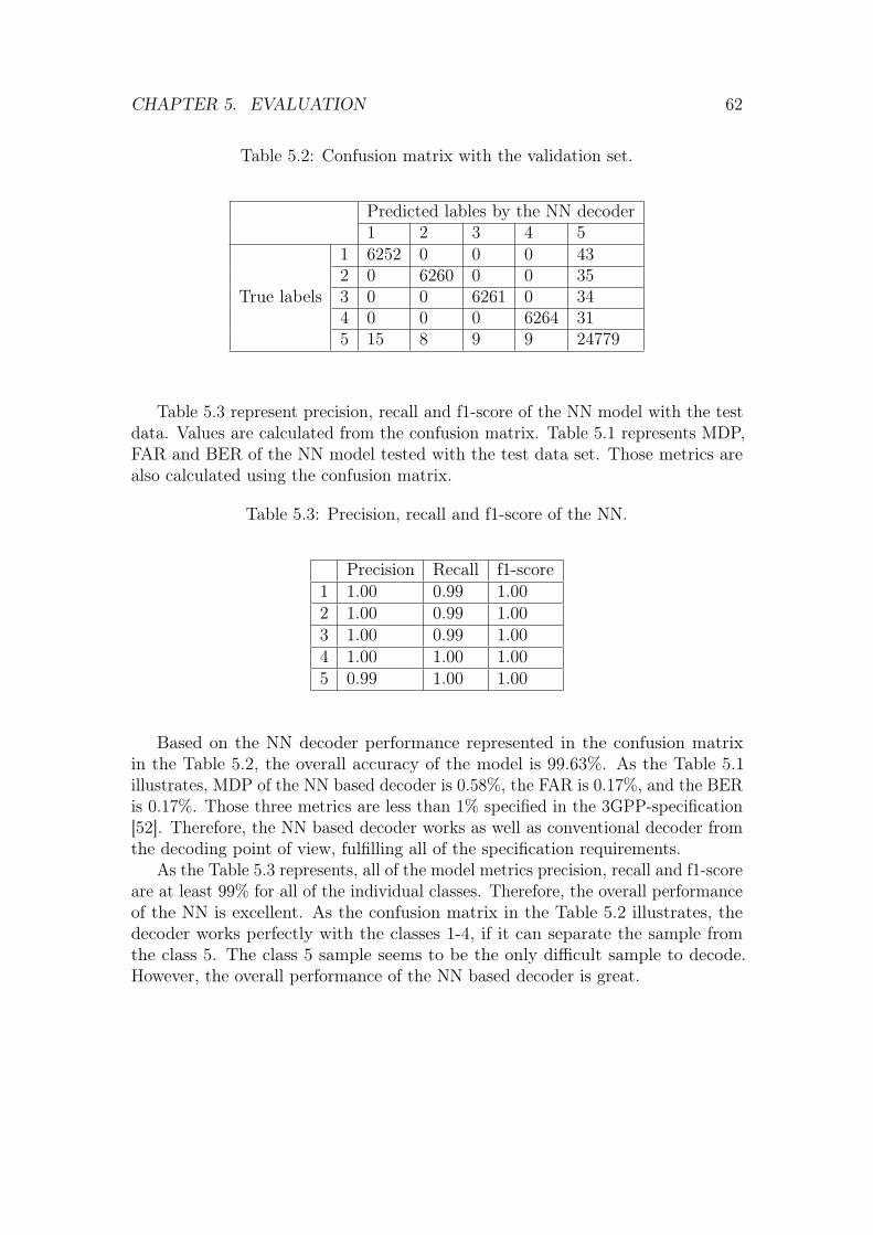
CHAPTER 5. EVALUATION 62
Table 5.2: Confusion matrix with the validation set.
Predicted lables by the NN decoder1 2 3 4 5
True labels
1 6252 0 0 0 432 0 6260 0 0 353 0 0 6261 0 344 0 0 0 6264 315 15 8 9 9 24779
Table 5.3 represent precision, recall and f1-score of the NN model with the testdata. Values are calculated from the confusion matrix. Table 5.1 represents MDP,FAR and BER of the NN model tested with the test data set. Those metrics arealso calculated using the confusion matrix.
Table 5.3: Precision, recall and f1-score of the NN.
Precision Recall f1-score1 1.00 0.99 1.002 1.00 0.99 1.003 1.00 0.99 1.004 1.00 1.00 1.005 0.99 1.00 1.00
Based on the NN decoder performance represented in the confusion matrixin the Table 5.2, the overall accuracy of the model is 99.63%. As the Table 5.1illustrates, MDP of the NN based decoder is 0.58%, the FAR is 0.17%, and the BERis 0.17%. Those three metrics are less than 1% specified in the 3GPP-specification[52]. Therefore, the NN based decoder works as well as conventional decoder fromthe decoding point of view, fulfilling all of the specification requirements.
As the Table 5.3 represents, all of the model metrics precision, recall and f1-scoreare at least 99% for all of the individual classes. Therefore, the overall performanceof the NN is excellent. As the confusion matrix in the Table 5.2 illustrates, thedecoder works perfectly with the classes 1-4, if it can separate the sample fromthe class 5. The class 5 sample seems to be the only difficult sample to decode.However, the overall performance of the NN based decoder is great.
CHAPTER 5. EVALUATION 63
5.2 DSP implementations
Different DSP implementations A-G and their differences are explained in thefollowing subsections. Implementation A is the reference implementation, containingoptimized stochastic model based implementation with compiler optimization level-O3. Implementations B-G are profiled without compiler optimizations (-O0) andwith the compiler optimization level -O3.
Implementation A
Implementation A is the reference implementation, containing stochastic modelbased decoder (and DTX-decision). This implementation is not related to themachine learning. This implementation is fully optimized, and it is compiled withthe optimization level -O3. This implementation is currently used in real Nokiabaseband products.
Implementation B
Implementation B is another reference implementation. This implementationis a NN inference, but it is coded purely on C language without any manualoptimizations or DSP related intrinsics. It is totally reusable and scalable fordifferent applications. It can be compiled and executed on any computer withoutcode modifications.
Implementation C
Implementation C is a NN inference with some manual optimizations. It uses theapproach described in the algorithm 3, in which neurons in a layer are inferred oneat a time. The bias is excluded from the input as described in the algorithm 5. Inthis implementation, the induced local field calculations are performed in a VCU,but activation functions follow GCU-based calculus.
Implementation D
Implementation D is similar to the implementation C, except that the activationfunctions are also calculated in the VCU as described in the algorithms 7 and 8.The bias is still excluded from the input according to the algorithm 5, and theinduced local field is calculated in a neuron after neuron basis as described in thealgorithm 3.
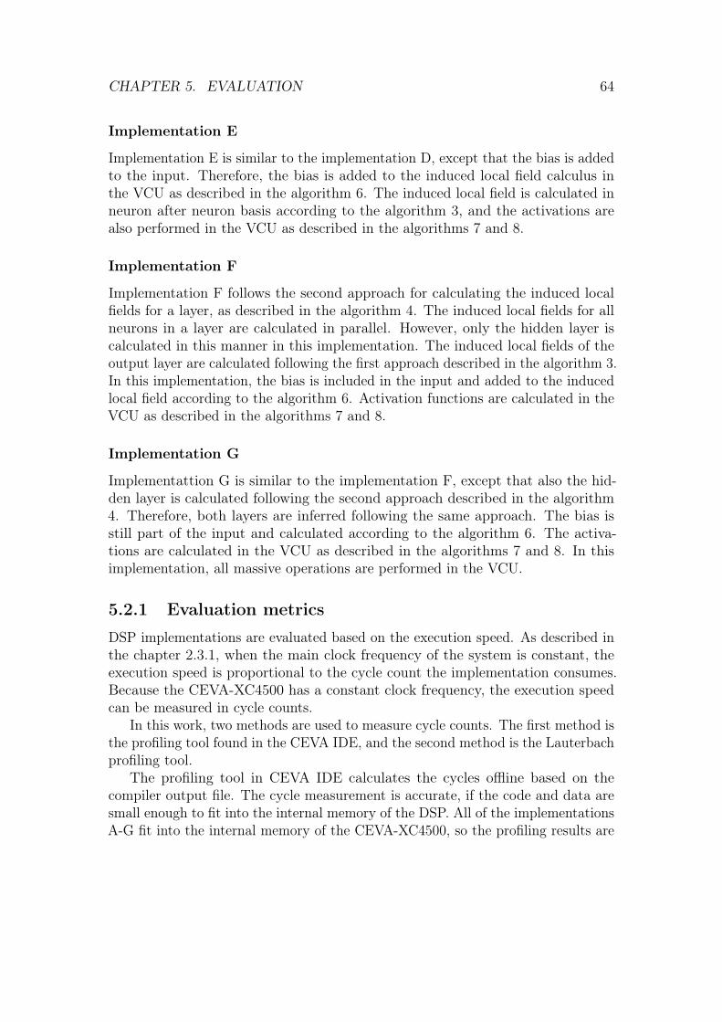
CHAPTER 5. EVALUATION 64
Implementation E
Implementation E is similar to the implementation D, except that the bias is addedto the input. Therefore, the bias is added to the induced local field calculus inthe VCU as described in the algorithm 6. The induced local field is calculated inneuron after neuron basis according to the algorithm 3, and the activations arealso performed in the VCU as described in the algorithms 7 and 8.
Implementation F
Implementation F follows the second approach for calculating the induced localfields for a layer, as described in the algorithm 4. The induced local fields for allneurons in a layer are calculated in parallel. However, only the hidden layer iscalculated in this manner in this implementation. The induced local fields of theoutput layer are calculated following the first approach described in the algorithm 3.In this implementation, the bias is included in the input and added to the inducedlocal field according to the algorithm 6. Activation functions are calculated in theVCU as described in the algorithms 7 and 8.
Implementation G
Implementattion G is similar to the implementation F, except that also the hid-den layer is calculated following the second approach described in the algorithm4. Therefore, both layers are inferred following the same approach. The bias isstill part of the input and calculated according to the algorithm 6. The activa-tions are calculated in the VCU as described in the algorithms 7 and 8. In thisimplementation, all massive operations are performed in the VCU.
5.2.1 Evaluation metrics
DSP implementations are evaluated based on the execution speed. As described inthe chapter 2.3.1, when the main clock frequency of the system is constant, theexecution speed is proportional to the cycle count the implementation consumes.Because the CEVA-XC4500 has a constant clock frequency, the execution speedcan be measured in cycle counts.
In this work, two methods are used to measure cycle counts. The first method isthe profiling tool found in the CEVA IDE, and the second method is the Lauterbachprofiling tool.
The profiling tool in CEVA IDE calculates the cycles offline based on thecompiler output file. The cycle measurement is accurate, if the code and data aresmall enough to fit into the internal memory of the DSP. All of the implementationsA-G fit into the internal memory of the CEVA-XC4500, so the profiling results are
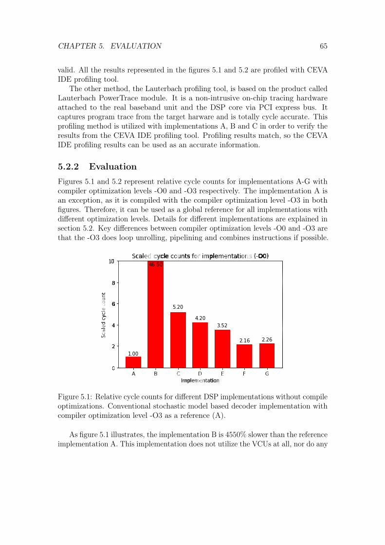
CHAPTER 5. EVALUATION 65
valid. All the results represented in the figures 5.1 and 5.2 are profiled with CEVAIDE profiling tool.
The other method, the Lauterbach profiling tool, is based on the product calledLauterbach PowerTrace module. It is a non-intrusive on-chip tracing hardwareattached to the real baseband unit and the DSP core via PCI express bus. Itcaptures program trace from the target harware and is totally cycle accurate. Thisprofiling method is utilized with implementations A, B and C in order to verify theresults from the CEVA IDE profiling tool. Profiling results match, so the CEVAIDE profiling results can be used as an accurate information.
5.2.2 Evaluation
Figures 5.1 and 5.2 represent relative cycle counts for implementations A-G withcompiler optimization levels -O0 and -O3 respectively. The implementation A isan exception, as it is compiled with the compiler optimization level -O3 in bothfigures. Therefore, it can be used as a global reference for all implementations withdifferent optimization levels. Details for different implementations are explained insection 5.2. Key differences between compiler optimization levels -O0 and -O3 arethat the -O3 does loop unrolling, pipelining and combines instructions if possible.
Figure 5.1: Relative cycle counts for different DSP implementations without compileoptimizations. Conventional stochastic model based decoder implementation withcompiler optimization level -O3 as a reference (A).
As figure 5.1 illustrates, the implementation B is 4550% slower than the referenceimplementation A. This implementation does not utilize the VCUs at all, nor do any
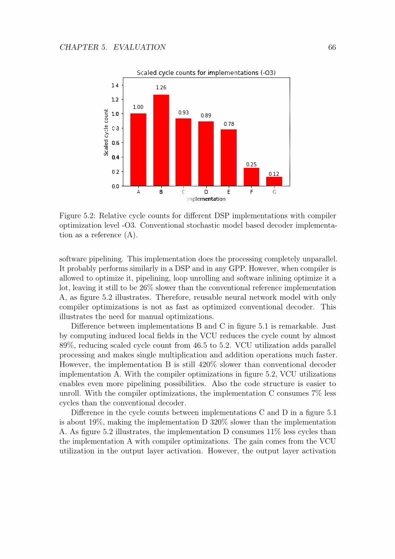
CHAPTER 5. EVALUATION 66
Figure 5.2: Relative cycle counts for different DSP implementations with compileroptimization level -O3. Conventional stochastic model based decoder implementa-tion as a reference (A).
software pipelining. This implementation does the processing completely unparallel.It probably performs similarly in a DSP and in any GPP. However, when compiler isallowed to optimize it, pipelining, loop unrolling and software inlining optimize it alot, leaving it still to be 26% slower than the conventional reference implementationA, as figure 5.2 illustrates. Therefore, reusable neural network model with onlycompiler optimizations is not as fast as optimized conventional decoder. Thisillustrates the need for manual optimizations.
Difference between implementations B and C in figure 5.1 is remarkable. Justby computing induced local fields in the VCU reduces the cycle count by almost89%, reducing scaled cycle count from 46.5 to 5.2. VCU utilization adds parallelprocessing and makes single multiplication and addition operations much faster.However, the implementation B is still 420% slower than conventional decoderimplementation A. With the compiler optimizations in figure 5.2, VCU utilizationsenables even more pipelining possibilities. Also the code structure is easier tounroll. With the compiler optimizations, the implementation C consumes 7% lesscycles than the conventional decoder.
Difference in the cycle counts between implementations C and D in a figure 5.1is about 19%, making the implementation D 320% slower than the implementationA. As figure 5.2 illustrates, the implementation D consumes 11% less cycles thanthe implementation A with compiler optimizations. The gain comes from the VCUutilization in the output layer activation. However, the output layer activation
CHAPTER 5. EVALUATION 67
is performed only once during the inference, and the amount of operations inthe argmax-activation is very small compared to the amount of operations wheninferring induced local field for total of 576 input-weight-pairs, as counted in theTable 4.4. Also, the argmax-activation includes mostly intra-vector operations,which are generally slower compared to the inter-vector calculations. Therefore,the gain in the compiler optimized version is only 4% in cycle counts.
Implementation E includes predicated ReLU-activation for the hidden layer. Thecycle reduction compared to the implementation D is about 16% without compileroptimizations, as illustrated in the figure 5.1. This makes the implementation 252%slower than implementation A. In the compiler optimized version in the figure 5.2,the cycle reduction is about 8% compared to the implementation D, reducing thecycle count 22% compared to the conventional implementation A. Vector predicatemechanisms reduces the amount of processing, making the implementation moreparallel. The cycle count result in this case also depends on the number of negativeoutputs in the induced local field inferences, as by default, the execution expectspositive comparison result. The cycle penalty is added only when this expectationis not met.
Implementations F and G utilize the second approach for the calculation ofthe induced local fields inference, as described in the algorithm 4. This optimizesthe implementation a lot. The total number of multiplications remains same,but all of them are executed as hardware-based MAC-operations, so the additioncomes without extra cycle cost. In the implementations C-E, only half of themultiplications are MAC-operations. There are not intra-vector operations in theF and G, whereas in the implementations C-E, the inference of the every neuronincludes intra-vector additions and VCU to VCU moves. The total number ofoperations is reduced, which itself reduces the cycle count a lot. Inter-vectoroperations are also easier to pipeline than intra-vector operations. Only additionto the processing is the modification of the input, as described in section 4.3.2.Without compiler optimizations, the implementation F consumes about 37% lesscycles than the implementation E, and the implementation G consumes about36% less cycles than the implementation E. Without compiler optimizations, theimplementation F is 116% slower than the reference implementation A, and theimplementation G is 126% slower than the implementation A. It is interesting torealize that the implementation F consumes actually 4.6% less cycles than theimplementation G without compiler optimizations. This is due to added memoryaccesses for modifying the input of the output layer. However, when compileroptimization level -O3 is used, as figure 5.2 illustrates, the implementation Gconsumer 52% less cycles than the implementation F, 84.6% less cycles than theimplementation E, and 88% less cycles than conventional decoder implementationA. Pipelining, unrolling, reduction in operations and the maximum VCU utilization
CHAPTER 5. EVALUATION 68
makes the implementation G very speed efficient compared to the conventionalmethod.
5.3 Evaluation summary
The objective of this thesis was to implement optimal neural network inferencefor CEVA-XC4500 digital signal processor under hard real-time constraints. Theuse case, neural network model, and model’s DSP implementation was describedin the chapter 4. In this chapter, NN model and the DSP implementation wereevaluated based on different metrics. NN model evaluation was based on the MDP,FAR and BER, defined in the 3GPP specification requirements. The NN modelwas also evaluated based on accuracy, recall, precision and f1-score. The DSPimplementation was evaluated based on the relative cycle count compared to theconventional decoder implementation.
As the results in the chapter 5.1.2 showed, the NN based decoder fulfills all ofthe 3GPP specification requirements of 1.0% for the MDP, FAR and BER. Also,the overall NN classification performance is excellent, as the total accuracy of themodel is 99%, and all of the individual precision, recall and f1-scores for differentclasses are at least 99% each.
The DSP implementation is also very fast compared to the conventional decoder.As the Table 5.2.2 illustrates, the most optimized implementation option consumesonly 12% of the cycle count the conventional implementation consumes, making itmore than 8 times faster.
Chapter 6
Conclusions
Machine learning and neural networks in particular are powerful tools for classifi-cation analysis, and are used in a wide range of applications. Their potential inphysical layer software has also received attention in the field’s literature lately.This thesis aimed to create optimized feedforward neural network inference imple-mentation for CEVA-XC4500 digital signal processor. The purpose was to study ifneural network based DSP implementation could solve the given decoder use casefaster than the conventional stochastic model based decoder implementation. Theimplementation was based on the NN model, which was created based on the datafrom the Matlab-simulation model. The model implementation speed performancewas compared against conventional stochastic mathematical model based symboldecoder implementation, and different implementation strategies were also com-pared against each others. The evaluation consisted of classification performanceevaluation for the NN model itself, and speed performance measurements for theimplementation.
Th results show that even the CEVA compiler itself is capable of doing massiveoptimizations for the C-based NN source code, if the source code is developedfrom the DSP optimization point of view. It seems to be significant that theimplementation architecture and processing order is chosen correctly. The compilerperforms poorly if the code is wholly reusable on any machine, and the processingorder is not planned comprehensively. Even though the compiler itself can dosubservient optimizations, manual optimizations by the developer are still neededin order to achieve maximum speed performance. Especially, VCU utilization isvery important.
The results also show that the implemented NN model is able to decode the givenuse case in a way that it passes the 3GPP specification performance requirements.The specification performance was passed, even the NN model was designed to beas small as possible due to fact there was no previous knowledge about the speed
69
CHAPTER 6. CONCLUSIONS 70
performance of a NN implementation in a CEVA-XC4500. The results show thatthe implemented NN was 88% faster than the conventional decoder, thus the NNmodel could have been extended. The bigger and especially deeper NN model couldhave further improved the decoding performance, still being many times faster thanthe conventional decoder. Implementation in this thesis gives very promising resultsfrom the productization point of view. The optimal neural network implementationrequires comprehensive knowledge about the target processor. It is important totailor neural network architecture to be suitable for the target DSP, so that it’sVCUs can be fully utilized. Fixed point calculus does not seem to be a problem fora small network, as the cumulative error that is generated during swift-operationsis relatively small.
For future research, bigger and deeper neural networks could be researched forthe given use case. Also, other types of neural network models, such as CNN andRNN, and their speed performances on a CEVA-XC4500, could be researched. NNinference speed performance could also be evaluated against some ML dedicatedhardware-accelerator chip, and they could be also compared from the developmentand manufacturing cost point of view. Also, multicore DSP inference and itsoptimal implementation could be considered, as it will enable even bigger NNs.
Bibliography
[1] J. G. Andrews, S. Buzzi, W. Choi, S. V. Hanly, A. Lozano, A. C. Soong,and J. C. Zhang, “What will 5g be?” IEEE Journal on selected areas incommunications, vol. 32, no. 6, pp. 1065–1082, 2014.
[2] T. Wang, C.-K. Wen, H. Wang, F. Gao, T. Jiang, and S. Jin, “Deep learning forwireless physical layer: Opportunities and challenges,” China Communications,vol. 14, no. 11, pp. 92–111, 2017.
[3] Z. Qin, H. Ye, G. Y. Li, and B.-H. F. Juang, “Deep learning in physical layercommunications,” IEEE Wireless Communications, vol. 26, no. 2, pp. 93–99,2019.
[4] R. Oshana, DSP for Embedded and Real-Time Systems, 1st ed. Newnes, 2012.
[5] B. D. T. Inc, “Evaluating dsp processor performance,” 2000.
[6] A. Bateman and I. Paterson-Stephens, The DSP Handbook: Algorithms, Ap-plications and Design Techniques. Prentice Hall, 2002.
[7] S. J. O. Phillip A. Laplante, Real-time systems design and analysis: tools forthe practitioner, 4th ed. New York: Wiley, 2011.
[8] P. Vernon, “Systems in engineering,” IEE Review, vol. 35, no. 10, pp. 383–385,Nov 1989.
[9] P. Lapsley and G. Blalock, “How to estimate dsp processor performance,”IEEE Spectrum, vol. 33, no. 7, pp. 74–78, July 1996.
[10] D. A. Patterson and J. L. Hennessy, Computer Organization and Design, FifthEdition: The Hardware/Software Interface, 5th ed. San Francisco, CA, USA:Morgan Kaufmann Publishers Inc., 2013.
[11] C. Inacio and D. Ombres, “The dsp decision: fixed point or floating?” IEEESpectrum, vol. 33, no. 9, pp. 72–74, Sep. 1996.
71
BIBLIOGRAPHY 72
[12] R. Oshana, DSP software development techniques for embedded and real-timesystems, 1st ed. Newnes, 2006.
[13] R. Yates, “Fixed-point arithmetic: An introduction,” Digital Signal Labs,vol. 81, no. 83, p. 198, 2009.
[14] E. Lai, Practical Digital Signal Processing for Engineers and Technicians, ser.Electronics & Electrical. Newnes, 2004.
[15] E. A. Lee, “Programmable dsp architectures. i,” IEEE ASSP Magazine, vol. 5,no. 4, pp. 4–19, 1988.
[16] N. Dahnoun, Multicore DSP: From Algorithms to Real-time Implementationon the TMS320C66x SoC. Wiley, 2018.
[17] G. S. Murthy, M. Ravishankar, M. M. Baskaran, and P. Sadayappan, “Optimalloop unrolling for gpgpu programs,” in 2010 IEEE International Symposiumon Parallel & Distributed Processing (IPDPS). IEEE, 2010, pp. 1–11.
[18] S. Liao, S. Devadas, K. Keutzer, S. Tjiang, and A. Wang, “Code optimiza-tion techniques in embedded dsp microprocessors,” Design Automation forEmbedded Systems, vol. 3, no. 1, pp. 59–73, 1998.
[19] C. H. Gebotys and R. J. Gebotys, “Complexities in dsp software compilation:performance, code size, power, retargetability,” in Proceedings of the Thirty-First Hawaii International Conference on System Sciences, vol. 3. IEEE,1998, pp. 150–156.
[20] Ceva Compiler optimizations, Ceva, 2016.
[21] R. E. Kole, “The impact of language extensions on dsp programming,” pp.191–194, April 1996.
[22] M. D. Kleffner, D. L. Jones, J. D. Hiser, P. Kulkarni, J. Parent, S. Hines,D. Whalley, J. W. Davidson, and K. Gallivan, “On the use of compilers in dsplaboratory instruction,” in 2006 IEEE International Conference on AcousticsSpeech and Signal Processing Proceedings, vol. 2. IEEE, 2006.
[23] Ceva Architecture Specification Vol-I, Ceva, 2016.
[24] Ceva-XC4500 Methodology for Optimal Vectorization Application Note, Ceva,2014.
[25] C. Xiang, “Ee5904r neural networks lecture 1,” University Lecture in NationalUniversity of Singapore, 2017.
BIBLIOGRAPHY 73
[26] S. Shanmuganathan and S. Samarasinghe, Artificial Neural Network Modelling,1st ed. Springer Publishing Company, Incorporated, 2016.
[27] J. J. Buckley and Y. Hayashi, “Fuzzy neural networks: A survey,” Fuzzy Setsand Systems, vol. 66, no. 1, pp. 1–13, 1994.
[28] J. J. Hopfield, “Neural networks and physical systems with emergent collectivecomputational abilities,” Proceedings of the National Academy of Sciences,vol. 79, no. 8, pp. 2554–2558, 1982.
[29] T. Kohonen, “Self-organized formation of topologically correct feature maps,”Biological Cybernetics, vol. 43, no. 1, pp. 59–69, Jan 1982.
[30] W. S. McCulloch and W. Pitts, “A logical calculus of the ideas immanent innervous activity,” The bulletin of mathematical biophysics, vol. 5, no. 4, pp.115–133, 1943.
[31] F. Rosenblatt, “The perceptron: a probabilistic model for information storageand organization in the brain.” Psychological review, vol. 65, no. 6, p. 386,1958.
[32] H. Simon, Neural networks and learning machines, 3rd ed. Upper SaddleRiver, N.J.: Pearson, 2009.
[33] I. Goodfellow, Y. Bengio, and A. Courville, Deep Learning. MIT Press, 2016.
[34] M. D. Zeiler, M. Ranzato, R. Monga, M. Mao, K. Yang, Q. V. Le, P. Nguyen,A. Senior, V. Vanhoucke, J. Dean, and G. E. Hinton, “On rectified linear unitsfor speech processing,” in 2013 IEEE International Conference on Acoustics,Speech and Signal Processing, May 2013, pp. 3517–3521.
[35] C. Zhang, P. Patras, and H. Haddadi, “Deep learning in mobile and wirelessnetworking: A survey,” IEEE Communications Surveys Tutorials, pp. 1–1,2019.
[36] J. Bruck and J. W. Goodman, “A generalized convergence theorem for neuralnetworks,” IEEE Transactions on Information Theory, vol. 34, no. 5, pp.1089–1092, Sep. 1988.
[37] N. Farsad and A. Goldsmith, “Neural network detectors for sequence detectionin communication systems,” IEEE Transactions on Signal Processing, 2018.
[38] S. Linnainmaa, “The representation of the cumulative rounding error of analgorithm as a taylor expansion of the local rounding errors,” Master’s Thesis(in Finnish), Univ. Helsinki, pp. 6–7, 1970.
BIBLIOGRAPHY 74
[39] D. E. Rumelhart, G. E. Hinton, R. J. Williams et al., “Learning representationsby back-propagating errors,” Cognitive modeling, vol. 5, no. 3, p. 1, 1988.
[40] Y. Qiao, X. Yang, and E. Wu, “The research of bp neural network basedon one-hot encoding and principle component analysis in determining thetherapeutic effect of diabetes mellitus,” in IOP Conference Series: Earth andEnvironmental Science, vol. 267, no. 4. IOP Publishing, 2019, p. 042178.
[41] K. S. Narendra and K. Parthasarathy, “Gradient methods for the optimizationof dynamical systems containing neural networks,” IEEE Transactions onNeural networks, vol. 2, no. 2, pp. 252–262, 1991.
[42] S. Ruder, “An overview of gradient descent optimization algorithms,” 2016.
[43] D. P. Kingma and J. Ba, “Adam: A method for stochastic optimization,” 2014.
[44] T. Hesterberg, N. H. Choi, L. Meier, C. Fraley et al., “Least angle and 1penalized regression: A review,” Statistics Surveys, vol. 2, pp. 61–93, 2008.
[45] Z. Deng, K.-S. Choi, Y. Jiang, and S. Wang, “Generalized hidden-mapping ridgeregression, knowledge-leveraged inductive transfer learning for neural networks,fuzzy systems and kernel methods,” IEEE transactions on cybernetics, vol. 44,no. 12, pp. 2585–2599, 2014.
[46] G. Cybenko, “Approximation by superpositions of a sigmoidal function,” Math-ematics of control, signals and systems, vol. 2, no. 4, pp. 303–314, 1989.
[47] K. Hornik, “Some new results on neural network approximation,” Neuralnetworks, vol. 6, no. 8, pp. 1069–1072, 1993.
[48] J. X. Chen, “The evolution of computing: Alphago,” Computing in Science &Engineering, vol. 18, no. 4, p. 4, 2016.
[49] W. Liu, Z. Wang, X. Liu, N. Zeng, Y. Liu, and F. E. Alsaadi, “A survey ofdeep neural network architectures and their applications,” Neurocomputing,vol. 234, pp. 11–26, 2017.
[50] T. O’Shea and J. Hoydis, “An introduction to deep learning for the physicallayer,” IEEE Transactions on Cognitive Communications and Networking,vol. 3, no. 4, pp. 563–575, 2017.
[51] J. Sola and J. Sevilla, “Importance of input data normalization for the applica-tion of neural networks to complex industrial problems,” IEEE Transactionson nuclear science, vol. 44, no. 3, pp. 1464–1468, 1997.

BIBLIOGRAPHY 75
[52] 3GPP, “NR; Base Station (BS) radio transmission and reception,” 3rd Genera-tion Partnership Project (3GPP), Technical Specification (TS) 38.104, Jun2019, version 15.6.0.
Related Documents