Inference in Supervised Spectral Classifiers ... - remote sensing

remote sensing

Article

Inference in Supervised Spectral Classifiersfor On-Board Hyperspectral Imaging: An Overview

Adrián Alcolea 1 , Mercedes E. Paoletti 2 , Juan M. Haut 2,* , Javier Resano 1

and Antonio Plaza 2

1 Computer Architecture Group (gaZ), Department of Computer Science and Systems Engineering,Ada Byron Building, University of Zaragoza, C/María de Luna 1, E-50018 Zaragoza, Spain;[email protected] (A.A.); [email protected] (J.R.)

2 Hyperspectral Computing Laboratory (HyperComp), Department of Computer Technologyand Communications, Escuela Politecnica de Caceres, University of Extremadura,Avenida de la Universidad sn, E-10003 Caceres, Spain; [email protected] (M.E.P.); [email protected] (A.P.)

* Correspondence: [email protected]

Received: 13 December 2019; Accepted: 4 February 2020; Published: 6 February 2020�����������������

Abstract: Machine learning techniques are widely used for pixel-wise classification of hyperspectralimages. These methods can achieve high accuracy, but most of them are computationally intensivemodels. This poses a problem for their implementation in low-power and embedded systemsintended for on-board processing, in which energy consumption and model size are as importantas accuracy. With a focus on embedded and on-board systems (in which only the inference step isperformed after an off-line training process), in this paper we provide a comprehensive overviewof the inference properties of the most relevant techniques for hyperspectral image classification.For this purpose, we compare the size of the trained models and the operations required during theinference step (which are directly related to the hardware and energy requirements). Our goal is tosearch for appropriate trade-offs between on-board implementation (such as model size and energyconsumption) and classification accuracy.

Keywords: hyperspectral imaging; machine learning; on-board implementations; inference; classification

1. Introduction

Fostered by significant advances in computer technology that have taken place from the end ofthe last century to now, the Earth observation (EO) field has greatly evolved over the last 20 years [1].Improvements in hardware and software have allowed for the development of more sophisticated andpowerful remote sensing systems [2], which in turn has enhanced the acquisition of remote sensingdata in terms of both quantity and quality, and also improved the analysis and processing of thesedata [3]. In fact, remote sensing technology has become a fundamental tool to increase our knowledgeof the Earth and how human factors, such as globalization, industrialization and urbanization canaffect the environment [4]. It provides relevant information to address current environmental problemssuch as desertification [5,6], deforestation [7,8], water resources depletion [9], soil erosion [10–12],eutrophication of freshwater and coastal marine ecosystems [13,14], warming of seas and oceans [15],together with global warming and abnormal climate changes [16] or urban areas degradation [17],among others.

In particular, advances in optical remote sensing imaging [18] have allowed for the acquisition ofhigh spatial, spectral and temporal resolution images, gathered from the Earth’s surface in multipleformats, ranging from very-high spatial-resolution (VHR) panchromatic images to hyperspectralimages with hundreds of narrow and continuous spectral bands. Focusing on hyperspectral imaging

Remote Sens. 2020, 12, 534; doi:10.3390/rs12030534 www.mdpi.com/journal/remotesensing

Remote Sens. 2020, 12, 534 2 of 29

(HSI) [19], this kind of data comprises abundant spectral–spatial information for large coverage,obtained by capturing the solar radiation that is absorbed and reflected by ground targets at differentwavelengths, usually ranging from the visible, to the near (NIR) and short wavelength infrared(SWIR) [20]. In this sense, HSI data obtained by airborne and satellite platforms consist of hugedata cubes, where each pixel represents the spectral signature of the captured object. The shapeof these spectral signatures depends on the physical and chemical behavior of the materials thatcompose it, working as a fingerprint for each terrestrial material. This signature allows for a precisecharacterization of the land cover, and is currently widely exploited in the fields of image analysisand pattern recognition [21]. Advances in HSI processing and analysis methods have enabled thewidespread incorporation of these to a vast range of applications. Regarding the forest preservationand management [22–25], HSI data can be applied to invasive species detection [26–28], forestryhealth and diseases [29–31] and analyses of relationship between water precipitations, atmosphericconditions and forest health [32,33]. Also, regarding the management of other natural resources, thereare works focused on freshwater and maritime resources [34–37] and geological and mineralogicalresources [38–41]. In relation to agricultural and livestock farming activities, [42], the availableliterature compiles a large number of works about HSI applied to precision agriculture [43,44],analyzing the soil properties and status [45–47], investigating diseases and pests affecting crops [48,49]and developing libraries of spectral signatures specialized in crops [50]. Moreover, HSI data can beapplied to urban planning [51–53], military and defense applications [54–56] and disaster predictionand management [57,58], among others.

The wide applications of HSI images call for highly efficient and accurate methods to make the mostof the rich spectral information contained in HSI data. In this context, machine learning algorithms havebeen adopted to process and analyze the HSI data. These algorithms include spectral unmixing [59,60],image segmentation [61–63], feature extraction [64,65], spectral reduction [66,67], anomaly, change and targetdetection [68–73] and land-cover classification methods [74,75], among others. Among these algorithms,supervised pixel-wise classifiers can derive more accurate results and thence more widely used for imagesclassification compared to unsupervised approaches. This higher accuracy is mainly due to the class-specificinformation provided during the training stage.

In order to define the classification problem in mathematical terms, let X ∈ RN×B ≡ {x1, · · · , xN}denote the HSI scene—considered as an array of N vectors, where each one xi ∈ RB ≡ {xi,1, · · · , xi,B} iscomposed by B spectral bands—and let Y ≡ {1, · · · , K} be a set of K land-cover classes. Classificationmethods define f (·, Θ) : X→ Y as a mapping function with learnable parameters Θ that essentiallydescribes the relationship between the spectral vector xi (input) and its corresponding label yi ∈ Y(output), creating feature–label pairs {xi, yi}N

i=1. The final goal is to obtain the classification mapY ∈ RN ≡ {y1, · · · , yN} by modeling the conditional distribution P(y ∈ Y|x ∈ X, Θ) in order to inferthe class labels for each pixel. Usually, this posterior distribution is optimized by training the classifieron a subset Dtrain composed by M random independent identically distributed (i.i.d.) observations thatfollow the joint distribution P(x, y) = P(x)P(y|x), i.e., a subset of known and representative labeleddata, adjusting parameters Θ to minimize the empirical riskR( f ) [76] defined as Equation (1) indicates:

R( f ) =∫L ( f (x, Θ), y)dP(x, y) =

1M

M

∑i=1L ( f (xi, Θ), yi) (1)

where L is the loss function defined over P(x, y) as the discrepancy between the expected label yand the obtained classifier’s output f (x, Θ). A wide variety of supervised-spectral techniques havebeen developed within the machine learning field to perform the classification of HSI data [77].Some of the most popular ones can be categorized into [74]: (i) probabilistic approaches, such asthe multinomial logistic regression (MLR) [62,78] and its variants (sparse MLR (SMLR) [79,80]and subspace MLR -MLRsub- [81,82]), the logistic regression via variable splitting and augmentedLagrangian (LORSAL) [63,83] or the maximum likelihood estimation (MLE) [84], among others, which

Remote Sens. 2020, 12, 534 3 of 29

obtain as a result the probability of xi belonging to each of K considered classes [85]; (ii) decision tree(DT) [86–88], which defines a non-parametric classification/regression method with a hierarchicalstructure of branches and leaves; (iii) ensemble methods, which are composed of multiple classifiersto enhance the classification performance, for instance random forests (RFs) [89,90], whose output iscomposed by the collective decisions of several DTs to which majority voting is applied, or boostingand bagging-based methods such as RealBoost [91,92], AdaBoost [93–96], Gradient Boosting [97,98]or the ensemble extreme learning machine (E2LM) [99], among others; (iv) kernel approaches, such as thenon-probabilistic support vector machine (SVM) [100,101], which exhibits a good performance whenhandling high-dimensional data and limited training samples, (although its performance is greatlyaffected by the kernel selection and the initial hyperparameters setting) and (v) the non-parametricartificial neural networks (ANNs), which exhibit a great generalization power without prior knowledgeabout the statistical properties of the data, also offering a great variety of architectures thanks to theirflexible structure based on the stacking of layers composed by computing neurons [75], allowing forthe implementation of traditional shallow-fully-connected models (such as the multilayer perceptron(MLP) [102,103]) and deep-convolutional models (such as convolutional neural networks (CNNs) [104]and complex models as residual networks (ResNets) [105] and capsule models [106]).

These methods need to face the intrinsic complexity of processing HSI data, related to the hugeamount of available spectral information (curse of dimensionality [107]), the spectral bands correlationand redundancies [108], the lack of enough labeled samples to perform supervised training [109]and overfitting problems. Moreover, current HSI classification methods must satisfy a growingdemand for effective and efficient methodologies from a computational point of view [110–112],with the idea of being executed on low-power platforms that allow for on-board processing of data(e.g., smallsats [113,114]). In this sense, high performance computing (HPC) approaches such ascommodity clusters [115,116] and graphic processing units (GPUs) have been widely employed toprocess HSI data [117]. However, the adaptation of these computing platforms to on-board processingis quite difficult due to their high requirements in terms of energy consumption.

Traditionally, the data gathered by remote sensors have to be downloaded to the ground segment,when the aircraft or spacecraft platform is within the range of the ground stations, in order to bepre-processed by applying registration and correction techniques and then distributed to the finalusers, which perform the final processing (classification, unmixing and object detection). Nevertheless,this procedure introduces important delays related to the communication of a large amount of remotesensing data (which is usually in the range of GB–TB) between the source and the final target,producing a bottleneck that can seriously reduce the effectiveness of real-time applications [118].Hereof, real-time on-board processing is a very interesting topic within the remote sensing field thathas significantly grown in recent years to mitigate these limitations, and to provide a solution tothese types of applications [119–123]. In addition to avoiding communication latencies, the on-boardprocessing can considerably reduce the amount of bandwidth and storage required in the collection ofHSI data, allowing for the development of a more selective data acquisition and reducing the cost ofon-the-ground processing systems [124]. As a result, low-power consumption architectures such asfield-programmable gate array (FPGAs) [125,126] and efficient GPU architectures [110] have emergedas an alternative to transfer part of the processing from the ground segment to the remote sensingsensor. A variety of techniques have been adapted to be carried out on-board [127], ranging frompre-processing methods, such as data calibration [128], correction [129], compression [123,130] andgeoreferencing [131], to final user applications, for instance data unmixing [126], object detection [132]and classification [110,133]. In the context of classification, usually, the training of supervised methodsshould be performed offline (in external systems), so that only the trained model will be implementedin the device (which will only perform the inference operation). On embedded and on-board systems,the size and energy consumption of the model are crucial parameters, so it is necessary to findan appropriate trade-off between performance (in terms of accuracy measurements) and energyconsumption (in terms of power consumption and execution times). In this paper, we perform a

Remote Sens. 2020, 12, 534 4 of 29

detailed analysis and study of the performance of machine learning methods in the task of supervised,spectral-based classification of HSI data, with particular emphasis on the inference stage, as it is thepart that is implemented in on-board systems. Specifically, we conduct an in-depth review and analysisof the advantages and disadvantages of these methods in the aforementioned context.

The remainder of this paper is organized as follows. Section 2 provides an overview of theconsidered machine learning methods to perform supervised, spectral-based HSI classification.Section 3 presents the considered HSI scenes and the experimental setting configurations adopted toconduct the analysis among the selected HSI classifiers. Section 4 provides a detailed experimentaldiscussion, highlighting the advantages and disadvantages of each method in terms of accuracy andcomputational measurements. Finally, Section 5 concludes the paper with some remarks and hints atplausible future research lines.

2. Inference Characteristics of Models for Hyperspectral Images Classification

We selected some of the most relevant techniques for HSI data classification to be compared inthe inference stage. These techniques are: multinomial logistic regression (MLR), random forest (RF),support vector machine (SVM), multi-layer perceptron (MLP) and a shallow convolutional neuralnetwork (CNN) with 1D kernel as well as gradient boosting decision Trees (GBDT), a tree basedtechnique that has successfully been used in other classification problems. In order to compare them,it is necessary to perform the characterization of each algorithm in the inference stage, measuring thesize in memory of the trained model and analyzing the number and type of operations needed toperform the complete inference stage for the input data.

In the case of HSI classification, the input is a single pixel vector composed of a series of features,and each one of these features is a 16-bit integer value. Each model treats the data in different ways so,for instance, the size of the layers of a neural network will depend on the number of features of thepixels of each data set, while the size of a tree-based model will not. We will explain the characteristicsof the different models and the inference process for each of them.

2.1. Multinomial Logistic Regression

The MLR classifier is a probabilistic model that extends the performance of binomial logisticregression for multi-class classification, approximating the posterior probability of each class by asoftmax transformation. In particular, for a given HSI training set Dtrain = {xi, yi}M

i=1 composed byM pairs of spectral pixels xi ∈ RB and their corresponding labels yi ∈ Y = {1, · · · , K}, the posteriorprobability P(yi = k|xi, Θ) of the k-th class is given by Equation (2) [134]:

P(yi = k|xi, Θ) =exp (θk · h(xi))

K

∑j=1

exp(θj · h(xi)

) (2)

where θk is the set of logistic regressors for class k, considering Θ = {θ1, · · · , θK−1, 0} as all thecoefficients of the MLR, while h(·) is a feature extraction function defined over the spectral data xi,which can be linear, i.e., h(xi) = {1, xi,1, · · · , xi,B}, or non-linear (for instance, kernel approaches [135]).In this work, linear MLR is considered.

Standardization of the data set is needed before training, so the data are compacted and centeredaround the average value. This process implies the calculation of the average (x) and standarddeviation (s) values of the entire data set X to apply Equation (3) to each pixel xi. In HSI processing,it is common to pre-process the entire data set before splitting it into the training and testing subsets,so x and s include the test set, which is already standardized to perform the inference after training.Nevertheless, in a real environment, x and s values will be calculated from the training data and thenthe standardization should be applied on-the-fly, applying these values to the input data receivedfrom the sensor. This implies not only some extra calculations to perform the inference for each pixel,

Remote Sens. 2020, 12, 534 5 of 29

but also some extra assumptions on the representativeness of the training data distribution. These extracalculations are not included in the measurements of Section 4.2.

x′i =xi − x

s(3)

The MLR model has been implemented in this work with the scikit learn logistic regressionmodel with a multinomial approach and lbfgs solver [136]. The trained model consists of one estimatorfor each class, so the output of each estimator represents the probability of the input belonging tothat class. The formulation of the inference for the class k estimator (yk) corresponds to Equation (4),where xi = {1, xi,1, · · · , xi,B} is the input pixel and θk = {θk,0, · · · , θk,B} correspond to the bias valueand the coefficients of the estimator of class k.

yk,i = θk · xi = θk,0 + θk,1xi,1 + θk,2xi,2 + · · ·+ θk,Bxi,B (4)

As a result, the model size depends on the number of classes (K) and features (B), having K(B + 1)parameters. The inference of one pixel requires KB floating point multiplications and KB floating pointaccumulations. In this case, we have a very small model and it does not require many calculations.However, since it is a linear probabilistic model, its accuracy may be limited in practice, although itcan be very accurate when there is a linear relation between the inputs and outputs.

2.2. Decision Trees

A decision tree is a decision algorithm based on a series of comparisons connected among them asin a binary tree structure, so that the node comparisons lead the search to one of the child nodes, and soon, until reaching a leaf node that contains the result of the prediction. During training, the mostmeaningful features are selected and used for the comparisons in the tree. Hence the features thatcontain more information will be used more frequently for the comparison, and those that do notprovide useful information for the classification problem will simply be ignored [137]. This is aninteresting property of this algorithm since, based on the same decisions made during training tochoose features, we can easily determine the feature importance. This means that decision trees canalso be used to find out which features carry the main information load, and that information canbe used to train even smaller models keeping most of the information of the image with much lessmemory impact.

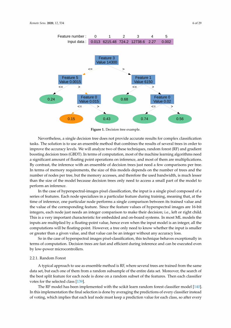
Figure 1 shows the inference operation of a trained decision tree on a series of feature inputs witha toy example. In the first place, this tree takes feature 3 of the input and compares its value with thethreshold value 14,300; as the input value is lower than the threshold it continues on the left child,and keeps with the same procedure until it reaches the leaf with 0.15 as output value.

One of the benefits of using decision trees over other techniques is that they do not need anyinput pre-processing such as data normalization, scaling or centering. They work with the inputdata as it is [138]. The reason is that features are never mixed. As can be seen in Figure 1, in eachcomparison the trees compare the value of an input feature with another value of the same feature.Hence, several features can have different scales. In other machine learning models, as we just saw inMLR for example, features are mixed to generate a single value so, if their values belong to differentorders of magnitude, some features will initially dominate the result. This can be compensated forduring the training process, but in general normalization or other pre-processing technique will beneeded to speed up training and improve the results. Besides, the size of the input data does not affectthe size of the model, so dimensionality reduction techniques such as principal component analysis(PCA) are not needed to reduce the model size, which substantially reduces the amount of calculationneeded at inference.

Remote Sens. 2020, 12, 534 6 of 29

0 1 2 3 4 5

0.013 6215.48 724.2 12738.6 2.27 0.002

Feature number :

Input data :

Feature 3Value 14300

Feature 5Value 0.0015

Feature 1Value 6150

Feature 0Value 0.015

Feature 0Value 0.02

0.24 0.68

0.560.740.430.15

<= >

<= > <= >

<= ><= >

Figure 1. Decision tree example.

Nevertheless, a single decision tree does not provide accurate results for complex classificationtasks. The solution is to use an ensemble method that combines the results of several trees in order toimprove the accuracy levels. We will analyze two of these techniques, random forest (RF) and gradientboosting decision trees (GBDT). In terms of computation, most of the machine learning algorithms needa significant amount of floating point operations on inference, and most of them are multiplications.By contrast, the inference with an ensemble of decision trees just need a few comparisons per tree.In terms of memory requirements, the size of this models depends on the number of trees and thenumber of nodes per tree, but the memory accesses, and therefore the used bandwidth, is much lesserthan the size of the model because decision trees only need to access a small part of the model toperform an inference.

In the case of hyperspectral-images pixel classification, the input is a single pixel composed of aseries of features. Each node specializes in a particular feature during training, meaning that, at thetime of inference, one particular node performs a single comparison between its trained value andthe value of the corresponding feature. Since the feature values of hyperspectral images are 16-bitintegers, each node just needs an integer comparison to make their decision; i.e., left or right child.This is a very important characteristic for embedded and on-board systems. In most ML models theinputs are multiplied by a floating-point value, hence even when the input model is an integer, all thecomputations will be floating-point. However, a tree only need to know whether the input is smalleror greater than a given value, and that value can be an integer without any accuracy loss.

So in the case of hyperspectral images pixel-classification, this technique behaves exceptionally interms of computation. Decision trees are fast and efficient during inference and can be executed evenby low-power microcontrollers.

2.2.1. Random Forest

A typical approach to use as ensemble method is RF, where several trees are trained from the samedata set, but each one of them from a random subsample of the entire data set. Moreover, the search ofthe best split feature for each node is done on a random subset of the features. Then each classifiervotes for the selected class [139].

The RF model has been implemented with the scikit learn random forest classifier model [140].In this implementation the final selection is done by averaging the predictions of every classifier insteadof voting, which implies that each leaf node must keep a prediction value for each class, so after every

Remote Sens. 2020, 12, 534 7 of 29

tree performs the inference the class is selected from the average of every prediction. This generatesbig models but, as we said, it only needs to access a small part of it during inference.

2.2.2. Gradient Boosting

However, even better results can be obtained applying a different ensemble approach calledgradient boosting. This technique is an ensemble method that combines the results of differentpredictors in such a way that each tree attempts to improve the results of the previous ones. Specifically,the gradient boosting method consists of training predictors sequentially so each new iteration tries tocorrect the residual error generated in the previous one. That is, each predictor is trained to correct theresidual error of its predecessor. Once the trees are trained, they can be used for prediction by simplyadding the results of all the trees [138,141].

The GBDT model has been implemented with the LightGBM library Classifier [142].For multi-class classification, one-vs-all approach is used in GBDT implementation, which meansthat the model trains a different estimator for each class. The output of the correspondent estimatorrepresents the probability that the pixel belongs to that class, and the estimator with the highest resultis the one that corresponds to the selected class. On each iteration, the model adds a new tree to eachestimator. The one-vs-all approach makes it much easier to combine the results given that each classhas their own trees, so we just need to add the results of the trees of each class separately, as shown inFigure 2. This accumulations of the output values of the trees are the only operations in floating pointthat the GBDT need to perform.

++

Trees of Class 1 Trees of Class N

... ... ...

Class 1 percentage Class N percentage

Figure 2. Gradient boosting decision trees (GBDT) results accumulation with one-vs-all approach.

Due to its iterative approach, the GBDT model also allows designers to trade-off accuracy forcomputation and model size. For example, if a GBDT is trained for 200 iterations, it will generate200 trees for each class. Afterwards, the designer can decide whether to use all of them, or to discardthe final ones. It is possible to find similar trade-off with other ML models, for instance reducingthe number of convolutional layers in a CNN or the number of hidden neurons in a MLP. However,in that case, each possible design must be trained again, whereas in GBDT only one train is needed,and afterwards the designer can simply evaluate the results when using different number of trees andgenerate a Pareto curve with the different trade-offs.

2.3. Support Vector Machine

A support vector machine (SVM) is a kernel-based method commonly used for classification andregression problems. It is based on a two-class classification approach, the support vector networkalgorithm. To find the smallest generalization error, this algorithm searches for the optimal hyperplane,i.e., a linear decision function that maximizes the margin among the support vectors, which are theones that define the decision boundaries of each class [143]. In the case of pixel-based classificationof hyperspectral images, we need to generalize this algorithm to a multi-class classification problem.This can be done following a one-vs-rest, or one-vs-all, approach, training K separate SVMs, one foreach class, so each two-class classifier will interpret the data from its own class as positive examplesand the rest of the data as negative examples [134].

Remote Sens. 2020, 12, 534 8 of 29

The SVM model has been implemented with the scikit learn support vector classification (SVC)algorithm [144], which implements one-vs-rest approach for multi-class classification. SVM modelalso requires pre-processing of the data applying the standardization Equation (3), with the sameimplications explained in Section 2.1. According to scikit learn SVC mathematical formulation [144],the decision function is found in Equation (5), where K(vi, x) corresponds to the kernel. We usedthe radial basis function (RBF) kernel, whose formulation is found in Equation (6). So the completeformulation of the inference operations is found in Equation (7), where vi corresponds to the i-thsupport vector, yiαi product is the coefficient of this support vector, x corresponds to the input pixel,ρ is the bias value and γ is the value of the gamma training parameter.

sgn

(M

∑i=1

yiαiK(vi, x) + ρ

)(5)

exp(−γ‖vi − x‖2

)(6)

sgn

(M

∑i=1

yiαi exp(−γ‖vi − x‖2

)+ ρ

)(7)

The number of support vectors defined as M in Equation (7) of the SVM model will be the amountof data used for the training set. So this model does not keep too many parameters, which makes itsmall in memory size, but in terms of computation, it requires a great amount of calculus to performone inference. The number of operations will depend on the number of features and the number oftraining data, which makes it unaffordable in terms of computation for really big data sets. Moreover,as it uses one-vs-all, it will also depends on the number of classes because it will train an estimator foreach one of them.

2.4. Neural Networks

Neural networks have become one of the most used machine learning techniques for imagesclassification, and they have also proved to be a good choice for hyperspectral images classification.A neural network consists of several layers sequentially connected so that the output of one layerbecomes the input of the next one. Some of the layers can be dedicated to intermediate functions,like pooling layers that reduce dimensionality highlighting the principal values, but the main operation,as well as most of the calculations, of a neural network resides in the layers based on neurons. Eachneuron implements Equation (8), where x is the input value and w and b are the learned weight andbias respectively, which are float values.

y = xw + b (8)

Usually, when applying groups of neurons in more complex layers, the results of several neuronsare combined such as in a dot product operation, as we will see for example in Section 2.4.1, and this wand b values are float vectors, matrices or tensors, depending on the concrete scenario. So the maincalculations in neural networks are float multiplications and accumulations, and the magnitude of thesecomputations depends on the number and size of the layers of the neural network. The informationwe need to keep in memory for inference consists in all these learned values, so the size of the modelwill also depend on the number and size of the layers.

Neural network models also require pre-processing of the data. Without it, the features withhigher and lower values will initially dominate the result. This can be compensated during trainingprocess, but in general normalization will be needed to speed up training and improve the results.As for MLR and SVM models, a standardization Equation (3) of the data sets was applied.

Remote Sens. 2020, 12, 534 9 of 29

2.4.1. Multi Layer Perceptron

A multi layer perceptron (MLP) is a neural network with at least one hidden layer,i.e., intermediate activation values, which requires at least two fully-connected layers. Consideringthe l-th fully connected layer, its operation corresponds to Equation (9), where X(l−1) is the layer’sinput, which can come directly from the original input or from a previous hidden layer l− 1, X(l) is theoutput of the current layer, resulting from applying the weights W(l) and biases ρ(l) of the layer. If thesize of the input X(l−1) is (M, N(l−1)), being M the number of input samples and N(l−1) the dimensionof the feature space, and the size of the weights W(l) is (N(l−1), N(l)), the output size will be (M, N(l)),i.e., the M samples represented in the feature space of dimension N(l) and defined by the l-th layer.In the case of hyperspectral imaging classification, the input size for one spectral pixel will be (1, B),where B is the number of spectral channels, while the final output of the model size will be (1, K),where K is the number of considered classes.

X(l) = X(l−1)W(l) + ρ(l) (9)

The MLP model was implemented with the PyTorch neural network library [145], using the Linearclasses to implement two fully-connected layers. The number of neurons of the first fully-connectedlayer is a parameter of the network, and the size of each neuron of the last fully-connected layer willdepend on it. In the case of hyperspectral images pixel classification, the input on inference will bea single pixel (M = 1 according to last explanation) with B features and the final output will be theclassification for the K classes, so the size of each neuron of the first fully-connected layer will dependon the number of features, while the number of neurons of the last fully-connected layer will be thenumber of classes.

As the input for pixel classification is not very big, this model keeps a small size once trained.During inference it will need to perform a float multiplication and a float accumulation for each one ofits parameters, among other operations, so even being small the operations needed are expensive interms of computation.

2.4.2. Convolutional Neural Network

A convolutional neural network (CNN) is a neural network with at least one convolutional layer.Instead of fully-connected neurons, convolutional layers apply locally-connected filters per layer.These filters are smaller than the input and each one of them performs a convolution operation on it.During a convolution, the filter performs dot product operations within different sections of the inputwhile it keeps moving along it. For hyperspectral images pixel classification, whose input consist in asingle pixel, the 1D convolutional layer operation can be described with Algorithm 1, where inputpixel x has B features, the layer has F filters and each filter Q has q values, i.e., weights in the caseof 1D convolution, and one bias ρ, so the output X′ will be of shape (B− q + 1, F). The initializationvalues LAYER_FILTERS and LAYER_BIASES correspond respectively to the learned weights andbiases of the layer.

Remote Sens. 2020, 12, 534 10 of 29

Algorithm 1 1D convolutional layer algorithm.

1: Input:2: x ≡ INPUT_PIXEL . The input pixel is an array of B features3: Initialize:4: f ilters← LAYER_FILTERS . Array of F filters, each one with q weights5: bias← LAYER_BIASES . Array of F bias values, corresponding to each filter6: X′ ← New_matrix(size : [B− q + 1, F]) . Output structure generation7: for ( f = 0 ; F− 1 ; f ++) do . For each filter8: Q = f ilters[ f ] . Get current filter9: ρ = bias[ f ] . Get current bias value

10: for (i = 0 ; B− q ; i ++) do . Movement of the filter along the input11: X′i, f = 012: for (j = 0 ; q ; j++) do . Dot product along the filter in current position13: X′i, f += Qjxi+j . Qj corresponds to the weight value14: end for15: X′i, f += ρ . ρ corresponds to the bias value16: end for17: end for18: Return:19: X′ . The output matrix of shape (B− q + 1, F)

The CNN model was implemented with PyTorch neural network library [145], using theconvolution, the pooling and the linear classes to define a Network with respectively one 1Dconvolutional layer, one max pooling layer and two fully connected layers at the end. The inputof the 1D convolutional layer will be the input pixel, while the input of the rest of the layers will bethe output of the previous one, in the specified order. The number and size of the filters of the 1Dconvolutional layer are parameters of the network, nevertheless the relation between the profundity ofthe filters and the number of features will determine the size of the first fully connected layer, which isthe biggest one. The max pooling layer does not affect the size of the model, since it only performsa size reduction by selecting the maximum value within small sub-sections of the input, but it willaffect the number of operations as it needs to perform several comparisons. The fully connected layersare actually an MLP, as explained in Section 2.4.1. The size of the last fully connected layer will alsodepend on the number of classes. In terms of computation, the convolutional layer is very intensive incalculations, as can be observed in Algorithm 1, and most of them are floating point multiplicationsand accumulations.

2.5. Summary of the Relation of the Models with the Input

Each discussed model has different characteristics on its inference operation, and the size andcomputations of each one depends on different aspects of the input and the selected parameters.Table 1 summarizes the importance of the data set size (in the case of hyperspectral images this is thenumber of pixels of the image), the number of features (number of spectral band of each hyperspectralpixel) and the number of classes (labels) in relation to the size and the computations of each model.The dots in Table 1 correspond to a qualitative interpretation, from not influenced at all (zero dots)to very influenced (three dots), regarding how each model size and number of computations areinfluenced by the size of the data set, the number of features of each pixel and the number of classes.This interpretation is not intended to be quantitative but qualitative, i.e., just a visual support for thefollowing explanations.

The number of classes is an important parameter for every model, but it affects them in a verydifferent way. Regarding the size of the model, the number of classes defines the size of the outputlayer in the MLP and CNN, while for the MLR, GBDT and SVM the entire estimator is replied to

Remote Sens. 2020, 12, 534 11 of 29

as many times as the number of classes. Since the RF needs to keep the prediction for each class onevery leaf node, the number of classes is crucial to determine the final size of the model, and affects itmuch more. Regarding the computation, in the MLR, GBDT and SVM models the entire number ofcomputations is multiplied by the number of classes, so it affects them very much. Furthermore, in theSVM model the number of classes will also affect the number of support vectors needed, because it isnecessary to have enough training data for every class, so each new class not only increases the numberof estimators, but also increases the computational cost by adding new support vectors. In neuralnetworks, the number of classes defines the size of the output (fully connected) layer, which impliesmultiply and accumulate floating point operations, but this is the smallest layer for both models. In thecase of RF, it only affects the final calculations of the results, but it is important to remark that these areprecisely the floating point operations of this model.

The number of features is not relevant for decision tree models during inference, that is why theydo not need any dimensionality reduction techniques. The size of each estimator of the MLR and theSVM models will depend directly on the number of features, so it influences the size as much as thenumber of classes. In neural networks, it affects the size of the first fully connected layer (which is thebiggest one), so the size of these models is highly influenced by the number of features. Nevertheless,in the case of the MLP, it only multiplies the dimension of the fully connected layer so it does notimpact that much as in the case of the CNN, where it will be also multiplied by the number of filtersof the convolutional layer. In a similar way, the number of operations of each estimator of the MLRand the SVM models will be directly influenced by the number of features. Again, for the MLP itwill increase the number of operations of the first fully connected layer and for the CNN also theconvolutional layer, which is very intensive in terms of calculations.

The size of the data set (and specifically the size of the training set) only affects the SVM model,because it will generate as many support vectors as the number of different data samples used in thetraining process. Regarding the size of the model, it multiplies the number of parameters of eachestimator, so it will affect the size of the model as much as the number of classes. Actually, both thetraining set and the number of classes are related to each other. Regarding the number of operations,the core of Equation (7) depends on the number of support vectors, so its influence is very high.

Table 1. Summary of the size and computational requirements of the considered models.

Size Dependencies Computation Dependencies

Pre-Processing Data Set Features Classes Data Set Features Classes

MLR standardization - •• •• - •• ••RF - - - • • • - - •

GBDT - - - •• - - ••SVM standardization •• •• •• • • • •• • • •MLP standardization - •• • - •• •

CNN1D standardization - • • • • - • • • •

It is also worth noting that decision trees are the only ones that do not require any pre-processingto the input data. As we already explained in Section 2.1, this implies some extra calculations notincluded in the measurements of Section 4.2, but they can also be a source of possible inaccuraciesbecause of the implications they could have once applied to a real system with entirely new datataken in different moments and conditions. For instance, applying standardization means that wewill subtract the mean value of our training set to the data, and reduce it in relation to the standarddeviation of our training set.

Remote Sens. 2020, 12, 534 12 of 29

3. Data Sets and Training Configurations

The data sets selected for experiments are the Indian Pines (IP) [146], Pavia University (PU) [146],Kennedy Space Center (KSC) [146], Salinas Valley (SV) [146] and University of Houston (UH) [147].Table 2 shows the ground truth and the number of pixels per class for each image.

Table 2. Number of samples of the Indian Pines (IP), University of Pavia (UP), Salinas Valley (SV),Kennedy Space Center (KSC) and University of Houston (UH) hyperspectral data sets.

Indian Pines (IP) University of Pavia (UP) Salinas Valley (SV) Kennedy Space Center (KSC)

Color Land-cover type Samples Color Land-cover type Samples Color Land-cover type Samples Color Land-cover type Samples

Background 10,776 Background 164,624 Background 56,975 Background 309,157Alfalfa 46 Asphalt 6631 Brocoli-green-weeds-1 2009 Scrub 761

Corn-notill 1428 Meadows 18,649 Brocoli-green-weeds-2 3726 Willow-swamp 243Corn-min 830 Gravel 2099 Fallow 1976 CP-hammock 256

Corn 237 Trees 3064 Fallow-rough-plow 1394 Slash-pine 252Grass/Pasture 483 Painted metal sheets 1345 Fallow-smooth 2678 Oak/Broadleaf 161

Grass/Trees 730 Bare Soil 5029 Stubble 3959 Hardwood 229Grass/pasture-mowed 28 Bitumen 1330 Celery 3579 Swap 105

Hay-windrowed 478 Self-Blocking Bricks 3682 Grapes-untrained 11,271 Graminoid-marsh 431Oats 20 Shadows 947 Soil-vinyard-develop 6203 Spartina-marsh 520

Soybeans-notill 972 Corn-senesced-green-weeds 3278 Cattail-marsh 404Soybeans-min 2455 Lettuce-romaine-4wk 1068 Salt-marsh 419Soybean-clean 593 Lettuce-romaine-5wk 1927 Mud-flats 503

Wheat 205 Lettuce-romaine-6wk 916 Water 927Woods 1265 Lettuce-romaine-7wk 1070

Bldg-Grass-Tree-Drives 386 Vinyard-untrained 7268Stone-steel towers 93 Vinyard-vertical-trellis 1807

Total samples 21,025 Total samples 207,400 Total samples 111,104 Total samples 314,368

University of Houston (UH)

Color Land cover type Samples train Samples test

Background 649,816Grass-healthy 198 1053Grass-stressed 190 1064Grass-synthetic 192 505

Tree 188 1056Soil 186 1056

Water 182 143Residential 196 1072Commercial 191 1053

Road 193 1059Highway 191 1036Railway 181 1054

Parking-lot1 192 1041Parking-lot2 184 285Tennis-court 181 247

Running-track 187 473

Total samples 2832 12,197

• The IP data set is an image of an agricultural region, mainly composed of crop fields, collected bythe Airborne Visible Infra-Red Imaging Spectrometer (AVIRIS) sensor in Northwestern Indiana,USA. It has 145 × 145 pixels with 200 spectral bands after removal of the noise and waterabsorption bands. Of the total 21,025 pixels, 10,249 are labeled into 16 different classes.

• The UP data set is an image of an urban area, the city of Pavia in Italy, collected by the ReflectiveOptics Spectrographic Imaging System (ROSIS), a compact airborne imaging spectrometer. It iscomposed of 610 × 340 pixels with 103 spectral bands. Only 42,776 pixels from the total 207,400are labeled into nine classes.

• The KSC data set is an image with water and vegetation collected by the AVIRIS sensor overthe Kennedy Space Center in Florida, USA. It has 512 × 614 pixels with 176 spectral bands after

Remote Sens. 2020, 12, 534 13 of 29

removing the water absorption and low signal-to-noise bands. Only 5211 out of the available314,368 pixels are labeled into 13 classes.

• The SV data set is an image composed of agricultural fields and vegetation, collected by theAVIRIS sensor in Western California, USA. It has 512 × 217 pixels with 204 spectral bands afterremoving the noise and water absorption bands. Of the total 111,104 pixels, 56,975 are labeledinto 16 classes.

• The UH data set is an image of an urban area collected by the Compact Airborne SpectrographicImager (CASI) sensor over the University of Houston, USA. It has 349 × 1905 pixels with 144spectral bands. Only 15,029 of the total 664,845 pixels are labeled into 15 classes. As it wasproposed as the benchmark data set for the 2013 IEEE Geoscience and Remote Sensing Societydata fusion contest [148], it is already divided into training and testing sets, with 2832 and 12,197pixels, respectively.

The implementation of the algorithms used in this review were developed and tested on ahardware environment with an X Generation Intel R© CoreTMi9-9940X processor with 19.25M of Cacheand up to 4.40GHz (14 cores/28 way multi-task processing), installed over a Gigabyte X299 Aorus,with 128GB of DDR4 RAM. Also, a graphic processing unit (GPU) NVIDIA Titan RTX with 24GBGDDR6 of video memory and 4608 cores was used. We detailed in Section 2 the libraries and classesused for the implementation of each model: MLR with scikit learn logistic regression, random forestwith scikit learn random forest classifier, GBDT with LightGBM classifier, SVM with scikit learn supportvector classification, MLP with PyTorch neural network linear layers and CNN1D with PyTorch neuralnetwork convolutional, pooling and linear layers.

For each dataset we trained the models applying cross-validation techniques to select the finaltraining hyperparameters. After the cross-validation, the selected values did not always correspondto the best accuracy, but to the best relation between accuracy and model size and requirements.The selected hyperparameters shown in Table 3 are the penalty of the error (C) for the MLR, the numberof trees (n), the minimum number of data to split a node (m) and maximum depth (d) for both theRF and the GBDT, and also the maximum number of features to consider for each split ( f ) for theRF, the penalty of the error (C) and kernel coefficient (γ) for the SVM, the number of neurons in thehidden layer (h.l.) for the MLP and for the CNN, the number of filters of the convolutional layer( f ), the number of values of each filter (q), the size of the kernel of the max pooling layer (p) and thenumber of neurons of the first and last fully connected layers ( f 1) and ( f 2), respectively.

Table 3. Selected training parameters of the different tested models.

MLR RF GBDT SVM MLP CNN1D

C n m f d n m d C γ h.l. f q p f1 f2

IP 1 200 2 10 10 200 20 20 100 2−9 143 20 24 5 100 16PU 10 200 2 10 10 150 30 30 10 2−4 78 20 24 5 100 9

KSC 100 200 2 10 10 300 30 5 200 2−1 127 20 24 5 100 13SV 10 200 2 40 60 150 80 25 10 2−4 146 20 24 5 100 16HU 1e5 200 2 10 40 150 30 35 1e5 2−6 106 20 24 5 100 15

The final configurations of some models not only depend on the selected hyperparameters,but also on the training data set (for the SVM model) and the training process itself (for the RF andGBDT models). Table 4 shows the number of features (ft.) and classes (cl.) of each image and the finalconfigurations of RF, GBDT and SVM models. For the tree models, the shown values are the totalnumber of trees (trees), which in the case of the GBDT model depends on the number of classes of eachimage, the total number of non-leaf nodes (nodes) and leaf nodes (leaves) and the average depth of thetrees of the entire model (depth). For the SVM model, the number of support vectors (s.v.) depends onthe amount of training data.

Remote Sens. 2020, 12, 534 14 of 29

Table 4. Final configurations of random forest (RF), gradient boosting decision Trees (GBDT) andsupport vector machine (SVM) models.

RF GBDT SVM

ft. cl. Trees Nodes leaves Depth Trees Nodes Leaves Depth s.v.

IP 200 16 200 28,663 28,863 8.39 3200 54,036 57,236 5.65 1538PU 103 9 200 33,159 33,359 8.63 1350 36,415 55,646 8 4278

KSC 176 13 200 15,067 15,267 8.9 3900 17,883 75,814 2.64 782SV 204 16 200 23,979 24,179 8.46 2400 50,253 52,653 6.02 5413HU 144 15 200 44,597 44,787 12.34 2250 67,601 69,851 7.31 2832

4. Discussion Of Results

First we present the accuracy results for all models and images, and then we report the size andcomputational measurements on inference. Then, we summarize and analyze the characteristics ofeach model in order to target an embedded or an on-board system.

4.1. Accuracy Results

Figure 3 depicts the accuracy evolution of each model when increasing the percentage of pixels foreach class selected for training. Neural network models always achieve high accuracy values, with theCNN model outperforming all other models, and the SVM as a kernel-based model is always the nextone or even outperforming the MLP. The only behavior that does not this pattern is the high accuracyvalues achieved by the MLR model on the KSC data set. Except for this case, the results obtained byneural networks, kernel-based models and the other models were expected [75]. Nevertheless, it isworth mentioning that, for a tree based model, GBDT achieves great accuracy values which are veryclose to those obtained by neural networks and the SVM, which always provide higher values than theRF, which is also a tree based model.

The results obtained with the UH data set are quite particular, since it is not an entire image towork with, but two separated structures already prepared as training and testing sets. As we canobserve in the values of the overall accuracy in Table 9, the accuracy of all models is below the scoreobtained for other images. However, the distribution of the different models keeps the same behaviordescribed for the rest of the data sets, with the particularity that the MLR model outperforms theGBDT in this case.

Tables 5–9 show the accuracy results of the selected configurations of each model. For the IP andKSC images, the selected training set is composed of 15% of the pixels from each class, while in the UPand SV only consists of 10% of the pixels from each class. The fixed training set for the UH image iscomposed of around 19% of the total pixels.

Figure 4 shows the classification maps obtained for the different data sets by all the models.As we can observe, most of the classification maps have the typical salt and pepper effect of spectralmodels, i.e., classified trough individual pixels. There are some particular classes that are bettermodeled by certain models. For instance, the GBDT and SVM perfectly define the contour of thesoil–vinyard–develop class of SV, while CNN1D exhibits a very good behavior on the cloudy zone inthe right side of the UH data set, and both tree based models (RF and GBDT) perform very well onthe swampy area on the right side of the river in the KSC data set. Nevertheless, the most significantconclusion that can be derived from these class maps is that the different errors of each model aredistributed in a similar way along classes for each model, as it can be seen on Tables 5–9, but here wecan confirm that it is consistent for the entire classification map. In general, all the classification mapsare quite similar and well defined in terms of the contours, and the main classes are properly classified.We can conclude that the obtained accuracy levels are satisfactory, and the errors are well distributed,without significant deviations due to a particular class nor significant overfitting of the models.

Remote Sens. 2020, 12, 534 15 of 29

5 10 15 20Training Percent

67

70

73

76

79

82

85

Over

all A

ccur

acy

(%)

RFMLR

SVMMLP

CNN1DGBDT

1 5 10 15Training Percent

808284868890929496

Over

all A

ccur

acy

(%)

RFMLR

SVMMLP

CNN1DGBDT

(a) Indian Pines (b) Pavia University

5 10 15 20Training Percent

82

84

86

88

90

92

94

Over

all A

ccur

acy

(%)

RFMLR

SVMMLP

CNN1DGBDT

1 5 10 15Training Percent

86

88

90

92

94

96Ov

eral

l Acc

urac

y (%

)

RFMLR

SVMMLP

CNN1DGBDT

(c) KSC (d) Salinas Valley

Figure 3. Accuracy comparison for different training set sizes on (a) IP, (b) UP, (c) KSC and (d) SV.

Table 5. IP data set results.

Class MLR RF GBDT SVM MLP CNN1D

1 22.5 ± 6.71 18.0 ± 7.31 40.0 ± 5.0 40.5 ± 9.0 40.5 ± 20.27 33.5 ± 13.932 75.04 ± 1.17 62.73 ± 2.37 76.623 ± 1.967 80.3 ± 1.12 79.32 ± 2.6 81.52 ± 1.513 57.17 ± 1.76 50.14 ± 1.96 65.354 ± 1.759 70.06 ± 1.74 69.89 ± 3.22 68.07 ± 2.94 45.94 ± 3.64 30.5 ± 3.97 40.297 ± 2.356 67.82 ± 6.08 59.9 ± 6.03 60.99 ± 9.055 89.68 ± 2.32 86.18 ± 2.96 90.414 ± 1.338 93.19 ± 2.41 89.39 ± 1.79 90.27 ± 2.226 95.56 ± 1.5 94.78 ± 1.16 96.039 ± 1.011 95.97 ± 1.33 97.13 ± 1.41 97.39 ± 0.447 42.5 ± 16.75 8.33 ± 5.27 32.5 ± 23.482 71.67 ± 7.17 60.83 ± 10.07 53.33 ± 17.958 98.72 ± 0.42 97.74 ± 0.39 98.133 ± 0.481 97.3 ± 1.31 98.08 ± 0.57 99.16 ± 0.519 21.18 ± 7.98 0.0 ± 0.0 14.118 ± 8.804 47.06 ± 9.84 57.65 ± 15.96 50.59 ± 10.26

10 66.55 ± 2.76 66.31 ± 4.71 75.84 ± 4.367 75.62 ± 1.19 79.11 ± 0.44 75.38 ± 3.6811 80.24 ± 1.27 89.08 ± 1.27 87.877 ± 1.18 84.99 ± 1.08 83.56 ± 1.32 85.05 ± 0.5312 60.59 ± 3.36 47.96 ± 6.57 55.604 ± 1.551 76.83 ± 4.51 73.31 ± 1.97 83.25 ± 3.3113 98.29 ± 1.02 92.8 ± 2.74 93.371 ± 1.933 98.86 ± 1.2 99.2 ± 0.28 99.2 ± 0.6914 93.4 ± 0.64 95.61 ± 0.99 95.967 ± 0.607 94.07 ± 0.87 95.13 ± 0.3 94.89 ± 1.2915 65.71 ± 2.06 40.91 ± 0.81 56.839 ± 2.016 64.8 ± 1.35 66.08 ± 2.68 69.06 ± 2.9416 84.75 ± 3.1 82.5 ± 2.09 88.5 ± 3.102 87.75 ± 2.89 89.0 ± 4.77 89.0 ± 2.67

OA 77.81 ± 0.42 75.32 ± 0.44 80.982 ± 0.783 83.46 ± 0.35 83.04 ± 0.44 83.93 ± 0.5AA 68.61 ± 1.51 60.22 ± 0.57 69.217 ± 1.627 77.92 ± 0.88 77.38 ± 2.45 76.92 ± 1.93

K(x100) 74.54 ± 0.47 71.42 ± 0.53 78.16 ± 0.897 81.08 ± 0.41 80.62 ± 0.51 81.61 ± 0.59

Remote Sens. 2020, 12, 534 16 of 29

Table 6. UP data set results.

Class MLR RF GBDT SVM MLP CNN1D

1 92.41 ± 0.86 91.35 ± 0.98 90.044 ± 0.627 93.82 ± 0.62 94.31 ± 1.09 95.37 ± 1.32 96.02 ± 0.21 98.25 ± 0.18 96.571 ± 0.425 98.41 ± 0.23 97.98 ± 0.39 98.16 ± 0.273 72.75 ± 1.13 61.51 ± 3.47 74.952 ± 1.422 78.8 ± 1.33 80.38 ± 1.12 80.55 ± 1.914 88.17 ± 0.74 87.2 ± 1.25 90.986 ± 1.113 93.06 ± 0.67 93.72 ± 1.02 95.43 ± 1.545 99.41 ± 0.3 98.43 ± 0.56 99.026 ± 0.403 98.86 ± 0.25 99.36 ± 0.48 99.8 ± 0.176 77.5 ± 0.72 45.2 ± 1.52 86 ± 0.837 87.97 ± 0.62 91.58 ± 1.0 92.26 ± 1.547 54.77 ± 4.38 75.27 ± 4.56 84.194 ± 1.245 84.58 ± 1.57 85.23 ± 2.51 89.29 ± 3.788 86.05 ± 0.7 88.2 ± 1.03 87.827 ± 0.805 89.67 ± 0.44 87.32 ± 1.5 88.07 ± 1.599 99.7 ± 0.06 99.41 ± 0.29 99.906 ± 0.088 99.53 ± 0.3 99.62 ± 0.17 99.79 ± 0.2

OA 89.63 ± 0.12 86.8 ± 0.25 91.869 ± 0.181 93.98 ± 0.15 94.26 ± 0.18 94.92 ± 0.22AA 85.2 ± 0.54 82.76 ± 0.43 89.945 ± 0.211 91.63 ± 0.38 92.17 ± 0.16 93.19 ± 0.47

K(x100) 86.13 ± 0.17 81.98 ± 0.35 89.195 ± 0.228 91.99 ± 0.2 92.37 ± 0.24 93.25 ± 0.3

Table 7. KSC data set results.

Class MLR RF GBDT SVM MLP CNN1D

1 95.92 ± 1.22 95.49 ± 1.21 95.425 ± 1.188 95.12 ± 0.77 96.23 ± 0.43 97.03 ± 1.192 92.27 ± 3.28 88.02 ± 2.35 86.377 ± 2.013 90.92 ± 3.56 88.89 ± 2.78 91.3 ± 4.263 87.25 ± 4.77 86.79 ± 2.89 86.697 ± 2.228 84.95 ± 3.46 90.92 ± 2.98 92.29 ± 1.894 68.09 ± 4.61 71.44 ± 4.77 64.372 ± 1.705 69.4 ± 6.88 72.74 ± 3.35 81.21 ± 8.795 75.18 ± 3.13 57.66 ± 5.4 55.036 ± 8.644 63.94 ± 6.95 62.04 ± 4.33 76.93 ± 5.096 74.97 ± 3.33 51.79 ± 3.84 61.641 ± 4.344 64.92 ± 7.66 66.87 ± 3.93 78.36 ± 5.547 80.67 ± 5.9 78.22 ± 4.13 82.444 ± 4.411 71.33 ± 6.06 83.33 ± 7.95 85.56 ± 8.468 91.77 ± 1.59 83.65 ± 2.9 86.975 ± 2.541 91.77 ± 2.62 92.7 ± 2.33 93.62 ± 3.499 97.01 ± 0.92 94.52 ± 2.25 93.394 ± 3.033 94.75 ± 1.59 97.6 ± 0.7 98.55 ± 0.99

10 95.99 ± 0.67 88.78 ± 0.79 93.198 ± 2.172 94.83 ± 1.5 97.44 ± 1.36 98.26 ± 0.5811 98.1 ± 1.11 97.82 ± 1.17 94.678 ± 3.012 96.92 ± 1.59 98.26 ± 0.7 97.98 ± 0.8812 95.09 ± 0.42 89.81 ± 1.57 93.505 ± 1.12 90.75 ± 2.81 93.83 ± 1.08 96.45 ± 1.5813 100.0 ± 0.0 99.62 ± 0.24 99.67 ± 0.129 99.16 ± 0.46 100.0 ± 0.0 99.92 ± 0.06

OA 92.69 ± 0.23 88.88 ± 0.43 89.506 ± 0.604 90.51 ± 0.56 92.42 ± 0.23 94.59 ± 0.32AA 88.64 ± 0.61 83.36 ± 0.83 84.109 ± 0.973 85.29 ± 1.22 87.76 ± 0.4 91.34 ± 0.59

K(x100) 91.86 ± 0.26 87.61 ± 0.48 88.308 ± 0.674 89.43 ± 0.62 91.55 ± 0.26 93.97 ± 0.35

Table 8. SV data set results.

Class MLR RF GBDT SVM MLP CNN1D

1 99.19 ± 0.47 99.64 ± 0.15 99.514 ± 0.289 99.44 ± 0.36 99.64 ± 0.46 99.87 ± 0.172 99.93 ± 0.06 99.86 ± 0.09 99.827 ± 0.074 99.72 ± 0.15 99.83 ± 0.21 99.86 ± 0.223 98.85 ± 0.29 99.08 ± 0.53 98.775 ± 0.37 99.51 ± 0.12 99.47 ± 0.2 99.63 ± 0.254 99.39 ± 0.31 99.54 ± 0.27 99.554 ± 0.26 99.59 ± 0.11 99.62 ± 0.12 99.46 ± 0.065 99.19 ± 0.26 97.96 ± 0.49 98.109 ± 0.332 98.71 ± 0.51 99.11 ± 0.32 99.0 ± 0.366 99.94 ± 0.03 99.72 ± 0.11 99.624 ± 0.292 99.78 ± 0.12 99.84 ± 0.09 99.9 ± 0.077 99.74 ± 0.07 99.34 ± 0.18 99.559 ± 0.164 99.61 ± 0.16 99.71 ± 0.12 99.7 ± 0.18 88.07 ± 0.11 84.26 ± 0.42 85.507 ± 0.349 89.11 ± 0.34 88.84 ± 0.7 90.36 ± 1.019 99.79 ± 0.07 99.01 ± 0.24 99.219 ± 0.165 99.66 ± 0.21 99.88 ± 0.07 99.85 ± 0.13

10 96.34 ± 0.52 91.35 ± 0.61 93.473 ± 0.737 95.28 ± 0.87 96.32 ± 0.79 97.63 ± 0.5711 96.9 ± 1.0 94.2 ± 1.23 94.782 ± 0.532 98.0 ± 0.71 97.75 ± 0.76 98.42 ± 0.8512 99.79 ± 0.03 98.42 ± 0.67 99.239 ± 0.507 99.55 ± 0.34 99.8 ± 0.11 99.93 ± 0.1113 99.05 ± 0.33 98.08 ± 0.67 97.818 ± 0.957 98.5 ± 0.52 98.55 ± 0.7 99.25 ± 0.5614 95.89 ± 0.17 91.48 ± 1.29 95.202 ± 0.997 95.02 ± 0.81 98.17 ± 0.55 98.05 ± 0.8515 66.85 ± 0.18 60.42 ± 1.32 74.91 ± 0.524 71.72 ± 0.69 74.61 ± 1.66 80.02 ± 2.3516 98.45 ± 0.36 97.31 ± 0.19 97.406 ± 1.017 98.35 ± 0.17 98.7 ± 0.72 98.94 ± 0.53

OA 92.45 ± 0.07 90.08 ± 0.17 92.544 ± 0.079 93.2 ± 0.17 93.75 ± 0.1 94.91 ± 0.16AA 96.09 ± 0.1 94.35 ± 0.16 95.782 ± 0.056 96.35 ± 0.15 96.86 ± 0.02 97.49 ± 0.15

K(x100) 91.58 ± 0.07 88.93 ± 0.19 91.696 ± 0.087 92.42 ± 0.19 93.03 ± 0.11 94.33 ± 0.18

Remote Sens. 2020, 12, 534 17 of 29

Table 9. UH data set results.

Class MLR RF GBDT SVM MLP CNN1D

1 82.24 ± 0.35 82.53 ± 0.06 82.336 ± 0.0 82.24 ± 0.0 81.29 ± 0.32 82.55 ± 0.542 81.75 ± 1.13 83.31 ± 0.26 83.177 ± 0.0 80.55 ± 0.0 82.12 ± 1.18 86.9 ± 3.873 99.49 ± 0.2 97.94 ± 0.1 97.228 ± 0.0 100.0 ± 0.0 99.6 ± 0.13 99.88 ± 0.164 90.81 ± 3.67 91.59 ± 0.15 94.981 ± 0.0 92.52 ± 0.0 88.92 ± 0.55 92.8 ± 3.345 96.88 ± 0.08 96.84 ± 0.13 93.277 ± 0.0 98.39 ± 0.0 97.35 ± 0.32 98.88 ± 0.36 94.27 ± 0.28 98.88 ± 0.34 90.21 ± 0.0 95.1 ± 0.0 94.55 ± 0.28 95.94 ± 1.687 71.88 ± 1.26 75.24 ± 0.15 73.414 ± 0.0 76.31 ± 0.0 76.03 ± 1.74 86.49 ± 1.298 61.8 ± 0.68 33.2 ± 0.15 35.138 ± 0.0 39.13 ± 0.0 64.27 ± 9.17 78.02 ± 6.69 64.82 ± 0.23 69.07 ± 0.4 68.839 ± 0.0 73.84 ± 0.0 75.09 ± 2.27 78.7 ± 4.31

10 46.18 ± 0.35 43.59 ± 0.31 41.699 ± 0.0 51.93 ± 0.0 47.28 ± 1.07 68.22 ± 10.4111 73.51 ± 0.33 69.94 ± 0.16 72.391 ± 0.0 78.65 ± 0.0 76.11 ± 1.07 82.13 ± 1.6212 67.74 ± 0.26 54.62 ± 0.8 69.164 ± 0.0 69.03 ± 0.05 72.93 ± 3.56 90.85 ± 2.5713 69.75 ± 0.72 60.0 ± 0.59 67.018 ± 0.0 69.47 ± 0.0 72.28 ± 3.6 74.67 ± 3.4914 99.35 ± 0.49 99.27 ± 0.47 99.595 ± 0.0 100.0 ± 0.0 99.35 ± 0.41 99.11 ± 0.315 94.38 ± 0.89 97.59 ± 0.32 95.137 ± 0.0 98.1 ± 0.0 98.1 ± 0.48 98.48 ± 0.16

OA 76.35 ± 0.27 73.0 ± 0.07 74.182 ± 0.0 76.96 ± 0.0 78.61 ± 0.44 85.95 ± 0.94AA 79.66 ± 0.2 76.91 ± 0.06 77.573 ± 0.0 80.35 ± 0.0 81.68 ± 0.24 87.58 ± 0.8

K(x100) 74.51 ± 0.28 70.99 ± 0.07 72.101 ± 0.0 75.21 ± 0.0 76.96 ± 0.47 84.77 ± 1.02

(a1) GT (b1) MLR (c1) RF (d1) GBDT (e1) SVM (f1) MLP (g1) CNN1D

Figure 4. Cont.

Remote Sens. 2020, 12, 534 18 of 29

(a2) GT

(b2) MLR (c2) RF

(d2) GBDT (e2) SVM

(f2) MLP (g2) CNN1D

Figure 4. Classification maps obtained for the considered data sets by the different models:(a1,a2) Ground truth, (b1,b2) MLR, (c1,c2) RF, (d1,d2) GBDT, (e1,e2) SVM, (f1,f2) MLP and(g1,g2) CNN1D.

4.2. Size and Computational Measurements

To perform the characterization of each algorithm in inference it is necessary to analyze theirstructure and operation. The operation during inference of every model has been explained in Section 2,and the final sizes and configurations of the trained models after cross-validation for parameterselection has been detailed in Section 3. Figure 5 reports the sizes in Bytes of the trained models, whileFigure 6 shows the number and type of operations performed during the inference stage.

It is very important to remark that these measurements have been realized theoretically, basedon the described operations and model configurations. For instance, the size measurements do notcorrespond to the size of a file with the model dumped on it, which is software-dependent, i.e., dependson the data structures it uses to keep much more information for the framework than the actual learnedparameters needed for inference. As a result, Figure 5 shows the theoretical size required in memory tostore all the necessary structures for inference, based on the analysis of the models, exactly as it wouldbe developed for a specific hardware accelerator or an embedded system.

As we can observe, the size of RF models is one order of magnitude bigger than the others. This isdue to their need to save the values of the predictions for every class on each leaf node. This is a hugeamount of information, even compared to models that train an entire estimator for each class, likeGBDT. Actually, the size of MLR and SVM models is one order of magnitude smaller than GBDT, MLPand CNN1D models. Nevertheless, all the models (except the RF) are below 500 kilobytes, whichmakes them very affordable even for small low-power embedded devices.

In a similar way, the operational measurements shown on Figure 6 are based on the analysis ofeach algorithm, not in terms of software executions (that depend on the architecture, the system andthe framework), and they are divided into four groups according to their computational complexity.The only models that use integers for the inference computations are the decision trees, and theyonly need integer comparisons. Floating point operations are the most common in the rest of themodels, but they are also divided into three different categories. FP Add refers to accumulations,

Remote Sens. 2020, 12, 534 19 of 29

subtractions and comparisons, which can be performed on an adder and are less complex, FP Mulrefers to multiplications and divisions and FP Exp are exponential which are only performed by theSVM model. High-performance processors include powerful floating point arithmetic units, but forlow-power processors and embedded devices, these computations can be very expensive.

0

500000

1×106

1.5×106

2×106

2.5×106

3×106

MLR RF

GBDT

SVM

MLP

CNN1D

MLR RF

GBDT

SVM

MLP

CNN1D

MLR RF

GBDT

SVM

MLP

CNN1D

MLR RF

GBDT

SVM

MLP

CNN1D

MLR RF

GBDT

SVM

MLP

CNN1D

weightsactivations and outputs

Houston Salinas PaviaU KSC IndianPines

Figure 5. Size of the trained models in bytes.

0

50000

100000

150000

200000

250000

300000

MLR RF

GBDT

SVM

MLP

CNN1D

MLR RF

GBDT

SVM

MLP

CNN1D

MLR RF

GBDT

SVM

MLP

CNN1D

MLR RF

GBDT

SVM

MLP

CNN1D

MLR RF

GBDT

SVM

MLP

CNN1D

Houston Salinas PaviaU KSC IndianPines

1×107

2×107

3×107

4×107

5×107 FP ExpFP MulFP AddInteger

Figure 6. Number of operations performed during the inference stage.

Focusing on operations, the SVM model is two or even three orders of magnitude larger thanthe other models. Moreover, most of their operations are floating point multiplications and additions,but it also requires a great amount of complex operations such as exponential ones. In most of the datasets, it requires more exponential operations that the entire number of operations of the other models,except for the CNN. The number of operations required by the CNN model is one order of magnitudehigher than the rest of the models, and it is basically composed of floating point multiplications and

Remote Sens. 2020, 12, 534 20 of 29

accumulations. MLR and RF models are the ones that require less operations during inference, whileGBDT and MLP require several times the number of operations of the latter, sometimes even one orderof magnitude more.

4.3. Characteristics of the Models in Relation to the Results

In this section, we will review the characteristics of every model in relation to this results. RF andGBDT models are composed of binary trees. The number of trees of each model are decided in thetraining time according to the results of the cross-validation methods explained above. The non-leafnodes of each tree keep the value of the threshold and the number of features to compare with, whichare integer values, while the leaf nodes keep the prediction value, which is a float. In the case of RF,leaf nodes keep the prediction for every class, which makes them very big models. Although thesemodels are not the smallest, during inference they do not need to operate with the entire system; theyjust need to take the selected path of each tree. In terms of operations, each non-leaf node of a selectedpath implies an integer comparison, while the reached leaf node implies a float addition.

Notice that addressing operations, such as using the number of features to address thecorresponding feature value, are not taken into account and are not considered in Figure 6. The sameoccurs for the rest of the models, assuming that every computational operation needs its relatedaddressing, so the comparison is fair.

The MLR model only requires, during inference, one float structure of the same size andshape as the entry, i.e., one hyperspectral pixel for each class. The operations realized are the dotproduct of the input and these structures and the result of each one of them is the prediction for thecorresponding class.

The SVM model is small, in the same order of magnitude than the MLR, because it only needs thesupport vectors and the constants, some of which can be already pre-calculated together in just onevalue. But, in terms of computation, the calculation of Equation (7) requires an enormous amount ofoperations compared to the rest of the methods.

The size and number of operations of the MLP model depends on the number of neurons in thehidden layer and the number of classes. For each neuron, there is a float structure of the same size andshape of the entry, and then for each class there is a float structure of the same size and shape of theresult of the hidden layer. The operations realized correspond to all these dot products.

In the case of the CNN, the size corresponds to the filters of the convolutional layer and thenthe structures corresponding to the MLP at the end of the model, but this MLP is much bigger thanthe MLP model, because its entry is the output of the convolutional layer, which is much bigger thanthe original input pixel. The main difference with the MLP model (in terms of operations) lies in thebehavior of the convolutional layer. It requires a dot product between each filter and the correspondingpart of the input for each step of the convolutional filters across the entire input. This model also has amax pooling layer that slightly reduces the size of the model, because it is supposed to be executed onthe fly, but adds some extra comparisons to the operations.

Since embedded or on-board systems require small, efficient models, we analyze the trade-offbetween the hardware requirements of each model and its accuracy results. In summary, neuralnetworks and SVMs are very accurate models, and while they do not have large memory requirements,they require a great amount of floating point operations during inference. Furthermore, most of themare multiplications or other operations which are very expensive in terms of resources. Hence, they arethe best option when using high-performance processors, but they may not be suitable for low-powerprocessors or embedded systems. In the case of the RF, the number of operations is really small,and most of them are just integer comparisons, but the size of the model is very big compared to theother models, and it also achieves the lowest accuracy values.

According to our comparison, it seems that the best trade-off is obtained for MLR and GBDTmodels. Both models are reasonably small for embedded systems and require very few operationsduring inference. GBDT is bigger, but it still has very small dimensions. In terms of operations, even

Remote Sens. 2020, 12, 534 21 of 29

if GBDT needs to perform some more operations than the MLR, its important to remark that MLRoperations are floating point multiplications and additions, while most of the GBDT operations areinteger comparisons, which makes them a perfect target for on-board and embedded systems. In termsof accuracy, GBDT achieves better values in most scenarios.

5. Conclusions

In this work, we analyze the size and operations during inference of several state-of-the-artmachine learning techniques applied to hyperspectral image classification. The main target of this studyis to characterize them in terms of energy consumption and hardware requirements, for implementationin embedded systems or on-board devices, with a goal to develop specific hardware acceleratorsfor techniques that achieve a good trade-off between hardware requirements and accuracy values.Our main observations can be summarized as follows:

• In terms of accuracy, neural networks and kernel-based methods (such as SVMs) usually achievehigher values than the rest of the methods, while the RF obtains the lowest values on every dataset. The behavior of the MLR model is not very robust, obtaining high accuracy in some data setsand low values in others. The GBDT model always achieves higher accuracy than the RF and alsogets very close to the accuracies obtained by some of the SVMs and neural networks.

• Regarding the size of the trained models, most of them are reasonably small to fit into embeddedand reconfigurable small devices, except for the RF that is one order of magnitude bigger than therest of the models. The SVM and MLR models are specially small, in some cases even one orderof magnitude less than the size of the CNN, the MLP and the GBDT.

• Regarding the number and type of operations needed during inference, the RF and GBDT modelsclearly stand out from the rest (not only because they need very few operations during inference,but specially because most of these operations are integer comparisons). The rest of the modelsneed floating point operations, and most of them are multiplications, which are more expensivein terms of hardware resources and power consumption. Even when some models (such as MLRand MLP) need few operations to perform the inference, the type of operations are not the mostsuitable for low-power embedded devices.

• Neural networks and SVMs, in turn, are very expensive in terms of computations (not only interms of quantity, but also regarding the type of operations they perform). As a result, for smallenergy-aware embedded systems, they do not represent the best choice. Depending on the specificcharacteristics of the target device and the accuracy requirements of the addressed problem,an MLP could be an interesting option. The RF model is very big for an embedded system and itgenerally achieves low accuracy values.

• The MLR is one of the smallest models, and it also performs very few operations during inference.Nevertheless, even though the number of operations is small, they are expensive operationsbecause they are entirely based on floating point additions and multiplications. Furthermore,it achieves high accuracy values in some data sets but low values in others, so its behavior is verydependent on the data set characteristics. If it adapts well to the target problem, it can be a goodchoice depending on the embedded system characteristics.

• From our experimental assessment, we can conclude that GBDTs present a very interestingtrade-off between the use of computational and hardware resources and the obtained accuracylevels. They perform very well in terms of accuracy, achieving in many cases better results thanthe other techniques not based in kernels or neurons, i.e., RF and MLR, while they use lesscomputational resources than the techniques based on kernels or neurons, i.e., SVM, MLP andCNN. Moreover, most of their operations during inference are integer comparisons, which can beefficiently calculated even by very simple low-power processors, so they represent a good optionfor an embedded on-board system.

Remote Sens. 2020, 12, 534 22 of 29

Author Contributions: The authors have contributed as equally to this work. All authors have read and agreedto the published version of the manuscript.

Funding: This work has been supported by: Agencia Estatal de Investigación (AEI) and European RegionalDevelopment Fund (ERDF): TIN2016-76635-C2-1-R. Gobierno de Aragón and European Social Fund (ESF):T58_17R research group (gaZ). Gobierno de Aragón: ORDEN IIU/2023/2017, de 14 de diciembre por la que seconvocan subvenciones destinadas a la contratación de personal investigador predoctoral en formación para elperíodo 2017–2021 cofinanciadas con el Programa Operativo FSE Aragón 2014–2020. Ministerio de Educación:Resolución de 19 de noviembre de 2015, de la Secretaría de Estado de Educación, Formación Profesional yUniversidades, por la que se convocan ayudas para la formación de profesorado universitario, de los subprogramasde Formación y de Movilidad incluidos en el Programa Estatal de Promoción del Talento y su Empleabilidad, enel marco del Plan Estatal de Investigación Científica y Técnica y de Innovación 2013–2016. FPU15/02090. Juntade Extremadura: Decreto 14/2018, de 6 de febrero, por el que se establecen las bases reguladoras de las ayudaspara la realización de actividades de investigación y desarrollo tecnológico, de divulgación y de transferencia deconocimiento por los Grupos de Investigación de Extremadura, Ref. GR18060. The funders had no role in studydesign, data collection and analysis, decision to publish or preparation of the manuscript.

Acknowledgments: We gratefully thank the Associate Editor and the five Anonymous Reviewers for theiroutstanding comments and suggestions, which greatly helped us to improve the technical quality and presentationof our work.

Conflicts of Interest: The authors declare no conflict of interest.

References

1. Liang, S. Advances in Land Remote Sensing: System, Modeling, Inversion and Application; Springer Science& Business Media: Berlin, Germany, 2008.

2. Liang, S. Comprehensive Remote Sensing; Elsevier: Amsterdam, The Netherlands, 2017.3. Gruen, A. Scientific-technological developments in photogrammetry and remote sensing between 2004 and

2008. In Advances in Photogrammetry, Remote Sensing and Spatial Information Sciences: 2008 ISPRS CongressBook; CRC Press: Boca Raton, FL, USA, 2008; pp. 39–44.

4. Xu, H.; Wang, Y.; Guan, H.; Shi, T.; Hu, X. Detecting Ecological Changes with a Remote Sensing BasedEcological Index (RSEI) Produced Time Series and Change Vector Analysis. Remote Sens. 2019, 11, 2345.[CrossRef]

5. Yang, X.; Zhang, K.; Jia, B.; Ci, L. Desertification assessment in China: An overview. J. Arid Environ.2005, 63, 517–531. [CrossRef]

6. Mariano, D.A.; dos Santos, C.A.; Wardlow, B.D.; Anderson, M.C.; Schiltmeyer, A.V.; Tadesse, T.;Svoboda, M.D. Use of remote sensing indicators to assess effects of drought and human-induced landdegradation on ecosystem health in Northeastern Brazil. Remote Sens. Environ. 2018, 213, 129–143. [CrossRef]

7. Grinand, C.; Rakotomalala, F.; Gond, V.; Vaudry, R.; Bernoux, M.; Vieilledent, G. Estimating deforestation intropical humid and dry forests in Madagascar from 2000 to 2010 using multi-date Landsat satellite imagesand the random forests classifier. Remote Sens. Environ. 2013, 139, 68–80. [CrossRef]

8. Reiche, J.; Hamunyela, E.; Verbesselt, J.; Hoekman, D.; Herold, M. Improving near-real time deforestationmonitoring in tropical dry forests by combining dense Sentinel-1 time series with Landsat and ALOS-2PALSAR-2. Remote Sens. Environ. 2018, 204, 147–161. [CrossRef]

9. Castellazzi, P.; Longuevergne, L.; Martel, R.; Rivera, A.; Brouard, C.; Chaussard, E. Quantitative mappingof groundwater depletion at the water management scale using a combined GRACE/InSAR approach.Remote Sens. Environ. 2018, 205, 408–418. [CrossRef]

10. Zweifel, L.; Meusburger, K.; Alewell, C. Spatio-temporal pattern of soil degradation in a Swiss Alpinegrassland catchment. Remote Sens. Environ. 2019, 235, 111441. [CrossRef]

11. Xu, H.; Hu, X.; Guan, H.; Zhang, B.; Wang, M.; Chen, S.; Chen, M. A Remote Sensing Based Method toDetect Soil Erosion in Forests. Remote Sens. 2019, 11, 513. [CrossRef]

12. Gonsamo, A.; Ter-Mikaelian, M.T.; Chen, J.M.; Chen, J. Does Earlier and Increased Spring Plant GrowthLead to Reduced Summer Soil Moisture and Plant Growth on Landscapes Typical of Tundra-Taiga Interface?Remote Sens. 2019, 11, 1989. [CrossRef]

13. Liu, X.; Lee, Z.; Zhang, Y.; Lin, J.; Shi, K.; Zhou, Y.; Qin, B.; Sun, Z. Remote Sensing of Secchi Depth in HighlyTurbid Lake Waters and Its Application with MERIS Data. Remote Sens. 2019, 11, 2226. [CrossRef]

Remote Sens. 2020, 12, 534 23 of 29

14. Kratzer, S.; Kyryliuk, D.; Edman, M.; Philipson, P.; Lyon, S.W. Synergy of Satellite, In Situ and Modelled Datafor Addressing the Scarcity of Water Quality Information for Eutrophication Assessment and Monitoring ofSwedish Coastal Waters. Remote Sens. 2019, 11, 2051. [CrossRef]

15. Zhang, H.; Beggs, H.; Majewski, L.; Wang, X.H.; Kiss, A. Investigating sea surface temperature diurnalvariation over the Tropical Warm Pool using MTSAT-1R data. Remote Sens. Environ. 2016, 183, 1–12.[CrossRef]

16. Du, J.; Watts, J.D.; Jiang, L.; Lu, H.; Cheng, X.; Duguay, C.; Farina, M.; Qiu, Y.; Kim, Y.; Kimball, J.S.; etal. Remote Sensing of Environmental Changes in Cold Regions: Methods, Achievements and Challenges.Remote Sens. 2019, 11, 1952. [CrossRef]

17. He, C.; Gao, B.; Huang, Q.; Ma, Q.; Dou, Y. Environmental degradation in the urban areas of China: Evidencefrom multi-source remote sensing data. Remote Sens. Environ. 2017, 193, 65–75. [CrossRef]

18. Prasad, S.; Bruce, L.M.; Chanussot, J. Optical remote sensing. In Advances in Signal Processing and ExploitationTechniques; Springer: Berlin, Germany, 2011.

19. Goetz, A.F.; Vane, G.; Solomon, J.E.; Rock, B.N. Imaging spectrometry for earth remote sensing. Science1985, 228, 1147–1153. [CrossRef]

20. Goetz, A.F. Three decades of hyperspectral remote sensing of the Earth: A personal view.Remote Sens. Environ. 2009, 113, S5–S16. [CrossRef]

21. Van der Meer, F.D.; Van der Werff, H.M.; Van Ruitenbeek, F.J.; Hecker, C.A.; Bakker, W.H.; Noomen, M.F.;Van Der Meijde, M.; Carranza, E.J.M.; De Smeth, J.B.; Woldai, T. Multi-and hyperspectral geologic remotesensing: A review. Int. J. Appl. Earth Obs. Geoinf. 2012, 14, 112–128. [CrossRef]

22. Dalponte, M.; Bruzzone, L.; Gianelle, D. Fusion of hyperspectral and LIDAR remote sensing data forclassification of complex forest areas. IEEE Trans. Geosci. Remote Sens. 2008, 46, 1416–1427. [CrossRef]

23. Asner, G.P.; Jones, M.O.; Martin, R.E.; Knapp, D.E.; Hughes, R.F. Remote sensing of native and invasivespecies in Hawaiian forests. Remote Sens. Environ. 2008, 112, 1912–1926. [CrossRef]

24. Shang, X.; Chisholm, L.A. Classification of Australian native forest species using hyperspectral remotesensing and machine-learning classification algorithms. IEEE J. Sel. Top. Appl. Earth Obs. Remote Sens.2013, 7, 2481–2489. [CrossRef]

25. Corbane, C.; Lang, S.; Pipkins, K.; Alleaume, S.; Deshayes, M.; Millán, V.E.G.; Strasser, T.; Borre, J.V.; Toon, S.;Michael, F. Remote sensing for mapping natural habitats and their conservation status–New opportunitiesand challenges. Int. J. Appl. Earth Obs. Geoinf. 2015, 37, 7–16. [CrossRef]

26. Underwood, E.; Ustin, S.; DiPietro, D. Mapping nonnative plants using hyperspectral imagery. Remote Sens.Environ. 2003, 86, 150–161. [CrossRef]

27. Somers, B.; Asner, G.P. Hyperspectral time series analysis of native and invasive species in Hawaiianrainforests. Remote Sens. 2012, 4, 2510–2529. [CrossRef]

28. Somers, B.; Asner, G.P. Multi-temporal hyperspectral mixture analysis and feature selection for invasivespecies mapping in rainforests. Remote Sens. Environ. 2013, 136, 14–27. [CrossRef]

29. Peerbhay, K.Y.; Mutanga, O.; Ismail, R. Random Forests Unsupervised Classification: The Detection andMapping of Solanum mauritianum Infestations in Plantation Forestry Using Hyperspectral Data. IEEE J. Sel.Top. Appl. Earth Obs. Remote Sens. 2015, 8, 3107–3122. [CrossRef]

30. Lin, C.; Chen, S.Y.; Chen, C.C.; Tai, C.H. Detecting newly grown tree leaves from unmanned-aerial-vehicle imagesusing hyperspectral target detection techniques. ISPRS J. Photogramm. Remote Sens. 2018, 142, 174–189. [CrossRef]

31. Lin, Q.; Huang, H.; Wang, J.; Huang, K.; Liu, Y. Detection of Pine Shoot Beetle (PSB) Stress on Pine Forestsat Individual Tree Level using UAV-Based Hyperspectral Imagery and Lidar. Remote Sens. 2019, 11, 2540.[CrossRef]

32. Asner, G.P.; Carlson, K.M.; Martin, R.E. Substrate age and precipitation effects on Hawaiian forest canopiesfrom spaceborne imaging spectroscopy. Remote Sens. Environ. 2005, 98, 457–467. [CrossRef]

33. Zhou, X.M.; Wang, N.; Wu, H.; Tang, B.H.; Li, Z.L. Estimation of precipitable water from the thermalinfrared hyperspectral data. In Proceedings of the 2011 IEEE International Geoscience and Remote SensingSymposium, Vancouver, BC, Canada, 24 July 2011; pp. 3241–3244.

34. Koponen, S.; Pulliainen, J.; Kallio, K.; Hallikainen, M. Lake water quality classification with airbornehyperspectral spectrometer and simulated MERIS data. Remote Sens. Environ. 2002, 79, 51–59. [CrossRef]

Remote Sens. 2020, 12, 534 24 of 29

35. Olmanson, L.G.; Brezonik, P.L.; Bauer, M.E. Airborne hyperspectral remote sensing to assess spatialdistribution of water quality characteristics in large rivers: The Mississippi River and its tributaries inMinnesota. Remote Sens. Environ. 2013, 130, 254–265. [CrossRef]

36. Underwood, E.; Mulitsch, M.; Greenberg, J.; Whiting, M.; Ustin, S.L.; Kefauver, S. Mapping invasive aquaticvegetation in the Sacramento-San Joaquin Delta using hyperspectral imagery. Environ. Monit. Assess.2006, 121, 47–64. [CrossRef] [PubMed]

37. El-Magd, I.A.; El-Zeiny, A. Quantitative hyperspectral analysis for characterization of the coastal water fromDamietta to Port Said, Egypt. Egypt. J. Remote Sens. Space Sci. 2014, 17, 61–76. [CrossRef]

38. Resmini, R.; Kappus, M.; Aldrich, W.; Harsanyi, J.; Anderson, M. Mineral mapping with hyperspectraldigital imagery collection experiment (HYDICE) sensor data at Cuprite, Nevada, USA. Int. J. Remote Sens.1997, 18, 1553–1570. [CrossRef]

39. Kruse, F.A.; Taranik, J.V.; Coolbaugh, M.; Michaels, J.; Littlefield, E.F.; Calvin, W.M.; Martini, B.A. Effect ofreduced spatial resolution on mineral mapping using imaging spectrometry—Examples using HyperspectralInfrared Imager (HyspIRI)-simulated data. Remote Sens. 2011, 3, 1584–1602. [CrossRef]

40. Mielke, C.; Rogass, C.; Boesche, N.; Segl, K.; Altenberger, U. EnGeoMAP 2.0–Automated HyperspectralMineral Identification for the German EnMAP Space Mission. Remote Sens. 2016, 8, 127. [CrossRef]

41. Scafutto, R.D.M.; de Souza Filho, C.R.; de Oliveira, W.J. Hyperspectral remote sensing detection of petroleumhydrocarbons in mixtures with mineral substrates: Implications for onshore exploration and monitoring.ISPRS J. Photogramm. Remote Sens. 2017, 128, 146–157. [CrossRef]

42. Adão, T.; Hruška, J.; Pádua, L.; Bessa, J.; Peres, E.; Morais, R.; Sousa, J. Hyperspectral imaging: A review onUAV-based sensors, data processing and applications for agriculture and forestry. Remote Sens. 2017, 9, 1110.[CrossRef]

43. Haboudane, D.; Miller, J.R.; Tremblay, N.; Zarco-Tejada, P.J.; Dextraze, L. Integrated narrow-bandvegetation indices for prediction of crop chlorophyll content for application to precision agriculture.Remote Sens. Environ. 2002, 81, 416–426. [CrossRef]

44. Liaghat, S.; Balasundram, S.K.; others. A review: The role of remote sensing in precision agriculture. Am. J.Agric. Biol. Sci. 2010, 5, 50–55. [CrossRef]

45. Bannari, A.; Pacheco, A.; Staenz, K.; McNairn, H.; Omari, K. Estimating and mapping crop residues coveron agricultural lands using hyperspectral and IKONOS data. Remote Sens. Environ. 2006, 104, 447–459.[CrossRef]

46. Ge, Y.; Thomasson, J.A.; Sui, R. Remote sensing of soil properties in precision agriculture: A review.Front. Earth Sci. 2011, 5, 229–238. [CrossRef]

47. Schmid, T.; Rodríguez-Rastrero, M.; Escribano, P.; Palacios-Orueta, A.; Ben-Dor, E.; Plaza, A.; Milewski, R.;Huesca, M.; Bracken, A.; Cicuéndez, V. Characterization of soil erosion indicators using hyperspectraldata from a Mediterranean rainfed cultivated region. IEEE J. Sel. Top. Appl. Earth Obs. Remote Sens.2015, 9, 845–860. [CrossRef]

48. Zhang, M.; Qin, Z.; Liu, X.; Ustin, S.L. Detection of stress in tomatoes induced by late blight disease inCalifornia, USA, using hyperspectral remote sensing. Int. J. Appl. Earth Obs. Geoinf. 2003, 4, 295–310.[CrossRef]

49. Apan, A.; Held, A.; Phinn, S.; Markley, J. Detecting sugarcane ‘orange rust’disease using EO-1 Hyperionhyperspectral imagery. Int. J. Remote Sens. 2004, 25, 489–498. [CrossRef]

50. Rao, N.R.; Garg, P.; Ghosh, S.K. Development of an agricultural crops spectral library and classification ofcrops at cultivar level using hyperspectral data. Precis. Agric. 2007, 8, 173–185. [CrossRef]

51. Van der Linden, S.; Hostert, P. The influence of urban structures on impervious surface maps from airbornehyperspectral data. Remote Sens. Environ. 2009, 113, 2298–2305. [CrossRef]

52. Heldens, W.; Heiden, U.; Esch, T.; Stein, E.; Müller, A. Can the future EnMAP mission contribute to urbanapplications? A literature survey. Remote Sens. 2011, 3, 1817–1846. [CrossRef]

53. Heiden, U.; Heldens, W.; Roessner, S.; Segl, K.; Esch, T.; Mueller, A. Urban structure type characterizationusing hyperspectral remote sensing and height information. Landsc. Urban Plan. 2012, 105, 361–375.[CrossRef]

54. Ardouin, J.P.; Lévesque, J.; Rea, T.A. A demonstration of hyperspectral image exploitation formilitary applications. In Proceedings of the 2007 10th International Conference on Information Fusion,Quebec, ON, Canada, 9–12 July 2007; pp. 1–8.

Remote Sens. 2020, 12, 534 25 of 29

55. Tiwari, K.; Arora, M.K.; Singh, D. An assessment of independent component analysis for detection ofmilitary targets from hyperspectral images. Int. J. Appl. Earth Obs. Geoinf. 2011, 13, 730–740. [CrossRef]

56. Ardouin, J.P.; Lévesque, J.; Roy, V.; Van Chestein, Y.; Faust, A. Demonstration of hyperspectral imageexploitation for military applications. In Remote Sensing-Applications; IntechOpen: London, UK, 2012.

57. Tralli, D.M.; Blom, R.G.; Zlotnicki, V.; Donnellan, A.; Evans, D.L. Satellite remote sensing of earthquake, volcano,flood, landslide and coastal inundation hazards. ISPRS J. Photogramm. Remote Sens. 2005, 59, 185–198. [CrossRef]

58. Veraverbeke, S.; Dennison, P.; Gitas, I.; Hulley, G.; Kalashnikova, O.; Katagis, T.; Kuai, L.; Meng, R.;Roberts, D.; Stavros, N. Hyperspectral remote sensing of fire: State-of-the-art and future perspectives.Remote Sens. Environ. 2018, 216, 105–121. [CrossRef]

59. Keshava, N.; Mustard, J.F. Spectral unmixing. IEEE Signal Process. Mag. 2002, 19, 44–57. [CrossRef]60. Heylen, R.; Parente, M.; Gader, P. A review of nonlinear hyperspectral unmixing methods. IEEE J. Sel. Top.

Appl. Earth Obs. Remote Sens. 2014, 7, 1844–1868. [CrossRef]61. Tarabalka, Y.; Chanussot, J.; Benediktsson, J.A. Segmentation and classification of hyperspectral images

using watershed transformation. Pattern Recognit. 2010, 43, 2367–2379. [CrossRef]62. Li, J.; Bioucas-Dias, J.M.; Plaza, A. Semisupervised hyperspectral image segmentation using multinomial

logistic regression with active learning. IEEE Trans. Geosci. Remote Sens. 2010, 48, 4085–4098. [CrossRef]63. Li, J.; Bioucas-Dias, J.M.; Plaza, A. Hyperspectral image segmentation using a new Bayesian approach with

active learning. IEEE Trans. Geosci. Remote Sens. 2011, 49, 3947–3960. [CrossRef]64. Kumar, S.; Ghosh, J.; Crawford, M.M. Best-bases feature extraction algorithms for classification of

hyperspectral data. IEEE Trans. Geosci. Remote Sens. 2001, 39, 1368–1379. [CrossRef]65. Ren, J.; Zabalza, J.; Marshall, S.; Zheng, J. Effective feature extraction and data reduction in remote sensing

using hyperspectral imaging [applications corner]. IEEE Signal Process. Mag. 2014, 31, 149–154. [CrossRef]66. Bruce, L.M.; Koger, C.H.; Li, J. Dimensionality reduction of hyperspectral data using discrete wavelet

transform feature extraction. IEEE Trans. Geosci. Remote Sens. 2002, 40, 2331–2338. [CrossRef]67. Haut, J.M.; Paoletti, M.E.; Plaza, J.; Plaza, A. Fast dimensionality reduction and classification of hyperspectral

images with extreme learning machines. J. Real-Time Image Process. 2018, 15, 439–462. [CrossRef]68. Li, J.; Zhang, H.; Zhang, L.; Ma, L. Hyperspectral anomaly detection by the use of background joint sparse

representation. IEEE J. Sel. Top. Appl. Earth Obs. Remote Sens. 2015, 8, 2523–2533. [CrossRef]69. Ertürk, A.; Iordache, M.D.; Plaza, A. Sparse unmixing-based change detection for multitemporal

hyperspectral images. IEEE J. Sel. Top. Appl. Earth Obs. Remote Sens. 2015, 9, 708–719. [CrossRef]70. Ertürk, A.; Plaza, A. Informative change detection by unmixing for hyperspectral images. IEEE Geosci.

Remote Sens. Lett. 2015, 12, 1252–1256. [CrossRef]71. Zhou, J.; Kwan, C.; Ayhan, B.; Eismann, M.T. A novel cluster kernel RX algorithm for anomaly and change

detection using hyperspectral images. IEEE Trans. Geosci. Remote Sens. 2016, 54, 6497–6504. [CrossRef]72. Li, C.; Gao, L.; Wu, Y.; Zhang, B.; Plaza, J.; Plaza, A. A real-time unsupervised background extraction-based

target detection method for hyperspectral imagery. J. Real-Time Image Process. 2018, 15, 597–615. [CrossRef]73. Bernabé, S.; García, C.; Igual, F.D.; Botella, G.; Prieto-Matias, M.; Plaza, A. Portability Study of an OpenCL

Algorithm for Automatic Target Detection in Hyperspectral Images. IEEE Trans. Geosci. Remote Sens.2019, 57, 9499–9511. [CrossRef]

74. Ghamisi, P.; Plaza, J.; Chen, Y.; Li, J.; Plaza, A.J. Advanced spectral classifiers for hyperspectral images:A review. IEEE Geosci. Remote Sens. Mag. 2017, 5, 8–32. [CrossRef]

75. Paoletti, M.; Haut, J.; Plaza, J.; Plaza, A. Deep learning classifiers for hyperspectral imaging: A review.ISPRS J. Photogramm. Remote Sens. 2019, 158, 279–317. [CrossRef]

76. Vapnik, V.N. An overview of statistical learning theory. IEEE Trans. Neural Netw. 1999, 10, 988–999.[CrossRef]

77. Camps-Valls, G.; Tuia, D.; Bruzzone, L.; Benediktsson, J.A. Advances in hyperspectral image classification:Earth monitoring with statistical learning methods. IEEE Signal Process. Mag. 2013, 31, 45–54. [CrossRef]

78. Pal, M. Multinomial logistic regression-based feature selection for hyperspectral data.Int. J. Appl. Earth Obs. Geoinf. 2012, 14, 214–220. [CrossRef]

79. Borges, J.S.; Bioucas-Dias, J.M.; Marçal, A.R. Fast Sparse Multinomial Regression Applied to Hyperspectral Data;Springer: Berlin, Germany, 2006; pp. 700–709.

Remote Sens. 2020, 12, 534 26 of 29

80. Wu, Z.; Wang, Q.; Plaza, A.; Li, J.; Sun, L.; Wei, Z. Real-time implementation of the sparse multinomiallogistic regression for hyperspectral image classification on GPUs. IEEE Geosci. Remote Sens. Lett. 2015,12, 1456–1460.

81. Li, J.; Bioucas-Dias, J.M.; Plaza, A. Spectral–spatial hyperspectral image segmentation using subspacemultinomial logistic regression and Markov random fields. IEEE Trans. Geosci. Remote Sens. 2011, 50, 809–823.[CrossRef]

82. Khodadadzadeh, M.; Li, J.; Plaza, A.; Bioucas-Dias, J.M. A subspace-based multinomial logistic regressionfor hyperspectral image classification. IEEE Geosci. Remote Sens. Lett. 2014, 11, 2105–2109. [CrossRef]

83. Bioucas-Dias, J.; Figueiredo, M. Logistic Regression via Variable Splitting and Augmented Lagrangian Tools;Instituto Superior Técnico, TULisbon: Lisbon, Portugal, 2009.

84. Richards, J.A.; Jia, X. Using suitable neighbors to augment the training set in hyperspectral maximumlikelihood classification. IEEE Geosci. Remote Sens. Lett. 2008, 5, 774–777. [CrossRef]

85. Waske, B.; Benediktsson, J.A. Pattern recognition and classification. In Encyclopedia of Remote Sensing;Springer: Berlin, Germany, 2014; pp. 503–509.

86. Kuching, S. The performance of maximum likelihood, spectral angle mapper, neural network and decisiontree classifiers in hyperspectral image analysis. J. Comput. Sci. 2007, 3, 419–423.

87. Wang, Y.; Li, J. Feature-selection ability of the decision-tree algorithm and the impact of feature-selection/extraction on decision-tree results based on hyperspectral data. Int. J. Remote Sens. 2008,29, 2993–3010. [CrossRef]

88. Delalieux, S.; Somers, B.; Haest, B.; Spanhove, T.; Borre, J.V.; Mücher, C. Heathland conservationstatus mapping through integration of hyperspectral mixture analysis and decision tree classifiers.Remote Sens. Environ. 2012, 126, 222–231. [CrossRef]

89. Joelsson, S.R.; Benediktsson, J.A.; Sveinsson, J.R. Random forest classifiers for hyperspectral data.In Proceedings of the 2005 IEEE International Geoscience and Remote Sensing Symposium, Seoul, Korea,29 July 2005; Volume 1, p. 4.

90. Chan, J.C.W.; Paelinckx, D. Evaluation of Random Forest and Adaboost tree-based ensemble classificationand spectral band selection for ecotope mapping using airborne hyperspectral imagery. Remote Sens. Environ.2008, 112, 2999–3011. [CrossRef]

91. Schapire, R.E.; Singer, Y. Improved boosting algorithms using confidence-rated predictions. Mach. Learn.1999, 37, 297–336. [CrossRef]

92. Fu, Z.; Caelli, T.; Liu, N.; Robles-Kelly, A. Boosted band ratio feature selection for hyperspectral imageclassification. In Proceedings of the 18th International Conference on Pattern Recognition (ICPR’06),Hong Kong, China, 24 August 2006; Volume 1, pp. 1059–1062.

93. Freund, Y.; Schapire, R.E. Experiments with a new boosting algorithm. In Proceedings of the ThirteenthInternational Conference on Machine Learning, Bari, Italy, 3–6 July 1996; Volume 96, pp. 148–156.

94. Kawaguchi, S.; Nishii, R. Hyperspectral image classification by bootstrap AdaBoost with random decisionstumps. IEEE Trans. Geosci. Remote Sens. 2007, 45, 3845–3851. [CrossRef]

95. Ul Haq, Q.S.; Tao, L.; Yang, S. Neural network based adaboosting approach for hyperspectral dataclassification. In Proceedings of the 2011 International Conference on Computer Science and NetworkTechnology, Harbin, China, 26 December 2011; Volume 1, pp. 241–245.

96. Ramzi, P.; Samadzadegan, F.; Reinartz, P. Classification of hyperspectral data using an AdaBoostSVMtechnique applied on band clusters. IEEE J. Sel. Top. Appl. Earth Obs. Remote Sens. 2013, 7, 2066–2079.[CrossRef]

97. Lawrence, R.; Bunn, A.; Powell, S.; Zambon, M. Classification of remotely sensed imagery using stochasticgradient boosting as a refinement of classification tree analysis. Remote Sens. Environ. 2004, 90, 331–336.[CrossRef]

98. Filippi, A.M.; Güneralp, I.; Randall, J. Hyperspectral remote sensing of aboveground biomass on ariver meander bend using multivariate adaptive regression splines and stochastic gradient boosting.Remote Sens. Lett. 2014, 5, 432–441. [CrossRef]

99. Samat, A.; Du, P.; Liu, S.; Li, J.; Cheng, L. E2LMs: Ensemble Extreme Learning Machines for HyperspectralImage Classification. IEEE J. Sel. Top. Appl. Earth Obs. Remote Sens. 2014, 7, 1060–1069. [CrossRef]

100. Melgani, F.; Bruzzone, L. Classification of hyperspectral remote sensing images with support vector machines.IEEE Trans. Geosci. Remote Sens. 2004, 42, 1778–1790. [CrossRef]

Remote Sens. 2020, 12, 534 27 of 29

101. Colgan, M.; Baldeck, C.; Féret, J.B.; Asner, G. Mapping savanna tree species at ecosystem scales usingsupport vector machine classification and BRDF correction on airborne hyperspectral and LiDAR data.Remote Sens. 2012, 4, 3462–3480. [CrossRef]

102. Goel, P.K.; Prasher, S.O.; Patel, R.M.; Landry, J.A.; Bonnell, R.; Viau, A.A. Classification of hyperspectraldata by decision trees and artificial neural networks to identify weed stress and nitrogen status of corn.Comput. Electron. Agric. 2003, 39, 67–93. [CrossRef]

103. Uno, Y.; Prasher, S.; Lacroix, R.; Goel, P.; Karimi, Y.; Viau, A.; Patel, R. Artificial neural networks to predictcorn yield from Compact Airborne Spectrographic Imager data. Comput. Electron. Agric. 2005, 47, 149–161.[CrossRef]

104. Paoletti, M.; Haut, J.; Plaza, J.; Plaza, A. A new deep convolutional neural network for fast hyperspectralimage classification. ISPRS J. Photogramm. Remote Sens. 2018, 145, 120–147. [CrossRef]

105. Paoletti, M.E.; Haut, J.M.; Fernandez-Beltran, R.; Plaza, J.; Plaza, A.J.; Pla, F. Deep pyramidal residualnetworks for spectral–spatial hyperspectral image classification. IEEE Trans. Geosci. Remote Sens. 2018,57, 740–754. [CrossRef]

106. Paoletti, M.E.; Haut, J.M.; Fernandez-Beltran, R.; Plaza, J.; Plaza, A.; Li, J.; Pla, F. Capsule networks forhyperspectral image classification. IEEE Trans. Geosci. Remote Sens. 2018, 57, 2145–2160. [CrossRef]

107. Verleysen, M.; François, D. The Curse of Dimensionality in Data Mining and Time Series Prediction; Springer:Berlin, Germany, 2005; pp. 758–770.

108. Lunga, D.; Prasad, S.; Crawford, M.M.; Ersoy, O. Manifold-learning-based feature extraction for classificationof hyperspectral data: A review of advances in manifold learning. IEEE Signal Process. Mag. 2013, 31, 55–66.[CrossRef]

109. Haut, J.M.; Paoletti, M.E.; Plaza, J.; Li, J.; Plaza, A. Active learning with convolutional neural networksfor hyperspectral image classification using a new bayesian approach. IEEE Trans. Geosci. Remote Sens.2018, 56, 6440–6461. [CrossRef]

110. Haut, J.M.; Bernabé, S.; Paoletti, M.E.; Fernandez-Beltran, R.; Plaza, A.; Plaza, J. Low–High-PowerConsumption Architectures for Deep-Learning Models Applied to Hyperspectral Image Classification.IEEE Geosci. Remote Sens. Lett. 2018, 16, 776–780. [CrossRef]

111. Camps-Valls, G.; Benediktsson, J.A.; Bruzzone, L.; Chanussot, J. Introduction to the issue on advances inremote sensing image processing. IEEE J. Sel. Top. Signal Process. 2011, 5, 365–369. [CrossRef]

112. Khorram, S.; van der Wiele, C.F.; Koch, F.H.; Nelson, S.A.; Potts, M.D. Future trends in remote sensing.In Principles of Applied Remote Sensing; Springer: Berlin, Germany, 2016; pp. 277–285.

113. Neeck, S.P.; Magner, T.J.; Paules, G.E. NASA’s small satellite missions for Earth observation. Acta Astronaut.2005, 56, 187–192. [CrossRef]

114. Sandau, R. Status and trends of small satellite missions for Earth observation. Acta Astronaut. 2010, 66, 1–12.[CrossRef]

115. Plaza, A.; Valencia, D.; Plaza, J.; Martinez, P. Commodity cluster-based parallel processing of hyperspectralimagery. J. Parallel Distrib. Comput. 2006, 66, 345–358. [CrossRef]

116. Bernabé, S.; Plaza, A. Commodity cluster-based parallel implementation of an automatic target generationprocess for hyperspectral image analysis. In Proceedings of the 2011 IEEE 17th International Conference onParallel and Distributed Systems, Tainan, Taiwan, 9 December 2011; pp. 1038–1043.

117. Plaza, A.; Du, Q.; Chang, Y.L.; King, R.L. High performance computing for hyperspectral remote sensing.IEEE J. Sel. Top. Appl. Earth Obs. Remote Sens. 2011, 4, 528–544. [CrossRef]

118. Joyce, K.E.; Belliss, S.E.; Samsonov, S.V.; McNeill, S.J.; Glassey, P.J. A review of the status of satellite remotesensing and image processing techniques for mapping natural hazards and disasters. Prog. Phys. Geogr.2009, 33, 183–207. [CrossRef]

119. Stellman, C.M.; Hazel, G.; Bucholtz, F.; Michalowicz, J.V.; Stocker, A.D.; Schaaf, W. Real-time hyperspectraldetection and cuing. Opt. Eng. 2000, 39, 1928–1935. [CrossRef]

120. Chang, C.I.; Ren, H.; Chiang, S.S. Real-time processing algorithms for target detection and classification inhyperspectral imagery. IEEE Trans. Geosci. Remote Sens. 2001, 39, 760–768. [CrossRef]

121. Du, Q. Unsupervised real-time constrained linear discriminant analysis to hyperspectral image classification.Pattern Recognit. 2007, 40, 1510–1519. [CrossRef]

122. Zhao, C.; Wang, Y.; Qi, B.; Wang, J. Global and local real-time anomaly detectors for hyperspectral remotesensing imagery. Remote Sens. 2015, 7, 3966–3985. [CrossRef]

Remote Sens. 2020, 12, 534 28 of 29

123. Díaz, M.; Guerra, R.; Horstrand, P.; Martel, E.; López, S.; López, J.F.; Sarmiento, R. Real-time hyperspectralimage compression onto embedded GPUs. IEEE J. Sel. Top. Appl. Earth Obs. Remote Sens. 2019, 12, 2792–2809.[CrossRef]

124. Plaza, A.J.; Chang, C.I. High Performance Computing in Remote Sensing; CRC Press: Boca Raton, FL, USA, 2007.125. Plaza, A.; Chang, C.I. Clusters versus FPGA for parallel processing of hyperspectral imagery. Int. J. High

Perform. Comput. Appl. 2008, 22, 366–385. [CrossRef]126. Li, C.; Gao, L.; Plaza, A.; Zhang, B. FPGA implementation of a maximum simplex volume algorithm

for endmember extraction from remotely sensed hyperspectral images. J. Real-Time Image Process. 2019,16, 1681–1694. [CrossRef]

127. Maurer, P.; Glumb, A.J. On-Board Processing of Hyperspectral Data. U.S. Patent 15/966,470, 2019.128. Tadono, T.; Shimada, M.; Murakami, H.; Takaku, J. Calibration of PRISM and AVNIR-2 onboard ALOS

“Daichi”. IEEE Trans. Geosci. Remote Sens. 2009, 47, 4042–4050. [CrossRef]129. Henriksen, M.B.; Garrett, J.; Prentice, E.F.; Stahl, A.; Johansen, T.; Sigernes, F. Real-Time Corrections

for a Low-Cost Hyperspectral Instrument. In Proceedings of the 2019 10th Workshop on HyperspectralImaging and Signal Processing: Evolution in Remote Sensing (WHISPERS), Amsterdam, The Netherlands,26 September 2019; pp. 1–5.

130. Rodriguez, A.; Santos, L.; Sarmiento, R.; De La Torre, E. Scalable hardware-based on-board processing forrun-time adaptive lossless hyperspectral compression. IEEE Access 2019, 7, 10644–10652. [CrossRef]

131. Liu, D.; Zhou, G.; Huang, J.; Zhang, R.; Shu, L.; Zhou, X.; Xin, C.S. On-Board Georeferencing UsingFPGA-Based Optimized Second-Order Polynomial Equation. Remote Sens. 2019, 11, 124. [CrossRef]

132. Du, Q.; Nekovei, R. Fast real-time onboard processing of hyperspectral imagery for detection andclassification. J. Real-Time Image Process. 2009, 4, 273–286. [CrossRef]

133. Qi, B.; Shi, H.; Zhuang, Y.; Chen, H.; Chen, L. On-board, real-time preprocessing system for opticalremote-sensing imagery. Sensors 2018, 18, 1328. [CrossRef] [PubMed]

134. Bishop, C.M. Pattern Recognition and Machine Learning; Springer Science + Business Media: Berlin, Germany, 2006.135. Prabhakar, T.N.; Xavier, G.; Geetha, P.; Soman, K. Spatial preprocessing based multinomial logistic regression

for hyperspectral image classification. Procedia Comput. Sci. 2015, 46, 1817–1826. [CrossRef]136. Scikit Learn Generalized Linear Models. Logistic Regression. Available online: https://scikit-learn.org/

stable/modules/linear_model.html#logistic-regression (accessed on 1 February 2019).137. Breiman, L.; Friedman, J.; Olshen, R.; Stone, C. Classification and Regression Trees; Chapman & Hall,

Taylor & Francis Group: Abingdon, UK, 1984.138. Géron, A. Hands-on Machine Learning with Scikit-Learn and TensorFlow: Concepts, Tools, and Techniques to Build

Intelligent Systems; O’Reilly Media, Inc.: Boston, MA, USA, 2017.139. Breiman, L. Random forests. Mach. Learn. 2001, 45, 5–32. [CrossRef]140. Scikit Learn Ensemble Methods. Forests of Randomized Trees. Available online: https://scikit-learn.org/

stable/modules/ensemble.html#forest (accessed on 1 February 2019).141. Friedman, J.H. Greedy function approximation: A gradient boosting machine. Ann. Stat. 2001, 45, 1189–1232.

[CrossRef]142. LightGBM. LightGBM Docs. LGBMClassifier. Available online: https://lightgbm.readthedocs.io/en/latest/

pythonapi/lightgbm.LGBMClassifier.html (accessed on 1 February 2019).143. Cortes, C.; Vapnik, V. Support-vector networks. Mach. Learn. 1995, 20, 273–297. [CrossRef]144. Scikit Learn Support Vector Machines. Mathematical Formulation. Available online: https://scikit-learn.

org/stable/modules/svm.html#svm-mathematical-formulation (accessed on 1 February 2019).145. PyTorch. PyTorch Docs. Neural Network. Available online: https://pytorch.org/docs/stable/nn.html#

module-torch.nn (accessed on 1 February 2019).146. GIC. Hyperspectral Remote Sensing Scenes, Grupo de Inteligencia Computacional de la Universidad del

País Vasco. Available online: http://www.ehu.eus/ccwintco/index.php/Hyperspectral_Remote_Sensing_Scenes (accessed on 1 February 2019).

Remote Sens. 2020, 12, 534 29 of 29

147. Debes, C.; Merentitis, A.; Heremans, R.; Hahn, J.; Frangiadakis, N.; van Kasteren, T.; Liao, W.; Bellens, R.;Pižurica, A.; Gautama, S. Hyperspectral and LiDAR data fusion: Outcome of the 2013 GRSS data fusioncontest. IEEE J. Sel. Top. Appl. Earth Obs. Remote Sens. 2014, 7, 2405–2418. [CrossRef]

148. IEEE. IEEE GRSS Data Fusion Contest. 2013. Available online: http://www.grss-ieee.org/community/technical-committees/data-fusion/2013-ieee-grss-data-fusion-contest/ (accessed on 1 February 2019).

c© 2020 by the authors. Licensee MDPI, Basel, Switzerland. This article is an open accessarticle distributed under the terms and conditions of the Creative Commons Attribution(CC BY) license (http://creativecommons.org/licenses/by/4.0/).