Inference algorithms and learning theory for Bayesian sparse factor analysis

Inference algorithms and learning theory for

Bayesian sparse factor analysis

Magnus Rattray1, Oliver Stegle2,3, Kevin Sharp1 and John Winn4

1School of Computer Science, University of Manchester, Manchester M13 9PL, UK2Max-Planck-Institute for Biological Cybernetics, Tubingen, Germany3Max-Planck-Institute for Developmental Biology, Tubingen, Germany4Microsoft Research Cambridge, Roger Needham Building, Cambridge, CB3 0FB, UK

E-mail: [email protected]

Abstract. Bayesian sparse factor analysis has many applications; for example, it has beenapplied to the problem of inferring a sparse regulatory network from gene expression data. Wedescribe a number of inference algorithms for Bayesian sparse factor analysis using a slab andspike mixture prior. These include well-established Markov chain Monte Carlo (MCMC) andvariational Bayes (VB) algorithms as well as a novel hybrid of VB and Expectation Propagation(EP). For the case of a single latent factor we derive a theory for learning performance usingthe replica method. We compare the MCMC and VB/EP algorithm results with simulated datato the theoretical prediction. The results for MCMC agree closely with the theory as expected.Results for VB/EP are slightly sub-optimal but show that the new algorithm is effective forsparse inference. In large-scale problems MCMC is infeasible due to computational limitationsand the VB/EP algorithm then provides a very useful computationally efficient alternative.

1. IntroductionFactor analysis is a classical statistical approach for discovering latent structure in high-dimensional data. Sparse variants of factor analysis have been applied to the problemof uncovering latent variables that influence gene expression through a sparse regulatorynetwork [1, 2]. Bayesian approaches to sparse factor analysis use sparsity-inducing priors toinfer sparse posterior distributions over the factor loading matrix [3].

In this paper we describe a number of algorithms for Bayesian inference in sparse factoranalysis models. As well as describing well-established Markov chain Monte Carlo (MCMC)and variational Bayes (VB) algorithms we also describe a new message passing algorithm thatcan be considered a hybrid between VB and Expectation Propagation (VB/EP). We compare theperformance of these algorithms to the theoretical performance predicted by a replica analysisfor the single factor case with isotropic noise which corresponds to sparse probabilistic principalcomponent analysis (PCA).

2. Bayesian sparse factor analysisThe basic factor analysis model for a data vector y is given by,

y |W ,x ∼ N (Wx+ μ,Ψ) , x ∼ N (0, I) ,

International Workshop on Statistical-Mechanical Informatics 2009 (IW-SMI 2009) IOP PublishingJournal of Physics: Conference Series 197 (2009) 012002 doi:10.1088/1742-6596/197/1/012002

c© 2009 IOP Publishing Ltd 1

where Ψ is a diagonal noise covariance matrix. Such models are applied in many settings but inthe case of a transcriptional regulation model we might interpret the data y = [yj ] to representthe logged expression level for genes j = 1 . . . p while the latent variables (factors) x = [xk]represents the levels of regulatory proteins k = 1 . . .K such as transcription factors (TFs). Thefactor loading matrix W = [wjk] then represents the matrix of regulatory interactions betweenTFs and genes. We expect this to be sparse in the sense that each gene should be regulated byfew TFs. Protein concentration is difficult to measure in a high-throughput manner and TFsare often modified and regulated after transcription so that their expression level may be a poorproxy for the concentration of active protein in the nucleus. Therefore we do not consider themto be observed but instead we treat them as latent variables which have to be integrated out toderive the data likelihood,

y |W ∼ N (μ,Ψ+WW T) .

To simplify the discussion we will assume zero-mean data (μ = 0) and we will not explicitlydiscuss inference of the covariance matrixΨ although it would typically be inferred along withWin the algorithms that we describe below.

To infer a sparse matrix W we impose the following sparsity-inducing prior on the matrixelements

p(W |C, λ) =p∏

j=1

K∏k=1

(1− Cjk)δ(wjk) + CjkN (wjk | 0, λ−1) . (1)

Here the hyper-parameter C = [Cjk] encodes prior knowledge about the probability that thereis a regulatory link in the network. The hyper-parameter λ can be learned or more usually isset to a small and uninformative value.

Given a dataset Y = {y1,y2, . . .yn}, Bayesian inference can be used to determine theposterior distribution over the loading matrix,

p(W |Y ,C, λ) ∝ p(Y |W )p(W |C, λ)

and hence infer the sparse regulatory network. However, the normalisation of this probabilitycannot be computed in closed form and approximate inference algorithms are therefore required.

2.1. Markov chain Monte Carlo (MCMC)The traditional method for carrying out Bayesian inference is to use MCMC. A Markov chain isconstructed under which the intractable distribution of interest is invariant. Once convergenceis attained, the distribution is approximated by means of a finite set of samples of the statesvisited.

Gibbs sampling [4] is a variant where each variable is iteratively sampled from its distributionconditioned on the current values of all the others. To construct a Gibbs sampler for this model,a standard way of dealing with the posterior over W induced by the sparsity-inducing mixtureprior, is to introduce a binary matrix of indicator variables Z so that:

wjk | zjk = 0 ∼ δ(wjk) , wjk | zjk = 1 ∼ N (wjk | 0, λ−1) ,

with independent Bernoulli priors placed over the elements of this matrix:

p(Z |C) =p∏

j=1

K∏k=1

(1− Cjk)(1−zjk)C

zjkjk . (2)

However, although allowing calculation of convenient forms for the conditional distributions ofthe zjk and wjk, a Gibbs sampler so constructed would mix poorly owing to the high correlation


2

of these variables. Possible refinements that avoid this impasse are either a collapsed sampleror a soft spike and slab sampler.

In a collapsed sampler the zjk are sampled from their conditional distribution from whichthe wjk have been marginalised. This may be viewed as a way of sampling from their jointdistribution conditional on the current values of the other variables p(Z,W |Ψ,X,Y ) (whereX = {x1,x2, . . .xn}) by first sampling the elements of Z from p(Z |Ψ,X,Y ) followed by thoseof W from p(W |Ψ,X,Y ,Z, ). Provided no other variables are sampled between these stepsthe posterior remains an invariant distribution of the markov chain. This idea was used by[1] who exploited the conditional independence of the zj to sample these variables as binaryvectors. However, when no constraint is placed on the maximum number of ones in such avector, normalisation of the resulting multinomial distribution is a combinatorial problem. Weavoid this in the same manner as [2] by sampling each zjk independently. Despite this, however,each such step requires inversion of an s× s matrix where s is the number of ones in the currentstate of the vector zj

A soft spike sampler [5] is a relaxation of the sparsity-inducing mixture prior for theweights, wjk, that approximates δ(wjk) with a narrow Gaussian. Intuitively, the idea is that‘small’ values of the wjk are inferred to be 0. The relative widths of the narrow and broaderGaussians determine a trade-off between accuracy and efficient mixing of the chains. Although anapproximation, this allows for much cheaper sampling of the zjk as their conditional distributionsdepend on only the single corresponding wjk, so no costly matrix inversions are required. Thesampling steps are essentially the same as for the collapsed sampler, the principal differencebeing only in the form of the conditional distributions of wj and zjk.

2.2. Mean-field variational Bayes (VB)A typically faster alternative to MCMC are deterministic approximation algorithms. VariationalBayes (VB) [6] is a mean-field approximation that can be motivated from statistical physics.The basic idea is to approximate the true posterior p(W,X,Z |Y,C) by a simpler, factoriseddistribution, q(W,X,Z) =

∏pj=1 q(wj)

∏ni=1 q(xi)

∏jk q(zjk). Here, we explicitly represented

the binary indicator variables zjk, choosing between the two mixture components of the sparsityprior (recall equation 2).

Individual variational factors q(·) are updated iteratively. The corresponding update rulescan be derived by minimising the VB KL-divergence

KLVB[q || p] =∫Θ

q(Θ) logq(Θ)

p(Θ)dΘ,

where Θ denotes the set of all model parameters. Free form variational updates, withoutspecifying the functional form of the approximate factors follow then as

q(·) ∝ exp{〈ln p(W,X,Y,C〉q\},

where 〈〉q\ denotes the expectation value with respect to all approximate factors except for theone that is refined.

As an example, we discuss the update for a single weight vector wj , which follows as

q(wj) ∝ exp { 〈log p(Y,C,W,X,Z,Ψ)〉q\wj}

∝ exp { 〈log p(yj |wj ,X,Ψ) + log p(wj | zj)〉q\wj} (3)

∝ exp { 〈log p(yj |wj ,X,Ψ)〉q\wj}︸︷︷︸

MW·X→wj

exp { 〈log p(wj | zj)〉q\wj}︸︷︷︸

MW |Z→wj

. (4)


3

The resulting Gaussian overall approximate factor, q(wj), can be written as a product oftwo unnormalised Gaussian terms. The first term represents the evidence coming fromthe data likelihood, and the second term can be identified with the contribution from thesparsity prior. It is instructive to interpret MW·X→wj as the message sent from the productfactor fW·X to the weights variables wj . The parameters of this Gaussian, MW·X→wj ∝N(wj

∣∣∣ mW·X→wj , ΣW·X→wj

), can be read off from equation (4).

ΣW·X→wj =

(⟨1

Ψj,j

⟩n∑

i=1

⟨xix

Ti

⟩)−1

(5)

mW·X→wj = Σwj

(⟨1

Ψj,j

⟩n∑

i=1

〈xi〉 (yi)

). (6)

Using the definition of this message, the variational update in equation (3) follows as

q(wj) ∝ exp

{− 1

2

(wj − mW·X→wj

)TΣ

−1W·X→wj

(wj − mW·X→wj

)

−1

2wT

j diag

({1∑

c=0

q(zjk = c)λc

}k

)wj

}. (7)

Update rules for the responsibilities, q(zjk = 1) = Cjk, can be obtained in the same vein using

Cjk ∝ Cjk exp

{⟨logN

(wjk

∣∣∣ 0, λ−11

)⟩q\zjk

}

(1− Cjk) ∝ (1− Cjk) exp

{⟨logN

(wjk

∣∣∣ 0, λ−10

)⟩q\zjk

}. (8)

Note that the mixture component corresponding to an inactive weight, Cjk = 0, is not a delta

spike but has been relaxed to a Gaussian with small variance λ−10 � λ−1

1 .

2.3. VB/EP hybridThe accuracy of the pure mean-field solution, treating indicators Z and weights W as factorisedvariables can be improved, by considering a hybrid algorithm. This algorithms combines themean-field learning presented in the previous section with Expectation Propagation [7] (EP), analternative variational approximation based on a KL divergence with swapped arguments

KLEP[p || q] =∫Θ

p(Θ) logp(Θ)

q(Θ)dΘ.

Comparing VB and EP, there is no clear-cut answer as to which approximation is superior,although for a number of problems EP was shown to be more accurate [8, 9]. A drawback of EPis that it is more difficult to apply, can lead to improper messages, and for some models is nottractable at all. In fact, full EP inference in the considered sparse factor-analysis model is notfeasible. For EP we need the moments of the product factor fX·W, which are not available inclosed form. Note that for observed factor activations X, the factor analyser reduces to sparselinear regression and inference with EP is possible [10].

The idea of the hybrid scheme is to solve the problem of obtaining a posterior for weights andindicators in EP, while keeping the remainder of the inference within the mean-field framework.The posterior distribution of weights and indicators given the incoming message MW·X→wj is

P(wj , zj |MW·X→wj

)∝ N

(wj


) K∏k=1

p(wjk | zjk)p(zjk |Cjk). (9)


4

As for VB, we choose an approximate form

q(wj , zj) = s · N(wj


)∏Kk=1 q(wjk)q(zjk), (10)

where the factors q(wjk)q(zjk) are meant to approximate p(wjk | zjk)p(zjk |Cjk). Theexplicit scale of the approximation, s, will be dropped in the following. Choosing factordistributions that match the VB approximation, q-distributions for weights are Gaussian,

q(wjk) = N(wjk

∣∣∣ μwjk, σ2

wjk

), and factors of indicators are Bernoulli distributed, q(zjk) =

Bernoulli(zjk | Cjk). While the overall approximation in equation (10) is fully factorised overindicators zjk, it is multivariate Gaussian in the weights wj . Writing out the product of theGaussian prior and the individual Gaussian factors q(wjk) yields

q(wj , zj) ∝ N(wj

∣∣∣ mwj , Σwj

) K∏k=1

q(zjk). (11)

Defining μ =(μwj1 , . . . , μwjK

)and Σ = diag(1/σ2

wj1, . . . , 1/σ2

wjK), the covariance and the mean

of this Gaussian follow as

Σwj =(Σ

−1W·X→wj

+ Σ)−1

mwj = Σwj

[Σ

−1W·X→wj

mW·X→wj + Σ−1

μ]. (12)

The idea of EP is to iteratively refine individual pairs of factors for indicators and weights,leaving all other factors fixed. To update the ith pair, q(wji)q(zji), the local KL divergence is

KL

[N(wj


)∏k �=i

q(wjk)q(zjk)

exact factor︷︸︸︷p(wji | zji)p(zji)

∣∣∣∣∣∣∣∣

N(wj


)∏k �=i

q(wjk)q(zjk) q(wji)q(zji)︸︷︷︸approximation

]. (13)

As the arguments of the KL divergence differ only in that ith factor, all other dimensions aremarginalised out. This motivates the definition of a cavity distribution

q\i(wji) =

∫wj\i

N(wj


)∏k �=i

q(wjk) dwj\i

= N(wji

∣∣∣ μ\i, σ2\i). (14)

The cavity distribution q\i(wji) can be calculated efficiently from the current full approximation(equation (11)), dividing out the contribution of the ith factor (see for example [11], chapter 3).

Using this definition, the KL-divergence in equation (13) can be expressed in a compact form

KL

[q\i(wji)

exact factor︷︸︸︷p(wji | zji)p(zji)

∣∣∣∣∣∣∣∣ q\i(wji) q(wji | μwji , σ

2wji

)q(zji | Cji)︸︷︷︸approximation

]. (15)

Minimising equation (15) with respect to the parameters of the Gaussian factor q(wji) leads tomoment-matching conditions [12]. The new parameters of the approximation q(wji) are set such


5

that the moments of both arguments of the KL divergence match. The task hence reduces tocalculating a set of moments under the exact factor

FC =

∫wji

q\i(wji)∑

c={0,1}p(wji | zji = c)p(zji = c) dwji

Fμ =1

FC

∫wji

q\i(wji)∑

c={0,1}p(wji | zji = c)p(zji = c)wji dwji

Fσ2 + F 2μ =

1

FC

∫wji

q\i(wji)∑

c={0,1}p(wji | zji = c)p(zji = c)w2

ji dwji. (16)

Analytic expressions for these moments can be derived considering the moment generatingfunction [13].

In the same vein, optimisation of equation (15) with respect to Cji leads to updates of theposterior over the indicator variables

Cji ∝ Cji

∫wji

q\i(wji)N(wji

∣∣∣ 0, λ−11

)dwji

(1− Cji) ∝ (1− Cji)

∫wji

q\i(wji)N(wji

∣∣∣ 0, λ−10

)dwji. (17)

3. Replica theory for a single latent factorThe replica method from statistical mechanics can be used to derive the performance of learningfor an idealized situation in which data are produced by a sparse factor analysis generativemodel. We consider the simplest case of a single latent factor and set the data covariance Ψ = Iwhich corresponds to the probabilistic PCA model [14],

y = wx+ ε , (18)

where x ∼ N (0, 1) and ε ∼ N (0, I). Integrating out the latent factor gives the data densityunder the model,

y |w ∼ N (0, I +wwT) , (19)

where the model parameters are now in a vector w = [wj ] since there is only a single latentfactor. The log-likelihood for dataset Y is given by,

ln p(Y |w) = −n ln√(2π)p|I +wwT| − 1

2

n∑i=1

yTi (I +wwT)−1yi

= −np

2ln(2π)− n

2ln(1 + ||w||2)− 1

2

n∑i=1

yTi yi +

1

2

n∑i=1

(yTi w)2

1 + ||w||2 .

We use an equal sparsity hyper-parameter Cj = C for each parameter vector componentj = 1, . . . , p in the mixture prior p(w |C, λ) (recall equation (1)).

The marginal likelihood p(Y |C, λ) obtained by integrating out the model parameters w isanalogous to a partition function in Statistical Mechanics. The parameter-dependent terms inthe log-likelihood can be written,

E(w) =n

2ln(1 + ||w||2)− 1

2

n∑i=1

(yTi w)2

1 + ||w||2 . (20)


6

Then p(Y |C, λ) ∝ Z which is defined,

Z =

∫exp (−E(w)) p(w |C, λ) dw .

To study learning performance we assume that the data are produced by a similar “teacher”distribution to the model in equation (19). The teacher parameters wt are also generated froma similar prior p(wt |Ct, λt) except that the hyper-parameters λt and Ct may differ from thoseof the model.

The replica calculation has similarities to previous work on non-sparse PCA [15], dilutedneural networks [16] and a sparse Bayesian classifier [17]. The replica method makes use of theidentity

〈lnZ〉Y ,wt = limm→0

∂ ln〈Zm〉Y ,wt

∂m. (21)

The left-hand side shows the average we wish to compute but the calculation is intractable.However, we can compute the average over the right-hand side for integer m, then make ananalytical continuation to real m and take the limit (see e.g. [18]). Before that we also take thelimit p → ∞ in order to use the saddle point method. We find,

p−1〈lnZ〉Y ,wt = Extr,k,q,r,k,q

αG0(r, q, k)− rr + kk − 1

2qq +G1(r, q, k) (22)

where,

G0(r, q, k) =1

2

(q + r2

1 + q− ln(1 + q)

), (23)

G1(r, q, k) =

⟨∫ ∞

−∞dη√2π

e−η2

2 ln〈eprwwt−p(k+ 12q)w2+η

√pqw〉w|θ

⟩wt

. (24)

The angled brackets denote averages with respect to individual components of the vectors w andwt. Notice that although we have taken the limit p → ∞ it still appears in the terms multipliedby w or wt. This is because individual components of the parameter vectors should be scaledto be O(1/

√p) so that the length of these vectors remains O(1) as p → ∞. This is achieved by

choosing an appropriate scale for the hyper-parameters.The order parameters r, q and k obtained by solving the saddle point equations represent

the following quantities,

q = ||〈w〉post||2 = ||wPM||2 , k = 〈||w||2〉post , r = 〈w ·wt〉post = wPM ·wt , (25)

where averages are over the posterior distribution and wPM denotes the posterior mean (PM)parameter. These order parameters can be used to assess learning performance with respect tothe underlying data generating process.

A useful measure of performance is the cosine-angle, which we will refer to as the overlap,between the parameter estimate and the true parameter. For the posterior mean parameterestimate this can be written in terms of the order parameters as,

ρPM =r√Tq

where T = 〈||wt||2〉 = Ct/λt.


7

Another relevant measure of performance is the mean log-probability of a test data pointunder the model with the posterior mean parameter. This can also be written in terms of theorder parameters,

LPM = 〈ln p(ytest |wPM)〉ytest =1

2

(q + r2

1 + q− ln(1 + q)

)+ κ , (26)

where κ = −p ln(2π)/2 − (1 + T )/2 is a constant term that does not depend on the modelparameters.

For Bayesian learning a better prediction of test data may be obtained by averaging over theposterior distribution. In this case we have to average the log of the predictive distribution overtest data,

Lbayes = 〈ln〈p(ytest |w)〉post〉ytest =

⟨ln

⟨1√

1 + ||w||2 exp(

(yTw)2

2(1 + ||w||2)

)⟩post

⟩y|wt

+ κ . (27)

For large p we assume that the central limit theorem can be applied to the sum yTw =∑

j yjwj

in which case it has a Gaussian distribution for large p with mean and variance,

Epost[yTw] = rx+ εTwPM ,

Varpost[yTw] = 〈wTεεTw〉post − 〈wT〉postεεT〈w〉post +O(1/p)

= k − q +O(1/p) ,

where x and ε are defined after (18). The variance is self-averaging for large p and thisallows us to take the average with respect to the posterior distribution. We write yTw =rx + εTwPM + ν

√k − q with ν ∼ N (0, 1). The other terms in the log-likelihood only involve

||w||2, which is also self-averaging for large p, and we therefore obtain,

Lbayes =

⟨ln

⟨1√1 + k

exp

((rx+ εTwPM + ν

√k − q)2

2(1 + k)

)⟩ν

⟩z,ε

+ κ

=1

2

(r2 + q

1 + q− ln(1 + q)

)+ κ = LPM as p → ∞ . (28)

So we see that the performance of full Bayesian inference is equivalent to using the posteriormean parameter in the large p limit considered here.

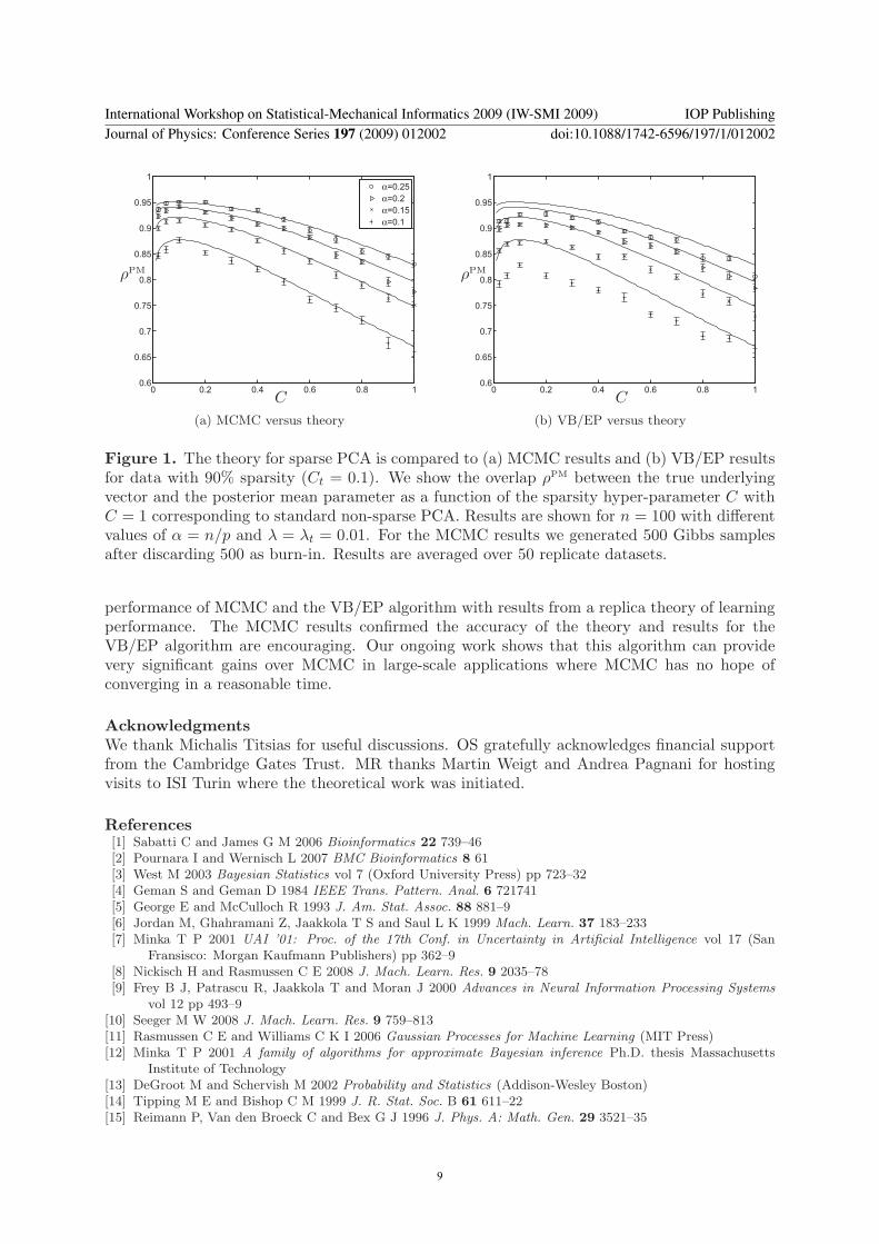
4. Simulation resultsIn figure 1 we compare the replica theory with results from MCMC and the VB/EP algorithmapplied to simulated data. MCMC can be considered a gold standard given sufficientcomputation time and we see that the results agree closely with the theoretical performance. Asexpected, optimal performance is achieved when the sparsity of the model matches the sparsityin the data (C = Ct = 0.1). The results for VB/EP show lower accuracy but still demonstratethat sparse inference provides a significant benefit over non-sparse PCA (C = 1 is the non-sparseresult). Also, we observe that the optimal performance of VB/EP is obtained when the modeland data sparsity are matched. Similar results are obtained for the predictive likelihood.

5. ConclusionWe have presented a number of MCMC and deterministic inference algorithms for Bayesiansparse factor analysis, including a novel VB/EP hybrid algorithm. We compared the empirical


8

0 0.2 0.4 0.6 0.8 10.6

0.65

0.7

0.75

0.8

0.85

0.9

0.95

1α=0.25α=0.2α=0.15α=0.1

ρPM

C

(a) MCMC versus theory

0 0.2 0.4 0.6 0.8 10.6

0.65

0.7

0.75

0.8

0.85

0.9

0.95

1

ρPM

C

(b) VB/EP versus theory

Figure 1. The theory for sparse PCA is compared to (a) MCMC results and (b) VB/EP resultsfor data with 90% sparsity (Ct = 0.1). We show the overlap ρPM between the true underlyingvector and the posterior mean parameter as a function of the sparsity hyper-parameter C withC = 1 corresponding to standard non-sparse PCA. Results are shown for n = 100 with differentvalues of α = n/p and λ = λt = 0.01. For the MCMC results we generated 500 Gibbs samplesafter discarding 500 as burn-in. Results are averaged over 50 replicate datasets.

performance of MCMC and the VB/EP algorithm with results from a replica theory of learningperformance. The MCMC results confirmed the accuracy of the theory and results for theVB/EP algorithm are encouraging. Our ongoing work shows that this algorithm can providevery significant gains over MCMC in large-scale applications where MCMC has no hope ofconverging in a reasonable time.

AcknowledgmentsWe thank Michalis Titsias for useful discussions. OS gratefully acknowledges financial supportfrom the Cambridge Gates Trust. MR thanks Martin Weigt and Andrea Pagnani for hostingvisits to ISI Turin where the theoretical work was initiated.

References[1] Sabatti C and James G M 2006 Bioinformatics 22 739–46[2] Pournara I and Wernisch L 2007 BMC Bioinformatics 8 61[3] West M 2003 Bayesian Statistics vol 7 (Oxford University Press) pp 723–32[4] Geman S and Geman D 1984 IEEE Trans. Pattern. Anal. 6 721741[5] George E and McCulloch R 1993 J. Am. Stat. Assoc. 88 881–9[6] Jordan M, Ghahramani Z, Jaakkola T S and Saul L K 1999 Mach. Learn. 37 183–233[7] Minka T P 2001 UAI ’01: Proc. of the 17th Conf. in Uncertainty in Artificial Intelligence vol 17 (San

Fransisco: Morgan Kaufmann Publishers) pp 362–9[8] Nickisch H and Rasmussen C E 2008 J. Mach. Learn. Res. 9 2035–78[9] Frey B J, Patrascu R, Jaakkola T and Moran J 2000 Advances in Neural Information Processing Systems

vol 12 pp 493–9[10] Seeger M W 2008 J. Mach. Learn. Res. 9 759–813[11] Rasmussen C E and Williams C K I 2006 Gaussian Processes for Machine Learning (MIT Press)[12] Minka T P 2001 A family of algorithms for approximate Bayesian inference Ph.D. thesis Massachusetts

Institute of Technology[13] DeGroot M and Schervish M 2002 Probability and Statistics (Addison-Wesley Boston)[14] Tipping M E and Bishop C M 1999 J. R. Stat. Soc. B 61 611–22[15] Reimann P, Van den Broeck C and Bex G J 1996 J. Phys. A: Math. Gen. 29 3521–35


9

[16] Kuhlmann P and Muller K R 1994 J. Phys. A: Math. Gen. 27 3759–74[17] Uda S and Kabashima Y 2005 J. Phys. Soc. Japan 74 2233–42[18] Engel A and Van den Broeck C 2001 Statistical Mechanics of Learning (Cambridge University Press)


10

Inference algorithms and learning theory for Bayesian sparse factor analysis

Documents