Inference algorithm for finite-dimensional spin glasses: Belief propagation on the dual lattice

arX

iv:1

102.

3305

v2 [

cond

-mat

.dis

-nn]

11

Apr

201

1

A very fast inference algorithm for finite-dimensional spin glasses: Belief

Propagation on the dual lattice.

Alejandro Lage-Castellanos, Roberto MuletDepartment of Theoretical Physics, Physics Faculty,

University of Havana, La Habana, CP 10400, Cuba.

Federico Ricci-TersenghiDipartimento di Fisica, INFN – Sezione di Roma 1 and CNR – IPCF, UOS di Roma,

Universita La Sapienza, P.le A. Moro 5, 00185 Roma, Italy

Tommaso RizzoDipartimento di Fisica, Universita La Sapienza, P.le A. Moro 5, 00185 Roma, Italy

(Dated: April 12, 2011)

Starting from a Cluster Variational Method, and inspired by the correctness of the param-agnetic Ansatz (at high temperatures in general, and at any temperature in the 2D Edwards-Anderson model) we propose a novel message passing algorithm — the Dual algorithm —to estimate the marginal probabilities of spin glasses on finite dimensional lattices. We showthat in a wide range of temperatures our algorithm compares very well with Monte Carlosimulations, with the Double Loop algorithm and with exact calculation of the ground stateof 2D systems with bimodal and Gaussian interactions. Moreover it is usually 100 timesfaster than other provably convergent methods, as the Double Loop algorithm.

2

I. INTRODUCTION

Inference problems are common to almost any scientific discipline. Often an inference problemcan be recast in that of computing some marginal probability on a small subset of variables, givena joint probability distribution over a large number N of variables, {s1, . . . , sN} ≡ σ. A typicalexample is the computation of the expectation value of a variable 〈si〉 ≡

∑sisi pi(si) where pi(si)

is the single-variable marginal probability defined as

pi(si) ≡∑

σ\si

P (σ) .

Clearly the computation of the sum in the r.h.s. is as difficult as the computation of the partitionfunction Z ≡∑σ P (σ), which is the main subject of statistical mechanics. In the general (and themost interesting) case, this problem can not be solved exactly in a time growing sub-exponentiallywith the size N . We are deemed to use some kind of approximation in order to compute marginalsin a time growing linearly in N . The approximation schemes used so far are mainly adopted fromthe field of statistical mechanics [1], where mean-field-like approximations are standard and wellcontrolled tools for approximating the free-energy, −βf = lnZ.

For non-disordered models, like the Ising ferromagnetic model, these approximations work quitewell and provide good results [2]. However, much less is known for models with disorder, and forthis reason we will focus on spin glasses in the present paper. In disordered models one usually dealswith an ensemble of problems (e.g. in spin glasses each sample has its own couplings, randomlychosen from a given distribution), and the results obtained by the statistical mechanics tools referto average quantities, i.e. those of the typical samples. In other words one is not concerned withthe behavior of a specific sample, but rather one looks at the whole ensemble. On the contrarywhen doing inference one is interested on the properties of a single specific problem and thus theabove approximation schemes (based on statistical mechanics mean-field approaches) need to beconverted into an algorithm that can be run on such a specific sample. Computing marginals on agiven sample clearly gives more information than computing averages over the ensemble.

To our knowledge, effective (i.e. linear time in N) algorithms for computing marginals can beessentially divided in two broad classes: stochastic local search algorithms, that roughly samplethe configurational space according to P (σ), and algorithms based on some kind of mean-fieldapproximation. The former are exact on the long run, but the latter can be much more useful if anapproximated answer is required in a short time. Unfortunately the latter also have some additionaldrawback due to the mean-field nature of the underlying approximation, e.g. the appearance ofspurious phase transitions, that may prevent the proper convergence of the algorithm.

One more reason why this latter class of algorithms has a limited scope of application is that theconvergence of the algorithm may strongly depend on the presence of short loops in the network ofvariables interactions. In this sense the successful application of one of these algorithms to modelsdefined on regular lattices (which have many short loops) would be a major achievement.

In this paper we introduce a fast algorithm for computing marginals in 2D and 3D spin glassmodels [3] defined by the Hamiltonian (further details are given below)

H(σ) = −∑

(i,j)

Jijsisj . (1)

The first non trivial mean-field approximation for the above model corresponds to the Bethe-Peierls approximation scheme and the Belief Propagation (BP) algorithm [4]. Unfortunately whenBP is run on a given spin glass sample defined on a D dimensional lattice, it seems to provideexactly the same output as if it were run on a random regular graph with fixed degree 2D: that

3

is, for T & TBethe it converges to a solution with all null local marginals (〈si〉 = 0), while forT . TBethe it does not converge to a fixed point.

The next step in the series of mean-field approximations (also known as Kikuchi approxima-tions or ‘cluster variation method’) is to consider joint probability distributions of the four spinsbelonging to the same plaquette [2, 5]. Under this approximation an algorithm has been derivedwhich is called Generalized Belief Propagation (GBP) [6]. To our knowledge, this algorithm hasbeen applied to 2D spin glasses, but only in presence of an external magnetic field, which is knownto improve the convergence properties of GBP. Our experience says that, running plain GBP ona generic sample of a 2D spin glass without external field, a fixed point is reached only for highenough temperatures, well above the interesting region. The lack of convergence of GBP (and othersimilar message-passing algorithms, MPA) is a well known problem, whose solution is in general farfrom being understood. For this reason, a new class of algorithms has been recently introduced [7],which provably converge to a fixed point: these algorithms use a double loop iterative procedure(to be compared to the single loop in GBP) and for this reason they are usually quite slow.

The algorithm we are going to introduce is as fast as BP (which is the fastest algorithm pre-senty available), and converges in a wider range of temperatures than BP. Moreover the marginalprobabilities provided by our algorithm are as accurate as those which can be obtained by DoubleLoop algorithms in a much larger running time.

Our algorithm works in the absence of external field, that is in the situation where MPA havemore problems in converging to a fixed point. In this sense it is a very important extension topresently available inference algorithms.

The rest of the work is organized as follows. First, in section II we derive the GBP equationsfor the 2D Edward Anderson model. Then, in section IIA we rewrite these equations in termsof fields, a notation that has a nicer physical interpretation and that we are going to use in therest of the work. Section III presents the novel algorithm, inspired by the paramagnetic Ansatzto the GBP equations. In section IV we show the results of running this algorithm on the 2DEdward-Anderson model. There we compare its performance with Monte Carlo simulations, withthe Double Loop algorithm and with exact calculation of the ground state of systems with bimodaland Gaussian interactions. Then, in section V we generalized our message passing equation togeneral dimensions and present some results for the 3D Edward-Anderson model. Finally, someconclusions are drawn in section VI.

II. GENERALIZED BELIEF PROPAGATION ON THE 2D EA MODEL

Here we present the GBP equations for the Edwards-Anderson (EA) model on a 2D squarelattice, and we refer the reader to [2, 6] for a more general introduction. In our case (as well as inmany other cases) GBP is equivalent to Kikuchi’s approximation, known as the Cluster VariationalMethod (CVM) [5]. We will try a presentation as physical as possible.

Consider the 2D EA model consisting of a set σ = {s1, . . . , sN} of N Ising spins si = ±1 locatedat the nodes of a 2D square lattice, interacting with a Hamiltonian

H(σ) = −∑

〈i,j〉

Jijsisj , (2)

where the sum runs over all couples of neighboring spins (first neighbors on the lattice). The Jijare the coupling constants between spins and are supposed to be fixed for any given instance ofthe model. If the interactions are not random variables, i.e. Jij = J , then the 2D ferromagnet isrecovered. We will focus on the two most common disorder distributions: bimodal interactions,P (J) = 1

2δ(J − 1) + 12δ(J + 1), and Gaussian interactions P (J) = exp(−J2/2)/

√2π.

4

The statistical mechanics of the EA model, at a given temperature T = 1/β, is given by theGibbs-Boltzmann distribution

P (σ) =e−βH(σ)

Z.

The direct computation of the partition function

Z =∑

σ

e−βH(σ)

or any marginal distribution p(si, sj) =∑

σ\si,sjP (σ) is a time consuming task, unattainable in

practice, since it involves the addition of 2N terms, and therefore an approximation is required1.The idea of the Region Graph Approximation to Free Energy [6] is to replace the real dis-

tribution P (σ) by a reduced set of its marginals. The hierarchy of approximations is given bythe size of such marginals, starting with the set of all single spins marginals pi(si) [mean-field],then following to all neighboring sites marginals pij(si, sj) [Bethe], then to all square plaquettesmarginals pijkl(si, sj, sk, sl), and so on. Since the only way of knowing such marginals exactly isthe unattainable computation of Z, the method pretends to approximate them by a set of beliefsbi(si), bij(si, sj), etc. obtained from the minimization of a region based free energy. In the RegionGraph Approximation to Free Energy, a set of regions, i.e. sets of variables and their interactions, isdefined, and a free energy is written in terms of the beliefs at each region. The Cluster VariationalMethod does a similar job, but instead of starting from an arbitrary choice of regions, it starts bydefining the set of largest regions, and smaller regions are defined recursively by the intersectionsof bigger regions. In this sense, CVM is a specific choice of region graph approximation to the freeenergy.

For the 2D EA model, we will consider the expansion of the free energy in terms of the marginalsat three levels of regions: single sites (or spins), links, and plaquettes. By plaquettes we mean thesquare basic cell of the 2D lattice. This choice of regions corresponds to the CVM having thesquare plaquettes as biggest regions. The free energy of the system is therefore written as

F =∑

R

cRFR ,

where R runs over all regions considered, and the free energy in a particular region depends on themarginals at that level bR(σR):

βFR =∑

σR

bR(σR)βER(σR) + bR(σR) log bR(σR) .

The symbol σR refers to the set of spins in region R, while ER is the energy contribution in that re-gion. The counting numbers cR (also Moebius coefficients) are needed to ensure that bigger regionsdo not over count the contribution in free energy of smaller regions, and follow the prescription

cR = 1−∑

R′⊃R

cR′ , (3)

where R′ is any region containing completely region R, as e.g. a plaquette containing a link or alink containing a site. In the case of the 2D lattice, the biggest regions are the square plaquettes,

1 The 2D case is special: indeed, thanks to the small genus topology, the partition function Z can be computed

efficiently. However we are interested in developing an algorithm for the general case, and we will not make use of

this peculiarity.

5

and therefore cplaq = 1, while the links regions have clink = 1 − 2cplaq = −1 (as each of them iscontained in 2 plaquettes regions), and finally the spins regions have csite = 1− 4cplaq − 4clink = 1(as each spin belongs to 4 links and 4 plaquettes). So the actual approximation for the EA modelon a 2D square lattice is

βF =∑

P

∑

σP

bP(σP) logbP(σP )

exp[−βEP(σP )]Plaquettes

−∑

L

∑

σL

bL(σL) logbL(σL)

exp[−βEL(σL)]Links (4)

+∑

i

∑

si

bi(si) logbi(si)

exp[−βEi(si)]Sites

where the sums run over all plaquettes, links and sites respectively. Please note that we are usingthe following notation for region indices: lower-case for sites, upper-case for links and upper-casecalligraphic for plaquettes. The energy term Ei(si) in the sites contribution is only relevant whenan external field acts over spins, and can be taken as zero in our case, since no external field isconsidered. Notice that whenever the interactions are included in more than one region (in ourcase are included in Link and Plaquette regions), the counting numbers guarantee that the exactthermodynamical energy U =

∑σ P (σ)H(σ) is obtained when the beliefs are the exact marginals

of the Boltzmann distribution. On the other hand, the entropy contribution is intrinsically ap-proximated, since the cutoff in the regions sizes imposes a certain kind of factorization of P (σ) interms of its marginals (see [2] for an explanation of the region graph approximation in terms ofcumulants expansions of the entropy).

The next step in the method, is to compute the beliefs from the minimization condition ofthe free energy. However, an unrestricted minimization will generally produce inconsistent solu-tions, since the beliefs (marginals) are not independent, as they are related by the marginalizationconditions

bi(si) =∑

σL\ibL(σL) =

∑sjbL(si, sj) ,

bL(σL) = bL(si, sj) =∑

σP\LbP(σP) =

∑sk,sl

bP(si, sj, sk, sl) ,(5)

where σL = {si, sj} and σP = {si, sj, sk, sl}. In order to minimize under the constraints in Eq. (5)and under the normalization condition for each belief, a set of Lagrange multipliers should beadded to the free energy in Eq. (4). There are different ways of choosing the Lagrange multipliers[6], and each of them will produce a different set of self consistency equations. We choose the socalled Parent to Child scheme (see section XX in [6]), in which constraints in Eq. (5) are imposedby two sets of Lagrange multipliers: µL→i(si) relating the belief at link L to that at site i, andνP→L(σL) relating the one at plaquette P to the one at link L.

With constraints (5) enforced by Lagrange multipliers, the free energy stationary conditions for

6

the beliefs are the following:

bi(si) =1

Ziexp

(−βEi(si)−

4∑

L⊃i

µL→i(si)

),

bL(σL) =1

ZLexp

−βEL(σL)−

2∑

P⊃L

νP→L(σL)−2∑

i⊂L

3∑

L′⊃iL′ 6=L

µL′→i(si)

, (6)

bP(σP ) =1

ZPexp

−βEP(σP )−

4∑

L⊂P

1∑

P ′⊃LP ′ 6=P

νP ′→L(σL)−4∑

i⊂P

2∑

L⊃iL 6⊂P

µL→i(si)

,

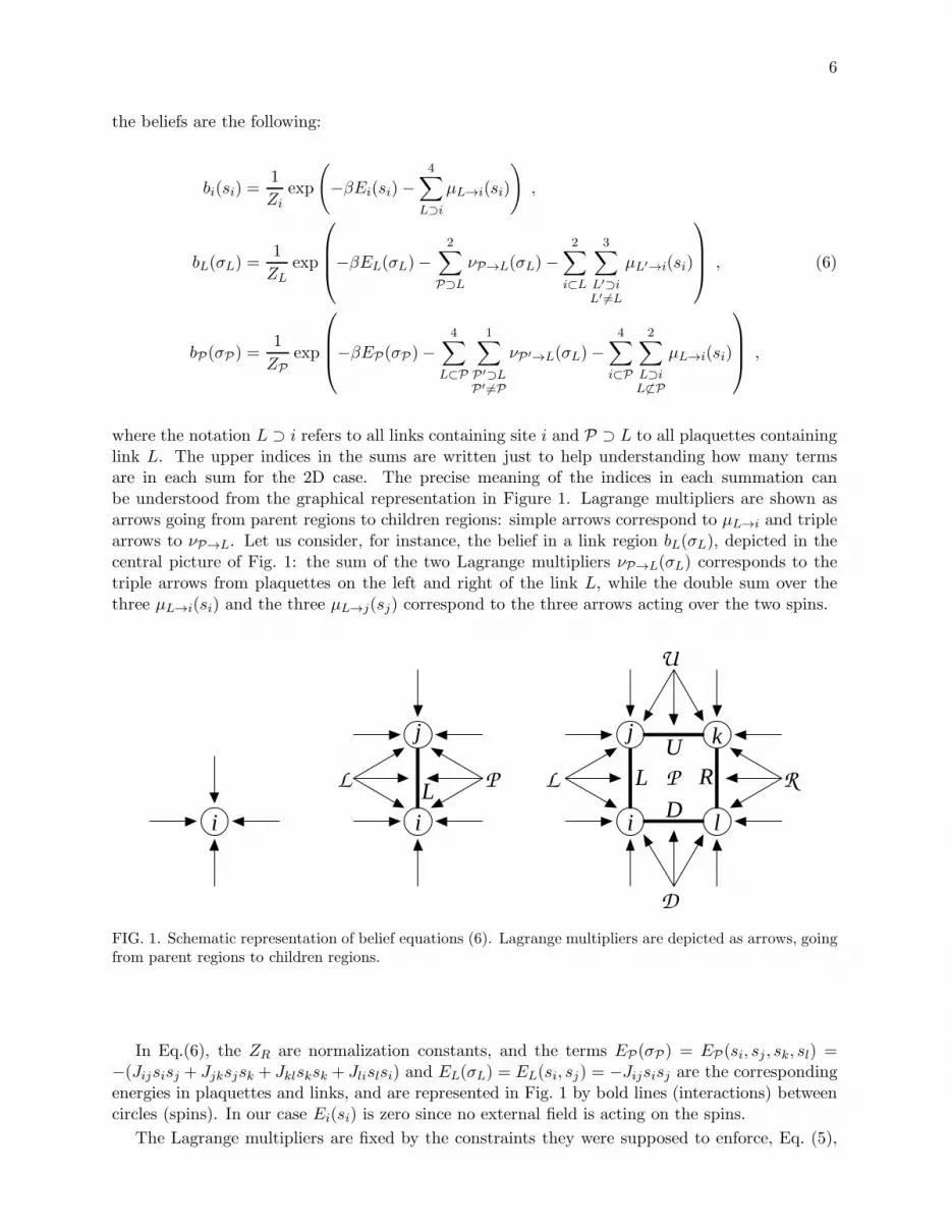
where the notation L ⊃ i refers to all links containing site i and P ⊃ L to all plaquettes containinglink L. The upper indices in the sums are written just to help understanding how many termsare in each sum for the 2D case. The precise meaning of the indices in each summation canbe understood from the graphical representation in Figure 1. Lagrange multipliers are shown asarrows going from parent regions to children regions: simple arrows correspond to µL→i and triplearrows to νP→L. Let us consider, for instance, the belief in a link region bL(σL), depicted in thecentral picture of Fig. 1: the sum of the two Lagrange multipliers νP→L(σL) corresponds to thetriple arrows from plaquettes on the left and right of the link L, while the double sum over thethree µL→i(si) and the three µL→j(sj) correspond to the three arrows acting over the two spins.

i

j

Li i

j

RU

D

L

k

l

L P L R

D

U

P

FIG. 1. Schematic representation of belief equations (6). Lagrange multipliers are depicted as arrows, goingfrom parent regions to children regions.

In Eq.(6), the ZR are normalization constants, and the terms EP(σP) = EP(si, sj , sk, sl) =−(Jijsisj + Jjksjsk + Jklsksk + Jlislsi) and EL(σL) = EL(si, sj) = −Jijsisj are the correspondingenergies in plaquettes and links, and are represented in Fig. 1 by bold lines (interactions) betweencircles (spins). In our case Ei(si) is zero since no external field is acting on the spins.

The Lagrange multipliers are fixed by the constraints they were supposed to enforce, Eq. (5),

7

and they must satisfy the following set of self-consistency equations:

exp[− µL→i(si)

]=∑

sj

exp

[− βEL\i(si, sj)−

2∑

P⊃L

νP→L(si, sj)−3∑

L′⊃j

L′ 6=L

µL′→j(sj)

]

exp[− νP→L(si, sj)− µD→i(si)− µU→j(sj)

]= (7)

∑

sk,sl

exp

[− βEP\L(si, sj , sk, sl)−

3∑

L′∈PL′ 6=L

1∑

P ′⊃L′

P ′ 6=P

νP ′→L′(σL′)−2∑

L′⊃kL′ 6⊂P

µL′→k(sk)−2∑

L′⊃lL′ 6⊂P

µL′→l(sl)

]

Again, to help understanding these equations, we provide in Fig. 2 their graphical representation.Note that there is one of these equations for every pair of Link-Site and every pair of Plaquette-Linkin the graph. With EP\L we refer to interactions in plaquette P that are not in link L.

i

L

ii

= = RU

D

k

l

j

L

j

i

LL

j

PPL P R

U

D

A U U E

B

D

G

C

F

FIG. 2. Message passing equations (7), shown schematically. Messages are depicted as arrows, going fromparent regions to children regions. On any link Jij , represented as bold lines between spins (circles), aBoltzmann factor eβJijsisj exists. Dark circles represent spins to be traced over. Messages from plaquettesto links νP→L(si, sj) are represented by a triple arrow, because they can be written in terms of threeparameters U , ui and uj, defining the correlation 〈sisj〉 and magnetizations 〈si〉 and 〈sj〉, respectively.

For each link L in the 2D lattice, there are two link-to-site multipliers, µL→i(si) and µL→j(sj).For each plaquette there are four plaquette-to-link multipliers νP→L(si, sj), corresponding to thefour links contained inside the plaquette. Let N be the number of spins in the lattice, there are 2Nlinks and N plaquettes. So the originally intractable problem of computing marginals, has beenreplaced by the problem of solving a set of 4N+4N coupled equations for the Lagrange multipliersas those in Eq. (7). Once these equations are solved, the approximation for the marginals isobtained from Eq. (6) for the beliefs, and all thermodynamic quantities are derived from them asin Eq. (4).

Minimizing a region graph approximation to free energy, as that in Eq. (4) with constraintsEq. (5), or equivalently solving the set of self-consistent equations in Eq. (7), is still a non trivialtask. Let us consider two ways of doing it. The first method is the “direct” minimization of theconstrained free energy, using a Double Loop algorithm [7]. This method is quite solid, since itguarantees convergence to an extremal point of the constrained free energy, but it may be very slowto converge. The second method, which is generally faster but is not guaranteed to converge, is thefamily of the so called Message-Passing algorithm (MPA), in which the Lagrange multipliers are

8

interpreted as messages νP→L(σL) going from plaquettes to links, and messages µL→i(si) from linksto sites. Self consistency equations (7) can be viewed as the update rules for the messages in theleft hand side, in terms of those in the right hand side. A random order updating of the messagesin the graph by Eq. (7) (message passing) can reach a fixed point solution, and therefore, to anextremal point of the constrained free energy [6]. Next, we show explicitly how the message-passingequations looks like in terms of fields.

A. From multipliers to fields

A particularly useful way of representing the multipliers (messages), with a nice physical inter-pretation, is the one used in [8], which we adopt here. In full generality [8, 9], these multiplierscan be written in terms of effective fields

µL→i(si) = β uL→i si (8)

νP→L(si, sj) = β (UP→L si sj + uP→i si + uP→j sj) (9)

In particular, the field u corresponds to the cavity field in the Bethe approximation [6]. UsingLagrange multipliers, messages or fields, is essentially equivalent. We will often refer to fieldsas u-messages to emphasize their role in a message-passing algorithm, and we will refer to self-consistency equations (7) as the message-passing equations.

This parametrization of the multipliers has proved useful to other endeavors, like the extensionof the replica theory to general region graph approximations [9]. Here, all the relevant informationin the Lagrange multipliers is translated to “effective fields” u and (U, ua, ub). Notice that inthis representation every single field u corresponds to an arrow in the schematic messages-passingequations in Figure 2. In particular, the messages going from plaquettes to links are characterizedby three fields (U, ua, ub), and the field U acts as an effective interaction term, that adds directlyto the energy terms in the Boltzmann factor. For instance, the first message-passing Eq. (7) is

exp[βuL→isi

]=∑

sj

exp

[β((uP→i + uL→i) si + (UP→L + UL→L + Jij) sisj+

(uP→j + uL→j + uA→j + uB→j + uU→j) sj

)](10)

where the indices refer to the notation used in Fig. 2 and Jij is the interaction coupling constantbetween spins si and sj. This equation naturally defines the updating rule for the message uL→i:

uL→i = u(uP→i + uL→i, UP→L + UL→L + Jij , uP→j + uL→j + uA→j + uB→j + uU→j) , (11)

where

u(u,U, h) ≡ u+1

2βlog

cosh β(U + h)

cosh β(U − h)

Note that the usual cavity equation for fields in the Bethe approximation [10] is recovered if allcontributions from plaquettes P and L are set to zero.

Working in a similar way for the second equation in (7) we end up with the updating rule forthe message (UP→L, uP→i, uP→j) sent from any given plaquette region P to one of its children

9

links L (see right picture in Fig. 2)

UP→L =1

4βlog

K(1, 1)K(−1,−1)K(1,−1)K(−1, 1)

uP→i = uD→i − uD→i +1

4βlog

K(1, 1)K(1,−1)K(−1, 1)K(−1,−1) (12)

uP→j = uU→j − uU→j +1

4βlog

K(1, 1)K(−1, 1)K(1,−1)K(−1,−1)

where

K(si, sj) =∑

sk,sl

exp

[β((UU→U + Jjk)sjsk + (UR→R + Jkl)sksl + (UD→D + Jli)slsi +

(uU→k + uC→k + uE→k + uR→k)sk + (uR→l + uF→l + uG→l + uD→l)sl

)]

Equations (11) and (12) are equivalent to equations in (7), once multipliers (messages) areparametrized in terms of fields. For instance, note that the µ multipliers in the left hand side ofsecond equation in (7) appear now subtracted in the right hand side of Eq. (12).

The field notation is more comprehensible and has a clear physical meaning. Each plaquetteP is telling its children links L that they should add an effective interaction term UP→L to thereal interaction Jij , due to the fact that spins si and sj are also interacting through the otherthree links in the plaquette P. Fields u act like magnetic fields upon spins, and the completeνP→L(si, sj)−message is characterized by the triplet (UP→L, uP→i, uP→j), and will be referred fromnow on as Uuu−message. Furthermore, it is clear that some fields enter directly in the message-passing equations like uP→i and uL→i in Eq. (11) and uD→i and uU→j in Eq. (12). Also note thatsince our model has no external field, the fields u break the symmetry of the original Hamiltonianwhenever they are non zero. For instance, in the ferromagnetic model, when all Jij = J , thesefields are zero at high temperature and become non zero at Kikuchi’s critical temperature T = 1.42[5], implying a spontaneous magnetization in the ferromagnet.

III. THE DUAL APPROXIMATION FOR THE PARAMAGNETIC PHASE

Unfortunately, the iterative message-passing algorithm for solving the GBP equations (11) and(12) often does not converge on finite dimensional lattices. While this is expected if long rangecorrelations are present, it is rather disappointing that it happens also in the paramagnetic phase,where one would like to find easily the solution to the model. Here we are going to focus only on theparamagnetic phase, and propose an improved solving algorithm based on physical assumptions.

In the paramagnetic phase of any spin model defined by the Hamiltonian in Eq. (2), that iswith no external field, variables have no polarization or magnetization: this in turn implies that inthe solution all u−fields must be zero, and only U−fields should be fixed self-consistently to nonzero values.

This paramagnetic solution has some interesting properties. First, it is always a solution ofthe GBP equations, since Eq. (11) and Eq. (12) are self-consistent with all u = 0. This meansthat starting from unbiased messages (all u = 0) the iterative GBP algorithm keeps this property.Second, the paramagnetic Ansatz is correct, from the GBP perspective, at least at high enoughtemperatures, meaning that even if we start with biased messages (u 6= 0), the iterative algorithmconverges to all u = 0 at high temperatures. And last, but not least, the well studied physicalbehavior for the 2D EA model with zero-mean random interactions Jij , is expected to remain

10

always paramagnetic, i.e. to have no transition to a spin glass phase at any finite temperature [11].Therefore, the Ansatz u = 0 is both physically plausible and algorithmically desirable.

i

RU

D

k

l

j

L P R

U

D

j

i

L P =

FIG. 3. Message passing of correlation messages in the dual approximation. In the right hand side the traceis taken over the black spins.

Under the paramagnetic Ansatz, which we shall also call Dual approximation for a reason to beexplained soon, the message-passing equation (11) is irrelevant, as it is always satisfied given thatu(0, U, 0) = 0, while Eq. (12) now turns into (see Fig. 3)

UP→L = U(UU→U , UR→R, UD→D) =

1

βarctanh

[tanh β(UU→U + Jjk) tanh β(UR→R + Jkl) tanh β(UD→D + Jli)

]. (13)

The only relevant messages now are those associated to the multipliers νP→L(si, sj) = βUP→L si sj,and they will be refereed to as U−messages. Eq. (13) can be interpreted as a correlation message-passing equation, giving the new interaction field U that a certain link shall experience as aconsequence of the correlations transmitted around the plaquette. The belief Eq. (6) also simplify.Obviously b(si) = 0.5 for every spin in the graph, and the link and plaquette beliefs are

bL(si, sj) =1

ZLeβ(UL→L+UP→L+Jij)sisj , (14)

bP(si, sj, sk, sl) =1

ZPeβ(UL→L+Jij)sisj+β(UU→U+Jjk)sjsk+β(UR→R+Jkl)sksl+β(UD→D+Jli)slsi .

The Dual algorithm we are proposing to study the paramagnetic phase of the EA model, is astandard message passing algorithm for the U -messages, which works as follows.

1: Start with all U -messages null2: repeat

3: Choose randomly one plaquette P and one of its children links L4: Update the field UP→L according to Eq. (13) as in Fig. 35: until The last change for any U -message is less than ǫ (we use typically ǫ = 10−10)6: return The beliefs bL(si, sj) defined in Eq. (14) for every pair of neighboring spins

Some damping factor γ ∈ [0, 1) can be added in the update step UP→L = γUP→L + (1 − γ)U inorder to help convergence.

11

A. Mapping to the dual model

It is worth noticing that Eq. (13) is nothing but the BP equation for the corresponding dualmodel (hence the name of the algorithm).

The dual model has a binary variable xij ≡ sisj on every link of the original model, and theoriginal coupling constants play now the role of an external polarizing (eventually random) field

Hdual(~x) = −∑

〈i,j〉

Jijxij .

This Hamiltonian looks like the sum of independent variables, but this is not the case. The dualvariables xij = ±1 must satisfy a constraint for each cycle (or closed path) in the original graph,enforcing that their product along the cycle must be equal to 1. On a regular lattice any closedpath can be expressed in terms of elementary cycles of 4 links (the plaquettes) and so it is enoughto enforce the constraint on every plaquette: xijxjkxklxli = 1. The Gibbs-Boltzmann probabilitydistribution for the dual model is then given by

P (~x) =1

Ze−βHdual(~x)

∏

〈i,j,k,l〉

δxijxjkxklxli, 1 , (15)

where the product runs over all elementary plaquette.The model described by the probability measure in Eq. (15) can be viewed as a constraint

satisfaction problem with a non uniform prior (given by e−βHdual(~x)). It is straightforward to derivethe BP equations for such a problem. Indeed by defining the marginal for the variable xij on link Lin the presence of the solely neighboring plaquette P as

(1+xij tanh βUP→L

)/2 ∝ exp(βUP→Lxij

),

the BP equations read

1

2

(1 + xij tanh βUP→L

)∝

∑

xjk ,xkl,xli

eβUU→UxjkeβJjkxjkeβUR→RxkleβJklxkleβUD→DxlieβJlixliδxjkxklxli, xij∝

∑

xjk ,xkl,xli:

xjkxklxli=xij

(1+ xjk tanh β(UU→U + Jjk)

)(1+ xkl tanh β(UR→R + Jkl)

)(1+ xli tanh β(UD→D + Jli)

)=

1 + xij tanh β(UU→U + Jjk) tanh β(UR→R + Jkl) tanh β(UD→D + Jli) . (16)

In the second summation the terms containing one or two x variables sums to zero, while the othertwo terms are those written in the last expression. Equating the first and the last expressions, thisequation is manifestly equal to Eq. (13).

B. Average Case Solution

GBP in general, and the Dual approximation in particular, are methods for the study of thethermodynamical properties of a given problem. However, in the limit of large systems (N →∞,thermodynamical limit), we expect a typical behavior to arise. This is the so called self-averaging

property of disordered systems. By typical we mean that almost every realization of the interactionsJij will result in a system whose thermodynamical properties (free energy, energy, entropy) are veryclose to the average value.

Normally, in disordered systems, we cope with the N → ∞ limit and with the average overthe random Jij by the replica method. The application of the replica trick to regions graph

12

approximations is a challenging task [9]. However, we can still grasp the average case behaviorwith a cavity average case solution of the dual message-passing equations, at the price of neglectingthe local structure of the graph (beyond plaquettes).

The idea is to represent the set of U -messages flowing in any given graph, by a population ofmessages Q(U). Then the message-passing Eq. (13) is used to obtain such population in a self-consistent way. More precisely, in every iteration three messages U1, U2, U3 are randomly drawnfrom the population Q(U) and a new message U0 = U(U1, U2, U3) is computed by Eq. (13) usingthree couplings randomly selected from P (J). The obtained message U0 is put back into thepopulation, and the iteration is repeated many times, until the population stabilizes.

Once we have the self consistent population of messages, we can compute the average energy

EAve = 〈−Jij tanh β (Jij + U1 + U2)〉Q(U1),Q(U2),P (Jij) (17)

by a random sampling of the population and of the interactions. The average case solution issupposed to be very good whenever the network of interactions has no or few short loops. This isnot the case in any finite dimensional lattice, since there the short loops (plaquettes) are abundant.Nonetheless, the average case solution gives a reasonably good approximation to the single instanceresults in 2D and 3D, as shown in the next Section.

IV. RESULTS ON 2D EA MODEL

Message-passing algorithms work fine in the high temperature regime (T > Tc) of models de-fined on random topologies: this is the reason why these methods have been successfully appliedin random constraint satisfaction problems, like random-SAT or random-Coloring [12, 13]. How-ever, when used on regular finite-dimensional lattices, they can experience difficulties even in theparamagnetic phase, because the presence of short loops spoils message-passing convergence.

It is well known that on a random graph of fixed degree (connectivity) c = 4 the cavity approx-imation gives a paramagnetic result above TBethe ≃ 1.52 (i.e. βBethe ≃ 0.66) with all cavity fieldsui = 0. Below the Bethe critical temperature, this solution becomes unstable to perturbations,and we expect many solutions to appear with non trivial messages ui 6= 0. The presence of manysolutions in the messages passing equations is connected to the existence of many thermodynami-cal states in the Gibbs-Boltzmann measure, or, equivalently, to the presence of replica symmetrybreaking. The appearance of such a spin glass phase is also responsible for the lack of convergenceof message-passing equations, since the intrinsic locality of the message-passing equations fails tocoordinate distant regions of the graph (which are now long-range correlated). As a consequence,the application of BP to the 2D EA model (that also has fixed degree c = 4) still finds the paramag-netic phase at high temperatures, but below TBethe, the Bethe instability takes the message-passingiteration away from the u = 0 solution and does not allow the messages to convergence to a fixedpoint (i.e. the algorithm wanders forever). In Figure 4 we show the convergence probability forthe BP message-passing equations in the 2D EA model.

On the other hand, a straightforward GBP Parent-to-Child implementation does not fully over-come this problem. At high temperatures, the Parent-to-Child equations converge to a param-agnetic solution with all u = 0 and non trivial U 6= 0, which turns out to be the same solutionfound by our Dual algorithm. When going down in temperature, the convergence properties of thealgorithm worsen, and are sensitive to tricks like damping and bounding in the fields. A thoroughdiscussion of these properties is left for a future work, but let us summarize that typically thealgorithm stop converging at low temperatures, somewhere below TBethe, as shown in Figure 4.

So, in general, BP and GBP equations are not simple to use in finite dimensional systemsat low enough temperatures: this warning was already reported in Refs. [2, 7, 14]. Indeed a

13

0

0.2

0.4

0.6

0.8

1

0 0.5 1 1.5 2 2.5

Pro

b co

nver

genc

e

β

βBethe = 0.66

GBP 32 x 32GBP 128 x 128

BP 32 x 32BP 128 x 128

FIG. 4. Convergence probability of BP (Bethe approximation) and GBP on a 2D square lattice, as a functionof inverse temperature. Data points are averages over 100 systems with random bimodal interactions. Systemsizes areN = L2 with L = 32, 128 and a damping factor γ = 0.5 has been used in the iteration of the message-passing equations. The Bethe spin glass transition is expected to occur at βBethe ≃ 0.66 (TBethe ≃ 1.52) fora random graph with the same connectivity as the 2D square lattice. Notably, that temperature also marksthe convergence threshold for BP equations in the 2D square lattice. GBP, on the contrary, reaches lowertemperatures, but eventually stop converging.

different method for extremizing the constrained free energy named Double Loop algorithm [7,15] was developed to overcome such difficulties. As mentioned earlier, Double Loop guaranteesconvergence of the beliefs, on any topology, with or without short loops. Given the convergenceproblems in GBP, researchers typically resort to Double Loop algorithms to extremize region graphapproximations to the free energy, below the Bethe critical temperature.

In order to make a fair comparison with our Dual algorithm, we have used an optimized codefor GBP and Double Loop algorithms: the open source LibDai library written in C++ [16].

The first interesting result of our work is that our Dual algorithm converges at all temperatures,just as Double Loop does. The reason why it converges is that there are no u-messages, so theBethe instability will not affect our message-passing iteration.

The second relevant result of our Dual algorithm, is the fact that it finds the same solutionfound by the Double Loop algorithm at all temperatures. In other words, the direct extremizationof the region graph approximation to free energy Eq. (4) via a Double Loop algorithm finds a

paramagnetic solution characterized by the beliefs bi(si) = 0.5 and bL(si, sj) =1ze−βJijsisj ; and the

effective interactions Jij found by the Double Loop algorithm are exactly equal to those found withour Dual algorithm, Jij = Jij +UP→L +UL→L. This means that beliefs and correlations found bythe two algorithms are identical: 〈sisj〉Double Loop = 〈sisj〉Dual.

The third result is that the running times of our Dual algorithm are nearly four orders ofmagnitude smaller than those required by the Double Loop implementation in libdai, at least ina wide range of temperatures (see figure 5). More precisely, the convergence time of the Dualalgorithm growth exponentially with β = 1/T , but still, in the relevant range of temperatures

14

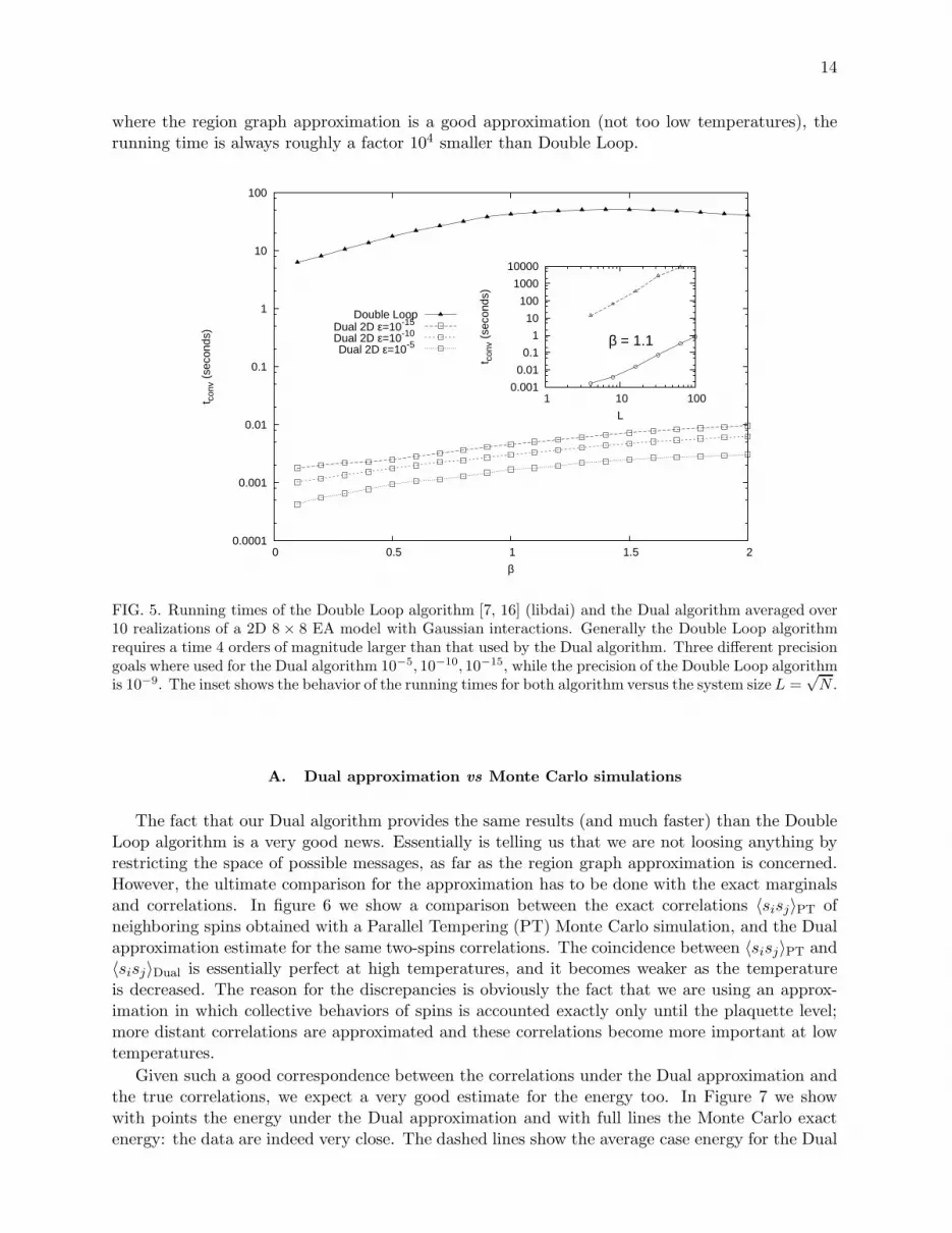
where the region graph approximation is a good approximation (not too low temperatures), therunning time is always roughly a factor 104 smaller than Double Loop.

0.0001

0.001

0.01

0.1

1

10

100

0 0.5 1 1.5 2

t con

v (s

econ

ds)

β

Double LoopDual 2D ε=10-15 Dual 2D ε=10-10 Dual 2D ε=10-5

0.001

0.01

0.1

1

10

100

1000

10000

1 10 100

t con

v (s

econ

ds)

L

β = 1.1

FIG. 5. Running times of the Double Loop algorithm [7, 16] (libdai) and the Dual algorithm averaged over10 realizations of a 2D 8 × 8 EA model with Gaussian interactions. Generally the Double Loop algorithmrequires a time 4 orders of magnitude larger than that used by the Dual algorithm. Three different precisiongoals where used for the Dual algorithm 10−5, 10−10, 10−15, while the precision of the Double Loop algorithmis 10−9. The inset shows the behavior of the running times for both algorithm versus the system size L =

√N .

A. Dual approximation vs Monte Carlo simulations

The fact that our Dual algorithm provides the same results (and much faster) than the DoubleLoop algorithm is a very good news. Essentially is telling us that we are not loosing anything byrestricting the space of possible messages, as far as the region graph approximation is concerned.However, the ultimate comparison for the approximation has to be done with the exact marginalsand correlations. In figure 6 we show a comparison between the exact correlations 〈sisj〉PT ofneighboring spins obtained with a Parallel Tempering (PT) Monte Carlo simulation, and the Dualapproximation estimate for the same two-spins correlations. The coincidence between 〈sisj〉PT and〈sisj〉Dual is essentially perfect at high temperatures, and it becomes weaker as the temperatureis decreased. The reason for the discrepancies is obviously the fact that we are using an approx-imation in which collective behaviors of spins is accounted exactly only until the plaquette level;more distant correlations are approximated and these correlations become more important at lowtemperatures.

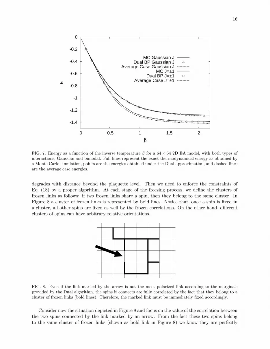
Given such a good correspondence between the correlations under the Dual approximation andthe true correlations, we expect a very good estimate for the energy too. In Figure 7 we showwith points the energy under the Dual approximation and with full lines the Monte Carlo exactenergy: the data are indeed very close. The dashed lines show the average case energy for the Dual

15

-1

-0.5

0

0.5

1

<S

i Sj>

PT

β = 0.1

ρ = 0.997

β = 0.5

ρ = 0.9998

-1

-0.5

0

0.5

1

-1 -0.5 0 0.5 1

<S

i Sj>

PT

<Si Sj>Dual

β = 1.1

ρ = 0.998

-1 -0.5 0 0.5 1 <Si Sj>Dual

β = 1.9

ρ = 0.988

FIG. 6. Comparison between the correlations 〈sisj〉Dual obtained by the Dual algorithm and the nearlyexact correlations obtained by a Parallel Tempering simulation. We used a 64×64 EA model with Gaussianinteractions. At each temperature the data correlation coefficient ρ is reported.

approximation, Eq. (17). In spite of the fact that the average case does not take into account thelocal structure of the lattice, the average case energy is quite close to the single instance one.

B. Ground State Configuration in 2D

The good agreement between the correlations found by the Dual algorithm, and those found ina Monte Carlo simulation, for the 2D EA model, compels us to push this correspondence down toT = 0. More precisely, using the correlations obtained by our Dual algorithm at low temperatures,we try to compute a ground state configuration by the following procedure. The idea is to freezeiteratively the relative position sisj of those interacting spins that are more strongly correlated,which is done by setting Jij → ±∞, and re-running the Dual algorithm until convergence everytime one pair of spins is frozen. Note that freezing the relative position of spins is equivalent tofreeze the dual variable xij = sisj . The freezing procedure is very simple, but for the fact one hasto check that frozen links must be consistent with a spin configuration. More precisely, frozen xijvariables must satisfy the requirement that on any closed loops the product is one,

closed loop∏

ij

xij = 1 . (18)

For very short loops the satisfaction of this condition is automatically induced by the Dual al-gorithm: for example if three links on a plaquette freeze, the fourth link is immediately frozento a value satisfy condition in Eq. (18). However, for longer loops (as the one shown in Fig. 8),the propagation of these constraints by the Dual algorithm is not perfect, since the information

16

-1.4

-1.2

-1

-0.8

-0.6

-0.4

-0.2

0

0 0.5 1 1.5 2

E

β

MC Gaussian JDual BP Gaussian J

Average Case Gaussian JMC J=±1

Dual BP J=±1Average Case J=±1

FIG. 7. Energy as a function of the inverse temperature β for a 64 × 64 2D EA model, with both types ofinteractions, Gaussian and bimodal. Full lines represent the exact thermodynamical energy as obtained bya Monte Carlo simulation, points are the energies obtained under the Dual approximation, and dashed linesare the average case energies.

degrades with distance beyond the plaquette level. Then we need to enforce the constraints ofEq. (18) by a proper algorithm. At each stage of the freezing process, we define the clusters offrozen links as follows: if two frozen links share a spin, then they belong to the same cluster. InFigure 8 a cluster of frozen links is represented by bold lines. Notice that, once a spin is fixed ina cluster, all other spins are fixed as well by the frozen correlations. On the other hand, differentclusters of spins can have arbitrary relative orientations.

FIG. 8. Even if the link marked by the arrow is not the most polarized link according to the marginalsprovided by the Dual algorithm, the spins it connects are fully correlated by the fact that they belong to acluster of frozen links (bold lines). Therefore, the marked link must be immediately fixed accordingly.

Consider now the situation depicted in Figure 8 and focus on the value of the correlation betweenthe two spins connected by the link marked by an arrow. From the fact these two spins belongto the same cluster of frozen links (shown as bold link in Figure 8) we know they are perfectly

17

correlated, however by running the Dual algorithm we could get a weak value for this correlationand then proceed by freezing a different link. A set of sub-optimal choices of this kind may finallyproduce a configuration of frozen links where the constraints in Eq. (18) are not all satisfied. Inorder to avoid these constraint violations we force any link whose spins are already part of thesame cluster to be polarized accordingly. The freezing algorithm, therefore, works as follows.

1: repeat

2: run the Dual algorithm until convergence (at a low enough temperature)3: find the link L with largest finite JL = JL + UP→L + UL→L

4: freeze that link by setting JL ← Sign(JL)∞5: if link L is connected to clusters C and C′ of frozen links then6: merge clusters C, C′ and link L in a unique cluster7: else

8: if link L is connected to a single cluster C of frozen links then9: add link L to cluster C

10: else

11: create a new cluster with link L12: end if

13: end if

14: for all non-frozen links L′ at the boundaries of a cluster of frozen links do15: if link L′ shares both spins with the same cluster then16: freeze link L′ accordingly {To avoid violations of constraint}17: end if

18: end for

19: until all links are frozen20: return the spins configuration obtained by setting one spin and fixing the rest according to

frozen links

The results obtained with this freezing procedure are quite good. In figure 9 we compare theresulting ground state energies with the exact solutions obtained using a web service running anexact solving algorithm [17]. We used an ensemble of 100 EA models on the 2D square latticewith Gaussian interactions (so the ground state is not degenerate) and with bimodal interactions.Most points are along the bisecting line, meaning that the ground state found by either methodsare the same. The relative error for the ground state energy is 0.0013 for Gaussian systems, and0.00078 for bimodal systems. Looking at how many links are frustrated in one of the solutions andunfrustrated in the other, we found that the Dual+Freezing algorithm returns 94.3% of the correctlink correlation signs with respect to the true ground state solution for the Gaussian models. Forthe bimodal system, given the degeneracy of the ground state configuration, it is more probableto find the actual ground state energy but for the same reason the link overlap between the exactGround State and the one found with Dual+Freezing is significantly lower (86.0%).

In general we believe these results on the ground states to be very encouraging, consideringthat the Dual algorithm is very fast and not restricted to the 2D case (at variance to fast exactalgorithms for computing ground states). They provide evidence that the marginals obtained bythis Dual algorithm are reliable even at very low temperatures.

V. GENERALIZATION TO OTHER DIMENSIONS

Let us now consider the region graph based approximation to the free energy for a genericD-dimensional (hyper-)cubic lattice, using the same hierarchy of regions: square plaquettes, linksand spins. After computing the counting numbers for a general D-dimensional lattice, see Eq. (3),

18

-1.52

-1.5

-1.48

-1.46

-1.44

-1.42

-1.4

-1.38

-1.36

-1.34

-1.32

-1.4 -1.38 -1.36 -1.34 -1.32 -1.3 -1.28 -1.26 -1.24-1.38

-1.36

-1.34

-1.32

-1.3

-1.28

-1.26

-1.24

-1.22-1.48 -1.46 -1.44 -1.42 -1.4 -1.38 -1.36 -1.34 -1.32 -1.3 -1.28

ED

ual (

+/-

J)

ED

ual (

Gau

ssia

n)

EGS (Gaussian)

EGS (+/-J)

EDual = EGS 93%

Link Overlap 86%

EDual = EGS 7%

Link Overlap 94%

f(x)=x(GS,Dual)

FIG. 9. Correlation of the Dual+Freezing ground state energy with the exact ground state energy inN = 16×16 systems. The top left points correspond to 100 bimodal systems Jij = ±1, while the right bottompoints correspond to 100 systems with Gaussian interactions. For bimodal interactions, the degeneracyof the ground state improves the probability of actually finding the correct ground state energy (93%),and conversely reduces the expected link correlation overlap with the exact ground state solution (86%).For Gaussian interactions, the ground state is not degenerated, and only in ∼ 7% of the samples theDual+Freezing method finds the actual ground state; however the average link overlap is very high (94%).The line f(x) = x is shown to guide the eye. Kindly note that two set of axes are being used.

the free energy approximation becomes

βF =∑

P

∑

σP

bP(σP ) logbP(σP)

exp(−βEP(σP))Plaquettes

−(2D − 3)∑

L

∑

σL

bL(σL) logbL(σL)

exp(−βEL(σL))Links (19)

+(2D2 − 4D + 1)∑

i

∑

si

bi(si) logbi(si)

exp(−βEi(si))Spins

Plaquettes are still the biggest regions considered at so have counting number 1, but now each linkis contained in 2(D − 1) plaquettes, and each spin is in 2D links and 2D(D − 1) plaquettes. Themessage passing equations for the Dual algorithm in D dimensions are then

UP→L =1

βarctanh

[tanh β

2(D−1)−1∑

i

UUi→U + JU

tanh β

2(D−1)−1∑

i

URi→R + JR

tanh β

2(D−1)−1∑

i

UDi→D + JD

], (20)

19

where Ui (resp. Ri and Di) are the 2(D− 1)− 1 plaquettes containing the link U (resp. R and D)excluding plaquette P.

In the high temperature phase, this Dual approximation with all u = 0 should be still a validapproach for any dimensionality D. At low temperatures, however, the EA model in more than twodimensions have a spin glass phase transition and, therefore, we expect the Dual approximation tobecome poorer, as it can not account for a non trivial order parameter.

By running the Dual algorithm for the 3D EA model we have found a divergence of U -fieldsaround β ≃ 0.39 for bimodal couplings and around β ≃ 0.41 for Gaussian couplings. This diver-gence is due to the fact the U -fields get too much self-reinforced under iteration. This divergencedoes not come as a surprise given that it happens also when studying the simpler pure ferromag-netic Ising model. However in the ferromagnetic model the temperature at which U -fields divergeis always below the critical temperature and so the Dual algorithm still provides a very gooddescription of the entire paramagnetic phase.

Unfortunately in the 3D EA the divergence of U -fields takes place well above the critical tem-perature (which is Tc ≃ 1.12 for bimodal coupling and at Tc ≃ 0.95 for Gaussian couplings, seeRef. 18 for a summary of critical temperatures in 3D spin glasses) and this would make the Dualalgorithm of very little use. We have studied the origin of this divergence and we have found ageneral principle for reducing the divergence of U -fields due to self-reinforcement, thus improvingthe convergence properties of the Dual algorithm. The idea is the following. When writing theDual approximation as a constraint satisfaction problem with a non uniform prior, see Eq. (15), theconstraints may be redundant. This is the case for the 3D cubic lattice: indeed both the numberof links (i.e. variables in the dual problem) and the number of plaquettes (i.e. constraints in thedual problem) are 3N . So, if constraints were independent, the entropy would be null at β = 0and negative for β > 0 (and this is clearly absurd). The solution to the apparent paradox is thatconstraints are not independent: actually only 2/3 of these are independent, and the remainingthird is uniquely fixed by the value of the former. In this way the correct entropy is recoveredat β = 0, given that a problem with 3N unbiased binary variables subject to 2N independentparity-check constraints has entropy N log(2). The dependence among constraints can be easilyappreciated by looking at the 6 plaquette around a cube: if 5 of the 6 constraints are satisfied,then the sixth one is automatically satisfied and redundant.

The general rule for improving the convergence of the Dual algorithm is to remove redundantconstraints (this principle is similar to the maxent-normal property of region based free energyapproximations [6]). Redundant constraints have no role in determining the fixed point values forthe beliefs (since they are redundant), but during the iterations they provide larger fluctuations tomessages and may be responsible for the lack of convergence. In practice, on a 3D cubic lattice, wemay remove redundant constraints in many different ways: the basic rule states that one constraint(i.e. a plaquette) should be removed for each elementary cube, otherwise if a cube remains with its 6plaquettes at least one redundant constraint will exist. We have used two different ways of removingone constraint per cube and we have found the same results in the entire paramagnetic phase. So,for simplicity, we are going to present data obtained by removing all constraints corresponding toplaquettes in the xy plane.

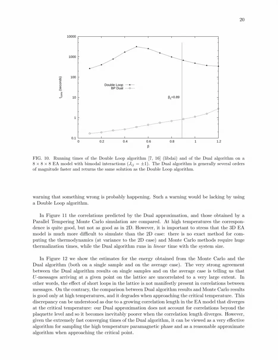
The Dual algorithm for the 3D EA model on the cubic lattice with no redundant constraintsconverges for any temperature above T ≃ 0.8 and so we can use it to study the entire paramagneticphase. The lack of convergence deep in the spin glass phase is to be expected. Just as in the 2Dcase, the Dual algorithm (when converges) still finds the same solution obtained by a Double Loopalgorithm, and again, it finds the solution nearly 100 times faster (see Fig. 10). Double Loop hasthe apparent advantage of converging at any temperature even at very low ones. However, deepin the spin glass phase, where the underlying paramagnetic approximation is clearly inaccurate,we believe that an algorithm (like the Dual one) that stops converging, is providing an important

20

0.1

1

10

100

1000

10000

0 0.2 0.4 0.6 0.8 1 1.2

t con

v (s

econ

ds)

β

βc=0.89

Double LoopBP Dual

FIG. 10. Running times of the Double Loop algorithm [7, 16] (libdai) and of the Dual algorithm on a8 × 8 × 8 EA model with bimodal interactions (Jij = ±1). The Dual algorithm is generally several ordersof magnitude faster and returns the same solution as the Double Loop algorithm.

warning that something wrong is probably happening. Such a warning would be lacking by usinga Double Loop algorithm.

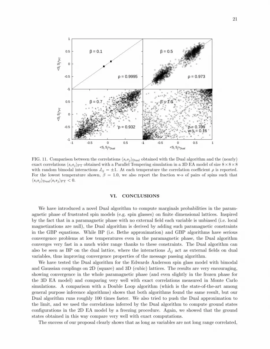
In Figure 11 the correlations predicted by the Dual approximation, and those obtained by aParallel Tempering Monte Carlo simulation are compared. At high temperatures the correspon-dence is quite good, but not as good as in 2D. However, it is important to stress that the 3D EAmodel is much more difficult to simulate than the 2D case: there is no exact method for com-puting the thermodynamics (at variance to the 2D case) and Monte Carlo methods require hugethermalization times, while the Dual algorithm runs in linear time with the system size.

In Figure 12 we show the estimates for the energy obtained from the Monte Carlo and theDual algorithm (both on a single sample and on the average case). The very strong agreementbetween the Dual algorithm results on single samples and on the average case is telling us thatU -messages arriving at a given point on the lattice are uncorrelated to a very large extent. Inother words, the effect of short loops in the lattice is not manifestly present in correlations betweenmessages. On the contrary, the comparison between Dual algorithm results and Monte Carlo resultsis good only at high temperatures, and it degrades when approaching the critical temperature. Thisdiscrepancy can be understood as due to a growing correlation length in the EA model that divergesat the critical temperature: our Dual approximation does not account for correlations beyond theplaquette level and so it becomes inevitably poorer when the correlation length diverges. However,given the extremely fast converging times of the Dual algorithm, it can be viewed as a very effectivealgorithm for sampling the high temperature paramagnetic phase and as a reasonable approximatealgorithm when approaching the critical point.

21

-1

-0.5

0

0.5

1

<S

i Sj>

PT

β = 0.1

ρ = 0.9995

β = 0.5

ρ = 0.973

-1

-0.5

0

0.5

1

-1 -0.5 0 0.5 1

<S

i Sj>

PT

<Si Sj>Dual

β = 0.7

ρ = 0.932

-1 -0.5 0 0.5 1 <Si Sj>Dual

β = 1.0

ρ = 0.799w-s = 0.16

FIG. 11. Comparison between the correlations 〈sisj〉Dual obtained with the Dual algorithm and the (nearly)exact correlations 〈sisj〉PT obtained with a Parallel Tempering simulation in a 3D EA model of size 8×8×8with random bimodal interactions Jij = ±1. At each temperature the correlation coefficient ρ is reported.For the lowest temperature shown, β = 1.0, we also report the fraction w-s of pairs of spins such that〈sisj〉Dual〈sisj〉PT < 0.

VI. CONCLUSIONS

We have introduced a novel Dual algorithm to compute marginals probabilities in the param-agnetic phase of frustrated spin models (e.g. spin glasses) on finite dimensional lattices. Inspiredby the fact that in a paramagnetic phase with no external field each variable is unbiased (i.e. localmagnetizations are null), the Dual algorithm is derived by adding such paramagnetic constraintsin the GBP equations. While BP (i.e. Bethe approximation) and GBP algorithms have seriousconvergence problems at low temperatures even in the paramagnetic phase, the Dual algorithmconverges very fast in a much wider range thanks to these constraints. The Dual algorithm canalso be seen as BP on the dual lattice, where the interactions Jij act as external fields on dualvariables, thus improving convergence properties of the message passing algorithm.

We have tested the Dual algorithm for the Edwards Anderson spin glass model with bimodaland Gaussian couplings on 2D (square) and 3D (cubic) lattices. The results are very encouraging,showing convergence in the whole paramagnetic phase (and even slightly in the frozen phase forthe 3D EA model) and comparing very well with exact correlations measured in Monte Carlosimulations. A comparison with a Double Loop algorithm (which is the state-of-the-art amonggeneral purpose inference algorithms) shows that both algorithms found the same result, but ourDual algorithm runs roughly 100 times faster. We also tried to push the Dual approximation tothe limit, and we used the correlations inferred by the Dual algorithm to compute ground statesconfigurations in the 2D EA model by a freezing procedure. Again, we showed that the groundstates obtained in this way compare very well with exact computations.

The success of our proposal clearly shows that as long as variables are not long range correlated,

22

-2

-1.5

-1

-0.5

0

0 0.2 0.4 0.6 0.8 1 1.2

E

β

J=±1 βc =0.89

Gauss J βc =1.05

MC Gaussian JDual BP Gaussian J

Average Case Gaussian JMC J=±1

Dual BP J=±1Average Case J=±1

FIG. 12. The energy predicted by the Dual approximation in 3D EA model, compared to the average caseenergy, and the Monte Carlo simulation. We used a 8×8×8 system with both types of random interactions,bimodal (Jij = ±1) and Gaussian distributed.

the computation of correlations in a generic spin model can be done in a very fast way by meansof message passing algorithms, based on mean-field like approximations. This kind of inferencealgorithms do not provide in general an exact answer (unless one uses it at very high temperaturesor on locally tree-like topologies), and so they can not be seen as substitutes for a Monte Carlo (MC)sampling. However there are many situations where a fast and approximate answer is required morethat a slow and exact answer. Let us just make a couple of examples of these situations. On theone side, if one need to sample from very noisy data, an approximated inference algorithm whoselevel of approximation is smaller than data uncertainty is as valid as a perfect MC sampler. Onthe other side, if one need to use the inferred correlations as input for a second algorithm (as forthe freezing algorithm in Section IVB) that will eventually modify/correct these correlations, afast and reasonably good inference is enough.

The promising results shown in the present work naturally ask for an improvement in severaldirections. For example, in the paramagnetic phase of a model defined on a 3D lattice, our inferencealgorithm could be improved by using the 2× 2× 2 cube as the elementary region, instead of theplaquette. An even more important improvement would be to extend the applicability range of thealgorithm to the low temperature phase: but this requires a rather non trivial modification, sincein low temperatures phase the assumption of zero local magnetizations needs to be broken.

ACKNOWLEDGMENTS

F. Ricci-Tersenghi acknowledges financial support by the Italian Research Minister throughthe FIRB project RBFR086NN1 on “Inference and optimization in complex systems: from the

23

thermodynamics of spin glasses to message passing algorithms”.

[1] M. Mezard and A. Montanari, Information, physics, and computation, Oxford University Press (2009).[2] A. Pelizzola, J. Phys. A 38, R309 (2005).[3] A.P. Young ed., Spin glasses and random fields, World Scientific (1998).[4] Y. Kabashima and D. Saad, Europhys. Lett. 44, 668 (1998).[5] R. Kikuchi, Phys. Rev. 81, 988 (1951).[6] J. Yedidia, W. T. Freeman, and Y. Weiss, IEEE Transactions on Information Theory 51, 2282 (2005).[7] T. Heskes, C. A. Albers, and H. J. Kappen, Proceedings of UAI-2003, 313 (2003).[8] Y. Kabashima, J. Phys. Soc. Jpn. 74, 2133 (2005).[9] T. Rizzo, A. Lage-Castellanos, R. Mulet, and F. Ricci-Tersenghi, J. Stat. Phys. 139, 375 (2010).

[10] M. Mezard and G. Parisi, Eur. Phys. J. B 20, 217 (2001); J. Stat. Phys. 111, 1 (2003). T. Castellani,F. Krzakala, and F. Ricci-Tersenghi, Eur. Phys. J. B 47, 99 (2005).

[11] T. Jorg, J. Lukic, E. Marinari, and O. Martin, Phys. Rev. Lett. 96, 237205 (2006).[12] M. Mezard and R. Zecchina, Phys. Rev. E 66, 056126 (2002). A. Montanari, F. Ricci-Tersenghi, and G.

Semerjian, J. Stat. Mech. P04004 (2008). F. Ricci-Tersenghi and G. Semerjian, J. Stat. Mech. P09001(2009).

[13] R. Mulet, A. Pagnani, M. Weigt, and R. Zecchina, Phys. Rev. Lett. 89, 268701 (2002). L. Zdeborovaand F. Krzakala, Phys. Rev. E 76, 031131 (2007).

[14] J. M. Mooij and H. J. Kappen, IEEE Transactions on Information Theory 53, 4422 (2007).[15] Y. S.-K. Eye and A. L. Yuille, Neural Computation 14, 2002 (2001).[16] J. M. Mooij, Journal of Machine Learning Research 11, 2169 (2010). http://www.libdai.org/[17] http://www.informatik.uni-koeln.de/ls juenger/research/sgs/index.html

[18] H. G. Katzgraber, M. Koerner, and A. P. Young, Phys. Rev. B 73, 224432 (2006).