Inequality comparisons when the populations differ in size

Inequality comparisons when the populations differ in size

An alternative to the population axiom

June 2007

Ronny Aboudi Department of Management Science

University of Miami P.O.B. 248237

Coral Gables, FL 33124, U.S.A. Tel: (305) 284 1966 Fax: (305) 284 2321 [email protected]

Dominique Thon Bodø Graduate School of Business

N-8049, Bodø, Norway Tel: (47) 75517029 Fax: (47) 75527268 [email protected]

Stein Wallace Molde University College

P.O. Box 2110, N-6402, Molde, Norway [email protected]

Abstract: We re-visit in detail the “population axiom” which was introduced by Dalton in 1920 and has since been a fixture of the literature on the measurement of income inequality. An alternative axiom is proposed, which provides a new way of looking at Lorenz dominance between two income distributions over populations that differ in size.

Key words: Majorization, income inequality, Lorenz dominance, population axiom. JEL classification: D31, D63, I31.

2

1 Introduction

The familiar “population axiom”, which is nearly universally postulated as a desirable

property for an inequality index, has been the object of very little discussion in the

literature since it was introduced by Dalton (1920, p. 357), who formulated it as

follows: “Inequality is unaffected if proportionate additions are made to the number

of persons receiving income of any given amount”. The axiom has never, it seems,

been the object of a detailed analysis. The purpose of this paper is to provide such an

analysis, which leads us to propose to the population axiom an alternative which is of

a quite different nature.

We consider in turn the constant-sum case, where a given total is divided between

either m or n persons, and the constant-mean case, where it is the mean income which

is common to an allocation to m persons and one to n persons. Obviously if m = n,

then assuming constant sum is equivalent to assuming constant mean. While the

constant-mean case is the canonical case in the literature on income inequality

comparisons, the constant-sum case has, as far as we know, never been discussed in a

situation where the populations differ in size. As will become clear, the constant-sum

case is in effect more basic than the constant-mean case because it provides a more

natural extension of the concept of majorization. Going from the constant-sum case

to the constant-mean case will turn out to be merely a matter of scaling.

In order to compare our variable population analysis with the constant population one,

and at the risk of belaboring the well-known, we first give a short account of the

mainstream principles of comparing two allocations of a given total income between

n persons, i.e. the constant population case. The idea that y is unambiguously more

equally distributed than x is usually expressed by the condition that x majorizes y.

Let ),...,,( )()2()1( xxxx n=↑ be an increasing re-arrangement of ℜ∈ nx .

Definition 1.1. Let ℜ∈ nyx, . Then we say that x majorizes y [written yx < ] if (1.1) ∑∑ ==

≤k

i ik

i i yx 1 )(1 )( ; k = 1, ..., n -1 and ∑∑ ===

n

i in

i i yx 11.

3

The idea that y is a more desirable distribution than x if yx < can be rationalized

first by interpreting the definition itself. It says that:

“the poorest person in y is richer than the poorest person in x; the two

(1.2) poorest persons in y are collectively richer than the two poorest

persons in x; etc.”,

which in itself suggests that y is a less unequal distribution than x (Lorenz (1905)).

A more illuminating characterization of < as an equality-favoring preorder is

obtained by considering a sequence of equalizing pair-wise transfers that could

construct y from x. The key result here is Muirhead’s Lemma (Muirhead (1903)).

Definition 1.2. A transfer of income between two persons is a Muirhead-Dalton-

transfer if, after the transfer is performed, the income of the recipient is not strictly

larger than the initial income of the donor.

Lemma 1.1 (Muirhead). Let ℜ∈ nyx, . Then yx < holds if and only if y can be

reached from x through a finite sequence of Muirhead-Dalton transfers.

We note for future reference the following result. Let TA represent the transpose of

the matrix A, and en = (1, 1, …, 1) nℜ∈ .

Theorem 1.2. Let ℜ∈ nyx, . Then yx < if and only if y = xB for some non-

negative matrix B satisfying:

(1.3) B Tne = T

ne

(1.4) ne B = ne .

A non-negative matrix satisfying (1.3), (1.4) is known as a bistochastic matrix. It is

well-known that the set of allocations y that are more equal than allocation x

according to < is the convex polytope whose extreme points are generated by

multiplying x by the extreme elements of the nn× bistochasic matrices, i.e. the

4

nn× permutation matrices, which number !n . Figures 1.1 and 1.2 illustrate for n = 2

and n = 3 the set of y’s that are such that yx < for some given x. Those results are

well-known (see Marshall and Olkin (1979)) and have been used in the study of

income inequality for decades (see for example Kolm(1969), Foster (1985), Lambert

(2001)). A function )(⋅F preserves the preorder <& if yx <& implies ≤)(xF )( yF .

A function that preserves < is known as a Schur concave function and when

comparing two income distributions over the same number of persons and the same

total income with some welfare function, one typically requires that such a function

be Schur concave.

Figure 1.1 and Figure 1.2 about here.

Consider now the standard problem of comparing the degree of inequality of two

distributions with different numbers of persons, where the mean income is the same in

both distributions (in which case, of course, the sum of incomes is not the same). The

central concept used in the literature is constant-mean second degree stochastic

dominance (a.k.a. Lorenz dominance). As regards the order-preserving functions of

this preorder, the tradition in economics is to require from such a function that it

should be Schur concave and that it should furthermore satisfy a “population axiom”

typically formulated as:

“ Inequality is unchanged if every income is replicated any number of times”.

The central result here is Theorem 2 of Dasgupta et al (1973) which essentially says

that “at constant mean, a welfare function preserves Lorenz dominance if this function

is Schur concave and satisfies the population axiom”.

Now, the equality-loving property of a function preserving constant-mean Lorenz

dominance over two populations of different sizes is not as straightforward to

paraphrase in economic terms as it is for a function preserving majorization. Let

ℜ∈ mx , ℜ∈ ny , x and y have the same mean and nm ≠ . A rewording of the

5

majorization preorder along the lines of (1.2) is clearly not available. Furthermore, it

is not possible to consider a sequence of pairwise equalizing transfers as in

Muirhead’s Lemma because of both the difference in population size and in total

income. There is though a well-known simple construction that allows one to bring

majorization and Muirhead’s Lemma into play: it is to construct two artificial

distributions by replicating the incomes in each distribution such a number of times

that one obtains two income vectors that have both the same population size and the

same total income. The simplest way to do this is to replicate n times every income

in x and m times every income in y, thereby obtaining two equal-sum nm×

vectors.

Definition 1.3. Let x ℜ∈ m , y ℜ∈ n , ∑∑ ===

n

i im

i i nymx11

// . Then •x , •y ℜ∈ ×nm are

== •×

•••• ),.....,,,( 321 nmxxxxx 43421n

xxx 111 ,...,( , 43421n

xxx 222 ,..., , ….. , 43421n

mmm xxx ,..., )

and == •

ו••• ),.....,,,( 321 nmyyyyy

43421m

yyy 111 ,...,( , 43421

m

yyy 222 ,..., , ….. , 43421

m

nnn yyy ,..., ).

It is immediate that ∑∑ ×

=•×

=• =

nm

i inm

i i yx11

. It is known that y Lorenz dominates x if

and only if <•x •y . Then (1.2) and/or Muirhead’s Lemma can be called upon to

show in what sense •x is more unequal than •y , and the population axiom is then

appealed to in order to pronounces x to be more unequal than y. We argue below

that this second step is not entirely convincing. The most explicit description of this

construction is found in Sen (1973, p. 60). See also Moyes (1999, p. 208).

This double cloning procedure is an ingenious way of being able to mobilize directly

Muirhead’s Lemma, yet it should be realized that it consists in appealing to the

existence of an artificial sequence of equalizing pair-wise transfers between non-

existing persons, as the “hypothetical countries”, in the words of Sen (1973), with

distributions •x and •y , are indeed hypothetical. This construction, even if it has

become familiar, is certainly not entirely satisfactory as a description of how a more

equal y can be constructed from x. The fact that •y can be reached from •x

6

through a sequence of equalizing transfers certainly does not provide such a

description. The original motivation for this paper was to find a way to formulate a

“path” result which is as close as possible to Muirhead’s Lemma (and becomes

Muirhead’s Lemma if n = m) without telling a tall tale of infeasible transfers between

non-existing persons. As a further result, we obtain also a description of the set of all

ℜ∈ ny which Lorenz dominate ℜ∈ mx in the same spirit as Figure 1.1 and Figure

1.2 do when n = m = 2 and n = m = 3, respectively. Furthermore, we formulate an

axiom which is a substitute to the population axiom in the axiomatization of the

welfare functions that preserve Lorenz dominance when the populations differ in size.

In our approach, the ubiquitous population axiom is completely dispensed with.

Sections 2 and 3 deal with the constant-sum case. Section 2 introduces a preorder

over vectors of any dimension, which is a generalization of majorization, in that it

becomes majorization if the vectors have the same dimension. Section 3 discusses the

properties of this preorder and of its preserving functions. Although our main interest

is the constant-sum case, in order to connect with the literature, we are led to consider

the constant-mean case. Section 4 shows that the constant-sum results of the previous

sections can easily be converted into results for the constant-mean case, and that the

latter are stochastic dominance results. Section 5 compares our results to the

treatment of inequality indices over populations of different sizes in the existing

literature and concludes.

7

2. A binary relation; the constant-sum case

Let øm = (0, 0, …, 0) mℜ∈ . Denote the nm× matrix with “1” in every position by

Emn , the nm× matrix with “0” in every position by Ømn , and the nn× identity

matrix by I n . Let LCM(m,n) be the least common multiple of the natural numbers

m, n. The following binary relation is a generalization of < ; compare to Theorem

1.2.

Definition 2.1. Let x ℜ∈ m , y ℜ∈ n . We say that yx nm⋅< if there exists a non-

negative nm× matrix R such that

(2.1) R Tne = T

me

(2.2) nm meRne =

(2.3) xRy = .

If one thinks of the problem of re-allocating a given total income from a population of

m persons to a population of n persons, then (2.1), “every row sum = 1”, expresses

that ∑∑ ===

n

i im

i i yx11

. We are thus dealing with the constant-sum case. The fact,

described by (2.2), “each column sum = m/n”, that mne maps into nme , expresses

that a perfectly equal allocation of income between the population of m persons

maps into a perfectly equal allocation in the population of n persons. If m = n, the

non-negative matrices satisfying (2.1), (2.2) are the bistochastic matrices and then

yx nm⋅< is equivalent to yx < , Definition 1.1, see Theorem 1.2. Given m and n,

call R nm ),( the set of non-negative nm× matrices satisfying (2.1) and (2.2); nm⋅< and

R nm ),( satisfy the following.

Lemma 2.1. A) yx nm⋅< is equivalent to kykx nm⋅< for all 0≠k . B) The set

R nm ),( is convex. C) If ∈1R R nm ),( and ∈2R R sn ),( , then ∈21RR R sm ),( . D) If

yx nm⋅< and zy sn⋅< , then zx sm⋅< .

8

For any given pair m, n, there exists a unique nm× matrix belonging to R nm ),( which

plays a very special role in what follows. It is presented in Definition 2.3 below,

which requires some preliminaries.

Definition 2.2. Let m and n be natural numbers. Let ),( nmr be a natural number

that is a multiple of both m and n. Let mnmrnmp /),(),( = , nnmrnmq /),(),( =

and define the ),( nmrm× matrix

=)),(,( nmrmA

⎟⎟⎟⎟⎟

⎠

⎞

⎜⎜⎜⎜⎜

⎝

⎛

),(),(

),(

),(),(),(

),(),(),(

......

.

nmpnmp

nmp

nmpnmpnmp

nmpnmpnmp

ee

ee

Ø

ØØ

ØØ

and the nnmr ×),( matrix

=)),,(( nnmrC

⎟⎟⎟⎟⎟

⎠

⎞

⎜⎜⎜⎜⎜

⎝

⎛

Tnmq

Tnmq

Tnmq

Tnmq

Tnmq

Tnmq

Tnmq

Tnmq

Tnmq

ee

ee

Ø

ØØ

ØØ

),(),(

),(

),(),(),(

),(),(),(

......

.

.

Example 2.1. With 4=m and 6=n , one can choose )6,4(r to be any multiple of 12. If one chooses )6,4(r = 12, then:

=)12,4(A⎟⎟⎟

⎠

⎞

⎜⎜⎜

⎝

⎛

111000000000000111000000000000111000000000000111

and =)6,12(C

⎟⎟⎟⎟⎟⎟⎟⎟⎟⎟⎟

⎠

⎞

⎜⎜⎜⎜⎜⎜⎜⎜⎜⎜⎜

⎝

⎛

100000100000010000010000001000001000000100000100000010000010000001000001

.

Two special choices of ),( nmr are: =),( nmr nm× and ),( nmr = LCM(m,n).

Lemma 2.2. Let m, n be natural numbers and R be an nm× matrix. Then,

),( nmRR∈ if and only if

(2.4) ),(),(1 nmnCBmnmAn

R ×××= ,

9

where B is an mnmn× bistochastic matrix.

Definition 2.3. Given m, n, define the following nm× matrix:

(2.5) ),(),(1),( nmnCmnmAn

nmH ××= .

Note that ),( nmH is a matrix such as in (2.4), with the bistochastic matrix B chosen

to be the mnmn× identity matrix. By Definition 2.3, given m, n, ),( nmH always

exists and is unique. Note that ),( nmH is invariant to the choice of ),( nmr . Note

also that ),( nnH = I n , corresponding to the case where nm = .

Theorem 2.1. For any pair m, n, the matrix ),( nmH in (2.5) has the following

properties: (a) ),(),( nmRnmH ∈ ; (b) ),( mnH = TnmHmn ),( .

We now present a main result. Let ↓x = ),...,,( ][]2[]1[ xxx n be a decreasing re-

arrangement of ℜ∈ nx .

Theorem 2.2. Let x ℜ∈ m , y ℜ∈ n . Then

yx nm⋅< if and only if ynmHx <),(×↓ .

Lemma 2.3. The n-vector ),( nmHx ×↓ is decreasingly ordered.

Theorem 2.2 leads to a characterization of the set of points y ℜ∈ n , which are such

that yx nm⋅< for some given ℜ∈ mx . For x ℜ∈ m , let )(xSnm⋅< be the set of all such

y’s (the “better-than-x set” according to nm⋅< ). Similarly, for x ℜ∈ n , let )(xS < be

the set of all y ℜ∈ n such that yx < (the “better-than-x set” according to < ). By

Theorem 2.2, )(xSynm⋅

∈ < and <Sy∈ )),(( nmHx ×↓ are equivalent.

10

Corollary 2.1. Let x ℜ∈ m . Then )(xSnm⋅< = <S )),(( nmHx ×↓ ℜ∈ n .

It is well-known that the extreme points of the set )(xS < are the vectors that are the

permutations of x and thus )(xSnm⋅< is the set of all the n-vectors that are a convex

combination of the permutations of ),( nmHx ×↓ . We illustrate with the only two

examples that can easily be represented graphically, namely m = 2, n = 3 and m = 3,

n = 2.

Example 2.1 Let 2=m and .3=n We have )3,2(H = ⎟⎠⎞

⎜⎝⎛

3231003132 . Consider

x = (3, 12). We have ↓x = (12, 3) and ),( nmHx ×↓ = (8, 5, 2). The permutations of

this vector give the n! = 6 extreme points of the set )(xSnm⋅< , illustrated on Figure

2.1.

Example 2.2. Let 3=m and .2=n We have )2,3(H = ⎟⎟⎟

⎠

⎞

⎜⎜⎜

⎝

⎛

102121

01. Consider

x = (1, 8, 4). We have ↓x = (8, 4, 1) and ),( nmHx ×↓ = (10, 3). The permutations

of this vector give the n! = 2 extreme points of the set )(xSnm⋅< , illustrated on Figure

2.2.

Figure 2.1 and Figure 2.2 about here.

In both figures, the arrow represents the construction of ),( nmHx ×↓ . The above

results make it clear that )(xSnm⋅< is the convex hull of the permutations of

),( nmHx ×↓ , which point is thus the keystone of the description of this set. Any

permutation of this vector provides the same description, and we call extremal m-to-n

redistribution the operation of obtaining from x any one of the extreme points of <S )),(( nmHx ×↓ . Once ),( nmHx ×↓ has been reached through an extremal m-to-n

redistribution, then any point y such that yx nm⋅< can be reached from there through

a sequence of Muirhead-Dalton transfers (Theorem 2.2 and Lemma 1.1),

11

remembering that the permutation of two elements of a vector constitutes an extreme

Muirhead-Dalton transfer.

It remains now to give a concrete description of the reallocation of income which

takes place when going from x ℜ∈ m to ),( nmHx ×↓ ℜ∈ n , in terms of the formal

definition of ),( nmH , Definition 2.3.

We illustrate with an example the meaning of the redistribution performed by the

extremal m-to-n redistribution ),( nmHxx ×⇒ ↓ . Let there be a pizza of size 50 that

m = 7 persons have divided between themselves according to =↓x (15, 10, 9, 7, 6, 2,

1) and let us now consider the redistribution to n = 3 persons. The matrix ),( nmH is:

(2.6) )3,7(H =

⎥⎥⎥⎥⎥⎥⎥

⎦

⎤

⎢⎢⎢⎢⎢⎢⎢

⎣

⎡

100100

3/13/2001003/23/1001001

Let the quota of each of the three recipients be m/n = 7/3 and then choose an arbitrary

order of the persons. Then let everyone of them in turn take some fraction of the

seven slices of pizza that have not yet been called for when his turn comes, such that

the sum of those fractions is 7/3. We assume everyone is greedy and will thus fill his

quota by taking the larger possible fraction of the largest slices still available. The

redistribution ),( nmHxx ×⇒ ↓ can be seen to correspond to the following

sequences of appropriations:

The first person in line will take 1/1 of the largest slice, 1/1 of the second

largest slice and 1/3 of the third largest slice, for a total of 7/3. This gives him in all

28 pizza units.

The second person will take what is left of the third largest slice (2/3), 1/1 of

the fourth largest slice and 2/3 of the fifth largest one, for a total of 7/3. This gives

him in all 17 pizza units.

The third person will be left with 1/3 of the fifth largest slice, and 1/1 of each

of the last two slices, again for a total of 7/3, and 5 pizza units.

12

This corresponds to )3,7(Hx ×↓ = (28, 17, 5). By letting the three persons make

their claims in all other orders produces all the vertices of )(xSnm⋅< . This, together

with Theorem 2.1 and Lemma 1.1 provides the following sequence of steps from

which y can be constructed from x if yx nm⋅< .

Proposition 2.1. Let x ℜ∈ m , y ℜ∈ n . If yx nm⋅< , then y can be obtained from x

through the following sequence of operations:

- perform on x an extremal m-to-n redistribution

- starting from the resulting n-vector, perform a sequence of

Muirhead-Dalton transfers.

If m = n, then Proposition 2.1 boils down to Muirhead’s Lemma, if one remembers

that then ),( nnH is an nn× unit matrix and that, thereby, the first step in Proposition

2.1 vanishes. In the pizza re-distribution example, an extremal n-to-n redistribution

means that each recipient in turn will simply pick up 100 % of the largest slice among

the ones that remain, performing thereby, together, the equivalent of a permutation.

We conclude this section by illustrating Proposition 2.1 using extreme initial

distributions. Suppose )0,0,0,0,0,0,1(=x , meaning that one of seven person gets

all the income. What distributions among three persons would be more egalitarian

according to 37⋅< ? Our results tell us that they are all the distributions majorized by

)3,7(Hx ×↓ = (1, 0, 0), see (2.6). Suppose now that )0,0,1(=x , meaning that one of

three person gets all the income. What distributions among seven persons would be

more egalitarian according to 73⋅< ? Our results tell us that they are all the

distributions majorized by )7,3(Hx ×↓ = )0,0,0,0,71,

73,

73( , using (2.6) and

Theorem 2.1 (b).

13

3. The properties of the preorder nm⋅< and its preserving functions

The properties we consider for a binary relation R are the following ones.

Reflexivity: xRx .

Transitivity: { xRy and yRz } implies xRz .

Antisymmetry: { xRy and yRx } implies x = y.

We say that a binary relation is a preorder if it is reflexive and transitive (it is a

partial order if it is also antisymmetric). Note that < , a particular case of nm⋅< , is a

preorder but not a partial order. The binary relation < is not antisymmetric as { xRy

and yRx } does not imply that x = y; it merely implies that the two vectors differ

only by a permutation. More precisely (Alberti and Uhlmann (1982, Lemma 1-10, p.

16)):

Lemma 3.1. Let nRyx ∈, . Then both yx < and xy < hold if and only if y is a

permutation of x

The binary relation nm⋅< is obviously reflexive. We know from Lemma 2.1 D) that is

transitive. As we now show, it is not antisymmetric and it is thus, like < , a preorder

and not a partial order. The way nm⋅< fails to be antisymmetric is of interest, as it

turns out to be related to the population axiom and is described in our next result,

Theorem 3.1, which generalizes Lemma 3.1. We first need the definition of two

vectors being scaled-p-proportionate, where “p” stands for “population”.

Definition 3.1. Let mRx∈ , nRy∈ . Then we say that },{ yx are scaled-p-

proportionate if x is a permutation of ),...,,(~21 qkqq eaeaeax = and y is a

permutation of ),...,,(~21 pkpp eaeaea

nmy = where ),( nmLCMr = ,

rmnk = ,

nrq = ,

mrp = and kaaa ,...,, 21 are constants.

14

Example 3.1. Let 3=m and 4=n . We have 12=r , 1=k , 3=q and .4=p

Thus, ),,(~111 aaax = and ),,,(

43~

1111 aaaay = .

Example 3.2. Let 4=m and 6=n . We have 12=r , 2=k , 2=q and .3=p

Thus, ),,,(~2211 aaaax = and ),,,,,(

64~

222111 aaaaaay = .

Example 3.3. Let 2=m and 8=n . We have 8=r , 2=k , 1=q and .4=p Thus,

),(~21 aax = and ),,,,,,,(

82~

22221111 aaaaaaaay = . For example, )40,20(~ =x and

)10,10,10,10,5,5,5,5(~ =y . Example 3.4. Let nm = . We have nr = , nk = , 1=q and .1=p Thus,

),...,,(~21 naaax = and ),...,,(~

21 naaay = .

If nm = , then },{ yx are scaled-p-proportionate if and only if the two vectors are

permutations of each other. We note the following Lemma, needed for the proof of

Theorem 3.1 below, but also of some independent interest.

Lemma 3.2. For x ℜ∈ m , y ℜ∈ n , yx nm⋅< if and only if

(3.1) ),(1),(1 mnnAym

mnmAxn

< .

Theorem 3.1. Let mRx∈ , nRy∈ . Then the following are equivalent: (3.2) },{ yx are scaled-p-proportionate.

(3.3) yx nm⋅< and xy mn⋅< (3.4) y is a permutation of ),( nmHx↓ and x is a permutation of ),( mnHy↓ .

If nm = , as in Example 3.4, then Theorem 3.1 boils down to Lemma 3.1. Now, our

Example 3.3 is special in that nr = , mk = , 1=q and mnp /= . Then, y~ is a

vector that contains every one element of x~ repeated the same number of times and

multiplied by nm / (trivially, the same is true of Example 3.4). This special case

(note that our other examples do not exhibit this property) is of some interest. It can

be defined as follows:

15

Definition 3.2. Let x mR∈ . Then, with l a natural number, rsx l is a permutation of

),(1 mmAx ll

.

Thus rsx l is a permutation of ),...,...,,,...,,,...,(1222111 434214342143421l

lll

mmm xxxxxxxxx mR l∈ .

We call rsx l a scaled l -replication of x, in that rsx l contains l times every income

in x divided by l . It is clear from the definitions that },{ rsxx l are scaled-p-

proportionate.

We now turn to the characterization of the order-preserving functions of nm⋅< .

Note that if )(⋅F preserves the preorder <& , then it is immediate that yx <&{ and

}xy <& implies =)(xF )( yF . The class of functions that are considered are those

that are defined for any dimension of the vector x; Example 3.5 below illustrates with

a couple of cases. Our results lead to the following characterization (necessary and

sufficient conditions) of the nm⋅< -preserving functions:

Theorem 3.2. The function )(⋅V preserves nm⋅< if and only if

(3.5) )(⋅V is Schur concave

and

(3.6) )(xV )),(( nmHxV ×≤ ↓ for all m, n.

Thus the nm⋅< -preserving functions can be characterized by two axioms expressed by

(3.5) and (3.6): that such functions be Schur concave and should be increasing in an

extremal m-to-n redistribution. Note that a Schur concave function is symmetric by

definition.

We now provide two other characterizations of nm⋅< -preserving functions, slightly

different from each other, but very different from the one given by Theorem 3.2.

16

Theorem 3.3. The function )(⋅V preserves nm⋅< if and only if

(3.7) )(⋅V is Schur concave

and

(3.8) )()( yVxV = whenever },{ yx are scaled-p-proportionate.

Theorem 3.4. The function )(⋅V preserves nm⋅< if and only if

(3.9) )(⋅V is Schur concave

and

(3.10) )()( xVxV rs =l for l any natural number.

Note that while Theorems 3.3 and 3.4 rely on equalities ((3.8) and (3.10),

respectively) which are in the spirit of the population axiom, Theorem 3.2 relies on an

inequality, (3.6), which is unrelated to this axiom.

To check that a function preserves nm⋅< , one needs thus to check that it is Schur

concave and that it satisfies either (3.6), (3.8) or (3.10), among which (3.10) is the

easiest to check. The Schur-Ostrowski Theorem is very useful to check a function’s

Schur concavity, as long as the function is differentiable. We recall the essence of

this result: “The differentiable function )(⋅F is Schur concave if and only if it is

symmetric and )(

)(

ixxF

∂∂ is decreasing in )(ix ” (see Marshall and Olkin 1979, p. 57 for a

rigorous statement).

Example 3.5. The following functions can easily be checked to be Schur concave

and to satisfy (3.10), and thereby to be nm⋅< -preserving: )(1 xV =

ninxn

i i /)21(1 )( −+−∑ =

; )(2 xV = 21

)( xxn n

i i −− ∑ =. By the above, those functions

satisfy (3.6).

17

4 Constant mean comparisons; stochastic dominance.

While Sections 2 and 3 dealt with constant-sum comparisons, this section deals with

constant-mean comparisons. Each of the result of this section corresponds to a result

of the previous two sections; as will becomes clear it is merely a matter of scaling the

R matrices. This inevitably results in a certain degree of near-repetition, that we have

tried to keep to a minimum. We define a new binary relation, nm⋅p .

Definition 4.1. Let x ℜ∈ m , y ℜ∈ n . We say that yx nm⋅p if there exists a non-

negative nm× matrix Q such that

(4.1) Qm Tne = T

men

(4.2) nm eQe =

(4.3) Qxy = .

Before we proceed with the analysis of the relation nm⋅p , we point out that it is

actually equivalent to constant-mean second degree stochastic (Lorenz) dominance as

defined in the “comparison of random variables” approach. If one uses the notation

⎟⎠⎞

⎜⎝⎛

m

mxxxπππ ...

...

21

21 to represent the random variable that has support ( )mxxx ...21

and probability measure ( )mπππ ...21 , then a special class of order-preserving

functions allows us to show that yx nm⋅p is equivalent to: “the random variable

⎟⎠⎞

⎜⎝⎛=

nnnyyy nY/1.../1/1

...21 dominates the random variable ⎟⎠⎞

⎜⎝⎛=

mmmxxx mX/1.../1/1

...21 by

second degree stochastic dominance”, where X and Y have the same mean. The

following result is the concave version of a specialization of Proposition A.1 of

Marshall and Olkin (1979, p. 417), itself a particular case of Blackwell’s Theorem.

Theorem 4.1. Let x ℜ∈ m , y ℜ∈ n . Then, yx nm⋅p is equivalent to:

(4.4) )(1)(111

yun

xum i

n

iim

i ∑∑ ==≤ for all u continuous concave.

The fact that (4.4) is equivalent to Y dominating X by constant-mean second

degree dominance is well-known from expected utility theory.

18

We now continue our analysis using Definition 4.1. Note that by (4.1), yx nm⋅p

implies that nymx // Σ=Σ . Thus, while nm⋅< of the previous sections compares

vectors at constant sum, nm⋅p compares vectors at constant mean. Like nm⋅< , nm⋅p

becomes < if m = n. Given m and n, call Q nm ),( the set of non-negative nm×

matrices satisfying (4.1) and (4.2). Note that for every matrix in R nm ),( , one obtains a

matrix in Q nm ),( , by multiplying every element by n / m, and vice-versa.

Lemma 4.1. Let m, n be natural numbers. Then for every non-negative nm× matrix

R that satisfies (2.1), (2.2), there is a non-negative nm× matrix RmnQ = that

satisfies (4.1), (4.2). Conversely, for every non-negative nm× matrix Q that

satisfies (4.1), (4.2), there is a non-negative nm× matrix QnmR = that satisfies

(2.1), (2.2).

The relationship between nm⋅p and nm⋅< is thus as follows.

Corollary 4.1. Let x ℜ∈ m , y ℜ∈ n . Then, yx nm⋅p is equivalent to yn

xm

nm 11 ⋅< .

The relation nm⋅p and the associated set Q nm ),( satisfy the following.

Lemma 4.2. A) yx nm⋅p is equivalent to kykx nm⋅p for all 0≠k . B) The set

Q nm ),( is convex. C) If ∈1Q Q nm ),( and ∈2Q Q sn ),( , then ∈21QQ Q sm ),( . D) If

yx nm⋅p and zy sn⋅p , then zx sm⋅p .

Definition 4.2. Given m, n, define the following nm× matrix:

(4.5) ),(),( nmHmnnmK = , see (2.5).

Theorem 4.2. For any pair m, n, the matrix ),( nmK in (4.5) satisfies:

19

(a) ),(),( nmQnmK ∈ (b) ),( mnK = nm TnmK ),( TnmH ),(= .

Theorem 4.3. Let x ℜ∈ m , y ℜ∈ n . Then

yx nm⋅p if and only if ×↓x ynmK <),( .

By Lemma 2.3, ×↓x ),( nmK is decreasingly ordered. For x ℜ∈ m , let )(xSnm⋅p be

the set of all y ℜ∈ n such that yx nm⋅p (the “better-than-x set” according to nm⋅p ).

By Theorem 4.3, )(xSynm⋅

∈ p and <Sy∈ ×↓x( )),( nmK are equivalent. We give a

couple of examples obtaining by doctoring the examples of Section 2, and thereby be

able to re-use the figures.

Example 4.1 Let 2=m and .3=n We have )3,2(K = ⎟⎠⎞⎜

⎝⎛

15.0005.01 . Consider x =

(3, 12). We have ↓x = (12, 3) and ),( nmKx ×↓ = (12, 7.5, 3). The permutations of

this vector give the n! = 6 extreme points of the set )(xSnm⋅p , illustrated on Figure

2.1, where the arrow represents the construction of ),( nmKx ×↓ .

Example 4.2. Let 3=m and .2=n We have )2,3(K = ⎟⎟

⎠

⎞

⎜⎜

⎝

⎛

3/203/13/1

03/2. Consider

x = (1, 8, 4). We have ↓x = (8, 4, 1) and ),( nmKx ×↓ = (20/3, 2). The

permutations of this vector give the n! = 2 extreme points of the set )(xSnm⋅p ,

illustrated on Figure 2.2.

In both figures, the arrow now represents the construction of ),( nmKx ×↓ . The

economic interpretation of the way x is transformed into ×↓x ),( nmK is the same as

the one of the way x is transformed into ),( nmHx ×↓ , as described in Section 2,

apart that the resulting incomes are scaled up/down by a factor n/m.

20

Proposition 4.1. Let x ℜ∈ m , y ℜ∈ n . If yx nm⋅p , then y can be obtained from x

through the following sequence of operations:

- perform on x an extremal m-to-n redistribution

- rescale the resulting n-vector by a factor n/m

- perform a sequence of Muirhead-Dalton transfers.

Definition 4.3. Let mRx∈ , nRy∈ . Then we say that },{ yx are p- proportionate if

x is a permutation of ),...,,(ˆ 21 qkqq eaeaeax = and y is a permutation of

),...,,(ˆ 21 pkpp eaeaeay = where ),( nmLCMr = , r

mnk = , nrq = ,

mrp = and

kaaa ,...,, 21 are constants.

If one compares Definition 4.3 to Definition 3.1 (“ },{ yx are UscaledU-p- proportionate”)

one sees that the only difference is that y~ is y scaled by a factor nm / .

Theorem 4.4. Let mRx∈ , nRy∈ . Then the following are equivalent:

(4.6) },{ yx are p-proportionate.

(4.7) yx nm⋅p and xy mn⋅p

(4.8) y is a permutation of ),( nmKx↓ and x is a permutation of ),( mnKy↓ .

The binary relation nm⋅p is obviously reflexive, it is transitive by Lemma 4.2 and is

thus a preorder; by Theorem 4.4, it is not antisymmetric. The following result

corresponds to Lemma 3.2.

Lemma 4.3. For x ℜ∈ m , y ℜ∈ n , yx nm⋅p if and only if

(4.9) ),(),( mnnAymnmAx < .

Note that (4.9) means that <•x •y , with •x , •y as in Definition 1.3. In parallel with

what we did in the constant-sum case, we define a particular case of Definition 4.3.

21

Definition 4.4. Let x mR∈ . Then, with l a natural number, rx l is a permutation of

),( mmAx l .

Thus rx l is a permutation of ),...,...,,,...,,,...,( 222111 434214342143421lll

mmm xxxxxxxxx mR l∈ . We

call rx l an l -replication of x. Comparing to Definition (3.4) shows that ll =rx rsx l .

We are now in a position to address the matter of axiomatizing the nm⋅p -preserving

functions. We start with the counterpart of Theorem 3.2.

Theorem 4.5. The function )(⋅W preserves nm⋅p if and only if

(4.10) )(⋅W is Schur concave

and

(4.11) )(xW )),(( nmKxW ×≤ ↓ for all m, n.

Thus the nm⋅p -preserving functions can be characterized by two axioms expressed by

(4.10) and (4.11): that such functions be Schur concave and should be increasing in an

extremal m-to-n redistribution cum rescaling.

The next two theorems, counterparts of Theorems 3.3, 3.4, give two alternative

axiomatizations, slightly different from each other. As nm⋅p is equivalent to constant-

mean Lorenz dominance, see above, Theorem 4.7 is essentially equivalent to

Theorem 2 of Dasgupta et al (1973).

Theorem 4.6. The function )(⋅W preserves nm⋅p if and only if

(4.12) )(⋅W is Schur concave

and

(4.13) )()( yWxW = whenever },{ yx are p-proportionate.

22

Theorem 4.7. The function )(⋅W preserves nm⋅p if and only if

(4.14) )(⋅W is Schur concave

and

(4.15) )( rxW l )(xW= for l any natural number.

To check that a function preserves nm⋅p , one needs thus to check that it is Schur

concave and that it satisfies either (4.11), (4.13) or (4.15), of which (4.15) is the

easiest to check.

Example 4.3. The following familiar functions can easily be checked to be Schur

concave and to satisfy (4.15), and thereby to be nm⋅p -preserving: )(1 xW =

21 )( /)21( ninx

n

i i −+−∑ =; )(2 xW = 2

1)(1 xx

nn

i i −− ∑ =. Compare to Example 3.5.

At constant mean, )(1 ⋅W ranks like minus the Gini coefficient (see e.g. Thon (1982) or

Foster (1985)); )(2 ⋅W is of course minus the variance. By the above, those functions

satisfy (4.11).

23

5. Conclusion

The way the “population axiom” is formulated in the literature is suitable for the case

where the two populations being compared have the same mean income, as they do in

our Section 4. We now turn to this population axiom. Note that the literature on

income distribution deals most often with an inequality index rather than a welfare

function. We take an inequality index to be minus a welfare function and thus, apart

for the sign, to characterize the one is to characterize the other.

The first formulation of a population axiom seems to have appeared in Dalton (1920,

p. 357) who called it the “principle of proportional addition to persons”. It reads as

follows.

Population Axiom I (Dalton)

(5.1) “ Inequality is unaffected if proportionate additions are made to the

number of persons receiving income of any given amount”

By “inequality”, Dalton means “the value taken by a symmetric inequality index”.

With )(⋅W taken to be a symmetric welfare function, (5.1) can be reformulated in our

terms:

(5.2) )()( yWxW = if },{ yx are p-proportionate, Definition 4.3.

Note that Dalton’s formulation corresponds exactly to those instances where one has

both yx nm⋅p and xy mn⋅p , see Theorem 4.4.

Dasgupta et al (1973) introduced a different population axiom, which they dub the

“population symmetry axiom” and which has since been the one most used in the

literature, where it is often, not quite correctly, attributed to Dalton. See Cowell

(1999, p. 56), Donaldson and Weymark (1980, p. 72), Nygård and Sandstrøm (1981,

p. 90), Foster (1985, p. 45), Amiel and Cowell (1999, p. 14), Blackorby et al (1999, p.

138), Moyes (1999, p. 207), Chakravarty (1999, p. 167), Cowell (2000, p. 97), and

many others. This population axiom is formulated as:

24

Population Axiom II.

(5.3) “ Inequality is unchanged if every income is replicated any number of times”

This can be formulated, see Definition 4.4, as follows:

(5.4) )()( yWxW = if rxy l= , Definition 4.4.

The two above population axioms are certainly different, as (5.1) implies (5.3) while

the opposite does not hold and yet they are perfect substitutes in the axiomatization of

the functions preserving nm⋅p , a fact that undoubtedly belongs to the folklore but has

never, as far as we know, been proven. This is established by the pair of Theorems

4.6, 4.7.

Our main point though is the equivalence between Theorems 4.6 and 4.7, on the one

hand and Theorem 4.5 on the other. The latter replaces the equalities (4.13) and

(4.15) of the population axioms by inequality (4.11).

We have avoided introducing other axioms than the ones we were directly concerned

with. We note though that, with a further very common axiom, our assumption that

the means of the two distributions are the same is not limiting. It is indeed usual to

introduce the additional axiom that the welfare function is homogeneous of degree

zero in incomes. In such a case the welfare function can be expressed in terms of

income shares rather than incomes (i.e. in terms of xxz ii Σ= / rather than ix ) and

the means of the two income distributions being compared need not be the same.

Then our constant-sum analysis of Sections 2 and 3 can be applied to the income

distributions if they are expressed in terms of income shares.

In the literature on the measurement of income inequality, the matter of comparing

income distributions over populations of different sizes is often approached from the

point of view of satisfying a consistency condition when considering the union of two

or several populations. For example, Sen (1973, p. 59) says about Population Axiom

II that:

25

“What this axiom demands is simply that if r countries with the same

population and identical income distributions are considered together, then

the mean welfare of the whole must be equal to the mean welfare of each

part.”

Cowell (1999) likewise talks about merging an economy with another identical one.

Other examples could be given.

The approach taken in the present paper is different. We do not concern ourselves at

all with the union of populations and eschew the “comparison of random variables”

approach. We do instead extend in the most natural possible way the extreme point

analysis of the majorization case (constant-sum and fixed population) in order to

construct a “path” from x ℜ∈ m to y ℜ∈ n , in the manner of Muirhead’s Lemma.

For this reason, we start with an analysis of the constant-sum case, Sections 2, 3,

which is of independent interest. Extending the analysis to the standard constant-

mean case (Section 4) is straightforward. We provide for this case an axiom which is

equivalent to the population axiom when complemented with Schur concavity for the

purpose of axiomatizing a classic class of welfare functions.

As explained in the Introduction, to uncover the equality-favoring nature of a welfare

function which satisfies the population axiom (in either version) in addition to Schur

concavity, it is necessary to consider two artificial distributions of clones and appeal

to Muirhead’s Lemma applied to those artificial distributions. Missing is a

convincing argument to establish that reducing inequality in the population of clones,

by a redistribution that could have been performed through a sequence of equalizing

pair-wise transfers, actually implies that the resulting actual distribution of income is

thereby less unequal. In our approach, there is no need to call in the clones and only

the “real” distributions to be compared need to be considered. We operate at the level

of a preorder rather than, as in the literature, at the level of the welfare functions. We

proceed by showing how y can be reached from x. This allow us to describe the

“better-than-set” of our preorder, a particular case of Lorenz dominance, in the same

spirit as done for majorization: by showing that it is a convex polytope and describing

it through the description of its extreme points. We have also taken the opportunity to

26

provide a rigorous proof of statements that are found in the literature but for which

one can find, at best, only a sketch of a proof.

27

APPENDIX

Proof of Lemma 2.1.

A) Since yxR = if and only if )()( kyRkx = for all 0≠k , the equivalence is clear.

B) Let ),(21 , nmRRR ∈ and let 21 )1( RRR λλ −+= where 10 ≤≤ λ . It is clear that R

is non-negative. Note that (2.1) holds as Tm

Tm

Tm

Tn

Tn

Tn eeeeReR =−+=−+= )1()1(Re 21 λλλλ . A similar argument can be

employed to show that (2.2) holds as well.

C) Let ),(1 nmRR ∈ , ),(2 snRR ∈ and 21RRR = . It is clear that R is a non-negative

sm× matrix. Note that

R Tm

Tn

Ts

Ts eeReRRe === 121 )(

and

ssnnmm menenmRse

nmRme

nsRRne

nsRse ===== )()( 2221

and therefore (2.1) and (2.2) hold, so ),(21 smRRRR ∈= .

D) Assume yx nm⋅< and zy sn⋅< . Then there exists ),(1 nmRR ∈ and ),(2 snRR ∈

where yxR =1 and zyR =2 . Since ),(21 smRRR ∈ and zyRRxRRRx === 22121 )()( ,

we have that zx sm⋅< . ■

Proof of Lemma 2.2. Let ),( nmr be a common multiple of n and m and denote it

by r . Let mrp /= and ./ nrq = It is clear that p and q are natural numbers.

)(⇐ Assume that B is an rr × bistochastic matrix and let ),(),( nrBCrmArmR = .

Since B is non-negative, it is clear that the matrix R is non-negative. Simple matrix

multiplications yield the following equalities:

(A.1) Tr

Tn eenrC =),( , T

mTr peermA =),( , rm ermAe =),( and nr qenrCe =),( .

By (A.1) and the fact that B is bistochastic, we have that (2.1) and (2.2) hold because

=TneR [ ]T

nenrCBrmArm ),(),( = [ ]=T

rBermArm ),( == T

mTr pe

rmermA

rm ),( T

me

and

28

[ ] [ ] nnrrmm meqer

nmnrCer

nmnrCBer

nmnrBCrmAer

nmRne ===== ),(),(),(),( .■

)(⇒ Let ),( nmRR∈ . Consider the rr × matrix

⎟⎟⎟⎟⎟⎟

⎠

⎞

⎜⎜⎜⎜⎜⎜

⎝

⎛

=

pqmnpqmpqm

pqnpqpq

pqnpqpq

ErErEr

ErErErErErEr

qB

............

..

..

1~

21

22221

11211

.

Since R is non-negative, B~ is non-negative. Note that a row of the matrix B~ is

constructed by replicating q times some row of the matrix R and dividing each

element of the resulting row by q. Since the sum of each row of R is 1, this implies

that the sum of each row of B~ is 1 as well. Similarly, a column of the matrix B~ is

constructed by replicating p times some column of the matrix R and dividing each

element of the resulting column by q. Since the sum of each column of R is nm ,

column sum of a column of B~ is 1==rr

nqmp . Thus B~ is bistochastic. We have that

qpBrmA =~),(

⎟⎟⎟⎟⎟⎟

⎠

⎞

⎜⎜⎜⎜⎜⎜

⎝

⎛

qmnqmqm

qnqq

qnqq

ererer

erererererer

............

..

..

21

22221

11211

and

qp

⎟⎟⎟⎟⎟⎟

⎠

⎞

⎜⎜⎜⎜⎜⎜

⎝

⎛

qmnqmqm

qnqq

qnqq

ererer

erererererer

............

..

..

21

22221

11211

pRnrC =),( .

Thus

( ) RpRrmnrBCrmA

rm

==),(),( .

When one chooses mnr = , the result follows. ■

29

Proof of Theorem 2.1(a). Since mnI is a bistochastic matrix, by letting mnIB = in

(2.4) we obtain ),( nmH , and by Lemma 2.2 we have that ),(),( nmRnmH ∈ . ■

Proof of Theorem 2.1(b). By Definition 2.2 we have that TnmnCmnnA )],([),( =

and .)],([),( TmnmAmmnC = Therefore,

nmnmmnCmnnA

mmnH 1),(),(1),( ×=×= ×TnmnC )],([ =TmnmA )],([ TnmH

mn ),( .■

We use two Lemmas to prove Theorem 2.2.

Lemma A.1. Let nxba ℜ∈,, where x is decreasingly ordered. Then

if ∑ ∑= =

≥k

i

k

iii ba

1 1

for 1,...,2,1 −= nk and ∑ ∑= =

=n

i

n

iii ba

1 1

. Then ∑ ∑= =

≥n

ii

n

iiii xbxa

1 1

.

Proof: Since ∑ ∑= =

≥−k

i

k

iii ba

1 10 and 01 ≥− +kk xx for 1,...,2,1 −= nk , we have

( ) 011 1

1

1≥−⎟

⎠

⎞⎜⎝

⎛− +

= =

−

=∑ ∑∑ kk

k

i

k

iii

n

kxxba , or equivalently,

( )1

1

1 1+

−

= =

−⎟⎠

⎞⎜⎝

⎛∑ ∑ kk

n

k

k

ii xxa ≥ ( )1

1

1 1+

−

= =

−⎟⎠

⎞⎜⎝

⎛∑ ∑ kk

n

k

k

ii xxb . But since ∑ ∑

= =

=n

i

n

iii ba

1 1

, the last

inequality is equivalent to

( )1

1

1 1+

−

= =

−⎟⎠

⎞⎜⎝

⎛∑ ∑ kk

n

k

k

ii xxa + n

n

ii xa ⎟⎠

⎞⎜⎝

⎛∑=1

≥ ( )1

1

1 1+

−

= =

−⎟⎠

⎞⎜⎝

⎛∑ ∑ kk

n

k

k

ii xxb + n

n

ii xb ⎟⎠

⎞⎜⎝

⎛∑=1

and simple

algebra yields that this is equivalent to ∑ ∑= =

≥n

ii

n

iiii xbxa

1 1

. ■

Lemma A.2. Let m and n be natural numbers and consider the matrix ),( nmH and

a matrix ),( nmRR∈ . Let sh and sr denote the sum of the first s columns of

),( nmH and R respectively. Then ∑ ∑= =

≥k

i

k

i

si

si rh

1 1

for 1,...,2,1 −= mk and

∑ ∑= =

=m

i

m

i

si

si rh

1 1

.

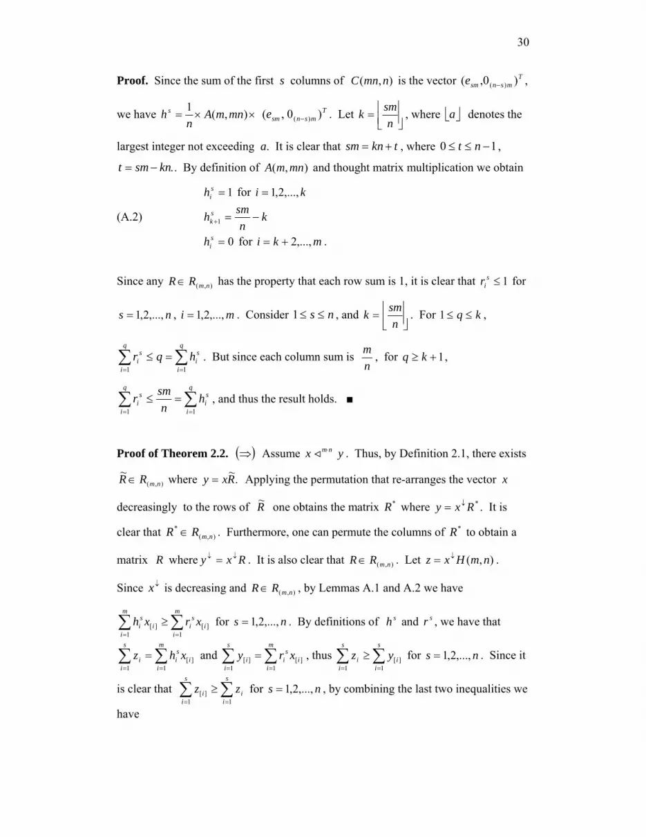
30

Proof. Since the sum of the first s columns of ),( nmnC is the vector Tmsnsme )0,( )( − ,

we have ××= ),(1 mnmAn

h s Tmsnsme )0,( )( − . Let ⎥⎦

⎥⎢⎣⎢=

nsmk , where ⎣ ⎦a denotes the

largest integer not exceeding a. It is clear that tknsm += , where 10 −≤≤ nt ,

.knsmt −= . By definition of ),( mnmA and thought matrix multiplication we obtain

1=sih for ki ,...,2,1=

(A.2) kn

smh sk −=+1

0=sih for mki ,...,2+= .

Since any ),( nmRR∈ has the property that each row sum is 1, it is clear that 1≤sir for

ns ,...,2,1= , mi ,...,2,1= . Consider ns ≤≤1 , and ⎥⎦⎥

⎢⎣⎢=

nsmk . For kq ≤≤1 ,

∑ ∑= =

=≤q

i

q

i

si

si hqr

1 1. But since each column sum is

nm , for 1+≥ kq ,

∑ ∑= =

=≤q

i

q

i

si

si h

nsmr

1 1, and thus the result holds. ■

Proof of Theorem 2.2. ( )⇒ Assume yx nm⋅< . Thus, by Definition 2.1, there exists

),(~

nmRR ∈ where .~Rxy = Applying the permutation that re-arranges the vector x

decreasingly to the rows of R~ one obtains the matrix *R where *Rxy ↓= . It is

clear that ),(*

nmRR ∈ . Furthermore, one can permute the columns of *R to obtain a

matrix R where Rxy ↓↓ = . It is also clear that ),( nmRR∈ . Let ),( nmHxz ↓= .

Since ↓x is decreasing and ),( nmRR∈ , by Lemmas A.1 and A.2 we have

∑ ∑= =

≥m

ii

m

i

sii

si xrxh

1][

1][ for ns ,...,2,1= . By definitions of sh and sr , we have that

∑∑==

=m

ii

si

s

ii xhz

1][

1

and ∑ ∑= =

=s

ii

m

i

sii xry

1][

1][ , thus ∑∑

==

≥s

ii

s

ii yz

1][

1

for ns ,...,2,1= . Since it

is clear that ∑∑==

≥s

ii

s

ii zz

11][ for ns ,...,2,1= , by combining the last two inequalities we

have

31

≥∑=

s

iiz

1][ ∑

=

s

iiy

1][ for ns ,...,2,1= . Note that by simple matrix algebra we have that

∑∑∑===

==m

ii

n

ii

n

ii xyz

111

. Since ≥∑=

s

iiz

1][ ∑

=

s

iiy

1][ for ns ,...,2,1= and ∑∑

==

=n

ii

n

ii yz

11

is

equivalent to ∑=

≤s

iiz

1)( ∑

=

s

iiy

1)( for ns ,...,2,1= , we have yz < (i.e. ynmHx <),(↓ ).

Furthermore, we remark that any permutation of ),( nmH is in ),( nmR , and thus

∑∑==

≥s

ii

s

ii uz

11

for ns ,...,2,1= where u is any permutation of z and therefore

),...,,( ][]2[]1[ nzzzz = ) so ),( nmHx↓ is decreasing. ■

( )⇐ Assume ynmHx <),(↓ . By Theorem 1.2, there exist an nn× bistochastic

matrix B where BnmHxy ×= ↓ ),( . Also, there exists an mm× permutation matrix

where xPx =↓ , thus xRy = where BnmHPR ××= ),( . By (2.1) and (2.2), it is

clear that if ),( nmRR∈ , then the same is true of its row and column permutations.

This latter observation, together with the fact that ),( nmR is convex (Lemma 2.1B),

gives that ),(),( nmRBnmHPR ∈××= . Thus, by Definition 2.1, yx nm⋅< . ■

Proof of Lemma 2.3. The proof that ),( nmHx↓ is decreasing appears in the proof of

Theorem 2.2. ■

Proof of Lemma 3.2.

)(⇒ Assume yx nm⋅< . By Definition 2.1 there exists ),( nmRR∈ where xRy = . By

Lemma 2.2 there exists an mnmn× bistochastic matrix B where

),(),(1 nmnCBmnmAn

xy ××××= . Multiplying by ),(1 mnnAm

we obtain

),(1),(),(1),(1 mnnAm

nmnCBmnmAxn

mnnAym

×××= . It remains to show that

),(1),(~ mnnAm

nmnCBB ××= is an mnmn× bistochastic matrix. By employing

(1.3), (1.4) and (A.1) we have,

=×× ),(1),( mnnAm

nmnCBemn =× ),(1),( mnnAm

nmnCemn

32

=× ),(1 mnnAm

men mnn emnnAe =),( ,

and

=×× TmnemnnA

mnmnCB ),(1),( =×× T

nmem

nmnCB 1),( =× TnenmnCB ),( =T

mnBe Tmne .

Therefore B~ is bistochastic and, by Theorem 1.2, ),(1),(1 mnnyAm

mnmxAn

< .

)(⇐ Assume ),(1),(1 mnnyAm

mnmxAn

< . By Theorem 1.2, there exists a mnmn×

bistochastic matrix B such that BmnmxAn

mnnyAm

×= ),(1),(1 . Multiplying by

),( nmnC we have ),(),(1),(),(1 nmnCBmnmxAn

nmnCmnnyAm

××=× . Lemma 2.2

and the fact that nmInmnCmnnA =× ),(),( imply that xRy = where ),( nmRR∈ ; thus

yx nm⋅< . ■

Proof of Theorem 3.1. Let ),( nmLCMr = , r

mnk = , nrq = ,

mrp = and

kaaa ≥≥≥ ...21 be constants.

[(3.2) ⇒ (3.3) and (3.4)] Assume that },{ yx are scaled-p-proportionate. Therefore

x is a permutation of ),...,,(~21 qkqq eaeaeax = and y is a permutation of

),...,,(~21 pkpp eaeaea

nmy = . Let ),(~1 mnmAx

nx =∗ and ),(~1 mnnAy

my =∗ , see

Definition 2.2. It is clear that ∗x is a permutation of n

x 1~ =∗ ),...,,( 21 qnkqnqn eaeaea

and ∗y is a permutation of nm

my 1~ =∗ ),...,,( 21 pmkpmpm eaeaea . But since

pmrqn == , we have that ∗∗ = yx ~~ and therefore ∗x is a permutation of ∗y .

Therefore, by Lemma 3.1, we have that ∗∗ yx < and ∗∗ xy < . Then, by Lemma 3.2,

yx nm⋅< and xy mn⋅< ; so (3.3) holds. By simple matrix algebra we have

),(~~ nmHxy = and ),(~~ mnHyx = . But since the constants kaaa ,...,, 21 are

decreasingly ordered, xx ~=↓ and yy ~=↓ , and therefore, (3.4) holds.

33

[(3.3) ⇒ (3.2)] Assume yx nm⋅< and xy mn⋅< . With ∗x and ∗y defined as above,

by Lemma 3.2, ∗∗ yx < and ∗∗ xy < and therefore by Lemma 3.1 ∗x is a permutation

of ∗y . Suppose the vector x contains the value α exactly s times. Thus ∗x

contains the value nα exactly ns× times. But since ∗x is a permutation of ∗y , ∗y

contains the value nα exactly ns× times as well. By definition of ∗y , this means

that the vector y must contain the value αnm exactly

msn times and therefore

msn

must be a natural number. Therefore ns× is a multiple of m. Since it is clear and

ns× is a multiple of n, we have that rtns ×=× where t is a natural number and

),( nmLCMr = . Therefore ⎟⎠⎞

⎜⎝⎛=

nrts , so each distinct value of the vector x must

appear a multiple of nrq = times. Similarly, each distinct value of the vector y must

appear a multiple of mrp = times. Note that in order to calculate the maximum

number of distinct values the vector x can have, we can choose 1=t , or nrs = . But

since mRx∈ , the maximum number of distinct values r

mnnr

mk ==/

. Thus the

vector x contains the constants kaaa ,...,, 21 (not necessarily distinct) that each

appears q times. The vector y contains the constants kanma

nma

nm ...,,, 21 each

appearing p times, thus x is a permutation of =x~ ),...,,( 21 qkqq eaeaea and y is a

permutation of =y~ ),...,,( 21 pkpp eaeaeanm so },{ yx are scaled-p-proportionate .

[(3.4) ⇒ (3.3)] Assume y is a permutation of ),( nmHx↓ . Therefore, there exist a

permutation matrices P and Q where PnmHxy ),(↓= and

PnmxQHy ),(= . By Theorem (2.1a), ),(),( nmRnmH ∈ . Furthermore, by Definition

2.1, it is clear that any column and row permutation of a matrix in ),( nmR remains in

the set, hence xRy = where ),(),( nmRPnmQHR ∈= and therefore, yx nm⋅< . A

34

similar argument can be employed to show that if x is a permutation of ),( mnHy↓

then xy mn⋅< . ■

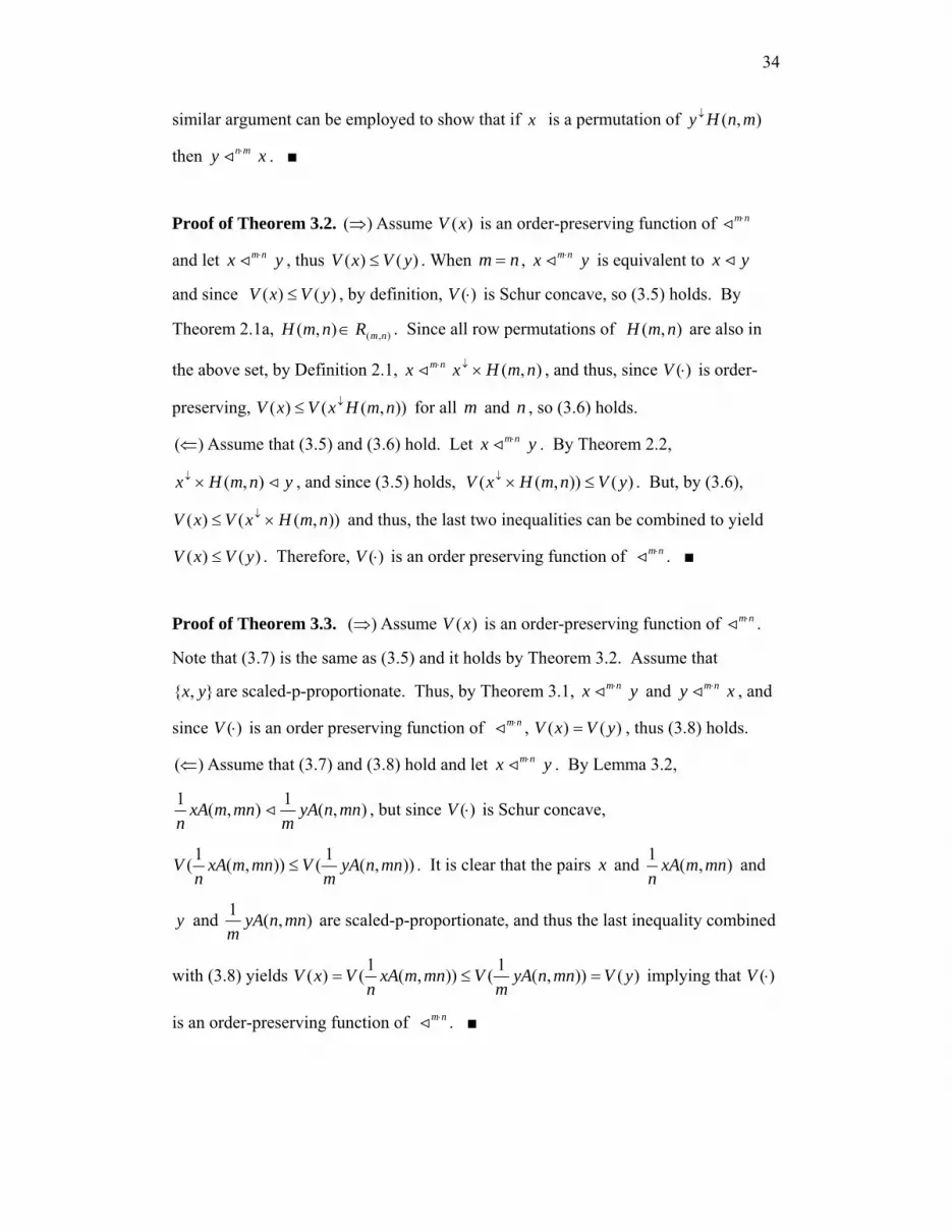
Proof of Theorem 3.2. )(⇒ Assume )(xV is an order-preserving function of nm⋅<

and let yx nm⋅< , thus )()( yVxV ≤ . When nm = , yx nm⋅< is equivalent to yx <

and since )()( yVxV ≤ , by definition, )(⋅V is Schur concave, so (3.5) holds. By

Theorem 2.1a, ),(),( nmRnmH ∈ . Since all row permutations of ),( nmH are also in

the above set, by Definition 2.1, nmx ⋅< ),( nmHx ×↓ , and thus, since )(⋅V is order-

preserving, )),(()( nmHxVxV ↓≤ for all m and n , so (3.6) holds.

)(⇐ Assume that (3.5) and (3.6) hold. Let yx nm⋅< . By Theorem 2.2,

ynmHx <),(×↓ , and since (3.5) holds, )()),(( yVnmHxV ≤×↓ . But, by (3.6),

)),(()( nmHxVxV ×≤ ↓ and thus, the last two inequalities can be combined to yield

)()( yVxV ≤ . Therefore, )(⋅V is an order preserving function of nm⋅< . ■

Proof of Theorem 3.3. )(⇒ Assume )(xV is an order-preserving function of nm⋅< .

Note that (3.7) is the same as (3.5) and it holds by Theorem 3.2. Assume that

},{ yx are scaled-p-proportionate. Thus, by Theorem 3.1, yx nm⋅< and xy nm⋅< , and

since )(⋅V is an order preserving function of nm⋅< , )()( yVxV = , thus (3.8) holds.

)(⇐ Assume that (3.7) and (3.8) hold and let yx nm⋅< . By Lemma 3.2,

),(1),(1 mnnyAm

mnmxAn

< , but since )(⋅V is Schur concave,

)),(1()),(1( mnnyAm

VmnmxAn

V ≤ . It is clear that the pairs x and ),(1 mnmxAn

and

y and ),(1 mnnyAm

are scaled-p-proportionate, and thus the last inequality combined

with (3.8) yields )()),(1()),(1()( yVmnnyAm

VmnmxAn

VxV =≤= implying that )(⋅V

is an order-preserving function of nm⋅< . ■

35

Proof of Theorem 3.4. )(⇒ Note that (3.7) and (3.9) are the same. By Definitions

3.1 and 3.2, x and rsx l are scaled-p-proportionate, thus (3.8) implies (3.10).

Therefore, (3.9) and (3.10) hold as a consequence of the “if” part of Theorem 3.3.

)(⇐ Assume that (3.9) and (3.10) hold and let yx nm⋅< . Note that for n=l , rsx l is a

permutation of ),(1 mnmxAn

and by Lemma 3.1, ),(1 mnmxAn

x rs <l and

rsxmnmxAn

l<),(1 . By (3.10) and since )(⋅V is an order preserving function of < ,

we have ⎟⎠⎞

⎜⎝⎛== ),(1)()( mnmxA

nVxVxV rsl . Similarly, for m=l , rsy l is a

permutation of ),(1 mnnyAm

, and hence .),(1)()( ⎟⎠⎞

⎜⎝⎛== mnnyA

mVyVyV rsl By using

the arguments of Theorem 3.3, we have ⎟⎠⎞

⎜⎝⎛≤⎟

⎠⎞

⎜⎝⎛ ),(1),(1 mnnyA

mVmnmxA

nV , which,

combined with the last two equalities, yields )()( yVxV ≤ , implying that )(⋅V is an

order-preserving function of nm⋅< . ■

Proof of Lemma 4.1. Let R be a non-negative nm× matrix that satisfies (2.1) and

(2.2). Note that TnRe = T

me if and only if Tnm

nm Re× = Tmne , or T

nmQe = Tmne where

RmnQ = . Also, nm meRne = if and only if nm eR

mne = , or nm eQe = . A similar

argument can be employed to show that if Q is a non-negative nm× matrix that

satisfies (4.1) and (4.2) then QnmR = satisfies (2.1) and (2.2). ■

Proof of Corollary 4.1. )(⇒ Let yx nm⋅p . Then there exists ∈Q Q nm ),(

where xQy = , and by Lemma 4.1, Rmnxy = where ),( nmRR∈ , or nxRmy = which

implies mynx nm⋅< .

)(⇐ The proof is similar. ■

Proof of Lemma 4.2.

36

A) The proof is similar to the proof of Lemma 2.1 (A).

B) Since the set ),( nmR is convex and, by Lemma 4.1 ⎭⎬⎫

⎩⎨⎧ ∈= ),(),( | nmnm RRR

mnQ , it is

clear that ),( nmQ is convex as well.

C) Let ∈1Q Q nm ),( and ∈2Q Q sn ),( . By Lemma 4.1, *2121 R

msRR

ns

mnQQ == ,

where by Lemma 2.1 (C), ),(*

smRR ∈ . Thus, by Lemma 4.1, ∈21QQ Q sm ),( .

D) Let yx nm⋅p and zy sn⋅p . Then there exists ),(1 nmQQ ∈ and ),(2 snQQ ∈ where

yxQ =1 and zyQ =2 . Since ),(21 smQQQ ∈ and zyQQxQQQx === 22121 )()( , we

have zx sm⋅p . ■

Proof of Theorem 4.2. This follows directly from Theorem 2.1, Lemma 4.1 and

Definition 4.2. ■

Proof of Theorem 4.3. By Corollary 4.1 yx nm⋅p if and only if mynx nm⋅< . By

Theorem 2.2, mynx nm⋅< if and only if mynmHnx <),(×↓ , or equivalently,

ynmHmnx <),(×↓ . By Definition 4.2, the latter is ynmKx <),(×↓ . ■

Proof of Theorem 4.4. [(4.7)⇒ (4.6)] Let yx nm⋅p and xy mn⋅p . By Corollary 4.1,

mynx nm⋅< and nxmy mn⋅< , and therefore, by Theorem 3.1, nx and my are scaled-p-

proportionate. Thus, by Definition 3.1, nx is a permutation of ),...,,( 21 qkqq eaeaea

and my is a permutation of ),...,,( 21 pkpp eaeaeanm , where p , q and k are given in

Definition 3.1. Thus, x is a permutation of ),...,,( 21 qkqq ebebeb and y is a

permutation of ),...,,( 21 pkpp ebebeb where na

b ii = for .,...,2,1 ki = Thus, by

Definition 4.3, x and y are p-proportionate.

[(4.6)⇒ (4.7)] By a similar argument, { x , y } p-proportionate imply that nx and

my are scaled-p-proportionate and by Theorem 3.1, mynx nm⋅< and nxmy mn⋅< ,

therefore, by Corollary 4.1 yx nm⋅p and xy mn⋅p .

37

[(4.7)⇒ (4.8)] Assume yx nm⋅p and xy mn⋅p . By Corollary 4.1, mynx nm⋅< and

nxmy mn⋅< , and therefore, by Theorem 3.1, my is a permutation of ),( nmHnx↓ and

nx is a permutation of ),( mnHmy ↓ . Equivalently, y is a permutation of

),( nmHmnx ×↓ and x is a permutation of ),( mnH

nmy ×↓ . By Definition 4.2,

),(),( nmHmnnmK = and ),(),( mnH

nmmnK = , thus (4.8) holds.

[(4.8)⇒ (4.7)] Assume y is a permutation of ),( nmKx↓ and x is a permutation of

),( mnKy↓ . By the equivalence established above, my is a permutation of

),( nmHnx↓ and nx is a permutation of ),( mnHmy↓ , and by Theorem 3.1,

mynx nm⋅< and nxmy mn⋅< . Thus, by Corollary 4.1, (4.7) holds. ■

Proof of Lemma 4.3.

The proof follows directly from Lemma 3.2 and Corollary 4.1. ■

Proof of Theorem 4.5. )(⇒ Assume )(xW is an order-preserving function of nm⋅p

and let yx nm⋅p , thus )()( yWxW ≤ . When nm = , yx nm⋅p is equivalent to yx <

and since )()( yWxW ≤ , by definition, )(⋅W is Schur concave, so (4.10) holds. By

Theorem 4.2 (a), ),(),( nmQnmK ∈ . Since all row permutations of ),( nmK are also in

),( nmQ , by Definition 4.1, nmx ⋅p ),( nmKx ×↓ , and thus, since )(⋅W is order-

preserving, )),(()( nmKxWxW ↓≤ for all m and n . Thus (4.11) holds.

)(⇐ Assume that (4.10) and (4.11) hold. Let yx nm⋅p . By Theorem 4.3,

ynmKx <),(×↓ , and since (4.10) holds, )()),(( yWnmKxW ≤×↓ . But by (4.11),

)),(()( nmKxWxW ×≤ ↓ and thus the last two inequalities can be combined to yield

)()( yWxW ≤ . Thus )(⋅W is an order preserving function of nm⋅p . ■

Proof of Theorem 4.6. )(⇒ Assume )(xW is an order-preserving function of nm⋅p .

Note that (4.12) is the same as (4.10) and it holds by Theorem 4.5. Assume that

38

},{ yx are p-proportionate. Thus, by Theorem 4.4, yx nm⋅p and xy nm⋅p , and since

)(⋅W is an order preserving function of nm⋅p , )()( yWxW = , thus (4.13) holds.

)(⇐ Assume that (4.12) and (4.13) hold and let yx nm⋅p . By Lemma 4.3,

),(),( mnnyAmnmxA < , but since )(⋅W is Schur concave,

)),(()),(( mnnyAWmnmxAW ≤ . It is clear that both pairs x and ),( mnmxA and y

and ),( mnnyA are p-proportionate, and thus the last inequality, combined with (4.13)

yields )()),(()),(()( yWmnnyAWmnmxAWxW =≤= , implying that )(⋅W is an

order-preserving function of nm⋅p . ■

Proof of Theorem 4.7. )(⇒ Note that (4.12) and (4.14) are the same. By

Definitions 4.3 and 4.4, x and rx l are p-proportionate, thus (4.13) implies (4.15).

Therefore, (4.14) and (4.15) hold as a consequence of the “if” part of Theorem 4.6.

)(⇐ Assume that (4.14) and (4.15) hold and let yx nm⋅p . Note that for n=l , rx l

is a permutation of ),( mnmxA and by Lemma 3.1 ),( mnmxAx r <l and rxmnmxA l<),( and since (4.15) holds and )(⋅W is an order preserving function of

< , we have ( )),()()( mnmxAWxWxW r == l . Similarly, for m=l , ry l is a

permutation of ),( mnnyA , and hence ( ).),()()( mnnyAWyWyW r == l

By using the arguments of Theorem 4.6, we have )),(()),(( mnnyAWmnmxAW ≤ ,

which, combined with the last two equalities yields )()( yWxW ≤ , implying that

)(⋅W is an order-preserving function of nm⋅p . ■

39

REFERENCES

Alberti, P. and A. Uhlmann (1982) Stochasticity and partial order. D. Reidel Publishing Co., Dordrecht. Amiel Y. and F. Cowell (1999) Thinking about inequality. Cambridge University Press. Blackorby, C., W. Bossert and D. Donaldson (1999) Income inequality measurement. In J. Silber (ed.) Handbook of Income Inequality Measurement. Kluwer. Chakravarty S. (1999) Measuring inequality: the axiomatic approach. In J. Silber (ed.) Handbook of Income Inequality Measurement. Kluwer. Cowell F. (1999) Measuring inequality, 2d Ed, Prentice Hall. Cowell F. (2000) Measurement of inequality. In A. Atkinson and F. Bourguignon (eds) Handbook of income distribution. North Holland. Dalton, H. (1920) The measurement of the inequality of income. Economic Journal, 30: 348-361. Dasgupta, P., A. Sen and D. Starrett (1973) Notes on the measurement of inequality. Journal of Economic Theory, 6: 180-187. Donaldson, D. and J. Weymark (1980) A single-parameter generalization of the Gini indices of inequality. Journal of Economic Theory, 22: 67-86. Foster, J. (1985) Inequality measurement. In H. P. Young (ed.) Fair Allocation. Proceedings of Symposia in Applied Mathematics, 33, American Mathematical Society, Providence. Kolm, S. (1969) The optimal production of social justice. In H. Guitton and J. Margolis (eds) Public Economics. Macmillan, London. Lambert, P. (2001) The distribution and redistribution of income. 3rd Ed. , Manchester University Press, Manchester. Lorenz, M. (1905) Methods of measuring the concentration of wealth. Journal of the American Statistical Association, 9: 209-219.

40

Marshall, A. and I. Olkin (1979) Inequalities: Majorization Theory and its Applications. Academic Press, New York. Moyes, P. (1999) Stochastic dominance and the Lorenz curve. In J. Silbert (ed.) Handbook of Income Inequality Measurement. Kluwer. Muirhead, R. (1903) Some methods applicable to identities and inequalities of symmetric algebraic functions of n letters. Proceedings of the Edinburgh Mathematical Society, 21: 144-157. Nygård, F. and A. Sandstrøm (1981) Measuring income inequality. Almqvist and Wiksell International, Stockholm. Sen, A. (1973) On economic inequality. Clarendon Press, Oxford. Thon, D. (1982) An axiomatization of the Gini coefficient. Mathematical Social Sciences, 2: 131-143.

41