Inequality and Asset Prices - Federal Reserve Bank of Atlanta...bond and in a production economy with capital. Daniel Barczyk: Department of Economics, McGill University, [email protected].

Inequality and Asset Prices∗

Daniel Barczyk and Matthias Kredler

February 15, 2012

Abstract

What is the relationship between wealth inequality and asset prices? Westudy this question in a dynamic two-agent economy with incomplete mar-kets. Agents face correlated labor-income risk, but there is no aggregate risk.The only asset is a Lucas tree, which is traded subject to a no-short-sellingconstraint. We find that asset prices are increasing in wealth inequality. Theasset price is highest when the poor agent hits the no-short-selling constraintand exits the asset market. Since the asset supply of the impoverished agentdries up while the rich agent’s demand stays high, there is a surge in theasset price at this point. Furthermore, asset-price volatility is increasing ininequality. Analogous results are obtained in an economy with a short-termbond and in a production economy with capital.

∗Daniel Barczyk: Department of Economics, McGill University, [email protected] Kredler: Departamento de Economıa, Universidad Carlos III de Madrid,[email protected]. Matthias Kredler acknowledges research funding by the Spanish Min-isterio de Ciencia e Innovacion, reference number SEJ2007-62908.

1 IntroductionOver the last three decades, both income and wealth inequality have risen in theU.S. and in other rich countries (for evidence, see Atkinson, Piketty & Saez (2011)for income inequality and Lindert (2000) and Kennickell (2009) for wealth in-equality). Ever larger fractions of aggregate wealth are held by a small share ofthe population, and the earning’s share of the rich has been increasing dramati-cally over the past 30 years. What are the implications for asset prices and assetreturns when markets are dominated by a group of rich individuals? More specif-ically, this paper asks the following question: what is the relationship betweenwealth inequality and asset prices?

If rich individuals have investment needs and strategies that are different fromthose of the average investor, this should have an impact on asset prices. For exam-ple, rich investors’ income is more correlated with capital returns than the incomeof the average investor. This means that rich investors will place more emphasis intheir investment decision on states of the world in which capital performs poorlythan the average investor (since their marginal utility of consumption is higher inthese states).1 Note that a mechanism along these lines also opens up the possibil-ity that government policy affects asset-market outcomes through redistributivepolicies. If the government passes tax legislation that favors the wealthy, thiswould exacerbate the potential effects of rising inequality on asset prices.

The first obvious approach to answer the question about the relationship be-tween inequality and asset prices is to study empirically how asset markets haveresponded to changes in inequality in the past. However, there is a severe draw-back to this approach: essentially, there are very few data points available. In-equality (in both income and wealth) were at high levels in the U.S. from the turnof the century until the Great Depression. From the 1930s on, inequality startedto drop significantly and stayed at relatively low levels until the 1980s, when itstarted its surge to current levels. Since inequality is extremely slow-moving, weare essentially left with three data points over the period where reliable data areavailable. Furthermore, other variables that also impact asset markets may haveco-moved with inequality, making it difficult – if not impossible – to identify the

1Other stories for why rich investors’ behavior could differ from the average investor are thatrich investors have different risk aversion (as in Dumas (1989)) or different discount factors thanpoorer investors (as in Krusell & Smith (1997)). However, our framework does not consider thesepossibilities and focuses on the effects that arise when preferences are uniform across agents.

1

contribution of inequality to changes in asset prices.2 3

In light of these severe drawbacks to the empirical approach, we opt for atheoretical approach. We study a simple two-agent incomplete-markets modelwith a single asset that generates joint dynamics in the wealth distribution andasset prices.

1.1 Model overviewThere are two groups of agents who face idiosyncratic labor-income risk in theform of a two-state Markov chain. Agents’ labor-income shocks are perfectlynegatively correlated, so that there is no aggregate risk in the economy. We delib-erately abstract away from aggregate risk in order to focus the analysis on inequal-ity. Markets are incomplete. In order to smooth consumption agents have a singleasset at their disposal, namely, a Lucas tree with a constant dividend (which maybe seen as a perpetual bond). There is a no-short-selling constraint on the asset,which occasionally binds for one group of agents.

In addition, we study two economies in which the Lucas tree is replaced by1) a short-term bond and 2) physical capital in a production economy. Again,there are borrowing limits that occasionally bind. The qualitative results from theLucas-tree economy also obtain in these modified settings.

1.2 ResultsAs expected, in all settings agents use the asset as a buffer stock to insure againstincome shocks. They accumulate the asset in times when they have high laborincome, and they decumulate it when labor income is low. When faced with avery long unproductive spell, agents ultimately hit the liquidity constraint and(endogenously) cease to participate in asset markets. At this point, consumptioninequality as well as wealth inequality reach their maximal levels.

Asset prices are higher, and expected returns are lower, when the wealth distri-bution becomes more unequal. Asset prices reach their maximal levels when theincome-poor agent ceases to participate in asset markets, in which case only rich

2Examples for such confounding variables are aggregate consumption growth and politicalconditions – note that the era of low inequality coincides almost perfectly with the Cold War.

3A stark pattern in the data is that stock markets were most volatile in pre-Great-Depressionera and after 1980, which coincides with times of high inequality. Our model is successful inexplaining this fact, but because of the low number of essential observations we are cautious tointerpret this as evidence favoring our model.

2

agents participate in asset markets. At this point rich agents’ asset demand is highsince they want to insure against the case that their income drops again. This highdemand drives up the asset price and thus lowers its return. The high asset pricefrom this extreme situation feeds back into regions where both groups of agentsstill participate in asset markets but where the wealth distribution is skewed: sincethere is a chance that the extreme state is reached and the asset can be sold off ata high price, the current valuation for the asset is high for both agents.

Large drops in asset prices occur when the wealth-rich agent receives a badincome shock. In this situation, the wealth-poor agent enters the market againand buys shares of the tree, whereas the wealth-rich agent sells them off. Thelikelihood that the economy enters the extreme state of the poor agent being con-strained drops, and with it the expectation of high asset prices in the future. Thelarge drops in prices in situations of high wealth inequality (or large increases inprice, in the case of income changing in the reverse direction) lead to the secondmain result: asset-price volatility is increasing in wealth inequality.

Using a continuous-time framework allows us to obtain sharp characteriza-tions of asset prices and consumption policies at the boundaries of the state spacewhere one group of agents becomes constrained. We find that the elasticity of theasset price with respect to the rich agent’s wealth share goes to infinity when ap-proaching the constraint. In the economy with the short-term bond, we can showthat a discrete downward jump in the bond yield occurs at the moment when thepoor agent exits the market.

1.3 LiteratureScheinkman & Weiss (1986) is the paper that is most similar to ours, but in theirframework the income-poor agent has no income at all. This income processtogether with an Inada condition on utility makes the household cling to the assetwhen income-poor, so that in equilibrium the liquidity constraint is never reached.Scheinkman & Weiss (1986) find that asset returns are increasing in the income-rich agent’s asset share, which is not the case in our setting – recall that theyare increasing in inequality, so they are inverse-U-shaped in an agent’s wealthshare. This difference stems from another assumption they make: They put a labordecision into the model and assume the disutility of labor to be linear. This utilityfunction essentially fixes the productive (i.e. income-rich) agent’s consumption ata constant level and so simplifies the analysis.

Dumas (1989) studies an economy with two agents who have different riskaversion. However, in his economy there is only aggregate risk and no idiosyn-

3

cratic risk. The welfare theorems hold and the market allocation can be backedout from a planner’s problem, which is not the case in our setting. Long spells ofpositive productivity shocks make the less risk-averse agent’s asset share increase,however the more risk-averse agent has a higher asset share after long spells ofbad luck.

There are also several computational papers studying economies inhabited bytwo types of agents: Telmer (1993), Lucas (1994) and Heaton & Lucas (1996).Haan (1996) studies settings with larger (finite) numbers of agents. All thesepapers have in common that they do not find an exact solution of the model butrecur to numerical approximating techniques. The literature focuses on globalproperties of equilibrium, such as the average equality premium, the average risk-free rate etc. While the models are capable – and indeed likely – to produceeffects like ours, the authors do not mention these. This is probably because ofthe large dimension of the state space and the different focus of their papers. Ourframework has the advantage that it is extremely simple and can so highlight thepricing differences that occur across the state space and at the constraint.

Another area where incomplete-markets models with a small number of (usu-ally two) agents is used is the international-finance and trade literature. Step-anchuk & Tsyrennikov (2011), for example, study a two-country setting with onetype of stock in each country and a risk-free bond. Again, the state space is vastlylarger in this model than it is in ours. Our more analytic approach may help toshed light on the behavior of asset prices in regions where constraints start to bindin models such as Stepanchuk & Tsyrennikov (2011). Furthermore, it can indi-cate when it is important to consider discontinuities in pricing functions in thecomputational algorithms used to solve such models.

Finally, an entire industry has evolved that uses heterogeneous-agents economieswith a continuum of agents to explain asset prices Krusell & Smith (1997), Gomes& Michaelides (2008), Guvenen (2009), etc. The key difference to our model isthat shocks to individual agents are independent across agents in these models,whereas they are correlated in our model. Independence of idiosyncratic shocksmakes changes in the relative wealth distribution wash out, which leads to Krusell& Smith (1998) approximate-aggregation result: prices can be forecast very ac-curately using only the mean asset holdings of all agents. Our economy is a starkcounterexample to approximate aggregation: the wealth share held by the richagent (the measure of inequality) is indeed very important for predicting futureasset returns.

4

2 Setting: A Lucas-tree economyFollowing Kehoe & Levine (2001), we write down the simplest-possible economywith idiosyncratic risk; there is no aggregate risk.

Two classes of agents (1 and 2) of the same measure inhabit the economy.There is one asset (a Lucas tree) in the economy, which is in fixed supply 1. Wewill come to the case of the bond and of physical capital in later sections. Theasset yields a constant dividend stream 0 ≤ r < 1. If r = 0, we may interpret theasset as fiat money. The asset’s price is denoted by Pt. Agent 1’s labor incomey follows a two-state Markov process with switching hazard η > 0 between thestates 0 < yl ≤ yh ≤ 1. The aggregate endowment of the economy is fixedat 1 (i.e. there is no aggregate uncertainty), so agent 2’s labor income is given by1−r−y. Time is continuous: t ∈ [0, T ]. Of course we are especially interested inthe limiting case where T →∞ or T =∞ (there might be equilibria for T =∞that are not the limit of a finite economy). Both agents have standard preferencesover consumption:

E0

∫ T

0

e−ρtu(ct)dt,

where u′ > 0 and u′′ < 0.

2.1 The agent’s problemThe budget constraint at t, given the inherited asset position from t−∆t, is

ct∆t+ Ptat = yt∆t+ rat−∆t + Ptat−∆t.

Dividing by ∆t and taking limits as ∆t→ 0, we obtain

ct + Ptat = yt + rat,

where we have denoted the drift in the asset position by at = lim∆t→0(at −at−∆t)/∆t.

Now, let the aggregate state be given by t, yt, At ∈ [0, 1], where At denotesthe asset position of a typical type-1 agent. Let the individual agent’s state be at.4

4Note that we have to give the individual the possibility to deviate with his position at fromthe aggregate position of his group At. Think big-K, little-K here. If we wrote a problem wherethe individual controls the aggregate state At, then this would give the individual control overprices. We are interested in the competitive setting where this is not the case; the case with twonon-atomistic players with market power is potentially interesting but beyond the scope of thispaper.

5

Then the (individual) agent’s problem is to choose a consumption function c(·)contingent on the state (t, y, A, a) in order to

maxc(·)

E0

∫ T

0

e−ρtu[c(t, yt, At, at)

]s.t. at =

yt + rat − c(t, yt, At, at)P (t, yt, At)

c(t, y, A, 0) ≤ y for all t ∈ [0, T ], for all A ∈ [0, 1]

given At = dA(t, yt, At)dt

P (t, y, A),

where the first constraint is the law of motion for the individual agent’s asset andthe second constraint is the liquidity constraint that limits the agent’s consumptionto his flow income when his asset position is zero. The agent takes as given the lawof motion for the aggregate stateA, which is summarized by a drift function dA(·).She also takes as given the pricing function P (·).

The HJB for the value function V (t, y, A, a) is

−Vt + ρV = maxc

{u(c) +

y + ra− cP

Va

}+ ηVy + dAVA,

where we introduce the “discrete derivative” Vy ≡ V (y′, ·) − V (y, ·) in which ydenotes the current state of income and y′ is the other income state (to which onemight jump).

The first-order condition is

Puc(c) = Va.

It asserts that the marginal value of keeping the asset Va has to equal the value ofselling a marginal unit at price Pt and consuming it.

It is now convenient to introduce the infinitesimal generator, which is a partialdifferential operator that tells us the expected growth of any smooth function f(·)defined on the state space (t, y, A, a):

Af = lim∆t→0

Et

[f(t+ ∆t, yt+∆t, At+∆t, at+∆t)− f(t, yt, At, at)

∆t

]=

= ft + ηfy + dAfA +y + ra− c∗

Pfa,

6

where c∗ is the optimal consumption rule for agent 1.Using the infinitesimal generator, we can re-state the HJB as follows:

AV = ρV − u(c∗).

Taking derivatives of the HJB with respect to a and using the first-order condition,we find the Euler equation

−Vat + ρVa =r

PVa +

y + ra− cP

Vaa + ηVya + dAVaA,

At this step it is important to note that Pa = 0, i.e. the individual agent cannotinfluence prices! (This is the important part of the big-K-little-k trick. . . ) Usingthe infinitesimal generator, we can re-write the first-order condition as

AVa = (Va)t + η(Va)y + dA(Va)A +y + ra− c

P(Va)a =

(ρ− r

P

)Va.

Using the FOC, we obtain the standard Euler equation,

A[Puc(c)]

Puc(c)=(ρ− r

P

),

It says that the agent’s marginal valuation of the asset Puc(c) follows a martingalewhen we adjust for discounting ρ and the dividend stream r. Precisely, it statesthat the percentage growth rate of the marginal valuation of the asset grows at rateρ minus the assets dividend-price ratio. By symmetry, this Euler equation musthold for the consumption plans of both type-1 and type-2 agents.

For the case of complete markets, agents enjoy perfect insurance and thus c isconstant. Then the above Euler equation tells us that the marginal valuation of theasset must be constant and the price is given by Pcm = r/ρ.

2.2 EquilibriumIn equilibrium (big-K,little-k), the privately chosen consumption must equal ag-gregate consumption of the respective group. Mathematically, this means thatc(t, y, A,A) = C(t, y, A), where C(·) is the consumption pattern associated withthe aggregate law of motion dA: The single agent always follows his group andthus at = At always.

7

So the marginal valuation of the asset given the marginal utility implied by theaggregate consumption pattern C must satisfy the martingale property establishedabove. Using C = c in the Euler equation gives us

A[Puc(C)]

Puc(C)= η

[P ′uc(C

′)

Puc(C)− 1

]︸ ︷︷ ︸

jump in y

+Pt + PAd

A

P︸ ︷︷ ︸%-change in P

+ucc(C)

uc(C)[Ct + CAd

A]︸ ︷︷ ︸%-change in uc︸ ︷︷ ︸

no jump

= ρ− r

P

(1)The percentage change in the valuation of the asset for a typical agent 1 is com-posed of two terms: The first term captures what happens if there is a reversal in yand both P and C ′ change discretely. The second group of terms captures whathappens when no reversal happens. The percentage change under this scenario isjust the sum of the percentage change in the asset price and the percentage changein marginal utility. The percentage change in marginal utility, in turn, is given bythe coefficient of absolute risk aversion times the time change in consumption.5

Note that we are following an approach here that is similar to the primal ap-proach in the Ramsey problem, or the first-order approach in moral-hazard prob-lems: We impose on the equilibrium that the allocation fulfill the agents’ first-order conditions. However, note that the Euler equation is only a necessary foroptimality, but not sufficient. We will have to check sufficiency later, which shouldnot be too probematic since the problem is well-behaved and concave.6

Of course, the Euler equation also has to hold for all agents of type 2. Letus denote variables pertaining to agent 2 by tildes: C for consumption etc. Assetmarket clearing requires that assets sold by group 1 are all bought by group 2,i.e. A + ˙A. Walras’ Law then tells us that the other market, the one for the con-sumption good, must be automatically in equilibrium when taking into accountthe information from the agents’ budget constraints: We obtain C+ C = 1, whichis the resource constraint for this economy.

5. . . or equal to the coefficient of relative risk aversion times the percentage change in consump-tion (multiply by C/C to see this) – but we will not be able to exploit this, unlike in the case ofabsolute risk aversion.

6A complication here is that we have to check if it is profitable for the agent to choose long-term deviations from his group (note that the relevant space here to apply the one-shot-deviationprinciple are all nodes in the space (t, y, A, a), not the space (t, y, A)!). This is maybe what Kehoe& Levine (2001) mean what they say that the state space is large in this kind of problems.

8

Using C = 1− C in agent 2’s Euler equation, we obtain

A[Puc(1− C)]

Puc(1− C)= η

[P ′uc(1− C ′)Puc(1− C)

− 1

]+Pt + PAd

A

P−ucc(1− C)

uc(1− C)[Ct+CAd

A] = ρ− rP.

2.3 Constant absolute risk aversionNow, use the preferences u(c) = − 1

λe−λc which have the property of constant ab-

solute risk aversion: ucc(c)/uc(c) = −λ. This gives us the opportunity to exploitthe fact that the last terms in agent 1 and agent 2’s Euler equations are of the samemagnitude when ucc/uc = const – note that d

dtC = Ct+CAd

A = −Ct− CAdA =

− ddtC.Add both Euler equations and divide by 2 to obtain an expression that tells us

about the evolution of prices in equilibrium:

Pt + PAdA

P︸ ︷︷ ︸≡p

= ρ− r

P− η

[P ′

P

(12

uc(C′)

uc(C)+ 1

2

uc(1− C ′)uc(1− C)︸ ︷︷ ︸

average insurance motive

)− 1

]. (2)

We have defined p =ddtP

Pon the left-hand side as the percentage change in prices

over a short interval of time under the scenario that no reversal in y occurs. Also,we introduce the following term: We will call the ratio uc(C ′)/uc(C) = eλ(C−C′)

“insurance motive”: The higher this ratio, the more does a reversal in y hurtthe agent in terms of marginal utility. We see that average consumption risk isplaying the role that the representative agent’s consumption risk played in therepresentative-agent economy (see section 2.9): The higher average consumptionrisk, the lower p, i.e. the lower is the assets returns in “normal times” (i.e. whenthe reversal does not occur).

We can also see from this equation how inequality influences asset prices.Using the fact that exp(λ∆C) is a convex function in ∆C and exp(λ0) = 1, wesee that the term 1

2[uc(C

′)/uc(C)+uc(1−C ′)/uc(1−C)]1 is always larger than 1;indeed, the higher the consumption jump ∆C = C ′ − C is for the agents, thehigher the average insurance motive. So consumption inequality will depress theasset return below the level of a representative-agent economy without aggregateconsumption risk ρ− r/P , see again section 2.9.7

7Note that in PDE language, we are following characteristic lines in (t, A)-space, always inthe scenario where the reversal in income y does not happen.

9

Now, subtract the two Euler equations from each other and divide by 2 toobtain

C = [Ct + CAdA] =

η

2λ

P ′

P

[uc(C

′)

uc(C)− uc(1− C ′)uc(1− C)

]. (3)

So we see that the evolution of consumption in normal times is governed by thedifference in the insurance motive between the two agents. If type 1’s insurancemotive is larger than unity (i.e. she fears a reversal), then type 2’s insurance mo-tive must be lower than unity by the aggregate resource constraint. So in this case,we have C > 0, i.e. type 1’s consumption rises in normal times. Intuitively, ifshe becomes worse off upon a reversal, she must become better off if no reversaloccurs. Once the reversal happens, by the same token the dynamics of the con-sumption distribution must reverse: His consumption will now trend upwards innormal times.

2.4 Constrained caseThe only situation in which consumption rates are constrained by the no-short-selling limit is at the boundaries of the state space, i.e. at a = 0 for her. Inequilibrium, we will have that the asset-poor agent is consuming less than herincome at a = 0: It is optimal to save for the case that income drops to thelow level. When income is low, however, the agent is constrained: The entireincome is consumed and no savings take place. For consumption, this means thatC(t, 0, yl) = yl and Ct(t, 0, yl) = 0 for all t. Agent 2’s Euler equation must holdwith equality and dA = 0, so we find that asset prices obey

Pt(t, 0, yl)

P (t, 0, yl)= ρ− r

P (t, 0, yl)− η

[P (t, 0, yh)uc(1− C(t, 0, yh))

P (t, 0, yl)uc(yh + r)− 1

]. (4)

In a mirror-symmetric way, for the case where agent 2 is constrained we find fromagent 1’s Euler equation

Pt(t, 1, yh)

P (t, 0, yl)= ρ− r

P (t, 1, yh)− η

[P (t, 1, yl)uc(C(t, 1, yh))

P (t, 1, yh)uc(yh + r)− 1

]. (5)

2.5 Solution strategyWe start with the time-dependent case and let the economy end at some T > 0.Consider the situation at T −∆t, where δT is small. The asset will be worthlessat T , so agents should just eat their endowment and the fruits that fall from the

10

tree, i.e. C(T −∆t, a, y) = ra+ y. So the tree must be worth exactly the numberof fruits that fall from it in the time interval [T −∆t, T ], i.e. we can approximateP (T −∆t, a, y) = r∆t. Now we can use standard PDE solution techniques on agrid to solve from T −∆t backwards: The pricing function is updated backwardin time using (2), and the consumption function is updated using (3). At theboundaries of the state space A ∈ {0, 1} we enforce the no-short-selling limitsand update prices using equations (4) and (5).

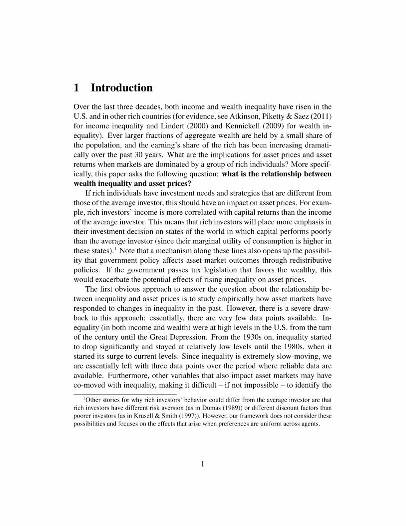
2.6 ResultsThe following figure shows the stationary equilibrium for CARA utility u(c) =−λ exp(−λc), parameterized by ρ = 0.04, λ = 2, η = 0.1, wl = 0.3, wh = 0.4and r = 0.3.

0 0.1 0.2 0.3 0.4 0.5 0.6 0.7 0.8 0.9 1

7.6

7.8

8

8.2

P: a

sset

pric

e

w1=loww1=highrepr.agent

0 0.1 0.2 0.3 0.4 0.5 0.6 0.7 0.8 0.9 10.03

0.035

0.04

0.045

z

R: e

xp. a

sset

retu

rn

w1=loww1=highrepr.agent

0 0.1 0.2 0.3 0.4 0.5 0.6 0.7 0.8 0.9 10.3

0.4

0.5

0.6

0.7

z

C: c

onsu

mpt

ion

Consumption wlConsumption wh

hand−to−mouth

Figure 1: Asset economy

11

The upper panel shows the pricing function. The solid red line depicts theprice as a function of agent 1’s asset position A when agent 1 is income-poor. Thesolid blue line depicts the price when agent 1’s income is high. The dashed blackline gives the benchmark return on the tree from the complete-markets economy.

The middle panel shows the return on the asset. Over a time interval ∆t thereturn is r∆t (dividends) plus the price increment Pt+∆t−Pt divided by the buyingprice Pt. So the expected return of the asset for a short time interval, normalizedby time, is

R = lim∆t→0

1

∆tEt

[r∆t+ Pt+∆t − Pt

Pt

]=r +APP

.

We see that the return is inverse-U-shaped in a and lowest when one agent is bothincome- and asset-rich. Also, it is easy to see that the volatility of asset prices andasset returns is highest when a goes to zero or one.

2.7 Pricing formulaThe results in figure 1 show that the asset price is increasing in wealth inequality:The further the A moves away from zero (the equitable wealth distribution), thehigher asset prices. Furthermore, the asset price is even higher if the asset-richagent is also income rich. We will now develop some intuition for this resultusing standard insights from asset pricing.

First, notice that whenever both agents participate in the asset market, we canthink of both of them pricing the asset. The discretized Euler equation for agent 1reads

P (A, y) = (1− ρ∆t)

[(1− η∆t)

[r∆t+ Pt+∆t]

uc(Ct+∆t)

uc(Ct)+ (6)

+ η∆t(r∆t+ P ′t+∆t)uc(C

′t+∆t)

uc(Ct)

]+ o(∆t).

It says that the price of the asset at t can be decomposed into the dividend streamr∆t over a short time interval plus the discounted value of the asset after thetime interval.8 For the discounting, we have to take into account marginal-utilityratios. If the agent is worse off in a future state, he will value payoffs in this state

8One can take limits of equation (6) as ∆t → 0 to see that it is equivalent to the Euler equa-tion (1).

12

higher. Note that in a situation where both agents are unconstrained, one of theutility ratios will be larger and the other one will be lower than one. If an agentis income-rich, he is saving and experiences steady small gains in consumption ifno reversal occurs. If a reversal occurs, however, there is a large sudden drop inconsumption, and payoffs in this scenario are highly valued.

In the situation where agent 1 is constrained, however, only agent 2 is activein the asset market and effectively prices the asset. Agent 2’s Euler equation thengives us the following pricing equation:

P (0, yl) = (1− ρ∆t)

[(1− η∆t)

(r∆t+ P (0, yl)

)+ (7)

+ η∆t(r∆t+ P (0, yh)

)uc(1− C(0, yh))

uc(1− C(0, yl)

) ]+ o(∆t).

Since consumption does not change when agent 1 stays with the low income, themarginal-utility ratio is unity for the case where no reversal occurs. In the caseof a reversal, the rich agent experiences a drop in consumption. The marginal-utility ratio is then positive, i.e. the rich agent values insurance for this bad state.Since times can only get worse for the rich agent in this situation, discount factorsare large. This manifests itself in asset returns being lowest in this situation, asthe second panel of figure 1 shows. The discount factor of the poor agent wouldbe low, but is not relevant for pricing since the agent is not participating in assetmarkets. Finally, note that we can obtain the symmetric case where agent 2 isconstrained by setting A = 1 is equation (6) and noting that Ct+∆t = Ct in thecase that no reversal occurs.

In order to think of the asset price as a sum of discounted future dividends,we can recursively substitute in for future prices Pt+∆t and P ′t+∆t using equations(6) and (7). Since discount rates are especially high (i.e. the pricing agent appearsespecially patient) in the situation when the income-rich agent owns all assets, fu-ture dividends are discounted less in situations where it is likely that the constraintis hit soon.

13

2.7.1 Formal pricing kernel

Formally, we define the following pricing kernel for this economy:

Λt = e−ρtuc(Ct)ξkt ,

where ξ =uc(1− C(0, yh)

)uc(1− C(0, yl)

) uc(C(0, yl))

uc(C(0, yh)

) > 1

and kt is the number of times that a reversal has occured until t when the economywas at state (A, y) = (0, yl). This pricing kernel uses marginal utility of agent 1almost always; only in the situation where agent 2 is income-rich and owns allassets do we have to make adjustments in the form of the term in ξ > 1. Withrespect to the usual representative-agent pricing kernel, the difference is in theterm in ξ. Each time that the agent ceases to participate in the market, the kernelis adjusted upward. This is because the other agent is in a favorable situation andplaces a high value on future payoffs.

Using the above pricing kernel we then guess the following pricing equation:

ΛtPt = Et

∫ T

t

Λsrds. (8)

We will now derive a difference equation for the random variable Ht = ΛtPt toshow that the above pricing equation indeed holds.

Using the law of iterated expectations, we can write

ΛtPt = Λtr∆t+ Et

[Et+∆t

∫ T

t+∆t

Λsrds︸ ︷︷ ︸=Λt+∆tPt+∆t

]+ o(∆t).

This gives us the difference equation Ht = Λtr∆t+Et[Ht+∆t], which we can seeas a recursive way of calculating Bt backward in time from the terminal conditionHT = 0 (note that PT = 0). We will now show that at each step, Ht+∆t =Λt+∆tPt+∆t implies Ht = ΛtPt, which together with the terminal condition willprove the assertion that Ht = ΛtPt for all t ≤ T .

Using the pricing equation at t + ∆t, re-arranging and dividing by e−ρtξkt∆twe obtain

Et

[e−ρ∆tξkt+∆t−ktuc(Ct+∆t)Pt+∆t − uc(Ct)Pt

∆t

]= −ruc(Ct) + o(∆t). (9)

14

We will now show that equation (9) is implied by the Euler equation of the agentthat is pricing the asset at t.

Whenever A > 0 or y = yh, ∆t may always be chosen small enough such thatkt+∆t = kt with probability 1− o(∆t). The above then implies that

−ρuc(Ct)Pt +A[uc(Ct)Pt] = −ruc(Ct),

which is agent 1’s Euler equation (1).In the situation (A, y) = (0, yl), kt goes up by one with probability η∆t over

a short period of time. The correction factor ξ then makes us use agent 2’s Eulerequation, as we will see now:

e−ρ∆t[(1− η∆t)uc(C)P + η∆tξuc(C

′)P ′]− uc(C)P

∆t= −ruc(C) + o(∆t)

Now multiply by uc(1 − C)/uc(C) and use the definition of ξ to see that this isequivalent to agent 2’s Euler equation:

A[uc(1− C)P ] = ρuc(1− C)P − uc(1− C)r.

We see that in each case, we can go the steps backwards and obtain equation (9)from the Euler equation of the pricing agent, which completes the argument that(8) is a valid pricing formula.

2.8 Stationary equilibria: Bubbles and fiat moneySo far, we have restricted ourselves to study equilibria that emerge as the limit ofa finite-horizon economy. Figure 1 showed equilibrium policies and prices for thecase r > 0. In the case where r = 0, the asset has the interpretation of fiat money.When using the above solution algorithm, we obviously end up with the non-monetary equilibrium where money is not valued (i.e. P (t, a, y) = 0). The assetis not valued in the final period T −∆t, and this feeds back forever since there areno dividends from it. Consumption equals the autarkic levels (i.e. C(t, a, y) = y),i.e. there is no insurance whatsoever.

However, there is clearly the possibility of stationary equilibria that do notarise as the limit of a finite-horizon economy. There could be bubble equilibriain which the asset price is higher than the value of its discounted dividends. Forthe case of money, this is the monetary equilibrium in which money has a positiveprice.

15

Any stationary equilibrium is characterized by taking the limiting case in equa-tions (2) and (3) where time derivatives are set to zero: Pt = 0 and Ct = 0. Thenthe PDEs collapse to a system of four ODEs for the functions Pl, Ph, Cl, Ch :[0, 0.5] → R+ in the variable a (where l is for y = yl and h for y = yh). TheODEs are given by:

PAdA = ρP − r − η

[P ′(

12

uc(C′)

uc(C)+ 1

2

uc(1− C ′)uc(1− C)

)− P

](10)

CAdA =

η

2λ

P ′

P

[uc(C

′)

uc(C)− uc(1− C ′)uc(1− C)

](11)

The initial conditions at A = 0 are Cl(0) = yl, Ch(0) = Ch0, Pl(0) = Pl0 andPh(0) = Ph0. We have to guess two variables (e.g. prices (Pl0, Ph0)) and can thenback out the third (e.g. Ch0) from agent 2’s Euler equation at (A = 0, y = yl),which is given in (4):

Ch0 = 1− yh + r

λln( ηPh0

ρPl0 − r

).

Symmetry of equilibrium imposes the following two terminal conditions at A =0.5:

Cl(0.5) = 1− Ch(0.5),

Pl(0.5) = Ph(0.5).

So we have to find two initial values to fulfill two conditions, which makes usexpect that there is generically a finite number of solutions/equilibria.

The system of ODEs (10) and (11) is difficult to solve because the functionsCl and Pl have infinite slope as A approaches zero (and so do Ch and Ph as Aapproaches one). To see this, note that the right-hand side of both (10) and (11)approaches a constant as A → 0 (since consumption and price functions are as-sumed continuous). However, the drift dA = yl + rA−Cl converges to zero sinceCl → yl by continuity of Cl. This implies that the derivatives of Cl and Pl mustconverge to plus or minus infinity in order for the ODEs to hold. This feature canclearly be seen in figure 1: Small movements in A lead to ever larger increases inPl as A→ C. As for Cl, its slope in A goes to minus infinity.

At first, it seems strange that the pricing function can have infinite slope. Whydo agents not demand more of the asset if small decreases in the aggregate state(which always occur when y = yl) lead to large increases in asset prices, which

16

suggests that returns to the asset should be high? The key is that asset prices donot change dramatically over time since the drift dA converges to zero as A → 0.In fact, since P = PAdA, equation (10) tells us that P converges to a constant asA→ 0. So asset returns are not going to infinity as PA →∞.

As for Cl, we also see that C = CAdA goes to a constant as A → 0. This

behavior is in line with the standard consumption-savings model in continuoustime: The consumption function is continuous and is equal to the endowment ylin the case that the constraint binds. So the drift dA converges to zero, whichimplies an infinite slope in the consumption function in A since C approaches aconstant.

Since dA → 0, it is not clear that the economy will ever reach the constraint– it might just approach it at an ever slower rate but never get there. However,again reading equation (11) with the equality C = CAd

A in mind tells us thatthe constraint must be reached in finite time. Since the right-hand side of (11)converges to a constant, C converges to a negative constant and Cl must reachCl(0) = yl at some point in time.

2.8.1 Computing stationary equilibria

In order to consider all possible cases, we will re-parameterize the initial con-ditions for the system of ODEs. We know that Cl0 = yl < Ch0 < yh, so weintroduce a parameter γ0 =∈ (0, 1) such that Ch0 = yl + γ0(yh − yl). For prices,we know that they always must lie above the complete-markets level r/ρ. So weintroduce a parameter π0 ∈ (0, 1) and set Ph0 = r

ρ− lnπ0 so that Ph0 may take on

any value between the complete-markets level and infinity. Pl0 can then be backedout from agent 2’s Euler equation (4), in which we set the time derivative of thefunction P to zero since we are looking for a stationary equilibrium.

We now summarize the following recursive procedure of mapping (γ0, π0) toprices and consumption at A = 0:

Cl,0 = yl,

Ch,0 = yl + γ0(yh − yl),

Ph,0 =r

ρ− lnπ0

Pl,0 =r + η uc(1−Ch0)

uc(yh+r)Ph0

ρ+ η

From these initial conditions we then have to solve the system of four ODEs given

17

in (10) and (11) and check if the two terminal conditions at A = 12

are satisfied.To do this, we vary the parameters (γ0, π0) on the unit square, which exhausts allpossible initial conditions.

However, since Pl and Cl have infinite slope at A = 0 standard methods fail.We circumvent this by making time t the independent variable instead of A. Wewill move backward in time in small steps ∆t in time for the low-income scenarioby:

At−∆t = At − dA∆t,

Cl,t−∆t = Cl,t − Cl∆t,Pl,t−∆t = Pl,t − Pl∆t.

So the increments will be very small (initially even zero) in A, which allows fora good approximation at the crucial point A = 0. In order to solve backward thefunctions (Cl, Pl), we also need to obtain the values of (Ch, Ph) at At+∆t. In orderto do this, we have to go forward in time in the high-income scenario. The timeincrement ∆th that makes the increment ∆Ah = dAh∆th the same as the increment∆Al = −dAl ∆t in the low-income scenario. This yields:

∆th = −dAl

dAh∆t.

In the first iterations ∆th is very small; indeed ∆th = 0 in the first step. We thencalculate

Ch(At−∆t) = Ch(At) + Ch∆th,

Ph(At−∆t) = Ph(At) + Ph∆th.

We iterate on this algorithm until At+∆t >12

and then check the terminal condi-tions. It may also happen that Al becomes non-negative, which also means thereis no solution for the given initial conditions.

2.9 Benchmark: Representative-agent economyFor comparison to the two-case case, consider a model where the only source ofincome are dividends y from a tree, which follow a two-state Markov process withtransition rate η. The Euler equation for the representative agent is

A[Puc(C)]

Puc(C)=PtP

+ η

[P (t, y′)uc(y

′)

P (t, y)uc(y)− 1

]= ρ− y

P,

18

where we have used the equilibrium condition C = y, which implies Ct(t, y) = 0.So we get

p =PtP

= ρ− y

P− η

[P (t, y′)uc(y

′)

P (t, y)uc(y)− 1

]For the case without (aggregate) risk, set y′ = y and P ′ = P and the bracket onthe right-hand side disappears.

2.10 Comparison to a Bewley economyWe will now compare the situation in our setting to a standard Bewley setting.Consider an incomplete-markets economy with a large number of ex-ante iden-tical agents that face uncorrelated income risk. Specifically, assume that there isa measure-one continuum of identical agents whose labor income switches be-tween yh and yl at hazard rate η. Unlike in the 2-agent setting before, assume thatthe labor-income processes are uncorrelated across agents. The only asset in theeconomy is again a Lucas tree with constant dividend r, so aggregate resourcesare constant over time and equal to y = yl + yh + r by the law of large numbers.As before, agents are not allowed to go short in the asset. We are looking for astationary equilibrium with a constant asset price P .

The agent’s budget constraint is

P at = rat + yt − ct.

For a given price level P and dividend r, the consumer chooses consumption andsavings to maximize expected discounted utility. In order to bring the model intothe form of the standard Bewley model, define the helper variable at ≡ Pat – notethat we are keeping P fixed while solving the agent’s problem. at denotes realasset holdings, i.e. asset holdings measured in terms of the consumption good. Inthe case of money at are real balances. Re-writing the budget constraint in termsof at yields

˙at =r

Pat + yt − ct.

Under this budget constraint we now have a standard Bewley problem in which asaver has access to one asset a with a constant real rate of return r/P ; for the caseof money this return is zero.9 This means we can apply standard methods to obtain

9Recall that we restrict attention to equilibria in which the price level is stationary. Of coursethere may be other equilibria in which the price level increases or decreases and so the return onmoney differs from zero, see the discussion in chapter 17 of Ljungqvist & Sargent (2004).

19

the saver’s optimal policy functions for real asset holdings at given the return r/P .As is well-known, r/P < ρ implies that there is a unique stationary distributionof asset holdings. If, however, r/P ≥ ρ then agents “save away to infinity” andthere exists no stationary distribution of asset holdings in the economy. We defineP (r) = r/ρ as the lower bound on the price level that ensures that a stationaryasset distribution exists.

As is standard, we start off the economy at the ergodic asset distributions sothat total real asset holdings in the economy remain constant over time. We denotetotal real asset holdings A in the economy as a function of the return by writing

A(r/P ) ≡∫ 1

0

ai(r/P )di

where ai(r/P ) are agent i’s real asset holding given the return r/P at time zero.It is well-known that A(r/P ) is a continuous, strictly increasing function in r/Pwith the property that limr/P↗ρ A(r/P ) = ∞. Since the borrowing limit is zero,we also know that A(0) > 0. To see this, note that even if the return to the asset iszero (the case of fiat money) some agents hold positive amounts in the tree. This isdue to the precautionary-savings motive: agents with the high income realizationbuild a buffer stock in order to save for the day when their income drops. This isthe reason why money is held and valued in the standard Bewley model.

In equilibrium, we must have that aggregate demand for real asset holdingsA(r/P ) equals its supply. The supply of real assets at price level P is given by P :there is one tree in the economy, which in terms of goods is worth P .

Let us first determine the equilibrium in the case of fiat money. The price levelis determined by the money-market-clearing condition

A(0) = MP,

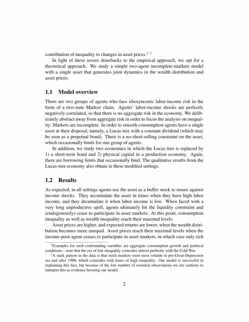
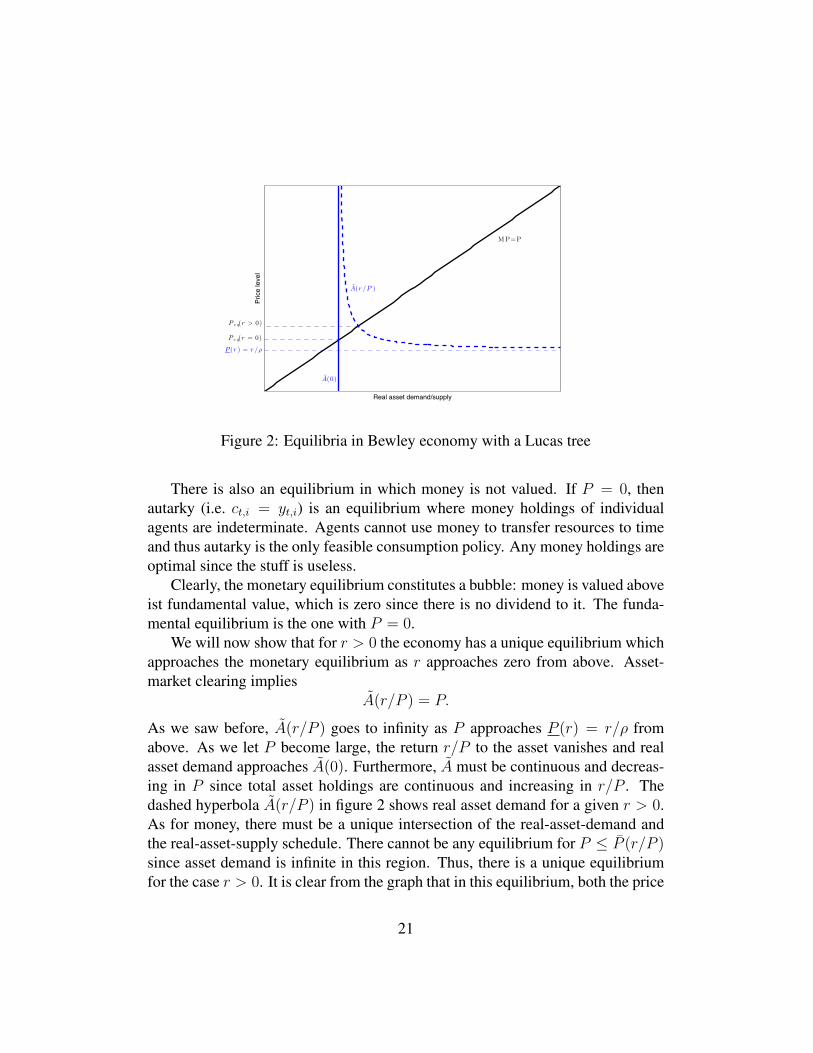
where the money supply M = 1 since we assumed that the asset is in unit supply.This equation pins down the price level in the economy as P = A(0) > 0. 10 Thesituation is illustrated in figure 2. The money demand schedule A(0) is a straightvertical line; for any price level the return of money is zero and so the demandfor real balances is invariant in P . The supply of real balances is given by the 45-degree line P . The unique intersection between the demand and supply schedulemarks the monetary equilibrium.11

10Note that the asset price P denotes the quantity of goods that can be obtained when sellingone unit of the asset. This is the inverse of how the price is usually denoted in monetary models:How much money do we need to buy one unit of the good.

11For a discussion of money in Bewley models see chapter 17 in Ljungqvist & Sargent (2004).

20

MP=P

A(0)

Real asset demand/supply

Pric

e le

vel

A(r /P )

P (r ) = r /!

P e q(r = 0)

P e q(r > 0)

Figure 2: Equilibria in Bewley economy with a Lucas tree

There is also an equilibrium in which money is not valued. If P = 0, thenautarky (i.e. ct,i = yt,i) is an equilibrium where money holdings of individualagents are indeterminate. Agents cannot use money to transfer resources to timeand thus autarky is the only feasible consumption policy. Any money holdings areoptimal since the stuff is useless.

Clearly, the monetary equilibrium constitutes a bubble: money is valued aboveist fundamental value, which is zero since there is no dividend to it. The funda-mental equilibrium is the one with P = 0.

We will now show that for r > 0 the economy has a unique equilibrium whichapproaches the monetary equilibrium as r approaches zero from above. Asset-market clearing implies

A(r/P ) = P.

As we saw before, A(r/P ) goes to infinity as P approaches P (r) = r/ρ fromabove. As we let P become large, the return r/P to the asset vanishes and realasset demand approaches A(0). Furthermore, A must be continuous and decreas-ing in P since total asset holdings are continuous and increasing in r/P . Thedashed hyperbola A(r/P ) in figure 2 shows real asset demand for a given r > 0.As for money, there must be a unique intersection of the real-asset-demand andthe real-asset-supply schedule. There cannot be any equilibrium for P ≤ P (r/P )since asset demand is infinite in this region. Thus, there is a unique equilibriumfor the case r > 0. It is clear from the graph that in this equilibrium, both the price

21

level P and real asset holdings A are above the levels in the monetary equilibriumof the fiat-money economy.

Furthermore, note that for any fixed P , real asset demand A(r/P ) approachesA(0) as we let r → 0. This clearly implies that the equilibrium price level andreal asset holdings converge to the monetary equilibrium as r → 0.

This seems to suggest that there must be a bubble in the price of the assetfor small r – after all, dividends become arbitrarily small while the price of theasset approaches a positive constant. Also, the limiting equilibrium constitutes abubble. However, we will now see that the equilibrium for r > 0 is actually nota bubble. Indeed, observe that when discounting future dividends by the equilib-rium interest rate r/P , we obtain∫ ∞

0

e−rPtrdt = r

P

r= P.

So the asset price equals the fundamental value of the asset and there is no bubble.This is possible since the interest rate and thus discounting go to zero in lockstepwith the dividend. For the limiting case of money the above expression contains adivision zero by zero and thus ceases to have meaning.

So interestingly, the price level Peq(r) and real asset holdings Aeq(r) associ-ated with the unique fundamental equilibrium for r > 0 converge to the bubbleequilibrium (and not the fundamental equilibrium) of the fiat-money economy aswe let r ↘ 0.12

3 The economy with a bondConsider the same setting as before, but now replace the tree with a bond as thesingle asset in the economy. Every agent can buy bonds bt ≥ −B at t, whereB ≥ 0 is an exogenous borrowing limit. The bond costs (1− qt∆t) at t and yieldsone unit of consumption at t+ ∆t. So qt is the bond yield. The budget constraintat t is

ct∆t+ bt(1− qt∆t) = (≤)yt∆t+ bt−∆t,

where bt−∆t is the asset position the agent has inherited from the previous period.Dividing by ∆t and taking limits ∆t→ 0, we find

ct + ab,t = yt + qtbt,

12We thank Viktor Tsyrennikov and Ludo Visschers for helpful discussions concerning the Be-wley economy.

22

where ab = lim∆t→0(bt − bt−∆t)/∆t denotes the drift in bonds.13 We see thatthere cannot be jumps in the position of the bond, if not consumption would havea mass point and cannot be smooth.

The Euler equation is easily derived as

Auc(c)uc(c)

= ρ− q,

which is of course entirely standard. In equilibrium, we look for a consumptionfunctionC(t, B, y), whereB ∈ [−B, B] is the asset position of agent 1. C(·) mustbe continuous in (t, B) for each y. (Clearly, we need a continuous consumptionfunction: If there was a jump in the function, then the growth rate of marginalutility is infinite when this jump is crossed, which makes it clearly desirable tore-allocate consumption between before and after the jump.)

Bond-market clearing requires that C + C = 1 (We re-normalize the totalendowment to 1, i.e. yl + yh = 1.). The two Euler equations are

ucc(C)

uc(C)

[Ct + (y + rB − C)CB

]+ η

[uc(C

′)

uc(C)− 1

]= ρ− q

ucc(1− C)

uc(1− C)

[− Ct − (y + rB − C)CB

]+ η

[uc(1− C ′)uc(1− C)

− 1

]= ρ− q

Again, assuming CARA preferences simplifies things considerably, since ucc/uc =−λ. Then, adding both equations and dividing by two yields

12

uc(C′)

uc(C)+ 1

2

uc(1− C ′)uc(1− C)

− 1 =ρ− qη

, (12)

so the average insurance motive in the economy determines the bond yield: Themore the average agent wants to insure, the lower the yield. Again, since eλ∆C

is strictly convex, higher consumption risk will translate into lower yields for theasset; the increase in demand for the asset by the agent with the downward riskis stronger that the decrease in demand for the agent with the upward risk for thisutility function. We can solve for the bond yield:

q = ρ− η(

12

uc(C′)

uc(C)+ 1

2

uc(1− C ′)uc(1− C)

− 1

)13Note that we can derive the same equation when starting from

ct∆t + bt = (≤)yt∆t + (1 + qt∆t)bt−∆t,

although here the yield from th bond is stochastic, i.e. it depends on the stat of y that realizes inthe next period. In continuous time this doesn’t seem to matter!!

23

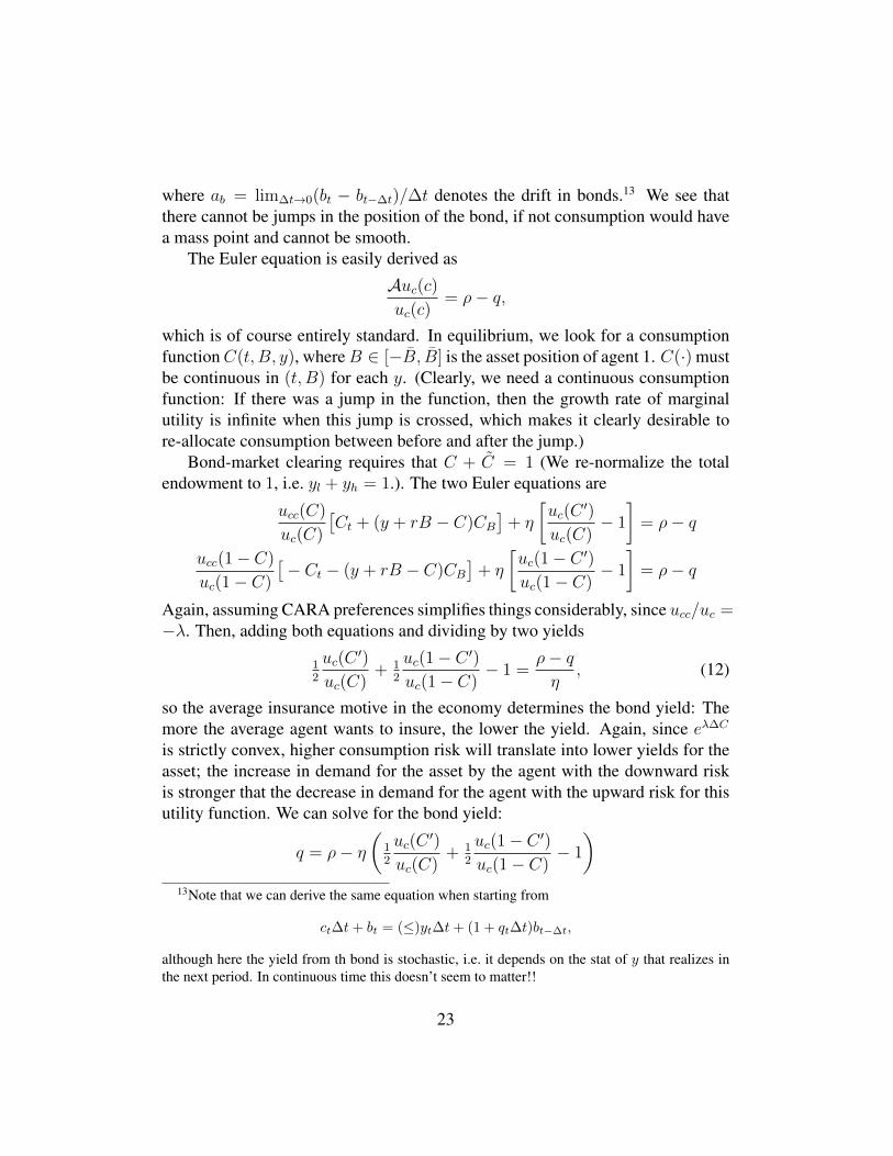
Again, it is instructive to think about the complete-markets case: if agents arefully insured and consumption is constant across time and states, then the insur-ance motives are one and the bond yield must equal ρ. The function eλ∆C tellsus how bond yields react to uncertainty. The higher ∆C, the larger the averageinsurance motive and the lower the bond yield. Increasing λ (the coefficient of ab-solute risk aversion) has the same effect. For a fixed ∆C, a higher λ means lowerbond yields since agents are more risk-averse and the average insurance motive ishigher.

Subtracting the agents’ Euler equations from each other and dividing by 2yields

C = Ct + (y + rB − C)CB =η

2λ

[uc(C

′)

uc(C)− uc(1− C ′)uc(1− C)

](13)

Again, the difference in insurance motives determines the trend in consumptionfor normal times.

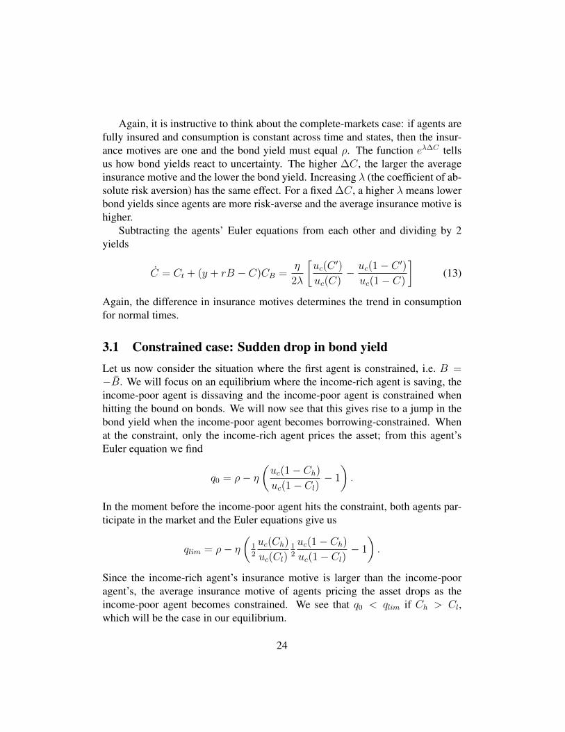
3.1 Constrained case: Sudden drop in bond yieldLet us now consider the situation where the first agent is constrained, i.e. B =−B. We will focus on an equilibrium where the income-rich agent is saving, theincome-poor agent is dissaving and the income-poor agent is constrained whenhitting the bound on bonds. We will now see that this gives rise to a jump in thebond yield when the income-poor agent becomes borrowing-constrained. Whenat the constraint, only the income-rich agent prices the asset; from this agent’sEuler equation we find

q0 = ρ− η(uc(1− Ch)uc(1− Cl)

− 1

).

In the moment before the income-poor agent hits the constraint, both agents par-ticipate in the market and the Euler equations give us

qlim = ρ− η(

12

uc(Ch)

uc(Cl)12

uc(1− Ch)uc(1− Cl)

− 1

).

Since the income-rich agent’s insurance motive is larger than the income-pooragent’s, the average insurance motive of agents pricing the asset drops as theincome-poor agent becomes constrained. We see that q0 < qlim if Ch > Cl,which will be the case in our equilibrium.

24

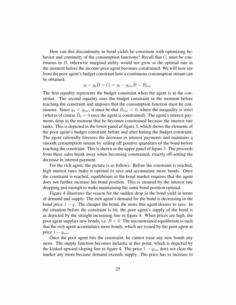
How can this discontinuity in bond yields be consistent with optimizing be-havior and continuity of the consumption functions? Recall that Cl must be con-tinuous in B, otherwise marginal utility would not grow at the optimal rate inthe moment before the income-poor agent becomes constrained. We will now seefrom the poor agent’s budget constraint how a continuous consumption stream canbe obtained:

yl − q0B = Cl = yl − qlimB − Blim.

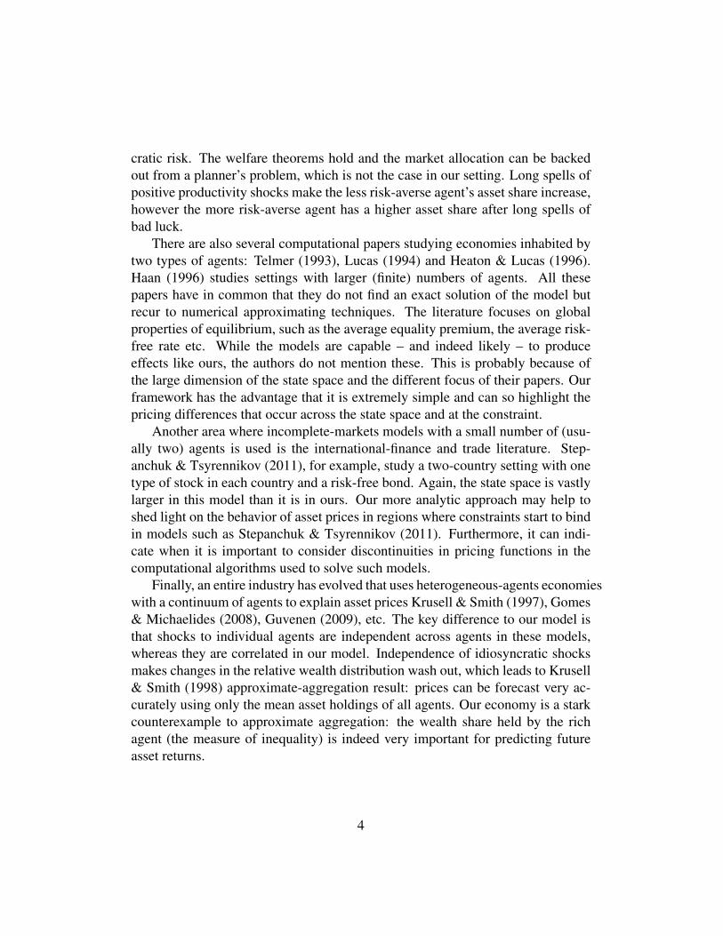
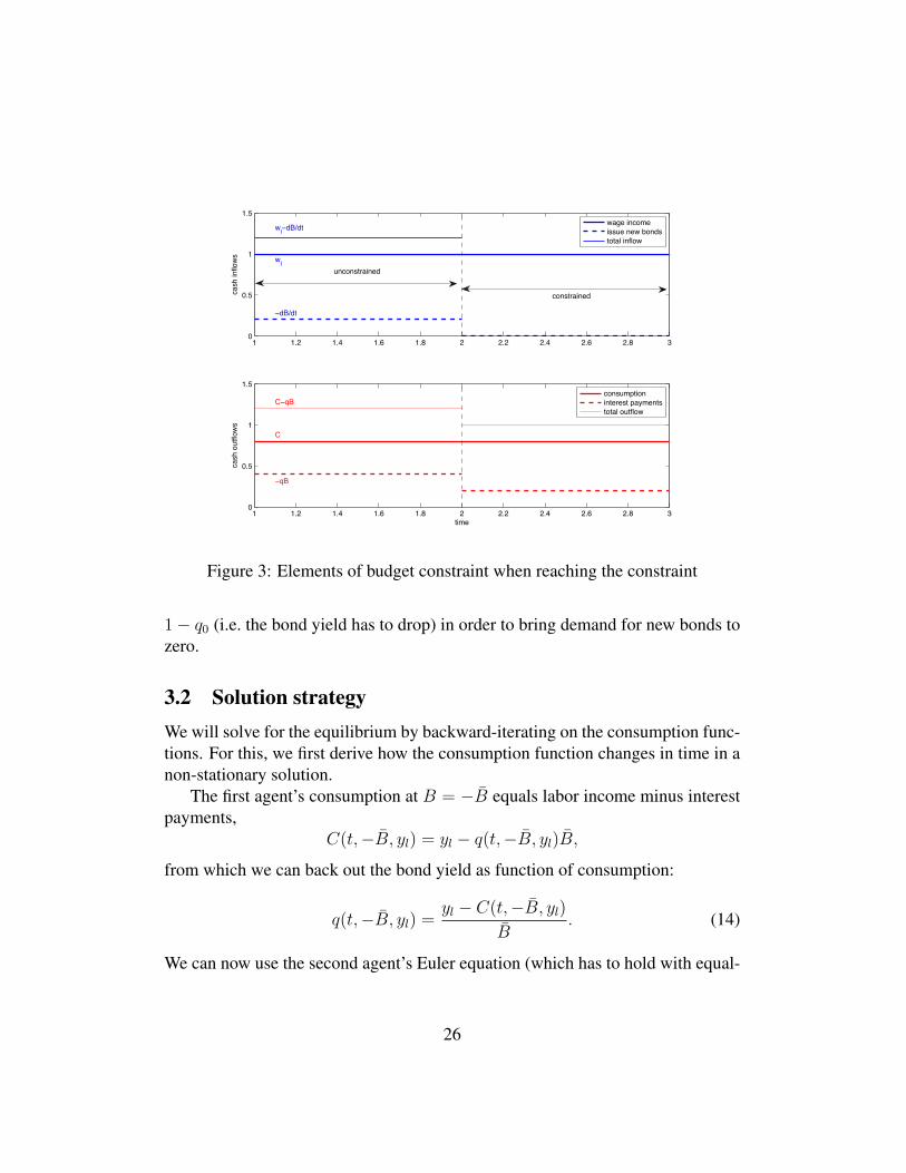
The first equality represents the budget constraint when the agent is at the con-straint. The second equality uses the budget constraint in the moment beforereaching the constraint and imposes that the consumption function must be con-tinuous. Since q0 < qlim, it must be that Blim < 0, where the inequality is strict(wheras of course B0 = 0 once the agent is constrained). The agent’s interest pay-ments drop in the moment that he becomes constrained because the interest ratetanks. This is depicted in the lower panel of figure 3, which shows the elements ofthe poor agent’s budget constraint before and after hitting the budget constraint.The agent rationally foresees the decrease in interest payments and maintains asmooth consumption stream by selling off positive quantities of the bond beforereaching the constraint. This is shown in the upper panel of figure 3. The proceedsfrom these sales break away when becoming constrained, exactly off-setting thedecrease in interest payment.

For the rich agent, the picture is as follows. Before the constraint is reached,high interest rates make it optimal to save and accumulate more bonds. Oncethe constraint is reached, equilibrium in the bond market requires that the agentdoes not further increase her bond position. This is ensured by the interest ratedropping just enough to make maintaining the same bond position optimal.

Figure 4 illustrates the reason for the sudden drop in the bond yield in termsof demand and supply. The rich agent’s demand for the bond is decreasing in thebond price 1 − q. The cheaper the bond, the more this agent desires to save. Inthe situation before the constraint is hit, the poor agent’s supply of the bond isas depicted by the straight increasing line in figure 4. When prices are high, thepoor agent supplies new bonds, i.e. B < 0. The unconstrained equilibrium is suchthat the rich agent accumulates more bonds, which are issued by the poor agent atprice 1− qlim.

Once the poor agent hits the constraint, he cannot issue any new bonds anymore. The supply function becomes inelastic at this point, which is depicted bythe kinked upward-sloping line in figure 4. The price 1 − qlim does not clear themarket any more because demand exceeds supply. The price has to increase to

25

1 1.2 1.4 1.6 1.8 2 2.2 2.4 2.6 2.8 30

0.5

1

1.5

cash

inflo

ws

wl

−dB/dt

wl−dB/dt wage incomeissue new bondstotal inflow

1 1.2 1.4 1.6 1.8 2 2.2 2.4 2.6 2.8 30

0.5

1

1.5

cash

out

flow

s

time

C

−qB

C−qBconsumptioninterest paymentstotal outflow

unconstrained

constrained

Figure 3: Elements of budget constraint when reaching the constraint

1− q0 (i.e. the bond yield has to drop) in order to bring demand for new bonds tozero.

3.2 Solution strategyWe will solve for the equilibrium by backward-iterating on the consumption func-tions. For this, we first derive how the consumption function changes in time in anon-stationary solution.

The first agent’s consumption at B = −B equals labor income minus interestpayments,

C(t,−B, yl) = yl − q(t,−B, yl)B,

from which we can back out the bond yield as function of consumption:

q(t,−B, yl) =yl − C(t,−B, yl)

B. (14)

We can now use the second agent’s Euler equation (which has to hold with equal-

26

0 (−dB/dt)_lim

1−q_lim

1−q_0

Unconstrained equilibrium

Constrained equilibrium

dB/dt

Bond

Pric

e

Constrained SupplySupplyDemand

Figure 4: Bond demand and supply at the constraint

ity, since he is not constrained) to find that

C(t,−B, y1) = Ct(t,−B, yl) =ρ

λ− yl − C(t,−B, yl)

λB− η

λ

(uc(1− C)

uc(1− C)− 1

),

(15)where we have used the fact that the economy stays put at B = −B, i.e. aB =yl − rB − C = 0 and so the term in CB is zero.

When the second agent is constrained, we analogously find

q(t, B, yh) =C(t, B, yh)− yh

B,

C(t, B, yh) = Ct(t, B, yh) = −ρλ

+C(t, B, yh)− yh

λB+η

λ

(uc(C)

uc(C)− 1

)Note that we can autonomously solve the PDE (or system of ODEs, in the

infinite-horizon case) for consumption given by equations (13) and (15) and thenback out the bond yield from this using (12) and (14). Economically, the restric-tion that both agents’ marginal utilities must grow at the same rate (plus continuityof consumption) is strong enough so that prices are not needed to solve for the al-location. Note that this is not the case in the economy with the risky asset, sinceasset returns are state-contingent there.

27

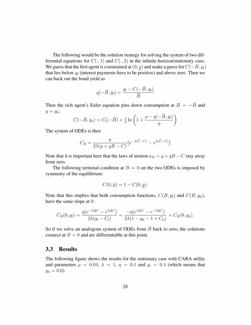
The following would be the solution strategy for solving the system of two dif-ferential equations for C(·, 1) and C(·, 2) in the infinite-horizon/stationary case:We guess that the first agent is constrained at (0, y) and make a guess forC(−B, yl)that lies below yl (interest payments have to be positive) and above zero. Then wecan back out the bond yield as

q(−B, yl) =yl − C(−B, yl)

B

Then the rich agent’s Euler equation pins down consumption at B = −B andy = yh:

C(−B, yh) = Cl(−B) + 1λ

ln

(1 +

ρ− q(−B, yl)η

)The system of ODEs is then

CB =η

2λ(y + qB − C)

(e−λ(C−C) − eλ(C−C)

)Note that it is important here that the laws of motion aB = y+ qB−C stay awayfrom zero.

The following terminal condition at B = 0 on the two ODEs is imposed bysymmetry of the equilibrium:

C(0, y) = 1− C(0, y).

Note that this implies that both consumption functions, C(B, yl) and C(B, yh),have the same slope at 0:

CB(0, yl) =η(e−λ∆C − eλ∆C)

2λ(yl − Cl)=−η(eλ∆C − e−λ∆C)

2λ(1− yh − 1 + Ch)= CB(0, yh).

So if we solve an analogous system of ODEs from B back to zero, the solutionsconnect at B = 0 and are differentiable at this point.

3.3 ResultsThe following figure shows the results for the stationary case with CARA utilityand parameters ρ = 0.04, λ = 1, η = 0.1 and yl = 0.4 (which means thatyh = 0.6).

28

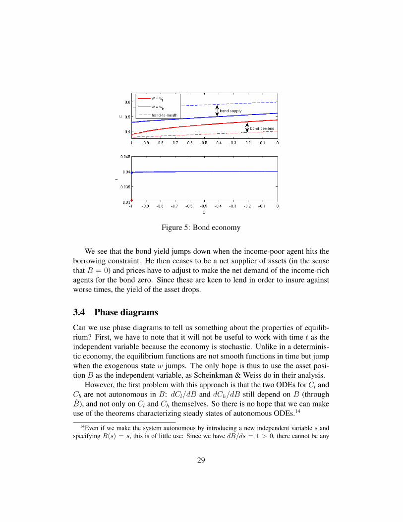
Figure 5: Bond economy

We see that the bond yield jumps down when the income-poor agent hits theborrowing constraint. He then ceases to be a net supplier of assets (in the sensethat B = 0) and prices have to adjust to make the net demand of the income-richagents for the bond zero. Since these are keen to lend in order to insure againstworse times, the yield of the asset drops.

3.4 Phase diagramsCan we use phase diagrams to tell us something about the properties of equilib-rium? First, we have to note that it will not be useful to work with time t as theindependent variable because the economy is stochastic. Unlike in a determinis-tic economy, the equilibrium functions are not smooth functions in time but jumpwhen the exogenous state w jumps. The only hope is thus to use the asset posi-tion B as the independent variable, as Scheinkman & Weiss do in their analysis.

However, the first problem with this approach is that the two ODEs for Cl andCb are not autonomous in B: dCl/dB and dCh/dB still depend on B (throughB), and not only on Cl and Ch themselves. So there is no hope that we can makeuse of the theorems characterizing steady states of autonomous ODEs.14

14Even if we make the system autonomous by introducing a new independent variable s andspecifying B(s) = s, this is of little use: Since we have dB/ds = 1 > 0, there cannot be any

29

However, we can still follow Scheinkman & Weiss and make some inferencein a Cl − Ch-diagram when just considering the signs of dCl/dB and dCh/dB.Let us assume that in equilibrium the income-rich agent always saves (Bh > 0)and the income-poor agent always dissaves (Bl < 0), at least on the interior ofthe state space. This essentially means that we restrict the analysis on a subset Sof the full (B,Cl, Ch)-space and on the trajectories that stay within this subset S.If we make this restriction, we can proceed in the same way as Scheinkman &Weiss. The signs of dCl/dB and dCh/dB now depend solely on the sign of thefunction

Γ(C,C ′) =uc(C

′)

uc(C)− uc(1− C ′)uc(1− C)

,

which is the difference in the insurance motives. We have Γ(C,C ′) = 0 iff C =C ′. So both consumption functions stay constant in B if and only if Cl = Chat the initial condition. Whenever Ch > Cl, then both dCl/dB and dCh/dB arestrictly positive. Also, we will always stay in the region where Ch > Cl since thetrajectory cannot cross a steady state Ch = Cl (trajectories cannot cross). Thisis the economically reasonable case: Consumption functions are increasing inincome and in assets. The economically unreasonable case arises when Ch < Cl.We will then always stay in the region where Ch < Cl and both dCl/dB anddCh/dB are negative throughout.

Analysis using this two-dimensional diagram becomes more complicated ifwe try to allow arbitrary signs of B. The signs of dCl/dB and dCh/dB thendepend on both the sign of Γ and the signs of Bl and Bh. However, the locuswhere Bl = 0 (or Bh = 0) in the Cl − Ch-plane changes when B changes. Thismakes it hard to analyze trajectories (although it might still be possible).

4 Capital accumulationConsider now an economy with standard capital accumulation and a Cobb-Douglasproduction function. Capital is the only asset, and capital holdings cannot be nega-tive for any of the two agents. The labor endowment zt follows a two-state Markovchain just as yt did before (however now, wages are endogenous since they dependon the capital-labor ratio).

The law of motion for an agents capital holdings kt isdktdt

= (rt − δ)kt + ztwt − ct.

steady state in this three-dimensional system.

30

For an unconstrained agent (i.e. kt > 0), the consumption process C must fulfillthe Euler equation

Auc(C)

uc(C)= η

[uc(C

′)

uc(C)− 1

]+ucc(C)

uc(C)

[Ct + Ck + Ck︸ ︷︷ ︸

=C

]= ρ+ δ − r,

where r is a function of the aggregate capital stock Kt = kt + kt.Now, let us assume CARA preferences as before. Then, when both agents

participate in asset markets, adding the two Euler equations yields

C + ˙C︸ ︷︷ ︸=Cagg

= r − δ − ρ+ η

[12

uc(C′)

uc(C)+ 1

2

uc(C′)

uc(C)− 1

].

The higher r (i.e. the lower the capital stock K), the higher consumption growth.Since consumption is increasing inK, this means that capital is accumulated whenits returns are high. Also, if the average insurance motive in the economy is high,then consumption growth and capital accumulation are high (unless a reversalhappens).

Subtracting the two Euler equations yields

C − ˙C =η

λ

[uc(C

′)

uc(C)− uc(C

′)

uc(C)

].

So as before, the difference in the two insurance motives is linked to consumptiongrowth in normal times. If agent 1 is in the good income state (and thus fears areversal and has a high insurance motive), then agent 2 would welcome a reversaland has thus a low insurance motive. This means agent 1 is saving and his con-sumption trends upward (in normal times), wheras agent 2 is dissaving and hisconsumption trends downward relative to agent 1 in normal times.

4.1 P-K spaceThe laws of motion for P and K are

K = (r − δ)K + w − C − C = Y − δK − C − C

P =(z − P )w

K+PC

K− (1− P )C

K

31

So if z > P (i.e. agent 1’s share of labor income is higher than his share ofcapital income), then P trends upward (when taking consumption decisions outof the picture). As for consumption, things are straighforward: When agent 1’sconsumption is high, then his asset share tends to decrease; when agent 2’s con-sumption is high, this tends to tilt the asset distribution in agent 1’s favor.

4.2 The constrained caseWhen agent 2 is constrained (i.e. k = 0), then only agents of type 1 price the asset.We have C = (1− z)w and

C =r − δ − ρ

λ+η

λ

[uc(C

′)

uc(C)− 1

].

So since agent 1 has consumption risk in this situation, any stationary point (i.e.C = 0) must have an interest rate lower than in the representative-agent case. Ingeneral, this insurance motive increases consumption growth, which means highersavings.

Another noteworthy feature is the point when k reaches zero. Note that in thismoment, the average insurance motive of participants in the asset market jumpsupward, which implies that average consumption growth of asset-market partici-pants jumps upward (since K and thus r is continuous in time). So the trend ofcapital returns changes since the savings rate changes.

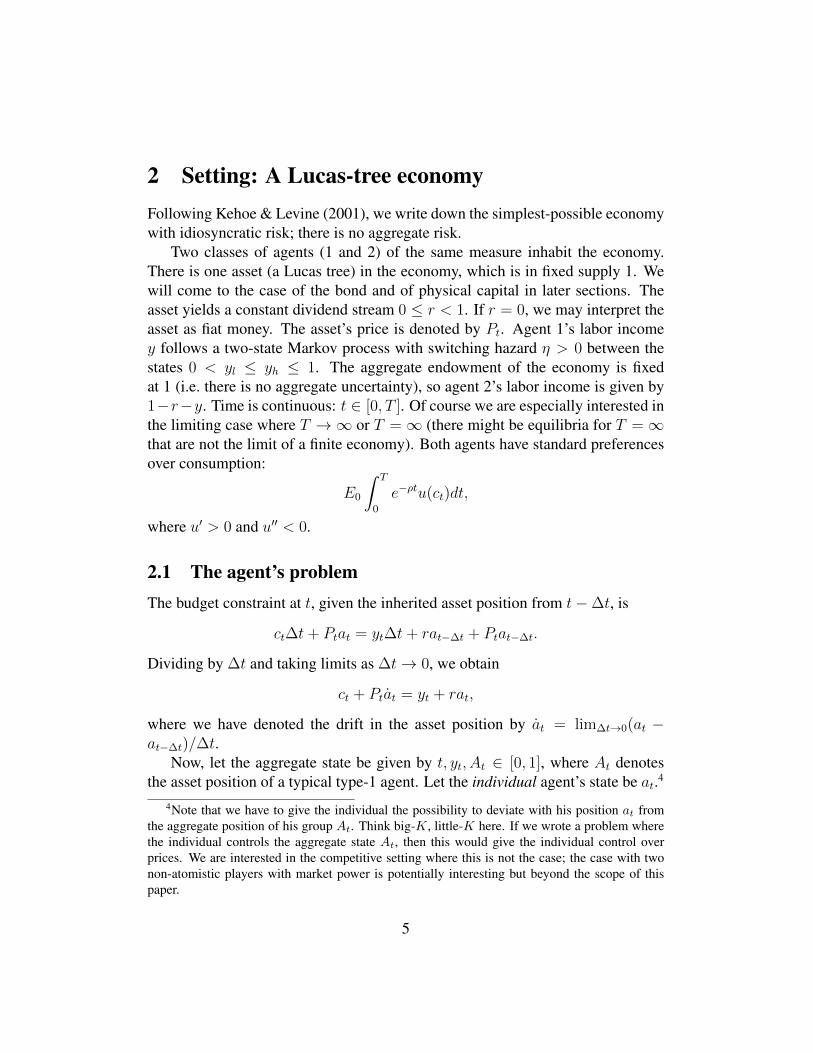
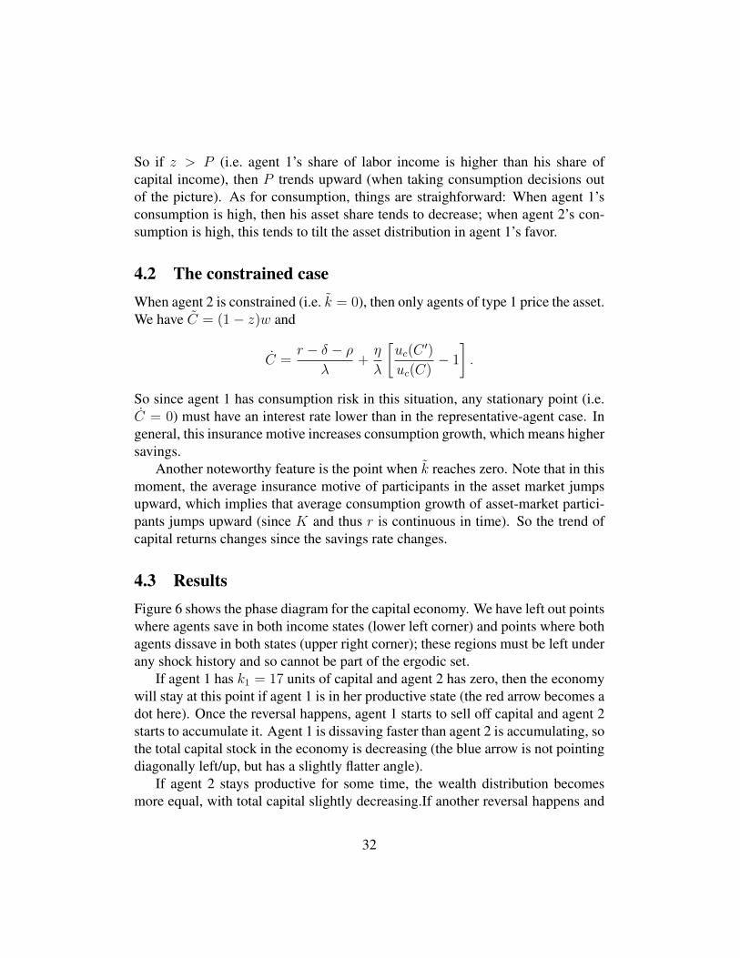
4.3 ResultsFigure 6 shows the phase diagram for the capital economy. We have left out pointswhere agents save in both income states (lower left corner) and points where bothagents dissave in both states (upper right corner); these regions must be left underany shock history and so cannot be part of the ergodic set.

If agent 1 has k1 = 17 units of capital and agent 2 has zero, then the economywill stay at this point if agent 1 is in her productive state (the red arrow becomes adot here). Once the reversal happens, agent 1 starts to sell off capital and agent 2starts to accumulate it. Agent 1 is dissaving faster than agent 2 is accumulating, sothe total capital stock in the economy is decreasing (the blue arrow is not pointingdiagonally left/up, but has a slightly flatter angle).

If agent 2 stays productive for some time, the wealth distribution becomesmore equal, with total capital slightly decreasing.If another reversal happens and

32

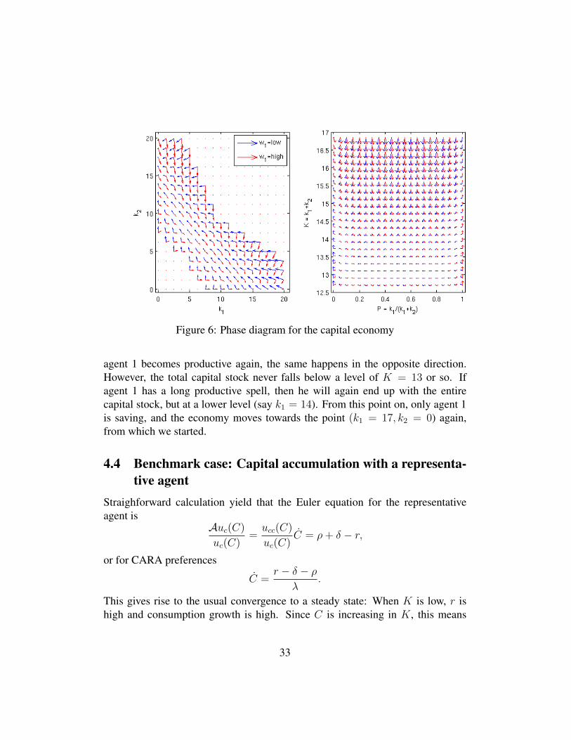
Figure 6: Phase diagram for the capital economy

agent 1 becomes productive again, the same happens in the opposite direction.However, the total capital stock never falls below a level of K = 13 or so. Ifagent 1 has a long productive spell, then he will again end up with the entirecapital stock, but at a lower level (say k1 = 14). From this point on, only agent 1is saving, and the economy moves towards the point (k1 = 17, k2 = 0) again,from which we started.

4.4 Benchmark case: Capital accumulation with a representa-tive agent

Straighforward calculation yield that the Euler equation for the representativeagent is

Auc(C)

uc(C)=ucc(C)

uc(C)C = ρ+ δ − r,

or for CARA preferences

C =r − δ − ρ

λ.

This gives rise to the usual convergence to a steady state: When K is low, r ishigh and consumption growth is high. Since C is increasing in K, this means

33

the agent is saving until reaching the steady state where r = δ + ρ. The agent isdissaving and consumption is decreasing when we start at a capital stock abovethe steady-state level.

In the steady state, we have

rss = ρ+ δ

Kss =

(α

ρ+ δ

) 11−α

ReferencesAtkinson, A., Piketty, T. & Saez, E. (2011), ‘Top incomes in the long run of

history’, Journal of Economic Literature 49, 3–71.

Dumas, B. (1989), ‘Two-person dynamic equilibrium in the capital market’, TheReview of Financial Studies 2, 157–188.

Gomes, F. & Michaelides, A. (2008), ‘Asset pricing with limited risk sharing andheterogeneous agents’, The Review of Financial Studies 21, 416–448.

Guvenen, F. (2009), ‘A parsimonious macroeconomic model for asset pri’, Ec77, 1711–1750.

Haan, W. J. D. (1996), ‘Heterogeneity, aggregate uncertainty, and the short-terminterest rate’, Journal of Business & Economic Statistics, 14, 399–411.

Heaton, J. & Lucas, D. J. (1996), ‘Evaluating the effects of incomplete markets onrisk sharing and asset pricing’, The Journal of Political Economy 104, 443–487.

Kehoe, T. J. & Levine, D. K. (2001), ‘Liquidity constrained markets versus debtconstrained markets’, Ec 691, 575–598.

Kennickell, A. B. (2009), Ponds and streams: Wealth and income in the u.s., 1989to 2007. Working Paper.

Krusell, P. & Smith, A. (1997), ‘Income and wealth heterogeneity, portfoliochoice, and equilibrium asset returns’, Macroeconomic Dynamics 1, 387–422.

Krusell, P. & Smith, A. (1998), ‘Income and wealth heterogeneity in the macroe-conomy’, The Journal of Political Economy 106, 867–896.

34

Lindert, P. (2000), ‘Three centuries of inequality in britain and america’, Hand-book of Income Distribution, Volume I pp. 167–216.

Ljungqvist, L. & Sargent, T. J. (2004), Recursive Macroeconomic Theory, 2ndEdition, Cambridge: MIT Press.

Lucas, D. J. (1994), ‘Asset pricing with undiversifiable income risk and short salesconstraints: Deepening the equity premium puzzle’, Journal of MonetaryEconomics 34, 325–341.

Scheinkman, J. A. & Weiss, L. (1986), ‘Borrowing constraints and aggregate eco-nomic activity’, Econometrica 54, 23–45.

Stepanchuk, S. & Tsyrennikov, V. (2011), International portfolios: An incompletemarkets general equilibrium approach. Working Paper.

Telmer, C. I. (1993), ‘Asset-pricing puzzles and incomplete markets’, The Journalof Finance 48, 1803–1832.

35