Induction - Rochester Institute of Technology

Models of Computation, 2010 1

Induction

We use a lot of inductive techniques in this course, both to give definitions

and to prove facts about our semantics. So, it’s worth taking a little while to

set out exactly what a proof by induction is, what a definition by induction is,

and so on.

When designing an algorithm to solve a problem, we want to know that the

result produced by the algorithm is correct, regardless of the input. For ex-

ample, the quicksort algorithm takes a list of numbers and puts them into

ascending order. In this example, we know that the algorithm operates on a

list of numbers, but we do not know how long that list is or exactly what num-

bers it contains. Similarly, one may raise questions about depth-first search

of a tree: how do we know it always visits all the nodes in a tree if we do not

know the exact size and shape of the tree?

In examples such as these, there are two important facts about the input data

which allows us to reason about arbitrary inputs:

• the input is structured: for example, a non-empty list has a first ele-

ment and a ‘tail’, which is the rest of the list, and the binary tree has a

root node and two subtrees;

• the input is finite.

In this situation, the technique of structural induction provides a principle by

which we may formally reason about arbitrary lists, trees, and so on.


Slide 1

What is induction for?

Induction is a technique for reasoning about and working with

collections of objects (things!) which are

• structured in some well-defined way;

• finite but arbitrarily large and complex.

Induction exploits the finite, structured nature of these objects to

overcome their arbitrary complexity.

These kinds of structured, finite objects arise in many areas of computer

science. Data structures such as lists and trees are common, but in fact

programs themselves can be seen as structured finite objects. This means

that induction can be used to prove facts about all programs in a certain

language. In semantics, we use this very frequently. We will also make use

of induction to reason about purely semantic notions, such as derivations of

assertions in the operational semantics of a language.

Mathematical Induction

The simplest form of induction is mathematical induction: that is to say, in-

duction over the natural numbers. The principle can be described as follows:

given a property P ( ) of natural numbers, to prove that P (n) holds for all

natural numbers n, it is enough to:

• prove that P (0) holds; and

• prove that if P (k) holds for arbitrary natural number k, then P (k+1)holds too.


Slide 2

You can use induction...

... to reason about things like

• natural numbers: each one is finite, but a natural number could be

arbitrary big;

• data structures such as lists, trees and so on;

• programs in a programming language: again, you can write

arbitrarily large programs, but they are always finite;

• derivations of semantic assertions like E ⇓ 4: these derivations

are finite trees of axioms and rules.

Slide 3

Proof by Mathematical Induction

Let P ( ) be a property of natural numbers. The principle of

mathematical induction states that if

P (0) ∧ [∀k.P (k) ⇒ P (k + 1)]

holds then

∀n.P (n)

holds. The number k is called the induction parameter.


Slide 4

Writing an Inductive Proof

To prove that P (n) holds for all natural numbers n, we must do two

things:

Base Case: prove that P (0) holds, any way we like.

Inductive Step: let k be an arbitrary number, and assume that P (k)

holds. This assumption is called the induction hypothesis (or IH) ,

with parameter k. Using this assumption, prove that P (k + 1) holds.

It should be clear why this principle is valid: if we can prove the two things

above, then we know:

• P (0) holds;

• since P (0) holds, P (1) holds;



• ...

Therefore, P (n) holds for any n, regardless of how big n is. This conclusion

can only be be drawn because every natural number can be reached by

starting at zero and adding one repeatedly. The two elements of the induction

can be read as saying:

• Prove that P is true at the place where you start: that is, at zero.

• Prove that the operation of adding one preserves P : that is, if P (k)is true then P (k + 1) is true.

Since every natural number can be ‘built’ by starting at zero and adding one

repeatedly, every natural number has the property P : as you build the num-

ber, P is true of everything you build along the way, and it’s still true when

you’ve build the number you’re really interested in.


Example

Here is perhaps the simplest example of a proof by mathematical induction.

We shall show thatn∑

i=0

i =n2 + n

2

So here the property P (n) is

the sum of numbers from 0 to n inclusive is equal to n2+n

2 .

Base Case: The base case, P (0), is

the sum of numbers from 0 to 0 inclusive is equal to 02+02 .

This is obviously true, so the base case holds.

Inductive Step: Here the inductive hypothesis, IH for parameter k, is the

statement P (k):

the sum of numbers from 0 to k inclusive is equal to k2+k

2 .

From this inductive hypothesis, with parameter k, we must prove that

the sum of numbers from 0 to k + 1 inclusive is equal to(k+1)2+(k+1)

2.

The proof is a simple calculation:

k+1∑

i=0

i = (k∑

i=0

i) + (k + 1)

=k2 + k

2+ (k + 1) using IH for k

=k2 + k + 2k + 2

2

=(k2 + 2k + 1) + (k + 1)

2

=(k + 1)2 + (k + 1)

2

which is what we had to prove.


Defining Functions and Relations over Natural Numbers

As well as using induction to prove properties of natural numbers, we can

use it to define functions which operate on natural numbers.

Just as proof by induction proves a property P (n) by considering the case of

zero and the case of adding one to a number known to satisfy P , so definition

of a function f by induction works by giving the definition of f(0) directly, and

building the value f(k + 1) out of f(k).

All this is saying is that if you define the value of a function at zero, by giving

some value a, and you show how to calculate the value at k + 1 from that at

k, then this does indeed define a function. This function is ‘unique’ , meaning

that it is completely defined by the information you have given; there is no

choice about what f can be.

Roughly, the fact that we use f(k) to define f(k + 1) in this definition

corresponds to the fact that we assume P (k) to prove P (k + 1) in a proof

by induction.

Slide 5

Definition by induction

We can define a function f on natural numbers by:

Base Case: giving a value for f(0) directly.

Inductive step: giving a value for f(k + 1) in terms of f(k).


Slide 6

Inductive Definition of Factorial

The factorial function fact is defined inductively on the natural

numbers:

• fact(0) = 1;

• fact(k + 1) = (k + 1) × fact(k).

For example, slide 6 gives an inductive definition of the factorial function over

the natural numbers. Slide 7 contains another definitional use of induction.

We have already defined the one-step operational semantics on expressions

E from SimpleExp. This is represented as a relation E → E′ over ex-

pressions. Suppose we wanted to define what is the effect of k reduction

steps, for any natural number k. This would mean defining a family of rela-

tions →k, one for each natural number k. Intuitively, E →k E′ is supposed

to meant that by applying exactly k computation rules to E we obtain E′.


Slide 7

Multi-step Reductions in SimpleExp

The relation E →n E′ is defined inductively by:

• E →0 E for every simple expression E in SimpleExp;

• E →k+1 E′ if there is some E′′ such that

E →k E′′ and E′′ → E′

In slide 7, the first point defines the relation →0 outright. In zero steps an

expression remains untouched, so E →0 E for every expression E. In the

second clause, the relation →(k+1) is defined in terms of →k . It says that

E reduces to E′ in (k + 1) steps if

• there is some intermediary expression E′′ to which E reduces to in

k steps;

• this intermediary expression E′′ reduces to E′ in one step.

The principle of induction now says that each of the infinite collection of rela-

tions →n are well-defined.

A Structural View of Mathematical Induction

We said in the last section that mathematical induction is a valid principle

because every natural number can be ‘built’ using zero as a starting point

and the operation of adding one as a method of building new numbers from

old. We can turn mathematical induction into a form of structural induction by

viewing numbers as elements in the following grammar:

N ::= zero |succ(N).


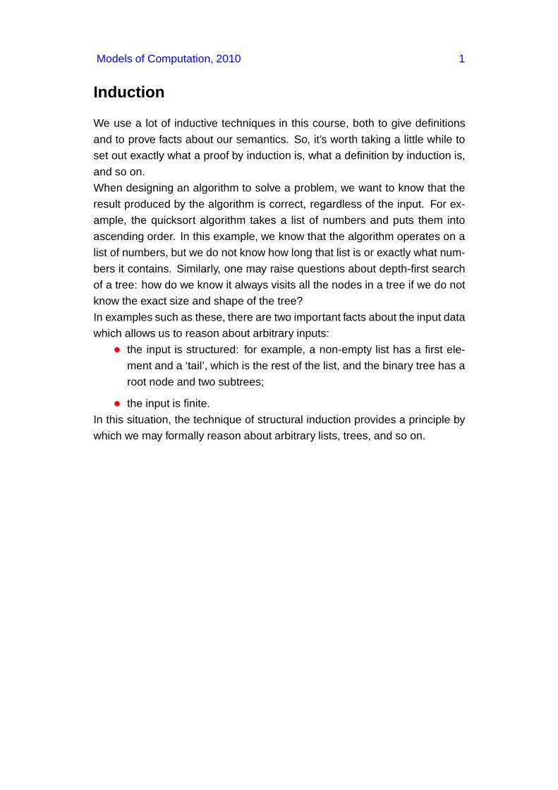
Here succ, short for successor, should be thought of as the operation of

adding one. Therefore, the number 0 is represented by zero and 3 is rep-

resented by

succ(succ(succ(zero)))

With this view, it really is the case that a number is built by starting from

zero and repeatedly applying succ. Numbers, when thought of like this,

are finite, structured objects. The principle of induction now says that, to

prove P (N) for all numbers N , it suffices to do two things:

Base Case: prove that P (0) holds.

Inductive Step: the inductive hypothesis IH is that P (K) holds for some

number K ; from this IH, prove that P (succ(K)) also holds.

This is summarized in slide 8.

Slide 8

Structural view of Mathematical Induction

We can view the natural numbers as elements of the following

grammar:

N ::= zero |succ(N).

To prove that property P (N) holds for every number N :

Base Case: prove P (zero) holds.

Inductive Step: the IH is that P (K) holds for some K ; assuming IH,

prove that P (succ(K)) follows.

Defining Functions

The principle of defining functions by induction works for this representation

of the natural numbers in exactly the same way as before. To define a function

f which operates on these numbers, we must


• define f(zero) directly;

• define f(succ(K)) in terms of f(K).

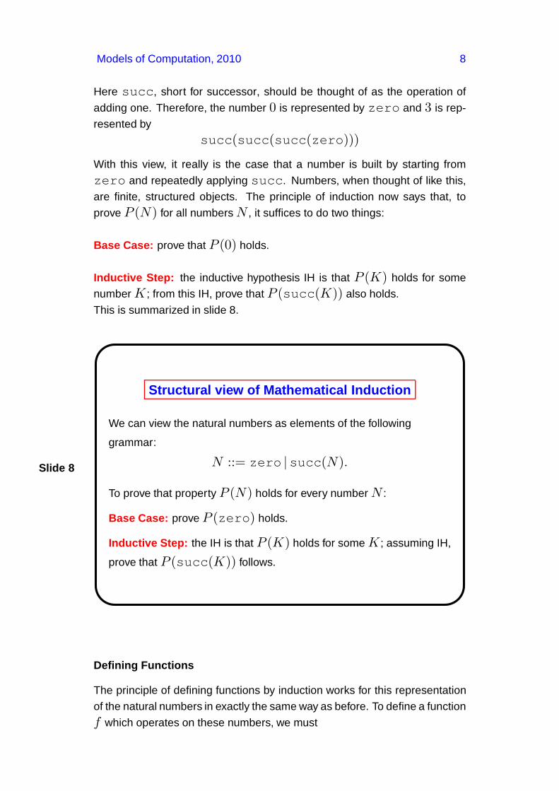
Structural Induction for Binary Trees

Binary trees are a commonly used data structure. Roughly, a binary tree is

either a single leaf node, or a branch node which has two subtrees.

Slide 9

A Syntax for Binary Trees

Binary trees are defined as elements of the following grammar:

bTree ::= Node | Branch(bTree,bTree)

Note the similarity with arithmetic expressions.

The principle of structural induction over binary trees states that to prove a

property P (T ) for all trees T , it is sufficient to do the following two things:

Base Case: prove that P (Node) holds;

Inductive Step: the inductive hypothesis IH is that P (T1) and P (T2) hold

for some arbitrary binary trees T1 and T2; then from this assumption prove

that P (Branch(T1, T2)) also holds.

Structural Induction over Simple Expressions

The syntax of our illustrative language SimpleExp also gives a collection of

structured, finite, but arbitrarily large objects over which induction may be


used. The syntax is repeated below:

E ∈ SimpleExp ::= n | (E + E) | (E × E)

Recall that n ranges over the numerals 0,1,2, ... This means that, in this

language, there are in fact an infinite number of indecomposable expressions;

contrast this with the cases above, where 0 is the only indecomposable nat-

ural number, and Node is the only indecomposable binary tree. Also, note

that we can build new expressions from old in two ways, by using + and ×.

The principle of induction for expressions reflects these differences as fol-

lows. If P is a property of expressions, then to prove that P (E) holds for

any E, we must do the following:

Base Cases: prove that P (n) holds for every numeral n.

Inductive Step: here the inductive hypothesis IH is that P (E1) and P (E1)hold for some E1 and E2; assuming IH, prove that both P ((E1 + E2))and P ((E1 × E2)) follow.

The conclusion will then be that P (E) is true for every expression E. Again,

this induction principle can be seen as a case analysis: expressions come in

two forms:

• numerals , which cannot be decomposed, so we have to prove P (n)directly for each of them; and

• composite expressions (E1 + E2) and (E1 × E2), which can

be decomposed into subexpressions E1 and E2. In this case, the

induction hypothesis says that we may assume P (E1) and P (E2)when trying to prove P ((E1 + E2)) and P ((E1 × E2)).


Slide 10

Structural Induction for Terms of SimpleExp

To prove that property P ( ) holds for all terms in SimpleExp, it

suffices to prove:

Base Cases: P (n) holds for all n;

Inductive Step: the IH is that P (E1) and P (E2) both hold for some

arbitrary expression E1 and E2; from IH we must prove that

P (E1 + E2) and P (E1 × E2) follow.

Slide 11

Determinacy and Normalization

Determinacy says that a simple expression cannot evaluate to more

than one answer:

for any expression E, if E ⇓ n and E ⇓ n′ then n = n′.

This proof is a little tricky. See the notes.

Normalization says that a simple expression evaluates to at least one

answer:

for every expression E, there is some n such that E ⇓ n.

This is proved by induction on the structure of E.


It is not difficult to show by induction on the structure of expressions that, for

any expression E, there is some numeral n for which E ⇓ n. Recall that

this property is called normalization: it says that all programs in our language

have a final answer or so-called ‘normal form’. It goes hand in hand with

another property, called determinacy, which states that the final answer is

unique.

Exercise (Normalization) For every expression E, there is some n such

that E ⇓ n.

Defining Functions over Simple Expressions

We may also use the principle of induction to define functions which operate

on simple expressions.

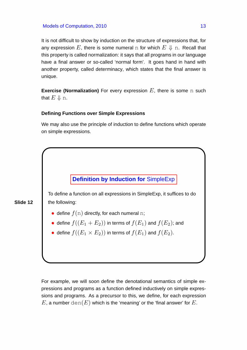
Slide 12

Definition by Induction for SimpleExp

To define a function on all expressions in SimpleExp, it suffices to do

the following:

• define f(n) directly, for each numeral n;

• define f((E1 + E2)) in terms of f(E1) and f(E2); and

• define f((E1 × E2)) in terms of f(E1) and f(E2).

For example, we will soon define the denotational semantics of simple ex-

pressions and programs as a function defined inductively on simple expres-

sions and programs. As a precursor to this, we define, for each expression

E, a number den(E) which is the ‘meaning’ or the ‘final answer’ for E.


Slide 13

The function den

For each simple expression E, a number den(E) is defined

inductively on the structure of E by:

• den(n) = n for each numeral n;

• den((E1 + E2)) = den(E1) + den(E2);

• den((E1 × E2)) = den(E1) × den(E2);

Exercise For every simple expression E and number n,

den(E) = n if and only if E ⇓ n.

Again, this definition should be regarded as showing how to build up the

‘meaning’ of a complex expression, as the expression itself is built up from

numberals and uses of + and ×.

Structural Induction over Derivations

Another example of a collection of finite, structured objects which we have

seen is the collection of proofs of statements E ⇓ n in the big-step seman-

tics of SimpleExp. In general, an operational semantics given by axioms and

proof rules defines a collection of proofs of this kind, and induction is avail-

able to us for reasoning about them. [To clarify the presentation, we will refer

to such proofs as derivations in this section.]

Recall the derivation of (3+(2+1)) ⇓ 6:

(B-ADD)

(B-NUM)3 ⇓ 3

(B-ADD)

(B-NUM)2 ⇓ 2

(B-NUM)1 ⇓ 1

(2+ 1) ⇓ 3

(3+(2+1)) ⇓ 6


This derivation has three key elements: the conclusion (3+(2+1)) ⇓ 6,

and the two subderivations, which are

(B-NUM)3 ⇓ 3

(B-ADD)

(B-NUM)2 ⇓ 2

(B-NUM)1 ⇓ 1

(2+ 1) ⇓ 3

We can think of a complex derivation like this as a structured object:

......

D1 D2

......

h1 h2

c

Here, we see a derivation whose last line is

h1 h2

c

where h1 and h2 are the hypothesis (or premises) of the rule and c is the

conclusion of the rule; c is also the conclusion of the whole derivation. Since

the hypotheses themselves must be derived, there are subderivations D1

and D2 with conclusions h1 and h2.

The only derivations which do not decompose into a last rule and a collection

of subderivations are those which are simply axioms. Our principle of induc-

tion will therefore treat the axioms as the base cases, and the more complex

proof as the inductive step.

The principle of structural induction for derivations says that, to prove a

property P (D) for every derivation D, it is enough to do the following:

Base Cases: Prove that P (A) holds for every axiom. In the case of the

big-step semantics, we must prove that every derivation

n ⇓ n

satisfies property P .

Inductive Step: For each rule of the form

h1 hn

c


prove that any derivation ending with a use of this rule satisfies the property.

Such a derivation has subderivations with conclusions h1, ..., hn, and we

may assume that property P holds for each of these subderivations. These

assumptions form the inductive hypothesis.

We give a proof of determinacy for the big-step operational semantics on

simple expressions, using structural induction on derivations. The proof is a

little tricky. We also give a proof of determinacy for the small-step semantics

using induction on derivations. We shall see that it is a little easier.

Proposition (Determinacy) For any simple expression E, if E ⇓ n and

E ⇓ n′ the n = n′.

Proof We prove this by induction on the structure of the derivation of E ⇓ n.

This in itself requires a little thought. The property we wish to prove is:

for any derivation D, if the conclusion of D is E ⇓ n, and it is

also the case that E ⇓ n′ is derivable, then n = n′.

So, during this proof, we will consider

• a derivation D of a statement E ⇓ n; and

• another statement E ⇓ n′ which is derivable.

and try to show that n = n′. We apply induction to the derivation of D, and

not to the derivation of E ⇓ n′.

Base Case: E ⇓ n is an axiom. In this case, E = n. We also have

E ⇓ n′: that is, n ⇓ n′. By examining the rules of the big-step semantics,

it is clear that this can only be the case if n ⇓ n′ is an axiom. It follows that

n = n′.

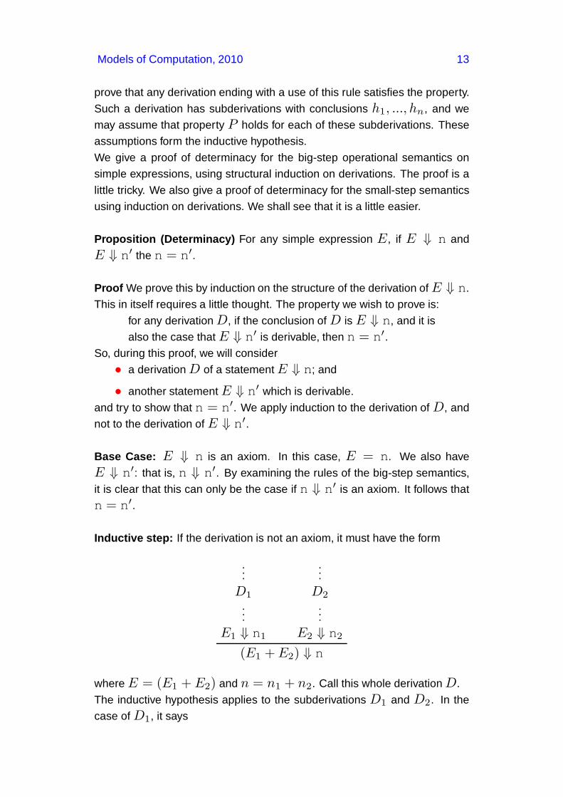
Inductive step: If the derivation is not an axiom, it must have the form

......

D1 D2

......

E1 ⇓ n1 E2 ⇓ n2

(E1 + E2) ⇓ n

where E = (E1 + E2) and n = n1 + n2. Call this whole derivation D.

The inductive hypothesis applies to the subderivations D1 and D2. In the

case of D1, it says


since D1 has conclusion E1 ⇓ n1, if a statement E1 ⇓ n′′ is

derivable, then n1 = n′′.

We will use this in a moment.

We must show that if E ⇓ n′ then n = n′. So suppose that E ⇓ n′: that

is, (E1 + E2) ⇓ n′ is derivable. This could not be derived using an axiom,

so it must be the case that it was derived using the rule

E1 ⇓ n3 E2 ⇓ n4

(E1 + E2) ⇓ n′

where n′ = n3 + n4. This means that E1 ⇓ n3 and E2 ⇓ n4 is derivable.

Using the induction hypothesis as spelled out above, we may assume that

n1 = n3.

Similarly, applying the induction hypothesis to D2, we may assume that

n2 = n4. Since we have the equations n = n1 + n2 and n′ = n3 + n4,

it follows that n = n′ as required. �

This is a tricky proof, because we not only do induction on the derivation of

E ⇓ n, but we must also perform some analysis on the derivation of E ⇓ n′

too. Don’t get too worried about understanding this proof, but do attempt to

understand the technique because it crops up all the time in semantics.

Some Proofs about the Small-step Semantics

We have seen how to use induction to prove some simple facts about the

big-step semantics of SimpleExp. In this section, we will see how to carry out

similar proofs for the small-step semantics, both to reassure ourselves that

we are on the right course and to make some intuitively obvious facts about

our language into formal theorems.


Slide 14

Some properties of →

Strong determinacy If E → E1 and E → E2 then E1 = E2.

Determinacy If E →∗ n and E →∗ n′ then n = n′.

Normalization For all E, there is some n such that E →∗ n.

An important property of the small-step semantics is that it is deterministic

in a very strong sense: not only does each expression have at most one

final answer, as in the big-step semantics, but also each expression can be

evaluated to its final answer in exactly one way. Here, we give a proof of

strong determinacy using structural induction on derivations. It is also possi-

ble to do a proof based on structural induction on the structure of expressions.

(Strong Determinacy) If E → E1 and E → E2 then E1 = E2.

Proof We use structural induction on the derivation of E → E1.

Base Case The axiom for this semantics is the case where E is (n1 + n2)and E1 is n3, where n3 = n1 +n2. Consider the derivation that E → E2:

that is, (n1 + n2) → E2. If this derivation is just an axiom, then E2 must

be n3 as required. Otherwise, the last rule of this derivation is either

n1 → E′

(n1 + n2) → (E′ + n2)


orn2 → E′

(n1 + n2) → (n1 + E′)

This implies that there is a derivation of n1 → E′ or n2 → E′, but it is easy

to see that no such derivation exists. Therefore this can’t happen!

Inductive Step (We just do the cases for +; the cases for × are similar.) If

E → E1 was established by a more complex derivation, we must consider

two possible cases, one for each rule that may have been used last in the

derivation.

1. For some E3, E4 and E′

3, it is the case that E = (E3 + E4) and

the last line of the derivation is

E3 → E′

3

(E3 + E4) → (E′

3 + E4)

where E1 = (E′

3 + E4). We also know that E → E2: that is,

(E3 + E4) → E2. Since E3 → E′

3, E3 cannot be a numeral, so

the last line in the derivation of this reduction must have the form

E3 → E′′

3

(E3 + E4) → (E′′

3 + E4)

where E2 = (E′′

3 + E4). But the derivation of E3 → E′

3 is a

subderivation of the derivation of E → E1, so our inductive hypoth-

esis allows us to assume that E′

3 = E′′

3 . It therefore follows that

E1 = E2.

2. In the second case, E = (n + E3) and the derivation of E → E1

has the shapeE3 → E′

3

(n+ E3) → (n+ E′

3)

as its last line where E1 = (n+ E′

3). Again we know that E3 is not

a numeral, so the derivation that E → E2 must also end with a rule

of the formE3 → E′′

3

(n+ E3) → (n+ E′′

3 )

where E2 = (n+E′′

3 ). Again we may apply the inductive hypothesis

to deduce that E′

3 = E′′

3 , from which it follows that E1 = E2. �

This result says that the one-step relation is deterministic. Let us now see

how from this we can prove that there can be at most one final answer.


First, we show that the k-step reduction relation, defined in slide 7, is also

deterministic.

Corollary For every natural number k and every expression E, if E →k E1

and E →k E2 then E1 = E2.

Proof We prove this by mathematical induction on the natural number k. Let

P (k) be the property:

E →k E1 and E →k E2 implies E1 = E2.

By mathematical induction, to prove P (n) holds for every n, we need to

establish two facts.

Base Case here we establish P (0): namely that, if E →0 E1 and

E →0 E2 then E1 = E2. But this is trivial. Looking at the definition of →k

in slide 7 we see that the only possibility for E1 and E2 is that they are E

itself, and therefore must be equal.

Inductive Case Here we assume the inductive hypothesis , namely P (k).

From this, we must prove P (k + 1), namely that if E →(k+1) E1 and

E →(k+1) E2 then E1 = E2.

Again looking at the definition of →(k+1) in slide 7 we know that there must

exist some expressions E′

1 and E′

2 such that

E →k E′

1 → E1

E →k E′

2 → E2

But the inductive hypothesis gives that E′

1 = E′

2, and the determinism

of the one-step relation, proved in the previous lemma, gives the required

E1 = E2. �

This corollary leads directly to the determinacy of the final result.

Lemma (Determinacy) If E →∗ n and E →∗ n′ then n = n′.

Proof The statement E →∗ n means that E reduces to n in some finite

number of steps. So there is some natural number k such that E →k n.

Similarly, we have some k′ such that E →k′

n′. Now either k ≤ k′ or

k′ ≤ k. Let’s assume the former; the proof in the latter case is completely


symmetric. Then these derivations take the form

E →k n

E →k E′ →(k′−k) n′

for some intermediary expression E′.

By the previous corollary, E′ must be the same as n. According to the

rules in slide 7, no reductions can be made from numerals. So the reduc-

tion E′ →(k′−k) n′ must be the trivial one n →0 n′. In other words,

n = n′. �

We now know that every term reaches at most one final answer; of course,

for this simple language, we can show that normalization for the one-step

semantics also holds: that is, there is a final answer for every expression.

Lemma (Normalization) For all E, there is some n such that E →∗ n.

Proof By induction (!!!) on the structure of E.

Base Case E is a numeral n. Then n →∗ n as required.

Inductive Step (We just do the cases for +; the cases for × are similar.) E

is (E1 + E2). By the inductive hypothesis, we have numbers n1 and n2

such that E1 →∗ n1 and E2 →∗ n2. For each step in the reduction

E1 → E′

1 → E′′

1 ... → n1

applying the rule for reducing the left argument of an addition gives

(E1 + E2) → (E′

1 + E2) → (E′′

1 + E2)... → (n1 + E2).

Applying the other rule to the sequence for E2 →∗ n2 allows us to deduce

that

(n1 + E2) →∗ (n1 + n2) → n3

where n3 = n1 + n2. Hence (E1 + E2) →∗ n3. �

Corollary For every expression E, there is exactly one n such that E →∗ n.

We now know that our one-step semantics computes exactly one final an-

swer for any given expression. We expect that the final answers given by the

one-step and big-step semantics should agree, and indeed they do.


Theorem For any expression E,

E ⇓ n if and only if E →∗ n.

Exercise Prove this theorem by induction on the structure of expressions.

Induction - Rochester Institute of Technology

Documents