Carnegie Mellon University Research Showcase @ CMU Tepper School of Business 7-2008 Inducing Optimal Scheduling with Selfish Users Paul Enders Carnegie Mellon University Anshul Gandhi Carnegie Mellon University Varun Gupta Carnegie Mellon University Laurens Debo University of Chicago Mor Harchol-Balter Carnegie Mellon University, [email protected] See next page for additional authors Follow this and additional works at: hp://repository.cmu.edu/tepper Part of the Economic Policy Commons , and the Industrial Organization Commons is Working Paper is brought to you for free and open access by Research Showcase @ CMU. It has been accepted for inclusion in Tepper School of Business by an authorized administrator of Research Showcase @ CMU. For more information, please contact [email protected].

Welcome message from author
This document is posted to help you gain knowledge. Please leave a comment to let me know what you think about it! Share it to your friends and learn new things together.
Transcript

Carnegie Mellon UniversityResearch Showcase @ CMU
Tepper School of Business
7-2008
Inducing Optimal Scheduling with Selfish UsersPaul EndersCarnegie Mellon University
Anshul GandhiCarnegie Mellon University
Varun GuptaCarnegie Mellon University
Laurens DeboUniversity of Chicago
Mor Harchol-BalterCarnegie Mellon University, [email protected]
See next page for additional authors
Follow this and additional works at: http://repository.cmu.edu/tepper
Part of the Economic Policy Commons, and the Industrial Organization Commons
This Working Paper is brought to you for free and open access by Research Showcase @ CMU. It has been accepted for inclusion in Tepper School ofBusiness by an authorized administrator of Research Showcase @ CMU. For more information, please contact [email protected].
AuthorsPaul Enders, Anshul Gandhi, Varun Gupta, Laurens Debo, Mor Harchol-Balter, and Alan Scheller-Wolf
This working paper is available at Research Showcase @ CMU: http://repository.cmu.edu/tepper/433

Inducing Optimal Scheduling with Selfish UsersPaul Enders1, Anshul Gandhi2, Varun Gupta2
Laurens Debo3, Mor Harchol-Balter2, Alan Scheller-Wolf11 Tepper School of Business, Carnegie Mellon University,penders,[email protected]
2 School of Computer Science, Carnegie Mellon University,anshulg,varun+,[email protected] Booth School of Business, University of Chicago,[email protected]
It is well known that scheduling jobs according to the Shortest-Remaining-Processing-Time (SRPT) policy
is optimal for minimizing mean response time in a single-server system with online arrivals. Unfortunately,
SRPT scheduling requires users to reveal their job size (service requirement), which is not always realistic.
This may be because some users are informed, but selfish (or rational): they know their job size but are
willing to lie about it if that is to their advantage. Alternatively, users may be uninformed – they may
genuinely not know their size. Complicating matters further, the system administrator may not be able to
differentiate between users of these two types. This adds significant complications to the management of such
systems, as threats that are credible to force informed users to reveal their size may be unfair to uninformed
users. This situation is common in supercomputing environments, for example.
To cope with such a situation we develop a novel approach for inducing the informed users into self-
scheduling themselves according to (an approximation of) SRPT while not, unfairly, penalizing the unin-
formed users. We achieve this by defining a game that users play, applying priority-boosting tokens to portions
of their job. For the informed users, we characterize the features of a unique equilibrium self-scheduling pol-
icy. We prove that the equilibrium policy is a dominant strategy, i.e. no user has any incentive to follow any
other strategy, regardless of other users’ behavior. We show that the optimal strategy of uninformed users
is highly complex and may lead to multiple, potentially unstable, equilibria. Then, via queueing-theoretic
analysis, we evaluate the effectiveness of our game as a function of job size variability, load, and other system
parameters. We find that our game results in a near approximation of SRPT scheduling for informed users
when the appropriate number of tokens (which we can determine) is distributed.
Key words : Strategic Queueing, Scheduling, SRPT, Equilibrium Analysis, Dominant Strategy,
Selfish/Rational Users
Area of review : Stochastic Models and Simulation
1. IntroductionWe consider the problem of online scheduling of jobs on a single machine. In this setting it is
well-known that always running the job with the Shortest-Remaining-Processing-Time (known as
1

2 Enders et al.: Inducing Optimal Scheduling with Selfish Users
SRPT scheduling), is optimal with respect to minimizing mean response time (Schrage 1968). A
job’s response time is the time from when it arrives until it completes. The optimality of SRPT
holds regardless of the arrival times and sizes (service requirements) of jobs – i.e., it holds for any
arrival sequence. Thus it is clear that the goal of any single machine scheduler concerned with
response time should be to strive to implement SRPT scheduling.
What is less well-understood is what one should do when the job sizes aren’t known. Within
the domain of operating systems, unknown job sizes (e.g., Linux jobs) are typically handled by
Round-Robin (RR) scheduling: jobs queue up to receive one small quantum of the processor, and
then move to the back of the queue, where they wait again (Peterson and Silberschatz 2002).
While RR has the advantage of not requiring knowledge of job size, in general it is nowhere near
as effective as SRPT in minimizing mean response time (Bansal and Gamarnik 2006). When job
sizes are unknown, but drawn from a specific type of distribution (decreasing failure rate), working
on the job with the least attained service (referred to as Foreground Background, FB) is know to
be optimal, (e.g. Yashkov 1978). However, FB is still outperformed by SRPT when job sizes are
known.
In our setting, job sizes may be unknown because a user genuinely does not know the service
requirement of his job (is uninformed), or because a user who does know his service requirement (is
informed) is selfish: willing to lie about his job size so as to minimize his own response time. (For
example, pretending that his job size is small so as to gain advantage under SRPT scheduling.)
We assume that both types of users – uninformed & informed selfish – may be present. We are
motivated by scheduling for supercomputing centers which often face uninformed and informed
selfish users (Lee et al. 2004). This mixture of uninformed and selfish users differentiates us from
the growing body of prior work dealing with scheduling under inexact job sizes (e.g., Lu et al.
2004a, Lu et al. 2004b, Wierman and Nuyens 2008). Within this context, we seek to schedule jobs
as closely as possible to SRPT with the aim of minimizing mean response time (as supercomputing
centers typically do).
One potential solution to our problem would be to just ask users for their job size, in the presence
of a credible threat (stop processing a user’s job if it exceeds its declared size). This would indeed
lead to SRPT performance, for the informed users. But what about the uninformed users? They
would have incentive to grossly overestimate their job sizes to avoid penalties. In fact, this occurs in
practice: In supercomputer applications it is common to ask users for a bound on their job size and
kill their job once this bound is exceeded. This leads to overestimation of job sizes, as documented
in the literature (e.g. Mu’alem and Feitelson 2001, Chiang et al. 2002, Snell et al. 2002). We seek

Enders et al.: Inducing Optimal Scheduling with Selfish Users 3
a policy that doesn’t penalize users for not knowing their job size, while simultaneously providing
SRPT scheduling for the informed but selfish users.
Our solution is very different from those proposed in the past: The users – instead of the system
administrator – schedule their own jobs, following rules that the system administrator devises.
While some authors have investigated user self-scheduling, their solutions all involve the exchange
of “real money” which has utility outside the system (and thus provides an ex-post credible threat
to all users): Dolan (1978), Hassin and Haviv (1997), and Mendelson and Whang (1990) all use
prices or Clark tax-based mechanisms. In many scheduling applications, e.g., scheduling at super-
computing centers, it is undesirable to use real money since processor-hours are already paid for,
e.g. by the NSF (Chun et al. 2005). Thus we devise a system that does not rely on real money. A
detailed discussion of this and other prior work is presented in §2.
The key idea in our solution is that each user schedules his own job by following the rules to a
particular game we devise. The basic game setting (§3) is as follows: We assume that all jobs are
comprised of a number of equal-sized quanta, which must be run sequentially, as shown in Figure 1.
There are two queues, one labeled high priority, and the other labeled low priority. Jobs in the
high-priority queue are always allowed to run before those in the low-priority queue. We give each
user – uninformed & informed – some number, say D = 2, of tokens. Upon arrival to the system,
and without any knowledge of the system state, the user must place these 2 tokens on two of the
quanta comprising his job. Quanta that have a token placed on them are allowed access to the high-
priority queue, whereas all other quanta are processed in the low-priority queue. In this setting, it
will turn out that if each user behaves selfishly, trying to minimize only his own response time, then
the strongly dominant strategy for informed users results in scheduling themselves close to SRPT
irrespective of the uninformed users’ strategy. In fact the resulting schedule for informed users
(§4.1) will be arbitrarily close to SRPT if we increase the complexity of the game appropriately.
Thus even with users behaving selfishly, we can induce SRPT scheduling, without eliciting their job
sizes or involving real money.
Due to their lack of knowledge uninformed users face a much more complex problem; we show
the may have multiple, potentially unstable, equilibria (§4.2).
We then develop a queueing-theoretic algorithm to calculate the equilibrium response time of
our game under the assumption of Poisson arrivals, in §5.1. This algorithm requires a strategy
for the uninformed users. Since the equilibrium behavior of the uninformed users is complex, we
assume they spend their tokens as soon as possible: This is least wasteful of tokens, and also is in

4 Enders et al.: Inducing Optimal Scheduling with Selfish Users
Figure 1 Illustration of 3 users playing the scheduling game. The first user’s job consists of 2 quanta, the
second user’s job consists of 5 quanta and the third of 8 quanta. Users are each given 2 tokens which they place
on 2 quanta of their choice, making these “high-priority” quanta. Jobs queue up at the 2-queue system, shown on
the right, where they receive only one quantum of service before returning to the back of the line again.
accordance with FB scheduling. We refer to this strategy as Immediate Gratification (IG)1. Given
these strategies for informed and uninformed (IG) customers, our algorithm enables us to answer
several relevant questions in §5.2, such as how many tokens one should distribute so as to minimize
overall mean response time, which factors determine this optimal number of tokens, and how do
they affect overall system performance? We find that our game, under optimal token endowment,
typically improves performance for both uninformed and informed customers. Specifically, for the
informed customers it significantly reduces the gap between the ideal SRPT and Round-Robin (or
Processor Sharing, PS, a limiting type of RR) performance. We provide insight into the optimal
token selection by identifying the different pains and gains tokens cause to informed and uninformed
users. We also find that in general, the optimal number of tokens increases as job sizes become
more variable, the system load increases, or as the fraction of uninformed users decreases.
In §5.3 we use our algorithm to briefly revisit the problem of optimal token placement for unin-
formed customers. We demonstrate numerically that their optimal strategy may be very complex;
for example when users have distributional knowledge about their size, their best response may be
to place tokens discontiguously.
As supercomputing centers typically operate as a multiserver system, we consider extending our
game to the multiserver setting in §6. We present our conclusions in §7.
2. Prior work
The present work lies at the intersection of the rich work on size-based scheduling (i.e. attempting
to achieve SRPT via prioritization of small jobs), and the vast amount of work on scheduling with
strategic users. Below, we briefly summarize some of the key results in both of these areas.
1 This assumption is further justified by the fact that if the equilibrium strategy is hard to compute, it is unlikelythat uninformed users adopt the equilibrium behavior, and thus may prefer a simple heuristic such as IG.

Enders et al.: Inducing Optimal Scheduling with Selfish Users 5
Centralized Scheduling Policies with Global Knowledge There is a large body of work on
analysis of single server scheduling policies where a centralized scheduler takes all the decisions.
Examples of such scheduling policies are SRPT, FB, RR, PS (in which the processor capacity is
evenly split among all users), and two-level PS (the processor is equally split between users that
have attained less than a threshold amount of service). The optimality of SRPT for minimizing the
mean response time was proven as early as 1968 by Schrage. However, SRPT assumes that the exact
service times of all jobs are known to the scheduler. The performance of n-level SRPT, where one
can only differentiate between n levels of job size, is compared to full SRPT via implementation in
Harchol-Balter et al. (2003) and via analysis in Wierman and Nuyens (2008). Both works conclude
that 2-level SRPT or 3-level SRPT already achieves most of the performance benefits of full-SRPT.
For the case where the scheduler does not know the job sizes, Yashkov (1978) (in Russian) proves
that FB is optimal when the job size distribution belongs to the class of decreasing hazard rate
(DHR) distributions. Righter and Shantikumar (1989) show that under DHR, FB is optimal in the
stochastic sense, i.e., the tail of the distribution of number of jobs in queue is minimized, for general
arrival processes. Feng and Misra (2003) show that under Poisson arrival, FB also minimizes the
mean slowdown (also known as stretch, and defined to be the ratio of the response time to the
size) of the jobs. Age-based scheduling has also been considered in the context of network flows. In
particular, a two-level processor sharing (TLPS) model has been considered by Aalto et al. (2004)
and Avrachenkov et al. (2007). Avrachenkov et al. (2007) present analytic results for mean delay
under TLPS, Aalto et al. (2004) show that PS is better than TLPS under an increasing hazard
rate.
Strategic Users - Equilibrium Strategies We now turn to the case where users possess private
information, which the scheduler is not aware of. Most of the literature focuses on waiting costs
as private information, and the goal of the scheduler is to design pricing schemes (also known as
mechanisms) so as to elicit the users’ private information and thereby maximize its revenue, or the
social utility. Users then join the system based on the cost of service and the queue lengths the
observe. As joining decisions of one user may impact the delay and thus costs of other users, with
strategic users, equilibrium strategies must be characterized: Users select a strategy that maximizes
their expected utility, assuming that other users likewise maximize their own expected utilities.
Hassin and Haviv (1997) introduce a queueing mechanism with a high and a low-priority queue.
Upon arrival, a user must select to which priority queue to route his job; users pay a premium price
to join the high-priority queue. Hassin and Haviv show that threshold policies of the type “Buy
priority when, upon arrival, you see more than n jobs in the system” are equilibrium strategies

6 Enders et al.: Inducing Optimal Scheduling with Selfish Users
when arriving users observe the system state and it is more expensive to join the high-priority
queue than joining the low-priority queue. Adiri and Yechiali (1974) consider a more general setting
than Hassin and Haviv. An iterative process is suggested in which the service station sets prices
for priorities and then users decide which priority to buy. The service station may then change the
prices to maximize its income. Again, threshold policies are shown to be equilibria in this general
case. In both of these works, the job sizes of users are independent and identically distributed as
an exponential random variable, and the users do not know their exact job sizes. However, in this
paper, we are concerned with general job size distributions where some users know their exact job
sizes.
Dolan (1978) considers the case in where users reveal their true size to the scheduler, but possess
private knowledge about their delay costs and may not truthfully reveal this information. All users
are assumed to be present at t= 0. Dolan proposes a Clarke tax based mechanism: It is shown that
a user can maximize his utility by revealing his true delay cost if the price that the system charges
equals the marginal delay cost imposed on other users. Some approximations are given for online
arrivals.
Mendelson and Whang (1990) consider a decentralized capacity allocation system via prices
where strategic users have private information about their delay costs and their mean job size
(users belong to one of several classes, where the jobs of each class are independent and identically
distributed as exponential random variable with some mean), and in which users do not observe
the system state upon arrival. The authors design a pricing mechanism in which users that have
truly high delay costs and larger mean job size need to pay a higher price to obtain priority. This
incentive compatible mechanism also optimizes the net value of the system. There is much other
related work; an excellent review can be found in Hassin and Haviv (2003). As opposed to the work
of Dolan (1978) and Mendelson and Whang (1990), in our setting, some users know their exact
job size, while some users may know their job size distribution, neither of which is revealed to the
scheduler.
In most of the above research, each user arrives with one, indivisible job to the service facility.
Furthermore, and perhaps more importantly, the focus is on eliciting heterogeneous private delay
costs. Hence, prices (or “real money”) are part of the coordination mechanism designed by the
system administrator. In our context, a job is divisible into smaller pieces that must be processed
in sequence. This provides more opportunities to minimize the expected delay and expands the
space of implementable policies, enabling preemption, Round Robin, and PS. In addition, we
devise a mechanism in which the exchange of real money is not required. Such an exchange is

Enders et al.: Inducing Optimal Scheduling with Selfish Users 7
often not realistic (as also noted by Chun et al. 2005) as the processing hours are often not being
sold, but granted. For such a situation we introduce “tokens” as a tool for eliciting users’ private
information.
3. The Game Set-up
In this section, we formally introduce the set-up of our game: The set of players (or users), their job
sizes and the arrival stream. Then we describe the strategy space for the players, as well as their
utility. To establish the players’ strategies under the game set-up, we define the conditions for the
players’ strategies to be an equilibrium. Finally, we introduce the notion of a strongly dominant
strategy. We have chosen to present a self-contained measure-theoretic definition of the game so
that a reader not familiar with game theory can easily follow our treatment.
We first begin with an informal description of our game to provide intuition behind our formal
definition. We consider N players, each of whom has a job which requires processing. The size
of the job of each player is an integral multiple of a minimum processing unit, called a quantum.
Further, the job size of each player is a random variable with an associated distribution. The job
size distributions of the N players need not be equal, but are assumed common knowledge among
the players. An arrival sequence, ω, of the N players is generated according to some stochastic
process. The measure induced on the path space by this stochastic process is also assumed common
knowledge. The arrival sequence gives the arrival instant of each player into the queueing system
which is operated by a system administrator.
The role of the system administrator is to enforce the rules of the games as follows: he maintains
one high-priority and one low-priority queue, always depleting the high-priority queue before pro-
ceeding with the low-priority queue. Upon the arrival of a new player, the system administrator
distributes D tokens to him; each token can be used to route one quantum of the player’s job to
the high-priority queue. For the service of his jth quantum, the player joins the back of the high
or the low-priority queue – depending on the token placement – only after his (j − 1)st quantum
has been serviced.
When the ith player arrives into the system, he observes some partial information, fi(ω). It is
important to note that this partial information is a function only of the arrival instants of the
N players (we give examples of fi(ω) below). Based on this partial information alone, player i
designates at most D quanta of his job to receive high priority. The delay of the ith player depends
on the arrival sequence realized, the strategies adopted by the other players, and the job size
realizations of all the players. Thus player i chooses his strategy so as to minimize his expected
delay, while considering the strategic behavior of the other players. We make this precise below.

8 Enders et al.: Inducing Optimal Scheduling with Selfish Users
Players: There are N players, each of whom has a job of certain size that needs processing. Player
i’s job is composed of a number of quanta – a discrete random variable Si ∈ N – that each take
one unit of time on the server. We denote the distribution of Si by Fi. Let F = F1, . . . ,FN; for
ease of analytical exposition, we assume here that F is common knowledge. This assumption is
not required for our analytical results of §4. We call a player i informed if Fi is deterministic,
otherwise, we call player i uninformed. We assume that the job sizes of the players are generated
independent of each other (and of the arrival sequence). We will also use F to denote the measure
induced on NN by generating job sizes independently of each other according to F.
Arrival process: We denote the space of all arrival sequences of N players by Ω = R+N . For
an ω = ω1, ω2, . . . , ωN ∈ Ω, ωi denotes the arrival time of player i on the sample path ω. The
measure on the space Ω according to which the sample paths are generated is denoted byM, which
is common knowledge.
Signal functions: To each player i, we associate a signal function, fi : Ω→X where X is some
topological space with an associated Borel σ-algebra X . Let Ai be the σ-algebra induced on Ω by
the function fi(·). Let A = A1, . . . ,AN, and is assumed common knowledge. We will use the signal
function fi(ω) to restrict the information about the actual realization of the sample path revealed
to the ith player. For example, if each player only observes his arrival instant, then fi(ω) = ωi,
with X = R and X the Borel σ-algebra on R. Another possible signal function is fi(ω) =∑
j 1ωj<ωi ,
which denotes the number of arrivals into the system before player i. Note that the notion of
informed and uninformed players is based entirely on the job size distribution of the respective
players, and has nothing to do with the partial information revealed by the signal function.
As a concrete example, let N = 3, and let Ω = ω1,ω2,ω3 consist of the following three arrival
sequences, each with a probability of 13:
ω1 = 0,1,2, ω2 = 2,1,0, ω3 = 1,2,0.
That is, on arrival sequence ω2, the arrival times of players 1,2 and 3 are t= 2,1 and 0, respectively.
Let the arrival sequence generated be ω2 and let the signal player for ith player be fi(ω) = ωi.
That is, the players only observe their own arrival instants. In this case, A1 = 2Ω, while A2 =
∅,ω1,ω2,ω3,Ω, and A3 = ∅,ω1,ω2,ω3,Ω. On the realization of ω2, player 1 can per-
fectly deduce the exact realization of sample path (but not the job sizes) based on the information
revealed to him. However, player 2 can not distinguish between ω1 and ω2, while player 3 cannot
distinguish between ω2 and ω3.

Enders et al.: Inducing Optimal Scheduling with Selfish Users 9
Strategy space: The space of pure strategies for each player is S = ND, where s = s1, s2, . . . , sD ∈
S specifies which of the D quanta the player assigns priority-boosting tokens to (if Si <D, at most
Si tokens can be used). The space of mixed strategies of a player is denoted by m(S), the space of
all probability measures on S. Player i’s strategy is a Ai-measurable mapping from Ω to m (S). We
denote this mapping by pi(·). The restriction that pi be Ai-measurable enforces the requirement
that the strategy of player i is only a function of the partial information about the arrival sequence
revealed to the player, and not of the strategies of other players. Let p = p1, . . . , pN be the strategy
profile of the N players.
The queueing system: The queueing system consists of two queues: high-priority and low-
priority. The server always processes one quantum of a job at a time, and depletes the high-priority
queue before proceeding with the low-priority queue, without preemption. When the server finishes
service of the jth quantum of a player i, the player joins the back of the high or the low-priority
queue – depending on the token placement on his (j + 1)st quantum. The server then picks the
next job to serve from the head of the high-priority queue if it is non-empty; otherwise the next
job to be served is picked from the head of the low-priority queue.
Utility: For a given sample path ω, and a strategy profile p = p1, . . . , pN for the N players, define
E[Wi|ω,p] to be the the mean delay of the ith user on sample path ω of arrival instants under the
product measure F×p on job sizes and token placements of the N players. Let W ip(·) = E[Wi|·,p].
Therefore, W ip : Ω→R+ is a random variable from Ω to R+.
In Game theory parlance, we have defined the following simultaneous game: At time t = 0,
Nature generates a sample path ω of arrival instants. The information sets of all players are then
created based on their individual signal functions. The information set, Ii, for player i is given by
Ii = ω′ : fi(ω′) = fi(ω). All the players are then required to simultaneously place their D tokens
on D quanta. Finally, Nature moves to resolve the remaining randomness in job sizes. The queueing
system is simulated and player i receives as penalty the mean delay experienced by his job.
Definition 1 (Best Response). For a player i, we call the Ai-measurable mapping p∗i a best
response to the set of strategies p−i = p1, . . . , pi−1, pi+1, . . . , pN (where each pj is Aj-measurable)
if
p∗i =BR(p−i), arg minpi
E[W ipi,p−i
|Ai].
Definition 2 (Equilibrium). A strategy vector p∗ = p∗1, . . . , p∗N is called an equilibrium if
for each i, p∗i =BR(p∗−i).
Definition 3 (Strongly Dominant Strategy). If pi ∈ arg minpi
E[Wi|ω, (pi,p−i)
], for any
p−i and ω, then pi is called a strongly dominant strategy for player i.

10 Enders et al.: Inducing Optimal Scheduling with Selfish Users
A strongly dominant strategy minimizes a player’s mean delay, irrespective of the strategy of all
other players, on every sample path. If a strongly dominant strategy exists for each player, then
the corresponding strategy profile is an equilibrium for a game with any measure M on arrival
sample paths; it follows immediately that a strongly dominant strategy is a best response to any
strategy and hence an equilibrium according to Definition 2.
4. Analysis of the GameHaving defined the game set-up, we now analyze the equilibrium behavior of users. In §4.1, we
characterize a strongly dominant strategy for informed users. Since the informed users have a
strongly dominant strategy, that is, an optimal strategy irrespective of the strategy adopted by
uninformed users, this allows us to decouple the analysis of uninformed users and informed users.
In §4.2 we then address the question of finding equilibrium strategies for uninformed users in the
presence of informed users playing their dominant strategy, and find that even in the simplest
system, the equilibrium behavior of uninformed users is quite complex.
4.1. Equilibrium analysis for informed users
In this section we characterize the strongly dominant strategy for informed users. We will, in fact,
prove a stronger result: We will show that a single pure strategy minimizes an informed user’s delay
on any given arrival sequence, for any deterministic assignment of job sizes to other users, for any
strategy profile for other users, and even if the numbers of tokens given to different users are not
the same. This in turn proves that the only requirement for our proposed strategy to be dominant
is that the arrival sequence, the job sizes, the token allotment to the users, and the actions (token
placement) of other users are not influenced by the action of the tagged informed user. These
conditions are certainly met in the game set-up described in §3. In addition some assumptions of
§3, such as the job size distributions being common knowledge, can be relaxed without influencing
the result presented in this section.
We begin by defining a specific pure strategy for informed users:
Definition 4 (Delayed Gratification). For an informed player with job size n and D
tokens, Delayed Gratification (DG) is the pure strategy which chooses high priority for the last D
quanta, i.e.
p((n−D+ 1)+, (n−D)+, . . . , (n− 1)+, n) = 1.
Theorem 1. DG is a strongly dominant strategy for informed users.
Before proceeding to the proof of Theorem 1, we will illustrate the intuition behind it on a
small example. We first define another pure strategy for all users, which is in some sense the exact
opposite of DG.

Enders et al.: Inducing Optimal Scheduling with Selfish Users 11
Definition 5 (Immediate Gratification). Immediate Gratification (IG) is the pure strat-
egy which chooses high priority for the first D quanta, i.e.
p(1,2, . . . ,min(n,D)) = 1.
Consider two users A and B who arrive at time tA = 0 and tB = ε (0< ε < 1), respectively. Both
users have a job of size two quanta and D= 1 token. The system is empty at t= 0− and there are
no further arrivals. There are only two possible pure strategies for each user: place the token on
the first quantum (IG) or on the second (DG). The delay (cost) matrix for this example is shown
in Figure 2:
User BDG IG
User A DG (2,4− ε) (3,4− ε)IG (4,3− ε) (3,4− ε)
Figure 2 The cost matrix for the two player example. An entry (a, b) denotes a cost of a to user A, and cost of
b to user B under the indicated strategy profile for each user.
We see that DG is the dominant strategy for both users. The benefits of delayed gratification are
two fold: (i) minimize overtake by later-arriving users in the L queue, as seen by comparing user
A’s strategies when user B adopts DG, and (ii) possibly overtake the L quanta of earlier-arriving
users who are not following DG, as seen by comparing user B’s strategies when user A adopts IG.
Proof of Theorem 1 Recall that proving that DG is a dominant strategy for informed users
entails proving that on every sample path of arrivals, the response time of a tagged informed user
is minimized by adopting DG, irrespective of the strategies of other users, under the assumption
that the strategies of users are independent of the actions taken by other users.
Consider a fixed sample path of arrivals and a tagged arrival U of size n. We will represent a
pure strategy for user U as a string in H,Ln, where the ith character is H iff under the pure
strategy, the ith quantum is assigned a token. Consider two possible pure strategies PHL and PLH
for U . The strategies PHL and PLH are identical except that one consecutive HL pair in PHL is
flipped to LH to obtain PLH . We will prove that the response time of U under strategy PLH is at
most the response time under strategy PHL. This will prove the theorem since we can keep flipping
HL to LH until we obtain the strategy corresponding to DG.
Let k be the index at which PHL and PLH first differ. Let t= 0− be the time at which U finishes

12 Enders et al.: Inducing Optimal Scheduling with Selfish Users
-t=0 t=TH t=TB t=T +1B t=T +1+mB
H queue emptiesfor the first time
L work ahead of U (andits busy period) drains
st1 phase of H arrivals
during (T ,T +1) B B
receive service
L phase of Uscheduled
U reaches headof H queue
Figure 3 Illustration of the scheduling under PLH strategy.
its (k− 1)th phase and chooses to follow L under PLH and H under PHL. Clearly, at t= 0− the
state of the system in both cases is identical. Let the state description at t= 0− is given by:
nH = number of users in H queue (excluding U)
nL = number of users in L queue (excluding U)
uHi ≡ user at the ith position in the H queue, i∈ 1, . . . , nH
uLi ≡ user at the ith position in the L queue, i∈ 1, . . . , nL
uS ≡ user at the server
ε= excess of the user at server (this allows k= 1)
hHi = the length of the H streak (series of consecutive high-priority quanta) in uHi ’s strategy(including and following the H phase it is waiting on)
hLi = the length of the H streak in uLi ’s strategy following the L phase its waiting on
hS = the length of the H streak in uS’s strategy following the phase its serving at t= 0+
Define BH(W,t) to be the length of the busy period initiated at time t by (high) work of length
W , which ends when the H queue becomes empty. That is, the busy period is the time to serve
W , and the initial H streak of all the arrivals during the busy period.
Define NHA (t1, t2) to be the number of external arrivals to the H queue in the time interval [t1, t2),
and NLA(t1, t2) to be the number of external arrivals to the L queue in the time interval [t1, t2).
Let TH =BH(ε+hS +∑nH
i=1 hHi ,0)
Let TB =BH(ε+hS +∑nH
i=1 hHi +
∑nLj=1(1 +hLj ), TH).
Let m=NHA (TB, TB + 1).
Note that t = T+H is the time at which under PLH , the first low-priority job starts receiving
service. Also, t= T+B is the time at which under PLH , U starts receiving service for the L phase of
interest. Further, t= TB + 1 +m is the time at which U starts receiving service for its following H
phase under PLH strategy. This is illustrated in Figure 3.
The following proposition compares the state of the system at t= TB + 1 +m under strategies
PLH and PHL:

Enders et al.: Inducing Optimal Scheduling with Selfish Users 13
Proposition 1. Under strategies PHL and PLH , at time t= TB + 1 +m:
1. Under PLH , U is at the head of the H queue.
2. Under PHL, U is in the L queue.
3. The set of users in the H queues in the two systems are identical. Further, these users are
waiting on the same phases in the two systems.
4. The set of users in the L queues in the two systems are identical. Further, these users are
waiting on the same phase in the two systems.
Using Proposition 1, it is easy to complete the proof of the Theorem. At t = TB +m+ 1, the
state of the systems is identical except that under PLH , U is at the head of the H queue and
under PHL, U is in the L queue (the order of the other users within the queues is immaterial).
Further, the arrival sequence to the two systems as well as the subsequent strategy followed by U
is also identical in the two systems. This is true since in our game, users choose their strategies
before observing the system state and hence user U ’s actions do not influence the strategies of
users arriving after U . Therefore, under PLH , U leaves the system no later than under PHL.
Note that we did not impose the condition that users know the sizes or job size distributions
of other users, or that all users get the same quantity of tokens, and hence Delayed Gratification
remains a strongly dominant strategy for informed users even in a more relaxed version of our
game.
Proof of Proposition 1 The proof is illustrated in Figure 4. Define BH =BH(1, t)− 1 to be the
busy period, of only high-priority jobs, initiated at time t, by execution of a single job (of size 1).
Points 1 and 2 of Proposition 1 are relatively straightforward. Point 1 follows from the definition
of TB and m, whereas point 2 follows from the fact that, under PHL, we can lower bound the time
for U to reach the head of the L queue by ignoring any external arrivals to the L queue after t= 0.
In that case user U reaches the head of the L queue at precisely t= T +B+ 1 +m. As there may
be external arrivals, under PHL U will reach the head of the L queue no sooner than U would
reach the head of the H queue under PLH , which is exactly at t= TB + 1 +m.
To prove points 3 and 4, it will be helpful to consider a reordered scheduling of jobs in the two
systems, as depicted in Figure 4. While this reordered scheduling changes the order of users in the
queue in the final state, the aim of the construction is to show the equivalence of the states of a
user under PHL and PLH strategies followed by user U . We use uS0 to denote the phase of the job
that is at server at t= 0 (note that this can be an L phase). We use uSj (j ≥ 1) to denote the jth
H phase (relative to the state at t= 0−) of uS (if there are any). By uHi,j, we mean the the jth H
phase (relative to the state at t= 0−) of user uHi . For the users present in the L queue at t= 0−,

14 Enders et al.: Inducing Optimal Scheduling with Selfish Users
Figure 4 Illustration of the equivalence of state under PLH and PHL via reordering.
uLi,0 denotes the L phase uLi is waiting on at t = 0−, and uLi,j for j ≥ 1 denotes the jth H phase
following the L phase.
The reordered scheduling is as follows: We start by processing the phase of the user already at
the server at time t = 0−. In Figure 4, this is depicted by uS0 . When this phase ends, we do not
schedule the next job until the busy period of incoming H jobs is finished. This is depicted by the
BH following uS0 , and includes the leading H streaks of the arrivals to the H queue during uS0 and
the new arrivals to the H queue during BH , which will subsequently move to the L queue by the
end of this busy period. Then we pick the next phase of uS (uS1 ) or the first scheduled phase of the
next user, if scheduled before TB + 1 +m, (uH1,1, . . . , uHnH ,1; or uL1,0, . . . , uLnL,hLnLif no jobs are waiting
in the high queue) and continue. The reordering preserves the final state (at t= TB + 1 +m) of the
jobs present in the system at t= 0−, and of the incoming jobs. Further, it is clear that for any user,
the final state (queue, phase) under the reordering shown in Figure 4 are identical. In particular,
refer to Figure 4, at t= TB + 1 +m,
1. All the nH users and uS present in the system at t= 0− finish their H streak and are in the
L queue (if they have an L following). Else, by definition they would have been served.
2. All the arrivals into the H queue during [0, TB) finish their initial H streak and are in the L
queue (if they have an L following). Else, by definition they would have been served.
3. All the arrivals into the H queue during [TB, TB +1) finish their first H phase and are waiting
in the queue corresponding to their second phase.
4. All the arrivals into the H queue during [TB + 1, TB + 1 +m) are in the H queue waiting for
their first H phase.
5. All the nL users in the L queue at t= 0− finish their L phase and the following H streak and
are back in the L queue (if they have an L following).

Enders et al.: Inducing Optimal Scheduling with Selfish Users 15
6. All the arrivals into the L queue during [0, TB + 1 +m) are in the L waiting for their first L
phase.
The order of jobs after reordering the scheduling can be easily determined, although for proving
Theorem 1, points 1 and 2 in the statement of the proposition about the position of U suffice.
It is somewhat surprising that saving tokens for the last quanta has such strong appeal to
the selfish informed users. Furthermore, as DG is a strongly dominant strategy, it remains an
equilibrium strategy for informed users for any arrival measure M for informed and uninformed
users and any strategy choice of other users independent of the informed user’s strategy. Hence,
DG is a very compelling strategy to play.
4.2. Equilibrium analysis for uninformed users
In §4.1, we proved that Delayed Gratification is a strongly dominant strategy for informed users. We
now consider the question of equilibrium behavior of uninformed users by numerically examining
a very simple system.
Example 1. We consider a system with both informed and uninformed users. The job size
distribution of all uninformed users is identical: the job size is 1 with probability p1, or 2 with
probability p2 = 1−p1. We have two classes of informed users: those with job size 1, and those with
job size 2. The uninformed users arrive according to a Poisson process with rate λα. Informed users
of size 1 arrive according to an independent Poisson process with rate λ(1−α)p1, and informed users
of size 2 arrive according to another independent Poisson process with rate λ(1−α)p2. Alternately,
we can view the arrival process as a Poisson process with rate λ, where each user has a job size
of 1 with probability p1, or 2 with probability p2. On arrival, each user is classified as uninformed
with probability α (and hence does not see his job size), or classified as informed with probability
(1− α) (and hence knows his job size). Each user gets D = 1 token. We use ρ= λ(1 · p1 + 2 · p2)
to denote the load of the system, and consider the equilibrium behavior under the assumption of
stationarity.
Although the game set-up in §3 was defined for a finite number of players, we can show that set
of equilibria the stationary game of Example 1 is an appropriately defined limit of the equilibria of
a sequence of games, parametrized by the number of players N , as N →∞. We present a formal
statement of this claim and proof in Appendix A.
We now specialize our definitions from §3 to Example 1. Under the above setup, there are two
pure strategies for users: placing the token on the first quantum, which we denote as HL, and
placing token on the second quantum, which we denote as LH. From Theorem 1, we know that all

16 Enders et al.: Inducing Optimal Scheduling with Selfish Users
informed users of size 1 follow HL, and all informed users of size 2 follow LH. It now remains to
identify the strategy for uninformed users.
We characterize the mixed strategy of an uninformed user by pHL, which denotes the probability
that the uninformed user places his token on the first quantum. The strategy pHL = 1 is equivalent
to the pure strategy - HL, and the strategy pHL = 0 is equivalent to the pure strategy LH. Note
that since Ai = ∅,Ω, the strategy pHL is a constant, and not a function of the arrival sequence.
Consider a tagged uninformed user U who chooses strategy pUHL, while all the other uninformed
users choose strategy puHL. Let E[Duninf
pUHL
,puHL
]denote the mean delay experienced by the tagged
uninformed user U in the given scenario. Upon observing puHL, user U ’s best response is given by:
BR(puHL) = arg minpUHL
E[Duninf
pUHL
,puHL
]Since all uninformed users are identical, the Nash equilibrium of the uninformed users will be a
symmetric equilibrium, p∗HL such that p∗HL =BR(p∗HL). For example, p∗HL = 1 will be an equilibrium
if and only if when every uninformed user adopts HL, the mean delay of a tagged uninformed user
is minimized by following HL as well. Clearly, 0< p∗HL < 1 can be an equilibrium if and only if the
mean delays of a tagged uninformed user under strategies HL and LH are equal. Given the above
definitions, all that remains to be done to compute the equilibria of our game is to compute the
function E[Duninf
pUHL
,puHL
]. We do this next.
Performance (Queueing) Analysis or Example 1 Our goal here is to derive the expression
for the expected delay of a tagged uninformed user under the stationary game, described in Exam-
ple 1, as a function of the tagged user’s strategy, pUHL, and the symmetric strategy profile of other
uninformed players, which we will shorthand as pHL.
To begin, we define two classes of users: HL and LH. The HL class is made up of the pHL fraction
of uninformed users who place their token on first quantum, and the p1 fraction of informed users
who are of size 1. The class LH is made up of the (1−pHL) fraction of uninformed users who place
their token on the second quantum and p2 fraction of informed users who are of size 2.
Define:
Dt` = expected delay of a type t∈ HL,LH user of size 2 in phase `∈ H,L,
Qt` = expected number of type t∈ HL,LH users in `∈ H,L priority queue
Given the above quantities the expected delay of the tagged uninformed user can be written as:
E[Duninf
pUHL
,pHL
]= pUHL(DHL
H + p2DHLL ) + (1− pUHL)(DLH
L + p2DLHH ).

Enders et al.: Inducing Optimal Scheduling with Selfish Users 17
Further, we can express the expected delay of the informed, and untagged uninformed users as:
E[Dinf
]= p1D
HLH + p2(DLH
L +DLHH )
E[Duninf
]= pHL(DHL
H + p2DHLL ) + (1− pHL)(DLH
L + p2DLHH ).
We will now derive expressions for Dt`, t ∈ HL,LH, ` ∈ H,L. To start, we have the following
relations from Little’s law:
QLHL = λ(α(1− pHL) + (1−α)p2)DLH
L
QLHH = λ(α(1− pHL)p2 + (1−α)p2)DLH
H
QHLL = λ(αpHLp2)DHL
L
QHLH = λ(αpHL + (1−α)p1)DHL
H
Finding the mean delay by conditioning on the state seen by a tagged user, and then unconditioning
by taking expectation over the initial state, we obtain the following relations:
DLHL =
ρ2
+QHLH +QLH
H +(
1 + α(1−pHL)p2+(1−α)p2α(1−pHL)+(1−α)p2
)QLHL +QHL
L
1−λ(αpHL + (1−α)p1)(1)
DLHH = λ(αpHL + (1−α)p1) (2)
DHLL =
[(1 + α(1−pHL)p2+(1−α)p2
α(1−pHL)+(1−α)p2
)QLHL +QHL
L + αpHLp2αpHL+(1−α)p1
QHLH
+λ(αpHL + (1−α)p1) + (α(1− pHL)(1 + p2) + 2(1−α)p2) (DHLH + 1)
]1−λ(αpHL + (1−α)p1)
(3)
DHLH =
ρ
2+QHL
H +QLHH (4)
We provide an explanation for the expressions for DLHH and DHL
L below. The other expressions
follow the same line of reasoning. We use a similar procedure (but with significantly more state
variables) for our numerical evaluations in §5.
Intuition for DLHH : Recall that DLH
H denotes the mean delay in the H queue for a tagged user of
size 2 who places his token on the second quantum. Observe that whenever an LH customer enters
service for the first time, the high-priority queue is necessarily empty. Once the L quantum of this
LH user is served, the user joins the back of the H queue. Thus the only jobs that delay the tagged
user while he is in the high-priority queue are the HL arrivals during the service time of the tagged
user’s first (L) quantum. This is given by λ(αpHL + (1−α)p1).
Intuition for DHLL : Recall that DHL
L denotes the mean delay in the L queue for a tagged user of
size 2 who places his token on the first quantum. By stationarity and PASTA, the mean number
of type t∈ HL,LH jobs that this tagged user sees in queue `∈ H,L is Qt`. All the QLH
H users

18 Enders et al.: Inducing Optimal Scheduling with Selfish Users
have left the system by the time the tagged user reaches the L priority queue. The QLHL users are
still in the L queue ahead of the tagged user. These are made up of both the informed users of size
2 and the uninformed users who follow LH. Of these QLHL users, α(1−pHL)p2+(1−α)p2
α(1−pHL)+(1−α)p2fraction of users
have a second quantum and will subsequently join the H queue, delaying the tagged user twice.
The QHLL users are also ahead of the tagged user in the L queue and each delays the tagged user by
one unit. Of the QHLH users that the tagged user saw in the H queue on arrival, αpHLp2
αpHL+(1−α)p1users
had a second L quantum and are also in front of the tagged user in L queue. Moreover, while the
tagged user was waiting (and receiving service for the first quantum) in the H queue for DHLH + 1
units, the new arrivals into the H and L queue also create additional delays, since the former are
now in the H queue, and the latter are in the L queue ahead of the tagged user. Finally, since the
tagged user is in the L queue, all new HL arrivals that happen while users that arrive while the
above users receive service also delay the tagged user. Thus the overall delay is given by the busy
period of new HL arrivals (due only to the first H quantum) caused by the jobs in the H queue
and in the L queue ahead of the tagged user when the tagged user joins the back of the L queue.
4.2.1. Equilibrium Behavior for Example 1 Figure 5 shows the potential behavior of
uninformed users. We fixed α = 1 for the results in Figure 5, that is, there are only uninformed
users in the system. In each of the subfigures, the DLH curve shows the mean delay of an arriving
uninformed user who follows LH while every other uninformed user places their token on the
first quantum (HL) with probability pHL. The DHL curve shows the mean delay of an arriving
uninformed user who follows HL while every other uninformed user places their token on the
first quantum with probability pHL. The E[D] curve shows the overall mean delay of users in the
system when all uninformed users follow strategy pHL. These delay measures are calculated using
Equations (1)-(4).
We observe the following:
1. There are three possible types of equilibria:
(a) Unique equilibrium at pHL = 1, i.e. use HL as displayed in Figure 5(a). Note that the
socially optimal policy for the uninformed users is to use LH which also reduces their own mean
delay. Thus this equilibrium is an example of Braess’ paradox (Braess 1969), whereby if the users
are forced to play a degenerate game by only allowing them the option of LH, then users achieve
optimal delays. However, if we add the option of HL and allow users to place tokens (in their own
best interest), then the mean delay of all users becomes worse.
(b) Unique equilibrium at pHL = 0, i.e. use LH as displayed in Figure 5(b).

Enders et al.: Inducing Optimal Scheduling with Selfish Users 19
0 0.5 11
1.5
2
2.5
3
pHL
Exp
ecte
d D
elay
DLHDHLE[D]
(a) Case 1: Equilibrium at HL
0 0.5 11
1.5
2
2.5
3
pHL
Exp
ecte
d D
elay
DLHDHLE[D]
(b) Case 2: Equilibrium at LH
0 0.5 11
1.5
2
2.5
3
pHL
Exp
ecte
d D
elay
DLHDHLE[D]
(c) Case 3: Multiple equilibria
0 0.5 10
0.5
1
puHL
BR
(pu H
L)
450
(d) Case 1: Equilibrium at HL
0 0.5 10
0.5
1
puHL
BR
(pu H
L)
450
(e) Case 2: Equilibrium at LH
0 0.5 10
0.5
1
puHL
BR
(pu H
L)
450
(f) Case 3: Multiple equilibria
Figure 5 Possible equilibria, as a function of puHL, the strategy adopted by other uninformed users. Figures
(a)-(c) show the mean delay of a tagged uninformed user for the two pure strategies, LH and HL, as a function
of the strategy adopted by other users. The dashed curve represents the mean delay under the pure strategy LH,
and the dotted curve shows the mean delay under the pure strategy HL. The solid curve shows the expected
delay of all users as a function of pHL. Figures (d)-(f) show the best response function BR(puHL) corresponding to
Figures (a)-(c), respectively. For each of the curves, we fixed ρ= 0.7 and α= 1. The value of p1 for Figures
(a)-(c) are 0.6, 0.1 and 0.4, respectively.
(c) Three equilibria: at pHL = 0, p∗HL,1, see Figure 5(c). The equilibrium at pHL = p∗HL is
unstable. If a positive fraction of users deviates to LH, then the system converges to pHL = 0 and
hence social optimality. If a positive fraction of users deviate towards HL, the system converges
to pHL = 12.
2. The socially optimal policy always seems to be pHL = 0, i.e. use LH. This can be seen from
E[D] being minimized at pHL = 0. While Figure 5 only shows the case α= 1, we have observed this
behavior across the entire range of α.
2 This is a follow-the-crowd situation (see e.g. §1.5.1 of Hassin and Haviv 2003).

20 Enders et al.: Inducing Optimal Scheduling with Selfish Users
Finally, we explore how the existence of the aforementioned equilibria depends on system char-
acteristics. Figure 6 illustrates how the existence of equilibria depends on load, p2, and α. Begin by
observing the case α= 1. When the load is approaching 1, the system is highly utilized and hence
jobs observe long delays. In this case, independent of p1, going to the high-priority queue first, and
then leaving the system with probability p1 is favored over saving the token for the second quantum
and possibly wasting it. For lower loads, all equilibria exist. As p2 increases users switch from using
HL, to the unstable equilibrium, to LH which in the limit p2→ 1 is equivalent to DG, as minimiz-
ing overtaking (using DG) becomes increasingly important. When α decreases due to addition of
informed users, the region where LH is the unique equilibrium increases. This is because informed
users follow DG and have the potential to overtake uninformed size 2 jobs who are suboptimally
following HL. Therefore, adding informed users to the system makes the uninformed users “better
behaved,” leading to socially optimal behavior for a larger range of system parameters.
Thus, even in the simple setting of Example 1, the equilibrium behavior of the informed users
is complex. Not only is the equilibrium sensitive to the system load, the job size distribution and
the fraction of informed users, but there are also settings where there are multiple equilibria, with
the possibility of some of them being unstable. This complexity will only increase further for other
job size distributions and it is extremely likely that faced with the task of placing tokens in a real
setting, an uninformed user will likely follow a heuristic - such as Immediate Gratification which
does not waste any tokens - rather than compute the equilibrium of a game with a high dimensional
strategy space. We will make such an assumption in the next section.
0 0.2 0.4 0.6 0.8 10
0.1
0.2
0.3
0.4
0.5
0.6
0.7
0.8
0.9
1
Load (ρ)
p 2
LH
UNSTABLE
HL
(a) α= 1
0 0.2 0.4 0.6 0.8 10
0.1
0.2
0.3
0.4
0.5
0.6
0.7
0.8
0.9
1
Load (ρ)
p 2
LH
UNSTABLE
HL
(b) α= 0.75
0 0.2 0.4 0.6 0.8 10
0.1
0.2
0.3
0.4
0.5
0.6
0.7
0.8
0.9
1
Load (ρ)
p 2
LH
UNSTABLE
HL
(c) α= 0.4
Figure 6 Illustration of the regions of possible equilibria as a function of system load ρ and p2 for different
values of fraction of uninformed users.

Enders et al.: Inducing Optimal Scheduling with Selfish Users 21
5. Performance (Queueing) Analysis
The analytical results presented in §4 enable us to establish the strategies of the (1−α) proportion
of users who know the sizes of their jobs: Delayed Gratification. Further, we saw that for the unin-
formed users, the equilibrium behavior can be quite complex, and difficult to determine. Therefore,
in this section we will assume that the α fraction of users who do not know their job size utilize
Immediate Gratification3. In support of this assumption we note that:
• We have already seen an example in §4.2 where Immediate Gratification is the unique equi-
librium;
• Immediate Gratification closely resembles the popular scheduling discipline of FB (also known
as Least Attained Service), in which jobs that have received the least service are given priority. FB
is known to be optimal in certain cases when the exact job sizes are not available (i.e. customers
are uninformed), Yashkov (1978); and
• From an uninformed user’s point of view, rather than spending significant computational effort
to find the optimal policy, it might be more reasonable to spend tokens on the initial quanta to
ensure none are wasted (saved only to have the job complete before they are used).
Thus, results of §4.1 coupled with our assumption that the uninformed users follow Immediate
Gratification completely specifies the behavior of the users in the system. We can now explore
questions such as:
1. What performance will users experience?
2. How many tokens should be distributed to each user so as to optimize performance?
3. How effective is our game at approximating SRPT-like performance?
4. Which factors most affect the optimal token distribution and performance of our system?
To answer these questions, we develop a queueing theory based algorithm to calculate mean
system delay experienced by DG and IG users, as a function of α, system load, the coefficient of
variation of the job sizes, and the token endowment. This algorithm is a significant extension of the
algorithm from §4.2 and the simpler algorithm provided by Wolff (1970) to analyze round-robin
scheduling; compared to Wolff (1970) we track significantly more state variables and distinguish
between different types of jobs, which change type while passing through the system.
We briefly describe our algorithm in §5.1, before presenting graphs derived from the application
of our algorithm, in §5.2, which answer the questions posed above. In §5.3, we use our algorithm
to generate additional insights into the uninformed users’ strategy.
3 A similar analysis could be carried out if we assumed uninformed users utilized an alternate heuristic policy, suchas putting all tokens at or before the expected job size.

22 Enders et al.: Inducing Optimal Scheduling with Selfish Users
5.1. Algorithm for Calculating System Performance
We now briefly outline the queueing-theoretic algorithm we devise to calculate mean customer
delay. We assume users arrive according to a Poisson process; each user brings a work requirement
which may be broken up into a discrete, finite number of quanta; and the number of quanta of
work that each user brings is i.i.d. Leveraging these assumptions, we first decompose a user’s total
time in queue into the sum of the mean delay of each quanta of the user’s job. This decomposition
is dependent upon three factors: (i) whether the user is an informed or uninformed user (playing
DG or IG); (ii) the user’s total job size; and (iii) the size of the token endowment.
Given this decomposition, we calculate the expected delay of each individual quanta by solving
a linear system of equations. These equations are derived by conditioning on the system state
that a “tagged user” sees upon arrival, as well as the characteristics of all users who will arrive
while the tagged user is in queue. As in §4.2, these arrivals complicate the analysis significantly:
If the tagged user is currently waiting in the low-priority queue and a new user arrives into the
high-priority queue, the tagged user must wait through the entire busy period initiated by this
new user’s high-priority quanta. Here we will describe and provide intuition for how to derive the
expected waiting time for the two types of quanta for informed users, and then relate these waiting
times to the number in system. More details, i.e. the approach for uninformed users and the precise
equations that need to be solved, can be found in Appendix B. For tractability we need a bounded
probability distribution. Let, the size of the job, x be the realization of Xi ∈N≤M , where M is
the maximum support of the probability distribution.
5.1.1. Delay for a DG user in High-priority queue We begin with the simplest case,
i.e. obtaining E[WLHi,DG], where WLH
i,DG is the (random variable for the) time spent in the high-
priority queue by a DG user, waiting for the service of the ith high-priority quantum (that is, the
(x−D+ i)th quantum overall). Note that this is for a job with original size x >D (x≤D is the
next case we cover). Therefore, this job has gone through the low-priority queue x−D times for
its first x−D quanta, and then migrated to the high-priority queue. Let S be the generic random
variable denoting size of other users in the system. The following types of jobs contribute to WLHi,DG
(see Appendix B.1):
1. All DG jobs with S ≤D (and hence those jobs that enter the H queue on arrival), that arrived
after the tagged job started its last low-priority quantum (at that point the high-priority queue
was empty) and that are still around when the tagged job starts waiting on its ith H quantum to be
processed. More precisely: DG users of size 1≤ S ≤D that arrive during a time interval of length
WLHi−1,DG + 1, DG users of size 2≤ S ≤D that arrive during a time interval of length WLH
i−2,DG + 1,
Enders et al.: Inducing Optimal Scheduling with Selfish Users 23
and so on up to all DG users of size i≤ S ≤D that arrive while the last low-priority quanta of the
tagged job was processed (WLH0,DG + 1, where WLH
0,DG = 0).
2. All IG jobs that arrived after the tagged job started its last low-priority quantum and that are
still around when the tagged job starts waiting on its ith quantum to be processed. More precisely:
IG users of size S ≥ 1 that arrive during a time interval of length WLHi−1,DG + 1, IG users of size
S ≥ 2 that arrive during a time interval of length WLHi−2,DG + 1, and so on up to all IG users of size
S ≥ i that arrive during a time interval of length WLH0,DG + 1.
We now consider the slightly more involved case for x≤D, and see how to obtain E[WHi,DG], where
WHi,DG is (the random variable for) the time spent in the high-priority queue by a DG user with
original size x≤D, waiting for service of the ith quantum. The following types of jobs contribute
to WHi,DG (see Appendix B.2):
1. All jobs present in the high-priority queue upon arrival of the tagged job into the system, that
had i or more quanta to go in the high-priority queue. These include IG users, and DG users with
remaining size larger than or equal to i and either original size S ≤D, or S >D but remaining size
less than or equal to D.
2. All DG jobs with S ≤D, that arrived after the tagged job first entered the system and that
are still around when the tagged job starts waiting on its ith quantum to be processed. More
precisely: DG users of size 1≤ S ≤D that arrive during a time interval of length WHi−1,DG + 1, DG
users of size 2≤ S ≤D that arrive during a time interval of length WHi−2,DG + 1, and so on up to
DG users of size i− 1≤ S ≤D that arrive during WH1,DG + 1.
3. All IG jobs that arrived after the tagged job first entered the system and that are still around
when the tagged job starts waiting on its ith quantum to be processed. More precisely: IG users
of size S ≥ 1 that arrive during a time interval of length WHi−1,DG + 1, IG users of size S ≥ 2 that
arrive during a time interval of length WHi−2,DG + 1, and so on up to all IG users of size S ≥ i− 1
that arrive during WH1,DG + 1.
4. If there was a job J in service when the tagged user arrived, the job J can contribute to
WHi,DG if it is one of the following types:
(a) A DG job processing its last low-priority quantum, and thus migrating to the high-priority
queue to process the last D quanta.
(b) A DG job with original size larger than D, and remaining size (number of quanta of the
job at the server that have not been completely processed yet) less than or equal to D but larger
than i− 1, thus processing a high-priority quantum upon arrival of the tagged job.
(c) A DG job with original size less than or equal to D, but remaining size larger than i− 1.

24 Enders et al.: Inducing Optimal Scheduling with Selfish Users
(d) An IG job with more than i− 1 quanta in the high-priority queue to go.
So far we have focused on DG jobs. The analysis of delay of uninformed users, that is those using
IG, in the High-priority queue is exactly the same as that for a DG user with original size x≤D.
The analysis of delay of DG and IG users in the Low-priority queue is conceptually similar, but
more tedious.
5.1.2. Relating waiting time to number in system The delay of any given quantum of
a tagged job depends on the system state observed by the job when it first arrives to the system.
Following the outline of §5.1.1, we can express the expected delay for each quanta of the tagged job
conditioned on the system state (number of users of each type (DG/IG, original size, remaining
size) in each queue). The expected delay conditioned on the state seen on arrival turns out to be
a linear function of the state. Thus, by linearity of expectation, by unconditioning on the arrival
state, we obtain a system of equations relating the mean delays of the quanta of a tagged user,
and the expected values of the state variables seen by a tagged user on arrival.
As job arrivals follow a Poisson process we can invoke PASTA (Poisson Arrivals See Time
Averages) to deduce that the expected values of the state variables seen by an arbitrary arrival
are the same as the time average values of these state variables. Next, we use Little’s law to relate
the expected delays of the quanta of each type of user to the time average number in system of
each type of user, and hence the time average values of the state variables. We thus obtain a linear
system of equations which can be solved to obtain the expected delay for each quanta of a tagged
user of any size or class (DG/IG).
To obtain the mean delay of all users, we uncondition again by integrating over the characteristics
of the tagged user (IG or DG and his total job size) which finally yields the mean delay of a
“typical” arrival to the system. See Appendix B for details.
For the instances that we consider, the algorithm takes no more than a couple of seconds. The
computational complexity is at most O(M 3) as we could use Gaussian elimination to solve our
system of 2M equations.
5.2. System Performance and Insights
In our calculations, we assume that the users’ number of quanta follows a mixture of truncated
geometric distributions; these allow us to model a variety of C2 values parsimoniously. We stress
though that our algorithm can be used with any discrete distribution with finite support.
Figures 7(a) - 7(d) show how the token endowment (horizontal axis) influences system delay of
the DG and IG customers individually, and in aggregate (vertical axis), for a representative problem
instance. Here C2 = 4.36, while both ρ and α are varied to change population characteristics.

Enders et al.: Inducing Optimal Scheduling with Selfish Users 25
0 10 20 30 40 5010
11
12
13
14
15
# Tokens
Exp
ecte
d D
elay
ρ=0.8, C2=4.3656, α=0.2, E[X]=5
IGCombinedDG
(a) ρ= 0.8 ,C2 = 4.36, α= 0.2.
0 10 20 30 40 5011
12
13
14
15
16
# Tokens
Exp
ecte
d D
elay
ρ=0.8, C2=4.3656, α=0.8, E[X]=5
IGCombinedDG
(b) ρ= 0.8, C2 = 4.36, α= 0.8.
0 10 20 30 40 503
3.5
4
4.5
# Tokens
Exp
ecte
d D
elay
ρ=0.5, C2=4.3656, α=0.2, E[X]=5
IGCombinedDG
(c) ρ= 0.5, C2 = 4.36, α= 0.2.
0 10 20 30 40 503
3.5
4
4.5
# Tokens
Exp
ecte
d D
elay
ρ=0.5, C2=4.3656, α=0.8, E[X]=5
IGCombinedDG
(d) ρ= 0.5, C2 = 4.36, α= 0.8.
0 10 20 30 40 5010
12
14
16
18
20
# Tokens
Exp
ecte
d D
elay
ρ=0.8, C2=1.181, α=0.2, E[X]=5
IGCombinedDG
(e) ρ= 0.8, C2 = 1.18, α= 0.2.
0 10 20 30 40 5012
14
16
18
20
# Tokens
Exp
ecte
d D
elay
ρ=0.8, C2=1.181, α=0.8, E[X]=5
IGCombinedDG
(f) ρ= 0.8, C2 = 1.18, α= 0.8.
0 10 20 30 40 508
9
10
11
12
# Tokens
Exp
ecte
d D
elay
ρ=0.8, C2=7.0487, α=0.2, E[X]=5
IGCombinedDG
(g) ρ= 0.8, C2 = 7.05, α= 0.2.
0 10 20 30 40 508
9
10
11
12
# Tokens
Exp
ecte
d D
elay
ρ=0.8, C2=7.0487, α=0.8, E[X]=5
IGCombinedDG
(h) ρ= 0.8, C2 = 7.05, α= 0.8.
Figure 7 Expected delay vs Number of tokens.

26 Enders et al.: Inducing Optimal Scheduling with Selfish Users
As expected, the delay of the DG customers is strictly less than the delay of the IG customers.
Note that the mean delay of each customer type (and in aggregate) decreases rapidly as the number
of tokens is increased toward optimal, before increasing more gradually as the token endowment
surpasses optimal. This illustrates the fundamental driver of behavior with respect to tokens, which
we call the token trade-off: An increase in tokens shifts some of each user’s (of size >D) quanta from
the low-priority to the high-priority queue. This increases the delay of those customers already in
the high-priority queue by interfering with their processing, but decreases the delay of the customers
who are shifted. Initially, as the endowment increases, the gain for the shifted customers outweighs
the pain inflicted on those customers already in the high-priority queue as this queue is relatively
sparsely populated. But as the number of tokens grows, more and more quanta are included within
the high-priority queue, and congestion in the high-priority queue increases to the point that the
pain outweighs the gains of increasing endowment.
Comparing Figures 7(a) and 7(c) with Figures 7(b) and 7(d) we see that system improvement
grows with the proportion of DG customers: The DG users’ job-size knowledge allows them to
utilize their tokens more efficiently – the token trade-off is better for DG customers than for IG
customers, as only those arriving DG customers with no more quanta than tokens are immediately
granted high priority, but under IG all arriving customers initially assume high priority. Thus large
DG arrivals only interfere with small jobs (size <D) when the system is “empty”, i.e. when they
move from the low to the high queue, but IG users interfere with all jobs immediately upon arrival.
Thus the greater the proportion of DG users, the less relative pain for the the same gain. Similarly,
the DG users’ delay is minimized at a slightly larger allocation than the IG users’; as their token
trade-off is better it would be in the interest of the system to grant them larger allotments.
Next, comparing Figures 7(a) and 7(b) with the pairs of Figures 7(e) and 7(f) and Fig-
ures 7(g) and 7(h). We observe that the optimal number of tokens seems to increase in C2. We will
further investigate this in Figure 8.
Note finally that with zero or very large numbers of tokens prioritization vanishes (all customers
are the same priority) and the scheduling policy becomes Round Robin. Compared to RR (or PS),
the optimal token allocation can reduce delays by 15%-25%, for our examples: Tokens can be an
effective tool at reducing system delays, assuming the system manager selects the optimal number
of tokens. We examine the sensitivity of optimal token allocation to system parameters next.
Figures 8(a) and 8(b) show how the optimal number of tokens, (vertical axis) decreases as the
proportion of IG customers grows (horizontal axis) for different values of job size C2, for ρ= 0.6,
and ρ= 0.8, respectively. These figures also show that as system traffic increases, or as the system

Enders et al.: Inducing Optimal Scheduling with Selfish Users 27
0 0.2 0.4 0.6 0.8 10
10
20
30
40
α = fraction of IG users
Op
tim
al T
oke
ns
ρ =0.6, E[X]=5
C2=9.3013
C2=4.3556
C2=2.7216
C2=1.181
C2=0.8
(a) ρ= 0.6.
0 0.2 0.4 0.6 0.8 10
10
20
30
40
α = fraction of IG users
Op
tim
al T
oke
ns
ρ =0.8, E[X]=5
C2=9.3013
C2=4.3556
C2=2.7216
C2=1.181
C2=0.8
(b) ρ= 0.8.
Figure 8 Optimal number of tokens vs α.
variability grows, the optimal token allocation grows larger, which is in agreement with the cutoffs
for job segmentation proposed in Bansal and Gamarnik (2006). Both of these effects spring again
from the the token trade-off: As load or variability grow, congestion at the low-priority queue grows
more rapidly than at the high-priority queue. In particular, jobs that immediately go to the high-
priority queue delay jobs in both the high and the low-priority queue, whereas jobs that go to the
low-priority queue will only increase congestion at the low-priority queue. Hence, all arriving jobs
increase congestion at the low-priority queue and only some increase congestion at the high-priority
queue. Thus shifting more quanta to the high-priority queue yields a net benefit; the relative gain
increases faster than the relative pain, and optimal endowment consequently increases.
Figure 9 builds upon the previous two, showing how the mean system delay given an optimal
token allocation changes (vertical axis), versus the proportion of IG customers (horizontal axis),
for different values of ρ and C2. Once again we see that systems with larger variability and larger
proportions of DG customers are more amenable to prioritization via tokens, and thus enjoy com-
parably smaller delays. In the case of α = 0, when all users utilize DG, our scheduling strategy
becomes identical with what Harchol-Balter et al. (2003) and Wierman and Nuyens (2008) define
as Two-level SRPT: These authors consider two queues; jobs of remaining size less than a certain
cutoff (the endowment) go to the high-priority queue, and all other jobs go to the low-priority
queue. But how effective is this Two-level SRPT as a scheduling policy?
From Figure 9 we see that it reduces the effects of job-size variability dramatically: As α
approaches zero and hence all users start using DG, the mean delay for all of the C2 values converge
to values very close to one another, between 9.77 and 9.85. As expected, our policy is not as effective
as running pure SRPT, which would lead to mean delay values between 5.73 (for C2 = 9.3013) and
6.78 (for C2 = 0.8). But when compared to PS, which would yield a mean delay of 20 for all values
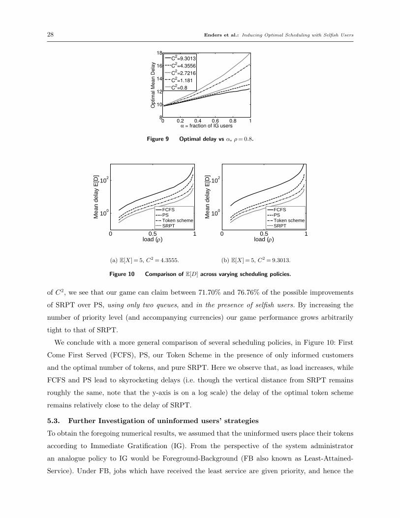
28 Enders et al.: Inducing Optimal Scheduling with Selfish Users
0 0.2 0.4 0.6 0.8 18
10
12
14
16
18
α = fraction of IG users
Op
tim
al M
ea
n D
ela
y
ρ =0.8, E[X]=5
C2=9.3013
C2=4.3556
C2=2.7216
C2=1.181
C2=0.8
Figure 9 Optimal delay vs α, ρ= 0.8.
0 0.5 1
100
102
load (ρ)
Mea
n de
lay
E[D
]
FCFSPSToken schemeSRPT
(a) E[X] = 5, C2 = 4.3555.
0 0.5 1
100
102
load (ρ)
Mea
n de
lay
E[D
]
FCFSPSToken schemeSRPT
(b) E[X] = 5, C2 = 9.3013.
Figure 10 Comparison of E[D] across varying scheduling policies.
of C2, we see that our game can claim between 71.70% and 76.76% of the possible improvements
of SRPT over PS, using only two queues, and in the presence of selfish users. By increasing the
number of priority level (and accompanying currencies) our game performance grows arbitrarily
tight to that of SRPT.
We conclude with a more general comparison of several scheduling policies, in Figure 10: First
Come First Served (FCFS), PS, our Token Scheme in the presence of only informed customers
and the optimal number of tokens, and pure SRPT. Here we observe that, as load increases, while
FCFS and PS lead to skyrocketing delays (i.e. though the vertical distance from SRPT remains
roughly the same, note that the y-axis is on a log scale) the delay of the optimal token scheme
remains relatively close to the delay of SRPT.
5.3. Further Investigation of uninformed users’ strategies
To obtain the foregoing numerical results, we assumed that the uninformed users place their tokens
according to Immediate Gratification (IG). From the perspective of the system administrator
an analogue policy to IG would be Foreground-Background (FB also known as Least-Attained-
Service). Under FB, jobs which have received the least service are given priority, and hence the

Enders et al.: Inducing Optimal Scheduling with Selfish Users 29
0 100 200 300 4000
500
1000
1500
2000
Size (x)
E[D
(x)]
=0.8, C2 =9.30, =0.2, E[X]=5
DGIG
Figure 11 Expected delay vs size.
priority of quanta decreases monotonically over time (this policy is known to be optimal in some
settings, see e.g. Yashkov 1978, 1987, Righter and Shantikumar 1989, Feng and Misra 2003). In this
section we will investigate plausible strategies for users who have partial, distributional, knowledge
about their job size in the presence of fully informed users.
Let us assume that a customer is at least certain that his job size lies within the range of [a, b]. If
D<a the user can delay gratification to quantum a−D without fear of letting tokens unnecessarily
go to waste, but could it be optimal to delay gratification further and risk wasting tokens? We show
that this may indeed be the case by comparing IG with the most delayed strategy, DG, assuming
job size b and seeing that for some uninformed customers DG is better than IG.
We examine this question in Figure 11, which compares the relative merits of a pure IG versus
a pure DG policy, showing mean delay under both IG and DG (vertical axis) against the user’s
job-size (horizontal axis) for a representative example under the assumption D = 35 (the optimal
allocation for this example). This figure assumes that the 80% informed users play DG, while the
uninformed users play IG.
Recall that the use of DG presumes the user knows his job size, whereas IG does not. Nevertheless,
for job sizes no larger than D the delays are identical, as both sets of users use all of their tokens
immediately. As job sizes grow DG begins to outperform IG. What is crucial for our discussion is
the horizontal gap between these two policies – see the line segment marked on the figure, linking
the delay of an IG user of size 325 with the equivalent delay of a DG customer of size 352.
Let us consider a tagged uninformed user who knows that his job size is between 325 and 352. In
this case, for this user, acting as though his job size were in fact 352 and using DG would lead to
a (weakly) smaller mean delay than using IG, as his delay is upper bounded by that of a DG job
of size 352. (If his job size is less than 352 he will just terminate earlier than he expects, wasting
tokens but also reducing his delay.) Thus it is beneficial for him to utilize DG, and potentially

30 Enders et al.: Inducing Optimal Scheduling with Selfish Users
waste a large proportion of his tokens. Note that DG is just one potential policy, there likely exist
other, more complex, policies for uninformed users that are better still. This leads us to our next
question:
With partial knowledge, can we be certain tokens that should be placed contiguously?
We now briefly consider the case where users have partial knowledge about their job size and
analyze how this affects their token placement.
Lemma 1. Users that know that their job size is drawn from a 2 point distribution should place
their tokens in at most 2 contiguous blocks, preceding their sizes with positive support.
Proof of Lemma 1 Consider a job of size a with probability 0 < pa < 1 and size b > a with
probability 1−pa, and an allocation of D< b tokens. We proceed by counterexample. If Da tokens
are placed on quanta a−Da + 1, a−Da, . . . , a, and Db tokens are placed on quanta b−Db + 1, b−
Db, . . . , b, and Da +Db <D there must exist a third block of tokens that is placed ahead of one of
the two blocks (of size Da and Db). By Theorem 1, using these tokens should optimally be delayed
and hence these tokens should be placed adjacent to the blocks of either Da or Db.
6. Extension to multiserver setting
Since one of the settings in which we envision our scheme of being useful is in scheduling supercom-
puting centers, it is natural to ask whether and to what extent our scheme extends to multiserver
scenarios. It is indeed straightforward to extend our token-based scheme when there are more than
one server: Whenever a server becomes free after serving a quantum, it picks the next job to serve
from the the head of the highest priority queue that is non-empty. In this setting Theorem 1 can
be easily extended to prove that DG is a strongly dominant strategy even in a multiserver setting.
Further, as we add more priority levels, our token based scheme is once again a better approxima-
tion of SRPT under multiserver setting. However, SRPT is not necessarily the optimal scheduling
policy when the number of servers exceeds 1. In particular, it has been shown in Leonardi and Raz
(1997) that there exist sample paths of arrivals on which the mean response time under SRPT can
be a factor log (P ) times the optimal mean response time, where P is the ratio of the largest to the
smallest job size in the arrival sequence. But, the authors also show that mean response time under
SRPT can be at worst a factor of 4 + log (P ) away from the optimal mean response time. Further,
no on-line scheduling policy, that is a scheduling policy that makes its decision based only on the
arrivals so far and can’t look into the future, has a better worst case performance guarantee than
SRPT within a constant factor. (Thus within a constant factor, SRPT is indeed the optimal on-line
scheduling policy.) The optimality and performance guarantee of SRPT under a stochastic arrival

Enders et al.: Inducing Optimal Scheduling with Selfish Users 31
process is still open. However, we believe that even in a multiserver setting, SRPT is the correct
scheduling policy, and hence our token-based scheme will guarantee competitive performance.
7. Conclusions
In this paper we consider the problem of online single-machine scheduling. When job sizes are
private information of all users, mechanism design has been used (primarily Clarke taxes) to induce
incentive compatibility and obtain job size information as well as job urgency. We consider for the
first time a mix of users: Users who know their job size and users who genuinely don’t. We derive
a system that will not unfairly punish the users who have no knowledge about their job size, as
one would want to do with users who behave strategically and lie about their job size.
The mechanism developed in this paper motivates users with private information about their job
size to provide truthful signals about their true remaining size. These signals are revealed through
the placement of a fixed number of tokens distributed to each user by the system administrator.
For the informed users, we show that there exists a strongly dominant strategy whereby these
users place tokens to “boost” priority for the final portion of their job. We refer to this strategy as
Delayed Gratification (DG). Intuitively, by choosing to prioritize the final portion of their job (i.e.
when remaining size is small), the users self-schedule themselves according to an approximation of
the optimal schedule: SRPT. We also show that strategies for uninformed users are complex and
remain an open question.
Our mechanism differs in at least two ways from the mechanisms proposed in the literature.
First, our mechanism allows for the fair treatment of both informed and uninformed users. Second,
we use a virtual currency that is of no value outside the system. Some existing papers also use
virtual currency, but rarely consider the question how much money (tokens) to endow users with,
and only have 1 class of users.
Using queueing-theoretic analysis, we calculate the expected waiting time and the optimal token
endowment given the system parameters. We find that the optimal token endowment increases
with the variance of job size distribution and the system load, but decreases as the fraction of
users who don’t know their job size increases. These are consequences of what we term the token
tradeoff, which we identify as the driving factor behind the optimal token allocation.
We hope our work will find application in areas such as supercomputing, where the job size infor-
mation is often private or nonexistent, and the use of real money to signal priority is undesirable.
While in this paper we focused on users with either exact, or absolutely no knowledge of the
job sizes, in many scenarios users may have a “reasonable” estimate of their size. Further, these

32 Enders et al.: Inducing Optimal Scheduling with Selfish Users
estimates will become tighter as the job is processed. One way to utilize this knowledge is instead
of asking users to place tokens on arrival. to allow them to place tokens in an as-you-go manner.
Developing and analyzing mechanisms to handle such users is significantly more complex, and
planned for future work.
References
Aalto, S., U. Ayesta, E. Nyberg-Oksanen. 2004. Two-level processor-sharing scheduling disciplines: mean
delay analysis. SIGMETRICS ’04/Performance ’04: Proceedings of the joint international conference
on measurement and modeling of computer systems 97–105.
Adiri, I., U. Yechiali. 1974. Optimal priority-purchasing and pricing decisions in nonmonopoly and monopoly
queues. Oper. Res. 22 1051–1066.
Avrachenkov, K., P. Brown, N. Osipova. 2007. Optimal choice of threshold in two level processor sharing.
ArXiv e-prints 706.
Bansal, N., D. Gamarnik. 2006. Handling load with less stress. Queueing Systems 54(1) 45–54.
Braess, D. 1969. Uber ein paradoxon aus der verkehrsplanung. Unternehmensforschung 12 258–268.
Chiang, S.H., A. Arpaci-Dusseau, M.K. Vernon. 2002. The impact of more accurate requested runtimes on
production job scheduling performance. Feitelson et al. (2002).
Chun, B.N., P. Buonadonna, A. AuYoung, Chaki Ng, D.C. Parkes, J. Shneidman, A.C. Snoeren, A. Vahdat.
2005. Mirage: A microeconomic resource allocation system for sensornet testbeds. Embedded Networked
Sensors, 2005. EmNetS-II. The Second IEEE Workshop on 19–28.
Dolan, R.J. 1978. Incentive mechanisms for priority queuing problems. Bell Journal of Econ. 9(2) 421–436.
Feitelson, D.G., L. Rudolph, U. Schweigelsohn. 2002. Job Scheduling Strategies for Parallel Processing .
Springer Verlag, Lect. Notes in Comput. Sci. vol. 2537.
Feng, H., V. Misra. 2003. Mixed scheduling disciplines for network flows. ACM SIGMETRICS Perform.
Eval. Rev. Special issue on MAMA 2003 31(2) 36–39.
Harchol-Balter, M., B. Schroeder, N. Bansal, M. Agrawal. 2003. Size-based scheduling to improve web
performance. ACM Transactions on Computer Systems 21 207–233.
Hassin, R., M. Haviv. 1997. Equilibrium threshold strategies: The case of queues with priorities. Oper. Res.
45(6) 966–973.

Enders et al.: Inducing Optimal Scheduling with Selfish Users 33
Hassin, R., M. Haviv. 2003. To Queue or not to Queue. Kluwer, Norwell, Ma, USA.
Lee, C.B., Y. Schwartzman, J. Hardy, A. Snavely. 2004. Are user runtime estimates inherently inaccurate?
10th Workshop on Job Scheduling Strategies for Parallel Processing .
Leonardi, S., D. Raz. 1997. Approximating total flow time on parallel machines. Proceedings of the Symposium
on Theory of Computation .
Lu, D., P. Dinda, Y. Qiao, H. Sheng, F. Bustamante. 2004a. Applications of SRPT scheduling with inaccurate
information. Proceedings of the 12th IEEE/ACM International Symposium on Modeling, Analysis, and
Simulation of Computer and Telecommunication Systems, MASCOTS .
Lu, D., H. Sheng, P. Dinda. 2004b. Size-based scheduling policies with inaccurate scheduling information.
Proceedings of the 12th IEEE/ACM International Symposium on Modeling, Analysis, and Simulation
of Computer and Telecommunication Systems, MASCOTS 31–38.
Mendelson, H., S. Whang. 1990. Optimal incentive-compatible priority pricing for the M/M/1 queue. Oper.
Res. 38(5) 870–883.
Mu’alem, A.W., D.G. Feitelson. 2001. Utilization, predictability, workloads, and user runtime estimates in
scheduling the ibm sp2 with backfilling. IEEE Trans. Prallel & Distributed Syst. 12(6) 529–543.
Peterson, J.L., A. Silberschatz. 2002. Operating systems concepts. John Wiley & Sons Inc.
Righter, R., J.G. Shantikumar. 1989. Scheduling multiclass single server queueing systems to stocastically
maximize the number of successful departures. Probability in the Engineering and Informational Sci-
ences 3 323–333.
Schrage, L.E. 1968. A proof of the optimality of the shortest remaining processing time discipline. Oper.
Res. 16(3) 687–690.
Snell, Q.O., M.J. Clement, D.B. Jackson. 2002. Preemption based backfill. Feitelson et al. (2002).
Wierman, A., M. Nuyens. 2008. Near-optimal scheduling despite inexact job-size information. SIGMETRICS
’08: Proceedings of the international conference on Measurement and modeling of computer systems.
Wolff, R.W. 1970. Time sharing with priorities. SIAM J. Appl. Math. 566–574.
Yashkov, S.F. 1978. On feedback sharing a processor among jobs with minimal serviced length (in Russian).
Technika Sredstv Svyazi. Ser. ASU (2) 51–62.
Yashkov, S.F. 1987. Processor-sharing queues: Some progress in analysis. Queueing Systems 2 1–17.

34 Enders et al.: Inducing Optimal Scheduling with Selfish Users
Appendix A: Convergence of finite game to stationary game
The goal of this section is to show that the equilibria of the stationary game defined in Example 1 are an
appropriately defined limit of a sequence of games with finite N number of players, as N →∞.
Consider a game with N players of whom dα ·Ne are uninformed with the job size distribution defined
in Example 1 (1 quantum with probability p1, 2 quantum with probability p2 = 1− p1), d(1−α) · p1 ·Ne
are informed with job size of 1 quantum, and the rest are informed with a job size of 2 quanta. The arrival
instants of the uninformed users are generated according to a Poisson process with rate λα starting at t= 0,
and the uninformed users are mapped to the Nα arrival instants at random (i.e., all permutations are equally
likely). The arrival instants of the informed users are generated similarly, by independent Poisson processes
with appropriate rates. Thus we have definedM, the measure on Ω = R+N , the space of arrival sequences
of the N players. The signal functions of all players are independent of the arrival sequence, and hence no
information about the realized sample path is available to the players. That is, Ai = ∅,Ω for all players.
Let Esta, EN,ε, E , EN and E be defined as follows:
Esta.= Set of Nash equilibria of the stationary game of Example 1
EN.= Set of Nash equilibria of the finite game with N players
EN,ε.= Set of ε-Nash equilibria4 of the finite game with N players
E .= limN→∞
EN = p∗| limN→∞
1p∗∈ENexists and equals 1
E .= limε→0
limN→∞
EN,ε
Proposition 2. The equilibria of the stationary game of Example 1 and the sequence of finite games
converge in the following sense:
Esta = E .
Proof: At t= 0, our queueing system is idle. We can now split the time interval [0,∞) into cycles and
a residual time period – C1,C2, . . . ,Cm,R – as follows: The cycle C1 begins at t = 0 and ends when the
first busy period ends, and thus includes one idle period and one busy period. Cycle C2 begins at the end
of cycle C1 and ends when the first busy period following C1 ends. The sequence of cycles ends when we
4 An ε-Nash equilibrium is defined to be a strategy profile where no player can improve his/her utility by more thanε by deviating unilaterally.

Enders et al.: Inducing Optimal Scheduling with Selfish Users 35
run out of either the uninformed, or informed users of either size. That is, Cm denotes the last cycle such
that there is at least one player of each class that hasn’t arrived by the end of Cm. The remaining time
period, from the end of Cm to +∞ is denoted by R. The cycles C1, . . . ,Cm are thus i.i.d. renewal cycles of a
stationary queueing system (the definitions of these cycles is independent of the strategies adopted by users
since we have a work conserving queueing system). As N →∞, the probability that any given player arrives
during a cycle approaches 1. This is because each permutation of the players is equally likely, and hence the
probability that a player arrives during a renewal cycle is the same as the expected fraction of players (of his
class) that arrive in some cycle. As N →∞, m→∞, while the number of users that arrive during R remains
stochastically bounded. Therefore the probability that a user arrives during a renewal cycle approaches 1 as
1−O(1/N).
For a fixed N , consider a tagged player U of one of the three types. Let p = puninf , pinf1 , pinf2 , pU denote
a strategy profile, where puninf denotes the (symmetric) strategy profile of the untagged uninformed users,
pinf1 denotes the (symmetric) strategy profile of the untagged informed users of size 1, pinf2 denotes the
(symmetric) strategy profile of the untagged informed users of size 2, and pU denotes the strategy of the
tagged player. For each N and for the stationary game, the delay (cost) of the tagged player is a uniformly
continuous function in each component of p (with sup norm on the measures) since it is a continuous function
with compact support. Further, as N →∞, the delay (cost) under the finite game converges uniformly to
the (delay) cost under the stationary game. To see this, note that the utility (equivalently cost) of a player
arriving in the residual period R is stochastically bounded above by an integrable random variable, uniformly
in the strategy adopted by the player. Thus as N →∞, the utility of the tagged user U is dominated by his
utility given he arrives in one of the renewal cycles. This utility, in turn, is the same as if the tagged user
arrived in a stationary game where the strategy profile of the other players is given by puninf , pinf1 , pinf2
and the tagged user adopt strategy pU .
Thus as N →∞, the best response function of the tagged player converges point-wise to the best response
function of the tagged player under the stationary game at points where the best response under the station-
ary game is unique. However, at points where the stationary game has multiple best responses, we may not
even have convergence of the best response of the N player game as N →∞. Further, we do not necessarily
have Esta = E (indeed, consider a hypothetical case where Esta = 1, while EN = 1− 1/N in which case
E = ∅). To get around this problem, we use the notion of ε-Nash equilibria. Due to uniform convergence of

36 Enders et al.: Inducing Optimal Scheduling with Selfish Users
delays, for all ε, there exists an Nε such that ∀ n≥Nε Esta ⊆En,ε. Further, for any p∗ /∈ Esta, there is some ε∗,
such that for all ε < ε∗, there exists an Nε, such that p∗ /∈ En,ε ∀n >Nε. Thus, Esta = limε→0 limN→∞ EN,ε =
E .
Appendix B: Performance (Queueing) Analysis (from Section 5)
The equations presented in this Appendix are a non-trivial adaptation of Wolff (1970). The reader intending
to understand the full analysis below is advised to consult Wolff first to see a simpler case. Tables 1 and 2
introduce the necessary notation and basic definitions.
α Fraction of uninformed (IG) usersD Number of tokens given to every userM Maximum size of a jobpi Pr[job needs i quanta ]
λDG Arrival rate of DG jobsλIG Arrival rate of IG jobsρ Time average probability that the server is busy (= λ ·E[job size])
WHi,DG Expected delay for the ith H of a DG job with zero L
WLHi,DG Expected delay for the ith H of a DG job with non-zero L
WLi,DG Expected delay for the ith L of a DG job with non-zero L
WHi,IG Expected delay for the ith H of an IG job
WLi,IG Expected delay for the ith L of an IG job with non-zero LqHDG Given the arrival sees server busy, the server is busy with an H of a DG jobqLHDG Time average probability that the server is busy with an H of a DG user with non-zero
LqL∗DG Time average probability that the server is busy with the last L of a DG user with
non-zero LqHIG Time average probability that the server is busy with an H of an IG user
nHi,j,DG Number of DG jobs (in H queue) of original size i≤D waiting for jth H phasenLi,j,DG Number of DG jobs (in L queue) of original size i+D waiting for jth L phasenLHj,DG Number of DG jobs (of original size >D but now in H queue) waiting for jth H phasenHi,IG Number of IG jobs (in H queue) waiting for ith H phasenLi,IG Number of IG jobs (now in L queue) waiting for ith L phase
mHk,DG Number of DG jobs in H queue requiring exactly k more H phases (including the phase
they are waiting for)mHk,IG Number of IG jobs in H queue requiring exactly k more H phases (including the phase
they are waiting for)RHDG Number of remainining H quanta of a DG job (possibly including the one in service),
conditioned on the server being busy with a DG jobRLDG Number of remainining L quanta of a DG job (possibly including the one in service),
conditioned on the server being busy with a DG jobRHIG Number of remainining H quanta of an IG job (possibly including the one in service),
conditioned on the server being busy with an IG jobRLIG Number of remainining L quanta of an IG job (possibly including the one in service),
conditioned on the server being busy with an IG jobTable 1 Notation
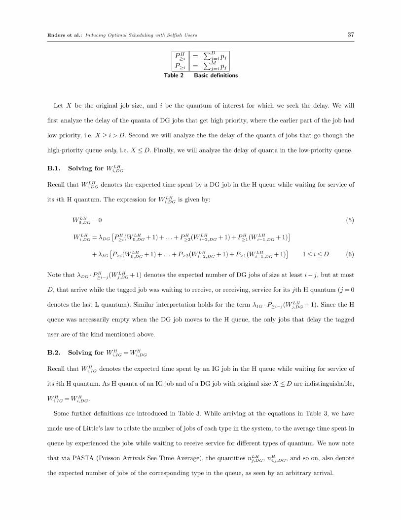
Enders et al.: Inducing Optimal Scheduling with Selfish Users 37
PH≥i =
∑D
j=i pjP≥i =
∑M
j=i pjTable 2 Basic definitions
Let X be the original job size, and i be the quantum of interest for which we seek the delay. We will
first analyze the delay of the quanta of DG jobs that get high priority, where the earlier part of the job had
low priority, i.e. X ≥ i > D. Second we will analyze the the delay of the quanta of jobs that go though the
high-priority queue only, i.e. X ≤D. Finally, we will analyze the delay of quanta in the low-priority queue.
B.1. Solving for WLHi,DG
Recall that WLHi,DG denotes the expected time spent by a DG job in the H queue while waiting for service of
its ith H quantum. The expression for WLHi,DG is given by:
WLH0,DG = 0 (5)
WLHi,DG = λDG
[PH≥i(W
LH0,DG + 1) + . . .+PH
≥2(WLHi−2,DG + 1) +PH
≥1(WLHi−1,DG + 1)
]+λIG
[P≥i(WLH
0,DG + 1) + . . .+P≥2(WLHi−2,DG + 1) +P≥1(WLH
i−1,DG + 1)]
1≤ i≤D (6)
Note that λDG ·PH≥i−j(W
LHj,DG + 1) denotes the expected number of DG jobs of size at least i− j, but at most
D, that arrive while the tagged job was waiting to receive, or receiving, service for its jth H quantum (j = 0
denotes the last L quantum). Similar interpretation holds for the term λIG ·P≥i−j(WLHj,DG + 1). Since the H
queue was necessarily empty when the DG job moves to the H queue, the only jobs that delay the tagged
user are of the kind mentioned above.
B.2. Solving for WHi,IG =WH
i,DG
Recall that WHi,IG denotes the expected time spent by an IG job in the H queue while waiting for service of
its ith H quantum. As H quanta of an IG job and of a DG job with original size X ≤D are indistinguishable,
WHi,IG =WH
i,DG.
Some further definitions are introduced in Table 3. While arriving at the equations in Table 3, we have
made use of Little’s law to relate the number of jobs of each type in the system, to the average time spent in
queue by experienced the jobs while waiting to receive service for different types of quantum. We now note
that via PASTA (Poisson Arrivals See Time Average), the quantities nLHj,DG, nHi,j,DG, and so on, also denote
the expected number of jobs of the corresponding type in the queue, as seen by an arbitrary arrival.

38 Enders et al.: Inducing Optimal Scheduling with Selfish Users
WHi,DG = WH
i,IG
nLHj,DG = λDG P≥D+1 WLHj,DG
nHi,j,DG = λDG pi WHj,DG
nHj,IG = λIG P≥j WHj,IG
mHk,DG = nLHD−k+1,DG +
∑D
i=k nHi,i−k+1,DG
mHk,IG =
∑D−ki=1 nHi,IG
pk+i−1
P≥i+nHD−k+1,IG
P≥DP≥D−k+1
= λIG
(∑D−ki=1 WH
i,IGpk+i−1 +WHD−k+1,IGP≥D
)qHDG = λDG
ρ(p1 + 2 · p2 + · · ·+D · pD)
qLHDG = λDGρD ·P≥D+1
qL∗DG = λDGρP≥D+1
qHIG = λIGρ
(p1 + 2 · p2 + · · ·+D ·P≥D)∑D
j=imHj,DG = λDG(WH
1,DGPH≥i + WH
2,DGPH≥i+1 + . . . + WH
D−i+1,DGPH≥D) + λDGP≥D+1(WLH
1,DG +. . .+WLH
D−i+1,DG)∑D
j=imHj,IG = λIG(WH
1,IGP≥i +WH2,IGP≥i+1 + . . .+WH
D−i+1,IGP≥D)Table 3 Definitions for WH
IG =WHDG
The above observations allow us to develop the following equations:
WH1,DG = (
D∑j=1
mHj,DG +
D∑j=1
mHj,IG) +
ρ
2
WH2,DG = (
D∑j=2
mHj,DG +
D∑j=2
mHj,IG) +λDGP
H≥1(WH
1,DG + 1) +λIGP≥1(WH1,DG + 1)
+ ρ
(qL∗DG · 1 + qLHDG
D− 1D
+ qHDGPr[RHDG > 1
]+ qHIGPr
[RHIG > 1
])WHi,DG = (
D∑j=i
mHj,DG +
D∑j=i
mHj,IG) +λDG
[PH≥1(WH
i−1,DG + 1) + . . .+PH≥i−1(WH
1,DG + 1)]
+λIG[P≥1(WH
i−1,DG + 1) + . . .+P≥i−1(WH1,DG + 1)
]+ ρ
(qL∗DG · 1 + qLHDG
D− i+ 1D
+ qHDGPr[RHDG > i− 1
]+ qHIGPr
[RHIG > i− 1
]).
We briefly describe what each quantity in the expression for WHi,DG means. The first paranthesis denotes the
delay due to the IG and DG jobs that the tagged arrival sees in the H queue on arrival, and which had at
least i remaining H quanta at that time. The second and third terms denote the delay caused by new IG and
DG arrivals into the H queue while the tagged job was waiting/receiving service for its first i− 1 H quanta.
The last term denotes the contribution due to the job that was occupying the server when the tagged job
first arrived into the system. This job could either be 1) a DG job serving its last L quantum, 2) a DG job
of original size larger than D who was now serving an H quantum, 3) a DG job of original size at most D,
or 4) and IG job serving its H quantum. While the job at the server could also be an IG job serving its L
quantum, or a DG job serving some (but not last) L quantum, these jobs will not interfere in the service of
the ith H quantum of the tagged job when i > 1.
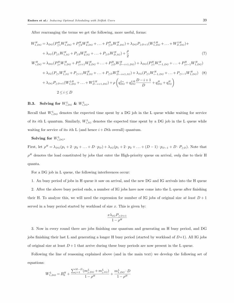
Enders et al.: Inducing Optimal Scheduling with Selfish Users 39
After rearranging the terms we get the following, more useful, forms:
WH1,DG = λDG(PH
≥1WH1,DG +PH
≥2WH2,DG + . . .+PH
≥DWHD,DG) +λDGP≥D+1(WLH
1,DG + . . .+WLHD,DG)+
+λIG(P≥1WH1,IG +P≥2W
H2,IG + . . .+P≥DW
HD,IG) +
ρ
2(7)
WHi,DG = λDG(PH
≥iWH1,DG +PH
≥i+1WH2,DG + . . .+PH
≥DWHD−i+1,DG) +λDG(PH
≥1WHi−1,DG + . . .+PH
≥i−1WH1,DG)
+λIG(P≥iWH1,IG +P≥i+1W
H2,IG + . . .+P≥DW
HD−i+1,IG) +λIG(P≥1W
Hi−1,DG + . . .+P≥i−1W
H1,DG) (8)
+λDGP≥D+1(WLH1,DG + . . .+WLH
D−i+1,DG) + ρ
(qL∗DG + qLHDG
D− i+ 1D
+ qHDG + qHIG
)2≤ i≤D
B.3. Solving for WLi,DG & WL
i,IG.
Recall that WLi,DG denotes the expected time spent by a DG job in the L queue whike waiting for service
of its ith L quantum. Similarly, WLi,IG denotes the expected time spent by a DG job in the L queue while
waiting for service of its ith L (and hence i+Dth overall) quantum.
Solving for WLi,DG.
First, let ρH = λDG(p1 + 2 · p2 + . . .+D · pD) + λIG(p1 + 2 · p2 + . . .+ (D − 1) · pD−1 +D · P≥D). Note that
ρH denotes the load constituted by jobs that enter the High-priority queue on arrival, only due to their H
quanta.
For a DG job in L queue, the following interferences occur:
1. An busy period of jobs in H queue it saw on arrival, and the new DG and IG arrivals into the H queue
2. After the above busy period ends, a number of IG jobs have now come into the L queue after finishing
their H. To analyze this, we will need the expression for number of IG jobs of original size at least D+ 1
served in a busy period started by workload of size x. This is given by:
xλIGP≥D+1
1− ρH
3. Now in every round there are jobs finishing one quantum and generating an H busy period, and DG
jobs finishing their last L and generating a longer H busy period (started by workload of D+1). All IG jobs
of original size at least D+ 1 that arrive during these busy periods are now present in the L queue.
Following the line of reasoning explained above (and in the main text) we develop the following set of
equations:
WL1,DG =BH
0 +
∑M−Dj=1 (mL
j,DG +mLj,IG)
1− ρH+mL
1,DG ·D1− ρH

40 Enders et al.: Inducing Optimal Scheduling with Selfish Users
nLi,j,DG = λDG pi+D WLj,DG
nLj,IG = λIG P≥j+D WLj,DG
mLk,DG =
∑M−Di=k nLi,i−k+1,DG
= λDG∑M−D
i=k pi+DWLi−k+1,DG
mLk,IG =
∑M−D−k+1
i=1 nLi,IGpD+k+i−1
P≥D+i
= λIG
(∑M−D−k+1
i=1 WLi,IGpD+k+i−1
)∑M−D
j=i mLj,DG = λDG(WL
1,DGP≥i+D +WL2,DGP≥i+1+D + . . .+WL
M−D−i+1,DGP≥M)∑M−Dj=i mL
j,IG = λIG(WL1,IGP≥i+D +WL
2,IGP≥i+1+D + . . .+WLM−D−i+1,IGP≥M)
E[HDG] = 1PH≥1
(p1 + 2 · p2 + · · ·+D · pD)
E[H2DG] = 1
PH≥1
(p1 + 22 · p2 + · · ·+D2 · pD)
E[HIG] = (p1 + 2 · p2 + · · ·+D ·P≥D)E[H2
IG] = (p1 + 22 · p2 + · · ·+D2 ·P≥D)
BH0 = ρ
1−ρH
[12
+D · qL∗DG + qHDG2·(
E[H2
DG
]E[HDG]
− 1)
+ qLHDG · D−12
+ qHIG2·(
E[H2
IG
]E[HIG]
− 1)]
+ 11−ρH
(∑D
i=1 i · (mHi,DG +mH
i,IG))
Table 4 Definitions for WLIG =WL
DG
WL2,DG =
ρH
1− ρH+ρ(qLDGPr[RLDG > 1] + qLIGPr[RLIG > 1])
1− ρH
+ρqLDGPr[RLDG = 2] ·D
1− ρH
+ρqHIGPr[IG job in last H]Pr[RLIG ≥ 1|IG job in last H]
1− ρH
+
∑M−Dj=2 (mL
j,DG +mLj,IG)
1− ρH+mL
2,DG ·D1− ρH
+λDGP≥D+1(WL
1,DG + 1)1− ρH
+λDGpD+1(WL
1,DG + 1)D1− ρH
+λIGP≥D+1(WL
1,DG)1− ρH
+
∑D
i=1 nHi,IG
P≥D+1
P≥i
1− ρH
WLi,DG =
ρH
1− ρH+ρ(qLDGPr[RLDG > i− 1] + qLIGPr[RLIG > i− 1])
1− ρH
+ρqLDGPr[RLDG = i] ·D
1− ρH
+ρqHIGPr[IG job in last H]Pr[RLIG ≥ i− 1|IG job in last H]
1− ρH
+
∑M−Dj=i (mL
j,DG +mLj,IG)
1− ρH+mLi,DG ·D1− ρ
+λDG
1− ρH[P≥D+1(WL
i−1,DG + 1) + . . .+P≥D+i−1(WL1,DG + 1)
]+λDG ·D1− ρH
[pD+1(WL
i−1,DG + 1) + . . .+ pD+i−1(WL1,DG + 1)
]+
λIG1− ρH
[P≥D+1(WL
i−1,DG + 1) + . . .+P≥D+i−2(WL2,DG + 1) +P≥D+i−1(WL
1,DG)]
+
∑D
j=1 nHj,IG
P≥D+i−1
P≥j
1− ρH.

Enders et al.: Inducing Optimal Scheduling with Selfish Users 41
These equations can be rearranged into the following useful form:
WL1,DG =BH
0 +λDG
1− ρH(WL
1,DGP≥1+D +WL2,DGP≥2+D + . . .+WL
M−D,DGP≥M)
+λIG
1− ρH(WL
1,IGP≥1+D +WL2,IGP≥2+D + . . .+WL
M−D,IGP≥M) (9)
+λDG ·D1− ρH
(M−D∑i=1
pi+DWLi,DG)
WLi,DG =
ρH
1− ρH+
ρqLDG1− ρH
+λIG(P≥D+i + . . .+P≥M)
1− ρH
+λDG ·P≥D+i ·D
1− ρH
+λIG ·P≥D+i−1
1− ρH
+λDG
1− ρH[WL
1,DGP≥i+D +WL2,DGP≥i+1+D + . . .+WL
M−D−i+1,DGP≥M]
+λIG
1− ρH[WL
1,IGP≥i+D +WL2,IGP≥i+1+D + . . .+WL
M−D−i+1,IGP≥M]
+λDG ·D1− ρH
[WL
1,DGpi+D +WL2,DGpi+1+D + . . .+WL
M−D−i+1,DGpM]
+λDG
1− ρH[P≥D+1(WL
i−1,DG) + . . .+P≥D+i−1(WL1,DG)
]+λDG ·D1− ρH
[pD+1(WL
i−1,DG + 1) + . . .+ pD+i−1(WL1,DG + 1)
]+
λIG1− ρH
[P≥D+1(WL
i−1,DG + 1) + . . .+P≥D+i−2(WL2,DG + 1) +P≥D+i−1(WL
1,DG)]
+
∑D
j=1
(nHj,IG
P≥D+i−1
P≥j
)1− ρH
=ρH
1− ρH+
ρqLDG1− ρH
+λIG(P≥D+1 + . . .+P≥M)
1− ρH
+λDG ·P≥D+1 ·D
1− ρH
+λDG
1− ρH[WL
1,DGP≥i+D +WL2,DGP≥i+1+D + . . .+WL
M−D−i+1,DGP≥M]
+λIG
1− ρH[WL
1,IGP≥i+D +WL2,IGP≥i+1+D + . . .+WL
M−D−i+1,IGP≥M]
(10)
+λDG ·D1− ρH
[WL
1,DGpi+D +WL2,DGpi+1+D + . . .+WL
M−D−i+1,DGpM]
+λDG
1− ρH[P≥D+1(WL
i−1,DG) + . . .+P≥D+i−1(WL1,DG)
]+λDG ·D1− ρH
[pD+1(WL
i−1,DG) + . . .+ pD+i−1(WL1,DG)
]+
λIG1− ρH
[P≥D+1(WL
i−1,DG) + . . .+P≥D+i−2(WL2,DG) +P≥D+i−1(WL
1,DG)]

42 Enders et al.: Inducing Optimal Scheduling with Selfish Users
+
∑D
j=1
(nHj,IG
P≥D+i−1
P≥j
)1− ρH
Solving for WLi,IG: When considering the low-priority quanta of an IG job, we know that, when the
quantum is about to start serving:
• all the only H DG jobs seen on arrival have left,
• all the IG jobs seen in H queue on arrival have either left or are in the L queue,
• if the job seen on arrival at the server was an IG job serving an H quantum, it has left or is in the L
queue,
• if the job seen on arrival at the server was a DG job serving an H quantum, it has left,
• if the job seen on arrival at the server was a DG job serving an L quantum, it has left or is in the L
queue, unless it was serving its last L quantum in which case it is in the H queue with one more remaining
quantum,
• if the job seen on arrival at the server was an IG job serving an L quantum, it has left or is in the L
queue,
• jobs which arrived while the tagged job was in the H queues may still be in the H queue and before the
tagged job can begin service in the L queue, these arrivals will cause a busy period.
The initial workload (job at the server, and the H quanta of the jobs in the H queue) that will cause the
busy period is
BH0 = ρqL∗DG · 1
+λDGD · pD(WH
D,IG + 1)
+ (D− 1) · [pD−1(WHD,IG + 1) + pD(WH
D−1,IG + 1)] + . . .
+1 · [p1(WHD,IG + 1) + . . .+ pD(WH
1,IG + 1)]
+λIG
[1 ·P≥D](WH1,IG + 1)
+ [1 · pD−1 + 2 ·P≥D](WH2,IG + 1) + . . .
[1 · p1 + 2 · p2 + . . .+D ·P≥D](WHD,IG + 1)
.
Using the reasoning from the start of this subsection we get the following equations for WLi,IG:
WL0,IG =
D∑j=1
(WHj,IG + 1)− 1

Enders et al.: Inducing Optimal Scheduling with Selfish Users 43
WL1,IG =
BH0
1− ρH+ρ(qLDGPr[RLDG > 1] + qLIGPr[RLIG > 1])
1− ρH
+ρqLDGPr[RLDG = 2] ·D
1− ρH
+ρqHIGPr[RLIG ≥ 1|IG job in H]
1− ρH
+
∑M−Dj=1 (mL
j,DG +mLj,IG)
1− ρH
+mL
1,DG ·D1− ρH
+λDG
1− ρH[P≥D+1(WL
0,IG + 1)]
+λDG ·D1− ρH
[pD+1(WL
0,IG + 1)]
+
∑D
j=1 nHj,IG
P≥D+1
P≥j
1− ρH
WLi,IG =
ρH
1− ρH+ρ(qLDGPr[RLDG > i] + qLIGPr[RLIG > i])
1− ρH
+ρqLDGPr[RLDG = i+ 1] ·D
1− ρH
+ρqHIGPr[RLIG ≥ i|IG job in H]
1− ρH
+
∑M−Dj=i (mL
j,DG +mLj,IG)
1− ρH
+mLi,DG ·D1− ρH
+λDG
1− ρH[P≥D+1(WL
i−1,IG + 1) + . . .+P≥D+i(WL0,IG + 1)
]+λDG ·D1− ρH
[pD+1(WL
i−1,IG + 1) + . . .+ pD+i(WL0,IG + 1)
]+
λIG1− ρH
[P≥D+1(WL
i−1,IG + 1) + . . .+P≥D+i−1(WL1,IG + 1) +P≥D+i−1(WL
0,IG)]
+
∑D
j=1
(nHj,IG
P≥D+i
P≥j
)1− ρH
.
Which can be rearranged into:
WL0,IG =
D∑j=1
(WHj,IG + 1)− 1 (11)
WL1,IG =
BH0
1− ρH+
ρqLDG1− ρH
+λIG(P≥D+2 + . . .+P≥M)
1− ρH
+λIG ·D ·P≥D+1
1− ρH
+λDGP≥D+1 ·D
1− ρH
+λDG
1− ρH(WL
1,DGP≥1+D +WL2,DGP≥2+D + . . .+WL
M−D,DGP≥M) (12)

44 Enders et al.: Inducing Optimal Scheduling with Selfish Users
+λIG
1− ρH(WL
1,IGP≥1+D +WL2,IGP≥2+D + . . .+WL
M−D,IGP≥M)
+λDG ·D1− ρH
(M−D∑i=1
pi+DWLi,DG)
+λDG
1− ρH[P≥D+1(WL
0,IG + 1)]
+λDG ·D1− ρH
[pD+1(WL
0,IG + 1)]
+
∑D
j=1 nHj,IG
P≥D+1
P≥j
1− ρH
WLi,IG =
ρH
1− ρH+
ρqLDG1− ρH
+λIG(P≥D+i+1 + . . .+P≥M)
1− ρH
+λIG ·D ·P≥D+i
1− ρH
+λIG(P≥D+1 + . . .+P≥D+i−1)
1− ρH
+λDGP≥D+1 ·D
1− ρH
+λDG
1− ρH[WL
1,DGP≥i+D +WL2,DGP≥i+1+D + . . .+WL
M−D−i+1,DGP≥M]
(13)
+λIG
1− ρH[WL
1,IGP≥i+D +WL2,IGP≥i+1+D + . . .+WL
M−D−i+1,IGP≥M]
+λDG ·D1− ρH
[WL
1,DGpi+D +WL2,DGpi+1+D + . . .+WL
M−D−i+1,DGpM]
+λDG
1− ρH[P≥D+1(WL
i−1,IG) + . . .+P≥D+i(WL0,IG)
]+λDG ·D1− ρH
[pD+1(WL
i−1,IG) + . . .+ pD+i(WL0,IG)
]+
λIG1− ρH
[P≥D+1(WL
i−1,IG) + . . .+P≥D+i−1(WL1,IG) +P≥D+i−1(WL
0,IG)]
+
∑D
j=1
(nHj,IG
P≥D+i
P≥j
)1− ρH
To get the delay of each quantum we now solve the system of equations as defined by (5) -(13). Then,
expectation with respect to the job size distribution, specified by pi needs to be taken to get the delay of an
average user. Thus, the expected delay of a DG user of size x is given by:
WDG(x) =
∑x
i=1WHi,DG x≤D∑x−D
i=1 WLi,DG +
∑D
i=1WLHi,DG x>D,
and the expected delay of an IG user of size x is given by:
WIG(x) =
∑x
i=1WHi,IG x≤D∑D
i=1WHi,IG +
∑x−Di=1 WL
i,IG x>D.
Related Documents