Individual-tree diameter growth models for black spruce and jack pine plantations in northern Ontario

This article appeared in a journal published by Elsevier. The attachedcopy is furnished to the author for internal non-commercial researchand education use, including for instruction at the authors institution

and sharing with colleagues.

Other uses, including reproduction and distribution, or selling orlicensing copies, or posting to personal, institutional or third party

websites are prohibited.

In most cases authors are permitted to post their version of thearticle (e.g. in Word or Tex form) to their personal website orinstitutional repository. Authors requiring further information

regarding Elsevier’s archiving and manuscript policies areencouraged to visit:

http://www.elsevier.com/copyright

Author's personal copy

Forest Ecology and Management 261 (2011) 2140–2148

Contents lists available at ScienceDirect

Forest Ecology and Management

journa l homepage: www.e lsev ier .com/ locate / foreco

Individual-tree diameter growth models for black spruce and jack pineplantations in northern Ontario

Nirmal Subedi ∗, Mahadev SharmaOntario Forest Research Institute, Ontario Ministry of Natural Resources, 1235, Queen St. East, Sault Ste. Marie, ON P6A-2E5 Canada

a r t i c l e i n f o

Article history:Received 11 January 2011Received in revised form 4 March 2011Accepted 5 March 2011Available online 29 March 2011

Keywords:Mixed-effects nonlinear modelBasal area incrementTree growth modelingCalibrated response

a b s t r a c t

Individual-tree distance independent diameter growth models were developed for black spruce and jackpine plantations. Data used in this study came via stem analysis on 1170 black spruce (Picea mariana[Mill.] B.S.P.) and 800 jack pine (Pinus banksiana Lamb.) trees sampled from 75 stands of 25 even-agedmonospecific plantations for each species in the Canadian boreal forest region of northern Ontario. Ofthe 75 stands, 50 were randomly selected for each species and all trees from these stands were used formodel development. Trees from the remaining stands were used for model evaluation.

A nonlinear mixed-effects approach was applied in fitting the diameter growth models. The predictiveaccuracy of the models was improved by including random effects coefficients. Four selection criteria –random, dominant or codominant, tree size close to quadratic mean diameter, and small sized – wereevaluated for accuracy in predicting random effects for a new stand using the developed models. Randomeffects predicted based on trees selected using the random selection criterion provided more accuratediameter predictions than those using trees obtained via other selection criteria for both species. Themodels developed here are very important to forest managers as the diameters predicted by these modelsor, their stand-level summaries (i.e., basal area, average diameter), are used as inputs in any forest growthand yield models. In addition, individual-tree diameter growth models can be used to directly forecastchanges in diameter distribution of stands.

Crown Copyright © 2011 Published by Elsevier B.V. All rights reserved.

1. Introduction

In growth and yield modeling, diameter at breast height isthe most used measure of tree size (Avery and Burkhart, 1983).Individual-tree diameter growth models are used to predict diam-eter increment of trees in a stand and these models are one of theessential inputs for many individual-tree based growth and yieldmodels (e.g., Forest Vegetation Simulator; Wykoff et al., 1982; LS-TWIGS; Miner et al., 1988).

Diameter growth models are commonly developed usingeither potential growth-based or potential growth-independentapproaches. In the case of potential growth-based models, diametergrowth is modeled as a product of potential growth and a compe-tition modifier function (Hahn and Leary, 1979; Holdaway, 1984;Miner et al., 1988; Teck and Hilt, 1991; Monserud and Sterba, 1996;Andreassen and Tomter, 2003). The potential growth and modifierfunctions in such models are usually constructed in separate steps(Holdaway, 1984; Amateis et al., 1989; Teck and Hilt, 1991). In thecase of potential growth-independent models, diameter growth isexpressed as a function of tree attributes, site characteristics, and

∗ Corresponding author. Tel.: +1 705 946 7423; fax: +1 705 946 2030.E-mail address: [email protected] (N. Subedi).

measures of competition among individual trees (Wykoff, 1990;Hann and Larsen, 1991; Zhang et al., 2004; Weiskittel et al., 2007;Kiernan et al., 2008; Pokharel and Froese, 2009). In fact, bothapproaches produce equally acceptable diameter growth predic-tions (Wykoff, 1990).

To estimate potential growth (i.e., maximum biologicallyachievable growth), researchers have used data for open-growntrees (e.g., Amateis et al., 1989), a proportion of the faster grow-ing trees in given sample (e.g., Teck and Hilt, 1991; Schroder et al.,2002), and the fastest growing dominant or codominant trees(Hahn and Leary, 1979). In recent studies (Murphy and Shelton,1996; Lynch et al., 1999; Budhathoki et al., 2008), potential growthhas been modeled using more flexible growth functions, such asChapman–Richards or logistic, and the parameters of both poten-tial growth and modifier functions are estimated simultaneously.Rather than using potential growth, another approach for modelingdiameter growth is to apply an average growth function (Lessardet al., 2001).

Black spruce (Picea mariana [Mill.] B.S.P.) and jack pine (Pinusbanksiana Lamb.) are the most common commercial tree speciesin Ontario, Canada. They represent approximately 37.4% (2.7 bil-lion cubic meters) and 10.9% (785 million cubic meters) of the totalgrowing stock, respectively (OMNR 2006), and are the main sourcesof pulp, lumber, and roundwood harvested in the province.

0378-1127/$ – see front matter. Crown Copyright © 2011 Published by Elsevier B.V. All rights reserved.doi:10.1016/j.foreco.2011.03.010

Author's personal copy

N. Subedi, M. Sharma / Forest Ecology and Management 261 (2011) 2140–2148 2141

During the last decade, much effort has gone into developingdiameter growth models for use in Ontario. Most of the studies(Hökkä and Groot, 1999; Zhang et al., 2004; Lacerte et al., 2006;Pokharel and Froese, 2009) used the potential growth-independentapproach to develop diameter growth models for natural stands.Thomas et al. (2008) developed a diameter distribution model usinglight detection and ranging (LiDAR) data for forest stands in cen-tral Ontario. None of the previous studies have produced diametergrowth models for plantations in the boreal forest region of theprovince.

Data for diameter growth studies generally originates from mul-tiple measurements of trees from a number of stands. These dataare commonly hierarchical (i.e., trees within stands). Observationsbetween sampling units (stands) are independent, but observa-tions within a sampling unit (stand) are dependent because theyare from the same sub-population (Demidenko, 2004). As a result,two sources of variation exist: between sampling units and withina sampling unit. To address the problem of autocorrelation withina sampling unit, recent studies have used a mixed-effects model-ing technique (Fang and Bailey, 2001; Leites and Robinson, 2004;Trincado and Burkhart, 2006; Sharma and Parton, 2007, 2009).This technique has the advantage of genuinely (i.e., logically) com-bining data by multi-level random effects (Gregoire et al., 1995;Schabenberger and Pierce, 2001; Demidenko, 2004). Mixed-effectsmodels have deterministic and fixed-effects parameters, represent-ing a population average response common to all sampling units,and random-effects parameters, representing localized responsesthat are specific to each sampling unit. When the random effects arecalibrated for an unsampled location, mixed-effects models haveimproved predictive accuracy (Calama and Montero, 2004). Fordetails on mixed modeling, see Schabenberger and Pierce (2001),and Demidenko (2004).

The objective of this study was to develop individual-tree,distance-independent diameter growth models for black spruceand jack pine plantations using a mixed-effects technique. Four treeselection criteria – random, dominant or codominant, tree diameterat breast height (dbh) size close to quadratic mean diameter (QMD),and small sized – were evaluated for their effects on the accuracyof predicting random effects for new stands using the developedmodels.

2. Methods

2.1. Data

Data used in this study came via stem analysis of samples col-lected from plantation-grown jack pine and black spruce trees. Foreach species, using Ontario’s growth and yield permanent sampleplot network, 25 even-aged monospecific plantations from borealOntario were selected for sampling. Within each plantation site,three variable-sized circular temporary sample plots (stands) wereestablished. The minimum plot size was set at 400 m2 but if neces-sary was increased, in increments of 100 m2, to include a minimumof 80 trees of the target species.

At each stand (plot), every tree dbh was measured usingOntario’s growth and yield plot assessment standards. Total basalarea (BA ha−1) and density (trees ha−1) were then calculated forthe plot for each species. All target species trees were sequentiallynumbered and the cumulative basal area determined. Trees repre-senting target species were sorted in ascending order of dbh, andstratified into five (equal interval) BA classes. Three trees that wereclassified as planted and did not exhibit any visible deformities,such as forks, major injuries, or dead or broken tops, were ran-domly selected from each basal area class for destructive sampling.In addition, the largest diameter tree was also selected from most

of the plots. Thus, a minimum of 15 trees were sampled from eachstand (temporary sample plot), which resulted in 45–48 trees perspecies from each plantation site.

Disks were cut from each sampled tree at approximately 0.15,0.5, 0.9 m and breast height (1.3 m). Above breast height, disks werecut using two sampling schemes: 10% and 5% relative height abovebreast height. The 10% scheme was implemented on 80% of thesample trees and the 5% scheme was implemented on the remain-der. Thus, either 13 or 23 disks were sampled from each tree. Aunique code was assigned to each disk to identify the site, plot,tree, and disk. These disks were placed in a large breathable bag,transported, and stored at −10 ◦C until 24 hours before prepara-tion. Geometric mean radius was then calculated from the tworadii (major and minor) on each disk [i.e., r = (r1 × r2)0.5]. Thesedisks were sanded and images of each were scanned to at least720 dpi resolution. Annual diameter increments were measuredfrom the scanned images using WINDENDROTM software (RegentInstruments, Inc., Quebec, QC, Canada, 2008). From annual diame-ter increments, the past annual diameter increments (inside bark –dib) were reconstructed. Since this study involves diameter growthat breast height, only the disks from breast height were used. Thisresulted in diameter increment data for 1170 black spruce and 800jack pine trees from 75 stands of 25 plantations for each species.From each plantation, two plots were randomly selected for eachspecies and the diameter increments of all the trees from theseplots were used to calibrate the models. The remaining trees wereused to evaluate the models.

Average annual diameter growth for each tree was calculatedusing five-year increments. For both species, heights of dominant orcodominant trees at a reference age were determined using Grave’smethod (1906), as recommended by Subedi and Sharma (2010).The reference age chosen for site index was 25 years above breastheight for both species, as suggested by Sharma et al. (in press) forthis data set. Summary statistics of tree and stand characteristics forthe calibration and evaluation data sets for each species are givenin Table 1.

2.2. Diameter growth equations

Diameter/basal area growth models are generally derived usinga composite model (Wykoff, 1990; Hann and Larsen, 1991; Hökkäand Groot, 1999; Andreassen and Tomter, 2003; Zhang et al., 2004;Lacerte et al., 2006; Weiskittel et al., 2007; Kiernan et al., 2008;Pokharel and Froese, 2009; and Leites et al., 2009) that includes treesize, and site and individual tree competition effects. Among thesemodels, two diameter growth models – one developed by Hann andLarsen (1991) (Eq. (1)) and the other developed by Lacerte et al.(2006) (Eq. (2)) – were considered in this study. Eq. (1) was consid-ered as it was originally developed for targeted conifer species treesfrom stands that are uniform in terms of species composition andcompetitive structure (Hann and Larsen, 1991). Eq. (2) was consid-ered as it was reported to provide accurate estimates for diametergrowth of trees in Ontario (Lacerte et al., 2006). The original formsof these equations are:

DGRO = exp{

˛0 + ˛1 ln(DBH1 + 1) + ˛2DBH21

+˛3 ln[

CR1 + 0.21.2

]+˛4 ln(SI − 4.5) + ˛5

BAL21

ln(DBH1 + 5)

+˛6BA1/21

}(1)

where DGRO is future five-year diameter growth rate (inches),˛1–˛6 are model coefficients, DBH1, CR1, BAL1, and BA1 are thediameter at breast height (inches), crown ratio, basal area of treeswith diameter larger than the subject tree (square feet), and total

Author's personal copy

2142 N. Subedi, M. Sharma / Forest Ecology and Management 261 (2011) 2140–2148

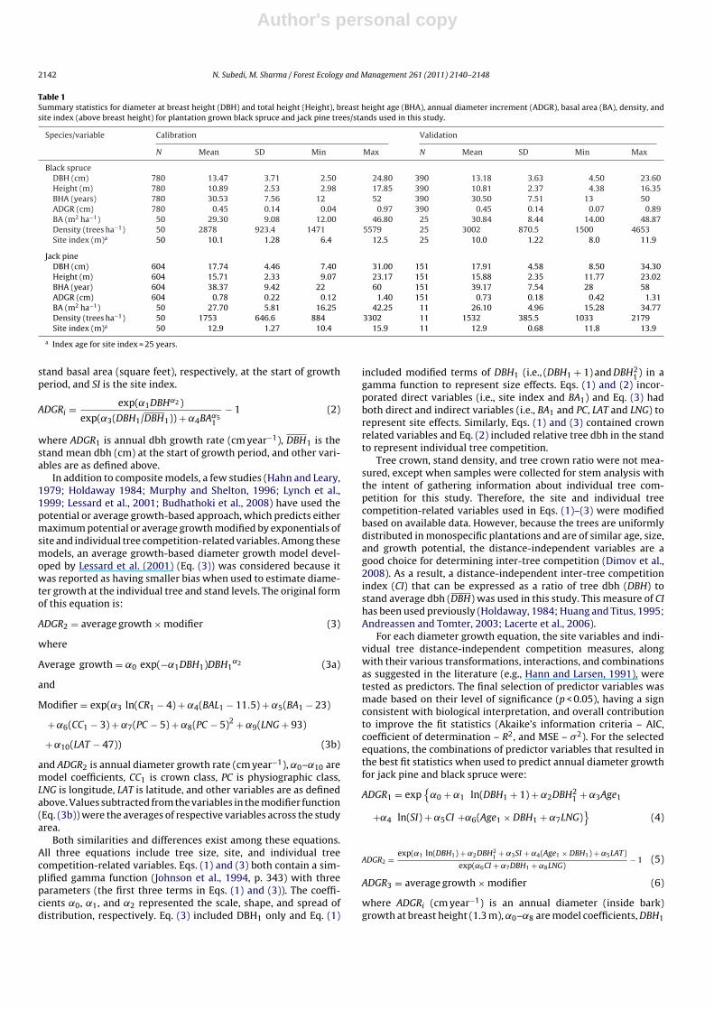
Table 1Summary statistics for diameter at breast height (DBH) and total height (Height), breast height age (BHA), annual diameter increment (ADGR), basal area (BA), density, andsite index (above breast height) for plantation grown black spruce and jack pine trees/stands used in this study.

Species/variable Calibration Validation

N Mean SD Min Max N Mean SD Min Max

Black spruceDBH (cm) 780 13.47 3.71 2.50 24.80 390 13.18 3.63 4.50 23.60Height (m) 780 10.89 2.53 2.98 17.85 390 10.81 2.37 4.38 16.35BHA (years) 780 30.53 7.56 12 52 390 30.50 7.51 13 50ADGR (cm) 780 0.45 0.14 0.04 0.97 390 0.45 0.14 0.07 0.89BA (m2 ha−1) 50 29.30 9.08 12.00 46.80 25 30.84 8.44 14.00 48.87Density (trees ha−1) 50 2878 923.4 1471 5579 25 3002 870.5 1500 4653Site index (m)a 50 10.1 1.28 6.4 12.5 25 10.0 1.22 8.0 11.9

Jack pineDBH (cm) 604 17.74 4.46 7.40 31.00 151 17.91 4.58 8.50 34.30Height (m) 604 15.71 2.33 9.07 23.17 151 15.88 2.35 11.77 23.02BHA (year) 604 38.37 9.42 22 60 151 39.17 7.54 28 58ADGR (cm) 604 0.78 0.22 0.12 1.40 151 0.73 0.18 0.42 1.31BA (m2 ha−1) 50 27.70 5.81 16.25 42.25 11 26.10 4.96 15.28 34.77Density (trees ha−1) 50 1753 646.6 884 3302 11 1532 385.5 1033 2179Site index (m)a 50 12.9 1.27 10.4 15.9 11 12.9 0.68 11.8 13.9

a Index age for site index = 25 years.

stand basal area (square feet), respectively, at the start of growthperiod, and SI is the site index.

ADGRi = exp(˛1DBH˛2 )

exp(˛3(DBH1/DBH1)) + ˛4BA˛51

− 1 (2)

where ADGR1 is annual dbh growth rate (cm year−1), DBH1 is thestand mean dbh (cm) at the start of growth period, and other vari-ables are as defined above.

In addition to composite models, a few studies (Hahn and Leary,1979; Holdaway 1984; Murphy and Shelton, 1996; Lynch et al.,1999; Lessard et al., 2001; Budhathoki et al., 2008) have used thepotential or average growth-based approach, which predicts eithermaximum potential or average growth modified by exponentials ofsite and individual tree competition-related variables. Among thesemodels, an average growth-based diameter growth model devel-oped by Lessard et al. (2001) (Eq. (3)) was considered because itwas reported as having smaller bias when used to estimate diame-ter growth at the individual tree and stand levels. The original formof this equation is:

ADGR2 = average growth × modifier (3)

where

Average growth = ˛0 exp(−˛1DBH1)DBH1˛2 (3a)

and

Modifier = exp(˛3 ln(CR1 − 4) + ˛4(BAL1 − 11.5) + ˛5(BA1 − 23)

+ ˛6(CC1 − 3) + ˛7(PC − 5) + ˛8(PC − 5)2 + ˛9(LNG + 93)

+ ˛10(LAT − 47)) (3b)

and ADGR2 is annual diameter growth rate (cm year−1), ˛0–˛10 aremodel coefficients, CC1 is crown class, PC is physiographic class,LNG is longitude, LAT is latitude, and other variables are as definedabove. Values subtracted from the variables in the modifier function(Eq. (3b)) were the averages of respective variables across the studyarea.

Both similarities and differences exist among these equations.All three equations include tree size, site, and individual treecompetition-related variables. Eqs. (1) and (3) both contain a sim-plified gamma function (Johnson et al., 1994, p. 343) with threeparameters (the first three terms in Eqs. (1) and (3)). The coeffi-cients ˛0, ˛1, and ˛2 represented the scale, shape, and spread ofdistribution, respectively. Eq. (3) included DBH1 only and Eq. (1)

included modified terms of DBH1 (i.e., (DBH1 + 1) and DBH21) in a

gamma function to represent size effects. Eqs. (1) and (2) incor-porated direct variables (i.e., site index and BA1) and Eq. (3) hadboth direct and indirect variables (i.e., BA1 and PC, LAT and LNG) torepresent site effects. Similarly, Eqs. (1) and (3) contained crownrelated variables and Eq. (2) included relative tree dbh in the standto represent individual tree competition.

Tree crown, stand density, and tree crown ratio were not mea-sured, except when samples were collected for stem analysis withthe intent of gathering information about individual tree com-petition for this study. Therefore, the site and individual treecompetition-related variables used in Eqs. (1)–(3) were modifiedbased on available data. However, because the trees are uniformlydistributed in monospecific plantations and are of similar age, size,and growth potential, the distance-independent variables are agood choice for determining inter-tree competition (Dimov et al.,2008). As a result, a distance-independent inter-tree competitionindex (CI) that can be expressed as a ratio of tree dbh (DBH) tostand average dbh (DBH) was used in this study. This measure of CIhas been used previously (Holdaway, 1984; Huang and Titus, 1995;Andreassen and Tomter, 2003; Lacerte et al., 2006).

For each diameter growth equation, the site variables and indi-vidual tree distance-independent competition measures, alongwith their various transformations, interactions, and combinationsas suggested in the literature (e.g., Hann and Larsen, 1991), weretested as predictors. The final selection of predictor variables wasmade based on their level of significance (p < 0.05), having a signconsistent with biological interpretation, and overall contributionto improve the fit statistics (Akaike’s information criteria – AIC,coefficient of determination – R2, and MSE – �2). For the selectedequations, the combinations of predictor variables that resulted inthe best fit statistics when used to predict annual diameter growthfor jack pine and black spruce were:

ADGR1 = exp{

˛0 + ˛1 ln(DBH1 + 1) + ˛2DBH21 + ˛3Age1

+˛4 ln(SI) + ˛5CI +˛6(Age1 × DBH1 + ˛7LNG)}

(4)

ADGR2 = exp(˛1 ln(DBH1) + ˛2DBH21 + ˛3SI + ˛4(Age1 × DBH1) + ˛5LAT)

exp(˛6CI + ˛7DBH1 + ˛8LNG)− 1 (5)

ADGR3 = average growth × modifier (6)

where ADGRi (cm year−1) is an annual diameter (inside bark)growth at breast height (1.3 m), ˛0–˛8 are model coefficients, DBH1

Author's personal copy

N. Subedi, M. Sharma / Forest Ecology and Management 261 (2011) 2140–2148 2143

(cm) is inside bark diameter at breast height, Age1 is the age of thetree above breast height, and CI is the ratio of DBH1 to stand aver-age dbh at the start of growth period. Similarly, SI (m) is the siteindex at index age 25 above breast height, LAT is latitude, LNG islongitude, and

Average growth = ˛0 exp(−˛1DBH1)DBH˛21 (6a)

and

Modifier = exp(˛3 ln(SI) + ˛4(Age1 × DBH1) + ˛5Age1

+ ˛6CI + ˛7LNG) (6b)

2.3. Model fitting and evaluation

Eqs. (4)–(6) were first fitted to the model data set using ordinarynonlinear least squares (MODEL procedure) in SAS (SAS Instituteand Inc., 2008) to conduct a preliminary evaluation. Fit statistics (R2

and MSE) and bias in estimates of average diameter growth (insidebark) were calculated for these equations across tree size (dbh)and age for both the model and evaluation data sets. Similarly, AICvalues were calculated using NLMIXED procedure for all equationsfor both species. Evaluation consisted of examining fit statistics andaccuracy in estimating diameter growth across tree size and agegroup.

The model resulting in the largest R2, least MSE and AIC, andsmallest values of average bias in estimating diameter growthacross tree size and age group was selected as the “best” model foreach tree species. The mixed-effects approach was then applied tothis “best” model, which was fitted using the NLMIXED procedure inSAS. This analysis assumed that within-stand variance was homo-geneous and residuals (εi) were uncorrelated. Random-effectsparameters were added sequentially starting at one coefficient asrandom for each species. The models with random effects wereevaluated based on goodness-of-fit criteria such as log-likelihood(twice the negative log-likelihood), assessment of model residuals,AIC, and �i (rescaled AIC values calculated as �i = AICi–minimumAIC) so that a model with minimum information criterion has avalue of 0 (Burnham and Anderson, 2001). The AIC is defined as:

AIC = −2 ln(L) + 2k

where ln is natural logarithm, L is the likelihood function, and kis the number of parameters in the model. The model with thesmallest goodness-of-fit values is considered best.

2.4. Predicting diameter increment for a new stand

The main purpose of a model is to predict the response vari-able using explanatory variables specified in the model. In themixed modeling approach, average diameter increment can be pre-dicted by (i) assuming the random parameters are zero if no priorsare known for diameter growth (typical mean response) and (ii)calibrating random-effects coefficients using priors on diametergrowth of a sub-sample (tree(s)) and combining both fixed- andrandom-effects parameters (calibrated response). Additional pre-dictions can be made using coefficients from a model fitted withoutrandom effects; these predictions are referred to as populationaveraged (PA) responses.

The typical mean response represents the mean behavior ofdiameter increment for a given tree in a particular (say the ith)stand and it can be predicted as

Est(ADGR)i = fi(�, Aiˆ ) (7)

where Est(ADGR)i is the estimated average diameter growth ofa tree from ith stand, � is the estimated vector of deterministic

parameter, ˆ is the population averaged parameter (fixed-effectscomponent of mixed-effects parameters), and Ai is the designmatrix. Note that fi is a function of covariates (representingtree, site, and competition-related attributes) as expressed in Eqs.(4)–(6).

To estimate a calibrated response, however, the random-effectsparameters need to be predicted using priors on diameter growthfrom a sub-sample of tree(s) for every new (unsampled) sub-ject/cluster (stand). In addition, tree- and site-level information isrequired to predict the random coefficient(s) for a new stand. Therandom effects coefficient(s) for a particular stand can be estimated(Vonesh and Chinchilli, 1997) as:

bi = DZTi (Ri + ZiDZT

i )−1

ei (8)

where D is the k × k variance-covariance matrix (k = number ofrandom-effects parameter(s) included in the model) for the among-plot variation, Ri is the ni × ni variance-covariance matrix for ithplot, the vector of residuals ei = yi − fi(�, Ai

ˆ ) is the ni × 1 and con-tains the difference between the observed and estimated annualdbh growth using the deterministic and fixed-effects coefficients.Zi is the ni × q matrix evaluated at � and ˆ for the ith plot and it canbe derived as:

∂fi(�, Aiˆ )

∂ˇ(9)

where ˇ is a k × 1 coefficient that was considered as mixed-effects.The mixed-effects parameter(s) can be obtained by adding the pop-ulation averaged and random-effects parameter(s) as:

ai = Aiˆ + bi (10)

where ai is the estimated mixed-effects parameter(s) for ith stand,and others as defined earlier. The calibrated response can then becalculated using the deterministic population averaged coefficientsand mixed-effects coefficients as:

Est(ADGRi|ai) = fi(�, ai) (11)

The function f is the “best” equation among Eqs. (4)–(6) interms of goodness of fits. Diameter growths are then predicted interms of size, site, competition-related variables, and both fixed-and random-effects parameters. Details on estimation of random-effects coefficients for unsampled subject/cluster in the forestrycontext can be found in previous studies (Calama and Montero,2004; Trincado and Burkhart, 2006; Sharma and Parton, 2007,2009).

Prediction accuracies of population averaged, typical mean, andcalibrated responses were compared using mean bias and stan-dard deviation of bias across tree size and age for each speciesusing the evaluation data set. For the calibrated responses, priorson diameter increments were required to calibrate random-effects.We selected a tree to calibrate the random effects for each plot usingfour tree selection criteria: (1) random, (2) top height (dominant orcodominant), (3) tree dbh closer to quadratic mean diameter, and(4) small sized were considered. Calibrated response in diametergrowth was obtained using priors on diameter growths from thesetree selection criteria. Mean bias in estimating diameter growthand its standard deviation were calculated for each species using100 simulation runs.

3. Results and discussions

Fit statistics for Eqs. (4)–(6) fitted using MODEL and NLMIXEDprocedures in SAS are given in Table 2. Eqs. (4) and (6) had verysimilar fit statistics with those for Eq. (4) slightly better than thosefor Eq. (6) for both species. Eq. (5) had the poorest fit statistics (i.e.,

Author's personal copy

2144 N. Subedi, M. Sharma / Forest Ecology and Management 261 (2011) 2140–2148

Table 2Fit statistics (coefficient of determination – R2*, mean square error – MSE, and Akaike Information Criterion – AIC) for Eqs. (4)–(6) by species.

Equation Black spruce Jack pine

R2a MSE AIC R2a MSE AIC

(4) 0.6902 0.0108 −8565 0.7622 0.0160 −6312(5) 0.6502 0.0121 −7950 0.7230 0.0186 −5571(6) 0.6865 0.0109 −8506 0.7569 0.0164 −6206

a Computed as (1 − residual sum of squares/corrected sum of squares).

-0.10

-0.08

-0.06

-0.04

-0.02

0.00

0.02

0.04

0.06

0.08

0.10

3 4-6 7-9 10-12 13-15 16-18 19

DBH class (cm)

Avera

ge b

ias (

cm

)

Eq. (4) Eq. (5) Eq. (6)

Eq. (4) Eq. (5) Eq. (6)

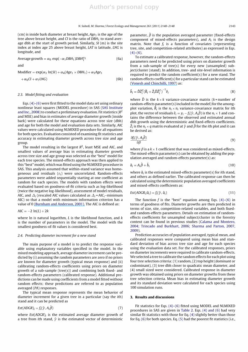
Fig. 1. Average bias (observed-predicted) in estimates of annual diameter growthat breast height across DBH-classes for independent evaluation data set using Eqs.(4)–(6) for black spruce (bold lines with filled markers) and jack pine (lines withoutfilled markers) trees.

the smallest R2 and the largest MSE and AIC) among the three equa-tions. These equations were further evaluated based on their biasin estimating annual average diameter growth across the range oftree size and age for both the calibration and evaluation data sets.These average biases are shown in Fig. 1 for the evaluation data setfor both black spruce and jack pine. For black spruce, Eq. (4) had thesmallest bias (bold line with filled circles). For jack pine, the bias inestimating dib was almost identical for Eqs. (4) and (6) across therange of tree size for both data sets. However, the bias was slightlylarger for Eq. (6) for age classes above 31 years (not shown in fig-ure). As Eq. (4) had the best fit statistics (i.e., largest R2 and smallestMSE and AIC) and produced consistently smaller bias in estimatingdiameter growths of black spruce and jack pine trees for both cali-bration and evaluation data sets, this equation was selected for usein the mixed-effects modeling.

In the next step, Eq. (4) was fitted using NLMIXED procedurein SAS. As mentioned earlier, to fit this equation, random-effectsparameters were added individually and sequentially. Among themodels with one random-effects parameter, the coefficient ˛3for black spruce and ˛1 for jack pine gave the best fit (small-est AIC and �i) (Table 3). Similarly, the coefficients ˛0 and ˛3and ˛0 and ˛1 as random-effects for black spruce and jack pine,respectively, provided the most improved fit among the mixed-effects models with two random-effects parameters. Similarly, thecoefficients ˛0, ˛1, and ˛3 as random-effects parameters resultedin the best fit (smallest AIC, −ln(Likelihood), �i, and �2 statis-tics) among all models with three mixed-effects parameters forboth species. The coefficient ˛7 became not significant (p > 0.05)in assuming other parameters as mixed-effects except ˛1 and ˛3for black spruce (one mixed-effects parameter model) and (˛0,˛3) for jack pine (two mixed-effects parameters model). In allcases, models containing random parameters (fixed-effects andsubject-specific random-effects) fitted the data better than mod-els containing only population-averaged deterministic parametersfor both species. Attempts to fit models with more than threerandom-effects parameters were unsuccessful because of conver-gence problems. As a result, the final diameter growth model for

black spruce and jack pine can be expressed as:

ADGR = exp

{ˇ0 + b0 + (ˇ1 + b1) ln(DBH1 + 1) + �1DBH2

1

+(ˇ2 + b2)Age1 + �2 ln(SI) + �3

(DBH1

DBH1

)+ �4(Age1 × DBH1)

+�5LNG

}(12)

where ˇ0, ˇ1 and ˇ2 are the fixed effects (population averaged),b0, b1, and b2 are random effects, �1, �2, �3, �4, and �5 arepopulation-averaged deterministic parameters, and other variablesare as defined above. Hereafter, for brevity the fixed effects (ˇ0, ˇ1and ˇ2) and population-averaged deterministic parameters (�1, �2,�3, �4, and �5) will be referred to as population-averaged parame-ters.

Estimated parameters for Eq. (12) for black spruce and jack pineare given in Table 4. Estimates of parameters, including variancecomponents for black spruce, were consistent with those found forjack pine and the nature of the coefficients (±) was consistent withbiological interpretation. In addition, the magnitudes of coefficientswere similar for both species. All the variance components weresignificant, except cov(b0, b2) for jack pine.

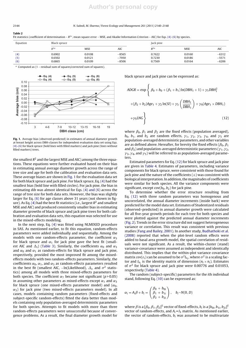
To determine whether the error structure resulting fromEq. (12) with three random parameters was homogenous anduncorrelated, the annual diameter increments (inside bark) werepredicted for the model data set. Estimates of Studentized residuals(observed–predicted) in annual diameter growth were calculatedfor all five-year growth periods for each tree for both species andwere plotted against the predicted annual diameter increments(Fig. 2). Trends in the error structure did not suggest heterogeneousvariance or correlation. This result was consistent with previousstudies (Fang and Bailey, 2001). In another study, Budhathoki et al.(2008) reported that when the plot-level random effects wereadded to basal area growth model, the spatial correlation of resid-uals were not significant. As a result, the within-cluster (stand)variance-covariance were assumed as independent and identicallydistributed. This implies that the within-plot variance covariancematrix cov(εi) can be assumed to be �2Ini

, where �2 is a scaling fac-tor and Ini

is the identity matrix of dimension (ni × ni). Estimatesof �2 for black spruce and jack pine were 0.00776 and 0.01053,respectively (Table 4).

The random (subject-specific) parameters for the ith individualstand, following Eq. (10) can be expressed as:

˛i = Aiˇ + bi =(

ˇ0 + b0i

ˇ1 + b1i

ˇ2 + b2i

), bi∼N(0, D)

where ˇ is a [ˇ0, ˇ1, ˇ2]T vector of fixed-effects, bi is a [b0i, b1i, b2i]T

vector of random-effects, and Ai = I3 matrix. As mentioned earlier,the vector of random-effects, bi was assumed to be multivariate

Author's personal copy

N. Subedi, M. Sharma / Forest Ecology and Management 261 (2011) 2140–2148 2145

Table 3Fit statistics for the annual diameter increment model (Eq. (4)) with fixed effects and a number of combinations of mixed-effects for black spruce and jack pine plantationdata from boreal Ontario.

Random parameters Parameters (k) Black spruce k Jack pine

�2 −2 Ln(L) AICc �i �2 −2Ln (L) AICc �i

Noneb 9 0.01074 −8583 −8565 1276 9 0.015980 −6330 −6312 1617˛0

a 9 0.009858 −8895 −8877 964 10 0.014680 −6623 −6603 1326˛1 10 0.009147 −9228 −9208 633 10 0.013680 −6914 −6894 1035˛3 10 0.008778 −9419 −9399 442 – – – –˛4

a 9 0.009859 −8893 −8875 966 10 0.014690 −6623 −6603 1326˛0 , ˛1

a 11 0.00831 −9604 −9582 259 12 0.011490 −7651 −7627 302˛0, ˛3

a 11 0.008003 −9752 −9730 111 11 0.011820 −7478 −7456 473˛1, ˛4

* 11 0.008319 −9598 −9576 265 – – – –˛3, ˛4

* 11 0.007997 −9741 −9719 122 – – – –˛1, ˛3

a 11 0.008304 −9588 −9566 275 – – – –˛0, ˛1, ˛3

a 14 0.007757 −9869 −9841 0 15 0.010523 −7959 −7929 0

�i = AIC − min(AIC) (Burnham and Anderson, 2001).a The coefficient ˛7 was not significant in assuming these parameters as mixed-effects except ˛1 and ˛3 for black spruce and (˛0,˛3) for jack pine.b Fixed-effects model.c AIC =−2 Ln(L) + 2k, and smaller AIC is better.

Table 4Parameter estimates and fit statistics (SE = standard error) for Eq. (12) fitted for black spruce and jack pine plantation grown trees from boreal Ontario.

Black spruce Jack pine

Estimates SE Estimates SE

Parametersˇ0 −2.4204 0.2486 −2.4880 0.5773ˇ1 0.8167 0.0255 0.3439 0.0272�1 −0.0071 0.0004 −0.0028 0.0002ˇ2 −0.1441 0.0047 −0.1205 0.0036�2 0.6597 0.1065 0.3933 0.1528�3 0.0578 0.0170 0.1503 0.0149�4 0.0070 0.0003 0.0044 0.0002�5 − − −0.0121 0.0035Variance components�2 0.00776 0.0002 0.01053 0.0002var(b0) 0.01879 0.0044 0.04559 0.0092var(b1) 0.01253 0.0034 0.02727 0.0053var(b2) 0.00036 9E−05 0.00029 9E−05cov(b0,b1) −0.00584 0.003 −0.01959 0.0076cov(b1, b2) −0.00129 0.0005 −0.00160 0.0005cov(b0, b3) −0.00100 0.0005 −0.00112 0.0007

normally distributed with E[bi] = 0 with an unstructured variance-covariance matrix D (Table 4). These matrices are:

D =(

0.01879 −0.00584 −0.00100− 0.00584 0.01253 −0.00129−0.00100 −0.00129 0.00036

)for black spruce

D =(

0.04559 −0.01959 −0.00112−0.01959 0.02727 −0.00160−0.00112 −0.00160 0.00029

)for jack pine

Although E[bi] = 0, the vector of random-effects parameter(bi = [b0i, b1i, b2i]T) could be different from zero for an individualstand. The random-effects parameters for a stand can be predictedif diameter increments, tree, and site information are available forat least a sub-sample of tree(s) in a stand. The population-averagedparameters (i.e., fixed-effects component of random parameters ˇ0,ˇ1, and ˇ2 and the deterministic parameters �1, �2, �3, �4, and �5)are fixed (Table 4) for entire population of stands, but the random-effects parameters (i.e., the column vector bi) need to be estimatedfor each stand.

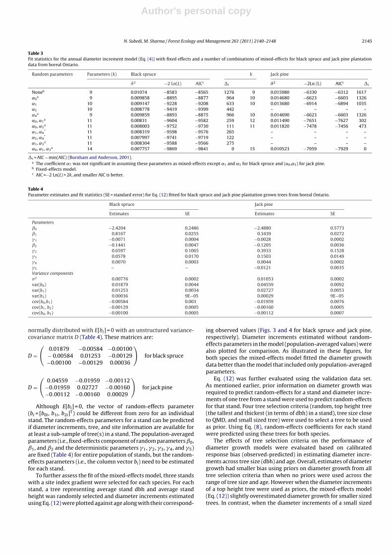
To further assess the fit of the mixed-effects model, three standswith a site index gradient were selected for each species. For eachstand, a tree representing average stand dbh and average standheight was randomly selected and diameter increments estimatedusing Eq. (12) were plotted against age along with their correspond-

ing observed values (Figs. 3 and 4 for black spruce and jack pine,respectively). Diameter increments estimated without random-effects parameters in the model (population-averaged values) werealso plotted for comparison. As illustrated in these figures, forboth species the mixed-effects model fitted the diameter growthdata better than the model that included only population-averagedparameters.

Eq. (12) was further evaluated using the validation data set.As mentioned earlier, prior information on diameter growth wasrequired to predict random-effects for a stand and diameter incre-ments of one tree from a stand were used to predict random-effectsfor that stand. Four tree selection criteria (random, top height tree(the tallest and thickest (in terms of dbh) in a stand), tree size closeto QMD, and small sized tree) were used to select a tree to be usedas prior. Using Eq. (8), random-effects coefficients for each standwere predicted using these trees for both species.

The effects of tree selection criteria on the performance ofdiameter growth models were evaluated based on calibratedresponse bias (observed-predicted) in estimating diameter incre-ments across tree size (dbh) and age. Overall, estimates of diametergrowth had smaller bias using priors on diameter growth from alltree selection criteria than when no priors were used across therange of tree size and age. However when the diameter incrementsof a top height tree were used as priors, the mixed-effects model(Eq. (12)) slightly overestimated diameter growth for smaller sizedtrees. In contrast, when the diameter increments of a small sized

Author's personal copy

2146 N. Subedi, M. Sharma / Forest Ecology and Management 261 (2011) 2140–2148

Fig. 2. Bias (observed-predicted) in predicting annual diameter growth inside barkof (A) black spruce and (B) jack pine trees using Eq. (12).

Fig. 3. Diameter growth profiles of three randomly selected black spruce trees alongthe site index (SI) gradient (i.e., with SI (index age = 25) 12, 10 and 6 m at breastheight) generated using population averaged parameters and parameters of mixed-effects model, with ˇ1, ˇ2 and ˇ3 having random effects in Eq. (12).

tree were used as priors, the mixed-effects model slightly under-estimated diameter growth for most of the trees. Thus, selectionof either a large (in terms of DBH and height) or a small (in termsof dbh) tree from which to use measurements as priors resulted inlarger bias in diameter increments than use of the other two treeselection criteria. For the other two selection criteria, bias result-ing from using the random-effects parameters calibrated with arandomly selected tree was slightly smaller than that when themodel was calibrated with a tree close to QMD. As a result, to cali-

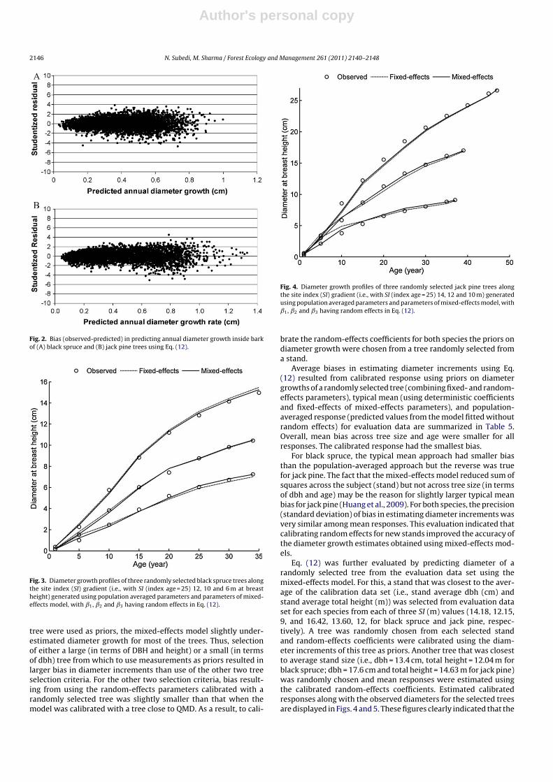
Fig. 4. Diameter growth profiles of three randomly selected jack pine trees alongthe site index (SI) gradient (i.e., with SI (index age = 25) 14, 12 and 10 m) generatedusing population averaged parameters and parameters of mixed-effects model, withˇ1, ˇ2 and ˇ3 having random effects in Eq. (12).

brate the random-effects coefficients for both species the priors ondiameter growth were chosen from a tree randomly selected froma stand.

Average biases in estimating diameter increments using Eq.(12) resulted from calibrated response using priors on diametergrowths of a randomly selected tree (combining fixed- and random-effects parameters), typical mean (using deterministic coefficientsand fixed-effects of mixed-effects parameters), and population-averaged response (predicted values from the model fitted withoutrandom effects) for evaluation data are summarized in Table 5.Overall, mean bias across tree size and age were smaller for allresponses. The calibrated response had the smallest bias.

For black spruce, the typical mean approach had smaller biasthan the population-averaged approach but the reverse was truefor jack pine. The fact that the mixed-effects model reduced sum ofsquares across the subject (stand) but not across tree size (in termsof dbh and age) may be the reason for slightly larger typical meanbias for jack pine (Huang et al., 2009). For both species, the precision(standard deviation) of bias in estimating diameter increments wasvery similar among mean responses. This evaluation indicated thatcalibrating random effects for new stands improved the accuracy ofthe diameter growth estimates obtained using mixed-effects mod-els.

Eq. (12) was further evaluated by predicting diameter of arandomly selected tree from the evaluation data set using themixed-effects model. For this, a stand that was closest to the aver-age of the calibration data set (i.e., stand average dbh (cm) andstand average total height (m)) was selected from evaluation dataset for each species from each of three SI (m) values (14.18, 12.15,9, and 16.42, 13.60, 12, for black spruce and jack pine, respec-tively). A tree was randomly chosen from each selected standand random-effects coefficients were calibrated using the diam-eter increments of this tree as priors. Another tree that was closestto average stand size (i.e., dbh = 13.4 cm, total height = 12.04 m forblack spruce; dbh = 17.6 cm and total height = 14.63 m for jack pine)was randomly chosen and mean responses were estimated usingthe calibrated random-effects coefficients. Estimated calibratedresponses along with the observed diameters for the selected treesare displayed in Figs. 4 and 5. These figures clearly indicated that the

Author's personal copy

N. Subedi, M. Sharma / Forest Ecology and Management 261 (2011) 2140–2148 2147

Table 5Mean bias (cm) (observed–predicted) and its standard deviations by tree size (dbh) (A) and age group (B) in predicting annual diameter increments at breast height amongthe models that used population averaged (PA), typical mean (TM), and calibrated response (CR) by species.

(A)Species DBH class Number of obs. Average bias (cm) SD of bias

PA TM CR PA TM CRBlack spruce

<3 784 0.002 0.008 0.005 0.1216 0.1033 0.11434–6 442 −0.014 −0.008 −0.011 0.0975 0.1758 0.09427–9 509 −0.006 −0.006 −0.009 0.0961 0.1830 0.0897

10–12 451 0.003 −0.005 −0.001 0.0872 0.1402 0.083213–15 250 0.012 −0.004 0.003 0.0863 0.0934 0.0886

16+ 89 0.012 −0.017 −0.002 0.0708 0.0573 0.0908Jack pine

<3 199 −0.056 −0.076 −0.032 0.1639 0.0951 0.16814–6 146 −0.011 −0.029 −0.003 0.1509 0.1539 0.15647–9 188 −0.006 −0.016 −0.011 0.1149 0.1627 0.1189

10–12 226 0.014 0.010 0.001 0.0992 0.1398 0.099713–15 217 0.027 0.030 0.014 0.0904 0.1024 0.092616–18 148 0.027 0.035 0.014 0.0705 0.0834 0.0732

19+ 123 −0.003 0.016 −0.016 0.0773 0.0676 0.0867

(B)Species Age group Number of obs. Average bias (cm) SD of bias

PA TM CR PA TM CRBlack spruce

<5 780 0.003 0.009 0.0053 0.1224 0.1058 0.11546–10 390 −0.023 −0.019 −0.0148 0.1059 0.1278 0.1036

11–15 388 −0.023 −0.027 −0.0201 0.0943 0.1033 0.092516–20 338 0.001 −0.007 -0.0015 0.0852 0.0848 0.082221–25 279 0.017 0.009 0.0092 0.0784 0.0720 0.073926–30 215 0.021 0.014 0.0100 0.0752 0.0626 0.0679

31+ 135 0.029 0.020 −0.0010 0.0772 0.0661 0.0907Jack pine

<5 302 −0.033 −0.053 −0.0140 0.1684 0.0832 0.17216–10 151 −0.001 −0.018 −0.0043 0.1354 0.0600 0.1371

11–15 151 −0.012 −0.023 −0.0244 0.1011 0.0508 0.101316–20 151 0.002 −0.002 −0.0124 0.0800 0.0473 0.081321–25 151 0.020 0.023 0.0063 0.0850 0.0462 0.085226–30 130 0.033 0.042 0.0189 0.0868 0.0463 0.086731–35 109 0.028 0.043 0.0145 0.0704 0.0480 0.0766

36+ 102 −0.003 0.025 −0.0035 0.0684 0.0612 0.0818

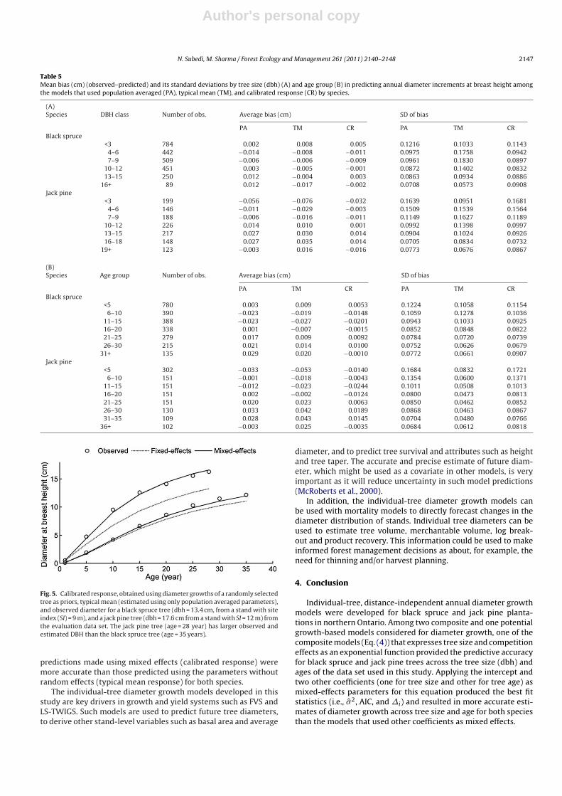
Fig. 5. Calibrated response, obtained using diameter growths of a randomly selectedtree as priors, typical mean (estimated using only population averaged parameters),and observed diameter for a black spruce tree (dbh = 13.4 cm, from a stand with siteindex (SI) = 9 m), and a jack pine tree (dbh = 17.6 cm from a stand with SI = 12 m) fromthe evaluation data set. The jack pine tree (age = 28 year) has larger observed andestimated DBH than the black spruce tree (age = 35 years).

predictions made using mixed effects (calibrated response) weremore accurate than those predicted using the parameters withoutrandom effects (typical mean response) for both species.

The individual-tree diameter growth models developed in thisstudy are key drivers in growth and yield systems such as FVS andLS-TWIGS. Such models are used to predict future tree diameters,to derive other stand-level variables such as basal area and average

diameter, and to predict tree survival and attributes such as heightand tree taper. The accurate and precise estimate of future diam-eter, which might be used as a covariate in other models, is veryimportant as it will reduce uncertainty in such model predictions(McRoberts et al., 2000).

In addition, the individual-tree diameter growth models canbe used with mortality models to directly forecast changes in thediameter distribution of stands. Individual tree diameters can beused to estimate tree volume, merchantable volume, log break-out and product recovery. This information could be used to makeinformed forest management decisions as about, for example, theneed for thinning and/or harvest planning.

4. Conclusion

Individual-tree, distance-independent annual diameter growthmodels were developed for black spruce and jack pine planta-tions in northern Ontario. Among two composite and one potentialgrowth-based models considered for diameter growth, one of thecomposite models (Eq. (4)) that expresses tree size and competitioneffects as an exponential function provided the predictive accuracyfor black spruce and jack pine trees across the tree size (dbh) andages of the data set used in this study. Applying the intercept andtwo other coefficients (one for tree size and other for tree age) asmixed-effects parameters for this equation produced the best fitstatistics (i.e., �2, AIC, and �i) and resulted in more accurate esti-mates of diameter growth across tree size and age for both speciesthan the models that used other coefficients as mixed effects.

Author's personal copy

2148 N. Subedi, M. Sharma / Forest Ecology and Management 261 (2011) 2140–2148

For both species, diameter growth estimates from calibratedresponses (i.e., estimates made using mixed-effects coefficients)were more accurate across tree size and age than those from typicalmean responses (i.e., estimates made using fixed-effects param-eters) and population-averaged responses (i.e., estimates madeusing the model fitted without random effects). Four differentmethods – random, dominant or codominant, tree diameter atbreast height (dbh) close to quadratic mean diameter (QMD), andsmall sized – of selecting a tree to predict random-effects for anew (unsampled) stand were also evaluated. For both black spruceand jack pine trees, the random-effects estimated using diametergrowth of a randomly selected tree gave the most accurate andprecise estimates of average diameter growth relative to those esti-mated using trees selected using other methods.

The accurate and precise estimate of future diameters, whichmay be used as a covariate in other models, is very important, as itwill reduce the uncertainty of other model predictions. The resultspresented here can be used to accurately forecast diameter distri-bution of stands, which allows for detailed product analysis. Thisdetailed product information may be used to make informed forestmanagement decisions such as thinning and economic analysis ofharvesting. How a tree should be selected to be used for predict-ing random-effects in the diameter growth models that results inmore accurate diameter estimates, is another important aspect ofthis study.

Acknowledgements

This study was supported by Ontario Ministry of NaturalResources. Support for data collection was provided by the ForestryFutures Trust Enhanced Forest Productivity Science Program. Weare grateful to Lisa Buse (Ontario Forest Research Institute) for edit-ing an earlier version of the manuscript and John Parton (OMNR)for his support in collecting the data.

References

Amateis, R.L., Burkhart, H.E., Walsh, T.A., 1989. Diameter increment and survivalequations for loblolly pine trees growing in thinned and unthinned plantationson cutover, site-prepared lands. South. J. Appl. For. 14, 170–174.

Andreassen, K., Tomter, S.M., 2003. Basal area growth models for individual treesof Norway spruce, scots pine, birch and other broadleaves in Norway. For. Ecol.Manage. 180, 11–24.

Avery, T.E., Burkhart, H.E., 1983. Forest Measurements. McGraw-Hill Book Company,New York, NY, 331 pp.

Budhathoki, C.B., Lynch, T.B., Guldin, J.M., 2008. Nonlinear mixed modeling of basalarea growth for shortleaf pine. For. Ecol. Manage. 255, 3440–3446.

Burnham, K.P., Anderson, D.R., 2001. Kullback-Liebler information as a basis forstrong inference in ecological studies. Wildlife Res. 28, 111–119.

Calama, R., Montero, G., 2004. Interregional nonlinear height–diameter model withrandom coefficients for stone pine in Spain. Can. J. For. Res. 34, 150–163.

Demidenko, E., 2004. Mixed Models: Theory and Applications. John Wiley & Sons,Inc., Hoboken, NJ, 704 pp.

Dimov, L.D., Chambers, J.L., Lockhart, B.R., 2008. Five-year radial growth of red oaksin mixed bottomland hardwood stands. For. Ecol. Manage. 255, 2790–2800.

Fang, Z., Bailey, R.L., 2001. Nonlinear mixed effects modeling for slash pine dominantheight growth following intensive silvicultural treatments. For. Sci. 47, 287–300.

Graves, H.S., 1906. Forest Mensuration. John Wiley & Sons, New York, NY, 458 pp.Gregoire, T.G., Schabenberger, O., Barrett, J.P., 1995. Linear modelling of irregularly

spaced, unbalanced, longitudinal data from permanent-plot measurements.Can. J. For. Res. 25, 137–156.

Hahn, J.T., Leary, R.A., 1979. Potential diameter growth function. In: A GeneralizedForest Growth Projection System Applied to the Lake States Region. USDA For.Serv. Gen. Tech. Rep. NC-49, pp. 22–26.

Hann, D.W., Larsen, D.R., 1991. Diameter Growth Equations for Fourteen Tree Speciesin Southwest Oregon. For. Res. Lab., Oregon State University Research Bulletin69, 18 pp.

Hökkä, H., Groot, A., 1999. An individual-tree basal area growth model for blackspruce in second-growth peatland stands. Can. J. For. Res. 29, 621–629.

Holdaway, M.R., 1984. Modeling the Effect of Competition on Tree Diameter Growthas Applied in Stems. USDA For. Serv. Gen. Tech. Rep. NC-94, 9 pp.

Huang, S., Titus, S., 1995. An individual tree diameter increment model for whitespruce in Alberta. Can. J. For. Res. 25, 1455–1465.

Huang, S., Meng, S.X., Yang, Y., 2009. Assessing the goodness of fit of forest modelsestimated by nonlinear mixed-model methods. Can. J. For. Res. 39, 2418–2436.

Johnson, N.L., Kotz, S., Balakrishnan, 1994. Continuous Univariate Distributions, vol.1., 2nd ed. John Wiley & Sons, New York, NY.

Kiernan, D.H., Bevilacqua, E., Nyland, R.D., 2008. Individual-tree diameter growthmodel for sugar maple trees in even-aged northern hardwood stands underselection system. For. Ecol. Manage. 256, 1579–1586.

Lacerte, V., Larocque, G.R., Woods, M., Parton, W.J., Penner, M., 2006. Calibrationof the forest vegetation simulator (FVS) model for the main forest species ofOntario. Can. Ecol. Model. 199, 336–349.

Leites, L.P., Robinson, A.P., 2004. Improving taper equations of loblolly pine withcrown dimensions in a mixed-effects modelling framework. For. Sci. 50,204–212.

Leites, L.P., Robinson, A.P., Crookston, N.L., 2009. Accuracy and equivalence test-ing of crown ratio models and assessment of their impact on diameter growthand basal area increment predictions of two variants of the Forest VegetationSimulator. Can. J. For. Res. 39, 655–665.

Lessard, V.C., McRoberts, R.E., Holdaway, M.R., 2001. Diameter growth models usingMinnesota forest inventory and analysis data. For. Sci. 47, 301–310.

Lynch, T.B., Huebschmann, M.M., Murphy, P.A., 1999. An individual-tree growth andyield prediction system for even-aged natural shortleaf pine forests. South. J.Appl. For. 23, 203–211.

McRoberts, R.E., Holdaway, M.R., Lessard, V.C., 2000. Comparing the STEMS and AFISgrowth models with respect to the uncertainty of predictions. In: Hansen, M.,Burk, T. (Eds.), Integrated Tools for Natural Resources Inventories in the 21stcentury, Proceeding of the IUFRO conference, August 16–20, 1998, Boise, ID.USDA For. Serv. Gen. Tech. Rep. NC-212, pp. 539–548, 744 pp.

Miner, C.L., Walters, N.R., Belli, M.L., 1988. A Guide to the TWIGS Program for theNorth Central United States. USDA For. Serv. Gen. Tech. Rep. NC-125, 105 pp.

Monserud, R.A., Sterba, H., 1996. A basal area increment model for individual treesgrowing in even- and uneven-aged forest stands in Austria. For. Ecol. Manage.80, 57–80.

Murphy, P.A., Shelton, M.G., 1996. An individual-tree basal area growth model forloblolly pine stands. Can. J. For. Res. 26, 327–331.

Ontario Ministry of Natural Resources (OMNR), 2006. Forest Resources of Ontario2006: State of the Forest Report 2006. Ont. Min. Nat. Resour., Queen’s Printer forOntario, ON, 159 pp.

Pokharel, B., Froese, R.E., 2009. Representing site productivity in the basal areaincrement model for FVS-Ontario. For. Ecol. Manage. 258, 657–666.

SAS Institute and Inc., 2008. SAS/STAT(R) 9.2 User’s Guide. SAS Institute Inc., Cary,NC.

Schabenberger, O., Pierce, F.J., 2001. Contemporary Statistical Models for the Plantand Soil Science. CRC Press LLC, Boca Raton, FL.

Schroder, J., Soalleiro, R.R., Alonsa, G.V., 2002. An age-independent basal area incre-ment model for maritime pine trees in northwestern Spain. For. Ecol. Manage.157, 55–64.

Sharma, M., Parton, J., 2007. Height–diameter equations for boreal tree speciesin Ontario using a mixed-effects modeling approach. For. Ecol. Manage. 249,187–198.

Sharma, M., Parton, J., 2009. Modeling stand density effects on taper for jack pineand black spruce plantations using dimensional analysis. For. Sci. 55, 268–282.

Sharma, M., Subedi, N., Ter-mikaelian, M., Parton, J. Modeling height growth andsite index for plantation grown jack pine and black spruce trees in a changingclimate, in press.

Subedi, N., Sharma, M., 2010. Evaluating height–age determination methods for jackpine and black spruce plantations using stem analysis data. North. J. Appl. For.27, 50–55.

Teck, R.M., Hilt, D.E., 1991. Individual Tree Diameter Growth Model for NortheasternUnited States. Res. Pap. NE-649. USDA For. Serv. Res. Pap. NE-649, 11 pp.

Thomas, V., Oliver, R.D., Lim, K., Woods, M., 2008. LiDAR and Weibull modeling ofdiameter and basal area. For. Chron. 84, 866–875.

Trincado, G., Burkhart, H.E., 2006. A generalized approach for modeling and localiz-ing stem profile curves. For. Sci. 52, 670–682.

Vonesh, E.F., Chinchilli, V.M., 1997. Linear and Nonlinear Models for the Analysis ofRepeated Measurements. Marcel Dekker Inc., New York, NY, 560 pp.

Weiskittel, A.R., Garber, S.M., Johnson, G.P., Maguire, D.A., Monserud, R.A., 2007.Annualized diameter and height growth equations for Pacific Northwestplantation-grown Douglas-fir, western hemlock, and red alder. For. Ecol. Man-age. 250, 266–278.

Wykoff, W.R., 1990. A basal area increment model for individual conifers in theNorthern Rocky Mountains. For. Sci. 36, 1077–1104.

Wykoff, W.R., Crookston, N.L., Stage, A.R., 1982. User’s Guide to the Stand PrognosisModel. USDA For. Serv. Gen. Tech. Rep. INT-133, 112 pp.

Zhang, L., Peng, C., Dang, Q., 2004. Individual-tree basal area growth models for jackpine and black spruce in northern Ontario. For. Chron. 80, 366–374.