Indirect-Instant Attention Optimization for Crowd Counting in ...

1

Indirect-Instant Attention Optimization forCrowd Counting in Dense Scenes

Suyu Han, Guodong Wang*, Donghua Liu

Abstract—One of appealing approaches to guiding learnableparameter optimization, such as feature maps, is global attention,which enlightens network intelligence at a fraction of the cost.However, its loss calculation process still falls short: 1)We canonly produce one-dimensional “pseudo labels” for attention, sincethe artificial threshold involved in the procedure is not robust;2) The attention awaiting loss calculation is necessarily high-dimensional, and decreasing it by convolution will inevitablyintroduce additional learnable parameters, thus confusing thesource of the loss. To this end, we devise a simple but efficientIndirect-Instant Attention Optimization (IIAO) module based onSoftMax-Attention , which transforms high-dimensional attentionmap into a one-dimensional feature map in the mathematicalsense for loss calculation midway through the network, whileautomatically providing adaptive multi-scale fusion to featurepyramid module. The special transformation yields relativelycoarse features and, originally, the predictive fallibility of regionsvaries by crowd density distribution, so we tailor the RegionalCorrelation Loss (RCLoss) to retrieve continuous error-proneregions and smooth spatial information . Extensive experimentshave proven that our approach surpasses previous SOTA methodsin many benchmark datasets. The code and pretrained modelsare publicly available in the manuscript submitted for review.

Index Terms—Attention optimization; softmax algorithm;crowd counting; density map.

I. INTRODUCTION

DENSE crowd counting is defined as estimating the num-ber of people in an image or video clip, generally using

the head as the counting unit. It is potentially of great value inimportant areas such as video surveillance, traffic flow control,cell counting, pest and disease prevention. In line with theprevalence of CNN network architectures, mainstream crowdcounting schemes have transitioned from detection [1]–[4]and regression [5]–[7] to density estimation strategy [8]–[10],where each pixel represents the number of head counts at thecorresponding location, thereby reducing the counting task toan accumulation of probabilities. Ideally this is possible, but inreal dense scenes with varying head scales and uneven densitydistribution, the density map cannot clearly reflect the informa-tion. In addition, heavily obscured areas are extremely similarto the complex background, further exacerbating the error.Hence, a robust counting model requires strong generalization

This work was supported by the Natural Science Foundation of ShandongProvince (No. ZR2019MF050) and the Shandong Province colleges anduniversities youth innovation technology plan innovation team project (No.2020KJN011).

S. Han, G. Wang and D. Liu are with the College of Computer Sci-ence and Technology, Qingdao University, Qingdao 266071, China (e-mail:[email protected], [email protected], [email protected]).

Corresponding author: Guodong Wang

2. Dimensional convolution

3. SoftMax-Attention

Ground-truth map

1. Dimensional averaging

GT: 60

PRE: 71.21

PRE: 67.58

PRE: 66.90

Fig. 1. Comparison of the final predicted density maps under differentdimensionality reduction methods for high-dimensional attention map.

ability to external disturbances such as noisy background, scalevariation, mutual occlusion, perspective distortion, etc.

The attention mechanism emphasizes biasing the computa-tional focus towards areas where the signal response is morepronounced, rather than processing the entire image indiscrim-inately [11]. It has been widely used in neural networks fora long time with impressive records [12], yet there is stillroom for optimization. In a nutshell, we note two major flawsin the flow of loss calculation. First, the current attentionlabel requires the involvement of artificial threshold [12],which is less robust. Specifically, the point annotations are firstprocessed by Gaussian function to get the density map, andthe value of each position represents the count of heads here.If this value is greater than the threshold, the correspondingposition in the attention label is considered as the head region,otherwise it is the background [12]. It can be seen that thequality of labels depends largely on the selection of thresholds,which are not universal in different crowd scenes and cannotguarantee the correctness of attention itself, let alone provideauthoritative guidance for feature learning. Additionally, wecan only make 1D labels, but the attention map in the networkwaiting for loss calculation is necessarily high-dimensional. Ifconvolutional dimensionality reduction is adopted, the sourceof loss becomes both the attention itself and the convolutionalparameters introduced by the dimensionality reduction. Thusthe efficiency of attentional supervision is discounted andnetwork convergence slowly. And if dimensional averagingis utilized, it means that each channel has the same weight,leading to the neutralization of high and low response features,which runs counter to the essence of the attention mechanism.

arX

iv:2

206.

0564

8v1

[cs

.CV

] 1

2 Ju

n 20

22

2

Based on the above analysis, in this paper, we devisethe Indirect-Instant Attention Optimization (IIAO) module,as shown in Figure 3. It has two main components: 1) Thesubmodule Adaptive Scale Pyramid (ASP), which followsthe feature pyramid paradigm [13] to alleviate the scalevariability troubles; 2) The submodule SoftMax Attention(SMA), which transforms high-dimensional attention map intoa one-dimensional feature map in the mathematical sense, thuscircumventing the attention optimization puzzles mentionedabove, while providing adaptive multi-scale feature fusion forASP. As shown in Figure 1, this scheme can show superiorresults in practice applications compared to dimensional aver-aging and convolutional dimensionality reduction. Soft Blockis the core device of SMA, it has two residual inputs, which arehigh-dimensional attention map and high-dimensional featuremap. The purpose of normalizing the former is to enable eachpixel to learn the weights of each channel at that location, andthe next step of element-wise multiplication with the high-dimensional feature map is the beginning of the transformation. By adding up the result just now in the direction of thechannel, the mathematical meaning is re-flipped (compared tothe sigmoid function): the pixel value represents the numberof heads here again, instead of the probability of being inthe center of a head. At this point, the high-dimensionalattention is transformed into a one-dimensional feature map,whose labels are relatively easy to obtain and reliable, sothis transformation is meaningful and feasible. This is anindirect way of correcting parameters in high-dimensionalattention that are difficult to optimize. At the same time werecognize that, due to the specificity of the transformation, theobtained feature data may be coarse and unsuitable for the finalprediction map, so we place this processing in the networkmidcourse, occurring instantly at the moment just after theattention map has finished its supervisory role. Thus, it is anindirect-instant attention optimization.

Furthermore,we propose a tailored Region Correlation Loss(RCLoss) to handle coarse data and penalize continuous error-prone regions. Considering different density distributions in acertain scene, we resort to sliding windows. Also, to ensurethe continuity of information between sub-windows and toatomize error-prone regions as much as possible, we allowwindows to overlap, where overlapping regions will be ana-lyzed multiple times, but only extremely error-prone positionswill be repeatedly penalized. RCLoss assists in the IIAOmodule, supporting its faster and more accurate convergence.

The contributions of this paper are highlighted below:• We propose the Indirect-instant attention Optimization

(IIAO) module, which transforms the body of the losscalculation from a high-dimensional attention map to anordinary 1D feature map, providing timely and reliablesupervision for regression, while contributing adaptivescale fusion service for multi-column architectures.

• We propose a tailored Region Correlation Loss (RCLoss)to cooperate with the IIAO module, which reduces thelocal estimation error and accelerates model convergence.

• The proposed scheme has shown excellent performancein several benchmark datasets, beating even many SOTAcounting methods.

II. RELATED WORK

A. Multi-scale Feature Extraction Strategy

This strategy emphasizes that targets at different scales needto be perceived by perceptual fields of different sizes, andis generally implemented using a multi-column convolutionalarchitecture.

MCNN [14] first uses a three-column network architectureto extract multi-scale features to accommodate scale variationsdue to different camera angles. Inspired by [14], Switching-CNN [15] retains the multi-column structure, but adds aclassifier to select the best branch suitable for the current scale.In addition, for multi-scale feature fusion, it is locally adaptiverather than the global fixed strategy in [14]. CSRNet [16]adapts a dilated convolutional layer to increase the receptivefield as an alternative to the pooling operations, but it tends tolead to grid effects, further leading to local information loss.DADNet [17] is dedicated to innovation in multi-scale featurefusion, which advocates the use of multi-column dilationconvolution to effectively learn multi-scale visual contextualcues, containing both the multi-column idea in [14] and theessence of dilation convolution in [16]. Unlike the abovemethods, AMSNet [18] utilizes neural architecture search andintroduces an end-to-end search encoder-decoder architectureto automatically design the network models.

B. Attention Mechanism Guidance Strategy

Attention mechanism is activated by the sigmoid function,which directs the model to focus on regions where the signalresponse is obvious and suppresses background noise, thusacting as a top-level supervision.

SFANet [12] trains attention as a separate task pathway,similar to W-Net [19]. However, its attention label are gen-erated by density map paired with artificial threshold, whichis not robust enough to generalize to scenes with differentdensities. ASNet [20] considers the density of different regionsin an image varies widely, which leads to different countingperformance, and thus proposes a density attention network.This method provides attention masks with different densitylevels for the convolutional extraction unit, which is an aid andalso a supervision. RANet [21] emphasizes the optimizationof attention, using two modules to handle global attentionand local attention separately, and then finally fusing themaccording to the interdependencies between features. PCC-Net[22] encodes the global, local and pixel-level features of thecrowd scene separately and processes them in separate tasks.One of the FBS modules is responsible for segmenting thehead region and background to further eliminate erroneousestimates. This fuels the accuracy of the prediction,but thetraining cost is high. DADNet [17] innovatively proposesscale-aware dilated attention, which uses multi-column dilatedconvolution to obtain attention maps responsible for differentreceptive fields, and thus focuses on heads with differentscales, reproducing scale-awareness in a new way.Also, con-sidering the adaptability to complex issues of scale variations,feature fusion is handled by direct summation instead ofconcatenation. Recognizing that it is often difficult to generateaccurate attention maps directly, CFANet [23] turns to a

3

IIAO IIAO

Final Prediction Map

Weighted Density Map(s)

Input Image

Upsample C

Primary Feature Extractor

Ground-truth Map

RCLoss

MSELoss

: 1x1 Convolution

C : Channel-wise Concatenation

Fig. 2. Overall architecture of the proposed network. It first borrows the residual-connected VGG-16 as the backbone, and then stacks two IIAO modulesconsecutively with a convolution kernel at the front and back. The network generates two weighted density maps and a final prediction map, which calculatethe loss using RCLoss and MSELoss, respectively.

coarse-to-fine progressive attention mechanism through twobranches, the crowd region recognizer (CRR) and the densitylevel estimator (DLE). This mode both suppresses the influ-ence of background to reduce misidentification and adaptivelyassigns attention weights to different density regions. SGANet[24], the underlying structure is similar to SFANet [12]: theattention map is homologous to the initial feature map, andthey both belong to the dual path task. However, the formerimproves the quality of attention due to the introduction of thetuned inception-v3 [25] as Encoder, which improves the modeleffect tremendously. Attention determines the authority of top-level supervision, and this method improves the decision-making ability of attention from the root.

C. Practical Application of Softmax Function

SASNet [26] applies softmax to the traditional convolutionalneural network, using it to rescale the attention weights,multiply them with the high-dimensional feature maps, andselect the highest scoring hierarchical feature map among theresulting feature fusion maps. Transformer [27] uses softmaxto guarantee the non-negativity of the matrix and local atten-tion amplification. However, its time complexity is the squareof the sequence length, resulting in excessive overhead. cos-former [28] replaces non-decomposable nonlinear softmax op-erations with linear operations with a decomposable nonlinearreweighting mechanism, which not only achieves comparableor better performance than softmax-attention across a rangeof tasks, but also has linear space and time complexity. [29]introduces softmax into network pruning. Softmax-attentionchannel pruning consists of training, pruning, and fine-tuningsteps. In the training step, it trains the network to be pruned;in the pruning step, it uses softmax to determine the impor-tance of each channel and remove the relatively unimportantchannels; in the fine-tuning step, the pruned model is trainedwith the same epochs used in the training step above [29].

III. METHOD

This paper aims to establish a crowd counting frameworkthat is suitable for dense scenes. The architecture of the pro-posed method is illustrated in Figure 2. It includes a primaryfeature extractor taken from the VGG-16 [30] model as thebackbone, an additional convolutional layer for adjusting thedimensionality, two consecutive IIAO modules, and anotherconvolutional layer for the final prediction map regression.In this chapter, we first briefly describe the backbone, andthen focus on the proposed IIAO module and the RCLoss lossfunction.

A. Primary Feature Extractor

Similar to previous work [12], we place the front thirteenconvolutional layers of VGG-16 [30] with four pooling layersin an encoder for extracting low-level features, such as edgesand textures. Its output map is then upsampled spatiallyby a factor of 2 using bilinear interpolation. Immediatelyafterwards, the upsampled map is merged with the feature mapobtained by the third convolution via channel-wise concatena-tion. Finally, the merged feature map is convolved through a1×1 layer to obtain Fin as the input of the first IIAO module,where convolution is used to reduce the aliasing effect due toupsampling [31]. Hence, the generated Fin spatial size is 8times smaller than the original input. Note that the resolutionof Fin no longer changes during all subsequent processingbefore the last single convolutional layer.

B. Indirect-Instant Attention Optimization Module

As shown in Figure 3, the Indirect-Instant Attention Opti-mization (IIAO) module consists of two main components: theAdaptive Scale Pyramid (ASP) submodule and the SoftMax-Attention (SMA) submodule. As mentioned in Section III-A,Fin ∈ RC×H×W is an input to IIAO module, where C denotesthe number of channels, and H and W represent the height

4

Input Map

IIAO ModuleSoftMax-Attention (SMA)

Output Map

𝐹wei

𝐹out𝐹mul

Transitive Attention Unit

1 1

Soft Block

x

Weighted Density Map

𝐹att

1 3

3 3

53

5 5

C𝐹in

1 3 5 : 1x1, 3x3, 5x5 Convolution

: Channel-wise Summation

: Relu activation function

: Sigmoid activation function

C : Channel-wise Concatenation

: Element-wise Multiplication

softmax

x

+

Adaptive Scale Pyramid (ASP)

Fig. 3. Structural details of the proposed IIAO module, which contains an Adaptive Scale Pyramid (ASP) submodule and a SoftMax-Attention (SMA)submodule, where the generated one-dimensional weighted density map jumps out instantly for loss calculation, while the high-dimensional output map keepsthe dimensionality continues to pass backwards.

and width, respectively, which are 8 times smaller than thoseof the original image. Fin will produce two different types offeature maps each time it passes through the IIAO module:Fout continues to pass backward; while Fwei fuses attentiondirectly with the ground-truth map for loss calculation.

Adaptive Scale Pyramid (ASP) submodule utilizes amulti-column architecture to acquire multi-scale features,while automatically completing the multi-scale feature fusiontask at the channel-level along with the generation of Fwei

(see the next submodule for details), alleviating the limitationwhere the receptive field of each branch is fixed within acertain range. In detail, to reduce the parameter overhead, weconduct a 1× 1 convolution filter at the beginning of ASP tocompress the dimensionality of Fin to 1/4, and then expandit into four branches, each containing two of the three sizes ofconvolution filters 1×1, 3×3, and 5×5. In accordance with thedesign pattern of feature pyramid [13], the further down thebranch, the larger the perceptual field, so as to build a multi-scale perceptron to obtain contextual information. In eachbranch, the first convolution filter reduces the dimension byanother factor of 4 , and after collating the feature information,the second convolution filter recovers it, at which point thedimension of Fin in each branch is [C/4, H,W ]. Alongthese lines, the Fmul generated by the ASP submodule hasexactly the same dimensions as the original Fin. Since thereis no message passing or parameter sharing in ASP , Fmul

at this time just incorporates features from multiple scaleswithout fusion or selection, which is essentially an immatureaggregate. We defer this work to the SMA submodule, whose

process of generating Fwei also involves the model learningthe dynamic weights of each location in Fmul online for allits channels, and finally using this weight, which representsthe critical degree of information, to complete the adaptivemulti-scale feature fusion task.

SoftMax-Attention (SMA) submodule receives Fin fromthe residual connection, and the Transitive Attention Unitprovides it contextual attention to obtain Fatt. Specifically,to facilitate arithmetic and extract feature information ofdiverse levels, the Transitive Attention Unit first uses 1 × 1convolution filter with ReLU activation function to reduce thechannels of Fin, and obtain Fin ∈ RC/r×H×W , where r isthe hyperparameter, specifying the reduction ratio. Then useanother 1 × 1 convolution filter to restore it and modulatewith the sigmoid function to get the global context attention,denoted by Fatt ∈ RC×H×W . At this node, Fatt splits intotwo paths, the first path replicates the traditional attentionmechanism [12], applying element-wise multiplication to Fatt

and Fmul, thus playing a supervisory role to enhance the keyinformation in Fmul and suppress its background noise. Theresult of multiplying the two is represented by Fout, which isstill identical to the shape of Fin, and is then transmitted tothe subsequent network sections.

Fout = Fatt ⊗ Fmul (1)

After the last IIAO module, Fout is regressed by a 1 × 1convolution filter to generate the final prediction map Fpre.

Crucially, if we pursue timely and reliable attentional su-pervision, we should start the loss and gradient computation

5

immediately after multiplying Fatt by Fmul, while keepingall its parameters unchanged. However, at this time, Fatt isgenerally in a high-dimensional state, and the correspondingpseudo-label can only be one-dimensional. Therefore, beforecalculating the loss, we must first reduce the dimensionalityof Fatt. To average it would mean that all feature layershave the same weight, the key information and environmentalnoise would be neutralized, which is contrary to the originalintention of the attention mechanism, whereas if convolutionaldimensionality reduction is used, additional learnable parame-ters will be introduced, which makes it impossible to knowwhether the effect of the model stems from the attentionsupervision or the convolution learning during the process ofdimensionality reduction.

Based on the above analysis, we propose a SoftMax-Attention strategy to optimize the loss calculation processof attention in the second path. This approach removespseudo-labeling and does not introduce additional learnableparameters, enabling loss and gradient computation to correctthe kernel parameters immediately after acting as a supervisor.We place this device halfway through the network multipletimes to ensure that the convergence of the network is alwayson track. To expand, after each Fatt is taken from TransitiveAttention Unit, it is transformed into a probability distributionbetween [0, 1] in the channel direction using the softmaxfunction, with the aim of learning the dynamic weight of thefeature expressed by each pixel in Fmul across all channelsat that location. Then, Fmul is multiplied by Fatt, noting thatthe result is different from Fout. All channels are summedvertically to obtain the weighted density map of fused attentionto features, denoted by Fwei ∈ R1×H×W .

Up to this point, the body of the attention loss calculationis mathematically transformed from a high-dimensional atten-tion map to an ordinary one-dimensional feature map, Fwei,because what each of its pixel values represents is, again, thenumber of heads at that location. We know that 1D featuremap labels are easy to produce and relatively reliable, sothis special transformation is feasible and meaningful. This isan indirect way of correcting parameters in high-dimensionalattention that are difficult to optimize; at the same time, thiscorrection occurs just after the attention map has completedits supervisory role, so it is also an instant way. Combined,this is called Indirect-Instant attention.

Fweii,j =

C∑k=1

(SoftMax(Fatt)⊗Fmul)k,i,j

{1≤i≤H1≤j≤W

(2)

Another thing to note is that this device allows the networkto learn the weights of each channel under each branch, sothe SoftMax-Attention acts on different feature branches. Anddifferent branches have different perceptual capabilities forfeatures of different scales, so the process to get Fwei alsocompletes the task of multi-scale feature fusion for the ASPsubmodule.

To summarize, the SoftMax-Attention strategy enables theattention map to pre-emptively complete loss and gradientcomputation in an indirect way midway through the network,thus addressing two defects in the attention loss calculation,

while it provides adaptive multi-scale feature fusion service forthe ASP submodule. So this is a simple but efficient approach.Ablation experiments demonstrate that the SoftMax-Attentionstrategy achieves better results than averaging or convolutionaldimensionality reduction methods.

SASNet [26] also borrows the softmax algorithm, whichutilizes VGG-16 [30] network regression to obtain 5 layersof Confidence Head and Density Head. The two are thenupsampled to the same size and each is concatenated to obtainConfidence Maps and Density Maps. Finally, the former issoftmaxed and multiplied with the latter, and then summed bydimensional direction to get the final prediction map. It canbe seen that the basic action is similar, but we note that thefeatures obtained by this treatment may not be smooth enough,and saturated training on it is not the only choice, so insteadof using it as the final estimates , we place it in the middleof the network and target the optimization by introducingRCLoss that focus on error-prone regions. In addition, theconcatenation operation requires undifferentiated upsamplingof multilayer feature maps with a maximum ratio of up to 16,which severely blurs the information at deeper levels and thusputs it at a disadvantage in the scale selection stage. In contrastto rough processing, we focus on the particular advantagesof softmax dimensionality reduction. Stacking IIAO modulesto progressively improve attentional reliability and guidingfeature pyramid regression to learn prediction maps for highratings. Also, feeding high-resolution patches alleviates theproblem of feature extinction in overly deep network.

C. Loss Function

Euclidean Distance. The vast majority of researchers tendto choose the euclidean distance to measure the pixel errorbetween the final prediction map and the ground-truth densitymap, which is defined as follows:

Lpre =1

N

N∑i=1

∥∥P (Xi;Θ)−GGTi

∥∥22

(3)

Where N is the number of images in a training batch, Xi

denotes the current training image, Θ is a set of learnableparameters in the network, so P (Xi;Θ) represents the pre-diction map for it, and GGT

i refers to its ground-truth densitymap.

Regional Correlation Loss. Realistic scenes with differentdensities of people are unevenly distributed, and there may bemultiple spatially uncorrelated error-prone regions in a singleimage, but MSELoss assumes that the pixels are isolated andindependent from each other, and spatial correlation cannotbe guaranteed. In addition, although the Fwei generated bySoft Block is mathematically equivalent to the ordinary densitymap, the internal data are coarser due to the specificity ofthe transformation method. To cope with above problem, weinnovatively propose the Regional Correlation Loss function(RCLoss) and apply it to the IIAO module, the pairing of thetwo can optimize attention more effective. At the end of thenetwork, the more general MSELoss is used to act on the finalprediction map, which is actually a review of the effectiveness

6

50

50

(a) Error map

Sliding Window Condition Analysis

Horizontal overlap areas

27

27

Vertical overlap areas

Pena

lty Streng

th

Hard point

Incremental penalty point

(b) Overlapping sub-windows (c) Quantitative penalty error points

Window size : 27

Sliding stride : 23

27

27

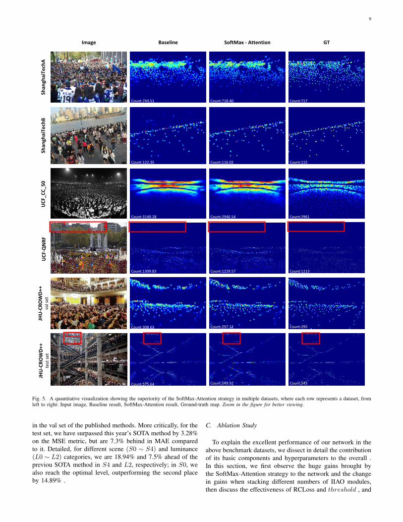
Fig. 4. RCLoss function computational flow. (a) Error map of the model predictions. (b) Sub-windows containing overlapping areas, designed to preventheads from being cut to affect the error analysis. (c) Each sub-window performs error analysis separately. First, define the position with the largest error valueas the hard point; then, determine whether the error at the remaining positions is higher than the product of the hard point value and threshold. If so, applyan incremental penalty, where the greater the error is, the greater the penalty increment it receives. Otherwise, simply take the square value of the originalerror as the penalty.

of the IIAO module paired with RCLoss. The computationalflow of RCLoss is shown in Figure 4.

RCLoss focuses on using the Fwei generated by the SMAsubmodule, subtracts it from the ground-truth map and obtainsthe absolute value, where the result is represented by the Errormap. Set the sliding window to traverse the Error map, findthe pixel point with a large error in each of the obtainedsub-windows, and apply an incremental penalty based on theerror value of the position itself, i.e. , the strength of thepenalty is determined by the degree of error in that position.To ensure information continuity between sub-windows, we setthe sliding stride slightly smaller than the sliding window size.In this way, the resulting overlapping regions will be analyzedmultiple times, but only extremely error-prone positions willbe repeatedly penalized, and low-sensitivity areas are simplyignored.

In detail, the Error map, denoted by E ∈ R1×H×W , isobtained first.

E =∣∣Fwei −GGT

∣∣ (4)

Assuming that the size and stride of the sliding windoware k and s, respectively, then the maximum sliding timesof the window in the horizontal and vertical directions canbe calculated, which are represented by Rmax and Dmax,respectively.

Rmax = bW − ksc+ 1, Dmax = bH − k

sc+ 1 (5)

Each sub-window has its pixel point with the largest value ofits error, called the hard point, whose value is MAXr,d, {1≤r ≤ Rmax, 1 ≤ d ≤ Dmax}. By analyzing each sub-windowin turn, penalizing positions where the error value is close toMAXr,d, the amount of penalty is determined by the constantthreshold, and the strength of the penalty is related to the

degree of deviation from its own prediction. For those pointswhere the error value is within the tolerance range, MSELossis used as their loss . The specific RCLoss algorithm is shownbelow:

EP : Ei,j > MAXr,d ∗ thresholdET : Ei,j ≤MAXr,d ∗ threshold

Lossr,d=

r∗s+k∑

i=r∗s+1

d∗s+k∑j=d∗s+1

(Ei,j

1+e−Ei,j+Ei,j)

2 if EP

r∗s+k∑i=r∗s+1

d∗s+k∑j=d∗s+1

Ei,j2 if ET

(6)

Lossr,d represents the total loss of each sub-window, and iand j are iterators of its width and height, respectively. Withineach sub-window, first determine the hard point and calculateits error value MAXr,d; then, search for error-prone pointswhose error value is greater than the product of threshold andMAXr,d; and finally calculate the loss together with the rest ofthe ordinary positions according to Equation (6) . EP and ETrepresent error-prone and error-tolerant points , respectively.

All reachable sub-window losses in a training batch areaccumulated to give the final RCLoss:

Lwei =1

N

N∑i=1

Rmax∑r=1

Dmax∑d=1

Lossr,d (7)

Final Loss Function. The entire network produces threedensity maps of the same size, including two Fweis outputfrom the IIAO module and a final prediction map Fpre. Byweighting the different tasks, the unified objective functionrequired by training can be formulated as:

L = λLwei1 + λLwei2 + γLpre (8)

7

where λ and γ are the weight terms of the two loss functions.Both can be set to fixed values for experiments with alldatasets, showing an excellent generalization ability.

SASNet [26] also mentions the concept of hard pixel, butit is quite different from this paper, which can be summarizedin three aspects. 1) It cuts the prediction map into fourparts, selects the one with the largest total error, and thenrecursively cuts and compares until the pixel with the largesterror in the entire prediction map is determined, which iscalled hard pixel. By contrast, we consider that the probabilityof large-scale human heads appearing on the dividing line ishigh, and forcible cutting will cause irreversible damage topotential targets and affect the prediction of the network. Wetherefore propose sliding windows with overlapping regionsand perform ablation experiments for the overlap length, whichis finally determined to be 8. Since the final prediction maphas the same 8X perceptual field, the mapping back to theoriginal map is a 64 × 64 region, which is close to the sizeof a larger human head. 2) The number of penalty objects isdifferent. Our hard point is not the only object to be punished,but plays a more important role as a reference. Each of thefour sub-windows has its own hard point, which indicates theposition with the largest prediction deviation in the currentsub-window. Suppose its value is MAX, search for points inthis sub-window whose error value is close to MAX, treat themas penalty objects as well, and whether they are close or notis evaluated by threshold. The purpose of this move is to takeinto account the uneven distribution of head density, whereerrors may be concentrated in a certain area. Restricting tohard pixel may have limited effect. 3) The intensity of penaltyvaries among different penalty objects; after all, their degree ofprediction deviation is different. The hard point, as the biggesttroublemaker, undoubtedly receives the most attention; for itsaffiliated penalty points, the penalty intensity is softened withthe decrease of the error . See Equation (6) for specific rules.

IV. TRAINING

This chapter introduces the specific training details in termsof data preprocessing, label generation, and hyperparametersetting.

A. Data Pre-processing

In the training phase, we randomly crop a 400 × 400patch and flip it horizontally with a probability of 0.5. Forthe ShanghaiTech Part A [14] and UCF-QNRF [32] datasetscontaining grey images, we change the color images to greywith a probability of 0.1. During the test phase, for the datasetscontaining extremely large resolution, i.e., UCF-QNRF [32],JHU-Crowd++ [33] and NWPU-Crowd [34],we scale imageswith side lengths greater than 5000 to 4/5 of their originalsize.

B. Label Generation

As in previous work [12], we blur each head annotationwith a Gaussian kernel to generate training labels. In detail,for crowd-sparse datasets, such as ShanghaiTech Part B [14],

we use fixed-size kernels to generate ground-truth, while forother datasets with relatively dense scenes, geometric adaptivekernel based on the nearest neighbor algorithm are utilized.

C. Hyperparameter Setting

Except for Primary Feature Extractor, the parameters ofthe subsequent layers are randomly initialized by a Gaussiandistribution with a mean of 0 and a standard deviation of0.01. The r in Transitive Attention Unit is set to 16. Fortraining details, we choose the Adam [35] optimizer to retrainthe model, with an initial learning rate of 1E-4, halved every100 rounds. Weight items λ and γ are set to 1.5 and 0.5,respectively, in the training of all datasets.

V. EXPERIMENTS

We demonstrate the effectiveness of the proposed methodon six official datasets: ShanghaiTech [14], UCF CC 50 [6],UCF-QNRF [32] JHU-Crowd++ [33] and NWPU-Crowd [34].

A. Evaluation Metrics

There are two mainstream metrics for evaluating the perfor-mance in crowd counting task: Mean Absolute Error (MAE)and Mean Squared Error (MSE). They are defined as follows:

MAE =1

N

N∑i=1

|Pi −Gi| (9)

MSE =

√√√√ 1

N

N∑i=1

|Pi −Gi|2 (10)

where N is the number of images in the test set, and Pi andgi are the predicted number of targets in the i-th image andits corresponding ground-truth number, respectively.

B. Comparisons and Analysis

ShanghaiTech dataset is composed of two parts. Part Acontains 482 images, sourced from the web, with rich scenesand variable scales, and the number of images used for trainingand test are 300 and 182, respectively; Part B contains 716images, collected from Shanghai streets, with relatively sparsedistribution and a fixed image size of 1024 × 768, furtherdivided into a training set containing 400 images and a test setcontaining 316 images. The experimental results are shown inTable I, which indicates that our method achieves the desiredlevel in both dense and sparse scenes.

UCF CC 50 dataset is a small but challenging dataset,containing 50 images collected from the internet. The numberof people annotated in each image varies widely from 94 to4,543. Due to the limited samples, there is no official divisionbetween the training and test set, but rather a 5-fold cross-validation is suggested as a unified test approach. We strictlyfollow this rule for our experiments, and the results are alsoshown in Table I. It can be seen that our method is 8.33%ahead of the SOTA level in terms of MAE metric, and it is13.8% ahead in terms of MSE. Thus, our method still performswell in extremely dense scenes.

8

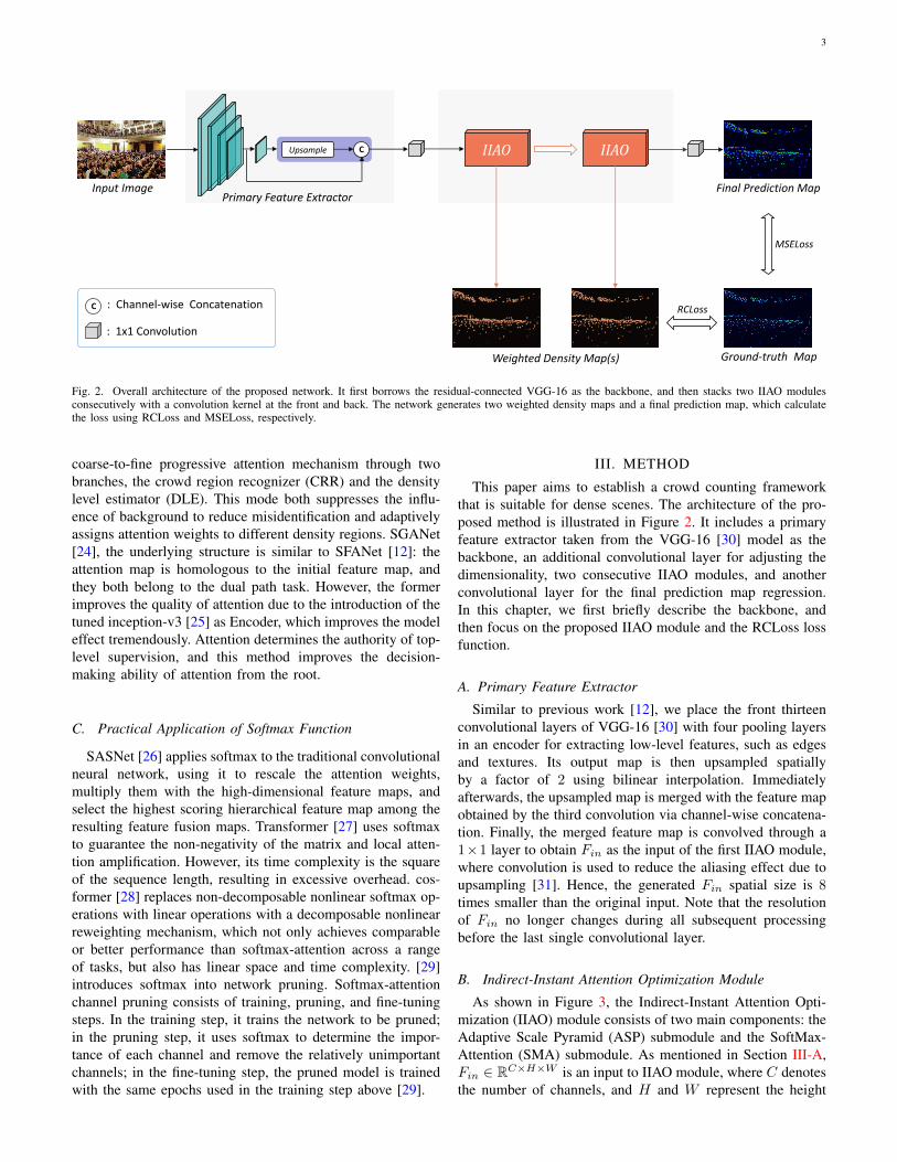
TABLE ICOMPARISON WITH STATE-OF-THE-ART METHODS ON FOUR CHALLENGING DATASETS. THE BEST PERFORMANCE IS INDICATED BY bold AND THE

SECOND BEST IS UNDERLINED.

Methods Venue Part A Part B UCF CC 50 UCF-QNRFMAE MSE MAE MSE MAE MSE MAE MSE

MCNN [14] CVPR 16 110.2 173.2 26.4 41.3 377.6 509.1 277.0 426.0Deem [36] T-CSVT 19 - - 8.09 12.98 253.4 364.4 - -PCC-Net [22] T-CSVT 19 73.5 124.0 11.0 19.0 183.2 260.1 148.7 247.3DADNet [17] ACM-MM 19 64.2 99.9 8.8 13.5 285.5 389.7 113.2 189.4BL [37] ICCV 19 62.8 101.8 7.7 12.7 229.3 308.2 88.7 154.8RANet [21] ICCV 19 59.4 102.0 7.9 12.9 239.8 319.4 111.0 190.0ZoomCount [38] T-CSVT 20 66.0 97.5 - - - - 128.0 201.0DM-Count [39] NeurIPS 20 59.7 95.7 7.4 11.8 211.0 291.5 85.6 148.3ASNet [20] CVPR 20 57.78 90.13 - - 174.84 251.63 91.59 159.71LibraNet [40] ECCV 20 55.9 97.1 7.3 11.3 181.2 262.2 88.1 143.7AMSNet [18] ECCV 20 56.7 93.4 6.7 10.2 208.4 297.3 101.8 163.2DCANet [41] T-CSVT 21 59.2 94.4 7.8 12.3 183.2 260.1 90.1 150.4CFANet [23] WACV 21 56.1 89.6 6.5 10.2 203.6 287.3 89.0 152.3DKPNet [42] ICCV 21 55.6 91.0 6.6 10.9 - - 81.4 147.2GLoss [43] CVPR 21 61.3 95.4 7.3 11.7 - - 84.3 147.5D2C [44] TIP 21 59.6 100.7 6.7 10.7 221.5 300.7 84.8 145.6SASNet [26] AAAI 21 53.59 88.38 6.35 9.9 161.4 234.46 85.2 147.3TopoCount [45] AAAI 21 61.2 104.6 7.8 13.7 184.1 258.3 89 159SGANet [24] TITS 22 57.6 101.1 6.6 10.2 221.9 289.8 87.6 152.5MAN [46] CVPR 22 56.8 90.3 - - - - 77.3 131.5Ours - 54.37 92.76 6.94 10.80 147.96 202.12 74.01 128.87

TABLE IICOMPARISON WITH STATE-OF-THE-ART METHODS ON THE JHU-CROWD++ (VAL SET) DATASET. ”LOW”, ”MEDIUM” AND ”HIGH” RESPECTIVELY

INDICATES THREE CATEGORIES BASED ON DIFFERENT RANGES: [0,50], (50,500) AND >500. THE BEST PERFORMANCE IS INDICATED BY bold AND THESECOND BEST IS UNDERLINED.

Method VenueVal set

Low Medium High OverallMAE MSE MAE MSE MAE MSE MAE MSE

MCNN [14] CVPR 16 90.6 202.9 125.3 259.5 494.9 856.0 160.6 377.7CSRNet [16] CVPR 18 22.2 40.0 49.0 99.5 302.5 669.5 72.2 249.9SANet [47] ECCV 18 13.6 26.8 50.4 78.0 397.8 749.2 82.1 272.6SFCN [48] CVPR 19 11.8 19.8 39.3 73.4 297.3 679.4 62.9 247.5CAN [49] CVPR 19 34.2 69.5 65.6 115.3 336.4 619.7 89.5 239.3DSSINet [50] ICCV 19 50.3 85.9 82.4 164.5 436.6 814.0 116.6 317.4MBTTBF [51] ICCV 19 23.3 48.5 53.2 119.9 294.5 674.5 73.8 256.8BL [37] ICCV 19 6.9 10.3 39.7 85.2 279.8 620.4 59.3 229.2LSC-CNN [52] PAMI 20 6.8 10.3 39.2 64.1 504.7 860.0 87.3 309.0CG-DRCN-CC-VGG16 [33] PAMI 20 17.1 44.7 40.8 71.2 317.4 719.8 67.9 262.1CG-DRCN-CC-Res101 [33] PAMI 20 11.7 24.8 35.2 57.5 273.9 676.8 57.6 244.4AutoScale [53] IJCV 21 10.0 15.3 33.5 54.2 351.7 720.3 65.7 258.9Ours - 8.24 12.73 30.44 50.47 276.57 589.73 54.08 212.73

UCF-QNRF dataset has 1535 images containing 1,251,642annotation points. The training and test sets are composed of1201 and 334 images, respectively. The density of annotatedtargets ranges from 49 to 12,865, and the average imagesize is 2013 × 2902, which poses an enormous challenge forcounting task. As shown in Table I, we achieve improvementsof 4.26% and 2% in terms of the MAE and MSE , respectively,compared to the SOTA methods.

JHU-Crowd++ dataset has a more complex context thanthe above datasets, with 4372 images and 1.51 million an-notations. All images are divided into 2722 training images,500 val images and 1600 test images. We follow the officialdescription, classify val and test by density level, and comparethem one by one. The results of both are shown in Tables IIand III. In the val set, both metrics in our Overall and Mediumparts outperform the previous SOTA method by 6.11%, 7.19%,9.13%, and 6.88%, respectively. In the High part, the MAE

trails that of the optimal method by 0.97%, and MSE leads by4.84%. More notably, for the test set, we have made progressacross the board in both High and Medium parts, leadingthe second place by 9.63%, 5.82%, 6.13%, and 1.57% inthe two metrics, respectively. Also, for the Low part, MSEsurpasses the previous SOTA method by 27.58%, which isa great improvement. Unfortunately, however, in the Overallpart, both metrics lag behind the MAN [46].

NWPU-Crowd is currently the most challenging datasetin the field of crowd counting. It includes 5109 images and2.13 million annotation points. The training set, val set andtest set contain 3109, 500 and 1500 images, respectively.This dataset introduces 351 negative sample images, i.e.,unoccupied scenes. The maximum number of targets for asingle image up to 20033, the average size is 2191×3209, andthe maximum size reaches 4028×19044, which requires highcomputing power. As can be seen from Table IV, we rank first

9

Image Baseline GTSh

angh

aiTe

chA

Shan

ghai

Tech

BU

CF_

CC

_5

0U

CF-

QN

RF

JHU

-CR

OW

D++

val s

etJH

U-C

RO

WD

++te

st s

et

Count:718.40 Count:717

Count:2961

Count:295

Count:543

Count:1309.83

Count:575.64

Count:2946.54

Count:1229.57

Count:549.92

Count:297.12

Count:744.51

Count:308.63

Count:3149.28

Count:1213

Count:122.35 Count:116.02 Count:115

SoftMax - Attention

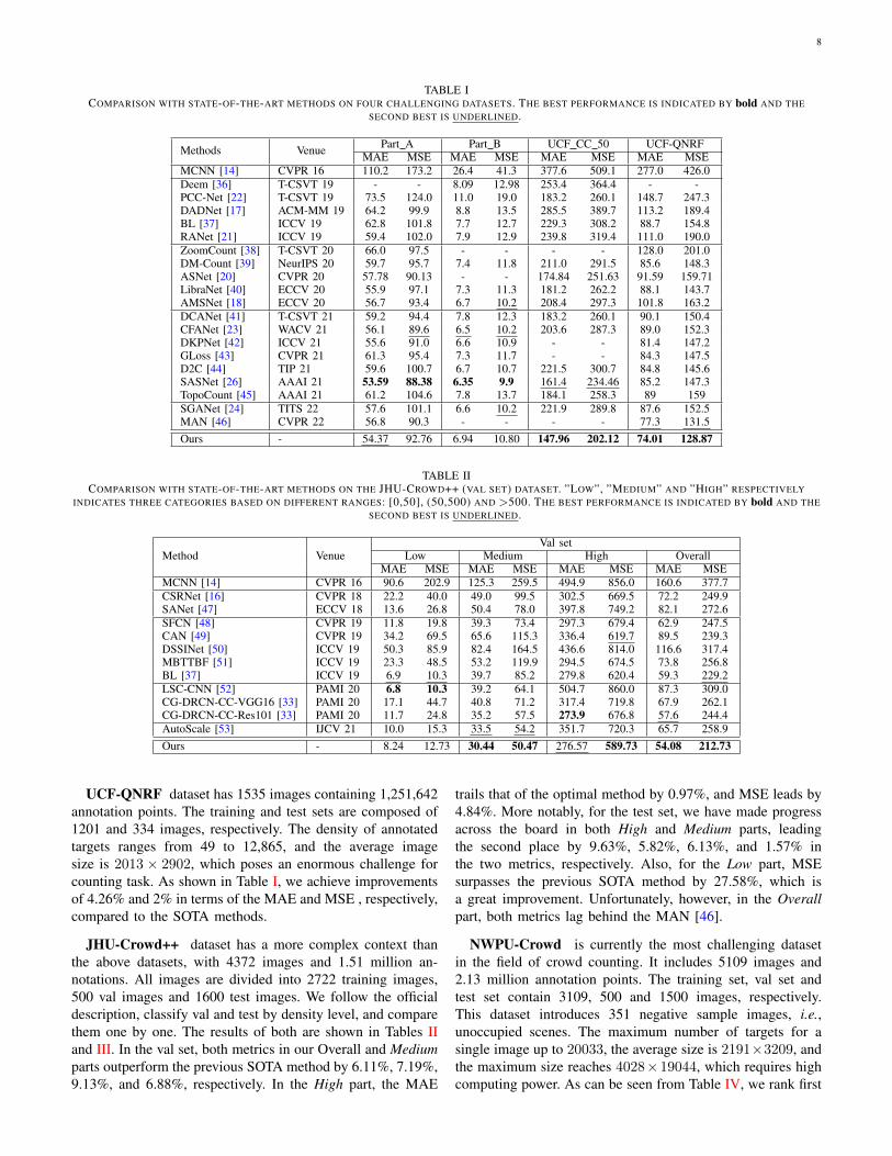
Fig. 5. A quantitative visualization showing the superiority of the SoftMax-Attention strategy in multiple datasets, where each row represents a dataset, fromleft to right: Input image, Baseline result, SoftMax-Attention result, Ground-truth map. Zoom in the figure for better viewing.

in the val set of the published methods. More critically, for thetest set, we have surpassed this year’s SOTA method by 3.28%on the MSE metric, but are 7.3% behind in MAE comparedto it. Detailed, for different scene (S0 ∼ S4) and luminance(L0 ∼ L2) categories, we are 18.94% and 7.5% ahead of thepreviou SOTA method in S4 and L2, respectively; in S0, wealso reach the optimal level, outperforming the second placeby 14.89% .

C. Ablation Study

To explain the excellent performance of our network in theabove benchmark datasets, we dissect in detail the contributionof its basic components and hyperparameters to the overall .In this section, we first observe the huge gains brought bythe SoftMax-Attention strategy to the network and the changein gains when stacking different numbers of IIAO modules,then discuss the effectiveness of RCLoss and threshold , and

10

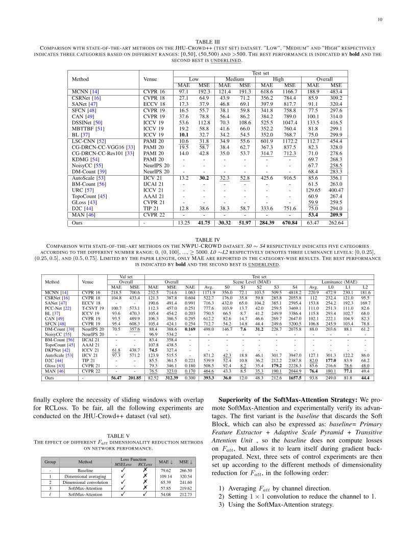
TABLE IIICOMPARISON WITH STATE-OF-THE-ART METHODS ON THE JHU-CROWD++ (TEST SET) DATASET. ”LOW”, ”MEDIUM” AND ”HIGH” RESPECTIVELY

INDICATES THREE CATEGORIES BASED ON DIFFERENT RANGES: [0,50], (50,500) AND >500. THE BEST PERFORMANCE IS INDICATED BY bold AND THESECOND BEST IS UNDERLINED.

Method VenueTest set

Low Medium High OverallMAE MSE MAE MSE MAE MSE MAE MSE

MCNN [14] CVPR 16 97.1 192.3 121.4 191.3 618.6 1166.7 188.9 483.4CSRNet [16] CVPR 18 27.1 64.9 43.9 71.2 356.2 784.4 85.9 309.2SANet [47] ECCV 18 17.3 37.9 46.8 69.1 397.9 817.7 91.1 320.4SFCN [48] CVPR 19 16.5 55.7 38.1 59.8 341.8 758.8 77.5 297.6CAN [49] CVPR 19 37.6 78.8 56.4 86.2 384.2 789.0 100.1 314.0DSSINet [50] ICCV 19 53.6 112.8 70.3 108.6 525.5 1047.4 133.5 416.5MBTTBF [51] ICCV 19 19.2 58.8 41.6 66.0 352.2 760.4 81.8 299.1BL [37] ICCV 19 10.1 32.7 34.2 54.5 352.0 768.7 75.0 299.9LSC-CNN [52] PAMI 20 10.6 31.8 34.9 55.6 601.9 1172.2 112.7 454.4CG-DRCN-CC-VGG16 [33] PAMI 20 19.5 58.7 38.4 62.7 367.3 837.5 82.3 328.0CG-DRCN-CC-Res101 [33] PAMI 20 14.0 42.8 35.0 53.7 314.7 712.3 71.0 278.6KDMG [54] PAMI 20 - - - - - - 69.7 268.3NoisyCC [55] NeurIPS 20 - - - - - - 67.7 258.5DM-Count [39] NeurIPS 20 - - - - - - 68.4 283.3AutoScale [53] IJCV 21 13.2 30.2 32.3 52.8 425.6 916.5 85.6 356.1BM-Count [56] IJCAI 21 - - - - - - 61.5 263.0URC [57] ICCV 21 - - - - - - 129.65 400.47TopoCount [45] AAAI 21 - - - - - - 60.9 267.4GLoss [43] CVPR 21 - - - - - - 59.9 259.5D2C [44] TIP 21 12.8 38.6 38.3 58.7 333.6 751.6 75.0 294.0MAN [46] CVPR 22 - - - - - - 53.4 209.9Ours - 13.25 41.75 30.32 51.97 284.39 670.84 63.47 262.64

TABLE IVCOMPARISON WITH STATE-OF-THE-ART METHODS ON THE NWPU-CROWD DATASET. S0 ∼ S4 RESPECTIVELY INDICATES FIVE CATEGORIES

ACCORDING TO THE DIFFERENT NUMBER RANGE: 0, (0, 100], ..., ≥ 5000. L0 ∼L2 RESPECTIVELY DENOTES THREE LUMINANCE LEVELS: [0, 0.25],(0.25, 0.5], AND (0.5, 0.75]. LIMITED BY THE PAPER LENGTH, ONLY MAE ARE REPORTED IN THE CATEGORY-WISE RESULTS. THE BEST PERFORMANCE

IS INDICATED BY bold AND THE SECOND BEST IS UNDERLINED.

Method VenueVal set Test setOverall Overall Scene Level (MAE) Luminance (MAE)

MAE MSE MAE MSE NAE Avg. S0 S1 S2 S3 S4 Avg. L0 L1 L2MCNN [14] CVPR 16 218.5 700.6 232.5 714.6 1.063 1171.9 356.0 72.1 103.5 509.5 4818.2 220.9 472.9 230.1 181.6CSRNet [16] CVPR 18 104.8 433.4 121.3 387.8 0.604 522.7 176.0 35.8 59.8 285.8 2055.8 112 232.4 121.0 95.5SANet [47] ECCV 18 - - 190.6 491.4 0.991 716.3 432.0 65.0 104.2 385.1 2595.4 153.8 254.2 192.3 169.7PCC-Net [22] T-CSVT 19 100.7 573.1 112.3 457.0 0.251 777.6 103.9 13.7 42.0 259.5 3469.1 111.0 251.3 111.0 82.6BL [37] ICCV 19 93.6 470.3 105.4 454.2 0.203 750.5 66.5 8.7 41.2 249.9 3386.4 115.8 293.4 102.7 68.0CAN [49] CVPR 19 93.5 489.9 106.3 386.5 0.295 612.2 82.6 14.7 46.6 269.7 2647.0 102.1 222.1 104.9 82.3SFCN [48] CVPR 19 95.4 608.3 105.4 424.1 0.254 712.7 54.2 14.8 44.4 249.6 3200.5 106.8 245.9 103.4 78.8DM-Count [39] NeurIPS 20 70.5 357.6 88.4 388.6 0.169 498.0 146.7 7.6 31.2 228.7 2075.8 88.0 203.6 88.1 61.2NoisyCC [55] NeurIPS 20 - - 96.9 534.2 - - - - - - - - - - -BM-Count [56] IJCAI 21 - - 83.4 358.4 - - - - - - - - - - -TopoCount [45] AAAI 21 - - 107.8 438.5 - - - - - - - - - - -DKPNet [42] ICCV 21 61.8 438.7 74.5 327.4 - - - - - - - - - - -AutoScale [53] IJCV 21 97.3 571.2 123.9 515.5 - 871.2 42.3 18.8 46.1 301.7 3947.0 127.1 301.3 122.2 86.0D2C [44] TIP 21 - - 85.5 361.5 0.221 539.9 52.4 10.8 36.2 212.2 2387.8 82.0 177.0 83.9 68.2Gloss [43] CVPR 21 - - 79.3 346.1 0.180 508.5 92.4 8.2 35.4 179.2 2228.3 85.6 216.6 78.6 48.0MAN [46] CVPR 22 - - 76.5 323.0 0.170 464.6 43.3 8.5 35.3 190.1 2044.9 76.4 180.1 77.1 49.4Ours - 56.47 201.85 82.52 312.39 0.300 393.3 36.0 12.0 48.3 212.6 1657.5 93.8 249.0 81.8 44.4

finally explore the necessity of sliding windows with overlapfor RCLoss. To be fair, all the following experiments areconducted on the JHU-Crowd++ dataset (val set).

TABLE VTHE EFFECT OF DIFFERENT Fatt DIMENSIONALITY REDUCTION METHODS

ON NETWORK PERFORMANCE.

Loss FunctionGroup Method MSELoss RCLoss MAE ↓ MSE ↓

- Baseline ! % 79.62 266.501 Dimensional averaging ! % 109.14 320.542 Dimensional convolution ! % 65.39 241.603 SoftMax-Attention ! % 57.85 219.62` SoftMax-Attention ! ! 54.08 212.73

Superiority of the SoftMax-Attention Strategy: We pro-mote SoftMax-Attention and experimentally verify its advan-tages. The first variant is the baseline that discards the SoftBlock, which can also be expressed as: baseline= PrimaryFeature Extractor + Adaptive Scale Pyramid + TransitiveAttention Unit , so the baseline does not compute losseson Fatt, but allows it to learn itself during gradient back-propagated. Next, three sets of control experiments are thenset up according to the different methods of dimensionalityreduction for Fatt, in the following order:

1) Averaging Fatt by channel direction.2) Setting 1× 1 convolution to reduce the channel to 1.3) Using the SoftMax-Attention strategy.

11

219.62

210

219

228

237

246

255

0.10.20.30.40.50.60.70.80.91

w/ RCLoss w/o RCLoss

57.85

52

54

56

58

60

62

64

0.1 0.2 0.3 0.4 0.5 0.6 0.7 0.8 0.9 1

w/ RCLoss w/o RCLoss

(a) Threshold - MAE (b) Threshold - MSE

53

54

55

56

57

58

0.9 0.91 0.92 0.93 0.94 0.95 0.96 0.97 0.98 0.99 1

210

212

214

216

218

220

0.90.910.920.930.940.950.960.970.980.991

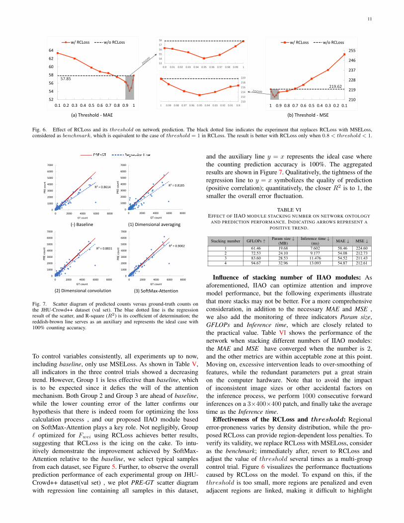
Fig. 6. Effect of RCLoss and its threshold on network prediction. The black dotted line indicates the experiment that replaces RCLoss with MSELoss,considered as benchmark, which is equivalent to the case of threshold = 1 in RCLoss. The result is better with RCLoss only when 0.8 < threshold < 1.

R² = 0.8185

0

1000

2000

3000

4000

5000

6000

7000

0 2000 4000 6000 8000

PR

E co

un

t

GT count

R² = 0.9002

0

1000

2000

3000

4000

5000

6000

7000

0 2000 4000 6000 8000

PR

E co

un

t

GT count

R² = 0.8831

0

1000

2000

3000

4000

5000

6000

7000

0 2000 4000 6000 8000

PR

E co

un

t

GT count

R² = 0.8614

0

1000

2000

3000

4000

5000

6000

7000

0 2000 4000 6000 8000

PR

E co

un

t

GT count

(-) Baseline (1) Dimensional averaging

(2) Dimensional convolution (3) SoftMax-Attention

Fig. 7. Scatter diagram of predicted counts versus ground-truth counts onthe JHU-Crowd++ dataset (val set). The blue dotted line is the regressionresult of the scatter, and R-square (R2) is its coefficient of determination; thereddish-brown line serves as an auxiliary and represents the ideal case with100% counting accuracy.

To control variables consistently, all experiments up to now,including baseline, only use MSELoss. As shown in Table V,all indicators in the three control trials showed a decreasingtrend. However, Group 1 is less effective than baseline, whichis to be expected since it defies the will of the attentionmechanism. Both Group 2 and Group 3 are ahead of baseline,while the lower counting error of the latter confirms ourhypothesis that there is indeed room for optimizing the losscalculation process , and our proposed IIAO module basedon SoftMax-Attention plays a key role. Not negligibly, Group` optimized for Fwei using RCLoss achieves better results,suggesting that RCLoss is the icing on the cake. To intu-itively demonstrate the improvement achieved by SoftMax-Attention relative to the baseline, we select typical samplesfrom each dataset, see Figure 5. Further, to observe the overallprediction performance of each experimental group on JHU-Crowd++ dataset(val set) , we plot PRE-GT scatter diagramwith regression line containing all samples in this dataset,

and the auxiliary line y = x represents the ideal case wherethe counting prediction accuracy is 100%. The aggregatedresults are shown in Figure 7. Qualitatively, the tightness of theregression line to y = x symbolizes the quality of prediction(positive correlation); quantitatively, the closer R2 is to 1, thesmaller the overall error fluctuation.

TABLE VIEFFECT OF IIAO MODULE STACKING NUMBER ON NETWORK ONTOLOGY

AND PREDICTION PERFORMANCE. INDICATING ARROWS REPRESENT APOSITIVE TREND.

Stacking number GFLOPs ↑ Param size ↓(MB)

Inference time ↓(ms) MAE ↓ MSE ↓

1 61.46 19.68 7.602 58.46 224.602 72.53 24.10 9.177 54.08 212.733 83.60 28.53 11.476 54.52 211.434 94.67 32.96 13.093 54.87 212.61

Influence of stacking number of IIAO modules: Asaforementioned, IIAO can optimize attention and improvemodel performance, but the following experiments illustratethat more stacks may not be better. For a more comprehensiveconsideration, in addition to the necessary MAE and MSE ,we also add the monitoring of three indicators Param size,GFLOPs and Inference time, which are closely related tothe practical value. Table VI shows the performance of thenetwork when stacking different numbers of IIAO modules:the MAE and MSE have converged when the number is 2,and the other metrics are within acceptable zone at this point.Moving on, excessive intervention leads to over-smoothing offeatures, while the redundant parameters put a great strainon the computer hardware. Note that to avoid the impactof inconsistent image sizes or other accidental factors onthe inference process, we perform 1000 consecutive forwardinferences on a 3×400×400 patch, and finally take the averagetime as the Inference time.

Effectiveness of the RCLoss and threshold: Regionalerror-proneness varies by density distribution, while the pro-posed RCLoss can provide region-dependent loss penalties. Toverify its validity, we replace RCLoss with MSELoss, consideras the benchmark; immediately after, revert to RCLoss andadjust the value of threshold several times as a multi-groupcontrol trial. Figure 6 visualizes the performance fluctuationscaused by RCLoss on the model. To expand on this, if thethreshold is too small, more regions are penalized and evenadjacent regions are linked, making it difficult to highlight

12

57.4658.23

54.08

58.98

218.61

221.46

212.73

223.74

210

214

218

222

226

52

54

56

58

60

50/50 25/25 27/23 18/16

window size/stride

MAE MSE

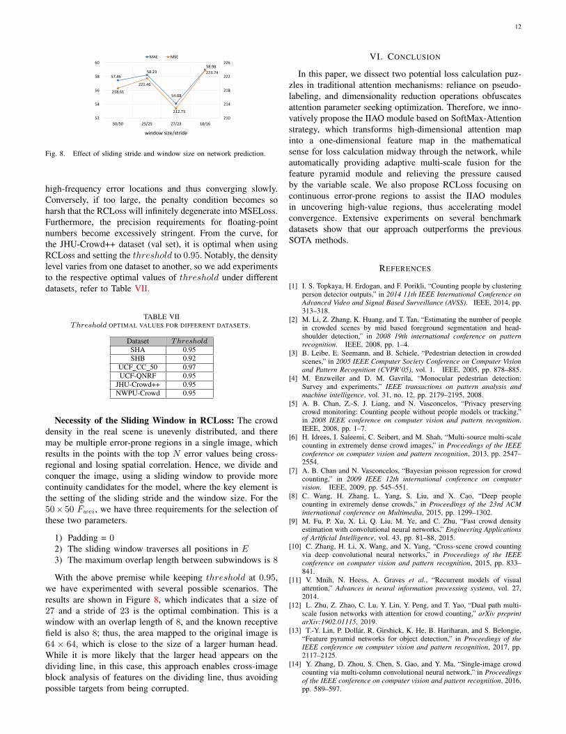
Fig. 8. Effect of sliding stride and window size on network prediction.

high-frequency error locations and thus converging slowly.Conversely, if too large, the penalty condition becomes soharsh that the RCLoss will infinitely degenerate into MSELoss.Furthermore, the precision requirements for floating-pointnumbers become excessively stringent. From the curve, forthe JHU-Crowd++ dataset (val set), it is optimal when usingRCLoss and setting the threshold to 0.95. Notably, the densitylevel varies from one dataset to another, so we add experimentsto the respective optimal values of threshold under differentdatasets, refer to Table VII.

TABLE VIIThreshold OPTIMAL VALUES FOR DIFFERENT DATASETS.

Dataset ThresholdSHA 0.95SHB 0.92

UCF CC 50 0.97UCF-QNRF 0.95

JHU-Crowd++ 0.95NWPU-Crowd 0.95

Necessity of the Sliding Window in RCLoss: The crowddensity in the real scene is unevenly distributed, and theremay be multiple error-prone regions in a single image, whichresults in the points with the top N error values being cross-regional and losing spatial correlation. Hence, we divide andconquer the image, using a sliding window to provide morecontinuity candidates for the model, where the key element isthe setting of the sliding stride and the window size. For the50× 50 Fwei, we have three requirements for the selection ofthese two parameters.

1) Padding = 02) The sliding window traverses all positions in E3) The maximum overlap length between subwindows is 8

With the above premise while keeping threshold at 0.95,we have experimented with several possible scenarios. Theresults are shown in Figure 8, which indicates that a size of27 and a stride of 23 is the optimal combination. This is awindow with an overlap length of 8, and the known receptivefield is also 8; thus, the area mapped to the original image is64 × 64, which is close to the size of a larger human head.While it is more likely that the larger head appears on thedividing line, in this case, this approach enables cross-imageblock analysis of features on the dividing line, thus avoidingpossible targets from being corrupted.

VI. CONCLUSION

In this paper, we dissect two potential loss calculation puz-zles in traditional attention mechanisms: reliance on pseudo-labeling, and dimensionality reduction operations obfuscatesattention parameter seeking optimization. Therefore, we inno-vatively propose the IIAO module based on SoftMax-Attentionstrategy, which transforms high-dimensional attention mapinto a one-dimensional feature map in the mathematicalsense for loss calculation midway through the network, whileautomatically providing adaptive multi-scale fusion for thefeature pyramid module and relieving the pressure causedby the variable scale. We also propose RCLoss focusing oncontinuous error-prone regions to assist the IIAO modulesin uncovering high-value regions, thus accelerating modelconvergence. Extensive experiments on several benchmarkdatasets show that our approach outperforms the previousSOTA methods.

REFERENCES

[1] I. S. Topkaya, H. Erdogan, and F. Porikli, “Counting people by clusteringperson detector outputs,” in 2014 11th IEEE International Conference onAdvanced Video and Signal Based Surveillance (AVSS). IEEE, 2014, pp.313–318.

[2] M. Li, Z. Zhang, K. Huang, and T. Tan, “Estimating the number of peoplein crowded scenes by mid based foreground segmentation and head-shoulder detection,” in 2008 19th international conference on patternrecognition. IEEE, 2008, pp. 1–4.

[3] B. Leibe, E. Seemann, and B. Schiele, “Pedestrian detection in crowdedscenes,” in 2005 IEEE Computer Society Conference on Computer Visionand Pattern Recognition (CVPR’05), vol. 1. IEEE, 2005, pp. 878–885.

[4] M. Enzweiler and D. M. Gavrila, “Monocular pedestrian detection:Survey and experiments,” IEEE transactions on pattern analysis andmachine intelligence, vol. 31, no. 12, pp. 2179–2195, 2008.

[5] A. B. Chan, Z.-S. J. Liang, and N. Vasconcelos, “Privacy preservingcrowd monitoring: Counting people without people models or tracking,”in 2008 IEEE conference on computer vision and pattern recognition.IEEE, 2008, pp. 1–7.

[6] H. Idrees, I. Saleemi, C. Seibert, and M. Shah, “Multi-source multi-scalecounting in extremely dense crowd images,” in Proceedings of the IEEEconference on computer vision and pattern recognition, 2013, pp. 2547–2554.

[7] A. B. Chan and N. Vasconcelos, “Bayesian poisson regression for crowdcounting,” in 2009 IEEE 12th international conference on computervision. IEEE, 2009, pp. 545–551.

[8] C. Wang, H. Zhang, L. Yang, S. Liu, and X. Cao, “Deep peoplecounting in extremely dense crowds,” in Proceedings of the 23rd ACMinternational conference on Multimedia, 2015, pp. 1299–1302.

[9] M. Fu, P. Xu, X. Li, Q. Liu, M. Ye, and C. Zhu, “Fast crowd densityestimation with convolutional neural networks,” Engineering Applicationsof Artificial Intelligence, vol. 43, pp. 81–88, 2015.

[10] C. Zhang, H. Li, X. Wang, and X. Yang, “Cross-scene crowd countingvia deep convolutional neural networks,” in Proceedings of the IEEEconference on computer vision and pattern recognition, 2015, pp. 833–841.

[11] V. Mnih, N. Heess, A. Graves et al., “Recurrent models of visualattention,” Advances in neural information processing systems, vol. 27,2014.

[12] L. Zhu, Z. Zhao, C. Lu, Y. Lin, Y. Peng, and T. Yao, “Dual path multi-scale fusion networks with attention for crowd counting,” arXiv preprintarXiv:1902.01115, 2019.

[13] T.-Y. Lin, P. Dollar, R. Girshick, K. He, B. Hariharan, and S. Belongie,“Feature pyramid networks for object detection,” in Proceedings of theIEEE conference on computer vision and pattern recognition, 2017, pp.2117–2125.

[14] Y. Zhang, D. Zhou, S. Chen, S. Gao, and Y. Ma, “Single-image crowdcounting via multi-column convolutional neural network,” in Proceedingsof the IEEE conference on computer vision and pattern recognition, 2016,pp. 589–597.

13

[15] D. Babu Sam, S. Surya, and R. Venkatesh Babu, “Switching convolu-tional neural network for crowd counting,” in Proceedings of the IEEEconference on computer vision and pattern recognition, 2017, pp. 5744–5752.

[16] Y. Li, X. Zhang, and D. Chen, “Csrnet: Dilated convolutional neuralnetworks for understanding the highly congested scenes,” in Proceedingsof the IEEE conference on computer vision and pattern recognition, 2018,pp. 1091–1100.

[17] D. Guo, K. Li, Z.-J. Zha, and M. Wang, “Dadnet: Dilated-attention-deformable convnet for crowd counting,” in Proceedings of the 27th ACMinternational conference on multimedia, 2019, pp. 1823–1832.

[18] Y. Hu, X. Jiang, X. Liu, B. Zhang, J. Han, X. Cao, and D. Doermann,“Nas-count: Counting-by-density with neural architecture search,” inEuropean Conference on Computer Vision. Springer, 2020, pp. 747–766.

[19] V. K. Valloli and K. Mehta, “W-net: Reinforced u-net for density mapestimation,” arXiv preprint arXiv:1903.11249, 2019.

[20] X. Jiang, L. Zhang, M. Xu, T. Zhang, P. Lv, B. Zhou, X. Yang, andY. Pang, “Attention scaling for crowd counting,” in Proceedings of theIEEE/CVF Conference on Computer Vision and Pattern Recognition,2020, pp. 4706–4715.

[21] A. Zhang, J. Shen, Z. Xiao, F. Zhu, X. Zhen, X. Cao, and L. Shao,“Relational attention network for crowd counting,” in Proceedings ofthe IEEE/CVF International Conference on Computer Vision, 2019, pp.6788–6797.

[22] J. Gao, Q. Wang, and X. Li, “Pcc net: Perspective crowd countingvia spatial convolutional network,” IEEE Transactions on Circuits andSystems for Video Technology, vol. 30, no. 10, pp. 3486–3498, 2019.

[23] L. Rong and C. Li, “Coarse-and fine-grained attention network withbackground-aware loss for crowd density map estimation,” in Proceedingsof the IEEE/CVF winter conference on applications of computer vision,2021, pp. 3675–3684.

[24] Q. Wang and T. P. Breckon, “Crowd counting via segmentation guidedattention networks and curriculum loss,” IEEE Transactions on IntelligentTransportation Systems, 2022.

[25] C. Szegedy, V. Vanhoucke, S. Ioffe, J. Shlens, and Z. Wojna, “Rethinkingthe inception architecture for computer vision,” in Proceedings of theIEEE conference on computer vision and pattern recognition, 2016, pp.2818–2826.

[26] Q. Song, C. Wang, Y. Wang, Y. Tai, C. Wang, J. Li, J. Wu, and J. Ma,“To choose or to fuse? scale selection for crowd counting,” in Proceedingsof the AAAI Conference on Artificial Intelligence, vol. 35, no. 3, 2021,pp. 2576–2583.

[27] A. Vaswani, N. Shazeer, N. Parmar, J. Uszkoreit, L. Jones, A. N. Gomez,Ł. Kaiser, and I. Polosukhin, “Attention is all you need,” Advances inneural information processing systems, vol. 30, 2017.

[28] Z. Qin, W. Sun, H. Deng, D. Li, Y. Wei, B. Lv, J. Yan, L. Kong, andY. Zhong, “cosformer: Rethinking softmax in attention,” arXiv preprintarXiv:2202.08791, 2022.

[29] S. Cho, H. Kim, and J. Kwon, “Filter pruning via softmax attention,” in2021 IEEE International Conference on Image Processing (ICIP). IEEE,2021, pp. 3507–3511.

[30] K. Simonyan and A. Zisserman, “Very deep convolutional networks forlarge-scale image recognition,” arXiv preprint arXiv:1409.1556, 2014.

[31] Q. Song, C. Wang, Z. Jiang, Y. Wang, Y. Tai, C. Wang, J. Li, F. Huang,and Y. Wu, “Rethinking counting and localization in crowds: A purelypoint-based framework,” in Proceedings of the IEEE/CVF InternationalConference on Computer Vision, 2021, pp. 3365–3374.

[32] H. Idrees, M. Tayyab, K. Athrey, D. Zhang, S. Al-Maadeed, N. Rajpoot,and M. Shah, “Composition loss for counting, density map estimation andlocalization in dense crowds,” in Proceedings of the european conferenceon computer vision (ECCV), 2018, pp. 532–546.

[33] V. Sindagi, R. Yasarla, and V. M. Patel, “Jhu-crowd++: Large-scalecrowd counting dataset and a benchmark method,” IEEE Transactionson Pattern Analysis and Machine Intelligence, 2020.

[34] Q. Wang, J. Gao, W. Lin, and X. Li, “Nwpu-crowd: A large-scalebenchmark for crowd counting and localization,” IEEE transactions onpattern analysis and machine intelligence, vol. 43, no. 6, pp. 2141–2149,2020.

[35] D. P. Kingma and J. Ba, “Adam: A method for stochastic optimization,”arXiv preprint arXiv:1412.6980, 2014.

[36] M. Zhao, C. Zhang, J. Zhang, F. Porikli, B. Ni, and W. Zhang, “Scale-aware crowd counting via depth-embedded convolutional neural net-works,” IEEE Transactions on Circuits and Systems for Video Technology,vol. 30, no. 10, pp. 3651–3662, 2019.

[37] Z. Ma, X. Wei, X. Hong, and Y. Gong, “Bayesian loss for crowdcount estimation with point supervision,” in Proceedings of the IEEE/CVFInternational Conference on Computer Vision, 2019, pp. 6142–6151.

[38] U. Sajid, H. Sajid, H. Wang, and G. Wang, “Zoomcount: A zoomingmechanism for crowd counting in static images,” IEEE Transactions onCircuits and Systems for Video Technology, vol. 30, no. 10, pp. 3499–3512, 2020.

[39] B. Wang, H. Liu, D. Samaras, and M. H. Nguyen, “Distribution matchingfor crowd counting,” Advances in Neural Information Processing Systems,vol. 33, pp. 1595–1607, 2020.

[40] L. Liu, H. Lu, H. Zou, H. Xiong, Z. Cao, and C. Shen, “Weighing counts:Sequential crowd counting by reinforcement learning,” in EuropeanConference on Computer Vision. Springer, 2020, pp. 164–181.

[41] Z. Yan, P. Li, B. Wang, D. Ren, and W. Zuo, “Towards learning multi-domain crowd counting,” IEEE Transactions on Circuits and Systems forVideo Technology, 2021.

[42] B. Chen, Z. Yan, K. Li, P. Li, B. Wang, W. Zuo, and L. Zhang,“Variational attention: Propagating domain-specific knowledge for multi-domain learning in crowd counting,” in Proceedings of the IEEE/CVFInternational Conference on Computer Vision, 2021, pp. 16 065–16 075.

[43] J. Wan, Z. Liu, and A. B. Chan, “A generalized loss function for crowdcounting and localization,” in Proceedings of the IEEE/CVF Conferenceon Computer Vision and Pattern Recognition, 2021, pp. 1974–1983.

[44] J. Cheng, H. Xiong, Z. Cao, and H. Lu, “Decoupled two-stage crowdcounting and beyond,” IEEE Transactions on Image Processing, vol. 30,pp. 2862–2875, 2021.

[45] S. Abousamra, M. Hoai, D. Samaras, and C. Chen, “Localization in thecrowd with topological constraints,” in Proceedings of AAAI Conferenceon Artificial Intelligence, 2021.

[46] H. Lin, Z. Ma, R. Ji, Y. Wang, and X. Hong, “Boosting crowd countingvia multifaceted attention,” arXiv preprint arXiv:2203.02636, 2022.

[47] X. Cao, Z. Wang, Y. Zhao, and F. Su, “Scale aggregation network foraccurate and efficient crowd counting,” in Proceedings of the Europeanconference on computer vision (ECCV), 2018, pp. 734–750.

[48] Q. Wang, J. Gao, W. Lin, and Y. Yuan, “Learning from synthetic data forcrowd counting in the wild,” in Proceedings of the IEEE/CVF Conferenceon computer vision and pattern recognition, 2019, pp. 8198–8207.

[49] W. Liu, M. Salzmann, and P. Fua, “Context-aware crowd counting,”in Proceedings of the IEEE/CVF Conference on Computer Vision andPattern Recognition, 2019, pp. 5099–5108.

[50] L. Liu, Z. Qiu, G. Li, S. Liu, W. Ouyang, and L. Lin, “Crowd countingwith deep structured scale integration network,” in Proceedings of theIEEE/CVF international conference on computer vision, 2019, pp. 1774–1783.

[51] V. A. Sindagi and V. M. Patel, “Multi-level bottom-top and top-bottomfeature fusion for crowd counting,” in Proceedings of the IEEE/CVFinternational conference on computer vision, 2019, pp. 1002–1012.

[52] D. B. Sam, S. V. Peri, M. N. Sundararaman, A. Kamath, and R. V.Babu, “Locate, size, and count: accurately resolving people in densecrowds via detection,” IEEE transactions on pattern analysis and machineintelligence, vol. 43, no. 8, pp. 2739–2751, 2020.

[53] C. Xu, D. Liang, Y. Xu, S. Bai, W. Zhan, X. Bai, and M. Tomizuka,“Autoscale: Learning to scale for crowd counting,” International Journalof Computer Vision, pp. 1–30, 2022.

[54] J. Wan, Q. Wang, and A. B. Chan, “Kernel-based density map generationfor dense object counting,” IEEE Transactions on Pattern Analysis andMachine Intelligence, 2020.

[55] J. Wan and A. Chan, “Modeling noisy annotations for crowd counting,”Advances in Neural Information Processing Systems, vol. 33, pp. 3386–3396, 2020.

[56] H. Liu, Q. Zhao, Y. Ma, and F. Dai, “Bipartite matching for crowdcounting with point supervision.”

[57] Y. Xu, Z. Zhong, D. Lian, J. Li, Z. Li, X. Xu, and S. Gao, “Crowdcounting with partial annotations in an image,” in Proceedings of theIEEE/CVF International Conference on Computer Vision, 2021, pp.15 570–15 579.