Strategic Analyses of the National River Linking Project (NRLP) of India Series 1 Upali A. Amarasinghe, Tushaar Shah and R. P. S. Malik, editors High potential in rainfed agriculture India USA China Canada Brazil Turkey Australia France Argentina Germany Rainfed grain area Rainfed grain yield Changing consumption patterns 1961 1971 1981 1991 2001 2025 2050 Food grains Non-grain crops Animal products Changing land use patterns 1956 1965 1974 1983 1992 2001 Investments in major/medium irrigation Net surface water irrigated area Net groundwater irrigated area Low growth in crop yield 0 2 4 6 8 1961 1971 1981 1991 2001 World India China USA Changing economic growth patterns 1955 1965 1975 1985 1995 2005 Per Capita GDP Agriculture Industrial Services Changing demographic patterns 1955 1975 1995 2015 2035 2055 Total population Urban population Rural population Ag population-% of rural India’s Water Future: Scenarios and Issues

Welcome message from author
This document is posted to help you gain knowledge. Please leave a comment to let me know what you think about it! Share it to your friends and learn new things together.
Transcript
Strategic Analyses of the NationalRiver Linking Project (NRLP) of IndiaSeries 1
Upali A. Amarasinghe, Tushaar Shah and R. P. S. Malik, editors
High potential in rainfed agriculture
IndiaUSA
ChinaCanada
BrazilTurkey
Australia
France
Argentina
GermanyRainfed grain area Rainfed grain yield
Changing consumption patterns
1961 1971 1981 1991 2001 2025 2050Food grains Non-grain crops Animal products
Changing land use patterns
1956 1965 1974 1983 1992 2001Investments in major/medium irrigationNet surface water irrigated area Net groundwater irrigated area
Low growth in crop yield
0
2
4
6
8
1961 1971 1981 1991 2001
World India China USA
Changing economic growth patterns
1955 1965 1975 1985 1995 2005Per Capita GDP AgricultureIndustrial Services
Changing demographic patterns
1955 1975 1995 2015 2035 2055Total population Urban populationRural population Ag population-% of rural
India’s Water Future: Scenarios and Issues
i
Strategic Analyses of the National RiverLinking Project (NRLP) of India
Series 1
India’s Water Future: Scenarios and Issues
Upali A. Amarasinghe, Tushaar Shahand R. P. S. Malik, editors
INTERNATIONAL WATER MANAGEMENT INSTITUTE
ii
The editors: Upali A. Amarasinghe is Senior Researcher, International Water Management Institute(IWMI), New Delhi; Tushaar Shah, IWMI, Anand; R.P.S Malik, Fellow, Agricultural Economics ResearchCentre, University of Delhi, New Delhi.
Amarasinghe, U. A.; Shah, T.; Malik, R. P. S. (Eds.) 2008. India’s water future: Scenarios and issues.Colombo, Sri Lanka: International Water Management Institute. 417p
river basin management/ water demand/ water transfer/ land use/ irrigation efficiency/ food consumption/water use/ groundwater irrigation/ irrigation systems/ crop production/ forecasting/ population/ casestudies/ models/ trade/ agricultural policy/ institutional constraints/ hydrogeology/ drip irrigation/sprinkler irrigation/ water conservation/ India
ISBN: 978-92-9090-697-1
Copyright © 2009, by IWMI. All rights reserved.
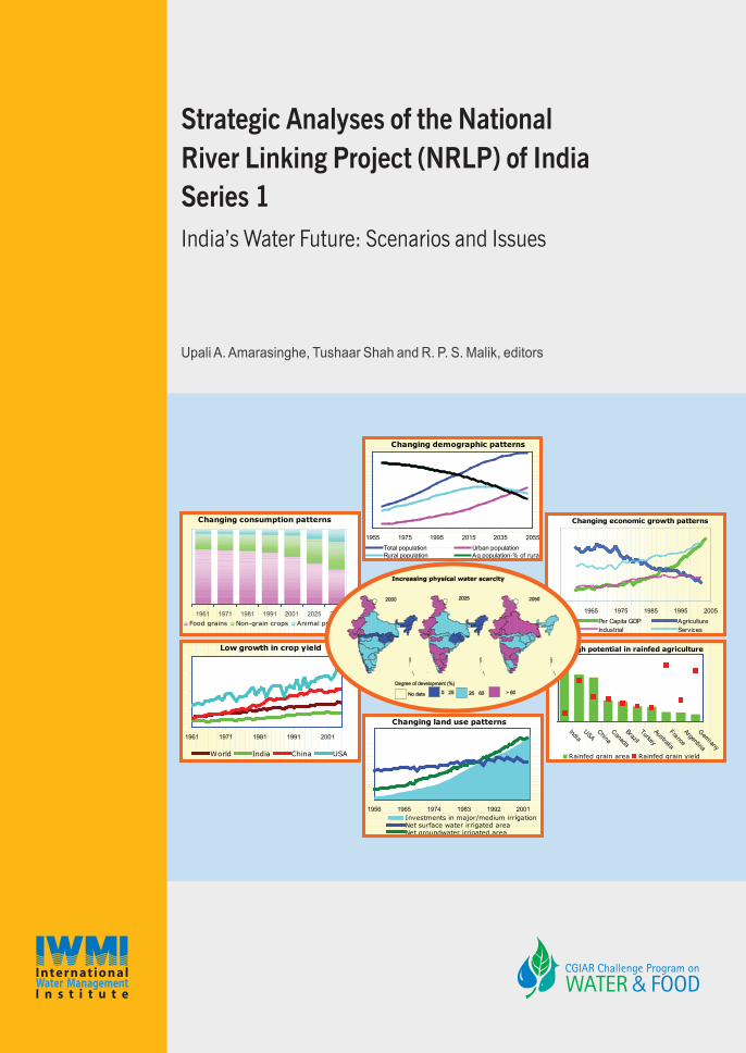
Cover photo by Cover Photo by Upali A. Amarasinghe. Data for the graphs in the cover photo are fromvarious sources including, Annual publications of Agriculture Statistics at a Glance (2004, 2006) by theGovernment of India, FAOSTAT database of the Food and Agriculture Organization, and Research Reports119 and 123 of IWMI.
Please direct inquires and comments to: [email protected]
IWMI receives its principal funding from 58 governments, private foundations, and international andregional organizations known as the Consultative Group on International Agricultural Research(CGIAR). Support is also given by the Governments of Ghana, Pakistan, South Africa, Sri Lankaand Thailand.
iii
Contents
Acknowledgements ................................................................................................................................. v
Preface ............................................................................................................................................ vii
List of contributing authors ................................................................................................................ ix
India’s National River Linking Project - A Synopsis ............................................................................ xi
Paper 1. India’s Water Future: Drivers of Change, Scenarios and Issues ........................................... 3Upali A. Amarasinghe, Tushaar Shah and R.P.S. Malik
Paper 2. India’s Water Future 2050: Potential Deviations from ‘Business-As-Usual’ Scenario ...... 25Shilp Verma and Sanjiv J. Phansalkar
Paper 3. Irrigation Demand Projections of India: Recent Changes inKey Underlying Assumptions ................................................................................................... 51Upali A. Amarasinghe, Peter G. McCornick and Tushaar Shah
Paper 4. India’s Water Demand Scenarios to 2025 and 2050: A Fresh Look ................................... 67Upali A. Amarasinghe, Peter G. McCornick and Tushaar Shah
Paper 5. Meeting India’s Water Future: Some Policy Options ........................................................... 85Upali A. Amarasinghe, Tushaar Shah and Peter G. McCornick
Paper 6. Demographic Projections for India 2006-2051: Regional Variations ................................. 101Aslam Mahmood and Amithabh Kundu
Paper 7. The ‘Tipping Point’ in Indian Agriculture: Understanding theWithdrawal of Indian Rural Youth ......................................................................................... 115Amrita Sharma and Anik Bhaduri
Paper 8. Changing Consumption Patterns of India: Implications on Future Food Demand ............ 131Upali A. Amarasinghe and Om Prakash Singh
Paper 9. Indian Agriculture: Recent Performance and Prospects in the Wake of Globalization ...... 147R. P.S. Malik
Paper 10. Converting Rain into Grain: Opportunities for Realizing thePotential of Rain-fed Agriculture in India .............................................................................. 169Bharat R. Sharma, K. V. Rao, and K. P. R. Vittal
Paper 11. Groundwater Expansion in Indian Agriculture:Past Trends and Future Opportunities .................................................................................... 181Anik Bhaduri, Upali A. Amarasinghe and Tushaar Shah
iv
Contents
Paper 12. Groundwater Exploitation in India, Environmental Impacts andLimits to Further Exploitation for Irrigation ........................................................................... 197Krishnan Sundarajan, Ankit Patel, Trishikhi Raychoudhury and Chaitali Purohit
Paper 13. Water Productivity at Different Scales under Canal,Tank and Well Irrigation Systems .......................................................................................... 217K. Palanisami, S. Senthilvel and T. Ramesh
Paper 14. Water Productivity of Irrigated Agriculture in India:Potential Areas for Improvement ............................................................................................ 227M. Dinesh Kumar, O. P. Singh, Madar Samad, Chaitali Purohitand Malkit Singh Didyala
Paper 15. Drip and Sprinkler Irrigation in India: Benefits, Potential and Future Directions ........... 253A. Narayanamoorthy
Paper 16. Water Saving and Yield Enhancing Micro-irrigation Technologies:How Far Can They Contribute to Water Productivity in Indian Agriculture ....................... 267M. Dinesh Kumar, O. P. Singh and Bharat R. Sharma
Paper 17. An Assessment of Environmental Flow Requirements of Indian River Basins .............. 293V. Smakhtin and M. Anputhas
Paper 18. Developing Procedures for Assessment of Ecological Status ofIndian River Basins in the Context of Environmental Water Requirements ......................... 329Vladimir Smakhtin, Muthukumarasamy Arunachalam, Sandeep Behera,Archana Chatterjee, Srabani Das, Parikshit Gautam, Gaurav D. Joshi,Kumbakonam G. Sivaramakrishnan and K. Sankaran Unni
Paper 19. Groundwater Situation in Urban India: Overview, Opportunities and Challenges .......... 367Ankit Patel and Krishnan Sunderrajan
Paper 20. Natural Flows Assessment and Creating Alternative Future Scenarios forMajor River Basins of Peninsular India ................................................................................. 381Anil D. Mohile and B. K. Anand
v
Acknowledgement
First and foremost we thank the “Challenge Program for Water and Food,” of the ConsultativeGroup of International Agriculture Research Institutes for providing the financial supportfor the project.
We greatly appreciate the comments and suggestions made by the members of the projectadvisory committee chaired by Prof. M.S. Swaminathan. The other eminent members of thiscommittee included Prof. Yojindra K. Alagh, Prof. Vijay S. Vyas, Prof. Kanchan Chopra, Prof.Vandana Shiva, Prof. Frank Rijsberman, Shri Anil D. Mohile, Shri S. Gopalakrishnan and ShriDeep Joshi. Their guidance at various stages of the project was immensely helpful.
We also acknowledge the assistance of various government institutions for providingthe necessary data and published documents for this project. A special thank goes to theCentral Water Commission of India for providing the flow data of various river basins inIndia. Many of the studies would not have been able to to be completed to our satisfactionwithout the river flow information. The project team would also like to thank Shri Anil D.Mohile, former Chairman of the Central Water Commission, for his constant help andsuggestions in this process.
We thank the participants from various government institutions, NGOs and civil societyfor their useful suggestions at the inception workshop of Phase I, held in April 2005 at NewDelhi. The studies were greatly benefited by the comments and suggestions received fromour peers in the CPWF and IWMI theme leaders, and the participants of various workshopswherein we presented our draft research reports. We also thank the organizers of variousworkshops for providing us the opportunity to present the findings of these studies. Theseinclude the IWMI-TATA Water Policy meetings in March 2006, the Project workshop in April2006 at Delhi, and many other national forums.
We thank the researchers in India and in IWMI for their contribution, and the DirectorGeneral of IWMI and other staff for their support and guidance for research and managementof the project. Also we thank many other Indian researchers who expressed their willingnessto contribute to research in various stages of the project. In that, we believe, they indicatedtheir appreciation of research conducted by IWMI and their liking to be part of it. Finally wethank Mr. Pantaleon Fernando for editing the manuscripts and Ms. Pavithra Amunugama, Mr.Nimal Attanayake and Ms. Mala Ranawake for their assistance in the production process.
vii
Preface
In 2005, the International Water Management Institute (IWMI) and the Challenge Program onWater and Food (CPWF) started a three-year research study on “Strategic Analysis of India’sRiver Linking Project”. The primary focus of the IWMI-CPWF project is to provide the publicand the policy planners with a balanced analysis of the social benefits and costs of the NationalRiver Linking Project (NRLP).
The project consists of research in three phases. Phase I analyzed India’s water futurescenarios to 2025/2050 and related issues. Phase II, analyses how effective a response NRLPis, for meeting India’s water future and its social costs and benefits. Phase III contributes toan alternative water sector perspective plan for India as a fallback strategy for NRLP. Thisbook presents the findings of research in Phase I.
In 1999, the National Commission of Integrated Water Resources Development (NCIWRD)published projections of India’s water supply and demand to 2025/2050. The trends of keydrivers before 1990’s were the basis for this projection. However, with economic liberalization,the trends of these key drivers changed in the 1990’s. Therefore, the major focus of researchin phase I was to assess the trends and turning points of the key drivers in recent years andassess their implications on future water supply and demand.
This volume, the first in a series of publications, presents the results of various researchactivities conducted in Phase I on India’s Water Futures. Many papers in this book werepresented in various regional and national workshops between 2006 and 2007. And, differentversions are submitted for publication in various journals.
ix
Contributing Authors
Dr. Upali A. Amarasinghe, Senior Researcher, International Water Management Institute (IWMI)
Dr. Tushaar Shah, Principal Researcher, IWMI
Dr. R.P.S.Malik, Fellow, Agricultural Economics Research Centre, University of Delhi
Dr. Peter McCornick, Former Director of Asia Region, IWMI
Dr. Madar Samad, Principal Researcher and Director, India Program, IWMI
Dr. Vladimir Smakhtin, Principal Researcher, IWMI
Dr. Bharat Sharma, Senior Researcher, IWMI
Dr. Anik Bhaduri, Post Doctoral Fellow, IWMI
Dr. K. Sundararajan, Post Doctoral Fellow, IWMI
Dr. Sanjive Phansalkar, Former Leader, IWMI-TATA Water Policy Program, India
Dr. Dinesh Kumar, Former Leader, IWMI-TATA Water Policy Program, India
Ms. Amrita Sharma, Former consultant, IWMI-TATA Water Policy Program, India
Mr. Shilp Verma, Former consultant, IWMI-TATA Water Policy Program, India
Prof. Aslam Mahmood, Department of Social Sciences, Jawaharlal Nehru University (JNU), NewDelhi
Prof. Amitabh Kundu, Dean, School of Social Sciences, JNU, New Delhi
Mr. Anil D. Mohile, Consultant (Former Chairman, CWC), New Delhi
Prof. A. Narayanamoorthy, Director, Centre for Rural Development, School of Rural Studies,Alagappa University, Karaikudi, Tamil Nadu
Dr. K. Palanisami, Director, IWMI-TATA Water Policy Program, India and Former Director,Tamil Nadu Agricultural University, Coimbotore
Dr. S. Senthilvel, Tamil Nadu Agricultural University, Coimbotore
Dr. T. Ramesh, Tamil Nadu Agricultural University, Coimbotore
Mr. Ankit Patel, Former Consultant, IWMI-TATA Water Policy Program, India
Dr. Omprakash Singh, Lecturer, Agricultural University, Varanesi
Mr. B.K. Anand, Former Research Assistant, IWMI New-Delhi Office
Mr. M. Anputhas, Senior Research Associate, IWMI
Dr. KV Rao, Central Research Institute for Dryland Agriculture, Hyderabad
x
Dr. KPR Vittal, Central Research Institute for Dryland Agriculture, Hyderabad
Dr. Muthukumarasamy Arunachalam, Associate Professor, Sri Paramakalyani Centre for
Environmental Sciences, Manonmaniam Sundaranar University, Alwarkurichi, Tamil Nadu
Mr. Sandeep Behera, Senior Coordinator, Freshwater and Wetlands Program, World Wide Fundfor Nature (WWF)-India
Ms. Archana Chatterjee, Senior Coordinator of the Freshwater and Wetlands Program,WWF-India,
Ms. Srabani Das, Former Consultant, IWMI-India
Mr. Gautam Parikshit, Director, Freshwater and Wetlands Program, WWF-India
Mr. Joshi Gaurav is an Independent Consultant, New Delhi, India
Mr. Kumbakonam G. Sivaramakrishnan, Principal Investigator, University Grants Commission(UGC) Research Project, Sri Paramakalyani Centre for Environmental
Sciences, Manonmaniam Sundaranar University, Alwarkurichi, Tamil Nadu
Mr. K. Sankaran Unni, Guest Professor, School of Environmental Sciences, Mahatma GandhiUniversity, Kottayam, Kerala

xi
India’s National River Linking Project - A Synopsis
The National River Linking Project (NRLP) envisages transferring water from the surplus riverbasins to ease the water shortages in western and southern India while mitigating the impacts ofrecurrent floods in eastern India. NRLP constitutes two basic components — the links whichwill connect the Himalayan rivers and those which will connect the peninsular rivers (figure 1).When completed, the project would consist of 30 river links and 3,000 storage structures to transfer174 km3 of water through a canal network of about 14,900 km.
Figure 1. The Himalayan and peninsular components of NRLP project.
xii
India’s National River Linking Project - A Synopsis
Components of the NRLP
The Himalayan component proposes to transfer 33 km3 of water through 16 river links. It hastwo subcomponents linking:
1. Ganga and Brashmaputra basins to Mahanadi basin (links 11-14), and
2. Eastern Ganga tributaries and Chambal, Sabramati river basins (links 1-10).
The Peninsular component proposes to transfer 141 km3 water through 14 river links. Ithas four subcomponents linking
1. Mahanadi and Godavari basins to Krishna, Cauvery and Vaigai rivers (links 1-9);
2. West-flowing rivers south of Tapi to north of Bombay (links 12 and 13);
3. Ken River to Betwa River and Parbati, Kalisindh rivers to Chambal rivers (links 10and 11); and
4. some west flowing rivers to the eastern rivers (links 14 -16).
Project Benefits
The NRLP envisages to:
• provide additional irrigation to 35 million ha of crop area and water supply to domesticand industrial sectors;
• add 34 GW of hydro-power potential to the national grid;
• mitigate floods in eastern India; and
• facilitate various other economic activities such as internal navigation, fisheries,groundwater recharge, environmental flow of water-scarce rivers etc.
The NRLP, when completed, will increase India’s utilizable water resources by 25 %, andreduce the inequality of water resource endowments in different regions. The increased capacitywill address the long ignored issue of increasing India’s per capita storage, which currentlystands at a mere 200 m3/person as against 5,960; 4,717 and 2,486 m3/person for the US, Australiaand China, respectively.
Project Costs
The NRLP will cost more than US$120 billon (in 2000 prices), of which
• the Himalayan component costs US$23 billion,
• the Peninsular component costs US$40 billion, and
• the hydro-power component costs US$58 billion.
xiii
India’s National River Linking Project - A Synopsis
Contentious Issues
The NRLP has many contentious issues to tackle, and these include the following:
• Resource mobilization, despite the fact that India finds it difficult to finance thecompletion of even the existing uncompleted projects;
• Environmental concerns, as it will
• increase seismic hazards,
• transfer river pollution,
• destroy forest and biodiversity, and
• change the ecological balance of land and oceans, and freshwater and sweaterecosystems;
• Social issues, as it will
• displace more than 580,000 people under the peninsular component alone, andsubmerge large areas of agriculture and nonagricultural land;
• Cost recovery issues, as
• the interest on the capital during the construction could be twice the estimatedcost, and
• the annual installment and interest on the capital could be more than Rs. 17,000/acre; and
• Political issues, which include issues regarding
• Interstate water transfers, and
• Water transfers between riparian countries-Nepal, Bangladesh and Buthan.

Part I
3
India’s Water Futures: Drivers of Change,Scenarios and Issues
Overview of the Research in Phase I of the IWMI-CPWF Project on‘Strategic Analyses of India’s River Linking Project’
1Upali A. Amarasinghe, 2Tushaar Shah and 3R P.S. Malik1International Water Management Institute, New Delhi, India
2International Water Management Institute, Anand, India3Agricultural Economics Research Centre, University of Delhi, New Delhi, India
Introduction
India is a vast country and its water availability varies significantly across regions and riverbasins. Water is in plenty in the north-eastern region, but few people live there and foodproduction is low. In the north-western region most of the water resources are diverted forcrop production, to such an extent that this region supplies food to the food deficit regions ofthe country, making it the largest provider of virtual water, that is, the water embedded in food.Water is scarce in the southern and western parts of the country, as the naturally drier areascome under increasing demand. Recurrent floods in the east and droughts in the south andwest compound water related challenges that India is facing today. All indications are thatIndia is heading towards a turbulent water future (World Bank 2005).
Proposed as an effective solution to the turbulent water future, the National River LinkingProject (NRLP) envisages meeting India’s future water needs up to 2050. The NRLP planstransferring surplus waters of the Ganga, Brahmaputra, Meghna, Mahanadi and Godavari riverbasins to the water scarce basins in the southern and the western parts. But, the proposedproject is a major contentious issue in public discourses in India and outside India. On theone hand, opponents argue that the concept of NRLP itself is dubious and the water needassessment of the project is not adequate. The environmentalist view is that the assessmentof water surpluses in river basins has ignored many ecosystem water needs. Activists sayNRLP will displace millions of poor, mainly tribal population. And, others argue that thealternative water management options are less costly, easily implementable and environmentallyacceptable. On the other hand, the proponents vision NRLP as the best option for facing India’sturbulent water futures. They argue that NRLP will increase the potentially utilizable waterresources and address the regional imbalances of water availability due to spatial variation ofrainfall. However, many of the arguments, for and against the NRLP project so far, are basedon assertions and opinions, and lack analytical rigor.

4
U. A. Amarasinghe, T. Shah and R. P. S. Malik
The International Water Management Institute and the Challenge Program for Water underthe Consultative Group on International Agricultural Research (CGIAR) have started a three yearresearch project for assessing India’s Water Futures to 2025/2050 and analyzing what alternativeoptions, including the River Linking Project, are adequate for meeting the future water challenges(CPWF 2005). The research project to some extent also attempts to fill the void of analyticalrigor in the discourse on the NRLP to date. The specific objectives of the project are to:
� assess the most plausible scenarios and issues of water futures given the presenttrends of key drivers of water demand;
� analyze whether the NRLP as a concept can be an adequate, cost effective and asustainable response in terms of the present socioeconomic, environmental andpolitical trends, and if India decides to implement it, how best the negative socialimpacts can be mitigated; and
� contribute to a plan of institutional and policy interventions as a fallback strategy forNRLP and identify best strategies to implement them.
Phase I of the project focused on analyzing India’s water future scenarios unto 2025/2050 and issues related therewith. This sets the stage for analyzing options for meeting waterfutures. Phase II, analyses how effective a response NRLP is for meeting India’s water futuresand its social costs and benefits. Phase III contributes to an alternative water sector perspectiveplan for India as a fallback strategy for NRLP. IWMI and CPWF would like to disseminatethese findings of the research amongst the policy makers and the general public. The findingsshall also add value to the on going debate on the NRLP, which is important to India and alsoto the neighboring countries of the region. This book is the first of a series of publicationsthat brings out the results of the studies conducted under various themes of the project andalso presented in various national workshops.
This volume, based on the studies conducted in the analysis in Phase I, has two parts.Part I, re-examining the key assumptions justifying the NRLP, provides an overview of thebusiness as usual scenario and possible deviations of key drivers; gives a fresh look of thewater supply and demand scenarios; and discusses some short to medium term policy optionsfor meeting water needs of the immediate future. Part II presents the background studiesconducted for the India’s water futures analysis. These studies have assessed the recent trends,both spatial and temporal, of the key drivers of India’s water futures. While some studies haveprojected the growth or estimated the requirements of key drivers in the future, others haveassessed possible growth patterns and the constraints and opportunities of future growth.
India’s Water Futures: Key Drivers of Water Supply and Demand
India is indeed a large country in many aspects that water has an intimate relationship. Withmore than one billion people, it has the world’s second largest population now, behind China,and will have the world’s largest population by the middle of this century. With more than aquarter of the population active in agriculture economic activities, it also has the world’s secondlargest population whose livelihoods directly depend on agriculture. With agriculture supportinglivelihoods of a large population, India also has the world’s largest cropped area. With large
5
Overview of the Research in Phase I of the IWMI-CPWF Project
crop areas under arid to semi-arid climatic conditions, it also has the world’s largest irrigatedarea. With food gains as the staple food, India is the world’s largest consumer and producer ofcereals and pulses, and most of that, produced under irrigated conditions. With milk as the majoranimal product in the diet, Indian agriculture raises the world’s largest cattle and buffalo population.And above all, it has the world’s largest poor population and the majority of them live in ruralareas and depend for their food security and livelihood on subsistence agriculture. And, India isalso one of the large economies in the world with an impressive economic growth in recent years.Indeed, water has an important relationship to many of the above. And, water has shown to playan increasingly integral role in the rural livelihoods and economic growth.
Many drivers, either exogenous or endogenous to water system influence India’s waterfutures (IWMI 2005). The exogenous drivers are mainly the primary drivers that set the directionof water futures. Some of the key drivers that are exogenous to water system of India are:
• changing demographic patterns;
• nutritional security and rural livelihood security;
• changing life style and consumption patterns;
• national food self-sufficiency;
• economic growth of India and that of other major regional economic powers;
• globalization and increasing world food trade;
• participation of private sector and nongovernmental organizations;
• political stability and relations between states and neighboring countries;
• technological advances, especially in water saving techniques; and
• global climate change.
The endogenous drivers to water system of a country are secondary drivers. They oftenare responses to the directions set by the primary drivers. Some of the key secondary driversof the water futures of India are:
• changing agriculture demography;
• increasing water productivity;
• expanding groundwater irrigation and overexploitation;
• improving rain-fed agriculture;
• artificial groundwater recharge;
• rainwater harvesting;
• environmental water needs;
• recycling of urban waste water and marginal or poor quality water use;
• advancements in biotechnology; and
• desalinization etc.
6
U. A. Amarasinghe, T. Shah and R. P. S. Malik
Various assumptions on the direction and magnitude of these key drivers give rise todifferent scenarios of water futures. For example, nutritional security of all the people, livelihoodsecurity of rural population and food self-sufficiency of India were primary drivers of future waterdemand projections of the National Commission of Integrated Water Resources and Development(NCIWRD) (GOI 1999). Two population growth scenarios have given rise to the NCIWRD’s low-and high-water demand projections (Verma et al. in this volume). The NCIWRD scenarios areconsidered to be the blueprint for future water development of India. And, the NRLP was virtuallytriggered by the projections of the NCIWRD high-water demand scenario. These scenarios weredeveloped using the information on primary and secondary drivers available at the time of theirprojections. But the settings that surround these assumptions constantly change. A slightchange of the assumptions of key primary drivers could significantly change the direction andmagnitude of secondary drivers, and accordingly, the outcome, that is India’s water futures (Paper2 by Verma and Paper 3 by Amarasinghe et al. in this volume and Amarasinghe et al. 2007).
To what extent can the magnitude of these key drivers change in the future? Themagnitude of the changes depends on vital turning points of primary drivers and the responsesto them thereafter. Many turning points, which are usually difficult to predict, are mainly basedon unforeseen human actions, political compulsions or natural catastrophes. Although turningpoints are difficult to predict, past trends of secondary drivers, which are largely the humanresponses to turning points, offer the best guide for us to extrapolate the likely course oftrends to assess scenarios of water futures and explore policy options for meeting them. Theassumptions of the primary and secondary drivers of the NCIWRD were mainly based on thepriorities and trends in the 1980s. Before 1990s, livelihoods of a significant part India’s ruralpopulation largely depended on agriculture. And, agriculture was the main engine of economicgrowth. With a large rural population and low foreign exchange reserves for large food imports,rural livelihood security and national food self-sufficiency were high priority then. However,the economic liberalization, which started in early 1990, has changed the course of many drivers.The various studies in this volume assess the turning points and recent trends of key driversand their implications on India’s food and water future scenarios.
Water Supply Drivers
Total Renewable Water Resources
The total renewable water resource (TRWR) of a country is the amount of resources that areavailable for utilization within its borders. The TRWR consists of water resources generatedby endogenous precipitation within the borders—the internally renewable water resources(IRWR), and the net inflow from other countries through natural processes or allocated bytreaties—the externally renewable water resources (ERWR). With 1,896 billion cubic meters(BCM) of surface runoff—636 and 1,260 BCM of ERWR1 and IRWR—India has the seventh
1 ERWR is the net inflow to India. Inflows to India are from Nepal and Burma and outflows from Indiaare to Pakistan and Bangladesh.
7
Overview of the Research in Phase I of the IWMI-CPWF Project
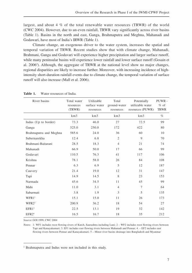
largest, and about 4 % of the total renewable water resources (TRWR) of the world(CWC 2004). However, due to un-even rainfall, TRWR vary significantly across river basins(Table 1). Basins in the north and east, Ganga, Brahmaputra and Meghna, Mahanadi andGodawari, have most of India’s IRWR (Table 1).
Climate change, an exogenous driver to the water system, increases the spatial andtemporal variation of TRWR. Recent studies show that with climate change, Mahanadi,Brahmani, Ganga and Godavari will experience higher precipitation and larger surface runoff,while many peninsular basins will experience lower rainfall and lower surface runoff (Gosain etal. 20062). Although, the aggregate of TRWR at the national level show no major changes,regional disparities are likely to increase further. Moreover, with increasing incidence of high-intensity short-duration rainfall events due to climate change, the temporal variation of surfacerunoff will also increase (Mall et al. 2006).
Table 1. Water resources of India.
River basins Total water Utilizable Total Potentially PUWR -resources surface water ground-water utilizable water % of(TRWR) resources resources resources (PUWR) TRWR
km3 km3 km3 km3 %
Indus (Up to border) 73.3 46.0 27 72.5 99
Ganga 525.0 250.0 172 422 80
Brahmaputra and Meghna 585.6 24.0 36 60 10
Subernarekha 12.4 6.8 2 9 70
Brahmani-Baitarani 28.5 18.3 4 21 74
Mahanadi 66.9 50.0 17 66 99
Godavari 110.5 76.3 41 117 106
Krishna 78.1 58.0 26 84 108
Pennar 6.3 6.9 5 12 187
Cauvery 21.4 19.0 12 31 147
Tapi 14.9 14.5 8 23 153
Narmada 45.6 34.5 11 45 99
Mahi 11.0 3.1 4 7 64
Sabarmati 3.8 1.9 3 5 135
WFR11 15.1 15.0 11 26 173
WFR22 200.9 36.2 18 54 27
EFR13 22.5 13.1 19 32 142
EFR24 16.5 16.7 18 35 212
Source:GOI 1999, CWC 2004
Notes: 1- WF1 includes west flowing rivers of Kutch, Saurashtra including Luni; 2 – WF2 includes west flowing rivers betweenTapi and Kanayakumari; 3. EF1 includes east flowing rivers between Mahanadi and Pennar; 4. – EF2 includes eastflowing rivers between Pennar and Kanayakumari; 5 – Minor river basins drainage into Bangladesh and Myanmar
2 Brahmaputra and Indus were not included in this study.
8
U. A. Amarasinghe, T. Shah and R. P. S. Malik
With monsoonal weather patterns, most of the rain that contributes to TRWR in manyriver basins falls in less than 100 days in the summer months between June and Septemberand a major part of precipitation falls in locations where surface runoff cannot be captureddue to limited storage potential. Therefore only a part of the TRWR can be stored or divertedfor human use within a basin.
Potentially Utilizable Water Resources (PUWR)
The PUWR is the portion of the TRWR that can be captured for human use within a riverbasin. This depends on the variation of precipitation and the potential of storage and diversionfacilities. For India, this is estimated to be only 58 % of the TRWR. Among the river basins,Brahmaputra and Meghna have the largest TRWR, but with limited storage opportunities, only10 % of TRWR can be captured as PUWR (Table 1).
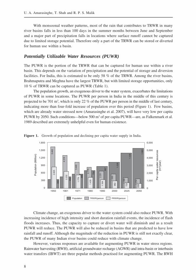
The population growth, an exogenous driver to the water system, exacerbates the limitationsof PUWR in some locations. The PUWR per person in India in the middle of this century isprojected to be 701 m3, which is only 22 % of the PUWR per person in the middle of last century,indicating more than four-fold increase of population over this period (Figure 1). Few basins,which are already water stressed now (Amarasinghe et al. 2007), will have very low per capitaPUWR by 2050. Such conditions—below 500 m3 of per capita PUWR—are, as Falkenmark et al.1989 described are extremely unhelpful even for human existence.
Climate change, an exogenous driver to the water system could also reduce PUWR. Withincreasing incidence of high intensity and short duration rainfall events, the incidence of flashfloods increases. Thus, the capacity to capture or divert water will diminish and as a resultPUWR will reduce. The PUWR will also be reduced in basins that are predicted to have lowrainfall and runoff. Although the magnitude of the reduction in PUWR is still not exactly clear,the PUWR of many Indian river basins could reduce with climate change.
However, various responses are available for augmenting PUWR in water stress regions.Rainwater harvesting (RWH), artificial groundwater recharge (AGWR) and intra-basin or interbasinwater transfers (IBWT) are three popular methods practised for augmenting PUWR. The RWH
Figure 1. Growth of population and declining per capita water supply in India.
9
Overview of the Research in Phase I of the IWMI-CPWF Project
and AGWR are mainly local level interventions and they will generate immediate impacts in aneighborhood of the location where water is captured. On the other hand, the IBWT, whichgenerally requires large infrastructure development, including storage reservoirs, barrages, riverlinks, and distributary canals etc., can increase water availability in far away locations from wherewater is originally stored or diverted. However, these interventions could incur social cost too.Extensive RW and AGWR in the up-stream of river basins, especially in those which areapproaching closure, can impact the uses and users in the down-stream of a basin. The IBWTscan displace many people and submerge large areas of forest or productive land. Yet, all theseinterventions can have significant spatially distributional benefits. The main question herehowever is, that with a significant part of the precipitation occurring in short spells, how muchcan these interventions effectively augment PUWR in Indian river basins?
Rainwater Harvesting
The extent that RWH can augment the PUWR depends on the capacity of RWH structures tostore part of the unutilizable water resources. The exact estimates of this are sketchy. Thestudy by Bharat et al. (Paper 10 in this volume) using a district level analysis shows that 99km3 of surface runoff are available for rainwater harvesting in 25 million ha of rain-fed lands.These lands exclude the extreme arid and extreme wet rain-fed areas. However, whether all ofthis quantity of harvested water will augment the net PUWR is not clear. Some harvested watercould well have been captured by reservoirs in the downstream, and may already have beenincluded in the present estimate of PUWR. In spite of whether it net augments or not, theRWH is very useful for distributing significant positive benefits to vast areas that a few storagestructures cannot provide. Bharat et al. study also shows that it requires only about 20 km3 ofthe above runoff to be captured to bring relief to about 25 million ha of rain-fed lands sufferingfrom mid-seasonal droughts. If this portion can be part of the unutilizable water resources,then it is only 2.5 % of the unutilizable runoff and augments the present estimates of PUWRonly by 1.7 %.
There are other viewpoints of RWH too. Kumar et al. 2006 argue that the impacts ofmany local watershed level RWH interventions will not always aggregate at the basin level.This argument is based on the premise that much of the water that RWH captures is part ofthe water already captured and used in the downstream. According to Kumar et al. the potentialof RWH for net augmenting of PUWR in water scarce areas is low due to varying hydrologicalregimes, extremely variable rainfall events, and constraints of geology. Furthermore, the demandfor water is low in locations where rainwater can sufficiently be captured, thus generatingonly a small economic benefit vis-à-vis to the cost of construction of many RWH structures.
Artificial Groundwater Recharge (AGWR)
The total renewable groundwater resource of India is estimated to be 432 BCM. For the countryas a whole, only about 37 % of the renewable groundwater resource is withdrawn at present.But, with intensive withdrawals for irrigation, groundwater resources of some regions areseverely over-stressed. The number of overexploited bocks is increasing, where groundwaterabstraction well exceeds the replenishable recharge (CGWB 2008). Yet, the uses and users inthe domestic, irrigation and industrial sectors that depend on groundwater are increasing.Sustaining the groundwater supply for various services, especially in the severely water
10
U. A. Amarasinghe, T. Shah and R. P. S. Malik
stressed blocks and in areas approaching overexploitation, and maintaining the base flow inrivers in the dry season is indeed a major challenge.
AGWR have the capacity to alleviate the stress in groundwater overexploited areas. Anideal example is the mass movement of groundwater recharge in the Saurashtra region of westernIndia (Shah 2000). According to the master plan prepared by the Central Groundwater Board, 36BCM of unutilizable surface runoff can be captured through AGWR (CGWB 2008). This augmentsIndia’s PUWR by 3.4 %. However, given the magnitude of the unutilizable surface runoff, manyconsidered this estimate to be quite low. In fact, Shah 2008 argues that groundwater rechargeusing the existing dug-wells alone can exceed the potential of AGWR estimated in the masterplan. Regardless of the magnitude of the recharge, AGWR is an important tool for net augmentingthe PUWR and distributing the hydrological and economic benefits, as in RWH, to vast areas.
Intra-basin or Interbasin Water Transfers (IBWT)
The IBWTs perhaps have the potential for large net augmentation of PUWR. They can captureunutilizable runoff of water surplus basins through large reservoirs or barrages, and then transferthem to water scarce areas within the same or to other basins. For example, the NRLP envisagestransferring 178 BCM from water surplus Brahmaputra, Maghanadi and Godavari basins to waterscarce basins such as Krishna, Cauvery, Pennar, and Sabramati, in the southern and westernregions (NWDA 2006). If all that diverted water in the NRLP is from unutilizable surface runoff,then it augments PUWR of India by 18 %. Indeed, this is one of the major contentious issues inrecent discourses. How, such large quantum of surplus water, mainly floods, in some basins canbe transferred to other basins when they also experience floods is indeed an important question.
In spite of the above concern, the IBWTs can have many socioeconomic and hydrologicalbenefits. For example, the NRLP expects to mitigate the damage caused by floods which ravagesthe eastern parts of the country every year, temporarily displacing many people, destroyingcrops and livestock, and disrupting the livelihood of many, especially the rural poor. The NRLPalso provides an insurance against recurrent droughts and expects to recharge groundwaterof overexploited blocks in many parts of the southern and western parts of India. In fact, itcan alleviate water scarcities in many river basins, which in some regions are becoming a seriousconstraint on further economic growth.
However, many other drivers, which are exogenous to the countries water system, alsoaffect implementing IBWTs (Shah et al. 2006). Financing such mega projects, estimated to bemore than US$125 billion (in 2000 prices) for NRLP, and their impacts on other social-welfareactivities are serious concerns under the prevailing economic conditions at present. But, withrapid economic growth, increasing at 7-9 % annually in recent years, financing of large IBWTsshall not be a major constraint on a trillion dollar3 economy in few years time.
The IBWTs often displace lakhs, if not millions of people and submerge large areas offorest and productive agriculture land. And the hardest hit by such displacements are theweakest sections of society, including tribal communities with forest as the main livelihoodresource, and landless laborers who depend for their livelihood on the daily wages from workingin those agriculture lands that get submerged. The resettlement and rehabilitation issues, ifnot properly addressed, are major bottlenecks for implementing large IBWTs.
3 India’s GDP has already passed one trillion. It was US$1,027 billion in 2007.
11
Overview of the Research in Phase I of the IWMI-CPWF Project
Political stability and relations between states and neighboring countries are also majordrivers of planning and implementing IBWTs. Often, IBWTs cut across several states and attimes, several countries. In NRLP, it is even required to build storage reservoirs in othercountries. Therefore, the existing level and the future prospects of trans-boundary or inter-state cooperation are major determining factors determining the feasibility of such IBWTs.
Ecosystem water needs, another major driver, is often ignored in IBWT planning. Butthey are highly contentious issues in the discourses thereafter. An important question oftenraised in these dialogues are whether water resources required for sustaining a healthyecosystem in one basin can be considered for augmenting water resources in other basins.According to Bandyopadhyaya and Praveen 2003, there is no free surplus of water availableto be transferred from one river basin to another basin. All water in the unutilizable waterresources, including floods, performs an important ecosystem service. Such assumptions,indeed, are an extreme view point in-terms of ecosystem water needs. A compromised formulacan determine the extent of surplus that can be transferred from the water surplus river basins.How much of water can be transferred depends on whether the environment is considered asa primary driver of water supply or as another sector of water use.
If environment is considered as another sector of water use, it often loses. Withincreasing demand, different sectors compete for scarce water resources. The agriculture,domestic, industrial, navigation and hydropower sectors have stakeholders who have a voiceand also theoretically can afford to pay for the services. However, the environmental sectorhas no voice by itself or cannot pay for its water demand. Thus, as a ‘water use sector’, thewater needs of the ecosystems are often ignored in IBWT planning. For instance, the NCIWRDwater demand scenarios considered the environment as a water use sector, and allocated only10 BCM, or less than 1 % of TRWR.
However, this situation can change if eco-system water needs are considered as a primarydriver of water availability. The premise here is that parts of the floods in the rainy season anda minimum river flow in the dry season play a major role in servicing the needs of the riverineecosystems. Thus, a major part of the unutilizable water resources cannot be captured andtransferred for water use in other basins. In this context, it is important then to know themagnitude of the water needs for sustaining ecosystem services in river basins.
Environmental Water Demand
As a primary driver, a good starting point is to assume that at least a minimum environmentalflow (EF)4 requirement is to be maintained for providing ecosystem services of a river basin.Two factors determine EF. They are the natural hydrological variability of the river flow, anendogenous driver to the water system, and the environmental management class that theriver ought to be maintained, often an exogenous driver to the water system. The latter dependson human decisions on the qualitative importance they want to place on riverine ecosystems.Smakhtin et al. (Papers 20 and 21) defined six environmental management classes (EMC), and
4 This is part of the research conducted under the project for assessing environmental water demand ofriver basins of India. Details of the procedures and estimation are available in Smakhtin and Anputhas2007 (or paper 14 in this volume) and Smakhtin et al. 2007 (paper 15 in this volume).
12
U. A. Amarasinghe, T. Shah and R. P. S. Malik
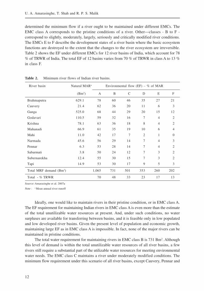
determined the minimum flow if a river ought to be maintained under different EMCs. TheEMC class A corresponds to the pristine conditions of a river. Other—classes - B to F -correspond to slightly, moderately, largely, seriously and critically modified river conditions.The EMCs E to F describe the development states of a river basin where the basic ecosystemfunctions are destroyed to the extent that the changes to the river ecosystem are irreversible.Table 2 shows the EF under different EMCs for 12 river basins of India, which account for 78% of TRWR of India. The total EF of 12 basins varies from 70 % of TRWR in class A to 13 %in class F.
Table 2. Minimum river flows of Indian river basins.
River basin Natural MARa Environmental flow (EF) – % of MAR
(Bm3) A B C D E F
Brahmaputra 629.1 78 60 46 35 27 21
Cauvery 21.4 62 36 20 11 6 3
Ganga 525.0 68 44 29 20 15 12
Godavari 110.5 59 32 16 7 4 2
Krishna 78.1 63 36 18 8 4 2
Mahanadi 66.9 61 35 19 10 6 4
Mahi 11.0 42 17 7 2 1 0
Narmada 45.6 56 29 14 7 4 3
Pennar 6.3 53 28 14 7 4 2
Sabarmati 3.8 50 24 12 7 3 2
Subernarekha 12.4 55 30 15 7 3 2
Tapi 14.9 53 30 17 9 5 3
Total MRF demand (Bm3) 1,065 731 501 353 260 202
Total - % TRWR 70 48 33 23 17 13
Source:Amarasinghe et al. 2007a
Note : a Mean annual river runoff
Ideally, one would like to maintain rivers in their pristine condition, or in EMC class A.The EF requirement for maintaining Indian rivers in EMC class A is even more than the estimateof the total unutilizable water resources at present. And, under such conditions, no watersurpluses are available for transferring between basins, and it is feasible only in low populatedand low developed river basins. Given the present level of population and economic growth,maintaining large EF as in EMC class A is impossible. In fact, none of the major rivers can bemaintained in pristine conditions.
The total water requirement for maintaining rivers in EMC class B is 731 Bm3. Althoughthis level of demand is within the total unutilizable water resources of all river basins, a fewrivers still require a substantial part of the utilizable water resources for meeting environmentalwater needs. The EMC class C maintains a river under moderately modified conditions. Theminimum flow requirement under this scenario of all river basins, except Cauvery, Pennar and
13
Overview of the Research in Phase I of the IWMI-CPWF Project
Tapi, is less than the unutilizable water resources (Amarasinghe et al. 2007). The unutilizablewater resources of Brahmaputra, Ganga, Mahanadi, and Godavari substantially exceed thecorresponding EF under EMC class C. Thus part of the excess flows in these basins cantheoretically be transferred to other basins. Nevertheless, if environmental water demand getshigh priority, the effective water supply that is available for augmenting PUWR could furtherdiminish in many river basins.
Besides these concerns, some studies show that the estimates of PUWR that are availableat present are significantly over-estimated (Garg and Hassan 2007). This is mainly due to doublecounting of surface and groundwater resources in the dry season. According to Garg andHassan, the presently available estimate of PUWR in India is overestimated by at least 66 %.Such estimates, indeed, are alarming and require thorough scrutiny before they are acceptedin water supply and demand modeling and such a scrutiny also requires a clear understandingof the interaction of surface and groundwater flows in river basins, for which the availabledata on water resources in many river basins are inadequate. According to Mohile et al. (Paper19 in this volume), a static estimate for PUWR is not any more a useful concept. Instead, theyprefer to replace PUWR by ‘limits of utilization’ of water resources in a basin. The limits ofutilization depend not only on the natural flows and the engineering and agronomic constraints,but also - on environmental constraints and methods of utilization of water resources. Theypropose that any surplus water over and above the ‘limits of utilization’ can be transferred toother basins. A major drawback of this approach is the way it estimates potential utilization ina river basin. It depends on a set of assumption of trends and magnitude of drivers of waterdemand and the potential water use according to them. As discussed before, these assumptions,especially on primary drivers, are difficult to forecast. Therefore, drivers pertaining to waterdemand estimation themselves require periodic assessment.
Water Demand Drivers
Changing Demographic Patterns
Population growth has a central place among primary drivers of future water demand. Thechanging regional demographic patterns also play an equally important role in assessing thecomposition of regional water demand. This is important for a large country like India with asignificant spatial variation of water availability, and also when irrigation is the largestconsumptive water use sector in many regions. Irrigation has played a vital role in the past inmany states where a major part of the rural population depended on agriculture fortheir livelihoods.
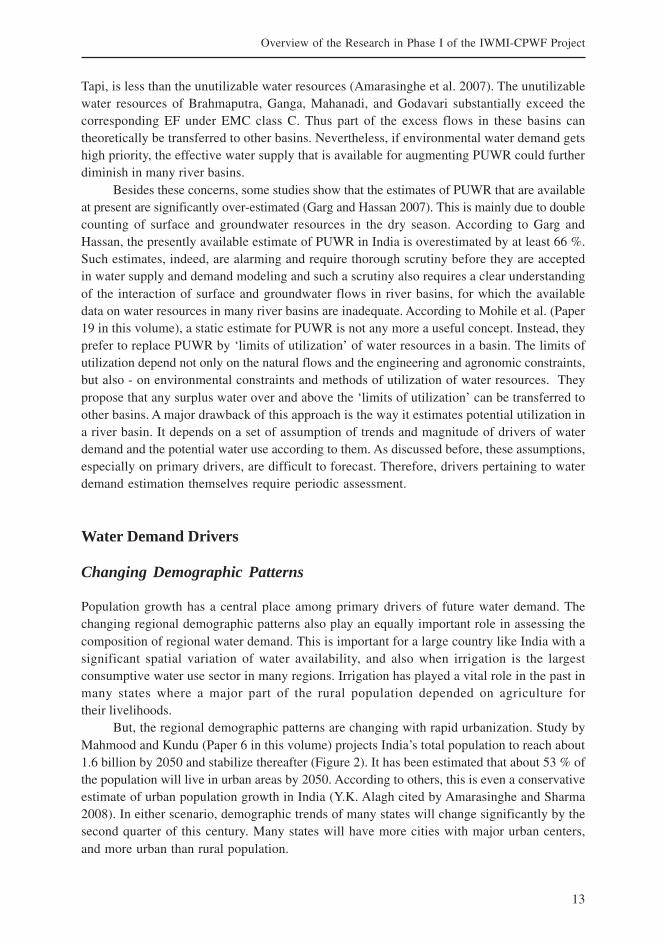
But, the regional demographic patterns are changing with rapid urbanization. Study byMahmood and Kundu (Paper 6 in this volume) projects India’s total population to reach about1.6 billion by 2050 and stabilize thereafter (Figure 2). It has been estimated that about 53 % ofthe population will live in urban areas by 2050. According to others, this is even a conservativeestimate of urban population growth in India (Y.K. Alagh cited by Amarasinghe and Sharma2008). In either scenario, demographic trends of many states will change significantly by thesecond quarter of this century. Many states will have more cities with major urban centers,and more urban than rural population.
14
U. A. Amarasinghe, T. Shah and R. P. S. Malik
Figure 2. Urban, rural and agriculture depended population in India.
Source:FAO 2005, Mahmood and Kundu 2006
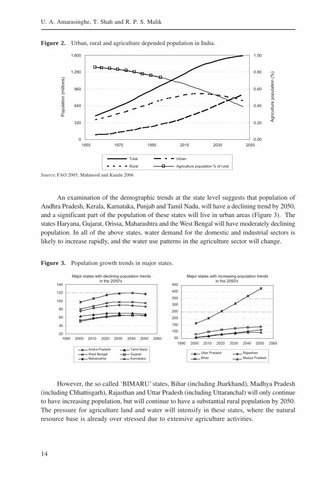
An examination of the demographic trends at the state level suggests that population ofAndhra Pradesh, Kerala, Karnataka, Punjab and Tamil Nadu, will have a declining trend by 2050,and a significant part of the population of these states will live in urban areas (Figure 3). Thestates Haryana, Gujarat, Orissa, Maharashtra and the West Bengal will have moderately decliningpopulation. In all of the above states, water demand for the domestic and industrial sectors islikely to increase rapidly, and the water use patterns in the agriculture sector will change.
Figure 3. Population growth trends in major states.
However, the so called ‘BIMARU’ states, Bihar (including Jharkhand), Madhya Pradesh(including Chhattisgarh), Rajasthan and Uttar Pradesh (including Uttaranchal) will only continueto have increasing population, but will continue to have a substantial rural population by 2050.The pressure for agriculture land and water will intensify in these states, where the naturalresource base is already over stressed due to extensive agriculture activities.
15
Overview of the Research in Phase I of the IWMI-CPWF Project
Many national level projections often do not incorporate regional population growthpatterns. This is one major shortcoming of the assumptions of the NCIWRD scenarios. Theyestimated the future population of states and basins on the basis of the 1991 population figures(page 70 in GOI 1999). Such an assumption can over estimate the rural population and part ofthe rural population that depend for their livelihood on agriculture in many southern andwestern states.
Rural Livelihood Security
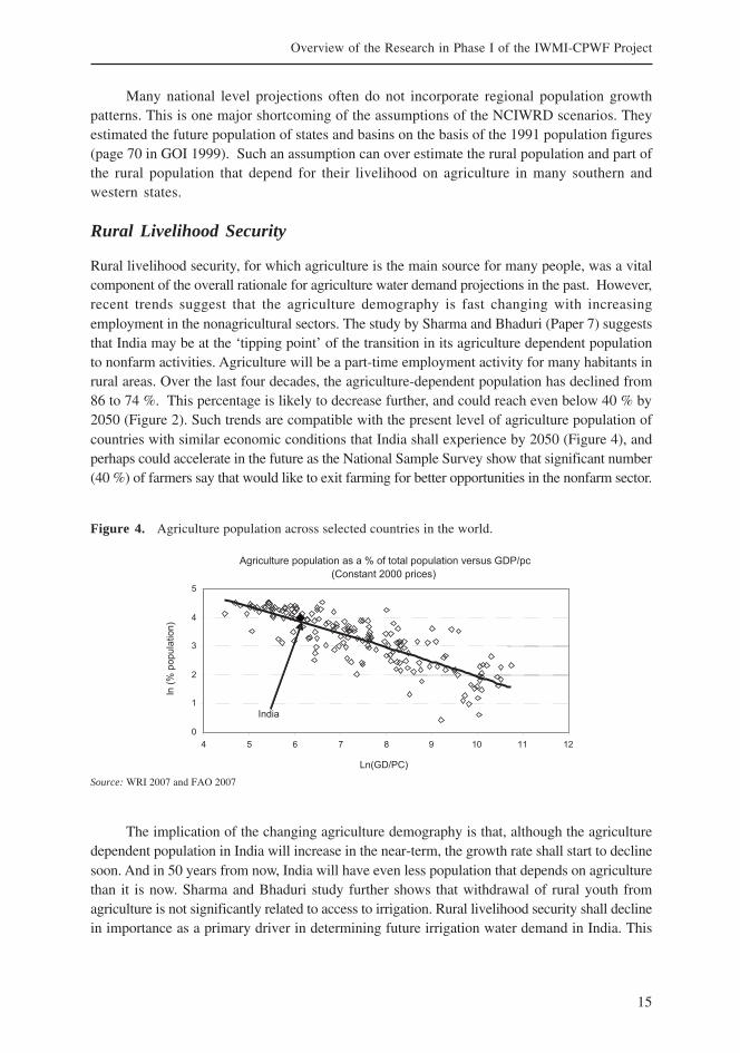
Rural livelihood security, for which agriculture is the main source for many people, was a vitalcomponent of the overall rationale for agriculture water demand projections in the past. However,recent trends suggest that the agriculture demography is fast changing with increasingemployment in the nonagricultural sectors. The study by Sharma and Bhaduri (Paper 7) suggeststhat India may be at the ‘tipping point’ of the transition in its agriculture dependent populationto nonfarm activities. Agriculture will be a part-time employment activity for many habitants inrural areas. Over the last four decades, the agriculture-dependent population has declined from86 to 74 %. This percentage is likely to decrease further, and could reach even below 40 % by2050 (Figure 2). Such trends are compatible with the present level of agriculture population ofcountries with similar economic conditions that India shall experience by 2050 (Figure 4), andperhaps could accelerate in the future as the National Sample Survey show that significant number(40 %) of farmers say that would like to exit farming for better opportunities in the nonfarm sector.
Figure 4. Agriculture population across selected countries in the world.
Source: WRI 2007 and FAO 2007
The implication of the changing agriculture demography is that, although the agriculturedependent population in India will increase in the near-term, the growth rate shall start to declinesoon. And in 50 years from now, India will have even less population that depends on agriculturethan it is now. Sharma and Bhaduri study further shows that withdrawal of rural youth fromagriculture is not significantly related to access to irrigation. Rural livelihood security shall declinein importance as a primary driver in determining future irrigation water demand in India. This
16
U. A. Amarasinghe, T. Shah and R. P. S. Malik
was another contentious assumption in the NCIWRD projections, where it was assumed thatirrigated agriculture would be a major part of the future rural livelihood security.
Changing Consumption Patterns
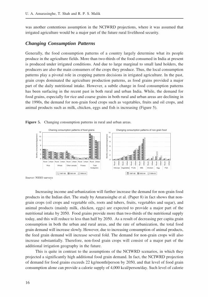
Generally, the food consumption patterns of a country largely determine what its peopleproduce in the agriculture fields. More than two-thirds of the food consumed in India at presentis produced under irrigated conditions. And due to large marginal to small land holders, theproducers are also the main consumers of the crops they produce. Thus, the local consumptionpatterns play a pivotal role in cropping pattern decisions in irrigated agriculture. In the past,grain crops dominated the agriculture production patterns, as food grains provided a majorpart of the daily nutritional intake. However, a subtle change in food consumption patternshas been surfacing in the recent past in both rural and urban India. While, the demand forfood grains, especially for rice and coarse grains in both rural and urban areas are declining inthe 1990s, the demand for non-grain food crops such as vegetables, fruits and oil crops, andanimal products such as milk, chicken, eggs and fish is increasing (Figure 5).
Figure 5. Changing consumption patterns in rural and urban areas.
Source: NSSO surveys
Increasing income and urbanization will further increase the demand for non-grain foodproducts in the Indian diet. The study by Amarasinghe et al. (Paper 8) in fact shows that non-grain crops (oil crops and vegetable oils, roots and tubers, fruits, vegetables and sugar), andanimal products (mainly milk, chicken, eggs) are expected to provide a major part of thenutritional intake by 2050. Food grains provide more than two-thirds of the nutritional supplytoday, and this will reduce to less than half by 2050. As a result of decreasing per capita grainconsumption in both the urban and rural areas, and the rate of urbanization, the total foodgrain demand will increase slowly. However, due to increasing consumption of animal products,the feed grain demand will increase several fold. The demand for non-grain crops will alsoincrease substantially. Therefore, non-food grain crops will consist of a major part of theadditional irrigation geography in the future.
This is quite in contrast to the assumptions of the NCIWRD scenarios, in which theyprojected a significantly high additional food grain demand. In fact, the NCIWRD projectionof demand for food grains exceeds 22 kg/month/person by 2050, and that level of food grainconsumption alone can provide a calorie supply of 4,000 kcal/person/day. Such level of calorie
17
Overview of the Research in Phase I of the IWMI-CPWF Project
supply is highly unlikely as it is even higher than the calorie intake in the most developedcountries with animal product dominated diet (Amarasinghe et al. Paper 3). Nevertheless, highdemand for food grains along with national self-sufficiency assumption required NCIWRDscenarios to project a large irrigated area expansion.
National Self-sufficiency
Another primary driver that dominated the selection of cropping patterns of agriculture in general,and irrigation in particular was full national self-sufficiency of food grains. This assumption wasmainly based on the three concerns that 1) India has a large population and the food grains arethe staple food of its people with mainly a vegetarian diet, because of which large productiondeficits, such as in the 1960s, are not acceptable; 2) agriculture was the main driver of economicgrowth and has contributed to substantial part of the gross domestic product; and 3) India’sforeign exchange reserves are too low to import large quantities of food from the world market.The first is still true, but as mentioned before, demographic and consumption patterns are fastchanging, and demand for non-grain food and feed products are increasing. With changingconsumption patterns, there will be more opportunities for Indian farmers to increase incomefrom growing high-value non-grain food products. Moreover, India’s agriculture export and importpatterns are also changing. Although the share of total agriculture exports is decreasing, whichis natural with rapidly growing industrial and service sectors, the total quantum of exports hasbeen increasing in recent years (Paper 9 by R.P.S. Malik). Also, India has been importing asignificant part of the requirements of vegetable oil, and also some pulses, fruits and nuts etc.However, the value of agriculture exports at present far exceeds that of imports, and the differenceis widening gradually. And with expanding global trade, India will have more opportunities forincreasing agriculture exports, and pay for its agriculture imports.
In the past, low foreign exchange reserves were indeed a constraint on large food imports.But that was only when the gross domestic product was only a few hundred billion dollars,and food grain production was a substantial part of it. But it is no longer valid under theprevailing economic growth. India has a trillion dollar economy now and has large foreignexchange reserves in comparison with those in the early 1990s. The share of the agriculturesector, let alone the value of food grain production, is only about 23 % of the total GDP in2000 (WRI 2007). And this share will decrease further, and India will have sufficient foreignexchange reserves to pay for even large food imports in a few decades time.
However, the only concern that India should have in large quantity of food imports is itseffect on prices. Potential price increases due to large food imports from countries such as Indiaand China can hurt the very consumers that the imports would expect to help, and also canincrease the volatility of global grain markets in the years of significant grain production deficits.So, a reasonable degree of food self-sufficiency, purely because of the volatility in the grainprices in the markets, can still be a good assumption for projecting future food and water demand.
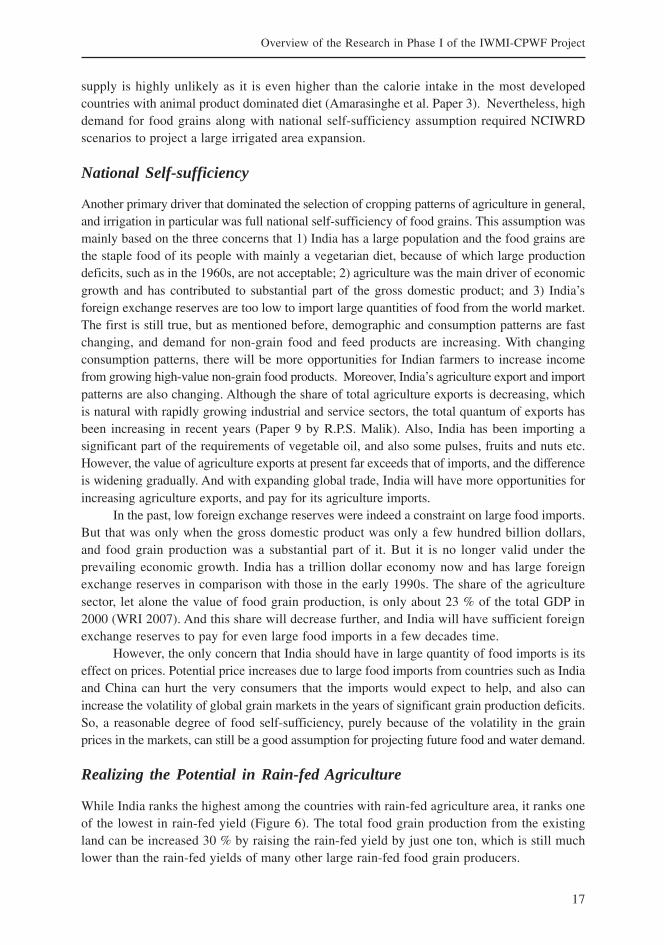
Realizing the Potential in Rain-fed Agriculture
While India ranks the highest among the countries with rain-fed agriculture area, it ranks oneof the lowest in rain-fed yield (Figure 6). The total food grain production from the existingland can be increased 30 % by raising the rain-fed yield by just one ton, which is still muchlower than the rain-fed yields of many other large rain-fed food grain producers.
18
U. A. Amarasinghe, T. Shah and R. P. S. Malik
Sharma et al. (Paper 10) finds that frequent occurrence of mid-season and terminal droughtswere the main cause for crop failures or low yield in a major part of the rain-fed cropped area.Small supplemental irrigation during the water stressed periods of mid-season and terminaldroughts can significantly increase the rain-fed yields. Providing supplemental irrigation throughdecentralized, more equitable and targeted rainwater harvesting structures can help millions ofresource poor farmers in rain-fed faming. They shall also reduce the requirement for large-scaleirrigation projects, which in the present states of water scarcities require large inter or intra-basinwater transfers. However, small RWH interventions could bring maximum benefits provided thatthe marginal cost does not exceed the marginal economic benefits in basins with high degree ofdevelopment and that there are no significant disparities of water demand in the upper and lowercatchments, where there is no significant tradeoff in maximizing benefits of the upstream vis-à-vis optimizing the basin wide benefits (Kumar et al. 2006).
Increasing Crop Productivity
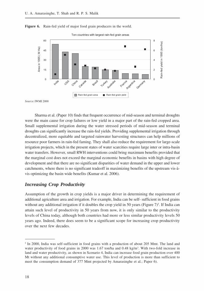
Assumption of the growth in crop yields is a major driver in determining the requirement ofadditional agriculture area and irrigation. For example, India can be self- sufficient in food grainswithout any additional irrigation if it doubles the crop yield in 50 years (Figure 7)5. If India canattain such level of productivity in 50 years from now, it is only similar to the productivitylevels of China today, although both countries had more or less similar productivity levels 50years ago. Indeed, there does seem to be a significant scope for increasing crop productivityover the next few decades.
5 In 2000, India was self-sufficient in food grains with a production of about 205 Mmt. The land andwater productivity of food grains in 2000 was 1.67 ton/ha and 0.48 kg/m3. With two-fold increase inland and water productivity, as shown in Scenario 4, India can increase food grain production over 400Mt without any additional consumptive water use. This level of production is more than sufficient tomeet the consumption demand of 377 Mmt projected by Amarasinghe et al.; Paper 6).
Source: IWMI 2000
Figure 6. Rain-fed yield of major food grain producers in the world.
19
Overview of the Research in Phase I of the IWMI-CPWF Project
Kumar et al. (Paper 14) show that significant variations of productivity exist across farmsin the same area and irrigation systems in the same regions growing similar crops. Theyconclude that a significant scope exists for increasing crop productivity in irrigated areas bymanipulating key factors which include reliable irrigation supply and input use. As shown bySharma et al. (Paper 10), small supplemental irrigation can double the productivity of crops inrain-fed areas. Study by Palanisami (Paper 13) explores ways of increasing the value ofproductivity through multiple cropping systems. This is a good strategy when there are limitedopportunities for increasing productivity through mono-cropping systems.
Growth in Irrigated Area
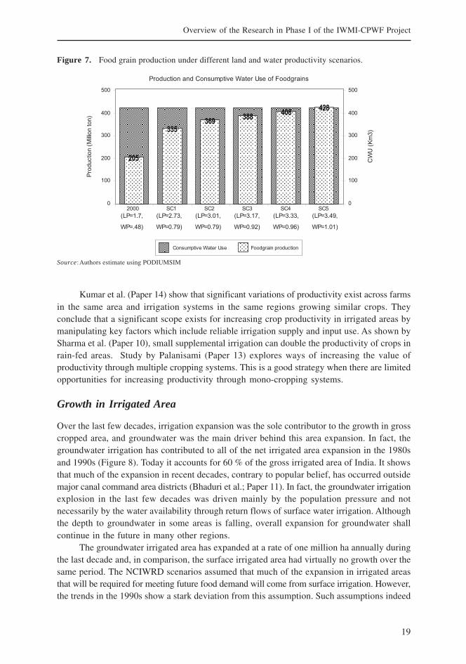
Over the last few decades, irrigation expansion was the sole contributor to the growth in grosscropped area, and groundwater was the main driver behind this area expansion. In fact, thegroundwater irrigation has contributed to all of the net irrigated area expansion in the 1980sand 1990s (Figure 8). Today it accounts for 60 % of the gross irrigated area of India. It showsthat much of the expansion in recent decades, contrary to popular belief, has occurred outsidemajor canal command area districts (Bhaduri et al.; Paper 11). In fact, the groundwater irrigationexplosion in the last few decades was driven mainly by the population pressure and notnecessarily by the water availability through return flows of surface water irrigation. Althoughthe depth to groundwater in some areas is falling, overall expansion for groundwater shallcontinue in the future in many other regions.
The groundwater irrigated area has expanded at a rate of one million ha annually duringthe last decade and, in comparison, the surface irrigated area had virtually no growth over thesame period. The NCIWRD scenarios assumed that much of the expansion in irrigated areasthat will be required for meeting future food demand will come from surface irrigation. However,the trends in the 1990s show a stark deviation from this assumption. Such assumptions indeed
Figure 7. Food grain production under different land and water productivity scenarios.
Source:Authors estimate using PODIUMSIM
20
U. A. Amarasinghe, T. Shah and R. P. S. Malik
have major implications on the financial cost and also on the total water demand. As regardsthe cost, expanding surface irrigation under the prevailing water scarcity conditions in manyriver basins will most probably require expensive IBWTs. As regards the water demand, surfaceirrigation may require significantly higher water withdrawals, as project efficiency of surfaceirrigation is much lower than groundwater irrigation.
Based on the present level of exploitation, availability, quality and the impact onenvironment, Sundararajan et al. (Paper 12) argue that there are only small pockets fordeveloping further groundwater irrigation. However, as argued by Amarasinghe et al. (Paper4), artificial groundwater recharge is an important policy prescription for sustaining thegroundwater irrigation in many river basins. And, based on the present trends, Amarasingheet al. 2007 shows that groundwater expansion will continue and the net groundwater irrigatedarea will reach about 50 mha, adding further 16 mha to the level in 2000.
Increasing Efficiency
The project efficiencies of surface and groundwater irrigation systems are another major driveraffecting irrigation demand projections. Many claimed that there is a significant scope forincreasing project efficiency, especially in surface irrigation systems. However, the littleinformation available suggests that the efficiencies of major systems are hovering around 30-40 % and no major increment of efficiency was also seen over the last few decades. Indeed,increasing irrigation efficiency in one location of river basins that are approaching closuremay not yield the desired result of gains in overall efficiency, as it affects another user in thedownstream of the closing basins. Thus, increasing surface irrigation efficiency to the levelsuggested by the NCIWRD projections, i.e., 60 % will have limited effect within the waterstressed basins.
But it is clear that many water saving technologies, especially micro-irrigation systems,can significantly increase water use-efficiency. Narayanamoorthy (Paper 15) show that sprinklerand drip irrigation can have efficiencies in the range of 75-90 %. And, it also shows that morethan 70 mha of land can potentially benefit from micro-irrigation. However, this potential canonly be reached by overcoming many constraints. Spreading micro-irrigation systems in India
Figure 8. Net surface and groundwater irrigated area growth.
Source:GOI 2004; Amarasinghe et al. 2007.
21
Overview of the Research in Phase I of the IWMI-CPWF Project
is difficult due to the many marginal and small farmers, lack of independent source of waterand pressurizing devices for these small farmers, poor extension services, lack of subsidies,unreliable electricity supplies etc. (Kumar et al. Paper 16).
Domestic and Industrial Water Needs
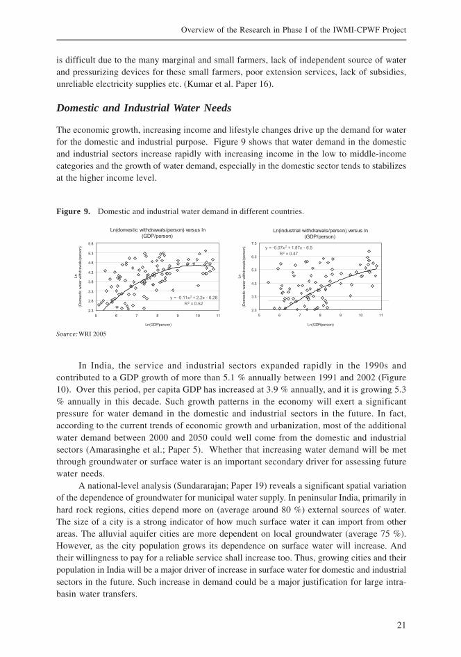
The economic growth, increasing income and lifestyle changes drive up the demand for waterfor the domestic and industrial purpose. Figure 9 shows that water demand in the domesticand industrial sectors increase rapidly with increasing income in the low to middle-incomecategories and the growth of water demand, especially in the domestic sector tends to stabilizesat the higher income level.
Figure 9. Domestic and industrial water demand in different countries.
Source:WRI 2005
In India, the service and industrial sectors expanded rapidly in the 1990s andcontributed to a GDP growth of more than 5.1 % annually between 1991 and 2002 (Figure10). Over this period, per capita GDP has increased at 3.9 % annually, and it is growing 5.3% annually in this decade. Such growth patterns in the economy will exert a significantpressure for water demand in the domestic and industrial sectors in the future. In fact,according to the current trends of economic growth and urbanization, most of the additionalwater demand between 2000 and 2050 could well come from the domestic and industrialsectors (Amarasinghe et al.; Paper 5). Whether that increasing water demand will be metthrough groundwater or surface water is an important secondary driver for assessing futurewater needs.
A national-level analysis (Sundararajan; Paper 19) reveals a significant spatial variationof the dependence of groundwater for municipal water supply. In peninsular India, primarily inhard rock regions, cities depend more on (average around 80 %) external sources of water.The size of a city is a strong indicator of how much surface water it can import from otherareas. The alluvial aquifer cities are more dependent on local groundwater (average 75 %).However, as the city population grows its dependence on surface water will increase. Andtheir willingness to pay for a reliable service shall increase too. Thus, growing cities and theirpopulation in India will be a major driver of increase in surface water for domestic and industrialsectors in the future. Such increase in demand could be a major justification for large intra-basin water transfers.

22
U. A. Amarasinghe, T. Shah and R. P. S. Malik
Conclusion
There are clear trends that India will require substantial additional water supply to cater toincreasing demand in the coming decades. It is estimated that India withdrew about 680 BCBfor meeting the demand in the irrigation, domestic and industrial sectors in 2000. According tothe recent growth patterns, the future demand is projected to increase by 22 % and 32 % by2025 and 2050, respectively (Amarasinghe et al.; Paper 4). The population and economic growth,increasing world trade, the changes in lifestyles and food consumption patterns, technologicaladvances in water saving technologies are the most influential primary drivers of India’s waterfuture in the short to medium term. The climate change will become an influencing factor inthe long-term.
Over the last two decades, groundwater has been the major source for meeting increasingdemand in all sectors. It is highly likely that this trend will continue. However, many riverbasins will have severe water stress conditions under business as usual water- supply anduse patterns. With increasing reliance on groundwater, particularly for irrigation, many riverbasins will have severe groundwater overexploitation-related problems. Indeed, meeting India’sshort to medium term water demand itself will be a challenging task.
However, many options are available to meet this challenge (Amarasinghe et al.; Paper5). Recharging groundwater to increase the groundwater stocks; harvesting rainwater forproviding the life-saving supplemental irrigation; promoting water saving technologies forincreasing water use efficiency; formal or informal water markets and providing reliable ruralelectricity supply for reducing uncontrolled groundwater pumping; increasing research andextension for enhancing agriculture water productivity; and carefully crafted virtual water tradebetween basins are important policy options for meeting the increasing demand. With increasingdisposable income, people’s affordability and willingness to pay for a reliable domestic and
Figure 10. Contribution to GDP growth from different sectors in India.
Source:WRI 2006
23
Overview of the Research in Phase I of the IWMI-CPWF Project
industrial water supply will increase. This, along with a reliable water supply for diversifyinghigh value cropping patterns, may require large surface water transfers. The interbasin watertransfers could increase the recharge groundwater in much overexploited area.
While artificial groundwater recharge, rainwater harvesting, and interbasin water transfersare a solution for meeting the water demand in the near-term, they are also solutions forincreasing the potential utilizable water supply in many water scarce river basins. They willindeed have major benefits when full influence of the climate change starts to impact theutilizable supply in many water scarce river basins.
References
Amarasinghe, U. A.; Shah, T.; Turral, H.; Anand, B. 2007. India’s water futures to 2025-2050: Businessas usual scenario and deviations. Research Report 123. Colombo, Sri Lanka: International WaterManagement Institute.
Bandyopadhyaya, J.; Perveen, S. 2003. The Interlinking of Indian Rivers: Some Questions on the Scientific,Economic and Environmental Dimensions of the Proposal. Paper presented at the Seminar on InterlinkingIndian Rivers: Bane or Boon? at IISWBM, Kolkata, June 17, 2003. SOAS Water Issues Study Group,Occasional Paper No. 60.
CGWB 2008. Master Plan for Artificial Recharge to Groundwater in India.http://cgwb.gov.in/documents/MASTER/20PLAN/20Final-2002.pdf.
CPWF 2005. Strategic Analysis of India’s River Linking Project. The Project Proposal. www.cpwf.org
CWC 2004. Water and related statistics. New Delhi: Water Planning and Projects Wing, Central WaterCommission.
Falkenmark, M.; Lundquvist, J.; Widstrand, C. 1989. Macro-scale water scarcity requires micro-scaleapproaches: Aspect of vulnerability in semi-arid development. Natural Resources Forum 13 (4):258-267.
Garg, N. K.; Hassan, Q. 2007. Alarming scarcity of water in India. Current Science, Vol. 93, No. 7. 10October 2007.
GOI 1999. Integrated water resources development. A plan for action. Report of the Commission forIntegrated Water Resource Development Volume I. New Delhi, India: Ministry of Water Resources.
GOI 2005. Agricultural Statistics at a Glance 2004. New Delhi, India: Ministry of Agriculture, Governmentof India.
Gosain, A. K.; Rao, S.; Basuray, D. 2006. Climate change impacts assessment on hydrology of Indian riverbasins. Current Science, Vol. 90, No. 3. 10 February 2006.
IWMI 2005. The India’s Water Futures Analyses. Scenarios and Issues. Unpublished Proceedings of theInception Workshop on the Project ‘Strategic Analyses of India’s Water Futures’
IWMI 2000. World water supply and demand 1995 to 2025 (draft).www.cgiar.org/iwmi/pubs/WWVison/WWSDOpen.htm
Kumar, M. D.; Samad, M.; Amarasinghe, U. A.; Singh, O. P. 2006. Rainwater Harvesting in Water-scarceRegions of India: Potential and Pitfalls. Draft prepared for the IWMI-CPWF project on ‘Strategic Analysisof National River Linking Project of India’.
Mall, R. K.; Gupta, A.; Singh, R.; Singh, R. S.; Rathore, L. S. 2006. Water resources and climate change:An Indian perspective. Current Science, Vol. 90, No. 12. 25 June 2006.
NWDA 2006. The Inter Basin Water Transfers: The Need. Accessible via http//nwda.gov.in/
24
U. A. Amarasinghe, T. Shah and R. P. S. Malik
Shah, T. 2000. Mobilizing social energy against environmental challenge: understanding the groundwaterrecharge movement in western India. Natural Resources Forum 24 (3): 197-209.
Shah, T 2008. An Assessment of India’s Groundwater Recharge Master plan. Draft prepared for the IWMI-CPWF research project ‘Strategic Analysis of India’s National River Linking Project’.
Shah, T.; Amarasinghe, U. A.; McCornick, P. G. 2006. India’s River Linking Project: The State of theDebate. Draft prepared for the IWMI-CPWF project on ‘Strategic Analysis of National River LinkingProject of India’.
Smakhtin, V.; Anputhas, M. 2006. An assessment of environmental flow requirements of Indian river basins.Research Report 107. Colombo, Sri Lanka: International Water Management Institute.
Smakhtin, V.; Arunachalam, M Behera,.; S.; Chatterjee, A.; Das, S.; Gautam, P.; Joshi, G. D.;Sivaramakrishnan, K. G.; Unni, K. S. 2007. Developing procedures for assessment of ecological statusof Indian river basins in the context of environmental water requirements. Research Report 114, Colombo,Sri Lanka: International Water Management Institute.
World Bank 2005. India’s Water Economy: Bracing for a Turbulent Future. Draft Report.http://go.worldbank.org/QPUTPV5530
WRI (World Resource Institute) 2007. Earth Trends. Environment Information. http://earthtrends.wri.org/searchable_db/index.php?theme=5
25
Overview of the Research in Phase I of the IWMI-CPWF Project
India’s Water Future 2050: Potential Deviations from‘Business-as-Usual’1
Shilp Verma and Sanjiv PhansalkarIWMI-TATA Water Policy Program, India
Background
India has for long been toying with the idea of having a national water grid to overcome thespatial inconsistencies in demand and availability of fresh water resources. The idea oftransferring the flood waters of the Ganga-Brahamaputra-Meghna (GBM) basin to the water-starved basins in western and peninsular India has been in existence for long2. More recently,the idea acquired a new life when, based on a public interest petition, the Supreme Court ofIndia issued an order directing the government to implement the plan prepared by the NWDA3
in 10 years. The government, in response to the court directive, set up a (now disbanded)high-powered task-force with the mandate to complete an analysis of how the project will unfoldby December 31, 2006 and subsequently to complete, by 2016, the project in this respect thatwill cost roughly US$120 billion and link 37 Himalayan and peninsular rivers. The project(National River Linking Project – NRLP) “will form a gigantic South Asian water grid whichwill handle 178 km3 of inter-basin water transfer/year, build 12,500 kms of canals, generate 35gigawatts of hydropower and add 35 mha to India’s irrigated areas” (IWMI 2003).
1 This paper is a modified and updated version of a paper by the same authors and with the sametitle published in the ‘International Journal of Rural Management’, Sage Publications (Verma andPhansalkar 2007).2 It started in late nineteenth century when Sir Arthur Cotton thought of a plan to link rivers in south-ern India for inland navigation. The idea was partially implemented but was abandoned with time asinland navigation lost ground to railways. In 1972, the then Union Minister for Irrigation, Dr. K.L.Rao, proposed the Ganga-Cauvery link and again, in 1977, Captain Dinshaw Dastur coined the phrase‘Garland Canal’ and while his plan was later rejected, the catchy phrase caught the imagination of peopleand continues to be popular.3 The National Water Development Agency (NWDA) was set-up by the Government of India (GOI) in1982 to work out basin-wise surpluses and deficits and to study the possibilities of storage, links andtransfers. It proposed two components of a mega river-linking plan – Himalayan and Peninsular – envisaging14 and 16 links, respectively.
26
S. Verma and S. Phansalkar
The ‘task force’ repeatedly cited projections made by the National Commission forIntegrated Water Resource Development (NCIWRD 1999) of the increased irrigated area requiredto feed the growing population as the key justification for NRLP. In this paper, we try to identifygrey areas and points of discontinuity with the aim of evolving a research agenda that willlead to a refined, textured and nuanced understanding of India’s water future 2050. The paperis organized as follows. First, we present an overview of India’s water resources; second, weprovide a summary of the projections made by the NCIWRD; third, we review other projectionsfor water availability and demand made at global and regional scale with special reference toIndia; fourth, we discuss potential deviations from the commission’s projections; and, finally,we conclude with a framework for ‘water future’ research.
Setting the Stage: India’s Water Resources
How much water do we have? How much of it is currently being used? How far can it bestretched further? Ironically, even the best estimates on these basic questions are oftenconfusing, inaccurate or inconsistent. In this section, we address these questions in a simpleand coherent manner to provide the reader a backdrop for NCIWRD’s estimates4.
Water Resource Accounting
India has a geographical area of a little over 329 million hectares (MHa), and a mean annualrainfall of 1,170 mm. This mean annual rainfall is added to the snow-melt in glaciers and netcross-border river-inflow (river-flow originating from outside India and coming into India MINUSriver-flow originating in India and draining to a neighboring country) to calculate average annualprecipitation. This amounts to around 4,000 BCM5. Of this, less than half is ‘accounted-for’while the rest constitutes what may be called the ‘unaccounted’ water resources of India. This‘unaccounted’ water is primarily used-up in four processes:
(1) Evaporation: A major portion of this ‘unaccounted’ water is lost to the atmosphere inthe form of evaporation. As the rain falls, a good amount of it is first intercepted by the foliageand this amount returns to the atmosphere without ever reaching the ground. This ‘deduction-at-source’ takes place in every spell of rainfall. However, this rain does get measured by therain gauges which are always kept in open areas, and is thus included in the above 4,000BCM. Besides the evaporation of rainwater, the evaporation taking place from land area andwater bodies accounts for a large amount of the ‘loss’.
4 All figures quoted in this section are with reference to the NCIWRD 1999 report, unless otherwisestated. The authors would like to acknowledge the help of Mr. Chetan Pandit, Mr. A.D. Mohile, Dr.Christopher Scott and Dr. M. Dinesh Kumar for their inputs and useful comments on previous ver-sions of this paper.5 BCM = Billion Cubic Meters; 1 BCM = 1 x 10⁹ m3
While this figure is calculated at mean annual rainfall on 329 MHa, there may be variations in this on atleast two counts: (1) 1,170 mm is a gross average for a continent-sized country and rainfall has huge inter-year variability; and (2) there are bound to be carry-overs and overdrafts between two consecutive years.
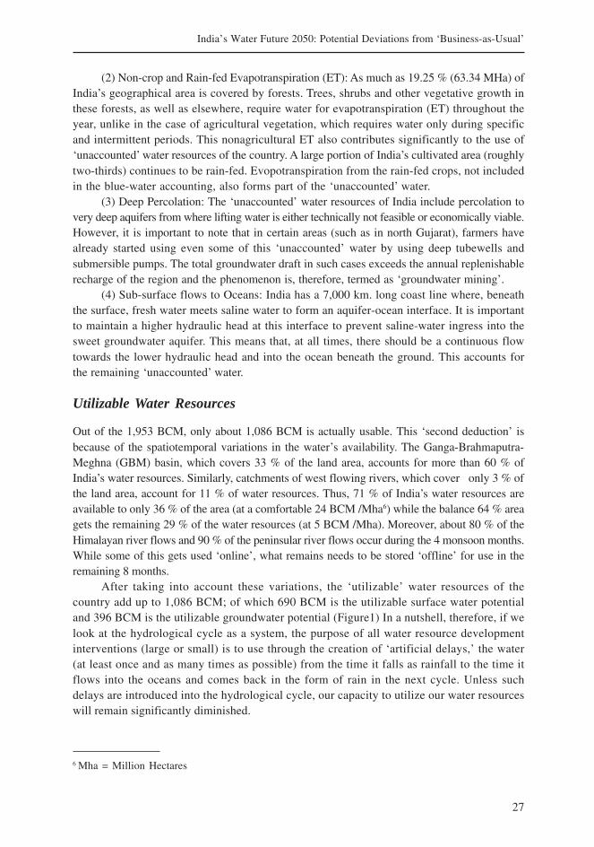
27
India’s Water Future 2050: Potential Deviations from ‘Business-as-Usual’
6 Mha = Million Hectares
(2) Non-crop and Rain-fed Evapotranspiration (ET): As much as 19.25 % (63.34 MHa) ofIndia’s geographical area is covered by forests. Trees, shrubs and other vegetative growth inthese forests, as well as elsewhere, require water for evapotranspiration (ET) throughout theyear, unlike in the case of agricultural vegetation, which requires water only during specificand intermittent periods. This nonagricultural ET also contributes significantly to the use of‘unaccounted’ water resources of the country. A large portion of India’s cultivated area (roughlytwo-thirds) continues to be rain-fed. Evopotranspiration from the rain-fed crops, not includedin the blue-water accounting, also forms part of the ‘unaccounted’ water.
(3) Deep Percolation: The ‘unaccounted’ water resources of India include percolation tovery deep aquifers from where lifting water is either technically not feasible or economically viable.However, it is important to note that in certain areas (such as in north Gujarat), farmers havealready started using even some of this ‘unaccounted’ water by using deep tubewells andsubmersible pumps. The total groundwater draft in such cases exceeds the annual replenishablerecharge of the region and the phenomenon is, therefore, termed as ‘groundwater mining’.
(4) Sub-surface flows to Oceans: India has a 7,000 km. long coast line where, beneaththe surface, fresh water meets saline water to form an aquifer-ocean interface. It is importantto maintain a higher hydraulic head at this interface to prevent saline-water ingress into thesweet groundwater aquifer. This means that, at all times, there should be a continuous flowtowards the lower hydraulic head and into the ocean beneath the ground. This accounts forthe remaining ‘unaccounted’ water.
Utilizable Water Resources
Out of the 1,953 BCM, only about 1,086 BCM is actually usable. This ‘second deduction’ isbecause of the spatiotemporal variations in the water’s availability. The Ganga-Brahmaputra-Meghna (GBM) basin, which covers 33 % of the land area, accounts for more than 60 % ofIndia’s water resources. Similarly, catchments of west flowing rivers, which cover only 3 % ofthe land area, account for 11 % of water resources. Thus, 71 % of India’s water resources areavailable to only 36 % of the area (at a comfortable 24 BCM /Mha6) while the balance 64 % areagets the remaining 29 % of the water resources (at 5 BCM /Mha). Moreover, about 80 % of theHimalayan river flows and 90 % of the peninsular river flows occur during the 4 monsoon months.While some of this gets used ‘online’, what remains needs to be stored ‘offline’ for use in theremaining 8 months.
After taking into account these variations, the ‘utilizable’ water resources of thecountry add up to 1,086 BCM; of which 690 BCM is the utilizable surface water potentialand 396 BCM is the utilizable groundwater potential (Figure1) In a nutshell, therefore, if welook at the hydrological cycle as a system, the purpose of all water resource developmentinterventions (large or small) is to use through the creation of ‘artificial delays,’ the water(at least once and as many times as possible) from the time it falls as rainfall to the time itflows into the oceans and comes back in the form of rain in the next cycle. Unless suchdelays are introduced into the hydrological cycle, our capacity to utilize our water resourceswill remain significantly diminished.
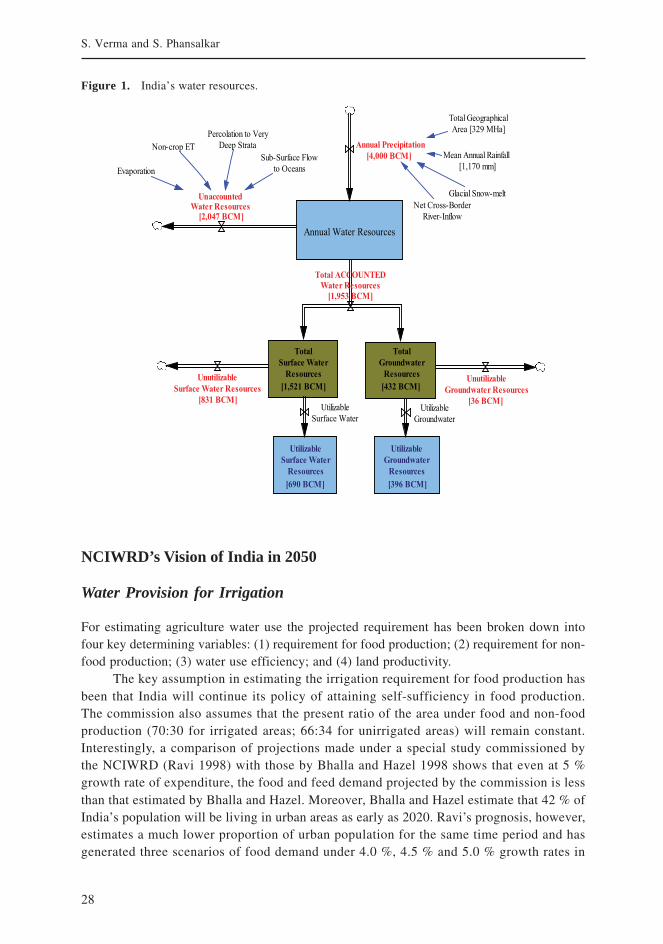
28
S. Verma and S. Phansalkar
NCIWRD’s Vision of India in 2050
Water Provision for Irrigation
For estimating agriculture water use the projected requirement has been broken down intofour key determining variables: (1) requirement for food production; (2) requirement for non-food production; (3) water use efficiency; and (4) land productivity.
The key assumption in estimating the irrigation requirement for food production hasbeen that India will continue its policy of attaining self-sufficiency in food production.The commission also assumes that the present ratio of the area under food and non-foodproduction (70:30 for irrigated areas; 66:34 for unirrigated areas) will remain constant.Interestingly, a comparison of projections made under a special study commissioned bythe NCIWRD (Ravi 1998) with those by Bhalla and Hazel 1998 shows that even at 5 %growth rate of expenditure, the food and feed demand projected by the commission is lessthan that estimated by Bhalla and Hazel. Moreover, Bhalla and Hazel estimate that 42 % ofIndia’s population will be living in urban areas as early as 2020. Ravi’s prognosis, however,estimates a much lower proportion of urban population for the same time period and hasgenerated three scenarios of food demand under 4.0 %, 4.5 % and 5.0 % growth rates in
Figure 1. India’s water resources.

29
India’s Water Future 2050: Potential Deviations from ‘Business-as-Usual’
expenditure. The commission has accepted the projections made by Ravi with theassumption of 4.5 % growth in expenditure to estimate their food and feed demand in 2010,2025 and 2050.
Based on these, the commission has calculated the total water requirement for irrigationin 2010, 2025 and 2050 under low as well as high population growth scenarios as shownin Table 1.
Population
Urbanization
Per capita fooddemand
at 4.5 % expenditure growth Kg/Cap/Yr. 194 218 284
Total water required
GIA/GSA
% Food crops
Food crop yields
Food plus production
Irrigation efficiency
GIR [NIR = 0.36]
Food plus demand
Table 1. Water requirement for irrigation 2010, 2025, 2050 (BCM).
Variable Remarks and Assumptions Units 2010 2025 2050
Low growth scenario* Million 1,156.60 1,286.30 1,345.90
High growth scenario** Million 1,146.00 1,333.00 1,581.00
Low growth scenario % 32 37 48
High growth scenario % 34 45 61
Low growth scenario MT 245 308 420
High growth scenario MT 247 320 494
NSA Marginal increase Mha 143 144 145
Low growth scenario % 40 45 52
High growth scenario % 41 48 63
Cropping intensity 20 % growth assumed over 50 years % 135 140-142 150-160
Rain-fed areas (no change) % 66 66 66
Irrigated areas (no change) % 70 70 70
Rain-fed areas (modest increase) T/Ha 1.10 1.25 1.50
Irrigated areas (modest increase) T/Ha 3.00 3.50 4.00
Low growth scenario MT 246 307 422
High growth scenario MT 249 322 494
Surface water irrigation % 40 50 60
Ground water irrigation % 70 72 75
Surface water irrigation 0.91 0.73 0.61
Ground water irrigation 0.52 0.51 0.49
SW dependence Growing dependence on SW assumed % 47 49-51 54.3
Low growth scenario BCM 543 561 628
High growth scenario BCM 557 611 807
Source:Adapted from various tables (NCIWRD 1999)
Notes: * Based on United Nations 1995 projections** Based on Visaria and Visaria 1996
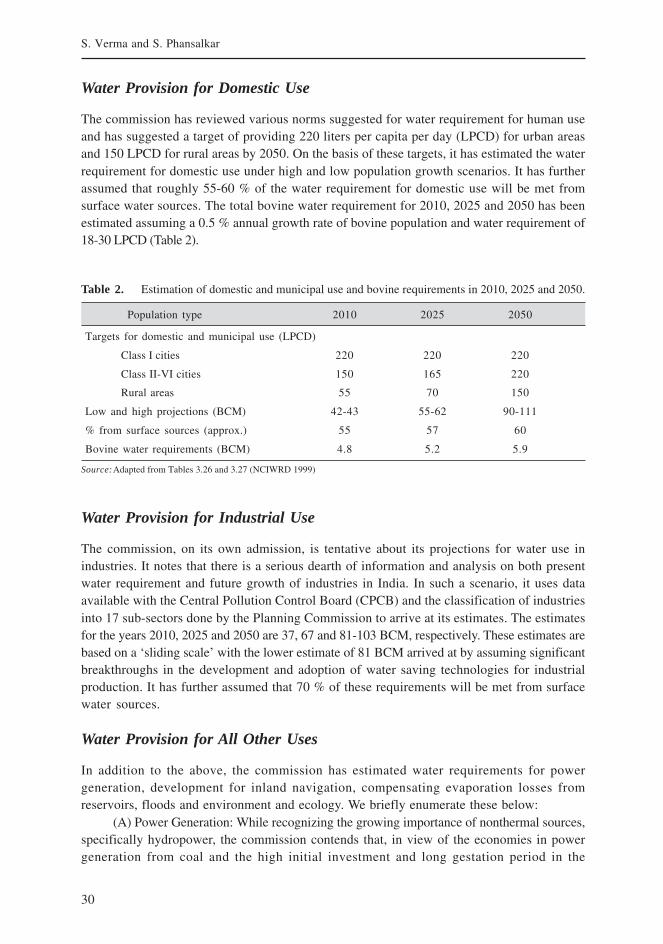
30
S. Verma and S. Phansalkar
Water Provision for Domestic Use
The commission has reviewed various norms suggested for water requirement for human useand has suggested a target of providing 220 liters per capita per day (LPCD) for urban areasand 150 LPCD for rural areas by 2050. On the basis of these targets, it has estimated the waterrequirement for domestic use under high and low population growth scenarios. It has furtherassumed that roughly 55-60 % of the water requirement for domestic use will be met fromsurface water sources. The total bovine water requirement for 2010, 2025 and 2050 has beenestimated assuming a 0.5 % annual growth rate of bovine population and water requirement of18-30 LPCD (Table 2).
Table 2. Estimation of domestic and municipal use and bovine requirements in 2010, 2025 and 2050.
Population type 2010 2025 2050
Targets for domestic and municipal use (LPCD)
Class I cities 220 220 220
Class II-VI cities 150 165 220
Rural areas 55 70 150
Low and high projections (BCM) 42-43 55-62 90-111
% from surface sources (approx.) 55 57 60
Bovine water requirements (BCM) 4.8 5.2 5.9
Source:Adapted from Tables 3.26 and 3.27 (NCIWRD 1999)
Water Provision for Industrial Use
The commission, on its own admission, is tentative about its projections for water use inindustries. It notes that there is a serious dearth of information and analysis on both presentwater requirement and future growth of industries in India. In such a scenario, it uses dataavailable with the Central Pollution Control Board (CPCB) and the classification of industriesinto 17 sub-sectors done by the Planning Commission to arrive at its estimates. The estimatesfor the years 2010, 2025 and 2050 are 37, 67 and 81-103 BCM, respectively. These estimates arebased on a ‘sliding scale’ with the lower estimate of 81 BCM arrived at by assuming significantbreakthroughs in the development and adoption of water saving technologies for industrialproduction. It has further assumed that 70 % of these requirements will be met from surfacewater sources.
Water Provision for All Other Uses
In addition to the above, the commission has estimated water requirements for powergeneration, development for inland navigation, compensating evaporation losses fromreservoirs, floods and environment and ecology. We briefly enumerate these below:
(A) Power Generation: While recognizing the growing importance of nonthermal sources,specifically hydropower, the commission contends that, in view of the economies in powergeneration from coal and the high initial investment and long gestation period in the
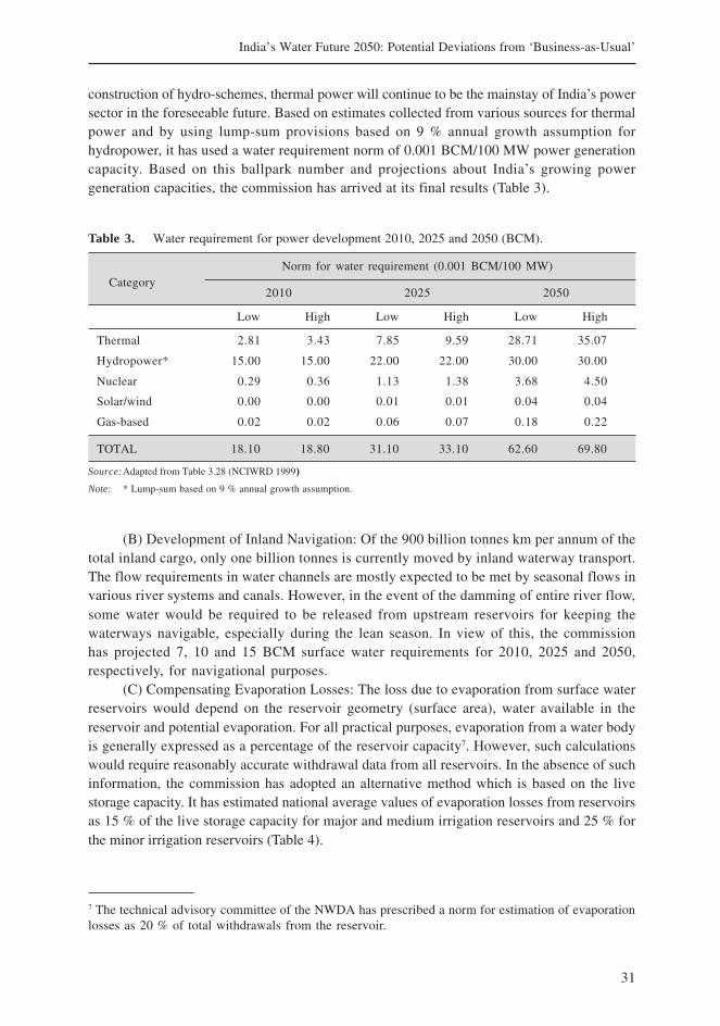
31
India’s Water Future 2050: Potential Deviations from ‘Business-as-Usual’
Table 3. Water requirement for power development 2010, 2025 and 2050 (BCM).
Norm for water requirement (0.001 BCM/100 MW)
2010 2025 2050
Low High Low High Low High
Thermal 2.81 3.43 7.85 9.59 28.71 35.07
Hydropower* 15.00 15.00 22.00 22.00 30.00 30.00
Nuclear 0.29 0.36 1.13 1.38 3.68 4.50
Solar/wind 0.00 0.00 0.01 0.01 0.04 0.04
Gas-based 0.02 0.02 0.06 0.07 0.18 0.22
TOTAL 18.10 18.80 31.10 33.10 62.60 69.80
Source:Adapted from Table 3.28 (NCIWRD 1999)
Note: * Lump-sum based on 9 % annual growth assumption.
Category
construction of hydro-schemes, thermal power will continue to be the mainstay of India’s powersector in the foreseeable future. Based on estimates collected from various sources for thermalpower and by using lump-sum provisions based on 9 % annual growth assumption forhydropower, it has used a water requirement norm of 0.001 BCM/100 MW power generationcapacity. Based on this ballpark number and projections about India’s growing powergeneration capacities, the commission has arrived at its final results (Table 3).
7 The technical advisory committee of the NWDA has prescribed a norm for estimation of evaporationlosses as 20 % of total withdrawals from the reservoir.
(B) Development of Inland Navigation: Of the 900 billion tonnes km per annum of thetotal inland cargo, only one billion tonnes is currently moved by inland waterway transport.The flow requirements in water channels are mostly expected to be met by seasonal flows invarious river systems and canals. However, in the event of the damming of entire river flow,some water would be required to be released from upstream reservoirs for keeping thewaterways navigable, especially during the lean season. In view of this, the commissionhas projected 7, 10 and 15 BCM surface water requirements for 2010, 2025 and 2050,respectively, for navigational purposes.
(C) Compensating Evaporation Losses: The loss due to evaporation from surface waterreservoirs would depend on the reservoir geometry (surface area), water available in thereservoir and potential evaporation. For all practical purposes, evaporation from a water bodyis generally expressed as a percentage of the reservoir capacity7. However, such calculationswould require reasonably accurate withdrawal data from all reservoirs. In the absence of suchinformation, the commission has adopted an alternative method which is based on the livestorage capacity. It has estimated national average values of evaporation losses from reservoirsas 15 % of the live storage capacity for major and medium irrigation reservoirs and 25 % forthe minor irrigation reservoirs (Table 4).
32
S. Verma and S. Phansalkar
(D) Floods, Environment and Ecology: This is perhaps the most intriguing section ofthe entire chapter on water requirement projections. The commission makes a case for settingaside some water capacity for moderating the releases from dams in the event of high floods.However, it concludes that since such situations are ‘casual’ in nature, there is no provisionmade for such purpose. In any case, the requirement for flood control is for water storagecapacity and not for additional water per se.
The commission report also talks at length about the poor state of the environment inthe country, citing indiscriminate depletion of forest cover. It also mentions that India’s forestscan sustainably provide only about 0.041 BCM of fuel wood every year compared with thecurrent demand for 0.240 BCM. Further, it adds that the industrial wood requirements are morethan twice the current silvicultural productivity; and also that while the carrying capacity offorests is only 31 million head of cattle, currently about 90 million graze in forests. The report,however, concludes that most of the water requirements for aforestation would be met fromprecipitation and soil moisture (green water) and that there is no need for any specificearmarking for this purpose.
The commission notes the alarming levels of water pollution in India’s rivers, givingexamples of cities such as Delhi which produces nearly 2 billion liters of sewage, most of whichis dumped untreated into the Yamuna River. It points out that for the treatment of sewage andfor maintaining the river ecology (environmental flow releases – EFR), Delhi alone, would requireabout 3 BCM of fresh water to restore the quality of water to a safe limit. And yet, at the end,it makes ‘a token provision’ of 5, 10 and 20 BCM for water for all the purposes listed above for2010, 2025 and 2050, respectively.
Total Water Requirement
Based on all the assumptions and projections above, the commission has estimated total waterrequirements under low and high demand scenarios as 629–694, 710–784 and 843–973 BCMfor 2010, 2025 and 2050, respectively (Table 5).
As the maximum utilizable surface water resource amounts to only 690 BCM, therequirement in 2050, under high population projections, will exceed the availability accordingto the commission’s projections. The same will be the situation in the case of groundwaterresources where the maximum utilizable resource is 396 BCM and the projected requirement is
Table 4. Estimates of evaporation losses in 2010, 2025 and 2050.
Particulars 1997 2010 2025 2050
Live capacity (major storages) 173.73 211.44 249.15 381.50
Evaporation (at 15 %) 26.10 31.70 37.40 57.20
Live capacity (minor storages) 34.70 42.30 49.80 76.30
Evaporation (at 25 %) 8.70 10.60 12.50 19.10
Total evaporation loss (rounded-off) 35.00 42.00 50.00 76.00
Source:Adapted from Table 3.29 (NCIWRD 1999).

33
India’s Water Future 2050: Potential Deviations from ‘Business-as-Usual’
428 BCM. The situation will be even worse when we take into account the spatial variation indemand and availability at the basin level.
Other Projections for Water Future 2050
Besides the NCIWRD projections, there are several other attempted projections regarding globaland regional water availability and demand. A neat summary of several of these can be foundin Strzepek 2001. While these efforts provide a sound body of knowledge to use as a soundingboard for methodologies and approaches, the results are of a global nature and not specificfor India. Seckler et al. 2000 and Rosegrant et al. 2002 have made global scenario building forwater future 2025 where they have fairly specific forecasts and comments about India. Wecompare the three projections up to the year 2025 to provide the reader an overview ofapproaches, assumptions and broad results (Table 6). The broad conclusions of the threeexercises are not remarkably different. Thus, irrespective of what one may wish to do aboutIndia’s water requirements, deny its size one cannot.
Table 5. Total water requirement 2010, 2025 and 2050 (BCM).
Uses of water 1997-98 Scenario 2010 2025 2050 %SW**
High 557 611 807
Low 543 561 628
High 43 62 111
Low 42 55 90
High 37 67 108
Low 37 67 81
High 19 33 70
Low 18 31 63
High 7 10 15
Low 7 10 15
High 5 10 20
Low 5 10 20
High 42 50 76
Low 42 50 76
High 710 843 1,180
Low 694 784 973
Source:Adapted from Table 3.30 (NCIWRD 1999)
Note: **Proportion of requirement proposed to be met from surface water sources
Irrigation 524 57-61
Domestic and municipal 30 53-59
Industries 30 70-71
Power 9 77-81
Inland navigation - 100
Environment - 100
Evaporation losses 36 100
Grand Total 629 63-65
34
S. Verma and S. Phansalkar
Table 6. Approaches, assumptions and broad results.
Aspects NCIWRD Seckler et al. Rosegrant et al.(up to 2025) (BaU*) (BaU*)
Approaches
Basic approach Building blocks Integrated, multi-year IMPACT-WATERapproach model model
Number of basins 24 Not specified 13considered
Whether trade considered? No Yes Yes
Calculation of irrigation Delta of 0.51 and 0.72 ET ratios for crops aswater requirement for ground and surface 1cumt per kg grain per FAO.
water, respectively
Scenario building exercise Not done except for Subsequently tried out; Policy and lifestylehigh and low Model permits scenario variables used to makepopulation growth building exercise 3 scenarios
Broad picture of India Tight overall balance; Economic water scarcity: Withdrawals will be 36 %2025 significant gaps and Investment needed for of the renewable water
mismatches in several expanding primary resource; difficult tobasins water supply is manage
unaffordable
Assumptions
Annual available water 1,953 BCM 2,037 BCM 1,721 BCMresources
Efficiency assumption 0.50 for SW; Basin efficiency Basin efficiency assumed0.72 for GW gains assumed to increase at specific rate
Domestic water 220 LPCD urban World Resources (based on rural % andrequirement estimation (Class I); Institute (WRI) % HH with piped supply,
165 LPCD urban data used income and prices(Class II-VI); of water) 41 BCM70 LPCD rural
Industrial water use CPCB norms WRI data used Water use intensity usedestimation very tentative along with estimates
GDP growth
Livestock water 24 LPCD WRI data used FAO estimates usedrequirement estimates
Broad Results
Population 1,286-1,333 million 1,216 million 1,352 million
% Rural 55-63 % 64 % 57 %
Projected irrigated area 67.00 MHa 63.10 Mha 76.00 MHa
Projected rain-fed area 77.00 MHa 81.00 Mha 68.00 MHa
Food grain requirement 308-320 MT 259 MT 275 MT
(Continued)
35
India’s Water Future 2050: Potential Deviations from ‘Business-as-Usual’
Aspects NCIWRD Seckler et al. Rosegrant et al.(up to 2025) (BaU*) (BaU*)
Approaches
Water required for 561-611 BCM 702 BCM 332 BCM consumptive;food production much higher withdrawals
Assumed total water supply SW: 382 BCM 1,263 BCM Not specifiedGW: 432 BCMTotal: 824 BCM
Total Water Demand 2025 784-843 BCM 811 BCM 815 BCM
Source:NCIWRD 1999, Seckler et al. 2000, Rosegrant 2002
Note: * BaU = ‘Business as Usual’ scenario
Table 6. Approaches, assumptions and broad results. (Continued)
Potential Deviations from Business-as-Usual
The commission’s report presents a rare case when issues of such diverse nature, requiringsuch diverse expertise, have all been dealt together, and thus making it compelling readingfor any concerned individual. Having said that, we believe that the estimates represent ultra-conservative ‘Business-as-Usual’ scenarios which, among other things, fail to take intoaccount two things: (1) coping mechanisms of the people and demand responses to policytriggers; and (2) technological and social breakthroughs on the horizon. Several autonomousand induced changes, which will profoundly influence the course of India’s food agriculturalsector over the coming 50 years do not find a place in the data and projections made by theNCIWRD (at least in the part available in the public domain). We discuss some such potentialdeviations here.
Rethinking Water Availability and Demand
(a) Accounting for Deductions at Source
The NCIWRD projections start with the assumption that the volume of water which can beput to use in India on a reasonably sustainable basis is 1,086 BCM (690 BCM of surface waterand 396 BCM of annually replenished groundwater). As we have already explained above, thereduction from 4,000 BCM to 1,953 BCM is caused primarily due to four ‘deductions-at-source’:(1) Evaporation; (2) Non-crop and rain-fed ET; (3) Deep percolation; and (4) Sub-surface flowsto the oceans. While little can be done to check evaporation and deep percolation, the othertwo ‘deductions’ can be seen as variables which are easily influenced by public policy andhuman actions (Figure 2).
Non-crop ET largely involves the water requirement by trees in the forests andnaturally growing vegetation including grasslands, shrubs and weeds. While hardly anyonewill want to suggest a policy to deplete forests to expand our utilizable water resource,how this will change in the coming 50 years needs to be looked at carefully. If our forestscontinue to deplete and degrade as they have in the recent past, much more of this water
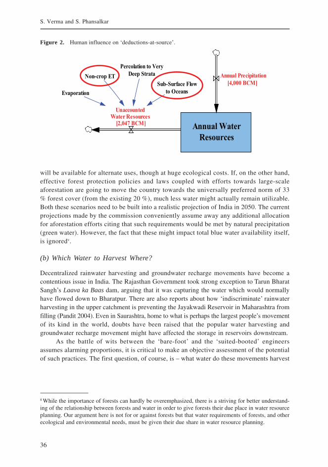
36
S. Verma and S. Phansalkar
will be available for alternate uses, though at huge ecological costs. If, on the other hand,effective forest protection policies and laws coupled with efforts towards large-scaleaforestation are going to move the country towards the universally preferred norm of 33% forest cover (from the existing 20 %), much less water might actually remain utilizable.Both these scenarios need to be built into a realistic projection of India in 2050. The currentprojections made by the commission conveniently assume away any additional allocationfor aforestation efforts citing that such requirements would be met by natural precipitation(green water). However, the fact that these might impact total blue water availability itself,is ignoredv.
(b) Which Water to Harvest Where?
Decentralized rainwater harvesting and groundwater recharge movements have become acontentious issue in India. The Rajasthan Government took strong exception to Tarun BharatSangh’s Laava ka Baas dam, arguing that it was capturing the water which would normallyhave flowed down to Bharatpur. There are also reports about how ‘indiscriminate’ rainwaterharvesting in the upper catchment is preventing the Jayakwadi Reservoir in Maharashtra fromfilling (Pandit 2004). Even in Saurashtra, home to what is perhaps the largest people’s movementof its kind in the world, doubts have been raised that the popular water harvesting andgroundwater recharge movement might have affected the storage in reservoirs downstream.
As the battle of wits between the ‘bare-foot’ and the ‘suited-booted’ engineersassumes alarming proportions, it is critical to make an objective assessment of the potentialof such practices. The first question, of course, is – what water do these movements harvest
Figure 2. Human influence on ‘deductions-at-source’.
8 While the importance of forests can hardly be overemphasized, there is a striving for better understand-ing of the relationship between forests and water in order to give forests their due place in water resourceplanning. Our argument here is not for or against forests but that water requirements of forests, and otherecological and environmental needs, must be given their due share in water resource planning.
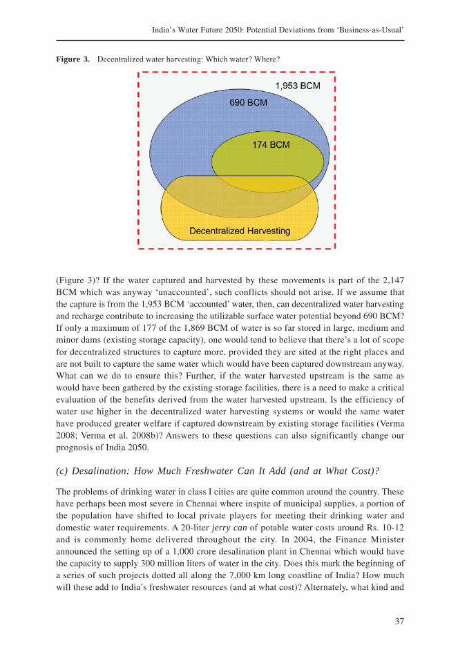
37
India’s Water Future 2050: Potential Deviations from ‘Business-as-Usual’
(Figure 3)? If the water captured and harvested by these movements is part of the 2,147BCM which was anyway ‘unaccounted’, such conflicts should not arise. If we assume thatthe capture is from the 1,953 BCM ‘accounted’ water, then, can decentralized water harvestingand recharge contribute to increasing the utilizable surface water potential beyond 690 BCM?If only a maximum of 177 of the 1,869 BCM of water is so far stored in large, medium andminor dams (existing storage capacity), one would tend to believe that there’s a lot of scopefor decentralized structures to capture more, provided they are sited at the right places andare not built to capture the same water which would have been captured downstream anyway.What can we do to ensure this? Further, if the water harvested upstream is the same aswould have been gathered by the existing storage facilities, there is a need to make a criticalevaluation of the benefits derived from the water harvested upstream. Is the efficiency ofwater use higher in the decentralized water harvesting systems or would the same waterhave produced greater welfare if captured downstream by existing storage facilities (Verma2008; Verma et al. 2008b)? Answers to these questions can also significantly change ourprognosis of India 2050.
(c) Desalination: How Much Freshwater Can It Add (and at What Cost)?
The problems of drinking water in class I cities are quite common around the country. Thesehave perhaps been most severe in Chennai where inspite of municipal supplies, a portion ofthe population have shifted to local private players for meeting their drinking water anddomestic water requirements. A 20-liter jerry can of potable water costs around Rs. 10-12and is commonly home delivered throughout the city. In 2004, the Finance Ministerannounced the setting up of a 1,000 crore desalination plant in Chennai which would havethe capacity to supply 300 million liters of water in the city. Does this mark the beginning ofa series of such projects dotted all along the 7,000 km long coastline of India? How muchwill these add to India’s freshwater resources (and at what cost)? Alternately, what kind and
Figure 3. Decentralized water harvesting: Which water? Where?
38
S. Verma and S. Phansalkar
level of inter-basin transfers will be required to meet the growing needs of cities and townsin the future9? Such questions also need to be addressed for a more nuanced prognosis.
(d) Re-use of Wastewater for Agriculture: Boon or Bane?
Domestic and industrial wastewater in most Indian towns and cities is disposed of without anytreatment. Increasingly, farmers in peri-urban areas have taken to using untreated wastewater forirrigation. In some of the class I cities in India, the peri-urban water economy may approach thesize of a mid-scale irrigation system, helping peri-urban farmers to improve their incomes andlivelihoods (Bhamoriya 2004; Buechler and Devi 2003). However, using untreated wastewatercan produce adverse health effects – direct, through farmers handling untreated wastewater, andindirect, through the consumption of food stuff irrigated with wastewater. The critical questionsto address are (1) by how much can the re-use of domestic and industrial wastewater multiplyIndia’s fresh water resources?; (2) how quickly will these economies grow?; and (3) what wouldbe the implications of agriculture wastewater on public health?
(e) Water Requirements vs. Water Demand
The commission’s approach ignores the impact of two key variables on demand – the price atwhich water is supplied; and the quality of the supply. The commission’s estimates of ‘waterdemand’ are built on the basis of minimum norms set down by various agencies. For example,the commission’s estimates of water demand are based on the 220 LPCD and 150 LPCD norms.However, these can hardly be termed as ‘demand’. In textbook economics, we find a definitionof demand very different from the one assumed here.
Demand is defined as the desire to possess a commodity or make use of a service,combined with the ability to acquire it. In other words, it is the amount of a commodity orservice that people are ready to buy for a given price. The commission’s definition of demand,however, completely misses the ability and price aspects of demand. Certainly, if the assumptionof the commission is that domestic water will be supplied at zero (or almost zero) price, theestimates are perhaps correct. However, such a policy is likely to lead to wastes of the orderwhich an economy facing water scarcity cannot afford. If, on the other hand, the assumptionis that 220 LPCD will be actually ‘demanded’ at a reasonably high price and at a given level of
9 There already exist examples of canal projects (near Mumbai, Ahmedabad and several cities) which,under pressure of growing metropolitans have been forced to divert water (initially planned to be usedfor irrigation) to meet domestic and municipal requirements. While the priority accorded to domesticuse is hardly debatable, it indicates that the growing needs of cities were not taken into account whileplanning the command area of irrigation projects. Recent studies suggest that within the next 3 years,half the world’s population will be living in cities. The NCIWRD projections based on Ravi 1998 es-timate that such a situation will not happen in India even in the year 2050.
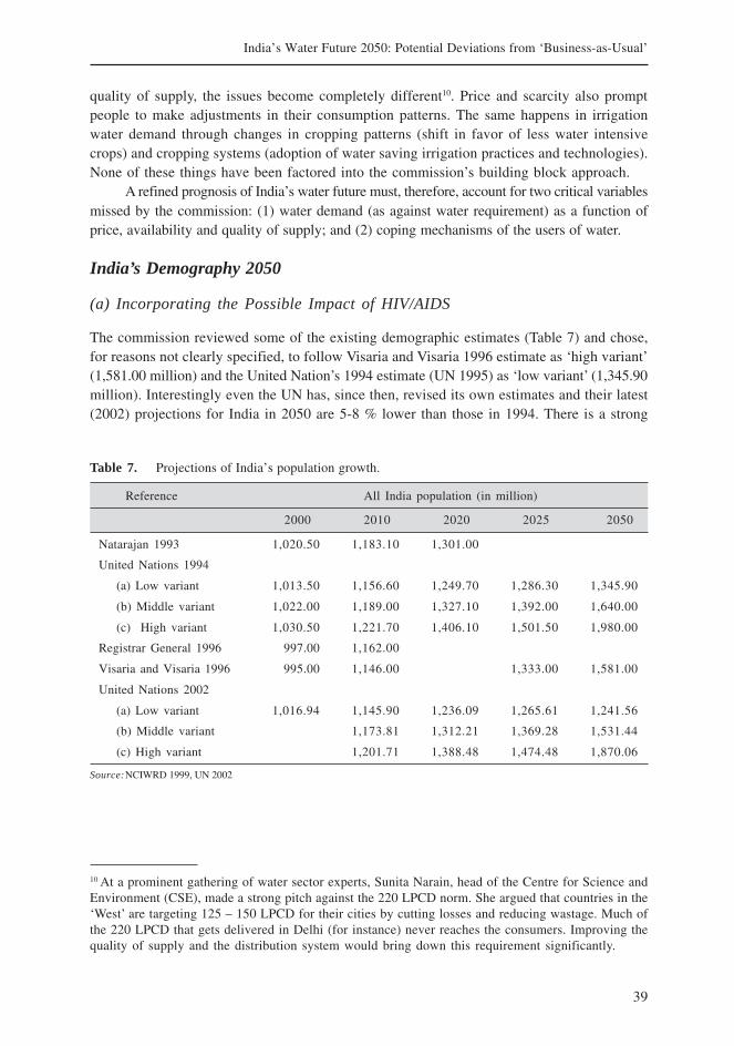
39
India’s Water Future 2050: Potential Deviations from ‘Business-as-Usual’
quality of supply, the issues become completely different10. Price and scarcity also promptpeople to make adjustments in their consumption patterns. The same happens in irrigationwater demand through changes in cropping patterns (shift in favor of less water intensivecrops) and cropping systems (adoption of water saving irrigation practices and technologies).None of these things have been factored into the commission’s building block approach.
A refined prognosis of India’s water future must, therefore, account for two critical variablesmissed by the commission: (1) water demand (as against water requirement) as a function ofprice, availability and quality of supply; and (2) coping mechanisms of the users of water.
India’s Demography 2050
(a) Incorporating the Possible Impact of HIV/AIDS
The commission reviewed some of the existing demographic estimates (Table 7) and chose,for reasons not clearly specified, to follow Visaria and Visaria 1996 estimate as ‘high variant’(1,581.00 million) and the United Nation’s 1994 estimate (UN 1995) as ‘low variant’ (1,345.90million). Interestingly even the UN has, since then, revised its own estimates and their latest(2002) projections for India in 2050 are 5-8 % lower than those in 1994. There is a strong
10 At a prominent gathering of water sector experts, Sunita Narain, head of the Centre for Science andEnvironment (CSE), made a strong pitch against the 220 LPCD norm. She argued that countries in the‘West’ are targeting 125 – 150 LPCD for their cities by cutting losses and reducing wastage. Much ofthe 220 LPCD that gets delivered in Delhi (for instance) never reaches the consumers. Improving thequality of supply and the distribution system would bring down this requirement significantly.
Table 7. Projections of India’s population growth.
Reference All India population (in million)
2000 2010 2020 2025 2050
Natarajan 1993 1,020.50 1,183.10 1,301.00
United Nations 1994
(a) Low variant 1,013.50 1,156.60 1,249.70 1,286.30 1,345.90
(b) Middle variant 1,022.00 1,189.00 1,327.10 1,392.00 1,640.00
(c) High variant 1,030.50 1,221.70 1,406.10 1,501.50 1,980.00
Registrar General 1996 997.00 1,162.00
Visaria and Visaria 1996 995.00 1,146.00 1,333.00 1,581.00
United Nations 2002
(a) Low variant 1,016.94 1,145.90 1,236.09 1,265.61 1,241.56
(b) Middle variant 1,173.81 1,312.21 1,369.28 1,531.44
(c) High variant 1,201.71 1,388.48 1,474.48 1,870.06
Source:NCIWRD 1999, UN 2002
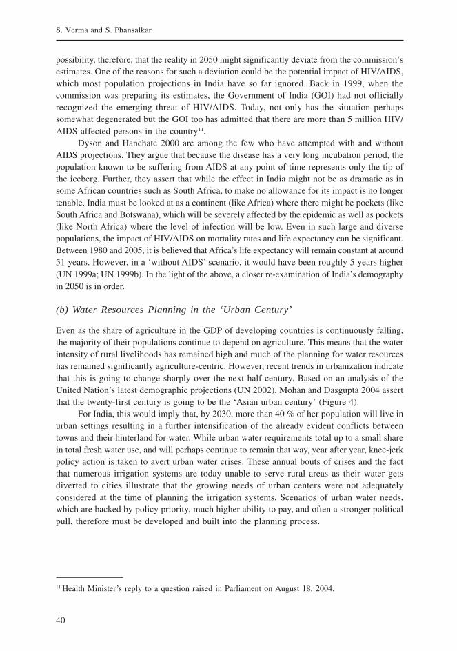
40
S. Verma and S. Phansalkar
possibility, therefore, that the reality in 2050 might significantly deviate from the commission’sestimates. One of the reasons for such a deviation could be the potential impact of HIV/AIDS,which most population projections in India have so far ignored. Back in 1999, when thecommission was preparing its estimates, the Government of India (GOI) had not officiallyrecognized the emerging threat of HIV/AIDS. Today, not only has the situation perhapssomewhat degenerated but the GOI too has admitted that there are more than 5 million HIV/AIDS affected persons in the country11.
Dyson and Hanchate 2000 are among the few who have attempted with and withoutAIDS projections. They argue that because the disease has a very long incubation period, thepopulation known to be suffering from AIDS at any point of time represents only the tip ofthe iceberg. Further, they assert that while the effect in India might not be as dramatic as insome African countries such as South Africa, to make no allowance for its impact is no longertenable. India must be looked at as a continent (like Africa) where there might be pockets (likeSouth Africa and Botswana), which will be severely affected by the epidemic as well as pockets(like North Africa) where the level of infection will be low. Even in such large and diversepopulations, the impact of HIV/AIDS on mortality rates and life expectancy can be significant.Between 1980 and 2005, it is believed that Africa’s life expectancy will remain constant at around51 years. However, in a ‘without AIDS’ scenario, it would have been roughly 5 years higher(UN 1999a; UN 1999b). In the light of the above, a closer re-examination of India’s demographyin 2050 is in order.
(b) Water Resources Planning in the ‘Urban Century’
Even as the share of agriculture in the GDP of developing countries is continuously falling,the majority of their populations continue to depend on agriculture. This means that the waterintensity of rural livelihoods has remained high and much of the planning for water resourceshas remained significantly agriculture-centric. However, recent trends in urbanization indicatethat this is going to change sharply over the next half-century. Based on an analysis of theUnited Nation’s latest demographic projections (UN 2002), Mohan and Dasgupta 2004 assertthat the twenty-first century is going to be the ‘Asian urban century’ (Figure 4).
For India, this would imply that, by 2030, more than 40 % of her population will live inurban settings resulting in a further intensification of the already evident conflicts betweentowns and their hinterland for water. While urban water requirements total up to a small sharein total fresh water use, and will perhaps continue to remain that way, year after year, knee-jerkpolicy action is taken to avert urban water crises. These annual bouts of crises and the factthat numerous irrigation systems are today unable to serve rural areas as their water getsdiverted to cities illustrate that the growing needs of urban centers were not adequatelyconsidered at the time of planning the irrigation systems. Scenarios of urban water needs,which are backed by policy priority, much higher ability to pay, and often a stronger politicalpull, therefore must be developed and built into the planning process.
11 Health Minister’s reply to a question raised in Parliament on August 18, 2004.
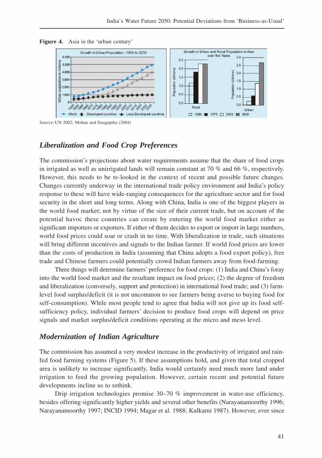
41
India’s Water Future 2050: Potential Deviations from ‘Business-as-Usual’
Liberalization and Food Crop Preferences
The commission’s projections about water requirements assume that the share of food cropsin irrigated as well as unirrigated lands will remain constant at 70 % and 66 %, respectively.However, this needs to be re-looked in the context of recent and possible future changes.Changes currently underway in the international trade policy environment and India’s policyresponse to these will have wide-ranging consequences for the agriculture sector and for foodsecurity in the short and long terms. Along with China, India is one of the biggest players inthe world food market; not by virtue of the size of their current trade, but on account of thepotential havoc these countries can create by entering the world food market either assignificant importers or exporters. If either of them decides to export or import in large numbers,world food prices could soar or crash in no time. With liberalization in trade, such situationswill bring different incentives and signals to the Indian farmer. If world food prices are lowerthan the costs of production in India (assuming that China adopts a food export policy), freetrade and Chinese farmers could potentially crowd Indian farmers away from food-farming.
Three things will determine farmers’ preference for food crops: (1) India and China’s forayinto the world food market and the resultant impact on food prices; (2) the degree of freedomand liberalization (conversely, support and protection) in international food trade; and (3) farm-level food surplus/deficit (it is not uncommon to see farmers being averse to buying food forself-consumption). While most people tend to agree that India will not give up its food self-sufficiency policy, individual farmers’ decision to produce food crops will depend on pricesignals and market surplus/deficit conditions operating at the micro and meso level.
Modernization of Indian Agriculture
The commission has assumed a very modest increase in the productivity of irrigated and rain-fed food farming systems (Figure 5). If these assumptions hold, and given that total croppedarea is unlikely to increase significantly, India would certainly need much more land underirrigation to feed the growing population. However, certain recent and potential futuredevelopments incline us to rethink.
Drip irrigation technologies promise 30–70 % improvement in water-use efficiency,besides offering significantly higher yields and several other benefits (Narayanamoorthy 1996;Narayanamoorthy 1997; INCID 1994; Magar et al. 1988; Kulkarni 1987). However, ever since
Figure 4. Asia in the ‘urban century’
Source:UN 2002; Mohan and Dasguptha (2004)
42
S. Verma and S. Phansalkar
they were first introduced (some three decades ago), the area under drip irrigation has expandedrather sluggishly from 1,500 ha in 1985 to a little over 70,000 ha in 1992 (Chakravarty and Singh1994) and rapid growth has only been seen in recent years as the area spread to 2, 25,000 hain 1998 (Polak and Sivanappan 1998). However, this is still miniscule when compared with theestimated potential of 10.50 million ha (Sivanappan 1994). Despite active promotion by agrowing private irrigation equipment industry and subsidies (up to 90 %) offered by thegovernment, the appeal of these technologies has remained confined only to ‘gentlemen farmers’(Shah and Keller 2002). Recent research suggests that when faced with groundwater stress;the same farmers who have rejected the capital intensive subsidized drip systems haveinnovated and embraced low-cost grassroots innovations such as Pepsee drips12 which act asstepping-stone technologies. How quickly and to what scale will these technologies expand?What would be the net impact of ‘more crop per drop’?
The impact of GM technologies, which for obvious reasons was not taken into account,could be another significant factor. So far, much of the debate on GM technologies in Indiahas been concentrated around cotton rather than food crops. How the GM revolution canchange the paradigms of food security needs to be studied in detail. Will future technologiesoffer seed varieties which will produce much more food grain for the same amount of water?What could be the implications of such technologies for the poor and for under-developedand developing countries? What kind of global system of governance will evolve to governthe GM revolution? Will intellectual property rights (IPRs) and patents play a big role indetermining dominance in the global food business? What would all this mean for India?
Then, there are certain ‘horizon’ technologies like the system of rice intensification (SRI)which promise to improve water use efficiency. SRI is drawing attention world-wide as a compactof paddy cultivation practices that boost paddy yield while reducing water use and cost of
Figure 5. NCIWRD’s projected yield growth.
Source:NCIWRD 1999
12 Pepsee systems are low-cost substitutes for drip irrigation systems made up of low density polytheneranging from 65 to 130 microns. At less than half the price of conventional drip systems, this grassrootsinnovation promises comparable results and has become very popular among cotton farmers in theMaikaal region of central India (Verma et al. 2004).
43
India’s Water Future 2050: Potential Deviations from ‘Business-as-Usual’
cultivation. Developed after over two decades of experimentation in Madagascar, under conditionsnot very different from those in India, SRI promises a significant increase in rice yields withoutthe introduction of new varieties of HYV seeds or increase in external chemical inputs and, mostimportantly, with much reduced water use. This technology has been successfully tried withfarmers in Sri Lanka, Tamil Nadu, Karnataka and Andhra Pradesh and by PRADAN with poorfarmers in Purulia. In regions where paddy cultivation is central to rural livelihood systems, suchas tribal Orissa, Jharkhand and Chattisgarh, SRI holds out a big promise that needs to bevigorously explored (Verma and Phansalkar 2004). Though there is little empirical data on SRI inIndia, data from other countries suggests it might become the mainstream practice in the yearsto come and could well be the ‘next-big-thing’ in rice cultivation. In Madagascar, average paddyyields among adopter farmers rose from 2 to 8 tonnes/ha. Is the promise offered by SRI toogood to be true? Can such high yields be sustained in the long-run without affecting soil fertility?
Efficiency and Productivity Gains
(a) The Surface Irrigation Challenge
The efficiency levels at which surface irrigation projects work in most parts of the countrydoes not require great elaboration. The Planning Commission contends that a mere 10 %increase in the efficiency of the existing irrigation infrastructure would lead to water supply to14 million additional hectares of agricultural land13.
The commission has projected that India’s surface irrigation systems will work at 40, 50and 60 % efficiency levels in 2010, 2025 and 2050, respectively. How these incredible efficiencygains will be achieved is mostly left to the readers’ imagination. The commission has suggestedthat “all state irrigation acts have to be amended to incorporate provision for the formation of
13 In a series of exchanges between noted water sector stalwarts Ramaswamy R. Iyer and Radha Singh,in the Economic and Political Weekly, the latter remarked (Singh 2003):
“Conceding that the efficiencies of our water systems, especially irrigation, must beimproved, the efficiencies within the major and medium sector (irrigation) are around40 %, while in the minor and groundwater sectors it is above 60 %. With a delta of0.95 m, total water use in major and medium irrigation sectors would be 37 MHa ×0.95 = 351 BCM. Improvements in efficiencies within this sector would render anadditional availability of approximately 52 BCM which, though significant, is hardly
enough to counter the widespread scarcity prevalent in numerous basins of our country.”
It is not clear as to how the figure of 52 BCM has been arrived at. If 351 BCM is taken to be a correctestimate, and assuming that surface irrigation projects do operate at 40 % efficiency level (which is thelevel that the commission projects India’s surface irrigation projects will achieve by 2010), it wouldmean that the amount of water which actually reaches the farmers’ fields would be 351*0.40 = 140.40BCM. Assuming that no additional surface irrigation projects are commissioned, with improvement inefficiency from 40 % to 60 %, this should change to 351*0.60 = 210.60 BCM. The additional availabil-ity, therefore, can be calculated as 210.60 - 140.40 = 70.20 BCM. Again using the commission’s ownassumptions of water required to grow food grains, this additional 18.20 BCM water (which we justnow discovered; 70.20-52) would amount to an additional food production of roughly 12 million tonnes!
44
S. Verma and S. Phansalkar
farmers’ bodies.” It then proceeds to review performance of user managed irrigation systemsin nine major states and concludes that their performance is far from satisfactory. Irrespectiveof the above, it hails the fact that over 25,000 water users’ associations (WUAs), covering 5.8Mha, have been created in various states.
Initiating a program for the user management of irrigation systems or the mere formationof irrigation communities will not automatically lead to improved efficiency in surface irrigationsystems. One school of thought argues that even when successful, participatory irrigationmanagement (PIM) only can help improve distribution efficiency, which, in any case, is only asmall part of the overall efficiency14. Proponents of this school argue that the main culprit inpoor efficiencies is the poor ‘Main System Management’. Factors such as lower water availability,untimely and unreliable supply, lower storage capacity and higher conveyance losses vis-à-visthose assumed at the planning stage, are responsible for poor efficiencies. The pertinentquestions, therefore, are: what kind of efficiency improvements (CE or DE or AE) can we achieveby 2050?; How, how much, and at what cost? To what extent will PIM or irrigation managementtransfer (IMT) salvage India’s public irrigation systems? Is there a need to think of and experimentwith alternative strategies and institutional arrangements for vitalizing this important sector?
(b) Relative Dependence on Surface and Groundwater
To us, there seems to be a distinct ‘surface water bias’ in the commission’s estimates. It assumesthat surface water will be used to meet 57–61 % agricultural; 53-59 % domestic and municipal;70–71 % industrial; 77–81 % power generation; and 100 % of all other requirements. Recentstudies, however, indicate that groundwater might be contributing much more than is commonlyunderstood. While the commission estimates that the total groundwater use in 2010 will onlybe around 230 BCM, recent estimates of present groundwater use already exceed this number.According to the Central Ground Water Board (CGWB 1995), the groundwater provision fordomestic, industrial and other (nonagricultural) uses totals to 71 BCM. If we add to this, theestimate for groundwater use in agriculture by Shah et al. 2003, 210 BCM, the total groundwateruse in India can be estimated as 281 BCM. Thus, in all, anywhere between 250 and 300 BCMof groundwater is currently being used15. Compared to this, the commission estimates thattotal groundwater use in 2010 will be around 230 BCM.
14 According to the International Commission on Irrigation and Drainage (ICID), Overall Efficiency(E) = CE * DE * AE where,CE = Volume of water delivered to the distribution system / Volume of water delivered at the canal head;DE = Volume of water delivered to the field / Volume of water drawn from the distribution system;AE = Volume of water made available to crops / Volume of water drawn at the field head.15 Here, it is important to note that a part of the groundwater use is caused not directly by rainfallrecharge but by the return flows from irrigation caused by the inefficiencies in irrigation. However, thedegree of this overlap is difficult to measure and quantify.
45
India’s Water Future 2050: Potential Deviations from ‘Business-as-Usual’
Other Macro Variables
(a) Changes in India’s Macro Hydrology
With a predominantly agrarian economy and a 7,000 km long, densely populated, and low lyingcoast-line, the impact of climate change in India can be expected to be significantly higherthan that suggested by the ‘token provisions’ made for by the commission. The most immediateimpact of higher temperatures on India’s water resources would be in the form of higher ratesof evaporation. Potential changes in temperature and precipitation might also have a dramaticimpact on soil moisture and aridity levels of hydrological zones, besides changingevapotranspiration, runoff coefficients, river flows and groundwater recharge.
Research carried out by the Hadley Centre16 indicates that the mean annual runoff inBrahamaputra would decline by 14 % by the year 2050. The Intergovernmental Panel on ClimateChange has predicted a likely increase in the frequency of heavy rainfall in South Asia (IPCC1998) and notes that the impacts of climate change in India will be felt more directly in thewestern Himalayas as the contribution of snow to the runoff of major rivers on the westernside is about 60 % compared with 10 % on the eastern side (IPCC 2001).
How real and how significant will be the impact of climate change in the context of waterresource availability and use? These potential implications need to be brought into theprognoses for India 2050.
(b) Virtual Water Trade and Food Policy
Much of the projections made by the commission are based on the assumption that India willcontinue to pursue its policy of food self-sufficiency. At present, much of India’s foodgrainsare produced in a handful of states, all of which are facing water shortages and groundwaterdepletion. On the other hand, India’s water rich regions, such as states in eastern India, areimporting food from these states since they are unable to produce enough to meet theirrequirements. If we view this inter-state food trade within India as trade in ‘Virtual Water’17,we see that water-scarce regions in India are exporting virtual water to water rich regions,thereby exacerbating the water crisis. In part, this is due to the food procurement policies ofthe Government of India, which encourage states like Punjab and Haryana to grow foodgrainsby offering them assured markets, lucrative prices and several input subsidies including thosefor electricity and fertilizers. On the other hand, farmers in water rich states are facing higher
16 www.metoffice.com/research/hadleycentre17 ‘Virtual Water’ refers to the volume of water needed to produce agricultural commodities. When acommodity (or service) is traded, the buyer essentially imports (virtual) water used in the productionof the commodity. In the context of international (food) trade, this concept has been applied with aview to optimizing the flow of commodities considering the water endowments of nations. Using theprinciples of international trade, it suggests that water-rich countries should produce and export waterintensive commodities (which indirectly carry embedded water needed for producing them) to water-scarce countries, thereby enabling the water-scarce countries to divert their precious water resources toalternative, higher valued uses (Allan 1998, Hoekstra 2003, Wichelns 2004).
46
S. Verma and S. Phansalkar
input costs and are able to derive lower market prices for their produce. This has lead to astagnant, low-input agriculture, resulting in sustained poverty. Some of the best water endowedstates are also the poorest. If, however, food policies were to be re-aligned to favor water richregions to encourage them to grow more foodgrains, India’s food demand and supply scenarioswould drastically change (Verma 2007; Verma et al. 2008a).
(c) Water Intensity of Rural Livelihoods
Agriculture continues to be the biggest absorber of people in India and even if food securityconcerns were to be met otherwise, people will continue to depend on agriculture for theirlivelihoods and, therefore, will continue to demand water for irrigation. It therefore becomesimportant to make studied projections as to what proportion of the country’s population willcontinue to depend on agriculture through to 2050.
As of now, some 64 % of the population in the country derives its livelihoodssubstantially from agricultural operations: either as cultivators or as agricultural wage laborers.The share of agriculture in GDP has fallen to about 29 % nationally. This fall in share ofagriculture in GDP is accompanied by a much smaller fall in the proportion of the peoplederiving their livelihoods from agriculture. For instance, agriculture contributes only 13 % tothe state domestic product in Gujarat while it continues to support 45 % of the main workers.While on the one hand, this indicates the declining share of agriculture, it also perhaps indicateslarge-scale diversification in rural livelihoods.
The important questions to address are (1) How water-centric will rural livelihoods be inthe future18?; and (2) Even if a large number of people move out of agriculture, would it meana reduction in cropped and irrigated area?
The Emerging Agenda for ‘Water Future’ Research
While the conservative estimates of the commission paint quite a grim picture of India’s waterfuture, it must be granted that if no corrective action is taken, no forward planning is doneand nothing is done to change the wasteful and inequitable use of water, the situation couldwell be like the one depicted by the commission. However, the broad statement of the demandand supply as made by the commission is only the canvass; the actual picture will emergeonly with people responding to the crisis as they see it cropping up. The report thus offers agood base, a starting point, which needs to be worked and built upon, rather than acceptingit as the last word. The authors of the report too were, perhaps, quite aware of some of theinherent drawbacks which might have resulted from the paucity of available data and analyses.That is why even the report itself does not shy away from categorically stating that:
“…These estimates should be treated basically as approximations…It wouldbe desirable to review these estimates regularly, say, at the interval of5-10 years.”
18 See Phansalkar 2005 for a detailed discussion on this issue.
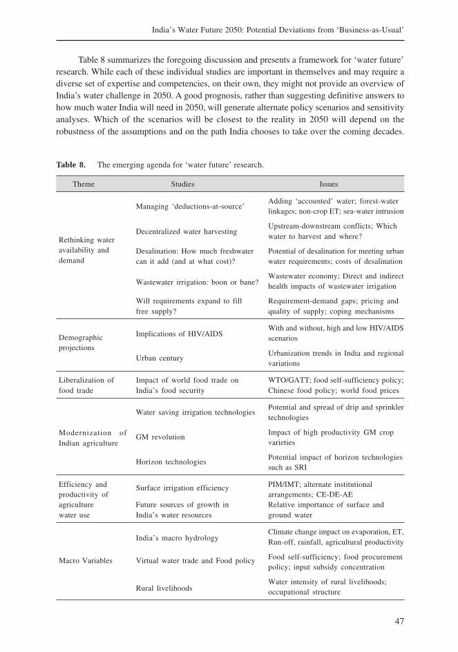
47
India’s Water Future 2050: Potential Deviations from ‘Business-as-Usual’
Table 8 summarizes the foregoing discussion and presents a framework for ‘water future’research. While each of these individual studies are important in themselves and may require adiverse set of expertise and competencies, on their own, they might not provide an overview ofIndia’s water challenge in 2050. A good prognosis, rather than suggesting definitive answers tohow much water India will need in 2050, will generate alternate policy scenarios and sensitivityanalyses. Which of the scenarios will be closest to the reality in 2050 will depend on therobustness of the assumptions and on the path India chooses to take over the coming decades.
Table 8. The emerging agenda for ‘water future’ research.
Theme Studies Issues
Adding ‘accounted’ water; forest-waterlinkages; non-crop ET; sea-water intrusion
Upstream-downstream conflicts; Whichwater to harvest and where?
Desalination: How much freshwater Potential of desalination for meeting urbancan it add (and at what cost)? water requirements; costs of desalination
Wastewater economy; Direct and indirecthealth impacts of wastewater irrigation
Will requirements expand to fill Requirement-demand gaps; pricing andfree supply? quality of supply; coping mechanisms
With and without, high and low HIV/AIDSscenarios
Urbanization trends in India and regionalvariations
Liberalization of Impact of world food trade on WTO/GATT; food self-sufficiency policy;food trade India’s food security Chinese food policy; world food prices
Potential and spread of drip and sprinklertechnologies
Impact of high productivity GM cropvarieties
Potential impact of horizon technologiessuch as SRI
Efficiency and PIM/IMT; alternate institutionalproductivity of arrangements; CE-DE-AEagriculture Future sources of growth in Relative importance of surface andwater use India’s water resources ground water
Climate change impact on evaporation, ET,Run-off, rainfall, agricultural productivity
Food self-sufficiency; food procurementpolicy; input subsidy concentration
Water intensity of rural livelihoods;occupational structure
Rethinking wateravailability anddemand
Decentralized water harvesting
Wastewater irrigation: boon or bane?
Managing ‘deductions-at-source’
Demographicprojections
Implications of HIV/AIDS
Urban century
Modernization ofIndian agriculture
Water saving irrigation technologies
GM revolution
Horizon technologies
Surface irrigation efficiency
Macro Variables
India’s macro hydrology
Virtual water trade and Food policy
Rural livelihoods
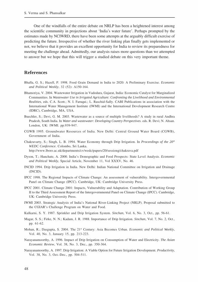
48
S. Verma and S. Phansalkar
One of the windfalls of the entire debate on NRLP has been a heightened interest amongthe scientific community in projections about ‘India’s water future’. Perhaps prompted by theestimates made by NCIWRD, there have been some attempts at the arguably difficult exercise ofpredicting the future. Irrespective of whether the river linking plan finally gets implemented ornot, we believe that it provides an excellent opportunity for India to review its preparedness formeeting the challenge ahead. Admittedly, our analysis raises more questions than we attemptedto answer but we hope that this will trigger a studied debate on this very important theme.
References
Bhalla, G. S.; Hazell, P. 1998. Food Grain Demand in India to 2020: A Preliminary Exercise. Economicand Political Weekly, 32 (52): A150-164.
Bhamoriya, V. 2004. Wastewater Irrigation in Vadodara, Gujarat, India: Economic Catalyst for MarginalizedCommunities. In Wastewater Use in Irrigated Agriculture: Confronting the Livelihood and EnvironmentalRealities, eds. C.A. Scott.; N. I. Faruqui.; L. Raschid-Sally. CABI Publications in association with theInternational Water Management Institute (IWMI) and the International Development Research Centre(IDRC), Cambridge, MA, USA.
Buechler, S.; Devi, G. M. 2003. Wastewater as a source of multiple livelihoods? A study in rural AndhraPradesh, South India. In Water and wastewater: Developing Country Perspectives. eds. R. Devi; N. Ahsan.London, UK: IWMI. pp.939-947.
CGWB 1995. Groundwater Resources of India. New Delhi: Central Ground Water Board (CGWB),Government of India.
Chakravarty, S.; Singh, L. B. 1994. Water Economy through Drip Irrigation. In Proceedings of the 20th
WEDC Conference. Colombo, Sri Lanka.http://www.lboro.ac.uk/departments/cv/wedc/papers/20/sessiong/chakrava.pdf
Dyson, T.; Hanchate, A. 2000. India’s Demographic and Food Prospects: State Level Analysis. Economicand Political Weekly, Special Article, November 11, Vol XXXV, No. 46.
INCID 1994. Drip Irrigation in India. New Delhi: Indian National Committee on Irrigation and Drainage(INCID).
IPCC 1998. The Regional Impacts of Climate Change: An assessment of vulnerability. IntergovernmentalPanel on Climate Change (IPCC). Cambridge, UK: Cambridge University Press.
IPCC 2001. Climate Change 2001: Impacts, Vulnerability and Adaptation. Contribution of Working GroupII to the Third Assessment Report of the Intergovernmental Panel on Climate Change (IPCC). Cambridge,UK: Cambridge University Press.
IWMI 2003. Strategic Analysis of India’s National River-Linking Project (NRLP). Proposal submitted tothe CGIAR’s Challenge Program on Water and Food.
Kulkarni, S. Y. 1987. Sprinkler and Drip Irrigation System. Sinchan, Vol. 6, No. 3, Oct., pp. 56-61.
Magar, S. S.; Firke, N. N.; Kadam, J. R. 1988. Importance of Drip Irrigation. Sinchan, Vol. 7, No. 2, Oct.,pp. 61-62.
Mohan, R.; Dasgupta, S. 2004. The 21st Century: Asia Becomes Urban. Economic and Political Weekly,Vol. 40, No. 3, January 15, pp. 213-223.
Narayanamoorthy, A. 1996. Impact of Drip Irrigation on Consumption of Water and Electricity. The AsianEconomic Review, Vol. 38, No. 3, Dec., pp. 350-364.
Narayanamoorthy, A. 1997. Drip Irrigation: A Viable Option for Future Irrigation Development. Productivity,Vol. 38, No. 3, Oct.-Dec., pp. 504-511.
49
India’s Water Future 2050: Potential Deviations from ‘Business-as-Usual’
NCIWRD 1999. Integrated Water Resource Development: A Plan for Action. Report of the NationalCommission for Integrated Water Resource Development (NCIWRD). Volume-I. Ministry of WaterResources, Government of India.
Pandit, C. 2004. E-Mail Correspondence. Personal Communication.
Phansalkar, S. J. 2005. Contours of rural livelihoods in India in the coming half-century. InternationalJournal of Rural Management, 1 (2), pp. 145-166.
Polak, P.; Sivanappan, R. K. 1998. The Potential Contribution of Low Cost Drip Irrigation to theImprovement of Irrigation Productivity in India. India - Water Resources Management Sector Review,Report on the Irrigation Sector. The World Bank in Cooperation with the Ministry of Water Resources,Government of India.
Ravi, C. 1998. Food Demand Projections for India. Unpublished Report, special study commissioned bythe National Commission for Integrated Water Resources Development (NCIWRD).
Rosegrant, M.; Cai, X.; Cline, S. A. 2002. World Water and Food to 2025: Dealing with Scarcity. USA:International Food Policy Research Institute (IFPRI).
Seckler, D.; Molden, D.; Amarasinghe, U.; de Fraiture, C. 2000. Overview of the Data and Analysis. InWorld Water Supply and Demand: 1995-2025. Monograph. Colombo, Sri Lanka: International WaterManagement Institute.
Shah, T.; Keller, J. 2002. Micro-irrigation and the Poor: A Marketing Challenge in Smallholder IrrigationDevelopment. In Private irrigation in sub-Saharan Africa: Regional Seminar on Private SectorParticipation and Irrigation Expansion in sub-Saharan Africa, eds. H. Sally, H.; C.L. Abernethy. Accra,Ghana, October 22-26. 2001, pp.165-183.
Shah, T.; Scott, C.; Kishore, A.; Sharma, A. 2003. Energy-irrigation nexus in south Asia: Improvinggroundwater conservation and power sector viability. Research Report 70. Colombo, Sri Lanka:International Water Management Institute.
Singh, R. 2003. Interlinking of Rivers: Discussion. Economic and Political Weekly. Vol. 38 No. 40.October 04-10.
Sivanappan, R. K. 1994. Prospects of Micro-irrigation in India. Irrigation and Drainage Systems, No. 8,pp. 49-58.
Strzepek, K. M. 2001. Models for Assessment of Global water Issues in 2025. In World Water Scenarios:Analyses, pp. 46-61, ed. F. R.Rijsberman. London, UK: Earthscan Publications Ltd.
U.N. 1995. World Population Prospects: The 1994 Revision. New York: United Nations.
U.N. 1999a. World Population Prospects: The 1998 Revision. United Nations (UN), Volume 1,Comprehensive Tables. New York.
U.N. 1999b. The Demographic Impact of HIV/AIDS. United Nations (UN). ESA/P/WP.152. New York.
U.N. 2002. World Population Prospects: The 2002 Revision. United Nations (UN) Population Division,Population Database. http://esa.un.org/unpp/
Verma, S. 2007. Can H-O work for H2O? Inter-state virtual water trade as an alternative to interbasin water
transfers in India. M.Sc. thesis. Delft, The Netherlands: UNESCO-IHE Institute for Water Education,
Verma, S. 2008. Small reservoirs, big impacts? Draft PhD Research Proposal. Delft, The Netherlands:UNESCO-IHE Institute for Water Education.
Verma, S.; Phansalkar, S. 2004. Water Control and Tribal Livelihoods in Orissa. Paper submitted forpresentation at the National Symposium on Participatory Natural Resource Management in Watersheds.Bhubaneshwar, Orissa: Orissa Watershed Development Mission.
Verma, S.; Phansalkar, S. J. 2007. India’s Water Future 2050: Potential Deviations from ‘Business-as-Usual’.International Journal of Rural Management, 3 (1), pp. 149-179.

50
S. Verma and S. Phansalkar
Verma, S.; Kampman, D. A.; Van der Zaag, P.; Hoekstra, A.Y. 2008a. Going against the flow: A criticalanalysis of inter-state virtual water trade in the context of India’s National River Linking Program.Physics and Chemistry of the Earth, Parts A/B/C. In Press, Corrected Proof.http://dx.doi.org/10.1016/j.pce.2008.05.002
Verma, S.; Tsephal, S.; Jose, T. 2004. Pepsee Systems: Grassroots Innovation Under Groundwater Stress.Water Policy, Issue 6 (3). pp. 1-16.
Verma, S.; Van der Zaag, P.; Uhlenbrook, S. 2008b. Small reservoirs, big impacts? Exploring alternate modelsof river basin development. Paper presented in poster format at the European Geosciences Union (EGU)General Assembly 2008, Vienna, Austria. Geophysical Research Abstracts, Vol. 10, EGU2008-A-00000.
Visaria, L.; Visaria, P. 1996. Prospective Population Growth and Policy Options for India, 1991-2001.New York: The Population Council.
51
India’s Water Future 2050: Potential Deviations from ‘Business-as-Usual’
Irrigation Demand Projections of India: Recent Changes inKey Underlying Assumptions
1Upali A. Amarasinghe, 2Peter G. McCornick and 3Tushaar Shah1International Water Management (IWMI), New Delhi, India
2International Water Management Institute (IWMI), Colombo, Sri Lanka3International Water Management Institute (IWMI), Anand, India
Introduction
Coping with annual floods and droughts has been a major concern for India’s agriculture in thepast several decades. Concerns are more acute today as much of India’s billion plus populationdepend on agriculture for their livelihood. Also, the slow growth of the agriculture sector, usuallythe hardest hit from floods and droughts, is a major constraint on the efforts to reduce ruralpoverty and also diversify and sustain the present economic boom. Annual floods on averageaffect more than 3 million ha of cropping area and 34 million people, mostly in the east, andinflict damage amounting to well over US$220 million. Droughts affect 19 % of the country, 68 %of the cropped area and 12 % of the population. Concerned on this twin menace, and respondingto public interest litigation, the Supreme Court of India ordered the Government of India toexpedite the interlinking of rivers plan, a series of large-scale interbasin transfers aimed at movingwater from surplus basins to water short basins, before the first quarter of this century. A majorfactor in the ‘National River Linking Project’ (NRLP) as originally conceived is that it would easewater scarcities, especially for irrigation, due to droughts in the southern and western parts ofIndia and mitigate the floods in the eastern parts of India and Bangladesh. However, althoughthere has been some renewed efforts to implement components of the NRLP since the SupremeCourt Decision, the NRLP is a very contentious issue today both within India and outside.
The significant irrigation water demand increases projected by the National Commissionof Integrated Water Resources Development (NCIWRD) were a major facet of the initialjustification of the NRLP (GOI 1999). The most prominent drivers of the NCIWRD irrigationdemand projections were national self-sufficiency; nutritional security for all people; and rurallivelihood security. However, even at that time the commission recognized that their projectionswere only a first approximation and would need periodic updating with the rapidly changingeconomic growth patterns.
The primary purpose of the paper is to re-examine the assumptions of irrigation demandestimation upon which the plans for the NRLP have been fashioned. The paper consists ofthree sections. Following this introduction, the second section investigates the recent trendsof drivers affecting irrigated agriculture and assesses possible deviations from the NCIWRD
52
U. A. Amarasinghe, P. G. McCornick and T. Shah
assumptions. We conclude the paper by highlighting the key drivers which influence the short-to medium-term policy options for meeting the future irrigation demand.
Assumptions of Irrigation Demand Projections - A Re-examination
The National Water Development Agency (NWDA), the government agency responsible forimplementing the NRLP project, states that “… for meeting the requirement of about 450 millionmetric tonnes of food grains the irrigation potential has to be increased to 160 million ha forall crops by 2050, and one of the most effective ways to increase the irrigation potential forincreasing the food grain production, mitigate floods and droughts and reduce regionalimbalances in the availability of water is the interlinking of rivers to transfer water from thesurplus rivers to deficit areas...” (NWDA 2006). The NWDA message primarily summarizedthe implications of NCIWRD food and water demand projections, where the irrigation demandprojections would expect to add another 34 million ha of surface irrigated area.
The NCIWRD projected water demand under high and low population projection scenarios(Paper 2). The plans for the NRLP were based on the ‘high’ population growth scenario. A majorpart, 68 %, of the NCIWRD high water demand projection (1,180 km3), is for irrigation (GOI 1999).Key assumptions leading to the irrigation demand estimation are as follows:
• Food grain demand increase from 155 to 450 million tonnes. The total demandprojection, including feed, seeds and waste, increases from 177 to 494 million tonnes.The Commission has assumed food grain self-sufficiency, and expected that food grainproduction would generate adequate income for the rural people.
• Irrigated and rain-fed grain yields, to grow 0.95 % and 0.71 % annually. Accordingly,irrigated and rain-fed yields are to increase from 2.3 to 4.0, and 1.0 to 1.5 tonnes/ha,respectively.
• The net irrigated area or the irrigable area increases from about 50 to 91 million ha;gross irrigated area from 68 to 146 million ha, and irrigation coverage of grain cropsremains the same at 70 %.
• Surface to groundwater irrigated area ratio changes from 45:55 to 55:45.
• Net sown area remains the same at 142 million ha; gross crop area increases from 186to 232 million ha; and grain crops cover 69 % of gross crop area. The latter assumption,an increase of 2 % from the 1993/94 level, basically maintains the dominance of grainproduction in Indian agriculture and a very slow growth of crop diversification.
• Surface irrigation efficiency increases from 35-40 % to 60 %; and groundwater irrigationefficiency from 65 to 75 %.
However, many of the above assumptions are either not in line with the trends since thetime of the projections, or now seem to be rather conservative given the increasing scope fortechnology use in the Indian agriculture. Therefore, we re-examine the NCIWRD assumptionsin line with the trends of the key-drivers observed in the 1990s, in what we refer to as thebusiness-as-usual scenario. That is, what we expect to happen in the future, based on recenttrends, past conditions, and no major changes in the policy environment.
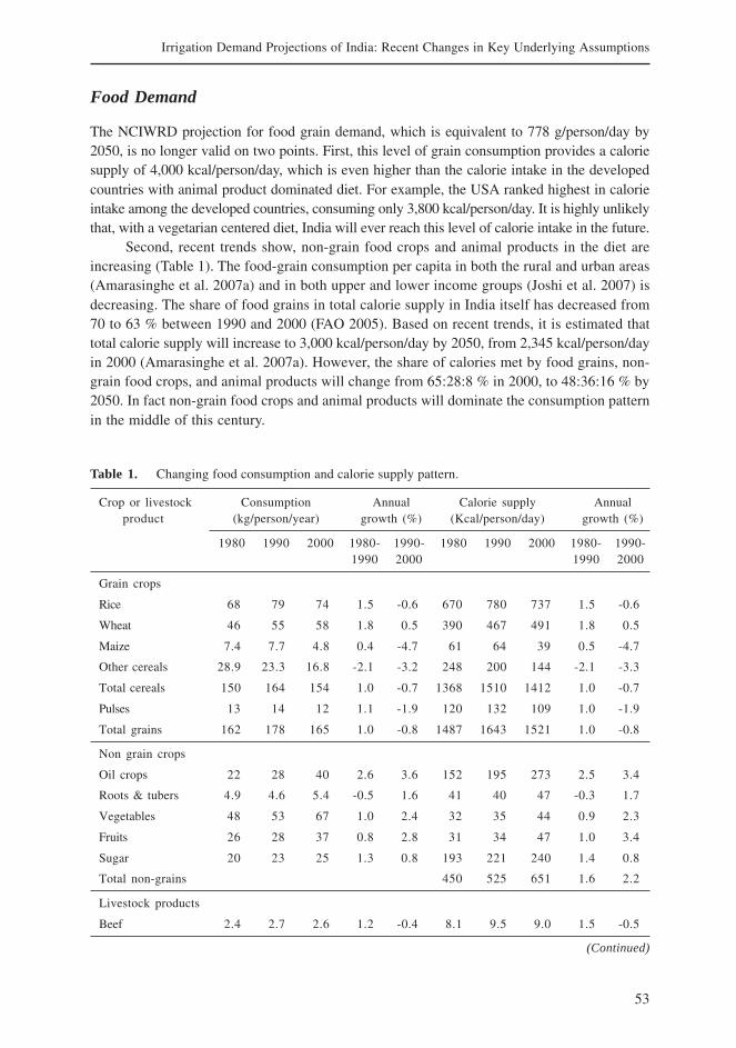
53
Irrigation Demand Projections of India: Recent Changes in Key Underlying Assumptions
Food Demand
The NCIWRD projection for food grain demand, which is equivalent to 778 g/person/day by2050, is no longer valid on two points. First, this level of grain consumption provides a caloriesupply of 4,000 kcal/person/day, which is even higher than the calorie intake in the developedcountries with animal product dominated diet. For example, the USA ranked highest in calorieintake among the developed countries, consuming only 3,800 kcal/person/day. It is highly unlikelythat, with a vegetarian centered diet, India will ever reach this level of calorie intake in the future.
Second, recent trends show, non-grain food crops and animal products in the diet areincreasing (Table 1). The food-grain consumption per capita in both the rural and urban areas(Amarasinghe et al. 2007a) and in both upper and lower income groups (Joshi et al. 2007) isdecreasing. The share of food grains in total calorie supply in India itself has decreased from70 to 63 % between 1990 and 2000 (FAO 2005). Based on recent trends, it is estimated thattotal calorie supply will increase to 3,000 kcal/person/day by 2050, from 2,345 kcal/person/dayin 2000 (Amarasinghe et al. 2007a). However, the share of calories met by food grains, non-grain food crops, and animal products will change from 65:28:8 % in 2000, to 48:36:16 % by2050. In fact non-grain food crops and animal products will dominate the consumption patternin the middle of this century.
Table 1. Changing food consumption and calorie supply pattern.
Crop or livestock Consumption Annual Calorie supply Annualproduct (kg/person/year) growth (%) (Kcal/person/day) growth (%)
1980 1990 2000 1980- 1990- 1980 1990 2000 1980- 1990-1990 2000 1990 2000
Grain crops
Rice 68 79 74 1.5 -0.6 670 780 737 1.5 -0.6
Wheat 46 55 58 1.8 0.5 390 467 491 1.8 0.5
Maize 7.4 7.7 4.8 0.4 -4.7 61 64 39 0.5 -4.7
Other cereals 28.9 23.3 16.8 -2.1 -3.2 248 200 144 -2.1 -3.3
Total cereals 150 164 154 1.0 -0.7 1368 1510 1412 1.0 -0.7
Pulses 13 14 12 1.1 -1.9 120 132 109 1.0 -1.9
Total grains 162 178 165 1.0 -0.8 1487 1643 1521 1.0 -0.8
Non grain crops
Oil crops 22 28 40 2.6 3.6 152 195 273 2.5 3.4
Roots & tubers 4.9 4.6 5.4 -0.5 1.6 41 40 47 -0.3 1.7
Vegetables 48 53 67 1.0 2.4 32 35 44 0.9 2.3
Fruits 26 28 37 0.8 2.8 31 34 47 1.0 3.4
Sugar 20 23 25 1.3 0.8 193 221 240 1.4 0.8
Total non-grains 450 525 651 1.6 2.2
Livestock products
Beef 2.4 2.7 2.6 1.2 -0.4 8.1 9.5 9.0 1.5 -0.5
(Continued)
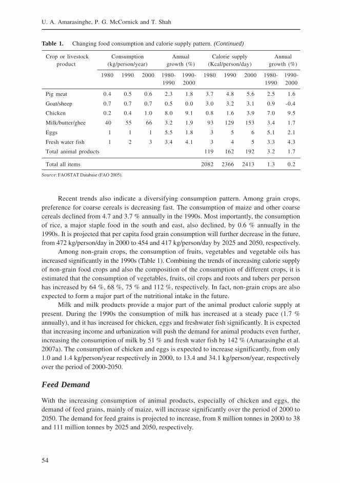
54
U. A. Amarasinghe, P. G. McCornick and T. Shah
Table 1. Changing food consumption and calorie supply pattern. (Continued)
Crop or livestock Consumption Annual Calorie supply Annualproduct (kg/person/year) growth (%) (Kcal/person/day) growth (%)
1980 1990 2000 1980- 1990- 1980 1990 2000 1980- 1990-1990 2000 1990 2000
Pig meat 0.4 0.5 0.6 2.3 1.8 3.7 4.8 5.6 2.5 1.6
Goat/sheep 0.7 0.7 0.7 0.5 0.0 3.0 3.2 3.1 0.9 -0.4
Chicken 0.2 0.4 1.0 8.0 9.1 0.8 1.6 3.9 7.0 9.5
Milk/butter/ghee 40 55 66 3.2 1.9 93 129 153 3.4 1.7
Eggs 1 1 1 5.5 1.8 3 5 6 5.1 2.1
Fresh water fish 1 2 3 3.4 4.1 3 4 5 3.3 4.3
Total animal products 119 162 192 3.2 1.7
Total all items 2082 2366 2413 1.3 0.2
Source:FAOSTAT Database (FAO 2005).
Recent trends also indicate a diversifying consumption pattern. Among grain crops,preference for coarse cereals is decreasing fast. The consumption of maize and other coarsecereals declined from 4.7 and 3.7 % annually in the 1990s. Most importantly, the consumptionof rice, a major staple food in the south and east, also declined, by 0.6 % annually in the1990s. It is projected that per capita food grain consumption will further decrease in the future,from 472 kg/person/day in 2000 to 454 and 417 kg/person/day by 2025 and 2050, respectively.
Among non-grain crops, the consumption of fruits, vegetables and vegetable oils hasincreased significantly in the 1990s (Table 1). Combining the trends of increasing calorie supplyof non-grain food crops and also the composition of the consumption of different crops, it isestimated that the consumption of vegetables, fruits, oil crops and roots and tubers per personhas increased by 64 %, 68 %, 75 % and 112 %, respectively. In fact, non-grain crops are alsoexpected to form a major part of the nutritional intake in the future.
Milk and milk products provide a major part of the animal product calorie supply atpresent. During the 1990s the consumption of milk has increased at a steady pace (1.7 %annually), and it has increased for chicken, eggs and freshwater fish significantly. It is expectedthat increasing income and urbanization will push the demand for animal products even further,increasing the consumption of milk by 51 % and fresh water fish by 142 % (Amarasinghe et al.2007a). The consumption of chicken and eggs is expected to increase significantly, from only1.0 and 1.4 kg/person/year respectively in 2000, to 13.4 and 34.1 kg/person/year, respectivelyover the period of 2000-2050.
Feed Demand
With the increasing consumption of animal products, especially of chicken and eggs, thedemand of feed grains, mainly of maize, will increase significantly over the period of 2000 to2050. The demand for feed grains is projected to increase, from 8 million tonnes in 2000 to 38and 111 million tonnes by 2025 and 2050, respectively.
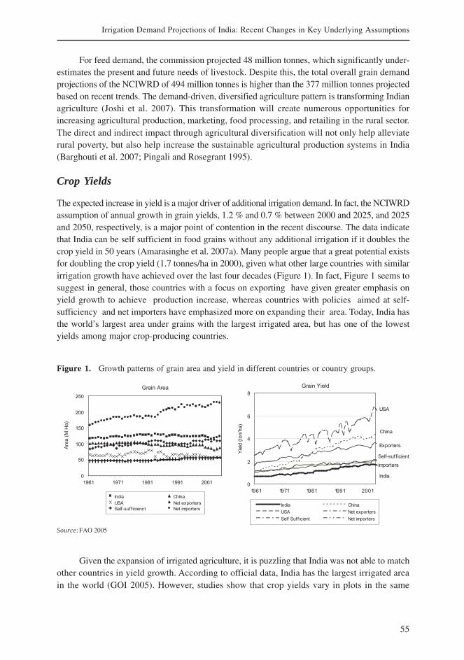
55
Irrigation Demand Projections of India: Recent Changes in Key Underlying Assumptions
For feed demand, the commission projected 48 million tonnes, which significantly under-estimates the present and future needs of livestock. Despite this, the total overall grain demandprojections of the NCIWRD of 494 million tonnes is higher than the 377 million tonnes projectedbased on recent trends. The demand-driven, diversified agriculture pattern is transforming Indianagriculture (Joshi et al. 2007). This transformation will create numerous opportunities forincreasing agricultural production, marketing, food processing, and retailing in the rural sector.The direct and indirect impact through agricultural diversification will not only help alleviaterural poverty, but also help increase the sustainable agricultural production systems in India(Barghouti et al. 2007; Pingali and Rosegrant 1995).
Crop Yields
The expected increase in yield is a major driver of additional irrigation demand. In fact, the NCIWRDassumption of annual growth in grain yields, 1.2 % and 0.7 % between 2000 and 2025, and 2025and 2050, respectively, is a major point of contention in the recent discourse. The data indicatethat India can be self sufficient in food grains without any additional irrigation if it doubles thecrop yield in 50 years (Amarasinghe et al. 2007a). Many people argue that a great potential existsfor doubling the crop yield (1.7 tonnes/ha in 2000), given what other large countries with similarirrigation growth have achieved over the last four decades (Figure 1). In fact, Figure 1 seems tosuggest in general, those countries with a focus on exporting have given greater emphasis onyield growth to achieve production increase, whereas countries with policies aimed at self-sufficiency and net importers have emphasized more on expanding their area. Today, India hasthe world’s largest area under grains with the largest irrigated area, but has one of the lowestyields among major crop-producing countries.
Figure 1. Growth patterns of grain area and yield in different countries or country groups.
Source:FAO 2005
Given the expansion of irrigated agriculture, it is puzzling that India was not able to matchother countries in yield growth. According to official data, India has the largest irrigated areain the world (GOI 2005). However, studies show that crop yields vary in plots in the same
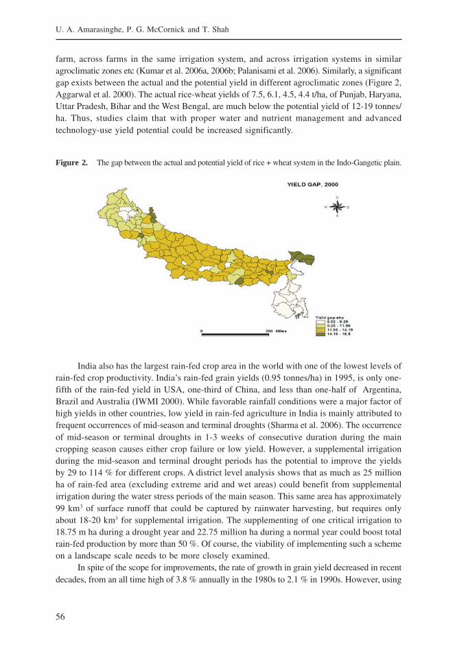
56
U. A. Amarasinghe, P. G. McCornick and T. Shah
farm, across farms in the same irrigation system, and across irrigation systems in similaragroclimatic zones etc (Kumar et al. 2006a, 2006b; Palanisami et al. 2006). Similarly, a significantgap exists between the actual and the potential yield in different agroclimatic zones (Figure 2,Aggarwal et al. 2000). The actual rice-wheat yields of 7.5, 6.1, 4.5, 4.4 t/ha, of Punjab, Haryana,Uttar Pradesh, Bihar and the West Bengal, are much below the potential yield of 12-19 tonnes/ha. Thus, studies claim that with proper water and nutrient management and advancedtechnology-use yield potential could be increased significantly.
Figure 2. The gap between the actual and potential yield of rice + wheat system in the Indo-Gangetic plain.
India also has the largest rain-fed crop area in the world with one of the lowest levels ofrain-fed crop productivity. India’s rain-fed grain yields (0.95 tonnes/ha) in 1995, is only one-fifth of the rain-fed yield in USA, one-third of China, and less than one-half of Argentina,Brazil and Australia (IWMI 2000). While favorable rainfall conditions were a major factor ofhigh yields in other countries, low yield in rain-fed agriculture in India is mainly attributed tofrequent occurrences of mid-season and terminal droughts (Sharma et al. 2006). The occurrenceof mid-season or terminal droughts in 1-3 weeks of consecutive duration during the maincropping season causes either crop failure or low yield. However, a supplemental irrigationduring the mid-season and terminal drought periods has the potential to improve the yieldsby 29 to 114 % for different crops. A district level analysis shows that as much as 25 millionha of rain-fed area (excluding extreme arid and wet areas) could benefit from supplementalirrigation during the water stress periods of the main season. This same area has approximately99 km3 of surface runoff that could be captured by rainwater harvesting, but requires onlyabout 18-20 km3 for supplemental irrigation. The supplementing of one critical irrigation to18.75 m ha during a drought year and 22.75 million ha during a normal year could boost totalrain-fed production by more than 50 %. Of course, the viability of implementing such a schemeon a landscape scale needs to be more closely examined.
In spite of the scope for improvements, the rate of growth in grain yield decreased in recentdecades, from an all time high of 3.8 % annually in the 1980s to 2.1 % in 1990s. However, using
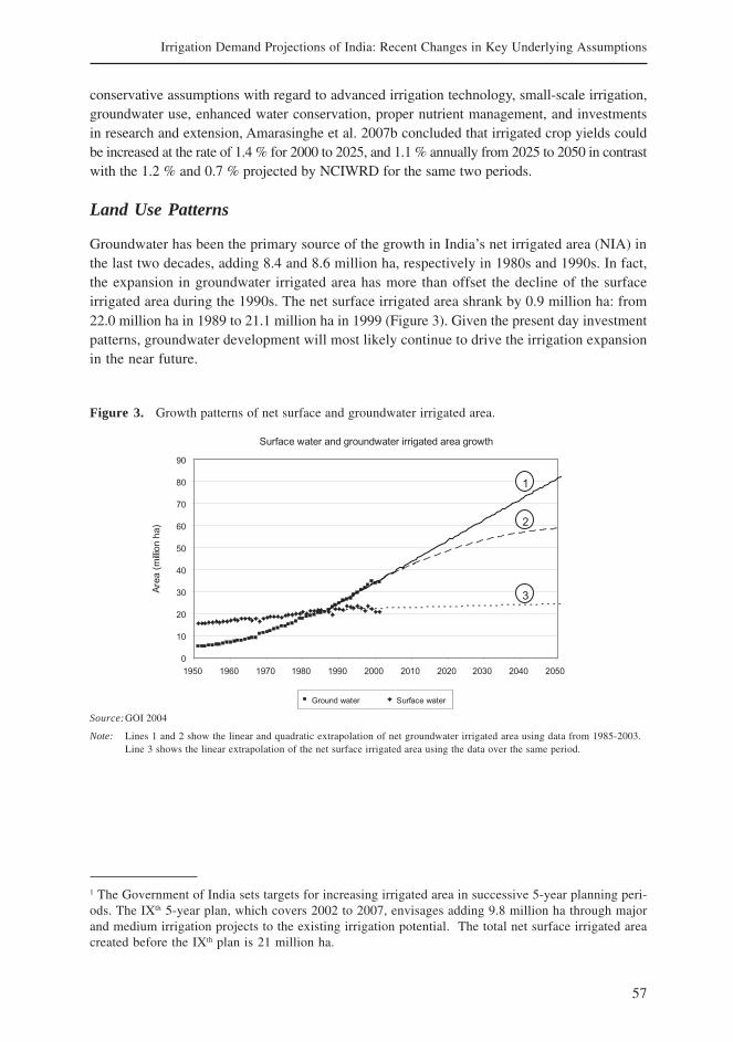
57
Irrigation Demand Projections of India: Recent Changes in Key Underlying Assumptions
conservative assumptions with regard to advanced irrigation technology, small-scale irrigation,groundwater use, enhanced water conservation, proper nutrient management, and investmentsin research and extension, Amarasinghe et al. 2007b concluded that irrigated crop yields couldbe increased at the rate of 1.4 % for 2000 to 2025, and 1.1 % annually from 2025 to 2050 in contrastwith the 1.2 % and 0.7 % projected by NCIWRD for the same two periods.
Land Use Patterns
Groundwater has been the primary source of the growth in India’s net irrigated area (NIA) inthe last two decades, adding 8.4 and 8.6 million ha, respectively in 1980s and 1990s. In fact,the expansion in groundwater irrigated area has more than offset the decline of the surfaceirrigated area during the 1990s. The net surface irrigated area shrank by 0.9 million ha: from22.0 million ha in 1989 to 21.1 million ha in 1999 (Figure 3). Given the present day investmentpatterns, groundwater development will most likely continue to drive the irrigation expansionin the near future.
1 The Government of India sets targets for increasing irrigated area in successive 5-year planning peri-ods. The IXth 5-year plan, which covers 2002 to 2007, envisages adding 9.8 million ha through majorand medium irrigation projects to the existing irrigation potential. The total net surface irrigated areacreated before the IXth plan is 21 million ha.
Figure 3. Growth patterns of net surface and groundwater irrigated area.
Source:GOI 2004
Note: Lines 1 and 2 show the linear and quadratic extrapolation of net groundwater irrigated area using data from 1985-2003.Line 3 shows the linear extrapolation of the net surface irrigated area using the data over the same period.
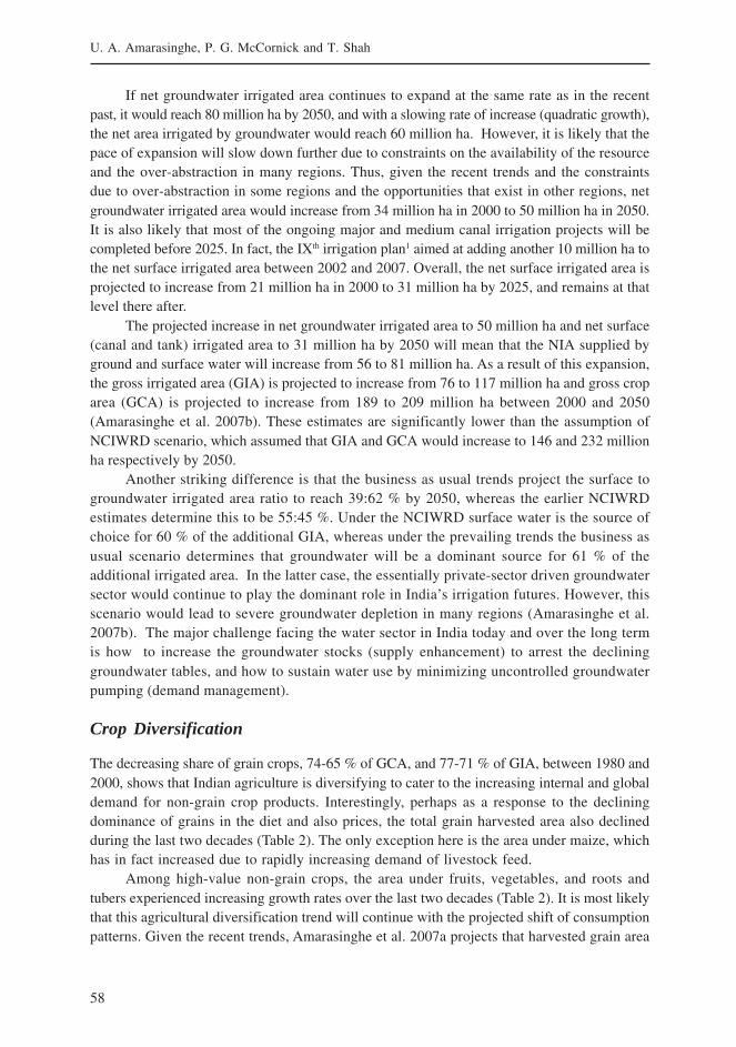
58
U. A. Amarasinghe, P. G. McCornick and T. Shah
If net groundwater irrigated area continues to expand at the same rate as in the recentpast, it would reach 80 million ha by 2050, and with a slowing rate of increase (quadratic growth),the net area irrigated by groundwater would reach 60 million ha. However, it is likely that thepace of expansion will slow down further due to constraints on the availability of the resourceand the over-abstraction in many regions. Thus, given the recent trends and the constraintsdue to over-abstraction in some regions and the opportunities that exist in other regions, netgroundwater irrigated area would increase from 34 million ha in 2000 to 50 million ha in 2050.It is also likely that most of the ongoing major and medium canal irrigation projects will becompleted before 2025. In fact, the IXth irrigation plan1 aimed at adding another 10 million ha tothe net surface irrigated area between 2002 and 2007. Overall, the net surface irrigated area isprojected to increase from 21 million ha in 2000 to 31 million ha by 2025, and remains at thatlevel there after.
The projected increase in net groundwater irrigated area to 50 million ha and net surface(canal and tank) irrigated area to 31 million ha by 2050 will mean that the NIA supplied byground and surface water will increase from 56 to 81 million ha. As a result of this expansion,the gross irrigated area (GIA) is projected to increase from 76 to 117 million ha and gross croparea (GCA) is projected to increase from 189 to 209 million ha between 2000 and 2050(Amarasinghe et al. 2007b). These estimates are significantly lower than the assumption ofNCIWRD scenario, which assumed that GIA and GCA would increase to 146 and 232 millionha respectively by 2050.
Another striking difference is that the business as usual trends project the surface togroundwater irrigated area ratio to reach 39:62 % by 2050, whereas the earlier NCIWRDestimates determine this to be 55:45 %. Under the NCIWRD surface water is the source ofchoice for 60 % of the additional GIA, whereas under the prevailing trends the business asusual scenario determines that groundwater will be a dominant source for 61 % of theadditional irrigated area. In the latter case, the essentially private-sector driven groundwatersector would continue to play the dominant role in India’s irrigation futures. However, thisscenario would lead to severe groundwater depletion in many regions (Amarasinghe et al.2007b). The major challenge facing the water sector in India today and over the long termis how to increase the groundwater stocks (supply enhancement) to arrest the declininggroundwater tables, and how to sustain water use by minimizing uncontrolled groundwaterpumping (demand management).
Crop Diversification
The decreasing share of grain crops, 74-65 % of GCA, and 77-71 % of GIA, between 1980 and2000, shows that Indian agriculture is diversifying to cater to the increasing internal and globaldemand for non-grain crop products. Interestingly, perhaps as a response to the decliningdominance of grains in the diet and also prices, the total grain harvested area also declinedduring the last two decades (Table 2). The only exception here is the area under maize, whichhas in fact increased due to rapidly increasing demand of livestock feed.
Among high-value non-grain crops, the area under fruits, vegetables, and roots andtubers experienced increasing growth rates over the last two decades (Table 2). It is most likelythat this agricultural diversification trend will continue with the projected shift of consumptionpatterns. Given the recent trends, Amarasinghe et al. 2007a projects that harvested grain area
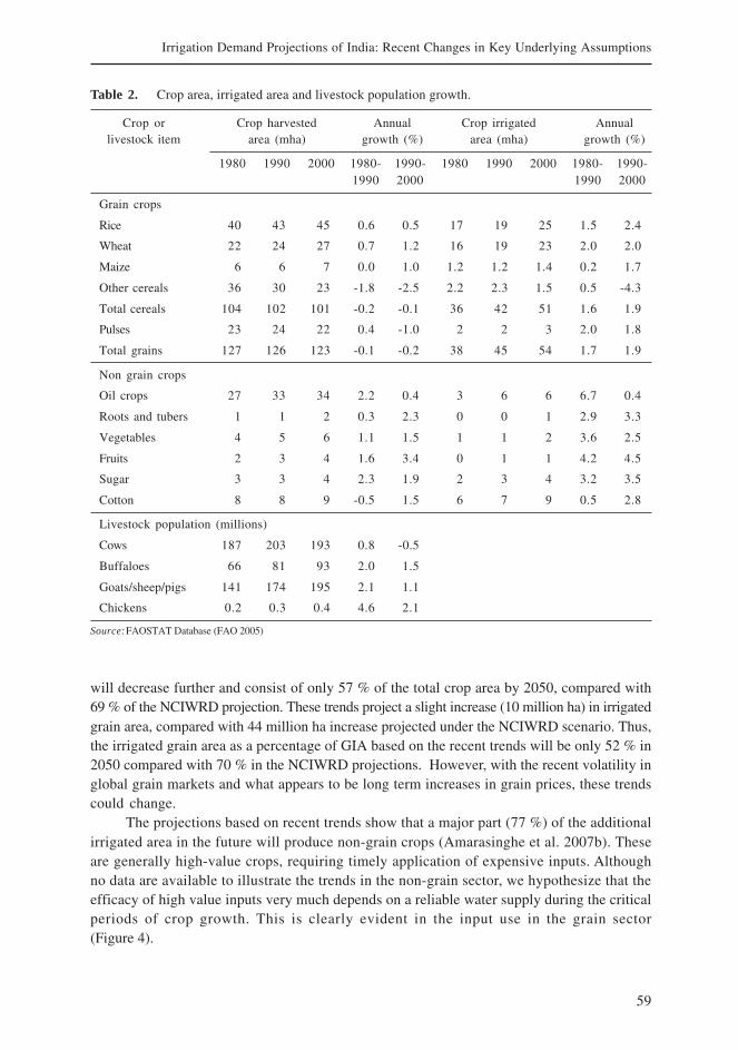
59
Irrigation Demand Projections of India: Recent Changes in Key Underlying Assumptions
will decrease further and consist of only 57 % of the total crop area by 2050, compared with69 % of the NCIWRD projection. These trends project a slight increase (10 million ha) in irrigatedgrain area, compared with 44 million ha increase projected under the NCIWRD scenario. Thus,the irrigated grain area as a percentage of GIA based on the recent trends will be only 52 % in2050 compared with 70 % in the NCIWRD projections. However, with the recent volatility inglobal grain markets and what appears to be long term increases in grain prices, these trendscould change.
The projections based on recent trends show that a major part (77 %) of the additionalirrigated area in the future will produce non-grain crops (Amarasinghe et al. 2007b). Theseare generally high-value crops, requiring timely application of expensive inputs. Althoughno data are available to illustrate the trends in the non-grain sector, we hypothesize that theefficacy of high value inputs very much depends on a reliable water supply during the criticalperiods of crop growth. This is clearly evident in the input use in the grain sector(Figure 4).
Table 2. Crop area, irrigated area and livestock population growth.
Crop or Crop harvested Annual Crop irrigated Annuallivestock item area (mha) growth (%) area (mha) growth (%)
1980 1990 2000 1980- 1990- 1980 1990 2000 1980- 1990-1990 2000 1990 2000
Grain crops
Rice 40 43 45 0.6 0.5 17 19 25 1.5 2.4
Wheat 22 24 27 0.7 1.2 16 19 23 2.0 2.0
Maize 6 6 7 0.0 1.0 1.2 1.2 1.4 0.2 1.7
Other cereals 36 30 23 -1.8 -2.5 2.2 2.3 1.5 0.5 -4.3
Total cereals 104 102 101 -0.2 -0.1 36 42 51 1.6 1.9
Pulses 23 24 22 0.4 -1.0 2 2 3 2.0 1.8
Total grains 127 126 123 -0.1 -0.2 38 45 54 1.7 1.9
Non grain crops
Oil crops 27 33 34 2.2 0.4 3 6 6 6.7 0.4
Roots and tubers 1 1 2 0.3 2.3 0 0 1 2.9 3.3
Vegetables 4 5 6 1.1 1.5 1 1 2 3.6 2.5
Fruits 2 3 4 1.6 3.4 0 1 1 4.2 4.5
Sugar 3 3 4 2.3 1.9 2 3 4 3.2 3.5
Cotton 8 8 9 -0.5 1.5 6 7 9 0.5 2.8
Livestock population (millions)
Cows 187 203 193 0.8 -0.5
Buffaloes 66 81 93 2.0 1.5
Goats/sheep/pigs 141 174 195 2.1 1.1
Chickens 0.2 0.3 0.4 4.6 2.1
Source:FAOSTAT Database (FAO 2005)
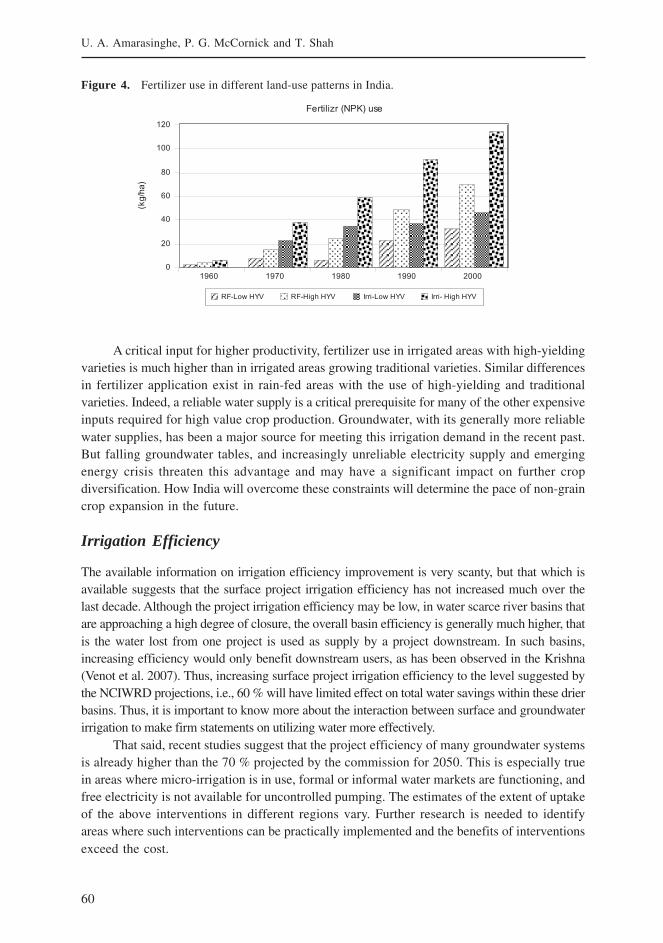
60
U. A. Amarasinghe, P. G. McCornick and T. Shah
A critical input for higher productivity, fertilizer use in irrigated areas with high-yieldingvarieties is much higher than in irrigated areas growing traditional varieties. Similar differencesin fertilizer application exist in rain-fed areas with the use of high-yielding and traditionalvarieties. Indeed, a reliable water supply is a critical prerequisite for many of the other expensiveinputs required for high value crop production. Groundwater, with its generally more reliablewater supplies, has been a major source for meeting this irrigation demand in the recent past.But falling groundwater tables, and increasingly unreliable electricity supply and emergingenergy crisis threaten this advantage and may have a significant impact on further cropdiversification. How India will overcome these constraints will determine the pace of non-graincrop expansion in the future.
Irrigation Efficiency
The available information on irrigation efficiency improvement is very scanty, but that which isavailable suggests that the surface project irrigation efficiency has not increased much over thelast decade. Although the project irrigation efficiency may be low, in water scarce river basins thatare approaching a high degree of closure, the overall basin efficiency is generally much higher, thatis the water lost from one project is used as supply by a project downstream. In such basins,increasing efficiency would only benefit downstream users, as has been observed in the Krishna(Venot et al. 2007). Thus, increasing surface project irrigation efficiency to the level suggested bythe NCIWRD projections, i.e., 60 % will have limited effect on total water savings within these drierbasins. Thus, it is important to know more about the interaction between surface and groundwaterirrigation to make firm statements on utilizing water more effectively.
That said, recent studies suggest that the project efficiency of many groundwater systemsis already higher than the 70 % projected by the commission for 2050. This is especially truein areas where micro-irrigation is in use, formal or informal water markets are functioning, andfree electricity is not available for uncontrolled pumping. The estimates of the extent of uptakeof the above interventions in different regions vary. Further research is needed to identifyareas where such interventions can be practically implemented and the benefits of interventionsexceed the cost.
Figure 4. Fertilizer use in different land-use patterns in India.
61
Irrigation Demand Projections of India: Recent Changes in Key Underlying Assumptions
Self-sufficiency in Grains
Can national self-sufficiency goals in food grains be a realistic assumption any more forprojecting India’s irrigation demand? This was so when the agricultural output in general, andgrain production in particular, was a major part of the gross domestic product (GDP). Thecontribution of the agricultural sector to the GDP decreased from 46-25 % during 1961-2000,and will decrease further with rapidly growing services and industrial sector outputs. Moreover,the value of grain production, in comparison with total agricultural production is very smallnow, and is also declining, and demand for food grains is declining too. Thus, in purelyeconomic terms, although it was a constraint for the Indian economy to import part of thegrain demand now, it will be insignificant for a trillion dollar economy in a few years from now.
However, the recent volatility in the global grain markets, partly induced by significantproduction shortfalls in grain exporting countries and aggressive plans for developing bio-fuels, has significantly affected the price and supply of grains in a number of countries,including India. In the future, large importations of grain from populous countries like Indiaand China could further add to the volatility. The increased costs for imports could hurt thevery consumers that the imports are expected to help. In India, the major grain productiondeficit in the future will be for feed grains, especially for maize (Amarasinghe et al. 2007b).However, production surpluses of rice and wheat are expected to offset the productiondeficits of maize. Thus, in spite of price increase concerns, India’s food trade will increase,and self-sufficiency of all grains need not be a rigid formula (more on this subject isdiscussed by R.P.S. Malik in Paper 9).
Agriculture Dependent Livelihoods
The high dependency of rural livelihoods on agriculture was a further component of the overallrationale for the commission’s projections for future irrigation demand. The recent trendssuggest that the agriculture demography is fast changing with increasing non-agriculturalemployment. Although it is not expected to see the general depopulation of all rural areas inIndia, as has happened in parts of South-East Asia, there are already indications that this ishappening in parts of rural India. Over the last four decades, the agriculture dependedpopulation has decreased from 86-74 %. A quadratic extrapolation of the present trends (R2=98%) show this percentage will decline to about 58 % by 2025 and 40 % by 2050. This projectedtrend is more or less compatible with the present agricultural population of countries withsimilar economic conditions as projected for India by 2050. This means that although agriculturedependent population will increase in the short-term, it will start to decline after the next decade.And in 50 years from now, India will even have a less populace who depend on agriculturethan they do now.
In fact, trends of rural population moving out of agriculture is already happening andwill likely accelerate in the future with increasing employment opportunities in the non-agriculture sector (Sharma et al. 2006). There is a high probability that young rural farmers willmove out of agriculture for various reasons particularly where non-agriculture employmentopportunities are accessible, and the youth have better skills and education. Certainly, theseconditions are increasingly apparent in many areas as urban centers continue to expand withbooming industrial and service sectors.
62
U. A. Amarasinghe, P. G. McCornick and T. Shah
Implications on Irrigation Demand
The above discussion shows that the key determinants of irrigation water demand of theNCIWRD projections, upon which the requirements for the NRLP have been based, are nolonger consistent with the present-day trends. The NCIWRD assumed,
• increasing demand for food grains, whereas while the demand for food grains willcontinue to increase in the short term it will be at a declining rate, and the moresignificant actual trend is the increasing demand for non-food grain products;
• the grain production to dominate the future of Indian agriculture, whereas cropdiversification is the actual and expected trend;
• the surface irrigation to dominate the land-use patterns, yet groundwater has beenthe engine of irrigation growth, and is expected to continue to be so, despite localizedconstraints of sustainability;
• a rather low crop yield growth, although substantial scope exists for yieldimprovements in both irrigated and rain-fed areas; and
• a high level of surface project irrigation efficiency, although many river basins relyon the recharge from surface return flows for groundwater irrigation and surfaceirrigation downstream and in these systems, surface irrigation efficiency is still aslow as 30-35 %.
On the other hand, the recent trends suggest:
• consumption patterns will shift towards a non-food grain product dominated diet;
• agriculture will continue to expand, but it will diversify to meet the increasing demandfor non food grain crops and animal products;
• groundwater irrigation will continue to expand in spite of the severe depletions insome regions;
• advanced irrigation and other water-saving technologies will spread to increase cropyields and water-use efficiency;
• better water and nutrient management will reverse the recent decline in the rate ofcrop yield increases, to some extent; and
• self-sufficiency in all grain crops will no longer be a concrete goal, and the productionsurpluses of some crops will pay for the production deficits of other crops.
Thus, irrigation water demand according to the Business as Usual (BaU) scenario trends,which is mostly based on the recent changes in key drivers as discussed above (Amarasingheet al. 2007b), differs in many key aspects from the irrigation water demand projections of theNCIWRD report (Fgure 5).
• The BaU scenario results in a slightly lower additional irrigation demand (by about10 billion m3) between 2000 and 2025, and a much lower additional irrigation demand
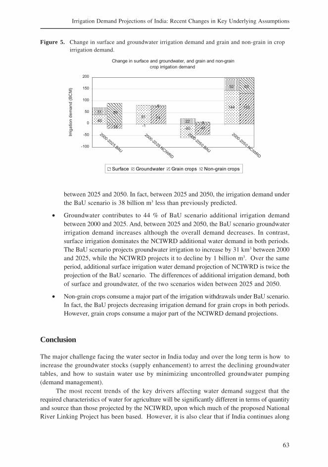
63
Irrigation Demand Projections of India: Recent Changes in Key Underlying Assumptions
Figure 5. Change in surface and groundwater irrigation demand and grain and non-grain in cropirrigation demand.
between 2025 and 2050. In fact, between 2025 and 2050, the irrigation demand underthe BaU scenario is 38 billion m3 less than previously predicted.
• Groundwater contributes to 44 % of BaU scenario additional irrigation demandbetween 2000 and 2025. And, between 2025 and 2050, the BaU scenario groundwaterirrigation demand increases although the overall demand decreases. In contrast,surface irrigation dominates the NCIWRD additional water demand in both periods.The BaU scenario projects groundwater irrigation to increase by 31 km3 between 2000and 2025, while the NCIWRD projects it to decline by 1 billion m3. Over the sameperiod, additional surface irrigation water demand projection of NCIWRD is twice theprojection of the BaU scenario. The differences of additional irrigation demand, bothof surface and groundwater, of the two scenarios widen between 2025 and 2050.
• Non-grain crops consume a major part of the irrigation withdrawals under BaU scenario.In fact, the BaU projects decreasing irrigation demand for grain crops in both periods.However, grain crops consume a major part of the NCIWRD demand projections.
Conclusion
The major challenge facing the water sector in India today and over the long term is how toincrease the groundwater stocks (supply enhancement) to arrest the declining groundwatertables, and how to sustain water use by minimizing uncontrolled groundwater pumping(demand management).
The most recent trends of the key drivers affecting water demand suggest that therequired characteristics of water for agriculture will be significantly different in terms of quantityand source than those projected by the NCIWRD, upon which much of the proposed NationalRiver Linking Project has been based. However, it is also clear that if India continues along
64
U. A. Amarasinghe, P. G. McCornick and T. Shah
a business-as-usual path and follows these recent trends without timely and informedinterventions it will lead to severe regional water crises.
Excessive groundwater exploitation will be a major component of the challenge to betackled. In the medium-term, this will have major repercussion on changing cropping patterns,because groundwater is and will continue to be the main source of water for successful cropdiversification. The challenges for the irrigation sector in India in the medium-term are,
• how to promote crop diversification to increase the benefits for every drop ofconsumptive water use, and
• how to promote sustainable groundwater expansion to reap the benefits of changingcropping patterns.
While it is clear from the above that the water requirements of the agricultural sector ofthe future will be quite different from those underpinning the NRLP as presently conceived,India does need to further develop its water resources to meet the needs of the people andthe economy. Conditions will dictate that this will include large scale developments thatincorporate intra - or inter-basin water transfers with surface storage. This is particularly truewhere increasing domestic and industrial water requirements are the dominant waterconsumptive factors in a relatively dry basin, and also other factors such as increasing cropdiversification to high-value crops which will require a more reliable water supply and areaswith declining groundwater tables which may demand better surface water supply forsustainable production and profits.
Also, there are likely to be other contingencies under which large scale inter-basin watertransfers as envisioned under the NRLP are required for meeting India’s future water demand.The foremost among the contingencies is that the economic growth is even more rapid thanthat assumed here. In such a case the domestic and industrial sector demand will be greaterand will have the capacity to pay for a good quality and reliable surface water supply for theirdaily water needs.
Finally, the demand for biofuels will have a significant impact on water-use patterns,especially on groundwater use and may also have a significant impact on prices. Further, theclimate change could have a significant impact on overall water demand and supply in manyriver basins. Climate change is expected to accelerate the seasonal melting of the snow packfrom the Himalayas, affect the overall volume of precipitation and increase the frequency andmagnitude of extreme rainfall events, which all may require large storage facilities for wateruse in the dry seasons (Sharma and McCornick 2006). Further research is necessary to assessthe implications of these on future surface water demand.
References
Agarwal, P.K.; Talukdar, K.K.; Mall, R.K. 2000. Potential yields of rice-wheat systems in the Indo-Gangeticplains of India. Rice-Wheat Consortium Paper Series 10. New Delhi, India: Rice-Wheat Consortium forthe Indo-Gangetic Plains.
Amarasinghe, U. A.; Shah, T.; Singh, O. P. 2007a. Changing consumption patterns: implications forfood and water demand in India. IWMI Research Report 119, Colombo, Sri Lanka: International WaterManagement Institute.
65
Irrigation Demand Projections of India: Recent Changes in Key Underlying Assumptions
Amarasinghe, U. A.; Shah, T.; Turral, H.; Anand, B.K. 2007b. India’s Water Futures to 2025-2050:BAU Scenario and Deviations. IWMI Research Report 123, Colombo, Sri Lanka: International WaterManagement Institute.
Barghouti, S.; Kane, S.; Sorby, K. 2007. Poverty and Agricultural Diversification in Developing Countries.In Agriculture Diversification and Smallholders in South Asia. ed. Joshi, P. K.; Glati, A.; Cummings,R. Jr. New Delhi, India: Academic Foundation.
De Fraiture, C.; Giordano, M.; Liao, Y. 2008. Biofuels and implications for agricultural water use: blueimpacts on green energy. In: Water-Energy-Food-Environment Interface: Synergies and Conflicts,a special issue of the Water Policy journal.
FAO 2005. FAOSATAT Data Base. Rome: Food and Agriculture Organization.
GOI 1999. Integrated water resources development. A plan for action. Report of the Commission forIntegrated Water Resource Development, Vol.I. New Delhi, India: Ministry of Water Resources.
GOI 2005. Agricultural Statistics at a Glance 2004. New Delhi, India: Ministry of Agriculture, Governmentof India.
IWMI 2000. World Water Supply and Demand 1995 to 2025 (Draft).www.cgiar.org/iwmi/pubs/WWVison/WWSDOpen.htm. Colombo, India: International WaterManagement Institute.
Joshi, P.K.; Gulati, A.; Cummings, R. Jr. 2007. Overview in Agriculture Diversification and Smallholdersin South Asia. New Delhi, India: Academic Foundation.
Kumar, M.D.; Samad, M.; Amarasinghe, U.A.; Singh, O.P. 2006a. Water saving technologies: How farcan they contribute to water productivity enhancement in Indian agriculture? Draft prepared for theIWMI-CPWF project on ‘Strategic Analysis of National River Linking Project of India’.
Kumar, M.D.; Singh, O.P.; Samad, M.; Purihit, C.; Didyla, D. 2006b. Water productivity of irrigatedagriculture in India. Potential areas of improvement. Draft prepared for the IWMI-CPWF project on‘Strategic Analysis of National River Linking Project of India’.
NWDA 2006. http://nwda.gov.in/index2.asp?sublinkid=46&langid=1
Palanisami, K.P.; Senthivel, K.; Ranganathan, C.R.; Ramesh, T. 2006. Water productivity at different scalesunder canal, tank and tubewell irrigation systems. Draft prepared for the IWMI-CPWF project on ‘StrategicAnalysis of National River Linking Project of India’.
Pingali, P.L.; Rosegrant, M.W. 1995. Agricultural Commercialization and Diversification: Processes andPolicies. Food Policy 20 (3): 171-86.
Sharma, B. R.; McCornick, P. G. 2006. Domestic policy framework on adaptation to climate change inwater resources: Case study for India. (Commissioned Paper). Proceedings ‘Working Together toRespond to Climate Change’- Annex I Expert Group Seminar of OECD Global Forum on SustainableDevelopment, Paris, France. (available at www.oecd.org)
Sharma, B.R.; Rao, K.V.; Vittal, K.P.R. Amarasinghe, U. A. 2006. Realizing the Potential of Rain-fedAgriculture in India. Draft prepared for the IWMI-CPWF project on ‘Strategic Analysis of NationalRiver Linking Project of India’.
Venot, J. P.; Turral, H.; Samad, M.; Molle, F. 2007. Explaining Basin Closure through Shifting Waterscapein the Lower Krishna Basin, South India. Research Report 121. Colombo, Sri Lanka: International WaterManagement Institute.
67
India’s Water Demand Scenarios to 2025 and 2050:A Fresh Look
1Upali A. Amarasinghe, 2Peter G. McCornick and 3Tushaar Shah1International Water Management Institute (IWMI), NewDelhi, India
2International Water Management Institute (IWMI), Colombo, Sri Lanka3International Water Management Institute (IWMI), Anand, India
Introduction
India is a vast country and its water supply varies significantly across regions and riverbasins. Water is plenty in the northeast (Brahmaputhra and Meghna basins), but few peoplelive there, and land availability and food production is low. In the northwest most of thewater resources are diverted for crop production to the extent that this region supplies foodto the deficit regions of the country making it the largest provider of virtual water, that iswater embedded in food, in the county (Amarasinghe et al. 2005). Water is scarce in thesouth and west of the country as the naturally drier areas come under increasing demand,and the aquifers have low storage capacity.
Much of the runoff in the peninsular river basins is from the highly variable monsoon,which means it occurs during the 2 to 3 months of monsoonal rains. Thus, the regional wateravailability vis-à-vis changing water demand patterns and the determinants of these changinggrowth patterns are particularly important factors for medium to long-term water investmentstrategies in general in India, and in particular in the water-scarce peninsular river basins.
This report examines the implications of future water supply demand of India underbusiness as usual (BaU) scenario trends of key water demand drivers and also under possibledivergences. The assumptions of the growth of key drivers in the BaU scenario (Annex 1) inthis paper significantly differ from the assumptions of the scenarios of the NCIWRD (discussedin detail in Paper 2). The BaU scenario considers the year 2000 data as the base year and thetrends in the 1990s for its demand projections whereas the NCIWRD scenarios considered1993/94 data for the base year and the trends in 1980s for determining the key drivers. Thisreport, which is primarily, based on the studies by Amarasinghe et al. 2007a and 2007b,
• gives an overview of the business as usual (BaU) scenario food and water demandup to 2025/2050 in India;
• discusses the past trends of key determinants or ‘drivers’ of water and food demand;and
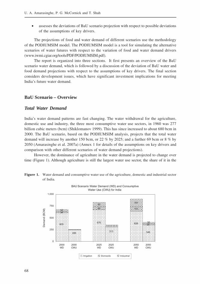
68
U. A. Amarasinghe, P. G. McCornick and T. Shah
• assesses the deviations of BaU scenario projection with respect to possible deviationsof the assumptions of key drivers.
The projections of food and water demand of different scenarios use the methodologyof the PODIUMSIM model. The PODIUMSIM model is a tool for simulating the alternativescenarios of water futures with respect to the variation of food and water demand drivers(www.iwmi.cgiar.org/tools/PDF/PODIUMSIM.pdf).
The report is organized into three sections. It first presents an overview of the BaUscenario water demand, which is followed by a discussion of the deviation of BaU water andfood demand projections with respect to the assumptions of key drivers. The final sectionconsiders development issues, which have significant investment implications for meetingIndia’s future water demand.
BaU Scenario – Overview
Total Water Demand
India’s water demand patterns are fast changing. The water withdrawal for the agriculture,domestic use and industry, the three most consumptive water use sectors, in 1960 was 277billion cubic meters (bcm) (Shiklomanov 1999). This has since increased to about 680 bcm in2000. The BaU scenario, based on the PODIUMSIM analysis, projects that the total waterdemand will increase by another 150 bcm, or 22 % by 2025; and a further 69 bcm or 8 % by2050 (Amarasinghe et al. 2007a) (Annex 1 for details of the assumptions on key drivers andcomparison with other different scenarios of water demand projections).
However, the dominance of agriculture in the water demand is projected to change overtime (Figure 1). Although agriculture is still the largest water use sector, the share of it in the
Figure 1. Water demand and consumptive water use of the agriculture, domestic and industrial sectorof India.
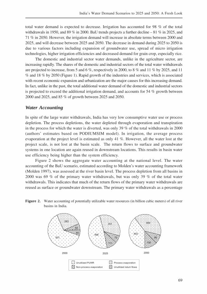
69
India’s Water Demand Scenarios to 2025 and 2050: A Fresh Look
total water demand is expected to decrease. Irrigation has accounted for 98 % of the totalwithdrawals in 1950, and 89 % in 2000. BaU trends projects a further decline – 81 % in 2025, and71 % in 2050. However, the irrigation demand will increase in absolute terms between 2000 and2025, and will decrease between 2025 and 2050. The decrease in demand during 2025 to 2050 isdue to various factors including expansion of groundwater use, spread of micro irrigationtechnologies, higher irrigation efficiencies and decreased demand for grain crop, especially rice.
The domestic and industrial sector water demands, unlike in the agriculture sector, areincreasing rapidly. The shares of the domestic and industrial sectors of the total water withdrawalsare projected to increase, from 5 and 6 %, respectively in 2000, to 8 % and 11 % by 2025, and 11% and 18 % by 2050 (Figure 1). Rapid growth of the industries and services, which is associatedwith recent economic expansion and urbanization are the major causes for this increasing demand.In fact, unlike in the past, the total additional water demand of the domestic and industrial sectorsis projected to exceed the additional irrigation demand, and accounts for 54 % growth between2000 and 2025, and 85 % of growth between 2025 and 2050.
Water Accounting
In spite of the large water withdrawals, India has very low consumptive water use or processdepletion. The process depletions, the water depleted through evaporation and transpirationin the process for which the water is diverted, was only 39 % of the total withdrawals in 2000(authors’ estimates based on PODIUMSIM model). In irrigation, the average processevaporation at the project level is estimated as only 41 %. However, all the water lost at theproject scale, is not lost at the basin scale. The return flows to surface and groundwatersystems in one location are again reused in downstream locations. This results in basin wateruse efficiency being higher than the system efficiency.
Figure 2 shows the aggregate water accounting at the national level. The wateraccounting of the BaU scenario, estimated according to Molden’s water accounting framework(Molden 1997), was assessed at the river basin level. The process depletion from all basins in2000 was 69 % of the primary water withdrawals, but was only 39 % of the total waterwithdrawals. This indicates that much of the return flows of the primary water withdrawals arereused as surface or groundwater downstream. The primary water withdrawals as a percentage
Figure 2. Water accounting of potentially utilizable water resources (in billion cubic meters) of all riverbasins in India.
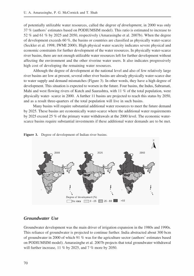
70
U. A. Amarasinghe, P. G. McCornick and T. Shah
of potentially utilizable water resources, called the degree of development, in 2000 was only37 % (authors’ estimates based on PODIUMSIM model). This ratio is estimated to increase to52 % and 61 % by 2025 and 2050, respectively (Amarasinghe et al. 2007b). When the degreeof development exceeds 60 %, the basins or countries are classified as physically water-scarce(Seckler et al. 1998; IWMI 2000). High physical water scarcity indicates severe physical andeconomic constraints for further development of the water resources. In physically water-scarceriver basins, there are not enough utilizable water resources left for further development withoutaffecting the environment and the other riverine water users. It also indicates progressivelyhigh cost of developing the remaining water resources.
Although the degree of development at the national level and also of few relatively largeriver basins are low at present, several other river basins are already physically water-scarce dueto water supply and demand mismatches (Figure 3). In other words, they have a high degree ofdevelopment. This situation is expected to worsen in the future. Four basins, the Indus, Sabramati,Mahi and west flowing rivers of Kutch and Saurashtra, with 11 % of the total population, werephysically water- scarce in 2000. A further 11 basins are projected to reach this status by 2050,and as a result three-quarters of the total population will live in such basins.
Many basins will require substantial additional water resources to meet the future demandby 2025. These basins are economically water-scarce where the additional water requirementsby 2025 exceed 25 % of the primary water withdrawals at the 2000 level. The economic water-scarce basins require substantial investments if these additional water demands are to be met.
Groundwater Use
Groundwater development was the main driver of irrigation expansion in the 1980s and 1990s.This reliance of groundwater is projected to continue further. India abstracted about 300 bcmof groundwater in 2000 of which 91 % was for the agriculture sector (authors’ estimates basedon PODIUMSIM model). Amarasinghe et al. 2007b projects that total groundwater withdrawalwill further increase, 11 % by 2025, and 7 % more by 2050.
Figure 3. Degree of development of Indian river basins.
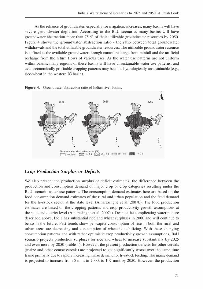
71
India’s Water Demand Scenarios to 2025 and 2050: A Fresh Look
As the reliance of groundwater, especially for irrigation, increases, many basins will havesevere groundwater depletion. According to the BaU scenario, many basins will havegroundwater abstraction more than 75 % of their utilizable groundwater resources by 2050.Figure 4 shows the groundwater abstraction ratio - the ratio between total groundwaterwithdrawals and the total utilizable groundwater resources. The utilizable groundwater resourceis defined as the available groundwater through natural recharge from rainfall and the artificialrecharge from the return flows of various uses. As the water use patterns are not uniformwithin basins, many regions of these basins will have unsustainable water use patterns, andeven economically profitable cropping patterns may become hydrologically unsustainable (e.g.,rice-wheat in the western IG basin).
Crop Production Surplus or Deficits
We also present the production surplus or deficit estimates, the difference between theproduction and consumption demand of major crop or crop categories resulting under theBaU scenario water use patterns. The consumption demand estimates here are based on thefood consumption demand estimates of the rural and urban population and the feed demandfor the livestock sector at the state level (Amarasinghe et al. 2007b). The food productionestimates are based on the cropping patterns and crop productivity growth assumptions atthe state and district level (Amarasinghe et al. 2007a). Despite the complicating water picturedescribed above, India has substantial rice and wheat surpluses in 2000 and will continue tobe so in the future. Past trends show per capita consumption of rice in both the rural andurban areas are decreasing and consumption of wheat is stabilizing. With these changingconsumption patterns and with rather optimistic crop productivity growth assumptions, BaUscenario projects production surpluses for rice and wheat to increase substantially by 2025and even more by 2050 (Table 1). However, the present production deficits for other cereals(maize and other coarse cereals) are projected to get significantly worse over the same timeframe primarily due to rapidly increasing maize demand for livestock feeding. The maize demandis projected to increase from 5 mmt in 2000, to 107 mmt by 2050. However, the production
Figure 4. Groundwater abstraction ratio of Indian river basins.
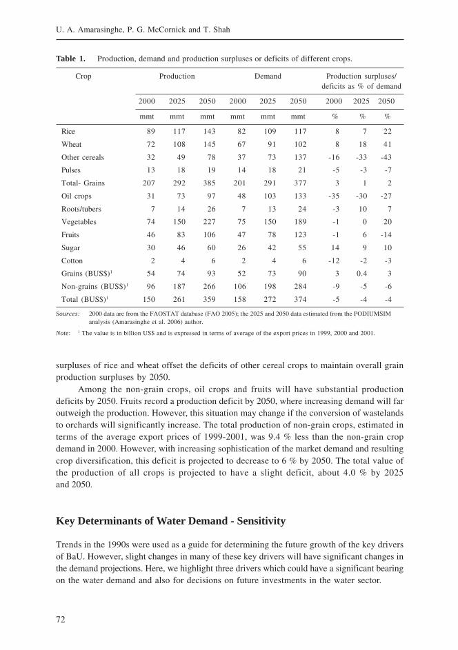
72
U. A. Amarasinghe, P. G. McCornick and T. Shah
Table 1. Production, demand and production surpluses or deficits of different crops.
Crop Production Demand Production surpluses/deficits as % of demand
2000 2025 2050 2000 2025 2050 2000 2025 2050
mmt mmt mmt mmt mmt mmt % % %
Rice 89 117 143 82 109 117 8 7 22
Wheat 72 108 145 67 91 102 8 18 41
Other cereals 32 49 78 37 73 137 -16 -33 -43
Pulses 13 18 19 14 18 21 -5 -3 -7
Total- Grains 207 292 385 201 291 377 3 1 2
Oil crops 31 73 97 48 103 133 -35 -30 -27
Roots/tubers 7 14 26 7 13 24 -3 10 7
Vegetables 74 150 227 75 150 189 -1 0 20
Fruits 46 83 106 47 78 123 -1 6 -14
Sugar 30 46 60 26 42 55 14 9 10
Cotton 2 4 6 2 4 6 -12 -2 -3
Grains (BUS$)1 54 74 93 52 73 90 3 0.4 3
Non-grains (BUS$)1 96 187 266 106 198 284 -9 -5 -6
Total (BUS$)1 150 261 359 158 272 374 -5 -4 -4
Sources: 2000 data are from the FAOSTAT database (FAO 2005); the 2025 and 2050 data estimated from the PODIUMSIManalysis (Amarasinghe et al. 2006) author.
Note: 1 The value is in billion US$ and is expressed in terms of average of the export prices in 1999, 2000 and 2001.
surpluses of rice and wheat offset the deficits of other cereal crops to maintain overall grainproduction surpluses by 2050.
Among the non-grain crops, oil crops and fruits will have substantial productiondeficits by 2050. Fruits record a production deficit by 2050, where increasing demand will faroutweigh the production. However, this situation may change if the conversion of wastelandsto orchards will significantly increase. The total production of non-grain crops, estimated interms of the average export prices of 1999-2001, was 9.4 % less than the non-grain cropdemand in 2000. However, with increasing sophistication of the market demand and resultingcrop diversification, this deficit is projected to decrease to 6 % by 2050. The total value ofthe production of all crops is projected to have a slight deficit, about 4.0 % by 2025and 2050.
Key Determinants of Water Demand - Sensitivity
Trends in the 1990s were used as a guide for determining the future growth of the key driversof BaU. However, slight changes in many of these key drivers will have significant changes inthe demand projections. Here, we highlight three drivers which could have a significant bearingon the water demand and also for decisions on future investments in the water sector.
73
India’s Water Demand Scenarios to 2025 and 2050: A Fresh Look
Groundwater Irrigation Growth
Until mid-1980s, surface irrigation was the major source of irrigation in Indian Agriculture, andthe groundwater development was considered to have been within the canal commands. But,since mid 1980s, groundwater is the major source of irrigation for many regions and districts,and in some cases spreading to areas even outside the canal commands (Bhaduri et al. in thisvolume, Shah et al. 2001). In fact, groundwater irrigation has contributed to virtually all of thenet irrigated area (NIA) growth since mid 1980s. BaU scenario projects this trend to continue,and assumes that
• the on-going major to medium irrigation projects will also add another 10 million ha(mha) of net surface irrigated area (NSIA) by 2025, and growth of NIA after 2025 isprimarily groundwater driven; but
• the groundwater irrigated area expansion will slow down due to excessive depletionin some basins and net groundwater irrigated area (NGWIA) is assumed to increasefrom 37 mha in 2000 to 50 mha by 2050; and
• as a result, the gross irrigated area increases from 77 Mha in 2000 to 117 Mha by 2050.
But, the crucial question is how far can groundwater irrigation expand in India beyondthe 2000 level? If NGWIA increases to 50 Mha (as assumed in the BaU scenario), because ofthe increased cropping intensity the gross groundwater irrigated area (GGWIA) is estimatedto increases to about 70 Mha. But according to the Central Ground Water Board the estimatedgross groundwater irrigation potential stands at only 65 Mha, and according to Sanghal (1987)the groundwater coverage is estimated as 80 Mha. A recent study (Thenkabail et al. 2006),using remote sense imageries, estimates that NIA of India is already 100 Mha, in contrast withthe 56 Mha reported by official statistics. The same study also determined that a greater portionof the irrigated area is supplied by groundwater, and the gross irrigated area is close to 133Mha. So, the assumption on the growth of groundwater irrigation still could deviatesubstantially than that assumed under BaU scenario.
First, we assess the implications of these deviations on the total irrigation demandusing four alternative scenarios (SC1-SC4) of slower growth of the groundwater irrigatedarea (Figure 5). SC1 relates to no further expansion of the ground water irrigated area fromthe level of 2000 and SC2, SC3 and SC4 relate to the increase of gross groundwater irrigatedarea to 55 Mha, 60 Mha or 65 Mha, respectively. In each case, we assumed gross irrigatedarea (117 Mha) and the efficiencies of surface water and groundwater irrigation remainthe same.
Deviations SC1 and SC2 from the BaU scenario require substantial increases inwithdrawals of surface water (140 km3 under SC1 and 80 km3 under SC2), but lower withdrawalsof groundwater (57 km3 under 18 km3 under SC2) from the 2000 level (Overall water requirementunder SC1 and SC2 will increase by 14 % and 10 %, respectively. While such growth in irrigationscenarios can be a big relief for over exploited groundwater basins, it requires substantialinvestments in surface water development for meeting the projected food demand.
On the other hand, deviations SC3 and SC4 from the BaU scenario would result in anincrease in both surface and groundwater irrigation withdrawals (43 km3 and 6 km3 in SC3 and11 km3 and 29 km3 in SC4, respectively) from the 2000 level. These two scenarios, while still
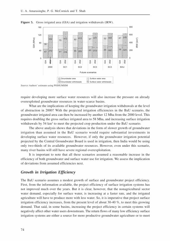
74
U. A. Amarasinghe, P. G. McCornick and T. Shah
require developing more surface water resources will also increase the pressure on alreadyoverexploited groundwater resources in water-scarce basins.
What are the implications of keeping the groundwater irrigation withdrawals at the levelof abstraction in 2000? With the projected irrigation efficiencies in the BaU scenario, thegroundwater irrigated area can then be increased by another 12 Mha from the 2000 level. Thisrequires doubling the gross surface irrigated area to 58 Mha, and increasing surface irrigationwithdrawals by 54 km3 to meet the projected crop production under the BaU scenario.
The above analysis shows that deviations in the form of slower growth of groundwaterirrigation than assumed in the BaU scenario would require substantial investments indeveloping surface water resources. However, if only the groundwater irrigation potentialprojected by the Central Groundwater Board is used in irrigation, then India would be usingonly two-thirds of its available groundwater resources. However, even under this scenario,many river basins will still have severe regional overexploitation.
It is important to note that all these scenarios assumed a reasonable increase in theefficiency of both groundwater and surface water use for irrigation. We assess the implicationof deviations from assumed efficiencies next.
Growth in Irrigation Efficiency
The BaU scenario assumes a modest growth of surface and groundwater project efficiency.First, from the information available, the project efficiency of surface irrigation systems hasnot improved much over the years. But it is clear, however, that the nonagricultural sectorwater demand, especially for surface water, is increasing at a faster rate, and the irrigatedagriculture will have to produce more with less water. So, it is imperative that project surfaceirrigation efficiency increases, from the present level of about 30-40 %, to meet this growingdemand. That said, in some basins, increasing the project efficiency in certain systems willnegatively affect other water users downstream. The return flows of many low efficiency surfaceirrigation systems are either a source for more productive groundwater agriculture or to meet
Figure 5. Gross irrigated area (GIA) and irrigation withdrawals (IRW).
Source:Authors’ estimates using PODIUMSIM
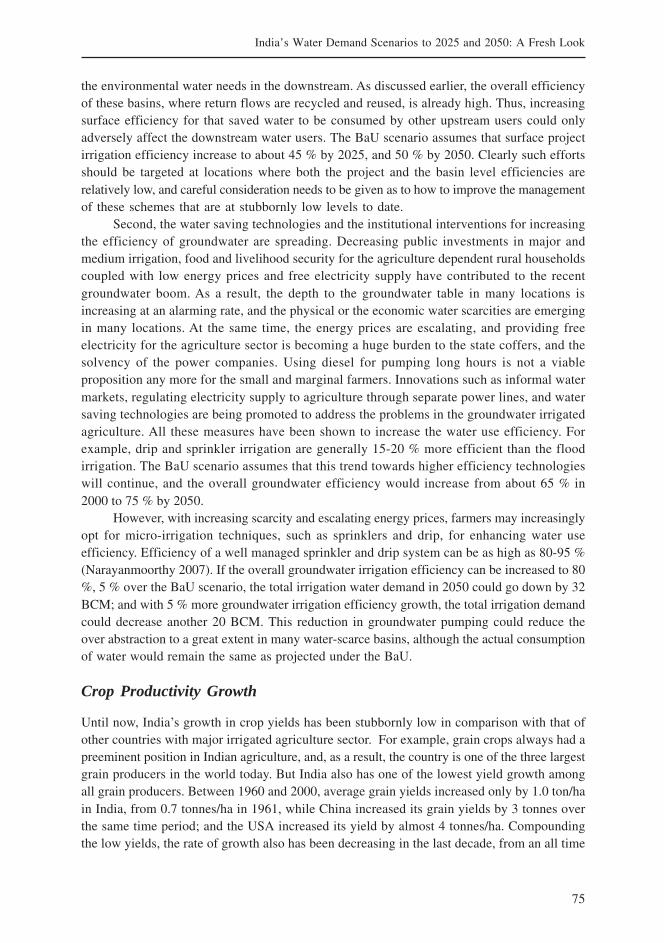
75
India’s Water Demand Scenarios to 2025 and 2050: A Fresh Look
the environmental water needs in the downstream. As discussed earlier, the overall efficiencyof these basins, where return flows are recycled and reused, is already high. Thus, increasingsurface efficiency for that saved water to be consumed by other upstream users could onlyadversely affect the downstream water users. The BaU scenario assumes that surface projectirrigation efficiency increase to about 45 % by 2025, and 50 % by 2050. Clearly such effortsshould be targeted at locations where both the project and the basin level efficiencies arerelatively low, and careful consideration needs to be given as to how to improve the managementof these schemes that are at stubbornly low levels to date.
Second, the water saving technologies and the institutional interventions for increasingthe efficiency of groundwater are spreading. Decreasing public investments in major andmedium irrigation, food and livelihood security for the agriculture dependent rural householdscoupled with low energy prices and free electricity supply have contributed to the recentgroundwater boom. As a result, the depth to the groundwater table in many locations isincreasing at an alarming rate, and the physical or the economic water scarcities are emergingin many locations. At the same time, the energy prices are escalating, and providing freeelectricity for the agriculture sector is becoming a huge burden to the state coffers, and thesolvency of the power companies. Using diesel for pumping long hours is not a viableproposition any more for the small and marginal farmers. Innovations such as informal watermarkets, regulating electricity supply to agriculture through separate power lines, and watersaving technologies are being promoted to address the problems in the groundwater irrigatedagriculture. All these measures have been shown to increase the water use efficiency. Forexample, drip and sprinkler irrigation are generally 15-20 % more efficient than the floodirrigation. The BaU scenario assumes that this trend towards higher efficiency technologieswill continue, and the overall groundwater efficiency would increase from about 65 % in2000 to 75 % by 2050.
However, with increasing scarcity and escalating energy prices, farmers may increasinglyopt for micro-irrigation techniques, such as sprinklers and drip, for enhancing water useefficiency. Efficiency of a well managed sprinkler and drip system can be as high as 80-95 %(Narayanmoorthy 2007). If the overall groundwater irrigation efficiency can be increased to 80%, 5 % over the BaU scenario, the total irrigation water demand in 2050 could go down by 32BCM; and with 5 % more groundwater irrigation efficiency growth, the total irrigation demandcould decrease another 20 BCM. This reduction in groundwater pumping could reduce theover abstraction to a great extent in many water-scarce basins, although the actual consumptionof water would remain the same as projected under the BaU.
Crop Productivity Growth
Until now, India’s growth in crop yields has been stubbornly low in comparison with that ofother countries with major irrigated agriculture sector. For example, grain crops always had apreeminent position in Indian agriculture, and, as a result, the country is one of the three largestgrain producers in the world today. But India also has one of the lowest yield growth amongall grain producers. Between 1960 and 2000, average grain yields increased only by 1.0 ton/hain India, from 0.7 tonnes/ha in 1961, while China increased its grain yields by 3 tonnes overthe same time period; and the USA increased its yield by almost 4 tonnes/ha. Compoundingthe low yields, the rate of growth also has been decreasing in the last decade, from an all time
76
U. A. Amarasinghe, P. G. McCornick and T. Shah
high of 3.8 % annually for grains in the 1980s to 2.0 % in the 1990s. Recent policy decisionsof the government of India suggest that there will be more investments for research anddevelopment for increasing crop productivity in the coming decades. Therefore, although theBaU scenario does not anticipate a complete reversal of the declining trends of cropproductivity, it expects a reduction in the rate of decline of the growth rates. In fact, this ratheroptimistic assumption of growth in crop yield is a key component of BaU scenario food andwater demand projections.
In spite of these decreasing trends, this analysis assumes that a substantial scope existsfor increasing the yield beyond the current level. A significant gap exists in many locationsbetween the highest and the lowest actual yields, and between the actual and the potentialyields. The future investments, both private and public sector, focus on small-scaleinfrastructure and technologies that enhance the crop yields. Breeding of rice hybrids andimproved varieties of other crops (improving harvest index), reducing losses through pestsand diseases and post-harvest losses, expanding groundwater use and micro irrigationtechnologies offer significant opportunities for the irrigated yield growth. And thesupplementary irrigation, through water harvesting (Sharma et al. in this volume), at criticalperiods of water stress, can substantially boost rain-fed yields. Moreover, farmers will havean incentive to increase crop productivity to benefit from the increasing internal and externalfood trade. Thus, the BaU scenario crop productivity growth rate assumptions are somewhatoptimistic than the assumptions recent trends indicate. Even these assumptions to some extentare conservative according to some, as they argue that a second green revolution is welloverdue. If that happened it could dramatically change this yield growth scenario.
BaU scenario in this paper projects the decreasing trend of yield growth to continue,albeit at a slower rate. The grain yield growth is expected to be 1.5 % annually between 2000and 2025, and 1.0 % annually between 2025 and 2050. BaU scenario assumes a similar growthpattern for non-grain crops.
Irrigated agriculture is estimated to contribute three-quarters of the crop production by2050. Thus, a small increase in the irrigated yield from the BaU scenario can significantly increasethe crop output from the same irrigated area or reduce the irrigation demand to maintain thesame production levels. For example, the BaU scenario expects the irrigated grain yield to increasefrom 2.6 to 4.43 tonnes/ha between 2000 and 2050. But our analysis shows that crop yield growthassumptions indeed are very sensitive to the total crop production and irrigation water demandprojections. Figure 6 shows grain production and irrigation demand under different landproductivity (LP in tonnes/ha) and water productivity (WP in kg/m3 of consumptive water use)growth assumptions. SCE1-SCE4 assume that land or water productivity increase annually at0.08 to 0.30 % higher than the assumed growth in the BaU scenario.
If irrigated land productivity can be doubled by 2050, as indicated in SCE4, then thegrain production can be increased by 13 % from the same irrigated area. On the other hand, ifwater productivity is doubled, the crop production can be maintained at the BaU scenariolevel with 15 % less irrigation withdrawals. Is this a realistic goal to achieve? One could arguethat, given the significant productivity variations that exist in similar agro-climatic zones(Molden et al. 1998), doubling water productivity in 50 years is not an impossible target toachieve. The SCE4 has the average grain yields of China in 2000. Can India reach the China’syield levels in 50 years from now? If it can, future grain production requires much less irrigationwater than they use now.
77
India’s Water Demand Scenarios to 2025 and 2050: A Fresh Look
Figure 6. Grain production and irrigation demand under different assumptions of land and waterproductivity growth.
Source:Authors estimates based on PODIUMSIM analysis.
Rain-fed Crop Production
Although the above discussion mostly focused on irrigation, a brief description of the potentialimprovements in the rain-fed agriculture is required here. Rain-fed agriculture, water harvestingand the related yield improvements are discussed in detail in two later papers. We discusshere only the rain-fed agriculture contribution to the BaU scenario. Another key assumptionof the BaU scenario is that India’s net sown area will remain the same in the period 2000-2050.This assumption implies that the existing rain-fed area is either replaced by the new irrigatedarea or taken over for the nonagricultural purposes. Over the period 2000-2050, the rain-fedcrop area under the BaU scenario is projected to decrease from 60-44 % of the gross croppedarea. How will then rain-fed agriculture contribute to overall crop production?
In 2000, grain area under rain-fed agriculture was 57 % of the total grain area, andcontributed to 33 % of the crop production. Abysmally low rain-fed yield was the main reasonfor low contribution. India’s grain yield, only 0.97 tonnes/ha in 2000, is one of the lowestamong the countries with significant rain-fed areas. It is only 20 %, 32 % and 37 % of the rain-fed yield of the USA, China and Argentina, respectively. Given these differences, it seems thata substantial scope exists for improvements in the rain-fed yield in the future. Indeed, in Paper10, Bharat et al. show that with proper application of inputs and a small dose of supplementalirrigation in the water stress crop periods the yields of many rain-fed crops can even double.
The BaU scenario assumes that the rain-fed yield will increase to 1.3 tonnes/ha in 2025,and 1.8 tonnes/ha by 2050. That is the BaU assumes that rain-fed yield will increase by 80 %over the 50-year period from 2000. By 2050, the rain-fed area will consist of 34 % of the totalgrain area, but contributes to 28 % of the total grain production. This contribution can be increasedfurther with the higher growth in rain-fed yield. The results of that obviously is lower requirementfor irrigated area expansion and hence irrigation. In Paper 10, Bharat et al. show that local waterharvesting, in extremely non-arid or non-wet areas, could indeed provide the small supplementalirrigation that is required for the rain-fed yield increase. However, in Paper 14, Dinesh et al. show
78
U. A. Amarasinghe, P. G. McCornick and T. Shah
that water harvesting potential is very low in water- scarce areas due to physical and institutionalconstraints. Further research is required to identify the high potential rain-fed areas where waterharvesting is feasible for providing the small supplemental irrigation.
Conclusion
This report discussed the implications of future food and water demand under the businessas usual scenario trends. For most determinants, the BaU scenario assumes the growth patternsof the recent years for future projection. For the yield growth, based slightly optimistic assertionof agriculture investments, we assume somewhat higher growth rates than the recent trends.
On the water demand side the BaU scenario projects that:
• India’s total water demand, for the irrigation, industrial and domestic sectors, increases22 % and 32 %, respectively by 2025 and 2050, from the estimated withdrawals of 680bcm in 2000;
• industrial and domestic sectors account for 54 % and 85 % of the additional waterdemand by 2025 and 2050, respectively;
• groundwater use will contribute to a major share of the future irrigation waterwithdrawals;
• and on the supply side several basins will reach physical water-scarce condition by2050, where the remaining utilizable water supply cannot be developed further withoutmaking a severe impact on the environment and riverrine water users down stream; and
• groundwater abstraction to increase significantly and many basins will haveunsustainable water use regions, where the total available groundwater throughrecharge from natural rainfall and return flows in some regions are not adequate formeeting the increasing demand.
The agriculture water demand projections have accounted for the expected changes inconsumption patterns. The BaU projections show that on the food demand side,
• India’s preeminence in food grains in the diet is changing, and food grain consumptionwill continue to decrease from 471 grams/person/day in 2000 to 454 and 417 grams/person/day, respectively by 2025 and 2050;
• non-grain crop products including vegetables, fruits and vegetable oil, and animalproducts, primarily from dairy and eggs, will provide a major part of the nutritionalintake by 2050; and
• due to increasing animal product consumption, the feed grain demand will increasesignificantly from a mere 8 mmt in 2000 to about 38 and 111 mmt by 2025 and 2050.
And, on the food supply side,
• there will be production deficits of maize and pulses, but the production surpluses ofrice and wheat offset this deficit, and will have grain production surpluses over thedemand;
79
India’s Water Demand Scenarios to 2025 and 2050: A Fresh Look
• oil crops and fruits will have production deficits by 2050; but
• crop diversification will help decrease the overall value of crop production deficitsfrom 9 % of the demand in 2000 to about 4 % by 2050.
The sensitivity analysis shows that changes in the ground water irrigated area,groundwater efficiency and crop productivity could significantly alter the BaU food and waterdemand projections. A slight crop productivity growth, in both irrigated and rain-fed agriculture,beyond the BaU assumption could result in a significant
• reduction in water needs for meeting the projected food demands; or
• increase in food production from the projected level of BaU irrigation withdrawals.
In fact crop water productivity growth is by far the best option for meeting future fooddemand while reducing the pressure on water resources. It is imperative that India shouldinvest in increasing research and extension for increasing their crop productivity from thedismal levels at present.
Groundwater expansion is also an influential driver on future water demand. Given thepresent investment patterns, groundwater will continue to play a major role in irrigationexpansion in the short to medium terms. Groundwater expansion not only reduces thewithdrawal requirement, but could also lead to higher crop productivity and economic benefits.However, overexploitation in different river basins could be a serious constraint for sustaininggroundwater expansion in the future. India should invest in artificial recharge programs forincreasing the groundwater stocks where opportunities exist to capture water from underdeveloped basins or sub-basins and recharge into appropriate aquifers as long as it does notcreate adverse impacts in the down stream water users.
India should also introduce physical and institutional interventions including microirrigation techniques, regulating the electricity supply and introducing efficient water markets,for reducing the uncontrolled pumping in many river basins. Depending on the extent of thesuccess of these programs groundwater expansion will continue to expand and benefit theirrigation users.
It is also important to note that it may be inevitable that India will have to find adequatesurface water resource for meeting the increasing domestic and industrial water requirements.The additional surface water resource required for these two sectors exceed the estimatedsurface water reallocation from the irrigation sector. This requirement may increase beyondthe BaU scenario estimates with a higher growth in Indian economy.
80
U. A. Amarasinghe, P. G. McCornick and T. Shah
Annex 1.
Assumption of Key Drivers in the BaU Scenario
The assessment of BaU scenario uses the methodology of PODIUMSIM model Policy DialogueModel Simulation for projecting India’s water future. The PODIUMSIM is a tool for simulatingthe alternative scenarios of food and water future with respect to the variation of food andwater demand drivers. The model has four major components, which can assess food and waterdemand at various temporal and spatial scales: crop demand (annual and state/river basins/national), crop production (seasonal and districts/state/river basins), water demand (monthlyand districts/state/river basins) and water accounting (annual and river basins) (for more detailssee www.iwmi.org/applications/podium). Annex Table 1 gives the key drivers of the BaU scenarioand few other comparable scenarios projecting India’s water futures.
Changing consumption patterns is a key driver for estimating food demand in the BaUscenario. The BaU scenario projects that significant increase in contribution from non-grainfood crops and animal products increase the total nutritional intake, whereas the NCIWRDscenario projects increasing dependency on food grains. According to the BaU trends,expanding groundwater irrigation and changing cropping patterns are key drivers for projectingthe irrigation demand, whereas the NCIWRD scenario projects significant increases in surfaceirrigation of grain crops, with a substantial rice area. Changes in cropping patterns and irrigationefficiencies reduce the irrigation demand under BaU scenario between 2025 and 2050. However,due to high demand for irrigating grain crops, total irrigation demand under the NCIWRDscenario increases significantly over the same time period. Increase in domestic and industrialwater demand is more than 85% of the additional water demand between 2000 and 2050 underthe BaU scenario, while it is only 48 % under the NCIWRD scenario.
Seckler et al. 1998; IWMI 2000; and Rosegrant et al. 2002 scenarios only projected foodand water demand to 2025. Both scenarios assumed lower population projections and higherdemand for food grains than the BaU. The overall water demand projection of Rosegrant et al.scenario, after adjustment for the differences of population projects, is similar to that of BaU,while Seckler et al. 1998 scenario project higher total water demand.

81
India’s Water Demand Scenarios to 2025 and 2050: A Fresh Look
Annex Table 1. Summary of the key drivers and water demand projections of BaU and other scenariosfor India.
Drivers Unit 2000i BaU NCIWRD Seckler Roasgrantscenario high demand et al.ii et al.ii
projectionsii scenarioii
2025 2050 2025 2050 2025 2025
Population Million 1,007 1,389 1,583 1,383 1,581 1,273 1,352
- % urban population % 28 37 51 45 61 43 43
Total calorie supply/person/day Kcal 2,495 2,775 3,000 - - 2,812 -
- % of food grains % 65 57 48 - - 58 -
- % from non-grain food crops % 28 33 36 - - 32 -
- % from animal products % 8 12 16 - - 11 -
Food grain demand/person/year Kg 172 166 152 210 284 188 183
Total grain demand/person/year Kg 200 210 238 231 312 215 215
Net sown area Mha 142 142 142 144 145 - -
Net irrigated area Mha 55 74 81 67iii 93iii - -
- from groundwater Mha 34 43 50 34iv 42iv - -
Gross irrigated area Mha 76 105 117 98 146 90 76
Irrigated area of grains Mha 54 59 63 69 102 61 51
Rain-fed area of grains Mha 69 62 57 70 57 61 69
Total grain availability/person/year Kg 208 213 240 242 312 216 206
Net irrigation requirement Km3 245 313 346 359iv 536iv 323 332
Irrigation efficiency- surface water % 30-45 35-50 42-60 50 60 - -
Irrigation efficiency- groundwater % 55-65 70 75 72 75 - -
Total irrigation demand Km3 605 675 637 611 807 702 741
- from groundwater Km3 272 304 325 245 344 - -
Irrigation for grain crops Km3 417 398 351 428 565 - -
Domestic water demand/person m3/day 33 45 64 45 70 31 31
Industrial water demand/person m3/day 42 66 102 48 51 55
Total water demand Km3 680 833 900 773 1,069 811 822
Notes: i Data for 2000 is from various publications of Government of India;ii BaU, NCIWRD, Seckler et al. and Rosegrant et al. Information is compiled from GOI 1999, Amarasinghe et al. 2007b,IWMI 2001, and Rosegrant et al. 2002, respectively.iii Estimated with cropping intensities- 141 % in 2025 and 155 % in 2050; iv Estimated with percent from groundwaterirrigation- 50 % in 2025 and 43.7 % in 2050.
82
U. A. Amarasinghe, P. G. McCornick and T. Shah
References
Amarasinghe, U. A.; Shah, T.; Turral, H. 2006. India’s Water Futures to 2025-2050: Business as UsualScenario and Issues. Draft prepared for the IWMI-CPWF project on ‘Strategic Analyses of NationalRiver Linking Project of India’.
Amarasinghe, U.A.; Sharma, B.R.; Aloysius, N.; Scott, C.; Smakhtin, V.; de Fraiture, C. 2005. Spatialvariation of water supply and demand across river basins of India. Research Report 83. Colombo, SriLanka: International Water Management Institute.
Amarasinghe, U. A.; Shah, T.; Singh, O. P. 2007a. Changing consumption patterns: implications forfood and water demand in India. IWMI Research Report 119, Colombo, Sri Lanka: International WaterManagement Institute.
Amarasinghe, U. A.; Shah, T.; Turral, H.; Anand, B.K. 2007b. India’s water futures to 2025-2050: BAUscenario and deviations. IWMI Research Report 123, Colombo, Sri Lanka: International WaterManagement Institute.
Bhaduri, A.; Amarasinghe, U.A.; Shah, T. (2006). Groundwater irrigation India: Analysis and Prognostics.Draft prepared for the IWMI-CPWF project on ‘Strategic Analyses of National River Linking Projectof India’.
FAO. 2005. FAOSATAT Data Base. Rome: Food and Agriculture Organization.
GOI. 1999. Integrated water resources development. A plan for action. Report of the Commission forIntegrated Water Resource Development Volume I. New Delhi, India: Ministry of Water Resources.
GOI. 2004. Agricultural statistics at a glance 2004. New Delhi, India: Ministry of Agriculture, Governmentof India.
Hemme, T.; Garcia, O.; Saha, A. 2003. Review of milk production with a particular emphasis on small-scale producers. PPLPI Working Paper No 2. Rome: FAO
IWMI. 2000. World water supply and demand 1995 to 2025 (draft).www.cgiar.org/iwmi/pubs/WWVison/WWSDOpen.htm
Kumar, M.D.; Samad, M.; Amarasinghe, U. A.; Singh, O.P. 2006. Water saving technologies: How far canthey contribute to water productivity enhancement in Indian agriculture? Draft prepared for the IWMI-CPWF project on ‘Strategic Analyses of National River Linking Project of India’.
Kundu, A. 2006. Estimating urban population and its size class distribution at regional level in the contextof demand for water: Methodological issues. Draft prepared for the IWMI-CPWF project on ‘StrategicAnalyses of National River Linking Project of India’.
Mahmood, A.; Kundu, A. 2006. Demographic projections for India 2006-2051: Regional variations. Draftprepared for the IWMI-CPWF project on ‘Strategic Analyses of National River Linking Project of India’.
Molden, D.J. 1997. Accounting for water use and productivity. SWIM Paper 1. Colombo, Sri Lanka:International Water Management Institute.
Molden, D.; Sakthivadivel, R.; Perry, C. J.; de Fraiture, C.; Kloezen, W. K. 1998. Indicators for comparingperformance of irrigated agricultural systems. Research Report 20. Colombo, Sri Lanka: InternationalWater Management Institute.
Narayanamoorthy, A. 2006. Potential for drip and sprinkler irrigation in India. Draft prepared for theIWMI-CPWF project on ‘Strategic Analyses of National River Linking Project of India’.
Pandey, U.K. 1995. The Livestock Economy of India: A Profile. Journal of Indian Agricultural Economics.Vol 50, No. 3. pp 264-282.
Rosegrant, M.; Cai, X.; Cline, S. 2002. World Water and Food to 2025. Dealing with Scarcity. WashingtonD.C.: International Food Policy Research Institute.
83
India’s Water Demand Scenarios to 2025 and 2050: A Fresh Look
Shah, T.; Roy, A.D.; Qureshi, A.S.; Wang, J. 2001. Sustaining Asia’s Groundwater Boom: An Overview ofIssues ad Evidence. Draft paper prepared for the International Conference on Freshwater in Bonn
Seckler, D.; Amarasinghe, U. A.; Molden, D.; de Silva, R.; Barker, R. 1998. World water demand andsupply 1995 to 2025: Scenarios and issues. Research Report No. 19. Colombo, Sri Lanka: InternationalWater Management Institute
Shiklomonav, I. 1999. World Water Resources and their Use.http://webworld.unesco.org/water/ihp/db/shiklomanov/
Thenkabail, P. S.; Biradar, C. M.; Turral, H.; Noojipady, P.; Li, Y. J.; Vithanage, J.; Dheeravath, V.; Velpuri,M.; Schull, M.; Cai, X. L.; Dutta, R. 2006. An irrigated area map of the world (1999) derived fromremote sensing. Research Report 105. Colombo, Sri Lanka: International Water Management Institute.
UN. 2004. World population prospects, the 2004 revision. New York: UN Department for PolicyCoordination and Sustainable Development.
WRI. 2005. Earth trends. Searchable database http://earthtrends.wri.org. Washington, D.C.
85
Meeting India’s Water Future: Some Policy Options
1Upali A. Amarasinghe, 2Tushaar Shah and 3Peter G. McCornick 1International Water Management Institute (IWMI), New Delhi, India
2International Water Management Institute (IWMI), Anand, India3International Water Management Institute (IWMI), Sri Lanka
Introduction
The best course for managing and further developing India’s water resources is a hotly debatedsubject, with some of the more contentious arguments centered on the large scale interbasintransfers planned as part of the National River Linking Project (NRLP). As part of a broaderstudy to examine the NRLP and potential alternatives, this paper seeks to identify some of themore promising policy options which could be part of a strategic and holistic effort to addressIndia’s future water challenges.
Accounting for the characteristics of recent water resources development andmanagement, the paper considers the future water needs should the country continue alongthis business as usual (BaU) path. In addition to the developments proposed under the NRLP,the other considered policy options , which could serve to replace or remove the need forelements of the NRLP, or which compliment elements of the NRLP, include increased emphasison recharging groundwater to offset the over abstraction; adoption of water savingtechnologies for increasing water use efficiency1; formal or informal water markets; provisionof more reliable yet rationed rural electricity supply to reduce uncontrolled groundwaterabstraction; and increasing research and extension for enhancing agriculture water productivity.
As in many countries, agriculture is the largest user of water in India, and as such hasand will continue to be a major driver of water resources management and development in thecountry. The dominance of food grains and the prominence of surface irrigation in India’sagricultural production are gradually changing. In fact groundwater is already the dominantwater source for agriculture, and recent trends show that agriculture is diversifying to cater tothe changing domestic consumption patterns and increasing export opportunities. Groundwaterirrigation is continuing to expand to meet the increasing demand of water in agriculture. Generallythe agricultural diversification is to higher value crops and livestock, which in most casesrequires costlier inputs, and necessitates a relatively reliable water supply. Until now, theinherent reliability of groundwater has made it the source of choice.
1 However, in many cases while such technologies may reduce the amount of water pumped, it maynot result in water savings at the basin scale.
86
U. A. Amarasinghe, T. Shah and R. P. S. Malik
The unplanned development of the resource, and the difficulties of managing it thereaftermeans that an increasing number of aquifers are over exploited, resulting in high social andenvironmental cost, and jeopardizing the reliability of the supply. Groundwater resources withinmany river basins will soon reach this critical stage with continuing groundwater expansion(Amarasinghe et al. 2007). Without appropriate management strategies and interventions, theseunsustainable practices will lead to serious crises, perhaps in the near future and most certainlywithin the next four to five decades for some regions. We discuss the pending water crisis inthe next section.
However, there are a number of policy options which could avert such a crisis. Artificialgroundwater recharge, increasing efficiency of groundwater use, reducing uncontrolledgroundwater pumping can sustain the groundwater expansion. Among others, increasingproductivity and diversifying with proper cropping patterns can also offer a significantleverage. We discuss these policy options in detail in the third section.
In spite of these options, there are situations where major interbasin transfers may stillbe inevitable, especially over the long term. The justification and necessary support for suchinvestments is unlikely to come from the development of new irrigated areas, at least not as asignificant part of the investments, but is more likely from a combination of increased domesticand industrial water demand, providing a reliable water supply for high-value crops, growingpressure on the groundwater systems, escalating energy prices, and from increased efforts toaccount for environmental needs. We discuss them in the final section.
Pending Water Crisis
India already withdraws about 273 cubic kilometer (km3) of groundwater per annum, which isestimated to be around 60 % of the sustainable yield (Amarasinghe et al. 2007). Given thatmost of the groundwater is abstracted for agriculture and that most has been developed bythe private sector, it is anticipated that groundwater will continue to be the major source forfuture growth in irrigated areas.
Projections based on the most recent trends estimate that a further 14 million ha of landwill be brought under irrigation by 2025 (Figure 1), and an additional 10 million ha by 2050(Amarasinghe et al. 2007). Consequently, the Business as Usual Scenario projects that 31 km3
of additional groundwater withdrawals will occur by 2025, and a further 22 km3 by 2050. Theresult will be that by 2025 and 2050 India would be withdrawing 75 % and 85 % of thesustainable groundwater supply, respectively, accounting for both natural and return flowrecharge. With this, several river basins would become water scarce and the rate of use wouldbe unsustainable. In fact, 10 basins will withdraw more than 75 % of their available groundwatersupply, and these 10 basins account for 69 % of the total groundwater supply in India.
On the other hand, if groundwater withdrawals are to remain at the 2000 level, then theadditional surface withdrawal requirement will need to increase further by 65 km3 by 2025, inpart because surface water systems are less efficient than groundwater based systems. Thepeninsular basins, some of which are already water scarce, will require more than half of thetotal additional surface water withdrawals projected for the country, which is more than 35km3. Given the past investment trends and the slow growth of canal irrigation in recent decades,it is difficult to envisage adding this quantity of surface water in the next 25 years. Furthermore,such demands cannot be met in the peninsular rivers without diverting from elsewhere.
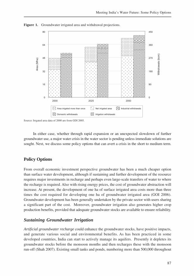
87
Meeting India’s Water Future: Some Policy Options
In either case, whether through rapid expansion or an unexpected slowdown of furthergroundwater use, a major water crisis in the water sector is pending unless immediate solutions aresought. Next, we discuss some policy options that can avert a crisis in the short to medium term.
Policy Options
From overall economic investment perspective groundwater has been a much cheaper optionthan surface water development, although if sustaining and further development of the resourcerequires major investments in recharge and perhaps even large-scale transfers of water to wherethe recharge is required. Also with rising energy prices, the cost of groundwater abstraction willincrease. At present, the development of one ha of surface irrigated area costs more than threetimes the cost required for developing one ha of groundwater irrigated area (GOI 2006).Groundwater development has been generally undertaken by the private sector with users sharinga significant part of the cost. Moreover, groundwater irrigation also generates higher cropproduction benefits, provided that adequate groundwater stocks are available to ensure reliability.
Sustaining Groundwater Irrigation
Artificial groundwater recharge could enhance the groundwater stocks, have positive impacts,and generate various social and environmental benefits. As has been practiced in somedeveloped countries, India can start to actively manage its aquifers. Presently it depletes itsgroundwater stocks before the monsoon months and then recharges these with the monsoonrun-off (Shah 2007). Existing small tanks and ponds, numbering more than 500,000 throughout
Figure 1. Groundwater irrigated area and withdrawal projections.
Source: Irrgated area data of 2000 are from GDI 2005.
88
U. A. Amarasinghe, T. Shah and R. P. S. Malik
India, which are already augmenting the natural groundwater recharge, can be modified tofurther increase recharge, while meeting the drinking water demand for the human beings andlivestock (Sakthivadivel 2007). Also, new small tanks and ponds need to be designed andconstructed with a view to optimizing groundwater recharge, where appropriate. However, weneed to know more about the negative impacts of groundwater recharge on downstream usersbefore embarking on large-scale recharging programs, especially in water scarce river basins.Also the underlying hydrogeology will dictate whether recharge will result in improved suppliesof groundwater in a form which can be appropriately utilized.
Rainwater harvesting programs, such as johads in Alawr district in Rajasthan(Sakthivadivel 2007) and also groundwater recharge movements in Saurashtra and Kutch (Shahand Desai 2002), have proven to rejuvenate the groundwater resources available for irrigation.However, some interventions, such as rain water harvesting in the upstream catchments, havebeen shown to reduce the inflows to existing reservoirs downstream (Kumar et al. 2006a), andcan incur more cost than the benefits they generate.
The existing knowledge on surface and groundwater interaction across river basins inIndia is generally site-specific and neither sufficient to identify the locations where suchnegative impacts can occur nor, in fact, to determine where and how to improve groundwaterrecharge. Further research is required to identify the locations where artificial groundwaterrecharge harnesses water; the quantity of water that can be harnessed and the extent to whichit meets the additional demand; and the net social benefits that these programs generate.
Increasing groundwater irrigation efficiency by an additional 5 % from the level assumedunder the BaU scenario (70 %) can reduce the additional groundwater demand in 2025 byabout 20 km3 or two-thirds, assuming that these savings result in savings at the basin scale.Recent research shows that modern irrigation technologies — sprinklers and drip irrigation— are operating at 70-85 % efficiency in some irrigation systems in India (Kumar et al. 2006b,Narayanmoorthy 2006). Modern irrigation technologies also improve the uniform distributionof the irrigation water, reduce non-beneficial transpiration, and in general have higherproductivity than the traditional flood irrigation methods. However, adoption of thesetechnologies in India has been very slow. And these technologies were mainly adopted fora few crops, such as fruits and vegetables, in the groundwater irrigated areas(Narayanamoorthy 2006; Kumar et al. 2006b). Further research and extension are needed todetermine the potential of such irrigation technologies in the Indian context, their neteconomic benefits and practical modalities to scale them up where appropriate. In addition,it is imperative that it be determined that these interventions would result in actual watersavings, and not result in the transfer of water from other users further down the basin, ashas been the case elsewhere.
Reducing uncontrolled groundwater pumping could mitigate over abstraction in manybasins. In 2000, India withdrew about 273 km3 of groundwater to meet only 151 km3 of cropconsumptive water-use demand. Indeed, proper policy and institutional interventions canreduce over abstraction even when traditional irrigation methods are utilized. Formal or informalwater markets (Somanathan and Ravindranath 2006; Banerji et al. 2006), and regulating and/orproviding a reliable rural electricity supply (Shah and Verma 2000) have been shown to havesome effect on controlling unnecessary pumping and increasing water-use efficiency.Replicating these interventions, with adjustments to satisfy local socioeconomy, could helparrest the uncontrolled groundwater pumping in many water-stressed river basins.
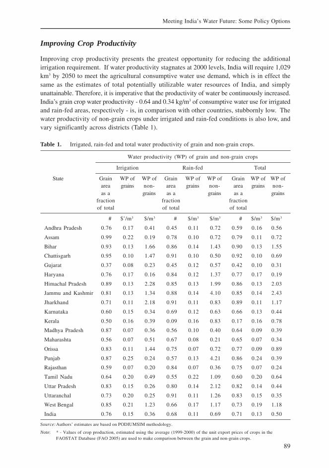
89
Meeting India’s Water Future: Some Policy Options
Improving Crop Productivity
Improving crop productivity presents the greatest opportunity for reducing the additionalirrigation requirement. If water productivity stagnates at 2000 levels, India will require 1,029km3 by 2050 to meet the agricultural consumptive water use demand, which is in effect thesame as the estimates of total potentially utilizable water resources of India, and simplyunattainable. Therefore, it is imperative that the productivity of water be continuously increased.India’s grain crop water productivity - 0.64 and 0.34 kg/m3 of consumptive water use for irrigatedand rain-fed areas, respectively - is, in comparison with other countries, stubbornly low. Thewater productivity of non-grain crops under irrigated and rain-fed conditions is also low, andvary significantly across districts (Table 1).
Table 1. Irrigated, rain-fed and total water productivity of grain and non-grain crops.
Water productivity (WP) of grain and non-grain crops
Irrigation Rain-fed Total
State Grain WP of WP of Grain WP of WP of Grain WP of WP ofarea grains non- area grains non- area grains non-as a grains as a grains as a grains
fraction fraction fractionof total of total of total
# $*/m3 $/m3 # $/m3 $/m3 # $/m3 $/m3
Andhra Pradesh 0.76 0.17 0.41 0.45 0.11 0.72 0.59 0.16 0.56
Assam 0.99 0.22 0.19 0.78 0.10 0.72 0.79 0.11 0.72
Bihar 0.93 0.13 1.66 0.86 0.14 1.43 0.90 0.13 1.55
Chattisgarh 0.95 0.10 1.47 0.91 0.10 0.50 0.92 0.10 0.69
Gujarat 0.37 0.08 0.23 0.45 0.12 0.57 0.42 0.10 0.31
Haryana 0.76 0.17 0.16 0.84 0.12 1.37 0.77 0.17 0.19
Himachal Pradesh 0.89 0.13 2.28 0.85 0.13 1.99 0.86 0.13 2.03
Jammu and Kashmir 0.81 0.13 1.34 0.88 0.14 4.10 0.85 0.14 2.43
Jharkhand 0.71 0.11 2.18 0.91 0.11 0.83 0.89 0.11 1.17
Karnataka 0.60 0.15 0.34 0.69 0.12 0.63 0.66 0.13 0.44
Kerala 0.50 0.16 0.39 0.09 0.16 0.83 0.17 0.16 0.78
Madhya Pradesh 0.87 0.07 0.36 0.56 0.10 0.40 0.64 0.09 0.39
Maharashta 0.56 0.07 0.51 0.67 0.08 0.21 0.65 0.07 0.34
Orissa 0.83 0.11 1.44 0.75 0.07 0.72 0.77 0.09 0.89
Punjab 0.87 0.25 0.24 0.57 0.13 4.21 0.86 0.24 0.39
Rajasthan 0.59 0.07 0.20 0.84 0.07 0.36 0.75 0.07 0.24
Tamil Nadu 0.64 0.20 0.49 0.55 0.22 1.09 0.60 0.20 0.64
Uttar Pradesh 0.83 0.15 0.26 0.80 0.14 2.12 0.82 0.14 0.44
Uttaranchal 0.73 0.20 0.25 0.91 0.11 1.26 0.83 0.15 0.35
West Bengal 0.85 0.21 1.23 0.66 0.17 1.17 0.73 0.19 1.18
India 0.76 0.15 0.36 0.68 0.11 0.69 0.71 0.13 0.50
Source:Authors’ estimates are based on PODIUMSIM methodology.
Note: * - Values of crop production, estimated using the average (1999-2000) of the unit export prices of crops in theFAOSTAT Database (FAO 2005) are used to make comparison between the grain and non-grain crops.
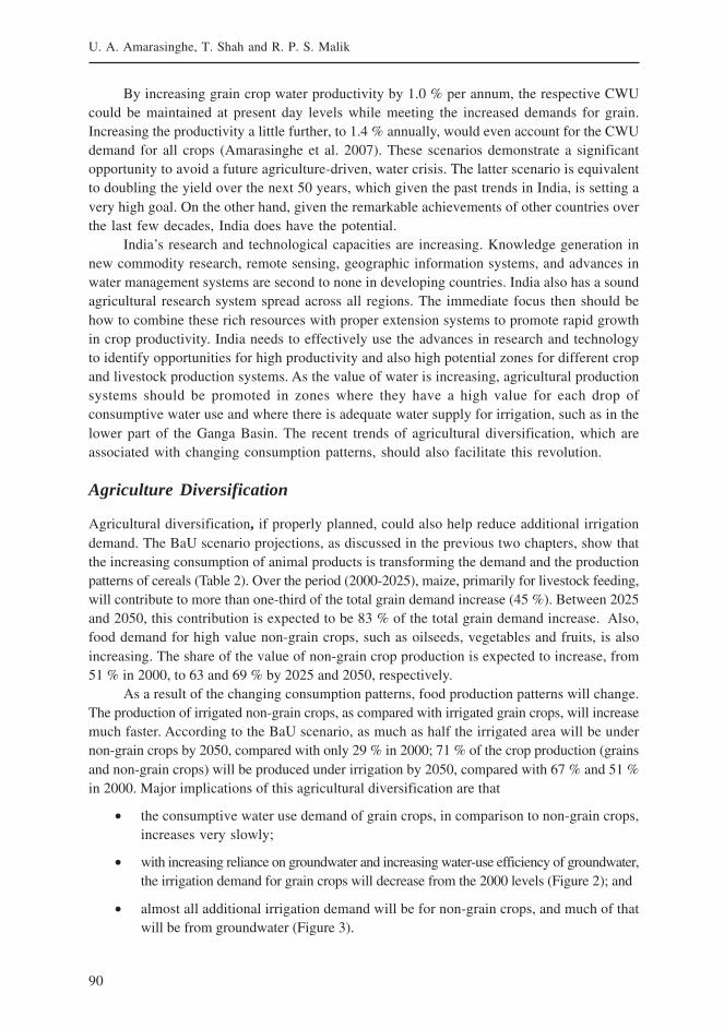
90
U. A. Amarasinghe, T. Shah and R. P. S. Malik
By increasing grain crop water productivity by 1.0 % per annum, the respective CWUcould be maintained at present day levels while meeting the increased demands for grain.Increasing the productivity a little further, to 1.4 % annually, would even account for the CWUdemand for all crops (Amarasinghe et al. 2007). These scenarios demonstrate a significantopportunity to avoid a future agriculture-driven, water crisis. The latter scenario is equivalentto doubling the yield over the next 50 years, which given the past trends in India, is setting avery high goal. On the other hand, given the remarkable achievements of other countries overthe last few decades, India does have the potential.
India’s research and technological capacities are increasing. Knowledge generation innew commodity research, remote sensing, geographic information systems, and advances inwater management systems are second to none in developing countries. India also has a soundagricultural research system spread across all regions. The immediate focus then should behow to combine these rich resources with proper extension systems to promote rapid growthin crop productivity. India needs to effectively use the advances in research and technologyto identify opportunities for high productivity and also high potential zones for different cropand livestock production systems. As the value of water is increasing, agricultural productionsystems should be promoted in zones where they have a high value for each drop ofconsumptive water use and where there is adequate water supply for irrigation, such as in thelower part of the Ganga Basin. The recent trends of agricultural diversification, which areassociated with changing consumption patterns, should also facilitate this revolution.
Agriculture Diversification
Agricultural diversification, if properly planned, could also help reduce additional irrigationdemand. The BaU scenario projections, as discussed in the previous two chapters, show thatthe increasing consumption of animal products is transforming the demand and the productionpatterns of cereals (Table 2). Over the period (2000-2025), maize, primarily for livestock feeding,will contribute to more than one-third of the total grain demand increase (45 %). Between 2025and 2050, this contribution is expected to be 83 % of the total grain demand increase. Also,food demand for high value non-grain crops, such as oilseeds, vegetables and fruits, is alsoincreasing. The share of the value of non-grain crop production is expected to increase, from51 % in 2000, to 63 and 69 % by 2025 and 2050, respectively.
As a result of the changing consumption patterns, food production patterns will change.The production of irrigated non-grain crops, as compared with irrigated grain crops, will increasemuch faster. According to the BaU scenario, as much as half the irrigated area will be undernon-grain crops by 2050, compared with only 29 % in 2000; 71 % of the crop production (grainsand non-grain crops) will be produced under irrigation by 2050, compared with 67 % and 51 %in 2000. Major implications of this agricultural diversification are that
• the consumptive water use demand of grain crops, in comparison to non-grain crops,increases very slowly;
• with increasing reliance on groundwater and increasing water-use efficiency of groundwater,the irrigation demand for grain crops will decrease from the 2000 levels (Figure 2); and
• almost all additional irrigation demand will be for non-grain crops, and much of thatwill be from groundwater (Figure 3).
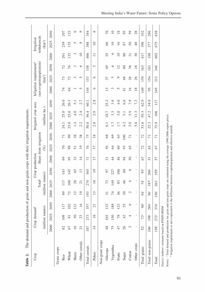
91
Meeting India’s Water Future: Some Policy Options
Tab
le 2
.T
he d
eman
d an
d pr
oduc
tion
of
grai
n an
d no
n-gr
ain
crop
s w
ith
thei
r ir
riga
tion
req
uire
men
ts.
Cro
pC
rop
dem
andi
Cro
p pr
oduc
tion
Irri
gate
d cr
op a
rea
Irri
gati
on r
equi
rem
entii
Irri
gati
onT
otal
iS
hare
fro
m i
rrig
atio
n(n
et-e
vapo
tran
spir
atio
n)w
ithd
raw
als
(mil
lion
ton
nes)
(mil
lion
ton
nes)
(%)
(mil
lion
ha
)(k
m3 )
(km
3 )
2000
2025
2050
2000
2025
2050
2000
2025
2050
2000
2025
2050
2000
2025
2050
2000
2025
2050
Gra
in c
rops
Ric
e82
109
117
8911
714
369
7071
24.1
25.0
26.0
7473
7226
123
920
7
Whe
at67
9110
272
108
145
9599
9923
.025
.026
.364
7276
132
135
122
Mai
ze16
5012
112
2865
3251
381.
44.
05.
11
33
35
6
Oth
er c
erea
ls21
2316
1921
1314
1938
2.2
2.4
2.7
55
610
99
Tot
al c
erea
ls18
727
335
719
327
436
571
7675
50.8
56.4
60.1
144
153
158
406
388
344
Puls
es14
1821
1318
1917
1718
2.8
2.9
2.8
66
511
108
Non
-gra
in c
rops
Oil
crop
s48
103
133
3173
9731
5668
6.1
18.7
25.2
1337
4925
6676
Veg
etab
les
7515
018
974
149
227
4464
691.
73.
33.
83
56
610
10
Frui
ts47
7812
346
8310
646
6063
1.7
3.0
4.0
59
1210
1618
Sug
ar26
4255
3046
6094
9310
04.
25.
16.
641
4860
8087
95
Cot
ton
24
62
46
5065
713.
05.
97.
916
2838
3150
59
Oth
er c
rops
--
--
--
--
-5.
611
.37.
318
2618
3648
28
Tot
al g
rain
s52
i73
i90
i54
i74
i93
i67
7272
53.6
59.3
62.9
149
159
163
417
398
352
Tot
al n
on-g
rain
s10
6i19
8i28
4i96
i18
7i26
6i51
6571
22.3
47.2
54.8
9515
418
318
827
728
6
Tot
al15
8i27
2i37
4i15
0i26
1i35
9i57
6771
75.9
106
117
245
313
346
605
675
638
Sour
ce:A
utho
rs’
esti
mat
es b
ased
on
PO
DIU
MS
IM
Not
es:
i Tot
al d
eman
d an
d pr
oduc
tion
for
gra
in a
nd n
on-g
rain
cro
ps a
re e
stim
ated
usi
ng t
he a
vera
ge 1
990-
2000
exp
ort
pric
es.
ii I
rrig
atio
n re
quir
emen
t or
net
eva
pora
tion
is
the
diff
eren
ce b
etw
een
evap
otra
nspi
rati
on a
nd e
ffec
tive
rai
nfal
l.
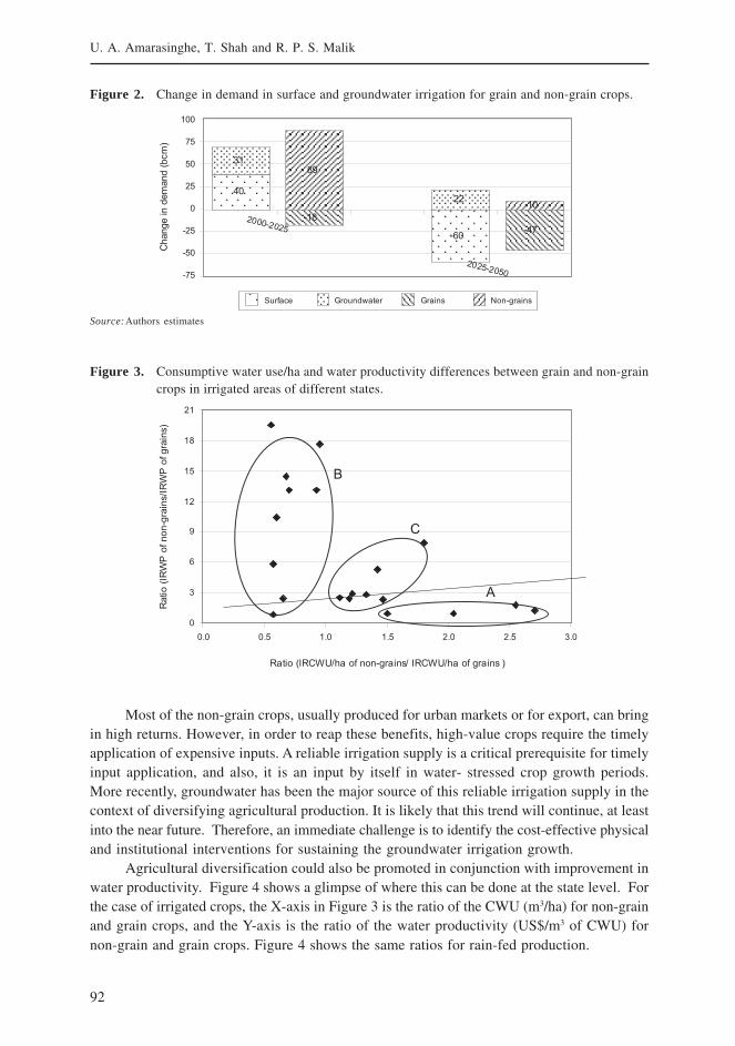
92
U. A. Amarasinghe, T. Shah and R. P. S. Malik
Most of the non-grain crops, usually produced for urban markets or for export, can bringin high returns. However, in order to reap these benefits, high-value crops require the timelyapplication of expensive inputs. A reliable irrigation supply is a critical prerequisite for timelyinput application, and also, it is an input by itself in water- stressed crop growth periods.More recently, groundwater has been the major source of this reliable irrigation supply in thecontext of diversifying agricultural production. It is likely that this trend will continue, at leastinto the near future. Therefore, an immediate challenge is to identify the cost-effective physicaland institutional interventions for sustaining the groundwater irrigation growth.
Agricultural diversification could also be promoted in conjunction with improvement inwater productivity. Figure 4 shows a glimpse of where this can be done at the state level. Forthe case of irrigated crops, the X-axis in Figure 3 is the ratio of the CWU (m3/ha) for non-grainand grain crops, and the Y-axis is the ratio of the water productivity (US$/m3 of CWU) fornon-grain and grain crops. Figure 4 shows the same ratios for rain-fed production.
Figure 2. Change in demand in surface and groundwater irrigation for grain and non-grain crops.
Source:Authors estimates
Figure 3. Consumptive water use/ha and water productivity differences between grain and non-graincrops in irrigated areas of different states.
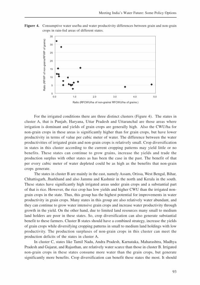
93
Meeting India’s Water Future: Some Policy Options
For the irrigated conditions there are three distinct clusters (Figure 4). The states incluster A, that is Punjab, Haryana, Uttar Pradesh and Uttaranchal are those areas whereirrigation is dominant and yields of grain crops are generally high. Also the CWU/ha fornon-grain crops in these areas is significantly higher than for grain crops, but have lowerproductivity in terms of value per cubic meter of water. The difference between the waterproductivities of irrigated grain and non-grain crops is relatively small. Crop diversificationin states in this cluster according to the current cropping patterns may yield little or nobenefits. These states can continue to grow grains, increase the yields and trade theproduction surplus with other states as has been the case in the past. The benefit of thatper every cubic meter of water depleted could be as high as the benefits that non-graincrops generate.
The states in cluster B are mainly in the east, namely Assam, Orissa, West Bengal, Bihar,Chhattisgarh, Jharkhand and also Jammu and Kashmir in the north and Kerala in the south.These states have significantly high irrigated areas under grain crops and a substantial partof that is rice. However, the rice crop has low yields and higher CWU than the irrigated non-grain crops in the state. Thus, this group has the highest potential for improvements in waterproductivity in grain crops. Many states in this group are also relatively water abundant, andthey can continue to grow water intensive grain crops and increase water productivity throughgrowth in the yield. On the other hand, due to limited land resources many small to mediumland holders are poor in these states. So, crop diversification can also generate substantialbenefit to these farmers. Cluster B states should have a combined strategy, increase the yieldsof grain crops while diversifying cropping patterns in small to medium land holdings with lowproductivity. The production surpluses of non-grain crops in this cluster can meet theproduction deficits of the states in cluster A.
In cluster C, states like Tamil Nadu, Andra Pradesh, Karnataka, Maharashtra, MadhyaPradesh and Gujarat, and Rajasthan, are relatively water scarce than those in cluster B. Irrigatednon-grain crops in these states consume more water than the grain crops, but generatesignificantly more benefits. Crop diversification can benefit these states the most. It should
Figure 4. Consumptive water use/ha and water productivity differences between grain and non-graincrops in rain-fed areas of different states.
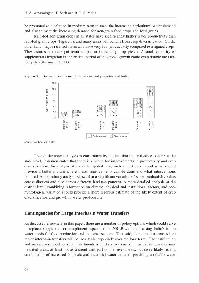
94
U. A. Amarasinghe, T. Shah and R. P. S. Malik
be promoted as a solution in medium-term to meet the increasing agricultural water demandand also to meet the increasing demand for non-grain food crops and feed grains.
Rain-fed non-grain crops in all states have significantly higher water productivity thanrain-fed grain crops (Figure 5), and many areas will benefit from crop diversification. On theother hand, major rain-fed states also have very low productivity compared to irrigated crops.These states have a significant scope for increasing crop yields. A small quantity ofsupplemental irrigation in the critical period of the crops’ growth could even double the rain-fed yield (Sharma et al. 2006).
Figure 5. Domestic and industrial water demand projections of India.
Source:Authors estimates
Though the above analysis is constrained by the fact that the analysis was done at thestate level, it demonstrates that there is a scope for improvements in productivity and cropdiversification. An analysis at a smaller spatial unit, such as district or sub-basins, shouldprovide a better picture where these improvements can de done and what interventionsrequired. A preliminary analysis shows that a significant variation of water productivity existsacross districts and also across different land-use patterns. A more detailed analysis at thedistrict level, combining information on climate, physical and institutional factors, and geo-hydrological variation should provide a more rigorous estimate of the likely extent of cropdiversification and growth in water productivity.
Contingencies for Large Interbasin Water Transfers
As discussed elsewhere in this paper, there are a number of policy options which could serveto replace, supplement or compliment aspects of the NRLP while addressing India’s futurewater needs for food production and the other sectors. That said, there are situations wheremajor interbasin transfers will be inevitable, especially over the long term. The justificationand necessary support for such investments is unlikely to come from the development of newirrigated areas, at least not as a significant part of the investments, but more likely from acombination of increased domestic and industrial water demand, providing a reliable water
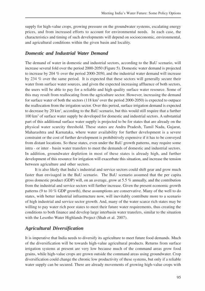
95
Meeting India’s Water Future: Some Policy Options
supply for high-value crops, growing pressure on the groundwater systems, escalating energyprices, and from increased efforts to account for environmental needs. In each case, thecharacteristics and timing of such developments will depend on socioeconomic, environmental,and agricultural conditions within the given basin and locality.
Domestic and Industrial Water Demand
The demand of water in domestic and industrial sectors, according to the BaU scenario, willincrease several fold over the period 2000-2050 (Figure 5). Domestic water demand is projectedto increase by 204 % over the period 2000-2050, and the industrial water demand will increaseby 234 % over the same period. It is expected that these sectors will generally secure theirwater from surface water sources, and given the expected increasing affluence of both sectors,the users will be able to pay for a reliable and high quality surface water resource. Some ofthis may result from reallocating from the agriculture sector. However, increasing the demandfor surface water of both the sectors (118 km3 over the period 2000-2050) is expected to outpacethe reallocation from the irrigation sector. Over this period, surface irrigation demand is expectedto decrease by 20 km3, according to the BaU scenario, but this would still require that a further100 km3 of surface water supply be developed for domestic and industrial sectors. A substantialpart of this additional surface water supply is projected to be for states that are already on thephysical water scarcity threshold. These states are Andra Pradesh, Tamil Nadu, Gujarat,Maharashtra and Karnataka, where water availability for further development is a severeconstraint or the cost of further development is prohibitively expensive if it has to be conveyedfrom distant locations. So these states, even under the BaU growth patterns, may require someintra - or inter - basin water transfers to meet the demands of domestic and industrial sectors.In addition, groundwater depletion in most of these states is already high, and furtherdevelopment of this resource for irrigation will exacerbate this situation, and increase the tensionbetween agriculture and other sectors.
It is also likely that India’s industrial and service sectors could shift gear and grow muchfaster than envisaged in the BaU scenario. The BaU scenario assumed that the per capitagross domestic product (GDP) will, on an average, grow at 5.5 % annually, and the contributionfrom the industrial and service sectors will further increase. Given the present economic growthpatterns (9 to 10 % GDP growth), these assumptions are conservative. Many of the well to dostates, with better industrial infrastructure now, will inevitably contribute more to a scenarioof high industrial and service sector growth. And, many of the water scarce rich states may bewilling to pay water rich poor states to meet their future water requirements, thus creating theconditions to both finance and develop large interbasin water transfers, similar to the situationwith the Lesotho Water Highlands Project (Shah et al. 2007).
Agricultural Diversification
It is imperative that India needs to diversify its agriculture to meet future food demands. Muchof the diversification will be towards high-value agricultural products. Returns from surfaceirrigation systems at present are very low because much of the command areas grow foodgrains, while high-value crops are grown outside the command areas using groundwater. Cropdiversification could change the chronic low productivity of these systems, but only if a reliablewater supply can be secured. There are already movements of growing high-value crops with
96
U. A. Amarasinghe, T. Shah and R. P. S. Malik
a reliable water supply for urban markets or export. Should this gather momentum, water scarcesouthern and western India, with their increasing income from high-value agriculture, may bewilling to invest for interbasin water transfers. However, if low productivity of these surfaceirrigation systems persists, and further irrigation sources have to be developed, includinginterbasin transfers to meet the demands for high-value crops it will be a significantly moreexpensive solution both in terms of economics and water resources.
Rising Cost of Energy
Irrigation expansion in India in the last two decades was primarily due to small-scale liftirrigation systems using mostly groundwater, but also surface water. These systems are highlyflexible and provide reliable irrigation supply on demand. Yet, this mode of irrigationdevelopment is, in most cases, highly energy intensive. So far, the energy supplies of manystates are highly subsidized. But the cost of energy, whether it be in the form of electricity ordiesel, has been rapidly increasing in recent times. States can no longer continue to providesubsidies on electricity as they are an impediment to economic growth in other sectors. Asenergy prices increase, the farmers may opt for direct surface water for irrigation or reducetheir pumping costs by groundwater recharge. Thus, rising energy cost could be anothercondition from the agriculture sector that supports, to some extent, the development of large-scale interbasin water transfers. Conceivably there could also be an indirect argument forinterbasin transfers where concurrent development of hydropower could provide increasedsupplies of electricity, however, from an economic perspective this new power source wouldbe better utilized in the industrial and service sectors.
Conclusion
Increasing agricultural water productivity offers one of the greatest opportunities to reducethe demand for additional irrigation. By doubling the water productivity over the next fivedecades, no additional irrigation would be required, at least on-balance. The achievement ofthis will require major investments in research, development, extension on better managementof other inputs, and infrastructure particularly to improve the reliability of water supply.
Crop diversification offers opportunities to increase the value produced by the sameamount of water, which would be particularly important in the water scarce basins in peninsularIndia. Crop diversification in already high water productivity areas, such as in north and northwest, will need further understanding as the water productivity is already high for grain crops.In the water abundant east there is considerable scope to increase the productivity of graincrops, yet crop diversification would help the poor small farmers increase their returns fromtheir land.
Based on recent trends, groundwater will continue to be the source of choice for furtherdevelopment of irrigation for the foreseeable future. However, in an increasing number of basins,aquifers are becoming over exploited. Continuing along this business as usual pathway meansthat India is heading for an increasing number of regional water crises. Depending on thespecific conditions, artificial recharge could significantly enhance groundwater supplies. Suchinterventions should include renewed efforts for small scale water recharge systems, but also
97
Meeting India’s Water Future: Some Policy Options
carefully consider large scale facilities, including as components of inter - basin transferprojects. The implementation of any large scale programs or interventions must determine,among other things, the hydrogeological suitability, the likely negative implications on thedownstream water users, and the relative economic viability. Increasing groundwater irrigationefficiency and other demand management strategies will also be helpful for reducing thegroundwater over-abstraction.
While it is acknowledged that the interactions between the surface and groundwaterresources will be different for a given basin and the dynamics will very much depend on howthese resources are developed, the important point to emphasize is that the policy environmentfor water resources management in India must take into account the present realities, and allowfor not only the realistic future demands, but the real constraints of the availability of theresource. Specifically, much more emphasis needs to be placed on effective management ofthe groundwater resources through enhancing the supply by artificial recharge andconservation. Also, revived efforts should be made to improve the existing surface irrigationsystems, in particular to reconfigure the systems to provide more reliable water supply andallow effective community level management, where appropriate. To achieve this requires alevel of study and investigation beyond what has been hither to done in most situations.
Further development of groundwater, and water savings and reallocation of water fromthe agricultural sector will not be sufficient to meet the water requirements of other sectors.The increasing capacity and willingness of the domestic and industrial sectors to pay for cleanand reliable water supply would increase the pressure for further surface water resourcesdevelopment. Such conditions are likely to emerge soon in states with high economic growth,particularly in the basins that are water scarce. Most of these are located in peninsular India,and meeting the additional surface water demand in these basins may require large intra - orinterbasin water transfers.
Acknowledgements
This paper presents findings of the project ‘Strategic Analyses of India’s River Linking Project’,a part of the CGIAR’s Challenge Program for Water for Food.
98
U. A. Amarasinghe, T. Shah and R. P. S. Malik
References
Amarasinghe, U. A.; Shah, T.; Turral, H. Anand B. 2007. India’s water futures to 2025-2050: Business asusual scenario and deviations. IWMI Research Report 123. Colombo, Sri Lanka: International WaterManagement Institute.
Banerji, A.; Khanna, G.; Meenakshi, J.V. 2006. Markets, institutions and efficiency: groundwater irrigationin north India. Working Paper 152. New Delhi, India: Department of Economics, Delhi School ofEconomics.
GOI 2005. Agricultural Statistics at a Glance 2004. New Delhi, India: Ministry of Agriculture, Governmentof India.
GOI 2006. Report of the Working Group on Water Resources for the XI Five-year Plan (2002-2007).New Delhi, India: Ministry of Water Resources.
Kumar, M.D.; Patel, A.; Singh, O.P. 2006a. Rainwater Harvesting in Water-scarce Regions of India. Draft,IWMI-CPWF Project on ‘Strategic Analyses of India’s National River-Linking Project’, Colombo, SriLanka: International Water Management Institute.
Kumar, M. D.; Samad, M.; Amarasinghe, U. A.; Singh, O.P. 2006b. Water saving and yield enhancingtechnologies: How far can they contribute to water productivity enhancement in Indian agriculture?Draft, IWMI-CPWF Project on ‘Strategic Analyses of India’s National River-Linking Project’, Colombo,Sri Lanka: International Water Management Institute.
Narayanamoorthy, A. 2006. Potential for drip and sprinkler irrigation in India. Draft, IWMI-CPWF Projecton ‘Strategic Analyses of India’s National River-Linking Project’, Colombo, Sri Lanka: InternationalWater Management Institute.
Sakthivadivel, R. 2007. The Groundwater Recharge Movements in India. In The Agricultural GroundwaterRevolution: Opportunities and Threats to Development, eds. M. Giordano; K. G. Villholth. CABInternational, Wallingford, UK, pp. 191-210.
Shah, T. 2000. Mobilizing social energy against environmental challenge: understanding the groundwaterrecharge movement in western India. Natural Resources Forum 24 (3): 197-209.
Shah, T. 2007. The Groundwater Economy of South Asia: An Assessment of Size, Significance and Socio-ecological Impacts. In The Agricultural Groundwater Revolution: Opportunities and Threats toDevelopment, eds. M. Giordan.; Villholth. CAB International, Wallingford, UK pp. 7-36.
Shah, T.; Desai R. 2002. Decentralized water harvesting and groundwater recharge: Can these save Saurashtraand Kutch from desiccation? Paper presented at the First IWMI-TATA Annual Water Policy Workshopheld at Anand, India during February 13-14, 2002.
Shah, T.; Amarasinghe, U.A.; McCornick, P.G. 2007. India’s River Linking Project: The state of the debate.Draft, IWMI-CPWF Project on ‘Strategic Analyses of India’s National River-Linking Project’, Colombo,Sri Lanka: International Water Management Institute.
Shah, T.; Verma, S. 2008. Co-management of Electricity and Groundwater: An Assessment of Gujarat’sJyotirgram Scheme. Economic and Political Weekly, Vol.43 (7): 59-66.
Sharma, B.; Rao, K. V.; Vittal, K. P. R. 2006. Realizing the rain-fed agriculture potential in India. Draftprepared for the IWMI-CPWF project on ‘Strategic Analysis of National River Linking Project of India’.
Somanathan, E.; Ravindranath, R. 2006. Measuring the Marginal Value of Water and Elasticity of Demandfor Water in Agriculture. Economic and Political Weekly, June 30, 2006.

99
Meeting India’s Water Future: Some Policy Options
Part II
101
Demographic Projections for India 2006-2051:Regional Variations
Aslam Mahmood and Amitabh KunduJawaharlal Nehru University, New Delhi
Introduction
The size and growth of population in India and in many other developing countries of theworld was not a serious concern of the planners and administrators until the first quarter ofthe last century. Even during the second quarter of the last century, the rapid population growthin many of the developing countries was not taken seriously. It is only during the third quarterof the last century that the growth of population in India and in many other developingcountries started showing its serious consequences on their resources. Population stabilizationhas thus emerged as a major agenda, particularly in the context of acute pressure on agriculturalresources and urban facilities.
Planning for the future requirements of the population, therefore, has become the majorconcern of the planners and requires accurate estimates of the future population growth. UnitedNations and several other national and international agencies, therefore prepare populationprojections and keep on updating them as and when fresh information becomes available. ForIndia main projections in the recent past have been prepared by United Nations, ExpertCommittee of the Planning Commission, Population Foundation of India (Natrajan 2000) andPopulation Council (Visaria and Visaria 1996)
A review of these projection exercises reveals that the figures vary extensively dependingon the developmental parameters incorporated in their models. Importantly, the NationalCommission for Integrated Water Resources Development (NCIWRD 1999) has taken estimatesgiven by Visaria and Visaria 1996 as the ‘higher side variant’ (1,581.00 million) and those of theUnited Nations 2006 as the ‘low side variant’ (1,345.90) for the year 2050. These have then beenused for making future estimates of food requirement for the growing population in the country.
The projections, providing the basis for the analysis undertaken by the Commission,suffer from two major limitations: (a) both the projections were made prior to 2001 andtherefore did not have the benefit of the data provided by the Census of India 2001, withregard to the size and its age structure, geographical distribution, estimate of fertility andmortality etc., and base their projections on the basic age structure and the total populationgiven a decade ago by the Census of India 1991, and (b) none of the projections had beenmade giving due consideration to the impact of the HIV/AIDS on the expectancy of life andother demographic parameters.
102
A. Mahmood and A. Kundu
Another important limitation of almost all the population projections from the planningpoint of view is that they do not give projections at micro level such as districts. Natrajan andJaychandran’s district level estimates are among few such projections which suffer from thefact that they also use the base year data prior to 2001.
In the present paper an attempt has been made to prepare the fresh country levelpopulation projections by incorporating the age structure of the population given by the GOI2003. Also, at country level projections have been made which take into consideration theimpact of HIV/AIDS on the future estimates of mortality. These projections have been madefor average and high variant of fertility with HIV/AIDS and without HIV/AIDS.
These projections have been made for quinquennial periods: from 2001 to 2051 – Cohortusing Component method has been used. After making the all India population projectionsthe state wise population projections have also been prepared by using the state level basepopulation figures provided by GOI 2003 and projected figures of fertility and mortality usedby Natrajan and Jaychandra after adjusting them for the Sample Registration System (SRS)figures of 2001. They have used the time series data of TFR provided by the Sample RegistrationSystem (1971-1996) and using the mid point of 1983 as origin have projected the TFR valuesfrom 1996 to 2051 using the least square linear regression fit. They also assume that once theTFR of a state reaches 1.6 it can not further fall down from this level, the criterion used in thepresent case also. These estimates are quite reliable as they use the data of a time series endingvery close to 2001. However, on comparing their estimate of TFR for 2001 with the actualestimates of 2001 provided by SRS, it was found that the two differ marginally. It was thereforeconsidered appropriate to adjust the figures accordingly.
While making the population projection only two variants have been attempted: averageand high variants. The average variants correspond to the TFR generated by the regressionline. For the high variant of population projection, the upper limits of the 99 % confidenceinterval of the TFR were chosen. In view of the relatively stable values of the life expectancy,it was considered to keep them constant for both the projections.
In the second section of the paper the population projections are made for the majorstates of India using the same methodology as mentioned above for the country as a whole.At the state level, however, the effect of HIV/AIDS was not estimated due to the considerationsof accuracy.
Methods of Population Projection
Methods of making population projections can be classified mainly into following two methods:
1. Cohort Component Method
2. Mathematical Methods
Cohort Component Method of Population Projection
Growth of population in an area basically depends on births, deaths and net migration of peopleduring the period under consideration. The estimate of births and deaths is possible only whenthe estimates of fertility and mortality parameters of the population are available. For fertility,
103
Demographic Projections for India 2006-2051: Regional Variations
the parameters are age specific fertility rates (ASFR) and gross reproduction rates (GRR). Formortality projections one would require life expectancy or longevity of life (e0) and thecorresponding Life table to give age specific survival ratios. In case the population for whichprojection is being made is open to migration, estimates of migration are also needed. Thebasic task involved in population projection, therefore, is the projection of the future levels offertility, mortality and migration rates, if the population is open for migration.
Component method of population projection involves separate projection of the numberof males and females in different age groups. This method takes into account separately futurecourse of fertility, mortality and migration and is therefore considered more accurate than anymathematical method based on past trends. The ability to provide age sex break up of the projectedpopulation is an added advantage of this method. The method requires the following data:
• initial population with age and sex break up;
• past trends in mortality and assumptions about future trends in terms of survival ratiosby age and sex;
• past trends in fertility and assumptions about future trends; and
• past trend of migration and future assumption about its change.
A large majority of developing countries do not have reliable data on many of the aboveaspects. Consequently, appropriate estimates are to be obtained in place of actual data, basedon certain assumptions. The assumptions made in such exercises are briefly discussed below.
Initial Population
It is noted that the data related to actual population invariably suffer from both content andcoverage errors. Research studies by Coale and Hoover 1958, ORG Group 1974, Cassen andDysen 1976 etc. begin by correcting population figures before using them for making theirprojections. The basic assumption in this regard is that population growth will follow a smoothcurve over time and also from one age to another.
Mortality
The basic approach in the component method is that the survivors of the population of oneage group will move into the next age group over time. It should, therefore, be possible toobtain the number of persons in an age group at a given point of time by projecting the numberof survivors from a preceding (appropriate) age group. This, one can compute by multiplyingthe survival ratios worked out from a Life table to the population in the preceding age group.Thus, choosing a Life table is a critical task in any exercise of population projection. For thecountries for which a reliable Life table is not available, scholars have used the Model LifeTables prepared by the United Nations. Keeping in view the differences in the regional mortalitypatterns, separate sets of Model Life Tables have been prepared for major regions in the world.Among these, one can select a typical Life table suitable for the country. The figure of lifeexpectancy (e0), which is a powerful summary statistic of the Life Tables, is often very helpfulin the selection. Future changes in the level of mortality can also be affected by changing thevalues of life expectancy.
104
A. Mahmood and A. Kundu
Fertility
For estimating the number of births during a given period, we need the information on thefertility behavior of the population as reflected by Age Specific Fertility Rates (ASFR) of thefemale population. Assumptions about ASFR are made in terms of Gross Reproduction Rates(GRR) or Total Fertility Rate (TFR). TFR is a measure showing the average number of babiesborn to a couple during their whole span of reproductive period. A value of TFR=2.1 isgenerally taken as replacement level of fertility.
Migration
It would be important to consider international migration when population projections are tobe made at national level. However, in view of the fact that this is not very large in India, wemay choose to ignore this factor. However, for making the projections of urban population,the assumptions about rural to urban migration would be critical. As migration is one of themost complex phenomenon in population studies and is governed by a host of socioeconomicfactors, determining the trend and the absolute number of immigrants into urban areas will beextremely difficult. Notwithstanding the problems, one must make an attempt to determine themigration trend based on most likely socioeconomic configuration.
Mathematical Methods
For population projections, generally two types of methods are used: Exponential and Logistic.
Exponential Growth Method
In case the detailed information required for component method of population projection isnot available or if only broad estimates are required without the age and sex break up, it ispossible to make population projections with the help of the past trends determined statisticallyusing the past data. This would involve fitting a mathematical curve or a regression line to thetime series data on population. One can compute the population figures for a future time pointby extrapolating for the future values of time.
Logistic Growth Method
Due to natural and other constraints, it is argued that population growth can not go onindefinitely and certain internal checks are likely to emerge from within the system slowingdown the growth rate and bringing it to the equilibrium vis–a-vis the resources. Populationanalysts also observe that the growth curve of a population follows an exponential pathonly for a short period of time, say 30 to 40 years. Consequently, when it comes toprojecting the population for a longer period of time, there has to be provision for thestabilization of the population. Logistic functions that have this inbuilt characteristic, are,therefore, noted as useful in making long term projections of a population. The advantageof the logistic function is that it can stabilize the population at an exogenously determinedupper limit.
105
Demographic Projections for India 2006-2051: Regional Variations
Population Projections for India 2001 -2051
As pointed out earlier the population projections made so far have depended on the dataprovided by the census of India 1991. Since the results of the population census of 2001 areavailable there is a need to update the projections by using the latest figures for the parametersof fertility and mortality and the base population with its age-sex break-up.
Base Population
The latest age data for male and female for the country, provided by the GOI 2003, whichconstitutes the basis of our projection exercise, is given in Annex Table 1.
Assumption about Mortality
Dyson and Hanchate have incorporated the effect of HIV/AIDS on the future mortality ratesin making their population projection for India. This hopefully would bring the projected figurescloser to reality as the country is witnessing a high incidence of HIV/AIDS which is showinga steep rise in recent years. The methodology adopted by these scholars is in line with that ofa UN study which has empirically determined the relationship between the prevalence rates ofHIV/AIDS and the reduction in the life expectancy (e0), using the data of only six countrieswhere the prevalence rate was below 2.0 % (UN 1999). Based on this scanty data set, Dysonand Hanchate have assumed that while the life expectancy will continue to increase in future,the actual achievement during a period of about 15 years (starting from 1998 to that of 2011-2016) will be less by 1.7 years over the projected figure for males. Similarly, actual life expectancyfor females during 2011-2015 is taken to be less than the projected figure by 0.9 years.
It may be argued that the impact of HIV/AIDS incorporated in the model is somewhat onthe higher side. We have computed the life expectancy figures, as given in Table 1, based onthe values estimated by Natrajan and Jayachandra. Adjustments have nonetheless been madein these values to take into consideration the impact of HIV/AIDS. However, unlike Dysonand Hanchate, the decline has been assumed here to be somewhat less. Male life expectancyis projected to decline by 1.7 years over a period of 25 years. It is implied that the disease willbring down life expectancy by 0.34 years in every 5 years from 2001 up to 2026 (0.34*5= 1.7).From 2026 to 2051, the decline would be 1.5 years only, the five yearly decline being 0.3 yearsonly (0.3*5=1.5). In case of females, too, the values have been reduced at a lower rate (thanaccording to Dyson and Hanchate), keeping in view their lower status and prevailing familynorms, which are responsible for lower spread of the disease among women in India. It isassumed that AIDS will bring down life expectancy at a flat rate of one year in every 20 years.These life expectancy figures are given below in Table 1.
The lower impact of the epidemic can be justified in terms of growing awarenessabout the disease, precautionary steps by the public and non governmental agencies andthe considerable medical and food aid being provided to the affected people, as reportedby National Aids Control Organization (NACO). Also, the higher impact as proposed byDyson and Hanchette is based on the scanty data of a few countries that have asignificantly larger proportion of reported cases. The spread is likely to be less during thefollowing decades also because the channel of communication through the clients of the
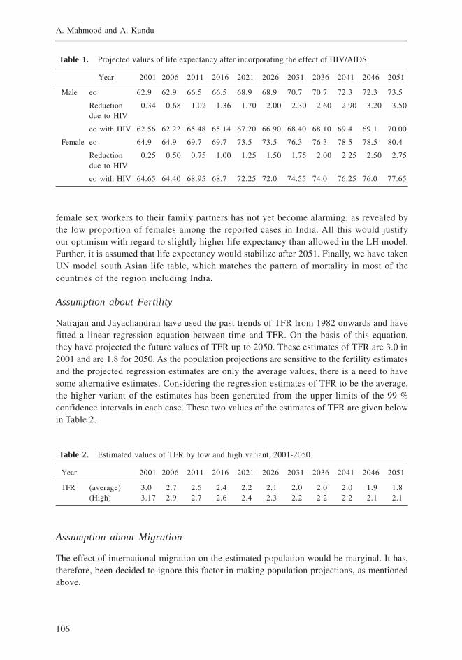
106
A. Mahmood and A. Kundu
female sex workers to their family partners has not yet become alarming, as revealed bythe low proportion of females among the reported cases in India. All this would justifyour optimism with regard to slightly higher life expectancy than allowed in the LH model.Further, it is assumed that life expectancy would stabilize after 2051. Finally, we have takenUN model south Asian life table, which matches the pattern of mortality in most of thecountries of the region including India.
Assumption about Fertility
Natrajan and Jayachandran have used the past trends of TFR from 1982 onwards and havefitted a linear regression equation between time and TFR. On the basis of this equation,they have projected the future values of TFR up to 2050. These estimates of TFR are 3.0 in2001 and are 1.8 for 2050. As the population projections are sensitive to the fertility estimatesand the projected regression estimates are only the average values, there is a need to havesome alternative estimates. Considering the regression estimates of TFR to be the average,the higher variant of the estimates has been generated from the upper limits of the 99 %confidence intervals in each case. These two values of the estimates of TFR are given belowin Table 2.
Table 1. Projected values of life expectancy after incorporating the effect of HIV/AIDS.
Year 2001 2006 2011 2016 2021 2026 2031 2036 2041 2046 2051
Male eo 62.9 62.9 66.5 66.5 68.9 68.9 70.7 70.7 72.3 72.3 73.5
Reduction 0.34 0.68 1.02 1.36 1.70 2.00 2.30 2.60 2.90 3.20 3.50due to HIV
eo with HIV 62.56 62.22 65.48 65.14 67.20 66.90 68.40 68.10 69.4 69.1 70.00
Female eo 64.9 64.9 69.7 69.7 73.5 73.5 76.3 76.3 78.5 78.5 80.4
Reduction 0.25 0.50 0.75 1.00 1.25 1.50 1.75 2.00 2.25 2.50 2.75due to HIV
eo with HIV 64.65 64.40 68.95 68.7 72.25 72.0 74.55 74.0 76.25 76.0 77.65
Table 2. Estimated values of TFR by low and high variant, 2001-2050.
Year 2001 2006 2011 2016 2021 2026 2031 2036 2041 2046 2051
TFR (average) 3.0 2.7 2.5 2.4 2.2 2.1 2.0 2.0 2.0 1.9 1.8(High) 3.17 2.9 2.7 2.6 2.4 2.3 2.2 2.2 2.2 2.1 2.1
Assumption about Migration
The effect of international migration on the estimated population would be marginal. It has,therefore, been decided to ignore this factor in making population projections, as mentionedabove.

107
Demographic Projections for India 2006-2051: Regional Variations
Projected Population of India 2001 -2051
Using the gender and age distribution of the population for 2001, the parameters of mortalitywith and without HIV/AIDS and the two variants of fertility, projections for population havebeen made based on the cohort component method. Population estimates have been obtainedfor each decade from 2001 up to 2051. We obtain a high as well as a low variant of thepopulations, with and without HIV/AIDS. These projections are given in Table 3 and Table 4below. The projections are also represented by the bar diagrams given in Figures 1 and 2.
Table 3. Population projections by average variant.
Year With HIV Without HIV Difference % Difference
2001 1,028,600 1,028,600 0 0
2006 1,106,008 1,106,652 644 0.058
2011 1,177,693 1,179,662 1,969 0.167
2016 1,258,887 1,262,724 3,837 0.304
2021 1,337,469 1,344,029 6,560 0.488
2026 1,405,370 1,415,278 9,908 0.700
2031 1,456,834 1,470,976 14,142 0.961
2036 1,501,831 1,520,732 18,901 1.243
2041 1,541,046 1,566,101 25,055 1.600
2046 1,573,836 1,605,119 31,283 1.949
2051 1,588,899 1,626,993 38,094 2.341
Our average variant of the population projections of 2051 (1,589 million) are very closeto projections prepared by Visaria and Visaria (1,581 million). The medium projections made byUN are also of the similar order (1,531). The high variant of our population projections (1,771million) are also close to latest UN high variant projections of 2002 (1,870 million) as comparedwith their earlier projection (1,980 million) of 1995. These projections also indicate that for abouttwo decades from now there is not going to be any respite in terms of the population growthrate. It is only after the second decade of this century that population growth is likely to showany retarding effect. In the first quarter of this century there is going to be the addition ofabout 430 million people as per high variant of the population projections whereas in the secondquarter, the addition is going to be 313 million. In the low variant of population projectionssimilar figures are 387 million and 211 million people.
Another important aspect of these projections is the likely effect of HIV/AIDS on thepopulation projections. Dyson and Hanchate have used UN estimates of HIV/AIDS onmortality in terms of its reduction of life expectancy for 1997 to 2011-2016. Their estimatesof population for 2026 with HIV/AIDS show a population of 1,394 million as compared toour low variant with HIV/AIDS of 1,405 million population. Part of the lowering effect onDyson and Hanchate’s projections is due to the initially lower estimate of 2001 which theyhave found as 1,010 million.
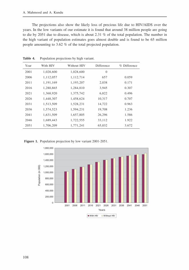
108
A. Mahmood and A. Kundu
The projections also show the likely loss of precious life due to HIV/AIDS over theyears. In the low variants of our estimate it is found that around 38 million people are goingto die by 2051 due to disease, which is about 2.31 % of the total population. The number inthe high variant of population estimates goes almost double and is found to be 65 millionpeople amounting to 3.62 % of the total projected population.
Table 4. Population projections by high variant.
Year With HIV Without HIV Difference % Difference
2001 1,028,600 1,028,600 0
2006 1,112,057 1,112,714 657 0.059
2011 1,191,169 1,193,207 2,038 0.171
2016 1,280,865 1,284,810 3,945 0.307
2021 1,368,920 1,375,742 6,822 0.496
2026 1,448,307 1,458,624 10,317 0.707
2031 1,513,509 1,528,231 14,722 0.963
2036 1,574,523 1,594,231 19,708 1.236
2041 1,631,509 1,657,805 26,296 1.586
2046 1,689,443 1,722,555 33,112 1.922
2051 1,706,209 1,771,241 65,032 3.672
Figure 1. Population projection by low variant 2001-2051.
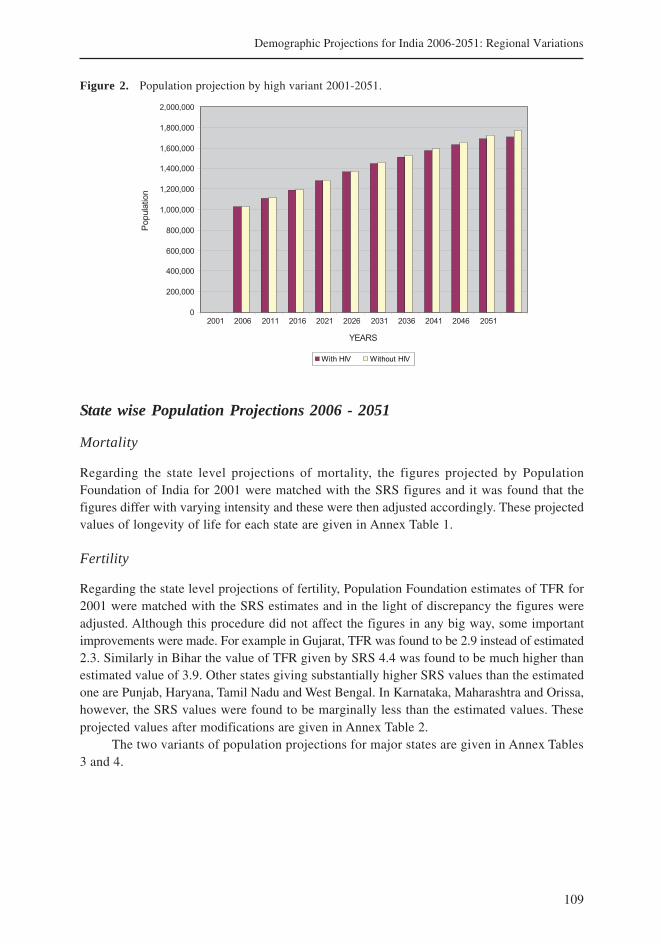
109
Demographic Projections for India 2006-2051: Regional Variations
Figure 2. Population projection by high variant 2001-2051.
State wise Population Projections 2006 - 2051
Mortality
Regarding the state level projections of mortality, the figures projected by PopulationFoundation of India for 2001 were matched with the SRS figures and it was found that thefigures differ with varying intensity and these were then adjusted accordingly. These projectedvalues of longevity of life for each state are given in Annex Table 1.
Fertility
Regarding the state level projections of fertility, Population Foundation estimates of TFR for2001 were matched with the SRS estimates and in the light of discrepancy the figures wereadjusted. Although this procedure did not affect the figures in any big way, some importantimprovements were made. For example in Gujarat, TFR was found to be 2.9 instead of estimated2.3. Similarly in Bihar the value of TFR given by SRS 4.4 was found to be much higher thanestimated value of 3.9. Other states giving substantially higher SRS values than the estimatedone are Punjab, Haryana, Tamil Nadu and West Bengal. In Karnataka, Maharashtra and Orissa,however, the SRS values were found to be marginally less than the estimated values. Theseprojected values after modifications are given in Annex Table 2.
The two variants of population projections for major states are given in Annex Tables3 and 4.
110
A. Mahmood and A. Kundu
References
Aggarwala, S. N. 1966. Some problems of India’s Population. Bombay: Vohra and Co.
Cassen, R. H.; Dyson, T. 1976. New Population Projections for India. Population and Development Review,Vol. 2 No.1. March.
Coale, A. J.; Hoover, E. M. 1958. Population Growth and Economic Development in Low Income Countries.Princeton: Princeton University Press.
Chaudhary, M. 1986. Poparative study of India’s Population Projections Based on the 1981 Census.Demography India, Vol. 15, No.1.
Dyson, T.; Hanchate, A. 2000. India’s Demographic and Food Prospects: State Level Analysis. Economicand Political Weekly, November 11, Vol. 35, No. 46.
GOI. 1996. Population Projection of India and States. Registrar General of India, New Delhi.
GOI. 2003. Final population totals – India (India, state, district, sub-district, town, ward-in-town and village).New Delhi, India: Office of the Registrar General and Census Commissioner.
Natrajan, K. S. 1982. Population Projections in Population of India: Country Monograph Series No.10.United Nations Economic and Social Commission for Asia and the Pacific, New York.
Natrajan, K. S.; Jayachandran, V. 2000. Population Growth in 21st Century India. Population Foundationof India, New Delhi.
Visaria, L.; Visaria, P. 1966. Perspective Population Growth and Policy Options for India 1991-2001. NewYork, The Population Council.
United Nations. 1999. The Demographic Impact of HIV/AIDS, ESA/P/WP152.
United Nations. 1982. Model Life Table for Developing Countries. New York.
United Nations. 1996. World Population Prospects (The Revision). New York: Department of Economicand Social Affairs Population Division.
United Nations. 1998. World Population Prospects (The Revision). New York: Department of Economicand Social Affairs Population Division.
United Nations. 2002. World Population Prospects (The Revision). New York: Department of Economicand Social Affairs Population Division.
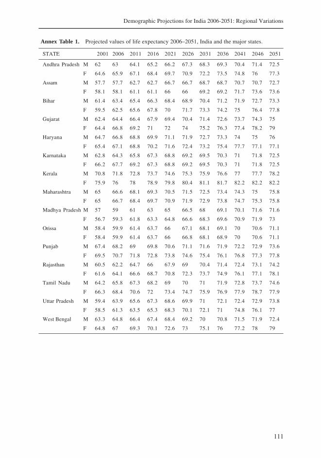
111
Demographic Projections for India 2006-2051: Regional Variations
Annex Table 1. Projected values of life expectancy 2006–2051, India and the major states.
STATE 2001 2006 2011 2016 2021 2026 2031 2036 2041 2046 2051
Andhra Pradesh M 62 63 64.1 65.2 66.2 67.3 68.3 69.3 70.4 71.4 72.5
F 64.6 65.9 67.1 68.4 69.7 70.9 72.2 73.5 74.8 76 77.3
Assam M 57.7 57.7 62.7 62.7 66.7 66.7 68.7 68.7 70.7 70.7 72.7
F 58.1 58.1 61.1 61.1 66 66 69.2 69.2 71.7 73.6 73.6
Bihar M 61.4 63.4 65.4 66.3 68.4 68.9 70.4 71.2 71.9 72.7 73.3
F 59.5 62.5 65.6 67.8 70 71.7 73.3 74.2 75 76.4 77.8
Gujarat M 62.4 64.4 66.4 67.9 69.4 70.4 71.4 72.6 73.7 74.3 75
F 64.4 66.8 69.2 71 72 74 75.2 76.3 77.4 78.2 79
Haryana M 64.7 66.8 68.8 69.9 71.1 71.9 72.7 73.3 74 75 76
F 65.4 67.1 68.8 70.2 71.6 72.4 73.2 75.4 77.7 77.1 77.1
Karnataka M 62.8 64.3 65.8 67.3 68.8 69.2 69.5 70.3 71 71.8 72.5
F 66.2 67.7 69.2 67.3 68.8 69.2 69.5 70.3 71 71.8 72.5
Kerala M 70.8 71.8 72.8 73.7 74.6 75.3 75.9 76.6 77 77.7 78.2
F 75.9 76 78 78.9 79.8 80.4 81.1 81.7 82.2 82.2 82.2
Maharashtra M 65 66.6 68.1 69.3 70.5 71.5 72.5 73.4 74.3 75 75.8
F 65 66.7 68.4 69.7 70.9 71.9 72.9 73.8 74.7 75.3 75.8
Madhya Pradesh M 57 59 61 63 65 66.5 68 69.1 70.1 71.6 71.6
F 56.7 59.3 61.8 63.3 64.8 66.6 68.3 69.6 70.9 71.9 73
Orissa M 58.4 59.9 61.4 63.7 66 67.1 68.1 69.1 70 70.6 71.1
F 58.4 59.9 61.4 63.7 66 66.8 68.1 68.9 70 70.6 71.1
Punjab M 67.4 68.2 69 69.8 70.6 71.1 71.6 71.9 72.2 72.9 73.6
F 69.5 70.7 71.8 72.8 73.8 74.6 75.4 76.1 76.8 77.3 77.8
Rajasthan M 60.5 62.2 64.7 66 67.9 69 70.4 71.4 72.4 73.1 74.2
F 61.6 64.1 66.6 68.7 70.8 72.3 73.7 74.9 76.1 77.1 78.1
Tamil Nadu M 64.2 65.8 67.3 68.2 69 70 71 71.9 72.8 73.7 74.6
F 66.3 68.4 70.6 72 73.4 74.7 75.9 76.9 77.9 78.7 77.9
Uttar Pradesh M 59.4 63.9 65.6 67.3 68.6 69.9 71 72.1 72.4 72.9 73.8
F 58.5 61.3 63.5 65.3 68.3 70.1 72.1 71 74.8 76.1 77
West Bengal M 63.3 64.8 66.4 67.4 68.4 69.2 70 70.8 71.5 71.9 72.4
F 64.8 67 69.3 70.1 72.6 73 75.1 76 77.2 78 79

112
A. Mahmood and A. Kundu
Annex Table 2. Projected total fertility rates 2006 – 2051.
STATE 2001 2005 2011 2016 2021 2026 2031 2036 2041 2046 2051
Andhra Pradesh 2.3 1.95 1.6 1.6 1.6 1.6 1.6 1.6 1.6 1.6 1.6
Assam 3 2.65 2.3 1.95 1.6 1.6 1.6 1.6 1.6 1.6 1.6
Bihar 4.4 3.84 3.28 2.72 2.16 1.6 1.6 1.6 1.6 1.6 1.6
Gujarat 2.9 2.47 2.03 1.6 1.6 1.6 1.6 1.6 1.6 1.6 1.6
Haryana 3.1 2.6 2.1 1.6 1.6 1.6 1.6 1.6 1.6 1.6 1.6
Karnataka 2.4 2.2 2 1.8 1.6 1.6 1.6 1.6 1.6 1.6 1.6
Kerala 1.8 1.7 1.6 1.6 1.6 1.6 1.6 1.6 1.6 1.6 1.6
Maharashtra 2.4 2.2 2 1.8 1.6 1.6 1.6 1.6 1.6 1.6 1.6
Madhya Pradesh 3.9 3.57 3.24 2.91 2.59 1.6 1.6 1.6 1.6 1.6 1.6
Orissa 2.7 2.42 2.15 1.88 1.6 1.6 1.6 1.6 1.6 1.6 1.6
Punjab 2.4 2 1.6 1.6 1.6 1.6 1.6 1.6 1.6 1.6 1.6
Rajasthan 4 3.76 3.52 3.28 3.04 2.8 2.56 2.32 2.08 1.84 1.6
Tamil Nadu 2 1.8 1.6 1.6 1.6 1.6 1.6 1.6 1.6 1.6 1.6
Uttar Pradesh 4.56 4.38 4.16 3.93 3.71 3.94 3.27 3.04 2.82 2.6 2.6
West Bengal 2.4 2 1.6 1.6 1.6 1.6 1.6 1.6 1.6 1.6 1.6
Annex Table 3. Population projection of major states of India 2006-2051—average variant.
State 2001 2011 2021 2031 2041 2051
Andhra 76,209,000 82,737,600 87,485,896 89,700,104 89,153,800 86,659,896
Assam 26,655,000 29,943,400 32,616,000 34,159,800 34,776,600 34,403,300
Bihar 82,999,000 99,473,800 115,984,000 125,760,000 133,386,000 137,740,000
Chattisgarh 20,834,000 25,300,200 29,068,700 31,200,400 32,942,102 33,740,000
Gujrat 50,596,992 57,241,500 61,244,900 64,116,800 65,138,000 64,064,000
Haryan 21,145,000 24,105,300 26,136,200 27,597,300 28,298,200 27,993,500
Jharkhand 26,946,000 31,890,100 34,897,700 37,422,000 38,829,900 39,012,300
Karnataka 52,851,000 58,766,700 63,319,100 65,491,300 65,989,704 64,524,500
Kerala 31,842,000 34,554,800 36,348,400 37,284,000 37,078,800 35,747,000
Maharashtra 96,879,000 106,638,000 114,336,000 118,404,000 119,423,000 116,786,000
MP 60,348,000 70,850,600 82,203,400 90,738,704 95,479,504 98,350,600
Orissa 36,805,000 40,437,300 43,207,900 44,513,800 44,744,700 43,579,800
Punjab 24,359,000 26,617,100 28,221,400 29,056,300 28,945,000 27,973,500
Rajasthan 56,507,000 66,788,500 80,096,104 94,075,000 106,136,000 114,619,000
Tamil Nadu 62,406,000 67,117,400 69,934,104 70,962,296 70,091,400 67,458,200
UP 166,198,000 205,184,992 255,864,000 310,872,000 368,574,016 424,812,000
Uttranchal 8,489,000 10,698,600 13,222,700 15,947,600 18,971,900 21,880,200
WB 80,176,000 88,136,848 94,565,584 97,759,616 97,642,960 95,154,536
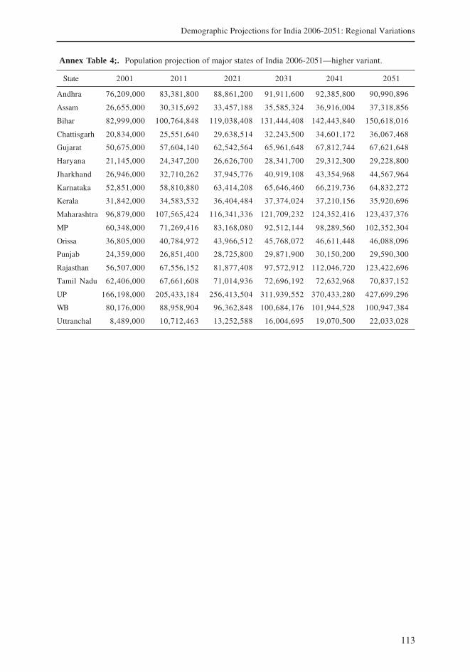
113
Demographic Projections for India 2006-2051: Regional Variations
Annex Table 4;. Population projection of major states of India 2006-2051—higher variant.
State 2001 2011 2021 2031 2041 2051
Andhra 76,209,000 83,381,800 88,861,200 91,911,600 92,385,800 90,990,896
Assam 26,655,000 30,315,692 33,457,188 35,585,324 36,916,004 37,318,856
Bihar 82,999,000 100,764,848 119,038,408 131,444,408 142,443,840 150,618,016
Chattisgarh 20,834,000 25,551,640 29,638,514 32,243,500 34,601,172 36,067,468
Gujarat 50,675,000 57,604,140 62,542,564 65,961,648 67,812,744 67,621,648
Haryana 21,145,000 24,347,200 26,626,700 28,341,700 29,312,300 29,228,800
Jharkhand 26,946,000 32,710,262 37,945,776 40,919,108 43,354,968 44,567,964
Karnataka 52,851,000 58,810,880 63,414,208 65,646,460 66,219,736 64,832,272
Kerala 31,842,000 34,583,532 36,404,484 37,374,024 37,210,156 35,920,696
Maharashtra 96,879,000 107,565,424 116,341,336 121,709,232 124,352,416 123,437,376
MP 60,348,000 71,269,416 83,168,080 92,512,144 98,289,560 102,352,304
Orissa 36,805,000 40,784,972 43,966,512 45,768,072 46,611,448 46,088,096
Punjab 24,359,000 26,851,400 28,725,800 29,871,900 30,150,200 29,590,300
Rajasthan 56,507,000 67,556,152 81,877,408 97,572,912 112,046,720 123,422,696
Tamil Nadu 62,406,000 67,661,608 71,014,936 72,696,192 72,632,968 70,837,152
UP 166,198,000 205,433,184 256,413,504 311,939,552 370,433,280 427,699,296
WB 80,176,000 88,958,904 96,362,848 100,684,176 101,944,528 100,947,384
Uttranchal 8,489,000 10,712,463 13,252,588 16,004,695 19,070,500 22,033,028
115
The ‘Tipping Point’ in Indian Agriculture: Understanding the Withdrawal of Indian Rural Youth
The ‘Tipping Point’ in Indian Agriculture: Understandingthe Withdrawal of Indian Rural Youth
1Amrita Sharma and 2Anik Bhaduri1IWMI-TATA Water Policy Program
2IWMI, New Delhi, India
“We are all, at heart, gradualists, our expectations set by the steady passageof time. But the world of tipping point is a place where the unexpected becomesexpected, where radical change is more than a possibility. It is contrary to allour expectations a certainty.”
-Malcolm Gladwell, Tipping Point
Introduction
A number of recent occurrences suggest that India might very well be at the ‘tipping point’ ofthe (de)growth in its agricultural population and with growing urbanization, better literacystandards and greater skill attainment by rural youth it might take a steep turn downwardsthus changing the nature of farming in the country drastically.
At times the ‘gradualist’ in us tells that it’s probably too early and too ambitious tomake such assertions – more than 50 % of the population is currently engaged in farming; therate of growth of nonfarm jobs is abysmal, the services sector has too little job opportunitiesto offer and the manufacturing sector has only been experiencing jobless growth. The transition,even if it were to happen, will take a long time. However, if one took cognizance of thesurroundings and the developments therein, there are a sufficient number of reasons for us tothink to the contrary. First, the farming population in several parts of India registered a declinein absolute terms for the first time in 2001 with states such as Tamil Nadu and Kerala at theforefront (Economist 2001). Notably, the rural male cultivator population has declined by 2.8million between 1991 and 2001 (a decline of 3.6 %) changing the male-female cultivator ratiofrom 80:20 in 1991 to 67:33 in 2001. These are significant developments, given the impact ofdropping populations have on the nature of farming practiced in an economy1. Second, the
1 Bicanic (1972 cited by Griggs 1982) classified countries on the basis of rate of growth of their agri-cultural populations as relative and absolute and identified how fall in agricultural population causedsignificant reorganization of farming, the most drastic changes coming when the population fell in ab-solute numbers - peasants move from maximizing output per unit of land to maximizing output perhead (as there are more number of people to feed per farmer); farm size becomes larger and the agricul-tural populace is dominated by large farmers; there is acute labor shortage as young and able bodiedmen withdraw driving mechanization, and finally as the gap between farm and nonfarm incomes widengovernments intervene to restore parity.

116
A. Sharma and A. Bhaduri
growth performance of the Indian economy gives sufficient grounds to expect a significantchange in the employment scenario2. The 6th economic census which reports that the growthin labor opportunities in the nonfarm sector is outpacing the growth in labor force gives furtherhope. Third, the current farm crisis in the country seems to be another dominant force causingmany to quit out of desperation. The mounting number of farmer suicides and the risingdisenchantment with the profession among farmers (NSSO 2005) are some subtle but disturbingindicators. Further, if we look back in time we find that in most cases withdrawal from farmingtook place in a very short concentrated period of time either because of growth in the nonfarmsector or farm crisis as experienced by US in 1980s. Most of the East Asian economies suchas Japan, South Korea, and Taiwan which are similar to India in being land scarce and laborsurplus underwent steep fall in agricultural population within a short span of less than 20years. To support the argument further, most of them were experiencing similar economic growthrates (that India is experiencing now). Last but definitely not the least, the talks of efflux ofyouth from farming is increasingly gaining weight among the premier Indian academic circles.The noted agricultural scientist, Dr M S Swaminathan, pointed out recently that in the comingyears one of the biggest challenges for Indian agriculture would be to retain its youth inagriculture and unless farming became both ‘intellectually stimulating and economicallyrewarding’ it would be difficult to attract or retain rural youth in farming (Swaminathan 2001).
Place of This Study in the Strategic Analyses of India’s River Inter-inkingProgram
The river-linking proposal claims to address the water needs of India in 2050 and beyond. Forthat to happen it is important to understand what shape Indian agriculture (as it is the largestuser of water) would take in 2050. Human capital, being one of the most important factorsdriving changes in structure of agriculture (Boelhje 1992; Bicanic 1972 cited by Griggs 1982),a look at the withdrawal of Indian farmer population and its drivers becomes crucial to theanalysis of the proposal. It is in this regard that the paper takes an intensive look at the landedrural youth of India across 14 locations in 12 states and their association with farming, andfinally tries to identify (with the help of logit models) the factors fuelling the process of theirwithdrawal from agriculture.3 In order to place the phenomenon in its larger context, we alsoreview some international literature on withdrawal of farmers from agriculture.
2 Bhalla and Hazell 2003 in their paper on employment growth in India had projected that with anoverall economic growth rate of 9 % and with an employment elasticity of 0.1, employment in Indiawill match the labor force by 2010 and if the employment elasticity was taken to be higher the countrywill reach full employment by 2004!....and by 2020 will have an excess of 68.4 jobs.3 The rationale for focusing on landed rural youth is similar to ‘prosumer’ analysis that market researchersdo. ‘Prosumers’ are the trendsetters for any particular product category. Their usage and involvementwith the product defines how the product would evolve in future. Market researchers have been thustracing the behavior of these consumers to fine tune their products. For Indian agriculture, landed youthare the ‘prosumers’ as they would define how Indian agriculture would evolve in future.
117
The ‘Tipping Point’ in Indian Agriculture: Understanding the Withdrawal of Indian Rural Youth
Why Farmers Quit – Existing Wisdom
Why do farmers quit or what makes farmers quit farming en masse, the occupation they havebeen in all their lives? The theory of farm exit and a related yet more widely known concept -the ‘farm problem’ has been an issue of keen interest to scholars since a long time.Unfortunately, most of the contribution to the literature has come from work done on US farms,posing limitations to its applicability to other economies such as India. However, we believethat much of the understanding (by virtue of the basic nature of farm sector) would hold forall type of economies. In this section we put together some of the work done on answeringthe question –”why farmers quit?” and assemble the major hypotheses and debates in thefield to serve as a foreground to our study and analyses.
The Farm Problem
There is no agreement among scholars on what exactly constitutes the ‘farm problem’, thougha significant amount of work has been done on the issue (Gardner 1992). The nature of theproblem has also been changing over time with increasing heterogeneity of the farmerpopulation (Offutt 2000). Broadly, the term can be taken to mean economic difficulties facedby farmers as a result of low farm incomes (vis-à-vis nonfarm) and large instability and variabilityin the income from farming. The common response of farmers to the problem is to migrate tourban areas or to nonfarm occupations which provide higher returns to per unit of labor applied.The question that arises is - what explains the difference in farm and nonfarm incomes? Gardner1992 attributed the difference to the factor market conditions. Johnson 1959 (Gardner 1992)also wrote that the farm problem was “as a result of the employment of more labor in agriculturethan can earn as large a real income as the same labor could earn elsewhere in the economy.”Further, one of the many ironies of the sector is that most of the times the aforesaid ‘farmproblem’ arises out of success of farming itself.
“The greater the increase in farm productivity, the greater the imbalancebetween supply and demand of farm products which has to be corrected byan outflow of labor or by lower farm prices. Unless the outflow of labor fromfarming is fast enough, an increase in farm productivity leads only to lowerfarm prices and lower farm incomes.”
(Houthakker 1967 cited by Gardner 1992)
Thus the incentives for a farmer to farm go on declining even with a good performanceand many a time there is no option but to quit. Offutt 2000 in her paper on “Can the farmproblem be solved?” puts it very well – “there is and always will be money to be made infarming but the question is by how many?”
Why Farmers Quit
As rational actors, while making a decision to quit farming, farmers compare the utility theyderive from farming vis-à-vis that derived from quitting and taking up full-time nonfarmemployment. The theory of farm exit and most of the studies done on the subject essentially
118
A. Sharma and A. Bhaduri
rest on this assumption. Transaction costs involved in making a shift (including relocation) isalso an important determinant (Goetz and Debertin 2001). Lower the costs, higher the propensityto shift. Goetz and Debertin 2001 in a cross-county analysis of US farms conclude that in caseof counties facing a net loss of farm operators, lower transaction costs led to faster rate ofwithdrawal from farming. These costs/utilities are either aggravated or lowered by various factors.Scholars have gone into significant depth exploring the impact of these factors which can beclassified into three types - farmer associated (such as education and skill level of farmers,involvement in nonfarm activities, family size); farm-specific (size of farm, value of production)and nonfarm (such as proximity to metropolitan areas, overall GDP of the region, governmentinterventions etc.).
Glauben et al. (2003) notes that at a broad level, farmer withdrawal studies can be classifiedinto two types - the first type is empirical studies at the farm household level while the secondtype focuses on adjustment of farm labor at aggregate (sector/regional) level. While the firsttype help bring in more household and farm specific characters in the analyses, the secondtype help capture the macro-economic forces and the influence of government policies onchanges in labor allocation in the farm sector. Authors have tested the impact of several farm/nonfarm, household/ regional level variables on the decision of farmers and have found bothsimilar and divergent results. We shall first take a look at the points of dissent.
One of the most popular debates in the field is on the question whether a priorinvolvement in nonfarm occupation reduces or increases the chances of withdrawal fromfarming? A large number of farmers in developed economies today practice farming as a part-time activity. The trend is becoming increasingly in vogue and does not give conclusiveevidence on whether part-time farming sets them on their way out of agriculture. Authorslike Kimhi and Bollman 1999, Kimhi 2000, Goetz and Demertin 2001 in their studies on Canadian,Israeli and US farmers, respectively, conclude that nonfarm income has a stabilizing impacton the farmer’s household economy. Farmers in these cases use their nonfarm income toaugment their farm activities and it thus serves as a stabilizing factor rather than an avenuefor exit. On the contrary, authors such as Pfeffer 1989 and Weiss 1999, see a strong linkbetween nonfarm employment and withdrawal from agriculture. That is, growth in nonfarmemployment causes people to move away from farming by providing the much needed outlet.They propose that an exposure to nonfarm occupation lowers the transaction costs (Glaubenet al. 2003 have also called ‘the beaten path’ effect) involved in the shift making the exitdecision easier.
Another point of deviation has been on the impact of government intervention andmacro-economic environment. A comprehensive study done in the OECD countries (1994)concluded that farm family labor as well as hired labor is not particularly sensitive to businesscycle conditions or to agricultural prices. However, Andermann and Schmidt (1995, cited byGlauben 2003) in a study on Germany have found the labor significantly responsive to macro-economic changes and agricultural prices. Government payments too have been found to havea contrasting impact. On the one hand, while income assistance in terms of price supportsresults in slow down of migration; on the other land diversions lead to greater migration outof farming (Barkley 1990).
Among the farm specific characteristics, it is found that an increase in average farm-sizesignificantly reduces the tendency to close down farms (Pietola 2002; Glauben et al. 2003;Goetz and Debertin 2001). The justification being that large farm sizes make farming much more
119
The ‘Tipping Point’ in Indian Agriculture: Understanding the Withdrawal of Indian Rural Youth
economically viable for the farmers by enabling them to reap economies of scale and bring inuse better and cost-effective technologies. There are, however, evidences to the contrary. Forexample, Speare 1974 in case of Taiwan found that the large landholders showed a greatertendency to withdraw. This was by virtue of their being able to gain good quality educationand to move to better occupations. Large farmers could also take greater risks compared tothe small and venture out more in search of greener pastures.
Most of the authors with exceptions such as Zhao 1999 have found that highereducation and greater number of skills lead to greater propensity to migrate. Weiss 1999found several other farmer associated characteristics to be playing a role such as gender,age, family size, succession information and attitude towards risk. Among these the trend inage has lately been a cause of worry among the developed countries. A number ofpolicymakers and academicians have been expressing serious concerns over the ‘graying offarm sector’ because of (1) increased exit and (2) dropping of rates of entry into farming bythe rural youth (Gale 2002). What roles do these factors –age, land size, education andskillfulness etc., play in the context of Indian farmers? We shall try and address this questionin the later sections.
The Case of Labor Surplus Economies
As mentioned earlier, one of the lacunae in the literature on the theory of farm exit is that notmuch work has been done on labor surplus economies. This could possibly be because oftheir very definition- labor surplus and thus not requiring much attention on this aspect.However, there is a serious flaw in this line of thinking. Zhou 2004 critiques the work of Schultzchallenging one of his assertions that low income countries saddled with traditional agriculturedo not suffer from the problem of many farmers leaving agriculture for nonfarm jobs. He saysthat many low income countries especially from 1950 onwards have been increasingly open tohigh income economy… “small peasants migrate to those rural areas which have entered thehigh wage stage, cities and abroad to earn higher income as part-time and absent farmers,thus are up against the problem of adapting the agricultural sector to a high incomecountry”(Zhou 2004). The changes in post World War II Japan, where the full-time farminghouseholds declined from 50 % in 1950 to 20.5 % in 1965 is a case in point (ibid) which provesthat how even a labor surplus economy could undergo a steep fall in its agricultural laborforce in a short period of time and defy existing wisdom.
In most of the East Asian economies, however, mass withdrawal of population fromagriculture was largely a post - World War II phenomenon (Ohkawa 1961) thus, bringing intoplay a very different set of factors. There was also a great emphasis on industrialization andconcentrated efforts were made to channelize resources, including human capital, to fuel theindustry-led growth of the economy. China started experiencing mass rural-urban migration oflabor during the 80s. However, much of this was the floating population. Rarely, migrants settled(or could afford to settle) in cities. Part-time farming became a popular arrangement wherefarmers spent most of their productive time in rural nonfarm or urban activities. In peakagricultural seasons they came back to their farms only to leave again (Zhao 1999). In Indiatoo, this has become increasingly in vogue in a large number of regions (Sharma, forthcoming).How this part-time arrangement affects farming, however, is a less understood phenomenonand needs to be studied.

120
A. Sharma and A. Bhaduri
In economies such as India, the ‘farm problem’ is probably worsened by virtue of itslabor surplus nature. Dantwala and Donde 1949 wrote about the ‘uneconomic cultivators’ ofIndia way back in the 1950s saying that the problem with Indian agriculture was not so muchof uneconomic cultivation but of ‘uneconomic cultivators’ and it was this group of farmersthat needed maximum policy attention. In a study of 11 villages in the then Bombay province,the authors found that 71 % of the cultivators came in the category of ‘uneconomic cultivators’who continue to till land without necessary resources, living a life of insecurity and sub-marginal existence. For the 70 % of land that was cultivated as economic units, the roadblockto efficient production was fragmentation of landholdings. The authors observed that thenumber of fragments operated grew with the size of cultivated holding of a farmer thus “whatseemed to have been gained in the size was lost in the number of fragments that comprisedthe unit of cultivation” (past tense added) (ibid). There was widespread leasing in and out ofland to make farming units viable but taking all that into account, still, only 27 % of thecultivators operated 55 % of the land. According to the authors’ estimates 50 % of the cultivatorpopulation in the region was redundant! (ibid). There were suggestions made to redistributeland - transfer from those holding more than economically viable holdings to the uneconomiccultivators. Rural industrialization was also proposed as an effective medium to promotediversification of livelihoods thus reducing the pressure on land. Unfortunately, none of thepolicies could be implemented effectively and the uneconomic mode of cultivation continuedruining the economics of cultivation in the subcontinent even further. Bhalla and Hazell 2003observe that with 60 % of the labor force producing around a quarter of the GDP, the relativeproductivity of workers in agriculture is less than one-fourth of the nonagricultural occupations.In recent times several macro-economic changes and farm level changes have worsened theagricultural employment scenario. For example, in the post-liberalization period the employmentgrowth in agriculture dropped from 1.49 % pa to 0.01 % pa (Bhalla and Hazell 2003). The recenttrend of the over-capitalization of agriculture also influenced the employment elasticity ofagriculture adversely. The employment elasticity of agriculture is approaching zero (0.01 in thepost-reform period, Planning Commission report cited in Bhalla and Hazell 2003) and has beenreported to be negative in some states such as AP (-0.13), Kerala (-0.92) and UP (-0.13).
Given this, much of the pessimism about the status of employment in Indian agricultureis justified. We, however, aim to add another leaf to the discussion by arguing that the dropin employment in agriculture cannot be solely attributed to the happenings on the agriculturalfront. There are developments on the nonfarm side which are having significant and sometimes greater impact.4 At present much of the deliberation on the withdrawal of Indian farmersseems to be pre-occupied with declaring it to be a distress phenomenon. We believe that thereality is much more complex. Indian villages are undergoing a major transformation causingperceptible changes in aspirations of the rural mass, especially the youth who are now optingout of farming. Some of these aspects have been dealt in greater detail in another of our papers(Sharma, forthcoming). The participation rates of the 5-14 and 15-29 age groups are declining
4 Bhalla and Hazell 2003 hypothesize that growth in secondary and tertiary sectors has a majorcontribution in the decline in farmer population. There has been a notable increase in labor productivityand wages in agriculture and the wages in nonagricultural sector are now significantly higher than inagriculture. This suggests that the shift from agriculture to nonagriculture is not a distress phenomenon.
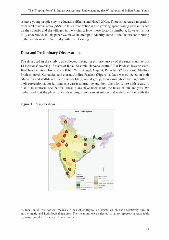
121
The ‘Tipping Point’ in Indian Agriculture: Understanding the Withdrawal of Indian Rural Youth
as more young people stay in education (Bhalla and Hazell 2003). There is increased migrationfrom rural to urban areas (NSSO 2003). Urbanization is also growing apace casting great influenceon the suburbs and the villages in the vicinity. How these factors contribute, however, is notfully understood. In this paper we make an attempt to identify some of the factors contributingto the withdrawal of the rural youth from farming.
Data and Preliminary Observations
The data used in the study was collected through a primary survey of the rural youth across14 locations5 covering 13 states of India- Kashmir, Haryana, central Uttar Pradesh, lower Assam,Jharkhand, central Orissa, north Bihar, West Bengal, Gujarat, Rajasthan (2 locations), MadhyaPradesh, north Karnataka, and coastal Andhra Pradesh (Figure 1). Data was collected on theireducation and skill-level, their asset-holding, social group, their association with agriculture,their perception about farming as a career alternative and their plans for future with regard toa shift to nonfarm occupation. These plans have been made the basis of our analysis. Weunderstand that the plans to withdraw might not convert into actual withdrawal but with the
5A location in this context means a block of contiguous districts which have relatively similaragro-climatic and hydrological features. The locations were selected so as to represent a reasonablehydro-geographic diversity of the country.
Figure 1. Study locations.
122
A. Sharma and A. Bhaduri
question – ‘Do you have immediate plans to shift to another occupation’? Further supportedby the mention of the job they were considering to take up, we expect to paint a reasonablepicture of the withdrawal phenomenon.
We also collected data on irrigation availability and proximity to the nearest urban centre.At the beginning of the study, some pilot survey results revealed that the nature of theinvolvement of the youth in farming varied with respect to the degree of their association withthe day to day management of the farm. Based on this, we classified the respondents into full-time and part-time farmers and those with no-involvement in farming.6
A significant proportion of the rural youth were found to be practicing part-time farming(35 %). The phenomenon was more pronounced in villages close to town rather than thoseaway from town (40 % vis-à-vis 29 %). We also found a significant correlation between thedegree of association with farming and per capita value of agricultural production (0.62). Lowerthe value of agricultural production per capita, higher the number of part time farmers/no-involvement farmers.
About 35 % of the youth migrated for work outside their villages and most of thismigration was seasonal. A large number of youth (30 %) commuted to nearby towns/villages.Most of them worked as agricultural labor, construction workers and contractual workers atagricultural produce markets (mandis), factories, bus stops and railway stations. These jobswere low-paying and irregular in nature.
Most of the people interviewed had education up to secondary level (37 %), followedby primary education (32 %). 16 % of the youth interviewed were illiterate and a negligible1 % had professional education from technical training institutions such as Industrial TrainingInstitutes (ITIs). A very small number of youth (24 %) possessed some kind of nonfarm skills,reflecting the poor skill-set of India’s rural youth. This prevented them from gaining entry intoremunerative occupations. The most common skills found among the youth were driving,electrical and mechanical repair work, and masonry. A small percentage possessed knowledgein computer applications as reported.
There was a visible sign of aging of the farmer population. Along with the details of theyouth being interviewed we also took some relevant family details. The average age of a personfarming was found to be 36 (for an effective sample of 8,500 plus in the working age group).Among the youth, also there was a difference in age of the part-time and the full-involvementfarmers (Figure 2). Though the mean age is not much different, it shows that the proportion offull-time farmers is relatively skewed towards the higher age group.
6 The classification was done based on the following criteria. The ‘high involvement’ category includedthe youth who were actively involved in management and supervision of their farms. One can term it‘full-time farming’. The ‘medium involvement’ category included the youth who contributed labor ontheir farms when they were free from their main activity. One can term it ‘part-time farming’. The ‘noinvolvement’ category included youth who had almost no involvement in the management of their farms.

123
The ‘Tipping Point’ in Indian Agriculture: Understanding the Withdrawal of Indian Rural Youth
Figure 2. Age distribution of part time and high involvement farmers.
Source:Primary Survey, 2005
Another interesting phenomenon we observed on the field was that both the small andlarge farmers were on their way out. Reverse tenancy has been talked about much where smalland marginal farmers, because of the nonviability of their small parcels of land are handing itto large or middle farmers. Recent studies of Jodhka 2006 also shed light on this phenomenonin Punjab agriculture where he says that the phenomenon of withdrawal is much stronger insmall and marginal farmers. However, in our field work we saw several instances of large farmersfallowing their land and moving out of rural life.
Finally, one of the key questions we wanted to look into was the impact of irrigation onwithdrawal behavior. It is generally believed that irrigation has a significant impact onemployment generation. Thus, if the national river interlinking program was to get functionaland provide irrigation to newer areas it should ideally contribute to reducing rural-urbanmigration by generating employment. We shall test for all these hypotheses by using someoccupational choice models in the next section.
Occupational Choice Models
Based on these preliminary observations we postulate that a farmer, characterized by his age,skill level, education, landholding size, irrigation facilities and location of his farmland, seeksto maximize his welfare by making a choice regarding his present agricultural occupation. Inthis section, using a suitable regression model we attempt to address the question why youthare planning to shift to other nonagricultural activities, and assess the odds of an averagerural youth moving out of agriculture.
Here the behavioural response of the youth involves a discrete binary choice of eithershifting to other nonagricultural activities or staying in agriculture. We consider the farmer’swillingness to shift as a dependent variable and code it as 1 for his plan to shift tononagricultural activities and 0 for otherwise. The independent variables explaining thedependent variable include skills (S), education (E), age of the farmers (A), land holding sizeof the farm (AVL) and irrigation (I). The variables are described in more detail in Table 1.
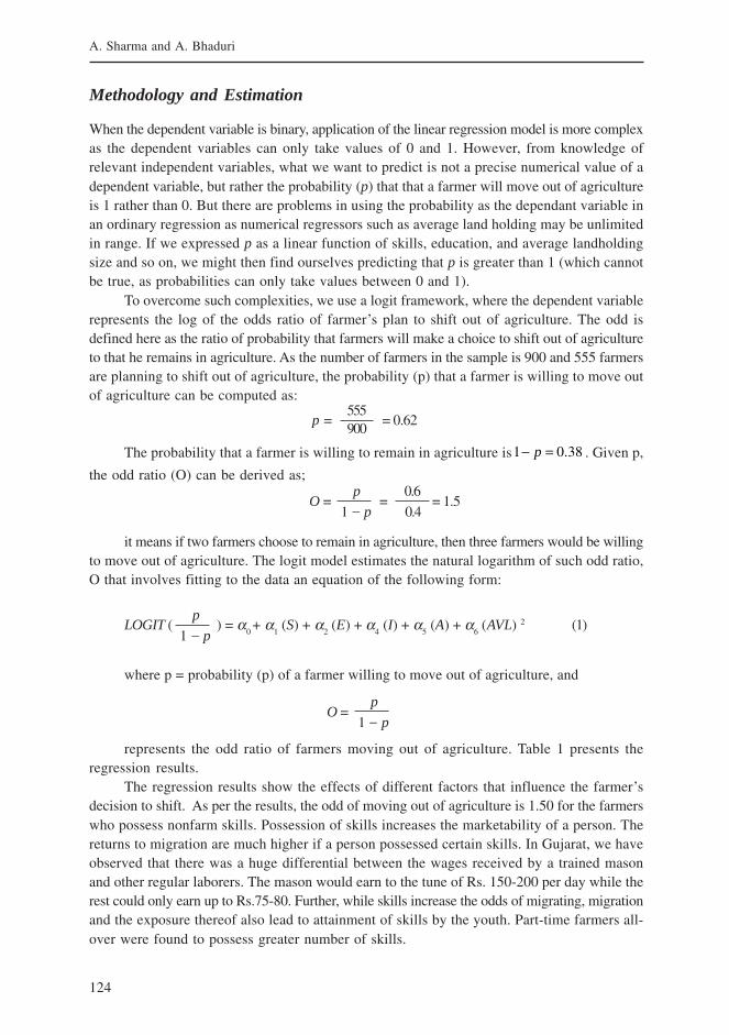
124
A. Sharma and A. Bhaduri
Methodology and Estimation
When the dependent variable is binary, application of the linear regression model is more complexas the dependent variables can only take values of 0 and 1. However, from knowledge ofrelevant independent variables, what we want to predict is not a precise numerical value of adependent variable, but rather the probability (p) that that a farmer will move out of agricultureis 1 rather than 0. But there are problems in using the probability as the dependant variable inan ordinary regression as numerical regressors such as average land holding may be unlimitedin range. If we expressed p as a linear function of skills, education, and average landholdingsize and so on, we might then find ourselves predicting that p is greater than 1 (which cannotbe true, as probabilities can only take values between 0 and 1).
To overcome such complexities, we use a logit framework, where the dependent variablerepresents the log of the odds ratio of farmer’s plan to shift out of agriculture. The odd isdefined here as the ratio of probability that farmers will make a choice to shift out of agricultureto that he remains in agriculture. As the number of farmers in the sample is 900 and 555 farmersare planning to shift out of agriculture, the probability (p) that a farmer is willing to move outof agriculture can be computed as:
The probability that a farmer is willing to remain in agriculture is 38.01 =− p . Given p,
the odd ratio (O) can be derived as;
p = = 0.62555900
it means if two farmers choose to remain in agriculture, then three farmers would be willingto move out of agriculture. The logit model estimates the natural logarithm of such odd ratio,O that involves fitting to the data an equation of the following form:
LOGIT ( ) = α0 + α
1 (S) + α
2 (E) + α
4 (I) + α
5 (A) + α
6 (AVL) 2 (1)
where p = probability (p) of a farmer willing to move out of agriculture, and
p
1 _ p
represents the odd ratio of farmers moving out of agriculture. Table 1 presents theregression results.
The regression results show the effects of different factors that influence the farmer’sdecision to shift. As per the results, the odd of moving out of agriculture is 1.50 for the farmerswho possess nonfarm skills. Possession of skills increases the marketability of a person. Thereturns to migration are much higher if a person possessed certain skills. In Gujarat, we haveobserved that there was a huge differential between the wages received by a trained masonand other regular laborers. The mason would earn to the tune of Rs. 150-200 per day while therest could only earn up to Rs.75-80. Further, while skills increase the odds of migrating, migrationand the exposure thereof also lead to attainment of skills by the youth. Part-time farmers all-over were found to possess greater number of skills.
O = = = 1.5p 0.6
1 _ p 0.4
O =p
1 _ p
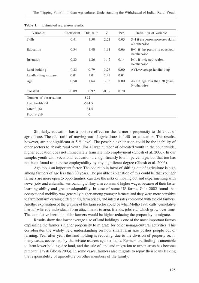
125
The ‘Tipping Point’ in Indian Agriculture: Understanding the Withdrawal of Indian Rural Youth
Similarly, education has a positive effect on the farmer’s propensity to shift out ofagriculture. The odd ratio of moving out of agriculture is 1.40 for education. The results,however, are not significant at 5 % level. The possible explanation could be the inability ofother sectors to absorb rural youth. For a large number of educated youth in the countryside,higher education does not immediately translate into employment (Ghosh et al. 2006). In oursample, youth with vocational education are significantly low in percentage, but that too hasnot been found to increase employability by any significant degree (Ghosh et al. 2006).
Age too is an important factor. The odd ratio in favor of shifting out of agriculture is highamong farmers of age less than 30 years. The possible explanation of this could be that youngerfarmers are more open to opportunities, can take the risks of moving out and experimenting withnewer jobs and unfamiliar surroundings. They also command higher wages because of their fasterlearning ability and greater adaptability. In case of some US farms, Gale 2002 found thatoccupational mobility was generally higher among younger farmers and they were more sensitiveto farm nonfarm earning differentials, farm prices, and interest rates compared with the old farmers.Another explanation of the graying of the farm sector could be what Molho 1995 calls ‘cumulativeinertia’ whereby individuals form attachments to area, friends, jobs etc, which grow over time.The cumulative inertia in older farmers would be higher reducing the propensity to migrate.
Results show that lower average size of land holdings is one of the most important factorsexplaining the farmer’s higher propensity to migrate for other nonagricultural activities. Thiscorroborates the widely held understanding on how small farm size pushes people out offarming. Year after year, the land holding is reducing, due to the division of property or, inmany cases, accessions by the private usurers against loans. Farmers are finding it untenableto farm lower holding size land, and the sale of land and migration to urban areas has becomerampant (Jayati Ghosh 2003). In some cases, farmers also migrate to repay their loans leavingthe responsibility of agriculture on other members of the family.
Table 1. Estimated regression results.
Variables Coefficient Odd ratio Z P>z Definition of variable
Skills 0.41 1.50 2.21 0.03 S=1 if the person possesses skills,=0 otherwise
Education 0.34 1.40 1.91 0.06 E=1 if the person is educated,0=otherwise
Irrigation 0.23 1.26 1.47 0.14 I=1, if irrigated region,0=otherwise
Land holding - 0.23 0.79 -3.25 0.00 AVL=Average landholding
Landholding -square 0.01 1.01 2.47 0.01
Age 0.50 1.64 3.33 0.00 A=1 if age less than 30 years,0=otherwise
Constant -0.09 0.92 -0.39 0.70
Number of observations 892
Log likelihood -574.5
LRchi2 (6) 34.5
Prob > chi2 0

126
A. Sharma and A. Bhaduri
In the field, however, we observed that alongside this distress phenomenon was anotherreality where large farmers too were making their way out of farming. To check for this weintroduced another variable ‘landholding-square’. The positive coefficient of the square ofthe average landholding size in the quadratic relationship suggests a strictly convex or Ushaped (Figure 3) relationship between farmer’s willingness to move out of agriculture andaverage land holding size.
Policymakers often cite that irrigation is one of the key factors that may reduce thepropensity to migrate. Our results, however, indicate an insignificant role of irrigation relativeto other factors in influencing farmer’s decision to shift to other activities.
Finally, many policymakers argue that in the villages close to town, farmers are morelikely to shift out of agriculture (Lucas 2000). It is an illustration of the bandwagon effect.People are attracted towards the better standard of living and the facilities available in towns.Also there is no dearth of literature suggesting why longer distance migrations may be lesscommon. In a survey of migration in the developed countries, Greenwood 1997 identifiesthat moves over longer distances impose higher costs of foregone, intervening opportunities.Although in the Indian context much of migration is intra district and the internal travel costis not too high, the general proposition that distance deters migration, seems to be consistent(Lucas 2000). For farmers far away from urban centers alternate occupational opportunitiesare also limited. Distance does not allow him to operate as a part-time farmer i.e., be partiallyinvolved in agriculture and work in town during the lull periods in agriculture. Our sampledata also suggests strong positive correlation between distance and full time involvementof farmers in agriculture, which means that a farmer located far away from a town is morelikely to be fully employed in agriculture. What factors would be driving migration from suchareas then? We expect that factors affecting farmers’ willingness to shift out of agriculturewould be stronger in terms of the odd ratio and statistical significance if he is far away fromthe town. We attempt to test our hypothesis by restricting the sample only to the case wherethe distance of the farms from the nearest town is above 14km. The distance of 14 km as apoint of reference is taken based on the median value of the sample distance. Table 2 presentsthe regression results.
Figure 3.

127
The ‘Tipping Point’ in Indian Agriculture: Understanding the Withdrawal of Indian Rural Youth
Comparing tables 1 and 2, we find that all the factors explaining the farmer’s willingnessto shift out of agriculture are far more significant if the farmer is located at least 14 km awayfrom a town. Striking is the improvement in the significance of the factors like skill andeducation. This implies that being skilled and educated becomes an important precondition. Itis important to justify a drastic step such as leaving agriculture and working in some far awayplace. Our fieldwork shows that the unskilled category of youth could only get low-payingjobs such as loading-unloading of goods which did not fetch enough to sustain them in cities.In villages located far away from urban areas we find many cases of reverse migration wherea number of youths had come back to the farm after some time because they were not able tosustain themselves in towns on the meager salaries they earned. Further, contrary to the resultspresented earlier, lack of irrigation, here has a positive impact on farmer’s willingness to migrate,and was significant at 10 % level. This implies that the distance from urban centers accentuatethe negative impacts of water scarcity rendering out-migration from farming as the only optionavailable to distressed farmers.
To conclude, five important points emerge from the analysis. Possession of skill seemsto be an important factor in determining out-migration from agriculture. The odds of a farmermoving out of farming increase with skill attainment. Education too lends a positive push tomigration but is not significant at 5 % level. Most of the out-migration is visible in the lowerage group making age another critical variable. Among the farm level factors, farm size has animpact but the relationship manifests itself differently in the smallholder group and among thelarge farmers. Both appear to be withdrawing but for different reasons. Irrigation has nosignificant impact on the withdrawal behavior. Finally, proximity to towns is found to be acritical determinant fuelling out-migration decisions of farmers.
Table 2. Estimation results for sample >14 km away from urban centers.
Variables Coefficient Odd ratio Z P>z Definition of variable
Skills 0.83 2.30 2.75 0.01 S=1 if the person possesses skills,= 0 otherwise
Education 0.86 2.37 3.46 0.00 E=1 if the person is educated,0=otherwise
Irrigation -0.38 0.69 -1.58 0.10 I=1, if the region is irrigated, 0= otherwise
Land holding - 0.23 0.79 -2.58 0.01 AVL=Average landholding
Landholding - square 0.01 1.01 2.03 0.04
Age 0.58 1.79 2.70 0.01 A=1 if age is less than 30 years,0=otherwise
Constant -0.03 0.97 -0.10 0.92
Number of observations 456
Log likelihood -277.9
LRchi2 (6) 39.8
Prob > chi2 0
128
A. Sharma and A. Bhaduri
Policy Implications
What would be the face of Indian agriculture say 20-30 years hence? This paper is a deliberateattempt to add a new dimension to the present discourse which presupposes the persistenceof overpopulated workforce in agriculture. We propose that the livelihood decisions of therural youth would be the key to the future of Indian agriculture and there is a need to understandthe various processes affecting it fully. This paper attempts to identify some of those andtries to check/validate some widely held notions through the use of statistical models. We,however, accept that the model is far from comprehensive. The blame may go little on theprimary nature of the data which makes analysis difficult and more on our inability to quantifycertain imponderables such as the changing aspirations of the rural youth and its impact onwithdrawal.
Based on the present analysis, two kinds of implications, however, emerge – one for theshort term and the other aimed towards long term changes in policies and institutions. In theshort term we need to recognize that the current withdrawal from agriculture by the youth isnot only inevitable but it is, to some extent, good for the economy. It would reduce the burdenon agriculture and raise effective income for the residual population. But the situation as ofnow is troubling. The study shows that while a large mass of youth is trying to make its wayout of farming few have the necessary skills to be able to move out of farming profitably. Theresult is poor quality migration, creating problems for urban habitations while not necessarilyreducing the burden on rural areas. In the short term, skill building of the rural youth could betreated as a priority area. This would not only increase the pay-off to migration but facilitatewithdrawal from farming as well.
Further, in the face of the withdrawal of the youth from farming we expect drastic changesin the agricultural demography. The low quality migration suggests that farming householdswould still need to depend on farming to meet a part of their requirements as the remittanceswill not be enough. In this case, farms would be left to manage on either old men or women.In several areas such as Bihar, Orissa, Kashmir, the farmer population is already showing signsof aging. Male farmer withdrawal is also leading to more number of women farmers in severalparts of the country (Krishnaraj and Shah 2003). This raises important issues about thepreparedness of the agricultural institutions and extension agencies to cater to the needs ofwomen and old men as farmers. The 10th plan recognized the rights of women as farmers andthere have been regular attempts to sensitize agricultural extension to the growing dominanceof female farmers, however, on the ground the efforts are far from making a difference. Thereis a need for a fresh look at the changes in rural labor markets and changes in the roles playedby men and women on the farms.
129
The ‘Tipping Point’ in Indian Agriculture: Understanding the Withdrawal of Indian Rural Youth
References
Barkley, A. P. 1990. The determinants of the migration of labor out of agriculture in the United States-1940-85. American Journal of Agricultural Economics, Vol. 72 No. 3.
Bhalla, G. S.; Hazell, P. 2003. Rural Employment and Poverty: Strategies to Eliminate Rural Poverty withina Generation. Economic and Political Weekly, Vol. 38, No. 33.
Boelhje, M. 1992. Alternative models of structural change in agriculture and related industries. AGRISCentre, NAL/USDA, Vol. 8 No. 3, p. 219-231.
Dantwala, M. L.; Donde, W. B. 1949. The Uneconomic Cultivator. Indian Journal of AgriuculturalEconomics, 4 (1).
Economist 2001. Grim Reapers, May 31st, 2001.
Gale, F. 2002. The Graying farm sector: Legacy of Off-farm Migration. Rural America, Vol. 17, Issue 3.
Gardner, B.L. 1992. Changing Economic Perspectives on Farm Problem. Journal of Economic Literature,Vol. 30, No. 1.
Ghosh, J.; Chandrashekhar, C. P.; Roychowdhury, A. 2006. The ‘Demographic dividend’ and Young India’sEconomic Future. Economic and Political Weekly, Vol. 41, No. 49.
Ghosh, J.; Chandrasekhar, C. P. 2003. Why is Agricultural Employment Generation Falling?www.macroscan.org, April 22.
GOI. 2006. http://www.censusindia.gov.in.
Gladwell, M. 2000. The Tipping Point: How Little Things Can Make a Big Difference. Back Bay Publishing.
Glauben, T.; Tietje, H.; Weiss, C 2003. Agriculture on the move: Exploring regional differences in farmexit rates. Working Paper EWP 0308, Department of Food Economics and Consumption Studies,University of Kiel.
Goetz, S. J.; Debertin, D. L. 2001. Why Farmers Quit: A country level Analysis. American Journal ofAgricultural Economics, Vol. 83 Issue 4.
Griggs, D. 1982. Dynamics of Agricultural Change, Hutchinson and Co. (Publishers) Ltd.
Greenwood, M. J. 1997. Internal Migration in Developed Countries. In Handbook of Population and FamilyEconomics, eds. M. R. Rosenzweig; O. Stark. Elsevier, Edition 1, Vol. 1, No. 1.
Houthakker, H. S. 1967. Economic Policy for the Farm Sector. American Enterprise Institute for PublicPolicy Research.
Jodhka, S. S. 2006. Beyond ‘Crises’: Rethinking Contemporary Punjab Agriculture. Economic and PoliticalWeekly, April 22, Vol. 41, No. 16.
Kimhi, A.; Bollman, R. 1999. Family farm dynamics in Canada and Israel: The case of farm exits.Agricultural Economics, Vol. 21, No. 1.
Kimhi, A. 2000. Is part-time farming really a way out of agriculture? American Journal of AgriculturalEconomics, Volume 82, No. 1.
Krishnaraj, M.; Shah, A. 2003. Women Farmers in India, State of Indian Farmer: A Millennium Study,Vol. 25. Academic Foundation, Department of Agriculture and Cooperation, Ministry of Agriculture,Government of India.
Lucas, RobertR. E. B. 2000. The Effects of Proximity and Transportation on Developing Country PopulationMigrations. Boston University.
Molho, I. 1995. Migrant inertia, accessibility and local unemployment. Economica, 62, February: 123-132.
NSSO, 55th round 2003. Migration in India, (July 1999 to June 2000). National Sample Survey Organization,Ministry of Statistics & Programme Implementation, Government of India.
130
A. Sharma and A. Bhaduri
NSSO, 59th Round 2005. Situation Assessment Survey of Farmers: Some Aspects of Farming(January–December 2003). National Sample Survey Organization, Ministry of Statistics and ProgrammeImplementation Government of India.
Offutt, S.; 2003. Can the farm problem be solved? M. E. John Lecture, Pennsylvania State University.http://www.aers.psu.edu/announce/aeseminar/offutt.pdf
Ohkawa, K. 1961. Significant changes in Japanese Agriculture since 1945. Journal of Farm Economics,Volume 43, No: 5.
Oshima, H. T. 1986. The Transition from an Agricultural to an Industrial Economy in East Asia. EconomicDevelopment and Cultural Change, Vol. 34, No. 4.
Pfeffer, J. M. 1989. Part-time Farming and the Stability of family-farms in the Federal Republic of Germany.European Review of Agricultural Economics, 425-44, p.16
Pietola, K.; Vare, M. 2003. Timing and Type of Exit from Farming: Farmer’s Early Retirement Programmesin Finland. European Review of Agricultural Economics, Vol 30 [1], pp. 90-116.
Sharma, A. 2007. The Changing Agricultural Demography of India: Evidences from a Rural YouthPerception Survey. International Journal of Rural Management, Vol. 3 Issue 1.
Speare, A. 1974. Urbanization and Migration in Taiwan. Economic Development and Cultural Change,22-302.
Swaminathan, M. S. 2001. Shaping our agricultural future. The Hindu, Thursday, January 11, 2001.
Weiss, C. R. 1997. Farm Growth and Survival: Econometric Evidence for Individual Farms in Upper Austria.American Journal of Agricultural Economics, 81 (1), pp. 103-116.
Zhao, Y. 1999. Labor Migration and Earnings Differences: The Case of Rural China. Economic Developmentand Cultural Change, Vol. 47, No. 4, 767-782.
Zhou, J. 2004. The Irrational Land Use in Japan and Other Parts of the World - The Root of AgriculturalProtectionism Ignored by Nobel Laureate Schultz and Nominee Hirschman. Paper for the Japan EconomicPolicy Association Third International Conference ‘Policy Implementation and Its Consequences: WhatGood Does Economics Do?’ at Meiji University, Tokyo, Japan. November 13-14, 2004.
131
The ‘Tipping Point’ in Indian Agriculture: Understanding the Withdrawal of Indian Rural Youth
Changing Consumption Patterns of India: Implications onFuture Food Demand
1Upali A. Amarasinghe and 2Om Prakash Singh1International Water Management Institue, New Delhi, India
2Agricultural University, Varanesi, Uttap Pradesh, India
Introduction
Food grains dominate the vegetarian centered diet of the Indian people, although the compositionvaries across different regions. Grains provided 65 % of the calorie supply in 2000, and thisvaried from 60 % in the north to 74 % in the south. Rice is the main food grain in the south andthe east, followed by wheat in the east and coarse cereals in the south; wheat is the principalfood grain in the north followed by rice; and wheat comprises half of the grain consumption inthe west, followed equally by rice and other coarse cereals. The non-grain food crops and animalproducts provided 27 % and 8 % of the remaining calorie supply in 2000. Due to cultural andreligious reasons, the meat consumption in India is very low, and much of the animal productcalorie supply at present is from milk and milk products. Milk consumption also varies significantlyfrom 101 liters per person per year in the north to 26 liters in the south.
However, recent trends show shifts in food consumption patterns, with increasingconsumption in non-grain food crops and animal products. The FAOSTAT data (FAO 2005)show per capita grain consumption has been decreasing since the 1980s. This decline is dueto various factors, including income growth, urbanization and associated changes in life styles,changes in relative prices and the availability of non-grain food, etc. The National SampleSurvey Organization (NSSO) survey results show that the average monthly per capita cerealconsumption in the urban areas of India has decreased from 11.2 kg in 1973-1974 to 10.6 kg in1993-1994. The corresponding decline in the rural areas is 15.3 kg and 13.4 kg, respectively.Within the grain products, there is a shift from coarse cereals to superior cereals such as riceand wheat (Viswanathan 2001). Nilkanth Rath 2003 has suggested that the per capita grainconsumption will further decrease due to the reduction in physical labor requirement in ruralareas. It is likely that these changing patterns will accelerate in the future with increasing incomeand urbanizations. The purpose of this paper is to capture these changing consumption patternsand assess their implication on India’s food demand.
Several studies in the past have also projected India’s food grain demand for 2020 (Bhallaet al. 1999; IWMI 2000; Kumar 1998; Rosegrant et al. 1995; Radhakrishna and Reddy 2004).These studies have, in varying degrees, accounted for the emerging trends of increasing animalproduct consumption and the resulting feed demand. However, most of the studies have
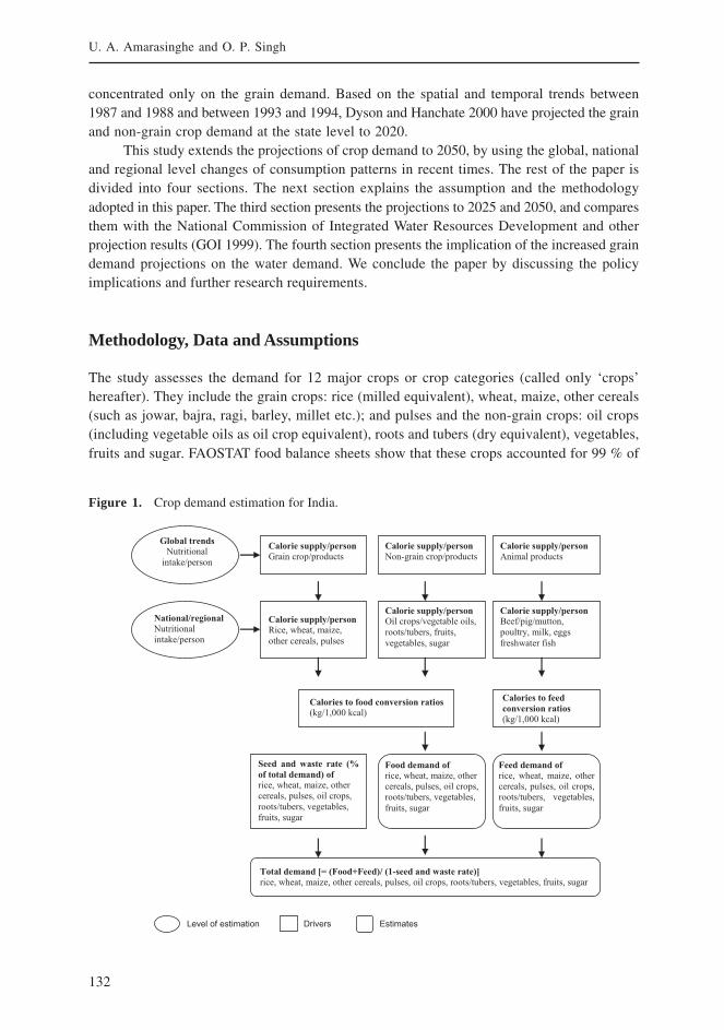
132
U. A. Amarasinghe and O. P. Singh
concentrated only on the grain demand. Based on the spatial and temporal trends between1987 and 1988 and between 1993 and 1994, Dyson and Hanchate 2000 have projected the grainand non-grain crop demand at the state level to 2020.
This study extends the projections of crop demand to 2050, by using the global, nationaland regional level changes of consumption patterns in recent times. The rest of the paper isdivided into four sections. The next section explains the assumption and the methodologyadopted in this paper. The third section presents the projections to 2025 and 2050, and comparesthem with the National Commission of Integrated Water Resources Development and otherprojection results (GOI 1999). The fourth section presents the implication of the increased graindemand projections on the water demand. We conclude the paper by discussing the policyimplications and further research requirements.
Methodology, Data and Assumptions
The study assesses the demand for 12 major crops or crop categories (called only ‘crops’hereafter). They include the grain crops: rice (milled equivalent), wheat, maize, other cereals(such as jowar, bajra, ragi, barley, millet etc.); and pulses and the non-grain crops: oil crops(including vegetable oils as oil crop equivalent), roots and tubers (dry equivalent), vegetables,fruits and sugar. FAOSTAT food balance sheets show that these crops accounted for 99 % of
Figure 1. Crop demand estimation for India.
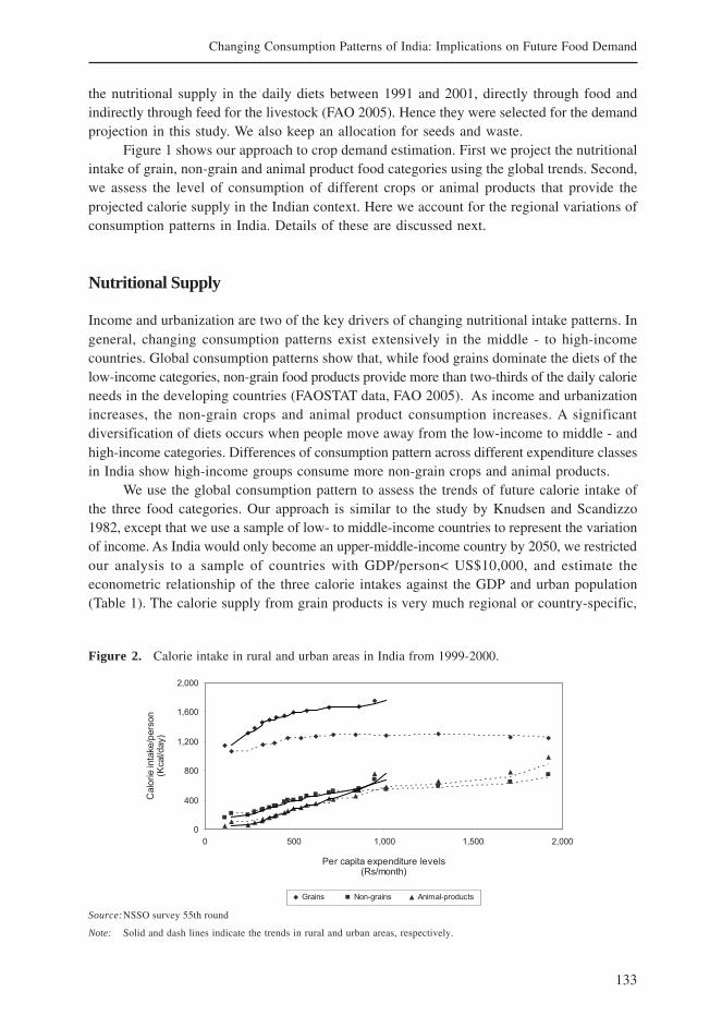
133
Changing Consumption Patterns of India: Implications on Future Food Demand
the nutritional supply in the daily diets between 1991 and 2001, directly through food andindirectly through feed for the livestock (FAO 2005). Hence they were selected for the demandprojection in this study. We also keep an allocation for seeds and waste.
Figure 1 shows our approach to crop demand estimation. First we project the nutritionalintake of grain, non-grain and animal product food categories using the global trends. Second,we assess the level of consumption of different crops or animal products that provide theprojected calorie supply in the Indian context. Here we account for the regional variations ofconsumption patterns in India. Details of these are discussed next.
Nutritional Supply
Income and urbanization are two of the key drivers of changing nutritional intake patterns. Ingeneral, changing consumption patterns exist extensively in the middle - to high-incomecountries. Global consumption patterns show that, while food grains dominate the diets of thelow-income categories, non-grain food products provide more than two-thirds of the daily calorieneeds in the developing countries (FAOSTAT data, FAO 2005). As income and urbanizationincreases, the non-grain crops and animal product consumption increases. A significantdiversification of diets occurs when people move away from the low-income to middle - andhigh-income categories. Differences of consumption pattern across different expenditure classesin India show high-income groups consume more non-grain crops and animal products.
We use the global consumption pattern to assess the trends of future calorie intake ofthe three food categories. Our approach is similar to the study by Knudsen and Scandizzo1982, except that we use a sample of low- to middle-income countries to represent the variationof income. As India would only become an upper-middle-income country by 2050, we restrictedour analysis to a sample of countries with GDP/person< US$10,000, and estimate theeconometric relationship of the three calorie intakes against the GDP and urban population(Table 1). The calorie supply from grain products is very much regional or country-specific,
Figure 2. Calorie intake in rural and urban areas in India from 1999-2000.
Source:NSSO survey 55th round
Note: Solid and dash lines indicate the trends in rural and urban areas, respectively.
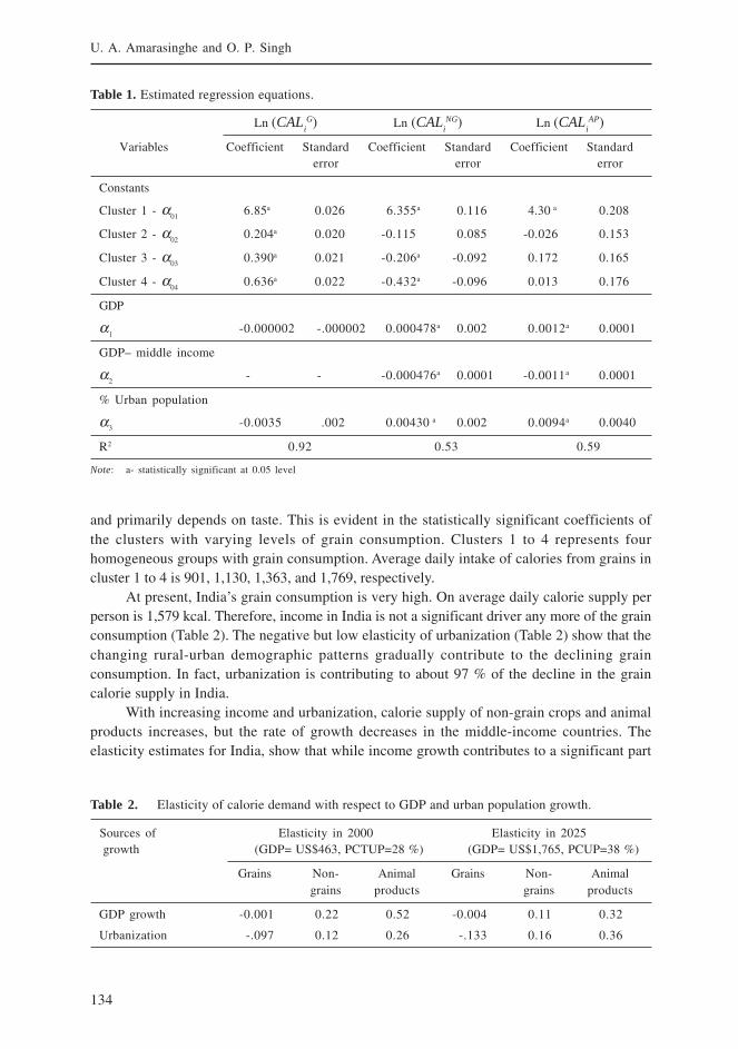
134
U. A. Amarasinghe and O. P. Singh
and primarily depends on taste. This is evident in the statistically significant coefficients ofthe clusters with varying levels of grain consumption. Clusters 1 to 4 represents fourhomogeneous groups with grain consumption. Average daily intake of calories from grains incluster 1 to 4 is 901, 1,130, 1,363, and 1,769, respectively.
At present, India’s grain consumption is very high. On average daily calorie supply perperson is 1,579 kcal. Therefore, income in India is not a significant driver any more of the grainconsumption (Table 2). The negative but low elasticity of urbanization (Table 2) show that thechanging rural-urban demographic patterns gradually contribute to the declining grainconsumption. In fact, urbanization is contributing to about 97 % of the decline in the graincalorie supply in India.
With increasing income and urbanization, calorie supply of non-grain crops and animalproducts increases, but the rate of growth decreases in the middle-income countries. Theelasticity estimates for India, show that while income growth contributes to a significant part
Table 1. Estimated regression equations.
Ln (CALiG) Ln (CAL
iNG) Ln (CAL
iAP)
Variables Coefficient Standard Coefficient Standard Coefficient Standarderror error error
Constants
Cluster 1 - α01
6.85a 0.026 6.355a 0.116 4.30 a 0.208
Cluster 2 - α02
0.204a 0.020 -0.115 0.085 -0.026 0.153
Cluster 3 - α03
0.390a 0.021 -0.206a -0.092 0.172 0.165
Cluster 4 - α04
0.636a 0.022 -0.432a -0.096 0.013 0.176
GDP
α1
-0.000002 -.000002 0.000478a 0.002 0.0012a 0.0001
GDP– middle income
α2
- - -0.000476a 0.0001 -0.0011a 0.0001
% Urban population
α3 -0.0035 .002 0.00430 a 0.002 0.0094a 0.0040
R2 0.92 0.53 0.59
Note: a- statistically significant at 0.05 level
Table 2. Elasticity of calorie demand with respect to GDP and urban population growth.
Sources of Elasticity in 2000 Elasticity in 2025growth (GDP= US$463, PCTUP=28 %) (GDP= US$1,765, PCUP=38 %)
Grains Non- Animal Grains Non- Animalgrains products grains products
GDP growth -0.001 0.22 0.52 -0.004 0.11 0.32
Urbanization -.097 0.12 0.26 -.133 0.16 0.36

135
Changing Consumption Patterns of India: Implications on Future Food Demand
(85 % in 2000) of the non-grain calorie supply change between 2000 and 2025, urbanizationalso contributes to the majority of this change after 2025. However, the income growthcontinued to be a significant factor of animal product calorie supply growth in both periods.
To assess the extent of the diversification of consumption patterns of different crops,we project the calorie intake of grains, non-grain crops and animal products in the Indian diet.For this projection we use global trends of energy intake of different food categories withrespect to the changes in income and urbanization. We project India’s calorie intake of grains,non-grain crops and animal products, with respect to the changes in income and urbanizationfrom the levels of the base year 2000. The projections of calorie supply in 2025 and 2050 aregiven in Table 3.
Our projections show that non-grain crop products will dominate the Indian diet by 2050.The total calorie supply is projected to further increase, 15 % by 2025, and another 8 % by2050. Almost the entire increase in calorie intake after 2025 is due to the increased consumptionof non-grain crops and animal products. Our projections show a slight decline of the caloriesupply from grains (9 %) by 2050, but significant increases in the non-grain crops (75 %) andanimal products (144 %). The composition of calories supply from grain, non-grain and animalproducts changes from 63, 29 and 8 % in 2000 to 55, 33 and 12 %, respectively, by 2025 and48, 36 and 16 %, respectively, by 2050.
Table 3. Calorie supply projections to 2025/2050 for India.
Year GDP Urban Calorie supply/person/day
(person/year) population Grains Non-grains Animal Total( % of total) products
$ % kcal kcal kcal kcal
1990 313 25 1,640 562 163 2,365
2000 463 27 1,579 673 183 2,435
2025 1,765 37 1,520 912 343 2,775
2050 6,731 53 1,440 1,083 477 3,000
Source:Mamhood and Kundu 2006 (for urban population projection)
Note: GDP in 1995 in constant $ (source for 1990 and 2000 is WRI 2005). We assume a 5.5 % annual growth rate for 2025 and2050 projections.
Composition of Nutritional Intake of Grains
The composition of the diet in different food categories depends on the taste and preferenceof the people, and as mentioned before, it varies significantly across regions. Thus, we needto take these differences into account in projecting individual crop demands. In India, thereis a declining trend of consumption of coarse cereals. In 2000, rice and wheat contributed tomost of the calorie intake (47 % and 31 %) from grains, while maize, other cereals and pulsescontributed to 5, 9 and 7 %, respectively, of the calorie intake of grains. Dyson and Hanchate2000, using the trends between 1987 and 1988 and 1993-1994 National Sample SurveyOrganization (NSSO) rounds observed that the per capita cereal consumption has declinedin all states except in Kerala and West Bengal. The consumption of rice and wheat remains
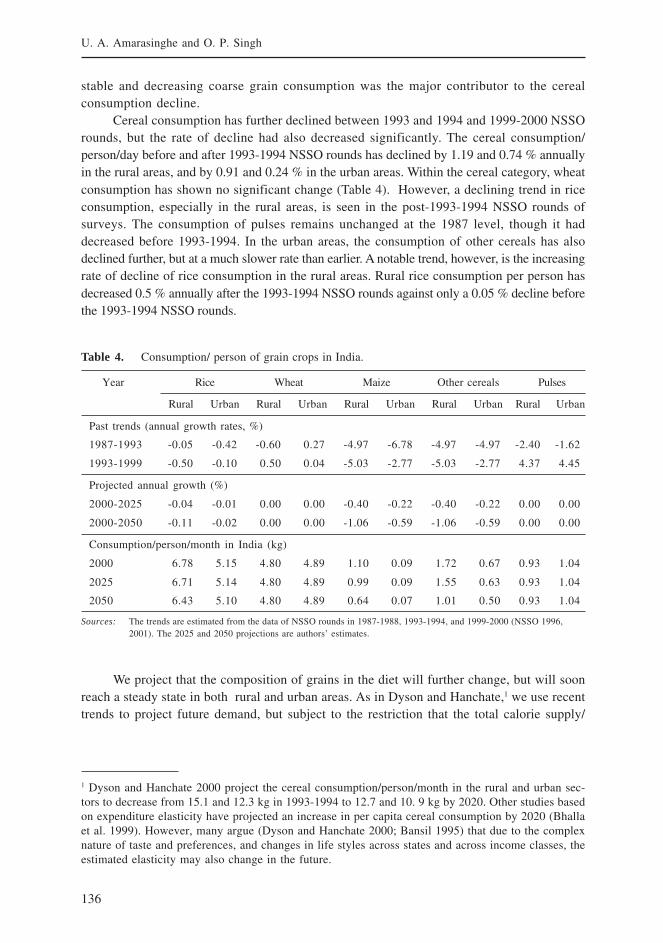
136
U. A. Amarasinghe and O. P. Singh
stable and decreasing coarse grain consumption was the major contributor to the cerealconsumption decline.
Cereal consumption has further declined between 1993 and 1994 and 1999-2000 NSSOrounds, but the rate of decline had also decreased significantly. The cereal consumption/person/day before and after 1993-1994 NSSO rounds has declined by 1.19 and 0.74 % annuallyin the rural areas, and by 0.91 and 0.24 % in the urban areas. Within the cereal category, wheatconsumption has shown no significant change (Table 4). However, a declining trend in riceconsumption, especially in the rural areas, is seen in the post-1993-1994 NSSO rounds ofsurveys. The consumption of pulses remains unchanged at the 1987 level, though it haddecreased before 1993-1994. In the urban areas, the consumption of other cereals has alsodeclined further, but at a much slower rate than earlier. A notable trend, however, is the increasingrate of decline of rice consumption in the rural areas. Rural rice consumption per person hasdecreased 0.5 % annually after the 1993-1994 NSSO rounds against only a 0.05 % decline beforethe 1993-1994 NSSO rounds.
Table 4. Consumption/ person of grain crops in India.
Year Rice Wheat Maize Other cereals Pulses
Rural Urban Rural Urban Rural Urban Rural Urban Rural Urban
Past trends (annual growth rates, %)
1987-1993 -0.05 -0.42 -0.60 0.27 -4.97 -6.78 -4.97 -4.97 -2.40 -1.62
1993-1999 -0.50 -0.10 0.50 0.04 -5.03 -2.77 -5.03 -2.77 4.37 4.45
Projected annual growth (%)
2000-2025 -0.04 -0.01 0.00 0.00 -0.40 -0.22 -0.40 -0.22 0.00 0.00
2000-2050 -0.11 -0.02 0.00 0.00 -1.06 -0.59 -1.06 -0.59 0.00 0.00
Consumption/person/month in India (kg)
2000 6.78 5.15 4.80 4.89 1.10 0.09 1.72 0.67 0.93 1.04
2025 6.71 5.14 4.80 4.89 0.99 0.09 1.55 0.63 0.93 1.04
2050 6.43 5.10 4.80 4.89 0.64 0.07 1.01 0.50 0.93 1.04
Sources: The trends are estimated from the data of NSSO rounds in 1987-1988, 1993-1994, and 1999-2000 (NSSO 1996,2001). The 2025 and 2050 projections are authors’ estimates.
We project that the composition of grains in the diet will further change, but will soonreach a steady state in both rural and urban areas. As in Dyson and Hanchate,1 we use recenttrends to project future demand, but subject to the restriction that the total calorie supply/
1 Dyson and Hanchate 2000 project the cereal consumption/person/month in the rural and urban sec-tors to decrease from 15.1 and 12.3 kg in 1993-1994 to 12.7 and 10. 9 kg by 2020. Other studies basedon expenditure elasticity have projected an increase in per capita cereal consumption by 2020 (Bhallaet al. 1999). However, many argue (Dyson and Hanchate 2000; Bansil 1995) that due to the complexnature of taste and preferences, and changes in life styles across states and across income classes, theestimated elasticity may also change in the future.
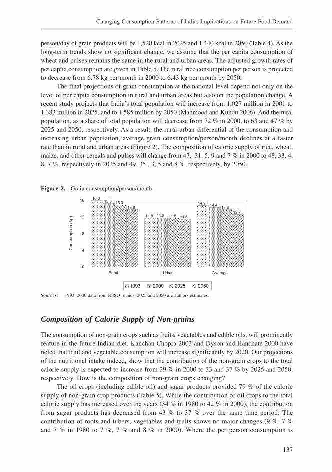
137
Changing Consumption Patterns of India: Implications on Future Food Demand
person/day of grain products will be 1,520 kcal in 2025 and 1,440 kcal in 2050 (Table 4). As thelong-term trends show no significant change, we assume that the per capita consumption ofwheat and pulses remains the same in the rural and urban areas. The adjusted growth rates ofper capita consumption are given in Table 5. The rural rice consumption per person is projectedto decrease from 6.78 kg per month in 2000 to 6.43 kg per month by 2050.
The final projections of grain consumption at the national level depend not only on thelevel of per capita consumption in rural and urban areas but also on the population change. Arecent study projects that India’s total population will increase from 1,027 million in 2001 to1,383 million in 2025, and to 1,585 million by 2050 (Mahmood and Kundu 2006). And the ruralpopulation, as a share of total population will decrease from 72 % in 2000, to 63 and 47 % by2025 and 2050, respectively. As a result, the rural-urban differential of the consumption andincreasing urban population, average grain consumption/person/month declines at a fasterrate than in rural and urban areas (Figure 2). The composition of calorie supply of rice, wheat,maize, and other cereals and pulses will change from 47, 31, 5, 9 and 7 % in 2000 to 48, 33, 4,8, 7 %, respectively in 2025 and 49, 35 , 3, 5 and 8 %, respectively, by 2050.
Figure 2. Grain consumption/person/month.
Sources: 1993, 2000 data from NSSO rounds. 2025 and 2050 are authors estimates.
Composition of Calorie Supply of Non-grains
The consumption of non-grain crops such as fruits, vegetables and edible oils, will prominentlyfeature in the future Indian diet. Kanchan Chopra 2003 and Dyson and Hanchate 2000 havenoted that fruit and vegetable consumption will increase significantly by 2020. Our projectionsof the nutritional intake indeed, show that the contribution of the non-grain crops to the totalcalorie supply is expected to increase from 29 % in 2000 to 33 and 37 % by 2025 and 2050,respectively. How is the composition of non-grain crops changing?
The oil crops (including edible oil) and sugar products provided 79 % of the caloriesupply of non-grain crop products (Table 5). While the contribution of oil crops to the totalcalorie supply has increased over the years (34 % in 1980 to 42 % in 2000), the contributionfrom sugar products has decreased from 43 % to 37 % over the same time period. Thecontribution of roots and tubers, vegetables and fruits shows no major changes (9 %, 7 %and 7 % in 1980 to 7 %, 7 % and 8 % in 2000). Where the per person consumption is
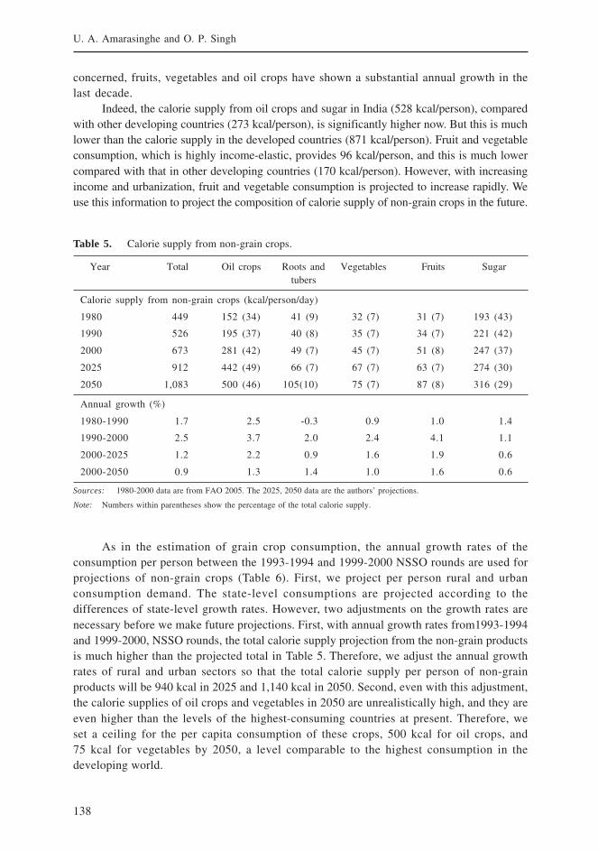
138
U. A. Amarasinghe and O. P. Singh
concerned, fruits, vegetables and oil crops have shown a substantial annual growth in thelast decade.
Indeed, the calorie supply from oil crops and sugar in India (528 kcal/person), comparedwith other developing countries (273 kcal/person), is significantly higher now. But this is muchlower than the calorie supply in the developed countries (871 kcal/person). Fruit and vegetableconsumption, which is highly income-elastic, provides 96 kcal/person, and this is much lowercompared with that in other developing countries (170 kcal/person). However, with increasingincome and urbanization, fruit and vegetable consumption is projected to increase rapidly. Weuse this information to project the composition of calorie supply of non-grain crops in the future.
Table 5. Calorie supply from non-grain crops.
Year Total Oil crops Roots and Vegetables Fruits Sugartubers
Calorie supply from non-grain crops (kcal/person/day)
1980 449 152 (34) 41 (9) 32 (7) 31 (7) 193 (43)
1990 526 195 (37) 40 (8) 35 (7) 34 (7) 221 (42)
2000 673 281 (42) 49 (7) 45 (7) 51 (8) 247 (37)
2025 912 442 (49) 66 (7) 67 (7) 63 (7) 274 (30)
2050 1,083 500 (46) 105(10) 75 (7) 87 (8) 316 (29)
Annual growth (%)
1980-1990 1.7 2.5 -0.3 0.9 1.0 1.4
1990-2000 2.5 3.7 2.0 2.4 4.1 1.1
2000-2025 1.2 2.2 0.9 1.6 1.9 0.6
2000-2050 0.9 1.3 1.4 1.0 1.6 0.6
Sources: 1980-2000 data are from FAO 2005. The 2025, 2050 data are the authors’ projections.
Note: Numbers within parentheses show the percentage of the total calorie supply.
As in the estimation of grain crop consumption, the annual growth rates of theconsumption per person between the 1993-1994 and 1999-2000 NSSO rounds are used forprojections of non-grain crops (Table 6). First, we project per person rural and urbanconsumption demand. The state-level consumptions are projected according to thedifferences of state-level growth rates. However, two adjustments on the growth rates arenecessary before we make future projections. First, with annual growth rates from1993-1994and 1999-2000, NSSO rounds, the total calorie supply projection from the non-grain productsis much higher than the projected total in Table 5. Therefore, we adjust the annual growthrates of rural and urban sectors so that the total calorie supply per person of non-grainproducts will be 940 kcal in 2025 and 1,140 kcal in 2050. Second, even with this adjustment,the calorie supplies of oil crops and vegetables in 2050 are unrealistically high, and they areeven higher than the levels of the highest-consuming countries at present. Therefore, weset a ceiling for the per capita consumption of these crops, 500 kcal for oil crops, and75 kcal for vegetables by 2050, a level comparable to the highest consumption in thedeveloping world.
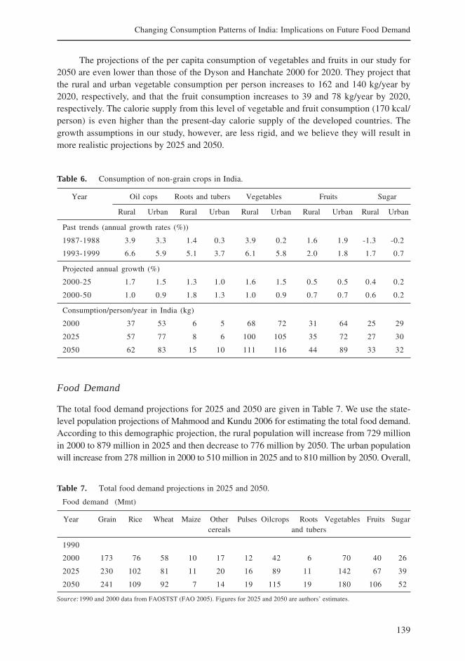
139
Changing Consumption Patterns of India: Implications on Future Food Demand
The projections of the per capita consumption of vegetables and fruits in our study for2050 are even lower than those of the Dyson and Hanchate 2000 for 2020. They project thatthe rural and urban vegetable consumption per person increases to 162 and 140 kg/year by2020, respectively, and that the fruit consumption increases to 39 and 78 kg/year by 2020,respectively. The calorie supply from this level of vegetable and fruit consumption (170 kcal/person) is even higher than the present-day calorie supply of the developed countries. Thegrowth assumptions in our study, however, are less rigid, and we believe they will result inmore realistic projections by 2025 and 2050.
Table 6. Consumption of non-grain crops in India.
Year Oil cops Roots and tubers Vegetables Fruits Sugar
Rural Urban Rural Urban Rural Urban Rural Urban Rural Urban
Past trends (annual growth rates (%))
1987-1988 3.9 3.3 1.4 0.3 3.9 0.2 1.6 1.9 -1.3 -0.2
1993-1999 6.6 5.9 5.1 3.7 6.1 5.8 2.0 1.8 1.7 0.7
Projected annual growth (%)
2000-25 1.7 1.5 1.3 1.0 1.6 1.5 0.5 0.5 0.4 0.2
2000-50 1.0 0.9 1.8 1.3 1.0 0.9 0.7 0.7 0.6 0.2
Consumption/person/year in India (kg)
2000 37 53 6 5 68 72 31 64 25 29
2025 57 77 8 6 100 105 35 72 27 30
2050 62 83 15 10 111 116 44 89 33 32
Food Demand
The total food demand projections for 2025 and 2050 are given in Table 7. We use the state-level population projections of Mahmood and Kundu 2006 for estimating the total food demand.According to this demographic projection, the rural population will increase from 729 millionin 2000 to 879 million in 2025 and then decrease to 776 million by 2050. The urban populationwill increase from 278 million in 2000 to 510 million in 2025 and to 810 million by 2050. Overall,
Table 7. Total food demand projections in 2025 and 2050.
Food demand (Mmt)
Year Grain Rice Wheat Maize Other Pulses Oilcrops Roots Vegetables Fruits Sugarcereals and tubers
1990
2000 173 76 58 10 17 12 42 6 70 40 26
2025 230 102 81 11 20 16 89 11 142 67 39
2050 241 109 92 7 14 19 115 19 180 106 52
Source:1990 and 2000 data from FAOSTST (FAO 2005). Figures for 2025 and 2050 are authors’ estimates.
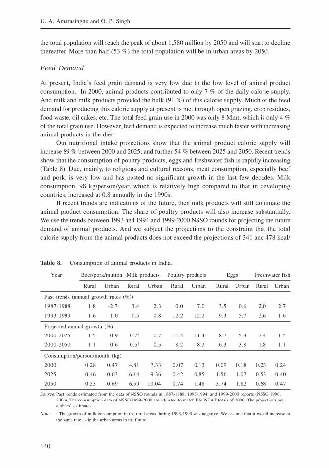
140
U. A. Amarasinghe and O. P. Singh
the total population will reach the peak of about 1,580 million by 2050 and will start to declinethereafter. More than half (53 %) the total population will be in urban areas by 2050.
Feed Demand
At present, India’s feed grain demand is very low due to the low level of animal productconsumption. In 2000, animal products contributed to only 7 % of the daily calorie supply.And milk and milk products provided the bulk (91 %) of this calorie supply. Much of the feeddemand for producing this calorie supply at present is met through open grazing, crop residues,food waste, oil cakes, etc. The total feed grain use in 2000 was only 8 Mmt, which is only 4 %of the total grain use. However, feed demand is expected to increase much faster with increasinganimal products in the diet.
Our nutritional intake projections show that the animal product calorie supply willincrease 89 % between 2000 and 2025; and further 54 % between 2025 and 2050. Recent trendsshow that the consumption of poultry products, eggs and freshwater fish is rapidly increasing(Table 8). Due, mainly, to religious and cultural reasons, meat consumption, especially beefand pork, is very low and has posted no significant growth in the last few decades. Milkconsumption, 98 kg/person/year, which is relatively high compared to that in developingcountries, increased at 0.8 annually in the 1990s.
If recent trends are indications of the future, then milk products will still dominate theanimal product consumption. The share of poultry products will also increase substantially.We use the trends between 1993 and 1994 and 1999-2000 NSSO rounds for projecting the futuredemand of animal products. And we subject the projections to the constraint that the totalcalorie supply from the animal products does not exceed the projections of 341 and 478 kcal/
Table 8. Consumption of animal products in India.
Year Beef/pork/mutton Milk products Poultry products Eggs Freshwater fish
Rural Urban Rural Urban Rural Urban Rural Urban Rural Urban
Past trends (annual growth rates (%))
1987-1988 1.8 -2.7 3.4 2.3 0.0 7.0 3.5 0.6 2.0 2.7
1993-1999 1.6 1.0 -0.5 0.8 12.2 12.2 9.3 5.7 2.6 1.6
Projected annual growth (%)
2000-2025 1.5 0.9 0.71 0.7 11.4 11.4 8.7 5.3 2.4 1.5
2000-2050 1.1 0.6 0.51 0.5 8.2 8.2 6.3 3.8 1.8 1.1
Consumption/person/month (kg)
2000 0.28 0.47 4.81 7.33 0.07 0.13 0.09 0.18 0.23 0.24
2025 0.46 0.63 6.14 9.36 0.42 0.85 1.56 1.07 0.53 0.40
2050 0.53 0.69 6.59 10.04 0.74 1.48 3.74 1.82 0.68 0.47
Source:Past trends estimated from the data of NSSO rounds in 1887-1888, 1993-1994, and 1999-2000 reports (NSSO 1996,2006). The consumption data of NSSO 1999-2000 are adjusted to match FAOSTAT totals of 2000. The projections areauthors’ estimates.
Note: 1 The growth of milk consumption in the rural areas during 1993-1990 was negative. We assume that it would increase atthe same rate as in the urban areas in the future.
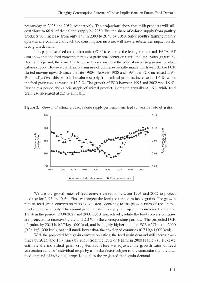
141
Changing Consumption Patterns of India: Implications on Future Food Demand
person/day in 2025 and 2050, respectively. The projections show that milk products will stillcontribute to 66 % of the calorie supply by 2050. But the share of calorie supply from poultryproducts will increase from only 1 % in 2000 to 20 % by 2050. Since poultry farming mainlyoperates at a commercial level, the consumption increase will have a substantial impact on thefeed grain demand.
This paper uses feed conversion ratio (FCR) to estimate the feed grain demand. FAOSTATdata show that the feed conversion ratio of grain was decreasing until the late 1980s (Figure 3).During this period, the growth of feed use has not matched the pace of increasing animal productcalorie supply. However, with increasing use of grains, especially maize, for livestock, the FCRstarted moving upwards since the late 1980s. Between 1988 and 1995, the FCR increased at 9.3% annually. Over this period, the calorie supply from animal products increased at 1.6 %, whilethe feed grain use increased at 13.2 %. The growth of FCR between 1995 and 2002 was 1.9 %.During this period, the calorie supply of animal products increased annually at 1.6 % while feedgrain use increased at 5.3 % annually.
Figure 3. Growth of animal product calorie supply per person and feed conversion ratio of grains.
We use the growth rates of feed conversion ratios between 1995 and 2002 to projectfeed use for 2025 and 2050. First, we project the feed conversion ratios of grains. The growthrate of feed grain conversion ratio is adjusted according to the growth rates of the animalproduct calorie supply. The animal product calorie supply is projected to increase by 2.2 and1.7 % in the periods 2000-2025 and 2000-2050, respectively, while the feed conversion ratiosare projected to increase by 2.7 and 2.0 % in the corresponding periods. The projected FCRof grains by 2025 is 0.37 kg/1,000 kcal, and is slightly higher than the FCR of China in 2000(0.34 kg/1,000 kcal), but still much lower than the developed countries (0.74 kg/1,000 kcal).
With the projected feed grain conversion ratios, the feed grain demand will increase 4.6times by 2025; and 13.7 times by 2050, from the level of 8 Mmt in 2000 (Table 9) . Next weestimate the individual grain crop demand. Here we adjusted the growth rates of feedconversion ratios of individual crops by a similar factor subject to the constraint that the totalfeed demand of individual crops is equal to the projected feed grain demand.
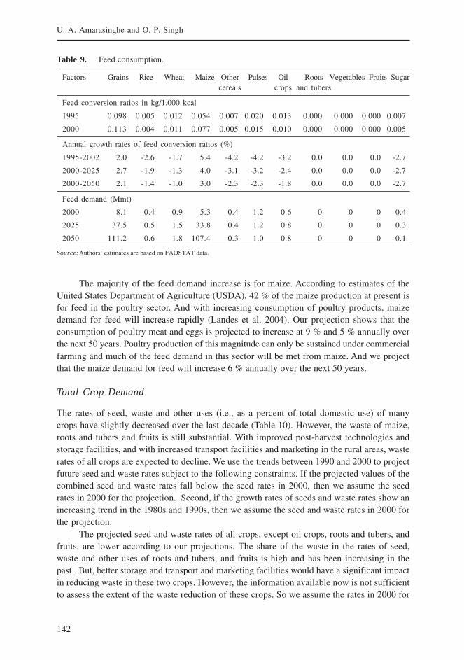
142
U. A. Amarasinghe and O. P. Singh
The majority of the feed demand increase is for maize. According to estimates of theUnited States Department of Agriculture (USDA), 42 % of the maize production at present isfor feed in the poultry sector. And with increasing consumption of poultry products, maizedemand for feed will increase rapidly (Landes et al. 2004). Our projection shows that theconsumption of poultry meat and eggs is projected to increase at 9 % and 5 % annually overthe next 50 years. Poultry production of this magnitude can only be sustained under commercialfarming and much of the feed demand in this sector will be met from maize. And we projectthat the maize demand for feed will increase 6 % annually over the next 50 years.
Total Crop Demand
The rates of seed, waste and other uses (i.e., as a percent of total domestic use) of manycrops have slightly decreased over the last decade (Table 10). However, the waste of maize,roots and tubers and fruits is still substantial. With improved post-harvest technologies andstorage facilities, and with increased transport facilities and marketing in the rural areas, wasterates of all crops are expected to decline. We use the trends between 1990 and 2000 to projectfuture seed and waste rates subject to the following constraints. If the projected values of thecombined seed and waste rates fall below the seed rates in 2000, then we assume the seedrates in 2000 for the projection. Second, if the growth rates of seeds and waste rates show anincreasing trend in the 1980s and 1990s, then we assume the seed and waste rates in 2000 forthe projection.
The projected seed and waste rates of all crops, except oil crops, roots and tubers, andfruits, are lower according to our projections. The share of the waste in the rates of seed,waste and other uses of roots and tubers, and fruits is high and has been increasing in thepast. But, better storage and transport and marketing facilities would have a significant impactin reducing waste in these two crops. However, the information available now is not sufficientto assess the extent of the waste reduction of these crops. So we assume the rates in 2000 for
Table 9. Feed consumption.
Factors Grains Rice Wheat Maize Other Pulses Oil Roots Vegetables Fruits Sugarcereals crops and tubers
Feed conversion ratios in kg/1,000 kcal
1995 0.098 0.005 0.012 0.054 0.007 0.020 0.013 0.000 0.000 0.000 0.007
2000 0.113 0.004 0.011 0.077 0.005 0.015 0.010 0.000 0.000 0.000 0.005
Annual growth rates of feed conversion ratios (%)
1995-2002 2.0 -2.6 -1.7 5.4 -4.2 -4.2 -3.2 0.0 0.0 0.0 -2.7
2000-2025 2.7 -1.9 -1.3 4.0 -3.1 -3.2 -2.4 0.0 0.0 0.0 -2.7
2000-2050 2.1 -1.4 -1.0 3.0 -2.3 -2.3 -1.8 0.0 0.0 0.0 -2.7
Feed demand (Mmt)
2000 8.1 0.4 0.9 5.3 0.4 1.2 0.6 0 0 0 0.4
2025 37.5 0.5 1.5 33.8 0.4 1.2 0.8 0 0 0 0.3
2050 111.2 0.6 1.8 107.4 0.3 1.0 0.8 0 0 0 0.1
Source:Authors’ estimates are based on FAOSTAT data.

143
Changing Consumption Patterns of India: Implications on Future Food Demand
future projections. With the projected rates of seeds, waste and other uses, we are now set toestimate the total crop demand (last three rows of Table 11).
The total grain demand is projected to increase by 45 % and 88 % in 2025 and 2050,respectively. The increasing maize demand, especially for feed, contributes to much of thetotal grain demand increase. The total grain demand is projected to increase by 176 Mmtbetween 2000 and 2050. The maize demand increase, of 101 Mmt, contributes to 57 % of theadditional grain demand. Although the rice and wheat demand increases are the same (35 Mmt),the level of increase of wheat demand over the 2000 consumption level is significantly higher.Another important observation is the increasing demand of non-grain crop products. Thedemand for non-grain crops will more than double over the next 50 years.
Table 10. Seed and waste rates and total crop demand.
Factors Grains Rice Wheat Maize Other Pulses Oil Roots Vegetables Fruits Sugarcereals crops and tubers
Seeds and waste rates of total consumption (%)
1980 10.2 8.3 12.8 19.6 9.4 10.2 18.9 16.4 7.2 12.9 0.02
1990 10.1 7.6 12.1 19.3 9.4 9.0 11.3 18.9 7.0 13.2 0.03
2000 9.6 6.8 11.7 17.0 9.7 8.2 12.7 19.2 6.7 14.0 0.04
Projected seeds and waste rates as a percent of total consumption
2025 5.9b 9.9 10.1 9.7a 5.9b 12.7a 19.2a 5.5 14.0a 0.04a
2050 5.9b 8.3 6.0 9.7a 5.9b 12.7a 19.2a 4.5 14.0a 0.04a
Total crop demand (Mmt)
2000 201 82 67 18 20 14 49 7 75 47 26
2025 291 109 91 50 23 18 103 13 150 78 40
2050 377 117 102 121 16 21 133 24 189 123 52
Notes: a An increasing trend is seen in the growth of seeds and waste rates from 1980 to 2000. For them, we project the seedsand waste rates at the 2000 level.
b The decreasing trends are significant in that the projected seeds and waste rates fall even below the seed rate in 2000.For them we assume the seed rates at the 2000 level.
Comparison with Other Food Demand Projections
We started our projections analyses with a view to assessing the impacts of recent consumptionpattern changes on the NCIWRD commission’s grain demand projections. A part of thedeviation of various demand projections is attributable to the different assumptions of thetotal population projections. In order to make proper comparison, we standardized theprojection to the same level of population as illustrated in Dyson and Hanchate 2000. Table 11summarizes six demand projections. The latter four studies only estimate cereal demand.Therefore, the per capita demand of these studies is adjusted by adding the pulses demand ofthe present study (12 kg for food and 13 kg for total). The totals are adjusted to the populationof 1,315 million by 2025 as projected by Dyson and Hanchate 2000, and of 1,581 million by2050 as assumed by the NCIWRD commission.
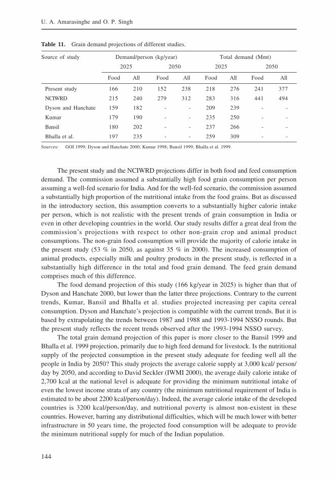
144
U. A. Amarasinghe and O. P. Singh
The present study and the NCIWRD projections differ in both food and feed consumptiondemand. The commission assumed a substantially high food grain consumption per personassuming a well-fed scenario for India. And for the well-fed scenario, the commission assumeda substantially high proportion of the nutritional intake from the food grains. But as discussedin the introductory section, this assumption converts to a substantially higher calorie intakeper person, which is not realistic with the present trends of grain consumption in India oreven in other developing countries in the world. Our study results differ a great deal from thecommission’s projections with respect to other non-grain crop and animal productconsumptions. The non-grain food consumption will provide the majority of calorie intake inthe present study (53 % in 2050, as against 35 % in 2000). The increased consumption ofanimal products, especially milk and poultry products in the present study, is reflected in asubstantially high difference in the total and food grain demand. The feed grain demandcomprises much of this difference.
The food demand projection of this study (166 kg/year in 2025) is higher than that ofDyson and Hanchate 2000, but lower than the latter three projections. Contrary to the currenttrends, Kumar, Bansil and Bhalla et al. studies projected increasing per capita cerealconsumption. Dyson and Hanchate’s projection is compatible with the current trends. But it isbased by extrapolating the trends between 1987 and 1988 and 1993-1994 NSSO rounds. Butthe present study reflects the recent trends observed after the 1993-1994 NSSO survey.
The total grain demand projection of this paper is more closer to the Bansil 1999 andBhalla et al. 1999 projection, primarily due to high feed demand for livestock. Is the nutritionalsupply of the projected consumption in the present study adequate for feeding well all thepeople in India by 2050? This study projects the average calorie supply at 3,000 kcal/ person/day by 2050, and according to David Seckler (IWMI 2000), the average daily calorie intake of2,700 kcal at the national level is adequate for providing the minimum nutritional intake ofeven the lowest income strata of any country (the minimum nutritional requirement of India isestimated to be about 2200 kcal/person/day). Indeed, the average calorie intake of the developedcountries is 3200 kcal/person/day, and nutritional poverty is almost non-existent in thesecountries. However, barring any distributional difficulties, which will be much lower with betterinfrastructure in 50 years time, the projected food consumption will be adequate to providethe minimum nutritional supply for much of the Indian population.
Table 11. Grain demand projections of different studies.
Source of study Demand/person (kg/year) Total demand (Mmt)
2025 2050 2025 2050
Food All Food All Food All Food All
Present study 166 210 152 238 218 276 241 377
NCIWRD 215 240 279 312 283 316 441 494
Dyson and Hanchate 159 182 - - 209 239 - -
Kumar 179 190 - - 235 250 - -
Bansil 180 202 - - 237 266 - -
Bhalla et al. 197 235 - - 259 309 - -
Sources: GOI 1999; Dyson and Hanchate 2000; Kumar 1998; Bansil 1999; Bhalla et al. 1999.
145
Changing Consumption Patterns of India: Implications on Future Food Demand
Conclusion
This paper started assessing the recent food consumption pattern shifts in India and theirimplication for total crop demand. The recent trends clearly show changing patterns ofconsumption. While direct grain consumption is decreasing, non-grain product consumption inthe daily diet is increasing in both rural and urban areas. This study projects that, with increasingincome and urbanization, the non-grain crops and the animal products (dairy and poultry) woulddominate the consumption basket by 2050. The contribution of grain products to the total caloriesupply is projected to decrease from 65 % in 2000 to 55 and 48 % by 2025 and 2050, respectively.However, the total calorie supply is projected to increase to about 2,770 and 3,000 kcal/person/day by 2025 and 2050, respectively. This level of average calorie supply is sufficient for providingadequate nutritional security to the people even in the lowest income percentiles.
A major implication of the changing consumption pattern is the increasing feed graindemand. The total grain demand will increase from 201 Mmt in 2000 to 291 and 377 Mmt by 2025and 2050, respectively. The feed demand is projected to increase many times, from a mere 8 Mmtat present to 38 and 117 Mmt by 2025 and 2050, respectively. The increasing feed grain demandis projected to consist of a major part of the total grain demand increase, 33 and 83 % respectivelyover the periods 2000-2025, and 2025-2050. The food demand projection in this study issignificantly different from the NCIWRD projections. According to the commission, food grainsprovide the bulk of the nutritional demand in the future. This study holds a diametrically oppositeview. The total food grain demand in the present study in 2050 is only 241 Mmt but thecommission projects 441 Mmt. The total grain demand of the present study is 117 Mmt less thanthe commission projections. Thus, as mentioned in the introduction, the reservations expressedby many on the NCIWRD’s projection increase in irrigated area (by 30 Mha), which is based onincreased food grain demand, are justifiable. Thus, food grain demand cannot be a justificationfor large-scale water transfers such as aimed at by India’s river linking project.
Another implication of the changing consumption patterns is the high level ofconsumption of non-grain crops. The demand for oil crops (including edible oil), vegetablesand fruits will increase several times from the present level. In fact, India’s predominance offood grains in the agriculture consumption and production patterns is changing. A majorchallenge for Indian agriculture in the next few decades in this century is how to meet theincreasing demand for the feed grains. And even a greater challenge in the future is how Indiais going to meet the increasing demand for non-grain crops. The study shows the need forthe diversification of future agricultural production, especially to high-value non-grain crops.The increasing demand for non-grain crop products will outpace the increasing demand forgrains. Where and to what extent the crop diversification is possible depends on the accessand availability of water resources and how they are consumed.
References
Bansil, P. S. 1999. Demand for food grains by 2020 AD. New Delhi: Observer Research Foundation.
Bhalla, G. S.; Hazell, P.; Kerr, J. 1999. Prospects of India’s cereal supply and demand to 2020. Food,Agriculture and the Environment Discussion Paper 29. Washington, D.C., USA: International Food PolicyResearch Institute (IFPRI).
146
U. A. Amarasinghe and O. P. Singh
Chopra, K. 2003. Sustainable use of water, the next two decades. Economic and Political Weekly PerspectivesAugust 9, 2003.
Dyson, T.; Hanchate, A. 2000. India’s demographic and food prospects: State level analysis. Economicand Political Weekly 11: 4021-4036. (November)
FAO. 2005. FAOSTAT database. www.fao.org. Rome.
GOI. 1999. Report of the National Planning Commission: Integrated Water Resources Development, India.
IWMI. 2000. World water supply and demand 1995 to 2025 (draft). www.cgiar.org/iwmi/pubs/WWVison/WWSDOpen.htm
Knudsen, Odin K.; Scandizzo Pasquale, L. 1982. Demand for Calories in Developing Countries. AmericanJournal of Agriculture Economics (1982) 80-86.
Kumar, P. 1998. Food demand and supply projection for India. Agricultural Economics Policy Paper 98-01, New Delhi: Indian Agricultural Research Institute.
Kumar, P.; Mathur, V.C. 1997. Agriculture in future: Demand and supply prospective. In Agriculturaldevelopment paradigm for the ninth plan under new economic development, ed. B.M. Desai. New Delhi,India: Oxford and IBH Publishing.
Landes, M. ; Persaud, S. ; Dyck, J. 2004. India’s poultry sector: Development and prospects. Agricultureand Trade Report No. WRS04-03. Washington, D.C.: United States Department of Agriculture.
Mahmood, A.; Kundu, A. 2006. Demographic projections for India 2006-2051: Regional variations. Draftprepared for the IWMI-CPWF project on ‘Strategic Analyses of National River Linking Project of India’.
NSSO. 1996. Key results on household consumer expenditure in 1993-94, 50th round. Report No. 401.New Delhi: Department of Statistics, Government of India.
NSSO. 2001. Key results on household consumer expenditure in 1999-2000, 55th round. Report No. 461.New Delhi: Department of Statistics, Government of India.
Radhakrishna, R.; Reddy, K.V. 2004. Food security and nutrition: Vision 2020. In India Vision 2020. Thereport of the committee on India Vision 2020. New Delhi: Academic Foundation.
Rao, C.H.H. 2000. Declining demand for foodgrains in rural India: Census and implications. Economicand Political Weekly January 22.
Rath, N. 2003. Linking of rivers: Some elementary arithmetic. Economic and Political Weekly 38 (29):3032-3033.
Rosegrant, M.R.; Agcaoili, A.; Perez, N. 1995. Global food projections to 2020: Implications for investment.Food, Agriculture and the Environment Discussion Paper 5. Washington, D.C.: IFPRI.
Viswanathan, B. 2001. Structural breaks in consumption patterns: India 1952-1991. Applied Economics33:1187-1200.
WRI 2005. Earth trends. Searchable database. http://earthtrends.wri.org. Washington, D.C.

147
Changing Consumption Patterns of India: Implications on Future Food Demand
Indian Agriculture: Recent Performance and Prospects inthe Wake of Globalization
R.P.S .MalikAgricultural Economics Research Centre, University of Delhi, New Delhi, India
Introduction
Following macroeconomic reforms introduced in the Indian economy in the early 1990s, andthe reforms in the multilateral trading order brought about in the wake of GATT negotiationsand the setting up of the WTO, the Indian agriculture has entered into the phase of globalizationand diversification. It is expected that the combined effect of the reforms in the domestic policiesand international trade reforms would result in a much larger integration of the Indian economywith the rest of the world, and such a scenario would bring about substantial benefits to theIndian farmers. The reforms undertaken so far have, however, failed to bring about the expectedgains to Indian farmers. The process of reforms is still continuing and it is hoped that oncethe negotiations on reforms conclude and the envisaged reforms are implemented in letter andspirit, the gains to Indian agriculture would be positive and substantial.
To realize the expected gains from trade liberalization, apart from improvement ininfrastructure, the Indian agriculture would need to become more competitive. The recentdeceleration of growth in Indian agriculture - both in production as well as in crop productivity- has however been a cause of worry. Unless this trend is reversed, India may not be able totake on the opportunities that may be made available to it in the wake of globalization.
Based on some of the available literature on the subject, the present paper attempts topresent a brief review of the recent growth performance of Indian agriculture and some of theagricultural support policies that have a major impact on agriculture. The paper provides abrief description of the status of WTO negotiations in agriculture and the Indian stand onsome of these issues under negotiation. In the light of this discussion the paper then gives abrief review of some of the recently conducted studies on the potential impacts of thesenegotiations on agricultural prices, trade, production and welfare.
Performance of Indian Agriculture
India is the second largest producer of food in the world, its share being more than 200million tonnes of food grains, 150 million tonnes of fruits and vegetables, 91 million tonnesof milk, 1.6 million tonnes of poultry meat, 417 million livestock, and 6.05 million tonnes of
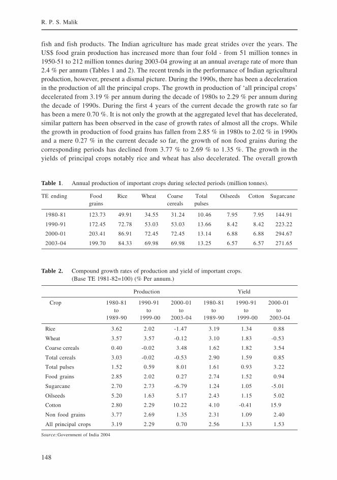
148
R. P. S. Malik
fish and fish products. The Indian agriculture has made great strides over the years. TheUS$ food grain production has increased more than four fold - from 51 million tonnes in1950-51 to 212 million tonnes during 2003-04 growing at an annual average rate of more than2.4 % per annum (Tables 1 and 2). The recent trends in the performance of Indian agriculturalproduction, however, present a dismal picture. During the 1990s, there has been a decelerationin the production of all the principal crops. The growth in production of ‘all principal crops’decelerated from 3.19 % per annum during the decade of 1980s to 2.29 % per annum duringthe decade of 1990s. During the first 4 years of the current decade the growth rate so farhas been a mere 0.70 %. It is not only the growth at the aggregated level that has decelerated,similar pattern has been observed in the case of growth rates of almost all the crops. Whilethe growth in production of food grains has fallen from 2.85 % in 1980s to 2.02 % in 1990sand a mere 0.27 % in the current decade so far, the growth of non food grains during thecorresponding periods has declined from 3.77 % to 2.69 % to 1.35 %. The growth in theyields of principal crops notably rice and wheat has also decelerated. The overall growth
Table 1. Annual production of important crops during selected periods (million tonnes).
TE ending Food Rice Wheat Coarse Total Oilseeds Cotton Sugarcanegrains cereals pulses
1980-81 123.73 49.91 34.55 31.24 10.46 7.95 7.95 144.91
1990-91 172.45 72.78 53.03 53.03 13.66 8.42 8.42 223.22
2000-01 203.41 86.91 72.45 72.45 13.14 6.88 6.88 294.67
2003-04 199.70 84.33 69.98 69.98 13.25 6.57 6.57 271.65
Table 2. Compound growth rates of production and yield of important crops.(Base TE 1981-82=100) (% Per annum.)
Production Yield
Crop 1980-81 1990-91 2000-01 1980-81 1990-91 2000-01to to to to to to
1989-90 1999-00 2003-04 1989-90 1999-00 2003-04
Rice 3.62 2.02 -1.47 3.19 1.34 0.88
Wheat 3.57 3.57 -0.12 3.10 1.83 -0.53
Coarse cereals 0.40 -0.02 3.48 1.62 1.82 3.54
Total cereals 3.03 -0.02 -0.53 2.90 1.59 0.85
Total pulses 1.52 0.59 8.01 1.61 0.93 3.22
Food grains 2.85 2.02 0.27 2.74 1.52 0.94
Sugarcane 2.70 2.73 -6.79 1.24 1.05 -5.01
Oilseeds 5.20 1.63 5.17 2.43 1.15 5.02
Cotton 2.80 2.29 10.22 4.10 -0.41 15.9
Non food grains 3.77 2.69 1.35 2.31 1.09 2.40
All principal crops 3.19 2.29 0.70 2.56 1.33 1.53
Source:Government of India 2004
149
Indian Agriculture: Recent Performance and Prospects in the Wake of Globalization
rate of the yield of all the principal crops has decelerated from 2.56 % in 1980s to 1.33 % in1990s and has recovered slightly to 1.53 % during the 4 years of the current decade. Whilethe growth in food grain production during the 1990s has managed to be just equal topopulation growth rate (2.02 % versus 2.16 %), the preliminary data for the more recent yearsindicate a food grain production growth rate far behind the population growth rate. In fact,the underlying trend of rice and wheat production was already less than population growthby the end of the Ninth Plan. The official data show that the net per capita availability offood grains in the country came down from 471 gram per capita per day during the TE ending1990 to 456 gram per capita per day during the TE ending 2000.
Apart from occasional poor monsoons and some demand-related problems, the long-term trend of agricultural production in India can largely be attributed to a variety of factorssuch as declining public investment; failure to carry out essential reforms to conserve waterand soil; unabated degradation of natural resources, and weakened support systems due tofinancial problems of state governments. While reversing the trend of declining investment inagriculture, often cited as the most important factor for deceleration in growth, especially duringthe 1990s, could contribute significantly to reversing the observed deceleration in the growthof agriculture, it will not, however, be prudent to expect that investment alone will reverse thistrend. In order to make investment in agricultural infrastructure yield the desired results interms of higher productivity and production, it would be imperative to pursue reforms vigorouslyin many areas such as agricultural research, extension, credit, marketing, etc., since these reformscollectively would determine the reduction in cost of production and profitability of agriculture.It is the profitability that would ultimately drive the engine of innovation, entrepreneurshipand growth.
India’s Agricultural Trade: Some Recent Trends
Exports
India has been both an importer and exporter of agricultural commodities for a very long time.India’s agricultural exports after growing at a rate of only 0.78 % per annum during the periodfrom 1961 to 1971, registered a steep hike and during the period 1971 to 1981 increased at anannual average growth rate of 18.36 %. During the decade of 1980s the growth rate of exportsagain plummeted to 2.24 % per annum. The economic liberalization and trade reforms introducedin 1991, helped India accelerate the growth rate of exports to 7.42 % per annum (Bhalla 2004).While during the first half of the 1990s India’s agricultural exports performed extremely well,however since 1995-96 these have shown extreme fluctuations. Although the World TradeOrganization (WTO) Agreement on Agriculture in 1995 was expected to improve India’sagricultural exports, this does not seem to have happened. There have recently been somesigns of a turnaround during 2002-03 and it is expected that this trend will continue. Bhalla2004, however, opines that this sudden surge in Indian exports has to some extent been theresult of the existence of large stocks and transport subsidy made available to exporters.
Examined from another angle, the share of agricultural exports, which constituted morethan 30 % of the total exports from the country during 1970-71 and 1980-81, have of late beendeclining consistently, more so in recent years. The declining trend is more noticeable in the
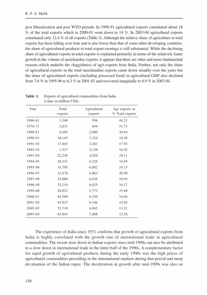
150
R. P. S. Malik
post liberalization and post WTO periods. In 1990-91 agricultural exports constituted about 18% of the total exports which in 2000-01 went down to 14 %. In 2003-04 agricultural exportsconstituted only 12.4 % of all exports (Table 3). Although the relative share of agriculture in totalexports has been falling over time and is also lower than that of some other developing countries,the share of agricultural products in total export earnings is still substantial. While the decliningshare of agricultural exports in total exports is explained primarily in terms of the relatively fastergrowth in the volume of merchandise exports, it appears that there are other and more fundamentalreasons which underlie the sluggishness of agri-exports from India. Further, not only the shareof agricultural exports in the total merchandise exports came down steadily over the years butthe share of agricultural exports (including processed food) in agricultural GDP also declinedfrom 7.6 % in 1995-96 to 6.3 % in 2001-02 and recovered marginally to 6.9 % in 2003-04.
Table 3. Exports of agricultural commodities from India(value in million US$).
Year Total Agricultural Agr exports asexports exports % Total exports
1960-61 1,348 596 44.21
1970-71 2,031 644 31.71
1980-81 8,484 2,600 30.64
1990-91 18,145 3,354 18.49
1991-92 17,865 3,203 17.93
1992-93 1,537 3,136 16.92
1993-94 22,238 4,028 18.11
1994-95 26,331 4,226 16.05
1995-96 31,795 6,082 19.13
1996-97 33,470 6,863 20.50
1997-98 35,006 6,626 18.93
1998-99 33,219 6,035 18.17
1999-00 36,822 5,773 15.68
2000-01 44,560 6,256 14.04
2001-02 43,827 6,146 14.03
2002-03 52,719 6,962 13.21
2003-04 63,843 7,888 12.36
The experience of India since 1971 confirms that growth of agricultural exports fromIndia is highly correlated with the growth rate of international trade in agriculturalcommodities. The recent slow down in Indian exports since mid-1990s can also be attributedto a slow down in international trade in the latter half of the 1990s. A complementary factorfor rapid growth of agricultural products during the early 1990s was the high prices ofagricultural commodities prevailing in the international markets during that period and steepdevaluation of the Indian rupee. The deceleration in growth after mid-1990s was also on
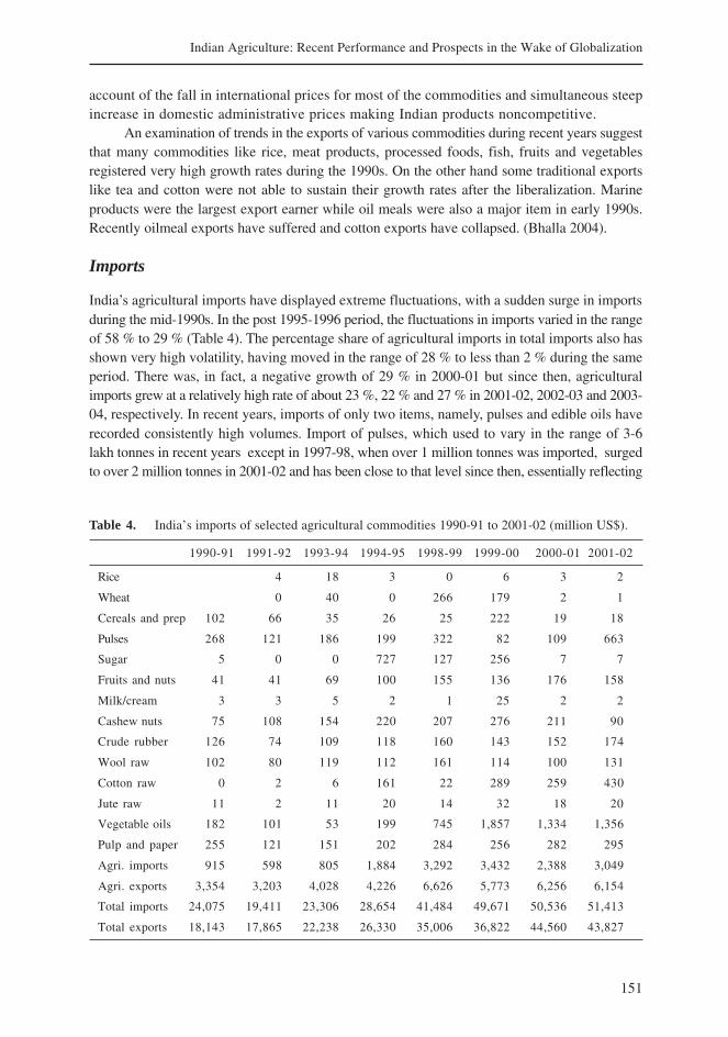
151
Indian Agriculture: Recent Performance and Prospects in the Wake of Globalization
account of the fall in international prices for most of the commodities and simultaneous steepincrease in domestic administrative prices making Indian products noncompetitive.
An examination of trends in the exports of various commodities during recent years suggestthat many commodities like rice, meat products, processed foods, fish, fruits and vegetablesregistered very high growth rates during the 1990s. On the other hand some traditional exportslike tea and cotton were not able to sustain their growth rates after the liberalization. Marineproducts were the largest export earner while oil meals were also a major item in early 1990s.Recently oilmeal exports have suffered and cotton exports have collapsed. (Bhalla 2004).
Imports
India’s agricultural imports have displayed extreme fluctuations, with a sudden surge in importsduring the mid-1990s. In the post 1995-1996 period, the fluctuations in imports varied in the rangeof 58 % to 29 % (Table 4). The percentage share of agricultural imports in total imports also hasshown very high volatility, having moved in the range of 28 % to less than 2 % during the sameperiod. There was, in fact, a negative growth of 29 % in 2000-01 but since then, agriculturalimports grew at a relatively high rate of about 23 %, 22 % and 27 % in 2001-02, 2002-03 and 2003-04, respectively. In recent years, imports of only two items, namely, pulses and edible oils haverecorded consistently high volumes. Import of pulses, which used to vary in the range of 3-6lakh tonnes in recent years except in 1997-98, when over 1 million tonnes was imported, surgedto over 2 million tonnes in 2001-02 and has been close to that level since then, essentially reflecting
Table 4. India’s imports of selected agricultural commodities 1990-91 to 2001-02 (million US$).
1990-91 1991-92 1993-94 1994-95 1998-99 1999-00 2000-01 2001-02
Rice 4 18 3 0 6 3 2
Wheat 0 40 0 266 179 2 1
Cereals and prep 102 66 35 26 25 222 19 18
Pulses 268 121 186 199 322 82 109 663
Sugar 5 0 0 727 127 256 7 7
Fruits and nuts 41 41 69 100 155 136 176 158
Milk/cream 3 3 5 2 1 25 2 2
Cashew nuts 75 108 154 220 207 276 211 90
Crude rubber 126 74 109 118 160 143 152 174
Wool raw 102 80 119 112 161 114 100 131
Cotton raw 0 2 6 161 22 289 259 430
Jute raw 11 2 11 20 14 32 18 20
Vegetable oils 182 101 53 199 745 1,857 1,334 1,356
Pulp and paper 255 121 151 202 284 256 282 295
Agri. imports 915 598 805 1,884 3,292 3,432 2,388 3,049
Agri. exports 3,354 3,203 4,028 4,226 6,626 5,773 6,256 6,154
Total imports 24,075 19,411 23,306 28,654 41,484 49,671 50,536 51,413
Total exports 18,143 17,865 22,238 26,330 35,006 36,822 44,560 43,827
152
R. P. S. Malik
the shortage of domestic production. Similarly, import of edible oils surged from 1 million tonnesin 1995-96 to over 4 million tonnes in 1999-2000 and has since been moving in the range of 4.2to 5.3 million tonnes per year, accounting for about half of domestic consumption. As in thecase of agricultural export items, concerted efforts are required to raise the productivity andproduction of both pulses and oilseeds in the domestic sector.
Thus on balance, while after 1996 there was a deceleration in export growth, theagricultural imports have shown an increase. In fact the gap between agricultural exports andimports has been narrowing down in recent years. Although India abolished its quantitativerestrictions (QRs) in 2001, this has not resulted in any surge of agricultural imports (Table 4).There is an increase in growth but this is mainly because of large imports of edible oils. Recentlythere has also been a sharp increase in the imports of cotton, raw wool and rubber.
India has a large potential to increase its agricultural exports in a liberalized worldprovided it can diversify a significant part of its agriculture into high-value crops and in agro-processing. This would depend first on undertaking large infrastructure investment inagricultural and agro-processing as also in rural infrastructure and research and development.India has not only to create export surplus but also to become competitive through increasedefficiency of production in agriculture. The potential for exports would also depend on freeingof agricultural markets by the developed countries.
Agricultural Support Policies
India, like most of the other countries including developed countries, employs a variety ofinstruments to both protect and support its agriculture. These instruments can broadly beclubbed into three categories: domestic policies, import policies and export policies. Thedomestic policies comprise a wide range of policy instruments like input subsidies on fertilizers,power, irrigation water, public investment in development of water resources – surface andgroundwater, government intervention in markets, direct payment to farmers (such as thosein the form of deficiency payments, insurance and disaster payments, stabilization payments,and also some compensatory payments), price support for major crops , general services (suchas government transfers to agricultural research and development, extension services, trainingand agricultural infrastructure etc.), other support (comprising such measures like certain taxconcessions specific to agriculture or local or substantial level funding for agriculture etc.).Import policies refer essentially to border protection through trade barriers such as quantitativerestrictions, quotas and tariffs on imports, which in the process create a wedge between domesticand world market prices. Export policies include those that either promote export (throughinstruments like subsidies and marketing arrangements that make exportables of a country morecompetitive) or those policies that constrain exports (often through canalization and restrictionof exports and export taxes etc.). Usually, however, import policies are discussed in the contextof trade policies rather than support to agriculture per se. Domestic support and export policiesare often intermingled - export subsidies are more often than not a fallout of domestic supportpolicies that maintain domestic prices of agricultural products within a country at levels higherthan international prices. Of the different types of domestic support to agriculture, however,the most important have been through subsidization of input prices and subsidization throughpayment of higher prices of crop output than that would prevail in a free trade scenario.
153
Indian Agriculture: Recent Performance and Prospects in the Wake of Globalization
Impact of Domestic Agricultural Support Policies
The measure of domestic support is often discussed in terms of two parameters - the AggregateMeasure of Support (AMS) and the Producer Support Estimate (PSE). In terms of both themeasures, despite heavy input subsidies, the aggregate impact of the whole gamut of domesticsupport policies, when viewed in an international trading context, indicate that when allcommodities were treated as imports, aggregate farm output was taxed by this policy regimeduring 1986-2002. Outlays on price support and input subsidies are large, but the impacts ofthese measures have typically been more than offset by relatively low domestic farm gate pricesthat prevail due to quantitative import and export restrictions and high marketing costs. Morerecent protection estimates show that through a combination of rising budgetary subsidiesand smaller gaps between domestic and world prices, the taxation of Indian agriculture hasdeclined significantly. When the major commodities are treated as exportables - and relativeprices are compared at the border rather than the farm gate - protection even turns positive for2001 and 2002 (Landes and Gulati 2004; Gulati and Narayanan 2003; Gulati and Kelly 1999).
WTO Agreements and Agriculture: An Overview and Current Status ofNegotiations
After the Uruguay Round negotiations, agriculture trade is now firmly within the multilateraltrading system. The WTO Agriculture Agreement, together with individual countries’commitments to reduce export subsidies, domestic support and import duties on agriculturalproducts formed a significant first step towards reforming the agricultural trade.
The Uruguay Round agreement had set up a framework of rules and started reductionsin protection and trade-distorting support. But this was only the first phase of the reform.Article 20 of the Agriculture Agreement committed members to start negotiations on continuingthe reform at the end of 1999 (or beginning of 2000). Those negotiations, currently underway,began using Article 20 as their basis. The November 2001 Doha Ministerial Declaration set anew mandate by making the objectives more explicit, building on the work carried out thus far,and setting deadlines. The negotiations have been difficult because of the wide range of viewsand interests among member governments.
The prominent issues in the negotiations mandated under Article 20 have been referred toas a ‘tripod’ whose three legs are export subsidies, domestic support, and market access (morecommonly called ‘the three pillars’ of agricultural trade reform). Non-trade concerns and specialand differential treatment for developing countries would be taken into account as appropriate.The negotiations are now in their fifth year. Negotiators missed the March 31, 2003 deadline forproducing numerical targets, formulas and other ‘modalities’ for countries’ commitments. A reviseddraft ‘modalities’ paper was put up in March 2003 and although it was not agreed, it was usedto discuss technical details in subsequent months. A number of ‘framework’ proposals dealingwith main points of the modalities were submitted and discussed before and during the FifthMinisterial Conference in Cancun, Mexico, September 2003, but it was not until August 1, 2004that a ‘framework’ was agreed on. The next stage now is to agree on full ‘modalities’, which willin turn be used to work out the final agreement on revised rules, and individual countries’commitments. The Doha Declaration had envisaged that countries would submit comprehensive
154
R. P. S. Malik
draft commitments, based on the ‘modalities’ by the Cancun Ministerial Conference — but withoutmodalities, this target was not met either. Meanwhile, the final deadline for completing thenegotiations, January 1, 2005, was officially postponed on August 1, 2004, without a new dateset, though unofficially it was set for December 2006.
August 2004 Agreed Framework: Salient Features
On Domestic Support
All developed countries will make substantial reductions in distorting supports, and thosewith higher levels are to make deeper cuts from ‘bound’ rates (the actual levels of supportcould be lower than the bound levels). The way to achieve this will include reductions bothin overall current ceilings (bound levels), and in two components — Amber Box and de minimissupports. The third component, Blue Box supports, will be capped; at the moment the BlueBox has no limits. The fine print contains a number of details but also stresses that these haveto meet the long-term objective of ‘substantial reductions’.
All of these reduction commitments and caps will apply. However, the new WTO ceilingat the end of the implementation period will be the lower of the value of trade-distorting supportresulting from (i) the overall cut and (ii) the sum of the reductions/caps of the three components.In other words, countries would have to make the required reductions in Amber Box and deminimis support, and be within the capped limit of the Blue Box. Then, if they are still abovethe overall limit, they will have to make additional cuts in at least one of the three componentsin order to match the ceiling set by the overall cut.
Developing countries will be allowed gentler cuts over longer periods, and will continueto be allowed exemptions under Article 6.2 of the Agriculture Agreement (they can giveinvestment and input subsidies that are generally available and are integral parts of developmentprograms, and provide domestic support to help farmers shift away from producing illicit crops).
On Export Subsidies and Competition:
The framework states clearly that all forms of export subsidies will be eliminated by a ‘credible’date. The elimination will work in parallel for all types of subsidies, including those in government-supported export credit, food aid, and state-sanctioned exporting monopolies. The negotiationswill also develop disciplines on all export measures whose effects are equivalent to subsidies.
On Market Access
The framework commits members to ‘substantial improvements in market access for allproducts’. Three or four key points emerged in the bargaining over the framework: the type oftariff reduction formula that would produce the agreed result of ‘substantial improvements inmarket access’; how all countries’ sensitive products might be treated; how developingcountries might be given further flexibility for their ‘special products’ and be able to use ‘specialsafeguard’ actions to deal with surges in imports or falls in prices; how to deal with conflictinginterests among developing countries over preferential access to developed countries’ markets;and how to provide market access for tropical products and crops grown as alternatives toillicit narcotics. Also discussed was a possible trade-off between cuts in some developedcountries’ subsidies and improved market access in developing countries.
155
Indian Agriculture: Recent Performance and Prospects in the Wake of Globalization
WTO Negotiations on Agriculture: India’s Stand
India has been active in WTO negotiations both as a sovereign nation and also collectivelyas a principal member of G20 and G33 groups of nations. While conforming to the substanceof framework agreement these countries have emphasized that the reforms in all three pillarsform an interconnected whole and must be approached in a balanced and equitable manner.These countries have individually and collectively suggested:
On Domestic Support
In order to fulfill the mandate of ‘substantial reductions in trade-distorting domestic support’,negotiations should determine base periods and initial and final numbers for the overall trade-distorting domestic support in a technically consistent and politically credible manner. Anychange in the Blue Box (Article 6.5 of the Agreement on Agriculture) is contingent uponagreement on additional criteria in order to make it substantially less trade-distorting than it isnow. It should be ensured that in the Green Box no, or at most minimal, trade-distorting effectsor effects on production will be generated by any direct payments claimed to be exempt fromreduction commitments. Green Box should be reviewed and clarified to include specificprovisions designed to accommodate genuine agriculture and rural development program ofdeveloping countries aimed at alleviating poverty, promoting agrarian reform and settlementpolicies, and ensuring food security and addressing livelihood security needs. Further, forfacilitating implementation of Green Box measures in developing countries, their specialcircumstances would also need to be taken into account. Further, given that de minimis supportis the only form of support available to farmers in most developing countries, any attempt toreduce de minimis support in developing countries would negatively affect the programsbenefiting subsistence and resource poor farmers.
On Export Competition
In the export competition pillar, a key decision to be taken is the date of elimination of allforms of export subsidies. They have urged countries that apply such instruments to eliminatethem in a period no longer than 5 years and with a front-loading of commitments. An earlyagreement would inject new momentum to the agriculture negotiations and make progress easierin other fronts. They stressed the need to develop new disciplines on export credits, exportcredit guarantees and insurance programs and food aid so that these instruments are not usedso as to displace exports or to promote surplus disposal. They have also recalled the need formaking operative the ‘July Framework’ provisions for special and differential treatment includingState Trading Enterprises and the concerns of Net Food Importing Developing Countries(NFIDCs) as provided in the Marrakesh Decision.
On Market Access
On market access, the crucial importance of conversion into ad valorem equivalents (AVEs)for the completion of the core modality – the tariff reduction formula has been emphasized.The treatment of non-ad valorem (NAVs) duties should clearly spell out the methodologiesused for conversion so that the verification process does not become cumbersome. The long
156
R. P. S. Malik
held view that the tariff reduction formula is the main component of the market access pillarand should be negotiated before addressing the issue of flexibilities has been reaffirmed. Ithas been underlined that the tariff reduction formula must contain: (i) progressiveness – deepercuts to higher bound tariffs; (ii) proportionality – developing countries making lesser reductioncommitments than developed countries and neutrality in respect of tariff structures; and (iii)flexibility – to take account of the sensitive nature of some products without undermining theoverall objective of the reduction formula and ensuring substantial improvement in marketaccess for all products. It has been strongly stressed that special and differential treatmentfor developing countries must constitute an integral part of all elements with a view topreserving food security, rural development and livelihood concerns of millions of people thatdepend on the agriculture sector. The concepts of Special Products and Special SafeguardMechanism are integral elements of special and differential treatment for developing countries.The elimination of tariff escalation is important for developing countries, as it would allowthem to diversify and increase their export revenues by adding value to their agriculturalproduction. A serious concern about the increasing use of Non-Tariff Barriers by developedcountries, which acts as impediments to the exports of products of interest to developingcountries, has also been raised.
Globalization and Domestic Policy Reforms
The importance of domestic reforms in an environment of increased global integration hasbeen widely acknowledged. It has been asserted that large-scale welfare gains from multilateralagricultural liberalization are contingent on well-functioning domestic economies and that iffactor markets were inflexible or public infrastructures were in poor shape only a fraction ofthe gains from trade reforms would be realized (Anderson 2003). The Reserve Bank of India(RBI) observed in its 2001 Annual Report that “…the pace of progress in liberalization of externaltrade in agriculture warrants a sense of urgency and priority to institutional reform inagriculture.”(RBI 2001). While stressing the importance of public investment in basicinfrastructure the RBI stressed the importance of effective supply chain arrangements thatencompassed storage, processing and trading. It also noted a major concern of regulatingintermediaries. There is a strong perception that inadequate regulation of intermediaries inagricultural trade acutely affects farmers on account of low farm gate prices. Policy constraintssuch as restrictions on movement of agricultural commodities and ad hocism in export policyhave been cited as a major source of regulatory problems (Government of Kerala 2003). TheGovernment of India removed several statutory restrictions in its 2002 National AgriculturalPolicy. In early 2004 the government liberalized procurement of food grains for the export market;exporters are now permitted to procure rice and wheat from farmers at market-determined rates.Food grain market policy in India has tended to be highly interventionist with the central andstate governments actively involved in grain storage and restrictions on the movement of foodgrains across states (Jha and Srinivasan 2004). Transport costs are also extremely high in India.It has been estimated that comprehensive reform and infrastructure intervention consisting ofrationalization of internal movement controls, reduction of transport costs by 50 % anddecentralization of public procurement and the PDS would have the effect of increasing welfareby about US$2 billion. The efficacy of India’s Public Distribution System (PDS) in ensuringfood security to the poor has been a subject of extensive criticism. Implementation of modifiedPDS programs, such as the targeted public distribution system (TPDS), has also proven difficult
157
Indian Agriculture: Recent Performance and Prospects in the Wake of Globalization
in India as a result of weak administrative capacity and resource constraints at the local level.The Planning Commission’s mid-term review acknowledges that the minimum support policy(MSP) policy has been ineffective, farm incomes declined in regions subject to the MSP, andin 2001 it was decided to lower stocks by lowering sales prices and increasing food for work.Nearly a third of the growth in the unirrigated regions since the mid-1990s has been throughcrop diversification, especially to horticultural products. Support price policy, particularly forwheat and rice, has remained delinked from domestic and international market realities, creatingsignificant budgetary costs and market distortion. Although initial upward adjustments indomestic prices may have been justified due to the prevailing negative support to cereals,policy was unable to adjust with market conditions. The inability to reform price policy andcertain input subsidies has led to a decline in public investment in agriculture at a time wheninvestment in new infrastructure and institutions is needed. Although the incentives and climatefor private investment have improved, it may not be able to fully substitute for weak publicinvestment. Reforms at the border, when they have been implemented, have typically exposedinefficiencies in the domestic market that limit competitiveness. These weaknesses limit thebenefits of border reform and, at least in India’s case, will require significant investment intransport and marketing infrastructure and institutional capacities to overcome.
As a result of commitments under the Uruguay Round, India has bound all the tarifflines in agriculture. India had bound its tariffs at 100 % for primary products, 150 % for processedproducts and 300 % for edible oils, except for certain items (comprising about 119 tariff lines),which were historically bound at a lower level in the earlier negotiations. The applied rateshave been much lower than the bound rates. In India the product-specific support is negative,while the non-product specific support i.e., subsidies on agricultural inputs, such as power,irrigation and fertilizers is well below the permissible level of 10 % of the value of agriculturaloutput. Therefore, India is under no obligation to reduce domestic support currently extendedto the agricultural sector. Export subsidies of the kind listed in the Agreement on Agriculture,which attract reduction commitments, are not extended in India. Also, developing countriesare free to provide certain subsidies, such as for export marketing costs, internal andinternational transport and freight charges etc.
India: Effects of Past Liberalization
Trade liberalization primarily causes changes in producer and consumer surplus and the neteffects of this liberalization depend on which of the two effects is stronger. Several researchershave attempted to quantify the effects of trade liberalization. The available results point tomixed evidence of the effects of trade liberalization. A study by Ramesh Chand 1999 attemptedto quantify the impact of globalization of agriculture on producer surplus, consumer surplusand net social welfare in the case of four crops, namely, paddy (rice), maize, chickpea andrapeseed-mustard. The study concluded that in the case of studied crops, free trade is likelyto have sharp positive impact on net return from production of exportables like maize and rice,whereas, it is likely to have small negative impact on net return from the importables likerapeseed-mustard. In rice where level of input subsidy is high, free trade would not be sufficientto counter the adverse impact on income due to withdrawal of subsidies.
In a recent study Jayati Ghosh, examined the impact and policies strategies with specialreference to India, however, opined that more liberal external trade has not, in general, had abeneficial impact on cultivators in India. This has been partly because of the patterns in world

158
R. P. S. Malik
trade which have led to volatile and declining crop prices internationally. But it also has a greatdeal to do with internal macroeconomic and sectoral policies which have reduced protection tocultivators, caused input prices to rise sharply, made marketing of crops more difficult andexploitative for the direct producers and reduced the flow of institutional credit. The criticalquestion, therefore, in the current context is how to manage trade liberalization and domesticpolicies so as to ensure the viability of small cultivators and food security in the countryside.
In some products, such as edible oils, international prices on account of subsidies haveconsistently been lower than domestic prices. Analysts addressing this issue have consistentlyshown that Indian edible oils do not compete well with imports (Gulati and Sharma 1998).Comparing the ratio of domestic and international prices of oilseeds and oil, Chand 2002 showsthat oilseed production, particularly in rapeseed-mustard and soybean, is fairly competitive.This is also shown by a World Bank 1997 study. It is in oils that India is on shaky grounds(Chand 2002). Inefficiencies in the oil-processing sector is one reason; the other factor is thesubsidy-driven ability of foreign producers to sell cheap oil. These and other findings indicatethat oilseed production in the country faces a threat due to inefficiency of processing andmarketing and also due to the transmission of volatility in world prices to the domestic market.India liberalized its, soybean and soy oil import policy in August 1999. This led to dumping ofsubsidized imports of soybeans on the Indian market. These imports totaled 3 million tonnesin one year (a 60 % rise compared to earlier years) and cost nearly US$1 billion. Within onegrowing season, prices crashed by more than two-thirds, and millions of oilseed-producingfarmers had lost their market, unable even to recover what they had spent on cultivation. Whilethe declining prices have hurt producers, consumers have gained considerably. This wouldrequire the government to balance the competing interests of producers and consumers andperhaps lean towards poor and small-scale producers (Chand et al 2004). In another study onoilseeds, as a result of successive lowering of tariffs on edible oils – first from 65 to 30 %,and then to 15 % in 1998- and lifting of non-tariff restrictions, imports soared, and India wentfull circle from self-sufficiency to the world’s largest importer in only 5 years. As a result ofwhich, thousands of Indian farmers lost their livelihoods (Mark Fried 2004).
In the case of pulses, Sathe and Agarwal 2004 examined the issues related to the openingup of the Indian pulses sector. The study shows that pulses (lentils) imports have not augmentedsupply to such an extent that there would be a strong, negative relationship between prices andimports of pulses. Though the import duties on pulses have been generally low the result of ourimport regime has been such that it has not depressed prices in a substantial way.
Liberalization of imports may have a negative effect on the Indian agrarian economymainly on account of the huge subsidization of agriculture by most of the developed countries,which implies that imports are sold below the cost of production in India, the imperfect natureof world agricultural markets and also on account of higher volatility of agricultural prices ininternational markets which in turn gets transmitted to the domestic markets.
A study by Sekhar 2004 attempts to assess the implications for food security of thepoor through transmission of international price volatility into domestic markets which ariseson account of globalization in agriculture. The commodities selected for study are wheat,rice, groundnut oil, soybean oil, coconut oil, sugar, cotton and coffee. His study shows thatextreme volatility in commodity prices, particularly of food commodities, adversely affectspoor agricultural laborers and those engaged in the unorganized sector because their wagesare not index-linked. For exporters, price volatility increases cash-flow variability and reduces
159
Indian Agriculture: Recent Performance and Prospects in the Wake of Globalization
collateral value of inventories. In order to understand the implications of trade liberalization,particularly import liberalization, it is essential to examine the long-term movements ofdomestic and international prices and assess the degree of divergence between the two.A price wedge – percentage difference between the monthly domestic and international pricesfor 10 years since 1990 – has been calculated for this purpose. His study shows that wherebound tariffs are much higher than the observed price wedges, the bound rates may belowered. He concludes by stating that as short-term variability in agricultural prices ininternational markets is not found to be higher than domestic markets in India, internationaltrade may be used as a short-term price stabilization strategy in case of supply shocks. Atthe same time, care should be taken to negotiate appropriate tariff bindings to protect againstcheap imports resulting from unfair subsidization in some developed countries.
Potential Impacts of Liberalization
Estimating the potential impacts of liberalization of trade in agricultural and non agriculturalcommodities in the wake of WTO negotiations on agriculture is complicated and would dependon the outcome of the negotiations currently underway. More specifically it would in largepart depend upon the extent to which the developed countries are willing to scale down theirdomestic support, export subsidies, tariffs, and non-tariff barriers and let increase their marketaccess for the developing and least developed countries. While several proposals are currentlyon the table in respect of each of these components, agreements have alluded all of them.Several researchers have nevertheless attempted to evaluate, using the scenario analysisapproach, the likely impacts of some of the alternative proposals under discussion in one ormore of these areas on one or more of the affected variables viz international prices, production,trade and welfare at the global and /or at the level of a region/country. In the followingparagraphs we attempt to very briefly give a summary of impacts from a few of the selectedrecent studies on the subject. It may, however, be important to mention that the results obtainedfrom different studies are not strictly comparable because of the differences in underlyingassumptions, the differences in methodology employed, the time frame considered and thenature of impacts analyzed. The results from most of the studies on liberalization of agriculturaltrade point towards an increase in international prices of a majority of the agriculturalcommodities, increase in volume of international trade and an increased welfare consequentupon liberalization. The impacts on production of different crops, principally the cereals,however, appear to be marginal.
USDA 2001 has estimated that the full elimination of global agricultural policydistortions would result in an annual world welfare gain of US$56 billion. Moreover,elimination of agricultural trade and domestic policy distortions could raise world agriculturalprices by about 12 %. Evaluating the impacts of comprehensive multilateral liberalization ofagricultural trade policies using a CGE model, Cline estimates that the welfare benefits froma free trade in agriculture for India will be to the tune of U$0.82 billion. Full liberalization ofOECD farm policies would boost the volume of global agricultural trade by more than 50 %but would cause real food prices to rise by only 5 % on average (Anderson, 2003). Somemodels have projected food price rises of about 8 - 12 % (Diao et al. 2002). Another study(Beghin and Aksoy 2003) estimate that world prices are likely to go up by even higher margins:
160
R. P. S. Malik
10-20 % for cotton, 20-40 % for dairy products, 10-20 % for groundnuts, 33-90 % for riceand 20-40 % for sugar. Results of a World Bank study indicate that a removal of agriculturaltariffs and subsidies by all WTO countries would generate an increase in developing countryexports of 15 % and increase in imports of 12 %. In terms of this study, India would experiencean increase in exports of 13 %. World prices of wheat are expected to rise by about 10 %and prices of rice are expected to rise by about 16 %. As a net exporter of both rice andwheat, India, therefore, stands to gain significantly from terms-of-trade improvements.
Babcock et al. 2003 using the FAPRI model have analyzed the impact of liberalizingagricultural markets on world trade flows, prices and market equilibrium. The analysis has beencarried out under two possible scenarios - the full trade liberalization scenario and trade-onlyliberalization scenario. The results obtained suggest that under a full liberalization scenario,the world wheat, rice and cotton prices are estimated to go up by 4.8 %, 10.3 % and 15 %,respectively. Under the trade-only liberalization scenario the corresponding increase in theprices of wheat, rice and cotton are likely to be of the order of 7.6, 10.6 and 3 %, respectively.Because of the removal of export subsidies Indian exports of wheat are estimated to decreaseunder the full liberalization scenario and India is projected to become a net importer by 2003/04 with trade only scenario. Rice trade increases by 29 % under the full trade scenario and byabout 27 % in the trade-only scenario. Most of these exports are captured by China, India andVietnam followed by Thailand. On an average Indian exports of rice are estimated to grow byover 100 % under the full liberalization and by 56 % under the trade-only scenario. In the caseof cotton, under the full liberalization scenario net cotton imports decline by 16 %. In the tradeonly scenario Indian exports of cotton increase by just 2 %. Thus India is likely to gain muchmore in the rice and cotton sectors under a scenario of full liberalization. The present exercise,however, does not take in to account the transportation cost when estimating the flow of trade.In the case of wheat, the transportation cost vis-à-vis the US is relatively high, and India islikely to have an advantage when competing with the US in export destinations closer to theformer even after elimination of export subsidies.
Evaluating the implications of some of the alternative tariff reduction structures, a studyby Vanzetti and Peters 2003 using general equilibrium models, shows that the onetariff-harmonizing Swiss formula component with rather ambitious coefficients of 25 fordeveloped and 50 for developing countries gives overall welfare effects that are not muchhigher than a continuation of the Uruguay Round approach. Assuming reduction in exportsubsides by 45 % and domestic support by 55 % further reduces the global welfare gains.
Another recent World Bank study shows that in terms of potential reform, or the pillars ofagriculture negotiations, increased agricultural market access is the key to successful liberalizationof merchandise trade, accounting for well over half the potential economic welfare gains todeveloping countries and the world as a whole from removing all merchandise trade distortionsand farm subsidies. Within agriculture, the potential gains from market access are shown to befar more important than those from abolition of domestic support and export subsidies, accountingfor 93 % of the gains from total agricultural liberalization (Anderson 2003).
Another study demonstrates how improving market access in the developed countriesthrough lowering of tariffs would be beneficial to India. Domestic support has been viewed asthe equivalent of implicitly imposing tariffs. Cline 2003 has estimated the tariff equivalent of allsubsidies and added it to tariff rates in the Quad (US, EU, Japan, Canada) to indicate the overalllevels of protection provided by the Quad to agriculture. Thus in the case of EU and US if
161
Indian Agriculture: Recent Performance and Prospects in the Wake of Globalization
tariff equivalents of subsidies are taken into account the overall tariff protection risessubstantially. Using this approach, it is suggested that unless domestic support is reducedthe real tariff reduction effects for India would be only two- thirds of the total gain. This wouldbe particularly the case for the US and the EU whose tariff equivalent of subsidies is far greaterthan for other countries. In fact, ‘tariffication’ of the level of subsidies and adding it to thetariff rates is a far more logical way of addressing the effects of subsidies than throughnotifications of subsidies and targeting reduction commitments on these notifications.
Anderson 2003 has projected that a complete global liberalization of agricultural trade(including the removal of massive agricultural protection by OECD countries) would havethe effect of increasing net annual exports of agricultural and food products by US$2.7 billionfrom India: a 40 % rise over the current level of agricultural exports. The current annualvalue of agricultural production in India is close to US$100 billion. A US$2.7 billion growthin exports would constitute in itself close to 2.7 % annual growth in value of Gross DomesticAgricultural Product, which equals the current average annual growth rate. This is basedon the assumption that all additional exports come from additional domestic agriculturalproduction and is not diverted from domestic consumption. Thus assuming an adequatesupply response, growth rates in agriculture production may tend to double on average forthe first few years.
UNCTAD using a GTAP - CGE model, has attempted to evaluate the impacts oftwoagricultural tariff reduction scenarios (1) 3 large band approach I-soft tariff reduction;and (2) 3 small band approach I- hard tariff reduction, on imports, exports, production andwelfare in India (UNCTAD 2005). The results obtained suggest that while welfare improveswith tariff cuts in the hard scenario the same is not true for other variables. Developedcountries as a whole see much larger gains in the soft scenario in comparison with the hardscenario (Table 5). Some products emerge as being sensitive on several counts. Paddy seesa decline in output and employment in the soft scenario, but both exports and importsincrease under both scenarios. However, the extent of import increase, from a smaller base,is much larger than the extent of export increase. The study thus suggests that paddy andrice trade should be liberalized cautiously. Vegetables, nuts and fruits also show an outputand employment decrease along with an increase in trade. Oilseeds and oil show an outputand employment decline accompanied by import increases and minor export increase.
In another major study to analyze the implications of selected scenarios in all the threepillars of agricultural negotiations, UNCTAD using partial equilibrium modeling employedAgricultural Trade Policy Simulation Model (ATPSM) to assess the implications of tariff cuts,export subsidy cut, and domestic subsidy cut on Indian agriculture (UNCTAD 2005).
Table 5. Impact on welfare: welfare gains (in million US$).
EV Soft Hard
India 210.93 331.05
Developed countries 2,036.05 22.11
Developing countries 752.34 42.74
Least developing countries 18.37 4.95
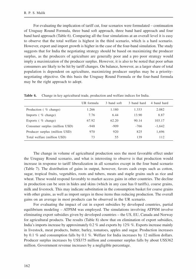
162
R. P. S. Malik
For evaluating the implication of tariff cut, four scenarios were formulated – continuationof Uruguay Round Formula, three band soft approach, three band hard approach and fourband hard approach (Table 6). Comparing all the four simulations at an overall level it is easyto observe that the total welfare is highest in the third scenario, which is a hard scenario.However, export and import growth is higher in the case of the four-band simulation. The studysuggests that for India the negotiating strategy should be based on maximizing the producersurplus, as the producers of agriculture are generally poor and a pro poor strategy wouldimply a maximization of the producer surplus. However, it is also to be noted that poor urbanconsumers are likely to be hit by tariff changes. On balance, however, as a larger share of totalpopulation is dependent on agriculture, maximizing producer surplus may be a priority-negotiating objective. On this basis the Uruguay Round Formula or the four-band formulamay be the right approach to adopt.
Table 6. Change in key agricultural trade, production and welfare indices for India.
UR formula 3 band soft 3 band hard 4 band hard
Production ( % change) 1.266 1.180 1.333 2.082
Imports ( % change) 7.76 6.44 13.90 8.87
Exports ( % change) 67.92 62.20 90.14 103.17
Consumer surplus (million USD) -948 -909 -766 -1,642
Producer surplus (million USD) 970 920 825 1,696
Total welfare (million USD) 73 55 139 112
The change in volume of agricultural production sees the most favorable effect underthe Uruguay Round scenario, and what is interesting to observe is that production wouldincrease in response to tariff liberalization in all scenarios except in the four band scenario(Table 7). The distribution of gains in output, however, favors cash crops such as cotton,sugar, tropical fruits, vegetables, roots and tubers, meats and staple grains such as rice andwheat. These would respond favorably to market access gains in other countries. The declinein production can be seen in hides and skins (which in any case has 0 tariffs), coarse grains,milk and livestock. This may indicate substitution in the consumption basket for coarse grainswith other grains, as well as import surges in those items thus reducing production. The overallgains on an average in most products can be observed in the UR scenario.
For evaluating the impact of cut in export subsidies by developed countries, partialequilibrium modeling – ATPSM was employed. The simulations involving ATPSM involveeliminating export subsidies given by developed countries – the US, EU, Canada and Norwayfor agricultural products. The results (Table 8) show that on elimination of export subsidies,India’s imports increase by approximately 0.2 % and exports by 12% %. Exports increase mainlyin livestock, meat products, butter, barley, tomatoes, apples and sugar. Production increasesby 0.1 % and consumption falls by 0.1 %. Welfare for India increases by 12 million dollars.Producer surplus increases by US$375 million and consumer surplus falls by about US$362million. Government revenue increases by a negligible percentage.
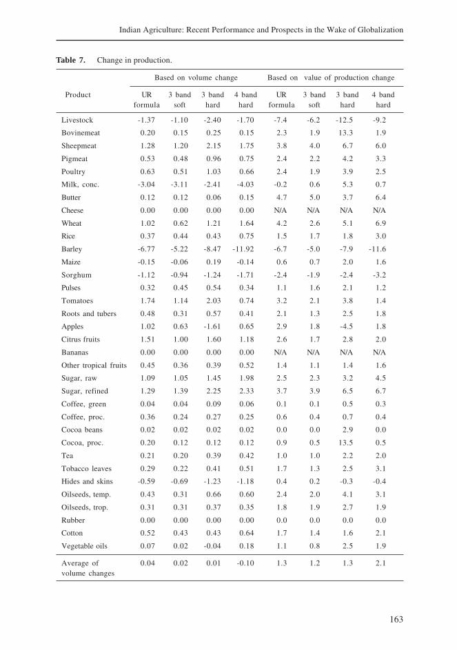
163
Indian Agriculture: Recent Performance and Prospects in the Wake of Globalization
Table 7. Change in production.
Based on volume change Based on value of production change
Product UR 3 band 3 band 4 band UR 3 band 3 band 4 bandformula soft hard hard formula soft hard hard
Livestock -1.37 -1.10 -2.40 -1.70 -7.4 -6.2 -12.5 -9.2
Bovinemeat 0.20 0.15 0.25 0.15 2.3 1.9 13.3 1.9
Sheepmeat 1.28 1.20 2.15 1.75 3.8 4.0 6.7 6.0
Pigmeat 0.53 0.48 0.96 0.75 2.4 2.2 4.2 3.3
Poultry 0.63 0.51 1.03 0.66 2.4 1.9 3.9 2.5
Milk, conc. -3.04 -3.11 -2.41 -4.03 -0.2 0.6 5.3 0.7
Butter 0.12 0.12 0.06 0.15 4.7 5.0 3.7 6.4
Cheese 0.00 0.00 0.00 0.00 N/A N/A N/A N/A
Wheat 1.02 0.62 1.21 1.64 4.2 2.6 5.1 6.9
Rice 0.37 0.44 0.43 0.75 1.5 1.7 1.8 3.0
Barley -6.77 -5.22 -8.47 -11.92 -6.7 -5.0 -7.9 -11.6
Maize -0.15 -0.06 0.19 -0.14 0.6 0.7 2.0 1.6
Sorghum -1.12 -0.94 -1.24 -1.71 -2.4 -1.9 -2.4 -3.2
Pulses 0.32 0.45 0.54 0.34 1.1 1.6 2.1 1.2
Tomatoes 1.74 1.14 2.03 0.74 3.2 2.1 3.8 1.4
Roots and tubers 0.48 0.31 0.57 0.41 2.1 1.3 2.5 1.8
Apples 1.02 0.63 -1.61 0.65 2.9 1.8 -4.5 1.8
Citrus fruits 1.51 1.00 1.60 1.18 2.6 1.7 2.8 2.0
Bananas 0.00 0.00 0.00 0.00 N/A N/A N/A N/A
Other tropical fruits 0.45 0.36 0.39 0.52 1.4 1.1 1.4 1.6
Sugar, raw 1.09 1.05 1.45 1.98 2.5 2.3 3.2 4.5
Sugar, refined 1.29 1.39 2.25 2.33 3.7 3.9 6.5 6.7
Coffee, green 0.04 0.04 0.09 0.06 0.1 0.1 0.5 0.3
Coffee, proc. 0.36 0.24 0.27 0.25 0.6 0.4 0.7 0.4
Cocoa beans 0.02 0.02 0.02 0.02 0.0 0.0 2.9 0.0
Cocoa, proc. 0.20 0.12 0.12 0.12 0.9 0.5 13.5 0.5
Tea 0.21 0.20 0.39 0.42 1.0 1.0 2.2 2.0
Tobacco leaves 0.29 0.22 0.41 0.51 1.7 1.3 2.5 3.1
Hides and skins -0.59 -0.69 -1.23 -1.18 0.4 0.2 -0.3 -0.4
Oilseeds, temp. 0.43 0.31 0.66 0.60 2.4 2.0 4.1 3.1
Oilseeds, trop. 0.31 0.31 0.37 0.35 1.8 1.9 2.7 1.9
Rubber 0.00 0.00 0.00 0.00 0.0 0.0 0.0 0.0
Cotton 0.52 0.43 0.43 0.64 1.7 1.4 1.6 2.1
Vegetable oils 0.07 0.02 -0.04 0.18 1.1 0.8 2.5 1.9
Average of 0.04 0.02 0.01 -0.10 1.3 1.2 1.3 2.1volume changes
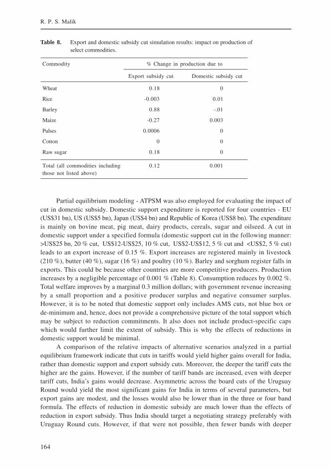
164
R. P. S. Malik
Partial equilibrium modeling - ATPSM was also employed for evaluating the impact ofcut in domestic subsidy. Domestic support expenditure is reported for four countries - EU(US$31 bn), US (US$5 bn), Japan (US$4 bn) and Republic of Korea (US$8 bn). The expenditureis mainly on bovine meat, pig meat, dairy products, cereals, sugar and oilseed. A cut indomestic support under a specified formula (domestic support cut in the following manner:>US$25 bn, 20 % cut, US$12-US$25, 10 % cut, US$2-US$12, 5 % cut and <US$2, 5 % cut)leads to an export increase of 0.15 %. Export increases are registered mainly in livestock(210 %), butter (40 %), sugar (16 %) and poultry (10 %). Barley and sorghum register falls inexports. This could be because other countries are more competitive producers. Productionincreases by a negligible percentage of 0.001 % (Table 8). Consumption reduces by 0.002 %.Total welfare improves by a marginal 0.3 million dollars; with government revenue increasingby a small proportion and a positive producer surplus and negative consumer surplus.However, it is to be noted that domestic support only includes AMS cuts, not blue box orde-minimum and, hence, does not provide a comprehensive picture of the total support whichmay be subject to reduction commitments. It also does not include product-specific capswhich would further limit the extent of subsidy. This is why the effects of reductions indomestic support would be minimal.
A comparison of the relative impacts of alternative scenarios analyzed in a partialequilibrium framework indicate that cuts in tariffs would yield higher gains overall for India,rather than domestic support and export subsidy cuts. Moreover, the deeper the tariff cuts thehigher are the gains. However, if the number of tariff bands are increased, even with deepertariff cuts, India’s gains would decrease. Asymmetric across the board cuts of the UruguayRound would yield the most significant gains for India in terms of several parameters, butexport gains are modest, and the losses would also be lower than in the three or four bandformula. The effects of reduction in domestic subsidy are much lower than the effects ofreduction in export subsidy. Thus India should target a negotiating strategy preferably withUruguay Round cuts. However, if that were not possible, then fewer bands with deeper
Table 8. Export and domestic subsidy cut simulation results: impact on production ofselect commodities.
Commodity % Change in production due to
Export subsidy cut Domestic subsidy cut
Wheat 0.18 0
Rice -0.003 0.01
Barley 0.88 -.01
Maize -0.27 0.003
Pulses 0.0006 0
Cotton 0 0
Raw sugar 0.18 0
Total (all commodities including 0.12 0.001those not listed above)

165
Indian Agriculture: Recent Performance and Prospects in the Wake of Globalization
progressive cuts would be better for India. However, the welfare gains of tariff liberalizationalong with domestic subsidy and export subsidy reductions are very significant.
In another comprehensive study on evaluating the impact of two agricultural tradeliberalization proposals viz the Swiss Formula and Uruguay Round on India, Kirit Parikh 2004employed a sequential applied general equilibrium model laying particular emphasis on theimpact on welfare. The model has a rich policy structure and provides for tariff policy, tradequotas, stock policy, tax policy and redistributive policy. The alternative scenarios analyzedare: SAM–Reference Scenario (which reproduces the base year SAM as a solution for theyear 1997 when the run is with actual 1997 tariffs), FTR- Free Trade Uruguay Round with 50% cut (all agricultural tariffs cut by 50 %, this is the Uruguay round scenario), and FS1 –Swiss Formulae with c = 1. In all the scenarios, the world market prices are kept the same. Thescenarios thus reflect a unilateral liberalization by India and also assume that India’s trade haslittle impact on world prices. All the scenarios are run for 4 years starting 1997. The policychanges are introduced in 1998. The impacts on agricultural prices are thus visible only in1998 and the impacts on output are seen only in 1999 as agricultural output comes with a one-year lag. The simulations show that the welfare impacts are not unambiguous and neither ofthe two policies can be shown to be superior to the reference policy. It does, however, indicatethat after a couple of years, greater trade liberalization is beneficial for a large number of personsindicating that with some safety net policy such as employment guarantee scheme, one maybe able to get a win-win outcome.
In general, thus, if the prices of agricultural commodities like rice, cotton, wheat andsugar were to rise, India could generally improve its exports. Developing countries and theagricultural market in general stand to gain major benefits of reducing and eliminating subsidiesand domestic support. It is, however, necessary to emphasize that this is only a generalequilibrium picture and might be slightly more optimistic than reality,2 as certain products ofparticular interest to India are likely to be liberalized least and there are other competitors whowill, because of high trade logistic costs in India, rush to fill the breach.
Will India Be Able to Make Use of the Opportunities: Supply Side Scenario
Various analyses of some of the proposals under discussion at the WTO show that in overallterms India stands to gain from liberalization of trade in agriculture. However, given the recenttrend of a slowdown in the growth of agricultural production and increasing domestic demand,will India be able to encash on the opportunities that may be made available to it by a moreliberalized trade regime?
The recent mid-term appraisal of the 10th Five-Year Plan, commenting on the supplyside scenario notes that agricultural growth has been poor, with productivity growth comingto almost a complete halt in several products. Within the crop sector only fruits, vegetables,
2 Critics also point to the many limitations of CGE models and the estimates they generate, andquestion the extent to which they should be informing trade policy at all.
166
R. P. S. Malik
condiments and spices have grown by over 2.5 % per annum. Output prices have fallen relativeto input prices reflecting a fall in profitability in agriculture. On the demand side per capitaconsumption of all cereals, pulses and edible oils have fallen, with the growth of consumptiondecelerating for all types of food including milk, vegetables and fruit. This situation impliesthat there may be a need to focus on production and demand, increasing the scope of theprovision of subsidies, through minimum support price in other areas such as the easternregion. Rao 2005, however, opines that the prospects for exports of food grains from Indiaseem real, at least for a decade, if the growth rate in food grains output of around 3 % can beachieved, as the domestic demand for food grains is unlikely to exceed 2.6 % per annum witheven 7 % growth rate in GDP. India is unlikely to absorb domestically the whole of food grainsoutput from a growth rate of around 3 % for quite sometimes unless drastic changes in incomedistribution can be effected.
Conclusion
The evidence available from a number of research studies carried out to ascertain the likelyimpact of trade liberalization on the Indian agricultural sector suggests mixed results dependingupon the assumptions made in the model employed to analyze and the extent to whichdeveloped countries cut their subsidies. On balance, the results tend to indicate that India’sagricultural markets in general stand to gain from liberalization and derive benefits of reductionin subsidies and domestic support by developed countries. To enable India realize these gainsit will need to increase its agricultural production through a step up in crop productivity, whichhas of late been showing the trend of a slowdown.
References
Anderson, K. 2003, ‘How Can Agricultural Trade Reform Reduce Poverty?’ Discussion Paper No.0321.Adelaide: Centre for International Economic Studies, University of Adelaide.
Bansil, P.C. 2003. Demand for Food grains by 2020. In Towards a Food secure India: Issues and Policies,eds. S. Dev Mahender; K.P. Kanan; N. Ramachandran. New Delhi: IHD and CESS.
Babcock, B. A.; Fabosia, J.; Matthey, H.; Isik, M.; Tokgoz, S.; El-Obeid, A.; Hart, C.; Fuller, F.; Meyer, S.2003. An analysis of the Proposed Doha Round Modalities. Staff Report 03-SR98, Food and AgriculturalPolicy Research Institute (FAPRI), Iowa State University.
Beghin, J. C.; Aksoy, A. 2003. Agricultural Trade and the Doha Round: Lessons from Commodity Studies.Briefing Paper 03-BP-42. Ames, Iowa: Centre for Agricultural and Rural Development, Iowa StateUniversity.
Bhalla, G.S. 2004. State of the Indian Farmer. Globalization and Indian Agriculture. Vol 19. New Delhi:Academic Foundation.
Cline, W. 2003. Trade Policy and Global Poverty. Washington DC: Institute for International Economics.
Dhanmanjari, S.; Agarwal, S. 2004. Liberalization of Pulses Sector: Production Prices and Imports, EPWJuly 2004.
Diao, X.; Roe, T.; Somwaru, A. 2002. Developing Country Interests In Agricultural Reforms Under TheWorld Trade Organization. Washington, DC: International Food Policy Research Institute.
167
Indian Agriculture: Recent Performance and Prospects in the Wake of Globalization
Fried, M. (Translator); Fisgon, E. 2004. How to Succeed at Globalization: A Premier for the RoadsideVendor. Henry Holt and Company.
GOI. 2004. Agricultural Statistics at a Glance. New Delhi: Ministry of Agriculture.
GOI. 2005. Mid Term Appraisal of X Five -Year Plan. New Delhi: Planning Commission.
Government of Kerala. 2003, Report of the Commission on WTO concerns in agriculture. Governmentof Kerala.
Gulati, A.; Narayanan, S. 2003. The Subsidies Syndrome in Indian Agriculture. New Delhi: Oxford UniversityPress.
Gulati, A.; Kelly, T. 1999. Trade Liberalization and Indian Agriculture. New Delhi: Oxford University Press.
Gulati, A.; Sharma, A. 1998. Freeing Trade in Agriculture: Implications for Resource Use Efficiency andCropping Pattern Changes. EPW, 1998.
Jha, S.; Srinivasan, P.V. 2004. Efficient Redistribution through Deregulation of Domestic Grain Markets.Paper prepared for presentation at the conference on Anti-poverty and Social Policy in India at theNeemrana Fort-Palace near Delhi, India, hosted by the MacArthur research network on Inequality andEconomic Performance, Indira Gandhi Institute of Development Research (IGIDR).
Kumar, P.; Mittal, S. 2003. Productivity and Supply of Food grains in India. In Towards a Food secureIndia: Issues and Policies, eds. S. Dev Mahender; K.P. Kanan; N. Ramachandran. New Delhi: IHDand CESS.
Landes, R.; Gulati, A. 2004. Farm Sector Performance and Reform Agenda. Economic and Political Weekly,August 7-13, pp 3611-3619.
NSSO. n.d. Consumer Expenditure Survey- Various Rounds. New Delhi: National Sample SurveyOrgainsation.
Opportunities. Report No. 15677-IN. World Bank Rural Development Sector Unit, South Asia Region.
Ramesh, C. 1999. Liberalization of Agricultural Trade and Net Social Welfare: A Study of Selected Crops,EPW, Dec.1999.
Ramesh, C.; Jha, D.; Mittal, S. 2004. WTO and Oilseeds Sector: Challenges of Trade Liberalization, EPW,Feb.2004.
Rao, C. H. H. 2005. Agriculture, Food Security, Poverty, Environment, New Delhi: Oxford University Press.
Rao, C. H. H. 1994. Indian Agriculture: Emerging Perspective and Policy Issues, EPW, December 1994.
RBI. 2001. Annual Report 2000-01. Mumbai: Reserve Bank of India.
Sekhar CSC. 2004. Agricultural Price Volatility. In International and Indian Markets. EPW, Oct.2004.
UNCTAD. 2005. Agricultural Trade Policy in India: Challenges and Opportunities. New Delhi: UNCTAD.
USDA. 2001. Agricultural Policy Reform in the WTO- The Road Ahead. Agricultural Economics Research,Economics Research Service, Report No AER 802, May 2001.
Vanzetti, D.; Peters, R. 2003. Strategic interactions in Trade Policy Negotiations. Paper presented at theSixth Annual Conference on Global Economic Analysis, The Hague, Netherlands.
World Bank. 1997. The Indian Oilseed Complex: Capturing Market.
169
Converting Rain into Grain: Opportunities for Realizingthe Potential of Rain-fed Agriculture in India
1Bharat R. Sharma, 2 K.V. Rao and 2K.P.R. Vittal1International Water Management Institute, New Delhi, India
2Central Research Institute for Dryland Agriculture, Hyderabad, India
Introduction
India ranks first among the rain-fed agriculture practicing countries of the world both in termsof extent (86 M ha) and value of the produce. Due to low opportunities and higher populationof landless households and agricultural laborers as well as low land and labor productivity,poverty is concentrated in rain-fed regions (Singh 2001). Yield gap analyses, undertaken byComprehensive Assessment of Water in Agriculture (CA 2007) for major rain-fed crops foundfarmer’s yield being a factor 2-4 times lower than achievable yields for major rain-fed crops.Grain yield oscillates around 1-2 t/ha compared with attainable yields of over 4-5 t/ha(Falkenmark and Rockstrom1993). The large yield gap between attainable yields and farmers’practice as well as between attainable and potential yields shows that a large potential of rain-fed agriculture remains to be tapped.
Rainfall is a truly random factor in the rain-fed production system and its variationand intensity is high in areas of low rainfall. Semi-arid regions, however, may receive enoughannual rainfall to support crops but it is distributed so unevenly in time or space that rain-fed agriculture becomes unviable (Reij et al. 1988). Rockstrom and Falkenmark 2000 notethat due to the high rainfall variation, a decrease of one standard deviation from the meanannual rainfall often leads to the complete loss of crop. Agricultural droughts, where primarilya skewed distribution of rainfall causes drought in the root zone, are more frequent than thereal meteorological droughts. Dry spells (or monsoon breaks), which generally are 2-4 weeksof no rainfall during critical stages of plant growth causing partial or complete crop failures,often occur every cropping season. Therefore, besides several other factors related toagriculture sector as a whole, adverse meteorological conditions resulting in long dry spellsand droughts, unseasonal rains and extended moisture stress periods with no mechanismsfor storing and conserving the surplus rain to tide over the scarcity/ deficit periods wereidentified as the major cause for non-remunerative yields and heightened distress in rain-fed regions (Kanwar 1999).
Supplemental (or deficit) irrigation is a key strategy, so far underutilized on a regional basis,to unlock rain-fed yield potentials. Supplemental irrigation to bridge dry spells in rain-fedagriculture has the potential of increasing yields and minimizing risks for rain induced yield loss.
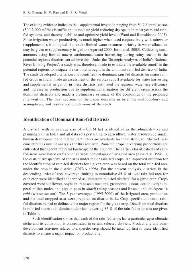
170
B. R. Sharma, K. V. Rao and K. P. R. Vittal
The existing evidence indicates that supplemental irrigation ranging from 50-200 mm/ season(500-2,000 m3/ha) is sufficient to mediate yield reducing dry spells in most years and rain-fed systems, and thereby stabilize and optimize yield levels (Wani and Ramakishna 2005).Since irrigation water productivity is much higher when used conjunctively with rainwater(supplemental), it is logical that under limited water resources priority in water allocationmay be given to supplementary irrigation (Agarwal 2000; Joshi et al. 2005). Collecting smallamounts using limited macro-catchments, water harvesting during rainy season in thepotential regions/ districts can achieve this. Under the ‘Strategic Analyses of India’s NationalRiver Linking Project’, a study was, therefore, made to estimate the available runoff in thepotential regions to mitigate the terminal drought in the dominant rain-fed districts of India.The study developed a criterion and identified the dominant rain-fed districts for major rain-fed crops in India, made an assessment of the surplus runoff available for water harvestingand supplemental irrigation in these districts, estimated the regional water use efficiencyand increase in production due to supplemental irrigation for different crops across thedominant districts and made a preliminary estimate of the economics of the proposedintervention. The next sections of the paper describe in brief the methodology andassumptions; and results and conclusions of the study.
Identification of Dominant Rain-fed Districts
A district (with an average size of ~ 0.5 M ha) is identified as the administrative andplanning unit in India and all data sets pertaining to agriculture, water resources, climate,human development and related parameters are available for the district; so, ‘district’ wasconsidered as unit of analysis for this research. Rain-fed crops in varying proportions arecultivated throughout the rural landscape of the country. The earlier classifications of rain-fed areas were based on fixed or variable percentages of irrigated area (Kerr et al. 1996) inthe district irrespective of the area under major rain-fed crops. An improved criterion forthe identification of rain-fed districts for a given crop was based on the total rain-fed areaunder the crop in the district (CRIDA 1998). For the present analysis, districts in thedescending order of area coverage limiting to cumulative 85 % of total rain-fed area foreach crop were identified and termed as ‘dominant rain-fed districts’ for a given crop. Cropscovered were sunflower, soybean, rapeseed mustard, groundnut, castor, cotton, sorghum,pearl millet, maize and pigeon peas in kharif (rainy season) and linseed and chickpeas inrabi (winter season). The 5-year averages (1995-2000) of the irrigated area, productionand the total cropped area were prepared on district basis. Crop-specific dominant rain-fed districts helped to delineate the major region for the given crop. Details on total districtsin rain-fed states and ‘dominant districts’ covering 85 % of the rain-fed crop area are givenin Table 1.
Such identification shows that each of the rain-fed crops has a particular agro-climaticniche and its cultivation is concentrated in certain selected districts. Productivity and otherdevelopment activities related to a specific crop should be taken up first in these identifieddistricts to ensure a major impact on productivity.
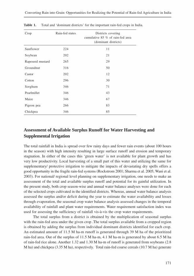
171
Converting Rain into Grain: Opportunities for Realizing the Potential of Rain-fed Agriculture in India
Table 1. Total and ‘dominant districts’ for the important rain-fed crops in India.
Crop Rain-fed states Districts coveringcumulative 85 % of rain-fed area
(dominant districts)
Sunflower 224 11
Soybean 202 21
Rapeseed mustard 265 29
Groundnut 316 50
Castor 202 12
Cotton 296 30
Sorghum 346 71
Pearlmillet 346 43
Maize 346 67
Pigeon pea 266 83
Chickpea 346 85
Assessment of Available Surplus Runoff for Water Harvesting andSupplemental Irrigation
The total rainfall in India is spread over few rainy days and fewer rain events (about 100 hoursin the season) with high intensity resulting in large surface runoff and erosion and temporarystagnation. In either of the cases this ‘green water’ is not available for plant growth and hasvery low productivity. Local harvesting of a small part of this water and utilizing the same forsupplementary/ protective irrigation to mitigate the impacts of devastating dry spells offers agood opportunity in the fragile rain-fed systems (Rockstrom 2001; Sharma et al. 2005; Wani et al.2003). For national/ regional level planning on supplementary irrigation, one needs to make anassessment of the total and available surplus runoff and potential for its gainful utilization. Inthe present study, both crop season-wise and annual water balance analyses were done for eachof the selected crops cultivated in the identified districts. Whereas, annual water balance analysisassessed the surplus and/or deficit during the year to estimate the water availability and lossesthrough evaporation, the seasonal crop water balance analysis assessed changes in the temporalavailability of rainfall and plant water requirements. Water requirement satisfaction index wasused for assessing the sufficiency of rainfall vis-à-vis the crop water requirements.
The total surplus from a district is obtained by the multiplication of seasonal surpluswith the rain-fed area under the given crop .The total surplus available from a cropped regionis obtained by adding the surplus from individual dominant districts identified for each crop.An estimated amount of 11.5 M ha-m runoff is generated through 39 M ha of the prioritizedrain-fed area. Out of the surplus of 11.5 M ha-m, 4.1 M ha-m is generated by about 6.5 M haof rain-fed rice alone. Another 1.32 and 1.30 M ha-m of runoff is generated from soybeans (2.8M ha) and chickpea (3.35 M ha), respectively. Total rain-fed coarse cereals (10.7 M ha) generate

172
B. R. Sharma, K. V. Rao and K. P. R. Vittal
about 2.1M ha-m of runoff. Spatial distribution of runoff on agro-ecological sub- region riverbasin wise is shown in Figure 1. However, based on experiences from watershed managementresearch and large-scale development efforts, practical harvesting of runoff is possible onlywhen the harvestable amount is greater than 50 mm or greater than 10 % of the seasonal rainfall(minimum utilizable runoff, CRIDA 2001). This constitutes about 10.5 M ha of rain-fed areawhich generates a seasonal runoff of less than 50 mm (10.25 M ha) or less than 10 % of theseasonal rainfall (0.25 M ha). Thus, the total estimated runoff surplus for various rain-fed cropsis about 11.4 million ha-m (114.02 billion cubic meters, BCM) from about 28.5 million ha whichcould be considered for water harvesting (Table 2). Among individual crops, rain-fed ricecontributes a higher surplus (4.12 M ha-m from an area of 6.33 M ha) followed by soybeans(1.30 M ha-m from 2.8 M ha). The deficit of rainfall for meeting crop water requirement is alsovisible for crops like groundnut, cotton, chickpea and pigeon pea.
Long- and short-term agricultural droughts and more pronounced meteorologicaldroughts are a common and recurrent phenomenon in the rain-fed areas served by monsoons.Though there is a good amount of surplus available as runoff in a season, all the runoff is notavailable at one time during the season. For the southwest Indian monsoon, usually there aretwo peaks of rainfall, the first occurring immediately after the onset of monsoon and the secondduring its withdrawal phase. During these two periods, there is a likely certainty of overflows(Ramakrishna et al. 1998) which can be harvested in suitable structures to mediate therandomness and enhance the structured supply of rainwater.
Figure 1. Spatial distribution of surplus runoff (ha-m) across dominant rain-fed districts and river basins.
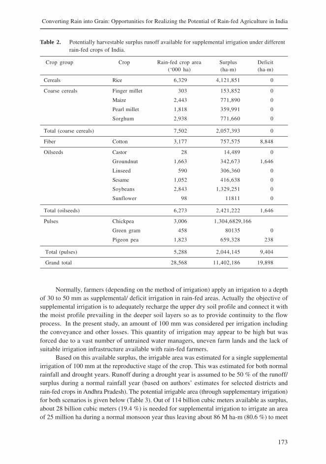
173
Converting Rain into Grain: Opportunities for Realizing the Potential of Rain-fed Agriculture in India
Normally, farmers (depending on the method of irrigation) apply an irrigation to a depthof 30 to 50 mm as supplemental/ deficit irrigation in rain-fed areas. Actually the objective ofsupplemental irrigation is to adequately recharge the upper dry soil profile and connect it withthe moist profile prevailing in the deeper soil layers so as to provide continuity to the flowprocess. In the present study, an amount of 100 mm was considered per irrigation includingthe conveyance and other losses. This quantity of irrigation may appear to be high but wasforced due to a vast number of untrained water managers, uneven farm lands and the lack ofsuitable irrigation infrastructure available with rain-fed farmers.
Based on this available surplus, the irrigable area was estimated for a single supplementalirrigation of 100 mm at the reproductive stage of the crop. This was estimated for both normalrainfall and drought years. Runoff during a drought year is assumed to be 50 % of the runoff/surplus during a normal rainfall year (based on authors’ estimates for selected districts andrain-fed crops in Andhra Pradesh). The potential irrigable area (through supplementary irrigation)for both scenarios is given below (Table 3). Out of 114 billion cubic meters available as surplus,about 28 billion cubic meters (19.4 %) is needed for supplemental irrigation to irrigate an areaof 25 million ha during a normal monsoon year thus leaving about 86 M ha-m (80.6 %) to meet
Table 2. Potentially harvestable surplus runoff available for supplemental irrigation under differentrain-fed crops of India.
Crop group Crop Rain-fed crop area Surplus Deficit(‘000 ha) (ha-m) (ha-m)
Cereals Rice 6,329 4,121,851 0
Coarse cereals Finger millet 303 153,852 0
Maize 2,443 771,890 0
Pearl millet 1,818 359,991 0
Sorghum 2,938 771,660 0
Total (coarse cereals) 7,502 2,057,393 0
Fiber Cotton 3,177 757,575 8,848
Oilseeds Castor 28 14,489 0
Groundnut 1,663 342,673 1,646
Linseed 590 306,360 0
Sesame 1,052 416,638 0
Soybeans 2,843 1,329,251 0
Sunflower 98 11811 0
Total (oilseeds) 6,273 2,421,222 1,646
Pulses Chickpea 3,006 1,304,6829,166
Green gram 458 80135 0
Pigeon pea 1,823 659,328 238
Total (pulses) 5,288 2,044,145 9,404
Grand total 28,568 11,402,186 19,898
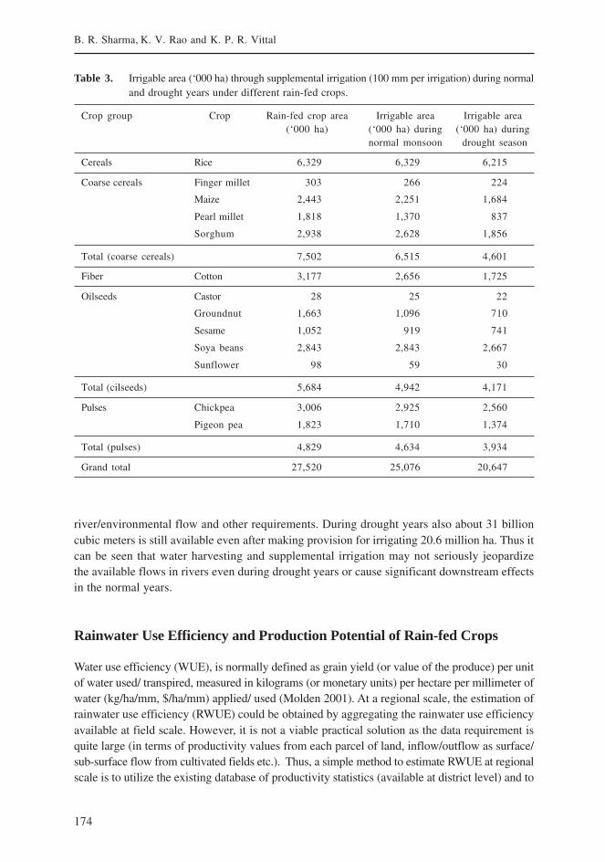
174
B. R. Sharma, K. V. Rao and K. P. R. Vittal
river/environmental flow and other requirements. During drought years also about 31 billioncubic meters is still available even after making provision for irrigating 20.6 million ha. Thus itcan be seen that water harvesting and supplemental irrigation may not seriously jeopardizethe available flows in rivers even during drought years or cause significant downstream effectsin the normal years.
Rainwater Use Efficiency and Production Potential of Rain-fed Crops
Water use efficiency (WUE), is normally defined as grain yield (or value of the produce) per unitof water used/ transpired, measured in kilograms (or monetary units) per hectare per millimeter ofwater (kg/ha/mm, $/ha/mm) applied/ used (Molden 2001). At a regional scale, the estimation ofrainwater use efficiency (RWUE) could be obtained by aggregating the rainwater use efficiencyavailable at field scale. However, it is not a viable practical solution as the data requirement isquite large (in terms of productivity values from each parcel of land, inflow/outflow as surface/sub-surface flow from cultivated fields etc.). Thus, a simple method to estimate RWUE at regionalscale is to utilize the existing database of productivity statistics (available at district level) and to
Table 3. Irrigable area (‘000 ha) through supplemental irrigation (100 mm per irrigation) during normaland drought years under different rain-fed crops.
Crop group Crop Rain-fed crop area Irrigable area Irrigable area(‘000 ha) (‘000 ha) during (‘000 ha) during
normal monsoon drought season
Cereals Rice 6,329 6,329 6,215
Coarse cereals Finger millet 303 266 224
Maize 2,443 2,251 1,684
Pearl millet 1,818 1,370 837
Sorghum 2,938 2,628 1,856
Total (coarse cereals) 7,502 6,515 4,601
Fiber Cotton 3,177 2,656 1,725
Oilseeds Castor 28 25 22
Groundnut 1,663 1,096 710
Sesame 1,052 919 741
Soya beans 2,843 2,843 2,667
Sunflower 98 59 30
Total (cilseeds) 5,684 4,942 4,171
Pulses Chickpea 3,006 2,925 2,560
Pigeon pea 1,823 1,710 1,374
Total (pulses) 4,829 4,634 3,934
Grand total 27,520 25,076 20,647
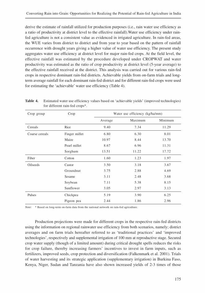
175
Converting Rain into Grain: Opportunities for Realizing the Potential of Rain-fed Agriculture in India
derive the estimate of rainfall utilized for production purposes (i.e., rain water use efficiency asa ratio of productivity at district level to the effective rainfall).Water use efficiency under rain-fed agriculture is not a consistent value as evidenced in irrigated agriculture. In rain-fed areas,the WUE varies from district to district and from year to year based on the pattern of rainfalloccurrence with drought years giving a higher value of water use efficiency. The present studyaggregates water use efficiency at district level for major rain-fed crops. At the field level, theeffective rainfall was estimated by the procedure developed under CROPWAT and waterproductivity was estimated as the ratio of crop productivity at district level (5-year average) tothe effective rainfall received at the district. This analysis was carried out for various rain-fedcrops in respective dominant rain-fed districts. Achievable yields from on-farm trials and long-term average rainfall for each dominant rain-fed district and for different rain-fed crops were usedfor estimating the ‘achievable’ water use efficiency (Table 4).
Table 4. Estimated water use efficiency values based on ‘achievable yields’ (improved technologies)for different rain-fed crops*.
Crop group Crop Water use efficiency (kg/ha/mm)
Average Maximum Minimum
Cereals Rice 9.40 7.34 11.29
Coarse cereals Finger millet 6.80 6.30 8.01
Maize 10.97 8.44 13.70
Pearl millet 8.67 6.96 11.31
Sorghum 13.51 11.22 17.72
Fiber Cotton 1.60 1.23 1.97
Oilseeds Castor 3.50 3.18 3.67
Groundnut 3.75 2.88 4.69
Sesame 3.11 2.48 3.68
Soybean 7.11 5.38 8.15
Sunflower 3.05 2.97 3.13
Pulses Chickpea 5.19 3.90 6.25
Pigeon pea 2.44 1.86 2.96
Note: * Based on long-term on-farm data from the national network on rain-fed agriculture.
Production projections were made for different crops in the respective rain-fed districtsusing the information on regional rainwater use efficiency from both scenarios, namely; districtaverages and on farm trials hereafter referred to as ‘traditional practices’ and ‘improvedtechnologies’, respectively and supplemental irrigation of 100 mm at reproductive stage. Securedcrop water supply (though of a limited amount) during critical drought spells reduces the risksfor crop failure, thereby increasing farmers’ incentives to invest in farm inputs, such asfertilizers, improved seeds, crop protection and diversification (Falkenmark et al. 2001). Trialsof water harvesting and its strategic application (supplementary irrigation) in Burkina Faso,Kenya, Niger, Sudan and Tanzania have also shown increased yields of 2-3 times of those

176
B. R. Sharma, K. V. Rao and K. P. R. Vittal
achieved in dryland farming (FAO 2002). The improved technologies involve the adoption ofimproved varieties, application of recommended doses of fertilizers, better management andfollow-up on recommended package of practices etc. The estimated production projectionsfor each crop and district and aggregates based on individual crop with improved practicesand over two types of seasons (normal and drought) summarized for crops and groups ofcrops are given in Table 5. Additional production was a product of irrigable area, water useefficiency and the amount of irrigation. The irrigable area through supplemental irrigation (at100 mm) for different crops during drought season varies between 50-98 % (98 % for rice cropto 50 % for sunflower districts) of the irrigable area during normal season.
Improved technologies, along with water, play an important part to harness the potentialbenefits. Under improved management practices an average of 50 % increase in total productioncutting across drought and normal seasons is realizable with supplemental irrigation from rain-fed area of 27.5 M ha (Table 5). Production enhancement in drought season in case of ricecrop is high due to higher water application efficiency and due to the sufficient surplus to
Table 5. Yield increases with supplemental irrigation (SI) in normal and drought seasons at twoirrigation efficiencies (based on WUE of improved technologies).
Crop Crop Rain- Traditional Irrigable area Additional productiongroup fed production (‘000 ha) (‘000 tonnes)
cropped (‘000area tonnes)
(‘000 ha)
Cereals Rice 6,329 7,612 6,329 6,215 3,549 4,141 3,776 4,357
Coarse Finger millet 303 271 266 224 107 124 97 112
cereals Maize 2,443 2,996 2,251 1,684 1,495 1,744 1,221 1,408
Pearl millet 1,818 1,902 1,370 837 717 836 481 555
Sorghum 2,938 3,131 2,628 1,856 2,091 2,439 1,616 1,864
Total coarse 7,502 8,300 6,515 4,601 4,409 5,144 3,414 3,939cereals
Fiber Cotton 3,177 430 2,656 1,725 252 294 178 206
Oilseeds Castor 28 10 25 22 5 6 5 6
Groundnut 1,663 1,182 1,096 710 244 284 176 203
Sesame 1,052 365 919 741 173 202 153 176
Soya beans 2,843 2,607 2,843 2,667 1,225 1,429 1,250 1,443
Sunflower 98 49 59 30 11 12 6 7
Total oilseeds 5,684 4,214 4,942 4,171 1,657 1,933 1,590 1,834
Pulses Chickpea 3,006 2,367 2,925 2,560 910 1,061 866 1,000
Pigeon pea 1,823 1,350 1,710 1,374 242 282 212 245
Total pulses 4,829 3,717 4,635 3,934 1,152 1,344 1,078 1,244
Grand total 27,520 24,272 25,076 20,647 11,020 12,856 10,037 11,581
Normal monsoon Drought season
Normal Drought 60 % 70 % 65 % 75 %season1 season1 SI SI SI SI
effi effi effi efficiency ciency ciency ciency
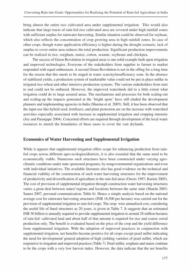
177
Converting Rain into Grain: Opportunities for Realizing the Potential of Rain-fed Agriculture in India
bring almost the entire rice cultivated area under supplemental irrigation. This would alsoindicate that large tracts of rain-fed rice cultivated area are covered under high rainfall zoneswith sufficient surplus for rainwater harvesting. Similar situation could be observed for soybean,which also reflects the concentration of crop growing area in high rainfall zones. In case ofother crops, though water application efficiency is higher during the drought scenario, lack ofsurplus to cover entire area reduces the total production. Significant production improvementscan be realized in rice, sorghum, maize, cotton, sesame, soybeans and chickpea.
The success of Green Revolution in irrigated areas is one solid example built upon irrigationand improved technologies. Everyone of the stakeholders from supplier to farmer to marketresponded with equal enthusiasm. A second Green Revolution is not in the offing for a long timefor the reason that this needs to be staged in water scarcity/insufficiency zone. In the absenceof stabilized yields, a production system of marketable value could not be put in place unlike inirrigated rice-wheat and other intensive production systems. The various stakeholders from startto end could not be enthused. However, the improved watersheds did to a little extent whatirrigation could do to large assured areas. The mechanisms and processes for both scaling-outand scaling-up the impacts generated at the ‘bright spots’ have still eluded the developmentplanners and implementing agencies in India (Sharma et al. 2005). Still, it has been observed thatthe input use like hybrid seed, fertilizers, and plant protection are on the increase with watershedactivities especially associated with increase in supplemental irrigation and cropping intensity(Joy and Paranjape 2004). Concerted efforts are required through development of the local waterresources to stretch the boundaries of these oases to cover the vast drylands.
Economics of Water Harvesting and Supplemental Irrigation
While it appears that supplemental irrigation offers scope for enhancing production from rain-fed crops across different agro-ecologies/districts, it is also essential that the same need to beeconomically viable. Numerous such structures have been constructed under varying agro-climatic conditions under state sponsored programs, by nongovernmental organizations and evenwith individual initiatives. The available literature also has good evidence on the technical andfinancial viability of the construction of such water harvesting structures for the improvementof productivity and diversification of agriculture in the rain-fed areas (Oweis 1997; Kurien 2005).The cost of provision of supplemental irrigation through construction water harvesting structuresvaries a great deal between states/ regions and locations between the same state (Sharda 2003;Samra 2007, personal communication; Table 6). Hence a simple analysis based on the nationalaverage cost for rainwater harvesting structures (INR 18,500 per hectare) was carried out for theprovision of supplemental irrigation to rain-fed crops. The crop- wise annualized cost, consideringthe useful life of lined structures as 20 years, is given in Table 7. It suggests that an estimatedINR 50 billion is annually required to provide supplemental irrigation to around 28 million hectaresof rain-fed- cultivated land and about half of that amount is required for rice and coarse cerealproduction only. The benefit is evaluated based on the price of the crop and the yield differencefrom supplemental irrigation. With the adoption of improved practices in conjunction withsupplemental irrigation, net benefits become positive for all crops except pearl millet indicatingthe need for development/ general adoption of high yielding varieties of pearl millet, which areresponsive to irrigation and improved practices (Table 7). Pearl millet, sorghum and maize continueto be the crops with a very low harvest index. However, the data indicate that the net benefits
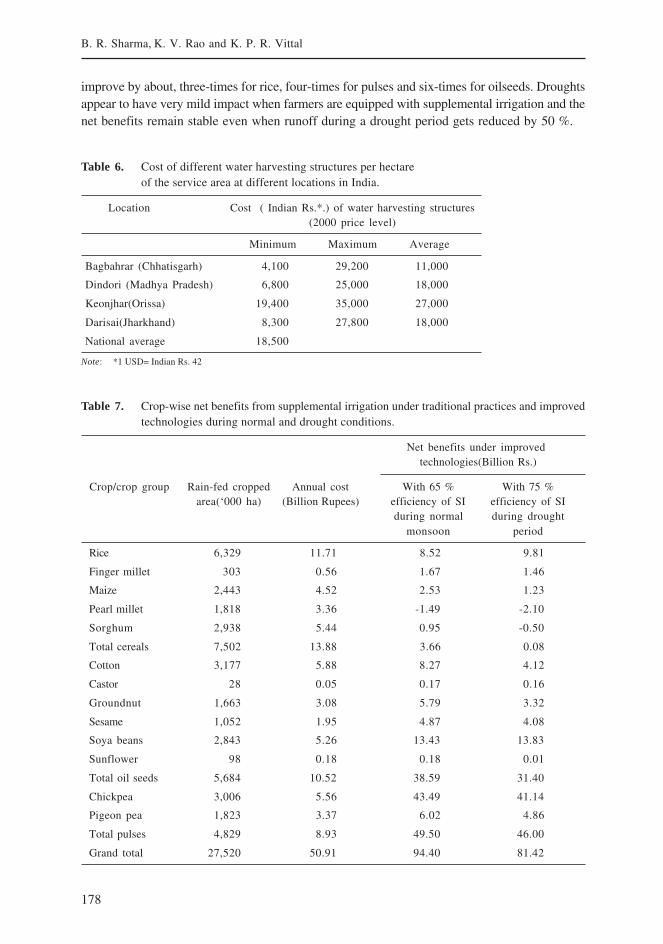
178
B. R. Sharma, K. V. Rao and K. P. R. Vittal
Table 6. Cost of different water harvesting structures per hectareof the service area at different locations in India.
Location Cost ( Indian Rs.*.) of water harvesting structures(2000 price level)
Minimum Maximum Average
Bagbahrar (Chhatisgarh) 4,100 29,200 11,000
Dindori (Madhya Pradesh) 6,800 25,000 18,000
Keonjhar(Orissa) 19,400 35,000 27,000
Darisai(Jharkhand) 8,300 27,800 18,000
National average 18,500
Note: *1 USD= Indian Rs. 42
Table 7. Crop-wise net benefits from supplemental irrigation under traditional practices and improvedtechnologies during normal and drought conditions.
Net benefits under improved technologies(Billion Rs.)
Crop/crop group Rain-fed cropped Annual cost With 65 % With 75 %area(‘000 ha) (Billion Rupees) efficiency of SI efficiency of SI
during normal during droughtmonsoon period
Rice 6,329 11.71 8.52 9.81
Finger millet 303 0.56 1.67 1.46
Maize 2,443 4.52 2.53 1.23
Pearl millet 1,818 3.36 -1.49 -2.10
Sorghum 2,938 5.44 0.95 -0.50
Total cereals 7,502 13.88 3.66 0.08
Cotton 3,177 5.88 8.27 4.12
Castor 28 0.05 0.17 0.16
Groundnut 1,663 3.08 5.79 3.32
Sesame 1,052 1.95 4.87 4.08
Soya beans 2,843 5.26 13.43 13.83
Sunflower 98 0.18 0.18 0.01
Total oil seeds 5,684 10.52 38.59 31.40
Chickpea 3,006 5.56 43.49 41.14
Pigeon pea 1,823 3.37 6.02 4.86
Total pulses 4,829 8.93 49.50 46.00
Grand total 27,520 50.91 94.40 81.42
improve by about, three-times for rice, four-times for pulses and six-times for oilseeds. Droughtsappear to have very mild impact when farmers are equipped with supplemental irrigation and thenet benefits remain stable even when runoff during a drought period gets reduced by 50 %.
179
Converting Rain into Grain: Opportunities for Realizing the Potential of Rain-fed Agriculture in India
Conclusion
Rain-fed agriculture is mainly and negatively influenced by the random behavior of rainfall,causing intermittent dry spells during the cropping season and especially, at critical growthstages coinciding with the terminal growth stage. District level analysis for different rain-fedcrops in India showed that the difference in the district average yields for rain-fed crops amongdifferent rainfall zones was not very high, indicating that the total water availability may notbe the major problem in different rainfall zones. Further, for each crop, there were few dominantdistricts which contributed most to the total rain-fed crop production. The most effectivepotential strategy to realize the potential of rain-fed agriculture in India (and elsewhere) appearsto be harvesting a small part of available surplus runoff and reutilizing it for supplementalirrigation at different critical crop growth stages. The study identified about 27.5 M ha ofpotential rain-fed area, which accounted for most of the rain-fed production and generatedsufficient runoff (114 BCM) for harvesting and reutilization. It was possible to raise the rain-fed production by 50 % over this entire area through application of one supplementary irrigation(28 BCM) and some follow up on the improved practices. Extensive area coverage rather thanintensive irrigation needs to be done in regions with higher than 750 mm/ annum rainfall, sincethere is a larger possibility of alleviating the in-season drought spells and ensuring the secondcrop with limited water application. This component may be made an integral part of theongoing and new development schemes in the identified rural districts. The proposed strategyis environmentally benign, equitable, poverty-targeted and financially attractive to realize theuntapped potential of rain-fed agriculture in India.
References
Agarwal, A. 2000. Drought? Try capturing the rain. Briefing paper for members of parliament and statelegislatures- An occasional paper. New Delhi, India: Center for Science and Environment.
CA 2007. Water for Food, Water for Life: A Comprehensive Assessment of Water Management in Agriculture.London: Earthscan, and Colombo: International Water Management Institute.
CRIDA 2001. Annual Progress Report. Hyderabad, India: Central Research Institute for Dryland Agriculture.
CRIDA 1998. Base paper - National Agricultural Technology Project. Hyderabad, India: Central ResearchInstitute for Dryland Agriculture.
Falkenmark, M.; Rockstrom, J. 1993. Curbing rural exodus from tropical drylands. Ambio, 22 (7): 427-437.
Falkenmark, M.; Patrick, F.; Gunn, P.; Rockstrom, J. 2001. Water Harvesting for Upgrading Rain-fedagriculture: Problem Analysis and Research Needs. Stockholm, Sweden: Stockholm Internationalwater Institute.
FAO 2002. World Agriculture: Towards 2015/ 2030: Summary report. Rome, Italy: Food and AgricultureOrganization.
Joshi, P.K.; Jha, A. K.; Wani, S. P.; Joshi, L.; Shiyani, R. L. 2005. Meta analysis to assess impact ofwatershed program and people’s action. Comprehensive Assessment Research Report 8. Colombo, SriLanka: International Water Management Institute. Colombo, Sri Lanka
Joy, K. J.; Paranjpe, S. 2004. Watershed Development Review: Issues and Prospects. Centre for Inter-disciplinary Studies in Environment and Development. Bangalore, India: ISEC.
180
B. R. Sharma, K. V. Rao and K. P. R. Vittal
Kanwar, J. S. 1999. Need for a future outlook and mandate for dryland agriculture in India. In. FiftyYears of Dryland agricultural research in India. ed. HP Singh. Central research institute for drylandagriculture, Hyderabad, India, pp 11-20.
Kerr, J. 1996. Sustainable development of rain-fed agriculture in India. EPTD Discussion Paper No. 20.Washington DC, USA: International Food Policy Research Institute.
Molden, D. 2001. Accounting for water use productivity. SWIM Publication No. 1. Colombo, Sri Lanka:International Water Management Institute.
Oweiss, T. 1997. Supplemental irrigation: A highly efficient water-use practice. Aleppo, Syria: InternationalCenter for Agricultural Research in Dry Areas.
Ramakrishna, Y. S.; Rao, G. G. S. N.; Rao, B. V. R.; Kumar, V. 1998. Agrometeorology. In Fifty Years ofNatural Resource Management Research. ed. Singh, G.B.; Sharma, B.R. Division of Natural ResourcesManagement. Indian Council of Agricultural Research, Krishi Bhawan, New Delhi, India. pp 505-536.
Reij, C.1988. Impact des techniques de conservation des eaux et du sol sur les rendements agricoles:analysesuccincte des donnees disponsibles pour le plateau central au Burkina faso. CEDRES/ AGRISK.
Rockstrom, J. 2001.Green water security for the food makers of tomorrow: Windows of opportunity indrought-prone savannahs. Water Science and Technology, 43 (4): 71-78.
Rockstrom, J.; Falkenmark, M. 2000. Semi-arid crop production from a hydrological perspective - Gapbetween potential and actual yields. Critical Reviews in Plant Sciences, 19 (4): 319-346.
Samra, J. S. 2007. Personal communication. Role of watersheds and Minor Irrigation in Food and LivelihoodSecurities. Presentation made before the Planning Commission. Government of India, New Delhi. June29, 2007.
Sharda, V. N. 2003. Technical Manual on Watershed Development for NWDPRA Scheme. Rain-fed FarmingSystems Division, Department of Agriculture and Cooperation. Krishi Bhawan, New Delhi, India. 353 pp.
Sharma, B. R.; Samra, J. S.; Scott, C. A.; Wani, S. P. (eds.) 2005. Watershed Management Challenges:Improving Productivity, resources and livelihoods. International Water Management Institute, Colombo,Sri Lanka. 334 pp.
Singh, R. P. 2001.Watershed management: A holistic approach for dryland agriculture. National Workshopon Watershed Area Development: Challenges and Solutions. Indian Institute of Management, Lucknow,India. 28-29 July, 2001.
Wani, S. P.; Pathak, P.; Sreedevi, T. K.; Singh, H. P.; Singh, P. 2003. Efficient management of rainwaterfor increased crop productivity and groundwater recharge in Asia, pp 199-215. In Water Productivityin Agriculture: Limits and Opportunities for Improvement. ed. Kijne, J. W.; Barker, R.; Molden, D.Wallingford, UK: Colombo, Sri Lanka: CABI-IWMI.
Wani, S. P.; Ramakrishna, Y. S. 2005. Sustainable management of rainwater through integrated watershedapproach for improved rural livelihoods. In Watershed Management Challenges: Improving Productivity,Resources and Livelihoods. ed. Sharma, B. R.; Samra, J. S.; Scott, C. A.; Wani, S. P. International WaterManagement Institute, Colombo, Sri Lanka. pp.39-60.
181
Converting Rain into Grain: Opportunities for Realizing the Potential of Rain-fed Agriculture in India
Groundwater Expansion in Indian Agriculture:Past Trends and Future Opportunities
1Anik Bhaduri, 1Upali Amarasinghe and 2Tushaar Shah1International Water Management Institute, New Delhi, India
2International Water Management Institute, Anand, India
Introduction
The importance of irrigation for agricultural production growth in India hardly needs anyemphasis. Irrigation, in 2000, contributed to 40 % of the crop area but 70 % of the total cropproduction. Improved reliability of water supply through canals or, more significantly throughgroundwater, has significantly contributed to the increase in agricultural productivity in India(Brown 2003). Recent studies show that the irrigation needs to play a larger role towards agoal of achieving a higher agricultural productivity and the national food security (Persaud etal. 2003; Kumar 1998; GOI 1999).
The National Commission of Integrated Water Resources Development (NCIWRD)projections show that the irrigated area should increase by about 35 million ha to reach thefood self-sufficiency goals (GOI 1999). A major part of the NCIWRD additional irrigated areaprojection is from the surface water, and it is a key factor for the proposed national river linkingproject (NRLP) concept of India. The NRLP envisages transferring 178 km3 water from thewater rich Himalayan rivers to water stressed southern and western part of India and irrigatingadditional 34 million ha (GOI 1999).
Currently, however, India is on a cross road of its future direction of irrigated agriculture.Many opponents of the Government of India’s NRLP concept argue that groundwaterirrigation can contribute in providing much of the additional irrigation needs in the future.It is true that groundwater was the major driver of net irrigated area expansion in the lasttwo decades (FAO 2002). But how long can this trend continue and in which location andin what magnitude? And how will the net groundwater area expansion contribute to grossirrigated area growth? To answer this it is necessary to review the past spatial and temporaltrends of surface and groundwater irrigation and assess their contributions to the grossirrigated area growth.
The recent boom in groundwater irrigation is due to many reasons. First, due to slowingdown in the growth of public investments in large-scale irrigation infrastructure andincompletion of on going projects, the surface irrigated area has not increased in the 1990s(Gulati et al.1999). The most severe problem facing Indian canal irrigation, however, is the rapiddeterioration of systems that have already been created (Gulati et al. 1999). In the absence of
182
A. Bhaduri, U. A. Aarasinghe and T. Shah
new large-scale surface irrigation schemes, and the availability of low cost electric and dieselpumps coupled with little or no electricity charges, the groundwater has been a major driver inthe irrigated area expansion. Second, expansion of groundwater-irrigated areas is in large partdue to the increase in the reliability of water supply. Groundwater irrigation, due to its lesservariation in its supply and higher reliability in irrigated water supply, reduces the risk ofinvestment in labor, seed, fertilizers, pesticides and other inputs and induces the farmers toincrease the agricultural productivity.
It is popularly believed that the recent groundwater irrigation expansion was taking placein and close to irrigation command areas, where recharge from canal irrigation is the main sourceof groundwater availability. We hypothesize such widely held belief and examine whether canalirrigation recharge is a necessary condition for the groundwater expansion. We also test thehypothesis that groundwater boom in India is largely contributed by demand factors, forinstance, rural population whose livelihood depends mostly on agriculture.
There are two main sources of growth in the gross irrigated area: expanding the irrigatedarea and increasing the frequency with which it is irrigated (irrigated land use intensity1). India’snet irrigated area has expanded by 24 % and 18 % in the 1980s and 1990s. The irrigated landuse intensity, representing one of the criteria of irrigated land productivity, has increased byonly 10 % over the past two decades. The average national irrigation land use intensity in2000 was 138 %. Is there any scope for increasing irrigation intensity further in existing lands?How will the surface and groundwater irrigation contribute to irrigation intensity increase?Answers to these are important to know. How much new surface is irrigated to develop formeeting future needs? Therefore, with a view to evaluating investment in major and minorirrigation projects in the light of intensive land use cropping, we here made an attempt toassess the contribution of the different sources of irrigation on gross irrigated area, whichreflects the irrigated land use intensity.
The structure of the paper is as follows. In the next section, we discuss the studyobjective, data and methodology. The following section discusses the spatial and temporaltrends associated with the groundwater boom in India. In the third section, we review thegrowth of the irrigated area of India in the past, and assess the contribution of different sourcesof irrigation on gross irrigated area. Finally, the last section summarizes the findings and resultsof the paper.
1 There are many crops like sugarcane, banana, coconut etc. that stand for more than 3 months in the field.In commuting the intensity it need some special consideration. Unlike the conventional measure of irriga-tion intensity, defined as the ratio of gross irrigated area (GIA) to net irrigated area (NIA), (GIA/NIA), wehave computed irrigated land use intensity (ILUI) as
where j is the number ofannual and perennial crops, which stands more than one cropping season in the field.
gia + n
niaj
niaj
183
Groundwater Expansion in Indian Agriculture: Past Trends and Future Opportunities
Study Objectives, Data and Methodology
The major objectives of this study are to assess the spatial and temporal trends of surfaceand groundwater irrigated area development in India and their contribution to gross irrigatedarea growth. Specifically this study assesses
1. whether the growth in surface irrigation is a necessary factor in net groundwaterirrigated area growth;
2. whether the rural population is a driver in groundwater expansion and if so where itis most significant; and
3. the relative contribution of surface and groundwater irrigation in increasing the grossirrigated area.
Data
We use a combination of time series and cross sectional data for our analysis. The time seriesdata from 1951 to 2001 assess the national level temporal trends of net surface, tanks andgroundwater irrigated area growth; and the sources of this data are the various issues of‘Agriculture at a Glance’ publications by the ministry of agriculture (GOI 2005). The district levelnet surface, tank and groundwater irrigated areas in 2000 assess the spatial trends, and the sourcesfor this data are various publications of Fertilizer Statistics (FIA 2000). The relative contributionsto gross irrigated area growth are assessed using time series and cross section data of 16 majorstates in India. These 16 states constitute more than 95 % of the agrarian economy of India, forthe period 1990-1996. Instead of using aggregate time series data only, we use panel data, wherethe cross sectional units are the different district. This allows for district-specific variation in allthe variables included, as compared with all- India data that could reduce such variation byaggregating some variables and averaging others. The source of this data is the databaseavailable in International Crops Research Institute for Semi Arid Tropics (ICRISAT).
Methodology
We use piece-wise time series regression analysis to assess the temporal variation ofnet surface and groundwater irrigated area growth. Spatial autocorrelation analyzes the spatialassociation of groundwater and surface irrigation expansion. The hypothesis here is that thepercentage of groundwater irrigated area in a district is spatially associated with the percentageof the surface irrigated area of the neighboring districts.
The global Moran’s I, a measure of spatial autocorrelation, shows the strength of thespatial dependence of a unit with its neighboring units (Anselin 1995). Moran’s I is the degreeof linear association of a variable in X-axis with its spatial lag variable in the Y-axis. TheMorans’s I takes values between -1 and 1. The two extremes indicate high-high or low-lowspatial dependence (Morans I =1) and high-low and low-high spatial dependence (Moran’sI=-1). Moran’s I close to zero show no significant pattern of spatial dependence.
For our analysis we estimate the bivariate Moran’s I. The bivariate Moran’s scatter plotshows the spatial lag of the groundwater-irrigated area variable in the Y-axis and the surfaceirrigated area variable in the X-axis. The Moran’s I not significantly different from zero supportsour hypothesis that groundwater expansion of a unit is not necessarily associated with thesurface irrigation expansion of the neighboring units.
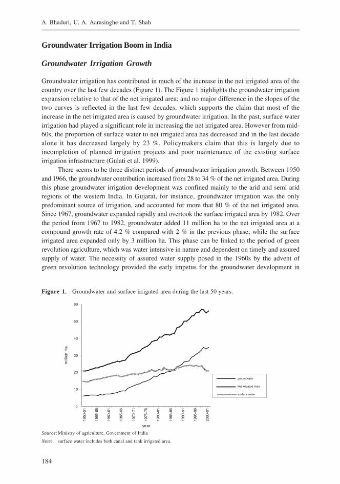
184
A. Bhaduri, U. A. Aarasinghe and T. Shah
Groundwater Irrigation Boom in India
Groundwater Irrigation Growth
Groundwater irrigation has contributed in much of the increase in the net irrigated area of thecountry over the last few decades (Figure 1). The Figure 1 highlights the groundwater irrigationexpansion relative to that of the net irrigated area; and no major difference in the slopes of thetwo curves is reflected in the last few decades, which supports the claim that most of theincrease in the net irrigated area is caused by groundwater irrigation. In the past, surface waterirrigation had played a significant role in increasing the net irrigated area. However from mid-60s, the proportion of surface water to net irrigated area has decreased and in the last decadealone it has decreased largely by 23 %. Policymakers claim that this is largely due toincompletion of planned irrigation projects and poor maintenance of the existing surfaceirrigation infrastructure (Gulati et al. 1999).
There seems to be three distinct periods of groundwater irrigation growth. Between 1950and 1966, the groundwater contribution increased from 28 to 34 % of the net irrigated area. Duringthis phase groundwater irrigation development was confined mainly to the arid and semi aridregions of the western India. In Gujarat, for instance, groundwater irrigation was the onlypredominant source of irrigation, and accounted for more that 80 % of the net irrigated area.Since 1967, groundwater expanded rapidly and overtook the surface irrigated area by 1982. Overthe period from 1967 to 1982, groundwater added 11 million ha to the net irrigated area at acompound growth rate of 4.2 % compared with 2 % in the previous phase; while the surfaceirrigated area expanded only by 3 million ha. This phase can be linked to the period of greenrevolution agriculture, which was water intensive in nature and dependent on timely and assuredsupply of water. The necessity of assured water supply posed in the 1960s by the advent ofgreen revolution technology provided the early impetus for the groundwater development in
Figure 1. Groundwater and surface irrigated area during the last 50 years.
Source:Ministry of agriculture, Government of India
Note: surface water includes both canal and tank irrigated area.
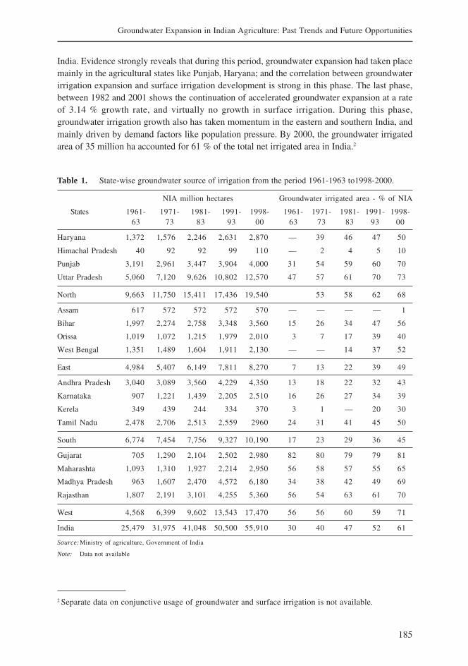
185
Groundwater Expansion in Indian Agriculture: Past Trends and Future Opportunities
India. Evidence strongly reveals that during this period, groundwater expansion had taken placemainly in the agricultural states like Punjab, Haryana; and the correlation between groundwaterirrigation expansion and surface irrigation development is strong in this phase. The last phase,between 1982 and 2001 shows the continuation of accelerated groundwater expansion at a rateof 3.14 % growth rate, and virtually no growth in surface irrigation. During this phase,groundwater irrigation growth also has taken momentum in the eastern and southern India, andmainly driven by demand factors like population pressure. By 2000, the groundwater irrigatedarea of 35 million ha accounted for 61 % of the total net irrigated area in India.2
2 Separate data on conjunctive usage of groundwater and surface irrigation is not available.
Table 1. State-wise groundwater source of irrigation from the period 1961-1963 to1998-2000.
NIA million hectares Groundwater irrigated area - % of NIA
States 1961- 1971- 1981- 1991- 1998- 1961- 1971- 1981- 1991- 1998-63 73 83 93 00 63 73 83 93 00
Haryana 1,372 1,576 2,246 2,631 2,870 — 39 46 47 50
Himachal Pradesh 40 92 92 99 110 — 2 4 5 10
Punjab 3,191 2,961 3,447 3,904 4,000 31 54 59 60 70
Uttar Pradesh 5,060 7,120 9,626 10,802 12,570 47 57 61 70 73
North 9,663 11,750 15,411 17,436 19,540 53 58 62 68
Assam 617 572 572 572 570 — — — — 1
Bihar 1,997 2,274 2,758 3,348 3,560 15 26 34 47 56
Orissa 1,019 1,072 1,215 1,979 2,010 3 7 17 39 40
West Bengal 1,351 1,489 1,604 1,911 2,130 — — 14 37 52
East 4,984 5,407 6,149 7,811 8,270 7 13 22 39 49
Andhra Pradesh 3,040 3,089 3,560 4,229 4,350 13 18 22 32 43
Karnataka 907 1,221 1,439 2,205 2,510 16 26 27 34 39
Kerela 349 439 244 334 370 3 1 — 20 30
Tamil Nadu 2,478 2,706 2,513 2,559 2960 24 31 41 45 50
South 6,774 7,454 7,756 9,327 10,190 17 23 29 36 45
Gujarat 705 1,290 2,104 2,502 2,980 82 80 79 79 81
Maharashta 1,093 1,310 1,927 2,214 2,950 56 58 57 55 65
Madhya Pradesh 963 1,607 2,470 4,572 6,180 34 38 42 49 69
Rajasthan 1,807 2,191 3,101 4,255 5,360 56 54 63 61 70
West 4,568 6,399 9,602 13,543 17,470 56 56 60 59 71
India 25,479 31,975 41,048 50,500 55,910 30 40 47 52 61
Source:Ministry of agriculture, Government of India
Note: Data not available
186
A. Bhaduri, U. A. Aarasinghe and T. Shah
To get further insight, we explore the state wise net irrigated area (NIA) and thegroundwater irrigation share in Table 1. The table shows the NIA and groundwater irrigatedarea as a percentage of NIA for the periods 1961-63, 1971-73 , 1981-83 , 1991-93 and 1998-2000.Many climatic factors like rainfall and drought affect irrigation. So, we have taken a three-yearaverage for the periods mentioned.
National growth of groundwater irrigation masks the regional variation in groundwaterirrigation expansion. There is state wise variation in the groundwater source of net irrigated area,which is reflected in Table 1. Part of this disparity in groundwater irrigation development can beexplained by the fact that during the period of the Green Revolution, Punjab and Haryana wereway ahead of other states in terms of irrigated area; and in the western states, particularly Gujaratand Rajasthan, groundwater was the major available source for irrigation in the post independenceperiod. In the post 1997 period, the proportion of groundwater irrigation to net irrigated areabecame more than 60 % in the northern and western states, while the share of groundwaterirrigation is still less than 50 % in the southern zone. Here the hydro-geo-morphological featuresare not as favorable as in the alluvial plains of Gangetic Basin, for recharge.
In the latter geographic zone, growth is mainly confined in Andhra Pradesh and Kerala,whereas not much growth has taken place in the Tamil Nadu and Karnataka due to declininggroundwater table. The rate of expansion on groundwater irrigated area in the eastern India(West Bengal and Bihar) is phenomenally high compared to the other states during 1990s.Recent studies also show that more than one-third of total pumps in India in early 1990 wasin the state of West Bengal alone (Bhattarai et al. 2003).
Surface Irrigation Recharge and Groundwater Area Growth: Spatial Dependence
A popular belief is that surface water recharge is a necessary condition for the expansion ofgroundwater-irrigated area. Groundwater pumping costs generally depend on the water tablelevel, which means that as the groundwater stock is increased, marginal extraction costs fall.Higher surface water withdrawals recharge the aquifers and induce the farmers to increasegroundwater usage and expand the gross irrigated area.
It could be true that surface irrigation recharges groundwater not only in the canalcommand areas, but also in the rain-fed areas outside the canal commands. But, how widespreadcan this recharge be, and to what extent this contributes to NGWIA expansion?
We attempt to address the issue by investigating the link between surface irrigationrecharge and the groundwater irrigation expansion using spatial auto correlation analysis. Here,first we attribute the groundwater area expansion within a district to the surface irrigation inthat district. (see annex A for the distribution of groundwater and surface irrigated area acrossdistricts). How would then the surface irrigation within a district be associated with thegroundwater irrigation in the surrounding districts? Our null hypothesis is that the groundwaterexpansion in the surrounding districts is dependent on the surface irrigation of the centraldistrict. Spatial autocorrelation shows the spatial dependence of a unit with its neighbors.Figure 2 is the scatter plot of the surface irrigated area in the X- axis and the spatial lag of thegroundwater irrigated area in the Y -axis. The spatial autocorrelation, which indicates thestrength of the linear relationship of the two variables, is not significantly different from zero.This contradicts the hypothesis that the surface irrigation is a necessary condition for largescale expansion of groundwater expansion in surrounding areas.
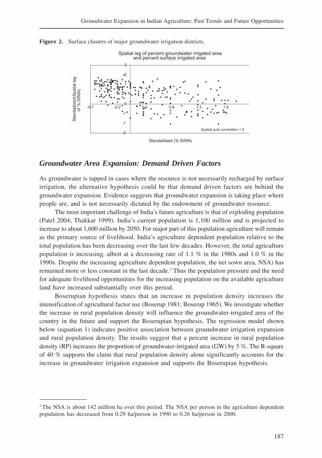
187
Groundwater Expansion in Indian Agriculture: Past Trends and Future Opportunities
Groundwater Area Expansion: Demand Driven Factors
As groundwater is tapped in cases where the resource is not necessarily recharged by surfaceirrigation, the alternative hypothesis could be that demand driven factors are behind thegroundwater expansion. Evidence suggests that groundwater expansion is taking place wherepeople are, and is not necessarily dictated by the endowment of groundwater resource.
The most important challenge of India’s future agriculture is that of exploding population(Patel 2004; Thakkar 1999). India’s current population is 1,100 million and is projected toincrease to about 1,600 million by 2050. For major part of this population agriculture will remainas the primary source of livelihood. India’s agriculture dependent population relative to thetotal population has been decreasing over the last few decades. However, the total agriculturepopulation is increasing, albeit at a decreasing rate of 1.1 % in the 1980s and 1.0 % in the1990s. Despite the increasing agriculture dependent population, the net sown area, NSA) hasremained more or less constant in the last decade.3 Thus the population pressure and the needfor adequate livelihood opportunities for the increasing population on the available agricultureland have increased substantially over this period.
Boserupian hypothesis states that an increase in population density increases theintensification of agricultural factor use (Boserup 1981; Boserup 1965). We investigate whetherthe increase in rural population density will influence the groundwater-irrigated area of thecountry in the future and support the Boserupian hypothesis. The regression model shownbelow (equation 1) indicates positive association between groundwater irrigation expansionand rural population density. The results suggest that a percent increase in rural populationdensity (RP) increases the proportion of groundwater-irrigated area (GW) by 5 %. The R-squareof 40 % supports the claim that rural population density alone significantly accounts for theincrease in groundwater irrigation expansion and supports the Boserupian hypothesis.
Figure 2. Surface clusters of major groundwater irrigation districts.
3 The NSA is about 142 million ha over this period. The NSA per person in the agriculture dependentpopulation has decreased from 0.29 ha/person in 1990 to 0.26 ha/person in 2000.
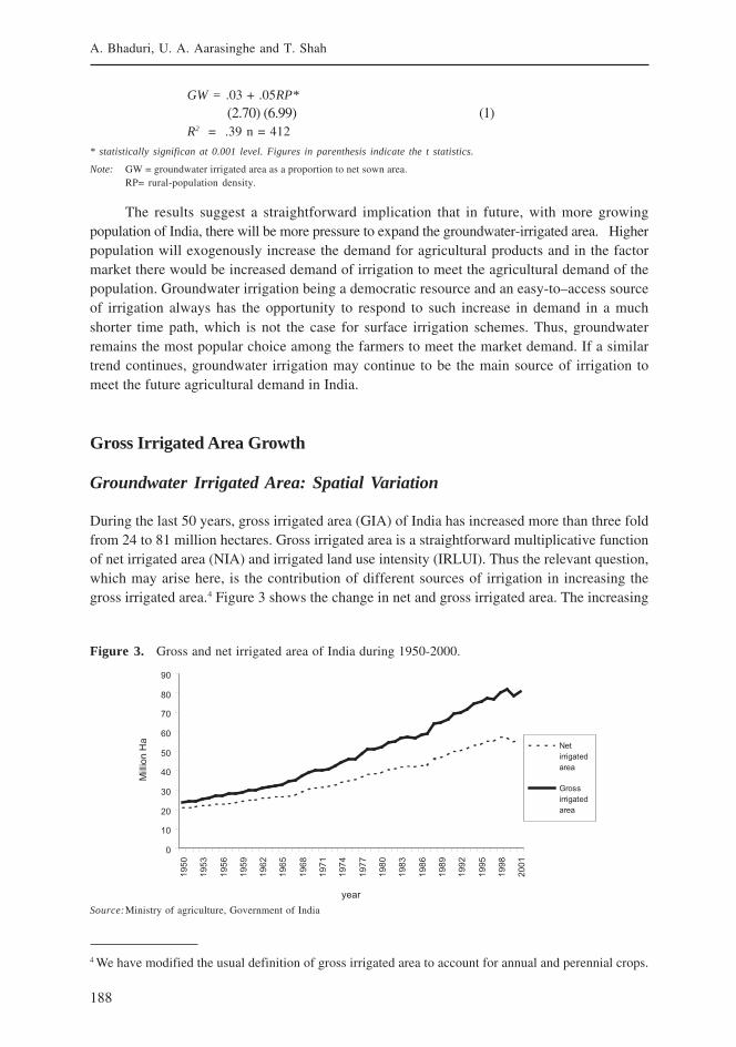
188
A. Bhaduri, U. A. Aarasinghe and T. Shah
GW = .03 + .05RP*
(2.70) (6.99) (1)R2 = .39 n = 412
* statistically significan at 0.001 level. Figures in parenthesis indicate the t statistics.
Note: GW = groundwater irrigated area as a proportion to net sown area.RP= rural-population density.
The results suggest a straightforward implication that in future, with more growingpopulation of India, there will be more pressure to expand the groundwater-irrigated area. Higherpopulation will exogenously increase the demand for agricultural products and in the factormarket there would be increased demand of irrigation to meet the agricultural demand of thepopulation. Groundwater irrigation being a democratic resource and an easy-to–access sourceof irrigation always has the opportunity to respond to such increase in demand in a muchshorter time path, which is not the case for surface irrigation schemes. Thus, groundwaterremains the most popular choice among the farmers to meet the market demand. If a similartrend continues, groundwater irrigation may continue to be the main source of irrigation tomeet the future agricultural demand in India.
Gross Irrigated Area Growth
Groundwater Irrigated Area: Spatial Variation
During the last 50 years, gross irrigated area (GIA) of India has increased more than three foldfrom 24 to 81 million hectares. Gross irrigated area is a straightforward multiplicative functionof net irrigated area (NIA) and irrigated land use intensity (IRLUI). Thus the relevant question,which may arise here, is the contribution of different sources of irrigation in increasing thegross irrigated area.4 Figure 3 shows the change in net and gross irrigated area. The increasing
4 We have modified the usual definition of gross irrigated area to account for annual and perennial crops.
Figure 3. Gross and net irrigated area of India during 1950-2000.
Source:Ministry of agriculture, Government of India
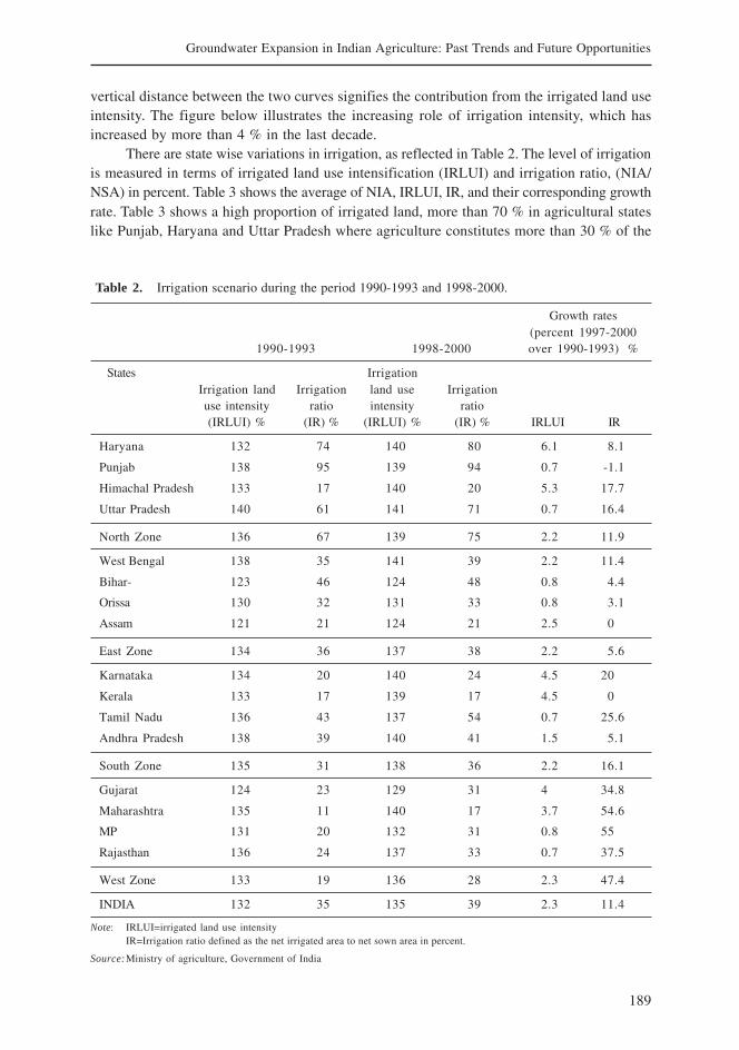
189
Groundwater Expansion in Indian Agriculture: Past Trends and Future Opportunities
vertical distance between the two curves signifies the contribution from the irrigated land useintensity. The figure below illustrates the increasing role of irrigation intensity, which hasincreased by more than 4 % in the last decade.
There are state wise variations in irrigation, as reflected in Table 2. The level of irrigationis measured in terms of irrigated land use intensification (IRLUI) and irrigation ratio, (NIA/NSA) in percent. Table 3 shows the average of NIA, IRLUI, IR, and their corresponding growthrate. Table 3 shows a high proportion of irrigated land, more than 70 % in agricultural stateslike Punjab, Haryana and Uttar Pradesh where agriculture constitutes more than 30 % of the
Table 2. Irrigation scenario during the period 1990-1993 and 1998-2000.
Growth rates(percent 1997-2000
1990-1993 1998-2000 over 1990-1993) %
States IrrigationIrrigation land Irrigation land use Irrigationuse intensity ratio intensity ratio(IRLUI) % (IR) % (IRLUI) % (IR) % IRLUI IR
Haryana 132 74 140 80 6.1 8.1
Punjab 138 95 139 94 0.7 -1.1
Himachal Pradesh 133 17 140 20 5.3 17.7
Uttar Pradesh 140 61 141 71 0.7 16.4
North Zone 136 67 139 75 2.2 11.9
West Bengal 138 35 141 39 2.2 11.4
Bihar- 123 46 124 48 0.8 4.4
Orissa 130 32 131 33 0.8 3.1
Assam 121 21 124 21 2.5 0
East Zone 134 36 137 38 2.2 5.6
Karnataka 134 20 140 24 4.5 20
Kerala 133 17 139 17 4.5 0
Tamil Nadu 136 43 137 54 0.7 25.6
Andhra Pradesh 138 39 140 41 1.5 5.1
South Zone 135 31 138 36 2.2 16.1
Gujarat 124 23 129 31 4 34.8
Maharashtra 135 11 140 17 3.7 54.6
MP 131 20 132 31 0.8 55
Rajasthan 136 24 137 33 0.7 37.5
West Zone 133 19 136 28 2.3 47.4
INDIA 132 35 135 39 2.3 11.4
Note: IRLUI=irrigated land use intensityIR=Irrigation ratio defined as the net irrigated area to net sown area in percent.
Source:Ministry of agriculture, Government of India
190
A. Bhaduri, U. A. Aarasinghe and T. Shah
state GDP. Among the southern states, the proportion of irrigated land is below 30 % inKarnataka and Kerala; while in Andhra Pradesh and Tamil Nadu, NIA/NSA is above 40 %.
Among the western states, Maharashtra has the lowest proportion of irrigated land whereonly 17 % of the net cropped area is irrigated. Most of the eastern states are well endowedwith irrigation where average NIA/NSA is 0.40. In the north-eastern state of Assam, however,less than 10 % of net cropped area is irrigated. In Punjab and Kerala, there is a slight decreasein the proportion of irrigated area, even with an increase in NIA.
It suggests that in post 1997 period, more rain-fed area has been brought under cultivationin both the states. In the northern zone, there is hardly any room for irrigation development as75 % of the net cropped is irrigated, and is reflected in lower growth. The growth of irrigationarea is striking in the western zone where NIA has grown by 46 % from 1990-1993 to 1997-2000. Eastern states register a much slower growth of irrigation except West Bengal. Amongthe southern states, higher growth in NIA took place in Andhra Pradesh and Tamil Nadu.
All states register an increase in irrigated land use intensity (IRLUI). Much of this increaseis noticed in states like Haryana, Himachal Pradesh, Karnataka, Kerala and Maharashtra. InHaryana, the increase in intensive use of irrigated land is contributed by limitation to increasethe net irrigated area. In the latter three states, higher intensive use of land is also contributedby the choice of cropping pattern. In these four states, the share of permanent crops is highcompared with that of other states.
In these states, however, the proportional irrigated area is not high. One possible reasoncould be that the opportunity cost of increasing the net irrigated area is higher than increasingthe intensity. As a result, irrigated land use intensity became the major driver of gross irrigatedarea in these states with the development of minor irrigation.
Gross Irrigated Area Expansion: Sources of Growth
Different sources of irrigation contribute in increasing the gross irrigated area (GIA). Thesesources include canal irrigation, tank irrigation and groundwater irrigation with tube wells anddug wells. We assess the patterns of GIA growth in four groups. The first group consists ofdistricts with canal, groundwater and tank irrigation. In these districts surface irrigation hasindeed contributed to increasing groundwater recharge. The second group consists of districtswith only canal-irrigated area. The third group consists of only groundwater irrigation districts.Before the introduction of groundwater, these districts were mainly rain-fed districts. Thegroundwater recharge in these districts is mainly from rainfall. The fourth group of districtsconsists of only tank and groundwater irrigated area. These districts are located mainly in thesouthern peninsular states.
We use a simple ordinary least squares regression to assess the contribution of surface,tanks and groundwater area expansions to GIA. The regression in the first group of districts,where canal, tanks as well as groundwater irrigation are present, a percentage increase ingroundwater irrigation will increase the GIA by 1.47 times. In the first group, a percentageincrease in canal irrigation will increase the GIA by 1.42 times. In districts without canal irrigation,the marginal contribution on GIA drops to 1.37. However, the marginal effect of groundwatercontribution on gross irrigated area is only 1.22 in districts irrigated using groundwater only.The areas were primarily the rain-fed areas where groundwater expansion has taken place. Themarginal contribution of canal irrigation in the command area, where only canal-irrigated areais present, is 1.98. It implies that a percentage increase in canal-irrigated area in the command
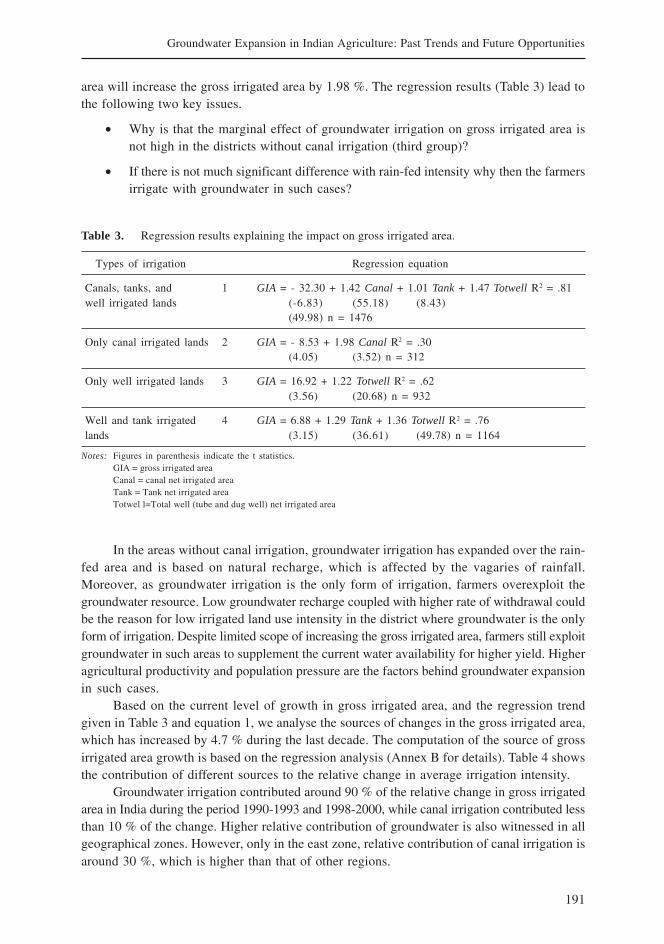
191
Groundwater Expansion in Indian Agriculture: Past Trends and Future Opportunities
area will increase the gross irrigated area by 1.98 %. The regression results (Table 3) lead tothe following two key issues.
• Why is that the marginal effect of groundwater irrigation on gross irrigated area isnot high in the districts without canal irrigation (third group)?
• If there is not much significant difference with rain-fed intensity why then the farmersirrigate with groundwater in such cases?
Table 3. Regression results explaining the impact on gross irrigated area.
Types of irrigation Regression equation
Canals, tanks, and 1 GIA = - 32.30 + 1.42 Canal + 1.01 Tank + 1.47 Totwell R2 = .81well irrigated lands (-6.83) (55.18) (8.43)
(49.98) n = 1476
Only canal irrigated lands 2 GIA = - 8.53 + 1.98 Canal R2 = .30(4.05) (3.52) n = 312
Only well irrigated lands 3 GIA = 16.92 + 1.22 Totwell R2 = .62(3.56) (20.68) n = 932
Well and tank irrigated 4 GIA = 6.88 + 1.29 Tank + 1.36 Totwell R2 = .76lands (3.15) (36.61) (49.78) n = 1164
Notes: Figures in parenthesis indicate the t statistics.GIA = gross irrigated areaCanal = canal net irrigated areaTank = Tank net irrigated areaTotwel l=Total well (tube and dug well) net irrigated area
In the areas without canal irrigation, groundwater irrigation has expanded over the rain-fed area and is based on natural recharge, which is affected by the vagaries of rainfall.Moreover, as groundwater irrigation is the only form of irrigation, farmers overexploit thegroundwater resource. Low groundwater recharge coupled with higher rate of withdrawal couldbe the reason for low irrigated land use intensity in the district where groundwater is the onlyform of irrigation. Despite limited scope of increasing the gross irrigated area, farmers still exploitgroundwater in such areas to supplement the current water availability for higher yield. Higheragricultural productivity and population pressure are the factors behind groundwater expansionin such cases.
Based on the current level of growth in gross irrigated area, and the regression trendgiven in Table 3 and equation 1, we analyse the sources of changes in the gross irrigated area,which has increased by 4.7 % during the last decade. The computation of the source of grossirrigated area growth is based on the regression analysis (Annex B for details). Table 4 showsthe contribution of different sources to the relative change in average irrigation intensity.
Groundwater irrigation contributed around 90 % of the relative change in gross irrigatedarea in India during the period 1990-1993 and 1998-2000, while canal irrigation contributed lessthan 10 % of the change. Higher relative contribution of groundwater is also witnessed in allgeographical zones. However, only in the east zone, relative contribution of canal irrigation isaround 30 %, which is higher than that of other regions.
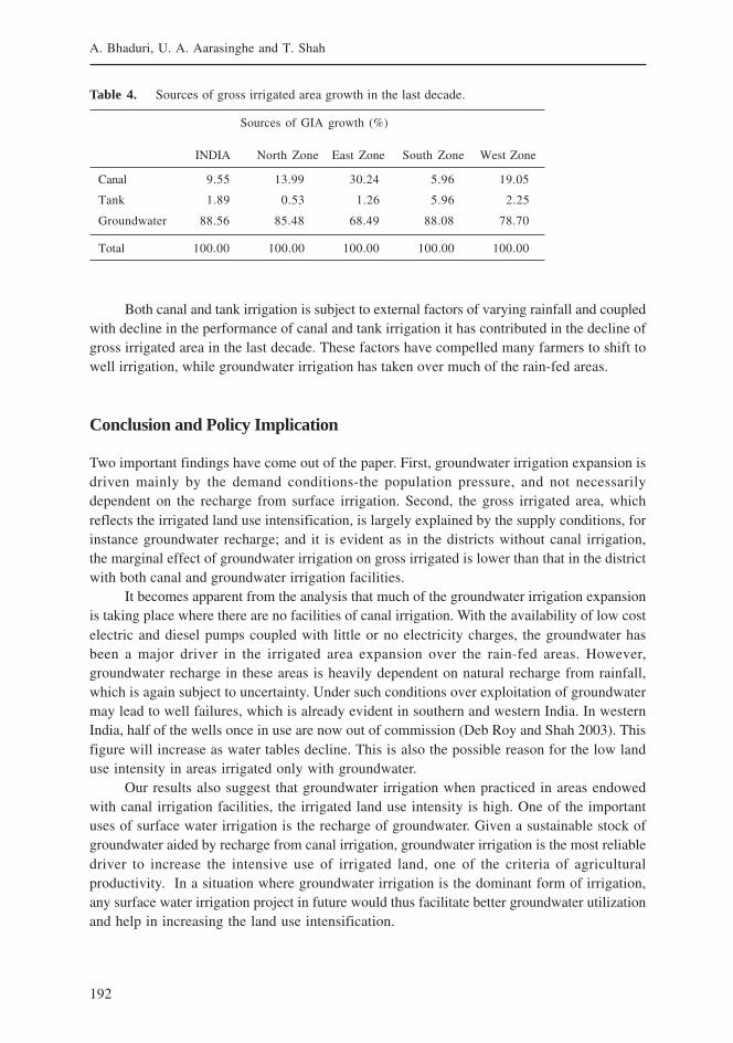
192
A. Bhaduri, U. A. Aarasinghe and T. Shah
Both canal and tank irrigation is subject to external factors of varying rainfall and coupledwith decline in the performance of canal and tank irrigation it has contributed in the decline ofgross irrigated area in the last decade. These factors have compelled many farmers to shift towell irrigation, while groundwater irrigation has taken over much of the rain-fed areas.
Conclusion and Policy Implication
Two important findings have come out of the paper. First, groundwater irrigation expansion isdriven mainly by the demand conditions-the population pressure, and not necessarilydependent on the recharge from surface irrigation. Second, the gross irrigated area, whichreflects the irrigated land use intensification, is largely explained by the supply conditions, forinstance groundwater recharge; and it is evident as in the districts without canal irrigation,the marginal effect of groundwater irrigation on gross irrigated is lower than that in the districtwith both canal and groundwater irrigation facilities.
It becomes apparent from the analysis that much of the groundwater irrigation expansionis taking place where there are no facilities of canal irrigation. With the availability of low costelectric and diesel pumps coupled with little or no electricity charges, the groundwater hasbeen a major driver in the irrigated area expansion over the rain-fed areas. However,groundwater recharge in these areas is heavily dependent on natural recharge from rainfall,which is again subject to uncertainty. Under such conditions over exploitation of groundwatermay lead to well failures, which is already evident in southern and western India. In westernIndia, half of the wells once in use are now out of commission (Deb Roy and Shah 2003). Thisfigure will increase as water tables decline. This is also the possible reason for the low landuse intensity in areas irrigated only with groundwater.
Our results also suggest that groundwater irrigation when practiced in areas endowedwith canal irrigation facilities, the irrigated land use intensity is high. One of the importantuses of surface water irrigation is the recharge of groundwater. Given a sustainable stock ofgroundwater aided by recharge from canal irrigation, groundwater irrigation is the most reliabledriver to increase the intensive use of irrigated land, one of the criteria of agriculturalproductivity. In a situation where groundwater irrigation is the dominant form of irrigation,any surface water irrigation project in future would thus facilitate better groundwater utilizationand help in increasing the land use intensification.
Table 4. Sources of gross irrigated area growth in the last decade.
Sources of GIA growth (%)
INDIA North Zone East Zone South Zone West Zone
Canal 9.55 13.99 30.24 5.96 19.05
Tank 1.89 0.53 1.26 5.96 2.25
Groundwater 88.56 85.48 68.49 88.08 78.70
Total 100.00 100.00 100.00 100.00 100.00
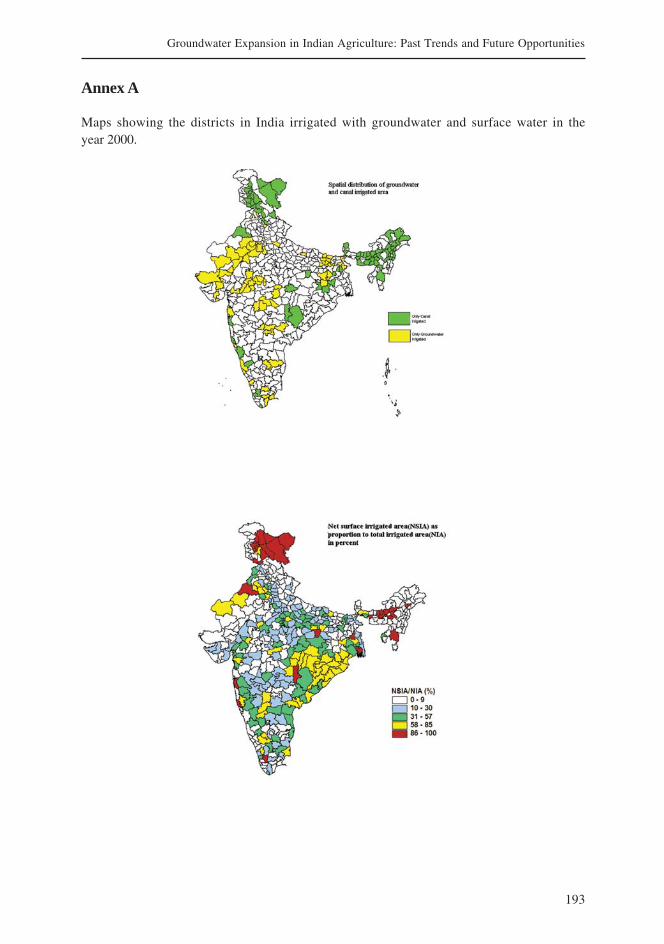
193
Groundwater Expansion in Indian Agriculture: Past Trends and Future Opportunities
Annex A
Maps showing the districts in India irrigated with groundwater and surface water in theyear 2000.
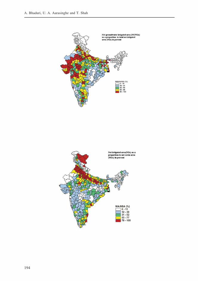
194
A. Bhaduri, U. A. Aarasinghe and T. Shah
195
Groundwater Expansion in Indian Agriculture: Past Trends and Future Opportunities
ΔGIA = [Δcanal] + [ΔΤank] + [ΔTotwell]∂f ∂f ∂f
∂canal ∂Tank ∂Totwell
∂f
∂i
ΔGIA [GIA2000
– GIA1990
]
[Δcanal] [[canal2000
– canal1990
]∂f ∂f
∂canal ∂canal
∂f∂canal
Annex B
Computation of the source of gross irrigated area growth.Suppose gross irrigated area (GIA) is a function of canals (canal), tanks (Tank) and
groundwater (Totwell).It can be expressed as GIA = f (canals, Tanks, Totwell). Taking total change of the
function, we get
where is the marginal change of GIA due to change in ith source of irrigation (i=canal,
tank, Totwell), and Δ(i) is the total change in ith factor.
So the contribution of canals in the relative change of GIA from year 1990 to 2000 can
be expressed as or ; where from
Table 3 and equation 1, we get = 1.42
References
Anselin, L. 1995. Local indicators of spatial association-LISA. Geographical Analysis 27: 93-115.
Boserup, E. 1981. Population and technological chance: A study of long-term trends. Chicago, USA:University of Chicago Press.
Boserup, E. 1965 .The Conditions of Agricultural Growth. London, UK: Allen and Unwin.
Damodaran, A. 2000. Towards an Agro-Ecosystem Policy for India — Lessons from Two Case Studies.Tata-McGraw Hill for the Centre for Environment Education, Ahmedabad, Environment andDevelopment Series, 2000.
Deb Roy, A.; Shah, T. 2002. The Socio-Ecology of Groundwater in India. Water Policy Briefing, Issue 4IWMI-TATA.
Deshingkar, P.; Anderson, E. 2004. People on the move: New Policy Challenges for Increasingly MobilePopulations. Natural Resource Perspectives, Number 92, June 2004, London: Overseas DevelopmentInstitute.
FAI.2000. Fertilizer Statistics: 1999-2000. New Delhi: Fertilizer Association of India (FAI).
FAO. 2002. Crops and Drops. FAO document 2002.
GOI. 2004. Agricultural Statistics at a Glance. New Delhi: Ministry of Agriculture, Government of India.
GOI. 2005. Agricultural Statistics at a Glance 2004. New Delhi, India: Ministry of Agriculture, Governmentof India.
196
A. Bhaduri, U. A. Aarasinghe and T. Shah
GOI. 1999. Integrated Water Resource Development – A Plan for Action. Report of the National Commissionfor Integrated. Water Resources Development, Vol. – I. New Delhi: Ministry of Water Resources ofIndia, Government of India.
Gulati, A.; Meinzen-Dick, R.; Rajus, K. V. 1999. From Top Down to Bottoms Up: Institutional Reforms inIndian Canal Irrigation. Delhi: Institute of Economic Growth.
Kanwar, S. 2004. Relative profitability, supply shifters and dynamic output response.The Indian food grains.Working Paper No. 133. Centre for Development Economics, Department of Economics, Delhi Schoolof Economics.
Karan, A. 2003. Changing Patterns of migration from rural Bihar pp102-139. In Migrant Labour andHuman rights in India, ed. K.G. Iyer. New Delhi, India: Kanishka Publishers.
Kumar, P.1998. Food Demand and supply Projections for India. Agricultural Economics Policy Paper 98-01. IARI, New Delhi.
Lester, B. R. 2003. Outgrowing the Earth: The Food Security Challenge.
Madhusudan, B.; Narayanamoorthy, A. 2003. Irrigation and other Factors Contribution to the AgriculturalGrowth and Development in India: A Cross-State Panel Data Analysis for 1970 to 1994. Paper presentedat the IWMI-Tata workshop in Anand, Gujarat, January 27-29, 2003.
Patel, V. B. 2004. Role of Irrigation and People’s Participation in Meeting Food requirement. Journal ofApplied Hydrology. Vol. XVII.
Roy, A. D.; Shah, T. 2002. The Socio-Ecology of Groundwater in India. Water Policy Briefing, Issue 4IWMI-TATA.
Roy, B. C.; Selvarajan, S.; Natesh, B. 2004. Methodological Issues in Future Water Food Security Analysis.Resource Analysis for Sustaining Water-Food Security, National Centre for Agricultural Economics andPolicy Research, pp 191-205.
Suresh, P.; Rosen, S. 2003. India’s Consumer and Producer Price Policies: Implications for Food Security.Economics Research Service, Food Security Assessment, GFA-14, Feb.
Shah, T.; Roy, A. D.; Qureshi, A. S.; Wang, J. 2003. Sustaining Asia’s Groundwater Boom: An Overviewof Issues and Evidence. Natural Resources Forum, 27 (2003) 130–140.
Shylendra, H. S.; Thomas, P. 1995. Non–farm Employment: Nature, Magnitude and Determinants in asemi arid village of western India. Indian Journal of agricultural Economics, 50 (3): 410-416.
Thakkar, H. 1999. Assessment of Irrigation in India. A WCD Contributing Paper prepared as an input tothe World Commission on Dams, Prepared for Thematic Review IV.2.
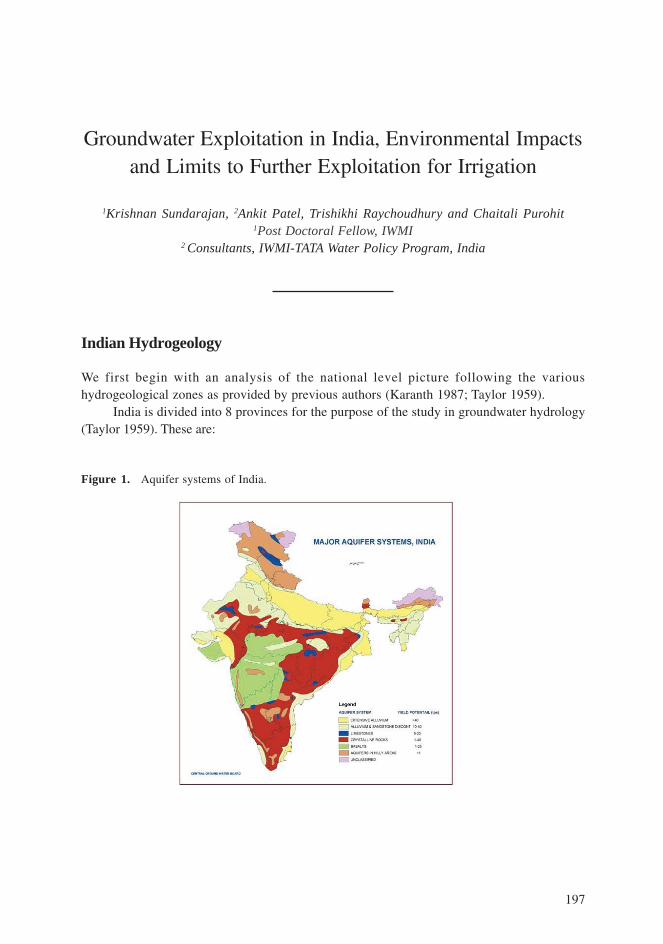
197
Groundwater Expansion in Indian Agriculture: Past Trends and Future Opportunities
Groundwater Exploitation in India, Environmental Impactsand Limits to Further Exploitation for Irrigation
1Krishnan Sundarajan, 2Ankit Patel, Trishikhi Raychoudhury and Chaitali Purohit1Post Doctoral Fellow, IWMI
2 Consultants, IWMI-TATA Water Policy Program, India
Indian Hydrogeology
We first begin with an analysis of the national level picture following the varioushydrogeological zones as provided by previous authors (Karanth 1987; Taylor 1959).
India is divided into 8 provinces for the purpose of the study in groundwater hydrology(Taylor 1959). These are:
Figure 1. Aquifer systems of India.
198
S. Krishnan, A. Patel, T. Raychoudhury and C. Purohit
Precambrian Crystalline Province
This comprises most of peninsular India from the southern tip and ranging up to Delhi. Exceptfor most of Maharashtra state, this mass of Plutonic, Igneous and Metamorphic rocks are ofcontiguous extant. Groundwater occurs mostly in the weathered zone in the top 10-20 meters,but connection with deeper groundwater is observed at many locations. In most areas, thetop weathered zone is underlain by mostly impermeable rock with local or regional fracturesyielding storage and transport of water. These entire formations mostly are poor aquifers withlow specific yield.
Precambrian Sedimentary Province
Located in 4 distinct regions of the country, these sedimentary formations mainly containlimestone, shale, sandstone, quartzite and local conglomerates. These are located in a)Cuddapah Basin of Andhra Pradesh, b) Raipur Basin of Madhya Pradesh, c) Vindhyan Basinand d) Western Rajasthan Basin. Karstification is observed in varying degrees and some localformations can be sources of springs e.g., as found in Himalayan foothills of Uttaranchal.
Gondwana Sedimentary Province
This province is located in patches of Gujarat, Rajasthan and the coal belt of Eastern India;fluvial or lacustrine consolidated to semi-consolidated shale or sandstone and is generallynot highly water bearing. The total thickness of these sediments is up to 6,000 m and can bevariable at different locations.
Deccan Trap Province
This is an important province comprising almost the entire state of Maharashtra and parts ofothers states, e.g., Saurashtra in Gujarat, Western parts of Madhya Pradesh and areas inKarnataka, Rajasthan and Andhra Pradesh. It occupies an area of 500,000 sq. km and consistsof volcanic products such as tuffs, breccia, ash and intertrappean basalts. The overall thicknessof these flows can be thousand meters or more in some places. Mostly, the water bearingstratum is a top weathered zone up to 50 meters. But at specific locations, the presence ofindividual horizontal flows can allow large amounts of groundwater storage. The water qualitycan be brackish especially when overlain by black cotton soils.
Cenezoic Sedimentary Province
This comprises some coastal plains on the Malabar and Coromandel coasts and coastal areasof Kutch and Saurashtra and a region of folded rocks in the far eastern parts of the country.It is underlain by semi-consolidated conglomerates, sandstone, shale and lignite.
Cenezoic Fault Basins
Three fault basins – Narmada, Poorna and Tapi – fall within this province. These contain lensesof sand and gravel along with silt and clay. These are generally good aquifers providing a
199
Groundwater Exploitation in India, Environmental Impacts and Limits to Further Exploitation for Irrigation
high yield. The valley fill can range from 50 m to 150 m in thickness. Groundwater quality inthe Poorna Basin is highly saline and unfit for irrigation or domestic purposes.
Ganges-Brahmaputra-Indus Alluvial Province
This is the main region of groundwater occurrence in the country with deep high-yieldingaquifers and several perennial rivers feeding recharge into these aquifers. Sloping down fromthe Himalayan foothills, the province can be divided into the a) Bhabhar: high sloping regionof the foothills with unsorted sand and gravel offering high infiltration and recharge into lowerareas and having deep water table b) Terai: gently sloping region beyond the Bhabhar withtongues of permeable sand, clay and gravel with shallow water table and c) Axial region ofdeep alluvium comprising sand, gravel and clay aquifers, multi-layered and connected withdepth up to several kilometers at some locations.
Himalayan Highland Province
This is a highly folded and faulted zone of mainly sedimentary rocks extending all over thenorthern region of the country to the far-east. These rocks are mainly limestone, sandstoneand shale with some crystalline rocks including granite. Groundwater is characterized by springin hollows between mountains and intermontane valleys which could have sand and alluviumyielding highly. Some of these intermontane valleys also serve as conduits to recharge thelower plain aquifers.
This sub-division maybe further refined in terms of groundwater provinces.When comparing statistics of groundwater across the country, the first question that
crops up is what is the appropriate unit to be considered? It is common practice amongstdifferent disciplines to use the administrative units for this purpose. But those units are lesssuitable for assessing groundwater. One option is to refine better this definition of groundwaterprovinces and consider these units as groups of districts.
In consistency with the division of the country into groundwater provinces, we canclassify the country into sub-regions based on these aquifer types. However, the wateravailability and stress on aquifers also depend on the specific river basin it lies in. For example,the alluvial aquifers of Sabarmati Basin would be much more stressed than those in say, GangesBasin since the Sabarmati River basin is as a whole a closed river basin. With this in mind, wehave divided the country into the major river basins and aquifer types taking a total of 26 riverbasins or sets of river basins and 7 aquifer zones. This gives a total of 182 sub-regions acrossthe country. Some of these regions are geographic units, for e.g., the Ganges alluvium, theBasalts of Luni which is the Saurashtra basalt block, the Krishna alluvium which correspondsto the delta stretches and so on. This division can provide us with a better unit for thecomparison of groundwater use and development that reflects the nature of the aquifer andwater availability within the sub-region.
Table 1 shows the total area lying within each of these aquifer-basins (A-B) units.90 % of the total area comprises 40 of the larger units such as Basaltic Ganges and Cauvery,the Alluvial Indus and Ganges etc. So finally, it is these 40 units which are most important andthose, in fact, are expansions of the eight groundwater provinces described earlier. For example,the fourth groundwater province, namely the Ganges-Brahmaputra-Indus Alluvial province ishere composed of six smaller A-B units totally comprising 25 % of the area of the country.
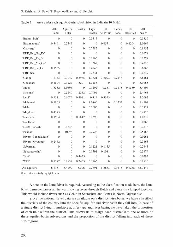
200
S. Krishnan, A. Patel, T. Raychoudhury and C. Purohit
A note on the Luni River is required. According to the classification made here, the LuniRiver basin comprises all the west flowing rivers through Kutch and Saurashtra lumped together.This would include rivers such as Gehlo in Saurashtra and Banas in North Gujarat also.
Since the national-level data are available on a district-wise basis, we have classifiedthe districts of the country into the specific aquifer and river basin they fall into. In case ofa single district lying in multiple aquifer type and river basin, we have taken the proportionof each unit within the district. This allows us to assign each district into one or more ofthese aquifer-basin sub-regions and the proportion of the district falling into each of thesesub-regions.
Table 1. Area under each aquifer-basin sub-division in India (in 10 MHa).
Allu_ Aquifer_ Basalts Cryst_ Ext_ Limes Un AllSand Hills Rocks Alluvium tone classified basins
‘Brahm_Bait’ 0 0 0 0.3515 0 0 0 0.5339
‘Brahmaputra’ 0.3461 0.3349 0 0 0.6531 0 0.6204 2.0169
‘Cauverg’ 0 0 0 0.7587 0 0 0 0.8932
‘ERF_Bet_Go_Kr’ 0 0 0 0 0 0 0 0.1078
‘ERF_Bet_Kr_Pe’ 0 0 0 0.1166 0 0 0 0.2297
‘ERF_Bet_Ma_Go’ 0 0 0 0.3262 0 0 0 0.4333
‘ERF_Bet_Pe_Ca’ 0.1555 0 0 0.4746 0 0 0 0.6363
‘ERF_Sca’ 0 0 0 0.2331 0 0 0 0.4237
‘Ganga’ 1.7143 0.7042 0.5985 1.7721 3.6093 0.2148 0 8.6161
‘Godavari’ 0.1504 0.1227 1.5201 1.3258 0 0 0 3.1965
‘Indus’ 1.5332 1.0896 0 0.1292 0.261 0.3118 0.1559 3.4807
‘Krishna’ 0 0.3249 1.2242 0.7996 0 0 0 2.4965
‘Luni’ 0.9311 0.1079 0.4011 0.314 0.3373 0 0 2.2092
‘Mahanadi’ 0.1865 0 0 1.0866 0 0.1253 0 1.4904
‘Mahi’ 0 0 0 0.2606 0 0 0 0.3727
‘Meghna’ 0.4375 0 0 0 0 0 0 0.4725
‘Narmada’ 0.1904 0 0.5642 0.2298 0 0 0 1.0312
‘No Data’ 0 0 0 0 0 0 0 0.0366
‘North Ladakh’ 0 0.1543 0 0 0 0 0 0.2513
‘Pennar’ 0 01.98 0 0.2928 0 0 0 0.5466
‘Rivers_Bangaladesh’ 0 0 0 0 0 0 0 0.0261
‘Rivers_Myanmar’ 0.2462 0 0 0 0 0 0 0.3165
‘Sabarmati’ 0 0 0 0.1221 0.1135 0 0 0.2643
‘Subarnarekha’ 0 0 0 0.1591 0.1081 0 0 0.3479
‘Tapi’ 0 0 0.4635 0 0 0 0 0.6292
‘WRF’ 0.1577 0.1857 0.2455 0.3766 0 0 0 0.9856
All aquifers 6.8151 3.4299 5.096 9.2891 5.5633 0.9275 0.9238 32.0447
Note: 0 = relatively negligible area
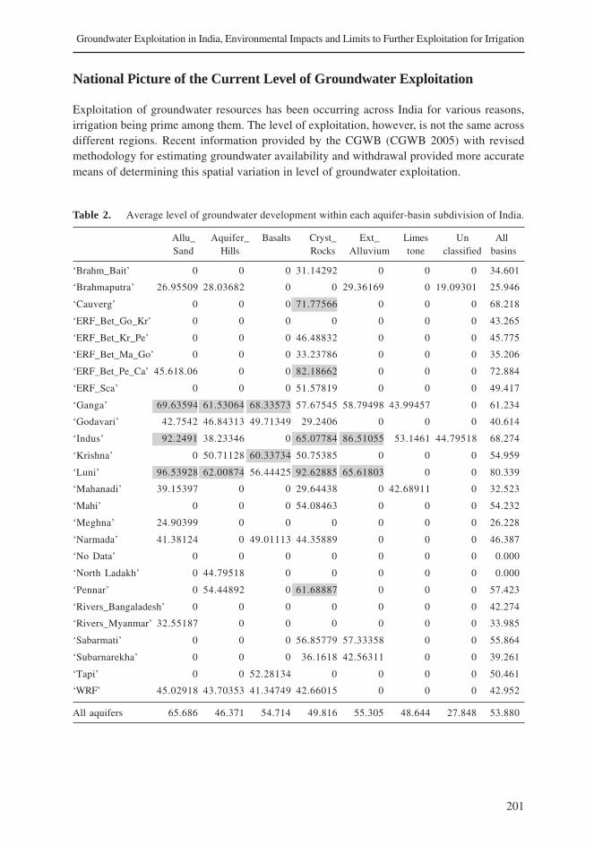
201
Groundwater Exploitation in India, Environmental Impacts and Limits to Further Exploitation for Irrigation
National Picture of the Current Level of Groundwater Exploitation
Exploitation of groundwater resources has been occurring across India for various reasons,irrigation being prime among them. The level of exploitation, however, is not the same acrossdifferent regions. Recent information provided by the CGWB (CGWB 2005) with revisedmethodology for estimating groundwater availability and withdrawal provided more accuratemeans of determining this spatial variation in level of groundwater exploitation.
Table 2. Average level of groundwater development within each aquifer-basin subdivision of India.
Allu_ Aquifer_ Basalts Cryst_ Ext_ Limes Un AllSand Hills Rocks Alluvium tone classified basins
‘Brahm_Bait’ 0 0 0 31.14292 0 0 0 34.601
‘Brahmaputra’ 26.95509 28.03682 0 0 29.36169 0 19.09301 25.946
‘Cauverg’ 0 0 0 71.77566 0 0 0 68.218
‘ERF_Bet_Go_Kr’ 0 0 0 0 0 0 0 43.265
‘ERF_Bet_Kr_Pe’ 0 0 0 46.48832 0 0 0 45.775
‘ERF_Bet_Ma_Go’ 0 0 0 33.23786 0 0 0 35.206
‘ERF_Bet_Pe_Ca’ 45.618.06 0 0 82.18662 0 0 0 72.884
‘ERF_Sca’ 0 0 0 51.57819 0 0 0 49.417
‘Ganga’ 69.63594 61.53064 68.33573 57.67545 58.79498 43.99457 0 61.234
‘Godavari’ 42.7542 46.84313 49.71349 29.2406 0 0 0 40.614
‘Indus’ 92.2491 38.23346 0 65.07784 86.51055 53.1461 44.79518 68.274
‘Krishna’ 0 50.71128 60.33734 50.75385 0 0 0 54.959
‘Luni’ 96.53928 62.00874 56.44425 92.62885 65.61803 0 0 80.339
‘Mahanadi’ 39.15397 0 0 29.64438 0 42.68911 0 32.523
‘Mahi’ 0 0 0 54.08463 0 0 0 54.232
‘Meghna’ 24.90399 0 0 0 0 0 0 26.228
‘Narmada’ 41.38124 0 49.01113 44.35889 0 0 0 46.387
‘No Data’ 0 0 0 0 0 0 0 0.000
‘North Ladakh’ 0 44.79518 0 0 0 0 0 0.000
‘Pennar’ 0 54.44892 0 61.68887 0 0 0 57.423
‘Rivers_Bangaladesh’ 0 0 0 0 0 0 0 42.274
‘Rivers_Myanmar’ 32.55187 0 0 0 0 0 0 33.985
‘Sabarmati’ 0 0 0 56.85779 57.33358 0 0 55.864
‘Subarnarekha’ 0 0 0 36.1618 42.56311 0 0 39.261
‘Tapi’ 0 0 52.28134 0 0 0 0 50.461
‘WRF’ 45.02918 43.70353 41.34749 42.66015 0 0 0 42.952
All aquifers 65.686 46.371 54.714 49.816 55.305 48.644 27.848 53.880
202
S. Krishnan, A. Patel, T. Raychoudhury and C. Purohit
Lacunae in Estimation Procedure
There are however still lacunae in this estimation procedure and many of the deficienciesshown by authors (Dhawan 1990; Shah et al. 1998) still persist. Inconsistencies betweendifferent sources of data provided by government data collection agencies have been reportedby various authors. The estimation of total groundwater use can be performed using differentmeans: a) a direction estimation through volumetric changes in groundwater storage and b)indirectly through accounting for different uses such as area irrigated by groundwater.Dhawan points out that there are high differences between these estimates partly due tothe procedures adopted by the agencies in the estimation procedures. The volumetricprocedure of the Central Groundwater Board (CGWB) takes as unit blocks or Talukas and insome states such as Maharashtra, the unit is a watershed. An entire water budgeting isperformed for this unit in terms of recharge, use for various purposes and discharge.However, estimates of discharge such as to streams are questionable since the data availablefor such estimation are not reliable. The estimates too have been changing over the yearsand in general, been observing a greater degree of exploitation of resources with each survey.Another important factor is regarding the density of the monitoring network and howinformative it is for computing the change in groundwater storage. Especially, in the hardrock area such estimation can be highly unreliable and can be compounded by poor data onspecific yield of unconfined aquifers.
On the other hand, the Planning Commission’s estimate of area irrigated by groundwaterand potential irrigable area show a different picture (Dhawan 1995). As pointed out by Dhawan,there has been full exploitation of groundwater resources on the country as a whole in early1990s and overexploitation in Uttar Pradesh and Gujarat, whereas the then CGWB estimatesshowed only 30 % exploitation on the country as a whole. One striking example ofinconsistencies provided by different data is the situation in Punjab. Whereas volumetricestimates of groundwater balance show a rise in water table, the groundwater level data showa fall in water table for the Sirhind Canal tract (Dhawan 1995).
These notwithstanding, the CGWB estimates of 2004 provide the only picture ofgroundwater in India which is closest to the reality. The deficiencies are being improved uponand would probably get closer to the true picture with further surveys.
In general, the level of exploitation in many aquifers still shows numbers on the lowerside, i.e., being optimistic about available reserves.
Observations from CGWB 2004 Data
The current CGWB methodology follows revised norms using the GES 1997 Estimationmethodology (GEC 1997). Under this methodology, the level of groundwater development in aunit of study (Taluka, block or watershed) is defined as:
• Stage of Groundwater Development = Annual Groundwater draft/Net AnnualGroundwater availability * 100
This definition adopted by CGWB has however been contested by some authors (Shahet al. 1998), who propose the denominator to be the ‘utilizable’ groundwater as opposed to‘available groundwater’ reserves. In the estimates by Shah et al. the stage of groundwaterdevelopment is as large as two to three times the CGWB estimates when using their proposed
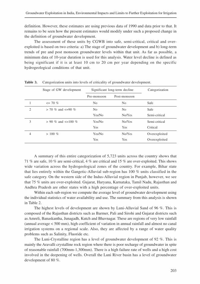
203
Groundwater Exploitation in India, Environmental Impacts and Limits to Further Exploitation for Irrigation
definition. However, these estimates are using previous data of 1990 and data prior to that. Itremains to be seen how the present estimates would modify under such a proposed change inthe definition of groundwater development.
The assessment of these units by CGWB into safe, semi-critical, critical and over-exploited is based on two criteria: a) The stage of groundwater development and b) long-termtrends of pre and post monsoon groundwater levels within that unit. As far as possible, aminimum data of 10-year duration is used for this analysis. Water level decline is defined asbeing significant if it is at least 10 cm to 20 cm per year depending on the specifichydrogeological conditions of that unit.
Table 3. Categorization units into levels of criticality of groundwater development.
Stage of GW development Significant long-term decline Categorization
Pre-monsoon Post-monsoon
1 <= 70 % No No Safe
2 > 70 % and <=90 % No No Safe
Yes/No No/Yes Semi-critical
3 > 90 % and <=100 % Yes/No No/Yes Semi-critical
Yes Yes Critical
4 > 100 % Yes/No No/Yes Overexploited
Yes Yes Overexploited
A summary of this entire categorization of 5,723 units across the country shows that71 % are safe, 10 % are semi-critical, 4 % are critical and 15 % are over-exploited. This showswide variation across the hydrogeological zones of the country. For example, Bihar statethat lies entirely within the Gangetic-Alluvial sub-region has 100 % units classified in thesafe category. On the western side of the Indus-Alluvial region in Punjab, however, we seethat 75 % units are over-exploited. Gujarat, Haryana, Karnataka, Tamil Nadu, Rajasthan andAndhra Pradesh are other states with a high percentage of over-exploited units.
Within each sub-region we compute the average level of groundwater development usingthe individual statistics of water availability and use. The summary from this analysis is shownin Table 2.
The highest levels of development are shown by Luni-Alluvial Sand of 96 %. This iscomposed of the Rajasthan districts such as Barmer, Pali and Sirohi and Gujarat districts suchas Amreli, Banaskantha, Junagadh, Kutch and Bhavnagar. These are regions of very low rainfall(annual average < 500 mm), high coefficient of variation in annual rainfall and almost no canalirrigation systems on a regional scale. Also, they are affected by a range of water qualityproblems such as Salinity, Fluoride etc.
The Luni-Crystalline region has a level of groundwater development of 92 %. This ismainly the Aravalli crystalline rock region where there is poor recharge of groundwater in spiteof reasonable rainfall (700mm-1,300mm). There is a high failure rate of wells and a high costinvolved in the deepening of wells. Overall the Luni River basin has a level of groundwaterdevelopment of 80 %.
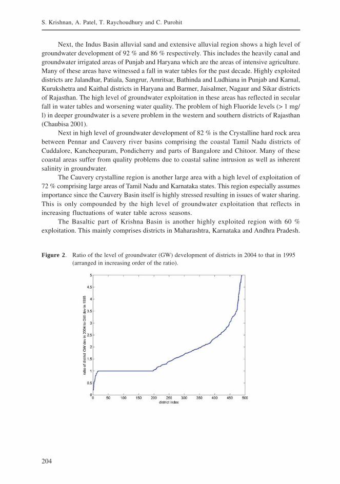
204
S. Krishnan, A. Patel, T. Raychoudhury and C. Purohit
Next, the Indus Basin alluvial sand and extensive alluvial region shows a high level ofgroundwater development of 92 % and 86 % respectively. This includes the heavily canal andgroundwater irrigated areas of Punjab and Haryana which are the areas of intensive agriculture.Many of these areas have witnessed a fall in water tables for the past decade. Highly exploiteddistricts are Jalandhar, Patiala, Sangrur, Amritsar, Bathinda and Ludhiana in Punjab and Karnal,Kurukshetra and Kaithal districts in Haryana and Barmer, Jaisalmer, Nagaur and Sikar districtsof Rajasthan. The high level of groundwater exploitation in these areas has reflected in secularfall in water tables and worsening water quality. The problem of high Fluoride levels (> 1 mg/l) in deeper groundwater is a severe problem in the western and southern districts of Rajasthan(Chaubisa 2001).
Next in high level of groundwater development of 82 % is the Crystalline hard rock areabetween Pennar and Cauvery river basins comprising the coastal Tamil Nadu districts ofCuddalore, Kancheepuram, Pondicherry and parts of Bangalore and Chitoor. Many of thesecoastal areas suffer from quality problems due to coastal saline intrusion as well as inherentsalinity in groundwater.
The Cauvery crystalline region is another large area with a high level of exploitation of72 % comprising large areas of Tamil Nadu and Karnataka states. This region especially assumesimportance since the Cauvery Basin itself is highly stressed resulting in issues of water sharing.This is only compounded by the high level of groundwater exploitation that reflects inincreasing fluctuations of water table across seasons.
The Basaltic part of Krishna Basin is another highly exploited region with 60 %exploitation. This mainly comprises districts in Maharashtra, Karnataka and Andhra Pradesh.
Figure 2. Ratio of the level of groundwater (GW) development of districts in 2004 to that in 1995(arranged in increasing order of the ratio).
205
Groundwater Exploitation in India, Environmental Impacts and Limits to Further Exploitation for Irrigation
The increase in level of GW development from 1995 statistics to 2004 statistics.
Ratio of GW development No. of districtsfrom 1995-2004
0-1 20
1-2 330
2-3 100
3-4 25
4-5 25
The previous CGWB groundwater statistics were brought out in 1995. Since then, therehas been a revision in methodology of groundwater computation (GEC 1997). The revision inmethodology corrects some of the lacunae mentioned earlier and it is expected that a morecorrect picture is now reflected in the current methodology. When the 2004 levels ofgroundwater development are compared with the 1995 levels, (Figure 2, the districts have beenarranged in increasing order of ratio of 2004 to 1995 levels of GW development), we see thatvery few districts (less than 20) show a decrease in levels of GW development. Most showthe same or an increase in levels of GW development from before with some showing as muchas a 5 time increase. Note that this reflects a change in methodology as well as fresh data fromthe past decade. The introduction of HLDR piezometers in the peninsular states under theHydrology project also has an impact.
Environmental Impacts of Overexploitation
Nevertheless, a comparison across the country offers us a possibility of comparing acrossthe same bias (assuming similar errors due to this methodology). These figures should betaken along with observations of local adverse impacts on the environment such as fallingwater tables, high seasonal fluctuations in water tables, deteriorating water quality, landsubsidence – all of which together provide us with a picture of groundwater exploitation.
We first start from the Himalayan region where groundwater exploitation has not beenvery high, but has been showing pockets of disturbance in the past decade. Most rural areasin the mountains and towns in this region depend on spring water for their domestic and otheruses. In the past, such use of spring water was not exploited on a large scale, but is nowwidespread and therefore leading to overexploitation. One example is that of the Almora Town(Kumar and Rawat 1996). Spring water is essentially groundwater that is discharged at pointswhere the piezometric surface intersects the ground level. Therefore, the discharge of springsis closely related to exploitation of groundwater and development activities in recharge areasof the springs. The major problem with such springs in mountain towns such as Almora is thepollution levels due to inadequate protection. This when combined with increasing use causelowering of discharge and poor water quality. Fast developing areas in the Himalayan regionsuch as the Doon Valley face critical problems of groundwater exploitation (Bartarya 1997).Such valleys are composed of rich intermontane alluvial aquifers recharged by the springsoriginating in surrounding hills, in this case the Mussourie Hill region. However, there is a
206
S. Krishnan, A. Patel, T. Raychoudhury and C. Purohit
combined effect of the springs being diverted for other uses and high overdraft in the valleyregion that results in depleting groundwater levels in the Doon Valley.
The Siwalik and foothill region of the Himalayas are characterized by typical groundwaterproblems. The Kandi region spanning from Kashmir region, Punjab and Haryana is thetransitional zone between the Siwaliks and the plains (Shardha and Bagchi 2001). Deepgroundwater tables, high speed of groundwater flow, uncertain composition of aquifers andsome challenges associated with the groundwater use in this area. In such areas, even anymoderate development of groundwater results in high levels of exploitation.
In the Himalayan region more than in any other place, the impact of groundwaterdevelopment on interaction between surface and groundwater is clearly visible. Springs areone example of this interaction. Lack of protection of recharge areas has led to drying up of alarge number of such mountain springs all across the Himalayan region (Valdiya and Bartarya1989). But this is visible in the lean season flows of the Himalayan rivers for which much ofthe non-monsoon flows are fed by base flow components from contributing catchments. Theeffluent nature of Doon Valley aquifer into the Son River is one example. Ongoing research islooking at this magnitude of base flow contribution and its variation with high groundwaterdevelopment in the catchment areas.
The Indus-Gangetic Alluvial plains from Punjab up to West Bengal form the maingroundwater occurring region of the country. There is a vast variation, however, in the aquiferstructures, availability of groundwater and groundwater quality across this region. The Punjabplains have in the past 3-4 decades witnessed a boom in groundwater use and many authorshave studied this problem of depleting water quality and fall in water tables (Dhawan 1995;Sondhi et al. 2001; Ambast et al. 2006). Many districts of Punjab show 100 % or greater levelsof exploitation which is exhibited by a secular decline in pre-monsoon water tables except forextremely wet years. The Bist-Doab tract lying between the Beas and Sutlej rivers consists ofseveral districts that have now local aquifers with an annual decline of more than a meter inphreatic water levels. The problem with authenticating these facts with scientific observationlies in the poor quality of data referred to earlier. Most water level data sets collected by agenciesare fraught with missing data, inconsistent information and lack of agreement with local‘common sense’. An analysis of pre-monsoon water level data of Bist-Doab area of 33monitoring wells show 22 % of missing data in the data set.
The central and eastern parts of the Indus-Gangetic Plains have in general a problem ofeconomic access to groundwater rather than actual physical scarcity. In these regions withpoor rural electricity, a marginal rise in diesel prices or a few meters fall in water table resultsin groundwater irrigation becoming economically unfeasible for many crops and smalllandholders. Therefore, even a 50-60 % level of current groundwater exploitation in many ofthese eastern areas can cause difficult access to groundwater.
The alluvial aquifers of North Gujarat are another zone of high groundwater exploitation(Kumar and Singh 2007). In the highly overexploited Mehsana aquifer, water tables have beenfalling at rates of more than a meter every year and currently the 5th or 6th aquifer is being usedby wells that are the deepest ones in the country. Spurred by the dairy industry and highwater yielding crops, this region has witnessed one of the extreme cases of groundwateroveruse. This exploitation has also led to quality problems in water, especially high levels ofFluoride (Gupta et al. 2005) as a result of exploiting water of high residence time (> 1,000 years)that has led to excessive mineralization.
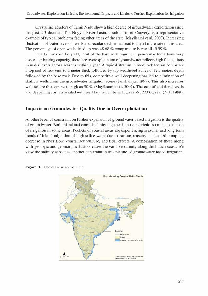
207
Groundwater Exploitation in India, Environmental Impacts and Limits to Further Exploitation for Irrigation
Crystalline aquifers of Tamil Nadu show a high degree of groundwater exploitation sincethe past 2-3 decades. The Noyyal River basin, a sub-basin of Cauvery, is a representativeexample of typical problems facing other areas of the state (Mayilsami et al. 2007). Increasingfluctuation of water levels in wells and secular decline has lead to high failure rate in this area.The percentage of open wells dried up was 48.68 % compared to borewells 9.99 %.
Due to low specific yield, most of the hard rock regions in peninsular India have veryless water bearing capacity, therefore overexploitation of groundwater reflects high fluctuationsin water levels across seasons within a year. A typical stratum in hard rock terrain comprisesa top soil of few cms to a meter thick followed by top weathered zones of few meters depthfollowed by the base rock. Due to this, competitive well deepening has led to elimination ofshallow wells from the groundwater irrigation scene (Janakarajan 1999). This also increaseswell failure that can be as high as 50 % (Mayilsami et al. 2007). The cost of additional wellsand deepening cost associated with well failure can be as high as Rs. 22,000/year (NIH 1999).
Impacts on Groundwater Quality Due to Overexploitation
Another level of constraint on further expansion of groundwater based irrigation is the qualityof groundwater. Both inland and coastal salinity together impose restrictions on the expansionof irrigation in some areas. Pockets of coastal areas are experiencing seasonal and long termtrends of inland migration of high saline water due to various reasons – increased pumping,decrease in river flow, coastal aquaculture, and tidal effects. A combination of these alongwith geologic and geomorphic factors cause the variable salinity along the Indian coast. Weview the salinity aspect as another constraint in this picture of groundwater based irrigation.
Figure 3. Coastal zone across India.
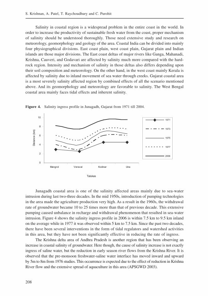
208
S. Krishnan, A. Patel, T. Raychoudhury and C. Purohit
Salinity in coastal region is a widespread problem in the entire coast in the world. Inorder to increase the productivity of sustainable fresh water from the coast, proper mechanismof salinity should be understood thoroughly. Those need extensive study and research onmeteorology, geomorphology and geology of the area. Coastal India can be divided into mainlyfour physiographical divisions. East coast plain, west coast plain, Gujarat plain and Indianislands are those major divisions. The East coast deltas of major rivers like Ganga, Mahanadi,Krishna, Cauveri, and Godavari are affected by salinity much more compared with the hard-rock region. Intensity and mechanism of salinity in those deltas also differs depending upontheir soil composition and meteorology. On the other hand, in the west coast mainly Kerala isaffected by salinity due to inland movement of sea water through creeks. Gujarat coastal areais a most severely salinity affected region by combined effects of all the scenario mentionedabove. And its geomorphology and meteorology are favorable to salinity. The West Bengalcoastal area mainly faces tidal effects and inherent salinity.
Figure 4. Salinity ingress profile in Junagadh, Gujarat from 1971 till 2004.
Junagadh coastal area is one of the salinity affected areas mainly due to sea-waterintrusion during last two-three decades. In the mid 1950s, introduction of pumping technologiesin the area made the agriculture production very high. As a result in the 1960s, the withdrawalrate of groundwater became 10 to 25 times more than that of previous decade. This extensivepumping caused unbalance in recharge and withdrawal phenomenon that resulted in sea-waterintrusion. Figure 4 shows the salinity ingress profile in 2006 is within 7.5 km to 9.5 km inlandon the average while in 1977 it was observed within 5 km to 7.5 km. Since the past two decades,there have been several interventions in the form of tidal regulators and watershed activitiesin this area, but they have not been significantly effective in reducing the rate of ingress.
The Krishna delta area of Andhra Pradesh is another region that has been observing anincrease in coastal salinity of groundwater. Here though, the cause of salinity increase is not exactlyingress of saline water, but the reduction in early season river flows from the Krishna River. It isobserved that the pre-monsoon freshwater-saline water interface has moved inward and upwardby 5m to 8m from 1976 studies. This occurrence is expected due to the effect of reduction in KrishnaRiver flow and the extensive spread of aquaculture in this area (APSGWD 2003).
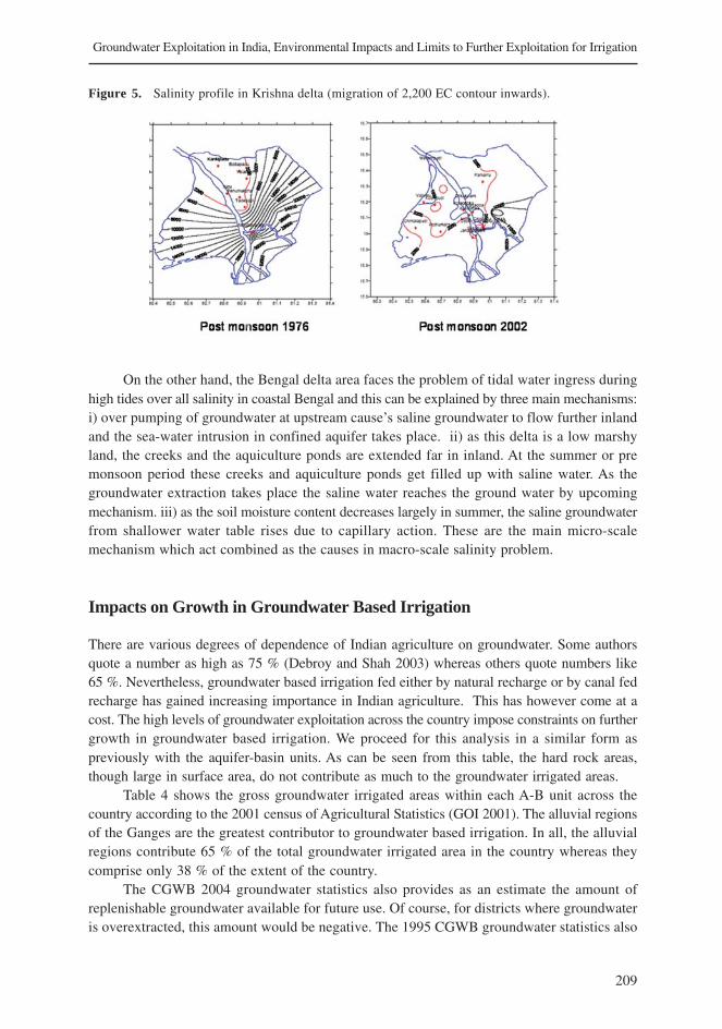
209
Groundwater Exploitation in India, Environmental Impacts and Limits to Further Exploitation for Irrigation
On the other hand, the Bengal delta area faces the problem of tidal water ingress duringhigh tides over all salinity in coastal Bengal and this can be explained by three main mechanisms:i) over pumping of groundwater at upstream cause’s saline groundwater to flow further inlandand the sea-water intrusion in confined aquifer takes place. ii) as this delta is a low marshyland, the creeks and the aquiculture ponds are extended far in inland. At the summer or premonsoon period these creeks and aquiculture ponds get filled up with saline water. As thegroundwater extraction takes place the saline water reaches the ground water by upcomingmechanism. iii) as the soil moisture content decreases largely in summer, the saline groundwaterfrom shallower water table rises due to capillary action. These are the main micro-scalemechanism which act combined as the causes in macro-scale salinity problem.
Impacts on Growth in Groundwater Based Irrigation
There are various degrees of dependence of Indian agriculture on groundwater. Some authorsquote a number as high as 75 % (Debroy and Shah 2003) whereas others quote numbers like65 %. Nevertheless, groundwater based irrigation fed either by natural recharge or by canal fedrecharge has gained increasing importance in Indian agriculture. This has however come at acost. The high levels of groundwater exploitation across the country impose constraints on furthergrowth in groundwater based irrigation. We proceed for this analysis in a similar form aspreviously with the aquifer-basin units. As can be seen from this table, the hard rock areas,though large in surface area, do not contribute as much to the groundwater irrigated areas.
Table 4 shows the gross groundwater irrigated areas within each A-B unit across thecountry according to the 2001 census of Agricultural Statistics (GOI 2001). The alluvial regionsof the Ganges are the greatest contributor to groundwater based irrigation. In all, the alluvialregions contribute 65 % of the total groundwater irrigated area in the country whereas theycomprise only 38 % of the extent of the country.
The CGWB 2004 groundwater statistics also provides as an estimate the amount ofreplenishable groundwater available for future use. Of course, for districts where groundwateris overextracted, this amount would be negative. The 1995 CGWB groundwater statistics also
Figure 5. Salinity profile in Krishna delta (migration of 2,200 EC contour inwards).
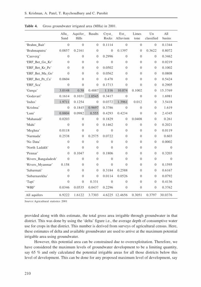
210
S. Krishnan, A. Patel, T. Raychoudhury and C. Purohit
provided along with this estimate, the total gross area irrigable through groundwater in thatdistrict. This was done by using the ‘delta’ figure i.e., the average depth of consumptive wateruse for crops in that district. This number is derived from surveys of agricultural census. Here,these estimates of delta and available groundwater are used to arrive at the maximum potentialirrigable area using groundwater.
However, this potential area can be constrained due to overexploitation. Therefore, wehave considered the maximum levels of groundwater development to be a limiting quantity,say 65 % and only calculated the potential irrigable areas for all those districts below thislevel of development. This can be done for any proposed maximum level of development, say
Table 4. Gross groundwater irrigated area (MHa) in 2001.
Allu_ Aquifer_ Basalts Cryst_ Ext_ Limes Un AllSand Hills Rocks Alluvium tone classified basins
‘Brahm_Bait’ 0 0 0 0.1114 0 0 0 0.1344
‘Brahmaputra’ 0.0857 0.2161 0 0 0.1397 0 0.3622 0.8072
‘Cauverg’ 0 0 0 0.2996 0 0 0 0.3462
‘ERF_Bet_Go_Kr’ 0 0 0 0 0 0 0 0.0219
‘ERF_Bet_Kr_Pe’ 0 0 0 0.0502 0 0 0 0.1002
‘ERF_Bet_Ma_Go’ 0 0 0 0.0562 0 0 0 0.0808
‘ERF_Bet_Pe_Ca’ 0.0604 0 0 0.478 0 0 0 0.5424
‘ERF_Sca’ 0 0 0 0.1713 0 0 0 0.2905
‘Ganga’ 3.0148 0.58 0.4887 1.116 10.074 0.1002 0 15.3769
‘Godavari’ 0.1614 0.1031 1.0545 0.3417 0 0 0 1.6981
‘Indus’ 1.9711 0.1254 0 0.0372 1.3961 0.012 0 3.5418
‘Krishna’ 0 0.1845 0.9697 0.3786 0 0 0 1.619
‘Luni’ 0.8804 0.0982 0.555 0.4293 0.4234 0 0 2.4345
‘Mahanadi’ 0.0203 0 0 0.1829 0 0.0408 0 0.261
‘Mahi’ 0 0 0 0.1462 0 0 0 0.2021
‘Meghna’ 0.0118 0 0 0 0 0 0 0.0119
‘Narmada’ 0.2538 0 0.2575 0.0722 0 0 0 0.603
‘No Data’ 0 0 0 0 0 0 0 0.0002
‘North Ladakh’ 0 0 0 0 0 0 0 0
‘Pennar’ 0 0.1047 0 0.1806 0 0 0 0.3203
‘Rivers_Bangaladesh’ 0 0 0 0 0 0 0 0
‘Rivers_Myanmar’ 0.158 0 0 0 0 0 0 0.1595
‘Sabarmati’ 0 0 0 0.3184 0.2588 0 0 0.6167
‘Subarnarekha’ 0 0 0 0.0114 0.0526 0 0 0.0792
‘Tapi’ 0 0 0.331 0 0 0 0 0.4136
‘WRF’ 0.0346 0.0535 0.0437 0.2296 0 0 0 0.3762
All aquifers 6.9222 1.6122 3.7303 4.6225 12.4656 0.3051 0.3797 30.0376
Source:Agricultural statistics 2001
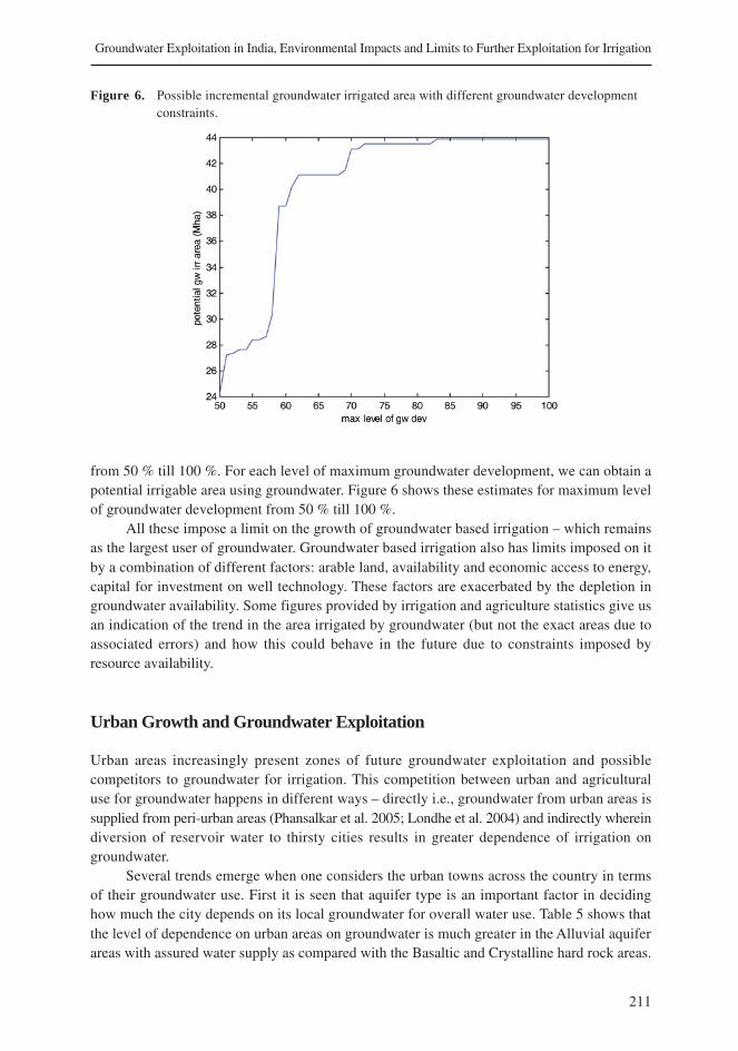
211
Groundwater Exploitation in India, Environmental Impacts and Limits to Further Exploitation for Irrigation
from 50 % till 100 %. For each level of maximum groundwater development, we can obtain apotential irrigable area using groundwater. Figure 6 shows these estimates for maximum levelof groundwater development from 50 % till 100 %.
All these impose a limit on the growth of groundwater based irrigation – which remainsas the largest user of groundwater. Groundwater based irrigation also has limits imposed on itby a combination of different factors: arable land, availability and economic access to energy,capital for investment on well technology. These factors are exacerbated by the depletion ingroundwater availability. Some figures provided by irrigation and agriculture statistics give usan indication of the trend in the area irrigated by groundwater (but not the exact areas due toassociated errors) and how this could behave in the future due to constraints imposed byresource availability.
Urban Growth and Groundwater Exploitation
Urban areas increasingly present zones of future groundwater exploitation and possiblecompetitors to groundwater for irrigation. This competition between urban and agriculturaluse for groundwater happens in different ways – directly i.e., groundwater from urban areas issupplied from peri-urban areas (Phansalkar et al. 2005; Londhe et al. 2004) and indirectly whereindiversion of reservoir water to thirsty cities results in greater dependence of irrigation ongroundwater.
Several trends emerge when one considers the urban towns across the country in termsof their groundwater use. First it is seen that aquifer type is an important factor in decidinghow much the city depends on its local groundwater for overall water use. Table 5 shows thatthe level of dependence on urban areas on groundwater is much greater in the Alluvial aquiferareas with assured water supply as compared with the Basaltic and Crystalline hard rock areas.
Figure 6. Possible incremental groundwater irrigated area with different groundwater developmentconstraints.

212
S. Krishnan, A. Patel, T. Raychoudhury and C. Purohit
This dependence on local groundwater also varies across the size of cities in terms ofpopulation. It is seen that in general, smaller towns have lesser ability to attract water from faraway sources, hence more dependant on local groundwater. Table 6 shows that across classsizes, the average dependence of an urban area on groundwater increases from 12 % for themetropolitan cities to 36 % and 49 % for Class I and Class II cities.
When we compare the level of groundwater development in a basin along with thedependence of urban areas within that basin for groundwater, a picture of overall stress withinthat basin can be obtained (Table 7). Basins where there is already a high level of groundwaterdevelopment and urban areas depending upon surface water more for their needs, one wouldsee greater competition between urban and other uses for basin water resources in the futuree.g., Krishna and Sabarmati basins.
Table 5. Groundwater dependence of urban areas for each aquifer type.
Aquifers No. of towns Dependance on local groundwater
Alluvium and sandstone discourse 78 44 %
Aquifer in hilly areas 19 47 %
Basalt 43 8 %
Crystalline rocks 70 21 %
Extensive alluvium 84 75 %
Limestone 2 5 %
Total 296 42 %
Figure 7. 300 urban areas of India over river basins and aquifer types.
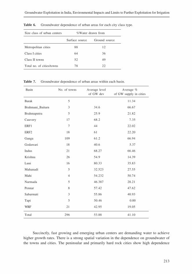
213
Groundwater Exploitation in India, Environmental Impacts and Limits to Further Exploitation for Irrigation
Table 6. Groundwater dependence of urban areas for each city class type.
Size class of urban centers %Water drawn from
Surface source Ground source
Metropolitan cities 88 12
Class I cities 64 36
Class II towns 52 49
Total no. of cities/towns 78 22
Table 7. Groundwater dependence of urban areas within each basin.
Basin No. of towns Average level Average %of GW dev of GW supply in cities
Barak 5 11.34
Brahmani_Baitarn 3 34.6 66.67
Brahmaputra 5 25.9 21.82
Cauvery 17 68.2 7.35
ERF1 7 44 22.02
ERF2 18 61 22.20
Ganga 109 61.2 66.94
Godawari 18 40.6 5.37
Indus 21 68.27 66.46
Krishna 26 54.9 14.39
Luni 16 80.33 35.83
Mahanadi 5 32.523 27.55
Mahi 4 54.232 50.74
Narmada 5 46.387 28.21
Pennar 8 57.42 47.62
Sabarmati 3 55.86 40.93
Tapi 5 50.46 0.00
WRF 21 42.95 19.05
Total 296 53.88 41.10
Succinctly, fast growing and emerging urban centers are demanding water to achievehigher growth rates. There is a strong spatial variation in the dependence on groundwater ofthe towns and cities. The peninsular and primarily hard rock cities show high dependence
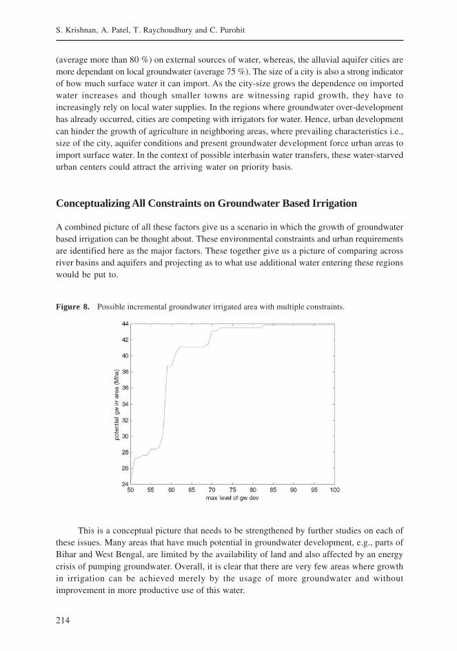
214
S. Krishnan, A. Patel, T. Raychoudhury and C. Purohit
(average more than 80 %) on external sources of water, whereas, the alluvial aquifer cities aremore dependant on local groundwater (average 75 %). The size of a city is also a strong indicatorof how much surface water it can import. As the city-size grows the dependence on importedwater increases and though smaller towns are witnessing rapid growth, they have toincreasingly rely on local water supplies. In the regions where groundwater over-developmenthas already occurred, cities are competing with irrigators for water. Hence, urban developmentcan hinder the growth of agriculture in neighboring areas, where prevailing characteristics i.e.,size of the city, aquifer conditions and present groundwater development force urban areas toimport surface water. In the context of possible interbasin water transfers, these water-starvedurban centers could attract the arriving water on priority basis.
Conceptualizing All Constraints on Groundwater Based Irrigation
A combined picture of all these factors give us a scenario in which the growth of groundwaterbased irrigation can be thought about. These environmental constraints and urban requirementsare identified here as the major factors. These together give us a picture of comparing acrossriver basins and aquifers and projecting as to what use additional water entering these regionswould be put to.
Figure 8. Possible incremental groundwater irrigated area with multiple constraints.
This is a conceptual picture that needs to be strengthened by further studies on each ofthese issues. Many areas that have much potential in groundwater development, e.g., parts ofBihar and West Bengal, are limited by the availability of land and also affected by an energycrisis of pumping groundwater. Overall, it is clear that there are very few areas where growthin irrigation can be achieved merely by the usage of more groundwater and withoutimprovement in more productive use of this water.
215
Groundwater Exploitation in India, Environmental Impacts and Limits to Further Exploitation for Irrigation
References
Ambast, S. K.; Tyagi, N. K.; Raul, S. K. 2005. Management of declining groundwater in the Trans Indo-Gangetic Plain (India): Some options. Agricultural Water Management, 82 (3) (2006-04-24): 279-296.
APSGWD. 2003. Fresh-water, Saline water interrelationship in the multi aquifer system of Krishna delta.
Bartarya, S. K. 1997. Hydrogeology and water resources of intermontane Doon valley. Jour. Him. Geol.6 (2):17- 28.
Chaubisa, S. L. 2001. Endemic Fluorosis in Southern Rajasthan, India. Fluoride, Vol. 34, pg. 61-70.
CGWB. 1995. Groundwater Statistics of India. Ministry of Water Resources, Government of India.
CGWB. 2004. Dynamic groundwater resources of India. Faridabad, India: Central Groundwater Board.
CGWB. 2005. The dynamic Groundwater resources of India. Ministry of Water Resources, Governmentof India.
Roy, D. A.; Shah, T. 2003. Socio-ecology of Groundwater Irrigation in India. In Intensive Use ofGroundwater: Challenges and Opportunities, eds. R. Llamas.; E. Custodio. The Netherlands: Swets andZetlinger Publishing Co.
Dhawan, B. D. 1990. How reliable are groundwater estimates? Economic and Political Weekly, 19:1073-1078 (May).
Dhawan, B. D. 1995. Groundwater depletion, land degradation and irrigated agriculture in India. NewDelhi: Commonwealth Publishers.
GEC. 1997. Groundwater Estimation Committee, Central Groundwater Board, Faridabad, India.
GOI. 2001. Agricultural statistics at a glance 2001. New Delhi: Directorate of Economics and Statistics,Department of Agriculture and Cooperation, Ministry of Agriculture.
Gupta, S. K.; Deshpande, R. D.; Agarwal, M.; Raval, B. R. 2005. Depleting groundwater levels and increasingfluoride in villages of Mehsana district, Gujarat, India: Cost to economy and health. HydrogeologyJournal, vol. 13, no. 4.
Groundwater Estimation Committee. 1997. Groundwater Estimation Methodology – 1997. New Delhi:Ministry of Water Resources, Govt. of India.
Janakarajan, S. 1999. Conflicts Over the Invisible Resource: Is there a Way Out? In Rethinking the Mosaic:Investigations into Local Water Management, eds. M.Moench; E. Caspari; E.; A. Dixit. USA: NWCFand ISET.
Karanth, K. R. 1987. Groundwater Assessment, Development and Management. Tata-McGraw HillPublishing Company.
Kumar, D. 2007. Groundwater Management in India: Physical, Institutional and Policy Alternatives. SAGEPublications.
Kumar, D.; Singh, O. P. 2007. Groundwater Management in India: Physical, Institutional and PolicyAlternatives. Sage Publications.
Kumar, K.; Rawat, D. S. 1996. Water Management in Himalayan Ecosystem: A study of natural springs ofAlmora. New Delhi: Indus Publishing Company.
Londhe, A.; Talati, J.; Singh, S. K.; Dhaunta, V. S.; Rawlley, B.; Ganapathy, K. K.; Mathew, R. P. 2004.Urban-Hinterland Water Transactions: A Scoping Study of Six Class I Indian Cities. In Proceedings ofIWMI-Tata Annual Partner’s Meet. Anand.
Mayilsami, C.; Chellamuthu, M.; Bosu, S.; Palanisamy, D.; Ranghaswami, M. V.; Palanisami, K. 2008.Mathematical Modeling of Groundwater Resources in the Hard Rock aquifer system of Noyil riverbasin. In Groundwater resources assessment, recharge and modeling, eds. M.V. Ranghaswami; K.Palanisami; C. Mayilswami.: Macmillan India Ltd.
216
S. Krishnan, A. Patel, T. Raychoudhury and C. Purohit
NIH. 1999. Hydrological Problems of Hard rock region.
Patel, A.; Krishnan, S. 2006. Groundwater situation in urban India: Overview, opportunities and challenges.In Proceedings of 2nd International Groundwater Conference. Coimbatore, India.
Phansalkar, S. J.; Kher, V.; Deshpande, P. 2005. Expanding rings of dryness: Water Imports fromHinterlands to Cities and the Rising Demands of Mega-Cities. In Proceedings of IWMI-Tata AnnualPartner’s Meet. Anand.
Raj, P. 2004. Classification and interpretation of piezometer well hydrographs in parts of southeasternpeninsular India. Journal of Environmental Geology, vol. 46, pp 808-819.
Raychoudhury, T.; Krishnan, S. 2005. (unpublished), Coastal salinity of Indian coast: An overview. IWMI-Tata Program Report.
Shah, M. 1998. India’s dry lands: Tribal societies and development through environmental regeneration,eds. D.Banerji; P.S. Vijayshankar. Oxford University Press.
Sondhi, S. K.; Kaushal, M. P.; Aggrawal, R. 2001. Management of Groundwater Resources in Punjab. InICAR-IWMI Groundwater Policy Initiative-2001.
Taylor, G. C. (Jr.). 1959. Groundwater Provinces of India. Econ. Geol., 54 (4), p. 683-697.
Shardha, Y. P.; Bagchi, J. 2001. An approach to meet the challenge of unpredictable hydrology in smallcatchments with reference to Kandi watershed area, Punjab, in National Symposium: Role of EarthSciences in Integrated Development and Related Societal Issues, 2-4 November 2001, Lucknow. SpecialPublication No. 65: Vol. II. Kolkata. Geological Survey of India, 2001, 242 p.
Valdiya, K. S.; Bartarya, S. K. 1989. Diminishing discharges of mountain springs in a part of the KumaonHimalaya. Current Science, vol. 58, no. 8, pp. 417-426.
217
Groundwater Exploitation in India, Environmental Impacts and Limits to Further Exploitation for Irrigation
Water Productivity at Different Scales under Canal, Tankand Well Irrigation Systems
K. Palanisami, S. Senthilvel and T. RameshTamil Nadu Agricultural University, Coimbotore, India
Introduction
Generally speaking, the term ‘water productivity’ refers to the magnitude of output or benefitresulting from the input quantum of water as applied on a unit base. In the domain of agriculture,it is expressed as the net consumptive use efficiency in terms of yield per unit depth of waterconsumed per unit area of cultivation. If the field water conveyance, application, storage anddistribution efficiencies are accounted to depict the seepage, runoff and deep percolation losses(not consumed by plant; evapotranspiration loss is included as an implicit component of fieldwater balance) it would be termed as the gross irrigation water use efficiency. When isolatedas ‘water productivity’ it becomes a partial productivity of one factor viz., water, irrespectiveof the land unit but in reference to the scale of production in the range of a single plant’seffective root zone to a basin or system of irrigation command. As more and more water lossesare incurred when the scale of reference expands, the apparent or relative water productivityis bound to decrease. However, for an increasing scale, the chances of recovering the so called‘losses’ of water are bound to increase and at one stage, may be a project or basin scale, theloss at one point will be a gain at another point (as deep percolation leading to groundwaterrecharge or runoff leading to surface detention and storage) for recycling. In other words, thebasic net input of water required in the effective root zone of a plant scale is subsequentlyreckoned as a gross input of water incorporating the irrigation efficiencies (h) at farm/fieldlevel and fixing the flow duty (D), field duty (D) and storage duty (S) at a system/project/basin/command level. The overall conceptual framework should account for all thesetransformation parameters from scale to scale.
Agricultural Water Productivity
Agricultural water productivity can be expressed either as a physical productivity in termsof the yield over unit quantity of water consumed (tonnes per ha.cm of water or kg yield perkg water consumed) in accordance with the scale of reference that includes or excludes thelosses of water or an economic productivity replacing the yield term by the gross or netpresent value of the crop yield for the same water consumption (rupees per unit volumeof water).
218
K. Palanisami, S. Senthilvel and T. Ramesh
Water productivity is defined as ‘crop production’ per unit ‘amount of water used’(Molden 1997). Concept of water productivity in agricultural production systems is focusedon ‘producing more food with the same water resources’ or ‘producing the same amount offood with less water resources’. Initially, irrigation efficiency or water use efficiency was usedto describe the performance of irrigation systems. In agronomic terms, ‘water use efficiency’ isdefined as the amount of organic matter produced by a plant divided by the amount of waterused by the plant in producing it (De Wit 1958). However, the used terminology ‘water useefficiency’ does not follow the classical concept of ‘efficiency’, which uses the same units forinput and output. Therefore, International Water Management Institute (IWMI) has proposeda change of the nomenclature from ‘water use efficiency’ to ‘water productivity’. Waterproductivity can be further defined in several ways according to the purpose, scale and domainof analysis (Molden et al. 2001; Bastiaanssen et al. 2003).
Stakeholder Definition Scale Target
Farmer Yield / irrigation Field Maximize yield
Irrigation engineer Yield / canal water supply Irrigation scheme Maximize water allocation
Policymaker $ / available water River basin Maximize profits
Scales of Reference and Water Productivity Transformations
The definition of water productivity is scale-dependent. Increasing water productivity is thenthe function of several components at different levels viz., the plant, field, irrigation systemand river-basin. An increase in production per unit of water diverted at one scale does notnecessarily lead to an increase in productivity of water diverted at a larger scale. The classicalirrigation efficiency decreases as the scale of the system increases (Seckler et al. 2003). InIndia, the on-farm irrigation efficiency of most canal irrigation systems ranges from 30 to 40 %(Navalawala 1999; Singh 2000) whereas, the irrigation efficiency at basin level is as high as 70to 80 % (Chaudhary 1997). Basin water productivity takes into consideration beneficial depletionfor multiple uses of water, including not only crop production but also uses by thenonagricultural sector, including the environment. Here, the problem lies in allocating the wateramong its multiple uses and users.
Methodology to Workout Water Productivity
The assessment of water productivity would involve a sequence of mathematical operationsthat may be in accordance with the scale of reference. The scale based models are to beintegrated for the final quantification of agricultural water productivity on an ultimate regionalscale for the purpose of planning.
Plant/Crop Scale Water Productivity (WP [p]):
Here, the effective root zone of the plant/crop is the reference or datum over which the cropconsumptive use exclusive of the inevitable gravitational irrigation system losses (seepage,runoff and deep percolation) is considered as the input for the single plant/crop output. In
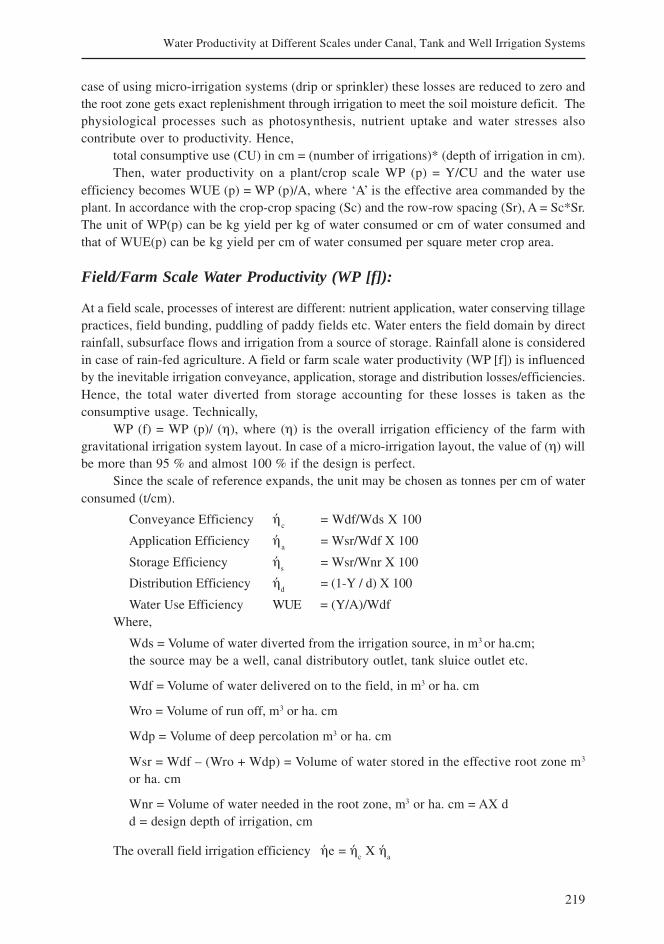
219
Water Productivity at Different Scales under Canal, Tank and Well Irrigation Systems
case of using micro-irrigation systems (drip or sprinkler) these losses are reduced to zero andthe root zone gets exact replenishment through irrigation to meet the soil moisture deficit. Thephysiological processes such as photosynthesis, nutrient uptake and water stresses alsocontribute over to productivity. Hence,
total consumptive use (CU) in cm = (number of irrigations)* (depth of irrigation in cm).Then, water productivity on a plant/crop scale WP (p) = Y/CU and the water use
efficiency becomes WUE (p) = WP (p)/A, where ‘A’ is the effective area commanded by theplant. In accordance with the crop-crop spacing (Sc) and the row-row spacing (Sr), A = Sc*Sr.The unit of WP(p) can be kg yield per kg of water consumed or cm of water consumed andthat of WUE(p) can be kg yield per cm of water consumed per square meter crop area.
Field/Farm Scale Water Productivity (WP [f]):
At a field scale, processes of interest are different: nutrient application, water conserving tillagepractices, field bunding, puddling of paddy fields etc. Water enters the field domain by directrainfall, subsurface flows and irrigation from a source of storage. Rainfall alone is consideredin case of rain-fed agriculture. A field or farm scale water productivity (WP [f]) is influencedby the inevitable irrigation conveyance, application, storage and distribution losses/efficiencies.Hence, the total water diverted from storage accounting for these losses is taken as theconsumptive usage. Technically,
WP (f) = WP (p)/ (h), where (h) is the overall irrigation efficiency of the farm withgravitational irrigation system layout. In case of a micro-irrigation layout, the value of (h) willbe more than 95 % and almost 100 % if the design is perfect.
Since the scale of reference expands, the unit may be chosen as tonnes per cm of waterconsumed (t/cm).
Conveyance Efficiency ªc
= Wdf/Wds X 100
Application Efficiency ªa
= Wsr/Wdf X 100
Storage Efficiency ªs
= Wsr/Wnr X 100
Distribution Efficiency ªd
= (1-Y / d) X 100
Water Use Efficiency WUE = (Y/A)/WdfWhere,
Wds = Volume of water diverted from the irrigation source, in m3 or ha.cm;the source may be a well, canal distributory outlet, tank sluice outlet etc.
Wdf = Volume of water delivered on to the field, in m3 or ha. cm
Wro = Volume of run off, m3 or ha. cm
Wdp = Volume of deep percolation m3 or ha. cm
Wsr = Wdf – (Wro + Wdp) = Volume of water stored in the effective root zone m3
or ha. cm
Wnr = Volume of water needed in the root zone, m3 or ha. cm = AX dd = design depth of irrigation, cm
The overall field irrigation efficiency ªe = ªc X ª
a

220
K. Palanisami, S. Senthilvel and T. Ramesh
Project/Command Area Scale
In Tamil Nadu, three distinct kinds of command areas are in vogue viz., canal (or reservoir)command, tank (system and nonsystem) command and well (groundwater) command. Whilethe canal and tank commands mostly fall intact under a project operation, well commandsoccur in a scattered fashion (Figure 1). When water is distributed in an irrigation system ata major scale like this, the important processes include allocation, distribution, conflictresolution and drainage. Allocation and distribution of irrigation water are primarily forirrigation besides meeting the nonagricultural demands like domestic, industrial, livestockand fisheries.
For canal command areas, irrigation scheduling cannot be done on a micro-scalecalculating the depth of irrigation required, frequency of irrigation and the duration of irrigationowing to a larger areal extent with different crops and a different system of irrigation supplythroughout the season on a rotational basis. Here, irrigation scheduling refers to the quantumof water to be stored or diverted for meeting the overall command area crop and allied demands.The water productivity concept shall be redefined by way of incorporating the overall irrigationefficiency and the duty of water at storage, flow and field level. The base period (B) overwhich irrigation flow is continuous through the canal network with suitable time rotations atoutlets for distribution, also decides the productivity.
Canal Command / Project Water Productivity (WP(c))
The overall productivity of this scale of reference depends ultimately on the total quantum ofwater released from storage over the base period, the area covered and the project yield. Thestorage duty (S) includes the losses during conveyance, distribution and application over andabove the field duty (Δ) in a canal network project.
Field duty (Δ) is expressed as the seasonal water requirement for crop and relatedactivities, in cm, at the tail most end area of the canal network.
Δ= CU/h where, h represents the farm/field efficiency
Then, the storage duty (S) = Δ / h(c) where h(c) represents the overall conveyanceefficiency of the canal network/project.
The flow duty (D) in ha/cumec is devised in accordance with S and Δ to cover the givencommand area (A) over the base period (B) of the project water supply, as,
D = (864B) / Δ , and S = A. Δ / h(c)
As the command area/project scale is expanding, the apparent losses like runoff and/ordeep percolation would be considered for recycling or conjunctive use with canal flows. Then,the water productivity will be based on the total volume of water diverted from the irrigationsource or simply the storage duty (S).
WP (c) = Y / S Where,
Y = project yield, in tonnes and S = Storage duty, in ha.cm
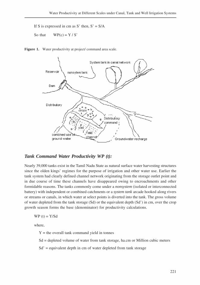
221
Water Productivity at Different Scales under Canal, Tank and Well Irrigation Systems
If S is expressed in cm as S’ then, S’ = S/A
So that WP(c) = Y / S’
Figure 1. Water productivity at project/ command area scale.
Tank Command Water Productivity WP (t):
Nearly 39,000 tanks exist in the Tamil Nadu State as natural surface water harvesting structuressince the olden kings’ regimes for the purpose of irrigation and other water use. Earlier thetank system had clearly defined channel network originating from the storage outlet point andin due course of time these channels have disappeared owing to encroachments and otherformidable reasons. The tanks commonly come under a nonsystem (isolated or interconnectedbattery) with independent or combined catchments or a system tank arcade hooked along riversor streams or canals, in which water at select points is diverted into the tank. The gross volumeof water depleted from the tank storage (Sd) or the equivalent depth (Sd’) in cm, over the cropgrowth season forms the base (denominator) for productivity calculations.
WP (t) = Y/Sd
where,
Y = the overall tank command yield in tonnes
Sd = depleted volume of water from tank storage, ha.cm or Million cubic meters
Sd’ = equivalent depth in cm of water depleted from tank storage
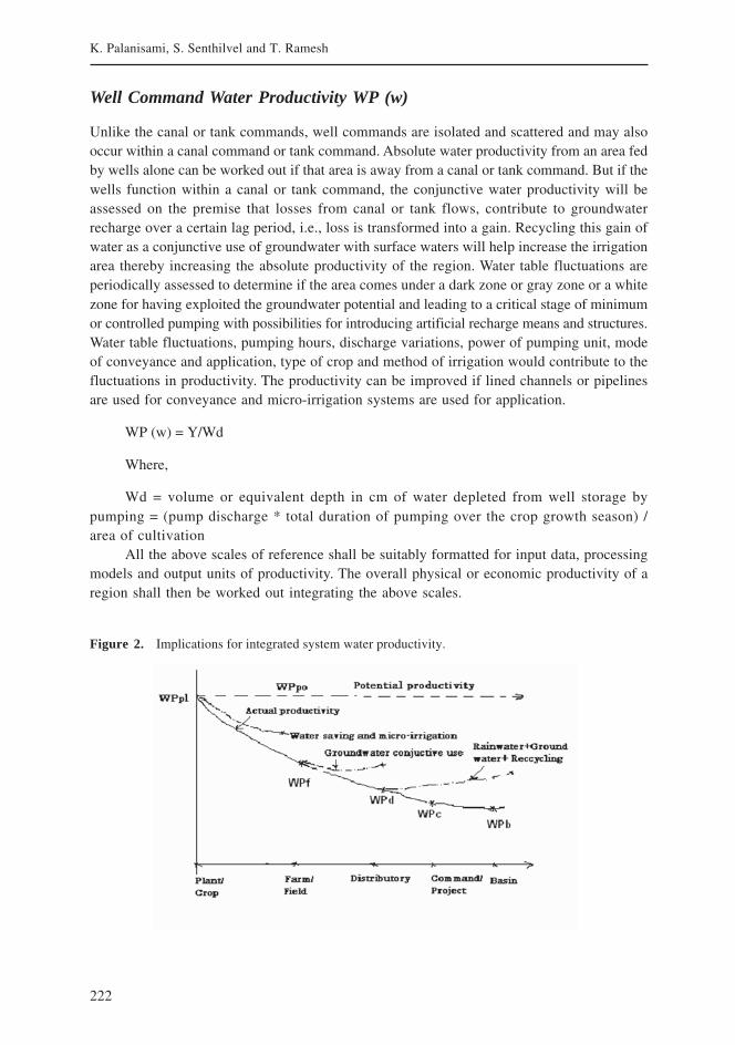
222
K. Palanisami, S. Senthilvel and T. Ramesh
Well Command Water Productivity WP (w)
Unlike the canal or tank commands, well commands are isolated and scattered and may alsooccur within a canal command or tank command. Absolute water productivity from an area fedby wells alone can be worked out if that area is away from a canal or tank command. But if thewells function within a canal or tank command, the conjunctive water productivity will beassessed on the premise that losses from canal or tank flows, contribute to groundwaterrecharge over a certain lag period, i.e., loss is transformed into a gain. Recycling this gain ofwater as a conjunctive use of groundwater with surface waters will help increase the irrigationarea thereby increasing the absolute productivity of the region. Water table fluctuations areperiodically assessed to determine if the area comes under a dark zone or gray zone or a whitezone for having exploited the groundwater potential and leading to a critical stage of minimumor controlled pumping with possibilities for introducing artificial recharge means and structures.Water table fluctuations, pumping hours, discharge variations, power of pumping unit, modeof conveyance and application, type of crop and method of irrigation would contribute to thefluctuations in productivity. The productivity can be improved if lined channels or pipelinesare used for conveyance and micro-irrigation systems are used for application.
WP (w) = Y/Wd
Where,
Wd = volume or equivalent depth in cm of water depleted from well storage bypumping = (pump discharge * total duration of pumping over the crop growth season) /area of cultivation
All the above scales of reference shall be suitably formatted for input data, processingmodels and output units of productivity. The overall physical or economic productivity of aregion shall then be worked out integrating the above scales.
Figure 2. Implications for integrated system water productivity.
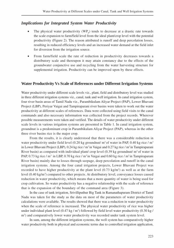
223
Water Productivity at Different Scales under Canal, Tank and Well Irrigation Systems
Implications for Integrated System Water Productivity
• The physical water productivity (WPP) tends to decrease at a drastic rate towards
the scale expansion to farm/field level from the ideal plant/crop level with the potentialproductivity (Figure 2). The reason attributed is runoff and deep percolation losses,resulting in reduced efficiency levels and an increased water demand at the field inletfor diversion from the irrigation source.
• From farm/field scale the rate of reduction in productivity decreases towards adistributory scale and thereupon it may attain constancy due to the effects of thegroundwater conjunctive use and recycling from the water harvesting structure forsupplemental irrigation. Productivity can be improved upon by these effects.
Water Productivity Vs Scale of References under Different Irrigation Systems
Water productivity under different scale levels viz., plant, field and distributory level was studiedin three different irrigation systems viz., canal, tank and well irrigation. In canal irrigation system,four river basin areas of Tamil Nadu viz., Parambikulam Aliyar Project (PAP), Lower BhavaniProject (LBP), Periyar Vaigai and Tampiraparani river basins were taken to work out the waterproductivity at different scales of references. Data were collected using field visits to the canalcommands and also necessary information was collected from the project records. Whereverpossible measurements were taken and verified. The details of water productivity under differentscale levels in various irrigation systems are presented in Table 1. In canal irrigation system,groundnut is a predominant crop in Parambikulam Aliyar Project (PAP), whereas in the otherthree river basins rice is the major crop.
From the results, it is clearly understood that there was a considerable reduction inwater productivity under field level (0.20 kg groundnut/ m3 of water in PAP, 0.40 kg rice / m3
in Lower Bhavani Project (LBP), 0.24 kg rice / m3 in Vaigai and 0.27 kg rice / m3 in TampiraparaniRiver basin) as compared with individual plant/ crop level (0.39 kg groundnut/ m3 of water inPAP, 0.73 kg rice / m3 in LBP, 0.70 kg rice / m3 in Vaigai and 0.60 kg rice / m3 in TampiraparaniRiver basin) mainly due to losses through seepage, deep percolation and runoff in the canalirrigation systems. Among the four canal irrigation projects, Lower Bhavani Project wasrecorded to have higher productivity at the plant level (0.73 kg/m3) as well as at the farmlevel (0.40 kg/m3) compared to other projects. At distributory level, conveyance losses causedreduction in water productivity, which means that a more quantity of water is being used forcrop cultivation. So water productivity has a negative relationship with the scale of referencethat is the expansion of the boundary of the command area (Figure 3).
In the case of tank irrigation, Srivilliputhur Big Tank in Ramanathapuram District of TamilNadu was taken for the study as the data on most of the parameters of water productivitycalculations were available. The results showed that there was a reduction in water productivitywhen the scale of reference is increased. The physical water productivity of rice was higherunder individual plant level (0.47 kg / m3) followed by field level water productivity (0.30 kg /m3) and comparatively lower water productivity was recorded under tank system level.
In sum, among the different irrigation systems, the well system has comparatively higherwater productivity both in physical and economic terms due to controlled irrigation application,

224
K. Palanisami, S. Senthilvel and T. Ramesh
comparatively higher crop yields and multiple crops/ enterprises combinations. In canal andtank systems, mono-cropping, uncontrolled irrigations, and scarcity of water during criticalcrop periods result in lower water productivity.
Table 1. Physical and economic water productivity under different irrigation systems with the differentscale of reference in Tamil Nadu.
Scale of references Total water used (m3) Output Water productivity
Physical Economic Physical Economic(Rs.) (kg/m3) (Rs./m3) (kg)
I. Canal system
1. Parambikulam Aliyar Project (PAP)
Plant/ crop level 0.013 0.0051 0.0312 0.39 2.40
Field level (0.4 ha) 3,388.8 680 4,160 0.20 1.23
Distributory level 1,335,283.7 1,85,661 1,135,810 0.14 0.85
2. Lower Bhavani Project (LBP)
Plant/ crop level 0.0180 0.0131 0.029 0.73 1.61
Field level (0.4 ha) 5,473.5 2,200 7,000 0.40 1.28
Distributory level 8,33,824.4 2,13,796 6,21,952 0.26 0.75
3. Vaigai River Basin
Plant/ crop level 0.020 0.014 0.033 0.70 1.65
Field level (0.4 ha) 6,931.25 1,650 4,390 0.24 0.63
Distributory level 2,486,534.4 3,96,000 1,053,600 0.16 0.42
4. Tampiraparani River Basin
Plant/ crop level 0.028 0.017 0.068 0.60 2.43
Field level (0.4 ha) 7,909.4 2,100 7,100 0.27 0.90
Distributory level 37,647,968.0 3,549,038 12,066,949.5 0.09 0.30
II. Tank system
Plant/ crop level 0.0202 0.0095 0.007125 0.49 0.35
Field level (0.4 ha) 11,608.1 3,160 2,375 0.27 0.20
System level 3,099,174 8,21,000 9,54,750 0.26 0.30
III. Well system
Plant/ crop level
Maize 0.048 0.050 0.21 1.04 4.38
Banana 6.6 8.5 59.70 1.28 8.99
Field level
Crops alone (0.9 ha) 12,003.0 15,833.33* 1,15,752 1.31 9.64
Crops + Dairy (1.0 ha) 10,068.4 32,116.67** 1,15,752 3.19 11.27
Crops + Fishery (1.20 ha) 16,352.0 72,045.83* 6,78,350 4.41 41.43
Note: * banana equivalent yield ** maize equivalent yield
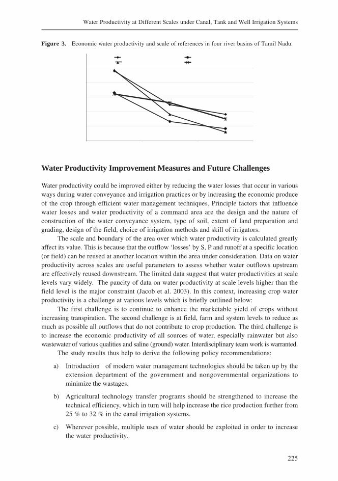
225
Water Productivity at Different Scales under Canal, Tank and Well Irrigation Systems
Water Productivity Improvement Measures and Future Challenges
Water productivity could be improved either by reducing the water losses that occur in variousways during water conveyance and irrigation practices or by increasing the economic produceof the crop through efficient water management techniques. Principle factors that influencewater losses and water productivity of a command area are the design and the nature ofconstruction of the water conveyance system, type of soil, extent of land preparation andgrading, design of the field, choice of irrigation methods and skill of irrigators.
The scale and boundary of the area over which water productivity is calculated greatlyaffect its value. This is because that the outflow ‘losses’ by S, P and runoff at a specific location(or field) can be reused at another location within the area under consideration. Data on waterproductivity across scales are useful parameters to assess whether water outflows upstreamare effectively reused downstream. The limited data suggest that water productivities at scalelevels vary widely. The paucity of data on water productivity at scale levels higher than thefield level is the major constraint (Jacob et al. 2003). In this context, increasing crop waterproductivity is a challenge at various levels which is briefly outlined below:
The first challenge is to continue to enhance the marketable yield of crops withoutincreasing transpiration. The second challenge is at field, farm and system levels to reduce asmuch as possible all outflows that do not contribute to crop production. The third challenge isto increase the economic productivity of all sources of water, especially rainwater but alsowastewater of various qualities and saline (ground) water. Interdisciplinary team work is warranted.
The study results thus help to derive the following policy recommendations:
a) Introduction of modern water management technologies should be taken up by theextension department of the government and nongovernmental organizations tominimize the wastages.
b) Agricultural technology transfer programs should be strengthened to increase thetechnical efficiency, which in turn will help increase the rice production further from25 % to 32 % in the canal irrigation systems.
c) Wherever possible, multiple uses of water should be exploited in order to increasethe water productivity.
Figure 3. Economic water productivity and scale of references in four river basins of Tamil Nadu.
226
K. Palanisami, S. Senthilvel and T. Ramesh
References
Bastiaanssen, W. G. M.; van Dam J. C.; Droogers, P. 2003. Introduction. In Water productivity of irrigatedcrops in Sirsa district, India. Integration of remote sensing, crop and soil models and geographicalinformation systems, eds. J.C. van Dam; R.S. Malik. WATPRO final report, including CD-ROM. ISBN90-6464-864-6: 11-19.
Chaudhary, T. N. 1997. Vision-2020. DWMR Perspective Plan. Directorate of Water Research, Patna,India, 73 p.
De Wit, C. T. 1958. Transpiration and crop yields. Verslaa, van Landbouw, Onderzoek No. 64.6: 88 p.
Jacob, W. K.; Barker, R. Molden, D. 2003. Improving Water Productivity in Agriculture: Editors Overview.In Water Productivity in Agriculture: Limits and Opportunities for Improvement, eds. J.W. Kijne;R.Barker; D.Molden, UK: CABI Publishing.
Molden, D. 1997. Accounting for water use and productivity. SWIM Paper 1. Colombo, Sri Lanka:International Irrigation Management Institute.
Molden, D.; Murray-Rust, H.; Sakthivadivel, R.; Makin, I. 2001. A water productivity framework forunderstanding and action. Workshop on Water productivity. Wadduwa, Sri Lanka, November 12 and13, 2001.
Navalawala, B. N. 1999. Improving management of irrigation resources. Yojana, January: 81-87.
Seckler, D.; Molden, D.; Sakthivadivel, R. 2003. The Concept of Efficiency in Water Resources Managementand Policy. In Water Productivity in Agriculture: Limits and Opportunities for Improvement, eds. J.W.Kijne; R. Barker; D. Molden. UK: CABI Publishing. Pp -37-53.
Singh, P. 2000. Methods of irrigation in different crops. In Efficient management of irrigation water inHaryana, eds. V. Kumar; A.S.Dhindwal; M.S. Kuhad; B.C. Sethi. Hisar, India. CCS Haryana AgriculturalUniversity. 41-54.
227
Water Productivity of Irrigated Agriculture in India: Potential Areas for Improvement
Water Productivity of Irrigated Agriculture in India:Potential Areas for Improvement
1M. Dinesh Kumar, 2O.P. Singh, 3Madar Samad, 4Chaitali Purohitand 4Malkit Singh Didyala
1IWMI-TATA Water Policy Program, Hyderabad, India2Department of Agricultural Economics, Institute of Agricultural Sciences,
Banaras Hindu University, Varanasi.3India Program, International Water Management Institute, Hyderabad, India
4IWMI-TATA Policy Program
Introduction
Economic value of water in agriculture is much lower than that in other sectors (Barker et al.2003), including manufacturing (Xie et al. 1993). Growing physical shortage of water on theone hand, and scarcity of economically accessible water owing to increasing cost of productionand supply of the resource on the other had preoccupied researchers with the fundamentalquestion of increasing the productivity of water use in agriculture in order to get maximumproduction or value from every unit of water used (Kijne et al. 2003). Raising water productivityis the cornerstone of any demand management strategy (Molden et al. 2001).
Raising crop water productivity means raising crop yields per unit of water consumed,though with declining crop yield growth globally, the attention has shifted to potentialoffered by improved management of water resources (Kijne et al. 2003). It is necessary toease water scarcity and to leave more water for other human uses and nature, if we want toreduce the negative consequences of reallocating water to other sectors. But the key tounderstanding the ways to enhance water productivity is to understand what it means (Kijneet al. 2003). After Molden et al. 2003, the definition of water productivity is scale dependent.Water productivity can be analyzed at the plant level, field level, farm level, system leveland basin level, and its value would change with the changing scale of analysis. Manyresearchers have argued that the scope for improving water productivity through watermanagement, or efficiency improvement, is often over-estimated and the reuse of water isunder-estimated (Seckler et al. 2003).
The classical concept of irrigation efficiency used by water engineers omitted economicvalues and looked at the actual evapotranspiration (ET) against the total water diverted forcrop production (Kijne et al. 2003). Moreover, it does not factor in the ‘scale effect’ (Keller etal. 1996). With a greater opportunity to manipulate crop yields without altering consumptiveuse (ET) and growing cost of production and supply of water, with increased cost of water
228
M. D. Kumar, O. P. Singh, M. Samad, C. Purohit and M. S. Didyala
control to achieve higher physical efficiency in water use, and with growing pressure to divertthe water to alternative uses, there have been major advancements in the theoretical discourseon ways to analyze water productivity in crop production. This seems to have led to morecomprehensive definitions of water productivity.
Analyzing crop water productivity involves complex considerations and there is no singleparameter which could determine the efficiency with which water is used in crop production.The major crop water productivity parameters used in literature are physical productivity ofwater expressed in kilograms of crop per cubic meter of water diverted or depleted (kg/m3); netor gross present value of the crop produced per cubic meter of water (Rs/m3) known either ascombined physical and economic productivity of water use or water productivity in economicterms; and net or gross present value of the crop produced against the value of the waterdiverted or depleted (Kijne et al. 2003).
Although crop production is the major consumptive use of water in many river basins,increasingly there are other competing uses of water, usually with higher returns per unit ofwater depleted. Therefore, changing inter-sectoral water allocation norms in favor of moreefficient uses would result in higher overall basin water productivity, although it is importantthat existing users are properly compensated. Also, at the level of river basin, opportunitiesmight exist for enhancing crop water productivity by growing certain water-intensive crops inregions where water productivity is greater due to more favorable climatic and agronomic factors(Abdulleev and Molden 2004), indicating the need for inter-regional water allocation.
On the other hand, enhancing water productivity at the field or irrigation system levelthrough water control may adversely affect the availability of water for downstream uses in aclosed basin. The reason is the probable reduction in the non-consumptive part of the waterapplied, along with the reduction in non-beneficial part of the depleted water that can occurdue to water control measures. If those downstream uses have a higher return per unit ofwater use, water control measures would result in productivity losses. Also, at the basin level,regional food security and employment needs would be other important considerations besidesmaximizing water productivity in crop production. Size of the market would be anotherconsideration for making choices for large-scale shift to high-valued crops that give higherreturn per unit of depleted water, at the basin scale. Hence, considerations for enhancing basinlevel water productivity would be different from that for maximizing the farm level and systemlevel water productivity.
In a nutshell, if one integrates the ‘scale consideration’ and various physical andeconomic considerations in assessing water productivity, there could be many opportunitiesand constraints in enhancing water productivity in crop production. The opportunities couldcome from yield improvements through better agronomic inputs and obtaining greater watercontrol to reduce the ‘depleted water’; diverting the available water to crops that give highercash return per unit volume of water consumed; growing crops in areas where their ET valuesare lower; and reducing the amount of applied water which has high opportunity costs whereasthe constraints could come from the regional food and employment security concerns, andpotential decline in market value of the high-valued crops in the face of surplus production.
Great opportunities exist for enhancing the productivity of water use in agriculture inIndia. Some of them include: 1) rationing water allocation to ensure meeting theevapotranspirative needs of the plants at the critical stages, which means establishing greatercontrol over timing and the quantum of water delivery; 2) providing appropriate quantum of
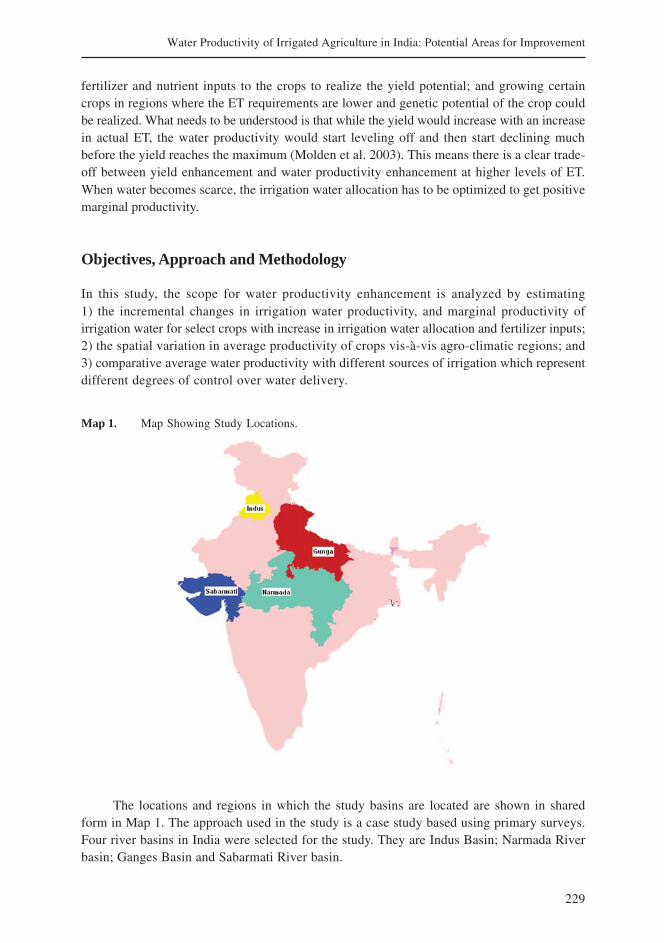
229
Water Productivity of Irrigated Agriculture in India: Potential Areas for Improvement
fertilizer and nutrient inputs to the crops to realize the yield potential; and growing certaincrops in regions where the ET requirements are lower and genetic potential of the crop couldbe realized. What needs to be understood is that while the yield would increase with an increasein actual ET, the water productivity would start leveling off and then start declining muchbefore the yield reaches the maximum (Molden et al. 2003). This means there is a clear trade-off between yield enhancement and water productivity enhancement at higher levels of ET.When water becomes scarce, the irrigation water allocation has to be optimized to get positivemarginal productivity.
Objectives, Approach and Methodology
In this study, the scope for water productivity enhancement is analyzed by estimating1) the incremental changes in irrigation water productivity, and marginal productivity ofirrigation water for select crops with increase in irrigation water allocation and fertilizer inputs;2) the spatial variation in average productivity of crops vis-à-vis agro-climatic regions; and3) comparative average water productivity with different sources of irrigation which representdifferent degrees of control over water delivery.
Map 1. Map Showing Study Locations.
The locations and regions in which the study basins are located are shown in sharedform in Map 1. The approach used in the study is a case study based using primary surveys.Four river basins in India were selected for the study. They are Indus Basin; Narmada Riverbasin; Ganges Basin and Sabarmati River basin.
230
M. D. Kumar, O. P. Singh, M. Samad, C. Purohit and M. S. Didyala
The study analyzed water productivity variations across 1) farms within the same typeof crops and with the same pattern of irrigation; and 2) irrigation types from wells, canals andconjunctive use; and 3) agro-climates within the same basin. It involved collection of data onparameters governing water productivity in crop production such as cropping system, croppedarea, crop inputs (bio and chemical fertilizers, farm labour, irrigation water use, irrigationschedules, and crop technology), crop outputs (main product, by product, market price ofcrops), and method of irrigation. For each irrigated crop, the sample size is 30-35 for each agro-climate within a river basin. In addition to that, there were samples for each type of irrigationsource. Hence, the maximum sample size was 90 in the one location; but limited to only situationswhere sufficient samples for different modes of irrigation were available.
Data and Sources
Data used for water productivity analysis are primary data from farmers. Data collection wasdone using a structured questionnaire from locations in all the four basins, viz., Indus, Ganges,Narmada and Sabarmati. From the Indus, only one location was covered; from Ganges alsoone location was covered; from Narmada, nine locations, each representing one agro-climaticcondition, was covered. From Sabarmati, four locations, each representing one agro-climate,were selected. The data collected from farmers included data on crop inputs comprising costof seeds, labor, fertilizer and pesticides, quantum of irrigation water, and quantity (weight inkg) and market price (Rs/kg) of main and byproducts of the crop output. In addition, thedischarge of irrigation wells (liter/sec) was measured using a bucket and stop watch to quantifythe volume of water pumped, for which data on number and hours of irrigation concerningeach crop and for each season were obtained from the farmers.
Analytical Procedure
The physical water productivity σ irri, i
(kg/m3) and water productivity in economic terms,
θ irri, i
(Rs/m3) in a purely irrigated crop i are estimated as:
σ irri, i
=; θ
irri, i = ..................1, 2,
Δ irri ,i
, and ∇ irri ,i
are the irrigation water dosage (mm) and yield (kg/ha) for purely irrigatedcrop
i , respectively in mm. NR
irri, i is the net return per unit area of the crop (Rs/ha). All winter
crops selected for the study are treated as purely irrigated crops, and the green water use forthese crops was ignored. The reason is that their yields under un-irrigated condition as wellas residual soil moisture before sowing are negligible. All crops covering two seasons, viz.,kharif and winter, having no rain-fed yields were also treated as irrigated crops. Winter wheatin Narmada Basin, cotton in West Nimar in the Narmada Basin, winter wheat in Uttar Pradesh(UP), Punjab, and all crops selected from Sabarmati basin (namely, wheat, castor, bajra andcotton) were treated as irrigated crops and, therefore, the water productivity values estimatedfor them are irrigation water productivity1.
1 In areas with moderate rainfall like eastern UP, this must have resulted in over-estimation of irrigationwater productivity.
∇ irri, i
NRirri, i
1,000Δ irri ,i i
1,000Δ irri ,i i
231
Water Productivity of Irrigated Agriculture in India: Potential Areas for Improvement
Marginal physical productivity of water, σ comb-irri, j
(kg/m3), and marginal water productivityin economic terms θ
comb-irri, j(Rs/m3) for crops, which receive supplementary irrigation, and having
rain-fed yields, with respect to irrigation, are estimated as:
σ comb-irri, j
=; θ
comb-irri, j = ..................3, 4,
Where, ∇ comb-irri, j
is the yield corresponding to irrigation water applied (kg) and Δ comb,j
isthe irrigation water applied for the crop j (mm). NR
comb-irri, j is the net return per unit area
corresponding to the irrigation water applied for the same crop (Rs/ha). σ comb-irri, j
and θ comb-irri, j
were obtained by running a regression of yield and net returns from the crop against irrigationwater applied for each crop, respectively. The regression coefficients give the marginal physicalproductivity of water and water productivity in economic terms, respectively, of irrigation forthese crops. This gives the mean value of marginal water productivity for all the farmers growingthat crop. One major assumption involved in this analysis is that the water application is still inthe scarcity regime, meaning the total consumptive use may fall short of or just meet theevapotranspirative demands. Therefore, the response curve of yield and net return to irrigationwater use were treated as linear. This no way means that the volumetric water applied (effectiverainfall and irrigation) is below ET demand, as farmers can provide excessive irrigation in certainperiods of the crop season, resulting in losses.
The marginal water productivity of irrigation water for individual farmers were estimatedby subtracting the ‘a’ coefficient , i.e., Y intercept, of the regression equation for yield and netreturn, respectively, from their corresponding crop yield and net returns, and dividing by thevolume of irrigation water applied. Paddy from Jabalpur and Mandla in Narmada River basinwas considered for this methodology, as it had rain-fed yield in many locations.
The drivers of change in water productivity were analyzed by running regressions ofcrop yield (dependent variable) against irrigation dosage and fertilizer dosage (as separateindependent variables) for select crops (viz., wheat and cotton); and crop water productivityin economic terms against fertilizer dosage and irrigation water dosage for the same crops.
Field Level Water Productivity: Results from Four Indian River Basins
There are several studies done over the past 2 years analyzing water productivity in irrigatedproduction covering many heterogeneous physical settings in India, in terms of agro-climateand overall water resource availability and quality. The locations included part of Indus Basinin south-western Punjab; part of Ganga Basin in eastern Uttar Pradesh; and different locationsin Sabarmati River basin in Gujarat. The studies included analyses of the productivity ofirrigation water for several crops from both physical and economic point of view. All the analysesare based on well-irrigated crops and the volume of applied water was used in the denominatorof water productivity.
The results of the analyses are presented in summary form in Table 1 to Table 2 tohighlight the variations in water productivity with the same location across farmers; and acrosslocations within the same basins; and across basins for the same crop. The irrigated cropsconsidered for the analyses are winter wheat (Punjab, UP, Gujarat, and Madhya Pradesh); andkharif paddy in Punjab, UP, Gujarat, Madhya Pradesh.
∇ comb-irri, j
NRcomb-irri, j
1,000Δ comb,j
1,000Δ comb,j
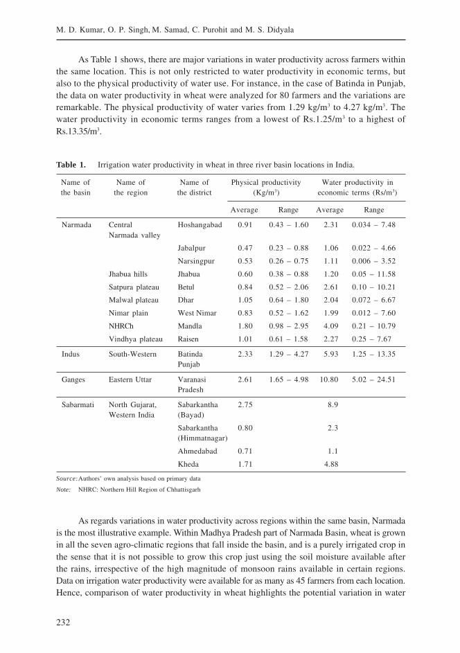
232
M. D. Kumar, O. P. Singh, M. Samad, C. Purohit and M. S. Didyala
As Table 1 shows, there are major variations in water productivity across farmers withinthe same location. This is not only restricted to water productivity in economic terms, butalso to the physical productivity of water use. For instance, in the case of Batinda in Punjab,the data on water productivity in wheat were analyzed for 80 farmers and the variations areremarkable. The physical productivity of water varies from 1.29 kg/m3 to 4.27 kg/m3. Thewater productivity in economic terms ranges from a lowest of Rs.1.25/m3 to a highest ofRs.13.35/m3.
Table 1. Irrigation water productivity in wheat in three river basin locations in India.
Name of Name of Name of Physical productivity Water productivity inthe basin the region the district (Kg/m3) economic terms (Rs/m3)
Average Range Average Range
Narmada Central Hoshangabad 0.91 0.43 – 1.60 2.31 0.034 – 7.48Narmada valley
Jabalpur 0.47 0.23 – 0.88 1.06 0.022 – 4.66
Narsingpur 0.53 0.26 – 0.75 1.11 0.006 – 3.52
Jhabua hills Jhabua 0.60 0.38 – 0.88 1.20 0.05 – 11.58
Satpura plateau Betul 0.84 0.52 – 2.06 2.61 0.10 – 10.21
Malwal plateau Dhar 1.05 0.64 – 1.80 2.04 0.072 – 6.67
Nimar plain West Nimar 0.83 0.52 – 1.62 1.99 0.012 – 7.60
NHRCh Mandla 1.80 0.98 – 2.95 4.09 0.21 – 10.79
Vindhya plateau Raisen 1.01 0.61 – 1.58 2.27 0.25 – 7.67
Indus South-Western Batinda 2.33 1.29 – 4.27 5.93 1.25 – 13.35Punjab
Ganges Eastern Uttar Varanasi 2.61 1.65 – 4.98 10.80 5.02 – 24.51Pradesh
Sabarmati North Gujarat, Sabarkantha 2.75 8.9Western India (Bayad)
Sabarkantha 0.80 2.3(Himmatnagar)
Ahmedabad 0.71 1.1
Kheda 1.71 4.88
Source:Authors’ own analysis based on primary data
Note: NHRC: Northern Hill Region of Chhattisgarh
As regards variations in water productivity across regions within the same basin, Narmadais the most illustrative example. Within Madhya Pradesh part of Narmada Basin, wheat is grownin all the seven agro-climatic regions that fall inside the basin, and is a purely irrigated crop inthe sense that it is not possible to grow this crop just using the soil moisture available afterthe rains, irrespective of the high magnitude of monsoon rains available in certain regions.Data on irrigation water productivity were available for as many as 45 farmers from each location.Hence, comparison of water productivity in wheat highlights the potential variation in water

233
Water Productivity of Irrigated Agriculture in India: Potential Areas for Improvement
productivity possible for irrigated crops. The average physical productivity of irrigation waterin wheat ranges from 0.47 kg/m3 in Jabalpur to 1.8 kg/m3 in Mandla.
Also highly significant are the water productivity variations across the four river basins,viz., Indus, Ganges, Narmada and Sabarmati. This could be the result of variations in wateravailability situation, agro-climate and the level of agricultural development. First of all, Indusis a physically water-scarce river basin; so is Sabarmati, and are all ‘closed’ basins, wherein allthe surface water resources are diverted for various uses within the basin and are fully depleted,and additionally, the groundwater resources in these basins are also fully utilized. NarmadaBasin still has unutilized water resources, particularly surface water. Agro-climatically, southwestern Punjab has arid climate; MP part of Narmada has climatic conditions varying fromsub-humid to semi-arid. Finally, the degree of the adoption of crop technologies varies frombasin to basin. While Punjab is known for progressive farmers, and a high level of adoptionof green revolution technologies and high agricultural productivity, Madhya Pradesh’sagriculture is relatively very backward. The adoption of modern farming technologies, includingirrigation is quite recent in MP. The average water productivity of wheat ranges from a lowestof 0.47 to a highest of 1.8 kg/m3 in Narmada Basin to 2.33 kg/m3 in Batinda, Punjab (Indus) to2.61 kg/m3 in Banaras, UP (Ganges).
The variations in physical productivity of water across farmers within one location; acrossdifferent locations within a basin; and between basins result in a higher degree of variation inthe productivity of water use in economic terms as shown in last columns of Table 2. Whilethe ratio of the highest and the lowest values of physical productivity is 3.0 in eastern UP inGanges, the corresponding ratio for combined physical and economic productivity is 4.8 forthe same location. While the ratio of the highest and the lowest values of physical productivityof irrigation water in wheat is 3.25 in south-western Punjab in the Indus, the correspondingvalue for water productivity in economic terms for the same location is 12.6. The ratio of averagephysical productivity of irrigation water in wheat across basins is 1.45 (3.69/2.54) and whensouth western Punjab and eastern UP are compared, the corresponding ratio for combinedphysical and economic productivity is 2.15 (10.57/4.90).
Table 2. Marginal productivity of irrigation water in paddy in three selected river basins in India.
Name of Name of Name of Physical productivity Water productivity inthe basin the region the district (Kg/m3) Economic terms (Rs/m3)
Average Range Average Range
Narmada Central Narmada Jabalpur 1.62 0.85 – 2.57 3.95 0.05 – 10.28valley
NHR.C Mandla 2.13 1.20 – 4.00 1.43 0.43 – 7.74
Indus Punjab Batinda 3.69 3.17 - 4.36 10.57 4.47 – 24.94
Ganga UP Varanasi 2.54 1.21 – 3.96 4.90 0.94 – 11.89
Sabarmati North Gujarat, Sabarkantha 0.42 0.91
Western India Ahmedabad 1.06 3.34
Kheda 0.92 2.98
Source:Authors’ own analysis based on primary data collected from the three basin areas
Note: NHRC: Northern Hill Region of Chhattisgarh
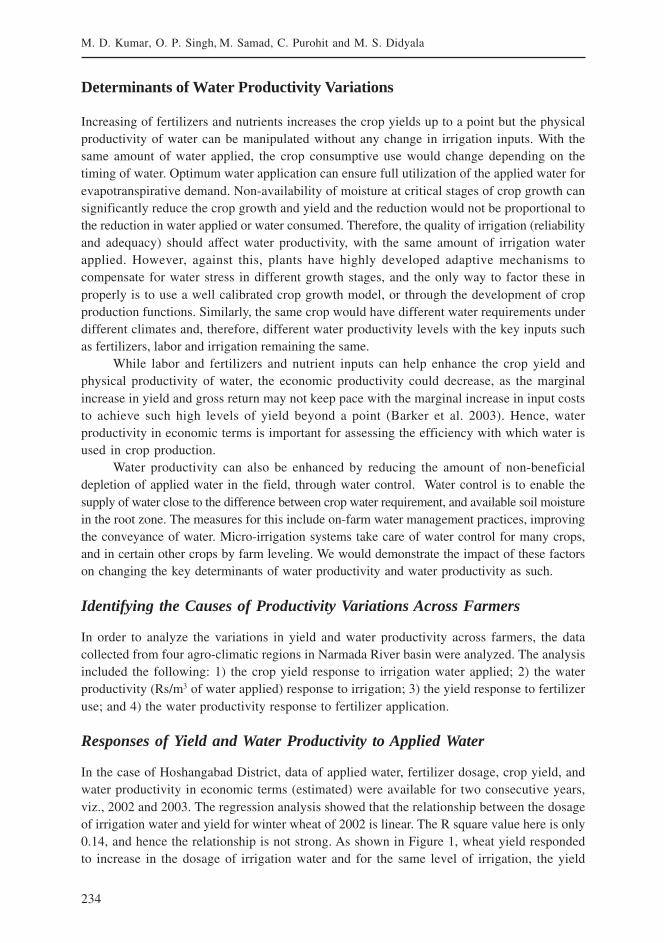
234
M. D. Kumar, O. P. Singh, M. Samad, C. Purohit and M. S. Didyala
Determinants of Water Productivity Variations
Increasing of fertilizers and nutrients increases the crop yields up to a point but the physicalproductivity of water can be manipulated without any change in irrigation inputs. With thesame amount of water applied, the crop consumptive use would change depending on thetiming of water. Optimum water application can ensure full utilization of the applied water forevapotranspirative demand. Non-availability of moisture at critical stages of crop growth cansignificantly reduce the crop growth and yield and the reduction would not be proportional tothe reduction in water applied or water consumed. Therefore, the quality of irrigation (reliabilityand adequacy) should affect water productivity, with the same amount of irrigation waterapplied. However, against this, plants have highly developed adaptive mechanisms tocompensate for water stress in different growth stages, and the only way to factor these inproperly is to use a well calibrated crop growth model, or through the development of cropproduction functions. Similarly, the same crop would have different water requirements underdifferent climates and, therefore, different water productivity levels with the key inputs suchas fertilizers, labor and irrigation remaining the same.
While labor and fertilizers and nutrient inputs can help enhance the crop yield andphysical productivity of water, the economic productivity could decrease, as the marginalincrease in yield and gross return may not keep pace with the marginal increase in input coststo achieve such high levels of yield beyond a point (Barker et al. 2003). Hence, waterproductivity in economic terms is important for assessing the efficiency with which water isused in crop production.
Water productivity can also be enhanced by reducing the amount of non-beneficialdepletion of applied water in the field, through water control. Water control is to enable thesupply of water close to the difference between crop water requirement, and available soil moisturein the root zone. The measures for this include on-farm water management practices, improvingthe conveyance of water. Micro-irrigation systems take care of water control for many crops,and in certain other crops by farm leveling. We would demonstrate the impact of these factorson changing the key determinants of water productivity and water productivity as such.
Identifying the Causes of Productivity Variations Across Farmers
In order to analyze the variations in yield and water productivity across farmers, the datacollected from four agro-climatic regions in Narmada River basin were analyzed. The analysisincluded the following: 1) the crop yield response to irrigation water applied; 2) the waterproductivity (Rs/m3 of water applied) response to irrigation; 3) the yield response to fertilizeruse; and 4) the water productivity response to fertilizer application.
Responses of Yield and Water Productivity to Applied Water
In the case of Hoshangabad District, data of applied water, fertilizer dosage, crop yield, andwater productivity in economic terms (estimated) were available for two consecutive years,viz., 2002 and 2003. The regression analysis showed that the relationship between the dosageof irrigation water and yield for winter wheat of 2002 is linear. The R square value here is only0.14, and hence the relationship is not strong. As shown in Figure 1, wheat yield respondedto increase in the dosage of irrigation water and for the same level of irrigation, the yield
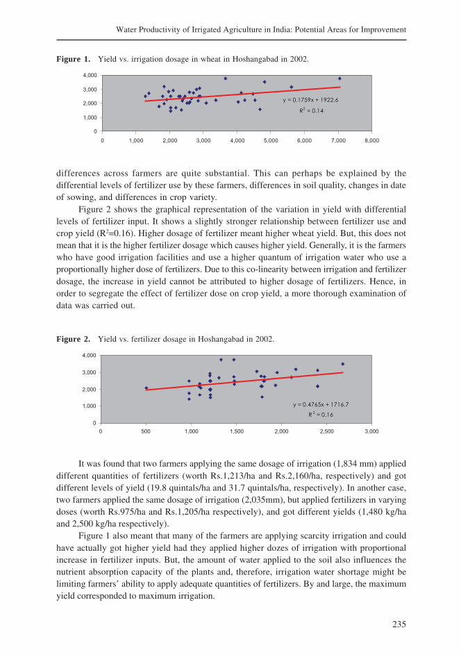
235
Water Productivity of Irrigated Agriculture in India: Potential Areas for Improvement
differences across farmers are quite substantial. This can perhaps be explained by thedifferential levels of fertilizer use by these farmers, differences in soil quality, changes in dateof sowing, and differences in crop variety.
Figure 2 shows the graphical representation of the variation in yield with differentiallevels of fertilizer input. It shows a slightly stronger relationship between fertilizer use andcrop yield (R2=0.16). Higher dosage of fertilizer meant higher wheat yield. But, this does notmean that it is the higher fertilizer dosage which causes higher yield. Generally, it is the farmerswho have good irrigation facilities and use a higher quantum of irrigation water who use aproportionally higher dose of fertilizers. Due to this co-linearity between irrigation and fertilizerdosage, the increase in yield cannot be attributed to higher dosage of fertilizers. Hence, inorder to segregate the effect of fertilizer dose on crop yield, a more thorough examination ofdata was carried out.
Figure 1. Yield vs. irrigation dosage in wheat in Hoshangabad in 2002.
Figure 2. Yield vs. fertilizer dosage in Hoshangabad in 2002.
It was found that two farmers applying the same dosage of irrigation (1,834 mm) applieddifferent quantities of fertilizers (worth Rs.1,213/ha and Rs.2,160/ha, respectively) and gotdifferent levels of yield (19.8 quintals/ha and 31.7 quintals/ha, respectively). In another case,two farmers applied the same dosage of irrigation (2,035mm), but applied fertilizers in varyingdoses (worth Rs.975/ha and Rs.1,205/ha respectively), and got different yields (1,480 kg/haand 2,500 kg/ha respectively).
Figure 1 also meant that many of the farmers are applying scarcity irrigation and couldhave actually got higher yield had they applied higher dozes of irrigation with proportionalincrease in fertilizer inputs. But, the amount of water applied to the soil also influences thenutrient absorption capacity of the plants and, therefore, irrigation water shortage might belimiting farmers’ ability to apply adequate quantities of fertilizers. By and large, the maximumyield corresponded to maximum irrigation.
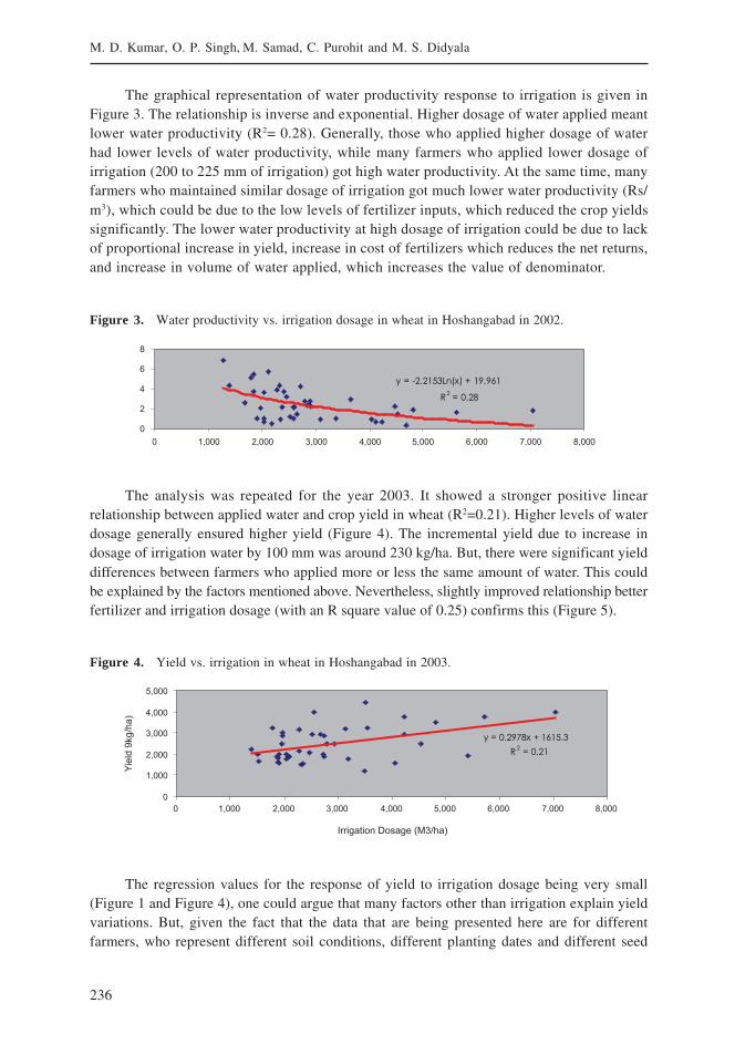
236
M. D. Kumar, O. P. Singh, M. Samad, C. Purohit and M. S. Didyala
The graphical representation of water productivity response to irrigation is given inFigure 3. The relationship is inverse and exponential. Higher dosage of water applied meantlower water productivity (R2= 0.28). Generally, those who applied higher dosage of waterhad lower levels of water productivity, while many farmers who applied lower dosage ofirrigation (200 to 225 mm of irrigation) got high water productivity. At the same time, manyfarmers who maintained similar dosage of irrigation got much lower water productivity (Rs/m3), which could be due to the low levels of fertilizer inputs, which reduced the crop yieldssignificantly. The lower water productivity at high dosage of irrigation could be due to lackof proportional increase in yield, increase in cost of fertilizers which reduces the net returns,and increase in volume of water applied, which increases the value of denominator.
Figure 3. Water productivity vs. irrigation dosage in wheat in Hoshangabad in 2002.
The analysis was repeated for the year 2003. It showed a stronger positive linearrelationship between applied water and crop yield in wheat (R2=0.21). Higher levels of waterdosage generally ensured higher yield (Figure 4). The incremental yield due to increase indosage of irrigation water by 100 mm was around 230 kg/ha. But, there were significant yielddifferences between farmers who applied more or less the same amount of water. This couldbe explained by the factors mentioned above. Nevertheless, slightly improved relationship betterfertilizer and irrigation dosage (with an R square value of 0.25) confirms this (Figure 5).
Figure 4. Yield vs. irrigation in wheat in Hoshangabad in 2003.
The regression values for the response of yield to irrigation dosage being very small(Figure 1 and Figure 4), one could argue that many factors other than irrigation explain yieldvariations. But, given the fact that the data that are being presented here are for differentfarmers, who represent different soil conditions, different planting dates and different seed
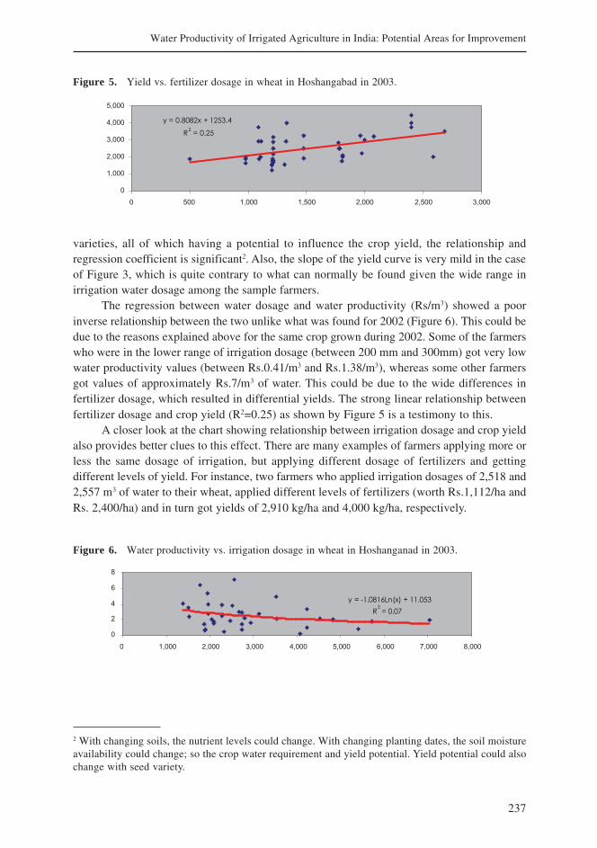
237
Water Productivity of Irrigated Agriculture in India: Potential Areas for Improvement
varieties, all of which having a potential to influence the crop yield, the relationship andregression coefficient is significant2. Also, the slope of the yield curve is very mild in the caseof Figure 3, which is quite contrary to what can normally be found given the wide range inirrigation water dosage among the sample farmers.
The regression between water dosage and water productivity (Rs/m3) showed a poorinverse relationship between the two unlike what was found for 2002 (Figure 6). This could bedue to the reasons explained above for the same crop grown during 2002. Some of the farmerswho were in the lower range of irrigation dosage (between 200 mm and 300mm) got very lowwater productivity values (between Rs.0.41/m3 and Rs.1.38/m3), whereas some other farmersgot values of approximately Rs.7/m3 of water. This could be due to the wide differences infertilizer dosage, which resulted in differential yields. The strong linear relationship betweenfertilizer dosage and crop yield (R2=0.25) as shown by Figure 5 is a testimony to this.
A closer look at the chart showing relationship between irrigation dosage and crop yieldalso provides better clues to this effect. There are many examples of farmers applying more orless the same dosage of irrigation, but applying different dosage of fertilizers and gettingdifferent levels of yield. For instance, two farmers who applied irrigation dosages of 2,518 and2,557 m3 of water to their wheat, applied different levels of fertilizers (worth Rs.1,112/ha andRs. 2,400/ha) and in turn got yields of 2,910 kg/ha and 4,000 kg/ha, respectively.
Figure 5. Yield vs. fertilizer dosage in wheat in Hoshangabad in 2003.
Figure 6. Water productivity vs. irrigation dosage in wheat in Hoshanganad in 2003.
2 With changing soils, the nutrient levels could change. With changing planting dates, the soil moistureavailability could change; so the crop water requirement and yield potential. Yield potential could alsochange with seed variety.
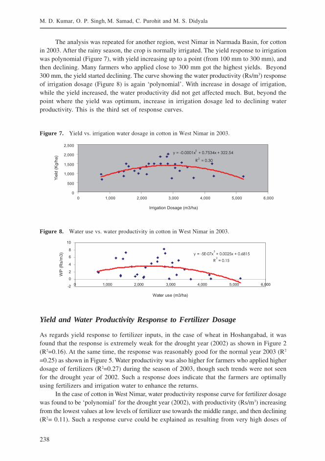
238
M. D. Kumar, O. P. Singh, M. Samad, C. Purohit and M. S. Didyala
The analysis was repeated for another region, west Nimar in Narmada Basin, for cottonin 2003. After the rainy season, the crop is normally irrigated. The yield response to irrigationwas polynomial (Figure 7), with yield increasing up to a point (from 100 mm to 300 mm), andthen declining. Many farmers who applied close to 300 mm got the highest yields. Beyond300 mm, the yield started declining. The curve showing the water productivity (Rs/m3) responseof irrigation dosage (Figure 8) is again ‘polynomial’. With increase in dosage of irrigation,while the yield increased, the water productivity did not get affected much. But, beyond thepoint where the yield was optimum, increase in irrigation dosage led to declining waterproductivity. This is the third set of response curves.
Figure 7. Yield vs. irrigation water dosage in cotton in West Nimar in 2003.
Figure 8. Water use vs. water productivity in cotton in West Nimar in 2003.
Yield and Water Productivity Response to Fertilizer Dosage
As regards yield response to fertilizer inputs, in the case of wheat in Hoshangabad, it wasfound that the response is extremely weak for the drought year (2002) as shown in Figure 2(R2=0.16). At the same time, the response was reasonably good for the normal year 2003 (R2
=0.25) as shown in Figure 5. Water productivity was also higher for farmers who applied higherdosage of fertilizers (R2=0.27) during the season of 2003, though such trends were not seenfor the drought year of 2002. Such a response does indicate that the farmers are optimallyusing fertilizers and irrigation water to enhance the returns.
In the case of cotton in West Nimar, water productivity response curve for fertilizer dosagewas found to be ‘polynomial’ for the drought year (2002), with productivity (Rs/m3) increasingfrom the lowest values at low levels of fertilizer use towards the middle range, and then declining(R2= 0.11). Such a response curve could be explained as resulting from very high doses of
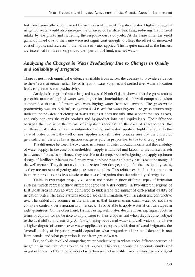
239
Water Productivity of Irrigated Agriculture in India: Potential Areas for Improvement
fertilizers generally accompanied by an increased dose of irrigation water. Higher dosage ofirrigation water could also increase the chances of fertilizer leaching, reducing the nutrientintake by the plants and flattening the response curve of yield. At the same time, the yieldgains obtained due to the same were not significant enough to offset the effect of increasedcost of inputs, and increase in the volume of water applied. This is quite natural as the farmersare interested in maximizing the returns per unit of land, and not water.
Analyzing the Changes in Water Productivity Due to Changes in Qualityand Reliability of Irrigation
There is not much empirical evidence available from across the country to provide evidenceto the effect that greater reliability of irrigation water supplies and control over water allocationleads to greater water productivity.
Analysis from groundwater irrigated areas of North Gujarat showed that the gross returnsper cubic meter of applied water were higher for shareholders of tubewell companies, whencompared with that of farmers who were buying water from well owners. The gross waterproductivity was Rs. 5.61/m3, as against Rs.4.61/m3 for water buyers. The gross returns onlyindicate the physical efficiency of water use, as it does not take into account the input costs,and only converts the main product and by-product into cash equivalents. The differencebetween the two is in the ‘terms of irrigation services’. In the case of shareholders, theentitlement of water is fixed in volumetric terms, and water supply is highly reliable. In thecase of water buyers, the well owner supplies enough water to make sure that the cultivatorgets sufficient yield as his irrigation charge is paid in proportion to the total crop yield.
The difference between the two cases is in terms of water allocation norms and the reliabilityof water supply. In the case of shareholders, supply is rationed and known to the farmers muchin advance of the season. Hence, they are able to do proper water budgeting and apply optimumdosage of fertilizers whereas the farmers who purchase water on hourly basis are at the mercy ofthe well owners. They do not try to optimize fertilizer dosage, and go for the best quality seeds,as they are not sure of getting adequate water supplies. This reinforces the fact that net returnfrom crop production is less elastic to the cost of irrigation than the reliability of irrigation.
Yields in two major crops, viz., wheat and paddy in three different types of irrigationsystems, which represent three different degrees of water control, in two different regions ofBist Doab area in Punjab were compared to understand the impact of differential quality ofirrigation water. The three systems selected are canal irrigation, well irrigation and conjunctiveuse. The underlying premise in the analysis is that farmers using canal water do not havecomplete control over irrigation and, hence, will not be able to apply water at critical stages inright quantities. On the other hand, farmers using well water, despite incurring higher costs interms of capital, would be able to apply water to their crops as and when they require, subjectto the availability of electricity. As farmers using both canal water and well water should havea higher degree of control over water application compared with that of canal irrigators, the‘overall quality of irrigation’ would depend on what proportion of the total demand is metfrom canals, and what proportion is met from groundwater.
But, analysis involved comparing water productivity in wheat under different sources ofirrigation in two distinct agro-ecological regions. This was because an adequate number ofirrigators for each of the three sources of irrigation was not available from the same agro-ecological
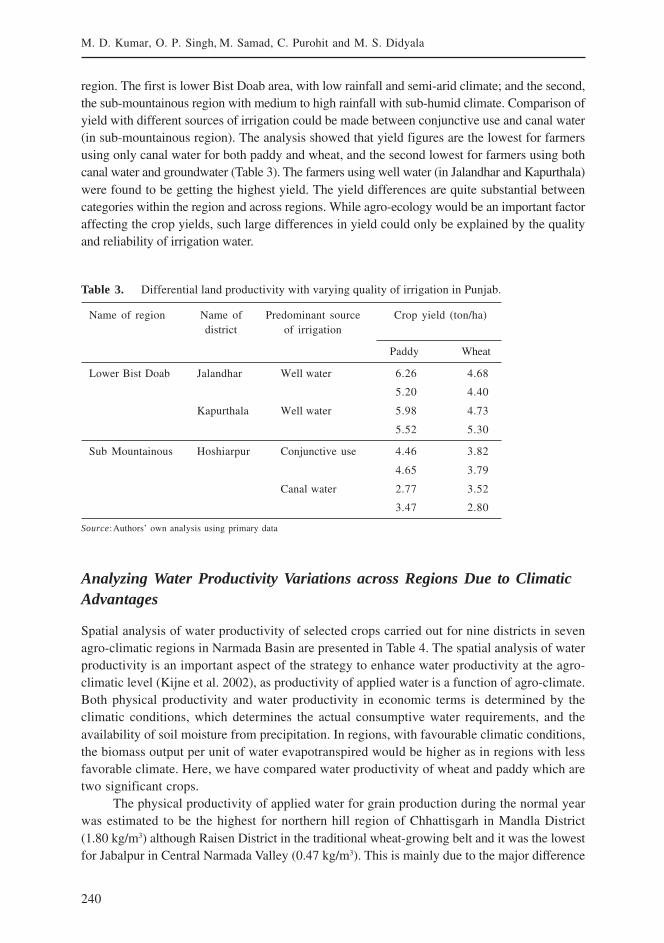
240
M. D. Kumar, O. P. Singh, M. Samad, C. Purohit and M. S. Didyala
region. The first is lower Bist Doab area, with low rainfall and semi-arid climate; and the second,the sub-mountainous region with medium to high rainfall with sub-humid climate. Comparison ofyield with different sources of irrigation could be made between conjunctive use and canal water(in sub-mountainous region). The analysis showed that yield figures are the lowest for farmersusing only canal water for both paddy and wheat, and the second lowest for farmers using bothcanal water and groundwater (Table 3). The farmers using well water (in Jalandhar and Kapurthala)were found to be getting the highest yield. The yield differences are quite substantial betweencategories within the region and across regions. While agro-ecology would be an important factoraffecting the crop yields, such large differences in yield could only be explained by the qualityand reliability of irrigation water.
Table 3. Differential land productivity with varying quality of irrigation in Punjab.
Name of region Name of Predominant source Crop yield (ton/ha)district of irrigation
Paddy Wheat
Lower Bist Doab Jalandhar Well water 6.26 4.68
5.20 4.40
Kapurthala Well water 5.98 4.73
5.52 5.30
Sub Mountainous Hoshiarpur Conjunctive use 4.46 3.82
4.65 3.79
Canal water 2.77 3.52
3.47 2.80
Source:Authors’ own analysis using primary data
Analyzing Water Productivity Variations across Regions Due to ClimaticAdvantages
Spatial analysis of water productivity of selected crops carried out for nine districts in sevenagro-climatic regions in Narmada Basin are presented in Table 4. The spatial analysis of waterproductivity is an important aspect of the strategy to enhance water productivity at the agro-climatic level (Kijne et al. 2002), as productivity of applied water is a function of agro-climate.Both physical productivity and water productivity in economic terms is determined by theclimatic conditions, which determines the actual consumptive water requirements, and theavailability of soil moisture from precipitation. In regions, with favourable climatic conditions,the biomass output per unit of water evapotranspired would be higher as in regions with lessfavorable climate. Here, we have compared water productivity of wheat and paddy which aretwo significant crops.
The physical productivity of applied water for grain production during the normal yearwas estimated to be the highest for northern hill region of Chhattisgarh in Mandla District(1.80 kg/m3) although Raisen District in the traditional wheat-growing belt and it was the lowestfor Jabalpur in Central Narmada Valley (0.47 kg/m3). This is mainly due to the major difference
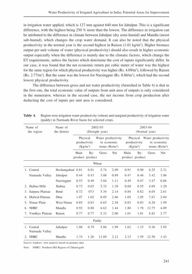
241
Water Productivity of Irrigated Agriculture in India: Potential Areas for Improvement
in irrigation water applied, which is 127 mm against 640 mm for Jabalpur. This is a significantdifference, with the highest being 250 % more than the lowest. The difference in irrigation canbe attributed to the difference in climate between Jabalpur (dry semi-humid) and Mandla (moistsub-humid), which changes the crop water demand. It can also be noted that the physicalproductivity in the normal year is the second highest in Raisen (1.01 kg/m3). Higher biomassoutput per unit volume of water (physical productivity) should also result in higher economicoutput especially when the difference is mainly due to the climatic factors, which change theET requirements, unless the factors which determine the cost of inputs significantly differ. Inour case, it was found that the net economic return per cubic meter of water was the highestfor the same region for which physical productivity was higher (Rs. 4.09/m3), followed by Raisen(Rs. 2.77/m3). But the same was the lowest for Narsingpur (Rs. 0.86/m3), which had the secondlowest physical productivity.
The difference between gross and net water productivity (furnished in Table 4) is that inthe first one, the total economic value of outputs from unit area of outputs is only consideredin the numerator, whereas in the second case, the net income from crop production afterdeducting the cost of inputs per unit area is considered.
Table 4. Region-wise irrigation water productivity (wheat) and marginal productivity of irrigation water(paddy) in Narmada River basin for selected crops.
Name of Name of 2002-03 2003-04the region the district (Drought year) (Normal year)
Physical Water productivity Physical Water productivityproductivity in economic productivity in economic
(Kg/m3) terms (Rs/m3) (Kg/m3) terms (Rs/m3)
Main By- Gross Net Main By- Gross Netproduct product product product
Wheat
1. Central Hoshangabad 0.81 0.81 5.74 2.09 0.91 0.90 6.25 2.31
Narmada Valley Jabalpur 0.44 0.43 3.08 0.89 0.47 0.46 3.42 1.06
Narsingpur 0.53 0.49 3.84 1.11 0.49 0.47 3.47 0.86
2. Jhabua Hills Jhabua 0.73 0.65 5.32 1.38 0.60 0.55 4.69 1.20
3. Satpura Plateau Betul 0.72 073 5.34 2.14 0.84 0.82 6.05 2.61
4. Malwal Plateau Dhar 1.07 1.02 8.05 2.46 1.05 1.05 7.67 2.04
5. Nimar Plain West Nimar 0.85 0.83 6.65 2.38 0.83 0.83 6.20 1.99
6. NHRC Mandla 0.92 0.88 6.62 1.44 1.80 1.78 12.75 4.09
7. Vindhya Plateau Raisen 0.77 0.77 5.33 2.00 1.01 1.01 6.82 2.77
Paddy
1. Central Jabalpur 1.08 0.79 5.86 1.99 1.62 1.15 9.36 3.95Narmada Valley
2. NHRC Mandla 1.74 1.26 11.69 2.12 2.13 1.59 12.50 1.43
Source:Authors’ own analysis based on primary data
Note: NHRC: Northern Hill Region of Chhattisgarh
242
M. D. Kumar, O. P. Singh, M. Samad, C. Purohit and M. S. Didyala
As regards paddy, there are only two regions which irrigate paddy. The physicalproductivity for grain during the normal year was estimated to be higher for northern hill regionof Chhattisgarh in Mandla District (2.13 kg/m3) whereas it was only 1.62 kg/m3 in JabalpurDistrict of Central Narmada Valley. Likewise, water productivity in economic terms was foundto be higher for northern hill region of Chhattisgarh (Rs.3.95/m3) as against Rs.1.43/m3 forJabalpur in Central Narmada Valley. Similar figures were found for the drought year (2002) inwhich the physical productivity of applied water was 1.74 kg/m3 in Mandla against 1.08 kg/m3
in Jabalpur.Spatial analysis of water productivity in three agro-climatic regions of Sabarmati Basin
showed that there is significant variation in physical water productivity and water productivityin economic terms (gross and net) of irrigation water across different agro-climatic regionsfor all the four crops selected from Sabarmati River basin. For instance, water productivityin physical terms for wheat ranged from 0.71 kg/m3 in Daskroi to 2.75 kg/m3 in Bayad.The water productivity in economic terms (gross) ranged from Rs. 4.66/m3 in Daskroi toRs. 18.39/m3 in Bayad. The net water productivity for wheat for the same locations rangedfrom Rs. 1.38/m3 to Rs.4.66/m3. Similar variations in physical productivity of water were foundfor castor oil between Himmatnagar and Kapadwanj. The physical productivity of waterranged from 0.66 kg/m3 to 1.62 kg/m3. The gross economic water productivity ranged fromRs. 9.69/m3 in Himmatnagar to Rs. 25.57/m3 for Bayad. The net economic water productivityranged from Rs. 3.56/m3 in Himmatnagar to Rs. 16.4/m3 for Bayad. Interestingly, unlike in thecase of wheat which gave the highest physical productivity of water and also gave thehighest water productivity in economic terms, in case of castor oil, the locations which gavethe highest economic water productivity did not coincide with those of the highest physicalproductivity of water.
Ways to Enhance Irrigation Water Productivity in Economic Terms
Improving Water Control and Its Potential Impact
The analyses presented in the earlier sections clearly show that water productivity is a functionof applied water; and dosage of fertilizers, and that it can be manipulated through water control.It is based on the premise that in many situations farmers do not have control over waterdelivery and fertilizer dosage, or else are tempted to apply more water to maximize the yieldsand returns per unit of land. The lack of control over water delivery could be either due to lackof physical control over water delivery or due to lack of sufficient water to irrigate. The tendencyto apply water or fertilizer in the low productivity regime could be due to two reasons:
1) Farmers are not able to make correct judgments about water allocation for maximizingthe aggregate returns (which is the multiple of net returns per ha of the crop, andtotal area of the irrigated crop), due to lack of correct information about the levels ofirrigation that result in the maximum net return per unit of land, and which enablesmaximizing the area irrigated.
2) Farmers are not confronted with either marginal cost or opportunity cost of usingexcess water.

243
Water Productivity of Irrigated Agriculture in India: Potential Areas for Improvement
In the process, they are not able to get optimum level of yield that gives the highestwater productivity.3 To what extent ‘water control’ interventions would help enhance waterproductivity depends on the shape of the yield and water productivity response curves of thecrop in question to irrigation inputs. It would also depend on what fraction of the appliedwater is actually used for non-beneficial depletion from the crop land. We do not have anyinformation about non-beneficial depletion from the applied water. But the major sources ofnon-beneficial depletion are a) the deep percolation, which is either lost in the vadose zone,4
or which joins the saline aquifer; b) the evaporation of soil moisture after crop harvest duringthe fallow period; c) direct evaporation from the soil surface, especially during cropestablishment and d) possibly unnecessary watering at the end of the season when it doesnot contribute to the yield.
We have seen three different types of responses of yield and water productivity toirrigation dosage. We discuss the strategy for enhancing WP in each of these cases. In thefirst situation: a) the relationship between applied water and yield is positive, but weak; andb) the response of water productivity to applied water is inverse and exponential. In suchsituations, the reduction in dosage of irrigation water would not affect the yield significantly;and the effect often may not even be adverse. But the same would enhance water productivitysignificantly. But, this strategy would work only if there is sufficient amount of arable land,which remains uncultivated due to shortage of water. The reason is the water saved from thefield can be diverted to expand the area under irrigation.
The second situation is one in which the relationship between applied water and yieldis strong and positive, wherein most farmers are applying water under scarcity regime andvery few under water abundance regime (Figures 4, 5 and 6). Then, it is likely that with anincrease in dosage of irrigation, the physical productivity of water also might increase slightly.But, the water productivity (Rs/m3) response to applied water is ‘inverse-logarithmic’. Here,the best strategy for most of the farmers would be to minimize the irrigation dosage, whichwould help obtain the highest water productivity in economic terms. Here, it may be necessaryfor the farmers to expand the area under irrigation slightly to maintain the net returns.
In the third situation, the relationship between applied water and yield is ‘polynomial’,where yield increases with irrigation dosage up to a certain point, and then declines. This isthe situation found in the case of irrigated cotton in West Nimar District (based on Figure 7).In such a case, with increasing dosage of water, the productivity would decline abruptly beyondthe point which corresponds to the maximum yield. Hence, the relationship between appliedwater and water productivity is ‘polynomial’. This is the most ideal situation where those farmerswho are losing on the yield and income returns have an incentive to reduce irrigation dosage,by which they could enhance both yield and water productivity. The reason why it occurs isthe zero marginal cost of electricity used for groundwater pumping owing to the flat rate systemof pricing electricity in all the groundwater irrigated states. This mode of pricing creates no
3 It is also to be noted that water productivity is not an objective for farmers to realize when water isin plenty. On the contrary, they would try to maximize the income returns per unit of land, for whichcrop yield (kg/ha) enhancement is the best route.4 The water which is ‘lost in the vadose zone’ normally becomes non beneficial E or ET as bare soilevaporation or transpiration through other (non-productive) vegetation.
244
M. D. Kumar, O. P. Singh, M. Samad, C. Purohit and M. S. Didyala
incentives for farmers to use groundwater efficiently. In such situations, it is not even necessarythat farmers expand the area under irrigation to maximize their aggregate returns from farming.But, there are many farmers who are not getting optimum yield and water productivity due toinadequate dosage of irrigation water. It is important for them to reduce the area under irrigationwhile increasing irrigation dosage to optimize yield and water productivity.
There are many water allocation and control measures to improve water productivity. Watercontrol is possible through either of the two methods: 1) micro-irrigation technologies, mainlyfor non-field crops; and, 2) establishing water delivery control devices such as storage systems,particularly in the case of surface irrigation systems where water delivery through tertiary canalsis not regular. Micro-irrigation systems can help achieve two things: a) improving control overapplied water; and b) reducing the non-beneficial depletion of the applied water and maximizingthe consumptive use fraction of the applied water. The potential impact of the second interventionwould be in limiting the amount each time. This, in a way, also may help reduce non-beneficialdepletion but its impact may be less significant as compared with micro-irrigation.
But, we have not come across situations where farmers are not able to secure optimumlevels of water productivity due to water shortages. Farmers have reasonably high degree ofcontrol over water delivery as they are all well-owners, power supply being the only factorthat reduces the control over water delivery. In states such as Punjab, Gujarat and MadhyaPradesh, the quality of power supply in agriculture is poor. The supply is provided in rotations,and sometimes during night hours. They tend to apply heavy doses of water when powersupply is available. This may be leading to a situation where the water productivity startsdeclining as found in most cases, or yield (Rs/m3) itself starts declining.
It is quite understandable that farmers do not care about water productivity much. Thisis in spite of the fact that water availability is extremely limited in some of the areas we havecovered in our study like west Nimar and Dhar. Hence, the option of ‘controlling applied waterdosage’ for enhancing water productivity would work only in areas where a good part of thecultivable land is kept fallow due to water shortage.
Now, let us look at the option of micro-irrigation. For a given amount of nutrient inputs,the only determinant of the crop yield is the consumptive use of water by the crop (ET) andhow far the transpirative requirements of the crop area met during critical stages of crop growth.Using micro-irrigation for row crops, the non-beneficial depletion of applied water could bereduced to nil. Such non-beneficial depletion under traditional method of irrigation would besignificant in the case of row crops. Therefore, the twin-objective of achieving higher waterproductivity and higher yield is possible through micro-irrigation devices. The response curveof yield (Kg/ha) and water productivity in economic terms (Rs/m3) to irrigation dosage undertraditional irrigation and micro-irrigation is given in Figure 9.
It shows that the yield corresponding to the same amount of ‘applied water dosage’would be higher under micro-irrigation. Or in other words, for the same amount of appliedwater, the yield would be higher. Research in many parts of India had already shown that forcash crops, particularly those grown in rows such as cotton, the net incremental returns fordrip irrigation plots over flood irrigated plots are higher than the sum of capital and operationalcosts of drip systems.5 This means that even in situations, where the entire land is irrigated,
5 Such crops include banana, sugarcane, orange, grapes and cotton.
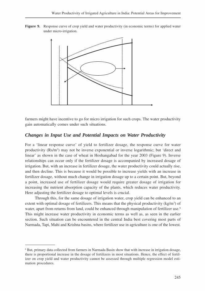
245
Water Productivity of Irrigated Agriculture in India: Potential Areas for Improvement
farmers might have incentive to go for micro irrigation for such crops. The water productivitygain automatically comes under such situations.
Changes in Input Use and Potential Impacts on Water Productivity
For a ‘linear response curve’ of yield to fertilizer dosage, the response curve for waterproductivity (Rs/m3) may not be inverse exponential or inverse logarithmic; but ‘direct andlinear’ as shown in the case of wheat in Hoshangabad for the year 2003 (Figure 9). Inverserelationships can occur only if the fertilizer dosage is accompanied by increased dosage ofirrigation. But, with an increase in fertilizer dosage, the water productivity could actually rise,and then decline. This is because it would be possible to increase yields with an increase infertilizer dosage, without much change in irrigation dosage up to a certain point. But, beyonda point, increased use of fertilizer dosage would require greater dosage of irrigation forincreasing the nutrient absorption capacity of the plants, which reduces water productivity.Here adjusting the fertilizer dosage to optimal levels is crucial.
Through this, for the same dosage of irrigation water, crop yield can be enhanced to anextent with optimal dosage of fertilizers. This means that the physical productivity (kg/m3) ofwater, apart from returns from land, could be enhanced through manipulation of fertilizer use.6
This might increase water productivity in economic terms as well as, as seen in the earliersection. Such situation can be encountered in the central India best covering most parts ofNarmada, Tapi, Mahi and Krishna basins, where fertilizer use in agriculture is one of the lowest.
Figure 9. Response curve of crop yield and water productivity (in economic terms) for applied waterunder micro-irrigation.
6 But, primary data collected from farmers in Narmada Basin show that with increase in irrigation dosage,there is proportional increase in the dosage of fertilizers in most situations. Hence, the effect of fertil-izer on crop yield and water productivity cannot be assessed through multiple regression model esti-mation procedures.
246
M. D. Kumar, O. P. Singh, M. Samad, C. Purohit and M. S. Didyala
If fertilizer dosage is in a regime where the yield does not respond positively, then simplereduction in dosage would result in saving of input costs, thereby increasing water productivityin rupee terms. Such situations are possible in Punjab and Haryana where application ofnitrogenous fertilizer is excessively high.
Potential Impacts of Improving Quality of Irrigation and Water Allocation
The analysis of Punjab and North Gujarat clearly show that improvement in quality of irrigationwould significantly impact on yield (as shown in the case of Punjab) and water productivity(as shown in case of North Gujarat). Here, quality of irrigation includes adequacy and reliability(based on Kumar 2005). With greater reliability and adequacy of irrigation water deliveries,farmers would be able to adopt good agronomic practices and adjust nutrient use. Withincreasing uncertainty of water, farmers hesitate to apply adequate quantities of fertilizers,thereby compromising on the yield.
In case of farmers who are mainly using canal water for irrigation, it is quite commonthat the depth of each application is much higher than the optimum dosage decided by thefield capacity as compared with those using well water. This leads to heavy percolation lossesand reduces the efficiency of storage of water in the soil profile. It leads to excessive residualmoisture after harvesting as well, which gets depleted in soil evaporation. Greater dosagesmay also increase the changes of fertilizer leaching, which leads to reduced nutrient useefficiency. Improving the quality of irrigation in such situation would help farmers optimizethe irrigation dosages in each watering and give adequate number of waterings withoutchanging the volume. This would not only increase the yield, but also reduce the wastagein irrigation, thereby enhancing water productivity of not only applied water, but alsodepleted water.
Allocating Water across Regions and Productivity Gains at the BasinLevel
Spatial analyses of crop water productivity in Narmada Basin showed that water productivityof irrigated crops varies significantly across regions with changing agro-climate. The northernhills region of Chhattisgarh has moist sub-humid to dry-sub-humid climate. The four regions,viz., Kymore Plateau and Satpura Hills, Vindhya Plateau, Satpura Plateau and Central NarmadaValley (CNV) have ‘dry sub-humid’ climate. The regions, viz., Malwal Plateau, and Nimar Plainhave semi-arid climatic conditions. The district of Jhabua, which falls in the region, named‘Jhabua Hills’, is ‘semi-arid’7.
While water productivity variations between two regions for the same crop can also beattributed to differential dosage of fertilizers, differential transpiration ratio and seed varieties,it is assumed here that variations in the same across regions are not significant.
7 Kumar and Singh 2006 for detailed description of average annual rainfall and reference evapotranspi-ration in all the nine agro-climatic regions falling in Narmada Basin.
247
Water Productivity of Irrigated Agriculture in India: Potential Areas for Improvement
The physical productivity figures are far below the normal figures for wheat in manyregions. It was found to be the highest in the northern hill region of Mandla (Rs.1.8 kg/m3),and the lowest in Jabalpur (0.47 kg/m3) during a normal year. This difference could beattributed to the difference in agro-climate across regions, which reduces the denominatorof water productivity, if we consider the fact that there are no major variations in yield levelsbetween these regions. The variations are larger if one compares water productivity in Punjab.There, farmers obtain a return of 2.33 kg/m3, irrespective of the aridity which increasesirrigation water demand. This may be due to the high yield the farmers secure, with efficientuse of water and fertilizers, and with the help of favorable agro-climate for growing winterwheat. The question, therefore, is whether the natural advantage which certain crops enjoyin certain regions in terms of higher water productivity by virtue of the agro-climate can bemade use of, without compromising on farmers’ need and priorities. This means, earmarkingcertain crops only in those regions where they have relative advantage in terms of gettinghigh water productivity—both physical productivity and productivity in economic terms.
Potential for Improving Irrigated Water Productivity in India
Possible Crops and Areas for Increasing Irrigated Water Productivity
Regions which receive intensive canal irrigation are regions that should get priority in waterproductivity improvements because of 1) the water-intensive crops grown in these regions; 2)‘poor water delivery control’; and, 3) poor quality of irrigation. But, the regions should besuch that irrigation water management practices comprising water delivery control andimprovement in quality of irrigation result in reduction in non-beneficial evaporation. Therefore,semi-arid and arid regions with low water table conditions are ideal for this.
It is a general notion that water productivity is generally high in regions such as Punjaband Haryana, which receive extensive and intensive canal irrigation. This is based on highyield levels obtained for wheat and paddy in these regions. These regions are also known forintensive cropping of wheat and paddy. Our analysis for Punjab suggests that there is amplescope for improving yield in wheat and paddy through improving the quality of irrigation interms of adequacy and reliability. In Punjab, such improvement of canal water supplies wouldlead to greater yield for wheat and paddy, apart from reducing non-beneficial depletion andimproving water productivity. Hence, Irrigation Department should have incentive to go forimproving both adequacy and reliability (quality) of irrigation water, and water delivery control.Since the area that can be irrigated cannot be expanded, it would lead to reduction ingroundwater draft as well.
Groundwater irrigated areas, where a substantial area is still left uncultivated due to waterscarcity, should receive attention for water productivity enhancements. The reason is it makeseconomic sense for the farmers as they can expand the area under irrigation and increaseaggregate returns. The priority areas would be hard rock areas of peninsular, central and westernIndia. A wide variety of crops are being grown in these regions such as cotton, castor,groundnut, mustard, banana, sugarcane, potato, and cereals such as paddy, bajra and sorghum.Among these, the water-intensive ones that are grown in large areas are paddy, cotton,sugarcane, banana, cotton, castor, groundnut, and potato. In crops such as paddy, water
248
M. D. Kumar, O. P. Singh, M. Samad, C. Purohit and M. S. Didyala
productivity enhancement has to come through ‘water control’8 and ‘improving the quality ofirrigation’. Wheat would be another crop which should receive attention in western Gujarat,Maharashtra and Rajasthan, and Central India. Such enhancement would come mainly fromachieving ‘water control’.
In case of crops such as cotton, groundnut, potato, castor, banana and sugarcane, itcan also come from the use of micro-irrigation devices, especially in sandy soils as it is verydifficult to maintain high distribution uniformity in water application with traditional methodsof irrigation such as level borders and furrows. Large-scale adoption of drip irrigation for bananaand sugarcane in Maharashtra and for potato, groundnut, cotton and castor in North Gujaratbears testimony to this. Some recent analysis by Narayanamoorthy 2004 and Kumar et al. 2004justify farmer investment on drip irrigation for banana and sugarcane. If it is so, enhancementin water productivity through micro-irrigation devices would be much higher than that throughwater delivery control.
Potential Improvements in Water Productivity at the Basin level
We have seen that the levels of water productivity achieved by most farmers in the samplefrom the three basins, viz., Indus, Ganges and Narmada, are much less than the maximumpotential. We have also seen that there is some scope for raising the productivity of appliedwater in India for several crops through ‘water delivery control’”. But, under this approach,the productivity improvement comes from reduction in yield, resulting from reduction inconsumptive use of water. The gain in applied water productivity results in the same extentof gain in productivity of depleted water only in semi-arid and arid regions where the depthto groundwater table is large.9 and where non-beneficial evaporation from fallow is high.Hence, only in such regions where a significant portion of the applied water is depleted,there would be basin level productivity gains through water delivery control.10 But, for farmersto go for water delivery control measures, they must have extra land to maintain thefarm returns.
Though micro-irrigation would raise crop water productivity both in physical andeconomic terms without reducing yield (as illustrated by Figure 13), the impact of micro-irrigation again would be significant in arid and semi-arid areas, and for row crops. This isbecause in the case of row crops evaporation component of consumptive use of water bycrop (ET) is quite large, especially under aridity. Again, the area under row crops is very smallin the sub-humid and humid areas and water abundant areas.
The peninsular India and western India have substantial area under crops that areconducive to micro-irrigation technologies. Adoption of MI systems would lead to basin level
8 We refer to only water delivery control and possibility of water control through micro-irrigation isruled out.9 Deep groundwater table and aridity means that the return flows from applied water are not signifi-cant; and evaporation of residual soil moisture from fallow is very high.10 In sub-humid and humid regions with shallow water-table, basin level water productivity gain wouldbe very much lower.
249
Water Productivity of Irrigated Agriculture in India: Potential Areas for Improvement
water productivity improvements. Uttar Pradesh accounts for nearly 2 5% of the area that canbe potentially brought under WSTs from 16 major states of India. But, the likely rate of adoptionof WSTs in this state is going to be poor due to rural infrastructure, particularly ruralelectrification; relative water abundance; shallow groundwater in most areas; and very lowsize of operational holdings of farmers. Even if this region adopts WSTs on a large-scale, itmay result not in reduction in depleted water, but a little difference in crop yields, with theresultant increase in basin level water productivity being meager. Western part of Mahanadi isanother area that would be conducive to WSTs.
If we keep these considerations, the basins that are conducive to measures forimprovement in water productivity through water control (comprising ‘water delivery control’and ‘micro-irrigation’) are 1) all east-flowing rivers of peninsular India; 2) west-flowing basinsnorth of Tapi in Gujarat and Rajasthan; Mahanadi; some parts of Indus Basin covering south-western Punjab; and west- flowing rivers of South India. The basins that are not conducive towater control measures are Ganga, Brahmaputra and Meghna. But, there are areas such asBihar, eastern UP and Assam, where the crop yields are currently low. Increase in use ofnitrogenous fertilizers and high-yielding varieties would help enhance the crop yieldssignificantly. With no changes in the consumptive use of water, this could create major changesin water demand drivers. Due to economic scarcity of water,11 farmers in Bihar would haveincentive to enhance the return per unit of pumped water.
There are many regions in India where water productivity is not a consideration forindividual farmers, though the economy would benefit a lot by reducing the amount of waterdepleted and the energy used for growing crops. These are groundwater irrigated areas wherethere are no physical or economic constraints on the amount of water farmers can pump. Inthese areas, farmers want to maximize the returns per unit of land as their entire land is alreadyirrigated. Such areas include parts of Indus in central Punjab, Haryana and UP. In these areas,water availability is not a constraint in maximizing farm returns, but land availability is. In suchareas, water productivity improvement measures should help raise income returns from everyunit of land irrigated. Hence, the only option to enhance water productivity available is waterdelivery control, and can be used in situations where excessive irrigation leads to yield losses.
Implications of Water Productivity Change on Water Demand Drivers
Enhancement in applied water productivity through ‘micro irrigation’, would have significantimplications for water demand in agriculture per unit area of cultivated land in semi-arid and aridarea, if the depth to groundwater table is large or the aquifers are saline. But, it will have leasteffect in sub-humid and humid areas. But, in semi-arid and arid areas, the farmers would use thesaved water to expand the area under irrigation to maximize their aggregate returns in the presenceof sufficient uncultivated land, and as a result the aggregate demand for water may not change.
On the other hand, reduction in non-beneficial depletion of water through ‘water deliverycontrol’ would nevertheless be high in arid and semi-arid areas with deep groundwater tables.But, here again, farmers would expand the area under irrigation, as their returns per unit areawould decline. The result would be no reduction in aggregate demand for water. Exceptions
11 Many marginal and small farmers pay very high charges for pump rental services for irrigating crops.
250
M. D. Kumar, O. P. Singh, M. Samad, C. Purohit and M. S. Didyala
would be those in which farmers water their crops in excess of the crop requirement leading toyield losses. On the other hand, in sub-humid and humid and cold climates with shallowgroundwater conditions, the reduction in non-beneficial depletion would be much less. Thisis because, with increase in dosage of water under traditional methods of irrigation, the amountof water which is available as return flows as a percentage of the total water applied would behigher. Examples are eastern region of India where groundwater table is very shallow. But, insuch areas, it is very unlikely that farmers adopt measures which are at the cost of yieldreduction. Hence, no reduction in aggregate demand for water is expected in such basins also.
At the same time, in sub-humid and humid areas having plenty of water—either surfaceor groundwater—the enhancement in applied water productivity through manipulation offertilizer and crop technology inputs can reduce the irrigation water supply requirement perunit area if the yields are just to be maintained at the current level. Such outcomes are extremelyvaluable in view of the fact that there are millions of farmers in this area, who are still dependenton purchased water for irrigating their crops. But, in practice, with the adoption of high yieldingvarieties and increased fertilizer dosage, farmers would proportionally increase the dosage ofirrigation. Therefore, the aggregate demand for irrigation would go up even if one does notanticipate any change in area under irrigation.
Conclusion
Overall, the empirical evidence provided from three important river basins shows that: a)there are major variations in physical productivity of water and water productivity ineconomic terms across farmers in the same area; b) the same crop grown in different regionshas remarkably different levels of physical productivity of water and water productivity ineconomic terms; and, c) the same crop has differential water productivity with differentqualities of irrigation water applied. The variation in water productivity (Rs/m3) for the sameacross farmers in the same location was explained by the following facts: 1) most farmersare applying water within a regime where the yield response to both irrigation and fertilizerdosage is positive; and 2) water productivity response to irrigation is negative. Nevertheless,in certain situations, the water application regime of farmers corresponds to a regime whereboth yield and water productivity responses to irrigation are either positive or negative. Insum, the water productivity realized by farmers is much less than the maximum potential.
Following are the four major ways of enhancing crop water productivity: a) water controlcomprising ‘control over water delivery’ and micro-irrigation; b) improving quality (adequacyand reliability) of irrigation; c) manipulating other inputs, mainly fertilizers; and d) earmarkingcertain crops only for those regions where they have relative advantage in terms of gettinghigh water productivity. But, in most situations, trade-offs exist between enhancing waterproductivity in economic terms and crop yields through water delivery control. Due to thistrade off, farmers would have incentive to pursue water productivity improvement measuresonly if extra land is available, so as to divert the saved water to expand the area under irrigationand sustain the aggregate returns.
Field level water productivity improvements through water delivery control and use ofmicro irrigation, together called ‘water control’, would result in basin-level water productivityimprovement in basins falling in semi-arid and arid regions of India with deep water table
251
Water Productivity of Irrigated Agriculture in India: Potential Areas for Improvement
conditions. But, this would not result in water-saving at the basin level. Situations where bothbasin-level water productivity enhancement and real aggregate level water saving, occur dueto water control are quite rare.
References
Abdulleev, I.; Molden, D. 2004. Spatial and temporal variability of water productivity in the Syr DaryaBasin, Central Asia. Water Resources Research, Vol. 40, W08S02.
Barker, R.; Dawe, D.; Inocencio, A. 2003. Economics of Water Productivity in Managing Water forAgriculture. In Water Productivity in Agriculture: Limits and Opportunities for Improvement, eds. J.W.Kijne; D. Molden; R. Barker. Comprehensive Assessment of Water Management in Agriculture. UK:CABI Publishing in Association with International Water Management Institute.
Keller, A.; Keller, J.; Seckler, D. 1996. Integrated water resources systems: Theory and policy implications.Research Report 3, Colombo: International Water Management Institute.
Kijne, J. W.; Tuong, T. P.; Bennett, J.; Bouman, B.; Oweis, T. 2002. Challenge Program on Water andFood-Background Papers. Consultative Group on International Agricultural Research.
Kijne, J.; Barker, R.; Molden, D. 2003. Improving Water Productivity in Agriculture: Editors’ Overview.In Water Productivity in Agriculture: Limits and Opportunities for Improvement, ComprehensiveAssessment of Water Management in Agriculture, eds. J. W. Kijne; D.Molden; R.Barker. UK: CABIPublishing in Association with International Water Management Institute.
Kumar, M. D.; 2005. Impact of Electricity Prices and Volumetric Water Allocation on Groundwater DemandManagement: Analysis from Western India. Energy Policy, 33 (1).
Kumar, M. D.; Singh, K.; Singh, O. P.; Shiyani, R. L. 2004. Impacts of water saving and energy savingirrigation technologies in Gujarat. Research Report 2. India Natural Resources Economics andManagement Foundation, Anand, India.
Kumar, M. D.; Singh, O. P. 2006. Blue and Green Water Use and Productivity in Agriculture: A Study ofNarmada River Basin in Madhya Pradesh, India. Proceedings of the 3rd Conference of the Asia PacificAssociation of Hydrology and Water Resources. Bangkok, October 16-18, 2006.
Molden, D.; Murray-Rust, H.; Sakthivadivel, R.; Makin, I. 2003. A Water Productivity Framework forUnderstanding and Action. In Water Productivity in Agriculture: Limits and Opportunities forImprovement, Comprehensive Assessment of Water Management in Agriculture, eds. J.W. Kijne;D.Molden; R. Barker. UK: CABI Publishing in Association with International Water Management Institute.
Molden, D.; Sakthivadivel, R.; Habib, Z. 2001. Basin-level use and productivity of water: Examples fromSouth Asia. IWMI Research Report 49, Colombo: International Water Management Institute.
Narayanamoorthy, A. 2004. Drip irrigation in India: Can it solve water scarcity? Water Policy, 6 (2004):117-130.
Seckler, D.; Molden, D.; Sakthivadivel, R. 2003. The Concept of Efficiency in Water Resources Management.In Water Productivity in Agriculture: Limits and Opportunities for Improvement, ComprehensiveAssessment of Water Management in Agriculture, eds. J.W. Kijne; D. Molden; R. Barker. UK: CABIPublishing in Association with International Water Management Institute.
Xie, M.; Kuffner, U.; Le Moigne, G. 1993. Using Water Efficiently, Technological Options. TechnicalPaper 205. Washington D.C: World Bank.

253
Drip and Sprinkler Irrigation in India: Benefits, Potentialand Future Directions
A.NarayanmoorthyAlagappa University, Karaikudi, Tamil Nadu, India
Background
Water is becoming increasingly scarce worldwide and more than one-third of the worldpopulation would face absolute water scarcity by the year 2025 (Seckler et al. 1998; Seckler etal. 1999; Rosegrant et al. 2002). The worst affected areas would be the semi-arid regions ofAsia, the Middle-East and sub-Saharan Africa, all of which are already having a heavyconcentration of population living below poverty line. The situation in India is also critical,where absolute water scarcity is already affecting a substantial part of the population and thisproportion is increasing rapidly (Amarasinghe et al. 2005, 2007).
Much of the water scarcity in India is due to spatial variation in demand and supply ofwater. Irrigation, is the largest water consuming sector, accounting for more than 80 % of thetotal withdrawals. Yet, irrigation so far has covered only about 40 % of the gross cropped area,even though India has the largest irrigated area in the world. Given the increasing scarcity andalso nonagricultural water demand, demand management is receiving special attention. In India,although a number of demand management strategies in the irrigation sector have been introducedwith a view to increasing the water use efficiency (Vaidyanathan 1998; Dhawan 2002), howeverthe net impact of these strategies in increasing the water use efficiency so far has not been veryimpressive. One of the demand management strategies introduced relatively recently to managewater consumption in Indian agriculture is micro-irrigation (MI). Unlike flood method of irrigation(FMI), micro-irrigation supplies water at the required interval and in desired quantity at the locationwhere water is demanded using a pipe network, emitters and nozzles. Therefore, MI in principleshould result in low conveyance and distribution losses and lead to higher water use efficiency.
Among advanced micro-irrigation (MI) techniques, drip and sprinklers are gaining specialattention. Drip irrigation (DIM) and sprinkler irrigation (SIM) methods have distinctcharacteristics in parameters such as flow rate, pressure requirement, wetted area and mobility(Kulkarni 2005), but they have the potential of significantly increasing water use efficiency.While DIM supplies water directly to the root zone through a network of pipes and emitters,SIM sprinkles water, similar to rainfall, into the air through nozzles which subsequently breaksinto small water drops and fall on the field surface. DIM has little or no water losses throughconveyance (INCID 1994; Narayanamoorthy 1996, 1997; Dhawan 2002), and the on-farmirrigation efficiency of a properly designed and managed drip irrigation system can be as high
254
A. Narayanmoorthy
as 90 %, compared with 35 to 40 % efficiency in surface method of irrigation (INCID 1994).However, SIM has relatively less water saving (up to 70 % efficiency), since it supplies waterover the entire field of the crop (INCID 1998; Kulkarni 2005).
Besides higher water use efficiency, MI has other economic and social benefits too.Research station experiments show MI increases productivity by 20 to 90 % for different crops(INCID 1994, 1998); reduces weeds, soil erosion; cost of cultivation, especially in labor-intensiveoperations; energy use (electricity) for operating irrigation wells due to reduced waterconsumption (Narayanamoorthy 1996 and 2001).
Studies show MI has an enormous potential in India, where DIM and SIM can coverabout 80 crops (overview of MI development in INCID 1994 and 1998). DIM is highly suitablefor wide spaced crops, but it is also being used for cultivating oilseeds, pulses, cotton andeven for wheat crop. SIM is mostly suitable for closely grown crops like cereals, pulses, wheat,sugarcane, groundnut, cotton, vegetables, fruits, flowers, spices and condiments. Anexperimental study suggests that sprinklers can also be used successfully for cultivating paddycrop (Kundu et al. 1998). Unlike conventional method, MI also has the advantage of irrigatingundulating terrain, rolling topography, hilly areas, barren land and areas which have shallowsoils (Sivanappan 1994). In spite of many advantages, MI coverage in India, except in a fewstates, is not appreciable. High capital investments (ranging from Rs. 20,000 to 55,000 perhectare depending upon the nature of crops and the material to be used), little or no cost ofsurface irrigation supplies; free electricity for pumping groundwater have been the importantimpediments for faster adoption of MI techniques. However, an increase in the DIM adoptionhas taken place since the 1980s, mainly as a result of various promotional programmesintroduced by the Central and State Governments (Narayanamoorthy 2005).
In spite of the enormous potential for different crops, not many studies seem to havebeen undertaken to analyse the potential and prospects of drip and sprinkler irrigation fordifferent states in India. This paper, using the available secondary information, attempts to fillthis void. The specific objectives of the study are: (a) to assess the past trends in drip andsprinkler irrigated area across states; (b) to estimate the potential area for drip and sprinklerirrigation in different states; and (c) to suggest policies for increasing the adoption of WSTsin the future.
Trends in Area under Drip and Sprinkler Irrigation1
DIM and SIM adoption in India are not the same across crops and regions. While DIM islargely found in states like Maharashtra, Andhra Pradesh and Tamil Nadu, SIM is largelyadopted in states like Haryana, Rajasthan and Madhya Pradesh (INCID 1994, 1998; GOI 2004).
1 One of the serious constraints faced by the researchers working on micro-irrigation is the data availability.Though most of the area currently cultivated under micro-irrigation is established through various governmentsponsored schemes, coverage of area under MI by states and by crops are seldom published by anysingle agency. This does not allow the researchers to study the trends and determinants of micro-irrigationacross states in a detailed manner. This section is written with great data constraint.
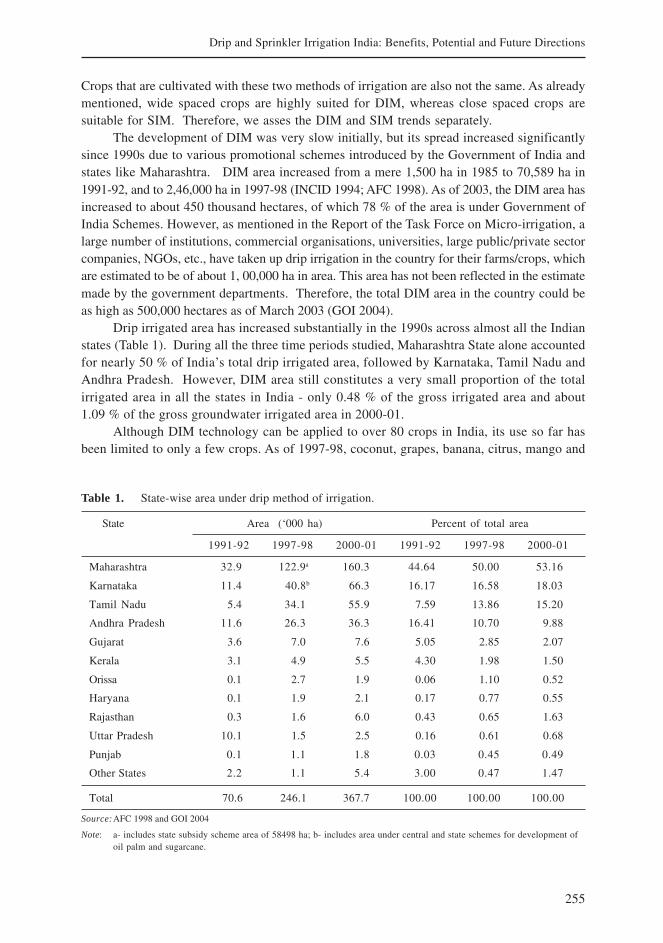
255
Drip and Sprinkler Irrigation India: Benefits, Potential and Future Directions
Table 1. State-wise area under drip method of irrigation.
State Area (‘000 ha) Percent of total area
1991-92 1997-98 2000-01 1991-92 1997-98 2000-01
Maharashtra 32.9 122.9a 160.3 44.64 50.00 53.16
Karnataka 11.4 40.8b 66.3 16.17 16.58 18.03
Tamil Nadu 5.4 34.1 55.9 7.59 13.86 15.20
Andhra Pradesh 11.6 26.3 36.3 16.41 10.70 9.88
Gujarat 3.6 7.0 7.6 5.05 2.85 2.07
Kerala 3.1 4.9 5.5 4.30 1.98 1.50
Orissa 0.1 2.7 1.9 0.06 1.10 0.52
Haryana 0.1 1.9 2.1 0.17 0.77 0.55
Rajasthan 0.3 1.6 6.0 0.43 0.65 1.63
Uttar Pradesh 10.1 1.5 2.5 0.16 0.61 0.68
Punjab 0.1 1.1 1.8 0.03 0.45 0.49
Other States 2.2 1.1 5.4 3.00 0.47 1.47
Total 70.6 246.1 367.7 100.00 100.00 100.00
Source:AFC 1998 and GOI 2004
Note: a- includes state subsidy scheme area of 58498 ha; b- includes area under central and state schemes for development ofoil palm and sugarcane.
Crops that are cultivated with these two methods of irrigation are also not the same. As alreadymentioned, wide spaced crops are highly suited for DIM, whereas close spaced crops aresuitable for SIM. Therefore, we asses the DIM and SIM trends separately.
The development of DIM was very slow initially, but its spread increased significantlysince 1990s due to various promotional schemes introduced by the Government of India andstates like Maharashtra. DIM area increased from a mere 1,500 ha in 1985 to 70,589 ha in1991-92, and to 2,46,000 ha in 1997-98 (INCID 1994; AFC 1998). As of 2003, the DIM area hasincreased to about 450 thousand hectares, of which 78 % of the area is under Government ofIndia Schemes. However, as mentioned in the Report of the Task Force on Micro-irrigation, alarge number of institutions, commercial organisations, universities, large public/private sectorcompanies, NGOs, etc., have taken up drip irrigation in the country for their farms/crops, whichare estimated to be of about 1, 00,000 ha in area. This area has not been reflected in the estimatemade by the government departments. Therefore, the total DIM area in the country could beas high as 500,000 hectares as of March 2003 (GOI 2004).
Drip irrigated area has increased substantially in the 1990s across almost all the Indianstates (Table 1). During all the three time periods studied, Maharashtra State alone accountedfor nearly 50 % of India’s total drip irrigated area, followed by Karnataka, Tamil Nadu andAndhra Pradesh. However, DIM area still constitutes a very small proportion of the totalirrigated area in all the states in India - only 0.48 % of the gross irrigated area and about1.09 % of the gross groundwater irrigated area in 2000-01.
Although DIM technology can be applied to over 80 crops in India, its use so far hasbeen limited to only a few crops. As of 1997-98, coconut, grapes, banana, citrus, mango and
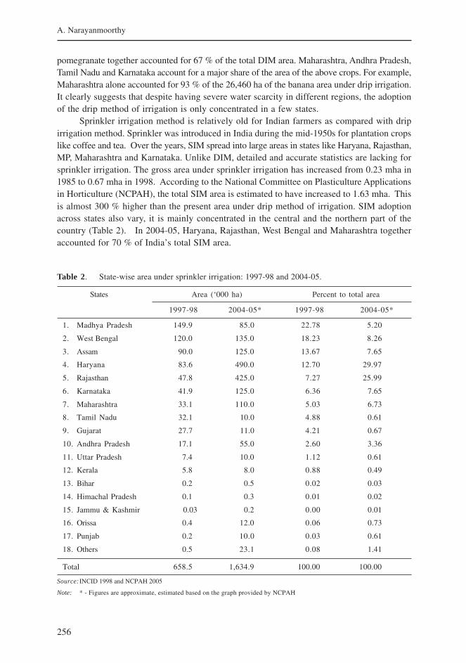
256
A. Narayanmoorthy
pomegranate together accounted for 67 % of the total DIM area. Maharashtra, Andhra Pradesh,Tamil Nadu and Karnataka account for a major share of the area of the above crops. For example,Maharashtra alone accounted for 93 % of the 26,460 ha of the banana area under drip irrigation.It clearly suggests that despite having severe water scarcity in different regions, the adoptionof the drip method of irrigation is only concentrated in a few states.
Sprinkler irrigation method is relatively old for Indian farmers as compared with dripirrigation method. Sprinkler was introduced in India during the mid-1950s for plantation cropslike coffee and tea. Over the years, SIM spread into large areas in states like Haryana, Rajasthan,MP, Maharashtra and Karnataka. Unlike DIM, detailed and accurate statistics are lacking forsprinkler irrigation. The gross area under sprinkler irrigation has increased from 0.23 mha in1985 to 0.67 mha in 1998. According to the National Committee on Plasticulture Applicationsin Horticulture (NCPAH), the total SIM area is estimated to have increased to 1.63 mha. Thisis almost 300 % higher than the present area under drip method of irrigation. SIM adoptionacross states also vary, it is mainly concentrated in the central and the northern part of thecountry (Table 2). In 2004-05, Haryana, Rajasthan, West Bengal and Maharashtra togetheraccounted for 70 % of India’s total SIM area.
Table 2. State-wise area under sprinkler irrigation: 1997-98 and 2004-05.
States Area (‘000 ha) Percent to total area
1997-98 2004-05* 1997-98 2004-05*
1. Madhya Pradesh 149.9 85.0 22.78 5.20
2. West Bengal 120.0 135.0 18.23 8.26
3. Assam 90.0 125.0 13.67 7.65
4. Haryana 83.6 490.0 12.70 29.97
5. Rajasthan 47.8 425.0 7.27 25.99
6. Karnataka 41.9 125.0 6.36 7.65
7. Maharashtra 33.1 110.0 5.03 6.73
8. Tamil Nadu 32.1 10.0 4.88 0.61
9. Gujarat 27.7 11.0 4.21 0.67
10. Andhra Pradesh 17.1 55.0 2.60 3.36
11. Uttar Pradesh 7.4 10.0 1.12 0.61
12. Kerala 5.8 8.0 0.88 0.49
13. Bihar 0.2 0.5 0.02 0.03
14. Himachal Pradesh 0.1 0.3 0.01 0.02
15. Jammu & Kashmir 0.03 0.2 0.00 0.01
16. Orissa 0.4 12.0 0.06 0.73
17. Punjab 0.2 10.0 0.03 0.61
18. Others 0.5 23.1 0.08 1.41
Total 658.5 1,634.9 100.00 100.00
Source: INCID 1998 and NCPAH 2005
Note: * - Figures are approximate, estimated based on the graph provided by NCPAH
257
Drip and Sprinkler Irrigation India: Benefits, Potential and Future Directions
The reasons for the large-scale adoption of sprinkler irrigation vary from state to state.Though MP receives medium rainfall, it is irregular and the summer has long dry spells.This encourages MP farmers to adopt sprinkler irrigation for crops like soybean in variousparts of the state. In Haryana, the soil condition, topography and the climates that areprevailing in the south western part of the state, especially in districts of Bhiwani,Mahindergarh, Rothak, Sirsa and Hisar, have prompted the adoption of sprinkler irrigation.Similarly, favorable cropping patterns for MI and water scarcity during the summer seasonare the main reasons for the relatively higher adoption of sprinkler irrigation in Rajasthan(INCID 1998).
Although the SIM reported area is much higher than that under drip irrigation, no reliabledata is available on the composition of crops that are cultivated presently using this methodof irrigation. The INCID 1998 report presents a whole lot of information about the sprinklermethod, but does not provide where and what crops are cultivated under this method. In fact,reliable and time series data on micro-irrigation is seldom available even for research purpose.Agencies involved in promoting MI should make all efforts to publish data on the developmentof micro-irrigation in terms of crop composition, area by state, districts and different size classes,area by state promoted schemes and other schemes. This would help one to analyse theunderlying factors and suggest possible ways and means to increase the adoption of suchwater saving technologies.
Potential Areas for Drip and Sprinkler Irrigation in India
In spite of the large capital investments, MI seems to generate better returns for farmers, evenwithout government subsidies (Table 3). Although micro-irrigation has proved to be a veryuseful method for efficient use of irrigation water, not many studies have attempted to estimatethe total potential area for drip and sprinkler method of irrigation for different states in India.Therefore, in this section, we try to estimate the total potential area for drip and sprinklerirrigation methods across different states in India.
Before presenting our own estimates, we first discuss the estimates of potential DIMand SIM l area on the basis of available literature. Two estimates are available as the potentialDIM area - 18.2 Mha by NCPA 1990, and 27.0 Mha by the Task Force on Micro-Irrigation(TFMI) (GOI 2004). The potential SIM area estimates vary, from 42.5 Mha of INCID 1998 to69.5 Mha of TFMI, (Table 4). What could be the possible reasons for such wide variation inthese estimates? It appears that there are some methodological problems with the availableestimates. It is not clear whether the estimates include irrigated cropped area alone or bothirrigated plus un-irrigated cropped area. It also appears that the TFMI estimate includes bothirrigated and un-irrigated cropped areas (example cotton area). Since water sources are neededto use micro-irrigation, one should not include un-irrigated cropped area while estimatingpotential area for drip and sprinkler irrigation.2 Moreover, both the estimates have not provided
2 Potential area for MI can be estimated in various ways using different assumptions. If one wants toinclude un-irrigated crops that are suitable for MI for estimation, it is essential to specify under whatcondition this would be possible. In any case un-irrigated crop area may not be immediately broughtunder the method of MI.
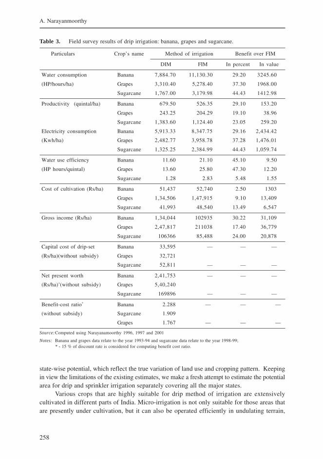
258
A. Narayanmoorthy
Table 3. Field survey results of drip irrigation: banana, grapes and sugarcane.
Particulars Crop’s name Method of irrigation Benefit over FIM
DIM FIM In percent In value
Water consumption Banana 7,884.70 11,130.30 29.20 3245.60
(HP/hours/ha) Grapes 3,310.40 5,278.40 37.30 1968.00
Sugarcane 1,767.00 3,179.98 44.43 1412.98
Productivity (quintal/ha) Banana 679.50 526.35 29.10 153.20
Grapes 243.25 204.29 19.10 38.96
Sugarcane 1,383.60 1,124.40 23.05 259.20
Electricity consumption Banana 5,913.33 8,347.75 29.16 2,434.42
(Kwh/ha) Grapes 2,482.77 3,958.78 37.28 1,476.01
Sugarcane 1,325.25 2,384.99 44.43 1,059.74
Water use efficiency Banana 11.60 21.10 45.10 9.50
(HP hours/quintal) Grapes 13.60 25.80 47.30 12.20
Sugarcane 1.28 2.83 5.48 1.55
Cost of cultivation (Rs/ha) Banana 51,437 52,740 2.50 1303
Grapes 1,34,506 1,47,915 9.10 13,409
Sugarcane 41,993 48,540 13.49 6,547
Gross income (Rs/ha) Banana 1,34,044 102935 30.22 31,109
Grapes 2,47,817 211038 17.40 36,779
Sugarcane 106366 85,488 24.00 20,878
Capital cost of drip-set Banana 33,595 — — —
(Rs/ha)(without subsidy) Grapes 32,721
Sugarcane 52,811 — — —
Net present worth Banana 2,41,753 — — —
(Rs/ha)*(without subsidy) Grapes 5,40,240
Sugarcane 169896 — — —
Benefit-cost ratio* Banana 2.288 — — —
(without subsidy) Sugarcane 1.909
Grapes 1.767 — — —
Source:Computed using Narayanamoorthy 1996, 1997 and 2001
Notes: Banana and grapes data relate to the year 1993-94 and sugarcane data relate to the year 1998-99;* - 15 % of discount rate is considered for computing benefit cost ratio.
state-wise potential, which reflect the true variation of land use and cropping pattern. Keepingin view the limitations of the existing estimates, we make a fresh attempt to estimate the potentialarea for drip and sprinkler irrigation separately covering all the major states.
Various crops that are highly suitable for drip method of irrigation are extensivelycultivated in different parts of India. Micro-irrigation is not only suitable for those areas thatare presently under cultivation, but it can also be operated efficiently in undulating terrain,
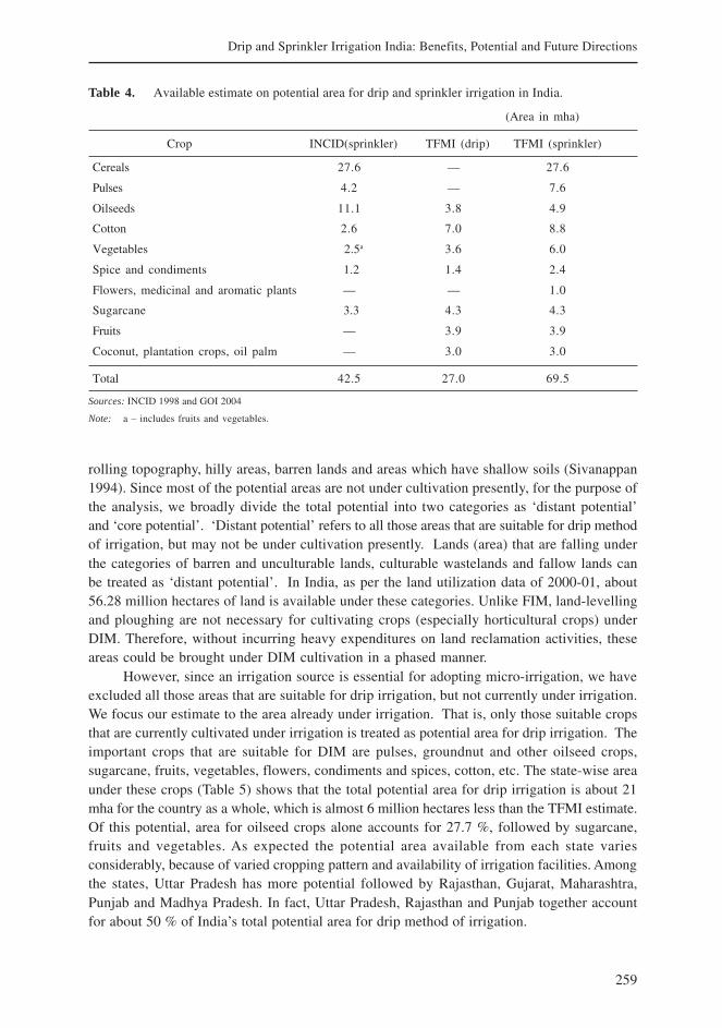
259
Drip and Sprinkler Irrigation India: Benefits, Potential and Future Directions
rolling topography, hilly areas, barren lands and areas which have shallow soils (Sivanappan1994). Since most of the potential areas are not under cultivation presently, for the purpose ofthe analysis, we broadly divide the total potential into two categories as ‘distant potential’and ‘core potential’. ‘Distant potential’ refers to all those areas that are suitable for drip methodof irrigation, but may not be under cultivation presently. Lands (area) that are falling underthe categories of barren and unculturable lands, culturable wastelands and fallow lands canbe treated as ‘distant potential’. In India, as per the land utilization data of 2000-01, about56.28 million hectares of land is available under these categories. Unlike FIM, land-levellingand ploughing are not necessary for cultivating crops (especially horticultural crops) underDIM. Therefore, without incurring heavy expenditures on land reclamation activities, theseareas could be brought under DIM cultivation in a phased manner.
However, since an irrigation source is essential for adopting micro-irrigation, we haveexcluded all those areas that are suitable for drip irrigation, but not currently under irrigation.We focus our estimate to the area already under irrigation. That is, only those suitable cropsthat are currently cultivated under irrigation is treated as potential area for drip irrigation. Theimportant crops that are suitable for DIM are pulses, groundnut and other oilseed crops,sugarcane, fruits, vegetables, flowers, condiments and spices, cotton, etc. The state-wise areaunder these crops (Table 5) shows that the total potential area for drip irrigation is about 21mha for the country as a whole, which is almost 6 million hectares less than the TFMI estimate.Of this potential, area for oilseed crops alone accounts for 27.7 %, followed by sugarcane,fruits and vegetables. As expected the potential area available from each state variesconsiderably, because of varied cropping pattern and availability of irrigation facilities. Amongthe states, Uttar Pradesh has more potential followed by Rajasthan, Gujarat, Maharashtra,Punjab and Madhya Pradesh. In fact, Uttar Pradesh, Rajasthan and Punjab together accountfor about 50 % of India’s total potential area for drip method of irrigation.
Table 4. Available estimate on potential area for drip and sprinkler irrigation in India.
(Area in mha)
Crop INCID(sprinkler) TFMI (drip) TFMI (sprinkler)
Cereals 27.6 — 27.6
Pulses 4.2 — 7.6
Oilseeds 11.1 3.8 4.9
Cotton 2.6 7.0 8.8
Vegetables 2.5a 3.6 6.0
Spice and condiments 1.2 1.4 2.4
Flowers, medicinal and aromatic plants — — 1.0
Sugarcane 3.3 4.3 4.3
Fruits — 3.9 3.9
Coconut, plantation crops, oil palm — 3.0 3.0
Total 42.5 27.0 69.5
Sources: INCID 1998 and GOI 2004
Note: a – includes fruits and vegetables.
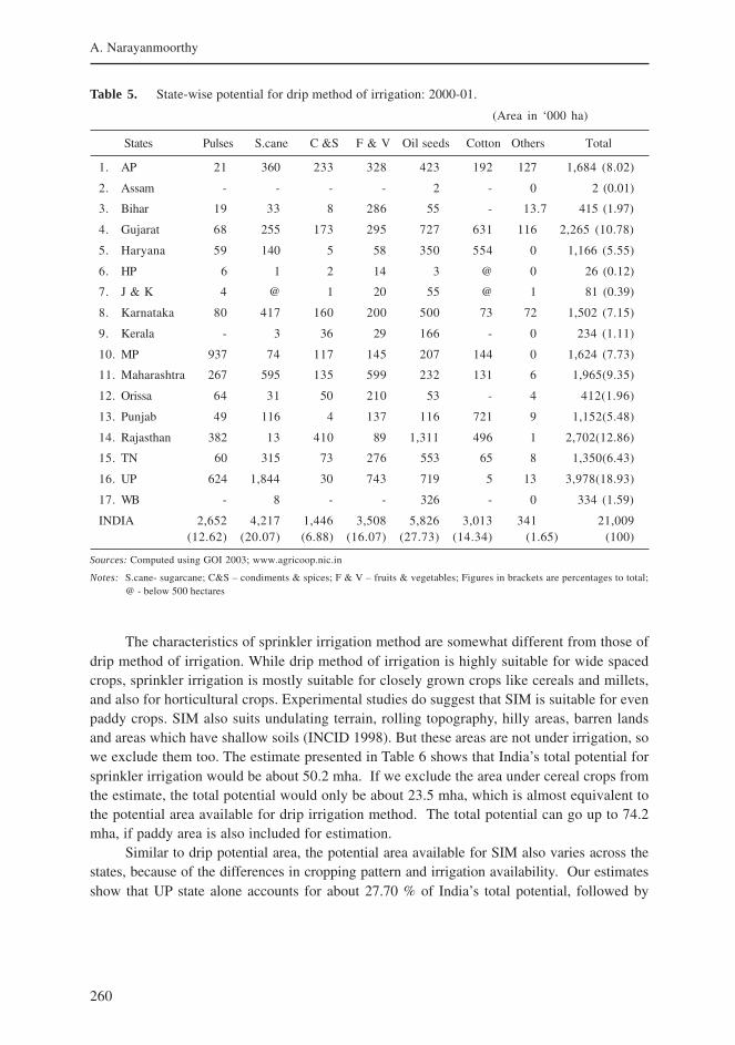
260
A. Narayanmoorthy
The characteristics of sprinkler irrigation method are somewhat different from those ofdrip method of irrigation. While drip method of irrigation is highly suitable for wide spacedcrops, sprinkler irrigation is mostly suitable for closely grown crops like cereals and millets,and also for horticultural crops. Experimental studies do suggest that SIM is suitable for evenpaddy crops. SIM also suits undulating terrain, rolling topography, hilly areas, barren landsand areas which have shallow soils (INCID 1998). But these areas are not under irrigation, sowe exclude them too. The estimate presented in Table 6 shows that India’s total potential forsprinkler irrigation would be about 50.2 mha. If we exclude the area under cereal crops fromthe estimate, the total potential would only be about 23.5 mha, which is almost equivalent tothe potential area available for drip irrigation method. The total potential can go up to 74.2mha, if paddy area is also included for estimation.
Similar to drip potential area, the potential area available for SIM also varies across thestates, because of the differences in cropping pattern and irrigation availability. Our estimatesshow that UP state alone accounts for about 27.70 % of India’s total potential, followed by
Table 5. State-wise potential for drip method of irrigation: 2000-01.
(Area in ‘000 ha)
States Pulses S.cane C &S F & V Oil seeds Cotton Others Total
1. AP 21 360 233 328 423 192 127 1,684 (8.02)
2. Assam - - - - 2 - 0 2 (0.01)
3. Bihar 19 33 8 286 55 - 13.7 415 (1.97)
4. Gujarat 68 255 173 295 727 631 116 2,265 (10.78)
5. Haryana 59 140 5 58 350 554 0 1,166 (5.55)
6. HP 6 1 2 14 3 @ 0 26 (0.12)
7. J & K 4 @ 1 20 55 @ 1 81 (0.39)
8. Karnataka 80 417 160 200 500 73 72 1,502 (7.15)
9. Kerala - 3 36 29 166 - 0 234 (1.11)
10. MP 937 74 117 145 207 144 0 1,624 (7.73)
11. Maharashtra 267 595 135 599 232 131 6 1,965(9.35)
12. Orissa 64 31 50 210 53 - 4 412(1.96)
13. Punjab 49 116 4 137 116 721 9 1,152(5.48)
14. Rajasthan 382 13 410 89 1,311 496 1 2,702(12.86)
15. TN 60 315 73 276 553 65 8 1,350(6.43)
16. UP 624 1,844 30 743 719 5 13 3,978(18.93)
17. WB - 8 - - 326 - 0 334 (1.59)
INDIA 2,652 4,217 1,446 3,508 5,826 3,013 341 21,009(12.62) (20.07) (6.88) (16.07) (27.73) (14.34) (1.65) (100)
Sources: Computed using GOI 2003; www.agricoop.nic.in
Notes: S.cane- sugarcane; C&S – condiments & spices; F & V – fruits & vegetables; Figures in brackets are percentages to total;@ - below 500 hectares
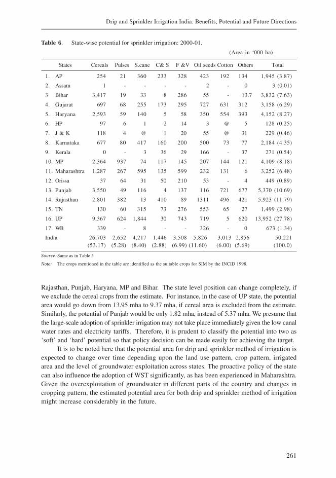
261
Drip and Sprinkler Irrigation India: Benefits, Potential and Future Directions
Rajasthan, Punjab, Haryana, MP and Bihar. The state level position can change completely, ifwe exclude the cereal crops from the estimate. For instance, in the case of UP state, the potentialarea would go down from 13.95 mha to 9.37 mha, if cereal area is excluded from the estimate.Similarly, the potential of Punjab would be only 1.82 mha, instead of 5.37 mha. We presume thatthe large-scale adoption of sprinkler irrigation may not take place immediately given the low canalwater rates and electricity tariffs. Therefore, it is prudent to classify the potential into two as‘soft’ and ‘hard’ potential so that policy decision can be made easily for achieving the target.
It is to be noted here that the potential area for drip and sprinkler method of irrigation isexpected to change over time depending upon the land use pattern, crop pattern, irrigatedarea and the level of groundwater exploitation across states. The proactive policy of the statecan also influence the adoption of WST significantly, as has been experienced in Maharashtra.Given the overexploitation of groundwater in different parts of the country and changes incropping pattern, the estimated potential area for both drip and sprinkler method of irrigationmight increase considerably in the future.
Table 6. State-wise potential for sprinkler irrigation: 2000-01.
(Area in ‘000 ha)
States Cereals Pulses S.cane C& S F &V Oil seeds Cotton Others Total
1. AP 254 21 360 233 328 423 192 134 1,945 (3.87)
2. Assam 1 - - - - 2 - 0 3 (0.01)
3 Bihar 3,417 19 33 8 286 55 - 13.7 3,832 (7.63)
4. Gujarat 697 68 255 173 295 727 631 312 3,158 (6.29)
5. Haryana 2,593 59 140 5 58 350 554 393 4,152 (8.27)
6. HP 97 6 1 2 14 3 @ 5 128 (0.25)
7. J & K 118 4 @ 1 20 55 @ 31 229 (0.46)
8. Karnataka 677 80 417 160 200 500 73 77 2,184 (4.35)
9. Kerala 0 - 3 36 29 166 - 37 271 (0.54)
10. MP 2,364 937 74 117 145 207 144 121 4,109 (8.18)
11. Maharashtra 1,287 267 595 135 599 232 131 6 3,252 (6.48)
12. Orissa 37 64 31 50 210 53 - 4 449 (0.89)
13. Punjab 3,550 49 116 4 137 116 721 677 5,370 (10.69)
14. Rajasthan 2,801 382 13 410 89 1311 496 421 5,923 (11.79)
15. TN 130 60 315 73 276 553 65 27 1,499 (2.98)
16. UP 9,367 624 1,844 30 743 719 5 620 13,952 (27.78)
17. WB 339 - 8 - - 326 - 0 673 (1.34)
India 26,703 2,652 4,217 1,446 3,508 5,826 3,013 2,856 50,221(53.17) (5.28) (8.40) (2.88) (6.99) (11.60) (6.00) (5.69) (100.0)
Source:Same as in Table 5
Note: The crops mentioned in the table are identified as the suitable crops for SIM by the INCID 1998.
262
A. Narayanmoorthy
Conclusion and Policy Interventions
The estimate presented in the preceding section suggests that the potential for both drip andsprinkler irrigation is very large in different states of India. Micro-irrigation reduces the costof cultivation, weed problems, soil erosion and increases water use efficiency as well aselectricity use efficiency, besides helping reduce the overexploitation of groundwater. In spiteof having many economic and other advantages, the growth of area under micro-irrigation hasnot so far been appreciable compared to the total potential. As of now, the area under dripirrigation has extended to only 2.13 % of its potential while in the case of sprinkler irrigationthe corresponding proportion is 3.30 %. Additionally most of this development has been dueto the support (subsidy) from state agency. Quite a few policy and technical reasons havebeen identified for the slow growth and the adoption of WSTs in India. Given the vast potentialbenefits of micro-irrigation and fast decline of irrigation water potential in the country, a numberof technical and policy interventions are required to be introduced so as to increase theadoption of micro-irrigation in India. Some specific interventions needed are presented below:
1. Sprinkler irrigation has generally been promoted through subsidy schemes and notas an on-farm water and land management strategy. In certain states (for example,Maharashtra), under subsidy scheme, no consideration is given in respect of fieldsize, shape, topography, type and the location of water source, seasonal fluctuations,type of soil and crops to be grown. The design aspect is ignored so as to reduce thecost of the system. According to Kulkarni 2005, “in most cases the subsidy sets donot match the site specific situations of an individual farmer. As a result, the sets donot operate satisfactorily” (p.5). This can discourage the farmers not to adopt sprinklerirrigation. Therefore, the subsidy scheme needs to be modified and must take in toconsideration the design aspect of the system.
2. Both drip and sprinkler irrigation are driven through the state and central governmentsponsored subsidy schemes. In order to earn quick profit from the subsidy programs,many companies are marketing various sub-standard components in the market. Oftenthe sub-standard components affect the working condition of the system whichcreates enormous doubt in the farmer’s mind about the functioning of the system. Itis to be ensured that only good quality components having the certification of Bureauof Indian Standards (BIS/ISO) are supplied to the farmers. There is also a need toestablish a Central Testing Facility (CTF) to deal comprehensively with the design,development and testing of all equipment, devices and machines used in sprinklerand micro-systems using state-of-the-art technology (Kulkarni 2005; GOI 2004).
3. There has been a significant development in sprinkler technology all over the world.Several variations of sprinkler irrigation system, with improved design and componentsare available in those countries, where it is popularly used. Efforts should be madeto manufacture such improved sprinkler systems through joint ventures, with thecondition that the imported components and technology would be transferred toindigenous manufacture within a period of 2 years. This would help reducing thecost of the system and increasing the adoption of micro-irrigation at a large scale. Assuggested by TFMI, at least 1 % of the outlay on micro-irrigation needs to beearmarked for micro-irrigation research.
263
Drip and Sprinkler Irrigation India: Benefits, Potential and Future Directions
4. One of the major reasons for the slow growth of micro-irrigation in India is the highinitial investment. In spite of the availability of subsidy from state agencies, themajority of the farmers are reluctant to invest in micro-irrigation system even inhorticulture crops, which is highly suitable for drip irrigation. Therefore, as suggestedby TFMI, there is a need to look into the technological options, of which crop geometrymodification is the most important one. Instead of adopting traditional spacing,adoption of paired row planting has been found to reduce the cost of the system by40 % in many crops including tomato, brinjal, okra, etc. Therefore, micro-irrigationsystem should be tailor made, i.e., planned and designed based on location specificparameters. Standard procedure provided under subsidy scheme may not always helpto reduce the cost of the system.
5. It is understood from the field studies that capital cost required to install drip irrigationis relatively high. Because of this reason, considerable percentage of farmers haveexpressed that they are unable to adopt this technology for low- value crops. If dripsystem is made available at a low cost, area under drip irrigation can be increased at afaster rate. Therefore, measures need to be taken to reduce the fixed cost of drip irrigationby promoting research and development activities. By recognizing drip industry as aninfrastructure industry as well as announcing tax holiday for specific time periods to allthose drip set industries which produce genuine drip materials, the competition can beincreased to ultimately bring down the cost of the system. Some companies have comeout with low-cost drip irrigation systems, which can be adopted even by the farmershaving less than one acre of land. Studies need to be carried out to find out the feasibilityof low- cost drip materials including its environment feasibility using field level data.
6. The centrally sponsored scheme of drip irrigation does not provide a subsidy for thesugarcane crop. The logic behind this is not clearly known. Since it is an importantand also a heavy water-consuming crop, this restriction should be removed to increasethe drip irrigated area at a faster rate. This would also ultimately help to reduce thewater crisis faced by various states to some extent.
7. The rate of subsidy provided through government schemes is fixed uniformly for bothwater-intensive as well as less water-intensive crops. This needs to be restructured.Special subsidy program may be introduced for water-intensive crops like sugarcane,banana, vegetables, etc. Differential subsidy rates can be fixed based on the typesof crops and the rate of consumption of water. Uniform level of subsidy schemescurrently followed for water-scarce and water-abundant areas need to be changedand higher subsidy should be provided for those regions where the scarcity of wateris acute and exploitation of groundwater is very high as well.
8. Sugar industries always try to increase the area under sugarcane to increase theircapacity utilization in almost all the states in India. They are least bothered aboutthe method of sugarcane cultivation. Since sugar industries have close contact withsugarcane cultivators, some kind of target may be fixed for each sugar industry tobring cultivation of sugarcane under DIM. Apart from the saving of water, this wouldalso help achieve cultivation of sugarcane in a sustainable manner. Despite irrigationwater shortage in many states, not only does the area under sugarcane continue to
264
A. Narayanmoorthy
grow at a relatively faster rate, but it is cultivated predominantly under flood methodof irrigation. This puts additional pressure on our limited water resources.
9. Drip set manufacturers should be asked to involve intensively in promoting micro-irrigation by organizing frequent demonstrations at farmers’ fields. Since the use ofmicro-irrigation is still in the take-off stage in India, an active role of the manufacturersis essential in promoting drip irrigation as well as developing confidence among thefarmers about the usefulness of this new technology. The micro-system manufacturersshould be involved in providing advice on agronomic packages to the farmers so asto encourage the adoption of WSTs on a large scale.
10. For a speedy growth of micro-irrigation, a special package scheme can be introducedwhere priority can be given to providing bank loans for digging wells and electricityconnection (pump-set) for those farmers who are ready to adopt micro-irrigation forcultivating any crop.
11. Groundwater is the only source of water being used for drip method of irrigation inIndia. Unlike other countries, water from surface sources (dams, reservoirs, etc.) isnot used for drip method of irrigation. Since water use efficiency under surface sourcesis very low owing to heavy losses through conveyance and distribution, farmersshould be encouraged to use water from surface sources for drip method of irrigation.This can be done by allocating a certain proportion of water from each irrigationprojects only for the use of micro-irrigation.
12. One of the important reasons for the low spread of this technology even in the water-scarce area is the availability of highly subsidized canal water as well as electricityfor irrigation pump sets. Appropriate pricing policies on these two inputs may alsoencourage the farmers to adopt this technology.
To conclude, the potential area for MI presented above is estimated based on thepresent cropping pattern and irrigation coverage of different states in India. One may notbe able to argue that this potential area would be the same even after 10 or 20 years becauseof changes in the parameters that determine MI potential. The potential area available forMI is governed by factors such as cropping pattern, irrigation coverage, groundwater scarcity,price of canal water, price of electricity as well as its supply (in hours) for agriculture,technology development in MI, proactive policy (subsidy and other incentives) of the stateand central governments. In case farmers shift the cropping pattern more in favour ofhorticultural crops because of their high profitability, the potential area for DIM mightincrease significantly in the future. Similarly, if the depletion in groundwater in differentregions aggravates further, it might also encourage the farmers to shift the irrigation methodfrom flood to MI methods. What will be the potential area for DIM and SIM if croppingpattern changes drastically in favor of high-value horticultural crops in another 10 years?Does the potential for MI change if one estimates it under different scenarios of groundwaterdepletion? Will the potential area for MI change if full cost pricing is introduced in canalwater and electricity supplied for irrigation pump sets? One may be able to find someinteresting results if comprehensive analysis is carried out covering the issues flagged here.In any case, the potential area for MI is not going to be static.
265
Drip and Sprinkler Irrigation India: Benefits, Potential and Future Directions
References
AFC. 1998. Evaluation of Drip Irrigation System. Agricultural Finance Corporation (AFC) Limited,Mumbai, October.
Amarasinghe, U. A.; Sharma, B. R.; Aloysius, N.; Scott, C.; Smakhtin, V.; de Fraiture, C. 2005. Spatialvariation of water supply and demand across river basins of India. Research Report 83. Colombo, SriLanka: International Water Management Institute.
Amarasinghe, U. A.; Shah, T.; Turral, H.; Anand, B. 2007. India’s water futures to 2025-2050: Businessas usual scenario and deviations. IWMI Research Report 123. Colombo, Sri Lanka: International WaterManagement Institute.
Biswas, A. K. 2001. Water Policies in Developing World. Water Resources Development, Vol. 17, No. 4,pp. 489-499.
Dhawan, B. D. 2002. Technological Change in Indian Irrigated Agriculture: A Study of Water SavingMethods. New Delhi: Commonwealth Publishers.
GOI. 2003. Agricultural Statistics at a Glance. New Delhi: Ministry of Agriculture, Government of India.
GOI. 2004. Report of Task Force on Micro-irrigation. (Chairman: N. Chandrababu Naidu), Ministry ofAgriculture, Government of India, January.
INCID. 1994. Drip Irrigation in India. Indian National Committee on Irrigation and Drainage, New Delhi.
INCID. 1998. Sprinkler Irrigation in India. Indian National Committee on Irrigation and Drainage,New Delhi.
Kulkarni, S. A. 2005. Looking Beyond Eight Sprinklers. Paper presented at the National Conference onMicro-Irrigation. G. B. Pant University of Agriculture and Technology, Pantnagar, India, June 3-5, 2005.
Kundu, D. K.; Neue, H. U.; Singh R. 1998. Comparative Effects of Flooding and Sprinkler Irrigation onGrowth and Mineral Composition of Rice in an Alfisol. Proceedings of the National Seminar on Micro-Irrigation Research in India: Status and Perspective for the 21st Century. Bhubaneswar, July 27-28, 1998.
MOWR. 1999. Report of the Working Group on Water Availability for Use. National Commission for IntegratedWater Resources Development Plan, Ministry of Water Resources, Government of India, New Delhi.
Narayanamoorthy, A. 1996. Evaluation of Drip Irrigation System in Maharashtra. Mimeograph SeriesNo. 42, Agro-Economic Research Centre, Gokhale Institute of Politics and Economics, Pune,Maharashtra.
Narayanamoorthy, A. 1997. Economic Viability of Drip Irrigation: An Empirical Analysis from Maharashtra.Indian Journal of Agricultural Economics, Vol.52, No.4, October-December, pp.728-739.
Narayanamoorthy, A. 1997a. Beneficial Impact of Drip Irrigation: A Study Based on Western India. WaterResource Journal, No.195, December, pp. 17-25.
Narayanamoorthy, A. 2001. Impact of Drip Irrigation on Sugarcane Cultivation in Maharashtra. Agro-Economic Research Centre, Gokhale Institute of Politics and Economics, Pune, June.
Narayanamoorthy, A. 2003. Averting Water Crisis by Drip Method of Irrigation: A Study of TwoWater-Intensive Crops. Indian Journal of Agricultural Economics, Vol. 58, No. 3, July-September,pp. 427-437.
Narayanamoorthy, A. 2004. Drip Irrigation in India: Can it Solve Water Scarcity? Water Policy, Vol. 6,No.2. pp. 117-130.
Narayanamoorthy, A. 2004a. Impact Assessment of Drip Irrigation in India: The Case of Sugarcane.Development Policy Review, Vol. 22, No. 4, pp. 443-462.
Narayanamoorthy, A. 2005. Efficiency of Irrigation: A Case of Drip Irrigation. Occasional Paper: 45,Department of Economic Analysis and Research, National Bank for Agriculture and Rural Development,Mumbai, India.
266
A. Narayanmoorthy
NCPA. 1987. Proceedings of the National Seminar on Use of Plastics in Agriculture. Organised jointly bythe Directorate of Extension (Ministry of Agriculture) and the National Committee on the Use of Plasticsin Agriculture (Ministry of Industry), Government of India, New Delhi, February 6.
NCPA. 1990. Status, Potential and Approach for Adoption of Drip and Sprinkler Irrigation Systems. NationalCommittee on the Use of Plastics in Agriculture, Pune, India.
NCPAH. 2005. Status of Drip and Sprinkler Irrigation in India, National Committee on PlasticultureApplications in Horticulture. New Delhi: Government of India.
Postal, S.; Polak, P.; Gonzales, F.; Keller, J. 2001. Drip Irrigation for Small Farmers: A New Initiative toAlleviate Hunger and Poverty. Water International, Vol. 26, No. 1.
Rosegrant, W. M.; Ximing, C.; Cline, S. A. 2002. World Water and Food to 2020: Dealing with Scarcity,International Food Policy Research Institute, Washington, D.C., USA and International Water ManagementInstitute, Colombo, Sri Lanka.
Saleth, R. M. 1996. Water Institutions in India: Economics, Law and Policy. New Delhi: CommonwealthPublishers.
Seckler, D.; Amarasinghe, U.; Molden, D.; de Silva, R.; Barker, R. 1998. World water demand and supply,1990 to 2025: Scenarios and issues. Research Report 19. Colombo, Sri Lanka: International WaterManagement Institute.
Seckler, D.; Barker R.; Amarasinghe, U. 1999. Water Scarcity in Twenty-First Century. International Journalof Water Resources Development, Vol.15, Nos. 1-2, pp. 29-42.
Sivanappan, R. K. 1994. Prospects of Micro Irrigation in India. Irrigation and Drainage System, Vol.8,No. 1 pp. 49-58.
Vaidyanathan, A. 1998. Water Resource Management: Institutions and Irrigation Development in India.New Delhi, India: Oxford University Press.
267
Drip and Sprinkler Irrigation India: Benefits, Potential and Future Directions
Water Saving and Yield Enhancing Micro-irrigationTechnologies: How Far Can They Contribute to Water
Productivity in Indian Agriculture?
1M. Dinesh Kumar, 2Bharat Sharma and 3O. P. Singh1IWMI-TATA Water Policy Program, Hyderabad, India
2IWMI New Delhi Office, New Delhi, India3Department of Agricultural Economics, Institute of Agricultural Sciences,
Banaras Hindu University, Varanasi
Introduction
Demand management becomes the key to the overall strategy for managing scarce waterresources (Molden et al. 2001). Since agriculture is the major competitive user of divertedwater in India (GOI 1999), demand management in agriculture in water-scarce and water-stressed regions would be central to reducing the aggregate demand for water to match withthe available future supplies, thereby reducing the extent of water stress that the country islikely to face (Kumar 2003a; Kumar 2003b). Improving water productivity in agriculture isimportant in the overall framework for managing agricultural water demand, thereby increasingthe ability of agencies and other interested parties to transfer the water thus ‘saved’ toeconomically more efficient or other high priority domestic and industrial use sectors (Barkeret al. 2003; Kijne et al. 2003).
Three dimensions of water productivity include physical productivity, expressed in kgper unit of water consumed; combined physical and economic productivity expressed in termsof net return per unit of water consumed, and economic productivity expressed in terms ofnet income returns from a given amount of water consumed against the opportunity cost ofusing the same amount of water (Kijne et al. 2003). The discussion in the present paperwould be largely on the first parameter, i.e., physical productivity. There are two major waysof improving the physical productivity of water used in irrigated agriculture. First: the waterconsumption or depletion for producing a certain quantum of biomass for the same amountof land is reduced. Second: the yield generated for a particular crop is enhanced withoutchanging the amount of water consumed or depleted per unit of land. Often these twoimprovements can happen together with an intervention either on the agronomic side or onthe water control side.
There are several conceptual level issues in defining the term ‘water saving’ and irrigationefficiency. This is because with changing contexts and interests, the ‘unit of analysis’ changes
268
M. D. Kumar, B. Sharma and O. P. Singh
from field to farm, to irrigation system to river basin. With the concepts of ‘dry’ and ‘wet’water saving, which capture the phenomena such as ‘return flows from field’ and ‘depletedwater’, becoming dominant in the irrigation science literature in the last one decade, the oldconcepts of ‘water saving’ and irrigation efficiencies have become obsolete. The real watersaving or the ‘wet water’ saving in irrigated production at the field level can come only fromreduction in the depleted water and not the water applied (Molden et al. 2001). But, there aremethodological and logical issues involved in estimating the depletion fraction of the watereffectively applied to the crop. These are due to the complex considerations, includingagronomic, hydrologic, geo-hydrological and geo-chemical, in determining the ‘depletion’fraction. Nevertheless, for the limited purpose of analysis, throughout this paper, ‘water saving’refers to ‘wet’ water saving.
Water productivity is an important driver in projecting future water demands(Amarasinghe et al. 2004; Kijne 2003). Efficient irrigation technologies help establish greatercontrol over water delivery (water control) to the crop roots, reduce the non-beneficialevaporation from field and non-recoverable percolation,1 and return flows into ‘sinks’ andoften increases the beneficial ET, though the first component could be very low for fieldcrops. Water productivity improves with the reduction in depleted fraction and yieldenhancement. Since at the theoretical level, water productivity improvements in irrigatedagriculture can result in saving water used for crop production, any technologicalinterventions which improve the crop yields are also, in effect, water saving technologies.Hence, water saving technologies in agriculture can be broadly classified into three: watersaving crop technologies; water saving and yield enhancing irrigation technologies; and,yield improving crop technologies.
There are several technologies and practices for water-saving in irrigation. But, onlymicro- irrigation technologies, which are based on plastics, are dealt with in this paper. Indiastands 27th in terms of the scale of the adoption of water-saving and yield enhancing micro-irrigation devices (source: www.oznet.ksu.edu/sdi/News/Whatisnew.htm). There are severalconstraints to the adoption of MI devices. These are physical, socioeconomic, financial,institutional—pricing, subsidies, extension service—and policy-related in nature(Narayanamoorthy 1997; Sivanappan 1994; Kumar 2003a). Nevertheless, a systematic attemptto find out the conditions under which MI systems become a best bet technology, and assessthe magnitude of the reduction in water requirement possible through them is hardly ever made.Such efforts are crucial from the point of view of assessing our ability to address future waterscarcity problems at the regional and national level.
The ultimate objective of this research is to find out under what conditions micro-irrigationsystem offers the best bet. It aims at determining the potential benefits from the use of MIsystems. This includes assessing a) the conditions that are suitable or unsuitable for MIsystems; b) the field level and aggregate level impacts of the systems on water use; and c) theyield and economic benefits due to the adoption of MI system. The research also aims atassessing the potential future coverage of MI systems in India, and the reduction in aggregatewater requirement in crop production possible with that.
1Allen et al. 1998 for definitions of non-beneficial evaporation and non-recoverable deep percolation.
269
Water Saving and Yield Enhancing Micro-irrigation Technologies: How Far Can They Contribute toWater Productivity in Indian Agriculture?
Contribution of Micro-irrigation Technologies in Indian Agriculture
Present Spread of Micro-irrigation Technologies in Indian Agriculture
There were no systematic attempts in the past to assess the spread for water-saving irrigationtechnologies in India. The most recent data shows that nearly 1.3 m ha of irrigated land isunder drip irrigation (Narayanamoorthy 2004b).
They cited high initial cost (including mis-targetted subsidies), clogging of drippersand cracking of pipes, lack of adequate technical inputs, damage done by rodents; highcost of spare components; and insufficient extension education effort as the major problemscausal of the slow rate of adoption of drips. The National Committee on Irrigation andDrainage also added factors such as salinity hazards to the list of problems (GOI 1994).Difficulty in inter-cultivation was found as another reason for non-adoption by Shiyani etal. 1999, whereas Palanichamy et al. 2002 cited joint ownership of wells as additional reasonfor non-adoption based on their study in Coimbatore (Tamil Nadu). However, some of theproblems listed above such as clogging, lack of adequate technical inputs and high cost ofspare components, to a limited extent, are being by-passed with the introduction oflow-cost micro-irrigation systems in India, pioneered by international developmententerprises.
The recent data released by the Task Force on Micro-irrigation in India shows thatduring the past 4 years, peninsular India had recorded the highest growth in the adoptionof drip systems. Maharashtra ranks first (22,358 ha), followed by Andhra Pradesh (17,556ha) and Karnataka (16,731 ha). The major crops for which drip systems are currently adoptedare cotton, sugarcane; banana, orange, grapes, pomegranate, lemon, citrus, mangoes, flowers,and coconut.
Though exact state-wise data on the spread of sprinkler systems are not available, it hasbeen found that sprinkler systems are in vogue in regions where conditions are unfavorablefor the traditional method of irrigation, such as loose sandy soils and highly undulating fields.These are well-irrigated areas. Farmers in other well-irrigated areas have also procured thesystem under the government subsidy program, but were found to be using the HDPE pipesfor water conveyance in the field except during droughts when they are used for providingsupplementary irrigation to kharif crops.
In India, sprinkler systems are mainly used for field crops such as wheat, sorghum,pearl millet, groundnut and mustard. But the use of sprinklers is often limited to certain partsof the crop season when farmers face severe shortage of water in their wells. Normally, thisis just before the onset of monsoon when the farmers have to do sowing of these crops, orwhen there is a long dry spell during the monsoon season. Sprinklers for groundnut arecommon in Saurashtra in Gujarat; they are also common for mustard in Khargaon District ofMadhya Pradesh and the Ganga Nagar District of Rajasthan. In the high ranges of Keralaand Tamil Nadu, sprinklers are used for irrigating tea and coffee plantations. However,recently, farmers have started using micro-sprinklers and mini-micro-sprinklers for potato,groundnut and alfalfa.

270
M. D. Kumar, B. Sharma and O. P. Singh
Potential Contribution of Micro-irrigation Technologies in India
Physical Impact of Micro-irrigation Technologies on Water Demand forCrop Production
Analyzing the potential impact of MI systems on the aggregate demand for water in cropproduction involves three important considerations. The first concerns the extent of coveragethat can be achieved in MI system adoption at the country level. The second concerns theextent of real water saving possible with MI system adoption at the field level. The thirdconcerns what farmers do with the water saved through MI systems, and the changes in thecropping systems associated with such adoption. But, most of the past research on physicalimpacts of MI systems had dealt with the issue of changes in irrigation water use, crop growthand crop yield.
There is limited analysis available on the potential coverage of MI systems in India, andthe water saving possible at the aggregate level and these analyses suffer from severe limitations.First, the analyses of potential coverage of MI systems are based on simplistic considerationsof the area under crops that are amenable to MI systems, and do not take into account the rangeof physical, socioeconomic and institutional factors that induce severe constraints to the adoptionof these technologies. Second, they do not distinguish between saving in applied water and realwater saving, while the latter possible through MI adoption could be much lower than the former.Third, there is an inherent assumption that area under irrigation remains the same and, therefore,the saved water would be available for reallocation. But, in reality, it may not be so. With theintroduction of MI systems, farmers might change the very cropping system itself, includingexpansion in the irrigated area. Therefore, all these assumptions result in over-estimation of thepotential coverage of MI systems and the extent of water-saving possible with MI adoption.These complex questions are addressed in the subsequent sections of this paper.
A) Physical Constraints and Opportunities for Adoption of MI Systems
Determining the potential coverage that can be achieved in MI system adoption requires asystematic identification of the conditions that are favorable or unfavorable for adoption anda geographical assessment of areas where such conditions exist. Such conditions can bephysical, socioeconomic or institutional. These physical, socioeconomic and institutionalconstrains in the adoption of MI systems are discussed below.
If we do not consider the difficult options of shifting to less water-intensive crops andthe crops having higher water productivity, there are two major pre-requisites for reducing theoverall demand for water in agriculture in the region. They are i) reducing the non-beneficialevapotranspiration from crop land; and ii) maintaining the area under irrigation. The secondissue is not dealt with here. The time-tested and widely available technology for increasingwater productivity is pressurized irrigation systems such as sprinklers and drips (or trickleirrigation). However, their adoption is very low in India. While, there are several constraints atthe field level, which limit the adoption of this technology by the farmer, some of the verycritical ones that are physical in nature are analyzed here.
First of all, MI systems need a reliable daily water supply. But, nearly 41.24 % of the netirrigated area in the country gets their supplies from surface sources such as canals and tanks
271
Water Saving and Yield Enhancing Micro-irrigation Technologies: How Far Can They Contribute toWater Productivity in Indian Agriculture?
(GOI 2002). Drips and sprinklers are not conducive to flow irrigation due to two reasons. First isthe mismatch between water delivery schedules followed in canal irrigation and that to be followedwhen MI systems are used. Normally, in surface command areas in India, farmers get their turnonce in 10-15 days at flow rates ranging from 0.5 to 1 cusec. But, for drips and sprinklers to givetheir best, water should be applied to the crop either daily or once in 2 days with lower flowrates equal to evapotranspiration. This means, intermediate storage systems would be essentialfor farmers to use water from surface schemes for running MIs. Storage systems are also requiredas settling tanks for cleaning large amounts of silt content in the canal water supplies. Second,there is a need for pumps for lifting water from the storage facilities and running the MI systems.These two investments would reduce the economic viability of MI.
Therefore, in the current situation the adoption of MI would be largely limited to areasirrigated by wells. Having said that, an increasingly large number of farmers in groundwaterirrigated areas manage their supplies from water purchase. This also includes areas wheregroundwater overdraft is not a concern like in Bihar and western Orissa, and where economicaccess to water is a problem. It is difficult to imagine that these farmers would adopt anywater saving irrigation devices.
MI systems are also energy-intensive systems and, therefore, need pressuring devicesto run. Therefore, in groundwater over-exploited areas such as north and central Gujarat,Coimbatore District in Tamil Nadu and Kolar District of Karnataka, ownership of wells mostlydoes not remain with individual farmers but with groups. Also, a large number of farmers donot own wells, and have to depend on water purchase. They get water through undergroundpipelines at almost negligible water pressure (head). These farmers constitute a major chunkof the irrigators in the region. In order to use the conventional sprinkler and drip systems,high operating pressure (1.0-1.2 kg/cm2) is required. Unless the systems are directly connectedto the tubewell, the required amount of ‘head’ to run the sprinkler and drip system cannot bedeveloped. The need for a booster pump and the high cost of energy required for pressurizingthe system to run the sprinklers and drips reduce the economic viability. But, there are newMI technologies, which require very low operating head such as sub-surface irrigation systemsand the micro-tube drips. The farmers who are either water buyers or share wells can store thewater in small tanks and lift it to small heights to generate the required head for running thesub-surface drip system or micro-tube systems.
Another important constraint is the poor quality of groundwater. Due to the high TDSlevel of the pumped groundwater (the TDS levels are as high as 2,000 ppm (parts per million) inmany parts of India where groundwater is still being used for irrigation), the conventional drippersthat are exposed to sunlight get choked up due to salt deposition in the dripper perforations.The saline groundwater areas include south western Punjab, north and central Gujarat, parts ofRajasthan, and many parts of Haryana. This needs regular cleaning using mild acids like thehydrochloric acid. This is a major maintenance work, and farmers are not willing to bear the burdenof carrying out this regular maintenance. However, in limited cases, rich farmers in South WestPunjab use large surface tanks for storing canal water when it is available, and blend it withbrackish groundwater, and use for irrigating kinnow (a kind of citrus) orchards. These farmerscan also use this water for drip irrigation to prevent problems of clogging.
In addition to the areas irrigated by groundwater, there are hilly areas of the western andeastern Ghat regions, north-western Himalayas (Himachal Pradesh, J & K and Uttaranchal) andstates in north-eastern hill region, where surface streams in steep slopes could be tapped for
272
M. D. Kumar, B. Sharma and O. P. Singh
irrigating horticulture/plantation crops. Such practices are very common in the upper catchmentareas of many river basins of Kerala, which are hilly. Farmers tap the water from the streamsusing hose pipes and connect them to sprinkler systems. The high pressure required to run thesprinkler system is obtained by virtue of the elevation difference, which is in the order of 30-40meters. Such systems are used to irrigate banana, vegetables and other cash crops such as vanilla.With the creation of an intermediate storage, drips could be run for irrigating crops such ascoconut, arecanut and other fruit crops during the months of February to June.
The geological setting has a strong influence on MI adoption in well-irrigated areas. Inhard rock areas, farmers will have a strong incentive to go for MI systems. The reason is dugwells and bore wells in hard rock areas of Maharashtra, Madhya Pradesh, Tamil Nadu,Karnataka and Andhra Pradesh have very poor yield and well owners leave a part of their landfallow due to the shortage of water. In most of these areas, farmers will have to discontinuepumping after 2-3 hours for the wells to recuperate. When pressurized irrigation systems areused, the rate at which water is pumped decreases giving enough opportunity time for wellsto recuperate. Since, the pump will eventually run for more number of hours, the same quantityof water could be pumped out, and the command area can be expanded. This factor providesa great economic incentive for farmers to go for water-saving micro-irrigation systems.
B) Socioeconomic and Institutional Constraints for MI Adoption
Another major constraint on the adoption of conventional MI technologies is the predominantcropping pattern in the water-scarce regions. MI systems are best adaptable for horticulturalcrops from an economic point of view (Dhawan 2000). This is because the additional investmentfor drips has to be offset mainly by the better yield, and the returns farmers get as the savingin input costs are not very significant. But, the percentage area under horticultural crops isvery low in these regions, except Maharashtra. Though the low-cost drip irrigation systemsappear to be a solution, they have low physical efficiency when used for crops in which theplant spacing is small (chilly, vegetables, groundnut and potato)—(source: IWMI research inBanaskantha). In such situations, they also score low in the economic viability front. The low-cost systems can be used for some of the row crops such as castor, cotton and fennel, whichare very common. However, to use the system for these crops, it is very important that thefarmers maintain a fixed spacing between different rows and different plants. So far asmaintaining the spacing between rows is concerned, farmers pay sufficient attention. But,spacing between plants is not maintained. Due to this uneven (unfavorable) field conditions,designing and installing drippers becomes extremely difficult. Therefore, for the adoption ofthese water saving technologies, the farmers’ agricultural practices need major changes.
Further, there are crops such as paddy for which neither drips nor sprinkler irrigationsystems are feasible. Paddy is an important crop in many arid and semi-arid regions wherewater levels are falling. Certain studies at ICAR (Patna) have developed Low-Energy WaterApplication (LEWA) systems which apply regulated water supplies to paddy and havedemonstrated potential to save water. But the technology is still in its infancy and requireslarge- scale testing before any field-scale adoption. Adopting suitable cropping patterns thatwould increase the adoptability of water-saving technologies is one strategy. But, as mentionedin the beginning of the section, ‘crop shift’ is a harder option for farmers.
273
Water Saving and Yield Enhancing Micro-irrigation Technologies: How Far Can They Contribute toWater Productivity in Indian Agriculture?
The socioeconomic viability of crop shifts increases with the size of the operational holdingof farmers. Given the fact that small and marginal farmers account for a large percentage of theoperational holders in India, the adoptability of horticultural crops by farmers in these regionscannot be expected to be high. This is because these crops need at least 3-4 years to start yieldingreturns, (except for pomegranate and papaya). It will be extremely difficult for these farmers toblock their parcel of land for investments that do not give any returns in the immediate future,say after a season or so. Market is another constraint. Large-scale shift to fruit crops can leadto sharp decline in the market prices of these fruits. Labor absorption is another major issuewhen traditional crops such as paddy, which are labor-intensive, get replaced by orchards.Orchards require less labor, it is also seasonal, and the chances for mechanization are higher.
Plot size also influences farmers’ choices. Conventional MI systems will be physicallyand economically less feasible for smaller plots due to the fixed overhead costs of energy, andthe various components of these irrigation systems such as filters and overhead tanks. Also,the additional energy required for running the system will decrease with every additionalsprinkler, the reason being that only the pressure loss increases with the increase in the numberof sprinklers/drippers (Kumar 2003a). However, organizations like International DevelopmentEnterprises (IDE) have developed and promoted MI systems for very smallholder farmers/ plots,which use small storage cisterns for providing the required pressure.
Poor rural infrastructure, mainly in respect of power connections to agro-wells and thequality of power supply, is another major constraint on the adoption of MI systems. Difficultyin obtaining power connections for farm wells, and the poor quality of power supply forcefarmers to use diesel pump sets for irrigating their crops. The use of diesel pumps increasesthe cost of abstraction of well water. Regions such as Bihar, eastern UP and Orissa areexamples. Here, many cash-starved farmers do not own wells, and depend on water purchasedfrom well owners for irrigation. Drips and sprinklers are energy-intensive systems, and installingsuch systems would mean extra capital investments on higher capacity pump sets as well asrecurring expenses for buying diesel. These factors act as deterrents to adopting MI systems.
The current water pricing and energy pricing policies in most states also reduce theeconomic incentives for MI adoption. Due to these policies, the water-saving and energy-savingbenefits that can be accrued from the use of MI systems do not get converted into private benefits.
Unscientific water delivery schedules followed in surface irrigation systems, and powersupply restrictions on the farm sector also induce constraints on MI adoption. It is commonin surface irrigation systems that while plenty of water is released for the crops during a certainpart of the season, in the last leg of the crop season the crops are subject to moisture stress.Poor reliability of water delivery services or lack of adherence to standard delivery schedulesand poor control over volumetric supplies force farmers to adopt crops that are less sensitiveto water stress such as paddy and sugarcane and also resort to flood irrigation. Regulatedpower supply in agriculture is also reducing the economic incentive for the adoption of MIsystems that are energy-intensive.
Poor extension services offered by concerned agencies pose another major constraint.It is not common for the extension wings of Agricultural Universities to set up demonstrationsof new technologies in farmers’ fields. This is applicable to companies which manufacture andsell MI devices. Because of this, there is very little knowledge about MI technologies amongthe farmers in water-scarce regions. The existing knowledge is filled more with misconceptions.Many farmers believe that MI systems have severe limitations vis-à-vis crops for which they
274
M. D. Kumar, B. Sharma and O. P. Singh
could be used. Another misconception is that the coverage of sprinklers being circular leavesa lot of dry spots in the irrigated fields. This belief has mainly come from the experience offarmers who have used the system with improper designs.
The administration of subsidies in MI devices also works against the interest of promotingMI systems. Since in many states, the governments continue to pay the subsidy directly to themanufacturers, many farmers purchase MI systems just to avail themselves of the subsidybenefits, and do not maintain them. The suppliers do not to offer any after-sales services to thefarmers and hence are not interested in ensuring quality control. The systems being suppliedare often of substandard quality. Over and above, as the amount of funds available for subsidiesis limited, the smartest of the farmers take the benefit. On the other hand, the government officials,who come and inspect the systems installed, only check the amount of materials supplied, andcertify them for the release of the subsidy to the irrigation company. Since the manufacturershad the hassle of doing the entire documentation for obtaining the subsidy, they keep the price(without subsidy) high enough to recover their interests on capital and transaction costs.
The present institutional framework governing the use of groundwater, which puts nolimit on the amount of water farmers can pump from the aquifer, does not provide clear economicincentives to use water efficiently. This is particularly so for well owners, who have goodsources of water supply. Though it is the opportunity cost of using water, which influencesfarmers’ decision-making framework, such opportunity costs are not felt clearly. This is in spiteof the prevalence of water markets in these regions. The reason is that the demand for waterfrom the water buyers and for ones own irrigation use, is much less than the number of hoursfor which the farmers could run their pumps. In such cases, the direct additional financial returnsthe farmer gets by introducing MI systems are from the increased crop yield. This will nothappen unless the farmer adopts new agronomic practices.
Due to this reason, the well owners would rather pump for extra hours to sell water tothe needy farmers than trying to use water more efficiently by making substantial capitalinvestments. The reason is that the gain through the economic efficiency of water use for theirrigated crops grown in the area even with current inefficient practices is much higher thanthe price at which water is traded (Kumar and Singh 2001).
Presence of negative externalities in groundwater pumping poses an important constraintfor those who like to adopt MI systems. Well interference is very common not only in hardrock areas, but also in shallow alluvial areas. Under such conditions, pumping by one farmerwill affect the prospects of pumping by another farmer. Due to this reason, the efforts to cutdown pumping rates by a farmer may not result in increased future availability of groundwaterfor him/her. The efforts to save water from the system by an individual farmer might meanincreased availability of groundwater for pumping by his/her neighboring farmers. Hence, undersuch situations, the farmers do not have any incentive to invest in MI systems. The technicalexternality becomes negative externality for well irrigators in the absence of well-defined waterrights for groundwater.
C) Real Water Saving and Water Productivity Impacts of MI Systems inthe Field
The real water saving impact of MI systems at the field level depends on the improvements inwater use efficiency. All the available data on the efficiency impact of micro-irrigation systems
275
Water Saving and Yield Enhancing Micro-irrigation Technologies: How Far Can They Contribute toWater Productivity in Indian Agriculture?
are on application efficiency. The classical definition of irrigation efficiency is the ratio of theamount of water consumed by the crop to the amount of water applied. Sivanappan 1994provides the data on application efficiencies at various stages such as conveyance efficiency,field application efficiency and soil moisture evaporation. These figures do not take into accounttwo factors:1) in certain situations, water will have to be applied in excess of the ET requirementsif the irrigated soils have salts for the purpose of leaching; and 2) the actual field performanceof the irrigation systems is not as good as that shown in experiments and demonstrations.
But in estimating water-saving, what matters is the amount of depleted water, rather thanthe amount of water applied. The depleted water includes moisture evaporation from theexposed soil and non-recoverable deep percolation. It would be less than the applied water solong as the unconsumed water is not lost in natural sinks like saline aquifers or swamps (Allenet al. 1998). This means, the application of the concept of irrigation efficiencies is no longeruseful in analyzing the performance of irrigation systems, with a greater understanding of agro-hydrology and appreciation of deep percolation from irrigated fields2 as a component of theavailable water resources (Keller et al. 1996), except in situations where the groundwater issaline or deep or the unconsumed water goes into swamps.
Water use efficiency improvements through MI adoption, and therefore the field levelwater-saving impacts, depend on three major factors: 1) the geo-hydrological environment,including the depth to the groundwater table and the nature of the aquifer, whether freshwateror saline; 2) the type of crops; and 3) the agro-climate.
In regions where the water table is deep and showing declining trends, MI adoption canlead to real water saving at the field level. The reason is deep percolation that occurs underthe traditional method of irrigation, does not reach the groundwater table. This can be explainedin the following way. The reason is that the depth of groundwater table is in the range of 20m to 135 m. The 20-135 m thick vadose zone holds the vertically moving water as hygroscopicwater and capillary water. Some of the water from the soil profile within or below the root zone,having higher levels of moisture, also can move up due to differential hydraulic gradients(Ahmed et al. 2004). All this water would eventually get evaporated from the crop land afterthe harvest if the fallow period is significant depending, on the climate. The depth of soilbelow the surface from which evaporation could take place can be up to 2-3 meters in semi-arid and arid regions (Todd 2003). Some water in the deep vadoze zone would get suckedaway by the deep-rooted trees around the farms during the non-rainy season.
Since, under MI system, water is applied daily in small quantities to meet the dailycrop water requirements, deep percolation is prevented. Such regions include alluvial tractsof north and central Gujarat, central Punjab, hard rock areas of northern Karnataka, TamilNadu, Andhra Pradesh, Maharashtra, Madhya Pradesh and many parts of Rajasthan. Thoughdeep percolation could be quite significant in paddy irrigation, so far, no water-savingirrigation devices are being tried in paddy, though many water-saving practices have evolvedover time in paddy irrigation.
2 Deep percolation is due to the drainage below the root zone, which can find its way to perched watertable or true groundwater table. Deep percolation is common in all surface methods of irrigation suchas border irrigation (both leveled and unleveled small and large border), furrow irrigation and flooding.
276
M. D. Kumar, B. Sharma and O. P. Singh
Nevertheless, in areas where groundwater levels are still within 20 meters below groundlevel, the saving in applied water achieved through MI devices would mostly result in savingin pumping cost, but no real saving in water from the system. The reason is that a good shareof the excess water used in irrigation under the traditional irrigation practices finally goes backto the groundwater system through return flows. It is important to note that the areas havinghigh water table conditions coincide with areas with low level of aridity or mostly sub-humidor humid climate where evaporation losses from soil would be low even in summer months.
The real water saving that can be achieved through MI system would be high undersemi-arid and arid climatic conditions. This is because the non-beneficial depletion of moisturefrom the exposed soil could be high under such situation due to high temperature, wind speedand low humidity. Such losses would be significant during initial stages of crop growth whenthe canopy cover is small.
The real water saving would be more for row crops, including orchards, cotton, fennel,castor, and many vegetables, where the spacing between plants is large. The reason is thearea exposed to solar radiation and wind between plants would be large, and as a result thenon-beneficial evaporation would be a major component of the total water depleted, undertraditional method of irrigation. With drip irrigation, water could be directly applied to plants,preventing this loss. Hence, the reduction in non-beneficial evaporation from soils and non-recoverable deep percolation, and hence actual water saving through micro-irrigation couldbe in the range of 10-25 % depending on the type of crops and the natural environment (soils,climate and geo-hydrology).
There are no scientific data available in India on the actual impact of MI systems on wateruse efficiency, which estimates the depleted water against the water consumed by the crop, orwhich takes into account the amount of water available for reuse from the total water applied.Sivanappan 1994 does not provide figures of ‘real water saving’. The extent of this would bedetermined by the climate (arid, semi-arid or sub-humid or humid), depth to the, groundwatertable and groundwater quality, and the amount of water available for deep percolation.
There is effectively no research in India quantifying the real water saving and waterproductivity impacts of water saving irrigation technologies on various crops, at the field level.An extensive review of literature shows that all the data on water-saving are based on appliedwater, and within that, more reliable data are on experimental farms, for limited number of cropsand system types and for a few locations. Data on water-saving, yield rise and water useefficiency improvements with drip irrigation over flood irrigation in several crops, which werecompiled from experimental data from different research stations across India (INCID 1994;NCPA 1990) as cited in Narayanamoorthy 2004b: shows that the reduction in water consumptionvaries from a mere 12 % for ash gourd and bottle gourd to 81 % for lemon.
Some of the figures on water saving provided by INCID and NCPA are quite high. But,it is important to remember here that the condition of flood irrigation system chosen forcomparison influences the findings on water saving and yield improvements in DMI (dripmethod of irrigation). Poorly managed flood irrigation systems used for comparison couldsignificantly affect the result in favor of DMI. However, to obtain high efficiencies, surfacemethods (furrow, border, and basin) are generally demanding of operating skills and require ahigh degree of flexibility in water supply. In contrast, much of the complexity of drip andsprinkler irrigation systems is in their design rather than in their operation, and they can moreeasily be operated (but are not always) with low losses. Generally, the natural environment
277
Water Saving and Yield Enhancing Micro-irrigation Technologies: How Far Can They Contribute toWater Productivity in Indian Agriculture?
imposes constraints on realistically achievable efficiency levels (Carter et al. 1999)3, andtherefore in what environments the comparisons are made is also important. But, it is a truismthat with the same technology, and with the same crop, the water saving and yield impacts ofthese irrigation technologies would depend on the agro-climate.
One major limitation of the database is that they are generated for a single location.Another limitation is that it compares DMI with one traditional method only. But, the extent offield level water saving through DMI would be heavily influenced by the conventional irrigationmethod practiced for that crop in the region under consideration, and the precision irrigationfollowed in drip irrigation. Flooding in large basins is just one of the many traditional irrigationmethods used by Indian farmers. Its use is generally limited to canal irrigated fields, and fieldsirrigated by wells in canal command areas due to high flow rates from canals. The other methodsare small border irrigation, trench irrigation and furrow irrigation, and are generally used bywell irrigators.
Crops such as cotton, potato and groundnut are irrigated in furrow as well as smallborders. Orchards are irrigated using trench irrigation. On-farm efficiencies are much higherunder furrow, trench and small border irrigation as compared with flooding. Another limitationis that data obtained from experimental farms are for ideal conditions, and using such data canlead to over-estimation of field level water saving and water use efficiency impacts of DMI.The reason is it is difficult to simulate the ideal conditions of experimental farms in farmers’fields. For instance, in drip irrigation, the best results are obtained when water is applied daily.But, in actual field conditions, farmers may not be able to apply water daily due to irregularpower supply and many other field constraints.
The rest of the data on field level water savings and yield improvements through MIsystems are from socioeconomic studies based on respondent surveys involving adopters andnon-adopters. The data on water saving are arrived at using figures of the total applied water.The available data from the experimental farms do not enable the analysis of reduction in depletedwater under various treatments. Based on the earlier discussions, it is reasonable to assume thatfor traditional methods of irrigation, the ‘applied water’ would be very close to the depleted waterfor row crops. Under semi-arid and arid climatic conditions, there are no hard empirical dataobtained from experiments to prove this. Here, one unknown parameter is deep percolation.
While MI systems are expected to have likely impact on deep percolation from the fields,such deep percolation can be treated as loss into the sink because of the following reasons: 1)drip irrigation is normally used in well-irrigated fields; 2) the amount of water percolating in non-paddy irrigated fields would normally be low (based on Ahmed et al. 2004), especially for wellirrigation, as the dosage per watering is generally low; 3) the depth of vadoze zone in which thepercolating water could be held as hygroscopic water or capillary water would be high in aridand semi-arid areas which depend on groundwater; and, 4) part of the water going into the vadozezone can get lost in soil evaporation during the fallow period (based on Todd 2003). Hence,applied water saving which the available literature refer to can be treated as real water saving.
3 Soil types, climate and hydrology can affect water losses. Surface irrigation is likely to be more effi-cient on vertisols than sandy soils. Undulating or sloping land may dictate the use of drip or sprinklerirrigation which can then be managed with less water loss than surface techniques. Unpredictabilitycomplicates management and normally reduces efficiency. Total irrigation is easier to schedule and managethan supplementary irrigation because of the unpredictability of natural rainfall (Carteret al. 1999).
278
M. D. Kumar, B. Sharma and O. P. Singh
But, these studies are not complete in themselves, as they cover a few crops, and a fewMI devices. Also, these studies have serious limitations. First, they are mostly based on dataobtained from respondent surveys, which capture relative benefits of the technology from thefarmers’ perspective. Second, they are also likely to be influenced by respondents’ bias. In orderto understand the extent to which the water productivity of crops could be enhanced throughMI technologies, it is crucial to get realistic data on potential changes in irrigation water use andcrop yield, the two determinants of water productivity, with different technologies.
Field experiments conducted in Banaskantha District of Gujarat with different MI deviceson various crops to analyze the impact of the technology on irrigation water use, crop yieldand water productivity covered the crops alfalfa, castor, groundnut and potato. Thetechnologies used are inline drip system for alfalfa; micro-tube drip with and without plasticand organic mulching, and flooding with and without plastic/organic mulching; micro-tubesand inline drippers for groundnut; and inline drippers and micro-tubes in potato.
The treatments used for alfalfa are different spacing of drippers without changing the waterdelivery through drippers (30 cm*40 cm in F1 to 50 cm*40 cm in F4); maintaining the same spacingof drippers (30 cm*30 cm) with different intensities of daily irrigation (G1 to G4); maintainingsame spacing of drippers with different intensities of irrigation, and with watering on alternatedays; and small level border irrigation with different intensities and with various irrigationschedules (from an average of 7-8 days in winter to 5 days in summer to an average of 6 daysin winter to 4 days in summer). FYM was applied in all the plots in equal dozes, and no chemicalfertilizers were used. The volume of water applied in the field was measured using water meterseach time when irrigation is done, and output is weighted each time harvest/cutting is done.
The results show that the yield is the highest for plot with a dripper spacing of 30 cm*40 cm (11.36 kg/m2) of green matter, followed by one with a spacing of 35 cm*40 cm (10.71 kg/m2). But, water productivity was the highest (7.8 kg/m3 of water) for the plot which recordedthe second highest yield (F
2). Therefore, the highest yield corresponds to a depth of application
of 1.6 m, while the highest water productivity corresponds to a depth of 1.37 m. With floodirrigation, the yield values were the highest for treatment I
5 in which the amount of water applied
was 4.3 m. Though these are very high figures for small border irrigation, it can be attributedto sandy soils. Here, I
1 is a case of over-irrigation with very heavy doses of irrigation (139
mm) and can be discarded. The figures are relevant in the sense that even with such highdozes of irrigation no field run off was generated, meaning there are chances for farmers toactually apply such high doses in sandy soils under well irrigation.
The yield figure almost touched that obtained with daily irrigation through drips (F1 and
F2). But, the amount of water applied was far higher than that under F type treatments—almost
three times in most cases. The water productivity values were in the range of 1.47 kg/m3 and 2.79kg/m3, which were only 20 to 30 % of that obtained with drip irrigation under F
2 treatment. The
results show that with drip irrigation, the water productivity could be enhanced significantly inalfalfa without compromising on the yield. As regards economic viability, even if we compare thedrip irrigated plots with some of the best plots under flood irrigation, the reduction in water useis very substantial, with modest improvements in yield. Therefore, when water availability becomesa constraint, drip for alfalfa would be economically viable under a lateral spacing of 30 cm*40cm. This is because, one of the earlier analysis with similar type of drip system on alfalfa showedthat even with 10 % increase in yield, and 45 % reduction in water use, drips could be economicallyviable, when the social benefits of water saving are taken into account.

279
Water Saving and Yield Enhancing Micro-irrigation Technologies: How Far Can They Contribute toWater Productivity in Indian Agriculture?
The results (I1 to I
10) also show that there are significant variations in water productivity
levels of alfalfa under flood irrigation with changing irrigation intensity. The highest yield wasobtained under the second highest level of water application (4.33m over the full crop year).The highest water productivity (2.79 kg/m3) was obtained with the lowest level of irrigation(3.15 m). The lowest water productivity (1.47 kg/m3) was obtained under the highest level ofirrigation (6.0 m).
Experiments were carried out with micro- tube drips with plastic and organic mulchingand micro-tubes with broad furrows as the control in Manka Village of Vadgam in Banaskantha.There were four treatments followed. In the first three treatments, watering was done dailywith daily irrigation water requirement estimated roughly on the basis of the crop waterrequirement (K
c*ET
0), and daily dosage was adjusted on the basis of the field observations of
soil moisture conditions. In the fourth case, the irrigation water dosage was determined bymaking provision for evaporative losses from the exposed soil in the crop land and deeppercolation losses. The scheduling was the same as that practiced in the area for castor fortraditional method. While a total of 96 watering were done with C
1, C
2 and C
3, irrigation was
applied nine times under C4. The results showed that the water application rate was the lowest
when micro-tube drips were used with plastic mulching (treatment C1), followed by micro-tube
with organic mulch (treatment C2). The water application rate was highest for broad furrow
treatment (C4). The yield was the highest for C
1, followed by C
4. The water productivity was
the highest for C1, and the second highest for C
2. The difference in water productivity was in
the order of 100 % between the first and the last treatment.Experiments conducted on groundwater with inline drip systems and micro-tube drips
showed the highest level of reduction in applied water use in the case of inline drippers whencompared against border irrigation. The treatment included daily application of water to theplot through inline drippers and micro-tube drips. The fertilizer doses were same in all theplots which were of the same size. The reduction in water dosage was nearly 18 cm, while theyield was higher by 0.013 kg/m2, with a net effect on water productivity in the order of 0.18 kg/m3 of water. The micro-tube irrigated plot though gave same yield as that of furrow irrigatedplot, the applied water was less with micro-tube. The study shows that the inline drippers arephysically more efficient than furrow method and inline drip irrigation.
Another interesting experiment was done with different types of MI devices to understandthe physical productivity of irrigation water in potato. In this experiment, five different typesof MI devices were used, viz., inline drippers; easy drips (or drip systems with flexible lateralshaving a thickness ranging from 125 microns to 500 microns and having perforations insteadof drippers to emit water); micro-tube drips; micro-sprinklers; and mini-sprinklers. The resultsshowed that the yield and physical productivity of water is the highest for fields irrigated withmicro-sprinklers, followed by mini-sprinklers. This is in spite of the fact that the water dosagewas more than double in the case of treatments P4 and P5.
On the basis of the values of irrigation dosage and the corresponding yield and waterproductivity values under different treatments, one could infer that water dosage was muchlower than required in the case of inline drip, easy drip and micro-tube drip irrigated plots,resulting in water stress and significant yield losses. Also, another inference is that in all thetreatments, water dosage was in the ascending part of the yield and water productivity responsecurves for irrigation water application, which also means that with higher dosage of irrigation,the chances for getting higher yield are higher. It can be seen that with micro-tubes, though
280
M. D. Kumar, B. Sharma and O. P. Singh
the amount of water applied was the same as that with inline drips (P1), the yield (0.148 kg/m2)was much lower than that with P1. This could be due to poor distribution efficiency obtainedwith micro- tubes.
D) Potential Aggregate Impact of MI Systems on Water Use for CropProduction
There is debate about the extent of water saving at system and basin levels due to the widespreadadoption of MI systems. This concerns: 1) whether there are real water savings in the first place;and, 2) what users do with the saved water. We have addressed the first question in the earliersection. As regards the second question, many scholars believe that the aggregate impact ofdrips on water use would be similar to what it makes on water use per unit area of land. Whileseveral others believe that with a reduction in the water applied per unit area of land, the farmerswould divert the saved water for expanding the area under irrigation, subject to favorableconditions regarding water and equipment availability, and power supplies for pumping water(Kumar 2003a),.4 and therefore the net effect of the adoption of micro-irrigation systems such asdrips and sprinklers on water use could be nil or insignificant at the system level. At the sametime, there are others who believe that with the adoption of WSTs, there is a greater threat ofdepletion of water resources, as in the long run, the return flows from irrigated fields woulddecline, while the area under irrigation would increase under WSTs.
These arguments have, however, missed certain critical variables that influence farmers’decision making with regard to the area to be put under irrigated production, and the aggregatewater used for irrigation. They are groundwater availability vis-à-vis power supply availability;crops chosen; and the amount of land and finances available for intensifying cultivation. Themost important of these factors is the overall availability of groundwater in an area; and thepower supply situation vis-à-vis water availability in the wells.
If power supply restrictions limit pumping of groundwater by farmers, then it is very unlikelythat as a result of the adoption of conventional WSTs, farmers would expand the area underirrigation. Let us see how this happens. In the states of Punjab, Gujarat, Karnataka and MadhyaPradesh, power supply to agriculture sector is only for limited hours (GOI 2002). It acts as aconstraint on expanding the irrigated area, or increasing irrigation intensity, in those areas wheregroundwater availability and demand is more than what the restricted power supply can pump.
Since the available power supply is fully utilized during winter and summer seasons,farmers will be able to just irrigate the existing command with MI system. This is because thewell discharge would drop when the sprinkler and drip systems connected to the well outletstart running, owing to the increase in pressure developed in the system. In other words, theenergy required to pump out and deliver a unit volume of groundwater increases with theintroduction of MI system. The only way to overcome this is to install a booster pump forrunning the MI system. As electricity charges are based on connected load, farmers have leastincentive to do this. Such outcomes are expected in the alluvial areas of North Gujarat and
4 If power supply is more than what is required to pump the available water from wells, then watersaving can lead to expansion in irrigated area. Whereas, if power supply is less than what is requiredto pump the available water from wells, then water saving per unit area cannot result in area expansionKumar 2003a).
281
Water Saving and Yield Enhancing Micro-irrigation Technologies: How Far Can They Contribute toWater Productivity in Indian Agriculture?
Punjab. In this area, even in situations where extra land is available, it won’t be possible forfarmers to expand the area under irrigated crops due to restrictions on power supply.
The other factor is the lack of availability of extra arable land for cultivation. This isapplicable to areas where land use and irrigation intensity is already high. Central Punjab is anexample. But, farmers might still adopt water-saving technologies for cash crops to raise yieldsor for newly introduced high-valued crops to increase their profitability. So, in such situations,adoption would result in a reduction in aggregate water demand.
On the other hand, if the availability of water in wells is less than what the availablepower supply can abstract, it is very likely that with the adoption of micro-irrigation systems,the farmers would expand the area under irrigation. This is the situation in most of the hardrock areas of peninsular India, central India and Saurashtra. Due to limited groundwater potentialand overexploitation, well water is very scarce in these areas. The available power supply ismore than what is needed to abstract the water in the wells and farmers have strong economicincentive to go for MI systems other than yield enhancement (Dhawan 2000). The reason isthat the saved water could be used to expand the irrigated area and improve the economics ofirrigated farming. In Michael region of central India, for instance, farmers use low-cost drips togive pre-sowing irrigations to cotton, before monsoon, when there is extreme scarcity ofgroundwater. This helps them grow cotton in a larger area as water availability improves afterthe monsoon (Verma et al. 2005), and hence there is no water saving at the aquifer level.
The third factor is the crops chosen. Often MI technologies follow a set cropping pattern.All the areas/pockets in the country where adoption of drip irrigation systems has undergonea ‘scale’, orchard crops are the most preferred crops (Dhawan 2000; Narayanamoorthy 2004b).Therefore, when farmers adopt MI systems, the crops also change, normally from field cropsto fruits. While for many fruit crops, the gestation period is very large extending from 3–10years (for instance, citrus, orange and mango), for many others like grapes, pomegranate andbanana, it is quite short extending from 1–2 years. Also, farmers can go for intercropping ofsome vegetables and watermelon, which reduces their financial burden of establishing theorchards. This flexibility enables small and marginal farmers also to adopt MI systems, as foundin North Gujarat and Jalgaon and Nasik districts of Maharashtra. Access to credit and subsidyfurther increases MI adoption among small and marginal farmers. The irrigation waterrequirement of the cropping system consisting of field crops such as paddy, wheat, pearl millet/sorghum combinations is much higher than that of fruit crops such as pomegranate, gooseberry,sapota and lemon. Also for other orchard crops such as mango, the irrigation water requirementsduring the initial years of growth would be much less than that of these field crops. Therefore,even with expansion in cropped area, the aggregate water use would drop. Only in raresituations, the system design for one crop is adaptable for another crop.
Economic Impacts of MI Systems
There is an enormous amount of research-based literature showing the positive economicimpacts of water-saving irrigation devices. Many research studies available from India duringthe past one decade quantified economic benefits from drips.
Synthesizing, there is very little data across agro-climatic conditions on the yield impactsof micro-irrigation systems for the same crop. The research is heavily skewed towards dripirrigation systems, and there is hardly any data on the economics of other WSTs. As we haveseen early, for a given crop, the yield as well as water-saving benefits of MI system could

282
M. D. Kumar, B. Sharma and O. P. Singh
change across systems and so are the capital costs. Also, it could change across crops. But,the research is also heavily skewed towards orchard crops, banana, sugarcane and cotton.These crops still occupy a small percentage of the irrigated area in the country. Further, theseeconomic analyses were not contextualized for the socioeconomic and institutional environmentfor which they were performed. The socioeconomic and institutional environments determinethe extent to which various physical benefits get translated into private and economic benefits.We would explain it in the subsequent paragraphs.
Normally, it has been found that drip irrigation is economically viable for horticultural cropsand orchards such as banana, grapes, orange, coconut, and sugarcane (Dhawan 2000 [pp 3,775];Sivanappan 1994; Narayanamoorthy 2004b). The reason for this is that the crops are high valuedand even a marginal increase in yield results in a significant rise in the value of crop output.Dhawan 2000 argues that the higher value of the crop output is realized also from improvedprice realization due to quality improvements on one hand and the early arrival of the drip-irrigatedcrop in the market on the other. The same need not be true for other cash crops, and field crops.
For instance, the income benefit due to yield improvement depends on the type of crop.For cereals, it cannot be significant. A 10 % rise in yield would result in an incremental gain of400-500 kg of wheat or Rs.3,000-Rs.3,750 per ha of irrigated wheat. At the same time, a 10 %rise in the yield of pomegranate, whose minimum yield is 60,000 kg per ha per year, wouldresult in an incremental gain of 6,000 kg/ha or Rs.90,000 per ha. Besides the incremental valueof outputs, an important factor which influences the economic performance of the drip systemis the cost of installation of the system.
From the point of view of deciding on the investment priorities including the provisionof subsidies, it is important to know the social benefits from drip irrigation. As Dhawan 2000notes, cost-benefit analyses, which do not take into account social costs and benefits, are onweak conceptual footing as the government subsidies in micro-irrigation systems are basedon the premise that there are positive externality effects on society due to water saving. Inareas, where available water in wells is extremely limited, it is logical to take water-saving benefitsand convert the same in monetary terms based on market price or in terms of additional areathat can be irrigated. Same is the case with energy saving. But the same methodology cannotbe applied to areas where access to water is not a limiting factor for enhancing the area underirrigation, or energy is not a scarce resource.
Given the range of variables—physical, socioeconomic and financial—that affect thecosts and returns from crops irrigated by MI systems, it is important to carry out comprehensiveanalysis taking into account all these variables, across situations where at least the physical,socioeconomic conditions change. Now, we would examine how these variables operate changesunder different situations.
As regards water saving, in many areas, the well owners are not confronted with theopportunity cost of wasting water. Hence, water saving does not result in any private gainswhereas in some hard-rock areas like Kolar District in Karnataka, the amount of water that thefarmer can pump from the well is limited by the geo-hydrology. The price at which water is soldis also high in such areas (Deepak et al. 2005), and the opportunity cost of using water is highin those areas. Hence, the amount of water saved would mean income saving for the adopters.
As regards benefit due to energy-saving, it is applicable to certain MI devices, especiallylow pressure systems and gravity systems such as drip tapes, micro-tube drips and easy drips.But, farmers of many water-scarce regions are not confronted with marginal cost of usingenergy. Hence, for them energy saving does not result in any private gain. But, from a macro
283
Water Saving and Yield Enhancing Micro-irrigation Technologies: How Far Can They Contribute toWater Productivity in Indian Agriculture?
economic perspective, if one wants to examine the economic viability of the system, it isimportant to consider the full cost of supplying electricity to the farms while evaluating theeconomics of irrigation using the system. Also, we consider the price at which water is tradedin the market for irrigation. and any saving in water resulting from drip use could be treated asan economic gain. The real economic cost of pumping water would range from Rs.1.5/m3 inNorth Gujarat to Rs. 2/m3 in Kolar District.
The private income benefit due to water saving is applicable to only those who purchasewater on hourly basis. Dhawan 2000 cautions that over-assessment of private benefits arepossible in certain situations where return flows from conventional irrigation are significant(Dhawan 2000 [pp 3,777]). But in regions where reduction in deep percolation means real watersaving, it leads to private benefits. Here, for water buyers, the private income gain from theuse of drip or sprinkler system depends on the price at which water is purchased (volumetric)and the reduction in water use achieved. There could be significant social benefits due towater saving in water-scarce regions, owing to the reduced stress on precious water resources(Dhawan 2000 [pp 3,775]), resulting from reduced pumping. In situations like North Gujarat,such social benefits could not be over-emphasized.
As regards the cost, the capital costs could vary widely depending on the crop. Forwidely spaced crops (mango, sapota, orange and gooseberry) the cost could be relatively lowdue to low density of laterals and drippers. For closely spaced crops such as pomegranate,lemon, papaya, grapes, the cost could go up. For crops such as castor, cotton, fennel andvegetables, the cost would go further up as denser laterals and drippers would be required.Even for low-cost micro- tube drips, the cost per ha would vary from Rs.12,000 for sapota andmango to Rs.28,000 for pomegranate to Rs.40,000 for castor.
Keeping in view these perspectives and situations, economics of water-savingtechnologies can be simulated for four typical situations for alfalfa in Banaskantha District ofNorth Gujarat based on real time data collected from four demo plots in farmers’ fields.
The first level of analysis is limited to private cost-benefits (level 1). Yield increase andlabor saving are the private gains here. The annual yield benefit was estimated by takingcalculated daily yield increase and multiplying it by 240, which is the approximate number ofdays for which the fodder field yields in a year. The labor-saving benefit was calculated bytaking the irrigation equivalent (in daily terms) of total water saved (total volume of watersaved/discharge of pump in 8 hours) and multiplying it by the daily wage.
In the second level of analysis, the actual economic cost of using every unit of electricityis considered as a benefit from saving every unit of the energy (level 2). In this case, theenergy saving and cost saving depend on two factors: the energy required to pump a unitvolume of groundwater, and the total volume of water saved. In the third level of analysis, theunit price of water in the market was treated as economic gain from the ‘actual saving’ ofevery unit of water and was added to the cost of electricity to pump a unit volume of water(level 3). This was multiplied by the total volume of water saved to obtain the total economicgain in excess of the gain from yield increase and labor saving. The fourth level of analysisconcerns farmers who are irrigating with purchased water. Here in this case, the unit price ofwater could be considered as a private gain from saving every unit of water (level 4). In thiscase, the cost of constructing a storage tank and a 0.5 HP pump are added to the cost ofinstalling the system. The private benefit-cost ratio ranged from 1.09 to 1.29; economic benefit-cost ratio (level 2), from 1.18 to 1.83; economic benefit-cost (level 3), from 1.28 to 2.78 andprivate benefit-cost for water buyers, from 0.88 to 1.39 (Kumar et al. 2004).
284
M. D. Kumar, B. Sharma and O. P. Singh
An analysis of economics of some water-saving technologies (pressurized drips,sprinklers and micro-tubes) was attempted on the basis of data on crop inputs and outputs,and capital investments collected from a primary survey on adopters and non-adopters inKachchh, Bhavnagar, Rajkot and Banaskantha districts. The analysis is based on the estimatesof incremental returns from drip irrigation over the entire life of the system against the additionalcapital investment for the system. For calculating the present value of an annuity, a discountrate of 6 % was used and the life of the system was considered as 10 years. The incrementalreturns considered are the average of two consecutive years. This was done to take care ofthe problems of yield reduction due to crop failure and price fluctuations. While estimatingthe incremental returns, the effect of differential input costs, and differential return wereconsidered. The benefit cost analysis was carried out for three important crops in all the fourdistricts irrigated by micro-irrigation systems.
In the case of Kachchh, the B/C ratio ranges from the lowest of 0.56 for castor to 6.0 forbanana. Apart from castor, there was one more crop for which the B/C ratio was found to beless than 1.0. For all other crops, the B/C ratio was more than 1.0. In the case of Banaskantha,the B/C ratio ranged from 1.37 for bajra to 5.2 for castor. In the case of Bhavnagar, the B/Cratio ranged from 0.84 for bajra to 15.3 for mango. For crops in Rajkot, the B/C ratio rangedfrom 1.06 for chilly to 3.3 for cotton. Overall, two major findings emerge from the results ofbenefit-cost analysis. First, for cash crops and orchard crops, the B/C ratio often become veryhigh but with wide variations across crops. For instance, in case of castor in Banaskantha, theB/C ratio is 5.2, whereas it is only 0.56 for the same crop in Kachchh. Second, for conventionalfield crops, the B/C ratios are generally low, but with low variation (Kumar et al. 2004).
It is noteworthy that the incremental net returns were generally markedly higher for cashcrops viz., ground nut, cotton, castor; and fruits viz., mango and banana than for food cropsviz., bajra and wheat. This is in conformation with the work of earlier researchers(Narayanamoorthy 1997; Sivanappan 1994). The incremental returns from cash crops,particularly fruits, could, however, fluctuate significantly depending on the price and yieldfluctuations. At the same time, it is also equally striking to note that the benefit-cost ratios aregood for even cereals given the fact that the capital cost of the system is high and the marketvalue of the produce is not high. Perhaps, this could be due to the reason that the farmers,who did not use the system faced significant yield losses due to water stress.
Potential Future Benefits from Micro-irrigation Technologies
This section is based on inferences drawn from section two concerning the conditions underwhich micro-irrigation system becomes a good bet technology.
Water-scarce River Basins That Can Benefit from Micro-irrigationTechnologies
Though the economic viability of MI systems for a given crop would depend on a wide rangeof factors, such as natural environment (soils and climate), production conditions, marketconditions, spread of the technology in an area and the type of price considered for economicevaluation (whether, farm gate price or market price) due to paucity of data on the actual
285
Water Saving and Yield Enhancing Micro-irrigation Technologies: How Far Can They Contribute toWater Productivity in Indian Agriculture?
conditions for which the evaluation is performed, general conclusions are drawn on theconduciveness of the basins to the technologies based on the available data and the knowledgeabout the regions’ physical and socioeconomic conditions and institutional settings.
That said, there are many basins that can benefit from MI devices. But, the extent towhich it can contribute to overall improvement in basin water productivity would depend on1) the total area under crops that are conducive to micro-irrigation devices in the basin;2) the types of sources of irrigation of those crops, i.e., whether lift irrigated or gravity irrigated;3) the climatic conditions in the basin; and, 4) the geo-hydrological conditions.
We have seen that the crops that are served by gravity irrigation are least likely to becovered under MI systems due to physical, socioeconomic and institutional constraints.Hence, large areas of Haryana, Uttar Pradesh, and Punjab offer no potential for scaling upof micro-irrigation systems as mostly they are covered under canal systems. Over and above,water saving irrigation devices are not conducive to paddy, one of the major crops grown inthese areas, too. Though sprinklers can be used for wheat, the water-saving and yield impactsare not likely to be significant enough to motivate farmers to go for it. Nearly 55 % of thegroundwater in Haryana is of poor quality with salinity and alkalinity, and the problems aremore severe for deeper aquifers in the region. The use of groundwater for irrigation itself ismarginal, making micro-irrigation system adoption difficult. In Bihar, leaving aside the problemof low appropriateness of the prevailing cropping system (comprising wheat and paddy),power crisis would be a major stumbling block for the adoption of sprinklers which areenergy-intensive.
As regards climate, most of Gangetic-Brahmaputra-Megha basin covering most parts ofUttar Pradesh, Bihar, and north- east has sub-humid and cold climate, and the extent of water-saving possible through MI system adoption could be quite insignificant.
If we consider factors such as the physical availability of water, physical conditions ofwater supply and land use, cropping systems and groundwater table conditions, the basinswhere MI system adoption could take-off and where it would result in enhancement in basinlevel water productivity are west flowing rivers north of Tapi (river basins of Saurashtra,Kachchh and Luni in Rajasthan); Banas, Sabarmati, south-western parts of Punjab and Haryanain Indus; Cauvery Basin; Krishna Basin; Pennar Basin; Vaghai Basin; Narmada; downstreamareas of Tapi; Mahanadi and Godavari.
The enhancement in water productivity would come from two phenomena: 1) Reductionin the amount of water depleted with no effect on crop consumptive use; and 2) Raising theyield of all the crops that are grown in these basins. Nevertheless, within these basins, thereare areas where the groundwater table is very shallow, and climate is sub-humid. They includesouth and central Gujarat, which are in the downstream areas of Tapi and Narmada.
The western Ghat areas in Kerala, Karnataka, Maharashtra and Goa provide a veryfavorable environment for the adoption of micro-irrigation devices due to the presence oftree and fruit crops and plantation crops—coconut, arecanut, coffee, tea, mango and banana.The semi-arid, hard-rock areas of Tamil Nadu, Karnataka, Andhra Pradesh, Maharashtra andmost parts of Gujarat, provide a favorable environment for the adoption of MI systems owingto limited groundwater potential; the dominance of well irrigation; and dominance of treecrops, fruit crops, cash crops, row crops and vegetables as mentioned above. At the sametime, there would be real saving in water due to the fact that the groundwater table is fallingin these regions.
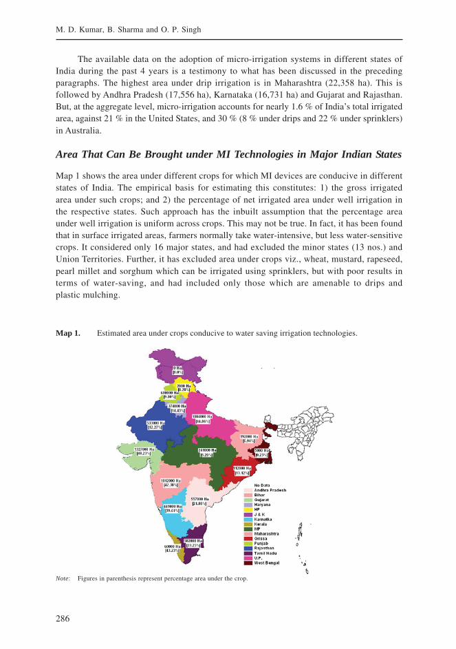
286
M. D. Kumar, B. Sharma and O. P. Singh
The available data on the adoption of micro-irrigation systems in different states ofIndia during the past 4 years is a testimony to what has been discussed in the precedingparagraphs. The highest area under drip irrigation is in Maharashtra (22,358 ha). This isfollowed by Andhra Pradesh (17,556 ha), Karnataka (16,731 ha) and Gujarat and Rajasthan.But, at the aggregate level, micro-irrigation accounts for nearly 1.6 % of India’s total irrigatedarea, against 21 % in the United States, and 30 % (8 % under drips and 22 % under sprinklers)in Australia.
Area That Can Be Brought under MI Technologies in Major Indian States
Map 1 shows the area under different crops for which MI devices are conducive in differentstates of India. The empirical basis for estimating this constitutes: 1) the gross irrigatedarea under such crops; and 2) the percentage of net irrigated area under well irrigation inthe respective states. Such approach has the inbuilt assumption that the percentage areaunder well irrigation is uniform across crops. This may not be true. In fact, it has been foundthat in surface irrigated areas, farmers normally take water-intensive, but less water-sensitivecrops. It considered only 16 major states, and had excluded the minor states (13 nos.) andUnion Territories. Further, it has excluded area under crops viz., wheat, mustard, rapeseed,pearl millet and sorghum which can be irrigated using sprinklers, but with poor results interms of water-saving, and had included only those which are amenable to drips andplastic mulching.
Map 1. Estimated area under crops conducive to water saving irrigation technologies.
Note: Figures in parenthesis represent percentage area under the crop.
287
Water Saving and Yield Enhancing Micro-irrigation Technologies: How Far Can They Contribute toWater Productivity in Indian Agriculture?
It shows that Uttar Pradesh has the largest area (1.884 M ha) under crops amenable toWSTs. It is followed by Gujarat with 1.327 M ha, and Maharashtra with 1.012 M ha.
Basins and Cropped Area Conducive to Adoption of Micro-irrigationTechnologies
In order to estimate the figures for the ‘total irrigated cropped area that would benefit from MIsystems’, we have superimposed the cropped areas for which MI systems are conducive, andthe basins where MI adoption would lead to real water saving, and water productivityimprovements. We would explain the logic behind this.
The earlier analysis has shown that peninsular and western India had a substantial areaunder crops that are conducive to MI technologies. It has also shown that central and northIndia have very little area under such crops. The exception is Uttar Pradesh, which accountsfor nearly 25 % of the area that is conducive to MI systems. The basins in peninsular, westernand central India have favorable natural environment comprising soil, geo-hydrology andclimate due to which MI system adoption can actually result in real water saving, and basinlevel water productivity improvement. But, in Ganga-Brahmaputra basin, in which UP is, theadoption is going to be poor due to poor rural electrification; relative water abundance; shallowgroundwater in most areas; and very low size of operational holdings of farmers. Even if thisregion adopts MI systems on a large-scale, it may result not in a reduction in depleted water,but a little difference in crop yields, with the resultant increase in basin level water productivitybeing meager. The western part of Mahanadi is another area that would be conducive to MIsystems. Hence, Ganga-Brahmaputra-Meghna have to be excluded from our analysis.
Hence, the cropped areas that will benefit from MI system would be from: 1) basins ofall east-flowing rivers of peninsular India; 2) basins of west-flowing rivers north of Tapi inGujarat and Rajasthan; Mahanadi; 3) some parts of Indus Basin covering south-western Punjab;and 4) west flowing rivers of South India. Hence, the total would be 5.844 m ha (79.30-20.86)of cropped area. This is the absolute potential, and the real adoption would depend on severalsocioeconomic and institutional factors.
Now, let us look at the area estimates provided by Narayanamoorthy 2004b, and thetask force on MI in India. Narayanamoorthy 2004b provided an estimate of 21.27 m. ha as thenet area under all irrigated crops that can be brought under drip systems in India, with anupper figure of 51.42 m. ha including the area under those crops, which are currently rain-fed.But this analysis did not consider the several physical and socioeconomic factors that wouldultimately determine the viability of drips for these crops. Whereas the task force on MI hadestimated a figure of 69 m. ha as the area suitable for MI systems in India, it is quite clear fromsuch a high figure that the task force estimates had included all regions and the area irrigatedby different types of irrigation systems, therefore, has not considered the physical (technical,and hydro-meteorological), and socioeconomic constraints in the adoption of MI systems.
Quantification of Potential Future Impact of MI Systems on WaterRequirements
In order to analyze the impact of MI devices on aggregate water requirement for crop productionin India, we started with the data provided by INCID and NCAP where data on water use

288
M. D. Kumar, B. Sharma and O. P. Singh
efficiency5 impact of drip irrigation for various crops are presented. A total of six crops, forwhich country-level data on the irrigated crop area are available, were considered for estimatingthe future water-saving benefits. Then the data on aggregate output from these crops areobtained. Assuming that the same output for the respective crops is to be maintained in future,the future water requirement for growing the crops could be estimated by dividing the improvedwater use efficiency figures by the crop output.
The reduction in water requirement for crop i= Present Output of Crop
i [1/Current Water
Productivity -1/Improved Water Productivity]The procedure can be repeated for all crops.While estimating the crop area that is likely to be brought under drips, the area under the
respective crops in water-abundant states viz., UP, Bihar, West Bengal, Haryana and north easternstates was subtracted. The aggregate reduction in crop water requirement due to the adoptionof drip systems was estimated to be 44.46 BCM (Table 1). It can also be seen that the highestwater-saving could come from the use of drips in sugarcane, followed by cotton. This is themaximum area that can be covered under the crops listed in well-irrigated areas, provided all theconstraints facing the adoption are overcome through appropriate institutional and policyenvironments. In the subsequent section, we would discuss what these policies are.
Table 1. Aggregate reduction in water requirement possible with drip irrigation systems.
Sr. no Name of Current yield Expected Water Improved Watercrop (tonnes/ha) yield coming productivity water saving
from the (kg/m3) productivity (BCM)potential (kg/m3)states*
(million tonnes)
1 Sugarcane 128.0 170.0 5.950 18.09 31.00
2 Cotton 2.600 4.391 0.303 1.080 10.42
3 Groundnut 1.710 2.840 0.340 0.950 1.453
4 Potato 23.57 34.47 11.79 17.21 0.127
5 Castor 1.260 1.350 0.340 0.670 0.497
6 Onion 9.300 12.20 1.544 2.700 0.963
7 Total 44.46
Note: * States where MI systems are likely to be adopted. This is obtained by multiplying the average crop yield underconventional irrigation with the sum of the estimated area under that crop in each state. The water productivity figuresare estimated from the yield and water consumption figures provided for the respective crops in INCID 1994 and NCPA1990 as cited in Narayanamoorthy 2004b: pp 122.
5 We treat these water productivity values as the modified values of WUE capturing the net effect ofimproved water application and improved agronomic practices.
289
Water Saving and Yield Enhancing Micro-irrigation Technologies: How Far Can They Contribute toWater Productivity in Indian Agriculture?
Institutional and Policy Alternatives for Spreading Micro-irrigationTechnologies
The most ideal policy environment for the promotion of MI technologies in well-irrigated areaswould be pro-rata pricing of electricity. While this would create direct incentive for efficientwater use (Kumar 2005), the extent to which MI technologies would reduce energy use resultingin pro-rata pricing creating incentive for the adoption of MI devices depends on the crop typeand the type of technology—whether pressurized system or gravity drip system—used forthe crop. The reason is not all MI technologies are energy-efficient. Hence, bringing non-conventional (non-pressurized) drip systems under the ambit of subsidies is very important,once pro-rata pricing of electricity is introduced. It would also force farmers in areas irrigatedby diesel engines to adopt such MI systems as it could save diesel and reduce input costs.
While in the long run, total metering and consumption-based pricing would be the mostdesired scenario to emerge (Kumar 2007), the government can start with metering of agriculturalconsumption. Cash incentives or heavy subsidy for MI devices could be provided to farmerswho are willing to use them, subject to their minimizing the consumption of electricity. Thiscash incentive could be an inverse function of the total energy use for irrigation, and thepercentage area under MI technology. This would create incentives for farmers to maximizethe coverage of MI systems in their irrigated crops, particularly those which are less energy-intensive; and limit the total irrigated area.
Improving power supply conditions—both quality of power and hours of supply—isextremely important for boosting the adoption of pressurized MI devices in many areas. Suchareas include alluvial North Gujarat and south-western Punjab. One could argue that withimproved power supply, groundwater use could go up. But, in reality, with improved hours ofpower supply, the quality of irrigation would go up, enabling farmers to realize the full potentialof MI systems. The actual impact of improved power supply regime on sustainability woulddepend on the type of crops farmers grow with MI systems, and the availability of extra landfor area expansion. In areas where the entire cultivable land is under irrigation as in the tubewellcommands of North Gujarat, and alluvial areas of central Punjab, the adoption of MI deviceswould result in reducing groundwater use at the farm level. MI adoption could result in farmersexpanding the area under irrigation. Subsidies are required here to promote MI adoption as itwould lead to social benefits from reduced stress on groundwater.
Improving the administration of subsidies is also of paramount importance to increasethe welfare impacts. The farmers should be made to pay the full cost of the system initially,and subsidies released paid in installments based on periodic review of system performance.As manufacturers have to sell the system at the market price, it would compel them to improvethe competitiveness of their products, and also provide good technical input services so as tosustain the demand. The rural credit institutions can advance loans to farmers for the purchaseof MI systems so as to maximize the coverage of small and marginal farmers. In Gujarat, a newmodel for promoting MI devices is being implemented by the state government through a state-owned company called Gujarat Green Revolution Company (GGRC). Under this model, thesubsidy is paid by GGRC to the farmer in installments, and the results are very encouraging.Not only that the adoption of MI devices is fast, but a significant percentage of the adoptersbelongs to smallholder category, having less than 2.0 ha of land, and they use it for cashcrops viz., cotton, ground nut, potato and vegetables.
290
M. D. Kumar, B. Sharma and O. P. Singh
On the other hand, there is a need for creating a separate agency for promoting MI ineach state to increase the speed of processing of application from farmers. The agency canwork in tandem with the manufacturers and farmers to enable timely technical inputs to thefarmers. In areas where agricultural processing units are concentrated, provision of all criticalinputs including subsidies would not be a problem, as they could come from these processingunits. An example is the sugarcane and grape grower cooperatives of Maharashtra. But, inareas where demand for drip irrigation is scattered vis-à-vis crops and geographical spread,this would be an issue. This substantiates the need for a separate agency. The agency shouldfacilitate the survey of farmers’ fields by the manufacturer, and get the designs and estimatesprepared along with the most desirable cropping system. This would also help farmers procurethe system well in advance of the crop season to make full benefit of it. Within a year after thecreation of GGRC, a total of 30,000 ha of crop land had already been brought under drips inthe state.
Summing Up
The adoption of MI systems is likely to pick up fast in arid and semi-arid, well-irrigated areas,where farmers have independent irrigation sources, and where groundwater is scarce. Further,high-average land-holdings, large size of individual plots, and a cropping system dominatedby widely spaced row crops, which are also high-valued, would provide the ideal environmentfor the same. The extent of real water-saving and water productivity improvements at the fieldlevel through the adoption of MI systems would be high for widely spaced row crops, in aridand semi-arid conditions, when the groundwater table is deep or aquifer is saline. In hard-rockareas with poor groundwater potential, MI adoption would result in improved efficiency ofwater use, but would not reduce the total groundwater draft.
In semi-arid and arid areas which face severe groundwater scarcity, the economics ofMI systems would be sound for high-valued cash crops. In areas where electricity chargesare not based on power consumption, and the opportunity cost of using water is zero, thesaving in energy and water achieved through MI system does not get translated into economicbenefits. Hence, economics of MI system will not be sound in such areas. But, the evaluationstudies are skewed towards drip systems, and do not capture the effect of changing physical,socioeconomic and institutional settings on the economic dynamic.
The future potential of MI systems in improving basin level water productivity isprimarily constrained by the physical characteristics of basins vis-à-vis the opportunitiesthey provide for real water-saving at the field level, and area under crops that are conduciveto MI systems in those basins. Preliminary analysis shows very modest potential of MIsystems to the tune of 5.69 m ha, with an aggregate impact on crop water requirement to thetune of 43.35 BCM possible with drip adoption for six selected crops. Creating appropriateinstitutions for extension, designing water and electricity pricing policies apart from buildingproper irrigation and power supply infrastructure would play a crucial role in facilitatinglarge-scale adoption of different MI systems. The subsidies for MI promotion should betargeted at regions and technologies, where MI adoption results in real water and energysaving at the aggregate level.
291
Water Saving and Yield Enhancing Micro-irrigation Technologies: How Far Can They Contribute toWater Productivity in Indian Agriculture?
References
Ahmad, M. D.; Masih, I.; Turral, H. 2004. Diagnostic analysis of spatial and temporal variations in cropwater productivity: A field scale analysis of the rice-wheat cropping system of Punjab, Pakistan. Journalof Applied Irrigation Science, 39 (10).
Allen, R. G.; Willardson, L. S.; Frederiksen, H. 1998. Water Use Definitions and Their Use for Assessingthe Impacts of Water Conservation. Proceedings, ICID Workshop on Sustainable Irrigation in Areas ofWater Scarcity and Drought. ed. de Jager, J. M.; Vermes, L. P.; Rageb, R. Oxford, England, September11-12, pp 72-82.
Amarasinghe, U.; Bharat, R.; Sharma, N. A.; Christopher, S.; Smakhtin, V.; de Fraiture, C.; Sinha, A. K.;Shukla, A. K. 2004. Spatial Variation in Water Supply and Demand across River Basins of India IWMIResearch Report 83, Colombo, Sri Lanka.
Barker, R.; Dawe, D.; Inocencio, A. 2003. Economics of Water Productivity in Managing Water forAgriculture. In Water Productivity in Agriculture: Limits and Opportunities for Improvement. ed. Kijne,J. W.; Molden, D.; Barker, R. Comprehensive Assessment of Water Management in Agriculture. UK:CABI Publishing in Association with International Water Management Institute.
Carter, R.; Kay, M.; Weatherhead, K. 1999. Water Losses in Smallholder Irrigation Schemes, AgriculturalWater Management, 40 (1): 15-24.
Deepak, M. R.; Narumalani, S.; Rundquist, D.; Lawson, M. 2005. Water Demand Management: A Strategyto Deal with Water Scarcity. Paper presented at the 4th Annual Partners’ Meet of IWMI-Tata WaterPolicy Research Programme, February.
Dhawan, B. D. 2000. Drip Irrigation: Evaluating Returns. Economic and Political Weekly, pp 3775-3780,October 14.
GOI 1994. Drip irrigation in India, Indian National Committee on Irrigation and Drainage, Ministry ofWater Resources, Government of India, New Delhi.
GOI 1999. Integrated Water Resource Development. A Plan for Action. Report of the National Commissionon Integrated Water Resources Development, Volume I, Ministry of Water Resources.
GOI 2002. Annual Report (2001-02) of the Working of State Electricity Boards and Electricity Departments2001-2002. Planning Commission-Power & Energy Division, May 2002.
INCID 1994. Drip Irrigation in India. Indian National Committee on Irrigation and Drainage, New Delhi.
Keller, A.; Keller, J.; Seckler, D. 1996. Integrated Water Resources Systems: Theory and Policy Implications.Research Report 3, Colombo: International Water Management Institute.
Kijne, J.; Barker R.; Molden, D. (ed.) 2003. Improving Water Productivity in Agriculture: Editors’ Overview.In Water Productivity in Agriculture: Limits and Opportunities for Improvement, ComprehensiveAssessment of Water Management in Agriculture. UK: CABI Publishing in Association with InternationalWater Management Institute.
Kumar, M. D. 2003a. Food Security and Sustainable Agriculture in India: The Water Management Challenge.Paper presented at the 2nd Annual Partners’ meet of IWMI-TATA Water Policy research programme,January 27-29.
Kumar, M. D. 2003b. Micro Management of Groundwater in North Gujarat, Water Policy Research Highlight# 5: IWMI-Tata Water Policy Programme, Anand.
Kumar, M. D. 2005. Impact of Electricity Prices and Volumetric Water Allocation on Groundwater DemandManagement: Analysis from Western India. Energy Policy, 33 (1).
Kumar, M. D. 2007. Groundwater Management in India: Physical, Institutional and Policy Alternatives,New Delhi: Sage Publications.
292
M. D. Kumar, B. Sharma and O. P. Singh
Kumar, M. D.; Singh, O. P. 2001. Market Instruments for Demand Management in the Face of Scarcityand Overuse of Water in Gujarat, Western India. Water Policy, 5 (3): 387-403.
Kumar, M. D.; Shah, T.; Bhatt, M.; Kapadia, M. 2004. Dripping Water to a Water Guzzler: Techno-economic Evaluation of Efficiency of Drip Irrigation in Alfalfa, India. Paper presented at the 2nd
International Conference of the Asia Pacific Association of Hydrology and Water Resources (APHW2004), Singapore, July 5-9.
Kumar, M. D.; Singh, K.; Singh, O. P.; Shiyani, R. L. 2004. Impacts of Water Saving and Energy SavingIrrigation Technologies in Gujarat. Research Report 2, India Natural Resources Economics andManagement Foundation, Anand.
Kumar, M. D.; Singh, O. P. 2007. Groundwater Management in India: Physical, Institutional and PolicyAlternatives. New Delhi: Sage Publications.
Molden, D.; Sakthivadivel, R.; Habib, Z. 2001. Basin-Level Use and Productivity of Water: Examples fromSouth Asia. IWMI Research Report 49, Colombo: International Water Management Institute.
Narayanamoorthy, A. 1997. Economic Viability of Drip Irrigation: An Empirical Analysis from Maharashtra.Indian Journal of Agricultural Economics. October-December, 52 (4), pp. 728-739.
Narayanamoorthy, A. 2004a. Impact Assessment of Drip Irrigation in India: The Case of Sugarcane.Development Policy Review, 22 (4): 443-462.
Narayanamoorthy, A. 2004b. Drip irrigation in India: can it solve water scarcity? Water Policy, 6 (2004):117-130.
NCPA 1990. Status, Potential and Approach for Adoption of Drip and Sprinkler Irrigation Systems. NationalCommittee on the Use of Plastics in Agriculture, Pune, India.
Palanichamy, N. V.; Palanisamy, K.; Shanmugam, T. R. 2002. Economic performance of drip irrigation incoconut farmers in Coimbatore. Agricultural Economics Research Review, Conference Issue, pp. 40-48.
Shiyani, R. L.; Kuchhadiya, D. B.; Patat, M. V. 1999. Economic impact of drip irrigation technology oncotton growers of Saurashtra region. Agricultural Situation in India, 56 (7): 407-412.
Sivanappan, K. V. 1994. Prospects of Micro-irrigation in India. Irrigation and Drainage Systems, 8 (1),pp 49-58.
Todd, D. K. 2003. Groundwater Hydrology, Second Edition. Singapore: John Wiley and Sons (Asia)Pte Ltd.
Verma; Shilp; Stephaine; Jose 2005. Pepsee Systems: Farmer Innovations under Groundwater Stress.Water Policy.
293
Water Saving and Yield Enhancing Micro-irrigation Technologies: How Far Can They Contribute toWater Productivity in Indian Agriculture?
An Assessment of Environmental Flow Requirements ofIndian River Basins
V. Smakhtin and M. AnputhasInternational Water Management Institute, Colombo, Sri Lanka.
Introduction
India faces a number of water related challenges, including increasing water scarcity andcompetition for water between different sectors and states. Some of the river basins in thesouthern and western states are experiencing physical or economic water scarcity. Basins inthe east of the country are often perceived as having ‘surplus’ water and encounter recurrentfloods. The National River Linking Project (NRLP) has been proposed as the solution towater related problems in India. The NRLP envisages transferring flood water of the Ganga,Brahmaputra and Meghna Rivers to the water scarce basins in the south and west (e.g.,http://www.riverlinks.nic.in/). However, the NRLP is a contentious issue in Indian society,the media and amongst academics (e.g., Jain et al. 2005). Many scholars argue that the needsassessment of NRLP is inadequate. Others are of the view that the assessment of watersurplus/deficits in Indian river basins, conducted as part of the NRLP proposal, has ignoredenvironmental issues. Yet, others think that the very definition of “surplus water” needs tobe clarified and that alternative water management options - less costly, easier to implementand more environmentally acceptable - have not been considered (e.g., Vaidyanathan 2003;http://www.lk.iwmi.org/nrlp/main; http://www.sdnpbd.org/river_basin/). Indeed, noassessment of ecological impacts of the future developments of water resources in the countryseems to exist.
In India, as elsewhere in the world, freshwater and freshwater-dependent ecosystemsprovide a range of services for humans, including fish, flood protection, wildlife, etc. (e.g.,Postel and Carpenter 1997; Revenga et al. 2000; http://www.maweb.org). To maintain theseservices, water needs to be allocated to ecosystems, as it is allocated to other users likeagriculture, power generation, domestic use and industry. Balancing the requirements of theaquatic environment and other uses is becoming critical in many of the world’s river basins aspopulation and associated water demands increase. India is no exception. On the other hand,the assessment of water requirements of freshwater-dependent ecosystems represents a majorchallenge due to the complexity of physical processes and interactions between thecomponents of the ecosystems. For day-to-day management of particular rivers, environmentalrequirements are often defined as a suite of flow discharges of certain magnitude, timing,
294
V. Smakhtin and M. Anputhas
frequency and duration. These flows ensure a flow regime capable of sustaining a complex setof aquatic habitats and ecosystem processes and are referred to as “environmental flows”,“environmental water requirements”, “environmental flow requirements”, “environmentalwater demand”, etc. (Knights 2002; Lankford 2002; Dyson et al. 2003; Smakhtin et al. 2004a,2004b). Many methods for determining these requirements have emerged in recent years. Theyare known as environmental flow assessments (EFA). The mean annual sum of estimatedenvironmental flows represents a total annual water volume, which could be allocated forenvironmental purposes. In this report, we use the term ‘environmental flows’ (EF) to refer tothe ecologically acceptable flow regime and the term ‘environmental water requirements’ (EWR)to refer to the total annual volume of EF.
The issues of EF assessment and management are high on the world agenda at present.At the same time, it remains a new research field. In many countries, including India, there hasnot even been a crude nationwide assessment of water requirements of rivers and theirassociated aquatic ecosystems. It is prudent to start addressing these issues which, in India,have become particularly relevant in the view of the major inter-basin water transfers plannedunder the NRLP.
This report starts with the description of India’s physiography, water resources and waterresources related problems. It proceeds by reviewing the emerging development of EFphilosophy in India. It then reviews the current status of quick desktop EF estimation methodsin the world and examines the applicability of those in the Indian context. It further formulatesa simple EF assessment method which takes into account the limitations of available informationin the country and illustrates its application using several major Indian river basins as examples.This is followed by recommendations on the immediate next steps in EFA in the context of theNRLP and for a longer-term EF research program.
The study does not intend to give prescriptions for EF estimation in India or elsewhere.It suggests one potentially useful technique, which needs further development with moreinput from Indian hydrologists, aquatic ecologists, water engineers and other relevantspecialists. The primary purpose of this work is therefore to stimulate the debate about EFAin India. It should be seen as a step towards the development of more detailed andcomprehensive future national EF tools and policies and towards building the nationalcapacity in the field of EFA. This study is a small component of a larger and longer-termresearch project which aims to assess multiple aspects of NRLP and the future of India’swater resources in general.
Rivers in India
Hydrography
India has a large network of rivers, all of which are characterized by very large seasonalvariation in their discharge due to seasonal rainfall and prolonged dry periods. The Indianmainland is drained by 15 major (drainage basin area >20,000 square kilometers [km2]), 45medium (2,000 to 20,000 km2) and over 120 minor (<2,000 km2) rivers, besides numerousephemeral streams in the western arid region (Rao 1975). These river systems are traditionally

295
An Assessment of Environmental Flow Requirements of Indian River Basins
grouped, according to their origin - into Himalayan and Peninsular rivers, or according tothe direction of flow - into east flowing and west flowing rivers (NCIWRDP 1999;Amarasinghe et al. 2005). For large-scale analyses of water resources, the country is oftenseparated into some 19 major river basins/drainage regions, which are shown in figure 1(Amarasinghe et al. 2005). The main characteristics of these 19 river basins/drainage regionsare given in Table 1.
Figure 1. A map of India, showing the boundaries of the major river basins/drainage regions and states.
Source:Amarasinghe et al. 2005
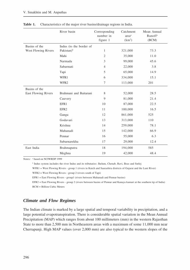
296
V. Smakhtin and M. Anputhas
Climate and Flow Regimes
The Indian climate is marked by a large spatial and temporal variability in precipitation, and alarge potential evapotranspiration. There is considerable spatial variation in the Mean AnnualPrecipitation (MAP) which ranges from about 100 millimeters (mm) in the western RajasthanState to more than 2,500 mm in Northeastern areas with a maximum of some 11,000 mm nearCherrapunji. High MAP values (over 2,000 mm) are also typical to the western slopes of the
Table 1. Characteristics of the major river basins/drainage regions in India.
River basin Corresponding Catchment Mean Annualnumber in areaa Runoffa
figure 1 (km2) (BCM)
Basins of the Indus (to the border ofWest Flowing Rivers Pakistan)b 1 321,000 73.3
Mahi 2 35,000 11.0
Narmada 3 99,000 45.6
Sabarmati 4 22,000 3.8
Tapi 5 65,000 14.9
WFR1 6 334,000 15.1
WFR2 7 113,000 201
Basins of theEast Flowing Rivers Brahmani and Baitarani 8 52,000 28.5
Cauvery 9 81,000 21.4
EFR1 10 87,000 22.5
EFR2 11 100,000 16.5
Ganga 12 861,000 525
Godavari 13 313,000 110
Krishna 14 259,000 78.1
Mahanadi 15 142,000 66.9
Pennar 16 55,000 6.3
Subarnarekha 17 29,000 12.4
East India Brahmaputra 18 194,000 585
Meghna 19 42,000 48.4
Notes: a based on NCIWRDP 1999
b Indus system includes the river Indus and its tributaries: Jhelum, Chenab, Ravi, Beas and Sutlej
WFR1 = West Flowing Rivers - group 1 (rivers in Kutch and Saurashtra districts of Gujarat and the Luni River)
WFR2 = West Flowing Rivers - group 2 (rivers south of Tapi)
EFR1 = East Flowing Rivers - group1 (rivers between Mahanadi and Pennar basins)
EFR2 = East Flowing Rivers - group 2 (rivers between basins of Pennar and Kanaya kumari at the southern tip of India)
BCM = Billion Cubic Meters
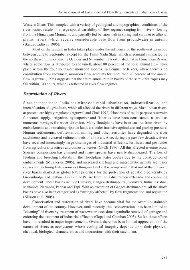
297
An Assessment of Environmental Flow Requirements of Indian River Basins
Western Ghats. This, coupled with a variety of geological and topographical conditions of theriver basins, results in a large spatial variability of flow regimes ranging from rivers flowingfrom the Himalayan Mountains and partially fed by snowmelt in spring and summer to alluvialplains’ rivers, which receive considerable base flow from groundwater in autumn(Bandyopadhyay 1995).
Most of the rainfall in India takes place under the influence of the southwest monsoonbetween June to September except for the Tamil Nadu State, which is primarily impacted bythe northeast monsoon during October and November. It is estimated that in Himalayan Rivers,where some flow is attributed to snowmelt, about 80 percent of the total annual flow takesplace within the four southwest monsoon months. In Peninsular Rivers, where there is nocontribution from snowmelt, monsoon flow accounts for more than 90 percent of the annualflow. Agrawal (1998) suggests that the entire annual rain in basins of the semi-arid tropics mayfall within 100 hours, which is reflected in river flow regimes.
Degradation of Rivers
Since independence, India has witnessed rapid urbanization, industrialization, andintensification of agriculture, which all affected the rivers in different ways. Most Indian rivers,at present, are highly regulated (Agrawal and Chak 1991). Hundreds of multi-purpose reservoirsfor water supply, irrigation, hydropower and fisheries have been constructed, as well asnumerous barrages for water diversion. Many floodplains have been cut out from rivers byembankments and remaining riparian lands are under intensive agriculture and grazing pressure.Human settlements, deforestation, mining and other activities have degraded the rivercatchments and increased sediment loads of all rivers. Also, during the past few decades, rivershave received increasingly large discharges of industrial effluents, fertilizers and pesticidesfrom agricultural practices and domestic wastes (CPCB 1996). All this affected riverine biota.Species composition has changed and many species have nearly disappeared. The loss offeeding and breeding habitats in the floodplain water bodies due to the construction ofembankments (Mukherjee 2005), and increased silt load and macrophytic growth are majorcauses for declining fish resources (Jhingran 1991). It is symptomatic that out of the 30 worldriver basins marked as global level priorities for the protection of aquatic biodiversity byGroombridge and Jenkins (1998), nine (9) are from India due to their extensive and continuingdevelopment. These basins include Cauvery, Ganges-Brahmaputra, Godavari, Indus, Krishna,Mahanadi, Narmada, Pennar and Tapi. With an exception of Ganges-Brahmaputra, all the abovebasins have also been categorized as “strongly affected” by flow fragmentation and regulation(Nilsson et al. 2005).
Conservation and restoration of rivers have become vital for the overall sustainabledevelopment of the country. However, until recently, this “conservation” has been limited to“cleaning” of rivers by treatment of wastewater, occasional symbolic removal of garbage andenforcing the treatment of industrial effluents (Gopal and Chauhan 2003). So far, these effortshave not resulted in major improvements. Overall, there has been limited appreciation of thenature of rivers as ecosystems whose ecological integrity depends upon their physical,chemical, biological characteristics and interactions with their catchment.

298
V. Smakhtin and M. Anputhas
Environmental Flows in the Indian Context
Development of Environmental Flow Philosophy
As in much of the world, Indian water planning and management considered water flowing tothe sea as ‘wasted’. The approach was to harness river waters through dams and otherstructures to the extent that was technically feasible. Even the new National Water Policy(MOWR 2002) still ranks “ecology” as the fourth item in the list of priorities for water-allocation.As the progressive degradation of the water environment became evident, environmentalconcerns have started to gain strength. This is, perhaps, where and when the term ‘minimumflow’ originated from. Minimum flow was understood as a flow, which is needed (to be released)downstream from the dams for environmental maintenance. As the term implies, such releaseswere minimal. In fact, there is no documented evidence suggesting that such releases wereactually made.
The first National Workshop on Environmental Flows, held in New Delhi in March 2005,brought together over 60 participants from national agencies and research institutions andhighlighted a great interest in the concept of environmental flows in India. Several relevantstudies and activities currently conducted in the country have been presented and the issuesof terminology were high on the agenda.
Iyer (2005) suggested that expressions such as “environmental flows” or “water fornature” imply that in allocating water for different uses, an allocation must be made “fornature as well”. This may be seen as inappropriate in principle because “water itself is partof nature and one cannot presume to allocate water to nature”. Therefore, aquatic ecologyshould be seen as a user of the highest priority. Ecological considerations may imposeconstraints on other uses of water and ecological imperatives must guide the water-use andwater resources development of the future. Iyer (2005) further pointed out that while theidea of a “minimum flow” or “environmental flows” in streams and rivers is welcome in sofar as some flow is better than no flow, this may not necessarily imply any major change inthinking; abstractions and diversions continue to be the norm and “minimum flow” clearlyimplies maximum abstraction. If “environmental flow” is understood as a synonym of“minimum”, then the only change is in semantics. He further suggested that impacts on riversare quantified against a reference condition of “natural flow”, which, for all practical purposescould be accepted as the flow which existed prior to major river regulation. Most of theabove statements are similar to that of Silk et al. (2000) or to the philosophy adopted inSouth Africa, for the protection of aquatic ecosystems, whereby EF – known as ‘ecologicalReserve’ - are estimated for a water body first. Then only the difference between the totalavailable water resource (natural flow) and the Reserve is considered to be utilizable. Suchschool of thought represents a very pro-environment position and is unlikely to succeed, inthe short-term, in a country without strong pro-environmental traditions and practices inthe conditions of increasing water scarcity.
Iyer (2005) also advocated the importance of distinguishing between in-stream flowsfor different purposes: “Flows are needed for maintaining the river regime, making it possiblefor the river to purify itself, sustaining aquatic life and vegetation, recharging groundwater,supporting livelihoods, facilitating navigation, preserving estuarine conditions, preventingthe incursion of salinity, and enabling the river to play its role in the cultural and spiritual
299
An Assessment of Environmental Flow Requirements of Indian River Basins
lives of the people.” The latter appears to be a very important component in the Indiancontext (Sharma 2005), as water is necessary, amongst others, for cultural festivals andreduced flows can lead to depreciation of some religious places (e.g., Sinha and Prasad 2005).While several in-stream flow needs listed above can be satisfied by the same flow at theright time simultaneously, it appears important to agree on what ‘ecological flows’ or‘environmental flows’ actually include. Mohile and Gupta (2005) suggested that requirementsfor drinking water, commercial fisheries, livelihoods and navigation as well as water fordilution of effluents are not included as part of EF, but rather considered as water for people,livelihoods and industries and estimated separately. As for effluents, they should be treatedat source.
Mohile and Gupta (2005) also examined a wider concept of environmental waterrequirements and suggested that it should include the requirements of both terrestrial andaquatic ecosystems. The former would include direct evapotranspiration through forests,wetlands and other lands, all supporting distinct ecologies, while the latter would then beunderstood as EF. This is an interesting view given first, that the requirements of terrestrialecosystems are currently not explicitly considered, and, second, that at present the‘environmental flow requirements’ and ‘environmental water requirements’ are normally takenas synonyms (except rare cases when EWR is used to denote the total volume of EF (e.g.,Smakhtin et al. 2004a)). At the same time, expanding the term EWR beyond the requirementsof aquatic ecosystems will only add confusion to the already existing terminology. The issuesof water requirements of terrestrial ecosystems are not considered in this report.
Previous Environmental Flow Assessment Work and Related Activities
The status of EF research in India at present may be characterized as being in its infancy. TheNational Commission for Integrated Water Resource Development Plan (NCIWRDP 1999)effectively accepted that it was not possible to estimate the amount of water needed forenvironmental purposes. They pointed out that the knowledge base for making any approximatecalculation of this requirement was very limited. A provisional projection of the environmentalneeds has been given as 5 cubic kilometers (km3), 10 km3 and 20 km3 in the years 2010, 2025and 2050, respectively. The reason for such growth is unclear, but less important in the contextof the fact that overall the water requirement for ‘environment and ecology’ has been estimatedat about 2 percent of the total national water requirements. The values given were not referencedto rivers, wetlands or groundwater and were just bulk volumes for the entire country withoutany geographical specification. The NCIWRDP ‘estimates’ do not appear to be based on anyscientific reasoning.
The issue of minimum flow was highlighted in a judgment of the Supreme Court of India,which in 1999 directed the government to ensure a minimum flow of 10 cubic meters per second(m3/s) in the Yamuna River as it flows through New Delhi for improving its water quality. Sincethen the minimum flow requirement in rivers has been discussed at several forums (but primarilyin the context of water quality). In 2001, the Government of India constituted the Water QualityAssessment Authority (WQAA) which in turn constituted, in 2003, a Working Group (WG) toadvise the WQAA on ‘minimum flows in rivers to conserve the ecosystem’. Despite thecontinuous use of the term ‘minimum flow’, the emphasis on ‘ecosystem’ is noteworthy(Prof. B. Gopal, NIE, personal communication). The WG reviewed the existing EFA practice
300
V. Smakhtin and M. Anputhas
and suggested that due to a variety of reasons, including the high hydrological variability,difficult tradeoffs between environment and agriculture, expensive waste treatment, disputesfor water between States, etc., the practices adopted in other countries for assessment of EFare unlikely to be applicable in India. The WG also suggested that only a simple method (likeTennant, see section: Review of Environmental Flow Assessment Methods) may be adoptedfor estimating ‘minimum flows’ to be maintained in the rivers in India. These flows wouldprimarily serve the purpose of maintaining prescribed water quality standards.
Perhaps, the first scientific attempt to assess EF for entire India has recently been donein the report by Amarasinghe et al. (2005). This estimate is based on the global study conductedby Smakhtin et al. (2004a; 2004b) and was made separately for major river basins/drainageregions in India, as shown in figure 1. The estimate turned out to be about 476 km3, whichconstitutes approximately 25 percent of the total renewable water resources in the country.This, however, was not in fact an estimate of EF per se, but rather an estimate of the totalvolume of EF (i.e., EWR). The approach was based on hydrological data simulated by a globalhydrological model, which was not calibrated for Indian conditions. No observed flow datafrom Indian rivers were used and no ecological data were present in the approach, althoughthe hydrological hypotheses used were ecologically based. Also, it was an estimate representingonly one scenario of environmental management – that all major river basins are maintained in“fair” conditions as explained in Smakhtin et al. (2004a).
The known attempts to approach the issue of EF in India (CWC, WG on Minimum Flows;Amarasinghe et al. 2005) addressed it at the scale of the entire country. More detailed, basin-specific EF research has not yet been initiated. One known exception is the project carried outby the National Institute of Hydrology (NIH) at Roorkie aiming at the EFA in the Brahmani-Baitarani River System (Table 1; Figure 1), where a hydrology-based Range of Variability Approachof Richter et al. (1997) (see section: Review of Environmental Flow Assessment Methods) is used.Preliminary recommendations for the Baitarani River have been formulated based on the need tomaintain 7-day minimum and 1-day maximum flows in the river and its water quality within itscurrent state (R. Jha, NIH, Roorkie, personal communication). This and some other EF-relatedactivities in India are yet to be documented.
Review of Environmental Flow Assessment Methods
Basic Principles
‘Environmental Flows’ is a very simple concept. First of all, this term should always be usedin plural, implying that a synonym to environmental flows is an ecologically acceptableflow regime designed to maintain a river in an agreed or predetermined state. Therefore,second, EF are a compromise between water resources development, on one hand, and rivermaintenance in a healthy or at least reasonable condition, on the other. Another useful wayof thinking about EF is that of ‘environmental demand’ similarly to crop water requirements,industrial or domestic water demand. Despite the simplicity of the concept, difficulties arisein the actual estimation of EF values. This is primarily due to the inherent lack of both theunderstanding of and quantitative data on relationships between river flows and multiplecomponents of river ecology.
301
An Assessment of Environmental Flow Requirements of Indian River Basins
Ecologists agree that the major criteria for determining EF should include the maintenanceof both spatial and temporal patterns of river flow, i.e., the flow variability, which affect thestructural and functional diversity of rivers and their floodplains, and which in turn influencethe species diversity of the river (Ward and Tockner 2001; Ward et al. 2001; Knights 2002).Thus, EF should not only encompass the amounts of water needed, but also when and howthis water should be flowing in the river. All components of the hydrological regime have certainecological significance (Knights 2002). High flows of different frequency are important forchannel maintenance, bird breeding, wetland flooding and maintenance of riparian vegetation.Moderate flows may be critical for cycling of organic matter from river banks and for fishmigration, while low flows of different magnitudes are important for algae control, water qualitymaintenance and the use of the river by local people. Therefore, many elements of flowvariability have to be maintained in a modified-EF-regime.
The focus on maintenance of flow variability has several important implications. First, itmoves away from a ‘minimum flow attitude’ to aquatic environment. Second, it effectively considersthat aquatic environment is also ‘held accountable’ and valued similarly to other sectors – toallow informed tradeoffs to be made in water scarcity conditions. Because wetland and riverecosystems are naturally subjected to droughts or low flow periods and can recover from those,then building this variability into the picture of EFA may be seen as environmental water demandmanagement. This brings us back to the issue of ‘compromise’ and implies that EF is a verypragmatic concept: it does not accept a bare minimum, but it is prepared for a trade. Bunn andArthington (2002) have formulated four basic principles that emphasize the role of flow regime instructuring aquatic life and show the link between flow and ecosystem changes:
• Flow is a major determinant of physical habitat in rivers, which in turn is the majordeterminant of biotic composition. Therefore, river flow modifications eventually leadto changes in the composition and diversity of aquatic communities.
• Aquatic species have evolved life history strategies primarily in response to the naturalflow regimes. Therefore, flow regime alterations can lead to loss of biodiversity ofnative species.
• Maintenance of natural patterns of longitudinal and lateral connectivity in river-floodplain systems determine the ability of many aquatic species to move betweenthe river and floodplain or between the main river and its tributaries. Loss oflongitudinal and lateral connectivity can lead to local extinction of species.
• The invasion of exotic and introduced species in rivers is facilitated by the alterationof flow regimes. Inter-basin water transfers may represent a significant mechanismfor the spread of exotic species.
Major Categories of Environmental Flow Assessment Methods
Many EFA methodologies, which directly or indirectly encompass the above principles, haveemerged in recent years. They differ significantly in accuracy and required input information.The discussion of these techniques may be found in many published sources including reviewsby Jowett (1997), Tharme (2003), Acreman and Dunbar (2004) and is not repeated here. DifferentEFA methods should be used for different purposes – from general water resources planningto managing dam releases. In some countries, there is a move towards hierarchical multi-tier
302
V. Smakhtin and M. Anputhas
EFA frameworks, driven by the availability or access to resources, including data, time, technicalcapacity and finances (http://www.dwaf.gov.za; Dyson et al. 2003). The two major tiers include:
• Detailed assessment, using primarily holistic methods, or methods based on habitatmodeling
• Desktop, rapid assessment, using primarily ecologically relevant hydrologicalcharacteristics (indices) or analysis of hydrological time series
Methods from the first group often adopt a whole-ecosystem view in assessing EF,whereby ecologically and/or socially important flow events are identified and an ecologicallyacceptable flow regime is defined by a multi-disciplinary panel of experts. These methodsinclude substantial amounts of field work and may take significant amounts of time (e.g., 2 to3 years for a basin like Krishna – due to the need for ecological data collection at certain timesof the year and the mere size of the basin) and resources to complete for a single river basin(e.g., King and Louw 1998; King et al. 2003). Habitat models, also included in this group aredifferent from holistic methods, as they primarily focus on fish. However, they are very complexand also require a lot of input data and field work. They are used to assess the impacts ofchanging flow regime on physical habitat for key life stages of target fish species. Flow-habitatmodels quantify changes in physical in-channel hydraulic characteristics arising from flowregulation. Hydraulic output is combined with the physical habitat preferences of target species(e.g., Parasiewicz and Dunbar 2001). Both the habitat modeling approach and some holisticmethods (e.g., King et al. 2003) are designed to address trade-offs. They are naturally suitedto scenario analysis and are commonly used where negotiation is a feature of EF setting.
Methods from the second group - desktop EFA - are much more diverse, more suitablefor initial, reconnaissance or planning-level assessments of EF. They can take a form of a look-up table (e.g., Tennant 1976; Matthews and Bao 1991) or be based on the detailed analysis ofhydrological time series (e.g., Richter et al. 1997; Hughes and Hannart 2003). The look-up tablestake a significant amount of time to develop, before they can be used, while the methods basedon the time series naturally require either observed or simulated discharge time series (or both).
The number of available EFA techniques is sometimes grossly overstated (Tharme 2003).Most of them are simple hydrological indices which have existed and been used in varioushydrological and water resources applications for decades. However, the number of ‘genuine’EFA techniques continues to grow thus reflecting the quest for a better technique which suitsthe specifics of a particular task, region, data available, importance of an ecosystem and manyother factors. Any classification of EFA methodologies is, however, rather arbitrary and differentauthors sometimes use different categories to refer to the same method (compare, for example,Dunbar et al. 1996; and Tharme 2003).
Regardless of the type of the EFA methods, all of them have been designed and/or appliedin a developed country context. Distinct gaps in EF knowledge and practice are evident incurrent approaches to water resources management in almost all developing countries, includingIndia, most of which lack technical and institutional capacity to establish environmental waterallocation practices (Tharme and Smakhtin 2003). The existing EFA methods are either complexand resource-intensive (holistic approaches) or not tailor-made for the specific conditions ofa particular country, region or basin (desktop methods).
The above ‘classification’ into comprehensive (detailed) and planning-type (desktop)methodologies, is therefore useful in the context of this study as most of the discussion below

303
An Assessment of Environmental Flow Requirements of Indian River Basins
is focused on the second type - quick desktop EFA methods. The use of such methods maybe seen as the starting point towards the understanding of EF and their importance in principle.While such methods provide estimates of low confidence (due to the lack of ecological datainvolved), they may be used to set the feasible limits for future water resource exploitation.Their application may change the still dominant perception about the insignificance ofenvironmental water allocations in river basin planning and about the very nature of suchallocations.
Desktop Environmental Flow Assessment Methods
The first example from this group is the Tennant method, which attempts to separate a priorithe entire range of the Mean Annual Runoff (MAR) at a site of a river into severalecologically relevant ranges. All suggested ranges correspond to different levels of aquatichabitat maintenance or degradation and have been justified by observations in many streamsin the USA. A threshold of 10 percent of the MAR reserved for an aquatic ecosystem wasconsidered to be the lowest limit for EF recommendations (corresponding to severedegradation of a system). Fair/good habitat conditions could be ensured if 35 percent of theMAR is allocated for environmental purposes. Allocations in the range of 60 to 100 percentof the MAR represent an environmental optimum. This technique is still widely used in NorthAmerica (Tharme 2003), but is somewhat outdated by now and is scientifically weak as athreshold selection (% of the MAR) is arbitrary and no flow variability is accounted for.One positive aspect of Tennant is the awareness that 10 % of the MAR may be consideredthe lowest and highly undesirable threshold for EF allocations and that at least some 30 %of the total natural MAR may need to be retained in the river throughout the basin to ensurefair conditions of riverine ecosystems.
Another frequently cited hydrological EFA technique is the Range of Variability Approach(RVA)(Richter et al. 1997), which aims to protect a range of flows in a river. The 32 hydrologicalparameters, which jointly reflect different aspects of flow variability (magnitude, frequency,duration and timing of flows), are estimated from a natural daily flow time series at a site ofinterest. It is further suggested that in a modified (ecologically acceptable) flow regime, all 32parameters should be maintained within the limits of their natural variability. For each parameter,a threshold of one standard deviation from the mean is suggested as a default arbitrary limitfor setting EF targets in the absence of other supporting ecological information.
The RVA may be applied as a desktop EFA tool. It can ensure that sufficient water isavailable for human uses and effectively accepts that the full range of natural streamflowvariability will not be possible to maintain in regulated or otherwise affected river systems.However, despite the relatively advanced nature of the RVA, the number of parameters used init is too large for the level of subjectivity associated with their selection. In addition, manyparameters are either likely to be correlated with each other, or there is little difference betweentheir values. Smakhtin and Shilpakar (2005) justified and illustrated the simplification of thistechnique through a significant reduction of the number of parameters. At the same time, eventhe simplified RVA approach requires a great deal of hydrological data (daily flow time series,which are not readily available - see section: Developing a Prototype Desktop EnvironmentalFlow Assessment Tool) and, ideally, ecological data (for better setting of acceptable thresholdson parameters). It should be possible, for pilot assessment, to use monthly instead of dailyflow data, select a limited number of flow parameter values and develop a stepwise decrement

304
V. Smakhtin and M. Anputhas
procedure for each of these parameters. This could effectively lead to a new, much simplermethod, where all flow parameters are estimated by the same principle and data requirementsare consistent with availability (at least in the Indian context at present).
The environmental water allocation procedures practiced by UK Environment Agency(2001) are known as CAMS (Catchment Abstraction Management Strategies). This allocationis determined through consideration of four elements: (i) physical characterization;(ii) fisheries; (iii) macrophytes; and (iv) macro-invertebrates (e.g., Acreman 2002). Each elementis given a score from 1 to 5 based on its sensitivity to reductions in flow. In terms of physicalcharacterization, rivers with steep gradients and/or wide shallow cross-sections score 5, sinceit is assumed that small reductions in flow result in a relatively large reduction in wettedperimeter. At the other extreme, lowland river reaches that are deep are assumed to be lesssensitive to flow reduction and score 1. Scoring for fisheries is determined either by flow-habitat modeling, or by using expert opinion to classify the river according to description ofeach of the score classes. Once a score for each of the four elements has been defined, thescores are combined to categorize the river into one of the five environmental weighting Bands,where Band A is the most sensitive (mean score of 5) and Band E is the least sensitive (meanscore of 1).
The next stage in CAMS is the definition of a target flow duration curve (FDC) thatguides the setting of limits on abstraction (Petts 1996). First, a naturalized FDC is produced,either by a deterministic process of adding abstractions and subtracting discharges from arecorded flow time-series or by a regional steady-state model based on catchment characteristics(area, geology) and climate. A set of simple tabulated rules is then used to determine thepercentage of natural low flow that can be abstracted, depending on the environmental Bandsdefined above. A low flow is defined as the flow exceeded 95 % of the time (95 percentile onthe FDC). Rules for determining percentage of allowable abstractions at other flow percentilesat FDC are also provided. In this way, an entire target environmental FDC can be derived.The output figures are based largely on professional judgment of specialists, since criticallevels have not been defined directly by scientific studies at present. Any such figures areopen to revision, but with no clear alternative, this provides a pragmatic way forward. Theentire procedure provides a first level estimate and any catchment may then be subjected toa more detailed analysis using habitat simulation models or other, more detailed methods(Parasiewicz and Dunbar 2001; Extence et al. 1999). This is effectively, an example of a two-tier approach mentioned earlier.
Perhaps the most advanced existing hydrology-based desktop EFA method has beendeveloped by Hughes and Münster (2000) and further refined by Hughes and Hannart (2003).It is known as the ‘Desktop Reserve Model’ (DRM). The ‘ecological Reserve for rivers’ iseffectively a South African term for ‘environmental flows’ (there are also procedures developedfor the determination of ecological reserve for wetlands, estuaries and aquifers). Quantifyingthe ecological Reserve involves determining the volumes and discharges which will sustain ariver in a predetermined condition. The latter is referred to as an ‘Ecological ManagementCategory’ (or Class) – EMC (or, more recently, ‘Level of Ecological Protection’ - LEP) and isrelated to the extent to which this condition deviates from the natural. There are four LEPs -A, B, C, and D - where A rivers are largely natural and D are largely modified. These categoriesare determined by a sophisticated scoring system based on a number of indicators related toriver importance and sensitivity.
305
An Assessment of Environmental Flow Requirements of Indian River Basins
The DRM originates from the Building Block Methodology (BBM) (King and Louw 1998).‘Building Blocks’ (BBs) are environmental flows, which jointly comprise the ecologicallyacceptable, modified flow regime. The major BBs are low flows, small increases in flow (‘freshes’)and larger high flows, which are required for floodplain flooding and for river channelmaintenance. BBs are defined for each of the 12 calendar months and differ between ‘normalyears’ and ‘drought years’. The first are referred to as ‘maintenance requirements’ and thesecond as ‘drought requirements’. The set of BBs, therefore, include maintenance low flows,maintenance high flows, drought low flows and drought high flows.
The DRM uses similar BBs and was developed as a rapid, low confidence EFA approach.The basis for the model was an extrapolation of higher confidence EWR determinations (withspecialist inputs from ecologists and geomorphologists) using the hydrological characteristicsof the river flow regimes. Hughes and Münster (2000) analyzed the results of previouscomprehensive EFAs of South African rivers in the context of hydrological variability of theserivers, and developed empirical equations which related the above BBs with flow variabilityand EMCs (Hughes and Münster 2000). The main variability characteristic - hydrologicalvariability index - is calculated from the coefficients of variation (standard deviation/mean) ofseveral calendar month flows and the baseflow index (baseflow contribution divided by totalflow). The higher the variability index, the more variable is the river flow regime.
The main result of this analysis and the basic assumption of the DRM is that the riverswith more stable flow regimes (a higher proportion of their flow occurring as baseflow) may beexpected to have relatively higher environmental low flow requirements in normal years(‘maintenance low flow requirements’ in Reserve terminology). Rivers with more variable flowregimes would be expected, from a purely hydrological perspective, to have relatively lowermaintenance low flow requirements and/or lower levels of assurance associated with them.The consequence of these assumptions is that the long-term mean EWR would be lower forrivers with more variable flow regimes. The DRM therefore explicitly introduces the principleof ‘assurance of supply’ into EFA. The estimated BBs are then combined into a time series ofEF using a set of assurance rules and the natural flow time series.
The underlying concepts of the DRM are attractive and, to an extent, ecologicallyjustified, as they emerge from the results of comprehensive EFAs, which involve a varietyof ecological disciplines. Smakhtin et al. (2004a, 2004b) have used the principles behind theDRM in their global assessment of EWR. One stumbling block for direct DRM applicationsin other countries (e.g., in India) is that regional DRM parameters have been estimated onthe basis of South African case studies, but are not generally available for other areas.Symphorian et al. (2002) used DRM to study reservoir operation for environmental waterreleases in Zimbabwe, where hydrological conditions are similar to South Africa. The DRMhas recently been tested for several rivers in England (M. Acreman, CEH, personalcommunication) while Smakhtin et al. (2006) attempted to use DRM in Nepal. In both cases,the general conclusion was that the direct application of DRM or any other desktop EFAmethod outside of the region, it was originally developed for, requires recalibration in newconditions. One possible alternative is to simplify the DRM so that the use of regionalparameters can be avoided, while the main principles are retained. One additional advantageof the DRM is that it is originally based on monthly flow data which are more readily availableor accessible in developing countries like India.
306
V. Smakhtin and M. Anputhas
Implications for Future Environmental Flow Assessment in India
There are different ways of developing EF research and environmental water allocation practicesin a country with limited exposure to EF concepts, like India at present. It is possible to developa simple prototype assessment tool which illustrates the main EF concepts and allowspreliminary EFA to be made in real river basins, using available national data. This should alsoallow unsound past practices/concepts (e.g., ‘minimum flow’) to be gradually left behind andfurther development of planning EFA tools to be stimulated, with input from the national eco-hydrological community. This approach would build the EF-related expertise and prepare aground for more comprehensive, detailed and resource intensive EFA in the future.
Alternatively, EF-related capacity can be built through national workshops, which wouldaim to undertake detailed EF studies in specific national river basins and use the expert opinionof local ecologists and hydrologists who know their rivers. Even if this knowledge is not ‘EFtailor made’, and the results are uncertain, attempting such comprehensive EFA develops teambuilding and interactions between experts in different disciplines.
Both approaches are complementary. The very limited time available for the current study,speaks in favour of the first approach, which may also be seen as a stimulus for more EFA tooldevelopment, more comprehensive EFA studies in the future and as a starting point for capacitybuilding in EFA overall.
The above review of desktop EFA methods highlights several important considerationsfor the development of a prototype EFA method for India.
• To sustain ecological processes and associated animal and plant communities in riverfreshwater ecosystems, it is necessary to maintain ecologically relevant elements ofnatural hydrological variability (e.g., frequency, duration, magnitude of some flows,etc.). Therefore, the method has to take flow variability into account.
• The method has to be commensurate with the current level of understanding of riverecology and flow data available. The simpler and less information consuming thebetter at this stage. This allows EF issues to be explicitly highlighted for some ormost of the major river basins in India within a short-term. Given the extreme level ofuncertainty and data limitations in which this study is conducted, the method to bedeveloped should be seen as a ‘rule of thumb’, be as generic as possible to form thebasis for future refinement and application for river basins of various sizes.
• In most of the desktop methods, EF depend upon the category of protection in whicha river ecosystem needs to be maintained. The closer this category to the naturalstate of an ecosystem, the higher the EWR should be and the more elements of naturalflow variability should be preserved. While these categories are simply a managementconcept, it facilitates desktop EFA and allows preliminary EF estimates to be made. Itis therefore logical to design a prototype desktop EFA method so that it relatesflow variability, conservation category and EF.
• As evident from the above review, all existing EFA methods (comprehensive ordesktop) leave a lot to professional judgment or expert opinion, which means thata strong scientific basis is not always present, even in detailed approaches and theyremain essentially subjective. For example, various scoring systems are commonly

307
An Assessment of Environmental Flow Requirements of Indian River Basins
used to determine current ecological status or the desired level of environmentalprotection of a river basin or reach. In the absence of other alternatives this allowsexpert knowledge to be formalized and ‘quantified’ and also brings at least limitedecological information/consideration into the EFA. If existing ecological knowledgeis limited and the scale of the EFA is coarse, aggregate environmental indicators,which reflect different features or conditions of a river basin, could be used forscoring.
Developing a Prototype Desktop Environmental Flow Assessment Tool
Observed Flow Data
One primary aspect associated with the desktop EFA method development and application isthe observed flow data. Due to the need to relate hydrological characteristics to EWR, theavailability, type and quality of observed flow data determines how reliable the EFA method couldbe. Considering that daily flow time series carry much more information about flow variabilityand that monthly flow data can naturally be calculated from daily values, the daily flow timeseries are always the preferred data type. The reality, however, is that almost no daily flow timeseries are publicly available in India, and when the data are made available their quality appearsto be low.
The lack of daily flow data may not be a major problem in itself as some EFA methods(e.g., DRM) successfully work with good quality monthly flow data. The minimum requirementfor desktop EFA application at any site in a river basin is therefore sufficiently long (at least20 years) monthly flow time series reflecting, as much as possible, the pattern of naturalflow variability. However, the availability of monthly flow data in India is also limited. Somemonthly flow time series for Peninsular Rivers (primarily for the last 15-20 years) have beenprovided by the Central Water Commission (CWC) of India. Additional monthly flow data (foryears prior to the 1980s) for several Indian rivers may be downloaded from several websiteson the Internet (these sites also contain data on other world rivers):
(i) http://www-eosdis.ornl.gov/
(ii) http://dss.ucar.edu/catalogs/ranges/range550.html
(iii) http://webworld.unesco.org/water/ihp/db/shiklomanov/index.shtml
(iv) http://grdc.bafg.de/servlet/is/Entry.987.Display/
The data available at these sites for Indian rivers are the same and therefore do not helpto expand the available observed dataset. The origin of these data is also not specificallyindicated but it is most likely that they have been provided by the Indian government to theinternational community in the past in the context of some global water resources assessmentproject(s).
Most of the monthly flow time series available from the Internet are very short (1 to 8years), ending in the early 1980s or late 1970s and with many gaps due to missing data. Theyare therefore largely unsuitable for any meaningful hydrological analysis. The data found on
308
V. Smakhtin and M. Anputhas
the Internet therefore have been considered for use only if the total number of months withoutmissing data was over 120. This allowed stations with a minimum of 10 years of observationsto be included (if they had no missing data), or stations with longer records to be included(even if they still had some missing data). In any case, such selection has been based on anarbitrary minimum, which is effectively below the requirements stipulated above. In summary,over 50 monthly flow time series (acquired from CWC and the Internet) for various river basinswere considered for use. Due to severe data limitations described above, only a few of thosewere finally selected (Table 2).
Simulating Reference Hydrological Conditions at the Outlets of Major Basins
The desktop EFA method suggested and tested in this study is built around a period-of-recordFDC and includes several subsequent steps. The first step is the calculation of a representativeFDC for each site where the EWR are to be calculated. In this study, the sites where EF arecalculated are coincident either with outlets of the major river basins or with the mostdownstream flow observation station. The sites with observed flow data are further oftenreferred to in this report as ‘source’ sites. The sites where reference FDC and time series areneeded for the EF estimation (e.g., basin outlets) are further referred to as ‘destination’ sites.The destination sites are either ungauged or significantly impacted by upstream basindevelopments. Therefore, representative ‘unregulated’ monthly flow time series, orcorresponding aggregated measures of unregulated flow variability, like FDCs, have to besimulated/derived from available observed (source) records.
Any FDC can be represented by a table of flow values (percentiles) covering the entirerange of probabilities of occurrence. All FDCs in this study are represented by a table of flowscorresponding to the 17 fixed percentage points: 0.01, 0.1, 1, 5, 10, 20, 30, 40, 50, 60, 70, 80, 90,95, 99, 99.9 and 99.99 percent. These points (i) ensure that the entire range of flows is adequatelycovered, and (ii) easy to use in the context of the following steps. For all source sites listed intable 2, FDC tables were calculated directly from the observed record or from part of the recordwhich could be considered ‘unregulated’. Normally the earlier part of each record - precedingmajor dams’ construction - was used to ensure that monthly flow variability, captured by theperiod-of-record FDC, is not seriously impacted.
For each destination site, a FDC table was calculated using a source FDC table from eitherthe nearest or the only available observation flow station upstream. To account for land-useimpacts, flow withdrawals, etc., and for the differences between the size of a source and adestination basin, the source FDC is scaled up by the ratio of ‘natural’ long-term mean annualrunoff (MAR) at the outlet and the actual MAR calculated from the source record. The applicationof such ratio effectively ‘naturalizes’ the observed flow source time series and ‘moves’ it to thebasin outlet. The estimates of ‘natural’ MAR for major rivers are available from Indian sources(e.g., Table 1). The estimates of ‘natural’ MAR for smaller basins in India could be obtained bymeans of hydrological regionalization (e.g., Kothyari and Garde 1991; Kothyari 1995).
The scaling up of the curves is effectively equivalent to the scaling of the actual timeseries. It is important to stress that both the calculated FDC and the corresponding time seriesreflect the flow amounts and variability which no longer exist at the outlets of river basins.They are perceived to represent the hydrological reference conditions that existed in the pastprior to major basin developments.

309
An Assessment of Environmental Flow Requirements of Indian River Basins
Tab
le 2
.D
etai
ls o
f se
lect
ed o
bser
ved
mon
thly
flo
w d
ata
sets
.*
Lat
Lon
gR
iver
Loc
atio
nA
rea
Rec
ord
Com
men
tD
D.
DD
.(k
m2 )
Per
iod
deci
mal
deci
mal
26.1
91.7
Bra
hmap
utra
Pan
du40
5,00
019
56-1
979
Mis
sing
dat
a pa
tche
d us
ing
the
mea
n m
onth
ly f
low
. N
o re
cent
dat
a av
aila
ble.
The
enti
re r
ecor
d w
as u
sed
as a
n in
dica
tor
of r
efer
ence
‘na
tura
l’ f
low
var
iabi
lity
.
12.4
76.6
Cau
very
Kri
shna
raj
Sag
ar10
,600
1934
-197
9M
issi
ng d
ata
patc
hed
usin
g th
e m
ean
mon
thly
flo
w.
The
ear
lies
t pa
rt o
f th
ere
cord
(19
34-1
957)
was
use
d as
an
indi
cato
r of
‘na
tura
l’ v
aria
bili
ty.
10.8
78.8
Cau
very
Mus
iri
66,2
4319
90-2
002
An
indi
cato
r of
pre
sent
day
hyd
rolo
gy
24.8
87.9
Gan
gaF
arak
ka95
1,60
019
49-1
973
Mis
sing
dat
a in
196
1-19
64 p
atch
ed.
No
rece
nt d
ata
avai
labl
e. T
he e
ntir
e re
cord
was
use
d as
an
indi
cato
r of
ref
eren
ce ‘
natu
ral’
flo
w v
aria
bili
ty.
16.5
81.5
God
avar
iD
avla
ishw
aram
299,
300
1901
-197
9T
he r
ecor
d w
as u
sed
as a
n in
dica
tor
of r
efer
ence
flo
w v
aria
bili
ty.
N/A
N/A
God
avar
iP
olav
aram
307,
880
1990
-200
5A
n in
dica
tor
of p
rese
nt d
ay h
ydro
logy
16.5
80.6
Kri
shna
Vij
ayaw
ada
251,
360
1901
-200
5T
he e
arli
er p
art
of t
he r
ecor
d (1
901-
1959
) is
use
d as
an
indi
cato
r of
ref
eren
ce‘n
atur
al’
flow
var
iabi
lity
, th
e la
test
– a
s an
ind
icat
or o
f pr
esen
t da
y hy
drol
ogy.
N/A
N/A
Mah
anad
iH
. K
. S
amba
lpur
83,4
0019
26-1
956
The
rec
ord
was
use
d as
an
indi
cato
r of
ref
eren
ce f
low
var
iabi
lity
.
N/A
N/A
Mah
anad
iB
asan
tpur
57,7
8019
90-2
003
An
indi
cato
r of
pre
sent
day
hyd
rolo
gy
22.3
73.0
Mah
iS
eval
ia33
,670
1968
-197
9N
o re
cent
dat
a av
aila
ble.
The
rec
ord
was
use
d as
an
indi
cato
r of
ref
eren
ce f
low
var
iabi
lity.
21.9
73.6
Nar
mad
aG
arud
eshw
ar89
,345
1948
-200
4T
he e
arli
er p
art
of t
he r
ecor
d (1
948-
1970
) w
as u
sed
as a
n in
dica
tor
of r
efer
ence
flow
var
iabi
lity
, th
e la
test
– a
s an
ind
icat
or o
f pr
esen
t da
y hy
drol
ogy.
22.2
76.0
Nar
mad
aM
orta
kka
67,0
0019
48-2
001
The
rec
ord
1980
-200
1 is
an
indi
cato
r of
pre
sent
day
hyd
rolo
gy.
14.6
80.0
Pen
nar
Nel
lore
53,2
9019
65-1
979
No
rece
nt d
ata
avai
labl
e. T
he r
ecor
d w
as u
sed
as a
n in
dica
tor
of r
efer
ence
flo
w v
aria
bilit
y.
21.3
72.9
Tap
iK
atho
re/G
hal
63,3
2519
23-2
004
The
ear
lier
par
t of
the
rec
ord
(193
9-19
79)
was
use
d as
an
indi
cato
r of
ref
eren
cefl
ow v
aria
bili
ty,
the
late
st a
s an
ind
icat
or o
f pr
esen
t da
y hy
drol
ogy.
10.2
76.7
Per
iyar
Pla
ncho
tte
5,38
719
67-1
979
Exa
mpl
e of
a ‘
smal
l’ r
iver
fro
m t
he W
est
Coa
st.
Loc
ated
in
the
sout
h of
the
WF
R2
drai
nage
reg
ion
(tab
le 1
). N
o re
cent
dat
a av
aila
ble.
Rec
ord
is u
sed
as a
n in
dica
tor
ofre
fere
nce
flow
var
iabi
lity
.
23.1
73.4
Sab
arm
ati
Ahm
edab
ad12
,950
1968
-197
9N
o re
cent
dat
a av
aila
ble.
Rec
ord
is u
sed
as a
n in
dica
tor
of r
efer
ence
flo
w v
aria
bili
ty.
23.0
85.0
Sub
arna
rekh
aK
okpa
raN
/A19
64-1
974
No
rece
nt d
ata
avai
labl
e. R
ecor
d is
use
d as
an
indi
cato
r of
ref
eren
ce f
low
var
iabi
lity
.
*Mos
t of
the
dat
a w
ere
used
to
sim
ulat
e re
fere
nce
mon
thly
flo
ws
at t
he u
ngau
ged
basi
n ou
tlet
s w
ith
the
subs
eque
nt E
WR
est
imat
ion
from
sim
ulat
ed t
ime
seri
es.
Sha
ded
row
s sh
ow s
tati
ons
wit
hob
serv
ed d
ata
whi
ch w
ere
used
for
com
pari
son
wit
h es
tim
ated
EW
R.
310
V. Smakhtin and M. Anputhas
Defining Environmental Management Classes
EF aim to maintain an ecosystem in, or upgrade it to, some prescribed or negotiated condition/status also referred to as “desired future state”, “environmental management class”/ “ecologicalmanagement category”, “level of environmental protection”, etc. (e.g., Acreman and Dunbar2004; DWAF 1997). This report uses the term ‘environmental management class’ (EMC). Thehigher the EMC, the more water will need to be allocated for ecosystem maintenance orconservation and more flow variability will need to be preserved.
Ideally, these classes should be based on empirical relationships between flow andecological status/conditions associated with clearly identifiable thresholds. However, so far thereis insufficient evidence for such thresholds (e.g., Beecher 1990; Puckridge et al. 1998). Thesecategories are therefore a management concept, which has been developed and used in the worldbecause of a need to make decisions in the conditions of limited lucid knowledge. As shown inthe review section (see section: Review of Environmental Flow Assessment Methods), placing ariver into a certain EMC is normally accomplished by expert judgment using a scoring system.Alternatively, the EMCs may be used as default ‘scenarios’ of environmental protection andcorresponding EWR and EF - as ‘scenarios’ of environmental water demand.
Six EMCs are used in this study and six corresponding default levels of EWR may bedefined. The set of EMCs (Table 3) is similar to the one described in DWAF (1997). It startswith the unmodified and largely natural conditions (rivers in classes A and B), where no orlimited modification is present or should be allowed from the management perspective. Inmoderately modified river ecosystems (class C rivers), the modifications are such that theygenerally have not (or will not – from the management perspective) affected the ecosystemintegrity. Largely modified ecosystems (class D rivers) correspond to considerable modificationfrom the natural state where the sensitive biota is reduced in numbers and extent. Seriouslyand critically modified ecosystems (classes E and F) are normally in poor conditions wheremost of the ecosystem’s functions and services are lost. Rivers which fall into classes C to Fwould normally be present in densely populated areas with multiple man-induced impacts. Poorecosystem conditions (classes E or F) are sometimes not considered acceptable from themanagement perspective and the management intention is always to “move” such rivers up tothe least acceptable class D through river rehabilitation measures (DWAF 1997). This restrictionis not however applied in this report, primarily because the meaning of every EMC is somewhatarbitrary and needs to be filled with more ecological substance in the future. Some studies usetransitional EMCs (e.g., A/B, B/C, etc.) to allow for more flexibility in EWR determinations. Itcan be noted, however, that ecosystems in class F are likely to be those which have beenmodified beyond rehabilitation to anything approaching a natural condition.
It is possible to estimate EWR corresponding to all or any of the above EMCs and thenconsider which one is best suited/feasible for the river in question, given existing and futurebasin developments. On the other hand, it is possible to use expert judgment and availableecological information in order to place a river into the most probable/achievable EMC. Asevident from the above reviews of EFA methods, this approach is widely practiced. One canthink of an ‘ecological water report card’ for a basin. Such a ‘report card’ could includeanswers to the following three broad questions:
• The first question is: what is the ecological sensitivity and importance of the riverbasin? The rational for this is that the higher the ecological sensitivity and
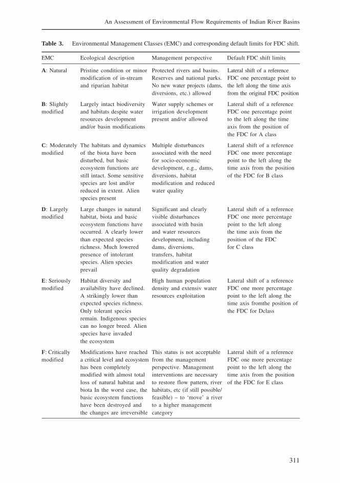
311
An Assessment of Environmental Flow Requirements of Indian River Basins
Table 3. Environmental Management Classes (EMC) and corresponding default limits for FDC shift.
EMC Ecological description Management perspective Default FDC shift limits
A: Natural Pristine condition or minor Protected rivers and basins. Lateral shift of a referencemodification of in-stream Reserves and national parks. FDC one percentage point toand riparian habitat No new water projects (dams, the left along the time axis
diversions, etc.) allowed from the original FDC position
B: Slightly Largely intact biodiversity Water supply schemes or Lateral shift of a referencemodified and habitats despite water irrigation development FDC one percentage point
resources development present and/or allowed to the left along the timeand/or basin modifications axis from the position of
the FDC for A class
C: Moderately The habitats and dynamics Multiple disturbances Lateral shift of a referencemodified of the biota have been associated with the need FDC one more percentage
disturbed, but basic for socio-economic point to the left along theecosystem functions are development, e.g., dams, time axis from the positionstill intact. Some sensitive diversions, habitat of the FDC for B classspecies are lost and/or modification and reducedreduced in extent. Alien water qualityspecies present
D: Largely Large changes in natural Significant and clearly Lateral shift of a referencemodified habitat, biota and basic visible disturbances FDC one more percentage
ecosystem functions have associated with basin point to the left alongoccurred. A clearly lower and water resources the time axis from thethan expected species development, including position of the FDCrichness. Much lowered dams, diversions, for C classpresence of intolerant transfers, habitatspecies. Alien species modification and waterprevail quality degradation
E: Seriously Habitat diversity and High human population Lateral shift of a referencemodified availability have declined. density and extensiv water FDC one more percentage
A strikingly lower than resources exploitation point to the left along theexpected species richness. time axis fromthe position ofOnly tolerant species the FDC for Dclassremain. Indigenous speciescan no longer breed. Alienspecies have invadedthe ecosystem
F: Critically Modifications have reached This status is not acceptable Lateral shift of a referencemodified a critical level and ecosystem from the management FDC one more percentage
has been completely perspective. Management point to the left along themodified with almost total interventions are necessary time axis from the positionloss of natural habitat and to restore flow pattern, river of the FDC for E classbiota In the worst case, the habitats, etc (if still possible/basic ecosystem functions feasible) – to ‘move’ a riverhave been destroyed and to a higher managementthe changes are irreversible category
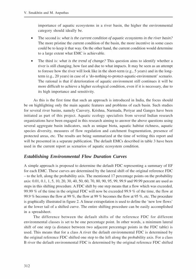
312
V. Smakhtin and M. Anputhas
importance of aquatic ecosystems in a river basin, the higher the environmentalcategory should ideally be.
• The second is: what is the current condition of aquatic ecosystems in the river basin?The more pristine the current condition of the basin, the more incentive in some casescould be to keep it that way. On the other hand, the current condition would determineto a large extent what EMC is achievable.
• The third is: what is the trend of change? This question aims to identify whether ariver is still changing, how fast and due to what impacts. It may be seen as an attemptto foresee how the river will look like in the short-term (e.g., 5 years) and in the long-term (e.g., 20 years) in case of a ‘do-nothing-to-protect-aquatic-environment’ scenario.The rational is that if deterioration of aquatic environment still continues it will bemore difficult to achieve a higher ecological condition, even if it is necessary, due toits high importance and sensitivity.
As this is the first time that such an approach is introduced in India, the focus shouldbe on highlighting only the main aquatic features and problems of each basin. Such studiesfor several river basins, namely Cauvery, Krishna, Narmada, Periyar and Ganges have beeninitiated as part of this project. Aquatic ecology specialists from several Indian researchorganizations have been engaged in this research aiming to answer the above questions usingseveral aggregate basin indicators, such as unique biota, aquatic habitat richness, aquaticspecies diversity, measures of flow regulation and catchment fragmentation, presence ofprotected areas, etc. The results are being summarized at the time of writing this report andwill be presented in a separate publication. The default EMCs described in table 3 have beenused in the current report as scenarios of aquatic ecosystem condition.
Establishing Environmental Flow Duration Curves
A simple approach is proposed to determine the default FDC representing a summary of EFfor each EMC. These curves are determined by the lateral shift of the original reference FDC– to the left, along the probability axis. The mentioned 17 percentage points on the probabilityaxis: 0.01, 0.1, 1, 5, 10, 20, 30, 40, 50, 60, 70, 80, 90, 95, 99, 99.9 and 99.99 percent are used assteps in this shifting procedure. A FDC shift by one step means that a flow which was exceeded,99.99 % of the time in the original FDC will now be exceeded 99.9 % of the time, the flow at99.9 % becomes the flow at 99 %, the flow at 99 % becomes the flow at 95 %, etc. The procedureis graphically illustrated in figure 2. A linear extrapolation is used to define the ‘new low flows’at the lower tail of a shifted curve. The entire shifting procedure can be easily accomplishedin a spreadsheet.
The difference between the default shifts of the reference FDC for differentenvironmental classes is set to be one percentage point. In other words, a minimum lateralshift of one step (a distance between two adjacent percentage points in the FDC table) isused. This means that for a class A river the default environmental FDC is determined bythe original reference FDC shifted one step to the left along the probability axis. For a classB river the default environmental FDC is determined by the original reference FDC shifted
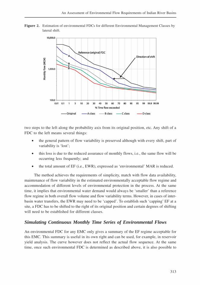
313
An Assessment of Environmental Flow Requirements of Indian River Basins
two steps to the left along the probability axis from its original position, etc. Any shift of aFDC to the left means several things:
• the general pattern of flow variability is preserved although with every shift, part ofvariability is ‘lost’;
• this loss is due to the reduced assurance of monthly flows, i.e., the same flow will beoccurring less frequently; and
• the total amount of EF (i.e., EWR), expressed as ‘environmental’ MAR is reduced.
The method achieves the requirements of simplicity, match with flow data availability,maintenance of flow variability in the estimated environmentally acceptable flow regime andaccommodation of different levels of environmental protection in the process. At the sametime, it implies that environmental water demand would always be ‘smaller’ than a referenceflow regime in both overall flow volume and flow variability terms. However, in cases of inter-basin water transfers, the EWR may need to be ‘capped’. To establish such ‘capping’ EF at asite, a FDC has to be shifted to the right of its original position and certain degrees of shiftingwill need to be established for different classes.
Simulating Continuous Monthly Time Series of Environmental Flows
An environmental FDC for any EMC only gives a summary of the EF regime acceptable forthis EMC. This summary is useful in its own right and can be used, for example, in reservoiryield analysis. The curve however does not reflect the actual flow sequence. At the sametime, once such environmental FDC is determined as described above, it is also possible to
Figure 2. Estimation of environmental FDCs for different Environmental Management Classes bylateral shift.
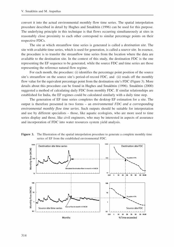
314
V. Smakhtin and M. Anputhas
convert it into the actual environmental monthly flow time series. The spatial interpolationprocedure described in detail by Hughes and Smakhtin (1996) can be used for this purpose.The underlying principle in this technique is that flows occurring simultaneously at sites inreasonably close proximity to each other correspond to similar percentage points on theirrespective FDCs.
The site at which streamflow time series is generated is called a destination site. Thesite with available time series, which is used for generation, is called a source site. In essence,the procedure is to transfer the streamflow time series from the location where the data areavailable to the destination site. In the context of this study, the destination FDC is the onerepresenting the EF sequence to be generated, while the source FDC and time series are thoserepresenting the reference natural flow regime.
For each month, the procedure: (i) identifies the percentage point position of the sourcesite’s streamflow on the source site’s period-of-record FDC, and (ii) reads off the monthlyflow value for the equivalent percentage point from the destination site’s FDC (Figure 3). Moredetails about this procedure can be found in Hughes and Smakhtin (1996). Smakhtin (2000)suggested a method of calculating daily FDC from monthly FDC. If similar relationships areestablished for India, the EF regimes could be calculated similarly with a daily time step.
The generation of EF time series completes the desktop EF estimation for a site. Theoutput is therefore presented in two forms – an environmental FDC and a correspondingenvironmental monthly flow time series. Such outputs should be suitable for interpretationand use by different specialists – those, like aquatic ecologists, who are more used to timeseries display and those, like civil engineers, who may be interested in aspects of assuranceand incorporation of FDC into water resources system yield analysis.
Figure 3. The Illustration of the spatial interpolation procedure to generate a complete monthly timeseries of EF from the established environmental FDC.
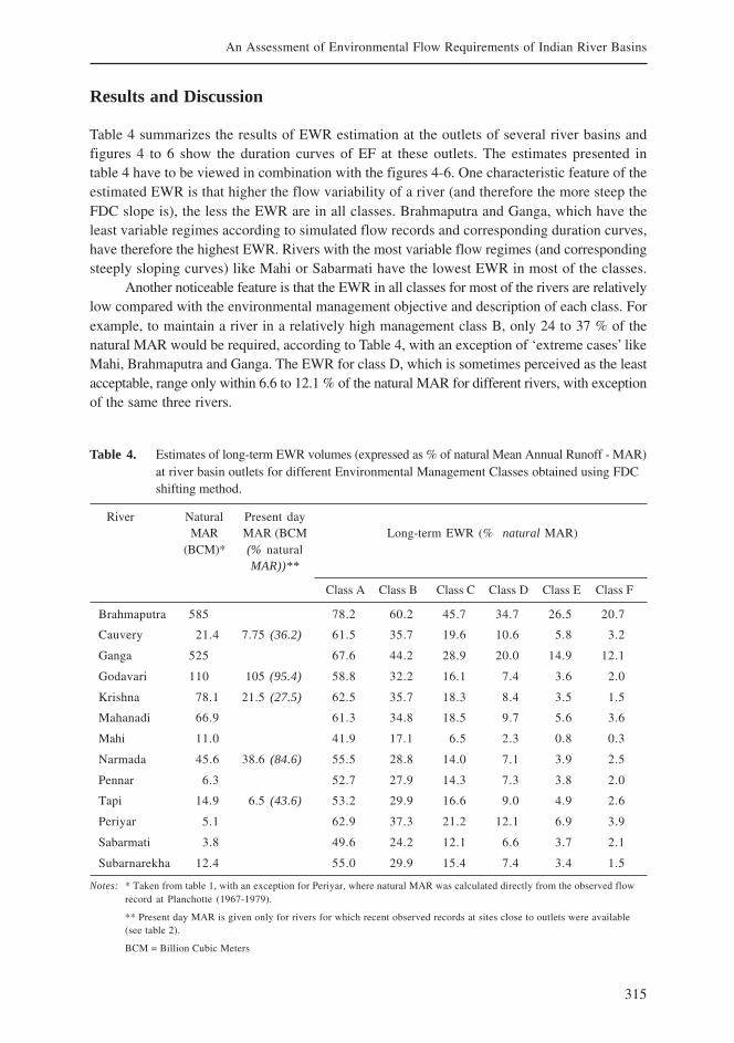
315
An Assessment of Environmental Flow Requirements of Indian River Basins
Results and Discussion
Table 4 summarizes the results of EWR estimation at the outlets of several river basins andfigures 4 to 6 show the duration curves of EF at these outlets. The estimates presented intable 4 have to be viewed in combination with the figures 4-6. One characteristic feature of theestimated EWR is that higher the flow variability of a river (and therefore the more steep theFDC slope is), the less the EWR are in all classes. Brahmaputra and Ganga, which have theleast variable regimes according to simulated flow records and corresponding duration curves,have therefore the highest EWR. Rivers with the most variable flow regimes (and correspondingsteeply sloping curves) like Mahi or Sabarmati have the lowest EWR in most of the classes.
Another noticeable feature is that the EWR in all classes for most of the rivers are relativelylow compared with the environmental management objective and description of each class. Forexample, to maintain a river in a relatively high management class B, only 24 to 37 % of thenatural MAR would be required, according to Table 4, with an exception of ‘extreme cases’ likeMahi, Brahmaputra and Ganga. The EWR for class D, which is sometimes perceived as the leastacceptable, range only within 6.6 to 12.1 % of the natural MAR for different rivers, with exceptionof the same three rivers.
Table 4. Estimates of long-term EWR volumes (expressed as % of natural Mean Annual Runoff - MAR)at river basin outlets for different Environmental Management Classes obtained using FDCshifting method.
River Natural Present dayMAR MAR (BCM Long-term EWR (% natural MAR)
(BCM)* (% naturalMAR))**
Class A Class B Class C Class D Class E Class F
Brahmaputra 585 78.2 60.2 45.7 34.7 26.5 20.7
Cauvery 21.4 7.75 (36.2) 61.5 35.7 19.6 10.6 5.8 3.2
Ganga 525 67.6 44.2 28.9 20.0 14.9 12.1
Godavari 110 105 (95.4) 58.8 32.2 16.1 7.4 3.6 2.0
Krishna 78.1 21.5 (27.5) 62.5 35.7 18.3 8.4 3.5 1.5
Mahanadi 66.9 61.3 34.8 18.5 9.7 5.6 3.6
Mahi 11.0 41.9 17.1 6.5 2.3 0.8 0.3
Narmada 45.6 38.6 (84.6) 55.5 28.8 14.0 7.1 3.9 2.5
Pennar 6.3 52.7 27.9 14.3 7.3 3.8 2.0
Tapi 14.9 6.5 (43.6) 53.2 29.9 16.6 9.0 4.9 2.6
Periyar 5.1 62.9 37.3 21.2 12.1 6.9 3.9
Sabarmati 3.8 49.6 24.2 12.1 6.6 3.7 2.1
Subarnarekha 12.4 55.0 29.9 15.4 7.4 3.4 1.5
Notes: * Taken from table 1, with an exception for Periyar, where natural MAR was calculated directly from the observed flowrecord at Planchotte (1967-1979).
** Present day MAR is given only for rivers for which recent observed records at sites close to outlets were available(see table 2).
BCM = Billion Cubic Meters
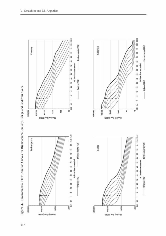
316
V. Smakhtin and M. Anputhas
Fig
ure
4.E
nvir
onm
enta
l F
low
Dur
atio
n C
urve
s fo
r B
rahm
aput
ra, C
auve
ry, G
anga
and
God
avar
i ri
vers
.
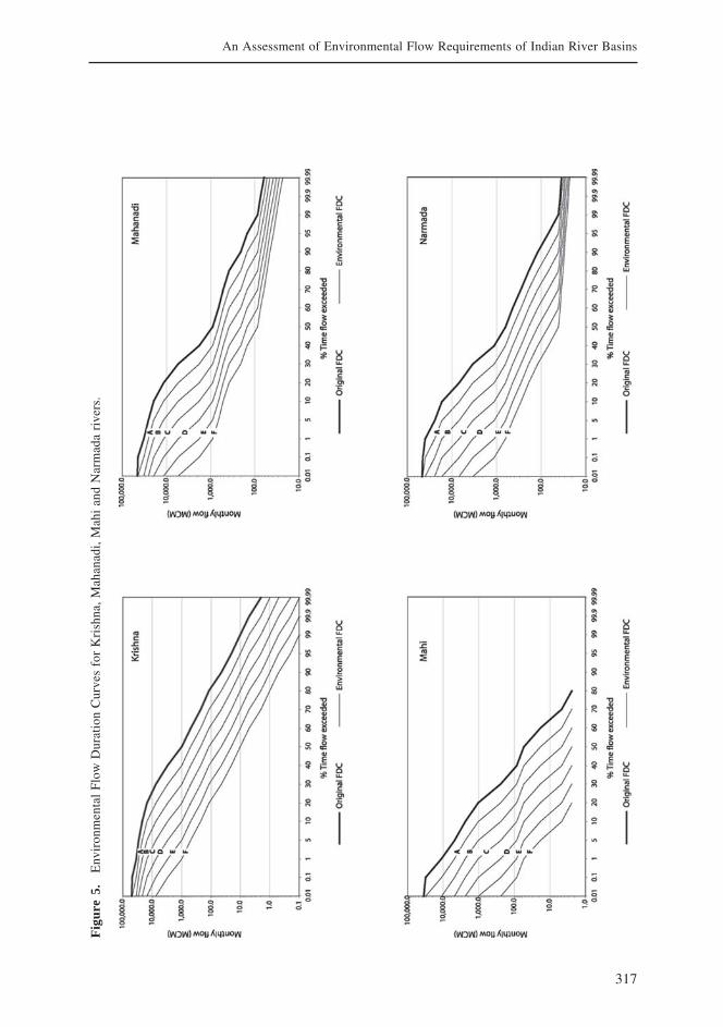
317
An Assessment of Environmental Flow Requirements of Indian River Basins
Fig
ure
5.E
nvir
onm
enta
l F
low
Dur
atio
n C
urve
s fo
r K
rish
na, M
ahan
adi,
Mah
i an
d N
arm
ada
rive
rs.

318
V. Smakhtin and M. Anputhas
Figure 6. Environmental Flow Duration Curves for Pennar, Tapi, Periyar, Sabarmati andSubarnarekha rivers.
The main methodological issue is the justification of currently used magnitudes of lateralFDC shifts per EMC. The step of a FDC shift currently used has been inferred partially fromliterature sources and partially through limited ‘calibration’ against the EF estimates obtained byDRM. Australian experience suggests that “the probability of having a healthy river falls fromhigh to moderate when the hydrological regime is less then two-thirds of the natural”(Jones 2002). Despite the general vagueness of this statement, it could indicate that the EWR of
319
An Assessment of Environmental Flow Requirements of Indian River Basins
some 60-70 % of natural MAR are likely to be required for the maintenance of rivers in A and Bclasses. By progressively shifting the curves for different rivers one step at a time and calculatingcorresponding EWR, it is possible to establish how many such shifts are generally permissibleto ensure A and B class rivers. A FDC shift of one percentage point has been found to achievethe above flow reduction in most of the cases (Table 4). On the other hand, the already mentionedTennant method suggests that the lowest feasible limit for the EWR, corresponding to severedegradation of a riverine ecosystem, is 10 % of the natural MAR. In most cases, this benchmarkmay be achieved or exceeded by four subsequent FDC shifts to the left along the probabilityaxis (Table 4). This may then be interpreted as the EWR of a class D river.
Overall, the determination of the number of FDC shifts per EMC is difficult withoutknowing the relationships between ecological characteristics and flow modifications in riverswith different hydrological regimes. In the absence of such knowledge, we use the minimumpossible lateral shift per EMC. This may be seen as a conservative ‘pro-environmental’approach, as shifts by only one step per EMC minimize losses in flow volumes and variabilityallocated to an ecosystem. However, as shown in Table 4, even this limited shift step resultsin significant losses of flow volumes and variability per class.
It is possible that as a result of subsequent future research, the procedure will differbetween more variable, mostly non-perennial rivers and less variable, mostly perennial riversin terms of how much FDC shifts are permissible in different classes. For example, the resilienceof aquatic ecosystems is usually the strongest when they are healthy (A and B class rivers).Therefore, larger FDC shifts – by two steps per EMC - and, consequently, larger correspondingflow reductions could be assumed acceptable to derive the default estimates of EWR for ‘morenatural’ classes A and B. Accordingly, smaller FDC shifts (by one step per EMC) could beaccepted to derive the default estimates of EWR for moderately to significantly modifiedecosystems described by classes C to F.
It is important to stress that the shift limits assumed above for each class are the defaults.Furthermore, variable shifts for different percentile flows can be used, if there is a specificjustification for this. For example, while estimating environmental FDC for A and B classes, flowsexceeded 90, 95 % and more of the time in the reference FDC may need to be fixed at their ‘existingpositions’; other flows may be shifted as in the default case. Alternatively, various shifts couldbe used for different percentile flows to define an EF duration curve in any EMC. The samelogic can be taken even further. Fixed EMCs may become unnecessary if a limited set ofecologically important flows is identified and permissible shifts in each (determined by the panelof experts for example) will jointly describe the final prescribed/negotiated state of the river. Itshould be possible to establish better shifting procedure and more justified levels of shift throughone or several national specialist workshops involving local hydrologists and ecologists. Theproposed approach therefore can provide the basis for further technique development.
The EWR estimates obtained using the FDC shifting technique may also be interpretedin the context of the EWR estimates produced by the Desktop Reserve Model (DRM), describedin the Review section (see section: Review of Environmental Flow Assessment Methods).Comparing EWR obtained by both DRM and FDC shifting methods should be seen as a formof calibration of the latter. The rational for this is that the DRM is effectively based on theresults of more comprehensive and higher-confidence EFA, which, in turn, are based onBuilding Block methodology with a good ‘track record’. Comparing the estimates obtained bytwo methods is effectively the only possible form of testing the proposed shifting technique
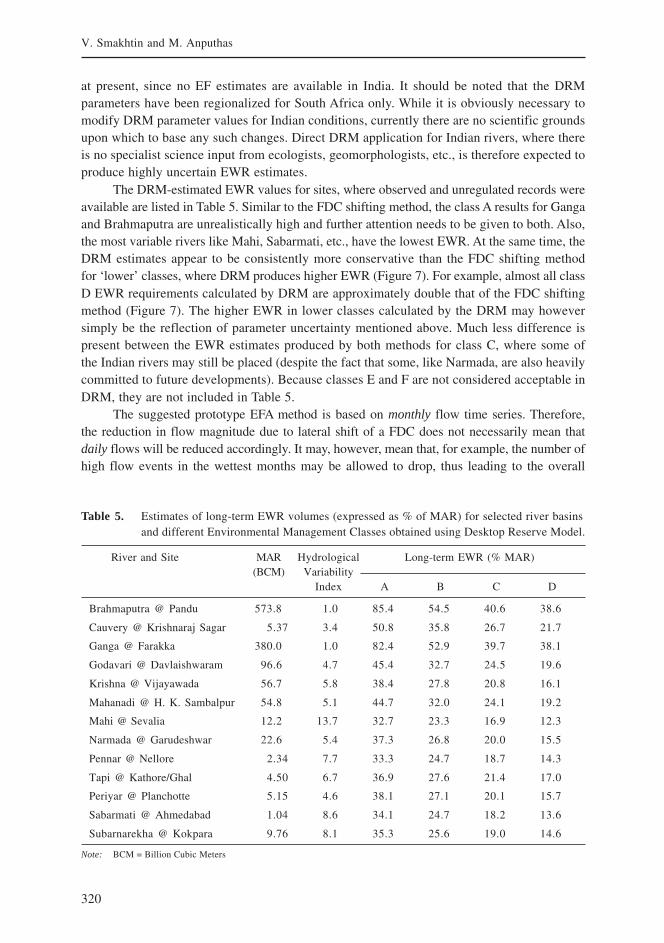
320
V. Smakhtin and M. Anputhas
at present, since no EF estimates are available in India. It should be noted that the DRMparameters have been regionalized for South Africa only. While it is obviously necessary tomodify DRM parameter values for Indian conditions, currently there are no scientific groundsupon which to base any such changes. Direct DRM application for Indian rivers, where thereis no specialist science input from ecologists, geomorphologists, etc., is therefore expected toproduce highly uncertain EWR estimates.
The DRM-estimated EWR values for sites, where observed and unregulated records wereavailable are listed in Table 5. Similar to the FDC shifting method, the class A results for Gangaand Brahmaputra are unrealistically high and further attention needs to be given to both. Also,the most variable rivers like Mahi, Sabarmati, etc., have the lowest EWR. At the same time, theDRM estimates appear to be consistently more conservative than the FDC shifting methodfor ‘lower’ classes, where DRM produces higher EWR (Figure 7). For example, almost all classD EWR requirements calculated by DRM are approximately double that of the FDC shiftingmethod (Figure 7). The higher EWR in lower classes calculated by the DRM may howeversimply be the reflection of parameter uncertainty mentioned above. Much less difference ispresent between the EWR estimates produced by both methods for class C, where some ofthe Indian rivers may still be placed (despite the fact that some, like Narmada, are also heavilycommitted to future developments). Because classes E and F are not considered acceptable inDRM, they are not included in Table 5.
The suggested prototype EFA method is based on monthly flow time series. Therefore,the reduction in flow magnitude due to lateral shift of a FDC does not necessarily mean thatdaily flows will be reduced accordingly. It may, however, mean that, for example, the number ofhigh flow events in the wettest months may be allowed to drop, thus leading to the overall
Table 5. Estimates of long-term EWR volumes (expressed as % of MAR) for selected river basinsand different Environmental Management Classes obtained using Desktop Reserve Model.
River and Site MAR Hydrological Long-term EWR (% MAR)(BCM) Variability
Index A B C D
Brahmaputra @ Pandu 573.8 1.0 85.4 54.5 40.6 38.6
Cauvery @ Krishnaraj Sagar 5.37 3.4 50.8 35.8 26.7 21.7
Ganga @ Farakka 380.0 1.0 82.4 52.9 39.7 38.1
Godavari @ Davlaishwaram 96.6 4.7 45.4 32.7 24.5 19.6
Krishna @ Vijayawada 56.7 5.8 38.4 27.8 20.8 16.1
Mahanadi @ H. K. Sambalpur 54.8 5.1 44.7 32.0 24.1 19.2
Mahi @ Sevalia 12.2 13.7 32.7 23.3 16.9 12.3
Narmada @ Garudeshwar 22.6 5.4 37.3 26.8 20.0 15.5
Pennar @ Nellore 2.34 7.7 33.3 24.7 18.7 14.3
Tapi @ Kathore/Ghal 4.50 6.7 36.9 27.6 21.4 17.0
Periyar @ Planchotte 5.15 4.6 38.1 27.1 20.1 15.7
Sabarmati @ Ahmedabad 1.04 8.6 34.1 24.7 18.2 13.6
Subarnarekha @ Kokpara 9.76 8.1 35.3 25.6 19.0 14.6
Note: BCM = Billion Cubic Meters
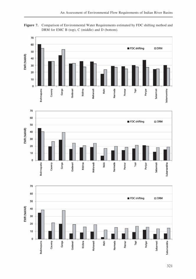
321
An Assessment of Environmental Flow Requirements of Indian River Basins
Figure 7. Comparison of Environmental Water Requirements estimated by FDC shifting method andDRM for EMC B (top), C (middle) and D (bottom).

322
V. Smakhtin and M. Anputhas
decrease in monthly flow volume. Some comprehensive EFA methods (e.g., DRIFT, King et al.2003) consider possible scenarios of flow changes in terms of how many events of certainmagnitude can be allowed to be “lost” (e.g., can all dry season freshes be lost, or can the numberof floods occurring at least once a wet month be halved). Reduction in corresponding monthlyflows, which results from the FDC shifting, effectively reflects these daily flow scenarios.
The estimated EF should be interpreted in the context of natural and present day riverflows. This could show what level of environmental protection is achievable in principle, giventhe current extent of water resources development. Figure 8 illustrates the present-day flowconditions at Krishna at Vijayawada town – the closest to the outlet - in the context of naturalized(simulated) flow at the outlet and the simulated EF time series for EMCs B and D. The simulatedtime series were obtained using the spatial interpolation procedure discussed in the previoussection and illustrated in Figure 3. Figure 8 shows that despite the seemingly highpresent-day ‘observed’ MAR (28% of the natural MAR) monthly flows at the outlet in certainyears drop to the level of the EF corresponding to class D, which is the least acceptable.
Figure 8. Extracts from observed and simulated monthly flow hydrographs for Krishna at Vijayawada.
Low flows during the non-monsoon period normally exceed the simulated ‘natural’ lowflows (Figure 8). This may be due to irrigation return flows or be the result of flow regulation.Figure 9 illustrates this point further by showing extracts from two observed daily flow timeseries in Krishna. The first time series is from the upstream site of Agraharam town located onthe main stream of Krishna. This site commands the catchment area of 132,920 km2. The secondsite is located at Vijayawada and commands almost the entire basin area of Krishna (251,360km2). The Agraharam site is located upstream of all major dams on Krishna’s main channel andmay reflect unregulated daily flow conditions. The flow at Vijayawada, on the other hand, isseverely impacted by flow regulation from dams located downstream of Agraharam. This
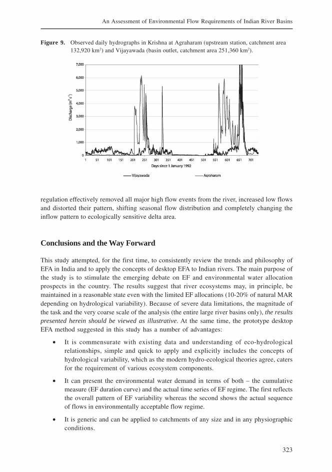
323
An Assessment of Environmental Flow Requirements of Indian River Basins
regulation effectively removed all major high flow events from the river, increased low flowsand distorted their pattern, shifting seasonal flow distribution and completely changing theinflow pattern to ecologically sensitive delta area.
Conclusions and the Way Forward
This study attempted, for the first time, to consistently review the trends and philosophy ofEFA in India and to apply the concepts of desktop EFA to Indian rivers. The main purpose ofthe study is to stimulate the emerging debate on EF and environmental water allocationprospects in the country. The results suggest that river ecosystems may, in principle, bemaintained in a reasonable state even with the limited EF allocations (10-20% of natural MARdepending on hydrological variability). Because of severe data limitations, the magnitude ofthe task and the very coarse scale of the analysis (the entire large river basins only), the resultspresented herein should be viewed as illustrative. At the same time, the prototype desktopEFA method suggested in this study has a number of advantages:
• It is commensurate with existing data and understanding of eco-hydrologicalrelationships, simple and quick to apply and explicitly includes the concepts ofhydrological variability, which as the modern hydro-ecological theories agree, catersfor the requirement of various ecosystem components.
• It can present the environmental water demand in terms of both – the cumulativemeasure (EF duration curve) and the actual time series of EF regime. The first reflectsthe overall pattern of EF variability whereas the second shows the actual sequenceof flows in environmentally acceptable flow regime.
• It is generic and can be applied to catchments of any size and in any physiographicconditions.
Figure 9. Observed daily hydrographs in Krishna at Agraharam (upstream station, catchment area132,920 km2) and Vijayawada (basin outlet, catchment area 251,360 km2).

324
V. Smakhtin and M. Anputhas
• It can and should be made more flexible by applying different shifts at differentpercentile flows and examining the results on the output EF time series. It is thereforeimportant to stress that the method suggested should rather be seen as a step towardsa better justified desktop EFA tool in the future.
The main issue with the method at present is a limited justification of the permissibleFDC shifts per EMC. The currently accepted step of a shift (one FDC table point per class) isbased on limited calibration of the proposed method against a more advanced DRM technique,which however has also not been adjusted for use in Indian conditions and therefore produceuncertain EF estimates itself. It is very difficult to evaluate the results when there are noecological data available to confirm or deny the suitability of the estimated EF. It is, in principle,possible to collect some limited hydraulic information for rivers and examine the characteristicsof the available habitat (water depth, wetted area and velocity, for example) under differentflow conditions (natural and FDC shifting method recommendations). This is not, however, areal substitute for scientific information on the relationships between ecological characteristicsand flow. It is also recognized that the collection of such information will be very timeconsuming and expensive.
For rivers with less variable flow regimes (and hence gently sloping FDCs), the techniquemay reduce high flows significantly more than low flows. However, first, at the monthly timestep, this does not necessarily imply the reduction of daily peaks; it could be the number ofhigh–flow events which is reduced. Second, from a management perspective this may not bea major issue. Unless major storage dams exist with substantial high flow release facilities, thehigh flows may not be controlled. The management focus therefore should be on the low flows,while the assumption can be made that high flows will occur, more-or-less naturally.
For the long-term, the focus of the future EFA in India has to be on the quantification ofeco-hydrological relationships in rivers and on inventory of already existing ecologically relevantinformation. It is necessary to consider initiating several comprehensive EFA projects in differentparts of the country and to relate the results to hydrology of the basins. This would also helpto better justify and improve the FDC shifting method suggested here.
It is logical to initiate such projects at several sites which will be affected by the plannedNRLP inter-basin water transfers. Immediate EFA of some ‘signed’ off links has to be done –like those between Ken River and Betwa River, on which the agreement has been signed byMadhya Pradesh and Uttar Pradesh governments in August 2005. Such detailed EFA studieswill effectively initiate a long-term capacity building programme in this field in the country byengaging ecologists and hydrologists who know their local rivers. Even if they have limitedinformation required for such assessment and the results are therefore still uncertain, attemptinga detailed EFA develops team building and interactions between experts in different disciplines.
At the same time, simple EFA tools, such as the one suggested in this report, may helpto illustrate the type of expected outcome from a more comprehensive EFA. Simple tools donot exclude, but rather encourage capacity building and the use of comprehensive EFA methodsat the same time. One possible merge of the two approaches (complex and simple) could bethrough a workshop of Indian ecologists and hydrologists, which could discuss and/or definethe required shifts of FDCs for different EMCs.
Eventually, a set of EFA tools will need to be developed and tested in a specific contextof India’s flow regimes, ecology and water resources development. The types of EFA methods
325
An Assessment of Environmental Flow Requirements of Indian River Basins
have to be selected based on the type of proposed development (abstractions, in-stream oroff-channel reservoirs, flow reduction activities, etc.), the level of impact of the proposeddevelopment, the ecological importance and sensitivity of the river, the degree to which it isalready developed, the socio-economic importance of the river and its proposed development,etc. The more critical the proposed development is from the above issues, the more likely thatmore comprehensive EFA will need to be used.
It is also necessary to initiate an assessment of ecological importance and sensitivityand ecological conditions of all major river basins in India and with the detailed spatialresolution. The information provided through such assessment is also useful in its own right– outside of the context of EF, because it gives the idea of the ecological condition andimportance of aquatic ecosystems (albeit in a semi-quantitative way) and therefore contributesto the vision of India’s water future.
The study has effectively not been supplied with observed flow data of reasonableamounts and quality. The data which have been acquired and used were primarily from publiclyavailable sources (Internet) where data are outdated and no conclusions on the accuracy oreven origin of the data could be made. If the situation with access to data in India is notchanged, any further EFA will be largely speculative. On the other hand, the agenciesresponsible for hydrological data provision will increasingly realize that the recent advancesin global hydrological modeling and remotely sensed data acquisition have been so significantthat in the near future (5-10 years) lack of access to observed data may no longer be anobstacle, because the representative and reliable flow time series for any site at any river couldbe simulated and be more reliable than observed.
One issue, which has not been addressed in this report, is how EF relates to the waterquality of rivers. This is an even more complex issue than EF estimation itself, but a fewstatements can be made to that effect. First, EF should aim to achieve some ecological objective(e.g., provide flow-related habitat or geomorphological function), but not to solve river waterquality problems by dilution. At the same time, once EF are recommended and expressed as atime series/duration curve, it should be possible to simulate flow-concentration relationshipsfor important constituents. Through this, the anticipated water quality consequences ofmodified flows could be explored and examined in the context of some pre-defined water qualityclasses (Palmer et al. 2005). The latter could be established using some benchmarks - literatureor field-data based boundary values. If recommended EF does not allow the agreed waterquality targets to be met (e.g., in cases when a river has naturally high salinity and recommendedenvironmental low flows would lead to increased salinity beyond some critical levels) thenhigher EF should be considered. Severely polluted Indian rivers are at risk only if therecommended EF remain in the river without non-point source pollution control and withouteffluent treatment at source.
Last but not the least is the issue of actual EF provisions as opposed to EF assessment.No matter how advanced and accurate the EFA is, its output remains on paper if no actualreleases are made or if the prescribed limit of water resource exploitation is violated. There arevery few examples in the world when environmental water requirement are actually satisfiedby EF provisions. Similarly, this may be the major stumbling block on the way to environmentallysustainable water resources development in India. Therefore, a due consideration to relevantpolicy support and enforcement has to be given to it.
326
V. Smakhtin and M. Anputhas
References
Acreman, M. C. 2002. Environmental flow setting in England and Wales: current practice and futurechallenges. Proceedings of the international conference on Environmental Flows for River Systems.Cape Town, South Africa, March 2002 (available on a CD).
Acreman, M.; Dunbar, M. J. 2004. Defining environmental river flow requirements – a review. Hydrologyand Earth System Sciences 8: 861-876.
Agrawal, A. 1998. Coping with dry spells and drought years: India’s traditions in water harvesting. StockholmWater Front, No. 1-2, May 1998. Stockholm, Sweden: Stockholm International Water Institute.
Agrawal, A.; Chak, A. 1991. Floods, Flood Plains and Environmental Myths. State of India’s Environment- A Citizen’s Report 3. New Delhi: Centre for Science and Environment. 167 pp.
Amarasinghe, U. A.; Sharma, B. R.; Aloysius, N.; Scott, C.; Smakhtin, V. U.; De Fraiture, C.; Sinha, A. K.;and Shukla, A. K. 2005. Spatial variation in water supply and demand across the river basins of India.Colombo, Sri Lanka: International Water Management Institute. 37 pp. (IWMI Research Report 83).
Bandyopadhyay, J. 1995. Water Management in the Ganges-Brahmaputra Basin: emerging challenges forthe 21st century. Water Resources Development 11(4): 411-442.
Beecher, H. A. 1990. Standards for Instream Flows. Rivers 1(2): 97-109.
Bunn, S. E.; Arthington, A. H. 2002. Basic principles and ecological consequences of altered flow regimesfor aquatic biodiversity. Environmental Management 30: 492-507.
CPCB (Central Pollution Control Board). 1996. Water Quality Status and Statistics (1993 & 1994).Monitoring of Indian Aquatic Resources (MINARS/10/1995-96). New Delhi: Central Pollution ControlBoard. 459 pp.
DWAF (Department of Water Affairs and Forestry). 1997. White paper on a National Water Policy forSouth Africa. Pretoria, South Africa: Department of Water Affairs and Forestry.
Dyson, M.; Bergkamp, G.; Scanlon, J. eds. 2003. Flow. The essentials of environmental flows. Gland,Switzerland and Cambridge, UK: IUCN. xiv + 118 pp.
Environment Agency. 2001. Managing Water Abstraction: the Catchment Abstraction Management StrategyProcess. Bristol, UK: Environment Agency.
Extence, C. A.; Balbi, D. M.; Chadd, R. P. 1999. River flow indexing using British benthicmacroinvertebrates: a framework for setting hydroecological objectives. Regulated Rivers: Researchand Management 15: 543-574.
Gopal, B.; Chauhan, M. 2003. River Restoration in India: A Case Study of River Yamuna East Asia RegionalSeminar on River Restoration, Kuala Lumpur, January 13-15, 2003.
Groombridge, B.; Jenkins, M. 1998. Freshwater Biodiversity: A preliminary global assessment. WorldConservation Monitoring Centre (WCMC) Biodiversity Series No. 8. World Conservation Press.http://www.unep-wcmc.org/resources/publications/biodiv_series.htm.
Hughes, D. A.; Hannart, P. 2003. A desktop model used to provide an initial estimate of the ecologicalinstream flow requirements of rivers in South Africa. Journal of Hydrology 270: 167-181.
Hughes, D. A.; Münster, F. 2000. Hydrological information and techniques to support the determinationof the water quantity component of the ecological reserve. Water Research Commission Report TT 137/00, Pretoria, South Africa. 91 pp.
Hughes, D. A.; Smakhtin, V. U. 1996. Daily flow time series patching or extension: a spatial interpolationapproach based on flow duration curves. Journal of Hydrological Sciences 41(6): 851–871.
Iyer, R. R. 2005. The Notion of Environmental Flows: A Caution NIE/IWMI Workshop on EnvironmentalFlows, New Delhi, March 23-24, 2005.
327
An Assessment of Environmental Flow Requirements of Indian River Basins
Jain, S. K.; Sharma, K. D.; Singh, V. P. 2005. Interlinking of Indian Rivers – Issues and analyticalframework. Proceedings of the IWRA XII World Water Congress. November 2005, New Delhi. Vol. 1:1.25-1.34.
Jhingran, V. G. 1991. Fish and Fisheries of India. Third Edition. New Delhi: Hindustan PublishingCorporation.
Jones, G. 2002. Setting environmental flows to sustain a healthy working river. Watershed February 2002.Canberra: Cooperative Research Centre for Freshwater Ecology. http://freshwater.canberra.edu.au.
Jowett, I. G. 1997. Instream flow methods: a comparison of approaches. Regulated Rivers: Research andManagement 13: 115-127.
King, J.; Louw, D. 1998. Instream flow assessment for regulated rivers in South Africa using the BuildingBlock Methodology. Aquatic Ecosystem Health and Management 1: 109-124.
King, J.; Brown, C.; Sabet, H. 2003. A scenario-based holistic approach to environmental flow assessmentsfor rivers. River research and applications 19: 619-639.
Knights, P. 2002. Environmental flows: lessons from an Australian experience. Proceedings of InternationalConference: Dialog on Water, Food and Environment. Hanoi, Vietnam. 18 pp.
Kothyari, U. C.; Garde, R. J. 1991. Annual runoff estimation for catchments in India. Journal of WaterResources Planning and Management 117(1).
Kothyari, U. C. 1995. Estimation of Monthly Runoff from Small Catchments in India. Journal ofHydrological Sciences 40: 533-541.
Lankford, B. A. 2002. Environmental water requirements: A demand management perspective. Journal ofthe Chartered Institution of Water and Environmental Management 17 (1): 19-22.
Matthews, R. C.; Bao, Y. 1991. The Texas method of preliminary instream flow determination. Rivers2(4): 295-310.
Mohile, A. D.; Gupta, L. N. 2005. Environmental water requirement – concept and coverage. Abstracts ofthe NIE/IWMI Workshop on Environmental Flows. New Delhi, March 2005, p. 3-4.
MOWR. 2002. National Water Policy. Ministry of Water Resources, Government of India, New Delhi. 9 pp.
Mukherjee, A. 2005. Environmental flows – its impacts on fisheries. Abstracts of the NIE/IWMI Workshopon Environmental Flows. New Delhi, March 2005, p. 7.
NCIWRDP (National Commission for Integrated Water Resource Development Plan). 1999. Integrated waterresource development: a plan for action. Ministry of Water Resources, New Delhi.
Nilsson, C.; Reidy, C. A.; Dynesius, M.; Revenga, C. 2005. Fragmentation and flow regulation of theworld’s largest river systems. Science 308: 405-408.
Palmer, C. G.; Rossouw, N.; Muller, W. J.; Scherman, P. A. 2005. The development of water qualitymethods within ecological Reserve assessments, and links to environmental flows. Water SA 31(2):161-170.
Parasiewicz, P.; Dunbar, M. J. 2001. Physical Habitat Modelling for Fish: A developing approach. LargeRivers 12(2-4): 239-268 (Arch. Hydrobiol. Suppl. 135(2-4)).
Petts, G. E. 1996. Water allocation to protect river ecosystems. Regulated Rivers: Research and Management12: 353-365.
Postel, S.; Carpenter, S. 1997. Freshwater Ecosystem Services. In: Nature’s Services: Societal Dependenceon Natural Ecosystems, ed. G. C. Daily. Washington DC: Island Press. pp. 195-214.
Puckridge, J. T.; Sheldone, F.; Wlaker, K. F.; Boulton, A. J. 1998. Flow variability and ecology of largerivers. Marine and Freshwater Research 49, 55-72.
Rao, K. L. 1975. India’s Water Wealth: Its Assessment, Uses and Projec-tions. New Delhi: Orient Longman.255 pp.
328
V. Smakhtin and M. Anputhas
Revenga, C.; Brunner, J.; Henninger, N.; Kassem, K.; Payne, R. 2000. Pilot Analysis of FreshwaterEcosystems: Freshwater Systems. Washington, DC, USA: World Resources Institute. 83 pp.
Richter, B. D.; Baumgartner, J. V.; Wigington, R.; Braun, D. P. 1997. How much water does a river need?Freshwater Biology 37: 231-249.
Sharma, K. N. 2005. Unique ideas on water in ancient Indian scriptures and culture. Proceedings of theIWRA XII World Water Congress. November 2005, New Delhi. Vol. 3: 6.1-6.8.
Silk, N.; McDonald, J.; Wigington, R. 2000. Turning Instream Flow water rights upside down. Rivers 7(4):298-313.
Sinha, R. K.; Prasad, K. 2005. Environmental flows vis-à-vis Biodiversity: The current scenario in theriver Ganga. Abstracts of the NIE/IWMI Workshop on Environmental Flows. New Delhi, March 2005,p. 13.
Smakhtin, V. U.; Revenga, C.; Döll, P. 2004a. Taking into account environmental water requirements inglobal-scale water resources assessments. Research Report of the CGIAR Comprehensive AssessmentProgramme of Water Use in Agriculture. Colombo, Sri Lanka: International Water Management Institute.24 pp. (IWMI Comprehensive Assessment Research Report 2).
Smakhtin, V.; Revenga, C.; Döll, P. 2004b. A pilot global assessment of environmental water requirementsand scarcity. Water International 29: 307-317.
Smakhtin, V. U. 2000. Estimating daily flow duration curves from monthly streamflow data. Water SA26(1): 13-18.
Smakhtin, V. U.; Shilpakar, R. L. 2005. Planning for environmental water allocations: An example ofhydrology-based assessment in the East Rapti River, Nepal. Colombo, Sri Lanka: International WaterManagement Institute. 20 pp. (IWMI Research Report 89).
Smakhtin, V. U.; Shilpakar, R. L.; Hughes, D. A. 2006. Hydrology-based assessment of environmentalflows: an example from Nepal. Hydrological Sciences Journal 47: 207-222.
Symphorian, G. R.; Madamombe, E.; van der Zaag, P. 2002. Dam operation for environmental waterreleases: the case of Osborne Dam, Save Catchment, Zimbabwe. Proceedings of the 3rd WaterNet/Warfsa Symposium ‘Water Demand Management for Sustainable Development’. Dar es Salaam, October30-31, 2002.
Tennant, D. L. 1976. Instream flow regimens for fish, wildlife, recreation and related environmentalresources. Fisheries 1: 6–10.
Tharme, R. E.; Smakhtin, V. U. 2003. Environmental Flow Assessment in Asia: Capitalizing on existingmomentum. In: Proceedings of the First Southeast Asia Water Forum, November 17-21, 2003, ChiangMai, Thailand. Volume 2: 301-313. Bangkok, Thailand: Thailand Water Resources Association.
Tharme, R. E. 2003. A global perspective on environmental flow assessment: emerging trends in thedevelopment and application of environmental flow methodologies for rivers. River Research andApplications 19: 397-441.
Vaidyanathan, A. 2003. Interlinking of Peninsular Rivers: a Critique. Economic and Political Weekly, July5, 2003: 2865-2871.
Ward, J. V.; Tockner, K.; Uehlinger, U.; Malard, F. 2001. Understanding natural patterns and processes inriver corridors as the basis for effective river restoration. Regulated Rivers: Research and Management17: 311-323.
Ward, J. V.; Tockner, K. 2001. Biodiversity: towards a unifying theme for river ecology. FreshwaterBiology 46: 807-819.
329
An Assessment of Environmental Flow Requirements of Indian River Basins
Developing Procedures for Assessment of EcologicalStatus of Indian River Basins in the Context of
Environmental Water Requirements
1V. Smakhtin, 2M. Arunachalam, 2K. G. Sivaramakrishnan 3S. Behera, 3A. Chatterjee,3P. Gautam, 4S. Das, 4G. D. Joshi, and 5K. Sankaran Unni
1International Water Management Institute Colombo, Sri Lanka2Manonmaniam Sundaranar University, Alwarkurichi, Tamil Nadu, India
3World Wide Fund for Nature (WWF)-India, New Delhi, India4IWMI-India, New Delhi, India
5Mahatma Gandhi University, Kottayam, Kerala, India.
Introduction
Environmental water requirements, also referred to as ‘Environmental Flows’ (Dyson et al. 2003;Acreman and Dunbar 2004), are a compromise between water resources development and themaintenance of a river in some ecologically acceptable or agreed condition. The issue ofenvironmental flows is relatively new in the world. Existing environmental flow assessmentmethods reflect the diversity of opinions on this subject and range from comprehensive expertpanel approach to arbitrarily selected hydrological indices (e.g., Tharme 2003). In manydeveloping countries, such as India, the issues of environmental water demand have not yetreceived the required attention. The first National Workshop on Environmental Flows, held inNew Delhi, in March 2005, brought together over 60 participants from national agencies andresearch institutions. The workshop generated a significant interest on the concept ofenvironmental flows in the country, and it also revealed the existing confusion in this field.Smakhtin and Anputhas (2006), attempted to further stimulate the debate on environmentalwater demand in India by suggesting a simple desktop assessment method and using it inseveral major river basins. The method, however, was designed in conditions with very limitedhydrological, and no ecological, data. One of the major problems with developing environmentalflow work in countries like India, is that despite existing significant knowledge on some aquaticecosystem components (e.g., fish), it has never been interpreted in the context of environmentalflow assessments. This means that it is not, as a rule, known how different ecosystemcomponents in different biogeographical settings react to changes of flow caused by waterresources or land developments. The impacts of reducing/increasing high or low flows onfish, invertebrates, riparian vegetation, or sediment regime (which is one determinant of aquatichabitat), for example, are not quantified. In some countries, the lack of such relationships and
330
V. Smakhtin, M. Arunachalam, K. G. Sivaramakrishnan, S. Behera, A. Chatterjee, P. Gautam,S. Das, G. D. Joshi, and K. Sankaran Unni
quantitative knowledge is addressed by expert panels and/or by certain scoring systems, whichrank a condition of an ecosystem and/or its sensitivity to flow changes (Cottingham et al.2002; DWAF 1999; Rogers and Bestbier 1997). Such scores are then fed into the determinationof an environmental category or environmental management class (EMC). EMC, in turn, isused (together with measures of flow variability or analysis of hydrological time series) todetermine the acceptable limits of flow reduction/increase in a river, i.e., actual environmentalflows. It is assumed that the higher the EMC, the more water will need to be allocated forecosystem maintenance or conservation and, more flow variability will need to be preserved.The existing scoring systems reflect the level of available expertise and ecological data. Thisreport attempts, for the first time, to introduce a prototype scoring system for the ecologicalstatus of rivers in India and illustrates the same through its application in several major riverbasins. The attempt has been significantly inspired by the South African experience. However,it is a major simplification of the existing practice. It is presented here as an attempt to showone possible protocol for placing a river into a certain environmental management class, ratherthan to prescribe it for use in its current form.
Methodology
Ideally, the definition of the environmental management class (EMC) should be based onexisting empirical relationships between flow changes and ecological status/conditions, whichare associated with clearly identifiable thresholds. Despite some documented examples, limitedevidence or knowledge is available of such thresholds (e.g., Beecher 1990; Puckridge et al.1998). Therefore, EMC is a management concept that has been developed and used in theworld because of a need to make decisions regardless of the limited lucid hydro-ecologicalknowledge available. In these conditions of uncertainty with regard to which EMC is requiredfor a particular river, the EMCs may be used as default ‘scenarios’ of environmental protectionand associated environmental flows—as ‘scenarios’ of environmental water demand (Smakhtinand Anputhas 2006). It is possible to estimate environmental demand corresponding to all orany of such default EMCs and then consider which one is the most feasible for a river inquestion, given the existing and future basin developments. Alternatively, it is also possibleto use expert judgment in order to place a river into the most ‘achievable’ EMC. One can thinkof an ‘ecological water passport’ for a basin. Such a ‘passport’ could include answers to thefollowing three, broad questions:
• What is the ecological sensitivity and importance of a river basin? The rationale forthis is that the higher the ecological sensitivity and importance of aquatic ecosystemsin a river basin is, the higher the EMC should be, ideally.
• What is the current condition of aquatic ecosystems in a river basin? The morenatural the current condition of the basin is, the greater the incentive for itsmaintenance as such.
• What is the trajectory of change? This question aims to identify whether a river is stillchanging, and in what direction, how fast and due to what impacts. The rationale isthat if the deterioration of aquatic environment continues, it will be more difficult toachieve a higher EMC, even if it is necessary, due to its high importance and sensitivity.
331
Developing Procedures for Assessment of Ecological Status of Indian River Basins in the Context ofEnvironmental Water Requirements
As this is the first time that such an approach is introduced in India, the focus shouldbe on highlighting the main aquatic features and problems of each basin. This means thataggregate environmental indicators, which reflect different features or conditions of a riverbasin, could be used for scoring. The literature on environmental indicators is fairly extensiveand its comprehensive review is beyond the scope of this report. Some of the relevant recentworks include, for example, Galbraith (2001), who developed a set of indicators that could beused to assess the condition and coping capacity of freshwater ecosystems at the basin scale.These indicators include: percentage of the basin under natural vegetation; percentage of thefloodplain under agricultural and urban land use; percentage of the lakes in eutrophic state;and several others. A similar indicator approach has been widely used in large-scale internationalwater assessment programs such as Global International Waters Assessment (GIWA,http://www.giwa.net), Watersheds of the World (Revenga et al. 1998) or Land-Ocean Interactionsin the Coastal Zone (LOICZ, http://www.loicz.org). However, the aggregate environmentalindicators have never been previously used in the context of environmental flow assessment.
The first question above may be seen as an attempt to design a condensed measure ofthe ecological value of the basin, albeit in non-monetary terms. An arbitrarily selected set ofsemi-quantitative and quantitative indicators includes:
• Presence of rare and endangered aquatic biota
• Presence of unique (e.g., ‘endemic’ ) aquatic biota
• Diversity of aquatic habitats
• Presence of protected areas, areas of natural heritage and pristine areas, which arecrossed by the main water course in the basin
• Sensitivity of aquatic ecosystems to flow reduction
Indicators from this group are calculated using national ecological surveys and databases.Considering that most of the ‘ecological’ attention in countries like India has so far been givento fish, such indicators as rare and endangered biota and unique biota are calculated hereusing available fish data. Rare and endangered fish species are first identified using IUCN(1994) categories such as CR (critically endangered) and EN (endangered). Their cumulativenumber is then expressed as the proportion of the total number of fish species found in a riverbasin. The assessment of diversity of aquatic habitats and sensitivity of aquatic ecosystemsto flow reduction requires expert judgment and knowledge of a particular river. Presence ofprotected or pristine areas can be assessed against existing guidelines for protected areamanagement, i.e., IUCN (1980), which sets the aim of 10 % of the basin to be protected.
The second question above relates to what the river system looks like at present, comparedto a reference condition in the past (e.g., prior to construction of major dams), or compared tosome similar and relatively undisturbed subbasins in the same physiographic settings. Theindicators used in this study include:
• percentage of the watershed remaining under natural vegetation cover types
• percentage of the floodplain areas remaining under natural cover types
• percentage of aquatic biota that are exotics
332
V. Smakhtin, M. Arunachalam, K. G. Sivaramakrishnan, S. Behera, A. Chatterjee, P. Gautam,S. Das, G. D. Joshi, and K. Sankaran Unni
• overall richness of aquatic species
• the degree of flow regulation
• the degree of river fragmentation
• human population density in a river basin (percentage of population density in themain floodplains)
• overall water quality in the basin
The first two indicators are normally estimated from the GIS maps, remote sensingdata, or already published literature sources. In some cases, a percentage of the floodplainareas actually remaining in a basin compared to some past reference condition may be usedas an alternative to the second indicator. A proportion of exotic species (e.g., fish), can becalculated as a percentage of the number of total fish species recorded in the basin. Overallspecies richness may be assessed as a proportion of the total number of species in a country,or in a larger geographical region, whichever is more appropriate, or by an expert score ona scale from low to high. The most straightforward way of calculating the degree of flowregulation is as a ratio of total storage of all dams to the long-term mean annual naturalflow volume of the basin. It is acknowledged though that this approach does not recognizetiming or types of flow events that are altered—which may be more critical than change involume per se. A degree of river fragmentation can be represented by a simple indicator ofspatial changes to habitat—longitudinal and latitudinal (river-floodplain) connectivity ofrivers. Human population density in a river basin as a percentage of population densityin the main floodplains (which could be seen as an aggregate indicator of human pressureon aquatic ecosystems) may be calculated using Census data and GIS, where the floodplainsare arbitrarily defined as areas within 2.5 kilometers (km) of either side of the main channeland the channels of the main tributaries (e.g., Revenga et al. 1998). (It is acknowledged thatsuch a definition does not fully recognize the difference between the typical riparian zoneand floodplains). An approximation of the overall water quality in a river is indexed usingIndian national water quality categorization, which has several classes, from A to E —depending on the level of pollution—expressed by ranges of several constituents.
With regard to the third question above, no specific indicators are used and ‘trendassessment’ is left primarily to professional judgment. It may be seen as an attempt to foreseehow the river will look like in the short-term (e.g., 5 years) and in the long-term (e.g., 20 years)in case of a ‘do-nothing-to-protect-aquatic-environment’ scenario.
Regardless of the original units and ways of estimation of every individual indicator, allindicator values in this study are then converted to a standard scoring system, which includesratings: 1 (none), 2 (minor), 3 (moderate), 4 (high) and 5 (very high). Table 1 summarizes theindicators which have been used in this study, and explains why an indicator has beenconsidered and how it is relevant in the context of the estimation of environmental waterdemand. The scores for individual indicators are then summed up and their sum is expressedas a percentage of the maximum achievable score. The actual percentage shows the degree ofthe deviation of a basin from its natural condition and, therefore, the most probable EMC. Thelatter, in turn, may be related to the amount of water that needs to be allocated for environmentalpurposes in this basin.
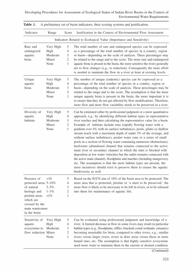
333
Developing Procedures for Assessment of Ecological Status of Indian River Basins in the Context ofEnvironmental Water Requirements
Table 1. A preliminary set of basin indicators, their scoring systems and justification.
Indicator Range Score Justification in the Context of Environmental Flow Assessment
Indicators Related to Ecological Value (Importance and Sensitivity)
Rare and Very High 5 The total number of rare and endangered species can be expressedendangered High 4 as a percentage of the total number of species in a country, regionaquatic Moderate 3 or basin—depending on the scale of analysis. These percentages maybiota Minor 2 be related to the range and to the score. The more rare and endangered
None 1 aquatic biota is present in the basin, the more sensitive the rivers generallyare to flow changes (e.g., to reduction). Consequently the more effortis needed to maintain the flow in a river at least at existing levels.
Unique Very High 5 The number of unique (endemic) species can be expressed as aaquatic High 4 percentage of the total number of species in a country, region orbiota Moderate 3 basin—depending on the scale of analysis. These percentages may be
Minor 2 related to the range and to the score. The assumption is that the moreNone 1 unique aquatic biota is present in the basin, the more important it is
to ensure that they do not get affected by flow modifications. Therefore,more flow and more flow variability needs to be preserved in a river.
Diversity of Very High 5 Can be estimated either by professional judgment or a more quantitativeaquatic High 4 approach, e.g., by identifying different habitat types in representativehabitats Moderate 3 river reaches and then calculating the representative value for a basin.
Minor 2 Example of habitats include runs (rapidly flowing water with aNone 1 gradient over 4% with no surface turbulence), pools, glides (a shallow
stream reach with a maximum depth of under 5% of the average, andwithout surface turbulence), pocket water (one or a series of smallpools in a section of flowing water containing numerous obstructions),backwater (abandoned channel that remains connected to the activemain river or secondary channel in which the inlet is blocked withdeposition at low water velocities but the outlet remains connected withthe active main channel), floodplains and marshes (including mangroves),etc. The assumption is that the more habitat types are present, themore incentives should exist to preserve them to ensure the aquaticbiodiversity as well.
Presence of >10 5 Based on the IUCN aim of 10% of the basin area to be protected. Theprotected areas 5–10% 4 more area that is protected, pristine or ‘a must to be preserved,’ theof natural 3–5% 3 more flow is likely to be necessary to be left in rivers, or to be releasedheritage and 1–3% 2 into them for maintenance of aquatic life.pristine areas <1% 1which arecrossed by themain watercoursein the basin
Sensitivity of Very High 5 Can be evaluated using professional judgment and knowledge of aaquatic High 4 river. A limited decrease in flow in some rivers may result in particularecosystems to Moderate 3 habitat types (e.g., floodplains, riffles, brackish costal wetlands, estuaries)flow reduction Minor 2 becoming unsuitable for biota, compared to other rivers, e.g., smaller
None 1 rivers versus larger rivers, rivers in drier areas versus those in morehumid ones, etc. The assumption is that highly sensitive ecosystemsneed more water to maintain them in the current or desired condition.
(Continued)
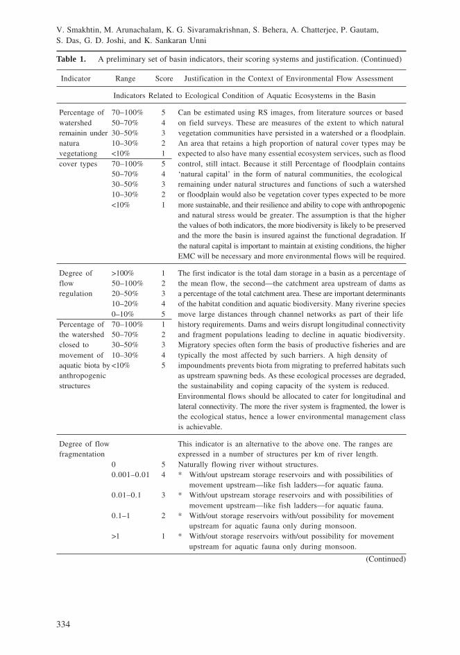
334
V. Smakhtin, M. Arunachalam, K. G. Sivaramakrishnan, S. Behera, A. Chatterjee, P. Gautam,S. Das, G. D. Joshi, and K. Sankaran Unni
Table 1. A preliminary set of basin indicators, their scoring systems and justification. (Continued)
Indicator Range Score Justification in the Context of Environmental Flow Assessment
Indicators Related to Ecological Condition of Aquatic Ecosystems in the Basin
Percentage of 70–100% 5 Can be estimated using RS images, from literature sources or basedwatershed 50–70% 4 on field surveys. These are measures of the extent to which naturalremainin under 30–50% 3 vegetation communities have persisted in a watershed or a floodplain.natura 10–30% 2 An area that retains a high proportion of natural cover types may bevegetationg <10% 1 expected to also have many essential ecosystem services, such as floodcover types 70–100% 5 control, still intact. Because it still Percentage of floodplain contains
50–70% 4 ‘natural capital’ in the form of natural communities, the ecological30–50% 3 remaining under natural structures and functions of such a watershed10–30% 2 or floodplain would also be vegetation cover types expected to be more<10% 1 more sustainable, and their resilience and ability to cope with anthropogenic
and natural stress would be greater. The assumption is that the higherthe values of both indicators, the more biodiversity is likely to be preservedand the more the basin is insured against the functional degradation. Ifthe natural capital is important to maintain at existing conditions, the higherEMC will be necessary and more environmental flows will be required.
Degree of >100% 1 The first indicator is the total dam storage in a basin as a percentage offlow 50–100% 2 the mean flow, the second—the catchment area upstream of dams asregulation 20–50% 3 a percentage of the total catchment area. These are important determinants
10–20% 4 of the habitat condition and aquatic biodiversity. Many riverine species0–10% 5 move large distances through channel networks as part of their life
Percentage of 70–100% 1 history requirements. Dams and weirs disrupt longitudinal connectivitythe watershed 50–70% 2 and fragment populations leading to decline in aquatic biodiversity.closed to 30–50% 3 Migratory species often form the basis of productive fisheries and aremovement of 10–30% 4 typically the most affected by such barriers. A high density ofaquatic biota by <10% 5 impoundments prevents biota from migrating to preferred habitats suchanthropogenic as upstream spawning beds. As these ecological processes are degraded,structures the sustainability and coping capacity of the system is reduced.
Environmental flows should be allocated to cater for longitudinal andlateral connectivity. The more the river system is fragmented, the lower isthe ecological status, hence a lower environmental management classis achievable.
Degree of flow This indicator is an alternative to the above one. The ranges arefragmentation expressed in a number of structures per km of river length.
0 5 Naturally flowing river without structures.0.001–0.01 4 * With/out upstream storage reservoirs and with possibilities of
movement upstream—like fish ladders—for aquatic fauna.0.01–0.1 3 * With/out upstream storage reservoirs and with possibilities of
movement upstream—like fish ladders—for aquatic fauna.0.1–1 2 * With/out storage reservoirs with/out possibility for movement
upstream for aquatic fauna only during monsoon.>1 1 * With/out storage reservoirs with/out possibility for movement
upstream for aquatic fauna only during monsoon.
(Continued)

335
Developing Procedures for Assessment of Ecological Status of Indian River Basins in the Context ofEnvironmental Water Requirements
Table 1. A preliminary set of basin indicators, their scoring systems and justification. (Continued)
Indicator Range Score Justification in the Context of Environmental Flow Assessment
Indicators Related to Ecological Condition of Aquatic Ecosystems in the Basin
Percentage 0% 5 Successful invasion by exotic species often incurs losses and disruptionsaquatic biota <5% 4 in ecosystem structures and functions (e.g., loss of biodiversity due tothat are <10% 3 competitive exclusion and predation, disruption and modification ofexotics <20% 2 food webs, loss of habitat for fish and wildlife). Thus, the percentage
>20% 1 of exotic species in a reach or a basin provides information on itslikely sustainability and coping capacity. The higher the proportionof exotic species the lower the achievable EMC is.
Fish species Very High 5 These are measures of biodiversity remaining in a system andrelative High 4 therefore—of its ecological capital and ability to self-organize andrichness, Moderate 3 sustain itself and cope with stressors. It is important to address relativeaquatic plant Minor 2 richness, rather than just speciescounts because the baseline biodiversityspecies relative None 1 of an area is conditional on habitat types, geographical locations, etc.richness, etc. Thus, the number of species that inhabit a watershed should be expressed
as a percentage of the number that would be expected to occur therein the absence of human interventions. Xenopoulos et al. (2005) haveshown that fish species numbers are reducing with reducing discharge.The reference condition is, however, very often difficult to establish andconsequently the quantification of ranges is also difficult. As a surrogatefor the percentage of some ‘natural’ reference condition, the speciesrichness may be quantified as a percentage of overall species in thecountry or geographical zone, or established by professional judgment.
Human <10% 1 Can be estimated using Census data. Districts located primarily inpopulation 10–20% 2 floodplain areas can be used to estimate population density indensity in the 20–40% 3 floodplains, other districts - to estimate population density in the restentire river 40–60% 4 of the basin. It is assumed that this measure may be seen as anbasin as a >60% 5 aggregate indicator of human pressure on aquatic ecosystems and aspercentage of an indicator of disruption of lateral connectivity in river basins.the populationdensity in themain floodplains
Overall water Class A 5 National Indian categorization of water quality is used, where eachquality in the Class B 4 class is characterized by certain ranges of constituents. Water in Classbasin Class C 3 A can be used for drinking after disinfection; water in class B is only
Class D 2 for swimming and bathing; water in Class C requires conventionalClass E 1 treatment and disinfection before drinking; water in Class D is suitable
for propagation of wildlife and fisheries; and water in class E is onlysuitable for such uses as irrigation and industry cooling.
The Study Basins
The river basins which have been selected for this study include Krishna, Cauvery, Narmada,Periyar and part of Ganga. The selection has been based primarily on availability of expertiseand data for each basin. The attempt, however, has been made to ensure the geographical
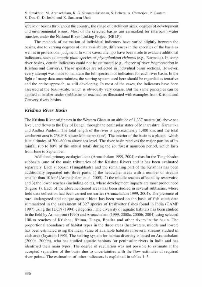
336
V. Smakhtin, M. Arunachalam, K. G. Sivaramakrishnan, S. Behera, A. Chatterjee, P. Gautam,S. Das, G. D. Joshi, and K. Sankaran Unni
spread of basins throughout the country, the range of catchment sizes, degrees of developmentand environmental issues. Most of the selected basins are earmarked for interbasin watertransfers under the National River-Linking Project (NRLP).
The methods of estimation of individual indicators have varied slightly between thebasins, due to varying degrees of data availability, differences in the specifics of the basin aswell as in professional judgment. In some cases, attempts have been made to evaluate additionalindicators, such as aquatic plant species or phytoplankton richness (e.g., Narmada). In someriver basins, certain indicators could not be estimated (e.g., degree of river fragmentation inKrishna and Cauvery). These specifics are reflected in individual basin sections. However,every attempt was made to maintain the full spectrum of indicators for each river basin. In thelight of many data uncertainties, the scoring system used here should be regarded as tentativeand the entire approach, as still developing. In most of the cases, the indicators have beenassessed at the basin-scale, which is obviously very coarse. But the same principles can beapplied at smaller scales (subbasins or reaches), as illustrated with examples from Krishna andCauvery rivers basins.
Krishna River Basin
The Krishna River originates in the Western Ghats at an altitude of 1,337 meters (m) above sealevel, and flows to the Bay of Bengal through the peninsular states of Maharashtra, Karnatakaand Andhra Pradesh. The total length of the river is approximately 1,400 km, and the totalcatchment area is 258,948 square kilometers (km2). The interior of the basin is a plateau, whichis at altitudes of 300–600 m above sea level. The river basin receives the major portion of itsrainfall (up to 80% of the annual total) during the southwest monsoon period, which lastsfrom June to September.
Additional primary ecological data (Arunachalam 1999, 2004) exists for the Tungabhadrasubbasin (one of the main tributaries of the Krishna River) and it has been evaluatedseparately. Each subbasin (Tungabhadra and the remaining part of the Krishna) has beenadditionally separated into three parts: 1) the headwater areas with a number of streamssmaller than 10 km2 (Arunachalam et al. 2005); 2) the middle reaches affected by reservoirs;and 3) the lower reaches (including delta), where development impacts are most pronounced(Figure 1). Each of the aforementioned areas has been studied in several subbasins, wherefield data collection had been carried out earlier (Arunachalam 1999, 2004). The presence ofrare, endangered and unique aquatic biota has been rated on the basis of fish catch datasummarized in the assessment of 327 species of freshwater fishes found in India (CAMP1997) using the IUCN (1994) categories. The diversity of aquatic habitats has been studiedin the field by Armantrout (1990) and Arunachalam (1999, 2000a, 2000b, 2004) using selected100-m reaches of Krishna, Bhima, Tunga, Bhadra and other rivers in the basin. Theproportional abundance of habitat types in the three areas (headwaters, middle and lower)has been estimated using the mean value of available habitats in several streams studied ineach area (Jayaram 1995). The scoring system for habitat diversity is based on Arunachalam(2000a, 2000b), who has studied aquatic habitats for peninsular rivers in India and hasidentified their main types. The degree of regulation was not possible to estimate at theaccepted separation of the basin due to uncertainties with the flow estimates at requiredriver points. The estimation of other indicators is explained in tables 1–3.
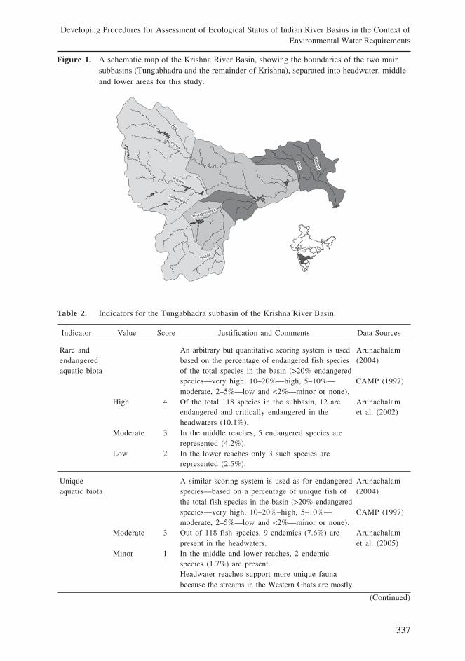
337
Developing Procedures for Assessment of Ecological Status of Indian River Basins in the Context ofEnvironmental Water Requirements
Figure 1. A schematic map of the Krishna River Basin, showing the boundaries of the two mainsubbasins (Tungabhadra and the remainder of Krishna), separated into headwater, middleand lower areas for this study.
Table 2. Indicators for the Tungabhadra subbasin of the Krishna River Basin.
Indicator Value Score Justification and Comments Data Sources
Rare and An arbitrary but quantitative scoring system is used Arunachalamendangered based on the percentage of endangered fish species (2004)aquatic biota of the total species in the basin (>20% endangered
species—very high, 10–20%—high, 5–10%— CAMP (1997)moderate, 2–5%—low and <2%—minor or none).
High 4 Of the total 118 species in the subbasin, 12 are Arunachalamendangered and critically endangered in the et al. (2002)headwaters (10.1%).
Moderate 3 In the middle reaches, 5 endangered species arerepresented (4.2%).
Low 2 In the lower reaches only 3 such species arerepresented (2.5%).
Unique A similar scoring system is used as for endangered Arunachalamaquatic biota species—based on a percentage of unique fish of (2004)
the total fish species in the basin (>20% endangeredspecies—very high, 10–20%–high, 5–10%— CAMP (1997)moderate, 2–5%—low and <2%—minor or none).
Moderate 3 Out of 118 fish species, 9 endemics (7.6%) are Arunachalampresent in the headwaters. et al. (2005)
Minor 1 In the middle and lower reaches, 2 endemicspecies (1.7%) are present.Headwater reaches support more unique faunabecause the streams in the Western Ghats are mostly
(Continued)

338
V. Smakhtin, M. Arunachalam, K. G. Sivaramakrishnan, S. Behera, A. Chatterjee, P. Gautam,S. Das, G. D. Joshi, and K. Sankaran Unni
Table 2. Indicators for the Tungabhadra subbasin of the Krishna River Basin. (continued)
Indicator Value Score Justification and Comments Data Sources
bedrock valleys and are strongly confined. Out of11 endemic species 5 species (Barilius canarensis,Glyptothorax trewavsae, Botia straita, Longischisturabhimachari and Hypselobarbus dobsoni) havenarrow distribution.
Diversity of High 4 In the upstream reaches of Tunga and Bhadra, Arunachalamaquatic falls, cascades, pools, riffles, glides, runs and (2004)habitats ‘pocketwater’ are all present.
Moderate 3 In the middle reaches, reservoir habitat types are Jayaram (1995)wetlands and deepwater, while downstream ofreservoirs and the reaches in between—runs,deep pools and backwater Scott (1989)habitats are present.
Minor 2 In the lower reaches, the only habitat types are Arunachalamruns with fine sand and occasional large pools. et al. (2005)
Presence of 1–3% 2 The subbasin has 1.62% as protected area with Arunachalamprotected and two wildlife sanctuaries (Bard and Ghataprabha) (2004)pristine areas and the Kudremukh National Park. More forests Manjrekar
can be protected as buffer zones of the (2000)Kudremukh National Park and sanctuaries. Jayaram (1995)
Percentage of 70–00% 5 In the headwaters almost all the streams are under Arunachalamwatershed natural cover type (90%). (2004)remaining 50–70% 3 In the reservoirs and the reaches 10–15 kmunder natural downstream of them, the percentage of natural Jayaram (1995)vegetation cover is under 65%, but in most of the middle
reach the percentage is under 50%.
10–30% 2 In the lower reach in the Karnataka part up to the (for middle andconfluence of Tungabhadra with Krishna river: lower reaches)28–30%.
Percentage of Floodplains are present in the middle and lowerfloodplain reaches only.remaining 30–50% 3 Middle reaches before the Tungabhadra Reservoir.under natural 10–30% 2 From the Tungabhadra Reservoir towards thevegetation AP boundary.
Percentage of 0% 5 In the headwater reach there are no exotic fish species. Arunachalamaquatic biota <5% 4 In the middle reaches, particularly—in the reservoir (2004)that are sector—introduced species of Cirrhinus mrigala, Sugunan (1995)exotics Labeo rohita are present. But the proportion in rivers
upstream and downstream of the reservoir is still smallin spite of having introduced these species 40 years ago.
Fish species 50–70% 4 Upstream reach is represented by 68 species Arunachalamrelative (57.6%) of the total 118 recorded in the subbasin. (2004)richness 70–100% 5 Middle reach is represented by 78 species (66.1%).
30–50% 3 Lower reaches are represented by 31 species (26.3%). Jayaram (1995)
(Continued)
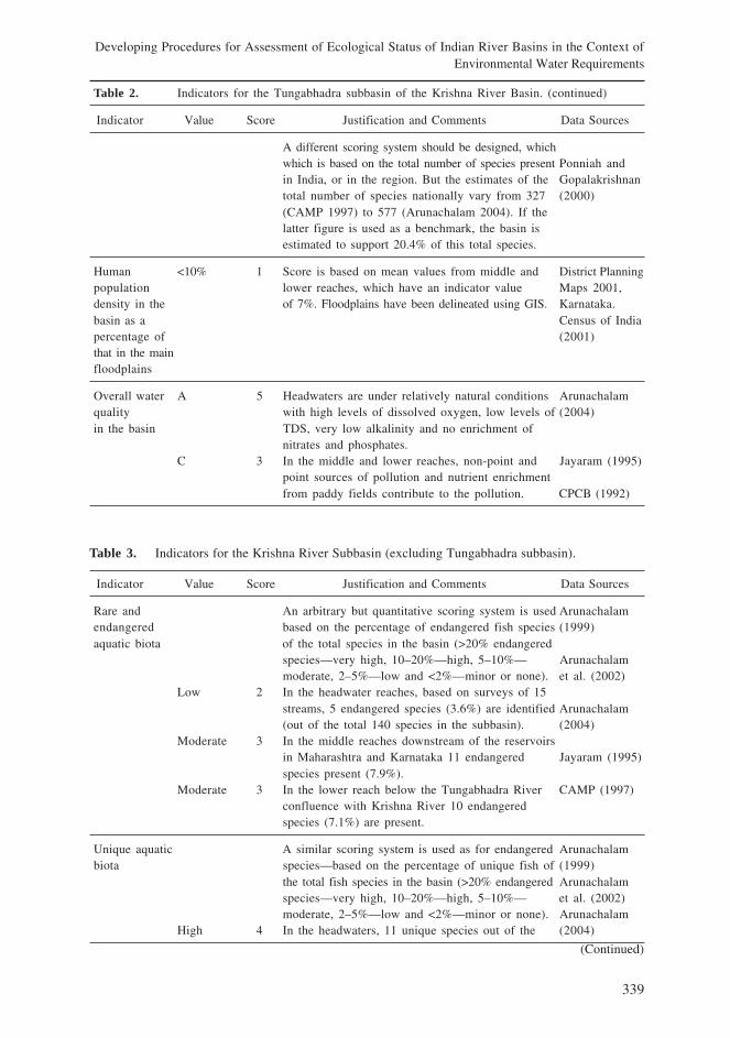
339
Developing Procedures for Assessment of Ecological Status of Indian River Basins in the Context ofEnvironmental Water Requirements
Table 2. Indicators for the Tungabhadra subbasin of the Krishna River Basin. (continued)
Indicator Value Score Justification and Comments Data Sources
A different scoring system should be designed, whichwhich is based on the total number of species present Ponniah andin India, or in the region. But the estimates of the Gopalakrishnantotal number of species nationally vary from 327 (2000)(CAMP 1997) to 577 (Arunachalam 2004). If thelatter figure is used as a benchmark, the basin isestimated to support 20.4% of this total species.
Human <10% 1 Score is based on mean values from middle and District Planningpopulation lower reaches, which have an indicator value Maps 2001,density in the of 7%. Floodplains have been delineated using GIS. Karnataka.basin as a Census of Indiapercentage of (2001)that in the mainfloodplains
Overall water A 5 Headwaters are under relatively natural conditions Arunachalamquality with high levels of dissolved oxygen, low levels of (2004)in the basin TDS, very low alkalinity and no enrichment of
nitrates and phosphates.C 3 In the middle and lower reaches, non-point and Jayaram (1995)
point sources of pollution and nutrient enrichmentfrom paddy fields contribute to the pollution. CPCB (1992)
Table 3. Indicators for the Krishna River Subbasin (excluding Tungabhadra subbasin).
Indicator Value Score Justification and Comments Data Sources
Rare and An arbitrary but quantitative scoring system is used Arunachalamendangered based on the percentage of endangered fish species (1999)aquatic biota of the total species in the basin (>20% endangered
species—very high, 10–20%—high, 5–10%— Arunachalammoderate, 2–5%—low and <2%—minor or none). et al. (2002)
Low 2 In the headwater reaches, based on surveys of 15streams, 5 endangered species (3.6%) are identified Arunachalam(out of the total 140 species in the subbasin). (2004)
Moderate 3 In the middle reaches downstream of the reservoirsin Maharashtra and Karnataka 11 endangered Jayaram (1995)species present (7.9%).
Moderate 3 In the lower reach below the Tungabhadra River CAMP (1997)confluence with Krishna River 10 endangeredspecies (7.1%) are present.
Unique aquatic A similar scoring system is used as for endangered Arunachalambiota species—based on the percentage of unique fish of (1999)
the total fish species in the basin (>20% endangered Arunachalamspecies—very high, 10–20%—high, 5–10%— et al. (2002)moderate, 2–5%—low and <2%—minor or none). Arunachalam
High 4 In the headwaters, 11 unique species out of the (2004)
(Continued)
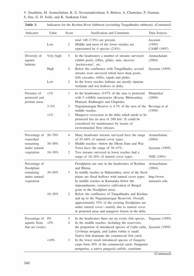
340
V. Smakhtin, M. Arunachalam, K. G. Sivaramakrishnan, S. Behera, A. Chatterjee, P. Gautam,S. Das, G. D. Joshi, and K. Sankaran Unni
Table 3. Indicators for the Krishna River Subbasin (excluding Tungabhadra subbasin). (Continued)
Indicator Value Score Justification and Comments Data Sources
total 140 (7.9%) are present. JayaramLow 2 Middle and most of the lower reaches are (1995)
represented by 4 species (2.8%). CAMP (1997)
Diversity of Very high 5 In the headwaters a number of streams surveyed Arunachalamaquatic exhibit pools, riffles, glides, runs, alcoves/ (2004)habitats ‘pocketwater’, etc.
High 4 Below the confluence with Tungabhadra, several Jayaram (1995)streams were surveyed which have deep pools,falls cascades, riffles, rapids and glides.
Low 2 In the lower reaches habitats are mostly riparianwetlands and wet hollows in delta.
Presence of <1% 1 In the headwaters, 0.97% of the area is protected Manjrekarprotected and with 5 wildlife sanctuaries (Koyna, Bhimsankar, (2000)pristine areas Phansad, Radhnagiri and Chaprala).
3–5% 3 Nagarjunasagar Reserve is 4.7% of the area of the Revenga et al.middle reaches. (1998)
<1% 1 Mangrove ecosystem in the delta which needs to beprotected has an area of 200 km2. It could beconsidered for maintenance by means ofenvironmental flow releases.
Percentage of 50–70% 4 Many headwater streams surveyed have the range Arunachalamwatershed of 55–68% of natural cover types. (2004)remaining 30–50% 3 Middle reaches—below the Dhom Dam and Waiunder natural Town have the range of 38–47%. Jayaram (1995)vegetation 10–30% 2 Two streams surveyed in lower reaches had a
range of 18–28% of natural cover types. NSII (1991)
Percentage of Floodplains are rare in the headwaters of Krishna Arunachalamfloodplain and Bhima. (2004)remaining 30–50% 3 In middle reaches in Maharashtra, most of the floodunder natural plains are flood hollows with natural cover types. http://www.vegetation In middle reaches in Karnataka below the annauniv.edu
impoundments, extensive cultivation of Bengalgram in the floodplain areas.
10–30% 2 Below the confluence of Tungabhadra and Krishnaand up to the Nagarjunasagar Reservoir. Overall,approximately 55% of the existing floodplains areunder natural cover—mainly due to natural coverin protected areas and mangrove forests in the delta.
Percentage of 0% 5 In the headwaters there are no exotic fish species. Sugunan (1995)aquatic biota <5% 4 In the middle reaches, including the reservoirs,that are exotics the proportion of introduced species of Catla catla, Jayaram (1995)
Cirrhinus mrigala, and Labeo rohita is small.Native fish dominate the commercial fish catch.
<10% 3 In the lower reach introduced species of Gangeticcarps form 30% of the commercial catch. Pangasiuspangasius, a native pangasid catfish, constitute
(Continued)
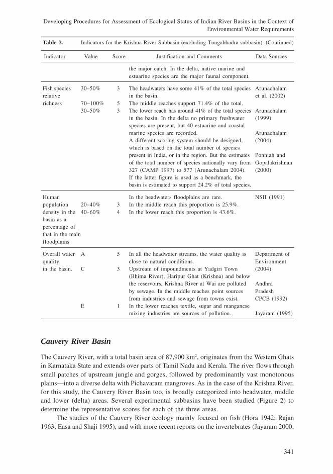
341
Developing Procedures for Assessment of Ecological Status of Indian River Basins in the Context ofEnvironmental Water Requirements
Table 3. Indicators for the Krishna River Subbasin (excluding Tungabhadra subbasin). (Continued)
Indicator Value Score Justification and Comments Data Sources
the major catch. In the delta, native marine andestuarine species are the major faunal component.
Fish species 30–50% 3 The headwaters have some 41% of the total species Arunachalamrelative in the basin. et al. (2002)richness 70–100% 5 The middle reaches support 71.4% of the total.
30–50% 3 The lower reach has around 41% of the total species Arunachalamin the basin. In the delta no primary freshwater (1999)species are present, but 40 estuarine and coastalmarine species are recorded. ArunachalamA different scoring system should be designed, (2004)which is based on the total number of speciespresent in India, or in the region. But the estimates Ponniah andof the total number of species nationally vary from Gopalakrishnan327 (CAMP 1997) to 577 (Arunachalam 2004). (2000)If the latter figure is used as a benchmark, thebasin is estimated to support 24.2% of total species.
Human In the headwaters floodplains are rare. NSII (1991)population 20–40% 3 In the middle reach this proportion is 25.9%.density in the 40–60% 4 In the lower reach this proportion is 43.6%.basin as apercentage ofthat in the mainfloodplains
Overall water A 5 In all the headwater streams, the water quality is Department ofquality close to natural conditions. Environmentin the basin. C 3 Upstream of impoundments at Yadgiri Town (2004)
(Bhima River), Haripur Ghat (Krishna) and belowthe reservoirs, Krishna River at Wai are polluted Andhraby sewage. In the middle reaches point sources Pradeshfrom industries and sewage from towns exist. CPCB (1992)
E 1 In the lower reaches textile, sugar and manganesemixing industries are sources of pollution. Jayaram (1995)
Cauvery River Basin
The Cauvery River, with a total basin area of 87,900 km2, originates from the Western Ghatsin Karnataka State and extends over parts of Tamil Nadu and Kerala. The river flows throughsmall patches of upstream jungle and gorges, followed by predominantly vast monotonousplains—into a diverse delta with Pichavaram mangroves. As in the case of the Krishna River,for this study, the Cauvery River Basin too, is broadly categorized into headwater, middleand lower (delta) areas. Several experimental subbasins have been studied (Figure 2) todetermine the representative scores for each of the three areas.
The studies of the Cauvery River ecology mainly focused on fish (Hora 1942; Rajan1963; Easa and Shaji 1995), and with more recent reports on the invertebrates (Jayaram 2000;

342
V. Smakhtin, M. Arunachalam, K. G. Sivaramakrishnan, S. Behera, A. Chatterjee, P. Gautam,S. Das, G. D. Joshi, and K. Sankaran Unni
Sivaramakrishnan et al. 1995). As in the Krishna Basin, CAMP (1997) data have been used, CRand EN and unique fish species (IUCN 1994) found in different experimental subbasins havebeen identified and their proportion of the total number of species has been calculated.A number of fish species in more than 50 sites in the headwater subbasins and 30 sites in themiddle and lower reaches have been used to evaluate the overall fish richness (Arunachalam1999, 2004; Jayaram 2000) as a proportion of the overall species reported in India. The averagesof these proportions have then been calculated for headwater, middle and lower areas, toproduce the representative indicator values. The diversity of aquatic habitats has beenevaluated by estimating the number of different habitat types present in the same reachesfrom all three areas, based on the scoring system proposed by Arunachalam (2000a). Thepercentage of watershed and floodplain remaining in natural cover types has been calculatedas the mean value of this percentage in experimental subbasins of headwaters and middle areas,based on field surveys by Arunachalam (2004). For the lower area, these indicators are assessedfrom the literature of Jayaram (2000). The percentage of exotic fish species is calculated (as inthe case of rare and endangered species) using the primary data by Arunchalam (2004), andthe published literature of Sugunan (1995) and Sreenivasan (1989). Six districts in Karnataka,three districts in Kerala, seven districts in Tamil Nadu and one district in Pondicherry havebeen used to approximate the human population density in the floodplains of the main riverand its tributaries (NSII 1991). Other indicators are estimated as explained in Tables 1 and 4.
Narmada River Basin
The Narmada River, with a catchment area of 94,235 km2 and total length of 1,312 km, is thelargest west flowing river on the Indian Peninsula (figure 3), crossing three states—MadhyaPradesh (MP), Maharashtra (MS) and Gujarat (GS). The climate ranges from temperate at thesource to subtropical at the outlet. The rainfall varies from between 1,400–1,700 millimeters (mm)
Figure 2. A schematic map of the Cauvery River Basin, showing the boundaries of headwater, middleand lower areas and sites where field data were collected.
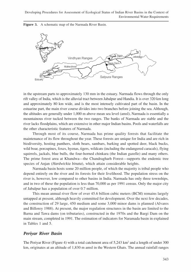
343
Developing Procedures for Assessment of Ecological Status of Indian River Basins in the Context ofEnvironmental Water Requirements
in the upstream parts to approximately 130 mm in the estuary. Narmada flows through the onlyrift valley of India, which is the alluvial tract between Jabalpur and Handia. It is over 320 km longand approximately 80 km wide, and is the most intensely cultivated part of the basin. In theestuarine part, the main river course divides into two branches before joining the sea. Although,the altitudes are generally under 1,000 m above mean sea level (amsl), Narmada is essentially amountainous river tucked between the two ranges. The banks of Narmada are stable and theriver lacks floodplains, which are extensive in other major Indian basins. Pools and waterfalls arethe other characteristic features of Narmada.
Through most of its course, Narmada has prime quality forests that facilitate themaintenance of its flow throughout the year. These forests are unique for India and are rich inbiodiversity, hosting panthers, sloth bears, sambars, barking and spotted deer, black bucks,wild boar, porcupines, foxes, hyenas, tigers, wildcats (including the endangered caracals), flyingsquirrels, jackals, blue bulls, the four-horned chinkara (the Indian gazelle) and many others.The prime forest area at Khandwa—the Chandragharh Forest—supports the endemic treespecies of Anjan (Hardwickia binata), which attain considerable heights.
Narmada basin hosts some 20 million people, of which the majority is tribal people whodepend entirely on the river and its forests for their livelihood. The population stress on theriver is, however, low compared to other basins in India. Narmada has only three townships,and in two of these the population is less than 70,000 as per 1991 census. Only the major cityof Jabalpur has a population of over 0.7 million.
This mean annual river flow of over 45.6 billion cubic meters (BCM) remains largelyuntapped at present, although heavily committed for development. Over the next few decades,the construction of 29 large, 450 medium and some 3,000 minor dams is planned (Alvaresand Billorey 1988). At present, the major regulation structures in the basin are limited to theBarna and Tawa dams (on tributaries), constructed in the 1970s and the Bargi Dam on themain stream, completed in 1991. The estimation of indicators for Naramada basin in explainedin Tables 1 and 5.
Periyar River Basin
The Periyar River (Figure 4) with a total catchment area of 5,243 km2 and a length of under 300km, originates at an altitude of 1,830 m amsl in the Western Ghats. The annual rainfall ranges
Figure 3. A schematic map of the Narmada River Basin.
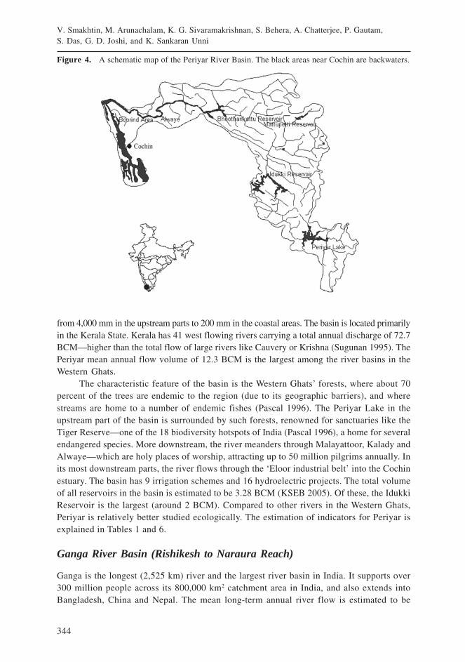
344
V. Smakhtin, M. Arunachalam, K. G. Sivaramakrishnan, S. Behera, A. Chatterjee, P. Gautam,S. Das, G. D. Joshi, and K. Sankaran Unni
from 4,000 mm in the upstream parts to 200 mm in the coastal areas. The basin is located primarilyin the Kerala State. Kerala has 41 west flowing rivers carrying a total annual discharge of 72.7BCM—higher than the total flow of large rivers like Cauvery or Krishna (Sugunan 1995). ThePeriyar mean annual flow volume of 12.3 BCM is the largest among the river basins in theWestern Ghats.
The characteristic feature of the basin is the Western Ghats’ forests, where about 70percent of the trees are endemic to the region (due to its geographic barriers), and wherestreams are home to a number of endemic fishes (Pascal 1996). The Periyar Lake in theupstream part of the basin is surrounded by such forests, renowned for sanctuaries like theTiger Reserve—one of the 18 biodiversity hotspots of India (Pascal 1996), a home for severalendangered species. More downstream, the river meanders through Malayattoor, Kalady andAlwaye—which are holy places of worship, attracting up to 50 million pilgrims annually. Inits most downstream parts, the river flows through the ‘Eloor industrial belt’ into the Cochinestuary. The basin has 9 irrigation schemes and 16 hydroelectric projects. The total volumeof all reservoirs in the basin is estimated to be 3.28 BCM (KSEB 2005). Of these, the IdukkiReservoir is the largest (around 2 BCM). Compared to other rivers in the Western Ghats,Periyar is relatively better studied ecologically. The estimation of indicators for Periyar isexplained in Tables 1 and 6.
Ganga River Basin (Rishikesh to Naraura Reach)
Ganga is the longest (2,525 km) river and the largest river basin in India. It supports over300 million people across its 800,000 km2 catchment area in India, and also extends intoBangladesh, China and Nepal. The mean long-term annual river flow is estimated to be
Figure 4. A schematic map of the Periyar River Basin. The black areas near Cochin are backwaters.
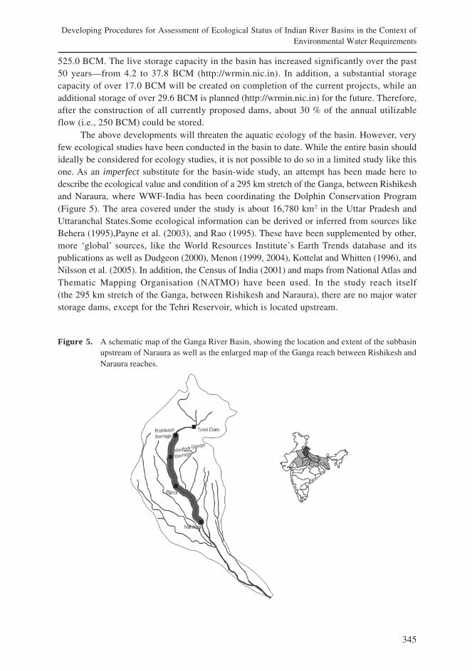
345
Developing Procedures for Assessment of Ecological Status of Indian River Basins in the Context ofEnvironmental Water Requirements
525.0 BCM. The live storage capacity in the basin has increased significantly over the past50 years—from 4.2 to 37.8 BCM (http://wrmin.nic.in). In addition, a substantial storagecapacity of over 17.0 BCM will be created on completion of the current projects, while anadditional storage of over 29.6 BCM is planned (http://wrmin.nic.in) for the future. Therefore,after the construction of all currently proposed dams, about 30 % of the annual utilizableflow (i.e., 250 BCM) could be stored.
The above developments will threaten the aquatic ecology of the basin. However, veryfew ecological studies have been conducted in the basin to date. While the entire basin shouldideally be considered for ecology studies, it is not possible to do so in a limited study like thisone. As an imperfect substitute for the basin-wide study, an attempt has been made here todescribe the ecological value and condition of a 295 km stretch of the Ganga, between Rishikeshand Naraura, where WWF-India has been coordinating the Dolphin Conservation Program(Figure 5). The area covered under the study is about 16,780 km2 in the Uttar Pradesh andUttaranchal States.Some ecological information can be derived or inferred from sources likeBehera (1995),Payne et al. (2003), and Rao (1995). These have been supplemented by other,more ‘global’ sources, like the World Resources Institute’s Earth Trends database and itspublications as well as Dudgeon (2000), Menon (1999, 2004), Kottelat and Whitten (1996), andNilsson et al. (2005). In addition, the Census of India (2001) and maps from National Atlas andThematic Mapping Organisation (NATMO) have been used. In the study reach itself(the 295 km stretch of the Ganga, between Rishikesh and Naraura), there are no major waterstorage dams, except for the Tehri Reservoir, which is located upstream.
Figure 5. A schematic map of the Ganga River Basin, showing the location and extent of the subbasinupstream of Naraura as well as the enlarged map of the Ganga reach between Rishikesh andNaraura reaches.
346
V. Smakhtin, M. Arunachalam, K. G. Sivaramakrishnan, S. Behera, A. Chatterjee, P. Gautam,S. Das, G. D. Joshi, and K. Sankaran Unni
Indicators and Trends in Study Basins
Krishna River Basin
Tables 2 and 3 summarize the results for Tungabhadra subbasin and the rest of Krishna RiverBasin, respectively. Both subbasins are more natural in the upstream areas, with diverse andrelatively unfragmented habitat, limited or no exotics and a high percentage of natural covertypes. Both subbasins are broadly similar in most of the indicator scores, which have a cleartendency to deteriorate downstream with the progressive increase of human pressure. Theexception is the higher richness of fish in both subbasins in their middle reaches, which ispartially due to the effects of tributaries that create more diverse and deeper habitats. In thelower reaches, however, species richness drops due to overfishing that occurs downstream ofreservoirs and the impacts of urbanization. The practice of using trawl nets with a small meshsize (8–10 mm), for example, almost eliminates the entire fish population (Arunachalam, personalobservations). In the Krishna subbasin, the middle reaches support more species than theheadwater and lower reaches, primarily due to the increasing size of the streams that still remainin a more natural condition compared to the lower areas. The lower reach, including the delta(Jayaram 1995), has limited freshwater species, but is represented by 40 species of brackishand coastal marine fish.
Overall, the pressure in the upstream parts of the basin has been relatively limited comparedto the lower reaches, where the deteriorating trends are alarming. River discharge, for example,has been decreasing at the outlet from 1968 onwards. In addition, water-sharing conflicts existbetween the states of Karnataka and Andhra Pradesh. The major flow of water is obstructed bythe increasing number of large- and medium-sized dams, which has completely changed thesediment regime of the river and fragmented its habitats in the middle and lower reaches. Krishnadelta, with a mangrove forest area of some 200 km2, faces threats of deforestation, overgrazing,harvesting of juvenile fauna and expansion of agriculture and shrimp aquaculture.
Cauvery River Basin
Field studies in the streams of the Cauvery River Basin, from the headwater reaches to theiroutlets, revealed significant habitat heterogeneity, which is exploited by guilds of fish species(Table 4). Headwaters tend to support more endangered fishes and, as such, these streamscan be used as ‘reference sites’ for the entire basin. These headwater streams have highgradients and predominantly bedrock substrates, and endangered fishes are confined to suchrocky stream types. Similar sites are found in the middle areas, but to a lesser extent. In thelower reaches, however, fish diversity and their formerly abundant population are declining.
Most protected areas are found in the headwaters, less than one percent is foundin the middle and lower reaches, while the mangrove swamps of Pichavaram and Muthupetlagoons—are protected by the State Forest Department. Some pristine areas may still be declaredprotected in the upstream areas (e.g., in the catchments of Moyar, Bhavani and Amaravathistreams). In the middle and lower reaches there are a few heritage sites such as the Vishnu Templesat Srirangapatnam, Sivasamudram and Srirangam; and Kaveri-Poompattinam (an ancient capitalof the Cholas Kingdom in the first century AD). Most of the headwaters are still under naturalvegetation cover, but the pressure from human settlements is increasing progressively downstream.
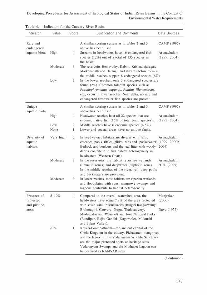
347
Developing Procedures for Assessment of Ecological Status of Indian River Basins in the Context ofEnvironmental Water Requirements
Table 4. Indicators for the Cauvery River Basin.
Indicator Value Score Justification and Comments Data Sources
Rare and A similar scoring system as in tables 2 and 3 CAMP (1997)endangered above has been used.aquatic biota High 4 Streams in headwaters have 16 endangered fish Arunachalam
species (12%) out of a total of 135 species in (1999, 2004)the basin.
Moderate 3 The reservoirs Hemavathy, Kabini, Krishnarajasagar,Markonahalli and Harangi, and streams below them inthe middle reaches, support 8 endangered species (6%).
Low 2 In the lower reaches, only 3 endangered species arefound (2%). Common tolerant species such asPseudophromanus cupanus, Puntius filamentosus,etc., occur in lower reaches. Near delta, no rare andendangered freshwater fish species are present.
Unique A similar scoring system as in tables 2 and 3 CAMP (1997)aquatic biota above has been used.
High 4 Headwater reaches host all 22 species that are Arunachalamendemic native fish (16% of total basin species). (1999, 2004)
Low 2 Middle reaches have 6 endemic species (4.5%).None 1 Lower and coastal areas have no unique fauna.
Diversity of Very high 5 In headwaters, habitats are diverse with falls, Arunachalamaquatic cascades, pools, riffles, glides, runs and ‘pocketwater’.(1999, 2000b,habitats Bedrock and boulders and the leaf litter with woody 2004)
debris contribute to fish habitat heterogeneity inheadwaters (Western Ghats).
Moderate 3 In the reservoirs, the habitat types are wetlands Arunachalam(limnetic zones) and deepwater (euphotic zone). et al. (2005)In the middle reaches of the river, run, deep poolsand backwaters are prevalent.
Moderate 3 In lower reaches, most habitats are riparian wetlandsand floodplains with runs, mangrove swamps andlagoons contribute to habitat heterogeneity.
Presence of 5–10% 4 Compared to the overall watershed area, the Manjrekarprotected headwaters have some 7.8% of the area protected (2000)and pristine with seven wildlife sanctuaries (Biligiri Rangaswamy,areas Brahmagiri, Cauvery, Nugu, Thalacauvery, Dave (1957)
Mudumalai and Wynaad) and four National Parks(Bandipur, Rajiv Gandhi (Nagarhole), Mukurthiand Silent Valley).
<1% 1 Kaveri-Poompattinam—the ancient capital of theChola Kingdom in the estuary. Pichavaram mangrovesand the lagoon in the Vedaranyam Wildlife Sanctuaryare the major protected spots or heritage sites.Vedaranyam Swamps and the Muthupet Lagoon canbe declared as RAMSAR sites.
(Continued)
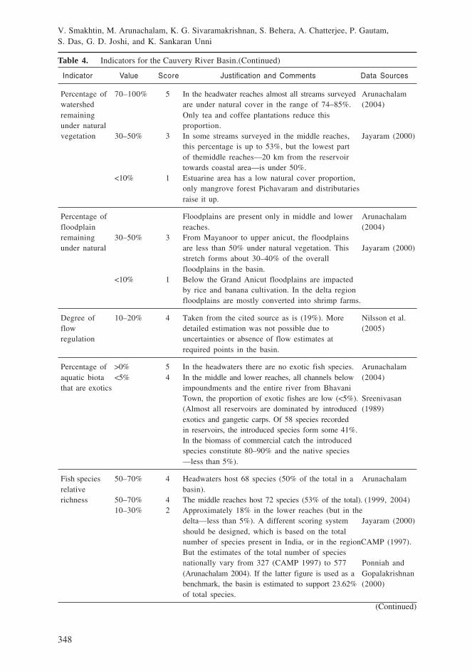
348
V. Smakhtin, M. Arunachalam, K. G. Sivaramakrishnan, S. Behera, A. Chatterjee, P. Gautam,S. Das, G. D. Joshi, and K. Sankaran Unni
Table 4. Indicators for the Cauvery River Basin.(Continued)
Indicator Value Score Justification and Comments Data Sources
Percentage of 70–100% 5 In the headwater reaches almost all streams surveyed Arunachalamwatershed are under natural cover in the range of 74–85%. (2004)remaining Only tea and coffee plantations reduce thisunder natural proportion.vegetation 30–50% 3 In some streams surveyed in the middle reaches, Jayaram (2000)
this percentage is up to 53%, but the lowest partof themiddle reaches—20 km from the reservoirtowards coastal area—is under 50%.
<10% 1 Estuarine area has a low natural cover proportion,only mangrove forest Pichavaram and distributariesraise it up.
Percentage of Floodplains are present only in middle and lower Arunachalamfloodplain reaches. (2004)remaining 30–50% 3 From Mayanoor to upper anicut, the floodplainsunder natural are less than 50% under natural vegetation. This Jayaram (2000)
stretch forms about 30–40% of the overallfloodplains in the basin.
<10% 1 Below the Grand Anicut floodplains are impactedby rice and banana cultivation. In the delta regionfloodplains are mostly converted into shrimp farms.
Degree of 10–20% 4 Taken from the cited source as is (19%). More Nilsson et al.flow detailed estimation was not possible due to (2005)regulation uncertainties or absence of flow estimates at
required points in the basin.
Percentage of >0% 5 In the headwaters there are no exotic fish species. Arunachalamaquatic biota <5% 4 In the middle and lower reaches, all channels below (2004)that are exotics impoundments and the entire river from Bhavani
Town, the proportion of exotic fishes are low (<5%). Sreenivasan(Almost all reservoirs are dominated by introduced (1989)exotics and gangetic carps. Of 58 species recordedin reservoirs, the introduced species form some 41%.In the biomass of commercial catch the introducedspecies constitute 80–90% and the native species—less than 5%).
Fish species 50–70% 4 Headwaters host 68 species (50% of the total in a Arunachalamrelative basin).richness 50–70% 4 The middle reaches host 72 species (53% of the total). (1999, 2004)
10–30% 2 Approximately 18% in the lower reaches (but in thedelta—less than 5%). A different scoring system Jayaram (2000)should be designed, which is based on the totalnumber of species present in India, or in the regionCAMP (1997).But the estimates of the total number of speciesnationally vary from 327 (CAMP 1997) to 577 Ponniah and(Arunachalam 2004). If the latter figure is used as a Gopalakrishnanbenchmark, the basin is estimated to support 23.62% (2000)of total species.
(Continued)
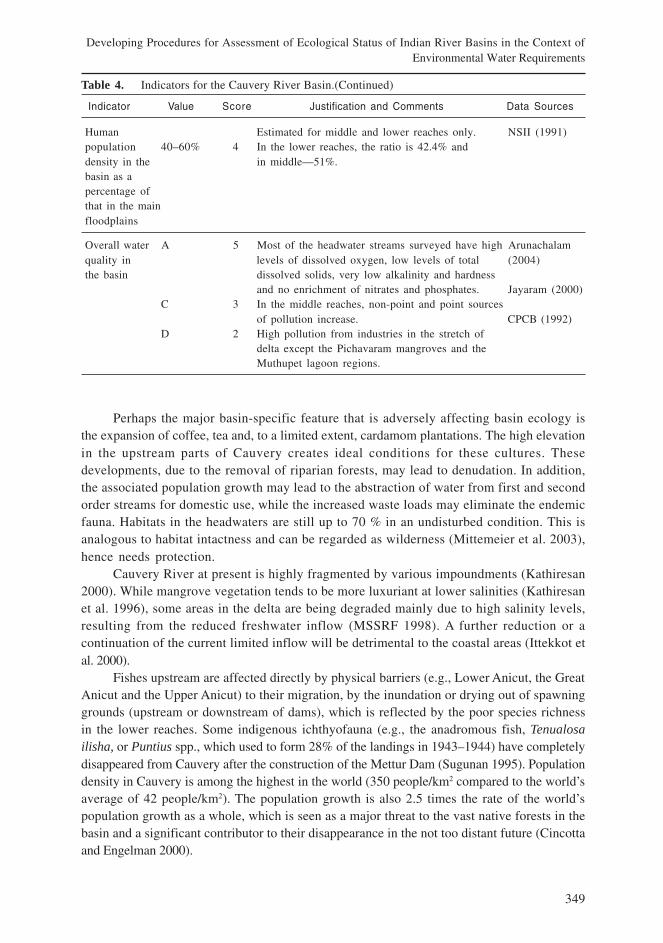
349
Developing Procedures for Assessment of Ecological Status of Indian River Basins in the Context ofEnvironmental Water Requirements
Perhaps the major basin-specific feature that is adversely affecting basin ecology isthe expansion of coffee, tea and, to a limited extent, cardamom plantations. The high elevationin the upstream parts of Cauvery creates ideal conditions for these cultures. Thesedevelopments, due to the removal of riparian forests, may lead to denudation. In addition,the associated population growth may lead to the abstraction of water from first and secondorder streams for domestic use, while the increased waste loads may eliminate the endemicfauna. Habitats in the headwaters are still up to 70 % in an undisturbed condition. This isanalogous to habitat intactness and can be regarded as wilderness (Mittemeier et al. 2003),hence needs protection.
Cauvery River at present is highly fragmented by various impoundments (Kathiresan2000). While mangrove vegetation tends to be more luxuriant at lower salinities (Kathiresanet al. 1996), some areas in the delta are being degraded mainly due to high salinity levels,resulting from the reduced freshwater inflow (MSSRF 1998). A further reduction or acontinuation of the current limited inflow will be detrimental to the coastal areas (Ittekkot etal. 2000).
Fishes upstream are affected directly by physical barriers (e.g., Lower Anicut, the GreatAnicut and the Upper Anicut) to their migration, by the inundation or drying out of spawninggrounds (upstream or downstream of dams), which is reflected by the poor species richnessin the lower reaches. Some indigenous ichthyofauna (e.g., the anadromous fish, Tenualosailisha, or Puntius spp., which used to form 28% of the landings in 1943–1944) have completelydisappeared from Cauvery after the construction of the Mettur Dam (Sugunan 1995). Populationdensity in Cauvery is among the highest in the world (350 people/km2 compared to the world’saverage of 42 people/km2). The population growth is also 2.5 times the rate of the world’spopulation growth as a whole, which is seen as a major threat to the vast native forests in thebasin and a significant contributor to their disappearance in the not too distant future (Cincottaand Engelman 2000).
Table 4. Indicators for the Cauvery River Basin.(Continued)
Indicator Value Score Justification and Comments Data Sources
Human Estimated for middle and lower reaches only. NSII (1991)population 40–60% 4 In the lower reaches, the ratio is 42.4% anddensity in the in middle—51%.basin as apercentage ofthat in the mainfloodplains
Overall water A 5 Most of the headwater streams surveyed have high Arunachalamquality in levels of dissolved oxygen, low levels of total (2004)the basin dissolved solids, very low alkalinity and hardness
and no enrichment of nitrates and phosphates. Jayaram (2000)C 3 In the middle reaches, non-point and point sources
of pollution increase. CPCB (1992)D 2 High pollution from industries in the stretch of
delta except the Pichavaram mangroves and theMuthupet lagoon regions.
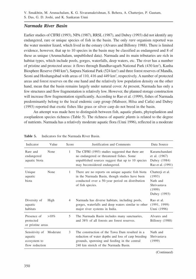
350
V. Smakhtin, M. Arunachalam, K. G. Sivaramakrishnan, S. Behera, A. Chatterjee, P. Gautam,S. Das, G. D. Joshi, and K. Sankaran Unni
Narmada River Basin
Earlier studies of CIFRI (1993), NPA (1987), RRSL (1987), and Dubey (1993) did not identify anyendangered, rare or unique species of fish in the basin. The only rare organism reported wasthe water monitor lizard, which lived in the estuary (Alvares and Billorey 1988). There is limitedevidence, however, that up to 10 species in the basin may be classified as endangered and 8 ofthese as unique (Arunuchalam, unpublished data). Narmada and its main tributaries are rich inhabitat types, which include pools, gorges, waterfalls, deep waters, etc. The river has a numberof pristine and protected areas: it flows through Bandhavagarh National Park (430 km2), KanhaBiosphere Reserve (940 km2), Satpura National Park (524 km2) and three forest reserves of Mandla,Seoni and Hoshangabad with areas of 110, 416 and 449 km2, respectively. A number of protectedareas and forest reserves on the one hand and the relatively low population density on the otherhand, mean that the basin remains largely under natural cover. At present, Narmada has only afew structures and flow fragmentation is relatively low. However, the planned storage constructionwill increase flow fragmentation significantly. According to Rao et al. (1999), fishes of Narmadapredominantly belong to the local endemic carp group (Mahseer, Hilsa and Catla) and Dubey(1993) reported that exotic fishes like grass or silver carp do not breed in the basin.
An attempt was made here to distinguish between fish, aquatic plants, phytoplankton andzooplankton species richness (Table 5). The richness of aquatic plants is related to the degreeof nutrients. Narmada has a relatively moderate aquatic flora (Unni 1996), reflected in a moderate
Table 5. Indicators for the Narmada River Basin.
Indicator Value Score Justification and Comments Data Source
Rare and None 1 The CIFRI (1993) studies suggested that there are Karamchandaniendangered no endangered or threatened fishes. Some et al. (1967)aquatic biota unpublished sources suggest that up to 10 species Dubey (1984)
may beconsidered endangered. Rao et al. (1991)
Unique None 1 There are no reports on unique aquatic fish biota Chatterji et al.aquatic in the Narmada Basin, though studies have been (1993)biota conducted over a 50-year period on distribution Nath and
of fish species. Shrivastava(1999)Dubey (1993)
Diversity of High 4 Narmada has diverse habitats, including pools, Rao et al.aquatic gorges, waterfalls and deep waters similar to other (1991, 1999)habitats major river systems in India. Unni (1996)
Presence of >10% 5 The Narmada Basin includes many sanctuaries, Alvares andprotected and 38% of all forests are forest reserves. Billorey (1988)or pristine areas
Sensitivity of Moderate 3 The construction of the Tawa Dam resulted in a Nath andaquatic reduction of water depths and loss of carp breeding Shrivastavaecosystem to grounds, spawning and feeding in the central (1999)flow reduction 240 km stretch of the Narmada Basin.
(Continued)
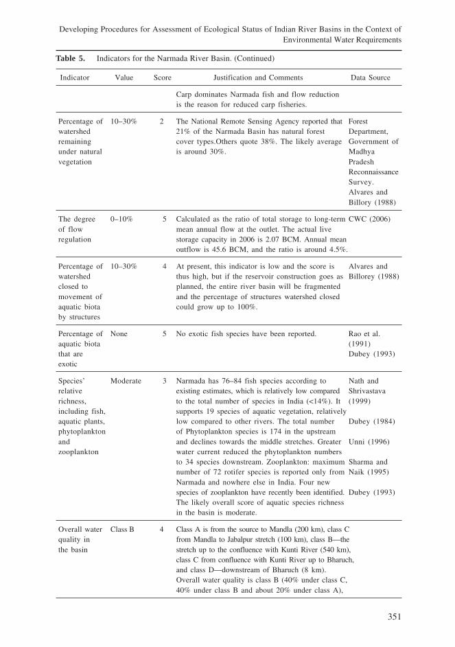
351
Developing Procedures for Assessment of Ecological Status of Indian River Basins in the Context ofEnvironmental Water Requirements
Table 5. Indicators for the Narmada River Basin. (Continued)
Indicator Value Score Justification and Comments Data Source
Carp dominates Narmada fish and flow reductionis the reason for reduced carp fisheries.
Percentage of 10–30% 2 The National Remote Sensing Agency reported that Forestwatershed 21% of the Narmada Basin has natural forest Department,remaining cover types.Others quote 38%. The likely average Government ofunder natural is around 30%. Madhyavegetation Pradesh
ReconnaissanceSurvey.Alvares andBillory (1988)
The degree 0–10% 5 Calculated as the ratio of total storage to long-term CWC (2006)of flow mean annual flow at the outlet. The actual liveregulation storage capacity in 2006 is 2.07 BCM. Annual mean
outflow is 45.6 BCM, and the ratio is around 4.5%.
Percentage of 10–30% 4 At present, this indicator is low and the score is Alvares andwatershed thus high, but if the reservoir construction goes as Billorey (1988)closed to planned, the entire river basin will be fragmentedmovement of and the percentage of structures watershed closedaquatic biota could grow up to 100%.by structures
Percentage of None 5 No exotic fish species have been reported. Rao et al.aquatic biota (1991)that are Dubey (1993)exotic
Species’ Moderate 3 Narmada has 76–84 fish species according to Nath andrelative existing estimates, which is relatively low compared Shrivastavarichness, to the total number of species in India (<14%). It (1999)including fish, supports 19 species of aquatic vegetation, relativelyaquatic plants, low compared to other rivers. The total number Dubey (1984)phytoplankton of Phytoplankton species is 174 in the upstreamand and declines towards the middle stretches. Greater Unni (1996)zooplankton water current reduced the phytoplankton numbers
to 34 species downstream. Zooplankton: maximum Sharma andnumber of 72 rotifer species is reported only from Naik (1995)Narmada and nowhere else in India. Four newspecies of zooplankton have recently been identified. Dubey (1993)The likely overall score of aquatic species richnessin the basin is moderate.
Overall water Class B 4 Class A is from the source to Mandla (200 km), class Cquality in from Mandla to Jabalpur stretch (100 km), class B—thethe basin stretch up to the confluence with Kunti River (540 km),
class C from confluence with Kunti River up to Bharuch,and class D—downstream of Bharuch (8 km).Overall water quality is class B (40% under class C,40% under class B and about 20% under class A),
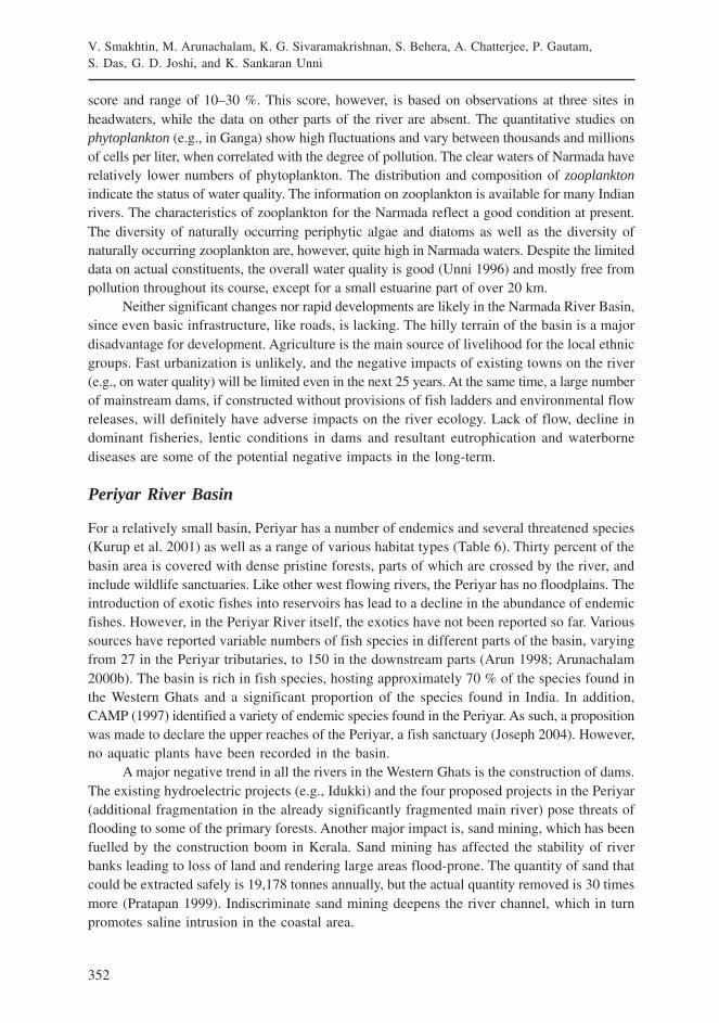
352
V. Smakhtin, M. Arunachalam, K. G. Sivaramakrishnan, S. Behera, A. Chatterjee, P. Gautam,S. Das, G. D. Joshi, and K. Sankaran Unni
score and range of 10–30 %. This score, however, is based on observations at three sites inheadwaters, while the data on other parts of the river are absent. The quantitative studies onphytoplankton (e.g., in Ganga) show high fluctuations and vary between thousands and millionsof cells per liter, when correlated with the degree of pollution. The clear waters of Narmada haverelatively lower numbers of phytoplankton. The distribution and composition of zooplanktonindicate the status of water quality. The information on zooplankton is available for many Indianrivers. The characteristics of zooplankton for the Narmada reflect a good condition at present.The diversity of naturally occurring periphytic algae and diatoms as well as the diversity ofnaturally occurring zooplankton are, however, quite high in Narmada waters. Despite the limiteddata on actual constituents, the overall water quality is good (Unni 1996) and mostly free frompollution throughout its course, except for a small estuarine part of over 20 km.
Neither significant changes nor rapid developments are likely in the Narmada River Basin,since even basic infrastructure, like roads, is lacking. The hilly terrain of the basin is a majordisadvantage for development. Agriculture is the main source of livelihood for the local ethnicgroups. Fast urbanization is unlikely, and the negative impacts of existing towns on the river(e.g., on water quality) will be limited even in the next 25 years. At the same time, a large numberof mainstream dams, if constructed without provisions of fish ladders and environmental flowreleases, will definitely have adverse impacts on the river ecology. Lack of flow, decline indominant fisheries, lentic conditions in dams and resultant eutrophication and waterbornediseases are some of the potential negative impacts in the long-term.
Periyar River Basin
For a relatively small basin, Periyar has a number of endemics and several threatened species(Kurup et al. 2001) as well as a range of various habitat types (Table 6). Thirty percent of thebasin area is covered with dense pristine forests, parts of which are crossed by the river, andinclude wildlife sanctuaries. Like other west flowing rivers, the Periyar has no floodplains. Theintroduction of exotic fishes into reservoirs has lead to a decline in the abundance of endemicfishes. However, in the Periyar River itself, the exotics have not been reported so far. Varioussources have reported variable numbers of fish species in different parts of the basin, varyingfrom 27 in the Periyar tributaries, to 150 in the downstream parts (Arun 1998; Arunachalam2000b). The basin is rich in fish species, hosting approximately 70 % of the species found inthe Western Ghats and a significant proportion of the species found in India. In addition,CAMP (1997) identified a variety of endemic species found in the Periyar. As such, a propositionwas made to declare the upper reaches of the Periyar, a fish sanctuary (Joseph 2004). However,no aquatic plants have been recorded in the basin.
A major negative trend in all the rivers in the Western Ghats is the construction of dams.The existing hydroelectric projects (e.g., Idukki) and the four proposed projects in the Periyar(additional fragmentation in the already significantly fragmented main river) pose threats offlooding to some of the primary forests. Another major impact is, sand mining, which has beenfuelled by the construction boom in Kerala. Sand mining has affected the stability of riverbanks leading to loss of land and rendering large areas flood-prone. The quantity of sand thatcould be extracted safely is 19,178 tonnes annually, but the actual quantity removed is 30 timesmore (Pratapan 1999). Indiscriminate sand mining deepens the river channel, which in turnpromotes saline intrusion in the coastal area.
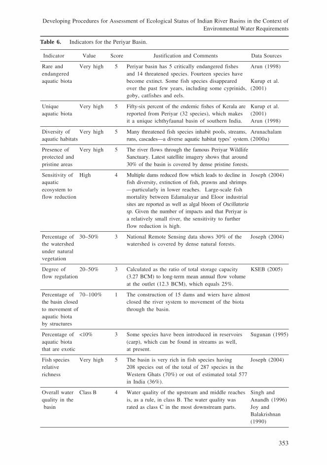
353
Developing Procedures for Assessment of Ecological Status of Indian River Basins in the Context ofEnvironmental Water Requirements
Table 6. Indicators for the Periyar Basin.
Indicator Value Score Justification and Comments Data Sources
Rare and Very high 5 Periyar basin has 5 critically endangered fishes Arun (1998)endangered and 14 threatened species. Fourteen species haveaquatic biota become extinct. Some fish species disappeared Kurup et al.
over the past few years, including some cyprinids, (2001)goby, catfishes and eels.
Unique Very high 5 Fifty-six percent of the endemic fishes of Kerala are Kurup et al.aquatic biota reported from Periyar (32 species), which makes (2001)
it a unique ichthyfaunal basin of southern India. Arun (1998)
Diversity of Very high 5 Many threatened fish species inhabit pools, streams, Arunachalamaquatic habitats runs, cascades—a diverse aquatic habitat types’ system. (2000a)
Presence of Very high 5 The river flows through the famous Periyar Wildlifeprotected and Sanctuary. Latest satellite imagery shows that aroundpristine areas 30% of the basin is covered by dense pristine forests.
Sensitivity of High 4 Multiple dams reduced flow which leads to decline in Joseph (2004)aquatic fish diversity, extinction of fish, prawns and shrimpsecosystem to —particularly in lower reaches. Large-scale fishflow reduction mortality between Edamalayar and Eloor industrial
sites are reported as well as algal bloom of Oscillatoriasp. Given the number of impacts and that Periyar isa relatively small river, the sensitivity to furtherflow reduction is high.
Percentage of 30–50% 3 National Remote Sensing data shows 30% of the Joseph (2004)the watershed watershed is covered by dense natural forests.under naturalvegetation
Degree of 20–50% 3 Calculated as the ratio of total storage capacity KSEB (2005)flow regulation (3.27 BCM) to long-term mean annual flow volume
at the outlet (12.3 BCM), which equals 25%.
Percentage of 70–100% 1 The construction of 15 dams and wiers have almostthe basin closed closed the river system to movement of the biotato movement of through the basin.aquatic biotaby structures
Percentage of <10% 3 Some species have been introduced in reservoirs Sugunan (1995)aquatic biota (carp), which can be found in streams as well,that are exotic at present.
Fish species Very high 5 The basin is very rich in fish species having Joseph (2004)relative 208 species out of the total of 287 species in therichness Western Ghats (70%) or out of estimated total 577
in India (36%).
Overall water Class B 4 Water quality of the upstream and middle reaches Singh andquality in the is, as a rule, in class B. The water quality was Anandh (1996) basin rated as class C in the most downstream parts. Joy and
Balakrishnan(1990)
354
V. Smakhtin, M. Arunachalam, K. G. Sivaramakrishnan, S. Behera, A. Chatterjee, P. Gautam,S. Das, G. D. Joshi, and K. Sankaran Unni
Another major threat in the basin is, water pollution. The physico-chemical analyses andreviews of the Periyar River water quality are available from 1976 onwards for a period of25 years (Paul and Pillai 1976, 1981). These analyses show a consistent decline in: pH and oxygenlevels; and an increase in: water temperature, radioactivity, pesticide pollution, and levels of heavymetals. Crabs and prawns that were found downstream have now become almost extinct due towater pollution (Joseph 2004). Greenpeace (2003) describes the ‘Eloor industrial area’, which islocated in the downstream of the Periyar River, as one of the most vulnerable ‘hotspots’ ofindustrial pollution in the world. A parallel reduction in the flow of water will further increasealgal blooms, resulting in occasional ‘fish kills’ as has already been experienced in the past.
Ganga River Basin (Rishikesh to Naraura reach)
The indicator values for this reach of the Ganga River are summarized in table 7. Ganga is thetop basin in India with regard to fish species richness, but estimates of the total number of speciesvary significantly. The World Bank identified about 350 species (Kottelat and Whitten 1996),while Talwar (1991) reported 375 species. Of these, the estimates of freshwater species are between104 and 161 (Menon 1999; Payne et al. 2003). In the study reach between Rishikesh and Naraura,Behera (1995) recorded 82 species of fish. Of these 4 to 10 are threatened or endangered accordingto different sources (Menon 1999; Behera 1995; Arunachalam, personal observations). Theseinclude the ‘endangered’ Tor tor, a Mahseer, Bagarius bagarius, Pangasius pangasius, and Ritarita (Behera 1995). In addition, 12 species of freshwater turtles are present, out of which 6 speciesare considered endangered in terms of Schedule I of the Indian Wildlife Protection Act, 1972(Rao 1995). In the same stretch, two species of crocodile Crocodylus palustris and the Gavialisgangeticus, locally known as ‘Gharial’, are found. Both are considered endangered (IUCN 1994).The Common Indian Otter (Lutra lutra), and Smooth Indian Otter (Lutra perspicillata), havealso been sighted in this stretch of the river. Both species are classified as threatened (IUCN1994). More than 100 species of birds, both migratory and residential have been sighted (Behera1995), of which several are endangered. The area around Naraura was proposed as a potentialbird sanctuary in 1978 (Rao 1995); 51 species of aquatic insects and 15 species of mollusks havealso been observed in this area.
By comparing the list of fish species from the stretch (Behera 1995) with the list of endemicfish species of India (Karmakar and Das 2004), it is inferred that no endemic freshwater speciesof fish have been reported from the stretch. However, one species of Crocodile, Crocodyluspalustris, twelve species of turtles and one aquatic mammal species, Platanista gangetica—theGangetic Dolphin, have been recorded (Rao 1995). Though the Gangetic Dolphin is also foundin the Brahmaputra, it is considered unique to the entire Ganga-Brahmaputra-Meghna (GBM)basin, and its characteristics that separate it from the Irrawady and Indus Dolphins have beenwell documented (Behera 1995). Though the crocodile is not unique to the Ganga system, it isan ‘endangered’ animal as per IUCN classification (IUCN 1994), as such, it is protected underSchedule I of the Wildlife Act, 1972. Although these species are not unique in the strictest sense,their presence warrants the conservation of this reach.
The Ganga becomes a mature river after Haridwar, flowing over hundreds of meters ofalluvium. In the upper part of the reach, the aquatic habitats include riffle areas, rocky, sandyand muddy river banks, while the lower part is dominated by sandy and muddy banks anddeep pools (Rao 1995). The shallow parts of the river turn into islands during low flows andthereby become good nesting grounds for turtles and island breeding birds.
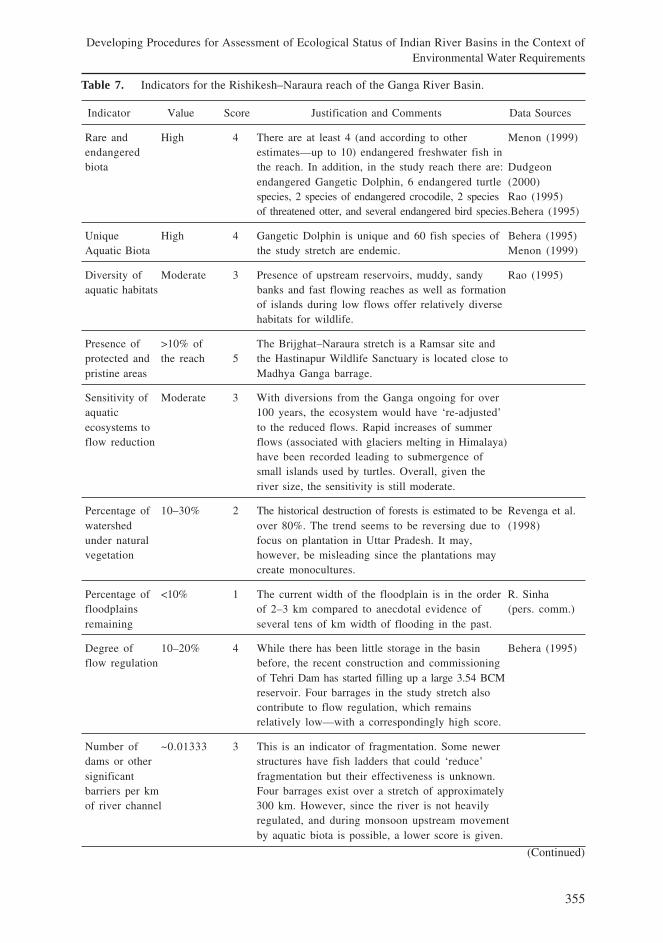
355
Developing Procedures for Assessment of Ecological Status of Indian River Basins in the Context ofEnvironmental Water Requirements
Table 7. Indicators for the Rishikesh–Naraura reach of the Ganga River Basin.
Indicator Value Score Justification and Comments Data Sources
Rare and High 4 There are at least 4 (and according to other Menon (1999)endangered estimates—up to 10) endangered freshwater fish inbiota the reach. In addition, in the study reach there are: Dudgeon
endangered Gangetic Dolphin, 6 endangered turtle (2000)species, 2 species of endangered crocodile, 2 species Rao (1995)of threatened otter, and several endangered bird species.Behera (1995)
Unique High 4 Gangetic Dolphin is unique and 60 fish species of Behera (1995)Aquatic Biota the study stretch are endemic. Menon (1999)
Diversity of Moderate 3 Presence of upstream reservoirs, muddy, sandy Rao (1995)aquatic habitats banks and fast flowing reaches as well as formation
of islands during low flows offer relatively diversehabitats for wildlife.
Presence of >10% of The Brijghat–Naraura stretch is a Ramsar site andprotected and the reach 5 the Hastinapur Wildlife Sanctuary is located close topristine areas Madhya Ganga barrage.
Sensitivity of Moderate 3 With diversions from the Ganga ongoing for overaquatic 100 years, the ecosystem would have ‘re-adjusted’ecosystems to to the reduced flows. Rapid increases of summerflow reduction flows (associated with glaciers melting in Himalaya)
have been recorded leading to submergence ofsmall islands used by turtles. Overall, given theriver size, the sensitivity is still moderate.
Percentage of 10–30% 2 The historical destruction of forests is estimated to be Revenga et al.watershed over 80%. The trend seems to be reversing due to (1998)under natural focus on plantation in Uttar Pradesh. It may,vegetation however, be misleading since the plantations may
create monocultures.
Percentage of <10% 1 The current width of the floodplain is in the order R. Sinhafloodplains of 2–3 km compared to anecdotal evidence of (pers. comm.)remaining several tens of km width of flooding in the past.
Degree of 10–20% 4 While there has been little storage in the basin Behera (1995)flow regulation before, the recent construction and commissioning
of Tehri Dam has started filling up a large 3.54 BCMreservoir. Four barrages in the study stretch alsocontribute to flow regulation, which remainsrelatively low—with a correspondingly high score.
Number of ~0.01333 3 This is an indicator of fragmentation. Some newerdams or other structures have fish ladders that could ‘reduce’significant fragmentation but their effectiveness is unknown.barriers per km Four barrages exist over a stretch of approximatelyof river channel 300 km. However, since the river is not heavily
regulated, and during monsoon upstream movementby aquatic biota is possible, a lower score is given.
(Continued)
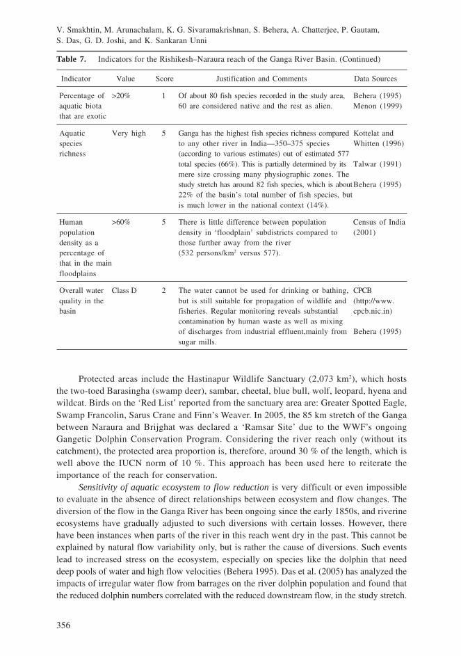
356
V. Smakhtin, M. Arunachalam, K. G. Sivaramakrishnan, S. Behera, A. Chatterjee, P. Gautam,S. Das, G. D. Joshi, and K. Sankaran Unni
Protected areas include the Hastinapur Wildlife Sanctuary (2,073 km2), which hoststhe two-toed Barasingha (swamp deer), sambar, cheetal, blue bull, wolf, leopard, hyena andwildcat. Birds on the ‘Red List’ reported from the sanctuary area are: Greater Spotted Eagle,Swamp Francolin, Sarus Crane and Finn’s Weaver. In 2005, the 85 km stretch of the Gangabetween Naraura and Brijghat was declared a ‘Ramsar Site’ due to the WWF’s ongoingGangetic Dolphin Conservation Program. Considering the river reach only (without itscatchment), the protected area proportion is, therefore, around 30 % of the length, which iswell above the IUCN norm of 10 %. This approach has been used here to reiterate theimportance of the reach for conservation.
Sensitivity of aquatic ecosystem to flow reduction is very difficult or even impossibleto evaluate in the absence of direct relationships between ecosystem and flow changes. Thediversion of the flow in the Ganga River has been ongoing since the early 1850s, and riverineecosystems have gradually adjusted to such diversions with certain losses. However, therehave been instances when parts of the river in this reach went dry in the past. This cannot beexplained by natural flow variability only, but is rather the cause of diversions. Such eventslead to increased stress on the ecosystem, especially on species like the dolphin that needdeep pools of water and high flow velocities (Behera 1995). Das et al. (2005) has analyzed theimpacts of irregular water flow from barrages on the river dolphin population and found thatthe reduced dolphin numbers correlated with the reduced downstream flow, in the study stretch.
Table 7. Indicators for the Rishikesh–Naraura reach of the Ganga River Basin. (Continued)
Indicator Value Score Justification and Comments Data Sources
Percentage of >20% 1 Of about 80 fish species recorded in the study area, Behera (1995)aquatic biota 60 are considered native and the rest as alien. Menon (1999)that are exotic
Aquatic Very high 5 Ganga has the highest fish species richness compared Kottelat andspecies to any other river in India—350–375 species Whitten (1996)richness (according to various estimates) out of estimated 577
total species (66%). This is partially determined by its Talwar (1991)mere size crossing many physiographic zones. Thestudy stretch has around 82 fish species, which is aboutBehera (1995)22% of the basin’s total number of fish species, butis much lower in the national context (14%).
Human >60% 5 There is little difference between population Census of Indiapopulation density in ‘floodplain’ subdistricts compared to (2001)density as a those further away from the riverpercentage of (532 persons/km2 versus 577).that in the mainfloodplains
Overall water Class D 2 The water cannot be used for drinking or bathing, CPCBquality in the but is still suitable for propagation of wildlife and (http://www.basin fisheries. Regular monitoring reveals substantial cpcb.nic.in)
contamination by human waste as well as mixingof discharges from industrial effluent,mainly from Behera (1995)sugar mills.
357
Developing Procedures for Assessment of Ecological Status of Indian River Basins in the Context ofEnvironmental Water Requirements
Other scientists have identified reduced river flows as one of the primary threats not only tothe populations of dolphins, but also to Mahseer (a local endemic carp group), crocodiles andturtles (Rao 1995); although no quantitative data on this is available.
Since the Gangetic Plains have been inhabited for centuries, the dominant land-use hasbeen agriculture, which has certainly affected the proportion of natural cover in the basin.According to some recent sources (Revenga et al. 1998), over 80 % of the original forest coverin the entire Ganga basin has been lost. However, some areas in the subbasin of the study reachstill remain under grasslands (e.g., protected areas like the Hastinapur Sanctuary). Forests haverecently started to show a tendency of recovering some of its lost cover (a marginal increase inforest area of 2–5% has been reported in the past decade—Census of India 2001). However,most of the basin is now under agriculture. Similarly, almost the entire floodplain of the Gangahas been converted to agricultural land. The remaining floodplain areas range from 1.5 km (atboth sides of the river in total) at Haridwar to some 20 km near the Naraura Barrage (estimatedusing images from http://www.earth.google.com). Less than approximately 10 percent of theoriginal (i.e., 10,000 years ago) floodplains still remain (R. Sinha personal communication).
The degree of flow regulation in the basin is still relatively low. There were no storagereservoirs along the stretch or upstream of it, until the completion of the Tehri Dam in 2005.Nilsson et al. (2005) classify the entire basin, including the main channel and tributaries as‘moderately affected’ by regulation. However, four major barrages have been constructed inthe study reach from 1850s onwards. Some sources suggest that diversion and regulation inthe reach remove approximately 50 % of the discharge compared to 66 % for the entire basin(Payne et al. 2003). This, however, is likely to be significantly overestimated as the data onobserved historical flows in the Ganga are not readily available. The barrages fragment themain river into three reaches, resulting in 0.013 structures per km across the flow, which isused here as an estimate of the degree of river fragmentation (Table 1 and 7). Some of thebarrages constructed more recently, like the refurbished lower Ganga barrage at Naraura, havefish ladder arrangements that restore connectivity to a limited degree. However, these structuresare based on designs for rivers in the temperate zone (Kottelat and Whitten 1996) and, assuch, their effectiveness in the tropical rivers is unknown.
Behera (1995) reports over 80 species of fish in the study stretch. A comparison withMenon’s (1999) description of freshwater fish in the Ganga basin reveals that about 60 of thesespecies are native. Thus, slightly over 20 % of the fish species recorded in the stretch may beseen as exotic fish—including carps and catfishes that may have been introduced for fisheries.At the same time, this may be an overestimation as exotic carp in India are few (V. V. Sugunan,ICAR, New Delhi, pers. comm.). Hence, the above figure needs to be verified in the future.
According to the Census of India (2001), there is little difference in the human populationdensity between areas adjacent to the river and those further away from it (Table 7). The waterquality of the study reach is regularly monitored by the Central Pollution Control Board ofIndia (CPCB - http://www.cpcb.nic.in) at Rishikesh, Haridwar, Garhmukteshwar, and Naraura;and occasionally—during research projects (Behera 1995). It varies in different parts of thereach from class B to D with most of it falling into class D, due to contamination of the riverby human wastes that exceed the permissible thresholds and high Biochemical Oxygen Demand(BOD) values around Naraura (due to the presence of sugar industries in the area).
In the short-term, the flow downstream of the Tehri Dam is likely to decrease, while theincreased use of groundwater for irrigation may reduce the baseflow, especially during summermonths. The increasing diversion of river water for irrigation is the single most important
358
V. Smakhtin, M. Arunachalam, K. G. Sivaramakrishnan, S. Behera, A. Chatterjee, P. Gautam,S. Das, G. D. Joshi, and K. Sankaran Unni
consumptive use in the study reach. In addition, the power generation facility of the TehriDam will need its peaking power requirement met, which, in turn, will create a pulse dischargeinto the river downstream that can be felt as far as Rishikesh or even Haridwar. These factorsadversely affect the single most important ecological issue in the reach—the protection of theGangetic Dolphin. Although, due to recent conservation efforts its population has doubled(from 22 to 45) since 1995, the habitat for the dolphin in the Ganga is threatened by irrigationdiversions and changes in flow variability. The overall prospects for the dolphins in the countryremain a concern with their annual fatality rate nearing 10 %.
Discussion and Conclusions
Once the scores for individual indicators have been estimated, it is possible to calculatetheir sum and express it as the percentage of the total maximum possible sum of all indicators.This percentage may then be converted into the most likely Environmental ManagementClass (EMC), which, in turn, determines how much water (environmental flows) needs to beallocated for environmental purposes in each river basin (Smakhtin and Anputhas 2006).These environmental flows are determined by the modification of the natural (reference) flowduration curves according to the class. Similar to the various number and types of ecologicalindicators used, various procedures and categories can be proposed on how to use theindicators to establish the EMC, or directly—the environmental flows themselves. In thisstudy, the scores have been divided into six unequal categories, each representing one ofthe six EMCs described in Table 8. The ‘score ranges’ in groups are arbitrary, with largerranges in lower classes C and D.
The rule of thumb has been that rivers/basins in the most natural category (A) are rareand, even if present, may not be assigned to this category due to development needs. The otherextremes—classes E and F—should generally not be considered as feasible management options(which stem from the rules adopted in South Africa, e.g., DWAF 1999). Classes B, C and Dtogether, thus cover most of the available range of percentage values (Table 8). This system isclearly arbitrary at present, and a much more extensive research effort as well as further expertdiscussions are required to justify how to convert the indicator scores into different EMCs.
The final sum of all indicators and the estimation of EMCs for each basin or subbasinare given in Table 9. Most of the basins examined in this study fall into class C, three—intoclass B and two—into class D. The basins/reaches in the highest class (B) are primarilyheadwater or ‘smallish’ basins located/originating in the Western Ghats, with high habitatdiversity, species richness and, are relatively less developed compared to basins located furtherdownstream. This combination of relatively natural conditions on the one hand, and highersensitivity/importance due to greater species diversity, etc., on the other, places these basinsin a high category. Two subbasins (in this study), placed in the lowest class D, are on thecontrary, located in the most downstream parts of the basins. It can also be noted that LowerKrishna, although in class C, is at the lowest boundary of this class (Tables 8 and 9). Aninteresting example is the Narmada basin: it falls into class C primarily due to its two low scoreson rare and unique species (Table 9). This reduces the importance of the basin and makes theotherwise relatively natural basin an ‘attractive’ candidate for development. But as Table 5indicates, there are unpublished sources suggesting that rare and unique species do exist in
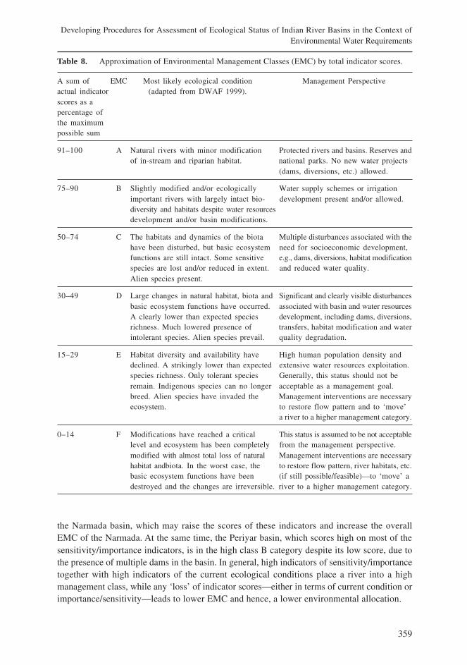
359
Developing Procedures for Assessment of Ecological Status of Indian River Basins in the Context ofEnvironmental Water Requirements
Table 8. Approximation of Environmental Management Classes (EMC) by total indicator scores.
A sum of EMC Most likely ecological condition Management Perspectiveactual indicator (adapted from DWAF 1999).scores as apercentage ofthe maximumpossible sum
91–100 A Natural rivers with minor modification Protected rivers and basins. Reserves andof in-stream and riparian habitat. national parks. No new water projects
(dams, diversions, etc.) allowed.
75–90 B Slightly modified and/or ecologically Water supply schemes or irrigationimportant rivers with largely intact bio- development present and/or allowed.diversity and habitats despite water resourcesdevelopment and/or basin modifications.
50–74 C The habitats and dynamics of the biota Multiple disturbances associated with thehave been disturbed, but basic ecosystem need for socioeconomic development,functions are still intact. Some sensitive e.g., dams, diversions, habitat modificationspecies are lost and/or reduced in extent. and reduced water quality.Alien species present.
30–49 D Large changes in natural habitat, biota and Significant and clearly visible disturbancesbasic ecosystem functions have occurred. associated with basin and water resourcesA clearly lower than expected species development, including dams, diversions,richness. Much lowered presence of transfers, habitat modification and waterintolerant species. Alien species prevail. quality degradation.
15–29 E Habitat diversity and availability have High human population density anddeclined. A strikingly lower than expected extensive water resources exploitation.species richness. Only tolerant species Generally, this status should not beremain. Indigenous species can no longer acceptable as a management goal.breed. Alien species have invaded the Management interventions are necessaryecosystem. to restore flow pattern and to ‘move’
a river to a higher management category.
0–14 F Modifications have reached a critical This status is assumed to be not acceptablelevel and ecosystem has been completely from the management perspective.modified with almost total loss of natural Management interventions are necessaryhabitat andbiota. In the worst case, the to restore flow pattern, river habitats, etc.basic ecosystem functions have been (if still possible/feasible)—to ‘move’ adestroyed and the changes are irreversible. river to a higher management category.
the Narmada basin, which may raise the scores of these indicators and increase the overallEMC of the Narmada. At the same time, the Periyar basin, which scores high on most of thesensitivity/importance indicators, is in the high class B category despite its low score, due tothe presence of multiple dams in the basin. In general, high indicators of sensitivity/importancetogether with high indicators of the current ecological conditions place a river into a highmanagement class, while any ‘loss’ of indicator scores—either in terms of current condition orimportance/sensitivity—leads to lower EMC and hence, a lower environmental allocation.
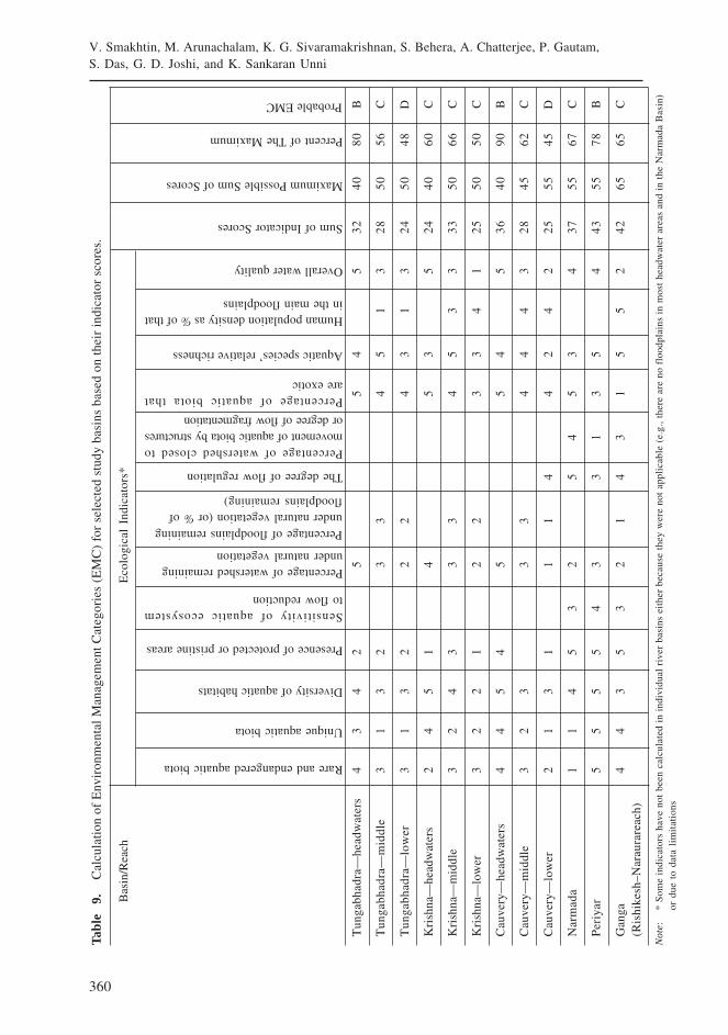
360
V. Smakhtin, M. Arunachalam, K. G. Sivaramakrishnan, S. Behera, A. Chatterjee, P. Gautam,S. Das, G. D. Joshi, and K. Sankaran Unni
Bas
in/R
each
Eco
logi
cal
Indi
cato
rs*
Tun
gabh
adra
—he
adw
ater
s4
34
25
54
532
4080
B
Tun
gabh
adra
—m
iddl
e3
13
23
34
51
328
5056
C
Tun
gabh
adra
—lo
wer
31
32
22
43
13
2450
48D
Kri
shna
—he
adw
ater
s2
45
14
53
524
4060
C
Kri
shna
—m
iddl
e3
24
33
34
53
333
5066
C
Kri
shna
—lo
wer
32
21
22
33
41
2550
50C
Cau
very
—he
adw
ater
s4
45
45
54
536
4090
B
Cau
very
—m
iddl
e3
23
33
44
43
2845
62C
Cau
very
—lo
wer
21
31
11
44
24
225
5545
D
Nar
mad
a1
14
53
25
45
34
3755
67C
Per
iyar
55
55
43
31
35
443
5578
B
Gan
ga4
43
53
21
43
15
52
4265
65C
(Ris
hike
sh–N
arau
rare
ach)
Not
e:*
Som
e in
dica
tors
hav
e no
t be
en c
alcu
late
d in
ind
ivid
ual
rive
r ba
sins
eit
her
beca
use
they
wer
e no
t ap
plic
able
(e.
g.,
ther
e ar
e no
flo
odpl
ains
in
mos
t he
adw
ater
are
as a
nd i
n th
e N
arm
ada
Bas
in)
or d
ue t
o da
ta l
imit
atio
ns
Tabl
e 9
.C
alcu
lati
on o
f E
nvir
onm
enta
l Man
agem
ent C
ateg
orie
s (E
MC
) fo
r se
lect
ed s
tudy
bas
ins
base
d on
thei
r in
dica
tor
scor
es.
Sensitivity of aquatic ecosystemto flow reduction
Percentage of watershed remainingunder natural vegetation
Percentage of floodplains remainingunder natural vegetation (or % offloodplains remaining)
Percentage of watershed closed tomovement of aquatic biota by structuresor degree of flow fragmentation
Percentage of aquatic biota thatare exotic
Aquatic species’ relative richness
Human population density as % of thatin the main floodplains
Rare and endangered aquatic biota
Unique aquatic biota
Diversity of aquatic habitats
Presence of protected or pristine areas
The degree of flow regulation
Overall water quality
Sum of Indicator Scores
Maximum Possible Sum of Scores
Percent of The Maximum
Probable EMC
361
Developing Procedures for Assessment of Ecological Status of Indian River Basins in the Context ofEnvironmental Water Requirements
Smakhtin and Anputhas (2006) presented, among others, relationships between EMCsand the amount of natural long-term mean flow at the outlets of major river basins in India.If their relationships are used together with the procedure suggested herein, theenvironmental water requirements at the outlet of Krishna, for example, would be 18 % ofthe long-term mean flow; Cauvery around 11 %; Narmada 14 %; and Periyar28 % of their long-term flows, respectively. It is important to understand that this reportintroduces the approach rather than the final method for setting EMCs for Indian rivers.Even if the existing EMC setting approach is retained for future management of Indian riversin principle, it is necessary to be aware of its multiple limitations, including, but not confinedto the following:
• The set of indicators used here is very preliminary and the selection of indicatorsneeds to be revisited. Apart from the rather general nature of some indicators, noindicators relating to the social importance of rivers have been considered in theapproach, at present. This is acknowledged as a serious limitation and one that needsto be addressed in future work.
• The existing information base for determining any ecological indicator in India is verylimited. The authors of this report used their own knowledge of and judgment onspecific rivers, but other specialists will need to be involved in estimating the scoresto improve the level of confidence in the approach.
• The scale of the analysis was very coarse and a similar or a different set of indicatorsneeds to be used at much smaller scales, e.g., for a particular reach of any river, ratherthan for arbitrarily selected, big areas of already very large river basins (with Periyarbeing the only exception).
• There seems to be a lack of agreement on such specifics as how many fish speciesthere are in India as a whole, which, in turn, determines the estimation of several otherindicators. There is little knowledge on the diversity of other aquatic species.Uncertainty and lack of information will, however, always be unavoidable factors, andit will be necessary to find ways to handle them generally, in such an approach.
• It is a challenge to bring into account coastal fish diversity to an EMC estimation fora river basin unless, of course, estuarine freshwater requirements are estimated usinga protocol different from environmental flow assessment for inland rivers.
• The procedures used in this report to convert the indicator scores into EMC are veryarbitrary but illustrative. They are given here primarily to stimulate further developmentin this field.
• There is currently no system of rating the level of confidence for the indicators and/or overall score. This is typically done with similar approaches, and the one presentedherein would benefit from attention to this aspect in future work.
• The estimation methods of individual indicators have varied slightly between thebasins, due to varying data availability, specifics of the basin and professionaljudgment. These differences should be eliminated in the future, and be replaced witha more strict assessment protocol.
362
V. Smakhtin, M. Arunachalam, K. G. Sivaramakrishnan, S. Behera, A. Chatterjee, P. Gautam,S. Das, G. D. Joshi, and K. Sankaran Unni
• Some indicators, like sensitivity of aquatic ecosystem to flow reduction, are verydifficult or even, impossible to evaluate in the absence of direct relationships betweenecosystem and flow changes. The above appears to be the most weakly developedindicator and yet a critical one for the entire process. It may need to be replaced bya set of different and more specific indicators in the future. Such indicators may bedefined through an expert workshop on indicators (see below).
It should also be noted that although useful, the scoring approach should not be usedonly for the estimation of EMCs. It may also be applied to estimate the permissible levels ofreduction/increase of various flows—directly, as suggested by Smakhtin and Anputhas (2006).
As an immediate follow-up to this preliminary study on ecological scoring, the authorsof this report propose to hold a national workshop, which would engage several aquaticecologists, hydrologists, social scientists, etc. The objective of this exercise would be to designa more reliable assessment methodology of environmental importance and conditions of Indianwater bodies.
The authors also consider it important to start the process of ecological statusassessment of all Indian water resources—at the fine scale of spatial resolution. This newlarge-scale program should tap into the already existing ecological expertise in the country,and should redirect it from largely descriptive/inventory type work into the context ofquantification of ecological water requirements of Indian rivers and wetlands.
References
Acreman, M.C.; Dunbar, M.J. 2004. Methods for defining environmental river flow requirements - A review.Hydrology and Earth System Sciences 8: 121-133.
Alvares, C.; Billorey, R. 1988. Damming the Narmada - India’s greatest planned environmental disaster.Dehradun, India. Natraj Publishers. 196 pp.
Armantrout, N. B. 1990. Aquatic Habitat Inventory. Bureau of Land Management. Eugene District, USA:Bureau of Land Management. 32 pp.
Arun, L.K. 1998. Status and distribution of fishes in Periyar lake-stream systems of Southern-WesternGhats. Fish Genetics and Biodiversity Conservation: National Bureau of Fish Genetic ResourcesPublications, Nature Conservators, Muzaffarnagar 251001: 492 pp.
Arunachalam, M. 1999. Biodiversity and ecological structure of fishes in streams of South India. Departmentof Biotechnology, Government of India, New Delhi, India: Department of Biotechnology. 119 pp.
Arunachalam, M. 2000a. Stream fish habitat inventory methodology. In: Endemic fish diversity of WesternGhats, eds. A.G. Ponniah; A. Gopalakrishnan. National Bureau of Fish Genetic Resources - NationalAgricultural Technology Project. Lucknow, India. 347 pp.
Arunachalam, M. 2000b. Assemblage structure of stream fishes in the Western Ghats (India). Hydrobiologica430: 1-31.
Arunachalam, M.; Sankaranarayanan, A.; Manimekalan, A.; Soranam R.; Johnson, J. A. 2002. Fish faunaof some streams and rivers in the Western Ghats of Maharashtra. Journal of the Bombay Natural HistorySociety 99: 337-341.
Arunachalam, M. 2004. Germplasm inventory, evaluation and gene banking of freshwater fishes. NationalAgricultural Technology Project. Government of India. Project Report (unpublished). 204 pp.
363
Developing Procedures for Assessment of Ecological Status of Indian River Basins in the Context ofEnvironmental Water Requirements
Arunachalam, M.; Sivakumar, P.; Muralidharan, M. 2005. Habitat evaluation of pristine headwater streams ofWestern Ghats mountain ranges, Peninsular India. In: Proceedings of the National Seminar: New Trendsin Fishery Development in India, ed. M.S. Johal. Punjab University. Chandigarh, India. 286 pp.
Beecher, H.A. 1990. Standards for instream flows. Rivers 1(2): 97-109.
Behera, S. 1995. Studies on Population Dynamics, Habitat Utilization, and Conservation Aspects of Platantistagangetica between Bijnor and Naraura, Ph.D. thesis, submitted to Jiwaji University, Gwalior, NorthMadhya Pradesh, India.
CAMP (Conservation Assessment and Management Plan). 1997. Report of the workshop Freshwater fishesof India 1997. Zoo Outreach Organization and National Bureau of Fish Genetic Resources, Lucknow,India. 137 pp.
Census of India. 2001. Village Directory Data CD. New Delhi.
Chatterji, S.N.; Rao, K.S.; Singh, A.K. 1993. Recent advances in Freshwater Biology. New Delhi, India:Anmol Publications Pvt. Ltd. 380 pp.
CIFRI (Central Inland Fisheries Research Institute). 1993. Studies on the fish conservation in NarmadaSagar, Sardar Sarovar and its downstream. West Bengal, India: CIFRI.
Cincotta, R.P.; Engelman, R. 2000. Nature’s place: Human population and the future of biological diversity,Washington, D. C., USA: Population Action International. 80 pp.
CPCB (Central Pollution Control Board). 1992. A system for surface water classification in India, Mimeo.CPCB. 1– 16 pp.
Cottingham, P.; Thoms, M.C.; Quinn, G.P. 2002. Scientific panels and their use in environmental flow assessmentin Australia. Australian Journal of Water Resources 5(1): 103-111.
CWC (Central Water Commission). 2006. Integrated Hydrological Data Book (non-classified river basins).New Delhi, India, 383 pp.
Das, S.; Chatterjee, A.; Behera, S.; Bhatia, S.; Gautam, P. 2005. Concerns of environmental flows in riversin the context of the proposed Interlinking of Rivers in India. Abstracts of the NIE/IWMI Workshop onEnvironmental Flows. New Delhi, India. March 2005.
Dave, J.H. 1957. Immortal India. Mumbai, India: Bhavan’s Publication. 168 pp.
Dubey, G.P. 1984. Narmada Basin Water Development Plan: Part 1: Development of Fisheries. NarmadaPlanning Agency, Government of Madhya Pradesh, India: Narmada Planning Agency.
Dubey, G.P. 1993. Status prior to the year 1980 of Hydrobiology, Fisheries and Socioeconomic conditionsof fishermen in Narmada Basin. In: Recent Advances in Freshwater Biology, ed. K.S. Rao. New Delhi,India: Anmol Publications Pvt. Ltd. 380 pp.
DWAF (Department of Water Affairs and Forestry). 1999. Resource directed measures for protection ofwater resources. Volume 3: River ecosystems. Version 1.0. Institute for Water Quality Studies, Departmentof Water Affairs and Forestry. Pretoria, South Africa: DWAF.
Dudgeon, D. 2000. Large-scale hydrological changes in tropical Asia: Prospects for biodiversity. Bio Science50(9): 793-806.
Dyson, M.; Bergkamp, G.; Scanlon, J. (eds.) 2003. Flow - The essentials of environmental flows. TheWorld Conservation Union - International Union for the Conservation of Nature (IUCN)), Gland,Switzerland and Cambridge, UK: IUCN. 118 pp.
Easa, P.S.; Shaji, C.P. 1995. Freshwater fish diversity in the Kerala part of the Nilgiri Biosphere Reserve.Current Science 73: 180–182.
Galbraith, H. 2001. Indicators of Ecosystem condition, sustainability and coping capacity. UnpublishedReport to the United Nations World Assessment Program Indicator Development Unit. UnpublishedReport, Galbraith Environmental Sciences, Boulder, Colorado, USA: Galbraith Environmental Sciences.
364
V. Smakhtin, M. Arunachalam, K. G. Sivaramakrishnan, S. Behera, A. Chatterjee, P. Gautam,S. Das, G. D. Joshi, and K. Sankaran Unni
Greenpeace. 2003. Status of human health at the Eloor Industrial Belt. Kerala, India. A cross sectionalEpidermological study. India. Greenpeace.
Hora, S.L. 1942. A list of fishes of Mysore state and of the neighboring hill ranges of the Nilgiris, Wynadand Coorg. Records of the Indian Museum 44: 193–200.
Ittekkot, V.; Humberg, C.; Schafer, P. 2000. Hydrobiological alterations and marine biogeochemistry asilicate issue? Bioscience 50: 776–782.
IUCN (International Union for the Conservation of Nature). 1980. World Conservation Strategy, IUCN,Gland, Switzerland: IUCN.
IUCN. 1994. Guidelines for applications of IUCN Redlist criteria at Regional levels: Version 2.3. IUCNspecies survival commission. IUCN, Gland, Switzerland and Cambridge, UK: IUCN. 12 pp.
Jayaram, K.C. 1995. The Krishna River system Bioresources study. Records of the Zoological Survey ofIndia, Occasional Paper No. 160. Calcutta, India: Zoological Survey of India, 167 pp.
Jayaram, K.C. 2000. Cauvery Riverine System: An Environmental Study. The Madras Science Foundation.India. The Madras Science Foundation. 257 pp.
Joseph, M.L. 2004. Status Report on Periyar River. Kerala, India. 43 pp.
Joy, C.M.; Balakrishnan, K.P. 1990. Physico chemical aspects of a tropical river receiving industrialeffluents 17-236. In: River pollution in India, ed. R.K. Trivedy. New Delhi, India: Ashish PublishingHouse. 294 pp.
Karamchandani, S.J.; Desai, K.R.; Pisolkar, M.D.; Bhatnagar, G.K. 1967. Biological investigations on thefish and fisheries of Narmada River, 1958-1966. Bulletin of Central Inland Fisheries Research Institute,Barrackpore, 10: 40 pp.
Karmakar, A.K.; Das, A. 2004. Endemic Freshwater Fishes of India, Zoological Survey of India, OccasionalPaper No. 230. Kolkata, India: Zoological Survey of India. 1-125 pp.
Kathiresan, K. 2000. A review of studies on pichavaram mangrove, southeast India. Hydrobiologia 430:185–205.
Kathiresan, K.; Moorthy, P.; Ravikumar, S. 1996. A note on the influence of salinity and PH on rooting ofRhizopora mucronata Lamk seedlings. Indian Forestry 122: 763–764.
Kottelat, M.; Whitten, T. 1996. Freshwater Biodiversity in Asia with Special Reference to Fish, World BankTechnical Paper No. 343. Washington D.C., USA: World Bank. 28 pp.
KSEB (Kerala State Electricity Board). 2005. Fact file on dams. Government of Kerala. Thiruvananthapuram,India: KSEB.
Kurup, B.M.; Radhakrishnanan, K.V.; Manoj Kumar, T.J. 2001. Biodiversity status of fishes inhabitingRivers of Kerala, India, with special reference to endemism – threats and conservation.Thiruvananthapuram, India: 76 pp.
Manjrekar, N. 2000. A walk on the wild side. Information Guide to National Parks and Wildlife Sanctuariesof Karnataka. State of Karnataka, India: Forest Department - Wildlife Wing. 78 pp.
Menon, A.G.K. 1999. Checklist – Freshwater Fishes of India, Occasional Paper No.175. Zoological Surveyof India. Kolkata, India: Zoological Survey of India.
Menon, A.G.K. 2004. Threatened fishes of India and their conservation. Zoological Survey of India. Kolkata,India: Zoological Survey of India. 1-170 pp.
Mittemeier, R.A.; Mittemeier, C.G.; Brooks, T.M.; Pilgrim, J.D.; Konstant, W.R.; da Fonseca, G.A.B.; Kormes,C. 2003. Wilderness and biodiversity conservation. Proceedings of the National Academy of Sciences100: 10309–10313.
MSSRF (M. S. Swaminathan Research Foundation). 1998. Coastal wetlands: Mangrove conservation andmanagement, MSSRF. 12 pp.

365
Developing Procedures for Assessment of Ecological Status of Indian River Basins in the Context ofEnvironmental Water Requirements
Nath, D.; Shrivastava, N.P. 1999. Decline of Carp fishery in Narmada in the context of construction ofdam on the river and its tributaries. Journal of Inland Fisheries Society (India) 31(2): 25-27.
Nilsson, C.; Reidy, C.A.; Dynesius, M.; Revenga, C. 2005. Fragmentation and flow regulation of the world’slarge river systems. Science 308: 405-408.
NPA (Narmada Planning Agency). 1987. Narmada basin water development plan – Development of fisheries.Narmada Planning Agency, Government of Madhya Pradesh State, India: Narmada Planning Agency.
NSII (National Statistical Institute of India). 1991. Population statistics, India. Population data. New Delhi,India: NSII.
Pascal, J.P. 1996. Wild and Fragile – Analysis 28-32. Down to Earth August 15, 1996.
Paul, A.C.; Pillai, K.C. 1976. Studies of pollution aspects in Periyar river. Unpublished project report.
Paul, A.C.; Pillai, K.C. 1981. Geochemical transport of trace metals in Periyar River. Proceedings of seminaron status of Environmental Studies in India. Trivandrum, Kerala, India. 357-362 pp.
Payne, A.I.; Sinha, R.; Singh, H.S.; Huq, S. 2003. A Review of the Ganges Basin: Its Fish and Fisheries.In: Proceedings of the Second International Symposium on the Management of Large Rivers for fisheries,eds. R. Wellcome; T. Petr. Food and Agriculture Organization, Regional Office for Asia and the Pacific,Bangkok, Thailand: 229-251 pp.
Ponniah, A.G.; Gopalakrishnan, A. (eds.) 2000. Endemic Fish Diversity of Western Ghats. National Bureauof Fish Genetic Resources - National Agricultural Technology Project. Lucknow, India: National Bureauof Fish Genetic Resources. 347 pp.
Pratapan, S. 1999. Periyar - Under Severe Strain. The Hindu Survey of Environment.
Puckridge, J.T.; Sheldone, F.; Wlaker, K.F.; Boulton, A. J. 1998. Flow variability and ecology of largerivers. Marine and Freshwater Research 49: 55-72.
Rajan, S. 1963. Ecology of the fishes of the River Pykara and Moyar (Nilgiris), South India. Proceedingsof the Indian Academy of Science 58: 291–323.
Rao, K.S.; Chatterjee, S.N.; Singh, A.K. 1991. Studies on preimpoundment fishery potential of NarmadaBasin (Western region) in the context of Indira Sagar, Maheshwar Omkareshwar and Sardar SarovarReservoirs. Journal of the Inland Fisheries Society of India 23(1): 34-41.
Rao, K.S.; Shrivastava, S.; Choubey, U. 1999. Utility of Macro invertebrate in biological water quality insome Central Indian Rivers. In: Inland Water Resources of India, eds. Durgaprasad and Pichia. NewDelhi, India: Discovery Publishing House, 223-246 pp.
Rao, R. J. 1995. Studies on Biological Restoration of Ganga River in Uttar Pradesh: An indicator speciesapproach, School of Studies in Zoology, Jiwaji University. Gwalior, India: Jiwaji University.
Revenga, C.; Murray, S.; Abramowitz, J.; Hammond, P. 1998. Watersheds of the world: Ecological valueand vulnerability. Washington, D.C., USA: World Resources Institute.
Rogers, K.; Bestbier, R. 1997. Development of a protocol for the definition of the desired state of riverinesystems in South Africa. Department of Environmental Affairs and Tourism. Pretoria, South Africa:Department of Environmental Affairs and Tourism. 100 pp.
RRSL (Rapid Reconnaissance Survey of Limnological aspects of Narmada). 1987. Bhopal, Vikram Universityand RD University. Jabalpur for Govt. of Madhya Pradesh, India.
Scott, P.A. (ed.) 1989. A directory of Asian wetlands, IUCN, Gland, Switzerland and Cambridge, U.K.:IUCN. 118 pp.
Sharma, B.K.; Naik, L.P. 1995. Species composition distribution and abundance of Rotifers in river Narmada,M.P. (Central India). In: Tropical Limnology, Vol.III, eds. K.H. Timotius; F. Goltenboth. Satya WacanaChristian University, Salatiga, Indonesia. 77-87 pp.
Singh, R.K.; Anandh, H. 1996. Water quality index of some Indian Rivers. Indian Journal of EnvironmentalHealth 38(1): 21-34.
366
V. Smakhtin, M. Arunachalam, K. G. Sivaramakrishnan, S. Behera, A. Chatterjee, P. Gautam,S. Das, G. D. Joshi, and K. Sankaran Unni
Sivaramakrishnan, K.G.; Venkataraman, K.; Sridhar, S.; Marimuthu, S. 1995. Spatial patterns of benthicmacroinvertebrate distribution along river Kaveri and its tributaries. International Journal of Ecologyand Environmental Science 21: 141–161.
Smakhtin, V.U.; Anputhas, M. 2006. An assessment of environmental flow requirements of Indian riverbasins. IWMI Research Report 107. Colombo, Sri Lanka: International Water Management Institute (IWMI).
Sreenivasan, A.1989. Status of some exotic fish introductions in Tamil Nadu. In: Exotic Aquatic Species inIndia, ed. M. Mohan Joseph. 59 – 62, special publication, Asian Fisheries Society, Indian Branch.
Sugunan, V.V. 1995. Reservoir fisheries in India. FAO Fisheries Technical Report, 345. Rome: Food andAgriculture Organization of United Nations (FAO). 423 pp.
Tharme, R.E. 2003. A global perspective on environmental flow assessment: emerging trends in thedevelopment and application of environmental flow methodologies for rivers. River Research andApplications 19: 397-441.
Talwar, P.K. 1991. Pisces and Faunal Resources of Ganga, Part I, 1-11, Zoological Survey of India. Kolkata,India: Zoological Survey of India. 91 pp.
Unni, K.S. 1996. Ecology of the River Narmada. New Delhi, India: A.P.H. Publishing Corporation. 371 pp.
Xenopoulos, M.A.; Lodge, D.M.; Alcamo, J.; Märker, M.; Schulze, K.; van Vuuren, D.P. 2005. Scenariosof fish extinction from climate change and water withdrawal. Global Change Biology 11: 1–8.
367
Developing Procedures for Assessment of Ecological Status of Indian River Basins in the Context ofEnvironmental Water Requirements
Groundwater Situation in Urban India: Overview,Opportunities and Challenges
1Ankit Patel and 2Sunderrajan Krishnan1IWMI-TATA Water Policy Program, India
2International Water Management Institute
Introduction
Groundwater is a major source of water and is intensively exploited for private, domesticand industrial uses in many urban centers of the developing world. At the same time, thesubsurface has also come to serve as the receptor for much of the urban and industrialwastewater and for solid waste disposal (World Bank 1998). Groundwater plays a fundamentalrole in shaping the economic and social health of many urban areas. However, nocomprehensive statistics exist on the proportion of urban water supply world-wide derivedfrom groundwater. It is estimated that more than 1 billion urban dwellers in Asia and 150million in Latin America depend directly or indirectly upon well, spring and borehole sources(World Bank 1998a).
A number of factors determine the extent to which a city would depend upongroundwater to meet its water demand. The first set of factors can be called physical/geographic—availability of sufficient groundwater either from natural recharge due tocombination of good rainfall and receptive subsurface geology or from other sources suchas canals, good aquifers that can store and transmit groundwater, availability of goodquality groundwater that is not subject to constraints such as saline water intrusion. Thesecond set of factors is determined by the ability of the urban area to cope with its waterdemand from external sources. This is driven by the economic scarcity rather than physicalscarcity, or the latter may compound the former. In the event of physical scarcity, cities/towns will still continue to grow with its buffer capacity. The available empirical evidencesuggests that, by and large, cities have been able to obtain supplies, often at a greatercost than is necessary but without significantly compromising their ability to expand andprosper even in the most unhelpful locations (Molle and Berkoff 2006). Hence, water supplyto any urban center is determined by its physical characteristics or economic and financialcapacity. In the competition for water, cities generally win over agriculture (Molle andBerkoff 2006), but when it comes to competition between two cities or towns the dynamicsare very different. Negotiation for water is more difficult for smaller urban centers thathave lesser say on the water stored at distant reservoirs. In contrast, the larger urban
368
A. Patel and S. Krishnan
areas1 backed by population mass, financial capacity and political influence can attractsurface water from distances of hundreds of kilometers. Newly developing urban centers(class-III to class-VI2) also have to depend upon their local water resources.
On the overlapping of these two sets of factors, one can arrive at the general level ofdependence of urban areas on groundwater and their vulnerability at present and in thefuture in meeting their water demands from external sources. An accumulation of many suchvulnerable urban areas within a small region or within a single river basin also implies anadditional stress on water resources in the region and possible diversions of water fromother uses such as irrigation or even from other regions. Therefore, one can also envisagesuch areas as those with high competition in the future between urban and other uses.
How would such patterns of dependence and vulnerability of urban areas togroundwater emerge? One can expect that a dominant factor driving these patterns wouldbe the hydrogeological conditions. In India, the peninsular areas with basaltic and crystallineformations, unsuitable for groundwater exploitation, would exhibit relatively greaterdependence on external surface water sources than the northern urban areas over the alluvialbelt. On these would be superimposed factors such as local rainfall, location within canalcommands, problems of coastal salinity, proximity to reservoirs etc. The peninsular riverbasins, therefore, on an average would exhibit higher proportion of urban areas dependingon surface water than the northern urban areas, which have good access to local groundwatersupplies from rich aquifers augmented by natural and canal recharge. But, the rich alluvialaquifers of northern India, where groundwater overexploitation has already taken place byirrigators and/or urban centers, will have to tap new water sources (surface or groundwater)in the near future.
This paper analyzes the impact and effect of ‘supply-based’ urban water managementstrategies and endeavors to identify, using some assumptions and hypothesis, the urbanpockets or regions, which may face problems relating to groundwater and eventually becomea black-hole for any imported water in the vicinity in India. Although there are two sets offactors - economical and physical - that mainly govern groundwater use in any urban area,the present study is restricted only to the physical aspects of it.
1 The census of 1961 adopted a two-fold categorization to identify urban centers. First, the settlementsthat were given urban civic status like corporation, municipality and cantonment by state governmentswere identified as statutory towns. Second, three demographic criteria were applied to identify thecensus towns. These were (a) population size of 5,000 or more, (b) density of at least 400 persons persquare kilometer, and (c) at least 75 % of the male workers to be engaged outside agriculture(Sivaramakrishnan, Kundu and Singh 2005).2 According to the census of India, urban areas are classified into six classes based on population. Class-I = 100,000 and above; Class-II = 50,000 – 99,999; Class-III = 20,000 – 49,999; Class-IV = 10,000 –19,999; Class-V = 5,000 – 9,999; Class-VI = less than 5,000.
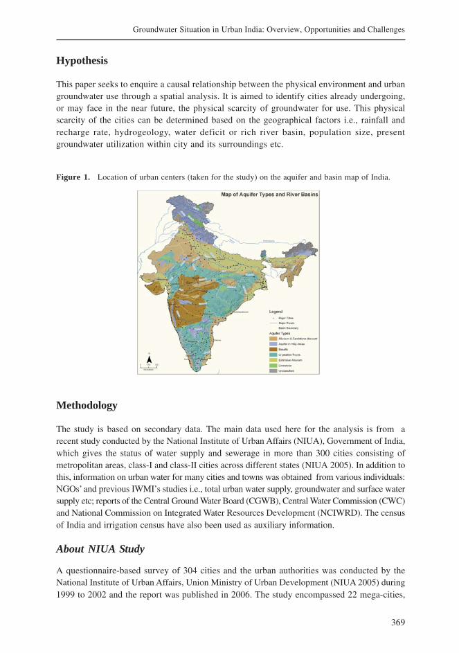
369
Groundwater Situation in Urban India: Overview, Opportunities and Challenges
Hypothesis
This paper seeks to enquire a causal relationship between the physical environment and urbangroundwater use through a spatial analysis. It is aimed to identify cities already undergoing,or may face in the near future, the physical scarcity of groundwater for use. This physicalscarcity of the cities can be determined based on the geographical factors i.e., rainfall andrecharge rate, hydrogeology, water deficit or rich river basin, population size, presentgroundwater utilization within city and its surroundings etc.
Figure 1. Location of urban centers (taken for the study) on the aquifer and basin map of India.
Methodology
The study is based on secondary data. The main data used here for the analysis is from arecent study conducted by the National Institute of Urban Affairs (NIUA), Government of India,which gives the status of water supply and sewerage in more than 300 cities consisting ofmetropolitan areas, class-I and class-II cities across different states (NIUA 2005). In addition tothis, information on urban water for many cities and towns was obtained from various individuals:NGOs’ and previous IWMI’s studies i.e., total urban water supply, groundwater and surface watersupply etc; reports of the Central Ground Water Board (CGWB), Central Water Commission (CWC)and National Commission on Integrated Water Resources Development (NCIWRD). The censusof India and irrigation census have also been used as auxiliary information.
About NIUA Study
A questionnaire-based survey of 304 cities and the urban authorities was conducted by theNational Institute of Urban Affairs, Union Ministry of Urban Development (NIUA 2005) during1999 to 2002 and the report was published in 2006. The study encompassed 22 mega-cities,
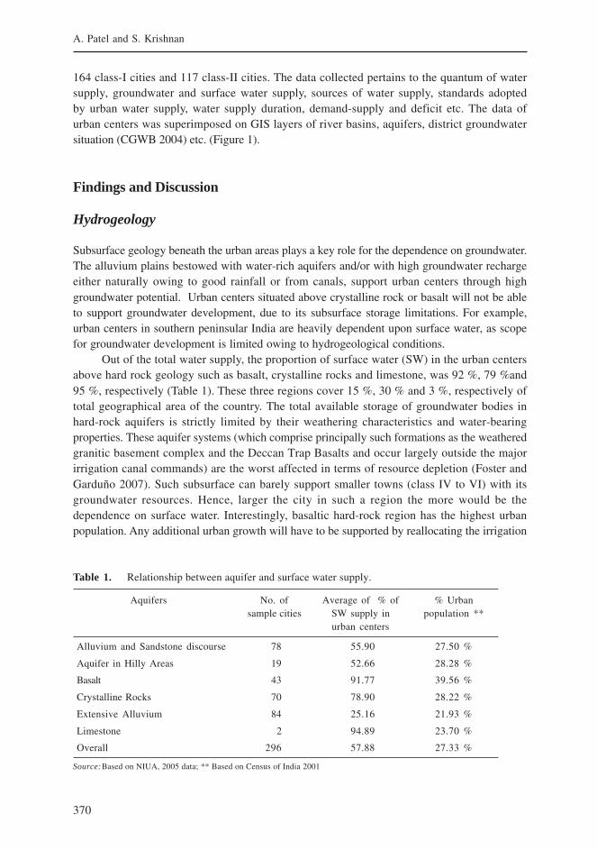
370
A. Patel and S. Krishnan
164 class-I cities and 117 class-II cities. The data collected pertains to the quantum of watersupply, groundwater and surface water supply, sources of water supply, standards adoptedby urban water supply, water supply duration, demand-supply and deficit etc. The data ofurban centers was superimposed on GIS layers of river basins, aquifers, district groundwatersituation (CGWB 2004) etc. (Figure 1).
Findings and Discussion
Hydrogeology
Subsurface geology beneath the urban areas plays a key role for the dependence on groundwater.The alluvium plains bestowed with water-rich aquifers and/or with high groundwater rechargeeither naturally owing to good rainfall or from canals, support urban centers through highgroundwater potential. Urban centers situated above crystalline rock or basalt will not be ableto support groundwater development, due to its subsurface storage limitations. For example,urban centers in southern peninsular India are heavily dependent upon surface water, as scopefor groundwater development is limited owing to hydrogeological conditions.
Out of the total water supply, the proportion of surface water (SW) in the urban centersabove hard rock geology such as basalt, crystalline rocks and limestone, was 92 %, 79 %and95 %, respectively (Table 1). These three regions cover 15 %, 30 % and 3 %, respectively oftotal geographical area of the country. The total available storage of groundwater bodies inhard-rock aquifers is strictly limited by their weathering characteristics and water-bearingproperties. These aquifer systems (which comprise principally such formations as the weatheredgranitic basement complex and the Deccan Trap Basalts and occur largely outside the majorirrigation canal commands) are the worst affected in terms of resource depletion (Foster andGarduño 2007). Such subsurface can barely support smaller towns (class IV to VI) with itsgroundwater resources. Hence, larger the city in such a region the more would be thedependence on surface water. Interestingly, basaltic hard-rock region has the highest urbanpopulation. Any additional urban growth will have to be supported by reallocating the irrigation
Table 1. Relationship between aquifer and surface water supply.
Aquifers No. of Average of % of % Urbansample cities SW supply in population **
urban centers
Alluvium and Sandstone discourse 78 55.90 27.50 %
Aquifer in Hilly Areas 19 52.66 28.28 %
Basalt 43 91.77 39.56 %
Crystalline Rocks 70 78.90 28.22 %
Extensive Alluvium 84 25.16 21.93 %
Limestone 2 94.89 23.70 %
Overall 296 57.88 27.33 %
Source:Based on NIUA, 2005 data; ** Based on Census of India 2001
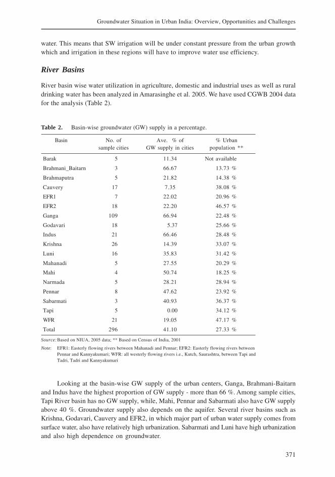
371
Groundwater Situation in Urban India: Overview, Opportunities and Challenges
water. This means that SW irrigation will be under constant pressure from the urban growthwhich and irrigation in these regions will have to improve water use efficiency.
River Basins
River basin wise water utilization in agriculture, domestic and industrial uses as well as ruraldrinking water has been analyzed in Amarasinghe et al. 2005. We have used CGWB 2004 datafor the analysis (Table 2).
Table 2. Basin-wise groundwater (GW) supply in a percentage.
Basin No. of Ave. % of % Urbansample cities GW supply in cities population **
Barak 5 11.34 Not available
Brahmani_Baitarn 3 66.67 13.73 %
Brahmaputra 5 21.82 14.38 %
Cauvery 17 7.35 38.08 %
EFR1 7 22.02 20.96 %
EFR2 18 22.20 46.57 %
Ganga 109 66.94 22.48 %
Godavari 18 5.37 25.66 %
Indus 21 66.46 28.48 %
Krishna 26 14.39 33.07 %
Luni 16 35.83 31.42 %
Mahanadi 5 27.55 20.29 %
Mahi 4 50.74 18.25 %
Narmada 5 28.21 28.94 %
Pennar 8 47.62 23.92 %
Sabarmati 3 40.93 36.37 %
Tapi 5 0.00 34.12 %
WFR 21 19.05 47.17 %
Total 296 41.10 27.33 %
Source:Based on NIUA, 2005 data; ** Based on Census of India, 2001
Note: EFR1: Easterly flowing rivers between Mahanadi and Pennar; EFR2: Easterly flowing rivers betweenPennar and Kannyakumari; WFR: all westerly flowing rivers i.e., Kutch, Saurashtra, between Tapi andTadri, Tadri and Kannyakumari
Looking at the basin-wise GW supply of the urban centers, Ganga, Brahmani-Baitarnand Indus have the highest proportion of GW supply - more than 66 %. Among sample cities,Tapi River basin has no GW supply, while, Mahi, Pennar and Sabarmati also have GW supplyabove 40 %. Groundwater supply also depends on the aquifer. Several river basins such asKrishna, Godavari, Cauvery and EFR2, in which major part of urban water supply comes fromsurface water, also have relatively high urbanization. Sabarmati and Luni have high urbanizationand also high dependence on groundwater.
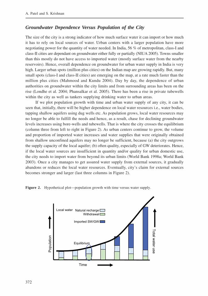
372
A. Patel and S. Krishnan
Groundwater Dependence Versus Population of the City
The size of the city is a strong indicator of how much surface water it can import or how muchit has to rely on local sources of water. Urban centers with a larger population have morenegotiating power for the quantity of water needed. In India, 56 % of metropolitan, class-I andclass-II cities are dependant on groundwater either fully or partially (NIUA 2005). Towns smallerthan this mostly do not have access to imported water (mostly surface water from the nearbyreservoirs). Hence, overall dependence on groundwater for urban water supply in India is veryhigh. Larger urban spots (million plus cities) on the Indian map are growing rapidly. But, manysmall spots (class-I and class-II cities) are emerging on the map, at a rate much faster than themillion plus cities (Mahmood and Kundu 2004). Day by day, the dependence of urbanauthorities on groundwater within the city limits and from surrounding areas has been on therise (Londhe et al. 2004; Phansalkar et al. 2005). There has been a rise in private tubewellswithin the city as well as tankers supplying drinking water to urban areas.
If we plot population growth with time and urban water supply of any city, it can beseen that, initially, there will be higher dependence on local water resources i.e., water bodies,tapping shallow aquifers using dug wells etc. As population grows, local water resources mayno longer be able to fulfill the needs and hence, as a result, chase for declining groundwaterlevels increases using bore-wells and tubewells. That is where the city crosses the equilibrium(column three from left to right in Figure 2). As urban centers continue to grow, the volumeand proportion of imported water increases and water supplies that were originally obtainedfrom shallow unconfined aquifers may no longer be sufficient, because (a) the city outgrowsthe supply capacity of the local aquifer; (b) often quality, especially of GW deteriorates. Hence,if the local water sources are insufficient in quantity and/or quality for urban domestic use,the city needs to import water from beyond its urban limits (World Bank 1998a; World Bank2003). Once a city manages to get assured water supply from external sources, it graduallyabandons or reduces the local water resources. Eventually, city’s claim for external sourcesbecomes stronger and larger (last three columns in Figure 2).
Figure 2. Hypothetical plot—population growth with time versus water supply.
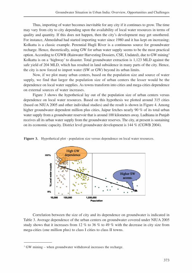
373
Groundwater Situation in Urban India: Overview, Opportunities and Challenges
Thus, importing of water becomes inevitable for any city if it continues to grow. The timemay vary from city to city depending upon the availability of local water resources in terms ofquality and quantity. If this does not happen, then the city’s development may get smothered.For instance, Ahmedabad had started importing water since 1980 and it has kept on increasing;Kolkatta is a classic example. Perennial Hugli River is a continuous source for groundwaterrecharge. Hence, theoretically, using GW for urban water supply seems to be the most practicaloption. According to CGWB (Rainwater Harvesting Dossiers, CSE, Undated), due to GW mining3
Kolkatta is on a ‘highway’ to disaster. Total groundwater extraction is 1,123 MLD against thesafe yield of 204 MLD, which has resulted in land subsidence in many parts of the city. Hence,the city is now forced to import water (SW or GW) beyond its urban limits.
Now, if we plot many urban centers, based on the population size and source of watersupply, we find that larger the population size of urban centers the lesser would be thedependence on local water supplies. As towns transform into cities and mega-cities dependenceon external sources of water increases.
Figure 3 shows the hypothetical lay out of the population size of urban centers versusdependence on local water resources. Based on this hypothesis we plotted around 315 cities(based on NIUA 2005 and other individual studies) and the result is shown in Figure 4. Amonghigher groundwater dependent million plus cities, Jaipur fetches nearly 90 % of its total urbanwater supply from a groundwater reservoir that is around 100 kilometers away. Ludhiana in Punjabreceives all its urban water supply from the groundwater reserves. The city, at present is sustainingon its economic capacity. District level groundwater development is 144 % (CGWB 2004).
Figure 3. Hypothetical plot - population size versus dependence on local water resources.
3 GW mining – when groundwater withdrawal increases the recharge.
Correlation between the size of city and its dependence on groundwater is indicated inTable 3. Average dependence of the urban centers on groundwater covered under NIUA 2005study shows that it increases from 12 % to 36 % to 49 % with the decrease in city size frommega-cities (one million plus) to class I cities to class II towns.
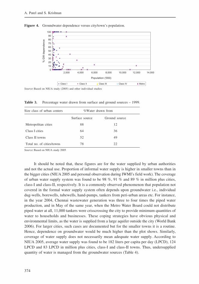
374
A. Patel and S. Krishnan
It should be noted that, these figures are for the water supplied by urban authoritiesand not the actual use. Proportion of informal water supply is higher in smaller towns than inthe bigger cities (NIUA 2005 and personal observation during IWMI’s field work). The coverageof urban water supply system was found to be 98 %, 91 % and 89 % in million plus cities,class-I and class-II, respectively. It is a commonly observed phenomenon that population notcovered in the formal water supply system often depends upon groundwater i.e., individualdug-wells, borewells, tubewells, hand-pumps, tankers from peri-urban areas etc. For instance,in the year 2004, Chennai wastewater generation was three to four times the piped waterproduction, and in May of the same year, when the Metro Water Board could not distributepiped water at all, 11,000 tankers were crisscrossing the city to provide minimum quantities ofwater to households and businesses. These coping strategies have obvious physical andenvironmental limits, as the water is supplied from a large aquifer outside the city (World Bank2006). For larger cities, such cases are documented but for the smaller towns it is a routine.Hence, dependence on groundwater would be much higher than the plot shows. Similarly,coverage of water supply does not necessarily mean adequate water supply. According toNIUA 2005, average water supply was found to be 182 liters per capita per day (LPCD), 124LPCD and 83 LPCD in million plus cities, class-I and class-II towns. Thus, undersuppliedquantity of water is managed from the groundwater sources (Table 4).
Figure 4. Groundwater dependence versus city/town’s population.
Table 3. Percentage water drawn from surface and ground sources – 1999.
Size class of urban centers %Water drawn from
Surface source Ground source
Metropolitan cities 88 12
Class I cities 64 36
Class II towns 52 49
Total no. of cities/towns 78 22
Source:Based on NIUA study 2005
Source:Based on NIUA study (2005) and other individual studies
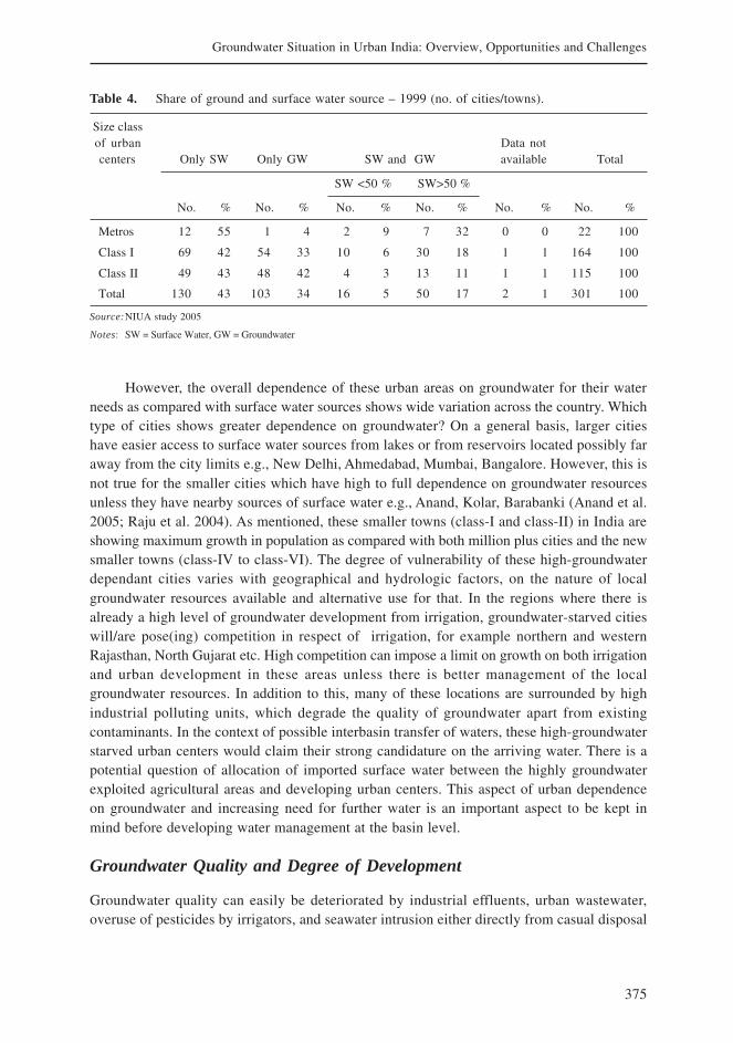
375
Groundwater Situation in Urban India: Overview, Opportunities and Challenges
However, the overall dependence of these urban areas on groundwater for their waterneeds as compared with surface water sources shows wide variation across the country. Whichtype of cities shows greater dependence on groundwater? On a general basis, larger citieshave easier access to surface water sources from lakes or from reservoirs located possibly faraway from the city limits e.g., New Delhi, Ahmedabad, Mumbai, Bangalore. However, this isnot true for the smaller cities which have high to full dependence on groundwater resourcesunless they have nearby sources of surface water e.g., Anand, Kolar, Barabanki (Anand et al.2005; Raju et al. 2004). As mentioned, these smaller towns (class-I and class-II) in India areshowing maximum growth in population as compared with both million plus cities and the newsmaller towns (class-IV to class-VI). The degree of vulnerability of these high-groundwaterdependant cities varies with geographical and hydrologic factors, on the nature of localgroundwater resources available and alternative use for that. In the regions where there isalready a high level of groundwater development from irrigation, groundwater-starved citieswill/are pose(ing) competition in respect of irrigation, for example northern and westernRajasthan, North Gujarat etc. High competition can impose a limit on growth on both irrigationand urban development in these areas unless there is better management of the localgroundwater resources. In addition to this, many of these locations are surrounded by highindustrial polluting units, which degrade the quality of groundwater apart from existingcontaminants. In the context of possible interbasin transfer of waters, these high-groundwaterstarved urban centers would claim their strong candidature on the arriving water. There is apotential question of allocation of imported surface water between the highly groundwaterexploited agricultural areas and developing urban centers. This aspect of urban dependenceon groundwater and increasing need for further water is an important aspect to be kept inmind before developing water management at the basin level.
Groundwater Quality and Degree of Development
Groundwater quality can easily be deteriorated by industrial effluents, urban wastewater,overuse of pesticides by irrigators, and seawater intrusion either directly from casual disposal
Table 4. Share of ground and surface water source – 1999 (no. of cities/towns).
Size classof urban Data notcenters Only SW Only GW SW and GW available Total
SW <50 % SW>50 %
No. % No. % No. % No. % No. % No. %
Metros 12 55 1 4 2 9 7 32 0 0 22 100
Class I 69 42 54 33 10 6 30 18 1 1 164 100
Class II 49 43 48 42 4 3 13 11 1 1 115 100
Total 130 43 103 34 16 5 50 17 2 1 301 100
Source:NIUA study 2005
Notes: SW = Surface Water, GW = Groundwater
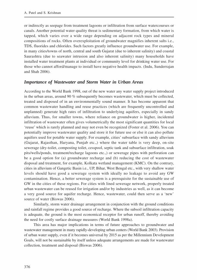
376
A. Patel and S. Krishnan
or indirectly as seepage from treatment lagoons or infiltration from surface watercourses orcanals. Another potential water quality threat is sedimentary formation, from which water istapped, which varies over a wide range depending on adjacent rock types and mineralcompositions of rocks. Often overexploitation of groundwater magnifies inherent salts i.e.,TDS, fluorides and chlorides. Such factors greatly influence groundwater use. For example,in many cities/towns of north, central and south Gujarat (due to inherent salinity) and coastalSaurashtra (due to seawater intrusion and also inherent salinity) many households haveinstalled water treatment plants at individual or community level for drinking water use. Forthose who cannot afford/manage to install have negative health impacts. (Indu, Sunderrajanand Shah 2006).
Importance of Wastewater and Storm Water in Urban Areas
According to the World Bank 1998, out of the new water any water supply project introducedin the urban areas, around 90 % subsequently becomes wastewater, which must be collected,treated and disposed of in an environmentally sound manner. It has become apparent thatcommon wastewater handling and reuse practices (which are frequently uncontrolled andunplanned) generate high rates of infiltration to underlying aquifers, especially in sandyalluvium. Thus, for smaller towns, where reliance on groundwater is higher, incidentalinfiltration of wastewater often gives volumetrically the most significant quantities for local‘reuse’ which is rarely planned and may not even be recognized (Foster et al. 2006). You canpotentially improve wastewater quality and store it for future use or else it can also polluteaquifers used for potable water supply. For example, cities’ subsurface with sandy alluvium(Gujarat, Rajasthan, Haryana, Punjab etc.,) where the water table is very deep, on-sitesewerage (dry-toilet, composting toilet, cesspool, septic tank and subsurface infiltration, soakpits/wells/ponds, treatment/recharge lagoons etc.,) or sewerage pipes with perforation canbe a good option for (a) groundwater recharge and (b) reducing the cost of wastewaterdisposal and treatment, for example, Kolkata wetland management (KMC). On the contrary,cities in alluvium of Gangetic Basin i.e., UP, Bihar, West Bengal etc., with very shallow waterlevels should have good a sewerage system with ideally no leakage to avoid any GWcontamination. Hence, a better sewerage system is a prerequisite for the sustainable use ofGW in the cities of these regions. For cities with lined sewerage network, properly treatedurban wastewater can be reused for irrigation and/or by industries as well, as it can becomea very good source for aquifer recharge. Hence, wastewater, could then serve as a ‘new’source of water (Biswas 2006).
Similarly, storm water drainage arrangement in conjunction with the ground conditionsand rainfall regime provides a good source of recharge. Where the subsoil infiltration capacityis adequate, the ground is the most economical receptor for urban runoff, thereby avoidingthe need for costly surface drainage measures (World Bank 1998a).
This area has major implications in terms of future approaches to groundwater andwastewater management in many rapidly-developing urban centers (World Bank 2003). Provisionof urban water supply, even if it becomes universal by 2015 as per the Millennium DevelopmentGoals, will not be sustainable by itself unless adequate arrangements are made for wastewatercollection, treatment and disposal (Biswas 2006).

377
Groundwater Situation in Urban India: Overview, Opportunities and Challenges
Urbanization and Water Management
Urbanization in India
It should also be noted that, it is not only that urbanization is taking place in great magnitudein class-I cities4, but, the urban centers are also increasing in terms of absolute numbers.Strategically for the water sector, these towns are important for the investment point of view.Most of the class-I and class-II cities face day-to-day problems of financial crunch, low returnson investments, inadequate operating and maintenance expertise and poor civic andinfrastructure facilities. Such urban authorities also need reform (World Bank 1998b). Per capitawater demand for class-I cities increases dramatically by almost 1.5 times compared with othersmaller class cities from 150 LPCD to 220 LPCD (NCIWRD 1999).
Urban Agglomeration
Another important stand-out in urbanization is the increasing trend of ‘megalopolis’ or ‘sub-urbanism’. The cities tend to sprawl. The second cadres of the cities are coming up aroundthe mega-cities. The reason is high prices in the urban core and traditional suburbs drivepeople to distant suburbs. This pattern owes largely to the preference of middle and theworking classes for privacy and space, while elites crave for better living environment whichencourages urban sprawl. For corporates, it is taxes that force to keep their godowns andother commercial activities outside municipal limits. In fact, the new sub-urbanism seeks notto fight market forces, but to address the problems. These are not mere bedroom communitieswith malls, but boast well-developed business parks, town centers and in many cases notably,large amount of well-preserved or developed natural open spaces. Majority of these sprawlsare now turning into ‘garden cities’. For instance, around Delhi there are peripheral citiesemerging to solve all the requirements of the big cities. One key that becomes crucial in thisregard is the excellent transportation, which is also argued by Faroohar 2006. BurgeoningIT hubs outside Delhi like Gurgaon, Noida and Gaziabad serve as new bedroom communitiesand all sit on good roads into the capital. More examples are Virar, Vashi (Navi Mumbai),Pune for Mumbai, Bopal, Vejalpur, Science city for Ahmedabad. Most of these peripheral orsecond cities depend heavily on groundwater. These cities are normally not covered undermunicipal corporations, especially for the provision of water supply and sewerageinfrastructure. That is why it is very important that these second cities or urbanagglomerations need to be covered under urban water supply schemes. Recent amendmentin Jawaharlal Nehru National Urban Renewal Mission (GOI 2006) for inclusion of city’s peri-urban areas, out growths and urban corridors and other peripheral areas is a step towardsaddressing the issue.
4 Proportion of total urban population of class-1 has increased from 22 % % in 1901 to 60 % % in2001 (Source: Registrar General and Census Commissioner 1993; Indiastat.com 2006; Mahemood andKundu 2005).
378
A. Patel and S. Krishnan
Linkage Between Urbanization, Infrastructure Development, Tourism and Water
With the increase in urbanization and with better infrastructure facilities i.e., roads, electricity,communication etc., tourism activities shoot up. New trend of buying properties for thevacations and holidays in near by hill-stations, lake side etc., is emerging among urban elites.For, example, domestic tourists from Delhi visiting Mussourie, Shimla, Haridwar increaseduring weekends; Similarly mountains Abu and Udaipur for Ahmedabad; Lonawala, Khandalafor Mumbai and Pune elites. Such tourist destinations are increasing in number. Many ofsuch tourist towns are witnessing unexpected growth and unable to cope with water demandfrom their local water resources. Often tourist destinations are located in geographicallyadverse conditions. In spite of that, such towns can become black-holes to attract waterfrom distant sources.
Future Work and Conclusion
Methodology for Vulnerability Analysis
What we have presented in this paper is the current status and potential threat ofgroundwater use in urban centers of India and our conceptual picture of how differentgeographical factors contribute to vulnerability in terms of urban groundwater. In this section,we outline a proposed procedure to evaluate this vulnerability based on various factors.This methodology utilizes data that is mostly available, but some need to be generated aswell. The important factors are: (a) level of current dependence on groundwater for overallurban water use; (b) level of groundwater development in surrounding block/district; (c)average distance to external sources of water; (d) level of development of river basin; and(e) hydrogeological factors e.g., specific yield. A combination of these factors will enable usto identify the current hotspots and future attractors of excess or imported water in anyriver basin. Some examples follow:
1. Bharuch is a class-I city in Gujarat which uses 90 % of surface water since the localgroundwater is overexploited and contains a high concentration of saline. In thesurrounding districts groundwater development is around 50 % (source: 2004Groundwater statistics of CGWB), but it lies within Narmada and Mahi river basinswhich still have water available for supply to the city. In that case, the city is notunder further high stress as far as groundwater vulnerability is concerned.
2. Ludhiana is a metropolitan city in Punjab, which completely relies on groundwatersources. The district level groundwater development is 144 % and it lies within theIndus River basin that is almost closed and highly exploited. The groundwater in thiscity is highly vulnerable to further exploitation and is already suffering from severepollution from industries.
3. Barielly is a class-I city in Uttar Pradesh, which receives 100 % of its supplies fromgroundwater. The district level groundwater development is 86 % and it lies withinthe Ganges Basin. In this case, even though there is a high dependence ongroundwater and high degree of groundwater development, perpetual recharge from
379
Groundwater Situation in Urban India: Overview, Opportunities and Challenges
canal system that contributes 40 % of the groundwater recharge in this area (source:2004 Groundwater Statistics of CGWB), means that there is no current highvulnerability of groundwater exploitation in this town.
On a macro-scale we conclude that the level of dependence on groundwater is greater forsmaller sized towns, which have lesser power to demand and have lesser economic strength topay for water sources that are located at distant places. Though, smaller towns with all the adverseconditions would eventually win over other uses for urban water supply. Rajasthan’s IndiraGandhi Nahar (IGNP) Canal is a case in point. The proportion of drinking water has increasedover time and will continue so. Gradually all the cities, towns as well as villages in northern andwestern Rajasthan are being covered by IGNP water. We also see a marked difference spatiallyin dependence on groundwater with the northern urban areas, which are located on rich alluvialaquifers and get good recharge from canals, highly dependant on local groundwater for theiroverall water usage. On the other hand, peninsular towns in hard-rock regions have lesseropportunity to develop groundwater resources. To sustain the growth they have to depend onexternal sources. In case of nonavailability of such external sources of water, this can impose alimit to overall growth of the urban areas. Integration of all the factors such as hydrogeological,within or outside canal command area, rainfall and recharge, population size, proximity to waterbodies, urban out-growths, and utilization of wastewater would help planners in designing betterand sustainable urban water supply and sanitation systems.
References
Amarasinghe, U. A.; Sharma, B. R.; Noel, A.; Scott, C.; Smakhtin, V.; Fraiture, C.; Sinha, A.; Shukla, A.2005. Spatial variation in water supply and demand across river basins of India. IWMI Research Report83. Colombo, Sri Lanka: International Water Management Institute (IWMI).
Anand, B. K.; Raju, K. V.; Praveen, N.; Deepa, N.; Latha, N. 2005. Urban water supplies dependency ongroundwater: Can it sustain – Initial findings from South Indian cities, Discussion Paper, IWMI-TATApartners meet - 2005, Anand, Gujarat.
Biswas, A. K. 2006. Water management for major urban centers. Water Resources Development. Vol. 22,No. 2, 183–197, June 2006.
CSE. Kolkata water profile: city of joy weeps for water. http://www.rainwaterharvesting.org/asp/d_feedback.htm
CGWB. 2004. Groundwater statistics, 2004. New Delhi: GOI.
CWC. 2004. Water and related statistics May 2004, Information System Organization, CWC (WP and P),New Delhi: GOI.
Foster, S.; Garduno, H.; Tuinhof, A.; Kemper, K.; Nanni, M. 2002- 2006. Urban wastewater as groundwaterrecharge evaluating and managing the risks and benefits, World Bank, GW-MATE Briefing Note Series12. Washington DC, USA.
Foster, S.; Garduño, H. 2007. Groundwater resource depletion in Indian aquifers, underlying causes andmanagement approaches. Proceedings of 3rd International Groundwater Conference, Feb. 7-10, 2007.Coimbatore, INDIA: Tamil Nadu Agriculture University.
GOI. Union ministry of urban affairs 2006. http://jnnurm.nic.in/toolkit/modified_guidelines.pdf Visited onJuly 27, 2007, 15:32, IST.
Indiastat.com 2006. Population (2001 Census) in http://www.indiastat.com.
380
A. Patel and S. Krishnan
Kolkata Municipal Corporation (KMC). (undated). Kolkata Environmental Improvement Project http://www.keiponline.com/east_kolkata_wetland.htm Visited on July 31, 2007, 15:10, IST.
Londhe, A.; Talati, J.; Singh, L. K.; Vilayasseril, M.; Dhaunta, S.; Rawlley, B.; Ganapathy, K. K.; Mathew,R. P. 2004. Urban hinterland water transactions: A scoping study of six class one Indian cities. Presentedat the Annual Partners’ Meet 2004, IWMI-Tata Water Policy Program, Anand.
Mahmood, A.; Kundu, A. 2005. India’s demography in 2050: size, structure and habitat. Discussion Paper,IWMI-TATA partners meet - 2005, Anand, Gujarat.
Molle, F.; Berkoff, J. 2006. Cities versus agriculture: Revisiting intersectoral water transfers, potential gainsand conflicts. Comprehensive Assessment Research Report 10. Colombo, Sri Lanka: ComprehensiveAssessment Secretariat.
NCIWRD. 1999. Integrated water resource development a plan for action, the National Commission forintegrated water resources development Vol. 1. Ministry of Water Resources, New Delhi: GOI.
NIUA. 2005. Status of water supply, sanitation and solid waste management in urban areas. New Delhi,URL: http://urbanindia.nic.in/moud/what’snew/main.htm
Phansalkar, S. J.; Kher, V.; Deshpande, P. 2005. “Expanding Rings of Dryness: Water Imports from Hinterlandsto Cities and the Rising Demands of Mega-Cities”, in IWMI-Tata Annual Partner’s Meet, Anand.
Indu, R.; Sunderrajan, K.; Shah, T. 2006. Impacts of groundwater contamination with fluoride and arsenic:affliction severity, medical cost and wage loss in some villages of India. Paper presented in APM-2006,IWMI-Tata Program, Anand.
Raju, K. V.; Praveen, N.; Anand, B. K. 2004. Groundwater in urban market: Can it sustain? – A case studyof Kolar city in south India. CERNA, Paper presented at the conference on Market development ofwater and waste technologies through environmental economics, May 28-29, 2004, Paris.
Registrar General and Census Commissioner. 1993. Emerging trends of urbanization in India - an analysisof 1991 Census Results. Occasional Paper No. 1 of 1993. New Delhi: Registrar General and CensusCommissioner, GOI.
Sivaramakrishnan, K. C.; Amitabh, K.; Singh, B. N. 2005. Handbook of Urbanization. New Delhi: OxfordUniversity Press.
World Bank. 1998a. Groundwater in Urban Development – Assessing management needs and formulatingpolicy strategies. WTP – 390, World Bank, Washington D.C.
World Bank. 1998b. India – Water resources management sector review - groundwater regulation andmanagement report. Rural Development Unit, South Asia Region, World Bank, Washington D.C.
World Bank. 2003. Sustainable groundwater management: concepts and tools. GW-MATE (GroundwaterManagement Advisory Team) (available at: http://www.worldbank.ogr/gwmate).
World Bank. 2006. India: water supply and sanitation - bridging the gap between infrastructure and service.Background paper. Urban water supply and sanitation, India Country Team, Energy and InfrastructureDepartment, South Asia Region, World Bank, Washington D.C.
381
Groundwater Situation in Urban India: Overview, Opportunities and Challenges
Natural Flows Assessment and Creating Alternative FutureScenarios for Major River Basins of Peninsular India
1Anil D. Mohile and 2B.K. Anand1Consultant (Former Chairman CWC), New Delhi.
2IWMI, New Delhi Office, India
Summary
The current study focuses on the six major peninsular basins of India namely, Brahmani-Baitarni, Cauvery, Godavari, Krishna, Mahanadi and Narmada, for estimating natural flows andresidual flows under different scenarios to investigate whether ‘surplus’ water is available inthese basins and also to assess the limits of utilization of massive water transfers.
The first part of the study uses the recent historical flow and information, about wateruse and other anthropogenic changes in the water cycle, to establish a monthly ‘Natural Flows’series for the basin. This is done by using a simple hydrologic model of the land phase,incorporating a linear groundwater reservoir, and incorporating the anthropogenic changes.The concept of natural flows is being used as a ‘peg’ while proceeding from the currentcondition to the likely future condition.
The second part, aims to assess the likely future alternate water situation and processthe monthly time series of natural flows as established in the first part. The objective was totest the ability of the basin to support alternative possible development scenarios, whilemaintaining an acceptable level of residual flows. Therefore, different alternate developmentscenarios are worked out and incorporated in the model. The operation of the reservoir capacityis adjusted, to ensure the availability of a positive, or, if necessary, ‘above a threshold’ flow.Simultaneously, the water use is increased to a level where sustaining the use and maintainingthe residual flows becomes impossible, and failures occur in some years. By adjusting theincidence of the failures (in meeting the specified demands) to an acceptable level, the ‘limit ofwater use’ under the scenario is established. The ‘limits of utilization’ is determined not onlyby natural flows and the engineering-agronomic constraints, but also by the manner in whichthe utilization is achieved, including the environmental constraints. Thus, according to theauthors, a simple concept of a fixed ‘utilizable flow’ is inadequate.
The analysis was to be done for the hydrologic and developmental environments asexpected in the year 2025. The natural flows as would occur in that year, as well as the initialconditions (the storage available at the beginning of the year) cannot be known. Since a seriesof natural flows for about 15 years (as established in the first part) was available, the analysis
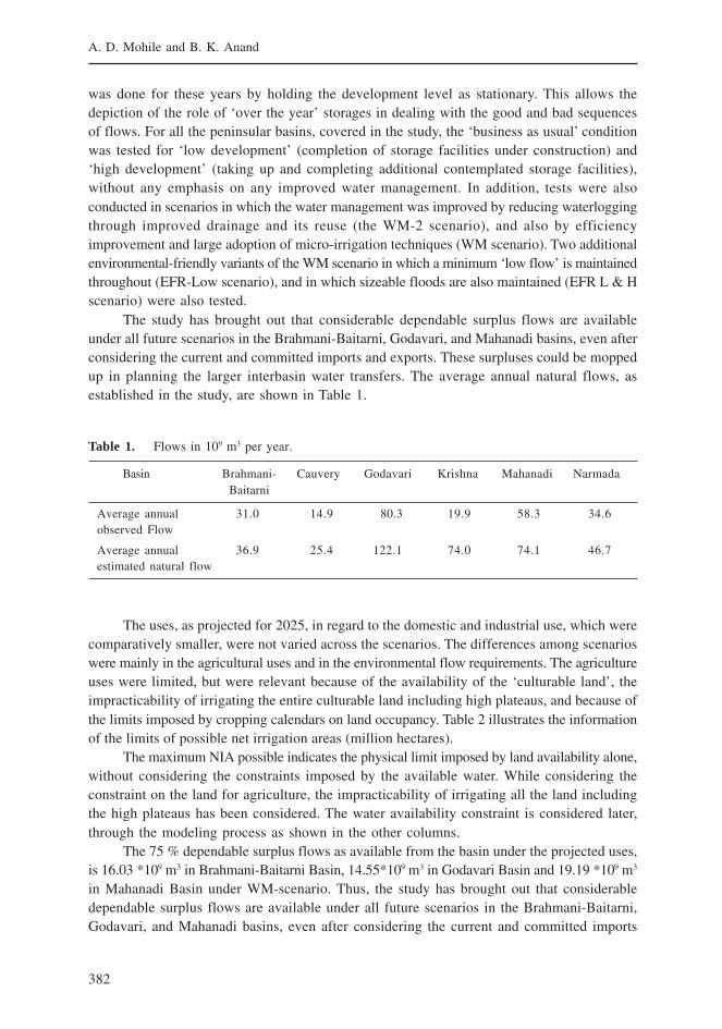
382
A. D. Mohile and B. K. Anand
was done for these years by holding the development level as stationary. This allows thedepiction of the role of ‘over the year’ storages in dealing with the good and bad sequencesof flows. For all the peninsular basins, covered in the study, the ‘business as usual’ conditionwas tested for ‘low development’ (completion of storage facilities under construction) and‘high development’ (taking up and completing additional contemplated storage facilities),without any emphasis on any improved water management. In addition, tests were alsoconducted in scenarios in which the water management was improved by reducing waterloggingthrough improved drainage and its reuse (the WM-2 scenario), and also by efficiencyimprovement and large adoption of micro-irrigation techniques (WM scenario). Two additionalenvironmental-friendly variants of the WM scenario in which a minimum ‘low flow’ is maintainedthroughout (EFR-Low scenario), and in which sizeable floods are also maintained (EFR L & Hscenario) were also tested.
The study has brought out that considerable dependable surplus flows are availableunder all future scenarios in the Brahmani-Baitarni, Godavari, and Mahanadi basins, even afterconsidering the current and committed imports and exports. These surpluses could be moppedup in planning the larger interbasin water transfers. The average annual natural flows, asestablished in the study, are shown in Table 1.
Table 1. Flows in 109 m3 per year.
Basin Brahmani- Cauvery Godavari Krishna Mahanadi NarmadaBaitarni
Average annual 31.0 14.9 80.3 19.9 58.3 34.6observed Flow
Average annual 36.9 25.4 122.1 74.0 74.1 46.7estimated natural flow
The uses, as projected for 2025, in regard to the domestic and industrial use, which werecomparatively smaller, were not varied across the scenarios. The differences among scenarioswere mainly in the agricultural uses and in the environmental flow requirements. The agricultureuses were limited, but were relevant because of the availability of the ‘culturable land’, theimpracticability of irrigating the entire culturable land including high plateaus, and because ofthe limits imposed by cropping calendars on land occupancy. Table 2 illustrates the informationof the limits of possible net irrigation areas (million hectares).
The maximum NIA possible indicates the physical limit imposed by land availability alone,without considering the constraints imposed by the available water. While considering theconstraint on the land for agriculture, the impracticability of irrigating all the land includingthe high plateaus has been considered. The water availability constraint is considered later,through the modeling process as shown in the other columns.
The 75 % dependable surplus flows as available from the basin under the projected uses,is 16.03 *109 m3 in Brahmani-Baitarni Basin, 14.55*109 m3 in Godavari Basin and 19.19 *109 m3
in Mahanadi Basin under WM-scenario. Thus, the study has brought out that considerabledependable surplus flows are available under all future scenarios in the Brahmani-Baitarni,Godavari, and Mahanadi basins, even after considering the current and committed imports
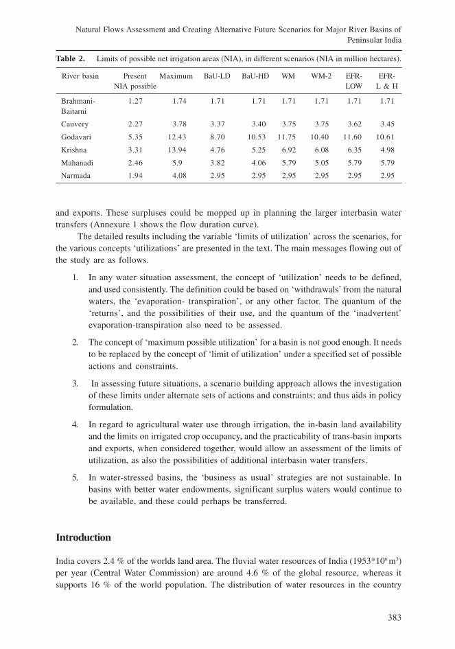
383
Natural Flows Assessment and Creating Alternative Future Scenarios for Major River Basins ofPeninsular India
and exports. These surpluses could be mopped up in planning the larger interbasin watertransfers (Annexure 1 shows the flow duration curve).
The detailed results including the variable ‘limits of utilization’ across the scenarios, forthe various concepts ‘utilizations’ are presented in the text. The main messages flowing out ofthe study are as follows.
1. In any water situation assessment, the concept of ‘utilization’ needs to be defined,and used consistently. The definition could be based on ‘withdrawals’ from the naturalwaters, the ‘evaporation- transpiration’, or any other factor. The quantum of the‘returns’, and the possibilities of their use, and the quantum of the ‘inadvertent’evaporation-transpiration also need to be assessed.
2. The concept of ‘maximum possible utilization’ for a basin is not good enough. It needsto be replaced by the concept of ‘limit of utilization’ under a specified set of possibleactions and constraints.
3. In assessing future situations, a scenario building approach allows the investigationof these limits under alternate sets of actions and constraints; and thus aids in policyformulation.
4. In regard to agricultural water use through irrigation, the in-basin land availabilityand the limits on irrigated crop occupancy, and the practicability of trans-basin importsand exports, when considered together, would allow an assessment of the limits ofutilization, as also the possibilities of additional interbasin water transfers.
5. In water-stressed basins, the ‘business as usual’ strategies are not sustainable. Inbasins with better water endowments, significant surplus waters would continue tobe available, and these could perhaps be transferred.
Introduction
India covers 2.4 % of the worlds land area. The fluvial water resources of India (1953*106 m3)per year (Central Water Commission) are around 4.6 % of the global resource, whereas itsupports 16 % of the world population. The distribution of water resources in the country
Table 2. Limits of possible net irrigation areas (NIA), in different scenarios (NIA in million hectares).
River basin Present Maximum BaU-LD BaU-HD WM WM-2 EFR- EFR-NIA possible LOW L & H
Brahmani- 1.27 1.74 1.71 1.71 1.71 1.71 1.71 1.71Baitarni
Cauvery 2.27 3.78 3.37 3.40 3.75 3.75 3.62 3.45
Godavari 5.35 12.43 8.70 10.53 11.75 10.40 11.60 10.61
Krishna 3.31 13.94 4.76 5.25 6.92 6.08 6.35 4.98
Mahanadi 2.46 5.9 3.82 4.06 5.79 5.05 5.79 5.79
Narmada 1.94 4.08 2.95 2.95 2.95 2.95 2.95 2.95
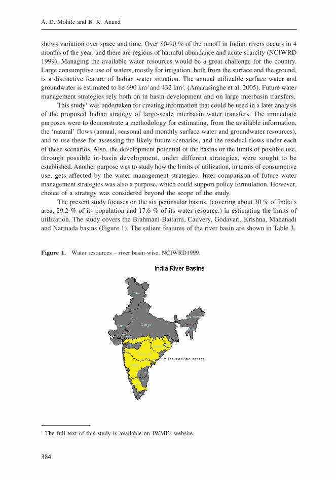
384
A. D. Mohile and B. K. Anand
shows variation over space and time. Over 80-90 % of the runoff in Indian rivers occurs in 4months of the year, and there are regions of harmful abundance and acute scarcity (NCIWRD1999). Managing the available water resources would be a great challenge for the country.Large consumptive use of waters, mostly for irrigation, both from the surface and the ground,is a distinctive feature of Indian water situation. The annual utilizable surface water andgroundwater is estimated to be 690 km3 and 432 km3. (Amarasinghe et al. 2005). Future watermanagement strategies rely both on in basin development and on large interbasin transfers.
This study1 was undertaken for creating information that could be used in a later analysisof the proposed Indian strategy of large-scale interbasin water transfers. The immediatepurposes were to demonstrate a methodology for estimating, from the available information,the ‘natural’ flows (annual, seasonal and monthly surface water and groundwater resources),and to use these for assessing the likely future scenarios, and the residual flows under eachof these scenarios. Also, the development potential of the basins or the limits of possible use,through possible in-basin development, under different strategies, were sought to beestablished. Another purpose was to study how the limits of utilization, in terms of consumptiveuse, gets affected by the water management strategies. Inter-comparison of future watermanagement strategies was also a purpose, which could support policy formulation. However,choice of a strategy was considered beyond the scope of the study.
The present study focuses on the six peninsular basins, (covering about 30 % of India’sarea, 29.2 % of its population and 17.6 % of its water resource.) in estimating the limits ofutilization. The study covers the Brahmani-Baitarni, Cauvery, Godavari, Krishna, Mahanadiand Narmada basins (Figure 1). The salient features of the river basin are shown in Table 3.
Figure 1. Water resources – river basin-wise, NCIWRD1999.
1 The full text of this study is available on IWMI’s website.

385
Natural Flows Assessment and Creating Alternative Future Scenarios for Major River Basins ofPeninsular India
The concept of ‘an utilizable flow’ is, much more complex than it appears to be. There isno uniformity in defining the use. The governmental sources in India, generally, define it interms of ‘withdrawals’. This is, however, less appropriate from a scientific-hydrologic viewpointin view of the returns. The NCIWRD has realized this and has accounted for the returns whileusing withdrawals as a yardstick. The scientifically pleasing procedure of defining the use interms of consumption (that is, the evaporationtranspiration) also does not solve the problemof a part of the return occurring into ‘sinks’ (or where, because of its quality, it has to be ledto a ‘sink’), and is not capable of future withdrawal and use.
Methodology
A good approach in the present and future water situation assessment is to model thecomplete land phase of the hydrologic cycle, through a model capable of depicting the likelyfuture changes in the processes, caused by land use changes. Such an approach, asdeveloped earlier (Gopalkrishnan et al. 2006) could not be followed in the present study inview of the large data requirements of that approach. In the present study, only theanthropogenic changes in the land phase of hydrologic cycle have been modeled andestimated.
The general hydrologic concept used by us is depicted below (Figure 2). This is for the‘Pseudo-Natural condition’, under which human interventions through rain-fed agriculture areallowed, but other anthropogenic water cycle interventions through uses, including irrigationuse, are not allowed. The hydrologic concept used in the current study under anthropogenicallymodified state of the basin is shown below (Figure 3).
Table 3. Salient features of river basins studied.
Serial River basins Area Percent No. Basin population Average NaturalNo. (sq.km) of of (2001) (estimated) annual water water
India’s states resources, resourcearea involved (NCIWRD per
estimates) person.
Thousands Percent 109 m3 Percent m3/of of person/
Indian Indian yearpopulation resource
1 Brahmani-Baitarni 51,882 1.7 3 18,382 1.9 28.48 1.46 1,549
2 Cauvery Basin 87,900 2.7 3 35,097 3.5 21.36 1.09 608
3 Godavari Basin 312,812 9.5 5 85,351 8.6 110.54 5.66 1,295
4 Krishna Basin 258,948 8 3 73,968 7.5 69.81 3.57 943
5 Mahanadi Basin 141,589 4.3 4 29,690 3.0 66.88 3.42 2,252
6 Narmada Basin 98,796 3 3 19,144 1.9 45.64 2.34 2,384
Total for basin studied 951,927 29.2 261,632 26.4 342.71 17.55 1,310
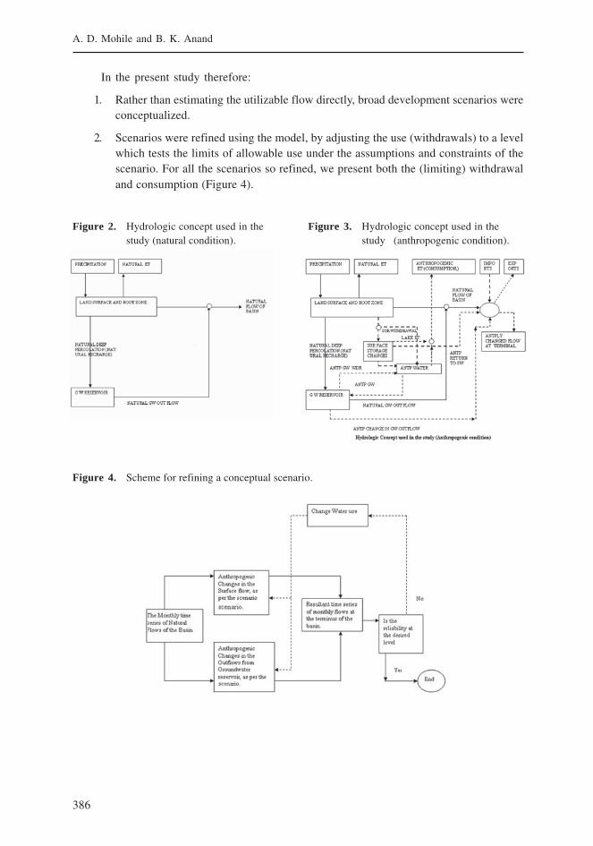
386
A. D. Mohile and B. K. Anand
In the present study therefore:
1. Rather than estimating the utilizable flow directly, broad development scenarios wereconceptualized.
2. Scenarios were refined using the model, by adjusting the use (withdrawals) to a levelwhich tests the limits of allowable use under the assumptions and constraints of thescenario. For all the scenarios so refined, we present both the (limiting) withdrawaland consumption (Figure 4).
Figure 2. Hydrologic concept used in thestudy (natural condition).
Figure 3. Hydrologic concept used in thestudy (anthropogenic condition).
Figure 4. Scheme for refining a conceptual scenario.
387
Natural Flows Assessment and Creating Alternative Future Scenarios for Major River Basins ofPeninsular India
Data Availability and Sources
Storage
Information about storage facilities under construction, storage facilities under considerationand ultimate irrigation potential in the basin was taken from CWC’s water-related statistics(2004).
Runoff
The observed runoff, at or near the terminal site of the six basins, as a monthly time seriesfrom 1989 to 2003 was used in the first part to establish a monthly series of natural flows. Inthe second part, the natural flows so estimated were used for scenario analysis. For somebasins, the series available was for a shorter period.
The period of minimum length data2 required for assessing the reliability of a plan ofdevelopment would depend on (i) the interannual variability of hydrologic data and (ii) thepredominant type of the development, i.e., runoff of the river, within the year storage and overthe year storage. Among the basins studied, the Krishna and Narmada have a predominantstorage development with the carry over component as a significant proportion of the total.All other basins have predominantly a ‘within the year storage’. Although a 40-year and 25-year long series of monthly flows would have been preferred for a planning exercise, for wantof readily available data and in view of the time and resource constraints, the present studywas based on a 15-year series.
Land Use and Irrigated Areas
This was obtained from the government statistics. However, a few changes had to be made intwo basins, namely Krishna and Godavari, as the data from the government statistics were notconsistent with the data obtained from other sources, e.g., remotely sensed data.
Reference Crop Evapotranspiration
The reference evapotranspiration figures for various locations in India and the rainfall figuresfor these locations were taken from www.iwmi.cgiar.org/WAtlas. Monthly information for 475locations (districts) of India in regard to the following parameters was available. Penman ET-(minimum, maximum, mean, standard deviation) (mm/day for the month); Precipitation (50 %)(mm/day for the month); Precipitation (75 %) (mm/day for the month); and Moisture AvailabilityIndex (mm/day for the month).
2 The general Indian practice, in regard to the minimum length of data necessary for project planning isas follows: runoff of the river development -10 years, in weekly or 10 daily time units; within the yearstorage development - 25 years, in 10 daily or monthly time units; over the year storage development- 40 years, in monthly or seasonal time units.
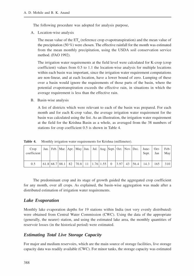
388
A. D. Mohile and B. K. Anand
The following procedure was adopted for analysis purpose,
A. Location-wise analysis
The mean value of the ET0 (reference crop evapotranspiration) and the mean value of
the precipitation (50 %) were chosen. The effective rainfall for the month was estimatedfrom the mean monthly precipitation, using the USDA soil conservation servicemethod. (FAO 1992).
The irrigation water requirements at the field level were calculated for K-crop (cropcoefficient) values from 0.5 to 1.1 the location-wise analysis for multiple locationswithin each basin was important, since the irrigation water requirement computationsare non-linear, and at each location, have a lower bound of zero. Lumping of theseover a basin would ignore the requirements of those parts of the basin, where thepotential evapotranspiration exceeds the effective rain, in situations in which theaverage requirement is less than the effective rain.
B. Basin-wise analysis
A list of districts which were relevant to each of the basin was prepared. For eachmonth and for each K-crop value, the average irrigation water requirement for thebasin was calculated using the list. As an illustration, the irrigation water requirementat the field for the Krishna Basin as a whole, as averaged from the 38 numbers ofstations for crop coefficient 0.5 is shown in Table 4.
The predominant crop and its stage of growth guided the aggregated crop coefficientfor any month, over all crops. As explained, the basin-wise aggregation was made after adistributed estimation of irrigation water requirements.
Lake Evaporation
Monthly lake evaporation depths for 19 stations within India (not very evenly distributed)were obtained from Central Water Commission (CWC). Using the data of the appropriate(generally, the nearer) station, and using the estimated lake area, the monthly quantities ofreservoir losses (in the historical period) were estimated.
Estimating Total Live Storage Capacity
For major and medium reservoirs, which are the main source of storage facilities, live storagecapacity data was readily available (CWC). For minor tanks, the storage capacity was estimated
Table 4. Monthly irrigation water requirements for Krishna (millimeter).
Crop Jan. Feb. Mar. Apr. May Jun. Jul. Aug. Sept. Oct. Nov. Dec. June- Oct- Feb-coefficient Sept. Jan May
0.5 61.8 68.7 88.1 82 70.8 11 1.76 1.55 0 3.97 43 56.4 14.3 165 310
389
Natural Flows Assessment and Creating Alternative Future Scenarios for Major River Basins ofPeninsular India
by an approximate analysis, which indicated that for irrigating thousand hectares, a live capacityof 3.5 *10 6 m3 would have been built. When building up the future scenarios, the likely lossof capacity due to sedimentation was considered. As per our estimates, the total live capacityof the Indian reservoirs (2003) was 262.87 *109 m3, and, the six basins under study had a totallive storage of 125.9 *109 m3.
Estimating Monthly Live-storages and Lake Areas
Of the total live storage of 125.9 * 109 m3 available in the study area, about 67 *109 m3, availablein 36 of the comparatively larger reservoirs, is being monitored by the Central Water Commission(CWC). The monthly water level and live capacity information for each of the monitored reservoirsin the six basins were obtained from the CWC and were used to fit a logarithmic reservoir height-capacity curve for each. By differentiating this, a logarithmic area reservoir height-curve wasalso obtained. In the absence of the readily available data, the values of dead storage and elevationof the reservoir bottom were determined by trials and by using secondary information as available.In general, a very high coefficient of correlation around 0.99 could be achieved through trials. Itwas also ensured that, in general, the value of exponential in the reservoir height-capacity curvewas within the normally acceptable range of 1.5 to 5.
Scenarios
The model built comprised five scenarios, namely BaU-LD; BaU-HD; HD-WM; HD-WM2; EFR-L; and EFR-L&H. None of the scenarios considered massive interbasin transfers beyond thoseexisting at present, which are shown in the table below. The BaU-LD scenario considered alow level of future storage development, whereas other scenarios consider that most of thepossible storages would be built by 2025. All the scenarios (except BaU LD and BaU HD)considered a massive drainage improvement to reduce waterlogging, and reuse of the drainedwater for irrigation as a future strategy. In addition, the HD-WM, EFR L and EFR L&H scenariosconsidered improvements in surface water distribution efficiency through canal lining etc. Theprovision of environmental flows in the low-flow season was included in EFR L. Additionalenvironmental flows during the flood period were provided in EFR L & H.
Irrigation Efficiencies and Returns
The irrigation efficiencies (combined conveyance, distribution and application) and thedistribution of excess withdrawals, based on the general experience in India, as assumed inthe various scenarios, are abstracted below.
The overall surface water irrigation efficiency in the wet season (kharif—June-September)was assumed as 0.4 for the BaU conditions and was increased to 0.5 for the scenario withimproved distribution. For the other non-wet seasons (rabi—Oct-January and hot weather—February-May) the corresponding values were 0.3 and 0.4. For groundwater irrigation, higherefficiencies, ranging from 0.6 to 0.7 (June-October and November-January seasons) and 0.5to 0.6 for the hot season (February-May) were assumed. Depending on the overall efficiencyand irrigation water requirements the withdrawal from the surface or groundwater was computed.The excess of withdrawal over the additional evapotranspirational needs was accounted by
390
A. D. Mohile and B. K. Anand
dividing it in three parts, namely that lost as additional ET from anthropogenic swamps, thatwhich returns to the surface water system ,and that which returns to the groundwater system.In the BaU scenarios, the distribution ratios were 0.4, 0.15 and 0.45, respectively; whereas inthe other scenarios, which involved drainage improvements, the ratios were changed to 0.2,0.2 and 0.6, respectively.
Domestic and Industrial Uses
The domestic uses depend on the population projections for 2025. For the present, we estimatedthese as follows. The averages of the ‘All India’ projections, low and high, as projected byNCIWRD for 2025 were used. These were segregated statewise, and also into rural and urbancomponents. In doing so, the differences in the processes of population growth andurbanization, within the states were considered. The state-wise figures were converted to basin-wise figures, in the proportion of the state areas in each basin. Domestic and industrial useswere calculated by changing the current norms to more reasonable norms for 2025 situation.
The industrial requirements were projected through an approximate but elaborate study,which separately worked out the requirements for 11 types of major industries plus the generalsmall-scale industries. The requirements for each type were partly related to the natural resourcedistribution and partly to the population growth. An overall increase of more than 400 % forthe all India withdrawal figures between 2000 and 2025 was assumed in the BaU type scenarios.In the scenario depicting improved water management, the consumption levels were kept thesame as that of BaU type, but with improved water use efficiency, the withdrawal and thereturn figures were reduced.
The Model Operation, Including the Reservoir Operation
1. The approach was to decide, beforehand, the development parameters of the scenario(storage capacity, imports and exports), the agro-climatologic parameters (ET
0, ETcrop,
Effective rainfall), the water management parameters (efficiencies and distribution ofexcess withdrawals) and also the ecology-related constraints (environmental flows—both low flows and floods), and then to vary the use-related parameters, (target irrigationareas ) to estimate the limits of use within the acceptable reliability. Even within theuse-related parameters of a scenario, the domestic and industrial uses were held at aprescribed level, and only the irrigated areas were changed in the ‘trial and error’procedure for investigating the limits of development. Each basin would be having alarge number of major, medium, and minor reservoirs, however, in this generally lumpedmodel of the basin, all reservoirs were lumped into a single reservoir. The approximationsinvolved in such lumping were dealt separately as described in (5) below.
2. The reliability: As per the prevalent Indian practice, the failures in meeting the targetsof irrigation, on an annual basis, of less than 25 %, was allowed. The failure percentage,on a crop-year basis was also computed. Irrigation failures were managed by reducingirrigated areas during a failure.
3. The storage facilities were so operated that as much water as possible is held backfor future use, after meeting the requirements for uses, and also the requirements for
391
Natural Flows Assessment and Creating Alternative Future Scenarios for Major River Basins ofPeninsular India
EFR (Low Flow) and EFR( High Flow) as specified in the scenario. The storageoperation was done in a recursive way.
4. Failures were imposed mostly in surface irrigation, and even in these, failures in rabiand hot weather were imposed before imposing failures in the subsequent kharif andin perennials.
5. The maximum practicable value for the transient storage has the upper bound in termsof the available live capacity, in 2025, under the scenario. However, the limiting storagewas assumed to be at 90 % of the live capacity. Similarly, the minimum practicablelive storage may not reach the physical bound of zero live capacity. An integratedoperation, across political units, may not be fully achieved. Even within a unit, isolatedreservoirs may not be operated to cater to deficits much downstream. A small carry-over to cater to a delayed monsoon may be preserved even in the face of a currentoverall deficit. Considering all these, we kept a small minimum live storage limit ofaround 1,000 million cubic meters in all scenarios, in the studies. Both these correctionsrepresent an attempt to overcome modeling limitations involved in considering a singlelumped reservoir, instead of the distributed reservoirs within the basin.
6. The suggested operational pattern was then used to compute the residual flows forthe basin, as also the residual flows at a critical point near the basin outlet. Often,initially, the residual flows included some monthly flow values, which were below theEFR threshold, or were negative. In such cases:
• Cuts on irrigation areas were applied from the earlier post-monsoon period .Cutsin other seasons were also imposed, if necessary, until the physically impossiblenegative flows were eliminated. As the hydrologic and storage situation improveswith time, beyond the bad run, the cuts in forthcoming seasons becomeunnecessary.
• Considering the short period of simulation, it was necessary to leave an ‘end ofthe period’ storage at a level not far below the average storage for that month.Apart from the number of failures, this became an important consideration.
• The irrigation area targets were increased or decreased, if the failures were toofew or too many, as compared to the criterion of 75 % annual reliability ofirrigation. . An account of the cuts, as imposed, was kept, to work out thereliability.
• The ‘critical point’: All balances were done for the basin as a whole. However,the availability of non-negative (or above threshold) flows at the basin outletdoes not imply such conditions at all places in the upstream. Balances had to beworked out at one or more points which may be critical from the water depletionconsiderations. The decision about which point is to be considered as ‘critical’would require some knowledge of the basin. For most studied basins, thewithdrawal-related stresses occur in the middle and lower portions, since upperparts are comparatively wet, and have less withdrawal. Hence, critical conditionswould be occurring at points downstream of the last large withdrawal, andbalances at such points were worked out.
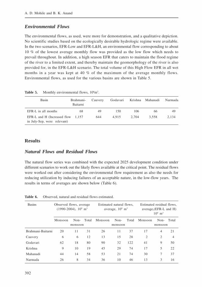
392
A. D. Mohile and B. K. Anand
Environmental Flows
The environmental flows, as used, were more for demonstration, and a qualitative depiction.No scientific studies based on the ecologically desirable hydrologic regime were available.In the two scenarios, EFR-Low and EFR-L&H, an environmental flow corresponding to about10 % of the lowest average monthly flow was provided as the low flow which needs toprevail throughout. In addition, a high season EFR that caters to maintain the flood regimeof the river to a limited extent, and thereby maintain the geomorphology of the river is alsoprovided for, in the EFR-L&H scenario. The total volume of this High Flow EFR in all wetmonths in a year was kept at 40 % of the maximum of the average monthly flows.Environmental flows, as used for the various basins are shown in Table 5.
Table 5. Monthly environmental flows, 106m3.
Basin Brahmani- Cauvery Godavari Krishna Mahanadi NarmadaBaitarni
EFR-L in all months 68 49 150 106 66 49
EFR-L and H (Increased flow 1,157 644 4,915 2,704 3,558 2,134in July-Sep, were relevant)
Results
Natural Flows and Residual Flows
The natural flow series was combined with the expected 2025 development condition underdifferent scenarios to work out the likely flows available at the critical point. The residual flowswere worked out after considering the environmental flow requirement as also the needs forreducing utilization by inducing failures of an acceptable nature, in the low-flow years. Theresults in terms of averages are shown below (Table 6).
Table 6. Observed, natural and residual flows estimated.
Basins Observed flows, average Estimated natural flows, Estimated residual flows,(1990-2004), 109 m3 average, 109 m3 average,(EFR-L and H)
109 m3
Monsoon Non- Total Monsoon Non- Total Monsoon Non- Totalmonsoon monsoon monsoon
Brahmani-Baitarni 20 11 31 26 11 37 17 4 21
Cauvery 6 6 12 13 15 28 2 2 4
Godavari 62 18 80 90 32 122 41 9 50
Krishna 9 10 19 45 29 74 17 5 22
Mahanadi 44 14 58 53 21 74 30 7 37
Narmada 26 8 34 36 10 46 13 3 16
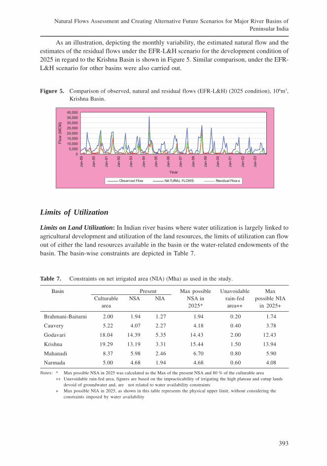
393
Natural Flows Assessment and Creating Alternative Future Scenarios for Major River Basins ofPeninsular India
As an illustration, depicting the monthly variability, the estimated natural flow and theestimates of the residual flows under the EFR-L&H scenario for the development condition of2025 in regard to the Krishna Basin is shown in Figure 5. Similar comparison, under the EFR-L&H scenario for other basins were also carried out.
Figure 5. Comparison of observed, natural and residual flows (EFR-L&H) (2025 condition), 106m3,Krishna Basin.
Limits of Utilization
Limits on Land Utilization: In Indian river basins where water utilization is largely linked toagricultural development and utilization of the land resources, the limits of utilization can flowout of either the land resources available in the basin or the water-related endowments of thebasin. The basin-wise constraints are depicted in Table 7.
Table 7. Constraints on net irrigated area (NIA) (Mha) as used in the study.
Basin Present Max possible Unavoidable MaxCulturable NSA NIA NSA in rain-fed possible NIA
area 2025* area++ in 2025+
Brahmani-Baitarni 2.00 1.94 1.27 1.94 0.20 1.74
Cauvery 5.22 4.07 2.27 4.18 0.40 3.78
Godavari 18.04 14.39 5.35 14.43 2.00 12.43
Krishna 19.29 13.19 3.31 15.44 1.50 13.94
Mahanadi 8.37 5.98 2.46 6.70 0.80 5.90
Narmada 5.00 4.68 1.94 4.68 0.60 4.08
Notes: * Max possible NSA in 2025 was calculated as the Max of the present NSA and 80 % of the culturable area++ Unavoidable rain-fed area, figures are based on the impracticability of irrigating the high plateau and cutup lands
devoid of groundwater and, are not related to water availability constraints+ Max possible NIA in 2025, as shown in this table represents the physical upper limit, without considering the
constraints imposed by water availability
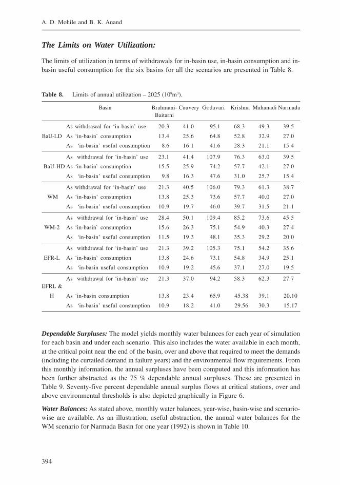
394
A. D. Mohile and B. K. Anand
The Limits on Water Utilization:
The limits of utilization in terms of withdrawals for in-basin use, in-basin consumption and in-basin useful consumption for the six basins for all the scenarios are presented in Table 8.
Table 8. Limits of annual utilization – 2025 (109m3).
Basin Brahmani- Cauvery Godavari Krishna Mahanadi NarmadaBaitarni
As withdrawal for ‘in-basin’ use 20.3 41.0 95.1 68.3 49.3 39.5
BaU-LD As ‘in-basin` consumption 13.4 25.6 64.8 52.8 32.9 27.0
As ‘in-basin’ useful consumption 8.6 16.1 41.6 28.3 21.1 15.4
As withdrawal for ‘in-basin’ use 23.1 41.4 107.9 76.3 63.0 39.5
BaU-HD As ‘in-basin` consumption 15.5 25.9 74.2 57.7 42.1 27.0
As ‘in-basin’ useful consumption 9.8 16.3 47.6 31.0 25.7 15.4
As withdrawal for ‘in-basin’ use 21.3 40.5 106.0 79.3 61.3 38.7
WM As ‘in-basin’ consumption 13.8 25.3 73.6 57.7 40.0 27.0
As ‘in-basin’ useful consumption 10.9 19.7 46.0 39.7 31.5 21.1
As withdrawal for ‘in-basin’ use 28.4 50.1 109.4 85.2 73.6 45.5
WM-2 As ‘in-basin` consumption 15.6 26.3 75.1 54.9 40.3 27.4
As ‘in-basin’ useful consumption 11.5 19.3 48.1 35.3 29.2 20.0
As withdrawal for ‘in-basin’ use 21.3 39.2 105.3 75.1 54.2 35.6
EFR-L As ‘in-basin` consumption 13.8 24.6 73.1 54.8 34.9 25.1
As ‘in-basin useful consumption 10.9 19.2 45.6 37.1 27.0 19.5
As withdrawal for ‘in-basin’ use 21.3 37.0 94.2 58.3 62.3 27.7EFRL &
H As ‘in-basin consumption 13.8 23.4 65.9 45.38 39.1 20.10
As ‘in-basin’ useful consumption 10.9 18.2 41.0 29.56 30.3 15.17
Dependable Surpluses: The model yields monthly water balances for each year of simulationfor each basin and under each scenario. This also includes the water available in each month,at the critical point near the end of the basin, over and above that required to meet the demands(including the curtailed demand in failure years) and the environmental flow requirements. Fromthis monthly information, the annual surpluses have been computed and this information hasbeen further abstracted as the 75 % dependable annual surpluses. These are presented inTable 9. Seventy-five percent dependable annual surplus flows at critical stations, over andabove environmental thresholds is also depicted graphically in Figure 6.
Water Balances: As stated above, monthly water balances, year-wise, basin-wise and scenario-wise are available. As an illustration, useful abstraction, the annual water balances for theWM scenario for Narmada Basin for one year (1992) is shown in Table 10.
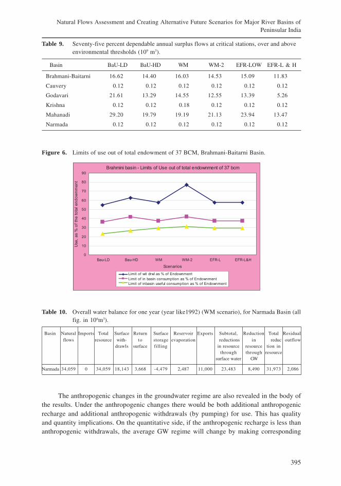
395
Natural Flows Assessment and Creating Alternative Future Scenarios for Major River Basins ofPeninsular India
Table 9. Seventy-five percent dependable annual surplus flows at critical stations, over and aboveenvironmental thresholds (109 m3).
Basin BaU-LD BaU-HD WM WM-2 EFR-LOW EFR-L & H
Brahmani-Baitarni 16.62 14.40 16.03 14.53 15.09 11.83
Cauvery 0.12 0.12 0.12 0.12 0.12 0.12
Godavari 21.61 13.29 14.55 12.55 13.39 5.26
Krishna 0.12 0.12 0.18 0.12 0.12 0.12
Mahanadi 29.20 19.79 19.19 21.13 23.94 13.47
Narmada 0.12 0.12 0.12 0.12 0.12 0.12
Figure 6. Limits of use out of total endowment of 37 BCM, Brahmani-Baitarni Basin.
Table 10. Overall water balance for one year (year like1992) (WM scenario), for Narmada Basin (allfig. in 106m3).
Basin Natural Imports Total Surface Return Surface Reservoir Exports Subtotal, Reduction Total Residualflows resource with- to storage evaporation reductions in reduc outflow
drawls surface filling in resource resource tion inthrough through resource
surface water GW
Narmada 34,059 0 34,059 18,143 3,668 -4,479 2,487 11,000 23,483 8,490 31,973 2,086
The anthropogenic changes in the groundwater regime are also revealed in the body ofthe results. Under the anthropogenic changes there would be both additional anthropogenicrecharge and additional anthropogenic withdrawals (by pumping) for use. This has qualityand quantity implications. On the quantitative side, if the anthropogenic recharge is less thananthropogenic withdrawals, the average GW regime will change by making corresponding
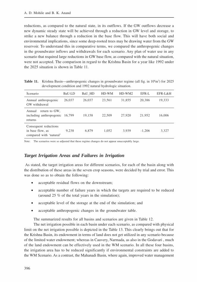
396
A. D. Mohile and B. K. Anand
reductions, as compared to the natural state, in its outflows. If the GW outflows decrease anew dynamic steady state will be achieved through a reduction in GW level and storage, tostrike a new balance through a reduction in the base flow. This will have both social andenvironmental implications, since some deep-rooted trees may be drawing water from the GWreservoir. To understand this in comparative terms, we compared the anthropogenic changesin the groundwater inflows and withdrawals for each scenario. Any plan of water use in anyscenario that required large reductions in GW base flow, as compared with the natural situation,were not accepted. The comparison in regard to the Krishna Basin for a year like 1992 underthe 2025 situation is shown in Table 11.
Target Irrigation Areas and Failures in Irrigation
As stated, the target irrigation areas for different scenarios, for each of the basin along withthe distribution of these areas in the seven crop seasons, were decided by trial and error. Thiswas done so as to obtain the following:
• acceptable residual flows on the downstream;
• acceptable number of failure years in which the targets are required to be reduced(around 25 % of the total years in the simulation);
• acceptable level of the storage at the end of the simulation; and
• acceptable anthropogenic changes in the groundwater table.
The summarized results for all basins and scenarios are given in Table 12.The net irrigation possible in each basin under each scenario, as compared with physical
limit on the net irrigation possible is depicted in the Table 13. This clearly brings out that forthe Krishna Basin, its endowment in terms of land does not get utilized in any scenario becauseof the limited water endowment; whereas in Cauvery, Narmada, as also in the Godavari , muchof the land endowment can be effectively used in the WM scenario. In all these four basins,the irrigation area has to be reduced significantly if environmental constraints are added tothe WM Scenario. As a contrast, the Mahanadi Basin, where again, improved water management
Table 11. Krishna Basin—anthropogenic changes in groundwater regime (all fig. in 106m3) for 2025development condition and 1992 natural hydrologic situation.
Scenario BaU-LD BaU_HD HD-WM HD-WM2 EFR-L EFR-L&H
Annual anthropogenic 26,037 26,037 23,561 31,855 20,386 19,333GW withdrawal
Annual return to GW,including anthropogenic 16,799 19,158 22,509 27,920 21,952 16,006returns
Consequent reductionsin base flow, as 9,238 6,879 1,052 3,939 -1,206 3,327compared with ‘natural’
Note: The scenarios were so adjusted that these regime changes do not appear unacceptably large.
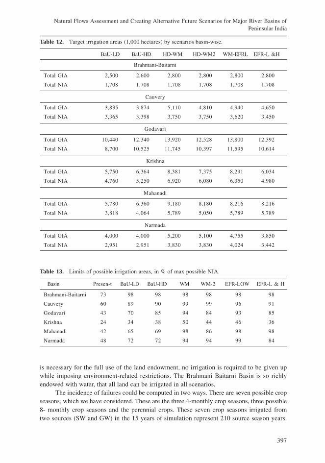
397
Natural Flows Assessment and Creating Alternative Future Scenarios for Major River Basins ofPeninsular India
is necessary for the full use of the land endowment, no irrigation is required to be given upwhile imposing environment-related restrictions. The Brahmani Baitarni Basin is so richlyendowed with water, that all land can be irrigated in all scenarios.
The incidence of failures could be computed in two ways. There are seven possible cropseasons, which we have considered. These are the three 4-monthly crop seasons, three possible8- monthly crop seasons and the perennial crops. These seven crop seasons irrigated fromtwo sources (SW and GW) in the 15 years of simulation represent 210 source season years.
Table 12. Target irrigation areas (1,000 hectares) by scenarios basin-wise.
BaU-LD BaU-HD HD-WM HD-WM2 WM-EFRL EFR-L &H
Brahmani-Baitarni
Total GIA 2,500 2,600 2,800 2,800 2,800 2,800
Total NIA 1,708 1,708 1,708 1,708 1,708 1,708
Cauvery
Total GIA 3,835 3,874 5,110 4,810 4,940 4,650
Total NIA 3,365 3,398 3,750 3,750 3,620 3,450
Godavari
Total GIA 10,440 12,340 13,920 12,528 13,800 12,392
Total NIA 8,700 10,525 11,745 10,397 11,595 10,614
Krishna
Total GIA 5,750 6,364 8,381 7,375 8,291 6,034
Total NIA 4,760 5,250 6,920 6,080 6,350 4,980
Mahanadi
Total GIA 5,780 6,360 9,180 8,180 8,216 8,216
Total NIA 3,818 4,064 5,789 5,050 5,789 5,789
Narmada
Total GIA 4,000 4,000 5,200 5,100 4,755 3,850
Total NIA 2,951 2,951 3,830 3,830 4,024 3,442
Table 13. Limits of possible irrigation areas, in % of max possible NIA.
Basin Presen-t BaU-LD BaU-HD WM WM-2 EFR-LOW EFR-L & H
Brahmani-Baitarni 73 98 98 98 98 98 98
Cauvery 60 89 90 99 99 96 91
Godavari 43 70 85 94 84 93 85
Krishna 24 34 38 50 44 46 36
Mahanadi 42 65 69 98 86 98 98
Narmada 48 72 72 94 94 99 84

398
A. D. Mohile and B. K. Anand
The percentage of source season years involving failures among these is one measure. Withoutconsidering the seasons, and the source, the number of years would be 15 and the percentageof failure years in another measure. The computations have been done using both measures.As an illustration, the failures for Krishna are depicted in Table 14.
Table 14. Failures in all scenarios, Krishna Basin.
Summary of failures BaU-LD HD HD-WM HD-WM2 WM-EFRL EFR-L &H
KRISHNA
Percentage by source-season-years 6.19 7.14 8.10 8.57 6.19 6.67
Percentage by years 20 20 20 20 20 33.33
Basin-wise Results
As an illustration, some details of the results for Brahmani-Baitarni Basin are presented below.The Brahmani-Baitarni Basin has an estimated average natural flow of 37x 109 m3. No importsand exports are contemplated in the present study and thus the total endowment is 36.9x10⁹ m3. The Figure 6 shows that in terms of useful in-basin consumption, only 30 % of thiswater can be used in WM, WM-2, EFR-L and EFR-L&H and the consumption would belesser in other scenarios. In terms of total in-basin consumption only about 40 % of theendowment would get consumed as evapotranspiration. In terms of withdrawal, the WM-2scenario would be able to withdraw around 77 % of endowment, whereas the scenarios withbetter water management (WM, EFR-L, and EFR_L&H) would require a withdrawal of 57 %of the withdrawal.
The basin has a current net sown area 1.94 Mha, which we assume would continue upto2025, with some 0.2 Mha as the unavoidable rain-fed area in plateau lands without enoughgroundwater, the maximum NIA would be around 1.74 Mha against the present NIA of 1.27Mha. The full available area has been proposed to be irrigated in all future scenarios. Thusland and not water is the constraint for in-basin use in the Brahmani-Baitarni Basin. In termsof GIA, we have assumed that for the NIA of 1.7 Mha the GIA cannot exceed 2.8 Mha. Withthe assumed cropping pattern having perennial and two seasonal crops hardly any irrigableland would be lying unoccupied in the kharif season. The occupancies as resulting from assumedcropping pattern are shown in Figure 7.
As mentioned, the land and not water is the restriction in the in-basin use in Brahmani-Baitarni Basin. Table 15 shows the 75 % dependable surplus flows at critical station over theenvironmental flow for Brahmani-Baitarni Basin and different scenarios.
Thus for Brahmani-Baitarni Basin a dependable surplus of 16.68*109 m3 is available inthe BaU (low development) scenario which decreases to 14.46 * 109 in the BaU (highdevelopment) scenario. With more efficient water use through water management activities,the surplus can be increased to 16.09*109 in WM scenario. However, when the low-flow EFRconstraint is used, the surplus reduces to 15.15*109 m3 when both low-flow and high-flowconstraints for environmental flow are imposed, the surplus reduces to 11.89 * 109m3.
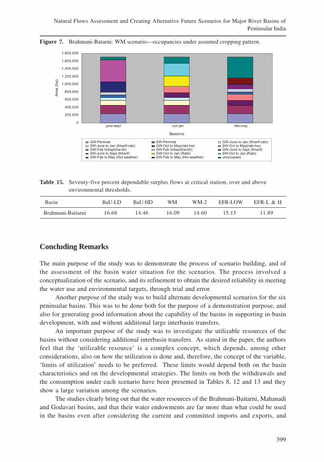
399
Natural Flows Assessment and Creating Alternative Future Scenarios for Major River Basins ofPeninsular India
Concluding Remarks
The main purpose of the study was to demonstrate the process of scenario building, and ofthe assessment of the basin water situation for the scenarios. The process involved aconceptualization of the scenario, and its refinement to obtain the desired reliability in meetingthe water use and environmental targets, through trial and error.
Another purpose of the study was to build alternate developmental scenarios for the sixpeninsular basins. This was to be done both for the purpose of a demonstration purpose, andalso for generating good information about the capability of the basins in supporting in-basindevelopment, with and without additional large interbasin transfers.
An important purpose of the study was to investigate the utilizable resources of thebasins without considering additional interbasin transfers. As stated in the paper, the authorsfeel that the ‘utilizable resource’ is a complex concept, which depends, among otherconsiderations, also on how the utilization is done and, therefore, the concept of the variable,‘limits of utilization’ needs to be preferred. These limits would depend both on the basincharacteristics and on the developmental strategies. The limits on both the withdrawals andthe consumption under each scenario have been presented in Tables 8, 12 and 13 and theyshow a large variation among the scenarios.
The studies clearly bring out that the water resources of the Brahmani-Baitarni, Mahanadiand Godavari basins, and that their water endowments are far more than what could be usedin the basins even after considering the current and committed imports and exports, and
Table 15. Seventy-five percent dependable surplus flows at critical station, over and aboveenvironmental thresholds.
Basin BaU-LD BaU-HD WM WM-2 EFR-LOW EFR-L & H
Brahmani-Baitarni 16.68 14.46 16.09 14.60 15.15 11.89
Figure 7. Brahmani-Batarni: WM scenario—occupancies under assumed cropping pattern.
400
A. D. Mohile and B. K. Anand
possible future uses. Thus, these basins are candidates for supporting additional water transferswithout reducing the in-basin use possibility.
In regard to the Narmada Basin, where large exports from the basin are already envisaged,the studies bring out that the full potential of in-basin development for irrigation cannot beachieved, particularly in the low-development and high-development scenarios of the‘business-as-usual’ strategy. Almost the full development can be achieved in the scenariosinvolving improved water management (The WM, WM-2, EFR-L and EFR-L&H scenarios).Thus for the full in-basin development of Narmada, either improved water management practicesneed to be installed or some reduction in the already committed export needs to be considered.
The studies establish that for Krishna and Cauvery basins, the water endowments are notenough to reach the full in-basin development potential. The Krishna Basin, even under thesecircumstances, is currently an exporting basin. Considerable water is being exported to Pennarand other east flowing rivers. The current study has not covered these basins which import theKrishna waters and it is likely that both equity and marginal productivity considerations wouldjustify such exports even from a basin, which is not rich in water endowments. The basin alsoexports water for hydroelectric purposes, to the already water-rich west-flowing rivers. Thusthere is a case for either reducing the exports from or increasing the exports to the Krishna Basin.Similarly, there is a strong case in considering new imports to the Cauvery Basin.
The study brings out the impracticability of continuation of the ‘business as usual’approach in the water-stressed basins, by bringing out the effects on the limits of utilization,as also the effects on groundwater regime and on residual flows.
The study has also shown that the scope for in-basin development only throughconstruction of additional storage-based projects is rather limited in the Krishna, Cauvery andthe Narmada basins. This is because on one hand the basins of Krishna and Cauvery alreadyhave built a large number of storage facilities so that the marginal utility of additional storagefacilities would be comparatively less (in both cases the terminal reservoirs hardly ever spilland the basins are effectively closed), and on the other hand because there are hardly anysignificant storage facilities remaining to be built. For the Narmada also, large storage projectsare under construction and these would be completed in the next few years; after which thereis hardly any scope for in-basin storage facilities.
The current studies have been done under some data limitations and assumptions. Whilethe studies may have to be repeated when better data and information becomes available, theauthors believe that the overall conclusions are unlikely to change substantially.
The limits of development of all the six basins under the six scenarios have beenestablished, and the surplus water available in the three well endowed basins of Brahmani-Baitarni, Mahanadi and Godavari have been computed. However, large-scale plans for furtherwater transfers, somewhat on the lines of the current plans of the National Water DevelopmentAgency (NWDA) have not been investigated in the current studies. While the dependablesurpluses can be exploited, however, these are available mostly in the monsoons. Their usemay require the construction of additional storage facilities in the surplus basin or the transferof floodwater into additional storage facilities elsewhere, as well as changes in the currentreservoir operation and in-basin uses. These possibilities may constrain the use of all thesurplus water. This aspect requires a separate study as a continuation of the present one.
A separate scenario HD-WM2 which focuses only on drainage improvement and reusehas been created, and one of the main purposes of water development is to increase the useful
401
Natural Flows Assessment and Creating Alternative Future Scenarios for Major River Basins ofPeninsular India
consumption of water within the hydrologic, engineering, land-availability-related, andenvironmental-related constraints. The comparison of the WM and WM2 scenarios ispresented in Table 8.
The study shows that it is difficult to maintain the environmental flows and, in particular,the environmental flows for maintaining the flood regime, in the relatively stressed basins,without reducing other uses. For example, in the Krishna Basin a useful in-basin consumptionthrough irrigation 35.3*109m3 is possible in the WM scenario and this gets reduced to29.6*109m3 for the EFR-L&H scenario. The desirability of providing a large environmental flowrequirement is to be considered against these consequent reductions in in-basin consumptions.The societal preferences in this regard need to be established through studies, debates andtrade- offs in a multi-stakeholder and multidisciplinary environment.
The study allows a comparative analysis of the scenarios, by developmental andenvironmental objectives, for each of the studied basin. While the choice of appropriatescenarios is considered outside the scope of the present study, such an analysis will allowthe decision maker to reach the decision, or at least to shortlist a few scenarios for furthersocioeconomic analysis. To illustrate this point, a comparative analysis for the Krishna Basinhas been included in the detailed report (www.nrlp.iwmi.org) and is abstracted below.
• The BaU LD scenario for Krishna involves an unacceptable groundwater regime andindicates that a large fall in groundwater table would take place under this scenario.
• The BaU HD scenario for Krishna indicates that with increased storage, and increasedsurface irrigation, without corresponding increase in groundwater irrigation, a slightlybetter groundwater regime can be expected.
• The HD-WM scenario for Krishna indicates, that with improvements in drainage asalso water distribution efficiency, a still better groundwater regime can be obtainedalong with the largest possible irrigated area among the scenario. However, low flowswould be too low.
• The HD-WM2 scenario for Krishna indicates, that if only the drainage improvementsis done without canal efficiency improvements the irrigated area would have to besome what lower than the HDWM scenario.
• The EFR-L scenario for Krishna indicates, that as compared to WM scenario,significant irrigation has to be given up for maintaining the low flows. In the process,the groundwater regime, in this scenario is the best among all. However, the incidenceof spills is the least among all scenarios and this may have adverse effects on theecology and morphology.
• The EFR L & H scenario for Krishna indicates, that both in terms of consumptionand possible irrigation, this scenario, indicates a situation in between the BaU LDand BaU HD scenarios. Thus, all the effort in improved water management throughthe drainage improvements and distribution efficiency improvements, and a part ofthe efforts in creating additional storage, go only towards the maintenance ofenvironmental flows in both the low flows and high flows. The groundwater regime,is not as good as in the WM scenarios. However, spills or controlled flushing floodswould be available each year.
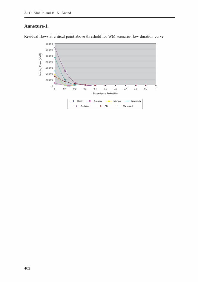
402
A. D. Mohile and B. K. Anand
Annexure-1.
Residual flows at critical point above threshold for WM scenario-flow duration curve.
403
Natural Flows Assessment and Creating Alternative Future Scenarios for Major River Basins ofPeninsular India
Annexure 2.
Terminology
In India, due to marked seasonality in rainfall, seasonal crops are very common. These areroughly 4-month crops; the wet season (south-west monsoon, June-Sept, kharif), the autumnseason (Oct-Jan, rabi) and the dry-hot season (Feb-May, hot weather) are common.Nomenclatures and the calendar can vary. Also, apart from perennial, some two season cropsalso prevail.
The ‘gross cropped area (GCA)’ indicates the total cropped area (rain-fed and irrigated)and includes the area which is cropped more than once. If and only the irrigated area is socounted the nomenclature used is ‘gross irrigated area (GIA)’.
The ‘net sown area (NSA)’is the geographical area which is under crop, at least for sometime, during the year. If only irrigated area is counted the geographical coverage is known as‘net irrigated area (NIA)’. (Note that these intensity-related parameters do not really depictthe intensity of occupation. For example, if the whole area of 100 ha were fully occupied in anyear under sugarcane, the GCA would have been only 100 ha and the cropping intensity wouldhave been 1.0, but if the land was fully occupied in June-September, occupied to 50 % in October- January, and occupied to 10 % in February-May, under seasonal crops, the GCA would havebeen higher at 160 ha.
References
Amarasinghe, U. A.; Sharma, B. R.; Noel, A.; Scott, C.; Smakhtin, V.; Fraiture, C.; Sinha, A.; Shukla, A.2005. Spatial variation in water supply and demand across river basins of India. Research Report 83.Colombo, Sri Lanka: International Water Management Institute (IWMI).
FAO (Food and Agricultural Organization). 1992. CROPWAT, FAO Irrigation and Drainage Paper, No. 46.Rome, Italy: FAO.
Gopalkrishnan, M.; Mohile, A. D.; Gupta, L. N.; Kuberan, R.; Kulkarni, S. A. 2006. An Integrated WaterAssessment Model for Supporting Indian Water Policy. Irrigation and Drainage, 55: 33-50, 2006.
NCIWRD (National Commission for Integrated Water Resources Development).1999. Report of the NationalCommission for Integrated Water Resources Development, Volume-1. New Delhi, India: Ministry ofWater Resources, Government of India.

ISBN 978-92-9090-697-1
Postal AddressP O Box 2075ColomboSri Lanka
Location127, Sunil MawathaPelawattaBattaramullaSri Lanka
Telephone+94-11-2880000
Fax+94-11-2786854
Websitehttp://www.iwmi.org
I n t e r n a t i o n a lWater ManagementI n s t i t u t e
India’s Water Future: Scenarios and Issues
Related Documents