India: Demand and Supply Prospects for Agriculture - World ...

India: Demand and Supply Prospectsfor Agriculture

SWP500

World Bank Staff Working Paper No. 500

October 1981

Prepared by: James Q. HarrisonSouth Asia Programs DepartmentJon A. HitchingsTreasurer's DepartmentJohn W. WallSouth Asia Programs Department

Copyright ® 1981The World Bank1818 H Street, N.W.Washington, D.C. 20433, U.S.A.

ws and interpretations in this document are those of the authors 44-01 0220PUBI )uld not be attributed to the World Bank, to its affiliatedHG I ations, or to any individual acting in their behalf. Feathery Ja8ies38811.5 IN 234.W57

W671no . 500

Pub

lic D

iscl

osur

e A

utho

rized

Pub

lic D

iscl

osur

e A

utho

rized

Pub

lic D

iscl

osur

e A

utho

rized

Pub

lic D

iscl

osur

e A

utho

rized

Pub

lic D

iscl

osur

e A

utho

rized

Pub

lic D

iscl

osur

e A

utho

rized

Pub

lic D

iscl

osur

e A

utho

rized

Pub

lic D

iscl

osur

e A

utho

rized

The views and interpretations in this document are those of the authors andshould not be attributed to the World Bank, to its affiliated organizations,or to any individual acting in their behalf.

WORLD BANK

Staff Working Paper No. 500

INDIA: PAPERS ON DEMAND AND SUPPLY PROSPECTS FOR AGRICULTURE

October 1981

Since India's foodgrain situation began to improve after themid-1970s, the World Bank's economic work on Indian agriculture hasconcentrated on the implications of this development both for foodgrains andfor other major agricultural commodities. This volume contains severalpapers that report on work accomplished so far. Jon Hitchings' paperprojects demand for major agriculture commodities through the year 2000 basedon consumption expenditure data from the 1973/74 National Sample Survey alongw4th estimates of future population and income growth, rates of urbanizationand trends in the distribution of income. The analysis reveals thedifferential effects of long-run income growth, and other factors, on demandfor various crops. The individual commodity papers were prepared to analyzethe long-run supply prospects and to compare these with the projected demand.The foodgrain paper, prepared by James Harrison and John Wall, raises thedistinct possibility of foodgrain self-sufficiency and even a potential foran eventual exportable surplus. The vegetable oil paper, by John Wall, isless optimistic and projects a persistent domestic shortage of vegetableoils. This underlines the need for greater efforts by the agriculturalsupport institutions to stimulate oilseed production and for an incentivepricing policy. The sugar paper, by James Harrison, analyzes the sugar cycleand stresses the disruptive effects of very large fluctuations around theproduction trend, which is essentially adequate to meet domestic requirementsand provide for some exports. The utility of maintaining a buffer stock ofsugar to stabilize year-to-year sugar supply is discussed.

prepared by: James Q. HarrisonSouth Asia Programs Department

Jon A. HitchingsTreasurer's Department

John W. WallSouth Asia Programs Department

Copyright0 1981

The World Bank1818 H Street, N.W.Washington, D.C. 20433U.S.A.

INDIA

PAPERS ON DEMAND AND SUPPLY PROSPECTS FOR AGRICULTURE

Table of Contents

Page Number

Part I: DEMAND PROJECTIONS FOR INDIA . . . . . . . . . 1Jon A. Hitchings

Part II: THE FOODGRAIN ECONOMY. . . . . . . . . . . . . 51James Q. Harrison and John W. Wall

Part III: THE VEGETABLE OIL ECONOMY . . . . . . . . . . 67John W. Wall

Part IV: THE SUGAR ECONOMY . . . . . . . . . . . . . . 109James Q. Harrison

PART I

DEMAND PROJECTIONS FOR INDIA

Jon A. HitchingsJune 1981

1

DEMAND PROJECTIONS FOR INDIA

TABLE OF CONTENTS

INTRODUCTION

Page

I. Data and Methodology ..................................

A. Population Projections ............................ 5

B. Baseline Consumption .............................. 7

C. Estimation Approach ....... ............ 10

II. Elasticities and Projection Results ................... 12

A. Comparisons of Expenditure Elasticities . . 12

B. Quantity Projections .. 15

III. Income Redistribution . . . 21

A. Gini Ratio Estimation and Comparisons ........ 22

B. Effects of Income Redistribution on Demand Projections 28

IV. Sensitivity Analysis ...... ............................ 31

A. Population Growth and Urbanization . . 31

B. Expenditure Growth and Redistribution ...... ....... 35

V. Conclusions ........................................... 41

APPENDICES

I. Demand Projections with Moderate Redistribution ....... 44

II. Gini Ratio Estimation Program ......................... 45

III. Sensitivity Analysis Data .. 46

IV. Foodgrain Equivalents .. ...... . .... ............. ....... 47

V. List of Consumption Groups and Items ....... .. ......... 48

REFERENCES ........ 49

- 3 -

LIST OF TABLES AND FIGURES

Tables

Table 1 Population and Urban Share Projections

Table 2 Selection of Base Quantities for Projections

Table 3 Expenditure Elasticity Estimates

Table 4A, 4B Demand Projections Assuming 3.5% and 5.0% Expenditure Growth

Table 5 Projected Annual Growth Rates of Demand for SelectedCommodities

Table 6 Comparisons of Demand Projections

Table 7 Projections of Food Energy Demand

Table 8 International Comparisons of Income Distribution Ordered by theGini Ratio

Table 9 Some Estimates of Gini Ratios for India

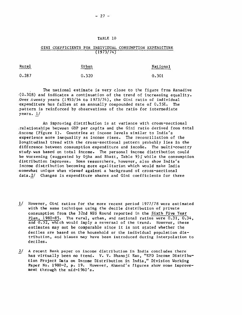
Table 10 Gini Coefficients for Individual Consumption Expenditure

Table 11 Future Expenditure Shares and Gini Ratios Given Redistribfi-tion Rates

Table 12 Changes in Quantities Demanded Resulting from ExpenditureRedistribution

Table 13 Population and Urban Share Values for Sensitivity Analysis

Table 14 Sensitivity of Projections for Year 2000 to AlteredPopulation and Urban Share Assumptions

Table 15 Sensitivity Comparisons

Table 16 Sensitivity Analysis of Expenditure Growth Rates

Table 17 Elasticities of Projections

Table 18 Correspondence of Multiplicative Factors and Annual GiniRatio Change Rates

- 4 -

Figures

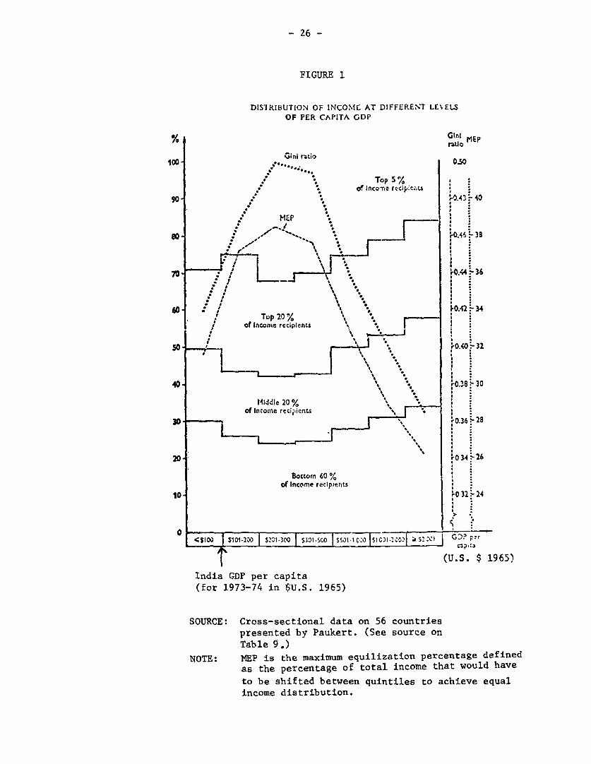
Figure 1 Distribution of Income at Different Levels of Per CapitaGDP

Figure 2 Projection Isoquants for Year 2000

- 5 -

INTRODUCTION

This paper reports a set of demand projections for agriculturalcommodities in India. The main objective was to assess the effects ofincome growth, population growth and other non-price variables on thefuture pattern of consumption of agricultural commodities in India. Asecond objective was the development of a projection model that would becompact, flexible and fully documented. The model should be capable ofprojecting demand for any number of commodities and future time periodsin a single pass with a minimum of file manipulation. It should alsoreadily accommodate altered assumptions regarding urbanization,expenditure growth, income redistribution and population growth. Theresulting model is documented separately. 1/

The 28th Round of the National Sample Survey (1973/74) is the mostrecent large-scale expenditure survey available. The 32nd Round (1977/78)is also directed to household expenditures, but it has not yet beenreleased. Restricted to this data base, the projections assume relativeprices are constant, and model only the demand side of the market.

Projections for 17 commodities at five year intervals, expenditureelasticities, and calorie demand per capita are presented and comparedwith other research. Changes in income distribution and consequenteffects on demand received particular attention. 2/ Sensitivity analysiswas performed on expenditure and population growth, expendituredistribution, and urbanization. As a final step in sensitivity analysis,estimates were made of the elasticities of future demand with respect tokey assumptions.

I. DATA AND METHODOLOGY

A. Population Projections. Four types of data were required forthe projections: population and urban share projections, the startingquantities of consumption, the sectoral distribution of initialconsumption, and expenditure data from a household consumption survey.The population and urbanization forecasts that were used are given inTable 1. Historical figures for the urban share of the population show agrowth rate of about 0.2% per year. 3/ Projections made by the UNPopulation Division/Urbanization show a general but bumpy continuation of

1/ "Documentation of a Demand Projection Model Prepared for India," JonHitchings, Division Paper for ASADB (March 25, 1981). Available fromthe India Division of the World Bank, Washington, D.C.

2/ Appendix II contains a program for estimating Gini coefficients.

3/ Census estimates for 1951, 1961 and 1971 are 15.9%, 18.0% and 19.9%.(UN Source).

- 6-

Table 1

Population and UrbanShare Projections

Population Urban Share(million) ----(%)

1973/74 595.6 20.6

1979/80 672.2 22.3

1984/85 744.2 24.3

1989/90 820.5 26.9

1994/95 897.7 28.1

1999/2000 973.6 30.0

Sources: For population, World Bank estimates. For urbanshare, Population Reference Bureau, which interpolatedprojections from U.N. Population Division/Urbanization.The urban share for 1999/2000 was somewhat arbitrarilylowered from a U.N. projection of 34.0% which impliedan abnormally large increase in the last five years ofthe century. The population forecasts are also reported

in Population Projections 1980-2000, World Bank, DEDHR,(July, 1980), p. 212.

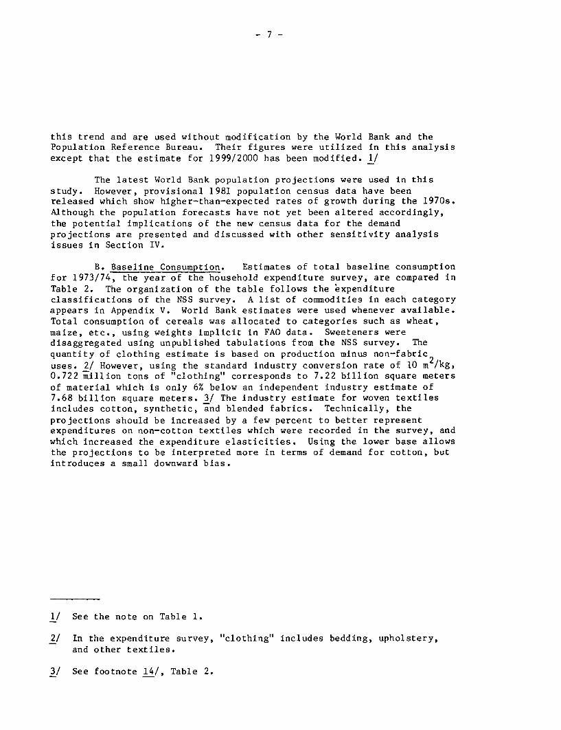
this trend and are used without modification by the World Bank and thePopulation Reference Bureau. Their figures were utilized in this analysisexcept that the estimate for 1999/2000 has been modified. 1/

The latest World Bank population projections were used in thisstudy. However, provisional 1981 population census data have beenreleased which show higher-than-expected rates of growth during the 1970s.Although the population forecasts have not yet been altered accordingly,the potential implications of the new census data for the demandprojections are presented and discussed with other sensitivity analysisissues in Section IV.

B. Baseline Consumption. Estimates of total baseline consumptionfor 1973/74, the year of the household expenditure survey, are compared inTable 2. The organization of the table follows the expenditureclassifications of the NSS survey. A list of commodities in each categoryappears in Appendix V. World Bank estimates were used whenever available.Total consumption of cereals was allocated to categories such as wheat,maize, etc., using weights implicit in FAO data. Sweeteners weredisaggregated using unpublished tabulations from the NSS survey. Thequantity of clothing estimate is based on production minus non-fabric2uses. 2/ However, using the standard industry conversion rate of 10 m2 /kg,0.722 million tons of "clothing" corresponds to 7.22 billion square metersof material which is only 6% below an independent industry estimate of7.68 billion square meters. 3/ The industry estimate for woven textilesincludes cotton, synthetic, and blended fabrics. Technically, theprojections should be increased by a few percent to better representexpenditures on non-cotton textiles which were recorded in the survey, andwhich increased the expenditure elasticities. Using the lower base allowsthe projections to be interpreted more in terms of demand for cotton, butintroduces a small downward bias.

1/ See the note on Table 1.

2/ In the expenditure survey, "clothing" includes bedding, upholstery,and other textiles.

3/ See footnote 14/, Table 2.

-8-

Table 2

lNDIA

SELECTION OF BASE QUANTITIES FOR P'ROJECTIONS(Hiousehold Demand or Net Food Avai lability)

'ACGREGOR- FAO IBRD SOURCES NSS IMfPLIE1D SANDBRSON/gOY-/ GROSSIT8 SELECTED1973-74 1972-74 1973-74 1973-74 31 1973-74 IACTOR- BASE

__ _ _ _ _ . ------------------________…1,000,000 mt--… ---------------------

ulses, Cereal Substitutes 11.082-/ 8.210 8 715/ 1.143 S,71Edible Oils 2.90 2.748 2 .6 6 7 7/ 1.79 1.109 2.667

Meat/Fish/Eggs -_ 2.398 1.0 2.398Vegetables 6.928 33,428 1.0 6.928Fruits/Nuts 7.18212/ 16.571-/8 1.0 16.571

Sugar/Khandsari 11,621- 3.690 4 ,519-D 2.64 1.0 4,519Gur/Other Sweeteners 6.429 7.3368/ 3.53 1.0 7.336

Spices 0.684 0,691 1.0 0.691Beverages 0,305 0,318 1.0 0.318

Tobacco/Pan/Itltoxicants 0.46414/ --- 1.0 0,464Clothing 0,722- --- 1.0 0.722

Milk and Products 24.2102/ 19.748 1.0 19.748Rice 36.593-7/ 38.131 48,31 1.143 40.363-2/ ~~~~~~~~~~~~~~~~~~~~~~~~11)Wheat 23 362- 21,283 28.12 1.143 22 536-.Maize 3.943,-L 3,848 5.20 1.143 4.0361-3/3 1/Sorghum/M'illet/Barley 19.596- 16,182 23.54 1.143 17,154-/

A31 Sugars 11,621 10,119 11.8555/ 6.17All Cereals 83.495 79.444 84.09 - 105.17 96.81 84,09

__________. __________-_-… - … …1------- -1,000,000 …--------

Population 583.9 595.6 588.3 595.6

NOTES -/ c :rcaf±gure 1f 5.6/1 s-r - ,v-r-tpd ton 'u-r atr t1% oxtractton.

-/59.956 for rice & wheat, allocated by NSS quantity weights. (These cereals were not dis-aggregated by MlacGreggor.)

3/23.539 for other cereals, allocated by NSS quantity weights. (maize was grouped with theother coarse cereals in the study.)

A/Cashews, almonds, walnuts, groundnuts, coconuts, and fruit.

5/ 1973-74 average. Excludes Topioca-/Includes topioca,

7/IBRD, ASADB source,

8/ IBRD, ASADB source,

9/Fred H. Sanderson and Shyamal Roy, Food Trends and Prospects in India (Washington, D, C.: The Brook-ings Institution, 1979), Table 6.1.

10/The projections for pulses, cereals, and oils contain a grossing factor shown in this column to re-present nion-household demand. Seed, feed and waste account for about 12.5% of final demand for foodgrains:

it/ 1/(1-.125) = 1.143.- The selected base quantities for cereals were found by allocating the IBRD total for cereals according12/to proportions iap;iicit in FAO quantities.- Includes gur and other sweeteners.

12/The 'SS im'plied base figutres are inferred fre, data on nuantities consumed Per capita.

Refers to residual of production weight of baled cotton mLinus seed, post-harvest loss,and exports. Ihis is about 6% lower than the estimate of 7.68 billion square meter: of

cotton, non-cotton, and mixed fibre cloth, assuming ten squiare meters per kg. This estimate isfrom the altndboolk of Statistics o01 the Cottotn Te\tile [n_uJtrv, The Indidn Cotton Mills Federation,Bowbay (September 1, 1980), p. 35. Ihe 1974 e-stimated aggregate household consumption was adjustedfor 1973/74 average availability (Table 19).

_ -John Macgregor "Agricultural Dcmand Projections for India," The World Bank, ASADB (Draft DivisionalPaper, 1979).

- 9 -

Fixed grossing factors for non-household demand (seed, feed,minimal industrial use, and loss) are shown for foodgrains and edibleoils. Future demand for these commodities represents total demand,whereas projections for other items refer only to household demand.

As a consistency check, baseline quantities for food can becompared with the population estimate in terms of calories per capita perday. The conversion from weight to calories utilized foodgrain equivalentfactors shown in Appendix IV. The level of food availability implied bythe selected baseline quantities is quite consistent with other estimates:1,952 calories per capita per day (Table 7).

Production indices in 1973/74 for foodgrains contracted somewhat,but were comparable with other below-average years, such as 1970/71 and1976/77. Cereal production in calendar 1973 was 5% below the surroundingfive-year average. However, an increase in net cereals imports in 1973,which partially offset the production shortfall, the reasonableness of theper capita calorie estimate, and the fact that FAQ base quantities whichwere adopted for some commodities were already three-year averages, led toa decision to dispense with more elaborate modifications of the base levelof total consumption to adjust for starting period aberrations.

Consumers may have been adjusting expenditures to rapid priceincreases in 1973/74. Price indices for major agricultural commoditiesrose rapidly in the early 1970's, particularly 1973-75, in contrast to themore stable pteice environment of the late 1960's. These considerationshighlight a second area of potential sensitivity of the projections to thebase year chosen. Set against these precautionary notes is the ratheruniform set of expenditure elasticities obtained from various sources andtime periods which are compared with estimates from these data in thefollowing section. The similarity suggests typical patterns of demand maynot have been too disrupted by these price movements.

Weights for sectoral consumption are required to combine urbanand rural demand into a national estimate. Quantity-based weights shouldbe used to avoid price differentials and these were derived from the NSSsurvey for edible oils, sweeteners, and cereals. Value-based weightswithout price adjustment were used for the other commodities.

A detailed exposition of the methodology adopted for projectionsis presented in a separate paper, available from the India Division of theWorld Bank, "Documentation of a Demand Projection Model Prepared forIndia." The principal features of the approach are outlined below.

- 10 -

C. Estimation Approach. Cross-sectional survey data from the NSS28th round were used to estimate expenditure regressions and elasticities.1/ Generalized least squares (GLS) regressions were run on the expendituresurvey data using the ratio semilog inverse functional form. 2/ This formautomatically satisfies the Engel aggregation condition of consumer demandtheory since the dependent variables are budget shares. 3/ (If thiscondition were not met, the sum of marginal propensities to consume wouldnot exhaust marginal expenditure which would introduce awkwardinconsistencies into a set of demand projections). The functional formalso does not impose an a priori relationship between the income level andthe elasticity. One regression per commodity or commodity group was usedto estimate the elasticity expression for all expenditure classes. Theexpression yields distinct elasticities for each expenditure class when itis evaluated using that group's mean total expenditure, and meancommodity-specific expenditure. Thus projections for each income levelutilize separate elasticities, although they are derived from a singleregression. GLS methods are needed to compensate for the heteroscedasticproperties of grouped data having different numbers of observations pergroup. Persons per household times households per class formed theweights.

Future demand was geared to the growth rate of expenditure in theeconomy, which can be selected at will during a computer projection run.From this growth rate, urban and rural per capita expenditure growth rateswere derived for each projection period (base date to projection date)which are consistent with:

a) the selected total rate of expenditure expansion;

b) population growth and urbanization rates;

1/ National Sample Survey Organization, Tables on Consumer Expenditure,28th Round, No. 240, Department of Statistics (1977), New Delhi.

2/ This form is Y/X = a + b ln X + c/X where Y is the commodity expendi-ture and X is the total expenditure. The expenditure elasticity isthen e = (a + b + b lnX) X/Y.

3/ Price data would be necessary to check the other conditions, namelythe negativity of the own substitution effect, the symmetry ofcross-substitution effects, and homogeneity of degree zero for thesystem of demand equations. (The last condition implies that multi-plication of prices and income by a constant would leave demand pat-terns unchanged, i.e., there is no "money illusion" in consumption.)

- 11 -

c) historical rates of growth between the base year and the mostrecent observation--about 3.5% in real terms from 1973/74 to1979/80.

Table 3 of the documentation paper provides evidence that since 1961,there has been very little difference between the sectors in nominal percapita expenditure growth rates. Consequently, none is assumed here.

An annual rate of change in the Gini ratio can also be selectedduring program execution. The effects of redistribution on demand areincornporated through a reallocation rule which satisfies the Gini ratiomodification in such a way that changes in expenditure are proportionateto an income group's distance from income equality.

Per capita demand growth for each commodity was projected forevery income class, both sectors, and the future time periods of interestgiven the rate of redistribution and the derived per capita expendituregrowth rate. The future periods chosen were five year intervals beginningin 1979/80 (to better coincide with the Plan period) and ending in1999/2000. Rural and urban population growth factors were applied, theincome classes were aggregated, and the sectors combined, usingappropriate weights. Since demand growth is expressed as a multiplicativeincrease, the outcome can be multiplied by grossing factors fornon-household demand (for foodgrains and edible oils) and by the baselevels of consumption. The result is final demand in quantity terms.

The adopted approach assumes that relative prices are constantthrough time, and equal for all consumers within same sector, either ruralor urban. Non-household demand is neglected except for edible oils andfoodgrains. Proportionality assumptions are made to infer non-householddemand from household demand for these commodities. Individual householddata such as occupational category or educational level of thehead-of-household, caste/ethnic group, farm characteristics of farminghouseholds, etc., were not available, although they can illuminateconsumption patterns. A final important assumption is thatreal-expenditure growth per capita is equal in the rural and urbansectors. This assumption at least holds in nominal terms since 1961.(Evidence to this effect is presented in the model documentation paper.)

The programs in the model print out the expenditure elasticities,the starting and ending Gini ratios, expenditure shares held by populationgroups, projected demand for all commodities and time periods under theredistribution and expenditure growth assumptions, and aggregate demandfor foodgrains and sweeteners.

- 12 -

II. ELASTICITIES AND PROJECTION RESULTS

A. Comparisons of Expenditure Elasticities. The expenditureelasticities in this study satisfy the Engel aggregation condition for therural and urban sectors (Table 3): the sum of expenditure elas5icitiesweighted by budget shares equals one. 1/ The' lowest adjusted R for the

underlying generalized least squares reg essions was around 0.95 and mostwere 0.98 or above. However, the high R s are partly the consequence ofusing observations grouped by income class. 2/ The elasticities for anumber of commodities are quite similar to previous estimates. Note, for

example, comparisons with estimates from the National Commission onAgriculture (NCA) for pulses, meat/fish/eggs, sugar and khandsari,beverages, clothing, milk and maize. 3/

Although the expenditure elasticities for wheat and rice arehigher than found by NCA, the estimates for foodgrains as a whole areconsistent with other research. Desai's estimates of the rural and urbanelasticities for foodgrains are 0.52 and 0.30 (not shown in Table 3) which,are close to the present estimates of 0.63 and 0.39. 4/ Mellor's nationalestimate is the same as the present urban figure. The national estimateof the expenditure elasticity for foodgrains is 0.59 in the presentstudy, 5/ whereas the middle of the range reported by Scandizzo and Brucefor India is 0.60. The estimates they report use longitudinal data

1/ Meeting this condition is an attraction of using theratio-semilog-inverse form in which budget shares are dependent vari-

ables. The weighted expenditure elasticities equalled 1+ 0.001 ineach case.

2/ This is an additional reason why the correlation coefficient is notparticularly suited for choosing among functional forms even afterappropriate weighting and econometric techniques have been applied.

3/ The "Other" category in Table 3 includes fuel and light, footwear,miscellaneous goods and services, rents, taxes, and durable goods. Anelasticity for this category must be estimated to check the Engelaggregation condition. The projections for this category areexpressed in terms of a multiplicative increase over the base level.

4/ B. M. Desai, "Analysis of Consumption Expenditure Patterns in India,"Occasional Paper No. 54, Department of Agricultural Economics, CornellUniversity (August 1972), Table 3. Found from log-log-inverse regres-sions on 1963/64 NSS data.

5/ Found by combining the urban and rural estimates with population andexpenditure weights.

- 13 -

TABLE 3

EXPENDITURE ELASTICITY ESTIMATES

FOR INDIA

Present Study 1/ NCA 2/ Mellor VariousRural Urban Rural Urban National 3/ National 4/

Pulses 0.86 0.81 0.85 0.66 - 0.32Edible Oils 1.00 1.01 0.88 0.97 5/ 1.05 -Meat, Fish, Eggs 1.15 1.12 1.22 1.07 6/ 1.33Vegetables 0.82 0.94 - - -Fruits, Nuts 1.36 1.54 - - -Sugar, Khandsari 1.51 1.06 1.65 1.11 1.10 7/ -

Gur, Other Sweeteners 1.09 0.53 0.96 0.23 -Spices 0.67 0.50 - - -Beverages 1.20 1:43 1.29 1.33 6/ - -Tobacco, Pan, Int6x. 0.90 0.96 0.72 0.79 - -Clothing 1.82 1.68 1.86 1.64 8/ - -Milk and Products 1.73 1.43 1.46 1.30 1.60 -Rice 0.71 0.42 0.41 0.18 - 0.94Wheat 1.01 0.55 0.67 0.37 - 1.06Maize 0.03 -0.76 0.01 -0.47 --

Sorghum, Millet 0.07 -0.59 - - -

All Other 1.11 1.28 - - -

Foodgrains 0.63 0.39 - - 0.39 0.49-0.71

1/ Found from regressions of the ratio semilog inverse form on NSS 28th Round data(1973/74) weighted for households per income class and persons per household.Elasticities at the mean are reported,

2/ Report of the National Commission on Agriculture, Demand and Supply (1976),Appendix 10.2.

3/ John W. Mellor, "Agricultural Price Policy and Income Distribution in Low IncomeCountries", World Bank Staff Working Paper No. 214, September 1974. Estimatedfrom NCAER "All-India Consumer Expenditure Survey, 1961L/65" using log-log-inversefunctional forms.

4/ Various sources using longitudinal data compiled in "Methodologies for MeasuringPrice Intervention Effects", Pasquale L. Scandizzo and Colin Bruce, World BankStaff Working Paper No. 394 (March 1980), p. 80.

5/ These elasticities are for vegetable oils. Elasticities for vanaspati arerural: 1.98, urban: 1.48, (reported by NCA).

6/ Budget shares were not reported, so these elasticities are simple averages forcommodities (average of tea and coffee for beverages).

7/ Applies to all sweeteners.

8/ These elasticities are for mill-made cotton clothing, and are intermediatebetween handloom cotton clothing and khadi cotton clothing.

- 14 -

through the mid to late sixties. I/ The similarity of estimates fromlongitudinal data, cross-sectional data a decade earlier, and the currentanalysis, (Desai--1963/64, current--1973/74) indicates stability in thedemand pattern for foodgrains and increases confidence in the projections.

Several factors motivated re-estimating the elasticities despitetheir availability in other sources. Foremost among these is the factthat the elasticities derived here and used in the projections varybetween expenditure classes, although they are only shown in Table 3 asthey appear after evaluation at the grand mean. Moreover, while manyfunctional forms have this property, the elasticities are usually forcedto vary in the same direction across income groups, regardless of thecommodity. The derivative of the elasticity with respect to income isnegative a priori for certain estimation forms. In the regressionsestimated in this study, the direction in which the elasticity changesdepends on the commodity. This variation was required.since future demandfor a given commodity was projected for each expenditure class, andmarginal propensities to consume generally are not constant across incomegroups. Additional advantages of these estimates include more commoditydisaggregation, weighting by persons per household and households perincome group, and the consistency of Engel aggregation, as alreadymentioned. Thus the similarity of some elasticities at the overall meanto other estimates does not greatly detract from the fruitfulness of theexercise.

Some of the notable features of this set of expenditureelasticities are:

1) the urban and rural preference for wheat and pulses comparedwith rice as total expenditure increases (a pattern supportedby NCA estimates); 2/

2) higher foodgrains elasticities in rural than in urban areas;

3) very low rural and negative urban elasticities for maize,sorghum, and millet; and

4) high elasticities for clothing, milk, milk products, fruit andnuts.

These relationships among the elasticities foreshadow certaincharacteristics of the projections and sensitivity analysis, namely:

1/ See Footnote 4/, Table 3.

2/ This preference may have implications for the proportions of wheatand rice the public sector should hold for distribution.

- 15 -

1) the increase in the proportion of wheat and pulses demanded outof foodgrains if expenditure growth is rapid (Table 16);

2) the apparent dampening effect of faster urbanization on thegrowth in foodgrains consumption (Table 14);

3) the somewhat reduced demand for coarse cereals givenaccelerated economic growth; and

4) the sensitivity of projections for clothing, milk, and milkproducts to expenditure growth rates.

B. Quantity Projections. The projections for two rates ofexpenditure growth, assuming no income redistribution, are given in Tables4A and 4B. The projections for various foodgrains and edible oils containgrossing factors listed above (Table 2) for non-household demand.Foodgrain demand would more than double by the end of the century underthe lower rate of growth, and increase by 220% if 5% expenditure growthwere experienced. 1/ Higher expenditure growth adds at least one percentto the growth rate of demand for sweeteners, edible oils, wheat and pulsesthrough 1984/85 (Table 5). Although the growth in demand slackenssomewhat after 1984/85 for these commodities, rice, and all foodgrains, itremains well above 3.0% for sugar/khandsari and edible oils even under thelower alternative. Pressures, therefore, may persist either to continuethe importation of large volumes of edible oils, or to let prices risesufficiently to induce a substantial supply response.

1/ These increases are relative to the 1973-74 base year.

- 16 -

TABLE 4ADemand Projections Assuming 3.5% Expenditure Growth

FOR THE FOLLOWING PROJECTIONTOTAL EXPENDITURE GROWTH ASSUMPTION IS 3.5 PERCENTGINI RATIO CHANGE RATE IS 0 PERCENT

DEMAND IN MILLION METRIC TONS

73/74 79/80 84/85 89/90 94/95 99/00

PULSES 3/ 8.71 11.36 13.19 15.26 17.64 20.25EDIBLE 01LS 2.67 3.36 3.99 4 75 5.59 6 56MEAT, FISH. 6 EGGS 2.40 2 70 3.25 3.91 4 68 5.62VEGETABLES 6.93 7.84 9.21 10.81 12 S9 14 62FRUITS & NUTS 16.57 18.51 23.13 29 05 36.39 45 91SUGAR & KHANDSARI 4.52 5.25 6.44 7.89 9.57 11.63GUR & OTHER SUGARS 7.34 8.33 9.60 10.96 12.61 14.31SPICES 0.69 0 77 0.89 1.01 1.15 1.30BEVERAGES 0.32 0.34 0.43 0 56 0.70 0.90TOBACCO. PAN & INTOX 0.46 0.51 0 60 0.71 0.83 0.98CLOTHING 0.72 0.83 1.05 1.31 1.67 2.13MILK 19.75 23 24 28 74 35.48 43.84 54.17RICE 40.36 52.22 59.31 66 87 75.26 83.51WHEAT 22.54 29.19 33.97 39 29 45.20 51 47MAIZE 4.04 5.09 5.50 5 87 6 28 6.59SORGHUM & MILLET 4/ 17.15 21 59 23.52 25.36 27.28 28 84OTHER V/ 1.00 1.06 1.30 1.61 1.99 2.47

SWEETENERS 11.85 13.58 16.04 ,18.84 22.18 25.93

FOODGRAINS 92.80 119.46 135.49 152 65 171.66 190.66

TABLE 4B

Demand Projections Assuming 5.0% Ex-enditure GrowthFOR THE FOtLOWING PROJECTION

TOTAL EXPENDITURE GROWTH ASSUMPTION IS 5 PERCENTGINI RATIO CHANGE RATE IS 0 PERCENT

DEMAND IN MILLION METRIC TONS

73/74 79/80 4/84/85 89/90 94/95 99/00

PULSES 3/ 8.71 11.36 13.92 16.89 20.39 24.29EDIBLE OILS 2.67 3 36 4.24 5.33 6.56 8 00MEAT. FISH. & EGGS 2.40 2.70 3.51 4.55 5.86 7.52VEGETABLES 6.93 7.84 9.71 11.97 14.55 17.55FRUITS & NUTS 16.57 18.51 25.93 36.45 50.98 71 60SUGAR 6 KHANDSARI 4.52 5.25 7.04 9 36 12.27 15.99GUR & OTHER SUGARS 7.34 8 33 10.18 12.20 14 60 17.00SPICES 0.69 0.77 0.92 1.08 1.26 1.45BEVERAGES 0.32 0.34 0.49 0.70 0.99 1.42TOBACCO. PAN & INTOX 0.46 0 Si 0.64 0.81 1 02 1 29CLOTHING 0.72 0.83 1.21 1.74 2 52 3 62MILK 19.75 23 24 32.12 43.94 59.81 80.82RICE 40.36 52.22 61.30 70.72 80 34 88 54WHEAT 22.54 29.19 35.70 42.91 50 68 58 60MAIZE 4.04 5.09 5.48 5.78 6.08 6.20SORGHUM & MILLET 4/ 17.15 21.59 '23.38 24 91 26 32 27 08OTHER 1/ - t.00 1 06 1.44 1.98 2.71 3.73

SWEETENERS 11.85 13.58 17.22 21.57 26.87 32.99

FOOOGRAINS 92.80 119.46 139.78 161 21 183.82 204.71

1/ Multiplicative factors, not million metric tons.

2/ Assumes 3.5% expenditure growth through 1979-80.

3/ Includes cereal substitutes and grams.

4/ Includes barley and other coarse cereals.

- 17 -

TABLE 5

Projected Annual Growth Rates of Demand for Selected Commodities a/

1979/80 to 1984/85 1984/85 to 1999/2000Low High Low High

…____________________(% )…______ ___________

Sugar & Khandsari 4.2 6.0 4.0 5.6Gur & other sweeteners 2.9 4.1 2.7 3.5Edible oils 3.5 4.8 3.4 4.3Rice 2.6 3.3 2.3 2.5Wheat 3.1 4.1 2.8 3.4Pulses 3.0 4.1 3.0 3.8Foodgrains 2.6 3.2 2.3 2.6

a/ The "Low" and "High" growth rates assume 3.5% and 5.0% total expendituregrowth, respectively.

The reasonableness of the projections can be examined through:

1) coinparisons with actual demand (availability) in 1979/80, whichis the first projection period;

2) comparisons with other quantity projections;

3) converting food demand to calories per capita and comparingthese figures with expected levels of consumption and othercalorie projections.

The actual availability of foodgrains for calendar year 1979 isestimated to be 114.11 million tons (103.44 million tons cereals and 10.66million tons pulses) which can be compared with the projection for fiscal1979/80 of 119.46 million tons (108.1 million tons cereals, 11.36 milliontons pulses), which is about 5% higher. Foodgrain production in 1979/80was 17% below the previous year's record level and availability incalendar year 1980 was sharply reduced. The projections would thereforefurther exceed availability if 1979 and 1980 were averaged. Nevertheless,it is to be expected that the decline in incomes and upward pressure onprices following a sharp decline in the production of foodgrains wouldhave dampened demand beneath its forecast level and this undoubtedlyexplains part of the discrepancy.

- 18 -

Household consumption of sweeteners, averaged for 1978/79 and1979/80, was 13.1 million tons whereas the projection was 13.6 milliontons. 1/ The 1979/80 consumption of edible oils (including non-householdconsumption) was estimated to be 3.55 million tons compared with aprojection of 3.36 million tons. 2/ The projections for these commoditiesare fairly close to observed and estimated consumption, particularly ifallowances are made for the 1979/80 crop year.

Projections for the year 2000 by the National Commission onAgriculture for rice, wheat, foodgrains, sugar and khandsari, edible oilsand meat/fish/eggs are very much in line with those in the present study(Table 6). Estimates of demand in 1984/85 for rice from several sourceslie in a narrow range. The present projections for sugar also closelymatch EPD's longitudinal estimates.

Converting food demand to calories per capita allows adetermination of whether the projected demand levels for all foods arereasonable in comparison with the population projections. First, thegrossing factors were removed (since household consumption alone isrelevant here), then quantities were converted to foodgrain equivalentswith food energy weights, and finally the cross-commodity summation wasexpressed in calories per capita per day (Table 7). 3/ The resultingfigure of 1,952 calories for 1973/74 is similar to estimates by NCA, TheBrookings Institution, FAO, and the World Bank in its World DevelopmentReport. 4/ NCA's high projection for 2000 differs by only 22 calories percapita per day from the present analysis, and the low projections areeight calories apart. These differences are negligible in per capitaterms. This is a remarkable concurrence considering that differentconsumption data, population projections, and methodologies were used.Sanderson and Roy's low projection (Brookings Institution Alternative C)

1/ Consumption estimate from U.S.D.A. preliminary figures and "SugarSituation in India," GOI, (September, 1980 mimeo). Averaging compen-sated for the reduced cane production in 1979/80. Sweeteners do notcontain adjustments for non-household demand.

2/ World Bank, estimate.

3/ The food energy weights and conversion factors are reported in Appen-dix IV.

4/ Some FAO base figures were adopted which makes this estimate lessindependent of the present study, but differences in population,foodgrains and some other crops remained which balanced out in termsof calories per capita.

- 19 -

1ABILE 6

CoMp&risons of Demsi,d Projeetlons 1/

1985 1990 2000

Low High Low High Low 111gb

Rice -------- tillion tons-----------Present Study 59.31 61.30 66.87 73.72 83.51 88.54NCA 59.89 64.69 - - 78.59 84.56EPD 56.45 - 64.19 - - -

USDA - 62.00 - - - -

Iowa State 57.0 - - - - -

WheatPrcsent Study 33.97 35.70 39.29 42.91 51.47 58.60NCA 33.83 38.16 - - 46.91 52.45EPD - 43.02 - 53.61 - -USDA - 41.00 - - - -

Other CerealsPresent Study 29.02 34.28 - - 35.43 33.28NCA 35.35 35.36 - - 43.19 42.90

PulsesPresent Study 13.19 13.92 - - 20.25 24.29NCA 16.95 20.27 - - 23.15 28.23

FoodgrainsPresent Study 135.49 139.78 152.65 161.25 190.66 204.71IICA 146.03 158.25 - - 192.36 208.14Brookings - - - 173.30 - -

SugarPresent Study 2/ 5.09 5.56 6.23 7.39 - -EPD 5.39 - 6.30 - - -

Sugar and RhandsariPresent Study 6.44 7.04 - - 11.63 15.99NCA 6.55 8.62 - - 10.33 13.31

Edible OilsPreseuit Study 3.99 4.24 - 6.56 8.00NCA 4.19 5.27 - - 6.45 8.05

MilkPresent Study 28.74 32.12 - - 54.17 80.82NCA 33.73 44.17 - - 49.36 64.40

Meat, Fish. EggsPresent Study 3.25 3.51 - - 5.62 7.52NCA 3/ 3.95 5.16 - - 6.00 8.00

Notes: I The low and high projections reported for "Present Study"assum. 3.5% and 5.0% total expenditure growth, respectively,and no income redistribution. The NCA estimates presented forcomparison are based on .onsumer demand, miltiplied by constantgrcssirg factors given in Table 2. NCA's gross demand estimatesfor some tommodities actually use increasing factors fornan-hojsehold demand.

2/ Found from sugar and khandsari projections by assuming 34% ofthe cane crop was processed into sugar and 9Z into khandsart.

3/ A conversion factor of 48g/egg was used.

Source": NCA - Report of the National Commission on Agriculture, PartIll,Demand and Suipply (1976). Table 10.7 (see Footnote 1).

EPD - Econz,mic Analvsis and Projectiton, Depirtment, World Bank,

USDA - U.S. Dcpartment of Agriculture, Anthony Rojko, et al,Alternative Futtires fir World Fvocd. 1985, Vol. I (1978),Table 28.

Iowv State - Leroy Bla.keslee, Earl Heady, Charle3 Trani1ngham, Worldn,^l ProId, tion Deimnnd. anI Trade, Center for Agriculture

and Pural i)eveluiment, Iowj State UTniver,.ity (1973), Ames.

Rrookinpgq - The Bronkings l11,ritIlEtin, Fred It. Sansderso,n and ShyfatRIoy, Fnnd Trenis nn.l Fro'ip.t I n tndia,(1919).

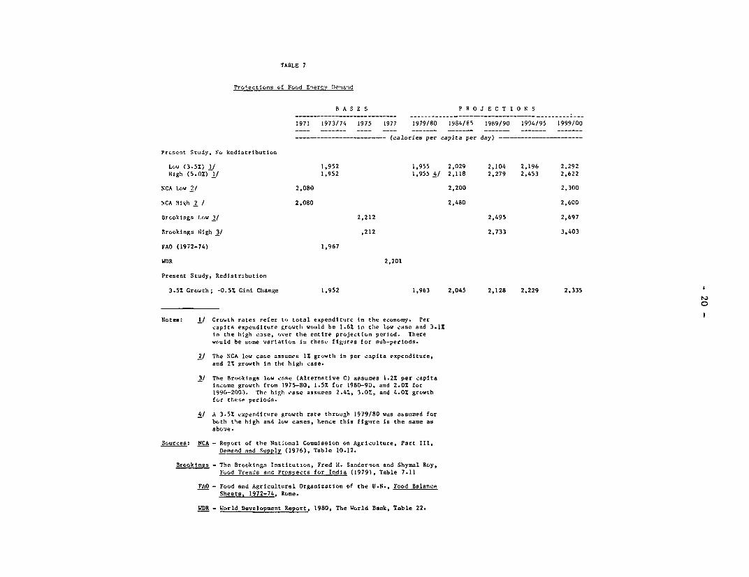
TABLE 7

Projections of Food Energv Deand

B A S E S P R O J E C T I O N S

1971 1973/74 1975 1977 1979/80 1984/85 1989/90 1994/95 1999/00

… -------- - (calories per capita per day) --------- - ---- ----

Prosent Study, No kedistribution

Low (3.5%) 1/ 1,952 1,955 2,029 2,104 2,196 2.292

High (5.0%) 1/ 1,952 1,955 4/ 2,118 2,279 2,453 2,622

NCA Low 2/ 2,080 2,200 2,300

NCA High 2 / 2,080 2,480 2.600

Brookings Low 3/ 2,212 2,495 2,697

Brookings High 3/ ,212 2,733 3,403

FAO (1972-74) 1,967

WDR 2,201

Present Study, Redistribution

3.5% Growth; -0.5% Gini Change 1,952 1,963 2,045 2,128 2,229 2,335

Notes: 1/ Grovth rates refer to, total expenditure in the economy. Per

capita expeniditure growth wotild be 1.62 in the low case and 3.1%

in the high c3se, r,ver the entire projection period. There

would be some variation in these figures for sub-periods.

2/ The NCA low case assumes 1% growth in per capita expenditure,

and 2% growth in the high case.

3/ The Brookings low case (Alternative C) assumes 1.2% per capita

income growth from 1975-80, 1.5% for 1980-90, and 2.0% for

1990-2003. The high easc assumesn 2.4X, 3.0%, and 4.0% growth

for these periods.

4/ A 3.5% .xpenditure growth rate through 1979/80 was assumed for

both the high and low cases, hence this figXtre is the same as

above.

Sources: NCA - Report of the National Commission on Agriculture, Part III,

Demand and Supply (1976), Table 10.12.

Brookings - The Brookings Institution, Fred H. Sanderson and Shymal Roy,

Food Trends and Prospects for India (1979), Table 7.11

FAO - Food and Agricultural Organization of the U.N., Food Balance

Sheets. 1972-74, Rome.

WDR - World Development Report, 1980, The World Bank, Table 22.

- 21 -

is similar to the high case here and in the NCA study. However, theirhigh projection appears to be-unrealistic.

Per capita food energy demand would increase by about 15% by year2000 at a 3.5% expenditure growth rate. 1/ A moderate rate of expenditureredistribution, i.e., a 0.5%/year drop in the Gini ratio, would leave themean level of food energy demand virtually unaltered. However, a gradualincrease in equality might have a more significant effect on thedistribution of consumption. The next section presents evidence that theGini ratio based on personal expenditures has actually been falling atthis rate. The sensitivity of the projections to various assumptions isexamined in Section IV.

In general, the projections in Tables 4A and 4B appear consistentwith actual consumption of some commodities in 1979/80. The projectionsinto the 1980's and 1990's accord well with other research on consumerdemand in India, expressed both in terms of quantities and in terms ofcalories per capita.

III. INCOME REDISTRIBUTION

Since demand is projected for each expenditure class using uniqueelasticities, income redistribution would alter the-aggregate. There area number of measures of income distribution available to summarize thelevel of economic equality in a society: the Gini coefficient, Kuznets'Index, Theil's Index, the Pareto coefficient, the equally distributedequivalent, the coefficient of variation, and the standard deviation ofthe log-normal distribution, to name a few. Atkinson presents aninteresting comparison of several of these.2/ Despite the ambiguities ofcrossing Lorenz curves inherent in the Gini coefficient, it remains themost widely recognized measure, and has been calculated frequently withhistorical data which facilitates trend comparisons. Since changes inincome distribution affect the pattern of consumption, the projection

1/ It should be noted that the increase is moderated by the fact thatthe average energy requirement per capita is also rising slightly.As the population growth rate slows, the age structure of the popula-tion matures, and the mean requirement rises.

2/ Anthony B. Atkinson "On the Measurement of Inequality", Journal ofEconomic Theory, Vol. 2 (1970), pp. 244-257. Atkinson shows that theranking of countries according to inequality obtained from the Giniratio, the standard deviation of logarithms, and the coefficient ofvariation are similar to the rankings found with the equally dis-tributed equivalent measure using a different index of aversion toinequality.

- 22 -

programs were designed to model assumptions about an altered distributionand their impact on demand. Changes in the income distribution are

summarized in terms of the Gini coefficient and shares of the totalexpenditures accounted for by given shares of the population.Redistribution is assumed to be proportionate to a population group's

departure from economic equality. Crossing Lorenz curves (which may

present problems when countries are compared with one another) are not,

therefore, introduced. This section reviews an estimation procedure for

the Gini ratio, makes historical and international comparisons, andreports the effects of redistribution on demand. The following section

expands on the issue of redistribution in a sensitivity analysisframework, although the commodity focus is narrower.

A. Gini Ratio Estimation and Comparisons. Gini ratios lie in a

fairly tight band even when taken from a broad spectrum of countries.Ratios from a selection of countries which are based on similar years and

population coverages are shown in Table 8. When countries are ordered bythe ratios, a clear inverse pattern emerges between the Gini coefficientand the percent of income held by the least affluent 40% of the

population. However, exceptions to this generalization can be found.

Most of the estimates listed in the table rely on household incomedata. Changes in the distribution of individual consumption expenditure

will obviously be related more closely to the demand pattern. Gini ratios

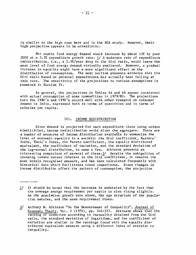
derived from these data will be lower since savings behavior isdisregarded. The Ranadive Gini ratio estimates for individual consumption

in India are, therefore, the most pertinent series for this analysis(Table 9). They indicate an improvement in the distribution evidenced by

a 8.3% drop in the Gini ratio over 15 years. Ahmed's figures on Gini

coefficients derived from the personal income of individuals support this

trend. Some of the series calculated by other investigators are more

ambiguous in trend.

- 23 -

TABLE 8

INTERNATIONAL COMPARISONS OF INCOME DISTRIBUTION ORDERED BY THE GINI RATIO

Income Share Held ByPercent of Population

Year Population a/ Gini Ratio Bottom 40% Top 20%

Taiwan 1972 HH 0.284 22.3 37.2Pakistan 1969/70 HH 0.336 20.2 41.8United Kingdom 1968 HH 0.338 18.5 40.3Yugoslavia 1968 HH 0.347 18.4 41.4

Korea (Rep. of) 1970 HH 0.372 17.7 44.5Sri Lanka 1969/70 HH 0.377 17.8 44.9Indonesia 1971 IR 0.463 17.3 52.0El Salvador 1969 POP 0.465 12.4 50.8

India 1967/68 HH 0.478 13.1 53.1Philippines 1971 HH 0.494 11.9 54.0Chile 1968 HH 0.506 13.0 55.8Ivory Coast 1970 IR 0.534 10.6 58.5

Mexico 1969 HH 0.583 10.2 63.2Tanzania 1969 HH 0.597 7.8 63.3Kenya 1969 IR 0.637 9.5 66.9Brazil 1970 IR 0.646 8.1 67.3

a/ The coverage is national in all cases. IR: Income Recipient;HH: Household; POP: Population.

Source: Adapted from Shail Jain, Size Distribution of Income:A Compilation of Data (Washington, D.C.: The World Bank, 1975)

TABLE 9

SOME ESTIMATES OF OINI RATIOS FOR INDIA

OJha and nhati Ahmed Ranadive Swamy

Yer 1964 1971 1971 1971 1971 1971 1964

Pironal Income Pononal Incomo Peonal Income Personal Income Personal ltIcome Consumption Consuniptinhouseholds Individuas indIviduals Individuass houicholda especid ture *vpendJturemisdivIdusla ht.useI,ulds

1951-52 . . . . . . 0.366

1952-53 . . . . . . 0.361

1953-54 043 0.359-0.374 0.437-0.511 0.336 0.3691954-55 0 0 0.399-0.420 . 0.3901955-56 -.30393-0.419 . 0.3701956-57 0.341 . 0.4527 0.377-0.410 0.333 0.4071957-58 . . . 0.371-0.391 0.432-0.540 . 0.3981958-59 . . . . 0.383

1959-60 0.355-0.378 . 0.385

1960-61 . 0.4136 . . .

19(1-62 . 0.356-0.379 . 0.3201962-63 0.385 .

1963-64 *

1964-65 . * 0.3873 * * 0.3031965-66 . . . . .

1966-67 . . . . . *

1967-68 . . . . . .

1968-69 . . . . . 0.308

Sources P. D. Olba ad V. V. lBlutat Pattern of inCome ditttrbutIon In an uanderdeveloped economy: a cae study of India " In Anuricax &o_wik Xaview(Mcnasha (W lu.nsln)) Sep. 1964. p. 714: and Idem: * Pattern of Income distribution In India: 19513-5 to 1961.64 " (Pape presented at the Seminat on Income Distributiono0;nised by ttic Indian Statistical Institute. New Delhi. February 21-26. 1971). p. S. Mahfooz Ahmed: - SIw dbtribution of personal Income In India 1956-57. 1960-61 and21'4-63 - (Pipcr presented at the Seminar .... 1971). table 6. K. R. Ranadive: - Pattern of Income distribution In India, 1953-54 to 1959-60 ;- InOuIlkiln of she OrfordU.! .. rity Insl,iUfe of Economics and Statlstikc. Aug. 1968. p. 212 (distribution of Income of Individuals In 1953-54. 1954-55. 1995-56; 1957-58 and 193940: ranges are duetn rItinmites bjscd on different assumptions about savings and tax evasion); and Idem: " Distribution of income: Trends since planning" (Paper presented at the Seminar1921). pp 16. 17 end 33 Subramanian Swamy: 'Structural changes and the distribution of Income by size: The ease of Indiea. In Review of Inro,ae arnd Wealth (New2le'en (Cosinecitcut)), June 1967. p. 173.

SOURCE: Felix Paukert, "Income Distribution at Different Levels of Development: A Surveyof Evidence," International Labor Review, Aug.-Sept., 1973, pp. 97-124.

- 25 -

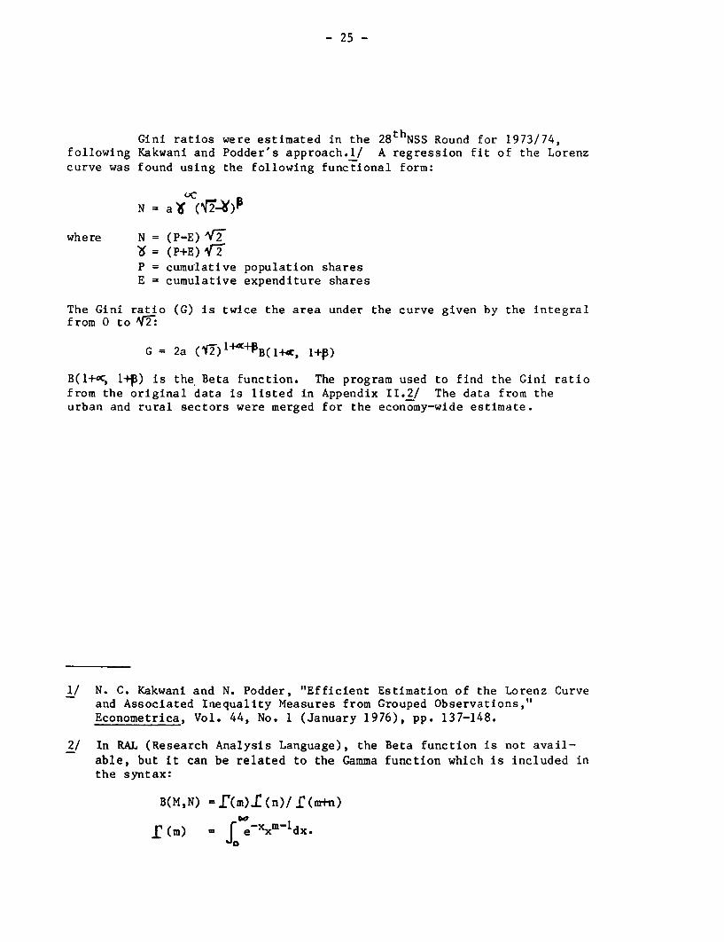
Gini ratios were estimated in the 28 thNSS Round for 1973/74,following Kakwani and Podder's approach.l/ A regression fit of the Lorenzcurve was found using the following functional form:

N =a V ( ff 4,

where N = (P-E) IT= (P+E) V

P = cumulative population sharesE = cumulative expenditure shares

The Gini ratio (G) is twice the area under the curve given by the integralfrom 0 to Nr2V

G = 2a (1 )1++PB(1+c, 1+P)

B(l+S, 1+P) is the Beta function. The program used to find the Gini ratiofrom the original data is listed in Appendix II.2/ The data from theurban and rural sectors were merged for the economy-wide estimate.

1/ N. C. Kakwani and N. Podder, "Efficient Estimation of the Lorenz Curveand Associated Inequality Measures from Grouped Observations,"Econometrica, Vol. 44, No. 1 (January 1976), pp. 137-148.

2/ In RAL (Research Analysis Language), the Beta function is not avail-able, but it can be related to the Gamma function which is included inthe syntax:

B(M,N) = r(m). (n)/ (m+n)

f(M) = J"exxm-ldx0

- 26 -

FIGURE 1

DISiRIBUTION OF INCOME AT DIFFEREN7 LEA ELSOF PER CAPITA GDP

% Gini MEP.rjUo

100I Gini t-atio 050

' *! fIncone reci.pviis90 .. '. *0.43 40

0 7XX~~~~~~~~~~~~~~~~~~~~~~~~~~~~'04 i 38

60 . Top 20 % 't, *'0-t.4.3, of Incomc reclptents ' :

SO * T 3 < | *. ,r O.40 .- 32

40 \-*. ,0.X8: * 30

Middle 20 % _* of Income recipients

30 * r4 .. 36 28

.5~ ~ ~ ~ '

Bottom 60 %.o1 Inecone recipients.

10 'rO 32 L 24

, '>

O0 .4 .04_3_

C jlOa sto-200| $2.01-300 5301-5co S5S01D-n;a 5 w GDP .r

(U.S. $ 1965)

India GDP per capita

(for 1973-74 in $U.S. 1965)

SOURCE: Cross-sectional data on 56 countriespresented by Paukert. (See source onTable 9.)

NOTE: MEP is the maximum equilization percentage definedas the percentage of total income that would haveto be shifted between quintiles to achieve equalincome distribution.

* 27 -

TABLE 10

GINI COEFFICIENTS FOR INDIVIDUAL CONSUMPTION EXPENDITURE(1973/74)

Rural Urban National

0.287 0.320 0.301

The national estimate is very close to the figure from Ranadive(0.308) and indicates a continuation of the trend of increasing equality.:Over .twenty years (1953/54 to 1973/74), the Gini ratio of individual*expeniditure has fallen at an annually compounded rate of 0.55%. Thepattern is reinforced by observations of the ratio for intermediateyears. 1/

An improving distribution is at variance with cross-sectionalrelationships between GDP per capita and the Gini ratio derived from total

,income (Figure 1). Countries at income levels similar to India'sexperience more inequality as income rises. The reconciliation of thelongitudinal trend with the cross-sectional pattern probably lies in thedifference-between consumption expenditure and incom"e. The multi-countrystudy. was based on total income. The personal income distribution couldbe worsening (suggested by Ojha and Bhatt, Table 9)r while the consumptiondistribution improves. Some researchers, however, also show India'sincome distribution becoming more egalitarian which would make Indiasomewhat unique when viewed against a background of cross-sectionaldata.2/ Changes in expenditure shares and Gini coefficients for three

1/ However, Gini ratios for the more recent period 1977/78 were estimatedwith the same technique using the decile distribution of privateconsumption from the 32nd NSS Round reported in the Sixth Five YearPlan, 1980-85. The rural, urban, and national ratios were 0.31, 0.34,and 0.32, which would imply a reversal of the trend. However, theseestimates may not be comparable since it is not stated whether thedeciles are based on the household or the individual population dis-tribution, and biases may have been introduced during interpolation todeciles.

2/ A recent Bank paper on income distribution in India concludes therehas virtually been no trend. V. V. Bhanoji Rao, "EPD Income Distribu-tion Project Data on Income Distribution in India," Division WorkingPaper No. 1980-2, p. 19. However, Ahmend's figures show some improve-ment through the mid-1960's.

- 28 -

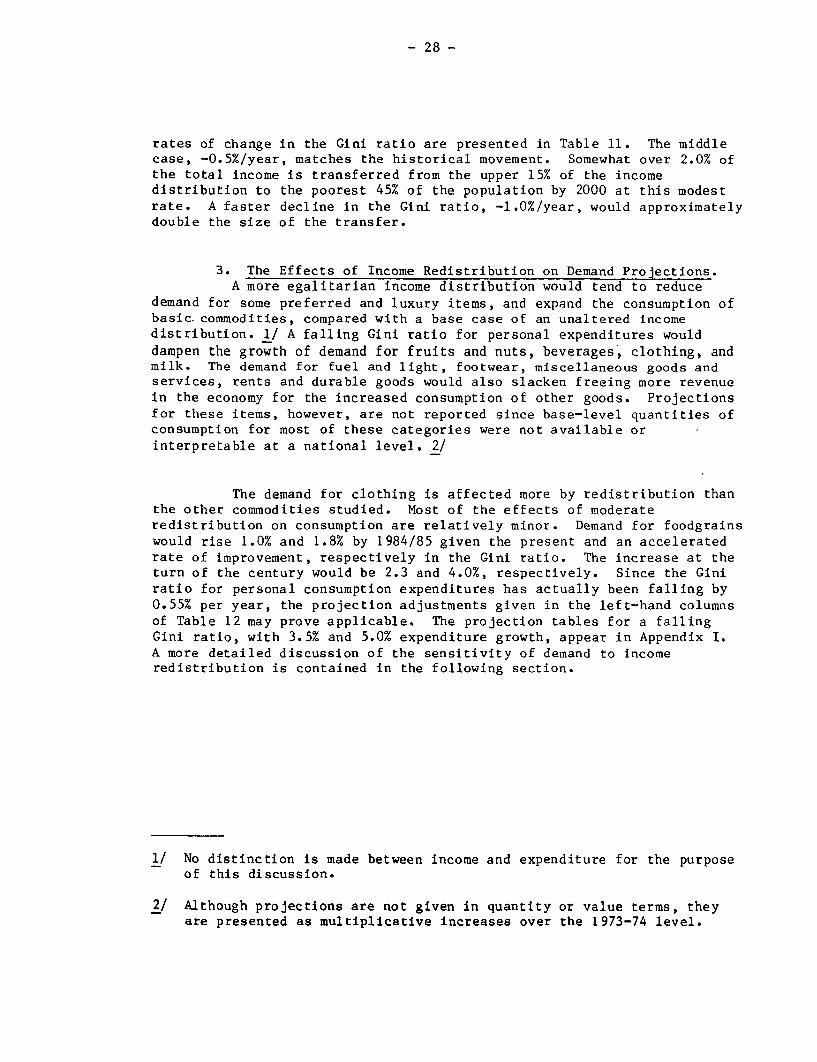
rates of change in the Gini ratio are presented in Table 11. The middlecase, -0.5%/year, matches the historical movement. Somewhat over 2.0% ofthe total income is transferred from the upper 15% of the incomedistribution to the poorest 45% of the population by 2000 at this modestrate. A faster decline in the Gini ratio, -1.0%/year, would approximatelydouble the size of the transfer.

B. The Effects of Income Redistribution on Demand Projections.A more egalitarian income distribution would tend to reduce

demand for some preferred and luxury items, and expand the consumption ofbasic. commodities, compared with a base case of an unaltered incomedistribution. 1/ A falling Gini ratio for personal expenditures woulddampen the growth of demand for fruits and nuts, beverages, clothing, andmilk. The demand for fuel and light, footwear, miscellaneous goods andservices, rents and durable goods would also slacken freeing more revenuein the economy for the increased consumption of other goods. Projectionsfor these items, however, are not reported since base-level quantities ofconsumption for most of these categories were not available orinterpretable at a national level. 2/

The demand for clothing is affected more by redistribution thanthe other commodities studied. Most of the effects of moderateredistribution on consumption are relatively minor. Demand for foodgrainswould rise 1.0% and 1.8% by 1984/85 given the present and an acceleratedrate of improvement, respectively in the Gini ratio. The increase at theturn of the century would be 2.3 and 4.0%, respectively. Since the Giniratio for personal consumption expenditures has actually been falling by0.55% per year, the projection adjustments given in the left-hand columnsof Table 12 may prove applicable. The projection tables for a fallingGini ratio, with 3.5% and 5.0% expenditure growth, appear in Appendix I.A more detailed discussion of the sensitivity of demand to incomeredistribution is contained in the following section.

1/ No distinction is made between income and expenditure for the purposeof this discussion.

2/ Although projections are not given in quantity or value terms, theyare presented as multiplicative increases over the 1973-74 level.

- 29 -

TABLE 11

FUTURE EXPENDITURE SHARES AND GINI RATIOS GIVEN REDISTRIBUTION RATES

R U R A L U R B A NGini Ratio Bottom TOP Gini Ratio Bottom TOP

Population Share 42.5 16.9 47.6 16.2

1973/74Expenditure Share 24.8 33.7 26.3 36.0Gini Ratio 0.287 0.320

1999-2000Gini Change + 0.5%/Year

Expenditure Share 22.3 36.1 23.4 38.7Gini Ratio 0.327 0.364

Gini Change - 0.5%/YearExpenditure Share 27.0 31.7 28.7 33.6Gini Ratio 0.252 0.281

Gini Change - 1.0%/YearExpenditure Share 28.9 29.8 31.0 31.4Gini Ratio 0.221 0.246

Notes: Redistribution followed the rule:

si = si-(AGIG)(P -S.)

where S = starting expenditure share of ith group;

iSi = expenditure share after redistribution

a G/G = proportionate change in Gini ratio over the period;

Pi = population share of the i th group.

See Section II.C for further details. To avoidpossible interpolation errors, the table is based on populationshare divisions aggregated from the reported data. (Interpolationwould have resulted in exact decile or quintile shares.)

It is demonstrated in the paper documenting the demand model thatthe redistribution rule satisfies the condition that the new Giniratio G , based on expenditure shares S equals G+ANG.

- 30 -

TABLE 12

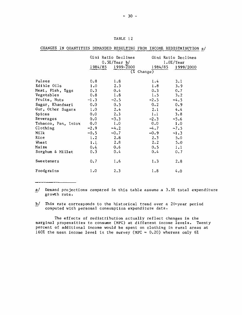
CHANGES IN QUANTITIES DEMANDED RESULTING FROM INCOME REDISTRIBUTION a/

Gini Ratio Declines Gini Ratio Declines0.5%/Year b/ 1.0%/Year

1984/85 1999-2000 1984/85 1999/2000(% Change)

Pulses 0.8 1.8 1.4 3.1Edible Oils 1.0 2.3 1.8 3.9Meat, Fish, Eggs 0.3 0.4 0.3 0.7Vegetables 0.8 1.8 1.5 3.2Fruits, Nuts -1.3 -2.5 -2.5 -4.5Sugar, Khandsari 0.0 0.5 0.2 0.9Gur, Other Sugars 1.0 2.4 2.1 4.4Spices 0.0 2.3 1.1 3.8Beverages 0.0 -3.3 -2.3 -5.6Tobacco, Pan, Intox 0.0 1.0 0.0 1.0Clothing -2.9 -4.2 -4.7 -7.5Milk -0.5 -0.7 -0.9 -1.3Rice 1.2 2.8 2.3 5.0Wheat 1.1. 2.8 2.2 5.0Maize 0.4, 0.6 0.5 1.1Sorghum & Millet 0.3 0.4 0.4 0.7

Sweeteners 0.7 1.6 1.3 2.8

Foodgrains 1.0 2.3 1.8 4.0

a/ Demand projections compared in this table assume a 3.5% total expendituregrowth rate.

b/ This rate corresponds to the historical trend over a 20-year periodcomputed with personal consumption expenditure data.

The effects of redistribution actually reflect changes in themarginal propensities to consume (MPC) at different income levels. Twentypercent of additional income would be spent on clothing in rural areas at160% the mean income level in the survey (MPC = 0.20) whereas only 6%

- 31 -

would be allocated to clothing at 60% of the mean income level. 1/ Henceredistribution significantly reduces the demand for clothing. Thecorresponding high and low MPCs for gur and other sweetners are 0.01 and0.03. This opposite ordering implies an elevated demand would accompanyredistribution. Likewise, in a neutral case in which demand was virtuallyunaltered, the MPCs are similar across a range of incomes. The rural MPCsfor meat, fish and eggs at 160% and 60% of the mean income, for example,are 0.027 and 0.034.

IV. SENSITIVITY ANALYSIS

Sensitivity analysis was performed on the projections forfoodgrains, edible oils, sweeteners, and the share of wheat in foodgrainsby varying the assumptions regarding population growth, urbanization,expenditure growth, and income distribution. The proportions of rice andpulses demanded out of total foodgrains were also considered. Thepopulation parameters were altered in a few discrete cases, butsensitivity analysis for expenditure growth and income distributionproceeded from a set of 27 projections with a blend of assumptions.Regressions were then run treating the set of demand levels asobservations on a dependent variable. This approach yielded elasticitiesof future demand with respect to rates of expenditure growth and"income" 2/ redistribution. In most cases, sensitivity analysis wasreferenced to the projected demand in the year 2000. 3/

A. Population Growth and Urbanization. Population growth rateswere varied by +0.1% and +0.05%, and urbanization by +1% of the totalpopulation per five years. 4/ A very high rate of urbanization was alsotested in which the urban share was 2% higher than the base case per fiveyears of projection. 5/ The span of the assumptions used for sensitivity

1/ The income levels selected for the comparison were chosen arbitrarily.The asymmetry of 60% versus 160% is intended to reflect some of theskewness of the income distribution.

2/ Technically, expenditure redistribution is being modeled since datasavings behavior were not collected.

3/ The previous section discussed the effects of two rates of incomeredistribution on the complete set of commodities.

4/ In the "plus" case, for example, the urban share of total populationwould be 4.0% higher at the end of 20 years.

5/ See the right-hand column of Table 13.

Table 13

POPULATION AND URBAN SHARE VALUESFOR SENSITIVITY ANALYSIS

Population With Urban Share WithBase Case Growth Rate Varied Urbanization Rate Varied 1/

Year Population Urban Share -0.1% -0.05% +0.05% +0.1% -1. O%5 yrs +1.0%/5 yrs +2.0%/5 yrs

-- million -------- .- (%)M _ ____-__ million…---------- ---------…M -(-%-)-----

1973/74 595.6 20.6 595.6 595.6 595.6 595.6 20.6 20.6 20.61979/80 672.2 22.3 668.2 670.2 674.2 676.2 21.3 23.3 24.31984/85 744.2 24.3 736.1 740.1 748.3 752.4 22.3 26.3 28.31989/90 820.5 26.9 807.5 813.9 827.1 833.7 23.9 29.9 32.91994/95 897.7 28.1 879.1 888.3 907.2 916.7 24.1 32.1 36.11999/00 973.6 30.0 948.7 961.0 986.4 999.2 25.0 35.0 40.0

…__ _ _ _ _ _ _ _ _ _ _ _ _ _ _ _ _ _ _ _ _ _ _ _ _ _ _ _(% )…__ _ _ _ _ _ _ _ _ _ _ _ _ _ _ _ _ _ _ _ _ _ _ _ _ _ _ _ _

Change in 2000 -2.6 -1.3 1.3 2.6 -5.0 5.0 10.0

1/ The adjustment for 1979/80 is spread over more than five years.

- 33 -

analysis is indicated in Table 13. At the extremes, the total populationin year 2000 is varied by +2.6% and the urban share by -5% to +10%.

The projections for total foodgrains demand vary in almost thesame proportion as population. The composition of foodgrains demanded ishardly affected by altered population growth rates. Demands forsweeteners and edible oils are relatively insensitive to populationassumptions compared with demand for foodgrains. These results are ratherintuitive.

The effects of urbanization rates are more interesting.Projections for total foodgrains, sweeteners, and edible oils are modifiedmore by a 5% change in the urban share of population than by a 2.6% changein total population. Unfortunately, estimating the future urban share ismore difficult and uncertain than forecasting the total population. Rapidurbanization lowers the growth in demand for foodgrains and sweeteners andraises the growth in demand for edible oils. The proportion of wheatdemanded in total foodgrains would also increase somewhat, at the expenseof demand for coarse cereals. 1/

Overall, the projections for these commodities are fairlyinsensitive to reasonable variations in population growth and urbanizationrates, which supports the approach of using one set of populationparameters for the primary presentation of results. 2/ Further testingconfirmed that the effects of changing the population and urban sharefigures were independent and additive, and indicated that the compoundresult could therefore be inferred from Table 14. For instance, if rapidpopulation growth coincided with faster than expected urbanization, theimpact on foodgrain demand would be offsetting, resulting in a -0.3%change from the base case (+1.8% from population growth -2.1% from

1/ Caution must be used when interpreting the effects of urbanizationsince abstracting the differences in demand patterns between urban andrural consumers involves altered relative prices, subsistence consump-tion opportunities, income, and commodity availability, all of whichaffect the acquisition of new "tastes and preferences". In addition,urbanization will have unexplored second round effects on patterns ofproduction and distribution, and on prices. To the extent that dif-ferences in consumption are explained by differences in income, incomegrowth would have to be faster to allow for the acquisition of urbanmigration. Yet for the purposes of sensitivity analysis, urbanizationand expenditure growth were varied independently.

2/ Therefore, complete sets of alternative projections were not reportedin which population parameters were varied simultaneously with expen-diture growth rates. The number of cases under consideration wasthereby reduced.

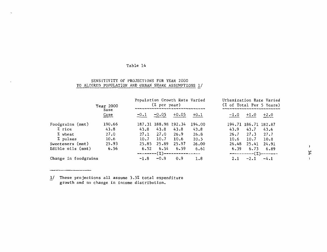
Table 14

SENSITIVITY OF PROJECTIONS FOR YEAR 2000TO ALTERED POPULATION AND URBAN SHARE ASSUMPTIONS 1/

Population Growth Rate Varied Urbanization Rate Varied

Year 2000 (% per year) (% of Total Per 5 Years)Base ----------------------------- ------------------------

Case -0.1 -0.05 +0.05 +0.1 -1.0 +1.0 +2.0

Foodgrains (mmt) 190.66 187.31 188.98 192.34 194.00 194.71 186.71 182.87

% rice 43.8 43.8 43.8 43.8 43.8 43.9 43.7 43.6

% wheat 27.0 27.1 27.0 26.9 26.8 26.7 27.3 27.7% pulses 10.6 10.7 10.7 10.6 10.5 10.6 10.7 10.8

Sweeteners (mmt) 25.93 25.85 25.89 25.97 26.00 26.48 25.41 24.91

Edible oils (mit) 6.56 6.52 6.54 6.59 6.61 6.39 6.73 6.89________(% )…(-- - - - - - -- - - - - M ---%) … ---

Change in foodgrains -1.8 -0.9 0.9 1.8 2.1 -2.1 -4.1

1/ These projections all assume 3.5% total expendituregrowth and no change in income distribution.

- 35 -

urbanization). The effects of population pressure on arable land mightlead to the expectation that the rates of population growth andurbanization would be positively related. The foodgrain projections aresatisfactorily robust with respect to popujlat-ion assumptions even iftrends have a reinforcing effect on demand. Reinforcement would occur ifpopulation growth were accelerated and urbanization were retarded, or viceversa.

Provisional census figures have recently been released reporting apopulation of 683.8 million as of February 1981. 1/ The census implies ahigher-than-expected population growth rate of 2.2% over the seventies andabout 0.1% higher for the last half of the decade than used in the demandprojections. Revised population projections incorporating the census datahave not appeared yet, but it is unlikely that they will reflect a 0.1%higher growth rate than earlier projections for the rest of the century.However, if this more rapid trend continues, demand for foodgrains may be1-2% higher (2-4 million tons) by 2000. 2/

B. Expenditure Growth and Income Redistribution. The projectionsof foodgrain demand are sensitive to the expenditure growth assumptions.The demand for wheat and pulses as a proportion of total foodgrains in2000 rises by about one-half of a percent (say 2 million tons) perone-half percent rise in the expenditure growth rate over the projectionperiod. This generalization approximately holds for a wide range ofgrowth rates extending from 2.5% to 6.0%. The proportion of rice infoodgrain demand is more stable and only begins to drop at the higherexpenditure growth levels. These trends indicate that rapid economicexpansion in real terms would stimulate a marked shift in consumptionpatterns in favor of wheat (Table 16) by the turn of the century.

Future demand for sweeteners and edible oils is more criticallyinfluenced by expenditure assumptions than projected foodgrain consumption(Table 15). The higher expenditure elasticities for these two lessessential foods are of course responsible for their sensitivity.

1/ Census of India 1981, Series 1, Provisional Population Totals.

2/ The assumptions regarding urbanization could not be checked againstthe provisional census figures since the urban population has not yetbeen reported.

- 36 -

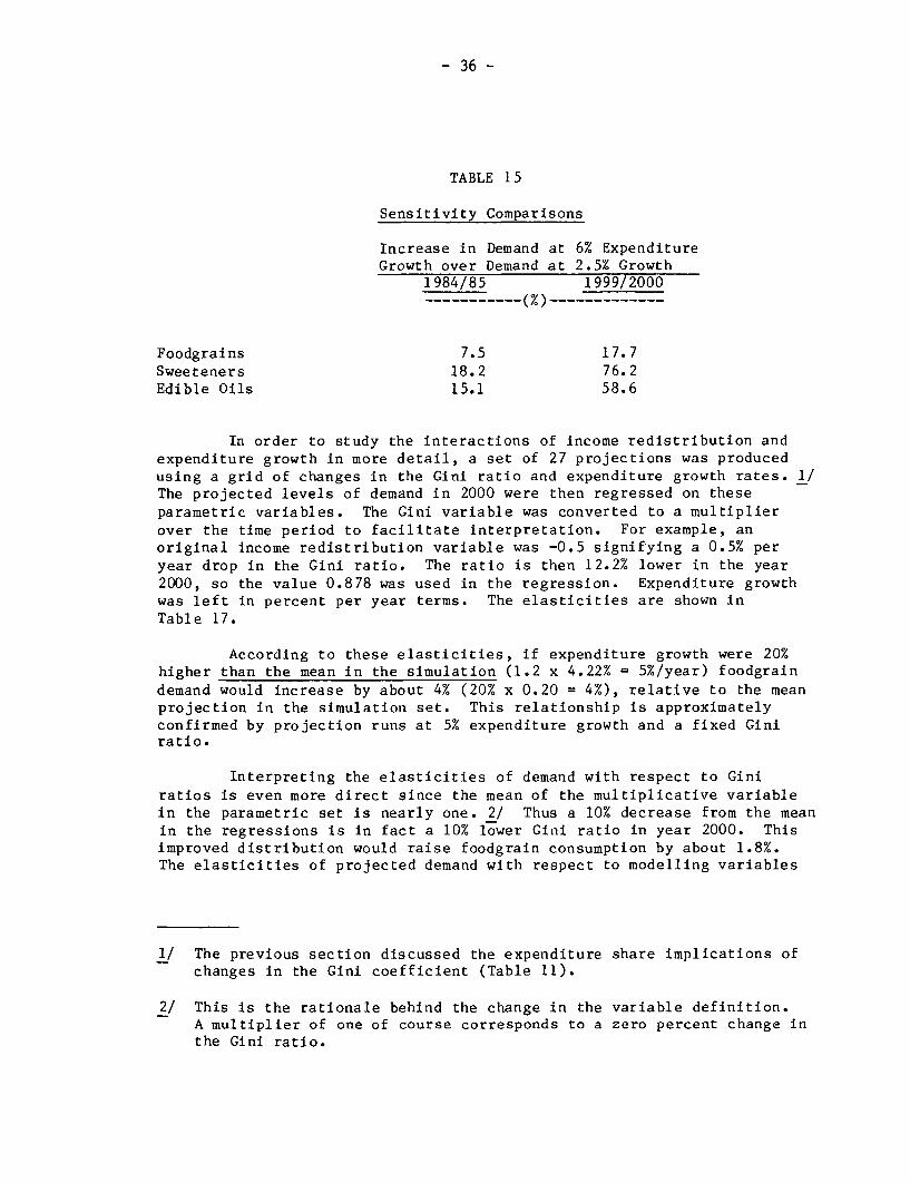
TABLE 1 5

Sensitivity Comparisons

Increase in Demand at 6% ExpenditureGrowth over Demand at 2.5% Growth

1984/85 1999/2000…(%)…------ M -------------

Foodgrains 7.5 17.7Sweeteners 18.2 76.2Edible Oils 15.1 58.6

In order to study the interactions of income redistribution andexpenditure growth in more detail, a set of 27 projections was producedusing a grid of changes in the Gini ratio and expenditure growth rates. 1/The projected levels of demand in 2000 were then regressed on theseparametric variables. The Gini variable was converted to a multiplierover the time period to facilitate interpretation. For example, anoriginal income redistribution variable was -0.5 signifying a 0.5% peryear drop in the Gini ratio. The ratio is then 12.2% lower in the year2000, so the value 0.878 was used in the regression. Expenditure growthwas left in percent per year terms. The elasticities are shown inTable 17.

According to these elasticities, if expenditure growth were 20%higher than the mean in the simulation (1.2 x 4.22% = 5%/year) foodgraindemand would increase by about 4% (20% x 0.20 = 4%), relative to the meanprojection in the simulation set. This relationship is approximatelyconfirmed by projection runs at 5% expenditure growth and a fixed Giniratio.

Interpreting the elasticities of demand with respect to Giniratios is even more direct since the mean of the multiplicative variablein the parametric set is nearly one. 2/ Thus a 10% decrease from the meanin the regressions is in fact a 10% lower Gini ratio in year 2000. Thisimproved distribution would raise foodgrain consumption by about 1.8%.The elasticities of projected demand with respect to modelling variables

1/ The previous section discussed the expenditure share implications ofchanges in the Gini coefficient (Table 11).

2/ This is the rationale behind the change in the variable definition.A multiplier of one of course corresponds to a zero percent change inthe Gini ratio.

Table 16

SENSITIVITY ANALYSIS OF EXPENDITURE GROWTH RATES 1/

Demand in million tons Given Expenditure Growth 2/

ExpenditureGrowth (%) 3/ 2.5 3.0 3.5 4.0 4.5 5.0 5.5 6.0

1984/85

Foodgrains 132.56 134.04 135.49 136.94 138.37 139.78 141.15 142.50% rice 43.7 43.7 43.7 43.8 43.8 43.8 43.8 43.8% wheat 24.7 24.9 25.0 25.2 25.3 25.5 25.6 25.8% pulses 9.5 9.6 9.7 9.8 9.8 9.9 10.0 10.1

Sweeteners 15.26 15.65 16.04 16.43 16.82 17.22 17.62 18.03 wEdible Oils 3.83 3.91 3.99 4.08 4.16 4.24 4.33 4.41

1999/2000

Foodgrains 177.30 184.31 190.66 196.19 201.02 204.71 207.24 208.67% rice 43.7 43.8 43.7 43.7 43.5 43.2 42.8 42.3% wheat 25.8 26.4 26.9 27.5 28.0 28.6 29.1 29.6% pulses 9.9 10.2 10.6 11.0 11.4 11.8 12.3 13.0

Sweeteners 21.65 23.75 25.93 28.20 30.55 32.99 35.52 38.15Edible Oils 5.63 6.09 6.56 7.04 7.52 8.00 8.47 8.93

1/ The expenditure distribution is held constant.2/ Except where demand is indicated as a percent of foodgrains.3/ After 1979/80. Between 1973-74 and 1979-80, 3.5% growth was used in all cases.

Table 17

ELASTICITIES OF PROJECTIONS

Elasticity of Demand in Year 2000 Mean Demand

With Respect to: 1/ In Simulation Set

For: Gini Change Expenditure Growth -- million tons --

Foodgrains -0.18 0.20 197.84

Percent wheat -0.04 0.17 27.8 1/

Sweeteners -0.17 0.53 30.68

Edible Oils -0.12 0.64 7.58

Mean Parametric Values 2/ 0.948 4.22

1/ Percent

2/ Gini ratio change is measured as a multiplier over the period; expenditure

growth is measured for the whole economy in percent per year.

- 39 -

compress a volume of sensitivity analysis into a readily interpretableform.

Referring to Table 17, it can be concluded that:

1) A percentage change in the Gini ratio over the entire periodwould have an opposite and nearly equal effect on the demand forfoodgrains as a similar proportionate change in the annual expendituregrowth rate. (A 10% fall in the Gini ratio multiplier over the periodwould have an effect similar to a 10% rise in the mean expenditure growthrate from 4.2% to 4.6%: demand would increase by 2% in year 2000.)

2) The sensitivity of demand for foodgrains, wheat, I/sweeteners, and edible oils is fairly similar with respect to

changes in the income distribution. (An improved distribution would boostdemand among the lower income groups for all items but would decreasedemand among upper income groups especially for commodities with highmarginal propensities to consume.)

3) The sensitivity of demand with respect to expenditure growthrates, unlike the response to redistribution, varies greatly betweencommodities, as expected.

Appendix III contains the "data" used in the elasticity calculations,i.e., the set of parameter combinations and projection results.

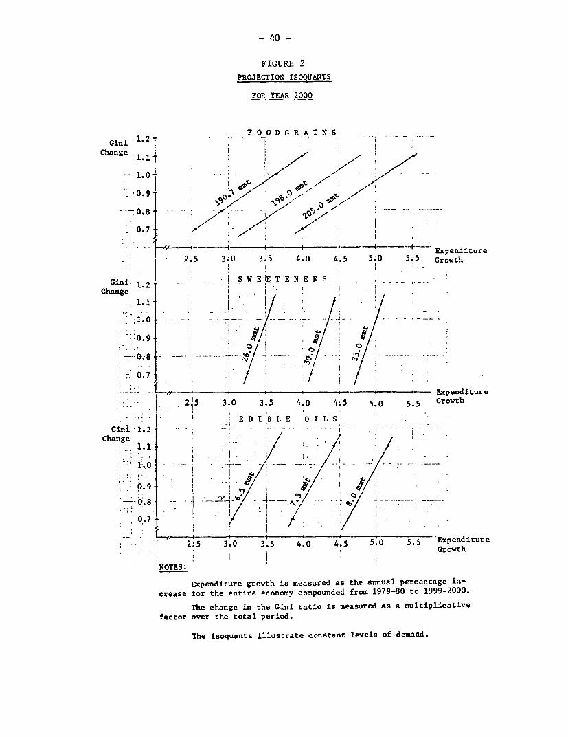
Graphing isoquants of projected demand against expenditure growthand altered Gini ratios is another approach to interpreting sensitivityanalysis (Figure 2). The slopes of the isoquants describe the relativeimportance of the two modelling variables. The flatter the slope, theless important economic growth is relative to income redistribution sincesmall changes in the Gini coefficient would offset larger changes in totalexpenditure and leave demand unaltered. The isoquant map conveys resultsfrom a large number of projection runs.

The Gini ratio change scale used in Figure 2 is matched againstannual change rates in Table 18. The discussion of historical rates ofredistribution in the previous section highlights a scale value of 0.88(-0.5%/yr) as a likely possibility. Although severe redistribution ofincome, improving or worsening, would have a decided effect on demand, theprobable range of outcomes is narrow. The expenditure growth ratetherefore remains the most critical and uncertain parameter in theprojection model.

l/ The demand for wheat would respond in a fashion similar to the demandfor foodgrains in view of the low elasticity of the percent of wheatin the total.

- 40 -

FIGURE 2

PROJECTION ISOQUANTS

FOR YEAR 2000

Gini 1-2 ~~~F O O D G R A I N S, __ _1.2 - aGini

Change 1.1

1.0 .-. / -

--0.9 5/--

0.7 - / i / , 07 I~~~~~~~~~~~~~~~~~~~~~~~~~~~~~~~~~~~~~~~~~~~~~~~~~~~~~~~~~~~~~~~~~~~~~~~~~~~~~~~~~~~~~~~~~~~~~~~~~~~~~~~~~~I

I - -Expenditure

* ( 2.5 3.0 3.5 4.0 4.5 5.0 5.5 Growth

Gini- 1.2 -- ' t ~S W EIE T E N E R S

I f - P | i i e Expenditure

j .- 'A | ~2j5 3;0 315 4,0 4,.5 5t0 5.5 Growth

~!E D I B L E O I L S

Gini -1.2 - W 4T N R

Change .-

, -'--1.0 ' - I -°

-0.9 4.

_ _ _ -~~~~-------4-- ~~~Expenditure

2,5 3.0 3.5 4.0 4.5 5.0 55 Gxowth

NOrTES:

Expenditure growth is measured as the annual percentage in-crease for the entire economy compounded from 1979-80 to 1999-2000.

The change in the Gini ratio is measured as a multiplicativefactor over the total period.

The isoquants illustrate constant levels of demand.

- 41 -

TABLE 18

Correspondence of Multiplicative Factors and AnnualGini Ratio Change Rates

Annual PercentageChange by 2000 Change

1.29 1.01.14 0.51.00 0.0

0.88 -0.50.77 -1.0

V. CONCLUSIONS

The absence of prices is the most obvious and important limitationto projections based on cross-sectional expenditure data. Relative pricesare necessarily assumed to be fixed, whereas they would respond tochanging consumption patterns, production levels, factor prices, tradeflows, and government policies in a number of areas.

Not only are relative prices assumed fixed over the projectionperiod, but prices between consumers in the survey should be the same forexpenditures to carry a constant quantity interpretation. One step inovercoming this obstacle has been taken: separate urban and ruralprojections have been combined using quantity weights for somecommodities.

Key assumptions were that real per capita expenditure growth wouldbe equal in rural and urban areas, and that any income distribution whichdid occur would follow a symmetric and proportional re-allocation rule inboth sectors.

Projections for 1979/80 for cereals, pulses, edible oils, andsweeteners are comparable with actual consumption if some allowances aremade for the poor crop year. Demand in terms of calories per capita wasclosely aligned with other base period estimates and future projections,projections were fairly robust with respect to moderate variations inpopulation growth and income redistribution.

This study and projections by the National Commission ofAgriculture indicate a 15% increase in per capita calorie demand to 2300calories per day by year 2000 under the low economic growth alternative.

- 42 -

Foodgrain demand would grow by 2.6% through the mid-1980s, and then slowto an average rate of 2.3%. The total increase in the last two decades ofthe century would be 60-70% if real expenditure growth is 3.5-5.0% peryear.

The composition of foodgrains demanded would shift away frommaize, sorghum, and millet in favor of wheat and pulses. If foodgraindemand grew by 60-70%, wheat demand would grow by 75-100%, and coarsecereals by 33-16%. There would be less increase in demand for the less:preferred grains if expenditure growth were more rapid. The proportion ofrice demanded in foodgrains would remain almost fixed at 43-44% under awide range of economic growth assumptions. At a 5% expenditure growthrate, the proportion of wheat demanded would increase 5% by 2000, and theshare of coarse cereals would drop 7%. One percent of foodgrain demandwould be 2 million tons in 2000, so the shift would be considerable.Faster urban migration would slightly dampen foodgrain demand, ceterisparibus.

Demand for sugar/khandsari and edible oils is expected to be verybuoyant even given slow expenditure growth. In the case of edible oils,this trend has strong implications for future prices and/or imports.

Improvement in the expenditure distribution would affect demandaccording to differences in marginal propensities to consume at various,income levels. These differences cannot be inferred from expenditureelasticities at the mean. 1/ A continuation of the 0.5%/year drop in theGini ratio would contract demand (relative to the constant ratio case)for fruits and nuts, beverages, clothing, milk and milk products by a fewpercent and slightly expand demand for edible oils, gur, rice and wheat.

The predominant determinant of the projections and the primarysource of uncertainty, is the expenditure growth rate. Elasticities ofthe projections with respect to the growth rate indicated that demand forfoodgrains, sweeteners and edible oils would respectively be 4, 2, and 0.5million tons higher at the turn of the century for each half of a percentincrease in this critical parameter.

1/ The elasticities were one or above for edible oils, sugar/khandsari,and milk/milk products, but redistribution had positive, neutral andnegative effects, respectively.

- 43 -

A P P E N D I C E S

- 44 -

API'ENDIX I

Demand ProjecLions with Moderate Redistribution

The following tables give the complete set of projections with low

and high expenditure growth, and the historical rate of redistribution.

FOR THE FOLLOWING PROJECTION'7OTAL EXPEtoDrTURE GROWTH ASSUMPTION IS 3.5 PERCENTGINI RATIO CHANGE RATE IS -0.5 PERCENTOUTPUT IN MILtlION ME1RIC TONS

73/74 79/80 84/85 89/90 94/95 99/00

PULSES 3/ 8.71 11.40 13 29 15.42 17.89 20.61EDIBLE OILS .2.67 3.37 4.03 4.81 5.69 6.71MEAT. FISH, & EGGS 2.40 2.71 3.20 3.92 4.70 5.64VEGETABLES 6.93 7.88 9.28 10.93 12.17 14.89FRUIlS & NUTS 16.57 18 36 22 83 28.53 35.58 44 74SUGAR & ''HANDSARI 4.52 5.25 6 44 7.91 9 61 11.69CUR & OTHER SUJGARS 7 34 8 38 9.70 11.13 12.86 14.66SPICES 0.69 0.77 0.89 1.03 1.17 1.33BEVERAGES 0.32 0.34. 0 43 0.54 0.68 0.87TOBACCO. PAN & INTOX. 0.46 0.51 0 60 0.71 0 84 0.99CLOTHING 0.72 0.82 1.02 1.27 1.61 2.04MILK 19.75 23.16' 2S.59 35.26 43 55 53.78RICE 40.36 52.58 60.04 68.01 76.94 85.87WHEAT 22.54 29.37 34.36 39.96 46.21 52 91MAIZE 4.04 5.10 5.52 5.89 6.31 6.63SORGHUM e MILLET 4/ 17.15 21.G2 23 58 25.43 27.38 23.95OTHER 1/ - 1.00 1.05 1.29 1.59 1.95 2.42

SWEETENERS 11.85 13.63 16.15 19.03 22.47 26.35

FOODGRAINS 92.80 120 08 136.79 154.71 174.73 194.97

FOR THE FOLLOWING PROJECTIONTOTAL EXPENDITURE GROWTH ASSUMPTION IS 5 PERCENTGINI RATIO CHANGE RAlE IS -O 5 PEOCENTOUTPUT IN MILLION METR!C TONS

73/74 79/80 1/84/85 89/90 94/95 99/00

PULSES 3/ 8.71 11.40 14.02 17.07 20.70 24.76EDIBLE OrIS 2.67 3.37 4.28 5.40 6 68 8.19MEAT, FISH. & EGGS 2.40 2.71 3.52 4.57 5.88 7 56VEGETABLES 6.93 7.88 9.79 12 It 14.78 17.90FRUITS & NUTS 16 57 18.3G 25 60 35 85 49 99 70.04SUGAR & KHANDSARI 4.52 5.25 7.05 9.38 12.32 16.07CUR & OTHER SUGARS 7.34 8.38 10.29 12.40 14.91 17.46SPICES 0.69 0.77 0.93 1.10 1.29 1.48BEVERAGES 0.32 0.34 0 .18 0.68 0.96 1.38TOBACCO, PAN & INTOX. 0 40 0.51 O064 0 81 1.02 1 29CLOTiHING 0.72 0 82 1.18 1 69 2.44 3.50MILK 19.75 23.10 31.97 43 71 59.45 80.30RICE 40.36 52 58 62 03 71 99 82 28 91.29WIIEAT 22.54 29 37 36 12 43.67 51 90 60.26MAIZE 4.04 5 10 5.49 5.80 6.11 6.24SORGHIUM i MILLET 4/ 17.15 21 62 23.44 24.99 26 38 27.14OTIIER / - 1.00 1.05 1.42 1.95 2 66 3.66

SWEEtENERS 11.85 13.6i 17.34 21.78 27.22 33.53

rOODGRAINS 92.80 120.08 141.09 163.53 187.37 209.69

1/ Irojcctions for "OLher" are niultiplicr.tivc factors on a1973-74 base.

2/ Assunm:s 3,5% expenditure -rowth through 1979-30.

3/ Includes cereal substitutes and grams.

4/ Includes barley and other coarse cereals.NOTE: Grossing factors for non-household demand for foodgrains

and edible oils were added.

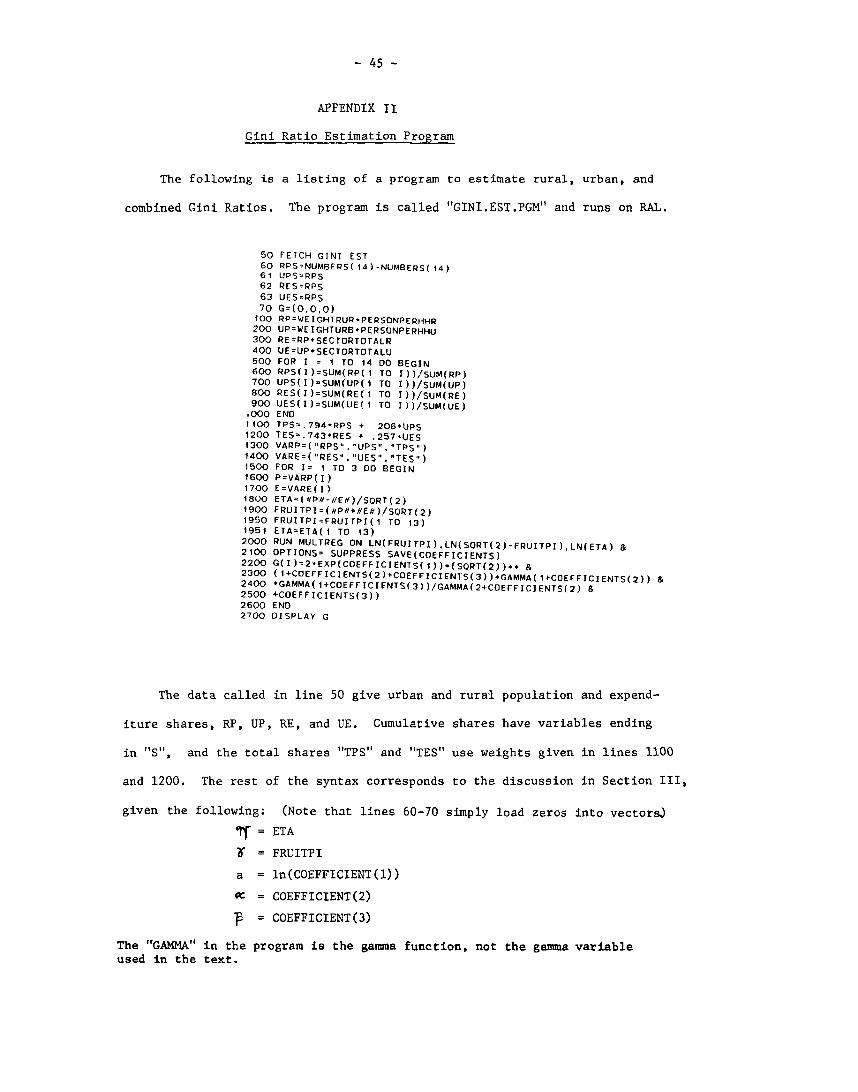
- 45 -

APFENDIX II

Gini Ratio Estimation Program

The following is a listing of a program to estimate rural, urban, and

combined Gini Ratios. The program is called "GINI.EST.PGM" and runs on RAL.

50 FETCH GINI EST60 RPS:NUMBERS(14)-NUMBERS(14)61 UPS-RPS62 RES-RPS63 UES-RPS70 G=(0.0.O)100 RP=WEIGHTRUR*PERSONPERHHR200 UP=WEIGHTURB*PERSONPERHHU300 RE=RP*SECTORTOTALR400 UE=UP*SECTORTOTALU500 FOR I = I TO 14 00 BEGIN600 RPS(I)=SUM(RP(1 TO 1))/SUM(RP)700 UPS(I)=SUM(UP(1 TO l))/SUM(UP)800 RES(I)=SUM(RE(1 TO 1))/SUM(RE)900 UES(I)=SUM(UE(1 TO 1))/SUM(UE)0Oo END1100 TPS=.794*RPS + 206*UPS1200 TES=.743*RES + .257*UES1300 VARP=("RPS`,"UPS"."TPS")1400 VARE=("RES","UES"."TES")1500 FOR 1= 1 TO 3 DO BEGIN1600 P=VARP(I)1700 E=VARE(I)1800 ETA=(#P#-//E#)/SORT(2)1900 FRUITPI=(#P#+#E#)/SQRT(

2)1950 FRUITPI=FRUITPI(1 TO 13)1951 ETA=ETA(1 TO 13)2000 RUN MULTREG ON LN(FRUITPI),LN(SORT(2)-FRUITPI),LN(ETA) &2100 OPTIONS= SUPPRESS SAVE(COEFFICIENTS)2200 G(I)=2=EXP(COEFFICIENTS(1)).(SORT(2))** &2300 (l+COEFFICIENTS(2)+COEFFICIENTS(3))*GAMMA(1+COEFFICIENTS(

2)) &2400 *GAMMA(1+COEFFICIENTS(3))/GAMMA(2+COEFFICJENTS(2) &2500 +COEFFICIENTS(3))2600 END2700 DISPLAY G

The data called in line 50 give urban and rural population and expend-

iture shares, RP, UP, RE, and UE. Cumulative shares have variables ending

in "S", and the total shares "TPS" and "TES" use weights given in lines 1100

and 1200. The rest of the syntax corresponds to the discussion in Section III,

given the following: (Note that lines 60-70 simply load zeros into vectors)

= ETA

= FRUITPI

a = ln(COEFFICIENT(l))

O = COEFFICIENT(2)

= COEFFICIENT(3)

The "GAMMA" in the program is the gamma function, not the gamma variableused in the text.

- 46 -

APPENDIX III

Sensitivity Analysis Data

The following is a listing of data from file PROJ.2000.

Cl El G2 E2 F WPER E S-1.5 2.5 0.675 1.90 186.52 26.2 5.91 22.51-1.5 3.5 0.675 2.45 200.99 27.3 6.90 26.93-1.5 4.5 0.675 3.14 212.48 28.4 7 93 31.75-1.5 5.0 0.675 3.56 216.52 28.9 8.45 34.32-1.5 5.5 0.675 4.02 219.33 29.4 8.97 36.91-1.0 3.5 0.770 2.45 198.29 27.2 6.82 26.67-1.0 5.0 0.770 3.56 213.48 28.8 8.34 33.96-0.5 2.5 0.878 1.90 181.08 26.0 5.75 22.00-0.5 3.5 0.878 2.45 194.97 27.1 6.71 26.35-0.5 4.5 0.878 3.14 205.71 28.2 7.69 31.06-0.5 5.5 0.878 4.02 212.23 29.3 8.68 36.100.0 2.5 1.000 1.90 177.30 25.8 5.63 21.650.0 3.0 1.000 2.16 184.31 26.4 6.09 23.750.0 3.5 1.000 2.45 190.66 26.9 6.56 25.930.0 4.0 1.000 2.77 196.19 27.5 7.04 28.200.0 4.5 1.000 3.14 201.02 28.0 7.52 30.550.0 5.0 1.000 3.56 204.71 28.6 8.00 32.990.0 5.5 1.000 4.02 207.24 29.1 8.47 35.520.0 6.0 1.000 4.55 208.67 29.6 8.93 38.150.5 2.5 1.138 1.90 172.55 25.6 5.48 21.230.5 3.5 1.138 2.45 185.06 26.8 6.38 25.400.5 4.5 1.138 3.14 194.86 27.9 7 30 29.910.5 5.0 1.138 3.56 198.43 28.5 7.75 32.310.5 5.5 1.138 4.02 200.90 29.0 8.20 34.811.0 3.5 1.295 2.45 178.13 26.6 6.16 24.781.0 5.0 1.295 3.56 190 41 28.3 7.45 31.52

-0.5 5.0 0.878 3.56 209.69 28.7 8.19 33.53

Each line contains output from a projection run for the year 2000. A large

number of projections created a simulation data set which was used to find

elasticities of projections with respect to assumptions, and projection

isoquants in Section IV, The variable definitions are:

Gl Annual rate of change of Gini ratio for personalconsumption expenditure, in percentage terms.

El Annual percentage growth rate in total expenditure.

G2 Multiplicative change in Gini ratio by 2000,

E2 Multiplicative change in total expenditure by 2000.

F Foodgrains projection for 2000, in mat.

WPER Wheat percentage of foodgrains demanded in 2000.

E Edible oils projection for 2000, in mmt.

S Sweeteners projection for 2000, in mmt,

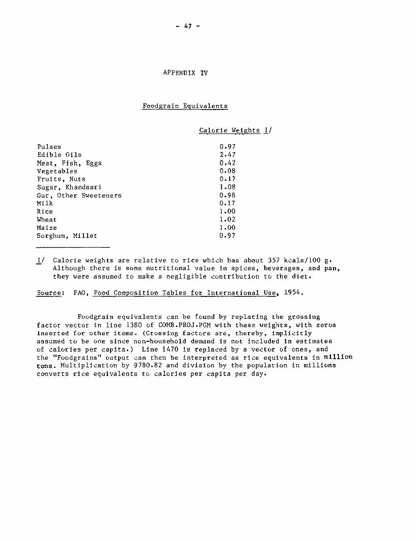
- 47 -

APPENDIX IV

Foodgrain Equivalents

Calorie Weights 1/

Pulses 0.97Edible Oils 2.47Meat, Fish, Eggs 0.42Vegetables 0.08Fruits, Nuts 0.17Sugar, Khandsari 1.08Gur, Other Sweeteners 0.98Milk 0.17Rice 1.00Wheat 1.02Maize 1.00Sorghum, Millet 0.97

1/ Calorie weights are relative to rice which has about 357 kcals/100 g.Although there is some nutritional value in spices, beverages, and pan,they were assumed to make a negligible contribution to the diet.

Source: FAO, Food Composition Tables for International Use, 1954.

Foodgrain equiValents can be found by replacing the grossingfactor vector in line 1380 of COMB.PROJ.PGM with these weights, with zerosinserted for other items. (Grossing factors are, thereby, implicitlyassumed to be one since non-household demand is not included in estimatesof calories per capita.) Line 1470 is replaced by a vector of ones, andthe "Foodgrains" output can then be interpreted as rice equivalents in milliontons. Multiplication by 9780.82 and division by the population in millionsconverts rice equivalents to calories per capita per day.

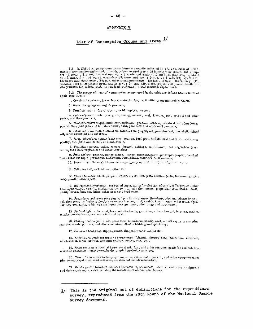
- 48 -

APPENDIX V

List of Consumption Groups and Items -

3. I In NSS, d tta oni CQ5iUTIICI ccIpelditLire at c iist uII ly collcet cdI lot .I la t C numbe of ite m.But in plesentiig the I csni t- inil.i it itsim have been nicigeti toh III 21 hono,i4tn,,u' gi OlpS 'I Te gi o I,p,

are ;1) ccrca Is, (2) gi A in, , 3 ) t c lea I su,tit utist., ( 1l Pluc a- Itl pI oduct-(s, (5j n 'k a id pt odutts, (G6 cdi, PCoil, (7) mcat, fith -I Id cgg (8) vc,cthlesIC%, (9) [liiit ai tt inlits, (10) S I.al , II) salt, (12) .phes, l3beverages an iJf Icshnsiciuts, (14) pan, tobtcrcoarid Iti toxIc.itn Is, (15) fucl a idI Itlt, (16) clot Ih g, (17)footwear, 18) tilitccl laicous goods .niis SC ,ILCs, (,19) iciits, (20, taxcs, (21) ( tli.ib!c goods. Rcsults aI calso prcscnted for (') food-tottal, (ll) tiowi-food tottal alid (iII) tot,sl cotisutncexpetdititI C.

3.2 The groups of itcms of conlsumptioi as picsented in tlie table atc defiIed IIel il terms oftheir constitucits:

1. Cereats:iicc, vlscat,josvar,bbata, rnlaizc,batley,smallmillcts, tagi niul tllcii piodticts,

2. Gfan: bengal-giami anid its pioduicts,

3. Cerealsubstitules: Crcalsubstitute Iikc topioca,pea ctc.,

4. Puleasandprod otsc :athl:r,tut,granr,tnooisg, inasoor, uid, khscs.irl, pea, soyabitiatsd othcrpulscs, and thici 1p oducts,

5. Milk andPlrosdurts liquid rilk(cow,buffalow, goatanlls othets),baby-foocl inik(conidensecpo%vdei etc.) glice (cow and buffslo,, buttcer, tl sit, ghol, lassi and othel milk pioducts,

6. Edible oil: vanaspati, nintstatd oil, cocoanut oll, gingilIy oil, gtoutidnit oil, linsecd oil, scscfiitoil, other edible oil axid oil seeds,

7. Aleal, Jisit and eggs mcat (goat nieat, muttotn, becf, pork, buffalo inca t and other nmcat , Cggpoultry, fish (freih anid dried), biid and otlscis,

8. Vegetablcs potato, uniois, tomato, brinjal, cabbage, cauli-flo%ser, toot Negetables (arstrradish, etc.) Icafy vegetablCs atid other %cgetables,

9. Fruitsatd nuts :banana,oiange,lemon, mango, cocoanut,guava,pincappilc.grapes,othierfresfruits,cocoanutcop. Is,groundisut,c ashzvwtiut,d-teo,iaisin,otierdtyfruiltsatid nuts,

10. Su 9ar :sw!mi (fi Ctoils kh t-! :-:,C Zs!^-,..;' : -;8bu-I

II. Sall sca salt, rock salt and other salt,

12. Spices cururinic, bl.tck peppet, pepper, dty chillies, giceti ceiillics, gsilc, tasmatiid,giniger,curiy powvder, otlter spices,

13. lBtosrages atl refresLnictils lea (,Io. ofCups), tet leCI, Cc,ffcc (t1o. of Clips5, coffcL potsdci .otherd riskitig be-a,-i.,bIscitts, coafect noin,tcs et .. s.alted Icli ltiticILts, picpaicdb%ssets, cooked sticalstpickle, saucc, j tIltS andLI jeleI(s, OthCt pt ocCstd lod tteiiis,

14. Pan,tobacco antdints antls p.i iclaf, p fii linished,,supa i (betcl ilit,otlis ingredicnts fot pati)ls,i,cig icttet, Itftobicco, tookilt tob.tcco, (Ieitoot, slff, Zs d.tdls, kimarnin su,ti otlier tobi,c,o pio-ducts,opium, gatsji, rodlds, co.i,stt y liquoi,loicigi liqtior, othci drugs and intoxticasts,

15 Fuel atid lhgit coke, coal, hicssood, clectricit), gas, dlunig cake, charcoal, ketoscien, calllilc,nAtchcs, nsethylated spUlt, otlhcr fuel atd IgIt,

IG. Clothing :cototl (mnilli sslie,rklloosrl,land-loom, klsadi) stool,al tlkrac oit om anyotlc,si,jtlletictextilc, parc tlk,ansdotlhcsttllclttdtiig itctnsol beddttga Lidulptholstcly,

17. Footwcar boot, shoe, slippei, sstidlc, chappal, swoodets sanidal etc.,

18. 4Alscella,sjeous goods andsertices amusements (ciascissa, tlhcatre etc.) cducationl, niediciite,toilct at ticles, sunct latticlcs, coissunie scvicts, (oncyances, ctc.,

19. Rt,it: rets on I ciidentnal house, re.id.sitial Lind anicl other consunisem goods (no coniputlatioofremt fot rc,dent,lal houscs owned by thc ..ampic househioldl s%as m.sdc),

20. Taxes liecnce fees for keeping *,un, rAdio, cycle. tnotor car etc , tiltd other co,isuniser taxestikc tihe JiLmaiCIpal taxes, toad taxes etc., but dueb not icitide incomc tax,

21. Durable gools furniture, itnuicil inistrunimits, ornaments, utensile anlc othes c.quipmcntantd thcir I eairaiv, expctiscs including tic mnaintenaisce ofrCstdleiti.,l houses.

l/ This is the original set of definitions for the expendituresurvey, reproduced from the 28th Round of the National SampleSurvey document.

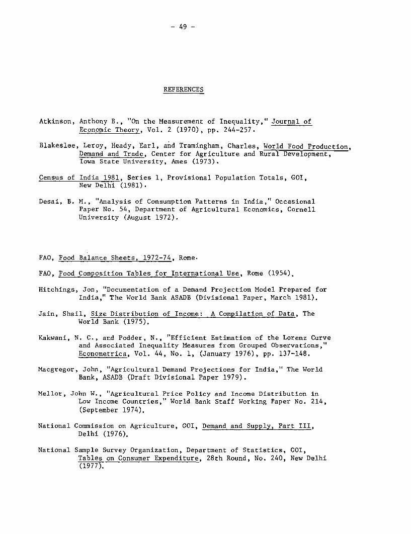
- 49 -

REFERENCES

Atkinson, Anthony B., "On the Measurement of Inequality," Journal ofEconomic Theory, Vol. 2 (1970), pp. 244-257.

Blakeslee, Leroy, Heady, Earl, and Tramingham, Charles, World Food Production,Demand and Trade, Center for Agriculture and Rural Development,Iowa State University, Ames (1973).

Census of India 1981, Series 1, Provisional Population Totals, GOI,New Delhi (1981).

Desai, B. M., "Analysis of Consumption Patterns in India," OccasionalPaper No. 54, Department of Agricultural Economics, CornellUniversity (August 1972).

FAO, Food Balance Sheets, 1972-74, Rome.

FAO, Food Composition Tables for International Use, Rome (1954).

Hitchings, Jon, "Documentation of a Demand Projection Model Prepared forIndia," The World Bank ASADB (Divisional Paper, March 1981).

Jain, Shail, Size Distribution of Income: A Compilation of Data, TheWorld Bank (1975).

Kakwani, N. C., and Podder, N., "Efficient Estimation of the Lorenz Curveand Associated Inequality Measures from Grouped Observations,"Econometrica, Vol. 44, No. 1, (January 1976), pp. 137-148.

Macgregor, John, "Agricultural Demand Projections for India," The WorldBank, ASADB (Draft Divisional Paper 1979).

Mellor, John W., "Agricultural Price Policy and Income Distribution inLow Income Countries," World Bank Staff Working Paper No. 214,(September 1974).

National Commission on Agriculture, GOI, Demand and Supply, Part III,Delhi (1976).

National Sample Survey Organization, Department of Statistics, GOI,Tables on Consumer Expenditure, 28th Round, No. 240, New Delhi(1977).

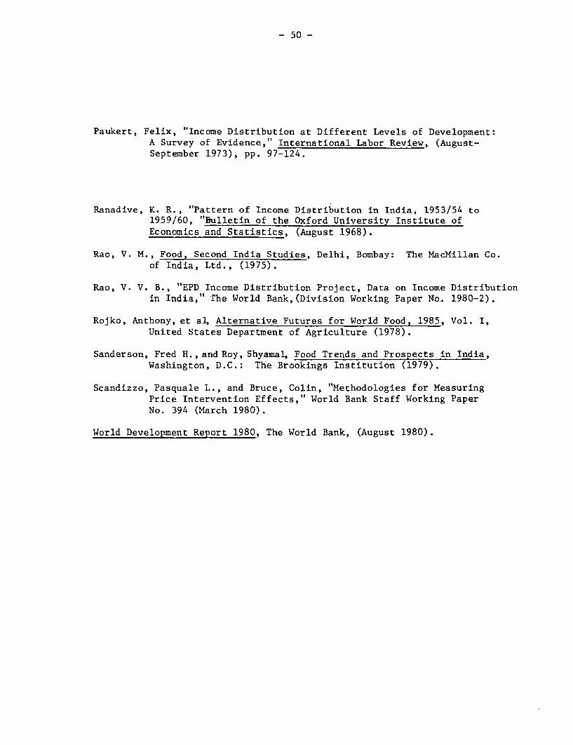
- 50 -

Paukert, Felix, '"Income Distribution at Different Levels of Development:A Survey of Evidence," International Labor Review, (August-September 1973), pp. 97-124.

Ranadive, K. R., "Pattern of Income Distribution in India, 1953/54 to1959/60, "Bulletin of the Oxford University Institute ofEconomics and Statistics, (August 1968).

Rao, V. M., Food, Second India Studies, Delhi, Bombay: The MacMillan Co.of India, Ltd., (1975).

Rao, V. V. B., "EPD Income Distribution Project, Data on Income Distributionin India," The World Bank,(Division Working Paper No 1980-2).

Rojko, Anthony, et al; Alternative Futures for World Food, 1985, Vol. I,United States Department of Agriculture (1978).

Sanderson, Fred H., and Roy, Shyamal, Food Trends and Prospects in India,Washington, D.C.: The Brookings Institution (1979).

Scandizzo, Pasquale L., and Bruce, Colin, "Methodologies for MeasuringPrice Intervention Effects," World Bank Staff Working PaperNo. 394 (March 1980).

World Development Report 1980, The World Bank, (August 1980).

PART II

THE FOODGRAIN ECONOMY

James Q. Harrison and John W. WallSouth Asia ProgramsJuly 1981

51

- 52 -

The Foodgrain Economy

Table of Contents

Page

Introduction, Summary and Conclusions ............... 53

Supply-Demand Balances . . .57

Government Projections ... 58

Implications .. . 61

Table Annex 1 . .65

Table Annex 2 . .... 66

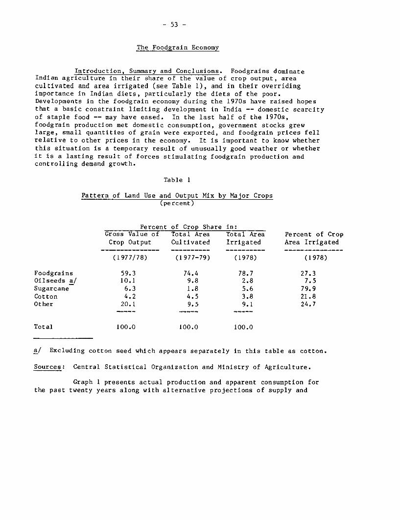
- 53 -

The Foodgrain Economy

Introduction, Summary and Conclusions. Foodgrains dominateIndian agriculture in their share of the value of crop output, areacultivated and area irrigated (see Table 1), and in their overridingimportance in Indian diets, particularly the diets of the poor.Developments in the foodgrain economy during the 1970s have raised hopesthat a basic constraint limiting development in India -- domestic scarcityof staple food -- may have eased. In the last half of the 1970s,foodgrain production met domestic consumption, government stocks grewlarge, small quantities of grain were exported, and foodgrain prices fellrelative to other prices in the economy. It is important to know whetherthis situation is a temporary result of unusually good weather or whetherit is a lasting result of forces stimulating foodgrain production andcontrolling demand growth.

Table 1

Pattern of Land Use and Output Mix by Major Crops(percent)

Percent of Crop Share in:Gross Value of Total Area Total Area Percent of CropCrop Output Cultivated Irrigated Area Irrigated

(1977/78) (1977-79) (1978) (1978)

Foodgrains 59.3 74.4 78.7 27.3Oilseeds a/ 10.1 9.8 2.8 7.5Sugarcane 6.3 1.8 5.6 79.9Cotton 4.2 4.5 3.8 21.8Other 20.1 9.5 9.1 24.7

Total 100.0 100.0 100.0

a/ Excluding cotton seed which appears separately in this table as cotton.

Sources: Central Statistical Organization and Ministry of Agriculture.

Graph 1 presents actual production and apparent consumption forthe past twenty years along with alternative projections of supply and

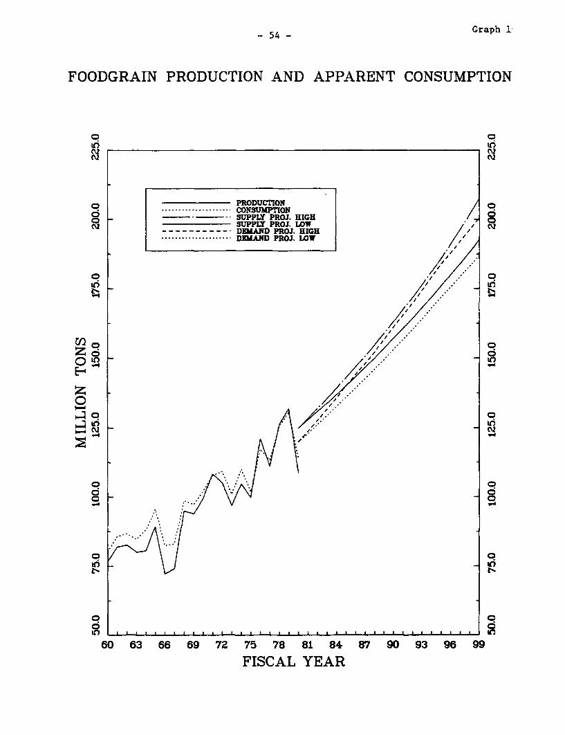
54 Graph 1-

FOODGRAIN PRODUCTION AND APPARENT CONSUMPTION

o 0

N NQ

PRODUCTION ;. .......... CONSUMPTON

O - SUPPLY PROJ. HIGH01 SUPPLY PROJ. LOW \NQ ----------- DEMAND PROJ. HIGH

........... DEMAND PROJ. LOW //

Z~~~~~~~~~~~~~~~~~~~~~~~~~~~~~~~~

;° _ X"" _ O

tO _

60 63 66 69 72 75 78 81 84 87 90 93 96 99

FISCAL YEAR

- 55 -

demand for foodgrains for the next twenty years.1/ The historical datareveal a convergence of the supply and demand lines in the last half ofthe 1970s. The projections suggest the possibility of continuedself-sufficiency or even an emerging surplus in foodgrains in the future.Nevertheless, bad weather in 1979/80 resulted in a drop of 23 million tonsor 17% from the record production of foodgrains achieved in 1978/79.Through the judicious use of foodgrain stocks built up over the pastseveral years, the Government was able to contain the worst effects of thedrought -- preventing serious famine, moderating foodgrain priceincreases, avoiding foodgrain imports, even managing to export a modestamount of grain. As creditable as this achievement is, the drop inproduction which made it necessary should serve as a reminder that thebalance between the supply and demand for foodgrain is still precarious.While the performance of the recent past and the probable future trendspoint to India's self-sufficiency and emerging export potential infoodgrains, the balance remains delicate and a succession of poor monsoonscould still result in a need for foodgrain imports to maintain consumersupplies or adequate buffer stocks.

In this.context, the decision to resume imports in 1981/82 torebuild stocks drawn down following the 1979 drought was a prudent measureto avoid speculative price pressures. The weaknesses of the 1981 monsoonmade the need for imports even clearer. The resort to imports to maintainfoodgrain supplies indicates the Government's continued commitment to usemarket mechanisms for this purpose rather than resorting to administrativecontrols on foodgrain movement and compulsory procurement.

Changes in foodgrain prices will cause these projections tovary. The projections in Graph 1 have been made for illustrative purposesassuming prices remain essentially constant in real terms. In reality,prices will operate on both the supply and demand side, shifting both tooffset persistent large imbalances. As can be seen in Graph 2, the realprices of foodgrain have varied in the past. They rose in real terms fromthe early 1960s (a period during which relative prices of agriculturalcommodities were among the lowest since Independence) through theunprecedented drought years early in 1967. They then fell in response tothe Green Revolution until the spate of bad weather and constrainedimports of the early 1970s, when they again began to rise. Good weatherbeginning in 1975, along with a well-designed pricing policy backed upwith a large public stocks, initiated a fall in the real foodgrain price

1/ Apparent consumption is defined here as gross availability offoodgrains in the economy -- gross production plus net imports lesschanges in public stocks.

- 56 - Graph 2

REAL PRICE OF FOODGRAINS

RIAL PRICE OF FOODGRADS..- ----- --- ---- TRED Ln 196 TO 90

o o

44~~~~~~~~~~~~~~~~~~~~~~~~~~~~~~~~~~~~~~~~~-

0-

60 62 64 66 68 70 72 74 76 78 so

CALENDAR YEARnffDI OF LMSM PRII oF P0OIMRAS DID Y STTUWHLEAL PRI:8 CM OF ALL NO9PODRI COM'

- 57 -

that has continued through 1980 despite bad weather and a short crop in1979/80. The trend rate of decline of the real prices from 1968 through1980 is 2.2% per annum.

A continuation of a low, and even falling, real price offoodgrains is one option facing India. A lower real price has abeneficial impact on equity of consumption, as foodgrains occupy adominant place in the consumption budget of the poorest families in India.By the same token, lower prices will stimulate demand and dampen theproduction increase so that the projected surplus would disappear.

Supply-Demand Balances. Historical trend rates of growth offoodgrain production vary considerably from as low as 2% to as high as 3%,depending on the time periods chosen for calculating the rates. Findingrates as low as 2% is a result of including a very bad year at the end ofthe period and rates as high as 3% is a result of including a very goodyear at the end, as well as a bad year at the beginning. The supply linesin Graph 1 are based on two alternative trend rates, 2.3% per annum and2.7% per annum. The lower rate is slightly below that calculated overthe period 1967/68 through 1977/78, both fairly good years.l/ The highrate is that calculated over 1949/50 through 1979/80, a period whichincorporates all of the information available. 2/

The demand projections presented in Graph I are taken from JonHitchings' "Demand Projections for India", the first paper in this volume.The method of projection and underlying assumptions are discussed indetail there. The main difference between the low and high cases is theassumed rate of growth of total consumption expenditure. The low case isbased on a 3.5% per annum growth, which is just below the historicaltrend. The high case is based on a 5% per annum growth in totalconsumption expenditure, a rate roughly consistent with the Sixth Planprojections and achievable under stimulative economic policies.

1/ If production in 1978/79, a very good year, is added to the period ofcalculation, the trend rate becomes 2.7% per annum. If production in1979/80, a very bad year, is added, the trend rate drops to 2.1%. Ifproduction in 1980/81 is taken to be 133 million tons and added, thetrend rate is again 2.3%.

2/ This is also the rate calculated for the period 1960/61 through1978/79. If production for the year 1979/80 is added, the rate fallsto 2.6%. If production for 1980/81 (assumed to be 133 million tons)is added, the rate remains 2.6%. This indicates that the sensitivityin the rates to individual years falls as the period is lengthened.

- 58 --

It should be noted that the high demand line probably is noteconomically consistent with the low supply line. Foodgrain production issuch a large proportion of the value of agricultural output (c.60%) andagriculture constitutes such a significant portion of value added in theeconomy (c.40%) that to generate a 5% per annum growth in consumptionexpenditure in practice depends on a fairly rapid growth in foodgrainproduction. Slowly growing production of foodgrain dampens the rise intotal income, and consumption expenditure, in proportion to its weight invalue added. It also causes the price of India's main wage good (grain)to rise, dampening demand and raising costs of producing other goods sothat overall growth is constrained. Moreover, foodgrain imports, whenneeded, take priority over other imports necessary for sustained rapidgrowth elsewhere in the economy. The Sixth Plan, which projects a 4.7%per annum growth in consumption expenditure through 1984/85 and 5% perannum from 1984/85 through 1994/95, projects foodgrain output to risebetween 3.1% and 3.7% through 1984/85 and between 2.9% and 3.5% from1984/85 to 1994/95. These are the rates of growth for foodgrainproduction internally consistent with the target rates of growth ofexpenditure. While it is logically conceivable for the economy to growrapidly while foodgrain production lags, the history and structure of theIndian economy make this unlikely. Consequently, the relevant supply lineto compare with the high demand line is. the high supply projection, as itis probably not possible to reach the high demand line if production is aslow as on the low supply line.

Government Projections. Government supply projections arehigher than either of the trend lines discussed above (see Table 2). TheNational Commission on Agriculture (NCA) and the Planning Commission bothproject foodgrain production based on an analysis of projected land use,irrigation availability, technological potential and fertilizerconsumption. In the cases of NCA supply projections, rough rules of thumbwere used to convert these factors into expected foodgrain production. 1/The production targets from the Sixth Five Year Plan 2/ are based on theproduction technology and inputs expected to be available during the Planperiod, although the Plan document is not explicit about the methods usedin the projections.

1/ In the NCA projections, one additional hectare of area under irriga-tion is assumed to add 0.5 tons of foodgrain production and one addi-tional ton of fertilizer applied to foodgrains is assumed to yield 10additional tons of grain. (Report of the National Commission onAgriculture, 1976, Part III, pp. 96-98.

2/ Sixth Five Year Plan, 1980-85, p. 25 and p. 119.

- 59 -

The NCA supply projections assume little change in the totalarea under foodgrains from the 1970/71 base period to the year 2000, butthe proportion of foodgrain area irrigated is assumed to rise from about25% in 1970/71 to 42% by the year 2000. It is notable that whilevirtually all of the projected increase is from an increase in averageyields rather than area, the yield increases are expected to be generatedprimarily by applying increased inputs of water and fertilizer, ratherthan by any substantial change in technology itself or any increasedefficiency in input use. The assumed rates of growth of fertilizer (7% to8% per annum) and irrigation (1.5 million hectares per year) are wellbelow actual achievements in recent years. The two NCA projections differin assumed rates of growth of fertilizer consumption between 1970/71 and1984/85, with the low path assuming a rate of growth of 7.2% and the high

path a rate of 10.2% per annum. For the entire 1970/71 to 2000 period,the rate of growth of fertilizer consumption is projected to be 6.3% to 7%per annum. Both of NCA's supply paths converge by the year 2000.

The Sixth Plan targets, while lower than the NCA projections,are higher than past trends. The lower target of 149 million tons impliesa rate of growth of 3.1%. While such growth rates have been achieved inpast periods, as noted above such periods usually included a base yearwell below trend or an end year well above trend. The links betweenGovernment policies, programs and input supplies on the one hand andoutput on the other are not explicit in the Plan document. The Plantargets for agricultural input use are quite ambitious, with irrigatedarea expected to rise an average of 2.7 million hectares per year,fertilizer consumption to rise 12.9% per annum, gross cropped area to rise10 million hectares and total area under high yielding varieties offoodgrains to rise more than 20 million hectares. Other agriculturalsupport programs are expected to increase their coverage similarly.

The NCA demand projections are considerably higher than those ofHitchings. The NCA projections are based on growth in consumptionexpenditure at lower rates than Hitchings' (NCA high: 4.7% per annumthrough 1980 and 3.5% per annum from 1980 through 2000; NCA low: 3.0% perannum through 1980 and 2.8% per annum from 1980 through 2000).Nevertheless, the projected quantities are higher due to a much higherstarting base and a much greater provision for animal feed than inHitchings' projections. The base year chosen for the NCA projections,1971, had one of the highest per capita consumption levels in recenttimes. Starting from that base the NCA projects demand in 1979/80 at 133(low) to 140 million tons (high). Hitchings' projections used 1973/74 asa base and project 1979/80 consumption at 120 million tons. Apparentavailability (gross production plus net imports minus change in stock) was114 million tons in 1979/80, well below trend due to the drought. Actualconsumption no doubt was higher than 114 million tons, allowed by somedrawdown of private stocks. Although the extent of drawdown of privatestocks is not known, trend consumption cannot be much greater than the

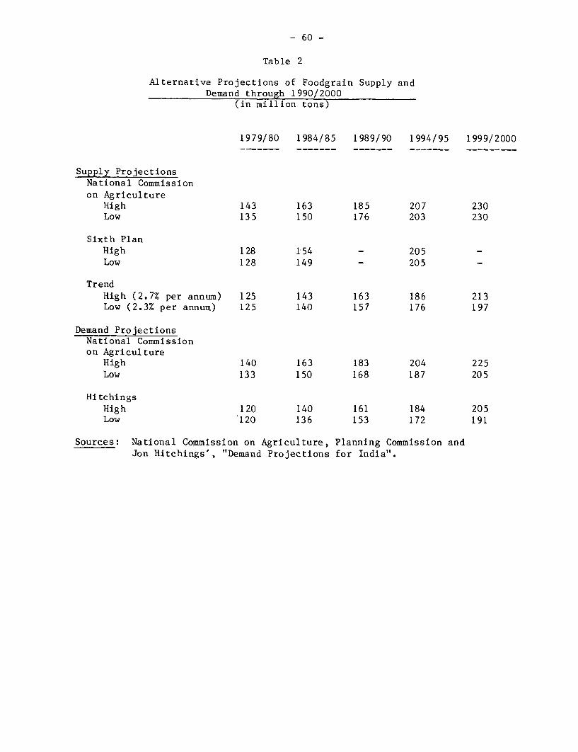
- 60 -

Table 2

Alternative Projections of Foodgrain Supply andDemand through 1990/2000

(in million tons)

1979/80 1984/85 1989/90 1994/95 1999/2000

Supply ProjectionsNational Commissionon Agriculture

High 143 163 185 207 230Low 135 150 176 203 230

Sixth PlanHigh 128 154 - 205 -Low 128 149 - 205 -

TrendHigh (2.7% per annum) 125 143 163 186 213Low (2.3% per annum) 125 140 157 176 197

Demand ProjectionsNational Commissionon Agriculture

High 140 163 183 204 225Low 133 150 168 187 205

HitchingsHigh 120 140 161 184 205Low 120 136 153 172 191

Sources: National Commission on Agriculture, Planning Commission andJon Hitchings', "Demand Projections for India".

- 61 -

trend of availability. Trend availability in 1979/80 would be the same astrend production (125 million tons), given the lack of imports.Consumption in 1979/80 will be below trend due to the fall in income.Consequently, actual consumption in 1979/80 is likely to have been muchcloser to Hitchings' projected 1979/80 base of 120 million tons than theNCA's 133 to 140 million tons.

The NCA projections incorporate provision of foodgrain foranimal feeding, derived from an accelerated and modernized animaldevelopment program contained in the NCA report, that grows to reach 20 to25 million tons by the year 2000. World Bank estimates, based on animalhusbandry sector work, suggest animal feed requirements considerably lowerthan this, perhaps less than half. The Hitchings demand estimatespresented here incorporate an allowance for seed, feed and waste of 12.5%of gross production. The provision for animal feed from this is generallyplaced at 5%, or 9.5 million tons and 10.2 million tons for the low andhigh projections, respectively, by the year 2000. The NCA also makes aslightly greater allowance for wastage, 4% (8 to 9 million tons by 2000)than Hitchings' allowance of 2.5% (4.8 to 5.1 million tons).

In summary, it is unlikely that foodgrain consumption will reachthe levels projected by the National Commission on Agriculture. The SixthPlan's projection of demand for 1984/85 of 150 million tons is similarlyunlikely in light of Hitchings' demand analysis. Consumption is likely toreach the levels projected under Hitchings' high demand alternative onlyif growth of foodgrain production is also fairly high. The high supplyprojection easily meets Hitchings' high demand projection, just as the lowsupply projection covers his low demand projection. Governmentprojections of supply lie considerably above either of the supplyprojections. Although the Government's demand projections also lieconsiderably above Hitchings', they are probably even less plausible thanthose for supply.

Implications. The projections suggest the real possibility ofIndia moving into a period of sustainable foodgrain self-sufficiency orsurplus. This outlook is substantially more optimistic than many pastprojections. As a new conclusion, it deserves to be treated with cautionand interpreted with perspective. Foodgrain production will still dependon the moonsoon and a failure of the monsoon could lead India to importgrain. As Graph 1 indicates, actual foodgrain production has fluctuatedsignificantly around the trend. In some years, weather conditions arelikely to make it necessary to draw down stocks and/or import, while inyears of good monsoons stocks are likely to be replenished and/or somegrain exported. The analysis contains new projections based on theprospects for population growth, household expenditure patterns andproduction which lead one to the optimistic conclusion as far as marketsupply/demand balances are concerned. The optimism of this conclusionshould not translate into complacency about the prospects for eliminating

- 62 -

poverty and undernutrition in India by the year 2000. The projectionsimply rising per capita consumption of foodgrains, and this, together withthe possibility of falling real prices for foodgrains discussed below,would have a beneficial impact on poverty and nutrition. But theprojected rise in per capita consumption would take place from a basewhich is very low on average and pitifully low for the poorer segmentsof the population. Nor should there be complacency that the projectedsupply/demand balances will come about without continued efforts on thesupply side to develop the technological base, input supply system,irrigation infrastructure and incentives needed for sustained productiongrowth and, on the demand side, to moderate the rate of growth ofpopulation.

Foodgrain self-sufficiency or surplus, if it comes about, willbe an impressive achievement of a long standing goal of Indian economicdevelopment. It indicates that India, by continuing its major efforts inagriculture, may be in the desirable position of having a range of optionswhich were not available during the period when domestic foodgrainsupplies were inadequate. Among these options are the following:

(a) Increase Consumption. A slowly falling real price offoodgrains would absorb a greater quantity of foodgrains inhousehold consumption and slow production growth, so thatthe projected surpluses would not arise. The past severalyears have already seen a modest decline in real foodgrainprices and rise in per capita consumption, and the currentlevel of household foodgrain consumption is approximatelyequal to a caloric-sufficient quantity, on average, for theIndian population. With unequal distribution of thisconsumption, this means undernutrition for lower incomegroups. It is the lowest income groups, who spend thegreatest proportion of their income on foodgrains, for whomlower real prices are the most important. Effects of lowerprice on producer incentives are also important but so farat least technical change has offset the decline inproducer prices and has kept profits sufficiently high toencourage greater production.

(b) Exports of Foodgrains. The Bank projections are notreliable enough to predict exports, which are a smallresidual between two very large and fluctuating variables,demand and supply. Nevertheless, the prospects offoodgrain exports are real ones. The Sixth Plan projectsthe export of 3 million tons of rice by 1984/85 which, onthe basis of the Bank projections, appears feasible fromthe point of view of domestic supply, keeping in mind thecaveats concerning fluctuations in individual years. Theprices at which the Government procures foodgrains relative

- 63 -

to world market prices become important in this regard.Currently, Indian procurement and market prices for riceare not higher than world market prices, and rice could beexported without losses to the Government.

(c) Diversification in Agriculture. The demand projectionscontained in the first section of the paper indicate thedemand for several other important agricultural commoditieswill grow faster than for foodgrains (see Table 3). Mostfarmers grow a variety of crops in which foodgrains aredominant (Table 1). Changes in foodgrain productiontechnology or prices can increase the relativeprofitability of foodgrains, causing farmers to plant agreater proportion of their area to them. Alternatively,farmers who see greater profit opportunities in other cropscan apply yield-increasing technology to meet their ownfoodgrain needs on less area, thereby freeing land forother crops. The introduction of shorter durationvarieties of foodgrains (especially paddy) gives farmersgreater opportunities for planting a second crop.Relatively small shifts in foodgrain area can meansubstantial shifts in area and production of other crops.For example, 1% of the foodgrain area is equivalent to 8%of the oilseed area, 17% of the cotton area or 40% of thesugarcane area. Thus management of foodgrain supply anddemand is of central importance for both foodgrains and formost other agricultural commodities as well. Moreover, ifthe foodgrain situation is under control, India'ssubstantial agricultural infrastructure, with its technical(research and extension), physical (irrigation and otherinvestments), logistical (input supply and distribution)and economic (pricing policy, procurement and distribution)dimensions, has more flexibility to meet the needs of othercrops.

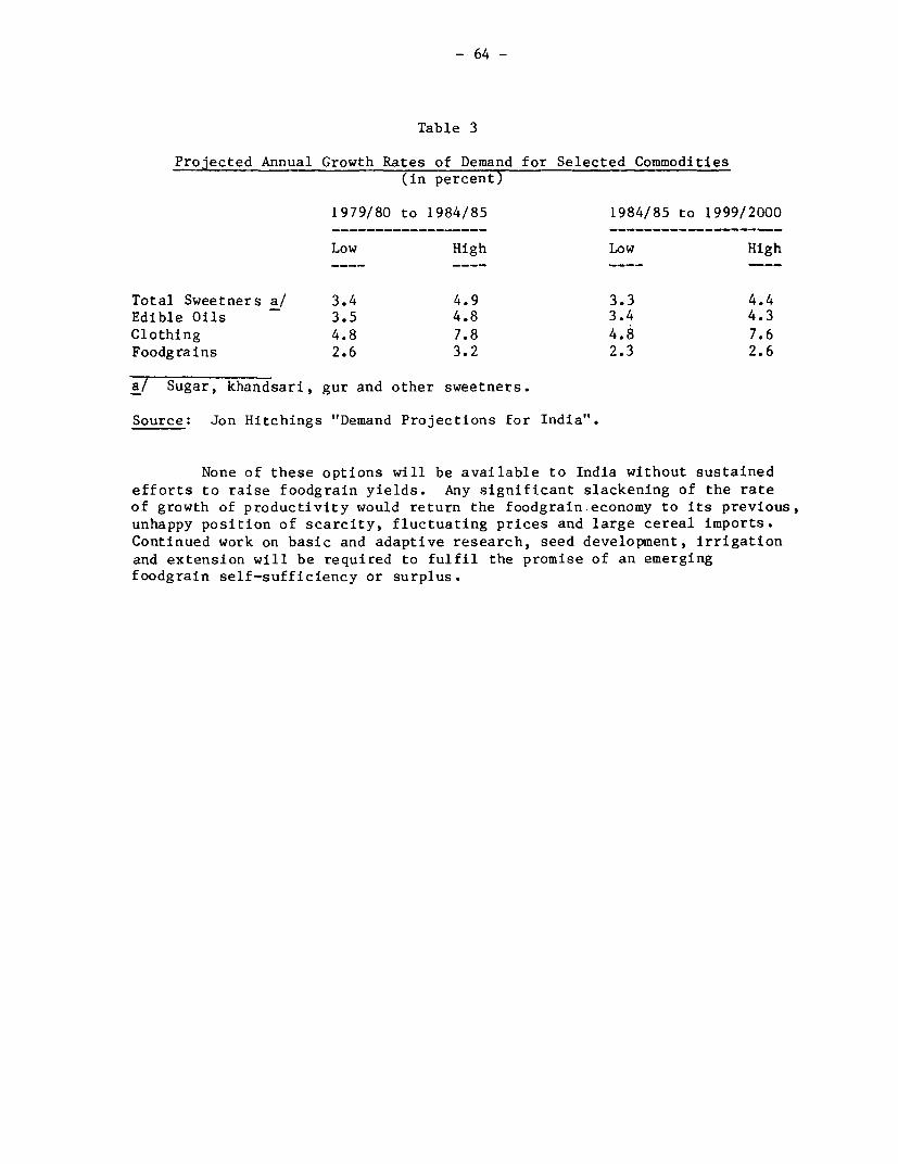
- 64 -

Table 3

Projected Annual Growth Rates of Demand for Selected Commodities(in percent)

1979/80 to 1984/85 1984/85 to 1999/2000

Low High Low High

Total Sweetners a/ 3.4 4.9 3.3 4.4Edible Oils 3.5 4.8 3.4 4.3Clothing 4.8 7.8 4.8 7.6Foodgrains 2.6 3.2 2.3 2.6

a/ Sugar, khandsari, gur and other sweetners.

Source: Jon Hitchings "Demand Projections for India".

None of these options will be available to India without sustainedefforts to raise foodgrain yields. Any significant slackening of the rateof growth of productivity would return the foodgrain.economy to its previous,unhappy position of scarcity, fluctuating prices and large cereal imports.Continued work on basic and adaptive research, seed development, irrigationand extension will be required to fulfil the promise of an emergingfoodgrain self-sufficiency or surplus.

Annex Table I

AREA, PRODUCTION AND YIELD OP FOODGRAINS,1949/50 TO 1979/80

(Area - '000 HectaresProduction - '000 TonsYield - Kg per Hectare)

RICE WHEAT COARSE CERALS PULSES TOTAL FOODGRAINS

A P Y A P Y A P Y A p Y A P Y1949/50 30519 23542 771 9758 6391 655 38836 16824 433 20167 8159 405 992801 54916 55330810 20576 668 9746 6462 663 37674 15376 408 19091 8411 1441 97321 50625 152252 29830 21300 714 9471 6183 653 3988 16093 414 18775 6420 449 96961 51996 1536

53 29969 22899 764 9828 7501 763 42446 19612 462 19845 9189 463 102088 59201 58054 31289 28214 902 10691 8017 750 45366 22972 506 21729 10619 489 109065 69921 640t65 30764 25219 820 11259 9043 903 43921 22823 520 21914 10950 500 107858 68035 63156 31521 27557 874 12367 8760 708 43456 19498 448 23216 11045 476 110560 66850 605i; 32277 29037 800 13524 9403 695 42019 19864 473 23316 11551 495 111136 69955 629B.E1 32298 25525 790 11730 7998 682 42914 21226 495 22538 9562 424 109480 64311 58733172 30847 930 12617 9958 7 44664 23187 519 2431t 13149 541 114764 77141 672no 33820 31676 937 13360 10324 772 43790 22973 522 24833 11799 475 115823 76672 66261 34128 34574 1013 12927 10997 851 44963 23743 1529 23563 12704 539 115581 82018 i71062 34694 35663 1028 13570 12072 990 44725 23216 519 24243 111755 485 117232 82706 '70563 35695 33217 931 13590 10776 793 44294 24630 556 24265 111528 475 117844 80151 '68064 35809 36999 1033 13499 9853 730 43927"23718 540 24186 10073 !416 117421 90642 16B765 36462 39308 1078 13422 12257 913 44353 25374- 572 23875 12417 520 118112 89356 75766 35470 30589 862 12572 10394 827 44343 21420 483 22718 9944 438 115103 72347 62967 35251 30438 863 12838 11393 887 45092 24053 533 22121 8347 377 115302 74231 644 .68 36437 37612 1032 14998 16540 1103 47337 28798 608 22649 .12102 534 121421 95052 78369 36967 39761 1076 15958 18651 1169 46241 25183 545 21264 '10418 490 120430 94013 79170 37680 40430 1073 16626 20093 1209 47241 27287 578 22023 11691 531 123570 99501 805-1 37592 42225 1123 18241 23832 1307 45949 30547 665 22534 11819 524 124316 108422 87272 37758 43068 1141 19139 26410 1380 43575 24596 564 22151 11094 501 122623 105168 85873 36688 39245 1070 194631 24735 1271 42211 123139 548 20915 9907 474 119277 97026 81374 38286 44051 1151 19853 21778 1172 46242 '28828 623 23427 10008 427 126538 104665 82775 37999 39579 1045 18010. 24104 1338 43152 26129 606 22024 10014 *455 121075 99826182476 39475 43740 1235 20454 28846 1410 43798 35409 808 24454 13039 533 128181 121034 94477 33511 41917 1088 20922 29010 1387 46940 28979 615 22963 11361 494 124356 111167 89478 40292 52671 1308 21456 31749 1480 42280 30014 710 23497 11973 510 127515 126407 99179 40480 53770 1328 22640 35510 1568 42230 30440 721 23660 12180 515 129010 131900-1022so 38980 42190 1082 21960 31560 1437 41220 26730 1648 21750 8370 385 123910 108950 878

Annual Z Ratesof Growth

1949/50 - 1979/80 0.9 2.6 1.7 2.8 5.9 3.0 0.2 1.8 1.6 0.3 0.4 0.1 0.8 2.7 1.9

1949/50 - 1964/65 1.3 4.0 2.6 2.6 4.2 1.6 0.9 2.8 1.9 1.7 2.4 0.7 1.4 3.4 2.0

1967/68 - 1979/80 0.5 1.8 1.2 3.0 5.3 2.3 -0.9 0.9 1.8 0.5 -0.6 -1.1 0.4 2.1 1.7

1967/68 - 1978/79 Q.5 2.4 1.7 3.2 5.7 2.5 -0.8 1.3 2.1 0.8 0.5 -0.3 0.5 2.6 2.1Sources: Estimates of Area and Production of Principal Crops in India, 1978-79

published by Directorate of Economics and Statistics, Ministry of Agriculture; and,Economic Survey, 1980-81, published by Government of India.

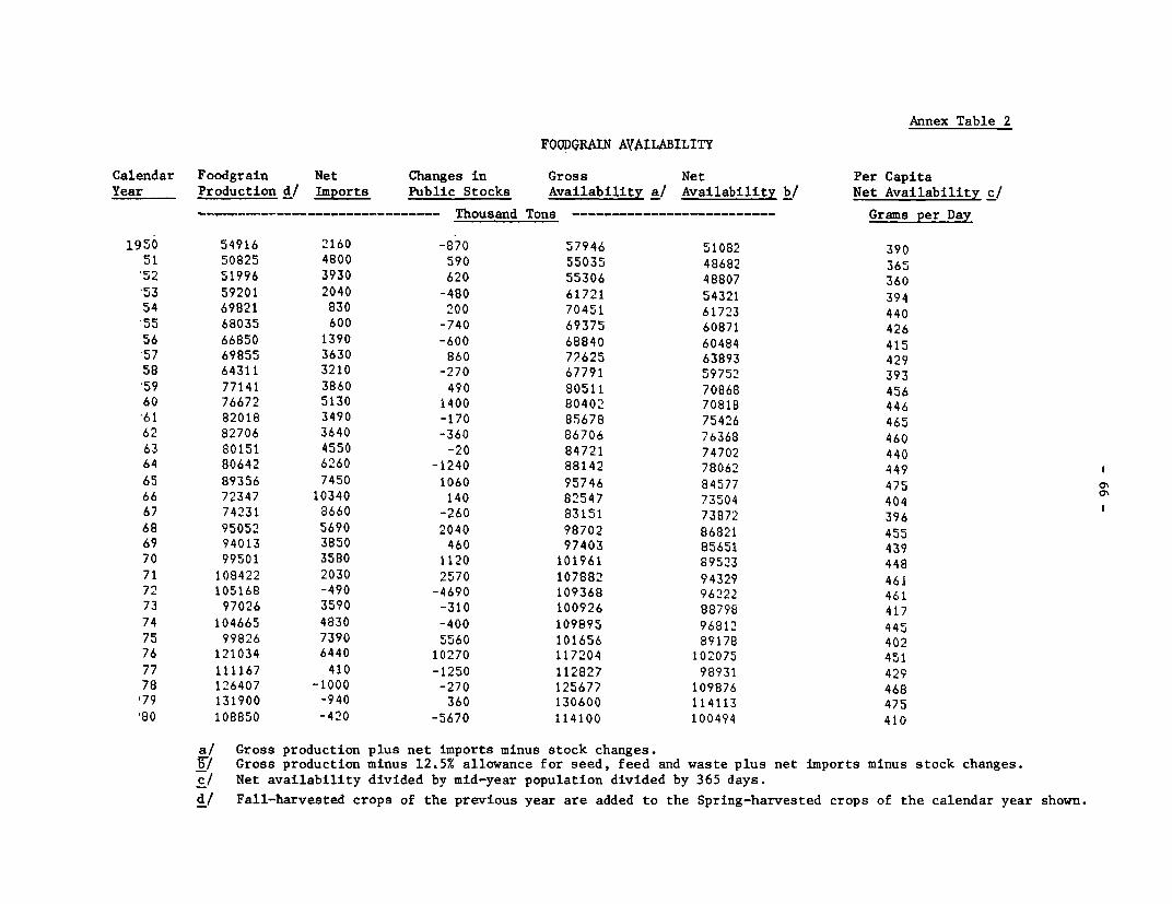
Annex Table 2

FOODORAIN AVAILABILITY

Calendar Foodgrain Net Changes in Gross Net Per CapitaYear Production d/ Imports Public Stocks Availability a/ Availability b/ Net Availability c/

- ------------------------ Thousand Tons ------------------------- Grams per Day

1950 54916 2160 -870 57946 51082 39051 50825 4800 590 55035 48682 365

*52 51996 3930 620 55306 48807 360

'53 59201 2040 -480 61721 54321 394

54 69821 830 200 70451 61723 440

55 68035 600 -740 69375 60871 426

56 66850 1390 -600 68840 60484 415

'57 69855 3630 860 72625 63893 429

58 64311 3210 -270 67791 59752 393

59 77141 3860 490 80511 70868 45660 76672 5130 1400 80402 70818 44661 82018 3490 -170 85678 75426 46562 82706 3640 -360 86706 76368 460

63 80151 4550 -20 84721 74702 44064 80642 6260 -1240 88142 78062 449 1

65 89356 7450 1060 95746 84577 475 0'

66 72347 10340 140 82547 73504 404 167 74231 8660 -260 83151 73872 396

68 95052 5690 2040 98702 86821 45569 94013 3850 460 97403 85651 43970 99501 3580 1120 101961 89523 44871 108422 2030 2570 107882 94329 46172 105168 -490 -4690 109368 96222 46173 97026 3590 -310 100926 88798 417

74 104665 4830 -400 109895 96812 44575 99826 7390 5560 101656 89178 40276 121034 6440 10270 117204 102075 451

77 111167 410 -1250 112827 98931 42978 126407 -1000 -270 125677 109876 468'79 131900 -940 360 130600 114113 47580 108850 -420 -5670 114100 100494 410

a/ Gross production plus net imports minus stock changes.b/ Gross production minus 12.5% allowance for seed, feed and waste plus net imports minus stock changes.c/ Net availability divided by mid-year population divided by 365 days.

d/ Fall-harvested crops of the previous year are added to the Spring-harvested crops of the calendar year shown.

Part III

THE VEGETABLE OIL ECONOMY

John W. WallJune 1981

67

- 68 -

The Vegetable Oil Economy

Table of Contents

Page No.

Introduction .. ............. 69

Supply Trends. . . . 70

Demand Conditions . ........ . ...... . . .......... 71

Supply/Demand Balance . . . .71

Supply Prospects .... 74

Oilseeds Production . . . .74

Oilseeds Processing . . . .76

Pricing Policy... 78

Medium-Term Management of the Vegetable OilEconomy and the Plan............. . 82

- 69 -

Introduction. Oilseeds constitute one of the most important groupsof agricultural commodities in India. Oilseeds (including cottonseed andcoconut) occupy about 15% of gross cropped area and contribute about 10% ofthe value of output from agriculture. The oilseeds group contains a largenumber of field crops: groundnut, rape and mustard, castor, sesame, linseed,niger, safflower, sunflower, cottonseed and soyabean. In addition vegetableoil is extracted from rice bran and a variety of tree crops: coconut, oilpalm and various forest seeds such as sal and neem. Vegetable oil is an itemof mass consumption in India and is the main source of the basic human require-ment for essential fatty acids. Most vegetable oil is consumed directly asfood, although the demand for vegetable oil for soaps and paints is risingmore rapidly than for food purposes. A growing proportion of edible oil,reaching about 17% in 1979, is consumed in the form of hydrogenated oil,mainly in urban areas and northern parts of India. The remainder is consumedas either unrefined or refined liquid oil. Total consumption of vegetableoils of around 6 kg per capita is low compared with over 25 kg per capita indeveloped countries and over 10 kg per capita for the world average.

Oilseeds and vegetable oils loom large in India's foreign trade.India is a traditional exporter of oilseed cakes and meals, particularlydeoiled groundnut and cottonseed meals; of speciality oils such as castor andlinseed; and of handpicked, selected (1iPS) groundnuts. Recently, deoiled ricebran has become a major export. During the period 1975/76 to 1978/79, exportsof oilseeds and their derivatives averaged over US$200 million per year, about14% of all agricultural exports and 3% of all exports. Since 1976/77, importsof vegetable oils have grown large, to 1 million tons or more per year withimport values of US$600-800 million through 1979/80. Next to petroleum vege-table oils have been the largest item in the import bill, replacing cereals,which had been the largest item of food imports up to 1975/76.

Almost half of all vegetable oil produced in India is derived fromgroundnut (see Table 1). Groundnut is grown mainly as a rainfed crop insemi-arid areas of western and southern India--particularly Gujarat, TamilNadu, Andhra Pradesh and Karnataka--in the kharif (June to October) season.About 11% of groundnut area and about 19% of groundnut produced is planted inJanuary and February and harvested in May (hot weather or summer groundnut).Rape and mustard seed is the next largest source of oil. Rape/mustard isgrown in the rabi season (October to April) in the northern and eastern partsof India, particularly in Uttar Pradesh, which alone accounts for more thanhalf of total area. Cotton is grown mainly in Gujarat, Punjab, Maharashtraand Karnataka in the kharif season, mainly for cotton fiber and only secon-darily for the seed. A lower proportion of cottonseed is crushed for oil thanother oilseeds as a higher proportion of the seed is fed directly to cattle.Nevertheless an increasing proportion of cottonseed is being processed toextract its oil. Coconut is a perennial crop grown in tropical coastal areasof India, mainly in Kerala, which accounts for more than half of total coconutproduction, followed by Tamil Nadu and Karnataka. Linseed is grown mainly inUttar Pradesh, Madhya Pradesh and Maharashtra. Castor is grown mainly inGujarat and Andhra Pradesh.

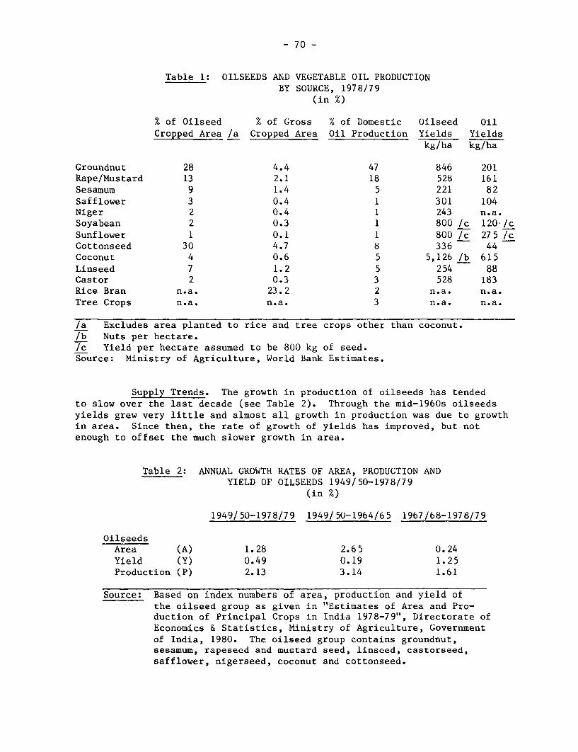
- 70 -

Table 1: OILSEEDS AND VEGETABLE OIL PRODUCTIONBY SOURCE, 1978/79

(in %)

% of Oilseed % of Gross % of Domestic Oilseed OilCropped Area /a Cropped Area Oil Production Yields Yields

kg/ha kg/ha

Groundnut 28 4.4 47 846 201Rape/Mustard 13 2.1 18 528 161Sesamum 9 1.4 5 221 82Safflower 3 0.4 1 301 104Niger 2 0.4 1 243 n.a.Soyabean 2 0.3 1 800 /c 120 /cSunflower 1 0.1 1 800 /c 275 /cCottonseed 30 4.7 8 336 44Coconut 4 0.6 5 5,126 /b 615Linseed 7 1.2 5 254 88Castor 2 0.3 3 528 183Rice Bran n.a. 23.2 2 n.a. n.a.Tree Crops n.a. n.a. 3 n.a. n.a.

/a Excludes area planted to rice and tree crops other than coconut./b Nuts per hectare./c Yield per hectare assumed to be 800 kg of seed.Source: Ministry of Agriculture, World Bank Estimates.

Supply Trends. The growth in production of oilseeds has tendedto slow over the last decade (see Table 2). Through the mid-1960s oilseedsyields grew very little and almost all growth in production was due to growthin area. Since then, the rate of growth of yields has improved, but notenough to offset the much slower growth in area.

Table 2: ANNUAL GROWTH RATES OF AREA, PRODUCTION ANDYIELD OF OILSEEDS 1949/50-1978/79

(in %)

1949/50-1978/79 1949/50-1964/65 1967/68-1978/79

OilseedsArea (A) 1.28 2.65 0.24Yield (Y) 0.49 0.19 1.25Production (P) 2.13 3.14 1.61

Source: Based on index numbers of area, production and yield ofthe oilseed group as given in "Estimates of Area and Pro-duction of Principal Crops in India 1978-79", Directorate ofEconomics & Statistics, Ministry of Agriculture, Governmentof India, 1980. The oilseed group contains groundnut,sesamum, rapeseed and mustard seed, linseed, castorseed,safflower, nigerseed, coconut and cottonseed.

- 71 -

During the period 1967/68 to 1978/79, domestic production of vege-table oil grew on average by 2.5% per annum, substantially faster than totalsupply of oilseeds. This is due to several factors. An increasing proportionof some oilseeds, mainly cottonseed, has been processed for oil. The intro-duction of solvent extraction methods has meant an increasing proportion ofthe oil in the seed has become available for use. Finally, there has been agrowing extraction of oil from sources other than those included in the abovedefinition of oilseeds. These other sources are minor oilseeds of tree originsuch as sal, neem and kusum, and rice bran.

Demand Conditions. Household,consumption data indicate that demandfor vegetable oils for food increases at roughly the same rate as income, pro-viding relative prices are constant. The growth in consumption would be dam-pened by a relative price rise since households would substitute other goods.With per capita income growing at 1.5% per annum and population growing at 2%per annum or more, growth in total demand would exceed 3.5% per annum, assum-ing no relative price movements. However, from the early 1960s through themid-1970s, growth in demand of vegetable oils was, constrained by growth insupply, which was lower than 3.5% per annum. Vegetable oil imports were insig-nificant between 1960/61 and 1975/76, so fluctuations in domestic productiondirectly caused fluctuations in domestic supply and domestic prices. In yearsof short harvests, prices rose rapidly to choke demand back to available supply.Through the mid-1970s, there was a tendency for relative prices of vegetableoils to rise, although the fluctuations were so wide as to obscure any strongtrend. These relationships can be seen in Graphs 1, 2 and 3.

Starting in 1976/77, large scale imports of edible oil allowed demandto rise by more than domestic supply. Imports in the oil year (November toOctober) of 1976/77 through 1979/80 were one million tons or more per year,comprising one-fourth or more of domestic supply. Per capita availabilityrose from an average of five kg for the period 1974 to 1976 to an average ofover six kg for period 1977 to 1980. These imports of vegetable oil kept thevegetable oil prices from rising significantly relative to other commoditiesdespite low oilseed production during this period. Indeed some have arguedthat the large scale import of vegetable oils had adversely affected theproduction of oilseeds by keeping their prices low. The imports now alsocontribute to India's very large trade deficit which must be reduced.

Supply-Demand Balance. Assuming stable relative vegetable oilprices and based on past trends, World Bank projections of demand lie aboveprojections of supply for the foreseeable future (see Graph 3). The supplyprojection is based on a simple extrapolation of past trends. DL, the lowdemand projection, is based on a 3.5% per annum rate of growth in total expen-diture. DH, the high demand projection, is based on a 5% per annum growth intotal expenditure. With either demand line the gap between supply and demandbecomes quite large. By 1990, filling the gap through imports would meanspending between US$3-4 billion (6-8% of total imports) and absorbing between8-10% of total projected world exports of vegetable oils. The alternative toimporting to fill the gap is to increase the rate of growth of domestic supplyand decrease the rate of growth of demand. Decreasing the rate of growth ofdemand in a country with such low per capita consumption as in India wouldnot be desirable in itself but a consequence of pursuing other policies.

- 72 -

Graph 1

110 -

100 A Vegetable oils

90 Retative

80 s / V \/ Price Index"70 _ V 1970/ 71 = 100

19 61 62 64 66 68 70 72 74 76 78 80

(J INDEX OF WHOLESALE PRICES

OF VEGETABLE OILS DIVIDEDBY INDEX OF WHOLESALE PRICES

OF ALL COMMODITIES.

Graph 2

Consumption of'7 - Vegetabte oits6 per capita

4. </ < , /in kg/year5

4

19.61 62 64 66 68 70 72 74 76 78 80

SOURCE:WORLD BANK ESTIMATES

10.0

9.'5-

9.o INDIA:VEGETABLE OIL SUPPLY-DEMAND DH

8.5 1960-61 - 1999-2000 /

IN MILLION TONS / DL8.0 /UPL

SUPPLY ______/

7.5 DEMAND ------ /-

7.0 /

6.5

6.0

5.5 ,/

2 5.0

-J~~~~~~~~~~~~~~~~~~~~~~~~~~~~~~~~~~~~~~~~~~~~~~~~~~~~~~~~~~~~~~~~~~J

I I I t I @ 1---e , §~~~I--.

3.5 - 68

3. 0 - -SOURCE WORLD BANK ESTIMATES

2.5 - ~ ~ ~ ~ ~ "I AND PROJECTIONS.

2.5 -.

1960.61 62 64 66 6 8 70 72 '74 76 '78 8S0 182 8 4 8 6 88 90 92 94 '96 '98 2000

- 74 -

Table 3: VEGETABLE OIL SUPPLY-DEMAND GAP 1985-2000(in million tons)

1985 1990 1995 2000

High Demand 5.0 6.2 7.6 9.2Low Demand 4.8 5.7 6.8 7.9Supply (past trend) 3.6 4.1 4.6 5.3

GapHigh Demand 1.4 2.1 3.0 3.9Low Demand 1.2 1.6 2.2 2.6

Source: World Bank Projections.

Supply Prospects. India has under-utilized potential for raisingdomestic supply of vegetable oils. There is scope to increase the supplyof traditional oilseeds by increasing cropped area and by increasing yieldsthrough use of better land, improved varieties, good seed, pest protectionand more effective cultural practices. There is also the possibility ofintroducing new oilseeds, such as soyabean, that could contribute signifi-cantly to India's oil supply. Improvements in the organization of oilseedsprocessing can yield extra oil from under-utilized sources such as rice bran,cottonseed and a variety of oilseed expeller cakes not yet processed in sol-vent extraction plants. Finally, an increasing proportion of minor oilseedsof tree origin, such as sal and neem can be collected and utilized for oilextractions.

Oilseed Production. Although the rate of growth of cropped areaunder oilseeds has been very low since 1969/70, it could be increased withappropriate policies. Farmers in India shift their cropping patterns inways that reflect the relative profitability of crops. As the technology ofproducing oilseeds has been fairly stagnant, prices farmers receive have beenparticularly important in determining cropped area devoted to oilseeds. 1/

Despite the relatively slow improvement in oilseeds varieties thereis considerable scope to increase yields from their present levels. Yields inIndia are generally much lower than in many other large countries (see Table4). A fundamental reason for the low yields is that oilseeds are grown onmarginal lands without assured moisture. hence oilseeds compete with otherlow-yielding crops, such as sorghum and millets, which can better withstandmoisture stress. On better quality and irrigated land oilseeds currently lose

1/ Karam Singh, "Oilseeds in India--Paradox of Price or Rains." The find-ings were based on regression analysis analysing the relative effects ofrainfall, prices and time on area, production and yield of the five majoroilseeds (groundnut, rape/mustard, sesame; castor and linseed). Areacropped was found to be very sensitive to the previous year's price,along with a time trend. Yield was affectea relatively little by pricesbut very significantly by rainfall.

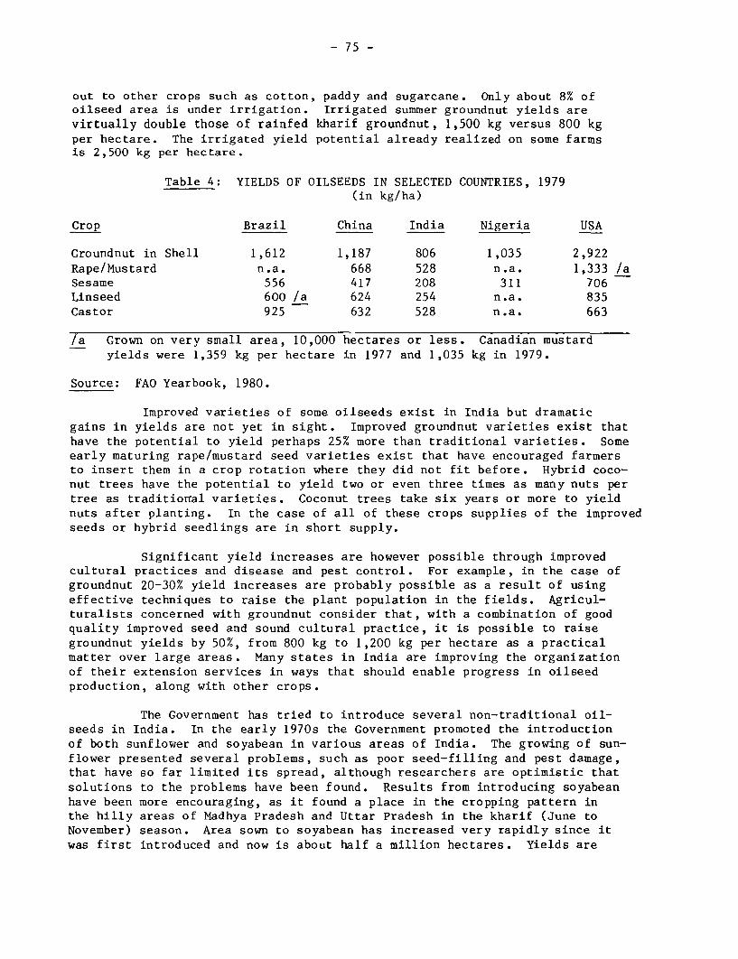
- 75 -

out to other crops such as cotton, paddy and sugarcane. Only about 8% ofoilseed area is under irrigation. Irrigated summer groundnut yields arevirtually double those of rainfed kharif groundnut, 1,500 kg versus 800 kgper hectare. The irrigated yield potential already realized on some farmsis 2,500 kg per hectare.

Table 4: YIELDS OF OILSEEDS IN SELECTED COUNTRIES, 1979(in kg/ha)

Crop Brazil China India Nigeria USA

Croundnut in Shell 1,612 1,187 806 1,035 2,922Rape/Mustard n.a. 668 528 n.a. 1,333 /aSesame 556 417 208 311 706Linseed 600 /a 624 254 n.a. 835Castor 925 632 528 n.a. 663

/a Grown on very small area, 10,000 hectares or less. Canadian mustardyields were 1,359 kg per hectare in 1977 and 1,035 kg in 1979.

Source: FAO Yearbook, 1980.

Improved varieties of some oilseeds exist in India but dramaticgains in yields are not yet in sight. Improved groundnut varieties exist thathave the potential to yield perhaps 25% more than traditional varieties. Someearly maturing rape/mustard seed varieties exist that have encouraged farmersto insert them in a crop rotation where they did not fit before. Hybrid coco-nut trees have the potential to yield two or even three times as many nuts pertree as traditionfal varieties. Coconut trees take six years or more to yieldnuts after planting. In the case of all of these crops supplies of the improvedseeds or hybrid seedlings are in short supply.

Significant yield increases are however possible through improvedcultural practices and disease and pest control. For example, in the case ofgroundnut 20-30% yield increases are probably possible as a result of usingeffective techniques to raise the plant population in the fields. Agricul-turalists concerned with groundnut consider that, with a combination of goodquality improved seed and sound cultural practice, it is possible to raisegroundnut yields by 50%, from 800 kg to 1,200 kg per hectare as a practicalmatter over large areas. Many states in India are improving the organizationof their extension services in ways that should enable progress in oilseedproduction, along with other crops.

The Government has tried to introduce several non-traditional oil-seeds in India. In the early 1970s the Government promoted the introductionof both sunflower and soyabean in various areas of India. The growing of sun-flower presented several problems, such as poor seed-filling and pest damage,that have so far limited its spread, although researchers are optimistic thatsolutions to the problems have been found. Results from introducing soyabeanhave been more encouraging, as it found a place in the cropping pattern inthe hilly areas of Madhya Pradesh and Uttar Pradesh in the kharif (June toNovember) season. Area sown to soyabean has increased very rapidly since itwas first introduced and now is about half a million hectares. Yields are

- 76 -

fairly low, about 800 kg per hectare and the oil yield per hectare is consi-derably lower than groundnut or rape and mustard. However, much of it is nowgrown in hilly areas which otherwise would lie fallow. Therefore, any increasein such areas represents a net addition to India's oil supply.

Oilseed Processing. The growth in the production of vegetable oilhas exceeded growth in oilseed production because an increasing proportionof oil potentially available has been extracted due to improvements in theorganization of oilseed processing. Animal-powered wooden village oil presseshave given way increasingly to electric-powered mechanical presses that areable to expel a higher proportion of oil in the seed, although some oil isstill left in the oil cake. An increasing proportion of oil cake has beenprocessed in modern solvent extraction plants, which extract most of theremaining oil left in the cake. Solvent extraction plants also are necessaryto extract oil from rice bran and other seeds which have a relatively low oilcontent, such as soyabean, sal and other forest seeds. As the number of sol-vent extraction plants has grown, an increasing proportion of the previouslyunder-utilized oil-bearing material has been processed for oil. There iscurrently excess solvent extraction capacity in the aggregate, although mostof this capacity is concentrated in a few areas, such as Bombay. Neverthe-less, there is scope to increase the oil extraction of under-utilized sourcesby changing certain policies and by further improving the organization ofprocessing.

One policy that restricts the solvent extraction of expeller oilcake and rice bran is the restriction on the export of deoiled meals. Suchrestrictions were placed on exports during years when domestic supplies wereshort due to bad weather. The domestic market for deoiled meals in India islimited by the extent of the market for compound feed, which is very small.Most Indian farmers feed their animals a diet formulated of feedstuff--mainlystraw, stalks, cane and oil cakes--available in the village or nearby towns.Farmers are said to prefer oil cakes to deoiled meals as feeds because theyfeel their animals need the oil residual in the cake. In any case, a domesticmarket has not developed for deoiled meal beyond the very small one providedby compound feed manufacturers. After that market is satisfied, solventextraction of the oil in expeller oil cake occurs only when the deoiled mealcan be exported. Only then can a solvent extractor make a profit by buyingoil cake, solvent extracting the oil and selling the oil and meal.

The Government restricts the export of various oilseed products toincrease their domestic availability. Exports of groundnut, cottonseed andrice bran deoiled meals are restricted, although not soyabean meal. Thisincreases domestic availability and reduces the domestic price of oil cakes.The oil left in the cake is used by animals as a high grade source of caloriesto produce milk, butter fat, eggs and poultry, expensive sources of fat whencompared with vegetable oil. The Government also restricts the export of hand-picked, selected (HPS) groundnuts and linseed oil to increase the domesticavailability of vegetable oil. Paradoxically these restrictions actuallyreduce India's vegetable oil supply.

Table 5 presents calculations of the net effect of the export ofoilseeds and their derivatives on domestic vegetable oil supply. The year1976/77 is taken as it reflects a period when the export of oilseeds productswas relatively unrestricted and in fact when the exports of HPS groundnut,

- 77 -

castor oil and linseed oil were much higher than they have been since. Itwas also a record year for the export of groundnut meal and deoiled rice bran.Exports of oilseeds reduce oil supply by the recoverable oil content of seedsexported. Export of deoiled meals increases domestic oil supply by the amountof oil recovered from expeller cake by the solvent extraction method. Thissolvent extraction would not take place if the export market for the mealdid not exist. In 1976/77, the export,of oilseed products resulted in a netaddition to Indian vegetable oil supply as the extra oil produced due to thesolvent extraction to produce deoiled meals slightly exceeded the oil exportedin the form of seeds and oil. In addition, as indicated in the last column,the export of oilseed products could finance many times the oil exported. At1980 prices, the export of HPS groundnut could finance the import of ten timesthe oil content of nuts exported. The export of specialty oils, which areconsidered inedible, could finance at least the same quantity of edible oils,and usually more.

The easing of restrictions on exports of deoiled meals, expansionof the market for compound feeds,and farmers' increased acceptance of deoiledmeals as animal feeds will increase the solvent extraction of vegetable oilsnow left in the cakes. Other improvements in the organization of oilseedprocessing also will lead to an increased proportion of the potentiallyavailable vegetable oil being produced. Perhaps the most important of theseis in the organization of rice milling to increase the availability of ricebran for oil extraction.

Rice bran contains up to 15% oil which is recoverable through sol-vent extraction. In 1978/79 if all the potentially available rice bran oilhad been recovered in India it would have amounted to 590,000 tons of oil.Recovery of a large portion of this is a long way off. Only about 12-15%of the available oil is recovered at present. Much of the paddy in India isstill processed in hullers, which yield about two-thirds of paddy in the formof rice and one-third in a mixture of hulls, bran, broken rice and foreignmatter. The hull/bran/brokens mixture is unsuitable for solvent extractionmills, as the oil percentage is only about 5%. It is also unsuitable foranimal feed, given the high hull content. Paddy processed in huller-and-sheller and modern rice mills, which first separate hulls from the unpolishedrice using rubber rollers, yields a high quality rice bran suitable for solventextraction. Modern mills have the added advantage of having a higher dailyoutturn, which expedites the collection of bran for shipment to extractionplants. One way to increase the production of rice bran oil is to encouragean increased proportion of rice or rice bran to be processed in modern mills.Several Government policies work against this, particularly the levy procure-ment of rice from modern mills at below market price, which smaller riceprocessors escape. At the moment, levy prices of rice are not far belowmarket prices in surplus areas but the continuation of the levy itself dis-courages investment in modern rice mills.

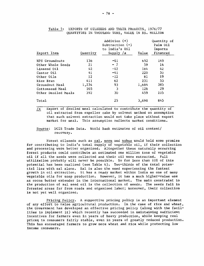
- 78 -

Table 5: EXPORTS OF OILSEEDS AND THEIR PRODUCTS, 1976/77QUANTITIES IN THOUSAND TONS, VALUE IN RS. MILLION

Addition (+) Quantity ofSubtraction (-) Palm Oilto India's Oil Imports

Export Item Quantity Supply /a Value Financed

EPS Groundnuts 136 -61 652 149Other Whole Seeds 21 - 7 59 14Linseed Oil 42 -42 184 42Castor Oil 41 -41 220 50Other Oils 12 -12 81 19Rice Bran 411 62 231 53Groundnut Meal 1,234 93 1,684 385Cottonseed Meal 103 3 126 29Other Deoiled Meals 392 30 459 105

Total 25 3,698 845

/a Export of deoiled meal calculated to contribute the quantity ofoil extracted from expeller cake by solvent method on assumptionthat such solvent extraction would not take place without exportmarket for meal. This assumption reflects market conditions.

Source: DCIS Trade Data. World Bank estimates of oil content/recovery.

Forest oilseeds such as sal, neem and mahua would hold some promisefor contributing to India's total supply of vegetable oil, if their collectionand processing were better organized. Altogether these naturally occurringforest products could contribute an estimated one million tons of vegetableoil if all the seeds were collected and their oil were extracted. Fullutilization probably will never be possible. So far less than 10% of thispotential has been realized (see Table 6). Two-thirds of the total poten-tial lies with sal alone. Sal is also the seed experiencing the fastestgrowth in oil extraction. It has a ready market within India as one of manyvegetable oils for soap production. However, it has a much higher-value useas cocoa butter extender in the international market. The main constraint tothe production of sal seed oil is the collection of seeds. The seeds fall inforested areas far from roads and organized labor; moreover, their collectionis not yet well organized.

Pricing Policy. A supportive pricing policy is an important elementof any effort to raise agricultural production. In the case of rice and wheat,the Government has developed an effective pricing policy (along with the facil-ities to implement it) which recently has succeeded in maintaining sufficientincentives for farmers even in years of heavy production, while keeping realprices to consumers fairly stable, even in years of greatly reduced production.This has encouraged farmers to grow more wheat and rice while protecting lowincome consumers.

- 79 -

The oilseed and vegetable oil economy would benefit similarly froma judicious pricing policy. Oilseed prices fluctuate more widely than manyother crops because, as mainly rainfed crops, their production fluctuatesmore. Although vegetable oils take up a much smaller portion of the budgetsof consumers, particularly of low income consumers, than foodgrains, pricefluctuations in oilseeds are nevertheless disruptive and contribute to infla-tion. The average levels around which prices fluctuate are also important intheir effect on production through the response of cropped area and on demandmanagement.

Table 6: POTENTIAL AND ACTUAL PRODUCTION OF FOREST OILSEEDS1970/71-1978/79 IN '000 TONS OF OIL

UltimatePotential 1970/71 1974/75 1978/79

Mahua 171 25 28 20Neem 84 20 28 30Karanj 30 7 8 8Kusum 30 3 3 4Sal 688 3 6 21

Total 1,023 59 75 86

Source: J. C. Rao, "Oilseeds ProcessinglyIndustry in India:A Sub-Sector Study," Industrial..Finance Corporationof India, January 1978 and World Bank Estimates.

The Agricultural Prices Commission recommends support prices forsoyabean, sunflower and groundnut and the Government of India subsequentlyadopts a set of support prices. however, an effective nationwide system tomaintain these support prices through procurement, storage aAd disposal doesnot yet exist. The National Agricultural Cooperative Marketing Federation(NAFED) has been appointed agent for the Government of India to procuresoyabean and sunflower as a price support operation. NAFED has been able toaccomplish this in the so far quite limited areas in which these two oilseedsare grown. The price support for soyabean has been quite important in popu-larizing the crop among farmers and NAFED has purchased significant propor-tions of the crop in the first years after its introduction. NAFED is stillactive in the soyabean markets. Outside of the soyabean area NAFED's procure-ment organization is weak and needs to be strengthened. There is no insti-tution corresponding in size and reach to the Food Corporation of India toprocure groundnut in the many and widely spread areas in which it is grown.The support price historically has been far enough below the harvest pricesin most areas to make the lack of procurement capability largely an academicmatter.

The Government needs to proceed with caution in further developingits oilseed pricing policy. On the one hand there is a need to provide somemeaningful price support to guard farmers against sharp price falls when thenation's oilseed crop is very large. In addition there is a need to providea guaranteed market at incentive prices in areas where the Government hopes

- 80 -

to introduce a new crop. On the other hand the Government must be carefulnot to set the price too high so that it is required suddenly to buy largequantities in the face of a good harvest. There are two important considera-tions to bear in mind at the present. The first is that weather conditionsfor oilseeds production have been poor for the past two years and harvestprices are higher than they otherwise would be, considering the edible oilimports. A return to good weather should increase the crop and reduce harvestprices. The second is that there is no tested system to procure, store andsubsequently dispose of oilseeds across India should the support price becomeeffective in a large number of markets. If the market prices fell belowthe support prices at the moment, the Government would be hard pressed tomaintain the support price level.

These considerations argue for only gradual increases in the supportprices of oilseeds to the extent warranted by the desire to avoid price fluc-tuation, while keeping close watch over market developments. Should marketprices approach the support prices in certain markets, the Government shouldmake adequate arrangements to procure some of the crop in those markets ifnecessary. The Government's procurement agent, NAFED, for instance, wouldneed to be alert and responsive to these market conditions. If, over time,certain areas became heavily and chronically surplus in a particular oilseedand Government procurement were heavy, then a more permanent arrangementfor Government procurement would become necessary. However, it is not yetnecessary to build a nationwide system, such as the Food Corporation of Indiahas for foodgrains, for oilseeds. Some experience with the higher supportprices in good years and bad is first required.

The Government also affects the prices farmers receive by its importand export policies for the crop. In the case of oilseeds, the effect ofGovernment trade policies has been important in the last several years. TheGovernment has imported large quantities of vegetable oil--one-quarter ofdomestic supply for several years--and restricted the export of oilseedproducts. The imported vegetable oil has been released to vanaspati manu-facturers and through the fair price system at prices somewhat below thoseprevailing in the market, although still above the even lower import prices.These policies no doubt have kept domestic prices of vegetable oil and oil-seeds lower than they would have been otherwise.

Nevertheless the prices of vegetable oils in India are currentlyhigher than those in international markets. Graph 4 compares the Bombay andRotterdam prices for groundnut oil, the oil for which the price differentialis least among oils common in India; for other oils, such as rape and mustard,the Indian prices exceed international prices by a greater margin.

The prices of oilseeds and deoiled meals have been generally lowerin India than in international markets since 1974. The paradox of Indianprices of oil being higher and of seeds and meals being lower than interna-tional prices is, at least partially, explained by different demand patternsfor oilseed products. In India demand is relatively small for animal products,and the protein meals and cakes used to feed animals, compared with that indeveloped countries, and demand is therefore relatively greater for vegetableoils for direct human consumption. The situation would seem to provide anexcellent opportunity for India to gain from an increased trade in oilseedproducts, selling more seeds and meals while importing oil, if necessary.

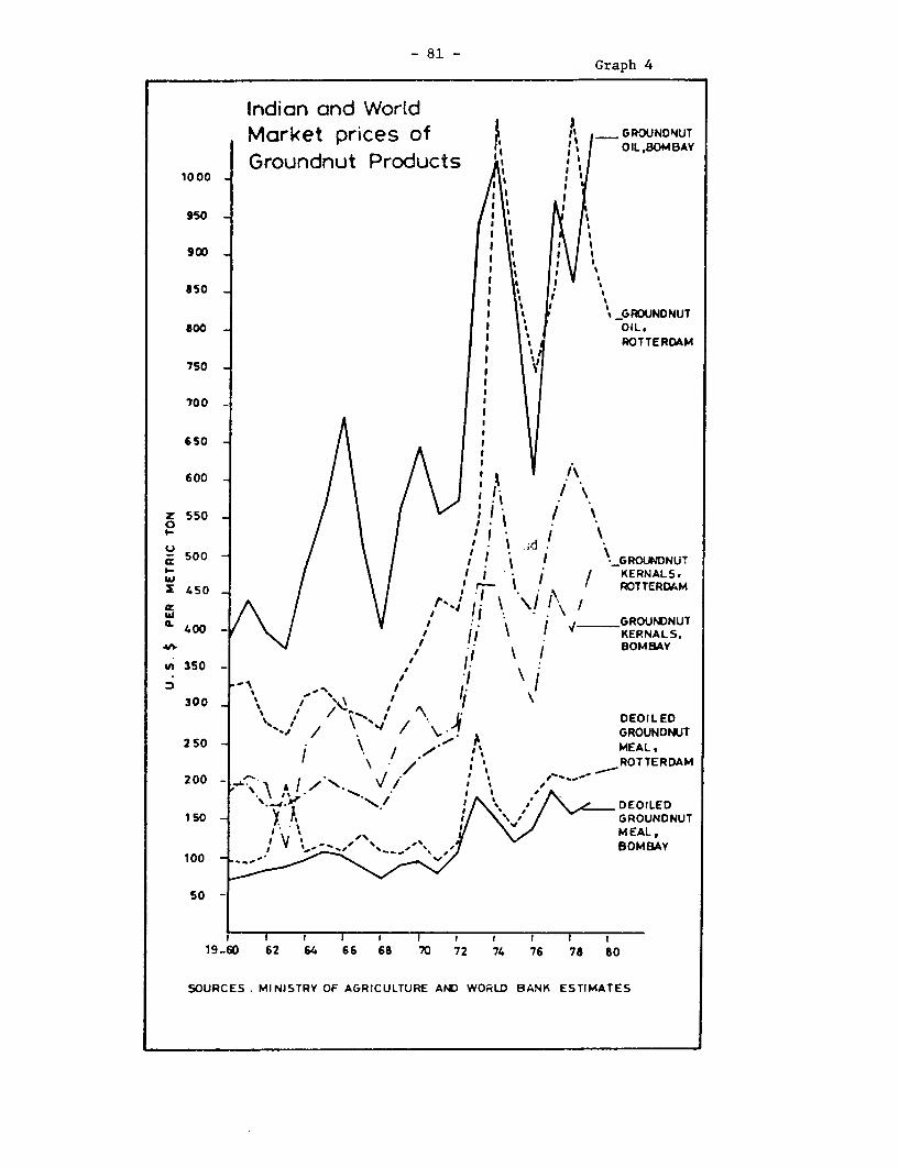
- 81 -Graph 4

Indian and WorldMarket prices of -t _GROUNDNUT

Groundnut Products L,BOMBAY10 00

950

900 I

850 _ \

| 1 % * g _GROUNDNUT800 OIL.

I 450 _/ \ # r 'ROTTERDAM

750 -

700 - D

2650- .X 'ROTRA

600 -

z 550 -0

500 -cc \~~~~~~~~~~~~-~~GROU*4DNUT

I K I I E RNALS.Y 1 60 62" ROTTERDAM

SOURCES . MI Y OF AGROUNDNUTBOMBAY

tn 350 -

300' / \~~~*~~ '\~~~ DEOILED

N' / .'~~~~~ 'V ~GROUNDNUT2 50 10,MEAL.

ROT TERDAM

NI . ' ~~~~~DEOILED150 ~ ~ ~ ~ ~ ~ ~~I /GROUNDNUT

19-60 62 64 66 68 70 72 74 76 78 80

SOURCES. MINISTRY OF AGRICULTURE AND WORLD BANK ESTIMATES

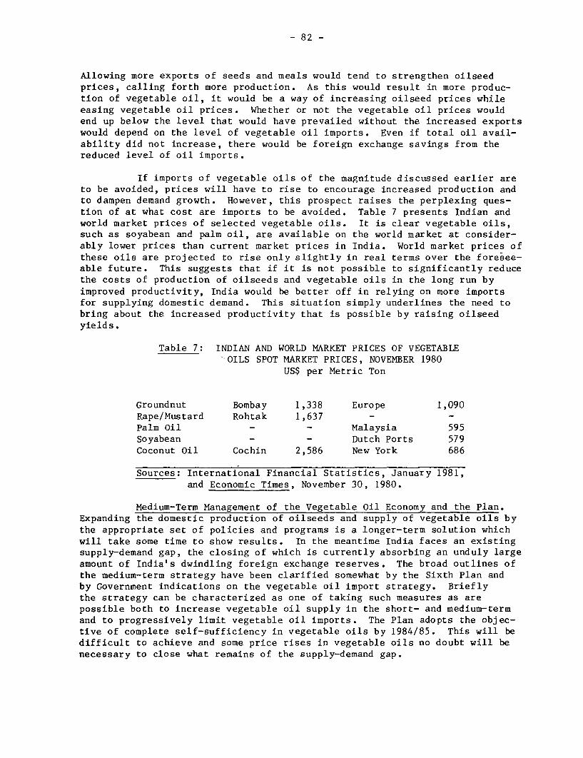
- 82 -

Allowing more exports of seeds and meals would tend to strengthen oilseedprices, calling forth more production. As this would result in more produc-tion of vegetable oil, it would be a way of increasing oilseed prices whileeasing vegetable oil prices. Whether or not the vegetable oil prices wouldend up below the level that would have prevailed without the increased exportswould depend on the level of vegetable oil imports. Even if total oil avail-ability did not increase, there would be foreign exchange savings from thereduced level of oil imports.

If imports of vegetable oils of the magnitude discussed earlier areto be avoided, prices will have to rise to encourage increased production andto dampen demand growth. However, this prospect raises the perplexing ques-tion of at what cost are imports to be avoided. Table 7 presents Indian andworld market prices of selected vegetable oils. It is clear vegetable oils,such as soyabean and palm oil, are available on the world market at consider-ably lower prices than current market prices in India. World market prices ofthese oils are projected to rise only slightly in real terms over the foresee-able future. This suggests that if it is not possible to significantly reducethe costs of production of oilseeds and vegetable oils in the long run byimproved productivity, India would be better off in relying on more importsfor supplying domestic demand. This situation simply underlines the need tobring about the increased productivity that is possible by raising oilseedyields.

Table 7: INDIAN AND WORLD MARKET PRICES OF VEGETABLE"OILS SPOT MARKET PRICES, NOVEMBER 1980

US$ per Metric Ton

Groundnut Bombay 1,338 Europe 1,090Rape/Mustard Rohtak 1,637 - -

Palm Oil - - Malaysia 595Soyabean - - Dutch Ports 579Coconut Oil Cochin 2,586 New York 686

Sources: International Financial Statistics, January 1981,and Economic Times, November 30, 1980.

Medium-Term Management of the Vegetable Oil Economy and the Plan.Expanding the domestic production of oilseeds and supply of vegetable oils bythe appropriate set of policies and programs is a longer-term solution whichwill take some time to show results. In the meantime India faces an existingsupply-demand gap, the closing of which is currently absorbing an unduly largeamount of India's dwindling foreign exchange reserves. The broad outlines ofthe medium-term strategy have been clarified somewhat by the Sixth Plan andby Government indications on the vegetable oil import strategy. Brieflythe strategy can be characterized as one of taking such measures as arepossible both to increase vegetable oil supply in the short- and medium-termand to progressively limit vegetable oil imports. The Plan adopts the objec-tive of complete self-sufficiency in vegetable oils by 1984/85. This will bedifficult to achieve and some price rises in vegetable oils no doubt will benecessary to close what remains of the supply-demand gap.

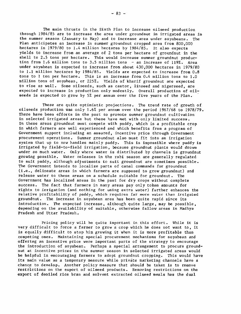
- 83 -

The main thrusts in the Sixth Plan to increase oilseed productionthrough 1984/85 are to increase the area under groundnut in irrigated areas inthe summer season (January to May) and to increase area under soyabeans. ThePlan anticipates an increase in summer groundnut cropped area from 800,000hectares in 1979/80 to 1.4 million hectares by 1984/85. It also expectsyields to increase from an average of 2 tons per hectare of groundnut in theshell to 2.5 tons per hectare. This would increase summer groundnut produc-tion from 1.6 million tons to 3.5 million tons - an increase of 119%. Areaunder soyabean is expected to increase from about 430,000 hectares in 1979/80to 1.1 million hectares by 1984/85. Yields are expected to increase from 0.8tons to 1 ton per hectare. This is an increase from 0.4 million tons to 1.0million tons of soyabean, or 225%. Yields of kharif groundnut are expectedto rise as well. Some oilseeds, such as castor, linseed and nigerseed, areexpected to increase in production only modestly. Overall production of oil-seeds is expected to grow by 5% per annum over the five years of the Plan.

These are quite optimistic projections. The trend rate of growth ofoilseeds production was only 1.6% per annum over the period 1967/68 to 1978/79.There have been efforts in the past to promote summer groundnut cultivationin selected irrigated areas but these have met with only limited success.In these areas groundnut must compete with paddy, which is a profitable cropin which farmers are well experienced and which benefits from a program ofGovernment support including an assured, incentive price through Governmentprocurement operations. Summer groundnut also must fit into an irrigationsystem that up to now handles mainly paddy. This is impossible where paddy isirrigated by field-to-field irrigation, because groundnut plants would drownunder so much water. Only where water is distributed by channels is groundnutgrowing possible. Water releases in the rabi season are generally regulatedto suit paddy, although adjustments to suit groundnut are sometimes possible.The Government intends to localize parts of canal commands for groundnut(i.e., delineate areas in which farmers are supposed to grow groundnut) andrelease water to these areas on a schedule suitable for groundnut. TheGovernment has localized areas in the past for dry crops without completesuccess. The fact that farmers in many areas pay only token amounts forrights to irrigation (and nothing for using extra water) further enhances therelative profitability of paddy, which requires far more water than irrigatedgroundnut. The increase in soyabean area has been quite rapid since itsintroduction. The expected increase, although quite large, may be possible,depending on the availability of suitable, otherwise fallow areas in MadhyaPradesh and Uttar Pradesh.

Pricing policy will be quite important in this effort. While it isvery difficult to force a farmer to grow a crop which he does not want to, itis equally difficult to stop him growing it when it is more profitable thancompeting ones. Maintaining special procurement mechanisms for soyabean andoffering an incentive price were important parts of the strategy to encouragethe introduction of soyabean. Perhaps a special arrangement to procure ground-nut at incentive prices in the summer season in selected irrigated areas wouldbe helpful in encouraging farmers to adopt groundnut cropping. This would haveits main value as a temporary measure while private marketing channels have achance to develop. Another policy measure that should be taken is to removerestrictions on the export of oilseed products. Removing restrictions on theexport of deoiled rice bran and solvent extracted oilseed meals has the dual

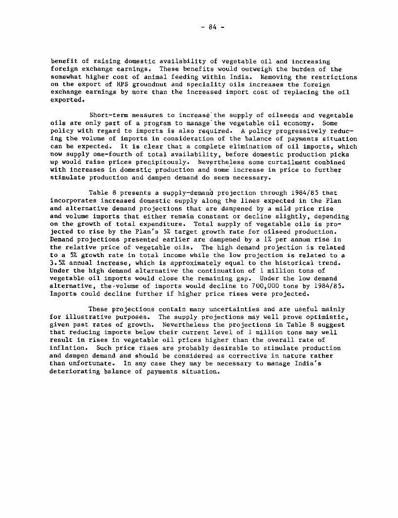
- 84 -

benefit of raising domestic availability of vegetable oil and increasingforeign exchange earnings. These benefits would outweigh the burden of thesomewhat higher cost of animal feeding within India. Removing the restrictionson the export of HPS groundnut and speciality oils increases the foreignexchange earnings by more than the increased import cost of replacing the oilexported.

Short-term measures to increase the supply of oilseeds and vegetableoils are only part of a program to manage the vegetable oil economy. Somepolicy with regard to imports is also required. A policy progressively reduc-ing the volume of imports in consideration of the balance of payments situationcan be expected. It is clear that a complete elimination of oil imports, whichnow supply one-fourth of total availability, before domestic production picksup would raise prices precipitously. Nevertheless some curtailment combinedwith increases in domestic production and some increase in price to furtherstimulate production and dampen demand do seem necessary.

Table 8 presents a supply-demand projection through 1984/85 thatincorporates increased domestic supply along the lines expected in the Planand alternative demand projections that are dampened by a mild price riseand volume imports that either remain constant or decline slightly, dependingon the growth of total expenditure. Total supply of vegetable oils is pro-jected to rise by the Plan's 5% target growth rate for oilseed production.Demand projections presented earlier are dampened by a 1% per annum rise inthe relative price of vegetable oils. The high demand projection is relatedto a 5% growth rate in total income while the low projection is related to a3.5% annual increase, which is approximately equal to the historical trend.Under the high demand alternative the continuation of 1 million tons ofvegetable oil imports would close the remaining gap. Under the low demandalternative, the-volume of imports would decline to 700,000 tons by 1984/85.Imports could decline further if higher price rises were projected.

These projections contain many uncertainties and are useful mainlyfor illustrative purposes. The supply projections may well prove optimistic,given past rates of growth. Nevertheless the projections in Table 8 suggestthat reducing imports below their current level of 1 million tons may wellresult in rises in vegetable oil prices higher than the overall rate ofinflation. Such price rises are probably desirable to stimulate productionand dampen demand and should be considered as corrective in nature ratherthan unfortunate. In any case they may be necessary to manage India'sdeteriorating balance of payments situation.

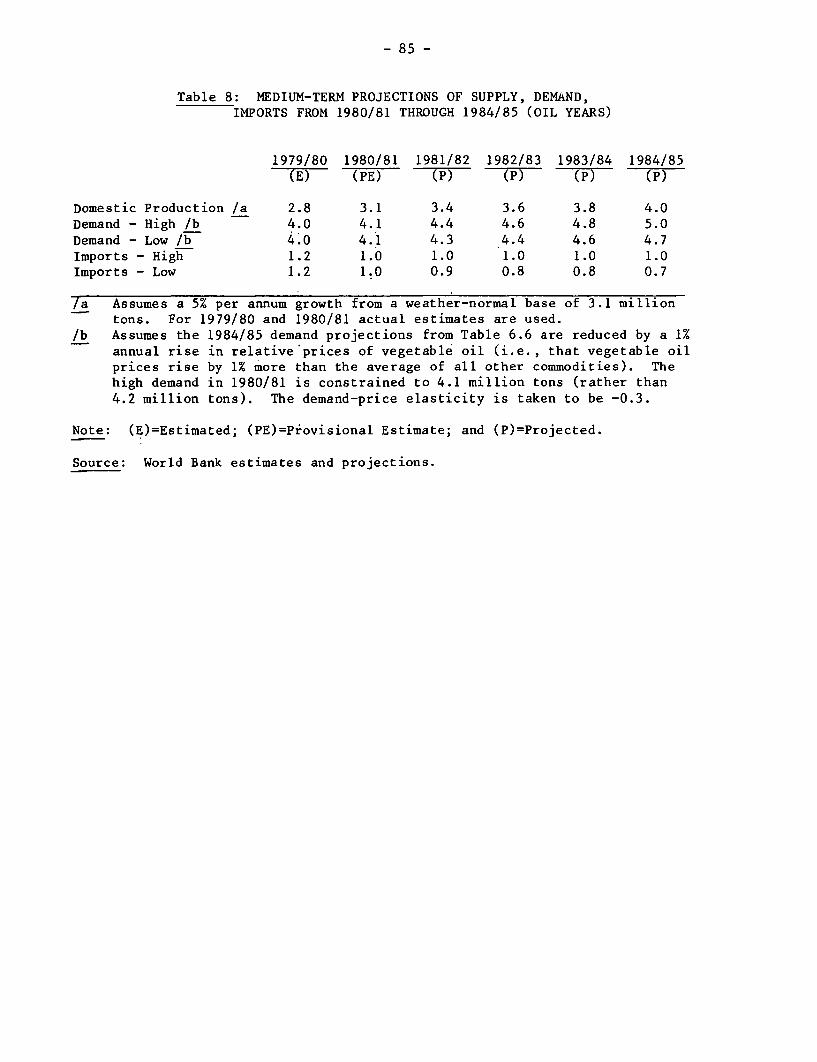
- 85 -

Table 8: MEDIUM-TERM PROJECTIONS OF SUPPLY, DEMAND,IMPORTS FROM 1980/81 THROUGH 1984/85 (OIL YEARS)

1979/80 1980/81 1981/82 1982/83 1983/84 1984/85(E) (-PE-) (P) -(P-) -(P)T -(-P)

Domestic Production /a 2.8 3.1 3.4 3.6 3.8 4.0Demand - High /b 4.0 4.1 4.4 4.6 4.8 5.0Demand - Low lb 4.0 4.1 4.3 4.4 4.6 4.7Imports - High 1.2 1.0 1.0 1.0 1.0 1.0Imports - Low 1.2 1.0 0.9 0.8 0.8 0.7

/a Assumes a 5% per annum growth from a weather-normal base of 3.1 milliontons. For 1979/80 and 1980/81 actual estimates are used.

lb Assumes the 1984/85 demand projections from Table 6.6 are reduced by a 1%

annual rise in relative'prices of vegetable oil (i.e., that vegetable oil

prices rise by 1% more than the average of all other commodities). The

high demand in 1980/81 is constrained to 4.1 million tons (rather than

4.2 million tons). The demand-price elasticity is taken to be -0.3.

Note: (E)=Estimated; (PE)=Provisional Estimate; and (P)=Projected.

Source: World Bank estimates and projections.

Annex TABLE IA Domestic Availability of Vegetable Oils

1960 to 1980

Per Capita Availability of Vegetable OilsNon-Edible Non-Edible

Calender Year Edible Oils b/ Oils b/ Total b/ Population a/ Edible Oils Oils Total(million kgs) (million kgs) (million kgs) (millions) (kgs) (kgs) (kgs)

1961 1954 109 2063 443.935 4.402 0.246 4.6471962 1986 150 2136 454.379 4.371 0.330 4.7011963 1996 132 2128 465.093 4.292 0.284 4.5751964 1891 115 2006 476.091 3.972 0.242 4.2131965 2370 166 2536 487.324 4.863 0.341 5.2041966 1862 1L6 1978 498.831 3.733 0.233 3.9651967 1887 109 -1996 510.536 3.696 0.214 3.9101968 2355 158 2513 522.555 4.507 0.302 4.8091969 1999 104 2103 534.895 3.737 0.194 3.9321970 2247 219 2466 547.569 4.104 0.400 4.5041971 2711 252 2963 560.119 4.840 0.450 5.2901972 2468 284 2752 571.613 4.318 0.497 4.8141973 2166 224 2390 583.429 3.713 0.384 4.0961974 2715 288 3003 595.579 4.559 0.484 5.0421975 2622 297 2919 608.072 4.312 0.488 4.8001976 2899 284 3183 620.440 4.672 0.458 5.130 g1977 2789 270 3059 631.726 4.415 0.427 4.8421978 3845 382 4227 643.896 5.971 0.593 6.5651979 N 3864 440 4304 658.066 5.872 0.669 6.5411980 c/ 3640 357 3997 672.235 5.415 0.531 5.946

a/ World Bank estimates.

b/ This may not tally strictly with the figures given in Table IA due to rounding off errors.

c/ Calculated by assuming edible oil imports wer 1130 million kgs in 1978/79 and 1200 million kgs in 1979/80and assuming no non-edible oil imports.

Sources for Tables IA through ID: Ministry of Agriculture, DCGIS Trade Data and World Bank estimates.

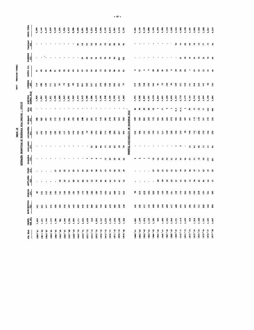
- B7 -

-O - - - C - s - - - - -

. a . . .C . . . . . .. 4 C - - C - _ - - -

- - - - C I -N - A N N - - - - 4 C N N C C N C 4

C , -I

n .

4 4. . . . . - - - - - - - - - - - C -

°- - - - - - - - - - - - - - - - ---- ---- -

8 C C C I iN 8 C N C C N~~~~~P C C C

- N C - - - - - - N C N d _--No - ,, ,, .-. . - r

C N * q . , i N r Cs N N C C )¢s..*..............

" ~~~~~~~~4 N N ° C 8 N N C N r NrX^r as^-s...............e .̂ -^s^"^^

8° --------- ........ --------

C- N g * N g° .... .. .. .. .. .... C n N N C sr°-gs-°C C . . . . . . . . / /.............................................. , N N ~. 4 NN . N 8...... 1<>w- - N 0V1

g l ........ ^<- ~o r3 w4 S V < <Z" ........................................C....C.. oN...- . . . C°O N N N NS N N_ N N N_ >i

* N - C C N C C - C N C C C C C - C _ C C N N C C N C C - C C N C N - C

_ _ _ _ _ _ _ _ _ _ _ _ _ _ _ _ _ _ C_C C_ _ _ _ _ _ __C N_C C_ _C_ _N_ _C_ C N

N N C N Cs * Ni * N 4i N N C C N C CsN . 4 4 N N C 4 . C 4 N C C s w eg > 3 b S u o > t

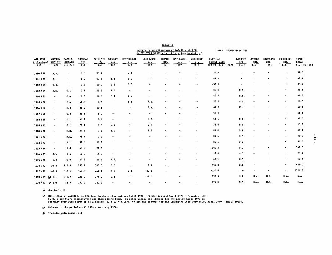
TABLE IC

IMPORTS OF VEGETABLE OILS 1960/61 - 1978/79 Unit, THOUSAND TONNESON OIL YEAR BASIS (i.e Julv - June basis) a/

OIL YEAR GROUND RAPE & SOYBEAN PALM OIL COCONUT COTTONSEED SUNFLOWER SESAME SAFFLOWER NICERSEED SUBTOTAL LINSEED CASTOR RICEBRAN TREECROP GRAND(July-June) NUT OIL MUSTARD OIL 4/ OIL OIL OIL OIL OIL OIL EDIBLE OILS OIL OIL OIL OIL TOTAL

(1) (2) OIL (3) (4) (5) (6) (7) (8) (9) (10) (11) (2) to (11) = (12) -TIT 14) (TT5) (16) (T2co (16)

1960/61 N.S. - 0 5 33.7 - 0.3 - - - - 34.5 - - 34.5

1961 /62 0.1 _ 1.7 37 B 1.1 1.0 - _ _ 41 7 - - _ _ 41.7

1962 /63 N.S. - 0.7 29.2 3.6 0.6 - - - - .34.1 - - - 34.1

1963/64 N.S. 0.1 2.1 35.5 1.1 - _ _ _ 38 B N.S. - _ _ 38.8

1964/65 - 0.4 17.6 24 6 0.1 2.0 _ _ 44 7 N.S. - - - 44.7

1965 /66 - 0.4 42.9 6.9 - 6.1 N.S. _ _ _ 56.3 N,S. - _ _ 56.3

1966/67 - 0.3 31.9 10.6 - - N,.S _ _ _ 42 8 N.S. - _ 42.8

1967 /68 - 0.3 49.8 5.0 - - - _ _ 55.1 - - _ 55.1

1968/69 - 01 50.7 0.6 - - N,5. - - - 51 4 NS, - - - 51.4

1969/70 - 0.1 74.1 0.3 0.4 - 09 - 7 _ 15.8 N.S. - _ _ 75.8

1970 /71 - N,s, 84.6 0 5 1.1 _ 2.8 _ _ 89 0 0 1 - - _ 89 1

1971 /72 - N.S. 88.7 0.7 - - - - - - 89 4 0.3 - - - 89.7

1972 /73 - 7.1 52.8 24.2 - - - - - - 84.1 0 2 - _ 84.3

1973 /74 - 21 0 49.0 72.3 - - - - - _ 142 3 0.2 - - - 142 5

1974 /75 0.5 1 5 12.0 14 9 - - - _ 28.9 0 3 - _ 29.2

1975 /76 6.2 10 0 24 6 21.3 N.S. - - _ _ 62.1 0.5 - - - 62 6

1976 /77 35 2 113.2 152.4 145 0 5.3 - 7.1 - _ _ 458.2 0.8 - - - 459.0

1977 /78 66 9 352.6 347.0 444.4 16 5 0.1 29 1 - - 1256.6 1.0 - _ _ 1257 6

1978 /79 bj 8.1 213.2 331.2 375.0 2.8 - 23.0 - - - 953.3 N.A N A. N.A. N A. N.A.

1979/80 c/ 3.0 88 7 250.0 282.3 - - - 624.0 N.A. N.A. N.A. N.A. N.A.

a/ See Table ID.

b/ Calculated by aultiplying the imports during the periods April 1978 - March 1979 and April 1979 - February 1980by 0.75 and 0.273 respectively and then adding them. In other vords, the figures for the period April 1979 toFebruary 1980 were blown up by a factor (12 e 11 - 1.0909) to get the figures for the financial year 1980 (i.e. April 1979 - March 1980).

c/ Relates to the period April 1979 - February 1980.

df Includes palm kernel oil.

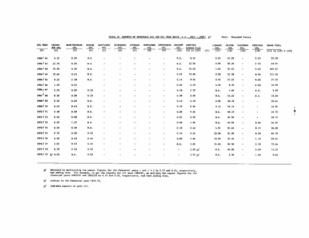
TABLE ID EXPORTS OF VEGETABLE OIL (ON OIL YEAR BASIS, i e, JULY - JUNE) a/ Unit: Thousand Tonnes

OIL YEAR GROUND RAPE/11USTARD SESAME SAFFLOWER NIGERSEED SOYBEAN SUNFLOWER COTTONSEED COCONUT SUBTOTAL LINSEED CASTOR RICEBRAN TREECROP GRAND TOTALNUT OIL OIL OIL OIL OIL OIL OIL OIL OIL EDIBLE OILS OIL OIL OIL OIL

(1) (2) (3) (4) (5) (6) (7) (8) (9) (10) (2) to (10) (11) (12) (13) (14) (15) (11) to (15). (16)

1960/ 61 8.15 0.20 N.S. - - - - N.S. 8.35 5.65 41.25 - 0.03 55.28

1961/ 62 22.75 0.20 N.S. - - - - - N.S. 22.95 0.80 26.20 - 0 02 49.97

1962/ 63 70.83 0 20 N.S. - - - N.S. 71.03 1.03 31.43 - 0.02 103 51

1963/ 64 78.60 0.23 N.S. - - - - - 0.03 78.86 0.88 31.38 - 0.04 111.16

1964/ 65 8.53 0 38 N.S. - - - - - 0.13 9 04 0.93 17.23 - 0.02 27.22

1965/ 66 1.50 0.53 - - - - _ 0.20 2.23 0.30 8.30 - 0.02 10 85

1966/ 67 0.75 0.30 0.10 - - - - _ 0.18 1 33 N.S. 1.85 - N.S. 3.18

1967/ 68 0.25 0.38 0.10 - - _ _ 0.10 0.83 N.S. 14.23 - N.S. 15.06

1968/ 69 0.10 0.58 N.S. - - - - - 0.10 0.78 0.05 30.78 - - 31.61

1969/ 70 0.13 0.43 N.S. - - - - - 0.10 0 66 0.15 14.10 - - 14 91

1970/71 0.18 0.28 N.S. - - - - - 0.08 0.54 N.S. 16.18 - - 16 72

1971/ 72 0.10 0.80 N.S. - - - - - 0.02 0.92 N.S. 24 85 - - 25 77

1972/ 73 0.10 1.33 N.S. - - - - - 0.48 1.91 N.S. 43.05 - 0.01 44.97

1973/ 74 0.10 0.20 N.S. - - - - - 010 0.40 4.91 31.43 - 0.15 36.85

1974/ 75 0 10 0.20 0.15 - - - - - 0.10 0.55 22.06 21.00 - 0.58 44 19

1975/76 0.93 0.18 0.45 - - - - - 0.08 1.64 32.50 27.35 - 1.12 62.61

1976/ 77 2.63 0.13 0.10 - - _- - N.S. 2.86 31.58 34 98 - 2.30 71.66

1977/ 78 0.33 0 15 0 15 - - - - - - 1.03 c/ N.S, 14.00 - 2.69 17.72

1978/ 79 b/ 0.43 N.S. 0.01 - - - - - - 2 42 S/ N.S. 5.36 - 1.85 9.63

a/ Obtained by multiplying the export figures for the financial years t and t + I by 0.75 and 0.25, respectively,and adding them For example, to get the figures for oil year 1960/61, we multiply the export figures for thefinancial years 1960/61 and 1961/62 by 0.75 and 0.25, respectively, and then adding them,

b/ relates to the financial year 1978-79,

C/ indudes exports of pal. oil.

- 90 -

Table 2A

INDIA - Oilseeds Production - Groundnut

Area Production Yield

Thousand Thousand tons

hectares (in the shell) kg/hectare

1949/50 3979 3433 863

1950/51 4494 3481 7751951/52 4917 3192 649

1952/53 4795 2929 6111953/54 4247 3445 811

1954/55 5541 4245 7661955/56 5133 3862 7521956/57 5532 4369 7831957/58 6420 4710 734

1958/'59 6251 5178 8281559/60 6442 4562 7081960/61 6463 4812 7451961/62 6889 4994 7251962/63 7283 5064 6951963/64 6886 5298 769

1964/65 7376 6004 8141965/66 7698 4263 5541966/67 7299 4411 604

1967/68 7553 5731 7591968/69 7088 4631 6531969/70 7125 5130 7201970/71 7326 6111 8341971/72 7510 6181 8231872/73 6990 4092 5851973/74 7024 5932 8451974/75 7063 5111 7241975/76 7222 6754 9351976/77 7043 5264 7471977/78 7029 6087 8661978/79 (Revised) 7433 6208 8351979/80 (Final) 7238 5772 797

Compound Growth Rates % % %

1949/50-1978/79 1.8 2.0 0.21949/50-1964/65 3.9 4.0 0.11967/68-1978/79 -0.2 1.3 1.51949/50-1979/80 1.7 1.9 0.21967/68-1979/80 -0.1 1.2 1.3

Source: Estimates of Area and Production of Principal Crops in India.1978-79, Ministry of Agriculture and World Bank estimates.

- 91 -

Table 2B

INDIA - Oilseeds Production - Rape & Mustard Seed

Area Production Yield

Thousand Thousand tons

hectares kg/hectare

1949/50 1935 806 4171950/51 2071 762 3681951/52 2401 943 3931952/53 2105 858 4081953/54 2244 872 3891954/55 2439 1037 4251955/56 2556 860 3361956/57 2539 1043 4111957/58 2412 933 3871958/59 2447 1042 4261559/60 2910 1063 3651960/61 2883 1347 4671961/62 3168 1346 4251962/63 3127 1303 4171963/64 3046 915 3001964/65 2910 1474 5071965/66 2913 1298 4461966/67 3006 1228 4081967/68 3244 1568 4831968/69 2870 1347 4691969/70 3172 1564 4931970/71 3323 1976 5941971/72 3614 1433 3961872/73 3319 1808 5451973/74 3457 1704 4931974/75 3680 2252 6121975/76 3339 1936 5801976/77 3129 1551 4961977/78 3584 1650 4601978/79 (Revised) 3544 1860 5251979/80 (Final) 3475 1433 412

Compound Growth Rates % % %

1949/50-1978/79 1.9 3.1 1.31949/50-1964/65 3.0 3.4 0.41965/66-1978/79 1.3 2.6 1.31967/68-1978/79 1.0 1.7 0.71949/50-1979/80 1.8 2.9 1.11965/66-1979/80 1.2 1.8 0.61967/68-1979/80 0.9 0.8 -0.2

Source: Estimates of Area and Production of Principal Crops in India1978-79, Ministry of Agriculture and World Bank estimates.

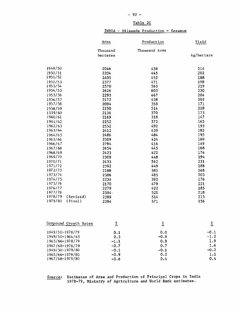
- 92 -

Table 2C

INDIA - Oilseeds Production - Sesamum

Area Production Yield

Thousand Thousand tonshectares kg/hectare

1949/50 2046 438 2141950/51 2204 445 2021951/52 2405 452 1881952/53 2377 471 1981953/54 2570 563 2191954/55 2626 603 2301955/56 2293 467 2041956/57 2172 438 2021957/58 2094 359 1711958/59 2250 514 2281559/60 2136 370 1731960/61 2169 318 1471961/62 2252 372 1651962/63 2552 492 1931963/64 2412 439 1821964/65 2486 484 1951965/66 2509 424 1691966/67 2794 416 1491967/68 2654 445 1681968/69 2423 422 1741969/70 2309 448 1941970/71 2433 562 2311971/72 2392 449 1881872/73 2288 385 1681973/74 2386 485 2031974/75 2234 392 1761975/76 2170 479 2211976/77 2279 422 1851977/78 2384. 520 2181978/79 (Revised) 2389 514 2151979/80 (Final) 2384 371 156

Compound Growth Rates % % %

1949/50-1978/79 0.1 0.0 -0.11949/50-1964/65 0.3 -0.9 -1.21965/66-1978/79 -1.1 0.9 1.91967/68-1978/79 -0.7 0.7 1.61949/50-1979/80 -0.1 -0.1 -0.21965/66-1979/80 -0.9 0.2 1.11967/68-1979/80 -0.6 0.1 0.4

Source: Estimates of Area and Production of Principal Crops in India1978-79, Ministry of Agriculture and World Bank estimates.

- 93 -

Table 2D

INDIA - Oilseeds Production - Linseed

Area Production Yield

Thousand Thousand tonshectares kg/hectare

1949/50 1521 418 2751950/51 1403 367 2621951/52 1380 333 2411952/53 1362 372 2731953/54 1387 385 2781954/55 1361 390 2871955/56 1529 420 2751956/57 1682 390 2321957/58 1283 259 2021958/59 1595 452 2831559/60 1974 446 2261960/61 1789 398 2221961/62 1977 463 2341962/63 1904 430 2261963/64 1995 379 1901964/65 2042 494 2421965/66 1723 331 1921966/67 1495 260 1741967/68 1777 438 2471968/69 1697 329 1941969/70 1803 469 2601970/71 1897 474 2501971/72 2064 529 2561872/73 1726 428 2481973/74 2038 504 2471974/75 2071 564 2721975/76 2119 598 2821976/77 1888 419 2221977/78 2010 527 2621978/79 (Revised) 2092 535 2561979/80 (Final) 1641 270 165

Compound Growth Rates _ % %

1949/50-1978/79 1.4 1.2 -0.21949/50-1964/65 2.9 1.2 -1.61967/68-1978/79 1.5 2.5 1.01949/50-1979/80 1.3 0.8 -0.41967/68-1979/80 0.7 0.1 -0.6

Source: Estimates of Area and Production of Principal Crops in India1978-79, Ministry of Agriculture and World Bank estimates.

- 94 -Table 2E

INDIA - Oilseeds Production - Castorseed

Area Production Yield

Thousand Thousand tonshectares kg/hectare

1949/50 590 130 2201950/51 555 103 1861951/52 582 108 1861952/53 536 104 1941953/54 545 105 1931954/55 555 124 2231955/56 574 125 2181956/57 569 124 2181957/58 447 89 1991958/59 458 112 2451559/60 492 115 2341960/61 466 107 2301961/62 486 109 2241962/63 469 99 2121963/64 484 102 2111964/65 441 107 2421965/66 405 80 1991966/67 401 110 2741967/68 439 121 2761968/69 394 116 2941969/70 402 123 3061970/71 439 136 3101971/72 453 154 3401872/73 426 145 3411973/74 546 229 4191974/75 590 210 3561975/76 375 143 3811976/77 496 179 3611977/78 380 217 5721978/79 (Revised) 447 229 5121979/80 (Final) 438 233 532

Compound Growth Rates % % %

1949/50-1978/79 -1.0 2.1 3.11949/50-1964/65 -1.8 0.7 1.11967/68-1978/79 0.6 5.9 5.41949/50-1979/80 -0.9 2.3 3.21967/68-1979/80 0.4 5.9 5.5

Source: Estimates of Area and Production of Principal Crops in India1978-79, Ministry of Agriculture and World Bank estimates.

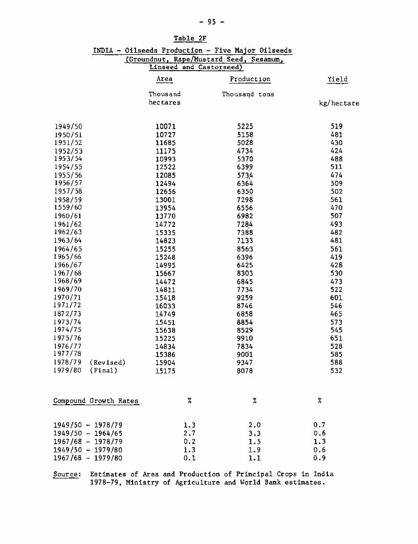
- 95 -

Table 2F

INDIA - Oilseeds Production - Five Major Oilseeds(Groundnut, Rape/Mustard Seed, Sesamum,

Linseed and Castorseed)

Area Production Yield

Thousand Thousand tonshectares kg/hectare

1949/50 10071 5225 5191950/51 10727 5158 4811951/52 11685 5028 4301952/53 11175 4734 4241953/54 10993 5370 4881954/55 12522 639,9 5111955/56 12085 573,4 4741956/57 12494 6364 5091957/58 12656 6350 5021958/59 13001 7298 5611559/60 13954 6556 4701960/61 13770 6982 5071961/62 14772 7284 4931962/63 15335 7388 4821963/64 14823 7133 4811964/65 15255 856,3 5611965/66 15248 6396 4191966/67 14995 6425 4281967/68 15667 8303 5301968/69 14472 6845 4731969/70 14811 7734 5221970/71 15418 9259 6011971/72 16033 8746 5461872/73 14749 6858 4651973/74 15451 8854 5731974/75 15638 8529 5451975/76 15225 9910 6511976/77 14834 7834 5281977/78 15386 9001 5851978/79 (Revised) 15904 9347 5881979/80 (Final) 15175 8078 532

Compound Growth Rates % % %

1949/50 - 1978/79 1.3 2.0 0.71949/50 - 1964/65 2.7 3.3 0.61967/68 - 1978/79 0.2 1.5 1.31949/50 - 1979/80 1.3 1.9 0.61967/68 - 1979/80 0.1 1.1 0.9

Source: Estimates of Area and Production of Principal Crops in India1978-79, Ministry of Agriculture and World Bank estimates.

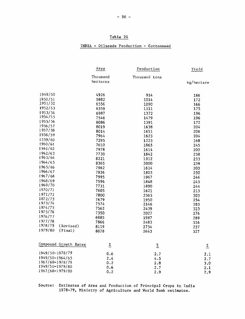
- 96 -

Table 2G

INDIA - Oilseeds Production - Cottonseed

Area Production Yield

Thousand Thousand tonshectares kg/hectare

1949/50 4926 914 1861950/51 5882 1014 1721951/52 6556 1090 1661952/53 6359 1111 1751953/54 6987 1372 1961954/55 7546 1479 1961955/56 8086 1391 1721956/57 8019 1638 2041957/58 8014 1651 2061958/59 7964 1623 2041559/60 7295 1223 1681960/61 7610 1865 2451961/62 7978 1614 2021962/63 7730 1842 2381963/64 8221 1912 2331964/65 8365 2000 2391965/66 7962 1614 2031966/67 7836 1803 2301967/68 7995 1967 2461968/69 7596 1848 2431969/70 7731 1890 2441970/71 7605 1621 2131971/72 7800 2363 3031872/73 7679 1950 2541973/74 7574 2146 2831974/75 7562 2439 3231975/76 7350 2027 2761976/77 6885 1987 2891977/78 7866 2483 3161978/79 (Revised) 8119 2734 2371979/80 (Final) 8078 2643 327

Compound Growth Rates _ % %

1949/50-1978/79 0.6 2.7 2.11949/50-1964/65 2.4 4.5 2.71967/68-1978/79 0.2 2.8 3.01949/50-1979/80 0.6 2.7 2.11967/68-i979/80 0.2 2.9 2.9

Source: Estimates of Area and Production of Principal Crops in India1978-79, Ministry of Agriculture and World Bank estimates.

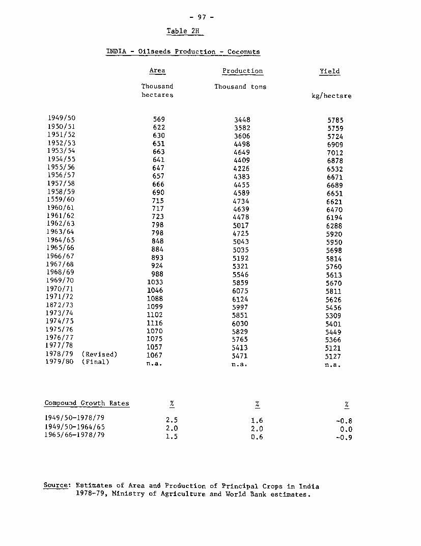
- 97 -

Table 2H

INDIA - Oilseeds Production - Coconuts

Area Production Yield

Thousand Thousand tonshectares kg/hectare

1949/50 569 3448 57851950/51 622 3582 57591951/52 630 3606 57241952/53 651 4498 69091953/54 663 4649 70121954/55 641 4409 68781955/56 647 4226 65321956/57 657 4383 66711957/58 666 4455 66891958/59 690 4589 66511559/60 715 4734 66211960/61 717 4639 64701961/62 723 4478 61941962/63 798 5017 62881963/64 798 4725 59201964/65 848 5043 59501965/66 884 5035 56981966/67 893 5192 58141967/68 924 5321 57601968/69 988 5546 56131969/70 1033 5859 56701970/71 1046 6075 58111971/72 1088 6124 56261872/73 1099 5997 54561973/74 1102 5851 53091974/75 1116 6030 54011975/76 1070 5829 54491976/77 1075 5765 53661977/78 1057 5413 51211978/79 (Revised) 1067 5471 51271979/80 (Final) n.a. n.a. n.a.

Compound Growth Rates % %

1949/50-1978/79 2.5 1.6 -0.81949/50-1964/65 2.0 2.0 0.01965/66-1978/79 1.5 0.6 -0.9

Source: Estimates of Area and Production of Principal Crops in India1978-79, Ministry of Agriculture and World Bank estimates.

- 98 -

Table 2I

INDIA - Oilseeds Production - Nigerseed

Area Production Yield

Thousand Thousand tonshectares kg/hectare

1964/65 487 97 1991965/66 522 91 1731966/67 473 79 1661967/68 468 98 2091968/69 441 89 2031969/70 482 98 2031970/71 489 128 2611971/72 494 116 2351972/73 467 93 1981973/74 552 136 2461974/75 621 132 2131975/76 615 151 2451976/77 568 113 1991977/78 (Revised) 609 148 2431978/79 (Revised) 612 147 2401979/80 (Final) 576 96 167

Compound Growth Rates % % %

1964/65-1978/79 2.1 3.9 1.81967/68-1978/79 3.1 4.1 0.91964/65-1979/80 1.9 2.9 1.01967/68-1979/80 2.7 2.5 -0.2

Source: Estimates of Area and Production of Principal Crops in India1978-79, Ministry of Agriculture and World Bank estimates.

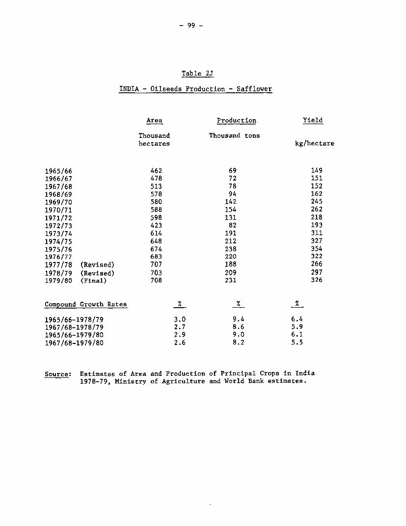
- 99 -

Table 2J

INDIA - Oilseeds Production - Safflower

Area Production Yield

Thousand Thousand tonshectares kg/hectare

1965/66 462 69 1491966/67 478 72 1511967/68 513 78 1521968/69 578 94 1621969/70 580 142 2451970/71 588 154 2621971/72 598 131 2181972/73 423 82 1931973/74 614 191 3111974/75 648 212 3271975/76 674 238 3541976/77 683 220 3221977/78 (Revised) 707 188 2661978/79 (Revised) 703 209 2971979/80 (Final) 708 231 326

Compound Growth Rates % % %

1965/66-1978/79 3.0 9.4 6.41967/68-1978/79 2.7 8.6 5.91965/66-1979/80 2.9 9.0 6.11967/68-1979/80 2.6 8.2 5.5

Source: Estimates of Area and Production of Principal Crops in India1978-79, Ministry of Agriculture and World Bank estimates.

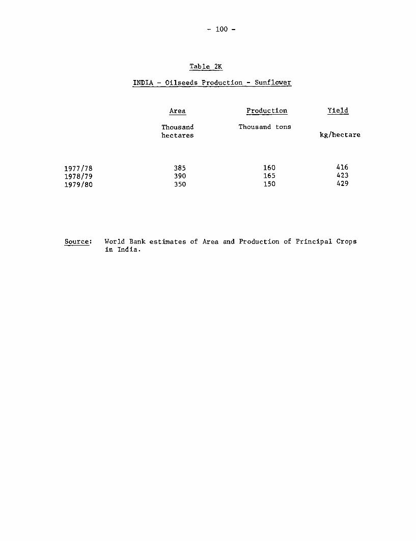
- 100 -

Table 2K

INDIA - Oilseeds Production - Sunflower

Area Production Yield

Thousand Thousand tonshectares kg/hectare

1977/78 385 160 4161978/79 390 165 4231979/80 350 150 429

Source: World Bank estimates of Area and Production of Principal Cropsin India.

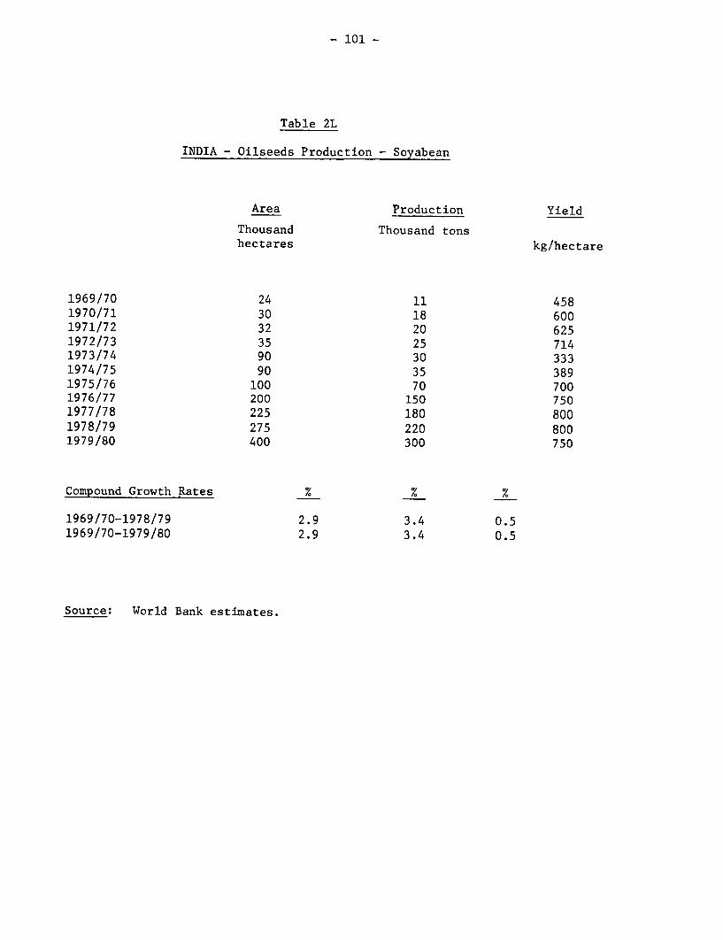
- 101 -

Table 2L

INDIA - Oilseeds Production - Soyabean

Area Production Yield

Thousand Thousand tonshectares kg/hectare

1969/70 24 11 4581970/71 30 18 6001971/72 32 20 6251972/73 35 25 7141973/74 90 30 3331974/75 90 35 3891975/76 100 70 7001976/77 200 150 7501977/78 225 180 8001978/79 275 220 8001979/80 400 300 750

Compound Growth Rates % %

1969/70-1978/79 2.9 3.4 0.51969/70-1979/80 2.9 3.4 0.5

Source: World Bank estimates.

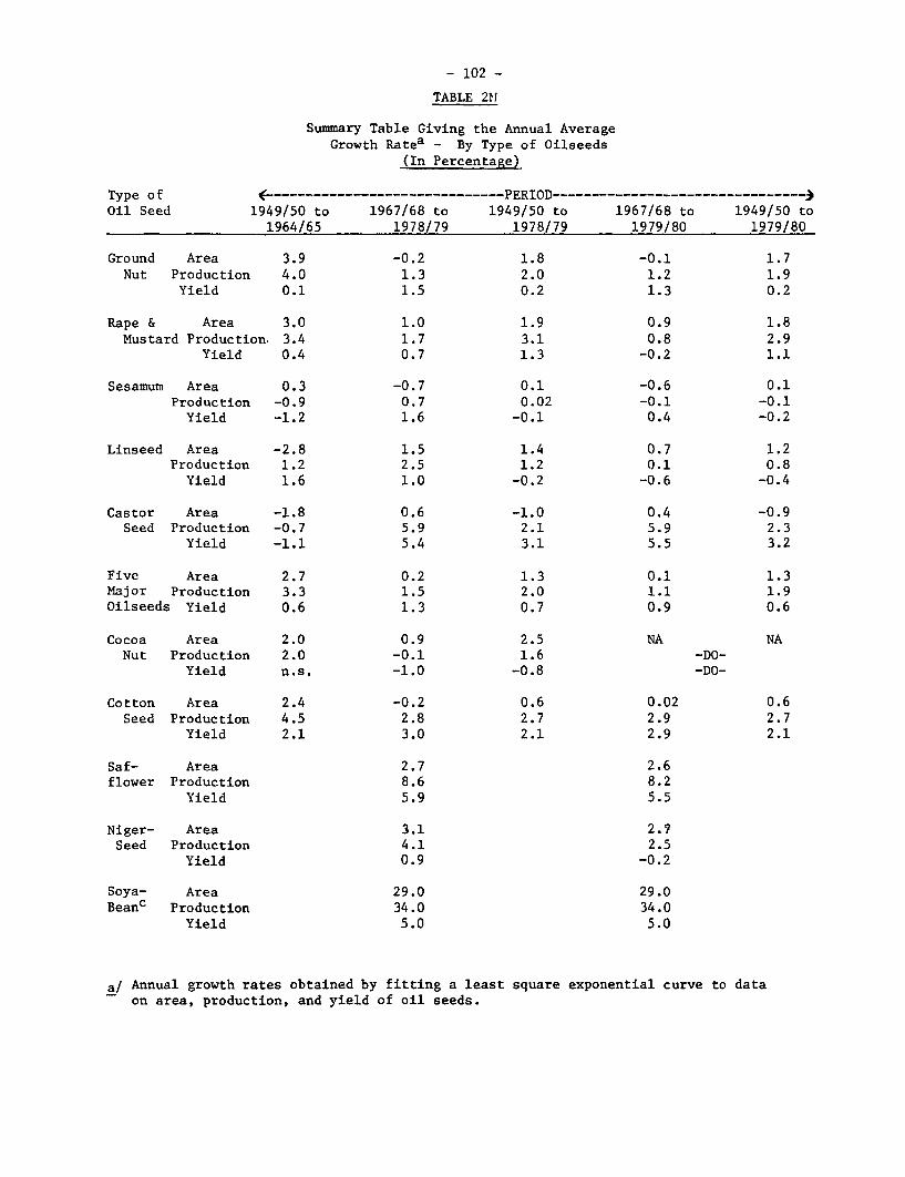
- 102 -

TABLE 211

Summary Table Giving the Annual AverageGrowth Ratea - By Type of Oilseeds

(In Percentage)

Type of (…------------------------PERIOD…--------_-______________________

Oil Seed 1949/50 to 1967/68 to 1949/50 to 1967/68 to 1949/50 to1964/65 1978/79 1978/79 1979/80 1979/80

Ground Area 3.9 -0.2 1.8 -0.1 1.7Nut Production 4.0 1.3 2.0 1.2 1.9

Yield 0.1 1.5 0.2 1.3 0.2

Rape & Area 3.0 1.0 1.9 0.9 1.8Mustard Production. 3.4 1.7 3.1 0.8 2.9

Yield 0.4 0.7 1.3 -0.2 1.1

Sesamum Area 0.3 -0.7 0.1 -0.6 0.1Production -0.9 0.7 0.02 -0.1 -0.1

Yield -1.2 1.6 -0.1 0.4 -0.2

Linseed Area -2.8 1.5 1.4 0.7 1.2Production 1.2 2.5 1.2 0.1 0.8

Yield 1.6 1.0 -0.2 -0.6 -0.4

Castor Area -1.8 0.6 -1.0 0.4 -0.9Seed Production -0.7 5.9 2.1 5.9 2.3

Yield -1.1 5.4 3.1 5.5 3.2

Five Area 2.7 0.2 1.3 0.1 1.3Major Production 3.3 1.5 2.0 1.1 1.9Oilseeds Yield 0.6 1.3 0.7 0.9 0.6

Cocoa Area 2.0 0.9 2.5 NA NANut Production 2.0 -0.1 1.6 -DO-

Yield n.s. -1.0 -0.8 -DO-

Cotton Area 2.4 -0.2 0.6 0.02 0.6Seed Production 4.5 2.8 2.7 2.9 2.7

Yield 2.1 3.0 2.1 2.9 2.1

Saf- Area 2.7 2.6flower Production 8.6 8.2

Yield 5.9 5.5

Niger- Area 3.1 2.7Seed Production 4.1 2.5

Yield 0.9 -0.2

Soya- Area 29.0 29.0Beanc Production 34.0 34.0

Yield 5.0 5.0

a/ Annual growth rates obtained by fitting a least square exponential curve to dataon area, production, and yield of oil seeds.

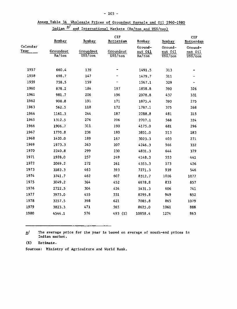
- 103 -

Annex Table 3A Wholesale Prices of Groundnut Kernels and Oil 1960-1980

Indian -/ and International Markets (Rs/ton and US$/ton)

CIF CIFBombay Bombay Rotterdam Bombay Bombay Rotterdam

Calendar Ground- Ground- Ground-Year Groundnut Groundnut Groundnut nut Oil nut Oil nut Oil

Rs/ton US$/ton US$/ton Rs/ton US$/ton US$/ton

1957 660.4 139 - 1491.5 313 -

1958 698.7 147 - 1479.7 311 -

1959 758.5 159 - 1567.1 329 -

1960 878.2 184 197 1858.8 390 326

1961 981.7 206 196 2078.8 437 331

1962 908.8 191 171 1875.4 390 275

1963 562.5 118 172 1787.1 375 268

1964 1161.3 244 187 2288.8 481 315

1965 1312.5 276 206 2707.1 568 324

1966 1906.7 311 190 4175.0 681 296

1967 1770.8 236 180 3851.0 513 283

1968 1420.0 189 167 3023.3 403 271

1969 1973.3 263 207 4246.3 566 332

1970 2240.8 299 230 4831.3 644 379

1971 1928.0 257 249 4148.3 553 441

1972 2069.2 272 261 4353.3 573 426

1973 3583.3 463 393 7271.3 939 546

1974 3741.7 462 607 8312.7 1026 1077

1975 3049.2 364 452 6978.8 833 857

1976 2722.5 304 424 5431.3 606 741

1977 3975.0 455 551 8295.8 949 852

1978 3257.5 398 621 7085.8 865 1079

1979 3823.3 471 565 8625.0 1061 888

1980 4544.1 576 493 (E) 10058.4 1274 863

a/ The average price for the year is based on average of month-end prices inIndian market.

(E) Estimate.

Sources: Ministry of Agriculture and World Bank.

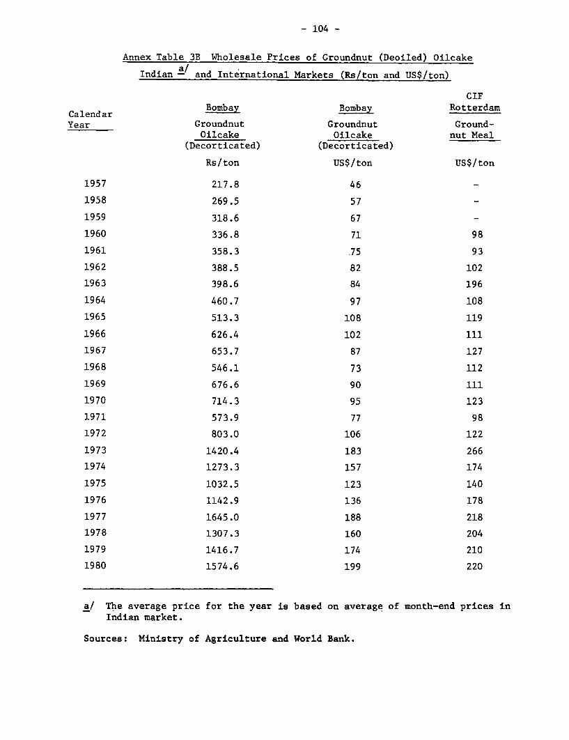
- 104 -

Annex Table 3B Wholesale Prices of Groundnut (Deoiled) Oilcake

Indian -/ and International Markets (Rs/ton and US$/ton)

CIF

Calendar Bombay Bombay Rotterdam

Year Groundnut Groundnut Ground-Oilcake Oilcake nut Meal

(Decorticated) (Decorticated)

Rs/ton US$/ton US$/ton

1957 217.8 46

1958 269.5 57

1959 318.6 67 -

1960 336.8 71 98

1961 358.3 35 93

1962 388.5 82 102

1963 398.6 84 196

1964 460.7 97 108

1965 513.3 108 119

1966 626.4 102 111

1967 653.7 87 127

1968 546.1 73 112

1969 676.6 90 111

1970 714.3 95 123

1971 573.9 77 98

1972 803.0 106 122

1973 1420.4 183 266

1974 1273.3 157 174

1975 1032.5 123 140

1976 1142.9 136 178

1977 1645.0 188 218

1978 1307.3 160 204

1979 1416.7 174 210

1980 1574.6 199 220

a/ The average price for the year is based on average of month-end prices inIndian market.

Sources: Ministry of Agriculture and World Bank.

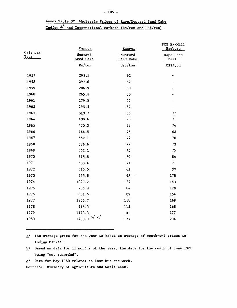
- 105 -

Annex Table 3C Wholesale Prices of Rape/Mustard Seed Cake

Indian and International Markets (Rs/ton and US$/ton)

FOB Ex-MillKanpur Kanpur Hamburg

Calendar Mustard Mustard Rape SeedYear Seed Cake Seed Cake Meal

Rs/ton US$/ton US$/ton

1957 293.1 62

1958 297.6 62

1959 286.9 60

1960 265.8 56

1961 279.5 59

1962 295.5 62

1963 313.7 66 72

1964 430.6 90 71

1965 470.0 99 74

1966 464.5 76 68

1967 552.1 74 70

1968 576.6 77 73

1969 562.1 75 75

1970 515.8 69 84

1971 533.4 71 71

1972 616.5 81 90

1973 755.8 98 178

1974 1029.2 127 143

1975 705.8 84 128

1976 801.6 89 154

1977 1206.7 138 169

1978 916.3 112 168

1979 1143.3 141 177

1980 1400.0 b/ c/ 177 204

a/ The average price for the year is based on average of month-end prices in

Indian Market.

b/ Based on data for 11 months of the year, the date for the month of June 1980

being "not recorded".

c/ Data for May 1980 relates to last but one week.

Sources: Ministry of Agriculture and World Bank.

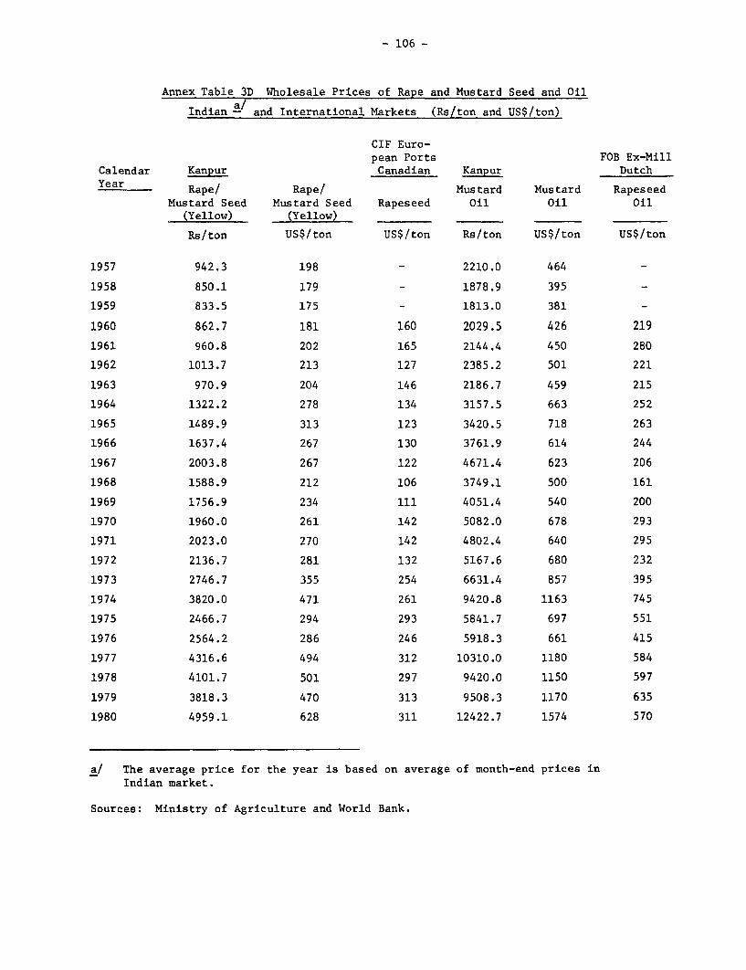
- 106 -

Annex Table 3D Wholesale Prices of Rape and Mustard Seed and Oil

Indian -/ and International Markets (Rs/ton and US$/ton)

CIF Euro-pean Ports FOB Ex-Mill

Calendar Kanpur Canadian Kanpur DutchYear Rape/ Rape/ Mustard Mustard Rapeseed

Mustard Seed Mustard Seed Rapeseed Oil Oil Oil(Yellow) (Yellow)

Rs/ton US$/ton US$/ton Rs/ton US$/ton US$/ton

1957 942.3 198 - 2210.0 464

1958 850.1 179 - 1878.9 395

1959 833.5 175 - 1813.0 381 -

1960 862.7 181 160 2029.5 426 219

1961 960.8 202 165 2144.4 450 280

1962 1013.7 213 127 2385.2 501 221

1963 970.9 204 146 2186.7 459 215

1964 1322.2 278 134 3157.5 663 252

1965 1489.9 313 123 3420.5 718 263

1966 1637.4 267 130 3761.9 614 244

1967 2003.8 267 122 4671.4 623 206

1968 1588.9 212 106 3749.1 500 161

1969 1756.9 234 111 4051.4 540 200

1970 1960.0 261 142 5082.0 678 293

1971 2023.0 270 142 4802.4 640 295

1972 2136.7 281 132 5167.6 680 232

1973 2746.7 355 254 6631.4 857 395

1974 3820.0 471 261 9420.8 1163 745

1975 2466.7 294 293 5841.7 697 551

1976 2564.2 286 246 5918.3 661 415

1977 4316.6 494 312 10310.0 1180 584

1978 4101.7 501 297 9420.0 1150 597

1979 3818.3 470 313 9508.3 1170 635

1980 4959.1 628 311 12422.7 1574 570

a/ The average price for the year is based on average of month-end prices inIndian market.

Sources: Ministry of Agriculture and World Bank.

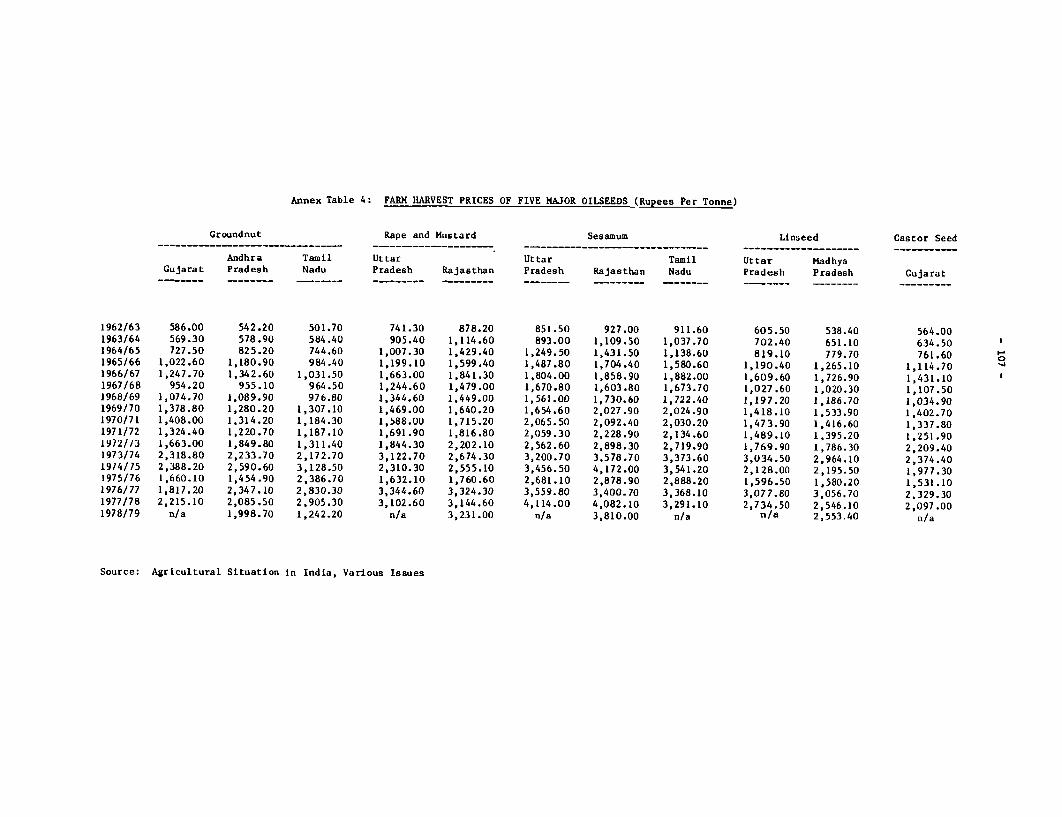
Annex Table 4: FARM HARVEST PRICES OF FIVE MAJOR OILSEEDS (Rupees Per Tonne)

Groundnut Rape and Mustard Sesamum Linseed Castor Seed…_______…__ …-… - ---- - ---- -- --- - -_---_-----__ ___-__ __ __ __-_ __ __-----_-__----_-_ _-- -…-

Andhra Tamil Uttar Uttar Tamil Uttar MadhyaGujarat Pradesh Nadu Pradesh Rajasthan Pradesh Rajasthan Nadu Pradesh Pradesh Cujarat

-- ____ - _____ _ __ __ - - ------ ------- -_ … - ----

1962/63 586.00 542.20 501.70 741.30 878.20 851.50 927.00 911.60 605.50 538.40 564.001963/64 569.30 578.90 584.40 905.40 1,114.60 893.00 1,109.50 1,037.70 702.40 651.10 634.501964/65 727.50 825.20 744.60 1,007.30 1,429.40 1,249.50 1,431.50 1,138.60 819.10 779.70 761.601965/66 1,022.60 1,180.90 984.40 1,199.10 1,599.40 1,487.80 1,704.40 1,580.60 1,190.40 1,265.10 1,114.701966/67 1,247.70 1,342.60 1,031.50 1,663.00 1,841.30 1,804.00 1,858.90 1,882.00 1,609.60 1,726.90 1,431.101967/68 954.20 955.10 964.50 1,244.60 1,479.00 1,670.80 1,603.80 1,673.70 1,027.60 1,020.30 1,107.501968/69 1,074.70 1,089.90 976.80 1,344.60 1,449.00 1,561.00 1,730.60 1,722.40 1,197.20 1,186.70 1,034.901969/70 1,378.80 1,280.20 1,307.10 1,469.00 1,640.20 1,654.60 2,027.90 2,024.90 1,418.10 1,533.90 1,402.701970/71 1,408.00 1,314.20 1,184.30 1,588.00 1,715.20 2,065.50 2,092.40 2,030.20 1,473.90 1,416.60 1,337.801971/72 1,324.40 1,220.70 1,187.10 1,691.90 1,816.80 2,059.30 2,228.90 2,134.60 1,489.10 1,395.20 1,251.901972/73 1,663.00 1,849.80 1,311.40 1,844.30 2,202.10 2,562.60 2,898.30 2,719.90 1,769.90 1,786.30 2,209.401973/74 2,318.80 2,233.70 2,172.70 3,122.70 2,674.30 3,200.70 3,578.70 3,373.60 3,034.50 2,964.10 2,374.401974/75 2,388.20 2,590.60 3,128.50 2,310.30 2,555.10 3,456.50 4,172.00 3,541.20 2,128.00 2,195.50 1,977.301975/76 1,660.10 1,454.90 2,386.70 1,632.10 1,760.60 2,681.10 2,878.90 2,888.20 1,596.50 1,580.20 1,531.101976/77 1,817.20 2,347.10 2,830.30 3,344.60 3,324.30 3,559.80 3,400.70 3,368.10 3,077.80 3,056.70 2,329.301977/78 2,215.10 2,085.50 2,905.30 3,102.60 3,144.60 4,114.00 4,082.10 3,291.10 2,734.50 2,546.10 2,097.001978/79 n/a 1,998.70 1,242.20 n/a 3,231.00 n/a 3,810.00 n/a n/a 2,553.40 n/a

Source: Agricultural Situation in India, Various Issues

PART IV

THE SUGAR ECONOMY

James Q. HarrisonJune 1981

109

- 110 -

The Sugar Economy

Table of Contents

Page No.

The Role and Scope of the Sugar Economy .... ................ 111

Market Structure and Public Policies ....................... 111

Short-Term Market Instability .............................. 113

Long-Term Supply and Demand Trends ......................... 116

Sugar Production and Export ................................ 122

Policy Implications ........................................ 124

Annex . ..................................................... 126

Annex Tables ........... .................................... 130

- ill -

THE SUGAR ECONOMY

1. The Role and Scope of the Sugar Economy. India is the world's lar-gest producer of sugarcane. Although sugarcane covers only 1.8% of India'sgross cultivated area, it is one of the most important non-foodgrain crops,for it contributes about 6.3% of the gross value of agricultural output, about3.5 times as much per hectare as the average of all other crops. About 80% ofthe sugarcane area is irrigated which is equivalent to about 5.6% of India'stotal irrigated area. Fertilizer used on cane was about 84 kg of nutrientsper hectare in 1975/76, about four times the average for all crops. Whilesugarcane is grown in nearly every state, its greatest concentrations are inU.P. and Maharashtra where 45% and 14%,, respectively, of India's cane is pro-duced. Sugarcane is cultivated by about 25% of India's 80 million farmers, onfarms of all sizes, though the proportion of area devoted to cane is somewhathigher on the smaller farms.

2. Sugarcane processing, including the production of mill sugar, khand-sari and gur, is a major industry. It employs nearly 8% of all manufacturingworkers and about 3.6% of the capital invested in manufacturing to produceabout 2% of the total value added in manufacturing. Throughout the two decadesbefore 1980, India has been an exporter of sugar, but exports were generallylow before 1974/75, when they rose rapidly, peaking at levels of over 1 milliontons in 1975/76, providing 12% of India's foreign exchange earnings. Sincethen exports have been much lower and highly volatile. In 1980, India islikely to be a net importer of sugar. Sugar is a large item of personal con-sumption accounting for about 5% of private consumption expenditures. The7.7% weight of sugar products in the wholesale price index suggests its sensi-tive role. In 1979/80, the rise in the prices of sugar products alone accountedfor about 30% of the entire 20% rise in the wholesale price index of all com-modities. Rising prices of sugar thus provoke sharp consumer reactions andgive rise to considerable political controversy. The high volatility of outputand prices which often characterizes the sugar economy in India (and other coun-tries as well) is thus a matter of serious concern. The underlying importanceand visibility of the sugar economy have led to extensive and varied Governmentinterventions in its operations.

3. Market Structure and Public Policies. Virtually all sugar productsin India are based on sugarcane. The structure of the market for sugarcaneand its products and the network of public policies governing sugar productionstrongly influence the performance of the sugar economy. In contrast withmany countries, sugarcane is not grown in large blocks on plantations as amonocrop, but rather in relatively small patches forming a part of the crop-ping pattern of millions of individual farmers. Thus cane production isscattered rather widely among vast numbers of independent farmers who grow arange of other crops. Sugarcane production is highly seasonal with the bulkof the crop in most areas harvested in the December-March period. The sugarcontent of cane in most areas drops sharply with the onset of warmer weather.The sugar content and weight of cane drop rapidly after harvesting, making itnecessary to process the cane as soon as possible, usually within two days ofcutting. The production of sugar products is thus also highly seasonal with70% of sugar being produced between December and March. Cane is a relativelylong-duration crop, standing in the field 9 to 18 months between planting and

- 112 -

harvesting. It is a common practice to allow a second or ratoon crop of caneto grow from the stubble of a harvested field. Thus there is a considerable

time lag between the decision to plant an area under cane and the full effect

of that decision on the supply of cane.

4. An estimated 11-12% of the cane crop is used for seed, animal feed

and direct human consumption, or disappears as post-harvest loss. On average,

about 46% of the crop is used to produce gur, which consists of condensed and

solidified cane juice produced with very simple equipment in rural areas,

often by farmers themselves. Gur typically weighs about 10% of the weight of

the cane used to produce it and contains about 60-65% sucrose. It is by far

the most important sweetener, particularly for the rural population and for

low income consumers. Gur's weight in the wholesale price index is more

than twice that of sugar and nearly ten times that of khandsari, yet it has

attracted the least direct public intervention, a pragmatic recognition that

efforts to control such large numbers of tiny scattered units would be imprac-tical. About 8-9% of the cane crop is used for khandsari, a white crystal

sweetener similar to mill sugar but produced through a smaller-scale, less

technically efficient process. The quality of khandsari is generally consi-

dered inferior to mill sugar and this is reflected in the 15-20% price dif-

ferential between the two products. An average of about 34% of cane crop is

used by large-scale sugar mills to produce sugar, often referred to as "mill

sugar" to distinguish it from other sweeteners. Sugar mills are much larger

in scale than khandsari units (the average sugar mill produces about 20,000

tons of sugar a year while a large khandsari unit produces about 750 tons),

and more efficient physically, extracting 9.5-10.5% of the weight of cane as

sugar compared with 6-7% for khandsari units.

5. Gur and khandsari units are virtually free from controls on the

prices they pay for their cane or the prices they charge for their products.

Gur production is not taxed and while khandsari is taxed, it is at much lower

effective rates than mill sugar (in 1977/78, excise tax revenues on khandsari

were Rs 93 per ton compared with Rs 466 per ton of sugar). Although the sugar

mills are neither the largest consumers of cane nor the major producers of

sweeteners, the importance of their product on the urban market, their size

and their manageably small numbers, have made them the main focus of govern-ment intervention in the sugar economy. The primary instruments of government

control have been: (a) setting a minimum price for cane purchased by the

mills; (b) varying controls over the monthly releases; (c) requiring mills to

sell to the Government a fixed proportion of their production at a fixedprice, usually below the market price; and (d) imposition of excise taxes of

varying levels and partial excise tax rebates. The blend of these various

policies has changed significantly at least ten times since 1960/61 and many

more times than that if one counts changes in the formulae for calculating

the fixed sugar prices or excise taxes. The present policy, and the one which

was dominant through most of the 1970s, is partial control: minimum priceswhich mills must pay for their cane are set by the Central Government and

- 113 -

often augmented by State Governments; mills must sell the bulk of their pro-duction (usually and at present 65%) to the Government at fixed prices, 1/while the remainder is sold in the free market, with the Government control-ing the monthly releases of both levy and free market sugar. The levy sugaris sold in government fair price shops at the same fixed price all over India,with this retail price based on the average ex-factory price plus someallowances for transportation and distribution.

6. Short-Term Market Instability. The aspects of market structure dis-cussed above help explain the large fluctuations in the production of sugar-cane and sugar products over the past several years. Variations in weathercombine with the lagged response of cane production to prices (see para 3above) to produce oscillations in the production of cane. A short crop sendsprices up, but the full impact on production is felt only one to two yearslater due to the long time between planting and harvesting, and the practiceof ratooning. These oscillations, however, are amplified by the controls onsugar mills so that the fluctuations in sugar production are even more violentthan those in cane production. The reason for this is clear: in years of ashort crop, gur and khandsari producers are able to offer higher prices to far-mers, and since the prices of gur and khandsari are not controlled, pass thecost on to the consumers. Sugar manufacturers lack this flexibility since theprice of the bulk of their output is fixed and since their profit margins arealready under pressure due to high excise taxes. Consequently, in such yearsfarmers sell as much cane as they can to the gur and khandsari producers,causing mill sugar production to fall proportionally more than cane production.When the cane crop is large the reverse takes place. The cane price drops,and the gur and khandsari units, unbound by the statutory minimum cane price,pay as little as the market will bear. Since they are competitive, much ofthe cane cost reduction is passed on to consumers. The mills, in contrast,are bound to pay the statutory minimum price, so farmers clamor to sell asmuch of their cane to the mills as possible. In such years the mills areoften obligated to extend the crushing season into unprofitable months andto build up stocks which are a drain on profits. The relationship betweenthe size of the cane crop and the proportion of it that is crushed by sugarmills emerges clearly in Graph 1. 2/ A measure of the instability in sugarproduction generated by this set of policy instrumunts is that while thestandard deviation of cane production is only about 18% of its mean, for sugarproduction it is 31% of its mean.

1/ These ex-factory selling prices for levy sugar are calculated separatelyfor each of 16 sugar zones, adding to the zone's average cane cost(including cane purchase taxes if any) and the zone's average cost ofconverting cane to sugar, a fixed return equal for all zones. In 1979/80these prices ranged from Rs 2.44/kg in Gujarat to Rs 3.06 in South Bihar.Rs 0.23/kg was calculated "return" for all zones.

2/ The asterisks in the graph are data points and the diagonal solid lineis an equation fitted to those points relating the total cane (TC) crop(in million tons) to the percentage of cane sold to the mills, PMC. Theequation (PMC = 7.3 + 0.18TC) explains 84% of the variation in PMC. SeeAnnex.

- 114 -

7. Cane production rose very rapidly after 1974/75. As expected,prices of khandsari and gur began falling from 1975 and 1976, respectively,reflecting the emergence of excess supplies of cane. This should have reducedthe average prices cane farmers received, but this signal was obscured bytwo factors: farmers increased the proportion of cane sold to mills (sincethe fixed statutory minimum price was much higher than the open market priceoffered by gur and khandsari units), and reinforcing this, a number of stategovernments required the mills to pay "state advised prices" which were sub-stantially above the minimum. The results can be seen in Graph 2. Eventhough the index of gur prices was falling after 1976, the index of averagerealized cane prices 1/ fell only slightly in 1975/76 and rose to a thenrecord level in 1976/77. Thus, even though gur prices fell sharply in 1977,farmers were encouraged by the cane price signals (and excellent weather inthe 1977 planting season) to plant a record area and achieve a record produc-tion of 177 million tons in 1977/78. This was 16% higher than the 1976/77crop of 153 million tons which itself had been substantially higher than anyprevious crop. Naturally, with gur and khandsari prices already falling,farmers made every effort to sell the greatest possible quantity of theircane to the mills.

8. Urged by State and Central Governments, the mills extended the crush-ing season and produced 6.46 million tons of sugar in 1977/78--33% more thanthe previous year, and about 16% above rated capacity. Despite this, farmersaverage cane realization fell sharply because of the very low prices offeredby gur and khandsari units. In some areas farmers reported prices of aboutRs 40 per ton, while in others they were not able to sell their cane at alleither burning it or leaving it in the ground for next year. Even farmersselling to mills did not get full payment because as the mills' stocks ofunsold cane peaked over the year to 4.6 million tons, many mills simply didnot have the funds to pay for the cane, despite obtaining large and costlybank advances against these stocks. As this large sugar glut emerged, inAugust 1978, the Government announced the complete decontrol of sugar. Sugarprices dropped 18% over the next six months as many mills sought to liquidatetheir stocks before the price dropped further. This was possible since theGovernment had also lifted all restrictions on monthly sales. For a while,sugar was sold at less than the levy price, and even substantially below cost.In March 1979, the sugar industry introduced voluntary distribution controlsand by June 1979, the Government had reintroduced controls on releases followedby full price control in September 1979. Due to low prices, internal consump-tion of sugar in 1978/79 was a record 6.2 million tons, necessitating a largedrawdown in stocks, despite production of a near record 5.8 million tons ofsugar in that year. By the end of the 1979 season, stocks of sugar were downto 2.05 million tons.

1/ Since the official wholesale price index reflects only the statutoryminimum price, an index of "average realized cane prices" was calculatedas an average of the gur price index at harvest time and the index basedon the statutory minimum price, weighted by the proportion of cane soldto the mills. This index does not reflect the state advised prices orthe higher prices offered by cooperatives. *Some states require millsto pay 20%-30% higher than the statutory minimum. Where cooperatives6perate, mill profits are normally passed on to grower members as highercane prices since agricultural income is not taxed. Both these factorsfurther distort the prices perceived by farmers.

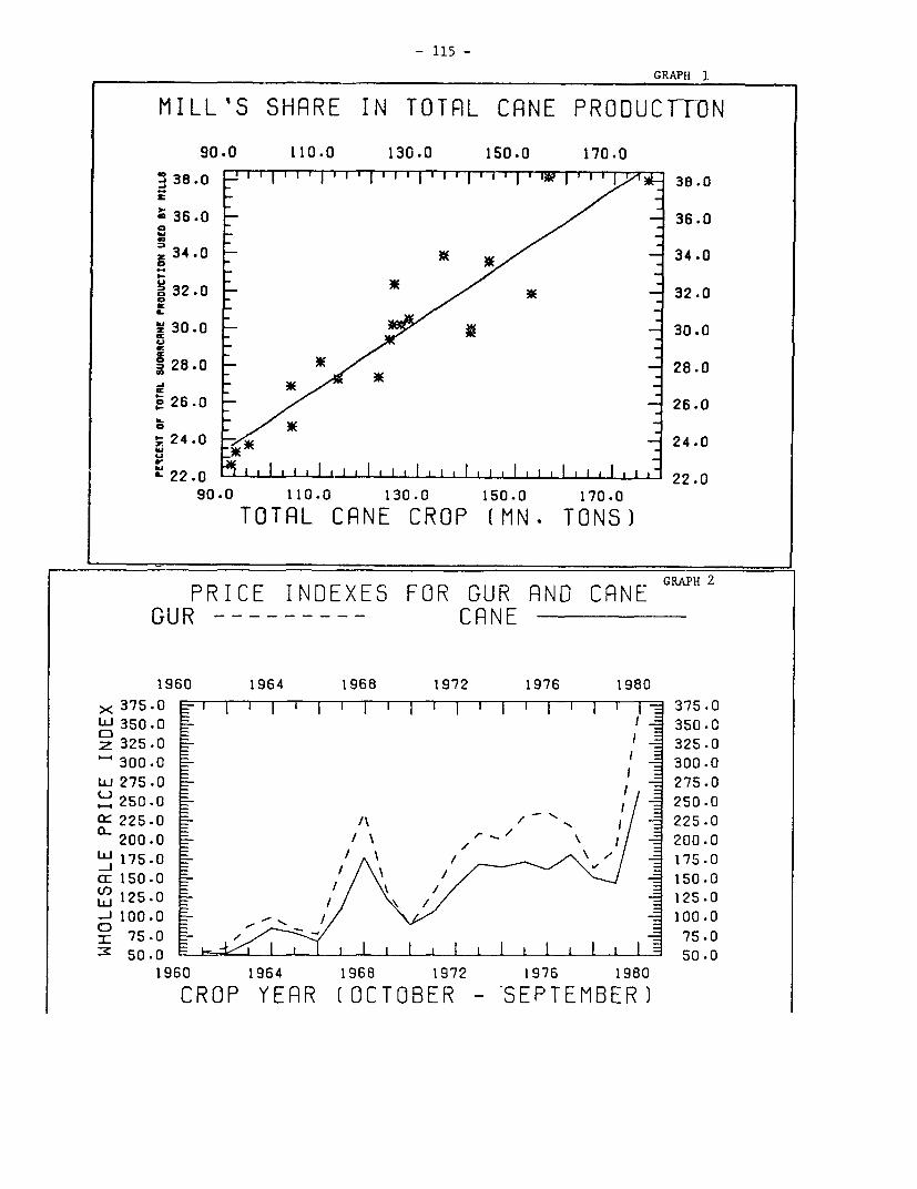
- 115 -

GRAPH

MILL'S SHRRE IN TOTRL CANE PRODUCTTON

90.0 110.0 130.0 150.0 170.0

z 38.0 38.0

36.0 36.0

34.0 34.0

o 32.0 32.0

z 30.0 30.0CC

n 28.0 28.0

o 26.0 26.0

0~24.0 _24.0

'22.0 j , , iz,, , ,,l,,,l,,,l,z _ 22 .090.0 110.0 130.0 150.0 170.0

TOTRL CRNE CROP (MN. TONS)

PRICE INDEXES FOR GUR RND CRNE GRPH2

GUR --- CANE

1960 1964 1968 1972 1976 1980

x 375.0 _ I I I I I I I - 375.0

LU 350.0 350.0

z 325.0 325.0` 300.0 300.0

Lu 275.0 275.0

- 250.0 250.0w 225.0 A 225.0

200.0 200.0L*1 0 175.0cr 150.0 150.0

w 12 5.0 _ / 125.0IJ100.0 - 100.0

r 75.0 _ 75.0:K 50.0 50.0

1960 1964 1968 1972 1976 1980

CROP YERR (OCTOBER - SEPTEMBER)

- 116 -

9. Meanwhile, the farmers reacted to the low 1978 cane prices by plant-ing little new area to cane and relying mainly on a ratoon crop, bringingcane production down to 156 million tons in 1978/79. This was still a largecrop, and with gur and khandsari prices still low, farmers sold a record38.2% of their crop to the mills. Their average realizations, however, werelower than in 1978. There were signs of gur prices beginning to rise butthese were not as clear as they might have been due to the unusually highavailability of unusually cheap mill sugar. The full impact of the effectivecane price reductions was felt at the time of planting the 1979/80 crop.With little new planting the previous year, there was little scope for aratoon crop and little incentive for new planting. Weather conditions wereunfavorable. Area and yield both dropped sharply, resulting in a crop of 128million tons, the lowest in seven years, and 38% below the 1977/78 record.By harvest time, gur and khandsari prices had risen sharply, resulting inonly 30% of the crop being sold to the mills. Mill sugar production fell to3.9 million tons, 40% below the 1977/78 record. During the year the fullprice controls on sugar were lifted and partial controls (65% levy, 35% openmarket) went into effect December 1979 and continue to date. From November1979 through most of 1980, sugar prices rose at unprecedented rates and onoccasion sugar disappeared entirely from the open market. While sugar pricesrose by 52% between September 1979 and September 1980, gur prices rose 110%.Although there was press speculation of unfair trade practices in the sugarindustry, the far more rapid and significant rise in gur and khandsari prices--where trade is decentralized and competitive--suggests the real reason forthe price increase was a severe shortage of cane, a shortage brought on, para-doxically, by the glut two years earlier. The rise in prices of sweetenersalone accounts for 35.2% of the rise in the general wholesale price indexduring that period.

10. With cane prices high in the planting season for the 1980/81 crop,cane production is expected to recover to about 155 million tons. Poorweather conditions at planting time (February-March 1980) probably preventeda more rapid recovery. With even higher statutory prices and high gur andkhandsari prices in the early months of 1981, 1/ one can expect the 1981/82crop to be even larger--possibly on the order of the 1977/78 record. Thefollowing sections assess the longer-term supply and demand prospects. Itis worth noting, however, that the structural causes of the volatility inthe cane and sugar products markets remain. Without an appropriate balancebetween the price of cane and its products and between the price of cane andalternative crops, it is difficult to see how these wide oscillations canbe avoided. Ways of obtaining such balance are discussed below in the sectionon policy implications.

11. Long-Term Supply and Demand Trends. The production of sugarcanehas grown significantly over the past two decades. As Table 1 indicates,however, the aggregate growth trends have varied among regions and betweendecades. Graph 3 shows very sharp year-to-year fluctuations around theselonger-term trends. Over the past twenty years as a whole, the rate of growthof cane production has been 2.70% per annum. Over the last decade, it has

1/ The Government raised the statutory minimum price of cane by 25% in1979/80 and by another 4% in 1980/81. The price index for gur inDecember 1980 was about 50% higher than it was a year earlier.

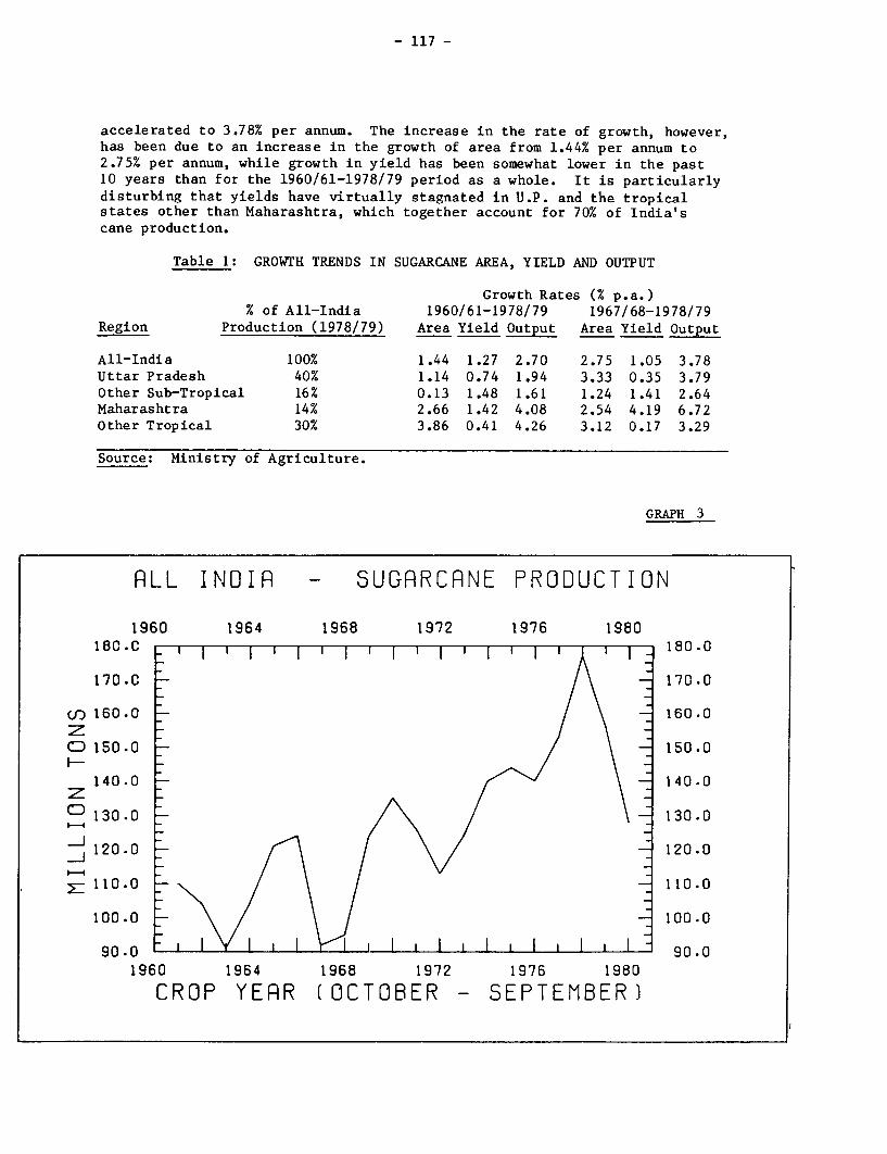
- 117 -

accelerated to 3.78% per annum. The increase in the rate of growth, however,has been due to an increase in the growth of area from 1.44% per annum to2.75% per annum, while growth in yield has been somewhat lower in the past10 years than for the 1960/61-1978/79 period as a whole. It is particularlydisturbing that yields have virtually stagnated in U.P. and the tropicalstates other than Maharashtra, which together account for 70% of India'scane production.

Table 1: GROWTH TRENDS IN SUGARCANE AREA, YIELD AND OUTPUT

Growth Rates (% p.a.)% of All-India 1960/61-1978/79 1967/68-1978/79

Region Production (1978/79) Area Yield Output Area Yield Output

All-India 100% 1.44 1.27 2.70 2.75 1.05 3.78Uttar Pradesh 40% 1.14 0.74 1.94 3.33 0.35 3.79Other Sub-Tropical 16% 0.13 1.48 1.61 1.24 1.41 2.64Maharashtra 14% 2.66 1.42 4.08 2.54 4.19 6.72Other Tropical 30% 3.86 0.41 4.26 3.12 0.17 3.29

Source: Ministry of Agriculture.

GRAPH 3

RLL INDIR - SUGRRCRNE PRODUCTION

1960 1964 1968 1972 1976 198018C.C I 180.0

170.0C 170.0

() 160.0 160.0zCD 150.0- 150.0

140.0 140.0

130.0 130.0

120.0 120.0

E 110.0 110.0

100.0 100.0

90.0 90.01960 1964 1968 1972 1976 1980

CROP YERR (OCTOBER - SEPTEMBER)

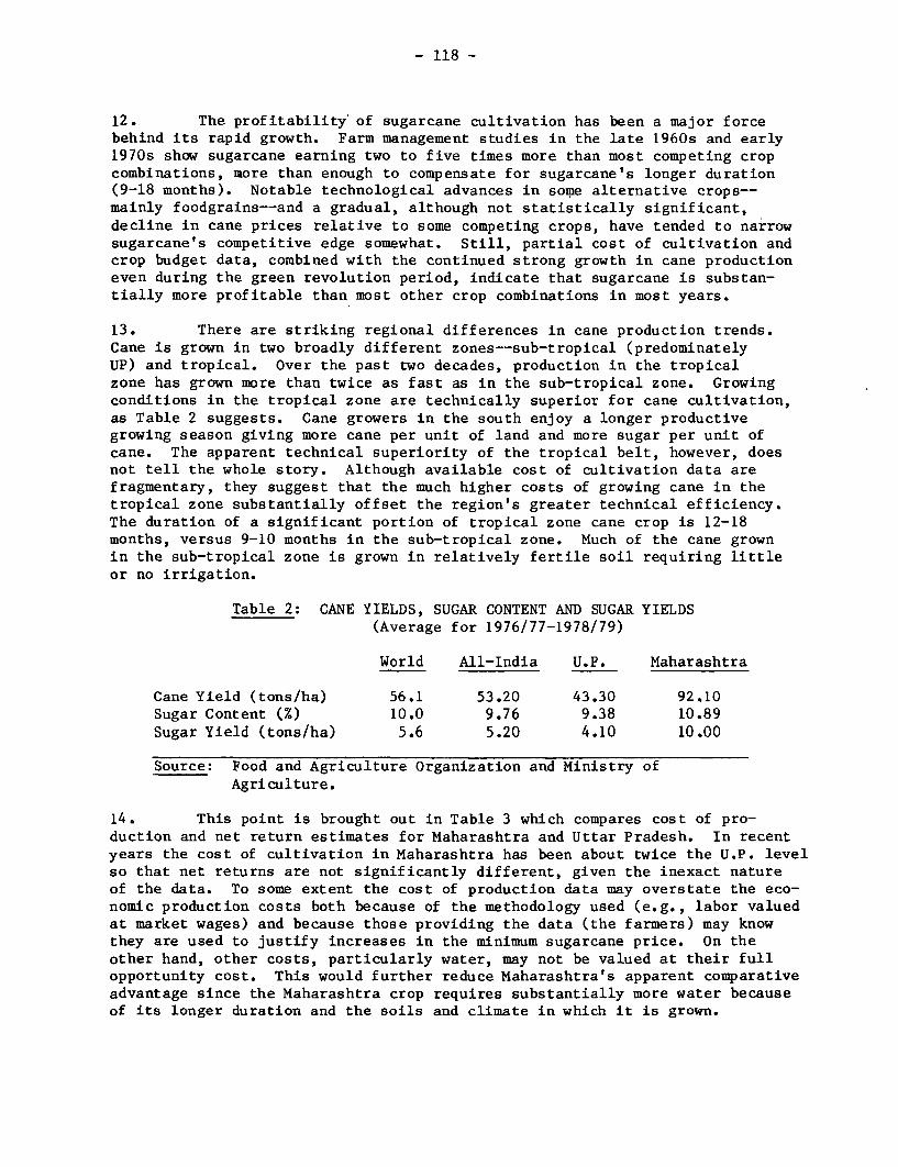
- 118 -

12. The profitability of sugarcane cultivation has been a major forcebehind its rapid growth. Farm management studies in the late 1960s and early1970s show sugarcane earning two to five times more than most competing cropcombinations, more than enough to compensate for sugarcane's longer duration(9-18 months). Notable technological advances in some alternative crops--mainly foodgrains--and a gradual, although not statistically significant,decline in cane prices relative to some competing crops, have tended to narrowsugarcane's competitive edge somewhat. Still, partial cost of cultivation andcrop budget data, combined with the continued strong growth in cane productioneven during the green revolution period, indicate that sugarcane is substan-tially more profitable than most other crop combinations in most years.

13. There are striking regional differences in cane production trends.Cane is grown in two broadly different zones--sub-tropical (predominatelyUP) and tropical. Over the past two decades, production in the tropicalzone has grown more than twice as fast as in the sub-tropical zone. Growingconditions in the tropical zone are technically superior for cane cultivation,as Table 2 suggests. Cane growers in the south enjoy a longer productivegrowing season giving more cane per unit of land and more sugar per unit ofcane. The apparent technical superiority of the tropical belt, however, doesnot tell the whole story. Although available cost of cultivation data arefragmentary, they suggest that the much higher costs of growing cane in thetropical zone substantially offset the region's greater technical efficiency.The duration of a significant portion of tropical zone cane crop is 12-18months, versus 9-10 months in the sub-tropical zone. Much of the cane grownin the sub-tropical zone is grown in relatively fertile soil requiring littleor no irrigation.

Table 2: CANE YIELDS, SUGAR CONTENT AND SUGAR YIELDS(Average for 1976/77-1978/79)

World All-India U.P. Maharashtra

Cane Yield (tons/ha) 56.1 53.20 43.30 92.10Sugar Content (%) 10.0 9.76 9.38 10.89Sugar Yield (tons/ha) 5.6 5.20 4.10 10.00

Source: Food and Agriculture Organization and Ministry ofAgriculture.

14. This point is brought out in Table 3 which compares cost of pro-duction and net return estimates for Maharashtra and Uttar Pradesh. In recentyears the cost of cultivation in Maharashtra has been about twice the U.P. levelso that net returns are not significantly different, given the inexact natureof the data. To some extent the cost of production data may overstate the eco-nomic production costs both because of the methodology used (e.g., labor valuedat market wages) and because those providing the data (the farmers) may knowthey are used to justify increases in the minimum sugarcane price. On theother hand, other costs, particularly water, may not be valued at their fullopportunity cost. This would further reduce Maharashtra's apparent comparativeadvantage since the Maharashtra crop requires substantially more water becauseof its longer duration and the soils and climate in which it is grown.

- 119 -

Table 3: SUGARCANE PRODUCTION COSTS AND RETURNS 1976/77

Maharashtra Uttar Pradesh

Gross Returns (Rs/ha) 8,939 5,576Costs (Rs/ha) 4,164 1,849Profit (Rs/ha) 4,775 3,727

Yield (tons/ha) 65.9 41.9

Costs (Rs/ton) 63.2 44.1Profit (Rs/ton) 72.5 89.0

Source: Ministry of Agriculture.

15. As noted earlier, the longer-term growth in India's sugar productionis marked by sharp year-to-year fluctuations. Measures to reduce such insta-bility are discussed below. Here an effort is made to discuss the level andadequacy of the long-term growth rates. Graph 4 shows actual productionand domestic consumption of all sweeteners from 1960 to 1980 and alternativeprojections of. production and domestic demand from 1980 to 2000. The threeproduction projections are based on extrapolations of: (a) the higher his-torical growthrate (3.8%) in cane production experienced since 1967/68 (thehigh production projection); (b) the lower growth rate (2.7%) experienced overthe period since 1960/61 (the low projection); and (c) an equation relatingcane production to a time trend and lagged cane prices relative to prices ofcompeting crops (the medium projection). The consumption projections arebased on: (a) an extrapolation of the historical growth rate in consumption(2.44%) (the lowest projection); (b) estimates of per capita expenditureelasticity of demand for sweeteners based on NSS cross-sectional survey dataand World Bank population projections assuming, alternatively, 5% and 3.5%rates of growth in total expenditures; and (c) estimates of expenditure andprice elasticities for sweeteners derived from time series data, again assum-ing 5% and 3.5% as alternative expenditure growth rates. 1/

1/ Data and methodology underlying the projections are given in the Annex.

- 120 -

GRAPH 4

PRODUCTION RND CONSUMPTION OF SWEETENERSPRODUCTION CONSUMPTION

1960 1965 1970 1975 1980 1985 1990 1995 2000

35.0 11111111111111 jI 11111111111111 II 1111_ 35.0

° 32.5 32.5

2 30.0 30.0

27 .527.

25 .0250, 22.5 22.5I-

' 20 .0 20 0

U17 .5 17 .5

c 15 0 1 5 °0

12 .5 12 .5

o10.0 _ 10 .0

Mc 7 .5 ~~~~~~~~~~~7 .51960 1965 1970 1975 1980 1985 1990 1995 2000

CROP YERR (OCTOBER - SEPTEMBER)

16. The projections suggest that if past growth rates in cane productioncan be sustained, serious chronic shortages of sweeteners are not likely toemerge. 1/ The projection of recent growth in cane production more thancovers even the highest demand scenario. The two highest demand projectionsassume an unprecedented growth in expenditure of 5% per annum sustained over20 years and may be assumed to represent the upper limit to likely demand.Even if the highest demand projection is taken as given, cane prices wouldneed to rise relative to competing crops by only about 0.4% per annum abovepresent levels to bring the medium production projection into balance with

1/ It should be emphasized that this statement refers to average trends. Ifthe wide fluctuations in production described above in paras 6 to 10remain, there will be years of acute shortage (as well as years of excesssupply).

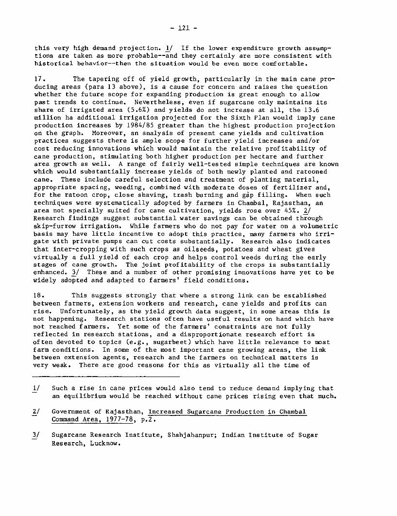
- 121 -

this very high demand projection. 1/ If the lower expenditure growth assump-tions are taken as more probable--and they certainly are more consistent withhistorical behavior--then the situation would be even more comfortable.

17. The tapering off of yield growth, particularly in the main cane pro-ducing areas (para 13 above), is a cause for concern and raises the questionwhether the future scope for expanding production is great enough to allowpast trends to continue. Nevertheless, even if sugarcane only maintains itsshare of irrigated area (5.6%) and yields do not increase at all, the 13.6million ha additional irrigation projected for the Sixth Plan would imply caneproduction increases by 1984/85 greater than the highest production projectionon the graph. Moreover, an analysis of present cane yields and cultivationpractices suggests there is ample scope for further yield increases and/orcost reducing innovations which would maintain the relative profitability ofcane production, stimulating both higher production per hectare and furtherarea growth as well. A range of fairly well-tested simple techniques are knownwhich would substantially increase yields of both newly planted and ratoonedcane. These include careful selection and treatment of planting material,appropriate spacing, weeding, combined with moderate doses of fertilizer and,for the ratoon crop, close shaving, trash burning and gap filling. When suchtechniques were systematically adopted by farmers in Chambal, Rajasthan, anarea not specially suited for cane cultivation, yields rose over 45%. 2/Research findings suggest substantial water savings can be obtained throughskip-furrow irrigation. While farmers who do not pay for water on a volumetricbasis may have little incentive to adopt this practice, many farmers who irri-gate with private pumps can cut costs substantially. Research also indicatesthat inter-cropping with such crops as oilseeds, potatoes and wheat givesvirtually a full yield of each crop and helps control weeds during the earlystages of cane growth. The joint profitability of the crops is substantiallyenhanced. 3/ These and a number of other promising innovations have yet to bewidely adopted and adapted to farmers' field conditions.

18. This suggests strongly that where a strong link can be establishedbetween farmers, extension workers and research, cane yields and profits canrise. Unfortunately, as the yield growth data suggest, in some areas this isnot happening. Research stations often have useful results on hand which havenot reached farmers. Yet some of the farmers' constraints are not fullyreflected in research stations, and a disproportionate research effort isoften devoted to topics (e.g., sugarbeet) which have little relevance to mostfarm conditions. In some of the most important cane growing areas, the linkbetween extension agents, research and the farmers on technical matters isvery weak. There are good reasons for this as virtually all the time of

1/ Such a rise in cane prices would also tend to reduce demand implying thatan equilibrium would be reached without cane prices rising even that much.

2/ Government of Rajasthan, Increased Sugarcane Production in ChambalCommand Area, 1977-78, p.2.

3/ Sugarcane Research Institute, Shahjahanpur; Indian Institute of Sugar

Research, Lucknow.

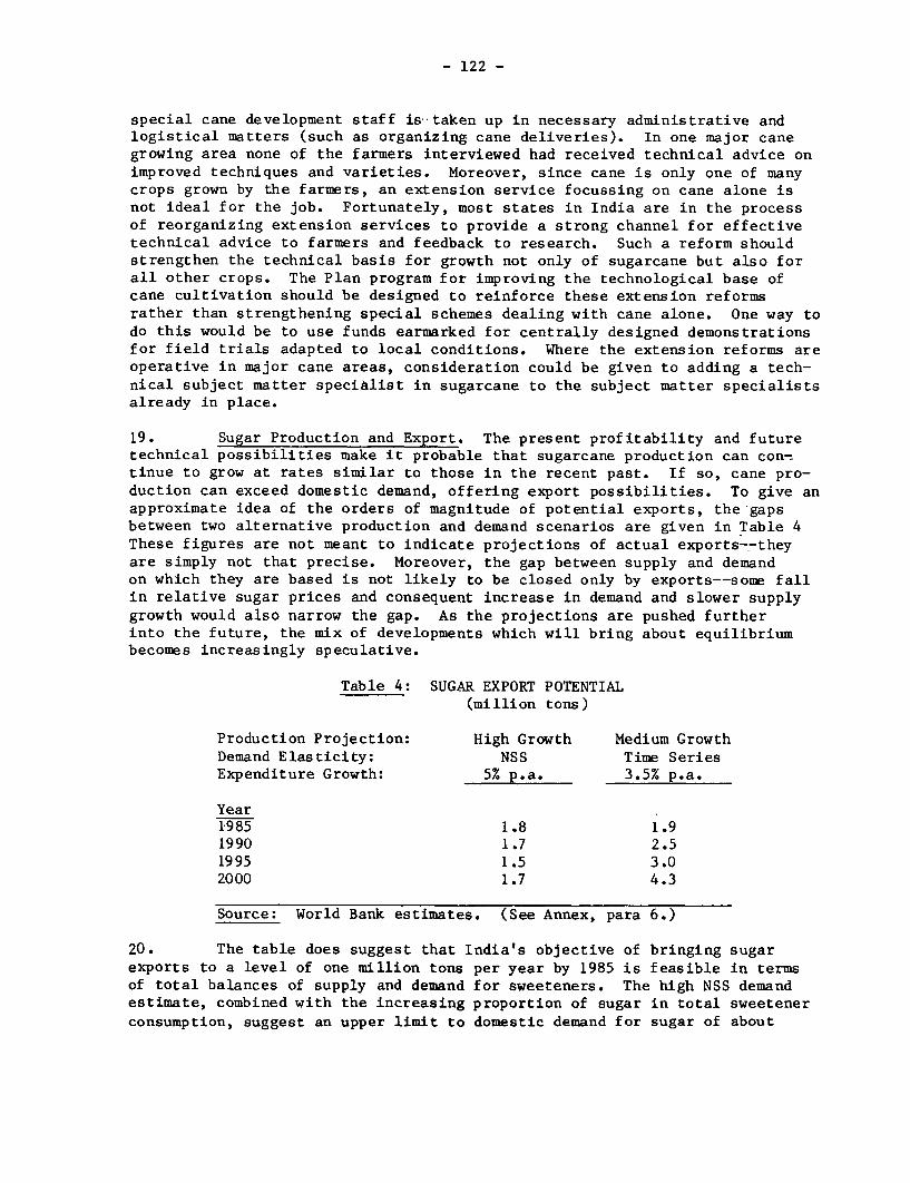
- 122 -

special cane development staff is taken up in necessary administrative andlogistical matters (such as organizing cane deliveries). In one major canegrowing area none of the farmers interviewed had received technical advice onimproved techniques and varieties. Moreover, since cane is only one of manycrops grown by the farmers, an extension service focussing on cane alone isnot ideal for the job. Fortunately, most states in India are in the processof reorganizing extension services to provide a strong channel for effectivetechnical advice to farmers and feedback to research. Such a reform shouldstrengthen the technical basis for growth not only of sugarcane but also forall other crops. The Plan program for improving the technological base ofcane cultivation should be designed to reinforce these extension reformsrather than strengthening special schemes dealing with cane alone. One way todo this would be to use funds earmarked for centrally designed demonstrationsfor field trials adapted to local conditions. Where the extension reforms areoperative in major cane areas, consideration could be given to adding a tech-nical subject matter specialist in sugarcane to the subject matter specialistsalready in place.

19. Sugar Production and Export. The present profitability and futuretechnical possibilities make it probable that sugarcane production can con-tinue to grow at rates similar to those in the recent past. If so, cane pro-duction can exceed domestic demand, offering export possibilities. To give anapproximate idea of the orders of magnitude of potential exports, the gapsbetween two alternative production and demand scenarios are given in Table 4These figures are not meant to indicate projections of actual exports---theyare simply not that precise. Moreover, the gap between supply and demandon which they are based is not likely to be closed only by exports--some fallin relative sugar prices and consequent increase in demand and slower supplygrowth would also narrow the gap. As the projections are pushed furtherinto the future, the mix of developments which will bring about equilibriumbecomes increasingly speculative.

Table 4: SUGAR EXPORT POTENTIAL(million tons)

Production Projection: High Growth Medium GrowthDemand Elasticity: NSS Time SeriesExpenditure Growth: 5% p.a. 3.5% p.a.

Year1985 1.8 1.91990 1.7 2.51995 1.5 3.02000 1.7 4.3

Source: World Bank estimates. (See Annex, para 6.)

20. The table does suggest that India's objective of bringing sugarexports to a level of one million tons per year by 1985 is feasible in termsof total balances of supply and demand for sweeteners. The high NSS demandestimate, combined with the increasing proportion of sugar in total sweetenerconsumption, suggest an upper limit to domestic demand for sugar of about

- 123 -

6.8-6.9 million tons in 1985. This is consistent with the targeted increasein installed sugar mill capacity to about 8.04 million tons by 1984/85. Thetargeted investment of about Rs 8,050 million would increase total crushingcapacity by about 171,250 tons of cane per day, with about 60% of new capacityto be from new plants and 40% from expansions of existing mills. While thisis higher than the 150,000 tpd capacity strictly needed to reach 8.04 millionton production level, it is probably wise to allow for some slippage and costincrease. Most of the investment is likely to be in the cooperative sectorsince government policy offers cooperatives highly favorable financing terms.If Plan resources are constrained, incentives to encourage a higher proportionof private investment could be considered. Careful consideration should alsobe given to increasing the proportion of expansions of existing plants in thetotal increase in capacity. Expansions cost 40% less than new plants per tonof capacity, and probably involve shorter gestation periods and fewer logis-tical problems. The locations of new plants will have to be selected care-fully to ensure adequate cane supplies. The reintroduction of incentives fornew mills and mill expansion 1/ combined with the recovery of sugar prices hasincreased the attractiveness of investments in this sector substantially, butthe violent fluctuations in cane supplied to the mills will remain a majordisincentive unless remedial measures are taken.

21. The volatility of sugar both in India and in the world market makesit difficult to project the competitiveness and profitability of India'ssugar exports. Both Indian and world sugar markets appear cyclical and theprofitability of India's sugar exports depends on India's cycle being in orout of phase with the world market. Prior to 1973/74 the unit value ofIndia's exports was generally below both domestic market prices and theex-factory levy prices. In 1974 and 1975 world market prices were high andresulted in sharp increases in the volume and value of India's sugar exports.Between 1976 and 1979 world prices were generally lower than Indian domesticprice but higher than ex-factory levy prices (which exclude excise taxes). In1980 world sugar prices were high and are expected to remain well above Indianproduction costs through 1981. Indian cane yields and sugar production costsappear fairly competitive with other suppliers. From the Annual Survey ofIndustries 1977/78 and from the calculations used to determine the ex-factorylevy price, Indian sugar production costs appeared to be about US$171-208 perton of D-29 sugar in 1977/78, a year when developing country sugar productioncosts were estimated at US$220-310 per ton for raw sugar of lower quality. 2/World market prices for raw sugar in 1985 are estimated at US$412 per ton in1980 dollars compared with 1980 Maharashtra production costs of about US$320for a more refined grade of sugar. 3/ Continued improvements in cane produc-tivity, such as those discussed earlier, would help ensure the continued

1/ New plants and expansions of existing plants intially are allowed to sella greater proportion of their sugar in the free market, with the propor-tion falling gradually over several years to the same level as that ofexisting plants. Moreover, they face lower excise taxes intially.

2/ IBRD, Price Prospects for Major Primary Commodities, January 1980.

3/ IBRD, Commodity Price Forecasts - Updating, November 12, 1980, p. 4.

- 124 -

competitiveness of India's sugar exports by keeping costs down. The availabil-ity of a buffer stock would give India greater control over the timing of sugarexports to take advantage of fluctuations in world market prices.

22. Policy Implications. Sugarcane and sugar products policy in Indiahas been the subject of many detailed studies, each of which called for along-term, stable policy. The very volatility of the sugar economy, however,has prevented this, and as noted earlier, sugar policies in India have beenchanged frequently and substantially. As the sugar economy emerges from theacute shortage and rapid price rises of the past year it is difficult to lookahead to implementing longer-run policies. Yet successful implementation oflonger-term policies could also contribute to resolving the short and medium-term problems of supply management.

23. Sugarcane price policy is clearly central to the sugar economy.The recent past has suggested that the prices set by the Agricultural PricesCommission (APC) provided a reasonable stimulus to cane production. The price,which has been uniform across states but linked to the sugar content of cane,helps promote locational efficiency. The state advised prices and cooperativeprofits distribution to cane growers, however, counteracted the APC effortsand encouraged excess production in 1977/78 which led directly to the short-ages and price rises in 1980. Hopefully, this experience will lead to greaterreliance on the APC's technical judgment and a realization that unrealisti-cally high cane prices do not really benefit most farmers in the long run.While it will be difficult to resist political pressures from farm groups toraise prices, avoiding excessively high minimum support prices will be essen-tial if the 1977/78 experience is to be avoided in the near future.

24. A well executed cane price policy is an essential element but onlyone element in a longer-term policy. Weather and price variations in othersugarcane uses will continue to cause year-to-year variations around longer-term trends in cane production. Due to the duration of the cane crop andratooning, these variations will tend to take time to even themselves out bywhich time new shocks will have destabilized the system. A buffer stockingpolicy implemented at a suitable time would offer the Government a useful toolfor controlling supply variations and dampening the price swings, therebyreducing one of the sources of instability in cane production. Moreover, abuffer stock could give the Government flexibility in the timing of its exportsales to take advantage of world market conditions. The suggestion of abuffer stock dates back at least as far as the 1965 Sugar Enquiry CommissionReport and is included in the Sixth Plan. Concern over the cost of such apolicy has been one major reason why it has not been tried. Also, withoutan appropriate cane price one could envision ever-increasing stocks of sugaraccumulating with the Government. With an appropriate cane price policy,however, the costs of such a buffer stock could be kept reasonably low. Bykeeping the stocks with the mills themselves (which managed stocks over 4million tons in 1978) the Government could restrict its financial outlay tothe interest charges. Since India is just emerging from a sugar shortage, nowis obviously not the time to start a buffer stock. Next year, however, thecane crop is likely to be much larger, perhaps approaching the 1977/78 level.World market prices may be such that excess sugar production could be profit-ably exported, but ISA quotas may limit such possibilities. In any case it

- 125 -

would seem to make sense for the Government to be ready from next year tostart establishing a buffer stock, should the domestic crop be large enough.

25. In years of a short cane crop, mills will continue to have difficul-ties in competing with gur and khandsari units since controls on sugar pricesput effective limits on prices mills can offer for cane. In this context andafter building up a sugar buffer stock, the possibility of gradually relaxingand eventually removing the sugar levy system should be considered carefully.While the rather disastrous experience with the recent decontrol may make itdifficult to advocate decontrol now, it is clear in retrospect that the timing(when sugar stocks were over 4 million tons) and abruptness (including decon-trol of monthly releases) of the 1978 decontrol had more to do with theresults than decontrol itself. If the Government maintained buffer stocksplus controls on monthly releases, such wild market fluctuations would not bepossible. In addition to allowing mills to compete more effectively for cane,such a decontrol would remove some of the locational inefficiencies built intothe present levy price system which pays higher prices for levy sugar to millslocated in areas with higher cane costs and which have higher conversion costs.With decontrolled prices, mills would face the same prices, which would encour-age new investment in low cost areas. In striving for better locationalefficiency the Government should also consider whether the present system ofgreater investment incentives (in the form of lower proportions of levy sugar)in areas with lower sugar recovery is in the long-term interest of the sugarindustry. 1/

26. The mix of policies--an appropriate minimum price for cane, bufferstocking, and gradual relaxation of the levy system--would go far in reducingthe year-to-year fluctuations in cane production and cane available to thesugar mills. This would reduce' the market risks faced by farmers and millsalike and would help to ensure that the Plan's investment goals in this indus-try are met. Under this system the mills would be more certain of a steadysupply of cane and would not bear the entire burden of excessive stock buildupshould it develop in years of a large crop. The reciprocal instability in thegur and khandsari sectors, which mirrors the instability in sugar would alsobe reduced. By reducing the proportion of levy sugar gradually, incentivesfor shifts to more efficient locations would build up gradually so that suchshifts would also be gradual, avoiding the hardship of a rapid dislocation.

27. The long-term competitiveness of India's sugar economy depends onits technical base. Continued emphasis should be placed on improving researchand extension efforts in both the cane production and the cane processingfields. The general programs now underway to improve agricultural researchinstitutions and extension services in most states in India should continueto receive high priority.

1/ It is by no means clear where locational advantages really lie. We haveseen that Maharashtra's high yields and sugar recovery may be offset byhigher costs. Moreover, changes in technology and relative prices maycause locational advantage to shift over time.

- 126 -

THE SUGAR ECONOMYANNEX

Supply and Demand Projections for Sugarcane

1. Sugarcane Production:

Three equations were estimated to project sugarcane production:(i) an estimation of the rate of growth achieved over the 1967/68-1978/79

period:

ln (SCP) = 4.65520 + .03785(T); R2 = .69(84.67) (5.066)

where SCP equals sugarcane production in millions of tons and T = time(1967/68 =1...). Fiaures in parentheses are t statistics.

ii) an estimation of the rate of growth over the 1960/61-1978/79 period:

ln (SCP) = 4.5447 + .02700(T); R2 = .66(88.49) (5.995)

where T = time (1960/61=1,...)

iii) an equation including the response of production to relative pricesas well as its trend rate of growth:

ln (SCP) = 4.455 + .02995(T) + .4487(ln(Pc)); R2 = .72(77.7) (7.10) (3.086)

where T = time (1960/61=1,...) and Pc = an index of the average realizedcane price for the preceding two years deflated by the price index ofmajor competing crops (foodgrains, oilseeds, cotton). The average real-ized cane price index was constructed by calculating a weighted average ofthe index of statutory minimum cane prices (the official cane price index)and the price index for gur during the main harvest months (Decem-ber-March). The weights were the proportion of cane crushed by mills andthe proportion crushed by gur and khandsari units. For projection pur-poses, the 20 year average value for Pc was used (1.122). The value forPc as of January 1981 was about 1.3183. This would imply a 1981/82 cropof over 180 million tons. Using the 20 year average Pc(l.122) shifts theproduction projections down from what they would have been had presentprice levels been used. Thus this projection has an implicit assumptionof a 15% fall in relative cane prices.

2. Sweetener Production

To relate a given level of cane production to production ofsweeteners, the following equation was estimated:

TSP = .08774 SCP; R2 = .9996(218.14)

although this equation gives an excellent fit to the historical data it issomewhat conservative to use it in the projections because the proportion

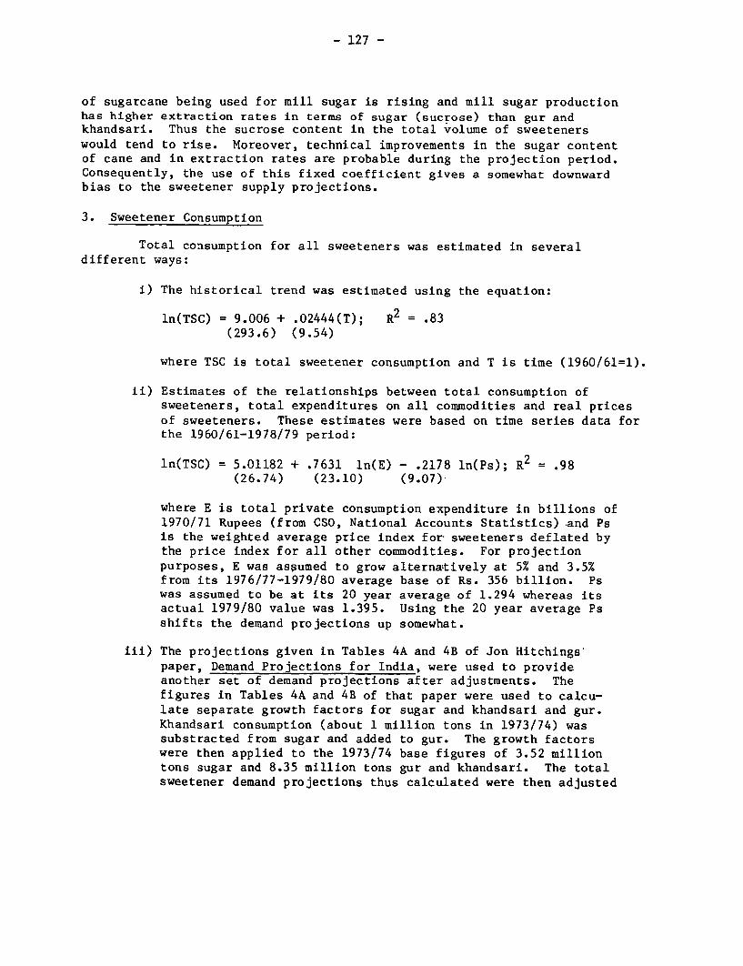
- 127 -

of sugarcane being used for mill sugar is rising and mill sugar productionhas higher extraction rates in terms of sugar (sucrose) than gur andkhandsari. Thus the sucrose content in the total volume of sweetenerswould tend to rise. Moreover, technical improvements in the sugar contentof cane and in extraction rates are probable during the projection period.Consequently, the use of this fixed coefficient gives a somewhat downwardbias to the sweetener supply projections.

3. Sweetener Consumption

Total consumption for all sweeteners was estimated in severaldifferent ways:

i) The historical trend was estimated using the equation:

ln(TSC) = 9.006 + .02444(T); R2 = .83(293.6) (9.54)

where TSC is total sweetener consumption and T is time (1960/61=1).

ii) Estimates of the relationships between total consumption ofsweeteners, total expenditures on all commodities and real pricesof sweeteners. These estimates were based on time series data forthe 1960/61-1978/79 period:

ln(TSC) = 5.01182 + .7631 ln(E) - .2178 ln(Ps); R2 = .98(26.74) (23.10) (9.07)

where E is total private consumption expenditure in billions of1970/71 Rupees (from CSO, National Accounts Statistics) and Psis the weighted average price index for sweeteners deflated bythe price index for all other commodities. For projectionpurposes, E was assumed to grow alternattively at 5% and 3.5%from its 1976/77-1979/80 average base of Rs. 356 billion. Pswas assumed to be at its 20 year average of 1.294 whereas itsactual 1979/80 value was 1.395. Using the 20 year average Psshifts the demand projections up somewhat.

iii) The projections given in Tables 4A and 4B of Jon Hitchingspaper, Demand Projections for India, were used to provideanother set of demand projections after adjustments. Thefigures in Tables 4A and 4B of that paper were used to calcu-late separate growth factors for sugar and khandsari and gur.Khandsari consumption (about 1 million tons in 1973/74) wassubstracted from sugar and added to gur. The growth factorswere then applied to the 1973/74 base figures of 3.52 milliontons sugar and 8.35 million tons gur and khandsari. The totalsweetener demand projections thus calculated were then adjusted

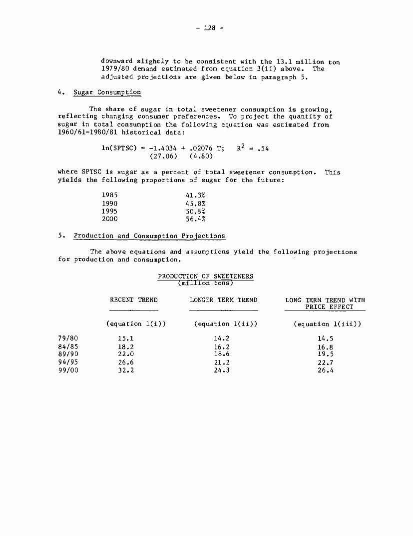
- 128 -

downward slightly to be consistent with the 13.1 million ton1979/80 demand estimated from equation 3(ii) above. Theadjusted projections are given below in paragraph 5.

4. Sugar Consumption

The share of sugar in total sweetener consumption is growing,reflecting changing consumer preferences. To project the quantity of

sugar in total consumption the following equation was estimated from1960/61-1980/81 historical data:

ln(SPTSC) = -1.4034 + .02076 T; R2 = .54(27.06) (4.80)

where SPTSC is sugar as a percent of total sweetener consumption. Thisyields the following proportions of sugar for the future:

1985 41.3%

1990 45.8%1995 50.8%2000 56.4%

5. Production and Consumption Projections

The above equations and assumptions yield the following projectionsfor production and consumption.

PRODUCTION OF SWEETENERS(million tons)

RECENT TREND LONGER TERM TREND LONG TERM TREND WITHPRICE EFFECT

(equation l(i)) (equation 1(ii)) (equation l(iii))

79/80 15.1 14.2 14.5

84/85 18.2 16.2 16.889/90 22.0 18.6 19.594/95 26.6 21.2 22.799/00 32.2 24.3 26.4

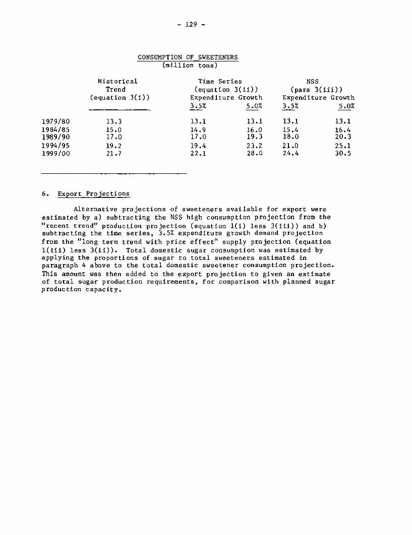
- 129 -

CONSUMPTION OF SWEETENERS(million tons)

Historical Time Series NSSTrend (equation 3(ii)) (para 3(iii))

(equation 3(i)) Expenditure Growth Expenditure Growth3.5% 5.0% 3.5% 5.0%

1979/80 13.3 13.1 13.1 13.1 13.11984/85 15.0 14.9 16.0 15.4 16.41989/90 17.0 17.0 19.3 18.0 20.31994/95 19.2 19.4 23.2 21.0 25.11999/00 21.7 22.1 28.0 24.4 30.5

6. Export Projections

Alternative projections of sweeteners available for export wereestimated by a) subtracting the NSS high consumption projection from the"recent trend" production projection (equation 1(i) less 3(iii)) and b)subtracting the time series, 3.5% expenditure growth demand projectionfrom the "long term trend with price effect" supply projection (equationl(iii) less 3(ii)). Total domestic sugar consumption was estimated byapplying the proportions of sugar to total sweeteners estimated inparagraph 4 above to the total domestic sweetener consumption projection.This amount was then added to the export projection to given an estimateof total sugar production requirements, for comparison with planned sugarproduction capacity.

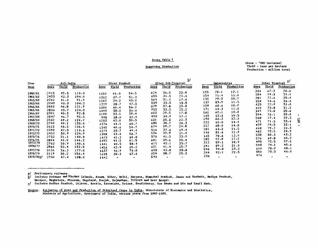
Annex Table1

(Area '000 hectares)Sugarcane Production Yield - tons per hectare

Production - million tons)

b/ RCrop All-India Uttar Pradesh Other Sub-Tropical Maharashtra Other Tropical -Year Area Yield Production Area Yield Production Area Yield Production Area Yield Production Area Yield Production

1960161 2415 45.5 110.0 1330 41.0 54-5 624 36.5 22.8 155 78.1 12.1 306 67.3 20.61961/62 2455 42.3 104.0 1362 37.7 51.3 655 31.5 20.6 154 71.4 11.0 284 74.3 21.11962/63 2242 41.0 91.9 1262 34.2 43.2 564 31.2 17.6 135 79.3 10,7 281 72.6 20.41963/64 2249 46.3 104 2 1229 38.7 47.5 529 35.5 18.8 137 83.9 11.5 354 74.6 26.41964/65 2603 46,8 121 .9 1390 40.4 56.2 629 37.8 23.8 159 68-6 10.9 425 72.9 31.01965/66 2836 43.7 124.0 1490 38.0 56.6 752 33.5 25.2 171 64.3 11.0 423 73.8 -31.21966/67 2301 40.3 92.8 1190 33.1 39.4 603 29.5 17.8 161 62.1 10.0 347 73.8 25.61967/68 2047 46.7 95.5 998 38.0 37.9 490 34.9 17.1 165 63.6 10,5 394 76.1 30.01968/69 2532 49.2 124.7 1203 42.0 50.5 631 35.3 22.3 190 66.3 12.6 508 77.4 39.31969/70 2749 49.1 135.0 1376 44.1 60.7 680 38.7 26,3 222 65.0 14.4 471 71.3 33.61970/71 2615 48.3 126.4 1345 40.6 54.7 624 39.7 24.8 217 68.0 14.8 429 74.8 32.11971/72 2390 47.5 113.6 1274 38.7 49.4 516 37.6 19.4 182 63.2 11.5 418 79.7 33.31972/73 2452 50.9 124.9 1308 43.4 56.7 536 39.9 21.4 146 81.6 11.9 462 75.5 34,91973/74 2752 51.1 140.8 1473 41.3 60.8 576 41.5 23.9 165 78.6 12.9 538 80.3 43.21974/75 2894 49.9 144.3 1492 41.2 61.5 641 39.6 25.4 185 92.8 17.2 576 69.8 40.21975/76 2762 50.9 140.6 1441 40.5 58.4 611 42.1 25.7 212 89.1 18.9 498 75.5 37.61976/77 2866 53.4 153.0 1456 42.9 65.2 621 41.4 25.7 241 89.2 21.5 548 74.1 40.61977/78 3151 56.2 177.0 1637 46.9 76.8 658 43.8 28,8 *246 94.8 23.3 610 78.9 48.11978/79 3119 50.2 156.4 1635 38.3 62.6 654 38.7 25.3 244 92.1 22.5 586 78.5 46.01979/80a/ 2700 47.4 128.0 1442 - - 546 - - 236 - _ 476 - -

a/ Preliminary estimate.b/ Includes Andaman and Nicobar Islands, Assam, Bihar, Delhi, Haryana, Himachal Pradesh, Jammu and Kashmir, Madhya Pradesh,

Manipur, Meghalaya, Mizoram, Nagaland, Punjab, Rajasthan, Tripura and West Bengal.c/ Includes Andhra Pradesh, Gujarat, Kerala, Karnataka, Orissa, Pondicherry, Goa Daman and Diu and Tamil Nadu.

Source: Estimates of Area and Production of Principal Crops in India, Directorate of Economics and Statistics,Ministry of Agriculture, Government of India, various years from 1960-1980.

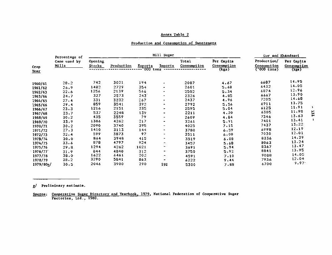
Annex Table 2

Production and Consumption of Sweeteners

Percentage of Mill Sugar Gur and Khandsari

Cane used by Opening Total Per Capita Production/ Per Capita

Crop Mills Stocks Production Exports Imports Consumption Consmption Cons ption Cons tionYear ------------------------- rOOtons -------------------- (kgs) u tons (kgs)

1960/61 28.2 742 3021 194 - 2087 4.67 6687 14.95

1961/62 26.9 1482 2729 354 - 2601 5.68 6432 14.05

1962/63 22.6 1256 2139 566 - 2502 5.34 6074 12.96

1963/64 24.7 327 2573 243 - 2326 4 .85 6667 13.90

1964/65 27.4 331 3232 267 - 2437 4 .96 7205 14.68

1965/66 29.4 859 3541 392 - 2792 5.56 6911 13.75

1966/67 23.3 1216 2151 235 - 2595 5.04 6125 11.911967/68 23.7 537 2248 139 - 2211 4.20 6305 11.98

1968/69 30.2 435 3559 79 - 2609 4.84 7346 13.63 F

1969/70 33.9 1306 4262 217 - 3261 5.91 7401 13.41

1970/71 30,2 2090 3740 395 - 4025 7.15 7437 13.22

1971/72 27,3 1410 3113 144 - 3780 6.59 6998 12.19

1972/73 32.4 599 3873 97 3511 6.00 7030 12.01

1978/74 30.0 864 3948 415 - 3519 6.08 8336 14,391974/75 33.6 878 4797 924 - 3457 5,68 8063 13.241975/76 29.8 1294 4262 1021 - 3691 5.94 8367 13.47

1976/77- 31.9 844 4840 312 - 3750 5.92 8841 13.95

1977/78 38.0 1622 6461 202 - 4591 7.10 9088 14.051978/79 38.2 3290 5841 863 - 6222 9.44 7936 12.04

1979/80a/ 30.5 2046 3900 290 192 5300 7.88 6700 9.97-

a/ Preliminary estimate.

Source: Cooperative Sugar Directory and Yearbook, 1979, National Federation of Cooperative SugarFactories, Ltd., 1980.

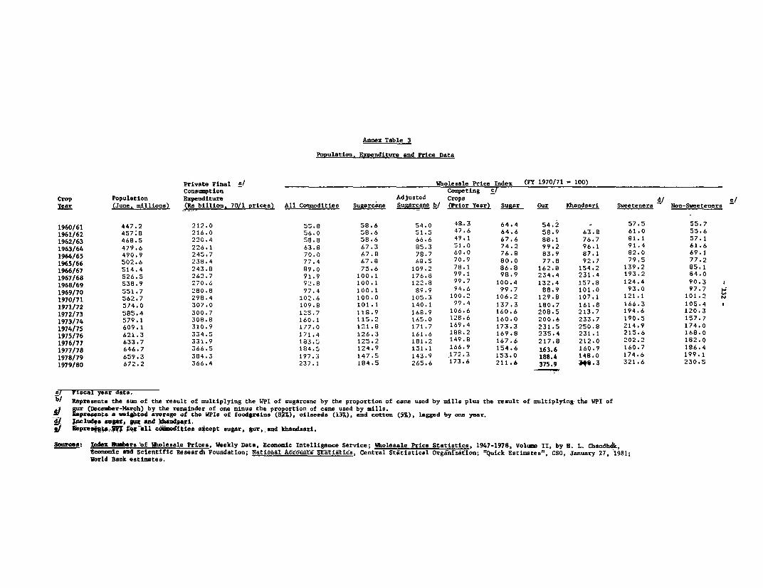
Annex Table 3

Population. Expenditure and Price Data

Private Final a/ Wholesale Price Index (FY 1970/71 - 100)

Consumption Competing c/

Crop Population Expenditure Adjusted Crops d/ e/

Year (June, millions) (Rs billion, 7Q/1 prices) All Commodities Sugarcane Sugarcane b/ (Prior Year) Sugar Gur Khandsari Sweeteners Non-Sweeteners

1960/61 447.2 212.0 55.8 58.6 54.0 48,.3 64.4 54.2 - 57.5 55.7

1961/62 457;8 216.0 56.0 58.6 S1.S 47.6 64.6 58.9 63.8 61.0 55.6

1962/63 468.5 220.4 58.8 58.6 66.6 49.1 67.6 88.1 76.7 81.1 57.1

1963/64 479.6 226.1 63.8 67.3 85.3 51.0 74.2 99.2 96.1 91.4 61.6

1964/65 490.9 245.7 70.0 67.8 78.7 60.0 76.8 83.9 87.1 82.0 69.1

1965/66 502.6 238.4 77.4 67.8 68.5 70.9 80.0 77.8 92.7 79.5 77.2

1966/67 514.4 243.8 89.0 75.6 109.2 78.1 86.8 162.8 154.2 139.2 85.1

1967/68 526.5 262.7 91.9 100.1 176.8 99.1 98.9 234.4 231.4 193.2 84.0

1968/69 538.9 270.6 92.8 100.1 122.8 99.7 100.4 132.4 157.8 124.4 90.3 a

1969/70 551.7 280.8 97.4 100.1 89.9 94.6 99.7 88.9 101.0 93.0 97.7

1970/71 562.7 298.4 102.6 100.0 105.3 100.2 106.2 129.8 107.1 121.1 101.2 S

1971/72 574.0 307.0 109.8 101.1 140.1 99.4 137.3 180.7 161.8 166.3 105.4 a

1972/73 585.4 300.7 125.7 118.9 168.9 106.6 160.6 208.5 213.7 194.6 120.3

1973/74 579.1 308.8 160.1 115.2 165.0 128.6 160.0 200.6 233.7 190.5 157.7

1974/75 609.1 310.9 177.0 121.8 171.7 169.4 173.3 231.5 250.8 214.9 174.0

1975/76 621.3 334.5 171.4 126.3 161.6 188.2 169.8 235.4 231.1 215.6 168.0

1976/77 633.7 331.9 183.5 125.2 181.2 149.8 167.6 217.8 212.0 202.2 182.0

1977/78 646.7 366.5 184.5 124.9 151.1 166.9 154.6 163.6 16Q.9 160.7 186.4

1978/79 659.3 384.3 197.3 147.5 143.9 172.3 153.0 188.4 148.0 174.6 199.1

1979/80 672.2 366.4 237.1 184.5 265.6 173.6 211.6 375.9 3 321.6 230.5

a/ riscal year data.

b/ Represents the sum of the result of multiplying the WPI of sugarcane by the proportion of cane used by mills plus the result of multiplying. the WPI of

, u (December-March) by the remainder of one minus the proportion of cane used by mills.p rceant6 a weighted average of the WPIs of foodgrains (82Z), oilseeda (137.), and cotton (5%), legged by one year.

4 Aclud.a supr, VW Apd Waudpari,3/ lipresj~ate ~oia11 eitive except sugar. gur, and khandsari.

Sotrcaes: Index ! a.ro 'of Wholesale Prices, Weekly Data, Economic Intelligence Service; Wholesale Price Statistics, 1947-1978, Volume II, by H. L. Chandhjk,

Economic snd Scientific Researdh Foutrdation; National Az6,conts SWatidti6cs, Central Statistical Orginfzation; "Quick Estimates", CSO, January 27, 1981;World Blank estimates.

Annex Table 4

Sugar Trade Data

World (ISA daily) Weighted Average LevySugar Sugar Sugar Sugar Exports Price, f.o.b. major Average Ex-FactoryCrop Exports Exports Exchange Exports Unit Value Calendar Caribbean parts Price PriceYear (000 tons) (Rs million) Rate (US$ million) ($/ton) Year ( ($/ton)b/ ($/ton)R/

1960/61 56.0 24.8 4.762 5.2 92.9 1961 69 214.71961/62 284.8 145.7 4.76' 30.6 107.4 1962 60 213.71962/63 418 . 0 1 70. 1 4. oD_ 35.7 85 .4 1963 61 216. ,1963/64 432.3 257.3 4.76_ 54.0 124.9 1964 184 23 0. 31964/65 282.1 189.2 4.762 39.7 140.7 1965 127 2S2.31965/66 314.1 15 .1 4. 762 24.2 77.0 1966 44 25.,3 _ 31966/67 356.7 167.0 7.000 23.5 67.0 1967 40 183.7 _ 1967/68 228.0 159.S 7.50i' 21.3 93.4 1968 42 189.4 - w1968/69 100.0 102.1 7.500 13.6 136.0 1969 42 213.8 -1969/70 82.0 85.5 7,500 11.4 139.0 1920 71 212.11970/71 348.0 276.0 7.50O0 36.8 105.7 £971 81 210.8 -1971/72 317.0 302.2 7.444 40.6 128.1 1972 99 240. J -1972/73 102.0 133.0 7.706 17.3 169.6 1973 160 301.6 186.81973/74 252.5 426.9 7,791 54.8 217.0 1974 208 321.5, 185. j1974/75 69S.0 3390.0 7.976 425.0 6111.5 1975 b54 330.2 196.81975/76 1201.0 4723.0 8. c- .3 545. 8 454.5 1976 449 3i3.3 172. 31976/77 5B0.0 1481.0 8.73; 165.7 285.7 1977 255 306.8 165.41977/78 70.0 95.0 B. 65I3 22.8 325.7 1978 175 302.7 I81.I1978/79 73a.0 1319.0 8.206 160.7 217.8 1979 172 29 0.0 207.91979/80a/ 564.6 1199.0 8.100 148.0 262.1 1980 213 313.9 2 31 .'i

a/ Preliminary estimate.b/ Calculated from calendar year Wholesale Price Index for sugar by dividing index number by a factor of 0.063

,which represents the relationship between the WPI and the weighted average of the market prices used toestimate the WPI.

c/ For D-29 grade sugar, ex-Maharashtra factories.

Source: Cooperative Sugar Directory and Yearbook. 1979, National Federation of Cooperative Sugar Factories, Ltd., 1980.

RECENT PAPERS IN THIS SERIES

No. TITLE OF PAPER AUTHOR

470 Industrial Country Policy and Adjustment to Imports J.M. Fingerfrom Developing Countries

471 The Political Structure of the New Protectionism D. Nelson (consultant)

472 Adjustment to External Shocks in Developing Countries B. Balassa

473 Food Policy Issues in Low-Income Countries E. Clay (consultant)

474 Energy, International Trade, and Economic Growth A. Manne (consultant)

475 Capital-Importing Oil Exporters: Adjustment Issues A.H. Gelband Policy Choices

476 Notes on the Analysis of Capital Flows to Developing R.C. Bryant (consultant)Nations and the 'Recycling' Problem

477 Adjustment Experience and Growth Prospects of the F. JaspersenSemi-Industrial Countries

478 Trade Policy Issues for the Developing Countries I. Frank (consultant)in the 1980s

479 Trade among Developing Countries: Theory, Policy 0. HavrylyshynIssues, and Principal Trends (consultant)

M. Wolf

480 Trade in Services: Economic Determinants and A. Sapir (consultant)Development-Related Issues E. Lutz

481 International Migrant Workers' Remittances: Issues G. Swamyand Prospects

482 Private Bank Lending to Developing Countries R. O'Brien (consultant)

483 Development Prospects of the Capital Surplus R. HablutzelOil-Exporting Countries

484 Private Capital Flows to Developing Countries and A. FlemingTheir Determination

485 International Adjustment in the 1980s V. Joshi (consultant)

- 2 -

No. TITLE OF PAPER AUTHOR

486 Adjustment in Low-Income Africa R. Liebenthal

487 A Comparative Analysis of Developing Country C. WallichAdjustment Experiences in the 1970s: Low-IncomeSouth Asia

488 Developments in and Prospects for the External N. HopeDebt of the Developing Countries: 1970-80 andBeyond

489 Global Energy Prospects B.J. ChoeA. LambertiniP. Pollak

490 Sociocultural Aspects of Developing Small-Scale R. B. Pollnac (consultant)Fisheries: Delivering Services to the Poor

491 The Educational Use of Mass Media S. Futagami et al

492 The Political Market for Protection in T. AndersonIndustrial Countries R. Baldwin

493 On Protectionism in the Netherlands K. Koekkoek

494 Patterns of Barriers to Trade in Sweden L. Lundberg

495 Social Infrastructure and Services in Zimbabwe R. Faruqee

496 Economic Aspects and Policy Issues in Groundwater I. CarruthersR. Stoner (consultants)

497 Labor Productivity: Un Tour D'Horizon S. Horton (consultant)T. King

498 The Determinants of Labour Earnings in Developing R. MohanMetropoli: Estimates from Bogota and Cali, Colombia

PUB HG3881.5.W57 W67 no.500Harrison, James Q.Irxiia, denand ard supply

prospects for agriculture /