INDEPENDENT COMPONENT ANALYSIS FOR AUDIO AND BIOSIGNAL APPLICATIONS Edited by Ganesh R. Naik

Welcome message from author
This document is posted to help you gain knowledge. Please leave a comment to let me know what you think about it! Share it to your friends and learn new things together.
Transcript

INDEPENDENT COMPONENT ANALYSIS
FOR AUDIO AND BIOSIGNAL APPLICATIONS
Edited by Ganesh R. Naik

Independent Component Analysis for Audio and Biosignal Applications Edited by Ganesh R. Naik Published by InTech Janeza Trdine 9, 51000 Rijeka, Croatia Copyright © 2012 InTech All chapters are Open Access distributed under the Creative Commons Attribution 3.0 license, which allows users to download, copy and build upon published articles even for commercial purposes, as long as the author and publisher are properly credited, which ensures maximum dissemination and a wider impact of our publications. After this work has been published by InTech, authors have the right to republish it, in whole or part, in any publication of which they are the author, and to make other personal use of the work. Any republication, referencing or personal use of the work must explicitly identify the original source. As for readers, this license allows users to download, copy and build upon published chapters even for commercial purposes, as long as the author and publisher are properly credited, which ensures maximum dissemination and a wider impact of our publications. Notice Statements and opinions expressed in the chapters are these of the individual contributors and not necessarily those of the editors or publisher. No responsibility is accepted for the accuracy of information contained in the published chapters. The publisher assumes no responsibility for any damage or injury to persons or property arising out of the use of any materials, instructions, methods or ideas contained in the book. Publishing Process Manager Iva Lipovic Technical Editor Teodora Smiljanic Cover Designer InTech Design Team First published October, 2012 Printed in Croatia A free online edition of this book is available at www.intechopen.com Additional hard copies can be obtained from [email protected] Independent Component Analysis for Audio and Biosignal Applications, Edited by Ganesh R. Naik p. cm. ISBN 978-953-51-0782-8


Contents
Preface IX
Section 1 Introduction 1
Chapter 1 Introduction: Independent Component Analysis 3 Ganesh R. Naik
Section 2 ICA: Audio Applications 23
Chapter 2 On Temporomandibular Joint Sound Signal Analysis Using ICA 25 Feng Jin and Farook Sattar
Chapter 3 Blind Source Separation for Speech Application Under Real Acoustic Environment 41 Hiroshi Saruwatari and Yu Takahashi
Chapter 4 Monaural Audio Separation Using Spectral Template and Isolated Note Information 67 Anil Lal and Wenwu Wang
Chapter 5 Non-Negative Matrix Factorization with Sparsity Learning for Single Channel Audio Source Separation 91 Bin Gao and W.L. Woo
Chapter 6 Unsupervised and Neural Hybrid Techniques for Audio Signal Classification 117 Andrés Ortiz, Lorenzo J. Tardón, Ana M. Barbancho and Isabel Barbancho
Chapter 7 Convolutive ICA for Audio Signals 137 Masoud Geravanchizadeh and Masoumeh Hesam
Section 3 ICA: Biomedical Applications 163
Chapter 8 Nonlinear Independent Component Analysis for EEG-Based Brain-Computer Interface Systems 165 Farid Oveisi, Shahrzad Oveisi, Abbas Efranian and Ioannis Patras

VI Contents
Chapter 9 Associative Memory Model Based in ICA Approach to Human Faces Recognition 181 Celso Hilario, Josue-Rafael Montes, Teresa Hernández, Leonardo Barriga and Hugo Jiménez
Chapter 10 Application of Polynomial Spline Independent Component Analysis to fMRI Data 197 Atsushi Kawaguchi, Young K. Truong and Xuemei Huang
Chapter 11 Preservation of Localization Cues in BSS-Based Noise Reduction: Application in Binaural Hearing Aids 209 Jorge I. Marin-Hurtado and David V. Anderson
Chapter 12 ICA Applied to VSD Imaging of Invertebrate Neuronal Networks 235 Evan S. Hill, Angela M. Bruno, Sunil K. Vasireddi and William N. Frost
Chapter 13 ICA-Based Fetal Monitoring 247 Rubén Martín-Clemente and José Luis Camargo-Olivares
Section 4 ICA: Time-Frequency Analysis 269
Chapter 14 Advancements in the Time-Frequency Approach to Multichannel Blind Source Separation 271 Ingrid Jafari, Roberto Togneri and Sven Nordholm
Chapter 15 A Study of Methods for Initialization and Permutation Alignment for Time-Frequency Domain Blind Source Separation 297 Auxiliadora Sarmiento, Iván Durán, Pablo Aguilera and Sergio Cruces
Chapter 16 Blind Implicit Source Separation – A New Concept in BSS Theory 321 Fernando J. Mato-Méndez and Manuel A. Sobreira-Seoane


Preface
Background and Motivation
Independent Component Analysis (ICA) is a signal-processing method to extract independent sources given only observed data that are mixtures of the unknown sources. Recently, Blind Source Separation (BSS) by ICA has received considerable attention because of its potential signal-processing applications such as speech enhancement systems, image processing, telecommunications, medical signal processing and several data mining issues.
This book presents theories and applications of ICA related to Audio and Biomedical signal processing applications and include invaluable examples of several real-world applications. The seemingly different theories such as infomax, maximum likelihood estimation, negentropy maximization, and cumulant-based techniques are reviewed and put in an information theoretic framework to merge several lines of ICA research. The ICA algorithm has been successfully applied to many biomedical signal-processing problems such as the analysis of Electromyography (EMG), Electroencephalographic (EEG) data and functional Magnetic Resonance Imaging (fMRI) data. The ICA algorithm can furthermore be embedded in an expectation maximization framework for unsupervised classification.
It is also abundantly clear that ICA has been embraced by a number of researchers involved in Biomedical Signal processing as a powerful tool, which in many applications has supplanted decomposition methods such as Singular Value Decomposition (SVD). The book provides wide coverage of adaptive BSS techniques and algorithms both from the theoretical and practical point of view. The main objective is to derive and present efficient and simple adaptive algorithms that work well in practice for real-world Audio and Biomedical data.
This book is aimed to provide a self-contained introduction to the subject as well as offering a set of invited contributions, which we see as lying at the cutting edge of ICA research. ICA is intimately linked with the problem of Blind Source Separation (BSS) – attempting to recover a set of underlying sources when only a mapping from these sources, the observations, is given - and we regard this as canonical form of ICA. This book was created from discussions with researchers in the ICA community and aims to provide a snapshot of some current trends in ICA research.

X Preface
Intended Readership
This book brings the state-of-the-art of Audio and Biomedical signal research related to BSS and ICA. The book is partly a textbook and partly a monograph. It is a textbook because it gives a detailed introduction to BSS/ICA techniques and applications. It is simultaneously a monograph because it presents several new results, concepts and further developments that are brought together and published in the book. It is essential reading for researchers and practitioners with an interest in ICA. Furthermore, the research results previously scattered in many scientific journals and conference papers worldwide are methodically collected and presented in the book in a unified form. As a result of its dual nature the book is likely to be of interest to graduate and postgraduate students, engineers and scientists - in the field of signal processing and biomedical engineering. This book can also be used as handbook for students and professionals seeking to gain a better understanding of where Audio and Biomedical applications of ICA/BSS stand today. One can read this book through sequentially but it is not necessary since each chapter is essentially self-contained, with as few cross-references as possible. So, browsing is encouraged.
This book is organized into 16 chapters, covering the current theoretical approaches of ICA, especially Audio and Biomedical Engineering, and applications. Although these chapters can be read almost independently, they share the same notations and the same subject index. Moreover, numerous cross-references link the chapters to each other.
As an Editor and also an Author in this field, I am privileged to be editing a book with such intriguing and exciting content, written by a selected group of talented researchers. I would like to thank the authors, who have committed so much effort to the publication of this work.
Dr. Ganesh R. Naik
RMIT University, Melbourne,
Australia


Section 1
Introduction


1. Introduction
Consider a situation in which we have a number of sources emitting signals which areinterfering with one another. Familiar situations in which this occurs are a crowded roomwith many people speaking at the same time, interfering electromagnetic waves from mobilephones or crosstalk from brain waves originating from different areas of the brain. In each ofthese situations the mixed signals are often incomprehensible and it is of interest to separatethe individual signals. This is the goal of Blind Source Separation (BSS). A classic problemin BSS is the cocktail party problem. The objective is to sample a mixture of spoken voices,with a given number of microphones - the observations, and then separate each voice into aseparate speaker channel -the sources. The BSS is unsupervised and thought of as a black boxmethod. In this we encounter many problems, e.g. time delay between microphones, echo,amplitude difference, voice order in speaker and underdetermined mixture signal.
Herault and Jutten Herault, J. & Jutten, C. (1987) proposed that, in a artificial neural networklike architecture the separation could be done by reducing redundancy between signals.This approach initially lead to what is known as independent component analysis today.The fundamental research involved only a handful of researchers up until 1995. It wasnot until then, when Bell and Sejnowski Bell & Sejnowski (1995) published a relativelysimple approach to the problem named infomax, that many became aware of the potentialof Independent component analysis (ICA). Since then a whole community has evolvedaround ICA, centralized around some large research groups and its own ongoing conference,International Conference on independent component analysis and blind signal separation.ICA is used today in many different applications, e.g. medical signal analysis, soundseparation, image processing, dimension reduction, coding and text analysis Azzerboni et al.(2004); Bingham et al. (2002); Cichocki & Amari (2002); De Martino et al. (2007); Enderle et al.(2005); James & Hesse (2005); Kolenda (2000); Kumagai & Utsugi (2004); Pu & Yang (2006);Zhang et al. (2007); Zhu et al. (2006).
ICA is one of the most widely used BSS techniques for revealing hidden factors that underliesets of random variables, measurements, or signals. ICA is essentially a method for extractingindividual signals from mixtures. Its power resides in the physical assumptions that thedifferent physical processes generate unrelated signals. The simple and generic nature ofthis assumption allows ICA to be successfully applied in diverse range of research fields.In ICA the general idea is to separate the signals, assuming that the original underlyingsource signals are mutually independently distributed. Due to the field’s relatively young
Introduction: Independent Component Analysis Ganesh R. Naik
RMIT University, Melbourne Australia
1

2 Will-be-set-by-IN-TECH
age, the distinction between BSS and ICA is not fully clear. When regarding ICA, the basicframework for most researchers has been to assume that the mixing is instantaneous andlinear, as in infomax. ICA is often described as an extension to PCA, that uncorrelatesthe signals for higher order moments and produces a non-orthogonal basis. More complexmodels assume for example, noisy mixtures, Hansen (2000); Mackay (1996), nontrivialsource distributions, Kab’an (2000); Sorenson (2002), convolutive mixtures Attias & Schreiner(1998); Lee (1997; 1998), time dependency, underdetermined sources Hyvarinen et al. (1999);Lewicki & Sejnowski (2000), mixture and classification of independent component Kolenda(2000); Lee et al. (1999). A general introduction and overview can be found in Hyvarinen et al.(2001).
1.1 ICA model
ICA is a statistical technique, perhaps the most widely used, for solving the blind sourceseparation problem Hyvarinen et al. (2001); Stone (2004). In this section, we present the basicIndependent Component Analysis model and show under which conditions its parameterscan be estimated. The general model for ICA is that the sources are generated througha linear basis transformation, where additive noise can be present. Suppose we have Nstatistically independent signals, si(t), i = 1, ...,N. We assume that the sources themselvescannot be directly observed and that each signal, si(t), is a realization of somefixed probabilitydistribution at each time point t. Also, suppose we observe these signals using N sensors,then we obtain a set of N observation signals xi(t), i = 1, ..., N that are mixtures of the sources.A fundamental aspect of the mixing process is that the sensors must be spatially separated(e.g. microphones that are spatially distributed around a room) so that each sensor recordsa different mixture of the sources. With this spatial separation assumption in mind, we canmodel the mixing process with matrix multiplication as follows:
x(t) = As(t) (1)
where A is an unknown matrix called the mixing matrix and x(t), s(t) are the twovectors representing the observed signals and source signals respectively. Incidentally, thejustification for the description of this signal processing technique as blind is that we have noinformation on the mixing matrix, or even on the sources themselves.
The objective is to recover the original signals, si(t), from only the observed vector xi(t). Weobtain estimates for the sources by first obtaining the SunmixingmatrixTW, where,W = A−1.
This enables an estimate, s(t), of the independent sources to be obtained:
s(t) = Wx(t) (2)
The diagram in Figure 1 illustrates both the mixing and unmixing process involved in BSS.The independent sources are mixed by the matrix A (which is unknown in this case). We seekto obtain a vector y that approximates s by estimating the unmixing matrix W. If the estimateof the unmixing matrix is accurate, we obtain a good approximation of the sources.
The above described ICAmodel is the simple model since it ignores all noise components andany time delay in the recordings.
4 Independent Component Analysis for Audio and Biosignal Applications

Introduction: Independent Component Analysis 3
Fig. 1. Blind source separation (BSS) block diagram. s(t) are the sources. x(t) are therecordings, s(t) are the estimated sources A is mixing matrix and W is un-mixing matrix
1.2 Independence
A key concept that constitutes the foundation of independent component analysis is statisticalindependence. To simplify the above discussion consider the case of two different randomvariables s1 and s2. The random variable s1 is independent of s2, if the information about thevalue of s1 does not provide any information about the value of s2, and vice versa. Here s1and s2 could be random signals originating from two different physical process that are notrelated to each other.
1.2.1 Independence definition
Mathematically, statistical independence is defined in terms of probability density of thesignals. Consider the joint probability density function (pdf) of s1 and s2 be p(s1, s2). Letthe marginal pdf of s1 and s2 be denoted by p1(s1) and p2(s2) respectively. s1 and s2 are saidto be independent if and only if the joint pdf can be expressed as;
ps1,s2(s1, s2) = p1(s1)p2(s2) (3)
Similarly, independence could be defined by replacing the pdf by the respective cumulativedistributive functions as;
Ep(s1)p(s2) = Eg1(s1)Eg2(s2) (4)
where E. is the expectation operator. In the following section we use the above properties toexplain the relationship between uncorrelated and independence.
1.2.2 Uncorrelatedness and Independence
Two random variables s1 and s2 are said to be uncorrelated if their covariance C(s1,s1) is zero.
C(s1, s2) = E(s1 −ms1)(s2 −ms2)= Es1s2 − s1ms2 − s2ms1+ ms1ms2= Es1s2 − Es1Es2= 0
(5)
5Introduction: Independent Component Analysis

4 Will-be-set-by-IN-TECH
where ms1 is the mean of the signal. Equation 4 and 5 are identical for independent variablestaking g1(s1) = s1. Hence independent variables are always uncorrelated. How ever theopposite is not always true. The above discussion proves that independence is strongerthan uncorrelatedness and hence independence is used as the basic principle for ICA sourceestimation process. However uncorrelatedness is also important for computing the mixingmatrix in ICA.
1.2.3 Non-Gaussianity and independence
According to central limit theorem the distribution of a sum of independent signals witharbitrary distributions tends toward a Gaussian distribution under certain conditions. Thesum of two independent signals usually has a distribution that is closer to Gaussian thandistribution of the two original signals. Thus a gaussian signal can be considered as a linercombination of many independent signals. This furthermore elucidate that separation ofindependent signals from their mixtures can be accomplished by making the linear signaltransformation as non-Gaussian as possible.
Non-Gaussianity is an important and essential principle in ICA estimation. To usenon-Gaussianity in ICA estimation, there needs to be quantitative measure of non-Gaussianityof a signal. Before using any measures of non-Gaussianity, the signals should be normalised.Some of the commonly used measures are kurtosis and entropy measures, which areexplained next.
• Kurtosis
Kurtosis is the classical method of measuring Non-Gaussianity. When data is preprocessed tohave unit variance, kurtosis is equal to the fourth moment of the data.
The Kurtosis of signal (s), denoted by kurt (s), is defined by
kurt(s) = Es4 − 3(Es4)2 (6)
This is a basic definition of kurtosis using higher order (fourth order) cumulant, thissimplification is based on the assumption that the signal has zeromean. To simplify things, wecan further assume that (s) has been normalised so that its variance is equal to one: Es2 = 1.
Hence equation 6 can be further simplified to
kurt(s) = Es4 − 3 (7)
Equation 7 illustrates that kurtosis is a nomralised form of the fourth moment Es4 = 1. ForGaussian signal, Es4 = 3(Es4)2 and hence its kurtosis is zero. For most non-Gaussiansignals, the kurtosis is nonzero. Kurtosis can be both positive or negative. Random variablesthat have positive kurtosis are called as super Gaussian or platykurtotic, and thosewith negativekurtosis are called as sub Gaussian or leptokurtotic. Non-Gaussianity is measured using theabsolute value of kurtosis or the square of kurtosis.
Kurtosis has been widely used as measure of Non-Gaussianity in ICA and related fieldsbecause of its computational and theoretical and simplicity. Theoretically, it has a linearityproperty such that
kurt(s1 ± s2) = kurt(s1)± kurt(s2) (8)
6 Independent Component Analysis for Audio and Biosignal Applications

Introduction: Independent Component Analysis 5
andkurt(αs1) = α4kurt(s1) (9)
where α is a constant. Computationally kurtosis can be calculated using the fourth momentof the sample data, by keeping the variance of the signal constant.
In an intuitive sense, kurtosis measured how "spikiness" of a distribution or the size of thetails. Kurtosis is extremely simple to calculate, however, it is very sensitive to outliers inthe data set. It values may be based on only a few values in the tails which means that itsstatistical significance is poor. Kurtosis is not robust enough for ICA. Hence a better measureof non-Gaussianity than kurtosis is required.
• Entropy
Entropy is a measure of the uniformity of the distribution of a bounded set of values, suchthat a complete uniformity corresponds to maximum entropy. From the information theoryconcept, entropy is considered as the measure of randomness of a signal. Entropy H ofdiscrete-valued signal S is defined as
H(S) = −∑ P(S = ai)logP(S = ai) (10)
This definition of entropy can be generalised for a continuous-valued signal (s), calleddifferential entropy, and is defined as
H(S) = −∫
p(s)logp(s)ds (11)
One fundamental result of information theory is that Gaussian signal has the largest entropyamong the other signal distributions of unit variance. entropy will be small for signals thathave distribution concerned on certain values or have pdf that is very "spiky". Hence, entropycan be used as a measure of non-Gaussianity.
In ICA estimation, it is often desired to have a measure of non-Gaussianity which is zero forGaussian signal and nonzero for non-Gaussian signal for computational simplicity. Entropyis closely related to the code length of the random vector. A normalised version of entropy isgiven by a new measure called Negentropy J which is defined as
J(S) = H(sgauss)− H(s) (12)
where sgauss is the Gaussian signal of the same covariance matrix as (s). Equation 12 showsthat Negentropy is always positive and is zero only if the signal is a pure gaussian signal.It is stable but difficult to calculate. Hence approximation must be used to estimate entropyvalues.
1.2.4 ICA assumptions
• The sources being considered are statistically independent
The first assumption is fundamental to ICA. As discussed in previous section, statisticalindependence is the key feature that enables estimation of the independent components s(t)from the observations xi(t).
7Introduction: Independent Component Analysis

6 Will-be-set-by-IN-TECH
• The independent components have non-Gaussian distribution
The second assumption is necessary because of the close link between Gaussianity andindependence. It is impossible to separate Gaussian sources using the ICA frameworkbecause the sum of two or more Gaussian random variables is itself Gaussian. That is,the sum of Gaussian sources is indistinguishable from a single Gaussian source in the ICAframework, and for this reason Gaussian sources are forbidden. This is not an overlyrestrictive assumption as in practice most sources of interest are non-Gaussian.
• The mixing matrix is invertible
The third assumption is straightforward. If the mixing matrix is not invertible then clearly theunmixing matrix we seek to estimate does not even exist.
If these three assumptions are satisfied, then it is possible to estimate the independentcomponents modulo some trivial ambiguities. It is clear that these assumptions are notparticularly restrictive and as a result we need only very little information about the mixingprocess and about the sources themselves.
1.2.5 ICA ambiguity
There are two inherent ambiguities in the ICA framework. These are (i) magnitude and scalingambiguity and (ii) permutation ambiguity.
• Magnitude and scaling ambiguity
The true variance of the independent components cannot be determined. To explain, we canrewrite the mixing in equation 1 in the form
x = As
=N
∑j=1
ajsj(13)
where aj denotes the jth column of the mixing matrix A. Since both the coefficients aj of themixing matrix and the independent components sj are unknown, we can transform Equation13.
x =N
∑j=1
(1/αj aj)(αjsj) (14)
Fortunately, in most of the applications this ambiguity is insignificant. The natural solutionfor this is to use assumption that each source has unit variance: Esj2 = 1. Furthermore, thesigns of the of the sources cannot be determined too. This is generally not a serious problembecause the sources can be multiplied by -1 without affecting the model and the estimation
• Permutation ambiguity
The order of the estimated independent components is unspecified. Formally, introducing apermutation matrix P and its inverse into the mixing process in Equation 1.
x = AP−1Ps
= A′s′ (15)
8 Independent Component Analysis for Audio and Biosignal Applications

Introduction: Independent Component Analysis 7
Here the elements of P s are the original sources, except in a different order, and A′ = AP−1 isanother unknown mixing matrix. Equation 15 is indistinguishable from Equation 1 within theICA framework, demonstrating that the permutation ambiguity is inherent to Blind SourceSeparation. This ambiguity is to be expected U in separating the sources we do not seek toimpose any restrictions on the order of the separated signals. Thus all permutations of thesources are equally valid.
1.3 Preprocessing
Before examining specific ICA algorithms, it is instructive to discuss preprocessing steps thatare generally carried out before ICA.
1.3.1 Centering
A simple preprocessing step that is commonly performed is to ScenterT the observation vectorx by subtracting its mean vector m = Ex. That is then we obtain the centered observationvector, xc, as follows:
xc = x−m (16)
This step simplifies ICA algorithms by allowing us to assume a zeromean. Once the unmixingmatrix has been estimated using the centered data, we can obtain the actual estimates of theindependent components as follows:
s(t) = A−1(xc + m) (17)
From this point on, all observation vectors will be assumed centered. The mixing matrix, onthe other hand, remains the same after this preprocessing, so we can always do this withoutaffecting the estimation of the mixing matrix.
1.3.2 Whitening
Another step which is very useful in practice is to pre-whiten the observation vector x.Whitening involves linearly transforming the observation vector such that its components areuncorrelated and have unit variance [27]. Let xw denote the whitened vector, then it satisfiesthe following equation:
ExwxTw = I (18)
where ExwxTw is the covariance matrix of xw. Also, since the ICA framework is insensitive
to the variances of the independent components, we can assume without loss of generalitythat the source vector, s, is white, i.e. EssT = I
A simple method to perform the whitening transformation is to use the eigenvaluedecomposition (EVD) [27] of x. That is, we decompose the covariance matrix of x as follows:
ExxT = VDVT (19)
where V is the matrix of eigenvectors of ExxT, and D is the diagonal matrix of eigenvalues,i.e. D = diagλ1,λ2, ...,λn. The observation vector can be whitened by the followingtransformation:
xw = VD−1/2VT x (20)
9Introduction: Independent Component Analysis
8 Will-be-set-by-IN-TECH
where the matrix D−1/2 is obtained by a simple component wise operation as D−1/2 =
diagλ−1/21 ,λ−1/22 , ...,λ−1/2n . Whitening transforms the mixing matrix into a new one, whichis orthogonal
xw = VD−1/2VT As = Aws (21)
hence,
ExwxTw = AwEssTAT
w
= Aw ATw
= I
(22)
Whitening thus reduces the number of parameters to be estimated. Instead of having toestimate the n2 elements of the originalmatrix A, we only need to estimate the new orthogonalmixing matrix, where An orthogonal matrix has n(n − 1)/2 degrees of freedom. One cansay that whitening solves half of the ICA problem. This is a very useful step as whiteningis a simple and efficient process that significantly reduces the computational complexity ofICA. An illustration of the whitening process with simple ICA source separation process isexplained in the following section.
1.4 Simple illustrations of ICA
To clarify the concepts discussed in the preceding sections two simple illustrations of ICA arepresented here. The results presented below were obtained using the FastICA algorithm, butcould equally well have been obtained from any of the numerous ICA algorithms that havebeen published in the literature (including the Bell and Sejnowsiki algorithm).
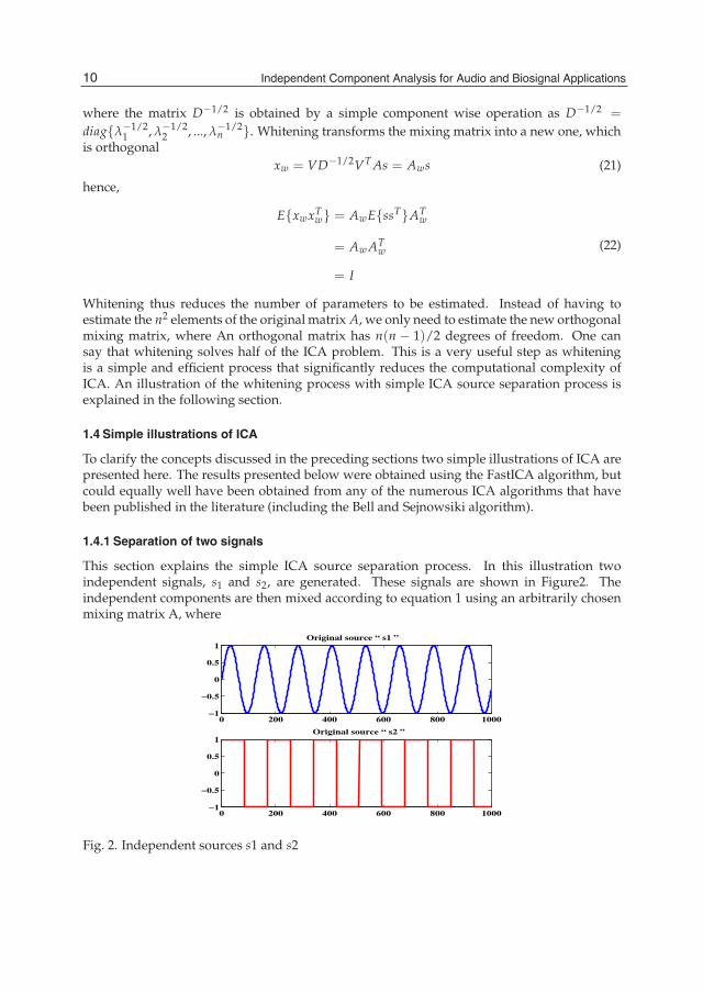
1.4.1 Separation of two signals
This section explains the simple ICA source separation process. In this illustration twoindependent signals, s1 and s2, are generated. These signals are shown in Figure2. Theindependent components are then mixed according to equation 1 using an arbitrarily chosenmixing matrix A, where
0 200 400 600 800 1000−1
−0.5
0
0.5
1
0 200 400 600 800 1000−1
−0.5
0
0.5
1Original source “ s2 ”
Original source “ s1 ”
Fig. 2. Independent sources s1 and s2
10 Independent Component Analysis for Audio and Biosignal Applications

Introduction: Independent Component Analysis 9
0 200 400 600 800 1000−2
−1
0
1
2Mixed signal “ x1 ”
Mixed signal “ x2 ”
0 200 400 600 800 1000−2
−1
0
1
2
Fig. 3. Observed signals, x1 and x2, from an unknown linear mixture of unknownindependent components
0 200 400 600 800 1000−2
−1
0
1
2
0 200 400 600 800 1000−2
−1
0
1
2Estimated signal “ s1 ”
Estimated signal “ s2 ”
Fig. 4. Estimates of independent components
A =
(0.3816 0.86780.8534 −0.5853
)
The resulting signals from this mixing are shown in Figure 3. Finally, the mixtures x1 and x2are separated using ICA to obtain s1 and s2, shown in Figure 4. By comparing Figure 4 toFigure 2 it is clear that the independent components have been estimated accurately and thatthe independent components have been estimated without any knowledge of the componentsthemselves or the mixing process.
This example also provides a clear illustration of the scaling and permutation ambiguitiesdiscussed previously. The amplitudes of the corresponding waveforms in Figures 2 and 4are different. Thus the estimates of the independent components are some multiple of theindependent components of Figure 3, and in the case of s1, the scaling factor is negative. Thepermutation ambiguity is also demonstrated as the order of the independent components hasbeen reversed between Figure 2 and Figure 4.
11Introduction: Independent Component Analysis

10 Will-be-set-by-IN-TECH
−2 −1.5 −1 −0.5 0 0.5 1 1.5 2−2
−1.5
−1
−0.5
0
0.5
1
1.5
2
s1
s2
Fig. 5. Original sources
−4 −3 −2 −1 0 1 2 3 4−2
−1.5
−1
−0.5
0
0.5
1
1.5
2
x1
x2
Fig. 6. Mixed sources
1.4.2 Illustration of statistical independence in ICA
The previous example was a simple illustration of how ICA is used; we start with mixturesof signals and use ICA to separate them. However, this gives no insight into the mechanicsof ICA and the close link with statistical independence. We assume that the independentcomponents can be modeled as realizations of some underlying statistical distribution ateach time instant (e.g. a speech signal can be accurately modeled as having a Laplacian
12 Independent Component Analysis for Audio and Biosignal Applications

Introduction: Independent Component Analysis 11
−4 −3 −2 −1 0 1 2 3 4−4
−3
−2
−1
0
1
2
3
4
x1
x2
Fig. 7. Joint density of whitened signals obtained from whitening the mixed sources
−4 −3 −2 −1 0 1 2 3 4−4
−3
−2
−1
0
1
2
3
4
Estimated s1
Est
ima
ted
s2
Fig. 8. ICA solution (Estimated sources)
distribution). One way of visualizing ICA is that it estimates the optimal linear transformto maximise the independence of the joint distribution of the signals Xi.
The statistical basis of ICA is illustrated more clearly in this example. Consider two randomsignals which are mixed using the following mixing process:
(x1x2
)=
(1 21 1
)(s1s2
)
13Introduction: Independent Component Analysis

12 Will-be-set-by-IN-TECH
Figure 5 shows the scatter-plot for original sources s1 and s2. Figure 6 shows the scatter-plot ofthe mixtures. The distribution along the axis x1 and x2 are now dependent and the form of thedensity is stretched according to the mixing matrix. From the Figure 6 it is clear that the twosignals are not statistically independent because, for example, if x1 = -3 or 3 then x2 is totallydetermined. Whitening is an intermediate step before ICA is applied. The joint distributionthat results from whitening the signals of Figure 6 is shown in Figure 7. By applying ICA, weseek to transform the data such that we obtain two independent components.
The joint distribution resulting from applying ICA to x1 and x2 is shown in Figure 7. This isclearly the joint distribution of two independent, uniformly distributed random variables.Independence can be intuitively confirmed as each random variable is unconstrainedregardless of the value of the other random variable (this is not the case for x1 and x2. Theuniformly distributed random variables in Figure 8 take values between 3 and -3, but due tothe scaling ambiguity, we do not know the range of the original independent components.By comparing the whitened data of Figure 7 with Figure 8, we can see that, in this case,pre-whitening reduces ICA to finding an appropriate rotation to yield independence. Thisis a simplification as a rotation is an orthogonal transformation which requires only oneparameter.
The two examples in this section are simple but they illustrate both how ICA is used and thestatistical underpinnings of the process. The power of ICA is that an identical approach canbe used to address problems of much greater complexity.
2. ICA for different conditions
One of the important conditions of ICA is that the number of sensors should be equal tothe number of sources. Unfortunately, the real source separation problem does not alwayssatisfy this constraint. This section focusses on ICA source separation problem under differentconditions where the number of sources are not equal to the number of recordings.
2.1 Overcomplete ICA
Overcomplete ICA is one of the ICA source separation problem where the number of sourcesare greater than the number of sensors, i.e (n > m). The ideas used for overcomplete ICAoriginally stem from coding theory, where the task is to find a representation of some signalsin a given set of generators which often are more numerous than the signals, hence theterm overcomplete basis. Sometimes this representation is advantageous as it uses as few‘basis’ elements as possible, referred to as sparse coding. Olshausen and Field Olshausen(1995) first put these ideas into an information theoretic context by decomposing naturalimages into an overcomplete basis. Later, Harpur and Prager Harpur & Prager (1996) and,independently, Olshausen Olshausen (1996) presented a connection between sparse codingand ICA in the square case. Lewicki and Sejnowski Lewicki & Sejnowski (2000) then were thefirst to apply these terms to overcomplete ICA, which was further studied and applied by Leeet al. Lee et al. (2000). De Lathauwer et al. Lathauwer et al. (1999) provided an interestingalgebraic approach to overcomplete ICA of three sources and two mixtures by solving asystem of linear equations in the third and fourth-order cumulants, and Bofill and ZibulevskyBofill (2000) treated a special case (‘delta-like’ source distributions) of source signals afterFourier transformation. Overcomplete ICA has major applications in bio signal processing,
14 Independent Component Analysis for Audio and Biosignal Applications

Introduction: Independent Component Analysis 13
due to the limited number of electrodes (recordings) compared to the number active muscles(sources) involved (in certain cases unlimited).
Fig. 9. Illustration of “overcomplete ICA"
In overcomplete ICA, the number of sources exceed number of recordings. To analyse this,consider two recordings x1(t) and x2(t) from three independent sources s1(t), s2(t) and s3(t).The xi(t) are then weighted sums of the si(t), where the coefficients depend on the distancesbetween the sources and the sensors (refer Figure 9):
x1(t) = a11s1(t) + a12s2(t) + a13s3(t) (23)
x2(t) = a21s1(t) + a22s2(t) + a23s3(t)
The aij are constant coefficients that give the mixing weights. The mixing process of thesevectors can be represented in the matrix form as (refer Equation 1):
(x1x2
)=
(a11 a12 a13a21 a22 a23
)⎛⎝s1
s2s3
⎞⎠
The unmixing process and estimation of sources can be written as (refer Equation 2):⎛⎝s1
s2s3
⎞⎠ =
⎛⎝w11 w12
w21 w22w31 w32
⎞⎠(
x1x2
)
In this example matrix A of size 2×3 matrix and unmixing matrix W is of size 3×2. Hencein overcomplete ICA it always results in pseudoinverse. Hence computation of sources inovercomplete ICA requires some estimation processes.
2.2 Undercomplete ICA
The mixture of unknown sources is referred to as under-complete when the numbers ofrecordings m, more than the number of sources n. In some applications, it is desired tohave more recordings than sources to achieve better separation performance. It is generallybelieved that with more recordings than the sources, it is always possible to get better estimateof the sources. This is not correct unless prior to separation using ICA, dimensional reduction
15Introduction: Independent Component Analysis

14 Will-be-set-by-IN-TECH
is conducted. This can be achieved by choosing the same number of principal recordings asthe number of sources discarding the rest. To analyse this, consider three recordings x1(t),x2(t) and x3(t) from two independent sources s1(t) and s2(t). The xi(t) are then weightedsums of the si(t), where the coefficients depend on the distances between the sources and thesensors (refer Figure 10):
Fig. 10. Illustration of “undercomplete ICA"
x1(t) = a11s1(t) + a12s2(t)
x2(t) = a21s1(t) + a22s2(t) (24)
x3(t) = a31s1(t) + a32s2(t)
The aij are constant coefficients that gives the mixing weights. The mixing process of thesevectors can be represented in the matrix form as:⎛
⎝x1x2x3
⎞⎠ =
⎛⎝a11 a12
a21 a22a31 a32
⎞⎠(
s1s2
)
The unmixing process using the standard ICA requires a dimensional reduction approach sothat, if one of the recordings is reduced then the square mixing matrix is obtained, which canuse any standard ICA for the source estimation. For instance one of the recordings say x3 isredundant then the above mixing process can be written as:(
x1x2
)=
(a11 a12a21 a22
)(s1s2
)
Hence unmixing process can use any standard ICA algorithm using the following:(s1s2
)=
(w11 w12w21 w22
)(x1x2
)
The above process illustrates that, prior to source signal separation using undercomplete ICA,it is important to reduce the dimensionality of the mixing matrix and identify the requiredand discard the redundant recordings. Principal Component Analysis (PCA) is one of thepowerful dimensional reduction method used in signal processing applications, which isexplained next.
16 Independent Component Analysis for Audio and Biosignal Applications

Introduction: Independent Component Analysis 15
3. Applications of ICA
The success of ICA in source separation has resulted in a number of practical applications.Some of these includes,
• Machine fault detection Kano et al. (2003); Li et al. (2006); Ypma et al. (1999);Zhonghai et al. (2009)
• Seismic monitoring Acernese et al. (2004); de La et al. (2004)• Reflection canceling Farid & Adelson (1999); Yamazaki et al. (2006)• Finding hidden factors in financial data Cha & Chan (2000); Coli et al. (2005); Wu & Yu
(2005)• Text document analysis Bingham et al. (2002); Kolenda (2000); Pu & Yang (2006)• Radio communications Cristescu et al. (2000); Huang & Mar (2004)• Audio signal processing Cichocki & Amari (2002); Lee (1998)• Image processing Cichocki & Amari (2002); Déniz et al. (2003); Fiori (2003); Karoui et al.
(2009); Wang et al. (2008); Xiaochun & Jing (2004); Zhang et al. (2007)• Data mining Lee et al. (2009)• Time series forecasting Lu et al. (2009)• Defect detection in patterned display surfaces Lu1 & Tsai (2008); Tsai et al. (2006)• Bio medical signal processing Azzerboni et al. (2004); Castells et al. (2005);
De Martino et al. (2007); Enderle et al. (2005); James & Hesse (2005); Kumagai & Utsugi(2004); Llinares & Igual (2009); Safavi et al. (2008); Zhu et al. (2006).
3.1 Audio and biomedical applications of ICA
Exemplary ICA applications in biomedical problems include the following:
• Fetal Electrocardiogram extraction, i.e removing/filtering maternal electrocardiogramsignals and noise from fetal electrocardiogram signals Niedermeyer & Da Silva (1999);Rajapakse et al. (2002).
• Enhancement of low level Electrocardiogram components Niedermeyer & Da Silva (1999);Rajapakse et al. (2002)
• Separation of transplanted heart signals from residual original heart signals Wisbeck et al.(1998)
• Separation of low level myoelectric muscle activities to identify various gesturesCalinon & Billard (2005); Kato et al. (2006); Naik et al. (2006; 2007)
One successful and promising application domain of blind signal processing includesthose biomedical signals acquired using multi-electrode devices: Electrocardiography(ECG), Llinares & Igual (2009); Niedermeyer & Da Silva (1999); Oster et al. (2009);Phlypo et al. (2007); Rajapakse et al. (2002); Scherg & Von Cramon (1985); Wisbeck et al.(1998), Electroencephalography (EEG) Jervis et al. (2007); Niedermeyer & Da Silva (1999);Onton et al. (2006); Rajapakse et al. (2002); Vigário et al. (2000); Wisbeck et al. (1998),Magnetoencephalography (MEG) Hämäläinen et al. (1993); Mosher et al. (1992); Parra et al.(2004); Petersen et al. (2000); Tang & Pearlmutter (2003); Vigário et al. (2000).
One of the most practical uses for BSS is in the audio world. It has been used for noise removalwithout the need of filters or Fourier transforms, which leads to simpler processing methods.
17Introduction: Independent Component Analysis

16 Will-be-set-by-IN-TECH
There are various problems associated with noise removal in this way, but these can mostlikely be attributed to the relative infancy of the BSS field and such limitations will be reducedas research increases in this field Bell & Sejnowski (1997); Hyvarinen et al. (2001).
Audio source separation is the problem of automated separation of audio sources presentin a room, using a set of differently placed microphones, capturing the auditory scene. Thewhole problem resembles the task a human listener can solve in a cocktail party situation,where using two sensors (ears), the brain can focus on a specific source of interest, suppressingall other sources present (also known as cocktail party problem) Hyvarinen et al. (2001); Lee(1998).
4. Conclusions
This chapter has introduced the fundamentals of BSS and ICA. The mathematical frameworkof the source mixing problem that BSS/ICA addresses was examined in some detail, aswas the general approach to solving BSS/ICA. As part of this discussion, some inherentambiguities of the BSS/ICA framework were examined as well as the two importantpreprocessing steps of centering and whitening. The application domains of this noveltechnique are presented. The material covered in this chapter is important not only tounderstand the algorithms used to perform BSS/ICA, but it also provides the necessarybackground to understand extensions to the framework of ICA for future researchers.
The other novel and recent advances of ICA, especially on Audio and Biosignal topics arecovered in rest of the chapters in this book.
5. References
Acernese, F., Ciaramella, A., De Martino, S., Falanga, M., Godano, C. & Tagliaferri, R. (2004).Polarisation analysis of the independent components of low frequency events atstromboli volcano (eolian islands, italy), Journal of Volcanology and Geothermal Research137(1-3): 153–168.
Attias, H. & Schreiner, C. E. (1998). Blind source separation and deconvolution: the dynamiccomponent analysis algorithm, Neural Comput. 10(6): 1373–1424.
Azzerboni, B., Carpentieri, M., La Foresta, F. & Morabito, F. C. (2004). Neural-ica and wavelettransform for artifacts removal in surface emg, Neural Networks, 2004. Proceedings.2004 IEEE International Joint Conference on, Vol. 4, pp. 3223–3228 vol.4.
Bell, A. J. & Sejnowski, T. J. (1995). An information-maximization approach to blind separationand blind deconvolution., Neural Comput 7(6): 1129–1159.
Bell, A. J. & Sejnowski, T. J. (1997). The "independent components" of natural scenes are edgefilters., Vision Res 37(23): 3327–3338.
Bingham, E., Kuusisto, J. & Lagus, K. (2002). Ica and som in text document analysis, SIGIR’02: Proceedings of the 25th annual international ACM SIGIR conference on Research anddevelopment in information retrieval, ACM, pp. 361–362.
Bofill (2000). Blind separation of more sources than mixtures using sparsity of their short-timefourier transform, pp. 87–92.
Calinon, S. & Billard, A. (2005). Recognition and reproduction of gestures using aprobabilistic framework combining pca, ica and hmm, ICML ’05: Proceedings of the22nd international conference on Machine learning, ACM, pp. 105–112.
18 Independent Component Analysis for Audio and Biosignal Applications

Introduction: Independent Component Analysis 17
Castells, F., Igual, J., Millet, J. & Rieta, J. J. (2005). Atrial activity extraction from atrialfibrillation episodes based on maximum likelihood source separation, Signal Process.85(3): 523–535.
Cha, S.-M. &Chan, L.-W. (2000). Applying independent component analysis to factor model infinance, IDEAL ’00: Proceedings of the Second International Conference on Intelligent DataEngineering and Automated Learning, Data Mining, Financial Engineering, and IntelligentAgents, Springer-Verlag, pp. 538–544.
Cichocki, A. & Amari, S.-I. (2002). Adaptive Blind Signal and Image Processing: LearningAlgorithms and Applications, John Wiley & Sons, Inc.
Coli, M., Di Nisio, R. & Ippoliti, L. (2005). Exploratory analysis of financial time seriesusing independent component analysis, Information Technology Interfaces, 2005. 27thInternational Conference on, pp. 169–174.
Cristescu, R., Ristaniemi, T., Joutsensalo, J. & Karhunen, J. (2000). Cdma delay estimationusing fast ica algorithm, Vol. 2, pp. 1117–1120 vol.2.
de La, Puntonet, C. G., Górriz, J. M. & Lloret, I. (2004). An application of ica to identifyvibratory low-level signals generated by termites, pp. 1126–1133.
DeMartino, F., Gentile, F., Esposito, F., Balsi, M., Di Salle, F., Goebel, R. & Formisano, E. (2007).Classification of fmri independent components using ic-fingerprints and supportvector machine classifiers, NeuroImage 34: 177–194.
Déniz, O., Castrillón, M. & Hernández, M. (2003). Face recognition using independentcomponent analysis and support vector machines, Pattern Recogn. Lett.24(13): 2153–2157.
Enderle, J., Blanchard, S. M. & Bronzino, J. (eds) (2005). Introduction to Biomedical Engineering,Second Edition, Academic Press.
Farid, H. & Adelson, E. H. (1999). Separating reflections and lighting using independentcomponents analysis, cvpr 01.
Fiori, S. (2003). Overview of independent component analysis technique with an applicationto synthetic aperture radar (sar) imagery processing, Neural Netw. 16(3-4): 453–467.
Hämäläinen, M., Hari, R., Ilmoniemi, R. J., Knuutila, J. & Lounasmaa, O. V.(1993). Magnetoencephalography—theory, instrumentation, and applicationsto noninvasive studies of the working human brain, Reviews of Modern Physics65(2): 413+.
Hansen (2000). Blind separation of noicy image mixtures., Springer-Verlag, pp. 159–179.Harpur, G. F. & Prager, R. W. (1996). Development of low entropy coding in a recurrent
network., Network (Bristol, England) 7(2): 277–284.Herault, J. & Jutten, C. (1987). Herault, J. and Jutten, C. (1987), Space or time adaptive signal
processing by neural networkmodels, in ’AIP Conference Proceedings 151 on NeuralNetworks for Computing’, American Institute of Physics Inc., pp. 206-211.
Huang, J. P. & Mar, J. (2004). Combined ica and fca schemes for a hierarchical network, Wirel.Pers. Commun. 28(1): 35–58.
Hyvarinen, A., Cristescu, R. & Oja, E. (1999). A fast algorithm for estimating overcompleteica bases for image windows, Neural Networks, 1999. IJCNN ’99. International JointConference on, Vol. 2, pp. 894–899 vol.2.
Hyvarinen, A., Karhunen, J. & Oja, E. (2001). Independent Component Analysis,Wiley-Interscience.
James, C. J. & Hesse, C. W. (2005). Independent component analysis for biomedical signals,Physiological Measurement 26(1): R15+.
19Introduction: Independent Component Analysis

18 Will-be-set-by-IN-TECH
Jervis, B., Belal, S., Camilleri, K., Cassar, T., Bigan, C., Linden, D. E. J., Michalopoulos,K., Zervakis, M., Besleaga, M., Fabri, S. & Muscat, J. (2007). The independentcomponents of auditory p300 and cnv evoked potentials derived from single-trialrecordings, Physiological Measurement 28(8): 745–771.
Kab’an (2000). Clustering of text documents by skewness maximization, pp. 435–440.Kano, M., Tanaka, S., Hasebe, S., Hashimoto, I. & Ohno, H. (2003). Monitoring independent
components for fault detection, AIChE Journal 49(4): 969–976.Karoui, M. S., Deville, Y., Hosseini, S., Ouamri, A. &Ducrot, D. (2009). Improvement of remote
sensingmultispectral image classification by using independent component analysis,2009 First Workshop on Hyperspectral Image and Signal Processing: Evolution in RemoteSensing, IEEE, pp. 1–4.
Kato, M., Chen, Y.-W.& Xu, G. (2006). Articulated hand tracking by pca-ica approach, FGR ’06:Proceedings of the 7th International Conference on Automatic Face and Gesture Recognition,IEEE Computer Society, pp. 329–334.
Kolenda (2000). Independent components in text, Advances in Independent ComponentAnalysis, Springer-Verlag, pp. 229–250.
Kumagai, T. & Utsugi, A. (2004). Removal of artifacts and fluctuations from meg data byclustering methods, Neurocomputing 62: 153–160.
Lathauwer, D., L. Comon, P., De Moor, B. & Vandewalle, J. (1999). Ica algorithms for 3 sourcesand 2 sensors, Higher-Order Statistics, 1999. Proceedings of the IEEE Signal ProcessingWorkshop on, pp. 116–120.
Lee, J.-H. H., Oh, S., Jolesz, F. A., Park, H. & Yoo, S.-S. S. (2009). Application of independentcomponent analysis for the data mining of simultaneous eeg-fmri: preliminaryexperience on sleep onset., The International journal of neuroscience 119(8): 1118–1136.URL: http://view.ncbi.nlm.nih.gov/pubmed/19922343
Lee, T. W. (1997). Blind separation of delayed and convolved sources, pp. 758–764.Lee, T. W. (1998). Independent component analysis: theory and applications, Kluwer Academic
Publishers.Lee, T. W., Girolami, M., Lewicki, M. S. & Sejnowski, T. J. (2000). Blind source separation
of more sources than mixtures using overcomplete representations, Signal ProcessingLetters, IEEE 6(4): 87–90.
Lee, T. W., Lewicki, M. S. & Sejnowski, T. J. (1999). Unsupervised classification withnon-gaussian mixture models using ica, Proceedings of the 1998 conference on Advancesin neural information processing systems, MIT Press, Cambridge,MA, USA, pp. 508–514.
Lewicki, M. S. & Sejnowski, T. J. (2000). Learning overcomplete representations., NeuralComput 12(2): 337–365.
Li, Z., He, Y., Chu, F., Han, J. & Hao, W. (2006). Fault recognition method forspeed-up and speed-down process of rotating machinery based on independentcomponent analysis and factorial hidden markov model, Journal of Sound andVibration 291(1-2): 60–71.
Llinares, R. & Igual, J. (2009). Application of constrained independent component analysisalgorithms in electrocardiogram arrhythmias, Artif. Intell. Med. 47(2): 121–133.
Lu, C.-J., Lee, T.-S. & Chiu, C.-C. (2009). Financial time series forecasting usingindependent component analysis and support vector regression, Decis. Support Syst.47(2): 115–125.
Lu1, C.-J. & Tsai, D.-M. (2008). Independent component analysis-based defect detection inpatterned liquid crystal display surfaces, Image Vision Comput. 26(7): 955–970.
20 Independent Component Analysis for Audio and Biosignal Applications

Introduction: Independent Component Analysis 19
Mackay, D. J. C. (1996). Maximum likelihood and covariant algorithms for independentcomponent analysis, Technical report, University of Cambridge, London.
Mosher, J. C., Lewis, P. S. & Leahy, R. M. (1992). Multiple dipole modeling andlocalization from spatio-temporal meg data, Biomedical Engineering, IEEE Transactionson 39(6): 541–557.
Naik, G. R., Kumar, D. K., Singh, V. P. & Palaniswami, M. (2006). Hand gestures for hciusing ica of emg, VisHCI ’06: Proceedings of the HCSNet workshop on Use of vision inhuman-computer interaction, Australian Computer Society, Inc., pp. 67–72.
Naik, G. R., Kumar, D. K., Weghorn, H. & Palaniswami, M. (2007). Subtle hand gestureidentification for hci using temporal decorrelation source separation bss of surfaceemg, Digital Image Computing Techniques and Applications, 9th Biennial Conference of theAustralian Pattern Recognition Society on, pp. 30–37.
Niedermeyer, E. & Da Silva, F. L. (1999). Electroencephalography: Basic Principles, ClinicalApplications, and Related Fields, Lippincott Williams and Wilkins; 4th edition .
Olshausen (1995). Sparse coding of natural images produces localized, oriented, bandpassreceptive fields, Technical report, Department of Psychology, Cornell University.
Olshausen, B. A. (1996). Learning linear, sparse, factorial codes, Technical report.Onton, J., Westerfield, M., Townsend, J. & Makeig, S. (2006). Imaging human eeg
dynamics using independent component analysis, Neuroscience & BiobehavioralReviews 30(6): 808–822.
Oster, J., Pietquin, O., Abächerli, R., Kraemer, M. & Felblinger, J. (2009). Independentcomponent analysis-based artefact reduction: application to the electrocardiogramfor improved magnetic resonance imaging triggering, Physiological Measurement30(12): 1381–1397.URL: http://dx.doi.org/10.1088/0967-3334/30/12/007
Parra, J., Kalitzin, S. N. & Lopes (2004). Magnetoencephalography: an investigational tool ora routine clinical technique?, Epilepsy & Behavior 5(3): 277–285.
Petersen, K., Hansen, L. K., Kolenda, T. & Rostrup, E. (2000). On the independent componentsof functional neuroimages, Third International Conference on Independent ComponentAnalysis and Blind Source Separation, pp. 615–620.
Phlypo, R., Zarzoso, V., Comon, P., D’Asseler, Y. & Lemahieu, I. (2007). Extraction of atrialactivity from the ecg by spectrally constrained ica based on kurtosis sign, ICA’07:Proceedings of the 7th international conference on Independent component analysis andsignal separation, Springer-Verlag, Berlin, Heidelberg, pp. 641–648.
Pu, Q. & Yang, G.-W. (2006). Short-text classification based on ica and lsa, Advances in NeuralNetworks - ISNN 2006 pp. 265–270.
Rajapakse, J. C., Cichocki, A. & Sanchez (2002). Independent component analysis and beyondin brain imaging: Eeg, meg, fmri, and pet,Neural Information Processing, 2002. ICONIP’02. Proceedings of the 9th International Conference on, Vol. 1, pp. 404–412 vol.1.
Safavi, H., Correa, N., Xiong, W., Roy, A., Adali, T., Korostyshevskiy, V. R., Whisnant,C. C. & Seillier-Moiseiwitsch, F. (2008). Independent component analysis of 2-delectrophoresis gels, ELECTROPHORESIS 29(19): 4017–4026.
Scherg, M. & Von Cramon, D. (1985). Two bilateral sources of the late aep as identified by aspatio-temporal dipole model., Electroencephalogr Clin Neurophysiol 62(1): 32–44.
Sorenson (2002). Mean field approaches to independent component analysis, NeuralComputation 14: 889–918.
21Introduction: Independent Component Analysis

20 Will-be-set-by-IN-TECH
Stone, J. V. (2004). Independent Component Analysis : A Tutorial Introduction (Bradford Books), TheMIT Press.
Tang, A. C. & Pearlmutter, B. A. (2003). Independent components ofmagnetoencephalography: localization, pp. 129–162.
Tsai, D.-M., Lin, P.-C. & Lu, C.-J. (2006). An independent component analysis-basedfilter design for defect detection in low-contrast surface images, Pattern Recogn.39(9): 1679–1694.
Vigário, R., Särelä, J., Jousmäki, V., Hämäläinen, M. & Oja, E. (2000). Independent componentapproach to the analysis of eeg and meg recordings., IEEE transactions on bio-medicalengineering 47(5): 589–593.
Wang, H., Pi, Y., Liu, G. & Chen, H. (2008). Applications of ica for the enhancement andclassification of polarimetric sar images, Int. J. Remote Sens. 29(6): 1649–1663.
Wisbeck, J., Barros, A. & Ojeda, R. (1998). Application of ica in the separation of breathingartifacts in ecg signals.
Wu, E. H. & Yu, P. L. (2005). Independent component analysis for clustering multivariate timeseries data, pp. 474–482.
Xiaochun, L. & Jing, C. (2004). An algorithm of image fusion based on ica andchange detection, Proceedings 7th International Conference on Signal Processing, 2004.Proceedings. ICSP ’04. 2004., IEEE, pp. 1096–1098.
Yamazaki, M., Chen, Y.-W. & Xu, G. (2006). Separating reflections from images usingkernel independent component analysis, Pattern Recognition, 2006. ICPR 2006. 18thInternational Conference on, Vol. 3, pp. 194–197.
Ypma, A., Tax, D. M. J. & Duin, R. P. W. (1999). Robust machine fault detectionwith independent component analysis and support vector data description, NeuralNetworks for Signal Processing IX, 1999. Proceedings of the 1999 IEEE Signal ProcessingSociety Workshop, pp. 67–76.
Zhang, Q., Sun, J., Liu, J. & Sun, X. (2007). A novel ica-based image/video processingmethod,pp. 836–842.
Zhonghai, L., Yan, Z., Liying, J. & Xiaoguang, Q. (2009). Application of independentcomponent analysis to the aero-engine fault diagnosis, 2009 Chinese Control andDecision Conference, IEEE, pp. 5330–5333.
Zhu, Y., Chen, T. L., Zhang, W., Jung, T.-P., Duann, J.-R., Makeig, S. & Cheng, C.-K. (2006).Noninvasive study of the human heart using independent component analysis, BIBE’06: Proceedings of the Sixth IEEE Symposium on BionInformatics and BioEngineering,IEEE Computer Society, pp. 340–347.
22 Independent Component Analysis for Audio and Biosignal Applications

Section 2
ICA: Audio Applications


0
On Temporomandibular Joint Sound SignalAnalysis Using ICA
Feng Jin1 and Farook Sattar21Dept of Electrical & Computer Engineering,
Ryerson University, Toronto, Ontario2Dept of Electrical & Computer Engineering,
University of Waterloo,Waterloo, OntarioCanada
1. Introduction
The Temporomandibular Joint (TMJ) is the joint which connects the lower jaw, called themandible, to the temporal bone at the side of the head. The joint is very importantwith regard to speech, mastication and swallowing. Any problem that prevents thissystem from functioning properly may result in temporomandibular joint disorder (TMD).Symptoms include pain, limited movement of the jaw, radiating pain in the face, neck orshoulders, painful clicking, popping or grating sounds in the jaw joint during opening and/orclosing of the mouth. TMD being the most common non-dental related chronic source oforal-facial pain(Gray et al., 1995)(Pankhurst C. L, 1997), affects over 75% of the United Statespopulation(Berman et al., 2006). TMJ sounds during jaw motion are important indicationof dysfunction and are closely correlated with the joint pathology(Widmalm et al., 1992).The TMJ sounds are routinely recorded by auscultation and noted in dental examinationprotocols. However, stethoscopic auscultation is very subjective and difficult to document.The interpretations of the sounds often vary among different doctors. Early detection of TMD,before irreversible gross erosive changes take place, is extremely important.
Electronic recording of TMJ sounds therefore offers some advantages over stethoscopicauscultation recording by allowing the clinician to store the sound for further analysis andfuture reference. Secondly, the recording of TMJ sounds is also an objective and quantitativerecord of the TMJ sounds during the changes in joint pathology. The most importantadvantage is that electronic recording allows the use of advanced signal processing techniquesto the automatic classification of the sounds. A cheap, efficient and reliable diagnostic toolfor early detection of TMD can be developed using TMJ sounds recorded with a pair ofmicrophones placed at the openings of the auditory canals. The analysis of these recordedTMJ vibrations offers a powerful non-invasive alternative to the old clinical methods such asauscultation and radiation.
In early studies, the temporal waveforms and power spectra of TMJ sounds wereanalyzed(Widmalm et al., 1991) to characterize signals based on their time behavior or theirenergy distribution over a frequency range. However, such approaches are not sufficient to
2

2 Will-be-set-by-IN-TECH
fully characterize non-stationary signals like TMJ sounds. In other words, for non-stationarysignals like TMJ vibrations, it is required to know how the frequency components of the signalchange with time. This can be achieved by obtaining the distribution of signal energy overthe TF plane(Cohen L., 1995). Several joint time-frequency analysis methods have then beenapplied to the analysis and classification of TMJ vibrations into different classes based on theirtime-frequency reduced interference distribution (RID)(Widmalm&Widmalm, 1996)(Akan etal., 2000). According to TF analysis, four distinct classes of defective TMJ sounds are defined:click, click with crepitation, soft crepitation, and hard crepitation(Watt, 1980) Here, clicks areidentified as high amplitude peaks of very short duration, and crepitations are signals withmultiple peaks of various amplitude and longer duration as well as a wide frequency range.
In this chapter, instead of discussing the classification of TMJ sounds into various typesbased on their TF characteristics, we address the problem of source separation of the stereorecordings of TMJ sounds. Statistical correlations between different type of sounds and thejoint pathology have been explored by applying ICA based methods to present a potentialdiagnostic tool for temporomandibular joint disorder.
The chapter outline is as follows: The details for data acquisition are elaborated in Section2, followed by the problem definition and the possible contribution of the independentcomponent analysis (ICA) based approach. The proposed signal mixing and propagationmodels are then proposed in Section 3, with the theoretical background of ICA and theproposed ICA based solutions described in Sections 4 to 6. The illustrative results of thepresent method on both simulated and real TMJ signals are compared with other existingsource separation methods in Section 7. The performance of the method has been furtherevaluated quantitatively in Section 8. Lastly, the chapter summary and discussion arepresented in Section 9.
2. Data acquisition
The auditory canal is an ideal location for the non-invasive sensor (microphone) to comeas close to the joint as possible. The microphones were held in place by earplugs made ofa kneadable polysiloxane impression material (called the Reprosil putty and produced byDentsply). A hole was punched through each earplug to hold the microphone in place and toreduce the interference of ambient noise in the recordings.
In this study, the TMJ sounds were recorded on a Digital Audio Tape (DAT) recorder. Duringrecording session, the necessary equipments are two Sony ECM-77-B electret condensermicrophones, Krohn-Hite 3944 multi-channel analog filter and TEAC RD-145T or TASCAMDA-P1 DAT recorder. The microphones have a frequency response ranges from 40–20,000 Hzand omni-directional. It acts as a transducer to capture the TMJ sounds. The signals were thenpassed through a lowpass filter to prevent aliasing effect of the digital signal. A Butterworthfilter with a cut-off frequency of 20 KHz and attenuation slope of 24 dB/octave was set at theanalog filter. There is an option to set the gain at the filter to boost up the energy level of thesignal. The option was turned on when the TMJ sounds were too soft and the signals fromthe microphones were amplified to make full use of the dynamic range of the DAT recorder.Finally, the signals from the analog filter were sampled in the DAT recorder at the rate of 48KHz and data were saved on a disc.
26 Independent Component Analysis for Audio and Biosignal Applications

On Temporomandibular Joint Sound Signal Analysis Using ICA 3
3. Problems and solution: The role of ICA
One common and major problem in both stethoscopic auscultation and digital recordingis that the sound originating from one side will propagate to the other side, leading tomisdiagnosis in some cases. It is shown in Fig. 1(a) that short duration TMJ sounds (less than10ms) are frequently recorded in both channels very close in time. When the two channelsshow similarwaveforms, with one lagging and attenuated to some degree, it can be concludedthat the lagging signal is in fact the propagated version of the other signal(Widmalm et al.,1997).
0 2 4 6 8 10 12 14 16−1500
−1000
−500
0
500
1000
1500
2000
time (ms)
ampl
itude
40 41 42 43 44 45 46 47 48 49 50−0.04
−0.03
−0.02
−0.01
0
0.01
0.02
0.03
0.04
time (ms)
ampl
itude
id02056o2.wav
(a) (b)Fig. 1. TMJ sounds of two channels.
This observation is very important. It means that a sound heard at auscultation on one sidemay have actually come from the other TMJ. This has great clinical significance because it isnecessary to know the true source of the recorded sound, for example in diagnosing so calleddisk displacement with reduction(Widmalm et al., 1997). The TMJ sounds can be classifiedinto two major classes: clicks and crepitations. A click is a distinct sound, of very limitedduration, with a clear beginning and end. As the name suggests, it sounds like a “click”. Acrepitation has a longer duration. It sounds like a series of short but rapidly repeating soundsthat occur close in time. Sometimes, it is described as “grinding of snow” or “sand falling”.The duration of a click is very short (usually less than 10ms). It is possible to differentiatebetween the source and the propagated soundwithout much difficulty. This is due to the shortdelay (about 0.2ms) and the difference in amplitude between the signals of the two channels,especially if one TMJ is silent. However, it is sometimes very difficult to tell which is the sourcesignals from the recordings. In Fig. 1(b), it seems that the dashed line is the source if we simplylook at the amplitude. On the other hand, it might seem that the solid line is the source ifwe look at the time (it comes first). ICA could have vital role to solve this problem sinceboth the sources (sounds from both TMJ) and the mixing process (the transfer function of thehuman head, bone and tissue) are unknown. If ICA is used, one output should be the originalsignal and the other channel should be silent with very low amplitude noise picked up by themicrophone. Then it is very easy to tell which channel is the original sound. Furthermore, inthe case of crepitation sounds, the duration of the signal is longer, and further complicated bythe fact that both sides may crepitate at the same time. The ICA is then proposed as a meansto recover the original sound for each channel.
27On Temporomandibular Joint Sound Signal Analysis Using ICA

4 Will-be-set-by-IN-TECH
4. Mixing model of TMJ sound signals
In this chapter, the study is not limited to patients with only one defective TMD joint. Wethus consider the TMJ sounds recorded simultaneously from both sides of human head asa mixture of crepitations/clicks from the TMD affected joint and the noise produced by theother healthy TMJ or another crepitation/click. Instead of regarding the ‘echo’ recordedon thecontra (i.e. opposite) side of the TMD joint as the lagged version of the TMD source(Widmalmet al., 2002), we consider here the possibility that this echo as a mixture of the TMD sources.Mathematically, the mixing model of the observed TMJ sound measurements is representedas
xi(t) =2
∑j=1
hijsj(t− δij) + ni(t) (1)
with sj being the jth source and xi as the ith TMJ mixture signal with i = 1, 2. The additivewhite Gaussian noise at discrete time t is denoted by ni(t). Also, the attenuation coefficients,as well as the time delays associated with the transmission path between the jth source andthe ith sensor (i.e. microphone) are denoted by hij and δij, respectively.
Fig. 2 shows how the TMJ sounds are mixed. Sounds originating from a TMJ are pickedup by the microphone in the auditory canal immediately behind the joint and also by themicrophone in the other auditory canal as the sound travels through the human head.
A (11)
A (21)
A (12)
Human Head
A (22)
Left
Microphone
Right
Microphone
LeftTMJ
Right
TMJ
Fig. 2. Mixing model of TMJ sounds (Aij refers to the acoustic path between the j = 1 (i.e. leftside of human head) source and the i = 2 (right side of the human head) sensor.
The mixing matrix H could therefore be defined as below with z−1 indicating unit delay:
H =
(h11z−δ11 h12z−δ12
h21z−δ21 h22z−δ22
)(2)
Please note that the time delay δ is not necessarily to be integer due to the uncertainty in soundtransmission time in tissues.
The independency of the TMJ sound sources on both sides of the head might not hold as bothjoints operate synchronously during the opening and closing of mouth. Therefore, unlike theconvolutive mixing model assumed in our previous paper(Guo et al., 1999), the instantaneousmixing model presented here does not depend on the assumption of statistical independence
28 Independent Component Analysis for Audio and Biosignal Applications

On Temporomandibular Joint Sound Signal Analysis Using ICA 5
of the sources. In this work, the main assumptions made include the non-stationarity of allthe source signals as well as anechoic head model. Here, the anechoic model is assumed dueto the facts that:
1. TMJ sound made by the opposite side of the TMD joint has been reported as a delayedversion of its ipsi(Widmalm et al., 2002).
2. The TMJ sounds has a wide bandwidth of [20, 3200]Hz. While it travels across the head,the high frequency components (>1200Hz) have been severely attenuated(OBrien et al.,2005).
Single effective acoustic path from one side of the head to the other side is thus assumed.Also, the mixing model in Eq. (1) holds with mixing matrix presented in Eq. (2). However,due to the wide bandwidth of crepitation, source TMJ signals are not necessarily to be sparsein the time-frequency domain. This gives the proposed ICA based method better robustnessas compared to the blind source separation algorithm proposed in(Took et al., 2008).
5. Theoretical background of ICA
There are three basic and intuitive principles for estimating the model of independentcomponent analysis.
1) ICA by minimization of mutual information
This is based on information-theoretic concept, i.e. information maximization (InfoMax) asbriefly explained here.
The differential entropy H of a random vector y with density p(y) is defined as (Hyvärinen,1999):
H(y) = −∫
p(y)logp(y)dy (3)
Basically, the mutual information I between m (scalar) random variables yi, i = 1 · · ·m isdefined as follows:
I(y1, y2, · · · , ym) =m
∑i=1
H(yi)− H(y) (4)
The mutual information is I(y1, y2) = ∑2i=1 H(yi)− H(y1, y2), where ∑2
i=1 H(yi) is marginalentropy and H(y1, y2) is joint entropy. The mutual information is a natural measure of thedependence between random variables. It is always nonnegative, and zero if and only ifthe variables are statistically independent. Therefore, we can use mutual information as thecriterion for finding the ICA representation, i.e. to make the output "decorrelated". In any case,minimization of mutual information can be interpreted as giving the maximally independentcomponents(Hyvärinen, 1999).
2) ICA by maximization of non-Gaussianity
Non-Gaussianity is actually most important in ICA estimation. In classic statistical theory,random variables are assumed to have Gaussian distributions. So we start by motivating themaximization of Non-Gaussianity by the central limit theorem. It has important consequencesin independent component analysis and blind source separation. Even for a small number ofsources the distribution of the mixture is usually close to Gaussian. We can simply explainedthe concept as follows:
29On Temporomandibular Joint Sound Signal Analysis Using ICA

6 Will-be-set-by-IN-TECH
Let us assume that the data vector x is distributed according to the ICA data model: x = Hsis a mixture of independent source components s and H is the unknown full rank (n × m)mixing matrix for m mixed signals and n independent source components. Estimating theindependent components can be accomplished by finding the right linear combinations of themixture variables. We can invert the mixing model in vector form as: s = H−1x, so the linearcombination of xi. In other words, we can denote this by y = bTx = ∑m
i=1 bixi. We could take bas a vector that maximizes the Non-Gaussianity of bTx . This means that y = bTx equals one ofthe independent components. Therefore,maximizing the Non-Gaussianity of bTx gives us oneof the independent components(Hyvärinen, 1999). To find several independent components,we need to find all these local maxima. This is not difficult, because the different independentcomponents are uncorrelated. We can always constrain the search to the space that givesestimates uncorrelated with the previous ones(Hyvärinen, 2004).
3) ICA by maximization of likelihood
Maximization of likelihood is one of the popular approaches to estimate the independentcomponents analysis model. Maximum likelihood (ML) estimator assumes that the unknownparameters are constants if there is no prior information available on them. It usually appliesto large numbers of samples. One interpretation of ML estimation is calculating parametervalues as estimates that give the highest probability for the observations. There are twoalgorithms to perform the maximum likelihood estimation:
• Gradient algorithm: this is the algorithms for maximizing likelihood obtained by thegradient based method(Hyvärinen, 1999).
• Fast fixed-point algorithm(Ella, 2000): the basic principle is to maximize the measuresof Non-Gaussianity used for ICA estimation. Actually, the FastICA algorithm(gradient-based algorithm but converge very fast and reliably) can be directly applied tomaximization of the likelihood.
6. The proposed ICA based TMJ analysis method
The proposed ICA based TMJ analysis method is based on the following considerations:i) asymmetric mixing, ii) non-sparse source conditions. Based on the above criterion weconsider to apply the ICA technique based on information maximization as introduced abovein Section 5 for the analysis of TMJ signals. We therefore propose an improved Infomaxmethod based on its robustness against noise and general mixing properties. The presentmethod has an adaptive contrast function (i.e. adaptive log-sigmoidal function) together withnon-causal filters over the conventional Infomax method in Bell & Sejnowski (1995); Torkkola(1996) to get better performance for a pair of TMJ sources.
The nonlinear function, f , must be a monotonically increasing or decreasing function. In thispaper, the nonlinear function proposed is defined as
y = f (u; b,m) = [1/(1+ e−bu)]m. (5)
Maximizing the output information can be then achieved by minimizing the mutualinformation between the outputs y1 and y2 of the above adaptive f function. In Eq. (5) theadaptation in the slope parameter b is equivalent to adaptive learning rate during our iterativeprocess. This let us perform the iterationwith a small learning rate followed by larger learning
30 Independent Component Analysis for Audio and Biosignal Applications

On Temporomandibular Joint Sound Signal Analysis Using ICA 7
rate as the iteration proceeds. On the other hand, during iteration the exponent parameter mis kept as m = 1 in our case in order to make sure that the important ’click’ signals are notskewed.
Moreover, algorithm in (Torkkola, 1996) performs well when there is stable inverse of thedirect channel(i.e. ipsi side) which is not always feasible in real case. In the separation of TMJsound signals, the direct channel is the path from the source (TMJ) through the head tissueto the skull bone, then to the air in the auditory canal directly behind the TMJ and finally tothe ipsi microphone. The corresponding acoustic response would come from a very complexprocess, for which it is not guaranteed that there will a stable inverse for this transfer function.
However, even if a filter does not have a stable causal inverse, there still exists a stablenon-causal inverse. Therefore, the algorithm of Torkkola can be modified and used eventhough there is no stable (causal) inverse filter for the direct channel. The relationshipsbetween the signals are now becomes:
u1(t) = ∑Mk=−M w11
k x1(t− k) + ∑Mk=−M w12
k u2(t− k)u2(t) = ∑M
k=−M w22k x2(t− k) + ∑M
k=−M w21k u1(t− k)
(6)
where M(even) is half of the (total filter length-1) and the zero lag of the filter is at (M + 1). In(6) there exist an initialization problem regarding filtering. To calculate the value of u1(t), thevalues of u2(t), u2(t + 1), · · · , u2(t + M) are required which are not initially available. Sincelearning is an iteration process, we have used some pre-assigned values to solve this filterinitialization problem. For example, the value of x2(t) is used for u2(t) at the first iteration.The new values generated at the first iteration are then used for the second iteration. Thisprocess is repeated until its convergence to certain values. For each iteration, the value ofthe parameter b in the corresponding f function is updated based on its empirical initial/endvalues and total number of iterations. The expressions of b in Eq. (5) at the pth iteration is thendefined as:
b(p) = bo + (p− 1)Δb (7)
where p = 1, 2, · · · , iter and iter is the total number of iterations. The Δb are obtained as Δb =(be − bo)/iter with b ∈ [bo, be]. To avoid the saturation problem of the adaptive log-sigmoidfunction and for better use of nonlinearity, we restrict the b parameter within the interval[1, 10].
The derivative of the learning rule can follow the same procedure as in Torkkola (1996).According to (6), only the unmixing coefficients of W12 and W21 have to be learned. Thelearning rule is the same in notation but different in nature because the values of k havechanged:
Δwijk ∝ (1− 2yi)uj(t− k) (8)
where k = −M,−M + 1, · · · , M.
7. Results
7.1 Illustrative results on simulated signals
Simulated click signals are generated following the definition present in (Akan et al., 2000) asan impulse with very short duration ( 20 ms) and high amplitude peaks. Since normal TMJ isassumed to produce no sound, we have used a sinewave at 20Hzwith 1/10 click amplitude to
31On Temporomandibular Joint Sound Signal Analysis Using ICA

8 Will-be-set-by-IN-TECH
represent normal TMJ sound. Fig. 3(a) shows an example simulation of TMJ sourceswith theircorresponding mixtures captured by the sensors being simulated and illustrated in Fig. 3(b).The illustrated plots are generated to describe the signals being captured by sensors placed ineach auditory canal of a patient with right TMD joint producing unilateral clicking. No powerattenuation and delay for transmissions between sources and sensors on the same side of thehead have thus been assumed.
0 0.05 0.1 0.15 0.2 0.25 0.3 0.35 0.4−2
−1.5
−1
−0.5
0
0.5
1
1.5x 10
4
Time [sec]
Ampl
itude
Right: Click
Left: Normal TMJ
0 0.05 0.1 0.15 0.2 0.25 0.3 0.35 0.4−2
−1.5
−1
−0.5
0
0.5
1
1.5x 10
4
Time [sec]
Ampl
itude
Right sensor x1
Left sensor x2
(a) (b)
Fig. 3. Simulated (a) TMJ sources (click and normal TMJ sounds) and (b) the correspondingmixed signals.
The simulated mixing model parameters are therefore set as: h11 = h22 = 1 and δ11 = δ22 = 0.Also, a time delay of 1 ms between the two TMJ sounds has been observed in Fig. 6 whichfalls within the range of 0.2 to 1.2 ms reported in (Widmalm et al., 2002). Thus, δ12 = 1.1 msand δ21 = 1.5 ms are set based on the above observations and the fact that signal with lowerfrequency travels slower than that of higher frequency. According to (Widmalm et al., 2003),frequencies greater than 1200 Hz of the ipsi TMJ sound were found to be severely attenuatedwhen it propagates to the contra side, h12 = h21 is thus set to have an impulse response of alowpass filter with stopband at 1200 Hz and passband attenuation of 3 dB. The noise on bothsides is considered as n1 = n2 = 0 for simplicity purpose. The illustrative results of ICA forthe signals in Fig. 3 are presented in Figs. 4(a)-(b).
7.2 Illustrative results on real TMJ recordings
Fig. 5 shows a typical recording of TMJ crepitation sounds from the two microphones. Eachrecording is a mixture of the two TMJ sources. The sampling rate of the recorded TMJ signalsis 48 KHz.
If we zoom in on Fig. 5 near 0.045s, the signals are shown in Fig. 6(a) for both channels (solidline for channel one and dashed line for channel two). It is difficult to tell how much of thesignal in each channel comes from the ipsi (same side) TMJ and how much comes from thecontra (opposite) TMJ(Widmalm et al., 1997). If we look at the signals near 0.35s (Fig. 6(b)), itis even more difficult to differentiate the source from the propagated component because thesignals are almost 180o out of phase. It is almost impossible to determine the short time delayand difference in amplitudes between the two signals.
The results of ICA for the signals in Fig. 5 are presented in Fig. 7. In order to see the importantrole of ICA, let us look at the signals near 0.35s (Fig. 8). It clearly shows that the signal onlycomes from the first channel (solid line) and the second channel (dashed line) is basically
32 Independent Component Analysis for Audio and Biosignal Applications

On Temporomandibular Joint Sound Signal Analysis Using ICA 9
silent. From Fig. 7, it is also clear that the source is now coming from channel two at the timenear 0.045s.
8. Performance evaluation
For comparison purposes, the source estimates of Infomax(Guo et al., 1999),FastICA(Hyvärinen et al, 2000), and the original DUET(Widmalm et al., 2002) approachare also included in the simulation studies. The un-mixing filter length was set to be 161 forthe Infomax approach, and the DUET approach assumes the W-disjoint orthogonality of thesource signals, where at most one source is dominating over any particular TF interval. Theillustrative results of the extracted sources from real TMJ recordings by these three referencemethods are depicted in Fig 7. The source separation results on simulated mixture of clickand normal TMJ sounds using various methods are denoted in Fig 4. The signal in the leftcolumn is evidently the click source, while the reduced traces of those prominent peaks insignal from right column suggests that it is in fact the sound produced by the healthy/normaljoint. Although the FastICA method is able to estimate the normal source with the minimum
0 0.05 0.1 0.15 0.2 0.25 0.3 0.35 0.4−2
−1.5
−1
−0.5
0
0.5
1
1.5x 10
4
Time [sec]
Amplit
ude
0 0.05 0.1 0.15 0.2 0.25 0.3 0.35 0.4−12
−10
−8
−6
−4
−2
0
2
4
6
8
Time [sec]
Amplit
ude
(a) (b)
0 0.05 0.1 0.15 0.2 0.25 0.3 0.35 0.4−10000
−8000
−6000
−4000
−2000
0
2000
4000
Time [sec]
Amplit
ude
0 0.05 0.1 0.15 0.2 0.25 0.3 0.35 0.4−2000
−1000
0
1000
2000
3000
4000
Time [sec]
Amplit
ude
(c) (d)
0 0.05 0.1 0.15 0.2 0.25 0.3 0.35 0.4−12
−10
−8
−6
−4
−2
0
2
4
6
8
Time [sec]
Amplit
ude
0 0.05 0.1 0.15 0.2 0.25 0.3 0.35 0.4−12
−10
−8
−6
−4
−2
0
2
4
6
8
Time [sec]
Amplit
ude
(e) (f)
0 0.05 0.1 0.15 0.2 0.25 0.3 0.35 0.4−8
−6
−4
−2
0
2
4
6
8
10
12
Time [sec]
Amplit
ude
0 0.05 0.1 0.15 0.2 0.25 0.3 0.35 0.4−12
−10
−8
−6
−4
−2
0
2
4
6
8
Time [sec]
Amplit
ude
(g) (h)
Fig. 4. The results of (a-b) the proposed ICA based source extraction method; (c-d) DUETmethod in (Widmalm et al., 2002); (e-f) Infomax approach in (Guo et al., 1999); (g-h) FastICAapproach in (Hyvärinen et al, 2000) on simulated TMJ mixtures in Fig. 3.
33On Temporomandibular Joint Sound Signal Analysis Using ICA

10 Will-be-set-by-IN-TECH
0 0.05 0.1 0.15 0.2 0.25 0.3 0.35 0.4−2500
−2000
−1500
−1000
−500
0
500
1000
1500
Time [sec]
Am
plitu
de
id02020o2.wav, channel one
0 0.05 0.1 0.15 0.2 0.25 0.3 0.35 0.4−1500
−1000
−500
0
500
1000
1500
2000
Time [sec]
Am
plitu
de
id02020o2.wav, channel two
(a) (b)
Fig. 5. Typical TMJ signals (crepitation).
0.042 0.043 0.044 0.045 0.046 0.047 0.048 0.049 0.05 0.051 0.052−1500
−1000
−500
0
500
1000
Am
plitu
de
Time [sec]
id02020o2.wav
0.34 0.342 0.344 0.346 0.348 0.35 0.352 0.354 0.356 0.358 0.36−2500
−2000
−1500
−1000
−500
0
500
1000
1500A
mpl
itude
Time [sec]
id02020o2.wav
(a) (b)
Fig. 6. The zoomed version of the typical TMJ signals (crepitation).
click interference, it estimates the first source for click TMJ with a π phase shift, while theDUET method failed to estimate both source signals as shown in Fig. 4(d).
On the other hand, the proposed source separation method outperforms the existing ones onreal TMJ mixtures as well. With the extracted crepitation labeled in circles, one could observethat both the FastICA and DUET approaches estimate sources with overlapping crepitations(i.e. the crepitations occur at the same time in both sources). This indicates the ineffectivenessof the separation scheme which does not happen in the estimated sources by the proposedmethod.
In order to quantitatively evaluate the separation performance, we have used mutualinformation of two separated TMJ signals. The mutual information of two random variablesis a quantity that measures the mutual dependence of the two variables. Mutual informationof two random variables y1 and y2 can be expressed as
I(y1; y2) = H(y1) + H(y2)− H(y1, y2) (9)
where H(y1) and H(y2) are marginal entropies, and H(y1, y2) is the joint entropy of y1 andy2. The value of mutual information (MI) for the pair of used mixture recording signals is
34 Independent Component Analysis for Audio and Biosignal Applications

On Temporomandibular Joint Sound Signal Analysis Using ICA 11
0 0.05 0.1 0.15 0.2 0.25 0.3 0.35 0.4−15
−10
−5
0
5
10
0 0.05 0.1 0.15 0.2 0.25 0.3 0.35 0.4−8
−6
−4
−2
0
2
4
6
Time [sec]
Ampli
tude
(a) (b)
0 0.05 0.1 0.15 0.2 0.25 0.3 0.35 0.4−800
−600
−400
−200
0
200
400
600
800
Time [sec]
Ampli
tude
0 0.05 0.1 0.15 0.2 0.25 0.3 0.35 0.4−400
−300
−200
−100
0
100
200
300
400
500
Time [sec]
Ampli
tude
(c) (d)
0 0.05 0.1 0.15 0.2 0.25 0.3 0.35 0.4−15
−10
−5
0
5
10
Time [sec]
Ampli
tude
0 0.05 0.1 0.15 0.2 0.25 0.3 0.35 0.4−10
−5
0
5
Time [sec]
Ampli
tude
(e) (f)
0 0.05 0.1 0.15 0.2 0.25 0.3 0.35 0.4−10
−5
0
5
10
15
Time [sec]
Ampli
tude
0 0.05 0.1 0.15 0.2 0.25 0.3 0.35 0.4−8
−6
−4
−2
0
2
4
6
8
Time [sec]
Ampli
tude
(g) (h)
Fig. 7. The results of (a)(b) the proposed ICA based source extraction method; (c-d) DUETmethod in (Widmalm et al., 2002); (e-f) Infomax approach in (Guo et al., 1999); (g-h) FastICAapproach in Hyvärinen et al (2000) on real TMJ recordings in Fig. 5.
0.5853 for the simulated TMJ signals and the MI value for the real TMJ recordings are 0.2770,and the respective average mutual information for the pair of source signals estimated byvarious methods are summarized in Table 1. It can be seen that, as compared to the existingapproaches, this value for the source signals estimated by the proposed method is muchlower than the value of mutual information of the mixture signals. Also, for the real TMJrecordings, the lower values of mutual information between the pair of estimates as obtained
35On Temporomandibular Joint Sound Signal Analysis Using ICA

12 Will-be-set-by-IN-TECH
0.34 0.342 0.344 0.346 0.348 0.35 0.352 0.354 0.356 0.358 0.36−12
−10
−8
−6
−4
−2
0
2
4
6
id02020o2.wav, source signals
Am
plitu
de
Time [sec]
Fig. 8. The results of the proposed ICA based source extraction method (near 0.35s).
Method Proposed ICA DUET Infomax FastICA
SimulatedTMJ Mixture 0.1275 0.4771 0.1296 0.4949Real TMJRecording 0.0812 0.1928 0.0875 0.2670
Table 1. The mutual information of the recovered/separated source signals by the proposedICA based BSS and other existing methods in both simulated and real experiments
by the proposedmethod show that this ICA based source separation scheme achieves a betterdegree of statistical independence between their respective estimates than the Infomax andDUET estimates. Similar low values of mutual information has been observed between thepair of Infomax and the proposed ICA based estimates, which shows that both methods areable to achieve high degree of statistical independence between their respective estimates.Nevertheless, as compared to the Infomax estimates, the proposedmethod estimates the clicksource more accurately as depicted in Fig. 4. The averaged values of Pearson correlationbetween the simulated source and the estimated source obtained by the proposed ICAmethod, the DUET method, the Infomax method, and the FastICA method are 0.7968, 0.4524,0.6686, 0.3355, respectively. The highest value by the proposed method indicates the highresemblance between the estimated and the actual sources.
To assess the robustness of the present schemewith respect to the noise effect, the performanceof the proposed ICA based BSS method is also evaluated in the presence of additive noise.Pink noise and white Gaussian noise at various signal to noise ratio (SNR) have been addedto the simulated TMJ mixtures.
The separation quality based on the estimated unmixing matrix W obtained from simulatedTMJ mixture and the actual mixing matrix H for the noisy simulated TMJ mixtures has beencomputed as follow (Choi et al, 2000):
36 Independent Component Analysis for Audio and Biosignal Applications
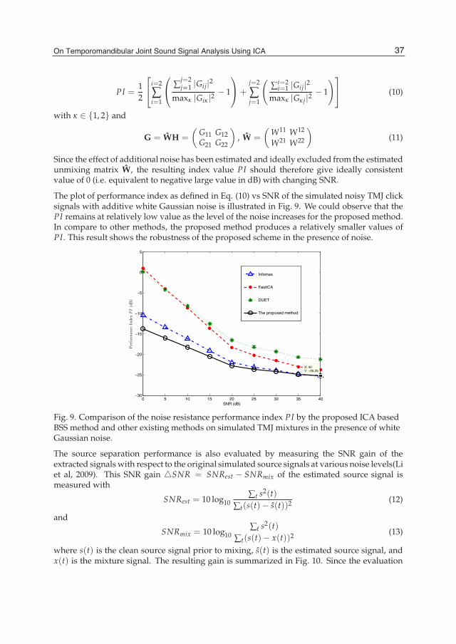
On Temporomandibular Joint Sound Signal Analysis Using ICA 13
PI =12
⎡⎣i=2
∑i=1
⎛⎝ ∑
j=2j=1 |Gij|2
maxκ |Giκ |2− 1
⎞⎠+
j=2
∑j=1
(∑i=2
i=1 |Gij|2maxκ |Gκ j|2
− 1
)⎤⎦ (10)
with κ ∈ 1, 2 and
G = WH =
(G11 G12G21 G22
), W =
(W11 W12
W21 W22
)(11)
Since the effect of additional noise has been estimated and ideally excluded from the estimatedunmixing matrix W, the resulting index value PI should therefore give ideally consistentvalue of 0 (i.e. equivalent to negative large value in dB) with changing SNR.
The plot of performance index as defined in Eq. (10) vs SNR of the simulated noisy TMJ clicksignals with additive white Gaussian noise is illustrated in Fig. 9. We could observe that thePI remains at relatively low value as the level of the noise increases for the proposed method.In compare to other methods, the proposed method produces a relatively smaller values ofPI. This result shows the robustness of the proposed scheme in the presence of noise.
0 5 10 15 20 25 30 35 40−30
−25
−20
−15
−10
−5
0
5
X: 40Y: −25.25
SNR (dB)
Per
form
ance
Inde
xP
I(d
B)
Infomax
FastICA
DUET
The proposed method
Fig. 9. Comparison of the noise resistance performance index PI by the proposed ICA basedBSS method and other existing methods on simulated TMJ mixtures in the presence of whiteGaussian noise.
The source separation performance is also evaluated by measuring the SNR gain of theextracted signals with respect to the original simulated source signals at various noise levels(Liet al, 2009). This SNR gain SNR = SNRest − SNRmix of the estimated source signal ismeasured with
SNRest = 10 log10∑t s2(t)
∑t(s(t)− s(t))2(12)
and
SNRmix = 10 log10∑t s2(t)
∑t(s(t)− x(t))2(13)
where s(t) is the clean source signal prior to mixing, s(t) is the estimated source signal, andx(t) is the mixture signal. The resulting gain is summarized in Fig. 10. Since the evaluation
37On Temporomandibular Joint Sound Signal Analysis Using ICA

14 Will-be-set-by-IN-TECH
is performed on the two-source condition, the average value of SNR for two sources isadopted. As compared to other methods, the consistent higher SNRest with decreasingSNR produced by the proposed method verifies the noise resistance of the proposed sourceextraction scheme from another aspect. Furthermore, the proposed method is more resistantto white Gaussian noise than it to pink noise by providing higher SNR gain value at low SNR.
−15 −10 −5 0 5 10 15 20 25 30 35−1
0
1
2
3
4
5
6
SNR (dB)
SNR
Gai
n
SN
R(d
B)
Infomax
DUET
FastICA
The proposed method
−15 −10 −5 0 5 10 15 20 25 30 35−1
0
1
2
3
4
SNR (dB)
SNR
Gai
n
SN
R(d
B)
Infomax
DUET
FastICA
The proposed method
(a) (b)Fig. 10. The results of ICA based BSS method on simulated TMJ mixtures in the presence of(a) white Gaussian noise; and (b) pink noise.
9. Summary and discussion
In this article, it is shown that how ICA could play a vital role in order to develop a cheap,efficient and reliable diagnostic tool for the detection of temporomandibular joint disorders(TMD). The sounds from the temporomandibular joint (TMJ) are recorded using a pair ofmicrophones inserted in the auditory canals. However, the TMJ sounds originating fromone side of head can also be picked up by microphone at the other side. The presentedICA based method ensures that the signals used for the subsequent analysis are the actualsource signals, and not contaminated by the sounds propagated from the contra side. Thechallenge of allocating the TMJ sound sources with respect to each side of the head hastherefore been solved which provides an efficient non-invasive and non-intrusive procedurefor TMD diagnosis.
The detailed technical issues together with elaborative results, quantitative evaluation as wellas subsequent analysis have been presented in this chapter. In compared to the Infomaxapproach, the proposed ICA based method with adaptive parameters gives a better sourceseparation performance and a higher noise resistance. Unlike any existing papers, theassumption that the two TMJ sound sources are non-overlapped in time-frequency (TF)domain has been removed here, and a more generalized mixing is considered by includingthe challenging source separation problem of two abnormal TMJ sounds which might beoverlapped in TF domain. The proposed signal processing technique then allows for anenhanced clinical utility and an automated approach to the diagnosis of TMD.
38 Independent Component Analysis for Audio and Biosignal Applications

On Temporomandibular Joint Sound Signal Analysis Using ICA 15
10. Future directions
Since the anechoic head model is assumed in this paper, no reverberation of the sound sourcesis considered. A more generalized transmission models for the TMJ sounds would thus bediscussed and compared together with the effects of themodel parameters on the TMJ analysisin our future work. Although the general trend of blind source separation researchmakes useof linear models for source separation, it could also be possible to consider non-linear modelsfor some complex systems (Ming et al, 2008) with additional constraints and assumptions.This topic therefore remains as a developing research area with a lot of potential for real-life.
Another interesting aspect of the problem could be the use of noise extracted fromTMJ for the analysis of different types of non-stationarity to identify temporomandibulardisorder (Ghodsi et al, 2009). Furthermore, it can be considered to extent ICA methods for2D images in order to develop imaging methods in the diagnosis of temporomandibularjoint disorders (Tvrdy, 2007). Besides, it could also be possible to further improve the TMDanalysis performance assisted by a postprocessing scheme (Parikh, 2011). We would thuscombine/fuse sound with the visual data such as those related to facial movement which arecomfortable and safe to acquire, in order to further help the audio analysis to characterizeTMD.
11. References
R. J. M. Gray, S. J. Davies, & A. A. Quayle (1995). Temporomandibular Disorders: A ClinicalApproach, 1st ed. London, U.K.: British Dental Association.
C. L. Pankhurst(1997). Controversies in the aetiology of temporomandibular disorders, Part 1:Temporomandibular disorders all in the mind. Primary Dental Care, Vol. 3, 1997, 1–6.
S. A. Berman, A. Chaudhary, & J. Appelbaum (1997). Temporomandibular disorders.Emedicine. Available: http://www.emedicine.com/neuro/topic366.htm, Jun. 2006 [Online].
S. E. Widmalm, P. L. Westeesson, S. L. Brooks, M. P. Hatala, & D. Paesani (1992).Temporomandibular joint sounds: correlation to joint structure in fresh autopsyspecimens. American Journal of Orthodontics and Dentofacial Orthopedics, Vol. 101, 1992,60–69.
S. E.Widmalm,W. J.Williams, &C. Zheng (1991). Time frequency distributions of TMJ sounds.J Oral Rehab, Vol. 18, 1991, 403–412.
L. Cohen (1995) Time-frequency analysis. Englewood Cliffs, NJ: Prentice Hall, 1995.S. E. Widmalm, W. J. Williams, R. L. Christiansen, S. M. Gunn, & D. K. Park (1996).
Classification of temporomandibular joint sounds based upon there reducedinterference distributions. Journal of Oral Rehabilitation, Vol. 23, 1996, 35–43.
A. Akan & R. B. Unsal (2000). Time-frequency analysis and classification oftemporomandibular joint sounds. J Franklin Inst Special issue on time-frequencysignal analysis and applicatio, Vol. 337, No. 4, 2000, 437–451.
W. D. OBrien & Y. Liu (2005). Evaluation of acoustic propagation paths into the human head.NATO Res. Technol. Organization: New Directions for Improving Audio Effectiveness. Vol.15, Apr. 2005, 1–24.
Y. Guo, F. Sattar, & C. Koh (1999). Blind separation of temporomandibular joint sound signals.Proc. IEEE Int. Conf. Acoust. Speech Signal Process. Vol. 2, 1999, 1069–1072.
C. C. Took, S. Sanei, S. Rickard, J. Chambers, & S. Dunne (2008). Fractional delay estimation forblind source separation and localization of Temporomandibular joint sounds. IEEETrans Biomed Eng. Vol. 55, No. 3, 2008, 949–956.
39On Temporomandibular Joint Sound Signal Analysis Using ICA
16 Will-be-set-by-IN-TECH
A.J. Bell & T.J. Sejnowski(1995). An information maximisation approach to blind separation.Neural Computation, vol. 7, 1995, pp. 1129–1159.
K. Torkkola(1996). Blind separation of convolved sources based on informationmaximization.IEEE Workshop Neural Networks for Signal Processing, Kyoto, Japan, 1996.
S. E. Widmalm, W. J. Williams, K. H. Koh, E. T. Koh, E. K. Chua, K. B. C. Tan, A. U. J. Yap,& S. B. Keng (1997). Comparison of bilateral recording of TMJ joint sounds in TMJdisorders. Int. Conf. Biomedical Engineering, Singapore, 1997.
S. E. Widmalm, W. J. Williams, B. K. Ang, & D. C. Mckay (2002). Localization of TMJ soundsto side. Oral Rehabil, Vol. 29, 2002, 911–917.
A. Hyvärinen (1999). Survey on Independent Component Analysis. Helsinki university ofTechnology Laboratory of Computer and Information Science,1999.
A. Hyvärinen (2004). Principle of ICA estimation. http://www.cis.hut.fi, 2004.S. E. Widmalm, W. J. Williams, D. Djurdjanovic, & D. C. Mckay (2003). The frequency range of
TMJ sounds. Oral Rehabil, Vol. 30, 2003, 335–346.D. M. Watt (1980). Temporomandibular joint sounds. Journal of Dentistry, Vol. 8, No. 2, 1980,
119–127.B. Ella & H. Aapo (2002). A fast fixed-point algorithm for independent component analysis
of complex valued signals. Neural Networks Research Centre, Helsinki University ofTechnology, 2000.
A. Hyvärinen & E. Oja (2000). Independent Component Analysis: Algorithms andApplications. Neural Networks, Vol. 13, No. 4-5, 2000, 411–430.
S. Choi & A. Cichocki (2000). Blind separation of non-stationary sources in noisy mixture.Electronics Letters, Vol. 36, No. 9, 2000, 848–849.
Y. Li, J. Woodruff, & D. L. Wang (2009). Monaural musical sound separation based on pitchand common amplitude modulation. IEEE Trans Audio Speech Language Process, Vol.17, No. 7, 2009, 1361–1371.
M. Ming, Y. Y.-lin, G. W.-Juan, Z. Q.-Hai, & X. W.-Hao (2008). Blind speech separation basedon homotopy nonlinear model. Int. Conf. MultiMedia and Information Technology, 2008,369–372.
M. Ghodsi, H. Hassani, S. Sanei, & Y. Hicks (2009). The use of noise information for detectionof temporomandibular disorder. Biomedical Signal Processing and Control, Vol. 4, 2009,79–85.
P. Tvrdy (2007). Methods of imaging in the diagnosis of temporomandibular joint disorders.Biomed Pap Med Fac Univ Palacky Olomouc Czech Repub, 2007.
D. N. Parikh & D. V. Anderson (2011). Blind source separation with perceptual postprocessing. IEEE 2011 DSP/SPE Workshop, 2011, 321–325.
40 Independent Component Analysis for Audio and Biosignal Applications

0
Blind Source Separation for Speech ApplicationUnder Real Acoustic Environment
Hiroshi Saruwatari and Yu TakahashiNara Institute of Science and Technology
Japan
1. Introduction
A hands-free speech recognition system [1] is essential for the realization of an intuitive,unconstrained, and stress-free human-machine interface, where users can talk naturallybecause they require no microphone in their hands. In this system, however, since noiseand reverberation always degrade speech quality, it is difficult to achieve high recognitionperformance, compared with the case of using a close-talk microphone such as a headsetmicrophone. Therefore, we must suppress interference sounds to realize a noise-robusthands-free speech recognition system.
Source separation is one approach to removing interference sound source signals. Sourceseparation for acoustic signals involves the estimation of original sound source signals frommixed signals observed in each input channel. Various methods have been presented foracoustic source signal separation. They can be classified into two groups: methods basedon single-channel input, e.g., spectral subtraction (SS) [2], and those based on multichannelinput, e.g., microphone array signal processing [3]. There have been various studies onmicrophone array signal processing; in particular, the delay-and-sum (DS) [4–6] array andadaptive beamformer (ABF) [7–9] are the most conventionally used microphone arrays forsource separation and noise reduction. ABF can achieve higher performance than the DSarray. However, ABF requires a priori information, e.g., the look direction and speech breakinterval. These requirements are due to the fact that conventional ABF is based on supervisedadaptive filtering, which significantly limits its applicability to source separation in practicalapplications. Indeed, ABF cannot work well when the interfering signal is nonstationarynoise.
Recently, alternative approaches have been proposed. Blind source separation (BSS) is anapproach to estimating original source signals using only mixed signals observed in eachinput channel. In particular, BSS based on independent component analysis (ICA) [10], inwhich the independence among source signals is mainly used for the separation, has recentlybeen studied actively [11–19]. Indeed, the conventional ICA could work, particularly inspeech-speech mixing, i.e., all sources can be regarded as point sources, but such a mixingcondition is very rare and unrealistic; real noises are often widespread sources. In thischapter, we mainly deal with generalized noise that cannot be regarded as a point source.Moreover, we assume this noise to be nonstationary noise that arises in many acousticalenvironments; however, ABF could not treat this noise well. Although ICA is not influencedby the nonstationarity of signals unlike ABF, this is still a very challenging task that can
3

2 Will-be-set-by-IN-TECH
hardly be addressed by conventional ICA-based BSS because ICA cannot separate widespreadsources.
To improve the performance of BSS, some techniques combining conventional ICA andbeamforming have been proposed [18, 20]. However, these studies dealt with the separation ofpoint sources, and the behavior of such methods under a non-point-source condition was notexplicitly analyzed to our knowledge. Therefore, in this chapter, first, we analyze ICA undera non-point-source noise condition and point out that ICA is proficient in noise estimationrather than in speech estimation under such a noise condition. This analysis implies that wecan still utilize ICA as an accurate noise estimator.
Next, we review blind spatial subtraction array (BSSA) [21], an improved BSS algorithmrecently proposed in order to deal with real acoustic sounds. BSSA consists of an ICA-basednoise estimator, and noise reduction in the proposed BSSA is achieved by subtractingthe power spectrum of the estimated noise via ICA from the power spectrum of thenoisy observations. This “power-spectrum-domain subtraction” procedure provides betternoise reduction than conventional ICA with estimation-error robustness. The efficacy ofBSSA can be determined in various experiments, including computer-simulation-based andreal-recording-based experiments. This chapter shows strong evidence of BSSA providingpromising speech enhancement results in a railway-station environment.
Finally, the real-time implementation issue of BSS is discussed. Several recent studies havedealt with the real-time implementation of ICA, but they still required high-speed personalcomputers. Consequently, BSS implementation on a small LSI still receives much attention inindustrial applications. In this chapter, an example of hardware implementation of BSSA isintroduced, which has yielded commercially available microphones adopted by the JapaneseNational Police Agency.
The rest of this chapter is organized as follows. In Sect. 2, the sound mixing model andconventional ICA are discussed. In Sect. 3, the analysis of ICA under a non-point-sourcecondition is described in detail. In Sect. 4, BSSA is reviewed in detail. In Sect. 5, theexperimental results are shown and compared with those of conventional methods. In Sect. 6,an example of hardware implementation of BSSA is introduced. Following the example, thechaper conclusions are given in Sect. 7.
2. Data model and conventional BSS method
2.1 Sound mixing model of microphone array
In this chapter, a straight-line array is assumed. The coordinates of the elements aredesignated dj(j = 1, . . . , J), and the direction-of-arrivals (DOAs) ofmultiple sound sources aredesignated θk(k = 1, . . . ,K) (see Fig. 1). Then, we consider that only one target speech signal,some interference signals that can be regarded as point sources, and additive noise exist.This additive noise represents noises that cannot be regarded as point sources, e.g., spatiallyuncorrelated noises, background noises, and leakage of reverberation components outsidethe frame analysis. Multiple mixed signals are observed at microphone array elements, anda short-time analysis of the observed signals is conducted by frame-by-frame discrete Fouriertransform (DFT). The observed signals are given by
x( f , τ) = A( f ) s( f , τ) + n( f , τ)+ na( f , τ), (1)
42 Independent Component Analysis for Audio and Biosignal Applications
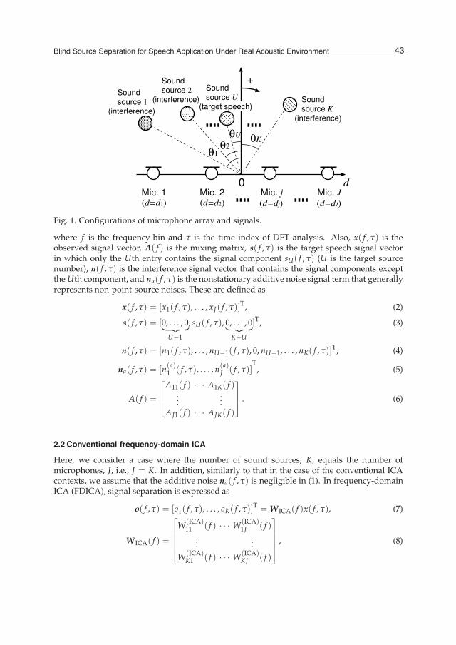
Blind Source Separation for Speech Application Under Real Acoustic Environment 3
Fig. 1. Configurations of microphone array and signals.
where f is the frequency bin and τ is the time index of DFT analysis. Also, x( f , τ) is theobserved signal vector, A( f ) is the mixing matrix, s( f , τ) is the target speech signal vectorin which only the Uth entry contains the signal component sU( f , τ) (U is the target sourcenumber), n( f , τ) is the interference signal vector that contains the signal components exceptthe Uth component, and na( f , τ) is the nonstationary additive noise signal term that generallyrepresents non-point-source noises. These are defined as
x( f , τ) = [x1( f , τ), . . . , xJ( f , τ)]T, (2)
s( f , τ) = [0, . . . , 0︸ ︷︷ ︸U−1
, sU( f , τ), 0, . . . , 0︸ ︷︷ ︸K−U
]T, (3)
n( f , τ) = [n1( f , τ), . . . , nU−1( f , τ), 0, nU+1, . . . , nK( f , τ)]T, (4)
na( f , τ) = [n(a)1 ( f , τ), . . . , n(a)
J ( f , τ)]T, (5)
A( f ) =
⎡⎢⎣
A11( f ) · · · A1K( f )...
...AJ1( f ) · · · AJK( f )
⎤⎥⎦ . (6)
2.2 Conventional frequency-domain ICA
Here, we consider a case where the number of sound sources, K, equals the number ofmicrophones, J, i.e., J = K. In addition, similarly to that in the case of the conventional ICAcontexts, we assume that the additive noise na( f , τ) is negligible in (1). In frequency-domainICA (FDICA), signal separation is expressed as
o( f , τ) = [o1( f , τ), . . . , oK( f , τ)]T = W ICA( f )x( f , τ), (7)
W ICA( f ) =
⎡⎢⎢⎢⎣
W(ICA)11 ( f ) · · · W(ICA)
1J ( f )...
...
W(ICA)K1 ( f ) · · · W(ICA)
KJ ( f )
⎤⎥⎥⎥⎦ , (8)
43Blind Source Separation for Speech Application Under Real Acoustic Environment

4 Will-be-set-by-IN-TECH
Fig. 2. Blind source separation procedure in FDICA in case of J = K = 2.
where o( f , τ) is the resultant output of the separation and W ICA( f ) is the complex-valuedunmixing matrix (see Fig. 2).
The unmixing matrix W ICA( f ) is optimized by ICA so that the output entries of o( f , τ)become mutually independent. Indeed, many kinds of ICA algorithm have been proposed.In the second-order ICA (SO-ICA) [15, 17], the separation filter is optimized by the jointdiagonalization of co-spectra matrices using the nonstationarity and coloration of the signal.For instance, the following iterative updating equation based on SO-ICA has been proposedby Parra and Spence [15]:
W [p+1]ICA ( f ) = −μ ∑
τb
χ( f ) off-diag (Roo ( f , τb))W [p]ICA( f )Rxx( f , τb) + W [p]
ICA( f ), (9)
where μ is the step-size parameter, [p] is used to express the value of the pth step in iterations,off-diag[X] is the operation for setting every diagonal element of matrix X to zero, andχ( f ) = (∑τb
‖Rxx( f , τb)‖2)−1 is a normalization factor (‖ · ‖ represents the Frobenius norm).Rxx( f , τb) and Roo( f , τb) are the cross-power spectra of the input x( f , τ) and output o( f , τ),respectively, which are calculated around multiple time blocks τb. Also, Pham et al. haveproposed the following improved criterion for SO-ICA [17]:
∑τb
12logdet diag[W ICA( f )Roo( f , τb)W ICA( f )H]− logdet[W ICA( f )]
, (10)
where the superscript H denotes Hermitian transposition. This criterion is to be minimizedwith respect to W ICA( f ).
On the other hand, a higher-order-statistics-based approach exists. In higher-order ICA(HO-ICA), the separation filter is optimized on the basis of the non-Gaussianity of the signal.The optimal W ICA( f ) in HO-ICA is obtained using the iterative equation
W [p+1]ICA ( f ) = μ[I− 〈ϕ(o( f , τ))oH( f , τ)〉τ ]W [p]
ICA( f ) + W [p]ICA( f ), (11)
where I is the identity matrix, 〈·〉τ denotes the time-averaging operator, and ϕ(·) is thenonlinear vector function. Many kinds of nonlinear function ϕ( f , τ) have been proposed.
44 Independent Component Analysis for Audio and Biosignal Applications

Blind Source Separation for Speech Application Under Real Acoustic Environment 5
Considering a batch algorithm of ICA, it is well-known that tanh(·) or the sigmoid functionis appropriate for super-Gaussian sources such as speech signals [22]. In this study, we definethe nonlinear vector functionϕ(·) as
ϕ(o( f , τ)) ≡ [ϕ(o1( f , τ)), . . . , ϕ(oK( f , τ))]T, (12)
ϕ(ok( f , τ)) ≡ tanh o(R)k ( f , τ) + i tanh o(I)k ( f , τ), (13)
where the superscripts (R) and (I) denote the real and imaginary parts, respectively. Thenonlinear function given by (12) indicates that the nonlinearity is applied to the real andimaginary parts of complex-valued signals separately. This type of complex-valued nonlinearfunction has been introduced by Smaragdis [14] for FDICA, where it can be assumedfor speech signals that the real (or imaginary) parts of the time-frequency representationsof sources are mutually independent. According to Refs. [19, 23], the source separationperformance of HO-ICA is almost the same as or superior to that of SO-ICA. Thus, in thischapter, HO-ICA is utilized as the basic ICA algorithm in the simulation (Sect. 3.4) andexperiments (Sect. 5).
3. Analysis of ICA under non-point-source noise condition
In this section, we investigate the proficiency of ICA under a non-point-source noise condition.In relation to the performance analysis of ICA, Araki et al. have reported that ICA-based BSShas equivalence to parallel constructed ABFs [24]. However, this investigation was focusedon separation with a nonsingular mixing matrix, and thus was valid for only point sources.
First, we analyze beamformers that are optimized by ICA under a non-point-sourcecondition. In the analysis, it is clarified that beamformers optimized by ICA becomespecific beamformers that maximize the signal-to-noise ratio (SNR) in each output (so-calledSNR-maximize beamformers). In particular, the beamformer for target speech estimation isoptimized to be a DS beamformer, and the beamformer for noise estimation is likely to bea null beamformer (NBF) [16].
Next, a computer simulation is conducted. Its result also indicates that ICA is proficient innoise estimation under a non-point-source noise condition. Then, it is concluded that ICA issuitable for noise estimation under such a condition.
3.1 Can ICA separate any source signals?
Many previous studies on BSS provided strong evidence that conventional ICA could performsource separation, particularly in the special case of speech-speech mixing, i.e., all soundsources are point sources. However, such soundmixing is not realistic under common acousticconditions; indeed the following scenario and problem are likely to arise (see Fig. 3):
• The target sound is the user’s speech, which can be approximately regarded as a pointsource. In addition, the users themselves locate relatively near the microphone array (e.g., 1 mapart), and consequently the accompanying reflection and reverberation components aremoderate.
• For the noise, we are often confronted with interference sound(s) which is not a point sourcebut a widespread source. Also, the noise is usually far from the array and is heavilyreverberant.
45Blind Source Separation for Speech Application Under Real Acoustic Environment

6 Will-be-set-by-IN-TECH
Fig. 3. Expected directivity patterns that are shaped by ICA.
In such an environment, can ICA separate the user’s speech signal and a widespread noisesignal? The answer is no. It is well expected that conventional ICA can suppress the user’sspeech signal to pick up the noise source, but ICA is very weak in picking up the target speechitself via the suppression of a distant widespread noise. This is due to the fact that ICAwith small numbers of sensors and filter taps often provides only directional nulls againstundesired source signals. Results of the detailed analysis of ICA for such a case are shown inthe following subsections.
3.2 SNR-maximize beamformers optimized by ICA
In this subsection, we consider beamformers that are optimized by ICA in the followingacoustic scenario: the target signal is the user’s speech and the noise is not a point source.Then, the observed signal contains only one target speech signal and an additive noise. In thisscenario, the observed signal is defined as
x( f , τ) = A( f )s( f , τ) + na( f , τ). (14)
Note that the additive noise na( f , τ) cannot be negligible in this scenario. Then, the output ofICA contains two components, i.e., the estimated speech signal ys( f , τ) and estimated noisesignal yn( f , τ); these are given by
[ys( f , τ), yn( f , τ)]T = W ICA( f )x( f , τ). (15)
Therefore, ICA optimizes two beamformers; these can be written as
W ICA( f ) = [gs( f ), gn( f )]T, (16)
46 Independent Component Analysis for Audio and Biosignal Applications

Blind Source Separation for Speech Application Under Real Acoustic Environment 7
where gs( f ) = [g(s)1 ( f ), . . . , g(s)
J ( f )]T is the coefficient vector of the beamformer used to pick
up the target speech signal, and gn( f ) = [g(n)1 ( f ), . . . , g(n)
J ( f )]T is the coefficient vector of thebeamformer used to pick up the noise. Therefore, (15) can be rewritten as
[ys( f , τ), yn( f , τ)]T = [gs( f ), gn( f )]Tx( f , τ). (17)
In SO-ICA, the multiple second-order correlation matrices of distinct time block outputs,
〈o( f , τb)oH( f , τb)〉τb , (18)
are diagonalized through joint diagonalization.
On the other hand, inHO-ICA, the higher-order correlationmatrix is also diagonalized. Usingthe Taylor expansion, we can express the factor of the nonlinear vector function of HO-ICA,ϕ(ok( f , τ)), as
ϕ(ok( f , τ)) = tanh o(R)k ( f , τ) + i tanh o(I)k ( f , τ),
=
⎧⎪⎨⎪⎩o(R)k ( f , τ)−
(o(R)k ( f , τ)
)33
+ · · ·
⎫⎪⎬⎪⎭+ i
⎧⎪⎨⎪⎩o(I)k ( f , τ)−
(o(I)k ( f , τ)
)33
+ · · ·
⎫⎪⎬⎪⎭ ,
= ok( f , τ)−
⎛⎜⎝
(o(R)k ( f , τ)
)33
+ i
(o(I)k ( f , τ)
)33
⎞⎟⎠+ · · · . (19)
Thus, the calculation of the higher-order correlation in HO-ICA, ϕ(o( f , τ))oH( f , τ), canbe decomposed to a second-order correlation matrix and the summation of higher-ordercorrelation matrices of each order. This is shown as
〈ϕ(o( f , τ))oH( f , τ)〉τ = 〈o( f , τ)oH( f , τ)〉τ + Ψ( f ), (20)
where Ψ( f ) is a set of higher-order correlation matrices. In HO-ICA, separation filters areoptimized so that all orders of correlation matrices become diagonal matrices. Then, at leastthe second-order correlationmatrix is diagonalized byHO-ICA. In both SO-ICA and HO-ICA,at least the second-order correlation matrix is diagonalized. Hence, we prove in the followingthat ICA optimizes beamformers as SNR-maximize beamformers focusing on only part ofthe second-order correlation. Then the absolute value of the normalized cross-correlationcoefficient (off-diagonal entries) of the second-order correlation, C, is defined by
C =|〈ys( f , τ)y∗n( f , τ)〉τ |√〈|ys( f , τ)|2〉τ
√〈|yn( f , τ)|2〉τ, (21)
ys( f , τ) = s( f , τ) + rsn( f , τ), (22)
yn( f , τ) = n( f , τ) + rns( f , τ), (23)
47Blind Source Separation for Speech Application Under Real Acoustic Environment

8 Will-be-set-by-IN-TECH
where s( f , τ) is the target speech component in ICA’s output, n( f , τ) is the noise componentin ICA’s output, rs is the coefficient of the residual noise component, rn is the coefficient of thetarget-leakage component, and the superscript ∗ represents a complex conjugate. Therefore,the SNRs of ys( f , τ) and yn( f , τ) can be respectively represented by
Γs = 〈|s( f , τ)|2〉τ/(|rs|2〈|n( f , τ)|2〉τ), (24)
Γn = 〈|n( f , τ)|2〉τ/(|rn|2〈|s( f , τ)|2〉τ), (25)
where Γs is the SNR of ys( f , τ) and Γn is the SNR of yn( f , τ). Using (22), (23), (24), and (25),we can rewrite (21) as
C =
∣∣∣1/√Γs · ej arg rs + 1/√
Γn · ej arg r∗n∣∣∣
√1+ 1/Γs
√1+ 1/Γn
=
∣∣∣1/√Γs + 1/√
Γn · ej(arg r∗n−arg rs)∣∣∣
√1+ 1/Γs
√1+ 1/Γn
, (26)
where arg r represents the argument of r. Thus, C is a function of only Γs and Γn. Therefore,the cross-correlation between ys( f , τ) and yn( f , τ) only depends on the SNRs of beamformersgs( f ) and gn( f ).
Now, we consider the minimization of C, which is identical to the second-order correlationmatrix diagonalization in ICA. When | arg r∗n − arg rs| > π/2, where −π < arg rs ≤ π
and −π < arg r∗n ≤ π, it is possible to make C zero or minimum independently of Γsand Γn. This case is appropriate for the orthogonalization between ys( f , τ) and yn( f , τ),which is related to principal component analysis (PCA) unlike ICA. However, SO-ICArequires that all correlation matrices in the different time blocks are diagonalized (jointdiagonalization) to maximize independence among all outputs. Also, HO-ICA requiresthat all order correlation matrices are diagonalized, i.e., not only 〈o( f , τ)oH( f , τ)〉τ butalso Ψ( f ) in (20) is diagonalized. These diagonalizations result in the prevention of theorthogonalization of ys( f , τ) and yn( f , τ); consequently, hereafter, we can consider only thecase of | arg r∗n − arg rs| ≤ π/2. Then, the partial differential of C2 with respect to Γs is givenby
∂C2
∂Γs=
(1− Γs)
(Γs + 1)2(Γn + 1)+
Γs√
ΓsΓn(1− Γs)
(Γs + 1)2(Γn + 1)· 2Re
[ej(arg r∗n−arg rs)
]< 0, (27)
where Γs > 1 and Γn > 1. Similarly to the partial differential of C2 with respect to Γn, we canalso prove that ∂C2/∂Γn < 0, where Γs > 1 and Γn > 1 in the same manner. Therefore, Cis a monotonically decreasing function of Γs and Γn. The above-mentioned fact indicates thefollowing in ICA.
• The absolute value of cross-correlation only depends on the SNRs of the beamformersspanned by each row of an unmixing matrix.
• The absolute value of cross-correlation is a monotonically decreasing function of SNR.
• Therefore, the diagonalization of a second-order correlation matrix leads to SNRmaximization.
Thus, it can be concluded that ICA, in a parallel manner, optimizes multiple beamformers,i.e., gs( f ) and gn( f ), so that the SNR of the output of each beamformer becomes maximum.
48 Independent Component Analysis for Audio and Biosignal Applications

Blind Source Separation for Speech Application Under Real Acoustic Environment 9
3.3 What beamformers are optimized under non-point-source noise condition?
In the previous subsection, it has been proved that ICA optimizes beamformers asSNR-maximize beamformers. In this subsection, we analyze what beamformers are optimizedby ICA, particularly under a non-point-source noise condition, wherewe assume a two-sourceseparation problem. The target speech can be regarded as a point source, and the noise is anon-point-source noise. First, we focus on the beamformer gs( f ) that picks up the targetspeech signal. The SNR-maximize beamformer for gs( f ) minimizes the undesired signal’spower under the condition that the target signal’s gain is kept constant. Thus, the desiredbeamformer should satisfy
mings( f )
gTs ( f )R( f )gs( f ) subject to gTs ( f )a( f , θs) = 1, (28)
a( f , θs( f )) = [exp(i2π( f/M) fsd1 sin θs/c), . . . , exp(i2π( f/M) fsdJ sin θs/c)]T, (29)
where a( f , θs( f )) is the steering vector, θs( f ) is the direction of the target speech, M is the DFTsize, fs is the sampling frequency, c is the sound velocity, and R( f ) = 〈na( f , τ)nHa ( f , τ)〉τ isthe correlation matrix of na( f , τ). Note that θs( f ) is a function of frequency because the DOAof the source varies in each frequency subband under a reverberant condition. Here, using theLagrange multiplier, the solution of (28) is
gs( f )T =a( f , θs( f ))HR−1( f )
a( f , θs( f ))HR−1( f )a( f , θs( f )). (30)
This beamformer is called a minimum variance distortionless response (MVDR)beamformer [25]. Note that theMVDR beamformer requires the true DOA of the target speechand the noise-only time interval. However, we cannot determine the true DOA of the targetsource signal and the noise-only interval because ICA is an unsupervised adaptive technique.Thus, the MVDR beamformer is expected to be the upper limit of ICA in the presence ofnon-point-source noises.
Although the correlation matrix is often not diagonalized in lower-frequency subbands [25],e.g., diffuse noise, we approximate that the correlation matrix is almost diagonalized insubbands in the entire frequency. Then, regarding the power of noise signals as approximatelyδ2( f ), the correlation matrix results in R( f ) = δ2( f ) · I. Therefore, the inverse of thecorrelation matrix R−1( f ) = I/δ2( f ) and (30) can be rewritten as
gs( f )T =a( f , θs( f ))H
a( f , θs( f ))Ha( f , θs( f )). (31)
Since a( f , θs( f ))Ha( f , θs( f )) = J, we finally obtain
gs( f ) =1J[exp (−i2π( f/M) fsd1 sin θs( f )/c) , . . . , exp
(−i2π( f/M) fsdJ sin θs( f )/c)]T. (32)
This filter gs( f ) is approximately equal to a DS beamformer [4]. Note that the filter gs( f ) is nota simple DS beamformer but a reverberation-adapted DS beamformer because it is optimized fora distinct θs( f ) in each frequency bin. The resultant noise power is δ2( f )/J when the noise is
49Blind Source Separation for Speech Application Under Real Acoustic Environment

10 Will-be-set-by-IN-TECH
spatially uncorrelated and white Gaussian. Consequently the noise-reduction performanceof the DS beamformer optimized by ICA under a non-point-source noise condition isproportional to 10 log10 J [dB]; this performance is not particularly good.
Next, we consider the other beamformer gn( f ), which picks up the noise source. Similarto the noise signal, the beamformer that removes the target signal arriving from θs( f ) is theSNR-maximize beamformer. Thus, the beamformer that steers the directional null to θs( f ) isthe desired one for the noise signal. Such a beamformer is called NBF [16]. This beamformercompensates for the phase of the signal arriving from θs( f ), and carries out subtraction. Thus,the signal arriving from θs( f ) is removed. For instance, NBF with a two-element array isdesigned as
gn( f )= [exp(−i2π( f/M) fsd1 sin θs( f )/c),−exp(−i2π( f/M) fsd2 sin θs( f )/c)]T · σ( f ), (33)
where σ( f ) is the gain compensation parameter. This beamformer surely satisfies gTn( f ) ·a( f , θs( f )) = 0. The steering vector a( f , θs( f )) expresses the wavefront of the plane wavearriving from θs( f ). Thus, gn( f ) actually steers the directional null to θs( f ). Note that thisalways occurs regardless of the number of microphones (at least two microphones). Hence,this beamformer achieves a reasonably high, ideally infinite, SNR for the noise signal. Also,note that the filter gn( f ) is not a simple NBF but a reverberation-adapted NBF because it isoptimized for a distinct θs( f ) in each frequency bin. Overall, the performance of enhancingthe target speech is very poor but that of estimating the noise source is good.
3.4 Computer simulations
We conduct computer simulations to confirm the performance of ICA under anon-point-source noise condition. Here, we used HO-ICA [14] as the ICA algorithm. Weused the following 8-kHz-sampled signals as the ICA’s input; the original target speech (3 s)was convoluted with impulse responses that were recorded in an actual environment, and towhich three types of noise from 36 loudspeakers were added. The reverberation time (RT60)is 200 ms; this corresponds to mixing filters with 1600 taps in 8 kHz sampling. The threetypes of noise are an independent Gaussian noise, actually recorded railway-station noise,and interference speech by 36 people. Figure 4 illustrates the reverberant room used in thesimulation. We use 12 speakers (6 males and 6 females) as sources of the original target speech,and the input SNR of test data is set to 0 dB.We use a two-, three-, or four-elementmicrophonearray with an interelement spacing of 4.3 cm.
The simulation results are shown in Figs. 5 and 6. Figure 5 shows the result for the averagenoise reduction rate (NRR) [16] of all the target speakers. NRR is defined as the output SNRin dB minus the input SNR in dB. This measure indicates the objective performance of noisereduction. NRR is given by
NRR [dB] =1J
J
∑j=1
(OSNR− ISNRj), (34)
where OSNR is the output SNR and ISNRj is the input SNR of microphone j.
From this result, we can see an imbalance between the target speech estimation and thenoise estimation in every noise case; the performance of the target speech estimation issignificantly poor, but that of noise estimation is very high. This result is consistent with
50 Independent Component Analysis for Audio and Biosignal Applications

Blind Source Separation for Speech Application Under Real Acoustic Environment 11
Fig. 4. Layout of reverberant room in our simulation.
Fig. 5. Simulation-based separation results under non-point-source noise condition.
the previously stated theory. Moreover, Fig. 6 shows directivity patterns shaped by thebeamformers optimized by ICA in the simulation. It is clearly indicated that beamformergs( f ), which picks up the target speech, resembles the DS beamformer, and that beamformergn( f ), which picks up the noise, becomes NBF. From these results, it is confirmed that thepreviously stated theory, i.e., the beamformers optimized by ICA under a non-point-sourcenoise condition are DS and NBF, is valid.
51Blind Source Separation for Speech Application Under Real Acoustic Environment
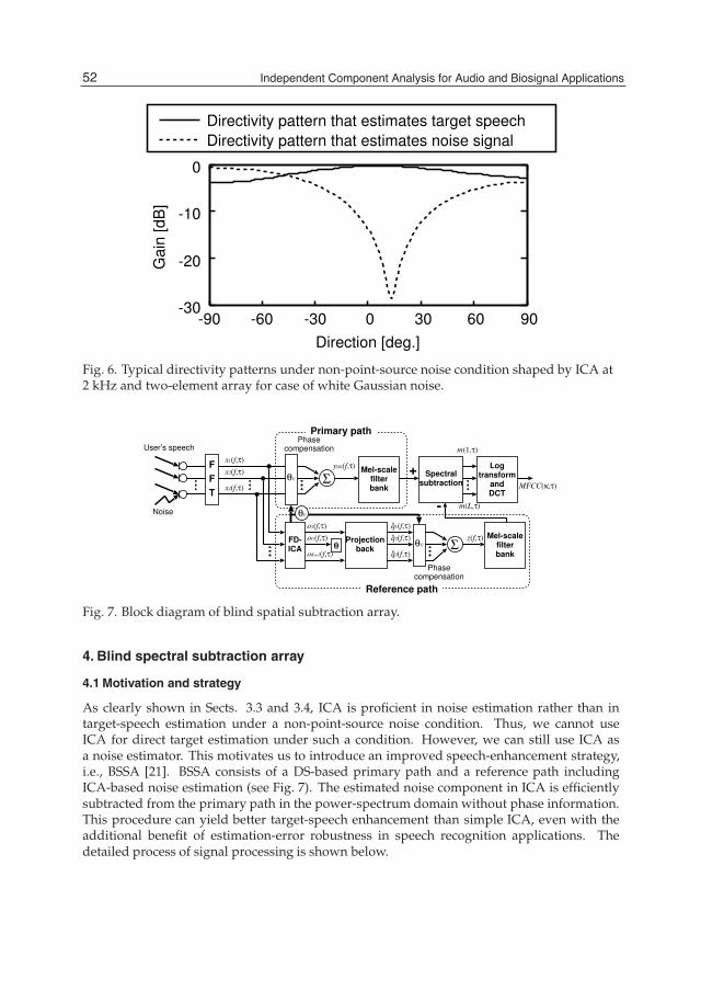
12 Will-be-set-by-IN-TECH
Fig. 6. Typical directivity patterns under non-point-source noise condition shaped by ICA at2 kHz and two-element array for case of white Gaussian noise.
Fig. 7. Block diagram of blind spatial subtraction array.
4. Blind spectral subtraction array
4.1 Motivation and strategy
As clearly shown in Sects. 3.3 and 3.4, ICA is proficient in noise estimation rather than intarget-speech estimation under a non-point-source noise condition. Thus, we cannot useICA for direct target estimation under such a condition. However, we can still use ICA asa noise estimator. This motivates us to introduce an improved speech-enhancement strategy,i.e., BSSA [21]. BSSA consists of a DS-based primary path and a reference path includingICA-based noise estimation (see Fig. 7). The estimated noise component in ICA is efficientlysubtracted from the primary path in the power-spectrum domain without phase information.This procedure can yield better target-speech enhancement than simple ICA, even with theadditional benefit of estimation-error robustness in speech recognition applications. Thedetailed process of signal processing is shown below.
52 Independent Component Analysis for Audio and Biosignal Applications
Blind Source Separation for Speech Application Under Real Acoustic Environment 13
4.2 Partial speech enhancement in primary path
We again consider the generalized form of the observed signal as described in (1). The targetspeech signal is partly enhanced in advance by DS. This procedure can be given as
yDS( f , τ)=wTDS( f )x( f , τ)=wT
DS( f )A( f )s( f , τ)+wTDS( f )A( f )n( f , τ)+wT
DS( f )na( f , τ), (35)
wDS = [w(DS)1 ( f ), . . . ,w(DS)
J ( f )]T, (36)
w(DS)j ( f ) =
1Jexp
(−i2π( f/M) fsdj sin θU/c
), (37)
where yDS( f , τ) is the primary-path output that is a slightly enhanced target speech, wDS( f )is the filter coefficient vector of DS, and θU is the estimated DOA of the target speech given bythe ICA part in Sect. 4.3. In (35), the second and third terms on the right-hand side express theremaining noise in the output of the primary path.
4.3 ICA-based noise estimation in reference path
BSSA provides ICA-based noise estimation. First, we separate the observed signal by ICA andobtain the separated signal vector o( f , τ) as
o( f , τ) = W ICA( f )x( f , τ), (38)
o( f , τ) = [o1( f , τ), . . . , oK+1( f , τ)]T, (39)
W ICA( f ) =
⎡⎢⎢⎢⎢⎣
W(ICA)11 ( f ) · · · W(ICA)
1J ( f )
......
W(ICA)(K+1)1( f ) · · · W(ICA)
(K+1)J( f )
⎤⎥⎥⎥⎥⎦ , (40)
where the unmixing matrix W ICA( f ) is optimized by (11). Note that the number of ICAoutputs becomes K + 1, and thus the number of sensors, J, is more than K + 1 because weassume that the additive noise na( f , τ) is not negligible. We cannot estimate the additive noiseperfectly because it is deformed by the filter optimized by ICA. Moreover, other componentsalso cannot be estimated perfectly when the additive noise na( f , τ) exists. However, we canestimate at least noises (including interference sounds that can be regarded as point sources,and the additive noise) that do not involve the target speech signal, as indicated in Sect. 3.Therefore, the estimated noise signal is still beneficial.
Next, we estimate DOAs from the unmixing matrix W ICA( f ) [16]. This procedure isrepresented by
θu = sin−1arg
([W−1
ICA( f )]ju
[W−1ICA( f )]j′u
)
2π fsc−1(dj − dj′ ), (41)
53Blind Source Separation for Speech Application Under Real Acoustic Environment

14 Will-be-set-by-IN-TECH
where θu is the DOA of the uth sound source. Then, we choose the Uth source signal, which isnearest the front of the microphone array, and designate the DOA of the chosen source signalas θU . This is because almost all users are expected to stand in front of the microphone array ina speech-oriented human-machine interface, e.g., a public guidance system. Other strategiesfor choosing the target speech signal can be considered as follows.
• If the approximate location of a target speaker is known in advance, we can utilize thelocation of the target speaker. For instance, we can know the approximate location of thetarget speaker at a hands-free speech recognition system in a car navigation system inadvance. Then, the DOA of the target speech signal is approximately known. For suchsystems, we can choose the target speech signal, selecting the specific component in whichthe DOA estimated by ICA is nearest the known target-speech DOA.
• For an interaction robot system [26], we can utilize image information from a cameramounted on a robot. Therefore, we can estimate DOA from this information, and we canchoose the target speech signal on the basis of this estimated DOA.
• If the only target signal is speech, i.e., none of the noises are speech, we can choose thetarget speech signal on the basis of the Gaussian mixturemodel (GMM), which can classifysound signals into voices and nonvoices [27].
Next, in the reference path, no target speech signal is required because we want to estimateonly noise. Therefore, we eliminate the user’s signal from the ICA’s output signal o( f , τ). Thiscan be written as
q( f , τ) = [o1( f , τ), ..., oU−1( f , τ), 0, oU+1( f , τ), ..., oK+1( f , τ)]T , (42)
where q( f , τ) is the “noise-only” signal vector that contains only noise components. Next,we apply the projection back (PB) [13] method to remove the ambiguity of amplitude. Thisprocedure can be represented as
q( f , τ) = W+ICA( f )q( f , τ), (43)
where M+ denotes the Moore-Penrose pseudo-inverse matrix of M. Thus, q( f , τ) is a goodestimate of the noise signals received at the microphone positions, i.e.,
q( f , τ) A( f )n( f , τ) + W+ICA( f )na( f , τ), (44)
where na( f , τ) contains the deformed additive noise signal and separation error due to anadditive noise. Finally, we construct the estimated noise signal z( f , τ) by applying DS as
z( f , τ) = wTDS( f )q( f , τ) wT
DS( f )A( f )n( f , τ) + wTDS( f )W+
ICA( f )na( f , τ). (45)
This equation means that z( f , τ) is a good candidate for noise terms of the primary pathoutput yDS( f , τ) (see the 2nd and 3rd terms on the right-hand side of (35)). Of course this noiseestimation is not perfect, but we can still enhance the target speech signal via oversubtractionin the power-spectrum domain, as described in Sect. 4.4. Note that z( f , τ) is a function ofthe frame index τ, unlike the constant noise prototype in the traditional spectral subtractionmethod [2]. Therefore, the proposed BSSA can deal with nonstationary noise.
54 Independent Component Analysis for Audio and Biosignal Applications

Blind Source Separation for Speech Application Under Real Acoustic Environment 15
4.4 Noise reduction processing in BSSA
In BSSA, noise reduction is carried out by subtracting the estimated noise power spectrum(45) from the partly enhanced target speech signal power spectrum (35). This procedure isgiven as
yBSSA( f , τ) =
⎧⎪⎨⎪⎩
|yDS( f , τ)|2 − β · |z( f , τ)|2 12
( if |yDS( f , τ)|2 − β · |z( f , τ)|2 ≥ 0 ),γ · |yDS( f , τ)| (otherwise),
(46)
where yBSSA( f , τ) is the final output of BSSA, β is the oversubtraction parameter, and γ isthe flooring parameter. Their appropriate setting, e.g., β > 1 and γ 1, results in efficientnoise reduction. For example, a larger oversubtraction parameter (β 1) leads to a largerSNR improvement. However, the target signal would be distorted. On the other hand, asmaller oversubtraction parameter (β 1) gives a less-distorted target signal. However, theSNR improvement is decreased. In the end, a trade-off between SNR improvement and thedistortion of the output signal exists with respect to the parameter β; 1 < β < 2 is usuallyused.
The system switches between two equations depending on the conditions in (46). If thecalculated noise components using ICA in (45) are underestimated, i.e., |yDS( f , τ)|2 >β|z( f , τ)|2, the resultant output yBSSA( f , τ) corresponds to power-spectrum-domainsubtraction among the primary and reference paths with an oversubtraction rate of β. Onthe other hand, if the noise components are overestimated in ICA, i.e., |yDS( f , τ)|2 <β|z( f , τ)|2, the resultant output yBSSA( f , τ) is floored with a small positive value to avoida negative-valued unrealistic spectrum. These oversubtraction and flooring procedures enableerror-robust speech enhancement in BSSA rather than a simple linear subtraction. Althoughthe nonlinear processing in (46) often generates an artificial distortion, so-called musicalnoise, it is still applicable in the speech recognition system because the speech decoder isnot very sensitive to such a distortion. BSSA involves mel-scale filter bank analysis anddirectly outputs the mel-frequency cepstrum coefficient (MFCC) [28] for speech recognition.Therefore, BSSA requires no transformation into the time-domain waveform for speechrecognition.
In BSSA, DS and SS are processed in addition to ICA. In HO-ICA or SO-ICA, to calculate thecorrelationmatrix, at least hundreds of product-sumoperations are required in each frequencysubband. On the other hand, in DS, at most J product-sum operations are required in eachfrequency subband. A mere 4 or 5 products are required for SS. Therefore, the complexity ofBSSA does not increase by as much as 10% compared with ICA.
4.5 Variation and extension in noise reduction processing
As mentioned in the previous subsection, the noise reduction processing of BSSA is mainlybased on SS, and therefore it often suffers from the problem ofmusical noise generation due toits nonlinear signal processing. This becomes a big problem in any audio applications aimedfor human hearing, e.g., hearing-aids, teleconference systems, etc.
To improve the sound quality of BSSA, many kinds of variations have been proposedand implemented in the post-processing part in (46). Generalized SS and parametricWiener filtering algorithms [29] have been introduced to successfully mitigate musical
55Blind Source Separation for Speech Application Under Real Acoustic Environment

16 Will-be-set-by-IN-TECH
Output
FFT
FD-ICA
ICA-based channel-wise noise estimation
User’s speech
Noise
Channel-wise
spectralsubtraction
Projectionback0 θU
θU Σ
Phasecompensation
Noise1
NoiseJ-1
Speech
Output
FFT
FD-ICA
ICA-based noise estimation
User’s speech
Noise
Spectralsubtraction
Projectionback0
Noise1
NoiseJ-1
Speech
θU Σ
Phasecompensation
θU
θU
θU Σ
(a) Original BSSA
(b) ChBSSA
Fig. 8. Configurations of (a) original BSSA and (b) chBSSA.
noise generation [30]. Furthermore, the minimum mean-square error (MMSE) short-timespectral amplitude (STSA) estimator [31] can be used for achieving low-distortion speechenhancement in BSSA [32]. In addition, this MMSE-STSA estimator with ICA-based noiseestimation has been modified to deal with binaural signal enhancement, where the spatial cueof the target speech signal can be maintained in the output of BSSA [33].
In recent studies, an interesting extension in the signal processing structure has beenaddressed [34, 35]. Two types of the BSSA structures are shown in Fig. 8. One is the originalBSSA structure that performs SS after DS (see Fig. 8(a)), and another is that SS is channelwiselyperformed before DS (chBSSA; see Fig. 8(b)). It has been theoretically clarified that chBSSA issuperior to BSSA in the mitigation of the musical noise generation via higher-order statisticsanalysis.
5. Experiment and evaluation
5.1 Experiment in reverberant room
In this experiment, we present a comparison of typical blind noise reductionmethods, namely,the conventional ICA [14] and the traditional SS [2] cascaded with ICA (ICA+SS). We utilizethe HO-ICA algorithm as conventional ICA [14]. Hereafter, ‘ICA’ simply indicates HO-ICA.For ICA+SS, we first obtain the estimated noise from the speech pause interval in the target
56 Independent Component Analysis for Audio and Biosignal Applications
Blind Source Separation for Speech Application Under Real Acoustic Environment 17
speech estimation by ICA. The noise reduction achieved by SS is
yICA+SS( f , τ) =
|oU( f , τ)|2 − β|nremain( f )|2 12 (where |oU( f , τ)|2 − β|nremain( f , τ)|2 ≥ 0),
γ|oU( f , τ)| (otherwise),(47)
where nremain( f ) is the noise signal from the speech pause in the target speech estimated byICA. Moreover, a DOA-based permutation solver[16] is used in conventional ICA and in theICA part in BSSA.
We used 16-kHz-sampled signals as test data; the original speech (6 s) was convoluted withimpulse responses recorded in an actual environment, to which cleaner noise or a male’sinterfering speech recorded in an actual environment was added. Figure 9 shows the layoutof the reverberant room used in the experiment. The reverberation time of the room is 200 ms;this corresponds to mixing filters of 3200 taps in 16 kHz sampling. The cleaner noise is not asimple point source signal but consists of several nonstationary noises emitted from a motor,an air duct, and a nozzle. Also, the male’s interfering speech is not a simple point source butis slightly moving. In addition, these interference noises involve background noise. The SNRof the background noise (power ratio of target speech to background noise) is about 28 dB.We use 46 speakers (200 sentences) as the source of the target speech. The input SNR is set to10 dB at the array. We use a four-element microphone array with an interelement spacing of2 cm. The DFT size is 512. The oversubtraction parameter β is 1.4 and the flooring coefficientγ is 0.2. Such parameters were experimentally determined. The speech recognition task andconditions are shown in Table 1.
Regarding the evaluation index, we calculate NRR described in (34), cepstral distortion (CD),and speech recognition, which is the final goal of BSSA, in which the separated sound qualityis fully considered. CD [36] is a measure of the degree of distortion via the cepstrum domain.It indicates the distortion among two signals, which is defined as
CD [dB] ≡ 1T
T
∑τ=1
Db
√√√√ B
∑ρ=1
2(Cout(ρ; τ)− Cref(ρ; τ))2, (48)
Db =20
log 10, (49)
where T is the frame length, Cout(ρ; τ) is the ρth cepstrum coefficient of the output signal inthe frame τ, Cref(ρ; τ) is the ρth cepstrum coefficient of the speech signal convoluted with theimpulse response, and Db is a constant that transforms the measure into dB. Moreover, B isthe number of dimensions of the cepstrum used in the evaluation. Moreover, we use the wordaccuracy (WA) score as a speech recognition performance. This index is defined as
WA [%] ≡ WWA − SWA − DWA − IWAWWA
× 100, (50)
where WWA is the number of words, SWA is the number of substitution errors, DWA is thenumber of dropout errors, and IWA is the number of insertion errors.
First, actual separation results obtained by ICA for the case of cleaner noise and interferencespeech are shown in Fig. 10. We can confirm the imbalanced performance between targetestimation and noise estimation, similar to the simulation-based results (see Sect. 3.4).
57Blind Source Separation for Speech Application Under Real Acoustic Environment

18 Will-be-set-by-IN-TECH
Database JNAS [37], 306 speakers (150sentences/speaker)
Task 20 k newspaper dictationAcoustic model phonetic tied mixture (PTM) [37], clean
modelNumber of training speakers for acousticmodel
260 speakers (150 sentences/speaker)
Decoder JULIUS [37] ver 3.5.1
Table 1. Conditions for Speech Recognition
Fig. 9. Layout of reverberant room used in our experiment.
Fig. 10. NRR-based separation performance of conventional ICA in environment shown inFig. 9.
Next, we discuss the NRR-based experimental results shown in Figs. 11(a) and 12(a). Fromthe results, we can confirm that the NRRs of BSSA are more than 3 dB greater than those ofconventional ICA and ICA+SS. However, we can see that the distortion of BSSA is slightlyhigher from Figs. 11(b) and 12(b). This is due to the fact that the noise reduction of BSSA
58 Independent Component Analysis for Audio and Biosignal Applications

Blind Source Separation for Speech Application Under Real Acoustic Environment 19
Fig. 11. Results of (a) noise reduction rate, (b) cepstral distortion, and (c) speech recognitiontest for each method (cleaner noise case).
Fig. 12. Results of (a) noise reduction rate, (b) cepstral distortion, and (c) speech recognitiontest using each method (interference speech case).
is performed on the basis of spectral subtraction. However, the increase in the degree ofdistortion is expected to be negligible.
Finally, we show the speech recognition result in Figs. 11(c) and 12(c). It is evident that BSSAis superior to conventional ICA and ICA+SS.
5.2 Experiment in real world
An experiment in an actual railway-station environment is discussed here. Figure 13shows the layout of the railway-station environment used in this experiment, where thereverberation time is about 1000 ms; this corresponds to mixing filters of 16000 taps in 16kHz sampling. We used 16-kHz-sampled signals as test data; the original speech (6 s) wasconvoluted with impulse responses recorded in the same railway-station environment, towhich a real-recorded noise was added. We use 46 speakers (200 sentences) as the originalsource of the target speech. The noise in the environment is nonstationary and is almost anon-point-source; it consists of various kinds of interference noise, namely, background noiseand the sounds of trains, ticket-vending machines, automatic ticket gates, footsteps, cars, andwind. Figure 14 shows two typical noises, i.e., noises 1 and 2, which are recorded in distincttime periods and used in this experiment. A four-element array with an interelement spacingof 2 cm is used.
59Blind Source Separation for Speech Application Under Real Acoustic Environment

20 Will-be-set-by-IN-TECH
Fig. 13. Layout of railway-station environment used in our experiment.
Fig. 14. Two typical noises in railway-station environment.
Figure 15 shows the real separation results obtained by ICA in the railway-stationenvironment. We can ascertain the imbalanced performance between target estimation andnoise estimation, similar to the simulation-based results (see Sect. 3.4).
In the next experiment, we compare conventional ICA, ICA+SS, and BSSA in terms of NRR,cepstral distortion, and speech recognition performance. Figure 16(a) shows the results ofthe average NRR for whole sentences. From these results, we can see that the NRR of BSSAthat utilizes ICA as a noise estimator is superior to those of conventional methods. However,we find that the cepstral distortion in BSSA is greater than compared with that in ICA fromFig. 16(b).
Finally, we show the results of speech recognition, where the extracted sound quality is fullyconsidered, in Fig. 16(c). The speech recognition task and conditions are the same as those inSect. 5.1, as shown in Table 1. From this result, it can be concluded that the target-enhancementperformance of BSSA, i.e., the method that uses ICA as a noise estimator, is evidently superiorto the method that uses ICA directly as well as ICA+SS.
60 Independent Component Analysis for Audio and Biosignal Applications

Blind Source Separation for Speech Application Under Real Acoustic Environment 21
Fig. 15. NRR-based noise reduction performance of conventional ICA in railway-stationenvironment.
Fig. 16. Experimental results of (a) noise reduction rate, (b) cepstral distortion, and (c) speechrecognition test in railway-station environment.
6. Real-time implementation of BSS
Several recent studies [19, 38, 39] have dealt with the issue of real-time implementationof ICA. The methods used, however, require high-speed personal computers, and BSSimplementation on a small LSI still receives much attention in industrial applications. Asa recent example of the implementation of real-time BSS, a real-time BSSA algorithm and itsdevelopment are described in the following.
In BSSA’s signal processing, the DS, SS, and separation filtering parts are possible towork in real-time. However, it is toilsome to optimize (update) the separation filter inreal-time because the optimization of the unmixing matrix by ICA consumes huge amountof computations. Therefore, we should introduce a strategy in which the separation filteroptimized by using the past time period data is applied to the current data. Figure 17illustrates the configuration of the real-time implementation of BSSA. Signal processing inthis implementation is performed as follows.
61Blind Source Separation for Speech Application Under Real Acoustic Environment

22 Will-be-set-by-IN-TECH
Channel 1
Channel 2
Noiseestimation
by ICA filter
DS(Main path)
Fill the buffer forICA optimization
SS SS SS
FFTFFTFFT
Noiseestimation
by ICA filter
DS(Main path)
Fill the buffer forICA optimization
SS SS SS
FFTFFTFFT
Speech enhanced signal
Time
WICA(f) WICA(f)WICA(f)
ICA filter updatingin 1.5 sec. duration
ICA filter updatingin 1.5 sec. duration
Send SendSend
Fig. 17. Signal flow in real-time implementation of BSSA.
Step 1: Inputted signals are converted into time-frequency domain series by using aframe-by-frame fast Fourier transform (FFT).
Step 2: ICA is conducted using the past 1.5-s-duration data for estimating the separation filterwhile the current 1.5 s. The optimized separation filter is applied to the next (not current)1.5 s samples. This staggered relation is due to the fact that the filter update in ICA requiressubstantial computational complexities and cannot provide an optimal separation filter forthe current 1.5 s data.
Step 3: Inputted data is processed in two paths. In the primary path, the target speech ispartly enhanced by DS. In the reference path, ICA-based noise estimation is conducted.Again, note that the separation filter for ICA is optimized by using the past time perioddata.
Step 4: Finally, we obtain the target-speech-enhanced signal by subtracting the powerspectrum of the estimated noise signal in the reference path from the power spectrumof the primary path’s output.
62 Independent Component Analysis for Audio and Biosignal Applications

Blind Source Separation for Speech Application Under Real Acoustic Environment 23
Fig. 18. BSS microphone (SSM-001 by KOBELCO Ltd., Japan) based on BSSA algorithm [40].
Although the update of the separation filter in the ICA part is not real-time processing, butinvolves a total latency of 3.0 s, the entire system still seems to run in real-time becauseDS, SS, and separation filtering can be carried out in the current segment with no delay. Inthe system, the performance degradation due to the latency problem in ICA is mitigated byoversubtraction in spectral subtraction.
Figure 18 shows an example of the hardware implementation of BSSA, which was developedby KOBELCO Ltd., Japan [40]. They have fabricated a pocket-size real-time BSS microphone,where the BSSA algorithm can work on a general-purpose DSP (TEXAS INSTRUMENTSTMS320C6713; 200 MHz clock, 100 kB program size, 1 MB working memory). Thismicrophone was made commercially available in 2007 and has been adopted for the purposeof surveillance by the Japanese National Police Agency.
7. Conclusion
This chapter addressed the BSS problem for speech applications under real acousticenvironments, particularly focusing on BSSA that utilizes ICA as a noise estimator. Undera non-point-source noise condition, it was pointed out that beamformers optimized by ICAare a DS beamformer for extracting the target speech signal that can be regarded as a pointsource and NBF for picking up the noise signal. Thus, ICA is proficient in noise estimationunder a non-point-source noise condition. Therefore, it is valid to use ICA as a noise estimator.In experiments involving computer-simulation-based and real-recording-based data, the SNRimprovement and speech recognition results of BSSA are superior to those of conventionalmethods. These results indicate that the ICA-based noise estimation is beneficial for speechenhancement in adverse environments. Also, the hardware implementation of BSS wasdiscussed with a typical example of a real-time BSSA algorithm.
8. References
[1] B. H. Juang and F. K. Soong, “Hands-free telecommunications,” Proc. InternationalConference on Hands-Free Speech Communication, pp. 5–10, 2001.
63Blind Source Separation for Speech Application Under Real Acoustic Environment

24 Will-be-set-by-IN-TECH
[2] S. Boll, “Suppression of acoustic noise in speech using spectral subtraction,” IEEETransactions on Acoustics, Speech, and Signal Processing, vol. ASSP-27, no. 2, pp. 113–120,1979.
[3] G. W. Elko, “Microphone array systems for hands-free telecommunication,” SpeechCommunication, vol. 20, pp. 229–240, 1996.
[4] J. L. Flanagan, J. D. Johnston, R. Zahn, and G. W. Elko, “Computer-steered microphonearrays for sound transduction in large rooms,” Journal of the Acoustical Society of America,vol. 78, no. 5, pp. 1508–1518, 1985.
[5] M. Omologo, M. Matassoni, P. Svaizer, and D. Giuliani, “Microphone array based speechrecognition with different talker-array positions,” Proc. ICASSP’97, pp. 227–230, 1997.
[6] H. F. Silverman and W. R. Patterson, “Visualizing the performance of large-aperturemicrophone arrays,” Proc. ICASSP’99, pp. 962–972, 1999.
[7] O. Frost, “An algorithm for linearly constrained adaptive array processing,” Proceedingsof the IEEE, vol. 60, pp. 926–935, 1972.
[8] L. J. Griffiths and C. W. Jim, “An alternative approach to linearly constrained adaptivebeamforming,” IEEE Transactions on Antennas and Propagation, vol. 30, no. 1, pp. 27–34,1982.
[9] Y. Kaneda and J. Ohga, “Adaptive microphone-array system for noise reduction,” IEEETrans. Acoust. Speech, Signal Process., pp. 2109–2112, 1986.
[10] P. Comon, “Independent component analysis, a new concept?” Signal Processing, vol. 36,pp. 287–314, 1994.
[11] J. F. Cardoso, “Eigenstructure of the 4th-order cumulant tensor with application to theblind source separation problem,” Proc. ICASSP’89, pp. 2109–2112, 1989.
[12] C. Jutten and J. Herault, “Blind separation of sources part i: An adaptive algorithm basedon neuromimetic architecture,” Signal Processing, vol. 24, pp. 1–10, 1991.
[13] S. Ikeda and N. Murata, “A method of ICA in the frequency domain,” Proc. InternationalWorkshop on Independent Component Analysis and Blind Signal Separation, pp. 365–371, 1999.
[14] P. Smaragdis, “Blind separation of convolved mixtures in the frequency domain,”Neurocomputing, vol. 22, no. 1-3, pp. 21–34, 1998.
[15] L. Parra and C. Spence, “Convolutive blind separation of non-stationary sources,” IEEETransactions on Speech and Audio Processing, vol. 8, pp. 320–327, 2000.
[16] H. Saruwatari, S. Kurita, K. Takeda, F. Itakura, and T. Nishikawa, “Blind sourceseparation combining independent component analysis and beamforming,” EURASIPJournal on Applied Signal Processing, vol. 2003, pp. 1135–1146, 2003.
[17] D.-T. Pham, C. Serviere, and H. Boumaraf, “Blind separation of convolutive audiomixtures using nonstationarity,” International Symposium on Independent ComponentAnalysis and Blind Signal Separation (ICA2003), pp. 975–980, 2003.
[18] H. Saruwatari, T. Kawamura, T. Nishikawa, A. Lee, and K. Shikano, “Blind sourceseparation based on a fast-convergence algorithm combining ICA and beamforming,”IEEE Transactions on Speech and Audio Processing, vol. 14, no. 2, pp. 666–678, 2006.
[19] Y. Mori, H. Saruwatari, T. Takatani, S. Ukai, K. Shikano, T. Hiekata, Y. Ikeda,H. Hashimoto, and T. Morita, “Blind separation of acoustic signals combiningSIMO-model-based independent component analysis and binary masking,” EURASIPJournal on Applied Signal Processing, vol.2006, Article ID 34970, 17 pages, 2006.
[20] B. Sallberg, N. Grbic, and I. Claesson, “Online maximization of subband kurtosis forblind adaptive beamforming in realtime speech extraction,” Proc. IEEE Workshop DSP2007, pp. 603–606, 2007.
64 Independent Component Analysis for Audio and Biosignal Applications

Blind Source Separation for Speech Application Under Real Acoustic Environment 25
[21] Y. Takahashi, T. Takatani, K. Osako, H. Saruwatari, and K. Shikano, “Blind spatialsubtraction array for speech enhancement in noisy environment,” IEEE Transactions onAudio, Speech and Language Processing, vol.17, no.4, pp.650–664, 2009.
[22] T.-W. Lee, Independent Component Analysis. Norwell, MA: Kluwer Academic, 1998.[23] S. Ukai, T. Takatani, T. Nishikawa, and H. Saruwatari, “Blind source separation
combining SIMO-model-based ICA and adaptive beamforming,” Proc. ICASSP2005, vol.III, pp. 85–88, 2005.
[24] S. Araki, S. Makino, Y. Hinamoto, R. Mukai, T. Nishikawa, and H. Saruwatari,“Equivalence between frequency domain blind source separation and frequency domainadaptive beamforming for convolutive mixtures,” EURASIP Journal on Applied SignalProcessing, vol. 2003, no. 11, pp. 1157–1166, 2003.
[25] M. Brandstein and D. Ward, Eds., Microphone Arrays: Signal Processing Techniques andApplications. Springer-Verlag, 2001.
[26] H. Saruwatari, N. Hirata, T. Hatta, R. Wakisaka, K. Shikano, and T. Takatani, "Semi-blindspeech extraction for robot using visual information and noise statistics," Proc. of the 11thIEEE International Symposium on Signal Processing and Information Technology (ISSPIT2011),pp.238–243, 2011.
[27] A. Lee, K. Nakamura, R. Nishimura, H. Saruwatari, and K. Shikano, “Noise robust realworld spoken dialogue system using GMM based rejection of unintended inputs,” Proc.8th International Conference on Spoken Language Processing (ICSLP2004), vol.I, pp.173–176,2004.
[28] S. B. Davis and P. Mermelstein, “Comparison of parametric representations formonosyllabic word recognition in continuously spoken sentences,” IEEE Trans. Acoustics,Speech, Signal Proc., vol. ASSP-28, no. 4, pp. 357–366, 1982.
[29] T. Inoue, H. Saruwatari, Y. Takahashi, K. Shikano, and K. Kondo, "Theoretical analysis ofmusical noise in generalized spectral subtraction based on higher-order statistics," IEEETransactions on Audio, Speech and Language Processing, vol.19, no.6, pp.1770–1779, 2011.
[30] R. Miyazaki, H. Saruwatari, R. Wakisaka, K. Shikano, and T. Takatani, "Theoreticalanalysis of parametric blind spatial subtraction array and its application to speechrecognition performance prediction," Proc. of Joint Workshop on Hands-free SpeechCommunication and Microphone Arrays 2011 (HSCMA2011), pp.19–24, 2011.
[31] Y. Ephraim, and D. Malah, "Speech enhancement using a minimum mean-square errorshort-time spectral amplitude estimator," IEEE Transactions on Acoustics, Speech, SignalProcessing, vol.32, no.6, pp.1109–1121, 1984.
[32] R. Okamoto, Y. Takahashi, H. Saruwatari, and K. Shikano, "MMSE STSA estimator withnonstationary noise estimation based on ICA for high-quality speech enhancement,"Proc. of IEEE International Conference on Acoustics, Speech, and Signal Processing(ICASSP2010), pp.4778–4781, 2010.
[33] H. Saruwatari, M. Go, R. Okamoto, and K. Shikano, "Binaural hearing aid usingsound-localization-preserved MMSE STSA estimator with ICA-based noise estimation,"Proc. of International Workshop on Acoustic Echo and Noise Control (IWAENC2010), 2010.
[34] Y. Takahashi, H. Saruwatari, K. Shikano, and K. Kondo, "Musicalnoise analysis inmethods of integrating microphone array and spectral subtraction based on higher-orderstatistics," EURASIP Journal on Advances in Signal Processing, vol.2010, Article ID 431347,25 pages, 2010.
[35] R. Miyazaki, H. Saruwatari, and K. Shikano, "Theoretical analysis of amounts of musicalnoise and speech distortion in structure-generalized parametric spatial subtraction
65Blind Source Separation for Speech Application Under Real Acoustic Environment
26 Will-be-set-by-IN-TECH
array," IEICE Transactions on Fundamentals of Electronics, Communications and ComputerSciences, vol.95-A, no.2, pp.586–590, 2012.
[36] L. Rabiner and B. Juang, Fundamentals of Speech Recognition. Upper Saddle River, NJ:Prentice Hall PTR, 1993.
[37] A. Lee, T. Kawahara, and K. Shikano, “Julius – an open source real-time large vocabularyrecognition engine,” European Conference on Speech Communication and Technology, pp.1691–1694, 2001.
[38] R. Mukai, H. Sawada, S. Araki, and S. Makino, “Blind source separation formoving speech signals using blockwise ICA and residual crosstalk subtraction,”IEICE Transactions on Fundamentals of Electronics, Communications and Computer Sciences,vol.E87-A, no.8, pp.1941–1948, 2004.
[39] H. Buchner, R. Aichner, andW. Kellermann, “A generalization of blind source separationalgorithms for convolutive mixtures based on second-order statistics,” IEEE Transactionson Speech and Audio Processing, vol.13, no.1, pp.120–134, 2005
[40] T. Hiekata, Y. Ikeda, T. Yamashita, T. Morita, R. Zhang, Y. Mori, H. Saruwatari, and K.Shikano, “Development and evaluation of pocket-size real-time blind source separationmicrophone,” Acoustical Science and Technology, vol.30, no.4, pp.297–304, 2009.
66 Independent Component Analysis for Audio and Biosignal Applications

4
Monaural Audio Separation Using Spectral Template and Isolated Note Information
Anil Lal and Wenwu Wang Department of Electronic Engineering, University of Surrey,
United Kingdom
1. Introduction Musical sound separation systems attempt to separate individual musical sources from sound mixtures. The human auditory system gives us the extraordinary capability of identifying instruments being played (pitched and non-pitched) from a piece of music and also hearing the rhythm/melody of the individual instrument being played. This task appears ‘automatic’ to us but has proved to be very difficult to replicate in computational systems. Many methods have been developed recently for addressing this challenging source separation problem. They can be broadly classified into two categories, respectively, statistical learning based techniques such as independent component analysis (ICA) and non-negative matrix/tensor factorization (NMF/NTF), and computational auditory scene analysis (CASA) based techniques.
One of the popular methods for source separation was based on ICA [1-10], where the underlying unknown sources are assumed to be statistically independent, so that a criterion for measuring the statistical distance between the distribution of the sources can be formed and optimised either adaptively [5] [10] [11], or collectively (in block or batch processing mode) [2], given mixtures as the input signals. Both high-order statistics (HOS) [2] [4] [5] and second order statistics (SOS) [12] have been used for this purpose. The ICA techniques have been developed extensively since the pioneering contributions in early 1990s, made for example by Jutten [1], Comon [3], and Cardoso [2]. The early work of ICA concentrates on the instantaneous model which was soon found to be limited for real audio applications such as in a cocktail party environment, where the sound sources reach listeners (microphones) through multi-path propagations (with surface reflections). Convolutive ICA [13] was then proposed to deal with such situations (see [21] for a comprehensive survey). Using Fourier transform, the convolutive ICA problem can be converted to multiple instantaneous but complex valued ICA problems in the frequency domain [14-17] thanks to its computational efficiency, and the sources can be separated after permutation correction for all the frequency bins [18-20]. Most of the aforementioned methods consider (over-) determined cases where the number of sources is assumed to be no greater than the number of observed signals. In practical situations, however, an underdetermined separation problem is usually encountered. A widely used method for tackling this problem is based on sparse signal representations [22-29], where the sources are assumed to be sparse in either the time domain or a transform domain such that the overlap between the sources at
Independent Component Analysis for Audio and Biosignal Applications
68
each time instant (or time-frequency point) is minimal. Audio signals (such as music and speech) become sparser when transformed into the time-frequency domain, therefore, using such a representation, each source within the mixture can be identified based on the probability of each time-frequency point of the mixture that is dominated by a particular source, using either sparse coding [26], or time-frequency masking [30] [31] [33], based on the evaluation of various cues from the mixtures, including e.g. statistical cues [20], and binaural cues [30] [32]. Other methods for source separation include, for instance, the non-negative ICA method [34], the independent vector analysis (IVA) [35], and NMF/NTF [37-43]. Comprehensive review of ICA (and other statistical learning) methods is out of the scope of this chapter, and for more references, we refer the interested readers to the recent handbook on ICA edited by Comon and Jutten [36], and a book on NMF by Cichocki [44].
Many ICA methods discussed above can be broadly applied to different types of signals. In contrast, CASA is another important technique dealing specifically with audio signals, which is based on the principles of Auditory Scene Analysis (ASA). In [60], Bregman attempts to explain ASA principles by illustrating the ability of the human auditory system to identify and perceptually isolate several sources from acoustic mixtures by separating the sources into individual (perceptual) acoustic streams for each source, which suggests that the auditory system operates in two main stages, segmentation and grouping. The segmentation stage separates the mixture into (time-frequency) components that would relate to an individual source. The grouping stage then groups the components that are likely to be from the same source e.g. using information such as simultaneous onset/offset of particular frequency amplitudes or relationships of particular frequencies to source pitch [45-50]. It is well-known that the ICA technique is not effective in separating the underdetermined mixtures, for which, as mentioned above, one has to turn to, e.g. the technique of sparse representations, by sparsifying the underdetermined mixtures into a transform domain, and to reconstruct the sources using sparse recovery algorithms [51-53]. In contrast, CASA technique evaluates the temporal and frequency information of the sources directly from the mixtures, and therefore it has the advantage in dealing with underdetermined source separation problem, without having to assume explicitly the system to be (over-) determined, or the sources to be sparse. This is especially useful for addressing the monaural (single-channel) audio source separation problem, which is an extreme case of the underdetermined source separation problem. The task of computationally isolating acoustic sources from a mixture is extremely challenging, and recent efforts attempt to isolate speech/singing sources from monaural musical pieces or to isolate an individual’s speech from a speech mixture [45] [54-59] [61] [62], and have achieved reasonable success. However, the task of separating musical sources from a monaural mixture has been, thus far, less successful in comparison.
The ability to isolate/extract individual musical components within an acoustic mixture would give an enormous amount of control over the sound. Musical pieces could be un-mixed and remixed for better musical fidelity. Signal processing, e.g. equalisation or compression, could be applied to individual instruments. Instruments could be removed from a mixture, possibly for musical students to accompany pieces of music for practice. Control over source location could be achieved in 3-D audio applications by placing the source in different locations within a 3D auditory scene.

Monaural Audio Separation Using Spectral Template and Isolated Note Information
69
Musical sources (instruments) have features in the frequency spectrum that are highly predictable due to the fact that they are typically constrained to specific notes (A to G# on the 12-tone musical scale) and so, frequencies are typically constrained to particular values. As such, harmonic frequencies are predictable as they can be derived from multiples of the fundamental frequency. If reliable pitch information for each source is available, harmonic frequencies for each source can be determined. With this information in hand, frequencies where harmonics from each source would overlap can be calculated. Non-overlapped harmonic frequencies in each source can therefore also be determined and non-overlapped and overlapped harmonic frequency regions in the mixture can be found, along with which particular source each non-overlapped harmonic would belong to. Existing systems [63-65] are successful in using this pitch information to identify non-overlapped harmonics and the source to which it belongs.
Polyphonic musical pieces typically have notes that complement each other (i.e. perfect 3rd, perfect 5th, minor 7th etc., explained by music theory) and so, result in a high, and regular, number of harmonics that overlap. For this reason, musical acoustic mixtures contain a larger number of overlapping harmonics in comparison to speech mixtures. Existing sound separation systems do not completely address the problem of resolving overlapping harmonics i.e. determining the contribution of each source to an overlapped harmonic. And so, because of typically higher numbers of overlapping harmonics in musical passages, musical sound separation is a difficult task and performance of existing source separation techniques has been limited. Therefore, the major challenge in musical sound separation is to effectively deal with overlapping harmonics.
A system proposed by Every and Szymanski [64] attempts to resolve overlapping harmonics by using adjacent non-overlapped harmonics to interpolate an estimate of the overlapped harmonic and so, ‘fills out’ the ‘missing’ harmonics for the spectrum of non-overlapped harmonics of each source. Nevertheless, this method relies heavily on the assumption that spectral envelopes are smooth and that amplitudes of any harmonic will have a ‘middle value’ of the amplitudes of the adjacent harmonics. In practice, however, spectral envelopes of real instruments rarely are smooth so this method produces varied results.
Hu [66] proposes a method of sound separation that uses onset/offset information (i.e. where performed notes start and end). Transient information in the amplitude envelope is used to determine onset/offset time by half-wave rectifying and low pass filtering the signals to obtain the amplitude envelope and the first order differential of the envelope highlights the time of sudden change in the envelope. This is a powerful cue as regions of isolated note performances can be determined. Li and Wang [63] also incorporate onset/offset information to separate sounds. However, the Li-Wang system uses the predetermined pitch information to find the onset/offset time; the time points where pitches change by at least a semi-tone are labelled appropriately as onset or offset times.
The Li-Woodruff-Wang system [67] incorporates a method utilizing common amplitude modulation (CAM) information to resolve overlapping harmonics. CAM suggests that all harmonics from a particular source have similar amplitude envelopes. The system uses the change in amplitude from the current time frame to the next of the strongest non-overlapped harmonic (in terms of a ratio), and the observed change in phase of the overlapped harmonic from the mixture to resolve the overlapped harmonic by means of least-squares estimation.

Independent Component Analysis for Audio and Biosignal Applications
70
The focus of this chapter is to investigate the musical sound separation performance using pitch information and CAM principles described by Li-Woodruff-Wang [67] and proposing methods for the improvements of the system performance. The methods outlined by the pitch and CAM separation system have shown promising results, but only a small amount of research has been carried out that uses both pitch and CAM techniques together [67]. Preliminary work reveals that the pitch and CAM based system produces good results for mixtures containing long notes with considerable sustained portions e.g. a violin holding a note, but produces poor quality results for attack sections of notes, i.e. mixtures containing instruments with smaller, or no sustain sections (just attack and decay sections), e.g. a piano. Modern music typically has a high number of non-sustained note performances so the pitch and CAM method would fail with a vast number of musical pieces. In addition, the pitch and CAM method has difficulty in dealing with the overlapping harmonics, in particular, for audio sources playing similar notes.
This study aims to investigate more reliable methods of resolving harmonics for the pitch and CAM based technique of music separation which improves results, particularly for attack sections of note performances and overlapping harmonics. A method of using isolated (or relatively isolated) sections of performances in mixtures by obtaining onset/offset information is used to provide more reliable information to resolve harmonics. Such information is also used to generate a spectral template which is further used to improve the separation performance of overlapping spectral regions in the mixtures, based on the reliable information from non-overlapping regions. Implementation of the proposed methods is then attempted using a baseline pitch and CAM source separation algorithm, and system performance is evaluated.
2. Pitch and CAM system and its performance analysis In general, the pitch and CAM system shows good performance for separating audio sources from single channel mixtures. However, according to our experimental evaluations briefly discussed below, its separation performance is limited for attack sections of notes and regions of same note performances.
We first evaluate the performance of the pitch and CAM system for separating the attack sections of music notes. To this end, we take the baseline pitch and CAM algorithm implemented in Matlab to test its performance. We use a sample database of real instrument recordings (available within ProTools music production software) to generate test files, so that the system performance on separating attack sections of notes could be evaluated. The audio file generated is a (monaural) single-channel mixture containing a melody played on a cello, and a different but complimentary melody played on a piano. The purpose of combining complimentary melodies from different sources is to generate a realistic amount of overlapping harmonics between sources, as would be found in typical musical pieces. Qualitative results show that the cello, which had long sustained portions of notes, is separated considerably well, while the attack sections of piano notes are in some cases lost as a result of the limited analysis time frame resolution. The piano has shorter notes with no sustain sections, only attacks and decays, but still contains considerable amount of harmonic content. As a result, the system performs less effectively in separating the piano source which highlights the difficulty the separation system has in isolating instruments playing short notes that are made up of regions of attack. Another

Monaural Audio Separation Using Spectral Template and Isolated Note Information
71
experiment on the mixture of audio sources played by clarinet and cello again confirms that the pitch and CAM system has difficulty in separating the soft attack sections of the notes played by the clarinet.
We then evaluate the system performance for the regions of same notes in the mixture. We generated a mixture containing a piano and a cello performing the same note (C4). Using the pitch and CAM system, the cello was separated from the mixture but with some artefacts and distortions. However, the system was unsuccessful in separating the piano source, and only a low level signal could be heard that did not resemble the original piano signal. In another experiment, we generated a mixture with a cello playing the note C4 and a piano playing all notes in sequence from C4 to C5 (C4, C#4, D4, D#4… etc.) and ended on the note C4. The cello was separated well from the mixture as were all notes played by the piano except the notes C4 and C5 at the both ends of the sequence. Due to the slow attack of the cello, the C4 note played by the piano at the beginning of the piece was better separated than the C4 note at the end of the sequence, as the C4 note at the beginning is more isolated. In addition, we have examined the performance of the system for mixtures with the same note and varying octaves. To this end, we generated another mixture with a cello playing the note C3 and a piano playing notes C1 to C6 in sequence and then ending on note C2. The results again show that the cello was separated well but with high distortions in sections where the piano attacks occur. The piano notes C1 and C2 were separated with some distortions but notes C3 through to C6 were almost not separated at all.
In summary, the pitch and CAM system does not perform well for recovering the sharp transients of the amplitude envelope from mixtures due to the limited time frame resolution, and it also has difficulty in separating notes with same fundamental frequencies and harmonics, caused by insufficient data for resolving the overlapping harmonics and for extracting the CAM information. For example, if one source has a pitch frequency of 50 Hz, its harmonics would occur at 100 Hz, 150 Hz, etc. If the pitch frequency of a second source is an octave higher, i.e. 100 Hz, its harmonics would occur at 200 Hz, 300 Hz, etc. As a result, the harmonics of the second source will be overlapped with those of the first source. To address these problems, we suggest two methods to improve the pitch and CAM system, respectively, isolated note and spectral template methods, which attempt to better resolve the overlapping harmonics when the information used by the pitch and CAM system is considered to be unreliable, as described next in detail.
3. Isolated note method The proposed isolated note system, shown in Figure 1, uses note onset/offset information to determine periods of isolated performance of an instrument so that the reliable spectral information from the isolated regions can be used to resolve overlapping harmonics in the remaining note performance regions. The proposed system is based on the pitch and CAM algorithm [67], with the addition of new processing stages shown in dotted lines in Figure 1. Same to the pitch and CAM system, the inputs to the proposed system are mixture signals and pitch information supplied by a pitch tracker. The details of each block in Figure 1 are explained below.

Independent Component Analysis for Audio and Biosignal Applications
72
Fig. 1. Diagram of Isolated Note System.
The first processing stage is the Pitch and CAM Separation stage. The mixture signal is separated using the method described in [67] and by using the pitch information provided. The separated signals are used later in Onset Note Extraction and Merge Signals stages by the isolated note system. When the pitch and CAM separation is carried out the time-frequency (TF) representations of the mixture signal and the separated signals are generated which are then utilized later by the Initialize TFs processing stage.
The next processing stage is the Find Isolated Regions stage. Using input pitch information, we attempt to find time frames for each source where isolated performances of notes occur. Each time frame of each source is evaluated to determine if other sources contain pitch information (i.e. if other notes are performing during the same time frame). A list of time frames for each source is created and a flag is raised (the time frame is set to 1) if the note for the current frame and current source is isolated. Each occurrence of an isolated region (indicated by the flag) in each source is then numbered so that each region can be identified and processed independently at a later stage (achieved by simply searching through time frames and incrementing the region number at each encounter of a transition from 0 to 1 in the list of flagged time frames).
Next, we determine the non-isolated regions for the notes that contain a region of isolated note performance. For each numbered isolated region we find the corresponding non-isolated note performance and generate a new list where time frames for the non-isolated regions are numbered with the number relating to the corresponding isolated region. Note that we do not number the isolated time frames themselves in the newly generated list.
The new list is generated by searching back (previous frames) from the relevant isolated region and numbering all frames appropriately, and we then repeat by searching forward from the isolated region. Searches are terminated at endpoints of the note or at occurrences of another isolated region. Each isolated region that generates a set of corresponding non-isolated frames is saved in a new list separately, the list is then collapsed to form a final list where time frames for which we have non-isolated regions relating to two isolated regions are split halfway.
This is better illustrated by Fig. 2. Fig. 2(a) shows an occurrence of a note with three isolated regions for which information of time frames with isolated performance is determined. Fig. 2(b) illustrates that the non-isolated regions relating to each isolated

Monaural Audio Separation Using Spectral Template and Isolated Note Information
73
region, are found by searching forwards and backwards and terminating at endpoints of notes or an occurrence of another isolated region. Each region is stored individually. Fig. 2(c) shows the final set of regions where time frames ‘belonging’ to two sets are split halfway.
The TF representation of each source is formed for the isolated notes in the Initialize TFs stage. We initialize the TF representation by starting with an empty set of frequency information for each time frame and then by searching through the list of isolated regions. For time frames that are identified as an isolated performance of a note (from the list), we copy all frequency information for those frames directly from the mixture to the corresponding TF representation of the sources. This is shown in Fig. 3 where the time frames for the isolated performances of the note C4 (in Fig. 3(a)) are copied directly to initialize the TF representation. Fig. 3(b) shows that all of the harmonic information is copied directly from the mixture; hence all harmonics are correctly present in the initialized isolated note TF representation.
(a) Time Frames with Numbered Isolated Regions.
(b) Non-Isolated Regions Corresponding to Each Isolated Region.
(c) Time Frames of Non-Isolated Regions Associated with Each Isolated Region.
Fig. 2. Method Used to Determine Non-Isolated Regions of Isolated Notes.

Independent Component Analysis for Audio and Biosignal Applications
74
(a) Note Performance and Isolated Note Regions.
(b) Initialized TF Representations
Fig. 3. Method Used to Initialize TFs.
After the TF initialization, the Isolated Notes TF Reconstruction stage extends these isolated performance regions for the remaining parts of the note performances that contain isolated performance sections. Each region is evaluated in turn using information from the list of time frames for note performances which contain regions of isolated performance. The note for each time frame in the current region, and notes performed by other sources in the same time frame are determined so that a binary harmonic mask can be generated. This is then used to extract the non-overlapped harmonics for the note during sections of non-isolated performance (shown in Fig. 4(a)), which are then passed to the TF representation for relevant time frames.

Monaural Audio Separation Using Spectral Template and Isolated Note Information
75
(a) TFs with Non-Overlapped Harmonics Added
(b) TFs with Overlapped Harmonics Estimated Using Harmonic Information in Isolated
Regions
Fig. 4. Method Used to Reconstruct TFs.
Having used non-overlapped harmonic information to update the isolated note TF representation, we can begin to estimate the overlapped harmonics for the relevant time frames. By using harmonic information available in isolated regions (for which information on all harmonics are available), amplitudes of overlapped harmonics can be estimated. Phase information for the overlapping harmonics is obtained from the corresponding harmonics in the separated TF representations found from the Pitch and CAM Separation stage.
As detailed earlier, each set of time frames for each source, relating to non-isolated notes containing an isolated section, are derived from time frames of corresponding isolated regions. Based on the boundary time frames, i.e. the first and last time frames of the isolated regions, we can estimate overlapped harmonic amplitudes (shown in figure 4(b)) by using the spectral information in these frames as templates. We use the first time frame frequency information in an isolated region to process previous time frames, and use the last time frame in the isolated region to process subsequent time frames. According to the CAM principle, amplitude envelopes are assumed to be the same for all harmonics. Hence, by following harmonic envelopes for the subsequent or previous time frames, we can determine the amplitude ratio
0t tr → between the template time frame 0t and the time frame
currently being processed htB associated with harmonic h in time frame t
0 0
h ht t t tB r B→= (1)

Independent Component Analysis for Audio and Biosignal Applications
76
Hence, by multiplying bins associated with an overlapped harmonic from the template frame with the ratio between frames, the amplitude for the corresponding bins in frame t can be found.
Once the TF information for notes with isolated performance regions has been constructed, it can be converted to the time domain as time-amplitude representation by the Isolated Note Re-Synthesis stage. The method is an adapted method used in [67]. Full frequency spectra are recreated from the half frequency spectra used in the TF representations, and the overlapped-add method is used to reconstruct the time-amplitude signals for each source. The system is designed to separate mixture signals comprising of two sources. Therefore, time domain signals of notes with isolated performance regions can be removed from the mixture signal to reveal the separated signal for the remaining source. We can simply subtract isolated note signal sample values from corresponding mixture signal sample values to generate the ‘extracted’ signals (performed by the Onset Note Extraction stage).
Finally, the Merge Signals stage uses isolated note signals, and the ‘extracted’ remaining signal, to update the separated signals obtained using the baseline pitch and CAM method. When isolated note information is available (determined by checking for a non-zero sample value) the final signal is updated with the corresponding sample in the isolated note signal for the current source being processed. The corresponding sample value is used to update the signal for the ‘other’ source, i.e. with the extracted signal. When isolated note information is unavailable (if a sample value of zero is encountered) the corresponding sample in the pitch and CAM separated signal, from the respective source, is used to update the final signal.
4. Spectral template method This method aims to generate a database of spectral envelope templates of the sources from the mixtures, and then use the templates to resolve the overlapped harmonics when the pitch and CAM information is known to be unreliable. In this method, we generate a spectral envelope template for each note, using the information from the mixture. Eventually, it builds a database of spectral envelopes for all notes that are performed for each source, e.g. spectral envelopes for notes C4, E5, D# etc. The note information occurring in the mixture can be determined from the supplied pitch information. In particular, we use the non-overlapped harmonics from the most reliable sections of the mixture to fill in the spectral template for each note that appears in the mixture, where the most reliable section is regarded as the time section having the most non-overlapped harmonics for a particular instance of a note occurrence. The number of non-overlapped harmonics can vary, depending on the other notes being played simultaneously. Within this most reliable time section, the frequency spectrum at the time frame in which the largest harmonic occurs is used to train the template. Other occurrences of the note within the mixture are used to update the template for remaining unknown harmonics by analysing the ratio to adjacent non-overlapped harmonics (CAM information), based on the extraction of the ‘exposed’ non-overlapping harmonics. For example, when the note C5 from a source is being played together with another note G6, the ‘exposed’ non-overlapped harmonics of C5 can be used to train the C5 note template. Other occurrences of C5 from the same source, whilst the note A7 from the other source is being played, would ‘expose’ a different set of non-overlapping harmonics. These non-overlapped harmonics can be used to update the spectral template in

Monaural Audio Separation Using Spectral Template and Isolated Note Information
77
order to ‘fill out’ the unknown harmonics by using the relative amplitudes of the harmonics. This provides a ‘backup’ set of information for the estimation of the overlapped harmonics and also enables us to better handle situations where other information for resolving overlapping harmonics is limited or unreliable e.g. concurrent same note occurrence. Figure 5 shows the diagram of the proposed system that uses the spectral envelope model, which uses the Pitch and CAM Separation algorithm (developed by Li, Woodruff and Wang [67]) as a basis and adds several components shown in large red blocks (implemented in Matlab), including Find Reliable Time Frames, Template Generation, Refine Templates, Update TFs, and Envelope Correction, discussed next.
Fig. 5. Diagram of the spectral template method for audio mixture separation.
The proposed spectral template system has two inputs: the mixture signal and pitch information. The input signals are the audio mixtures we attempt to separate, which can be a time-domain representation. Pitch information of each source can be extracted from the time-frequency representation of the signals, using a pitch estimator or a pitch tracker, as done in the pitch and CAM system [67]. In our proposed system, however, we use the supplied pitch information as inputs, and this essentially eliminates the influence of pitch estimation process on the separation performance. The pitch information is needed by the pitch and CAM algorithm (shown in the Pitch and CAM Separation stage in Figure 5) for producing an initial estimate of the sources from the TF representations of the mixtures. It is also used in Find Reliable Time Frames stage to determine the time frames within the TF representations that would convey the most reliable harmonic information. These time frames are then passed onto the Template Generation stage, and the harmonic information from these frames is used to initialize the template. In the Refine Templates stage, the missing harmonics of each template are estimated from the templates of other notes, when limited information is available in the mixture. The Update TFs stage then uses the templates at time-frames with non-overlapped harmonics to resolve the overlapped harmonics (by the Pitch and CAM Separation stage). These modified TF representations are passed onto the Re-Synthesis stage for the reconstruction of the time domain signals of each source. The Envelope Correction stage obtains envelope information by subtracting all but the current source from the mixture, and then use it to correct the envelope for time regions of the sources where the template was used.
In the Pitch and CAM Separation stage, we use the baseline algorithm developed by Li, Woodruff and Wang [67] to separate the audio mixtures, using the additional pitch contour information. More specifically, the audio mixture is transformed to the TF domain using short-time Fourier transform (STFT) with overlaps between adjacent time frames. TF

Independent Component Analysis for Audio and Biosignal Applications
78
representations are generated for each separated source by the pitch and CAM separation algorithm, and are updated in later processing stages with improved information for time frames of unreliable information before being finally transformed back to the time domain. The separated time domain signals are also used in the Envelope Correction stage to obtain envelope information for the refinement of the separated signal.
In the Find Reliable Time Frames stage, we first find the time frames of the mixture that are most likely to yield the best set of harmonics, and we then use them to generate the spectral templates. Notes played by different instruments may have different harmonic structures, and many of them contain unreliable harmonic content. This is especially true for attack sections of many notes, due to the sharp transients and the noise content in the attack. For example, when a string is struck, its initial oscillations caused by the initial displacement will be non-periodic, and it takes a short amount of time for the string to settle into stable resonances of the instrument, and hence provide more reliable harmonic information. Some instruments may have long, slow and weak attack section, and in such a case, the harmonic content only becomes reliable at some time after the onset of the note. A similar problem also happens for notes of a short duration. In order to provide reliable frequency information for updating the note templates, we generate a list of time frames that does not include time frames containing short note performances and attack sections of note performances.
The pitch information is supplied to the Find Reliable Time Frames stage of the system in the form of fundamental frequencies for each source and for all time frames. The fundamental frequencies of the notes are converted into numbers representing the closest note in the 12 tone scale, i.e. C0 is 1, C#0 is 2, B0 is 12, C1 is 13 and so on up to 96 representing note B7. To find the corresponding note numbers for each frequency in the input pitch information we first determine which octave range the frequency is in by selecting an integer m such that
min max2m
ff f< ≤ , where the lower and upper frequency limits of the first octave (C0 to B0)
are minf and maxf respectively and f is the (fundamental) frequency value that we wish to convert to a note number. In practice, minf is selected as the frequency value between C0 and the note that is one semi-tone lower (in theory, note B1), and maxf is selected as the frequency value between B0 and C1. The integer m can be determined by repeatedly halving the frequency until it falls within the first octave range. Once the octave range has been found, the note from A to G# on the 12-tone scale can then be found by further narrowing the searching range in terms of multiples of minf . In other words, we choose the integer n that satisfies the following inequality
( ) ( )112 12min min2 2
2n n
m
ff f
−< ≤ (2)
where m is the octave range value found previously. Once the octave range m and the note n are found, the list of note numbers at each time frame for each source can be easily calculated. From the list of notes selected, we further remove the invalid notes if they are from the attack sections of the notes, or their duration is too short. In our case, any notes whose duration is shorter than six time frames will be set to zero.
Monaural Audio Separation Using Spectral Template and Isolated Note Information
79
In the Template Generation stage, we update the spectral templates for each note with spectral information from the list of time frames that contains the valid notes obtained above. We search over each time frame in the list (also for each source in turn), and ignore the invalid time frames (with values of zero). We then determine the note performed by the current source and the notes by all other sources for the current time frame. Using such a particular note combination, we can generate binary harmonic masks to extract the non-overlapping harmonics from the TF representation of the mixtures for each of the frames. More specifically, the note performed by the current source is used to determine the frequencies of all harmonics. Notes performed simultaneously by all other sources are used to determine which of the current source harmonics are overlapped by all other sources thus, indicating the ‘exposed’ non-overlapping harmonics for the current note. Using such information, we can set frequency bins that are associated with non-overlapped harmonics to 1 and all other bins to 0. Firstly, the frequency of the note value for the current source must be found. According to the international standard (ISO 16 [68]), the note frequency for A4 is 440Hz, and note C0 is 57 semi-tones below A4. Hence, the frequency of C0 can be used as a basis to
find the fundamental frequency of other notes such as A4 using ( ) 1120 2
p
Cf f−
= , where p
is the note value and 0Cf is the fundamental frequency of note C0. We then associate frequency bin b to harmonic ih for the current source i using a similar method to that in [67], if it satisfies 1a ibf h f θ− < , where 1θ is a threshold and af is the frequency resolution
of the TF representation (both 1θ and af are determined previously in the Pitch and CAM
Separation stage). We use a second threshold 2θ to define the range in which the current
source harmonic ih is overlapped with any other source harmonic jh , i.e. 2jh if h f θ− < ,
where jhf is the frequency of harmonic jh . Again, this is a similar method to that in [67],
hence 2θ can be chosen in the same way as used in the Pitch and CAM Separation stage. As a result, we can define a TF mask bM which takes 1 if 1a ibf h f θ− < , otherwise 0. This binary mask is then used to extract all non-overlapped harmonics for all time frames from the TF representation of the mixture. All the harmonic sets for the current note combination are evaluated to find the set that contains the largest amplitude harmonic, which is then used to update the note template (or simply stored if the template is empty and has not yet been initialized). We continue to go through the whole list of valid note regions, and when a new note combination is encountered, we update the note templates based on the new harmonic mask generated using the new set of ‘exposed’ non-overlapped harmonics. After all note combinations have been evaluated, the note templates may contain several sets of harmonics for each note combination. If this happens, we merge them to create a final set for the note template. Note that one may wish to apply scaling to each set of harmonic templates to ensure harmonics are of correct magnitude when merging the template.
As done in the Refine Templates stage, the spectral templates generated, are further refined and improved by using information from all the templates. The reason that the spectral templates need to be refined is because for some notes, there may be only a limited set of non-overlapped harmonics, as some harmonics may not be available in the mixture. To improve the templates, harmonic information from other note templates that are available

Independent Component Analysis for Audio and Biosignal Applications
80
within a specified range of notes is used. Spectra of other note templates are pitch shifted to match the note we intend to improve, so that information for correlating harmonics can be obtained (after harmonics are aligned). However, spectral quality tends to deteriorate as the degree of pitch shifting increases. Therefore we first use the templates of notes that are closest in frequency to the note template for which we wish to improve, and then continue with templates of decreasing quality. In addition, lower frequency note templates yield higher quality spectra when the pitch is shifted up to match the frequency of the note template we wish to improve, and vice versa. Hence, we limit the range of notes and also the number of note templates to be used for improving note templates. This essentially excludes note templates that have been excessively pitch shifted, and also improves computational efficiency of the proposed system.
In the Update TFs stage, we update the TF representations of the separated sources from the Pitch and CAM Separation stage, using the note templates. Pitch information is used to determine, for each source, the time frames where reliable non-overlapped harmonics are unavailable for separation. As already mentioned, if a source is playing a note which is one octave lower than a note played by another source, the former one would have every other harmonic overlapped whereas the harmonics of the latter one would be totally overlapped by those of the former one. As a consequence, no reliable information is available to resolve the overlapped harmonics of the latter source. However, there are many other note combinations, leading to unavailable non-overlapping harmonics to be used to resolve the overlapped harmonics, e.g. when one source performs a note 7 semi-tones higher (perfect fifth interval) than the other it would result in every third harmonic of the latter source being overlapped by the former one. Of course, it would be exhaustive to find all possible combinations of notes that result in all of the source harmonics being overlapped. Using pitch information is an efficient way to calculate the resulting number of overlapped harmonics at each time frame for each source. The number of overlapping harmonics ( )i tϕ for source i at time frame t can be determined by finding the number of harmonics in a complete set ( )
iNH t that is not in the set of non-overlapped harmonics ( )iNH t based on the
pitch information of note ( )iN t .
We use the same method discussed above to generate binary masks, using current note information and information on all other notes that are performed simultaneously. We also create a binary mask with a complete set of harmonics from which the mask with non-overlapped harmonics is subtracted. This gives a mask containing harmonics that are overlapped. Evaluating the magnitude at bins closest to the expected harmonic frequencies allows the number of overlapped harmonics present to be determined. For all t where
( ) 0i tϕ = i.e. time frames for source i that have no reliable information for source separation, frequency spectra for the respective note templates are used to replace the frequency spectra in the TF representation of the separated source.
The Re-Synthesis stage, adapted from [67], involves the reconstruction of the time domain signals from the TF representations for each source. Specifically, symmetric frequency spectra are created from the half spectra used in the TF representations and the overlap-add method is used to generate the time domain signals.
Monaural Audio Separation Using Spectral Template and Isolated Note Information
81
No amplitude envelope information has been conveyed in the note templates for refining the separated sources. Hence, in the Envelope Correction stage, for the time regions with unresolved overlapped harmonics, the amplitude envelopes of the separated sources will be corrected. All sources that have been separated (in the Pitch and CAM Separation stage) except the current source, for which the envelope is being corrected, are removed from the original mixture signal. The remaining signal would then be a crude representation of the source we are attempting to correct as most of the high energy components from all other sources are removed. The envelope of the remaining signal is found by finding peaks of absolute amplitude values. We detect peaks at time instances where the first order derivative of the absolute time-amplitude signal is zero. The envelopes of the separated sources are then adjusted by applying a certain amount of scaling determined by the desired envelope obtained above.
5. System evaluation 5.1 Evaluation method
The system is evaluated using test signals specifically designed to highlight differences between the proposed systems and the original pitch and CAM separation system. The proposed systems aim to address the weak points of the pitch and CAM system, i.e. the lack of time domain detail arising from poor separation of attack regions of notes, and its difficulty in resolving the overlapping harmonics due to similar note performances. Hence, tests were designed to evaluate differences in these particular points between the proposed systems and the original system, rather than an evaluation of overall performance of the system.
For the proposed isolated note system, test signals which were generated using real instrument recordings with different musical scores, contain isolated performances of notes in order to show the effectiveness of the proposed system. The isolated note system aims to better resolve attack sections of notes for which the pitch and CAM system performs poorly. Hence, instruments with fast attacks and relatively higher energy in the higher frequency range (of the attacks), e.g. instruments that are struck, or particular instruments that are plucked were selected for the test signals. Two test signals meeting these criteria were generated; the first signal (test signal 1) was a two-source mixture containing a cello and a piano performance, the cello was played throughout the signal and the piano had sections of performance interspersed with sections of silence giving the cello regions of isolated performance. The second signal (test signal 2) was also a two-source mixture containing a string section and a guitar performance, again, the string section was played throughout the test signal and the guitar had interspersed sections of silence. Both test mixtures were created by mixing clean source signals (16-bit, 44100Hz sample rate).
For the spectral template system, two test signals with the same musical score are generated containing sections with the same note performance and also sections with sufficient information to train the templates. The first piece was a two source mixture of a cello and a piano, the second piece was a two source mixture of a cello and a clarinet (both pieces approximately four seconds long at 16 bit, 44100 kHz sampling rate). All the test signals were created using ProTools music production software and instruments were selected to avoid synthesized replications to achieve performances as realistic as possible (this avoids signals being created with stable frequency spectra for note performances). A database of
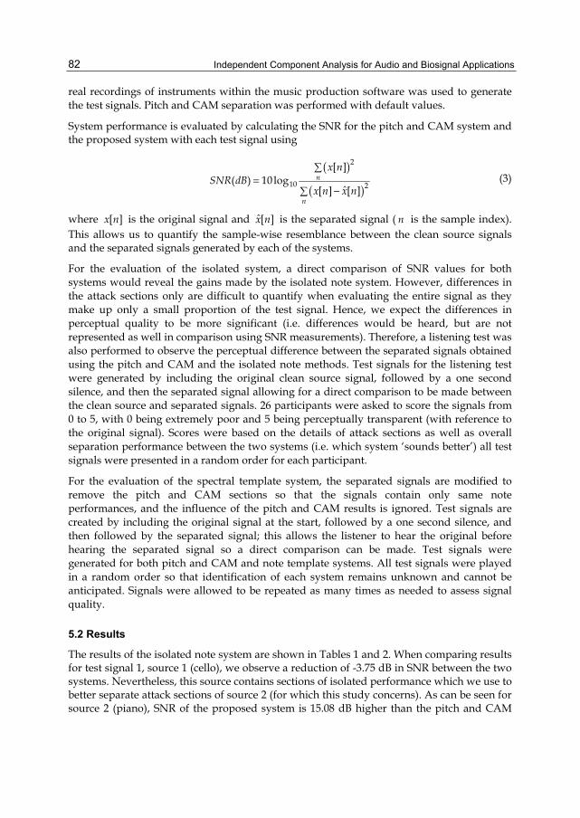
Independent Component Analysis for Audio and Biosignal Applications
82
real recordings of instruments within the music production software was used to generate the test signals. Pitch and CAM separation was performed with default values.
System performance is evaluated by calculating the SNR for the pitch and CAM system and the proposed system with each test signal using
( )
( )
2
10 2
[ ]( ) 10 log
ˆ[ ] [ ]n
n
x nSNR dB
x n x n
=
− (3)
where [ ]x n is the original signal and ˆ[ ]x n is the separated signal ( n is the sample index). This allows us to quantify the sample-wise resemblance between the clean source signals and the separated signals generated by each of the systems.
For the evaluation of the isolated system, a direct comparison of SNR values for both systems would reveal the gains made by the isolated note system. However, differences in the attack sections only are difficult to quantify when evaluating the entire signal as they make up only a small proportion of the test signal. Hence, we expect the differences in perceptual quality to be more significant (i.e. differences would be heard, but are not represented as well in comparison using SNR measurements). Therefore, a listening test was also performed to observe the perceptual difference between the separated signals obtained using the pitch and CAM and the isolated note methods. Test signals for the listening test were generated by including the original clean source signal, followed by a one second silence, and then the separated signal allowing for a direct comparison to be made between the clean source and separated signals. 26 participants were asked to score the signals from 0 to 5, with 0 being extremely poor and 5 being perceptually transparent (with reference to the original signal). Scores were based on the details of attack sections as well as overall separation performance between the two systems (i.e. which system ‘sounds better’) all test signals were presented in a random order for each participant.
For the evaluation of the spectral template system, the separated signals are modified to remove the pitch and CAM sections so that the signals contain only same note performances, and the influence of the pitch and CAM results is ignored. Test signals are created by including the original signal at the start, followed by a one second silence, and then followed by the separated signal; this allows the listener to hear the original before hearing the separated signal so a direct comparison can be made. Test signals were generated for both pitch and CAM and note template systems. All test signals were played in a random order so that identification of each system remains unknown and cannot be anticipated. Signals were allowed to be repeated as many times as needed to assess signal quality.
5.2 Results
The results of the isolated note system are shown in Tables 1 and 2. When comparing results for test signal 1, source 1 (cello), we observe a reduction of -3.75 dB in SNR between the two systems. Nevertheless, this source contains sections of isolated performance which we use to better separate attack sections of source 2 (for which this study concerns). As can be seen for source 2 (piano), SNR of the proposed system is 15.08 dB higher than the pitch and CAM

Monaural Audio Separation Using Spectral Template and Isolated Note Information
83
system, so a significant gain in separation performance is achieved. Looking at SNR results for test signal 2 source 1 (string section) we see a marginal increase of 0.34 dB in separation performance from the isolated note system, again, this source contains the isolated region of performance which is used to improve separation of source 2. For source 2 (guitar), we see a significant improvement in separation performance by the isolated note system with a SNR 8.44 dB higher than the pitch and CAM system.
Test Signal Source Pitch and CAM System Isolated Note System
1 1 19.04 15.29 2 5.87 20.95
2 1 15.78 16.09 2 3.63 12.07
Table 1. SNR (dB) results for Isolated Note System as compared with the pitch and CAM system.
Test Signal Source Pitch and CAM Mean Score Isolated Note Mean Score
1 1 4.88 4.73 2 2.50 4.50
2 1 3.85 3.69 2 1.65 3.54
Table 2. Listening test results for Isolated Note System as compared with the pitch and CAM system.
For test signal 1 we can see similar mean opinion scores for separation of source 1 by both systems suggesting a similar level of separation performance between the two systems. However, listening test results suggest a significant improvement of separation performance by the isolated note system for source 2. For test signal 1 and source 2, the pitch and CAM system achieved a mean score of 2.50 and the isolated note system achieved a mean score of 4.50. Again, the isolated note system achieved similar separation performance compared to the pitch and CAM system for test signal 2, source 1, while giving a significant improvement for source 2. The pitch and CAM system achieved a mean score of 1.65 whereas the isolated note achieved a higher mean score of 3.54. Both SNR and listening test results indicate that the note isolation separation system achieves better separation performance. We can see significant quantitative gains from the SNR results for signals with fast attacks (source 2 in both test signals 1 and 2). Qualitative results from the listening test also show significant perceptual gains obtained in the separation of attack sections in addition to overall separation.
The results of the spectral template system are summarised in Tables 3 and 4. Table 3 shows SNR results for the proposed note template separation system compared with the pitch and CAM separation system. We can see that for both test signals, we have the same separation performance for source 1 (cello). Sufficient harmonic information is available for source 1 to resolve overlapping harmonics so the note template system also uses the pitch and CAM method to separate the signal which is why the same performance result can be observed. However, for source 2 (piano), SNR results appear to be poor. For test signal 1 we see that the pitch and CAM system has a SNR of 0.79 dB whereas the note template system has a SNR of -

Independent Component Analysis for Audio and Biosignal Applications
84
2.35 dB, suggesting that the level of noise introduced by the system is greater than the level of input signal. Likewise, test signal 2 shows poor SNR results for source 2, the pitch and CAM system has a SNR of 2.90 dB while the note template system has a SNR of -3.65 dB.
Test Signal Source Pitch and CAM System Note Template System
1 1 2.62 2.62 2 0.79 -2.35
2 1 7.79 7.79 2 2.90 -3.65
Table 3. SNR (dB) results for Note Template System as compared with the pitch and CAM system.
Test Signal Source Pitch and CAM System Note Template System
1 1 4.08 3.77 2 1.96 0.92
2 1 4.77 4.81 2 1.65 0.92
Table 4. Listening test results for Note Template System as compared with the pitch and CAM system.
Table 4 shows average results for the listening test for the pitch and CAM separation system and the note template separation system. For test signal 1, source 1, we see a mean score of 4.08 for the pitch and CAM separation system and a mean score of 3.77 for the note template system despite the same pitch and CAM separated signal being used by both systems, as explained earlier. For test signal 1, source 2, we see a mean score of 4.77 for the pitch and CAM system. We see a reduction of the score for the note template system, with a mean score of 0.92. Comparing scores for test signal 2, similar scores for source 1 can be seen for both systems, with the pitch and CAM system scoring a mean of 4.77 and the note template system scoring a mean of 4.81. Again, both systems use the pitch and CAM separated signals for source 1, as explained earlier. The score for the note template system is lower than the score for the pitch and CAM system, for test signal 2, source 2; we see a mean score of 1.65 for the pitch and CAM system and a mean score of 0.92 for the note template system. The spectral template system does not work as promising as we would have expected, due to the following possible reasons. The templates trained from mixtures may not be accurate enough to represent the sources, because of the limited number of non-overlapped harmonics and isolated notes within the mixture. Using clean music source data (instead of the monaural mixture) to train the templates may be able to mitigate this problem and further to improve the results. Also, in the proposed template systems, pitch shifting which was used to fill up the missing notes that are not available in the mixture, apparently introduces errors in harmonic estimation. These are interesting points for future investigation.
6. Conclusions We have presented two new methods for music source separation from monaural mixture using the isolated note information and note spectral template, both evaluated

Monaural Audio Separation Using Spectral Template and Isolated Note Information
85
from the sound mixture. The proposed methods were designed to improve the separation performance of the baseline pitch and CAM system especially for the separation of attack sections of notes, and overlapping time-frequency regions. In the pitch and CAM system, the fast attack sections are almost completely lost in the separated signals, resulting in poor separation results for the transient part of the signal. In the proposed isolate note system, accurate harmonic information available in the isolated regions is used to reconstruct harmonic content for the entire note performance, and so, the harmonic content can be removed from the mixture to reveal the remaining note performance (in a two-source case). The isolated note system has been shown to be successful in improving the separation performance of attack sections of notes, offering a large improvement in separation quality over the baseline system. In the proposed note template system, the overlapping time-frequency regions of the mixtures are resolved using the reliable information from the non-overlapping regions of the sources, based on the spectral template matching. Preliminary results show that the spectral templates evaluated from the mixtures can be noisy and may degrade the results. Using spectral template generated directly from clean training data (i.e. containing single signals, instead of mixtures) has the potential to improve the system performance which will be our future study.
7. Future directions We have studied the potentials of using spectral template and isolated note information for music sound separation. A major challenge is however to identify the regions from which the note information can be regarded as reliable and thereby used to estimate the note information for the unreliable and overlapped regions. Under noisy and multiple source conditions, more ambiguous regions may be identified, and using such information may further distort the separation results. Pitch information is relatively reliable under noisy conditions and can be used to improve the system performance [81]. Another potential direction is to use the property of the sources and noise/interferences, such as sparseness, to facilitate the identification of the reliable regions within the mixture that can be used to estimate the sources [74-77]. This is mainly due to the following three reasons. Firstly, as mentioned earlier, music audio can be made sparser if it is transformed into another domain, such as the TF domain, using an analytically pre-defined dictionary such as discrete Fourier transform (DFT) or discrete cosine transform (DCT) [69] [70]. Recent studies show that signal dictionaries directly adapted from training data using machine learning techniques, based on some optimisation criterion (such as the reconstruction error regularised by a sparsity constraint), can offer better performance than the pre-defined dictionary [71] [72]. Secondly, the sparse techniques using learned dictionary have been shown to possess certain denoising capability for corrupted signals [72]. Thirdly, identification of reliable regions from sound mixtures, and estimation of the probability of each TF point dominated by a source can be potentially cast as an audio-inpainting [73] or matrix completion problem. This naturally links the two important areas: source separation and sparse coding. Hence, the emerging algorithms developed in the sparse coding area could be potentially used for the CASA based monaural separation system. Separating music sources from mixtures with uncertainties [78] [79], such as under the condition of unknown number of sources, is also a promising direction for
Independent Component Analysis for Audio and Biosignal Applications
86
future research, as required in many practical applications. In addition, online optimisation will be necessary when the separation algorithms operate on resource limited platforms [80].
8. References [1] Jutten, C., & Herault, J. (1991). Blind Separation of Sources, Part I: An Adaptive
Algorithm Based on Neuromimetic Architecture, Signal Processing, vol. 24, pp. 1-10. [2] Cardoso, J.-F., & Souloumiac, A. (1993). Blind Beamforming for Non Gaussian Signals,
IEE Proc. F, Radar Signal Processing, vol. 140, no. 6, pp. 362-370. [3] Comon, P. (1994). Independent Component Analysis: a New Concept?, Signal
Processing, vol. 36, no. 3, pp. 287–314. [4] Bell, A. J., & Sejnowski, T. J. (1995). An Information Maximization Approach to Blind
Separation and Blind Deconvolution, Neural Computation, vol. 7, no. 6, pp. 1129-1159.
[5] Amari, S.-I., Cichocki, A., & Yang, H. (1996). A New Learning Algorithm for Blind Signal Separation, Advances Neural Information Processing System, vol. 8, pp. 757–763.
[6] Cardoso, J.-F. (1998). Blind Signal Separation: Statistical Principles, Proceedings of the IEEE, vol. 9, no. 10, pp. 2009–2025.
[7] Lee, T.-W. (1998). Independent Component Analysis: Theory and Applications. Boston, MA: Kluwer Academic.
[8] Haykin, S. (2000). Unsupervised Adaptive Filtering, Volume 1, Blind Source Separation. New York: Wiley.
[9] Hyvärinen, A., Karhunen, J., & Oja, E. (2001). Independent Component Analysis. New York: Wiley.
[10] Cichocki, A., & Amari, S.-I. (2002). Adaptive Blind Signal and Image Processing, Learning Algorithm and Applications. New York: Wiley.
[11] Cardoso, J. F., & Laheld, B. (1996). Equivariant Adaptive Source Separation, IEEE Transactions Signal Processing, vol. 44, no. 12, pp. 3017–3030.
[12] Belouchrani, A., Abed-Meraim, K., Cardoso, J., & Moulines, E. (1997). A Blind Source Separation Technique Using Second-Order Statistics, IEEE Transactions Signal Processing, vol. 45, no. 2, pp. 434–444.
[13] Thi, H., & Jutten, C. (1995). Blind Source Separation for Convolutive Mixtures, Signal Processing, vol. 45, pp. 209-229.
[14] Smaragdis, P. (1998). Blind Separation of Convolved Mixtures in the Frequency Domain, Neurocomputing, vol. 22, pp. 21–34.
[15] Parra, L., & Spence, C. (2000). Convolutive Blind Source Separation of Nonstationary Sources, IEEE Transactions Speech Audio Processing, vol. 8, no. 3, pp. 320–327.
[16] Rahbar, K., & Reilly, J. (2001). Blind Source Separation of Convolved Sources by Joint Approximate Diagonalization of Cross-Spectral Density Matrices, in Proc. IEEE International Conference Acoustics, Speech and Signal Processing, Utah, USA.
[17] Davies, M. (2002). Audio Source Separation, in Mathematics in Signal Separation V. Oxford, U.K.: Oxford Univ. Press.
[18] Sawada, H., Mukai, R., Araki, S., & Makino, S. (2004). A Robust and Precise Method for Solving the Permutation Problem of Frequency-Domain Blind Source Separation, IEEE Transactions Speech and Audio Processing, vol.12, no. 5, pp. 530-538.
Monaural Audio Separation Using Spectral Template and Isolated Note Information
87
[19] Wang, W., Sanei, S., & Chambers, J.A. (2005). Penalty Function Based Joint Diagonalization Approach for Convolutive Blind Separation of Nonstationary Sources, IEEE Transactions on Signal Processing, vol. 53, no. 5, pp. 1654-1669.
[20] Sawada, H., Araki, S., & Makino, S. (2010). Underdetermined Convolutive Blind Source Separation via Frequency Bin-Wise Clustering and Permutation Alignment, IEEE Transactions on Audio Speech and Language Processing, vol. 18, pp. 516-527.
[21] Pedersen, M., Larsen, J., Kjems, U., & Parra, L. (2007). A Survey on Convolutive Blind Source Separation Methods, Handbook on Speech Processing and Speech Communication, Springer.
[22] Belouchrani, A., & Amin, M. G. (1998). Blind Source Separation Based on Time-Frequency Signal Representations, IEEE Transactions Signal Processing, vol. 46, no. 11, pp. 2888–2897, 1998.
[23] Chen, S., Donoho, D. L., & Saunders, M. A. (1998). Atomic Decomposition by Basis Pursuit, SIAM Journal Scientific Computing, vol. 20, no. 1, pp. 33-61.
[24] Lee, T., Lewicki, M., Girolami, M., & Sejnowski, T. (1998), Blind Source Separation of More Sources Than Mixtures Using Overcomplete Representations, IEEE Signal Processing Letters, vol. 6, no. 4, pp. 87-90.
[25] Lewicki, M. S., & Sejnowski, T. J. (1998). Learning Overcomplete Representations, Neural Computation, vol. 12, no. 2, pp. 337–365.
[26] Bofill, P., & Zibulevsky, M. (2001). Underdetermined Blind Source Separation Using Sparse Representation, Signal Processing, vol. 81, pp. 2253–2362.
[27] Zibulevsky, M., & Pearlmutter, B. A. (2001). Blind Source Separation by Sparse Decomposition in a Signal Dictionary, Neural Computation, vol. 13, no. 4, pp. 863–882.
[28] Li, Y., Amari, S., Cichocki, A., Ho, D. W. C., & Xie, S. (2006). Underdetermined Blind Source Separation Based on Sparse Representation. IEEE Transactions on Signal Processing, vol. 54, no. 2, pp. 423-437.
[29] He, Z., Cichocki, A., Li, Y., Xie, S., & Sanei, S. (2009). K-Hyperline Clustering Learning for Sparse Component Analysis. Signal Processing, vol. 89, no. 6, pp. 1011-1022.
[30] Yilmaz, O., & Richard, S. (2004). Blind Separation of Speech Mixtures via Time-Frequency Masking, IEEE Transactions on Signal Processing, vol. 52, no. 7, pp. 1830-1847.
[31] Wang, D.L. (2005). On Ideal Binary Mask as the Computational Goal of Auditory Scene Analysis. In Divenyi P. (ed.), Speech Separation by Humans and Machines, pp. 181-197, Kluwer Academic, Norwell MA.
[32] Mandel, M. I., Weiss, R. J., & Ellis, D. P. W. (2010). Model-based Expectation Maximisation Source Separation and Localisation, IEEE Transactions on Audio Speech and Language Processing, vol. 18, pp. 382-394.
[33] Duong, N. Q. K., Vicent, E., & Gribonval, R. (2010). Under-determined Reverberant Audio Source Separation Using a Full-Rank Spatial Covariance Model, IEEE Transactions on Audio Speech and Language Processing, vol. 18, pp. 1830-1840.
[34] Plumbley, M. D. (2003). Algorithms for Nonnegative Independent Component Analysis, IEEE Transactions on Neural Networks, vol. 14, no. 2, pp. 534–543.
[35] Kim, T., Attias, H., & Lee, T.-W. (2007). Blind Source Separation Exploiting Higher-Order Frequency Dependencies, IEEE Transactions on Audio Speech and Language Processing, vol. 15, pp. 70-79.

Independent Component Analysis for Audio and Biosignal Applications
88
[36] Comon, P., & Jutten, C., eds. (2010). Handbook of Blind Source Separation, Independent Component Analysis and Applications, Academic Press.
[37] Smaragdis, P. (2004). Non-Negative Matrix Factor Deconvolution; Extraction of Multiple Sound Sources from Monophonic Inputs. In Proceedings of the 5th International Conference on Independent Component Analysis and Blind Signal Separation, Grenada, Spain.
[38] Schmidt, M. N., & Mørup, M. (2006). Nonnegative Matrix Factor 2-D Deconvolution for Blind Single Channel Source Separation, in Proceedings of the International Conference on Independent Component Analysis and Signal Separation, Charleston, USA.
[39] Wang, W., Cichocki, A., & Chambers, J. A. (2009). A Multiplicative Algorithm for Convolutive Non-negative Matrix Factorization Based on Squared Euclidean Distance, IEEE Transactions on Signal Processing, vol. 57, no. 7, pp. 2858-2864.
[40] Ozerov, A., & Févotte, C. (2010). Multichannel Nonnegative Matrix Factorization in Convolutive Mixtures for Audio Source Separation, IEEE Transactions on Audio, Speech and Language Processing.
[41] Mysore, G., Smaragdis, P., & Raj, B. (2010). Non-Negative Hidden Markov Modeling of Audio with Application to Source Separation. In Proceedings of the 9th international conference on Latent Variable Analysis and Signal Separation (LCA/ICA). St. Malo, France.
[42] Ozerov, A., Févotte, C., Blouet, R., & Durrieu, J.L. (2011). Multichannel Nonnegative Tensor Factorization with Structured Constraints for User-guided Audio Source Separation, Proceedings of the IEEE International Conference Acoustics, Speech and Signal Processing, Prague, Czech Republic.
[43] Wang, W. & Mustafa, H. (2011). Single Channel Music Sound Separation Based on Spectrogram Decomposition and Note Classification, in Computer Music Modelling and Retrieval, Springer.
[44] Cichocki, A., Zdunek, R., Phan, A.H., & Amari, S. (2009). Nonnegative Matrix and Tensor Factorizations: Applications to Exploratory Multi-way Data Analysis and Blind Source Separation. Wiley.
[45] Brown, G.J., & Cooke, M.P. (1994). Computational Auditory Scene Analysis, Computer Speech and Language, vol. 8, pp. 297–336.
[46] Wrigley, S. N., Brown, G. J., Renals, S., & Wan, V. (2005). Speech and Crosstalk Detection in Multi-Channel Audio, IEEE Transactions on Speech and Audio Processing, vol. 13, no. 1, pp. 84-91.
[47] Palomäki, K. J., Brown, G. J., & Wang, D. L. (2004). A Binaural Processor for Missing Data Speech Recognition in the Presence of Noise and Small-Room Reverberation, Speech Communication, vol. 43, no. 4, pp. 361-378.
[48] Wang, D.L., & Brown, G. (2006). Computational Auditory Scene Analysis: Principles, Algorithms, and Applications, Wiley/IEEE.
[49] Shao, Y., & Wang, D.L. (2009). Sequential Organization of Speech in Computational Auditory Scene Analysis. Speech Communication, vol. 51, pp. 657-667.
[50] Hu, K., & Wang, D.L. (2011). Unvoiced Speech Segregation from Nonspeech Interference via CASA and Spectral Subtraction. IEEE Transactions on Audio, Speech, and Language Processing, vol. 19, pp. 1600-1609.

Monaural Audio Separation Using Spectral Template and Isolated Note Information
89
[51] Xu, T., & Wang, W. (2009). A Compressed Sensing Approach for Underdetermined Blind Audio Source Separation with Sparse Representations, in Proceedings of the IEEE International Workshop on Statistical Signal Processing, Cardiff, UK.
[52] Xu, T., & Wang, W. (2010). A Block-based Compressed Sensing Method for Underdetermined Blind Speech Separation Incorporating Binary Mask, in Proceedings of the IEEE International Conference on Acoustics, Speech and Signal Processing, Dallas, Texas, USA.
[53] Xu, T., & Wang, W. (2011). Methods for Learning Adaptive Dictionary for Underdetermined Speech Separation, in Proceedings of the IEEE 21st International Workshop on Machine Learning for Signal Processing, Beijing, China.
[54] Kim, M., & Choi, S. (2006). Monaural Music Source Separation: Nonnegativity, Sparseness, and Shift-Invariance, in Proceedings of the IEEE International Conference on Independent Component Analysis and Blind Signal Separation, Charleston, USA.
[55] Virtanen, T. (2006). Sound Source Separation in Monaural Music Signals, PhD Thesis, Tampere University of Technology.
[56] Virtanen, T. (2007). Monaural Sound Source Separation by Nonnegative Matrix Factorization With Temporal Continuity and Sparseness Criteria, IEEE Transactions on Audio, Speech and Language Processing, vol. 15, no. 3, pp. 1066-1074.
[57] Ozerov, A., Philippe, P., Bimbot, F., & Gribonval, R. (2007). Adaptation of Bayesian Models for Single-Channel Source Separation and its Application to Voice/Music Separation in Popular Songs, Proceedings of the IEEE International Conference on Acoustics, Speech, and Signal Processing, Hawaii, USA.
[58] Richard, G., & David, B. (2009). An Iterative Approach to Monaural Musical Mixture De-Soloing, in Proceedings of the IEEE International Conference on Acoustics, Speech, and Signal Processing, Taipei, Taiwan.
[59] Klapuri, A., Virtanen, T., & Heittola, T. (2010). Sound Source Separation in Monaural Music Signals Using Excitation-Filter Model and EM Algorithm, in Proceedings of the IEEE International Conference on Acoustics, Speech, and Signal Processing, Dallas, USA.
[60] Bregman, A. S. (1990). Auditory Scene Analysis, MIT Press. [61] Li, Y. & Wang, D. L. (2007). Separation of Singing Voice From Music Accompaniment
for Monaural Recordings, IEEE Transactions on Audio, Speech and Language Processing, vol. 15, no. 4, pp. 1475-1487.
[62] Parsons, T. W. (1976). Separation of Speech from Interfering Speech By Means of Harmonic Selection, Journal of the Acoustical Society of America, vol. 60, no. 4, pp. 911-918, 1976.
[63] Li, Y. & Wang, D. L. (2009). Musical Sound Separation Based on Binary Time-Frequency Masking, EURASIP Journal on Audio, Speech and Music Processing, article ID 130567.
[64] Every, M. R. & Szymanski, J. E. (2006). Separation of Synchronous Pitched Notes by Spectral Filtering of Harmonics, IEEE Transactions on Audio, Speech and Language Processing, vol. 14, no. 5, pp. 1845-1856.
[65] Virtanen, T. & Klapuri, A. (2001). Separation of Harmonic Sounds Using Multipitch Analysis and Iterative Parameter Estimation, in Proceedings of the IEEE Workshop on Applications of Signal Processing in Audio and Acoustics, pp. 83-86.
[66] Hu, G. (2006). Monaural Speech Organization and Segregation, Ph.D. Thesis, The Ohio State University, USA.
Independent Component Analysis for Audio and Biosignal Applications
90
[67] Li, Y., Woodruff, J. & Wang, D. L. (2009). Monaural Musical Sound Separation Based on Pitch and Common Amplitude Modulation, IEEE Transactions on Audio, Speech and Language Processing, vol. 17, no. 7, pp. 1361-1371.
[68] ISO. Acoustics – Standard Tuning Frequency (Standard Musical Pitch), ISO 16:1975, International Organization for Standardization, Geneva, 1975.
[69] Nesbit, A., Jafari, M. G., Vincent, E., & Plumbley, M. D. (2010). Audio Source Separation Using Sparse Representations. In W. Wang (Ed), Machine Audition: Principles, Algorithms and Systems. Chapter 10, pp.246-264. IGI Global.
[70] Plumbley, M. D., Blumensath, T., Daudet, L., Gribonval, R., & Davies, M. E. (2010). Sparse Representations in Audio and Music: from Coding to Source Separation, Proceedings of the IEEE, vol. 98, pp. 995-1005.
[71] Dai, W., Xu, T. & Wang, W. (2012). Dictionary Learning and Update based on Simultaneous Codeword Optimisation (SIMCO), Proceedings of the IEEE International Conference on Acoustics, Speech and Signal Processing, Kyoto, Japan.
[72] Dai, W., Xu, T., & Wang, W. (2011). Simultaneous Codeword Optimisation (SimCO) for Dictionary Update and Learning, arXiv:1109.5302.
[73] Adler, A., Emiya V., Jafari, M.G., Elad, M., Gribonval, G., & Plumbley, M.D. (2012). Audio Inpainting, IEEE Transactions on Audio, Speech and Language Processing, vol. 20, pp. 922-932.
[74] Wang, W. (2011). Machine Audition: Principles, Algorithms and Systems, IGI Global Press. [75] Jan, T. & Wang, W. (2011). Cocktail Party Problem: Source Separation Issues and
Computational Methods, in W. Wang (ed), Machine Audition: Principles, Algorithms and Systems, IGI Global Press, pp. 61-79.
[76] Jan, T., Wang, W., & Wang, D.L. (2011). A Multistage Approach to Blind Separation of Convolutive Speech Mixtures. Speech Communication, vol. 53, pp. 524-539.
[77] Luo, Y., Wang, W., Chambers, J. A., Lambotharan, S., & Prouder, I. (2006). Exploitation of Source Non-stationarity for Underdetermined Blind Source Separation With Advanced Clustering Techniques, IEEE Transactions on Signal Processing, vol. 54, no. 6, pp. 2198-2212.
[78] Adiloglu, K. & Vincent, E. (2011). An Uncertainty Estimation Approach for the Extraction of Source Features in Multisource Recordings, in Proceedings of the European Signal Processing Conference, Barcelona, Spain.
[79] Adiloglu, K., & Vincent, E. (2012). A General Variational Bayesian Framework for Robust Feature Extraction in Multisource Recordings, in Proceedings of the IEEE International Conference on Acoustics, Speech and Signal Processing, Kyoto, Japan.
[80] Simon, L. S. R., & Vincent, E. (2012). A General Framework for Online Audio Source Separation, in Proceedings of the International conference on Latent Variable Analysis and Signal Separation, Tel-Aviv, Israel.
[81] Hsu, C.-L., Wang, D.L., Jang J.-S.R., & Hu, K. (2012). A Tandem Algorithm for Singing Pitch Extraction and Voice Separation from Music Accompaniment, IEEE Transactions on Audio, Speech, and Language Processing, vol. 20, pp. 1482-1491.

5
Non-Negative Matrix Factorization with Sparsity Learning for Single Channel
Audio Source Separation Bin Gao and W.L. Woo
School of Electrical and Electronic Engineering, Newcastle University, England, United Kingdom
1. Introduction 1.1 Single channel source separation (SCSS)
In this chapter, the special case of instantaneous underdetermined source separation problem termed as single channel source separation (SCSS) is focused. In general case and for many practical applications (e.g. audio processing) only one-channel recording is available and in such cases conventional source separation techniques are not appropriate. This leads to the SCSS research area where the problem can be simply treated as one observation instantaneous mixed with several unknown sources:
=
=1
( ) ( )sN
ii
y t x t (1)
where = 1, , si N denotes number of sources and the goal is to estimate the sources ( )ix t when only the observation signal ( )y t is available. This is an underdetermined system of equation problem. Recently, new advances have been achieved in SCSS and this can be categorized either as supervised SCSS methods or unsupervised SCSS methods. For supervised SCSS methods, the probabilistic models of the source are trained as a prior knowledge by using some or the entire source signals. The mixture is first transformed into an appropriate representation, in which the source separation is performed. The source models are either constructed directly based on knowledge of the signal sources, or by learning from training data (e.g. using Gaussian mixture model construct source models either directly based on knowledge of signal sources, or by learning from isolated training data). In the inference stage, the models and data are combined to yield estimates of the sources. This category predominantly includes the frequency model-based SCSS methods [1, 2] where the prior bases are modeled in time-frequency domain (e.g. spectrogram or power spectrogram), and the underdetermined-ICA time model-based SCSS method [3] which the prior bases are modeled in time domain. For unsupervised SCSS methods, this denotes the separation of completely unknown sources without using additional training information. These methods typically rely on the assumption that the sources are non-redundant, and the methods are based on, for example, decorrelation, statistical independence, or the minimum description

Independent Component Analysis for Audio and Biosignal Applications
92
length principle. This category includes several widely used methods: Firstly, the CASA-based unsupervised SCSS methods [4] whose goal is to replicate the process of human auditory system by exploiting signal processing approaches (e.g. notes in music recordings) and grouping them into auditory streams using psycho-acoustical cues. Secondly, the subspace technique based unsupervised SCSS methods using NMF [5, 6] or independent subspace analysis (ISA) [7] which usually factorizes the spectrogram of the input signal into elementary components. Of special interest, EMD [8] based unsupervised SCSS methods which can separate audio mixed signal in time domain and recover sources by combing other data analysis tools, e.g. independent component analysis (ICA) [9] or principle component analysis (PCA).
1.2 Unsupervised SCSS using NMF
In this book chapter, we propose a new NMF method for solving unsupervised SCSS problem. In a conventional NMF, given a data matrix [ ] ×
+= ∈ℜ1 , , K LLY y y with >, 0k lY ,
NMF factorizes this matrix into a product of two non-negative matrices:
≈Y DH (2)
where ×+∈ℜ KD and ×
+∈ℜ LH where K and L represent the total number of rows and columns in matrix Y , respectively. If is chosen to be = L , no benefit is achieved at all. Thus the idea is to determine < L so that the matrix D can be compressed and reduced to its integral components such as ×KD is a matrix containing a set of dictionary vectors, and
× LH is an encoding matrix that describes the amplitude of each dictionary vector at each time point. A popular approach to solve the NMF optimization problem is the multiplicative update (MU) algorithm by Lee and Seung [10]. The MU update rule for Least square (LS) distance is given by:
← T
TYH
D DDHH
and ← T
TD Y
H HD DH
(3)
Multiplicative update-based families of parameterized cost functions such as the Beta divergence [11], and Csiszar’s divergences [12] have also been presented as well. A sparseness constraint [13, 14] can be added to the cost function, and this can be achieved by regularization using the L1-norm. Here, ‘sparseness’ refers to a representational scheme where only a few units (out of a large population) are effectively used to represent typical data vectors [15]. In effect, this implies most units taking values close to zero while only few take significantly non-zero values. Several other types of prior over D and H can be defined e.g. in [16, 17], it is assumed that the prior of D and H satisfy the exponential density and the prior for the noise variance is chosen as an inverse gamma density. In [18], Gaussian distributions are chosen for both D and H . The model parameters and hyperparameters are adapted by using the Markov chain Monte Carlo (MCMC) [19-21]. In all cases, a fully Bayesian treatment is applied to approximate inference for both model parameters and hyperparameters. While these approaches increase the accuracy of matrix factorization, it only works efficient when large sample dataset is available. Moreover, it consumes significantly high computational complexity at each iteration to adapt the

Non-Negative Matrix Factorization with Sparsity Learning for Single Channel Audio Source Separation
93
parameters and its hyperparameters. Regardless of the cost function and sparseness constraint being used, the standard NMF or SNMF models [22] are only satisfactory for solving source separation provided that the spectral frequencies of the analyzed audio signal do not change over time. However, this is not the case for many realistic audio signals. As a result, the spectral dictionary obtained via the NMF or SNMF decomposition is not adequate to capture the temporal dependency of the frequency patterns within the signal. The recently developed two-dimensional sparse NMF deconvolution (SNMF2D) model [23, 24] extends the NMF model to be a two-dimensional convolution of D and H where the spectral dictionary and temporal code are optimized using the least square cost function with sparse penalty:
λ− + 2, ,
,
1: ( ) ( )2LS k l k l
k l
C fY Z H (4)
for ∀ ∈ ∀ ∈,k K l L where φ ττ φ
τ φ
↓ →
= ,
Z D H , τ τ τ
τ= 2
, , ,,
( )k d k d k dk
D D D and ( )f H can be any
function with positive derivative such as α α− >( 0)L norm given by ααφ
αφ
= =
1/
,, ,
( ) d ld l
f H H H . Here φτ↓D denotes the downward shift which moves each
element in the matrix τD down by φ rows, and τφ
→
H denotes the right shift which moves each element in the matrix φH to the right by τ columns. The SNMF2D is effective in single channel audio source separation (SCASS) because it is able to capture both the temporal structure and the pitch change of an audio source. However, the drawbacks of SNMF2D originate from its lack of a generalized criterion for controlling the sparsity of H . In practice, the sparsity parameter is set manually. When SNMF2D imposes uniform sparsity on all temporal codes, this is equivalent to enforcing each temporal code to be identical to a fixed distribution according to the selected sparsity parameter. In addition, by assigning the fixed distribution onto each individual code, this is equivalent to constraining all codes to be stationary. However, audio signals are non-stationary in the TF domain and have different temporal structure and sparsity. Hence, they cannot be realistically enforced by a fixed probability distribution. These characteristics are even more pronounced between different types of audio signals. In addition, since the SNMF2D introduces many temporal shifts, this will result in more temporal codes to deviate from the fixed distribution. In such situation, the obtained factorization will invariably suffer from either under- or over-sparseness which subsequently lead to ambiguity in separating the audio mixture. Thus, the above suggests that the present form of SNMF2D is still technically lacking and is not readily suited for SCASS especially mixtures involving different types of audio signals.
In this chapter, an adaptive sparsity two-dimensional non-negative matrix factorization is proposed. The proposed model allows: (i) overcomplete representation by allowing many spectral and temporal shifts which are not inherent in the NMF and SNMF models. Thus, imposing sparseness is necessary to give unique and realistic representations of the non-stationary audio signals. Unlike the SNMF2D, our model imposes sparseness on H element-wise so that each individual code has its own distribution. Therefore, the sparsity parameter can

Independent Component Analysis for Audio and Biosignal Applications
94
be individually optimized for each code. This overcomes the problem of under- and over-sparse factorization. (ii) Each sparsity parameter in our model is learned and adapted as part of the matrix factorization. This bypasses the need of manual selection as in the case of SNMF2D. The proposed method is tested on the application of single channel music separation and the results show that our proposed method can give superior separation performance.
The chapter is organized as follows: In Section II, the new model is derived. Experimental results coupled with a series of performance comparison with other NMF techniques are presented in Section III. Finally, Section IV concludes the paper.
2. Adaptive sparsity two-dimensional non-negative matrix factorization In this section, we derive a new factorization method termed as the adaptive sparsity two-dimensional non-negative matrix factorization. The model is given by
φ φτ ττ φ τ φτ φ τ φ
τ φ τ φ
↓ ↓→ →
= = = = == + = +
max max max max max
0 0 1 0 0
d
d dd
Y D H V D H V (5)
where ( ) ( )φ φ φ φ φ φλ λ= =
= −∏∏max max
, , ,1 1
| expd l
d l d l d ld l
pH H λ H . In (5), it is worth pointing out that each
individual element in φH is constrained to an exponential distribution with independent decay
parameter φλ ,d l . Here, τdD is the dth column of τD , φ
dH is the dth row of φH and V is assumed
to be independently and identically distributed (i.i.d.) as Gaussian distribution with noise having variance σ 2 . The terms maxd , τmax , φmax and maxl are the maximum number of
columns in τD , τ shifts, φ shifts and column length in Y , respectively. This is in contrast
with the conventional SNMF2D where φλ ,d l is simply set to a fixed constant i.e. φλ λ=,d l for all
φ, ,d l . Such setting imposes uniform constant sparsity on all temporal codes φH which enforces each temporal code to be identical to a fixed distribution according to the selected constant sparsity parameter. The consequence of this uniform constant sparsity has already been discussed in Section I. In Section III, we will present the details of the sparsity analysis for source separation and evaluate its performance against with other existing methods.
2.1 Formulation of the proposed adaptive sparsity NMF2D
To facilitate such spectral dictionaries with adaptive sparse coding, we first define τ = max0 1D D D D , φ = max0 1H H H H and φ = max1 2λ λ λ λ , and then
choose a prior distribution ( ),p D H over the factors ,D H in the analysis equation. The
posterior can be found by using Bayes’ theorem as
( ) ( ) ( )( )σ
σ =2
2, , ,
, , ,p p
pP
Y D H D H λD H Y λ
Y (6)

Non-Negative Matrix Factorization with Sparsity Learning for Single Channel Audio Source Separation
95
where the denominator is constant and therefore, the log-posterior can be expressed as
( ) ( ) ( )σ σ= + +2 2log , , , log | , , log , constp p pD H Y λ Y D H D H λ (7)
where ‘ const ’ denotes constant. The likelihood of the observations given D and H can be written1 as:
( )φ ττ φ
τ φσ σ
πσ
↓ → = − −
2
2 22
1| , , exp 22
d dd F
p Y D H Y D H (8)
where .F
denotes the Frobenius norm. The second term in (7) consists of the prior distribution of D and H where they are jointly independent. Each element of H is constrained to be exponential distributed with independent decay parameters, namely,
( ) ( )φ φ φ
φλ λ= −∏∏∏ , , ,| expd l d l d l
d l
p H λ H so that φ φ
φλ= , ,
, ,( ) d l d l
d l
f H H (9)
Hence, the negative log likelihood serves as the cost function defined as:
( )φ ττ φ
τ φ
φ ττ φ φ φ
τ φ φ
σ
λσ
↓ →
↓ →
∝ − +
= − +
2
2
2
, ,2, ,
12
12
d dd F
d d d l d ld d lF
L fY D H H
Y D H H
(10)
The sparsity term ( )f H forms the L1-norm regularization which is used to resolve the ambiguity by forcing all structure in H onto D . Therefore, the sparseness of the solution in (9) is highly dependent on the regularization parameter φλ ,d l .
2.1.1 Estimation of the dictionary and temporal code
In (10), each spectral dictionary was constrained to unit length. This can be easily satisfied
by normalizing each spectral dictionary according to τ τ τ
τ= 2
, , ,,
( )k d k d k dk
D D D for all
[ ]∈ max1 , ,d d . With this normalization, the two-dimensional convolution of the spectral
dictionary and temporal codes is now represented as φ ττ φ
τ φ
↓ →
= d d
d
Z D H . The derivatives of
(10) corresponding to τD and φH of the adaptive sparsity factorization model are given by:
1 To avoid cluttering the notation, we shall remove the upper limits from the summation terms. The upper limits can be inferred from (5).

Independent Component Analysis for Audio and Biosignal Applications
96
φ ττ
φ φ τφ ττ φ
τ
↓ ←
↓ ←← •
+
T
T
D YH H
D Z λ
(11)
τ τφφφ τ φ τ
φ ττ τ
τ τφ φφ τ φ τ
φ τ
→ →↑↑
→ →↑ ↑
+ •
← • + •
diag
diag
T T
T T
Y H D 1 Z H D
D D
Z H D 1 Y H D
where ( )τ
τ
τ
τ
=
,
, 2,
,
k dk d
k dk
DD
D (12)
In (11), superscript ‘ T ’ denotes matrix transpose, ‘ ’ is the element wise product and ( )⋅diag denotes a matrix with the argument on the diagonal. The column vectors of τD will
be factor-wise normalized to unit length.
2.1.2 Estimation of the adaptive sparsity parameter
Since τφ
→
H is obtained directly from the original sparse code matrix φ→0H , it suffices to
compute just for the regularization parameters associated with φ→0H . Therefore, we can set
the cost function in (10) with τ =max 0 as
( ) ( ) ( ) ( )φ φφ
φφ φ
φ φσ
↓
= =
= − ⊗ +
max max
2
20 0
1( )2
F
F Vec Vec VecT
H Y I D H λ H (13)
with ⋅( )Vec represents the column vectorization, ‘⊗ ’ is the Kronecker product, and I is the identity matrix. Defining the following terms:
φ
φ
φφ
φφ φ
λλ
λ
↓↓ ↓ = = ⊗ ⊗ ⊗
= = =
max
max maxmax max
0 1
00
1,111
2,1
,
( ) , ,
( )
( ), ,
( ) d l
Vec
Vec
Vec
Vec
y Y D I D I D I D
λH
H λh λ λ
H λ
(14)
Thus, (13) can be rewritten in terms of h as
σ
= − +2
21( )
2 FF Th y Dh λ h (15)

Non-Negative Matrix Factorization with Sparsity Learning for Single Channel Audio Source Separation
97
Note that h and λ are vectors of dimension × 1R where φ= × × +max max max( 1)R d l . To determine λ , we use the Expectation-Maximization (EM) algorithm and treat h as the hidden variable where the log-likelihood function can be optimized with respect to λ . Using the Jensen’s inequality, it can be shown that for any distribution ( )Q h , the log-likelihood function satisfies the following [25-27]:
( ) ( ) ( )( )
σσ
≥
2
2, | , ,
ln | , , lnp
p Q dQ
y h λ Dy λ D h h
h (16)
One can easily check that the distribution that maximizes the right hand side of (16) is given by ( ) ( )σ= 2| , , ,Q ph h y λ D which is the posterior distribution of h . In this paper, we
represent the posterior distribution in the form of Gibbs distribution:
( ) ( ) ( )= − = − 1 exp where exphh
Q F Z F dZ
h h h h (17)
The functional form of the Gibbs distribution in (17) is expressed in terms of ( )F h and this is crucial as it will enable us to simplify the variational optimization of λ . The maximum likelihood estimation of λ can be expressed by
( )( ) ( )
σ=
=
2arg max ln | , ,
arg max ln |
ML p
Q p d
λ
λ
λ y λ D
h h λ h (18)
Similarly,
( ) ( ) ( )( )( ) ( )
σ
σ
σ σ
σ
= +
=
2
2
2 2
2
arg max ln | , , ln |
arg max ln | , ,
ML Q p p d
Q p d
h y h D h λ h
h y h D h (19)
Since each element of H is constrained to be exponential distributed with independent decay parameters, this gives ( ) ( )λ λ= −∏| expp p p
p
p hh λ and therefore, (18) becomes:
( )( )λ λ= −arg max lnMLp p pQ h d
λλ h h (20)
The Gibbs distribution ( )Q h treats h as the dependent variable while assuming all other parameters to be constant. As such, the functional optimization of λ in (20) is obtained by differentiating the terms within the integral with respect to λp and the end
result is given by

Independent Component Analysis for Audio and Biosignal Applications
98
( )
λ =
1p
ph Q dh h for = 1,2, ,p R (21)
where λp is the pth element of λ . Since ( )( )
σσπσ
= − −
0
22/2 22
1 1| , , exp22
Np y h D y Dh
where = ×oN K L , the iterative update rule for σ 2ML is given by
( ) ( )
( )σ
σ πσσ
= − − −
= −
2
22 202
2
0
1arg max ln 22 2
1
MLN
Q d
Q dN
h y Dh h
h y Dh h (22)
Despite the simple form of (21) and (22), the integral is difficult to compute analytically and therefore, we seek an approximation to ( )Q h . We note that the solution h naturally
partition its elements into distinct subsets Ph and Mh consisting of components ∀ ∈p P such that = 0ph , and components ∀ ∈m M such that > 0mh . Thus, the ( )F h can be
expressed as following:
( ) ( )σ
σ σ σ
= − − + +
= − + + − + + −
= + +
2
2
2 2 2
2 2 2
1( )
21 1 1
22 2 2
( ) ( )( ) ( )
P MP M P MP MF
M P M PM M P P M PM PF F
M P
M P
F
F F G
GF F
T T
TT T
h y D h D h λ h λ h
y D h λ h y D h λ h D h D h y
h h
h h
(23)
In (23), the term 2
y in G is a constant and the cross-term ( ) ( )M PM P
TD h D h measures the
orthogonality between M MD h and P PD h . where PD is the sub-matrix of D that
corresponds to Ph , MD is the sub-matrix of D that corresponds to Mh . In this work, we intend to simply the expression in (23) by discounting the contribution from these terms and let ( )F h be approximated as ≈ +( ) ( ) ( )M PF F Fh h h . Given this approximation, ( )Q h can be decomposed as
[ ]
( )
[ ]
= −
≈ − +
= − −
=
1( ) exp ( )
1 exp ( ) ( )
1 1exp ( ) exp ( )
( ) ( )
h
P Mh
P MP M
P MP M
Q FZ
F FZ
F FZ ZQ Q
h h
h h
h h
h h
(24)

Non-Negative Matrix Factorization with Sparsity Learning for Single Channel Audio Source Separation
99
with ( ) = − expP P PZ F dh h and ( ) = − expM M MZ F dh h . Since =Ph 0 is on the
boundary of the distribution, this distribution is represented by using the Taylor expansion about the MAP estimate, MAPh :
( )
σ
∂ ≥ ∝ − − ∂ = − − + −
2
10 exp2
1 1exp2
MAP
PP P P P P
P
MAPPP P P
P
FQ
T
T
h
TT T
h h h Λ hh
Λh D y λ h h Λ h
(25)
where σ= 2
1P P P
TΛ D D ,
σ= 2
1 TΛ D D . We perform variational approximation to ( )P PQ h by
using the exponential distribution:
( ) ( )∈
≥ = −∏ 1ˆ 0 exp /P p pPpp P
Q h uu
h (26)
The variational parameters = puu for ∀ ∈p P are obtained by minimizing the Kullback-
Leibler divergence between PQ and ˆPQ :
( ) ( )
( )( ) ( ) ( )
=
= −
ˆˆarg min ln
ˆ ˆarg min ln ln
P PP P P
P P
P P PP P P P
QQ d
Q
Q Q Q d
u
u
hu h h
h
h h h h
(27)
In Eqn. (27).
( ) ( ) ( ) ( )
( )( )
( ) ( )
∈
∞
∈
∞ ∞
∈ ∈
∈
=
= − − −
= − − − −
= − +
0
0 0
ˆ ˆ ˆ ˆln ln
1 exp / ln /
ln exp / exp /
ln 1
P P P p P p pP P Pp P
p p p p p ppp P
p p pp p p p p
p p pp P p P
pp P
Q Q d Q h Q h dh
dh h u u h uu
h h hu d h u d h u
u u u
u
h h h
(28)
and

Independent Component Analysis for Audio and Biosignal Applications
100
( ) ( )
( )
( )
σ
σ∈ ∈ ∈
= − − + +
= − − − +
2
2,
ˆ ln
1 1 ˆ2
1 12
P PP P P
MAPP PP P P P P
P
MAPp m ppm
p P m M p P p
Q Q d
d Q
h h h
TT T
T
h h h
h Λh D y λ h h Λ h h
Λ Λh D y λ
(29)
with denotes the expectation under ( )ˆP PQ h distribution [28] such that =p m p mh h u u
and =p ph u which leads to:
∈
+ −1ˆ ˆmin ln2p
pPu p P
uT Tb u u Λu (30)
where σ
= − +
21ˆ MAP
PP
Tb Λh D y λ and ( )= +ˆ P PdiagΛ Λ Λ . The optimization of (30) can
be accomplished be expanding (30) as follows:
( )( )
∈ ∈= + −
2
ˆ1ˆ, ln2
pp pP
pp P p P
G u uu
TΛu
u u b u (31)
Taking the derivative of ( ),G u u in (31) with respect to u and setting it to be zero, we have:
( )
+ − =
ˆ1ˆ 0p
p pp p
u bu u
Λu (32)
The above equation is equivalent to the following quadratic equations:
( )
+ − =
2
ˆˆ 1 0p
p p pp
u b uu
Λu (33)
Solving (33) for pu leads to the following update:
( )
( )− + +
←
2ˆ
ˆ ˆ 4
ˆ2
pp p
pp p
p
b bu
u u
Λu
Λu (34)
As for components Mh , since none of the non-negative constraints are active, we
approximate ( )M MQ h as unconstrained Gaussian with mean MAPMh . Thus using the
factorized approximation ( ) ( ) ( )= ˆP MP MQ Q Qh h h in (21), we obtain the following:

Non-Negative Matrix Factorization with Sparsity Learning for Single Channel Audio Source Separation
101
( )
( )
λ
= ∈= = ∈
1 1
1 1ˆ
MAPpp M M M
p
pp P P P
if p Mhh Q d
if p Puh Q d
h h
h h
(35)
for = 1,2, ,p R and MAPph is the pth element of sparse code Ph computed from (11) and its
covariance C is given by
( )δ
− ∈=
1
2
,
Otherwise
Ppm
pm
p pm
if p m MC
u
Λ (36)
Thus, the update rule for σ 2 computed from (22) can be obtained as
( ) ( ) ( )σ = − − +
2
0
1 TrN
T Ty Dh y Dh D DC where
∈= ∈
MAPp
pp
h if p Mh
u if p P (37)
The specific steps of the proposed method can be summarized as the following table:
1. Initialize τD and φH with nonnegative random values.
2. Define τ τ τ
τ= 2
, , ,,
( )k d k d k dk
D D D and Compute φ ττ φ
τ φ
↓ →
= d d
d
Z D H .
3. Assign λ
∈= ∈
1 if
1 if
MAPp
p
p
p Mh
p Pu
.
4. Assign ( ) ( ) ( )σ = − − +
2
0
1 TrN
T Ty Dh y Dh D DC .
5. Update
φ ττ
φ φ τφ ττ φ
τ
↓ ←
↓ ←← •
+
p
T
T
D YH H
D Z λ
and compute φ ττ φ
τ φ
↓ →
= d d
d
Z D H .
6. Update
τ τφφφ τ φ τ
φ ττ τ
τ τφ φφ τ φ τ
φ τ
→ →↑↑
→ →↑ ↑
+ •
← • + •
diag
diag
T T
T T
Y H D 1 Z H D
D D
Z H D 1 Y H D
.
7. Repeat steps 2 to 6 until convergence.
Table 1. Proposed Adaptive Sparsity NMF2D

Independent Component Analysis for Audio and Biosignal Applications
102
3. Single channel audio source separation 3.1 TF representation
The classic spectrogram decomposes signals to components of linearly spaced frequencies. However, in western music, the typically used frequencies are geometrically spaced. Thus, obtaining an acceptable low-frequency resolution is absolutely necessary, while a resolution that is geometrically related to the frequency is desirable, although not critical. The constant Q transform as introduced in [29], tries to solve both issues. In general, the twelve-tone equal tempered scale which forms the basis of modern western music divides each octave into twelve half notes where the frequency ratio between each successive half note is equal [23]. The fundamental frequency of the note which is Qk half note above can be expressed as
= ⋅ 24fund 2 Q
Q
kQkf f . Taking the logarithmic, this gives = +fundlog log log 2
24Q
QQk
kf f . Thus, in a
log-frequency representation the notes are linearly spaced. In our method, the frequency axis of the obtained spectrogram is logarithmically scaled and grouped into 175 frequency bins in the range of 50Hz to 8kHz (given = 16kHzsf ) with 24 bins per octave and the bandwidth follows the constant-Q rule. Figure 1 shows an example of the estimated spectral dictionary D and temporal code H based on SNMF2D method on the log-frequency spectrogram.
Fig. 1. The estimated spectral dictionary and temporal code of piano and trumpet mixture log-frequency spectrum using SNMF2D.

Non-Negative Matrix Factorization with Sparsity Learning for Single Channel Audio Source Separation
103
3.2 Source reconstruction
The Figure 2 shows the framework of the proposed unsupervised SCSS methods. The single
channel audio mixture is constructed by several unknown sources, namely =
= max
1( ) ( )
d
dd
y t x t .
where = max1, ,d d denotes the sources number and = 1,2, ,t T denotes the time index. The goal is to estimate the sources ( )dx t when only the observation signal ( )y t is available. The mixture is then transformed into a suitable representation e.g. Time-Frequency (TF)
representation. Thus the mixture ( )y t is given by =
= max
1( , ) ( , )
d
s d sd
Y f t X f t where ( , )sY f t and
( , )d sX f t denote the TF components obtained by applying the short time Fourier transform
(STFT) on ( )y t and ( )dx t , respectively, e.g. ( ) ( )( )=, sY f t STFT y t . The time slots are given by = 1,2, ,s st T while frequency bins by = 1,2, ,f F . Since each component is a function
of st and f , we represent this as [ ] ===
1,2, ,1,2, ,( , )
s s
f Fs t TY f tY and [ ] =
==
1,2, ,1,2 , ,( , )
s s
f Fd d s t TX f tX . The
power spectrogram is defined as the squared magnitude STFT and hence, its matrix
representation is given by =
≈ max .2.2
1
d
dd
Y X where the superscript ‘ ⋅ ’ represents element wise
operation. The frequencies scale of power spectrogram .2Y can be mapped into log-frequency scale which described in Section III A and this will result log-frequency power
spectrogram =
= .2 .2
1
sN
dd
Y X . The matrices we seek to determine are =
.2
1
sN
d dX which will
be obtained during the feature extraction process by using the proposed matrix factorization
as φ ττ φ
τ φ
↓ →
= .2d d dX D H where τ
dD and φdH are estimated using (11) and (12). Once these
matrices are estimated, we form the dth binary mask according to =( , ) 1d sW f t if
> .2 .2( , ) ( , )d s j sX f t X f t ≠d j and zero otherwise to approach source separation. Finally, the
estimated time-domain sources are obtained as ( )ξ −= •
1d dx W Y where ( )ξ − •1 denotes the
inverse mapping of the log-frequency axis to the original frequency axis and followed by the inverse STFT back to the time domain. [ ]= (1), , ( )d d dx x T Tx denotes the dth estimated audio sources in the time-domain.
Fig. 2. A framework for the proposed unsupervised SCSS methods.

Independent Component Analysis for Audio and Biosignal Applications
104
3.3 Efficiency of source extraction in TF domain
In this sub-section, we will analyze how different sparsity factorization methods impact on the source extraction performance in TF domain for SCASS. For separation, one generates the TF mask corresponding to each source and applies the generated mask to the mixture to obtain the estimated source TF representation. In particular, when the sources have no overlap in the TF domain, an optimum mask ( , )opt
sdW f t (optimal source extractor) exists which allows one to extract the dth original source from the mixture as
=( , ) ( , ) ( , )optd s s sdX f t W f t Y f t (38)
Given any TF mask ( , )d sW f t (source extractor) such that ≤ ≤0 ( , ) 1d sW f t for all ( , )sf t , we define the efficiency of source extraction (ESE) in the TF domain for target source ( )dx t in
the presence of the interfering sources β= ≠
= max
1,( ) ( )
d
d jj j d
t x t as
( )ψ −2 2
2 2
( , ) ( , ) ( , ) ( , )
( , ) ( , )d s d s d s d sF F
dd s d sF F
W f t X f t W f t B f tW
X f t X f t (39)
where ( ),d sX f t and ( , )d sB f t are the TF representations of ( )dx t and β ( )d t , respectively. The above represents the normalized energy difference between the extracted source and interferences. We also define the ESE of the mixture with respect to all the maxd sources as
( )ψ=
Ω = max
max 1
1 d
id
Wd (40)
Eqn. (39) is equivalent to measuring the ability of extracting the dth source ( , )d sX f t from the mixture ( , )sY f t given the TF mask ( , )d sW f t . Eqn. (40) measures the ability of extracting all the maxd sources simultaneously from the mixture. To further study the ESE, we use the following two criteria [30]: (i) preserved signal ratio (PSR) which determines how well the mask preserves the source of interest and (ii) signal-to-interference ratio (SIR) which indicates how well the mask suppresses the interfering sources:
2
2
( , ) ( , )
( , )d
d
d s d sX FW
d s F
W f t X f tPSR
X f t and
2
2
( , ) ( , )
( , ) ( , )d
d
d s d sX FW
d s d s F
W f t X f tSIR
W f t B f t (41)
Using (41), (39) can be expressed as ( )ψ = −d d d
d d d
X X Xd W W WW PSR PSR SIR . Analyzing the terms
in (39), we have

Non-Negative Matrix Factorization with Sparsity Learning for Single Channel Audio Source Separation
105
[ ][ ]
== < ⊂
∞ ∩ =∅= ∩ ≠ ∅
1 , supp supp:
1 , supp supp
, supp supp:
, supp supp
d
d
d
d
optdX d
W optdd
d d dXW
d d d
if W WPSR
if W W
if W X BSIR
finite if W X B
(42)
where ‘supp’ denotes the support. When ( )ψ = 1dW (i.e. = 1d
d
XWPSR and = ∞d
d
XWSIR ), this
indicates that the mixture ( )y t is separable with respect to the dth source ( )dx t . In other words, ( , )d sX f t does not overlap with ( , )d sB f t and the TF mask ( , )d sW f t has perfectly separated the dth source ( , )d sX f t from the mixture ( , )sY f t . This corresponds to
=( , ) ( , )optd s sdW f t W f t in (38). Hence, this is the maximum attainable ( )ψ dW value. For
other cases of d
d
XWPSR and d
d
XWSIR , we have ( )ψ < 1dW . Using the above concept, we can
extend the analysis for the case of separating maxd sources. A mixture ( )y t is fully separable to all the N sources if and only if Ω = 1 in (40). For the case Ω < 1 , this implies that some of the sources overlap with each other in the TF domain and therefore, they cannot be fully separated. Thus, Ω provides the quantitative performance measure to evaluate how separable the mixture is in the TF domain. In the following, we show the analysis of how different sparsity factorization methods affect the ESE of the mixture.
4. Results and analysis 4.1 Experiment set-up
The proposed method is tested by separating music sources. Several experimental simulations under different conditions have been designed to investigate the efficacy of the proposed method. All simulations and analyses are performed using a PC with Intel Core 2 CPU 6600 @ 2.4GHz and 2GB RAM. MATLAB is used as the programming platform. We have tested the proposed method in the wider types of music mixtures. All mixed signals are sampled at 16 kHz sampling rate. 30 music signals including 10 jazz, 10 piano and 10 trumpet signals are selected from the RWC [31] database. Three types of mixture have been generated: (i) jazz mixed with piano, (ii) jazz mixed with trumpet, (iii) piano mixed with trumpet. The sources are randomly chosen from the database and the mixed signal is generated by adding the chosen sources. In all cases, the sources are mixed with equal average power over the duration of the signals. The TF representation is computed by normalizing the time-domain signal to unit power and computing the STFT using 2048 point Hanning window FFT with 50% overlap. The frequency axis of the obtained spectrogram is then logarithmically scaled and grouped into 175 frequency bins in the range of 50Hz to 8kHz with 24 bins per octave. This corresponds to twice the resolution of the equal tempered musical scale. For the proposed adaptive sparsity factorization model, the convolutive components in time and frequency are selected to be (i) For piano and trumpet mixture τ = 0, ,3 and φ = 0, ,31 , respectively; (ii) For piano and jazz mixture
τ = 0, ,6 and φ = 0, ,9 , respectively; (iii) For trumpet and jazz mixture τ = 0, ,6
and φ = 0, ,9 , respectively. The corresponding sparse factor was determined by (35). We

Independent Component Analysis for Audio and Biosignal Applications
106
have evaluated our separation performance in terms of the signal-to-distortion ratio (SDR) which is one form of perceptual measure. This is a global measure that unifies source-to-interference ratio (SIR), source-to-artifacts ratio (SAR) and source-to-noise ratio (SNR). MATLAB routines for computing these criteria are obtained from the SiSEC’08 webpage [32, 33].
4.2 Impact of adaptive and fixed sparsity
In this implementation, we have conducted several experiments to compare the performance of the proposed method with SNMF2D under different sparsity regularization. In particular, Figures 3 and 4 show the separated sources by using the proposed method in terms of spectrogram and time-domain representation, respectively.
Fig. 3. Spectrogram of the mixed signal (top panel), the recovered trumpet music and piano music (middle panels) and original trumpet music and piano music (bottom panels).
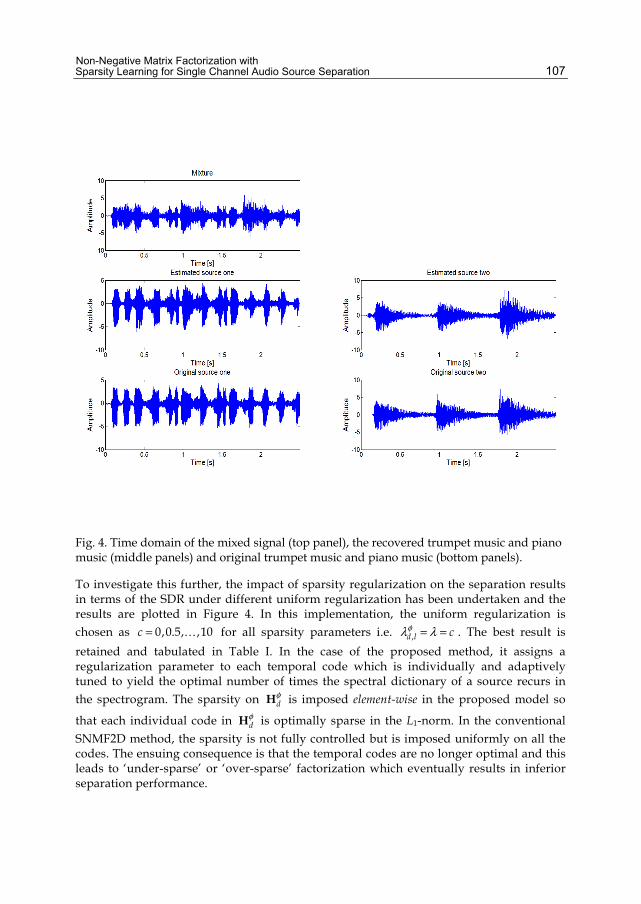
Non-Negative Matrix Factorization with Sparsity Learning for Single Channel Audio Source Separation
107
Fig. 4. Time domain of the mixed signal (top panel), the recovered trumpet music and piano music (middle panels) and original trumpet music and piano music (bottom panels).
To investigate this further, the impact of sparsity regularization on the separation results in terms of the SDR under different uniform regularization has been undertaken and the results are plotted in Figure 4. In this implementation, the uniform regularization is chosen as = 0,0.5, ,10c for all sparsity parameters i.e. φλ λ= =,d l c . The best result is retained and tabulated in Table I. In the case of the proposed method, it assigns a regularization parameter to each temporal code which is individually and adaptively tuned to yield the optimal number of times the spectral dictionary of a source recurs in the spectrogram. The sparsity on φ
dH is imposed element-wise in the proposed model so
that each individual code in φdH is optimally sparse in the L1-norm. In the conventional
SNMF2D method, the sparsity is not fully controlled but is imposed uniformly on all the codes. The ensuing consequence is that the temporal codes are no longer optimal and this leads to ‘under-sparse’ or ‘over-sparse’ factorization which eventually results in inferior separation performance.

Independent Component Analysis for Audio and Biosignal Applications
108
Fig. 5. Separation results of SNMF2D by using different uniform regularization.
In Figure 5, the results have clearly indicated that there are certain values of λ where the SNMF2D performs with exceptionally good results. In the case of piano and trumpet mixtures, the best performance is obtained when λ ranges from 0.5 to 2 where the highest SDR is 8.1dB. As for jazz and piano mixtures, the best performance is obtained when λ ranges from 1.0 to 2.5 where the highest SDR is 7.2dB and for jazz and trumpet mixtures, the best performance is obtained when λ ranges from 2 to 3.5 where the highest SDR is 8.6dB. On the contrary, when λ is set too high, the separation performance tends to degrade. It is also worth pointing out that the separation results are coarse when the factorization is non-regularized. Here, we see that (i) for piano and trumpet mixtures, the SDR is only 6.2dB, (ii) for jazz and piano mixtures, the SDR is only 5.6dB, (iii) for jazz and trumpet mixtures, the SDR is only 4.7dB. From above, it is evident that uniform sparsity scheme gives varying performance depending on the value of λ which in turn depends on the type of mixture. Hence, this poses a practical difficulty in selecting the appropriate level sparseness necessary for matrix factorization to resolve the ambiguity between the sources in the TF domain.
The overall comparison results between the adaptive and uniform sparsity methods have been summarized in Figure 6. According to the table, SNMF2D with adaptive sparsity tends to yield better result than the uniform sparsity-based methods. We may summarize the average performance improvement of our method against the uniform constant sparsity method: (i) For the piano and trumpet music, the improvement per source in terms of the SDR is 2dB (ii) For the piano and jazz music, the improvement per source in terms of SDR is 1.3dB. (iii) For the trumpet and jazz music, the improvement per source in terms of SDR is 1.1dB.

Non-Negative Matrix Factorization with Sparsity Learning for Single Channel Audio Source Separation
109
Fig. 6. SDR results comparison between adaptive and uniform sparsity methods.
4.2.1 Adaptive behavior of sparsity parameter
In this sub-section, the adaptive behavior of the sparsity parameters by using the proposed method will be demonstrated. Several sparsity parameters have been selected to illustrate its adaptive behavior. In the experiment, all sparsity parameters are initialized as φλ =, 5d l for all φ, ,d l and are subsequently adapted according to (35). After 300 iterations, the sparsity parameters converge to their steady-states. We have plotted the histogram of the converged adaptive sparsity parameters in Figure 7. The figure suggests that the histogram can be represented as a bimodal distribution that each element code has its own sparseness. In addition, it is worth pointing out that in the case of piano and trumpet mixture the SDR result rises to 10dB when φλ ,d l is adaptive. This represents a 2dB per source improvement over the case of uniform constant sparsity (which is only 8.1dB in Figure 6). On the separate hand, when no sparsity is imposed onto the codes the SDR result immediately deteriorates to approximately 6dB. This represents a 4dB per source depreciation compared with the proposed adaptive sparsity method. From above, the results are ready to suggest that the performances of source separation have been undermined when the uniform constant sparsity scheme is used. On the contrary, improved performances can be obtained by allowing the sparsity parameters to be individually adapted for each element code. This is evident based on source separation performance as indicated in Figure 6.

Independent Component Analysis for Audio and Biosignal Applications
110
Fig. 7. The histogram of the converged adaptive sparsity parameter.
4.2.2 Efficiency of source extraction in TF domain
In this sub-section, we will analyze the efficiency of source extraction based on SNMF2D and the proposed method. Binary masks are constructed using the approach discussed in Section III B for each of the both methods. To ensure fair comparison, we generate the ideal binary mask (IBM) [34] from the original source which is used as a reference for comparison. The IBM for a target source is found for each TF unit by comparing the energy of the target source to the energy of all the interfering sources. Hence, the ideal binary mask produces the optimal signal-to-distortion ratio (SDR) gain of all binary masks and thus, it can be considered as an optimal source extractor in TF domain. The comparison results between IBM, uniform sparsity and proposed adaptive sparsity are tabulated in Table II.
Fig. 8. Overall ESE performance

Non-Negative Matrix Factorization with Sparsity Learning for Single Channel Audio Source Separation
111
In Figure 8, the results of ESE for each mixture type are obtained by averaging over 100 realizations. From listening performance test, any ( )ψ > 0.8dW indicates acceptable quality of source extraction performance in TF domain. Therefore, it is noted from the results in Figure 7 that both IBM and the proposed method satisfy this condition. In addition, the proposed method yields better ESE improvement against the uniform sparsity method. The average improvement results have been summarized as follows: (i) For the piano and trumpet music, 18.4%. (ii) For the piano and jazz music 26.5%. (iii) For the trumpet and jazz music, 20.6%. In addition, the average SIR of the proposed method exhibits much a higher value than the uniform sparsity SNMF2D. This clearly shows that the amount of interference between any two sources is lesser for the proposed method. Therefore, the above results unanimously indicate that the proposed adaptive sparsity method leads to higher ESE results than the uniform constant sparsity method.
4.3 Comparison with other sparse NMF-based SCASS methods
In Section IV B, analysis has been carried out to investigate effects between adaptive sparsity and uniform constant sparsity on source separation. In this evaluation, we compare the proposed method with other sparse NMF-based source separation methods. These consist of the followings:
• SNMF [13]. The uniform constant sparsity parameter is progressively varied from 0 to 10 with every increment of 0.1 (i.e. λ = 0,0.1,0.2, ,10 ) and the best result is retained for comparison.
• Automatic Relevance Determination NMF (NMF-ARD) [35] exploits a hierarchical Bayesian framework SNMF that amounts to imposing an exponential prior for pruning and thereby enables estimation of the NMF model order. The NMF-ARD assumes prior on H , namely, ( )λ λ λ= − ∏ max
,( | ) expld d ld l
d
p H H and uses Automatic Relevance
Determination (ARD) approach to determine the desirable number of components in D .
• NMF with Temporal Continuity and Sparseness Criteria [14] (NMF-TCS) is based on factorizing the magnitude spectrogram of the mixed signal into a sum of components, which include the temporal continuity and sparseness criteria into the separation framework. In [14], the temporal continuity α is chosen as [0,1,10,100,1000] , sparseness weight β is chosen as [0,1,10,100,1000] . The best separation result is retained for comparison.
Figure 9 summarizes the SDR comparison results between our proposed method and the above three sparse NMF methods. From the results, it can be seen that the above methods fail to take into account the relative position of each spectrum and thereby discarding the temporal information. Better separation results will require a proper model that can represent both temporal structure and the pitch change which occurs when an instrument plays different notes simultaneously. If the temporal structure and the pitch change are not considered in the model, the mixing ambiguity is still contained in each separated source.

Independent Component Analysis for Audio and Biosignal Applications
112
Fig. 9. Performance comparison between other NMF based SCASS methods and proposed method
Fig. 10. ESE comparison between other NMF based SCASS methods and the proposed method
The improvement of our method compared with NMF-TCS, SNMF and NMF-ARD can be summarized as follows: (i) For the piano and trumpet music, the average improvement per source in terms of the SDR is 6.3dB. (ii) For the piano and jazz music, the average improvement per source in terms of SDR is 5dB. (iii) For the trumpet and jazz music, the average improvement per source in terms of SDR is 5.4dB. In the case of ESE (Figure 10), the proposed method exhibits much better average ESE of approximately 106.9%, 138.8% and 114.6% improvement with NMF-TCS, SNMF and NMF-ARD, respectively. Analyzing the separation results and ESE performance, the proposed method leads to the best separation performance for both recovered sources. The SNMF method performs with poorer results

Non-Negative Matrix Factorization with Sparsity Learning for Single Channel Audio Source Separation
113
whereas the separation performance by the NMF-TCS method is slightly better than the NMF-ARD and SNMF methods. Our proposed method gives significantly better performance than the NMF-TCS, SNMF and NMF-ARD methods. The spectral dictionary obtained via NMF-TCS, SNMF and NMF-ARD methods are not adequate to capture the temporal dependency of the frequency patterns within the audio signal. In addition, the NMF-TCS, SNMF and NMF-ARD do not model notes but rather unique events only. Thus if two notes are always played simultaneously they will be modeled as one component. Also, some components might not correspond to notes but rather to the model e.g. background noise.
4.4 Comparison with underdetermined-based ICA SCSS method
In the underdetermined-ICA SCSS method [3], the key point is to exploit the prior knowledge of the sources such as the basis functions to generate the sparse codes. In this work, these basis functions are obtained in two stages: (i) Training stage: the basis functions are obtained by performing ICA on each concatenated sources. In this experiment, we derive a set of 64 basis functions for each type of source. These training data exclude the target sources which have been exclusively used to generate the mixture signals. (ii) Adaptation stage: the obtained ICA basis functions from the training stage are further adapted based on the current estimated sources during the separation process. In this method, both the estimated sources and the ICA basis functions are jointly optimized by maximizing the log-likelihood of the current mixture signal until it converges to the steady-state solution. If two sets of basis functions overlap significantly with each other, the underdetermined-ICA SCSS method is less efficient in resolving the mixing ambiguity between sources. The improvement of proposed method compared with underdetermined-ICA SCSS method can be summarized as follows: (i) For the piano and trumpet music, the average improvement per source in terms of the SDR is 4.3dB. (ii) For the piano and jazz music, the average improvement per source in terms of SDR is 4dB. (iii) For the trumpet and jazz music, the average improvement per source in terms of SDR is 4.2dB.
Fig. 11. Performance underdetermined-ICA SCSS method and proposed method
Independent Component Analysis for Audio and Biosignal Applications
114
The performance of the underdetermined-ICA SCSS method relies on the ICA-derived time domain basis functions. High level performance can be achieved only when the basis functions of each source are sufficiently distinct. However, the result becomes considerably less robust in separating mixture where the original sources are of the same type e.g. mixture of music with music.
5. Conclusion The chapter has presented an adaptive strategy to sparsifying the non-negative matrix factorization. The impetus behind this work is that the sparsity achieved by conventional SNMF and SNMF2D is not enough; in such situations it might be useful to control the degree of sparseness explicitly. In the proposed method, the regularization term is adaptively tuned using a variational Bayesian approach to yield desired sparse decomposition, thus enabling the spectral dictionary and temporal codes of non-stationary audio signals to be estimated more efficiently. This has been verified concretely based on our simulation results. In addition, the proposed method has yielded significant improvements in single channel music separation when compared with other sparse NMF-based source separation methods. Future work could investigate the extension of the proposed method to separate non-stationary (here non-stationary refers to the sources not located in the fixed places, e.g. the speakers are talking while on the move) and reverberant mixing model. For non-stationary reverberant mixing model, this gives
ττ τ
−
= == − +
1
1 0( ) ( , ) ( ) ( )
s r
r
N L
i r i ri
y t m t x t n t
where τ( , )i rm t is the finite impulse response of causal filter at t time and τ r is the time delay. The expanded adaptive sparsity non-negative matrix factorization can then be developed to estimate mixing im and sources ix , respectively.
6. References [1] Radfa M.H, Dansereau R.M. Single-channel speech separation using soft mask filtering.
IEEE Trans. on Audio, Speech and Language Processing. 2007; 15: 2299-2310. [2] Ellis D. Model-based scene analysis, in Computational Auditory Scene Analysis:
Principles, Algorithms, and Applications, D. Wang and G. Brown, Eds. New York: Wiley/IEEE Press; 2006
[3] Jang G.J, Lee T.W. A maximum likelihood approach to single channel source separation. Journal of Machine Learning Research. 2003; 4: 1365–1392.
[4] Li P, Guan Y, Xu B, Liu W. Monaural speech separation based on computational auditory scene analysis and objective quality assessment of speech. IEEE Trans. on Audio, Speech and Language Processing. 2006; 14: 2014–2023.
[5] Paatero P, Tapper U. Positive matrix factorization: A non-negative factor model with optimal utilization of error estimates of data values. Environmetrics. 1994; 5: 111–126.

Non-Negative Matrix Factorization with Sparsity Learning for Single Channel Audio Source Separation
115
[6] Ozerov A, Févotte C. Multichannel nonnegative matrix factorization in convolutive mixtures for audio source separation. IEEE Transactions on Audio, Speech, and Language Processing 2010; 18: 550-563.
[7] Casey M. A, Westner A. Separation of mixed audio sources by independent subspace analysis. proceeding of. Int. Comput. Music Conf, 2000. 154–161; 2000
[8] Molla Md. K. I, Hirose K. Single-Mixture Audio Source Separation by Subspace Decomposition of Hilbert Spectrum. IEEE Trans. on Audio, Speech and Language Processing. 2007; 15: 893–900.
[9] Hyvarinen A, Karhunen J, Oja E, Independent component analysis and blind source separation, John Wiley & Sons 2005. p.20–60.
[10] Lee D, Seung H. Learning the parts of objects by nonnegative matrix factorisation. Nature. 1999; 401: 788–791.
[11] Kompass R. A generalized divergence measure for nonnegative matrix factorization. Neural Computation. 2007; 19: 780-791.
[12] Cichocki A, Zdunek R, Amari S.I. Csisz´ar’s divergences for non-negative matrix factorization: family of new algorithms. Proceeding of. Intl. Conf. on Independent Component Analysis and Blind Signal Separation (ICABSS’06), Charleston, USA, March 2006, 3889: 32–39. 2006.
[13] Hoyer P. O. Non-negative matrix factorization with sparseness constraints. Journal of Machine Learning Research. 2004; 5: 1457–1469.
[14] Virtanen T (2007) Monaural sound source separation by non-negative matrix factorization with temporal continuity and sparseness criteria. IEEE Transactions on Audio, Speech, and Language Processing. 2007; 15: 1066–1074.
[15] Vincent E (2006) Musical source separation using time-frequency source priors. IEEE Trans. Audio, Speech and Language Processing. 2006; 14: 91–98.
[16] Ozerov A, Févotte C. Multichannel nonnegative matrix factorization in convolutive mixtures. With application to blind audio source separation. Proceeding of IEEE International Conference on Acoustics, Speech, and Signal Processing (ICASSP'09), 3137-3140. 2009.
[17] Mysore G, Smaragdis P, Raj B. Non-negative hidden Markov modeling of audio with application to source separation. Proceeding of 9th international conference on Latent Variable Analysis and Signal Separation (LCA/ICA). 2010.
[18] Nakano M, et al. Nonnegative Matrix Factorization with Markov-chained Bases for Modeling Time-varying in Music Spectrograms. Proceeding of 9th international conference on Latent Variable Analysis and Signal Separation (LCA/ICA). 2010
[19] Salakhutdinov R, Mnih A. Bayesian probabilistic matrix factorization using Markov chain Monte Carlo. Proceedings of the 25th international conference on Machine learning. 880-887. 2008.
[20] Cemgil A. T. Bayesian inference for nonnegative matrix factorisation models. Computational Intelligence and Neuroscience. 2009; doi: 10.1155/2009/785152.
[21] Moussaoui S, Brie D, Mohammad-Djafari A, Carteret C, Separation of non-negative mixture of non-negative sources using a Bayesian approach and MCMC sampling. IEEE Trans. on Signal Processing. 2006; 54: 4133–4145.
[22] Schmidt M. N, Winther O, Hansen L.K. Bayesian non-negative matrix factorization. Proceeding of Independent Component Analysis and Signal Separation, International Conference. 2009

Independent Component Analysis for Audio and Biosignal Applications
116
[23] Morup M, Schmidt M.N. Sparse non-negative matrix factor 2-D deconvolution. Technical University of Denmark, Copenhagen, Denmark. 2006.
[24] Schmidt M.N, Morup M. Nonnegative matrix factor 2-D deconvolution for blind single channel source separation. Proceeding of Intl. Conf. Independent Component Analysis and Blind Signal Separation (ICABSS’06), Charleston, USA. 3889: 700–707. 2006.
[25] Lin Y. Q. l1-norm sparse Bayesian learning: theory and applications. Ph.D. Thesis, University of Pennsylvania. 2008.
[26] Gao Bin, Woo W.L, Dlay S.S. Single Channel Source Separation Using EMD-Subband Variable Regularised Sparse Features. IEEE Trans. on Audio, Speech, and Language Processing. 2011; 19: 961–976.
[27] Gao Bin, Woo W.L, Dlay S.S. Adaptive Sparsity Non-negative Matrix Factorization for Single Channel Source Separation. IEEE the Journal of Selected Topics in Signal Processing. 2011; 5: 1932-4553.
[28] Sha F, Saul L.K, Lee D.D. Multiplicative updates for nonnegative quadratic programming in support vector machines. Proceeding of Advances in Neural Information Process. Systems. 15: 1041–1048. 2002
[29] Brown J. C. Calculation of a constant Q spectral transform. J. Acoust. Soc. Am. 1991; 89: 425–434.
[30] Yilmaz O, Rickard S. Blind separation of speech mixtures via time-frequency masking. IEEE Trans. Signal Processing. 2004; 52: 1830–1847.
[31] Goto M, Hashiguchi H, Nishimura T, Oka R. RWC music database: Music genre database and musical instrument sound database. in Proc. of Intl. Symp. on Music Information Retrieval (ISMIR), Baltimore, Maryland, USA. 229–230. 2003.
[32] Signal Separation Evaluation Campaign (SiSEC 2008), (2008). [Online]. Available: http://sisec.wiki.irisa.fr
[33] Vincent E, Gribonval R, Fevotte C. Performance measurement in blind audio source separation. IEEE Trans. Speech Audio Process. 2006; 14: 1462–1469.
[34] Wang D. L. On ideal binary mask as the computational goal of auditory scene analysis. in Speech Separation by Humans and Machines, P. Divenyi, Ed. Norwell, MA: Kluwer, pp. 181–197. 2005.
[35] Mørup M, Hansen K.L. Tuning Pruning in Sparse Non-negative Matrix Factorization. Proceeding of 17th European Signal Processing Conference (EUSIPCO'2009), Glasgow, Scotland. 2009.

1. Introduction
Audio signal analysis and classification have arisen as an important research topic that hasbeen developed by many authors in different areas over the time. A main developmentcontext has been speech recognition Holmes & Huckvale (1994); Juang & Rabiner (2005);Kimura (1999). This specific topic is, in fact, an important source of references toapplications of artificial intelligence techniques Juang & Rabiner (2005); Prasad & Prasanna(2008). Many classical problems encountered in this research field have been addressed fromthis perspective by many authors Farahani & Ahadi (2005); Minematsu et al. (2006).
However, in this same context, a different point of view can be adopted to deal with theanalysis and classification of music signals. The tasks in this framework are varied, includingthe detection of pitch, tempo or rhythm Thornburg et al. (2007), but also other tasks likethe identification of musical instruments Müller et al. (2011) or musical genre recognitionTzanetakis & Cook (2002) can be considered. Also the classification of audio samples as musicor speech has been thoroughly considered in the literature Panagiotakis & Tziritas (2005),Tardón et al. (2010).
In this specific context of analysis of musical signals, we will expose some ideas regardingsignal classification and their application to a real task.
2. Models and applications
Audio signal classification involves the extraction of a number of descriptive features from thesound and the proper utilization of them as input for a classifier. Artificial Intelligence (AI)techniques provide a way to deal with signal processing and pattern classification tasks froma different point of view of classical techniques.
AI techniques play an important role in the signal processing and classification contextas they have been widely used by a number of authors in the literature for verydifferent tasks Haykin (1999); Kohonen et al. (1996); Ortiz, Górriz, Ramírez & Salas-Gonzalez(2011a); Ortiz, Gorriz, Ramirez & Salas-Gonzalez (2011b); Ortiz, Ortega, Diaz & Prieto (2011);Riveiro et al. (2008). Also, we must be aware of the fact that the current trend in artificialintelligence systems points to the utilization of both classical and AI-based methods inconjunction to improve the overall system performance. This leads to build hybrid
Unsupervised and Neural Hybrid Techniques for Audio Signal Classification
Andrés Ortiz, Lorenzo J. Tardón, Ana M. Barbancho and Isabel Barbancho Dept. Ingeniería de Comunicaciones, ETSI Telecomunicación-University of Malaga,
Campus Universitario de Teatinos s/n, Malaga Spain
6

2 Artificial Intelligence and Applications
artificial intelligence systems. These systems can include neural-based techniques, evolutivecomputation, or statistical classifiers as well as other statistical techniques such as multivariateor stochastic methods.
Through this chapter, we will present the problem of classification of musical signals. Theproblemwill be defined to be handled in a supervised or unsupervised way. It is be importantto point out that a preprocessing stage to determine the features to be used for the classificationtask must be done although the classifiers can be able to properly deal with the differentdiscrimination capability of the different features. Afterwards, a classifier will assign adifferent label related to the features employed to any different sound class in a processperformed in a supervised or unsupervised way.
Taking into account that unsupervised classification strategies are able to organize trainingsamples into suitable groups according to certain classes without using any a prioriinformation (the samples to be classified are not labelled), we will describe how to apply theseideas in this context. We will present features related to the analysis framework and samplesof the performance.
Unsupervised techniques include the Self-Organizing Maps (SOM) Kohonen (2001), a vectorquantization method with a competitive learning process. SOMs provide a generalization ofthe input space through the prototypes computed during the training phase. In this model,each prototype represents a set of input vectors on the basis of a given similaritymeasurement.Very often, the similarity measure selected is the Euclidean distance. Moreover, it will bespecially interesting to observe that SOMs group the prototypes maintaining the more similarones close to each other in the output space while the less similar prototypes ones are keptapart. In this way, SOMs provide valuable topological information that can be exploitedto make them more flexible than other vector quantization methods. This means that adescription of a SOM model for a certain application must be complemented by additionaldetails. Specifically, we are referring to two different aspects: the first one consists onthe modelling of the activation process of the neurons of the SOM which can be done bymeans of statistical techniques such as Gaussian Mixture Models (GMM) to account for aprobabilistic behaviour of the map. The second aspect to consider is related to the techniquesthat allow the extraction of valuable topological information from the SOM; this process can beaccomplished by classical clustering techniques such as k-means or other techniques Therrien(1989) specially developed for clustering the SOM.
On the other hand, supervised classification Murtagh (1991) techniques use a prioriinformation of at least some of the samples. It means that the training samples havelabels according to their corresponding class. Classical methods include different clusteringtechniques or statistical classifiers. We will introduce some labels and related features forclassification and describe the utilization of them to attain certain classification objectives.
3. Audio signal features for classification: Clarinet music example
In this section we describe five features extracted from audio signal. These features willcompose the input data used in the unsupervised classifiers shown in the following sections.The examples shown aims to detect four different playing techniques from clarinet music.The features extracted from the audio signal attempts to characterize the signal in both, timeand frequency domains in a simple way, being effective enough to perform classificationexperiments.
118 Independent Component Analysis for Audio and Biosignal Applications
Unsupervised and Neural Hybrid Techniquesfor Audio Signal Classification 3
Classification examples have been performed using three different clarinets from realrecordings taken from the Musical Instrument Sound Data Base RWC-MDB-1-2001-W08 Goto(2004). Clarinet 1 is a french clarinet made by Buffet, Clarinet 2 is a french clarinet made bySelmer and Clarinet 3 is a japanese clarinet many by Yamaha. For each clarinet, we have 120note samples that contain the whole clarinet note range played with different dynamics foreach playing technique (Normal, Staccato, Vibrato and Trill). This gives a total of 1440 notesamples.
3.1 Time domain characterization
In this Section, we describe the features used to characterize the audio signal in time domain.The duration and the shape of the envelope of the clarinet audio signals contain informationabout the technique used to play the notes.
Thus, as in Barbancho et al. (2009); Jenses (1999), the attack time (Ta) is considered from thefirst sample that reaches a 10% of the maximum of the amplitude of the waveform of the noteuntil it reaches the 90% of that amplitude. The release time (Tr) is considered from the lastsample that reaches 70% of the maximum of the amplitude of the waveform to the last oneover the 10% of the amplitude. On the other hand, the time between the attack time and therelease time is called the sustain time Ts. Ta, Tr and Ts depend on the playing technique.
The signal envelope is obtained by filtering the signal with a 5th order Butterworth filter withcut-off frequency of 66 Hz. After the application of the low-pass filter, the signal is normalizedso that the amplitude is 1. On the other hand, the samples with amplitude under 2.5% of themaximum are removed.
Additionally, we include another time domain feature Tf based on the presence of signalfading (i.e.: if the signal envelope is fading, Tf = 1, otherwise Ts = 0).
3.2 Frequency domain characterization
In order to characterize the clarinet in the frequency domain, we use the Fast Fourier Transform(FFT). In the frequency domain, the frequency axis is converted into MIDI numbers accordingto the following equation:
MIDI = 69+ 12 log2( f/440) (1)
Taking into account that the fundamental frequency of the notes of the clarinet ranges from146.83 Hz to 1975 Hz, the MIDI range of interest is 50 to 94.
However, it is necessary to remove redundant information from the FFT in order to simplifythe signal spectrum. Thus, for a certain MIDI number nMIDI the spectrum between nMIDI −0.5 and nMIDI + 0.5 is considered and the maximum value of the spectrum in that interval isassigned to nMIDI. Thus, the MIDI number spectrum (or MIDI simplified spectrum) of eachnote will have 45 samples. From this simplified spectrum, the pitch and the spectrum widtharound the pitch will be calculated. At this point, we have three time domain features (Ta,Tr , Ts and Tf ) and two frequency domain features, Fp and Fw. Fp is the pitch of the playednote, and Fw is the spectral width of the fundamental frequency defined and calculated as thenumber of significative samples around the fundamental frequency. We consider as significantsamples those over 30% of the value of the fundamental frequency. Thus, the feature spaceis composed by six-dimensional vectors in the form (Ta, Tr, Ts, Tf , Fp, Fw). These six featuresmay be discriminant enough to characterize the playing technique.
119Unsupervised and Neural Hybrid Techniques for Audio Signal Classification
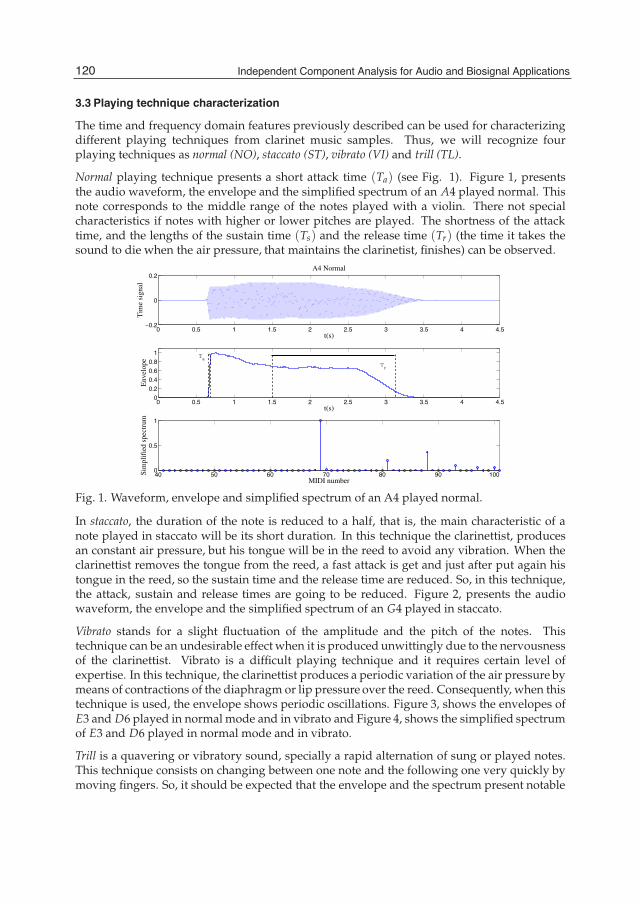
4 Artificial Intelligence and Applications
3.3 Playing technique characterization
The time and frequency domain features previously described can be used for characterizingdifferent playing techniques from clarinet music samples. Thus, we will recognize fourplaying techniques as normal (NO), staccato (ST), vibrato (VI) and trill (TL).
Normal playing technique presents a short attack time (Ta) (see Fig. 1). Figure 1, presentsthe audio waveform, the envelope and the simplified spectrum of an A4 played normal. Thisnote corresponds to the middle range of the notes played with a violin. There not specialcharacteristics if notes with higher or lower pitches are played. The shortness of the attacktime, and the lengths of the sustain time (Ts) and the release time (Tr) (the time it takes thesound to die when the air pressure, that maintains the clarinetist, finishes) can be observed.
0 0.5 1 1.5 2 2.5 3 3.5 4 4.5−0.2
0
0.2
t(s)
Tim
e si
gnal
A4 Normal
0 0.5 1 1.5 2 2.5 3 3.5 4 4.50
0.2
0.4
0.6
0.8
1
t(s)
Env
elop
e
40 50 60 70 80 90 1000
0.5
1
MIDI number
Sim
plif
ied
spec
trum
Tr
Ta
Fig. 1. Waveform, envelope and simplified spectrum of an A4 played normal.
In staccato, the duration of the note is reduced to a half, that is, the main characteristic of anote played in staccato will be its short duration. In this technique the clarinettist, producesan constant air pressure, but his tongue will be in the reed to avoid any vibration. When theclarinettist removes the tongue from the reed, a fast attack is get and just after put again histongue in the reed, so the sustain time and the release time are reduced. So, in this technique,the attack, sustain and release times are going to be reduced. Figure 2, presents the audiowaveform, the envelope and the simplified spectrum of an G4 played in staccato.
Vibrato stands for a slight fluctuation of the amplitude and the pitch of the notes. Thistechnique can be an undesirable effect when it is produced unwittingly due to the nervousnessof the clarinettist. Vibrato is a difficult playing technique and it requires certain level ofexpertise. In this technique, the clarinettist produces a periodic variation of the air pressure bymeans of contractions of the diaphragm or lip pressure over the reed. Consequently, when thistechnique is used, the envelope shows periodic oscillations. Figure 3, shows the envelopes ofE3 and D6 played in normal mode and in vibrato and Figure 4, shows the simplified spectrumof E3 and D6 played in normal mode and in vibrato.
Trill is a quavering or vibratory sound, specially a rapid alternation of sung or played notes.This technique consists on changing between one note and the following one very quickly bymoving fingers. So, it should be expected that the envelope and the spectrum present notable
120 Independent Component Analysis for Audio and Biosignal Applications

Unsupervised and Neural Hybrid Techniquesfor Audio Signal Classification 5
0 0.02 0.04 0.06 0.08 0.1 0.12 0.14 0.16−0.5
0
0.5
t(s)
Tim
e si
gnal
G4 Staccato
0 0.02 0.04 0.06 0.08 0.1 0.12 0.14 0.160
0.2
0.4
0.6
0.8
1
t(s)
Env
elop
e
40 50 60 70 80 90 1000
0.5
1
MIDI number
Sim
plif
ied
spec
trum
Tr
Ta
Fig. 2. Waveform, envelope and simplified spectrum of an G4 played staccato.
0 0.5 1 1.5 2 2.5 30
0.2
0.4
0.6
0.8
1
t(s)
Envelope E3 Normal
0 0.5 1 1.5 2 2.5 30
0.2
0.4
0.6
0.8
1
t(s)
Envelope E3 Vibrato
0 0.5 1 1.5 20
0.2
0.4
0.6
0.8
1
t(s)
Envelope D6 Vibrato
0 0.5 1 1.5 2 2.50
0.2
0.4
0.6
0.8
1
t(s)
Envelope D6 Vibrato
Fig. 3. Envelopes of E3 and D6 played in normal mode and in vibrato.
differences with respect to the ones found when the other playing techniques are employed.Figure 5, presents the time signal, the envelope and the simplified spectrum of an G5 playedwith trill.
4. Classification with Self-Organizing Maps
The Self-Organizing Map (SOM) is one of the most commonly used artificial neural networkmodels for unsupervised learning. This model, proposed by Kohonen Kohonen (2001), is abiologically inspired algorithm based on the search for the most economic representation ofdata and its relationships, as in the animal brain.
Sensory experience consists in capturing features from the surrounding world, and thesefeatures usually are multidimensional. For instance, the human visual system captures
121Unsupervised and Neural Hybrid Techniques for Audio Signal Classification

6 Artificial Intelligence and Applications
40 50 60 70 80 90 1000
0.2
0.4
0.6
0.8
1
MIDI number
Simplified spectrum E3 Normal
40 50 60 70 80 90 1000
0.2
0.4
0.6
0.8
1
MIDI number
Simplified spectrum E3 Vibrato
40 50 60 70 80 90 1000
0.2
0.4
0.6
0.8
1
MIDI number
Simplified spectrum D6 Normal
40 50 60 70 80 90 1000
0.2
0.4
0.6
0.8
1
MIDI number
Simplified spectrum D6 Vibrato
Fig. 4. Simplified spectrum of E3 and D6 played in normal mode and in vibrato.
0 0.2 0.4 0.6 0.8 1 1.2 1.4 1.6 1.8−0.5
0
0.5
t(s)
Tim
e si
gnal
G5 Trill
0 0.2 0.4 0.6 0.8 1 1.2 1.4 1.6 1.80
0.2
0.4
0.6
0.8
1
t(s)
Env
elop
e
40 50 60 70 80 90 1000
0.5
1
MIDI number
Sim
plif
ied
spec
trum
Ta
Tr
Fig. 5. Waveform, envelope and simplified spectrum of an G5 played with trill.
features from different objects such as colour, texture, size or shape, which will provideenough information to ensure further recognition of that object. The learning process inthe human brain projects the extracted features onto the neural structures of the brainto creating different maps corresponding to different types of features. Moreover, thelearning process stores the prototypes of the features in the maps created. These maps arecontinuously modified as the learning process progresses. Prototypes could be consideredas the smallest feature set needed to be able to represent the sensory information acquired.In other words, prototypes represent generalizations of the learnt features, being possible todistinguish between different objects, and associate similar ones. Moreover, sensory piecesof information coming from different organs are topologically ordered in the brain cortex(topology preservation in brain mapping).
122 Independent Component Analysis for Audio and Biosignal Applications
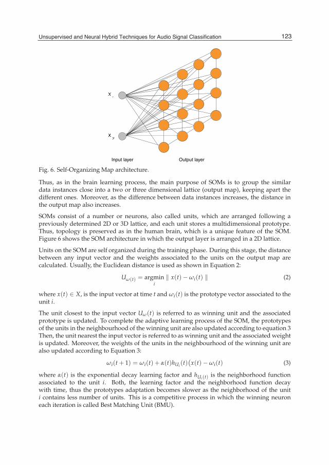
Unsupervised and Neural Hybrid Techniquesfor Audio Signal Classification 7
Input layer Output layer
Fig. 6. Self-Organizing Map architecture.
Thus, as in the brain learning process, the main purpose of SOMs is to group the similardata instances close into a two or three dimensional lattice (output map), keeping apart thedifferent ones. Moreover, as the difference between data instances increases, the distance inthe output map also increases.
SOMs consist of a number or neurons, also called units, which are arranged following apreviously determined 2D or 3D lattice, and each unit stores a multidimensional prototype.Thus, topology is preserved as in the human brain, which is a unique feature of the SOM.Figure 6 shows the SOM architecture in which the output layer is arranged in a 2D lattice.
Units on the SOM are self organized during the training phase. During this stage, the distancebetween any input vector and the weights associated to the units on the output map arecalculated. Usually, the Euclidean distance is used as shown in Equation 2:
Uω(t) = argmini
‖ x(t)−ωi(t) ‖ (2)
where x(t) ∈ X, is the input vector at time t and ωi(t) is the prototype vector associated to theunit i.
The unit closest to the input vector Uω(t) is referred to as winning unit and the associatedprototype is updated. To complete the adaptive learning process of the SOM, the prototypesof the units in the neighbourhood of the winning unit are also updated according to equation 3Then, the unit nearest the input vector is referred to as winning unit and the associated weightis updated. Moreover, the weights of the units in the neighbourhood of the winning unit arealso updated according to Equation 3:
ωi(t + 1) = ωi(t) + α(t)hUi (t)(x(t)−ωi(t) (3)
where α(t) is the exponential decay learning factor and hUi(t) is the neighborhood functionassociated to the unit i. Both, the learning factor and the neighborhood function decaywith time, thus the prototypes adaptation becomes slower as the neighborhood of the uniti contains less number of units. This is a competitive process in which the winning neuroneach iteration is called Best Matching Unit (BMU).
123Unsupervised and Neural Hybrid Techniques for Audio Signal Classification

8 Artificial Intelligence and Applications
The neighbour function defines the shape of the neighbourhood and it is usually a Gaussianfunction which shrinks at each iteration, as defined by the next equations:
hUi(t) = e− ‖rU−ri‖2
2σ2(t) (4)
σ(t) = σ0e−tτ1 (5)
In Equation 4, ri represents the position on the output space (2D or 3D) and ‖ rU − ri ‖ is thedistance between the winning unit and the i-neuron on the output space. On the other hand,σ(t) controls the reduction of the Gaussian neighborhood at each iteration. σ(t) usually takesthe form of exponential decay function as in Equation 5.
Similarly, the learning factor in Equation 3, also diminishes in time. However, αmay decay in alinear or exponential fashion. Therefore, during the training phase, the prototypes associatedto each unit are computed at each iteration. At the same time, the position of the units in theoutput space changes according to the similarity among the actual prototypes.
As previously commented, topology preservation is a unique feature of the SOM related tothe goodness of the clustering process performed during training. This way, the calculation ofthe quality of the output map, results essential to evaluate the overall process.
In order to perform a quantitative evaluation of the goodness of the SOM, two measures canbe accomplished. The first one is the quantization error, which is a measure of the resolutionof the map. This quantization error can be calculated by computing the average distancebetween all the BMUs and the input data vectors as shown in Equation 6:
qei = ∑xj∈c:i
‖ ωi − xj ‖ (6)
The second one measures the topographic error, i.e.: how the SOM preserves the topology.This error can be computed using Equation 7:
te =1N
N
∑i=1
u(−→xi ) (7)
In this equation, N is the total number of input vectors. u(−→xi ) is 1 if the first and thesecond BMU for the input vector−→xi are adjacent units and 0 otherwise Arsuaga & Díaz (2005);Kohonen (2001). Then, the lower qe and te, the better the SOM is adapted to the input patterns.
5. SOM clustering
In order to deal with fully unsupervised classification using SOMs, it is necessary to computethe clusters brought up during the training phase.
This clustering process consist on grouping the prototypes in different classes according to asimilarity criterion. This similarity criterion depends on the clustering technique used. Thus,several clustering approaches which use the Euclidean distance as similarity criterion havebeen developedMurtagh (1995); Rossi & Villa (2009); Vesanto et al. (2000); Wu & Chow (2004).In this chapter, we deal with SOM clustering using two different approaches.
124 Independent Component Analysis for Audio and Biosignal Applications

Unsupervised and Neural Hybrid Techniquesfor Audio Signal Classification 9
5.1 SOM clustering with K-means
k-means algorithmMacQueen (1967) is a well-known and widely used clustering method dueto its performance and simplicity. k-means aims to create k partitions from n observationsin such a way that each observation will belong to the cluster with the nearest mean tothat observation. In other words, the algorithm computes the centroids of each class ateach iteration, and computes the euclidean distance to each observation. Then, the nearestobservations to each centroid are considered as belonging to the centroid class.
Thus, given a n− dimensional data collection (x1...xn), k-means creates k, k < n classes, whileminimizing the mean squared error of the euclidean distance between each data point and thecorresponding cluster centroid, as shown in equation 8:
argminC
k
∑i=1
∑xj∈mi
‖ xj − si ‖2 (8)
where mi represents the mean (centroid) of all the points belonging to the class i.
Although k-means constitutes a usual way to cluster the SOMs in an unsupervised manner, itpresents two main drawbacks:
• The number of clusters to be found has to be determined in advance. In other words, it isnecessary to know beforehand the value of k.
• k-means only uses the Euclidean distance between prototypes, and does not take intoaccount the relationship between the output and the data topology to compute the clusters.This underutilizes the knowledge available at the output layer of the SOM given by datatopology and data distribution Tasdemir & Merenyi (2009); Tasdemir et al. (2011).
Hence, to deal with fully unsupervised classification using SOMs, supervised clusteringtechniques have to be used at the output layer. In this sense, the CONN clustering methodTasdemir et al. (2011), which is based on SOM visualization of a weighted Delaunay graph,not only performs unsupervised clustering but also takes into account data distribution andtopology.
5.2 CONN clustering
CONN clustering computes clusters on the SOMoutput layer using a new similaritymetric forthe prototypes Tasdemir & Merenyi (2009). This similarity measure is based on the receptivefield of each unit, instead of using the Euclidean distance, unlike other clustering algorithms.Moreover, this technique does not need to know the number of clusters to be found, as ink-means. CONN clustering computes the number of clusters during the clustering process.
As described in Section 4, each SOM unit has an associated prototype ωi. Each of these unitsis the centroid of its voronoi polyhedron containing the receptive field of unit i, as describedin equation 9:
RFi = xk ∈ X :‖ xk −ωi ‖≤‖ xk −ωj∀j ∈ S (9)
where X is the data manifold and S is the set of units on the SOM layer.
Then, it is possible to define the connectivity strength between two prototypes ωi and ωj asdata vectors for which ωi and ωj are the BMU and second BMU Tasdemir & Merenyi (2009);
125Unsupervised and Neural Hybrid Techniques for Audio Signal Classification

10 Artificial Intelligence and Applications
Tasdemir et al. (2011):
RFij = xk ∈ RFi/ ‖ xk −ωj ‖≤‖ xk −ωl ‖, ∀l = i (10)
Then, the connectivity strength matrix CONN(i, j) is created as CONN(i, j) = |RFij − RFji|where each element indicates the connectivity between the prototypes ωi and ωj. In this way,if CONN(i, j) = 0, it indicates that ωi and ωj are not connected.
Thus, it is possible to determine not only the similar prototypeswhich are included in a clusterbut also the number of clusters with a fully unsupervised clustering technique. In addition,this clustering technique exploits the relationship between the data topology and the SOMlayer in a hierarchical agglomerative clustering method.
Figure 7a shows the labels assigned to each SOMunit when audio signal features are extractedfrom clarinet music, and Figure 7b shows the clustering of the output layer using k-means,computed using the SOM toolbox Vesanto et al. (2000). As commented above, it is necessaryto know the number of clusters (k) beforehand to run the k-means algorithm. Thus, it ispossible to compute the number of clusters that attain the best performance using the k-meansalgorithm, using a measure of the validity of the clustering.
There are several metrics to evaluate the validity of the clustering process, such asthe Davies-Boulding index Davies & Bouldin (1979), the Generalized Dunn index (GDI)Bezdek & Pal (1998), PBM index Hassar & Bensaid (1999) or the silhouette width criterionKaufman & Rosseauw (1990). These validity indexes provide lower or higher values as theclustering improves depending on the specific algorithm. Particularly, DBI provides lowervalues for better clustering results. This index is defined by the next equation:
DBI =1K
K
∑k=1
maxi =j
(SKQi + SKQj
S(Qi,Qj)
)(11)
where K is the number of clusters, SK is the average distance of all objects from the cluster totheir cluster centre and S(Qi,Qj) the distance between clusters centroids.
Then after several runs of the k-means algorithm the DBI has been computed and representedin Figure 7c. According to this Figure, k = 4 leads to the best clustering scheme since it attainsthe minimum DBI.
On the other hand, Figure 8 shows the clustering found using the CONN clustering algorithmdescribed above.
6. SOM modelling
In Section 4, the SOM learning model was described. In that model, the unit correspondingto the prototype which is closest to the data instance is activated (BMU). This imposes witha binary response of each unit, since each unit is activated or deactivated but intermediatestates are not considered.
A variant of the SOM consist onmeasuring the response of themap units instead of calculatingthe BMU as the unit which is closest to the input data. This is related to a probabilisticview of the output layer. In order to provide the SOM with this probabilistic behaviour, aGaussian Mixture Model (GMM) is built over the output layer Kohonen (2001). Thus, the
126 Independent Component Analysis for Audio and Biosignal Applications

Unsupervised and Neural Hybrid Techniquesfor Audio Signal Classification 11
VI
VI
TL
TL
VI
VI
VI
TL
NO
NO
TL
ST
NO
NO
NO
ST
(a)
2 2.2 2.4 2.6 2.8 3 3.2 3.4 3.6 3.8 40
0.5
1
1.5
Number of clusters (k)
Dav
ies
Bou
ldin
g In
dex
(b)
VI
VI
TL
TL
VI
VI
VI
TL
NO
NO
TL
ST
NO
NO
NO
ST
1
2
3
4
(c)
Fig. 7. (a) Unit labels, (b) Davies-Boulding index for different values of k (c) Clustering resultfor minimum DBI.
VI
VI
TL
TL
VI
VI
VI
TL
NO
NO
TL
ST
NO
NO
NO
ST
1
2
3
4
Fig. 8. SOM clustering using the CONN Tasdemir et al. (2011) algorithm.
BMU is determined computing not only the minimum distance from an input vector but alsotaking into account the likelihood of a unit of being the BMU. This way,the responses of theunits surrounding the BMU can be taken into account.
127Unsupervised and Neural Hybrid Techniques for Audio Signal Classification

12 Artificial Intelligence and Applications
Thus, the prior probability of each map unit i is computed in a similar way as inAlhoniemi et al. (1999), as shown in equation 12:
p(i) =#Xi
#X(12)
where #X is the total number of input vectors and #Xi is the number of vectors whose closestprototype is ωi. More specifically, #Xi is the number of sample vectors found by equation 13:
Xi = x ∈ V / ‖x−mi‖ ≤ ‖x−mk‖ k = 1, ...N (13)
Thus, #Xi can be defined as the set of data samples whose first BMU is the unit i (Voronoi setof unit i).
The GMM is built according to the equation 14:
P(x1, ..., xn) = ∑N
piPi(x1, ..., xn) (14)
where the weights pi for each Gaussian component correspond to the prior probabilitiescomputed in equation 12. In 14, each individual Gaussian component Pi corresponds to then− dimensional weights associated to each unit (prototype vectors) Alhoniemi et al. (1999);Riveiro et al. (2008). The mean of each individual Gaussian component (kernel centre) is theweight vector of the correspondingunit itself, while the covariancematrix for the i-componentis given by the dispersion of the data samples around the prototype i.
Once the GMM model has been built, the response of the unit i can be computed as theposterior probability by using the Bayes theorem.
p(ωk|x) = p(x|ωk)P(ωk)
p(x)(15)
In equation 15, p(ωk|x) represents the probability that a sample vector x belongs to class ωk.p(x|ωk) is the probability density function of the prototype ωk computed from the GMM andp(x) is a normalization constant. This way, this posterior probability can be used to classifynew samples.
Figure 9 shows the mixing proportions of each component in the GMM that correspond toeach unit on the SOM. Thus, peaks and valleys can be used to identify th units to be activatedwith largest probability.
In this way, SOM modelling provides a framework to include a probabilistic behaviour tothe SOM, making it possible to modify the activation likelihood of each unit by means of themixing proportions.
On the other hand, 6-dimensional SOM prototypes can be projected into a 2 or 3 dimensionalspace using PCA and storing the 2 or 3 principal components with the largest eigenvalues,respectively. Then, also the reduced prototypes can be modelled using a GMM. Figure 10ashows the clusters computed by the projected prototypes considering a 2-dimensional GMM.Similarly, Figure 10b shows the clusters computed using a 3-dimensional GMM.
128 Independent Component Analysis for Audio and Biosignal Applications

Unsupervised and Neural Hybrid Techniquesfor Audio Signal Classification 13
1
1.5
2
2.5
3
3.5
4
11.5
22.5
33.5
40
0.2
0.4
0.6
0.8
X coordinateY coordinate
Pro
babi
lity
Fig. 9. Activation probability of each SOM unit.
−2 −1 0 1 2 3 4 5−3
−2
−1
0
1
2
3
X Coordinate
Y C
oord
inat
e
(a) (b)
Fig. 10. GMMmodelling of the projected prototyped into (a) 2D space and (b) 3D space.
6.1 SOM labeling
Once the map is trained, a label can be assigned to each unit in order to identify the receptivefield of this unit. This labelling process can be addressed in two main ways:
1. Labelling with majority voting scheme Vesanto & Alhoniemi (2000); Vesanto et al. (2000).Each unit is labelled with the most frequent label on its 1-neighbourhood. In this case, thesize of the neighbourhood for labelling is fixed to radius 1. This process is performed onceafter the SOM is trained and the assigned labels are used in further classification tasks.
2. Dynamic labelling Cruz et al. (2012); Ortiz, Górriz, Ramírez & Salas-Gonzalez (2011a);Ortiz, Gorriz, Ramirez & Salas-Gonzalez (2011b); Ortiz, Ortega, Diaz & Prieto (2011). Ascommented in Section 6, the response of the SOM units computed from the posteriorprobabilities are used to label those units which remain unlabelled during the trainingprocess. This way, when a new sample arrives, the BMU with the maximum a posterioriprobability is selected. However, this BMU could be unlabelled if the map is big enough.In that case, the label of this unit is computed taking into account the response of the unitsin the neighbourhood of the BMU. Hence, the label assigned to the BMUwill be the label ofthe unit in the neighbourhood Lp which provides the strongest response at the unlabelledBMU, as shown in equation 16:
Lp = Largmaxip(ωi|x) ∀i ∈ BN (16)
129Unsupervised and Neural Hybrid Techniques for Audio Signal Classification

14 Artificial Intelligence and Applications
This leads to a dynamic method which labels the units according to the response strengthof the neighbourhood units.
Figure 11a shows a posteriori probabilities associated to each unit in the 1-neighbourhoodof the BMU, which is currently unlabelled. As indicated in the figure legend, darker colorcorrespond to larger a posteriori activation probability. Then, the label of the unit in theneighbourhood with the largest activation probability is assigned to the BMU, as depictedin Figure 11b.
Pos
terio
r ac
tivat
ion
prob
abili
ty
0
0.5
1
L1
L1 L1
L3
L4
L2
BMU
(a)
Pos
terio
r ac
tivat
ion
prob
abili
ty
0
0.5
1
L1
L1 L1
L3
L4
L2
L 4
(b)
Fig. 11. Probabilistic labelling procedure Cruz et al. (2012).
7. SOM modelling and clustering using ICA
SOM modelling has been addressed by means of Gaussian Mixture Models. This assumesGaussian distributions on SOM prototypes. An alternative for SOM modelling consist inusing Independent Component Analysis (ICA) Mixture Models Ghahramani & Beal (2000);Lee et al. (2000); Tipping & Bishop (1999). This deals with an unsupervised classification ofSOM prototypes by modelling them as a mixture of several independent classes. Each of theseclasses are described by linear combinations of independent non-Gaussian densities Lee et al.(2000). Thus, in the same way the previously model uses multivariate Gaussian to model theSOM prototypes, ICA mixture models can be used to estimate the probability of each datainstance to be generated by a non-Gaussian structure. Let X = x1, ..., xn be the data setgenerated by a mixture model. The likelihood of the data can be expressed in terms of thecomponent densities in a similar way that in Equation 14, but in this case, each componenthas a non-gaussian density derived from the ICA model. Then, the data belonging to eachclass are described as
xt = Aksk (17)
where Ak is the mixing matrix in ICA and sk is the source vector.
Equation 17 assumes that the individual sources are independent, and each class wasgenerated from 17 using a different mixing matrix Ak. This way, it is possible to classifythe input data and to compute the probability of each class for each data point. In otherword, this allows calculating the probability of a data instance to be generated from an
130 Independent Component Analysis for Audio and Biosignal Applications

Unsupervised and Neural Hybrid Techniquesfor Audio Signal Classification 15
independent component. Nevertheless, as each SOM unit is considered as a kernel center,gaussian components are usually more suitable to provide a probabilistic measurement of theSOM units activation.
8. Growing Hierarchical Self-Organizing Map
The main drawback of SOMs is the size of the map, which has to be selected beforehand.In addition, the performance of the classification process depends on the size of the SOM.Additionally, the performance of SOMs with highly dimensional input data highly dependson the specific features and the calculation of the clusters borders may be not optimallydefined. Taking into account these issues, the Growing Hierarchical Self-organizing Map(GHSOM) Dittenbach et al. (2000); Rauber et al. (2002) arises as a convenient variant of SOMs.GHSOMs dynamically grow to overcomes the limitations of the SOMs and to discoverinherent hierarchies on the data.
GHSOM is a hierarchical and non-fixed structure developed to overcome the main limitationsof classical SOM Rauber et al. (2002). GHSOM structure (shown in Figure 12 consists ofmultiple layers in which each layer is composed by several independent SOM maps. Hence,during the training process, the number of the SOM maps on each layer and the size of eachof these SOMs is determined. This constitutes an adaptive growing process in horizontal andvertical ways. The growing process is controlled by two parameters that control the depthof the hierarchy and the breadth of each map. Therefore, these two parameters are the oneswhich have to be determined beforehand.
Fig. 12. GHSOM growing example.
In order to determine the limit of the growth of the GHSOM, the quantization error of eachunit is calculated according to the next equation:
qei = ∑xj∈ci
‖ ωi − xj ‖ (18)
where Ci is the set of input vectors mapped into the unit i, xj is the j-th input vector belongingto Ci and is the weight associated to the unit i.
Initially, all the input vectors are considered to belong to C0. This means that the wholeavailable input data are used to compute the initial quantization error, qe0. Then, thequantization errors qei for each neuron are calculated. Thus, if qei < τ2 × qe0, then the neuroni is expanded in a new map on the next level of the hierarchy. Each new map is trained asan independent SOM and the BMU calculation is performed as shown in Equation 3 by using
131Unsupervised and Neural Hybrid Techniques for Audio Signal Classification
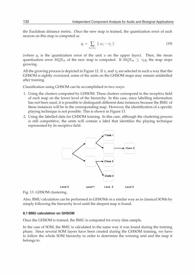
16 Artificial Intelligence and Applications
the Euclidean distance metric. Once the new map is trained, the quantization error of eachneuron on this map is computed as
qi = ∑xj∈Ci
‖ ωi − xj ‖ (19)
(where qi is the quantization error of the unit u on the upper layer). Then, the meanquantization error MQEm of the new map is computed. If MQEm ≤ τ1qi the map stopsgrowing.
All the growing process is depicted in Figure 12. If τ1 and τ2 are selected in such a way that theGHSOM is sightly oversized, some of the units on the GHSOM maps may remain unlabelledafter training.
Classification using GHSOM can be accomplished in two ways:
1. Using the clusters computed by GHSOM. These clusters correspond to the receptive fieldof each map on the lower level of the hierarchy. In this case, since labelling informationhas not been used, it is possible to distinguish different data instances because the BMU ofthese instances will be in the corresponding map. However, the identification of a specificplaying technique is not possible. This is shown in Figure 13.
2. Using the labelled data for GHSOM training. In this case, although the clustering processis still competitive, the units will contain a label that identifies the playing techniquerepresented by its receptive field.
Fig. 13. GHSOM clustering.
Also, BMU calculation can be performed in GHSOMs in a similar way as in classical SOMs bysimply following the hierarchy level until the deepest map is found.
8.1 BMU calculation on GHSOM
Once the GHSOM is trained, the BMU is computed for every data sample.
In the case of SOM, the BMU is calculated in the same way it was found during the trainingphase. Since several SOM layers have been created during the GHSOM training, we haveto follow the whole SOM hierarchy in order to determine the winning unit and the map itbelongs to.
132 Independent Component Analysis for Audio and Biosignal Applications

Unsupervised and Neural Hybrid Techniquesfor Audio Signal Classification 17
To this end, an iterative algorithm, depicted in Figure 14, has been developed. In this figure,an example of BMU calculation on a three-level GHSOM is represented. Assume that thedistances between an input pattern and the weight vectors of the level 0 map are calculated,then compute the minimum of these distances. As a result, the winning neuron on map 1 isfound. Since other maps could be grown from this winning neuron, we have to check if thewining neuron is a parent unit. This test can be carried out making use of the parent vectorsresulting from the GHSOM training process. If a new map arose from the wining neuron, theBMU on this map is calculated. This process is repeated until a BMU with no growing map isfound. Thus, the BMU in the GHSOM is associated to a map in a level of the hierarchy.
Fig. 14. GHSOM BMU calculation example.
At his point, a probability-based relabelling method can be applied using a 2DGaussian kernel centered at each BMU Ortiz, Górriz, Ramírez & Salas-Gonzalez (2011a);Ortiz, Gorriz, Ramirez & Salas-Gonzalez (2011b); Ortiz, Ortega, Diaz & Prieto (2011). Thus,a mayority-voting scheme with the units inside the Gaussian kernel is used to relabel theunlabelled units, assigning the calculated label to the data samples as shown in Figure 15.
Fig. 15. GHSOM map relabeling method.
In Equation 20, the Gaussian kernel used to estimate the label for unlabelled units is shown:
L(x, y, σ) =1
2πσ2e−
x2+y2
2σ2 (20)
In this equation, σ determines the width of the Gaussian kernel. In other words, it defines theneighbourhood considered for the relabelling process. On the other hand, (x, y) is the positionof the BMU in the SOM grid.
9. Concluding summary
In this chapter, we have presented the utilization of artificial intelligence techniques in thecontext of musical signal analysis.
133Unsupervised and Neural Hybrid Techniques for Audio Signal Classification

18 Artificial Intelligence and Applications
Wehave described some features related to a specific classification problemand, then, we havefocused on the utilization of neural models for the development of specific tasks in musicalaudio classification.
The classification task analysed in the context of the application of self-organizing maps andsome of its variants which make use of the competitive learning paradigm to implementunsupervised classification techniques applied to audio signals.
As it has been shown in this chapter, these performance of these models can be improved bymeans of hybridizing with other clustering and dimension reduction techniques like PrincipalComponent Analysis methodologies.
Also, the application of Gaussian Mixture Models provides a probabilistic behaviour of themaps instead of a binary activation of the neurons.
10. Acknowledgments
This work was supported by the Ministerio de Economía y Competitividad of the SpanishGovernment under Project No. TIN2010-21089-C03-02 and Project No. IPT-2011-0885-430000.
11. References
Alhoniemi, E., Himberg, J. & Vesanto, J. (1999). Probabilistic measures for responses ofself-organizing map units alhoniemi, Proceedings of the International ICSC Congresson Computational Intelligence Methods and Applications (CIMA’99).
Arsuaga, E. & Díaz, F. (2005). Topology preservation in som, International Journal ofMathematical and Computer Sciences 1(1): 19–22.
Barbancho, I., de la Bandera, C., Barbancho, A. M. & Tardon, L. J. (2009). Transcriptionand expressiveness detection system for violin music, Proc. IEEE Int. Conf. Acoustics,Speech and Signal Processing ICASSP 2009, pp. 189–192.
Bezdek, J. C. & Pal, N. R. (1998). Some new indexes of cluster validity, 28(3): 301–315.Cruz, R., Ortiz, A., Barbancho, A. & Barbancho, I. (2012). Unsupervised classification of audio
signals, 7th International Conference on Hybrid Artificial Intelligence (HAIS2012).Davies, D. L. & Bouldin, D. W. (1979). A cluster separation measure, (2): 224–227.Dittenbach, M., Merkl, D. & Rauber, A. (2000). The growing hierarchical self-organizing map,
Proc. IEEE-INNS-ENNS Int Neural Networks IJCNN 2000 Joint Conf, Vol. 6, pp. 15–19.Farahani, G. & Ahadi, S. M. (2005). Robust features for noisy speech recognition based on
filtering and spectral peaks in autocorrelation domain, Proc. of the European SignalProcessing Conference, Antalya (Turkey).
Ghahramani, Z. & Beal, M. (2000). Variational inference for bayesian mixtures of factoranalysers, Advances in Neural Information Processing Systems 12: 449–455.
Goto, M. (2004). Development of the rwc music database, Proceedings of the 18th InternationalCongress on Acoustics.
Hassar, H. & Bensaid, A. (1999). Validation of fuzzy and crisp c-partitions, Proc. NAFIPS FuzzyInformation Processing Society 18th Int. Conf. of the North American, pp. 342–346.
Haykin, S. (1999). Neural Networks: a comprehensive foundation, 2nd edn, Prentice-Hall.Holmes, W. J. & Huckvale, M. (1994). Why have HMMs been so successful for automatic
speech recognition and how might they be improved?, Speech, Hearing and Language,UCL Work in Progress, Vol. 8, pp. 207–219.
134 Independent Component Analysis for Audio and Biosignal Applications
Unsupervised and Neural Hybrid Techniquesfor Audio Signal Classification 19
Jenses, J. (1999). Envelope model of isolated musical sounds, Proceedings of the 2nd COST G-6workshop on digital audio effects, Trondheim (Norway).
Juang, B. H. & Rabiner, L. R. (2005). Automatic speech recognition – a brief history of thetechnology, in K. Brown (ed.), Encyclopedia of Language and Linguistics, Elsevier.
Kaufman, L. & Rosseauw, P. (1990). Finding groups in data, Wiley, New York.Kimura, S. (1999). Advances in speech recognition technologies, Fujitsu Sci. Tech. J.
35(2): 202–211.Kohonen, T. (2001). Self-Organizing Maps, Springer.Kohonen, T., Oja, E., Simula, O., Visa, A. & Kangas, J. (1996). Engineering applications of the
self-organizing map, Proc. of the IEEE.Lee, T., Lewicki, M. & Sejnowski, T. (2000). Ica mixture models for unsupervised classification
of non-gaussian classes and automatic context switching in blind signal separation,IEEE Transactions on Patt 22(10): 1078–1089.
MacQueen, J. B. (1967). Some methods for classification and analysis of multivariateobservations, Proceedings of 5th Berkeley Symposium on Mathematical Statistics andProbability. University of California Press. pp. 281–297.
Minematsu, N., Nishimura, T., Murakami, T. &Hirose, K. (2006). Speech recognition onlywithsuprasegmental features - hearing speech as music, Proc. of the International Conferenceon Speech Prosody, Dresden (Germany).
Müller, M., Ellis, D. P. W., Klapuri, A. & Richard, G. (2011). Signal processing for musicanalysis, IEEE Journal on Selected Topics in Signal Processing 5(6): 1088–1110.
Murtagh, F. (1991). Multilayer perceptrons for classification and regression, Neurocomputing2(5–6): 183–197.
Murtagh, F. (1995). Interpreting the kohonen self-organizing map usingcontiguity-constrained clustering, Pattern Recognition Letters 16(4): 399–408.
Ortiz, A., Górriz, J., Ramírez, J. & Salas-Gonzalez, D. (2011a). Mr brain imagesegmentation by growing hierarchical som and probability clustering, ElectronicsLetters 47(10): 585–586.
Ortiz, A., Gorriz, J., Ramirez, J. & Salas-Gonzalez, D. (2011b). Mri brain image segmentationwith supervised som and probability-based clustering method, Lecture Notes inComputer Science, LNCS-6686, pp. 49–58.
Ortiz, A., Ortega, J., Diaz, A. & Prieto, A. (2011). Network intrusion prevention by usinghierarchical self-organizing maps and probability-based labeling, Proceedings of the11th international conference on Artificial neural networks conference on Advances incomputational intelligence.
Panagiotakis, C. & Tziritas, G. (2005). A speech/music discriminator based on rms andzero-crossings, IEEE Transaction on Multimedia pp. 155–166.
Prasad, B. & Prasanna, S. R. M. (eds) (2008). Speech, Audio, Image and Biomedical SignalProcessing using Neural Networks, Vol. 83 of Studies in Computational Intelligence,Springer.
Rauber, A., Merkl, D. & Dittenbach, M. (2002). The growing hierarchical self-organizing map:exploratory analysis of high-dimensional data, 13(6): 1331–1341.
Riveiro, M., Johansson, F., Falkman, G. & Ziemke, T. (2008). Supporting maritime situationawareness using self organizing maps and gaussian mixture models, Proceedings ofthe 2008 conference on Tenth Scandinavian Conference on Artificial Intelligence: SCAI 2008.
Rossi, F. &Villa, N. (2009). Topologically orderedgraph clustering via deterministic annealing,Proceesdings of the 17th European Symposium on Artificial Neural Networks.
135Unsupervised and Neural Hybrid Techniques for Audio Signal Classification

20 Artificial Intelligence and Applications
Tardón, L. J., Sammartino, S. & Barbancho, I. (2010). Design of an efficient music-speechdiscriminator, J. Acoustical Society of America 127(1): 271–279.
Tasdemir, K. & Merenyi, E. (2009). Exploiting data topology in visualization and clustering ofself-organizing maps, 20(4): 549–562.
Tasdemir, K., Milenov, P. & Tapsall, B. (2011). Topology-based hierarchical clustering ofself-organizing maps, 22(3): 474–485.
Therrien, C. (1989). Decision estimation and classification: an introduction to pattern recognitionand related topics, John Wiley & Sons, Inc.
Thornburg, H., Leistikow, R. & Berger, J. (2007). Melody extraction and musical onsetdetection via probabilistic models of framewise stft peak data, IEEE Transactions onAudio, Speech, and Language Processing 15(4): 1257–1272.
Tipping, M. & Bishop, C. (1999). Mixtures of probabilistic preservationincipal componentanalyzers, Neural Computation 11(2): 443–482.
Tzanetakis, G. & Cook, P. R. (2002). Musical genre classification of audio signals, IEEETransactions on Speech and Audio Processing 10(5): 293–302.
Vesanto, J. & Alhoniemi, E. (2000). Clustering of the self-organizing map, 11(3): 586–600.Vesanto, J., Himberg, J., Alhoniemi, E. & Parhankangas, J. (2000). Som toolbox, Helsinki
University of Technology.URL: http://www.cis.hut.fi/somtoolbox/
Wu, S. & Chow, T. (2004). Clustering of the self organizing map using a clustering validityindex based on inter-cluster and intra-cluster density, Pattern Recognition Letters37(2): 175–188.
136 Independent Component Analysis for Audio and Biosignal Applications

7
Convolutive ICA for Audio Signals
Masoud Geravanchizadeh and Masoumeh Hesam Faculty of Electrical and Computer Engineering, University of Tabriz, Tabriz,
Iran
1. Introduction The goal of Blind Source Separation (BSS) is to estimate latent sources from their mixed observations without any knowledge of the mixing process. Under the assumption of statistical independence of hidden sources, the task in BSS is to obtain Independent Components (IC) from the mixed signals. Such algorithms are called ICA-based BSS algorithms [1, 2]. ICA-based BSS has been well studied in the fields of statistics and information theory for different applications, including wireless communication and biomedicine. However, as speech and audio signal mixtures in a real reverberant environment are generally convolutive mixtures, they involve a structurally much more challenging task than instantaneous mixtures, which are prevalent in many other applications [3, 4]. Such a mixing situation is generally modeled with impulse responses from sound sources to microphones. In a practical room situation, such impulse responses can have thousands of taps even with an 8 kHz sampling rate, and this makes the convolutive problem difficult to solve. Blind speech separation is applicable to the realization of noise-robust speech recognition, high quality hands-free telecommunication systems and hearing aids.
Various efforts have been devoted to the separation of convolutive mixtures. They can be classified into two major approaches: time-domain BSS [5, 6] and frequency-domain BSS [7]. With time-domain BSS, a cost function is defined for time-domain signals, and optimized with convolutive separation filters. However, the optimization with convolutive separation filters is not as simple as BSS for instantaneous mixtures, and generally computationally expensive. With frequency-domain BSS, time-domain mixed signals observed at microphones are converted into frequency-domain time-series signals by a short-time Fourier transform (STFT). However, choosing the length of STFT has relationship with the length of room impulse response [8]. The merit of these approaches is that the ICA algorithm becomes simple and can be performed separately at each frequency by any complex-valued instantaneous ICA algorithm [9-11]. However, the drawbacks of frequency-domain ICA are the permutation and scaling ambiguities of an ICA solution. In the frequency-domain ICA, different permutations at different frequencies lead to re-mixing of signals in the final output. Also, different scaling at different frequencies leads to distortion of the frequency spectrum of the output signal. For the scaling problem, in one method, the output is filtered by the inverse of the separation filter [12]. For the permutation problem, spatial information, such as the direction-of-arrivals (DOA) of sources, can be estimated and used [13, 14]. Another method utilizes the coherency of the mixing matrices in several

Independent Component Analysis for Audio and Biosignal Applications 138
adjacent frequencies [15]. For non-stationary sources such as speech, many methods exploit the dependency of separated signals across frequencies to solve the permutation problem [16, 17]. We propose a method for the permutation problem, by maximizing the correlation of power ratio measure of each bin frequency with the average of previous bin frequencies [18].
This chapter deals with the frequency-domain BSS for convolutive mixtures of speech signals. We begin by formulating the BSS problem for convolutive mixtures in Section 2. Section 3 provides an overview of the frequency-domain BSS. Section 4 discusses Principal Component Analysis (PCA) as a pre-processing step. Fast ICA algorithm for complex-valued signals is discussed in Section 5. We then present several important techniques along with our proposed method for solving the permutation problem in Section 6. Section 7 introduces a common method for the scaling problem. Section 8 considers ways of choosing the STFT length for a better performance of the separation problem. In Section 9, we compare our proposed method in the permutation problem with some other conventional methods by conducting several experiments. Finally, Section 10 concludes this chapter.
2. Mixing process and convolutive BSS
Convolutive mixing arises in acoustic scenarios due to time delays resulting from sound propagation over space and the multipath generated by reflections of sound from different objects, particularly in rooms and other enclosed settings. If we denote by ( )js t the signal emitted by the j-th source (1 )j N≤ ≤ , ( )ix t the signal recorded by the i-th microphone (1 )i M≤ ≤ , and ( )ijh t the impulse response from source j to sensor i , we have:
( ) ( ) ( )1
.N
i ij jj
x t h s tτ
τ τ=
= − (1)
We can write this equation into a more elegant form as:
( ) ( ) ( )x h s ,t tτ
τ τ= − (2)
where ( )h t is an unknown M N× mixing matrix. Now, the goal of a convolutive BSS is to obtain separated signals ( ) ( )1 ,..., Ny t y t , each of which corresponds to each of the source signals. The task should be performed only with M observed mixtures, and without information on the sources and the impulse responses:
( ) ( ) ( )1
,M
j ji ii
y t b x tτ
τ τ=
= − (3)
where ( )jib t represents the impulse response of the multichannel separation system. Convolutive BSS as applied to speech signal mixtures involves relatively-long multichannel FIR filters to achieve separation with even moderate amounts of room reverberation. While time-domain algorithms can be developed to perform this task, they can be difficult to code primarily due to the multichannel convolution operations involved [5, 6]. One way to simplify the conceptualization of the convolutive BSS algorithms is to transform the task

Convolutive ICA for Audio Signals 139
into the frequency domain, as convolution in time becomes multiplication in frequency. Ideally, each frequency component of the mixture signal contains an instantaneous mixture of the corresponding frequency components of the underlying source signals. One of the advantages of the frequency-domain BSS is that we can employ any ICA algorithm for instantaneous mixtures, such as the information maximization (Infomax) approach [19] combined with the natural gradient [20], Fast ICA [21], JADE [22], or an algorithm based on non-stationarity of signals [23].
3. Frequency-domain convolutive BSS
This section presents an overview of the frequency-domain BSS approach that we consider in this chapter. First, each of the time-domain microphone observations ( )jx t is converted into frequency-domain time-series signals ( ),jX k f by a short-time Fourier transform (STFT) with a K-sample frame and its S-sample shift:
( ) ( )win 2, ,i ftj j
st
SX k f x t t k e
fπ−
= −
(4)
for all discrete frequencies 1 10, ,..., Kf f fs sK K
−∈ , and for frame index k. The analysis
window win( )t is defined as being nonzero only in the K-sample interval 1 1,( 1)
2 2s s
K Kf f
− −
and tapers smoothly to zero at each end of the interval, such as a
Hanning window win21( ) 1 cos
2sft t
Kπ = +
.
If the frame size K is long enough to cover the main part of the impulse responses ijh , the convolutive model (2) can be approximated as an instantaneous model at each frequency [8, 24]:
( ) ( ) ( )X H S, , ,k f f k f= (5)
where H( )f is an M N× mixing matrix in frequency domain, and ( )X ,k f and ( )S ,k f are vectors of observations and sources in frequency domain, respectively. Notice that, the convolutive mixture problem is reduced to a complex but instantaneous mixture problem and separation is performed at each frequency bin by:
( ) ( ) ( )Y B X, , ,k f f k f= (6)
where B( )f is an N M× separation matrix. As a basic setup, we assume that the number of sources N is no more than the number of the microphones M, i.e., N M≤ . However, in a case with N M> that is referred to as underdetermined BSS, separating all the sources is a rather difficult problem [25].
We can limit the set of frequencies to perform the separations by 1 10, ,...,2s sf f
K
due to the relationship of complex conjugate:

Independent Component Analysis for Audio and Biosignal Applications 140
( )*( , ) , , 1,..., / 2 1 .j s j sm K m
X k f X k f m KK K
− = = −
(7)
We employ the complex-valued instantaneous ICA to calculate the separation matrix B( )f . Section 5 describes the detailed procedure for the complex-valued ICA used in our implementation and experiments. However, the ICA solution at each frequency bin has permutation and scaling ambiguity. In order to construct proper separated signals in time domain, frequency-domain separated signals originating from the same source should be grouped together. This is the permutation problem. Also, different scaling at different frequencies leads to distortion of the frequency spectrum of the output signal. This is the scaling problem. There are some methods to solve the permutation and scaling problems [12-18]. After solving the permutation and the scaling problem, the time-domain output signals ( )iy t are calculated with an inverse STFT (ISTFT) of the separated signals ( ),iY k f . The flow of the frequency-domain BSS is shown in Figure 1.
( )
( )
1
N
y t
y t
( ),k fX ( ),k fY
( )
( )
1
M
x t
x t
Fig. 1. System structure for the frequency-domain BSS
4. Pre-processing with principal component analysis
It is known that choosing the number of microphones more than the number of sources improves the separation performance. This is termed as the overdetermined case, in which the dimension of the observed signals is greater than the number of sources. Many methods have been proposed to solve the overdetermined problem. In a typical method, the subspace procedure is used as a pre-processing step for ICA in the framework of BSS [15, 26, 27]. The subspace method can be understood as a special case of principal component analysis (PCA) with M N≥ , where M and N denote the number of observed signals and source signals, respectively. This technique reduces room reflections and ambient noise [15]. Also, as pre-processing, PCA improves the convergence speed of ICA. Figure 2 shows the use of PCA as pre-processing to reduce the dimension of microphone signals.
In the PCA process, the input microphone signals are assumed to be modeled as:
X A S n( , ) ( ) ( , ) ( , ),k f f k f k f= + (8)
where the (m,n)-th element of A( )f is the transfer function from the n-th source to the m-th microphone as:

Convolutive ICA for Audio Signals 141
( ) ( ) ,2, , .m ni f
m n m nA f T f e π τ−= (9)
( )fH ( )fU ( )fW ( )fP ( )fS( , )k fS
( , )k fX
( , )k fZ
( , )k fY
Fig. 2. The use of PCA as a pre-processing step in the frequency-domain BSS
Here, the symbol , ( )m nT f is the magnitude of the transfer function. The symbol ,m nτ denotes the propagation time from the n-th source to the m-th microphone. The first term in Eq. (8),A S( ) ( , )f k f , expresses the directional components in X( , )k f and the second term, n( , )k f , is a mixture of less-directional components which includes room reflections and ambient noise.
The spatial correlation matrix R( )f of X( , )k f is defined as:
R X X( ) [ ( , ) ( , )].Hf E k f k f= (10)
The eigenvalues of R( )f are denoted as 1( ),..., ( )Mf fλ λ with 1( ) ,..., ( )Mf fλ λ≥ ≥ and the corresponding eigenvectors are denoted as e e1( ),..., ( )Mf f . Assuming that s( )t and n( )t are uncorrelated, the energy of the N directional signals s( )t is concentrated on the N dominant eigenvalues and the energy of n( )t is equally spread over all eigenvalues. In this case, it is generally satisfied that:
1 1( ),..., ( ) ( ),..., ( ).N N Mf f f fλ λ λ λ+>> (11)
The vectors 1 1( ),..., ( ) and ( ),..., ( )N N Mf f f f+e e e e are the basis of the signal and noise subspaces, respectively.
In the PCA method, the input signal is processed as:
Z U X( , ) ( ) ( , ),k f f k f= (12)
that reduces the energy of n( )t in the noise subspace, and the PCA filter is defined as:
U Λ E12( ) ( ) ( ),Hf f f
−= (13)
where
( ) [ ]Λ E1 1( ) ( ),..., ( ) , ( ) ( ),..., ( ) .N Nf diag f f f e f e fλ λ= = (14)

Independent Component Analysis for Audio and Biosignal Applications 142
The PCA filtering of X( , )k f reduces the dimension of input signal to the number of sources N which is equivalent to a spatially whitening operation, i.e., Z Z I ( , ) ( , )HE k f k f = where I is the N N× identity matrix.
5. Complex-valued fast fixed-point ICA
The ICA algorithm used in this chapter is fast fixed-point ICA (fast ICA). The fast ICA algorithm for the separation of linearly mixed independent source signals was presented in [21]. This algorithm is a computationally efficient and robust fixed-point type algorithm for independent component analysis and blind source separation. However, the algorithm in [21] is not applicable to frequency-domain ICA as these are complex-valued. In [9], the fixed-point ICA algorithm of [21] has been extended to involve complex-valued signals. The fast fixed-point ICA algorithm is based on the assumption that when the non-Gaussian signals get mixed, it becomes more Gaussian and thus its non-Gaussianization can yield independent components. The process of non-Gaussianization consists of two-steps, namely, pre-whitening or sphering and rotation of the observation vector. Sphering is half of the ICA task and gives spatially decorrelated signals. The process of sphering (pre-whitening) is accomplished by the PCA stage as described in the previous section. The task remaining after whitening involves rotating the whitened signal vector Z( , )k f such that Y W Z( , ) ( ) ( , )k f f k f= returns independent components. For measuring the non-Gaussianity, we can use the negentropy-based cost function:
( ) w Z 2| | ,HJ E G= (15)
where = +( ) log(0.01 )G t t [9].
The elements of the matrix W w w1( ,..., )N= are obtained in an iterative procedure. The fixed-point iterative algorithm for each column vector w is as follows (the frequency index f and frame index k are dropped hereafter for clarity):
w y w Z w Z w Z w Z w Z w2 2 2 2*( ) ,H H H H HE g E g g ′= − +
(16)
where (.)g and (.)g′ are first- and second-order derivatives of G:
2 2 21 .5( ) , ( ) .
(0.01 ) (0.01 )o
g t g tt t
′= =+ +
(17)
After each iteration, it is also essential to decorrelate W to prevent its convergence to the previously converged point. The decorrelation process to obtain W for the next iteration is obtained as [9]:
W W W W 1/2( ) .H −= (18)
Then, the separation matrix is obtained by the product of U( )f and W( ) :f

Convolutive ICA for Audio Signals 143
B W U( ) ( ) ( ).f f f= (19)
6. Solving the permutation problem
In order to get separated signals correctly, the order of separation vectors (position of rows) in B( )f must be the same at each frequency bin. This is called permutation problem. In this section, we review various methods which have already been proposed to solve permutation problem.
6.1 Solving permutation by Direction of Arrival (DOA) estimation
Some methods for permutation problem use the information of source locations, such as direction of arrival (DOA). In the totally blind setup, DOA cannot be known so it is estimated from the directivity pattern of the separation matrix. In this method, the effect of room reverberation is neglected, and the elements of the mixing matrix in Eq. (9) can be written as the following expression:
( ) ( ) ,2, , ,
1, ( sin ),m ni fm n m n m n m nA f T f e d
cπ τ τ θ−= ≡ (20)
where ,m nτ is the arriving lag with respect to the n-th source signal from the direction of nθ , observed at the m-th microphone located at md , and c is the velocity of sound. Microphone array and sound sources are shown in Figure 3.
Fig. 3. Configuration of a microphone array and sound sources
From the standpoint of array signal processing, directivity patterns (DP) are produced in the array system. Accordingly, directivity patterns with respect to ( )nmB f are obtained at every frequency bin to extract the DOA of the n-th source signal. The directivity pattern ( , )nF f θ is given by [13]:

Independent Component Analysis for Audio and Biosignal Applications 144
[ ]1
( , ) ( ).exp 2 sin / .M
n nm mm
F f B f i fd cθ π θ=
= (21)
The DP of the separation matrix contains nulls in each source direction. Figure 4 shows an example of directivity patterns at frequency bins f1 and f2 plotted for two sources. As it is observed, the positions of the nulls vary at each frequency bin for the same source direction. Hence, in order to solve the permutation problem and sort out the different sources, the separation matrix at each frequency bin is arranged in accordance with the directions of nulls.
1f f=
2f f=
Source1 Source2Gain
Gain
θ
Source1
Source1
Source1 Source2 Source2
Source2
θθ
θ
Permutation
Fig. 4. Examples of directivity patterns
This method is not always effective in the overdetermined case, because the directions giving the nulls of the directivity patterns of the separation matrix B( )f do not always correspond to the source directions. Figure 5 shows the directivity pattern for the case ( 2, 2M N= = ) , and the overdetermined case ( 8, 2M N= = ).
6.1.1 Closed-form formula for estimating DOAs
The DOA estimation method by the directivity pattern has three problems, a high computational cost, the difficulty of using it for mixtures of more than two sources, and for overdetermined case in which the number of microphones is more than the number of sources. Instead of plotting directivity patterns and searching for the minimum as a null direction, some propose a closed-form formula for estimating DOAs [16]. In principle, this method can be applied to any number of source signals as well as to the overdetermined case. It can be shown that the DOAs for sources are estimated by the following relation [16]:
( )
B
B
1
1
1
arg
arccos ,2
jk
j kk
j jfc d dθ
π
−
−′
−′
=−
(22)

Convolutive ICA for Audio Signals 145
where, jd and jd ′ are the positions of sensors jx and jx ′ .
-100 -80 -60 -40 -20 0 20 40 60 80 100-20
-10
0
10
20
30
40
50
60
DOA(deg)
Gai
n (d
B)
Directivitiy pattern for 2 sources and 8 microphones
Fig. 5. The directivity patterns for the case ( 2, 2M N= = ), and the overdetermined case ( 8, 2M N= = )
If the absolute value of the input variable of arccos(.) is larger than 1, kθ becomes complex and no direction is obtained. In this case, formula (22) can be tested with another pair j and j′ .
If N M< , the Moore–Penrose pseudoinverse B+ is used instead of B 1− . Based on these DOA estimations, the permutation matrix is determined. In this process, no reverberation is assumed for the mixing signals. Therefore, for the reverberant case the method based on DOA estimation is not efficient.
6.2 Permutation by interfrequency coherency of mixing matrix
Another method to solve the permutation problem utilizes the coherency of the mixing matrices in several adjacent frequencies [15]. For the mixing matrix A( )f in the Eq. (8), the n-th column vector (location vector of the n-th source) at frequency f has coherency with that at the adjacent frequency 0f f f= − Δ . Therefore, the location vector a ( )n f is a 0( )n fwhich is rotated by the angle nθ as depicted in Figure 6(a). Accordingly, nθ is expected to be the smallest for the correct permutation as shown in Figure 6. Based on this assumption, permutation is solved so that the sum of the angles 1 2 , ,..., Nθ θ θ between the location vectors in the adjacent frequencies is minimized. An estimate of the mixing matrix Α a a1ˆ ˆ ˆ( ) [ ( ),..., ( )]Nf f f= can be obtained as the pseudoinverse of the separation matrix as:
A Bˆ ( ) ( ).f f+= (23)
For this purpose, we define a cost function as [15]:
a aP
a a0
01
ˆ ˆ( ) ( )1( ) cos , cos .ˆ ˆ( ) . ( )
HNn n
n nn nn
f fF
N f fθ θ
== = (24)

Independent Component Analysis for Audio and Biosignal Applications 146
This cost function is calculated for all arranges of columns of mixing matrix Α a a1ˆ ˆ ˆ( ) [ ( ),..., ( )]Nf f f= and the permutation matrix P is obtained by maximizing it.
1θ
1θ2θ
2θ
1( )fa1( )fa
1 0( )fa1 0( )fa
2 0( )fa2 0( )fa
2 ( )fa2 ( )fa
(a) Correct Permutation (b) Incorrect Permutation Fig. 6. The column vectors of the mixing matrix in two adjacent frequencies, with correct and incorrect permutations
To increase the accuracy of this method, the cost function is calculated for a range of frequencies instead of the two adjacent frequencies and a confidence measure is used to determine which permutation is correct [15].
The mixing matrix is defined as the transfer function of direct path from each source to each microphone where the coherency of mixing matrices is used in several adjacent frequencies to obtain the permutation matrix.
This method assumes that the spectrum of microphone signals consists of the directional components and reflection components of sources and employs the subspace method to reduce the reflection components. However, if the reflection components are not reduced by the subspace method, the mixing matrix consists of indirect path components, and the method will not be efficient.
6.3 A new method to solve the permutation problem based on power ratio measure
Another group of permutation methods use the information on the separated signals which are based on the interfrequency correlation of separated signals. Conventionally, the correlation coefficient of separated signal envelopes has been employed to measure the dependency of bin-wise separated signals. Envelopes have high correlations at neighboring frequencies if separated signals correspond to the same source signal. Thus, calculating such correlations helps us to align permutations. A simple approach to the permutation alignment is to maximize the sum of the correlations between neighboring frequencies [16]. The method in [12] assumes high correlations of envelopes even between frequencies that are not close neighbors and so it does not limit the frequency range in which correlations are calculated.
However, this assumption is not satisfied for all pairs of frequencies. Therefore, the use of envelopes for maximizing correlations in this way is not a good choice. Recently, the power ratio between the i-th separated signal and the total power sum of all separated signals has been proposed as another type of measure [17]. In this approach, the dependence of bin-wise separated signals can be measured more clearly by calculating correlation coefficients with power ratio values rather than with envelopes. This is shown by comparing Figures 7 and 8.

Convolutive ICA for Audio Signals 147
Fig. 7. Correlation coefficients between the separated signal envelopes
Fig. 8. Correlation coefficients between the power ratios of separated signals
This method uses two optimization techniques for permutation alignment; a rough global optimization and a fine local optimization. In rough global optimization, a centroid is calculated for each source as the average value of power ratio with the current permutation. The permutations are optimized by an iterative maximization between the power ratio measures and the current centroid. In fine local optimization, the permutations are obtained by maximizing the correlation coefficients over a set of frequencies consisting of adjacent frequencies and harmonic frequencies. Here, the experiments show that the fine local optimization alone does not provide good results in permutation alignment. But using both
Freq
uenc
y(kH
z)
|y1| and |y1|
0 2 4
4
3
2
1
0 -1
-0.5
0
0.5
1
Freq
uenc
y(kH
z)
|y1| and |y2|
0 2 4
4
3
2
1
0 -1
-0.5
0
0.5
1
Freq
uenc
y(kH
z)
|y2| and |y1|
0 2 4
4
3
2
1
0 -1
-0.5
0
0.5
1
Freq
uenc
y(kH
z)
|y2| and |y2|
0 2 4
4
3
2
1
0 -1
-0.5
0
0.5
1
Freq
uenc
y(kH
z)
powRatio1 and powRatio1
0 2 4
4
3
2
1
0 -1
-0.5
0
0.5
1
Freq
uenc
y(kH
z)
powRatio1 and powRatio2
0 2 4
4
3
2
1
0 -1
-0.5
0
0.5
1
Freq
uenc
y(kH
z)
powRatio2 and powRatio1
0 2 4
4
3
2
1
0 -1
-0.5
0
0.5
1
Freq
uenc
y(kH
z)
powRatio2 and powRatio2
0 2 4
4
3
2
1
0 -1
-0.5
0
0.5
1

Independent Component Analysis for Audio and Biosignal Applications 148
global and local optimization achieves almost optimal results. This method, however, is somewhat complicated for calculating the permutations.
In our proposed method, we take a rather simple technique to compute the permutation matrices. Here, we assume that the correlation coefficients of power ratios of bin-wise separated signal to be high if they come from the same source for each two frequencies even if they are not close together. Therefore, we extend the frequency range for calculating correlation to all previous frequencies, where the permutation was solved for them. We decide on the permutation by maximizing the correlation of power ratio measure of each bin frequency with the average of power ratio measures of previous bin frequencies, iteratively with increasing frequency. Therefore, this criterion is not based on local information and does not have the drawback of propagation of mistakes by the computation of permutation at each frequency.
If the separation works well, the bin-wise separated signals Y Y1( , ),..., ( , )Nk f k f are the estimations of the original source signals S S1( , ),..., ( , )Nk f k f up to the permutation and scaling ambiguity. Thus, the observation vector X( , )k f can be represented by the linear combination of the separated signals as:
X A Y a1
( , ) ( ) ( , ) ( ) ( , ),N
i ii
k f f k f f Y k f=
= = (25)
where the mixing matrix A a a1( ) [ ( ),..., ( )]Nf f f= is the pseudoinverse of the separation matrix B( )f :
A B( ) ( ) .f f += (26)
Now, we use the power ratio measure as given by [17]:
a
a
2
21
( ) ( , )( , ) .
( ) ( , )i i
i Nn nn
f Y k fpowRatio k f
f Y k f=
=
(27)
In the following, ( ) ( , )lfi liv k powRatio k f= denotes the power ratio measure obtained at
frequency ( )/l sf l K f= ( 0,..., /2)l K= , where sf is the sampling rate. The details of the proposed method are as follows:
1. Obtain 0 ( )fiv k , ( 1,..., )i N= , set 1l = .
2. Obtain ( )lfiv k and
( ) ( )l gf
i ig T
c k v k∈
= ( 1,..., )i N= , where 0 1 ,..., lT f f −= .
3. Obtain all permutation matrices P ( )1,2,...,e e N= . Permutation matrix is an N N× matrix where in each row and each column there is one nonzero element of unit value. For example, for a case of 2 sources, the permutation matrices are:
P P1 21 0 0 1
, .0 1 1 0
= =
(28)
4. Obtain u P vl lf fe= for all permutation matrices.
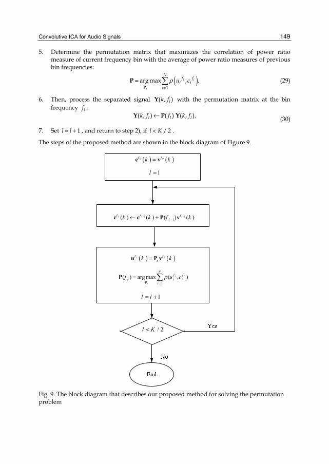
Convolutive ICA for Audio Signals 149
5. Determine the permutation matrix that maximizes the correlation of power ratio measure of current frequency bin with the average of power ratio measures of previous bin frequencies:
( )P
P1
arg max , .l l
e
Nf f
i ii
u cρ=
= (29)
6. Then, process the separated signal Y( , )lk f with the permutation matrix at the bin frequency lf :
Y P Y( , ) ( ) ( , ).l l lk f f k f← (30)
7. Set 1l l= + , and return to step 2), if / 2l K< .
The steps of the proposed method are shown in the block diagram of Figure 9.
1 11( ) ( ) ( ) ( )l l lf f f
lk k f k− −−← +c c P v
( ) ( )l lf fek k=u P v
1( ) arg max ( , )l l
e
Nf f
l i ii
f u cρ=
= P
P
1l l= +
/ 2l K<
1l =
( ) ( )0 0f fk k=c v
Fig. 9. The block diagram that describes our proposed method for solving the permutation problem

Independent Component Analysis for Audio and Biosignal Applications 150
7. Scaling problem
The scaling problem can be solved by filtering individual outputs of the separation filter by the inverse of B( )f separately [12]. In the overdetermined case, (i.e., M N> ), the pseudoinverse of B( )f , denoted as B( )f + , is used instead of the inverse of B( )f . This is due to the fact that in this case, because of employing the subspace method B( )f is not square. The scaling matrix can be expressed as:
S ,1 ,( ) [ ,..., ],m m Nf diag B B+ += (31)
where ,m nB+ denotes the ( , ) - thm n element of B( )f + .
8. Suitable length of STFT for better separation
It is commonly believed that the length of STFT (i.e., frame size), K, must be longer than P to estimate the unmixing matrix for a P-point room impulse response. The reasons for this belief are: 1) A linear convolution can be approximated by a circular convolution if 2 ,K P> and 2) If we want to estimate the inverse system of a system with impulse response of P-taps long, we need an inverse system that is Q-taps long, where Q P> . If we assume that the frame size is equal to the length of unmixing filter, then we should have K P> . Moreover, when the filter length becomes longer, the number of separation matrices to be estimated increases while the number of samples for learning at each frequency bin decreases. This violates the assumption of independence in the time series at each bin frequency, and the performance of the ICA algorithm becomes poor [8]. Therefore, there is an optimum frame size determined by a trade-off between maintaining the assumption of independence and the length of STFT that should be longer than the room impulse response length in the frequency-domain BSS. Section 9 shows this understanding by some experiments.
9. Experimental results The experiments are conducted to examine the effectiveness of the proposed permutation method [18]. We use two experimental setups. Setup A is considered to be a basic one, in which there are two sources and two microphones. In setup B, we have two sources and eight microphones, and discuss the effect of a background interference noise on our proposed method. Table 1 summarizes the configurations common to both setups. As the original speech, we use the wave files from ‘TIMIT speech database’ [28] to test the performance of different BSS algorithms. The lengths of the speech signals are 4 seconds. We have the voice of three male and three female speakers in our experiments and the investigations are carried out for nine different combinations of speakers. The image method
room dimension L = 3.12 m, W = 5.73 m, H = 2.70 m direction of arrivals 30 and -40
window function Hamming sample rate 16000 Hz
Table 1. Common Experimental Configuration
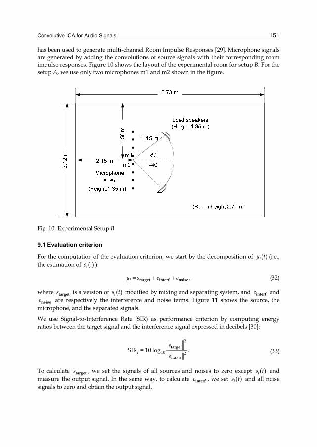
Convolutive ICA for Audio Signals 151
has been used to generate multi-channel Room Impulse Responses [29]. Microphone signals are generated by adding the convolutions of source signals with their corresponding room impulse responses. Figure 10 shows the layout of the experimental room for setup B. For the setup A, we use only two microphones m1 and m2 shown in the figure.
Fig. 10. Experimental Setup B
9.1 Evaluation criterion
For the computation of the evaluation criterion, we start by the decomposition of ( )iy t (i.e., the estimation of ( )is t ):
target interf noise ,iy s e e= + + (32)
where targets is a version of ( )is t modified by mixing and separating system, and interfe and noisee are respectively the interference and noise terms. Figure 11 shows the source, the
microphone, and the separated signals.
We use Signal-to-Interference Rate (SIR) as performance criterion by computing energy ratios between the target signal and the interference signal expressed in decibels [30]:
2
10 2SIR = 10 log .i
s
e
target
interf
(33)
To calculate targets , we set the signals of all sources and noises to zero except ( )is t and measure the output signal. In the same way, to calculate interfe , we set ( )is t and all noise signals to zero and obtain the output signal.

Independent Component Analysis for Audio and Biosignal Applications 152
Setup A: The case of 2-Sources and 2-Microphones
In this experiment, we use only two microphones m1 and m2 in Figure 10. In this case, the reverberation time of the room is set to 130 ms. The frame length and frame shift in the STFT analysis are set to 2048 and 256 samples, respectively. Three different methods for the permutation problem are applied on 9 pairs of speech signals. The results of our simulations are shown in Figure 12. In the MaxSir approach, we select the best permutation by maximizing SIR at each frequency bin for solving perfectly the permutation ambiguity [16]. This gives a rough estimate of the upper bound of the performance.
Ns
1s
1Mh
Mx
1y
Ny
11h
1n
1x
Mn Fig. 11. Block diagram of the separating system
As seen from Figure 12, the results with Murata’s method [12] are sometimes very poor, but our proposed method [18] offers almost the same results as that of MaxSir. Figure 13 shows SIRs at each frequency for the 8th pair of speech signals, obtained by the proposed method and Murata’s method. The change of signs of SIRs in this figure shows the regions of permutation misalignments. Here, we see the permutation misalignments below 500 Hz obtained by Murata’s method, whereas the proposed method has almost perfect permutation alignment. This shows that it is not always true to assume that frequencies not in close proximity have a high correlation of envelopes.
Setup B: The case of 2-Sources and 8-Microphones
In this experiment, we compare the separation performance of our proposed method with those of three other methods, namely, the Interfrequency Coherency method (IFC) [15], the DOA approach with a closed -form formula [17], and MaxSir for the case of 2-Sources and 8-Microphones [17]. To avoid aliasing in the DOA method, we select the distance between the microphones to be 2 cm. All these experiments are performed for three reverberation times
RT = 100 ms, 130 ms, and 200 ms. Before assessing different separation techniques, we first obtain the optimum frame length of STFT at each reverberation time. Then, we evaluate the proposed method in noisy and noise-free cases.
Optimum length of STFT for better separation
To show what frame length of STFT is suitable for better performance of BSS, we perform separation experiments at three reverberation times of RT = 100 ms, 130 ms, and 200 ms, and by different lengths of STFT. Since the sampling rate is 16 kHz, these reverberation times correspond to P = 1600, 2080, and 3200 taps, respectively.

Convolutive ICA for Audio Signals 153
Fig. 12. The separation results of 9 pairs of speech signals for three different methods of permutation problem: Murata’s method, proposed method, and MaxSir
Fig. 13. SIRs measured at different frequencies for the proposed method and the Murata’s method
Figure 14 shows the room impulse responses 11h for 100 ms, 130 ms, and 200 ms.RT = We vary the length of STFT by K = 512, 1024, 2048, 4096, and 8192 with corresponding frame shifts of S = 64, 128, 256, 512, and 1024, respectively. The best permutation is selected by maximizing SIR at each frequency bin. In this way, the results are ideal under the condition that the permutation problem is solved perfectly. The experimental results of SIR for different lengths of STFT are shown in Figure 15. These values are averaged over all nine combinations of speakers to obtain average values of SIR1 and SIR2. As it is observed from this figure, in the case of 100 msRT = we obtain the best performance with 1024K = . For
method by Murata proposed method maxsir0
5
10
15
20
25sir by 3 methods (beta=130ms)
sir(d
B)
average for 9 pairsother 8 pairs8th pair
0 500 1000 1500 2000 2500 3000 3500 4000
-20
0
20
SIR at each frequency by proposed method
frequency(Hz)
SIR
(dB
)
0 500 1000 1500 2000 2500 3000 3500 4000
-20
0
20
SIR at each frequency by Murata's method
frequency(Hz)
SIR
(dB
)

Independent Component Analysis for Audio and Biosignal Applications 154
Fig. 14. The room impulse responses 11h for 100 ms, 130 ms, and 200 msRT =
0 200 400 600 800 1000 1200-0.02
-0.01
0
0.01
0.02
0.03
0.04
0.05
0.06
0.07TR=100ms
sample
ampl
itude
0 200 400 600 800 1000 1200-0.02
-0.01
0
0.01
0.02
0.03
0.04
0.05
0.06
0.07TR=130ms
sample
ampl
itude
0 200 400 600 800 1000 1200-0.02
-0.01
0
0.01
0.02
0.03
0.04
0.05
0.06
0.07TR=200ms
sample
ampl
itude

Convolutive ICA for Audio Signals 155
Fig. 15. The experimental results of SIR for different lengths of STFT
the reverberant conditions with 130, and 200 ms,RT = the best performance is realized with 2048, and 4096K = , respectively. Figure 16 shows the average of neg-entropy (Eq. 15) as a
measurement of independence. We see that by longer lengths of STFT the independence is smaller, and the performance of the fixed-point ICA is poorer [8].
Fig. 16. The average of neg-entropy as a measurement of independence
Evaluation results without background noise
In this section, we compare our proposed method with three methods, namely, IFC, DOA, and MaxSir in the case of 2-Sources and 8-Microphones without the background noise. We select the optimum length of STFT obtained in the previous experiment for each of the three reverberation times. Figure 17 shows the separation results for nine pairs of speech signals
512 1024 2048 4096 81928
10
12
14
16
18
20
22
24
26
28
SIR
(dB
)
average sir for each frame length for Tr=100,130,200ms
Tr=100msTr=130msTr=200ms
512 1024 2048 4096 8192
1.4
1.6
1.8
2
2.2
2.4
2.6
aver
age
neg-
entro
py
average neg-entropy for each frame length for Tr=100,130,200ms
Tr=100msTr=130msTr=200ms

Independent Component Analysis for Audio and Biosignal Applications 156
(a)
(b)
Fig. 17. The separation results of 9 pairs of speech signals (a) with 100 msRT = and (b) with 200 msRT = as the reverberation times, for four different methods of the permutation
problem: the Interfrequency Coherency method (IFC), the DOA method, the proposed method, and the MaxSir method
in the cases where the reverberation times of the room are 100, and 200 msRT = , respectively. We observe that, when the reverberation time is 100 ms, the separation results for each of the three methods, i.e., IFC, DOA, and proposed methods, are close to the perfect solution obtained by MaxSir. For the reverberant case of 200 ms,RT = the separation performances of IFC and DOA are not good, but the results of SIR for the proposed method are close to the MaxSir approach.
IFC DOA proposed maxSIR10
15
20
25
30
35
SIR
(dB
)
SIR for 4 methods for Tr=100ms
average of 9 pairseach case
IFC DOA proposed maxSIR0
5
10
15
20
25
SIR
(dB
)
SIR for 4 methods for Tr=200ms
average of 9 pairseach case
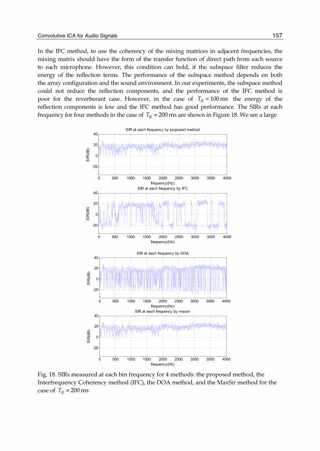
Convolutive ICA for Audio Signals 157
In the IFC method, to use the coherency of the mixing matrices in adjacent frequencies, the mixing matrix should have the form of the transfer function of direct path from each source to each microphone. However, this condition can hold, if the subspace filter reduces the energy of the reflection terms. The performance of the subspace method depends on both the array configuration and the sound environment. In our experiments, the subspace method could not reduce the reflection components, and the performance of the IFC method is poor for the reverberant case. However, in the case of 100 msRT = the energy of the reflection components is low and the IFC method has good performance. The SIRs at each frequency for four methods in the case of 200 msRT = are shown in Figure 18. We see a large
Fig. 18. SIRs measured at each bin frequency for 4 methods: the proposed method, the Interfrequency Coherency method (IFC), the DOA method, and the MaxSir method for the case of 200 msRT =
0 500 1000 1500 2000 2500 3000 3500 4000
-20
0
20
40SIR at each frequency by proposed method
frequency(Hz)
SIR
(dB
)
0 500 1000 1500 2000 2500 3000 3500 4000
-20
0
20
40SIR at each frequency by IFC
frequency(Hz)
SIR
(dB
)
0 500 1000 1500 2000 2500 3000 3500 4000
-20
0
20
40SIR at each frequency by DOA
frequency(Hz)
SIR
(dB
)
0 500 1000 1500 2000 2500 3000 3500 4000
-20
0
20
40SIR at each frequency by maxsir
frequency(Hz)
SIR
(dB
)

Independent Component Analysis for Audio and Biosignal Applications 158
number of frequencies with permutation misalignments for the IFC and DOA methods. As observed from the simulation results, the proposed approach outperforms the IFC and the DOA methods, where we achieve the best performance in the sense of SIR-improvement.
Evaluation results with background noise
In this part of experiments, we add the restaurant noise from the Noisex-92 database [31] with input SNRs of 5 dB, and 20 dB to the microphone signals. Here, again the optimum window length for the STFT analysis is chosen for each three reverberation times. Figures 19 and 20 show the average SIRs obtained for the proposed, IFC, DOA, and MaxSir methods for the reverberation times of 100 ms, 130 ms, and 200 msRT = , respectively with input SNRs of 5 dB and 20 dB. It is observed that under the experimental conditions of input SNR = 20 dB and reverberation time of 100 ms, all of the methods, i.e., the proposed, IFC, and DOA give the same separation results. However, as the reverberation time increases, the performance of IFC and DOA decreases. At the reverberation time of 200 ms, the average SIR of the proposed method is slightly reduced. Also, as it is expected, the comparison of Figures 19 and 20 shows that in lower values of input SNRs, the performance of source separation methods decreases. This shows that the ICA-based methods have in general poor separation results in noisy conditions.
Fig. 19. Average of SIRs for the proposed, IFC, DOA, and MaxSir methods for three reverberation times of 100 ms, 130 ms, and 200 msRT = , respectively, obtained at the input SNR of 20 dB
Tr=100ms Tr=130ms Tr=200ms0
5
10
15
20
25
30average of SIRs for 4 methods for 3 reverberation time ISNR=20dB
IFCDOAproposedmaxsir

Convolutive ICA for Audio Signals 159
Fig. 20. Average of SIRs for the proposed, IFC, DOA, and MaxSir methods for three reverberation times of 100 ms, 130 ms, and 200 msRT = , respectively, obtained at the input SNR of 5 dB
10. Conclusion This chapter presents a comprehensive description of frequency-domain approaches to the blind separation of convolutive mixtures. In frequency-domain approach, the short-time Fourier transform (STFT) is used to convert the convolutive mixtures in time domain to instantaneous mixtures at each frequency. In this way, we can use each of the complex-valued ICA at each frequency bin. We use the fast ICA algorithm for complex-valued signals. The key feature of this algorithm is that it converges faster than other algorithms, like natural gradient-based algorithms, with almost the same separation quality. We employ PCA as pre-processing for the purpose of decreasing the noise effect and dimension reduction. Also, we see that the length of STFT affects the performance of frequency-domain BSS. If the length of STFT becomes longer, the number of coefficients to be estimated increases while the number of samples for learning at each frequency bin decreases. This causes that the assumption of independence in the time series at each bin frequency to collapse, and the performance of the ICA algorithm to become poor. As a result, we select for the frame size an optimum value which is obtained by a trade-off between maintaining the assumption of independence and the length of STFT in the frequency-domain BSS.
We focus on the permutation alignment methods and introduce some conventional methods along with our proposed method to solve this problem. In the proposed method, we maximize the correlation of power ratio measure of each bin frequency with the average of power ratio measures of previous bin frequencies, iteratively with increasing frequency. In the case of 2-sources and 2-microphones, by conducting source separation experiments, we compare the performance of our proposed method with Murata’s method which is based on envelope correlation. The results of this comparison show that it is not always true to
Tr=100ms Tr=130ms Tr=200ms0
2
4
6
8
10
12
14
16
18
20average of SIRs for 4 methods for 3 reverberation time ISNR=5dB
IFCDOAproposedmaxsir

Independent Component Analysis for Audio and Biosignal Applications 160
assume that frequencies not in close proximity have a high correlation of envelopes. In another overdetermined case of experiment, the proposed method is compared with the DOA, IFC and MaxSir methods. Here, we see that in the reverberant room with high SNR values, the proposed method outperforms other methods. Finally, even though the performance of our proposed method degrades under reverberant conditions with high background noise (low SNRs), the experiments show that the separation results of the proposed method are still satisfactory.
11. Future directions In this chapter, we have used PCA as a pre-processing technique for the purpose of decreasing the effect of background noise and dimension reduction. This approach assumes that the noise and the signal components are uncorrelated and the noise component is spatially white. Practically, the performance of PCA depends on both the array configuration and the sound environment.
From the results of the experiments, it is clear that two factors affect the performance of BSS methods; background noise and room reverberation. These factors are those that significantly influence the enhancement of audio signals. Therefore, as a future work, we should consider other pre-processing techniques in ICA-based BSS that besides performing dimension reduction also help to decrease the effect of colored noise as well as room reverberation.
12. References [1] Lee T. W (1998) Independent Component Analysis - Theory and Applications. Norwell,
MA: Kluwer. [2] Comon P (1994) Independent Component Analysis, A New Concept? Signal Processing
vol. 36 no. 3: 287-314. [3] Benesty J, Makino S, Chen J (2005) Speech Enhancement. Springer-Verlag, Berlin,
Heidelberg. [4] Makino S, Lee T. W, Sawada H (2007) Blind Speech Separation. Springer. [5] Douglas S. C, Sun X (2003) Convolutive Blind Separation of Speech Mixtures Using the
Natural Gradient. Speech Communication, vol. 39: 65-78. [6] Aichner R, Buchner H, Yan F, Kellermann W (2006) A Real-Time Blind Source Separation
Scheme and its Application to Reverberant and Noisy Acoustic Environments. Signal Processing, vol. 86, no. 6: 1260-1277.
[7] Smaragdis P (1998) Blind Separation of Convolved Mixtures in the Frequency Domain. Neurocomputing, vol. 22: 21-34.
[8] Araki S, Mukai R, Makino S, Nishikawa T, Saruwatari H (2003) The Fundamental Limitation of Frequency-Domain Blind Source Separation for Convolutive Mixtures of Speech. IEEE Trans. on Speech and Audio Processing, vol. 11, no. 2.
[9] Bingham E, et al. (2000) A Fast Fixed-Point Algorithm for Independent Component Analysis of Complex-Valued Signal. Int. Journal of Neural Systems, vol. 10 (1) 1:8.
[10] Sawada H, Mukai R, Araki S, Makino S (2003) Polar Coordinate-Based Nonlinear Function for Frequency-Domain Blind Source Separation. IEICE Trans. Fundamentals, vol. E86-A, no. 3.

Convolutive ICA for Audio Signals 161
[11] Prasad R, Saruwatari H, Shikano K (2007) An ICA Algorithm for Separation of Convolutive Mixture of Speech Signals. International Journal of Information Technology, vol. 2, no. 4.
[12] Murata N, Ikeda S, Ziehe A (2001) An Approach to Blind Source Separation Based on Temporal Structure of Speech Signals. Neurocomput., vol. 41: 1-24.
[13] Kurita S, Saruwatari H, Kajita S, Takeda K, Itakkura F (2000) Evaluation of Blind Signal Separation Method Using Directivity Pattern Under Reverberant Conditions. ICASSP2000: 3140-3143.
[14] Saruwatari H, Kurita S, Takeda K, Itakura F, Nishikawa T, Shikano K (2003) Blind Source Separation Combining Independent Component Analysis and Beamforming. EURASIP2003: 1135-1146.
[15] Asano F, Ikeda S, Ogawa M, Asoh H, Kitawaki N (2003) Combined Approach of Array Processing and Independent Component Analysis for Blind Separation of Acoustic Signals. IEEE Trans. on Speech and Audio Processing, vol. 11, no. 3: 204-215.
[16] Sawada H, Mukai R, Araki S, Makino S (2004) A Robust and Precise Method for Solving the Permutation Problem of Frequency-Domain Blind Source Separation. IEEE Trans. on Speech and Audio Processing, vol. 12: 530-538.
[17] Sawada H, Araki S, Makino S (2007) Measuring Dependence of Bin-Wise Separated Signals for Permutation Alignment in Frequency-domain BSS. in Proc. ISCAS2007: 3247-3250.
[18] Hesam M, Geravanchizadeh M (2010) A New Solution for the Permutation Problem in the Frequency-Domain BSS Using Power-Ratio Correlation. IEEE Int. Symp. on telecommunications (IST 2010).
[19] Bell A. J, Sejnowski T. J (1995) An Information-Maximization Approach to Blind Separation and Blind Deconvolution. Neural Computation, vol. 7, no. 6: 1129-1159.
[20] Amari S (1998) Natural Gradient Works Efficiently in Learning. Neural Computation, vol. 10: 251-76.
[21] Hyvärinen A (1999) Fast and Robust Fixed-Point Algorithms for Independent Component Analysis. IEEE Trans. on Neural Networks, vol. 10: 626-634.
[22] Cardoso J.-F (1993) Blind Beamforming for Non-Gaussian Signals. IEE Proceedings-F, vol.140: 362-370.
[23] Matsuoka K, Ohya M, Kawamoto M (1995) A Neural Net for Blind Separation of Nonstationary Signals. Neural Networks, vol. 8: 411-419.
[24] Oppenhaim A. V, Schafer R. W, Buck J. R (1999) Discrete-Time Signal Processing. Prentice Hall, 1999.
[25] Araki S, Makino S, Blin A, Mukai R, Sawada H (2004) Underdetermined Blind Separation for Speech in Real Environments With Sparseness and ICA. in Proc. ICASSP 2004, vol. III: 881-884.
[26] Joho M, Mathis H, Lambert R. H (2000) Overdetermined Blind Source Separation: Using More Sensors Than Source Signals in a Noisy Mixture. Proceedings of ICA 2000: 81-86.
[27] Asano F, Motomura Y, Asoh H, Matsui T (2000) Effect of PCA Filter in Blind Source Separation. Proc. of Int. conf. on Independent Component Analysis (ICA2000).
[28] Allen J. B, Berkley D. A (1979) Image Method for Efficiently Simulating Small Room Acoustics. J. Acoust. Soc. Amer., vol. 65, no. 4: 943-950.
[29] http://www.ldc.upenn.edu/

Independent Component Analysis for Audio and Biosignal Applications 162
[30] Vincent E, Gribonval R, Févotte C (2006) Performance Measurement in Blind Audio Source Separation. IEEE Trans. On Audio, Speech, and Language Processing, vol. 14, no. 4.
[31] http://www.speech.cs.cmu.edu/comp.speech/Section1/Data/noisex.html.

Section 3
ICA: Biomedical Applications


8
Nonlinear Independent Component Analysis for EEG-Based Brain-Computer Interface Systems
Farid Oveisi1, Shahrzad Oveisi2, Abbas Efranian3 and Ioannis Patras1 1Queen Mary University of London
2Azad University 3Iran University of Science and Technology
1UK 2,3Iran
1. Introduction The electroencephalogram (EEG) is a complex and a periodic time series, which is a sum over a very large number of neuronal membrane potentials. Despite rapid advances of neuroimaging techniques, EEG recordings continue to play an important role in both the diagnosis of neurological diseases and understanding the psychophysiological processes. Recently, many efforts have been done to use the electroencephalogram as a new communication channel between human brain and computer (Lotte & Guan, 2011; Oveisi, 2009; Ortner et al., 2011). This new communication channel is called EEG-based brain–computer interface (BCI). Most of these efforts have been dedicated to the improvement of the accuracy and capacity of this EEG-based communication channel. One of the most important factors about the performance of BCI systems is classification system. A classification system typically consists of both a preprocessor and a classifier. Preprocessors are used to improve the performance of classifier systems. One of the preprocessors can be used to improve the performance of brain–computer interface (BCI) systems is independent component analysis (ICA) (Van et al., 2011; Oveisi, 2009). ICA is a signal processing technique in which observed random data are transformed into components that are statistically independent from each other (Oveisi et al., 2012). ICA is a useful technique for blind separation of independent sources from their mixtures. Sources are usually original, uncorrupted signals or noise sources. Linear ICA was used to separate neural activity from muscle and blink artifacts in spontaneous EEG data (Jung et al., 2000). It was verified that the ICA can separate artifactual, stimulus locked, response-locked, and non-event related background EEG activities into separate components (Jung et al., 2001). Furthermore, ICA would appear to be able to separate task-related potentials from other neural and artifactual EEG sources during hand movement imagination in form of independent components. In (Peterson et al., 2005), it has been showed that the power spectra of the linear ICA transformations provided feature subsets with higher classification accuracy than the power spectra of the original EEG signals. However, there is no guarantee for linear combination of brain sources in EEG signals. Thus the identification of non-linear dynamic of EEG signals should be taken into consideration. For non-linear mixing model, linear ICA algorithms fail to extract original signals and become inapplicable because the assumption of linear

Independent Component Analysis for Audio and Biosignal Applications 166
mixtures is violated and the linear algorithm cannot compensate for the information distorted by the non-linearity.
ICA is currently a popular method for blind source separation (BSS) of linear mixtures. However, nonlinear ICA does not necessarily lead to nonlinear BSS (Zhang & Chan, 2007). Hyvarinen and Pajunen (1999) showed that solutions to nonlinear ICA always exist, and that they are highly non-unique. In fact, nonlinear BSS is impossible without additional prior knowledge on the mixing model, since the independence assumption is not strong enough in the general nonlinear mixing case (Achard & Jutten, 2005; Singer & Coifman, 2007). If we constrain the nonlinear mixing mapping to have some particular forms, the indeterminacies in the results of nonlinear ICA can be reduced dramatically, and as a consequence, in these cases nonlinear ICA may lead to nonlinear BSS. But sometimes, the form of the nonlinear mixing procedure may be unknown. Consequently, in order to model arbitrary nonlinear mappings, one may need to resort to a flexible nonlinear function approximator, such as the multi-layer perceptron (MLP) (Woo & Sali, 2002; Almeida, 2003) or the radius basis function (RBF) network (Tan et al., 2001), to represent the nonlinear separation system. In this situation, in order to achieve BSS, nonlinear ICA requires extra constraints or regularization. In (Woo & Sali, 2002), a general framework for a demixer based on a feedforward multilayer perceptron (FMLP) employing a class of continuously differentiable nonlinear functions has been explained. In this method, Cost functions based on both maximum entropy (ME) and minimum mutual information (MMI) have been used. In (Almeida, 2003), the MLP has been used to model the separation system and trains the MLP by information maximization (Infomax). Moreover, smoothness provided by the MLP was believed to be a suitable regularization condition to achieve nonlinear BSS. In (Tan et al., 2001), a blind signal separation approach based on an RBF network is developed for the separation of nonlinearly mixed sources by defining a contrast function. This contrast function consists of mutual information and cumulants matching. However, the matching between the relevant moments of the outputs and those of the original sources was expected to guarantee a unique solution. But the moments of the original sources may be unknown.
In this research, a nonlinear ICA has been used to separate task-related potentials from other neural and artifactual EEG sources. The proposed method has been tested on several different subjects. Moreover, the results of proposed method were compared to the results obtained using linear ICA, and original EEG signals.
2. Background 2.1 Mutual information
Mutual information is a non-parametric measure of relevance between two variables. Shannon's information theory provides a suitable formalism for quantifying these concepts. Assume a random variable X representing continuous-valued random feature vector, and a discrete-valued random variable C representing the class labels. In accordance with Shannon's information theory, the uncertainty of the class label C can be measured by entropy ( )H C as
( ) ( )log ( ),c C
H C p c p c∈
= − (1)

Nonlinear Independent Component Analysis for EEG-Based Brain-Computer Interface Systems 167
where ( )p c represents the probability of the discrete random variable C. The uncertainty about C given X is measured by the conditional entropy as
( )( ) ( )log ( ) ,c C
H C X p p c p c d∈
= −
x x x x (2)
where ( )p c x is the conditional probability for the variable C given X.
In general, the conditional entropy is less than or equal to the initial entropy. It is equal if and only if the two variables C and X are independent. The amount by which the class uncertainty is decreased is, by definition, the mutual information ( ) ( ) ( ),I X C H C H C X= − and after applying the identities ( )( , ) ( )p c p c p=x x x and ( ) ( , )p c p c x dx= can be expressed as
( )( , ) ( , ) log( ) ( )c C
p cI X C p c d
p c p∈=
xx x
x, (3)
If the mutual information between two random variables is large, it means two variables are closely related. The mutual information is zero if and only if the two random variables are strictly independent. The mutual information and the entropy have the following relation, as shown in Fig. 1:
( ; ) ( ) ( )( ; ) ( ) ( )( ; ) ( ) ( ) ( , )( ; ) ( , )( , ) ( ).
I X Y H X H X Y
I X Y H Y H Y X
I X Y H X H Y H X YI X Y I Y XI X X H X
= −
= −= + −==
(4)
( )XYH( )YXH ( )YXI ;
( )XH ( )YH
( )YXH ,
Fig. 1. The relation between the mutual information and the entropy.

Independent Component Analysis for Audio and Biosignal Applications 168
2.2 Genetic algorithm
In a genetic algorithm, a population of strings (called chromosomes or the genotype of the genome), which encode candidate solutions (called individuals, creatures, or phenotypes) to an optimization problem, evolves toward better solutions. Traditionally, solutions are represented in binary as strings of 0s and 1s, but other encodings are also possible. The evolution usually starts from a population of randomly generated individuals and happens in generations. In each generation, the fitness of every individual in the population is evaluated, multiple individuals are stochastically selected from the current population (based on their fitness), and modified (recombined and possibly randomly mutated) to form a new population. The new population is then used in the next iteration of the algorithm. Commonly, the algorithm terminates when either a maximum number of generations has been produced, or a satisfactory fitness level has been reached for the population. If the algorithm has terminated due to a maximum number of generations, a satisfactory solution may or may not have been reached.
A standard representation of the solution is as an array of bits. Arrays of other types and structures can be used in essentially the same way. The main property that makes these genetic representations convenient is that their parts are easily aligned due to their fixed size, which facilitates simple crossover operations. Variable length representations may also be used, but crossover implementation is more complex in this case. Tree-like representations are explored in genetic programming and graph-form representations are explored in evolutionary programming.
The fitness function is defined over the genetic representation and measures the quality of the represented solution. The fitness function is always problem dependent. For instance, in the knapsack problem one wants to maximize the total value of objects that can be put in a knapsack of some fixed capacity. A representation of a solution might be an array of bits, where each bit represents a different object, and the value of the bit (0 or 1) represents whether or not the object is in the knapsack. Not every such representation is valid, as the size of objects may exceed the capacity of the knapsack. The fitness of the solution is the sum of values of all objects in the knapsack if the representation is valid or 0 otherwise. In some problems, it is hard or even impossible to define the fitness expression; in these cases, interactive genetic algorithms are used.
Once the genetic representation and the fitness function are defined, a GA proceeds to initialize a population of solutions (usually randomly) and then to improve it through repetitive application of the mutation, crossover, inversion and selection operators.
Initially many individual solutions are (usually) randomly generated to form an initial population. The population size depends on the nature of the problem, but typically contains several hundreds or thousands of possible solutions. Traditionally, the population is generated randomly, allowing the entire range of possible solutions (the search space). Occasionally, the solutions may be "seeded" in areas where optimal solutions are likely to be found (Akbari & Ziarati, 2010).
During each successive generation, a proportion of the existing population is selected to breed a new generation. Individual solutions are selected through a fitness-based process, where fitter solutions (as measured by a fitness function) are typically more likely to be selected. Certain selection methods rate the fitness of each solution and preferentially select

Nonlinear Independent Component Analysis for EEG-Based Brain-Computer Interface Systems 169
the best solutions. Other methods rate only a random sample of the population, as the latter process may be very time-consuming.
The next step is to generate a second generation population of solutions from those selected through genetic operators: crossover (also called recombination), and/or mutation.
For each new solution to be produced, a pair of "parent" solutions is selected for breeding from the pool selected previously. By producing a "child" solution using the above methods of crossover and mutation, a new solution is created which typically shares many of the characteristics of its "parents". New parents are selected for each new child, and the process continues until a new population of solutions of appropriate size is generated. Although reproduction methods that are based on the use of two parents are more "biology inspired", some research suggests more than two "parents" are better to be used to reproduce a good quality chromosome.
These processes ultimately result in the next generation population of chromosomes that is different from the initial generation. Generally the average fitness will have increased by this procedure for the population, since only the best organisms from the first generation are selected for breeding, along with a small proportion of less fit solutions, for reasons already mentioned above.
Although Crossover and Mutation are known as the main genetic operators, it is possible to use other operators such as regrouping, colonization-extinction, or migration in genetic algorithms.
This generational process is repeated until a termination condition has been reached. Common terminating conditions are:
• A solution is found that satisfies minimum criteria • Fixed number of generations reached • Allocated budget (computation time/money) reached • The highest ranking solution's fitness is reaching or has reached a plateau such that
successive iterations no longer produce better results • Manual inspection • Combinations of the above
Simple generational genetic algorithm procedure:
1. Choose the initial population of individuals 2. Evaluate the fitness of each individual in that population 3. Repeat on this generation until termination (time limit, sufficient fitness achieved, etc.):
1. Select the best-fit individuals for reproduction 2. Breed new individuals through crossover and mutation operations to give birth to
offspring 3. Evaluate the individual fitness of new individuals
4. Replace least-fit population with new individuals
3. Independent Component Analysis (ICA) 3.1 Linear ICA
We assume that we observe n linear mixtures 1 2, , , nx x x of n independent components:

Independent Component Analysis for Audio and Biosignal Applications 170
1 21 2 nj j j j nx a s a s a s= + + + (5)
In this equation the time has been ignored. Instead, it was assumed that each mixture jx as well as each independent component is are random variables and ( )jx t and ( )is t are samples of these random variables. It is also assumed that both the mixture variables and the independent components have zero mean (Oveisi et al., 2008).
If not subtracting the sample mean can always center the observable variables ix . This procedure reduces the problem to the model zero-mean:
( )x x E x= − (6)
Let x be the random vectors whose elements are the mixtures 1 2, , , nx x x and let s be the random vector with the components 1 2, , , ns s s . Let A be the matrix containing the elements
ija . The model can now be written:
x As= or 1
n
i ii
x a s=
= (7)
The above equation is called independent component analysis or ICA. The problem is to determine both the matrix A and the independent components s, knowing only the measured variables x. The only assumption the methods take is that the components is are independent. ICA looks a lot like the “blind source separation” (BSS) problem or blind signal separation: a source is in the ICA problem an original signal, so an independent component. In ICA case it is also no information about the independent components, like in BSS problem.
Whitening can be performed via eigenvalue decomposition of the covariance matrix:
ˆ ˆT TVDV E xx= (8)
where V is the matrix of orthogonal eigenvectors and D is a diagonal matrix with the corresponding eigenvalues. The whitening is done by multiplication with the transformation matrix P:
ˆx Px= (9)
12 TP VD V= (10)
The matrix for extracting the independent components from x is W , where W WP=
3.2 Nonlinear ICA
Conventional linear ICA approaches assume that the mixture is linear by virtue of its simplicity. However, this assumption is often violated and may not characterize real-life signals accurately. A realistic mixture needs to be non-linear and concurrently capable of
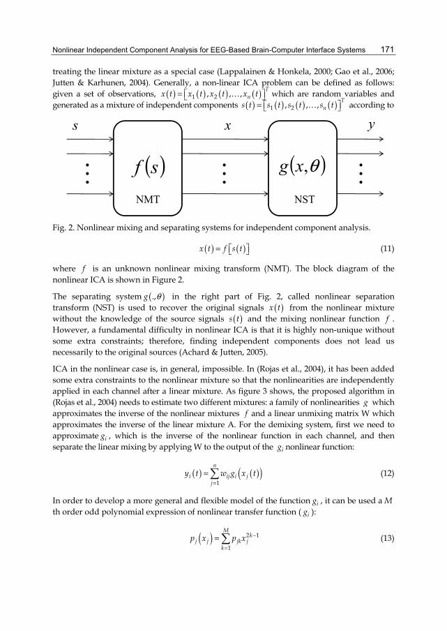
Nonlinear Independent Component Analysis for EEG-Based Brain-Computer Interface Systems 171
treating the linear mixture as a special case (Lappalainen & Honkela, 2000; Gao et al., 2006; Jutten & Karhunen, 2004). Generally, a non-linear ICA problem can be defined as follows: given a set of observations, ( ) ( ) ( ) ( )1 2, , , T
nx t x t x t x t= which are random variables and generated as a mixture of independent components ( ) ( ) ( ) ( )1 2, , , T
ns t s t s t s t= according to
( )θ,xg( )sfNMT NST
xs y
Fig. 2. Nonlinear mixing and separating systems for independent component analysis.
( ) ( )x t f s t= (11)
where f is an unknown nonlinear mixing transform (NMT). The block diagram of the nonlinear ICA is shown in Figure 2.
The separating system ( ).,g θ in the right part of Fig. 2, called nonlinear separation transform (NST) is used to recover the original signals ( )x t from the nonlinear mixture without the knowledge of the source signals ( )s t and the mixing nonlinear function f . However, a fundamental difficulty in nonlinear ICA is that it is highly non-unique without some extra constraints; therefore, finding independent components does not lead us necessarily to the original sources (Achard & Jutten, 2005).
ICA in the nonlinear case is, in general, impossible. In (Rojas et al., 2004), it has been added some extra constraints to the nonlinear mixture so that the nonlinearities are independently applied in each channel after a linear mixture. As figure 3 shows, the proposed algorithm in (Rojas et al., 2004) needs to estimate two different mixtures: a family of nonlinearities g which approximates the inverse of the nonlinear mixtures f and a linear unmixing matrix W which approximates the inverse of the linear mixture A. For the demixing system, first we need to approximate ig , which is the inverse of the nonlinear function in each channel, and then separate the linear mixing by applying W to the output of the ig nonlinear function:
( ) ( )( )1
n
i ij i jj
y t w g x t=
= (12)
In order to develop a more general and flexible model of the function ig , it can be used a Mth order odd polynomial expression of nonlinear transfer function ( ig ):
( ) 2 1
1
Mk
j j jk jk
p x p x −
== (13)

Independent Component Analysis for Audio and Biosignal Applications 172
where 1 2, , ,j j j jMp p p p = is a parameter vector to be determined. By using relations (12) and (13), we can write the following criterion for the output sources iy :
x
nf
1f
2f
ng
2g
1g
wAS Y
Fig. 3. Post-nonlinear mixing and demixing models for independent component analysis.
( ) 2 1
1 1.
n Mk
i ij jk jj k
y t w p x −
= == (14)
The parameter vector jp should be determined so that the inverse of the mutual information of the output sources iy is maximized. To achieve this objective, can be defined the following criterion (Rojas et al., 2004):
( ) ( )1_eval function y
I y= (15)
Nevertheless, computation of the parameter vectors jp is not easy, as it presents a problem with numerous local minima when the usual BSS cost functions are applied. Thus, we require an algorithm that is capable of avoiding entrapment in such a minimum. As a solution, in this work, a genetic algorithm (GA) (Goldberg, 1989) was used for mutual information optimization. Unlike many classical optimization techniques, GA does not rely on computing local first- or second-order derivatives to guide the search process; GA is a more general and flexible method that is capable of searching wide solution spaces and avoiding local minima (i.e., it provides more possibilities of finding an optimal or near-optimal solution). To implement the GA, we use genetic algorithm and direct search toolbox for use in Matlab (The Mathworks, R2007b).
The linear demixing stage has been performed by the well-known Infomax algorithm (Hyvarinen et al., 2001). To be precise, Infomax has been embedded into the GA in order to approximate the linear mixture.
In this application, the genetic algorithm is run for 30 generations with population size of 20, crossover probability 0.8, and uniform mutation probability of 0.01. The number of individuals that automatically survive to the next generation (i.e., elite individuals) is selected to be 2. The scattered function is used to create the crossover children by creating a random binary vector and selects the genes where the vector is a 1 from the first parent, and the genes where the vector is a 0 from the second parent.

Nonlinear Independent Component Analysis for EEG-Based Brain-Computer Interface Systems 173
4. Experimental setup The EEG data of healthy right-handed volunteer subjects were recorded at a sampling rate of 256 from positions Cz, T5, Pz, F3, F4, Fz, and C3 by Ag/AgCl scalp electrodes placed according to the International 10-20 system that has been shown in Fig. 4. The eye blinks were recorded by placing an electrode on the forehead above the left brow line. The signals were referenced to the right earlobe.
Data were recorded for 5 s during each trial experiment and low-pass filtered with a cutoff 45 Hz. There were 100 trails acquired from each subject during each experiment day. At
2 st = , a cross (“+”) was displayed on the monitor of computer as a cue visual stimulus. The subjects were asked to imagine the hand grasping in synchronization with the cue and to not perform a specific mental task before displaying the cue. In the present study, the tasks to be discriminated are the imaginative hand movement and the idle state. The experimental setup has been shown in Fig. 5.
Fig. 4. The international 10-20 system
Fig. 5. Experimental Setup

Independent Component Analysis for Audio and Biosignal Applications 174
Eye blink artifact was suppressed by using independent component analysis. The artifactual independent components were visually identified and set to zero. This process has been shown in Fig. 6.
(a)
(b)
F3C
zT5
Pz
F4Fz
C3
0 200 400 600 800 1000 1200
Blin
k
Time (ms)

Nonlinear Independent Component Analysis for EEG-Based Brain-Computer Interface Systems 175
(c)
Fig. 6. (a) Raw EEG signals, (b) ICA components, (c) EEG signals after eye blink removal.
5. Results The nonlinear ICA algorithm, proposed in (Rojas et al., 2004), was applied to given training 7-channel EEG data sets associated to the hand movement imagination and resting state. Original features are formed from 1 second interval of each component, in the time period 2.3–3.3 seconds, during each trial of experiment. The window starting 0.3 seconds after cue presentation is used for classification. The number of local extrema within interval, zero crossing, 5 AR parameters, variance, the mean absolute value (MAV), and 1Hz frequency components between 1 and 35Hz constitute the full set of features with size 44. The classifier is trained to distinguish between rest state and imaginative hand movement. The imaginative hand movement can be hand closing or hand opening. From 200 data sets, 100 sets are randomly selected for training, while the rest is kept aside for validation purposes. Training and validating procedure is repeated 10 times and the results are averaged.
Multiple classifiers are employed for classification using extracted components obtained by linear and nonlinear ICA. The Multiple Classifiers are used if different sensors are available to give information on one object. Each of the classifiers works independently on its own domain. The single classifiers are built and trained for their specific task. The final decision is made on the results of the individual classifiers. In this work, for each component, separate classifier is trained and the final decision is implemented by a simple logical majority vote function. The desired output of each classifier is −1 or +1. The output of classifiers is added and the signum function is used for computing the actual response of the classifier. The diagonal linear discrimination analysis (DLDA) (Krzanowski, 2000) is here considered as the classifier. The classifier is trained to distinguish between rest state and imaginative hand movement. The block diagram of classification process is shown in Fig. 7.
F3C
zT5
Pz
F4Fz
C3
0 200 400 600 800 1000 1200
Blin
k
Time (ms)

Independent Component Analysis for Audio and Biosignal Applications 176
Original Feature Creation Classification
Original Feature Creation
Classification
Original Feature Creation
Classification
EEG Ch-1
EEG Ch-2
EEG Ch-n
Nonlinear-ICA
Algorithm +
-
Com-1
Com-2
Com- m
Fig. 7. The block diagram of classification process.
The results have been recorded for four subjects (AE, ME, BM, SN) for different experiment days. Table 1 summarizes the results of classification accuracy of the original EEG signals. The average classification accuracy is 73.84%.
Table 2 summarizes the results of classification accuracy for different subjects by using linear ICA. For these experiments, the Infomax algorithm (Hyvarinen et al., 2001) as a linear ICA has been used. The average classification accuracy over all subjects is 74.61% which 1% better than that obtained original EEG signals. An average classification rate of 77.95% is achieved by using nonlinear ICA. As can be observed, components which are obtained by nonlinear ICA improved the EEG classification accuracy compared to the linear ICA and original EEG signals. These results are 4 percent higher than average classification results by using the raw EEG data. Fig. 8 shows the classification accuracy rate obtained by nonlinear ICA (NICA), linear ICA (LICA), and original EEG signals (channel).
Fig. 8. Mean classification accuracy of EEG patterns for different subjects using nonlinear ICA (NICA), linear ICA (LICA), and original EEG signals (channel).
AE ME BM SN60
65
70
75
80
85
Subject
Cla
ssifi
catio
n ac
cura
cy (%
)
NICALICAChannel

Nonlinear Independent Component Analysis for EEG-Based Brain-Computer Interface Systems 177
mean DAY5 DAY4 Day3Day2 DAY1 Subject
78.27 - 83.9 75.5 76.4 77.3 AE
74.65 -73.8 74.6 84.9 65.3 ME
74.75 -75.2 66 90.6 67.2 BM
67.7 64.169.4 61.6 66.1 77.4 SN
73.84 64.1 75.57 69.42 79.5 71.8 mean
Table 1. Classification Accuracy Rate of Original EEG Signals During Hand Movement Imagination.
mean DAY5 DAY4 Day3 Day2 DAY1 Subject
79.37 - 81.4 77.9 81.9 76.3AE
75.27 - 71.1 77.2 84.1 68.7 ME
73.97 - 72.5 63 93.3 67.1 BM
69.86 67.667.6 64.1 71.1 78.9 SN
74.61 67.6 73.1570.55 82.672.75mean
Table 2. Classification Accuracy Rate of Extracted Components During Hand Movement Imagination using Linear ICA.
mean DAY5 DAY4 Day3 Day2 DAY1 Subject
81 - 85.3 80.1 81 77.6AE
75.47 - 72 76.6 80.5 72.8 ME
78.6 - 76.2 69 93 76.2 BM
76.74 7272.5 81.7 79 78.5SN
77.95 72 76.576.85 83.3876.28mean
Table 3. Accuracy Rate of Extracted Components During Hand Movement Imagination using Nonlinear ICA.
6. Conclusion Preprocessing plays an important role in the performance of BCI systems. One of the preprocessors can be used to improve the performance of BCI systems is independent component analysis (ICA). ICA would appear to be able to separate task-related potentials from other neural and artifactual EEG sources during hand movement imagination in form of independent components. However, there is no guarantee for linear combination of brain

Independent Component Analysis for Audio and Biosignal Applications 178
sources in EEG signals. Therefore, in this research a novel method was proposed for EEG signal classification in BCI systems by using non-linear ICA algorithm. The results of applying this method on four subjects have demonstrated that the proposed method in this research has improved the mean classification accuracies in relation to raw EEG data and linear ICA. The analysis of variance (ANOVA) shows that the mean classification accuracies achieved by using non-linear ICA are significantly different ( 0.01).p <
7. Future directions There are a number of directions in which the research described in this chapter can be extended. One area currently under investigation is to design a non-linear model for separation of nonlinearly mixed sources in the brain. As clarified in this chapter, a fundamental difficulty in nonlinear ICA is that it is highly non-unique without some extra constraints. Now, the question is which extra constraints can more compensate the information distorted by the non-linear combination of brain sources. Answering to this question will be our future work.
8. References Achard, S.; Jutten, C. (2005). Identifiability of Post-Nonlinear Mixtures, IEEE Trans. Signal
Processing Letters, vol. 12, no. 5, pp. 423-426. Akbari, R. & Ziarati, K. (2010). A multilevel evolutionary algorithm for optimizing
numerical functions, International Journal of Industrial Engineering Computations, Vol. 2, no. 2, pp. 419– 430.
Almeida, L.B. (2003). MISEP – Linear and Nonlinear ICA Based on Mutual Information, Journal of Machine Learning Research 4, pp. 1297-1318.
Gao, P.; Woo, W.L. & Dlay, S.S. (2006). Non-Linear Independent Component Analysis Using Series Reversion and Weierstrass Network, IEE Proc., Vis. Image Process, Vol. 153, no. 2, pp.115– 131.
Goldberg, D. E. (1989). Genetic Algorithms in Search , Optimization and Machine Learning. Addison-Wesley.
Hyvarinen, A.; Karhunen, J. & Oja, E. (2001). Independent Component Analysis, John Wiley & Sons.
Hyvarinen, A. & Pajunen, P. (1999). Nonlinear Independent Component Analysis Existence and Uniqueness Results, Neural Network, Vol. 12, no. 3, pp.429-439.
Jung, T.; makeig, S.; humphiers, C.; Lee, T.; Mckeown, M. & Sejnowski, T. (2000). Removing Electroencephalographic Arifacts by Blind Source Separation, Psychophysiology, pp. 163- 178.
Jung, T.; makeig, S.; Westerfield, M.; Townsend, J. ; Courchesne, E. & Sejnowski, T. (2001). Analysis and Visualizion of Single-Trial Event-Related Potentials, Human Brain Mapping, vol. 14, pp. 166-185.
Jutten, C. & Karhunen, J. (2004). Advances in Blind Source Separation (BSS) and Independent Component Analysis (ICA) for Nonlinear Mixtures, International Journal of Neural Sysytems, vol. 14, no. 5, pp. 267-292.

Nonlinear Independent Component Analysis for EEG-Based Brain-Computer Interface Systems 179
Krzanowski, W. J. (2000). Principles of Multivariate Analysis: A User's Perspective, Oxford University Press, Oxford.
Lappalainen, H. & Honkela, A. (2000). Bayesian Nonlinear Independent Component Analysis by Multi-Layer Perceptrons, In Advances in Independent Component Analysis, pp. 93-121.
Lotte, F. & Cuntai Guan (2011). Regularizing Common Spatial Patterns to Improve BCI Designs: Unified Theory and New Algorithms, IEEE Transactions on Biomedical Engineering, vol. 58, no. 2, pp. 355-362.
Ortner, R.; Allison, B.Z.; Korisek, G.; Gaggl, H. & Pfurtscheller, G. (2011). An SSVEP BCI to Control a Hand Orthosis for Persons With Tetraplegia, IEEE Transactions on Neural Systems and Rehabilitation Engineering, vol. 19, no. 1, pp. 1-5.
Oveisi, F. (2009). EEG Signal Classification Using Nonlinear Independent Component Analysis, in Proceedings of the 34th IEEE International Conference on Acoustics, Speech, and Signal Processing (ICASSP).
Oveisi, F. (2009). Information Spectrum and Its Application to EEG-Based Brain-Computer Interface, in Proceedings of the 4th International IEEE EMBS Conference on Neural Engineering, Antalya, Turkey.
Oveisi, F. & Erfanian, A. (2008). A Minimax Mutual Information Scheme for Supervised Feature Extraction and Its Application to EEG-based brain-computer Interfacing, EURASIP Journal on Advances in Signal Processing, vol. 2008.
Oveisi, F.; Oveisi, S.; Erfanian, A.; Patras, I. (2012). Tree-Structured Feature Extraction Using Mutual Information, IEEE Transactions on Neural Networks and Learning Systems, Vol. 23, no. 1, pp.127-137.
Peterson, D. A.; Knight, J. N.; Kirby, M. J.; Anderson, C. & Thaut, M. (2005). Feature Selection and Blind Source Separation in an EEG-Based Brain-Computer Interface, EURASIP Journal on Applied Signal Processing, vol. 19, pp. 3128–3140.
Rojas, F.; Puntonet, C.; Alvarez, M.; Rojas, I. & Clemente, R. (2004). Blind Source Separation in Post-Nonlinear Mixtures Using Competitive Learning, Simulated Annealing, and a genetic algorithm, IEEE Trans. Systems, Man, and Cybernetics., vol. 34, no. 4, pp. 407-416.
Singer, A. & Coifman, R. R. (2007). Non-linear independent component analysis with diffusion maps, Applied and Computational Harmonic Analysis, vol. 25, pp. 226-239.
Tan, Y.; Wang, J. & Zurada, J. M. (2001). Nonlinear Blind Source Separation Using a Radial Basis Function Network, IEEE Trans. on Neural Networks , vol. 12, no. 1, pp. 124-134.
Van, L.; Wu, D. & Chen, C. (2011). Energy-Efficient FastICA Implementation for Biomedical Signal Separation, IEEE Trans. on Biomedical Engineering , vol. 58, no. 6, pp. 1865-1873.
Woo, W.L. & Sali, S. (2002). General Multilayer Perceptron Demixer Scheme for Nonlinear Blind Signal Separation, IEE Proc., Vis. Image Process, Vol.149, no. 5, pp.253–262.

Independent Component Analysis for Audio and Biosignal Applications 180
Zhang, K. & Chan, L. (2007). Nonlinear Independent Component Analysis with Minimal Nonlinear Distortion, 24th International Conference on Machine Learning, New York, USA.

0
Associative Memory Model Based in ICAApproach to Human Faces Recognition
Celso Hilario, Josue-Rafael Montes, Teresa Hernández,Leonardo Barriga and Hugo Jiménez
CIDESI- Centro de Ingeniería y Desarrollo IndustrialMéxico
1. Introduction
The human-like activities have been representing a research topic in several areas, which try tounderstand the internal processes involved. However, the complexity and the diversity of thissituation has allowed to propose approaches of different areas. These approaches pretend toimitate via simulation/emulation particular behaviors. Human perception as information ofan acquiring process and brain data manipulation process approach represent two open tasksin pattern recognition analysis. Human Face Recognition (HFR) involves two approaches.The main overcome is given by a set of adequate features to characterize a human face imageand multiple situations involved in the recognition process.
HFR is typically performed by the use of previous well-known features and a set of classifiers;both of them used to define a criterion for clustering and classifying each set of features.However, these features are not completely invariant on different environment conditions aswell as changes of perspective, luminance conditions and shadows generation. The majorityof existent approaches are limited and conditioned to specific scenario conditions, where facefeatures are well-behaved. In this sense, there are approximations as Santini & Jain (1999);Zhang & Zhang (2010); Zhao et al. (2003) ,where the authors show several criteria, focused onthe human face features and its invariance to different scenario conditions.
On the other hand, the classifiers used for clustering human face characteristics are deeplydependable on the feature behavior; i.e. over the space of features, faces with high degreeof similarity are spread in cumulus; then these cumulus are feasible for clustering via anygrouping criterion. In this scenario, the most representative approaches include Abdelkaderet al. (2001); Aggarwal & Cai (1999); Collins et al. (2002); Duda et al. (2000), where differentclustering criteria for human face recognition are shown. Note the foundations and paradigmsused are different, and consequently the results obtained are distinct in similar scenarios.Different approaches are similar in the point of each one proposed a new way to discriminateinformation that results independent1 one of the other. One well-accepted classifier describedabove are the associative memories . The associative memory approach is a connective one;which uses the linearity expressed in data set as well as a linear transformation. This approachusually is refereed as a kind ofNeural Network. In several scenarios it could represent a robust
1 Independent term is referred to the disposition of different measures that results different among themunder certain well-defined operators
9
2 Will-be-set-by-IN-TECH
approach because it supports the interference of noise in the data Duda et al. (2000); Minsky &Papert (1987). Some of the most distinctive works done around associative memories includeHopfield (1982); Kosko (1998); Polyn & Kahana (2008). The majority of current AssociativeMemories approaches use a binary representation or some discrete scenarios, where thecoding process consists on symmetric representation models. This situation might be a limitto express robust classifiers.
Finally, other approaches make emphasis in the mixture of a set of features and clusteringapproaches. Some of the most significant works are Ben et al. (2002); Bray (2005); Giese& Poggio (2000), where the authors explicitly show criteria to define human features and acluster approach to group each class.
In this work, we present a different way to figure out the problem of face recognition. Theproposal consists on consider the problem of HFR as an associative task. Face variationsrepresent the data mixed with noise. Then, the proposal consists of an heterogeneous process,where each different codification face represents a class and its variations the data versionsmixed with noise. The associative process expands traditional approaches, due to this ituses two ways of independence: the linear independence and the probabilistic independence.Both of them are deeply based on the superposition property of signal analysis Books (1991).Finally, the proposal has been tested with a data base of faces. This data base considersdifferent face position, luminance conditions and face gesticulation.
2. Foundations
In this chapter, we describe main concepts, where our proposal is based. In the firststage a description of the independence data concept viewed on different areas and whichcharacteristics are important to take care of. In second part is introduced the concept of linearindependence and its main properties. Finally, in the third part, the statistical independenceis introduce and its main properties.
2.1 Data independence
The concept of independence in several areas is related to the idea of analyzing when certainevents or objects are exclusive; i.e. there is no affectation in the behavior of any interactingobjects. Typically, the independence, according to the area of research is oriented of thetheoretical foundations used to express and measure it. The independence is close relatedwith its opposite, the dependence concept. Both definitions are completely dependable of theinformation representation and the way of operate it. This fact implies, the way of measureindependence/dependence is strictly related of what characteristic or form to manipulateinformation is used. For instance, two algebraic expression may be linear dependentTomasi(2004); but it does not imply being statistical dependentDuda et al. (2000), nor grammaticallydependent too. Analyzing several dependence definitions, there are common characteristicssurrounding the concept. These characteristics are:
1. A well-defined domain , which is usually mapped to an order/semiorden relationship2.
2. A representation of data structure.
3. An operator to determine the independence/dependence.
2 It could be discrete or continuous.
182 Independent Component Analysis for Audio and Biosignal Applications

Associative Memory Model Based in ICA Approach to Human Faces Recognition 3
4. An operator to mix independent data.
The first one is achieved with the aim to declare an explicit order in the work space. Thisorder establishes basic foundations to other operators. The second property is focusedto any data needs of a representation to figure out certain behaviors, which defines theinterdependence and dependency of the data.The next property consists on an explicitoperator or set of properties which define, for a particular space, which is the criteria ofdependence/independence using the last two points above mentioned. Finally, the lastproperty represents an operator as a Cartesian product like, which defines the rules of mixingtwo independent datum.
2.2 Linear independence
Firstly, a first kind of independence is discussed. It is linear independence. Linear algebra is abranch that studies vector spaces (also called linear spaces) along with linear maps, mappingsbetween vector spaces that preserve the linear structure. Because vector spaces have bases,matrices can be used to represent both vectors and linear transformations, this facilitatescomputation andmakes vector spaces more concrete. Linear algebra is commonly restricted tothe case of finite-dimensional vector spaces, while the peculiarities of the infinite-dimensionalcase are traditionally covered in linear functional analysis.
In linear algebra, a family of vectors is linearly independent if none of them can be writtenas a linear combination of finitely many other vectors in the collection. A family of vectorswhich is not linearly independent is called linearly dependent. This is, two or more functions,equations or vectors f1, f2, . . . , fn which are not linearly dependent can not be expressed inthe form
a1 f 1+a2 f2 + . . .+ an fn = 0 (1)
with a1, . . . , an constants which are not zero values.
The linear dependence of vectors is defined from basic operators in the algebra: Summationof two vectors and scalar product. Both of them in combination of basic structure elementsderive in concepts (like rank, determinant, inverse, Gauss diagonalizing), used to test thedependence of two vectors.
Associative Memories encode information as matrices; which make emphasis in lineardependent methods to group classes, and linear independent to discriminate among vectors.
2.3 Probabilistic independence
Probability independence is the second independence criterion. Probabilistic theory is thebranch of mathematics concerned with probability, the analysis of random phenomena. Thecentral objects of the probability theory are randomvariables, stochastic processes, and events:mathematical abstractions of non-deterministic events or measured quantities that may eitherbe single occurrences or evolve over time in an apparently random fashion.
In probability theory, to say that two events are independent intuitively means that theoccurrence of one event makes it neither more nor less probable that the other occurs.Similarly, two random variables are independent if the conditional probability distributionof either given the observed value of the other is the same as if the other’s value had not
183Associative Memory Model Based in ICA Approach to Human Faces Recognition

4 Will-be-set-by-IN-TECH
been observed. The concept of independence extends to dealing with collections of more thantwo events or random variables. Formally, this definition says: Two elements A and B areindependent if only if
Pr(A⋂
B) = Pr(A)Pr(B) (2)
Here A⋂
B is the intersection of A and B, that is, it is the event that both events A and B.
This kind of independence is oriented to the data probability of occurrence in the data domain.Note the probabilistic independence analyzes the form and behavior of the probabilisticdensity function (pdf) of a given data; which results totally different to the linear assumptionof a linear combination before described. This kind of independence is focused on match therange domain distribution. In pattern recognition it usually becomes useful, because a pdf ofan event represent the data variation representation of events with small affectations.
3. The proposal
The actual work is focused in the case of Human Face Recognition (HFR), where a new wayof classification and recognition based on the concept of independence is proposed. In thissection is described the process of the information coding for distinctive feature identificationand the associative model used to classify the different faces.
3.1 Information coding
Decision process given a set of evidence of a cluster of classes is dependable of data coding.The capabilities of clustering are deeply dependable of the information coding process andthe expressiveness of information encoded. Several authors has proposed different methodsfor classifying the information Chaitin (2004); Shannon & Weaver (1949). This classificationusually is based on a numerical criterion to define an order relationship over a descriptorspace; which is conformed with the characteristic measured. Typically the clustering consistson define any distance function and the establishment of a radius-like criterion; to choosewhich elements belongs to a particular class Duda et al. (2000). However they are limited bythe distribution of the information coding and the expressiveness of information coding.
The problem of face recognition should be viewed as a pattern recognition process; howeveras it was comment above, it consists on select a previouslywell-knowndescriptor, carrying thelimitations described in above paragraphs. Then, generalizing, we need to define a clusteringcriterion without explicit descriptors. Consequently, the descriptors must be located withoutexplicit knowledge of scenario. According to our proposes, we use a set of descriptors whichcontains the normalized distances of features. These features result of estimate the derivativesof order n of the distance matrix as is described as follows.
Given an image I(x), indexed by the vector position x, such that it contains a face. Image will
be operated with gradient operator (n)k I(x). The k parameter denotes the parameters of the
derivative approach used to estimate it, and (n) is the order of the operator. Furthermore, the
derivative is normalized from m× n size to m′ × n′, which is represented by I ′(x) = (n)k I(x).
The dimension m′ × n′ will be fixed by subsequent images to be analyzed. Using I ′(x), adistance matrix is built, representing the derivatives as a long vector of m′n′ dimension by
184 Independent Component Analysis for Audio and Biosignal Applications

Associative Memory Model Based in ICA Approach to Human Faces Recognition 5
linking of each row of the image derivative as follows
Md(i, j) = dk(I′(i), I′(j)) (3)
for all i, j positions in I′(x) which is the version as vector of I ′(x); dk is any given distancefunction defined and Md is a square matrix of m′n′ × m′n′. Matrix Md is used as a set ofdescriptors of each face.
Gradient operator (n)k provides information of pixel’s intensities variations, which they
indicates pixel the degree of texture and border information in the images. Note this operatorresults invariant at diffuse light sources. Additionally, matrix distance Md is dependable of dkdistance function based on Lk norm; i.e. values of k less than 1 increases the sparseness thedata on Md, and values greater than 1 for k decreases the sparseness of data.
3.2 Associative memory
In this section we describe the proposal of a new kind of associative memory based in linearand statistical independence.
3.2.1 The principles
Associative models consist on build a modelM such that for a pair of set A and B create arelationshipR : A → B. Being strictly the R relation has a property where a pair of elements(a, b) ∈ A×B, and the elements with almost a distance criteria da inA and db in B are relatedtoo; i.e. elements with a small similarity with a pair (a, b) ∈ A××B are related in the sameway. Typically the memories are classified according to the nature of associated sets: whenA = B memory is named as auto associative; when A = B is named as hetero associative;when |A| > |B| is considered as a classifier and finally, when |A| ≤ |B| is considered as atransducer Knuth (1998) or codifier Shannon & Weaver (1949).
Model M is build usually with a few samples (commonly named as learning or trainingsamples). Being strictly, there is no particular expressionswhich decide over related elements;instead, the process is well-based in theoretical foundations. M is build attending the maintheoretical foundations which define the class of the memory used. The nature of the majoritymodelsM are based in connective approaches, and consequently, it express a lineal mixtureamong inputs and outputs. The quality of learning process depends on the capabilities ofassociate with fewer errors the training samples and it will be used as good estimators fornon-considered pair of elements in the relationship Minsky & Papert (1987); Trucco & Verri(1998).
However, even the learning process results robust, there are situations where the linearityexpressed by the inputs and outputs results insufficient for establish a relationship betweenthem. In sections described above we speak about the independence concept. Then, definea theoretical framework which uses several independence criteria should be beneficial todevelop better modelsM and consequently better associative models.
The aim contribution of this work consists on a new model of Associative Memory basedon real domain and the mixing of two different approaches of independence: the linealindependence and statistic independence. The proposal works under the assumption that two
185Associative Memory Model Based in ICA Approach to Human Faces Recognition

6 Will-be-set-by-IN-TECH
signal can be mixed/unmixed if we know the structure of the distribution of each signal. Ourapproach works with large vectors, such that the distribution of the data inputs that conformthe event encoded can be estimated.
An associative Memory have at least two operators: similarity operator, which indicates theradio of match with some class previously learned; and belonging operator, which verifies thedata previously encoded in the memory. Additionally, an scheme to learn and estimate eachclass is needed. In further paragraphs the proposal is showed, which one mixes two kind ofindependences: the linear and statistic. Both of them are used to define a framework whichassociates inputs and outputs.
Given a set of information sources S1, . . . , Sn, the data contained in all signals should bemixed. This fact becomes true whenever sensing process is related and should be affectedby the same external variables. A first consideration is, the true variables of the system arenot perceived directly; but we can assume that they are the result of any combination of themeasured signals. For simplicity, this combination is viewed as a linear combination. Then,from the sources S1, . . . , Sn, we can estimate each true variable as any linear combination asfollows
Ui =n
∑j=1
wijSj (4)
Consequently, to obtain simplicity the expression above can be rewriting as the dot productof wi vector with a vector S = [S1, S2, . . . , Sn], as Ui = wiST. After, as it is appreciated, in nsources, there are a maximum of Un variables, it leads to U = Wn×nST, for a particular timestamp t.
Then, unmixing and mapping this sources to well-behaved space becomes an overcomethat could be estimated as Independent Component Analysis problem; i.e. the realsource measurement must be considered as linear and statistically independent among eachcomponent. Under these assumptions, one way to estimate the independent variables couldbe done with and ICA approach. The approach consists on estimate a W matrix such thatmix/unmix the sources to orthogonal variables as follows
U = Wn×nXn×m (5)
where X = [S1, S2, . . . , Sn]T is a matrix composed with all information sources; W a square
matrix with the form of W = [w1, . . . ,wn ] for unmixing the sources in X and U represents aset of linear and statistical independent variables. The values of W are estimated iterativelyvia fast-ICA algorithm as it is showed in Table 1. Fast-ICA algorithm consists on detectthe orthogonal protections which maximize the information. The last one is measured vianeg-entropy, as an approach to the real measurement result from the calculus of systementropy. As it can be appreciated the algorithm is non-deterministic starting from randomvalues for each one wi projection; which each iteration is tunning in direction of maximuminformation.
Unfortunately, one of the greatest disadvantages consists on the transformation W separatesthe mixed data, but the output are not sorted. This cause, the use of any component sort ofreturned by ICA is totally dependable of the phenomenon nature. However, for our purposes
186 Independent Component Analysis for Audio and Biosignal Applications

Associative Memory Model Based in ICA Approach to Human Faces Recognition 7
Pseudo-Code
Estimate for each component wi in W as follows1. Initialize wi with random numbers.
2. Let w+i ← Exg(wT
i x) − Exg′(wTi x)w.
3. Let wi ← w+i
||w+i ||
4. If the convergence is not achieved, go back to 2.
Table 1. Pseudo-code of W estimation
Fig. 1. Data Measurement Sparseness; as it is appreciated the eigen-values are located in theprincipal orthogonal axis.
this property could be used for developing a similarity criterion as is described in furtherparagraphs.
3.2.2 Similarity criterion
The similarity criterion for the proposal is based on the information given in the matrix W.The orthogonal components expressed in W can not be sorted, but it is possible to weight thecontribution of each orthogonal component.
The weight process is done by analyzing the eigen-values of the matrix W. The relativemagnitude of each eingen-value is used as a contribution of each orthogonal axis. This is,factorizing W as UΣVT , where Σ is an square matrix and the diagonal vector [λ1, . . . ,λn] hasthe singular values ofW. The eigen-values Σ ofW are related with the rank and the sparsenessof each orthogonal component in the source space (see Figure 1). The most simple case ofsimilarity using ICA is defined for two different signals as the proportion between each oneof different eigen-values of the unmixing matrix W; i.e. formally is defined as
d(s1, s2) =λ2λ1
(6)
where W = U[
λ1 00 λ2
]VT , and W is estimated with the algorithm described in Table 1.
This similarity criterion is given for a pair of signals and can be interpreted as a degree oforthogonality existent in two components lineal and statistical independent; i.e. for a pair ofsignals s1 and s2 both of them are similar if and only if both s1 and s2 are linear and statisticaldependent. The degree of independence is measured with the proportion of the second and
187Associative Memory Model Based in ICA Approach to Human Faces Recognition

8 Will-be-set-by-IN-TECH
the first eigen-value. If the proportion is near to 0 means, means s1 and s2 are linear andstatistical dependent; i.e. they are similar. The proportion λ2
λ1provides a normalized measure,
and λ1 is a normalized factor. In other scenarios we can use directly λ2 as the degree ofsimilarity between s1 and s2. Note, for a not normalized distance d(s1, d2) = λ2, the expressionis a metric Santini & Jain (1999).
Next,the belonging operator must be defined using a similarity function (see Equation 6), as afunction ελ : Rn ×Rn → true, f alse, and its equation is defined as
ελ(s1, s2) = d(s1, s2) ≥ λ (7)
where s1 and s2 represent the data information of encoded event. This operator is performedwith the aim to decide when a given reference data s1 and testing data s2, correspond to thesame information encoded.
3.2.3 Memory architecture
In last section the similarity criterion and the belonging operator has been defined. In thissection we describe the architecture of an Associative Model based on last definition. Thefocus consists on use a set of representative data vectors, which represent the different classesof the memory. These vectors are matched with the data for a classification process using thebelonging operator. Learning and discovering process are discussed in follows section. Afterthis, we make the assumption that the representative classes are known.
The architecture of the Associative Memory proposed consists on given k classes denotedby Ψ1,Ψ2, . . . ,Ψn. Each class Ψi is denoted by a set of signals with the form Ψi =s1, s2, . . . , sk. Each signal si represents the events coding as a large vector fixed vectors.The process of encoding must warranty the best descriptors are encoded. For HFR purposes,it is assumed, the coding process described above has been used. We point out, thequality and properties of encoding process will affect the association capabilities. To getadequate results we emphasize that the information representation follows the propertiesof linear and statistical independence in the created relationships in the memory. The mostrepresentative information, of each class, is used as reference to match for discovering whichclass corresponds. For each Ψi there is a representative element denoted by the operatorEi(Ψi). This operator is defined in general terms as the expected information of class Ψi.The nature of this operator is stochastic, but it might change, according to the data nature anddistribution of coding data.
Then, the Associative Memory is defined by amatrix Ξ =
⎡⎢⎣
E(Ψ1)...
E(Ψk)
⎤⎥⎦, such that it is conformed
by all expected elements of each class Ψi. The matrix Ξ represent the Associative Memory.
Next, the memory needs an operator to verify when it contains a particular data. The operatorof belongings aforementioned, is extended to verify if a given data si expressed as vector, iscontained in any class of a memoryΞ. The operator is extended in twoways: the first variationreturn which elements has a certain degree of similarity with the testing data si. This operatorwill be useful when someone need to know what classes have closed similarity to the data si.
188 Independent Component Analysis for Audio and Biosignal Applications

Associative Memory Model Based in ICA Approach to Human Faces Recognition 9
The operator is expressed as
∈Λ(Ξ, sj) = εΛ(E(Ψi), sj) = true (8)
for j = 1, 2, . . . , k.
Note that it return a set with the most similar classes. Second variation return the most similarclass to our testing data sj. Then a variation of last operator consists on returning the classwhich has the minimum distance to the representative information of the class. Finally, theoperator is defined as
∈∗Λ(Ξ, sj) = mindi(E(Ψi), sj) (9)
for all E(Ψi) ∈ εΛ(E(Ψi), sj). (10)
Both operators are used to determine when a given data sj belongs to any learned class. Asfinal comments, the value of Λ is a threshold of belongings, and it is a parameter dependableof the scenario.
3.2.4 Learning process
Learning process, in an Associative Memories, consists on discover the relationships betweenA and B sets, and it usually is viewed as a class discovering process under a metric criteriondefined by the belonging operator (see Equation 7).
The class discovering process, in the associative memory, is achieved with a learning processthat needs a belongings threshold Λ. Note that the signal used has been normalized infrequency and length. Both assumptions help to operate them. For general purposes, it hasbeen considered only the automatic learning process, which results useful in several scenarios.For a given set of signals S1, . . . , Sn, the process of discovering the classes is performed asfollows.
The simplest case is whenever the process involves only one class. At the beginning, class Ψ1is an empty set. First signal S1 is added to the first class Ψ1 ← Ψ1
⋃S1 and consequently,Ξ = [Ψ1]
T. For further signals Si, they are added to set Ψ1 if and only if ∈∗Λ (Ξ, Si) = 1.
Generalizing for k classes, whenever ∈∗Λ (Ξ, Si) = 0, a new class Ψk is created, such thatΞ ← [Ξ,Ψk]
T, where Λ is a distance threshold among classes. The number of classes Ψk addedrepresents the different orthogonal concepts in the memory. Note that, if we had previouslyinformation of k classes, it became as a supervised learning process. Analogous case, if we hadnot previously information, it became as dynamic learning process. Additional to mention,if learning process is always computed, the expected value E(Ψi) for each class should bechanged, adapting dynamically to new data evidence.
In this point we need to define the E(Ψi) operator. In several cases the expected operator isdefined as the average; which is computed as the average of each component of all elementsin Ψi. Note that we make the assumption of Ψi elements are sparse over the feature spaceuniformly. However, when the data distribution does not follows an uniform distribution, itwill be insufficient. In this sense E(Ψi) becomes as the expected value. The computation canbe easily computed and estimated for each component. In this situation, the expected value iscomputed for each vector position. Note for the estimation of expected value, we need to haveenough evidence to approximate component distribution and estimate global maximum. Theexpected value needs that the learning data must be sparse uniformly in the feature space.
189Associative Memory Model Based in ICA Approach to Human Faces Recognition

10 Will-be-set-by-IN-TECH
Sample 1 2 3 4 5 6 7 8 9 10 11 12 13 14 Total# Pictures 24 11 23 10 25 26 18 15 30 10 24 40 14 32 302
Table 2. Number of postures per sample of data base used.
The Two last approaches discussed above would result useful; however data in Ψ couldresult affected by noise or might not being sampled uniformly. In this cases is needed amethod to dismiss this variations. One approach consists on eliminate the least significantorthogonal components in Ψi. Then, the filter process would be performed via PCA(Principal Component Analysis) approach. PCA approach consists on reconstruct the originalinformation only taking most significant linear components. The advantage of eliminatesmall components is that eliminate several redundancies making more compact and bettersparseness the learning evidence in the feature space.
For Ψi signal set is constructed a matrix D with each data vector transposed as follows
D = [ST1 ST
2 . . . STn ] for S1, S2, . . . , Sn signals in Ψi (11)
For dismissing the noise effects and sparse better the feature space a matrix D∗ is buildfactorizing D as UΣVT and build a matrix D∗ without least significant data. D∗ isreconstructed with as
D∗ = UΣ∗V (12)
where Σ∗ is equal to Σ, but with the difference that the lasted singular values σ∗l , σ∗l+1 . . . σ
∗n
are zero values and l value is estimated considering a percentage of original information.Proportion between summation of l principal component and summation of all componentsrepresents noise/signal ratio. Then election of l must define a percentage function of totalinformation used in data. The percentage of information represented with l singular values
is computed with % = ∑li=1 σi
∑nj=1 σj
. The election of l value, must be defined covering at least α
percentage of information as follows
I(α) = max argl|1, 2, . . . , n (13)
such that∑l
i=1 σi
∑nj=1 σj
≤ α
Finally D∗ = [(S∗1)T(S∗2)T . . . (S∗n)T ] represents filtered data and it will be applied any schemeto estimate the calculus of expected value for Ψi.
4. Experimental results
In this section, we describe an experimental method for validating the proposal. Thevalidation process consists on developing an Associative Memory to classify and to recognizeHuman Faces. The implementation details are given and described in follows sections.
4.1 Experimental model
Our proposal was tested with the development of Human Face recognition. The informationconsists on a data base of Human Faces. The data base includes different faces and differentfaces gesticulations. Figure 2 (a) shows samples of the data base. Each face in data base hasseveral poses and gesticulation. The variation of each face is important, because it is used in
190 Independent Component Analysis for Audio and Biosignal Applications

Associative Memory Model Based in ICA Approach to Human Faces Recognition 11
(a)
(b)
Fig. 2. Face data base: (a) some different samples contained in the data base; where (b) foreach sample, there is different face gesticulation.
the learning process, for extraction of the main features which characterize each face. Pictureswere taken with a Panasonic Lumix Camera at 7.1 Megapixels (3072× 2304) in RAW format.The number of photos and persons involved are appreciated in Table 2.
In Section 3.1, a scheme for encoding was presented. This process is applied to the differentfaces in the data base. For practical purposes, derivative of order 1 has been used for encodingand characterizing each face. Derivative has been implemented with a symmetrical maskd = [−10+ 1], which has assumed Gaussian. The parameters of Gaussian were fixed to μ = 0and σ = 1 with length 9, which define a Gaussian from −4 to 4 in normalized dimensions.Finally, the derivative filter was defined as F = [−G(0, 1)0 + G(0, 1)]9×19. The Gaussianresults beneficial due to, it allows dismiss noise effects in images.
Next, features descriptors were estimated with Equation (3). This equation needs anormalized version of I with m′ × n′ dimensions. The amount of information encoded in apattern is directly affected by dimension of normalized image. A first view, a fixed value isused to compute these patterns (32× 32 pixels). In a second stage, dimensions of normalizedversion has changed in follows dimensions: 8, 16, 24, 32, 40, 48, 56, 64, 96, 128, 160, 192 and 224.Then a matrix M of descriptors has been created as comment in Section 3.2.4. Image patternsrepresent the relationships among all pixels in the image border.
Process learning uses a set of patterns, as input. This process computes distinctive facepatterns. In Section 3.2.4 were described two approaches for estimating these patterns. Inour implementation, we only test with a single average. This consideration might be strictlysimple; but for our approach the average results enough for implementations purposes. Thisis, superposition principle, states that, for all linear systems, the net response at a given placeand time caused by two or more stimuli is the sum of the responses which would have beencaused by each stimulus individually. So that if input A produces response X and inputB produces response Y then input (A + B) produces response (X + Y); which for a simpleaverage is the same, factorizing by 1
n each term involved in sum operator Books (1991).
To illustrate this process, in Figure 3 are shown some faces patterns. This patterns werecomputed with normalized images of 16 × 16. As is appreciated, vertical and horizontallines provided information of distribution and behavior data for several faces. Note, imagedescriptor has a resolution of 162 × 162 resulted of distance image.
191Associative Memory Model Based in ICA Approach to Human Faces Recognition

12 Will-be-set-by-IN-TECH
Fig. 3. Samples of patterns estimated in learning process. Visual patterns represent innerrelations among features borders of each face.
0 1 2 3 4 5 6 7 8 9 10 11 12 13 140
0.2
0.4
0.6
0.8
1
Sample
% o
f R
eco
gn
itio
n
8×816×1624×2432×3240×4048×4856×5664×64
Fig. 4. Efficiency of recognition changing dimensions of normalized image.
4.2 Results and discussion
After computing a face pattern from each different sample, a memory is created as follows;
M =
⎡⎢⎣
E(Ψ1)...
E(Ψn)
⎤⎥⎦
192 Independent Component Analysis for Audio and Biosignal Applications

Associative Memory Model Based in ICA Approach to Human Faces Recognition 13
0 1 2 3 4 5 6 7 8 9 10 11 12 13 140
0.05
0.1
0.15
Eigen Value (σi)
Rel
ativ
e C
on
trib
uti
on
8×816×1624×2432×3264×64128×128224×224
Fig. 5. Samples of patterns estimated in learning process. Visual patterns represent innerrelations among features borders of each face.
where E(Ψ1) corresponds to a distinctive pattern of Ψ. Hence, an associative memory iscreated. For putting the memory on line, it only need to verify an encoded face and infer,which class encoded in M has less similarity and estimate its class. Note, an associativemodel is developed with the aim to infer which class has less similarity, so one must becareful because the class with less similarity additionally, need to follow a threshold similaritycriterion too. This is, even there is no exist a similar class, memory return most similar.
Then, the validation of memory is performedmeasuring the degree of accuracy of recognitionany face, to corresponding class. To perform it, all faces s1, s2, . . . , sn in data base are tested.Normalized image dimension has changed. Results are shown in Figure 4.
The level of recognition of our approach is over 85% with pattern sizes of 24× 24 and 32× 32.Note, for small sizes (8 and 16) of image patterns, and for considerable high dimensions, thememory miss classify (64 or more). This is, in the first case there is not enough information forchoosing which class is more similar. To justify this fact, a matrix of similarity has been createdwith patterns inmemory. Thematrix has 14× 14 dimensions and represent in pseudo color thesimilarity degree. White color represents high degree of similarity and black color representsno similarity. In fact, the face patterns are analyzed; hence, we expect the matrix similarityhas only similitudes in the diagonal. Then, Figure 6 (a) shows that degree of similarity amongclasses is small and it might cause miss classification problems. But when dimensions becomehigher, the degree of independence usually increases too, as is appreciated in Figure 6 (b) andFigure 6 (c), for 32 × 32 and 224 × 224 respectively. Additionally this can be verified withFigure 5, where principal components of patterns are computed and its relative contribution.Note, in higher sizes, they become more linear.
Intuitively, someone expect to be more accurate with high dimensions. However, note, theface recognition approach is based on a distance matrix, and associative memory approachis founded in two kind of independences: linear and statistical. Whenever data becomehigher, distribution of face patterns becomes similar, being not possible to classify. This pointis illustrated in Figure 7, where two pdf’s of different classes are estimated with 8× 8, 32× 32and 224 × 224 pattern size. Note all of them, are dissimilar at the beginning and becomesimilar when dimension of pattern is increased. This is, this approach is suitable for classeswell differentiated.
193Associative Memory Model Based in ICA Approach to Human Faces Recognition

14 Will-be-set-by-IN-TECH
Face
Fac
e
1 2 3 4 5 6 7 8 9 10 11 12 13 14
1
2
3
4
5
6
7
8
9
10
11
12
13
14
Face
Fac
e
1 2 3 4 5 6 7 8 9 10 11 12 13 14
1
2
3
4
5
6
7
8
9
10
11
12
13
14
Face
Fac
e
1 2 3 4 5 6 7 8 9 10 11 12 13 14
1
2
3
4
5
6
7
8
9
10
11
12
13
14
(a) (b) (c)
Fig. 6. Similarity matrix among classes for (a) normalized image of 8× 8; 32× 32 and224× 224.
−1 −0.5 0 0.5 1 1.5 20
0.02
0.04
0.06
0.08
0.1
0.12
0.14
0.16
0.18
Normalized Domain
Pro
bab
ility
−1 −0.5 0 0.5 1 1.5 2 2.50
0.01
0.02
0.03
0.04
0.05
0.06
0.07
0.08
0.09
Normalized Domain
Pro
bab
ility
(a) (b)
−1 −0.5 0 0.5 1 1.5 2 2.5 30
0.02
0.04
0.06
0.08
0.1
0.12
0.14
Normalized Domain
Pro
bab
ility
−1 0 1 2 3 40
0.02
0.04
0.06
0.08
0.1
0.12
Normalized Domain
Pro
bab
ility
(c) (d)
−1 0 1 2 3 4 50
0.02
0.04
0.06
0.08
0.1
0.12
0.14
Normalized Domain
Pro
bab
ility
−1 −0.5 0 0.5 1 1.5 2 2.5 3 3.50
0.02
0.04
0.06
0.08
0.1
0.12
0.14
Normalized Domain
Pro
bab
ility
(e) (f)
Fig. 7. Probabilistic density functions of two image patterns (a),(c),(e) and (b),(d),(f) withdimension 8× 8; 32× 32; and 224× 224.
194 Independent Component Analysis for Audio and Biosignal Applications

Associative Memory Model Based in ICA Approach to Human Faces Recognition 15
At this point, the miss classification effects when data become increased might be consideredas inconvenient; however, it is not true, because framework is operated under its basicassumptions, and it shows the limits of encoding process; i.e. we need to define a betterscheme to extract the most suitable features for face recognition which warrant linearindependence and probabilistic independence. Then, to define an optimums classifier weneed to consider the amount of information and its distribution associated to these data;however this point escape of the scope of this paper.
Summarizing, through this work, we propose a scheme for face recognition based on simpletexture features, which uses a new paradigm of associative machines based on ICA approach.Its main characteristics include the use of real domain for characterizing data, including twokinds of independence.
5. Conclusion
In this chapter, we discussed about the independence concept, as an approach to characterizeinformation by different features properties. Additionally, we pointed out the importance ofdifferent features when they are used to classify or discriminate certain events encoded. Thisfact results important to the well-development of classifier and coding process. Typically,common approaches are based on linear independence or statistical independence. Bothapproaches are distinct and measure different structure over data.
In this chapter, we proposed a new approach for classifying which take the advantage of bothkind of linearity. It becomes relevant because we offer a new approach that characterize morestrictly the information features used for data identification and data grouping. In this order,this work proposes a new family of associative memories, based on the ICA approach. Themain characteristics include a real domain in the data, tolerance to certain data variations, andthe association is given by the possibility of express each class as an orthogonal componentand probabilistic independent. Preliminary tests show the viability of use this approach asgeneral classifier being applicable in several research areas.
To test and validate the proposal, we implement a face recognizer application. It uses a basiccoding data based on the derivative of the image. This encoding analyses differences betweenface border and its texture. In our tested scenario, the proposal is capable to discover anddefine a correct correspondence between the face variations and its corresponding face. Intested scenarios and information used the conditions were varied with the aim to show therobustness of the approach.
6. Future directions
As comment above paragraphs, a new framework based on linear independence andstatistical independence is presented. Its main contributions are focused to the developmentof new kind of classifiers. This work exhibits the basis for new classifiers and recognizers.Further researches are focused to the application of this framework on different areas as signalanalysis, image analysis and areas where the amount of information and lack of predefinedfeatures might difficult its analysis. This involves tasks as information coding, which extractgood features and make more feasible the data manipulation.
Parallel, other areas of interest are related with the characterization of accuracy and efficiencyof this approach, and the theoretical foundations that express new operators based on thisproposal to manage in a better way the data.
195Associative Memory Model Based in ICA Approach to Human Faces Recognition

16 Will-be-set-by-IN-TECH
Finally, one last direction is focused on the analysis of the feasibility to implement thisapproach in hardware, making more efficient time process and its application in real timesystems.
7. References
Abdelkader, C., Cutler, R., Nanda, H. & Davis, L. (2001). EigenGait: Motion-BasedRecognition of People using Image Self-Similarity, Audio- and Video-Based BiometricPerson Authentication pp. 284–290.
Aggarwal, J. K. & Cai, Q. (1999). HumanMotionAnalysis: A Review, IEEE Journal on ComputerVision and Image Understanding 73(3): 428–440.URL: citeseer.ist.psu.edu/aggarwal99human.html
Ben, J., Wang, Z., Pandit, P. & Rajaram, S. (2002). Human Activity Recognition usingMultidimensional Indexing, IEEE Transactions on Pattern Analysis and MachineIntelligence 24(8): 1091–1104.
Books, P. (1991). The Penguin Dictionary of Physics, Penguin Books, Valerie Illingworth, London.Bray, J. (2005). Markerless Based Human Motion Capture: A Survey, Technical report, Brunel
University, Department System Engineering.Chaitin, G. (2004). Algorithmic Information Theory, Cambridge University Press. IBM Research
Center.Collins, R. T., Gross, R. & Shi, J. (2002). Silhouette-Based Human Identification from Body
Shape andGait, IEEE International Conference on Automatic Face and Gesture Recognitionpp. 351–356.
Duda, R. O., Hart, P. E. & Stork, D. G. (2000). Pattern Classification, 2nd. edition edn,Wiley-Interscience.
Giese, M. & Poggio, T. (2000). Morphable Models for the Analysis and Synthesis of ComplexMotion Patterns, International Journal of Computer Vision 38(1): 59–73.
Hopfield, J. J. (1982). Neural networks and physical systems with emergent collectivecomputational abilities, Proceedings of the National Academy of Sciences of the USA79(8): 2554–2558.
Knuth, D. (1998). Art of Computer Programming, Vol. 1, 2 edn, Addison-Wesley Professional.Kosko, B. (1998). Bidirectional associative memories, IEEE Transactions on Systems, Man, and
Cybernetics 8(11): 40–46.Minsky, M. L. & Papert, S. A. (1987). Perceptrons - Expanded Edition: An Introduction to
Computational Geometry, second edition edn, The MIT Press; Expanded edition.Polyn, S. & Kahana, M. (2008). Memory search and the neural representation of context.,
Trends in Cognitive Sciences 12: 24–30.Santini, S. & Jain, R. (1999). Similarity Measures, IEEE Transactions on Pattern Analysis and
Machine Intelligence 21(9): 871.Shannon, C. & Weaver, W. (1949). The Mathematical Theory of Communication, University of
Illinois Press.Tomasi, C. (2004). Mathematical Modelling of Continuos Systems, Duke University.Trucco, E. & Verri, A. (1998). Introductory Techniques for 3-D Computer Vision, 1 edn, Prentice
Hall.Zhang, C. & Zhang, Z. (2010). A survey of recent advances in face detection, Technical Report
MSR-TR-2010-66, Microsoft Research Microsoft Corporation.Zhao, W., Chellappa, R., Phillips, P. & Rosenfeld, A. (2003). Face recognition: A literature
survey, ACM Computing Surveys 35(4): 399–458.
196 Independent Component Analysis for Audio and Biosignal Applications

1. Introduction
In independent component analysis (ICA), it is assumed that the components of the observedk-dimensional random vector x = (x1, . . . , xk) are linear combinations of the components of alatent k-vector s = (s1, . . . , sk) such that s1, . . . , sk are mutually independent. This is denotedby
x = As, (1)
where A is a k× k full-rank non-random mixing matrix. The main objective then is to extractthe mixingmatrix through a set of observations x1, x2, . . . , xn. For a detailed description of thismethod, including its motivation, existence and relationship with other well known statisticalmethods such as principal component analysis, factor analysis, see Hyvärinen et al. (2001).
In signal processing applications, it will be convenient to view the observations as valuesrecorded at k locations over time periods 1, . . . , n. The number of locations k varies dependingon the application area. For instance, k = 2 in a blind source seperation problem to k ≈ 105 ina typical human brain imaging data set. The number of time points n also varies and it rangesfrom n ≈ 102 to n ≈ 106.
The spatial (location) and temporal (time) description of the data has generated a hugenumber of biomedical applications such as cognitive or genomic research. In this paper, wewill focus on human brain data acquired from functional magnetic resonance imaging (fMRI)technique where k ≈ 105 and n ≈ 102. This imaging technique has been used to effectivelystudy brain activities in a non-invasive manner by detecting the associated changes in bloodflow. Typically, fMRI data consists of a 3D grid of voxels; each voxel’s response signal overtime reflects brain activity. However, response signals are often contaminated by other signalsand noise, the magnitude of which may be as large as that of the response signal. Therefore,independent component analysis has been applied to extract the spatial and temporal featuresof fMRI data (Calhoun & Adali, 2006; McKeown et al., 1998).
For fMRI datasets, we remark that it is theoretically possible to search for signals thatare independent over space (spatial ICA) or time (temporal ICA). In fact, the above ICAdescription involving the spatial k and temporal n scales should be called more precisely as
Application of Polynomial Spline Independent Component Analysis to fMRI Data
Atsushi Kawaguchi1, Young K. Truong2 and Xuemei Huang3
1Biostatistics Center, Kurume University, Kureme, Fukuoka 2Department of Biostatistics, University of North Carolina at Chapel Hill, NC
3Department of Neurology, Penn State University, PA 1Japan
2,3USA
10

2 Will-be-set-by-IN-TECH
the temporal ICA, while in spatial ICA, k will be treated as time, and n as location. Thusone can see that temporal ICA is just the transpose of spatial ICA. However, in practice, it isvery difficult to obtain accurate and meaningful results from the temporal ICA of fMRI databecause of the correlation among the temporal physiological components. Therefore, the useof spatial ICA is preferred for fMRI analysis (McKeown et al., 1998).
Our ICA on fMRI data is carried out by first reducing the number of independent components(IC) using tools such as principal component analysis (PCA) or singular value decomposition(SVD), followed with an algorithm for determining the ICs. The most commonly used ICAalgorithms for analyzing fMRI data are Infomax (Bell & Sejnowski, 1995), FastICA (Hyvärinen& Oja, 1997), and joint approximate diagonalization of eigenmatrices (JADE) (Cardoso &Souloumiac, 1993). Calhoun & Adali (2006) reported that Infomax consistently yielded themost reliable results, followed closely by JADE and FastICA. In this study, we propose a novelICA algorithm that is a modification of the logspline ICA algorithm (LICA) (Kawaguchi &Truong, 2011) and apply it to fMRI data. In ICA,we employ a likelihood approach to search forICs by estimating their probability distributions or density functions (pdf). This is equivalentto maximizing the independence among ICs, and it is realized by using polynomial splines toapproximate the logarithmic pdf; we call this the logspline model. To account for the sparsityof spatial fMRI maps, we further treat the pdf as a mixture of a logspline and a logistic densityfunction; this approach has proven to be very effective for treating sparse features in data.Using simulated and real data, we compared our method with several well-known methodsand demonstrated the relative advantage of our method in extracting ICs.
The remainder of this paper is organized as follows. Section 2 describes the proposed method.Section 3 presents the simulation studies. Section 4 describes the application of the proposedmethod to real data. Finally, Section 5 presents discussions and concluding remarks of ourmethod.
2. Method
Let Y denote a T × V data matrix: each column of this matrix corresponds to a voxel timeseries, and there are V voxels and T time points. We invoke singular value decomposition(SVD) to yield the approximation Y ≈ UDX, where U is a T × M orthogonal matrix,D = diag(d1, d2, . . . , dM) with d1 ≥ d2 ≥ · · · ≥ dM, and X is an M × V orthogonal matrix.Here, we selected (orthogonal) columns of U to represent some experimental task functionsas well as the physiological components. In addition, the dimension of D has been reducedby discarding values below a certain threshold; in other words, these values are essentiallytreated as noise.
We determine the ICs based on the matrix X so that X = AS, where A is an M × M mixingmatrix and S is an M×V source matrix. That is, the v-th column of X is equal to A multipliedby the v-th column of S, where v = 1, 2, . . . , V. Equivalently, each column of X is amixture of Mindependent sources. Let Sv denote the source vector at voxel v so that Sv = (S1, S2, . . . , SM),v = 1, 2, . . . , V. Suppose that each Sj has a density function f j for j = 1, 2, . . . , M. Then, thedensity function of X can be expressed as fX(x) = det(W)∏M
j=1 f j(wjx), where W = A−1 andwj is the j-th row of W.
We now model each source density according to the mixture with unknown probability a:
f j(x) = a f1j(x) + (1− a) f2j(x), (2)
198 Independent Component Analysis for Audio and Biosignal Applications

Application of Polynomial Spline Independent Component Analysis to fMRI Data 3
where the logarithm of f1j(x) is modeled by using polynomial splines
log( f1j(x)) = C(βj) + β01jx +mj
∑i=1
β1ij(x− rij)3+,
with βj = (β01j, β11j, . . . , β1mj j) being a vector of coefficients, C(βj) a normalized constant, rij
the knots; and f2j(x) = sech2 (x) /2 is a logistic density function. Here (y)+ = max(y, 0).
We denote the vector of parameters in the density function by θ = (a, β). The maximumlikelihood estimate (MLE) of (W, θ) is obtained bymaximizing the likelihood of X with respectto (W, θ):
(W,θ) =n
∑i=1
k
∑j=1
log( f j(wTj xi)).
We use a profile likelihood procedure to compute the MLE because a direct computation ofthe estimates is generally not feasible. The iterative algorithm is shown in Table 1. Note that
1. Initialize W = I.2. Repeat until the convergence of W, using the Amari metric.
(a) Given W, estimate the log density gj = log f j for the jth element Xj of X (separately foreach j) by using the stochastic EM algorithm shown in Appendix 7.
(b) Given gj (j = 1, 2, . . . , p),
wj ← ave[Xgj′(wT
j X)]− ave[gj′′(wT
j X)]wj
where wj is the jth column of W and ave is a sample average over X.(c) Orthogonalize W
Table 1. Algorithm
the Amari metric (Amari et al., 1996) used in the algorithms is defined as
d(P,Q) =1
p(p− 1)
⎧⎨⎩
p
∑i=1
(∑
pj=1 |aij|
maxj |aij| − 1
)+
p
∑j=1
(∑
pi=1 |aij|
maxi |aij| − 1
)⎫⎬⎭ ,
where aij = (P−1Q)ij, P, and Q are p× p matrices. This metric is normalized, and is between0 and 1.
Several authors have discussed initial guesses for ICA algorithms. Instead of setting severalinitial guesses, as discussed in Kawaguchi & Truong (2011), X is multiplied by W, whichis the output of the algorithm when the log density function g(x) is replaced with g(x) =
1/2b1/bΓ(1+ 1/b) exp−|x|b/b with b = 3. The final output is obtained in the form W =
WW0, where W0 is the output of the algorithm shown in Table 1.
The purpose of spatial ICA is to obtain independent spatial maps and the correspondingtemporal activation profiles (time courses). By multiplying X with W, we can obtain theestimates of the spatial map S as S = WX. On the other hand, the corresponding time coursesare obtained in the form A = W(UD)−1.
199Application of Polynomial Spline Independent Component Analysis to fMRI Data
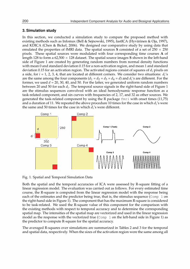
4 Will-be-set-by-IN-TECH
3. Simulation study
In this section, we conducted a simulation study to compare the proposed method withexisting methods such as Infomax (Bell & Sejnowski, 1995), fastICA (Hyvärinen & Oja, 1997),and KDICA (Chen & Bickel, 2006). We designed our comparative study by using data thatemulated the properties of fMRI data. The spatial sources S consisted of a set of 250 × 250pixels. These spatial sources were modulated with four corresponding time courses A oflength 128 to form a 62,500 × 128 dataset. The spatial source images S shown in the left-handside of Figure 1 are created by generating random numbers from normal density functionswithmean 0 and standard deviation 0.15 for a non-activation region, andmean 1 and standarddeviation 0.15 for an activation region. The activated regions consist of squares of di pixels ona side, for i = 1, 2, 3, 4, that are located at different corners. We consider two situations: di’sare the same among the four components (d1 = d2 = d3 = d4 = d) and di’s are different. For theformer, we used d = 20, 30, 40, and 50. For the latter, we generated uniform random numbersbetween 20 and 50 for each di. The temporal source signals in the right-hand side of Figure 1are the stimulus sequences convolved with an ideal hemodynamic response function as atask-related component, and sin curves with frequencies of 2, 17, and 32 as other sources. Wegenerated the task-related component by using the R package fmri with onset times (11,75)and a duration of 11. We repeated the above procedure 10 times for the case in which di’s werethe same and 50 times for the case in which di’s were different.
Comp 1 (Task) Comp 2
Comp 3 Comp 4
Fig. 1. Spatial and Temporal Simulation Data
Both the spatial and the temporal accuracies of ICA were assessed by R-square fitting of alinear regression model. The evaluation was carried out as follows. For every estimated timecourse, the R-square is computed from the linear regression model with the response beingeach of the estimates and the predictor being true, that is, the stimulus sequence (Comp 1 onthe right-hand side in Figure 1). The component that has the maximumR-square is consideredto be task-related. We used the R-square value of this component for the comparison withthe existing methods with respect to temporal accuracy and to determine the correspondingspatial map. The intensities of the spatial map are vectorized and used in the linear regressionmodel as the response with the vectorized true (Comp 1 on the left-hand side in Figure 1) asthe predictor to compute R-square for the spatial accuracy.
The averaged R-squares over simulations are summarized in Tables 2 and 3 for the temporaland spatial data, respectively. When the sizes of the activation region were the same among all
200 Independent Component Analysis for Audio and Biosignal Applications

Application of Polynomial Spline Independent Component Analysis to fMRI Data 5
Infomax fastICA KDICA PSICAd=50 0.627 0.852 0.679 0.843d=40 0.456 0.460 0.472 0.735d=30 0.408 0.463 0.424 0.586d=20 0.358 0.270 0.709 0.518
average 0.462 0.511 0.571 0.670rand 0.623 0.651 0.529 0.699
Table 2. Temporal R-square for simulation data. The mean over d = 20, 30, 40, and 50 iscalculated in the row labeled as average. The rand row shows the average over 50replications when di’s were chosen randomly from the range 20 to 50.
Infomax fastICA KDICA PSICAd=50 0.801 0.765 0.641 0.761d=40 0.462 0.502 0.545 0.726d=30 0.409 0.528 0.552 0.680d=20 0.323 0.478 0.624 0.587
average 0.499 0.568 0.591 0.688rand 0.537 0.607 0.579 0.643
Table 3. Spatial R-square for simulation data. The mean over d = 20, 30, 40, and 50 iscalculated in the row labeled as average. The rand row shows the average over 50replications when di’s were chosen randomly from the range 20 to 50.
components, R-squares of the proposed method were significantly larger than those of othersfor moderate sizes (d = 40 and 30) for both temporal and spatial data. For d = 50, fastICA hadthe largest R-square for both temporal and spatial data, with the difference from the resultof the proposed method being small. For d = 20, KDICA had the largest R-square for bothtemporal and spatial data, with the difference from the result of the proposed method beingsignificant for temporal data but not for spatial data. With respect to the average for d = 50,40, 30, and 20, the proposed method had the largest R-square value than the others did. Whendi was determined randomly, which might be more practical, we observed that the largestR-square value in the rand row of the table was achieved by the proposed method.
4. Application
To demonstrate the applicability of the proposed method to real data, we separate fMRIdata into independent spatial components that can be used to determine three-dimensionalbrain maps. To study brain regions that are related to different finger tapping movements,fMRI data were obtained from a twin pair (Twin 1 and Twin 2) performing different tasksalternately.The paradigm shown in Figure 2 consisted of externally guided (EG) or internallyguided (IG) movements based on three different finger sequencing movements performedalternately by either the right or the left hand.
The fMRI dataset has 128 scans that were acquired using amodified 3T SiemensMAGNETOMVision system. Each acquisition consists of 49 contiguous slices. Each slice contains 64×64voxels. Hence, each scan produces 64×64×49 voxels. The size of each voxel is 3 mm×3mm×3 mm. Each acquisition took 2.9388 s, with the scan-to-scan repetition time (TR) setto 3 s. The dataset was pre-processed using SPM5 (Friston et al., 1995). The preprocessing
201Application of Polynomial Spline Independent Component Analysis to fMRI Data

6 Will-be-set-by-IN-TECH
Fig. 2. Experimental Paradigm
included slice timing, realignment, and smoothing. We masked the image outside the humanhead using the GIFT software package (Group ICA of fMRI Toolbox, Calhoun et al., 2001). Weused 21 components for Twin 1 and 30 for Twin 2; these were estimated using the minimumdescription length (MDL) criteria.
We applied four ICA algorithms—Infomax (Bell & Sejnowski, 1995), fastICA (Hyvärinen &Oja, 1997), KDICA (Chen & Bickel, 2006), and the proposed method (PSICA)—to the twins’data. The R-square statistic was calculated from the fitted multiple linear regression modelwith the estimated time course as the response. The predictors were the right EG, right IG, leftEG, and left IG, which consists of the expected BOLD response for the task indicator functiongiven by the argument as a convolution with the hemodynamic response function modeledby the difference between two gamma functions. Table 4 shows the corresponding R-squarestatistics. From this table, we can see that the proposed method extracted more correlatedcomponents for a task than did the other methods for both twins.
Infomax fastICA KDICA PSICATwin 1 0.640 0.666 0.655 0.680Twin 2 0.847 0.661 0.805 0.862
Table 4. Temporal R-square statistics for the twin data
Figure 3 shows one of the resulting spatial maps of SPICA for Twins 1 and 2 respectively, inwhich the right motor area is highly activated and the corresponding time course shows a fitto the left-hand task paradigm.
We mention a few important observations in this real human brain analysis:
1. After the analysis, it was revealed to us that Twin 1 had shown signs and symptoms(tremors and slowed movements) of the Parkinson’s disease (PD), while Twin 2 wasconsidered normal at the time the data were collected. This may help to explain whyTwin 2 — the normal subject has higher R-squares in three of the four methods (Table 4).In these methods, fastICA shows practically no difference of the twins.
2. In interpreting results from ICA, one should note that ICA is ambiguous about the sign:x = As = (−A)(−s). This fact has produced different colour scales in the spatial maps(located in the lower right corner). With this in mind, one can say that Twin 2 or thenormal subject has a higher intensity or activation level in the right motor area (because ofthe left-hand task paradigm).
202 Independent Component Analysis for Audio and Biosignal Applications

Application of Polynomial Spline Independent Component Analysis to fMRI Data 7
Fig. 3. Spatial Images for Twin 1 (left) and Twin 2 (right)
3. Further examination of the spatial maps indicates that the normal subject (on the rightpanel) has a more focused location of the motor area, see particularly the red region inslices 51, 48, 45, 42, 39, 36 and 33. The activated motor area of the PD twin (the left panel)is not as sharply defined.
5. Discussion and conclusion
In this study, we developed an ICA algorithm based on amaximum likelihood approach usinga mixture of logspline and logistic density models with adaptive knot locations. The firstconcern about this approach is that its model dimension seems to bemuch higher than those ofits peers. Here model dimensionality is defined as the number of model parameters includingpossibly the spline knot locations. Depending on how noisy the data are, the built-in modelselection procedure (which is based on AIC or BIC) works in a sensible adaptive way: there isconstantly a trade-off in balancing the bias and variance of the estimate of the parameter sincethe optimal strategy is to minimize the mean square error loss at the expense of the modeldimension. Moreover, the logistic component is included to reduce the model dimensionfrom the spline part in handling the sparsity of the spatial map. The main issue then is thetime required to extract the ICs this way. It is considerably more time consuming, but theaccuracy is very rewarding. The improvement over its peers performance was demonstratednumerically in Tables 2 and 3 using the R-square as a criterion.
It is important to point out that we should also provide a sensitivity and specificity analysis ofthe activated spatial locations as described in Lee et al. (2011), where popular methods such asInfomax and fastICA were shown to have a higher false-positive/nagative rate. This impliesthat brain activation should be studied more carefully, and one should avoid using methodsthat tend to yield false activation.
As in our previous approahces to ICA, the key feature has always been the flexibility modelingthe source. In Kawaguchi & Truong (2011), the marginal distribution of the temporal sourcecomponent was modelled by the logspline methodology and we noted the improvement overits peers. The comparatrive study was based on a wide variety of density functions, some areknown to be very challenging to estimate. Further details of this approach can be found in
203Application of Polynomial Spline Independent Component Analysis to fMRI Data

8 Will-be-set-by-IN-TECH
Kawaguchi & Truong (2011). In pursuing spatial ICA for fMRI based on human brain data,we observed that simply taking the transpose of the temporal ICA approach mentioned in theintroduction did not always work. This is due to the fact that the spatial activation maps arevery sparse: density estimation using the logspline approach in the presence of sparsity hasnever been investigated before. One of the our findings is that the logspline estimate of thespatial distribution is too noisy, perhaps the model dimension is too high. Thus the logisticcomponent is added to our previous temporal ICA procedure in order to address this issue.The advantage over the simple tranposition of the temporal approach has been clearly shownin this paper.
The mixture modeling has been used previously for the detection of brain activation in fMRIdata (Everitt & Bullmore, 1999; Hartvig & Jensen, 2000; Neumann et al., 2008). In fMRI data,the density functions of spatial sources are known to be supergaussion with heavy tails due tothe fact that brain activation is sparse and highly localized (McKeown et al., 1998), and oftenskewed due to larger signal amplitudes in activated regions (Stone et al., 2002). Cordes &Nandy (2007) modeled source densities as improved exponential power family. Ourmodelingwould be more flexible than these approaches.
In addition, the method may have some important extensions. Namely, it has been animportant problem as how to assess the variability of ICA, especially how the variance of thespatial map can be best displayed. One way to examine the variation of the mixing coefficientestimates is to use bootstrap method while preserving information about the spatial structure.For example, in spatial ICA, one can generate bootstrap random samples from the logsplinedensity estimates of the source over space. Mix these samples using the estimate mixingcoefficients to yield the observed fMRI (BOLD) signals, which will then pass through ICAto produce the so called bootstrapped spatial maps and mixing coefficients. We outline this asan algorithm:
1. x ≈ As via our ICA algorithm.2. s → s∗ which is a bootstrapped source sample drawnn from the distribution of s.3. x∗ := As∗ to yield bootstrapped observed samples.4. x∗ = A∗ s∗ using our ICA algorithm.5. Repeat until a desirable number of bootstrap samples is achieved.
Table 5. Bootstrap Algorithm
The bootstrapped sample s∗ can be regarded as a by-product of the adequately modelledspatial map density function. The algorithm can be described similarly for temporal ICA.Thus it is feasible to develop the statistical inference framework for assessing the variabilityof the estimator of the mixing matrix via the bootstrap method while preserving informationabout the spatial or temporal structure.
In extending our temporal ICA to spatial ICA, we merely added the logistic component tothe logspline piece, which is essentially a one-dimensional density estimation, or marginaldensity estimation procedure. Alternatively, in order to capture the actual spatial feature ofthe three dimensional brain, or the two dimensional map, one can incorporate the spatialcorrelation structure of the spatial map by introducing tensor products of spline functions orthe interaction terms in the logspline formulation. For temporal ICA, this can be implementedby using time series models to account for the source serial correlations. Indeed, Lee et al.(2011) has reported that there is noticeable improvement over the marginal density based ICA
204 Independent Component Analysis for Audio and Biosignal Applications

Application of Polynomial Spline Independent Component Analysis to fMRI Data 9
procedures. It will be important to see if the samewill hold for the above spatial ICA approachusing tensor products of splines.
Another issue that we have not addressed is how to extend our method to compare groups ofsubjects. This is known as the group ICA problem. In principle, we can follow the Group ICAof fMRI Toolbox (Calhoun et al., 2001) by simply concatenating the observed data matrices.This will certainly increase the computational complexity and one has to address the efficiencyproblem as well.
Finally, we recall that prior to applying any of the ICA algorithms, one must carry out adimension reduction step on the observed data matrix first. In temporal ICA with T and Vas time and space scales, V will be reduced by, typically, employing the principal componentanalysis (PCA), while the time factor T will be reduced in the spatial ICA. We have foundthat even greater improvement can be achieved by using informative dimension reductionmethods such as singular value decomposition (SVD) by choosing the eigen-vectors to relateto the experimental task paradigm closely. This is being referred to as a supervised SVDdimension reduction procedure (Bai et al., 2008) and has been used effectively in Lee et al.(2011).
In conclusion, the results presented in this paper can be viewed as a tool for setting up anew framework for addressing some of known issues in applying ICA to fMRI or other brainimaging modalities such as EEG or neural spike sorting problems. We have demonstratedthat the key element here is the flexibility in modeling the source distribution and that wasachieved by using polynomial splines as an approximation tool. We also used a mixture ofdistribution approach to account for the spatial distribution in ICA for fMRI data analysis.Although there are still many issues to be addressed, we have illustrated the usefulness of ourapproach to fMRI brain activation detection in both simulated and real data analysis.
6. Acknowledgment
We are grateful to Dr. Aiyou Chen for providing the KDICA programming code. We are alsodeeply grateful to Dr. Mechelle Lewis for her insight about the Twin data set, and her fruitfuldiscussion on our analysis. This research was supported in part by the Banyu FellowshipProgram sponsored by the Banyu Life Science Foundation International and by Grants-in-Aidfrom the Ministry of Education, Culture, Sport, Science and Technology of Japan (21700312)to AK, and by NSF DMS-0707090 to YT.
7. Appendix
A. Stochastic EM algorithm for mixture density estimation
In statistics, an expectation-maximization (EM) algorithm is an iterative method for findingmaximum likelihood estimates (MLE) of parameters in statistical models. Typically thesemodels involve latent variables in addition to unknown parameters and known dataobservations (Dempster et al., 1977). In our mixture model (2), parameter a is associated withthe latent variable of the number of non-activated voxels in a given sample, and the unknownparameter β is related to the distribution of the fMRI intensity, coming from the logsplinecomponent.
The EM algorithm is particularly useful when the score function cannot be solved directly.The algorithm iteration alternates between performing an expectation (E) step, whichcomputes the expectation of the log-likelihood evaluated using the current estimate for the
205Application of Polynomial Spline Independent Component Analysis to fMRI Data

10 Will-be-set-by-IN-TECH
parameters, and a maximization (M) step, which locates parameters maximizing the expectedlog-likelihood resulted in the E step. A version of this algorithm called a stochastic EMalgorithm was introduced in (Celeux & Diebolt, 1992) to avoid stabilization on saddle pointsin parametric mixture models by incorporating the stochastic step (S-step) into the EMalgorithm. (Bordes et al., 2007) generalized it to semiparametric mixture models by usingkernel density estimation.
Suppose we have observations x1, x2, . . . , xn, and the observations are grouped by thek-means clustering method with k being the integer part of n/10. Let us denote the numberof members in each group by ng (g = 1, 2, . . . , k) and xg = (xig1 , xig2 , . . . , xigng
). The algorithmused in this paper is given below.
(1) E-step: Compute τ(j|xg) (g = 1, 2, . . . , k, j = 1, 2) using
τ(j|xg) =1
ng
ng
∑h=1
τ(j|xigh)
where τ(j|x) = a fj(x)/ f (x).(2) S-step: Draw z(xg) randomly from a Bernoulli distribution with probability of τ(1|xg)
and define z(xigh) = 1 if z(xg) = 1 and z(xigh
) = 1 otherwise for g = 1, 2, . . . , k and h = 1,2, . . . , ng.
(3) M-step: The estimator of a is given by
a =1n
n
∑i=1
z(xi).
f1 is estimated by maximizing the likelihood described in Appendix 7 based on xi fori ∈ i; z(xi) = 1.
These steps are repeated until convergence. For the log spline density f1, the maximumlikelihood estimation is applied. The data-driven knot locations in f1 are optimized asdescribed in Appendix 7. We use the k-means method to initialize a and f1. From theobservations that are separated by the k-means method, those having a larger mean are usedto initialize f1. It is possible that the stochastic EM algorithm may not converge but be stable(Bordes et al., 2007; Celeux & Diebolt, 1992). Therefore, we use a large number of iterationsso as to stabilize the estimate of f . We then select f as the final estimate, whose likelihood∑n
i=1 log f (xi) is the maximum among the iterations.
B. Logspline density estimation
Let X be a randomvariable having a continuous and positive density function. The log densityof X is modeled by
g(x) = log( f (x)) = C(β) + β01x +m
∑i=1
β1i(x− ri)3+,
where β = (β01, β11, . . . , β1m) is a vector of coefficients, C(β) is a normalized constant,rji are the knots, and (a)+ = max(a, 0). Let X1, . . . , Xn be independent random variableshaving the same distribution as X. The log-likelihood function corresponding to the logsplinefamily is given by (β) = ∑n
i=1 g(Xi). The maximum likelihood estimate β is obtained bymaximizing the log-likelihood function. This methodology was introduced by Stone (1990)
206 Independent Component Analysis for Audio and Biosignal Applications

Application of Polynomial Spline Independent Component Analysis to fMRI Data 11
and the software was implemented by Kooperberg & Stone (1991). An ICA algorithm basedon the logspline density estimation was initiated by Kawaguchi & Truong (2011).
The knot selection methodology involves initial knot placement, stepwise knot addition,stepwise knot deletion, and final model selection based on the information criterion. Weset the initial knot placement to be the minimum, median, and maximum values of thedistribution of data. At each addition step, we first find a good location for a new knot ineach of the intervals (L, r1), (r1, r2), . . . , (rK−1, rK), (rK , U) determined by the existing knots r1,r2, . . . , rK and some constants L and U. Let X(1), . . . , X(n) be the data written in nondecreasingorder. Set l1 = 0 and uK = n. Define li and ui by
li = dmin +maxj : 1 ≤ j ≤ n and X(j) ≤ ri, i = 2, . . . ,K
andui = −dmin +maxj : 1 ≤ j ≤ n and X(j) ≥ ri, i = 1, . . . ,K− 1,
where dmin is the minimum distance between consecutive knots in order statistics.
For i = 0, . . . ,K and for the model with Xji as a new knot where ji = [(li + ui)/2] with [x]being the integer part of x, we compute the Rao statistics Ri defined by
Ri =[S(β)]i√[I−1(β)]ii
,
where S(β) is the score function, that is, the vector with entries ∂(β)/∂β j, and I(β) is thematrix whose entry in row j and column k is given by−∂2(β)/∂β j∂βk. We place the potentialnew knot in the interval [Xli∗ , Xui∗ ] where i∗ = argmax Ri. Within this interval, we furtheroptimize the location of the new knot. To do this, we proceed by computing the Rao statisticsRl for the model with X(l) as the knot with l = [(li∗ + ji∗ )/2] and Ru for the model withX(u) as the knot with u = [(ji∗ + ui∗ )/2]. If Ri∗ ≥ Rl and Ri∗ ≥ Ru, we place the new knotat X(i∗); if Ri∗ < Rl and Rl ≥ Ru, we continue searching for a knot location in the interval[X(li∗ ), X(ji∗ )]; and if Ri∗ < Ru and Rl < Ru, we continue searching for a knot location in theinterval [X(ji∗ ), X(ui∗ )].
After a maximum number of knots Kmax = min(4n1/5, n/4, N, 30), where N is the number ofdistinct Xi’s, we continue with stepwise knot deletion. During knot deletion, we successivelyremove the knot that has minimumWald statistics, defined by
Wi =βi√
[I−1(β)]iiof the existing knots.
Among all the models that are fit during the sequence of knot addition and knot deletion, wechoose the model that minimizes the Bayesian information criterion (BIC) defined by BIC =−2(β) + m log(n).
8. References
Amari, S., Cichocki, A. & Yang, H. H. (1996). A new learning algorithm for blind signalseparation, Advances in Neural Information Processing Systems 8: 757–763.
207Application of Polynomial Spline Independent Component Analysis to fMRI Data

12 Will-be-set-by-IN-TECH
Bai, P., Shen, H., Huang, X. & Truong, Y. (2008). A Supervised Singular Value Decompositionfor Independent Component Analysis of fMRI, Statistica Sinica 18: 1233–1252.
Bell, A. J. & Sejnowski, T. J. (1995). An information maximisation approach to blind separationand blind deconvolution, Neural Computation 7: 1129–1159.
Bordes, L., Chauveau, D. & Vandekerkhove, P. (2007). A stochastic em algorithm for asemiparametric mixture model, Comput. Stat. Data Anal. 51: 5429–5443.
Calhoun, V. D. & Adali, T. (2006). Unmixing fmri with independent component analysis,Engineering in Medicine and Biology Magazine, IEEE 25: 79–90.
Calhoun, V. D., Adali, T., Pearlson, G. D. & Pekar, J. J. (2001). A method for making groupinferences from functional mri data using independent component analysis, HumanBrain Mapping 14: 140–151.
Cardoso, J. F. & Souloumiac, A. (1993). Blind beamforming for non gaussian signals,IEE-Proc.-F 140: 362–370.
Celeux, G. & Diebolt, J. (1992). A stochastic approximation type EM algorithm for the mixtureproblem, Stochastics Stochastics Rep. 41(1-2): 119–134.
Chen, A. & Bickel, P. J. (2006). Efficient independent component analysis, Annals of Statistics34: 2825–2855.
Cordes, D. & Nandy, R. (2007). Independent component analysis in the presence of noise infmri, Magnetic Resonance Imaging 25(9): 1237–1248.
Dempster, A., Laird, N. & Rubin, D. (1977). Maximum likelihood from incomplete data via theem algorithm, Journal of the Royal Statistical Society. Series B (Methodological) pp. 1–38.
Everitt, B. S. & Bullmore, E. T. (1999). Mixture model mapping of brain activation in functionalmagnetic resonance images, Human Brain Mapping 7: 1–14.
Friston, K., Holmes, A., Worsley, K., Poline, J., Frith, C. & Frackowiak, R. (1995). Statisticalparametric maps in functional imaging: A general linear approach, Human BrainMapping 2: 189–210.
Hartvig, N. V. & Jensen, J. L. (2000). Spatial mixture modeling of fmri data, Human BrainMapping 11: 233–248.
Hyvärinen, A., Karhunen, J. & Oja, E. (2001). Independent Component Analysis, John Wiley &Sons.
Hyvärinen, A. & Oja, E. (1997). A fast fixed point algorithm for independent componentanalysis, Neural Computation 9: 1483–1492.
Kawaguchi, A. & Truong, K. Y. (2011). Logspline independent component analysis, Bulletin ofInformatics and Cybernetics 43: 83–94.
Kooperberg, C. & Stone, C. (1991). A study of logspline density estimation, ComputationalStatistics & Data Analysis 12(3): 327–347.
Lee, S., Shen, H., Truong, Y., Lewis, M. & Huang, X. (2011). Independent componentanalysis involving autocorrelated sources with an application to functional magneticresonance imaging, Journal of the American Statistical Association 106(495): 1009–1024.
McKeown, M. J., Makeig, S., Brown, G., Jung, T.-P., Kindermann, S., Bell, T., Iragui, V. &Sejnowski, T. J. (1998). Analysis of fmri by blind separation into independent spatialcomponents, Human Brain Mapping 6: 160–188.
Neumann, J., von Cramon, D. Y. & Lohmann, G. (2008). Model-based clustering ofmeta-analytic functional imaging data, Human Brain Mapping 29(2): 177–192.
Stone, C. (1990). Large-sample inference for log-spline models, The Annals of Statistics18(2): 717–741.
Stone, J. V., Porrill, J., Porter, N. R. & Wilkinson, I. D. (2002). Spatiotemporal independentcomponent analysis of event-related fmri data using skewed probability densityfunctions, Neuroimage 15: 407–421.
208 Independent Component Analysis for Audio and Biosignal Applications

0
Preservation of Localization Cues inBSS-Based Noise Reduction: Application
in Binaural Hearing Aids
Jorge I. Marin-Hurtado1 and David V. Anderson2
1Universidad del Quindio, Department of Electronics Engineering, Armenia, Q.2Georgia Institute of Technology, School of Electrical and Computer
Engineering, Atlanta, GA1Colombia
2USA
1. Introduction
For speech applications, blind source separation provides an efficient strategy to enhance thetarget signal and to reduce the background noise in a noisy environment. Most ICA-basedblind source separation (BSS) algorithms are designed under the assumption that the targetand interfering signals are spatially located. When the number of interfering signals is small,one of the BSS outputs is expected to provide an excellent estimation of the target signal.Hence, the overall algorithm behaves as an "ideal" noise-reduction algorithm. However,when the number of interfering signals increases, problem known as the cocktail party effect,or when the background noise is diffusive (i.e., non-point-source noise), this BSS output isno longer a good estimation of the target signal. (Takahashi et al., 2009) showed that ina two-output ICA-based BSS algorithm under these adverse environments, one BSS outputincludes a mixture of the target signal and residual noise related to the interfering signals,while the other output provides an accurate estimation of the background noise. Thisparticular property validates the experimental results achieved by different post processingstrategies to enhance the BSS output associated to the target signal (Noohi & Kahaei, 2010;Parikh et al., 2010; Parikh & Anderson, 2011; Park et al., 2006). These methods are based onWiener filtering (Kocinski, 2008; Noohi & Kahaei, 2010; Park et al., 2006), spectral subtraction(Kocinski, 2008), least-square (LS) minimization (Parikh et al., 2010), and perceptual postprocessing (Parikh & Anderson, 2011). All these methods take advantage of a reliablebackground noise estimator obtained at one of the BSS outputs.
The above BSS-based noise-reduction methods provide a single output, which means that thedirection of arrival of the target signal (also known as binaural cue or localization cue) is lostin the enhanced signal. There are some applications such as the new generation of hearingaids, called binaural hearing aids, which demands noise-reduction algorithms that preservelocalization cues. These binaural hearing aids are targeted for hearing-impaired people whosuffer from hearing losses at both ears. A binaural hearing aid consists of two hearing devices,one per each ear, and a wireless link to exchange information between both hearing devices.
11

2 Will-be-set-by-IN-TECH
This wireless link can be used to synchronize the processing performed by both hearing aidsor to exchange the signals received at each side. The latter allows the use of multi-microphonenoise-reduction algorithms such as BSS-based noise reduction algorithms. The perceptualadvantages of a binaural processing over independent non-synchronized hearing aids havebeen extensively documented by (Moore, 2007; Smith et al., 2008; Van den Bogaert et al., 2006).These perceptual studies showed subject preference for those algorithms that preserve thedirection of arrival (localization cues) of the target and interfering signals. Hence, this chapteraddresses the problem about the preservation of the localization cues in noise-reductionalgorithms based on BSS, whose main target application is a binaural hearing aid.
This chapter includes an overview of the state-of-the-art BSS-based noise-reductionalgorithms that preserve localization cues. This overview describes in detail five BSSalgorithms to recover the localization cues: BSS constrained optimization (Aichner et al.,2007; Takatani et al., 2005), spatial-placement filter (Wehr et al., 2008; 2006), post processingbased on adaptive filters (Aichner et al., 2007), post processing based on aWiener filter (Reindlet al., 2010), and perceptually-inspired post processing (Marin-Hurtado et al., 2011; 2012). Thischapter also discusses the advantages and limitations of each method, and presents the resultsof a comparative study conducted under different kinds of simple and adverse scenarios:multi-talker scenario, diffusive noise, babble noise. Performance of these algorithms isevaluated in terms of signal-to-noise ratio (SNR) improvement, subjective sound quality, andcomputational cost. The comparative study concludes that the perceptually-inspired postprocessing outperforms the adaptive-filter-based and the Wiener-filter-based post processingin terms of SNR improvement, noise reduction, and computational cost. Therefore, theperceptually-inspired post processing is outlined as a good candidate for the implementationof a binaural hearing aid. A discussion about the proposed future work and improvements inthe proposed methods are also addressed at the end of this chapter.
2. The problem of preservation of localization cues in blind source separation
This section presents a general overview of a blind source separation (BSS) process, and itsproblem with respect to the spatial placement of the separated sources in the output of theBSS algorithm.
Suppose a BSS system with P sensors. In the frequency domain, a source signal s1(ω) isperceived at the sensor array as
x(ω) =
⎡⎢⎣
x1(ω)...
xP(ω)
⎤⎥⎦ = h1(ω)s1(ω) (1)
where xp(ω), p = 1, ..., P, are the signals at each sensor, and h1(ω) is a vector that describesthe propagation from the point source to each sensor. In particular for a hearing aid withone microphone per hearing device, i.e., P = 2, this vector is called the head-related transferfunction (HRTF). In a binaural system, the preservation of these HRTFs is critical since theyprovide information to the human auditory system about the direction of arrival of the targetsignals.
210 Independent Component Analysis for Audio and Biosignal Applications

Preservation of Localization Cues in BSS-Based Noise Reduction: Application in Binaural Hearing Aids 3
When Q sources are present in the environment, the input vector x(ω) at the sensor array isgiven by
x(ω) =Q
∑q=1
hq(ω)sq(ω) =
⎡⎢⎣
h11(ω) · · · h1Q(ω)...
. . ....
hP1(ω) · · · hPQ(ω)
⎤⎥⎦⎡⎢⎣
s1(ω)...
sQ(ω)
⎤⎥⎦ = H(ω)s(ω), (2)
where H(ω) = [h1(ω) · · ·hQ(ω)], is called the mixing matrix, and the vector s(ω) holds thefrequency components of each source signal. For BSS-based noise-reduction applications, thesource s1 is typically assigned to the target signal, and the sources sq, q = 2, . . . , Q, are relatedto the interfering signals.
The purpose of any blind source separation algorithm is to recover the source signals sq(ω)from themixture x(ω) bymeans of a linear operation denoted by the unmixingmatrixW (ω),
y(ω) =
⎡⎢⎣
y1(ω)...
yP(ω)
⎤⎥⎦ =
⎡⎢⎣
w11(ω) · · · w1Q(ω)...
. . ....
wP1(ω) · · · wPQ(ω)
⎤⎥⎦⎡⎢⎣
x1(ω)...
xP(ω)
⎤⎥⎦ = W (ω)x(ω), (3)
where the elements of the matrix W (ω) denote FIR filters designed to separate the sourcesignals (Fig. 1). These filter weights are designed by an optimization process, wherethe minimization of the mutual information between the source signals is one of the mostsuccessful methods to derive these filter weights (Haykin, 2000). This chapter does not includea detailed description about the methods to estimate the unmixing matrixW , except those torecover the localization cues in the BSS filter (Section 3.1).
The whole process can be described by
y(ω) = W (ω)H(ω)s(ω) = C(ω)s(ω), (4)
where C(ω) = W (ω)H(ω). When the number of the sources and sensors is identical, i.e.,P = Q, the problem is well-posed, and the matrix C(ω) becomes diagonal. In this case,y(ω) ≈ s(ω) or equivalently yp(ω) = sp(ω), p = 1, . . . , P, and sp(ω) is an estimate of thesource signal. Hence, the localization cues of each source signal are lost after the blind sourceseparation. For example, if a binaural hearing aid with one microphone per hearing device,i.e., P = 2, is used to cancel out the interfering signal in an environment with one targetand one interfering signal, i.e., Q = 2, the BSS outputs are expected to be y1(ω) = s1(ω)and y2(ω) = s2(ω). Then, the output y1(ω) holds an estimate of the target signal. If thesignal y1(ω) is applied simultaneously to the left and the right ear, the signal is heard comingalways from the front. To avoid this issue, a spatial placement of the estimate s1 is required atthe output of the entire process. This recovery of the localization cues is described by
z(ω) =
[z1(ω)z2(ω)
]= h1(ω)s1(ω) (5)
where z1 and z2 are the signals to deliver to the left and right channel, respectively, and h1denotes the HRTF for the target signal. The above process can be performed by differentapproaches. A first approach is to modify the derivation of the BSS filter weights, W , suchas the output of the BSS algorithm, z(ω) = W (ω)H(ω)s(ω) is constrained to be z(ω) ≈
211Preservation of Localization Cues in BSS-Based Noise Reduction: Application in Binaural Hearing Aids

4 Will-be-set-by-IN-TECH
Fig. 1. General description of the blind source separation process for P = Q (top); andtwo-sources and two-sensors P = Q = 2 (bottom).
h1(ω)s1(ω). These methods are discussed in the Section 3.1. Another approach, is to use aBSS post processing such as the output y1(ω) is placed spatially by means of a filter b(ω) suchas
z(ω) = b(ω)y1(ω) (6)
that ensures the fulfillment of the condition (5). This filter, called spatial-placement filter, isaddressed in the Section 3.2. Another approach to recover the localization cues is to estimatea set of noise-suppression gains from the BSS outputs, and to apply these noise-suppressiongains to the unprocessed signals. These methods are presented in the Sections 3.3 through3.5, and are shown to provide more advantages than the BSS constrained optimization or thespatial-placement filter.
Up to this point the problem about recovery of the localization cues has been discussed for thecase when P = Q but in many practical applications, such as noise reduction, this conditioncannot be met in adverse environments. In these environments, the number of interferingsignals is larger than the number of sources, Q > P. This situation, called the undeterminedcase, leads to an ill-conditioned problem. Although the performance of the BSS algorithmis degraded for an undetermined case, the strategies to recover the localization cues in theundetermined case are exactly the same as described above. The main difference betweenboth cases is regarding to the preservation of the localization cues for the interfering signals.These issues are described in detail in the next section.
3. BSS-based binaural noise-reduction algorithms
Most BSS algorithms are designed to support more than two sensors. As a general rule,increasing the number of sensors can separate more interfering sources but at expenses ofincreasing the computational complexity. In speech enhancement applications, for someadverse environments, the number of interfering signals is typically larger than the number ofsources, Q > P, or even worse, the interfering signals are non-point noise sources, e.g., babblenoise. Hence, increasing the number of sensors cannot improve significantly the quality ofthe source separation performed by the BSS algorithm. For this reason, a wide range ofBSS-based speech enhancement algorithms are proposed for two-output BSS systems. Usingtwo-output BSS algorithms provides additional advantages for some applications such asbinaural hearing aids since the computational complexity and the wireless-link bandwidthcan be reduced.
212 Independent Component Analysis for Audio and Biosignal Applications

Preservation of Localization Cues in BSS-Based Noise Reduction: Application in Binaural Hearing Aids 5
When two-output BSS algorithms are used in noise-reduction applications, the primaryBSS output provides an estimate of the target signal, and the secondary BSS output, anestimate of the interfering signals. However, the estimate of the target signal does notprovide information about the direction of arrival, and additional strategies are requiredto recover these localization cues. The approaches proposed in (Takatani et al., 2005) and(Aichner et al., 2007) employ a constrained optimization to derive the BSS filter weights.Unfortunately, these methods have shown a poor performance based on subjective tests(Aichner et al., 2007). More recent approaches use a BSS post processing stage to recoverthe localization cues and to enhance the target signal (Aichner et al., 2007; Marin-Hurtadoet al., 2011; Reindl et al., 2010; Wehr et al., 2006). In these post-processing methods, the BSSoutputs are used to compute noise-suppression gains that enhance the target signal. Thesepost-processing methods have shown to be successful in the recovery of the localization cuesand the reduction of the background noise, which is explained by the theoretical analysisconducted in (Takahashi et al., 2009) for two-output ICA-based BSS algorithms. In (Takahashiet al., 2009), authors showed that the estimate of the interfering signals is close to the truevalue whereas the estimate of the target signal includes a large amount of residual noise.Hence, when the estimate of the interfering signals is used in the post processing stage tocompute the noise-suppression gains, the background noise can be significantly reduced.
In the BSS post-processing methods, depending on how these noise-suppression gains areapplied to obtain the enhanced signal, it is possible to distinguish two groups. In the firstgroup, these gains are applied to enhance the BSS output corresponding to the estimateof the target signal (Fig. 2a). In the second group, these gains are applied directly to theunprocessed signals (Fig. 2b). In BSS-based binaural speech enhancement applications, thesenoise-suppression gains are used not only to enhance the speech signal but also to recover thedirection of arrival (or localization cues) of the speech signal. Although both groups of postprocessing are successful to recover the localization cues of the target signal, experimentaland theoretical analysis show that the first group, in which BSS noise-suppression gains areapplied to the BSS outputs, cannot recover the localization cues for the interfering signals(Aichner et al., 2007; Marin-Hurtado et al., 2012; Reindl et al., 2010; Wehr et al., 2008). In thiscase, the interfering signals are usually mapped to the direction of arrival of the target signal.This effect is not a desirable feature for binaural hearing aids, in which the displacement ofthe localization cues is identified as annoying through perceptual experiments (Moore, 2007;Smith et al., 2008; Sockalingam et al., 2009). On the other hand, the BSS post-processingmethods that apply the noise-reduction gains to the unprocessed signals are shown to besuccessful in the recovery of the localization cues for both target and interfering signalssimultaneously (Marin-Hurtado et al., 2012; Reindl et al., 2010).
3.1 BSS constrained optimization
As mentioned in the Section 2, localization cues can be recovered by using a constrainedoptimization in the derivation of the BSS filter weights, W , such as the BSS output z(ω) =W (ω)H(ω)s(ω) is constrained to be z(ω) ≈ h1(ω)s1(ω), where s1 and h1 are the targetsignal and its HRTF.
In (Takatani et al., 2005), authors proposed a BSS algorithm using the structure shown in Fig.3, which uses a cost function that involves two terms,
J (n) = Jy(n) + βJy(n). (7)
213Preservation of Localization Cues in BSS-Based Noise Reduction: Application in Binaural Hearing Aids

6 Will-be-set-by-IN-TECH
Fig. 2. BSS post processing to recover the localization cues: Post processing that enhances theBSS output (top), and post processing that enhances the unprocessed signals (bottom).
The first term, Jy(n), is related to the classical source separation algorithms by minimizationof the mutual information between the output channels y1 and y2, y(n) = [y1(n) y2(n)]T ,and the second term, Jy(n), is the minimization of the mutual information between thecombination of the channels, y(n) = [y1(n) y2(n)]T ,
y1(n) = x1(n− l)− y1(n)y2(n) = x2(n− l)− y2(n),
where l is a time delay to compensate the processing delay introduced by the unmixingfilters w, and the parameter β controls a trade-off between both cost functions. The costfunctions Jy(n) and Jy(n) are based on the statistical independence measurement given bythe Kullback-Leibler divergence (KLD) or relative entropy, (Takatani et al., 2005)
Jy(n) = Elog
py,P(y(n))
∏Pq=1 py,1(yq(n))
(8)
and
Jy(n) = Elog
py,P(y(n))
∏Pq=1 py,1(yq(n))
(9)
where py,P(.) is the estimate of the P-dimensional joint probability density function (pdf) ofall channels, py,1(.) is the estimate of the the uni-variate pdfs, and E. is the expected value.
A disadvantage of the Takatani et al.’s method is the huge computational cost and theslow convergence. An alternative solution proposed by (Aichner et al., 2007) replaces theminimization of the mutual information of the combined channels, y, by a minimization ofthe minimum mean-square error (MMSE) of the localization cues,
J (n) = Jy(n) + γE ‖x(n− l)− y(n)‖2 , (10)
where Jy(n) is given by (8), γ is a trade-off parameter, and l is a time delay to compensatethe processing delay introduced by the BSS algorithm (Fig. 4). The rationale behind the abovemethod is that localization cues of the target signal in BSS inputs, x(n), must be kept in theBSS outputs, y(n), which is equivalent to minimize the MMSE between the input and output.
214 Independent Component Analysis for Audio and Biosignal Applications

Preservation of Localization Cues in BSS-Based Noise Reduction: Application in Binaural Hearing Aids 7
Fig. 3. Block diagram of the BSS constrained optimization to recover the localization cuesproposed by (Takatani et al., 2005).
Fig. 4. Block diagram of the BSS constrained optimization to recover the localization cuesproposed by (Aichner et al., 2007).
Although the subjective test conducted in (Aichner et al., 2007) showed that both methodscan preserve the localization cues of the target signal, both methods cannot preserve thelocalization cues of the suppressed interfering signals, and the interfering signals are heardstrongly distorted. In terms of noise reduction, the BSS constrained optimization methodproposed in (Aichner et al., 2007) provides better performance than (Takatani et al., 2005).
3.2 Post processing based on spatial-placement filter
The main disadvantage of the BSS constrained optimization algorithms is their highcomputational cost. This issue can be solved by the spatial-placement filter introduced in(6), Section 2. A block diagram of the spatial-placement filter is shown in Fig. 5. Thepurpose of this filter is to recover the localization cues that are lost in the BSS output relatedto the target signal. If the BSS output holding the estimate of the target signal is y1(ω), thespatial-placement filter, b(ω), z(ω) = b(ω)y1(ω) must satisfy (5), i.e., in the ideal case,
b(ω)y1(ω) = h1(ω)s1(ω). (11)
According to (2), the HRTF h1(ω) corresponds to the first column of the mixing matrixH(ω),
h1(ω) = H(ω)e1 (12)
215Preservation of Localization Cues in BSS-Based Noise Reduction: Application in Binaural Hearing Aids

8 Will-be-set-by-IN-TECH
Fig. 5. Block diagram of the spatial-placement filter to recover the localization cues.
with e1 = [1 0 ... 0]T . From (4),
H(ω) = W−1(ω)C(ω), (13)
Thus, replacing (12) and (13) in (11),
b(ω)y1(ω) = W−1(ω) [C(ω)e1s1(ω)] (14)
where the term in brackets C(ω)e1s1(ω) = W (ω)H(ω)e1s1(ω) = W (ω)h1(ω)s1(ω) is theoutput of the BSS algorithm when only the target signal is present in the environment. Inother terms, the term in brackets becomes e1y1(ω). Thus,
b(ω) = W−1(ω)e1 (15)
or in other words, the coefficients of the spatial-placement filter correspond to the first columnof the inverse matrixW−1.
A practical implementation of (15) requires the regularization of the inverse matrix to avoidan unstable algorithm. However, even using this regularization, the method in (15) isimpractical for the recovery of the localization cues (Wehr et al., 2006). For example, supposean environment with two sources, one target signal, s1, and one interfering signal, s2. In thisenvironment, the signals perceived in the sensor array are given by
x = h1s1 + h2s2 =[
h11h21
]s1 +
[h12h22
]s2 (16)
Hence, in an ideal binaural noise-reduction system, the spatial-placement filter is expectedto provide an output with structure similar as (16) but scaling down the term related to theinterfering signal.
If a two-output BSS algorithm is used to cancel out the interfering signal, the output of thespatial-placement filter,
z(ω) = W−1(ω)e1y1(ω) = W−1(ω)e1P
∑j=1
c1jsj , (17)
is described in terms of the matrix elements cij and hij as
z =
[h11h21
]s1 − c21
c22
[h12h22
]s1 +
c12c11
[h11h21
]s2 (18)
216 Independent Component Analysis for Audio and Biosignal Applications

Preservation of Localization Cues in BSS-Based Noise Reduction: Application in Binaural Hearing Aids 9
where the above derivation used the facts that W−1(ω) = H(ω)C−1(ω), and C becomes adiagonal matrix in the determined case, i.e., ‖c11c22‖2 ‖c12c21‖2. In the above equations,the variable ω is omitted for mathematical convenience. In (18) is clear that the target signal,s1, is mapped to the desired direction of arrival, h1s1 = [h11 h21]Hs1. On the other hand, theinterfering signal, s2, is scaled by a factor c12/c11 but it is also mapped to the direction ofarrival of the target signal, which suggests that the localization cues for s2 are not preserved.Another critical problem of this spatial-placement filter arises from the second term in (18).This term suggests that the target signal, s1, is also mapped to the direction of arrival of theinterfering signal and scaled by a factor c21/c22.
To avoid the regularization of the inverse matrix W−1 and the mapping of the target signalinto the direction of arrival of the interfering signal, (Wehr et al., 2008; 2006) proposed to usethe adjoint of the mixing matrix, H , as unmixing matrix, i.e., W (ω) = adj H(ω). Underthis assumption, the spatial-placement filter that satisfies (11) is given by
b(ω) = adj W (ω) e1 (19)
Then the output of the spatial-placement filter is given by
z(ω) = adj W (ω) e1P
∑j=1
c1jsj (20)
Again, for an environment with one target and one interfering signal, the output of thespatial-placement filter of a two-output BSS algorithm is given by (Wehr et al., 2006)
z = detW (ω)([
h11h21
]s1 +
c12c11
[h11h21
]s2
). (21)
This equation shows that localization cues of the target signal, s1, can be recovered correctly.However, the localization cues of the interfering signal are lost since the interfering signalis mapped to the direction of arrival of the target signal. The effect of this displacement inthe localization cues for the interfering signal was evaluated in (Aichner et al., 2007) by asubjective test. Results showed that the post processing based on spatial-placement filter canbe outperformed by a post processing based on adaptive filter, which is discussed in the nextsection.
3.3 Post processing based on adaptive filter
Up to this point the approaches discussed to recover the localization cues, BSS constrainedoptimization and BSS post processing using spatial-placement filter, fail to recover thelocalization cues of the interfering signals even under the determined case, i.e., when thenumber of source signals and sensors is the same, P = Q. In these methods, the localizationcues of the interfering signals are usuallymapped to the direction of arrival of the target signal.
To avoid the displacement of the localization cues for the interfering signals, different authorshave reported the use of noise-suppression gains applied to the unprocessed signals ratherthan apply noise-suppression gains to the BSS outputs as in the spatial-placement filter. Thefirst approach proposed to recover efficiently the localization cues was reported by (Aichneret al., 2007), which uses adaptive filters to cancel out the background noise. A block diagramof the method proposed in (Aichner et al., 2007) is shown in Fig. 6. In this approach, a BSS
217Preservation of Localization Cues in BSS-Based Noise Reduction: Application in Binaural Hearing Aids

10 Will-be-set-by-IN-TECH
Fig. 6. BSS post processing based on adaptive filters. In this figure y2 provides an estimate ofthe interfering signals u(n).
algorithm provides an estimate of the interfering signals, u(n), and this estimate is used asinput for two adaptive filters, one for each side. The desired inputs for these adaptive filtersare the unprocessed signals at the left and right channel. Then, the error signals provideenhanced signals in which the localization cues can be preserved.
This post processing can be used together any BSS algorithm. The original description of thisalgorithm uses the BSS algorithm described in (Aichner et al., 2006). On the other hand, theadaptive filters are designed in the DFT domain to minimize the time-averaged error (Aichneret al., 2007):
JAF(n) = (1− λ)n
∑i=0
λn−iR−1∑k=0
∣∣zp(k, i)∣∣2 (22)
where zp(k, i), p ∈ 1, 2, represents the DFT of the output of the algorithm at the frequencybin k and time index i; 0 < λ < 1 is a forgetting factor; and R is the DFT length. The filtercoefficients derived from (22) are given by
bp(k, n) =rux(k, n)ruu(k, n)
(23)
where
rux(k, n) = λrux(k, n− 1) + xp(k, n) u(k, n)
ruu(k, n) = λruu(k, n− 1) + |u(k, n)|2 ;
xp(k, n) is the DFT of the input signal at the frequency bin k, time index n, and microphone p;and u(k, n) is the DFT of the BSS output related to the interfering signals.
3.3.1 Limitations
In (Aichner et al., 2007), authors compared the BSS constrained optimizations given in (7)and (10), the spatial-placement filter given in (20), and the post processing based on adaptivefilters given in (23), concluding that the post processing based on adaptive filters outperformsthe other methods and preserves efficiently the localization cues.
The experimental results of the Aichner’s study were conducted only for environments withtwo sources. Further research identified some problems in the BSS post processing based
218 Independent Component Analysis for Audio and Biosignal Applications

Preservation of Localization Cues in BSS-Based Noise Reduction: Application in Binaural Hearing Aids 11
on adaptive filters. In (Reindl et al., 2010), a theoretical analysis of the adaptive-filter-basedpost processing shows that the noise reduction can be performed efficiently only under thedetermined case, i.e., when P ≥ Q. In the undetermined case, P < Q, the noise reduction ispossible only if the interfering signals are located at the same position.
To show the above statements lets consider a two-input BSS algorithm. In this algorithm weassume that the BSS output y2 holds the estimate of the interfering signals, u(ω) = y2(ω).This estimate in the frequency domain is given by
u(ω) = w11(ω)x1(ω) + w21(ω)x2(ω) =2
∑p=1
wp1(ω)xp(ω). (24)
In the general case, xp(ω) is described by (2),
xp(ω) = eTp
Q
∑q=1
hq(ω)sq(ω) =Q
∑q=1
hpq(ω)sq(ω). (25)
Independent on the algorithm selected for the BSS algorithm, the target signal, s1, can beassumed to be perfectly canceled out in u(ω), which is expressed through
u(ω) =2
∑p=1
wp1(ω)Q
∑q=2
hpq(ω)sq(ω) (26)
The output of the adaptive filters can be obtained by means of
zp(ω) = xp(ω)− bp(ω)u(ω) p ∈ 1, 2 . (27)
Thus, replacing (25) and (26) in (27),
zp(ω) = h1p(ω)s1(ω) +Q
∑q=2
[hqp(ω)− bp(ω)cq(ω)
]sq(ω) (28)
wherecq(ω) = w11(ω)hq1(ω) + w21(ω)hq2(ω) . (29)
From (28), to cancel out all interfering point sources, the frequency response of the adaptivefilters must satisfy the condition
Q
∑q=2
[hqp(ω)− bp(ω)cq(ω)
]sq(ω) = 0 (30)
In the determined case, P = Q = 2, the above equation can be satisfied if bp(ω) =h2p(ω)c2(ω)
.In the non-determined case, Q > P, it is necessary to satisfy the following simultaneousconditions,
bp(ω) =h2p(ω)
c2(ω)∩ bp(ω) =
h3p(ω)
c3(ω)∩ · · · ∩ bp(ω) =
hQp(ω)
cQ(ω)(31)
219Preservation of Localization Cues in BSS-Based Noise Reduction: Application in Binaural Hearing Aids

12 Will-be-set-by-IN-TECH
or equivalently,h2p(ω)
c2(ω)=
h3p(ω)
c3(ω)= · · · = hQp(ω)
cQ(ω)
For the particular case of two interfering sources, Q = 3, and two microphones, P = 2,
h2p(ω)
c2(ω)=
h3p(ω)
c3(ω)
which leads to
w21(ω) [h21(ω)h32(ω)− h22(ω)h31(ω)] = 0
w11(ω) [h22(ω)h31(ω)− h21(ω)h32(ω)] = 0
Avoiding the trivial solution, these equations are true if h21(ω)h32(ω) − h22(ω)h31(ω) = 0,i.e., only if the interfering sources are located at the same position since h21(ω) = h31(ω)and h32(ω) = h22(ω). Hence, the performance of this post-processing method is fair inmultiple-source environments such as babble noise.
Furthermore, a subjective evaluation in (Marin-Hurtado et al., 2011) showed thatthe adaptive-filter-based post processing cannot preserve the localization cues in theundetermined case. In this case, the interfering signals are mapped to the direction ofarrival of the target signal. These experimental findings are explained by a mathematicalderivation in (Marin-Hurtado et al., 2012), which is based on an analysis of the interauraltransfer function (ITF). The magnitude of the ITF is called interaural level differences (ILD),and its phase is called interaural time differences (ITD). To preserve the localization cues,any post-processing method should ensure an output ITF similar to the input ITF for allfrequencies, i.e., ITFin(ω) = ITFout(ω) ∀ω. These ITFs are defined by the ratios
ITFin(ω) =x1(ω)
x2(ω); ITFout(ω) =
z1(ω)
z2(ω)(32)
In the post processing based on adaptive filters, the input and output ITF for every interferingsignal are defined as
ITFinq (ω)
hq1(ω)
hq2(ω); ITFout
q (ω) yq1(ω)
yq2(ω)(33)
whereyqp(ω) =
[hqp(ω)− bp(ω)cq(ω)
]sq(ω).
Thus,ITFout
q (ω) = ITFinq (ω) + Dq(ω)
where q = 2, ..., Q and
Dq(ω) =
[b2(ω)hq1(ω)− b1(ω)hq2(ω)
]cq(ω)[
hq2(ω)− b2(ω)cq(ω)]
hq2(ω)
is the ITF displacement. In other words, the perceived direction of arrival for each interferingsignal is shifted from its original position. In the determined case, the conditions given by(31) are satisfied, which leads to an ITF displacement Dq(ω) = 0. On the other hand, an ITFdisplacement Dq(ω) = 0 is obtained in the undetermined case since the conditions (31) arenot met.
220 Independent Component Analysis for Audio and Biosignal Applications
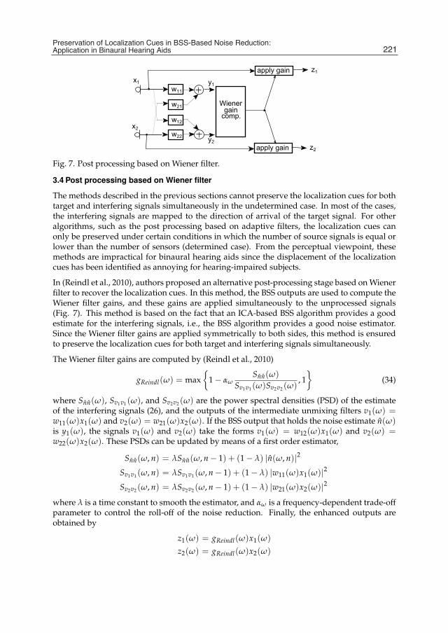
Preservation of Localization Cues in BSS-Based Noise Reduction: Application in Binaural Hearing Aids 13
Fig. 7. Post processing based on Wiener filter.
3.4 Post processing based on Wiener filter
The methods described in the previous sections cannot preserve the localization cues for bothtarget and interfering signals simultaneously in the undetermined case. In most of the cases,the interfering signals are mapped to the direction of arrival of the target signal. For otheralgorithms, such as the post processing based on adaptive filters, the localization cues canonly be preserved under certain conditions in which the number of source signals is equal orlower than the number of sensors (determined case). From the perceptual viewpoint, thesemethods are impractical for binaural hearing aids since the displacement of the localizationcues has been identified as annoying for hearing-impaired subjects.
In (Reindl et al., 2010), authors proposed an alternative post-processing stage based onWienerfilter to recover the localization cues. In this method, the BSS outputs are used to compute theWiener filter gains, and these gains are applied simultaneously to the unprocessed signals(Fig. 7). This method is based on the fact that an ICA-based BSS algorithm provides a goodestimate for the interfering signals, i.e., the BSS algorithm provides a good noise estimator.Since the Wiener filter gains are applied symmetrically to both sides, this method is ensuredto preserve the localization cues for both target and interfering signals simultaneously.
The Wiener filter gains are computed by (Reindl et al., 2010)
gReindl(ω) = max1− αω
Snn(ω)
Sv1v1 (ω)Sv2v2 (ω), 1
(34)
where Snn(ω), Sv1v1 (ω), and Sv2v2 (ω) are the power spectral densities (PSD) of the estimateof the interfering signals (26), and the outputs of the intermediate unmixing filters v1(ω) =w11(ω)x1(ω) and v2(ω) = w21(ω)x2(ω). If the BSS output that holds the noise estimate n(ω)is y1(ω), the signals v1(ω) and v2(ω) take the forms v1(ω) = w12(ω)x1(ω) and v2(ω) =w22(ω)x2(ω). These PSDs can be updated by means of a first order estimator,
Snn(ω, n) = λSnn(ω, n− 1) + (1− λ) |n(ω, n)|2Sv1v1 (ω, n) = λSv1v1 (ω, n− 1) + (1− λ) |w11(ω)x1(ω)|2Sv2v2 (ω, n) = λSv2v2 (ω, n− 1) + (1− λ) |w21(ω)x2(ω)|2
where λ is a time constant to smooth the estimator, and αω is a frequency-dependent trade-offparameter to control the roll-off of the noise reduction. Finally, the enhanced outputs areobtained by
z1(ω) = gReindl(ω)x1(ω)
z2(ω) = gReindl(ω)x2(ω)
221Preservation of Localization Cues in BSS-Based Noise Reduction: Application in Binaural Hearing Aids

14 Will-be-set-by-IN-TECH
BSS
SNR G
Σ
Σ1x
2y
1u
2u
FilterBank
FilterBank
Env.Det.
FilterBank
FilterBank
1y
OutputSelect.
pe
se
Env.Det.
1z
2z2x
Fig. 8. Perceptually-inspired post processing to preserve the localization cues.
Experimental results in (Reindl et al., 2010) and (Marin-Hurtado et al., 2012) showedthat this method can preserve the localization cues for both target and interfering signalssimultaneously; however, the performance of this method is slightly below the performanceof the post processing based on adaptive filters (Marin-Hurtado et al., 2012).
3.5 Perceptually-inspired post processing
In the previous sections, different BSS post-processing methods were discussed to recoverthe localization cues. All the above methods can preserve the localization cues of the targetsignal efficiently. However, only the BSS post-processing method based on Wiener filter canpreserve the localization cues for both target and interfering signals simultaneously. Thissection discusses an alternative BSS post-processing method that preserves both localizationcues. In this case, a perceptually-inspired post processing (BSS-PP) is used to compute a setof time-domain gains from the BSS outputs, and these gains are applied to the unprocessedsignals (Fig. 8) (Marin-Hurtado et al., 2011; 2012). The BSS post processing used in(Marin-Hurtado et al., 2011; 2012) is an adaptation of the method in (Parikh & Anderson,2011). This post processing is selected since it outperforms other BSS post processing formonaural speech enhancement applications. This post processing is modified so that it can beused for a binaural hearing aid (Marin-Hurtado et al., 2012):
1. To preserve the localization cues, the gains obtained by the BSS and perceptualpost-processing algorithm described in (Parikh & Anderson, 2011) are applied to theunprocessed signals received at each side (Figure 8).
2. To achieve low processing delay, the system is implemented assuming real-time operatingconstraints, with the envelopes (ep and es), SNR estimates, and gain parametersupdated in the frame-by-frame basis, while the gains and outputs are computed in thesample-by-sample basis. In (Parikh & Anderson, 2011), gains are computed assuming anentire knowledge of the signal.
3. To minimize artifacts and to achieve more quality outputs, it is necessary to hold along-term history for the maximum values of the primary envelope (ep). Different testsshow that the length of this memory should be at least one second.
4. To estimate the SNR, first-order estimators of the signal and noise PSD are used, and theSNR is computed as the ratio of these PSDs.
This perceptually-inspired BSS post processing is shown in Figure 8. Signals received at theleft, x1, and right, x2, microphones are passed through a BSS algorithm to get u1 and u2. An
222 Independent Component Analysis for Audio and Biosignal Applications

Preservation of Localization Cues in BSS-Based Noise Reduction: Application in Binaural Hearing Aids 15
output selection algorithm identifies which BSS output contains the separated target signal(y1), or primary channel, and the separated interfering signal (y2), or secondary channel.These outputs, y1 and y2, are analyzed using an auditory filter bank, and then, the envelopein each sub-band is extracted. These envelopes are used to estimate the SNR and to computethe noise-suppression gains. The SNR and gains are computed separately for each sub-band.These noise-suppression gains expand the dynamic range of each sub-band by lowering thenoise floor. These gains are finally applied simultaneously to the unprocessed signals bytime-domain multiplication, and the outputs from each sub-band are summed together toproduce the enhanced signals for the left and right ear.
To reduce computational complexity and processing delay in the BSS stage, an info-max BSSalgorithm that uses adaptive filters to minimize the mutual information of the system outputsis used. This algorithm is described by the following set of equations (Marin-Hurtado et al.,2012):
u1(n + 1) = x1(n) +wT12(n)u2(n) (35)
u2(n + 1) = x2(n) +wT21(n)u1(n) (36)
w12(n + 1) = w12(n)− 2μ tanh(u1(n + 1))u2(n) (37)
w21(n + 1) = w21(n)− 2μ tanh(u2(n + 1))u1(n) , (38)
where x1 and x2 are the signals received at the left and right microphones, w12 and w21are vectors of length Nw describing the unmixing filter coefficients, and u1(n) and u2 arevectors of length Nw whose elements are the previous outputs of the BSS algorithm, uj(n) =
[uj(n) uj(n − 1) · · · uj(n − Nw + 1)]T , j = 1, 2, and n is the time index. To determine which BSSoutput contains the target signal, the time-average energy of the envelopes of the signals u1and u2 are compared, and then, the output with higher time-average energy is selected asprimary channel y1. This time-average energy is computed by
uenvj (n) = ηenvuenv
j (n− 1) + (1− ηenv)u2j (n) (39)
where ηenv is a time constant. This update takes place every N samples.
The outputs of the BSS algorithm, y1 and y2, as well as the unprocessed input signals at theleft and right microphones, x1 and x2, are passed through a filter bank that resembles theauditory system. This filter bank was implemented using forth-order Butterworth filters. At22 kHz sampling rate, each filter bank provides 24 sub-bands. At the output of the filter banks,the vectors xj(l, k) and yj(l, k) of length N, j = 1, 2, are obtained, where l corresponds to theframe index and k to the sub-band number. Although the signals x and y are obtained in thesample-by-sample basis, they are analyzed in non-overlapped frames of length N to computethe gain parameters as we will show next.
For each output yj(l, k), the envelope is extracted using a full-wave rectifier followed by alow-pass filter. In particular, the primary envelope vector ep(l, k) is extracted from y1(l, k),and the secondary envelope vector es(l, k) from y2(l, k). The low-pass filters are implementedusing a first-order IIR filter whose cutoff frequency is selected to be a fraction of thecorresponding bandwidth of the band (Parikh & Anderson, 2011). These cutoff frequenciesare set to 1/5, 1/8 and 1/15 of the bandwidth of low, medium and high-frequency bands,respectively. These fractions ensure that the envelope tracks the signal closely but at the sametime does not change too rapidly to cause abrupt gain changes that introduce modulation.
223Preservation of Localization Cues in BSS-Based Noise Reduction: Application in Binaural Hearing Aids

16 Will-be-set-by-IN-TECH
The final outputs at the left, z1, and the right, z2, side are computed using the time-domaingains gl,k produced by the perceptual post-processing stage:
zj(l) = ∑kgl,k xj(l, k) (40)
where denotes the element-wise product. The vector form emphasizes that the gains arecomputed using parameters updated on a frame-by-frame basis. However, these outputs canbe computed on a sample-by-sample, reducing the processing delay.
In (Parikh & Anderson, 2011), inspired by a perceptual modeling, these gains modify theenvelope of each sub-band ek(t) such that ek(t) = βeα
k (t). To provide noise reduction, themaximum envelope value is preserved (i.e., ekmax = ekmax ) while the minimum envelope valueis lowered (i.e., ekmin
= Kekmin, where K is an expansion coefficient). Using the previous ideas,
(Parikh & Anderson, 2011) developed a method to estimate α and β from the entire signal.To provide a realistic implementation, equations in (Parikh & Anderson, 2011) are modifiedto a vector form to state the update of α and β is the frame-by-frame basis every N samples(Marin-Hurtado et al., 2012):
gk,l = βl,kep(l, k)(αl,k−1). (41)
The factors α and β are computed as
βl,k = max(epmax(k))(1−αk,l) (42)
αk,l = 1− logK/ log Ml,k , (43)
where Ml,k is the SNR at k-th sub-band and l-th frame, and epmax(k), a vector that holds themaximum values of the primary envelopes, is obtained from the previous Nmax frames:
epmax(k) = [max(ep(l, k)) ... max(ep(l − Nmax, k))] (44)
To avoid computational overflow and preserve the binaural cues, the value of α is constrainedin the range α = [0, 5]. To minimize artifacts and achieve better quality outputs, the historystored in the vector epmax should hold at least one second, but two-seconds memory, i.e.Nmax = 2 fs/N, is recommended. Since α and β are fixed for a given frame, these gainscan also be computed in the sample-by-sample basis.
To estimate the SNR at the given sub-band and frame, the signal and noise power areobtained from the envelopes of the primary and secondary channel. This approach reducesmiss-classification errors in the SNR estimationwhen the input SNR is low. To obtain a reliablenoise estimate, the noise power is updated using a rule derived from the noise PSD estimatorproposed in (Ris & Dupont, 2001):
Pe = ‖es(l, k)‖2
i f |Pe − Pv(l − 1, k)| < ε√
σv(l − 1, k)
Pv(l, k) = λvPv(l − 1, k) + (1− λv)Pe (45)
σv(l, k) = δσv(l − 1, k) + (1− δ) |Pe − Pv(l − 1, k)|2else
Pv(l, k) = Pv(l − 1, k)σv(l, k) = σv(l − 1, k)
end
224 Independent Component Analysis for Audio and Biosignal Applications

Preservation of Localization Cues in BSS-Based Noise Reduction: Application in Binaural Hearing Aids 17
where Pv(l, k) is the noise power at the k-th sub-band and l-th frame, σv(l, k) is an estimate ofthe variance of Pv, λ and δ are time constants to smooth the estimation, and ε is a thresholdcoefficient. Finally, the frame SNR is estimated by
Ml,k = max(
Px(l, k)Pv(l, k)
− 1 , 1)
(46)
where Px is the power of the primary channel estimated by
Px(l, k) = λxPx(l − 1, k) + (1− λx)∥∥ep(l, k)
∥∥2 (47)
The values λv = 0.95, λx = 0.9, δ = 0.9, and ε = 5 are selected in (Marin-Hurtado et al., 2012)to achieve good performance.
The performance of the BSS-PP depends on the tuning of two parameters: K and N. WhereasK controls the expansion of the dynamic range, N defines how often the parameters tocompute the noise-suppression gains are updated. A detailed analysis of the effect of theseparameters on the SNR improvement and sound quality is presented in (Marin-Hurtado et al.,2012). In summary, K = 0.01 and N = 8192 show to be suitable for all scenarios. Themathematical proof that localization cues are preserved in the BSS-PP algorithm is includedin (Marin-Hurtado et al., 2012).
3.5.1 Advantages and limitations
In the BSS-PP method, the noise-suppression gains are computed to expand the dynamicrange of the noisy signal, in such a way that the maximum signal level is maintained whilethe noise level is pushed down. The maximum signal level is estimated from the primarychannel, and the noise level from the secondary channel. Theoretical analysis conducted in(Takahashi et al., 2009) show that ICA-based BSS algorithms such as the algorithm used in theBSS-PP method provides an accurate noise estimate under non-point-source noise scenarios(e.g., diffusive or babble noise). Therefore, the performance of this method under thesescenarios is expected to be high. Since BSS-PP tracks the envelopes of the target speech andnoise level simultaneously, it is expected a good performance under highly non-stationaryenvironments. On the other hand, when the interfering signals are few point sources, the BSSalgorithm can provide accurate noise estimation only if the target signal is dominant. Thus,the performance of the BSS-PP algorithm is expected to be low under these scenarios at verylow input SNR. Fortunately, these kind of scenarios are uncommon. All the above statementsare verified through experiments discussed in the next section. In general, the BSS-PPmethod shows to be efficient in the removal of background noise, provides an acceptablespeech quality, preserves the localization cues for both target and interfering signals, andoutperforms existing BSS-based methods in terms of SNR improvement and noise reduction(Marin-Hurtado et al., 2012).
4. Comparative study
This chapter discussed different methods to preserve the localization cues in a binauralnoise-reduction system based on BSS. These methods are summarized in the Table 1. Based oncommon features of the algorithms, these methods can be classified in three categories: BSS
225Preservation of Localization Cues in BSS-Based Noise Reduction: Application in Binaural Hearing Aids

18 Will-be-set-by-IN-TECH
0 5000 10000 15000
Aichner−07
Reindl−10
BSS−PP
Number of operations per input sample
MPYADDDIV/TANH/POW
Fig. 9. Number of operations for BSS-PP, Reindl-10, and Aichner-07 per input samplegrouped into additions (ADD), multiplications (MPY), divisions (DIV), hyperbolic tangent(TANH), and power raise (POW).
constrained optimization, spatial-placement filters, and BSS post processing to enhance theunprocessed signals. In the first category, the BSS filter weights, wqp, are designed to performsource separation as well as to preserve the localization cues. In the second category, theBSS output corresponding to the estimate of the target signal is enhanced by a FIR filter thatrestores the localization cues. In the third category, the BSS outputs are used to computenoise-suppression gains that enhance the unprocessed signals. Under the third category,we can include the post-processing methods based on adaptive filters, Wiener filter, andperceptually-inspired processing.
Different reports have been shown that methods based on BSS constrained optimization andspatial-placement filters are unable to provide simultaneous preservation of localization cuesfor the target and interfering signals. In addition, most of these methods perform a mappingof the direction of arrival of the interfering signals to the direction of arrival of the targetsignal, which may be perceptually annoying. On the contrary, most methods belonging tothe third category, BSS post processing to enhance the unprocessed signals, can preservethe localization cues for both target and interfering signals simultaneously under certainconditions. In particular, among the different methods analyzed, the BSS post-processingmethod based on Wiener filter and the perceptually-inspired post processing are the onlymethods able to preserve these localization cues simultaneously.
Since the gains and outputs are computed in the sample-by-sample basis, the processing delayis very small (< 1 ms) in the BSS-PP method compared to other BSS-based post-processingmethods such as the method based on adaptive filters, Aichner-07, (Section 3.3), and themethod based onWiener filter, Reindl-10, (Section 3.4). In Aichner-07 and Reindl-10 methods,the processing delay is around 6 ms. In addition, the computational complexity of BSS-PP issignificantly smaller than Aichner-07 and Reindl-10 (Fig. 9).
4.1 Experiment
Among the different methods discussed in this chapter, only Aichner-07, Reindl-10, andBSS-PP are evaluated in this experiment. This selection takes into account only the BSSpost-processing methods capable of preserving the localization cues for the target andinterfering signals simultaneously under certain environmental conditions (Table 1). Thesemethods are implemented in Matlab and tested under different scenarios. Simulations todiscern the performance of these techniques are conducted under the following scenarios:
226 Independent Component Analysis for Audio and Biosignal Applications

Preservation of Localization Cues in BSS-Based Noise Reduction: Application in Binaural Hearing Aids 19
Metho
dStrategy
Preserve
Target
Cue
s
Preserve
Noise
Cue
sCom
p.Cost
Processing
Delay
Ref.
Taka
tani-05
BSScons
traine
dop
timization
Yes
No
High
?(Tak
atan
ieta
l.,20
05)
Aichn
er-07B
BSScons
traine
dop
timization
Yes
No
High
?(A
ichn
eret
al.,
2007
)
Weh
r-06
ASp
atial-placem
ent
filter
No
Map
pedto
target
DoA
Med
ium
?(W
ehret
al.,20
06)
Weh
r-06
BSp
atial-placem
ent
filter
Yes
Map
pedto
target
DoA
Med
ium
?(W
ehret
al.,20
06)
Aichn
er-07
Post
processing
basedon
adap
tive
filters
Yes
Und
ercertain
cond
itions
Med
ium
∼6ms
(Aichn
eret
al.,
2007
)
Reind
l-10
Post
processing
basedon
Wiene
rfilter
Yes
Yes
Med
ium
∼6ms
(Reind
leta
l.,20
10)
BSS-PP
Percep
tually-ins
pired
post
processing
Yes
Yes
Low
∼1ms
(Marin-H
urtado
etal.,20
12)
Table1.
Summaryof
thebina
ural
noise-redu
ctionmetho
dsba
sedon
BSS.
Processing
delayisestimated
forasystem
working
at16
kHzsamplingfreq
uenc
y.Que
stionmarkisinclud
edforthemetho
dsno
tana
lyzedin
thecompa
rative
stud
y.
227Preservation of Localization Cues in BSS-Based Noise Reduction: Application in Binaural Hearing Aids

20 Will-be-set-by-IN-TECH
1. Single source under constant-SNR diffusive noise. This scenario is widely used to testvirtually all binaural noise-reduction techniques. This background noise is generated byplaying uncorrelated pink noise sources simultaneously at 18 different spatial locations.
2. Single source under babble (or cafeteria) noise. The background noise corresponds to areal recording in a cafeteria.
3. Multi-talker. In this scenario, four distinguishable speakers are placed at differentazimuthal positions: 40o, 80o, 200o and 260o.
The above scenarios are generated by filtering the target signal with the HRTF measured fora KEMAR manikin in absence of reverberation (Gardner & Martin, 1994). The target signal isplaced at eight different azimuthal angles: 0o, 30o, 90o, 120o, 180o, 240o, 270o and 330o, where0o corresponds to the front of the KEMAR, 90o corresponds to the right ear, and 270o to theleft ear. Target signals are speech recordings of ten different speakers and sentences takenfrom the IEEE sentence database (IEEE Subcommittee, 1969). For all scenarios, the interferingsignals are added to the target signal at different SNR.
Since the HRTF database in (Gardner & Martin, 1994) is for non-reverberant environments,a secondary database using reverberant conditions is created using the HRTF recordingsdescribed in (Jeub et al., 2009; RWTH Aachen University, 2010). This database is includedsince it is widely known that the performance of the majority of the noise-reductionalgorithms is degraded significantly when reverberation is present. This database assumesa babble noise scenario and the following rooms: studio (RT60 = 0.12s), meeting room(RT60 = 0.23s), office (RT60 = 0.43s), and lecture room (RT60 = 0.78s).
The performance of these techniques is analyzed using the broadband intelligibility-weightedSNR improvement (ΔSNR-SII) (Greenberg et al., 1993). For the subjective test, a MUSHRA(multiple stimulus test with hidden reference and anchor) test is used to assess the overallsound quality. The protocol in (ITU-R, 2003) is used for the subjective test.
4.2 Performance evaluation
SNR improvement for diffusive, babble, and multi-talker scenarios is plotted in Figures 10-12.In general, the perceptually-inspired post-processing method (BSS-PP) outperforms the otherBSS-based noise-reduction methods in most scenarios.
The poor performance of BSS-PP in the multi-talker scenario at low input SNR is explainedby the errors introduced by a wrong selection of the primary output. When an ideal outputselection algorithm is used (dashed line in Fig. 12), the performance of BSS-PP is similaror better than that of the other BSS-based methods. The output selection algorithm canbe made more robust by using a direction-of-arrival-estimation algorithm or a permutationalgorithm at expenses of increasing the computational complexity. However, scenarios withvery few interfering signals at input SNR < 0 dB such as the multi-talker scenario of Fig. 12 arevery uncommon, and they are not challenging for the auditory system without any hearingaid. Likewise, binaural noise-reduction methods are useful for challenging scenarios such asbabble noise at low input SNR. Since BSS-PP provides an excellent performance under thesescenarios (Fig. 11), the output-selection algorithm used by BSS-PP is enough for a large set ofpractical applications.
Up to this point the performance of all methods has been verified under non-reverberantscenarios. For reverberant scenarios, Fig. 13 shows that for a large reverberant room
228 Independent Component Analysis for Audio and Biosignal Applications

Preservation of Localization Cues in BSS-Based Noise Reduction: Application in Binaural Hearing Aids 21
−4−2 0 2 4 6 8 10124
6
8
10
12
Input SNR (dB)
ΔS
NR
−S
II left (
dB)
−4−2 0 2 4 6 8 10124
6
8
10
12
Input SNR (dB)
ΔS
NR
−S
II right
(dB
)
Aichner−07Reindl−10BSS−PP
Fig. 10. SNR improvement under diffusive noise scenario.
−4−2 0 2 4 6 8 1012
4
6
8
10
12
Input SNR (dB)
ΔS
NR
−S
II left (
dB)
−4−2 0 2 4 6 8 1012
4
6
8
10
12
Input SNR (dB)
ΔS
NR
−S
II right
(dB
)
Aichner−07Reindl−10BSS−PP
Fig. 11. SNR improvement under babble noise scenario.
−4−2 0 2 4 6 8 1012−5
0
5
10
Input SNR (dB)
ΔS
NR
−S
II left (
dB)
−4−2 0 2 4 6 8 1012−5
0
5
10
Input SNR (dB)
ΔS
NR
−S
II right
(dB
)
Aichner−07Reindl−10BSS−PPBSS−PP (Ideal)
Fig. 12. SNR improvement under multi-talker scenario. The dashed line is the performancefor an ideal output-selection algorithm.
(RT60 = 0.78s), BSS-PP provides an acceptable SNR improvement and outperforms the otherexisting methods for input SNR ≥ 0 dB. Results for other reverberant rooms are included in(Marin-Hurtado et al., 2012).
A subjective test is conducted to assess the subjective sound quality of the methods understudy. These results are summarized in the Fig. 14. Sound quality is graded in the scale[0, 100], with 100 the highest value corresponding to a clean signal. To perform the grading,the subject listened to the samples that included clean speech, unprocessed speech in babblenoise at an input SNR of 0 dB, and enhanced speech processed by Aichner-07, Reindl-10,and BSS-PP methods. The reference and hidden reference signals are unprocessed noisy
229Preservation of Localization Cues in BSS-Based Noise Reduction: Application in Binaural Hearing Aids
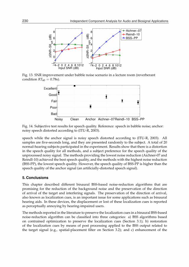
22 Will-be-set-by-IN-TECH
−4−2 0 2 4 6 8 1012−2
0
2
4
6
8
Input SNR (dB)
ΔS
NR
−S
II left (
dB)
−4−2 0 2 4 6 8 1012−2
0
2
4
6
8
Input SNR (dB)
ΔS
NR
−S
II right
(dB
)
Aichner−07Reindl−10BSS−PP
Fig. 13. SNR improvement under babble noise scenario in a lecture room (reverberantcondition RT60 = 0.78s).
Noisy Clean Anchor Aichner−07Reindl−10 BSS−PP
Bad
Poor
Fair
Good
Excellent
Fig. 14. Subjective test results for speech quality. Reference: speech in babble noise; anchor:noisy speech distorted according to (ITU-R, 2003).
speech while the anchor signal is noisy speech distorted according to (ITU-R, 2003). Allsamples are five-seconds long, and they are presented randomly to the subject. A total of 20normal-hearing subjects participated in the experiment. Results show that there is a distortionin the speech quality for all methods, and a subject preference for the speech quality of theunprocessed noisy signal. The methods providing the lowest noise reduction (Aichner-07 andReindl-10) achieved the best speech quality, and the methods with the highest noise reduction(BSS-PP), the lowest speech quality. However, the speech quality of BSS-PP is higher than thespeech quality of the anchor signal (an artificially-distorted speech signal).
5. Conclusions
This chapter described different binaural BSS-based noise-reduction algorithms that arepromising for the reduction of the background noise and the preservation of the directionof arrival of the target and interfering signals. The preservation of the direction of arrival,also known as localization cues, is an important issue for some applications such as binauralhearing aids. In these devices, the displacement or lost of these localization cues is reportedas perceptually annoying by hearing-impaired users.
Themethods reported in the literature to preserve the localization cues in a binaural BSS-basednoise-reduction algorithm can be classified into three categories: a) BSS algorithms basedon contrained optimization to preserve the localization cues (Section 3.1); b) restorationof the localization cues by means of post processing applied to the BSS output related tothe target signal (e.g., spatial-placement filter on Section 3.2); and c) enhancement of the
230 Independent Component Analysis for Audio and Biosignal Applications

Preservation of Localization Cues in BSS-Based Noise Reduction: Application in Binaural Hearing Aids 23
unprocessed inputs by noise-reduction gains computed from the BSS outputs (e.g., adaptivefilters, Wiener filter, and perceptual post-processing methods described on Sections 3.3,3.4, and 3.5). All methods proposed in the literature can preserve the localization cuesfor the target signal. However, the methods belonging to the first and second category,BSS constrained optimization and spatial-placement filters, cannot preserve the localizationcues for the interfering signals. In most cases, these localization cues are mapped to thedirection of arrival of the target signal, which suggests that these algorithms are not practicalfor binaural hearing aids. On the contrary, binaural BSS-based noise-reduction algorithmsbelonging to the third category, i.e., those methods that compute noise-suppression gainsfrom the BSS outputs and apply these gains to the unprocessed signals, can preserve thelocalization cues for both target and interfering signals simultaneously. This preservation isidentified through subjective and theoretical analysis. This chapter described three methodsbelonging to the third category: post processing with adaptive filters (Aichner-07), postprocessing withWiener filter (Reindl-10), and perceptually-inspired post processing (BSS-PP).An experimental evidence, confirmed through mathematical analysis, showed the postprocessing based on adaptive filters (Aichner-07) works only in the determined case, i.e., whenthe number of source signals is equal o lower than the number of sensors. On the contrary, themethods based on Wiener-filter post processing (Reindl-10) and perceptually-inspired postprocessing (BSS-PP) preserve the localization cues even in the undetermined case.
A comparative study conducted with the Aichner-07, Reindl-10, and BSS-PP methods underdifferent environments showed that BSS-PP outperforms the other methods in terms of SNRimprovement and noise reduction. In addition, the BSS-PP method provides a significantreduction in the number of operations compared to the other two methods, and its processingdelay is very small. Hence, the BSS-PP turns out a feasible solution for a binaural hearingaid. However, there are two limitations in the BSS-PP method. First, the subjective soundquality is acceptable, with a subjective sound quality graded slightly below the subjectivesound quality of the Aichner-07 and Reindl-10 methods. Second, the BSS algorithm demandswireless transmission at full rate. This issue is also present in the Aichner-07 and Reindl-10methods.
6. Future work
Although the BSS-PP method is a promising binaural noise-reduction algorithm, it isnecessary to solve two issues to obtain a practical implementation for a binaural hearingaid. First, to improve the sound quality, the dynamic range expansion performed by the postprocessing stage must include additional information to take into account a sound qualitycriteria, or use another perceptual model. Second, to reduce the transmission bandwidth,it is necessary to develop distributive or reduced bandwidth BSS algorithms, or to employstrategies other than BSS to estimate the target and interfering signals.
Most processing in the BSS-PP method can be easily replaced by an analog processing exceptthe BSS algorithm. Amixed-signal solution may reduce computational complexity and powerconsumption. To obtain a full-analog solution, analog BSS algorithms have to be developed.
Although most BSS-based noise-reduction algorithms such as Reindl-10 and BSS-PP werenot initially designed to deal with reverberant conditions, their performance underthese environments is acceptable. Hence, their performance could be improvement bymodifications in the mathematical framework to take into account the effect of reverberation.
231Preservation of Localization Cues in BSS-Based Noise Reduction: Application in Binaural Hearing Aids

24 Will-be-set-by-IN-TECH
Finally, it is known that the speech intelligibility in noise-reduction applications can beimproved by applying a binary mask to the unprocessed signal (Loizou & Kim, 2011).Hence, binary masking can be combined with a BSS algorithm in order to obtain asource separation algorithm that reduces the background noise and improves the speechintelligibility simultaneously. Although some attempts have been explored in (Han et al., 2009;Jan et al., 2011; Mori et al., 2007; Takafuji et al., 2008), these methods are unable to preserve thelocalization cues for both target and interfering signals simultaneously. Hence, it is necessaryto develop post processing algorithms to preserve the localization cues in BSS-based binarymasking algorithms.
7. Acknowledges
This work is supported in part by Texas Instruments Inc., formerly National SemiconductorCorporation. Jorge Marin wants to thank Georgia Institute of Technology–USA, Universidaddel Quindio–Colombia and Colciencias–Colombia for their financial support.
8. References
Aichner, R., Buchner, H., & Kellermann, W. (2006). A novel normalization and regularizationscheme for broadband convolutive blind source separation, Proc. Int. Symp.Independent Component Analysis and Blind Signal Separation, ICA 2006, Vol. 3889,pp. 527–535.
Aichner, R., Buchner, H., Zourub, M. & Kellermann, W. (2007). Multi-channel sourceseparation preserving spatial information, Proc. IEEE Int. Conf. Acoust., Speech SignalProcess., ICASSP 2007, Vol. 1, pp. I–5–I–8.
Gardner, B. & Martin, K. (1994). HRTF measurements of a KEMAR dummy-headmicrophone, Technical Report 280, MIT Media Lab Perceptual Computing.http://sound.media.mit.edu/KEMAR.html.
Greenberg, J. E., Peterson, P. M. & Zurek, P. M. (1993). Intelligibility-weighted measures ofspeech-to-interference ratio and speech system performance, J. Acoust. Soc. Amer.94(5): 3009–3010.
Han, S., Cui, J. & Li, P. (2009). Post-processing for frequency-domain blind source separationin hearing aids, Proc. Int. Conf. on Information, Communications and Signal Processing,2009. ICICS 2009, pp. 1 –5.
Haykin, S. (2000). Unsupervised Adaptive Filtering, Vol. 1: Blind Source Separation, John Wileyand Sons.
IEEE Subcommittee (1969). IEEE recommended practice for speech quality measurements,IEEE Trans. Audio Electroacoust. pp. 225–246.
ITU-R (2003). Recommendation BS.1534-1: Method for the subjective assessment ofintermediate quality levels of coding systems.
Jan, T., Wang, W. &Wang, D. (2011). A multistage approach to blind separation of convolutivespeech mixtures, Speech Communication 53(4): 524 – 539.
Jeub, M., Schafer, M. & Vary, P. (2009). A binaural room impulse response database for theevaluation of dereverberation algorithms, Proc. Int. Conf. Digital Signal Process., pp. 1–5.
Kocinski, J. (2008). Speech intelligibility improvement using convolutive blind sourceseparation assisted by denoising algorithms, Speech Commun. 50(1): 29 – 37.
232 Independent Component Analysis for Audio and Biosignal Applications

Preservation of Localization Cues in BSS-Based Noise Reduction: Application in Binaural Hearing Aids 25
Loizou, P. & Kim, G. (2011). Reasons why current speech-enhancement algorithms do notimprove speech intelligibility and suggested solutions, IEEE Transactions on Audio,Speech, and Language Processing 19(1): 47 –56.
Marin-Hurtado, J. I., Parikh, D. N. & Anderson, D. V. (2011). Binaural noise-reduction methodbased on blind source separation and perceptual post processing, Proc. Interspeech2011, Vol. 1, Florence, Italy, pp. 217–220.
Marin-Hurtado, J. I., Parkih, D. N. & Anderson, D. V. (2012). Perceptually inspirednoise-reduction method for binaural hearing aids, IEEE Transactions on Audio, Speechand Language Processing 20(4): 1372–1382.
Moore, B. C. J. (2007). Binaural sharing of audio signals: Prospective benefits and limitations,The Hearing Journal 60(11): 46–48.
Mori, Y., Takatani, T., Saruwatari, H., Shikano, K., Hiekata, T. & Morita, T. (2007).High-presence hearing-aid system using dsp-based real-time blind source separationmodule, Proc. IEEE Int. Conf. Acoustics, Speech and Signal Process., 2007. ICASSP 2007,Vol. 4, pp. IV–609 –IV–612.
Noohi, T. & Kahaei, M. (2010). Residual cross-talk suppression for convolutive blind sourceseparation, Proc. Int. Conf. Comp. Eng. Technology (ICCET), Vol. 1, pp. V1–543 –V1–547.
Parikh, D., Ikram, M. & Anderson, D. (2010). Implementation of blind source separation anda post-processing algorithm for noise suppression in cell-phone applications, Proc.IEEE Int. Conf. Acoust., Speech Signal Process., ICASSP, pp. 1634 –1637.
Parikh, D. N. & Anderson, D. V. (2011). Blind source separation with perceptual postprocessing, Proc. IEEE 2011 DSP/SPE Workshop.
Park, K. S., Park, J., Son, K. & Kim, H. T. (2006). Postprocessing with wiener filtering techniquefor reducing residual crosstalk in blind source separation, Signal Processing Letters,IEEE 13(12): 749 –751.
Reindl, K., Zheng, Y. & Kellermann, W. (2010). Speech enhancement for binaural hearing aidsbased on blind source separation, Proc. Int. Symp. Commun. Control Signal Process.(ISCCSP), pp. 1 –6.
Ris, C. & Dupont, S. (2001). Assessing local noise level estimation methods: Application tonoise robust ASR, Speech Commun. 34(1-2): 141 – 158.
RWTH Aachen University (2010). Aachen impulse response (AIR) database - version 1.2.http://www.ind.rwth-aachen.de/AIR.
Smith, P., Davis, A., Day, J., Unwin, S., Day, G. & Chalupper, J. (2008). Real-world preferencesfor linked bilateral processing, The Hearing Journal 61(7): 33–38.
Sockalingam, R., Holmberg, M., Eneroth, K. & Shulte, M. (2009). Binaural hearing aidcommunication shown to improve sound quality and localization, The HearingJournal 62(10): 46–47.
Takafuji, R., Mori, Y., Saruwatari, H. & Shikano, K. (2008). Binaural hearing-aid system usingsimo-model-based ica and directivity-dependency-reduced binary masking, Proc. 9th
Int. Conf. Signal Process., ICSP 2008, pp. 320 –323.Takahashi, Y., Takatani, T., Osako, K., Saruwatari, H. & Shikano, K. (2009). Blind spatial
subtraction array for speech enhancement in noisy environment, IEEE Transactionson Audio, Speech and Language Processing 17(4): 650 –664.
Takatani, T., Ukai, S., Nishikawa, T., Saruwatari, H. & Shikano, K. (2005). Evaluation ofSIMO separation methods for blind decomposition of binaural mixed signals, Proc.International Workshop on Acoustic Echo and Noise Control (IWAENC), pp. 233–236.
233Preservation of Localization Cues in BSS-Based Noise Reduction: Application in Binaural Hearing Aids

26 Will-be-set-by-IN-TECH
Van den Bogaert, T., Klasen, T. J., Moonen, M., Van Deun, L. & Wouters, J. (2006). Horizontallocalization with bilateral hearing aids: Without is better than with, J. Acoust. Soc.Amer. 119(1): 515–526.
Wehr, S., Puder, H. & Kellermann, W. (2008). Blind source separation and binauralreproduction with hearing aids: An overview, Proc. ITG Conf. Voice Communication(SprachKommunikation) pp. 1 –4.
Wehr, S., Zourub, M., Aichner, R. & Kellermann, W. (2006). Post-processing for BSS algorithmsto recover spatial cues, Proc. Int. Workshop Acoust. Echo Noise Control (IWAENC).
234 Independent Component Analysis for Audio and Biosignal Applications

12
ICA Applied to VSD Imaging of Invertebrate Neuronal Networks
Evan S. Hill1, Angela M. Bruno1,2, Sunil K. Vasireddi1 and William N. Frost1
1Department of Cell Biology and Anatomy, 2Interdepartmental Neuroscience Program,
Rosalind Franklin University of Medicine and Science, North Chicago, IL USA
1. Introduction Invertebrate preparations have proven to be valuable models for studies addressing fundamental mechanisms of nervous system function (Clarac and Pearlstein 2007). In general the nervous systems of invertebrates contain fewer neurons than those of vertebrates, with many of them being re-identifiable in the sense that they can be recognized and studied in any individual of the species. The large diameter of many invertebrate neurons makes them amenable for study with intracellular recording techniques, allowing for characterization of synaptic properties and connections, leading to circuit diagrams of neuronal networks. Further, there is often a rather straight-forward connection between neuronal networks and the relatively simple behaviors that they produce. For example, years of experimentation on the nervous systems of leeches, sea-slugs and crabs/lobsters have led to significant advances in the understanding of how small neuronal networks produce a variety of different behaviors (Harris-Warrick and Marder 1991; Hawkins et al. 1993; Katz 1998; Kristan et al. 2005). For the most part, these investigations have been carried out using sharp electrode recordings from about three to four neurons at a time (although see (Briggman and Kristan 2006)). Intracellular recording has been a very productive and fruitful technique for revealing details of neuronal connectivity and for studying synaptic changes caused by modulators or by simple forms of learning. However, since even simple behaviors are produced by the activity of populations of dozens to hundreds of neurons, the limited view offered by recording from only four neurons at a time makes it an inadequate technique for understanding larger-scale, network level phenomena that underlie behavior.
In order to understand how populations of neurons produce behaviors, methods are needed to simultaneously monitor the spiking activity of large numbers (dozens to hundreds) of individual neurons. Voltage-sensitive dye (VSD) imaging is a technique for accomplishing precisely this. However, after a promising start showing the immense power and potential of VSD imaging for understanding invertebrate neuronal networks (London et al. 1987; Wu et al. 1994a; Wu et al. 1994b; Zecevic et al. 1989), the technique has not been widely adopted by the field. This is possibly due to the difficulties inherent to the technique - the optical signals of interest are extremely small and are often mixed, redundant and noisy. These factors make it difficult to track the activity of individual neurons from recording trial to trial based solely on the raw optical data. Previous researchers used a spike-template

Independent Component Analysis for Audio and Biosignal Applications
236
matching technique to uncover single neuron spiking traces from VSD imaging data, but this method was very time consuming and involved substantial human judgment (Cohen et al. 1989). Automated, accurate and fast methods are thus needed to reliably and quickly extract single neuron spiking activity from such complex data sets.
In this chapter, we demonstrate the utility and accuracy of Infomax ICA for extracting single neuron spiking activity (i.e. spike-sorting) from VSD imaging data of populations of neurons located in the central ganglia of two invertebrate preparations, Tritonia diomedea and Aplysia californica, that are models for topics such as learning, modulation, pattern generation and pre-pulse inhibition (Brown et al. 2001; Cleary et al. 1998; Frost et al. 1998; Frost et al. 2006; Frost et al. 2003; Getting 1981; Katz and Frost 1995; Katz et al. 1994; Lennard et al. 1980). We also demonstrate certain features of the optical data sets that strongly influence the ability of ICA to return maximal numbers of components that represent the spiking activity of individual neurons (neuronal independent components or nICs).
2. Methods 2.1 Preparation
Tritonia diomedea central ganglia consisting of the bilaterally symmetric cerebral, pleural and pedal ganglia, and Aplysia californica central ganglia consisting of the cerebral, pleural and pedal ganglia, were dissected out and pinned onto the bottom of a Sylgard (Dow Corning) lined Petri dish containing Instant Ocean artificial seawater (Aquarium Systems). The thick connective tissue covering the ganglia and nerves was removed with fine forceps and scissors (for intracellular recording experiments the thin protective sheath covering the neurons was also removed). The preparation was then transferred and pinned to the Sylgard-lined coverslip bottom of the recording chamber used for optical recording (PC-H perfusion chamber, Siskiyou). In many experiments, to increase the number of neurons in focus, the ganglion to be imaged was flattened somewhat by pressing a cover slip fragment down upon it that was held in place with small blobs of Vaseline placed on the recording chamber floor.
2.2 Optical recording
Imaging was performed with an Olympus BX51WI microscope equipped with either 10x 0.6NA or 20x 0.95NA water immersion objectives. Preparation temperature was maintained at 10 – 11°C for Tritonia and 16 – 17°C for Aplysia, using Instant Ocean passed through a feedback-controlled in-line Peltier cooling system (Model SC-20, Warner Instruments). Temperature was monitored with a BAT-12 thermometer fitted with an IT-18 microprobe (Physitemp, Inc) positioned near the ganglion being imaged. For staining, the room was darkened and the perfusion saline was switched to saline containing the fast voltage sensitive absorbance dye RH-155 (Anaspec). Staining was carried out in one of two ways: either 5 min of 0.3 mg/ml or 1.5 hr of 0.03 mg/ml RH-155 in saline. Preparations were then perfused with 0.03 mg/ml RH-155 or dye-free saline throughout the experiment. Trans-illumination was provided with light from a 100W tungsten halogen lamphouse that was first passed through an electronic shutter (Model VS35 Vincent Associates), a 725/25 bandpass filter (Chroma Technology), and a 0.9 NA flip top achromat Nikon condenser on its way to the preparation. 100% of the light from the objective was directed either to an Optronics Microfire digital camera used for focusing and to obtain an image of the preparation to superimpose with the imaging data, or to the parfocal focusing surface of a 464-element photodiode array (NeuroPDA-III, RedShirtImaging) sampled at 1600 Hz.

ICA Applied to VSD Imaging of Invertebrate Neuronal Networks
237
2.3 Sharp electrode recordings
Intracellular recordings were obtained with 15-30 MΩ electrodes filled with 3M KCl or 3M K-acetate connected to a Dagan IX2-700 dual intracellular amplifier. The resulting signals were digitized at 2 KHz with a BioPac MP 150 data acquisition system.
2.4 Data analysis
Optical data were bandpass filtered in the Neuroplex software (5 Hz high pass and 100 Hz low pass Butterworth filters; RedShirtImaging), and then processed with ICA in MATLAB to yield single neuron action potential traces (independent components), see (Hill et al. 2010) for details. ICA run on 60 s of optical data typically takes about 5 minutes on a computer equipped with an Intel I7 processor. Statisical analyses were performed in Sigmaplot.
3. Results We bath applied the VSD RH-155 to the central ganglia of Tritonia diomedea and Aplysia californica, and used a 464-element photodiode array to image the action potential activity of populations of neurons on the surface of various ganglia during two rhythmic motor programs: escape swimming in T. diomedea, and escape crawling in A. californica. Here we show examples of ICA’s ability to extract single neuron activity from mixed, redundant and noisy raw optical data in both T. diomedea (Fig. 1) and A. californica (Fig. 2) and we demonstrate the ability of ICA to return maps of the neurons’ locations in the ganglia (based on the inverse weight matrix).
3.1 Validation of the accuracy of ICA
We previously demonstrated the accuracy of ICA spike-sorting by performing simultaneous intracellular and optical recordings in both Tritonia and Aplysia (Hill et al. 2010): in 34 out of 34 cases, one of the independent components returned by ICA matched up perfectly spike-for-spike with the intracellularly recorded data. Figure 3 shows an intracellular recording from a Tritonia pedal ganglion neuron while simultaneously recording the optical activity of many neurons in the same ganglion. The activity of the intracellularly recorded neuron was detected by many diodes (Fig. 3Ai). ICA returned 50 nICs, one of which matched up perfectly spike-for-spike with the intracellularly recorded neuron (Fig. 3Aii, iii and 3B). Plotting the data points for the intracellular and matching component traces against each other reveals a strong positive correlation (Fig. 3C; R2 value = 0.631). Another of the nICs burst in the same phase of the swim motor program as did the intracellularly recorded neuron (Fig. 3D), however plotting the values of the intracellular and non-matching component against each other revealed no correlation whatsoever (Fig. 3E). Figure 4 shows an intracellular recording from an Aplysia buccal ganglion neuron while simultaneously recording the optical activity of many neurons in the same ganglion. The activity of the intracellularly recorded neuron was detected by many diodes (Fig. 4Ai). ICA returned 10 nICs, one of which matched up perfectly spike-for-spike with the intracellularly recorded neuron (Fig. 4Aii, iii and 4B). Plotting the data points for the intracellular and matching component traces against each other revealed a strong positive correlation (Fig. 4C; R2 value = 0.629).

Independent Component Analysis for Audio and Biosignal Applications
238
Fig. 1. ICA returns single neuron traces from noisy, redundant, and mixed raw optical data of a Tritonia diomedea swim motor program. A The subset of diodes shown in black superimposed over an image of the pedal ganglion (inset) detected the spiking activity of many pedal ganglion neurons. The optical signals are redundant in the sense that many diodes detect the activity of the same neurons, and mixed in the sense that many diodes detect the activity of more than one neuron. Note that diode traces shown in blue redundantly detected the activity of the same neuron, as did the diode traces shown in red. Experimental set-up shown below the optical traces. Ce = cerebral, Pl = pleural, Pd = pedal ganglion, and pdn 3 = pedal nerve 3. B 123 of the 464 independent components returned by ICA represented the activity of single neurons (47 shown here). The redundancy of the optical data was eliminated by ICA – note that the blue and red independent components represent the activity of the two neurons that were detected by multiple diodes in A. C The maps returned by ICA show the ganglion locations of the neurons whose spiking activity is shown in blue and red in A and B. Arrows – stimulus to pedal nerve 3 to elicit swim motor program (10 V, 10 Hz, 2 s).

ICA Applied to VSD Imaging of Invertebrate Neuronal Networks
239
Fig. 2. ICA extracts the activity of individual pedal ganglion neurons from noisy, redundant, and mixed raw optical data of an Aplysia californica locomotion motor program. A The neural activity of many pedal ganglion neurons was detected by a subset of the 464 diodes shown in black (inset, diode array superimposed over an image of the pedal ganglion). Note that diode traces shown in green detected the activity of the same neuron, as did the diode traces shown in blue. Experimental set-up showing the region of the pedal ganglion imaged shown in the inset. Bc = buccal, Ce = cerebral, Pl = pleural, and Pd = pedal ganglion. B 95 of the 464 independent components returned by ICA represented the activity of single neurons (45 shown here). Note that the redundancies shown in A were eliminated by ICA. C The maps returned by ICA show the ganglion locations of the neurons whose spiking activity is shown in green and blue in A and B. Arrows – stimulus to pedal nerve 9 to elicit the locomotion motor program (10 V, 1 Hz, 155 s).
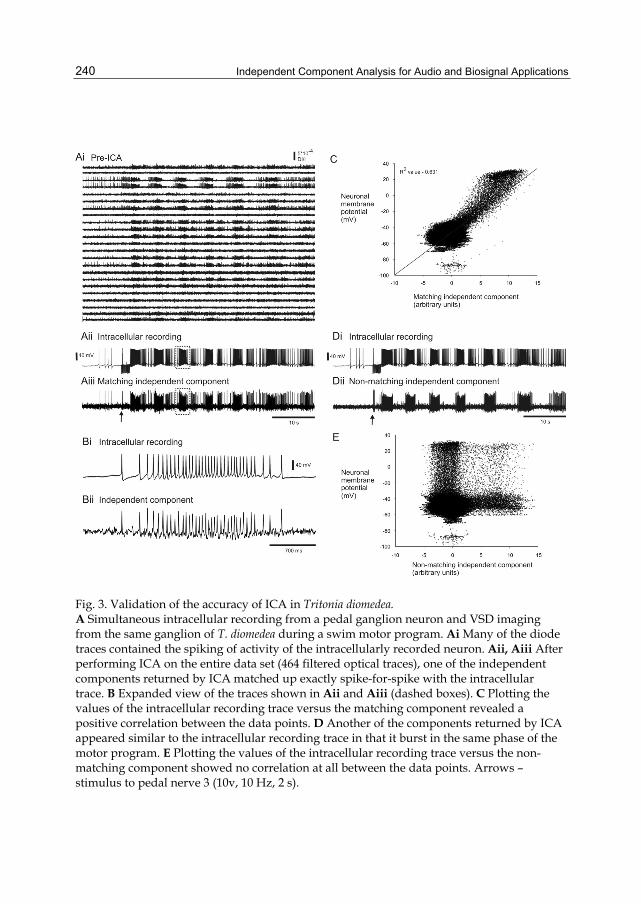
Independent Component Analysis for Audio and Biosignal Applications
240
Fig. 3. Validation of the accuracy of ICA in Tritonia diomedea. A Simultaneous intracellular recording from a pedal ganglion neuron and VSD imaging from the same ganglion of T. diomedea during a swim motor program. Ai Many of the diode traces contained the spiking of activity of the intracellularly recorded neuron. Aii, Aiii After performing ICA on the entire data set (464 filtered optical traces), one of the independent components returned by ICA matched up exactly spike-for-spike with the intracellular trace. B Expanded view of the traces shown in Aii and Aiii (dashed boxes). C Plotting the values of the intracellular recording trace versus the matching component revealed a positive correlation between the data points. D Another of the components returned by ICA appeared similar to the intracellular recording trace in that it burst in the same phase of the motor program. E Plotting the values of the intracellular recording trace versus the non-matching component showed no correlation at all between the data points. Arrows – stimulus to pedal nerve 3 (10v, 10 Hz, 2 s).

ICA Applied to VSD Imaging of Invertebrate Neuronal Networks
241
Fig. 4. Validation of the accuracy of ICA in Aplysia californica. A Simultaneous intracellular recording from a buccal ganglion neuron and VSD imaging from the same ganglion of A. californica. Current pulses were injected into the impaled neuron to make it to fire trains of action potentials. Ai Many of the diode traces contained the spiking of activity of the intracellularly recorded neuron. Aii, Aiii After running ICA on the entire data set, one of the independent components returned by ICA matched up exactly spike-for-spike with the intracellular trace. B Expanded view of the traces shown in Aii and Aiii (dashed boxes). C Plotting the values of the intracellular recording trace versus the matching component revealed a positive correlation between the data points.
3.2 Certain features of the data sets influence the number of nICs returned by ICA
Next we discuss our findings that certain features of the optical data sets strongly influence the number of nICs returned by ICA. First, we found that simply increasing the number of data points in the optical recording greatly increases the number of nICs returned by ICA (Fig. 5A). This could be due to the fact that with longer files, ICA is simply given more information, and is thus better able to determine which components are independent of each other. Increasing the file length only continues to increase the number of nICs returned by ICA up to a certain point though, usually around 45 s (for our data sets). Increasing file length also greatly decreases the variability of the number of nICs returned by ICA (Fig. 5A). We have also found that including spontaneous spiking activity (at least 10 s) preceding the Tritonia escape swim motor program greatly increases the number of nICs returned by ICA (Fig. 5B, C). For example, for seven preparations we found that when ICA was performed on 40 s of optical data including 10 s of spontaneous firing data preceding the swim motor program it returned a mean of 68.8 nICs, while ICA returned a mean of only 44.5 nICs when it was run on 40 s optical files that didn’t include any spontaneous

Independent Component Analysis for Audio and Biosignal Applications
242
firing preceding the motor program (Fig. 5C). Presumably neurons are more independent of each other when they are firing spontaneously than when they are bursting in near synchrony during the swim motor program. Thus, this period of greater independence is important for ICA to return maximal numbers of nICs.
Fig. 5. Increasing file length and including spontaneous firing data improve the performance of ICA. A Increasing file length leads to an increase in the number of nICs returned by ICA. The points on the graph show the average number of nICs returned by ICA for each data length. Note that with the shorter data lengths there is a fairly large variance in the number of nICs returned by ICA run on the exact same data set. This variance decreases greatly with increasing file length. After a certain point (~ 45 s) having more data points didn’t increase the number of nICs returned by ICA. B Including spontaneous spiking data preceding the rhythmic swim motor program data is important for ICA to return a maximal number of nICs. The points on the graph show the average number of nICs returned by ICA for each data length. Without the spontaneous firing data (10 s) included before the swim motor program, ICA returned fewer nICs even with longer files (same data set as in A). C In seven preparations, including 10 s of spontaneous firing data preceding the swim motor program significantly increased the average number of nICs returned by ICA for optical files of equal length (With spont firing = 10 s spontaneous firing + 30 s motor program, Without spont firing = 40 s motor program; paired t-test, * = p < 0.05).
3.3 Pre-filtering the data also strongly influences the number of nICs returned by ICA
Finally, we have found that filtering the optical data prior to running ICA to remove high frequency (100 Hz LP) and low frequency noise (5 Hz HP) consistently increases the number of nICs returned by ICA, and increases the signal-to-noise ratio of the nICs. Figure 6 shows an example of the effect of pre-filtering on the number of nICs returned by ICA. Without pre-filtering, ICA returned 34 nICs (Fig. 6A) whereas after pre-filtering it returned 73 nICs (Fig. 6B). Removing the low frequency noise in particular should make the components more independent of each other.
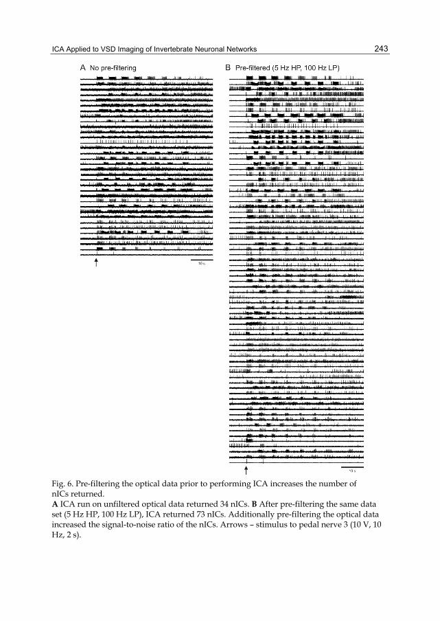
ICA Applied to VSD Imaging of Invertebrate Neuronal Networks
243
Fig. 6. Pre-filtering the optical data prior to performing ICA increases the number of nICs returned. A ICA run on unfiltered optical data returned 34 nICs. B After pre-filtering the same data set (5 Hz HP, 100 Hz LP), ICA returned 73 nICs. Additionally pre-filtering the optical data increased the signal-to-noise ratio of the nICs. Arrows – stimulus to pedal nerve 3 (10 V, 10 Hz, 2 s).
Independent Component Analysis for Audio and Biosignal Applications
244
4. Conclusions ICA is an ideal technique for quickly and accurately extracting single neuron spiking activity from noisy, mixed and redundant VSD imaging data. The lack of a technique such as ICA has possibly hindered widespread use of fast VSD imaging as a tool to study invertebrate neuronal networks. Here we have shown examples of ICA’s ability to extract single neuron spiking activity from optical files of escape motor programs in Tritonia and Aplysia. Additionally, we have demonstrated the accuracy of ICA with simultaneous intracellular and optical recording in the two molluscan species. We have also demonstrated that features of the optical data sets such as file length and the inclusion of spontaneous firing data are important for ICA to return a maximal number of components that represent the activity of individual neurons. Finally, we have shown that pre-filtering the optical data to remove high and low frequency noise is also beneficial for ICA to return maximal numbers of components that represent the activity of individual neurons.
5. Future directions The combination of fast VSD imaging and ICA may lead to a resurgence in the use of fast VSDs for deciphering how invertebrate neuronal networks operate and are modified with experience. While the combination of VSD imaging and ICA makes it possible to monitor the activity of well over one hundred neurons during various motor programs, methods are now needed to reveal how sub-groups or ensembles of neurons within these datasets behave during the production of various behaviors. Fortunately, many researchers have developed methods that do precisely this. For example, a recently developed spike-train correlation analysis method called the Functional Clustering Algorithm (Feldt et al. 2009) reveals clusters of neurons that fire spikes together in a statistically significant manner. Using the FCA, we have examined how functional clusters of neurons in the Tritonia pedal ganglion change with the transition from escape swimming to post-swim crawling (Hill et al. 2011). Finally, since ICA can be performed rapidly, during the course of an experiment, it will be possible to identify neurons of interest and then to impale those neurons with sharp electrodes and determine their roles in network function.
6. Acknowledgments The authors thank Caroline Moore-Kochlacs and Terry Sejnowski for helping us implement ICA and Jean Wang for technical assistance with some of the optical recordings.
7. References Briggman KL, and Kristan WB, Jr. Imaging dedicated and multifunctional neural circuits
generating distinct behaviors. J Neurosci 26: 10925-10933, 2006. Brown GD, Yamada S, and Sejnowski TJ. Independent component analysis at the neural
cocktail party. Trends in neurosciences 24: 54-63, 2001. Clarac F, and Pearlstein E. Invertebrate preparations and their contribution to neurobiology
in the second half of the 20th century. Brain research reviews 54: 113-161, 2007. Cleary LJ, Lee WL, and Byrne JH. Cellular correlates of long-term sensitization in Aplysia. J
Neurosci 18: 5988-5998, 1998.

ICA Applied to VSD Imaging of Invertebrate Neuronal Networks
245
Cohen L, Hopp HP, Wu JY, Xiao C, and London J. Optical measurement of action potential activity in invertebrate ganglia. Annu Rev Physiol 51: 527-541, 1989.
Feldt S, Waddell J, Hetrick VL, Berke JD, and Zochowski M. Functional clustering algorithm for the analysis of dynamic network data. Physical review 79: 056104, 2009.
Frost WN, Brandon CL, and Mongeluzi DL. Sensitization of the Tritonia escape swim. Neurobiology of learning and memory 69: 126-135, 1998.
Frost WN, Brandon CL, and Van Zyl C. Long-term habituation in the marine mollusc Tritonia diomedea. The Biological bulletin 210: 230-237, 2006.
Frost WN, Tian LM, Hoppe TA, Mongeluzi DL, and Wang J. A cellular mechanism for prepulse inhibition. Neuron 40: 991-1001, 2003.
Getting PA. Mechanisms of pattern generation underlying swimming in Tritonia. I. Neuronal network formed by monosynaptic connections. Journal of neurophysiology 46: 65-79, 1981.
Harris-Warrick RM, and Marder E. Modulation of neural networks for behavior. Annual review of neuroscience 14: 39-57, 1991.
Hawkins RD, Kandel ER, and Siegelbaum SA. Learning to modulate transmitter release: themes and variations in synaptic plasticity. Annual review of neuroscience 16: 625-665, 1993.
Hill ES, Moore-Kochlacs C, Vasireddi SK, Sejnowski TJ, and Frost WN. Validation of independent component analysis for rapid spike sorting of optical recording data. Journal of neurophysiology 104: 3721-3731, 2010.
Hill ES, Vasireddi S, Wang J, Maruyama D, Zochowski M, and Frost WN. A method for monitoring the temporal structure of neuronal networks. In: Society for Neuroscience Annual Meeting. Washington, D.C.: 2011.
Katz PS. Neuromodulation intrinsic to the central pattern generator for escape swimming in Tritonia. Annals of the New York Academy of Sciences 860: 181-188, 1998.
Katz PS, and Frost WN. Intrinsic neuromodulation in the Tritonia swim CPG: the serotonergic dorsal swim interneurons act presynaptically to enhance transmitter release from interneuron C2. J Neurosci 15: 6035-6045, 1995.
Katz PS, Getting PA, and Frost WN. Dynamic neuromodulation of synaptic strength intrinsic to a central pattern generator circuit. Nature 367: 729-731, 1994.
Kristan WB, Jr., Calabrese RL, and Friesen WO. Neuronal control of leech behavior. Progress in neurobiology 76: 279-327, 2005.
Lennard PR, Getting PA, and Hume RI. Central pattern generator mediating swimming in Tritonia. II. Initiation, maintenance, and termination. Journal of neurophysiology 44: 165-173, 1980.
London JA, Zecevic D, and Cohen LB. Simultaneous optical recording of activity from many neurons during feeding in Navanax. J Neurosci 7: 649-661, 1987.
Wu JY, Cohen LB, and Falk CX. Neuronal activity during different behaviors in Aplysia: a distributed organization? Science 263: 820-823, 1994a.
Wu JY, Tsau Y, Hopp HP, Cohen LB, Tang AC, and Falk CX. Consistency in nervous systems: trial-to-trial and animal-to-animal variations in the responses to repeated applications of a sensory stimulus in Aplysia. J Neurosci 14: 1366-1384, 1994b.

Independent Component Analysis for Audio and Biosignal Applications
246
Zecevic D, Wu JY, Cohen LB, London JA, Hopp HP, and Falk CX. Hundreds of neurons in the Aplysia abdominal ganglion are active during the gill-withdrawal reflex. J Neurosci 9: 3681-3689, 1989.

0
ICA-Based Fetal Monitoring
Rubén Martín-Clemente and José Luis Camargo-OlivaresUniversity of Seville
Spain
1. Introduction
Independent Component Analysis (ICA) has numerous applications in biomedical dataprocessing (James & Hesse, 2005; Nait-Ali, 2009; Tanskanen & Viik, 2012). For example, in thelast decade lots of contributions have been made in the field of EEG/MEG1 analysis (artifactdetection and removal, analysis of event-related brain responses, . . . see e.g. Zarzoso (2009),and the references therein, for a more detailed information). More recently, several researchershave oriented their efforts towards developing ICA-based approaches to the interpretation ofthe electrocardiogram (ECG) and the information that can be derived from it (Castells et al.,2007). For example, Vetter et al (Vetter et al., 2000) have shown the great potential of ICAin the analysis of the control of the heart by the autonomic nervous system. Arrhythmiadetection and, in particular, atrial fibrillation, also constitute possible applications, and severalsuccessful examples can be found in the literature (Llinares & Igual, 2009; Rieta et al., 2004).
A particularly appealing problem in tococardiography is that of applying ICA-based methodsto the extraction of the fetal ECG (fECG) from maternal cutaneous potential measurements.The present clinic standard procedure for recording the fECG consists in inserting a smallelectrode into the mother’s vagina, through the cervix, and directly under the skin ofthe fetus’s scalp (Symonds et al., 2001). The major shortcoming of this technique is itsinvasiveness. The placement of the fetal scalp electrode presents certain risks to fetal safety,and cases where the mother is infected have been reported as well. Last but not least, thisprocedure is not suitable for use during all stages of pregnancy, and can only be performedunder limited clinical circumstances: e.g. measuring the fECG with a scalp electrode is onlypossible during labor, as requires a dilated cervix and the rupture of the amniotic membranes.Due to these and other inconveniences, the scalp electrode is almost exclusively reserved forhigh risk births.
There exists, by contrast, an increasing interest in non-invasive fECG recording techniques(Hasan et al., 2009). These techniques should enable monitoring in stages of pregnancy earlierthan labor, i.e. when the membranes protecting the fetus are not broken (antepartum), as wellas being comfortable to women, while avoiding the risks of infection or trauma to the fetalscalp. A method for non-invasive fECG monitoring measures the fECG by means of surfaceelectrodes placed on the mother’s abdomen. It turns out that the electrical signals recorded
1 EEG and MEG are abbreviations for, respectively, electro-encephalography andmagneto-encephalography.
13

2 Will-be-set-by-IN-TECH
by the electrodes are a mixture of several electrophysiological signals and noise. Examplesof the former are the maternal electrocardiogram (mECG), the electrohysterogram (EHG, theelectrical activity of the uterus) and the fECG. The EHG usually lies below 3 Hz and can bereduced significantly by the use of a simple high-pass filter (Devedeux et al., 1993). The mainsource of noise is the power line signal (50 – 60 Hz, depending on your country), that canbe eliminated by a notch filter. The limiting factor in non-invasive fetal electrocardiographyis the low amplitude of the fetal electrocardiogram compared to the mECG2. As there is aconsiderable overlap between the frequency bands of the mECG and the fECG (Abboud &Sadeh, 1989), the mECG cannot be suppressed by a simple linear filter. A variety of differentapproaches have been proposed to extract the fECG from abdominal recordings (Hasan et al.,2009). In this Chapter, we describe and illustrate the specific application of ICA to this excitingproblem. Potential readers are assumed very familiar with ICA —if not, they are directed tothe classical textbooks Cichocki & Amari (2002); Comon & Jutten (2010); Hyvärinen et al.(2001). The Chapter is organized as follows: in Section 2, we introduce some basic conceptsof fetal electrocardiography. Sections 3 and 4 discuss a simple mathematical model of thefECG and its implications for ICA. In Section 5, we review some ICA-based approaches forthe fECG extraction problem. Rather than surveying superficially several methods, we shallconcentrate on some of the more conceptually appealing concepts. Section 6 introduces arecent and powerful approach, namely to use the mECG as reference for the ICA algorithms.Experiments, using real data, are presented in Section 7. Finally, Section 8 is devoted to theConclusions.
2. Basic background in cardiac physiology
The heart consist of four chambers: the right and left atrium and the right and left ventricle.
• In the adult, the atria are collecting chambers that receive the blood from the body andlungs, whereas the ventricles act as pumping chambers that send out the blood to thebody tissues and lungs. Blood circulates as follows (Guyton & Hall, 1996):1. Oxygen-depleted blood flows into the right atrium from the body, via the vena cava.2. From the right atrium the blood passes into the right ventricle.3. The right ventricle pumps the blood, through the pulmonary arteries, into the lungs,
where carbon dioxide is exchanged for oxygen.4. The oxygenated blood returns to the heart, via the pulmonary vein, into the left atrium.5. From the left atrium the blood passes into the left ventricle.6. The left ventricle pumps the oxygenated blood into all parts of the body through the
aorta artery, and the cycle begins again.• In the fetus, things are slightly different. The fetus receives the oxygen across the placenta
and, as a consequence, does not use its lungs until birth. To prevent the blood to bepumped to the lungs, the pulmonary artery is connected to the aorta by a blood vesselcalled the arterial duct (ductus arteriousus). Thus, after the right ventricle contraction, mostblood flows through the duct to the aorta. The fetal heart also has an opening between theright and left atria called the foramen ovale. The foramen ovale allows oxygenated blood
2 Whereas the mECG shows an amplitude of up to 10 mV, the fECG often does not reach more that 1 μV.
248 Independent Component Analysis for Audio and Biosignal Applications

ICA-Based Fetal Monitoring 3
to flow from the right atrium to the left atrium, where it gets pumped around the body,again avoiding the lungs. Both the ductus arteriousus and the foramen ovale disappearafter birth over the course of a few days or weeks (Abuhamad & Chaoui, 2009).
2.1 The fECG
The electrocardiogram (ECG) reflects the electrical activity of the heart as seen from the bodysurface. The heart generates electrical currents that radiate on all directions and result inelectrical potentials. The potential difference between a pair of electrodes placed in predefinedpoints of the surface of the body (cutaneous recordings), visualized as a function of time, is whatwe call the ECG.
The fetal electrocardiogram (fECG), like that of the adult, consists of a P wave, a QRS complexand a T wave, separated by the PR and ST intervals (see Fig. 1) (Symonds et al., 2001). Thesewaves represent the summation of the electrical potentials within the heart. Contraction(depolarization) of both atria begins at about the middle of the P wave and continues duringthe PR segment. The QRS complex precedes ventricular contraction: pumping of bloodnormally begins at the end of the QRS complex and continues to the end of the Twave. Finally,the T wave corresponds to the electrical activity produced when the ventricles are rechargingfor the next contraction (repolarizing)3. Note that the repolarization of the atria is too weakto be detected on the ECG. The fECG cannot be usually detected between 28 and 32 weeks(sometimes 34 weeks) of gestation due to the isolating effect of the vernix caseosa, a sebum thatprotects the skin of the fetus (Oostendorp et al., 1989a).
The fECG provides useful information about the health and the condition of the fetus (Pardiet al., 1986): for example, the duration of the ST-segment is important in the diagnosis of fetalhypoxia (i.e. a continued lack of oxygen), and it has been also shown that both the QT intervaland T-wave changes are predictive of fetal acidemia (Jenkins et al., 2005). The human heartbegins beating at around 21 days after conception with frequency about 65 beats per minute(bpm). This frequency increases during the gestation up to 110 – 160 bpm before delivery.When it is not within this range, it may be indicative of serious potential health issues: e.g.if the fetal heart rate (FHR) is below 110 bpm for 10 minutes or longer (bradycardia), it isconsidered a late sign of hypoxia (there is a depression of the heart activity caused by the lackof oxygen), and a fetal emergency (Freeman & Garite, 2003). On the contrary, an FHR thatexceeds 160 bpm (tachycardia) may be an early sign of hypoxia (other conditions that increasethe FHR include fetal infection, maternal dehydration, medication, et cetera) (Afriat & Kopel,2008).
3. Mathematical model of the ECG
In the adult, the cardiac surface potentials can be approximately considered as originatedfrom a current dipole located in the heart (Symonds et al., 2001). Assuming that the body is avolume conductor, homogeneous and infinite, the potential due to a dipole of moment p(t) ata point on the skin specified by the position vector r is given by (Keener & Sneyd, 2009):
3 Both atria contract and pump the blood together. Both ventricles also contract together. But the atriacontract before the ventricles. Nevertheless, all the four chambers relax (stop pushing in) together.
249ICA-Based Fetal Monitoring

4 Will-be-set-by-IN-TECH
−4
−3
−2
−1
0
1
2
3
4
Time
Vol
tage
P
Q
T
R
S
Fig. 1. Sketch of a typical single ECG recording. Note that the actual size and polarity of eachwave depend on the location of the recording electrodes (Chan, 2008; Keener & Sneyd, 2009).
v(t) = p(t)r
4πσ |r|3 (1)
where σ is the permittivity of the medium. Let e1, e2, e3 be orthonormal basis vectors in thereal three-dimensional space and let s1(t), s2(t), s3(t) be the coordinates of p(t) in this basis,i.e.,
p(t) =3
∑i=1
si(t) ei.
The body surface potential at r can be then written as linear combination of the signals si(t):
v(t) =3
∑i=1
ai si(t), (2)
where:ai
de f= ei
r4πσ |r|3 .
It is quite noteworthy that p(t) is allowed to change in orientation and strength as a functionof time. For the reference of the reader, the tip of the vector traces out a loop in the space that iscalled vectorcardiogram (VCG) (Symonds et al., 2001). Different models for p(t) can be found inthe literature. For example, Sameni, Clifford, Jutten & Shamsollahi (2007), based on McSharryet al. (2003)4, have proposed the following differential equations for the dipole vector:
4 In essence, McSharry et al. (2003) describe each wave of the ECG (P, Q, R, S and T) by a Gaussianfunction whose amplitude, width and temporal location have to be determined.
250 Independent Component Analysis for Audio and Biosignal Applications

ICA-Based Fetal Monitoring 5
ϑ =ω,
s1 =−∑i
α1i ω
(b1i )2
Δϑ1i exp
[− (Δϑ1
i )2
2(b1i )2
],
s2 =−∑i
α2i ω
(b2i )2
Δϑ1i exp
[− (Δϑ2
i )2
2(b2i )2
],
s3 =−∑i
α3i ω
(b3i )2
Δϑ1i exp
[− (Δϑ3
i )2
2(b3i )2
],
(3)
where Δϑ1i =
(ϑ− ϑ1
i)mod(2π), Δϑ2
i =(ϑ− ϑ2
i)mod(2π), Δϑ3
i =(ϑ− ϑ3
i)mod(2π)
and ω = 2π f , where f is the beat-to-beat rate. Note also that the equation ϑ = ωgenerates periodic signals with the frequency of the heart rate. The problem of estimatingthe parameters αk
i , bki , ϑ
ki of the model is complicated and has been addressed, e.g., in (Clifford
et al., 2005; Sameni, Shamsollahi, Jutten & Clifford, 2007).
3.1 The fECG case
Is the previous dipole-based model capable of describing the potential distribution created bythe fetal heart at the maternal abdomen? It depends. At early pregnancies, from week 20 until28 of gestation, the amplitude of the fECG increases and the model seems to be appropriateand fits the observations well (Oostendorp et al., 1989a). Late in pregnancy, however, greatcare is needed: we have already mentioned that the fECG is in general impossible to measurebetween 28th to 32th week of gestation due to the isolating effect of the vernix caseosa, thefatty layer that protects the skin of the fetus (Wakai et al., 2000). After the 32th week, thefECG is detected again, but the apparent fetal vectorcardiogram (fVCG), as calculated fromthe recorded surface potentials, describes almost a straight line (Oldenburg & Macklin, 1977).Hence it no longer corresponds to the activity of the fetal heart vector in an intelligible way.It has been hypothesized that, as the fetus grows, several holes appear in the vernix5 andcurrent can escape through them (Peters et al., 2005). It turns out that the potential is split upinto a contribution of the current dipole and a contribution of the volume currents induced inthe vernix. Experiments confirm that, after the 32th week, the fECG recorded at the mother’sabdomen can be still described by a model of the type (2), i.e.,
v(t) =n
∑i=1
ai si(t), (4)
but the fetal source signals si(t) cannot be longer interpretable as coordinates of a singlecurrent dipole. Rather, we should think of eqn. (4) more as a latent variable model. Notethat, by definition, the latent variables si(t) correspond to abstract or hypothetical concepts.Experiments also show that the number of summands n may be different (usually less) fromthree (Oostendorp et al., 1989b; Sameni, Clifford, Jutten & Shamsollahi, 2007). See also (Lewis,2003) and the references therein.
5 The most important hole is probably at the mouth. A second relevant hole can be expected at the baseof the umbilical cord.
251ICA-Based Fetal Monitoring

6 Will-be-set-by-IN-TECH
4. ICA model
Thus, in view of the previous Section, ECGs seem to satisfy some of the conditions for classicalICA:
• The body surface potentials are a linear mixture of several source signals.• Time delays in signal transmission are negligible.• It is feasible to have more observations than sources6.
Let v1(t), . . . , vp(t) be zero-mean signals recorded from electrodes placed on the mother’s body,where t ∈ Z is the discrete time. Each measurement signal vi(t) is modelled as a linearcombination of r (r ≤ 6) bioelectric source signals, that have similar definitions to the ones ineqns. (2)–(4), plus noise:
v1(t) = a11 s1(t)+ · · · +a1r sr(t) + n1(t)...
vp(t) = ap1 s1(t)+ · · · +apr sr(t) + np(t)
(5)
The noise represents the signal degradation due, for example, to baseline wander, mainsinterference, uterine contractions, and so on. Eqn. (5) can be rewritten in matrix form as:
v(t) = A s(t) + n(t) (6)
where v(t) be the vector whose ith component is vi(t) and so on. Eqn. (5) represents thesuperposition of the body surface potentials due to the fetus and the maternal cardiac dipole.Note that s(t) can be partitioned into a block of maternal signals and a block of fetal signals,and there exists a corresponding partitioning for A:
s(t) =[
sM(t)sF(t)
], A = [AM AF] (7)
Thus:v(t) = AM sM(t) + AF sF(t) + n(t) (8)
The fetal electrocardiogram contributions to the measurement signals can then be obtainedby:
vF(t) = AF sF(t) (9)
Observe that (9) allows the estimation of the fetal electrocardiogram contributions to all leads.Similarly, the mothers’ own ECG is given by:
vM(t) = AM sM(t) (10)
Note that vM(t) belongs to the column space of AM, which is usually renamed as themECG subspace. Similarly, the column space of AF will be denoted as the fECG subspace.Recalling again the discussion in the previous Section, the mECG space can be assumed athree dimensional vector space. However, the dimension of the fECG space is not necessarilyequal to three (three is its maximum value) and is subject to changes during the pregnancy(Sameni, Clifford, Jutten & Shamsollahi, 2007).
6 According to the model, there are, at most, six cardiac bioelectric sources.
252 Independent Component Analysis for Audio and Biosignal Applications

ICA-Based Fetal Monitoring 7
The main assumption of the ICA model, the independence between sources, leads to someconfusion. Even though this assumption is usually adopted (De Lathauwer et al., 2000a),there is no evidence to support it. The source signals can be actually partitioned into groups(a maternal group and a fetal group); components from different groups are statisticallyindependent (i.e., there is a lack of dependency between coincident source activations), butcomponents of the same group may be dependent. This is the concept of MultidimensionalIndependent Component Analysis (MICA), which is closely related to Independent SubspaceAnalysis (ISA) (Comon & Jutten, 2010; Hyvärinen et al., 2001). The idea of MICA, originallyproposed in Cardoso (1998), has been further developed in Theis (2004) and Vollgraf &Obermayer (2001) among others. MICA actually proceeds in two steps (Cardoso, 1998): firstly,it runs a traditional ICA algorithm7 and, then, it is determined which outputs of the algorithmare really independent and which should be grouped together (though the latter may not betrivial). Once we have recovered the source signals, we may use them to estimate (9), i.e. thefECG part of the composite signal, depending on the desired application.
4.1 Electrode placement
The number of electrodes and the positions at which these should be placed is notstandardized. The situation is complex due to the fact that the fetal heart position with respectto the maternal abdomen varies with time and cannot be easily determined. Nevertheless, forlate pregnancies, it has been observed that the fECG morphology is almost independent ofelectrode position (Lewis, 2003). A large number of electrodes (more than 30) arranged in awide belt around themother’s abdomen, also containing some electrodes at the back, has beenused in laboratory experiments (Cicinelli et al., 1994; Oostendorp, 1989; Vrins et al., 2004).
5. Algorithms
To the best of our knowledge, De Lathauwer et al were the first investigators to showthat the application of MICA (Cardoso, 1998), or ISA (Comon & Jutten, 2010; Hyvärinenet al., 2001), to v1(t), . . . , vN(t) succeeds in the extraction of the fECG (De Lathauweret al., 1995; 2000a). This observation has been subsequently confirmed by many otherresearchers (Clifford et al., 2011; Sameni et al., 2006; Zarzoso & Nandi, 2001), even intwin and triplet pregnancies (Keralapura et al., 2011; Taylor et al., 2003; 2005). Inthe literature, we have found numerous general-purpose ICA algorithms that solve thefECG extraction problem. For example, they include the contrast maximization (CoM2)method (Comon, 1994), JADE (Cardoso & Souloumiac, 1993), INFOMAX (Bell & Sejnowski,1995), FastICA (Hyvärinen, 1999), Barros’ method (Barros & Cichocki, 2001; Li & Yi, 2008),SOBI (Belouchrani et al., 1997), Pearson-ICA (Karvanen et al., 2000) or MERMAID (Marosseroet al., 2003). ICA has been also used in combination with Wavelet transforms (Azzerboniet al., 2005; Vigneron et al., 2003), singular value decompositions (Gao et al., 2003) and neuralnetworks (Yu & Chou, 2008), to cite some few examples. For a review of non-ICA basedapproaches, see, e.g. (Hasan et al., 2009). Naturally we cannot cover all the existing methods.Instead of surveying superficially several of them, we shall concentrate on some conceptuallyappealing aspects, some of which are not generally found in the literature.
7 Some ICA algorithms output signals that are solutions to the MICA problem in the two-step approachdescribed above.
253ICA-Based Fetal Monitoring
8 Will-be-set-by-IN-TECH
5.1 Subspace analysis (whitening)
Whitening is the classical pre-processing for ICA and it is surely well-known to most of thereaders of this book (otherwise, see, e.g., Comon & Jutten (2010)). For this reason, we offeran alternative viewpoint and present here whitening as a classical technique of subspaceanalysis. The idea is to use whitening to estimate the mECG subspace (or, more precisely,to estimate its orthogonal complement8). Then, the mECG can be easily projected out of thedataset. This approach (and its variants) has been conveniently addressed in several papers(see e.g. Callaerts et al. (1990); De Lathauwer et al. (2000b); Kanjilal et al. (1997)). We shall tryto focus on the most relevant aspects: consider that we are given q samples v(1), . . . , v(q) ofthe vector signal v(t). In order to get rid of the maternal electrocardiogram interference, theeigenvalue decomposition of the data covariance matrix:
Rv =1q
q
∑t=1
v(t) vT(t)
is first computed. Since Rv is always symmetric and nonnegative definite, it can be factorizedinto Rv = Q D QT , where:
D = diag(λ1 ≥ λ2 ≥ · · · ≥ λp
)is the p × p diagonal matrix whose elements are the eigenvalues of Rv and Q is the matrixcontaining the corresponding eigenvectors. If the maternal electrocardiogram is strongenough, it has been shown that the M largest eigenvalues in D are associated with it.Furthermore, it holds that the eigenvalues have usually the following typical relationship:
λ1 ≥ λ2 ≥ · · · ≥ λn > λn+1 ≈ · · · ≈ λp.
This means that the last (p− n) minor eigenvalues correspond to the noise. Matrices D andQ can be then partitioned into three groups:
D =
⎛⎝ D1 0 0
0 D2 00 0 D3
⎞⎠ Q = (Q1 Q2 Q3)
where D1 contains those M largest eigenvalues, and the columns of Q1 are the correspondingeigenvectors; D2 = diag (λM+1 · · · λn) and Q2 contains the associated eigenvectors, et cetera.The maternal electrocardiogram can be then eliminated by projecting the data onto thesubspace spanned by Q2. Specifically, this can be written as:
z(t) = QT2 v(t) (11)
where z(t) is the (p−M)× 1 vector that, in theory, contains no maternal contribution, makingthe identification of the fetal electrocardiogram a feasible task, even by simple inspection9. Ofcourse, the determination of M is an important problem. Seminal works considered M = 3;however, it has been recently argued that from M = 4 to M = 6may be required in some cases.In practice, experiments suggest finding M empirically from the gap between the eigenvalues
8 The orthogonal complement is the set of all vectors that are orthogonal to the vectors in the mECGspace.
9 In fact, under further hypotheses, it holds that sF(t) = D−1/22 QT
2 v(t) and AF = Q2 D1/22 .
254 Independent Component Analysis for Audio and Biosignal Applications

ICA-Based Fetal Monitoring 9
of the data covariance matrix. The complete procedure can be accomplished in real time withlow computational cost. In any case, the performance of the whitening-based approaches isstrongly dependent on the position of the electrodes (Callaerts et al., 1990), which usuallybecomes a matter of trial and error.
5.2 πCA
The combination of the measured signals vi(t) to enhance the periodic structure of the fECGalso seems to be a promising idea. The algorithm should combine in power (constructiveinterference) the fetal components and cancel each other out (destructive interference). Thebest-known approach is to seek for the linear combination y(t) = ∑i wi vi(t) = wT v(t) thatminimizes the following measure of periodicity:
ε(w, τ) = ∑t |y(t + τ)− y(t)|2∑t y2(t)
, (12)
where the time-lag τ is the period of interest (in theory, but not always in practice, τ =the fetal period —see below). This approach has been named Periodic Component Analysis(πCA), and was first used for representing periodic structure in speech (Saul & Allen, 2001).The application of πCA to the fECG extraction problem can be traced back to the paper(Sameni et al., 2008). The minimization of (12) can be easily accomplished in a linear algebraframework. Expanding the right-hand side of (12) gives:
ε(w, τ) = ∑t y2(t + τ) + y2(t)− 2 y(t + τ) y(t)∑t y2(t)
=∑t wT v(t + τ) vT(t + τ)w + ∑t wT v(t) vT(t)w− 2∑t wT v(t + τ) vT(t)w
∑t wT v(t) vT(t)w
= 2[1− wT Cv(τ)w
wT Cv(0)w
],
(13)
where Cv(τ) is the sample covariance matrix defined by:
Cv(τ) =1q ∑
tv(t + τ) v(t)T . (14)
Now consider the whitened data:
z(t) = D−1/21 UT
1 v(t) (15)
where D1 and U1 are the respective eigenvalue and eigenvector matrices of Cv(0), i.e.,
Cv(0) = U1 D1 UT1
Then we have:
Cz(0) = D−1/21 UT
1 Cv(0)U1 D−1/21 = I
Cz(τ) = D−1/21 UT
1 Cv(τ)U1 D−1/21
(16)
where Cz(τ) =1q ∑t z(t + τ) z(t)T . Let us define:
w = D1/21 UT
1 w (17)
255ICA-Based Fetal Monitoring

10 Will-be-set-by-IN-TECH
With this new vector, (13) can be rewritten as follows:
ε(w, τ) = 2[1− wT Cz(τ)w
wT Cz(0)w
]= 2
[1− wT Cz(τ)w
wT w
](18)
Then:
Proposition 1. By the Rayleigh-Ritz theorem of linear algebra (Bai et al., 2000), the vector weight wminimizing (18) is given by the eigenvector of the matrix Cz(τ) with the largest eigenvalue.
Denoting this eigenvector by wmax, πCA then outputs:
y(t) = wTmax z(t)
= wTmax D−1/2
1 UT1 v(t)
= wTmax v(t)
(19)
with wTmax
de f= wT
max D−1/21 UT
1 .
It is interesting to note that πCA is actually a particularization of the well-known Algorithmfor Multiple Unknown Signals Extraction (AMUSE) (Tong et al., 1991): by assuming D2 as thefull diagonal eigenvalue matrix of Cz(τ), with eigenvalues sorted in descending order, andU2 being the corresponding eigenvector matrix10, one can write the eigendecomposition:
Cz(τ) = U2 D2 UT2 .
Then, y(t) = UT2 z(t) verifies:
Cy(0) = UT2 Cz(0)U2 = UT
2 U2 = I
Cy(τ) = UT2 Cz(τ)U2 = D2
(20)
with Cy(τ) = 1q ∑t y(t + τ) y(t)T . Taking eqn. (16) into eqn. (20), we get that both matrices
Cv(0) and Cv(τ) are simultaneously diagonalized by matrix Q = UT2 D−1/2
1 UT1 :
Q Cv(0)QT = I
Q Cv(τ)QT = D2(21)
As can be easily verified, this implies that:
Cv(τ)QT = Cv(0)QT D2
C−1v (0)Cv(τ)QT = QT D2(22)
i.e. D2 and QT are the eigenvalues and eigenvectors, respectively, of the matrix C−1v (0)Cv(τ).Then, Q can be identified by the simultaneous diagonalization of Cv(0) and Cv(τ). This is thebasic idea behind AMUSE.
10 wmax is the first column of U2 and so on.
256 Independent Component Analysis for Audio and Biosignal Applications

ICA-Based Fetal Monitoring 11
Proposition 2. Let v(t) = A s(t), where A is of full column rank, and the sources si(t) are zero-meanWSS processes uncorrelated with each other. Let us choose any time delay τ for which C−1v (0)Cv(τ)has non-zero distinct eigenvalues. Then y(t) = Q v(t) is an estimate of the source signals except forthe usual scaling and ordering indetermination.
This proposition readily follows from (Tong et al., 1991). For virtually any time-lag τ = 0,AMUSE is able to output the (fetal and maternal) source signals. In addition, the requirementof the sources being mutually uncorrelated is much weaker than the classical ICA conditionof mutual independence11. The transformation y(t) = Q v(t) = [y1(t), . . . , yp(t)]T can be alsointerpreted as follows: y1(t) is the most periodic component with respect to the period of interestτ, yp(t) is the least periodic, and the intermediate components are ranked in descending orderof periodicity (Sameni et al., 2008). Of course, this does not mean that, in particular, y1(t) is(even approximately) periodic with period τ, neither does it mean that y1(t) has physicalmeaning. Both questions depend on the specific choice of τ.
5.2.1 Period calculation
No specific strategy for selecting τ was provided in (Tong et al., 1991). A natural approachin our context is to set τ to the value of the fetal heart beat period (which, for simplicity, isassumed to be an integer multiple of the sampling interval). However, such an approach isdifficult to implement in practice, since the fetal heart beat period has to be estimated on-line,which requires the prior extraction of the fetal R peaks.
As an alternative, (Sameni et al., 2008) reports good results when τ is chosen as the maternalECG period. In this way, the most periodic components span the mECG subspace. Inaddition, see (20), the periodic components y1(t), . . . , yp(t) happen to be uncorrelated witheach other. Hence, the space spanned by the less periodic components is orthogonal tothe mECG subspace. It follows that this method is similar in spirit to the whitening-basedapproaches described in the previous Section.
A more challenging problem arises from the fact that the heart beat period is actuallytime-dependent. Hence, the period has to be updated on a beat-to-beat basis (see Sameni et al.(2008) for a possible solution).
5.2.2 Extensions
AMUSE (and, subsequently, πCA) suffers from the limitation that the choice of τ is verycritical. To overcome this drawback, one powerful approach is to perform the simultaneousdiagonalization of more covariance matrices than just two, as is the case with AMUSE. Forexample, SOBI (Belouchrani et al., 1997) seeks the matrix Q as the joint diagonalizer of a setof covariance matrix Cv(τi) for a preselected set of time-lags τ1, τ2, τ3, . . .. Some steps toinvestigate the optimal choice of τ1, τ2, τ3, . . . in context of the fECG extraction problemhave been done by (Tsalaile et al., 2009).
5.3 HOS-based approach
It is well-known that, implicitly or explicitly, most ICA methods actually rely on higher-orderstatistics (HOS) (Comon & Jutten, 2010). Let us briefly review one of the simplest approaches:
11 Correlation can be always removed by an orthogonal transformation, i.e., a change of basis in 3D space.
257ICA-Based Fetal Monitoring

12 Will-be-set-by-IN-TECH
the maximization of the kurtosis (Hyvärinen et al., 2001). Let z(1), . . . , z(q) be the whiteneddata. Given an arbitrary vector w, it follows from the central limit theorem that
y(t) = wT z(t) (23)
is more Gaussian when it is a sum of the fECG and the interferences than when it is equal toonly one of them12. In consequence, to find w in such a way that the distribution of y(t) is asfar as possible from Gaussian seems to be a sound idea. This general approach to the problemof ‘unmixing’ mixed signals very common in ICA and is usually referred to as maximisationof non-Gaussianity (Hyvärinen et al., 2001). The simplest measure of non-Gaussianity is thekurtosis, defined by:
κy =1q
q
∑t=1
y4(t)− 3q
q
∑t=1
y2(t) (24)
We maximise the kurtosis of y(t) under the unit-power constraint
1q
q
∑t=1
y2(t) = 1 (25)
which avoids the solution y(t) → ∞. It is easily shown that this is equivalent to constrainingthe norm of w to be the unity. Traditional ICA algorithms, such as FastICA (Hyvärinen,1999), maximize the kurtosis using standard procedures. As an alternative, we review herethe FFD (Fast Fetal Detection) method (Martín-Clemente et al., 2011) which, paradoxically,does not require to compute HOS. Consider first the following theorem, whose proof isstraightforward:
Theorem 1. Let x(t), t = 1, . . . , q be the samples of a generic discrete-time signal. The kurtosis ofx(t), defined by
κx =1q
q
∑t=1
x4(t)− 3q
q
∑t=1
x2(t)
is maximized under the unit-power constraint 1q ∑
qt=1 x2(t) = 1 by signals of the form
x∗(t) = ±√q ek(t)
where ek(t) is a discrete-time signal that equals one at t = k and is zero elsewhere.
To explore the vicinity of the maximum√
q ek(t), where k ∈ 1, . . . , q, we perform a firstorder Taylor expansion of the kurtosis around this point (see Martín-Clemente et al. (2011) forthe details):
κy ≈ q− 3− 2q
∑t=1
(y(t)−√q ek(t))2 (26)
Hence κy is maximized whenq
∑t=1
(y(t)−√q ek(t))2 (27)
is minimum: i.e., the optimum y(t) is the signal that is as close as possible to√
q ek(t). Todetermine the best value for the time index k, note that the accuracy of (26) increases as (27)
12 The fECG can be assumed independent from the others as it has a different physical origin.
258 Independent Component Analysis for Audio and Biosignal Applications

ICA-Based Fetal Monitoring 13
decreases. Consequently, weminimize (27) among all possible values of k. Taking into accountthat y(t) = wT z(t), a bit of algebra shows that the minimum is obtained simply by setting
w∗ =z(K)‖z(K)‖ , where K = argmax
k‖z(k)‖ (28)
Consider the following additional interpretation: by construction, y(t) is the signal thatis as close as possible to the impulse signal
√q eK(t). If z(t) is periodic, one can prove
easily that y(t) is also the best approximation to an impulse train having the same periodand centered upon t = K. The ECG resembles an impulse train, but the interferencesdegrade the measurements. The algorithm restores this property and, as result, restores thesignal itself. The method may be then considered as a particular application of the class ofwaveform-preserving methods for recovering ECG signals.
Finally, to extract sequentially more signals, we can use the procedure described in Chapter4 of (Cichocki & Amari, 2002). Basically, we remove y(t) from the mixture by z′(t) =z(t)−w y(t). Then whitening is applied again to reduce the dimensionality in one unit. Thealgorithm is repeated until all the desired signals are recovered.
6. The mECG as reference
Incorporating prior information into ICAmay reduce the computational cost while improvingthe performance of the algorithms. The use of a reference signal has been proposed inAdib & Aboutajdine (2005), using an approach similar to that in Martín-Clemente et al.(2004). To get such a reference, ICA is often applied to data sets that include mECG signalstaken at the mother’s thoracic region. In this Section, we describe the variant proposed inCamargo-Olivares et al. (2011). The architecture of the proposed system is shown in Figure 2and each block is described separately next:
1. Pre-processing block: it aims to remove the baseline wander, the electromyografic (EMG)noise, and the power line interference from each signal vi(t). This is usual in mostcontemporary ECG processing systems.
2. MECG recording: in most previous approaches, the mECG is measured at the chest ofthe mother. By contrast, in this paper we propose recovering the mECG directly fromthe mother’s abdomen. We face a problem of recovering a signal (the mECG) corruptedby ‘noise’ (the fECG and others) at, fortunately, a very high signal-to-noise ratio. Astate-of-the-art solution is that proposed in Sameni, Shamsollahi, Jutten & Clifford (2007).This filter actually generates a synthetic mECG whose morphology and parameters (R-Rinterval and so on) are calculated from the filter input. The proposed procedure is henceas follows: 1.) Filter each signal taken at the mother’s abdomen by the filter describedin Sameni, Shamsollahi, Jutten & Clifford (2007). 2.) Perform a linear mapping of the filteroutputs to a lower dimensional space using whitening to reduce the number of mECGsignals under consideration.
3. ICA block: the inputs to ICA are the pre-processed abdominal maternal signals and themECG estimates (outputs of block 2).
4. Post-processing block: (optional) the fECG is filtered again with the filter describedin Sameni, Shamsollahi, Jutten & Clifford (2007) to improve the final signal to noise ratio.
259ICA-Based Fetal Monitoring

14 Will-be-set-by-IN-TECH
Fig. 2. Block diagram of the proposed system.
7. Examples
7.1 First example
Eight real cutaneous potential recordings of a pregnant woman were obtained from theDatabase for the Identification of Systems (DaISy)13. The data, see Fig. 3, consist of eightchannels of ECG signals: the first five channels correspond to electrodes placed on thewoman’s abdominal region. The last three signals correspond to electrodes located on themother’s region. For many years, these recordings have been extensively used as the standardtest data of fECG extraction algorithms (e.g., see Zarzoso & Nandi (2001)). Even thought the
−50
0
50
−200
0
200
−100
0
100
−50
0
50
−100
0
100
−1000
0
1000
−1000
0
1000
0 500 1000 1500 2000 2500−1000
0
1000
Sample number
Fig. 3. Cutaneous electrode recordings from a pregnant woman.
13 ftp://ftp.esat.kuleuven.be/pub/SISTA/data/biomedical/
260 Independent Component Analysis for Audio and Biosignal Applications
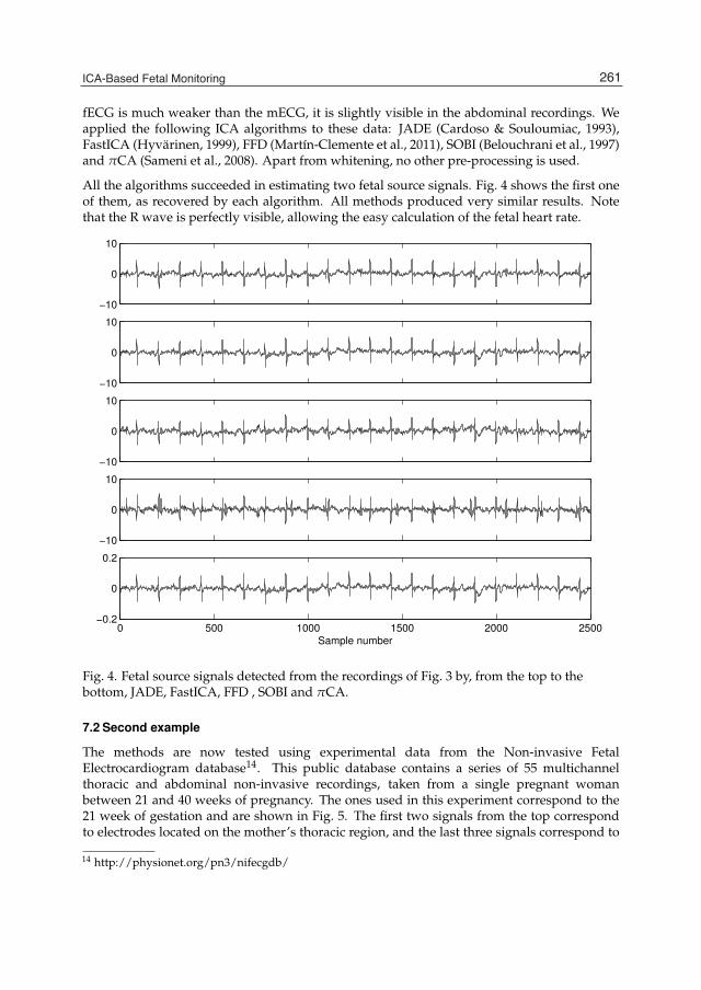
ICA-Based Fetal Monitoring 15
fECG is much weaker than the mECG, it is slightly visible in the abdominal recordings. Weapplied the following ICA algorithms to these data: JADE (Cardoso & Souloumiac, 1993),FastICA (Hyvärinen, 1999), FFD (Martín-Clemente et al., 2011), SOBI (Belouchrani et al., 1997)and πCA (Sameni et al., 2008). Apart from whitening, no other pre-processing is used.
All the algorithms succeeded in estimating two fetal source signals. Fig. 4 shows the first oneof them, as recovered by each algorithm. All methods produced very similar results. Notethat the R wave is perfectly visible, allowing the easy calculation of the fetal heart rate.
−10
0
10
−10
0
10
−10
0
10
−10
0
10
0 500 1000 1500 2000 2500−0.2
0
0.2
Sample number
Fig. 4. Fetal source signals detected from the recordings of Fig. 3 by, from the top to thebottom, JADE, FastICA, FFD , SOBI and πCA.
7.2 Second example
The methods are now tested using experimental data from the Non-invasive FetalElectrocardiogram database14. This public database contains a series of 55 multichannelthoracic and abdominal non-invasive recordings, taken from a single pregnant womanbetween 21 and 40 weeks of pregnancy. The ones used in this experiment correspond to the21 week of gestation and are shown in Fig. 5. The first two signals from the top correspondto electrodes located on the mother’s thoracic region, and the last three signals correspond to
14 http://physionet.org/pn3/nifecgdb/
261ICA-Based Fetal Monitoring

16 Will-be-set-by-IN-TECH
electrodes located on the woman’s abdomen. The recordings have been pre-processed: thebaseline was eliminated using a low-pass filter with cutoff frequency equal to 0.7 Hz, and thepowerline interference was attenuated using a notch filter.
Fig. 6 shows the source signals estimated by the same ICA algorithms used in the previousexample (JADE, FastICA, FFD, SOBI and πCA). Only the maternal source signals can berecognized. We must conclude that, even though ICA is generally reliable, it sometimes fail.
−5000
0
5000
−1
0
1x 10
4
−5000
0
5000
−1
0
1x 10
4
0 1 2 3 4 5 6 7 8 9 10−1
0
1x 10
4
time (s)
Fig. 5. Cutaneous electrode recordings from a pregnant woman in the 21 week of gestation.
7.3 Third example
We now repeat the previous (failed) experiment using the mECG as reference for the FFDmethodd, as explained in Section 6. FFD has been chosen as representative of the ICAmethods, but results are similar when any other of the algorithms is used. The estimatedsource signals are depicted in Fig. 7. Unlike in the previous experiment, the fECG is visiblein the third plot from the top, and the fetal heart rate can be estimated even though thesignal-to-noise ratio is low. Further denoising may necessary using other techniques –see,e.g., Sameni, Shamsollahi, Jutten & Clifford (2007); Vigneron et al. (2003)– but this is beyondthe scope of the present Chapter.
262 Independent Component Analysis for Audio and Biosignal Applications

ICA-Based Fetal Monitoring 17
−10
0
10
−5
0
5
−10
0
10
−20
0
20
0 1 2 3 4 5 6 7 8 9 10−5
0
5
time (s)
(a) JADE
−20
0
20
−10
0
10
−10
0
10
−5
0
5
0 1 2 3 4 5 6 7 8 9 10−5
0
5
time (s)
(b) FastICA
−10
0
10
−5
0
5
−20
0
20
−10
0
10
0 1 2 3 4 5 6 7 8 9 10−5
0
5
time (s)
(c) FFD
−5
0
5
−10
0
10
−20
0
20
−10
0
10
0 1 2 3 4 5 6 7 8 9 10−5
0
5
time (s)
(d) SOBI
−0.05
0
0.05
−0.1
0
0.1
−0.1
0
0.1
−0.1
0
0.1
0 1 2 3 4 5 6 7 8 9 10−0.1
0
0.1
time (s)
(e) πCA
Fig. 6. Source signals estimated by the different algorithms from the recordings of Fig. 5.
263ICA-Based Fetal Monitoring

18 Will-be-set-by-IN-TECH
−20
0
20
−10
0
10
−5
0
5
−10
0
10
0 1 2 3 4 5 6 7 8 9 10−5
0
5
time (s)
Fig. 7. Source signals detected from the recordings of Fig. 5 by using the mECG as reference.
8. Conclusions
This Chapter has presented a review of the state-of-the-art in the use of ICA for the fECGdetection problem. A significant improvement in technical support for fetal monitoringhas been obtained in the last decades. Compared to alternative techniques (e.g., filtering,average beat subtraction ...), ICA has proven to be a powerful and leading-edge approach.The most remarkable feature of higher-order ICA methods is that they do not seem to bevery sensitive to the location of the electrodes. However, it should be pointed out that, eventhough promising results have been obtained (the fetal heart rate can be almost routinelydetermined), there is at present a total lack of accuracy in the detection of the smallest waves(P, Q, S and T) of the fECG. Though it is true that in current clinical practice the physician onlyconsiders the fetal cardiac rate, further research is therefore needed to improve accuracy ofwave detection. The use of prior information (e.g., reference signals, or the knowledge aboutthe fECG waveform) may be the strategy to achieve this goal. The physical interpretationof the estimated source signals also seems to be an exciting field for future work, and theindependence of the sources need to be elucidated.
264 Independent Component Analysis for Audio and Biosignal Applications

ICA-Based Fetal Monitoring 19
9. Acknowledgement
This work was supported by a grant from the “Junta de Andalucía” (Spain) with referenceP07-TIC-02865.
10. References
Abboud, S. & Sadeh, D. (1989). Spectral analysis of the fetal electrocardiogram, Computers inbiology and medicine 19(6): 409–415.
Abuhamad, A. & Chaoui, R. (2009). A Practical Guide to Fetal Echocardiography: Normal andAbnormal Hearts, Lippincott Williams & Wilkins.
Adib, A. & Aboutajdine, D. (2005). Reference-based blind source separation using a deflationapproach, Signal Processing 85: 1943 – 1949.
Afriat, C. & Kopel, E. (2008). Electronic Fetal Monitoring, 2nd. edn, Lippincott Williams &Wilkins.
Azzerboni, B., La Foresta, F., Mammone, N. & Morabito, F. (2005). A new approach based onwavelet-ica algorithms for fetal electrocardiogram extraction, Proceeding of Europeansimposium on Artificial Neural Networks .
Bai, Z., Demmel, J., Dongarra, J., Ruhe, A. & van der Vorst, H. (eds) (2000). Templates for theSolution of Algebraic Eigenvalue Problems: A Practical Guide., SIAM.
Barros, A. & Cichocki, A. (2001). Extraction of specific signals with temporal structure, NeuralComputation 13(9): 1995–2003.
Bell, A. J. & Sejnowski, T. (1995). An information-maximization approach to blind separationand blind deconvolution, Neural Computation 7: 1129–1159.
Belouchrani, A., Abed-Meraim, K., Cardoso, J. & Moulines, E. (1997). A blindsource separation technique using second-order statistics, Signal Processing, IEEETransactions on 45(2): 434–444.
Callaerts, D., Moor, B. D., Vandewalle, J. & Sansen, W. (1990). Comparison of svd methodsto extract the foetal ecg from cutaneous electrode signals, Medical & Biolog. Eng. &Computing 28: 217–224.
Camargo-Olivares, J., Martín-Clemente, R., Hornillo, S., Elena-Pérez, M. & Román-Martínez,I. (2011). The maternal abdominal ecg as input to mica in the fetal ecg extractionproblem., IEEE Signal Processing Letters 18(3): 161 –164.
Cardoso, J. F. (1998). Multidimensional independent component analysis, Proc. ICASSP’98,Seattle, pp. 1941–1944.
Cardoso, J. F. & Souloumiac, A. (1993). Blind beamforming for non gaussian signals, IEEProceedings - F 140(6): 363 – 370.
Castells, F., Cebrián, A. & Millet, J. (2007). The role of independent component analysis in thesignal processing of ecg recordings, Biomedizinische Technik 52(1): 18 – 24.
Chan, A. (2008). Biomedical device technology: principles and design, Charles C. Thomas.Cichocki, A. & Amari, S.-I. (2002). Adaptive blind signal and image processing: learning algorithms
and applications, Wiley.Cicinelli, E., Bortone, A., Carbonara, I., Incampo, G., Bochicchio, M., Ventura, G., Montanaro,
S. & Aloisio, G. (1994). Improved equipment for abdominal fetal electrocardiogramrecording: description and clinical evaluation, International journal of bio-medicalcomputing 35(3): 193 – 205.
Clifford, G., Sameni, R., Ward, J., Robinson, J. & Wolfberg, A. J. (2011). Clinically accuratefetal ecg parameters acquired from maternal abdominal sensors, American Journal ofObstetrics and Gynecology 205 (1): 47.e1–47.e5.
265ICA-Based Fetal Monitoring

20 Will-be-set-by-IN-TECH
Clifford, G., Shoeb, A., McSharry, P. & Janz, B. (2005). Model-based filtering, compressionand classification of the ecg, Proceedings of Bioelectromagnetism and 5th InternationalSymposium on Noninvasive Functional Source Imaging within the Human Brain and Heart(BEM & NFSI).
Comon, P. (1994). Independent component analysis, a new concept?, Signal Processing (SpecialIssue Higher-Order Statistics) 36 (3): 287–314.
Comon, P. & Jutten, C. (eds) (2010). Handbook of blind source separation, independent componetanalysis and applications, Elsevier.
De Lathauwer, L., Callaerts, D., De Moor, B. D. & Vandewalle, J. (1995). Fetalelectrocardiogram extraction by source subspace separation, Proc. IEEE SP/ATHOSWorkshop on HOS, Girona, Spain, pp. 134–138.
De Lathauwer, L., De Moor, B. D. & Vandewalle, J. (2000a). Fetal electrocardiogram extractionby blind source subspace separation, IEEE Transactions on Biomedical Engineering 47(5): 567–572.
De Lathauwer, L., De Moor, B. & Vandewalle, J. (2000b). Svd-based methodologies forfetal electrocardiogram extraction, Proceedings of the 2000 IEEE Int. Conf. on Acoustics,Speech, and Signal Processing (ICASSP’00), Vol. 6, pp. 3771 – 3774.
Devedeux, D., Marque, C., Mansour, S., Germain, G., Duchêne, J. et al. (1993). Uterineelectromyography: a critical review., American journal of obstetrics and gynecology169(6): 1636 –1652.
Freeman, R. & Garite, T. (2003). Fetal Heart Rate Monitoring, Lippincott Williams & Wilkins.Gao, P., Chang, E. & Wyse, L. (2003). Blind separation of fetal ecg from single mixture using
svd and ica, Information, Communications and Signal Processing, 2003 and the FourthPacific Rim Conference on Multimedia. Proceedings of the 2003 Joint Conference of theFourth International Conference on, Vol. 3, IEEE, pp. 1418–1422.
Guyton, A. & Hall, J. (1996). Texbook of Medical Physiology, W. B. Saunders Company.Hasan, M., Reaz, M., Ibrahimy, M., Hussain, M. & Uddin, J. (2009). Detection and processing
techniques of fecg signal for fetal monitoring, Biological procedures online 11(1): 263 –295.
Hyvärinen, A. (1999). Fast and robust fixed-point algorithms for independent componentanalysis, IEEE Transactions on Neural Networks 10 (3): 626–634.
Hyvärinen, A., Karhunen, J. & Oja, E. (2001). Independent Component Analysis, John Wiley &Sons.
James, C. & Hesse, C. (2005). Independent component analysis for biomedical signals,Physiological measurement 26: R15.
Jenkins, H. M. L., Symonds, E. M., Kirk, D. L. & Smith, P. R. (2005). Can fetalelectrocardiography improve the prediction of intraparturn fetal acidosis?, BJOG: AnInternational Journal of Obstetrics & Gynaecology 93(1): 6–12.
Kanjilal, P., Palit, S. & Saha, G. (1997). Fetal ecg extraction from single-channel maternal ecgusing singular value decomposition, IEEE Tr. on Biomedical Engineering 44 (1): 51 – 59.
Karvanen, J., Eriksson, J. & Koivunen, V. (2000). Pearson system based method for blindseparation, Proceedings of Second International Workshop on Independent ComponentAnalysis and Blind Signal Separation (ICA2000), Helsinki, Finland, pp. 585–590.
Keener, J. & Sneyd, J. (2009). Mathematical Physiology, Vol. 2, Springer.Keralapura, M., Pourfathi, M. & Sirkeci-Mergen, B. (2011). Impact of contrast functions in
fast-ica on twin ecg separation, IAENG International Journal of Computer Science 38:1.Lewis, M. (2003). Review of electromagnetic source investigations of the fetal heart., Medical
Engineering and Physics 25 (10): 801 – 810.
266 Independent Component Analysis for Audio and Biosignal Applications

ICA-Based Fetal Monitoring 21
Li, Y. & Yi, Z. (2008). An algorithm for extracting fetal electrocardiogram, Neurocomputing 71(7–9): 1538 – 1542.
Llinares, R. & Igual, J. (2009). Application of constrained independent component analysisalgorithms in electrocardiogram arrhythmias, Artificial Intelligence in Medicine47: 121–133.
Marossero, D., Erdogmus, D., Euliano, N., Principe, J., Hild, K. et al. (2003). Independentcomponents analysis for fetal electrocardiogram extraction: a case for the dataefficient mermaid algorithm, Neural Networks for Signal Processing, 2003. NNSP’03.2003 IEEE 13th Workshop on, IEEE, pp. 399–408.
Martín-Clemente, R., Acha, J. & Puntonet, C. G. (2004). Eigendecomposition of self-tunedcumulant-matrices for blind source separation, Signal Processing 84(7): 1201 – 1211.
Martín-Clemente, R., Camargo-Olivares, J., Hornillo-Mellado, S., Elena, M. & Roman, I. (2011).Fast technique for noninvasive fetal ecg extraction, IEEE Transactions on BiomedicalEngineering 58(2): 227 – 230.
McSharry, P., G., C., Tarassenko, L. & Smith, L. (2003). A dynamical model for generatingsynthetic electrocardiogram signals, IEEE Tr. on Biomedical Engineering 50 (3): 289–294.
Nait-Ali, A. (2009). Advanced Biosignal Processing, Springer Verlag.Oldenburg, J. & Macklin, M. (1977). Changes in the conduction of the fetal electrocardiogram
to the maternal abdominal surface during gestation., American journal of obstetrics andgynecology 129(4): 425 – 433.
Oostendorp, T. F. (1989). Lead systems for the abdominal fetal electrocardiogram, ClinicalPhysics and Physiological Measurements 10(21): 21 – 26.
Oostendorp, T. F., van Oosterom, A. & Jongsma, H. W. (1989a). The effect of changes inthe conductive medium on the fetal ecg throughout gestation, Clinical Physics andPhysiological Measurements 10 (B): 11 – 20.
Oostendorp, T. F., van Oosterom, A. & Jongsma, H. W. (1989b). The fetal ecg throughout thesecond half of gestation, Clinical Physics and Physiological Measurements 10 (2): 147 –160.
Pardi, G., Ferrazzi, E., Cetin, I., Rampello, S., Baselli, G., Cerutti, S., Civardi, S. et al. (1986).The clinical relevance of the abdominal fetal electrocardiogram., Journal of perinatalmedicine 14(6): 371 – 377.
Peters, M., Stinstra, J., Uzunbajakau, S. & Srinivasan, N. (2005). Advances in electromagneticfields in living systems, Springer Verlag, chapter Fetal Magnetocardiography, pp. 1 –40.
Rieta, J., Castells, F., Sánchez, C., Zarzoso, V. & Millet, J. (2004). Atrial activity extractionfor atrial fibrillation analysis using blind source separation, IEEE Transactions onBiomedical Engineering 51(7): 1176 – 1186.
Sameni, R., Clifford, G., Jutten, C. & Shamsollahi, M. (2007). Multichannel ecg and noisemodeling: Application to maternal and fetal ecg signals, EURASIP Journal onAdvances in Signal Processing 2007.
Sameni, R., Jutten, C. & M. Shamsollahi, M. (2006). What ica provides for ecgprocessing:application to non-invasive fetal ecg extraction, Proc. 2006 IEEEInternational Symposium on Signal Processing and Information Technology.
Sameni, R., Jutten, C. & Shamsollahi, M. (2008). Multichannel electrocardiogramdecomposition using periodic component analysis, IEEE Transactions on BiomedicalEngineering 55 (8): 1935 – 1940.
Sameni, R., Shamsollahi, M., Jutten, C. & Clifford, G. (2007). A nonlinear bayesian filteringframework for ecg denoising, IEEE Tr. on Biomedical Engineering 54(12): 2172 – 2185.
267ICA-Based Fetal Monitoring

22 Will-be-set-by-IN-TECH
Saul, L. K. & Allen, J. B. (2001). Advances in Neural Information Processing Systems 13, MITPress: Cambridge, MA, chapter Periodic component analysis: an eigenvalue methodfor representing periodic structure in speech., pp. 807 – 813.
Symonds, E. M., Sahota, D. & Chang, A. (2001). Fetal Electrocardiography, Imperial CollegePress.
Tanskanen, J. & Viik, J. (2012). Advances in Electrocardiograms - Methods and Analysis, InTech,chapter Independent Component Analysis in ECG Signal Processing, pp. 349 – 372.
Taylor, M., Smith, M., Thomas, M., Green, A., Cheng, F., Oseku-Afful, S., Wee, L., Fisk, N. &Gardiner, H. (2003). Non-invasive fetal electrocardiography in singleton andmultiplepregnancies, BJOG: An International Journal of Obstetrics & Gynaecology 110(7): 668 –678.
Taylor, M., Thomas, M., Smith, M., Oseku, S., Fisk, N., Green, A., Paterson, S. & Gardiner, H.(2005). Non-invasive intrapartum fetal ecg: preliminary report., Br. J. Obstet. Gynaecol.112: 1016–1021.
Theis, F. J. (2004). Uniqueness of complex and multidimensional independent componentanalysis., Signal Processing 84 (5): 951–956.
Tong, L., Liu, R., Soon, V. C. & Huang, Y.-F. (1991). Indeterminacy and identifiability of blindidentification, IEEE Transactions on Circuit and Systems 38 (5): 499 – 509.
Tsalaile, T., Sameni, R., Sanei, S., Jutten, C. & Chambers, J. (2009). Sequential blind sourceextraction for quasi-periodic signals with time-varying period, IEEE Tr. on BiomedicalEngineering 56(3): 654 – 655.
Vetter, R., Virag, N., Vesin, J., Celka, P. & Scherrer, U. (2000). Observer of autonomic cardiacoutflow based on blind source separation of ecg parameters, IEEE Transactions onBiomedical Engineering 47: 589–593.
Vigneron, V., Paraschiv-Ionescu, A., Azancot, A., Sibony, O. & Jutten, C. (2003). Fetalelectrocardiogram extraction based on non-stationary ica and wavelet denoising,Signal Processing and Its Applications, 2003. Proceedings. Seventh InternationalSymposium on, Vol. 2, pp. 69 – 72.
Vollgraf, R. & Obermayer, K. (2001). Multi-dimensional ica to separate correlated sources.,Proceeding of Neural Information Processing System (NIPS), pp. 993–1000.
Vrins, F., Jutten, C. & Verleysen, M. (2004). Sensor array and electrode selection fornon-invasive fetal electrocardiogram extraction by independent component analysis,Independent Component Analysis and Blind Signal Separation pp. 1017–1024.
Wakai, R., Lengle, J. & Leuthold, A. (2000). Transmission of electric andmagnetic foetal cardiacsignals in a case of ectopia cordis: the dominant role of the vernix caseosa, Physics inmedicine and biology 45: 1989 – 1995.
Yu, S. & Chou, K. (2008). Integration of independent component analysis and neural networksfor ecg beat classification, Expert Systems with Applications 34(4): 2841–2846.
Zarzoso, V. (2009). Advanced Biosignal Processing, Springer, chapter Extraction ofECG Characteristics Using Source Separation Techniques: Exploiting StatisticalIndependence and Beyond.
Zarzoso, V. & Nandi, A. K. (2001). Noninvasive fetal electrocardiogram extraction: blindseparation versus adaptive noise cancelation., IEEE Tr. on Biomedical Engineering 48(1): 12–18.
268 Independent Component Analysis for Audio and Biosignal Applications

Section 4
ICA: Time-Frequency Analysis


0
Advancements in the Time-Frequency Approachto Multichannel Blind Source Separation
Ingrid Jafari1, Roberto Togneri1 and Sven Nordholm2
1The University of Western Australia2Curtin University
Australia
1. Introduction
The ability of the human cognitive system to distinguish between multiple, simultaneouslyactive sources of sound is a remarkable quality that is often taken for granted. This capabilityhas been studied extensively within the speech processing community andmany an endeavorat imitation has beenmade. However, automatic speech processing systems are yet to performat a level akin to human proficiency (Lippmann, 1997) and are thus frequently faced withthe quintessential "cocktail party problem": the inadequacy in the processing of the targetspeaker/s when there are multiple speakers in the scene (Cherry, 1953). The implementationof a source separation algorithm can improve the performance of such systems. Sourceseparation is the recovery of the original sources from a set of observations; if no a prioriinformation of the original sources and/or mixing process is available, it is termed blindsource separation (BSS). Rather than rely on the availability of a priori information of theacoustic scene, BSS methods often employ an assumption on the constituent source signals,and/or an exploitation of the spatial diversity obtained through a microphone array. BSS hasmany important applications in both the audio and biosignal disciplines, including medicalimaging and communication systems.
In the last decade, the research field of BSS has evolved significantly to be an importanttechnique in acoustic signal processing (Coviello & Sibul, 2004). The general BSS problemcan be summarized as follows. M observations of N sources are related by the equation
X = AS , (1)
where X is a matrix representing the M observations of the N sources contained in the matrixS, and A is the unknown M × N mixing matrix. The aim of BSS is to recover the sourcematrix S given simply the observed mixtures X, however rather than directly estimate thesource signals, the mixing matrix A is instead estimated. The number of sensors relativeto the number of sources present determines the class of BSS: evendetermined (M = N),overdetermined (M > N) or underdetermined (M < N). The evendetermined system can besolved via a linear transformation of the data; whilst the overdetermined case can be solvedby an estimation of the mixing matrix A. However, due to its intrinsic noninvertible nature,the underdetermined BSS problem cannot be resolved via a simple mixing matrix estimation,and the recovery of the original sources from the mixtures is considerably more complex than
14
2 Will-be-set-by-IN-TECH
the other aforementioned BSS instances. As a result of its intricacy, the underdetermined BSSproblem is of growing interest in the speech processing field.
Traditional approaches to BSS are often based upon assumptions about statistical propertiesof the underlying source signals, for example independent component analysis (ICA)(Hyvarinen et al., 2001), which aims to find a linear representation of the sources in theobservation mixtures. Not only does this rely on the condition that the constituent sourcesignals are statistically independent, it also requires that no more than one of the independentcomponents (sources) follows a Gaussian distribution. However, due to the fact thattechniques of ICA depend on matrix inversion, the number of microphones in the arraymust be at least equal to, or greater than, the number of sources present (i.e. even- oroverdetermined cases exclusively). This poses a significant restraint on its applicability tomany practical applications of BSS. Furthermore, whilst statistical assumptions hold well forinstantaneous mixtures of signals, in most audio applications the expectation of instantaneousmixing conditions is largely impractical, and the convolutive mixing model is more realistic.
The concept of time-frequency (TF) masking in the context of BSS is an emerging field ofresearch that is receiving an escalating amount of attention due to its ease of applicability to avariety of acoustic environments. The intuitive notion of TF masking in the speech processingdiscipline originates from analyses on human speech perception and the observation of thephenomenon of masking in human hearing: in particular, the fact that the human mindpreferentially processes higher energy components of observed speechwhilst compressing thelower components. This notion can be administered within the BSS framework as describedbelow.
In the TF masking approach to BSS, the assumption of sparseness between the speech sources,as initially investigated in (Yilmaz & Rickard, 2004), is typically exploited. There exists severalvarying definitions for sparseness in the literature; (Georgiev et al., 2005) simply defines itas the existence of "as many zeros as possible", whereas others offer a more quantifiablemeasure such as kurtosis (Li & Lutman, 2006). Often, a sparse representation of speechmixtures can be acquired through the projection of the signals onto an appropriate basis,such as the Gabor or Fourier basis. In particular, the sparseness of the signals in theshort-time Fourier transform (STFT) domain was investigated in (Yilmaz & Rickard, 2004)and subsequently termed W-disjoint orthogonality (W-DO). This significant discovery ofW-DO in speech signals motivated the degenerate unmixing estimation technique (DUET)which was proven to successfully recover the original source signals from simply a pair ofmicrophone observations. Using a sparse representation of the observation mixtures, therelative attenuation and phase parameters between the observations are estimated at each TFcell. The parameters estimates are utilized in the construction of a power-weighted histogram;under the assumption of sufficiently ideal mixing conditions, the histogram will inherentlycontain peaks that denote the true mixing parameters. The final mixing parameters estimatesare then used in the calculation of a binary TF mask.
This initiation into the TF masking approach to BSS is oft credited to the authors of this DUETalgorithm. Due to its versatility and applicability to a variety of acoustic conditions (under-,even- and overdetermined), the TF masking approach has since evolved as a popular andeffective tool in BSS, and the formation of the DUET algorithm has consequently motivated aplethora of demixing techniques.
272 Independent Component Analysis for Audio and Biosignal Applications

Advancements in the Time-Frequency Approach to Multichannel Blind Source Separation 3
Among the first extensions to the DUET was the TF ratio of mixtures (TIFROM) algorithm(Abrard & Deville, 2005) which relaxed the condition of W-DO of the source signals, andhad a particular focus on underdetermined mixtures for arrays consisting of more than twosensors. However, its performance in reverberant conditions was not established and theobservations were restricted to be of the idealized linear and instantaneous case. Subsequentresearch as in (Melia & Rickard, 2007) extended the DUET to echoic conditions with theDESPRIT (DUET-ESPRIT) algorithm; this made use of the existing ESPRIT (estimation ofsignal parameters via rotational invariance technique) algorithm (Roy & Kailath, 1989). ThisESPRIT algorithm was combined with the principles of DUET, however, in contrast to theDUET, it utilized more than two microphone observations with the sensors arranged in auniform linear array. However, due to this restriction in the array geometry, the algorithmwasnaturally subjected to front-back confusions. Furthermore, a linear microphone arrangementposes a constraint upon the spatial diversity obtainable from the microphone observations.
A different avenue of research as in (Araki et al., 2004) composed a two-stage algorithmwhichcombined the sparseness approach in DUET with the established ICA algorithm to yieldthe SPICA algorithm. The sparseness of the speech signals was firstly exploited in order toestimate and subsequently remove the active speech source at a particular TF point; followingthis removal, the ICA technique could be applied to the remaining mixtures. Naturally, arestraint upon the number of sources present at any TF point relative to the number of sensorswas inevitable due to the ICA stage. Furthermore, the algorithmwas only investigated for thestereo case.
The authors of the SPICA expanded their research to nonlinear microphones arrays in (Arakiet al., 2005; 2006a;b) with the introduction of the clustering of normalized observation vectors.Whilst remaining similar in spirit to the DUET, the research was inclusive of nonidealconditions such as room reverberation. This eventually culminated in the development ofthe multiple sensors DUET (MENUET) (Araki et al., 2007). The MENUET is advantageousover the DUET in that it allows more than two sensors in an arbitrary nonlinear arrangement,and is evaluated on underdetermined reverberant mixtures. In this algorithm the maskestimation was also automated through the application of the k-means clustering algorithm.Another algorithm which proposes the use of a clustering approach for the mask estimationis presented in (Reju et al., 2010). This study is based upon the concept of complex angles inthe complex vector space; however, evaluations were restricted to a linear microphone array.
Despite the advancements of techniques such as MENUET, it is not without its limitations:most significantly, the k-means clustering is not very robust in the presence of outliersor interference in the data. This often leads to non-optimal localization and partitioningresults, particularly for reverberant mixtures. Furthermore, binary masking, as employedin the MENUET, has been shown to impede on the separation quality with respect tothe musical noise distortions. The authors of (Araki et al., 2006a) suggest that fuzzy TFmasking approaches bear the potential to reduce the musical noise at the output significantly.In (Kühne et al., 2010) the use of the fuzzy c-means clustering for mask estimation wasinvestigated in the TF masking framework of BSS; on the contrary to MENUET, thisapproaches integrated a fuzzy partitioning in the clustering in order to model the inherentambiguity surrounding the membership of a TF cell to a cluster. Examples of contributingfactors to such ambiguous conditions include the effects of reverberation and additive channelnoise at the sensors in the array. However, this investigation, as with many others in
273Advancements in the Time-Frequency Approach to Multichannel Blind Source Separation

4 Will-be-set-by-IN-TECH
the literature, possessed the significant restriction in its limitation to a linear microphonearrangement.
Another clustering approach to TF mask estimation lies with the implementation of GaussianMixture Models (GMM). The use of GMMs in conjunction with the Expectation-Maximization(EM) algorithm for the representation of feature distributions has been previouslyinvestigated in the sparseness approach to BSS (Araki et al., 2009; Izumi et al., 2007; Mandelet al., 2006). This avenue of research is motivated by the intuitive notion that the individualcomponent densities of the GMM may model some underlying set of hidden parameters in amixture of sources. Due to the reported success of BSS methods that employ such Gaussianmodels, the GMM-EMmay be considered as a standard algorithm for mask estimation in thisframework, and is therefore regarded as a comparative model in this study.
However, each of the TF mask estimation approaches to BSS discussed above are yet to beinclusive of the noisy reverberant BSS scenario. Almost all real-world applications of BSShave the undesired aspect of additive noise at the recording sensors (Cichocki et al., 1996). Theinfluence of additive noise has been described as a very difficult and continually open problemin the BSS framework (Mitianoudis & Davies, 2003). Numerous studies have been proposedto solve this problem: (Li et al., 2006) presents a two-stage denoising/separation algorithm;(Cichocki et al., 1996) implements a FIR filter at each channel to reduce the effects of additivenoise; and (Shi et al., 2010) suggests a preprocessing whitening procedure for enhancement.Whilst noise reduction has been achieved with denoising techniques implemented as apre- or post-processing step, the performance was proven to degrade significantly at lowersignal-to-noise ratios (SNR) (Godsill et al., 1997). Furthermore, the aforementioned techniquesfor the compensation of additive noise have yet to be extended and applied in depth to the TFmasking approach to BSS.
Motivated by these shortcomings, this chapter presents an extension of the MENUETalgorithm via a novel amalgamation with the FCM as in (Kühne et al., 2010) (see Fig. 1).The applicability of MENUET to underdetermined and arbitrary sensor constellations rendersit superior in many scenarios over the investigation in (Kühne et al., 2010); however, itsperformance is hindered by its non-robust approach to mask estimation. Firstly, this studyproposes that the combination of fuzzy clustering with the MENUET algorithm, whichwill henceforth be denoted as MENUET-FCM, will improve the separation performance inreverberant conditions. Secondly, it is hypothesized that this combination is sufficiently robustto withstand the degrading effects of reverberation and random additive channel noise. Forall investigations in this study, the GMM-EM clustering algorithm for mask estimation isimplemented with the MENUET (and denoted MENUET-GMM) for comparative purposes.As a side note, it should be observed that all ensuing instances of the term MENUET are inreference to the original MENUET algorithm as in (Araki et al., 2007).
The remainder of the chapter is structured as follows. Section 2 provides a detailed overviewof the MENUET and proposed modifications to the algorithm. Section 3 explains the threedifferent clustering algorithms and their utilization for TF mask estimation. Section 4 presentsdetails of the experimental setup and evaluations, and demonstrates the superiority of theproposed MENUET-FCM combination over the baseline MENUET and MENUET-GMM forBSS in realistic acoustic environments. Section 5 provides a general discussion with insightinto potential directions for future research. Section 6 concludes the chapter with a briefsummary.
274 Independent Component Analysis for Audio and Biosignal Applications

Advancements in the Time-Frequency Approach to Multichannel Blind Source Separation 5
Fig. 1. Basic scheme of proposed time-frequency masking approach for BSS.
2. Source separation with TF masking
This section provides an introduction to the problem statement of underdetermined BSSand insight into the TF masking approach for BSS. The MENUET, MENUET-FCM andMENUET-GMM algorithms are described in greater detail.
2.1 Problem statement
Consider amicrophone arraymade up of M identical sensors in a reverberant enclosure whereN sources are present. It is assumed that the observation at the mth sensor can be modeled asa summation of the received images, denoted as smn(t), of each source sn(t) by
xm(t) =N
∑n=1
smn(t) , (2)
wheresmn(t) = ∑
phmn(p)sn(t− p) + nm(t) , (3)
and where t indicates time, hmn(p) represents the room impulse response from the nth sourceto the mth sensor and nm(t) denotes the additive noise present at the mth sensor.
The goal of any BSS system is to recover the sets of separated source signal images s11(t),. . . , sM1(t),. . . ,s1N(t), . . . , sMN(t), where each set denotes the estimated source signal sn(t),and smn(t) denotes the estimate of the nth source image, smn(t), at the mth sensor. Ideally,the separation is performed without any information about sn(t), hmn(p) and the true sourceimages smn(t).
2.2 Feature extraction
The time-domain microphone observations, sampled at frequency fs, are converted into theircorresponding frequency domain time-series Xm(k, l) via the STFT
Xm(k, l) =L/2−1∑
τ=−L/2win(τ)xm(τ + kτ0)e−jlω0τ , m = 1, . . . , M, (4)
where k ∈ 0, . . . ,K − 1 is a time frame index, l ∈ 0, . . . , L − 1 is a frequency bin index,win(τ) is an appropriately selected window function and τ0 and ω0 are the TF grid resolution
275Advancements in the Time-Frequency Approach to Multichannel Blind Source Separation
6 Will-be-set-by-IN-TECH
parameters. The analysis window is typically chosen such that sufficient information isretained within whilst simultaneously reducing signal discontinuities at the edges. A suitablewindow is the Hann window
win(τ) = 0.5− 0.5cos(2πτ
L) , τ = 0, . . . , L− 1, (5)
where L denotes the frame size.
It is assumed that the length of L is sufficient such that the main portion of the impulseresponses hmn is covered. Therefore, the convolutive BSS problem may be approximated asan instantaneous mixture model (Smaragdis, 1998) in the STFT domain
Xm(k, l) ≈N
∑n=1
Hmn(l)Sn(k, l) + Nm(k, l) , m = 1, . . . , M, (6)
where (k, l) represents the time and frequency index respectively, Hmn(l) is the room impulseresponse from source n and sensor m. Sn(k, l), Xm(k, l) and Nm(k, l) are the STFT of the mth
observation, nth source and additive noise at the mth sensor respectively. The sparseness ofthe speech signals assumes at most one dominant speech source Sn(k, l) per TF cell (Yilmaz &Rickard, 2004). Therefore, the sum in (6) is reduced to
Xm(k, l) ≈ Hmn(l)Sn(k, l) + Nm(k, l) , m = 1, . . . , M. (7)
Whilst this assumption holds true for anechoic mixtures, as the reverberation in the acousticscene increases it becomes increasingly unreliable due to the effects of multipath propagationand multiple reflections (Kühne et al., 2010; Yilmaz & Rickard, 2004).
In this work the TF mask estimation is realized through the estimation of the TF pointswhere a signal is assumed dominant. To estimate such TF points, a spatial feature vectoris calculated from the STFT representations of the M observations. Previous research hasidentified level ratios and phase differences between the observations as appropriate featuresin this BSS framework as such features retain information on the magnitude and the argumentof the TF points. A comprehensive review is presented in (Araki et al., 2007), with furtherdiscussion presented in Section 4.2.1. Should the source signals exhibit sufficient sparseness,the clustering of the level ratios and phase differences will yield geometric information on thesource and sensor locations, and thus facilitate effective separation.
The feature vectorθ(k, l) =
[θL(k, l), θP(k, l)
]T, (8)
per TF point is estimated as
θL(k, l) =[ |X1(k, l)|
A(k, l), . . . ,
|XM(k, l)|A(k, l)
], m = J, (9)
θP(k, l) =[1αarg
[X1(k, l)XJ(k, l)
], . . . ,
1αarg
[XM(k, l)XJ(k, l)
]], m = J, (10)
276 Independent Component Analysis for Audio and Biosignal Applications

Advancements in the Time-Frequency Approach to Multichannel Blind Source Separation 7
for A(k, l) =
√M∑
m=1|Xm(k, l)|2 and α = 4πc−1dmax, where c is the propagation velocity, dmax
is the maximum distance between any two sensors in the array and J is the index of thereference sensor. The weighting parameters A(k, l) and α ensure appropriate amplitude andphase normalization of the features respectively. It is widely known that in the presence ofreverberation, a greater accuracy in phase ratio measurements can be achieved with greaterspatial resolution; however, it should be noted that the value of dmax is upper bounded by thespatial aliasing theorem.
The frequency normalization in A(k, l) ensures frequency independence of the phase ratiosin order to prevent the frequency permutation problem in the later stages of clustering. It ispossible to cluster without such frequency independence, for example (Sawada et al., 2007;2011); however, the utilization of all the frequency bins in the clustering stage avoids this andalso permits data observations of short length (Araki et al., 2007).
Rewriting the feature vector in complex representation yields
θj(k, l) = θLj (k, l) exp(jθP
j (k, l)) , (11)
where θLj and θP
j are the jth components of (9) and (10) respectively. In this feature vectorrepresentation, the phase difference information is captured in the argument term, and thelevel ratio is normalized by the normalization term A(k, l).
Equivalently (Araki et al., 2007)
θj(k, l) = |Xj(k, l)| exp[
jarg[Xj(k, l)/XJ(k, l)]
αj f
], (12)
and
θ(k, l)← θ(k, l)‖θ(k, l)‖ , (13)
where θ(k, l) = [θ1(k, l), . . . , θM(k, l)]T . In the final representation of (13), the level and phaseinformation are captured in the amplitude and argument respectively.
Fig. 2(a) and 2(b) depict the histogram of extracted level ratios and phase differences,respectively, in the ideal anechoic environment. The clear peaks in the phase histogramin (b) are distinctively visible and correspond to the sources. However, when the anechoicassumption is violated and reverberation is introduced into the environment, the distinctionbetween peaks is reduced in clarity as is evident in the phase ratio histogram in Fig. 2(c).Furthermore, the degrading effects of additive channel noise can be seen in Fig. 2(d)where the phase ratio completely loses its reliability. It is hypothesized in this study that asufficiently robust TF mask estimation technique will be competent to withstand the effect ofreverberation and/or additive noise in the acoustic environment.
The masking approach to BSS relies on the observation that in an anechoic setting, theextracted features are expected to form N clusters, where each cluster corresponds to a sourceat a particular location. Since the relaxation of the anechoic assumption reduces the accuracy
277Advancements in the Time-Frequency Approach to Multichannel Blind Source Separation

8 Will-be-set-by-IN-TECH
of the extracted features as mentioned above in Section 2.2, it is imperative that a sufficientlyrobust TF clustering technique is implemented in order to effectively separate the sources.
The feature vector set Θ(k, l) = θ(k, l) | θ(k, l) ∈ R2(M−1), (k, l) ∈ Ω is divided into Nclusters, where Ω = (k, l) : 0 ≤ k ≤ K − 1, 0 ≤ l ≤ L − 1 denotes the set of TFpoints in the STFT plane. Depending on the selection of clustering algorithm, the clusters arerepresented by distinct sets of TF points (hard k-means clustering); a set of prototype vectorsand membership partition matrix (fuzzy c-means); or a parameter set (GMM-EM approach).
Specifically, the k-means algorithm results in N distinct clusters C1, . . . ,CN , where each cluster
is comprised of the constituent TF cells, andN∑
n=1|Cn| = |Θ(k, l)| where the operator |.|
denotes cardinality. The fuzzy c-means yields the N centroids vn and a partition matrixU = un(k, l) ∈ R | n ∈ (1, . . . , N), (k, l) ∈ Ω), where un(k, l) indicates the degree ofmembership of the TF cell (k, l) to the nth cluster. The GMM-EM clustering results in theparameter set associated with the Gaussian mixture densities Λ = λ1, . . . ,λG where Gis the number of mixture components in the Gaussian densities, and each λi vector has arepresentative mean and covariance matrix. Further details on the three main clusteringalgorithms used in this study are provided in Section 3.
2.3 Mask estimation and separation
In this work source separation is effectuated by the application of TF masks, which are thedirect result of the clustering step.
For the k-means algorithm, a binary mask for the nth source is simply estimated as
Mn(k, l) =
1 for θ(k, l) ∈ Cn ,0 otherwise.
(14)
In the instances of FCM clustering, the membership partition matrix is interpreted as acollection of N fuzzy TF masks, where
Mn(k, l) = un(k, l) . (15)
For the GMM-EM algorithm, the mask estimation is based upon the calculation ofprobabilities from the final optimized parameter set Λ = λ1, . . . ,λn. The parameter setis used to estimate the masks as follows
Mn(k, l) ∼ argmaxn
p(θ(k, l)|λn) , (16)
where λn denotes the parameter set pertaining to the nth source, and probabilitiesp(θ(k, l)|λn) are calculated using a simple normal distribution (Section 3.3).
The separated signal image estimates S11(k, l), . . . , S1M(k, l), . . . , SN1(k, l), . . . , SNM(k, l) inthe frequency domain are then obtained through the application of the mask per source to anindividual observation
Smn(k, l) = Mn(k, l)Xm(k, l) , m = 1, . . . , M. (17)
278 Independent Component Analysis for Audio and Biosignal Applications

Advancements in the Time-Frequency Approach to Multichannel Blind Source Separation 9
(a) (b)
(c) (d)
Fig. 2. Example histograms of the MENUET features as in (9) and (10) for varying acousticconditions: (a) histogram of level ratio in an anechoic environment, (b) histogram of phasedifference in an anechoic environment, (c) phase difference in presence of reverberant noise(RT60 = 300ms), (d) phase difference in presence of channel noise.
2.4 Source resynthesis
Lastly, the estimated source images are reconstructed to obtain the time-domain separatedestimates of the source images smn(t) for n = 1, . . . , N and m = 1, . . . , M. This is realized withthe application of the overlap-and-add method (Rabiner, 1978) onto the separated frequencycomponents Smn(k, l). The reconstructed estimate is
smn(t) =1
Cwin
L/τ0−1∑
k′=0sk+k′
mn (t) , (18)
279Advancements in the Time-Frequency Approach to Multichannel Blind Source Separation

10 Will-be-set-by-IN-TECH
where Cwin = 0.5/τ10L is a Hann window function constant, and individual frequencycomponents of the recovered signal are acquired through an inverse STFT
skmn(t) =
L−1∑l=0
Smn(k, l)ejlω0(t−kτ0) , (19)
if (kτ0 ≤ t ≤ kτ + L− 1), and zero otherwise.
3. Time-frequency clustering algorithms
3.1 Hard k -means clustering
Previous methods (Araki et al., 2006b; 2007) employ hard clustering techniques such as thehard k-means (HKM) (Duda et al., 2000). In this approach, the feature vectors θ(k, l) areclustered to form N distinct clusters C1, . . . ,CN .
The clustering is achieved through the minimization of the objective function
Jkmeans =N
∑n=1
∑θ(k,l)∈Cn)
‖θ(k, l)− cn‖2 , (20)
where the operator ‖.‖ denotes the Euclidean norm and cn denotes the cluster centroids.Starting with a random initialization for the set of centroids, this minimization is iterativelyrealized by the following alternating equations
C∗n = θ(k, l)|n = argminn
‖θ(k, l)− cn‖2 , ∀n, k, l, (21)
c∗n ← Eθ(k, l)θ(k,l)∈Cn, ∀n, (22)
until convergence is met, where E.θ(k,l)∈Cndenotes the mean operator for the TF points
within the cluster Cn, and the (*) operator denotes the optimal value. The resulting N clustersare then utilized in the mask estimation as described in Section 2.3. Due to the algorithm’ssensitivity to initialization of the cluster centres, it is recommended to either design initialcentroids using an assumption on the sensor and source geometry (Araki et al., 2007), or toutilize the best outcome of a predetermined number of independent runs.
Whilst this binary clustering performed satisfactorily in both simulated and realisticreverberant environments, the authors of (Jafari et al., 2011; Kühne et al., 2010) demonstratethat the application of a soft masking scheme improves the separation performancesubstantially.
Summary: K-means Algorithm
1 Initialize centroids c1, . . . , cN randomly2 For j = 1, 2, . . .3 Update cluster members Cn using (21)4 Update centroids cn with calculated clusters Cn according to (22)5 Repeat until for some j∗ the convergence is met6 Assign C∗1 , . . . ,C∗N and c∗1, . . . , c∗N to each TF point.
280 Independent Component Analysis for Audio and Biosignal Applications

Advancements in the Time-Frequency Approach to Multichannel Blind Source Separation 11
3.2 Fuzzy c-means clustering
In the fuzzy c-means clustering, the feature set Θ(k, l) = θ(k, l)|θ(k, l) ∈ R2(M−1), (k, l) ∈ Ωis clustered using the fuzzy c-means algorithm (Bezdek, 1981) into N clusters, where Ω =(k, l) : 0 ≤ k ≤ K − 1, 0 ≤ l ≤ L − 1 denotes the set of TF points in the STFT plane.Each cluster is represented by a centroid vn and partition matrix U = un(k, l) ∈ R|n ∈(1, . . . , N), (k, l) ∈ Ω) which specifies the degree un(k, l) to which a feature vector θ(k, l)belongs to the nth cluster. Clustering is achieved by the minimization of the cost function
J f cm =N
∑n=1
∑∀(k,l)
un(k, l)qDn(k, l) , (23)
whereDn(k, l) = ‖θ(k, l)− vn‖2 , (24)
is the squared Euclidean distance between the vector θ(k, l) and the nth cluster centre. Thefuzzification parameter q > 1 controls the membership softness; a value of q in the range ofq ∈ (1, 1.5] has been shown to result in a fuzzy performance akin to hard (binary) clustering(Kühne et al., 2010). However, superior mask estimation ability has been established whenq = 2; thus in this work, the fuzzification q is set to 2.
The minimization problem in (23) can be solved using Lagrange multipliers and is typicallyimplemented as an alternating optimization scheme due to the open nature of its solution(Kühne et al., 2010; Theodoridis & Koutroumbas, 2006). Initialized with a randompartitioning, the cost function J f cm is iteratively minimized by alternating the updates forthe cluster centres and memberships
v∗n = ∑
∀(k,l)
un(k, l)qθ(k, l)∑∀(k,l)
un(k, l)q , ∀n, (25)
u∗n(k, l) =
⎡⎣ N
∑j=1
(Dn(k, l)Dj(k, l)
) 1q−1
⎤⎦−1
, ∀n, k, l, (26)
where (*) denotes the optimal value, until a suitable termination criterion is satisfied.Typically, convergence is defined as when the difference between successive partitionmatricesis less than some predetermined threshold ε (Bezdek, 1981). However, as is also the case withthe k-means (Section 3.1), it is known that the alternating optimization scheme presented mayconverge to a local, as opposed to global, optimum; thus, it is suggested to independentlyimplement the algorithm several times prior to selecting the most fitting result.
3.3 Gaussian mixture model clustering
To further examine the separation ability of the MENUET-FCM scheme another clusteringapproach, based upon GMM clustering, is presented in this study. A GMM of a multivariatedistribution Θ(k, l) may be represented by a weighted sum of G component Gaussian
281Advancements in the Time-Frequency Approach to Multichannel Blind Source Separation

12 Will-be-set-by-IN-TECH
Summary: C-means Algorithm
1 Initialize partition matrix U randomly2 For j = 1, 2, . . .3 Update centroids vn according to (25)4 Update partition matrix U with calculated memberships un according to (26)5 Repeat until for some j∗ the convergence threshold ε is met6 Assign u∗n(k, l) and v∗n to each TF point (k, l).
densities as given by
p(Θ|Λ) =G
∑i
wig(Θ|λi) , (27)
where wi, i = 1, . . . , G are the mixture weights, g(Θ|Λ) are the component Gaussian densities,and Λ is the vector of hidden parameters such that Λ = λ1, . . . ,λG of the Gaussiancomponents. Each component density is a D-variate Gaussian function of the form
g(Θ|μi,Σi) =1
(2π)D/2|Σi|1/2exp
−12(Θ−μi)
′Σ−1i (Θ−μi)
, (28)
with mean vector μi and covariance matrix Σi. The constraint on the mixture weights is such
as to satisfy the conditionG∑
i=1wi = 1.
The goal of the GMM-EM clustering is to fit the source mixture data into a Gaussianmixture model and then estimate the maximum likelihood of the hidden parameters Λ =λ1, . . . ,λG, where each λi has its associated mean vector μi and covariance matrix Σi,associated with the mixture densities in the maximum likelihood of the features Θ(k, l). Thefeatures Θ(k, l) in this section will henceforth be denoted as Θ for simplicity. Under theassumption of independence between the features, the likelihood of the parameters, L(Λ|Θ)is related to Θ by
p(Θ|Λ) =T
∏t=1
p(θt|Λ) = L(Λ|Θ) , (29)
where T is the total number of TF cells per feature (i.e. k ∗ l). The estimation of the optimumhidden parameter set Λ∗ relies on the maximization of (29)
Λ∗ = argmaxΛ
L(Λ|Θ) . (30)
Due to the fact that the log of L(∗) is typically calculated in lieu of L(∗), the function (29)is a nonlinear function of Λ. Therefore, the maximization in the G mixture components isa difficult problem. However, the maximum-likelihood (ML) estimates of these parametersmay be calculated using the Expectation-Maximization (EM) algorithm (Izumi et al., 2007).The EM algorithm is iterated until a predetermined convergence threshold ε is reached.
The choice of the number of Gaussianmixtures for fitting the microphone array data is critical,and is typically determined by trial and error (Araki et al., 2007). In this study, the number ofmixture components is set equal to the number of sources in order to facilitate the associationof clusters to sources. In the casewhere G > N, the associationwill have an ambiguous nature.
282 Independent Component Analysis for Audio and Biosignal Applications

Advancements in the Time-Frequency Approach to Multichannel Blind Source Separation 13
This assumption that each resulting Gaussian cluster uniquely fits one source therefore allowsthe calculation of the probability that a TF cell originates from the nth source; this is becausethe probability is equivalent to the probability that the TF cell originates from the nth mixturecomponent. It is assumed in this study that the probability of membership follows a normaldistribution as
p(θ(k, l)|λ∗n) =1
(2π|Σ∗n|)1/2exp
−12(θ(k, l)−μ∗
n)′Σ∗−1n (θ(k, l)−μ∗
n)
, (31)
where λ∗n ∈ Λ∗ = λ∗1, . . . ,λ∗N.
Summary: GMM-EM Algorithm
1 Assume initial parameter set Λ2 For j = 1, 2, . . .3 Calculate expectation L(Λ|Θ) according to EM as in (Izumi et al., 2007)4 Estimate Λj according to (Izumi et al., 2007)5 Repeat until for some j∗ the convergence threshold ε is met6 Assign λ∗n to each TF point (k, l).
4. Experimental evaluations
4.1 Experimental setup
Fig. 3. The room setup for the three sensor nonlinear arrangement experimental evaluations.
The experimental setup was such as to reproduce that in (Araki et al., 2007) and (Jafari et al.,2011) for comparative purposes. Fig. 3 depicts the speaker and sensor arrangement, and Table1 details the experimental conditions. The wall reflections of the enclosure, as well as theroom impulse responses for each sensor, were simulated using the image model method forsmall-room acoustics (Lehmann & Johansson, 2008). The room reverberation was quantifiedin the measure RT60, where RT60 is defined as the time required for reflections of a directsound to decay by 60dB below the level of the direct sound (Lehmann & Johansson, 2008).
For the noise-robust evaluations, spatially uncorrelated white noise was added to each sensormixture such that the overall channel SNR assumed a value as in Table 1. The SNR definitionas in (Loizou, 2007) was implemented, which employs the standardized method given in
283Advancements in the Time-Frequency Approach to Multichannel Blind Source Separation

14 Will-be-set-by-IN-TECH
(ITU-T, 1994) to objectively measure the speech. The four speech sources, the genders ofwhich were randomly generated, were realized with phonetically-rich utterances from theTIMIT database (Garofolo et al., 1993) , and a representative number of mixtures for evaluativepurposes constructed in total. In order to avoid the spatial aliasing problem, the microphoneswere placed at a maximum distance of 4cm apart.
Experimental conditions
Number of microphones M = 3Number of sources N = 4R 50cmSource signals 6 sReverberation time 0 ms, 128 ms 300ms
(450ms for clean evaluations only)Input channel SNR 0 dB - 30 dBSampling rate 8 kHzSTFT window HannSTFT frame size 64 msSTFT frame overlap 50%
Table 1. The parameters used in experimental evaluations.
As briefly discussed in Section 3.1 and 3.2, it is widely recognized that the performance of theclustering algorithms is largely dependent on the initialization of the algorithm. For both theMENUET and MENUET-FCM, the best of 100 runs was selected for initialization in order tominimize the possibility of finding a local, as opposed to global, optimum. In order to ensurethe GMM fitting of the mixtures in the MENUET-GMM evaluations, the initial values for themean and variance in the parameter set Λ had to be selected appropriately. The initializationof the parameters has been proven to be an imperative yet difficult task; should the selectionbe unsuccessful, the GMM fitting may completely fail (Araki et al., 2007). In this study, themean and variance for each parameter set were initialized using the k-means algorithm.
4.1.1 Evaluation measures
For the purposes of speech separation performance evaluation, two versions of the publiclyavailable MATLAB toolboxes BSS_EVAL were implemented (Vincent et al., 2006; 2007).This performance criteria is applicable to all source separation approaches, and no priorinformation of the separation algorithm is required. Separation performance was evaluatedwith respect to the global image-to-spatial-distortion ratio (ISR), signal-to-interference ratio(SIR), signal-to-artifact ratio (SAR) and signal-to-distortion ratio (SDR) as defined in (Vincentet al., 2007); for all instances, a higher ratio is deemed as better separation performance.
This assumes the decomposition of the estimated source sn(t) as
smn(t) = simgmn (t) + espat
mn (t) + eintmn(t) + earti f
mn (t) , (32)
284 Independent Component Analysis for Audio and Biosignal Applications

Advancements in the Time-Frequency Approach to Multichannel Blind Source Separation 15
where simgmn (t) corresponds to the true source image, and espat
mn (t), eintmn(t) and earti f
mn (t) are theundesired error components that correlate to the spatial distortion, interferences and artifactsrespectively. This decomposition is motivated by the auditory notion of distinction betweensounds originating from the target source, sounds from other sound sources present, and"gurgling" noise corresponding to simg
mn (t) + espatmn (t), eint
mn(t) and earti fmn (t), respectively. The
decomposition of the estimated signal was executed using the function bss_eval_images, whichcomputes the spatial distortion and interferences by means of a least-squares projection ofthe estimated source image onto the corresponding signal subspaces. As recommended in(Vincent et al., 2007), the filter length was set to the maximal tractable length of 512 (64ms).
The ISR of the nth recovered source is then calculated as
ISRn = 10log10
M∑
m=1∑t
simgmn (t)2
M∑
m=1∑t
espatmn (t)2
, (33)
which provides ameasure for the relative amount of distortion present in the recovered signal.
The SIR, given by
SIRn = 10log10
M∑
m=1∑t(simg
mn (t) + espatmn (t))2
M∑
m=1∑t
eintmn(t)2
, (34)
provides an estimate of the relative amount of interference in the target source estimate. Forall SIR evaluations the gain SIRgain = SIRoutput − SIRinput was computed in order to quantifythe improvement between the input and the output of the proposed studies.
The SAR is computed as
SARn = 10log10
M∑
m=1∑t(simg
mn (t) + espatmn (t) + eint
mn(t))2
M∑
m=1∑t
earti fmn (t)2
, (35)
in order to give a quantifiable measure of the amount of artifacts present in the nth sourceestimate.
As an estimate of the total error in the nth recovered source (or equivalently, a measure for theseparation quality), the SDR is calculated as
SDRn = 10log10
M∑
m=1∑t
simgmn (t)2
M∑
m=1∑t
[espat
mn (t) + eintmn(t) + earti f
mn (t)]2 . (36)
285Advancements in the Time-Frequency Approach to Multichannel Blind Source Separation

16 Will-be-set-by-IN-TECH
Similarly, the SNR of the estimated output signal was also evaluated using the BSS_EVALtoolkit. The estimated source sn(t) was assumed to follow the following decomposition(Vincent et al., 2006)
sn(t) = stargetn (t) + enoise
n (t) + eintn (t) + earti f
n (t) , (37)
where stargetn (t) is an allowed distortion of the original source, and enoise
n (t), eintn (t) and earti f
n (t)are the noise, interferences and artifacts error terms respectively. The decomposition ofthe estimated signal in this instance was executed using the function bss_decomp_filt, whichpermits time-invariant filter distortions of the target source. As recommended in (Vincentet al., 2006), the filter length was set to 256 taps (32ms). The global SNR for the nth source wassubsequently calculated as
SNRn = 10log10||starget
n (t) + eintn (t)||2
||enoisen (t)||2 . (38)
4.2 Results
4.2.1 Initial evaluations of fuzzy c-means clustering
Firstly, to establish the feasibility of the c-means clustering as a credible approach to the TFmask estimation problem for underdetermined BSS, the algorithm was applied to a rangeof feature sets as defined in (Araki et al., 2007). The authors of (Araki et al., 2007) present acomprehensive review of suitable location features for BSS within the TF masking framework,and evaluate their effectiveness using the k-means clustering algorithm. The experimentalsetup for these set of evaluations was such as to replicate that in (Araki et al., 2007) to as closea degree as possible. In an enclosure of dimensions 4.55m x 3.55m x 2.5m, two omnidirectionalmicrophones were placed a distance of 4cm apart at an elevation of 1.2m. Three speechsources, also at an elevation of 1.2m, were situated at 30o, 70o and 135o; and the distanceR between the array and speakers was set to 50cm. The room reverberation was constant at128ms. The speech sources were randomly chosen from both genders of the TIMIT databasein order to emulate the investigations in (Araki et al., 2007) which utilized English utterances.
It is observed from the comparison of separation performance with respect to SIRimprovement as shown in Table 2 that the c-means outperformed the original k-meansclustering in all but one feature set. This firstly establishes the applicability of the c-meansclustering in the proposed BSS framework, and secondly demonstrates the robustness ofthe c-means clustering against a variety of spatial features. The results of this investigationprovide further motivation to extend the fuzzy TF masking scheme to other sensorarrangements and acoustic conditions.
4.2.2 Separation performance in reverberant conditions
Once the feasibility of the fuzzy c-means clustering for source separation was established,the study was extended to a nonlinear three sensor and four source arrangement as in Fig.3. The separation results with respect to the ISR, SIR gain, SDR and SAR for a range ofreverberation times are given in Fig. 4(a)-(d) respectively. Fig. 4(a) depicts the ISR results;from here it is evident that there are considerable improvements in the MENUET-FCM over
286 Independent Component Analysis for Audio and Biosignal Applications

Advancements in the Time-Frequency Approach to Multichannel Blind Source Separation 17
Feature θ(k, l) k-means (dB) c-means (dB)
θ(k, l) =[ |X2(k,l)||X1(k,l)| ,
12π f arg
[X2(k,l)X1(k,l)
]]T1.8 2.1
θ(k, l) =
[|X2(k,l)||X1(k,l)| −
1|X2(k,l)||X1(k,l)|
, 12π f arg
[X2(k,l)X1(k,l)
]]T
1.1 1.6
θ(k, l) =[ |X2(k,l)||X1(k,l)| ,
12π f c−1darg
[X2(k,l)X1(k,l)
]]T7.8 9.2
θ(k, l) = 12π f arg
[X2(k,l)X1(k,l)
]10.2 8.0
θ(k, l) = 12π f c−1darg
[X2(k,l)X1(k,l)
]10.1 17.2
θ(k, l) =[ |X1(k,l)|
A(k,l) , |X2(k,l)|A(k,l) , 1
2π arg[
X2(k,l)X1(k,l)
]]T4.2 5.4
θ(k, l) =[ |X1(k,l)|
A(k,l) , |X2(k,l)|A(k,l) , 1
2π f c−1darg[
X2(k,l)X1(k,l)
]]T10.4 17.4
θj(k, l) = |Xj(k, l)| exp[
j arg[Xj(k,l)/XJ(k,l)]αj f
],
θ(k, l)← θ(k,l)‖θ(k,l)‖ 10.2 17.2
Table 2. Comparison of separation performance in terms of SIR improvement in dB of typicalspatial features. Separation results are evaluated with SIRgain for the TF masking approach toBSS when the hard k-means and fuzzy c-means algorithms are implemented for maskestimation. The reverberation was constant at RT60 = 128ms.
both the MENUET and MENUET-GMM. Additionally, the MENUET-GMM demonstrates aslight improvement over the MENUET.
The SIR gain as in Fig. 4(b) clearly demonstrates the superiority in source separation withthe MENUET-FCM. For example, at the high reverberation time of 450ms, the proposedMENUET-FCM outperformed both the baseline MENUET and MENUET-GMM by almost5dB.
Similar results were noted for the SDR, with substantial improvements when fuzzy masks areused. As the SDR provides a measure of the total error in the algorithm, this suggests thatthe fuzzy TF masking approach to BSS is more robust against algorithmic error than the otheralgorithms.
The superiority of the fuzzymasking scheme is further established in the SAR values depictedin Fig. 4(d). A consistently high value is achieved across all reverberation times, unlikethe other approaches which fail to attain such values. This indicates that the fuzzy TFmasking scheme yields source estimates with fewer artifacts present. This is in accordancewith the study as in (Araki et al., 2006a) which demonstrated that soft TF masks bear theability to significantly reduce the musical noise in recovered signals as a result of the inherentcharacteristic of the fuzzy mask to prevent excess zero padding in the recovered sourcesignals.
287Advancements in the Time-Frequency Approach to Multichannel Blind Source Separation

18 Will-be-set-by-IN-TECH
It is additionally observed that there is a significantly reduced standard deviation resultingfrom the FCM algorithm which further implies consistency in the algorithm’s sourceseparation ability.
(a) (b)
(c) (d)
Fig. 4. Source separation results in reverberant conditions using three separation approaches:MENUET, MENUET-GMM and MENUET-FCM. Performance results given in terms of (a)ISR, (b) SIR gain, (c) SDR and (d) SAR for all RT60 values. The error bars denote the standarddeviation over all evaluations.
4.2.3 Separation performance in reverberant conditions with additive noise
The impact of additive white channel noise on separation quality was evaluated next. Thereverberation was varied from 0ms to 300ms, and the SNR at the sensors of the microphonearray was varied from 0dB to 30dB in 5dB increments.
Tables 3(a)-(d) depicts the separation results of the evaluations with respect to the measuredISR, SIR gain, SDR and SAR respectively. It is clear from the table that the proposedMENUET-FCM algorithm has significantly increased separation ability over all testedconditions and for all performance criteria. In particular, the MENUET-FCM scenariodemonstrates excellent separation ability even in the higher 300ms reverberation condition.
288 Independent Component Analysis for Audio and Biosignal Applications

Advancements in the Time-Frequency Approach to Multichannel Blind Source Separation 19
Conditions ISR (dB)
SNRin (dB) HKM GMM FCM
RT60 = 0ms0 4.92 3.68 4.525 5.13 4.07 5.8310 6.93 4.61 6.5315 7.18 6.09 8.3720 7.81 6.21 11.8125 7.96 7.15 11.9830 6.87 7.48 12.62
RT60 = 128ms0 3.18 3.21 4.155 4.05 4.16 5.0310 4.34 4.59 5.9115 5.13 4.77 7.9120 5.71 4.89 10.4125 6.24 5.67 10.8530 5.24 6.04 11.08
RT60 = 300ms0 3.49 2.84 3.865 3.05 3.00 4.1210 3.42 4.04 5.0515 3.55 4.11 5.9120 3.64 4.13 7.0525 4.10 4.59 7.9930 3.55 4.66 8.21
(a)
Conditions SIR gain (dB)
SNRin (dB) HKM GMM FCM
RT60 = 0ms0 5.01 3.49 4.955 6.21 4.89 7.0110 7.83 5.34 8.8615 8.01 6.00 17.8920 8.22 6.64 19.1525 8.56 7.12 19.0830 7.16 9.65 19.4
RT60 = 128ms0 2.78 2.84 4.465 3.08 3.27 5.9110 3.46 3.86 7.5015 5.17 5.03 13.0420 6.72 5.48 16.9025 7.01 7.58 16.7830 5.17 8.36 17.61
RT60 = 300ms0 2.96 1.79 3.85 2.95 3.05 4.1210 3.02 3.97 6.1115 4.28 4.49 8.5320 4.99 5.24 10.7825 5.32 6.65 11.5330 4.12 7.54 13.81
(b)
289Advancements in the Time-Frequency Approach to Multichannel Blind Source Separation

20 Will-be-set-by-IN-TECH
Conditions SDR (dB)
SNRin (dB) HKM GMM FCM
RT60 = 0ms0 -1.88 -2.41 -0.205 0.15 -1.14 1.7610 0.88 -0.24 3.1515 1.03 0.16 6.0120 1.19 0.45 8.2025 1.37 1.29 8.3930 0.76 1.39 8.50
RT60 = 128ms0 -2.22 -2.41 -0.295 -0.76 -0.71 1.6410 -0.50 -0.32 2.9415 0.57 -0.08 6.1920 0.68 0.09 7.3725 0.98 1.13 7.5630 -0.70 1.51 7.98
RT60 = 300ms0 -1.41 -2.6 -0.365 -1.07 -1.98 1.2310 -0.78 -0.31 2.1315 -0.35 -0.10 3.2420 -0.41 -0.09 4.3525 0.15 0.27 4.9330 -0.41 -0.61 5.97
(c)
Conditions SAR (dB)
SNRin (dB) HKM GMM FCM
RT60 = 0ms0 -4.83 -5.44 -2.475 -2.44 -2.65 1.8510 0.08 -0.76 4.6215 0.59 0.17 7.8420 1.83 0.74 10.1725 1.91 1.78 10.1930 2.18 2.23 10.22
RT60 = 128ms0 -4.42 -4.14 -1.305 -1.19 -1.01 2.5510 -0.80 -0.04 5.6015 1.65 1.61 8.7820 2.58 1.87 10.3925 2.93 2.98 10.7130 2.71 3.38 10.85
RT60 = 300ms0 -3.51 -4.14 -1.295 -1.64 -1.91 1.8210 -0.71 -0.07 4.5315 2.02 1.69 7.3720 2.73 1.85 8.2425 3.62 2.87 9.0230 3.43 3.03 10.48
(d)
Table 3. Source separation results for reverberant noisy mixtures using three separationapproaches: MENUET, MENUET-GMM and MENUET-FCM. Performance results are givenin terms of (a) ISR, (b) SIR gain, (c) SDR and (d) SAR for all RT60 and SNR values. Thehighest achieved ratios per acoustic scenario are denoted in boldface.
290 Independent Component Analysis for Audio and Biosignal Applications

Advancements in the Time-Frequency Approach to Multichannel Blind Source Separation 21
4.2.4 SNR evaluations
For the purposes of speech quality assessment, the SNR of each recovered speech signal wascalculated with the definition as in (Vincent et al., 2006) and averaged across all evaluations,with the results shown in Table 4. The MENUET-FCM approach is again observed to bemore robust against additive channel noise at the recovered output. However, a remarkableimprovement in SNR values for the recovered speech sources for all clustering techniques isalso observed. This suggests that the original MENUET, MENUET-GMM andMENUET-FCMhave implementations beyond that of simply BSS and in fact maybe useful in applicationsthat also require speech enhancement capabilities. This has important repercussions as itdemonstrates that these approaches are able to withstand additive noise without significantdegradations in performance, and thus bear the potential to additionally be utilized as aspeech enhancement stage in a BSS system.
5. Discussion
The experimental results presented have demonstrated that the implementation of the fuzzyc-means clustering with the nonlinear microphone array setup as in the MENUET renderssuperior separation performance in conditions where reverberation and/or additive channelnoise exist.
The feasibility of the fuzzy c-means clustering was firstly tested on a range of spatial featurevectors in an underdetermined setting using a stereomicrophone array, and compared againstthe original baseline k-means clustering of the MENUET algorithm. The successful outcomeof this prompted further investigation, with a natural extension to a nonlinear microphonearray. The GMM-EM clustering algorithm was also implemented as a second baseline tofurther assess the quality of the c-means against alternative binary masking schemes otherthan the k-means. Evaluations confirmed the superiority of c-means clustering with positiveimprovements recorded for the average performance in all acoustic settings. In addition tothis, the consistent performance even in increased reverberation establishes the potential offuzzy c-means clustering for the TF masking approach.
However, rather than solely focus upon the reverberant BSS problem, this study refreshinglyextended it to be inclusive of additive channel noise. It was suggested that due to the fuzzyc-means’ documented robustness in reverberant environments, the extension to the noisyreverberant case would demonstrate similar abilities. Evaluations confirmed this hypothesiswith especially noteworthy improvements in the measured SIR gain and SDR. Furthermore,the MENUET, MENUET-GMM and MENUET-FCM approaches were all proven to possessinherent speech enhancement abilities, with higher SNRs measured at the recovered signals.
However, a possible hindrance in the MENUET-GMM clustering was discussed previouslyregarding the correct selection of the number of fitted Gaussians (Section 3.3). Should thenumber of Gaussians be increased in a bid to improve the performance, an appropriateclustering approach should then be applied in order to group the Gaussians originatingfrom the same speaker together; for example, a nearest neighbour or correlative clusteringalgorithm may be used.
Ultimately, the goal of any speech processing system is to mimic the auditory and cognitiveability of humans to as close a degree as possible, and the appropriate implementation of a BSS
291Advancements in the Time-Frequency Approach to Multichannel Blind Source Separation

22 Will-be-set-by-IN-TECH
Conditions SNR (dB)
SNRin (dB) HKM GMM FCM
RT60 = 0ms0 15.41 14.40 17.055 18.10 17.19 21.9610 21.25 19.90 25.0415 21.91 21.18 28.8920 23.50 22.50 32.6125 23.29 23.97 32.6830 23.62 24.50 32.91
RT60 = 128ms0 14.25 14.04 17.685 18.25 18.98 21.8710 18.50 19.65 25.3715 22.16 22.87 28.9320 23.17 23.46 32.2225 23.58 24.96 31.9930 23.40 25.10 33.00
RT60 = 300ms0 15.11 13.31 16.955 16.96 17.11 20.8310 18.35 19.31 23.5415 22.08 22.10 26.9220 22.50 22.45 28.0125 23.44 23.27 29.1030 24.16 23.71 30.70
Table 4. Results for the measured SNR at the BSS output averaged over all the recoveredsignals. Results given for all RT60 and input channel SNR values. The highest achieved ratioper acoustic scenario is denoted in boldface.
scheme is an encouraging step towards reaching this goal. This study has demonstrated thatwith the use of suitable time-frequency masking techniques, robust blind source separationcan be achieved in the presence of both reverberation and additive channel noise. The successof the MENUET-FCM suggests that future work into this subject is highly feasible for real-lifespeech processing systems.
6. Conclusions
This chapter has presented an introduction into advancements in the time-frequency approachto multichannel BSS. A non-exhaustive review of mask estimation techniques was discussed
292 Independent Component Analysis for Audio and Biosignal Applications

Advancements in the Time-Frequency Approach to Multichannel Blind Source Separation 23
with insight into the shortcomings affiliated with such existing masking techniques. In a bidto overcome such shortcomings, the novel amalgamation of two existing BSS approaches wasproposed and thus evaluated in (simulated) realistic multisource environments.
It was suggested that a binary masking scheme for the TF masking approach to BSS isinadequate at encapsulating the inevitable reverberation present in any acoustic setup, andthus a more suitable means for clustering the observation data, such as the fuzzy c-means,should be considered. The presented MENUET-FCM algorithm integrated the fuzzy c-meansclustering with the established MENUET technique for automatic TF mask estimation.
In a number of experiments designed to evaluate the feasibility and performance of thec-means in the BSS context, the MENUET-FCM was found to outperform both the originalMENUET and MENUET-GMM in source separation performance. The experiments variedin conditions from a stereo (linear) microphone array setup to a nonlinear arrangement, inboth anechoic and reverberant conditions. Furthermore, additive white channel noise wasalso included in the evaluations in order to better reflect the conditions of realistic acousticenvironments.
Future work should endeavor upon the refinement of the robustness of the featureextraction/mask estimation stage, and on the betterment of the clustering technique in orderto propel theMENUET-FCM to a sincerely blind system. Details are presented in the followingsection. Furthermore, the evaluation of the BSS performance in alternative contexts such asautomatic speech recognition should also be considered in order to gain greater perspectiveon its potential for implementation in real-life speech processing systems.
7. Future directions
Future work should focus upon the improvement of the robustness of the mask estimation(clustering) stage of the algorithm. For example, an alternative distance measure in the FCMcan be considered: it has been shown (Hathaway et al., 2000) that the Euclidean distancemetric as employed in the c-means distance calculation may not be robust to the outliers dueto undesired interferences in the acoustic environment. A measure such as the l1-norm couldbe implemented in a bid to reduce error (Kühne et al., 2010).
Additionally, the authors of (Kühne et al., 2010) also considered the implementation ofobservation weights and contextual information in an effort to emphasize the reliable featureswhilst simultaneously attenuating the unreliable features. In such a study, a suitable metric isrequired to determine such reliability: in the formulation of such a metric, consideration maybe given to the behavior of proximate TF cells through a property such as variance (Kühneet al., 2009).
Alternatively, the robustness in the feature extraction stage can also be investigated. Asdescribed in Section 2.2, the inevitable conditions of reverberation and nonideal channelsinterfere with the reliability of the extracted features. A robust approach to the featureextraction would further ensure the accuracy of the TF mask estimation. The authors of (Rejuet al., 2010) employ a feature extraction scheme based upon the Hermitian angle between theobservation vector and a reference vector; and in a spirit similar to the MENUET-FCM, thefeatures were clustered using the FCM and encouraging separation results were reported.
293Advancements in the Time-Frequency Approach to Multichannel Blind Source Separation
24 Will-be-set-by-IN-TECH
Furthermore, in a bid to move the MENUET-FCM BSS algorithm to that of a truly blind andautonomous nature, a modification to the FCM is suggested. The automatic detection of thenumber of clusters may prove to be of significance as all three of the clustering techniquesin this chapter have required a priori knowledge of the number of sources. The authors of(Sun et al., 2004) describe two possible algorithms which employ a validation technique toautomatically detect the optimum number of clusters to suit the data. Successful results ofthis technique have been reported in the BSS framework (Reju et al., 2010).
In the current investigation evaluations were limited to artificial corruption provided by asimulated room environment, as such extensions for source separation in more realistic noisescenarios (e.g. as in the CHiME data (Christensen et al., 2010), or the SiSEC data (Araki &Nesta, 2011)) will be a subject of focus in future research.
Finally, as a further evaluation measure, the separation quality of the MENUET-FCM can beevaluated in an alternative context. A natural application of the BSS scheme presented inthis chapter is as a front-end to a complete speech processing system; for example, one whichincorporates automatic speech recognition. The application of the MENUET-FCM to such adiscipline would truly determine its functionality and relevance to modern speech systems.
8. Acknowledgements
This research is partly funded by the Australian Research Council Grant No. DP1096348.
9. References
Abrard, F. & Deville, Y. (2005). A time-frequency blind signal separation method applicableto underdetermined mixtures of dependent sources, Signal Processing 85: 1389–1403.
Araki, S., Makino, S., Blin, A., Mukai, R. & Sawada, H. (2004). Underdetermined blindseparation for speech in real environments with sparseness and ica, Acoustics, Speech,and Signal Processing, 2004. Proceedings. (ICASSP ’04). IEEE International Conference on,Vol. 3, pp. iii – 881–4 vol.3.
Araki, S., Nakatani, T., Sawada, H. & Makino, S. (2009). Blind sparse source separation forunknown number of sources using gaussian mixture model fitting with dirichletprior, Proceedings of the IEEE International Conference on Acoustics, Speech and SignalProcessing, Taipei, Taiwan, pp. 33 –36.
Araki, S. & Nesta, F. (2011). Signal separation evaluation campaign (sisec 2011).URL: http://sisec.wiki.irisa.fr/tiki-index.php
Araki, S., Sawada, H., Mukai, R. & Makino, S. (2005). A novel blind source separation methodwith observation vector clustering, International Workshop on Acoustic Echo and NoiseControl, pp. 117–120.
Araki, S., Sawada, H., Mukai, R. & Makino, S. (2006a). Blind sparse source separation withspatially smoothed time-frequency masking, Proceedings of the International Workshopon Acoustic Echo and Noise Control, Paris, France.
Araki, S., Sawada, H., Mukai, R. & Makino, S. (2006b). Doa estimation for multiplesparse sources with normalized observation vector clustering, Proceedings of the IEEEInternational Conference on Acoustics, Speech and Signal Processing, Vol. 5, Toulouse,France.
294 Independent Component Analysis for Audio and Biosignal Applications

Advancements in the Time-Frequency Approach to Multichannel Blind Source Separation 25
Araki, S., Sawada, H., Mukai, R. & Makino, S. (2007). Underdetermined blind sparse sourceseparation for arbitrarily arranged multiple sensors, Signal Processing 87: 1833–1847.
Bezdek, J. (1981). Pattern recognition with fuzzy objective function algorithms, Plenum Press, NewYork.
Cherry, E. C. (1953). Some experiments on the recognition of speech, with one and with twoears, Journal of the Acoustical Society of America 25(5): 975–979.
Christensen, H., J., B., N., M. & Green, P. (2010). The chime corpus: a resource and a challengefor computational hearing in multisource environments, Proceedings of Interspeech,Makuhari, Japan.
Cichocki, A., Kasprzak,W. &Amari, S.-I. (1996). Adaptive approach to blind source separationwith cancellation of additive and convolutional noise, Proceedings of InternationalConference on Signal Processing, Beijing, China, pp. 412–415.
Coviello, C. & Sibul, L. (2004). Blind source separation and beamforming: algebraic techniqueanalysis, IEEE Transactions on Aerospace and Electronic Systems 40(1): 221 – 235.
Duda, R., Hart, P. & Stork, D. (2000). Pattern Classification, 2nd edn, Wiley Interscience.Garofolo, J. S., Lamel, L. F., Fisher, W. M., Fiscus, J. G., Pallett, D. S., Dahlgren, N. L. & Zue, V.
(1993). Timit acoustic-phonetic continuous speech corpus.Georgiev, P., Theis, F. & Cichocki, A. (2005). Sparse component analysis and blind
source separation of underdetermined mixtures, IEEE Transactions onNeural Networks16(4): 992 –996.
Godsill, S., Rayner, P. & Cappé, O. (1997). Digital Audio Restoration, Kluwer AcademicPublishers.
Hathaway, R., Bezdek, J. & Hu, Y. (2000). Generalized fuzzy c-means clustering strategiesusing lp norm distances, IEEE Transactions on Fuzzy Systems 8(5): 576 –582.
Hyvarinen, H., Karhunen, J. & Oja, E. (2001). Independent Component Analysis, John Wiley &Sons, Inc.
ITU-T (1994). Objective measurement of active speech level, Technical report, InternationalTelecommunication Union.
Izumi, Y., Ono, N. & Sagayama, S. (2007). Sparseness-based 2ch bss using the em algorithmin reverberant environment, Proceedings of the IEEE Workshop on Applications of SignalProcessing to Audio and Acoustics, New Paltz, New York, pp. 147 –150.
Jafari, I., Haque, S., Togneri, R. & Nordholm, S. (2011). Underdetermined blind sourceseparation with fuzzy clustering for arbitrarily arranged sensors, Proceedings ofInterspeech, 2011, Florence, Italy.
Kühne, M., Togneri, R. & Nordholm, S. (2009). Robust source localization in reverberantenvironments based on weighted fuzzy clustering, IEEE Signal Processing Letters16(2): 85.
Kühne, M., Togneri, R. & Nordholm, S. (2010). A novel fuzzy clustering algorithmusing observation weighting and context information for reverberant blind speechseparation, Signal Processing 90: 653–669.
Lehmann, E. A. & Johansson, A. M. (2008). Prediction of energy decay in room impulseresponses simulated with an image-source model, Journal of the Acoustical Society ofAmerica 124(1): 269–277.
Li, G. & Lutman, M. (2006). Sparseness and speech perception in noise, Proceedings of theInternational Conference on Spoken Language Processing, Pittsburgh, Pennsylvania.
295Advancements in the Time-Frequency Approach to Multichannel Blind Source Separation

26 Will-be-set-by-IN-TECH
Li, H., Wang, H. & Xiao, B. (2006). Blind separation of noisy mixed speech signalsbased on wavelet transform and independent component analysis, Proceedings of theInternational Conference on Signal Processing, Vol. 1, Guilin, China.
Lippmann, R. (1997). Speech recognition by humans and machines, Speech Communication22(1): 1–15.
Loizou, P. C. (2007). Speech Enhancement: Theory and Practice, CRC Press, Boca Raton.Mandel, M., Ellis, D. & Jebara, T. (2006). An em algorithm for localizing multiple sound
sources in reverberant environments, Proceedings of Annual Conference on NeuralInformation Processing Systems, Vancouver, Canada.
Melia, T. & Rickard, S. (2007). Underdetermined blind source separation in echoicenvironments using desprit, EURASIP Journal on Advances in Signal Processing 2007.
Mitianoudis, N. & Davies, M. (2003). Audio source separation of convolutive mixtures, IEEETransactions of Speech and Audio Processing 11(5): 489–497.
Rabiner, L. (1978). Digital Processing of Speech Signals, Signal Processing Series, Prentice-Hall,New Jersey.
Reju, V., Koh, S. N. & Soon, I. Y. (2010). Underdetermined convolutive blind source separationvia time-frequency masking, Audio, Speech, and Language Processing, IEEE Transactionson 18(1): 101 –116.
Roy, R. & Kailath, T. (1989). Esprit - estimation of signal parameters via rotational invariancetechniques, IEEE Transactions on Acoustics, Speech and Signal Processing 37(7).
Sawada, H., Araki, S. & Makino, S. (2007). A two-stage frequency-domain blind sourceseparation method for underdetermined convolutive mixtures, Proceedings of IEEEWorkshop on Applications of Signal Processing to Audio and Acoustics, New Paltz, NY.
Sawada, H., Araki, S. & Makino, S. (2011). Underdetermined convolutive blind sourceseparation via frequency bin-wise clustering and permutation alignment, IEEETransactions on Audio, Speech, and Language Processing 19(3): 516 –527.
Shi, Z., Tan, X., Jiang, Z., Zhang, H. & Guo, C. (2010). Noisy blind source separation bynonlinear autocorrelation, Proceedings of International Congress on Image and SignalProcessing, Vol. 7, Yantai, China, pp. 3152 –3156.
Smaragdis, P. (1998). Blind separation of convolved mixtures in the frequency domain,Neurocomputing 22: 21–34.
Sun, H., Wang, W., Zhang, X. & Li, Y. (2004). Fcm–based model selection algorithms fordetermining the number of clusters, Pattern Recognition 37: 2027–2037.
Theodoridis, S. & Koutroumbas, K. (2006). Pattern Recognition, 3rd edn, Academic Press, NewYork.
Vincent, E., Gribonval, R. & Fevotte, C. (2006). Performance measurement in blindaudio source separation, IEEE Transactions on Audio, Speech, and Language Processing14(4): 1462 –1469.
Vincent, E., Sawada, H., Bofill, P., Makino, S. & Rosca, J. (2007). First stereo audiosource separation evaluation campaign: data, algorithms and results, Proceedingsof International Conference on Independent Component Analysis and Signal Separation,London, England.
Yilmaz, O. & Rickard, S. (2004). Blind separation of speech mixtures via time-frequencymasking, IEEE Transactions on Signal Processing 52(7): 1830–1847.
296 Independent Component Analysis for Audio and Biosignal Applications

0
A Study of Methods for Initialization andPermutation Alignment for Time-Frequency
Domain Blind Source Separation
Auxiliadora Sarmiento, Iván Durán, Pablo Aguilera and Sergio CrucesDepartment of Signal Theory and Communications, University of Seville, Seville
Spain
1. Introduction
The problem of the blind signal separation (BSS) consists of estimating the latent componentsignals in a linear mixture, referred to as the sources, starting from several observed signals,without relying on any specific knowledge of the sources. In particular, when the sourcesare audible, this problem is known as to the cocktail-party problem, making reference to theability of the human ear to isolate the conversation of our interest among several conversationsimmersed in a noisy environment with many people talking at the same time.
The complexity of the blind separation problem greatly depends on the mixture model, thenumber of sources and sensors that better adjust to reality and the presence of noise in themixture. The simplest case regards the linear and instantaneous mixture, that is, when thesources are mixed affected only by some scaling. However, in a real room recording thesituation becomes more difficult, since the source signals do not only follow the direct pathfrom the source to the sensor, but there are also other paths coming from the reflections in thewalls. Hence, the problem becomes convolutive rather than instantaneous, and the mixtureprocess is then modelled by means of a convolution of the sources by some acoustic mixingfilters. In the present chapter we assume that the channel between sources and microphonesis time-invariant, the number of sources equals the number of sensors, that is, the N× N case,and there is no additive noise. In such recording environments the separation is very complex,especially in highly reverberant conditions where the mixing filters can be very long (greaterthan 250 ms) and can contains strong peaks corresponding to the echoes.
Several component analysis techniques solve the instantaneous and determined case in thetime domain. One of the most popular is the Independent Component Analysis (ICA), whichis a method to recover statistically independent sources by using implicitly or explicitlyhigh-order statistics Comon (1994). Some of those techniques have been extended to solvethe convolutive case in the time domain. However, its use for the separation of real speechrecordings is limited because of the high length of the acoustical mixing filters (of the orderof hundreds of milliseconds). Since it is required the adjustment of too many parameters,those method present convergence problems and a high computational cost. An extendedstrategy, referred to as fd-ICA in the literature, consists of formulating the problem in thetime-frequency domain instead of the time domain (Smaragdis, 1998). The main reason isthat the convolutive mixture can be approximated by a set of instantaneous mixtures, one
15

2 Will-be-set-by-IN-TECH
for each frequency bin, that can be solved independently by applying several separationalgorithms. However, this simplification introduces some additional problems referred toas scaling and permutation problems, since the obtained solutions in each frequency exhibitan arbitrary complex scaling and order. The scaling ambiguity introduces a filtering effect inthe estimated sources, that can be removed by introducing some constraint on the separationfilters. Nevertheless, the permutation problem leads to non-consistent time-frequencyrepresentations of the estimated signals, and needs to be addressed to successfully recoverthe original sources. During the last years, several algorithms have been proposed in orderto solve this problem, although nowadays there is no satisfactory solution, specially forhighly reverberant environments. Furthermore, the problem increases in complexity with thenumber of sources in the mixture, and the developed algorithms usually deal with the case oftwo source signals and two observations only.
Here, we will focus our attention on the initialization of the separation algorithms and thepermutation problem. The initialization procedure is very important since some separationalgorithms are very sensitive to initial conditions, and often there are some frequency binsin which the separation algorithm fails to converge. Furthermore, a suitable initializationcan achieve a spectacular reduction of permutation misalignments, since it favours thepreservation of the order of the separated components in wide frequency blocks, whichfacilitate the permutation correction. A new permutation algorithm is also proposed basedon the spectral coherence property of the speech signal. For that, we will derive a contrastfunction which maximization achieves the solution to the permutation. For the assessmentof the developed algorithms, an exhaustive study has been performed in both syntheticmeasurements and real recordings, for various mixture environments.
2. Model of BSS of convolutive mixtures in the time-frequency domain
It is well known that any acoustic signal acquired from microphones in a real recordingenvironment suffers from reflections on the walls and surfaces inside the room. In this sense,the recorded signals can be accurately modelled as a convolutive mixture, where the mixingfilter is usually considered a high-order FIR filter. The standard convolutive mixing model ofN sources, sj(n), j = 1, · · · , N, in a noiseless situation can be written as
xi(n) =N
∑j=1
∞
∑k=−∞
hij(k)sj(n− k), i = 1, · · · , N , (1)
where xi(n), i = 1, . . . , N are the N sensor signals, and hij(n) is the impulse response fromsource jth to microphone ith. In order to blindly recover the original speech signals (sources)one can apply a matrix of demixing filters to the observations xi(n) that yields an estimate ofeach of the sources
yi(n) =N
∑j=1
Q−1
∑k=0
bij(k)xj(n− k), i = 1, · · · , N, (2)
where the coefficients bij(k) denote the impulse response of demixing system filter of Q taps.
The transformation of time-domain signals to the time-frequency domain is usuallyperformed by the short-time Fourier transform (STFT). The main advantage of using thetime-frequency domain is that convolutive mixture in Equation (1), can be approximated in
298 Independent Component Analysis for Audio and Biosignal Applications

A Study of Methods for Initialization and Permutation Alignment for Time-Frequency Domain Blind Source Separation 3
the time-frequency domain by a set of of instantaneous mixtures of complex values, one foreach frequency bin, that is an easier problem for which many algorithms have been developed.
Let Xi( f , t) and Si( f , t) be, respectively, the STFT of xi(n) and si(n), and Hij( f ) be thefrequency response of the channel hij(n). From Equation (1) we obtain
Xi( f , t) N
∑j=1
Hij( f )Sj( f , t), i = 1, · · · , N , (3)
which can be rewritten, in matrix notation, as X( f , t) H( f )S( f , t), where the observationand source vectors for each time-frequency point are X( f , t) = [X1( f , t), . . . , XN( f , t)]T andS( f , t) = [S1( f , t), . . . , SN( f , t)]T , respectively, and H( f ) is the frequency response of themixing filter whose elements are Hij( f ) = [H( f )]ij ∀i, j. The superscript T represents thematrix transpose operator. From now on, we will assume that the mixing matrices H( f ) arefull rank. In practice, the approximation (3) is considered valid when the length of the DFT issignificantly greater than the length of the mixing filters Parra & Spence (2000). For instance,in fd-ICA context for speech separation it is common that the DFT is twice as long as the lengthof the mixing filters Araki et al. (2003).
Each of the separation matrices B( f ) can be estimated independently with a suitable algorithmfor instantaneous mixtures of complex values, which is computationally very efficient. Thevector of outputs or estimated sources Y( f , t) = [Y1( f , t), . . . , YN( f , t)]T is thus given byapplying B( f ) to the observations in each frequency bin,
Y( f , t) = B( f )X( f , t). (4)
Nevertheless, the simplification (3) has some disadvantages that need to be solved tosuccessfully recover the sources. As each instantaneous separation problem is solvedindependently, the recovered signals will have an arbitrary permutation and scaling in eachfrequency bin. Those ambiguities are inherent to the problem of the blind source separation.In consequence, Y( f , t) is usually modelled as
Y( f , t) ≈ Π( f )D( f )S( f , t) , (5)
where Π(f) is a permutation matrix and D( f ) is an arbitrary nonsingular diagonal matrix ofcomplex scalars, representing respectively the permutation and scaling ambiguities.
The scaling ambiguity is not a serious problem. In fact, it causes an overall filtering ofthe sources. However, the correction of the permutation is essential. Even when perfectseparation is achieved in all frequency bins, the transformation of the recovered signals intothe time domain will be erroneous if the order of the extracted components are not the samein all frequency bins. Therefore, it is necessary to determine the permutation matrix P∗( f ) ineach frequency bin in such way that the order of the outputs remains constant over all thefrequencies,
Y( fk, t)← P∗( fk)Y( fk, t). (6)
Once the separated components are well aligned, the sources can be finally recovered byconverting the time-frequency representations Yj( f , t) back to the time domain. It is alsopossible to estimate the sources by first transforming the separation matrices B( f ) to the timedomain, correcting previously the ambiguities, and then by applying the Equation (2).
299A Study of Methods for Initialization and Permutation Alignment for Time-Frequency Domain Blind Source Separation

4 Will-be-set-by-IN-TECH
3. The separation stage
The most widely used methods for solving the instantaneous separation problems in thestandard fd-ICA approach relies on the statistical independence among different sources andon the notion of contrast function. The statistical independence of the sources is a plausibleassumption in real-room recordings, since each speakers acts independently of the others.On the other hand, the notion of contrast function defines a correspondence between thedistribution of the estimated sources and the real line which is only maximized when thesources are mutually independent Comon (1994).
In the fd-ICA context, it is important to note that the separation algorithm must be capable ofhandling complex data, given that the separation problem is formulated in the time-frequencydomain. Nowadays, most of the ICA methods that work with complex data often use apreliminary whitening step that leads to Z ≡ Z( f ) the spatially whitened observations. Thispreprocessing simplifies the problem and, in some cases, it is also used because it improvesthe convergence of the algorithm. The whitening procedure consists of a linearly transformof the observed variables to zero mean and unit variance, that can be accomplished by e.g.Principal Component Analysis (Comon, 1994). One of the most widely used algorithm isFastICA Hyvärinen & Oja (1997), which exploits the property of the non-Gaussianity of thesources. The extension to complex data was formulated in Bingham & Hyvärinen (2000). Thesolution is obtained by finding the extrema of the following contrast function
ΨBH(u) = E[
G(∣∣∣uHZ
∣∣∣2)]
s. t. E[∣∣∣uHZ
∣∣∣2]= 1 , (7)
where E represents expectation, u is the extraction vector (a row of the separating matrixUH), while G is a smooth even function whose expectation measures the departure (in a givensense) from the Gaussian distribution. Some usual choices for function G can be found inBingham & Hyvärinen (2000).
The optimization of the contrast function (7) is performed by the Newton’s method, resultingthe following update rule for the fixed-point algorithm for one unit
u(i) = E[
Z(
u(i−1)HZ)∗
g(|uHZ|2
)]− E
[g(|uHZ|2
)+ |uHZ|2g′
(|uHZ|2
)]u(i−1)
u(i) ← u(i)∥∥∥u(i)∥∥∥ , (8)
where i is the iteration index, and g(·) and g′(·) denote the first and the second derivatives ofG(·), respectively. This method can be combined with a deflation procedure to retrieve all theoriginal components. An optimized variant of FastICA consists of introducing an adaptivechoice of function G. For this purpose, the distributions of the independent components canbe modelled by a generalized Gaussian distribution. The resulting algorithm is called efficientFastICA or simply EFICA Koldovský et al. (2006).
The ICA algorithms previously commented ignore the time structure of source signals.However, for the speech signals, nearby samples are highly correlated and when comparingthe statistics for distant samples the nonstationary behaviour is revealed. It is possible toexploit any of these features to achieve the separation using only second order statistics (SOS).One important advantage of the SOS based systems is that they are less sensitive to noise
300 Independent Component Analysis for Audio and Biosignal Applications

A Study of Methods for Initialization and Permutation Alignment for Time-Frequency Domain Blind Source Separation 5
and outliers. One popular method of this family of algorithms is the second order blindidentification (SOBI) algorithm, proposed in Belouchrani et al. (1997).
Under the assumption of spatial decorrelation of the sources, the correlation matrices of thesources Rs(τ) = E[s(t + τ)s∗(t)] for any nonzero time lag τ are diagonal, where superscript* denotes conjugate operation. If we consider now time-delayed correlation matrices ofwhitened observations, the next relation for prewhitened sensor signals is satisfied
Rz(τ) = WRx(τ)WH = URs(τ)UH (9)
where W is the whitening matrix and U is the unitary mixing matrix. Since Rs(τ) is diagonal,the separation matrix UH may be estimated by enforcing an unitary diagonalization of acovariance matrix Rz(τ) for some non zero lag. Instead of use only one time lag, SOBIapproximated jointly diagonalizes a set of covariance matrices computed for a fixed set oftime lags.
An extension of this algorithm that jointly exploits the non-stationary and the temporalstructure of the source signals is second-order non-stationary source separation (SEONS)algorithm proposed in Choi & Cichocki (2000). This method estimates a set of covariancematrices at different time-frames. For that, the whitened observations are divided intonon-overlapping blocks, where different time-delayed covariance matrices are computed.Then, a joint approximate diagonalization method is applied to this set of matrices to estimatethe separation matrix. The application of the SEONS algorithm in the simulations of thischapter considers covariance matrices for τ = 0 and one sample in each block.
3.1 The ThinICA algorithm
The higher order cumulants of the outputs have been one of the first class of contrast functionsproposed in the context of blind deconvolution Donoho (1981) and later extensively used inthe context of blind source separation Comon (1994); Cruces et al. (2004a). In its simpler form,the contrast function takes the form of a sum of the fourth-order cumulants of the outputs
Ψ(U) =N
∑i=1|Cum (Yi(t), · · · , Yi(t))|2 , (10)
subject to a unitary constraint on the separation matrix (UHU = I). Indeed, thefirst implementation of the Fast-ICA algorithm Hyvärinen & Oja (1997) considered themaximization of (10). Nearly at the same time, other authors developed in DeLathauweret al. (2000) a higher-order power method that consider the separation of the sources with acontrast function based on a least squares fitting of a higher-order cumulant tensor.
The ThinICA algorithm was proposed in Cruces & Cichocki (2003) as a flexible tool to addressthe simultaneous optimization of several correlation matrices and/or cumulant tensors. Thesematrices and tensors can be arbitrarily defined, so the algorithm is able to exploit not only theindependence of the sources, but also their individual temporal correlations and also theirpossible large-term non-stationarity Cruces et al. (2004b).
For simplicity, it is assumed that sources are locally stationary and standardized to zero meanand unit variance. In order to determine the statistics that take part in the ThinICA contrastfunction one should specify the order of the cumulants q and the considered time tuples θ =(t1, · · · , tq) which are grouped in the set Θ = θm ∈ Rq, m = 1, · · · , r. The algorithm works
301A Study of Methods for Initialization and Permutation Alignment for Time-Frequency Domain Blind Source Separation

6 Will-be-set-by-IN-TECH
with positive weighting scalars wθ and with q unitary matrix estimates U[k], k = 1, · · · , q, ofthe mixing system WA and their respective linear estimates Y[k](t) = U[k]HZ(t), k = 1, . . . , q,of the vector of desired sources. It was shown in Cruces et al. (2004b) that the function
ΦΘ(U[1], . . . , U[q]) =N
∑i=1
∑θ∈Θ
wθ
∣∣∣Cum(
Y[1]i (t1), · · · , Y[q]
i (tq))∣∣∣2 , (11)
is a contrast function whose global maxima are only obtained when all the estimatesagree (U[1] = · · · = U[q]) and the sources of the mixture are recovered. Moreover, theconstrained maximization of the previous contrast function is equivalent to the constrainedminimization of the weighted least squares error between a set of q-order cumulant tensorsof the observations CZ
q (θ), ∀θ ∈ Θ and their best approximations that take into account the
mutual independence statistical structure of the sources CZq (Dθ , U[1], . . . , U[q]), ∀θ ∈ Θ. If
Dθ denote diagonal matrices, the maximization of (11) is equivalent to the minimization of
εΘ(U[1], . . . , U[q]) = ∑θ∈Θ
wθ minDθ
‖CZq (θ)− CZ
q (Dθ , U[1], . . . , U[q])‖2F (12)
with respect to the unitary matrices U[k], k = 1, · · · , q. See Cruces et al. (2004b) for more detailson the equivalence between the contrast functions (11) and (12).
The optimization of the ThinICA contrast function can be implemented either hierarchicallyor simultaneously, with respective implementations are based on the thin-QR and thin-SVDfactorizations. A MatLab implementation of this algorithm can be found at the ICAlab toolboxicalab (2012), or obtained from the authors upon request.
The ThinICA contrast function and the algorithm has been also extended in Durán & Cruces(2007) to allow the simultaneous combination of correlation matrices and cumulant tensors ofarbitrary orders. In this way, the algorithm is able to simultaneously exploit the information ofdifferent statistics of the observations, what makes it suitable for obtaining accurate estimatesfrom a reduced set of observations.
The application of the ThinICA algorithm in the simulations of this chapter tries to exploitthe non-stationarity behavior of the speech signals by considering q = 2 and the set Θ =(tm, tm) ∈ Rq, m = 1, · · · , r, i.e., it uses the information of several local autocorrelations ofthe observations in frequency domain in order to estimate the latent sources.
4. Initialization procedure for ICA algorithms
The ICA algorithm used for estimating the optimal separation system in each frequency bin,is often randomly initialized. However, there are several advantages to make a suitableinitialization of the algorithm. For instance, if the algorithm is initialized near the optimalsolution, one can guarantee a high convergence speed. Also, the permutation ambiguity canbe avoided if the mixture have some properties.
One interesting approach to develop an appropriate initialization method is to consider thecontinuity of the frequency response of the mixing filter H( f ) and its inverse. Under thisassumption, it seems reasonable to initialize the separation system Bini( f ) from the value ofthe optimal separation system at the previous frequency Bo( f − 1). However, we can notdirectly apply B( f ) = Bo( f − 1) in those separation algorithms that whiten the observationsas a preprocessing step.
302 Independent Component Analysis for Audio and Biosignal Applications

A Study of Methods for Initialization and Permutation Alignment for Time-Frequency Domain Blind Source Separation 7
The whitening is performed by premultiplying the observations with an N × N matrix W( f )as Z( f , t) = W( f )X( f , t), where W( f ) is chosen so as to enforce the covariance of Z( f , t)to be the identity matrix CZ( f , t) = IN . The computation of the whitening matrix can beaccomplished by e.g. Principal Component Analysis (Comon, 1994). After that, the newobservations Z( f , t) can be expressed as a new mixture of the sources through a new unitarymixing matrix Uo( f ) = W( f )H( f ),
Z( f , t) = U( f )S( f , t). (13)
Given an estimate of the unitary mixing matrix Uo( f ), then it is immediate to see that theseparation matrix U( f )−1 = U( f )H is also unitary. Therefore, the estimated components oroutputs
Y( f , t) = U( f )HZ( f , t) = B( f )X( f , t) (14)
yields the decomposition of the separation matrix B( f ) as the product of an unitary matrixand the whitening system B( f ) = U( f )HW( f ). Due to the variability of the sources spectra,even at contiguous frequencies, the whitening matrices W( f ) and W( f − 1) are different.Consequently, in general we violate the unitary assumption of U( f ) by solving directly forUini( f )H = Bo( f − 1)W−1( f ).
An alternative method to initialize from previous solutions while avoiding the previouslydescribed problem, consists of initially preprocessing the observations at frequency f by theseparation matrix determined for the previous frequency. This technique, referred on now asclassical initialization, first computes the new observations as
Xnew( f , t) = B( f − 1)X( f , t), (15)
and then, determines the matrix W( f ) which whitens these new observations. Finally, theseparation matrices are obtained by any preferred ICA method on those new observations.In brief, this classical initialization method decomposes the overall separation matrix in thefollowing three factors
B( f ) = U( f )HW( f )B( f − 1). (16)
Instead of this classical initialization, here we aim to exploit the continuity of the frequencyresponse of the separation filter in a different way. We propose to initialize the separationsystem Bini( f ) from its joint closest value to a set of optimal separation systems alreadycomputed at nearby frequencies (Sarmiento et al., 2009; 2010) This leads to the followingconstrained minimization problem
arg minU( f )H
∑i
αi‖B( f − i)− B( f )‖2F s.t. U( f )HU( f ) = IN , (17)
where ‖ · ‖F denotes the Frobenius norm and αi are weights assigned to the separationmatrices of nearby frequencies. This problem can be solved by applying Lagrange multipliers,where the corresponding Lagrangian function L is given by
L = Tr∑
iαi
[(B( f − i)−U( f )HW( f )
)H (B( f − i)−U( f )HW( f )
)]
−Λ(
U( f )HU( f )− IN
), (18)
303A Study of Methods for Initialization and Permutation Alignment for Time-Frequency Domain Blind Source Separation

8 Will-be-set-by-IN-TECH
where Λ is the Hermitian matrix of multipliers and Tr · denotes the trace of the argument.The minimization of the Lagrangian is obtained solving for U( f ) from the equation
∇U( f )∗L = −[∑
iαiW( f )
(B( f − i)H −W( f )HU( f )
)+ U( f )Λ
]= 0N , (19)
where 0N denotes null matrix of dimension N × N. After some manipulations, one obtainsthe desired solution
Uini( f )H = QRQHL . (20)
where QL and QR are, respectively, the left and right singular vectors of the followingfactorization
[QL, D, QR] = svd
(W( f )∑
iαiB( f − i)H
). (21)
As we will se below, this initialization procedure helps to preserve the ordering of theseparated components across the frequencies. However, we can not guarantee that all thefrequencies will be correctly aligned. In fact, in the audio context, the mixing filters, andtherefore the demixing filters, can contain strong echoes. Thus, in general, the assumption ofcontinuity of the filter frequency response is not valid in all the frequency bins.
Furthermore, it can exist some isolated frequency bins in which the separation problem is illconditioned, and in consequence, the estimated separation matrices should not correspondto the optimal solution. Despite those aspects, in practice, the initialization procedure canachieve a spectacular reduction of permutation misalignments when it is applied to variousICA separation algorithms.
In order to corroborate this point, we now present various 2× 2 separation experiments. InFigure 1, we show the number of transitions in the ordering of the estimated componentswhen we apply both, the classical and the initialization procedures aforementioned to variousstandard ICA algorithm that whitens the observations to the estimation of the separationmatrices. For comparison, we have selected three representative ICA algorithms: ThinICA,SEONS and EFICA. As it can be seen, the initialization overperforms the classical procedure,achieving a drastic reduction in the number of permutations in all the cases. Although it ispossible to take into account the separation matrices from several frequencies to estimate theinitial separation matrix, in our experience the best performing initialization is achieved whenwe use only one preceding frequency.
The initialization procedure also preserves the ordering of the separated components inwide frequency blocks. This last property is illustrated in Figure 2, where it is shown thespectrograms of the original and estimated components from a simulation for separatingtwo speech sources from a synthetic convolutive mixture. The estimated components havebeen obtained by using the ThinICA algorithm initialized with the procedure describedabove, but without correcting the permutation ambiguity. In this simulation there are onlyfour transitions in the order of the estimated components, where it is easy to see that thecomponents are well aligned in wide frequency blocks. This property is particularly veryinteresting for our purposes, because it could be used to alleviate the computational burdenof the algorithms that solve the permutation problem, although this issue will not be discussedin this chapter.
304 Independent Component Analysis for Audio and Biosignal Applications

A Study of Methods for Initialization and Permutation Alignment for Time-Frequency Domain Blind Source Separation 9
154
6
515
51
234
50
100
200
300
400
500
600
ThinICAEFICASEONS
classic
ini_1
Nu
mb
er
of
pe
rmu
tati
on
Fig. 1. Number of transitions in the ordering of the estimated components by applying theclassical and the initialization procedure to several ICA separation algorithms, explored onsynthetic 2× 2 convolutive mixtures. Results are the average number over 10 differentmixtures.
Time (s)
Fre
quen
cy (
Hz)
Y1(f,t)
1 2 3 40
1000
2000
3000
4000
5000
Fre
quen
cy (
Hz)
S1(f,t)
1 2 3 40
1000
2000
3000
4000
5000
S2(f,t)
1 2 3 40
1000
2000
3000
4000
5000
Time (s)
Y2(f,t)
1 2 3 40
1000
2000
3000
4000
5000
00
0 0
Fig. 2. Spectrograms estimated by the ThinICA algorithm using the initialization procedure.In the first row it is shown the spectrogram of the two original speech sources, whereas in thesecond row it is shown the estimated spectrograms. There are only four frequencies in whichthe order is not preserved, indicated by a dotted line.
5. Avoiding the indeterminacies
As we described above, due to the decoupled nature of the solutions across differentfrequencies, the correspondence between the true sources and their estimates, in generalsuffers from scaling and ordering ambiguities. Hereinafter, we describe some existing methodto try to avoid these ambiguities.
305A Study of Methods for Initialization and Permutation Alignment for Time-Frequency Domain Blind Source Separation

10 Will-be-set-by-IN-TECH
5.1 The scaling ambiguity
The scale ambiguity can be fixed by setting some constraints to the separation filters or byusing some a priori knowledge of the source signals. One option is to constraint the separatingmatrices to have unit determinant Smaragdis (1998), whereas another one is to constraint thediagonal elements of the separating matrices to unity Parra & Spence (2000). However, themost extended option is based on the minimal distortion principle introduced in Matsuoka& Nakashima (2001). The goal of this procedure is to obtain the signals as received bythe microphones, that is, including the distortion of the mixing system while not addingother distortion effects. The solution consists of multiplying the separation matrices in eachfrequency bin by the diagonal of the matrix B( f )−1
B( f )← diagB( f )−1B( f ). (22)
5.2 The permutation ambiguity
Nowadays the permutation ambiguity constitutes the main problem in fd-ICA of acousticsignals, and it is still not satisfactory solved in high reverberating environments or for a largenumber of sources and observations. In order to tackle the problem, it is necessary to takesome aspects into consideration. First, it is important to note that, when there are N sourcesin the mixtures, there are N! possible permutations in each frequency bins, so the problembecomes difficult as the number of sources increase. In fact, a great number of the existingmethods work only on the 2 × 2 case, and unfortunately, such methods cannot be directlyextended to the general N × N case. On the other hand, in general, we can not guaranteethe optimal solution of the instantaneous separation problem in all frequency bins, since thesource signals are not homogeneous in their statistical properties along different frequencies.Therefore, there will be some frequencies in which the estimated sources do not correspondto the original sources. This can affect hardly the robustness of the permutation correctionalgorithms, and often it causes fatal errors in some of the existing methods.
The general structure of the permutation correction algorithms is presented below. The maingoal of the permutation correction algorithms consist of estimating a set of permutation
correction matrices, one for each frequency bin, P: =
P f1, P f2 , · · · , P fnF
, P fk
∈ P , wherenF is the number of frequency bins and P represents all the possible permutation matrices ofdimension N × N. Those permutation matrices are applied either to the outputs Y( f , t) or tothe separation filters B( f ) to fix the permutation problem.
If we denote Π: =
Π f1, Π f2 , · · · , Π fnF
, Π fk
∈ P a set of permutation matrices, one for eachfrequency bin, that describes mathematically the permutation ambiguity, then it is possible to
define the set of global permutation matrices Q: =
Q f1, Q f2 , · · · , Q fnF
, whose elements
are Q fk= P fk
Π fk.
Then, it is immediate to deduce that the set P: will be an optimal solution to the permutationproblem if the corresponding set of global permutation matrices Q: satisfy the followingcondition,
Q f1= Q f2 = · · · = Q fnF
= Q, , ∀Q ∈ P , (23)
which implies that the permutation problem has N! possible optimal solutions.
306 Independent Component Analysis for Audio and Biosignal Applications

A Study of Methods for Initialization and Permutation Alignment for Time-Frequency Domain Blind Source Separation 11
5.2.1 Brief review of existing methods
Here, we present the main ideas emerged in last years to solve the permutation problem,putting special emphasis on the drawbacks and limitations of the techniques. Many differentapproaches have been proposed during last years. Basically, those methods are based onone of the following two assumptions, or in a combination of both (Pedersen et al., 2008):consistency of the spectrum of the recovered signals and consistency of the filter coefficients.
The first set of methods use the consistency of the spectrum of the recovered signals, whichrelies on the property of amplitude modulation correlation Anemüller & Kollmeier (2000)or simply co-modulation, of speech signals. This property refers to the spectrogram of aspeech signal reveals that there is a pattern in the changes in amplitude at different frequencybins. This can be explained since the energy seems to vary in time in a similar way overdifferent frequency bins, up to a gain factor. In fact, when a speaker starts talking, thepower of the signal increases in a similar way at all the frequencies, and the same happenswhen the speaker stops talking, that is, the power decreases in a similar way in all thefrequencies. This pattern is in general different for different speakers, at least at some parts ofthe recording. Therefore, it is possible to propose a permutation correction algorithm basedon some evaluation procedure of the similarity between the envelopes of separated signals.
This idea has been used extensively to propose different methods. One option consists ofadjusting the permutation between either adjacent or sorted frequency bins in a sequentialorder. The method was first proposed in Ikeda & Murata (1998); Murata et al. (2001), wherethe output components are ordered according to the highest correlation between the frequencybin to be order and a global envelope calculated with the already ordered frequency bins.However, the sequential approach has a major drawback, since an error while estimatingthe correct permutation at a frequency bin can be propagated to the rest of frequencies tobe ordered. In Rahbar & Reilly (2005) it is proposed a dyadic hierarchical sorting scheme toprevent this situation.
Rather than solving the permutation problem a posteriori, some methods try to avoid it. Oneoption consists of introducing some constraint that penalizes the permuted solutions in theseparation problem in each frequency bin. For instance, in Anemüller & Kollmeier (2000)the separation and permutation problems are solved simultaneously, so the computationalcost is limited. However, it does not work well in high reverberation environments. Anotheroption proposed in Kim et al. (2006) is based on the concept of Independent Vector Analysis(IVA), which is an extension of ICA from univariate components to multivariate components.This method models the time-frequency representations of speech signals with a multivariateprobability density function, and separates the fellow source components together. Thecontrast proposed is a multidimensional extension of the maximum likelihood (ML) approach.The method performs successfully in most conditions, recovering high quality speech signals.However, the convergence to local minima limits the robustness of the method, since in thosecases it does not successfully separate all the components.
The second set of methods, which are based on the spectral coherence of the separationfilters, includes methods based on the continuity and smoothness of the frequency responseof the separation filters and methods based on the sparsity of the separation filters. Theproperty of continuity and smoothness refers to the fact that the frequency response of theseparation filters has not got abrupt transitions. Under this assumption, in Pham et al. (2003)the permutation is solved by checking if the ratio R( f , f − 1) = B( f )B−1( f − 1) is close to adiagonal matrix, in which case the frequencies f and f − 1 are well aligned. In a similar way,
307A Study of Methods for Initialization and Permutation Alignment for Time-Frequency Domain Blind Source Separation

12 Will-be-set-by-IN-TECH
in Asano et al. (2003) the permutation is corrected by minimizing a distance measure betweenthe filters evaluated at contiguous frequencies. The main weakness of those methods is thepropagation of error, since an error in one frequency bin can lead to wrong permutations overthe rest of frequency bins to be solved.
The continuity of the separation filters is equivalent to constraint the separation filters tohave short support in the time domain. This idea, proposed in Parra & Spence (2000) isbased on the observation that the existence of permutations will produce time domain filterswith greater lengths. Therefore, if we impose a short length on the separation filters in theseparation stage, one can assume that the estimated filters will preserve the same order in allthe frequencies. Unfortunately, this method tends to fail in reverberant acoustic environmentssince the acoustic filters are already quite long. A recent method introduced in Sudhakar &Gribonval (2009) uses the temporal sparsity of the filters to solve the permutation problem,where the sparsity means that the filters have few non-zero coefficients. The main idea is thatthe permutation errors decreases the sparsity of the reconstructed filters in the time domain, soit is possible to solve the permutation problem by maximizing the sparsity of the time domaindemixing filters. This method has a high computational cost, and also only works in absenceof the scaling ambiguity, which is not a realistic assumption.
Another family of methods, closed to the beamforming techniques, are based on the differentdirection of arrival (DOA) of source signals Parra & Alvino (2002). For that, it is necessary theknowledge of the geometry of the sensor array, and the distance between the microphones tobe small enough to prevent the problem of spatial aliasing. Those methods assume that thedirect path dominates the mixing filter response, and therefore the frequency response of themixing filter from the i source to the j sensor can be approximately modelled as an anechoicmodel,
Hji( f ) = ej2π f τij , τij =dij sin θi
c, (24)
where θi is the direction of arrival of the i source, dij is the distance between the microphonesi and j, and c is the propagation speed of sound. Due to the coherence of the separation filter,some authors, as in Kurita et al. (2000); Saruwatari et al. (2003), assume that the quotient ofthe frequency response of the mixing filters between a given source and whatever two sensorswill present a continuous variation with frequency, so this property is exploited to match theorder of the components. However, a correct estimation of the DOAs is not always possibleand the method tends to fail in high reverberation conditions or when the sources are near.
Finally, some methods combine the direction of arrival estimation with signal inter-frequencydependence to provide robust solutions, as in Sawada et al. (2004). The method, first fix thepermutations by using the DOA approach in those frequencies where the confidence of themethod is high enough. Then the remaining frequencies are solved by a correlation approachon nearby frequencies, without changing the permutation fixed by the DOA approach. Thismethod has been extended when the geometry of the sensor array is unknown, in Sawada etal. (2005), and when spatial aliasing happens, in Sawada et al. (2006).
6. A coherence contrast for solving the permutation
In this section we present a method for solving the permutation problem in the general N×Ncase, based on the amplitude modulation correlation property of speech signals. For that, wewill define a global coherence measure of the separated components that constitutes a contrastfor solving the permutation problem Sarmiento et al. (2011). Then, the set of permutation
308 Independent Component Analysis for Audio and Biosignal Applications

A Study of Methods for Initialization and Permutation Alignment for Time-Frequency Domain Blind Source Separation 13
matrices to align the separated components are estimated in an iterative way by using ablock-coordinate gradient ascent method that maximize the contrast.
First, we transform the profiles of the separated components in a logarithmic scale, since itwill exhibit clearly the coherence property of speech signals. Given a source signal si(k) andits STFT Si( f , t), the spectrogram in dB |Si|dB( f , t) is defined as
|Si|dB( f , t) = 10 log10 |Si( f , t)|2 . (25)
Consider now two source signals si(k) and sj(k). The correlation coefficient between icomponent at fk frequency, |Si|dB( fk, t), and j component at fp frequency, |Sj|dB( fp, t) is givenby
ρij( fk, fp) = ρ(|Si|dB( fk, t), |Sj|dB( fp, t)) =rij( fk, fp)− μi( fk)μj( fp)
σi( fk)σj( fp), ∈ [−1, 1] , (26)
where the cross correlation, mean and variance of the spectrograms are respectively
rij( fk, fp) = E[|Si|dB( fk, t), |Sj|dB( fp, t)
](27)
μi( fk) = E [|Si|dB( fk, t)] (28)
σi( fk)2 = E
[|Si|2dB( fk, t)
]− μ2
i ( fk). (29)
Although, in general, the speech signals fulfil the co-modulation property , several authorshave stated that the direct comparison between the separated components at differentfrequencies is not always efficient to solve the permutation problem, mainly owing to thefact that the inter-frequency correlation is degraded in certain conditions. In fact, one speechsignal will have high correlation coefficients in nearby frequency bins, but this assumptionis not always correct if the frequencies are far apart or the correlation is evaluated in certainfrequency range, mainly at very low frequencies or very high frequencies (approximately over5 kHz).To overcome this, we define the mean correlation coefficient ρij ( fk), as an averagedmeasure of the correlation coefficients, in other words, a measure of similarity between the icomponent at frequency fk and the j component in all the frequencies
ρij ( fk) =1
nF
nF
∑p=1
ρij( fk, fp), ∈ [−1, 1] , (30)
where nF is the number of frequency bins.
Due to the spectral properties of speech signals, it is reasonable to expect that the meancorrelation coefficient between one source at any fk and itself will be greater than if wecompare with another different source. Therefore, given the set of sources s(k), one candeduce that the following property will be satisfied ∀ fk
ρii ( fk) > ρij( fk), ∀i, j = 1, · · · , N , j = i. (31)
This property is illustrated in Figure 3, where we it is shown the mean correlation coefficientsof a set of 3 sources, evaluated in all frequency bins. From Figure 3, we can see thatthe assumption of Equation (31) is clearly valid in most frequency bins, except at lowerfrequencies, as it was expected.
309A Study of Methods for Initialization and Permutation Alignment for Time-Frequency Domain Blind Source Separation

14 Will-be-set-by-IN-TECH
0 500 1000 1500 2000 2500 3000 3500 4000 4500 5000
0
0.2
0.4
0.6
0.8
1
Frequency (Hz)
ρ (f)11
ρ (f)22
ρ (f)33
12ρ (f)
21ρ (f)
31ρ (f)
13ρ (f)
23ρ (f)
32ρ (f)
0 500 1000 1500 2000 2500 3000 3500 4000 4500 5000
0 500 1000 1500 2000 2500 3000 3500 4000 4500 5000
0
0.2
0.4
0.6
0.8
1
0
0.2
0.4
0.6
0.8
1A
mpl
itude
Am
plitu
deA
mpl
itude
Fig. 3. Mean correlation coefficients between one speech and itself, denoted as ρ11, and 2 other speechsignals, denotes as ρ12 and ρ13.
Considering the mean correlation coefficient, we define the global coherence of the sourcevector ρ as the average as in frequency as in components of the mean correlation coefficients,that is
ρ =1N
1nF
∑i, fk
ρii( fk) ∈ [−1, 1]. (32)
6.1 Description of the permutation correction algorithm
Consider the ordering vector π fk= [π fk
(1), · · · , π fk(N)] associated to the existing
permutation matrix Π fk, defined in such way that its i element represents the non-nule row
index of the i column of Π fk. Therefore, the i component of the estimated source vector Si( fk, t)
at frequency fk corresponds to the component π fk(i) of the output vector, that is
Yπ fk(i)( fk, t) = Si( fk, t). (33)
310 Independent Component Analysis for Audio and Biosignal Applications

A Study of Methods for Initialization and Permutation Alignment for Time-Frequency Domain Blind Source Separation 15
In order to clarify this point, an example for N = 3 sources it is presented,
Π fk=
⎡⎢⎢⎣
0 1 0
0 0 1
1 0 0
⎤⎥⎥⎦→ π fk
= [3 1 2], (34)
which means that S1( fk) = Y3( fk), S2( fk) = Y1( fk), y S3( fk) = Y2( fk). The global coherenceof the outputs with alignment errors is given then by
ρ(Π:) =1N
1nF
∑i, fk
⎛⎝ 1
nF∑fp
ρπ fk(i),π fp (i)( fk, fp)
⎞⎠ ∈ [−1, 1]. (35)
From Equation (31) we can deduce that the global coherence of the outputs with alignmenterrors will be lower than the global coherence of the sources. Hence, it is possible to derive acontrast based on the global coherence which maximization achieves to solve the permutationproblem. For that, we define, analogously to Equation (35), a global coherence of the correctedoutputs
ρ(Q:) =1N
1nF
∑i, fk
⎧⎨⎩
1nF
∑fp
ρq fk(i)q fp (i)( fk, fp)
⎫⎬⎭ ∈ [−1, 1], (36)
where q fk(i) = p fk
(π fk(i)), i = 1, . . . , N are the elements of the ordering global vector at
frequency fk. This global coherence will be maximum when the global permutation matricessatisfy the condition of Equation (23). Hence, the Equation (36) constitutes a coherencecontrast for solving the permutation problem.
In order to calculate the permutation matrices that correct the alignment, it is necessary tosolve the next constrained optimization problem
P: =
P f1, P f2 , · · · , P fnF
= arg max
P:
ρ(Q:) . (37)
However, since it is not possible to find an analytical solution to the optimization problem,it is necessary to estimate the permutation correction matrices in an iterative way. Here weadopt a block coordinated ascent method, since it provides good permutation corrections withan efficient computational cost. In this method, at each iteration, the correction permutationmatrices are calculated in a independent manner in all the frequencies as follows,
• Step 1: Calculate the mean correlation coefficients ρ(l)ij ( fk) for all N separated components
and for all frequency bins. The superindex (l) denotes the iteration index of the algorithm.
ρ(l)ij ( fk) =
1nF
nF
∑p=1
ρ(l)ij ( fk, fp)
=1
nF
nF
∑p=1
ρ(|Yi|(l)dB( fk, t), |Yj|(l)dB( fp, t)). (38)
311A Study of Methods for Initialization and Permutation Alignment for Time-Frequency Domain Blind Source Separation

16 Will-be-set-by-IN-TECH
• Step 2: Find at each fk the permutation matrix P(l)( fk) that maximizes the sum of the meancorrelation coefficients
P(l)fk
= arg maxP fk∈P
N
∑i=1
1N
ρp(l)fk
(i),i( fk). (39)
• Step 3: If P(l)fk= IN for any fk, reorder the estimated components as
Y(l+1)( fk, t) = P(l)( fk)Y(l)( fk, t), (40)
set the iteration index l = l + 1 and go to step 1. Otherwise, it is considered that theestimated components are well aligned and end the algorithm.
It is important to note that convergence to the optimal solution is not guaranteed. However,in practice, the convergence to local optima that provide highly erroneous solutions is highlyimprobable.
6.2 Performance in a perfect separation situation
Here we present some experiments that were conducted to illustrate the robustness of theproposed method in perfect separation situation. For that, we artificially applied randomlyselected permutation matrices to a set of spectrograms of speech sources S( f , t) at eachfrequency bin. The result corresponds with the outputs of a frequency domain blind sourceseparation scheme, when the separation is achieved perfectly in all the frequencies. We usedspeech sources of 5-seconds long sampled at 10 kHz, randomly chosen from the databaseof 12 individual male and female sources in sources (2012). The parameter for the calculusof the STFT were FFT length of 2048 points, Hanning windows of 1024 samples and 90 %overlap. Then, we used the correction permutation algorithm in order to recover the originalspectrograms. In Table 1, it is presented the average number of unsolved permutations for aset of 30 different simulation for each configuration from N = 2, · · · , 8 speech sources.
2x2 3x3 4x4 5x5 6x6 7x7Errors 1.87 2.67 7.87 12.73 14.07 24.13
Table 1. Performance of the permutation correction algorithm in perfect separation situation.Results are the averaged remaining unsolved permutations (errors) when the number ofsources are N = 2, · · · , 8 over 30 simulations.
In all the simulations the algorithm correctly order the frequency components, remainingsome permuted solutions at lower frequencies as we expected, since the speech sources donot always satisfy the property of spectral coherence. However, those errors do not affect thequality of the recovered speech sources, since they are always located at very low frequencies.In Figure 4, we show the spectrograms of the original, permuted and recovered signals for onesimulation of 6 speech sources, where it can be corroborated the robustness of the permutationcorrection algorithm. Another important feature of the algorithm is its capacity to order thesource components by using a reduced number of iterations. For instance, in the previousexperiment, the convergence was achieved in only four iterations.
7. Simulations
In this section we are going to test the performance of the initialization procedure and thepermutation correction algorithm with both simulated and live recording by means of the
312 Independent Component Analysis for Audio and Biosignal Applications

A Study of Methods for Initialization and Permutation Alignment for Time-Frequency Domain Blind Source Separation 17
200400600800
1000
200400600800
1000
200400600800
1000
200400600800
1000
200400600800
1000
200400600800
1000
100 200 300 400
100 200 300 400
100 200 300 400
100 200 300 400
100 200 300 400
100 200 300 400time (s)
freq
uenc
y (H
z)fr
eque
ncy
(Hz)
freq
uenc
y (H
z)fr
eque
ncy
(Hz)
freq
uenc
y (H
z)fr
eque
ncy
(Hz)
(a) Original sources
100 200 300 400
200400600800
1000
100 200 300 400
200400600800
1000
100 200 300 400
200400600800
1000
100 200 300 400
200400600800
1000
100 200 300 400
200400600800
1000
100 200 300 400
200400600800
1000
time (s)
(b) Permuted sources
100 200 300 400
200400600800
1000
100 200 300 400
200400600800
1000
100 200 300 400
200400600800
1000
100 200 300 400
200400600800
1000
100 200 300 400
200400600800
1000
time (s)100 200 300 400
200400600800
1000
(c) Recovered sources
Fig. 4. Performance of the proposed correction permutation algorithm in perfect separationsituation for N = 6 speech sources. For clarity, we have arranged the outputs according tothe original sources.
quality of the recovered sources. This quality was measured in terms of both objective andperceptually measures. The objective measures are the Source to Distortion Ratio (SDR), theSource to Interferences Ratio (SIR) and the Source to Artifacts Ratio (SAR) computed by theBSS_EVAL toolbox, Fèvotte et al. (2006), whereas the perceptually measure is the PerceptualEvaluation of Speech Quality (PESQ) with a maximum value of 4.5. The Matlab code forcalculating the PESQ index can be found in Loizou (2007).
7.1 Performance for simulated recording
For the synthetic mixtures, we considered the 2 × 2 and 3 × 3 mixing system for theconfiguration of microphones and loudspeakers showed in Figure 5. The correspondingchannel impulse responses were determined by the Roomsim toolbox roomsim (2012). The
313A Study of Methods for Initialization and Permutation Alignment for Time-Frequency Domain Blind Source Separation

18 Will-be-set-by-IN-TECH
sources were randomly chosen from male and female speakers in a database of 12 individualrecordings of 5 s duration and sampled at 10 KHz, available in sources (2012), for the 2× 2case, and in a database of 8 individual recordings from the Stereo Audio Source SeparationEvaluation Campaign 2007 Vincent et al. (2007) of 10 second long sampled at 8 KHz for the3× 3 case.
4 m
6 m
3 m
2 m
1 m30 º
-30 º
RT60=50 ms
Room Height 3m Absorption coeff. 0.9
LoudspeakersHeight 1.1 m
OmnidirectionalmicrophonesSpacing 20 cmHeight 1.1 m
(a) 2× 2 simulated room recording
4 m
6 m
3 m
2 m
1 m30 º
-30 º
RT60=50 ms
Room Height 3m Absorption coeff. 0.9
LoudspeakersHeight 1.1 m
OmnidirectionalmicrophonesSpacing 20 cmHeight 1.1 m
(b) 3× 3 simulated room recording
Fig. 5. Microphones and loudspeakers positions for the simulated recording rooms.
The separation experiments have been carried out as following. For the computation ofthe STFT, the parameters chosen were: Hanning windows of length 1024 samples, FFT of2048 points and 90% overlap. Then, we estimated the separation matrices by initializing theThinICA algorithm with the two procedures presented in Section 4: the classical initializationand the initialization with k = 1 preceding frequency, which will be referred from now on asThinICAclassic and ThinICAini1, respectively. After that, we fixed the permutation problemapplying the method described in Section 6, and the scaling ambiguity by the MinimalDistortion Principle. Finally, we transformed the separation matrices back to the time domainand filtered the observations to obtain the time domain estimated sources and the qualityof those signals was computed with the aforementioned methods. For comparison, we alsocarried out the same separation experiments by using IVA algorithm. The obtained results arepresented In Table 2.
In Figure 6 is depicted an example of original sources, mixtures and demixed sources of one3× 3 separation experiment by using ThinICAini1 simulation configuration.
Note that, in the simplest case, the 2× 2 case, the initialization procedure does not seem tointroduce any significant improvement in the quality of the recovered sources respect to theclassical procedure. This can be explained when the separation algorithm and the permutationcorrection algorithm adequately converge in all the experiments. Nevertheless, in the mostcomplex 3× 3 case, where the convergence of the separation algorithms can be more difficultto achieve, the initialization procedure over perform the classical procedure. Thus, one canconclude that the initialization procedure can obtain better performances in hard situations,mainly as the increment of the number of sources, or when it is available a reduced numberof data. It is important to note that IVA method failed in three of the fifteen simulations. Inthose experiments IVA recovered only one sources, remaining the other two mixed.
From Table 2 we find another interesting result. The quality of the separated source obtainedwith fd-ICA methods by means of SIR, SAR and SDR ratios are better than those obtained
314 Independent Component Analysis for Audio and Biosignal Applications
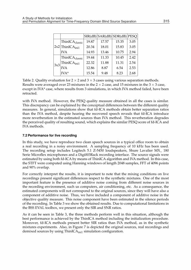
A Study of Methods for Initialization and Permutation Alignment for Time-Frequency Domain Blind Source Separation 19
SIR(dB) SAR(dB) SDR(dB) PESQ
2x2ThinICAclassic 19.87 17.57 15.35 3.05ThinICAini1 20.34 18.01 15.83 3.05IVA 14.93 13.46 10.75 2.94
3x3
ThinICAclassic 19.44 11.33 10.45 2.42ThinICAini1 22.32 11.88 11.31 2.54IVA 12.86 8.87 6.54 2.53IVA* 15.54 9.48 8.23 2.68
Table 2. Quality evaluation for 2× 2 and 3× 3 cases using various separation methods.Results were averaged over 23 mixtures in the 2× 2 case, and 15 mixtures in the 3× 3 case,except in IVA* case, where results from 3 simulations, in which IVA method failed, have beenretracted.
with IVA method. However, the PESQ quality measure obtained in all the cases is similar.This discrepancy can be explained by the conceptual differences between the different qualitymeasures. In general, simulations show that fd-ICA methods obtain better separation ratiosthan the IVA method, despite hearing the recovered speech reveals that fd-ICA introducemore reverberation in the estimated sources than IVA method. This reverberation degradesthe perceived quality of resulting sound, which explains the similar PESQ score of fd-ICA andIVA methods.
7.2 Performance for live recording
In this study, we have reproduce two clean speech sources in a typical office room to obtaina real recording in a noisy environment. A sampling frequency of 10 kHz has been used.The recording setup includes Logitech 5.1 Z-5450 loudspeakers, Shure Lavalier MX_ 180Serie Microflex microphones and a Digi003Rack recording interface. The source signals wereestimated by using both fd-ICA by means of ThinICA algorithm and IVA method. In this case,the STFT were computed using Hanning windows of length 2048 samples, FFT of 4096 pointsand 90% overlap.
For correctly interpret the results, it is important to note that the mixing conditions on liverecordings present significant differences respect to the synthetic mixtures. One of the mostimportant feature is the presence of additive noise coming from different noise sources inthe recording environment, such us computers, air conditioning, etc. As a consequence, theestimated components will not correspond to the original sources, since they will have also acomponent of additive noise. Thus, we have included a component of additive noise in theobjective quality measure. This noise component have been estimated in the silence periodsof the recording. In Table 3 we show the obtained results. Due to computational limitations inthe BSS EVAL toolbox, we present only the SIR and SNR ratios.
As it can be seen in Table 3, the three methods perform well in this situation, although thebest performance is achieved by the ThinICA method including the initialization procedure.Moreover, fd-ICA methods present better SIR ratios than IVA method, as in the syntheticmixtures experiments. Also, in Figure 7 is depicted the original sources, real recordings anddemixed sources by using ThinICAini1 simulation configuration.
315A Study of Methods for Initialization and Permutation Alignment for Time-Frequency Domain Blind Source Separation

20 Will-be-set-by-IN-TECH
0 2 4 6 8 10 0 2 4 6 8 10 0 2 4 6 8 10
0.1
-0.1
-0.05
0.05
0
0.1
-0.1
-0.05
0.05
0
0.1
-0.1
-0.05
0.05
0
Am
plitu
des1(k) s2(k) s3(k)
(a) Original sources.
0 2 4 6 8 10 0 2 4 6 8 10 0 2 4 6 8 10
0.1
-0.1
-0.05
0.05
0
0.1
-0.1
-0.05
0.05
0
0.1
-0.1
-0.05
0.05
0
Am
plitu
de
x1(k) x2(k) x3(k)
(b) Mixed signals.
0 2 4 6 8 10 0 2 4 6 8 10 0 2 4 6 8 10
0.1
-0.1
-0.05
0.05
0
0.1
-0.1
-0.05
0.05
0
0.1
-0.1
-0.05
0.05
0
Time (s) Time (s) Time (s)
Am
plitu
de
y1(k) y2(k) y3(k)
(c) Recovered signals.
Fig. 6. Example of 3× 3 separation experiment by using ThinICAini1 simulationconfiguration.
SIR(dB) SNR(dB) PESQThinICAclassic 13.37 14.73 1.96ThinICAini1 16.28 18.88 2.07IVA 8.84 14.27 1.77
Table 3. SIR (dB), SAR (dB), SDR (dB) and PESQ index for 2× 2 real recording separation.
To conclude, we have also applied the complete method to a live recording of 3 sources and3 mixtures provided in SISEC (2012). The quality of the estimated sources was measured interms of Source to Interferences Ratio (SIR) by E. Vincent, since the original sources are notpublic. An average SIR of 10.1 dB was obtained.
316 Independent Component Analysis for Audio and Biosignal Applications

A Study of Methods for Initialization and Permutation Alignment for Time-Frequency Domain Blind Source Separation 21
0 1 2 3 4 5-0.2
-0.1
0
0.1
0.2A
mpl
itude
s1(k)
0 1 2 3 4 5
s2(k)
-0.2
-0.1
0
0.1
0.2
(a) Original sources.
0 1 2 3 4 5
Am
plitu
de
x1(k)
0 1 2 3 4 5
x2(k)
-0.2
-0.1
0
0.1
0.2
-0.2
-0.1
0
0.1
0.2
(b) Recordered signals.
0 1 2 3 4 5
Time (s)
Am
plitu
de
y1(k)
0 1 2 3 4 5
Time (s)
y2(k)
-0.2
-0.1
0
0.1
0.2
-0.2
-0.1
0
0.1
0.2
(c) Recovered signals.
Fig. 7. Example of a separation experiment with real recordered signals by using ThinICAini1simulation configuration.
8. Conclusions
In this chapter we have considered the problem of the blind separation of speech signalsrecorded in a real room, when the number of speakers equals the number of simultaneousrecordings. We have adopted the time-frequency approach, focusing our attention in theinitialization of the separation algorithms and the permutation problem which is ubiquitousto fd-ICA methods. In order to improve the performance of the existing methods wehave incorporated an initialization procedure for those ICA algorithms that work in thetime-frequency domain and require the whitening of the observations as a preprocessingstep. This initialization exploit the local continuity of the demixing filter in the frequencydomain, which is a valid property for reverberant filters in a wide range of frequencies. Forthat, the separation matrix in one frequency bin is initialized from its joint closest value toa set of separation systems already computed at nearby frequencies. Computer simulationsshow that this initialization, when it is incorporated to the existing ICA algorithms, reducesdrastically the number of permutations, preserving the separated components well alignedin wide frequency blocks. Simulations with more than two sources reveal that the proposedinitialization also helps to the convergence of the ICA algorithms that solve the separation ineach frequency.
317A Study of Methods for Initialization and Permutation Alignment for Time-Frequency Domain Blind Source Separation

22 Will-be-set-by-IN-TECH
The permutation problem becomes a severe problem when the number of sources is largeor in high reverberant environments. Nowadays, it is still considered an open problem.For solving the permutation problem, we have present a method, based on the amplitudecorrelation modulation property of speech signals, that arises the general case of N sourcesand N observations. We have defined for each frequency bin a measure of coherence basedon the amplitude modulation correlation property of speech signals. This measure has beenused to formulate a coherence contrast function which maximization allows to successfullyarrange the estimated components. An iterative method has been provide for searching themaxima of the contrast. The robustness of the algorithm has been illustrated for artificiallypermuted sources, which corresponds with a situation of perfect separation. Results showthat the algorithm is able to reorder completely the frequency components, except for somevery low frequencies that in some cases remained permuted. However, this does not affect tothe quality of the recovered sources. Finally, experiments with simulated and live recordingin a room with reverberation, for the case where two or three sources are mixed, show that thecomplete method improves considerably the performance of classical fd-ICA method, as wellas IVA method, by means of both objective and perceptually measures.
9. Acknowledgements
This work has been supported by the Ministry of Science and Innovation project ofthe Government of Spain (Grant TEC2011-23559) and the Andalusian Government (GrantTIC-7869). We thank Emmanuel Vincent collaboration for the evaluation of the results.
10. References
Comon, P., Independent Component Analysis a new concept?, Signal Processing, Vol. 36, pp287-314, 1994.
Smaragdis P. (1998),Blind separation of convolved mixtures in the frequency domain,Neurocomputing, Vol. 2, Nov. 1998, pp. 21-34.
Parra, L. & Spence, C., Convolutive blind source separation of non-stationary sources, IEEETrans. on Speech and Audio Processing, May. 2000, pp. 320-327.
Araki, S., Mukai, R., Makino, S., Nishikawa, T. & Saruwatari, H. , The fundamental limitationof frequency domain blind source separation for convolutive mixtures of speech,IEEE Transactions on Speech and Audio Processing, Vol. 11, No. 2, Mar. 2003, pp. 109-116.
Hyvärinen, A. & Oja, E., A fast fixed point algorithm for independent component analysis,Neural Computation,Vol. 9, 1997, pp. 1483-1492.
Bingham, E. & Hyvärinen, A., A fast fixed point algorithm for independent componentanalysis of complex valued signals, International Journal of Neural Systems, Vol. 10,No. 1, 2000, pp. 1-8.
Koldovský, Z., Tichavský, P. & Oja, E., Efficient variant of algorithm FastICA for independentcomponent analysis attaining the Cramé Rao lower bound, IEEE Trans. on NeuralNetworks, Vol. 17, No. 5, Sep. 2006, pp. 1265-1277.
Belouchrani, A., Abed-Meraim, K., Cardoso, J.F., Moulines, E., A blind source separationtechnique using second-order statistics, IEEE Trans. on Signal Processing, Vol. 45, No.2, Feb. 1997, pp. 434-444.
Choi, S. & Cichocki, A., Blind separation of nonstationary sources in noisy mixtures, IEEEWorkshop on Neural Networks for Signal Processing (NNSP’2000), Sydney, Australia,Dec. 2000, pp. 11-13.
318 Independent Component Analysis for Audio and Biosignal Applications
A Study of Methods for Initialization and Permutation Alignment for Time-Frequency Domain Blind Source Separation 23
D. Donoho, On Minimun Entropy Deconvolution, Applied Time Series Analysis II, D. F. FindleyEditor, Academic Press, New York, 1981,pp. 565-608.
Cruces, S., Cichocki, A. & Amari, S., From Blind Signal Extraction to Blind InstantaneousSignal Separation: Criteria, Algortihms and Stability, IEEE Trans. on Neural Networks,vol 15(4), July 2004, pp. 859-873.
De Lathauwer, L., De-Moor, B. & Vandewalle, J., On the Best Rank-1 and Rank-(R1;R2;...;RN)Approximation of Higher-order Tensors, SIAM J. Matrix Anal. Appl., vol. 21(4), 2000,pp. 1324-1342.
S. Cruces & A. Cichocki, Combining Blind Source Extraction with Joint ApproximateDiagonalization: Thin Algorithms for ICA, Proceedings of the 4rd InternationalSymposium on Independent Component Analysis and Blind Signal Separation, Japan, 2003,pp. 463-468.
Cruces, S., Cichocki, A. & De Lathauwer, L., Thin QR and SVD factorizations for simultaneousBlind Signal Extraction, Proceeding of the European Signal Processing Conference(EUSIPCO’04), Viena Austria, 2004, pp. 217-220
Available: http://www.bsp.brain.riken.jp/ICALAB/, Accessed 2012 Feb. 1.Durán Díaz I. & Cruces, S., A joint optimization criterion for blind DS-CDMA detection,
EURASIP Journal of Applied Signal Processing, Special Issue: Advances in Blind SourceSeparation, 2007, pp. 1-11.
Sarmiento, A.; Cruces, S. & Durán, I., Improvement of the initialization of time-frequencyalgorithms for speech separation,Proceedings of Int Conf. on Independent ComponentAnalysis and Blind Source Separation (ICA’09), 2009, pp. 629-636.
Sarmiento, A., Durán-Díaz & I., Cruces S., Initialization method for speech separationalgorithms that work in the time frequency domain, The Journal of the AcousticalSociety of America, Vol. 127, No. 4, 2010, pp. 121-126.
Matsuoka, K. & Nakashima, S., Minimal distorsion principle for blind sourceseparation,Proceedings of Int. Conf. on Independent Component Analysis and BlindSource Separation, 2001, pp. 722-727.
Pedersen, M.S., Larsen, J., Kjems, U. & Parra, L.C., A survey of convolutive blind sourceseparation methods, Multichannel Speech Processing Handbook, Eds. Jacob Benesty andArden Huang, Springer 2007, Chapter 51, pp. 1065-1084.
Anemüller, J. & Kollmeier, B. , Amplitude modulation decorrelation for convolutiveblind source separation, Proceedings of Second International Workshop on IndependentComponent Analysis and Blind Signal Separation, Jun. 2000, pp. 215-220.
Ikeda, S. & Murata, N., An approach to blind source separation of speech signals, Proceedings ofInternational Conference on Artificial Neural Networks (ICANN’98), Sep. 1998, Sweden,pp.761-766.
Murata, N., Ikeda,S. & and Ziehe, A., An approach to blind source separation based ontemporal structure of speech signals, Neurocomputing, Vol. 41, Issue 1-4, Oct. 2001,pp.1-24.
Rahbar, K. & Reilly J.P., A frequency domain method for blind source separation ofconvolutive audio mixtures, IEEE Transactions on speech and audio processing, Vol.13,No. 5, 2005, pp. 832-844.
Kim, T., Lee, I. & Lee T.W., Independent Vector Analysis: definition and algorithms, Proceedingof Fortieth Asilomar Conference on Signals, Systems and Computers (ACSSC ’06), 2006,pp.1393-1396.
Pham, D.T., Serviére, C. & Boumaraf, H. , Blind separation of convolutive audio mixturesusing nonstationarity, Proceedings of Int Conf. on Independent Component Analysis andBlind Source Separation (ICA’03), Nara, Japan, Apr. 2003.
319A Study of Methods for Initialization and Permutation Alignment for Time-Frequency Domain Blind Source Separation

24 Will-be-set-by-IN-TECH
Asano, F., Ikeda, S., Ogawa, M., Asoh, H.& Kitawaki, N., Combined approach of arrayprocessing and independent component analysis for blind separation of acousticsignals, IEEE Transactions on Speech and Audio Processing,Vol.11, No. 3, May. 2003, pp.204- 215.
Sudhakar, P. & Gribonval, R., A sparsity-based method to solve permutation indeterminacyin frequency-domain convolutive blind source separation, Proceedings of the 8thInternational Conference on Independent Component Analysis and Signal Separation (ICA’09), pp. 338-345.
Parra, L.C. & Alvino, C.V., Geometric source separation: merging convolutive sourceseparation with geometric beamforming, IEEE Transactions on Speech and AudioProcessing, Vol.10, No.6, Sep. 2002, pp. 352- 362.
Kurita, S., Saruwatari, H., Kajita, S., Takeda, K. & Itakura, F., Evaluation of blindsignal separation method using directivity pattern under reverberant conditions,Proceedings of IEEE International Conference on Acoustics, Speech, and Signal Processing(ICASSP ’00), Vol. 5, 2000, pp. 3140-3143.
Saruwatari, H., Kurita, S., Takeda, K., Itakura, F., Nishikawa, T. & Shikano, K., Blind sourceseparation combining independent component analysis and beamforming, EURASIPJournal on Applied Signal Processing, Jan. 2003, pp. 1135-1146.
Sawada, H., Mukai, R., Araki, S. & Makino, S., A robust and precise method for solvingthe permutation problem of frequency-domain blind source separation, IEEETransactions on Speech and Audio Processing, Vol. 12, No. 5, Sept. 2004, pp. 530- 538.
Sawada, H., Mukai, R., Araki, S. & Makino, S., Frequency-domain blind source separationwithout array geometry information,Proceedings of Joint Workshop on Hands-FreeSpeech Communication and Microphone Arrays (HSCMA’05), Mar. 2005.
Sawada, H., Araki, S., Mukai, R. & Makino, S., Solving the permutation problemof frequency-domain BSS when spatial aliasing occurs with wide sensorspacing,Proceedings of the IEEE International Conference on Acoustics, Speech and SignalProcessing (ICASSP’06), Vol. 5, May. 2006, pp. 77-80.
Sarmiento, A., Durán-Díaz, I., Cruces, S. & Aguilera, P., Generalized method for solvingthe permutation problem in frequency-domain blind source separation of convolvedspeech signals, Proceedings of the 12th Annual Conference of the International SpeechCommunication Association (INTERSPEECH’11), Aug. 2011, pp. 565-568.
Available: http://www.imm.dtu.dk/pubdb/p.php?4400, Accessed 2012 Feb. 1.Fèvotte, C., Gribonval, R., Vincent, E. ,BSS_ EVAL toolbox user guide, Tech. Rep. 1706, IRISA,
Rennes, France, 2005, Available: http://www.irisa.fr/metiss/bss_ eval, Accessed2012 Feb. 1.
Loizou, P.C., Speech Enhancement. Theory and Practice, CRC Press, 2007.Campbell, D., Roomsim Toolbox, Available. http://media.paisley.ac.uk/ campbell/Roomsim/,
Accessed 2012 Feb. 1Vincent,E., Sawada, H., Bofill, P., Makino, S. & Rosca J. P., First Stereo Audio Source Separation
Evaluation Campaign: Data, algorithms and results,Proceedings of the 7th InternationalConference on Independent Component Analysis and Signal Separation (ICA’07), 2007, pp.552–559.
Available: http://sisec2010.wiki.irisa.fr/tiki-index.php, Accessed 2012 Feb. 1.
320 Independent Component Analysis for Audio and Biosignal Applications

1. Introduction
The Blind Source Separation (BSS) problem was first introduced (Herault et al., 1985;Jutten & Herault, 1988) in the context of biological problems (Ans et al., 1983; Herault & Ans,1984) with the aim of being able to separate a set of signals generated by the central nervoussystem. A few years later, several methods based on BSS were applied to other fields ofindustry and research (Deville, 1999). The BSS problem arises from the need to recover theoriginal sources from a blindly mixture. This extraction is characterised as a blind processbecause the lack of information about the following topics: the characterisation of the sources,the number of sources present at the time of the mixture, and the way that this mixtureis performed. Although this kind of information is unknown, the problem described canbe solved if the input signals to the mixture process are statistically independent. Relatedliterature provides several methods, most of which have been classified according to thecontext in which the mixture is performed: linear mixture model, convolutive mixture model,and non-linear mixture model. The first part of this chapter is devoted to describe the mostrelevant existing works in applying these methods to the audio field. Many of the realproblems, however, do not support this simplification, so this part stresses the need for fullcharacterisation of the problem,mainly about the mixing process and the nature of the sourcesinvolved.
Typically, the goal of the BSS theory is to extract a set of variables matching the sourcesinvolved in the mixture. We have detected, however, the existence of other research fieldswhere the goal is to extract from the mixture another set of variables which appear asimplicit functions of the hidden sources. Extracting these variables brings a new challengefor the BSS theory, becoming particularly complex when the sources have a noisy nature.In the second part of this chapter, a complete definition of this new problem is introduced,for which the BSS problem in its classical form must be reformulated. Used by first timein (Mato-Méndez & Sobreira-Seoane, 2011), within a pattern recognition context, the BlindImplicit Source Separation (BISS) concept opens an interesting research field. The BSS-PCAalgorithm proposed in the research work referenced above solves with success the problemof classification of traffic noise. Within this algorithm, the BISS problem is handled in anembedded way. Motivated by the promising results achieved, a new compact expression forthe BISS solution is now proposed. The new BISS-PCA method introduced here robustlysolves the feature extraction process for the problem described. The conclusions of this
Blind Implicit Source Separation – A New Concept in BSS Theory
Fernando J. Mato-Méndez and Manuel A. Sobreira-Seoane University of Vigo
Spain
16

2 Will-be-set-by-IN-TECH
research can be generalized to other application fields, so we believe that this chapter willbe of special interest for the readers.
2. Blind audio source separation
The aim of BSS theory is to extract p unknown sources, from m mixtures acquired through asensors network. To solve this problem, the literature provides a wide set of methods, mostcollected in (Comon & Jutten, 2010; Hyvärinen et al., 2001). In this sense, many algorithmshave been applied to the context of audio signals, and they can be classified according to thesolution of three different problems. First, the denoising process from an undesired mixtureprovided by both, the channel noise and the sensors network noise. Second, the separation ofmusical sources from an audio mixture. Finally, the problem created by the “cocktail party”effect (Cherry, 1953), generated when several speakers talk at the same time in reverberantfield conditions. Other problems appearing in the state of the art can be analysed as acombination of the above.
2.1 Mixture models
The study of the solution becomes very complex taking into account the existence of differenttypes of problems and application contexts. For many years, however, they have beenaddressed according to how the mixing process is performed. A generic mixture model forthe BSS problem can be written as
x(n) = H(s(n) + ε(n)), (1)
where H is a function of both, the channel and the sensor network, and ε is a Gaussianadditive noise signal, independent of the p sources of s. Thus, existing methods can beclassified according to this criterion (see (Comon & Jutten, 2010; Mansour & Kawamoto, 2003;Pedersen et al., 2007; Puntonet G., 2003) for more detail) into the categories that are describedbelow.
2.1.1 Instantaneous mixtures
Source separation from instantaneous mixtures has been one of the first applications of BSSin the audio field. For signals acquired into a recording studio, the mixing process canbe considered instantaneous: first, the signals associated with each of the sources can beconsidered independent because being acquired at different times and at different spatiallocations. Second, the multipath contributions associated with both, the sources and sensors,can be neglected thanks to the acquisition process of the mixture and third, studios canbe considered as “noise free” controlled environments. So the signals recorded underthese conditions does not contains neither relevant undesired reflections or significant noisecontributions. Thus, many authors approach this problem by means of an instantaneousmixture model. For this situation, the channel is characterised by have no memory, for whichthe mixture acquired by the j− th sensor can be modelled as
xj(n) =p
∑i=1
hijsi(n). (2)
In this context, the function H in (1) can be identified with a real matrix verifying that
x(n) = Hs(n), (3)
322 Independent Component Analysis for Audio and Biosignal Applications

Blind Implicit Source SeparationA New Concept in BSS Theory 3
where the vector x contains the contributions of the m sensors in the array. So, the separationproblem is reduced to solve the system of Eq. (3). In this case, the solution can be achieved byapplying ICA on this equation. Before proceed, it is necessary to have at least the same numberof mixtures than sources. Besides, at most, only one source can show a Gaussian distribution.Under these conditions, the separation is performed by calculating an estimation of themixingmatrix that minimises the statistical dependence between components of the original signals.
The contribution of the sensor array and the channel makes not possible to neglect the noiseeffect in most applications. Therefore, the signal acquired by the j− th sensor can be expressedas
xj(n) =p
∑i=1
hijsi(n) + εsj (n) + εc
j (n), (4)
where εsj (n) is the noise signal acquired by the j − th sensor, and εc
j (n) is the noise signalprovided by the channel. The last signal is typically characterised as wide-band noise, withN (μεc
j, σεc
j) distribution for that sensor. It is usual to express the sum of these two noise signals
asεj(n) = εs
j (n) + εcj (n). (5)
Taking into account this undesired effect, Eq. (3) must be rewritten as
x(n) = Hs(n) + ε(n), (6)
where the vector ε contains the values of the noise signals associated with the msensors. There are a large number of algorithms that apply ICA on instantaneous mixingproblems, which are deeply studied in (Comon & Jutten, 2010). These algorithms showa reasonable separation quality, even when applied on noisy mixtures. According tothe criteria used in the application of ICA, the literature provides research contributionsbased on: second order statistics (Mansour & Ohnishi, 2000; Matsuoka et al., 1995), higherorder statistics (Ihm & Park, 1999; Jutten et al., 1991a; Mansour & Ohnishi, 1999; Moreau,2001), the probability density function (Amari & Cichocki, 1998; Bofill & Zibulevsky, 2000;Cichocki et al., 1997; 1998; Diamantaras & Chassioti, 2000; Hild et al., 2001; Lappalainen,1999; Lee et al., 1999; Pham & Cardoso, 2001) and geometric models (Mansour et al., 2002;Prieto et al., 1998; 1999; Puntonet et al., 1995; 2000).
2.1.2 Convolutive mixtures
When the mixture is not instantaneous, the channel has memory, so the signal acquired by thej− th sensor can be expressed as
xj(n) =p
∑i=1
r−1∑l=0
hlijsi(n− l) + εj(n), (7)
where r is the order of the FIR filter that models the mixture. Thus, this mixture can bemodelled by means of the expression
x(n) = [H(z)]s(n) + ε(n) = ∑l
H(l)s(n− l) + ε(n). (8)
323Blind Implicit Source Separation – A New Concept in BSS Theory

4 Will-be-set-by-IN-TECH
This is the convolutive model, where H(l) is the matrix that models the channel and H(z) thematrix that models the effects of sources on the observations. Therefore, this last matrix canbe written by means of the Z transform as
[H(z)] = Z [H(n)] = ∑l
H(l)z−l. (9)
Several ICA-based algorithms can be applied in this case to carry the separation processout. In the context of audio, the convolutive problem is classically analysed by meansof second order statistics (Ehlers & Schuster, 1997; Ikram & Morgan, 2001; Kawamoto et al.,1999; Rahbar & Reilly, 2001; Sahlin & Broman, 1998; Weinstein et al., 1993), higher orderstatistics (Charkani & Deville, 1999; Jutten et al., 1991b; Nguyen et al., 1992; Nguyen & Jutten,1995; Van Gerven et al., 1994) and probability density function (Bell & Sejnowski, 1995;Koutras et al., 1999; 2000; Lee et al., 1997a;b; Torkkola, 1996).
2.1.3 Nonlinear mixtures
In a more general approach, the H function in Eq. (1) does not support a linear form. Thisis the case for the separation problem of traffic noise sources in a general context. In thisproblem, the original sources can not be observed and it is unknown how their signals havebeen mixed. So, if possible, the extraction of the signals that make up the resulting mixturecan be a priori characterised as a blind separation process.
For nonlinear mixtures it is usual to simplify the problem by using a post-nonlinear mixturemodel as
x(n) = H1[H2s(n)] + ε(n), (10)
being H2 a real matrix and H1 a nonlinear function. To solve it, research works based onsecond order statistics (Molgedey & Schuster, 1994) and based on the probability densityfunction (Solazzi et al., 2001; Valpola et al., 2001) can be consulted.
2.2 Full problem approach
The usual procedure in BSS is to analyse the problem by means of identifying its mixingmodel. A proper application of the methods described, however, requires an additionalknowledge about both, the mixing process and the nature of the sources involved. Thus,to set an accurate strategy of separation it is necessary to add other informations.
The BSS problem for those situations in which the number of observations is higher thanthe number of sources (over-determined problem), or equal (determined problem), is wellstudied. For other situations (underdetermined problem), much remains to be done. This newapproach leads to research works focused on solving underdetermined problems (Nion et al.,2010; Rickard et al., 2005; Sawada et al., 2011; Zhang et al., 1999a), and focused on optimisingthe solution for over-determined problems (Joho et al., 2000; Yonggang & Chambers, 2011;Zhang et al., 1999a;b).
In addition, a prior knowledge about both, the statistical and spectral characterisationof the sources, will lead to more efficient separation methods. Thus, the informationcan be extracted by means of BSS algorithms that exploit the study of second orderstatistics for non-stationarity sources (Kawamoto et al., 1999; Mansour & Ohnishi, 2000;Matsuoka et al., 1995; Pham & Cardoso, 2001; Weinstein et al., 1993) and cyclo-stationarity
324 Independent Component Analysis for Audio and Biosignal Applications

Blind Implicit Source SeparationA New Concept in BSS Theory 5
sources (Knaak et al., 2002; 2003). These will also be suitable for the separation of whitenesssources (Mansour et al., 1996; 2000). Some information, however, contained in wide-bandsources can not be extracted only using second order statistics. In this case, algorithms basedon higher order statistics must be applied.
Finally, many of the algorithms show an excellent performance working on syntheticmixtures. However, a significant degradation in the results is detected when they are appliedon real mixtures. In addition, a distinction between both, master-recorded and live-recordedmixtures, must be done. Research works carried out to solve audio signals separation inreal conditions can be found in (Kawamoto et al., 1999; Koutras et al., 2000; Lee et al., 1997a;Nguyen et al., 1992; Sahlin & Broman, 1998).
The BSS problem applied to extract signals from a noisy mixture is well studied. The residualsignal in this case is typically characterised as white noise. A particularly complex problemoccurs, however, when the signals to extract are noise signals. Besides, these are in generalcharacterised as coloured noise, as it occurs for traffic noise sources. In this sense, the researchcarried out by us regarding the application of BSS to traffic noise real mixtures may beconsider a pioneer work. The more closest researches can be found in the study of mechanicalfault diagnosis in combustion engines. This is a less complex problem because the signalacquisition process is performed by isolating the engine. The research is focused in applyingBSS for the study of its vibrational behaviour. Existing papers (Antoni, 2005; Gelle et al., 2000;Knaak & Filbert, 2001; Knaak et al., 2002; Wang et al., 2009; Wu et al., 2002; Ypma et al., 2002)show the difficulty in the search for satisfactory solutions. The complexity of application ofBSS theory will become higher by incorporating other sources for the generation of the trafficnoise signal. The next section is devoted to the study of this problem in the context of patternrecognition, for which the BSS problem needs to be reformulated.
3. Blind implicit source separation
This new concept is related to the classical definition of sources into a BSS problem and ithas been detected by us in classification problems of noise signals. In a generic classificationproblem, the main goal is to assign an unknown pattern ϕ to a given class Ci. This classbelongs to the set C of c classes previously determined. The starting condition is thateach pattern shall be represented by a single vector of features, and it can not belong tomore than one class. Under these hypotesis, this pattern may be uniquely represented byϕ = [ϕ1, ϕ2, . . . , ϕd]
T, where d is the number of the extracted features and the dimensionalityof the classification problem. For a better understanding of the new BSS concept, the followingtwo examples of application may be considered:
• Mechanical fault diagnosis in combustion enginesFor the context described, the fault diagnosis can be seen as the combination of twoproblems to be solved: a classification problem, and a source separation problem. Thus,the BSS application has two purposes: the first task, being able to separate relevantinformation from the wide-band noise associated with the vibration of the structure. Thisrelevant information is contained within the spectral lines associated with the combustionnoise, so that the first task may be characterised as a denoising process. The second task isfocused in extracting the information contained within the set of spectral lines and assign itto one of the engine phases. Thus, the strategy followed seeks to improve the identificationof possible faults associated with one of the engine phases. This identification task can be
325Blind Implicit Source Separation – A New Concept in BSS Theory

6 Will-be-set-by-IN-TECH
viewed as a classification problem. The prior application of BSS results therefore in a betterdefinition of the boundaries that separates the two classes previously established (faulty,non-faulty).
• Classification of traffic noiseAlthough, in a colloquial sense, being able to separate two sources of traffic noise mightseem synonymouswith being able to classify them, both concepts differ in practice becausethe processingmethods applied. There appears, however, a clear correlation between both,the difficulty in applying blind separation algorithms on specific classes of sources and thedifficulty in applying classification algorithms on them. To compare the problem withthe above, it must be simplified by considering only the combustion noise. In this case,the classification problem consists in assigning an unknown pattern with a predeterminedclass of vehicles regarding its noise emitted level. In this case, a single engine can belong totwo categories of vehicles. Unlike the previous case, the features vector does not providediscriminative information, so an extraction of information from extra sources is needed.The trouble, as the reader may guess, is the lack of uniqueness for the solution. This issueoccurs for other sources considered, so the problem is not successfully solved by addingthem into the feature extraction process.
As it will be shown, the problem of classification of traffic noise is much more complex thanthe one described in the example. The signal acquired by means of a sensors network is acombination of a large number of noise sources. Thus, the associated BSS problem becomesinto an extremely complex problem to solve:
• For a isolated pass-by, the vibration behaviour of the engine becomes more complex dueto the change of the mechanical model handled. This model is now in motion, and it isaffected by its interaction with the other parts of the structure. The information associatedwith the spectral lines, located at low frequencies, is now altered by energy from othersystems such as suspension or brakes. The resulting signal is thus combined with noiseinduced by the exhaust system.
• The turbulences created by the vehicle in motion (aerodynamic noise) spread energy athigh frequency on the acquired signal. Both, the distribution and intensity of this energy,will depend on the geometry and speed of the vehicle. For a given geometry, the higherthe speed of the vehicle, the higher the emission at high frequencies will be.
• Once exceeded 50 km/h, for motorcycles and cars, and 70 km/h for trucks, most of theenergy in the acquired signal is now associated with rolling noise. This noise is generatedby the contact of the wheel with the pavement surface. Thus, a masking of informationassociated with the three sources of noise described above is produced.
• The consideration of other features modifies the resulting signal: directivity pattern ofthe vehicle, vehicle maintenance/age, road conservation, ground effect, Doppler effect,type of pavement, distance from source to the sensor network, atmospheric conditions andreflexions of the signal on different surfaces close to the road (buildings, noise barriers, ...).
• The traffic noise signal results from a combined pass-by of vehicles. This combination addsboth, an interfering pattern and a masking effect, into the mixing process of the signalsassociated with each of the sources.
Several calculation methods have been developed to predict the noise levels emitted by thetraffic road. These are based on mathematical models trying to find the best approximationto the real model described above. This real model is too complex to be implemented, so
326 Independent Component Analysis for Audio and Biosignal Applications

Blind Implicit Source SeparationA New Concept in BSS Theory 7
an approach is carried out by simplifying the number of sources to be considered. Thus,part of the information needed to carry out this prediction is obtained by means of indirectmethods. Regarding the European predictionmodel (CNOSSOS-EU, 2010), information aboutthe average speed of the road, the pavement type and the traffic road intensity is thenneeded. This information must be collected according to the vehicle type categorisationperformed. Thus, we decided to address the design of a portable device capable to providesuch information in real time. For this purpose, the more complex trouble lies in the classifierdesign. Within this, the incorporation of BSS techniques was proposed with the hope toimprove the feature extraction process. To address this task into an intercity context, themixing process can be modelled according to the scheme of Fig. 1, where si(n) is the signalassociated with the vehicle to be classified.
Fig. 1. BSS model of convolutive mixture for the problem of classification of traffic noise onintercity roads.
The goal will be to extract the feature vector of an event whose signal is hidden in mixturewhere overlapping events are present. The extraction of the signal si itself does not help,because this signal carries information associated to other events. It is therefore necessaryto find another way to extract this features vector by means of the discriminative informationassociatedwith the event to be classified. So, it is proposed to express this information throughthe acquired mixture as si
Γ(n) = Γi(x(n)). Thus, the problem to be solved consists in finding
ϕi = [ϕi1, . . . , ϕid]T, by means of
siΓ(n)
ϕ−−→ (ϕi1(n), . . . , ϕid(n))T, (11)
for wich the BSS problem can be expressed as
ϕi(n) = ϕ(siΓ(n)) = ϕ(Γi(x(n))) = ϕ(Γi([H(z)]s(n) + ε(n))). (12)
As the reader can see, the BSS sources in its classical form remain hidden. For this reason, wehave named this new BSS problem as Blind Implicit Source Separation (BISS). To solve it, thesources definition handled in Fig. 1 is thus no longer valid.
327Blind Implicit Source Separation – A New Concept in BSS Theory

8 Will-be-set-by-IN-TECH
3.1 Dimensionality reduction
One of the typical problems that appear in pattern recognition is the need to reduce thedimensionality of the feature space. For this task both, Principal Component Analysis (PCA)and Independent Component Analysis (ICA), are the most usual techniques employed. Theperformance obtained, however, may be different according to the problem to be solved. Asit will be seen through this section, the explanation lies in the way that both techniques areapplied.
An overview of the original feature space shows in general the existence of values that donot efficiently contribute to the extraction of discriminative information for classificationpurposes. Under this assumption, for years a large number of techniques has beendeveloped (Fodor, 2002). The goal is to reduce the dimensionality of the original problem,while minimising the possible loss of information related with this process. Most arebased on the search of subspaces with better discriminative directions to project the data(Friedman & Tukey, 1974). This projection process involves a loss of information. So acompromise solution is achieved by means of a cost function. There are research works(Huber, 1985), however, which prove that the new subspaces show a higher noise immunity.Furthermore, it is achieved a better capability to filter features with a low discriminativepower. So, it results in a better estimation of the density functions (Friedman et al., 1984).
But there are two issues that must be taken into account and that are closely related to thetransformations to be used at this stage. First, outliers will be added due to the high variabilityof the patterns to classify, so an increase of between-class overlap inevitably will occur. Thus,this issue leads to a degradation in the classifier performance. Furthermore, the choice of asuitable rotation of the original data will allow a better view of the discriminative information,as it is shown in Fig. 2. So, it will be very important to find those transformations thatcontribute to both, a best definition of the between-class boundaries and a best clusteringof the within-class information.
(a) (b)
Fig. 2. Example of projection pursuit. Set of projection directions achieved by means of awrong geometric rotation (a). Set of projection directions achieved by means of an accurategeometric rotation (b).
Most of the techniques developed for dimensionality reduction are based on the assumptionof normality of the original data. For these, it is also shown that most of the projectionsin problems of high dimensionality allow to achieve transformed data with a statisticaldistribution that can be considered approximately normal. Among them, a technique ofproven effectiveness is PCA (Fukunaga, 1990).
328 Independent Component Analysis for Audio and Biosignal Applications

Blind Implicit Source SeparationA New Concept in BSS Theory 9
In certain cases, however, PCA may not provide the best directions for projecting the data, asit is shown in Fig. 3. (b). Moreover, this technique limits the analysis to second order statisticsso that, for features with a certain degree of statistical dependence between them, ICA(Hyvärinen et al., 2001) will be more suitable. In this technique, the search of independencebetween components is the basis for the projection directions pursuit, so it can be consideredas a dimensionality reduction technique, and therefore an alternative to PCA.
(a) (b)
Fig. 3. Example of PCA projection. One class (a). Two classes (b): accurate direction (left),and wrong direction (right).
ICA application, however, is subject to two major restrictions:
1. The assumption of independence of the data is a stronger condition than the assumptionof incorrelation, so the conditions for ICA application are more restrictive compared withPCA.
2. The data must show a non-Gaussian distribution, so ICA is not applicable to normalpopulations, as it occurs with the space of features studied here.
The traffic noise signal verifies the two previous hypotheses: the samples may be consideredindependent, because being acquired at different times and have different sources spatiallocation. Furthermore, these samples follow a non-Gaussian distribution, as it is shown in(Mato-Méndez & Sobreira-Seoane, 2008b). Although the extraction of features can be madeby using only one sensor, the assumptions handled are the following:
1. For isolated pass-bys, the acquired signal is the result of the combination of both, the signalassociated with the vehicle and the background noise.
2. For combined pass-bys, the problem becomes more complex because adding energyassociated with other vehicles to the signal associated with the vehicle intended to beclassified.
3. The removal of this residual information by source separation techniques would improvethe extraction process.
So why not apply this technique to the acquired signal?.
3.2 ICA approach
Taking in mind the ideas described into the previous section, the application of ICAis proposed within a first research work (Mato-Méndez & Sobreira-Seoane, 2008a). Thisapplication is carried out by transforming the convolutive problem, which follows the model
329Blind Implicit Source Separation – A New Concept in BSS Theory

10 Will-be-set-by-IN-TECH
in Fig. 1, into a linear problem. This transformation is achieved by performing a set ofsynthetic mixtures by means of the signal acquired. At this point, the reader must rememberthat the goal is to obtain a higher separability degree of the extracted features. It is nottherefore the extraction of the signals associated with the vehicles involved within the mixtureprocess. From this point of view, the transformation carried out is accurate. Thus, the problemto solve now is to find ϕi = [ϕi1, . . . , ϕid]
T, an estimation of ϕi, by applying ICA to the newmixture performed x.
In ICA, the separation is conducted by estimating the mixing matrix which minimises thestatistical dependence between components of the original signals. To apply it, at most onlyone source can show a Gaussian distribution. Besides, once the number of sources is known,it is necessary to get at least an equal number of mixtures. For the linear case, the processof extracting the independent components match with solving the blind source separationproblem. Under these hypothesis, the mathematical approach of the mixture can be expressedas
[x1(n), . . . , xm(n)]T ≈
⎛⎜⎝
a11 . . . a1p...
. . ....
am1 . . . amp
⎞⎟⎠ [s1(n), . . . , sp(n)]T. (13)
The convolutive problem can be therefore expressed by means of a linear system of m mixtureequations with p unknowns, X ≈ A · S, where A represents the mixing matrix, and S and Xare the vectors of sources and observations respectively. The solution for the linear problemis then conducted by finding the separation matrix B, which is an estimate of the inverse ofthe mixture matrix A. Although the uniqueness for the solution does not exist from a strictmathematical approach, regarding the independence of the extracted signals this uniquenesscan be achieved (Cao & Liu, 1996). In this sense, to ensure the separability of the sources it issufficient with applying a set of conditions before proceed:
1. The separation process is feasible if the linear function associated with the mixture isbijective, i.e., the regularity of the mixing matrix is needed to be able of estimate B.
2. Regarding the independence of the sources, if p − 1 sources shows a non-Gaussiandistribution, the independence of pairs of the extracted components is ensured. As result,the possibility of separating the original sources is also ensured.
3. The combined presence of Gaussian and non-Gaussian sources at the time of the mixturewill allow the separation of the last ones. This separation will be impossible, however, forthe first ones.
Under the above assumptions, an estimation of both unknowns, the coefficients of the matrixA and the values of the vector s, can therefore be achieved. Although the independencebetween the recovered sources is ensured in this way, there still exist two unsolved problemsin calculating the solution: the uncertainty associated with the energy of the signals obtained,and the uncertainty on the order that they appear. Despite these two uncertainties, ICA provesthe existence of uniqueness solving the BSS problem. Furthermore, the existence of these twouncertainties is not an inconvenience for classification purposes.
The process is conducted in two steps. In a first stage, the orthogonal projection of theinput mixtures is performed by means of a decorrrelation process. This stage thereforesimplifies the solution to a data rotation. Thus, the separation matrix can be factorized
330 Independent Component Analysis for Audio and Biosignal Applications

Blind Implicit Source SeparationA New Concept in BSS Theory 11
as B = R · W, being W a whitening matrix and R a rotation matrix. The whiteningprocess is started by subtracting the mean from the samples. After this, it concludes byapplying an orthonormalization process on the centred samples by means of the SingularValue Decomposition (SVD). Proceeding as above, the covariance matrix Σ = E[s(n) · sT(n)]match with the identity matrix. It is true that the study of second order statistics, and morespecifically the analysis provided by the decorrelation, allows to carry out a whitening of thesamples. This is, however, a necessary but not sufficient condition to ensure the independenceof the samples. The difficulty lies in the uncertainty introduced by their possible rotation. Thisis the reason why, at most, only one of the original sources may show a Gaussian distribution.If this condition is not ensured, the separation of two Gaussian sources is not possible. It isdue because the joint distribution for these sources will show a circular symmetry.
Among the wide set of ICA-based algorithms, the developed by Aapo Hyvärinen (Hyvärinen,1999) is used in (Mato-Méndez & Sobreira-Seoane, 2008a;b) due to its excellent relationshipbetween quality and computational cost. Also known as FastICA, this algorithm in fixed pointuse both statistics, the kurtosis and negentropy, as non-gaussianity criteria. The decorrelationprocess is performed by applying on X the SVD decomposition, widely used in data mining.The idea of this decompositionmethod was first raised by Carl Eckart and Gale Young in 1936(Eckart & Young, 1936), by approximating a rectangular matrix by another of lower rank. Itwas not until 1980, however, that a computational version was proposed by Virginia C. Klemaand Alan J. Laub (Klema & Laub, 1980). This new version allowed to discover its performancein solving complex problems. SVD decomposition makes possible to detect and to sort theprojection directions that contain the values of higher variance, by means of the use of twosquare matrices containing the singular vectors. Thus, the dimensionality reduction can beachieved by means of SVD, allowing to find subspaces that best approximate the originaldata. By applying SVD on X, this matrix can be expressed as X ≈ UΛ
12 VT, i.e.,
⎛⎜⎝
x11 . . . xn1
.... . .
...x1m . . . xn
m
⎞⎟⎠ ≈
⎛⎜⎝
u11 . . . um1
.... . .
...u1m . . . um
m
⎞⎟⎠
(√Λ 0
0 0
)⎛⎜⎝
v11 . . . vn1
.... . .
...v1n . . . vn
n
⎞⎟⎠ , (14)
where
√Λ =
⎛⎜⎝√
λ1 0. . .
0√
λr
⎞⎟⎠ . (15)
Fig. 4 graphically shows the changes that take place for a two-dimensional case. Theleft-multiplication by VT allows to transform both vectors, v1 and v2 showed in Fig. 4 (a),to the unit vectors of Fig. 4 (b). After this step, these vectors are scaled by the product of thecovariance matrix Σ, by transforming the unit circle into an ellipse of axes σ1Γ1 and σ2Γ2, as itis showed in Fig. 4 (c). Finally, the right-multiplication by the matrix U leads to a new rotationof the axes and the consequent rotation of the resulting ellipse of Fig. 4 (c) to its final positionshowed in Fig. 4 (d).
Thus, the whitening matrix can be expressed as
W = VT ≈ Λ12−1
UTX. (16)
331Blind Implicit Source Separation – A New Concept in BSS Theory

12 Will-be-set-by-IN-TECH
(a) (b)
(c) (d)
Fig. 4. Graphical evolution for the four steps involved in the SVD decomposition for atwo-dimensional case.
Finally, after obtaining the matrix R by finding a non-normal orthogonal projection, aestimation of the sources can be achieved by means of S = RW. Taking into account thatboth, U and V, are unitary matrices, and that the remaining m− r eigenvalues are null, thesingular value decomposition of the matrix X allows to express Eq. (14) as
⎛⎜⎝
x11 . . . xn1
.... . .
...x1m . . . xn
m
⎞⎟⎠ ≈
r
∑k=1
√λkukvT
k , (17)
where λ1, . . . ,λr is the set of singular eigenvalues of X. A suitable approximation for thismatrix can be achieved therefore by means of
ˆX =b
∑k=1
√λkukvT
k , (18)
332 Independent Component Analysis for Audio and Biosignal Applications

Blind Implicit Source SeparationA New Concept in BSS Theory 13
after removal the r − b values, whose contribution can be neglected. This approximation isoptimal for the Frobenius norm (Srebro, 2004), being equivalent to the Euclidean norm forthis case. The error is thus limited to
E[∥∥∥X− ˆX
∥∥∥2]F=
m
∑i=b+1
λi. (19)
3.3 Discussion
The method applied allows to improve the classification results. This improvement is dueto the previous remotion of energy that is not related with the event that is being processed.The separability degree of the extracted features, however, is suboptimal because of variouscauses analysed by us, and which are summarised as follows:
• Under ICA assumptions, its application on the acquired signal will always result ina set of independent components. But, are these components related with the eventto be classified?. For isolated pass-bys, the generated signal follows a sources modelmuch more complex that the used in Fig. 1. In this case, the traffic signal is generatedfrom a set o1, . . . , oq of q sources of noise, by combining the signals associated witheach one of them. Discriminative information associated with each of these sources istherefore masked within this process. This situation is worst when considering combinedpass-bys generated from a set s1, . . . , sp of p isolated pass-bys. Regarding discriminativeinformation, the goal is to obtain a features vector that maximises the between-classseparation, while minimising the within-class dispersion. In this sense, the features vectorobtained by applying ICA on the acquired signal is not optimal. The trouble lies in thatthe extracted features contain a mix of information generated by several sources withinthe set o1, . . . , oq. The reader should notice how the extraction of this information fromthe resulting coloured noise signal becomes a much more complex task for BSS theory.The situation becomes more complicated if a feature selection process is incorporated. Theadded complexity lies in how the extracted components are selected to be a part of the newcalculated subspaces.
• On one hand, ICA is highly dependent on the values of skewness and kurtosis shownby the distributions associated with the signals to be separated. In this sense, PCA ismost suitable to address the problem of dimensionality reduction of the feature space. Byother hand, although ICA and PCA provide similar benefits for this purpose, PCA usedalone can not be considered as a sources separation technique. Therefore, PCA must becombined with BSS for both purposes.
• From a classification point of view both, the distances and angles of the input values, arealtered because the whitening process carried out by ICA. This fact contributes to increasethe within-class dispersion resulting in a greater uncertainty on the separation boundaries.This dispersion will become even greater with the presence of outliers, for which ICA isfully vulnerable.
• The acquired signal can be considered approximately stationary for short time intervals,lower than 180 ms (Cevher et al., 2009). To process these type of signals, it is usual touse a HMM model, as in speech processing occurs. Thus, HMM provides a suitablemodel to extract hidden temporal information. This model is not supported by ICA,because the time dependence is removed by considering the matrix X as a set of iidrandom variables. Moreover, some discriminant information remains hidden in frequency.
333Blind Implicit Source Separation – A New Concept in BSS Theory

14 Will-be-set-by-IN-TECH
Therefore, because these two reasons, a T-F domain is most suitable for the BSS processto apply. Finally, the linear model used to solve this BISS problem is suboptimal. Theapplication of BSS on a convolutive mixture model can better exploit the informationacquired by the sensor network.
The search for a successful solution that supports these ideas leads to the BISS-PCA methoddescribed below.
3.4 BISS-PCA method
To better address the solution, therefore, the first step is to express the mixture modelas a function of the noise sources o1, . . . , oq. This new expression can be achieved byreformulating Eq. (12) by means of the mixture model of Fig. 5.
Fig. 5. Suitable BSS model of convolutive mixture for the problem of classification of trafficnoise on intercity roads.
For this more suitable model, the signal provided by the j − th sensor can be expressed interms of the sources set s1, . . . , sp as
xj(n) =p
∑i=1
r−1∑k=0
hkijsi(n− k) + εj(n), (20)
where r is the order of the FIR filter that models the mixture. The signal si is in turn generatedby the noise sources set o1, . . . , oq. This last one can be characterised as an instantaneousmixture, after applying a far-field approximation. This is a valid approximation, given thatthe distances between the sources o1, . . . , oq are much smaller than the distance from thisset to the sensors network. So, Eq. (20) can be expressed as
xj(n) =p
∑i=1
r−1∑k=0
hkij
q
∑b=1
hwibob(n− k) + εj(n), (21)
334 Independent Component Analysis for Audio and Biosignal Applications

Blind Implicit Source SeparationA New Concept in BSS Theory 15
where hwib indicates the contributions of the noise source ob on the signal si. Thus, the above
expression can be reordered as
xj(n) =q
∑b=1
p
∑i=1
hwib
r−1∑k=0
hkijob(n− k) + εj(n). (22)
This last equation already allows to express the BISS problem as a function of o1, . . . , oq. Todo this, since the goal is to extract a feature vector closest to the noise sources related with theevent to be classified, this vector will be different from Eq. (11). With this consideration, theBISS problem consists in finding ζi = [ζi1, · · · , ζid]
T, by solving
ζi(n) = ζ(oiΓ(n)) = ζ(Γi(x(n))) = ζ(Γi(H
W[H(z)]o(n) + ε(n))). (23)
To achieve a better solution, it is proposed to carry out the features projection onsubspaces closer to the sources o1, . . . , oq, by means of a three-stage strategy (see(Mato-Méndez & Sobreira-Seoane, 2011) for more detail). The first stage deals with thesegmentation of the acquired signal, by selecting a fragment of signal centred in the event toclassify. For finding discriminative information nearest to these sources, an abstracted featuresvector ψi = [ψi1,ψi2, . . . ,ψi f ]
T is extracted after removing energy unrelated to the event intoa T-F domain by adapting the technique proposed in (Rickard et al., 2001). The last step dealswith the suppression of possible correlation between the components of ψi by projecting themon the directions of maximum variance. This goal can be efficiently achieved by means ofthe Karhunen-Loeve Transformation (KLT) transformation. It was originally proposed by KariKarhunen yMichel Loeve (Karhunen, 1946; Loeve, 1945) as a method of development in seriesfor continuous random processes. Widely used in signal processing, it is commonly appliedin pattern recognition by means of the linear transformation ζ i = Ai
Tψi. The goal is to obtainthe values of the matrix Ai verifying that Rζ i
is diagonal. Thus,
Rζ i= E[ζiζi
T ] = E[Aiψi(Aiψi)T ] = AiE[ψiψi
T ]AiT = AiRψi Ai
T. (24)
It is sufficient with assign to the columns of the matrix Ai the eigenvectors of the matrix Rψi .So that an orthogonal basis can be achieved by means of them, because Rψi is a symmetricmatrix. It is achieved thus that Rζ i
= Λi, diagonal matrix formed by the eigenvalues 1 of Rψi .
Although PCA (Fukunaga, 1990; Jackson, 1991) is usually identified as the same technique,it differs in the calculation components of the matrix Ai when applying the transform KLT.In this case, columns of the matrix Ai are matched with the eigenvectors of the covariancematrix of ψi. The calculation is performed by obtaining each component so as to maximisethe variance of the dataset
ζil =f
∑k=1
akilψ
ki , ∀ l = 1, . . . , f , (25)
under the restrictionf
∑k=1
akil2= 1, ∀ l = 1, . . . , f . Before proceed it is necessary to achieve
a set of data having zero mean. So that centring the data by means of a mean estimator ispreviously needed. After this adjust, the estimation of the covariance matrix will match theautocorrelation matrix, so that Σψi = Rψi = Eψiψi
T. Thus both, the set of eigenvalues
1 The set of eigenvalues of the matrix Λi also be positive because Rψi is a positive definite matrix.
335Blind Implicit Source Separation – A New Concept in BSS Theory
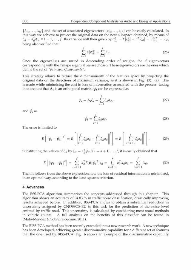
16 Will-be-set-by-IN-TECH
λi1, . . . ,λi f and the set of associated eigenvectors ai1, . . . , ai f can be easily calculated. Inthis way we achieve to project the original data on the new subspace obtained, by means ofζil = aT
il ψil , ∀ l = 1, . . . , f . Its variance will then given by σ2ζ il= E[ζ2il]− E2[ζil] = E[ζ2il] = λil ,
being also verified thatf
∑l=1
E[ψ2il] =
f
∑l=1
λil . (26)
Once the eigenvalues are sorted in descending order of weight, the d eigenvectorscorrespondingwith the dmajor eigenvalues are chosen. These eigenvectors are the oneswhichdefine the set of “Principal Components”.
This strategy allows to reduce the dimensionality of the features space by projecting theoriginal data on the directions of maximum variance, as it is shown in Fig. (3). (a). Thisis made while minimising the cost in loss of information associated with the process: takinginto account that Ai is an orthogonal matrix, ψi can be expressed as
ψi = Aiζi =f
∑l=1
ζil ail , (27)
and ψi as
ψi =d
∑l=1
ζil ail . (28)
The error is limited to
E[∥∥ψi − ψi
∥∥2] = E
⎡⎣∥∥∥∥∥
f
∑l=1
ζil ail −d
∑l=1
ζil ail
∥∥∥∥∥2⎤⎦ = E
⎡⎣∥∥∥∥∥
f
∑l=d+1
ζl ail
∥∥∥∥∥2⎤⎦ . (29)
Substituting the values of ζil by ζil = aTil ψil , ∀ l = d + 1, . . . , f , it is easily obtained that
E[∥∥ψi − ψi
∥∥2] = f
∑l=d+1
aTil E[ψiψi
T ]ail =f
∑l=d+1
aTil λil ail =
f
∑l=d+1
λil . (30)
Then it follows from the above expression how the loss of residual information is minimised,in an optimal way, according to the least squares criterion.
4. Advances
The BSS-PCA algorithm summarises the concepts addressed through this chapter. Thisalgorithm shows an accuracy of 94.83 % in traffic noise classification, drastically improvingresults achieved before. In addition, BSS-PCA allows to obtain a substantial reduction inuncertainty assigned by CNOSSOS-EU to this task for the prediction of the noise levelemitted by traffic road. This uncertainty is calculated by considering most usual methodsin vehicle counts. A full analysis on the benefits of this classifier can be found in(Mato-Méndez & Sobreira-Seoane, 2011).
The BISS-PCAmethod has been recently extended into a new researchwork. A new techniquehas been developed, achieving greater discriminative capability for a different set of featuresthat the one used by BISS-PCA. Fig. 6 shows an example of the discriminative capability
336 Independent Component Analysis for Audio and Biosignal Applications
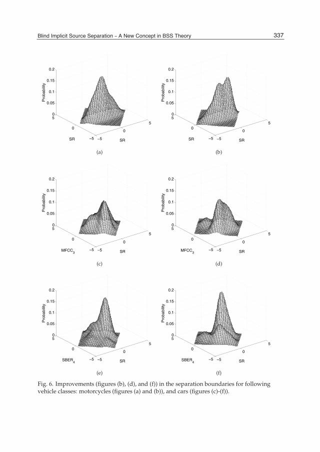
Blind Implicit Source SeparationA New Concept in BSS Theory 17
−5
0
5
−5
0
50
0.05
0.1
0.15
0.2
SRSR
Pro
babi
lity
−5
0
5
−5
0
50
0.05
0.1
0.15
0.2
SRSR
Pro
babi
lity
(a) (b)
−5
0
5
−5
0
50
0.05
0.1
0.15
0.2
SRMFCC3
Pro
babi
lity
−5
0
5
−5
0
50
0.05
0.1
0.15
0.2
SRMFCC3
Pro
babi
lity
(c) (d)
−5
0
5
−5
0
50
0.05
0.1
0.15
0.2
SRSBER4
Pro
babi
lity
−5
0
5
−5
0
50
0.05
0.1
0.15
0.2
SRSBER4
Pro
babi
lity
(e) (f)
Fig. 6. Improvements (figures (b), (d), and (f)) in the separation boundaries for followingvehicle classes: motorcycles (figures (a) and (b)), and cars (figures (c)-(f)).
337Blind Implicit Source Separation – A New Concept in BSS Theory

18 Will-be-set-by-IN-TECH
analysed before (figures (a), (c) and (e)) and after (figures (b), (d) and (f)) applying this newtechnique. By means of this example, we want to show the effect of this technique over onefeature (SR) working alone and combined with another feature (MFCC3 or SBER4). Thesethree features are fully described in the work cited above. It can be observed (figure (a)) howSR shows no between-class discriminative capability for the motorcycle class. After applyingthe new technique, however, a decision boundary appears. This fact allows now be able todiscriminate between two classes (figure (b)). By other hand, the discriminative capabilityof an isolated feature is generally lower than shown by one subset of the features vector.Figures (c) and (d) correspond to cars class, for which SR is applied in combination withMFCC3. It can be observed how the new technique improves the separability degree for thiscombination of features. Finally, a suitable selection (SR combined with SBER4) leads to abetter discrimination of all classes considered (motorcycles, cars and trucks). An example ofthis is shown in figures (e) and (f) for cars class. The separability between this class and both,motorcycle class and truck class, is clearly improved after applying this new technique (figure(f)).
5. Conclusions
The application of the existing BSS techniques requires a thorough study of the problem tosolve. In many cases, however, the BSS problem is simplified by identifying its mixturemodel.The first part of this chapter has been devoted to review this issue, which has allowed betterunderstand the need for additional information about the problem to be solved. After it, a newBSS problem has been introduced and discussed. This problemappears in situations for whichthe variables to extract are presented as implicit functions of the original sources. For thisreason, we have named this new problem as Blind Implicit Source Separation (BISS). Achievinga solution becomes a specially complex task when the original sources are identified withnoise sources. In these cases, the sources models used in BSS are no longer valid and theseparation problem needs to be reformulated. Throughout this chapter, a full characterisationfor the BISS problem has been presented.
An example of BISS problem occurs for the classification of traffic noise. Through the chapter,a detailed description about it within an intercity context has been given. To solve it, a firstapproximation has been proposed, by applying ICA to synthetic mixtures obtained from thesignal acquired by a sensor network. After a results analysis, however, it has been shown howICA does not optimally solves this problem.
After this, a thorough study on how better solve the BISS problem is conducted. As result,a novel feature extraction technique has been then introduced. This technique is usedin embedded form by the BSS-PCA classifier developed (Mato-Méndez & Sobreira-Seoane,2011). Its excellent performance lies in its conception, robustly solving the BISS problem.Unlike other methods described in the state of the art in pattern recognition, this algorithmcombines the use of both, an abstracted features vector and the application of BSS on theacquired signal. The compact design of this technique gives rise to the BISS-PCA methodthat has been introduced in this chapter. It has been explained how this method allows theextraction of discriminative information from the set of original noise sources. Unlike ICA, forwhich this information remains masked, this new technique allows emerge it. The featuresspace therefore wins in resolution while a dimensionality reduction is performed.
Detected by us in pattern recognition problems, the new BISS concept opens an interestingmultidisciplinary research field. This new approach allows to optimise the extraction ofdiscriminative information that otherwise remains hidden. For classification purposes, the
338 Independent Component Analysis for Audio and Biosignal Applications
Blind Implicit Source SeparationA New Concept in BSS Theory 19
BISS-PCA method introduced in this chapter can be extended to other application contexts.This work has been addressed in a recent research. As a result, a new technique solvingthe BISS problem has been achieved, allowing a highest resolution on the between-classboundaries for a different set of features that the one used by BISS-PCA. An example of theimprovements has been shown at the end of this chapter. The results of this new researchwork are expected to appear soon published, so the reader is invited from this moment tohave a look.
6. Acknowledgments
This work has been partially financed by the Spanish MCYT, ref. TEC2009-14414-C03-03,under the project Research on Combined Techniques of Multichannel Sound Source Separation forNoise Reduction. The authors would like to express their sincere gratitude to Ph.D. Ganesh R.Naik for his kind invitation to participate in this book.
7. References
Antoni, J. (2005). Blind separation of vibration components: Principles and demonstrations.Mechanical Systems and Signal Processing, Vol. 19, No. 6, November 2005, pp.1166-1180, ISSN 0888-3270.
Amari, S. & Cichocki, A. (1998). Adaptive blind signal processing - Neural networkapproaches, Proceedings of the IEEE, Vol. 86, No. 10, pp. 2026–2048, 1998.
Ans, B.; Gilhodes, J. C. & Herault, J. (1983). Simulation de reseaux neuronaux (SIRENE).II. Hypothese de decodage du message de mouvement porte par les afférencesfusoriales IA et II par un mecanisme de plasticite synaptique, Comptes Rendus del’Academie des Sciences Paris-Serie III (Sciences Naturelles), Vol. 297, pp. 419-422, 1983.
Bell, A.J. & Sejnowski, T.J. (1995). An information-maximization approach to blind separationand blind deconvolution. Neural Computation, Vol. 7, No. 6, November 1995,1129-1159, ISSN 0899-7667.
Bofill P. & ZibulevskyM. (2000). Blind separation ofmore sources than mixtures using sparsityof their short-time fourier transform, Proceedings of the International Conference onIndependent Component Analysis and Blind Source Separation, pp. 87-92, June 2000,Helsinki, Finland.
Cao, X. R. & Liu, R. W. (1996). General approach to blind source separation. IEEE Transactionson Signal Processing, Vol. 44, No. 3, March 1996, pp. 562–571. ISSN 1053-587X.
Cevher, V.; Chellappa, R. & McClellan, J. H. (2009). Vehicle speed estimation using acousticwave patterns. IEEE Transactions on Signal Processing, Vol. 57, No. 1, January 2009, pp.30–47. ISSN 1053-587X.
Charkani, N. & Deville, Y. (1999). Self-adaptive separation of convolutively mixed signalswith a recursive structure, Part I: Stability analysis and optimization of asymptoticbehaviour. Signal Processing, Vol. 73, No. 3, January 1999, pp. 225–254. ISSN0165-1684.
Cherry, E. C. (1953). Some experiments on the recognition of speech, with one and with twoears. Journal of Acoustic Society of America, Vol. 25, No. 5, September 1953, pp. 975–979.ISSN 0001-4966.
Cichocki, A.; Sabala, I; Choi, S.; Orsier, B. & and Szupiluk R. (1997). Self adaptive independentcomponent analysis for sub-Gaussian and super-Gaussian mixtures with unknownnumber of sources and additive noise, Proceedings of the International Symposium on
339Blind Implicit Source Separation – A New Concept in BSS Theory

20 Will-be-set-by-IN-TECH
Nonlinear Theory and its Applications, Vol. 2, pp. 731-734, December 1997, Hawaii,USA.
Cichocki, A.; Sabala, I & Amari, S. (1998). Intelligent neural networks for blind signalseparation with unknown number of sources, Proceedings of Conference Engineeringof Intelligent Systems, pp. 148-154, February 1998, Tenerife, Spain.
CNOSSOS-EU Group (2010). Draft JRC Reference Report 1 on Common Noise Assessment Methodsin EU (CNOSSOS-EU), Version 2d.
Comon, P. & Jutten, C. (2010). Handbook of Blind Source Separation. Independent ComponentAnalysis and Applications, Elsevier, ISBN 978-0-12-374726-6, USA.
Deville, Y. Towards industrial applications of blind source separation and independentcomponent analysis, Proceedings of International Conference on Independent ComponentAnalysis and Blind Source Separation, pp. 19-24, January 1999, Aussois, France.
Diamantaras, K. I. & Chassioti E. (2000). Blind separation of N binary sources from oneobservation: a deterministic approach, Proceedings of the International Conference onIndependent Component Analysis and Blind Source Separation, pp. 93-98, June 2000,Helsinki, Finland.
Ehlers, F. & Schuster, H. G. (1997). Blind separation of convolutive mixtures and an applicationin automatic speech recognition in a noisy environment. IEEE Transactions on SignalProcessing, Vol. 45, No. 10, October 1997, pp. 2608-2612, ISSN 1053-587X.
Eckart, C. & Young, G. (1936). The approximation of one matrix by another of lower rank.Psychometrika, Vol. 1, September 1936, pp. 211–218, ISSN 0033-3123.
Friedman, J. H. & Tukey, J. W. (1974). A projection pursuit algorithm for exploratory dataanalysis. IEEE Transactions on Computers, Vol. c-23, No. 9, September 1974, pp.881–890, ISSN 0018-9340.
Friedman, J. H.; Stuetzle, W & Schroeder, A. (1984). Projection pursuit density estimation.Journal of the American Statistical Association, Vol. 79, No. 387, September 1984, pp.599–608. ISSN 0162-1459.
Fodor, I. K. (2002). A Survey of Dimension Reduction Techniques, Center for Applied ScientificComputing, Lawrence Livermore National Laboratory.
Fukunaga, K. (1990). Introduction to Statistical Pattern Recognition, Academic Press, ISBN0-12-269851-7, San Diego, CA, USA.
Gelle, G.; Colas, M. & Delaunay, G. (2000). Blind sources separation applied to rotatingmachines monitoring by acoustical and vibrations analysis. Mechanical Systems andSignal Processing, Vol. 14, No. 3, May 2000, pp. 427-442, ISSN 0888-3270.
Herault, J. & Ans, B. (1984). Neural network with modifiable synapses : Decoding ofcomposite sensory messages under unsupervised and permanent learning. ComptesRendus de l’Academie des Sciences Paris-Serie III (Sciences Naturelles), Vol. 299, pp.525-528, 1984.
Herault, J.; Jutten, C. & Ans, B. (1985). Detection de grandeurs primitives dans un messagecomposite par une architecture de calcul neuromimetique en apprentissage nonsupervise, Proceedings of the X GRETSI Symposium on Signal and Image Processing, pp.1017-1022, May 1985, Nice, France.
Hild, K. E.; Erdogmus, D. & Principe J. C. (2001). Blind source separation using Renyi’s mutualinformation. IEEE Signal Processing Letters, Vol. 8, No. 6, June 2001, pp. 174-176, ISSN1070-9908.
Huber, P. J. (1985). Projection pursuit. The Annals of Statistics, Vol. 13, No. 2, June 1985, pp.435–475. ISSN 0090-5364.
340 Independent Component Analysis for Audio and Biosignal Applications

Blind Implicit Source SeparationA New Concept in BSS Theory 21
Hyvärinen, A. (1999). Fast and robust fixed-point algorithms for independent componentanalysis. IEEE Transactions on Neural Networks, Vol. 10, No. 3, May 1999, pp. 626–634.ISSN 1045-9227.
Hyvärinen A.; Karhunen, J. & Oja, E. (2001). Independent Component Analysis, John Wiley &Sons, ISBN 978-0-471-40540-5, New York, USA.
Ihm B. C. & Park D. J. (1999). Blind separation of sources using higher-order cumulants. SignalProcessing, Vol. 73, No. 3, January 1999, pp. 267-276, ISSN 0165-1684.
Ikram, M.Z. & Morgan, D.R. (2001). A multiresolution approach to blind separation of speechsignals in a reverberant environment, Proceedings of the IEEE International Conferenceon Acoustics, Speech and Signal Processing, Vol. 5, pp. 2757-2760, May 2001, Utah, USA.
Jackson, J. E. (1991). A User’s Guide to Principal Components, Wiley Series in Probability andStatistics, John Wiley & Sons, ISBN 9780471622673, New York, USA.
Joho, M.; Mathis, H. & Lambert, R. H. Overdetermined blind source separation: usingmore sensors than source signals in a noisy mixture, Proceedings of the InternationalConference on Independent Component Analysis and Blind Source Separation, pp. 81–86,June 2000, Helsinki, Finland.
Jutten, C & Herault, J. (1988). Independent components analysis versus principal componentsanalysis, In: Signal Processing IV, Theories and Applications, Lacoume J. L.; ChehikianA.; Martin N. & Malbos, J., (Ed.), pp. 643-646, Elsevier Science Publishers, Grenoble,France.
Jutten, C.; Nguyen H. L.; Dijkstra, E.; Vittoz, E. & Caelen, J. (1991a). Blind separation ofsources: an algorithm for separation of convolutive mixtures, Proceedings of theInternational Workshop on High Order Statistics, pp. 273-276, July 1991, Chamrousse,France.
Jutten, C.; Guérin, A. & Nguyen, H. L. (1991b). Adaptive optimization of neural algorithms,Proceedings of the International Workshop on Neural Networks, pp. 54-61, September1991, Granada, Spain.
Karhunen, K. (1946). Zur spektraltheorie stochastischer prozesse. Annales AcademiaeScientiarum Fennicae. Mathematica-Physica, Vol. 34, 1946, pp. 1–7, ISSN 1239-629X.
Kawamoto, M.; Barros, A. K.; Mansour, A.; Matsuoka, K. & Ohnishi N. (1999). Real worldblind separation of convolved non-stationary signals, Proceedings of the InternationalConference on Independent Component Analysis and Blind Source Separation, pp. 347-352,January 1999, Aussois, France.
Klema, C. & Laub, A. J. (1980). The singular value decomposition: its computation and someapplications. IEEE Transactions on Automatic Control, Vol. AC-25, No. 2, April 1980,pp. 164–176, ISSN 0018-9286.
Knaak, M. & Filbert, D. (2009). Acoustical semi-blind source separation for machinemonitoring, Proceedings of the International Conference on Independent ComponentAnalysis and Blind Source Separation, pp. 361-366, December 2001, San Diego, USA.
Knaak, M; Kunter, M; & Filberi, D. (2002). Blind Source Separation for Acoustical MachineDiagnosis, Proceedings of the International Conference on Digital Signal Processing, pp.159-162, July 2002, Santorini, Greece.
Knaak, M.; Araki, S. &Makino, S. (2003). Geometrically constrained ICA for robust separationof soundmixtures, Proceedings of the International Conference on Independent ComponentAnalysis and Blind Source Separation, pp. 951–956, April 2003, Nara, Japan.
Koutras, A.; Dermatas, E. & Kokkinakis, G. (1999). Blind signal separation and speechrecognition in the frequency domain, Proceedings of the IEEE International Conferenceon Electronics, Circuits and Systems, Vol. 1, pp. 427-430, September 1999, Pafos, Cyprus.
341Blind Implicit Source Separation – A New Concept in BSS Theory

22 Will-be-set-by-IN-TECH
Koutras, A.; Dermatas, E. & Kokkinakis, G. (2000). Blind speech separation of movingspeakers in real reverberant environments, Proceedings of the IEEE InternationalConference on Acoustics, Speech and Signal Processing, Vol. 2, pp. 1133-1136, June 2000,Istambul, Turkey.
H. Lappalainen, H. (1999). Ensemble learning for independent component analysis,Proceedings of the International Conference on Independent Component Analysis and BlindSource Separation, pp. 7-12, January 1999, Aussois, France.
Lee, T., Bell, A. J. & Orglmeister, R. (1997a). Blind source separation of real world signals,Proceedings of the International Conference on Neural Networks, Vol. 4, pp. 2129-2134,June 1997, Houston, USA.
Lee, T.; Bell, A. J. & Lambert, R. H. (1997b). Blind separation of delayed and convolved signals,In: Advances in Neural Information Processing Systems 9, pp. 758-764, MIT Press.
Lee, T.W.; Lewicki, M.S.; Girolami, M. & Sejnowski T.J. (1999). Blind source separation of moresources than mixtures using overcomplete representations. IEEE Signal ProcessingLetters, Vol. 6, No. 4, April 1999, pp. 87-90, ISSN 1070-9908.
Loeve, M. (1945). Sur les fonctions aleatoires stationnaires du second ordre. Revue Scientifique,Vol. 83, 1945, pp. 297-310, ISSN 0370-4556.
Mansour, A.; Jutten, C. & Loubaton. P. (1996). Subspace method for blind separation ofsources and for a convolutive mixture model. In: Signal Processing VIII, Theories andApplications, September 1996, pp. 2081–2084, Elsevier, Triest, Italy.
Mansour, A. & Ohnishi, N. (1999). Multichannel blind separation of sources algorithm basedon cross-cumulant and the Levenberg-Marquardtmethod. IEEE Transactions on SignalProcessing, Vol. 47, No. 11, November 1999, pp. 3172-3175, ISSN 1053-587X.
Mansour, A. & Ohnishi, N. (2000a). Discussion of simple algorithms and methods to separatenon-stationary signals, Proceedings of the IASTED International Conference on SignalProcessing and Communications, pp. 78-85, September 2000, Marbella, Spain.
Mansour, A.; Jutten, C. & Loubaton, P. (2000b). Adaptive subspace algorithm for blindseparation of independent sources in convolutive mixture. IEEE Transactions on SignalProcessing, Vol. 48, No. 2, February 2000, pp. 583–586, ISSN 1053-587X.
Mansour, A.; Ohnishi, N. & Puntonet C. G. (2002). Blindmultiuser separation of instantaneousmixture algorithm based on geometrical concepts. Signal Processing, Vol. 82, No. 8,August 2002, pp. 1155-1175, ISSN 0165-1684.
Mansour, A. & Kawamoto, M. (2003). ICA papers classified according to their applicationsand performances. IEICE Transactions on Fundamentals of Electronics, Communicationsand Computer Sciences, Vol. E86-A, No. 3, March 2003, pp. 620-633, ISSN 0916-8508.
Mato-Méndez, F. J. & Sobreira-Seoane, M. A. (2008a). Automatic segmentation of traffic noise,Proceedings of the International Congress on Acoustics, pp. 5867-5872, June 2008, Paris,France. Journal of the Acoustical Society of America, Vol. 123, No. 5, June 2008, p. 3818,ISSN 0001-4966.
Mato-Méndez, F. J. & Sobreira-Seoane, M. A. (2008b). Sustracción espectral de ruido enseparación ciega de fuentes de ruido de tráfico, Proceedings of the InternationalAcoustics European Symposium - Congresso Ibérico de Acústica - Congreso Espanol deAcústica (TecniAcústica), October 2008, Coimbra, Portugal.
Mato-Méndez, F. J. & Sobreira-Seoane, M. A. (2011). Blind separation to improve classificationof traffic noise. Applied Acoustics, Vol. 72, No. 8 (Special Issue on Noise Mapping),July 2011, pp. 590-598, ISSN 0003-682X.
Matsuoka, K.; Ohoya, M. & Kawamoto M. (1995). A neural net for blind separation ofnon-stationary signals. Neural Networks, Vol. 8, No. 3, 1995, pp. 411–419, ISSN0893-6080.
342 Independent Component Analysis for Audio and Biosignal Applications

Blind Implicit Source SeparationA New Concept in BSS Theory 23
Molgedey, L. & Schuster, H. G. (1994). Separation of a mixture of independent signals usingtime delayed correlations. Physical Review Letters, Vol. 72, No. 23, June 1994, pp.3634-3637.
Moreau, E. (2001). A generalization of joint-diagonalization criteria for source separation.IEEE Transactions on Signal Processing, Vol. 49, No. 3, March 2001, pp. 530–541, ISSN1053-587X.
Nguyen, H. L.; Jutten, C. & Caelen J. (1992). Speech enhancement: analysis and comparison ofmethods on various real situations, In: Signal Processing VI, Theories and Applications,Vandewalle, J.; Boite, R.; Moonen, M. & Oosterlinck, A. (Ed.), pp. 303–306, Elsevier.
Nguyen, H. L. & Jutten, C. (1995). Blind sources separation for convolutive mixtures. SignalProcessing, Vol. 45, No. 2, August 1995, pp. 209-229, ISSN 0165-1684.
Nion, D.; Mokios, K. N.; Sidiropoulos, N. D. & Potamianos, A. (2010). Batch and adaptivePARAFAC-based blind separation of convolutive speech mixtures. IEEE Transactionson Audio, Speech, and Language Processing, Vol. 18, No. 6, August 2010, pp. 1193-1207,ISSN 1558-7916.
Pedersen, M. S.; Larsen, J.; Kjems, U. & Parra L. C. (2007). A survey of convolutive blindsource separation methods, In: Multichannel Speech Processing Handbook, Benesty, J. &Huang, A. (Ed.), pp. 1065-1084, Springer, ISBN 978-3-540-49125-5.
Pham, D. T. and Cardoso, J. F. (2001). Blind separation of instantaneous mixtures of nonstationary sources. IEEE Transactions on Signal Processing, Vol. 49, No. 9, September2001, pp. 1837-1848, ISSN 1053-587X.
Prieto, A.; Puntonet, C. G. & Prieto B. (1998). Separation of sources: a neural learningalgorithm for blind separation of sources based on geometric properties. SignalProcessing, Vol. 64, No. 3, February 1998, pp. 315-331, ISSN 0165-1684.
Prieto, A.; Prieto, B.; Puntonet, C. G.; Canas, A. & Martín-Smith, P. (1999). Geometricseparation of linear mixtures of sources: application to speech signals, Proceedingsof the International Conference on Independent Component Analysis and Blind SourceSeparation, pp. 295-300, January 1999, Aussois, France.
Puntonet, C. G.; Prieto, A.; Jutten, C.; Rodriguez Alvarez, M. & Ortega J. (1995). Separation ofsources: A geometry-based procedure for reconstruction of n-valued signals. SignalProcessing, Vol. 46, No. 3, October 1995, pp. 267-284, ISSN 0165-1684.
Puntonet, C.G.; Bauer, C.; Lang, E.W.; Alvarez, M.R. & Prieto B. (2000). Adaptive-geometricmethods: application to the separation of EEG signals, Proceedings of the InternationalWorkshop on Independent Component Analysis and Blind Separation of Signals, pp.273-277, June 2000, Helsinki, Finland.
Puntonet G. (2003). Procedimientos y aplicaciones en separación de senales (BSS-ICA),Proceedings of the XVIII URSI Symposium, September 2003, La Coruna, Spain.
Rahbar, K. & Reilly J. (2001). Blind separation of convolved sources by joint approximatediagonalization of cross-spectral density matrices, Proceedings of the IEEE InternationalConference on Acoustics, Speech, and Signal Processing, Vol. 5, pp. 2745–2748, May 2001,Utah, USA.
Rickard, S.; Balan, R. & Rosca, J. (2001). Real-time time–frequency based blind sourceseparation, Proceedings of the International Conference on Independent ComponentAnalysis and Blind Source Separation, pp. 651-656, December 2001, San Diego, USA.
Rickard, S.; Melia, T. & Fearon, C. (2005). DESPRIT - histogram based blind source separationof more sources than sensors using subspace methods, Proceedings of the IEEEWorkshop on Applications of Signal Processing to Audio and Acoustics, pp. 5-8, October2005, New Paltz, New York.
343Blind Implicit Source Separation – A New Concept in BSS Theory
24 Will-be-set-by-IN-TECH
Sahlin, H. & Broman H. (1998). Separation of real-world signals. Signal Processing, Vol. 64, No.1, January 1998, pp. 103-113, ISSN 0165-1684.
Sawada, H.; Araki, S. & Makino, S. (2011). Underdetermined convolutive blind sourceseparation via frequency bin-wise clustering and permutation alignment. IEEETransactions on Audio, Speech, and Language Processing, Vol. 19, No. 3, March 2011,pp. 516-527, ISSN 1558-7916.
Solazzi, M.; Parisi, R. & Uncini, A. (2001). Blind source separation in nonlinear mixtures byadaptive spline neural network, Proceedings of the IEEE International Conference onAcoustics, Speech and Signal Processing, May 2001, Utah, USA.
Srebro, N. (2004). Learning with Matrix Factorizations, PhD thesis, Institute of Technology.Massachusetts.
Torkkola, K. (1996). Blind separation of convolved sources based on informationmaximization, Proceedings of the IEEE Workshop on Neural Networks for SignalProcessing, pp. 423-432, September 1996, Kyoto, Japan.
Valpola, H.; Honkela, A. & Karhunen J. (2001). Nonlinear static and dynamic blind sourceseparation using ensemble learning, Proceedings of the International Joint Conference onNeural Networks, Vol. 4, pp. 2750–2755, July 2001, Washington D. C., USA.
Van Gerven, S.; Van Compernolle, D.; Nguyen, H. L. & Jutten, C. (1994). Blind separation ofsources: a comparative study of a 2nd and a 4th order solution, In: Signal ProcessingVII, Theories and Applications, pp. 1153–1156, Elsevier, Edinburgh, Scotland.
Wang, Y.; Chi, Y.; Wu, X. & Liu, C. (2009). Extracting acoustical impulse signal of faultybearing using blind deconvolution method, Proceedings of the International Conferenceon Intelligent Computation Technology and Automation, pp. 590-594, October 2009,Changsa, China.
Weinstein, E.; Feder, M. & Oppenheim, A.V. (1993). Multi-channel signal separation bydecorrelation. IEEE Transactions on Speech Audio Processing, Vol. 1, No. 4, October 1993,pp. 405-413, ISSN 1063-6676.
Wu, J. B.; Chen, J.; Zhong, Z. M. & Zhong, P. (2002). Application of blind source separationmethod in mechanical sound signal analysis, Proceedings of the American Society ofMechanical Engineers International Mechanical Engineering Congress and Exposition, pp.785-791 , November 2002, New Orleans, USA.
Ypma, A.; Leshem, A.; & Duin. R. P. D. (2002). Blind separation of rotating machine sources:bilinear forms and convolutive mixtures. Neurocomputing, Vol. 49, December 2002,pp. 349-368, ISSN 0925-2312.
Yonggang, Z. & Chambers, J. A. (2011). Exploiting all combinations of microphone sensors inoverdetermined frequency domain blind separation of speech signals. InternationalJournal of Adaptive Control and Signal Processing, Vol. 25, No. 1, 2011, pp. 88–94, ISSN1099-1115.
Zhang, L. Q.; Amari, S. & Cichocki, A. (1999a). Natural gradient approach to blind separationof over- and undercomplete mixtures, Proceedings of the International Conference onIndependent Component Analysis and Blind Source Separation, pp. 455–460, January 1999,Aussois, France.
Zhang, L. Q.; Cichocki, A. and Amari, S. (1999b). Natural gradient algorithm for blindseparation of overdetermined mixture with additive noise, IEEE Signal ProcessingLetters, Vol. 6, No. 11, November 1999, pp. 293–295, ISSN 1070-9908.
344 Independent Component Analysis for Audio and Biosignal Applications
Related Documents