TRENDS in Cognitive Sciences Vol.6 No.2 February 2002 http://tics.trends.com 1364-6613/02/$ – see front matter © 2002 Elsevier Science Ltd. All rights reserved. PII: S1364-6613(00)01813-1 59 Research Update Techniques & Applications Independent component analysis (ICA) is a method for automatically identifying the underlying factors in a given data set. This rapidly evolving technique is currently finding applications in analysis of biomedical signals (e.g. ERP, EEG, fMRI, optical imaging), and in models of visual receptive fields and separation of speech signals. This article illustrates these applications, and provides an informal introduction to ICA. Independent component analysis (ICA) is essentially a method for extracting individual signals from mixtures of signals. Its power resides in the physically realistic assumption that different physical processes generate unrelated signals. The simple and generic nature of this assumption ensures that ICA is being successfully applied in a diverse range of research fields. Despite its wide range of applicability, ICA can be understood in terms of the classic ‘cocktail party’ problem, which ICA solves in an ingenious manner. Consider a cocktail party where many people are talking at the same time. If a microphone is present then its output is a mixture of voices. When given such a mixture, ICA identifies those individual signal components of the mixture that are unrelated. Given that the only unrelated signal components within the signal mixture are the voices of different people, this is precisely what ICA finds. (In practice, ICA requires more than one simultaneously recorded mixture in order to find the individual signals in any one mixture.) It is worth stressing here that ICA does not incorporate any knowledge specific to speech signals; in order to work, it requires simply that the individual voice signals are unrelated. On a more biological note, an EEG signal from a single scalp electrode is a mixture of signals from different brain regions. As with the speech example above, the signal recorded at each electrode is a mixture, but it is the individual components of the signal mixtures that are of interest (e.g. single voice, signal from a single brain region). Finding these underlying ‘source’ signals automatically is called ‘blind source separation’ (BSS), and ICA the dominant method for performing BSS. A critical caveat is that most BSS methods require at least as many mixtures (e.g. microphones, electrodes) as there are source signals. ICA in context: related methods The goal of decomposing measured signals, or variables, into a set of underlying variables is far from new (we use the terms ‘variable’ and ‘signal’ interchangeably here). For example, the literature on IQ assessment describes many methods for taking a set of measured variables (i.e. sub-test scores) and finding a set of underlying competences (e.g. spatial reasoning). In the language of BSS, this amounts to decomposing a set of signal mixtures (sub-test scores) into a set of source signals (underlying competences). In common with the IQ literature, many fields of research involve identifying a few key source signals from a large number of signal mixtures. Techniques commonly used for this data reduction (or data mining, as it is now known) are principal component analysis (PCA), factor analysis (FA), linear dynamical systems (LDS). The most commonly used data reduction methods (PCA and FA) identify underlying variables that are uncorrelated with each other. Intuitively, this is desirable because the underlying variables that account for a set of measured variables should correspond to physically different processes, which, in turn, should have outputs that are uncorrelated with each other. However, specifying that underlying variables should be uncorrelated imposes quite weak constraints on the form these variables take. It is the weakness of these constraints which ensures that the factors extracted by FA can be rotated (in order to find a more interpretable set of factors) without affecting the (zero) correlations between factors. Most factor rotation methods yield a statistically equivalent set of uncorrelated factors. The variety of factor rotation methods available is regarded with some skepticism by some researchers. This is because it is sometimes possible to use factor rotation to obtain new factors which are easily interpreted, but which are statistically no more significant than results obtained with other factor rotations. By contrast, any attempt to rotate the factors (‘independent components’) extracted by ICA would yield non-independent factors. Thus, the independent components of ICA do not permit post-ICA rotations because such factors are statistically independent, and are therefore uniquely defined. Independent components can also be obtained by making use of the observation that individual source signals tend to be less complex than any mixture of those source signals [1,2]. Statistical independence ICA is based on the assumption that source signals are not only uncorrelated, but are also ‘statistically independent’. Essentially, if two variables are independent then the value of one variable provides absolutely no information about the value of the other variable. By contrast, even though two variables are uncorrelated, the value of one variable can still provide information about the value of the other variable (see Box 1). ICA seeks a set of statistically independent signals amongst a set of ‘signal mixtures’, on the assumption that such statistically independent signals are derived from different physical processes (Box 2). The objective of finding such a set of statistically independent signals is achieved by maximizing a measure of the ‘joint entropy’ of the extracted signals. What is it good for? ICA has been applied in two fields of research relevant to cognitive science: analysis of biomedical data and computational modelling. One of the earliest biomedical applications of ICA Independent component analysis: an introduction James V. Stone

Welcome message from author
This document is posted to help you gain knowledge. Please leave a comment to let me know what you think about it! Share it to your friends and learn new things together.
Transcript

TRENDS in Cognitive Sciences Vol.6 No.2 February 2002
http://tics.trends.com 1364-6613/02/$ – see front matter © 2002 Elsevier Science Ltd. All rights reserved. PII: S1364-6613(00)01813-1
59Research Update
Techniques & Applications
Independent component analysis (ICA)
is a method for automatically identifying
the underlying factors in a given data set.
This rapidly evolving technique is currently
finding applications in analysis of
biomedical signals (e.g. ERP, EEG, fMRI,
optical imaging), and in models of visual
receptive fields and separation of speech
signals. This article illustrates these
applications, and provides an informal
introduction to ICA.
Independent component analysis
(ICA) is essentially a method for
extracting individual signals from
mixtures of signals. Its power resides
in the physically realistic assumption
that different physical processes
generate unrelated signals. The
simple and generic nature of this
assumption ensures that ICA is being
successfully applied in a diverse range
of research fields.
Despite its wide range of applicability,
ICA can be understood in terms of the
classic ‘cocktail party’problem, which ICA
solves in an ingenious manner. Consider a
cocktail party where many people are
talking at the same time. If a microphone
is present then its output is a mixture of
voices. When given such a mixture, ICA
identifies those individual signal
components of the mixture that are
unrelated. Given that the only unrelated
signal components within the signal
mixture are the voices of different people,
this is precisely what ICA finds.
(In practice, ICA requires more than one
simultaneously recorded mixture in order
to find the individual signals in any one
mixture.) It is worth stressing here that
ICA does not incorporate any knowledge
specific to speech signals; in order to work,
it requires simply that the individual
voice signals are unrelated.
On a more biological note, an EEG
signal from a single scalp electrode is a
mixture of signals from different brain
regions. As with the speech example
above, the signal recorded at each
electrode is a mixture, but it is the
individual components of the signal
mixtures that are of interest (e.g. single
voice, signal from a single brain region).
Finding these underlying ‘source’ signals
automatically is called ‘blind source
separation’ (BSS), and ICA the
dominant method for performing BSS.
A critical caveat is that most BSS methods
require at least as many mixtures
(e.g. microphones, electrodes) as there
are source signals.
ICA in context: related methods
The goal of decomposing measured
signals, or variables, into a set of
underlying variables is far from new
(we use the terms ‘variable’ and ‘signal’
interchangeably here). For example, the
literature on IQ assessment describes
many methods for taking a set of
measured variables (i.e. sub-test scores)
and finding a set of underlying
competences (e.g. spatial reasoning).
In the language of BSS, this amounts to
decomposing a set of signal mixtures
(sub-test scores) into a set of source
signals (underlying competences). In
common with the IQ literature, many
fields of research involve identifying a
few key source signals from a large
number of signal mixtures. Techniques
commonly used for this data reduction
(or data mining, as it is now known) are
principal component analysis (PCA),
factor analysis (FA), linear dynamical
systems (LDS).
The most commonly used data
reduction methods (PCA and FA) identify
underlying variables that are
uncorrelated with each other. Intuitively,
this is desirable because the underlying
variables that account for a set of
measured variables should correspond to
physically different processes, which, in
turn, should have outputs that are
uncorrelated with each other. However,
specifying that underlying variables
should be uncorrelated imposes quite
weak constraints on the form these
variables take. It is the weakness of these
constraints which ensures that the
factors extracted by FA can be rotated
(in order to find a more interpretable set
of factors) without affecting the (zero)
correlations between factors. Most factor
rotation methods yield a statistically
equivalent set of uncorrelated factors.
The variety of factor rotation methods
available is regarded with some
skepticism by some researchers. This is
because it is sometimes possible to use
factor rotation to obtain new factors
which are easily interpreted, but which
are statistically no more significant than
results obtained with other factor
rotations. By contrast, any attempt to
rotate the factors (‘independent
components’) extracted by ICA would
yield non-independent factors. Thus, the
independent components of ICA do not
permit post-ICA rotations because such
factors are statistically independent, and
are therefore uniquely defined.
Independent components can also be
obtained by making use of the observation
that individual source signals tend to be
less complex than any mixture of those
source signals [1,2].
Statistical independence
ICA is based on the assumption that
source signals are not only uncorrelated,
but are also ‘statistically independent’.
Essentially, if two variables are
independent then the value of one
variable provides absolutely no
information about the value of the other
variable. By contrast, even though two
variables are uncorrelated, the value of
one variable can still provide information
about the value of the other variable
(see Box 1). ICA seeks a set of
statistically independent signals
amongst a set of ‘signal mixtures’, on
the assumption that such statistically
independent signals are derived from
different physical processes (Box 2).
The objective of finding such a set of
statistically independent signals is
achieved by maximizing a measure of the
‘joint entropy’ of the extracted signals.
What is it good for?
ICA has been applied in two fields of
research relevant to cognitive science:
analysis of biomedical data and
computational modelling. One of the
earliest biomedical applications of ICA
Independent component analysis: an introduction
James V. Stone

TRENDS in Cognitive Sciences Vol.6 No.2 February 2002
http://tics.trends.com
60 Research Update
If two variables (signals) x and y arerelated then we usually expect thatknowing the value of x tells us somethingabout the corresponding value of y. Forexample, if x is a person’s height and y istheir weight then knowing the value of xprovides some information about y. Here,we consider how much information xconveys about y when these variables areuncorrelated and independent.
Uncorrelated variables
Even if x and y are uncorrelated thenknowing the value of x can still provideinformation about about y. For example,if we define x = sin(z) and y = cos(z)(where z = 0…2π) then x and y areuncorrelated (Fig. Ia; note that noise hasbeen added for display purposes).However, the variables x 2 = sin2(z) andy 2 = cos2(z) are (negatively) correlated; asshown in Fig. Ib, which is a graph of x 2
versus y 2. Thus, knowing the value of x 2
(and therefore x) provides information
about y 2 (and therefore about y), eventhough x and y are uncorrelated. Forexample, in Fig. Ia, if x = 0.5 then it canseen that either y ≈ –0.7 or y ≈ 0.7; so thatknowing x provides information about y.
Correlated variables
If two variables are correlated thenknowing the value of one variableprovides information about thecorresponding value value of the othervariable. For example, the variables inFig. Ib are negatively correlated(r = –0.962), and if the x-axis variable is0.4 then it can seen that the correspondingy-axis variable is approximately 0.3.
Independent variables
If two signals are independent thenknowing the value of one signal providesabsolutely no information about thecorresponding value of the other signal.For example, if two people are speakingat the same time then knowing the
amplitude of one voice at any givenmoment provides no information aboutthe value of the other voice at thatmoment. In Fig. Ic, each point representsthe amplitudes of two voices at a singlemoment in time; knowing the amplitude(x value) of one voice provides noinformation about the amplitude (y value) of the other voice.
Maximum entropy distributions
If two signals are plotted against eachother (as x and y in Fig. I) then thisapproximates the joint ‘probabilitydensity function’ (pdf) of the signals.For signals with bounded values(e.g. between 0 and 1), this joint pdf has‘maximum entropy’ if it is uniform (as inFig. Id). Note that if a set of signals has amaximum entropy pdf then this impliesthat the signals are mutually independent,but that a set of independent signals doesnot necessarily have a pdf with maximumentropy (e.g. Fig. Ic).
Box 1. Independent and uncorrelated variables
TRENDS in Cognitive Sciences
-1 -0.8-0.6-0.4-0.2 0 0.2 0.4 0.6 0.8 1-1
-0.8
-0.6
-0.4
-0.2
0
0.2
0.4
0.6
0.8
1
0 0.1 0.2 0.3 0.4 0.5 0.6 0.7 0.8 0.9 10
0.1
0.2
0.3
0.4
0.5
0.6
0.7
0.8
0.9
1
-6 -4 -2 0 2 4 6-6
-4
-2
0
2
4
6
0 0.1 0.2 0.3 0.4 0.5 0.6 0.7 0.8 0.9 10
0.1
0.2
0.3
0.4
0.5
0.6
0.7
0.8
0.9
1
(a) (b) (c) (d)
Fig. I
The general strategy underlying ICA canbe summarized as follows.
(1) It is assumed that different physicalprocesses (e.g. two speakers) give rise tounrelated source signals. Specifically,source signals are assumed to bestatistically independent (see Box 1).
(2) A measured signal (e.g. amicrophone output) usually containscontributions from many differentphysical sources, and therefore consistsof a mixture of unrelated source signals.[Note that most ICA methods require atleast as many simultaneously recorded
signal mixtures (e.g. microphoneoutputs) as there are signal sources(e.g. voices)].
(3) Unrelated signals are usuallystatistically independent, and it can beshown that a function g of independentsignals have ‘maximum entropy’ (seeBox 3). Therefore, if a set of signals withmaximum entropy can be recoveredfrom a set of mixtures then such signalsare independent.
(4) In practice, independent signalsare recovered from a set of mixtures byadjusting a separating matrix W until
the entropy of a fixed function g ofsignals recovered by W is maximized[where g is assumed to be thecumulative density function (cdf) ofthe source signals, see Box 3]. Theindependence of signals recoveredby W is therefore achieved indirectly,by adjusting W in order to maximize theentropy of a function g of signalsrecovered by W; as maximum entropysignals are independent, it can be shownthat this ensures the estimated sourcesignals recovered by W are alsoindependent (see Boxes 1 and 3).
Box 2. ICA in a Nutshell
involved analysis of EEG data, where ICA
was used to recover signals associated
with detection of visual targets [3]
(see Box 3). In this case, the output
sequence of each electrode is assumed to
consist of a mixture of temporal
independent components (tICs), which
are extracted by temporal ICA (tICA).
Another application of tICA is in optical
TRENDS in Cognitive Sciences Vol.6 No.2 February 2002
http://tics.trends.com
61Research Update
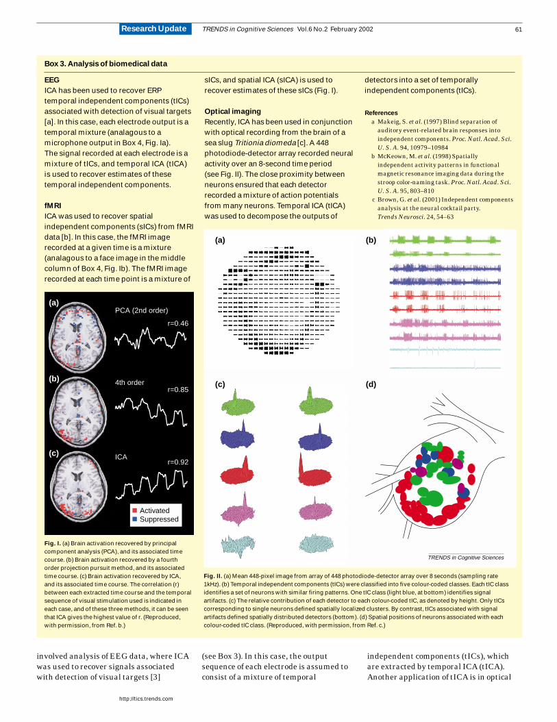
EEG
ICA has been used to recover ERPtemporal independent components (tICs)associated with detection of visual targets[a]. In this case, each electrode output is atemporal mixture (analagous to amicrophone output in Box 4, Fig. Ia).The signal recorded at each electrode is amixture of tICs, and temporal ICA (tICA)is used to recover estimates of thesetemporal independent components.
fMRI
ICA was used to recover spatialindependent components (sICs) from fMRIdata [b]. In this case, the fMRI imagerecorded at a given time is a mixture(analagous to a face image in the middlecolumn of Box 4, Fig. Ib). The fMRI imagerecorded at each time point is a mixture of
sICs, and spatial ICA (sICA) is used torecover estimates of these sICs (Fig. I).
Optical imaging
Recently, ICA has been used in conjunctionwith optical recording from the brain of asea slug Tritionia diomeda [c]. A 448photodiode-detector array recorded neuralactivity over an 8-second time period(see Fig. II). The close proximity betweenneurons ensured that each detectorrecorded a mixture of action potentialsfrom many neurons. Temporal ICA (tICA)was used to decompose the outputs of
detectors into a set of temporallyindependent components (tICs).
References
a Makeig, S. et al. (1997) Blind separation of
auditory event-related brain responses into
independent components. Proc. Natl. Acad. Sci.
U. S. A. 94, 10979–10984
b McKeown, M. et al. (1998) Spatially
independent activity patterns in functional
magnetic resonance imaging data during the
stroop color-naming task. Proc. Natl. Acad. Sci.
U. S. A. 95, 803–810
c Brown, G. et al. (2001) Independent components
analysis at the neural cocktail party.
Trends Neurosci. 24, 54–63
Box 3. Analysis of biomedical data
TRENDS in Cognitive Sciences
(a)
(b)
(c)
PCA (2nd order)
4th order
ICAr=0.92
r=0.85
r=0.46
ActivatedSuppressed
(d)(c)
(b)(a)
TRENDS in Cognitive Sciences
Fig. I. (a) Brain activation recovered by principalcomponent analysis (PCA), and its associated timecourse. (b) Brain activation recovered by a fourthorder projection pursuit method, and its associatedtime course. (c) Brain activation recovered by ICA,and its associated time course. The correlation (r)between each extracted time course and the temporalsequence of visual stimulation used is indicated ineach case, and of these three methods, it can be seenthat ICA gives the highest value of r. (Reproduced,with permission, from Ref. b.)
Fig. II. (a) Mean 448-pixel image from array of 448 photodiode-detector array over 8 seconds (sampling rate1kHz). (b) Temporal independent components (tICs) were classified into five colour-coded classes. Each tIC classidentifies a set of neurons with similar firing patterns. One tIC class (light blue, at bottom) identifies signalartifacts. (c) The relative contribution of each detector to each colour-coded tIC, as denoted by height. Only tICscorresponding to single neurons defined spatially localized clusters. By contrast, tICs associated with signalartifacts defined spatially distributed detectors (bottom). (d) Spatial positions of neurons associated with eachcolour-coded tIC class. (Reproduced, with permission, from Ref. c.)

imaging, where it has been used
to decompose the outputs of the
photodetector array used to record from
neurons of a sea slug [4]. Functional
magnetic resonance imaging data has also
been analysed using ICA [5]. Here, the
fMRI brain image collected at each time
point is treated as a mixture of spatial
independent components (sICs), which are
extracted by spatial ICA (sICA). Note that
sICA and tICA make use of the same core
ICA method; it is just that tICA seeks
temporally independent sequences in a set
of temporal mixtures, whereas sICA seeks
spatially independent images in a set of
image mixtures (Box 3).
The recent growth in interest in ICA
can be traced back to a (now classic) paper
[6], in which it was demonstrated how
temporal ICA could be used to solve a
simple ‘cocktail party’problem by
recovering single voices from voice
mixtures (see Box 4). From a modelling
perspective, it is thought that different
neurons might encode independent
physical attributes [7], because this
ensures maximum efficiency in
information-theoretic terms. ICA provides
a powerful method for finding such
independent attributes, which can then
be compared to attributes encoded by
neurons in primary sensory areas. This
approach has been demonstrated for
primary visual neurons [8] and spatial
ICA has also been applied to images of
faces (see Box 4).
Model-based vs data-driven methods
An ongoing debate in the analysis of
biomedical data concerns the relative
merits of model-based versus data-driven
methods [9]. ICA is an example of a data-
driven method, inasmuch as it is deemed
to be exploratory (other exploratory
methods are PCA and FA). By contrast,
conventional methods for analysing
biomedical data, especially fMRI data,
rely on model-based methods (also
known as parametric methods), such as
the ‘general linear model’ (GLM). For
example, with fMRI data, the GLM
extracts brain activations consistent with
the specific sequence of stimuli presented
to a subject.
The term ‘data driven’ is misleading
because it suggests that such methods
require no assumptions regarding the
data. In fact, all data-driven methods are
based on certain assumptions, even if
these assumptions are generic in nature.
For example, ICA depends critically on
the assumptions that each signal mixture
is a combination of source signals which
are independent and non-gaussian.
Similarly, the data-driven methods FA
and PCA are based on the assumption
that underlying source signals (factors
and eigenvectors, respectively) are
uncorrelated and gaussian.
TRENDS in Cognitive Sciences Vol.6 No.2 February 2002
http://tics.trends.com
62 Research Update
Speech separation
Given a set of N = 5 people speaking in a room with fivemicrophones, each voice si contributes differentially to eachmicrophone output xj [a]. The relative contribution of the fivevoices to each of the five mixtures is specified by the elementsof an unknown 5 × 5 mixing matrix A (see Fig. Ia). Each elementin A is defined by the distance between each person and eachmicrophone. The output of each microphone is a mixture xj offive independent source signals (voices) s = (s1,…,s5) (echoesand time delays are ignored in this example). ICA finds aseparating matrix W which recovers five independentcomponents u. These recovered signals u are taken to beestimates of the source signals s. (Note that ICA re-orderssignals, so that an extracted signal ui and its source signal si
are not necessarily on the same row.)
Face recognition
Fig. Ib shows how ICA treats each photograph X as a mixture ofunderlying spatial independent components S [b]. It is assumedthat these unknown spatial independent components are mixed
together with an unknown mixing matrix matrix A to form theobserved photographs X. ICA finds a separating matrix W whichrecovers estimates U of the spatial independent components S.Note how the estimated spatial independent components Ucontain spatially localized features corresponding toperceptually salient features, such as mouth and eyes.
Modelling receptive fields
ICA of images of natural scenes (Fig. Ic) yields spatialindependent components which resemble edges or bars [c]These independent components are similar to the receptive fieldsof neurons in primary visual areas of the brain (also see [d]).
References
a Bell, A. and Sejnowski, T. (1995) An information-maximization approach to
blind separation and blind deconvolution. Neural Comput. 7, 1129–1159
b Bartlett, M. (2001) Face Image Analysis by Unsupervised Learning
(Vol. 612), Kluwer Academic Publishers
c Hyvarinen, A. et al. (2001) Topographic independent component analysis.
Neural Comput. 13, 1527–1574
d Bell, A.J. and Sejnowski, T.J. (1997) The ‘independent components’ of
natural scenes are edge filters. Vis. Res. 37, 3327–3338
Box 4. Computational modelling and applications
TRENDS in Cognitive Sciences
?
Sources Faceimages
Separatedoutputs
S X U
A W
Unknownmixingprocess
Learnedweights
?
?
?
(a) (b) (c)S
A
X U
W
Fig . I
Data-driven methods therefore
implicitly incorporate a generic, or weak,
model of the type of signals to be
extracted. The main difference between
such weak models and that of (for
example) GLM is that GLM attempts to
extract a specific signal that is a best fit
to a user-specified model signal. For
example, using fMRI, this user-specified
signal often consists of a temporal
sequence of zeros and ones corresponding
to visual stimuli being switched on and off;
a GLM (e.g. SPM) would then be used to
identify brain regions with temporal
activations which correlated with the
timing of this visual switching. By
contrast, data-driven methods extract a
signal that is consistent with a general
TRENDS in Cognitive Sciences Vol.6 No.2 February 2002
http://tics.trends.com
63Research Update
The output of a microphone is atime-varying signal , which is a linear mixture of N independentsource signals (i.e. voices). Each mixturexi contains a contribution from eachsource signal . The relativeamplitude of each voice sj at themicrophone is related to the microphone–speaker distance, and can be defined as aweighting factor Aij for each voice. If N = 2then the relative contribution of each voicesj to a mixture xi is,
where s=(s1,s2) is a vector variable in whicheach variable is a source signal, and Ai isthe ith column of a matrix A of mixingcoefficients. If there are N = 2 microphonesthen each voice sj has a different relativeamplitude (defined by Aij) at eachmicrophone, so that each microphonerecords a different mixture xi:
<Equation 2>
where each column of the mixing matrix Aspecifies the relative contributions of thesource signals s to each mixture xi. Thisleads to the first equation in most paperson ICA:
,
where x = (x1,x2) is a vector variable, and x1 and x2 are signal mixtures.
The matrix A defines a lineartransformation on the signals s. Suchlinear transformations can usually bereversed in order to recover an estimate uof source signals s from signal mixtures x,
,
where the separating matrix W = A−1 is theinverse of A. However, the mixing matrix Ais not known, and cannot therefore beused to find W. The important point is thata separating matrix W exists which maps aset of N mixtures x to a set of N sources
signals u ≈ s (this exact inverse mappingexists, but numerical methods find a closeapproximation to it).
Given that we want to recover anestimate u = xW of the source signals s andthat the latter are mutually independentthen this suggests that W should beadjusted so as to make the estimated sourcesignals u mutually independent. This, inturn, can be achieved by adjusting W tomaximize the entropy of U = g(u) = g(Wx),where the function g is assumed to bethe cumulative density function (cdf) of s(see Box 2).
If a set of signals x is mapped toanother set U then the entropy H(U) of U isgiven by the entropy of x plus the changein entropy ∆H induced by the mappingfrom x to U, denoted (x → U),
As the entropy of the mixtures H(x) isfixed, maximizing H(U) depends onmaximizing the change in entropy ∆Hassociated with the mapping (x → U). Themapping from x to U = g(Wx) depends ontwo terms, the cumulative densityfunction g and the separating matrix W.The form of g is fixed, which means thatmaximizing H(U) amounts to maximizing∆H by adjusting W. In summary, a matrixW that maximizes the change in entropyinduced by the mapping (x → U) alsomaximizes the joint entropy H(U).The change in entropy ∆H induced by thetransformation g(Wx) can be consideredas the ratio of infinitesimal volumesassociated with corresponding points in xand U. This ratio is given by the expectedvalue of ln J , where . denotes theabsolute value of the determinant of theJacobian matrix J = ∂U/∂x. Omittingmathematical details, this yields:
where the summation over n samples(plus ln W ) is an estimate of the expected
value of ln J , and the functionis the probability density
function (pdf) of the ith source signal. Notethat the entropy H(x) is a constant, and cantherefore be ignored because it does notaffect the value of W that maximizes H(U).
Given that u = Wx, the derivativeof H(U) with respect to W is
where
where g′′ (uj) is the second derivative of g.Recall that we want to adjust W so
that it maximizes H(U). The standardmethod for adjusting W is gradientascent. This consists of iteratively addinga small amount of the gradient ofH(U) to W,
where η is a learning rate. The functionH(U) can be maximized by gradientascent using either Eqn (9), or using themore efficient ‘natural gradient’ [a].Alternatively, if both the function H(U)and its derivative can be evaluated(as here) then a second order technique,such as conjugate gradient, can be usedto obtain solutions relatively quickly.
The exposition above refers totemporal ICA (tICA) of speech signals.Spatial ICA (sICA) of images can beachieved by concatenating rows orcolumns of an image to produce aone-dimensional image signal xi. Eachimage xi is considered to be a mixture ofindependent source images (see Fig. Ib,Box 4). A set of N images is thenrepresented as an N-dimensional vectorvariable x, as in Equation 3. Spatial ICscan then be recovered using exactly thesame method as described for speechsignals above.
Reference
a Amari, S. (1998) Natural gradient works
efficiently in learning. Neural Comput.
10, 251–276
)(UH∇
),(UHWW oldnew ∇+= η
)(UH∇
,)()(
,...,)()(
)(1
1
′′′
′′′
=N
N
ugug
ugug
uψ
,)()( 1 tWH xuU ψ+=∇ −
)(UH∇
jjj ugg ∂∂=′ /
,ln)( ln1
)()( )(
1 1
Wugn
HH kjj
n
k
N
j
+′+= ∑∑= =
xU
))(()()()()(
xxx
UxxU
WgHHHHH
→∆+=→∆+=
Wxus =≈
Asx =
,
),(
))((),(
.2.1
.2.121
AAA
AAxx
s
s
ss
===
,
),)(,(
)()(
.
2121
2211
i
tii
iii
AAAss
AsAsx
s==
+=
tjjj sss ...},{ 21=
tiii xxx ,...},{ 21=
Box 5. The nuts and bolts of ICA

type of signal, where the signal type is
specified in terms of the general
statistical structure of the signal. Thus,
the models implicit in data-driven
methods are generic because they attempt
to extract a type of signal, rather than a
best fit to a specific model signal. The
difference between model-based and
data-driven methods is one of degree,
and involves the relative specificity of the
statistical assumptions associated with
each methods.
This suggests that both classes of
methods can be used, depending on the
specificity of the hypothesis being tested.
If there are sound reasons for
hypothesizing that a specific signal will be
present in the data (e.g. corresponding to a
sequence of visual stimuli) then a
model-based method might be preferred.
Conversely, if it is suspected that a
model-based method would not extract all
signals of interest then an exploratory
data-driven technique is appropriate.
On a pragmatic note, evaluating the
statistical significance of data-driven
methods tends to be more difficult than
that of model-based methods. Box 5 gives
some of the mathematical details of ICA.
Conclusion
ICA represents a novel and powerful
method, with applications in
computational neuroscience and
engineering. However, like all methods,
the success of ICA in a given application
depends on the validity of the
assumptions on which ICA is based. In
the case of ICA, the assumptions of linear
mixing and independence appear to be
physically realistic; which is perhaps why
it has been successfully applied to many
problems. However, these assumptions
are violated to some extent by most data
sets (see [9]). Whilst reports of ICA’s
successes are encouraging, they should
be treated with caution. Much
theoretical work remains to be done on
precisely how ICA fails when its
assumptions (i.e. linear mixing and
independence) are severely violated.
Acknowledgements
Thanks to N. Hunkin, A. Hyvarinen and
M. McKeown for comments on this paper.
References
1 Hyvarinen, A. (2001) Complexity pursuit:
separating interesting components from time
series. Neural Comput. 13, 883–898
2 Stone, J. (2001) Blind source separation using
temporal predictability. Neural Comput.
13, 1559–1574
3 Makeig, S. et al. (1997) Blind separation of
auditory event-related brain responses into
independent components. Proc. Natl. Acad. Sci.
U. S. A. 94, 10979–10984
4 Brown, G. et al. (2001) Independent
components analysis (ica) at the neural
cocktail party. Trends Neurosci.
24, 54–63
5 McKeown, M. et al. (1998) Spatially
independent activity patterns in functional
magnetic resonance imaging data during the
stroop color-naming task. Proc. Natl. Acad.
Sci. U. S. A. 95, 803–810
6 Bell, A. and Sejnowski, T. (1995) An
information-maximization approach to blind
separation and blind deconvolution.
Neural Comput. 7, 1129–1159
7 Barlow, H. (1989) Unsupervised learning.
Neural Comput. 1, 295–311
8 Hyvarinen, A. et al. (2001) Topographic
independent component analysis.
Neural Comput. 13, 1527–1574
9 Friston, K. (1998) Modes or models: a critque of
independent component analysis. Trends Cogn.
Sci. 2, 373–375
James V. Stone
Psychology Department, Sheffield University,Sheffield, UK S10 2TP.e-mail: [email protected]
TRENDS in Cognitive Sciences Vol.6 No.2 February 2002
http://tics.trends.com
64 Research Update
Books
• Bartlett, M.S. (2001) Face ImageAnalysis by Unsupervised Learning(International Series on Engineeringand Computer Science), KluwerAcademic Publishers
• Girolami, M. (1999) Self-OrganisingNeural Networks: IndependentComponent Analysis and Blind SourceSeparation, Springer-Verlag
• Girolami, M., ed. (2000) Advances inIndependent Component Analysis.Perspectives in Neural Computing,Springer-Verlag
• Hyvarinen, A. et al. (2001) IndependentComponent Analysis, John Wiley & Sons
• Lee, T.W. (1999) IndependentComponent Analysis: Theory andApplications, Kluwer AcademicPublishers
• Roberts, S. and Everson, R., eds (2001)Independent Component Analysis:Principles and Practice, CambridgeUniversity Press
Mailing list
http://tsi.enst.fr/~cardoso/icacentral/mailinglist.html
Annual conference
Abstract of the Third InternationalConference on Independent ComponentAnalysis and Signal Separation,San Diego, California 9–13 December 2001,ICA2001, http://ica2001.org.
Demonstrations and software
A good place to start is:http://www.cnl.salk.edu/~tewon/ica_cnl.htmlICA code for 2D images, anddemonstrations: http://www.shef.ac.uk/~pc1jvs
ICA Resources
Finding the TICS articles you want
From this year, indexes for Trends in Cognitive Sciences will no longerbeing produced. However, TICS is available on BioMedNet, includingthe archive going back to January 1998, so you can still find the articlesyou need, at the click of a mouse. The full text and pdf files of all articlescan be accessed at http://tics.trends.com, where an extensive searchfacility is available. Search facilities allows you to:
• view the latest issue• browse previous issues • search the journal using keywords, author names, or publication date• jump quickly to your desired volume and page number
Related Documents