KATHOLIEKE UNIVERSITEIT LEUVEN Faculteit Toegepaste Wetenschappen Departement Computerwetenschappen Celestijnenlaan 200A, B-3001 Leuven—Belgi¨ e INCREMENTAL LOOP TRANSFORMATIONS AND ENUMERATION OF PARAMETRIC SETS Promotoren: Prof. Dr. ir. M. Bruynooghe Prof. Dr. ir. F. Catthoor Proefschrift voorgedragen tot het behalen van het doctoraat in de toegepaste wetenschappen door Sven VERDOOLAEGE April 2005 In samenwerking met VZW Interuniversitair Micro-Elektronica Centrum vzw Kapeldreef 75 B-3001 Leuven (Belgi¨ e)

Welcome message from author
This document is posted to help you gain knowledge. Please leave a comment to let me know what you think about it! Share it to your friends and learn new things together.
Transcript
KATHOLIEKE UNIVERSITEIT LEUVEN
Faculteit Toegepaste Wetenschappen
Departement Computerwetenschappen
Celestijnenlaan 200A, B-3001 Leuven—Belgie
INCREMENTAL LOOP TRANSFORMATIONS AND
ENUMERATION OF PARAMETRIC SETS
Promotoren:Prof. Dr. ir. M. BruynoogheProf. Dr. ir. F. Catthoor
Proefschrift voorgedragen tothet behalen van het doctoraatin de toegepaste wetenschappen
door
Sven VERDOOLAEGE
April 2005
In samenwerking met
VZW
Interuniversitair Micro-Elektronica Centrum vzwKapeldreef 75B-3001 Leuven (Belgie)

KATHOLIEKE UNIVERSITEIT LEUVEN
Faculteit Toegepaste Wetenschappen
Departement Computerwetenschappen
Celestijnenlaan 200A, B-3001 Leuven—Belgie
INCREMENTAL LOOP TRANSFORMATIONS AND
ENUMERATION OF PARAMETRIC SETS
Examencommissie :Prof. Dr. ir. L. Froyen, voorzitterProf. Dr. ir. M. Bruynooghe, promoterProf. Dr. ir. F. Catthoor, promoterProf. Dr. ir. G. JanssensProf. Dr. B. DemoenProf. Dr. ir. R. CoolsDr. A. Darte (ENS Lyon)Dr. ir. B.A.C.J. Kienhuis (Universiteit Leiden)
Proefschrift voorgedragen tothet behalen van het doctoraatin de toegepaste wetenschappen
door
Sven VERDOOLAEGE
U.D.C. 681.3*D34 April 2005
In samenwerking met
VZW
Interuniversitair Micro-Elektronica Centrum vzwKapeldreef 75B-3001 Leuven (Belgie)
c©Katholieke Universiteit Leuven – Faculteit Toegepaste WetenschappenArenbergkasteel, B-3001 Leuven – Heverlee (Belgium)
Alle rechten voorbehouden. Niets uit deze uitgave mag vermenigvuldigd en/ofopenbaar gemaakt worden door middel van druk, fotocopie, microfilm, elektro-nisch of op welke andere wijze ook zonder voorafgaande schriftelijke toestem-ming van de uitgever.
All rights reserved. No part of the publication may be reproduced in any formby print, photoprint, microfilm or any other means without written permissionfrom the publisher.
D/2005/7515/28
ISBN 90-5682-594-1
Voorwoord
Al van kindsaf ben ik geboeid door wiskunde en grammatica. Toen ik na mijnstudies van ingenieur in de computerwetenschappen, waar ik voor de orientatietoegepaste wiskunde had gekozen, de gelegenheid kreeg om nog een jaar bijte studeren, heb ik beslist om de opleiding Master of Artificial Intelligence tevolgen, waar mijn keuzevakken vooral taalgerelateerd waren. Na enig zoekenvond ik ook een thesisonderwerp dat paste in een samenwerking tussen com-puterwetenschappen en computerlinguistiek. Ik had dan ook twee promotoren,Danny De Schreye en Frank Van Eynde, en wel drie begeleiders, Marc Denec-ker, Ness Schelkens en Kristof Van Belleghem. De bijkomende lezer, MauriceBruynooghe zou later nog een belangrijke rol spelen.
Op uitnodiging van Danny De Schreye heb ik mijn doctoraatsonderzoek aange-vangen in de groep Declaratieve Talen en Artificiele Intelligentie (meer bepaald,de groep kennistechnologie). Initieel heb ik mij geconcentreerd op een verdereuitwerking van het thema van mijn thesis, het extraheren van temporele in-formatie uit natuurlijke taal met behulp van ID-logica en abductie. Na eenjaar van samenwerking met vooral Bert Van Nuffelen en Emmanuel De Motin verband met implementatie-aspecten en met Ness Schelkens in verband mettaalaspecten, een jaar ook gekruid met interessante discussies met Frank VanEynde, werd het tijd om een ander onderwerp aan te snijden. Ondanks ver-woede pogingen van zowel Danny De Schreye als Marc Denecker om mij doorhet aanreiken van mogelijke onderwerpen op het rechte pad te houden, voeldeik mij toch eerder aangetrokken door de subgroep die zich bezighoudt met hetontwerp, de analyse en de implementatie van declaratieve programmeertalen.
Maurice Bruynooghe was bereid om als mijn promotor te fungeren en schakeldemij in in een nieuw-opgezette samenwerking met de DESICS groep van IMEC.De bedoeling van deze samenwerking was om de ervaring van onze groep metdeclaratieve talen aan te wenden bij het analyseren van imperatieve talen. Tij-dens een gesprek met mijn latere copromotor Francky Catthoor, werd de bredecontext geschetst van de methodologie waarin mijn onderzoek zou kaderen. Diemethodologie bestond er voornamelijk in om het vermogenverbruik van toepas-singen te verminderen met behulp van programmatransformaties. Enkele van
I
II
de stappen in de methodologie verdienden echter nog bijkomend onderzoek.Een van die stappen was de stap die zich bezighield met het transformeren vanlussen. Die stap, zo werd mij verteld, was eerder wiskundig en genoot daarommijn onmiddellijke voorkeur.
Koen Danckaert, die zich eerder in dit onderwerp had verdiept en werkte aan deafronding van zijn doctoraatsthesis, wijdde mij verder in in de mathemagischewereld van polytopen, die gebruikt werden om lussen in programma’s voor testellen. Hij vertelde over zijn methodologie van drie stappen, een lineaire trans-formatie, een translatie en een ordening, en hoe hij zich vooral geconcentreerdhad op de eerste stap.
Na enkele verbeteringen aangebracht te hebben aan de lineaire transformatie,kwam de uitdaging van het uitwerken van de volgende stap, de translatie. Hetwas daarbij belangrijk om die translatie zoveel mogelijk incrementeel uit tevoeren. Tijdens het uitwerken van die incrementele translatie werd duidelijk dathet garanderen dat in de ordeningsstap nog een geldige ordening kon gekozenworden, de grootste moeilijkheid vormde. Door de ordening op voorhand vastte leggen, werd de incrementele translatie veel eenvoudiger, maar verschilde zenog weinig van bestaand werk.
During the incremental translation, the order in which parts of the programsare optimized is important. As a heuristic for this ordering, the implementa-tion uses the size of some polytope related to the program parts. To calculatethe sizes of these non-parametric polytopes, I had used a counting procedurein PolyLib meant for parametric polytopes. This procedure is, however, veryinefficient for enumerating non-parametric polytopes as it will basically ex-haustively enumerate all integer points in these polytopes (expect for the finaldimension). During the summer of 2003, I was told by Martin Palkovic (whohad in turn heard about it from Kristof Beyls) of this wonderful tool calledLattE, which implemented a recent technique developed mainly by AlexanderBarvinok and which was reported to be considerably more efficient.
After downloading LattE, I noticed that it was just a binary without the sourcecode. Obviously, I could not just run a binary downloaded from the internet,so I asked Jesus A. De Loera, the project director of LattE, for the source. Hetold me that I would have to wait some time, probably until the next year.Telling him that he was required to give me the source since their tool wasbuilt on top of a GNU GPL’ed library called NTL did not appear to change hismind. Being an open source bigot, I was therefore forced to implement thisfunctionality myself.
Fortunately, the paper describing LattE proved very accessible, even to a lowlyengineer such as myself. Any remaining issues I had with the algorithm werequickly resolved by explanations from Jesus, who proved to be very helpful.After having finished a bare-bones implementation, I announced the availability
III
of this new library (with sources!) to the PolyLib mailing list. I figured theauthors of the counting routine might find it useful since the enumeration of aparametric polytope was based on the enumeration of a set of non-parametricpolytopes. Shortly afterwards, it dawned on me that with some (conceptually)minor modifications, the algorithm I had implemented could also be used toenumerate parametric polytopes. It was only much later that I realized thatthis use had basically already been described in a paper by Alexander Barvinokand Jamie Pommersheim.
Since I wanted to reuse some parts of the PolyLib code in my implementation,I asked Vincent Loechner, the maintainer of PolyLib and the implementor ofthe included enumeration algorithm, for some more information. As it hap-pened, a student of his, Rachid Seghir, had also been considering the use ofBarvinok’s algorithm to enumerate parametric polytopes. He had even writtenan (unpublished) report on this topic. Having read my message on the PolyLibmailing list, Vincent quickly guessed what I was working on and we decided tojoin forces.
Meanwhile, I was talking to Kristof Beyls about this new way of enumeratingparametric polytopes and it turned out that this new way was actually useful.He had a lot of experience with the use of PolyLib’s enumeration procedureand he told me that it had three problems: occasional high execution timeseven for non-parametric polytopes, degeneracy problems and large outputs forsolutions with large periodicity. The first two problems were inherently solvedby the new method and I quickly found a way to also solve the third problem.His explanation of his reuse distance application and his pessimism on beingable to solve some more difficult variations of this application, encouraged meto consider extensions of the enumeration algorithm to more general sets.
When talking to Jesus A. De Loera about possible ways to achieve these exten-sions, he invited me to a mini-workshop on Ehrhart Quasi-polynomials. Duringthis workshop I met many nice mathematicians, including Kevin Woods, whohad developed such an extension. This extension would produce a generatingfunction, however, rather than an explicit function. Together, we developedan efficient algorithm for the conversion from a generating function to the cor-responding explicit function. Kevin figured the conversion was in itself aninteresting topic of research and so we also developed an algorithm for theconversion from explicit function to generating function.
Ik wil hierbij iedereen bedanken die tot dit werk heeft bijgedragen. In de eersteplaats wil ik mijn (ex-)promotoren bedanken: Danny De Schreye, die mij dekans gegeven heeft om aan een doctoraat te werken; Maurice Bruynooghe, diemij altijd is blijven steunen, ook als mijn onderzoek niet zo vlot verliep, en diealtijd tot in de details mijn schrijfsels is blijven lezen, ook al hadden die nogweinig verband met declaratieve talen; Francky Catthoor, die mij in contactheeft gebracht met de wondere wereld der polytopen, altijd bereid was om over
IV
mijn onderzoek te discussieren en mij ook steeds is blijven motiveren.
Gerda Janssens, Bart Demoen en Ronald Cools, leden van de begeleidingscom-missie, wil ik bedanken voor de interesse en het nalezen van de tekst, ondankshet feit dat het onderwerp van mijn thesis ver verwijderd is van het onderzoekvan sommigen onder hen. Verder dank ik Ludo Froyen voor het waarnemenvan het voorzitterschap van de examencommissie.
Special thanks are due to Alain Darte and Bart Kienhuis for serving on myjury. Thanks also to Alain Darte and Antoine Fraboulet for the interestingdiscussions.
Dank ook aan iedereen waarmee ik heb samengewerkt en de collega’s van zo-wel computerwetenschappen en IMEC, ook zij die ik niet expliciet vernoem.Большое спасибо, Александр. Dakujem, Martin, for the many interestingconversations. Gracias, Jesus, por no haberme dado el codigo fuente de LattE
inmediatamente. Thank you, Kevin, for constantly reminding me when con-vergence is important and when it is not.
Bijzondere dank aan Arnout Vandecappelle voor het grondig nalezen van detekst en dank aan Karel Van Oudheusden en Peter Vanbroekhoven voor hetnalezen van de Nederlandse samenvatting en aan Tanja Van Achteren voor hetnalezen van dit voorwoord.
Tevens wil ik het GOA LP+-project en het Fonds voor WetenschappelijkOnderzoek–Vlaanderen bedanken voor de financiering van mijn onderzoek.
ó$·:¡\·¥©Õ.jS|½Z+Ç/4jS¦+·ñOF
Tenslotte wil ik ook mijn vrienden en familie bedanken voor hun trouwe steun.
Sven VerdoolaegeLeuven, maart 2005
V
Abstract
The geometrical model is a powerful tool for program analysis and optimizationand forms the basis on which we build the two parts of this dissertation, amethodology for incremental loop transformations and an efficient enumerationtechnique for parametric integer sets.
Power consumption for typical embedded multi-media applications is domina-ted by the storage of and the access to the large multi-dimensional arrays theymanipulate. It is now well known that a design methodology for reducing po-wer consumption and improving system performance should apply global looptransformations for increasing locality and regularity of data accesses. In thefirst part of this dissertation, we propose a two-step global loop transformationapproach consisting of a linear transformation focusing mainly on regularity,and a translation focusing on locality. We further develop a refined regularitycriterion and show how to perform the translation step incrementally, allowingmultiple complicated cost functions to be evaluated.
Many compiler optimization techniques depend on the enumeration of parame-tric integer sets defined by linear equations. In the second part of this disserta-tion, we present the first implementation of Barvinok’s algorithm applied tothe enumeration of parametric polytopes, extending an earlier implementationof this algorithm for a subclass of the enumeration problems we consider, andproviding a significant improvement over another implementation based on adifferent technique. The resulting enumerator may be obtained as an explicitfunction or as a generating function. We further show that these two represen-tations are polynomially interconvertible and we discuss some approaches forhandling generalized enumeration problems.
VI
Beknopte Samenvatting
Het geometrisch model is een krachtig hulpmiddel voor de analyse en optima-lisatie van programma’s. Het vormt de basis van beide delen van deze doc-toraatsverhandeling, een methodologie voor incrementele lustransformaties eneen efficiente enumeratietechniek voor parametrische gehele verzamelingen.
Het vermogenverbruik van typische ingebedde multimedia toepassingen wordtgedomineerd door de opslag van en toegang tot de grote multidimensionale ma-trices die in de toepassing gemanipuleerd worden. Het is algemeen geweten dateen ontwerpmethodologie gericht op het verminderen van het vermogenverbruiken het verbeteren van de systeemperformatie, globale lustransformaties moettoepassen om de lokaliteit en regulariteit van de gegevenstoegangen te verbe-teren. In het eerste deel van deze doctoraatsverhandeling stellen we aanpakvoor globale lustransformaties voor die bestaat uit twee stappen, een lineairetransformatie die vooral gericht is op regulariteit en een translatie gericht oplokaliteit. We ontwikkelen ook een verfijnd regulariteitscriterium en geven aanhoe de translatiestap incrementeel kan uitgevoerd worden, hetgeen toelaat ommeerdere ingewikkelde kostfuncties te evalueren.
Vele optimalisatietechnieken tijdens het compilatieproces zijn afhankelijk vande enumeratie van parametrisch gehele verzamelingen gedefinieerd door lineairevergelijkingen. In het tweede deel van deze doctoraatsverhandeling stellen wede eerste implementatie voor van Barvinoks algoritme, toegepast op de enu-meratie van parametrische polytopen. Dit is een uitbreiding van een eerdereimplementatie van dit algoritme voor een subklasse van onze enumeratiepro-blemen. Het is ook een significante verbetering ten opzichte van een andereimplementatie die gebaseerd is op een andere techniek. De enumerator van eenparametrisch verzameling kan verkregen worden in de vorm van een explicietefunctie of in de vorm van een genererende functie. We tonen aan dat deze tweevormen interconverteerbaar zijn in polynomiale tijd en we bespreken enkeleaanpakken voor gegeneraliseerde enumeratieproblemen.
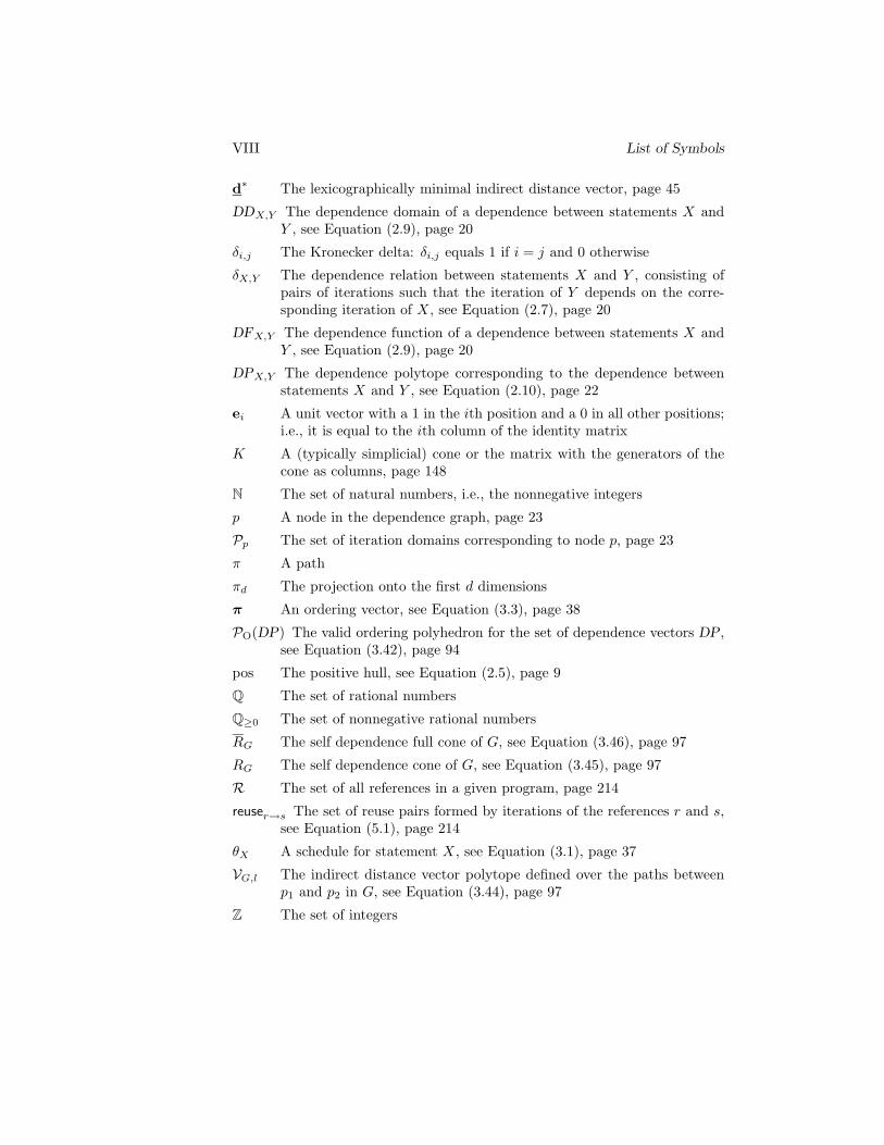
List of Symbols
≺ Lexicographically smaller, page 13
⌈·⌉ The least integer function, i.e., ⌈x⌉ = n, with n ∈ N and n− 1 < x ≤ n
⌊·⌋ The greatest integer function, i.e., ⌊x⌋ = n, with n ∈ N and n ≤ x <n + 1
· The fractional part function, i.e., x = x − ⌊x⌋
〈·, ·〉 The standard inner product
aX The offset of the affine transformation for statement X, see Equa-tion (3.2), page 37
AX The linear part of the affine transformation for statement X, see Equa-tion (3.2), page 37
AX An affine transformation for statement X, see Equation (3.2), page 37
ADSr→s The set of memory locations accessed between instances of referencesr and s that form a reuse pair, see Equation (5.3), page 214
aff The affine hull, see Equation (2.3), page 8
αp1,p2The relative offset of p2 with respect to p1, see Equation (3.11), page 46
BRDr←s The number of memory locations accessed between instances of ref-erences r and s that form a reuse pair, see Equation (5.5), page 215
BRDs The number of memory locations accessed since the previous accessto the memory location accessed by the instance of reference s, seeEquation (5.6), page 215
C The set of complex numbers
cS The enumerator of the integer points in the set S, see Equation (4.1),page 109
CG,T The global dependence cone for dependence graph G and translationT , see Equation (3.43), page 96
conv The convex hull, see Equation (2.4), page 9
d A distance vector, see Equation (2.10), page 21
d The lexicographically minimal dependence distance vector, see Equa-tion (3.8), page 44
VII
VIII List of Symbols
d∗ The lexicographically minimal indirect distance vector, page 45
DDX,Y The dependence domain of a dependence between statements X andY , see Equation (2.9), page 20
δi,j The Kronecker delta: δi,j equals 1 if i = j and 0 otherwise
δX,Y The dependence relation between statements X and Y , consisting ofpairs of iterations such that the iteration of Y depends on the corre-sponding iteration of X, see Equation (2.7), page 20
DFX,Y The dependence function of a dependence between statements X andY , see Equation (2.9), page 20
DPX,Y The dependence polytope corresponding to the dependence betweenstatements X and Y , see Equation (2.10), page 22
ei A unit vector with a 1 in the ith position and a 0 in all other positions;i.e., it is equal to the ith column of the identity matrix
K A (typically simplicial) cone or the matrix with the generators of thecone as columns, page 148
N The set of natural numbers, i.e., the nonnegative integers
p A node in the dependence graph, page 23
Pp The set of iteration domains corresponding to node p, page 23
π A path
πd The projection onto the first d dimensions
π An ordering vector, see Equation (3.3), page 38
PO(DP) The valid ordering polyhedron for the set of dependence vectors DP,see Equation (3.42), page 94
pos The positive hull, see Equation (2.5), page 9
Q The set of rational numbers
Q≥0 The set of nonnegative rational numbers
RG The self dependence full cone of G, see Equation (3.46), page 97
RG The self dependence cone of G, see Equation (3.45), page 97
R The set of all references in a given program, page 214
reuser→s The set of reuse pairs formed by iterations of the references r and s,see Equation (5.1), page 214
θX A schedule for statement X, see Equation (3.1), page 37
VG,l The indirect distance vector polytope defined over the paths betweenp1 and p2 in G, see Equation (3.44), page 97
Z The set of integers
List of Acronyms
ADS . . . . . . . . . . Accessed Data Set
BG . . . . . . . . . . . . Basic Group
BRD . . . . . . . . . . Backward Reuse Distance
CD . . . . . . . . . . . . Cavity Detection
CLooG . . . . . . . . . Chunky Loop Generator
CME . . . . . . . . . . Cache Miss Equations
DSA . . . . . . . . . . Dynamic Single Assignment
DTSE . . . . . . . . . Data Transfer and Storage Exploration
gcd . . . . . . . . . . . greatest common divisor
ILP . . . . . . . . . . . Integer Linear Programming
LBL . . . . . . . . . . . Linearly Bounded Lattice
lcm . . . . . . . . . . . least common multiple
LLL . . . . . . . . . . . Lenstra, Lenstra and Lovasz’ basis reduction algorithm
MC . . . . . . . . . . . Memory Compaction
MHLA . . . . . . . . Memory Hierarchy Layer Assignment
NDD . . . . . . . . . . Number Decision Diagram
OOM . . . . . . . . . Out Of Memory
ORC . . . . . . . . . . . . Open Research Compiler
PER . . . . . . . . . . . . Polyhedral Extraction Routine
pers . . . . . . . . . . . PER in SUIF
PIP . . . . . . . . . . . Parametric Integer Programming
RACE . . . . . . . . Reduction of Arithmetic Cost of Expressions
s2c . . . . . . . . . . . . SUIF to C
SBO . . . . . . . . . . Storage Bandwidth Optimization)
SCBD . . . . . . . . . Storage Cycle Budget Distribution
SCC . . . . . . . . . . strongly connected component
IX
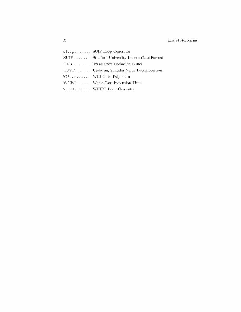
X List of Acronyms
sloog . . . . . . . . . SUIF Loop Generator
SUIF . . . . . . . . . . Stanford University Intermediate Format
TLB . . . . . . . . . . Translation Lookaside Buffer
USVD . . . . . . . . Updating Singular Value Decomposition
W2P . . . . . . . . . . . . WHIRL to Polyhedra
WCET . . . . . . . . Worst-Case Execution Time
WLooG . . . . . . . . . WHIRL Loop Generator
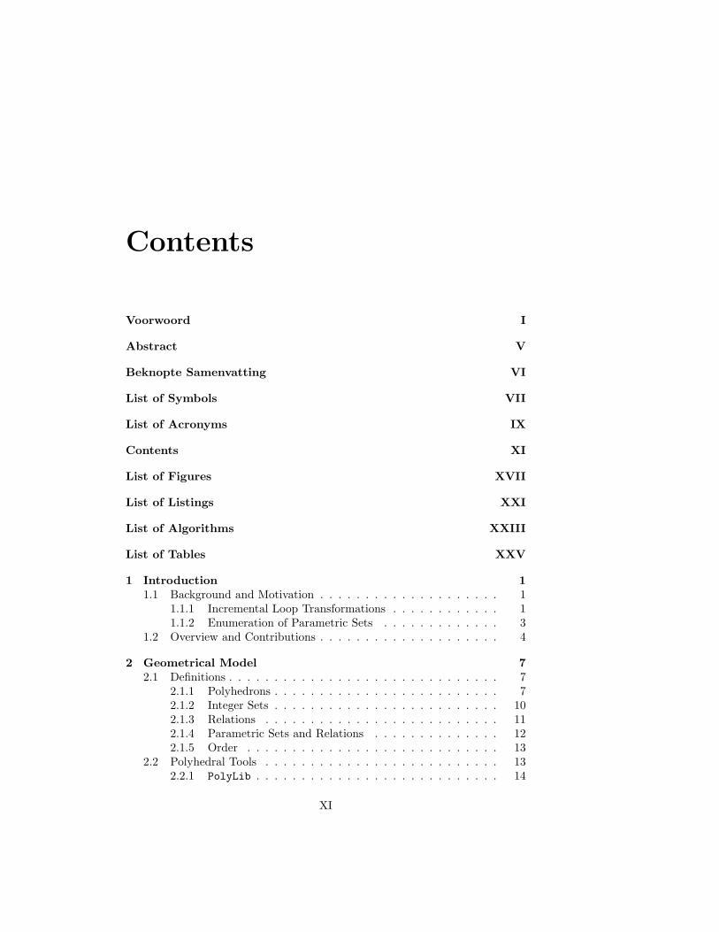
Contents
Voorwoord I
Abstract V
Beknopte Samenvatting VI
List of Symbols VII
List of Acronyms IX
Contents XI
List of Figures XVII
List of Listings XXI
List of Algorithms XXIII
List of Tables XXV
1 Introduction 11.1 Background and Motivation . . . . . . . . . . . . . . . . . . . . 1
1.1.1 Incremental Loop Transformations . . . . . . . . . . . . 11.1.2 Enumeration of Parametric Sets . . . . . . . . . . . . . 3
1.2 Overview and Contributions . . . . . . . . . . . . . . . . . . . . 4
2 Geometrical Model 72.1 Definitions . . . . . . . . . . . . . . . . . . . . . . . . . . . . . . 7
2.1.1 Polyhedrons . . . . . . . . . . . . . . . . . . . . . . . . . 72.1.2 Integer Sets . . . . . . . . . . . . . . . . . . . . . . . . . 102.1.3 Relations . . . . . . . . . . . . . . . . . . . . . . . . . . 112.1.4 Parametric Sets and Relations . . . . . . . . . . . . . . 122.1.5 Order . . . . . . . . . . . . . . . . . . . . . . . . . . . . 13
2.2 Polyhedral Tools . . . . . . . . . . . . . . . . . . . . . . . . . . 132.2.1 PolyLib . . . . . . . . . . . . . . . . . . . . . . . . . . . 14
XI
XII Contents
2.2.2 Omega . . . . . . . . . . . . . . . . . . . . . . . . . . . . 142.2.3 PIP . . . . . . . . . . . . . . . . . . . . . . . . . . . . . 152.2.4 LASH . . . . . . . . . . . . . . . . . . . . . . . . . . . . . 16
2.3 Iteration Domains . . . . . . . . . . . . . . . . . . . . . . . . . 162.4 Dependences . . . . . . . . . . . . . . . . . . . . . . . . . . . . 17
2.4.1 Dynamic Single Assignment Code . . . . . . . . . . . . 182.4.2 Multiple Assignment Code . . . . . . . . . . . . . . . . 24
3 Incremental Loop Transformations 273.1 The DTSE methodology . . . . . . . . . . . . . . . . . . . . . . 28
3.1.1 Platform independent steps . . . . . . . . . . . . . . . . 303.1.2 Platform dependent steps . . . . . . . . . . . . . . . . . 313.1.3 Other related methodologies and stages . . . . . . . . . 33
3.2 Overview of Loop Transformation Steps . . . . . . . . . . . . . 343.2.1 Source-to-source Transformations . . . . . . . . . . . . . 343.2.2 Affine Loop Transformations . . . . . . . . . . . . . . . 373.2.3 Validity . . . . . . . . . . . . . . . . . . . . . . . . . . . 383.2.4 Optimality . . . . . . . . . . . . . . . . . . . . . . . . . 393.2.5 Incremental Loop Transformations . . . . . . . . . . . . 413.2.6 Summary . . . . . . . . . . . . . . . . . . . . . . . . . . 43
3.3 Loop Fusion . . . . . . . . . . . . . . . . . . . . . . . . . . . . . 433.3.1 Validity . . . . . . . . . . . . . . . . . . . . . . . . . . . 433.3.2 Locality Heuristic . . . . . . . . . . . . . . . . . . . . . 513.3.3 2D Example . . . . . . . . . . . . . . . . . . . . . . . . . 523.3.4 Experimental Results . . . . . . . . . . . . . . . . . . . 533.3.5 Refinements . . . . . . . . . . . . . . . . . . . . . . . . . 553.3.6 Summary . . . . . . . . . . . . . . . . . . . . . . . . . . 60
3.4 Linear Transformation . . . . . . . . . . . . . . . . . . . . . . . 603.4.1 Validity . . . . . . . . . . . . . . . . . . . . . . . . . . . 603.4.2 Regularity Heuristic . . . . . . . . . . . . . . . . . . . . 703.4.3 Regularity Experiments . . . . . . . . . . . . . . . . . . 76
No Cycles . . . . . . . . . . . . . . . . . . . . . . . . . . 76No Self-Reuse and no Conflicts . . . . . . . . . . . . . . 77General Case . . . . . . . . . . . . . . . . . . . . . . . . 79Results . . . . . . . . . . . . . . . . . . . . . . . . . . . 80
3.4.4 Locality Heuristic . . . . . . . . . . . . . . . . . . . . . 833.4.5 Example . . . . . . . . . . . . . . . . . . . . . . . . . . . 873.4.6 Summary . . . . . . . . . . . . . . . . . . . . . . . . . . 91
3.5 Ordering . . . . . . . . . . . . . . . . . . . . . . . . . . . . . . . 923.5.1 Redundancy of Ordering . . . . . . . . . . . . . . . . . . 933.5.2 Translation before Ordering . . . . . . . . . . . . . . . . 943.5.3 Comparison . . . . . . . . . . . . . . . . . . . . . . . . . 98
3.6 Related Work . . . . . . . . . . . . . . . . . . . . . . . . . . . . 983.6.1 Previous Research at IMEC . . . . . . . . . . . . . . . . 983.6.2 Other Related Work . . . . . . . . . . . . . . . . . . . . 102
Contents XIII
3.7 Summary . . . . . . . . . . . . . . . . . . . . . . . . . . . . . . 103
4 Enumeration of Parametric Sets 1054.1 Preliminaries . . . . . . . . . . . . . . . . . . . . . . . . . . . . 106
4.1.1 Polyhedral Sets . . . . . . . . . . . . . . . . . . . . . . . 1074.1.2 Parametric Sets and their Enumerators . . . . . . . . . 1084.1.3 Generating Functions . . . . . . . . . . . . . . . . . . . 1094.1.4 Time Complexity . . . . . . . . . . . . . . . . . . . . . . 110
4.2 Parametric Counting Problems . . . . . . . . . . . . . . . . . . 1114.2.1 Ehrhart Quasi-Polynomials . . . . . . . . . . . . . . . . 1114.2.2 Vector Partition Functions . . . . . . . . . . . . . . . . 1154.2.3 Parametric Polytopes . . . . . . . . . . . . . . . . . . . 1184.2.4 Parametric Projected Sets . . . . . . . . . . . . . . . . . 129
4.3 Two Representations . . . . . . . . . . . . . . . . . . . . . . . . 1314.4 Barvinok’s Algorithm . . . . . . . . . . . . . . . . . . . . . . . 133
4.4.1 Overview . . . . . . . . . . . . . . . . . . . . . . . . . . 1334.4.2 Computing Generating Functions . . . . . . . . . . . . . 137
Unimodular Cones . . . . . . . . . . . . . . . . . . . . . 137Brion’s Theorem . . . . . . . . . . . . . . . . . . . . . . 138Barvinok’s Decomposition . . . . . . . . . . . . . . . . . 142Triangulation of Non-simplicial Cones . . . . . . . . . . 143Decomposition of Simplicial Cones . . . . . . . . . . . . 148Overview . . . . . . . . . . . . . . . . . . . . . . . . . . 152
4.4.3 Evaluating Generating Functions . . . . . . . . . . . . . 1574.4.4 Enumeration of Parametric Polytopes . . . . . . . . . . 163
4.5 Operations . . . . . . . . . . . . . . . . . . . . . . . . . . . . . 1694.5.1 Addition . . . . . . . . . . . . . . . . . . . . . . . . . . . 1694.5.2 Multiplication . . . . . . . . . . . . . . . . . . . . . . . . 1714.5.3 Set Operations . . . . . . . . . . . . . . . . . . . . . . . 1764.5.4 Summation . . . . . . . . . . . . . . . . . . . . . . . . . 1774.5.5 Conversion . . . . . . . . . . . . . . . . . . . . . . . . . 1794.5.6 Evaluation . . . . . . . . . . . . . . . . . . . . . . . . . 183
4.6 Projection . . . . . . . . . . . . . . . . . . . . . . . . . . . . . . 1844.6.1 Shift and Subtract . . . . . . . . . . . . . . . . . . . . . 1854.6.2 Elimination . . . . . . . . . . . . . . . . . . . . . . . . . 186
Unique Existential Variables . . . . . . . . . . . . . . . 186Redundant Existential Variables . . . . . . . . . . . . . 188Independent Splits . . . . . . . . . . . . . . . . . . . . . 189Overview . . . . . . . . . . . . . . . . . . . . . . . . . . 190
4.6.3 Parametric Integer Programming . . . . . . . . . . . . . 1914.6.4 Generating Functions . . . . . . . . . . . . . . . . . . . 1934.6.5 Line Removal . . . . . . . . . . . . . . . . . . . . . . . . 193
4.7 Optimizations . . . . . . . . . . . . . . . . . . . . . . . . . . . . 1944.7.1 One-dimensional Polytopes . . . . . . . . . . . . . . . . 1954.7.2 Simplification of Step-polynomials . . . . . . . . . . . . 197
XIV Contents
4.8 Related Work . . . . . . . . . . . . . . . . . . . . . . . . . . . . 2004.8.1 Pugh’s method . . . . . . . . . . . . . . . . . . . . . . . 2004.8.2 Clauss’s method . . . . . . . . . . . . . . . . . . . . . . 202
Interpolation and Degenerate Domains . . . . . . . . . . 202Large Solution Size . . . . . . . . . . . . . . . . . . . . . 203Comparison . . . . . . . . . . . . . . . . . . . . . . . . . 205
4.8.3 Other Techniques . . . . . . . . . . . . . . . . . . . . . . 2064.9 Applications and Experiments . . . . . . . . . . . . . . . . . . . 2074.10 Conclusions and Future Work . . . . . . . . . . . . . . . . . . . 210
5 Reuse Distance Computations 2135.1 Reuse Distance Equations . . . . . . . . . . . . . . . . . . . . . 2145.2 Reuse Distance Computation . . . . . . . . . . . . . . . . . . . 217
5.2.1 Omega Troubles . . . . . . . . . . . . . . . . . . . . . . 2175.2.2 Alternatives . . . . . . . . . . . . . . . . . . . . . . . . . 221
5.3 Experiments . . . . . . . . . . . . . . . . . . . . . . . . . . . . . 2245.3.1 Experimental Setup . . . . . . . . . . . . . . . . . . . . 2255.3.2 Alternative Strategies . . . . . . . . . . . . . . . . . . . 2255.3.3 PIP versus Heuristics . . . . . . . . . . . . . . . . . . . 2315.3.4 Barvinok versus Clauss . . . . . . . . . . . . . . . . . . 233
5.4 Conclusions . . . . . . . . . . . . . . . . . . . . . . . . . . . . . 234
6 Conclusions and Future Work 2376.1 Incremental Loop Transformations . . . . . . . . . . . . . . . . 237
6.1.1 Summary and Contributions . . . . . . . . . . . . . . . 2376.1.2 Directions for Future Research . . . . . . . . . . . . . . 239
6.2 Enumeration of Parametric Sets . . . . . . . . . . . . . . . . . . 2396.2.1 Summary and Contributions . . . . . . . . . . . . . . . 2396.2.2 Directions for Future Research . . . . . . . . . . . . . . 241
A Internal Representation of the barvinok library 243A.1 Existing Data Structures . . . . . . . . . . . . . . . . . . . . . . 243A.2 Data Structures for Quasi-polynomials . . . . . . . . . . . . . . 245A.3 Operations on Quasi-polynomials . . . . . . . . . . . . . . . . . 248A.4 Generating Functions . . . . . . . . . . . . . . . . . . . . . . . . 250A.5 Counting Functions . . . . . . . . . . . . . . . . . . . . . . . . . 251A.6 Auxiliary Functions . . . . . . . . . . . . . . . . . . . . . . . . 253
B Usage of the barvinok library 255
C Computed Backward Reuse Distances 261
D Ordering Proofs 267
References 275
Contents XV
List of Publications 297
Curriculum Vitae 301
Index 303
LLL***¬¬¬¢¢¢###¦¦¦¦¦¦kkkjjjøøø\\\jjj 3171 Ó . . . . . . . . . . . . . . . . . . . . . . . . . . . . . . . . . . . . 317
1.1 òµ¦Äå . . . . . . . . . . . . . . . . . . . . . . . . . . . . . 317L*¬¢#¦ . . . . . . . . . . . . . . . . . . . . . . . . . . . 317kjø\j . . . . . . . . . . . . . . . . . . . . . . . . . 318
1.2 ; . . . . . . . . . . . . . . . . . . . . . . . . . . . . . . . . . 3182 [ä6Ün . . . . . . . . . . . . . . . . . . . . . . . . . . . . . . . 3183 L*¬¢#¦ . . . . . . . . . . . . . . . . . . . . . . . . . . . . . . 319
3.1 5ó¬¢#¦ . . . . . . . . . . . . . . . . . . . . . . . . . . . . 3193.2 ¬¢\? . . . . . . . . . . . . . . . . . . . . . . . . . . . . . . . 3203.3 "u#¦ . . . . . . . . . . . . . . . . . . . . . . . . . . . . . . . 3203.4 ~ . . . . . . . . . . . . . . . . . . . . . . . . . . . . . . . . 321
4 kjø\j . . . . . . . . . . . . . . . . . . . . . . . . . . . . 3214.1 Ó . . . . . . . . . . . . . . . . . . . . . . . . . . . . . . . . . 3214.2 Ü«,+o* . . . . . . . . . . . . . . . . . . . . . . . . . . . . 3224.3 Barvinok® . . . . . . . . . . . . . . . . . . . . . . . . . . 3224.4 ä® . . . . . . . . . . . . . . . . . . . . . . . . . . . . . . . . . 3234.5 =k . . . . . . . . . . . . . . . . . . . . . . . . . . . . . . . . . 323
5 ¼~嬮 . . . . . . . . . . . . . . . . . . . . . . . . . . . 3236 X . . . . . . . . . . . . . . . . . . . . . . . . . . . . . . . . . . . . 324
6.1 L*¬¢#¦ . . . . . . . . . . . . . . . . . . . . . . . . . . . 324¦à . . . . . . . . . . . . . . . . . . . . . . . . . . . . . 324uÓ*0 . . . . . . . . . . . . . . . . . . . . . . . . . . . . 324
6.2 kjø\j . . . . . . . . . . . . . . . . . . . . . . . . . 325¦à . . . . . . . . . . . . . . . . . . . . . . . . . . . . . 325uÓ*0 . . . . . . . . . . . . . . . . . . . . . . . . . . . . 325
Nederlandse Samenvatting 3271 Inleiding . . . . . . . . . . . . . . . . . . . . . . . . . . . . . . . . . . 327
1.1 Achtergrond en Motivatie . . . . . . . . . . . . . . . . . . . . . 328Incrementele Lustransformaties . . . . . . . . . . . . . . . . . . 328Enumeratie van Parametrische Verzamelingen . . . . . . . . . . 328
1.2 Overzicht . . . . . . . . . . . . . . . . . . . . . . . . . . . . . . 3292 Geometrisch Model . . . . . . . . . . . . . . . . . . . . . . . . . . . . 3293 Incrementele Lustransformaties . . . . . . . . . . . . . . . . . . . . . 331
3.1 De DTSE methodologie . . . . . . . . . . . . . . . . . . . . . . 331Platformonafhankelijke stappen . . . . . . . . . . . . . . . . . . 331Platformafhankelijke stappen . . . . . . . . . . . . . . . . . . . 332
3.2 Affiene Lustransformaties . . . . . . . . . . . . . . . . . . . . . 332
XVI Contents
3.3 Lusversmelting . . . . . . . . . . . . . . . . . . . . . . . . . . . 3333.4 Lineaire Transformatie . . . . . . . . . . . . . . . . . . . . . . . 3333.5 Ordening . . . . . . . . . . . . . . . . . . . . . . . . . . . . . . . 335
4 Enumeratie van Parametrische Verzamelingen . . . . . . . . . . . . . 3354.1 Inleiding . . . . . . . . . . . . . . . . . . . . . . . . . . . . . . . 3354.2 Twee Voorstellingen . . . . . . . . . . . . . . . . . . . . . . . . 3364.3 Barvinoks Algoritme . . . . . . . . . . . . . . . . . . . . . . . . 3364.4 Operaties . . . . . . . . . . . . . . . . . . . . . . . . . . . . . . 3374.5 Projectie . . . . . . . . . . . . . . . . . . . . . . . . . . . . . . . 338
5 Hergebruiksafstandsberekeningen . . . . . . . . . . . . . . . . . . . . 3386 Besluit . . . . . . . . . . . . . . . . . . . . . . . . . . . . . . . . . . . 339
6.1 Incrementele Lustransformaties . . . . . . . . . . . . . . . . . . 339Samenvatting en Bijdragen . . . . . . . . . . . . . . . . . . . . . 339Toekomstig Werk . . . . . . . . . . . . . . . . . . . . . . . . . . 340
6.2 Enumeratie van Parametrische Verzamelingen . . . . . . . . . . 340Samenvatting en Bijdragen . . . . . . . . . . . . . . . . . . . . . 340Toekomstig Werk . . . . . . . . . . . . . . . . . . . . . . . . . . 341
List of Figures
1.1 Simple example program. . . . . . . . . . . . . . . . . . . . . . 3
2.1 Simple example. . . . . . . . . . . . . . . . . . . . . . . . . . . 17
2.2 Polyhedral model of the example from Figure 2.1 with N = 5. . 18
2.3 Distance vectors. . . . . . . . . . . . . . . . . . . . . . . . . . . 22
2.4 Cholesky factorization. . . . . . . . . . . . . . . . . . . . . . . . 25
3.1 DTSE methodology for data transfer and storage exploration:global overview. . . . . . . . . . . . . . . . . . . . . . . . . . . . 29
3.2 Loop Transformations Overview. . . . . . . . . . . . . . . . . . 35
3.3 Decomposition of translated distance vectors. . . . . . . . . . . 44
3.4 One iteration of Algorithm 3.1. . . . . . . . . . . . . . . . . . . 47
3.5 Combination Example. . . . . . . . . . . . . . . . . . . . . . . . 48
3.6 Example program with dependences. . . . . . . . . . . . . . . . 50
3.7 Initial dependence graph with dependence polytopes and mini-mal distance vectors. . . . . . . . . . . . . . . . . . . . . . . . 50
3.8 Intermediate dependence graphs. . . . . . . . . . . . . . . . . . 50
3.9 Translated dependence graph. . . . . . . . . . . . . . . . . . . . 51
3.10 Complete fusion. . . . . . . . . . . . . . . . . . . . . . . . . . . 51
3.11 Loop Fusion Example Source Code. . . . . . . . . . . . . . . . . 52
3.12 Original Dependence Graph of Program in Figure 3.11. . . . . 52
3.13 Intermediate Dependence Graphs of Program in Figure 3.11. . 53
3.14 Loop Fusion Example Target Code. . . . . . . . . . . . . . . . . 54
3.15 Livermore 18 backward reuse distances. . . . . . . . . . . . . . 56
3.16 Cavity Detection backward reuse distances. . . . . . . . . . . . 56
3.17 USVD backward reuse distances. . . . . . . . . . . . . . . . . . 57
3.18 Non-overlapping iteration domains. . . . . . . . . . . . . . . . . 58
3.19 Minimally overlapping iteration domains. . . . . . . . . . . . . 58
3.20 Program with no linear transformation. . . . . . . . . . . . . . 62
3.21 Validity Example. . . . . . . . . . . . . . . . . . . . . . . . . . 64
3.22 Exceptional Validity Example. . . . . . . . . . . . . . . . . . . 69
3.23 Two interdependent statements from the USVD algorithm. . . 70
XVII
XVIII List of Figures
3.24 Original iteration domains for the statements in Figure 3.23 withan “’irregular” dependence between iterations (i, i + 1) of state-ment “7” and iterations (i + 1, 0) of statement “3’. . . . . . . . 70
3.25 Transformed iteration domains for the statements in Figure 3.23with only regular dependences. . . . . . . . . . . . . . . . . . . 71
3.26 Irregular dependence. . . . . . . . . . . . . . . . . . . . . . . . 71
3.27 Locality Example. . . . . . . . . . . . . . . . . . . . . . . . . . 84
3.28 Dependence Polytopes for Programs in Figure 3.27. . . . . . . . 85
3.29 Simple example from Figure 2.1 after transformation of X. . . 88
3.30 Simple example from Figure 2.1 after transformation of both Xand Y . . . . . . . . . . . . . . . . . . . . . . . . . . . . . . . . . 89
3.31 Simple example from Figure 2.1 after complete transformation. 90
3.32 Transformed code of simple example from Figure 2.1. . . . . . . 91
3.33 Alternative mapping. . . . . . . . . . . . . . . . . . . . . . . . . 91
3.34 Dependence cone and valid ordering polyhedron . . . . . . . . . 95
3.35 Comparison between a cone and a dependence cone. . . . . . . 95
3.36 Comparison of translation before or after ordering. . . . . . . . 99
3.37 Dependence polytope and cone. . . . . . . . . . . . . . . . . . . 101
4.1 Two polyhedral complexes, (a) and (b), and two collections ofpolyhedra that are not polyhedral complexes, (c) and (d). . . . 107
4.2 Dilations of the polytope P =[0, 1
2
]. . . . . . . . . . . . . . . . 113
4.3 Magic square. . . . . . . . . . . . . . . . . . . . . . . . . . . . . 114
4.4 The six cones that define the chamber decomposition of Exam-ple 28. . . . . . . . . . . . . . . . . . . . . . . . . . . . . . . . . 117
4.5 The chamber decomposition of Example 28. . . . . . . . . . . . 117
4.6 Simple example program. . . . . . . . . . . . . . . . . . . . . . 118
4.7 The number of points in P4. . . . . . . . . . . . . . . . . . . . . 118
4.8 More complicated example program. . . . . . . . . . . . . . . . 119
4.9 Chamber decomposition of Example 30. . . . . . . . . . . . . . 120
4.10 Cell and chamber decomposition. . . . . . . . . . . . . . . . . . 123
4.11 The chamber decomposition and parametric vertices of the para-metric polytope in Example 34. . . . . . . . . . . . . . . . . . . 127
4.12 Example Program. . . . . . . . . . . . . . . . . . . . . . . . . . 130
4.13 Array elements accessed for p = 3. . . . . . . . . . . . . . . . . 130
4.14 The set S from Example 38. . . . . . . . . . . . . . . . . . . . . 135
4.15 Barvinok Example. For each integer point (i, j) in the polytopeT , there is a term xi
1xj2 in the generating function f(T ;x). . . . 136
4.16 Supporting cone cone(T, (0, 2)) of polytope T at vertex (0, 2). . 139
4.17 Intuitive explanation of Brion’s theorem. . . . . . . . . . . . . . 141
4.18 P(3,4) and its supporting cones. . . . . . . . . . . . . . . . . . . 141
4.19 A cone K and its polar K∗. . . . . . . . . . . . . . . . . . . . . 142
4.20 The polytope P from Example 44 in thick lines and the support-ing cone at the origin cone(P, o) in dashed lines. . . . . . . . . 145
List of Figures XIX
4.21 Slices of the cones Cλ and Cλ′ from Example 44 at x = −1 andthe projections of their lower envelopes onto the t = 0 plane. . 146
4.22 Slices of the cones Cλ↑ and Cλ′
↑ from Example 44 at x = −1 andthe projections of their lower envelopes onto the t = 0 plane. . 147
4.23 The triangulation of the supporting cone at the origin cone(P, o)of the polytope P from Example 44. . . . . . . . . . . . . . . . 148
4.24 Possible locations of the vector w with respect to the rays of a3-dimensional cone. . . . . . . . . . . . . . . . . . . . . . . . . . 150
4.25 Primal Unimodular Decomposition. . . . . . . . . . . . . . . . . 1554.26 Dual Unimodular Decomposition. . . . . . . . . . . . . . . . . . 1574.27 The enumerator of Pp, a step-polynomial in each chamber. . . 1634.28 One-dimensional Example. . . . . . . . . . . . . . . . . . . . . . 1674.29 Intersection sets A1 ∩Q2
≥0 and A2 ∩Q2≥0 for the alternative way
in Example 50 . . . . . . . . . . . . . . . . . . . . . . . . . . . . 1684.30 Common refinement of chamber complexes with different outer
walls. . . . . . . . . . . . . . . . . . . . . . . . . . . . . . . . . 1724.31 Dual Unimodular Decomposition for the cone in Example 52. . 1764.32 Barvinok example indicator decomposition. . . . . . . . . . . . 1844.33 The set Q4 from Example 58. . . . . . . . . . . . . . . . . . . . 1864.34 Decomposition of the set from Example 62. . . . . . . . . . . . 1904.35 Example of an answer generated by Pugh’s method. . . . . . . 2014.36 Geometrical representation of the chambers of Equation (4.3). . 2034.37 Matrix multiplication. . . . . . . . . . . . . . . . . . . . . . . . 204
5.1 Example program for reuse distance computation. . . . . . . . 2165.2 Reuse pairs for Example 69. . . . . . . . . . . . . . . . . . . . . 2175.3 Restricted reuse pairs for Example 70. . . . . . . . . . . . . . . 2245.4 ADS computation time. . . . . . . . . . . . . . . . . . . . . . . 2285.5 Enumerator computation time. . . . . . . . . . . . . . . . . . . 2295.6 Final enumerator size. . . . . . . . . . . . . . . . . . . . . . . . 2305.7 Comparison between PIP and our rules. . . . . . . . . . . . . . 2335.8 Execution time ratio for Clauss’s method compared to ours for
both the original and preprocessed polytopes. . . . . . . . . . . 233
A.1 The quasi-polynomial [1, 2]pp2 + 3p + 5
2 . . . . . . . . . . . . . . 246A.2 The quasi-polynomial
(1 + 2
p2
)p2 + 3p + 5
2 . . . . . . . . . . 247
A.3 Representation of(
32 x2
0x31 + 2x5
0x−71
)/((1 − x0x
−31 )(1 − x2
1)). . 251
C.1 Matrix-matrix multiplication. . . . . . . . . . . . . . . . . . . . 262
D.1 Pairing off two circuits. . . . . . . . . . . . . . . . . . . . . . . 270D.2 Decomposition of a circuit containing a pseudo-edge. . . . . . . 270D.3 Illustration of the proof of Lemma D.4. . . . . . . . . . . . . . 272

XX List of Figures
List of Listings
3.1 Program with bad locality. . . . . . . . . . . . . . . . . . . . . . 403.2 Program with good locality. . . . . . . . . . . . . . . . . . . . . 413.3 Non-overlapping iteration domains. . . . . . . . . . . . . . . . . 573.4 Minimally overlapping iteration domains. . . . . . . . . . . . . 583.5 Program with bad regularity. . . . . . . . . . . . . . . . . . . . 714.1 Artificial pointer conversion example. . . . . . . . . . . . . . . . 178
XXI

XXII List of Listings
List of Algorithms
3.1 Incremental translation. . . . . . . . . . . . . . . . . . . . . . . 463.2 Combining two nodes. . . . . . . . . . . . . . . . . . . . . . . . 474.1 Barvinok’s algorithm . . . . . . . . . . . . . . . . . . . . . . . . 1544.2 Enumeration of sets with existential variables. . . . . . . . . . . 191
XXIII

XXIV List of Algorithms
List of Tables
3.1 Effect of translation on memory compaction. . . . . . . . . . . 543.2 Overview of the improvement in dependence polytope dimen-
sion for the Updating Singular Value Decomposition (USVD)algorithm. . . . . . . . . . . . . . . . . . . . . . . . . . . . . . 81
3.3 Effect of change in search procedure and optimization criterion. 82
4.1 The contribution of each supporting cone to the constant termof the Laurent expansion of f(Pp, (t + 1, t + 1)) about t = 1. . . 162
4.2 The contribution of each supporting cone to the constant termof the Laurent expansion of f(Pp, (t+1, u+1)) about t = 1 andu = 1. . . . . . . . . . . . . . . . . . . . . . . . . . . . . . . . . 164
4.3 Elements of the piecewise step-polynomial from Example 50. . 1664.4 Comparison between the method of Clauss and Loechner (1998)
and the method of Section 4.4. . . . . . . . . . . . . . . . . . . 2064.5 Rule application distribution. . . . . . . . . . . . . . . . . . . . 2084.6 Computation time for Chatterjee’s sets. . . . . . . . . . . . . . 209
5.1 Backward reuse distances from Example 69. . . . . . . . . . . . 2165.2 Calculating reuse distances from restricted reuse pairs. . . . . . 2235.3 Problem cases. . . . . . . . . . . . . . . . . . . . . . . . . . . . 2275.4 ADS computation time. . . . . . . . . . . . . . . . . . . . . . . 2285.5 Enumerator computation time. . . . . . . . . . . . . . . . . . . 2295.6 Final enumerator size. . . . . . . . . . . . . . . . . . . . . . . . 2305.7 Rule application distribution for polytopes derived from reuse
distance equations. . . . . . . . . . . . . . . . . . . . . . . . . . 2315.8 Dimension decrease induced by PIP in terms of the number of
existential variables (#EV ). . . . . . . . . . . . . . . . . . . . . 2325.9 Number of polytopes constructed by reuse distance calculation,
number of degenerate domains using Clauss’s method, and exe-cution time of Clauss’s and our method. . . . . . . . . . . . . . 234
5.10 Enumerator sizes: fractional parts versus lookup-tables. . . . . 235
XXV

XXVI List of Tables
Chapter 1
Introduction
The exponential growth in processor execution speed according to Moore’s lawcoupled with a much lower growth in the access time to main memories hasresulted in an ever growing “memory wall” (Wilkes 2000). On embedded sys-tems, memories have also become the most power consuming subsystem, givingrise to higher packaging costs, lower reliability, and for portable systems alsoto a shorter battery life. The Data Transfer and Storage Exploration (DTSE)methodology developed at IMEC attempts to reduce this power consumptionby minimizing both the number of accesses to memories and the total memorysize requirements. Part of this reduction can be obtained through global looptransformations, which is the topic of the first major part of this dissertation.
Many compiler optimization techniques depend on the ability to calculate thenumber of integer values that satisfy a given collection of linear constraints.This number can depend on the value of other variables that appear in theselinear constraints, resulting in a parametric enumeration problem. Currentlyavailable tools have difficulties solving many of these problems. The secondmajor part of this dissertation reports on an implementation and extensionof recently developed mathematical counting techniques and is a step towardresolving the remaining deficiencies.
1.1 Background and Motivation
1.1.1 Incremental Loop Transformations
Multi-media systems such as medical image processing and video compressionalgorithms, typically use a very large amount of data storage and transfers.This is especially a problem for embedded systems because the needed mem-
1
2 Chapter 1. Introduction
ories and bus transfers consume a lot of power (De Man et al. 1990; Lippenset al. 1993). Wuytack et al. (1996b) have shown that between 50 and 80% ofthe power in embedded multi-media systems is consumed by data storage andtransfers (as opposed to the computations which consume much less), both forparallel and single-processor systems. Optimizing the global memory accessesof an application in a so-called Data Transfer and Storage Exploration (DTSE)step is therefore crucial for achieving low power realizations. Moreover, it alsohas a positive influence on the performance because it reduces the (external)bus traffic and it improves the cache hit rates (Danckaert et al. 2001).
An important factor in optimizing the global memory accesses is the improve-ment of data access regularity and locality through global loop transformations.Data locality is beneficial in two ways. First, by decreasing the distance be-tween the first and the last access to the same data element, the life-time ofthat element is shortened, freeing up memory for other data and typically re-ducing the total memory requirement. Second, when the second access of apair of accesses to the same data element is closer to the first, the element willtypically be in a smaller and faster memory because it is likely to have beencopied to such a memory on the first access. This reduces the number of ac-cesses to larger and slower memories that are further away from the processorin the memory hierarchy. Regularity is a measure for the uniformity of accessdependences and programs exhibiting good regularity lend themselves betterto locality optimization and parallelization.
The loop transformations form only part of the complete DTSE methodologyand should be performed independently of the target platform. Since the endresult is determined in part by subsequent, platform-dependent steps of themethodology, the loop transformation step should ideally not produce a singletransformed program, but several potentially optimal transformed programs.To obtain this set of transformed programs, the loop transformation step shouldconsider not only locality and regularity, but also other, more complicated, costfunctions. This requires the loop transformations to be performed incremen-tally as much as possible.
Building on earlier results, Danckaert (2001) developed a global loop trans-formation methodology based on a geometrical model. In this model, eachiteration of a loop is represented by an integer point in an iteration space andall points belonging to the same loop are transformed as a whole to effectuatea transformation of the corresponding loop. The methodology of Danckaert(2001) consists of two steps: a placement step which maps the geometricalrepresentations of all loops to a common iteration space and an ordering stepwhich determines an order in which the corresponding loop iterations are tobe executed, the idea being that this decoupling would make the problem lesscomplicated. The placement step is further subdivided into a first substep,mainly optimizing regularity, that linearly transforms the geometrical objectsand a second substep, mainly optimizing locality, that translates the objects
1.1. Background and Motivation 3
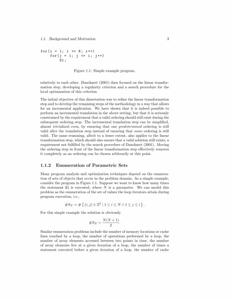
for(i = 1; i <= N; i++)
for(j = 1; j <= i; j++)
S1;
Figure 1.1: Simple example program.
relatively to each other. Danckaert (2001) then focused on the linear transfor-mation step, developing a regularity criterion and a search procedure for thelocal optimization of this criterion.
The initial objective of this dissertation was to refine the linear transformationstep and to develop the remaining steps of the methodology in a way that allowsfor an incremental application. We have shown that it is indeed possible toperform an incremental translation in the above setting, but that it is seriouslyconstrained by the requirement that a valid ordering should still exist during thesubsequent ordering step. The incremental translation step can be simplified,almost trivialized even, by ensuring that one predetermined ordering is stillvalid after the translation step instead of ensuring that some ordering is stillvalid. The same reasoning, albeit to a lesser extent, also applies to the lineartransformation step, which should also ensure that a valid solution still exists, arequirement not fulfilled by the search procedure of Danckaert (2001). Movingthe ordering step in front of the linear transformation step effectively removesit completely as an ordering can be chosen arbitrarily at this point.
1.1.2 Enumeration of Parametric Sets
Many program analysis and optimization techniques depend on the enumera-tion of sets of objects that occur in the problem domain. As a simple example,consider the program in Figure 1.1. Suppose we want to know how many timesthe statement S1 is executed, where N is a parameter. We can model thisproblem as the enumeration of the set of values the loop iterators attain duringprogram execution, i.e.,
#SN = #
(i, j) ∈ Z2 | 1 ≤ i ≤ N ∧ 1 ≤ j ≤ i
.
For this simple example the solution is obviously
#SN =N(N + 1)
2.
Similar enumeration problems include the number of memory locations or cachelines touched by a loop, the number of operations performed by a loop, thenumber of array elements accessed between two points in time, the numberof array elements live at a given iteration of a loop, the number of times astatement executed before a given iteration of a loop, the number of cache
4 Chapter 1. Introduction
misses generated by a loop or the amount of memory dynamically allocatedby a piece of code. The solution often needs to be expressed in terms of someparameters. In some optimization techniques, the need for parameters dependson the problem instance, e.g., the parameter N in the example above, while inother techniques, the counting problems are intrinsically parametric.
Similar counting problems occur in the mathematical community. Arguably themost appealing of these problems is counting the number of magic squares (see,e.g., Yoshida 2004a or Beck and Robins 2006), but applications occur in suchdiverse fields as representation theory, commutative algebra, approximationtheory and statistics.
Authors in the compiler community typically refer to Clauss and Loechner(1998) or Pugh (1994) for solving their enumeration problems. To the bestof our knowledge, the method of Pugh (1994) has never been implemented,however, and although the method of Clauss and Loechner (1998) established amajor breakthrough, it suffers from significant time-complexity and degeneracyproblems.
An efficient parametric enumeration algorithm was proposed by Barvinok andPommersheim (1999) and further extended by Barvinok and Woods (2003).The implementation of this technique by De Loera et al. (2003a) is suitablefor the enumeration problems they consider, but only covers a relatively smallsubclass of the more general parametric enumeration problems that occur incompiler optimization techniques. Furthermore, the representation of the so-lution produced by their LattE implementation (De Loera et al. 2003b) isunfamiliar and seemingly unsuitable for the compiler community.
The goal of the second major part of this dissertation is to continue the excellentwork of De Loera et al. (2004) and to explain the necessary details for a practicalimplementation of the algorithms of Barvinok and Pommersheim (1999) appliedto the general parametric enumeration problem. A subsidiary goal is to resolvesome of the conflicts in terminology that have arisen between the mathematicalcommunity and the compiler community.
1.2 Overview and Contributions
• Chapter 2: This chapter describes the geometrical model that will beused throughout this dissertation and mainly in Chapter 3. We firstdescribe the mathematical objects called polyhedra that correspond tothe solution sets of collections of linear inequalities as well as some relatedmathematical objects. We then compare some currently available toolsthat can be used to manipulate these objects and show how to model aprogram using these objects.
1.2. Overview and Contributions 5
• Chapter 3: Although many of the elements in this chapter have originallybeen developed in the context of a methodology with an additional order-ing phase, we first describe our two-step approach for incremental globalloop transformations, consisting of a linear transformation step and atranslation step, without this ordering phase. Our main contribution forthe linear transformation step is an improved regularity criterion with as-sociated search procedures and a criterion to ensure validity of the finalsolution independently of the subsequent translation step. We also adapta known locality criterion to a more general context. As to the translationstep, we show how to perform this step incrementally, allowing multiplecomplicated cost functions to be evaluated for real-life applications. Fi-nally, we show that although the incrementality of the translation stepcarries over to a context with an extra ordering phase, producing good oreven correct transformed programs is considerably more difficult in thiscontext.
Parts of this chapter have been previously published in
– A heuristic for improving the regularity of accesses by global looptransformations in the polyhedral model (Verdoolaege, Catthoor,Bruynooghe, and Janssens; 2001a),
– Feasibility of incremental translation (Verdoolaege, Catthoor, Bruy-nooghe, and Janssens; 2002),
– An access regularity criterion and regularity improvement heuristicsfor data transfer optimization by global loop transformations (Ver-doolaege, Danckaert, Catthoor, Bruynooghe, and Janssens; 2003b)and
– Multi-dimensional Incremental Loop Fusion for Data Locality (Ver-doolaege, Bruynooghe, Janssens, and Catthoor; 2003a).
• Chapter 4: We describe our implementation of the algorithm of Barvinokand Pommersheim (1999) applied to parametric polytopes with somerefinements inspired by the works of Clauss and Loechner (1998) andDe Loera et al. (2004). The usefulness of combining elements of thealgorithms of Clauss and Loechner (1998) and of Barvinok and Pommer-sheim (1999) was discovered independently by Seghir (2003), a studentof Vincent Loechner, and resulted in the joint publications mentionedbelow. The target application in these publications was contributed byKristof Beyls, who also collected the benchmarks, performed experimentsand helped writing the publications. We also show how the algorithm ofBarvinok and Pommersheim (1999) can be applied to obtain a differentrepresentation for the number of points in a parametric polytope that isa direct extension of the results of De Loera et al. (2003a). We furthershow that the two different representations are “equivalent” in the sensethat either representation can be “efficiently” converted into the other.
6 Chapter 1. Introduction
These conversion results were obtained in close collaboration with KevinWoods and can be combined with known algorithms that are tailored toproduce only one of these representations to obtain an algorithm thatalso produces the other representation. Arguably the most interestingsuch algorithm is that of Barvinok and Woods (2003) for an extendedenumeration problem. An implementation of the algorithm of Barvinokand Woods (2003) still remains a challenge, however, and we thereforealso discuss some alternatives which are theoretically not as interesting,but which work fairly well on practical problems.
Parts of this chapter have been previously published in
– Analytical computation of Ehrhart polynomials and its applicationsfor embedded systems (Verdoolaege, Beyls, Bruynooghe, Seghir, andLoechner; 2004b),
– Analytical Computation of Ehrhart Polynomials and its Applica-tion in Compile-Time Generated Cache Hints (Seghir, Verdoolaege,Beyls, and Loechner; 2004),
– Analytical computation of Ehrhart polynomials: Enabling morecompiler analyses and optimizations (Verdoolaege, Seghir, Beyls,Loechner, and Bruynooghe; 2004d),
– Experiences with enumeration of integer projections of parametricpolytopes (Verdoolaege, Beyls, Bruynooghe, and Catthoor; 2005a)and
– Computation and Manipulation of Enumerators of Integer Projec-tions of Parametric Polytopes (Verdoolaege, Woods, Bruynooghe,and Cools; 2005b).
• Chapter 5: This chapter mainly serves as an experimental validation ofthe previous chapter applied to the problem of reuse distance computa-tion. Many of the experimental results have also been published in thecorresponding publications mentioned above. Obtaining the parametricsets that need to be enumerated to compute the reuse distances posesserious challenges when using currently available tools and we thereforealso propose some alternative strategies and compare them to the morestraightforward strategy.
• Chapter 6: This chapter concludes the dissertation and points out someinteresting areas of future research.
Chapter 2
Geometrical Model
The geometrical model in its various guises is a popular model for representingand manipulating collections of loop nests. In this model, all iterations ofa statement in a piece of code are represented by a single geometrical object.These geometrical objects are typically polyhedra or related types of sets, sincesuch representations are very compact and since they can be manipulated moreefficiently than arbitrary sets. We will therefore also pay attention to currentlyavailable tools for manipulating such sets.
Section 2.1 defines polyhedra and related sets. Section 2.2 discusses somecurrently available tools that can be used to manipulate or to derive informationfrom such sets. Sections 2.3 and 2.4 explain how to represent iteration domainsand dependences in the geometrical model.
2.1 Definitions
2.1.1 Polyhedrons
Definition 2.1.1 (Rational polyhedron) A rational polyhedron P is a sub-space of Qd bounded by a finite number of hyperplanes.
P =x ∈ Qd | Ax ≥ c
, (2.1)
with A ∈ Zm×d and c ∈ Zm.
Since all the polyhedra in this text will be rational, we will usually omit thisqualification.
7
8 Chapter 2. Geometrical Model
The system Ax ≥ c can imply some equalities, known as the implicit equalities.We can then write
P =x ∈ Qd | Gx = g ∧ Fx ≥ f
, (2.2)
with Gx = g a maximal set of linearly independent equalities and Fx ≥ f theremaining inequalities.
Theorem 2.1.2 The set P ⊂ Qd is a rational polyhedron iff it can be writtenas
P =
∑
i
λipi +∑
i
µiri ∈ Qd | pi ∈ S, ri ∈ R, λi, µi ≥ 0,∑
i
λi = 1
with S and R finite subsets of Qd and 0 6∈ R.
Theorem 2.1.2 is a simple consequence of well known theorems by Minkowskiand Weyl (Schrijver 1986). The notation in Definition 2.1.1 is sometimes re-ferred to as the implicit representation, whereas the one in Theorem 2.1.2 isreferred to as the explicit representation. These representations are also knownas the external representation and the internal representation respectively. Wewill call the elements of the sets S and R in the explicit representation thesupporting points and rays respectively.
Definition 2.1.3 (Affine hull) The affine hull of a set X ⊂ Qd is the set
aff X =
∑
i
λixi | xi ∈ X,∑
i
λi = 1
. (2.3)
Definition 2.1.4 The dimension of a rational polyhedron P ⊂ Qd is the di-mension of its affine hull. Equivalently, it is equal to the dimension d of theambient space Qd minus the number of linearly independent (implicit) equalitiesin the system Ax ≥ c.
Definition 2.1.5 A face F of a rational polyhedron P (2.1) is the intersectionof P with x ∈ Qd | A′x = c′ , where A′x ≥ c′ is a subsystem of Ax ≥ c. IfP has dimension n, then the (n − 1)-dimensional faces are called facets. The0-dimensional faces are called vertices.
By convention, the empty set ∅ is a (−1)-dimensional face of every polyhedron.Note that every vertex v of P is an extremal point of P , i.e., v is a point thatcannot be expressed as a convex combination of other points in P .
2.1. Definitions 9
Definition 2.1.6 (Rational polytope) A rational polytope is a bounded ra-tional polyhedron.
Note that for a polytope, the set R in Theorem 2.1.2 is empty.
Example 1 The interval [0, 1] is a rational polytope:
[0, 1] = i | i ≥ 0 ∧ i ≤ 1 = λ00 + λ11 | λ0, λ1 ≥ 0, λ0 + λ1 = 1 .
The bounding hyperplanes are the points 0 and 1.
Definition 2.1.7 (Convex hull) The convex hull of a set X is the set of allconvex combinations of elements of X:
conv X =
∑
i
λixi | xi ∈ X,λi ∈ Q≥0,∑
i
λi = 1
. (2.4)
A polytope can also be defined as the convex hull of a set of generators.
Definition 2.1.8 (Positive hull) The positive hull of a set X is the set ofall positive combinations of elements from X:
pos X =
∑
i
λixi | xi ∈ X,λi ∈ Q≥0
. (2.5)
Definition 2.1.9 (Polyhedral cone) A polyhedral cone, or simply cone, isthe positive hull of a set of elements, called its generators.
Note that according to this definition, all faces of a cone contain the origin.In particular, if the cone has a vertex, then this vertex will be the origin. Atranslate of a cone is sometimes also referred to as simply a “cone”, but wewill use the term shifted cone instead. The vertex of such a shifted cone, if itexists, is also known as its apex.
Definition 2.1.10 (Sum) The sum of two polyhedra P1 and P2 is defined asthe set of all sums of an element from P1 and an element from P2,
P1 + P2 = x + y | x ∈ P1 ∧ y ∈ P2 .
10 Chapter 2. Geometrical Model
Theorem 2.1.2 states that a polyhedron is the sum of a polytope and a cone.
Definition 2.1.11 (Ray) A ray of a set K is a vector r 6= 0 such that x ∈ Kimplies (x + µr) ∈ K for all µ ∈ Q≥0.
Definition 2.1.12 (Line) A line of a set K is a vector ℓ 6= 0 such that x ∈ Kimplies (x + µℓ) ∈ K for all µ ∈ Q.
Definition 2.1.13 (Polyhedral hull) Let P1 and P2 be two polyhedra. IfP1 = P ′1 + C1 and P2 = P ′2 + C2 with P ′1 and P ′2 polytopes and C1 and C2
cones, then the polyhedral hull of P1 and P2 is P3 = P ′3 + C3, with P ′3 thepolytope generated by the union of the generators of P ′1 and P ′2 and C3 the conegenerated by the union of the generators of C1 and C2. I.e.,
P3 = conv(P ′1 ∪ P ′2) + pos(C1 ∪ C2).
2.1.2 Integer Sets
We will typically only be interested in the integer points inside a polytope.Since we will also be interested in more general sets of integer points we willneed the following definitions.
Definition 2.1.14 (Point lattice) A point lattice L is defined as a set ofregularly spaced points in Zd, i.e.,
L =
d∑
i=1
aivi | ai ∈ Z ∧ vi ∈ V
,
where V ⊂ Zd is a set of d linearly independent vectors.
Note that a point lattice is usually defined as a subset of Rd rather than Zd.
Definition 2.1.15 (Linearly bounded lattice) A linearly bounded latticeis the intersection of a polyhedron and a point lattice.
Definition 2.1.16 (Projected set) A projected set S is a set of the form
S =
x ∈ Zd | ∃y ∈ Zd′ : Ax + By ≥ c
,
for some A ∈ Zm×d, B ∈ Zm×d′ and c ∈ Zm.
2.1. Definitions 11
Note that a Linearly Bounded Lattice (LBL) is a special case of a projected setand that a projected set is equivalent to the projection onto the first dimensionsof the integer points in a polyhedron, whence the name. That is, the set S inthe above definition can be written as
S = πd(Zd+d′ ∩ P ),
with
P =
(x,y) ∈ Qd+d′ | Ax + By ≥ c
and πd the projection onto the first d dimensions. We call P the polyhedrondefining S. Projected sets have also been called integer projections of polyhedra(Pugh 1994).
Definition 2.1.17 (Presburger set) A Presburger set is a set that can bedescribed by a Presburger formula, which is a formula that consists of linearinequalities of integer variables, combined by existential and universal quanti-fiers, disjunction, conjunction and negation (∃,∀,∨,∧,¬).
Each Presburger set can be written as a union of projected sets, but the con-version can in general be very expensive, which is why we make the distinction.The Omega library (see Section 2.2.2) can be used to perform this conversion.Also note that Presburger arithmetic was originally defined on positive inte-gers (Presburger 1929), but most authors extend this to also include negativeintegers.
2.1.3 Relations
Relations are basically sets of pairs of elements. Using the natural isomorphismSd × Sd′ ∼= Sd+d′ , we can identify sets of pairs of integer or rational vectorswith sets of integer or rational vectors and we can use the same notions fromthe previous sections to represent relations. In the remainder of this text wewill in fact often not make a distinction between Sd × Sd′ and Sd+d′ and wewill assume that it is clear from the context which of the two is meant. We willsometime write x R y to mean (x, y) ∈ R.
In particular, a function f : S → R is a relation f ⊂ S×R such that if (a, b) ∈ fand (a, c) ∈ f then b = c and we will see occasion to write functions as sets.Applying a function f : Rd → Rd′ to a set S ⊂ Rd yields a set S′ = f(S) ⊂ Rd′ .If f and S are represented by the projected sets
f =
(x,y) ∈ Zd × Zd′ | ∃z ∈ Zd′′ : A1x + A2y + Bz ≥ c
S =
x ∈ Zd | ∃z ∈ Zd′′′ : A′x + B′z ≥ c′
12 Chapter 2. Geometrical Model
then, with a slight abuse of notation, we define the function f on subsets ofZd:
f : 2Zd
→ 2Zd′
S 7→ f(S) = S′
with
S′ = f(S) =
y ∈ Zd′ | ∃(x, z, z′) ∈ Zd × Zd′′ × Zd′′′ :
A1x + A2y + Bz ≥ c ∧ A′x + B′z′ ≥ c′
.
Note that the above construction of the function f : 2Zd
→ 2Zd′
equally appliesto the case where f ⊂ S ×R is not a function but rather a general relation. Itcan also be extended to the case where S itself is a relation S ⊂ Rd′′ × Rd. Inthe latter case, S′ is a relation S′ ⊂ Rd′′ × Rd′ .
Of particular interest will be the affine functions. These are functions of theform f(x) = Hx + h, or, written as a set,
f =
(x,y) ∈ Zd × Zd′ | y = Hx + h
.
A piecewise affine function f : Zd → Zd′ is such that f is equal to an affinefunction on each element of a partition of the domain Zd.
2.1.4 Parametric Sets and Relations
In some of our sets, some of the variables, called the parameters, will be treateddifferently from the other variables. These parameters are used to create para-metric sets, which represent collections of sets parametrized by the param-
eters. Such a parametric set can be modeled as a function f : Zn → 2Zd
from the parameter space to the set of polyhedra or projected sets or alterna-tively as a relation between the parameters and the elements of these sets, i.e.,S ⊂ Zn ×Zd. Using the latter representation we can use the construction fromSection 2.1.3 to “apply” this relation to the singleton p0 ⊂ Zn to obtaina set S(p0 ) = S(p0) = Sp0
⊂ Zd. I.e., Sp =x ∈ Zd | (p,x) ∈ S
⊂ Zd.
In particular, a parametric polytope is modeled by a polyhedron P ∈ Qn × Qd
such that for all p ∈ Qn, the set Pp is a polytope.
Relations may also be parametrized and represented by a subset of Zn×Zd×Zd′ .Application of such a parametric relation f ⊂ Zn × Zd × Zd′ to a parametricset S ⊂ Zn × Zd, which we simply write as S′ = f(S), yields a parametric setS′ ⊂ Zn × Zd′ such that S′(p) = f(p)(S(p)) for all p ∈ πnf ∩ πnS. That is iff and S are represented by the projected sets
f =
(p,x,y) ∈ Zn × Zd × Zd′ | ∃z ∈ Zd′′ : A1x + A2y + Bz + Dp ≥ c
S =
(p,x) ∈ Zn × Zd | ∃z ∈ Zd′′′ : A′x + B′z + D′p ≥ c′
2.2. Polyhedral Tools 13
then
S′ = f(S) =
(p,y) ∈ Zn × Zd′ | ∃(x, z, z′) ∈ Zd × Zd′′ × Zd′′′ :
A1x + A2y + Bz + Dp ≥ c ∧
A′x + B′z′ + D′p ≥ c′
.
2.1.5 Order
We will often need to be able to order the elements of a given polyhedron orprojected set. We will typically use the lexicographical order defined as follows.
Definition 2.1.18 (Lexicographical order) Given two d-dimensional vec-tors x and y, then x is said to be lexicographically smaller than y, denotedx ≺ y, iff there exists some k, 1 ≤ k ≤ d such that xi = yi for i < k andxk < yk.
Note that this lexicographical order can be expressed using linear constraints.
The lexicographically minimal element of a set S will be called the lexicograph-ical minimum and will be denoted by lexminS. If Sp is a parametric set, thenlexmin Sp will depend on the parameters. Furthermore, if S ⊂ Zn ×Zd definesa parametric set Sp, then we may also write
lexmin S := (p, lexmin Sp) | p ∈ πn(S) , (2.6)
i.e., lexmin S consists of the parameter values for which Sp is non-empty, pairedoff with the lexicographical minimum of this instantiation Sp.
2.2 Polyhedral Tools
Many tools exist for converting the implicit representation of a polyhedron toits explicit representation and back. Examples include cdd (Fukuda 1993),PORTA (Christof and Lobel 1997), qhull (Barber et al. 1996) and lrs (Avis2000). Consult Fukuda (2004) for a more complete overview. Some librariessuch as PolyLib (Wilde 1993), polka (Jeannet 2002) and PPL (Bagnara et al.2002) also include support for performing other operations on these polyhedra,e.g., intersections and affine transformations. Probably the most comprehensivelibrary is polymake (Gawrilow and Joswig 2001), which offers access to a widevariety of algorithms and packages within a common framework.
We first discuss the PolyLib library in Section 2.2.1, then a library for ma-nipulating Presburger formulas called Omega in Section 2.2.2 and a library for
14 Chapter 2. Geometrical Model
computing the parametric lexicographical minimum called PIP in Section 2.2.3.An integration of these three tools exists in SPPoC (Boulet and Redon 1999).Finally, we discuss an interesting alternative for representing Presburger for-mulas in Section 2.2.4.
2.2.1 PolyLib
PolyLib (Wilde 1993) is a C-library for manipulating what the author callspolyhedral domains, which represent the integer points in unions of rationalpolyhedra. The library has been extended to support both parametric polyhe-dra (Loechner 1999) and LBLs (Nookala and Risset 2000), but these extensionsare built on top of the core library rather than being fully integrated, leavingthe responsibility to the user of connecting the various pieces and choosingthe appropriate representations for different data. The core library also pro-vides separate functions for manipulating (the integer points in) polyhedra andunions of polyhedra, but not all functions are consistently available for bothcases. The DomainSimplify function is underspecified in the manual and thecurrent implementation yields unintuitive results in the presence of equalities.
Most operations treat polyhedral domains simply as unions of rational poly-hedra without performing any simplifications exploiting the fact that only theinteger points in these sets are of interest. The most prominent exception isDomainDifference, which computes a union of rational polyhedra such thatthe set of integer points it contains is the set difference of the integer pointsin its arguments. Note that the library would not be able to represent the setdifference of two (unions of) polyhedra in general since this requires supportfor strict inequalities, which PolyLib lacks. Support for strict inequalities isincluded in polka and PPL, but these libraries do not have a set differenceoperations.
Arguably PolyLib’s biggest problem is that it insists on maintaining both theimplicit and the explicit representation of each polyhedron. Other libraries,such as polka and PPL, convert representations lazily, i.e., only when this isneeded to perform a particular operation.
2.2.2 Omega
The Omega library (Kelly et al. 1996c) is a general library for manipulatingPresburger sets rather than just polyhedra, which makes it quite different fromother “polyhedral tools”. It also means that the library does not contain ex-plicit support for computing the vertices of a polyhedron.
Although Presburger arithmetic is decidable (Presburger 1929), the boundson storage and time required are superexponential (Fischer and Rabin 1974;Weispfenning 1997). The Omega library therefore employs some heuristics,
2.2. Polyhedral Tools 15
which appear to work reasonably well for dependence analysis (Pugh and Won-nacott 1994). As we report in Section 5.2.1, however, Omega can break downfor more difficult problems, sometimes simply aborting the computation. Nev-ertheless, as long as the computation does not abort, the result is usuallycorrect. Also note that it would not help to use PolyLib for these more diffi-cult problems since PolyLib simply does not support the necessary operationsor because it is too slow.
The internal representation that Omega uses to represent Presburger sets ba-sically corresponds to a union of what we called projected sets. In contrastto PolyLib, Omega performs simplifications on the equations defining the pro-jected sets exploiting the fact that only the integer points are of interest. Adrawback of these “simplifications” is that the result may be more difficult toprocess by subsequent algorithms that take the simplified formulas as input.In particular, we have seen that our counting algorithm described in Chapter 4can sometimes have more difficulty with the simplified formula than with theoriginal formula. The simplifications may also result in existential variablesassuming negative values, where the existential variables in the original for-mula were known to assume only positive values. This can be a problem fortechniques that adhere to the strict definition of Presburger formulas such asthe enumeration technique of Parker and Chatterjee (2004).
In general, Omega is significantly faster than PolyLib when performing compa-rable operations. The close integration around a single data type also makesit much easier to use than PolyLib. Despite its problems, we would thereforeadvise the use of Omega over PolyLib unless knowledge of the vertices of apolyhedron is needed, as may be the case when enumerating the integer pointsin a polytope (see Chapter 4).
We note that Omega can also be used to compute the (lexicographical) min-imum of a (parametric) set. Consider, for example, a set R ⊂ Z1 × Z1. Itslexicographical minimum S := lexmin R can be computed as
S = (p, y) ∈ R | ∀x : ((p, x) ∈ R ∧ x ≤ y) ⇒ x = y .
Although it is possible to use Omega to compute lexicographical minima, thepreferred way of computing these minima is to use PIP, a library specificallydesigned to perform this operation. We will briefly discuss this library in thefollowing section.
2.2.3 PIP
Parametric Integer Programming (PIP) is a technique developed by Feautrier(1988) for computing the lexicographical minimum of the integer points in aparametric polytope and has been implemented in the PIP library (Feautrieret al. 2002). It is based on a parametric version of the cutting plane algorithm
16 Chapter 2. Geometrical Model
of Gomory (1963). The algorithm assumes that all parameters assume onlypositive values. This is usually not a problem per se, but it does require thatthe user ensures this property holds. Although the algorithm is worst-caseexponential, it is usually very fast on problems that occur in practice. InChapter 5 we will see that PIP can sometimes successfully be applied to solveproblems that cannot be solved by Omega.
2.2.4 LASH
The LASH tool (Boigelot 1999) manipulates Presburger formulas representedas finite state machines. In particular, each Presburger formula as a NumberDecision Diagram (NDD) (Boigelot 1999; Wolper and Boigelot 1995). Althoughwe have no practical experience with this tool, we mention it here because of theinteresting feature that in contrast to the corresponding Presburger formula(s),such an NDD is canonical after determinization and minimization.
The basic idea is to represent each integer by its digits according to some base rand have the finite state machine accept the sequence of digits of integers thatbelong to the Presburger set. Since the maximal number of digits is typicallynot known a priori, this means that the machine should also accept sequencesof digits formed by adding zeros at the beginning or end of the sequence,depending on whether the machine accepts the most or least significant digitfirst. It has been known for a long time (Cobham 1969; Semenov 1977) thatthe sets that can be represented by such finite-state automata for every base rare exactly those that are definable in Presburger arithmetic.
Recently, Latour (2004) has also investigated the extraction of an explicit rep-resentation from an NDD, assuming that it encodes a polyhedron.
2.3 Iteration Domains
Given a statement inside a loop nest, we use polyhedra (or more general sets) torepresent all iterations of the enclosing loops. In particular, iterators of the en-closing loops form what is known as an iteration vector. The set of all iterationvectors is known as the iteration domain and can be described as the integerpoints in a polyhedron, if the loop bounds are affine expressions of the outerloop iterators and the parameters. These bounds correspond to the boundinghyperplanes of the polyhedron. We assume here that the iterators of all loopsincrease by one in each iteration of the loop. Any loop nest with constantstrides can be reduced to this form using a purely syntactical transformation.
Consider the example in Figure 2.1 taken from Danckaert (2001, Section 4.4.4).The set of all iterations of the loops enclosing the first statement is given by
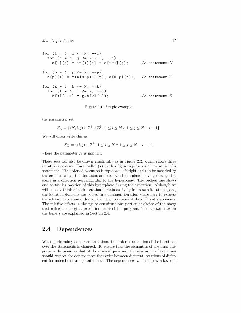
2.4. Dependences 17
for (i = 1; i <= N; ++i)
for (j = 1; j <= N-i+1; ++j)
a[i][j] = in[i][j] + a[i-1][j]; // statement X
for (p = 1; p <= N; ++p)
b[p][1] = f(a[N-p+1][p], a[N-p][p]); // statement Y
for (k = 1; k <= N; ++k)
for (l = 1; l <= k; ++l)
b[k][l+1] = g(b[k][l]); // statement Z
Figure 2.1: Simple example.
the parametric set
SX =(N, i, j) ∈ Z1 × Z2 | 1 ≤ i ≤ N ∧ 1 ≤ j ≤ N − i + 1
.
We will often write this as
SX =(i, j) ∈ Z2 | 1 ≤ i ≤ N ∧ 1 ≤ j ≤ N − i + 1
,
where the parameter N is implicit.
These sets can also be drawn graphically as in Figure 2.2, which shows threeiteration domains. Each bullet (•) in this figure represents an iteration of astatement. The order of execution is top-down left-right and can be modeled bythe order in which the iterations are met by a hyperplane moving through thespace in a direction perpendicular to the hyperplane. The broken line showsone particular position of this hyperplane during the execution. Although wewill usually think of each iteration domain as living in its own iteration space,the iteration domains are placed in a common iteration space here to expressthe relative execution order between the iterations of the different statements.The relative offsets in the figure constitute one particular choice of the manythat reflect the original execution order of the program. The arrows betweenthe bullets are explained in Section 2.4.
2.4 Dependences
When performing loop transformations, the order of execution of the iterationsover the statements is changed. To ensure that the semantics of the final pro-gram is the same as that of the original program, the new order of executionshould respect the dependences that exist between different iterations of differ-ent (or indeed the same) statements. The dependences will also play a key role
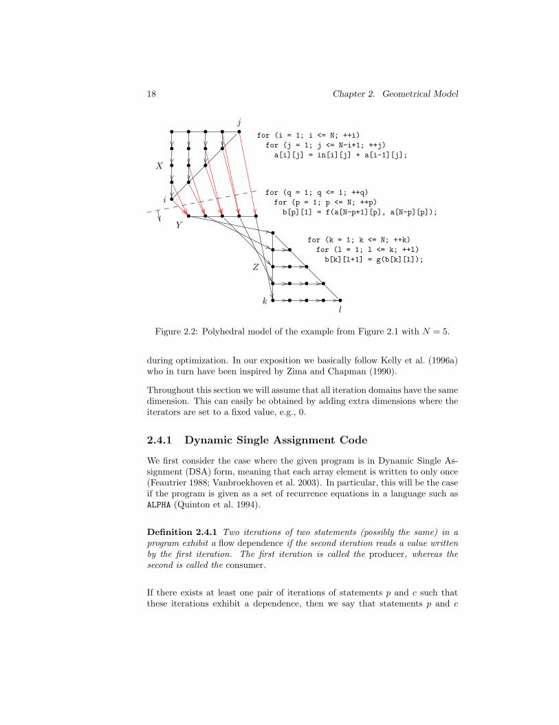
18 Chapter 2. Geometrical Model
• • • • •
• • • •
• • •
• •
•
• • • • •
•
• •
• • •
• • • •
• • • • •
for (i = 1; i <= N; ++i)
for (j = 1; j <= N-i+1; ++j)
a[i][j] = in[i][j] + a[i-1][j];
for (q = 1; q <= 1; ++q)
for (p = 1; p <= N; ++p)
b[p][1] = f(a[N-p+1][p], a[N-p][p]);
for (k = 1; k <= N; ++k)
for (l = 1; l <= k; ++l)
b[k][l+1] = g(b[k][l]);
j
i
lk
X
Y
Z
Figure 2.2: Polyhedral model of the example from Figure 2.1 with N = 5.
during optimization. In our exposition we basically follow Kelly et al. (1996a)who in turn have been inspired by Zima and Chapman (1990).
Throughout this section we will assume that all iteration domains have the samedimension. This can easily be obtained by adding extra dimensions where theiterators are set to a fixed value, e.g., 0.
2.4.1 Dynamic Single Assignment Code
We first consider the case where the given program is in Dynamic Single As-signment (DSA) form, meaning that each array element is written to only once(Feautrier 1988; Vanbroekhoven et al. 2003). In particular, this will be the caseif the program is given as a set of recurrence equations in a language such asALPHA (Quinton et al. 1994).
Definition 2.4.1 Two iterations of two statements (possibly the same) in aprogram exhibit a flow dependence if the second iteration reads a value writtenby the first iteration. The first iteration is called the producer, whereas thesecond is called the consumer.
If there exists at least one pair of iterations of statements p and c such thatthese iterations exhibit a dependence, then we say that statements p and c
2.4. Dependences 19
exhibit a dependence. Flow dependences are also known as true dependences.If a statement depends on in itself, we talk about a self dependence. Otherwisewe talk about a group dependence.
Definition 2.4.2 The (flow) dependence relation δp,c over two statements pand c is the set of all pairs of iterations that exhibit a (flow) dependence.
Definition 2.4.3 An access function is a function that maps the values of theiterators (and the parameters) to an index of an array.
We will usually assume that the access functions are affine functions, althoughin many cases it is sufficient if each access function can be described usinglinear constraints. If this is not the case, approximations may (have to) beused (Geigl 1997).
Example 2 Consider the access a[i-1][j] in the first statement of theprogram in Figure 2.1 on page 17. The a-array is a 2-dimensional array,which can be represented as the integer points in a polytope of a 2-dimensional space. In particular, this polytope is a rectangle. The valueof the first coordinate of the array element accessed in iteration (i, j) is
i − 1 =[1 0
][ij
]
− 1,
whereas the second coordinate is
j =[0 1
][ij
]
.
The complete (affine) access function is therefore
[1 00 1
] [ij
]
+
[−10
]
=
[i − 1
j
]
.
Let SX and SY be the iteration domains of statements X and Y respectively.Further assume that X writes to some array A through access function WX
and that Y reads from the same array A through access functions RY,k, wherek ranges over the possibly multiple read accesses to array A from statementY . For simplicity of notation, we will assume that the access functions WX
and RY,k also encode the arrays that are being accessed, either by having thefunction value be a pair of array and index vector or by considering an indexvector to a single global memory space. Then the flow dependence relation is
δX,Y =⋃
k
(i, j) ∈ SX × SY | WX(i) = RY,k(j) . (2.7)
20 Chapter 2. Geometrical Model
If some access function RY,k is such that multiple iterations of SY are pairedwith the same iteration of SX in the dependence relation δX,Y , then we willsay that the dependence exhibits self reuse. In particular, this means thatthe function RY,k is not invertible. As we will see later in this section, thisalso means that there is an input dependence between statement Y and itself.Note that any dependence between a statement and itself based on the samereference in the statement is also commonly known as a self reuse. Any otherdependence is known as a group reuse.
Note that by definition of the code being in DSA, each array element is writtento by at most one iteration of a statement. The access function WX is thereforeinvertible and we can write (2.7) as
δX,Y =⋃
k
(i, j) | j ∈ SY ∩ (W−1
X RY,k)−1(SX) ∧ i = W−1X RY,k(j)
, (2.8)
where (W−1X RY,k)−1(SX) is the preimage of SX under W−1
X RY,k and W−1X is
the inverse of WX . We call DDkX,Y := SY ∩ (W−1
X RY,k)−1(SX) the dependence
domain and DFkX,Y := W−1
X RY,k the dependence function. I.e.,
δX,Y =⋃
k
(i, j) | j ∈ DDkX,Y ∧ i = DFk
X,Y (j)
. (2.9)
If WX and RY,k are affine functions, then so is DFkX,Y . If furthermore SX and
SY are polytopes, then so is DDkX,Y .
Example 3 Consider once more the program in Figure 2.1 on page 17.The first statement writes to array a through access function
WX =
(N, i, j, a, b) ∈ Z1 × Z
2 × Z2 |[ab
]
=
[1 00 1
] [ij
]
+
[00
]
=
(N, i, j, i, j) ∈ Z1 × Z
2 × Z2
or simply
WX =(i, j, i, j) ∈ Z
2 × Z2 .
Since the iteration domain of the second statement is one-dimensional,we add an extra dimension in front, i.e., the iterations domain is givenby
SY =
(1, p) ∈ Z2 | 1 ≤ p ≤ N
.
The access functions of the second statement are then
RY,1 =(i, j, N − j + 1, j) ∈ Z
2 × Z2
RY,2 =(i, j, N − j, j) ∈ Z
2 × Z2 .
2.4. Dependences 21
The dependence relation δX,Y is therefore given by
δX,Y = (i, j, 1, p) | 1 ≤ i ≤ N ∧ 1 ≤ j ≤ N − i + 1 ∧1 ≤ p ≤ N ∧ N − p + 1 = i ∧ p = j ∪
(i, j, 1, p) | 1 ≤ i ≤ N ∧ 1 ≤ j ≤ N − i + 1 ∧1 ≤ p ≤ N ∧ N − p = i ∧ p = j
= (i, j, 1, p) | 1 ≤ p ≤ N ∧ N − p + 1 = i ∧ p = j ∪ (i, j, 1, p) | 1 ≤ p ≤ N − 1 ∧ N − p = i ∧ p = j .
This relation is depicted using arrows in Figure 2.2. The other depen-dence relations are depicted similarly. Note that the iteration domainsin Figure 2.2 have been placed in a common iteration space in a way thatreflects the original execution order of the program. The coordinates inthe dependence relation above do not however refer to the coordinatesof this common iteration space. Rather, the coordinates refer to the twodistinct iteration spaces that contain the two iteration domains. For thefirst part of the dependence above, the dependence domain is
DD1X,Y = (1, p) | 1 ≤ p ≤ N
and the dependence function is
DF1X,Y : DD
1X,Y → Q2
(q, p) 7→ (N − p + 1, p).
Note that statements X and Z depend on themselves.
During loop fusion (see Section 3.3) we will not need all the information avail-able in the dependence relation. It will be sufficient to consider the “distance”between two interdependent iterations, measured by the distance vector (Kucket al. 1972; Muraoka 1971).
Definition 2.4.4 Let i ∈ SX and j ∈ SY be such that i δX,Y j, then the differ-ence d between i and j, i.e.,
d = j − i (2.10)
is called the dependence distance vector or distance vector for short.
Note that a distance vector is simply a point in a vector space. In a figureshowing dependences between iterations, we typically draw an arrow from theproducer to the consumer to indicate the dependence. When drawing theactual distance vectors in their vector space, we usually draw the same arrow,but translated to the origin. The end point of this arrow is then the distancevector.
Example 4 Consider the self dependence of statement X in Figure 2.2,reproduced in Figure 2.3 on the left. All distance vectors generated bythis dependence are the same. This single distance vector is shown in itsvector space on the right of Figure 2.3.
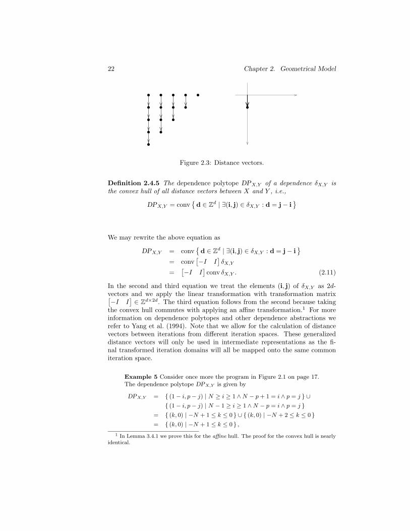
22 Chapter 2. Geometrical Model
• • • • •
• • • •
• • •
• •
•
•
Figure 2.3: Distance vectors.
Definition 2.4.5 The dependence polytope DPX,Y of a dependence δX,Y isthe convex hull of all distance vectors between X and Y , i.e.,
DPX,Y = convd ∈ Zd | ∃(i, j) ∈ δX,Y : d = j − i
We may rewrite the above equation as
DPX,Y = convd ∈ Zd | ∃(i, j) ∈ δX,Y : d = j − i
= conv[−I I
]δX,Y
=[−I I
]conv δX,Y . (2.11)
In the second and third equation we treat the elements (i, j) of δX,Y as 2d-vectors and we apply the linear transformation with transformation matrix[−I I
]∈ Zd×2d. The third equation follows from the second because taking
the convex hull commutes with applying an affine transformation.1 For moreinformation on dependence polytopes and other dependence abstractions werefer to Yang et al. (1994). Note that we allow for the calculation of distancevectors between iterations from different iteration spaces. These generalizeddistance vectors will only be used in intermediate representations as the fi-nal transformed iteration domains will all be mapped onto the same commoniteration space.
Example 5 Consider once more the program in Figure 2.1 on page 17.The dependence polytope DPX,Y is given by
DPX,Y = (1 − i, p − j) | N ≥ i ≥ 1 ∧ N − p + 1 = i ∧ p = j ∪ (1 − i, p − j) | N − 1 ≥ i ≥ 1 ∧ N − p = i ∧ p = j
= (k, 0) | −N + 1 ≤ k ≤ 0 ∪ (k, 0) | −N + 2 ≤ k ≤ 0 = (k, 0) | −N + 1 ≤ k ≤ 0 ,
1 In Lemma 3.4.1 we prove this for the affine hull. The proof for the convex hull is nearlyidentical.
2.4. Dependences 23
where we have taken the difference between vectors from SX and SY eventhough they may live in different iteration spaces.
Using these concepts, a program can be represented by a dependence graph,which contains all the required information about dependences to perform theset of program transformations that we consider in this text.
Definition 2.4.6 (Dependence Graph) A dependence graph is a tuple G =〈V,E,P,∆〉 consisting of the following elements:
• V is the set of nodes, each representing a set of statements in the originalprogram.
• Each node p is adorned by a set Pp of polytopes, each representing aniteration domain. P is the set of all such Pp.
• E is the (multi-)set of edges. An edge is a pair of nodes (p1, p2). Eachedge indicates the presence of a dependence between one of the iterationdomains associated with p1 and one of the iteration domains associatedwith p2.
• Each edge e ∈ E, e = (p1, p2) is adorned by a dependence δe or someabstraction of a dependence such as a dependence relation or a dependencepolytope. ∆ is the set of all such δe.
Example 6 Consider once more the program in Figure 2.1 on page 17.The set of nodes is V = X, Y, Z ; the set of edges is
E = (X, X), (X, Y ), (Y, Z), (Z, Z) .
The iteration domains are (see Section 2.3 and Example 3)
SX =
(i, j) ∈ Z2 | 1 ≤ i ≤ N ∧ 1 ≤ j ≤ N − i + 1
SY =
(1, p) ∈ Z2 | 1 ≤ p ≤ N
SZ =
(k, l) ∈ Z2 | 1 ≤ k ≤ N ∧ 1 ≤ l ≤ k
.
The dependences are computed as in Example 3 and we obtain
δX,X = (i, j, i′, j′) | 1 ≤ i ≤ N − 1 ∧ 1 ≤ j ≤ N − i + 1 ∧i′ = i + 1 ∧ j′ = j
δX,Y = (i, j, 1, p) | 1 ≤ p ≤ N ∧ N − p + 1 = i ∧ p = j ∪ (i, j, 1, p) | 1 ≤ p ≤ N − 1 ∧ N − p = i ∧ p = j (2.12)
δY,Z = (1, p, k, l) | 1 ≤ p ≤ N ∧ k = p ∧ l = 1 (2.13)
δZ,Z = (k, l, k′, l′) | 1 ≤ k ≤ N ∧ 1 ≤ l ≤ k − 1 ∧k′ = k ∧ l′ = l + 1 .
24 Chapter 2. Geometrical Model
Note that we allow a single node in the graph to represent several statements.This can be useful to group statements that should be transformed uniformly.We will also use this property during incremental loop fusion where we willsuccessively reduce the dependence graph until we obtain a graph with a singlenode. Also note that we allow multiple edges between pairs of nodes. This canbe useful if we want to treat dependences resulting from different accesses in thesame statement differently. We may also consider other kinds of dependences,such as input dependences.
Definition 2.4.7 Two iterations of two statements (possibly the same) in aprogram exhibit an input dependence if both iterations read from the samearray element.
Note that the input dependence relation is “reflexive” is the sense that for anytwo statements X and Y δX,Y = δ−1
Y,X . Input dependences will have no impacton the validity of a program transformation, but may have an impact on itsoptimality.
The simplified dependence analysis outlined in this section has been imple-mented in a prototype tool called sda.pl.
2.4.2 Multiple Assignment Code
In general, computing the dependence relations is slightly more complicatedthan in the simple case of DSA since an array element read by a given itera-tion of a given statement may be written to from several iterations of severalstatements. To find out which of those write accesses wrote the value read bythe given read access, we need to consider the order in which the statementsare executed. In particular, the value written by the last write operation to beexecuted before the read operation will be the value read by that read opera-tion.
The order of the iterations of a given statement is simply determined by thelexicographical order of the iteration vectors. To compare iterations of differentstatements, we need to place the iteration domains in a common iteration space.A simple way to accomplish this combination is to consider statement-level di-mensions, indicating the order of the statements in the program. If a programcontains d-dimensional loop nests, we add d + 1 statement-level dimensions.The first statement-level dimension is added in the first position and indicatesthe order of the statements in the function body. The second statement-leveldimension is added between the first and the second loop dimensions and indi-cates the order of the statements in the body of the outer loop. Statement-leveldimensions have also been used by, e.g., Feautrier (1992b), Kelly (1996) andBastoul et al. (2003).
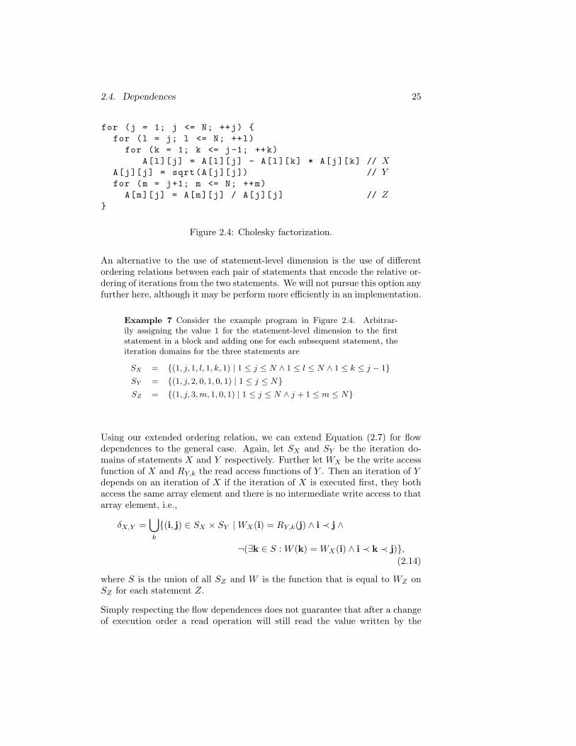
2.4. Dependences 25
for (j = 1; j <= N; ++j)
for (l = j; l <= N; ++l)
for (k = 1; k <= j-1; ++k)
A[l][j] = A[l][j] - A[l][k] * A[j][k] // XA[j][j] = sqrt(A[j][j]) // Yfor (m = j+1; m <= N; ++m)
A[m][j] = A[m][j] / A[j][j] // Z
Figure 2.4: Cholesky factorization.
An alternative to the use of statement-level dimension is the use of differentordering relations between each pair of statements that encode the relative or-dering of iterations from the two statements. We will not pursue this option anyfurther here, although it may be perform more efficiently in an implementation.
Example 7 Consider the example program in Figure 2.4. Arbitrar-ily assigning the value 1 for the statement-level dimension to the firststatement in a block and adding one for each subsequent statement, theiteration domains for the three statements are
SX = (1, j, 1, l, 1, k, 1) | 1 ≤ j ≤ N ∧ 1 ≤ l ≤ N ∧ 1 ≤ k ≤ j − 1SY = (1, j, 2, 0, 1, 0, 1) | 1 ≤ j ≤ NSZ = (1, j, 3, m, 1, 0, 1) | 1 ≤ j ≤ N ∧ j + 1 ≤ m ≤ N
Using our extended ordering relation, we can extend Equation (2.7) for flowdependences to the general case. Again, let SX and SY be the iteration do-mains of statements X and Y respectively. Further let WX be the write accessfunction of X and RY,k the read access functions of Y . Then an iteration of Ydepends on an iteration of X if the iteration of X is executed first, they bothaccess the same array element and there is no intermediate write access to thatarray element, i.e.,
δX,Y =⋃
k
(i, j) ∈ SX × SY | WX(i) = RY,k(j) ∧ i ≺ j ∧
¬(∃k ∈ S : W (k) = WX(i) ∧ i ≺ k ≺ j),
(2.14)
where S is the union of all SZ and W is the function that is equal to WZ onSZ for each statement Z.
Simply respecting the flow dependences does not guarantee that after a changeof execution order a read operation will still read the value written by the
26 Chapter 2. Geometrical Model
same write operation as in the original program. It may occur that some otherwrite operation is executed in between. We will therefore also need to consideranti-dependences δA
X,Y , which are formal dependences of write operations onpreceding read operations. Note that an anti-dependence is only used to enforcean ordering constraint. It is therefore not necessary to find the latest readoperation that precedes a given write operation. A write operation can simplybe said to depend on all preceding read operations, i.e.,
δAX,Y =
⋃
k
(i, j) ∈ SX × SY | WY (j) = RX,k(i) ∧ i ≺ j.
Note that in practice it may be useful to reduce the size of the anti-dependencesby only considering some subset of preceding read operations that is known toinclude the last read operation.
If the final state of the arrays is important, then we may also have to consideroutput dependences, which encode ordering information on pairs of write oper-ations and are defined in a very similar way to anti-dependences. Note that(explicit) output dependences are only needed for array elements that are notread in the piece of the program under consideration. If they are read, then theoutput dependence will be implicitly enforced by the flow and anti-dependences.
The dependence analysis outlined in this section has been implemented in aprototype tool called ada.pl. Anyone interested in such a dependence analysisshould also consider the functions implemented in the Petit tool and describedby Kelly et al. (1996a, Section 6).
Chapter 3
Incremental Loop
Transformations
As the memory subsystem typically accounts for over 50% of the power con-sumption, optimizing the global memory accesses of an application is crucialfor achieving low power realizations. This is especially true for multi-mediasystems such as medical image processing and video compression algorithms,which typically manipulate large multi-dimensional arrays resulting in a verylarge amount of data storage and transfers. Improving the global memory ac-cesses generally also has a positive influence on the performance because itreduces the (external) bus traffic and it improves the cache hit rates.
The Data Transfer and Storage Exploration (DTSE) methodology aims to solvethis global optimization problem. The methodology is split into several sub-steps combined in two groups: platform independent and platform dependentsteps. The platform independent steps transform the program independentlyof the parameters of the memory (data storage) target platform, which is, ineffect, chosen or constructed based on the results of these steps and subse-quently used to further optimize the program in the platform dependent steps.The global loop transformation step is one of the platform independent stepsand aims to optimize global data transfer and storage by increasing the accessregularity and locality of the program.
Instead of trying to solve a single linear programming problem, which hasbeen proved unfeasible for real world (multi-media) applications, the problemis better divided into several steps. As do other researchers, we apply an affinetransformation on each statement, but in order to reduce the complexity, wesplit the optimization problem into two phases, a linear transformation phasedetermining the linear parts of the affine transformations and a translation
27
28 Chapter 3. Incremental Loop Transformations
phase determining the offsets of the affine transformations. The translationphase is a general form of loop fusion with loop shifting and mainly focuseson optimizing data locality and produces the best results for dependences thatare uniform or close to uniform. In order to increase the level of uniformityof dependences, we try to improve the regularity of accesses in the precedinglinear transformation phase. To further reduce the complexity and increase theflexibility, we attempt to perform each of these two phases incrementally.
A summary of the DTSE methodology is given in Section 3.1. Section 3.2provides an overview of the loop transformations themselves and shows howthey can be split into two substeps. These substeps are discussed in Sections 3.3and 3.4. Section 3.5 investigates an alternative approach with three substeps.Section 3.6 provides a comparison to related work and Section 3.7 summarizesthe chapter’s contents.
3.1 The DTSE methodology
The goal of the DTSE methodology developed at IMEC is to determine anoptimal execution order for the background data transfers together with anoptimal background memory architecture for storing the array data of thegiven application. The cost functions currently incorporated for the storageand communication resources are both power and area oriented (Catthoor et al.1994). Due to the real-time nature of the targeted applications, the throughputis normally a constraint.
The complete DTSE methodology is described in detail by Catthoor et al.(1998b) for customized architectures and by Catthoor et al. (2002) for pro-grammable architectures, but to situate the loop transformation step in themain design flow, we give here a brief summary of its main stages. A globaloverview of the DTSE stages is given in Figure 3.1.
The starting point is an executable system specification with accesses to multi-dimensional (M-D) array signals. The output is a transformed source codespecification, potentially combined with a (partial) netlist of memories whichis the input for the final platform architecture design/linking stage when partlycustomizable or configurable memory realizations are envisioned. The trans-formed source code is input for the software compilation stage in the case ofinstruction-set processors. The flow is based on the idea of orthogonalization(Catthoor and Brockmeyer 2000), where in each step a problem is solved at acertain level of abstraction. The consequences of the decisions are propagatedto the next steps and as such decreases the search space of each of the nextsteps. The order of the steps should ensure that the most important decisionsand the decisions that do not put too many restrictions on the other steps aretaken earlier.
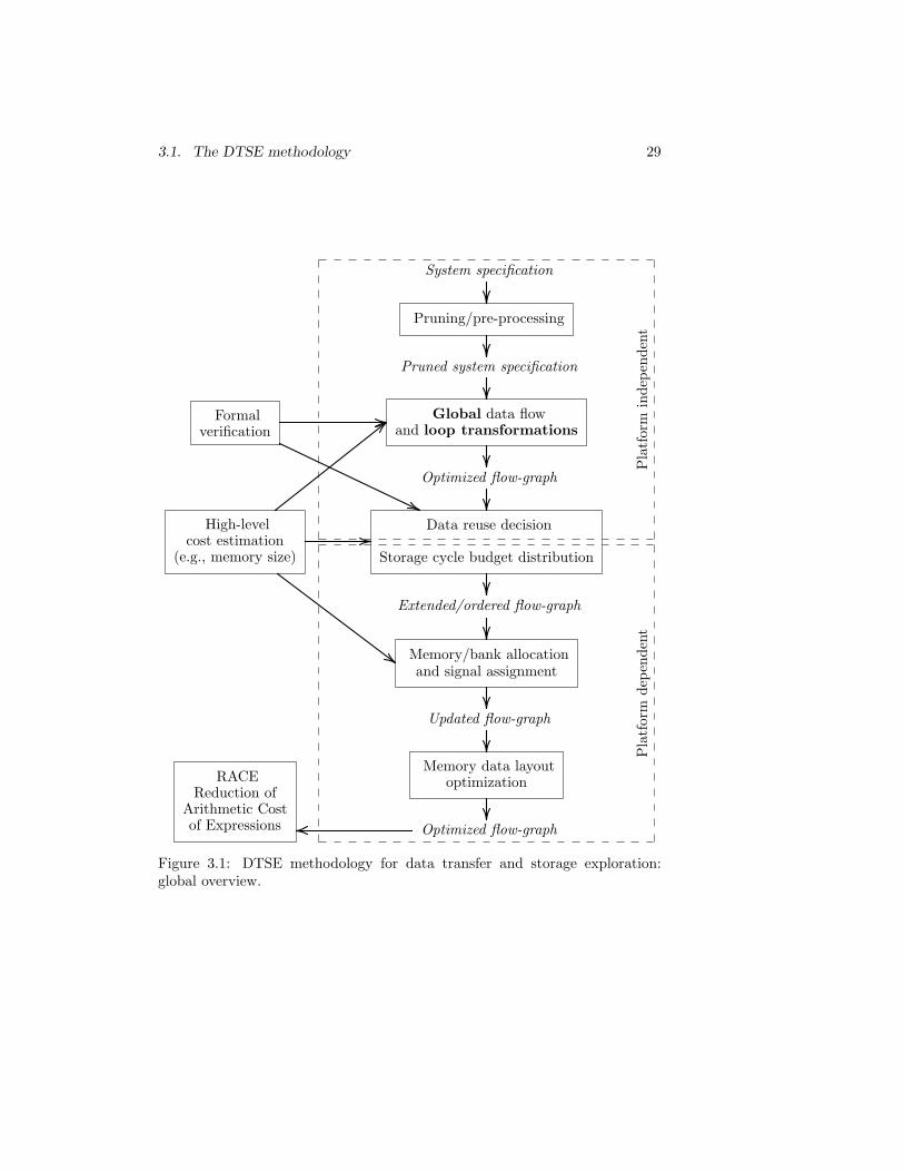
3.1. The DTSE methodology 29
Data reuse decision
Storage cycle budget distribution
Extended/ordered flow-graph
Memory/bank allocationand signal assignment
Updated flow-graph
Memory data layoutoptimization
Optimized flow-graph
Optimized flow-graph
Global data flowand loop transformations
Pruned system specification
Pruning/pre-processing
System specification
Pla
tfor
min
dep
enden
tP
latf
orm
dep
enden
t
Formalverification
High-levelcost estimation
(e.g., memory size)
RACEReduction of
Arithmetic Costof Expressions
Figure 3.1: DTSE methodology for data transfer and storage exploration:global overview.
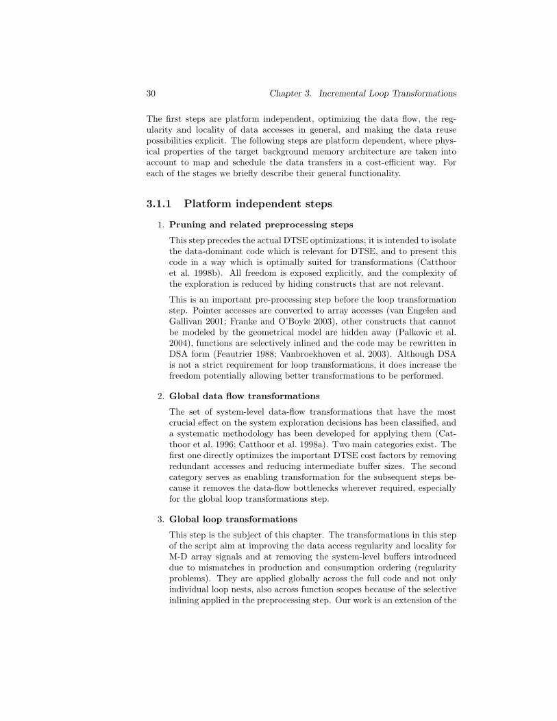
30 Chapter 3. Incremental Loop Transformations
The first steps are platform independent, optimizing the data flow, the reg-ularity and locality of data accesses in general, and making the data reusepossibilities explicit. The following steps are platform dependent, where phys-ical properties of the target background memory architecture are taken intoaccount to map and schedule the data transfers in a cost-efficient way. Foreach of the stages we briefly describe their general functionality.
3.1.1 Platform independent steps
1. Pruning and related preprocessing steps
This step precedes the actual DTSE optimizations; it is intended to isolatethe data-dominant code which is relevant for DTSE, and to present thiscode in a way which is optimally suited for transformations (Catthooret al. 1998b). All freedom is exposed explicitly, and the complexity ofthe exploration is reduced by hiding constructs that are not relevant.
This is an important pre-processing step before the loop transformationstep. Pointer accesses are converted to array accesses (van Engelen andGallivan 2001; Franke and O’Boyle 2003), other constructs that cannotbe modeled by the geometrical model are hidden away (Palkovic et al.2004), functions are selectively inlined and the code may be rewritten inDSA form (Feautrier 1988; Vanbroekhoven et al. 2003). Although DSAis not a strict requirement for loop transformations, it does increase thefreedom potentially allowing better transformations to be performed.
2. Global data flow transformations
The set of system-level data-flow transformations that have the mostcrucial effect on the system exploration decisions has been classified, anda systematic methodology has been developed for applying them (Cat-thoor et al. 1996; Catthoor et al. 1998a). Two main categories exist. Thefirst one directly optimizes the important DTSE cost factors by removingredundant accesses and reducing intermediate buffer sizes. The secondcategory serves as enabling transformation for the subsequent steps be-cause it removes the data-flow bottlenecks wherever required, especiallyfor the global loop transformations step.
3. Global loop transformations
This step is the subject of this chapter. The transformations in this stepof the script aim at improving the data access regularity and locality forM-D array signals and at removing the system-level buffers introduceddue to mismatches in production and consumption ordering (regularityproblems). They are applied globally across the full code and not onlyindividual loop nests, also across function scopes because of the selectiveinlining applied in the preprocessing step. Our work is an extension of the
3.1. The DTSE methodology 31
works of van Swaaij et al. (1992b), Franssen et al. (1994) and Danckaert(2001).
It is crucial that this step is applied before the data reuse explorationstep. Loop transformations change the execution order such that theproduction and the consumptions of data elements are moved closer to-gether in time. The result is that the data reuse copies in the memoryhierarchy can be made smaller since data is kept in the copy for a shortertime period, and higher data reuse factors can be achieved.
Note that during the loop transformation step, trade-offs may occur be-tween different cost functions. We will briefly return to this subject inSection 3.2.4.
4. Data reuse exploration
In this stage the data locality introduced by the previous global looptransformation step is exploited. Data reuse possibilities are made ex-plicit by analyzing virtual multi-copy hierarchies (including bypasses) forthe trade-off of power and memory size cost. Heavily reused data will becopied to smaller power-efficient on-chip memories, while costly accessesto external memory are reduced.
The basic methodology of Diguet et al. (1997) and Wuytack et al. (1998)is systematic, though it has restrictions on the actual data reuse behav-ior that can be handled. Van Achteren et al. (2003) and Catthoor et al.(2002) have extended this methodology by introducing some vital costparameters to describe a more complete search space. They further ex-plored the relationship between these parameters and the cost functionfor power and memory size, and proposed heuristics to steer the searchfor a good solution.
Van Achteren et al. (2002) formalized the extended search space by intro-ducing an analytical model for the cost parameters as a function of theindex expressions and loop bounds. This avoids long simulation timesand more importantly, it allows for the identification of exactly which ar-ray elements have to be copied to a sub-level for optimal data reuse. Thishas lead to a fully automatable design technique for all loop-dominatedapplications to find optimal memory hierarchies and generate the corre-sponding optimized code (Van Achteren 2004).
3.1.2 Platform dependent steps
1. Storage Cycle Budget Distribution (SCBD)
This step mainly determines the bandwidth/latency requirements andthe balancing of the available cycle budget over the different memoryaccesses.
32 Chapter 3. Incremental Loop Transformations
During Memory Hierarchy Layer Assignment (MHLA) (Brockmeyer et al.2003), the data reuse copy hierarchies resulting from the data reuse explo-ration and the corresponding transfers are partitioned over several hier-archical memory layers, based on the band-width and high-level memorysize estimation. The memory class of each of the memory layers is deter-mined (e.g., ROM, SRAM or DRAM and other RAM “flavors”).
Additional loop transformations are performed to meet the real-time con-straints, such as merging of loops without dependences, software pipelin-ing and partial loop unrolling (Shashidhar et al. 2001). These normallydo not influence the access order of data elements, so also the data reusebehavior remains the same.
The data reuse transformations introduce dependences in the code whichconstrain the freedom for SCBD transformations. However, a certaintransformation freedom is made available by defining the data reusecopies in single assignment form. This allows the SCBD transformationsto move copy update code out of a loop kernel for performance reasons.This extends the lifetime of the data, since the data is copied earlier to thecopy-candidate than actually needed. As a result, the performance gainhas to be traded off with a slightly larger final copy size cost (Dasygeniset al. 2004).
The initial data types (arrays or sets) are grouped/partitioned in basicgroups, a sub-step called Basic Group (BG) structuring (Ellervee et al.2001). Storage Bandwidth Optimization) (SBO) performs a partial order-ing of the flow graph at the BG level. It tries to minimize the requiredmemory bandwidth for a given cycle budget. This step produces a con-flict graph that expresses which BGs are accessed simultaneously andtherefore have to be assigned to different memories or different ports of amulti port memory (Wuytack et al. 1996a; Wuytack et al. 1999; Omnes2001).
2. Memory/bank allocation and signal assignment (MAA)
The goal in the memory/bank allocation and signal-to-memory/bank as-signment step (MAA) is to allocate memory units and ports (includingtheir types) from a memory library and to assign the data to the bestsuited memory units, given the cycle budget and other timing constraints(Balasa et al. 1997; Slock et al. 1997). The combination of the SCBD andMAA tools allows to derive real Pareto trade-off curves of the backgroundmemory related cost (e.g., power) versus the cycle budget (Brockmeyeret al. 2000).
3. Memory data layout optimization
In the memory allocation and signal-to-memory assignment step, signalswere assigned to physical memories or to banks within predefined mem-ories. However, the signals are still represented by multi-dimensional
3.1. The DTSE methodology 33
arrays, while the memory itself knows only addresses. In other words,the physical address for every signal element still has to be determined.This transformation is the data layout decision.
This involves several sub-steps and focuses both on the cache(s) and themain memory. One of the main issues involves in-place mapping of arraysand sub-arrays. In the worst case, all arrays require separate storagelocations. When the lifetimes of arrays or elements in the array are notoverlapping, the space reserved in the memory for these groups can beshared (De Greef 1998). The single assignment arrays and array copiesintroduced in the data reuse step are in-placed during this step, leadingto final optimal copy sizes. After the in-place data mapping step we nowdecide which signals will be locked in the data cache in case of a softwarecontrolled cache.
For hardware-controlled caches advanced main memory layout organiza-tion techniques have been developed, which allow to remove most of thepresent conflict misses due to the limited cache associativity (Kulkarni2001). Extensions on this methodology are based on the estimated copysize during the data reuse step (van Meeuwen 2002).
3.1.3 Other related methodologies and stages
• High-level memory size estimation
The memory data layout optimization (see above) is the last step in theDTSE methodology and determines the overall needed memory size ofthe application. However, in the earlier DTSE steps the final executionorder of the memory accesses is not yet fixed. Lower and upper boundsfor the needed memory size for a partially defined loop organization andorder, have been proposed by Kjeldsberg (2001). These can be used tosteer the many possible loop transformations for a given application, andare also useful during the data reuse step to help steering the exploration.
While Kjeldsberg (2001) mainly focuses on bounds on the memory neededfor individual arrays, Rydland et al. (2003) consider the effect of simul-taneously alive data-dependences to estimate the combined storage re-quirements for multiple arrays when the ordering of the accesses is fixed.Hu et al. (2004b) investigate bounds on memory requirement when onlypart of the global loop transformation has been fixed. In particular, theyconsider bounds over all possible loop fusion and loop shifting transfor-mations.
• Formal verification techniques for system-level transformations
In addition to the results on exploration and optimization methodologies,work has been done on system-level validation by formal verification ofglobal data-flow, loop and data reuse transformations (Samsom et al.
34 Chapter 3. Incremental Loop Transformations
1995; Cupak et al. 1998; Shashidhar et al. 2002). Such a formal verifica-tion stage avoids very CPU-time and design time costly re-simulation.
• Reduction of Arithmetic Cost of Expressions (RACE)
This stage is also not part of the DTSE methodology itself, but is vital todeal with the addressing and control flow overhead that is introduced bythe DTSE steps. The methodology to deal with this overhead is incorpo-rated into another system design stage developed at IMEC, namely theRACE project, previously known as the Adopt (ADdress OPTimization)project (Miranda et al. 1998). That methodology has been extended toprogrammable processor contexts (Gupta et al. 2000), including moduloaddressing reduction (Ghez et al. 2000).
The DTSE steps described above will typically significantly increase theaddressing complexity of the applications, e.g., by introducing more com-plex loop bounds, index expressions and conditions. When this compu-tational overhead is neglected, the optimized system will, although beingmore power efficient, suffer a severe performance degradation.
However, most of the additional complexity introduced by DTSE can beremoved again by source code optimizations such as constant propaga-tion, code hoisting, strength reduction and others. Code hoisting movesloop-invariant computations out of the scope of the loop body, eliminat-ing unnecessary re-computations of the same values. Strength reductionreplaces expensive operations in terms of performance by alternatives us-ing cheaper operations. For example, expensive modulo operations inaddressing arithmetic can be replaced by an alternative implementationusing cheaper increment and decrement operations (Ghez et al. 2000).The control flow complexity due to the introduction of conditional state-ments can also be removed (Falk and Marwedel 2003; Falk et al. 2003;Falk et al. 2003). The final result is that for most applications not onlythe power consumption is reduced, but also the system performance isincreased.
3.2 Overview of Loop Transformation Steps
3.2.1 Source-to-source Transformations
Since we perform our loop transformations on a geometrical model, we need tobe able to extract this model from a given program first. Similarly, the result ofthe transformation needs to be written out as code again. Figure 3.2 sketchesthis process which involves three basic steps:
• Extracting the geometrical model from the source code.
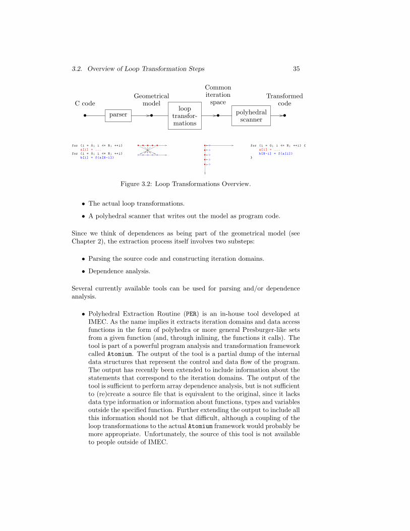
3.2. Overview of Loop Transformation Steps 35
•
C code
•
Geometricalmodel
•
Commoniteration
space
•
Transformedcode
parserloop
transfor-mations
polyhedralscanner
for (i = 0; i <= N; ++i)
a[i] = ...
for (i = 0; i <= N; ++i)
b[i] = f(a[N-i])
for (i = 0; i <= N; ++i)
a[i] = ...
b[N-i] = f(a[i])
• • • • •
•
•
•
•
•
Figure 3.2: Loop Transformations Overview.
• The actual loop transformations.
• A polyhedral scanner that writes out the model as program code.
Since we think of dependences as being part of the geometrical model (seeChapter 2), the extraction process itself involves two substeps:
• Parsing the source code and constructing iteration domains.
• Dependence analysis.
Several currently available tools can be used for parsing and/or dependenceanalysis.
• Polyhedral Extraction Routine (PER) is an in-house tool developed atIMEC. As the name implies it extracts iteration domains and data accessfunctions in the form of polyhedra or more general Presburger-like setsfrom a given function (and, through inlining, the functions it calls). Thetool is part of a powerful program analysis and transformation frameworkcalled Atomium. The output of the tool is a partial dump of the internaldata structures that represent the control and data flow of the program.The output has recently been extended to include information about thestatements that correspond to the iteration domains. The output of thetool is sufficient to perform array dependence analysis, but is not sufficientto (re)create a source file that is equivalent to the original, since it lacksdata type information or information about functions, types and variablesoutside the specified function. Further extending the output to include allthis information should not be that difficult, although a coupling of theloop transformations to the actual Atomium framework would probably bemore appropriate. Unfortunately, the source of this tool is not availableto people outside of IMEC.
36 Chapter 3. Incremental Loop Transformations
• The LooPo project (Ellmenreich et al. 2001) was set up to develop a pro-totype implementation of loop parallelization methods based on the geo-metrical model. The project includes both a parser (Schuler 1995; Gunz1998) and a dependence analysis module. Although it seemed promisingat first, practical experience has shown that the information that we needto perform our loop transformations is not readily available in the outputgenerated by these tools, at least in the version dated October 22, 2001.
• The WHIRL to Polyhedra (W2P) tool is part of the WRaP-IT library (Bas-toul et al. 2003) and constructs a polyhedral representation of a programfrom its WHIRL representation, which is the internal representation ofOpen Research Compiler (ORC). The disadvantage is that its use is tiedto a compiler which is a targeted at a single architecture, viz. the Ita-nium processor. Since its input is the intermediate WHIRL language, it isimpossible to generate C code again after any subsequent transformationwithout some form of WHIRL to C converter.
• Petit (Kelly et al. 1996a) is a research tool for dependence analysis andprogram transformations developed from Tiny (Wolfe 1991) and operateson programs in a simple Fortran-like language. The tool relies on theOmega library (Kelly et al. 1996c) for performing its analyses.
Since all of the currently available tools that have been developed as part ofthe DTSE methodology operate on C-code, none of the tools above is com-pletely appropriate. We therefore developed our own parser called PER inSUIF (pers). It basically consists of a pass in the Stanford University Inter-mediate Format (SUIF) compiler (Amarasinghe et al. 1995) that collects thesame information collected by PER but keeps a pointer to the internal SUIFdata structure that can be used during code generation. In this respect it isvery similar to the W2P tool. We have also written a tool called perparse.pl
which takes the output from PER and reproduces it in a form that can be usedin the remainder of our loop transformations framework. As explained above,the final code generation step will not be able to produce code that is equiva-lent to the original program when this path is taken. For dependence analysis,we use a prototype implementation of the techniques explained in Section 2.4.
For the code generation step after the loop transformations, the following toolsare available. Each of these tools scans the (possibly overlapping) target iter-ations domains and generates equivalent code.
• The Petit tool includes a code generation algorithm from Kelly et al.(1995). As reported by Bouchebaba (2002), this algorithm may some-times result in incorrect code.
• LoopGen, developed by Quillere et al. (2000), is a stand-alone C++ libraryfor performing code generation.
3.2. Overview of Loop Transformation Steps 37
• Chunky Loop Generator (CLooG) by Bastoul (2002) is a reimplementationof the algorithm of Quillere et al. (2000), but is easier to link into anapplication and includes some extra code generation options.
• The WRaP-IT library also contains a tool called WHIRL Loop Generator(WLooG) which uses CLooG to generate a WHIRL representation of the codeafter transformation.
When PER is used to extract the geometrical model, we use a modified versionof LoopGen to produce a C function that is similar to the (transformed) originalprogram. The modification consists of adding back the statement informationextracted from PER and changed to reflect the transformations performed onthe code. When pers is used to extract the geometrical model, the transformedC code can be obtained using our SUIF Loop Generator (sloog) tool whichuses CLooG and the information saved by pers to create a SUIF representationof the code. This SUIF representation can then be converted to C code usingthe standard SUIF to C (s2c) tool.
3.2.2 Affine Loop Transformations
Loop transformations have been widely used to optimize the execution timeand the memory usage of programs. In general, a loop transformation modi-fies the order in which loop iterations and statements within a loop body areexecuted. One way to perform this reordering is to define a schedule, assigningan execution time to each iteration of each statement in the program.
An example of this technique is affine-by-statement scheduling (Darte andRobert 1992; Feautrier 1992a; Lim and Lam 1997), where each statement isscheduled by a (piecewise) affine function θ that maps the iterations of thatstatement to time:
θX : i 7→ b T
X i + cX , (3.1)
where i is a vector in the iterations space of statement X, i.e., it has theiterator values of the loops surrounding the statement as elements. Alterna-tively, van Swaaij et al. (1992b) propose to split the scheduling operation intoa placement step, mapping the sets of iteration vectors for all statements toa common iteration space and an ordering step, defining an order, which is alinear schedule in that space. This technique was developed in parallel withthe affine-by-statement scheduling techniques and had already been applied byvan Swaaij et al. (1990) on the Hough transform. Using their proposed split,an affine schedule is decomposed into an affine transformation
AX : i 7→ AX(i) = AX i + aX (3.2)
for each statement X and a common ordering vector π. The resulting schedulefor statement X is then
θX : i 7→ πTAX i + πTaX , (3.3)
38 Chapter 3. Incremental Loop Transformations
i.e.,b T
X = πTAX and cX = πTaX . (3.4)
Although the latter technique requires the determination of a lot more coeffi-cients, it may still be preferable if it allows for an incremental search for thedifferent mappings. In Section 3.5 we will see that such an incremental searchis indeed possible but that the extra ordering step is not needed in our context.
The placement step of the second technique can be split up further into alinear transformation step, determining AX , and a translation step determiningaX . This split was already effectively made by van Swaaij (1992), and moreexplicitly so by Danckaert (2001). In this text we maintain this subdivisionand extend it to allow each of these substeps to be performed incrementally.We will however assume a fixed ordering in the common iteration space. Thatis, we will consider multi-dimensional schedules
θX : i 7→ AX i + aX ,
i.e., θX = AX . Such multi-dimensional schedules have also been used byFeautrier (1992b) and others. The fixed ordering in the common iterationspace is simply the lexicographical order. As we will see in Section 3.5, thisfixed ordering poses no real restriction on the optimality.
In our regularity experiments (see Section 3.4.3), we will further restrict ourattention to unimodular matrices, i.e., integer matrices with determinant 1 or−1. This means that A−1 also has integer elements and that the transformationis therefore a bijection between the integer points of a source polytope and theinteger points in the target polytope. This is mainly an implementation issueand it ensures that the target iteration domain is indeed a polytope ratherthan an LBL. Performing the subsequent loop fusion and code generation onLBLs does not pose any theoretical difficulties, but does require some care inthe implementation.
Affine loop transformations can be used to model many types of loop transfor-mations, e.g., loop interchange, loop reversal, statement reordering, loop skew-ing, loop distribution, loop fusion, loop alignment (Allen et al. 1987) and loopinterleaving (Sarkar and Thekkath 1992). Other types of loop transformationssuch as loop tiling (Irigoin and Triolet 1988; Wolfe 1989; Carr and Kennedy1992; Lam and Wolf 1992; Ramanujam 1992; Boulet et al. 1994; Rivera andTseng 1999; Song and Li 1999; Song et al. 2000; Bouchebaba 2002) and loopmorphing (Gomez et al. 2004) cannot be modeled by affine loop transformationsand therefore fall outside the scope of this dissertation.
3.2.3 Validity
As explained in Section 2.4, the dependence polytope contains the differencesbetween iterations and the iterations on which they depend. After transfor-
3.2. Overview of Loop Transformation Steps 39
mation, all iterations are mapped onto a common iteration space with a fixed,lexicographical order. For a given affine transformation, all iterations shouldbe executed after the iterations on which they depend. This means that thedifference between two interdependent iterations should be lexicographicallypositive. This constraint is commonly known as the causality condition (see,e.g., Feautrier 1992b). The dimension corresponding to the first non-zero (andtherefore positive) entry in such a lexicographically positive distance vector issaid to carry the dependence. The observation above leads to the followingdefinition of a valid transformation.
Definition 3.2.1 (Valid Transformation) A pair of affine transformationsAp, Aq for a pair of statements p, q is valid iff all transformed distance vectorsare lexicographically strictly positive.
d′ = Aq(i2) −Ap(i1) ≻ 0 if i1 δp,q i2. (3.5)
Note that the above only applies to distance vectors resulting from flow depen-dence (and output or anti-dependences), but not from input dependence sincethese do not impose any ordering constraint.
3.2.4 Optimality
Although we mainly focus on the feasibility of (incremental) loop transforma-tion, we will also consider some cost functions for optimality, mainly locality.Generally speaking, a program exhibits locality if the difference in executiontime of two statements that access the same or related data is small. In par-ticular we talk about temporal locality if the two statements access the samedata and about spatial locality if they access data that are placed close to-gether in memory, e.g., such that they would fit in the same cache line. Wewill mainly focus on temporal locality, which can be measured by means ofdistance vectors. In general, the smaller (lexicographically) a distance vectorbetween two statements, the better the locality between these two statements.Spatial locality is optimized by later, platform dependent, steps of the DTSEmethodology.
Optimizing locality between two accesses to the same memory element canhave a positive effect on the number of accesses. Optimizing locality over(flow) dependences, i.e., between a write and a read, reduces the life-timesof array elements, which can have an additional effect on the memory size.By reducing the distance between successive accesses to the same memoryelement, the likelihood of that element residing in a register or a cache increases,reducing the number of accesses to slower memories in the memory hierarchy.By reducing the maximal distance between a write and a read access, the arrayelement needs to be stored for a shorter amount of time, freeing up memory for
40 Chapter 3. Incremental Loop Transformations
for (i = 0; i <= n ; ++i)
a[i] = fa(a[i-1]);
for (i = 0; i <= n ; ++i)
b[i] = fb(a[i]);
for (i = 0; i <= n ; ++i)
c[i] = fc(c[i-1], b[i], b[n-i]);
for (i = 0; i <= n ; ++i)
d[i] = fd(a[i]);
for (i = 0; i <= n ; ++i)
e[i] = fe(e[i-1], d[i], d[n-i]);
for (i = 0; i <= n ; ++i)
f[i] = ff(a[i]);
for (i = 0; i <= n ; ++i)
g[i] = fg(c[i-1], f[i], f[n-i]);
result = c[n] + e[n] + g[n];
Listing 3.1: Program with bad locality.
other elements of the same or other arrays, which in general reduces the totalmemory requirements.
It should be noted that locality is not always good for memory size. Compare,for example, the programs in listings 3.1 and 3.2. The first has bad locality,since the elements of a, calculated in the first loop, are used in the loop thatcalculates f, but 4 loops separate these two loops. The program in Listing 3.2 ismaximally merged and values only need to be kept over a single loop. However,the number of array elements that need to be stored is larger in the secondprogram, since three arrays: b, d and f are alive between the two loops, whereasin the first program at most two arrays are simultaneously alive.
In Section 3.4.2 we will also consider a different characteristic called regularity,a concept which has also been used by van Swaaij (1992) and Danckaert (2001).We will say that a dependence exhibits regularity if the variation in distancevectors generated by the dependence is small. Regularity is an enabler for lo-cality and will be optimized during the linear transformation. In the optimalcase, all distance vectors over a dependence are equal or can be made equalduring the linear transformation. We call such a dependence a uniform depen-dence. In such a case the locality of all distance vectors of the dependence canin principle be fully optimized. For irregular dependences, only a subset of thedistance vectors can be optimized.
As mentioned above, regularity is optimized during the linear transformation.Locality over self dependences is also considered during linear transformation,whereas locality over group dependences is optimized during the translationstep. Note that locality and regularity are only heuristics and they are not the
3.2. Overview of Loop Transformation Steps 41
for (i = 0; i <= n ; ++i)
a[i] = fa(a[i -1]);
b[i] = fb(a[i]);
d[i] = fd(a[i]);
f[i] = ff(a[i]);
for (i = 0; i <= n ; ++i)
c[i] = fc(c[i-1], b[i], b[n-i]);
e[i] = fe(e[i-1], d[i], d[n-i]);
g[i] = fg(c[i-1], f[i], f[n-i]);
result = c[n] + e[n] + g[n];
Listing 3.2: Program with good locality.
only cost functions that need to be considered to obtain good final solutions.Some (Pareto) trade-offs may also exist between the different cost functions(Palkovic 2002; Hu et al. 2004a) which cannot be resolved until the platformdependent steps of the DTSE methodology. Ideally, the output of the looptransformation step would therefore not be a single solution, but a collectionof Pareto optimal solutions.
3.2.5 Incremental Loop Transformations
Many researchers have recognized the usefulness of data locality. However, ingeneral, the algorithms they propose only perform a limited set of transforma-tions, are of high complexity or make special assumptions on the initial code.Early research (Wolf and Lam 1991) focused on optimizing locality in singleperfectly nested loops by applying a single linear transformation, ignoring thelarge buffers that exist between loop nests.
Loop fusion is a loop transformation that optimizes over multiple loop nests.In its purest form, it only decides which loop nests should be fused togetherwithout performing any other transformation. Finding the optimal fusion hasbeen proven to be NP-complete, except for some special cases (Darte 1999).In general, these approaches require that all loops considered for fusing arecompatible, i.e., that they have the same number of iterations.
Loop shifting is a loop transformation where loops are shifted relatively toeach other, i.e., where the ranges of values attained by one or more loop it-erators is shifted (increased or decreased) by a constant amount. Extendingloop fusion with loop shifting allows more loops to be merged. The problem ofmaximizing the number of parallel loops that can be fused with loop shiftingis NP-complete, even for acyclic dependence graphs with uniform dependences
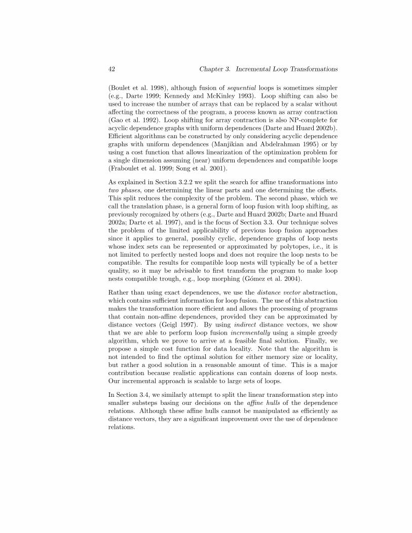
42 Chapter 3. Incremental Loop Transformations
(Boulet et al. 1998), although fusion of sequential loops is sometimes simpler(e.g., Darte 1999; Kennedy and McKinley 1993). Loop shifting can also beused to increase the number of arrays that can be replaced by a scalar withoutaffecting the correctness of the program, a process known as array contraction(Gao et al. 1992). Loop shifting for array contraction is also NP-complete foracyclic dependence graphs with uniform dependences (Darte and Huard 2002b).Efficient algorithms can be constructed by only considering acyclic dependencegraphs with uniform dependences (Manjikian and Abdelrahman 1995) or byusing a cost function that allows linearization of the optimization problem fora single dimension assuming (near) uniform dependences and compatible loops(Fraboulet et al. 1999; Song et al. 2001).
As explained in Section 3.2.2 we split the search for affine transformations intotwo phases, one determining the linear parts and one determining the offsets.This split reduces the complexity of the problem. The second phase, which wecall the translation phase, is a general form of loop fusion with loop shifting, aspreviously recognized by others (e.g., Darte and Huard 2002b; Darte and Huard2002a; Darte et al. 1997), and is the focus of Section 3.3. Our technique solvesthe problem of the limited applicability of previous loop fusion approachessince it applies to general, possibly cyclic, dependence graphs of loop nestswhose index sets can be represented or approximated by polytopes, i.e., it isnot limited to perfectly nested loops and does not require the loop nests to becompatible. The results for compatible loop nests will typically be of a betterquality, so it may be advisable to first transform the program to make loopnests compatible trough, e.g., loop morphing (Gomez et al. 2004).
Rather than using exact dependences, we use the distance vector abstraction,which contains sufficient information for loop fusion. The use of this abstractionmakes the transformation more efficient and allows the processing of programsthat contain non-affine dependences, provided they can be approximated bydistance vectors (Geigl 1997). By using indirect distance vectors, we showthat we are able to perform loop fusion incrementally using a simple greedyalgorithm, which we prove to arrive at a feasible final solution. Finally, wepropose a simple cost function for data locality. Note that the algorithm isnot intended to find the optimal solution for either memory size or locality,but rather a good solution in a reasonable amount of time. This is a majorcontribution because realistic applications can contain dozens of loop nests.Our incremental approach is scalable to large sets of loops.
In Section 3.4, we similarly attempt to split the linear transformation step intosmaller substeps basing our decisions on the affine hulls of the dependencerelations. Although these affine hulls cannot be manipulated as efficiently asdistance vectors, they are a significant improvement over the use of dependencerelations.
3.3. Loop Fusion 43
3.2.6 Summary
We have presented an overview of affine loop transformations and we haveshown how these transformations can be applied to source code as part ofa source-to-source transformation framework. Our affine loop transformationstep is split into a linear transformation step and a translation step, but itdoes not include an ordering step as used by van Swaaij (1992) and Danckaert(2001). We will return to the disadvantages of such an ordering step in Sec-tion 3.5. In both remaining steps, we need to ensure the final validity of thetransformed program and we need to consider the optimality of this program.In Section 3.3, we will explain how to perform the translation step incremen-tally and we will mainly focus on the validity. In Section 3.4, we will treat thelinear transformation step, focusing both on validity and a regularity criterion.
3.3 Loop Fusion
We first discuss the translation part of the affine transformations since this partwill enforce some requirements that need to be ensured by the preceding lineartransformation step. Since translation only changes the relative positioningof the different iteration domains, it does not change the order in which theiterations from a given iteration domain are executed, but only the amountby which different iteration domains overlap in different dimensions. Scanningthese overlapping polyhedra will result in (partially) merged loops. The useof statement-level dimensions allows for a more fine-grained control over therelative positioning of different statements.
After explaining how to ensure validity of the final result while performing loopfusion incrementally, we provide a very simple scalable locality heuristic. Weshow how this heuristic works on a 2-dimensional example and how it performsin practice on a set of programs. Finally, we discuss some refinements to furtherimprove the target code.
3.3.1 Validity
A translation T corresponds to the constant part of an affine transformation,i.e.,
i′ = T (i) = i + a.
For such a translation, the general validity constraint (3.5) reduces to
d′ = Tq(i2) − Tp(i1) = d + aq − ap ≻ 0 if i1 δp,q i2. (3.6)
We call d′ the translated distance vector. Figure 3.3 illustrates the graphicaldecomposition of such a translated distance vector.
44 Chapter 3. Incremental Loop Transformations
q
p
d
d
d+aq−ap
aq
ap
aq−ap
d
Figure 3.3: Decomposition of translated distance vectors. On the left, a de-pendence graph with a single dependence. On the right, the distance vectorcorresponding to the dependence with the top figure showing the canonical dis-tance vector and the bottom figure showing the distance vector after translationof the polytopes involved in the dependence.
Since Equation (3.6) should hold for all elements of a given dependence, weneed to have
DPp,q + aq − ap ≻ 0 if (p, q) ∈ EG,
where G is the dependence graph. Since aq − ap is constant for each pair ofstatements (p, q), it is sufficient to check (3.6) for the lexicographically minimaldistance vector dp,q between p and q:
dp,q + aq − ap ≻ 0 if (p, q) ∈ EG, (3.7)
where dp,q is defined asdp,q = lexmin DPp,q. (3.8)
In the special case of a self dependence, i.e., if p = q, Equation (3.7) furthersimplifies to
dp,p ≻ 0 (3.9)
which must be ensured by the linear transformation step since it is independentof the translation step. If the translation is performed without a prior lineartransformation step, then (3.9) will hold by definition for the programs weconsider according to the dependence analysis in Section 2.4.2.
Not only direct self dependences, but also indirect self dependences imposeconstraints on the linear transformation phase. Consider a cycle π of length l
3.3. Loop Fusion 45
in the dependence graph G:
π = (p0, p1, . . . , pl−1, pl), p0 = pl ∀i < l : (pi, pi+1) ∈ EG.
Each of the links in the cycle π needs to satisfy a constraint of the form (3.7),i.e.,
l−1∑
i=0
(di,i+1 + ai+1 − ai) ≻ 0.
Since al = a0, we obtainl−1∑
i=0
di,i+1 < eN ,
where N is the dimension of the problem. Let E∗G be the set of all indirectlinks in the graphs. That is, let El
G be the set of indirect links of length l inthe graph, i.e., E1
G = EG and
ElG =
(x, y) | ∃z : (x, z) ∈ El−1
G ∧ (z, y) ∈ EG
for l > 1
then
E∗G =∞⋃
l=1
ElG.
In other words, E∗G is the transitive closure of EG. Furthermore, let d∗p1,p2be
the lexicographically minimal distance vector over the indirect link (p1, p2) ∈E∗G, then the linear transformation needs to ensure:
∀(p, p) ∈ E∗G : d∗(p,p) ≻ 0, (3.10)
i.e., each indirect self dependence distance vector needs to be strictly lexico-positive. This yields the following proposition:
Proposition 3.3.1 If a valid fusion exists, then (3.10) must hold.
As we will show next, this is also a sufficient condition for a valid fusion to existand is therefore the only constraint on the linear transformation phase. Notethat this condition for valid fusion itself is well known (e.g., Darte and Huard2000). The interesting novel aspect is that performing this fusion incremen-tally does not impose any other constraints. The condition can be checked inO(|V ||E|) by an extension of the Bellman-Ford algorithm (Cormen et al. 1990)to multiple dimensions, as proposed by Darte and Huard (2000).
A valid translation will be determined incrementally, which means that in eachstep two nodes are combined with a certain relative offset until only a singlenode remains. This process is shown in Algorithm 3.1. The combination oftwo nodes in step 5 of in this algorithm is detailed in Algorithm 3.2. It is
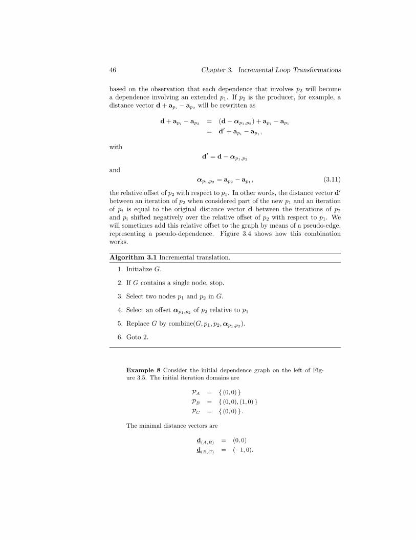
46 Chapter 3. Incremental Loop Transformations
based on the observation that each dependence that involves p2 will becomea dependence involving an extended p1. If p2 is the producer, for example, adistance vector d + api
− ap2will be rewritten as
d + api− ap2
= (d − αp1,p2) + api
− ap1
= d′ + api− ap1
,
with
d′ = d − αp1,p2
and
αp1,p2= ap2
− ap1, (3.11)
the relative offset of p2 with respect to p1. In other words, the distance vector d′
between an iteration of p2 when considered part of the new p1 and an iterationof pi is equal to the original distance vector d between the iterations of p2
and pi shifted negatively over the relative offset of p2 with respect to p1. Wewill sometimes add this relative offset to the graph by means of a pseudo-edge,representing a pseudo-dependence. Figure 3.4 shows how this combinationworks.
Algorithm 3.1 Incremental translation.
1. Initialize G.
2. If G contains a single node, stop.
3. Select two nodes p1 and p2 in G.
4. Select an offset αp1,p2of p2 relative to p1
5. Replace G by combine(G, p1, p2,αp1,p2).
6. Goto 2.
Example 8 Consider the initial dependence graph on the left of Fig-ure 3.5. The initial iteration domains are
PA = (0, 0) PB = (0, 0), (1, 0) PC = (0, 0) .
The minimal distance vectors are
d(A,B) = (0, 0)
d(B,C) = (−1, 0).
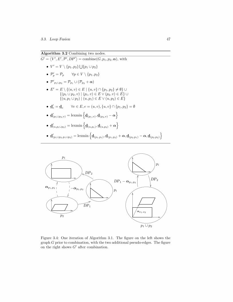
3.3. Loop Fusion 47
Algorithm 3.2 Combining two nodes.
G′ =⟨V ′, E′,P ′,DP′
⟩= combine(G, p1, p2,α), with
• V ′ = V \ p1, p2⋃p1 ∪ p2
• P ′p = Pp ∀p ∈ V \ p1, p2
• P ′p1∪p2= Pp1
∪ (Pp2+ α)
• E′ = E \ (u, v) ∈ E | u, v ∩ p1, p2 6= ∅ ∪(p1 ∪ p2, v) | (p1, v) ∈ E ∨ (p2, v) ∈ E ∪(u, p1 ∪ p2) | (u, p1) ∈ E ∨ (u, p2) ∈ E
• d′e = de ∀e ∈ E, e = (u, v), u, v ∩ p1, p2 = ∅
• d′(p1∪p2,v) = lexmin
d(p1,v),d(p2,v) − α
• d′(u,p1∪p2)= lexmin
d(u,p1),d(u,p2)
+ α
• d′(p1∪p2,p1∪p2)= lexmin
d(p1,p1),d(p1,p2)
+ α,d(p2,p1)− α,d(p2,p2)
p2
p1
pi
DP1
DP2
αp1,p2 −αp1,p2
p1 ∪ p2
pi
DP1 − αp1,p2
DP2
αp1,p2
Figure 3.4: One iteration of Algorithm 3.1. The figure on the left shows thegraph G prior to combination, with the two additional pseudo-edges. The figureon the right shows G′ after combination.
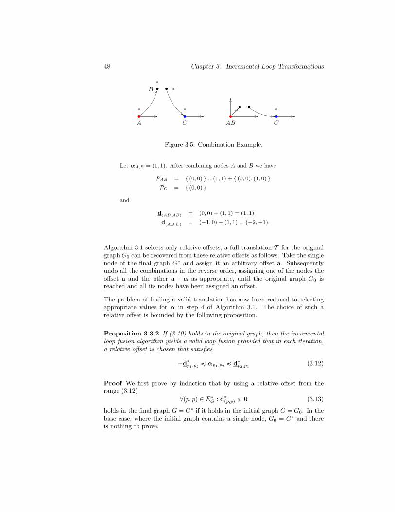
48 Chapter 3. Incremental Loop Transformations
•A
• •B
•C
•
• •
AB•C
Figure 3.5: Combination Example.
Let αA,B = (1, 1). After combining nodes A and B we have
PAB = (0, 0) ∪ (1, 1) + (0, 0), (1, 0) PC = (0, 0)
and
d(AB,AB) = (0, 0) + (1, 1) = (1, 1)
d(AB,C) = (−1, 0) − (1, 1) = (−2,−1).
Algorithm 3.1 selects only relative offsets; a full translation T for the originalgraph G0 can be recovered from these relative offsets as follows. Take the singlenode of the final graph G∗ and assign it an arbitrary offset a. Subsequentlyundo all the combinations in the reverse order, assigning one of the nodes theoffset a and the other a + α as appropriate, until the original graph G0 isreached and all its nodes have been assigned an offset.
The problem of finding a valid translation has now been reduced to selectingappropriate values for α in step 4 of Algorithm 3.1. The choice of such arelative offset is bounded by the following proposition.
Proposition 3.3.2 If (3.10) holds in the original graph, then the incrementalloop fusion algorithm yields a valid loop fusion provided that in each iteration,a relative offset is chosen that satisfies
−d∗p1,p24 αp1,p2
4 d∗p2,p1(3.12)
Proof We first prove by induction that by using a relative offset from therange (3.12)
∀(p, p) ∈ E∗G : d∗(p,p) < 0 (3.13)
holds in the final graph G = G∗ if it holds in the initial graph G = G0. In thebase case, where the initial graph contains a single node, G0 = G∗ and thereis nothing to prove.
3.3. Loop Fusion 49
For the induction case, first note that we only need to consider simple cycles,i.e., those that visit a node at most once, since if (3.13) holds for all simplecycles, then it also holds for the other cycles. After application of one stepof Algorithm 3.1, any new simple cycle passes through p′ = p1 ∪ p2 and thecorresponding minimal distance vector is therefore of the form either d∗p1,p2
+αp1,p2
or d∗p2,p1− αp1,p2
(see Algorithm 3.2). By substituting these two newdistance vectors in (3.13) we obtain (3.12). Since, by assumption,
0 4 d∗p1,p14 d∗p2,p1
+ d∗p1,p2,
this equation always has a solution.
To obtain a translation that satisfies (3.6), i.e., with strict inequality, add anextra innermost statement-level dimension. Let GZ be the graph resulting fromthe initial graph G by removing all the links with a non-zero minimal distancevector. Because of (3.10), GZ is acyclic and its nodes can be topologicallysorted. The sequence numbers of this sort can be used as the d+1st dimensionof the translation offsets such that (3.6) does hold for the (d + 1)-dimensionaltranslation offsets. This completes the proof.
Example 9 Consider the program on the left side of Figure 3.6. It iswritten in an applicative language and cannot be executed in the orderin which it is written down. This is clear from the graph on the right ofthe figure, which shows the individual dependences between iterations:the first iteration of the B-loop depends on an iteration of the D-loop,which follows. In Figure 3.6 and the following figures n = 5 is assumed.
Figure 3.7 shows the initial dependence graph with dependence polytopeson the left. Since the problem is one-dimensional, we can use intervalshere to represent the dependence polytopes. The graph contains a singlecycle, with indirect distance vectors in the range [−n−2,−2]. Since theseare negative, (3.10) does not hold and a linear transformation needs tobe applied. In this case we can simply reverse all the iteration domains.The resulting minimal distance “vectors” are shown in the same figureon the right. The single minimal self dependence distance vector is 2 andsatisfies (3.10).
We arbitrarily combine C and D first. The constraint on the relativeoffset (3.12) is
−0 4 αC,D 4 2
and we choose αC,D = 0. The resulting dependence graph G1 is shownin Figure 3.8. Next, A and B are combined at an offset of αA,B = 1,satisfying the constraint 1 4 αA,B and resulting in G2. Finally AB andCD are combined at an offset of αAB,CD = n−1, satisfying the constrainton the relative offset −(1−n) 4 αAB,CD 4 n + 1. We arbitrarily chooseaA = aABCD = 0 and obtain aB = 1 and aC = aD = n − 1.
Figure 3.9 on page 51 shows the dependence graph after translation.Some of the translated minimal distance vectors are zero and so a topo-
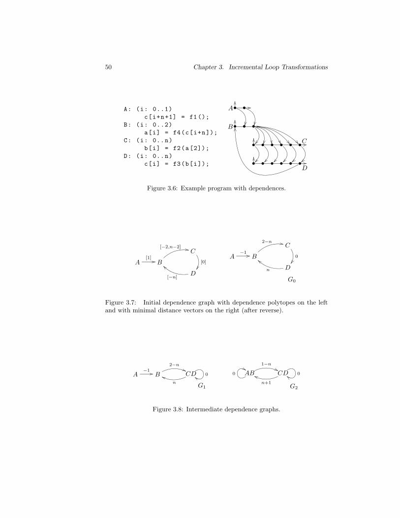
50 Chapter 3. Incremental Loop Transformations
A: (i: 0..1)
c[i+n+1] = f1();
B: (i: 0..2)
a[i] = f4(c[i+n]);
C: (i: 0..n)
b[i] = f2(a[2]);
D: (i: 0..n)
c[i] = f3(b[i]);
• • •
• •
• • • • • •
• • • • • •
A
B
C
D
Figure 3.6: Example program with dependences.
A B
C
D
[1]
[−2,n−2]
[0]
[−n]
A B
C
D
−1
2−n
0
n
G0
Figure 3.7: Initial dependence graph with dependence polytopes on the leftand with minimal distance vectors on the right (after reverse).
A B CD−1
2−n
0
nG1
AB CD
1−n
00
n+1G2
Figure 3.8: Intermediate dependence graphs.
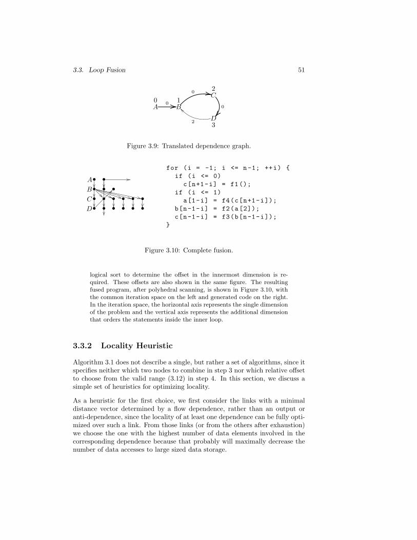
3.3. Loop Fusion 51
A0
B1
C2
D3
0
0
0
2
Figure 3.9: Translated dependence graph.
•••
••
••••••
••••••
A
B
C
D
for (i = -1; i <= n-1; ++i)
if (i <= 0)
c[n+1-i] = f1();
if (i <= 1)
a[1-i] = f4(c[n+1-i]);
b[n-1-i] = f2(a[2]);
c[n-1-i] = f3(b[n-1-i]);
Figure 3.10: Complete fusion.
logical sort to determine the offset in the innermost dimension is re-quired. These offsets are also shown in the same figure. The resultingfused program, after polyhedral scanning, is shown in Figure 3.10, withthe common iteration space on the left and generated code on the right.In the iteration space, the horizontal axis represents the single dimensionof the problem and the vertical axis represents the additional dimensionthat orders the statements inside the inner loop.
3.3.2 Locality Heuristic
Algorithm 3.1 does not describe a single, but rather a set of algorithms, since itspecifies neither which two nodes to combine in step 3 nor which relative offsetto choose from the valid range (3.12) in step 4. In this section, we discuss asimple set of heuristics for optimizing locality.
As a heuristic for the first choice, we first consider the links with a minimaldistance vector determined by a flow dependence, rather than an output oranti-dependence, since the locality of at least one dependence can be fully opti-mized over such a link. From those links (or from the others after exhaustion)we choose the one with the highest number of data elements involved in thecorresponding dependence because that probably will maximally decrease thenumber of data accesses to large sized data storage.
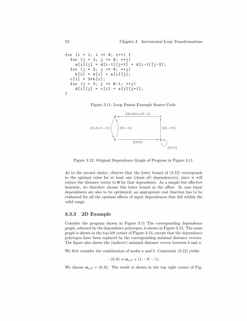
52 Chapter 3. Incremental Loop Transformations
for (i = 1; i <= N; i++)
for (j = 2; j <= N; ++j)
a[i][j] = d[i-1][j+1] + d[i-1][j-2];
for (j = 2; j <= N; ++j)
b[i] = b[i] + a[i][j];
c[i] = 2*b[i];
for (j = 0; j <= N-1; ++j)
d[i][j] = c[i] + a[i][j+1];
Figure 3.11: Loop Fusion Example Source Code.
a b
cd
(0,0)
(0,1)
(0,−N)
(0,i)|0≤i≤N−1
(1,2),(1,−1) (0,−1)
Figure 3.12: Original Dependence Graph of Program in Figure 3.11.
As to the second choice, observe that the lower bound of (3.12) correspondsto the optimal value for at least one (chain of) dependence(s), since it willreduce the distance vector to 0 for that dependence. As a simple but effectiveheuristic, we therefore choose this lower bound as the offset. In case inputdependences are also to be optimized, an appropriate cost function has to beevaluated for all the optimal offsets of input dependences that fall within thevalid range.
3.3.3 2D Example
Consider the program shown in Figure 3.11 The corresponding dependencegraph, adorned by the dependence polytopes, is shown in Figure 3.12. The samegraph is shown in the top left corner of Figure 3.13, except that the dependencepolytopes have been replaced by the corresponding minimal distance vectors.The figure also shows the (indirect) minimal distance vector between b and a.
We first consider the combination of nodes a and b. Constraint (3.12) yields
−(0, 0) 4 αa,b 4 (1,−N − 1).
We choose αa,b = (0, 0). The result is shown in the top right corner of Fig-
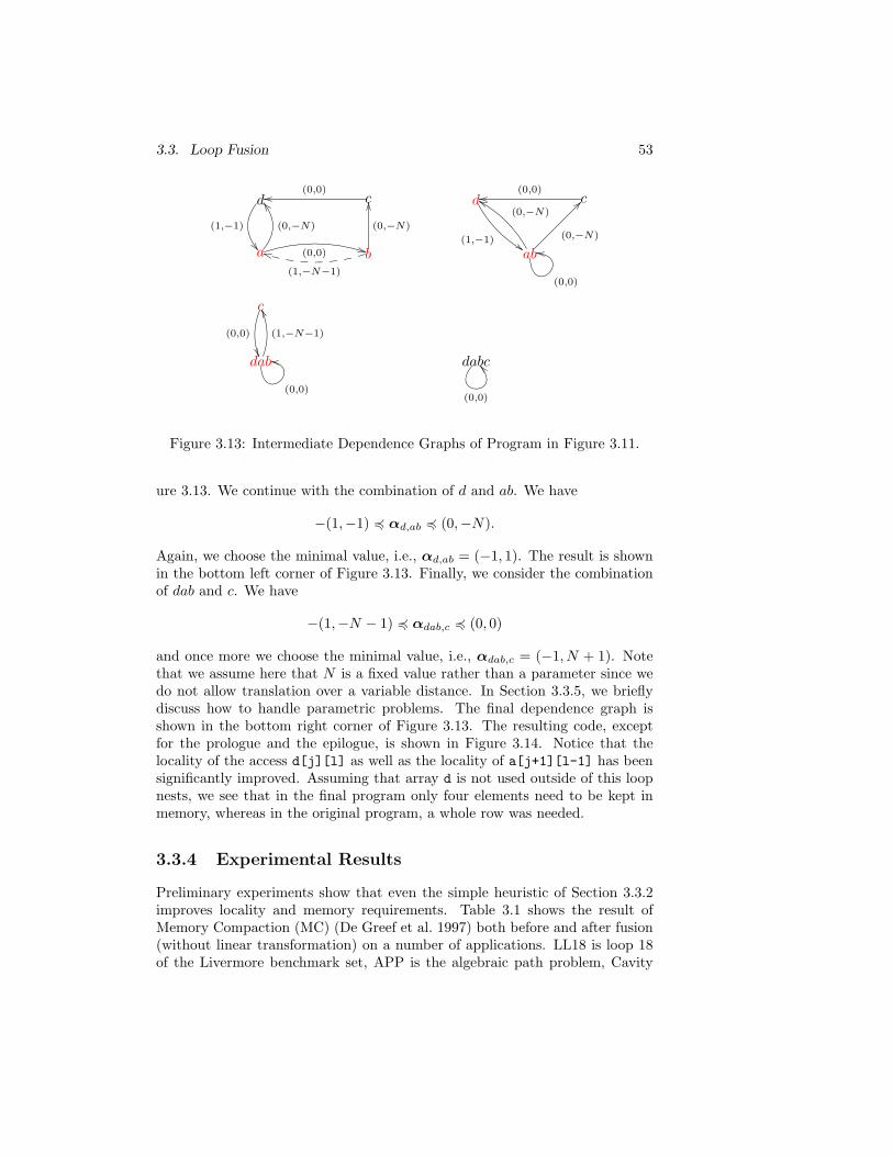
3.3. Loop Fusion 53
a b
cd
(0,0)
(0,−N)
(0,0)
(1,−1) (0,−N)
(1,−N−1)
ab
cd
(0,0)
(0,−N)
(0,0)
(1,−1)
(0,−N)
dab
c
(0,0)
(1,−N−1)(0,0)
dabc
(0,0)
Figure 3.13: Intermediate Dependence Graphs of Program in Figure 3.11.
ure 3.13. We continue with the combination of d and ab. We have
−(1,−1) 4 αd,ab 4 (0,−N).
Again, we choose the minimal value, i.e., αd,ab = (−1, 1). The result is shownin the bottom left corner of Figure 3.13. Finally, we consider the combinationof dab and c. We have
−(1,−N − 1) 4 αdab,c 4 (0, 0)
and once more we choose the minimal value, i.e., αdab,c = (−1, N + 1). Notethat we assume here that N is a fixed value rather than a parameter since wedo not allow translation over a variable distance. In Section 3.3.5, we brieflydiscuss how to handle parametric problems. The final dependence graph isshown in the bottom right corner of Figure 3.13. The resulting code, exceptfor the prologue and the epilogue, is shown in Figure 3.14. Notice that thelocality of the access d[j][l] as well as the locality of a[j+1][l-1] has beensignificantly improved. Assuming that array d is not used outside of this loopnests, we see that in the final program only four elements need to be kept inmemory, whereas in the original program, a whole row was needed.
3.3.4 Experimental Results
Preliminary experiments show that even the simple heuristic of Section 3.3.2improves locality and memory requirements. Table 3.1 shows the result ofMemory Compaction (MC) (De Greef et al. 1997) both before and after fusion(without linear transformation) on a number of applications. LL18 is loop 18of the Livermore benchmark set, APP is the algebraic path problem, Cavity
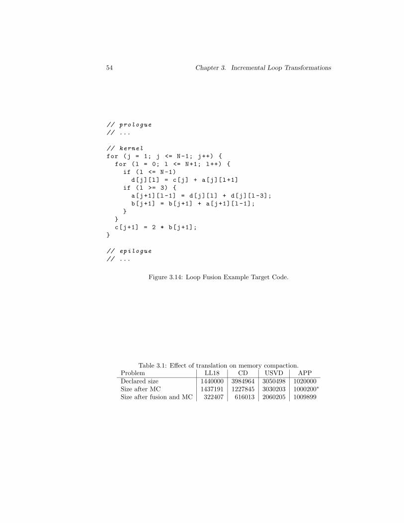
54 Chapter 3. Incremental Loop Transformations
// prologue
// ...
// kernel
for (j = 1; j <= N-1; j++)
for (l = 0; l <= N+1; l++)
if (l <= N-1)
d[j][l] = c[j] + a[j][l+1]
if (l >= 3)
a[j+1][l-1] = d[j][l] + d[j][l-3];
b[j+1] = b[j+1] + a[j+1][l-1];
c[j+1] = 2 * b[j+1];
// epilogue
// ...
Figure 3.14: Loop Fusion Example Target Code.
Table 3.1: Effect of translation on memory compaction.Problem LL18 CD USVD APPDeclared size 1440000 3984964 3050498 1020000Size after MC 1437191 1227845 3030203 1000200∗
Size after fusion and MC 322407 616013 2060205 1009899
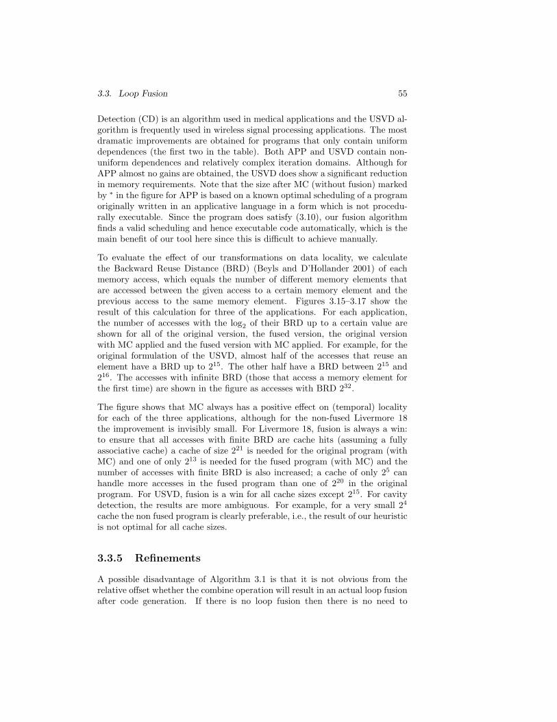
3.3. Loop Fusion 55
Detection (CD) is an algorithm used in medical applications and the USVD al-gorithm is frequently used in wireless signal processing applications. The mostdramatic improvements are obtained for programs that only contain uniformdependences (the first two in the table). Both APP and USVD contain non-uniform dependences and relatively complex iteration domains. Although forAPP almost no gains are obtained, the USVD does show a significant reductionin memory requirements. Note that the size after MC (without fusion) markedby ∗ in the figure for APP is based on a known optimal scheduling of a programoriginally written in an applicative language in a form which is not procedu-rally executable. Since the program does satisfy (3.10), our fusion algorithmfinds a valid scheduling and hence executable code automatically, which is themain benefit of our tool here since this is difficult to achieve manually.
To evaluate the effect of our transformations on data locality, we calculatethe Backward Reuse Distance (BRD) (Beyls and D’Hollander 2001) of eachmemory access, which equals the number of different memory elements thatare accessed between the given access to a certain memory element and theprevious access to the same memory element. Figures 3.15–3.17 show theresult of this calculation for three of the applications. For each application,the number of accesses with the log2 of their BRD up to a certain value areshown for all of the original version, the fused version, the original versionwith MC applied and the fused version with MC applied. For example, for theoriginal formulation of the USVD, almost half of the accesses that reuse anelement have a BRD up to 215. The other half have a BRD between 215 and216. The accesses with infinite BRD (those that access a memory element forthe first time) are shown in the figure as accesses with BRD 232.
The figure shows that MC always has a positive effect on (temporal) localityfor each of the three applications, although for the non-fused Livermore 18the improvement is invisibly small. For Livermore 18, fusion is always a win:to ensure that all accesses with finite BRD are cache hits (assuming a fullyassociative cache) a cache of size 221 is needed for the original program (withMC) and one of only 213 is needed for the fused program (with MC) and thenumber of accesses with finite BRD is also increased; a cache of only 25 canhandle more accesses in the fused program than one of 220 in the originalprogram. For USVD, fusion is a win for all cache sizes except 215. For cavitydetection, the results are more ambiguous. For example, for a very small 24
cache the non fused program is clearly preferable, i.e., the result of our heuristicis not optimal for all cache sizes.
3.3.5 Refinements
A possible disadvantage of Algorithm 3.1 is that it is not obvious from therelative offset whether the combine operation will result in an actual loop fusionafter code generation. If there is no loop fusion then there is no need to
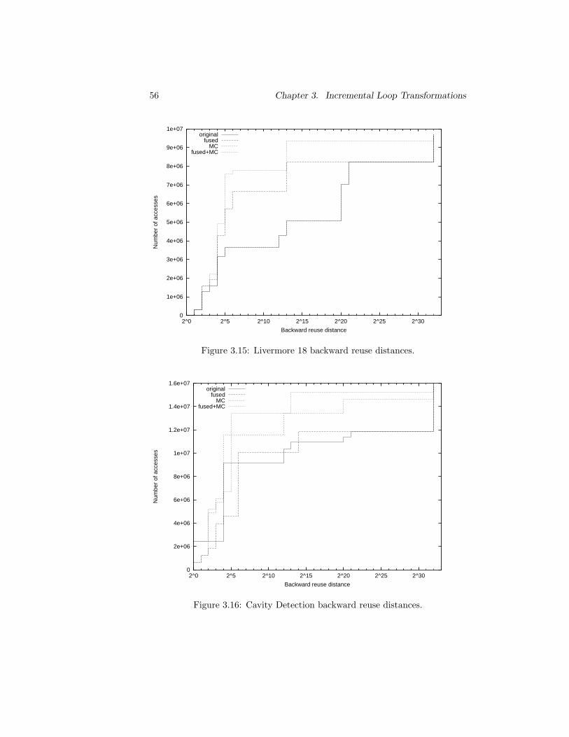
56 Chapter 3. Incremental Loop Transformations
0
1e+06
2e+06
3e+06
4e+06
5e+06
6e+06
7e+06
8e+06
9e+06
1e+07
2^0 2^5 2^10 2^15 2^20 2^25 2^30
Num
ber
of a
cces
ses
Backward reuse distance
originalfused
MCfused+MC
Figure 3.15: Livermore 18 backward reuse distances.
0
2e+06
4e+06
6e+06
8e+06
1e+07
1.2e+07
1.4e+07
1.6e+07
2^0 2^5 2^10 2^15 2^20 2^25 2^30
Num
ber
of a
cces
ses
Backward reuse distance
originalfused
MCfused+MC
Figure 3.16: Cavity Detection backward reuse distances.
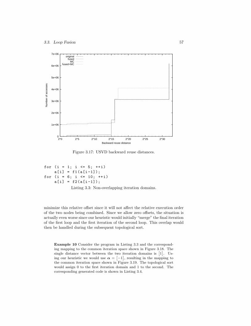
3.3. Loop Fusion 57
0
1e+06
2e+06
3e+06
4e+06
5e+06
6e+06
7e+06
2^0 2^5 2^10 2^15 2^20 2^25 2^30
Num
ber
of a
cces
ses
Backward reuse distance
originalfused
MCfused+MC
Figure 3.17: USVD backward reuse distances.
for (i = 1; i <= 5; ++i)
a[i] = f1(a[i -1]);
for (i = 6; i <= 10; ++i)
a[i] = f2(a[i -1]);
Listing 3.3: Non-overlapping iteration domains.
minimize this relative offset since it will not affect the relative execution orderof the two nodes being combined. Since we allow zero offsets, the situation isactually even worse since our heuristic would initially “merge” the final iterationof the first loop and the first iteration of the second loop. This overlap wouldthen be handled during the subsequent topological sort.
Example 10 Consider the program in Listing 3.3 and the correspond-ing mapping to the common iteration space shown in Figure 3.18. Thesingle distance vector between the two iteration domains is
[1]. Us-
ing our heuristic we would use α =[−1], resulting in the mapping to
the common iteration space shown in Figure 3.19. The topological sortwould assign 0 to the first iteration domain and 1 to the second. Thecorresponding generated code is shown in Listing 3.4.
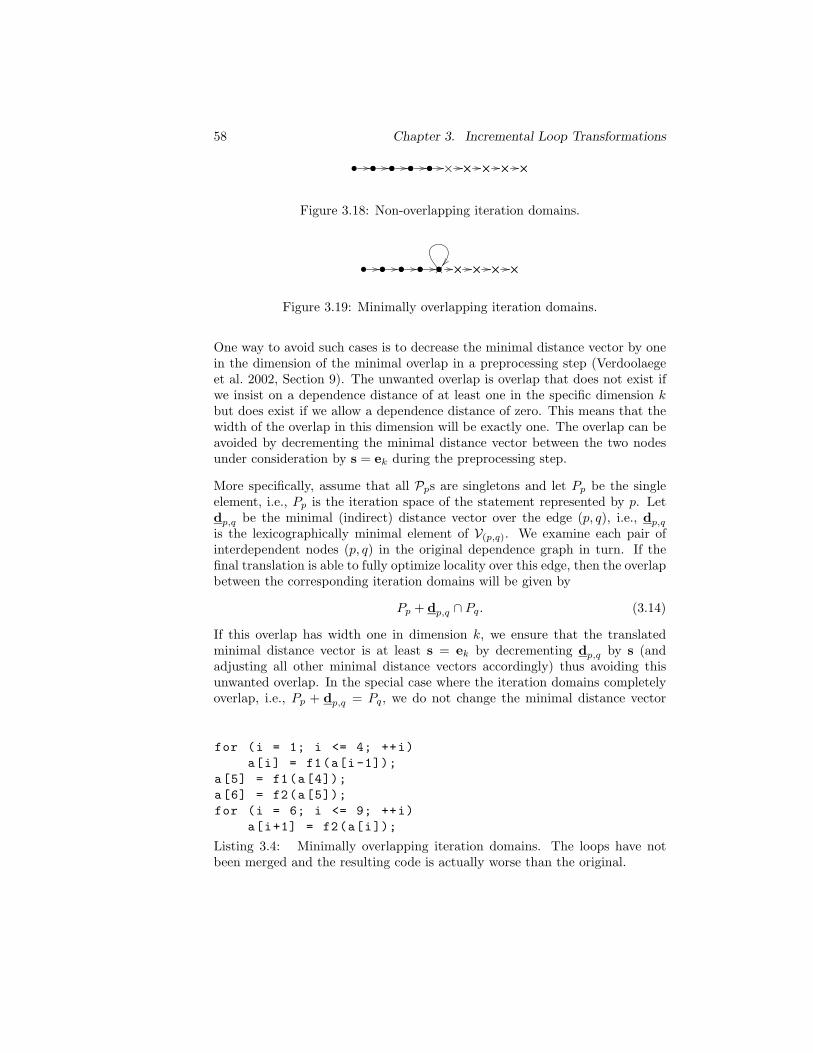
58 Chapter 3. Incremental Loop Transformations
• • • • •• • • • × × × × ×× × × ×
Figure 3.18: Non-overlapping iteration domains.
• • • • •• • • •× × × × ×× × × ×
Figure 3.19: Minimally overlapping iteration domains.
One way to avoid such cases is to decrease the minimal distance vector by onein the dimension of the minimal overlap in a preprocessing step (Verdoolaegeet al. 2002, Section 9). The unwanted overlap is overlap that does not exist ifwe insist on a dependence distance of at least one in the specific dimension kbut does exist if we allow a dependence distance of zero. This means that thewidth of the overlap in this dimension will be exactly one. The overlap can beavoided by decrementing the minimal distance vector between the two nodesunder consideration by s = ek during the preprocessing step.
More specifically, assume that all Pps are singletons and let Pp be the singleelement, i.e., Pp is the iteration space of the statement represented by p. Letdp,q be the minimal (indirect) distance vector over the edge (p, q), i.e., dp,q
is the lexicographically minimal element of V(p,q). We examine each pair ofinterdependent nodes (p, q) in the original dependence graph in turn. If thefinal translation is able to fully optimize locality over this edge, then the overlapbetween the corresponding iteration domains will be given by
Pp + dp,q ∩ Pq. (3.14)
If this overlap has width one in dimension k, we ensure that the translatedminimal distance vector is at least s = ek by decrementing dp,q by s (andadjusting all other minimal distance vectors accordingly) thus avoiding thisunwanted overlap. In the special case where the iteration domains completelyoverlap, i.e., Pp + dp,q = Pq, we do not change the minimal distance vector
for (i = 1; i <= 4; ++i)
a[i] = f1(a[i-1]);
a[5] = f1(a[4]);
a[6] = f2(a[5]);
for (i = 6; i <= 9; ++i)
a[i+1] = f2(a[i]);
Listing 3.4: Minimally overlapping iteration domains. The loops have notbeen merged and the resulting code is actually worse than the original.
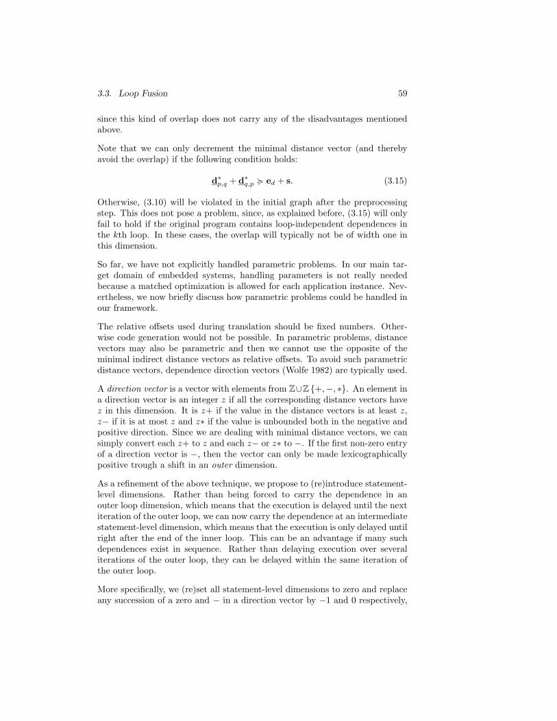
3.3. Loop Fusion 59
since this kind of overlap does not carry any of the disadvantages mentionedabove.
Note that we can only decrement the minimal distance vector (and therebyavoid the overlap) if the following condition holds:
d∗p,q + d∗q,p < ed + s. (3.15)
Otherwise, (3.10) will be violated in the initial graph after the preprocessingstep. This does not pose a problem, since, as explained before, (3.15) will onlyfail to hold if the original program contains loop-independent dependences inthe kth loop. In these cases, the overlap will typically not be of width one inthis dimension.
So far, we have not explicitly handled parametric problems. In our main tar-get domain of embedded systems, handling parameters is not really neededbecause a matched optimization is allowed for each application instance. Nev-ertheless, we now briefly discuss how parametric problems could be handled inour framework.
The relative offsets used during translation should be fixed numbers. Other-wise code generation would not be possible. In parametric problems, distancevectors may also be parametric and then we cannot use the opposite of theminimal indirect distance vectors as relative offsets. To avoid such parametricdistance vectors, dependence direction vectors (Wolfe 1982) are typically used.
A direction vector is a vector with elements from Z∪Z +,−, ∗. An element ina direction vector is an integer z if all the corresponding distance vectors havez in this dimension. It is z+ if the value in the distance vectors is at least z,z− if it is at most z and z∗ if the value is unbounded both in the negative andpositive direction. Since we are dealing with minimal distance vectors, we cansimply convert each z+ to z and each z− or z∗ to −. If the first non-zero entryof a direction vector is −, then the vector can only be made lexicographicallypositive trough a shift in an outer dimension.
As a refinement of the above technique, we propose to (re)introduce statement-level dimensions. Rather than being forced to carry the dependence in anouter loop dimension, which means that the execution is delayed until the nextiteration of the outer loop, we can now carry the dependence at an intermediatestatement-level dimension, which means that the execution is only delayed untilright after the end of the inner loop. This can be an advantage if many suchdependences exist in sequence. Rather than delaying execution over severaliterations of the outer loop, they can be delayed within the same iteration ofthe outer loop.
More specifically, we (re)set all statement-level dimensions to zero and replaceany succession of a zero and − in a direction vector by −1 and 0 respectively,
60 Chapter 3. Incremental Loop Transformations
i.e.,
...0−...
⇒
...−10...
.
The statement-level dimensions can also be used as an alternative to the methoddiscussed above to enforce that two loops will not be fused.
3.3.6 Summary
We have shown how to perform the translation step incrementally and we haveseen that the only requirement for the preceding linear transformation step isthat all (minimal) indirect self dependence distance vectors should be lexico-positive. We will explain how to fulfill this requirement in the next section.We have also discussed a simple locality heuristics with experimental results aswell as some refinements that may be applied to obtain better generated code.
3.4 Linear Transformation
In this section, we discuss the linear transformation part of the affine looptransformations. We first derive some simple criteria that ensure that a sub-sequent translation will still yield a valid solution. We then provide a measurefor the regularity of data accesses and show how to efficiently compute thismeasure for a given linear transformation as well as the best possible valuefor any linear transformation. We continue with a discussion of some searchstrategies for optimizing regularity and see how they perform in practice. Wefinish with another, self dependence locality based, optimization criterion andshow how to combine the regularity and locality criteria in an example.
3.4.1 Validity
As explained in Section 3.3.1, a valid translation can only be computed ifprior to the translation all minimal indirect self dependence distance vectorsare lexico-positive (3.10). This is equivalent to saying that all indirect selfdependence distance vectors should be lexico-positive, i.e.,
DP ≻ 0.
We wish to derive a simple criterion to test whether a linear transformationwill make this property hold.
3.4. Linear Transformation 61
Let us first consider a single direct self dependence δ. In the target iterationspace, after applying the affine transformation A, each iteration vector i ismapped to i′ = A(i) = Ai+a. Since the dependence is a set of pairs of iterationvectors, both of which are transformed by A, the dependence becomes
δ′ =
[A 00 A
]
δ +
[aa
]
.
The dependence polytope (2.11) is then1
DP =[−I I
][A 00 A
]
δ +[−I I
][aa
]
=[−A A
]δ − a + a. (3.16)
This can be rewritten asDP =
[A A
]δ∗ (3.17)
with
δ∗ =
[−I 00 I
]
δ.
Suppose that δ∗ is the polyhedron
δ∗ = x | Gx = g ∧ Fx ≥ f ,
with Gx = g a maximal set of linearly independent equalities and Fx ≥ f theremaining inequalities, and rewrite G such that
δ∗ =x | ∃n ∈ Nk : G0x = 0 ∧ G+x = n ∧ Fx ≥ f
, (3.18)
for some k ≥ 0. To ensure that (3.17) only yields lexico-positive values wecan simply take the first rows of
[A A
]to be positive linear combinations
of the rows of G0 and G+, provided that at least one of these initial rowscontains a contribution from G+. Note that since the rows of A appear twicein (3.17), the left half of the columns and the right half of the columns ofthese linear combinations should be equal. If no such linear combination canbe constructed, then we can either opt to perform no linear transformation onthis statement, i.e., use A = I, or to base our decision not only on the equalitiesbut also on the inequalities, which basically amounts to computing the actualdependence polytope.
Example 11 Consider the program fragment in Figure 3.20. The selfdependence relation is
δ = (x, y) | x + y = 9 ∧ 0 ≤ x ≤ 9 ∧ 0 ≤ y ≤ 9 ∧ x < y = (x, y) | x + y = 9 ∧ 5 ≤ y ≤ 9
1To ease the notation we tacitly assume here that δ represents the convex hull of thedependence relation.
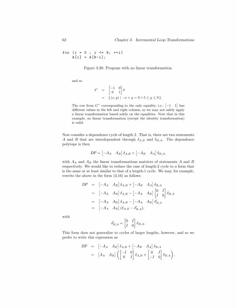
62 Chapter 3. Incremental Loop Transformations
for (i = 0 ; i <= 9; ++i)
A[i] = A[9-i];
Figure 3.20: Program with no linear transformation.
and so
δ∗ =
[−1 00 1
]
δ
= (x, y) | −x + y = 9 ∧ 5 ≤ y ≤ 9 .
The row from G+ corresponding to the only equality, i.e.,[−1 1
]has
different values in the left and right column, so we may not safely applya linear transformation based solely on the equalities. Note that in thisexample, no linear transformation (except the identity transformation)is valid.
Now consider a dependence cycle of length 2. That is, there are two statementsA and B that are interdependent through δA,B and δB,A. The dependencepolytope is then
DP =[−AA AB
]δA,B +
[−AB AA
]δB,A,
with AA and AB the linear transformations matrices of statements A and Brespectively. We would like to reduce the case of length-2 cycle to a form thatis the same or at least similar to that of a length-1 cycle. We may, for example,rewrite the above in the form (3.16) as follows
DP =[−AA AB
]δA,B +
[−AB AA
]δB,A
=[−AA AB
]δA,B −
[−AA AB
][0 II 0
]
δB,A
=[−AA AB
]δA,B −
[−AA AB
]δ′B,A
=[−AA AB
](δA,B − δ′B,A),
with
δ′B,A =
[0 II 0
]
δB,A.
This form does not generalize to cycles of larger lengths, however, and so weprefer to write this expression as
DP =[−AA AB
]δA,B +
[−AB AA
]δB,A
=[AA AB
]([
−I 00 I
]
δA,B +
[0 I−I 0
]
δB,A
)
,
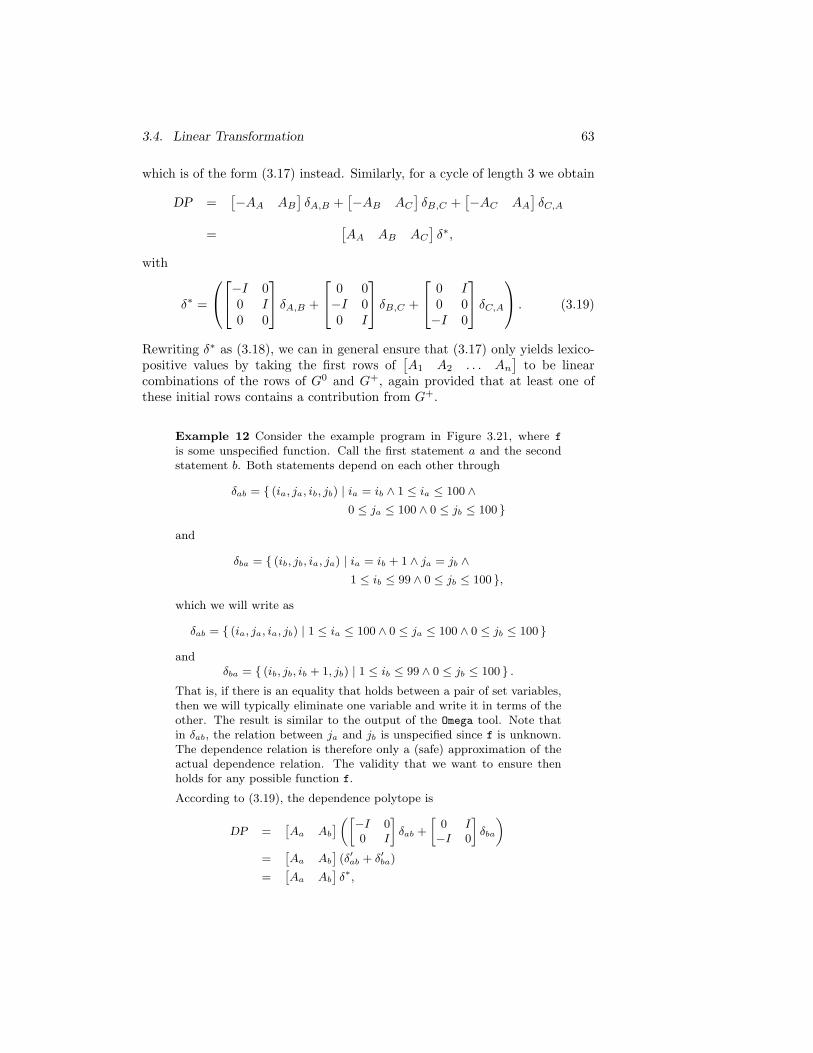
3.4. Linear Transformation 63
which is of the form (3.17) instead. Similarly, for a cycle of length 3 we obtain
DP =[−AA AB
]δA,B +
[−AB AC
]δB,C +
[−AC AA
]δC,A
=[AA AB AC
]δ∗,
with
δ∗ =
−I 00 I0 0
δA,B +
0 0−I 00 I
δB,C +
0 I0 0−I 0
δC,A
. (3.19)
Rewriting δ∗ as (3.18), we can in general ensure that (3.17) only yields lexico-positive values by taking the first rows of
[A1 A2 . . . An
]to be linear
combinations of the rows of G0 and G+, again provided that at least one ofthese initial rows contains a contribution from G+.
Example 12 Consider the example program in Figure 3.21, where f
is some unspecified function. Call the first statement a and the secondstatement b. Both statements depend on each other through
δab = (ia, ja, ib, jb) | ia = ib ∧ 1 ≤ ia ≤ 100 ∧0 ≤ ja ≤ 100 ∧ 0 ≤ jb ≤ 100
and
δba = (ib, jb, ia, ja) | ia = ib + 1 ∧ ja = jb ∧1 ≤ ib ≤ 99 ∧ 0 ≤ jb ≤ 100 ,
which we will write as
δab = (ia, ja, ia, jb) | 1 ≤ ia ≤ 100 ∧ 0 ≤ ja ≤ 100 ∧ 0 ≤ jb ≤ 100
andδba = (ib, jb, ib + 1, jb) | 1 ≤ ib ≤ 99 ∧ 0 ≤ jb ≤ 100 .
That is, if there is an equality that holds between a pair of set variables,then we will typically eliminate one variable and write it in terms of theother. The result is similar to the output of the Omega tool. Note thatin δab, the relation between ja and jb is unspecified since f is unknown.The dependence relation is therefore only a (safe) approximation of theactual dependence relation. The validity that we want to ensure thenholds for any possible function f.
According to (3.19), the dependence polytope is
DP =[Aa Ab
]([
−I 00 I
]
δab +
[0 I−I 0
]
δba
)
=[Aa Ab
](δ′ab + δ′ba)
=[Aa Ab
]δ∗,
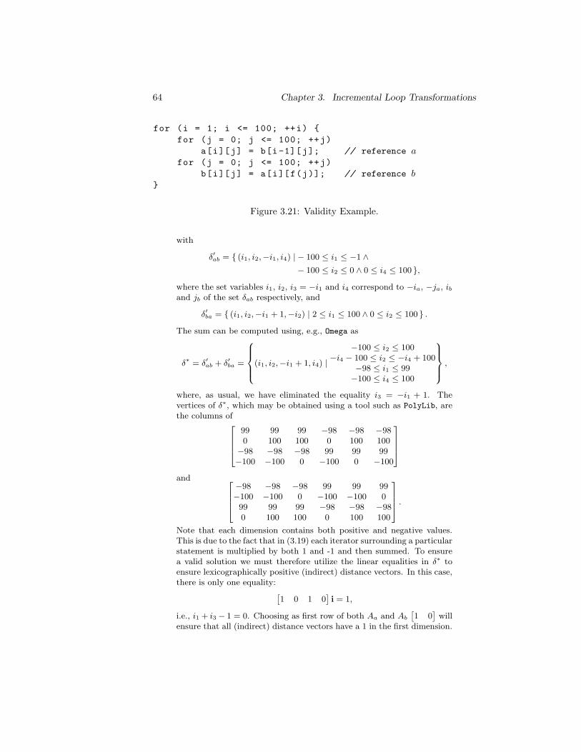
64 Chapter 3. Incremental Loop Transformations
for (i = 1; i <= 100; ++i)
for (j = 0; j <= 100; ++j)
a[i][j] = b[i-1][j]; // reference afor (j = 0; j <= 100; ++j)
b[i][j] = a[i][f(j)]; // reference b
Figure 3.21: Validity Example.
with
δ′ab = (i1, i2,−i1, i4) | − 100 ≤ i1 ≤ −1 ∧− 100 ≤ i2 ≤ 0 ∧ 0 ≤ i4 ≤ 100 ,
where the set variables i1, i2, i3 = −i1 and i4 correspond to −ia, −ja, iband jb of the set δab respectively, and
δ′ba = (i1, i2,−i1 + 1,−i2) | 2 ≤ i1 ≤ 100 ∧ 0 ≤ i2 ≤ 100 .
The sum can be computed using, e.g., Omega as
δ∗ = δ′ab + δ′ba =
(i1, i2,−i1 + 1, i4) |−100 ≤ i2 ≤ 100
−i4 − 100 ≤ i2 ≤ −i4 + 100−98 ≤ i1 ≤ 99
−100 ≤ i4 ≤ 100
,
where, as usual, we have eliminated the equality i3 = −i1 + 1. Thevertices of δ∗, which may be obtained using a tool such as PolyLib, arethe columns of
99 99 99 −98 −98 −980 100 100 0 100 100
−98 −98 −98 99 99 99−100 −100 0 −100 0 −100
and
−98 −98 −98 99 99 99−100 −100 0 −100 −100 099 99 99 −98 −98 −980 100 100 0 100 100
.
Note that each dimension contains both positive and negative values.This is due to the fact that in (3.19) each iterator surrounding a particularstatement is multiplied by both 1 and -1 and then summed. To ensurea valid solution we must therefore utilize the linear equalities in δ∗ toensure lexicographically positive (indirect) distance vectors. In this case,there is only one equality:
[1 0 1 0
]i = 1,
i.e., i1 + i3 − 1 = 0. Choosing as first row of both Aa and Ab
[1 0
]will
ensure that all (indirect) distance vectors have a 1 in the first dimension.
3.4. Linear Transformation 65
Example 13 Consider once more the example program in Figure 3.21on the previous page, but now assume that f is the identity function.The second dependence relation is not affected, but the first dependencerelation is now
δab = (i1, j1, i1, j1) | 1 ≤ i1 ≤ 100 ∧ 0 ≤ j1 ≤ 100
and after transformation
δ′ab = (i1, i2,−i1,−i2) | −100 ≤ i1 ≤ −1 ∧ −100 ≤ i2 ≤ 0
and so
δ∗ = δ′ab + δ′ba
= (i1, i2,−i1 + 1,−i2) | −98 ≤ i1 ≤ 99 ∧ −100 ≤ i2 ≤ 100 .
The vertices of δ∗ are:
99 −98 −98 99100 100 −100 −100−98 99 99 −98−100 −100 100 100
.
In this case, there are two equalities:
i3 = −i1 + 1
i4 = −i2
or [1 0 1 00 1 0 1
]
i =
[10
]
.
If we fix the first rows of the transformation matrices based on the firstequality, then validity is ensured and the remaining rows can be chosenarbitrarily. E.g., if we arbitrarily choose
[0 1
]as second row for both
transformation matrices, we obtain:
Aa = Ab =
[1 00 1
]
and the dependence polytope is
DP = (1, 0) .
If, for some reason, we were to choose a different second row for eitheror both of the transformation matrices, e.g.,
Aa =
[1 00 1
]
and Ab =
[1 01 1
]
,
we would still have a valid dependence polytope:
DP = (1, x) | −98 ≤ x ≤ 99 .
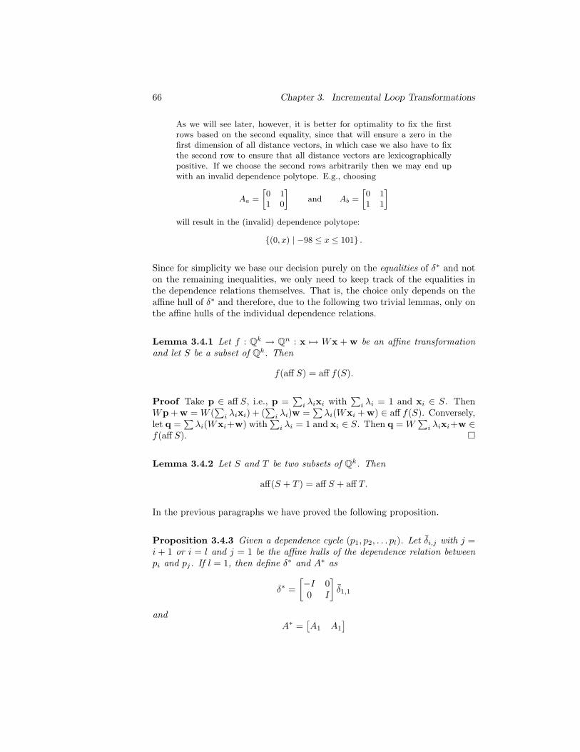
66 Chapter 3. Incremental Loop Transformations
As we will see later, however, it is better for optimality to fix the firstrows based on the second equality, since that will ensure a zero in thefirst dimension of all distance vectors, in which case we also have to fixthe second row to ensure that all distance vectors are lexicographicallypositive. If we choose the second rows arbitrarily then we may end upwith an invalid dependence polytope. E.g., choosing
Aa =
[0 11 0
]
and Ab =
[0 11 1
]
will result in the (invalid) dependence polytope:
(0, x) | −98 ≤ x ≤ 101 .
Since for simplicity we base our decision purely on the equalities of δ∗ and noton the remaining inequalities, we only need to keep track of the equalities inthe dependence relations themselves. That is, the choice only depends on theaffine hull of δ∗ and therefore, due to the following two trivial lemmas, only onthe affine hulls of the individual dependence relations.
Lemma 3.4.1 Let f : Qk → Qn : x 7→ Wx + w be an affine transformationand let S be a subset of Qk. Then
f(aff S) = aff f(S).
Proof Take p ∈ aff S, i.e., p =∑
i λixi with∑
i λi = 1 and xi ∈ S. ThenWp + w = W (
∑
i λixi) + (∑
i λi)w =∑
λi(Wxi + w) ∈ aff f(S). Conversely,let q =
∑λi(Wxi+w) with
∑
i λi = 1 and xi ∈ S. Then q = W∑
i λixi+w ∈f(aff S).
Lemma 3.4.2 Let S and T be two subsets of Qk. Then
aff(S + T ) = aff S + aff T.
In the previous paragraphs we have proved the following proposition.
Proposition 3.4.3 Given a dependence cycle (p1, p2, . . . pl). Let δi,j with j =i + 1 or i = l and j = 1 be the affine hulls of the dependence relation betweenpi and pj. If l = 1, then define δ∗ and A∗ as
δ∗ =
[−I 00 I
]
δ1,1
andA∗ =
[A1 A1
]
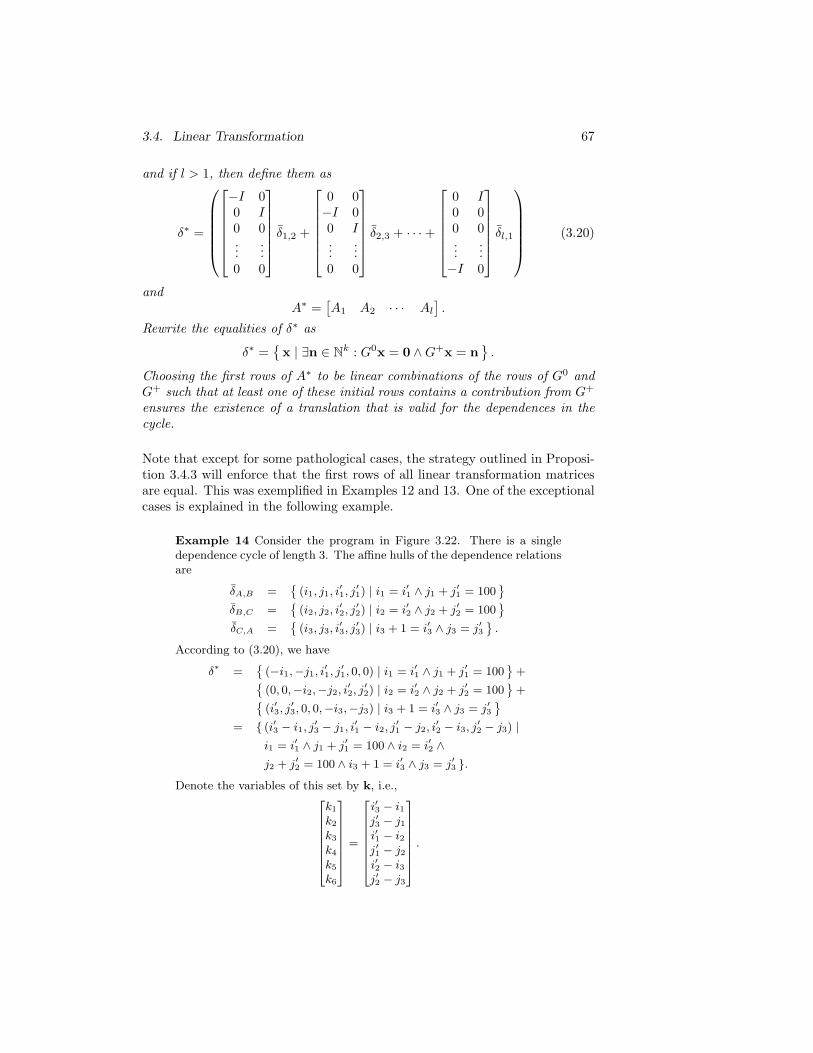
3.4. Linear Transformation 67
and if l > 1, then define them as
δ∗ =
−I 00 I0 0...
...0 0
δ1,2 +
0 0−I 00 I...
...0 0
δ2,3 + · · · +
0 I0 00 0...
...−I 0
δl,1
(3.20)
andA∗ =
[A1 A2 · · · Al
].
Rewrite the equalities of δ∗ as
δ∗ =x | ∃n ∈ Nk : G0x = 0 ∧ G+x = n
.
Choosing the first rows of A∗ to be linear combinations of the rows of G0 andG+ such that at least one of these initial rows contains a contribution from G+
ensures the existence of a translation that is valid for the dependences in thecycle.
Note that except for some pathological cases, the strategy outlined in Proposi-tion 3.4.3 will enforce that the first rows of all linear transformation matricesare equal. This was exemplified in Examples 12 and 13. One of the exceptionalcases is explained in the following example.
Example 14 Consider the program in Figure 3.22. There is a singledependence cycle of length 3. The affine hulls of the dependence relationsare
δA,B =
(i1, j1, i′1, j′1) | i1 = i′1 ∧ j1 + j′1 = 100
δB,C =
(i2, j2, i′2, j′2) | i2 = i′2 ∧ j2 + j′2 = 100
δC,A =
(i3, j3, i′3, j′3) | i3 + 1 = i′3 ∧ j3 = j′3
.
According to (3.20), we have
δ∗ =
(−i1,−j1, i′1, j′1, 0, 0) | i1 = i′1 ∧ j1 + j′1 = 100
+
(0, 0,−i2,−j2, i
′2, j′2) | i2 = i′2 ∧ j2 + j′2 = 100
+
(i′3, j
′3, 0, 0,−i3,−j3) | i3 + 1 = i′3 ∧ j3 = j′3
= (i′3 − i1, j′3 − j1, i
′1 − i2, j
′1 − j2, i
′2 − i3, j
′2 − j3) |
i1 = i′1 ∧ j1 + j′1 = 100 ∧ i2 = i′2 ∧j2 + j′2 = 100 ∧ i3 + 1 = i′3 ∧ j3 = j′3 .
Denote the variables of this set by k, i.e.,
k1
k2
k3
k4
k5
k6
=
i′3 − i1j′3 − j1i′1 − i2j′1 − j2i′2 − i3j′2 − j3
.
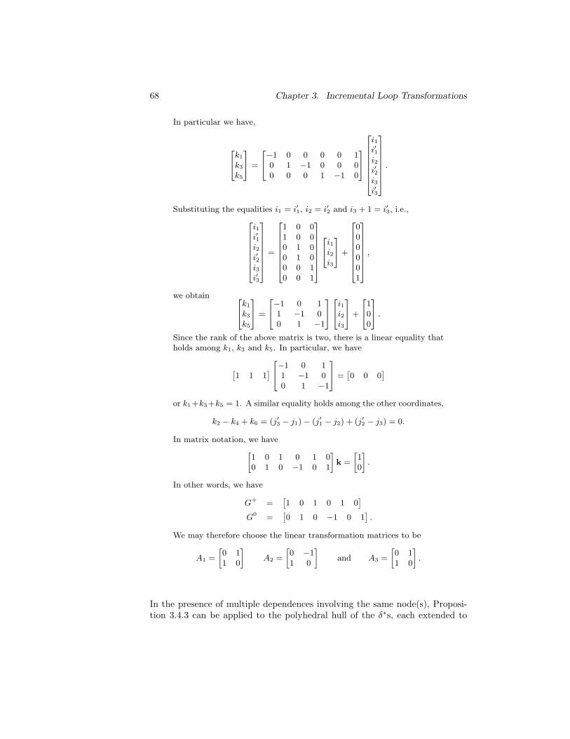
68 Chapter 3. Incremental Loop Transformations
In particular we have,
k1
k3
k5
=
−1 0 0 0 0 10 1 −1 0 0 00 0 0 1 −1 0
i1i′1i2i′2i3i′3
.
Substituting the equalities i1 = i′1, i2 = i′2 and i3 + 1 = i′3, i.e.,
i1i′1i2i′2i3i′3
=
1 0 01 0 00 1 00 1 00 0 10 0 1
i1i2i3
+
000001
,
we obtain
k1
k3
k5
=
−1 0 11 −1 00 1 −1
i1i2i3
+
100
.
Since the rank of the above matrix is two, there is a linear equality thatholds among k1, k3 and k5. In particular, we have
[1 1 1
]
−1 0 11 −1 00 1 −1
=[0 0 0
]
or k1+k3+k5 = 1. A similar equality holds among the other coordinates,
k2 − k4 + k6 = (j′3 − j1) − (j′1 − j2) + (j′2 − j3) = 0.
In matrix notation, we have
[1 0 1 0 1 00 1 0 −1 0 1
]
k =
[10
]
.
In other words, we have
G+ =[1 0 1 0 1 0
]
G0 =[0 1 0 −1 0 1
].
We may therefore choose the linear transformation matrices to be
A1 =
[0 11 0
]
A2 =
[0 −11 0
]
and A3 =
[0 11 0
]
.
In the presence of multiple dependences involving the same node(s), Proposi-tion 3.4.3 can be applied to the polyhedral hull of the δ∗s, each extended to
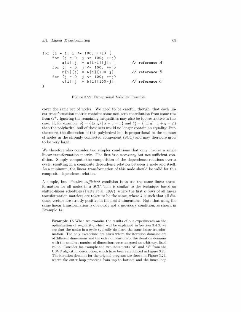
3.4. Linear Transformation 69
for (i = 1; i <= 100; ++i)
for (j = 0; j <= 100; ++j)
a[i][j] = c[i-1][j]; // reference Afor (j = 0; j <= 100; ++j)
b[i][j] = a[i][100-j]; // reference Bfor (j = 0; j <= 100; ++j)
c[i][j] = b[i][100-j]; // reference C
Figure 3.22: Exceptional Validity Example.
cover the same set of nodes. We need to be careful, though, that each lin-ear transformation matrix contains some non-zero contribution from some rowfrom G+. Ignoring the remaining inequalities may also be too restrictive in thiscase. If, for example, δ∗1 = (x, y) | x + y = 1 and δ∗2 = (x, y) | x + y = 2 then the polyhedral hull of these sets would no longer contain an equality. Fur-thermore, the dimension of this polyhedral hull is proportional to the numberof nodes in the strongly connected component (SCC) and may therefore growto be very large.
We therefore also consider two simpler conditions that only involve a singlelinear transformation matrix. The first is a necessary but not sufficient con-dition. Simply compute the composition of the dependence relations over acycle, resulting in a composite dependence relation between a node and itself.As a minimum, the linear transformation of this node should be valid for thiscomposite dependence relation.
A simple, but effective sufficient condition is to use the same linear trans-formation for all nodes in a SCC. This is similar to the technique based onshifted-linear schedules (Darte et al. 1997), where the first k rows of all lineartransformation matrices are taken to be the same, where k is such that all dis-tance vectors are strictly positive in the first k dimensions. Note that using thesame linear transformation is obviously not a necessary condition, as shown inExample 14.
Example 15 When we examine the results of our experiments on theoptimization of regularity, which will be explained in Section 3.4.3, wesee that the nodes in a cycle typically do share the same linear transfor-mation. The only exceptions are cases where the iteration domains areof different dimensions and the extra dimensions of the iteration domainswith the smallest number of dimensions were assigned an arbitrary, fixedvalue. Consider for example the two statements “3” and “7” from theUSVD algorithm description, which have been reproduced in Figure 3.23.The iteration domains for the original program are shown in Figure 3.24,where the outer loop proceeds from top to bottom and the inner loop
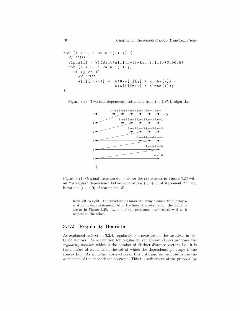
70 Chapter 3. Incremental Loop Transformations
for (i = 0; i <= n-1; ++i)
// ‘‘3’’
alpha[i] = W1(Wint(A[i][n+i]-Rin[i][i])*0.0625);
for (j = 0; j <= n-1; ++j)
if (j >= i)
// ‘‘7’’
A[j][n+i+1] = -W(Rin[i][j] * alpha[i]) +
W(A[j][n+i] * alpha[i]);
Figure 3.23: Two interdependent statements from the USVD algorithm.
i
j•0
•1
•2
•3
•4
•5
•0,n+1
•1,n+1
•1,n+2
•2,n+1
•2,n+2
•2,n+3
•3,n+1
•3,n+2
•3,n+3
•3,n+4
•4,n+1
•4,n+2
•4,n+3
•4,n+4
•4,n+5
•5,n+1
•5,n+2
•5,n+3
•5,n+4
•5,n+5
•5,n+6
Figure 3.24: Original iteration domains for the statements in Figure 3.23 withan “’irregular” dependence between iterations (i, i + 1) of statement “7” anditerations (i + 1, 0) of statement “3’.
from left to right. The annotations mark the array element from array A
written by each statement. After the linear transformation, the domainsare as in Figure 3.25, i.e., one of the polytopes has been skewed withrespect to the other.
3.4.2 Regularity Heuristic
As explained in Section 3.2.4, regularity is a measure for the variation in dis-tance vectors. As a criterion for regularity, van Swaaij (1992) proposes theregularity number, which is the number of distinct distance vectors, i.e., it isthe number of elements in the set of which the dependence polytope is theconvex hull. As a further abstraction of this criterion, we propose to use thedimension of the dependence polytope. This is a refinement of the proposal by
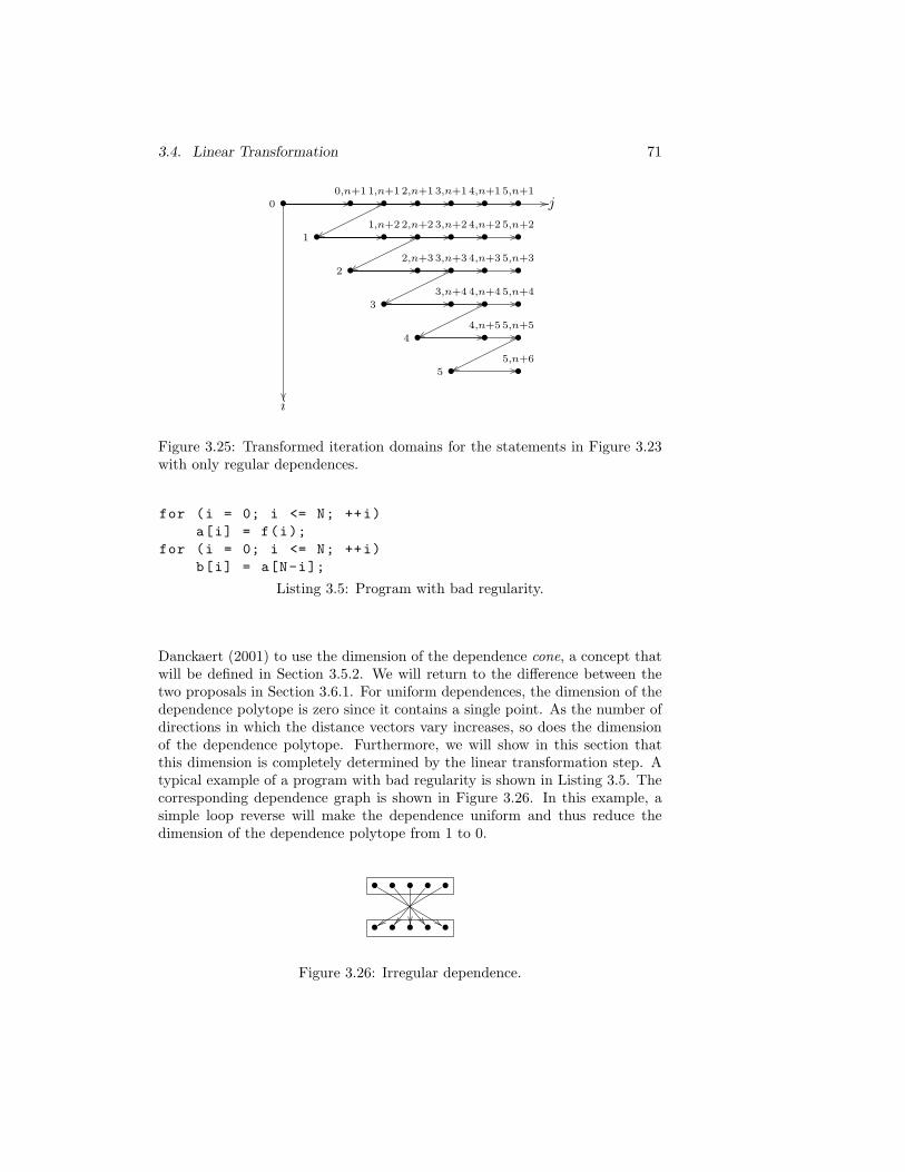
3.4. Linear Transformation 71
i
j•0
•1
•2
•3
•4
•5
•0,n+1
•1,n+1
•1,n+2
•2,n+1
•2,n+2
•2,n+3
•3,n+1
•3,n+2
•3,n+3
•3,n+4
•4,n+1
•4,n+2
•4,n+3
•4,n+4
•4,n+5
•5,n+1
•5,n+2
•5,n+3
•5,n+4
•5,n+5
•5,n+6
Figure 3.25: Transformed iteration domains for the statements in Figure 3.23with only regular dependences.
for (i = 0; i <= N; ++i)
a[i] = f(i);
for (i = 0; i <= N; ++i)
b[i] = a[N-i];
Listing 3.5: Program with bad regularity.
Danckaert (2001) to use the dimension of the dependence cone, a concept thatwill be defined in Section 3.5.2. We will return to the difference between thetwo proposals in Section 3.6.1. For uniform dependences, the dimension of thedependence polytope is zero since it contains a single point. As the number ofdirections in which the distance vectors vary increases, so does the dimensionof the dependence polytope. Furthermore, we will show in this section thatthis dimension is completely determined by the linear transformation step. Atypical example of a program with bad regularity is shown in Listing 3.5. Thecorresponding dependence graph is shown in Figure 3.26. In this example, asimple loop reverse will make the dependence uniform and thus reduce thedimension of the dependence polytope from 1 to 0.
• • • • •
•••••
Figure 3.26: Irregular dependence.
72 Chapter 3. Incremental Loop Transformations
During a search for a good or even optimal transformation, we may need toevaluate the dimension of the dependence polytope for many different instancesof transformation matrices. In this section we therefore derive a simple formulafor this dimension that avoids the computation of the actual dependence poly-tope. Furthermore, we derive a formula for the best possible dimension forany transformation matrix. This allows us to know when we have reached theoptimal case without an exhaustive search. We express both formulas for thegeneral case of a dependence represented by a dependence relation but alsoshow how each specializes for the case where a dependence can be representedby a pair of dependence domain and dependence function. In both cases, we seethat we do not need the full information available in the dependence relationor the dependence domain. As in the case of the validity criterion, it is suffi-cient to work with the affine hull of the dependence relation or the dependencedomain.2
Proposition 3.4.4 Let the dependence relation corresponding to the sourceprogram be defined by a polyhedron
δpc =
(x,y) ∈ Q2d | Gxx + Gyy = g ∧ Fxx + Fyy ≥ f
,
with Gxx + Gyy = g a maximal set of linearly independent equalities and letAp and Ac be affine transformations (3.2) applied to the iteration domains pand c, then the dimension of the dependence polytope rd := DP′pc in the targetprogram is
rd(Ap, Ac) = rank
[−Ap Ac
Gx Gy
]
− rank[Gx Gy
]. (3.21)
Proof After transformation by Ap and Ac, the (polyhedron defining the) de-pendence is given by
δ′pc =
[Ap 00 Ac
]
(x,y) ∈ Q2d | G
[xy
]
= g ∧ F
[xy
]
≥ f
+
[ap
ac
]
,
with F =[Fx Fy
]. and G =
[Gx Gy
]. The dependence polytope (2.11) is
then
DP′pq =[−Ap Ac
]
(x,y) ∈ Q2d | G
[xy
]
= g ∧ F
[xy
]
≥ f
+ ac − ap.
The offset ac−ap obviously does not influence the dimension and neither do theremaining inequalities (by Lemma 3.4.1). The desired dimension is therefore
rd = dim(Wz ∈ Q2d | Gz = g
), (3.22)
2In fact, we only need the lineality space Schrijver (1986) of the affine hulls.
3.4. Linear Transformation 73
with W =[−Ap Ac
]and z = (x,y). Let
Q :=z ∈ Q2d | Gz = g
.
The dimension k of Q is equal to the dimension 2d of the ambient space minusthe rank of the matrix defining the equalities,
k := dimQ = dimz ∈ Q2d | Gz = g
= 2d − rankG. (3.23)
Let X be a matrix with as columns a basis for the linear subspace parallel toQ, i.e.,
Q = z0 +z ∈ Q2d | ∃v ∈ Qk ∧ z = Xv
,
with z0 ∈ Q. Equation (3.22) can be rewritten as
rd = dim(Wz0 +
z ∈ Q2d | ∃v ∈ Qk ∧ z = WXv
). (3.24)
The dimension of the polyhedron in (3.24) is given by the dimension of theimage of the linear transformation f defined by
f : Qk → Q2d : w 7→ WXw.
For linear transformations with a k-dimensional domain, we know that
dim Ker f + dim Im f = k. (3.25)
The kernel of f are those vectors z ∈ Q that map to 0 under W , so
dim Ker f = dim
y ∈ Q2d |
[WG
]
y =
[0g
]
= 2d − rank
[WG
]
. (3.26)
Substituting (3.26) and (3.23) in (3.25), we obtain
rd = dim Im f = k − dim Ker f = (2d − rankG) −
(
2d − rank
[WG
])
,
whence (3.21).
If the dependence can be represented by a pair of a dependence domain DD anda dependence function DF and further assuming that the dependence functionis an affine function mapping x to Dx + d0, i.e., i = Dj + d0, then it followsfrom (2.9) that
G =
[−I D0 G′
]
, (3.27)
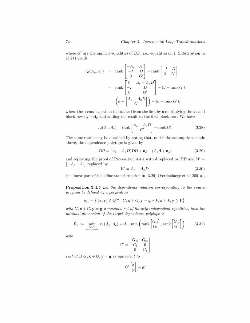
74 Chapter 3. Incremental Loop Transformations
where G′ are the implicit equalities of DD, i.e., equalities on j. Substitution in(3.21) yields
rd(Ap, Ac) = rank
−Ap Ac
−I D0 G′
− rank
[−I D0 G′
]
= rank
0 Ac − ApD−I D0 G′
− (d + rankG′)
=
(
d +
[Ac − ApD
G′
])
− (d + rankG′),
where the second equation is obtained from the first by a multiplying the secondblock row by −Ap and adding the result to the first block row. We have
rd(Ap, Ac) = rank
[Ac − ApD
G′
]
− rankG′. (3.28)
The same result may be obtained by noting that, under the assumptions madeabove, the dependence polytope is given by
DP = (Ac − ApD)DD + ac − (Apd + ap) (3.29)
and repeating the proof of Proposition 3.4.4 with δ replaced by DD and W =[−Ap Ac
]replaced by
W = Ac − ApD, (3.30)
the linear part of the affine transformation in (3.29) (Verdoolaege et al. 2001a).
Proposition 3.4.5 Let the dependence relation corresponding to the sourceprogram be defined by a polyhedron
δpc =
(x,y) ∈ Q2d | Gxx + Gyy = g ∧ Fxx + Fyy ≥ f
,
with Gxx + Gyy = g a maximal set of linearly independent equalities, then theminimal dimension of the target dependence polytope is
Rd := minAp,Ac
non-singular
rd(Ap, Ac) = d − min
(
rank
[Gcl
Gl
]
, rank
[Gcr
Gr
])
, (3.31)
with
G′ =
Gcl Gcr
Gl 00 Gr
such that Gxx + Gyy = g is equivalent to
G′[xy
]
= g′
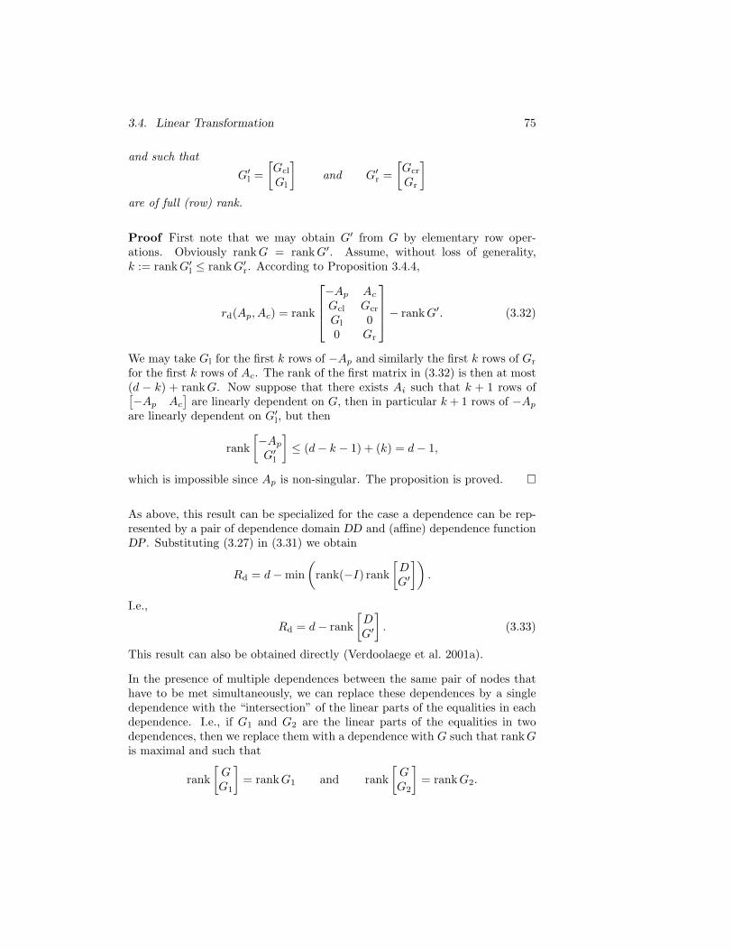
3.4. Linear Transformation 75
and such that
G′l =
[Gcl
Gl
]
and G′r =
[Gcr
Gr
]
are of full (row) rank.
Proof First note that we may obtain G′ from G by elementary row oper-ations. Obviously rankG = rankG′. Assume, without loss of generality,k := rankG′l ≤ rankG′r. According to Proposition 3.4.4,
rd(Ap, Ac) = rank
−Ap Ac
Gcl Gcr
Gl 00 Gr
− rankG′. (3.32)
We may take Gl for the first k rows of −Ap and similarly the first k rows of Gr
for the first k rows of Ac. The rank of the first matrix in (3.32) is then at most(d − k) + rankG. Now suppose that there exists Ai such that k + 1 rows of[−Ap Ac
]are linearly dependent on G, then in particular k + 1 rows of −Ap
are linearly dependent on G′l, but then
rank
[−Ap
G′l
]
≤ (d − k − 1) + (k) = d − 1,
which is impossible since Ap is non-singular. The proposition is proved.
As above, this result can be specialized for the case a dependence can be rep-resented by a pair of dependence domain DD and (affine) dependence functionDP. Substituting (3.27) in (3.31) we obtain
Rd = d − min
(
rank(−I) rank
[DG′
])
.
I.e.,
Rd = d − rank
[DG′
]
. (3.33)
This result can also be obtained directly (Verdoolaege et al. 2001a).
In the presence of multiple dependences between the same pair of nodes thathave to be met simultaneously, we can replace these dependences by a singledependence with the “intersection” of the linear parts of the equalities in eachdependence. I.e., if G1 and G2 are the linear parts of the equalities in twodependences, then we replace them with a dependence with G such that rankGis maximal and such that
rank
[GG1
]
= rankG1 and rank
[GG2
]
= rankG2.
76 Chapter 3. Incremental Loop Transformations
3.4.3 Regularity Experiments
In this section we discuss three search strategies for optimizing regularity andthe result of applying these strategies to a number of examples. Note thatduring these experiments we only consider regularity. That is, for the momentwe ignore validity or any other optimization criterion such as the locality tobe discussed in Section 3.4.4. Self dependences are therefore ignored, sincethe dimension of the corresponding dependence polytopes is not influenced byapplying a linear (non-singular) mapping. We further restrict our attention inthis section to dependences represented by a pair of dependence domain anddependence function. Extending these experiments to also consider validityand other optimization criteria is left to future work (Yang 2005).
No Cycles
The dependence graph is a directed graph with the statements with their iter-ation domain polytopes as vertices and for each dependence, an edge from theproduction iteration domain to the consumption iteration domain. The undi-rected dependence graph is the underlying undirected graph. If the undirecteddependence graph contains no cycles, then a solution can be found trivially.After assigning an arbitrary linear transformation, e.g., the identity transfor-mation, to all iteration domains that do not depend on any other iterationdomain, a linear transformation that yields optimal regularity (3.33) can beassigned to all the other polytopes on the basis of (3.30) while traversing thedependence graph.
The technique to be used is very simple. Assuming that the linear part W(3.30) of the affine transformation mapping the dependence domain to thedependence polytope can be made zero, i.e., the linear part of the dependencefunction D is of full rank, we can simply use
Ac = ApD. (3.34)
Otherwise, Ac can be adjusted using rows from G and, in case of self reuse,where the optimal dimension Rd is strictly positive, Rd arbitrary rows.
It is important to realize that it is the undirected dependence graph whichshould be cycle-free. The reason is that two constraints of the form (3.34) canconflict. That is, we may have
Ac = ApD1
Ac = ApD2,
with D1 6= D2. At first sight, then, this search strategy does not seem to beapplicable to the simple example from Figure 2.1, since it has two dependencesbetween polytopes X and Y . As far as the regularity criterion is concerned,
3.4. Linear Transformation 77
however, the two dependences are the same, because the dependence functionsare identical and the dependence domains have the same affine hull.
If the undirected dependence graph does contain cycles, the method can beused on the quotient graph based on the strongly connected components of theundirected dependence graph. Within an SCC one of the more complicatedtechniques below can be used. As a heuristic, the method could also be usedon a spanning tree of an SCC. If this yields an optimal solution for the wholeSCC, there is no need to use any of the other techniques.
No Self-Reuse and no Conflicts
If an SCC contains no dependence with self reuse, then the optimal dimension(3.33) for each dependence is zero. Due to conflicting constraints, it may not bepossible to reach this optimal dimension for each of the dependences. Even ifit is possible, then the previous method may still not be able to find it, becauseit only selects one of the possibly many optimal transformations for a givendependence. To avoid this problem, the method in this section manipulates acompact representation of all possible transformations that may still lead to anoptimal solution.
This compact representation is composed of one of the possible transformationmatrices and the set of rows that can be used to create the others. We call thesethe representative and the linear freedom respectively. Suppose the productionpolytope of a given dependence has representative A′p and linear freedom Lp,i.e.,
Ap = A′p + MpLp, (3.35)
where Lp is an l × n matrix and Mp any n × l matrix, then, using (3.34) andtaking into account the implicit equalities of the dependence,
Ac = A′pD + MpLpD + McG = A′c + MLc (3.36)
with
Lc =
[LpDG
]
and M =[Mp Mc
],
which is again of the same form as (3.35). It is also possible to traverse adependence in the opposite direction, by using
Ap = AcD−1 (3.37)
with D adjusted with rows from G in case it is singular.
If a polytope is involved in more than one dependence, then several constraintsof the form (3.35) will have to be combined. Suppose we have two constraints
A = A1 + M1L1 and A = A2 + M2L2.
78 Chapter 3. Incremental Loop Transformations
To ensure the existence of an A satisfying both constraints, an M1 and an M2
must exist such that
A1 + M1L1 = A2 + M2L2. (3.38)
Furthermore, the linear freedom will be restricted to the “intersection” of L1
and L2, that is, a basis for the intersection of the vector spaces generatedby L1 and L2. Let L∩ be this intersection and let La and Lb be such thattogether with L∩ they form bases for the vector spaces generated by L1 andL2 respectively. Then to be able to solve (3.38), we must have
A1 − A2 = M∩L∩ + MaLa + MbLb
for some M∩, Ma and Mb and we can take A2+MaLa (or A1−MbLb; they onlydiffer in a multiple of the common linear freedom) as the new representative ofthe linear transformation and the new combined constraint of the form (3.35)will be
A = (A2 + MaLa) + ML∩,
i.e., A2 + MaLa is the representative, L∩ is the linear freedom and M is anarbitrary matrix. The Ms are chosen such that the new representative is uni-modular, i.e., with determinant ±1. If no such choice can be made, this isconsidered to be a conflict.
To assign a unimodular transformation to each of the polytopes in the SCC,an arbitrary polytope is first selected and assigned an identity representativeand no linear freedom. This will be the first constrained polytope. The algo-rithm then iterates over all dependences with at least one constrained polytope,generating constraints using (3.36) and/or its backward counterpart. If bothpolytopes were already constrained, the newly generated constraints are com-bined with the existing ones and if any of the existing ones changes, thesechanges are propagated through the dependences that have been consideredpreviously. This continues until all polytopes in the SCC have been consideredor a conflict has been found. In the former case, the representatives can beused as transformation matrices.
As with the previous algorithm, the method can be used as a heuristic inmore general cases, by first considering a subgraph, i.e., one containing onlydependences without self reuse, and afterward evaluating the solution foundfor the other dependences. If a conflict is found, either during the constructionor during the evaluation for the other dependences, we may still be able toidentify subregions of the SCC free of conflicts. The general method of thenext section can then be used on the reduced graph over those subregions, i.e.,the graph in which each already optimized subregion is replaced by a singlenode.
3.4. Linear Transformation 79
General Case
For the general case of a cyclic dependence graph with dependences exhibitingself reuse and/or conflicting constraints, we solve a sequence of incrementalbacktracking searches, each searching for a better solution than the previousone. This search strategy is a refinement of the strategy outlined by Danckaert(2001, Section 6.5).
In a preprocessing step, we select a set of possible mappings for each polytope.Initially this set A comprises all unimodular n×n matrices consisting entirely of0s and 1s. For each polytope i, the set is reduced over the equivalence relationRi:
Ai = A/Ri
withA1 Ri A2 ⇐⇒ A1 − A2 = M · Gi,
the equivalence relation identifying all matrices that are equal up to a multipleof the linear equalities Gi for the given polytope.
Example 16 Consider once more the example program discussed in Ex-ample 6 with 2-dimensional iteration domains. The set of all unimodular2 × 2 matrices consisting entirely of 0s and 1s is
A =
[0 11 0
]
,
[1 11 0
]
,
[1 00 1
]
,
[1 01 1
]
,
[1 10 1
]
,
[0 11 1
]
.
The iteration domains SX and SZ are full-dimensional and we thereforehave AX = AZ = A. For the iteration domain SY we have the linearequality
[1 0
][qp
]
= 1
and it is therefore sufficient to consider, e.g., the unimodular matrices
AY =
[0 11 0
]
,
[1 00 1
]
,
[1 10 1
]
as the other matrices can be obtained from these matrices by addingmultiples of the row
[1 0
].
Each of the backtracking searches solves a set of constraints of the followingform for each of the dependences between polytopes:
rd ≤ c, (3.39)
where rd is the dimension of the dependence polytope (3.28) and c is a con-stant. Initially all cs are set equal to the dimension of the problem n and “thesolution of the previous search” is the solution corresponding to an identitymapping for each polytope. In each step, one of the cs is decreased by one. If
80 Chapter 3. Incremental Loop Transformations
the solution of the previous search no longer satisfies the resulting set of con-straints (3.39), a new backtracking search is initiated over the elements of Ai.The algorithm terminates when each c has reached the corresponding optimalvalue Rd (3.33). If one of the backtracking searches does not yield a solution,the c-value decreased last and its corresponding optimal value are set to thecurrent value of c plus one. The order in which the c-values are decreased cor-responds to the “importance” of the dependences. A dependence with a largerdependence domain is considered more important.
A number of optimizations are used within the backtracking search. Backjump-ing is performed and on a jump back, the polytopes are reordered such thatthe level where the jump back occurs is moved directly under the level thatis jumped back to. The polytopes are also reordered after a fixed number ofiterations based on the conflicts that have occurred. This order is kept over thesuccessive searches except that the two polytopes whose dependence constraintwas tightened are placed first. The set of possible mappings is ordered suchthat the solution of the previous search is placed first. This will obviously notdirectly yield a solution, but is usually a good starting point.
The reasons for performing a sequence of backtracking searches are many. First,directly solving for the optimal dimension, may not yield a solution. Second,transferring the ordering of the polytopes based on the conflicts in one search,may greatly increase the speed of subsequent searches. Finally, if the globalsearch takes too long, it can be interrupted and still yield a (sub-optimal)solution.
Results
We have implemented the search strategies explained previously in this sectionin a matlab prototype-tool and we will now present the results of the appli-cation of the tool to two examples: an algorithm for computing the USVDand Durbin’s algorithm. We further compare our results to those of Danckaert(2001) on three examples, including the USVD algorithm and the simple ex-ample from Figure 2.1.
The USVD algorithm is frequently used in signal processing applications. Al-though it is not the largest of algorithms we wish to handle, it was already toolarge to be handled by the approach described by Danckaert et al. (2000). Itconsists of four loop nests of maximally three nestings deep with statements atvarious levels of nesting, making it a three-dimensional problem. The polyhe-dral representation of the algorithm contain 26 polytopes and 87 dependences,six of which are self dependences and hence ignored when optimizing the di-mensions of the dependence polytopes.
An optimal solution is found using the backtracking search in a total numberof only 1990 iterations over all searches. Each iteration corresponds to a choice
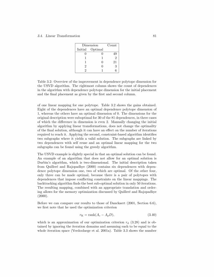
3.4. Linear Transformation 81
Dimension CountInitial Optimal
0 0 491 1 21 0 212 0 32 1 6
Table 3.2: Overview of the improvement in dependence polytope dimension forthe USVD algorithm. The rightmost column shows the count of dependencesin the algorithm with dependence polytope dimension for the initial placementand the final placement as given by the first and second column.
of one linear mapping for one polytope. Table 3.2 shows the gains obtained.Eight of the dependences have an optimal dependence polytope dimension of1, whereas the others have an optimal dimension of 0. The dimensions for theoriginal description were suboptimal for 30 of the 81 dependences, in three casesof which the difference in dimension is even 2. Manually changing the initialalgorithm by applying linear transformations, does not change the optimalityof the final solution, although it can have an effect on the number of iterationsrequired to reach it. Applying the second, constraint-based algorithm identifiestwo subgraphs where it yields a valid solution. The subgraphs are linked bytwo dependences with self reuse and an optimal linear mapping for the twosubgraphs can be found using the greedy algorithm.
The USVD example is slightly special in that an optimal solution can be found.An example of an algorithm that does not allow for an optimal solution isDurbin’s algorithm, which is two-dimensional. The initial description takenfrom Quillere and Rajopadhye (2000) contains six dependences with depen-dence polytope dimension one, two of which are optimal. Of the other four,only three can be made optimal, because there is a pair of polytopes withdependences that impose conflicting constraints on the linear mappings. Thebacktracking algorithm finds the best sub-optimal solution in only 50 iterations.The resulting mapping, combined with an appropriate translation and order-ing allows for the memory optimization discussed by Quillere and Rajopadhye(2000).
Before we can compare our results to those of Danckaert (2001, Section 6.6),we first note that he used the optimization criterion
rK = rank(Ac − ApD), (3.40)
which is an approximation of our optimization criterion rd (3.28) and is ob-tained by ignoring the iteration domains and assuming each to be equal to thewhole iteration space (Verdoolaege et al. 2001a). Table 3.3 shows the number
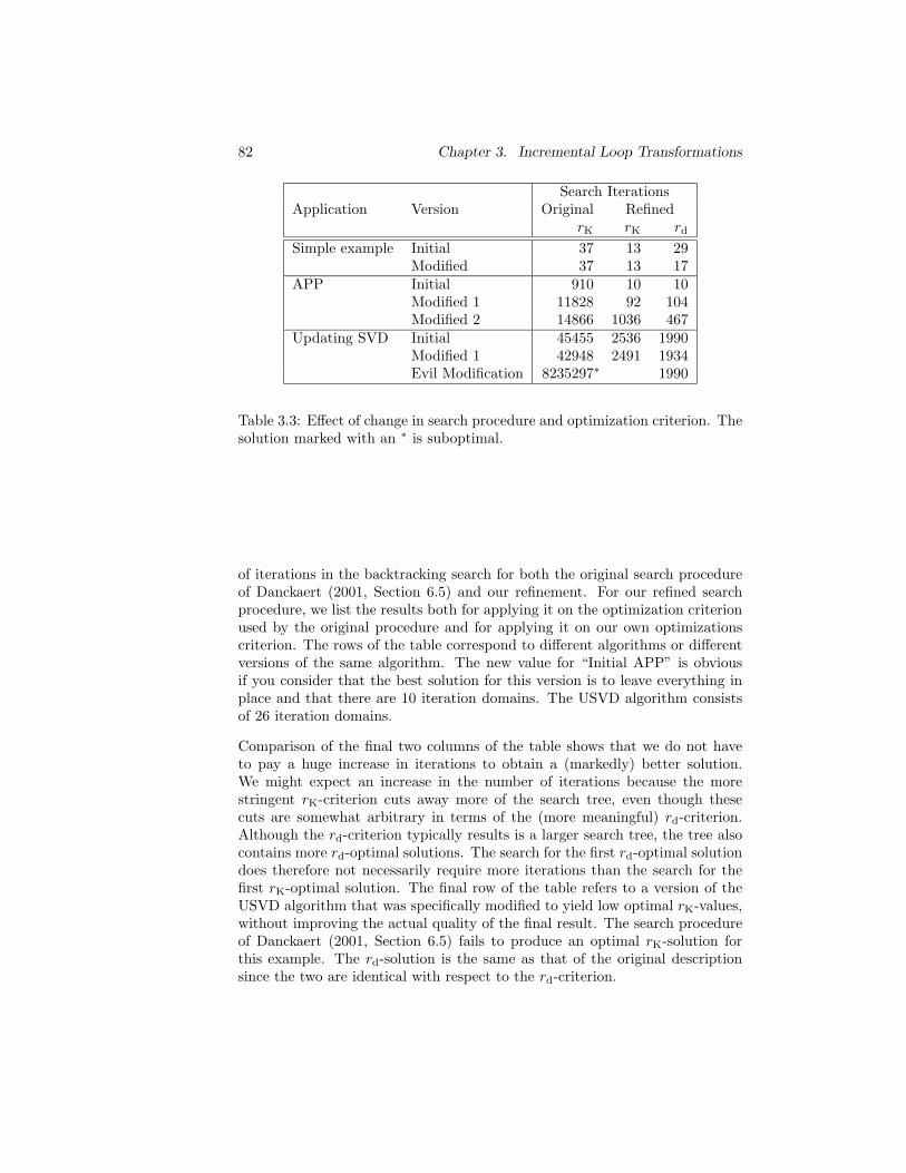
82 Chapter 3. Incremental Loop Transformations
Search IterationsApplication Version Original Refined
rK rK rd
Simple example Initial 37 13 29Modified 37 13 17
APP Initial 910 10 10Modified 1 11828 92 104Modified 2 14866 1036 467
Updating SVD Initial 45455 2536 1990Modified 1 42948 2491 1934Evil Modification 8235297∗ 1990
Table 3.3: Effect of change in search procedure and optimization criterion. Thesolution marked with an ∗ is suboptimal.
of iterations in the backtracking search for both the original search procedureof Danckaert (2001, Section 6.5) and our refinement. For our refined searchprocedure, we list the results both for applying it on the optimization criterionused by the original procedure and for applying it on our own optimizationscriterion. The rows of the table correspond to different algorithms or differentversions of the same algorithm. The new value for “Initial APP” is obviousif you consider that the best solution for this version is to leave everything inplace and that there are 10 iteration domains. The USVD algorithm consistsof 26 iteration domains.
Comparison of the final two columns of the table shows that we do not haveto pay a huge increase in iterations to obtain a (markedly) better solution.We might expect an increase in the number of iterations because the morestringent rK-criterion cuts away more of the search tree, even though thesecuts are somewhat arbitrary in terms of the (more meaningful) rd-criterion.Although the rd-criterion typically results is a larger search tree, the tree alsocontains more rd-optimal solutions. The search for the first rd-optimal solutiondoes therefore not necessarily require more iterations than the search for thefirst rK-optimal solution. The final row of the table refers to a version of theUSVD algorithm that was specifically modified to yield low optimal rK-values,without improving the actual quality of the final result. The search procedureof Danckaert (2001, Section 6.5) fails to produce an optimal rK-solution forthis example. The rd-solution is the same as that of the original descriptionsince the two are identical with respect to the rd-criterion.
3.4. Linear Transformation 83
3.4.4 Locality Heuristic
As explained in Section 3.2.4, the translation step should optimize locality overgroup dependences, whereas the linear transformation step should optimizeregularity as an enabling step for the locality optimization and should alsooptimize locality over (indirect) self dependences. In the presence of reuse,we basically follow the ideas of Wolf and Lam (1991), but apply them to thedependence relation abstraction.
We first recall the main ideas behind the locality optimization of Wolf andLam (1991). Consider an access that exhibits some reuse, i.e., an access thatreads the same array element more than once. This corresponds to a selfinput dependence. Let the (affine) access function be f(i) = Hi + h, then twoiterations i1 and i2 access the same array element if
Hi1 + h = Hi2 + h,
i.e., if H(i1 − i2) = 0. If Hed = 0, where d is the loop nest depth, thensuccessive iterations in the inner loop will access the same array element, whichis the optimal case.
After performing the affine transformation
i′ = Ai + a
we would like to have as much reuse as possible in the inner loops. Rewritingthe above equation as
i = Qi′ − Qa,
with Q = A−1, where we assume that A is unimodular, we have Hi1 + h =Hi2 + h if and only if HQ(i′1 − i′2) = 0. There is reuse in the inner loop ifHQed = 0, i.e., if
qd ∈ Ker H,
where qd is the final column of Q. If the dimension of KerH is l > 1, then wecan also obtain reuse in the second innermost dimension up to the lth innermostdimension by choosing l linearly independent vectors qd−l+1, . . . ,qd−1,qd from KerH.
We can express (almost) the same requirement using dependence relations asfollows. Let δ be the self input dependence, i.e.,
δ = (i, j) | Hi = Hj .
We want the elements of the corresponding dependence polytope
DP =[−A A
]δ
to be non-zero in the innermost dimensions. If the length of the innermostloops is greater than 2, then the dependence vectors will also have different
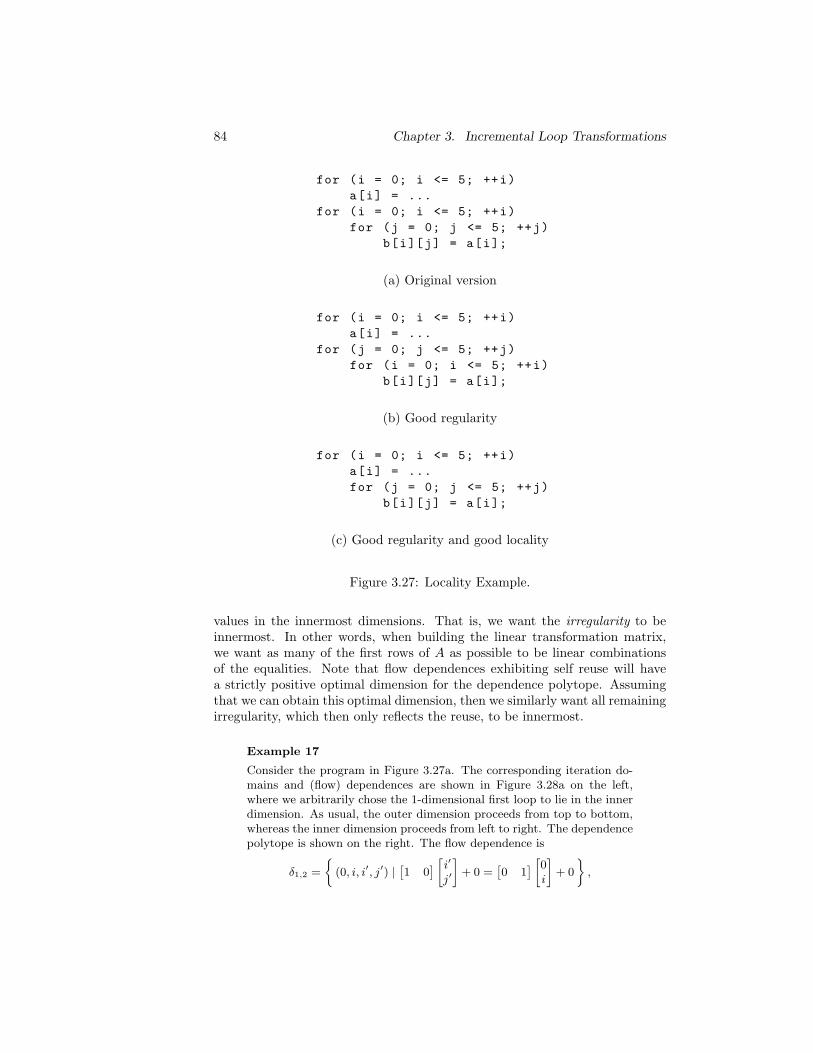
84 Chapter 3. Incremental Loop Transformations
for (i = 0; i <= 5; ++i)
a[i] = ...
for (i = 0; i <= 5; ++i)
for (j = 0; j <= 5; ++j)
b[i][j] = a[i];
(a) Original version
for (i = 0; i <= 5; ++i)
a[i] = ...
for (j = 0; j <= 5; ++j)
for (i = 0; i <= 5; ++i)
b[i][j] = a[i];
(b) Good regularity
for (i = 0; i <= 5; ++i)
a[i] = ...
for (j = 0; j <= 5; ++j)
b[i][j] = a[i];
(c) Good regularity and good locality
Figure 3.27: Locality Example.
values in the innermost dimensions. That is, we want the irregularity to beinnermost. In other words, when building the linear transformation matrix,we want as many of the first rows of A as possible to be linear combinationsof the equalities. Note that flow dependences exhibiting self reuse will havea strictly positive optimal dimension for the dependence polytope. Assumingthat we can obtain this optimal dimension, then we similarly want all remainingirregularity, which then only reflects the reuse, to be innermost.
Example 17
Consider the program in Figure 3.27a. The corresponding iteration do-mains and (flow) dependences are shown in Figure 3.28a on the left,where we arbitrarily chose the 1-dimensional first loop to lie in the innerdimension. As usual, the outer dimension proceeds from top to bottom,whereas the inner dimension proceeds from left to right. The dependencepolytope is shown on the right. The flow dependence is
δ1,2 =
(0, i, i′, j′) |[1 0
][i′
j′
]
+ 0 =[0 1
][0i
]
+ 0
,
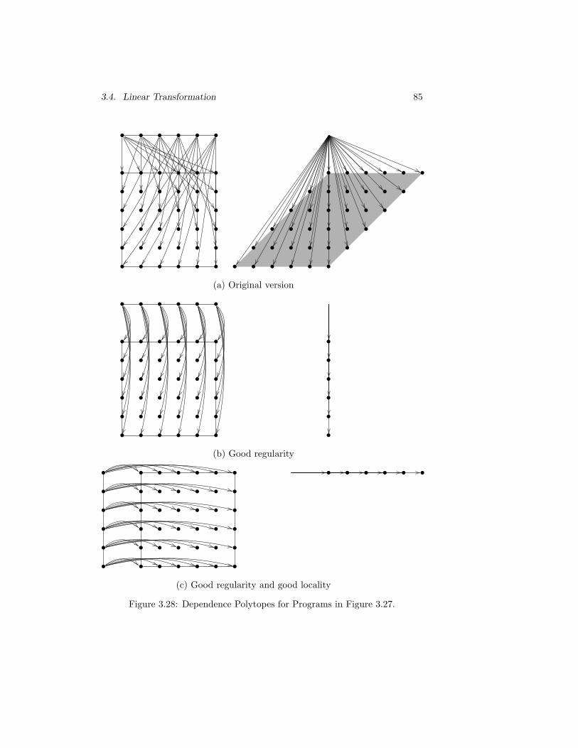
3.4. Linear Transformation 85
• • • • • •
•
•
•
•
•
•
•
•
•
•
•
•
•
•
•
•
•
•
•
•
•
•
•
•
•
•
•
•
•
•
•
•
•
•
•
•
•
•
•
•
•
•
•
•
•
•
•
•
•
•
•
•
•
•
•
•
•
•
•
•
•
•
•
•
•
•
•
•
•
•
•
•
(a) Original version
• • • • • •
• • • • • •
• • • • • •
• • • • • •
• • • • • •
• • • • • •
• • • • • •
•
•
•
•
•
•
(b) Good regularity
•
•
•
•
•
•
•
•
•
•
•
•
•
•
•
•
•
•
•
•
•
•
•
•
•
•
•
•
•
•
•
•
•
•
•
•
•
•
•
•
•
•
• • • • • •
(c) Good regularity and good locality
Figure 3.28: Dependence Polytopes for Programs in Figure 3.27.
86 Chapter 3. Incremental Loop Transformations
whereas the self input dependence on the second statement is
δ2,2 =
(i, j, i′, j′) |[1 0
][i′
j′
]
+ 0 =[1 0
][ij
]
+ 0
.
Each has a single equality,
[0 −1 1 0
]
0ii′
j′
= 0
and
[−1 0 1 0
]
iji′
j′
= 0
in the flow and input dependence respectively, i.e.,
G1,2 =[0 −1 1 0
]and G2,2 =
[−1 0 1 0
].
The original program corresponds to linear transformation matrices equalto the identity matrix. In this case
[−A1 A2
]=
[−1 0 1 00 −1 0 1
]
and[−A2 A2
]=
[−1 0 1 00 −1 0 1
]
.
We see that G1,2 is not a linear combination of the rows of[−A1 A2
]
and so the dimension of the dependence polytope (3.21) for the flowdependence is
rank
−1 0 1 00 −1 0 10 −1 1 0
− rank[0 −1 1 0
]= 3 − 1 = 2.
The minimum dimension (3.31) is
2 − min(rank
[0 −1
], rank
[1 0
])= 1,
however. For the input dependence, the first row of[−A2 A2
]is equal
to G2,2 and so the dimension of the dependence polytope for this depen-dence is 1, which is also the minimum.
Now consider the program in Figure 3.27b, where the loops surroundingthe second statement have been interchanges, which corresponds to thelinear transformation
A2 =
[0 11 0
]
.
We have[−A1 A2
]=
[−1 0 0 10 −1 1 0
]
3.4. Linear Transformation 87
and[−A2 A2
]=
[0 −1 0 1−1 0 1 0
]
.
The second row of[−A1 A2
]is now equal to G1,2 and so the dimension
of the dependence polytope is 1, as shown in Figure 3.28b on the right.Since it is the second row, however, we see that the reuse occurs in theouter dimension. Similarly for the input dependence, it is now the secondrow that is equal to G2,2.
Finally the program in Figure 3.27c corresponds to the transformations
A1 =
[0 11 0
]
and A2 =
[1 00 1
]
.
We now have[−A1 A2
]=
[0 −1 1 0−1 0 0 1
]
and[−A2 A2
]=
[−1 0 1 00 −1 0 1
]
and so for both dependences, the first row corresponds to the equality inthe dependence. That is, we have both good regularity and good locality.Note that the transformation corresponds to a “loop interchange” of thefirst “loop nest”. If we would have chosen this 1-dimensional loop to liein the outer dimension, then we would have obtained this solution byaccident.
In the absence of reuse or in the case of minimal reuse, i.e., in case of a loop oflength 2, we can still enhance locality of self dependences by making as manyof the initial coordinates of the distance vectors zero. This means that it is notsufficient to look at the linear part of the equalities, but that we also need toconsider the constant part. In particular, we need to use equalities from G0 forthe initial rows of the linear transformation matrices. We already applied thisheuristic in Example 13 and we will do so again in the next subsection.
3.4.5 Example
Recall the example shown in Figure 2.2 on page 18. The mapping of the itera-tion domains to the common iteration space used in this figure corresponds tothe original execution order of the program. As usual, the fixed order proceedstop down, left to right. This ordering is made more explicit in the figure bymeans of an equivalent ordering vector attached to a hyperplane (broken line)that scans the iteration space. The position of the hyperplane corresponds tothe point in the execution after the first loop has been executed and beforethe second loop is executed. Each dependence “cut” by this hyperplane cor-responds to a value that has been written already but has not been read yet.
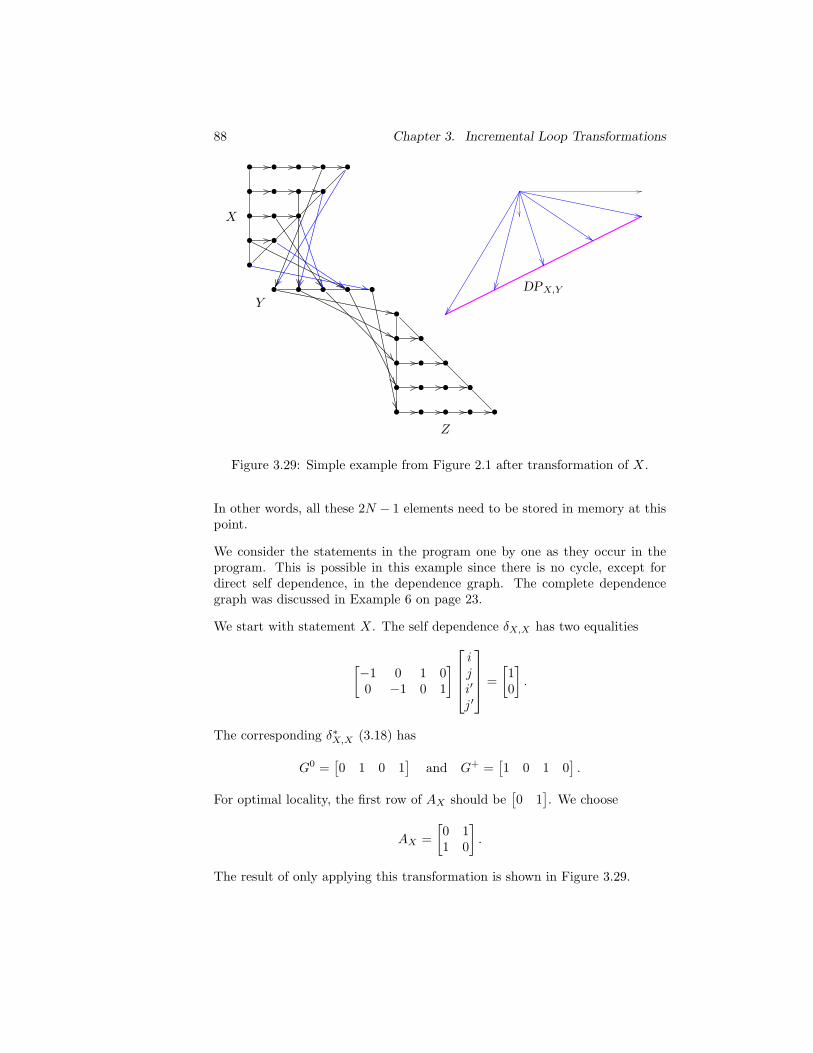
88 Chapter 3. Incremental Loop Transformations
DPX,Y
•
•
•
•
•
•
•
•
•
•
•
•
•
•
•
• • • • •
•
• •
• • •
• • • •
• • • • •
X
Y
Z
Figure 3.29: Simple example from Figure 2.1 after transformation of X.
In other words, all these 2N − 1 elements need to be stored in memory at thispoint.
We consider the statements in the program one by one as they occur in theprogram. This is possible in this example since there is no cycle, except fordirect self dependence, in the dependence graph. The complete dependencegraph was discussed in Example 6 on page 23.
We start with statement X. The self dependence δX,X has two equalities
[−1 0 1 00 −1 0 1
]
iji′
j′
=
[10
]
.
The corresponding δ∗X,X (3.18) has
G0 =[0 1 0 1
]and G+ =
[1 0 1 0
].
For optimal locality, the first row of AX should be[0 1
]. We choose
AX =
[0 11 0
]
.
The result of only applying this transformation is shown in Figure 3.29.
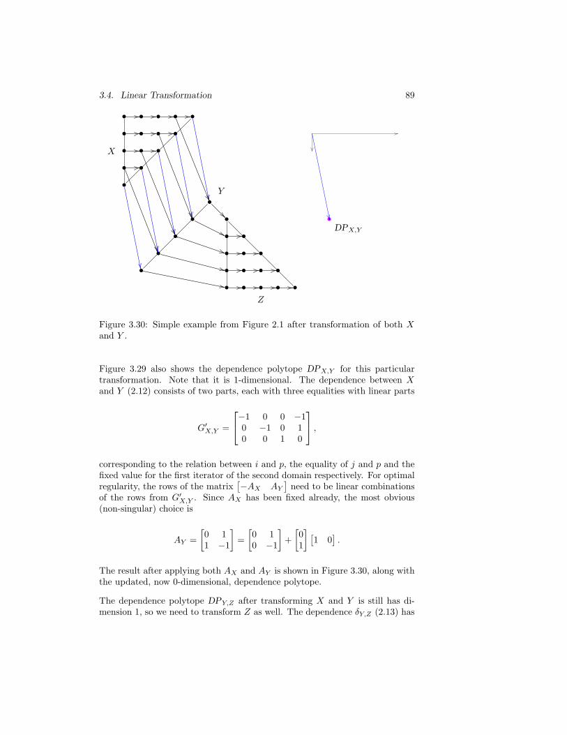
3.4. Linear Transformation 89
•DPX,Y
•
•
•
•
•
•
•
•
•
•
•
•
•
•
•
•
•
•
•
•
•
• •
• • •
• • • •
• • • • •
X
Y
Z
Figure 3.30: Simple example from Figure 2.1 after transformation of both Xand Y .
Figure 3.29 also shows the dependence polytope DPX,Y for this particulartransformation. Note that it is 1-dimensional. The dependence between Xand Y (2.12) consists of two parts, each with three equalities with linear parts
G′X,Y =
−1 0 0 −10 −1 0 10 0 1 0
,
corresponding to the relation between i and p, the equality of j and p and thefixed value for the first iterator of the second domain respectively. For optimalregularity, the rows of the matrix
[−AX AY
]need to be linear combinations
of the rows from G′X,Y . Since AX has been fixed already, the most obvious(non-singular) choice is
AY =
[0 11 −1
]
=
[0 10 −1
]
+
[01
][1 0
].
The result after applying both AX and AY is shown in Figure 3.30, along withthe updated, now 0-dimensional, dependence polytope.
The dependence polytope DPY,Z after transforming X and Y is still has di-mension 1, so we need to transform Z as well. The dependence δY,Z (2.13) has
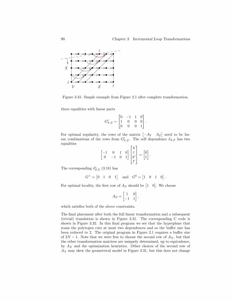
90 Chapter 3. Incremental Loop Transformations
•
•
•
•
•
•
•
•
•
•
•
•
•
•
• •
•
•
•
•
•
• •
• • •
• • • •
• • • • •j
i
l
X
Y Z
Figure 3.31: Simple example from Figure 2.1 after complete transformation.
three equalities with linear parts
G′Y,Z =
0 −1 1 01 0 0 00 0 0 1
.
For optimal regularity, the rows of the matrix[−AY AZ
]need to be lin-
ear combinations of the rows from G′Y,Z . The self dependence δZ,Z has twoequalities
[−1 0 1 00 −1 0 1
]
klk′
l′
=
[01
]
.
The corresponding δ∗Z,Z (3.18) has
G+ =[0 1 0 1
]and G0 =
[1 0 1 0
].
For optimal locality, the first row of AZ should be[1 0
]. We choose
AZ =
[1 0−1 1
]
,
which satisfies both of the above constraints.
The final placement after both the full linear transformation and a subsequent(trivial) translation is shown in Figure 3.31. The corresponding C code isshown in Figure 3.32. In this final program we see that the hyperplane thatscans the polytopes cuts at most two dependences and so the buffer size hasbeen reduced to 2. The original program in Figure 2.1 requires a buffer sizeof 2N − 1. Note that we were free to choose the second row of AX , but thatthe other transformation matrices are uniquely determined, up to equivalence,by AX and the optimization heuristics. Other choices of the second row ofAX may skew the geometrical model in Figure 3.31, but this does not change
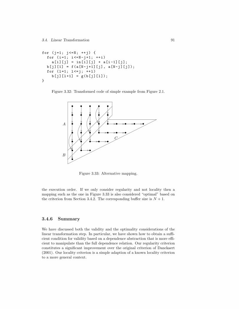
3.4. Linear Transformation 91
for (j=1; j<=N; ++j)
for (i=1; i<=N-j+1; ++i)
a[i][j] = in[i][j] + a[i-1][j];
b[j][1] = f(a[N-j+1][j], a[N-j][j]);
for (l=1; l<=j; ++l)
b[j][l+1] = g(b[j][l]);
Figure 3.32: Transformed code of simple example from Figure 2.1.
C
B
A
•
•
•
•
•
•
•
•
•
•
•
•
•
•
•
•
•
•
•
•
•
•
•
•
•
•
•
•
•
•
•
•
•
• •
Figure 3.33: Alternative mapping.
the execution order. If we only consider regularity and not locality then amapping such as the one in Figure 3.33 is also considered “optimal” based onthe criterion from Section 3.4.2. The corresponding buffer size is N + 1.
3.4.6 Summary
We have discussed both the validity and the optimality considerations of thelinear transformation step. In particular, we have shown how to obtain a suffi-cient condition for validity based on a dependence abstraction that is more effi-cient to manipulate than the full dependence relation. Our regularity criterionconstitutes a significant improvement over the original criterion of Danckaert(2001). Our locality criterion is a simple adaption of a known locality criterionto a more general context.
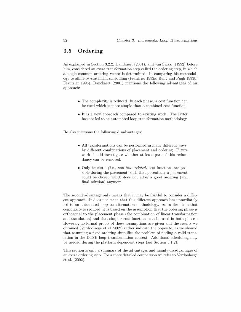
92 Chapter 3. Incremental Loop Transformations
3.5 Ordering
As explained in Section 3.2.2, Danckaert (2001), and van Swaaij (1992) beforehim, considered an extra transformation step called the ordering step, in whicha single common ordering vector is determined. In comparing his methodol-ogy to affine-by-statement scheduling (Feautrier 1992a; Kelly and Pugh 1993b;Feautrier 1996), Danckaert (2001) mentions the following advantages of hisapproach:
• The complexity is reduced. In each phase, a cost function canbe used which is more simple than a combined cost function.
• It is a new approach compared to existing work. The latterhas not led to an automated loop transformation methodology.
He also mentions the following disadvantages:
• All transformations can be performed in many different ways,by different combinations of placement and ordering. Futurework should investigate whether at least part of this redun-dancy can be removed.
• Only heuristic (i.e., non time-related) cost functions are pos-sible during the placement, such that potentially a placementcould be chosen which does not allow a good ordering (andfinal solution) anymore.
The second advantage only means that it may be fruitful to consider a differ-ent approach. It does not mean that this different approach has immediatelyled to an automated loop transformation methodology. As to the claim thatcomplexity is reduced, it is based on the assumption that the ordering phase isorthogonal to the placement phase (the combination of linear transformationand translation) and that simpler cost functions can be used in both phases.However, no formal proofs of these assumptions are given and the results weobtained (Verdoolaege et al. 2002) rather indicate the opposite, as we showedthat assuming a fixed ordering simplifies the problem of finding a valid trans-lation in the DTSE loop transformation context. Additional scheduling maybe needed during the platform dependent steps (see Section 3.1.2).
This section is only a summary of the advantages and mainly disadvantages ofan extra ordering step. For a more detailed comparison we refer to Verdoolaegeet al. (2002).
3.5. Ordering 93
3.5.1 Redundancy of Ordering
The ordering vector determines a one-dimensional schedule, which is whatvan Swaaij (1992) uses. However, in determining a one-dimensional schedule,he first builds a multi-dimensional schedule, which he transforms into a one-dimensional schedule through loop coalescing. In a multi-dimensional schedule,the schedule “time” is a vector and the execution order is determined by thelexicographical order of these time vectors. Loop coalescing maintains thisexecution order.
Danckaert et al. (2000) propose to apply conventional scheduling or space-timemapping techniques (Feautrier 1992a; Lamport 1974; Lengauer 1993) on thecommon iteration space in the ordering phase. Two of the referred to tech-niques consist of a one-dimensional schedule, the other of a multi-dimensionalschedule. Note that Feautrier (1992a) constructs a (piece-wise) affine scheduleper statement. Presumably what is meant is that the whole of all the itera-tion domains in the common iteration space is seen as a single (compound)statement, i.e., that the same affine transformation is applied to all iterationdomains. Otherwise, the ordering phase would not use any of the informationconstructed in the previous two phases, rendering them quite useless.
We are therefore justified in also considering multi-dimensional schedules. Infact, as we show in the next lemma, the problems of finding a one-dimensionalor a multi-dimensional schedule are equivalent (for non-parametric problems) inthe sense that any valid ordering vector (with greatest common divisor (gcd) ofits elements 1) can be transformed into a valid (unimodular) multi-dimensionalschedule and vice versa. For parametric problems, multi-dimensional schedulesmay exist that have no one-dimensional counterpart (Feautrier 1992b). It issufficient to only consider ordering vectors with gcd 1 and unimodular multi-dimensional schedules as scaling does not affect the relative execution order.
Lemma 3.5.1 Any valid ordering vector with gcd 1 is equivalent to a validunimodular multi-dimensional schedule and vice versa.
Proof The unimodular extension (Bik 1996) of the ordering vector is a validmulti-dimensional schedule since its first row separates all the dependences.Conversely, a unimodular schedule can be converted into an ordering vectorthrough loop coalescing. That is, let K be the multi-dimensional schedule andlet G∗ be the graph corresponding to the common iteration space, i.e., thegraph with all nodes of the original graph merged into a single node. Let P ∗
be the union of all iteration domains in G∗ after scheduling, i.e.,
P ∗ = K
⋃
P∈Pp
P
with VG∗ = p.
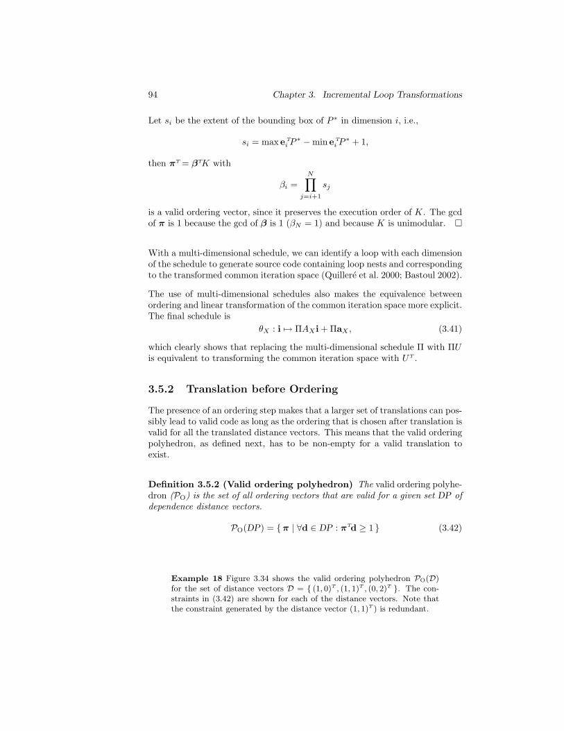
94 Chapter 3. Incremental Loop Transformations
Let si be the extent of the bounding box of P ∗ in dimension i, i.e.,
si = max e T
i P ∗ − min e T
i P ∗ + 1,
then πT = βTK with
βi =
N∏
j=i+1
sj
is a valid ordering vector, since it preserves the execution order of K. The gcdof π is 1 because the gcd of β is 1 (βN = 1) and because K is unimodular.
With a multi-dimensional schedule, we can identify a loop with each dimensionof the schedule to generate source code containing loop nests and correspondingto the transformed common iteration space (Quillere et al. 2000; Bastoul 2002).
The use of multi-dimensional schedules also makes the equivalence betweenordering and linear transformation of the common iteration space more explicit.The final schedule is
θX : i 7→ ΠAX i + ΠaX , (3.41)
which clearly shows that replacing the multi-dimensional schedule Π with ΠUis equivalent to transforming the common iteration space with UT .
3.5.2 Translation before Ordering
The presence of an ordering step makes that a larger set of translations can pos-sibly lead to valid code as long as the ordering that is chosen after translation isvalid for all the translated distance vectors. This means that the valid orderingpolyhedron, as defined next, has to be non-empty for a valid translation toexist.
Definition 3.5.2 (Valid ordering polyhedron) The valid ordering polyhe-dron (PO) is the set of all ordering vectors that are valid for a given set DP ofdependence distance vectors.
PO(DP) = π | ∀d ∈ DP : πTd ≥ 1 (3.42)
Example 18 Figure 3.34 shows the valid ordering polyhedron PO(D)for the set of distance vectors D = (1, 0)T , (1, 1)T , (0, 2)T . The con-straints in (3.42) are shown for each of the distance vectors. Note thatthe constraint generated by the distance vector (1, 1)T ) is redundant.
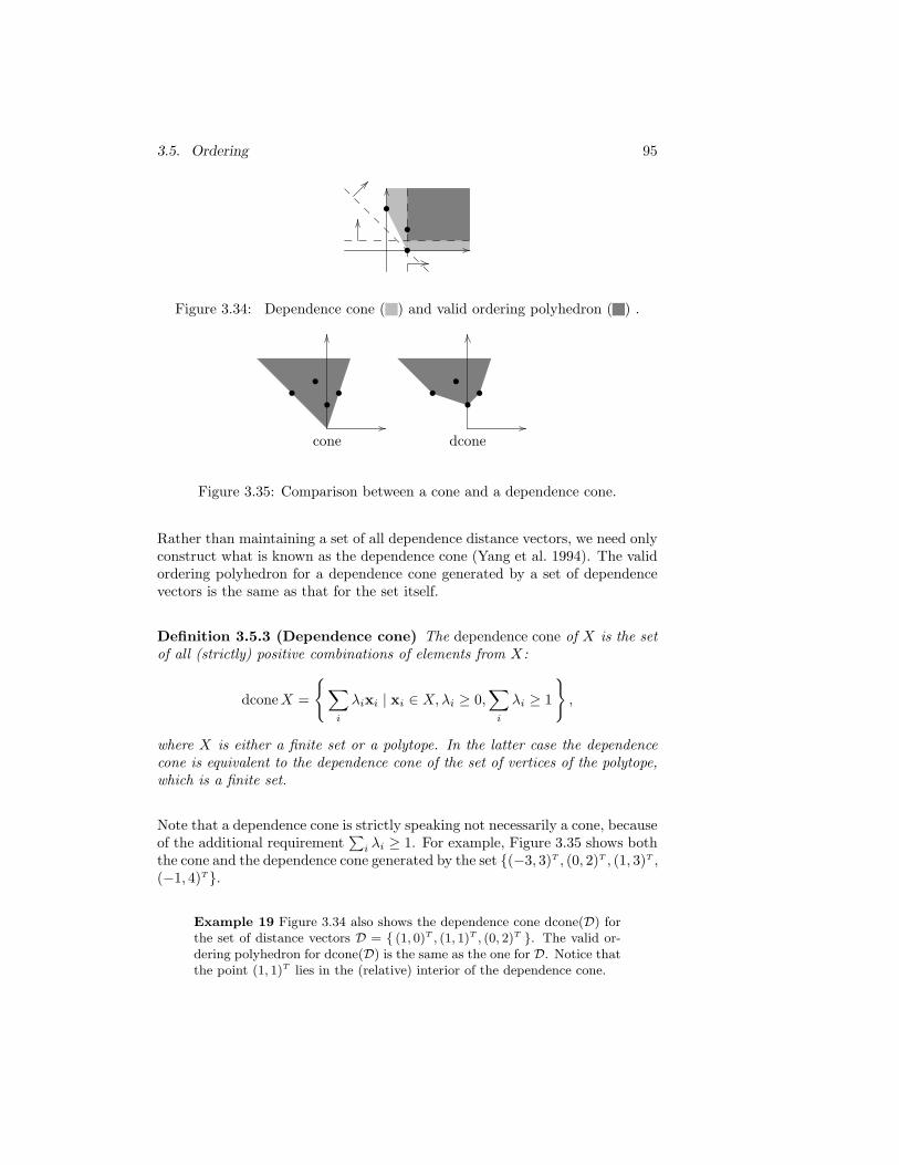
3.5. Ordering 95
•
•
•
Figure 3.34: Dependence cone ( ) and valid ordering polyhedron ( ) .
•••
•
dcone
•••
•
cone
Figure 3.35: Comparison between a cone and a dependence cone.
Rather than maintaining a set of all dependence distance vectors, we need onlyconstruct what is known as the dependence cone (Yang et al. 1994). The validordering polyhedron for a dependence cone generated by a set of dependencevectors is the same as that for the set itself.
Definition 3.5.3 (Dependence cone) The dependence cone of X is the setof all (strictly) positive combinations of elements from X:
dcone X =
∑
i
λixi | xi ∈ X,λi ≥ 0,∑
i
λi ≥ 1
,
where X is either a finite set or a polytope. In the latter case the dependencecone is equivalent to the dependence cone of the set of vertices of the polytope,which is a finite set.
Note that a dependence cone is strictly speaking not necessarily a cone, becauseof the additional requirement
∑
i λi ≥ 1. For example, Figure 3.35 shows boththe cone and the dependence cone generated by the set (−3, 3)T , (0, 2)T , (1, 3)T ,(−1, 4)T.
Example 19 Figure 3.34 also shows the dependence cone dcone(D) forthe set of distance vectors D = (1, 0)T , (1, 1)T , (0, 2)T . The valid or-dering polyhedron for dcone(D) is the same as the one for D. Notice thatthe point (1, 1)T lies in the (relative) interior of the dependence cone.
96 Chapter 3. Incremental Loop Transformations
Before defining the concept of a valid translation in the presence of an extraordering step, we will first establish a simple criterion for the dependence coneswith a non-empty valid ordering polyhedron.
Theorem 3.5.4 (Verdoolaege et al. (2002, Theorem 2)) The valid or-dering polyhedron for some distance vector polyhedron DP is non-empty iffDP does not contain the null-vector.
For a proof of this theorem we refer to Appendix D. We will call a dependencecone that contains the null-vector degenerate. According to Theorem 3.5.4the valid ordering polyhedron is empty iff the dependence cone on which it isdefined is degenerate. This dependence cone should include all the dependencesover the whole program.
Definition 3.5.5 (Global dependence cone) The global dependence coneCG,T for a given dependence graph G and a given translation T is the depen-dence cone generated by all the distance vectors.
CG,T = dcone
⋃
(p1,p2)∈EG
(D(p1,p2) + ap2
− ap1
)
(3.43)
Definition 3.5.6 (Valid translation) A translation is called valid if it de-termines a non-degenerate global dependence cone.
In the context of an extra ordering step, Algorithm 3.1 on page 46 for incre-mental translation still works, but the choice of a valid relative offset in step 4is governed by different, more complicated, constraints. The main idea is thatwe need to ensure that a valid ordering exists with respect to (indirect) selfdependences between a node in the dependence graph and itself. We will callthe associated distance vectors self dependence distance vectors. The followingdefinitions define indirect dependences and the dependence cone generated byself dependences.
Definition 3.5.7 (Fundamental path) A fundamental path between a pairof nodes l = (p1, p2) of a graph G is either a simple path from p1 to p2 or asimple circuit containing p1 = p2. A simple path [circuit] visits each node atmost once. The set of all fundamental paths is
ΠG,l = π | π = (u1, . . . , un), l = (u1, un), |ui| = n − δu1,un,
∀1 ≤ i ≤ n − 1 : (ui, ui+1) ∈ EG ,
3.5. Ordering 97
with δ the Kronecker-delta, i.e., the number of different nodes in the path iseither equal to or one less than the length of the path, depending on whetherthe first and last nodes of the path are the same.
Definition 3.5.8 (Indirect distance vector polytope) The indirect dis-tance vector polytope VG,l with l = (p1, p2) is the convex hull of all indirectdistance vectors over all fundamental paths in G between p1 and p2. An indi-rect distance vector over a path is the sum of distance vectors for each segmentof the path.
VG,l = conv
d | ∃π ∈ ΠG,l : ∀1 ≤ i ≤ n − 1 : ∃di ∈ DG,(ui,ui+1),d =
n−1∑
i=1
di
(3.44)
Definition 3.5.9 (Self-dependence (full) cone) The self dependence conefor a given node p of a graph G is the dependence cone generated by all selfdependence distance vectors.
RG,p = dconeVG,(p,p) (3.45)
The self dependence cone for the whole graph is the convex (hull of the) unionof the self dependence cones of all nodes in the graph.
RG = conv⋃
p∈VG
RG,p (3.46)
The self dependence full cone is then the cone generated by the self dependencecone.
RG = posRG
The existence of a valid translation and the valid choices for the relative offsetsare governed by the following two theorems. The proofs of these theorems canbe found in Appendix D.
Theorem 3.5.10 (Verdoolaege et al. (2002, Theorem 4)) If d ≥ 2, withd the dimension of the problem, and if the initial self dependence cone allowsfor a valid ordering, then a valid translation exists.
Note that the dimension of the problem space can arbitrarily be increased byadding extra dimensions, so the requirement d ≥ 2 is not a real restriction.
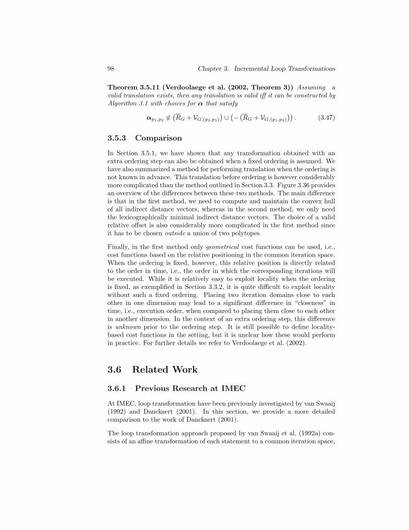
98 Chapter 3. Incremental Loop Transformations
Theorem 3.5.11 (Verdoolaege et al. (2002, Theorem 3)) Assuming avalid translation exists, then any translation is valid iff it can be constructed byAlgorithm 3.1 with choices for α that satisfy
αp1,p26∈(RG + VG,(p2,p1)
)∪(−(RG + VG,(p1,p2)
)). (3.47)
3.5.3 Comparison
In Section 3.5.1, we have shown that any transformation obtained with anextra ordering step can also be obtained when a fixed ordering is assumed. Wehave also summarized a method for performing translation when the ordering isnot known in advance. This translation before ordering is however considerablymore complicated than the method outlined in Section 3.3. Figure 3.36 providesan overview of the differences between these two methods. The main differenceis that in the first method, we need to compute and maintain the convex hullof all indirect distance vectors, whereas in the second method, we only needthe lexicographically minimal indirect distance vectors. The choice of a validrelative offset is also considerably more complicated in the first method sinceit has to be chosen outside a union of two polytopes.
Finally, in the first method only geometrical cost functions can be used, i.e.,cost functions based on the relative positioning in the common iteration space.When the ordering is fixed, however, this relative position is directly relatedto the order in time, i.e., the order in which the corresponding iterations willbe executed. While it is relatively easy to exploit locality when the orderingis fixed, as exemplified in Section 3.3.2, it is quite difficult to exploit localitywithout such a fixed ordering. Placing two iteration domains close to eachother in one dimension may lead to a significant difference in “closeness” intime, i.e., execution order, when compared to placing them close to each otherin another dimension. In the context of an extra ordering step, this differenceis unknown prior to the ordering step. It is still possible to define locality-based cost functions in the setting, but it is unclear how these would performin practice. For further details we refer to Verdoolaege et al. (2002).
3.6 Related Work
3.6.1 Previous Research at IMEC
At IMEC, loop transformation have been previously investigated by van Swaaij(1992) and Danckaert (2001). In this section, we provide a more detailedcomparison to the work of Danckaert (2001).
The loop transformation approach proposed by van Swaaij et al. (1992a) con-sists of an affine transformation of each statement to a common iteration space,
3.6
.R
elated
Work
99
Translation before Ordering Translation with fixed Ordering
Feasibilityd ≥ 2 ∧ 0 6∈ RG0
(Theorem 3.5.10)
RG0≻ 0
(Proposition 3.3.2)
Distance vectors DPG,e dG,e = lexmin DPG,e
Indirect distance vectors VG,(p1,p2) d∗G,e = lexminVG,(p1,p2)
Self-dependence cone required not required
Valid relative offsetsαp1,p2
6∈(RG + VG,(p2,p1)
)∪(−(RG + VG,(p1,p2)
))
(Equation (3.47))
−d∗p1,p24 αp1,p2
4 d∗p2,p1
(Equation (3.12))
Cost functions Only geometrical Geometrical + time related
Figure 3.36: Comparison of translation before or after ordering.
100 Chapter 3. Incremental Loop Transformations
followed by an additional linear transformation of the common iteration space,called the ordering phase. Danckaert (2001) further proposes to split the firststep into a linear transformation substep and a translation substep.
During the linear transformation he proposes to optimize regularity by optimiz-ing the “sharpness” of the dependence cone. During the translation substep heproposes to optimize the average lengths of the dependence vectors as a localitycriterion and further provides some cost functions for data reuse.
He then focuses on the linear substep and as a first approximation for thesharpness of the dependence cone he proposes to optimize the rank of thematrix I − D′, where D′ is the linear part of the dependence function afterthe linear transformation, i.e., D′ = A−1
c ApD, with D the linear part of thedependence function before the transformation. He develops a search procedurefor optimizing these ranks, but does not consider the validity of the final lineartransformation. That is, he does not guarantee that the translation substepcan still be performed after his linear substep. Throughout, he uses pairs ofdependence domains and dependence functions to represent dependences.
We showed (Verdoolaege et al. 2001a) that the rank of the matrix I − D′ isin fact the dimension of the dependence polytope when the iteration domain isapproximated by the whole iteration space. When the bounds of the iterationdomains are taken into account, or, equivalently, the constraints on the depen-dence domain, we obtain formula (3.28). We further devised a formula for theminimal possible dimension of the dependence polytope. The general searchprocedure of Section 3.4.3 is an extension and refinement of the search proce-dure outlined by Danckaert (2001, Section 6.5). Rather than using a formulafor the optimal value of his optimization criterion (3.40), the exploration strat-egy of Danckaert (2001) contained a separate phase to compute, for each pairof polytopes that share a dependence, the best possible value over all possibletransformation matrices for both polytopes using an exhaustive search. Thecomputation times for this extra phase are typically higher than those of theactual search for a good global transformation (see Danckaert 2001, Table 6.4).
In Section 3.4.2 we further extended the formulas for the dimension of the de-pendence polytope and the minimal possible dimension to the generalized casewhere a dependence is represented by a dependence relation rather than a pairof dependence domain and dependence function. In Section 3.4.1 we also con-sider how to ensure the validity of the linear transformation and in Section 3.4.4we show that some locality can and should also be optimized during the lineartransformation. The latter is only possible because we removed the orderingstep.
Note that it makes sense to only consider the dependence polytope during lin-ear transformation and not the dependence cone since the dimension of thedependence cone is not completely determined by the linear transformation,
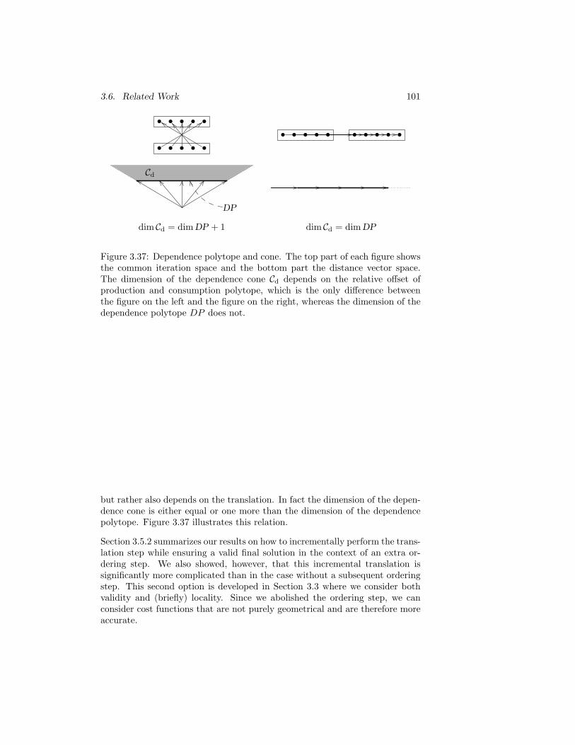
3.6. Related Work 101
• • • • •
•••••
••••• • • • • •
DP
Cd
dim Cd = dimDP + 1 dim Cd = dimDP
Figure 3.37: Dependence polytope and cone. The top part of each figure showsthe common iteration space and the bottom part the distance vector space.The dimension of the dependence cone Cd depends on the relative offset ofproduction and consumption polytope, which is the only difference betweenthe figure on the left and the figure on the right, whereas the dimension of thedependence polytope DP does not.
but rather also depends on the translation. In fact the dimension of the depen-dence cone is either equal or one more than the dimension of the dependencepolytope. Figure 3.37 illustrates this relation.
Section 3.5.2 summarizes our results on how to incrementally perform the trans-lation step while ensuring a valid final solution in the context of an extra or-dering step. We also showed, however, that this incremental translation issignificantly more complicated than in the case without a subsequent orderingstep. This second option is developed in Section 3.3 where we consider bothvalidity and (briefly) locality. Since we abolished the ordering step, we canconsider cost functions that are not purely geometrical and are therefore moreaccurate.
102 Chapter 3. Incremental Loop Transformations
3.6.2 Other Related Work
There has been a wealth of research on loop transformation. We only mentiona few of the results here.
Many researchers have investigated automatic loop transformations. The initialindividual loop transformations were generalized to linear (mostly unimodular)transformations for perfectly nested loop nests and later to affine transforma-tions for each statement in one or multiple nests, mainly focusing on parallelism(Darte and Robert 1995; Feautrier 1992a; Lim and Lam 1997), although re-cently locality has also received some attention (Lim et al. 2001). Most ofthese approaches use exact dependence information, which leads to relativelyexpensive algorithms and limits the scope of applicability. By contrast, we onlyuse the affine hull of the dependence relations during linear transformation andonly the minimal distance vector during translation.
Rather than splitting affine transformations into a linear and a translationstep, most researchers build up the affine transformation matrices row by row.One such example is the research by Kelly and Pugh (1994) who define asearch tree of valid mappings which could be traversed by e.g., an A∗ algorithm(Nilsson 1980) as in Kelly and Pugh (1993a). Like our method, theirs allows forconsiderable freedom in the choice of cost function. Darte and Vivien (1997),on the other hand, build up their their transformation matrices several rowsat a time. Although the heuristic they propose is oriented towards parallelism,their approach is still similar to ours since they also use the distance vectorabstraction and since their algorithm allows for some freedom in the choice ofcost function.
As to linear transformations, most researchers only apply a single linear trans-formation to a whole loop nest, which is often even restricted to being perfectlynested. Moreover, they typically handle loop nests individually. Wolf and Lam(1991) further only consider reuse between uniformly generated references, thenumber of which can be increased by using our regularity optimization tech-nique. More recently, Kandemir et al. (2001) do not require perfectly nestedloops, but report that their algorithm does not obtain very good results forimperfectly nested loops. They only consider self reuse, whereas the techniquein this paper is mostly concerned with group reuse. An entirely different ap-proach is taken by Olsen and Gao (1992). They do optimize across differentloop nests, but they only apply a very limited set of linear transformations,viz. loop reverse and the permutation of two loop levels, and they also requireperfectly nested loops.
Early research on loop fusion mostly focused on loop fusion without loop shift-ing, e.g., Kennedy and McKinley (1993). Manjikian and Abdelrahman (1995)only shift to allow loop fusion and not to optimize locality, i.e., they only shiftif the dependence distance would be negative otherwise. Furthermore, they
3.7. Summary 103
only consider uniform dependences and acyclic dependence graphs.
The most closely related research is that of Fraboulet et al. (1999) and itsextensions by Song et al. (2001). The former only consider uniform depen-dences and although the latter do not explicitly impose this restriction, theirassumption on the maximal dependence distances only allows for some excep-tional cases of non-uniform dependences. Their algorithms only apply to onedimension, which, in the case of Song et al. (2001), can be the result of coalesc-ing multiple dimensions, and a heuristic is used for multiple dimensions. Darteand Huard (2002b) do handle non-uniform dependences and provide an IntegerLinear Programming (ILP) formulation and complexity results for optimizingarray contraction for simple loops.
The key features of our proposed incremental approach for loop fusion are theapplicability to a general class of programs, the low complexity which makesit scalable, and the independence of cost function of the algorithm itself. Theheuristic to steer the optimization obviously does depend on that (set of) costfunction(s). Although Song et al. (2001) claim that their technique applies toimperfectly nested loops, they in fact rely on a preprocessing step including looppeeling and loop partitioning to identify and massage the loop nests that areto be fused. By contrast, we take any program as input, provided sufficient upfront dependence analysis can be performed. Loop peeling is the result of (thecode generation after) the fusion, rather than a step that must be performedto enable loop fusion.
The algorithm proposed by Song et al. (2001) is only valid for the particularcost function they use, which in turn depends on their limited program model.The cost function minimizes the maximal dependence distance for a given ar-ray. If a given array element is read in multiple statements, then only the lastaccess is optimized, ignoring the opportunity to also optimize locality over theother dependences. Furthermore, although the authors claim their algorithmminimizes the temporary array storage, this only applies to the individual ar-rays. The total storage space required at a given point in the program mayactually increase due to the fact that more temporary arrays are simultaneouslyalive. The simple heuristic we propose in Section 3.3.2 suffers from the sameshort-sightedness, but it can more easily be extended to include such effectssince the algorithm does not depend on the cost function.
3.7 Summary
In this chapter we have investigated incremental loop transformation. We havesituated the loop transformation step in a global DTSE flow and have shownhow to perform these loop transformations incrementally using the highestpossible data dependence abstractions. Although we mainly focused on means
104 Chapter 3. Incremental Loop Transformations
to ensure the validity of the final loop transformations, we also discussed someoptimization heuristics. We concluded with a comparison to related work.
Chapter 4
Enumeration of Parametric
Sets
Many compiler optimization techniques require the enumeration of certainkinds of objects as a substep, e.g., the number of times a statement is executed,the number of times a variable is accessed or the total number of accessed arrayelements. These counting problems can typically be formulated as the numberof integer points that satisfy certain linear constraints. The general form ofthis type of problems is
cS(p) = #Sp = #
x ∈ Zd | ∃y ∈ Zd′ : Ax + Dy + Bp + c ≥ 0
,
where x ∈ Zd represent the objects to be counted, p ∈ Zn are parameterson which the count depends and y ∈ Zd′ are extra existentially quantifiedvariables that are used to further constrain the number of objects. If d′ = 0,then S is the set of integer points in what is known as a rational parametricpolytope. For d′ 6= 0, S is the projection onto a lower-dimensional spaceof the integer points in such a parametric polytope. A technique for solvingproblems without existential variables (d′ = 0) was proposed by Clauss andLoechner (1998) and implemented in PolyLib. The technique is worst-caseexponential however, even for fixed dimension, and the current implementationeven fails to produce a solution on some problems. Recent automata-basedcounting techniques (Boigelot and Latour 2004; Parker and Chatterjee 2004)solve problems without parameters (n = 0) but are also exponential. Thetechnique of Pugh (1994) is intended to solve the general problem, but noimplementation has been reported and the technique is also exponential.
Barvinok (1993) described a polynomial-time algorithm (for fixed dimensiond) for computing the number of integer points in a fixed polytope (n = 0
105
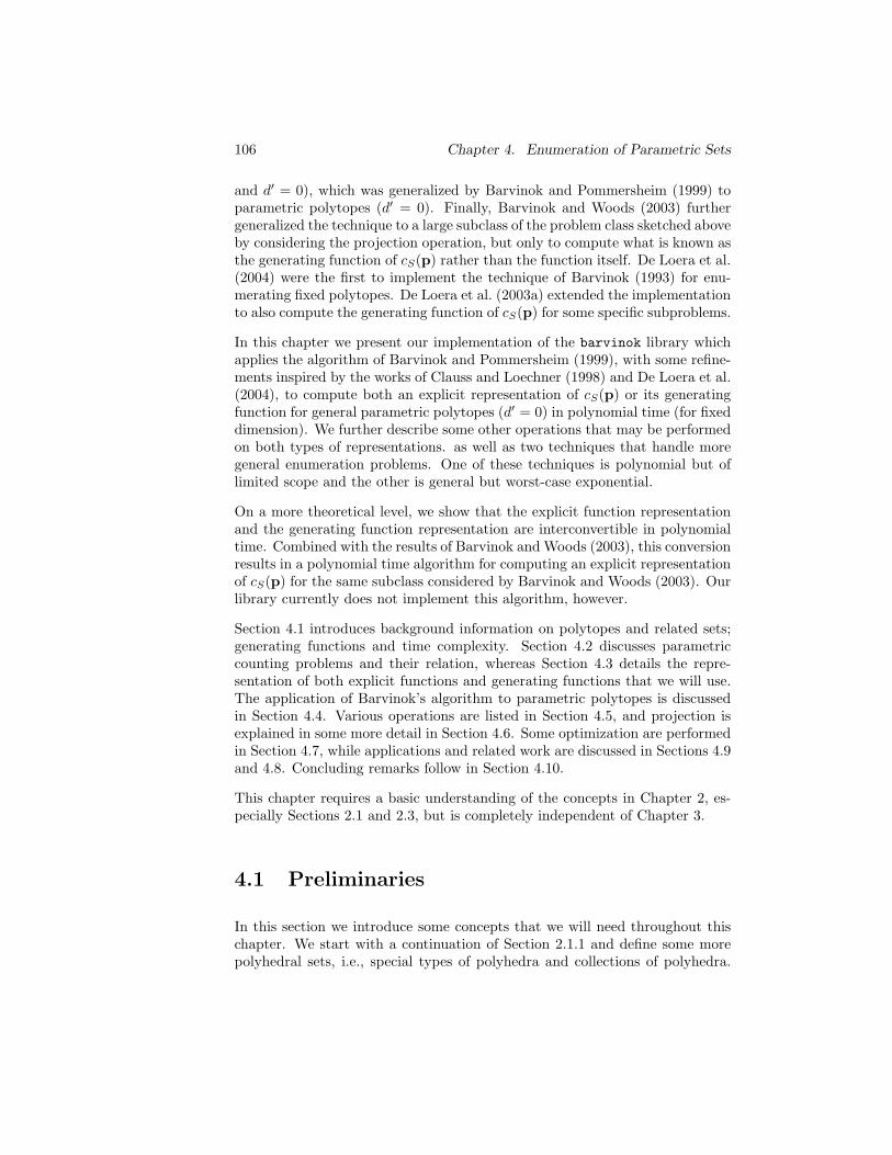
106 Chapter 4. Enumeration of Parametric Sets
and d′ = 0), which was generalized by Barvinok and Pommersheim (1999) toparametric polytopes (d′ = 0). Finally, Barvinok and Woods (2003) furthergeneralized the technique to a large subclass of the problem class sketched aboveby considering the projection operation, but only to compute what is known asthe generating function of cS(p) rather than the function itself. De Loera et al.(2004) were the first to implement the technique of Barvinok (1993) for enu-merating fixed polytopes. De Loera et al. (2003a) extended the implementationto also compute the generating function of cS(p) for some specific subproblems.
In this chapter we present our implementation of the barvinok library whichapplies the algorithm of Barvinok and Pommersheim (1999), with some refine-ments inspired by the works of Clauss and Loechner (1998) and De Loera et al.(2004), to compute both an explicit representation of cS(p) or its generatingfunction for general parametric polytopes (d′ = 0) in polynomial time (for fixeddimension). We further describe some other operations that may be performedon both types of representations. as well as two techniques that handle moregeneral enumeration problems. One of these techniques is polynomial but oflimited scope and the other is general but worst-case exponential.
On a more theoretical level, we show that the explicit function representationand the generating function representation are interconvertible in polynomialtime. Combined with the results of Barvinok and Woods (2003), this conversionresults in a polynomial time algorithm for computing an explicit representationof cS(p) for the same subclass considered by Barvinok and Woods (2003). Ourlibrary currently does not implement this algorithm, however.
Section 4.1 introduces background information on polytopes and related sets;generating functions and time complexity. Section 4.2 discusses parametriccounting problems and their relation, whereas Section 4.3 details the repre-sentation of both explicit functions and generating functions that we will use.The application of Barvinok’s algorithm to parametric polytopes is discussedin Section 4.4. Various operations are listed in Section 4.5, and projection isexplained in some more detail in Section 4.6. Some optimization are performedin Section 4.7, while applications and related work are discussed in Sections 4.9and 4.8. Concluding remarks follow in Section 4.10.
This chapter requires a basic understanding of the concepts in Chapter 2, es-pecially Sections 2.1 and 2.3, but is completely independent of Chapter 3.
4.1 Preliminaries
In this section we introduce some concepts that we will need throughout thischapter. We start with a continuation of Section 2.1.1 and define some morepolyhedral sets, i.e., special types of polyhedra and collections of polyhedra.
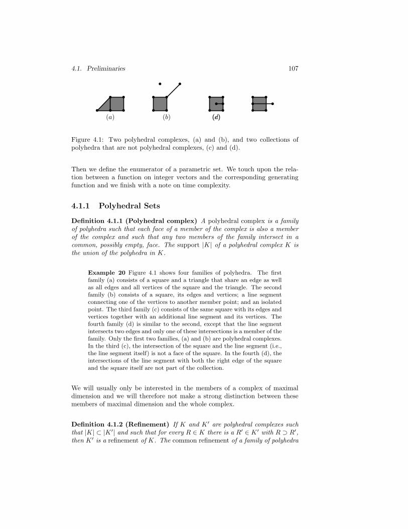
4.1. Preliminaries 107
• •
••
• • •
••
••
• •
••• •
• •
••• •
(a) (b) (c)(d)
Figure 4.1: Two polyhedral complexes, (a) and (b), and two collections ofpolyhedra that are not polyhedral complexes, (c) and (d).
Then we define the enumerator of a parametric set. We touch upon the rela-tion between a function on integer vectors and the corresponding generatingfunction and we finish with a note on time complexity.
4.1.1 Polyhedral Sets
Definition 4.1.1 (Polyhedral complex) A polyhedral complex is a familyof polyhedra such that each face of a member of the complex is also a memberof the complex and such that any two members of the family intersect in acommon, possibly empty, face. The support |K| of a polyhedral complex K isthe union of the polyhedra in K.
Example 20 Figure 4.1 shows four families of polyhedra. The firstfamily (a) consists of a square and a triangle that share an edge as wellas all edges and all vertices of the square and the triangle. The secondfamily (b) consists of a square, its edges and vertices; a line segmentconnecting one of the vertices to another member point; and an isolatedpoint. The third family (c) consists of the same square with its edges andvertices together with an additional line segment and its vertices. Thefourth family (d) is similar to the second, except that the line segmentintersects two edges and only one of these intersections is a member of thefamily. Only the first two families, (a) and (b) are polyhedral complexes.In the third (c), the intersection of the square and the line segment (i.e.,the line segment itself) is not a face of the square. In the fourth (d), theintersections of the line segment with both the right edge of the squareand the square itself are not part of the collection.
We will usually only be interested in the members of a complex of maximaldimension and we will therefore not make a strong distinction between thesemembers of maximal dimension and the whole complex.
Definition 4.1.2 (Refinement) If K and K ′ are polyhedral complexes suchthat |K| ⊂ |K ′| and such that for every R ∈ K there is a R′ ∈ K ′ with R ⊃ R′,then K ′ is a refinement of K. The common refinement of a family of polyhedra
108 Chapter 4. Enumeration of Parametric Sets
is a polyhedral complex such that its support is the union of the polyhedra andsuch that each member is the intersection of some of the polyhedra.
Example 21 Figure 4.5 on page 117 shows the common refinement ofthe family of cones in Figure 4.4.
Definition 4.1.3 (Subdivision) A subdivision of a polyhedron P is a poly-hedral complex K such that |K| = P . An element of a subdivision of maximaldimension is called a cell.
Example 22 The first complex in Figure 4.1 on the previous page is asubdivision containing two cells. The second complex is not a subdivisionsince its support is not a polyhedron. Figure 4.9 on page 120 shows asubdivision with 16 members: the whole polyhedron, the empty set, four2-dimensional cells (three of which are infinite), three outer walls, fourpairwise intersections of 2-dimensional cells and three vertices.
Definition 4.1.4 (Simplicial cone) A d-dimensional cone is simplicial if itis generated by d (linearly independent) generators.
Note that a 1- or 2-dimensional cone is always simplicial. Figure 4.20 onpage 145 shows a 3-dimensional cone that is not simplicial since it is generatedby the four points a, b, c and d.
Definition 4.1.5 (Triangulation) A triangulation of a cone C is a subdivi-sion of C such that each element is a simplicial cone.
Note that triangulations are typically defined on polytopes rather than cones,but we will only need it for cones. Also note that some authors, e.g., Fortune(1992), call a subdivision a triangulation and a triangulation a proper triangu-lation.
4.1.2 Parametric Sets and their Enumerators
Recall from Section 2.1.4 that a parametric set Sp is of the form
Sp =x ∈ Zd | (p,x) ∈ S
⊂ Zd,
with S a projected set. A parametric polytope is modeled by a polyhedronP ⊂ Qn × Qd such that for all p ∈ Qn, the set Pp is a polytope.
4.1. Preliminaries 109
Definition 4.1.6 (Enumerator) The enumerator cS of a parametric set S isa function from the set of n-dimensional integer vectors Zn to the set of naturalnumbers N. The function value at p, denoted cS(p), is the number of integerpoints in the set Sp.
cS : Zn → N
p 7→ cS(p) = #Sp(4.1)
If P ⊂ Qn × Qd defines a parametric polytope, then we will also say thatcP = #(Pp ∩ Zd) is the enumerator of Pp.
Note that Barvinok and Pommersheim (1999) call the parametric polytopesPp the fibers of the projection of the polyhedron P onto the parameter space.Other authors denote by this term the sets p × Pp. We will not use thisterminology.
4.1.3 Generating Functions
Definition 4.1.7 (Generating function of a sequence) Let ai∞i=0 be a
sequence of rational numbers ai ∈ Q, then the generating function of ai∞i=0
is a formal power series A(x) ∈ Q[[x]] with the ai as coefficients, i.e.,
A(x) =
∞∑
i=0
aixi.
Such generating functions can naturally be extended to multiple sequencesaii∈Nn . The corresponding generating functions are called multiple generat-ing functions (Srivastava and Manocha 1984). Note that a (multiple) sequenceis basically a (multivariate) function a : Nn → Q.
The concept of a generating function can be further extended to correspond to(some) functions over integer vectors.
Definition 4.1.8 (Generating function) Let a : Zn → Q be a function.The corresponding generating function, if it exists, is a function A : Cn → C
such that A has a Laurent power series expansion
A(x) =∑
s∈Zn
a(s)xs
which converges on some non-empty open region of Cn. We use the notationxs = xs1
1 xs22 · · ·xsn
n .
110 Chapter 4. Enumeration of Parametric Sets
Note that the convergence requirement means that not all generating functionsfrom Definition 4.1.7 are also generating functions according to Definition 4.1.8.We must also be careful when speaking of a correspondence between a functionand its generating function, because a generating function may have differentLaurent power series expansions which converge on different regions of Cn. Forexample, if A(x) = 1
1−x then
1 + x + x2 + x3 + · · · and − x−1 − x−2 − x−3 − · · ·
are Laurent power series expansions convergent for ‖x‖ < 1 and ‖x‖ > 1,respectively. The first is the well-known geometric series, while the secondfollows from the identity
1
1 − x=
−x−1
1 − x−1,
or in general1
1 − xu=
−x−u
1 − x−u. (4.2)
That is, A(x) is the generating function of both
a1(s) =
1 if s ≥ 0
0 if s < 0
and
a2(s) =
0 if s ≥ 0
−1 if s < 0,
but on different regions of C1.
4.1.4 Time Complexity
Whenever we say that an algorithm has polynomial time complexity, we willmean that the time complexity is polynomial in the input size. This inputsize is the number of bits that is needed to represent the input (Schrijver1986; Papadimitriou 1994). E.g., if the input is the implicit representation ofa polyhedron P ⊂ Qd, i.e., a collection of m linear inequalities Ax ≥ c, thenthe input size is approximately
md +∑
i,j
log2 |aij | +∑
i
log2 |ci| .
The algorithms will usually only by polynomial if we fix some size parame-ter, typically the dimension of the problem. E.g., if an algorithm has time-complexity O(nd), with n the input size and d the dimension of the problemthen we will say that the computation time is polynomial in the input size, forfixed dimension d.
4.2. Parametric Counting Problems 111
4.2 Parametric Counting Problems
Our main counting problem is the enumeration of parametric polytopes. Wefirst consider two special cases, Ehrhart quasi-polynomials and vector parti-tion functions. Then we consider the enumeration of parametric polytopes insome more detail, indicating the relation with vector partition functions andpreparing for the application of Barvinok’s algorithm to parametric polytopesin Section 4.4. Finally, we briefly discuss the generalization to parametric pro-jected sets.
4.2.1 Ehrhart Quasi-Polynomials
Consider a rational polytope P ⊂ Qd and its dilations sP by a factor of s ∈ N.Ehrhart (1962) showed that the number of integer points in sP as s varies isgiven by a special type of function called a quasi-polynomial. Many authors(e.g., Stanley 1986) use the following definition of a quasi-polynomial.
Definition 4.2.1 A function f : Z → Q is a (univariate) quasi-polynomial ofperiod q if there exists a list of q polynomials gi ∈ Q[T ] for 0 ≤ i < q such that
f(s) = gi(s) if s ≡ i mod q.
The functions gi are called the constituents.
Ehrhart (1977) uses a different definition, based on periodic numbers.
Definition 4.2.2 A rational periodic number U(p) is a function Z → Q, suchthat there exists a period q such that U(p) = U(p′) whenever p ≡ p′ mod q.
Definition 4.2.3 A (univariate) quasi-polynomial f of degree d is a function
f(n) = cd(n)nd + · · · + c1(n)n + c0,
where ci(n) are rational periodic numbers. I.e., it is a polynomial expression ofdegree d with rational periodic numbers for coefficients. The period of a quasi-polynomial is the least common multiple (lcm) of the periods of its coefficients.
These two definition are easily seen to be equivalent. Ehrhart (1977) uses alist of q rational numbers enclosed in square brackets to represent periodicnumbers.
Example 23 U(p) = [1, 3/4]p is a periodic number with period q = 2;U(p) = 1 if p mod 2 ≡ 0 and U(p) = 3/4 if p mod 2 ≡ 1. Furthermore,
1
4p2 + p −
[
1,3
4
]
p
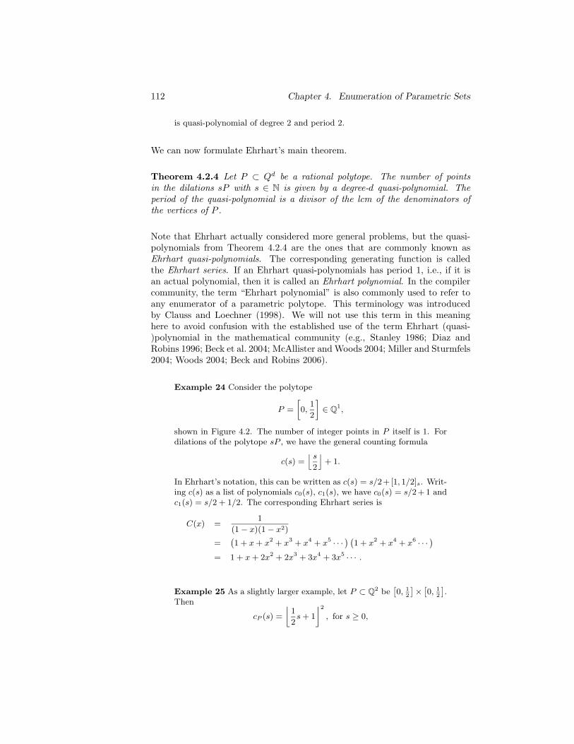
112 Chapter 4. Enumeration of Parametric Sets
is quasi-polynomial of degree 2 and period 2.
We can now formulate Ehrhart’s main theorem.
Theorem 4.2.4 Let P ⊂ Qd be a rational polytope. The number of pointsin the dilations sP with s ∈ N is given by a degree-d quasi-polynomial. Theperiod of the quasi-polynomial is a divisor of the lcm of the denominators ofthe vertices of P .
Note that Ehrhart actually considered more general problems, but the quasi-polynomials from Theorem 4.2.4 are the ones that are commonly known asEhrhart quasi-polynomials. The corresponding generating function is calledthe Ehrhart series. If an Ehrhart quasi-polynomials has period 1, i.e., if it isan actual polynomial, then it is called an Ehrhart polynomial. In the compilercommunity, the term “Ehrhart polynomial” is also commonly used to refer toany enumerator of a parametric polytope. This terminology was introducedby Clauss and Loechner (1998). We will not use this term in this meaninghere to avoid confusion with the established use of the term Ehrhart (quasi-)polynomial in the mathematical community (e.g., Stanley 1986; Diaz andRobins 1996; Beck et al. 2004; McAllister and Woods 2004; Miller and Sturmfels2004; Woods 2004; Beck and Robins 2006).
Example 24 Consider the polytope
P =
[
0,1
2
]
∈ Q1,
shown in Figure 4.2. The number of integer points in P itself is 1. Fordilations of the polytope sP , we have the general counting formula
c(s) =⌊ s
2
⌋
+ 1.
In Ehrhart’s notation, this can be written as c(s) = s/2+[1, 1/2]s. Writ-ing c(s) as a list of polynomials c0(s), c1(s), we have c0(s) = s/2+1 andc1(s) = s/2 + 1/2. The corresponding Ehrhart series is
C(x) =1
(1 − x)(1 − x2)
=(1 + x + x2 + x3 + x4 + x5 · · ·
) (1 + x2 + x4 + x6 · · ·
)
= 1 + x + 2x2 + 2x3 + 3x4 + 3x5 · · · .
Example 25 As a slightly larger example, let P ⊂ Q2 be[0, 1
2
]×[0, 1
2
].
Then
cP (s) =
⌊1
2s + 1
⌋2
, for s ≥ 0,
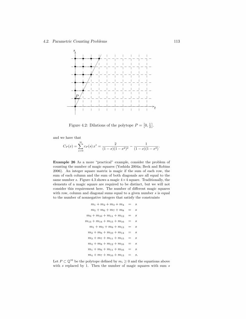
4.2. Parametric Counting Problems 113
t
s
P
•
•
•
•
•
•
•
•
•
•
•
•
•
•
• •
Figure 4.2: Dilations of the polytope P =[0, 1
2
].
and we have that
CP (x) =∞∑
s=0
cP (s) xs =2
(1 − x)(1 − x2)2− 1
(1 − x)(1 − x2).
Example 26 As a more “practical” example, consider the problem ofcounting the number of magic squares (Yoshida 2004a; Beck and Robins2006). An integer square matrix is magic if the sum of each row, thesum of each column and the sum of both diagonals are all equal to thesame number s. Figure 4.3 shows a magic 4×4 square. Traditionally, theelements of a magic square are required to be distinct, but we will notconsider this requirement here. The number of different magic squareswith row, column and diagonal sums equal to a given number s is equalto the number of nonnegative integers that satisfy the constraints
m1 + m2 + m3 + m4 = s
m5 + m6 + m7 + m8 = s
m9 + m10 + m11 + m12 = s
m13 + m14 + m15 + m16 = s
m1 + m5 + m9 + m13 = s
m2 + m6 + m10 + m14 = s
m3 + m7 + m11 + m15 = s
m4 + m8 + m12 + m16 = s
m1 + m6 + m11 + m16 = s
m4 + m7 + m10 + m13 = s.
Let P ⊂ Q16 be the polytope defined by mi ≥ 0 and the equations abovewith s replaced by 1. Then the number of magic squares with sum s
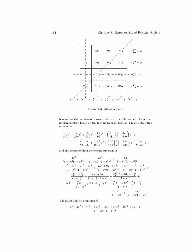
114 Chapter 4. Enumeration of Parametric Sets
∑= s
∑= s
∑= s
∑= s
∑= s
∑= s
∑= s
∑= s
∑= s
∑= s
m1 m2 m3 m4
m5 m6 m7 m8
m9 m10 m11 m12
m13 m14 m15 m16
Figure 4.3: Magic square.
is equal to the number of integer points in the dilation sP . Using ourimplementation based on the techniques from Section 4.4, we obtain thisnumber as
1
480s7 +
7
240s6 +
89
580s5 +
65
96s4 +
(1
48
⌊ s
2
⌋
+377
240
)
s3 +
(1
8
⌊ s
2
⌋
+377
160
)
s2 +
(17
48
⌊ s
2
⌋
+523
240
)
s +3
8
⌊ s
2
⌋
+ 1
and the corresponding generating function as
3x2
(1 − x)4(1 − x2)2+
7x4
(1 − x)4(1 − x2)3+
6x3
(1 − x)5(1 − x2)2+
10x5 + 4x4 + 2x3 + 2x2
(1 − x)5(1 − x2)3+
5x6 + 2x4 + x2
(1 − x)4(1 − x2)4+
4x4 + 5x3 + 4x2
(1 − x)6(1 − x2)2+
1058
x + 258
(1 − x)5+
8x3 + 9x2
(1 − x)7(1 − x2)+
4698
x2 − 10x − 1578
(1 − x)6+
92x3 − 1072
x2 + 112
x + 34
(1 − x)7+
932
x4 − 1012
x3 + 18x2 − 12x − 35
2
(1 − x)8+
1
(1 − x)4+
−x2
(1 − x)6(1 − x2).
The latter can be simplified to
x8 + 4x7 + 18x6 + 36x5 + 50x4 + 36x3 + 18x2 + 4x + 1
(1 − x)4(1 − x2)4,
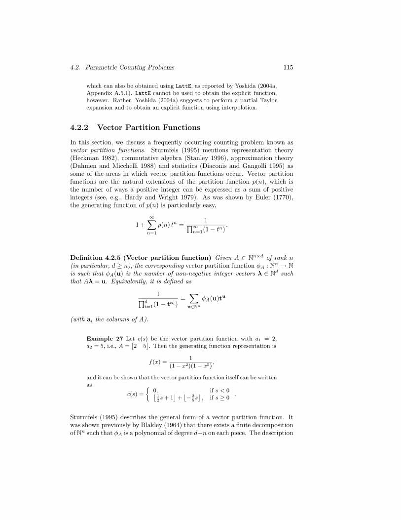
4.2. Parametric Counting Problems 115
which can also be obtained using LattE, as reported by Yoshida (2004a,Appendix A.5.1). LattE cannot be used to obtain the explicit function,however. Rather, Yoshida (2004a) suggests to perform a partial Taylorexpansion and to obtain an explicit function using interpolation.
4.2.2 Vector Partition Functions
In this section, we discuss a frequently occurring counting problem known asvector partition functions. Sturmfels (1995) mentions representation theory(Heckman 1982), commutative algebra (Stanley 1996), approximation theory(Dahmen and Micchelli 1988) and statistics (Diaconis and Gangolli 1995) assome of the areas in which vector partition functions occur. Vector partitionfunctions are the natural extensions of the partition function p(n), which isthe number of ways a positive integer can be expressed as a sum of positiveintegers (see, e.g., Hardy and Wright 1979). As was shown by Euler (1770),the generating function of p(n) is particularly easy,
1 +
∞∑
n=1
p(n) tn =1
∏∞n=1(1 − tn)
.
Definition 4.2.5 (Vector partition function) Given A ∈ Nn×d of rank n(in particular, d ≥ n), the corresponding vector partition function φA : Nn → N
is such that φA(u) is the number of non-negative integer vectors λ ∈ Nd suchthat Aλ = u. Equivalently, it is defined as
1∏d
i=1(1 − tai)=∑
u∈Nn
φA(u)tu
(with ai the columns of A).
Example 27 Let c(s) be the vector partition function with a1 = 2,a2 = 5, i.e., A =
[2 5
]. Then the generating function representation is
f(x) =1
(1 − x2)(1 − x5),
and it can be shown that the vector partition function itself can be writtenas
c(s) =
0, if s < 0⌊
12s + 1
⌋+⌊− 2
5s⌋, if s ≥ 0
.
Sturmfels (1995) describes the general form of a vector partition function. Itwas shown previously by Blakley (1964) that there exists a finite decompositionof Nn such that φA is a polynomial of degree d−n on each piece. The description
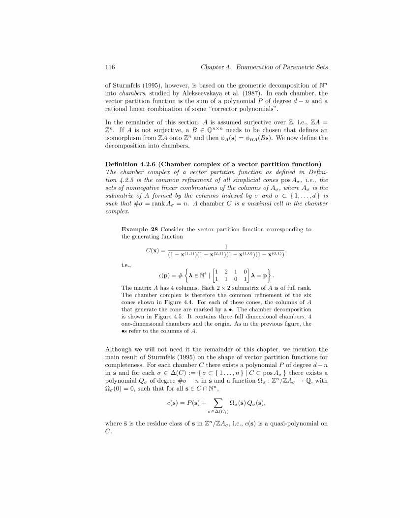
116 Chapter 4. Enumeration of Parametric Sets
of Sturmfels (1995), however, is based on the geometric decomposition of Nn
into chambers, studied by Alekseevskaya et al. (1987). In each chamber, thevector partition function is the sum of a polynomial P of degree d − n and arational linear combination of some “corrector polynomials”.
In the remainder of this section, A is assumed surjective over Z, i.e., ZA =Zn. If A is not surjective, a B ∈ Qn×n needs to be chosen that defines anisomorphism from ZA onto Zn and then φA(s) = φBA(Bs). We now define thedecomposition into chambers.
Definition 4.2.6 (Chamber complex of a vector partition function)The chamber complex of a vector partition function as defined in Defini-tion 4.2.5 is the common refinement of all simplicial cones pos Aσ, i.e., thesets of nonnegative linear combinations of the columns of Aσ, where Aσ is thesubmatrix of A formed by the columns indexed by σ and σ ⊂ 1, . . . , d issuch that #σ = rankAσ = n. A chamber C is a maximal cell in the chambercomplex.
Example 28 Consider the vector partition function corresponding tothe generating function
C(x) =1
(1 − x(1,1))(1 − x(2,1))(1 − x(1,0))(1 − x(0,1)),
i.e.,
c(p) = #
λ ∈ N4 |[1 2 1 01 1 0 1
]
λ = p
.
The matrix A has 4 columns. Each 2 × 2 submatrix of A is of full rank.The chamber complex is therefore the common refinement of the sixcones shown in Figure 4.4. For each of these cones, the columns of Athat generate the cone are marked by a •. The chamber decompositionis shown in Figure 4.5. It contains three full dimensional chambers, 4one-dimensional chambers and the origin. As in the previous figure, the•s refer to the columns of A.
Although we will not need it the remainder of this chapter, we mention themain result of Sturmfels (1995) on the shape of vector partition functions forcompleteness. For each chamber C there exists a polynomial P of degree d−nin s and for each σ ∈ ∆(C) := σ ⊂ 1 . . . , n | C ⊂ pos Aσ there exists apolynomial Qσ of degree #σ − n in s and a function Ωσ : Zn/ZAσ → Q, withΩσ(0) = 0, such that for all s ∈ C ∩ Nn,
c(s) = P (s) +∑
σ∈∆(Ci)
Ωσ(s)Qσ(s),
where s is the residue class of s in Zn/ZAσ, i.e., c(s) is a quasi-polynomial onC.
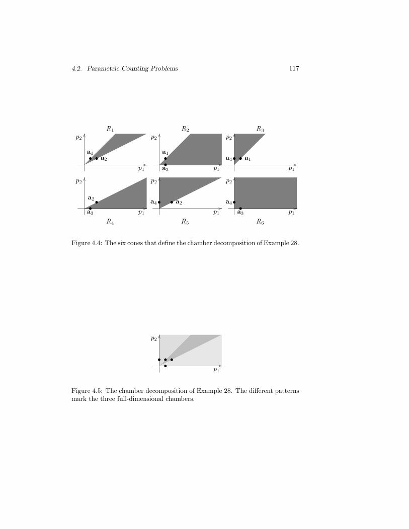
4.2. Parametric Counting Problems 117
p1
p2
•a1
• a2
R1
p1
p2
•a1
•a3
R2
p1
p2
• a1•a4
R3
p1
p2
•a2
•a3
R4
p1
p2
• a2•a4
R5
p1
p2
•a3
•a4
R6
Figure 4.4: The six cones that define the chamber decomposition of Example 28.
p1
p2
• ••
•
Figure 4.5: The chamber decomposition of Example 28. The different patternsmark the three full-dimensional chambers.
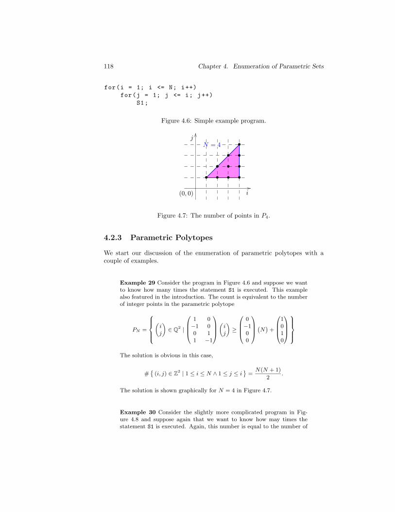
118 Chapter 4. Enumeration of Parametric Sets
for(i = 1; i <= N; i++)
for(j = 1; j <= i; j++)
S1;
Figure 4.6: Simple example program.
i
j
(0, 0)
N = 4
• • • •
• • •
• •
•
Figure 4.7: The number of points in P4.
4.2.3 Parametric Polytopes
We start our discussion of the enumeration of parametric polytopes with acouple of examples.
Example 29 Consider the program in Figure 4.6 and suppose we wantto know how many times the statement S1 is executed. This examplealso featured in the introduction. The count is equivalent to the numberof integer points in the parametric polytope
PN =
(ij
)
∈ Q2 |
1 0−1 00 11 −1
(ij
)
≥
0−100
(N)
+
1010
The solution is obvious in this case,
#
(i, j) ∈ Z2 | 1 ≤ i ≤ N ∧ 1 ≤ j ≤ i
=
N(N + 1)
2.
The solution is shown graphically for N = 4 in Figure 4.7.
Example 30 Consider the slightly more complicated program in Fig-ure 4.8 and suppose again that we want to know how may times thestatement S1 is executed. Again, this number is equal to the number of
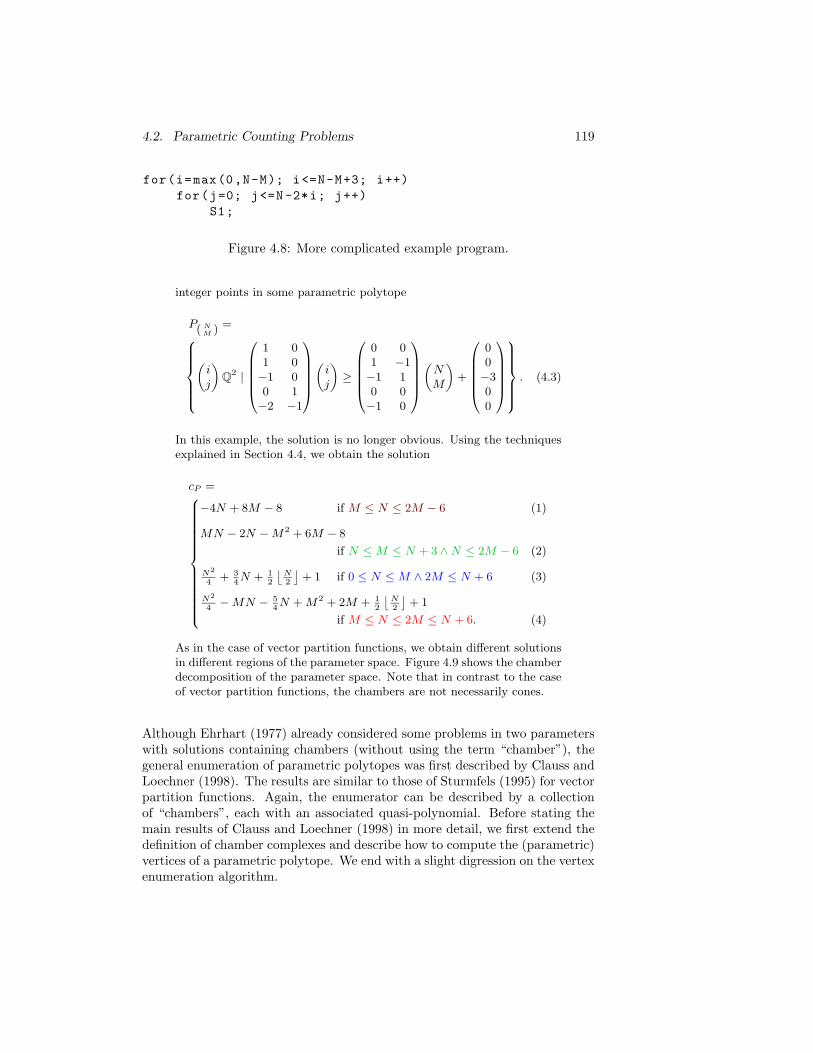
4.2. Parametric Counting Problems 119
for(i=max(0,N-M); i<=N-M+3; i++)
for(j=0; j<=N-2*i; j++)
S1;
Figure 4.8: More complicated example program.
integer points in some parametric polytope
P( NM ) =
(ij
)
Q2 |
1 01 0−1 00 1−2 −1
(ij
)
≥
0 01 −1−1 10 0−1 0
(NM
)
+
00−300
. (4.3)
In this example, the solution is no longer obvious. Using the techniquesexplained in Section 4.4, we obtain the solution
cP =
−4N + 8M − 8 if M ≤ N ≤ 2M − 6 (1)
MN − 2N − M2 + 6M − 8
if N ≤ M ≤ N + 3 ∧ N ≤ 2M − 6 (2)
N2
4+ 3
4N + 1
2
⌊N2
⌋+ 1 if 0 ≤ N ≤ M ∧ 2M ≤ N + 6 (3)
N2
4− MN − 5
4N + M2 + 2M + 1
2
⌊N2
⌋+ 1
if M ≤ N ≤ 2M ≤ N + 6. (4)
As in the case of vector partition functions, we obtain different solutionsin different regions of the parameter space. Figure 4.9 shows the chamberdecomposition of the parameter space. Note that in contrast to the caseof vector partition functions, the chambers are not necessarily cones.
Although Ehrhart (1977) already considered some problems in two parameterswith solutions containing chambers (without using the term “chamber”), thegeneral enumeration of parametric polytopes was first described by Clauss andLoechner (1998). The results are similar to those of Sturmfels (1995) for vectorpartition functions. Again, the enumerator can be described by a collectionof “chambers”, each with an associated quasi-polynomial. Before stating themain results of Clauss and Loechner (1998) in more detail, we first extend thedefinition of chamber complexes and describe how to compute the (parametric)vertices of a parametric polytope. We end with a slight digression on the vertexenumeration algorithm.
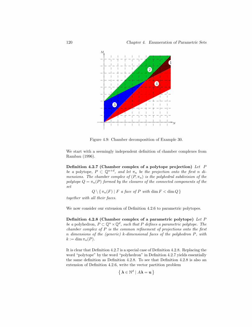
120 Chapter 4. Enumeration of Parametric Sets
N
M
3
2
4
1
Figure 4.9: Chamber decomposition of Example 30.
We start with a seemingly independent definition of chamber complexes fromRambau (1996).
Definition 4.2.7 (Chamber complex of a polytope projection) Let Pbe a polytope, P ⊂ Qn+d, and let πn be the projection onto the first n di-mensions. The chamber complex of (P, πn) is the polyhedral subdivision of thepolytope Q = πn(P ) formed by the closures of the connected components of theset
Q \ πn(F ) | F a face of P with dimF < dimQ
together with all their faces.
We now consider our extension of Definition 4.2.6 to parametric polytopes.
Definition 4.2.8 (Chamber complex of a parametric polytope) Let Pbe a polyhedron, P ⊂ Qn×Qd, such that P defines a parametric polytope. Thechamber complex of P is the common refinement of projections onto the firstn dimensions of the (generic) k-dimensional faces of the polyhedron P , withk := dimπn(P ).
It is clear that Definition 4.2.7 is a special case of Definition 4.2.8. Replacing theword “polytope” by the word “polyhedron” in Definition 4.2.7 yields essentiallythe same definition as Definition 4.2.8. To see that Definition 4.2.8 is also anextension of Definition 4.2.6, write the vector partition problem
λ ∈ Nd | Aλ = u
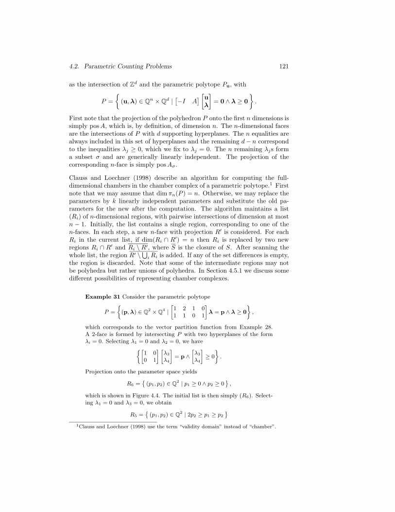
4.2. Parametric Counting Problems 121
as the intersection of Zd and the parametric polytope Pu, with
P =
(u,λ) ∈ Qn × Qd |[−I A
][uλ
]
= 0 ∧ λ ≥ 0
.
First note that the projection of the polyhedron P onto the first n dimensions issimply pos A, which is, by definition, of dimension n. The n-dimensional facesare the intersections of P with d supporting hyperplanes. The n equalities arealways included in this set of hyperplanes and the remaining d− n correspondto the inequalities λj ≥ 0, which we fix to λj = 0. The n remaining λjs forma subset σ and are generically linearly independent. The projection of thecorresponding n-face is simply pos Aσ.
Clauss and Loechner (1998) describe an algorithm for computing the full-dimensional chambers in the chamber complex of a parametric polytope.1 Firstnote that we may assume that dim πn(P ) = n. Otherwise, we may replace theparameters by k linearly independent parameters and substitute the old pa-rameters for the new after the computation. The algorithm maintains a list(Ri) of n-dimensional regions, with pairwise intersections of dimension at mostn − 1. Initially, the list contains a single region, corresponding to one of then-faces. In each step, a new n-face with projection R′ is considered. For eachRi in the current list, if dim(Ri ∩ R′) = n then Ri is replaced by two newregions Ri ∩ R′ and Ri \ R′, where S is the closure of S. After scanning thewhole list, the region R′ \
⋃
i Ri is added. If any of the set differences is empty,the region is discarded. Note that some of the intermediate regions may notbe polyhedra but rather unions of polyhedra. In Section 4.5.1 we discuss somedifferent possibilities of representing chamber complexes.
Example 31 Consider the parametric polytope
P =
(p, λ) ∈ Q2 × Q
4 |[1 2 1 01 1 0 1
]
λ = p ∧ λ ≥ 0
,
which corresponds to the vector partition function from Example 28.A 2-face is formed by intersecting P with two hyperplanes of the formλi = 0. Selecting λ1 = 0 and λ2 = 0, we have
[1 00 1
] [λ3
λ4
]
= p ∧[λ3
λ4
]
≥ 0
.
Projection onto the parameter space yields
R6 =
(p1, p2) ∈ Q2 | p1 ≥ 0 ∧ p2 ≥ 0
,
which is shown in Figure 4.4. The initial list is then simply (R6). Select-ing λ1 = 0 and λ3 = 0, we obtain
R5 =
(p1, p2) ∈ Q2 | 2p2 ≥ p1 ≥ p2
1Clauss and Loechner (1998) use the term “validity domain” instead of “chamber”.
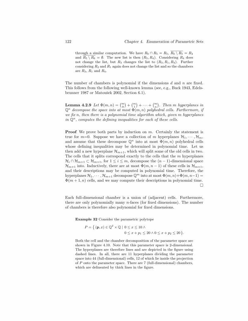
122 Chapter 4. Enumeration of Parametric Sets
through a similar computation. We have R6 ∩ R5 = R5, R6 \ R5 = R4
and R5 \ R6 = ∅. The new list is then (R5, R4). Considering R4 doesnot change the list, but R3 changes the list to (R3, R1, R4). Furtherconsidering R2 and R1 again does not change the list and so the chambersare R3, R1 and R4.
The number of chambers is polynomial if the dimensions d and n are fixed.This follows from the following well-known lemma (see, e.g., Buck 1943, Edels-brunner 1987 or Matousek 2002, Section 6.1).
Lemma 4.2.9 Let Φ(m,n) =(m0
)+(m1
)+ · · · +
(mn
). Then m hyperplanes in
Qn decompose the space into at most Φ(m,n) polyhedral cells. Furthermore, ifwe fix n, then there is a polynomial time algorithm which, given m hyperplanesin Qn, computes the defining inequalities for each of these cells.
Proof We prove both parts by induction on m. Certainly the statement istrue for m=0. Suppose we have a collection of m hyperplanes H1, · · · ,Hm,and assume that these decompose Qn into at most Φ(m,n) polyhedral cellswhose defining inequalities may be determined in polynomial time. Let usthen add a new hyperplane Hm+1, which will split some of the old cells in two.The cells that it splits correspond exactly to the cells that the m hyperplanesHi ∩Hm+1 ⊂ Hm+1, for 1 ≤ i ≤ m, decompose the (n − 1)-dimensional spaceHm+1 into. Inductively, there are at most Φ(m,n − 1) of these cells in Hm+1,and their descriptions may be computed in polynomial time. Therefore, thehyperplanes H1, · · · ,Hm+1 decompose Qm into at most Φ(m,n)+Φ(m,n−1) =Φ(m + 1, n) cells, and we may compute their descriptions in polynomial time.
Each full-dimensional chamber is a union of (adjacent) cells. Furthermore,there are only polynomially many n-faces (for fixed dimensions). The numberof chambers is therefore also polynomial for fixed dimensions.
Example 32 Consider the parametric polytope
P =
(p, x) ∈ Q2 × Q | 0 ≤ x ≤ 10 ∧
0 ≤ x + p1 ≤ 20 ∧ 0 ≤ x + p2 ≤ 20 .
Both the cell and the chamber decomposition of the parameter space areshown in Figure 4.10. Note that this parameter space is 2-dimensional.The hyperplanes are therefore lines and are depicted in the figure usingdashed lines. In all, there are 11 hyperplanes dividing the parameterspace into 44 (full-dimensional) cells, 12 of which lie inside the projectionof P onto the parameter space. There are 7 (full-dimensional) chambers,which are delineated by thick lines in the figure.
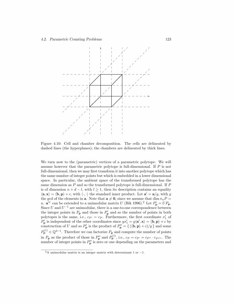
4.2. Parametric Counting Problems 123
Figure 4.10: Cell and chamber decomposition. The cells are delineated bydashed lines (the hyperplanes); the chambers are delineated by thick lines.
We turn now to the (parametric) vertices of a parametric polytope. We willassume however that the parametric polytope is full-dimensional. If P is notfull-dimensional, then we may first transform it into another polytope which hasthe same number of integer points but which is embedded in a lower dimensionalspace. In particular, the ambient space of the transformed polytope has thesame dimension as P and so the transformed polytope is full-dimensional. If Pis of dimension n + d − l, with l ≥ 1, then its description contains an equality〈a,x〉 = 〈b,p〉+ c, with 〈·, ·〉 the standard inner product. Let a′ = a/g, with gthe gcd of the elements in a. Note that a 6= 0, since we assume that dim πnP =n. a′T can be extended to a unimodular matrix U (Bik 1996).2 Let P ′p = UPp.Since U and U−1 are unimodular, there is a one-to-one correspondence betweenthe integer points in Pp and those in P ′p and so the number of points in bothpolytopes is the same, i.e., cP ′ = cP . Furthermore, the first coordinate x′1 ofP ′p is independent of the other coordinates since gx′1 = g〈a′,x〉 = 〈b,p〉+ c byconstruction of U and so P ′p is the product of P ′′p = (〈b,p〉+ c)/g and some
P(1)p ∈ Qd−1. Therefore we can factorize Pp and compute the number of points
in Pp as the product of those in P ′′p and P(1)p , i.e., cP = cP ′ = cP ′′ · cP (1) . The
number of integer points in P ′′p is zero or one depending on the parameters and
2A unimodular matrix is an integer matrix with determinant 1 or −1.
124 Chapter 4. Enumeration of Parametric Sets
can be represented by a periodic number.3 Repeating the above l times, yields aP (l) ∈ Qn×Qd−l of full dimension. Obviously, we may also remove all equalitiessimultaneously through a single unimodular transformation. Also note thatsince the unimodular transformation is independent of the parameters, theprojection of the faces of P onto the parameter space does not change. Inparticular, the chamber decomposition remains intact.
Example 33 Consider once more the vector partition function
c(p) = #
λ ∈ N4 |[1 2 1 01 1 0 1
]
λ = p
from Example 28. For a given p ∈ Zn, the solution set
Pp =
λ ∈ Q4 | λ ≥ 0 and
[1 2 1 01 1 0 1
]
λ = p
is a two dimensional polytope in Q4, so it is helpful to convert it to afull-dimensional polytope in Q2 (without changing the number of integerpoints). To do this, extend the matrix to
M =
1 2 1 01 1 0 10 0 1 00 0 0 1
,
which is unimodular (that is, it has determinant ±1 and so, as a lineartransformation, it bijectively maps Z4 to Z4), and perform the change ofcoordinates λ 7→ λ′ = Mλ. Then
c(p) = #
λ′ ∈ Z
4 | M−1λ
′ ≥ 0 and
[1 2 1 01 1 0 1
]
M−1λ
′ = p
= #λ
′ ∈ Z4 | M−1
λ′ ≥ 0 and λ′1 = p1, λ
′2 = p2
= #
(λ′3, λ′4) ∈ Z
2 |
−1 2 1 −21 −1 −1 10 0 1 00 0 0 1
p1
p2
λ′3λ′4
≥ 0
.
In this case P ′′ is simply(p1, p2, λ
′1, λ′2) ∈ Q2 × Q2 | λ′1 = p1 ∧ λ′2 = p2
and so cP ′′ = 1.
For computing the parametric vertices, we basically follow the algorithm ofLoechner and Wilde (1997), but use a simpler terminology.4 Consider a para-metric polytope Pp =
x ∈ Qd | Ax ≥ Bp + c
of dimension d with n param-
eters. The vertices are the 0-faces of Pp, i.e., each vertex is the unique element
3This periodic number may depend on several parameters. Such periodic numbers will bedefined in Definition 4.2.12 as the obvious extension of Definition 4.2.2.
4The idea of using this simpler terminology is due to Rachid Seghir (Seghir 2004).
4.2. Parametric Counting Problems 125
in the intersection Vp of Pp with some set x ∈ Qd | A′x = B′p + c′ , whereA′x ≥ B′p+ c′ is a subsystem of Ax ≥ Bp+ c such that the dimension of thisintersection is 0. I.e.,
Vp = v(p) = x ∈ Qd | A′x = B′p + c′ ∧ A′′x ≥ B′′p + c′′ ,
where A′′x ≥ B′′p + c′′ are the remaining inequalities of Pp. Since Pp is ofdimension d, at least d equalities are needed. In fact, all vertices can be obtainedby intersecting Pp with all possible combinations of d linearly independentequalities, i.e., such that A′ is non-singular. The vertex v(p) is obtained as thesolution of the linear system A′x = B′p + c′. Obviously, v(p) is a d-vector ofaffine functions of the parameters. Such a solution is only an actual vertex ofPp if the set Vp is non-empty. This set may be non-empty only for some valuesof the parameters. We say that v(p) is an active vertex of Pp for these valuesof the parameters, i.e., those that belong to the following polyhedron:
R = p ∈ Qn | A′′v(p) ≥ B′′p + c′′ .
Note that R is the projection onto the parameter space of V , the polyhedrondefining the parametric (0-dimensional) polytope Vp, and that V is an n-faceof the polyhedron P . It follows that the chambers are exactly those regionswith a fixed set of active vertices. Since the number of linearly independentsets of d constraints from the original set of m constraints is at most
(md
), the
total number of parametric vertices is polynomial in the number of constraints(for fixed d) and therefore polynomial in the input size.
Example 34 Consider the parametric polytope
P =
(p, t) ∈ Q2 × Q
2 |
−1 21 −10 00 0
p +
1 −2−1 11 00 1
t ≥ 0
,
which is the set we obtained in Example 33. The (parametric) vertices ofPp can be obtained as the intersections of pairs of (parametric) facets ofPp. The facets t1 = 0 and t1 − 2t2 = p1 − 2p2, for example, intersect atthe point v1 = (0,−p1/2 + p2). That is, we have chosen the subsystem
[−1 20 0
]
p +
[1 −21 0
]
t ≥ 0
and we have obtained
Vp = (0,−p1/2 + p2) .
Notice that the vertex corresponds to the affine transformation
T1 : Q2 → Q
2 :
[p1
p2
]
7→[
0−p1/2 + p2
]
.
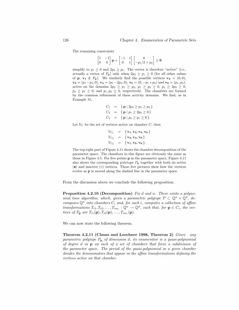
126 Chapter 4. Enumeration of Parametric Sets
The remaining constraints[1 −10 0
]
p +
[−1 10 1
] [0
−p1/2 + p2
]
≥ 0
simplify to p1 ≥ 0 and 2p2 ≥ p1. The vertex is therefore “active” (i.e.,actually a vertex of Pp) only when 2p2 ≥ p1 ≥ 0 (for all other valuesof p, v1 /∈ Pp). We similarly find the possible vertices v2 = (0, 0),v3 = (p1−p2, 0), v4 = (p1−2p2, 0), v5 = (0,−p1+p2) and v6 = (p1, p2),active on the domains 2p2 ≥ p1 ≥ p2, p1 ≥ p2 ≥ 0, p1 ≥ 2p2 ≥ 0,p2 ≥ p1 ≥ 0, and p1, p2 ≥ 0, respectively. The chambers are formedby the common refinement of these activity domains. We find, as inExample 31,
C1 = p | 2p2 ≥ p1 ≥ p2 C2 = p | p1 ≥ 2p2 ≥ 0 C3 = p | p2 ≥ p1 ≥ 0 .
Let VC be the set of vertices active on chamber C, then
VC1 = v1,v2,v3,v6 VC2 = v3,v4,v6 VC3 = v1,v5,v6 .
The top-right part of Figure 4.11 shows the chamber decomposition of theparameter space. The chambers in this figure are obviously the same asthose in Figure 4.5. For five points p in the parameter space, Figure 4.11also shows the corresponding polytope Pp together with both its active(•) and inactive () vertices. These five pictures show how the verticesevolve as p is moved along the dashed line in the parameter space.
From the discussion above we conclude the following proposition.
Proposition 4.2.10 (Decomposition) Fix d and n. There exists a polyno-mial time algorithm, which, given a parametric polytope P ⊂ Qn × Qd, de-composes Qn into chambers Ci and, for each i, computes a collection of affinetransformations Ti1, Ti2, . . . , Timi
: Qn → Qd, such that, for p ∈ Ci, the ver-tices of Pp are Ti1(p), Ti2(p), . . . , Timi
(p).
We can now state the following theorem.
Theorem 4.2.11 (Clauss and Loechner 1998, Theorem 2) Given anyparametric polytope Pp of dimension d, its enumerator is a quasi-polynomialof degree d in p on each of a set of chambers that form a subdivision ofthe parameter space. The period of the quasi-polynomial in a given chamberdivides the denominators that appear in the affine transformations defining thevertices active on that chamber.
4.2. Parametric Counting Problems 127
p1
p2
•
•
• • •
C3 C1
C2
t1
t2
•v5
•v1
•v6
v2
v3
v4
t1
t2
•v1
•v6
•v2 = v3 = v5
v4
t1
t2
v5
•v1
•v6
•v2
•v3
v4 t1
t2
v5
•v1 = v2 = v4
•v6
•v3
t1
t2
v5
v1
•v6
v2
•v3
•v4
Figure 4.11: The chamber decomposition and parametric vertices of the para-metric polytope in Example 34.
In Section 4.4.4 we will see that the quasi-polynomials from Theorem 4.2.11can be computed in polynomial time (for fixed dimensions). These quasi-polynomials are the natural extension of the univariate quasi-polynomials fromDefinition 4.2.3.
Definition 4.2.12 A rational n-periodic number U(p) is a function Zn → Q,such that there exist a period q = (q1, . . . , qn) ∈ Nn such that U(p) = U(p′)whenever pi ≡ p′i mod qi, for 1 ≤ i ≤ n.
Definition 4.2.13 A quasi-polynomial of degree d in n variables p is a poly-nomial expression of degree d in p with rational n-periodic numbers for co-efficients. The period of a quasi-polynomial is the lcm of the periods of itscoefficients.
In the parametric vertex enumeration algorithm above, several subsystemsA′x ≥ B′p + c′ may result in the same parametric vertex. It is importantto remove the duplicates from the resulting set of parametric vertices. Weslightly digress here to consider how Loechner and Wilde (1997) removed theseduplicates because it was implemented incorrectly in versions of PolyLib upuntil 5.20.0, resulting in the elimination of non-duplicate parametric vertices.
128 Chapter 4. Enumeration of Parametric Sets
They consider the (d + n)-dimensional polyhedron P and search for all combi-nations of d constraints such that the subset of P saturating these constraintsforms an n-face, which they check by counting the number of generators ofP that saturate this set of constraints. If this number is at least n + 1 andcontains at least on vertex, then the intersection is an n-face of P . They per-form a depth-first search on the (ordered) list of all constraints, which resultsin an implicit ordering on the solutions. To eliminate duplicate n-faces, theycheck whether a constraint that is not part of the selected constraints and thatoccurs earlier in the list of constraints than the last selected constraint alreadysaturates the generators saturated by the selected set of constraints. If thisis the case, then the same set of generators was also saturated by a previoussolution, so the current solution is dropped. To ensure that the face is actuallyof dimension n and not of some higher dimension, the search algorithm onlyadds a constraint to the set of constraints to be saturated, if the number ofgenerators saturated by both the new constraint and the already selected con-straints is smaller than the number of generators saturated by just the alreadyselected constraints. The idea is to only add a constraint that (as an equal-ity) is linearly independent of the other selected constraints (as equalities), butthey actually check whether the new equality is redundant with respect to theselected equalities and the remaining inequalities. Adding a test to see whetherthe considered constraint is actually linearly dependent of the already selectedequalities before discarding it solves the problem. Our fix should be availablein the next release of PolyLib.
Example 35 Consider the polyhedron P ⊂ Q4 × Q
(x, p) |
0 0 −20 00 1 20 00 −1 0 04 −20 0 0−4 20 0 00 1 0 200 0 0 −20
x +
19−200−11
−2019
p +
116423−22161
≥ 0
.
The parametric polytope Pp is 4-dimensional, so we need a subsystemof four linearly independent constraints to form a vertex of Pp (i.e., a1-face of P ). Saturating just three of the above constraints can yield a1-dimensional face. In particular, intersecting P with
(x, p) |
0 0 −20 00 1 20 04 −20 0 0
x +
19−20−1
p +
11623
= 0
.
yields the 1-dimensional face defined by the equalities
4 0 0 00 1 0 00 0 20 00 0 0 20
x +
−21−1−19−19
p +
36317−1−1
= 0
4.2. Parametric Counting Problems 129
and the inequality −p+21 ≥ 0. Since this set of 3 constraints already sat-urates the minimum number of generators, selecting a fourth constraintwould never saturate fewer, but still enough, generators and would there-fore never result in a parametric vertex in the old implementation. Inreality, both the systems
0 0 −20 00 1 20 04 −20 0 00 1 0 20
x +
19−20−1−20
p +
1162316
= 0
and
0 0 −20 00 1 20 04 −20 0 00 0 0 −20
x +
19−20−119
p +
116231
= 0
yield (the same) parametric vertices. The duplicate is correctly removedin the current implementation because the last constraint of the firstsystem saturates all generators of the second system.
4.2.4 Parametric Projected Sets
In this section we briefly discuss the most general counting problems we willconsider: the enumeration of parametric projected sets
S =
(p,x) ∈ Zn × Zd | ∃y ∈ Zd′ : Ax + By ≥ Dp + c
. (4.4)
The enumerator can be written as
cS(p) = #Sp
= #
x ∈ Zd | ∃y ∈ Zd′ : Ax + By ≥ Dp + c
= #(
πd
(
Zd+d′ ∩
(x,y) ∈ Qd+d′ | Ax + By ≥ Dp + c))
.
That is, cS enumerates the number of elements in the projection of the integerpoints in a parametric polytope. We conclude this brief discussion with anexample indicating that this problem is more difficult than the enumeration ofa parametric polytope.
Example 36 Consider the program shown in Figure 4.12, adapted froman example from Clauss (1997). Assume we want to know the totalnumber of array elements accessed by the statement in the inner loop asa function of the symbolic parameter p. This problem is equivalent tocounting the number of elements in the set
Sp = l ∈ Z | ∃i, j ∈ Z : l = 6i + 9j − 7 ∧ 1 ≤ j ≤ p ∧ 1 ≤ i ≤ 8 , (4.5)
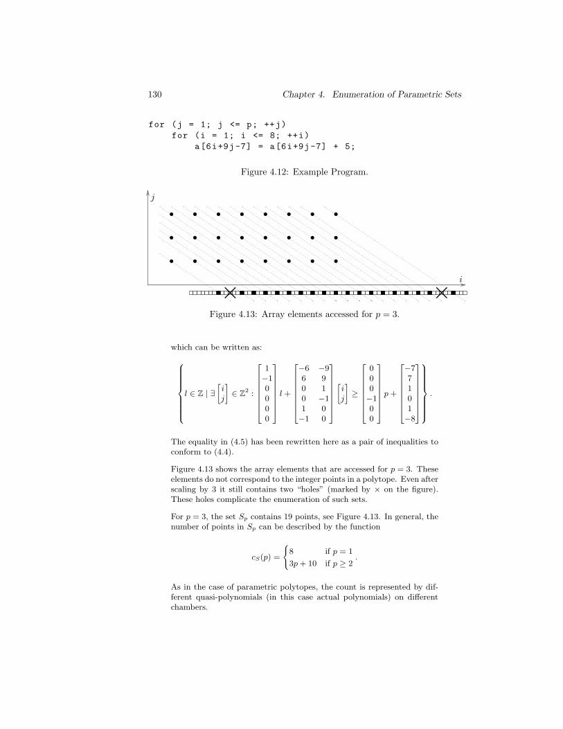
130 Chapter 4. Enumeration of Parametric Sets
for (j = 1; j <= p; ++j)
for (i = 1; i <= 8; ++i)
a[6i+9j-7] = a[6i+9j-7] + 5;
Figure 4.12: Example Program.
• • • • • • • •
• • • • • • • •
• • • • • • • •
j
i
× ×Figure 4.13: Array elements accessed for p = 3.
which can be written as:
l ∈ Z | ∃[ij
]
∈ Z2 :
1−10000
l +
−6 −96 90 10 −11 0−1 0
[ij
]
≥
000−100
p +
−77101−8
.
The equality in (4.5) has been rewritten here as a pair of inequalities toconform to (4.4).
Figure 4.13 shows the array elements that are accessed for p = 3. Theseelements do not correspond to the integer points in a polytope. Even afterscaling by 3 it still contains two “holes” (marked by × on the figure).These holes complicate the enumeration of such sets.
For p = 3, the set Sp contains 19 points, see Figure 4.13. In general, thenumber of points in Sp can be described by the function
cS(p) =
8 if p = 1
3p + 10 if p ≥ 2.
As in the case of parametric polytopes, the count is represented by dif-ferent quasi-polynomials (in this case actual polynomials) on differentchambers.
4.3. Two Representations 131
4.3 Two Representations
In the previous section we have discussed a variety of counting functions andin each case we have seen that we can represent this function as a set of quasi-polynomials, each associated to a chamber of the parameter space. For someof these counting problems we have also shown the corresponding generatingfunction, which is sometimes easier to compute. In fact, it is trivial to computefor vector partition functions.
We will use the following representations for generating functions and explicitfunctions. Note that neither of these representations is unique, i.e., any gener-ating function or explicit function can be represented in multiple ways.
Definition 4.3.1 By a rational generating function f(x), we will mean a func-tion written in the form
f(x) =∑
i∈I
αixqi
∏ki
j=1 (1 − xbij ), (4.6)
where x ∈ Cn, αi ∈ Q, qi ∈ Zn, and bij ∈ Zn \ 0.
Such a rational generating function is sometimes called short if the number offactors ki in each term is bounded by a constant and if the number of elementsin the index set I is polynomial in the input size of the enumerated set.
Definition 4.3.2 A step-polynomial g : Zn → Q is a function written in theform
g(p) =m∑
j=1
αj
dj∏
k=1
⌊〈ajk,p〉 + bjk⌋ ,
where αj ∈ Q, ajk ∈ Qn, bjk ∈ Q, 〈·, ·〉 is the standard inner product, and ⌊·⌋is the greatest integer function. We say that the degree of g(p) is maxj dj .
A piecewise step-polynomial c : Zn → Q is a decomposition of Qn into polyhe-dral chambers Ci with corresponding functions gi : Ci ∩ Zn → Q such that
1. c(p) = gi(p), for p ∈ Ci ∩ Zn and
2. each gi is a step-polynomial.
We say that the degree of c(p) is maxi deg gi.
Example 37 Recall the parametric polytope P ′′p = (〈b,p〉 + c)/g we encountered in Section 4.2.3 when reducing a parametric polytope
132 Chapter 4. Enumeration of Parametric Sets
that may not be full-dimensional to a full-dimensional polytope. As wealready mentioned, the number of integer points in P ′′p is zero or onedepending on the parameters. In particular, if g divides 〈b,p〉 + c, thencP ′′(p) = 1. Otherwise, cP ′′(p) = 0. We can represent this as thestep-polynomial
cP ′′ =
⌊ 〈b,p〉 + c
g
⌋
−⌊ 〈b,p〉 + c
g− 1
g
⌋
.
As we will explain in Section 4.7.2, we use “strides” to represent step-polynomials of this form in our implementation.
There are good reasons to consider both the explicit enumerator c(p) and itsgenerating function C(x). An explicit function representation c(p) has theadvantage of being easily evaluated for a particular value of p. Such a repre-sentation is therefore preferred in the compiler community (see, for example,Verdoolaege et al. 2004d). The most straightforward way of obtaining the co-efficient of xp, i.e., c(p), from a rational generating function C(x), on the otherhand, is to expand the Laurent power series up to power p, which is a processthat is exponential in the size of p.
The advantage of rational generating functions is that we may apply manycomputational tools to manipulate them and obtain information from them(see, for example, Barvinok and Woods 2003; Woods 2004). Consider, forexample, summation. Let C(x,y) be the generation function of c(p, t), i.e.,
C(x,y) =∑
(p,t)
c(p, t)xpyt.
Suppose we want to compute
d(t) =∑
p
c(p, t),
where we assume that for each t, c(p, t) is non-zero only for a finite numberof values of p. To compute d(t) explicitly we need to solve a set of new count-ing problems (see Section 4.5.4). To compute the corresponding generatingfunction D(y) = C(1,y), however, we “simply” need to plug in 1 for x.
More importantly, Barvinok and Woods (2003) show that given a generatingfunction that corresponds to a polytope, we may compute, in polynomial time,a generating function corresponding to the projection of this polytope.5 Usingour results on the polynomial interconvertibility of piecewise step-polynomialsand their rational generating functions (see Section 4.5.5), we will be able toshow that we can compute the explicit enumerator of a parametric projectedset in polynomial time. To the best of our knowledge, no other polynomialtime algorithms to compute this enumerator have been proposed before.
5We will be more precise about this correspondence in the next sections.
4.4. Barvinok’s Algorithm 133
4.4 Barvinok’s Algorithm
In this section we explain Barvinok’s algorithm for computing the number ofinteger points in a polytope and show how it can be applied to compute boththe explicit enumerator of a parametric polytope and its generating function.We try to provide enough background information to make the algorithm un-derstandable and focus on some implementation issues. For a more detailedtheoretical discussion of the basic algorithm we refer to Barvinok and Pommer-sheim (1999). Many of the implementation details were inspired by De Loeraet al. (2004) or Yoshida (2004a). Although most of this section is well-known,we are the first to combine the enumeration algorithm of Barvinok and Pom-mersheim (1999) with the chamber decomposition algorithm of Clauss andLoechner (1998). Furthermore, we extend the ideas of De Loera et al. (2004)for a practical implementation of Barvinok’s algorithm to a much broader con-text. We start with a general overview of the algorithm, followed by a moredetailed discussion of the two main substeps. In the final part, we show theapplication to parametric polytopes.
4.4.1 Overview
We first need a couple of definitions.
Definition 4.4.1 Let A ⊂ Qd be a set. The indicator function [A] of A isdefined by
[A] : Qd → Q : [A](s) =
1 if s ∈ A
0 if s 6∈ A
The reader with a background in functional programming may think of the
function [·] : 2Qd
→ Qd → 0, 1 as a curried version of the ∋-relation. Theindicator function [A] is then the partial evaluation of this function at A.
Definition 4.4.2 Let S be an integer set such that the convex hull of S doesnot contain a line. The generating function of S is
f(S;x) =∑
s∈S
xs.
The generating function of a set A ⊂ Qd is the generating function of theinteger points in A
f(A;x) =∑
s∈A∩Zd
xs,
provided A does not contain a line.
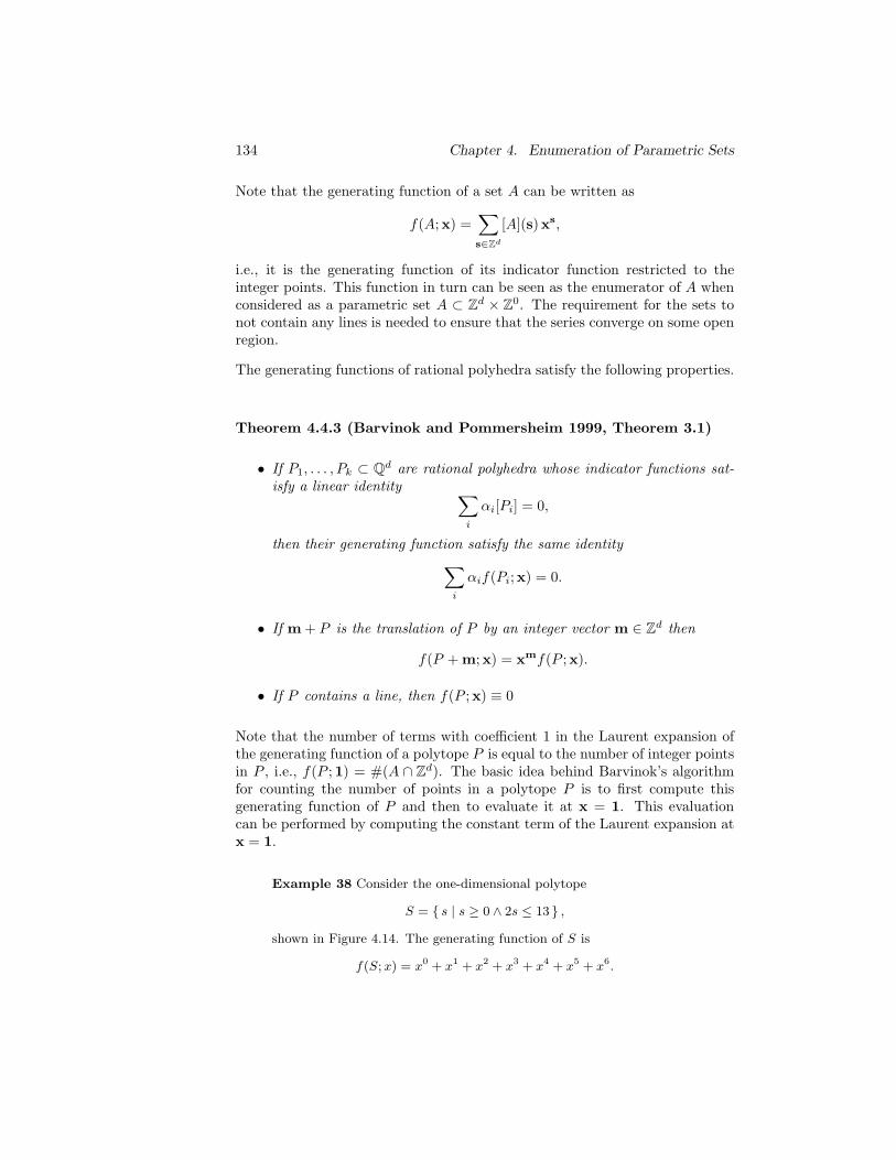
134 Chapter 4. Enumeration of Parametric Sets
Note that the generating function of a set A can be written as
f(A;x) =∑
s∈Zd
[A](s)xs,
i.e., it is the generating function of its indicator function restricted to theinteger points. This function in turn can be seen as the enumerator of A whenconsidered as a parametric set A ⊂ Zd × Z0. The requirement for the sets tonot contain any lines is needed to ensure that the series converge on some openregion.
The generating functions of rational polyhedra satisfy the following properties.
Theorem 4.4.3 (Barvinok and Pommersheim 1999, Theorem 3.1)
• If P1, . . . , Pk ⊂ Qd are rational polyhedra whose indicator functions sat-isfy a linear identity
∑
i
αi[Pi] = 0,
then their generating function satisfy the same identity
∑
i
αif(Pi;x) = 0.
• If m + P is the translation of P by an integer vector m ∈ Zd then
f(P + m;x) = xmf(P ;x).
• If P contains a line, then f(P ;x) ≡ 0
Note that the number of terms with coefficient 1 in the Laurent expansion ofthe generating function of a polytope P is equal to the number of integer pointsin P , i.e., f(P ;1) = #(A ∩ Zd). The basic idea behind Barvinok’s algorithmfor counting the number of points in a polytope P is to first compute thisgenerating function of P and then to evaluate it at x = 1. This evaluationcan be performed by computing the constant term of the Laurent expansion atx = 1.
Example 38 Consider the one-dimensional polytope
S = s | s ≥ 0 ∧ 2s ≤ 13 ,
shown in Figure 4.14. The generating function of S is
f(S; x) = x0 + x1 + x2 + x3 + x4 + x5 + x6.
4.4. Barvinok’s Algorithm 135
x0 x1 x2 x3 x4 x5 x6 x7 x8
s• • • • • • •• •
Figure 4.14: The set S from Example 38.
Evaluating this function at 1 yields
f(S; 1) = 10 + 11 + 12 + 13 + 14 + 15 + 16 = 7 = #S,
as expected. This is not how Barvinok’s algorithm would construct thegenerating function however. Consider instead the cone K = pos1. Wehave K ∩Z = N and the generating function is then simply the standardgeometric series
f(K; x) =1
1 − x=∞∑
s=0
xs.
This generating function contains more terms than we want, since italso contains the terms with power greater than or equal to 7. We canrectify this situation by subtracting the generating function of K shiftedto s = 7, whence
f(S;x) = f(K;x) − f(K + 7;x)
=x0
1 − x− x7
1 − x
=x0
1 − x+
x6
1 − x−1,
where in the last equality we applied (4.2). Note that the generatingfunction of S is the sum of the generating functions of the (shifted) conesemanating from its “integer vertices” 0 and 6, with the second cone inthe negative direction. The integer vertex appears as the power of x inthe numerator of each generating function, whereas the rays of the conesappear as the power of x in the denominator of the generating functions.We will see in the remainder of this section that this holds in general.Computing the Laurent expansion at x = 1, we find
x0
1 − x= − x0
x − 1= −1 (x − 1)−1 + 0 (x − 1)0 + · · ·
and
x6
1 − x−1=
((x − 1) + 1
)7
x − 1= 1 (x − 1)−1 + 7 (x − 1)0 + · · · .
The constant term in the Laurent expansion of f(S; x) is then f(S; 1) =0 + 7 = 7.
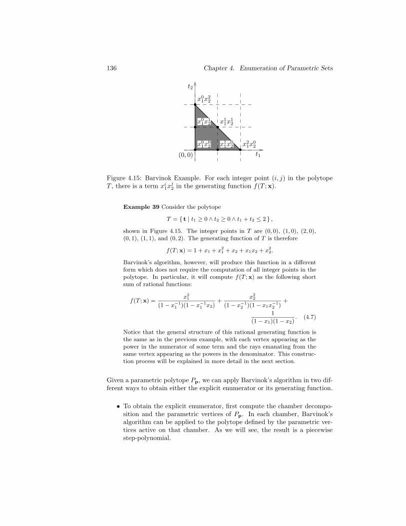
136 Chapter 4. Enumeration of Parametric Sets
•x0
1x02
•x1
1x02
•x0
1x12
•x1
1x12
•x2
1x02
•x0
1x22
t1
t2
(0, 0)
Figure 4.15: Barvinok Example. For each integer point (i, j) in the polytopeT , there is a term xi
1xj2 in the generating function f(T ;x).
Example 39 Consider the polytope
T = t | t1 ≥ 0 ∧ t2 ≥ 0 ∧ t1 + t2 ≤ 2 ,
shown in Figure 4.15. The integer points in T are (0, 0), (1, 0), (2, 0),(0, 1), (1, 1), and (0, 2). The generating function of T is therefore
f(T ;x) = 1 + x1 + x21 + x2 + x1x2 + x2
2.
Barvinok’s algorithm, however, will produce this function in a differentform which does not require the computation of all integer points in thepolytope. In particular, it will compute f(T ;x) as the following shortsum of rational functions:
f(T ;x) =x2
1
(1 − x−11 )(1 − x−1
1 x2)+
x22
(1 − x−12 )(1 − x1x
−12 )
+
1
(1 − x1)(1 − x2). (4.7)
Notice that the general structure of this rational generating function isthe same as in the previous example, with each vertex appearing as thepower in the numerator of some term and the rays emanating from thesame vertex appearing as the powers in the denominator. This construc-tion process will be explained in more detail in the next section.
Given a parametric polytope Pp, we can apply Barvinok’s algorithm in two dif-ferent ways to obtain either the explicit enumerator or its generating function.
• To obtain the explicit enumerator, first compute the chamber decompo-sition and the parametric vertices of Pp. In each chamber, Barvinok’salgorithm can be applied to the polytope defined by the parametric ver-tices active on that chamber. As we will see, the result is a piecewisestep-polynomial.
4.4. Barvinok’s Algorithm 137
• To obtain the generating function, first compute the generating functionf(P ; (x,y)) of the polyhedron P = (p, t) | t ∈ Pp and then com-pute the partial evaluation cP = f(P ; (x,1)). The result of this partialevaluation may be obtained as a rational generating function.
4.4.2 Computing Generating Functions
Following Barvinok and Pommersheim (1999), we will calculate the generatingfunction f(Pp ∩ Zd;x) as a rational generating function, and we will examinehow it changes as p varies within a chamber. From this, we will calculate
c(p) = #(Pp ∩ Zd) = f(Pp ∩ Zd;1).
Unimodular Cones
As a first step, we examine how to compute the generating function of an easyset: the integer points in a unimodular cone. We will then reduce the generalcase of a polyhedron to that of unimodular cones.
Definition 4.4.4 (Unimodular cone) A (parametric) rational unimodularcone is a rational (shifted) polyhedral cone
K =x ∈ Qd | Cx ≥ γ
,
such that C ∈ Zd×d is a unimodular matrix, i.e., such that the rows ci of Cform a basis for the lattice Zd. The righthand side may be parametric, i.e.,γ = Bp + d, with B ∈ Qd×n and d ∈ Qd.
We first consider the case where γ is zero. The unimodular cone K may thenbe written as
K =
λ1u1 + λ2u2 + · · · + λdud | λ ≥ 0,
with u1,u2, . . . ,ud the rays of K, i.e., u1,u2, . . . ,ud are the columns of U =C−1 since they satisfy Cui = 0. Clearly, U is also a unimodular matrix. Wethen have that
K ∩ Zd =s = λ1u1 + λ2u2 + · · · + λdud | λ ∈ Nd
,
and therefore
f(K;x) =1
(1 − xu1)(1 − xu2) · · · (1 − xud)(4.8)
=
∑
λ1≥0
(xu1)λ1
∑
λ2≥0
(xu2)λ2
. . .
∑
λd≥0
(xud)λd
,
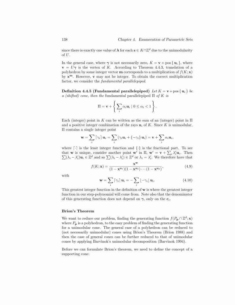
138 Chapter 4. Enumeration of Parametric Sets
since there is exactly one value of λ for each s ∈ K∩Zd due to the unimodularityof U .
In the general case, where γ is not necessarily zero, K = v + pos ui , wherev = Uγ is the vertex of K. According to Theorem 4.4.3, translation of apolyhedron by some integer vector m corresponds to a multiplication of f(K;x)by xm. However, v may not be integer. To obtain the correct multiplicationfactor, we consider the fundamental parallelepiped.
Definition 4.4.5 (Fundamental parallelepiped) Let K = v+pos ui bea (shifted) cone, then the fundamental parallelepiped Π of K is
Π = v +
∑
i
αiui | 0 ≤ αi < 1
.
Each (integer) point in K can be written as the sum of an (integer) point in Πand a positive integer combination of the rays ui of K. Since K is unimodular,Π contains a single integer point
w =∑
i
⌈γi⌉ui =∑
i
(γiui + −γiui) = v +∑
i
αiui,
where ⌈·⌉ is the least integer function and · is the fractional part. To seethat w is unique, consider another point w′ in Π, w′ = v +
∑
i λ′iui. Then∑
(λi − λ′i)ui ∈ Zd and so∑
(λi − λ′i) ∈ Zd or λi = λ′i. We therefore have that
f(K;x) =xw
(1 − xu1)(1 − xu2) · · · (1 − xud), (4.9)
withw =
∑
i
⌈γi⌉ui = −∑
i
⌊−γi⌋ui. (4.10)
This greatest integer function in the definition of w is where the greatest integerfunction in our step-polynomial will come from. Note also that the denominatorof this generating function does not depend on γ, only on the ci.
Brion’s Theorem
We want to reduce our problem, finding the generating function f(Pp ∩ Zd;x)where Pp is a polyhedron, to the easy problem of finding the generating functionfor a unimodular cone. The general case of a polyhedron can be reduced to(not necessarily unimodular) cones using Brion’s Theorem (Brion 1988) andthen the case of general cones can be further reduced to that of unimodularcones by applying Barvinok’s unimodular decomposition (Barvinok 1994).
Before we can formulate Brion’s theorem, we need to define the concept of asupporting cone.
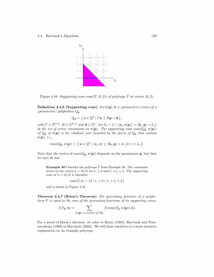
4.4. Barvinok’s Algorithm 139
t1
t2
Figure 4.16: Supporting cone cone(T, (0, 2)) of polytope T at vertex (0, 2).
Definition 4.4.6 (Supporting cone) Let v(p) be a (parametric) vertex of a(parametric) polyhedron Qp
Qp =x ∈ Qd | Cx ≥ Bp + d
,
with C ∈ Zd×d, B ∈ Zd×n and d ∈ Zd. Let Iv = i | 〈ci,v(p)〉 = 〈bi,p〉+ di be the set of active constraints on v(p). The supporting cone cone(Qp,v(p))of Qp at v(p) is the (shifted) cone bounded by the facets of Qp that containv(p), i.e.,
cone(Qp,v(p)) =x ∈ Qd | 〈ci,x〉 ≥ 〈bi,p〉 + di for i ∈ Iv
.
Note that the vertex of cone(Qp,v(p)) depends on the parameters p, but thatits rays do not.
Example 40 Consider the polytope T from Example 39. The constraintactive on the vertex v = (0, 2) are t1 ≥ 0 and t1 +t2 ≤ 2. The supportingcone at v = (0, 2) is therefore
cone(T,v) = t | t1 ≥ 0 ∧ t1 + t2 ≤ 2 and is shown in Figure 4.16.
Theorem 4.4.7 (Brion’s Theorem) The generating function of a polyhe-dron P is equal to the sum of the generating functions of its supporting cones,
f(Pp;x) =∑
v(p) a vertex of PP
f(cone(Pp,v(p));x).
For a proof of Brion’s theorem, we refer to Brion (1988), Barvinok and Pom-mersheim (1999) or Barvinok (2002). We will limit ourselves to a more intuitiveexplanation on an example polytope.
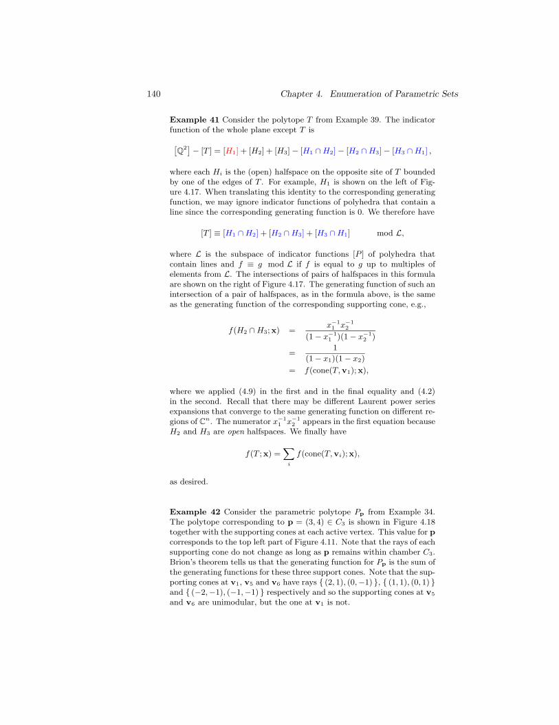
140 Chapter 4. Enumeration of Parametric Sets
Example 41 Consider the polytope T from Example 39. The indicatorfunction of the whole plane except T is
[Q
2]− [T ] = [H1] + [H2] + [H3] − [H1 ∩ H2] − [H2 ∩ H3] − [H3 ∩ H1] ,
where each Hi is the (open) halfspace on the opposite site of T boundedby one of the edges of T . For example, H1 is shown on the left of Fig-ure 4.17. When translating this identity to the corresponding generatingfunction, we may ignore indicator functions of polyhedra that contain aline since the corresponding generating function is 0. We therefore have
[T ] ≡ [H1 ∩ H2] + [H2 ∩ H3] + [H3 ∩ H1] mod L,
where L is the subspace of indicator functions [P ] of polyhedra thatcontain lines and f ≡ g mod L if f is equal to g up to multiples ofelements from L. The intersections of pairs of halfspaces in this formulaare shown on the right of Figure 4.17. The generating function of such anintersection of a pair of halfspaces, as in the formula above, is the sameas the generating function of the corresponding supporting cone, e.g.,
f(H2 ∩ H3;x) =x−1
1 x−12
(1 − x−11 )(1 − x−1
2 )
=1
(1 − x1)(1 − x2)
= f(cone(T,v1);x),
where we applied (4.9) in the first and in the final equality and (4.2)in the second. Recall that there may be different Laurent power seriesexpansions that converge to the same generating function on different re-gions of Cn. The numerator x−1
1 x−12 appears in the first equation because
H2 and H3 are open halfspaces. We finally have
f(T ;x) =∑
i
f(cone(T,vi);x),
as desired.
Example 42 Consider the parametric polytope Pp from Example 34.The polytope corresponding to p = (3, 4) ∈ C3 is shown in Figure 4.18together with the supporting cones at each active vertex. This value for p
corresponds to the top left part of Figure 4.11. Note that the rays of eachsupporting cone do not change as long as p remains within chamber C3.Brion’s theorem tells us that the generating function for Pp is the sum ofthe generating functions for these three support cones. Note that the sup-porting cones at v1, v5 and v6 have rays (2, 1), (0,−1) , (1, 1), (0, 1) and (−2,−1), (−1,−1) respectively and so the supporting cones at v5
and v6 are unimodular, but the one at v1 is not.
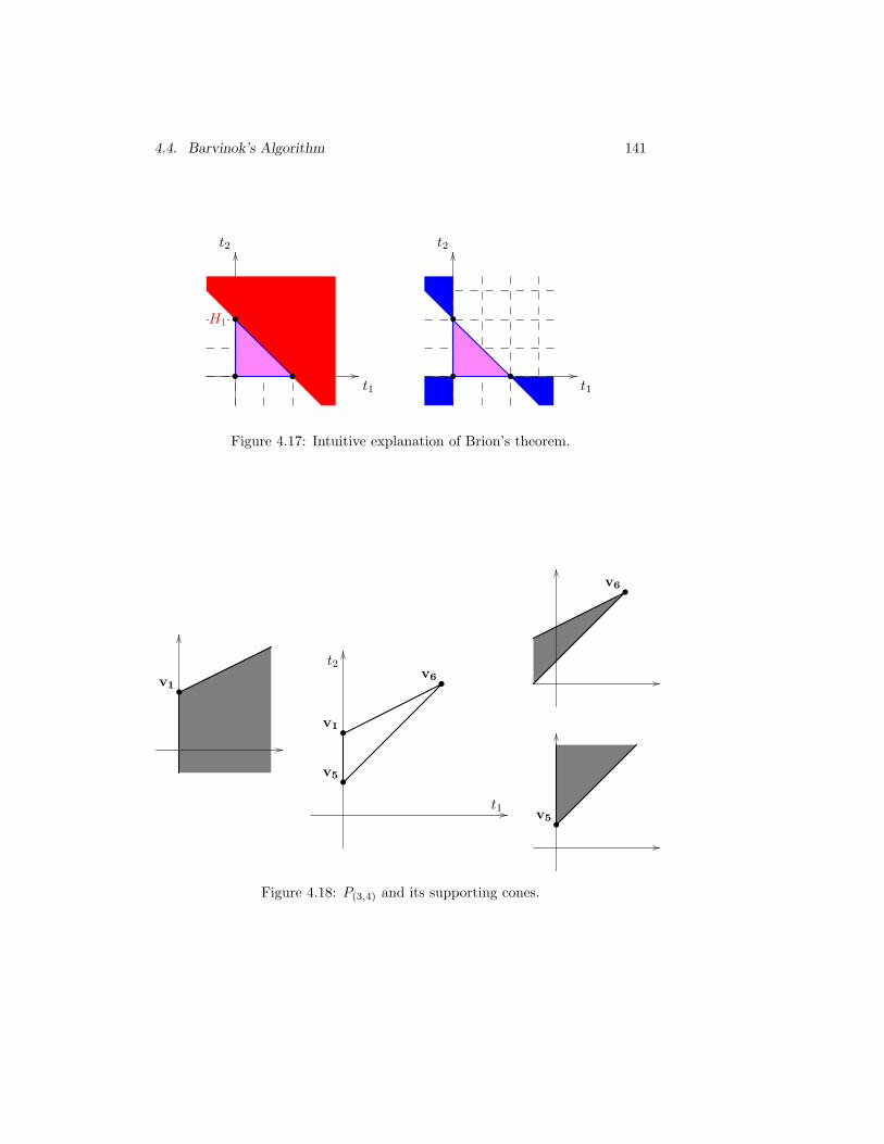
4.4. Barvinok’s Algorithm 141
t1
t2
H1
• •
•
t1
t2
• •
•
Figure 4.17: Intuitive explanation of Brion’s theorem.
t1
t2
•v5
•v1
•v6
•v1
•v6
•v5
Figure 4.18: P(3,4) and its supporting cones.
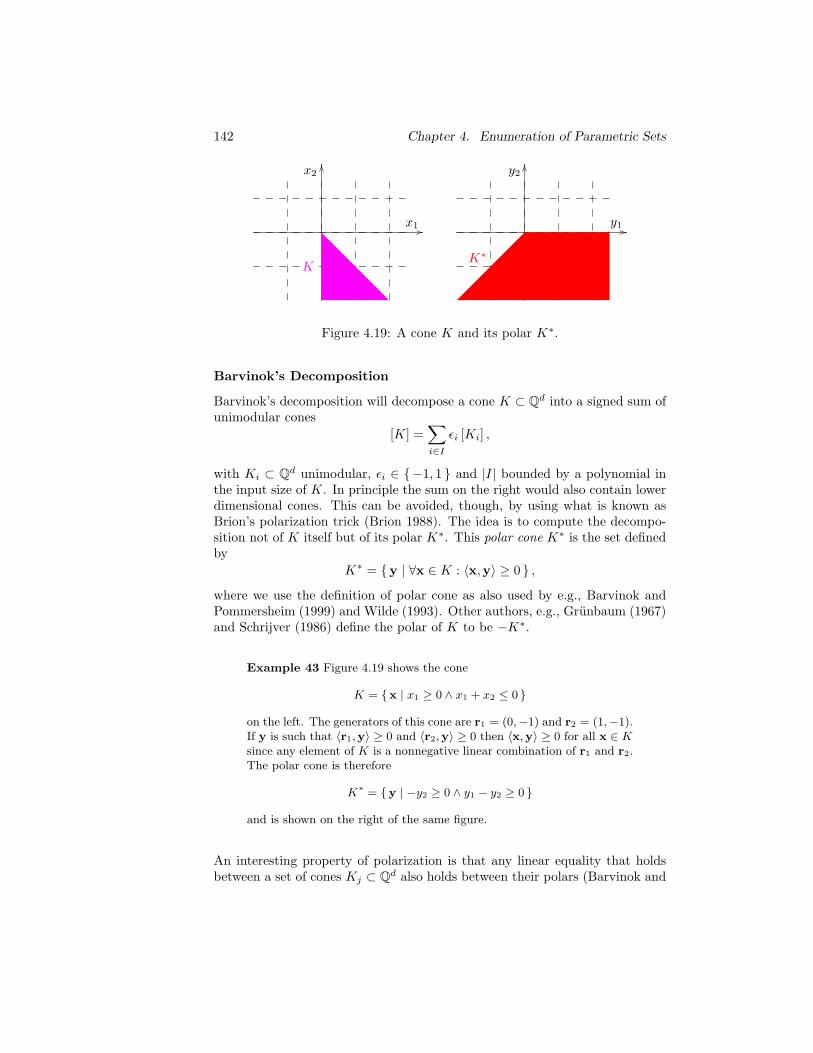
142 Chapter 4. Enumeration of Parametric Sets
x1
x2
K
y1
y2
K∗
Figure 4.19: A cone K and its polar K∗.
Barvinok’s Decomposition
Barvinok’s decomposition will decompose a cone K ⊂ Qd into a signed sum ofunimodular cones
[K] =∑
i∈I
ǫi [Ki] ,
with Ki ⊂ Qd unimodular, ǫi ∈ −1, 1 and |I| bounded by a polynomial inthe input size of K. In principle the sum on the right would also contain lowerdimensional cones. This can be avoided, though, by using what is known asBrion’s polarization trick (Brion 1988). The idea is to compute the decompo-sition not of K itself but of its polar K∗. This polar cone K∗ is the set definedby
K∗ = y | ∀x ∈ K : 〈x,y〉 ≥ 0 ,
where we use the definition of polar cone as also used by e.g., Barvinok andPommersheim (1999) and Wilde (1993). Other authors, e.g., Grunbaum (1967)and Schrijver (1986) define the polar of K to be −K∗.
Example 43 Figure 4.19 shows the cone
K = x | x1 ≥ 0 ∧ x1 + x2 ≤ 0
on the left. The generators of this cone are r1 = (0,−1) and r2 = (1,−1).If y is such that 〈r1,y〉 ≥ 0 and 〈r2,y〉 ≥ 0 then 〈x,y〉 ≥ 0 for all x ∈ Ksince any element of K is a nonnegative linear combination of r1 and r2.The polar cone is therefore
K∗ = y | −y2 ≥ 0 ∧ y1 − y2 ≥ 0
and is shown on the right of the same figure.
An interesting property of polarization is that any linear equality that holdsbetween a set of cones Kj ⊂ Qd also holds between their polars (Barvinok and
4.4. Barvinok’s Algorithm 143
Pommersheim 1999, Corollary 2.8), i.e.,
m∑
i=1
αi [Ki] = 0 ⇔m∑
i=1
αi [K∗i ] = 0.
We can therefore decompose the polar of K into a signed sum of full-dimensionalcones Kj and some lower-dimensional cones F ,
[K∗] =∑
j
ǫj [Kj ] +∑
F
ǫF [F ]
and polarize back to obtain the decomposition of K itself,
[K] =∑
j
ǫj
[K∗j]+∑
F
ǫF [F ∗] ≡∑
j
ǫj
[K∗j]
mod L
where we may ignore the polars of the lower-dimensional cones since the polar ofa lower-dimensional cone contains a line. An example of polarization will followafter we have explained Barvinok’s decomposition. Unless otherwise stated wewill assume from now on that we are working on the polar of the cone we wantto decompose and that we may therefore ignore lower-dimensional parts in thedecomposition.
Using PolyLib, the polarization of a cone is particularly easy to implement.The polar of a cone is the original cone with the rays and constraints inter-changed, both of which are maintained in PolyLib’s internal representationof a polyhedron. The function Polyhedron Polarize polarizes its argument,which is assumed to be a cone with apex 0, in place by interchanging its raysand constraints.
Triangulation of Non-simplicial Cones
The core of Barvinok’s unimodular decomposition algorithm takes a simplicialcone as input and produces a signed unimodular decomposition of the cone. Ifa supporting cone is not a (shifted) simplicial cone, then we first need to trian-gulate it. Efficient triangulation algorithms were described by Aurenhammerand Klein (2000) and Lee (1997). De Loera et al. (2004) use the Delaunaytriangulation in their LattE implementation (De Loera et al. 2003b).
We explain this Delaunay triangulation, or the more general regular triangula-tion, in some more detail. We follow the exposition of De Loera (1995), whichis in turn based on Lee (1991), but apply it to cones instead of polytopes. Aregular triangulation of a cone C ⊂ Qd is a triangulation obtained through thefollowing procedure. Let uii∈I be the generators of C. Consider the cone
Cλ = pos (ui, λi) ⊂ Qd+1,
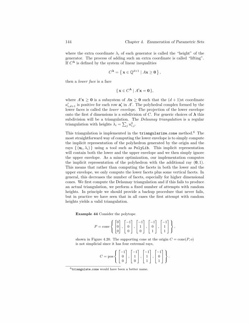
144 Chapter 4. Enumeration of Parametric Sets
where the extra coordinate λi of each generator is called the “height” of thegenerator. The process of adding such an extra coordinate is called “lifting”.If Cλ is defined by the system of linear inequalities
Cλ =x ∈ Qd+1 | Ax ≥ 0
,
then a lower face is a face
x ∈ Cλ | A′x = 0 ,
where A′x ≥ 0 is a subsystem of Ax ≥ 0 such that the (d + 1)st coordinatea′i,d+1 is positive for each row a′i in A′. The polyhedral complex formed by thelower faces is called the lower envelope. The projection of the lower envelopeonto the first d dimensions is a subdivision of C. For generic choices of λ thissubdivision will be a triangulation. The Delaunay triangulation is a regulartriangulation with heights λi =
∑
j u2i,j .
This triangulation is implemented in the triangularize cone method.6 Themost straightforward way of computing the lower envelope is to simply computethe implicit representation of the polyhedron generated by the origin and therays (ui, λi) using a tool such as PolyLib. This implicit representationwill contain both the lower and the upper envelope and we then simply ignorethe upper envelope. As a minor optimization, our implementation computesthe implicit representation of the polyhedron with the additional ray (0, 1).This means that rather than computing the facets in both the lower and theupper envelope, we only compute the lower facets plus some vertical facets. Ingeneral, this decreases the number of facets, especially for higher dimensionalcones. We first compute the Delaunay triangulation and if this fails to producean actual triangulation, we perform a fixed number of attempts with randomheights. In principle we should provide a backup procedure that never fails,but in practice we have seen that in all cases the first attempt with randomheights yields a valid triangulation.
Example 44 Consider the polytope
P = conv
000
,
−100
,
−110
,
−101
,
−111
,
shown in Figure 4.20. The supporting cone at the origin C = cone(P, o)is not simplicial since it has four extremal rays,
C = pos
−100
,
−110
,
−111
,
−101
.
6triangulate cone would have been a better name.
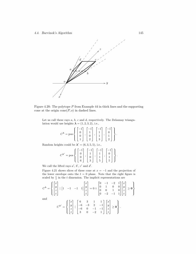
4.4. Barvinok’s Algorithm 145
o
a
d
b
c
y
x
z
Figure 4.20: The polytope P from Example 44 in thick lines and the supportingcone at the origin cone(P, o) in dashed lines.
Let us call these rays a, b, c and d, respectively. The Delaunay triangu-lation would use heights λ = (1, 2, 3, 2), i.e.,
Cλ = pos
−1001
,
−1102
,
−1113
,
−1012
.
Random heights could be λ′ = (6, 3, 5, 5), i.e.,
Cλ′ = pos
−1006
,
−1103
,
−1115
,
−1015
.
We call the lifted rays a′, b′, c′ and d′.
Figure 4.21 shows slices of these cone at x = −1 and the projection ofthe lower envelope onto the t = 0 plane. Note that the right figure isscaled by 1
2in the t dimension. The implicit representations are
Cλ =
xyzt
|[1 −1 −1 1
]
xyzt
= 0 ∧
0 −1 −2 10 1 0 00 0 1 00 −2 −1 1
xyzt
≥ 0
and
Cλ′ =
xyzt
|
6 3 1 1−6 −3 2 −1−6 0 −1 −13 0 −2 1
xyzt
≥ 0
.
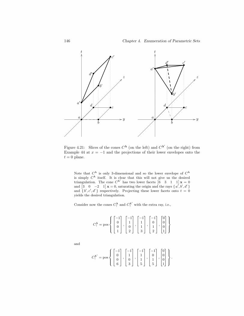
146 Chapter 4. Enumeration of Parametric Sets
•a
•d
•b
•c
y
z
t
•a′
•b′
•c′
•d′
•a
•d
•b
•c
y
z
t
•a′
•b′
•c′
•d′
Figure 4.21: Slices of the cones Cλ (on the left) and Cλ′ (on the right) fromExample 44 at x = −1 and the projections of their lower envelopes onto thet = 0 plane.
Note that Cλ is only 3-dimensional and so the lower envelope of Cλ
is simply Cλ itself. It is clear that this will not give us the desiredtriangulation. The cone Cλ′ has two lower facets
[6 3 1 1
]x = 0
and[3 0 −2 1
]x = 0, saturating the origin and the rays a′, b′, d′
and b′, c′, d′ respectively. Projecting these lower facets onto t = 0yields the desired triangulation.
Consider now the cones Cλ↑ and Cλ′
↑ with the extra ray, i.e.,
Cλ↑ = pos
−1001
,
−1102
,
−1113
,
−1012
,
0001
and
Cλ′
↑ = pos
−1006
,
−1103
,
−1115
,
−1015
,
0001
.
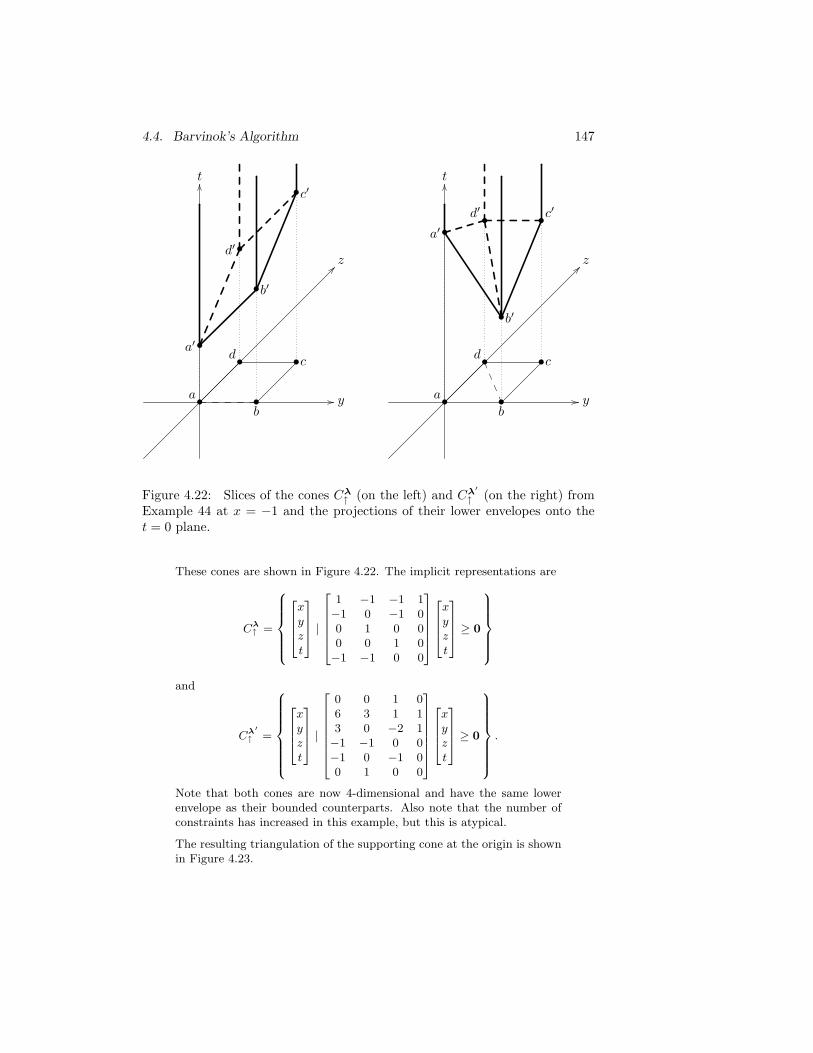
4.4. Barvinok’s Algorithm 147
•a
•d
•b
•c
y
z
t
•a′
•b′
•c′
•d′
•a
•d
•b
•c
y
z
t
•a′
•b′
•c′
•d′
Figure 4.22: Slices of the cones Cλ↑ (on the left) and Cλ′
↑ (on the right) fromExample 44 at x = −1 and the projections of their lower envelopes onto thet = 0 plane.
These cones are shown in Figure 4.22. The implicit representations are
Cλ↑ =
xyzt
|
1 −1 −1 1−1 0 −1 00 1 0 00 0 1 0−1 −1 0 0
xyzt
≥ 0
and
Cλ′
↑ =
xyzt
|
0 0 1 06 3 1 13 0 −2 1−1 −1 0 0−1 0 −1 00 1 0 0
xyzt
≥ 0
.
Note that both cones are now 4-dimensional and have the same lowerenvelope as their bounded counterparts. Also note that the number ofconstraints has increased in this example, but this is atypical.
The resulting triangulation of the supporting cone at the origin is shownin Figure 4.23.
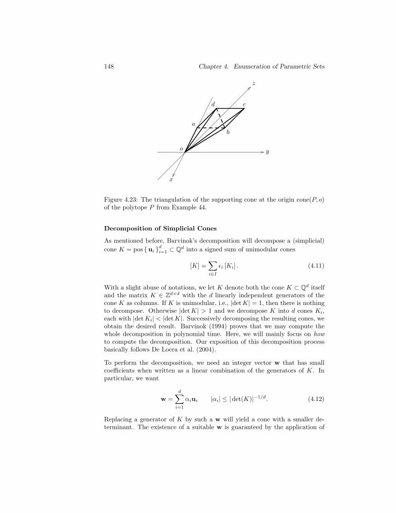
148 Chapter 4. Enumeration of Parametric Sets
o
a
d
b
c
y
x
z
Figure 4.23: The triangulation of the supporting cone at the origin cone(P, o)of the polytope P from Example 44.
Decomposition of Simplicial Cones
As mentioned before, Barvinok’s decomposition will decompose a (simplicial)
cone K = pos ui di=1 ⊂ Qd into a signed sum of unimodular cones
[K] =∑
i∈I
ǫi [Ki] . (4.11)
With a slight abuse of notations, we let K denote both the cone K ⊂ Qd itselfand the matrix K ∈ Zd×d with the d linearly independent generators of thecone K as columns. If K is unimodular, i.e., |det K| = 1, then there is nothingto decompose. Otherwise |det K| > 1 and we decompose K into d cones Ki,each with |detKi| < |det K|. Successively decomposing the resulting cones, weobtain the desired result. Barvinok (1994) proves that we may compute thewhole decomposition in polynomial time. Here, we will mainly focus on howto compute the decomposition. Our exposition of this decomposition processbasically follows De Loera et al. (2004).
To perform the decomposition, we need an integer vector w that has smallcoefficients when written as a linear combination of the generators of K. Inparticular, we want
w =
d∑
i=1
αiui |αi| ≤ |det(K)|−1/d. (4.12)
Replacing a generator of K by such a w will yield a cone with a smaller de-terminant. The existence of a suitable w is guaranteed by the application of
4.4. Barvinok’s Algorithm 149
Minkowski’s First Theorem (Schrijver 1986) to the convex body
B =
d∑
i=1
αiui | ∀i : |αi| ≤ |det(K)|−1/d
.
This convex body is just the closure of the fundamental parallelepiped Π scaledby 2|det(K)|−1/d in each dimension and centered around the origin. The scal-ing and the fact that the volume of Π is |det K| ensure that the volume ofB is 2d. Since B is a centrally symmetric convex body with volume ≥ 2d,Minkowski’s First Theorem tells us that B contains a non-zero integer vectorw, as required.
For 1 ≤ j ≤ d, let Kj be the cone generated by the generators of K with uj
replaced by w, i.e.,
Kj = pos(
ui di=1 \ uj ∪ w
)
. (4.13)
Then|det Kj | ≤ |αj ||det K| ≤ |det K|(d−1)/d < |det K| .
To see that we can use these Kj to perform a decomposition, rearrange the ui
such that for all 1 ≤ i ≤ k we have αi ≤ 0 and for all k + 1 ≤ i ≤ d we haveαi > 0. We may assume k < d; otherwise replace w ∈ B by −w ∈ B. We have
w +k∑
i=1
(−αi)ui =d∑
i=k+1
αiui
ork∑
i=0
βiui =
d∑
i=k+1
αiui, (4.14)
with u0 = w, β0 = 1 and βi = −αi ≥ 0 for 1 ≤ i ≤ k. Any two uj andul on the same side of the equality are on opposite sides of the affine hull Hof the other uis since their exists a convex combination of uj and ul on thishyperplane. In particular, since αj and αl have the same sign, we have
αj
αj + αluj +
αl
αj + αlul ∈ H.
The corresponding cones Kj and Kl (with K0 = K) therefore intersect in acommon face F ⊂ H. Let
K ′ := pos(
ui di=1 ∪ w
)
,
then any x ∈ K ′ lies both in some cone Ki with 0 ≤ i ≤ k and in some cone Ki
with k+1 ≤ i ≤ d. (Just subtract an appropriate multiple of Equation (4.14).)
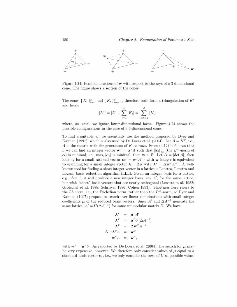
150 Chapter 4. Enumeration of Parametric Sets
+
+
+
w
+
−
+
w
−
+
−
w
Figure 4.24: Possible locations of w with respect to the rays of a 3-dimensionalcone. The figure shows a section of the cones.
The cones Ki ki=0 and Ki
di=k+1 therefore both form a triangulation of K ′
and hence
[K ′] = [K] +
k∑
i=1
[Ki] =
d∑
i=k+1
[Ki] ,
where, as usual, we ignore lower-dimensional faces. Figure 4.24 shows thepossible configurations in the case of a 3-dimensional cone.
To find a suitable w, we essentially use the method proposed by Dyer andKannan (1997), which is also used by De Loera et al. (2004). Let A = KT , i.e.,A is the matrix with the generators of K as rows. From (4.12) it follows thatif we can find an integer vector wT = αT A such that ‖α‖∞ (the L∞-norm ofα) is minimal, i.e., maxi |αi| is minimal, then w ∈ B. Let ∆ = |det A|, thenlooking for a small rational vector αT = wT A−1 with w integer is equivalentto searching for a small integer vector λ = ∆α with λT = ∆wT A−1. A well-known tool for finding a short integer vector in a lattice is Lenstra, Lenstra andLovasz’ basis reduction algorithm (LLL). Given an integer basis for a lattice,e.g., ∆A−1, it will produce a new integer basis, say A′, for the same lattice,but with “short” basis vectors that are nearly orthogonal (Lenstra et al. 1982;Grotschel et al. 1988; Schrijver 1986; Cohen 1993). Shortness here refers tothe L2-norm, i.e., the Eucledian norm, rather than the L∞-norm, so Dyer andKannan (1997) propose to search over linear combinations with small integercoefficients µ of the reduced basis vectors. Since A′ and ∆A−1 generate thesame lattice, A′ = U(∆A−1) for some unimodular matrix U . We have
λT = µT A′
λT = µT U(∆A−1)
λT = ∆wT A−1
∆−1λT A = wT
αT A = wT ,
with wT = µT U . As reported by De Loera et al. (2004), the search for µ maybe very expensive, however. We therefore only consider values of µ equal to astandard basis vector ej , i.e., we only consider the rows of U as possible values

4.4. Barvinok’s Algorithm 151
for wT . This appears to work very well in practice in the sense that we alwaysobtain a valid reduction. Note that ∆ may be any integer value that ensuresthat ∆A−1 is an integer matrix.
The search for a short vector is implemented in cone::short vector. Webasically call the LLL procedure from the NTL library (Shoup 2004) with thestandard parameters. Given a matrix B with a basis for a lattice as rows,this procedure will modify B to contain the reduced basis and will additionallyproduce the unimodular transformation matrix U . The standard parametersensure that the Eucledian length of the first basis vector is no more than 2d−1
times that of the shortest vector in the lattice. We then search for the row fromthe new B with smallest L∞-norm and assign it to λ. The corresponding rowfrom U is assigned to w. If no element of λ is strictly positive, then we replacew by −w to ensure that the right-hand side of (4.14) has at least one term.
The method decomposer::decompose computes Barvinok’s decomposition andcalls decomposer::handle on each resulting unimodular cone. The methodmaintains a list of non-unimodular cones, initialized to the original cone, if itis indeed not unimodular. As long as this list is non-empty, the method callscone::short vector to obtain both the short vector and the vector λ. Foreach 1 ≤ j ≤ d such that λj 6= 0 it constructs the cone Kj (4.13) and either addsit to the list or sends it to decomposer::handle. If λj = 0, then w contains nocontribution of uj and so Kj is not of full dimension and may be ignored. Toobtain the final sign ǫi in the decomposition (4.11), note that if (and only if)αj is negative during a single decomposition then the signs of detK and detKj
differ. The final sign is then simply the sign of the original cone multiplied bythe sign of the unimodular cone. Note that in our implementation, µ usually,but not always, ends up being equal to e1.
Example 45 For a (trivial) example where µ 6= e1, consider the conewith as generators the rows of
A =
[−2 12 3
]
.
Let
B = (det A) A−1 = −8A−1 =
[3 −1−2 −2
]
.
LLL yields
B′ =
[3 −1−2 −2
]
U =
[1 00 1
]
.
In this case, the second row of B′ is smaller than the first in both the L2
and L∞-norm and we choose λT =[−2 −2
]. Note that αT = ∆−1λT =
18
[−2 −2
]=[− 1
4− 1
4
]and its coefficients satisfy the constraint (4.12)
as 14≤ 1√
8.
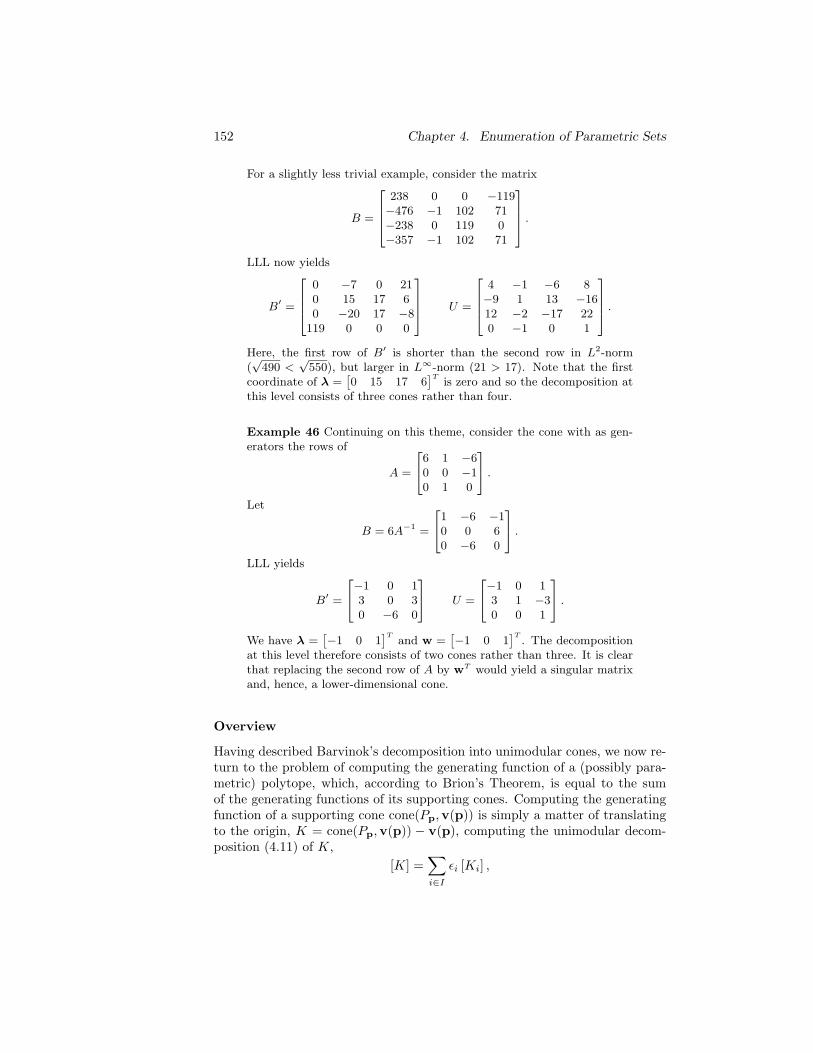
152 Chapter 4. Enumeration of Parametric Sets
For a slightly less trivial example, consider the matrix
B =
238 0 0 −119−476 −1 102 71−238 0 119 0−357 −1 102 71
.
LLL now yields
B′ =
0 −7 0 210 15 17 60 −20 17 −8
119 0 0 0
U =
4 −1 −6 8−9 1 13 −1612 −2 −17 220 −1 0 1
.
Here, the first row of B′ is shorter than the second row in L2-norm(√
490 <√
550), but larger in L∞-norm (21 > 17). Note that the firstcoordinate of λ =
[0 15 17 6
]Tis zero and so the decomposition at
this level consists of three cones rather than four.
Example 46 Continuing on this theme, consider the cone with as gen-erators the rows of
A =
6 1 −60 0 −10 1 0
.
Let
B = 6A−1 =
1 −6 −10 0 60 −6 0
.
LLL yields
B′ =
−1 0 13 0 30 −6 0
U =
−1 0 13 1 −30 0 1
.
We have λ =[−1 0 1
]Tand w =
[−1 0 1
]T. The decomposition
at this level therefore consists of two cones rather than three. It is clearthat replacing the second row of A by wT would yield a singular matrixand, hence, a lower-dimensional cone.
Overview
Having described Barvinok’s decomposition into unimodular cones, we now re-turn to the problem of computing the generating function of a (possibly para-metric) polytope, which, according to Brion’s Theorem, is equal to the sumof the generating functions of its supporting cones. Computing the generatingfunction of a supporting cone cone(Pp,v(p)) is simply a matter of translatingto the origin, K = cone(Pp,v(p)) − v(p), computing the unimodular decom-position (4.11) of K,
[K] =∑
i∈I
ǫi [Ki] ,
4.4. Barvinok’s Algorithm 153
translating back to v(p)
[cone(Pp,v(p))] =∑
i∈I
ǫi [Ki + v(p)]
and constructing the corresponding generating functions for the (shifted) uni-modular cones as in (4.9). Note that this is equivalent to first computing thegenerating functions (4.8) of the Ki and then multiplying each with the appro-priate xwi according to (4.10), where γ is such that
v =∑
i
γiui = Kγ, (4.15)
i.e.,
γ(p) = K−1v(p). (4.16)
Since the coordinates of v(p) are affine combinations of the parameters p, thenso are the coordinates of γ. Hence, w is a step-polynomial in p of degree one.We have the following proposition, a rephrasing of Theorem 4.4 of Barvinokand Pommersheim (1999).
Proposition 4.4.8 Fix d. There exists a polynomial time algorithm, which,given a parametric polyhedron P ⊂ Qn × Qd and a polyhedral chamber C suchthat for p ∈ C the vertices of Pp = t ∈ Qd | (p, t) ∈ P are given by affinetransformations T1(p), T2(p), · · · , Tm(p), computes the generating functions
f(Pp ∩ Zd;x) =∑
i∈I
ǫixwi(p)
(1 − xbi1)(1 − xbi2) · · · (1 − xbid),
where ǫ ∈ −1, 1 , bij ∈ Zd \ 0, and each coordinate of wi(p) : Zn → Zd isa step-polynomial of degree one, for each i.
An overview of Barvinok’s algorithm, applied to parametric polytopes, is shownin Algorithm 4.1. The function E(v(p),K) in step 1e returns the step-poly-nomial that determines the unique point in the fundamental parallelepiped ofv(p) + K. The notation vi ∈ C in step 2a means that vertex vi is active inchamber C. The evaluation in step 2b is explained in Section 4.4.3.
Example 47 We continue with the parametric polytope Pp from Exam-ples 34 and 42. In particular, we consider chamber C3 (see Figure 4.11).The supporting cones in this chamber are as shown in Figure 4.18. Re-call that the supporting cones at v5 and v6 are unimodular, but thatthe one at v1 is not. We therefore need to apply Barvinok’s unimodulardecomposition to the cone K = cone(Pp,v1) − v1.
154 Chapter 4. Enumeration of Parametric Sets
Algorithm 4.1 Barvinok’s algorithm
1. For each vertex vi(p) of Pp
(a) Determine supporting cone cone(Pp,vi(p))
(b) Let K = cone(Pp,vi(p)) − vi(p)
(c) Decompose K into unimodular cones ǫj ,Kj
i. Polarize K into K∗
ii. Triangulate K∗
iii. Decompose each simplicial cone in triangulation
iv. Polarize back
(d) For each Kj
i. Determine f(Kj ;x)
(e) f(cone(Pp,vi(p));x) =∑
j ǫjxE(vi(p),Kj)f(Kj ;x)
2. For each chamber C of Pp
(a) f(Pp;x) =∑
vi∈C f(cone(Pp,vi(p));x)
(b) Evaluate f(Pp;1)
We first consider a “primal decomposition”, i.e., without polarization.The generators of K are (2, 1) and (0,−1), i.e.,
A =
[2 10 −1
]
.
We have ∆ = |det A| = |det K| = 2 and so
∆A−1 =
[1 10 −2
]
.
LLL yields[1 10 −2
]
= UA′ =
[1 01 1
] [1 11 −1
]
.
Both rows of A′ have the same L∞-norm, so we arbitrarily choose thefirst row λT =
[1 1
], i.e., µ = e1, and the corresponding row from U
is wT =[1 0
]. We obtain
[K] = [K1] + [K2] − [K1 ∩ K2] ,
with the generators of K1, K2 and K′ = K1 ∩ K2
K1 =
[1 00 −1
]
, K2 =
[2 11 0
]
and K′ =
[10
]
.
This unimodular decomposition is shown in Figure 4.25, with K2 onthe left of K1 for reasons that will become clear when we consider the
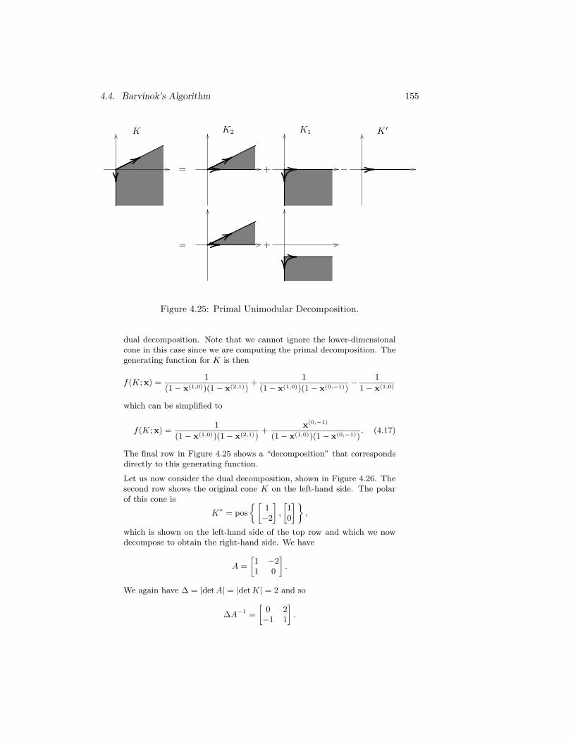
4.4. Barvinok’s Algorithm 155
K
=
K2
+
K1
−
K ′
= +
Figure 4.25: Primal Unimodular Decomposition.
dual decomposition. Note that we cannot ignore the lower-dimensionalcone in this case since we are computing the primal decomposition. Thegenerating function for K is then
f(K;x) =1
(1 − x(1,0))(1 − x(2,1))+
1
(1 − x(1,0))(1 − x(0,−1))− 1
1 − x(1,0)
which can be simplified to
f(K;x) =1
(1 − x(1,0))(1 − x(2,1))+
x(0,−1)
(1 − x(1,0))(1 − x(0,−1)). (4.17)
The final row in Figure 4.25 shows a “decomposition” that correspondsdirectly to this generating function.
Let us now consider the dual decomposition, shown in Figure 4.26. Thesecond row shows the original cone K on the left-hand side. The polarof this cone is
K∗ = pos
[1−2
]
,
[10
]
,
which is shown on the left-hand side of the top row and which we nowdecompose to obtain the right-hand side. We have
A =
[1 −21 0
]
.
We again have ∆ = |det A| = |det K| = 2 and so
∆A−1 =
[0 2−1 1
]
.
156 Chapter 4. Enumeration of Parametric Sets
LLL now yields[
0 2−1 1
]
= UA′ =
[0 11 −1
] [−1 11 1
]
.
Again, both rows of A′ have the same L∞-norm, so we arbitrarily choosethe first row λT =
[−1 1
], i.e., µ = e1, and the corresponding row
from U is wT =[0 1
]. We obtain
[K∗] ≡ [K2] − [K1] ,
with the generators of K1 and K2
K1 =
[0 11 0
]
and K2 =
[1 0−2 1
]
.
In the figure we have also shown the lower-dimensional intersection, butthis can be ignored since polarizing back yields a cone containing a line,as shown in the second row of the figure. We finally have
[K] ≡ [K∗2 ] − [K∗1 ] ,
with
K∗1 =
[1 00 1
]
and K∗2 =
[2 11 0
]
.
The generating function for K is then
f(K;x) =1
(1 − x(1,0))(1 − x(2,1))− 1
(1 − x(1,0))(1 − x(0,1)), (4.18)
which is equivalent to (4.17) through application of (4.2).
To obtain the generating function of K + v1 = cone(Ps,v1), Equa-tion (4.18) still needs to be translated to v1(p) = (0,−p1/2 + p2) using(4.10). From (4.16) we have
v1 =
[0
− p12
+ p2
]
= γ1
[10
]
+ γ2
[21
]
=
[1 20 1
]
γ.
We have
γ =
[1 −20 1
] [0
− p12
+ p2
]
=
[p1 − 2p2
− p12
+ p2
]
.
Note that this corresponds to
K∗2 + v1 =
t ∈ Q2 | t2 ≥ −p1
2+ p2 ∧ t1 − 2t2 ≥ p1 − 2p2
.
We conclude from (4.10) that
w = −⌊−γ1⌋[10
]
− ⌊−γ2⌋[21
]
=
[−2⌊ p1
2− p2⌋ + p1 − 2p2
−⌊ p12− p2⌋
]
.
Handling the second term similarly, we obtain
f((K + v1);x
)=
x(−2⌊ p12−p2⌋+p1−2p2,−⌊ p1
2−p2⌋)
(1 − x(1,0))(1 − x(2,1))
− x(0,−⌊ p12−p2⌋)
(1 − x(1,0))(1 − x(0,1)). (4.19)
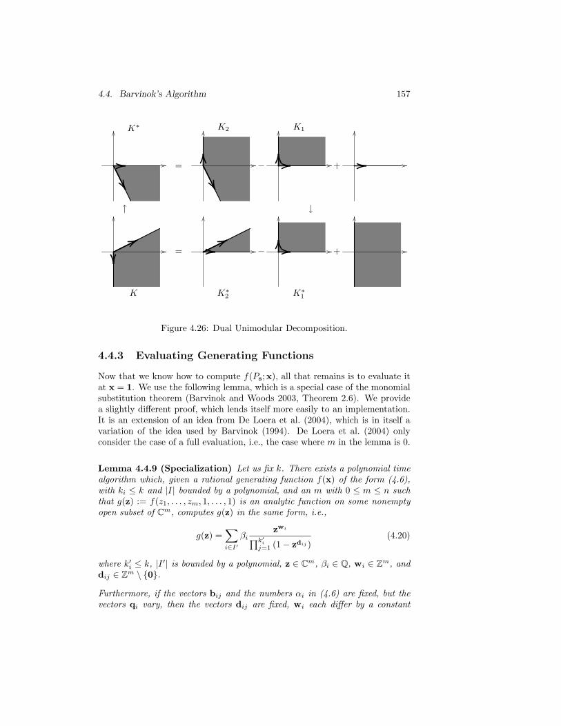
4.4. Barvinok’s Algorithm 157
K∗
=
K2
−
K1
+
↑ ↓
K
=
K∗2
−
K∗1
+
Figure 4.26: Dual Unimodular Decomposition.
4.4.3 Evaluating Generating Functions
Now that we know how to compute f(Ps;x), all that remains is to evaluate itat x = 1. We use the following lemma, which is a special case of the monomialsubstitution theorem (Barvinok and Woods 2003, Theorem 2.6). We providea slightly different proof, which lends itself more easily to an implementation.It is an extension of an idea from De Loera et al. (2004), which is in itself avariation of the idea used by Barvinok (1994). De Loera et al. (2004) onlyconsider the case of a full evaluation, i.e., the case where m in the lemma is 0.
Lemma 4.4.9 (Specialization) Let us fix k. There exists a polynomial timealgorithm which, given a rational generating function f(x) of the form (4.6),with ki ≤ k and |I| bounded by a polynomial, and an m with 0 ≤ m ≤ n suchthat g(z) := f(z1, . . . , zm, 1, . . . , 1) is an analytic function on some nonemptyopen subset of Cm, computes g(z) in the same form, i.e.,
g(z) =∑
i∈I′
βizwi
∏k′ij=1 (1 − zdij )
(4.20)
where k′i ≤ k, |I ′| is bounded by a polynomial, z ∈ Cm, βi ∈ Q, wi ∈ Zm, anddij ∈ Zm \ 0.
Furthermore, if the vectors bij and the numbers αi in (4.6) are fixed, but thevectors qi vary, then the vectors dij are fixed, wi each differ by a constant
158 Chapter 4. Enumeration of Parametric Sets
vector from some qi, and βi are each a polynomial of degree at most k in thecoordinates of some qi.
Proof The case m = n is trivial, so we will assume m < n. Note that wecannot simply plug in the values 1, since (z1, . . . , zm, 1, . . . , 1) may be a pole ofsome of the terms in (4.6). In fact, if m = 0, then it will be a pole of all thoseterms. For each n-dimensional vector v, we write v′ for the first m componentsof v and v′′ for the remaining n − m components. Consider
h(t) = f(z1, . . . , zm, (t + 1)λ1 , . . . (t + 1)λn−m
),
as a function of t only (i.e., z = (z1, . . . , zm) are treated as symbolic constants),where λ ∈ Zn−m is such that for each i ∈ I and j ≤ ki, either b′ij 6= 0or 〈b′′ij ,λ〉 6= 0. Such a λ can be found in polynomial time by choosing anappropriate point from the “moment curve” as do Barvinok and Pommersheim(1999, Algorithm 5.2). This moment curve is m(τ) = (1, τ, τ2, . . . , τn−1). Foreach of the bij the inner product with m(τ) is a polynomial of degree at mostn − 1 and thus has at most n − 1 zeros. Therefore, enumerating the pointson the moment curve m(0),m(1), . . . ,m(k) will yield a valid λ for k at mostn(n − 1)|I| + 1.
The function g(z) is then simply the constant term in the Laurent power seriesexpansion of
h(t) =∑
i∈I
hi(t)
about t = 0. This is the sum of the constant terms in the Laurent power seriesexpansions of
hi(t) = αizq′i(t + 1)ai
∏ki
j=1
(
1 − zb′ij (t + 1)vij
) ,
where we let ai = 〈q′′,λ〉 ∈ Z, and vij = 〈b′′ij ,λ〉 ∈ Z. It only remains to showthat this constant term is indeed of the form (4.20) and that we can computeall of these terms in polynomial time.
Consider a particular hi(t). For ease of notation, we will omit the i subscripton newly introduced variables. Partition the factors in the denominator basedon the variables that appear in each factor. Let r be the number of factorswith vij 6= 0 but b′ij = 0 and s the number of factors with both vij 6= 0 andb′ij 6= 0. The remaining ki − r − s factors have vij = 0. In the special spacethat r = 0 (in particular, this requires m 6= 0), then t = 0 is not a pole andwe can simply plug in 0 for t. We obtain a single term in the sum of the form(4.20) with k′i = ki. Otherwise, hi(t) has a pole of order r at t = 0 and we mustcompute the coefficient of tr in the Taylor series expansion of trhi(t), which is
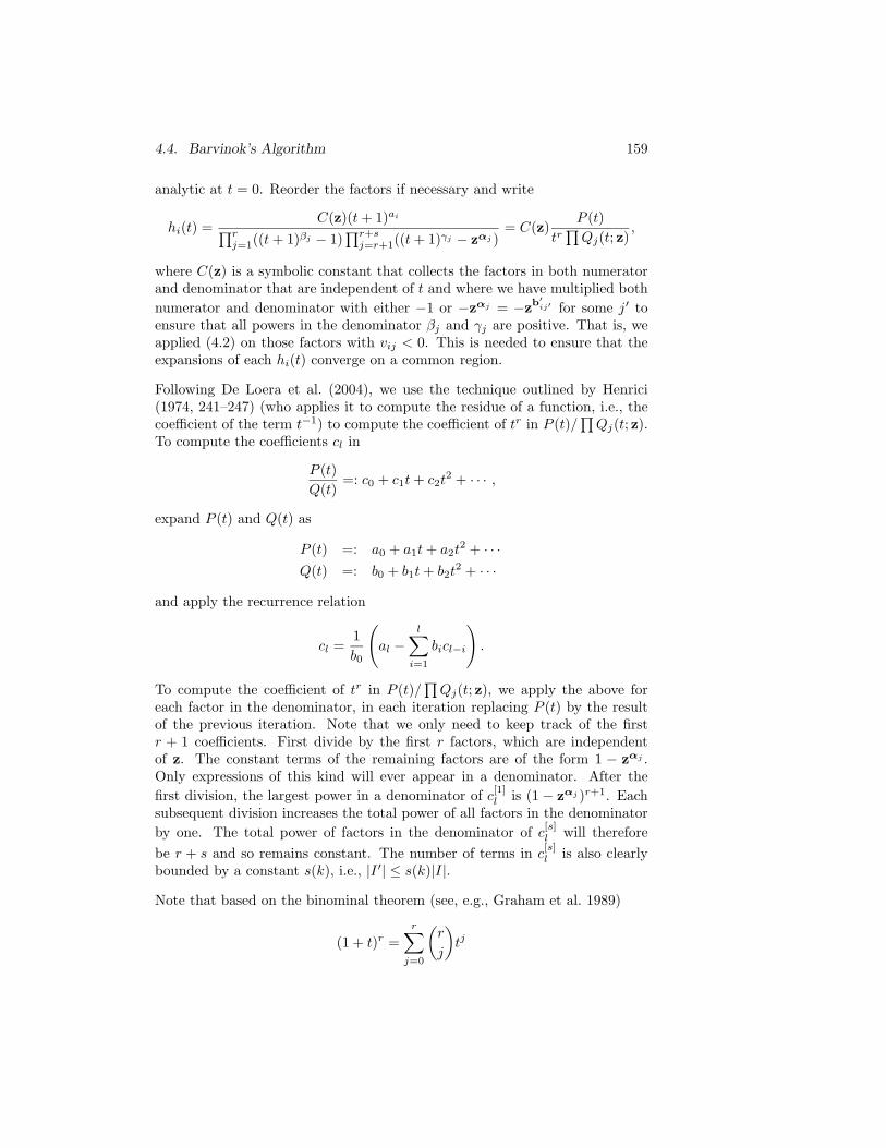
4.4. Barvinok’s Algorithm 159
analytic at t = 0. Reorder the factors if necessary and write
hi(t) =C(z)(t + 1)ai
∏rj=1((t + 1)βj − 1)
∏r+sj=r+1((t + 1)γj − zαj )
= C(z)P (t)
tr∏
Qj(t; z),
where C(z) is a symbolic constant that collects the factors in both numeratorand denominator that are independent of t and where we have multiplied both
numerator and denominator with either −1 or −zαj = −zb′ij′ for some j′ to
ensure that all powers in the denominator βj and γj are positive. That is, weapplied (4.2) on those factors with vij < 0. This is needed to ensure that theexpansions of each hi(t) converge on a common region.
Following De Loera et al. (2004), we use the technique outlined by Henrici(1974, 241–247) (who applies it to compute the residue of a function, i.e., thecoefficient of the term t−1) to compute the coefficient of tr in P (t)/
∏Qj(t; z).
To compute the coefficients cl in
P (t)
Q(t)=: c0 + c1t + c2t
2 + · · · ,
expand P (t) and Q(t) as
P (t) =: a0 + a1t + a2t2 + · · ·
Q(t) =: b0 + b1t + b2t2 + · · ·
and apply the recurrence relation
cl =1
b0
(
al −l∑
i=1
bicl−i
)
.
To compute the coefficient of tr in P (t)/∏
Qj(t; z), we apply the above foreach factor in the denominator, in each iteration replacing P (t) by the resultof the previous iteration. Note that we only need to keep track of the firstr + 1 coefficients. First divide by the first r factors, which are independentof z. The constant terms of the remaining factors are of the form 1 − zαj .Only expressions of this kind will ever appear in a denominator. After the
first division, the largest power in a denominator of c[1]l is (1 − zαj )r+1. Each
subsequent division increases the total power of all factors in the denominator
by one. The total power of factors in the denominator of c[s]l will therefore
be r + s and so remains constant. The number of terms in c[s]l is also clearly
bounded by a constant s(k), i.e., |I ′| ≤ s(k)|I|.
Note that based on the binominal theorem (see, e.g., Graham et al. 1989)
(1 + t)r =r∑
j=0
(r
j
)
tj
160 Chapter 4. Enumeration of Parametric Sets
the coefficients of the numerator P (t) are polynomial expressions in ai, whichis itself a linear combination of the coefficients of qi. The maximal degree ofsuch a polynomial expression is r ≤ k. The lemma is proved.
Note that as argued by De Loera et al. (2004), a λ from the moment curvemay not be the most appropriate choice to use in an implementation since it islikely to have large coefficients. They therefore propose to construct a randomvector with small coefficients and check whether 〈b′′ij ,λ〉 6= 0 for all i and j.(Or rather 〈bij ,λ〉 6= 0, since m = 0 in their case.) Only after a fixed numberof failed attempts would the implementation fall back onto the moment curve.
Both of these strategies have the disadvantage however that all the terms in(4.6) need to be available before the constant term of the first term can becomputed. This may induce a large memory bottleneck. The authors of LattEhave therefore also implemented an alternative strategy where a random vec-tor with larger coefficients is constructed at the beginning of the computation(Yoshida 2004b). If the coefficients are large enough, then the probability ofhaving constructed an incorrect vector is close to zero. The disadvantage ofthis technique is that the coefficients are larger and that the computation hasto be redone completely in the unlikely event the vector was incorrect.
We propose a different strategy which does not require all terms to be available,nor does it require the use of large coefficients. We simply repeatedly applyLemma 4.4.9 for m′ from n− 1 down to m. In each application, we can simplyuse λ = 1, which is known to be valid in any case.
Versions of barvinok up to version 0.11 implemented the method using therandom vector with small coefficients. Version 0.16 and newer support boththe method using the random vector with large coefficients and the incrementalapproach for enumerating parametric polytopes. The latter is the default andmay be switched off using the --disable-incremental configure option. Theeffect on memory usage can be dramatic in some cases. For example, enumer-ating the non-parametric polytope long 4D, included in the distribution, usingversion 0.11 requires nearly 170 MB, while version 0.16 needs less than 1.6MB. For small-dimensional problems, the difference between the large randomvector and the incremental approach is small, both in computation time andin the final resulting step-polynomial.
Example 48 Consider the rational generating function (4.7) from Ex-ample 39
f(z, x) =x2
(1 − x−1)(1 − x−1z)+
z2
(1 − z−1)(1 − xz−1)+
1
(1 − x)(1 − z),
where we renamed x1 and x2 to x and z respectively to fit the notation ofthe lemma. We want to compute g(z) = f(z, 1). Substituting x = t + 1,
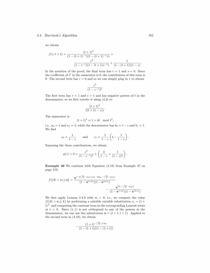
4.4. Barvinok’s Algorithm 161
we obtain
f(z, t + 1) =(t + 1)2
(1 − (t + 1)−1)(1 − (t + 1)−1z)+
z2
(1 − z−1)(1 − (t + 1)z−1)+
1
(1 − (t + 1))(1 − z).
In the notation of the proof, the final term has r = 1 and s = 0. Sincethe coefficient of t1 in the numerator is 0, the contribution of this term is0. The second term has r = 0 and so we can simply plug in 1 to obtain
z2
(1 − z−1)2.
The first term has r = 1 and s = 1 and has negative powers of t in thedenominator, so we first rewrite it using (4.2) to
(t + 1)4
t(t + (1 − z)).
The numerator is(t + 1)4 ≡ 1 + 4t mod t2,
i.e., a0 = 1 and a1 = 4, while the denominator has b0 = 1− z and b1 = 1.We find
c0 =1
1 − zand c1 =
1
1 − z
(
4 − 1
1 − z
)
.
Summing the three contributions, we obtain
g(z) = 0 +z2
(1 − z−1)2+
(4
1 − z+
1
(1 − z)2
)
.
Example 49 We continue with Equation (4.19) from Example 47 onpage 153:
f((K + v1);x
)=
x(−2⌊ p12−p2⌋+p1−2p2,−⌊ p1
2−p2⌋)
(1 − x(1,0))(1 − x(2,1))
− x(0,−⌊ p12−p2⌋)
(1 − x(1,0))(1 − x(0,1)).
We first apply Lemma 4.4.9 with m = 0, i.e., we compute the valuef((K + v1
);1) by performing a suitable variable substitution xi = (1 +
t)λi and computing the constant term in the corresponding Laurent seriesat t = 0. Since (1, 1) is not orthogonal to any of the powers in thedenominator, we can use the substitution x = (t + 1, t + 1). Applied tothe second term in (4.19), we obtain
− (1 + t)−⌊p12⌋+p2
(1 − (1 + t))(1 − (1 + t)).
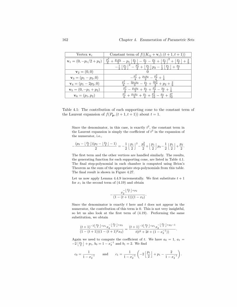
162 Chapter 4. Enumeration of Parametric Sets
Vertex vi Constant term of f((Kij + vi); (t + 1, t + 1))
v1 = (0,−p1/2 + p2)p21
6 + p1p2
3 − p1
⌊p1
2
⌋− p1
2 − p2
3 +⌊
p1
2
⌋2+⌊
p1
2
⌋+ 2
9
− 12
⌊p1
2
⌋2− p2
2
2 +⌊
p1
2
⌋p2 −
12
⌊p1
2
⌋+ p2
2
v2 = (0, 0) 0
v3 = (p1 − p2, 0) −p21
4 + p1p2
2 − p22
4 + 18
v4 = (p1 − 2p2, 0)p21
6 − 2p1p2
3 − p1
2 +2p2
2
3 + p2 + 29
v5 = (0,−p1 + p2)p21
4 − p1p2
2 + p1
2 +p22
4 − p2
2 + 18
v6 = (p1, p2)p21
6 + p1p2
6 + p1
2 +p22
12 − p2
2 + 4772
Table 4.1: The contribution of each supporting cone to the constant term ofthe Laurent expansion of f(Pp, (t + 1, t + 1)) about t = 1.
Since the denominator, in this case, is exactly t2, the constant term inthe Laurent expansion is simply the coefficient of t2 in the expansion ofthe numerator, i.e.,
− (p2 − ⌊ p12⌋)(p2 − ⌊ p1
2⌋ − 1)
2= −1
2
⌊p1
2
⌋2
− p22
2+⌊p1
2
⌋
p2− 1
2
⌊p1
2
⌋
+p2
2.
The first term and the other vertices are handled similarly. The results,the generating function for each supporting cone, are listed in Table 4.1.The final step-polynomial in each chamber is computed using Brion’sTheorem as the sum of the appropriate step-polynomials from this table.The final result is shown in Figure 4.27.
Let us now apply Lemma 4.4.9 incrementally. We first substitute t + 1for x1 in the second term of (4.19) and obtain
− x−⌊ p1
2 ⌋+p2
2
(1 − (t + 1))(1 − x2).
Since the denominator is exactly t here and t does not appear in thenumerator, the contribution of this term is 0. This is not very insightful,so let us also look at the first term of (4.19). Performing the samesubstitution, we obtain
(t + 1)−2⌊ p12 ⌋+p1x
−⌊ p12 ⌋+p2
2
(1 − (t + 1))(1 − (t + 1)2x2)=
(t + 1)−2⌊ p12 ⌋+p1x
−⌊ p12 ⌋+p2−1
2
t(t2 + 2t + (1 − x−12 ))
.
Again we need to compute the coefficient of t. We have a0 = 1, a1 =−2⌊
p12
⌋+ p1, b0 = 1 − x−1
2 and b1 = 2. We find
c0 =1
1 − x−12
and c1 =1
1 − x−12
(
−2⌊p1
2
⌋
+ p1 − 2
1 − x−12
)
.
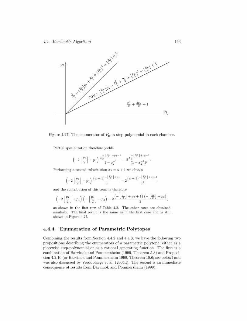
4.4. Barvinok’s Algorithm 163
p1
p2
p212
−⌊p1
2⌋p
1+
p1
2
+⌊p1
2⌋2 +
⌊p1
2⌋+
1
p1p2− ⌊
p1
2⌋p1
−p22
2+
p2
2+ ⌊
p1
2⌋2 + ⌊
p1
2⌋+ 1
p22
2 + 3p2
2 + 1
Figure 4.27: The enumerator of Pp, a step-polynomial in each chamber.
Partial specialization therefore yields
(
−2⌊p1
2
⌋
+ p1
) x−⌊ p1
2 ⌋+p2−1
2
1 − x−12
− 2x−⌊ p1
2 ⌋+p2−1
2
(1 − x−12 )2
.
Performing a second substitution x2 = u + 1 we obtain
(
−2⌊p1
2
⌋
+ p1
) (u + 1)−⌊p12 ⌋+p2
u− 2
(u + 1)−⌊p12 ⌋+p2+1
u2
and the contribution of this term is therefore
(
−2⌊p1
2
⌋
+ p1
) (
−⌊p1
2
⌋
+ p2
)
− 2
(−⌊
p12
⌋+ p2 + 1
) (−⌊
p12
⌋+ p2
)
2,
as shown in the first row of Table 4.2. The other rows are obtainedsimilarly. The final result is the same as in the first case and is stillshown in Figure 4.27.
4.4.4 Enumeration of Parametric Polytopes
Combining the results from Section 4.4.2 and 4.4.3, we have the following twopropositions describing the enumerators of a parametric polytope, either as apiecewise step-polynomial or as a rational generating function. The first is acombination of Barvinok and Pommersheim (1999, Theorem 5.3) and Proposi-tion 4.2.10 (or Barvinok and Pommersheim 1999, Theorem 10.6; see below) andwas also discussed by Verdoolaege et al. (2004d). The second is an immediateconsequence of results from Barvinok and Pommersheim (1999).
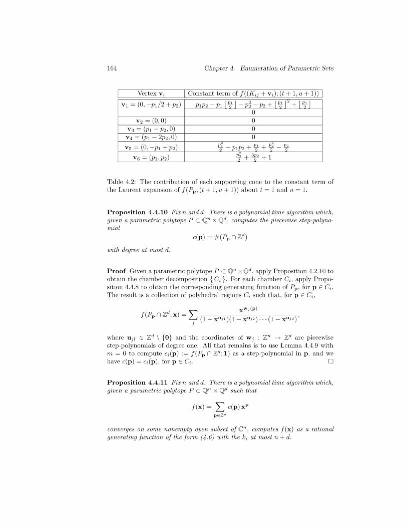
164 Chapter 4. Enumeration of Parametric Sets
Vertex vi Constant term of f((Kij + vi); (t + 1, u + 1))
v1 = (0,−p1/2 + p2) p1p2 − p1
⌊p1
2
⌋− p2
2 − p2 +⌊
p1
2
⌋2+⌊
p1
2
⌋
0v2 = (0, 0) 0
v3 = (p1 − p2, 0) 0v4 = (p1 − 2p2, 0) 0
v5 = (0,−p1 + p2)p21
2 − p1p2 + p1
2 +p22
2 − p2
2
v6 = (p1, p2)p22
2 + 3p2
2 + 1
Table 4.2: The contribution of each supporting cone to the constant term ofthe Laurent expansion of f(Pp, (t + 1, u + 1)) about t = 1 and u = 1.
Proposition 4.4.10 Fix n and d. There is a polynomial time algorithm which,given a parametric polytope P ⊂ Qn ×Qd, computes the piecewise step-polyno-mial
c(p) = #(Pp ∩ Zd)
with degree at most d.
Proof Given a parametric polytope P ⊂ Qn×Qd, apply Proposition 4.2.10 toobtain the chamber decomposition Ci . For each chamber Ci, apply Propo-sition 4.4.8 to obtain the corresponding generating function of Pp, for p ∈ Ci.The result is a collection of polyhedral regions Ci such that, for p ∈ Ci,
f(Pp ∩ Zd;x) =∑
j
xwj(p)
(1 − xuj1)(1 − xuj2) · · · (1 − xujd),
where ujl ∈ Zd \ 0 and the coordinates of wj : Zn → Zd are piecewisestep-polynomials of degree one. All that remains is to use Lemma 4.4.9 withm = 0 to compute ci(p) := f(Pp ∩ Zd;1) as a step-polynomial in p, and wehave c(p) = ci(p), for p ∈ Ci.
Proposition 4.4.11 Fix n and d. There is a polynomial time algorithm which,given a parametric polytope P ⊂ Qn × Qd such that
f(x) =∑
p∈Zn
c(p)xp
converges on some nonempty open subset of Cn, computes f(x) as a rationalgenerating function of the form (4.6) with the ki at most n + d.
4.4. Barvinok’s Algorithm 165
Proof Given a parametric polytope P ⊂ Qn × Qd, apply Theorem 4.4 ofBarvinok and Pommersheim (1999) (see Proposition 4.4.8) directly on P (thatis, not considering P as a parametric polytope but as a polyhedron in its ownright) to obtain the rational generating function
f(P ∩ Zn+d;x,y) =∑
(p,t)∈P∩Zn+d
xpyt
in polynomial time. Then
∑
p∈Zn
c(p)xp = f(P ∩ Zn+d;x,1
).
We may perform this substitution y = 1 in polynomial time using Lemma 4.4.9.The result is in the form (4.6).
For completeness, we now sketch an alternative for obtaining a result similarto that of Proposition 4.4.10. This alternative is based on Barvinok and Pom-mersheim (1999, Theorem 10.6), who propose to compute a partition Qj ofQn and then to compute the rational generating function of the enumerator ofthe parametric polytope Pp on each Qj . As in Proposition 4.4.10, an explicitfunction may then be obtained from this result by specializing each of theserational generating functions at 1.
Rather than directly computing the parametric vertices, Barvinok and Pom-mersheim (1999, Theorem 10.6) propose the following algorithm to obtain thepartition with corresponding rational generating functions. As in the proof ofProposition 4.4.11, compute the generating function of P ⊂ Qn+d
f(P ∩ Zn+d;x,y) =∑
(p,t)∈P∩Zn+d
xpyt =∑
p∈Zn
∑
t∈Pp∩Zd
xpyt.
The formula above shows that to obtain the generating function of Pp, i.e.,
∑
t∈Pp∩Zd
yt
we need to select the terms with a fixed value of p and then to specialize atx = 1. Applying identity (4.2) if needed, we may assume that all terms in (4.6)converge on a common open set of Cn+d. Let k := n + d and z := (x,y). Wehave
f(P ; z) =∑
i∈I
αi
∑
µ∈Nk
zwi+Biµ,
with Bi the matrix with bij as columns. To select only those terms with afixed power p for the first n variables, we intersect Nk with Ai(p) = µ |
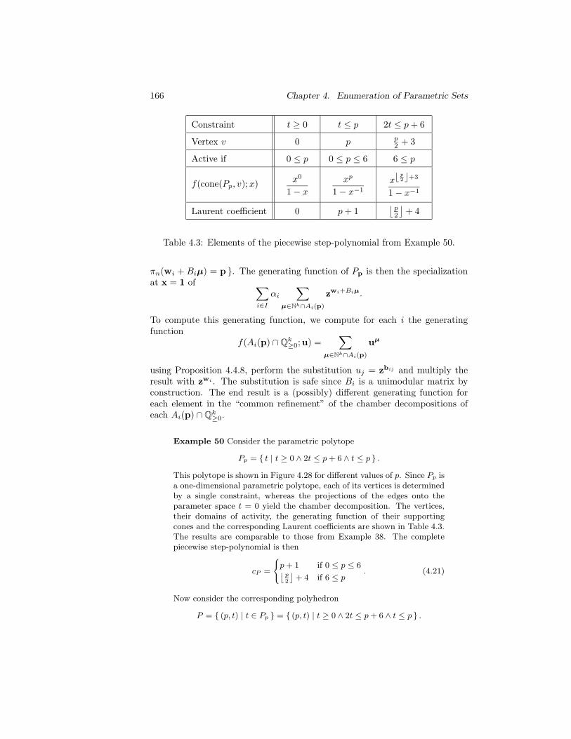
166 Chapter 4. Enumeration of Parametric Sets
Constraint t ≥ 0 t ≤ p 2t ≤ p + 6
Vertex v 0 p p2 + 3
Active if 0 ≤ p 0 ≤ p ≤ 6 6 ≤ p
f(cone(Pp, v);x)x0
1 − x
xp
1 − x−1
x⌊p2 ⌋+3
1 − x−1
Laurent coefficient 0 p + 1⌊
p2
⌋+ 4
Table 4.3: Elements of the piecewise step-polynomial from Example 50.
πn(wi + Biµ) = p . The generating function of Pp is then the specializationat x = 1 of ∑
i∈I
αi
∑
µ∈Nk∩Ai(p)
zwi+Biµ.
To compute this generating function, we compute for each i the generatingfunction
f(Ai(p) ∩ Qk≥0;u) =
∑
µ∈Nk∩Ai(p)
uµ
using Proposition 4.4.8, perform the substitution uj = zbij and multiply theresult with zwi . The substitution is safe since Bi is a unimodular matrix byconstruction. The end result is a (possibly) different generating function foreach element in the “common refinement” of the chamber decompositions ofeach Ai(p) ∩ Qk
≥0.
Example 50 Consider the parametric polytope
Pp = t | t ≥ 0 ∧ 2t ≤ p + 6 ∧ t ≤ p .
This polytope is shown in Figure 4.28 for different values of p. Since Pp isa one-dimensional parametric polytope, each of its vertices is determinedby a single constraint, whereas the projections of the edges onto theparameter space t = 0 yield the chamber decomposition. The vertices,their domains of activity, the generating function of their supportingcones and the corresponding Laurent coefficients are shown in Table 4.3.The results are comparable to those from Example 38. The completepiecewise step-polynomial is then
cP =
p + 1 if 0 ≤ p ≤ 6⌊
p
2
⌋+ 4 if 6 ≤ p
. (4.21)
Now consider the corresponding polyhedron
P = (p, t) | t ∈ Pp = (p, t) | t ≥ 0 ∧ 2t ≤ p + 6 ∧ t ≤ p .
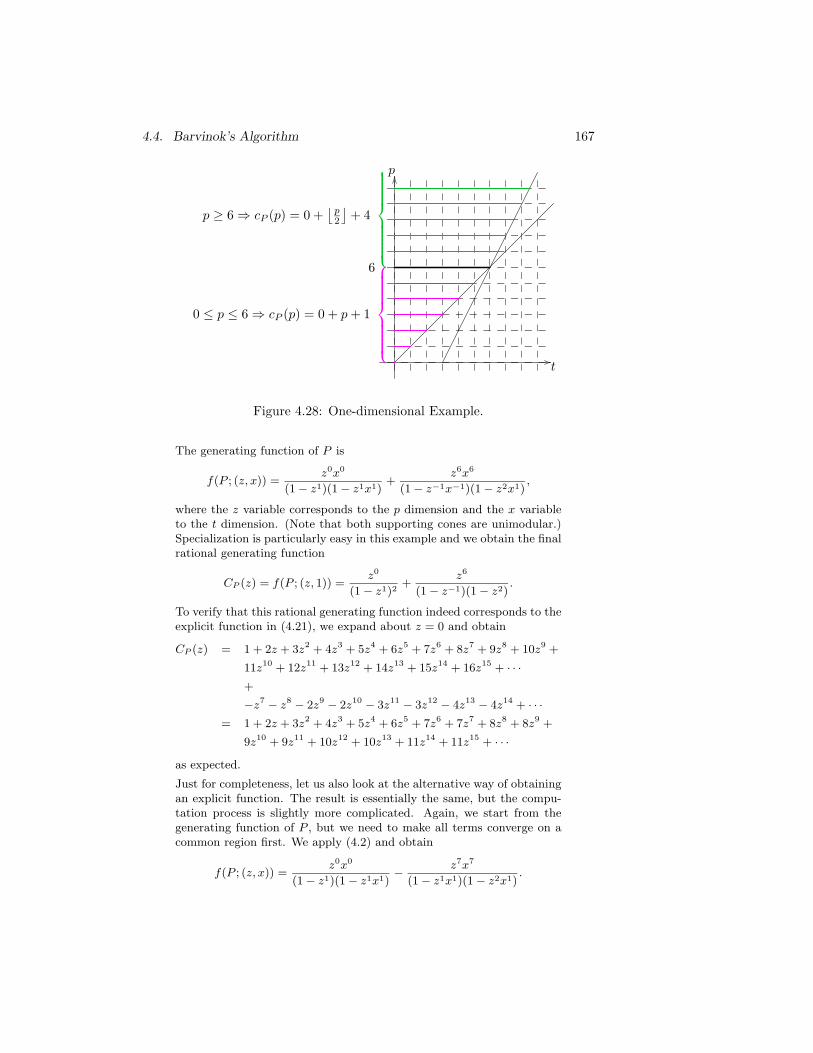
4.4. Barvinok’s Algorithm 167
t
p
0 ≤ p ≤ 6 ⇒ cP (p) = 0 + p + 10 ≤ p ≤ 6 ⇒ cP (p) = 0 + p + 1
p ≥ 6 ⇒ cP (p) = 0 +⌊
p2
⌋+ 4
6
Figure 4.28: One-dimensional Example.
The generating function of P is
f(P ; (z, x)) =z0x0
(1 − z1)(1 − z1x1)+
z6x6
(1 − z−1x−1)(1 − z2x1),
where the z variable corresponds to the p dimension and the x variableto the t dimension. (Note that both supporting cones are unimodular.)Specialization is particularly easy in this example and we obtain the finalrational generating function
CP (z) = f(P ; (z, 1)) =z0
(1 − z1)2+
z6
(1 − z−1)(1 − z2).
To verify that this rational generating function indeed corresponds to theexplicit function in (4.21), we expand about z = 0 and obtain
CP (z) = 1 + 2z + 3z2 + 4z3 + 5z4 + 6z5 + 7z6 + 8z7 + 9z8 + 10z9 +
11z10 + 12z11 + 13z12 + 14z13 + 15z14 + 16z15 + · · ·+
−z7 − z8 − 2z9 − 2z10 − 3z11 − 3z12 − 4z13 − 4z14 + · · ·= 1 + 2z + 3z2 + 4z3 + 5z4 + 6z5 + 7z6 + 7z7 + 8z8 + 8z9 +
9z10 + 9z11 + 10z12 + 10z13 + 11z14 + 11z15 + · · ·as expected.
Just for completeness, let us also look at the alternative way of obtainingan explicit function. The result is essentially the same, but the compu-tation process is slightly more complicated. Again, we start from thegenerating function of P , but we need to make all terms converge on acommon region first. We apply (4.2) and obtain
f(P ; (z, x)) =z0x0
(1 − z1)(1 − z1x1)− z7x7
(1 − z1x1)(1 − z2x1).
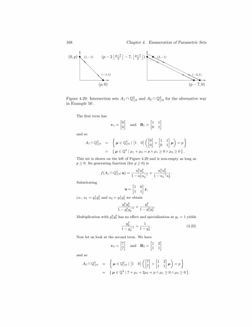
168 Chapter 4. Enumeration of Parametric Sets
(1,−1)
(−1,1)
•(0, p)
•(p, 0)
•
•
(2,−1)
(−2,1)
•
•(p − 7, 0)
(p − 2⌊
p−72
⌋− 7,
⌊p−72
⌋)
Figure 4.29: Intersection sets A1 ∩ Q2≥0 and A2 ∩ Q2
≥0 for the alternative wayin Example 50 .
The first term has
v1 =
[00
]
and B1 =
[1 10 1
]
and so
A1 ∩ Q2≥0 =
µ ∈ Q2≥0 |
[1 0
]([
00
]
+
[1 10 1
]
µ
)
= p
=
µ ∈ Q2 | µ1 + µ2 = p ∧ µ1 ≥ 0 ∧ µ2 ≥ 0
.
This set is shown on the left of Figure 4.29 and is non-empty as long asp ≥ 0. Its generating function (for p ≥ 0) is
f(A1 ∩ Q2≥0;u) =
u01u
p2
1 − u11u−12
+up
1u02
1 − u−11 u1
2
.
Substituting
u =
[1 01 1
]
y,
i.e., u1 = y11y0
2 and u2 = y11y1
2 we obtain
yp1yp
2
1 − y01y−1
2
+yp1
1 − y01y1
2
.
Multiplication with y01y0
2 has no effect and specialization at y1 = 1 yields
yp2
1 − y−12
+1
1 − y12
. (4.22)
Now let us look at the second term. We have
v2 =
[77
]
and B2 =
[1 21 1
]
and so
A2 ∩ Q2≥0 =
µ ∈ Q2≥0 |
[1 0
]([
77
]
+
[1 21 1
]
µ
)
= p
=
µ ∈ Q2 | 7 + µ1 + 2µ2 = p ∧ µ1 ≥ 0 ∧ µ2 ≥ 0
.
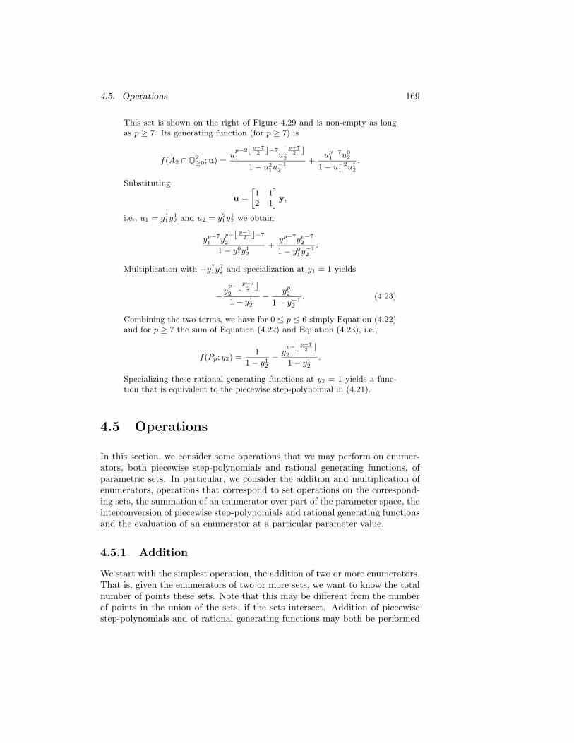
4.5. Operations 169
This set is shown on the right of Figure 4.29 and is non-empty as longas p ≥ 7. Its generating function (for p ≥ 7) is
f(A2 ∩ Q2≥0;u) =
up−2⌊ p−7
2 ⌋−7
1 u⌊ p−7
2 ⌋2
1 − u21u−12
+up−7
1 u02
1 − u−21 u1
2
.
Substituting
u =
[1 12 1
]
y,
i.e., u1 = y11y1
2 and u2 = y21y1
2 we obtain
yp−71 y
p−⌊ p−72 ⌋−7
2
1 − y01y1
2
+yp−71 yp−7
2
1 − y01y−1
2
.
Multiplication with −y71y7
2 and specialization at y1 = 1 yields
−yp−⌊ p−7
2 ⌋2
1 − y12
− yp2
1 − y−12
. (4.23)
Combining the two terms, we have for 0 ≤ p ≤ 6 simply Equation (4.22)and for p ≥ 7 the sum of Equation (4.22) and Equation (4.23), i.e.,
f(Pp; y2) =1
1 − y12
− yp−⌊ p−7
2 ⌋2
1 − y12
.
Specializing these rational generating functions at y2 = 1 yields a func-tion that is equivalent to the piecewise step-polynomial in (4.21).
4.5 Operations
In this section, we consider some operations that we may perform on enumer-ators, both piecewise step-polynomials and rational generating functions, ofparametric sets. In particular, we consider the addition and multiplication ofenumerators, operations that correspond to set operations on the correspond-ing sets, the summation of an enumerator over part of the parameter space, theinterconversion of piecewise step-polynomials and rational generating functionsand the evaluation of an enumerator at a particular parameter value.
4.5.1 Addition
We start with the simplest operation, the addition of two or more enumerators.That is, given the enumerators of two or more sets, we want to know the totalnumber of points these sets. Note that this may be different from the numberof points in the union of the sets, if the sets intersect. Addition of piecewisestep-polynomials and of rational generating functions may both be performed
170 Chapter 4. Enumeration of Parametric Sets
in polynomial time. It follows that the same holds for any Q-linear combinationof piecewise step-polynomials or rational generating functions.
The sum of a set of rational generating functions can trivially be computedin polynomial time. The index set in the summation of the sum is simplythe union of the index sets in the summations of the terms. For piecewisestep-polynomials we need the following lemma.
Lemma 4.5.1 Fix d. There is a polynomial time algorithm which, given piece-wise step-polynomials ci : Zd → Q, computes c(s) =
∑
i ci(s) as a piecewisestep-polynomial.
Proof Suppose ci(s) are given as piecewise step-polynomials, and let c(s) =∑
i ci(s). We would like to compute c(s) as a piecewise step-polynomial. Foreach i, let 〈aij ,x〉 ≤ bij j be the collection of linear inequalities that de-fine the chambers of the piecewise step-polynomial representation of ci(s). ByLemma 4.2.9, we can compute in polynomial time all cells in Qn determinedby the collection of all inequalities 〈aij ,x〉 ≤ biji,j . These are subsets of thefull-dimensional chambers in the piecewise step-polynomial representation ofc(s). Within a particular chamber, each ci(s) is defined by
ci(s) =
ni∑
j=1
αij
dij∏
k=1
⌊〈aijk, s〉 + bijk⌋ ,
where αij ∈ Q, aijk ∈ Qd, and bijk ∈ Q, and so c(s) =∑
i ci(s) in this chamberis simply of sum of such functions.
We must be careful here how we represent a chamber complex. One possibilityis to keep track of all chambers, that is, the full-dimensional chambers as wellas all their (common) faces. In this case, the chambers may be considered asopen polyhedra and then the associated step-polynomial is only valid in thisopen chamber. Using this representation, there is no problem with the lemmaabove. This is also conceptually the nicest option, but it is not ideal from animplementation perspective.
Another option is to only keep track of the full-dimensional chambers. Inthis case, the chambers should be considered as closed polyhedra. Otherwise,the piecewise step-polynomial would not be defined on common faces, i.e., onlower-dimensional chambers. This means that the step-polynomials on adjacentchambers should be equivalent when restricted to their common faces. Thisholds for the result of Proposition 4.4.10, but it may not hold for the result ofthe lemma above if the “outer walls” of all chamber complexes in the sum donot coincide. If a full-dimensional chamber of one chamber complex is cut byan outer wall of another chamber complex, then of the two resulting adjacent
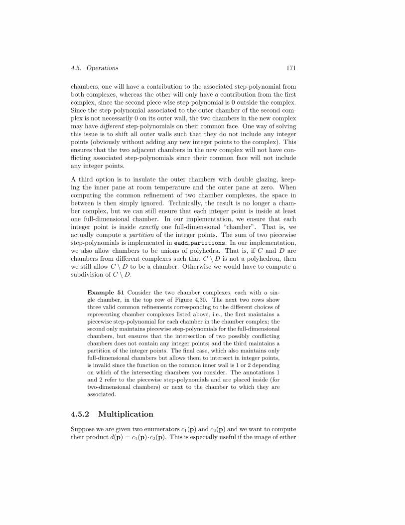
4.5. Operations 171
chambers, one will have a contribution to the associated step-polynomial fromboth complexes, whereas the other will only have a contribution from the firstcomplex, since the second piece-wise step-polynomial is 0 outside the complex.Since the step-polynomial associated to the outer chamber of the second com-plex is not necessarily 0 on its outer wall, the two chambers in the new complexmay have different step-polynomials on their common face. One way of solvingthis issue is to shift all outer walls such that they do not include any integerpoints (obviously without adding any new integer points to the complex). Thisensures that the two adjacent chambers in the new complex will not have con-flicting associated step-polynomials since their common face will not includeany integer points.
A third option is to insulate the outer chambers with double glazing, keep-ing the inner pane at room temperature and the outer pane at zero. Whencomputing the common refinement of two chamber complexes, the space inbetween is then simply ignored. Technically, the result is no longer a cham-ber complex, but we can still ensure that each integer point is inside at leastone full-dimensional chamber. In our implementation, we ensure that eachinteger point is inside exactly one full-dimensional “chamber”. That is, weactually compute a partition of the integer points. The sum of two piecewisestep-polynomials is implemented in eadd partitions. In our implementation,we also allow chambers to be unions of polyhedra. That is, if C and D arechambers from different complexes such that C \ D is not a polyhedron, thenwe still allow C \ D to be a chamber. Otherwise we would have to compute asubdivision of C \ D.
Example 51 Consider the two chamber complexes, each with a sin-gle chamber, in the top row of Figure 4.30. The next two rows showthree valid common refinements corresponding to the different choices ofrepresenting chamber complexes listed above, i.e., the first maintains apiecewise step-polynomial for each chamber in the chamber complex; thesecond only maintains piecewise step-polynomials for the full-dimensionalchambers, but ensures that the intersection of two possibly conflictingchambers does not contain any integer points; and the third maintains apartition of the integer points. The final case, which also maintains onlyfull-dimensional chambers but allows them to intersect in integer points,is invalid since the function on the common inner wall is 1 or 2 dependingon which of the intersecting chambers you consider. The annotations 1and 2 refer to the piecewise step-polynomials and are placed inside (fortwo-dimensional chambers) or next to the chamber to which they areassociated.
4.5.2 Multiplication
Suppose we are given two enumerators c1(p) and c2(p) and we want to computetheir product d(p) = c1(p)·c2(p). This is especially useful if the image of either
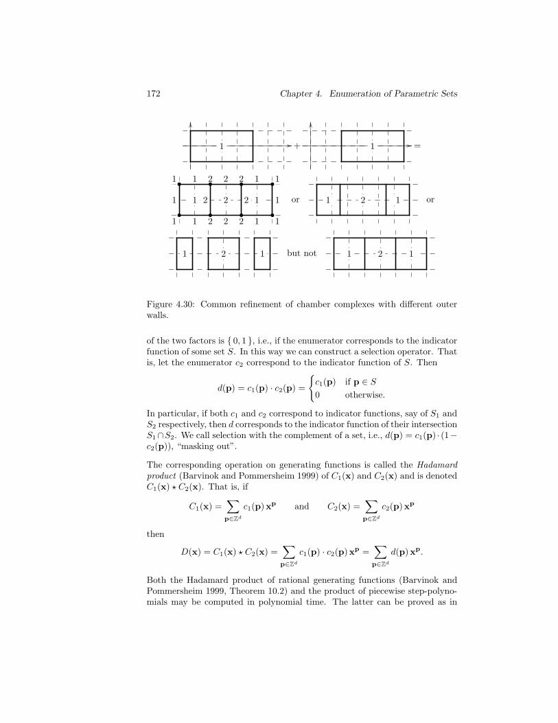
172 Chapter 4. Enumeration of Parametric Sets
1 + 1 =
1 1 2 2 2 1 1
1 1 2 2 2 1 1
1 2 2 1
• • • •
• • • •
1 2 1 or 1 2 1 or
1 2 1 but not 1 2 1
Figure 4.30: Common refinement of chamber complexes with different outerwalls.
of the two factors is 0, 1 , i.e., if the enumerator corresponds to the indicatorfunction of some set S. In this way we can construct a selection operator. Thatis, let the enumerator c2 correspond to the indicator function of S. Then
d(p) = c1(p) · c2(p) =
c1(p) if p ∈ S
0 otherwise.
In particular, if both c1 and c2 correspond to indicator functions, say of S1 andS2 respectively, then d corresponds to the indicator function of their intersectionS1∩S2. We call selection with the complement of a set, i.e., d(p) = c1(p) · (1−c2(p)), “masking out”.
The corresponding operation on generating functions is called the Hadamardproduct (Barvinok and Pommersheim 1999) of C1(x) and C2(x) and is denotedC1(x) ⋆ C2(x). That is, if
C1(x) =∑
p∈Zd
c1(p)xp and C2(x) =∑
p∈Zd
c2(p)xp
then
D(x) = C1(x) ⋆ C2(x) =∑
p∈Zd
c1(p) · c2(p)xp =∑
p∈Zd
d(p)xp.
Both the Hadamard product of rational generating functions (Barvinok andPommersheim 1999, Theorem 10.2) and the product of piecewise step-polyno-mials may be computed in polynomial time. The latter can be proved as in
4.5. Operations 173
Lemma 4.5.1 for addition. In this case, there are no problems with respect tothe representation of the chamber complexes since the support of the chambercomplex of the product is the intersection of the supports of the chamberscomplexes of the factors. Outer walls in the initial complexes will thereforeremain outer walls in the final chamber complex (or will be demolished).
To ensure a polynomial time complexity, however, we may only apply the(Hadamard) product operation a fixed number of times. The reason is thatin case of a product of piecewise step-polynomials the degree of the step-polynomials may increase. Generally, the maximal degree will be the sumof the degree of the factors. If we perform more than a fixed number of multi-plications, then this degree is no longer a constant in terms of the dimension.In the case of rational generating functions, the number of factors in the de-nominator of each term will in general be the sum of the number of factorsfor each factor in the Hadamard product. Again, if we perform more than afixed number of Hadamard products, then we may no longer assume that thisnumber of factors is bounded by a constant. An additional problem is that thenumber of terms in the sum may grow exponentially on repeated applicationof the Hadamard product.
In some cases, the Hadamard product may still be performed without increasein the number of factors in the denominators. To see this, let us look at thecomputation of Hadamard products (Barvinok and Pommersheim 1999, Proofof Theorem 10.2) in slow motion. It is sufficient to know how to perform theHadamard product on rational generating functions with a single term,
C1(x) =xv
∏k1
i=1(1 − xai)and C2(x) =
xw
∏k2
i=1(1 − xbi), (4.24)
with v,w,ai,bi ∈ Zd. Expansion as multiple geometric series yields
C1(x) =∑
µ∈Nk1
xv+∑k1
i=1 µiai =∑
m
c1(m)xm
with
c1(m) = #
µ ∈ Nk1 | m = v +
k1∑
i=1
µiai
and similarly
C2(x) =∑
ν∈Nk2
xw+∑k2
i=1 νibi =∑
m
c2(m)xm
with
c2(m) = #
ν ∈ Nk2 | m = w +
k2∑
i=1
νibi
.
174 Chapter 4. Enumeration of Parametric Sets
The product d(m) of c1(m) and c2(m) is then simply
d(m) = #
(µ,ν) ∈ Nk1+k2 | m = v +
k1∑
i=1
µiai ∧ m = w +
k2∑
i=1
νibi
.
This is the enumerator of a parametric polytope in Qk1+k2 with 2d equalities.To compute the generating function D(x) of this enumerator (see Proposi-tion 4.4.11, we need to consider the polyhedron
(m,µ,ν) ∈ Qd+k1+k2 |
[µ
ν
]
≥ 0 ∧ m = v +
k1∑
i=1
µiai ∧ m = w +
k2∑
i=1
νibi
,
(4.25)a polyhedron in Qd+k1+k2 . If the 2d equalities are linearly independent, thenthe dimension of this polyhedron will be k1 + k2 − d and so the number offactors in the denominators will be at most k1 + k2 − d.
In particular, if C1(x) and C2(x) are the generating functions of polyhedra, thenk1 = k2 = d and the 2d equalities are linearly independent since both ai andbi are the generators of a unimodular cone in this case. The number of factorstherefore remains constant at d. This should not be surprising as the Hadamardproduct in this case is just the generating function of the intersection, whichis itself a d-polyhedron. Note that the corresponding piecewise step-polyno-mial will just have the polyhedron itself as single chamber with as associatedstep-polynomial the constant 1.
A slightly more interesting case is selection with a polyhedron. In the world ofpiecewise step-polynomials, such selection is performed by simply intersectingeach chamber with the polyhedron. The equivalent on generating functions isslightly more expensive, but still cheap in the sense that the number of factorsin the denominators does not increase.
Example 52 Suppose we are given the following two rational generatingfunctions
C1(x) =1
(1 − x)2= 1 + 2 x + 3 x2 + 4 x3 + 5 x4 + 6 x5 + 7 x6 + · · ·
C2(x) =1
1 − x2= 1 + x2 + x4 + x6 + · · ·
and that we want to compute their Hadamard product. The correspond-ing piecewise step-polynomials are
c1(p) = p + 1 if p ≥ 0
c2(p) =⌊p
2
⌋
−⌊
p − 1
2
⌋
if p ≥ 0
and so their product is simply
d(p) = c1(p) · c2(p) = (p + 1)
(⌊p
2
⌋
−⌊
p − 1
2
⌋)
if p ≥ 0.
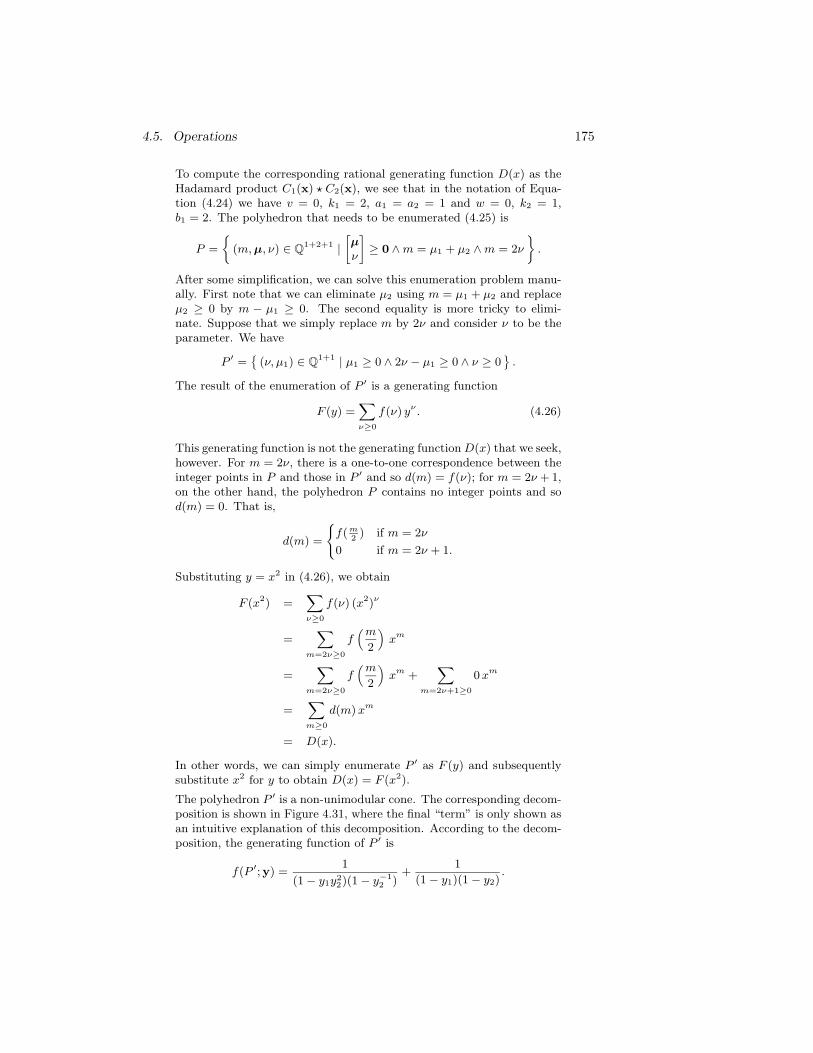
4.5. Operations 175
To compute the corresponding rational generating function D(x) as theHadamard product C1(x) ⋆ C2(x), we see that in the notation of Equa-tion (4.24) we have v = 0, k1 = 2, a1 = a2 = 1 and w = 0, k2 = 1,b1 = 2. The polyhedron that needs to be enumerated (4.25) is
P =
(m, µ, ν) ∈ Q1+2+1 |
[µ
ν
]
≥ 0 ∧ m = µ1 + µ2 ∧ m = 2ν
.
After some simplification, we can solve this enumeration problem manu-ally. First note that we can eliminate µ2 using m = µ1 + µ2 and replaceµ2 ≥ 0 by m − µ1 ≥ 0. The second equality is more tricky to elimi-nate. Suppose that we simply replace m by 2ν and consider ν to be theparameter. We have
P ′ =
(ν, µ1) ∈ Q1+1 | µ1 ≥ 0 ∧ 2ν − µ1 ≥ 0 ∧ ν ≥ 0
.
The result of the enumeration of P ′ is a generating function
F (y) =∑
ν≥0
f(ν) yν . (4.26)
This generating function is not the generating function D(x) that we seek,however. For m = 2ν, there is a one-to-one correspondence between theinteger points in P and those in P ′ and so d(m) = f(ν); for m = 2ν + 1,on the other hand, the polyhedron P contains no integer points and sod(m) = 0. That is,
d(m) =
f(m2
) if m = 2ν
0 if m = 2ν + 1.
Substituting y = x2 in (4.26), we obtain
F (x2) =∑
ν≥0
f(ν) (x2)ν
=∑
m=2ν≥0
f(m
2
)
xm
=∑
m=2ν≥0
f(m
2
)
xm +∑
m=2ν+1≥0
0 xm
=∑
m≥0
d(m) xm
= D(x).
In other words, we can simply enumerate P ′ as F (y) and subsequentlysubstitute x2 for y to obtain D(x) = F (x2).
The polyhedron P ′ is a non-unimodular cone. The corresponding decom-position is shown in Figure 4.31, where the final “term” is only shown asan intuitive explanation of this decomposition. According to the decom-position, the generating function of P ′ is
f(P ′;y) =1
(1 − y1y22)(1 − y−1
2 )+
1
(1 − y1)(1 − y2).
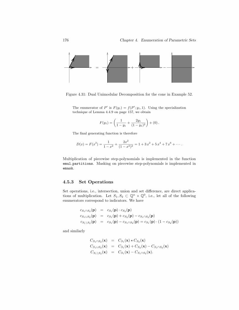
176 Chapter 4. Enumeration of Parametric Sets
= + −
Figure 4.31: Dual Unimodular Decomposition for the cone in Example 52.
The enumerator of P ′ is F (y1) = f(P ′; y1, 1). Using the specializationtechnique of Lemma 4.4.9 on page 157, we obtain
F (y1) =
(1
1 − y1+
2y1
(1 − y1)2
)
+ (0) .
The final generating function is therefore
D(x) = F (x2) =1
1 − x2+
2x2
(1 − x2)2= 1 + 3 x2 + 5 x4 + 7 x6 + · · · .
Multiplication of piecewise step-polynomials is implemented in the functionemul partitions. Masking on piecewise step-polynomials is implemented inemask.
4.5.3 Set Operations
Set operations, i.e., intersection, union and set difference, are direct applica-tions of multiplication. Let S1, S2 ⊂ Qn × Q0, i.e., let all of the followingenumerators correspond to indicators. We have
cS1∩S2(p) = cS1
(p) · cS2(p)
cS1∪S2(p) = cS1
(p) + cS2(p) − cS1∩S2
(p)
cS1\S2(p) = cS1
(p) − cS1∩S2(p) = cS1
(p) · (1 − cS2(p))
and similarly
CS1∩S2(x) = CS1
(x) ⋆ CS2(x)
CS1∪S2(x) = CS1
(x) + CS2(x) − CS1∩S2
(x)
CS1\S2(x) = CS1
(x) − CS1∩S2(x).
4.5. Operations 177
4.5.4 Summation
Suppose we are given an enumerator c(p) in n variables and we want to knowthe sum of all function values over some region of the parameter space. Thisregion will typically only involve some of the parameters and the resulting sumwill then be a function of the remaining parameters. In particular, we considera set S ⊂ Ql with l ≤ n and such that for each p′ ∈ Qn−l there are only finitelymany elements p′′ ∈ S such that c(p′,p′′) is non-zero. The summation of c(p)over S is defined as
d(p′) =∑
p′′∈S
c(p′,p′′).
Equivalently,
D(y) =∑
p′
d(p′)yp′ =∑
p′
∑
p′′∈S
c(p′,p′′)xp′ = C ′(y,1), (4.27)
withC ′(y, z) = C ′(x) = C(x) ⋆ f(Qn−l × S;x). (4.28)
Such a summation may be useful to enumerate unions of parametric polytopeswithout computing a disjoint union first. We can first consider all of the n +d variables to be parameters; enumerate all parametric polytopes to obtainenumerators in these n+d variables; compute the intersection as in the previoussection and finally sum over the d non-parameters. Another possible applicationof summation is pointer conversion or array recovery (van Engelen and Gallivan2001; Franke and O’Boyle 2003), a process in which array accesses throughpointers are converted to explicit array references.
Example 53 Consider the artificial program in Listing 4.1 and supposewe want to replace accesses to the array a through the pointer p byexplicit accesses to a. To obtain an explicit indexation in term of theiterators, we need to accumulate the increments to pointer p over allprevious iterations. That is, we need to sum the increment over all0 ≤ i′ ≤ 99 and i′ ≤ j′ ≤ 99 such that (i′, j′) 4 (i, j). Note that theincrement is the step-polynomial
c(i, j, i′, j′) = j′⌊
j′ − i′
4
⌋
.
The accumulated increment is therefore
d(i, j) =∑
(i′,j′)∈S
(i′,j′)4(i,j)
c(i, j, i′, j′), (4.29)
with S = (i′, j′) | 0 ≤ i′ ≤ 99 ∧ i′ ≤ j′ ≤ 99 .
We can split the summation process into two steps. The first is the selectionspecified in (4.28), which we may perform both on piecewise step-polynomials
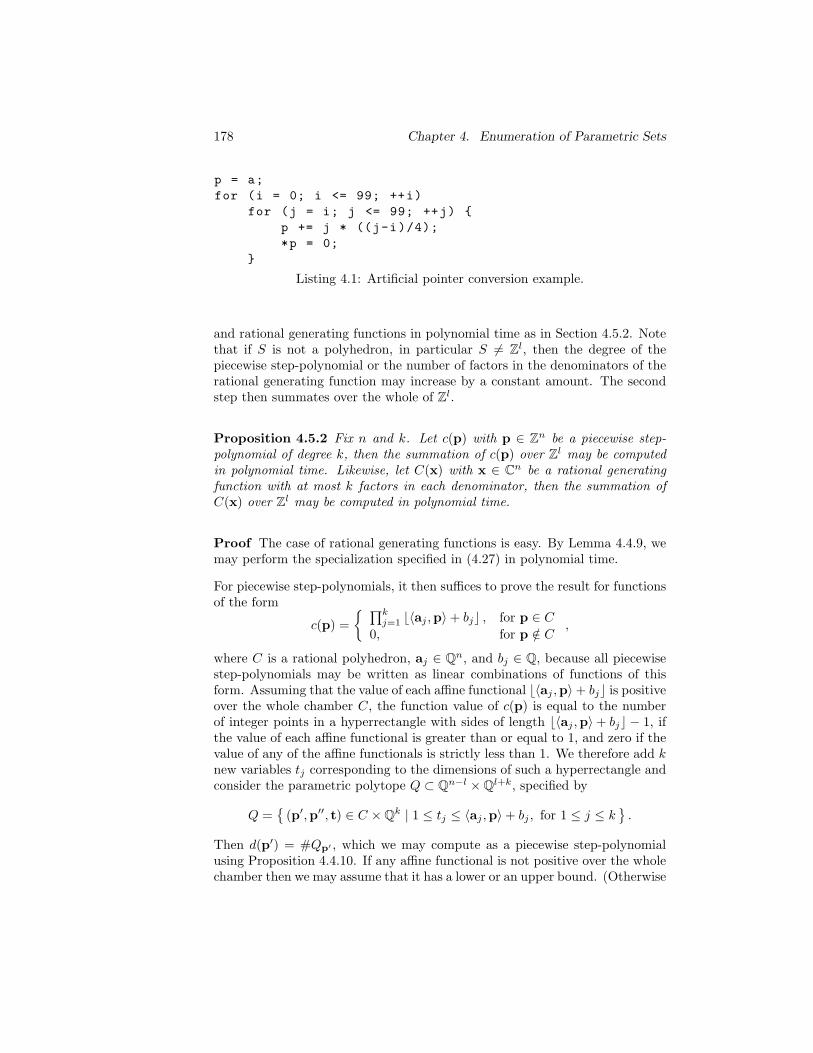
178 Chapter 4. Enumeration of Parametric Sets
p = a;
for (i = 0; i <= 99; ++i)
for (j = i; j <= 99; ++j)
p += j * ((j-i)/4);
*p = 0;
Listing 4.1: Artificial pointer conversion example.
and rational generating functions in polynomial time as in Section 4.5.2. Notethat if S is not a polyhedron, in particular S 6= Zl, then the degree of thepiecewise step-polynomial or the number of factors in the denominators of therational generating function may increase by a constant amount. The secondstep then summates over the whole of Zl.
Proposition 4.5.2 Fix n and k. Let c(p) with p ∈ Zn be a piecewise step-polynomial of degree k, then the summation of c(p) over Zl may be computedin polynomial time. Likewise, let C(x) with x ∈ Cn be a rational generatingfunction with at most k factors in each denominator, then the summation ofC(x) over Zl may be computed in polynomial time.
Proof The case of rational generating functions is easy. By Lemma 4.4.9, wemay perform the specialization specified in (4.27) in polynomial time.
For piecewise step-polynomials, it then suffices to prove the result for functionsof the form
c(p) =
∏kj=1 ⌊〈aj ,p〉 + bj⌋ , for p ∈ C
0, for p /∈ C,
where C is a rational polyhedron, aj ∈ Qn, and bj ∈ Q, because all piecewisestep-polynomials may be written as linear combinations of functions of thisform. Assuming that the value of each affine functional ⌊〈aj ,p〉 + bj⌋ is positiveover the whole chamber C, the function value of c(p) is equal to the numberof integer points in a hyperrectangle with sides of length ⌊〈aj ,p〉 + bj⌋ − 1, ifthe value of each affine functional is greater than or equal to 1, and zero if thevalue of any of the affine functionals is strictly less than 1. We therefore add knew variables tj corresponding to the dimensions of such a hyperrectangle andconsider the parametric polytope Q ⊂ Qn−l × Ql+k, specified by
Q =
(p′,p′′, t) ∈ C × Qk | 1 ≤ tj ≤ 〈aj ,p〉 + bj , for 1 ≤ j ≤ k
.
Then d(p′) = #Qp′ , which we may compute as a piecewise step-polynomialusing Proposition 4.4.10. If any affine functional is not positive over the wholechamber then we may assume that it has a lower or an upper bound. (Otherwise
4.5. Operations 179
split the (infinite) chamber according to the orthants of the parameter space.)If it has a lower bound, then let
mj := minp∈C
⌊〈aj ,p〉 + bj⌋ ∈ Z≤0
and replace ⌊〈aj ,p〉 + bj⌋ by ⌊〈aj ,p〉 + bj − mj⌋+ mj . If it only has an upperbound then replace ⌊〈aj ,p〉 + bj⌋ by
−1 −
⌊
〈−aj ,p〉 + bj −1
m
⌋
first, where m is the common denominator of ajk and bj .
Example 54 Consider the summation in Equation (4.29) from the pre-vious example. For simplicity, we will combine selection and summationand write the summation as the sum of two summations over polyhedra:
d(i, j) =∑
(i′,j′)∈S
i′<i
c(i, j, i′, j′) +∑
(i′,j′)∈S
i′=i∧j′≤j
c(i, j, i′, j′).
We will continue with the first of these two summation. The “chamber”is simply the whole of the parameter domain intersected with Q2×S andthe constraint i′ ≤ i − 1,
C = (i, j, i′, j′) | 0 ≤ i ≤ 99 ∧ i ≤ j ≤ 99 ∧0 ≤ i′ ≤ 99 ∧ i′ ≤ j′ ≤ 99 ∧ i′ ≤ i − 1 .
The parametric polytope Q that needs to be enumerated to compute thesummation is then
Q = (i, j, i′, j′, t1, t2) ∈ C × Q2 | 1 ≤ t1 ≤ j′ ∧ 4 ≤ 4t2 ≤ j′ − i′ .
Note that j′ − i′ is never negative in C and so we do not need to shiftthe step-polynomial or split the chamber.
Note that as in Section 4.5.2, we need to be careful how we represent cham-ber complexes. Keeping a list of overlapping full-dimensional chambers wouldresult in the points in their common intersections being counted twice on astraightforward application of the above proposition. As we mentioned in Sec-tion 4.5.2, we actually represent chamber complexes as a partition of the integerpoints. Summation on piecewise step-polynomials is implemented in esum.
4.5.5 Conversion
The operations we have seen so far are all polynomial for both piecewise step-polynomials and rational generating functions. In principle, it would have been
180 Chapter 4. Enumeration of Parametric Sets
sufficient to only consider either piecewise step-polynomials or rational gener-ating functions as we may convert between them in polynomial time, as we willshow in the following theorem. This is especially important for operations forwhich there was no previously known polynomial method for performing themon one of these representations. In particular, as we will discuss in Section 4.6.4,a polynomial algorithm for projection on rational generating functions was de-scribed by Barvinok and Woods (2003), but to the best of our knowledge, nopolynomial algorithm was ever described for performing projection on piecewisestep-polynomials.
Theorem 4.5.3 Fix n and k. There is a polynomial time algorithm which,given a rational generating function f(x) in the form (4.6) with n variablesand each ki ≤ k and given l ∈ Zn such that 〈l,bij〉 6= 0 for all i and j,computes the piecewise step-polynomial c : Zn → Q with degree at most k suchthat
C(x) =∑
p∈Zn
c(p)xp
is the Laurent power series expansion of C(x) convergent on a neighborhood ofel = (el1 , el2 , . . . , eld).
Conversely, there is a polynomial time algorithm which, given a piecewise step-polynomial c : Zn → Q of degree at most k such that C(x) =
∑
p∈Zn c(p)xp
converges on some nonempty open subset of Cn, computes the rational gener-ating function C(x) in the form (4.6) with ki ≤ k.
Proof In both directions, we reduce the problem to a set of counting problemsto which we apply either Proposition 4.4.10 or Proposition 4.4.11.
We first consider the conversion of rational generating functions to piecewisestep-polynomials. By Lemma 4.5.1 it suffices to consider rational generatingfunctions with a single term, i.e.,
C(x) = αxv
(1 − xa1)(1 − xa2) · · · (1 − xad).
Furthermore, we may assume that 〈l,ai〉 < 0 for all i (otherwise apply theidentity (4.2)) and that α = 1 and v = 0, because if c′(p) is a piecewise step-polynomial representation of the generating function C ′(x), then α · c′(p − v)is a piecewise step-polynomial representation of αxvC ′(x).
We expand C(x) as a product of infinite geometric series,
C(x) =
k∏
i=1
(1 + xai + x2ai + · · · ).
4.5. Operations 181
Then
C(el) =
k∏
i=1
(1 + e〈l,ai〉 + e2〈l,ai〉 + · · · ),
and this expansion is convergent on a neighborhood of el, since 〈l,ai〉 < 0. Wesee that we are looking to compute the enumeration
c(p) = #
λ = (λ1, λ2, . . . , λk) ∈ Nk | p = λ1a1 + λ2a2 + · · · + λkak
.
Let P be the parametric polytope
P =
(p,λ) ∈ Qn × Qk | λ ≥ 0 and p = λ1a1 + · · · + λkak
. (4.30)
Thenc(p) = #
λ ∈ Zk | (p,λ) ∈ P
,
which can be computed as a piecewise step-polynomial using Proposition 4.4.10.This proves the first half of the theorem.
The second half may be proved as in Proposition 4.5.2 with l = 0 and applyingProposition 4.4.11 on the parametric polytope Q instead of Proposition 4.4.10.
Note that if we are given a rational generating function and want to compute afunction c(p) which we know is only nonzero for p in some polyhedron Q suchthat Q does not contain any straight lines, then we may take any l such that〈l,bij〉 6= 0 for all i, j and such that
Q ∩ x ∈ Qn | 〈l,x〉 ≥ 0 (4.31)
is bounded. Such an l will give us the desired Laurent power series expansion∑
p c(p)xp. If such a polyhedron Q is known, then it can be advantageous
to intersect P from Equation (4.30) with Q × Qk. Some of these intersectionsmay be empty, avoiding the cost of enumerating them and, more significantly,avoiding the cost of adding them together to form step-polynomials outside Qthat are known to be zero.
Example 55 Take the parametric polytope g1 from the PolyLib distri-bution. Directly computing the enumerator function yields a piecewisestep-polynomial with 6 “chambers”. First computing the correspondinggenerating function yields a rational generating function with 56 terms,46 of which are non-zero only outside the projection Q of g1 onto itsparameter space. Converting the rational generating function to a piece-wise step-polynomial using the method above and taking into account thecontext Q takes 1.5s in total. The resulting piecewise step-polynomialhas 32 “chambers”. If we ignore Q, then summing the piecewise step-polynomials corresponding to the first 10 terms in the rational generating
182 Chapter 4. Enumeration of Parametric Sets
function already yields a piecewise step-polynomial with 114 chambers.Adding the piecewise step-polynomial corresponding to the 11th termtakes over one hour. Note that as we explain in Section 4.5.1, we allowour chambers to be unions of polyhedra. The main bottleneck during thecomputation of the sum of two piecewise step-polynomials appears to bethe function DomainDifference from PolyLib.
Example 56 Consider the function
C(x) =1
(1 − x(1,1))(1 − x(2,1))(1 − x(1,0))(1 − x(0,1)),
which is the generating function of the vector partition function
c(s) = #
λ ∈ N4 |[1 2 1 01 1 0 1
]
λ = s
.
This is the same as the example of Beck (2004, Section 4). The conversionof the rational generating function to the corresponding piecewise step-polynomial was discussed in Examples 28, 34, 42, 47 and 49. The finalresult is shown in Figure 4.27.
Example 57 Consider once more the generating function f(T ;x) (4.7)from Example 39. If we consider T as element of Q2 × Q0, i.e., if weconsider Tt to be a parametric polytope of dimension 0 with 2 parameters,then f(T ;x) is also the generating function of the enumerator of T . Letus convert this generating function to an explicit piecewise step-polyno-mial in slow motion. We choose l = (−1, 1) and obtain
f(T ;x) =x2
1(−x1)(−x1x−12 )
(1 − x1)(1 − x1x−12 )
+x2
2
(1 − x−12 )(1 − x1x
−12 )
+−x−1
2
(1 − x1)(1 − x−12 )
.
For the first term we get
x21(−x1)(−x1x
−12 )
(1 − x1)(1 − x1x−12 )
=x4
1x−12
(1 − x1)(1 − x1x−12 )
= x41x−12
∑
u≥0
xu1
∑
v≥0
(x1x−12 )v
= x41x−12
∑
u≥0,v≥0
1 xu+v1 x−v
2
= x41x−12
∑
−v≥0,u+v≥0
1 xu1xv
2
=∑
−v≥0,u+v≥0
1 xu+41 xv−1
2
=∑
v≤−1,u+v≥3
1 xu1xv
2
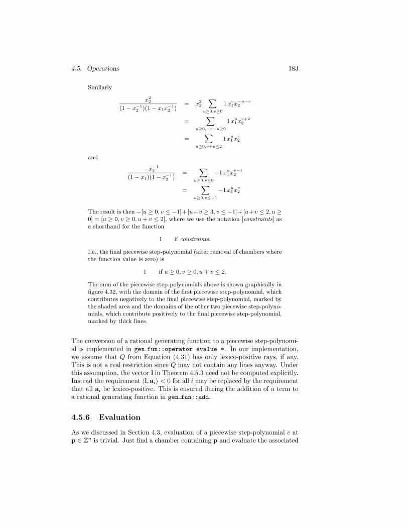
4.5. Operations 183
Similarly
x22
(1 − x−12 )(1 − x1x
−12 )
= x22
∑
u≥0,v≥0
1 xv1x−u−v
2
=∑
u≥0,−v−u≥0
1 xu1xv+2
2
=∑
u≥0,v+u≤2
1 xu1xv
2
and
−x−12
(1 − x1)(1 − x−12 )
=∑
u≥0,v≤0
−1 xu1xv−1
2
=∑
u≥0,v≤−1
−1 xu1xv
2
The result is then −[u ≥ 0, v ≤ −1]+[u+v ≥ 3, v ≤ −1]+[u+v ≤ 2, u ≥0] = [u ≥ 0, v ≥ 0, u + v ≤ 2], where we use the notation [constraints] asa shorthand for the function
1 if constraints.
I.e., the final piecewise step-polynomial (after removal of chambers wherethe function value is zero) is
1 if u ≥ 0, v ≥ 0, u + v ≤ 2.
The sum of the piecewise step-polynomials above is shown graphically infigure 4.32, with the domain of the first piecewise step-polynomial, whichcontributes negatively to the final piecewise step-polynomial, marked bythe shaded area and the domains of the other two piecewise step-polyno-mials, which contribute positively to the final piecewise step-polynomial,marked by thick lines.
The conversion of a rational generating function to a piecewise step-polynomi-al is implemented in gen fun::operator evalue *. In our implementation,we assume that Q from Equation (4.31) has only lexico-positive rays, if any.This is not a real restriction since Q may not contain any lines anyway. Underthis assumption, the vector l in Theorem 4.5.3 need not be computed explicitly.Instead the requirement 〈l,ai〉 < 0 for all i may be replaced by the requirementthat all ai be lexico-positive. This is ensured during the addition of a term toa rational generating function in gen fun::add.
4.5.6 Evaluation
As we discussed in Section 4.3, evaluation of a piecewise step-polynomial c atp ∈ Zn is trivial. Just find a chamber containing p and evaluate the associated
184 Chapter 4. Enumeration of Parametric Sets
u
v
(0, 0)
Figure 4.32: Barvinok example indicator decomposition.
step-polynomial at p. The most straightforward way of obtaining the coeffi-cient of xp, i.e., c(p), from a rational generating function C(x), on the otherhand, would be to expand the Laurent power series up to power p, which is aprocess that is exponential in the size of p. A better way is to first convert therational generating function to a piecewise step-polynomial using the resultsfrom Section 4.5.5. This can be slightly improved by immediately taking intoaccount the value of p during the enumeration of the polytope P in (4.30),reducing the parametric enumeration to a non-parametric enumeration.
4.6 Projection
In this section we consider techniques for enumerating parametric projectedsets as discussed in Section 4.2.4. We will mainly be interested in computingan explicit enumeration function. It is clear that these enumerators can alsobe represented as piecewise step-polynomials. It is not obvious, however, thatthey may be computed in polynomial time.
We consider four techniques for enumerating sets with existential variables.The first technique, proposed by Clauss (1996) and discussed in Section 4.6.1,is polynomial, but only works for the case of a single existential variable, i.e.,the case where only a single variable is projected out. Section 4.6.2 explains anew technique, which is more general and still polynomial, but which does nothandle all cases. It does seem to handle most cases that occur in compiler opti-mization, though (Verdoolaege et al. 2004a). The third technique, proposed byBoulet and Redon (1998a) and discussed in Section 4.6.3, is worst-case expo-nential, but works in general. The original proposal combined PIP (Feautrier
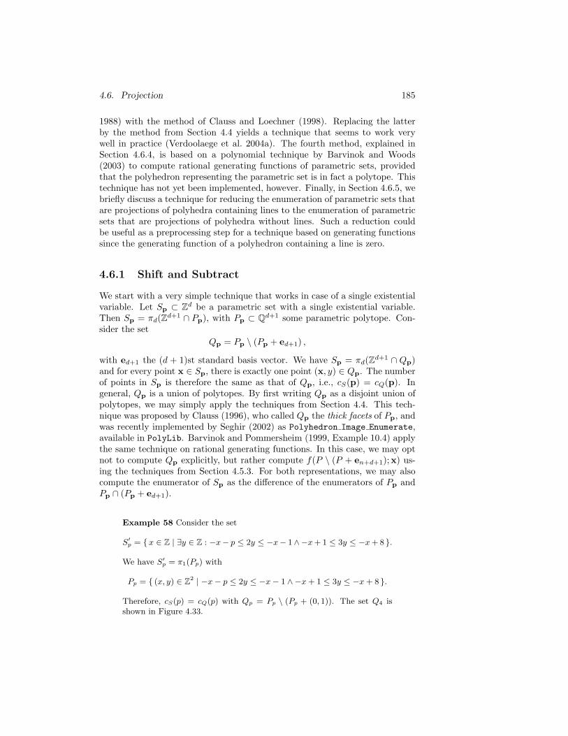
4.6. Projection 185
1988) with the method of Clauss and Loechner (1998). Replacing the latterby the method from Section 4.4 yields a technique that seems to work verywell in practice (Verdoolaege et al. 2004a). The fourth method, explained inSection 4.6.4, is based on a polynomial technique by Barvinok and Woods(2003) to compute rational generating functions of parametric sets, providedthat the polyhedron representing the parametric set is in fact a polytope. Thistechnique has not yet been implemented, however. Finally, in Section 4.6.5, webriefly discuss a technique for reducing the enumeration of parametric sets thatare projections of polyhedra containing lines to the enumeration of parametricsets that are projections of polyhedra without lines. Such a reduction couldbe useful as a preprocessing step for a technique based on generating functionssince the generating function of a polyhedron containing a line is zero.
4.6.1 Shift and Subtract
We start with a very simple technique that works in case of a single existentialvariable. Let Sp ⊂ Zd be a parametric set with a single existential variable.Then Sp = πd(Z
d+1 ∩ Pp), with Pp ⊂ Qd+1 some parametric polytope. Con-sider the set
Qp = Pp \ (Pp + ed+1) ,
with ed+1 the (d + 1)st standard basis vector. We have Sp = πd(Zd+1 ∩ Qp)
and for every point x ∈ Sp, there is exactly one point (x, y) ∈ Qp. The numberof points in Sp is therefore the same as that of Qp, i.e., cS(p) = cQ(p). Ingeneral, Qp is a union of polytopes. By first writing Qp as a disjoint union ofpolytopes, we may simply apply the techniques from Section 4.4. This tech-nique was proposed by Clauss (1996), who called Qp the thick facets of Pp, andwas recently implemented by Seghir (2002) as Polyhedron Image Enumerate,available in PolyLib. Barvinok and Pommersheim (1999, Example 10.4) applythe same technique on rational generating functions. In this case, we may optnot to compute Qp explicitly, but rather compute f(P \ (P + en+d+1);x) us-ing the techniques from Section 4.5.3. For both representations, we may alsocompute the enumerator of Sp as the difference of the enumerators of Pp andPp ∩ (Pp + ed+1).
Example 58 Consider the set
S′p = x ∈ Z | ∃y ∈ Z : −x− p ≤ 2y ≤ −x− 1∧−x + 1 ≤ 3y ≤ −x + 8 .
We have S′p = π1(Pp) with
Pp = (x, y) ∈ Z2 | −x − p ≤ 2y ≤ −x − 1 ∧ −x + 1 ≤ 3y ≤ −x + 8 .
Therefore, cS(p) = cQ(p) with Qp = Pp \ (Pp + (0, 1)). The set Q4 isshown in Figure 4.33.
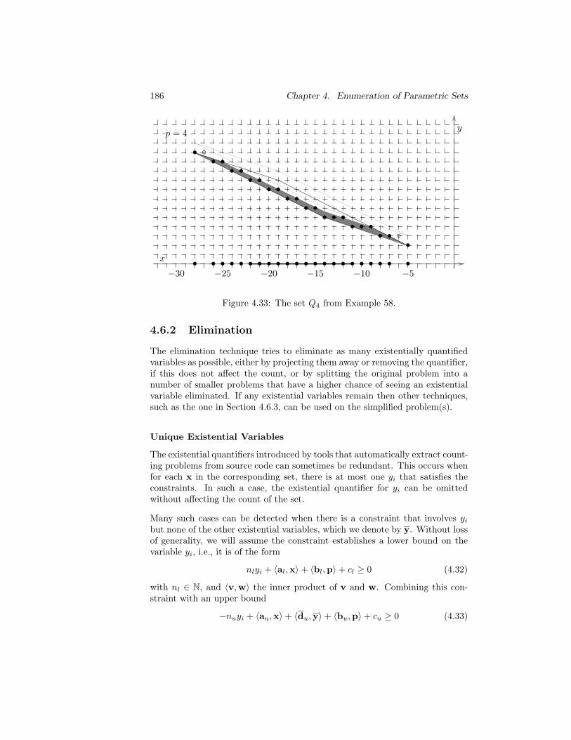
186 Chapter 4. Enumeration of Parametric Sets
p = 4
x
y
• • • • •• • • • • • • • • • • • • • • • •
•••
••••••
••••
••••
••••
•
−5−10−15−20−25−30
Figure 4.33: The set Q4 from Example 58.
4.6.2 Elimination
The elimination technique tries to eliminate as many existentially quantifiedvariables as possible, either by projecting them away or removing the quantifier,if this does not affect the count, or by splitting the original problem into anumber of smaller problems that have a higher chance of seeing an existentialvariable eliminated. If any existential variables remain then other techniques,such as the one in Section 4.6.3, can be used on the simplified problem(s).
Unique Existential Variables
The existential quantifiers introduced by tools that automatically extract count-ing problems from source code can sometimes be redundant. This occurs whenfor each x in the corresponding set, there is at most one yi that satisfies theconstraints. In such a case, the existential quantifier for yi can be omittedwithout affecting the count of the set.
Many such cases can be detected when there is a constraint that involves yi
but none of the other existential variables, which we denote by y. Without lossof generality, we will assume the constraint establishes a lower bound on thevariable yi, i.e., it is of the form
nlyi + 〈al,x〉 + 〈bl,p〉 + cl ≥ 0 (4.32)
with nl ∈ N, and 〈v,w〉 the inner product of v and w. Combining this con-straint with an upper bound
−nuyi + 〈au,x〉 + 〈du,y〉 + 〈bu,p〉 + cu ≥ 0 (4.33)
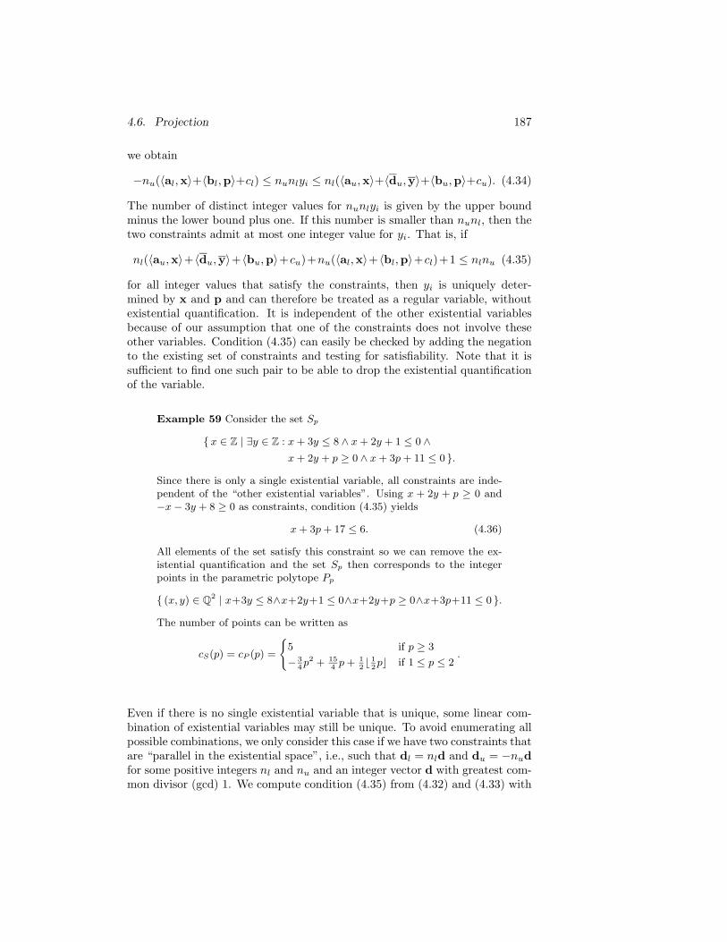
4.6. Projection 187
we obtain
−nu(〈al,x〉+〈bl,p〉+cl) ≤ nunlyi ≤ nl(〈au,x〉+〈du,y〉+〈bu,p〉+cu). (4.34)
The number of distinct integer values for nunlyi is given by the upper boundminus the lower bound plus one. If this number is smaller than nunl, then thetwo constraints admit at most one integer value for yi. That is, if
nl(〈au,x〉+〈du,y〉+〈bu,p〉+cu)+nu(〈al,x〉+〈bl,p〉+cl)+1 ≤ nlnu (4.35)
for all integer values that satisfy the constraints, then yi is uniquely deter-mined by x and p and can therefore be treated as a regular variable, withoutexistential quantification. It is independent of the other existential variablesbecause of our assumption that one of the constraints does not involve theseother variables. Condition (4.35) can easily be checked by adding the negationto the existing set of constraints and testing for satisfiability. Note that it issufficient to find one such pair to be able to drop the existential quantificationof the variable.
Example 59 Consider the set Sp
x ∈ Z | ∃y ∈ Z : x + 3y ≤ 8 ∧ x + 2y + 1 ≤ 0 ∧x + 2y + p ≥ 0 ∧ x + 3p + 11 ≤ 0 .
Since there is only a single existential variable, all constraints are inde-pendent of the “other existential variables”. Using x + 2y + p ≥ 0 and−x − 3y + 8 ≥ 0 as constraints, condition (4.35) yields
x + 3p + 17 ≤ 6. (4.36)
All elements of the set satisfy this constraint so we can remove the ex-istential quantification and the set Sp then corresponds to the integerpoints in the parametric polytope Pp
(x, y) ∈ Q2 | x+3y ≤ 8∧x+2y+1 ≤ 0∧x+2y+p ≥ 0∧x+3p+11 ≤ 0 .
The number of points can be written as
cS(p) = cP (p) =
5 if p ≥ 3
− 34p2 + 15
4p + 1
2⌊ 1
2p⌋ if 1 ≤ p ≤ 2
.
Even if there is no single existential variable that is unique, some linear com-bination of existential variables may still be unique. To avoid enumerating allpossible combinations, we only consider this case if we have two constraints thatare “parallel in the existential space”, i.e., such that dl = nld and du = −nudfor some positive integers nl and nu and an integer vector d with greatest com-mon divisor (gcd) 1. We compute condition (4.35) from (4.32) and (4.33) with
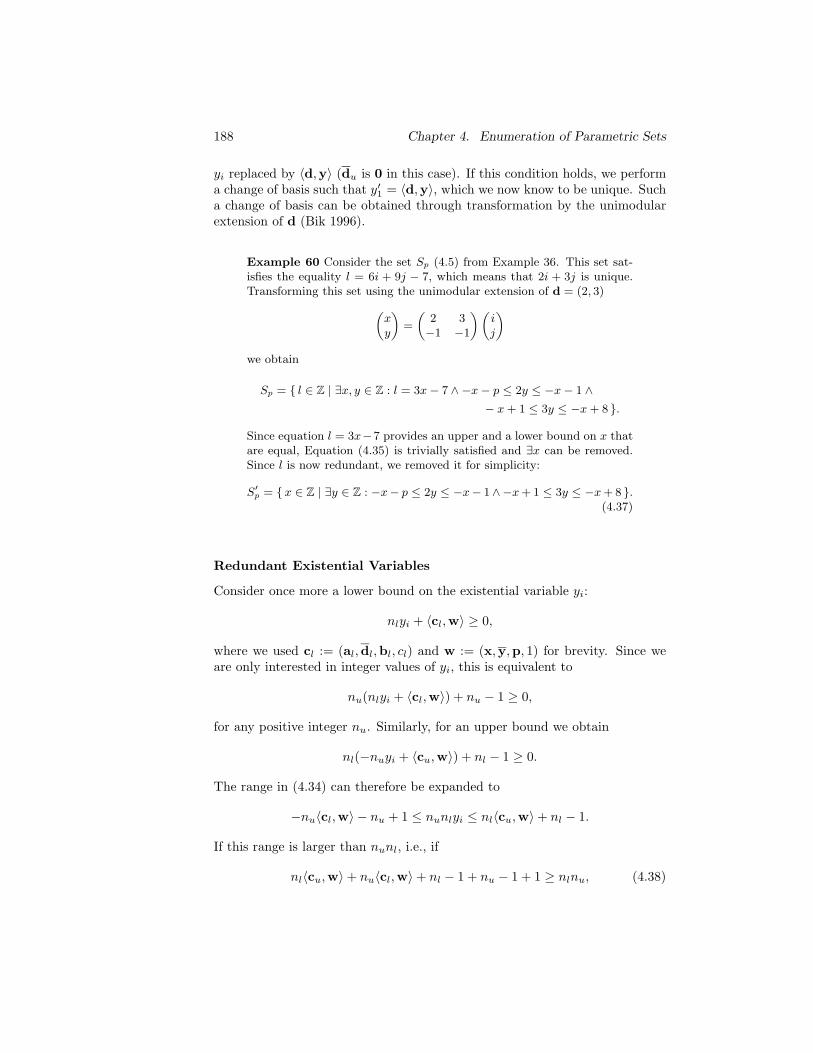
188 Chapter 4. Enumeration of Parametric Sets
yi replaced by 〈d,y〉 (du is 0 in this case). If this condition holds, we performa change of basis such that y′1 = 〈d,y〉, which we now know to be unique. Sucha change of basis can be obtained through transformation by the unimodularextension of d (Bik 1996).
Example 60 Consider the set Sp (4.5) from Example 36. This set sat-isfies the equality l = 6i + 9j − 7, which means that 2i + 3j is unique.Transforming this set using the unimodular extension of d = (2, 3)
(xy
)
=
(2 3−1 −1
)(ij
)
we obtain
Sp = l ∈ Z | ∃x, y ∈ Z : l = 3x − 7 ∧ −x − p ≤ 2y ≤ −x − 1 ∧− x + 1 ≤ 3y ≤ −x + 8 .
Since equation l = 3x−7 provides an upper and a lower bound on x thatare equal, Equation (4.35) is trivially satisfied and ∃x can be removed.Since l is now redundant, we removed it for simplicity:
S′p = x ∈ Z | ∃y ∈ Z : −x− p ≤ 2y ≤ −x− 1∧−x + 1 ≤ 3y ≤ −x + 8 .(4.37)
Redundant Existential Variables
Consider once more a lower bound on the existential variable yi:
nlyi + 〈cl,w〉 ≥ 0,
where we used cl := (al,dl,bl, cl) and w := (x,y,p, 1) for brevity. Since weare only interested in integer values of yi, this is equivalent to
nu(nlyi + 〈cl,w〉) + nu − 1 ≥ 0,
for any positive integer nu. Similarly, for an upper bound we obtain
nl(−nuyi + 〈cu,w〉) + nl − 1 ≥ 0.
The range in (4.34) can therefore be expanded to
−nu〈cl,w〉 − nu + 1 ≤ nunlyi ≤ nl〈cu,w〉 + nl − 1.
If this range is larger than nunl, i.e., if
nl〈cu,w〉 + nu〈cl,w〉 + nl − 1 + nu − 1 + 1 ≥ nlnu, (4.38)
4.6. Projection 189
then there is at least one integer value for each given value of the other variables.If this holds for all pairs of constraints, then variable yi does not restrict the so-lutions in any way and can simply be eliminated. This is known as the Omegatest (Pugh 1991; Pugh 1992). Note that unlike the case of unique existen-tial variables, the constraints need not be independent of the other existentialvariables.
Example 61 Consider the set
Sp = x ∈ Z | ∃y ∈ Z : −x − p ≤ 2y ≤ −x − 1 ∧ x ≤ −11 ∧− x + 1 ≤ 3y ≤ −x + 8 ∧ x + 3p + 10 ≥ 0 ∧ p ≥ 3 .
This set is shown ( ) in Figure 4.34. Pairwise combining the two upperand two lower bounds to form condition (4.38), we obtain 2p + 1 ≥ 4,26 ≥ 9, −x − 1 ≥ 6 and x + 20 + 3p ≥ 6. All of these are true in Sp.(Note that in practice we would use the lcm of nl and nu instead of theirproduct.) Variable y can therefore be eliminated and we obtain
Sp = x ∈ Z | x ≤ −11 ∧ p ≥ 3 ∧ x + 3p + 10 ≥ 0 .
Independent Splits
If neither of the two heuristics above apply, we can split the set into two ormore parts by cutting the polyhedron in the combined space along a hyper-plane. We only consider hyperplanes that are independent of the existentialvariables. This ensures that the enumerator of the original set is the sum of theenumerators of the parts. A cut that depends on existential variables, on theother hand, would result in sets that may intersect, requiring the computationof a disjoint union.
In particular, we consider all pairs of a lower and an upper bound on an exis-tential variable that do not depend on other existential variables, i.e., they areof the form (4.32). If neither condition (4.35) nor condition (4.38) is satisfiedover the whole set, then we cut off that part of the set where condition (4.35)does hold. In the remaining part, condition (4.38) holds for this particular pairof constraints. Since the number of pairs of constraints is polynomial in theinput size, the number of sets we split off is also polynomial and so the wholetechnique, if it applies, is polynomial in the input size (for fixed dimension). Asa special case, this technique always applies if there is only a single existentialvariable.
Example 62 Consider once more the set S′p (4.37) from Example 60.The bottom of Figure 4.34 shows the projection of the correspondingpolyhedron in the combined data-parameter space onto the xp-plane and
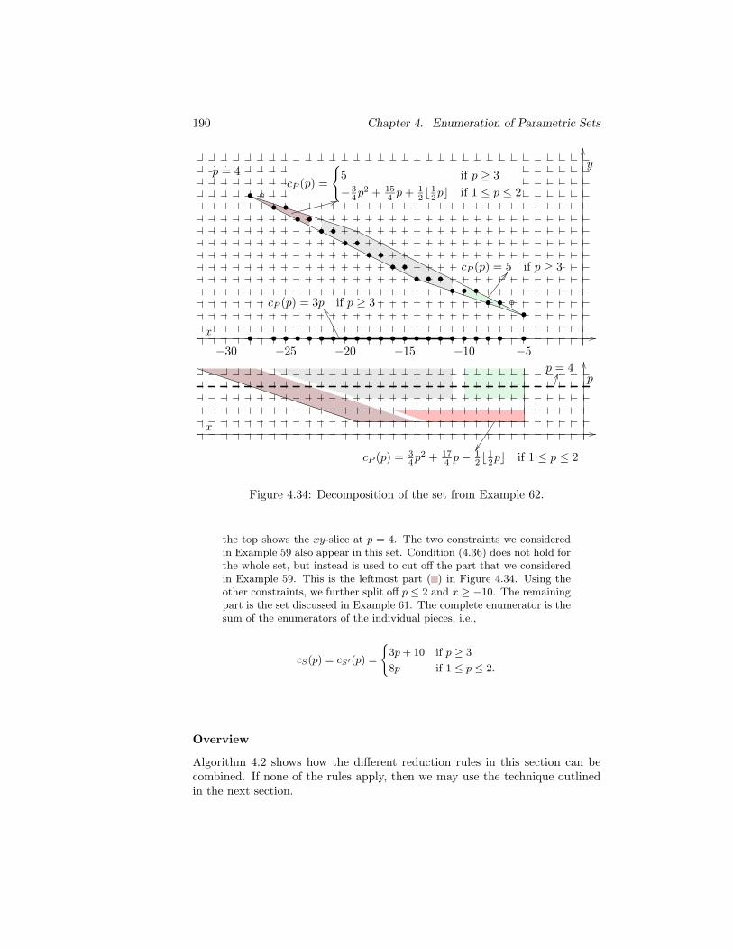
190 Chapter 4. Enumeration of Parametric Sets
p = 4
x
y
• • • • •• • • • • • • • • • • • • • • • •
•••
••••••
••••
••••
••••
•cP (p) =
5 if p ≥ 3
− 34p2 + 15
4 p + 12⌊
12p⌋ if 1 ≤ p ≤ 2
cP (p) = 5 if p ≥ 3
cP (p) = 3p if p ≥ 3
−5−10−15−20−25−30
p = 4
x
p
cP (p) = 34p2 + 17
4 p − 12⌊
12p⌋ if 1 ≤ p ≤ 2
Figure 4.34: Decomposition of the set from Example 62.
the top shows the xy-slice at p = 4. The two constraints we consideredin Example 59 also appear in this set. Condition (4.36) does not hold forthe whole set, but instead is used to cut off the part that we consideredin Example 59. This is the leftmost part ( ) in Figure 4.34. Using theother constraints, we further split off p ≤ 2 and x ≥ −10. The remainingpart is the set discussed in Example 61. The complete enumerator is thesum of the enumerators of the individual pieces, i.e.,
cS(p) = cS′(p) =
3p + 10 if p ≥ 3
8p if 1 ≤ p ≤ 2.
Overview
Algorithm 4.2 shows how the different reduction rules in this section can becombined. If none of the rules apply, then we may use the technique outlinedin the next section.
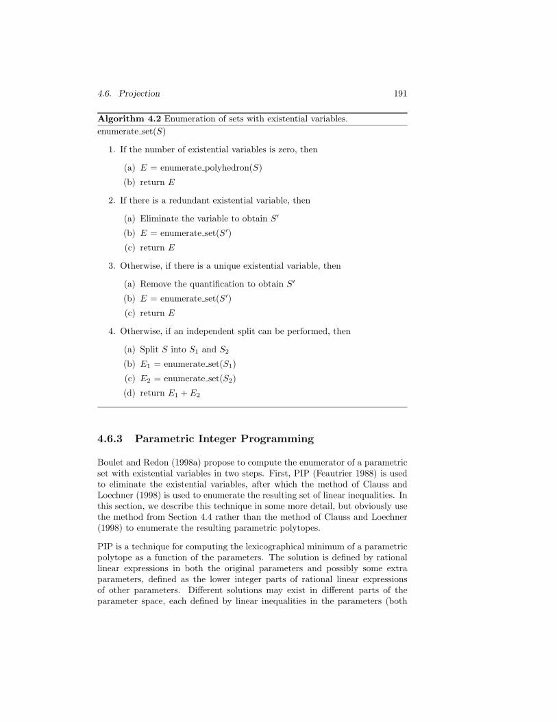
4.6. Projection 191
Algorithm 4.2 Enumeration of sets with existential variables.
enumerate set(S)
1. If the number of existential variables is zero, then
(a) E = enumerate polyhedron(S)
(b) return E
2. If there is a redundant existential variable, then
(a) Eliminate the variable to obtain S′
(b) E = enumerate set(S′)
(c) return E
3. Otherwise, if there is a unique existential variable, then
(a) Remove the quantification to obtain S′
(b) E = enumerate set(S′)
(c) return E
4. Otherwise, if an independent split can be performed, then
(a) Split S into S1 and S2
(b) E1 = enumerate set(S1)
(c) E2 = enumerate set(S2)
(d) return E1 + E2
4.6.3 Parametric Integer Programming
Boulet and Redon (1998a) propose to compute the enumerator of a parametricset with existential variables in two steps. First, PIP (Feautrier 1988) is usedto eliminate the existential variables, after which the method of Clauss andLoechner (1998) is used to enumerate the resulting set of linear inequalities. Inthis section, we describe this technique in some more detail, but obviously usethe method from Section 4.4 rather than the method of Clauss and Loechner(1998) to enumerate the resulting parametric polytopes.
PIP is a technique for computing the lexicographical minimum of a parametricpolytope as a function of the parameters. The solution is defined by rationallinear expressions in both the original parameters and possibly some extraparameters, defined as the lower integer parts of rational linear expressionsof other parameters. Different solutions may exist in different parts of theparameter space, each defined by linear inequalities in the parameters (both
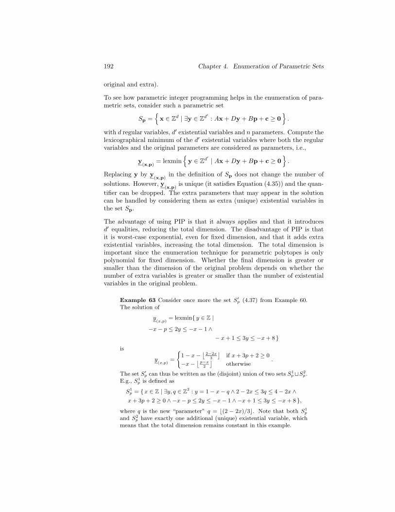
192 Chapter 4. Enumeration of Parametric Sets
original and extra).
To see how parametric integer programming helps in the enumeration of para-metric sets, consider such a parametric set
Sp =
x ∈ Zd | ∃y ∈ Zd′ : Ax + Dy + Bp + c ≥ 0
.
with d regular variables, d′ existential variables and n parameters. Compute thelexicographical minimum of the d′ existential variables where both the regularvariables and the original parameters are considered as parameters, i.e.,
y(x,p)
= lexmin
y ∈ Zd′ | Ax + Dy + Bp + c ≥ 0
.
Replacing y by y(x,p)
in the definition of Sp does not change the number of
solutions. However, y(x,p)
is unique (it satisfies Equation (4.35)) and the quan-
tifier can be dropped. The extra parameters that may appear in the solutioncan be handled by considering them as extra (unique) existential variables inthe set Sp.
The advantage of using PIP is that it always applies and that it introducesd′ equalities, reducing the total dimension. The disadvantage of PIP is thatit is worst-case exponential, even for fixed dimension, and that it adds extraexistential variables, increasing the total dimension. The total dimension isimportant since the enumeration technique for parametric polytopes is onlypolynomial for fixed dimension. Whether the final dimension is greater orsmaller than the dimension of the original problem depends on whether thenumber of extra variables is greater or smaller than the number of existentialvariables in the original problem.
Example 63 Consider once more the set S′p (4.37) from Example 60.The solution of
y(x,p)
= lexmin y ∈ Z |−x − p ≤ 2y ≤ −x − 1 ∧
− x + 1 ≤ 3y ≤ −x + 8 is
y(x,p)
=
1 − x −⌊
2−2x3
⌋if x + 3p + 2 ≥ 0
−x −⌊
p−x
2
⌋otherwise
.
The set S′p can thus be written as the (disjoint) union of two sets S1p ⊔S2
p .E.g., S1
p is defined as
S1p = x ∈ Z | ∃y, q ∈ Z
2 : y = 1 − x − q ∧ 2 − 2x ≤ 3q ≤ 4 − 2x ∧x + 3p + 2 ≥ 0 ∧ −x − p ≤ 2y ≤ −x − 1 ∧ −x + 1 ≤ 3y ≤ −x + 8 ,
where q is the new “parameter” q = ⌊(2 − 2x)/3⌋. Note that both S1p
and S2p have exactly one additional (unique) existential variable, which
means that the total dimension remains constant in this example.
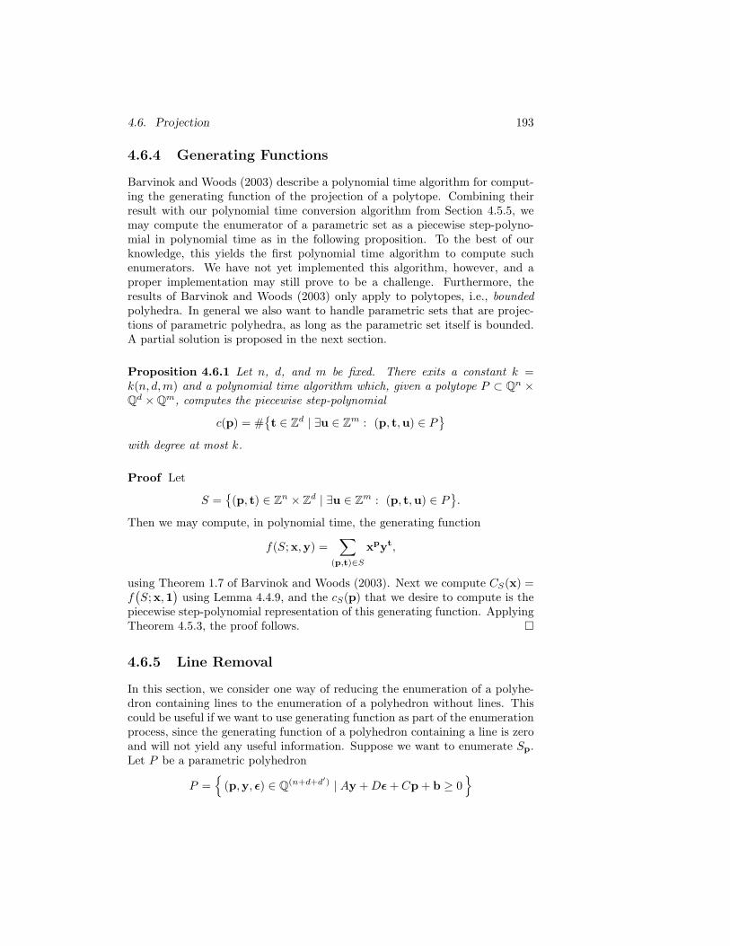
4.6. Projection 193
4.6.4 Generating Functions
Barvinok and Woods (2003) describe a polynomial time algorithm for comput-ing the generating function of the projection of a polytope. Combining theirresult with our polynomial time conversion algorithm from Section 4.5.5, wemay compute the enumerator of a parametric set as a piecewise step-polyno-mial in polynomial time as in the following proposition. To the best of ourknowledge, this yields the first polynomial time algorithm to compute suchenumerators. We have not yet implemented this algorithm, however, and aproper implementation may still prove to be a challenge. Furthermore, theresults of Barvinok and Woods (2003) only apply to polytopes, i.e., boundedpolyhedra. In general we also want to handle parametric sets that are projec-tions of parametric polyhedra, as long as the parametric set itself is bounded.A partial solution is proposed in the next section.
Proposition 4.6.1 Let n, d, and m be fixed. There exits a constant k =k(n, d,m) and a polynomial time algorithm which, given a polytope P ⊂ Qn ×Qd × Qm, computes the piecewise step-polynomial
c(p) = #t ∈ Zd | ∃u ∈ Zm : (p, t,u) ∈ P
with degree at most k.
Proof Let
S =(p, t) ∈ Zn × Zd | ∃u ∈ Zm : (p, t,u) ∈ P
.
Then we may compute, in polynomial time, the generating function
f(S;x,y) =∑
(p,t)∈S
xpyt,
using Theorem 1.7 of Barvinok and Woods (2003). Next we compute CS(x) =f(S;x,1
)using Lemma 4.4.9, and the cS(p) that we desire to compute is the
piecewise step-polynomial representation of this generating function. ApplyingTheorem 4.5.3, the proof follows.
4.6.5 Line Removal
In this section, we consider one way of reducing the enumeration of a polyhe-dron containing lines to the enumeration of a polyhedron without lines. Thiscould be useful if we want to use generating function as part of the enumerationprocess, since the generating function of a polyhedron containing a line is zeroand will not yield any useful information. Suppose we want to enumerate Sp.Let P be a parametric polyhedron
P =
(p,y, ǫ) ∈ Q(n+d+d′) | Ay + Dǫ + Cp + b ≥ 0
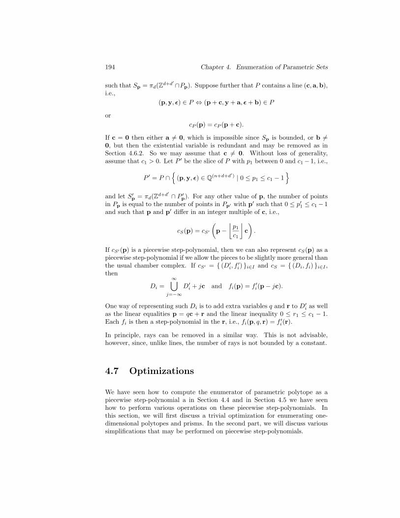
194 Chapter 4. Enumeration of Parametric Sets
such that Sp = πd(Zd+d′∩Pp). Suppose further that P contains a line (c,a,b),
i.e.,
(p,y, ǫ) ∈ P ⇔ (p + c,y + a, ǫ + b) ∈ P
or
cP (p) = cP (p + c).
If c = 0 then either a 6= 0, which is impossible since Sp is bounded, or b 6=0, but then the existential variable is redundant and may be removed as inSection 4.6.2. So we may assume that c 6= 0. Without loss of generality,assume that c1 > 0. Let P ′ be the slice of P with p1 between 0 and c1 − 1, i.e.,
P ′ = P ∩
(p,y, ǫ) ∈ Q(n+d+d′) | 0 ≤ p1 ≤ c1 − 1
and let S′p = πd(Zd+d′ ∩ P ′p). For any other value of p, the number of points
in Pp is equal to the number of points in Pp′ with p′ such that 0 ≤ p′1 ≤ c1 − 1and such that p and p′ differ in an integer multiple of c, i.e.,
cS(p) = cS′
(
p −
⌊p1
c1
⌋
c
)
.
If cS′(p) is a piecewise step-polynomial, then we can also represent cS(p) as apiecewise step-polynomial if we allow the pieces to be slightly more general thanthe usual chamber complex. If cS′ = (D′i, f
′i) i∈I and cS = (Di, fi) i∈I ,
then
Di =
∞⋃
j=−∞
D′i + jc and fi(p) = f ′i(p − jc).
One way of representing such Di is to add extra variables q and r to D′i as wellas the linear equalities p = qc + r and the linear inequality 0 ≤ r1 ≤ c1 − 1.Each fi is then a step-polynomial in the r, i.e., fi(p, q, r) = f ′i(r).
In principle, rays can be removed in a similar way. This is not advisable,however, since, unlike lines, the number of rays is not bounded by a constant.
4.7 Optimizations
We have seen how to compute the enumerator of parametric polytope as apiecewise step-polynomial a in Section 4.4 and in Section 4.5 we have seenhow to perform various operations on these piecewise step-polynomials. Inthis section, we will first discuss a trivial optimization for enumerating one-dimensional polytopes and prisms. In the second part, we will discuss varioussimplifications that may be performed on piecewise step-polynomials.
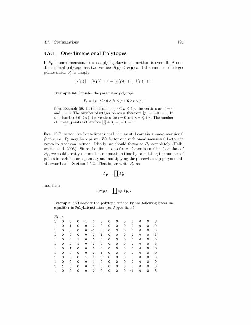
4.7. Optimizations 195
4.7.1 One-dimensional Polytopes
If Pp is one-dimensional then applying Barvinok’s method is overkill. A one-dimensional polytope has two vertices l(p) ≤ u(p) and the number of integerpoints inside Pp is simply
⌊u(p)⌋ − ⌈l(p)⌉ + 1 = ⌊u(p)⌋ + ⌊−l(p)⌋ + 1.
Example 64 Consider the parametric polytope
Pp = t | t ≥ 0 ∧ 2t ≤ p + 6 ∧ t ≤ p
from Example 50. In the chamber 0 ≤ p ≤ 6 , the vertices are l = 0and u = p. The number of integer points is therefore ⌊p⌋ + ⌊−0⌋ + 1. Inthe chamber 6 ≤ p , the vertices are l = 0 and u = p
2+ 3. The number
of integer points is therefore⌊
p
2+ 3⌋
+ ⌊−0⌋ + 1.
Even if Pp is not itself one-dimensional, it may still contain a one-dimensionalfactor, i.e., Pp may be a prism. We factor out such one-dimensional factors inParamPolyhedron Reduce. Ideally, we should factorize Pp completely (Halb-wachs et al. 2003). Since the dimension of each factor is smaller than that ofPp, we could greatly reduce the computation time by calculating the number ofpoints in each factor separately and multiplying the piecewise step-polynomialsafterward as in Section 4.5.2. That is, we write Pp as
Pp =∏
i
P ip
and thencP (p) =
∏
cP i(p).
Example 65 Consider the polytope defined by the following linear in-equalities in PolyLib notation (see Appendix B).
23 14
1 0 0 0 -1 0 0 0 0 0 0 0 0 8
1 0 1 0 0 0 0 0 0 0 0 0 0 0
1 0 0 0 0 -1 0 0 0 0 0 0 0 3
1 0 0 0 0 0 -1 0 0 0 0 0 0 3
1 0 0 1 0 0 0 0 0 0 0 0 0 0
1 0 0 -1 0 0 0 0 0 0 0 0 0 8
1 0 -1 0 0 0 0 0 0 0 0 0 0 8
1 0 0 0 0 0 1 0 0 0 0 0 0 0
1 0 0 0 1 0 0 0 0 0 0 0 0 0
1 0 0 0 0 1 0 0 0 0 0 0 0 0
1 1 0 0 0 0 0 0 0 0 0 0 0 0
1 0 0 0 0 0 0 0 0 0 -1 0 0 8
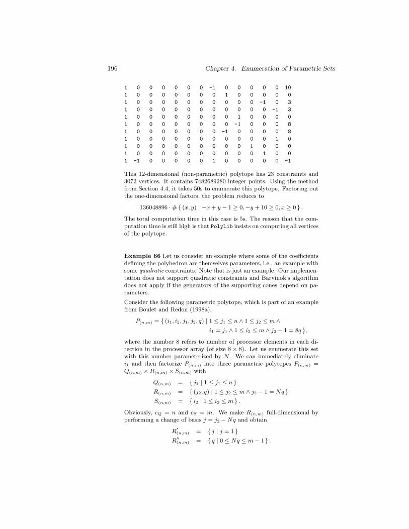
196 Chapter 4. Enumeration of Parametric Sets
1 0 0 0 0 0 0 -1 0 0 0 0 0 10
1 0 0 0 0 0 0 0 1 0 0 0 0 0
1 0 0 0 0 0 0 0 0 0 0 -1 0 3
1 0 0 0 0 0 0 0 0 0 0 0 -1 3
1 0 0 0 0 0 0 0 0 1 0 0 0 0
1 0 0 0 0 0 0 0 0 -1 0 0 0 8
1 0 0 0 0 0 0 0 -1 0 0 0 0 8
1 0 0 0 0 0 0 0 0 0 0 0 1 0
1 0 0 0 0 0 0 0 0 0 1 0 0 0
1 0 0 0 0 0 0 0 0 0 0 1 0 0
1 -1 0 0 0 0 0 1 0 0 0 0 0 -1
This 12-dimensional (non-parametric) polytope has 23 constraints and3072 vertices. It contains 7482689280 integer points. Using the methodfrom Section 4.4, it takes 50s to enumerate this polytope. Factoring outthe one-dimensional factors, the problem reduces to
136048896 · # (x, y) | −x + y − 1 ≥ 0,−y + 10 ≥ 0, x ≥ 0 .
The total computation time in this case is 5s. The reason that the com-putation time is still high is that PolyLib insists on computing all verticesof the polytope.
Example 66 Let us consider an example where some of the coefficientsdefining the polyhedron are themselves parameters, i.e., an example withsome quadratic constraints. Note that is just an example. Our implemen-tation does not support quadratic constraints and Barvinok’s algorithmdoes not apply if the generators of the supporting cones depend on pa-rameters.
Consider the following parametric polytope, which is part of an examplefrom Boulet and Redon (1998a),
P(n,m) = (i1, i2, j1, j2, q) | 1 ≤ j1 ≤ n ∧ 1 ≤ j2 ≤ m ∧i1 = j1 ∧ 1 ≤ i2 ≤ m ∧ j2 − 1 = 8q ,
where the number 8 refers to number of processor elements in each di-rection in the processor array (of size 8 × 8). Let us enumerate this setwith this number parameterized by N . We can immediately eliminatei1 and then factorize P(n,m) into three parametric polytopes P(n,m) =Q(n,m) × R(n,m) × S(n,m) with
Q(n,m) = j1 | 1 ≤ j1 ≤ n R(n,m) = (j2, q) | 1 ≤ j2 ≤ m ∧ j2 − 1 = Nq S(n,m) = i2 | 1 ≤ i2 ≤ m .
Obviously, cQ = n and cS = m. We make R(n,m) full-dimensional byperforming a change of basis j = j2 − Nq and obtain
R′(n,m) = j | j = 1 R′′(n,m) = q | 0 ≤ Nq ≤ m − 1 .
4.7. Optimizations 197
The enumerator of P(n,m) is then
cP (n, m) = cQ(n, m) · cR′(n, m) · cR′′(n, m) · cS(n, m)
= n · 1 ·(⌊
m − 1
N
⌋
+ 1
)
· m
=
(⌊m − 1
N
⌋
+ 1
)
nm.
4.7.2 Simplification of Step-polynomials
Many (piecewise) step-polynomials represent the same function on Zn. As atrivial example,
⌊p2 + 1
4
⌋and
⌊p2
⌋represent the same function on the integer
numbers. In particular, there are many ways of representing the zero function.Ideally we would want to detect (and remove) such zero functions and computea unique piecewise step-polynomial representation for each function on Zn.Failing this, we present here some simplifications on piecewise step-polynomialthat we have implemented. We explain the simplifications in terms of fractionalparts x = x−⌊x⌋ rather than floors since, as explained in Appendix A.2, thisis how we currently internally represent quasi-polynomials. This representationwas chosen because of the more direct correspondence to quasi-polynomialsdefined in terms of periodic numbers. Some other simplifications that are moreintimately tied to the internal representation are explained in Appendix A.3.
Note that it is in principle possible to check whether a piecewise step-polynomi-al is equal to the zero function. If the piecewise step-polynomial is given, thenthis can even be done in polynomial time. We just convert the piecewise step-polynomial to its corresponding rational generating function and then use thealgorithm of Woods (2004) to check whether this rational generating functionis zero. We have not implemented this functionality.
In our internal representation, we use an additional element, which we callstrides. Strides are used to represent enumerators that depend on the residueclass modulo some integer of a linear expression in the parameters. The residueclass is selected using a fractional part f(p) = h(p) of a degree-1 polynomialh(p). A stride has two branches representing a quasi-polynomial, one e1 forthe selected residue class and one e2 for all the other residue classes. (Stridesmay be nested.) The value of the stride
e′ = [f = 0] · e1 + [f 6= 0] · e2
is
e′(p) =
e1(p) if f(p) = 0
e2(p) otherwise
Note that a stride is equivalent to
e1(p) +
(
h(p) −
h(p) −1
m
+m − 1
m
)
(e2(p) − e1(p)),
198 Chapter 4. Enumeration of Parametric Sets
with m the common denominator of the coefficients of h(p). Often, the striderepresentation is more succinct.
Example 67 Consider the parametric polytope
Pp = x | 4x = p .
The enumerator iscP (p) =
[p
4
= 0]
· 1or
cP (p) = 1 −(p
4
−
p
4− 1
4
+3
4
)
.
We first describe some relatively cheap simplifications implemented in the func-tion reduce evalue. They are only relatively cheap because the simplifica-tion may induce a reordering of the internal structure representing the quasi-polynomial. The reason is that, as explained in Appendix A.3, we enforce afixed nesting order on the internal representation.
• “Normalization” of arguments of fractional parts
If m is the common denominator of the coefficients of the argument h ofa fractional part, then we have the following identity:
h =m − 1
m−
−h −1
m
.
We can therefore ensure that the leading coefficient is less than or equalto 1
2 . If it is equal to 12 , then we can do the same for next coefficient(s).
This normalization allows us to for example simplify
34p
+
14p + 3
4
to 34 since we may rewrite
34p
into 34 −
14p + 3
4
.
• Move out “constant part” of constant from fractional part
If the denominator of the constant in the argument of the fractional partdoes not divide the denominator m of the other coefficients in the sameargument, then the difference with the nearest multiple of 1
m may bemoved out of the fractional part. E.g.,
14p + 5
8
=
14p + 1
2
+ 1
8 .
• Elimination of variables using equalities in chambers
Although all chambers are initially of full dimension, addition or multi-plication of quasi-polynomials may result in lower-dimensional chambers.The resulting equalities can be used to eliminate some variables. E.g., ifp = q inside a chamber, then p − q can be simplified to 0.
• Reduction of the arguments of fractional parts using stride information
This is similar to the previous simplification, except that we use identitiesmodulo an integer.
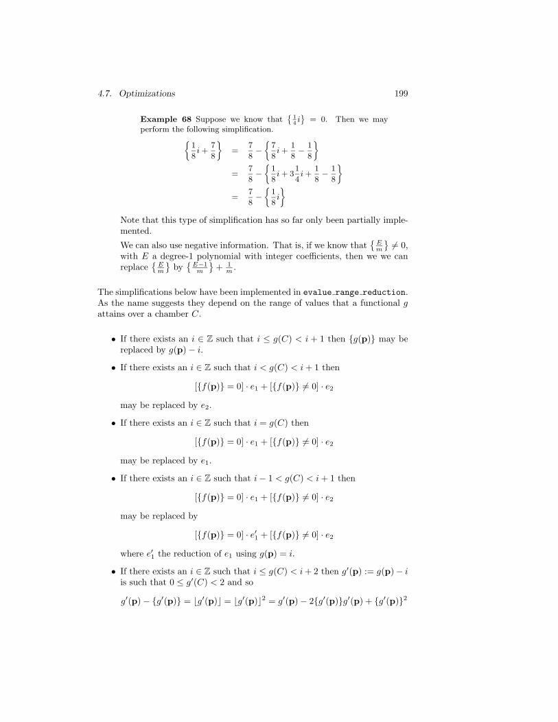
4.7. Optimizations 199
Example 68 Suppose we know that
14i
= 0. Then we mayperform the following simplification.
1
8i +
7
8
=7
8−
7
8i +
1
8− 1
8
=7
8−
1
8i + 3
1
4i +
1
8− 1
8
=7
8−
1
8i
Note that this type of simplification has so far only been partially imple-mented.
We can also use negative information. That is, if we know that
Em
6= 0,
with E a degree-1 polynomial with integer coefficients, then we we canreplace
Em
by
E−1m
+ 1
m .
The simplifications below have been implemented in evalue range reduction.As the name suggests they depend on the range of values that a functional gattains over a chamber C.
• If there exists an i ∈ Z such that i ≤ g(C) < i + 1 then g(p) may bereplaced by g(p) − i.
• If there exists an i ∈ Z such that i < g(C) < i + 1 then
[f(p) = 0] · e1 + [f(p) 6= 0] · e2
may be replaced by e2.
• If there exists an i ∈ Z such that i = g(C) then
[f(p) = 0] · e1 + [f(p) 6= 0] · e2
may be replaced by e1.
• If there exists an i ∈ Z such that i − 1 < g(C) < i + 1 then
[f(p) = 0] · e1 + [f(p) 6= 0] · e2
may be replaced by
[f(p) = 0] · e′1 + [f(p) 6= 0] · e2
where e′1 the reduction of e1 using g(p) = i.
• If there exists an i ∈ Z such that i ≤ g(C) < i + 2 then g′(p) := g(p)− iis such that 0 ≤ g′(C) < 2 and so
g′(p) − g′(p) = ⌊g′(p)⌋ = ⌊g′(p)⌋2 = g′(p) − 2g′(p)g′(p) + g′(p)2
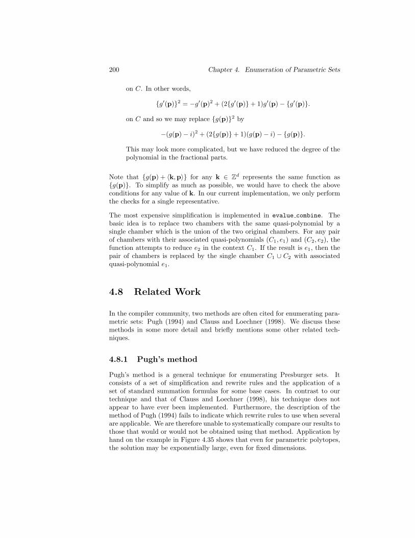
200 Chapter 4. Enumeration of Parametric Sets
on C. In other words,
g′(p)2 = −g′(p)2 + (2g′(p) + 1)g′(p) − g′(p).
on C and so we may replace g(p)2 by
−(g(p) − i)2 + (2g(p) + 1)(g(p) − i) − g(p).
This may look more complicated, but we have reduced the degree of thepolynomial in the fractional parts.
Note that g(p) + 〈k,p〉 for any k ∈ Zd represents the same function asg(p). To simplify as much as possible, we would have to check the aboveconditions for any value of k. In our current implementation, we only performthe checks for a single representative.
The most expensive simplification is implemented in evalue combine. Thebasic idea is to replace two chambers with the same quasi-polynomial by asingle chamber which is the union of the two original chambers. For any pairof chambers with their associated quasi-polynomials (C1, e1) and (C2, e2), thefunction attempts to reduce e2 in the context C1. If the result is e1, then thepair of chambers is replaced by the single chamber C1 ∪ C2 with associatedquasi-polynomial e1.
4.8 Related Work
In the compiler community, two methods are often cited for enumerating para-metric sets: Pugh (1994) and Clauss and Loechner (1998). We discuss thesemethods in some more detail and briefly mentions some other related tech-niques.
4.8.1 Pugh’s method
Pugh’s method is a general technique for enumerating Presburger sets. Itconsists of a set of simplification and rewrite rules and the application of aset of standard summation formulas for some base cases. In contrast to ourtechnique and that of Clauss and Loechner (1998), his technique does notappear to have ever been implemented. Furthermore, the description of themethod of Pugh (1994) fails to indicate which rewrite rules to use when severalare applicable. We are therefore unable to systematically compare our results tothose that would or would not be obtained using that method. Application byhand on the example in Figure 4.35 shows that even for parametric polytopes,the solution may be exponentially large, even for fixed dimensions.
4.8. Related Work 201
for(i=1;1000*i<=N;i++)
for(j=1;1000*j<=N;j++)
S1;
(a) How many times does S1 execute?
N2
1000000 if 1000 divides N(N−1)N1000000 − N−1
1000000 if 1000 divides N − 1
. . .(N−999)N1000000 − 999N−998001
1000000 if 1000 divides N − 999
(b) Solution computed by hand using the method of Pugh (1994)
⌊N
1000
⌋2
(c) Solution generated by our method
Figure 4.35: Example of an answer generated by Pugh’s method. The numberof different cases in Pugh’s answer is as large as the factor of i and j in theprogram in (a) (1000 in this example). Therefore, the solution size of Pugh’smethod is exponentially large.
202 Chapter 4. Enumeration of Parametric Sets
Pugh (1994) proposes two algorithms to eliminate variables, one from Pugh(1992), resulting in a collection of possibly overlapping sets, and a new oneresulting in disjoint sets. The basic idea behind both algorithms is to usethe Omega test to detect the part of the polytope where projection is exact,i.e., where the inverse image of the projection contains at least one integerpoint. The projection of this part is called the “dark shadow”. The remainingparts of the projection are collected in possibly overlapping “splinters”. Thenumber of splinters is linear (in the new algorithm even quadratic) in someof the coefficients that appear in the input and so exponential in the inputsize. The new algorithm avoids this overlap, but it is formulated for a singlevariable. It is not at all clear whether successively applying the algorithm twiceto eliminate two variables would still yield disjoint sets. For eliminating a singlevariable, the method from Section 4.6.1 is more appropriate. Note that the newalgorithm contains a check that is essentially the same as our constraint (4.35)for detecting unique existential variables. If the check holds, then the algorithmstill eliminates the variable, using exponential splintering no less, even though,as we pointed out, this is not needed for counting purposes.
4.8.2 Clauss’s method
As already explained in Section 4.2.3, our technique and Clauss’s method sharethe decomposition into chambers, but whereas our technique produces polyno-mially sized quasi-polynomials, the method of Clauss and Loechner (1998) canproduce exponentially sized quasi-polynomials or sometimes no solution at all.
Interpolation and Degenerate Domains
Based on the knowledge of the structure of the solution (Theorem 4.2.11),Clauss and Loechner (1998) calculate the number of points in a set of in-stances of Pp for fixed values of p in a given chamber, called initial countings,and then calculate the quasi-polynomial for this chamber through interpola-tion. They represent periodic numbers by lookup-tables, containing a separatevalue for each residue class (see Appendix A.1), and during their calculationsthey directly determine the elements in these lookup-tables. To interpolatea d-dimensional Ehrhart polynomial with periods qi their algorithm requires∏n
i=1(d + 1)qi initial countings. Since the implementation is based on Van-dermonde interpolation, it searches for fixed parameter values located in ahyperrectangle. However, it is not always possible to find a hyperrectangle ofthe correct size that is completely inside a given chamber.
For example, consider the chamber N ≤ M ≤ N + 3 ∧ N ≤ 2M − 7 from thepolytope in Equation (4.3). This chamber is geometrically represented by •sin Figure 4.36. For this chamber, the period in both dimensions is 1, and theimplementation of Clauss’s method in PolyLib (Loechner 1999) searches for a
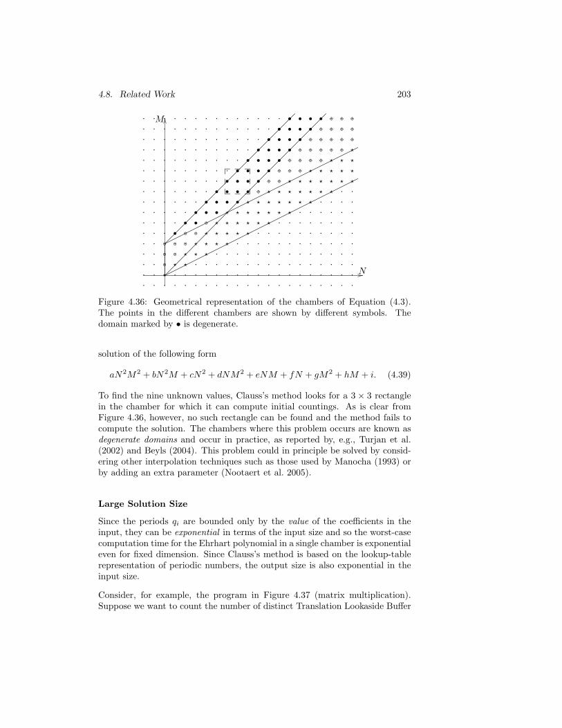
4.8. Related Work 203
·················
·················
··⋆···············
···⋆···•···········
···⋆·⋆···•··········
····⋆·⋆··•·•·········
····⋆·⋆·⋆··•·•········
·····⋆·⋆·⋆·•·•·•·······
·····⋆·⋆·⋆·⋆·•·•·•······
······⋆·⋆·⋆·•·•·•·•·····
······⋆·⋆·⋆·⋆·•·•·•·•····
·······⋆·⋆·⋆·⋄·•·•·•·•···
·······⋆·⋆·⋆·⋆·⋄·•·•·•·•··
········⋆·⋆·⋆·⋄·⋄·•·•·•·•·
········⋆·⋆·⋆·⋆·⋄·⋄·•·•·•·•
·········⋆·⋆·⋆·⋄·⋄·⋄·•·•·•
·········⋆·⋆·⋆·⋆·⋄·⋄·⋄·•·•
··········⋆·⋆·⋆·⋄·⋄·⋄·⋄·•
··········⋆·⋆·⋆·⋆·⋄·⋄·⋄·⋄
···········⋆·⋆·⋆·⋄·⋄·⋄·⋄
···········⋆·⋆·⋆·⋆·⋄·⋄·⋄M
N
Figure 4.36: Geometrical representation of the chambers of Equation (4.3).The points in the different chambers are shown by different symbols. Thedomain marked by • is degenerate.
solution of the following form
aN2M2 + bN2M + cN2 + dNM2 + eNM + fN + gM2 + hM + i. (4.39)
To find the nine unknown values, Clauss’s method looks for a 3 × 3 rectanglein the chamber for which it can compute initial countings. As is clear fromFigure 4.36, however, no such rectangle can be found and the method fails tocompute the solution. The chambers where this problem occurs are known asdegenerate domains and occur in practice, as reported by, e.g., Turjan et al.(2002) and Beyls (2004). This problem could in principle be solved by consid-ering other interpolation techniques such as those used by Manocha (1993) orby adding an extra parameter (Nootaert et al. 2005).
Large Solution Size
Since the periods qi are bounded only by the value of the coefficients in theinput, they can be exponential in terms of the input size and so the worst-casecomputation time for the Ehrhart polynomial in a single chamber is exponentialeven for fixed dimension. Since Clauss’s method is based on the lookup-tablerepresentation of periodic numbers, the output size is also exponential in theinput size.
Consider, for example, the program in Figure 4.37 (matrix multiplication).Suppose we want to count the number of distinct Translation Lookaside Buffer
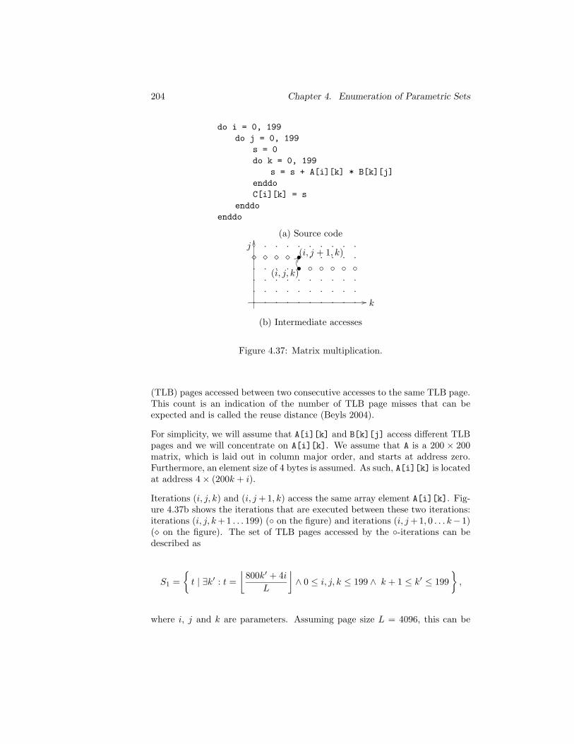
204 Chapter 4. Enumeration of Parametric Sets
do i = 0, 199
do j = 0, 199
s = 0
do k = 0, 199
s = s + A[i][k] * B[k][j]
enddo
C[i][k] = s
enddo
enddo
(a) Source code
.
.
.
.⋄
.
.
.
.
.⋄
.
.
.
.
.⋄
.
.
.
.
.⋄
.
.
.
.
.
.
.
.
.
.
.
.
.
.
.
.
.
.
.
.
.
.
.
.
.
.
.
.
.
.
.
.
•(i, j, k)
•(i, j + 1, k)j
k
(b) Intermediate accesses
Figure 4.37: Matrix multiplication.
(TLB) pages accessed between two consecutive accesses to the same TLB page.This count is an indication of the number of TLB page misses that can beexpected and is called the reuse distance (Beyls 2004).
For simplicity, we will assume that A[i][k] and B[k][j] access different TLBpages and we will concentrate on A[i][k]. We assume that A is a 200 × 200matrix, which is laid out in column major order, and starts at address zero.Furthermore, an element size of 4 bytes is assumed. As such, A[i][k] is locatedat address 4 × (200k + i).
Iterations (i, j, k) and (i, j +1, k) access the same array element A[i][k]. Fig-ure 4.37b shows the iterations that are executed between these two iterations:iterations (i, j, k +1 . . . 199) ( on the figure) and iterations (i, j +1, 0 . . . k−1)(⋄ on the figure). The set of TLB pages accessed by the -iterations can bedescribed as
S1 =
t | ∃k′ : t =
⌊800k′ + 4i
L
⌋
∧ 0 ≤ i, j, k ≤ 199 ∧ k + 1 ≤ k′ ≤ 199
,
where i, j and k are parameters. Assuming page size L = 4096, this can be
4.8. Related Work 205
written as a set of linear constraints:
S1 = t | ∃k′ : 1024t ≤ 200k′ + i ≤ 1024t + 1023
∧ 0 ≤ i, j, k ≤ 199 ∧ k + 1 ≤ k′ ≤ 199
and further simplified to (e.g., using Omega (Kelly et al. 1996b))
S1 = t | 0 ≤ i ∧ 1024t − 39800 ≤ i ≤ 199 ∧ 0 ≤ k ≤ 198
∧ 0 ≤ j ≤ 199 ∧ i + 200k ≤ 823 + 1024t
We obtain a similar expression S2 for the ⋄-iterations. The total count of TLBpages is #(S1∪S2) = #S1 +#(S2 \S1). Concentrating on S1, we see that it isa one-dimensional polytope and using PolyLib we can find out that its verticesare
i
1024+ 25
k
128−
823
1024and
i
1024+
4975
128.
Since the dimension of this polytope is d = 1 and the periods are qi = 1024,qj = 1 and qk = 128, the interpolation method requires 23 · 1024 · 128 initialcountings. If we assume we need two bytes to represent a value, then we needup to 256KiB just to store a single periodic number in the output. Using ourown technique, we obtain the following equivalent, but much shorter solutionin polynomial time (for fixed dimensions):
⌊i + 888
1024
⌋
−
⌊i + 200k + 199
1024
⌋
+ 39.
Although the degeneracy problem can in principle be solved, the problem of aworst-case exponentially-sized output is intrinsic to this approach.
A number of proposed compiler methods (e.g., Beyls 2004; Franke and O’Boyle2003; Loechner et al. 2002; Turjan et al. 2002) hard-code the resulting quasi-polynomials in the program they are optimizing. For these optimizations, largequasi-polynomials result in large binaries, making the optimizations less inter-esting, especially in an embedded systems context. Using our method, the sizeof the resulting quasi-polynomials does not grow exponentially.
Comparison
Table 4.4 shows a small comparison between the method of Clauss and Loech-ner (1998) (“interpolation”) to the method of Section 4.4 (“Barvinok”). Thefirst column shows the number of chambers, the second the number of degen-erate domains (only relevant for the interpolation method) and the remain-ing columns show the computation times for the interpolation method, ourmethod when using lookup-tables for periodic numbers and our method when
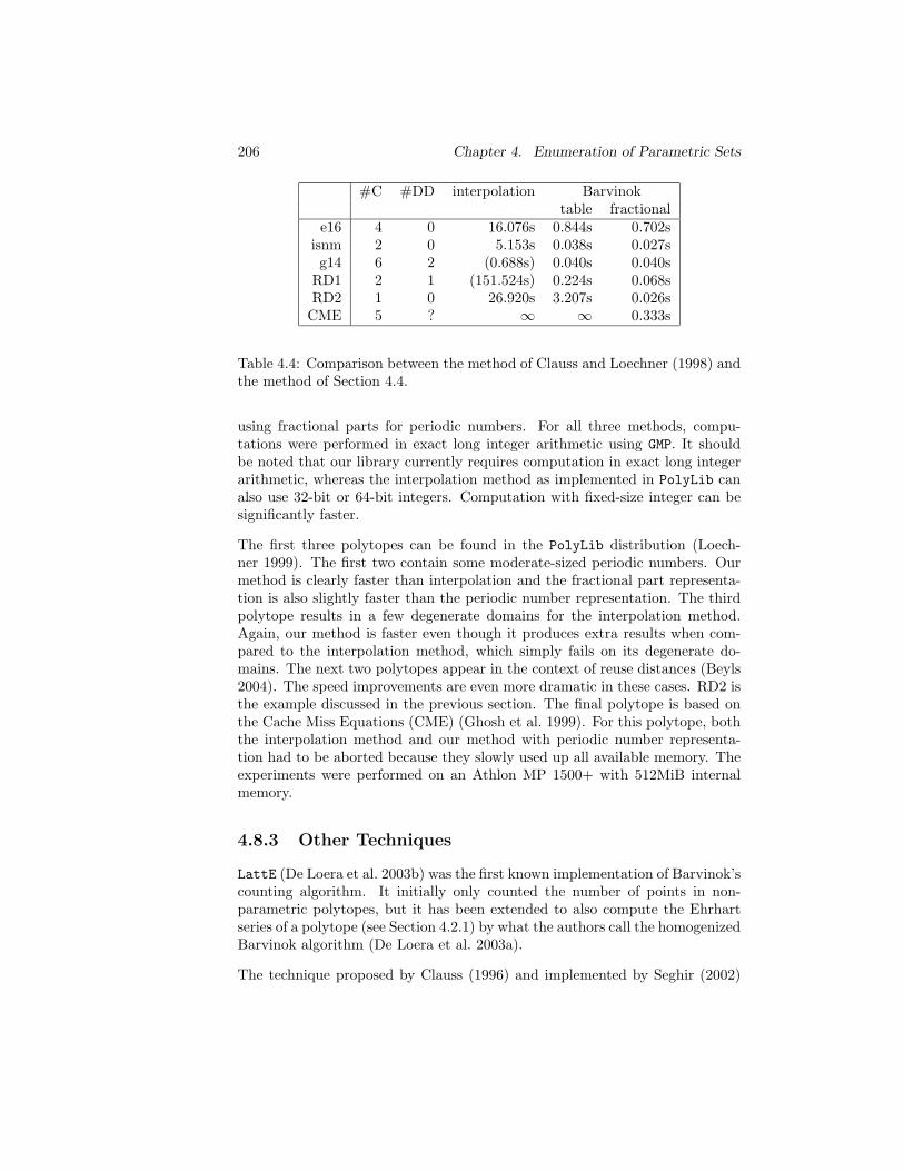
206 Chapter 4. Enumeration of Parametric Sets
#C #DD interpolation Barvinoktable fractional
e16 4 0 16.076s 0.844s 0.702sisnm 2 0 5.153s 0.038s 0.027sg14 6 2 (0.688s) 0.040s 0.040s
RD1 2 1 (151.524s) 0.224s 0.068sRD2 1 0 26.920s 3.207s 0.026sCME 5 ? ∞ ∞ 0.333s
Table 4.4: Comparison between the method of Clauss and Loechner (1998) andthe method of Section 4.4.
using fractional parts for periodic numbers. For all three methods, compu-tations were performed in exact long integer arithmetic using GMP. It shouldbe noted that our library currently requires computation in exact long integerarithmetic, whereas the interpolation method as implemented in PolyLib canalso use 32-bit or 64-bit integers. Computation with fixed-size integer can besignificantly faster.
The first three polytopes can be found in the PolyLib distribution (Loech-ner 1999). The first two contain some moderate-sized periodic numbers. Ourmethod is clearly faster than interpolation and the fractional part representa-tion is also slightly faster than the periodic number representation. The thirdpolytope results in a few degenerate domains for the interpolation method.Again, our method is faster even though it produces extra results when com-pared to the interpolation method, which simply fails on its degenerate do-mains. The next two polytopes appear in the context of reuse distances (Beyls2004). The speed improvements are even more dramatic in these cases. RD2 isthe example discussed in the previous section. The final polytope is based onthe Cache Miss Equations (CME) (Ghosh et al. 1999). For this polytope, boththe interpolation method and our method with periodic number representa-tion had to be aborted because they slowly used up all available memory. Theexperiments were performed on an Athlon MP 1500+ with 512MiB internalmemory.
4.8.3 Other Techniques
LattE (De Loera et al. 2003b) was the first known implementation of Barvinok’scounting algorithm. It initially only counted the number of points in non-parametric polytopes, but it has been extended to also compute the Ehrhartseries of a polytope (see Section 4.2.1) by what the authors call the homogenizedBarvinok algorithm (De Loera et al. 2003a).
The technique proposed by Clauss (1996) and implemented by Seghir (2002)
4.9. Applications and Experiments 207
for removing a single existential variable was discussed in Section 4.6.1. Thegeneral, but worst case exponential technique for removing existential vari-ables using PIP (Feautrier 1988) proposed by Boulet and Redon (1998a) wasdiscussed in Section 4.6.3. They proposed to use the method of Clauss andLoechner (1998) to enumerate the resulting parametric polytopes. The ap-pendix of their technical report (Boulet and Redon 1998b) indicates that usingthis method, their combined technique cannot compute the enumerator fullyautomatically. Meister (2004) proposes a similar technique using his more gen-eral periodic polyhedra instead of PIP. No implementation has been reported.
Beck (2004) describes a general technique for computing vector partition func-tions from their generating functions. For each variable in the generating func-tion, he computes partial fractions and then determines the constant term ofthe Laurent expansion. The latter part is similar to our specialization tech-nique from Section 4.4.3, except that we need the expansion at 1, whereasBeck (2004) needs the expansion at 0. He does not provide a complexity analy-sis, but standard techniques for computing partial fractions (Henrici 1974) areexponential, even for fixed dimensions.
Recently some advances have been made towards automata-based counting(Boigelot and Latour 2004; Parker and Chatterjee 2004). They handle the gen-eral case of Presburger formulas but they do not support symbolic parameters.Not surprisingly, these techniques are exponential, even for fixed dimensions.Preliminary experiments have shown that in the intersection of the applicationdomains, i.e., for non-parametric polytopes, our method is as fast or faster(up to a factor 100 in some exceptional cases) than Parker’s, except for poly-topes with a large number (say thousands) of vertices. For such polytopes,the homogenized Barvinok algorithm as implemented by LattE would be moreappropriate.7
4.9 Applications and Experiments
In this section we list some applications that require the enumeration of para-metric polytopes or more general parametric sets and that therefore may ben-efit from our implementation. We also mention some experimental results,comparing the method of Section 4.6.2 to that of Section 4.6.3. One of theseexperiments counts the number of times a particular rule from Section 4.6.2 wasused. Table 4.5 shows the results. These results will be extended in Table 5.7on page 231. The row “Fixed” refers to the special case of a unique existentialvariable determined by an equality; “Change” refers to a change of basis. Theindividual test sets in the columns are explained below. For more experimental
7This version embeds a polytope P in a single cone with a polar that has few rays if P
has few facets (De Loera et al. 2004).
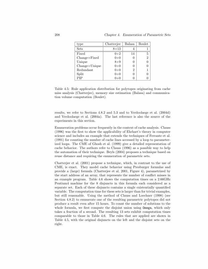
208 Chapter 4. Enumeration of Parametric Sets
type Chatterjee Balasa Boulet
Sets 8+13 4 1
Fixed 0+2 14 5Change+Fixed 0+0 0 2Unique 8+9 0 0Change+Unique 0+0 0 0Redundant 0+0 2 1Split 0+0 0 0PIP 0+0 0 0
Table 4.5: Rule application distribution for polytopes originating from cachemiss analysis (Chatterjee), memory size estimation (Balasa) and communica-tion volume computation (Boulet).
results, we refer to Sections 4.8.2 and 5.3 and to Verdoolaege et al. (2004d)and Verdoolaege et al. (2004a). The last reference is also the source of theexperiments in this section.
Enumeration problems occur frequently in the context of cache analysis. Clauss(1996) was the first to show the applicability of Ehrhart’s theory in computerscience and includes an example that extends the techniques of Ferrante et al.(1991) for counting the number of cache lines accessed by a loop to parameter-ized loops. The CME of Ghosh et al. (1999) give a detailed representation ofcache behavior. The authors refer to Clauss (1996) as a possible way to helpthe automation of their technique. Beyls (2004) proposes a technique based onreuse distance and requiring the enumeration of parametric sets.
Chatterjee et al. (2001) propose a technique, which, in contrast to the use ofCME, is exact. They model cache behavior using Presburger formulas andprovide a (large) formula (Chatterjee et al. 2001, Figure 4), parametrized bythe start address of an array, that represents the number of conflict misses inan example program. Table 4.6 shows the computation times on a 2.66GHzPentium4 machine for the 8 disjuncts in this formula each considered as aseparate set. Each of these disjuncts contains a single existentially quantifiedvariable. The computation time for these sets is larger than for trivial examples,but still reasonable. Using the method of Clauss and Loechner (1998) (seeSection 4.8.2) to enumerate one of the resulting parametric polytopes did notproduce a result even after 15 hours. To count the number of solutions to thewhole formula, we first compute the disjoint union using Omega, which onlytakes a fraction of a second. The resulting 13 sets exhibit computation timescomparable to those in Table 4.6. The rules that are applied are shown inTable 4.5, with the original disjuncts on the left and the disjoint sets on theright.
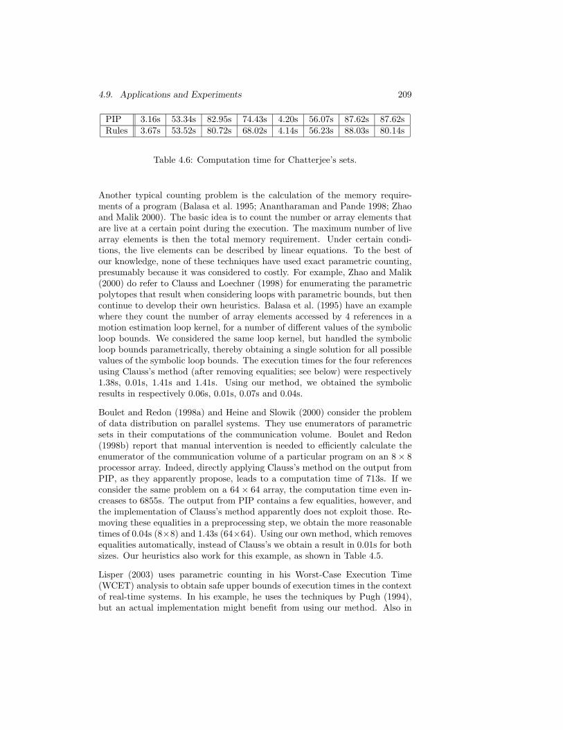
4.9. Applications and Experiments 209
PIP 3.16s 53.34s 82.95s 74.43s 4.20s 56.07s 87.62s 87.62sRules 3.67s 53.52s 80.72s 68.02s 4.14s 56.23s 88.03s 80.14s
Table 4.6: Computation time for Chatterjee’s sets.
Another typical counting problem is the calculation of the memory require-ments of a program (Balasa et al. 1995; Anantharaman and Pande 1998; Zhaoand Malik 2000). The basic idea is to count the number or array elements thatare live at a certain point during the execution. The maximum number of livearray elements is then the total memory requirement. Under certain condi-tions, the live elements can be described by linear equations. To the best ofour knowledge, none of these techniques have used exact parametric counting,presumably because it was considered to costly. For example, Zhao and Malik(2000) do refer to Clauss and Loechner (1998) for enumerating the parametricpolytopes that result when considering loops with parametric bounds, but thencontinue to develop their own heuristics. Balasa et al. (1995) have an examplewhere they count the number of array elements accessed by 4 references in amotion estimation loop kernel, for a number of different values of the symbolicloop bounds. We considered the same loop kernel, but handled the symbolicloop bounds parametrically, thereby obtaining a single solution for all possiblevalues of the symbolic loop bounds. The execution times for the four referencesusing Clauss’s method (after removing equalities; see below) were respectively1.38s, 0.01s, 1.41s and 1.41s. Using our method, we obtained the symbolicresults in respectively 0.06s, 0.01s, 0.07s and 0.04s.
Boulet and Redon (1998a) and Heine and Slowik (2000) consider the problemof data distribution on parallel systems. They use enumerators of parametricsets in their computations of the communication volume. Boulet and Redon(1998b) report that manual intervention is needed to efficiently calculate theenumerator of the communication volume of a particular program on an 8 × 8processor array. Indeed, directly applying Clauss’s method on the output fromPIP, as they apparently propose, leads to a computation time of 713s. If weconsider the same problem on a 64 × 64 array, the computation time even in-creases to 6855s. The output from PIP contains a few equalities, however, andthe implementation of Clauss’s method apparently does not exploit those. Re-moving these equalities in a preprocessing step, we obtain the more reasonabletimes of 0.04s (8×8) and 1.43s (64×64). Using our own method, which removesequalities automatically, instead of Clauss’s we obtain a result in 0.01s for bothsizes. Our heuristics also work for this example, as shown in Table 4.5.
Lisper (2003) uses parametric counting in his Worst-Case Execution Time(WCET) analysis to obtain safe upper bounds of execution times in the contextof real-time systems. In his example, he uses the techniques by Pugh (1994),but an actual implementation might benefit from using our method. Also in
210 Chapter 4. Enumeration of Parametric Sets
the context of real-time systems, Braberman et al. (2003) use enumerators ofparametric polytopes to automatically determine the size of the memory regionassociated with a scope in function of the arguments of the java method thatdefines the scope. Scoped memory (Bollella and Gosling 2000) is used hereto avoid the unpredictable behavior of regular garbage collection on real-timesystems. In their conversion of pointers to arrays (array recovery), Franke andO’Boyle (2003) count the number of times a pointer is incremented inside a loopnest. If these loops have parametrized bounds, then this results in a parametriccounting problem.
Loechner et al. (2002) try to reorder the data in memory according to the orderin which it is accessed. The access order is a function of the array indices andcan be computed as the enumerator of a parametric polytope. In the contextof converting matlab programs to process networks, Turjan et al. (2002) use asimilar idea to compute their rank function, which returns the number of iter-ation points of a for-statement executed before a given iteration point, as anenumerator. In the next step of converting the process networks to hardware(descriptions), Derrien et al. (2003) also use parametric counting to optimizethe resulting hardware. Earlier, Rijpkema et al. (1999) used parametric enu-merations during the linearization step of their method for converting param-eterized matlab programs to process networks. In a similar context, Bednaraet al. (2002) encounter parametric counting problems during optimization ofthe control of VLSI or FPGA-based processor arrays.
4.10 Conclusions and Future Work
We have presented the first known implementation of Barvinok’s enumera-tion algorithm applied to parametric polytopes. The resulting enumerator canbe obtained either as a piecewise step-polynomial or as a rational generatingfunction and both can be obtained in polynomial time. Furthermore, each rep-resentation can be converted into the other in polynomial time. For piecewisestep-polynomials this is a significant improvement over known, exponential,methods for enumerating parametric polytopes, making a whole class of knownoptimization techniques practically usable. For rational generating functionsthis is a major extension of an earlier implementation of Barvinok’s algorithmfor the subproblem of computing Ehrhart series.
We have also considered the extension to projections of the integer points inparametric polytopes. We have presented a polynomial-time algorithm (with-out implementation) for computing the enumerator of such sets as a piecewisestep-polynomial by combining earlier results on rational generating functionswith our polynomial-time conversion algorithm. We have further presented twoalternative methods (with implementation), one new and one proposed before,
4.10. Conclusions and Future Work 211
for reducing such problems to parametric polytope enumeration problems. Thefirst is not generally applicable and the second is worst-case exponential, butboth are easier to implement and appear to work fairly well in practice. Thisreduction, together with our polynomial method for enumerating parametricpolytopes, yields a method for enumerating parametric projected sets that cansolve many problems that were previously considered very difficult or evenunsolvable.
The resulting piecewise step-polynomials, though polynomially sized, can insome cases still be relatively large, even with the simplifications we performalready. Further research into additional simplifications is still needed. A moredetailed study of the relative benefits of piecewise step-polynomials and rationalgenerating functions, in particular a thorough evaluation of the assumptionthat piecewise step-polynomials are more appropriate for compiler optimizationproblems is also a point of further research. Finally, an actual implementationof the polynomial-time algorithm for enumerating parametric projected setswould be very interesting.

212 Chapter 4. Enumeration of Parametric Sets
Chapter 5
Reuse Distance
Computations
The reuse distance metric is a measure for the locality of memory accessesand it can be used to model interesting aspects of cache behavior. For us,the exact computation of reuse distances will serve as a testing vehicle forour enumeration library. As we will see, however, obtaining the sets to beenumerated can in itself be a challenge. This chapter is therefore also anexercise in engineering.
We start off in Section 5.1 with the basic definitions of the reuse distanceequations. In Section 5.2 we list some of the problems that may emerge whenusing the most straightforward way of obtaining the sets to be enumerated andshow different ways of circumventing these problems. Finally, in Section 5.3we present our experimental results.
This chapter requires a basic understanding of the concepts in Chapter 2, butis completely independent of Chapter 3. Although this chapter is basicallyan application of the techniques in Chapter 4, detailed knowledge of thesetechniques is not required to understand this chapter. The reader should befamiliar with the basic concept of an enumerator as defined in Section 4.1.2.Some notion of the two representations we use, as defined in Section 4.3, mayalso be helpful although we will mainly deal with just the piecewise step-poly-nomial representation. Understanding of Sections 4.6.2 and 4.6.3 is required toappreciate the experimental results in Section 5.3.3.
213
214 Chapter 5. Reuse Distance Computations
5.1 Reuse Distance Equations
Our description of reuse distances closely follows Beyls (2004, Section 4.2).
The reuse distance is a measure for the number of different memory locationsthat are accessed between consecutive accesses to the same memory location.Pairs of such consecutive accesses to the same memory location are called reusepairs. For each pair of references r and s in the program, we consider theiriteration domains Sr and Ss and define a relation reuser→s consisting of allpairs of iteration vectors in the respective iteration domains that form reusepairs. The definition of this relation as a Presburger formula is shown below.Note that the iterations domains include information on the statement in whichit occurs as well as on the relative order in which the references occur insidea given statement. This can be handled in a way that is entirely similar tostatement-level dimensions.
∀r, s ∈ R : reuser→s =
(i, j) ∈ Z2d : subject to conditions (5.2a)–(5.2d)
(5.1)
i ∈ Sr ∧ j ∈ Ss (iteration space) (5.2a)
i ≺ j (execution ordering)(5.2b)
r@i = s@j (same location) (5.2c)
∀t ∈ R : ¬ (∃k ∈ St : i ≺ k ≺ j ∧ t@k = r@i) (no intervening access)(5.2d)
In this formula, R is the set of all references in the program. The notation r@irefers to the memory location accessed by iteration i of reference r. The set ofreuse pairs is very similar to the dependence relations from Section 2.4. Themain difference is that no distinction is made between read and write accesses,that we always consider consecutive accesses (even for “input dependences”)and that the granularity is at the level of the accesses rather than at the levelof the statements.
Given an access to a memory location and the previous [next] access, the ac-cessed data set (ADS) is the set of all memory locations accessed in between.The backward [forward] reuse distance for a given access is then simply thenumber of those intermediately accessed locations. We will only consider thebackward reuse distance (BRD). Let L ⊂ Z be the set of all memory locations,then the accessed data set can be defined as
ADSr→s =⋃
t∈R
(i, j, l) ∈ reuser→s × L | ∃k ∈ St : i 4 k 4 j ∧ l = t@k .
(5.3)Note that this definition is slightly different from the one of Beyls (2004, Sec-tion 4.2.2) in that we consider the memory location l = r@i = s@j to be partof the accessed data set. This ensures that the reuse distance over a reuse pair
5.1. Reuse Distance Equations 215
is at least one and allows the reuse distance over a pair of iterations that doesnot form a reuse pair to simply be 0. This in turn avoids special treatment of“undefined” values (or ∞). The BRD of an iteration j of the second of a pairof given references is the number of locations l parametrized by j. That is, ifπd+1 is the projection onto the last d + 1 dimensions, i.e.,
BADSr←s := πd+1 (ADSr→s) = (j, l) ∈ Ss × L | ∃i ∈ Sr : (i, j, l) ∈ ADSr→s ,(5.4)
and if we consider BADSr←s ⊂ Zd × Z as defining a parametric set, then theBRD is the enumerator of this set, i.e.,
BRDr←s : Ss → Z
j 7→ #(BADSr←s) = cBADSr←s(j).
(5.5)
Since any iteration of a reference s can only form a reuse pair with an iterationfrom a single reference r, then for any j ∈ Ss, there can be at most one r ∈ Rsuch that BRDr←s(j) 6= 0. The actual reuse distance of a particular references (independent of the previous reference) is then simply the sum over all ref-erences of the reuse distances in which reference s is the second reference, i.e.,
BRDs =∑
r∈R
BRDr←s. (5.6)
An important application of reuse distances is cache analysis. Although asimilar analysis can be performed for instruction caches (Liveris et al. 2001;Van der Aa et al. 2003), we will focus on data caches. In this application, thereuse distance measures the number of distinct cache lines that are accessedin between two accesses to the same cache line. Assuming a fully associativecache with cache line size equal to L words, then the operator @ in the formulasabove needs to produce the index of the appropriate chunk of cache line size inmain memory. We will call this operator @L,
l = r@Li =
⌊r@i
L
⌋
.
Remember that the floor function can be expressed using linear constraints,
lL ≤ r@i ≤ lL + L − 1.
Note that if the original @-operator maps all accesses to a common memoryspace, then the @L-operator will also detect parts of different arrays beingmapped to the same cache line.
Example 69 Consider the example program in Figure 5.1. Assumea fully associative cache with line size three words. The third row ofTable 5.1 shows the element of array A accessed by each iteration of each
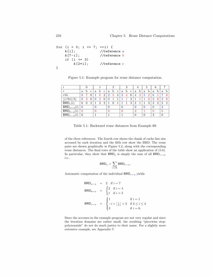
216 Chapter 5. Reuse Distance Computations
for (i = 0; i <= 7; ++i)
A[i]; //reference aA[7-i]; //reference bif (i <= 3)
A[2*i]; //reference c
Figure 5.1: Example program for reuse distance computation.
i 0 1 2 3 4 5 6 7
r a b c a b c a b c a b c a b a b a b a b
r@i 0 7 0 1 6 2 2 5 4 3 4 6 4 3 5 2 6 1 7 0
⌊(r@i)/3⌋ 0 2 0 0 2 0 0 1 1 1 1 2 1 1 1 0 2 0 2 0
BRDr(i) 0 0 2 1 2 2 1 0 1 1 1 3 2 1 1 3 3 2 2 2
BRDa←a(i) 0 0 0 0 0 0 0 2
BRDb←a(i) 0 0 0 0 2 1 0 0
BRDc←a(i) 0 1 1 1 0 0 3 0
Table 5.1: Backward reuse distances from Example 69.
of the three references. The fourth row shows the chunk of cache line sizeaccessed by each iteration and the fifth row show the BRD. The reusepairs are shown graphically in Figure 5.2, along with the correspondingreuse distances. The final rows of the table show an application of (5.6).In particular, they show that BRDa is simply the sum of all BRDr←a,i.e.,
BRDa =∑
r∈RBRDr←a.
Automatic computation of the individual BRDr←a yields
BRDa←a = 2 if i = 7
BRDb←a =
2 if i = 4
1 if i = 5
BRDc←a =
1 if i = 1
−i +⌊
i3
⌋+ 3 if 2 ≤ i ≤ 4
3 if i = 6.
Since the accesses in the example program are not very regular and sincethe iteration domains are rather small, the resulting “piecewise step-polynomials” do not do much justice to their name. For a slightly moreextensive example, see Appendix C
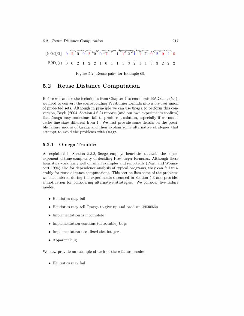
5.2. Reuse Distance Computation 217
0 2 0 0 2 0 0 1 1 1 1 2 1 1 1 0 2 0 2 0
0 0 2 1 2 2 1 0 1 1 1 3 2 1 1 3 3 2 2 2
⌊(r@i)/3⌋
BRDr(i)
Figure 5.2: Reuse pairs for Example 69.
5.2 Reuse Distance Computation
Before we can use the techniques from Chapter 4 to enumerate BADSr←s (5.4),we need to convert the corresponding Presburger formula into a disjoint unionof projected sets. Although in principle we can use Omega to perform this con-version, Beyls (2004, Section 4.6.2) reports (and our own experiments confirm)that Omega may sometimes fail to produce a solution, especially if we modelcache line sizes different from 1. We first provide some details on the possi-ble failure modes of Omega and then explain some alternative strategies thatattempt to avoid the problems with Omega.
5.2.1 Omega Troubles
As explained in Section 2.2.2, Omega employs heuristics to avoid the super-exponential time-complexity of deciding Presburger formulas. Although theseheuristics work fairly well on small examples and reportedly (Pugh and Wonna-cott 1994) also for dependence analysis of typical programs, they can fail mis-erably for reuse distance computations. This section lists some of the problemswe encountered during the experiments discussed in Section 5.3 and providesa motivation for considering alternative strategies. We consider five failuremodes:
• Heuristics may fail
• Heuristics may tell Omega to give up and produce UNKNOWNs
• Implementation is incomplete
• Implementation contains (detectable) bugs
• Implementation uses fixed size integers
• Apparent bug
We now provide an example of each of these failure modes.
• Heuristics may fail
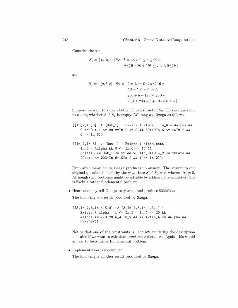
218 Chapter 5. Reuse Distance Computations
Consider the sets
S1 = (a, b, c) | ∃α : b = 4α ∧ 0 ≤ c ≤ 99 ∧
a ≤ 9 ∧ 80 + 19b ≤ 20a ∧ 0 ≤ b
and
S2 = (a, b, c) | ∃α, β : b = 4α ∧ 0 ≤ b ≤ 16 ∧
5β + 5 ≤ c ≤ 99 ∧
200 + b + 19a ≤ 20β ∧
20β ≤ 203 + b + 19a ∧ 0 ≤ b .
Suppose we want to know whether S1 is a subset of S2. This is equivalentto asking whether S1 \ S2 is empty. We may ask Omega as follows:
[In_2,In_6] -> [Out_1] : Exists ( alpha : In_6 = 4alpha &&
0 <= Out_1 <= 99 &&In_2 <= 9 && 80+19In_6 <= 20In_2 &&
0 <= In_6)
-
[In_2,In_6] -> [Out_1] : Exists ( alpha,beta :
In_6 = 4alpha && 0 <= In_6 <= 16 &&
5beta+5 <= Out_1 <= 99 && 200+In_6+19In_2 <= 20beta &&
20beta <= 203+In_6+19In_2 && 1 <= In_2);
Even after many hours, Omega produces no answer. The answer to ouroriginal question is “no”, by the way, since S1 ∩ S2 = ∅, whereas S1 6= ∅.Although such problems might be solvable by adding more heuristics, thisis likely a rather fundamental problem.
• Heuristics may tell Omega to give up and produce UNKNOWNs
The following is a result produced by Omega.
[3,In_2,3,In_4,5,0] -> [3,In_4,3,In_4,3,1] :
Exists ( alpha : 1 <= In_2 < In_4 <= 20 &&
4alpha <= 779+20In_4+In_2 && 776+21In_4 <= 4alpha &&
UNKNOWN)
Notice that one of the constraints is UNKNOWN, rendering the descriptionunusable if we want to calculate exact reuse distances. Again, this wouldappear to be a rather fundamental problem.
• Implementation is incomplete
The following is another result produced by Omega.
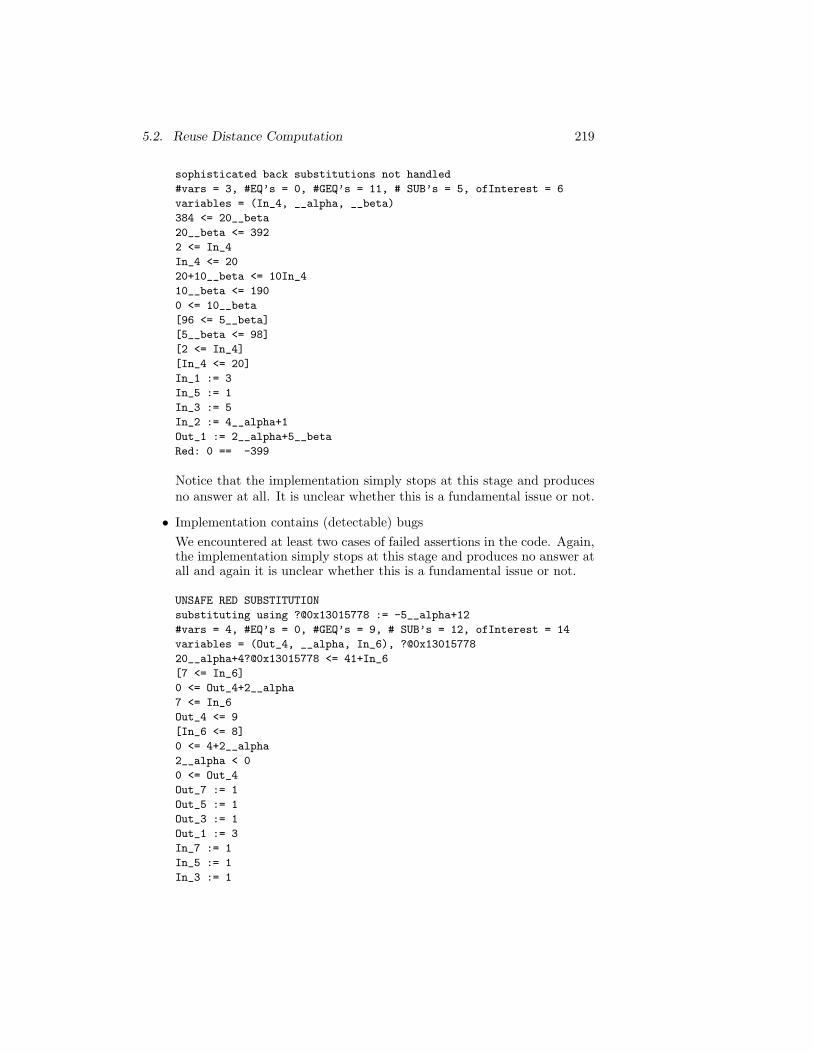
5.2. Reuse Distance Computation 219
sophisticated back substitutions not handled
#vars = 3, #EQ’s = 0, #GEQ’s = 11, # SUB’s = 5, ofInterest = 6
variables = (In_4, __alpha, __beta)
384 <= 20__beta
20__beta <= 392
2 <= In_4
In_4 <= 20
20+10__beta <= 10In_4
10__beta <= 190
0 <= 10__beta
[96 <= 5__beta]
[5__beta <= 98]
[2 <= In_4]
[In_4 <= 20]
In_1 := 3
In_5 := 1
In_3 := 5
In_2 := 4__alpha+1
Out_1 := 2__alpha+5__beta
Red: 0 == -399
Notice that the implementation simply stops at this stage and producesno answer at all. It is unclear whether this is a fundamental issue or not.
• Implementation contains (detectable) bugs
We encountered at least two cases of failed assertions in the code. Again,the implementation simply stops at this stage and produces no answer atall and again it is unclear whether this is a fundamental issue or not.
UNSAFE RED SUBSTITUTION
substituting using ?@0x13015778 := -5__alpha+12
#vars = 4, #EQ’s = 0, #GEQ’s = 9, # SUB’s = 12, ofInterest = 14
variables = (Out_4, __alpha, In_6), ?@0x13015778
20__alpha+4?@0x13015778 <= 41+In_6
[7 <= In_6]
0 <= Out_4+2__alpha
7 <= In_6
Out_4 <= 9
[In_6 <= 8]
0 <= 4+2__alpha
2__alpha < 0
0 <= Out_4
Out_7 := 1
Out_5 := 1
Out_3 := 1
Out_1 := 3
In_7 := 1
In_5 := 1
In_3 := 1
220 Chapter 5. Reuse Distance Computations
In_1 := 3
Out_6 := 0
In_2 := -2__alpha+5
Out_2 := -2__alpha+5
In_4 := -2__alpha-1
Red stride 2: 1+1In_4
Assertion "0 && \
"Added equality constraint to verified problem generates false"" \
failed: file "../src/omega_core/oc.c", line 65
• Implementation uses fixed size integers
Finally, Omega uses fixed size integers. Although it is fairly trivial tochange Omega to use long longs as its fixed size integers (which we did,but which is not supported in the official distribution), even long longsmay not be sufficient to store all the coefficients that may result duringour experiments. The following is such an example from our experimentswhere even long long precision is not sufficient.
Assertion "(((0x7ffffffffffffffLL))/4) / x > y" failed: \
file "../../basic/include/basic/util.h", line 68
Although changing the implementation to use exact long integer arith-metic is conceptually a triviality, it would require serious effort.
• Apparent bug
We have also found what at least appears to be a bug. The Omega functionDomain returns the domain of its argument, which should be a relation.The result of this function can in some cases depend on whether simplifywas called on the relation first. This is clearly an implementation issue.E.g., for the set shown below, the result of a call to Domain after call-ing simplify first is the (correct) set [4, 1, 4, 1, 3, 1]. Without callingsimplify first, the result is the empty set.
[In_1,In_2,In_3,In_4,In_5,In_6] ->
[Out_1,Out_2,Out_3,Out_4,Out_5,Out_6] :
exists ( : ( In_4 = 1 && In_6 = 1 && In_1 = 4 &&
In_3 = 4 && In_5 = 3 && Out_6 = 0 && Out_3 = 4 &&
Out_5 = 1 && Out_1 = 4 && In_2 = 1 &&
-10Out_4+219, 2 <= Out_2 <= -10Out_4+220, 20 &&
1 <= Out_4 <= 20 ))
5.2. Reuse Distance Computation 221
5.2.2 Alternatives
To the best of our knowledge, Omega is the only (publicly available) libraryfor manipulating Presburger formulas. In principle, intersection can be imple-mented relatively easily on top of a library that does not support existentialvariables. The set difference operation, however, is more difficult to implementand is also computationally the most difficult operation. Our strategy is there-fore to avoid set differences as much as possible. We have not investigatedalternatives for the other operations and simply perform them using Omega.
There are two places where set differences are used in a straightforward com-putation of BRDs,
• The negation in the “no intervening access” condition (5.2d).
• The union in the formula for ADSr→s (5.3), which needs to be convertedto a disjoint union as |S ∪ T | = |S| + |T \ S|.
Let us consider the union first. Instead of computing the disjoint union, wemay use the exclusion-inclusion principle, e.g., we compute |S ∪ T ∪ U | as
|S ∪ T ∪ U | = |S| + |T | + |U | − |S ∩ T | − |T ∩ U | − |U ∩ S| + |S ∩ T ∩ U |.
This results in many more sets that need to be enumerated, in fact exponentiallymany in the number of overlapping sets, but it does avoid the set difference,which is also exponential. In principle the computation can be simplified bychecking for duplicates among the sets or intersections thereof. As we have seenin Section 5.2.1, however, even checking whether one set is a subset of another(which would have to apply twice to check for equality) can be very expensiveusing Omega. This could be solved by converting the Presburger sets into NDDs,as explained in Section 2.2.4, or by computing their generating functions andapplying the algorithm of Woods (2004), as mentioned in Section 4.7.2.
Now consider the negation in (5.2d). Note that we have to subtract the setthat satisfies the argument of the negation for all references t ∈ R. We canalleviate the situation, by reducing this to just one set difference as follows.Consider the restricted reuse pairs reuser
r→s, defined below.
∀r, s ∈ R : reuserr→s =
(i, j) ∈ Z2d : subject to conditions (5.8a)–(5.8d)
(5.7)
i ∈ Sr ∧ j ∈ Ss (iteration space) (5.8a)
i ≺ j (execution ordering)(5.8b)
r@i = s@j (same location) (5.8c)
¬ (∃k ∈ Sr : i ≺ k ≺ j ∧ t@k = r@i) (no intervening access from r)(5.8d)
222 Chapter 5. Reuse Distance Computations
The definition of a restricted reuse pair is identical to that of a (regular) reusepair (5.1) except for the constraint (5.8d). Rather than imposing that therebe no intervening access to the same memory location from an iteration ofany reference, we only enforce that there be no such access from an iterationof the reference r (the superscript in reuser
r→s). Computing the correspondingADS
rr→s and its enumerator BRD
rr→s will obviously not yield the same function
as BRDr→s, but we can easily compute BRDr→s from BRDrr→s. The function
value of BRDrr→s is the same as that of BRDr→s for those restricted reuse pairs
that actually form a reuse pair. The difference is that BRDrr→s may also have
non-zero function values for restricted reuse pairs that do not form a reusepair. The extra pairs are those for which there is an intermediate access fromanother reference. That is,
reuser→s = reuserr→s \
⋃
t
reuserr→t→s (5.9)
with
reuserr→t→s = (i, j) ∈ reuse
rr→s | ∃k ∈ St : i ≺ k ≺ j ∧ t@k = r@i .
Computing BRDr→s from BRDrr→s is then simply a matter of “masking out”
the extraneous non-zero values (see Section 4.5.2). The mask is formed by alliterations of the reference s that form a restricted reuse pair such that there isan intermediate access from another reference, i.e., the elements of
reuserrr→t→s = πd(reuse
rr→t→s) = j ∈ Ss | ∃i ∈ Sr : (i, j) ∈ reuse
rr→t→s
for all t ∈ R. The enumerator of reuserrr→t→s has function values in the range 0, 1 and we have
BRDr←s = BRDrr←s ·
∏
t∈R
(1 − creuserrr→t→s
). (5.10)
The restricted reuse pairs themselves can be computed using Omega with a sin-gle set difference operation, but they can also be computed using PIP, withoutany set difference operation. To see this, consider the set reuse∅r→s of all orderedpairs of reference iterations that access the same memory, i.e., the set that sat-isfies conditions (5.8a)–(5.8c), but not (5.8d). The restricted reuse pairs areformed by the lexicographical maximum of the iteration of the first referencewith respect to the iteration of the second reference, i.e.,
reuserr→s =
(
lexmax(
reuse∅r→s
)−1)−1
.
We have to invert the relation reuse∅r→s because the parameters of the lexico-graphical maximum are in the second element of the pairs rather than in thefirst element, which is where we would expect them to be according to (2.6).Note that using PIP instead of Omega to compute restricted reuse pairs replacesone worst-case exponential operation with another worst-case exponential op-eration.
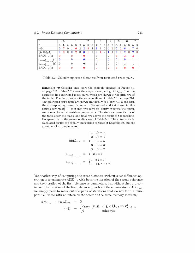
5.2. Reuse Distance Computation 223
i 0 1 2 3 4 5 6 7
r a b c a b c a b c a b c a b a b a b a b
r@i 0 7 0 1 6 2 2 5 4 3 4 6 4 3 5 2 6 1 7 0
⌊(r@i)/3⌋ 0 2 0 0 2 0 0 1 1 1 1 2 1 1 1 0 2 0 2 0
BRDbb←a(i) 0 0 0 1 2 1 3 3
creuserb
b→a→a(i) 0 0 0 0 0 0 0 1
creuserb
b→c→a(i) 0 0 0 1 0 0 1 1
BRDb←a(i) 0 0 0 0 2 1 0 0
Table 5.2: Calculating reuse distances from restricted reuse pairs.
Example 70 Consider once more the example program in Figure 5.1on page 216. Table 5.2 shows the steps in computing BRDb←a from thecorresponding restricted reuse pairs, which are shown in the fifth row ofthe table. The first rows are the same as those of Table 5.1 on page 216.The restricted reuse pairs are shown graphically in Figure 5.3, along withthe corresponding reuse distances. The second and third row in thisfigure show reuse
∅b→a, split into two rows for clarity, whereas the fourth
row shows the actual restricted reuse pairs. The sixth and seventh row ofthe table show the masks and final row shows the result of the masking.Compare this to the corresponding row of Table 5.1. The automaticallycalculated results are equally uninspiring as those of Example 69, but aregiven here for completeness,
BRDbb←a =
1 if i = 3
2 if i = 4
1 if i = 5
3 if i = 6
3 if i = 7
creuserb
b→a→a= 1 if i = 7
creuserb
b→c→a=
1 if i = 3
1 if 6 ≤ i ≤ 7.
Yet another way of computing the reuse distances without a set difference op-eration is to enumerate ADS
∅r→s with both the iteration of the second reference
and the iteration of the first reference as parameters, i.e., without first project-ing out the iteration of the first reference. To obtain the enumerator of ADSr→s
we simply need to mask out the pairs of iterations that do not form a reusepair, i.e., those with an intermediate access to the same memory location,
cADSr→s: reuse∅r→s → N
(i, j) 7→
cADS∅r→s
(i, j) (i, j) 6∈⋃
t∈R reuse∅r→t→s
0 otherwise
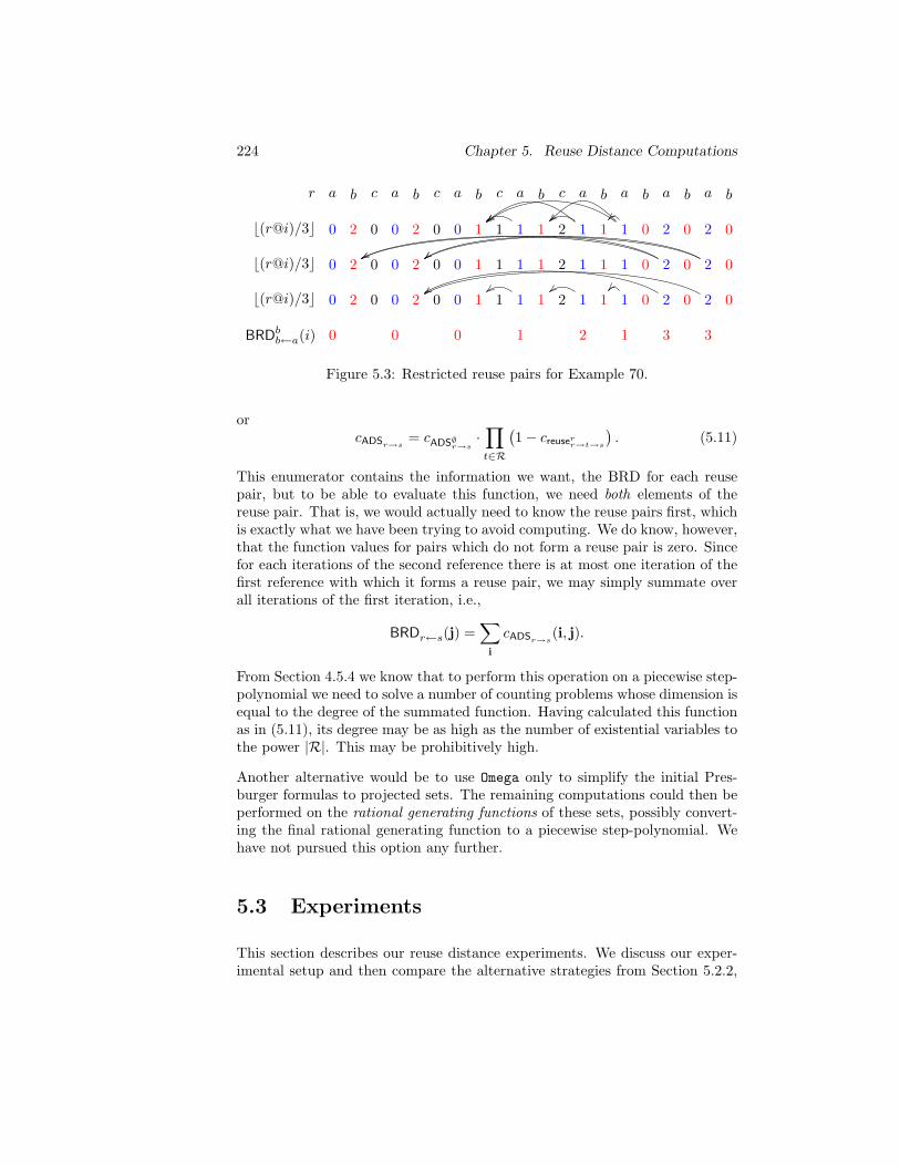
224 Chapter 5. Reuse Distance Computations
a b c a b c a b c a b c a b a b a b a b
0 2 0 0 2 0 0 1 1 1 1 2 1 1 1 0 2 0 2 0
0 2 0 0 2 0 0 1 1 1 1 2 1 1 1 0 2 0 2 0
0 2 0 0 2 0 0 1 1 1 1 2 1 1 1 0 2 0 2 0
0 0 0 1 2 1 3 3
r
⌊(r@i)/3⌋
⌊(r@i)/3⌋
⌊(r@i)/3⌋
BRDbb←a(i)
Figure 5.3: Restricted reuse pairs for Example 70.
orcADSr→s
= cADS∅r→s
·∏
t∈R
(1 − creuser
r→t→s
). (5.11)
This enumerator contains the information we want, the BRD for each reusepair, but to be able to evaluate this function, we need both elements of thereuse pair. That is, we would actually need to know the reuse pairs first, whichis exactly what we have been trying to avoid computing. We do know, however,that the function values for pairs which do not form a reuse pair is zero. Sincefor each iterations of the second reference there is at most one iteration of thefirst reference with which it forms a reuse pair, we may simply summate overall iterations of the first iteration, i.e.,
BRDr←s(j) =∑
i
cADSr→s(i, j).
From Section 4.5.4 we know that to perform this operation on a piecewise step-polynomial we need to solve a number of counting problems whose dimension isequal to the degree of the summated function. Having calculated this functionas in (5.11), its degree may be as high as the number of existential variables tothe power |R|. This may be prohibitively high.
Another alternative would be to use Omega only to simplify the initial Pres-burger formulas to projected sets. The remaining computations could then beperformed on the rational generating functions of these sets, possibly convert-ing the final rational generating function to a piecewise step-polynomial. Wehave not pursued this option any further.
5.3 Experiments
This section describes our reuse distance experiments. We discuss our exper-imental setup and then compare the alternative strategies from Section 5.2.2,
5.3. Experiments 225
the techniques from Sections 4.6.2 and 4.6.3, and finally our Barvinok-basedmethod and Clauss’s method discussed in Section 4.8.2.
5.3.1 Experimental Setup
We have written a prototype tool called frd.pl implementing most of the ba-sic strategies outlined in Section 5.2.2. The combination of strategies to use isconfigurable through command line options. The output of the tool is a list ofprojected sets that still need to be enumerated. The enumerators may also haveto be further manipulated depending on the strategy. We have also written asmall cache simulator that computes the actual reuse distances. In this simula-tor, we have used the implementation of random treaps, a data structure usedto efficiently calculate the reuse distances, by Beyls (2004, Section 3.2.1), whorefers to Aragon and Seidel (1989) and Kozen (1992) for further information.
The simulator first reads the descriptions of the projected sets, enumeratesthem using the barvinok library and performs any other further manipulationthat may be required. For every reference in the program, this calculation re-sults in an enumerator that represents the BRD of the given reference. Duringthe subsequent simulation and on every access to a memory location, the enu-merator is evaluated for the current iteration of the reference and the result iscompared to the actual BRD, computed by the simulator. The reason for per-forming this comparison “on-line” rather than computing and comparing twoseparate trace files, as is common practice, is that these trace files would beprohibitively large for some of the test cases. This simulator has been very in-strumental in stress-testing our library and also uncovered the bug in PolyLib
discussed in Section 4.2.3.
During our final tests, we have used version 0.15 of our barvinok library, con-figured with the --use-fractional option, and version 5.20.0 of PolyLib
with the additional fixes discussed in Section 4.2.3. The MaxRays argument ofthe barvinok enumerate e function (see Appendix A.5) is set to zero through-out our experiments. With these versions, all enumerators encountered as partof our tests have been verified to be correct.1
5.3.2 Alternative Strategies
Using our experimental setup we have compared 7 different combinations of thecomputation strategies from Section 5.2.2 on a set of 19 small test programscontributed by Kristof Beyls and on programs that perform matrix-matrixmultiplication and the Cholesky factorization. In all these experiments we have
1Except for one test application which accesses negative memory locations, due to anarray index that is negative in some iterations. For such accesses, the simulator producesan incorrect result. Due to the aberrant nature of this test application, we did not think itworthwhile to fix the simulator to also handle negative memory locations.
226 Chapter 5. Reuse Distance Computations
used a cache line size of four words, except when explicitly stated otherwise.The combinations are as follows:
• base
This is the base case, calculating everything with Omega. Only whenOmega returns a set containing UNKNOWNs while calculating reuse pairs, dowe resort to using PIP for calculating restricted reuse pairs. This happensfor the Cholesky factorization and one of the 19 test programs. We do nothave a back-up procedure for UNKNOWNs popping up in other contexts andthe other possible Omega problems do not allow for any remedial actionto be taken.
• decompose
This option uses the exclusion-inclusion principle to compute the Ac-cessed Data Set (ADS), rather than using Omega to compute it as disjointunion.
• PIP
This option uses PIP to calculate the restricted reuse pairs and then usesformula (5.9) to calculate the actual reuse pairs from the restricted reusepairs (using Omega).
• PIP + decompose
This is a combination of the previous two options.
• mask
This option also uses PIP to calculate the restricted reuse pairs but thenuses formula (5.10) to mask out the extraneous BRDs instead of usingformula (5.9) to calculate the actual reuse pairs.
• mask + decompose
This is a combination of “mask” and “decompose” and can obviouslyresult in much more sets that need to be enumerated than the base case.As an example, matrix-matrix multiplication with arrays of size 20 × 20yields 110 sets for the base case and 1176 for this case.
In Table 5.3, we have classified the test instances that did not result in afinal outcome. The numbers in the first column refer to the number of thetest program; “C” refers to the Cholesky factorization and “mxm 19” refersto matrix-matrix multiplication with arrays of size 19 × 19. We consider twobroad problem cases:
• Problems during ADS computations
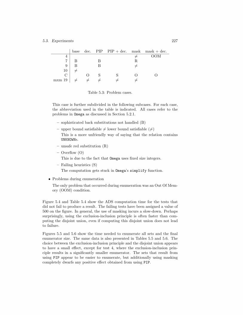
5.3. Experiments 227
base dec. PIP PIP + dec. mask mask + dec.4 6= OOM7 B B R9 B B 6=
10 6=C O S S O O
mxm 19 6= 6= 6= 6= 6=
Table 5.3: Problem cases.
This case is further subdivided in the following subcases. For each case,the abbreviation used in the table is indicated. All cases refer to theproblems in Omega as discussed in Section 5.2.1.
– sophisticated back substitutions not handled (B)
– upper bound satisfiable 6= lower bound satisfiable (6=)
This is a more unfriendly way of saying that the relation containsUNKNOWNs.
– unsafe red substitution (R)
– Overflow (O)
This is due to the fact that Omega uses fixed size integers.
– Failing heuristics (S)
The computation gets stuck in Omega’s simplify function.
• Problems during enumeration
The only problem that occurred during enumeration was an Out Of Mem-ory (OOM) condition.
Figure 5.4 and Table 5.4 show the ADS computation time for the tests thatdid not fail to produce a result. The failing tests have been assigned a value of500 on the figure. In general, the use of masking incurs a slow-down. Perhapssurprisingly, using the exclusion-inclusion principle is often faster than com-puting the disjoint union, even if computing this disjoint union does not leadto failure.
Figures 5.5 and 5.6 show the time needed to enumerate all sets and the finalenumerator size. The same data is also presented in Tables 5.5 and 5.6. Thechoice between the exclusion-inclusion principle and the disjoint union appearsto have a small effect, except for test 4, where the exclusion-inclusion prin-ciple results in a significantly smaller enumerator. The sets that result fromusing PIP appear to be easier to enumerate, but additionally using maskingcompletely dwarfs any positive effect obtained from using PIP.
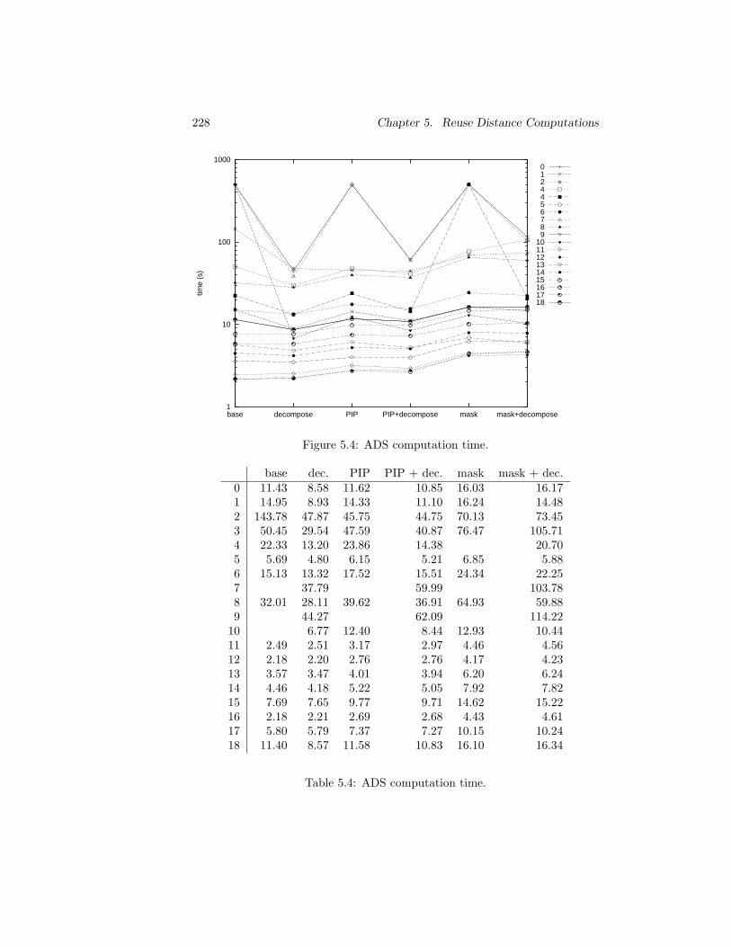
228 Chapter 5. Reuse Distance Computations
1
10
100
1000
mask+decomposemaskPIP+decomposePIPdecomposebase
time
(s)
0124456789
101112131415161718
Figure 5.4: ADS computation time.
base dec. PIP PIP + dec. mask mask + dec.0 11.43 8.58 11.62 10.85 16.03 16.171 14.95 8.93 14.33 11.10 16.24 14.482 143.78 47.87 45.75 44.75 70.13 73.453 50.45 29.54 47.59 40.87 76.47 105.714 22.33 13.20 23.86 14.38 20.705 5.69 4.80 6.15 5.21 6.85 5.886 15.13 13.32 17.52 15.51 24.34 22.257 37.79 59.99 103.788 32.01 28.11 39.62 36.91 64.93 59.889 44.27 62.09 114.22
10 6.77 12.40 8.44 12.93 10.4411 2.49 2.51 3.17 2.97 4.46 4.5612 2.18 2.20 2.76 2.76 4.17 4.2313 3.57 3.47 4.01 3.94 6.20 6.2414 4.46 4.18 5.22 5.05 7.92 7.8215 7.69 7.65 9.77 9.71 14.62 15.2216 2.18 2.21 2.69 2.68 4.43 4.6117 5.80 5.79 7.37 7.27 10.15 10.2418 11.40 8.57 11.58 10.83 16.10 16.34
Table 5.4: ADS computation time.
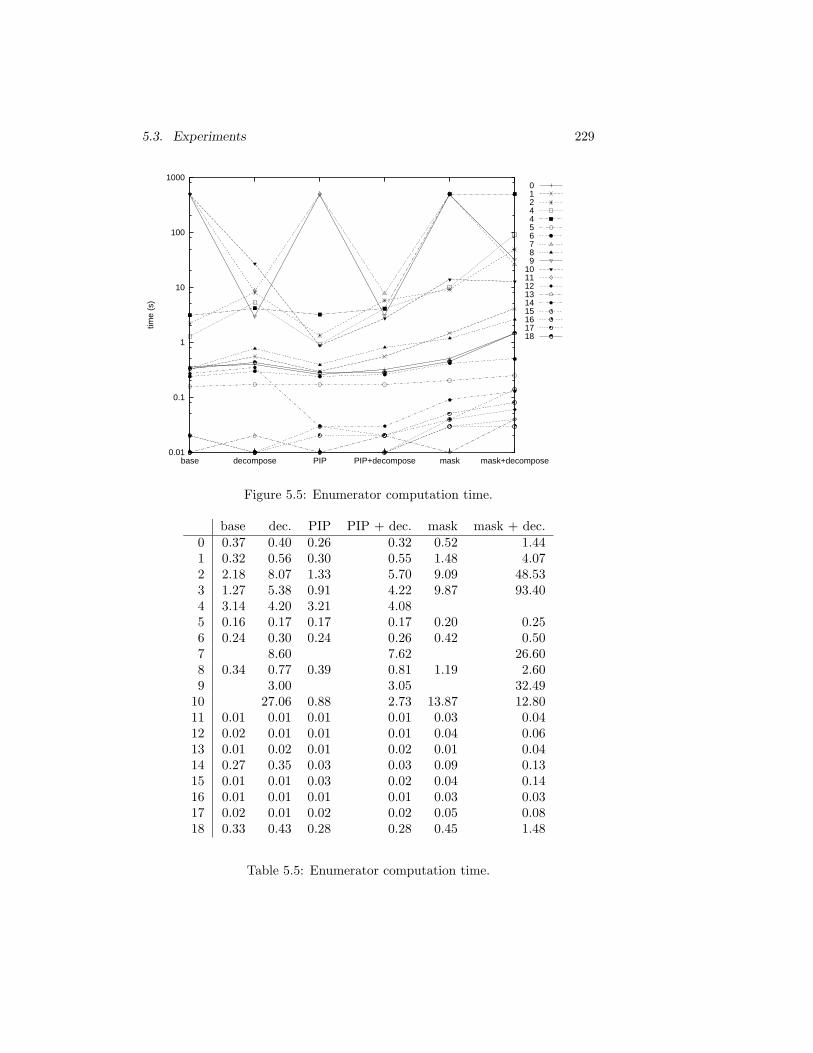
5.3. Experiments 229
0.01
0.1
1
10
100
1000
mask+decomposemaskPIP+decomposePIPdecomposebase
time
(s)
0124456789
101112131415161718
Figure 5.5: Enumerator computation time.
base dec. PIP PIP + dec. mask mask + dec.0 0.37 0.40 0.26 0.32 0.52 1.441 0.32 0.56 0.30 0.55 1.48 4.072 2.18 8.07 1.33 5.70 9.09 48.533 1.27 5.38 0.91 4.22 9.87 93.404 3.14 4.20 3.21 4.085 0.16 0.17 0.17 0.17 0.20 0.256 0.24 0.30 0.24 0.26 0.42 0.507 8.60 7.62 26.608 0.34 0.77 0.39 0.81 1.19 2.609 3.00 3.05 32.49
10 27.06 0.88 2.73 13.87 12.8011 0.01 0.01 0.01 0.01 0.03 0.0412 0.02 0.01 0.01 0.01 0.04 0.0613 0.01 0.02 0.01 0.02 0.01 0.0414 0.27 0.35 0.03 0.03 0.09 0.1315 0.01 0.01 0.03 0.02 0.04 0.1416 0.01 0.01 0.01 0.01 0.03 0.0317 0.02 0.01 0.02 0.02 0.05 0.0818 0.33 0.43 0.28 0.28 0.45 1.48
Table 5.5: Enumerator computation time.
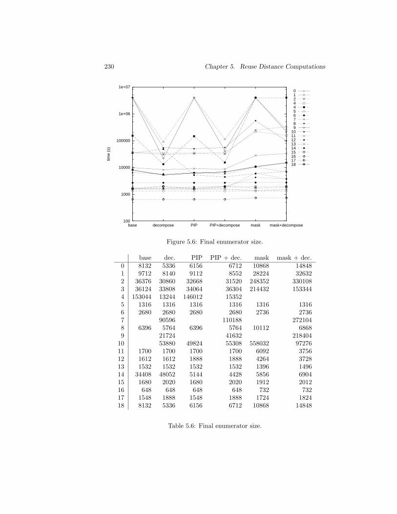
230 Chapter 5. Reuse Distance Computations
100
1000
10000
100000
1e+06
1e+07
mask+decomposemaskPIP+decomposePIPdecomposebase
time
(s)
0124456789
101112131415161718
Figure 5.6: Final enumerator size.
base dec. PIP PIP + dec. mask mask + dec.0 8132 5336 6156 6712 10868 148481 9712 8140 9112 8552 28224 326322 36376 30860 32668 31520 248352 3301083 36124 33808 34064 36304 214432 1533444 153044 13244 146012 153525 1316 1316 1316 1316 1316 13166 2680 2680 2680 2680 2736 27367 90596 110188 2721048 6396 5764 6396 5764 10112 68689 21724 41632 218404
10 53880 49824 55308 558032 9727611 1700 1700 1700 1700 6092 375612 1612 1612 1888 1888 4264 372813 1532 1532 1532 1532 1396 149614 34408 48052 5144 4428 5856 690415 1680 2020 1680 2020 1912 201216 648 648 648 648 732 73217 1548 1888 1548 1888 1724 182418 8132 5336 6156 6712 10868 14848
Table 5.6: Final enumerator size.
5.3. Experiments 231
type count
Sets 19177
Fixed 3470Change+Fixed 0Unique 4890Change+Unique 18Redundant 684Split 286PIP 0
Table 5.7: Rule application distribution for polytopes derived from reuse dis-tance equations.
Overall, we see that the original “base” version performs fairly well, but thatit fails to produce a result for some test cases. We also see that none of thecombinations of alternative strategies works for all cases, but that for all casesat least one of them does. Most of the problems occur inside Omega so it maybe worthwhile to also consider alternatives for other operations besides setdifferences.
5.3.3 PIP versus Heuristics
In this section we compare the use of the different ways of eliminating existentialvariables from Section 4.6 on the projected sets produced during our reusedistance experiments. Table 5.7 shows the number of times a particular rulefrom the heuristics based method from Section 4.6.2 was used on these projectedsets. Compare this table to Table 4.5 on page 208. As before, the row “Fixed”refers to the special case of a unique existential variable determined by anequality and “Change” refers to a change of basis. Notice that for all the setsin our experiments, we never had to resort to using PIP. We did need to splitthe sets, which means that simply ignoring the existential quantifiers wouldhave produced the wrong result. Curiously, some sets contained redundantexistential variables, even though they were created by Omega, which shouldhave removed them.
To investigate the impact of the input size, we calculated the reuse distancesfor matrix-matrix multiplication for varying sizes of the matrices, ranging from20 × 20 to 640 × 640. There was no measurable increase in computation timefor both the method using PIP and the heuristics based method. We alsoconsidered matrix sizes that are not multiples of the cache line size. As alreadymentioned in Section 5.3.2, only the “PIP + mask + decompose” strategy isable to compute the ADSs for such sizes. Furthermore, some of the resultingsets for matrices of size 19 × 19 and 41 × 41 proved too difficult to enumerate.
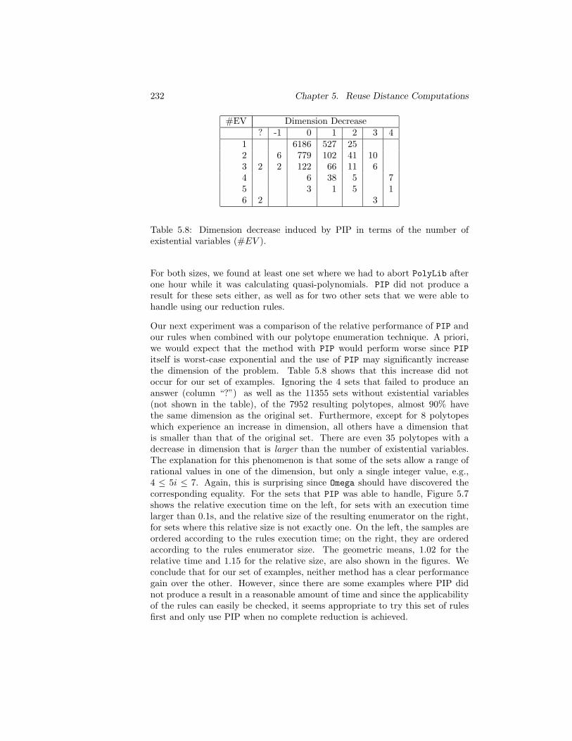
232 Chapter 5. Reuse Distance Computations
#EV Dimension Decrease? -1 0 1 2 3 4
1 6186 527 252 6 779 102 41 103 2 2 122 66 11 64 6 38 5 75 3 1 5 16 2 3
Table 5.8: Dimension decrease induced by PIP in terms of the number ofexistential variables (#EV ).
For both sizes, we found at least one set where we had to abort PolyLib afterone hour while it was calculating quasi-polynomials. PIP did not produce aresult for these sets either, as well as for two other sets that we were able tohandle using our reduction rules.
Our next experiment was a comparison of the relative performance of PIP andour rules when combined with our polytope enumeration technique. A priori,we would expect that the method with PIP would perform worse since PIP
itself is worst-case exponential and the use of PIP may significantly increasethe dimension of the problem. Table 5.8 shows that this increase did notoccur for our set of examples. Ignoring the 4 sets that failed to produce ananswer (column “?”) as well as the 11355 sets without existential variables(not shown in the table), of the 7952 resulting polytopes, almost 90% havethe same dimension as the original set. Furthermore, except for 8 polytopeswhich experience an increase in dimension, all others have a dimension thatis smaller than that of the original set. There are even 35 polytopes with adecrease in dimension that is larger than the number of existential variables.The explanation for this phenomenon is that some of the sets allow a range ofrational values in one of the dimension, but only a single integer value, e.g.,4 ≤ 5i ≤ 7. Again, this is surprising since Omega should have discovered thecorresponding equality. For the sets that PIP was able to handle, Figure 5.7shows the relative execution time on the left, for sets with an execution timelarger than 0.1s, and the relative size of the resulting enumerator on the right,for sets where this relative size is not exactly one. On the left, the samples areordered according to the rules execution time; on the right, they are orderedaccording to the rules enumerator size. The geometric means, 1.02 for therelative time and 1.15 for the relative size, are also shown in the figures. Weconclude that for our set of examples, neither method has a clear performancegain over the other. However, since there are some examples where PIP didnot produce a result in a reasonable amount of time and since the applicabilityof the rules can easily be checked, it seems appropriate to try this set of rulesfirst and only use PIP when no complete reduction is achieved.
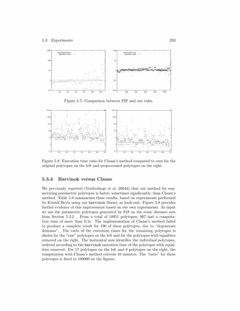
5.3. Experiments 233
0.1
1
10
100
1000
20 40 60 80 100 120
rules time/PIP timegeometric mean
0.01
0.1
1
10
100
0 200 400 600 800 1000
rules size/PIP sizegeometric mean
Figure 5.7: Comparison between PIP and our rules.
0.1
1
10
100
1000
10000
100000
0 100 200 300 400 500 600 700 0.1
1
10
100
1000
10000
100000
0 100 200 300 400 500 600 700
Figure 5.8: Execution time ratio for Clauss’s method compared to ours for theoriginal polytopes on the left and preprocessed polytopes on the right.
5.3.4 Barvinok versus Clauss
We previously reported (Verdoolaege et al. 2004d) that our method for enu-merating parametric polytopes is faster, sometimes significantly, than Clauss’smethod. Table 5.9 summarizes these results, based on experiments performedby Kristof Beyls using our barvinok library as back-end. Figure 5.8 providesfurther evidence of this improvement based on our own experiments. As inputwe use the parametric polytopes generated by PIP on the reuse distance setsfrom Section 5.3.2 . From a total of 18951 polytopes, 907 had a computa-tion time of more than 0.1s. The implementation of Clauss’s method failedto produce a complete result for 190 of these polytopes, due to “degeneratedomains”. The ratio of the execution times for the remaining polytopes isshown for the “raw” polytopes on the left and for the polytopes with equalitiesremoved on the right. The horizontal axis identifies the individual polytopes,ordered according to the barvinok execution time of the polytopes with equal-ities removed. For 17 polytopes on the left and 8 polytopes on the right, thecomputation with Clauss’s method exceeds 10 minutes. The “ratio” for thesepolytopes is fixed to 100000 on the figures.
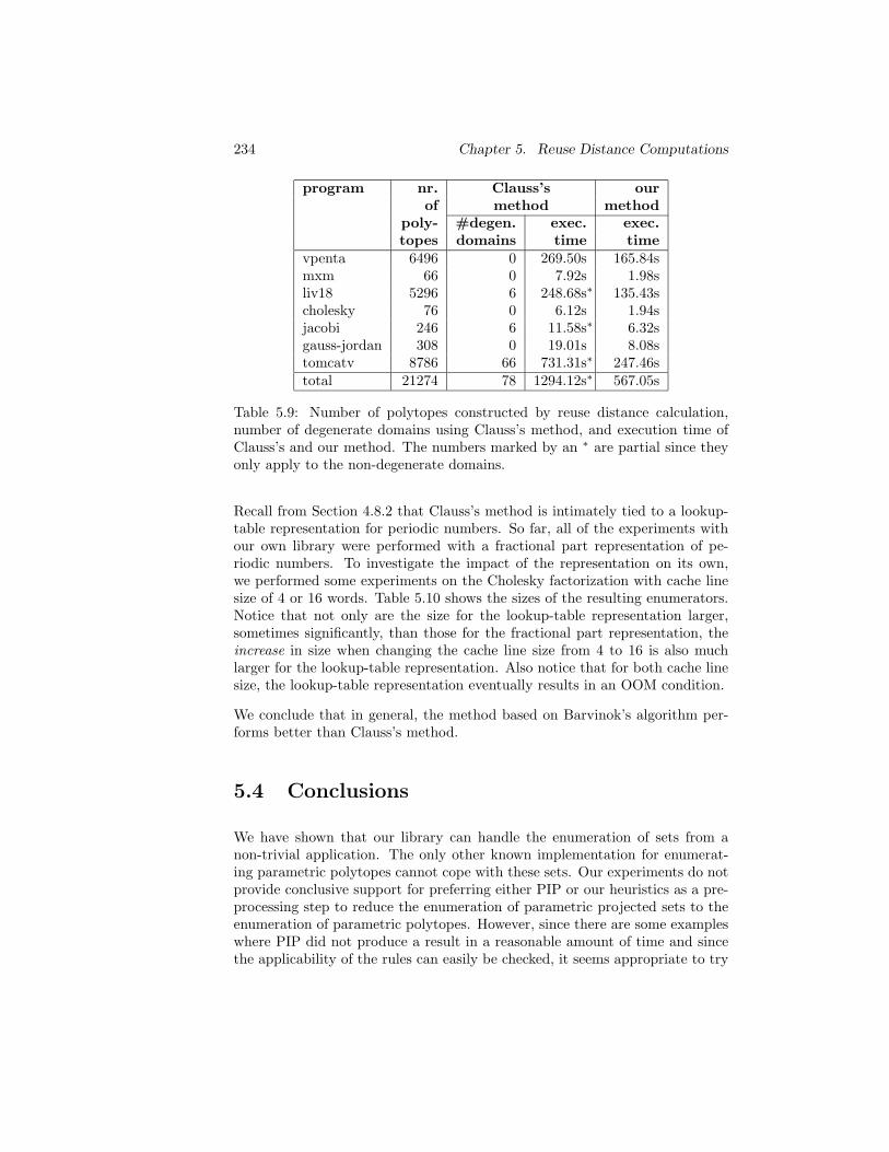
234 Chapter 5. Reuse Distance Computations
program nr. Clauss’s ourof method method
poly- #degen. exec. exec.topes domains time time
vpenta 6496 0 269.50s 165.84smxm 66 0 7.92s 1.98sliv18 5296 6 248.68s∗ 135.43scholesky 76 0 6.12s 1.94sjacobi 246 6 11.58s∗ 6.32sgauss-jordan 308 0 19.01s 8.08stomcatv 8786 66 731.31s∗ 247.46stotal 21274 78 1294.12s∗ 567.05s
Table 5.9: Number of polytopes constructed by reuse distance calculation,number of degenerate domains using Clauss’s method, and execution time ofClauss’s and our method. The numbers marked by an ∗ are partial since theyonly apply to the non-degenerate domains.
Recall from Section 4.8.2 that Clauss’s method is intimately tied to a lookup-table representation for periodic numbers. So far, all of the experiments withour own library were performed with a fractional part representation of pe-riodic numbers. To investigate the impact of the representation on its own,we performed some experiments on the Cholesky factorization with cache linesize of 4 or 16 words. Table 5.10 shows the sizes of the resulting enumerators.Notice that not only are the size for the lookup-table representation larger,sometimes significantly, than those for the fractional part representation, theincrease in size when changing the cache line size from 4 to 16 is also muchlarger for the lookup-table representation. Also notice that for both cache linesize, the lookup-table representation eventually results in an OOM condition.
We conclude that in general, the method based on Barvinok’s algorithm per-forms better than Clauss’s method.
5.4 Conclusions
We have shown that our library can handle the enumeration of sets from anon-trivial application. The only other known implementation for enumerat-ing parametric polytopes cannot cope with these sets. Our experiments do notprovide conclusive support for preferring either PIP or our heuristics as a pre-processing step to reduce the enumeration of parametric projected sets to theenumeration of parametric polytopes. However, since there are some exampleswhere PIP did not produce a result in a reasonable amount of time and sincethe applicability of the rules can easily be checked, it seems appropriate to try
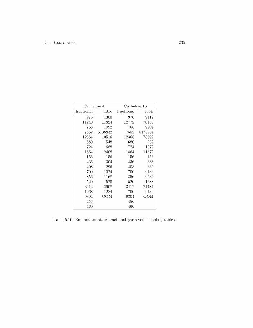
5.4. Conclusions 235
Cacheline 4 Cacheline 16fractional table fractional table
976 1300 976 941211240 11824 12772 70188
768 1092 768 92047552 5138832 7552 5173284
12364 10516 12368 78892680 548 680 932724 688 724 1072
1864 2408 1864 11672156 156 156 156436 304 436 688408 296 408 632700 1024 700 9136856 1168 856 9232520 520 520 1288
3412 2908 3412 274841068 1284 700 91369304 OOM 9304 OOM456 456460 460
Table 5.10: Enumerator sizes: fractional parts versus lookup-tables.
236 Chapter 5. Reuse Distance Computations
this set of rules first and only use PIP when no complete reduction is achieved.
As a side-effect we have devised different methods of computing the reuse dis-tance equations. None of these methods yields consistently better results thanany of the other methods. The limited success indicates that set differencesmay not be the only problem in the computation. There is obviously still muchroom for improvement in the actual implementation of these methods as wehave only made a prototype tool. It would be very interesting to see whetherthe method based on rational generating functions can outperform the alreadyimplemented methods. Although the sizes of our enumerator are typicallymuch smaller than those that would be obtained when using a lookup-tablerepresentation for periodic numbers, the enumerators can still be very large.Further research into the simplification of piecewise step-polynomials is stillneeded. For the problems we have considered in this chapter, the current sizesof the enumerators make them inappropriate to use on-line, but they may stillbe useful in modeling cache behavior.
Chapter 6
Conclusions and Future
Work
This dissertation consists of two major parts, one about incremental loop trans-formations and one about the enumeration of parametric sets. For each of thesetwo parts we summarize the contributions and point out some interesting issuesfor future research.
6.1 Incremental Loop Transformations
6.1.1 Summary and Contributions
The initial goal of this part of the dissertation was to refine and extend themethodology of Danckaert (2001) for global loop transformations. This method-ology consists of a placement and an ordering phase, with the placementphase further subdivided into a linear transformation and a translation step.Danckaert (2001) then focused on the linear transformation step, proposing aregularity criterion and a search procedure for optimizing this criterion locally,without ensuring the global correctness of the final result.
As our first contribution, we have shown how to perform the translation stepincrementally, both in the context of a subsequent ordering phase and in thecontext of a fixed predetermined ordering. Each step of our algorithm combinestwo nodes in the dependence graph at a relative offset. This relative offset isselected from the region of all relative offsets that lead to a valid final solution.Assuming that the result of the preceding linear transformation step still allowsfor a valid solution, this region is guaranteed to be non-empty. The choice of
237
238 Chapter 6. Conclusions and Future Work
relative offset is determined by a set of cost functions. In case of a fixed order-ing, the translation step is equivalent to the combination of loop fusion and loopshifting and our incremental algorithm can obtain significant improvements inlocality and memory requirements, even when used in conjunction with a verysimple heuristic.
A comparison between a subsequent ordering phase and a fixed predeterminedordering reveals that the uncertainty of the final ordering in the first optionseverely complicates the translation step. First, the region of valid relativeoffsets is determined by a set of polyhedra, one for each pair of nodes in thedependence graph, rather than a set of vectors. More importantly, however,the presence of a subsequent ordering phase does not allow for accurate costfunctions to be used during the translation step. As our second contribution, wehave therefore removed the ordering step and we have opted for a fixed ordering.This modification does not affect the set of possible program transformationsand brings the methodology closer to other loop transformation methodologiesthat had been developed in parallel.
As to the linear transformation step, the regularity criterion proposed byDanckaert (2001) was derived as an approximation of the dimension of thedependence polytope, obtained by ignoring the iteration domains. Althoughthis criterion was intended as an approximation of the dimension of the de-pendence cone, we contend that the dependence polytope is actually the mostappropriate dependence abstraction to use. We have made the following con-tributions:
• We have derived a simple and exact formula for the dimension of thedependence polytope, without ignoring the iteration domains.
• We have also derived an equally simple formula for the minimal attain-able dependence polytope dimension, removing the need to perform anexhaustive search to obtain these optimal values.
• We have refined the search procedure of Danckaert (2001). The re-fined procedure, combined with the improved dimension formulas, yieldsmarkedly better results with fewer computations.
• We have devised two additional search procedures which are not generallyapplicable, but which have a better time complexity.
• We have extended the dimension formulas to not only apply to depen-dences represented by pairs of a dependence domain and a dependencefunction to also apply to dependences represented by dependence rela-tions.
• We have investigated ways to ensure validity in the context of a fixedordering.
6.2. Enumeration of Parametric Sets 239
• Finally, we have adapted a known locality heuristic to the context ofdependence relations.
6.1.2 Directions for Future Research
Although our algorithm for incremental loop fusion has been designed to allowmore complicated cost functions to be evaluated, we have so far only considereda very simple locality heuristic. This should be extended to a larger set of costfunctions and trade-offs between these cost functions should be evaluated. Thisis a topic for current and future work (Palkovic 2002; Hu et al. 2004a). The finaloutcome of the algorithm should then not be a single solution, but a collectionof Pareto optimal solutions, which can be further evaluated in subsequent stepsof the DTSE methodology.
Although we have also considered validity and a locality heuristic for the lineartransformation step in a theoretical context, the proposed search proceduresfocus solely on regularity. The search procedures also assume that each de-pendence can be represented by a pair of dependence domain and dependencefunctions. Extending these procedures to also consider validity and locality andto handle more general dependence relations is a topic for current and futurework (Yang 2005).
6.2 Enumeration of Parametric Sets
6.2.1 Summary and Contributions
We have presented the first known implementation of Barvinok’s enumerationalgorithm applied to parametric polytopes with extensions to projections ofthe integer points in parametric polytopes. Our library enumerates parametricpolytopes in polynomial time resulting in either an explicit function or a gen-erating function. In particular, the result is either a piecewise step-polynomialor a rational generating function. This implementation has been experimen-tally validated on an application for computing reuse distances as piecewisestep-polynomials.
The implementation contains elements from a previous implementation byClauss and Loechner (1998) of a different algorithm for enumerating paramet-ric polytopes as well as elements from a previous implementation of Barvinok’salgorithm by De Loera et al. (2004). Compared to these previous results, ourlibrary has the following advantages.
• The implementation of Clauss and Loechner (1998) can only producean explicit function. Furthermore, the representation of this function
240 Chapter 6. Conclusions and Future Work
is based on lookup-tables and may therefore grow to be exponentiallylarge in the worst case. As a result, the worst-case computation time isalso exponential. By contrast, the sizes of the piecewise step-polynomi-als we compute are polynomial in the input size. In our experiments wehave indeed found that our representation based on fractional parts istypically smaller that the lookup-table representation. Our experimentalvalidation further shows that, in general, the use of our library results ina significant reduction of computation time when compared to this earlierimplementation. Finally and in contrast to the implementation of Claussand Loechner (1998), our library does not suffer from any degeneracyproblems.
• The implementation of De Loera et al. (2003a) only computes generat-ing functions. Furthermore, it does not handle the full set of parametricpolytopes, but only considers the subproblem of computing Ehrhart se-ries.
As a more theoretical contribution, we have shown that the piecewise step-polynomial and rational generating function representations of a parametricset are polynomially interconvertible. Combining this polynomial interconvert-ibility with the polynomial-time algorithm of Barvinok and Woods (2003) forenumerating parametric projected sets in the form of a rational generating func-tion yields a polynomial-time algorithm for enumerating parametric projectedsets in the form of a piecewise step-polynomial.
The implementation of the algorithm of Barvinok and Woods (2003) still re-mains a challenge, however, and we have therefore also presented two alterna-tive methods, a known worst-case exponential method and a new method thatis polynomial but not generally applicable. Both methods reduce the problemto the enumeration of parametric polytopes by either applying a set of rulesor by preprocessing the given sets using PIP. Both perform fairly well in ourexperiments, but as the average relative execution time is close to 1, these ex-periments do not provide conclusive support for preferring either PIP or ourheuristics. However, since there are some examples where PIP did not produceany result in a reasonable amount of time and since the applicability of therules can easily be checked, it seems appropriate to try this set of rules firstand only use PIP when no complete reduction is achieved.
Obtaining the parametric sets for our enumeration experiments using currentlyavailable tools from the reuse distance equations has also proved to be a chal-lenge. After identifying the set difference operation as the likely culprit, wehave devised different methods of computing these reuse distance equations.Although for all the example programs we have considered at least one of thesemethods produces the desired sets, none of them yields consistently better re-sults than any of the other methods. The limited success indicates that setdifferences may not be the only problem in the computation.
6.2. Enumeration of Parametric Sets 241
6.2.2 Directions for Future Research
In our reuse distance experiments we have only used the piecewise step-poly-nomial representation of an enumerator and have performed all necessary op-erations on enumerators on these piecewise step-polynomials. It would be in-teresting to see whether replacing some or all of these operations by equivalentoperations on the corresponding rational generating functions would be an im-provement. This includes the evaluation operation. Operations performed onthe sets defined by the reuse distance equations can also be replaced by equiv-alent operations on the corresponding rational generating functions, but someof these have not been implemented yet. In particular, the polynomial-timealgorithm of Barvinok and Woods (2003) for the projection operation wouldbe very interesting to implement. The implementation of the procedure forcomputing rational generating functions currently also assumes that the inputpolyhedron is full-dimensional.
Further research into the simplification of piecewise step-polynomials is stillneeded. Although the piecewise step-polynomials are only of polynomial size,they can in some cases still be relatively large. In particular, the current sizesof the enumerators in our reuse distance experiments make them inappropriateto use on-line.
Although the algorithm of Clauss and Loechner (1998) for computing the cham-ber decomposition is polynomial, further research may still result in an im-proved algorithm. A more practical but related issue is the replacement ofPolyLib with some other library for manipulating polyhedra or even just forcomputing the vertices of a polyhedron defined in terms of its facets.
Finally, a very challenging line of further research would be an investigation ofthe enumeration of sets defined be non-linear equations.

242 Chapter 6. Conclusions and Future Work
Appendix A
Internal Representation of
the barvinok library
Our barvinok library is built on top of PolyLib (Wilde 1993; Loechner 1999).In particular, it reuses the implementations of the algorithm of Loechner andWilde (1997) for computing parametric vertices and the algorithm of Clauss andLoechner (1998) for computing chamber decompositions. Initially, our librarywas meant to be a replacement for the algorithm of Clauss and Loechner (1998),also implemented in PolyLib, for computing quasi-polynomials. To ease thetransition of application programs we tried to reuse the existing data structuresas much as possible.
A.1 Existing Data Structures
Inside PolyLib integer values are represented by the Value data type. De-pending on a configure option, the data type may either by a 32-bit integer, a64-bit integer or an arbitrary precision integer using GMP. The barvinok libraryrequires that PolyLib is compiled with support for arbitrary precision integers.
The basic structure for representing (unions of) polyhedra is a Polyhedron.
typedef struct polyhedron
unsigned Dimension, NbConstraints, NbRays, NbEq, NbBid;
Value **Constraint;
Value **Ray;
Value *p_Init;
int p_Init_size;
243
244 Appendix A. Internal Representation of the barvinok library
struct polyhedron *next;
Polyhedron;
The attribute Dimension is the dimension of the ambient space, i.e., the numberof variables. The attributes Constraint and Ray point to two-dimensionalarrays of constraints and generators, respectively. The number of rows is storedin NbConstraints and NbRays, respectively. The number of columns in botharrays is equal to 1+Dimension+1. The first column of Constraint is either 0or 1 depending on whether the constraint is an equality (0) or an inequality (1).The number of equalities is stored in NbEq. If the constraint is 〈a,x〉 + c ≥ 0,then the next columns contain the coefficients ai and the final column containsthe constant c. The first column of Ray is either 0 or 1 depending on whetherthe generator is a line (0) or a vertex or ray (1). The number of lines is storedin NbBid. Let d be the lcm of the denominators of the coordinates of a vertexv, then the next columns contain dvi and the final column contains d. For aray, the final column contains 0. The field next points to the next polyhedronin the union of polyhedra. It is 0 if this is the last (or only) polyhedron in theunion. For more information on this structure, we refer to Wilde (1993).
Quasi-polynomials are represented using the evalue and enode structures.
typedef enum polynomial, periodic, evector enode_type;
typedef struct _evalue
Value d; /* denominator */
union
Value n; /* numerator (if denominator != 0) */
struct _enode *p; /* pointer (if denominator == 0) */
x;
evalue;
typedef struct _enode
enode_type type; /* polynomial or periodic or evector */
int size; /* number of attached pointers */
int pos; /* parameter position */
evalue arr[1]; /* array of rational/pointer */
enode;
If the field d of an evalue is zero, then the evalue is a placeholder for apointer to an enode, stored in x.p. Otherwise, the evalue is a rational numberwith numerator x.n and denominator d. An enode is either a polynomial ora periodic, depending on the value of type. The length of the array arr
is stored in size. For a polynomial, arr contains the coefficients. For aperiodic, it contains the values for the different residue classes modulo theparameter indicated by pos. For a polynomial, pos refers to the variable of the
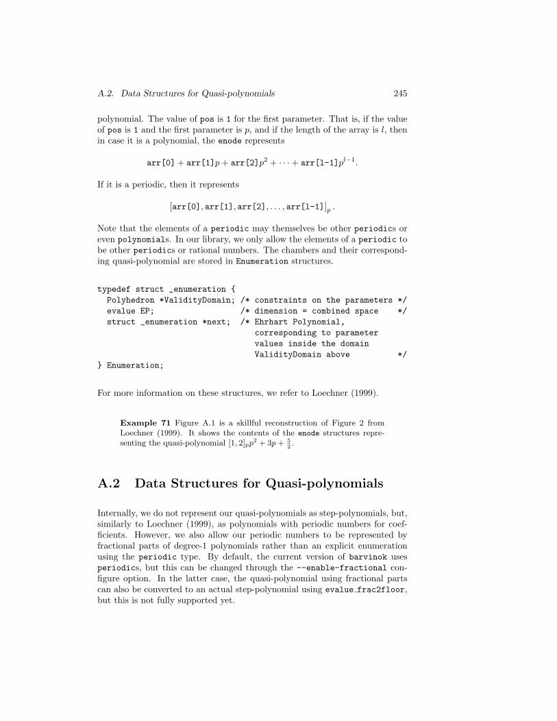
A.2. Data Structures for Quasi-polynomials 245
polynomial. The value of pos is 1 for the first parameter. That is, if the valueof pos is 1 and the first parameter is p, and if the length of the array is l, thenin case it is a polynomial, the enode represents
arr[0] + arr[1]p + arr[2]p2 + · · · + arr[l-1]pl−1.
If it is a periodic, then it represents
[arr[0], arr[1], arr[2], . . . , arr[l-1]]p .
Note that the elements of a periodic may themselves be other periodics oreven polynomials. In our library, we only allow the elements of a periodic tobe other periodics or rational numbers. The chambers and their correspond-ing quasi-polynomial are stored in Enumeration structures.
typedef struct _enumeration
Polyhedron *ValidityDomain; /* constraints on the parameters */
evalue EP; /* dimension = combined space */
struct _enumeration *next; /* Ehrhart Polynomial,
corresponding to parameter
values inside the domain
ValidityDomain above */
Enumeration;
For more information on these structures, we refer to Loechner (1999).
Example 71 Figure A.1 is a skillful reconstruction of Figure 2 fromLoechner (1999). It shows the contents of the enode structures repre-senting the quasi-polynomial [1, 2]pp2 + 3p + 5
2.
A.2 Data Structures for Quasi-polynomials
Internally, we do not represent our quasi-polynomials as step-polynomials, but,similarly to Loechner (1999), as polynomials with periodic numbers for coef-ficients. However, we also allow our periodic numbers to be represented byfractional parts of degree-1 polynomials rather than an explicit enumerationusing the periodic type. By default, the current version of barvinok usesperiodics, but this can be changed through the --enable-fractional con-figure option. In the latter case, the quasi-polynomial using fractional partscan also be converted to an actual step-polynomial using evalue frac2floor,but this is not fully supported yet.
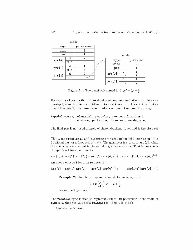
246 Appendix A. Internal Representation of the barvinok library
type polynomial
size 3
pos 1
arr[0]d 2
x.n 5
arr[1]d 1
x.n 3
arr[2]d 0
x.p
type periodic
size 2
pos 1
arr[0]d 1
x.n 1
arr[1]d 1
x.n 2
enode
enode
Figure A.1: The quasi-polynomial [1, 2]pp2 + 3p + 5
2 .
For reasons of compatibility,1 we shoehorned our representations for piecewisequasi-polynomials into the existing data structures. To this effect, we intro-duced four new types, fractional, relation, partition and flooring.
typedef enum polynomial, periodic, evector, fractional,
relation, partition, flooring enode_type;
The field pos is not used in most of these additional types and is therefore setto -1.
The types fractional and flooring represent polynomial expressions in afractional part or a floor respectively. The generator is stored in arr[0], whilethe coefficients are stored in the remaining array elements. That is, an enode
of type fractional represents
arr[1]+ arr[2]arr[0] + arr[3]arr[0]2 + · · · + arr[l-1]arr[0]l−2.
An enode of type flooring represents
arr[1] + arr[2]⌊arr[0]⌋ + arr[3]⌊arr[0]⌋2 + · · · + arr[l-1]⌊arr[0]⌋l−2.
Example 72 The internal representation of the quasi-polynomial(
1 + 2p
2
)
p2 + 3p +5
2
is shown in Figure A.2.
The relation type is used to represent strides. In particular, if the value ofsize is 2, then the value of a relation is (in pseudo-code):
1Also known as laziness.
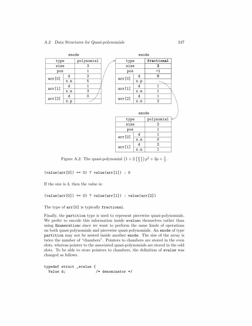
A.2. Data Structures for Quasi-polynomials 247
type polynomial
size 3
pos 1
arr[0]d 2
x.n 5
arr[1]d 1
x.n 3
arr[2]d 0
x.p
type fractional
size 3
pos -1
arr[0]d 0
x.p
arr[1]d 1
x.n 1
arr[2]d 1
x.n 2
fractional
3
-1
0
type polynomial
size 2
pos 1
arr[0]d 1
x.n 0
arr[1]d 2
x.n 1
enode enode
enode
Figure A.2: The quasi-polynomial(1 + 2
p2
)p2 + 3p + 5
2 .
(value(arr[0]) == 0) ? value(arr[1]) : 0
If the size is 3, then the value is:
(value(arr[0]) == 0) ? value(arr[1]) : value(arr[2])
The type of arr[0] is typically fractional.
Finally, the partition type is used to represent piecewise quasi-polynomials.We prefer to encode this information inside evalues themselves rather thanusing Enumerations since we want to perform the same kinds of operationson both quasi-polynomials and piecewise quasi-polynomials. An enode of typepartition may not be nested inside another enode. The size of the array istwice the number of “chambers”. Pointers to chambers are stored in the evenslots, whereas pointer to the associated quasi-polynomials are stored in the oddslots. To be able to store pointers to chambers, the definition of evalue waschanged as follows.
typedef struct _evalue
Value d; /* denominator */
248 Appendix A. Internal Representation of the barvinok library
union
Value n; /* numerator (if denominator > 0) */
struct _enode *p; /* pointer (if denominator == 0) */
Polyhedron *D; /* domain (if denominator == -1) */
x;
evalue;
Note that we allow a “chamber” to be a union of polyhedra as discussed inSection 4.5.1. Chambers with extra variables, i.e., those of Section 4.6.5, areonly partially supported. The field pos is set to the actual dimension, i.e., thenumber of parameters.
A.3 Operations on Quasi-polynomials
In this section we discuss some of the more important operations on evaluesprovided by the barvinok library. Some of these operations are extensions ofthe functions from PolyLib with the same name.
void eadd(evalue *e1,evalue *res);
void emul (evalue *e1, evalue *res );
The functions eadd and emul takes two (pointers to) evalues e1 and res
and computes their sum and product respectively. The result is stored in res,overwriting (and deallocating) the original value of res. It is an error if exactlyone of the arguments of eadd is of type partition (unless the other argument is0). The addition and multiplication operations are described in Sections 4.5.1and 4.5.2 respectively.
The function eadd is an extension of the function new eadd from Seghir (2002).Apart from supporting the additional types from Appendix A.2, the new versionalso additionally imposes an order on the nesting of different enodes. Withoutsuch an ordering, evalues could be constructed representing for example
(0y0 + (0x0 + 1x1)y1)x0 + (0y0 − 1y1)x1,
which is just a funny way of saying 0.
void eor(evalue *e1, evalue *res);
The function eor implements the union operation from Section 4.5.3. Botharguments are assumed to correspond to indicator functions.
A.3. Operations on Quasi-polynomials 249
evalue *esum(evalue *E, int nvar);
The function esum performs the summation operation from Section 4.5.4. Thepiecewise step-polynomial represented by E is summated over its first nvar vari-ables. Note that E must be zero or of type partition. The function returns theresult in a newly allocated evalue. Note also that E needs to have been con-verted from fractionals to floorings using the function evalue frac2floor.
void evalue_frac2floor(evalue *e);
This function also ensures that the arguments of the floorings are positivein the relevant chambers. It currently assumes that the argument of eachfractional in the original evalue has a minimum in the corresponding cham-ber.
double compute_evalue(evalue *e,Value *list_args);
Value *compute_poly(Enumeration *en,Value *list_args);
The functions compute evalue and compute poly evaluate a (piecewise) quasi-polynomial at a certain point. The argument list_args points to an arrayof Values that is assumed to be long enough. The double return value ofcompute evalue is inherited from PolyLib.
void print_evalue(FILE *DST,evalue *e,char **pname);
The function print evalue dumps a human-readable representation to thestream pointed to by DST. The argument pname points to an array of characterstrings representing the parameter names. The array is assumed to be longenough.
int eequal(evalue *e1,evalue *e2);
The function eequal return true (1) if its two arguments are structurally iden-tical. I.e., it does not check whether the two (piecewise) quasi-polynomialrepresent the same function.
void reduce_evalue (evalue *e);
The function reduce evalue performs some simplifications on evalues. Here,we only describe the simplifications that are directly related to the internal
250 Appendix A. Internal Representation of the barvinok library
representation. Some other simplifications are explained in Section 4.7.2. Ifthe highest order coefficients of a polynomial, fractional or flooring arezero (possibly after some other simplifications), then the size of the array isreduced. If only the constant term remains, i.e., the size is reduced to 1 forpolynomial or to 2 for the other types, then the whole node is replaced bythe constant term. Additionally, if the argument of a fractional has beenreduced to a constant, then the whole node is replaced by its partial evaluation.A relation is similarly reduced if its second branch or both its branches arezero. Chambers with zero associated quasi-polynomials are discarded from apartition.
A.4 Generating Functions
The representation of rational generating functions uses some basic types fromthe NTL library for representing arbitrary precision integers (ZZ) as well asvectors (vec ZZ) and matrices (mat ZZ) of such integers. Each term in a rationalgenerating function is represented by a short rat structure.
struct short_rat
struct
/* rows: terms in numerator */
mat_ZZ coeff;
mat_ZZ power;
n;
struct
/* rows: factors in denominator */
mat_ZZ power;
d;
;
The fields n and d represent the numerator and the denominator respectively.Note that in our implementation we combine terms with the same denominator.In the numerator, each row of coeff and power represents a single such term.The matrix coeff has two columns, one for the numerator and one for thedenominator of the rational coefficient αi of each term. The columns of powercorrespond to the powers of the variables. In the denominator, each row ofpower corresponds to the power bij of a factor in the denominator.
Example 73 Figure A.3 shows the internal representation of
32
x20x
31 + 2 x5
0x−71
(1 − x0x−31 )(1 − x2
1).
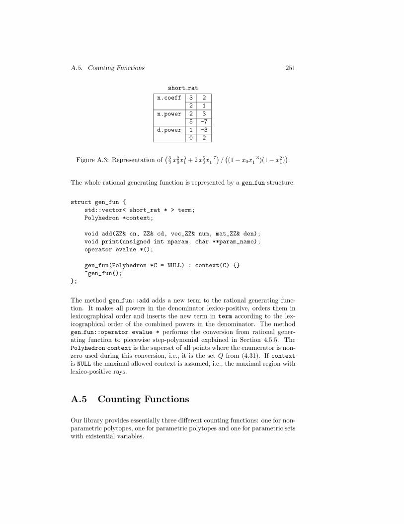
A.5. Counting Functions 251
n.coeff 3 2
2 1
n.power 2 3
5 -7
d.power 1 -3
0 2
short rat
Figure A.3: Representation of(
32 x2
0x31 + 2x5
0x−71
)/((1 − x0x
−31 )(1 − x2
1)).
The whole rational generating function is represented by a gen fun structure.
struct gen_fun
std::vector< short_rat * > term;
Polyhedron *context;
void add(ZZ& cn, ZZ& cd, vec_ZZ& num, mat_ZZ& den);
void print(unsigned int nparam, char **param_name);
operator evalue *();
gen_fun(Polyhedron *C = NULL) : context(C)
~gen_fun();
;
The method gen fun::add adds a new term to the rational generating func-tion. It makes all powers in the denominator lexico-positive, orders them inlexicographical order and inserts the new term in term according to the lex-icographical order of the combined powers in the denominator. The methodgen fun::operator evalue * performs the conversion from rational gener-ating function to piecewise step-polynomial explained in Section 4.5.5. ThePolyhedron context is the superset of all points where the enumerator is non-zero used during this conversion, i.e., it is the set Q from (4.31). If contextis NULL the maximal allowed context is assumed, i.e., the maximal region withlexico-positive rays.
A.5 Counting Functions
Our library provides essentially three different counting functions: one for non-parametric polytopes, one for parametric polytopes and one for parametric setswith existential variables.
252 Appendix A. Internal Representation of the barvinok library
void barvinok_count(Polyhedron *P, Value* result,
unsigned NbMaxCons);
The function barvinok count enumerates the non-parametric polytope P andreturns the result in the Value pointed to by result, which needs to havebeen allocated and initialized. The argument NbMaxCons is passed to variousPolyLib functions and defines the maximum size of a table used in the doubledescription computation in the PolyLib function Chernikova. In earlier ver-sions of PolyLib, this parameter had to be conservatively set to a high numberto ensure successful operation, resulting in significant memory overhead. Ourchange to allow this table to grow dynamically is available in recent versionsof PolyLib. In these versions, the value no longer indicates the maximal tablesize, but rather the size of the initial allocation. This value may be set to 0.
The function barvinok enumerate for enumerating parametric polytopes wasmeant to be a drop-in replacement of PolyLib’s Polyhedron Enumerate func-tion. Unfortunately, the latter has been changed to accept an extra argumentin recent versions of PolyLib as shown below.
Enumeration* barvinok_enumerate(Polyhedron *P, Polyhedron* C,
unsigned MaxRays);
extern Enumeration *Polyhedron_Enumerate(Polyhedron *P,
Polyhedron *C, unsigned MAXRAYS, char **pname);
The argument MaxRays has the same meaning as the argument NbMaxCons
above. The argument P refers to the (d + n)-dimensional polyhedron defin-ing the parametric polytope. The argument C is an n-dimensional polyhedroncontaining extra constraints on the parameter space. Its primary use is toindicate how many of the dimensions in P refer to parameters as any con-straint in C could equally well have been added to P itself. Note that thedimensions referring to the parameters should appear last. The result is anewly allocated Enumeration. As an alternative we also provide a function(barvinok enumerate ev) that returns an evalue.
evalue* barvinok_enumerate_ev(Polyhedron *P, Polyhedron* C,
unsigned MaxRays);
For enumerating parametric sets with existentially quantified variables, we pro-vide two functions: barvinok enumerate e and barvinok enumerate pip.
evalue* barvinok_enumerate_e(Polyhedron *P,
unsigned exist, unsigned nparam, unsigned MaxRays);
evalue *barvinok_enumerate_pip(Polyhedron *P,
unsigned exist, unsigned nparam, unsigned MaxRays);
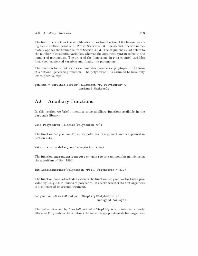
A.6. Auxiliary Functions 253
The first function tries the simplification rules from Section 4.6.2 before resort-ing to the method based on PIP from Section 4.6.3. The second function imme-diately applies the technique from Section 4.6.3. The argument exist refers tothe number of existential variables, whereas the argument nparam refers to thenumber of parameters. The order of the dimensions in P is: counted variablesfirst, then existential variables and finally the parameters.
The function barvinok series enumerates parametric polytopes in the formof a rational generating function. The polyhedron P is assumed to have onlylexico-positive rays.
gen_fun * barvinok_series(Polyhedron *P, Polyhedron* C,
unsigned MaxRays);
A.6 Auxiliary Functions
In this section we briefly mention some auxiliary functions available in thebarvinok library.
void Polyhedron_Polarize(Polyhedron *P);
The function Polyhedron Polarize polarizes its argument and is explained inSection 4.4.2.
Matrix * unimodular_complete(Vector *row);
The function unimodular complete extends row to a unimodular matrix usingthe algorithm of Bik (1996).
int DomainIncludes(Polyhedron *Pol1, Polyhedron *Pol2);
The function DomainIncludes extends the function PolyhedronIncludes pro-vided by PolyLib to unions of polyhedra. It checks whether its first argumentis a superset of its second argument.
Polyhedron *DomainConstraintSimplify(Polyhedron *P,
unsigned MaxRays);
The value returned by DomainConstraintSimplify is a pointer to a newlyallocated Polyhedron that contains the same integer points as its first argument
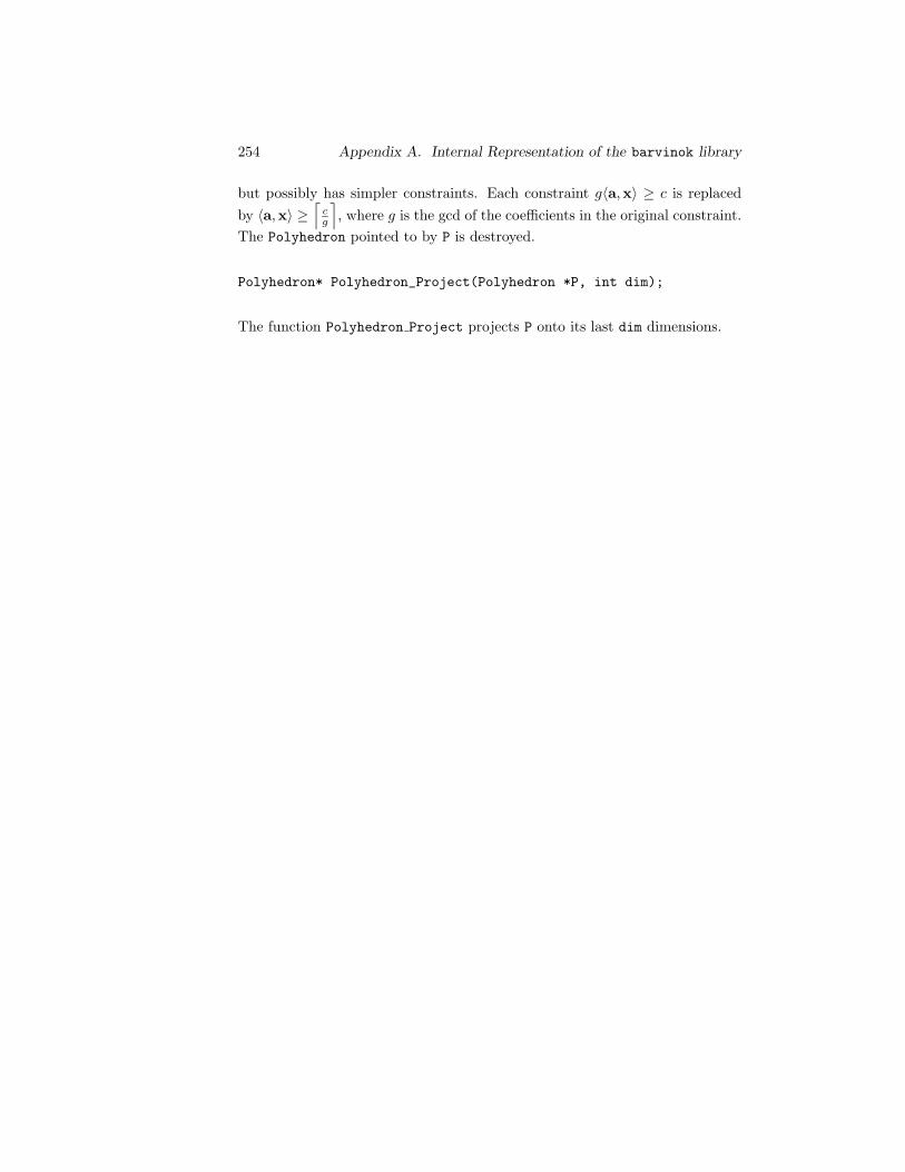
254 Appendix A. Internal Representation of the barvinok library
but possibly has simpler constraints. Each constraint g〈a,x〉 ≥ c is replaced
by 〈a,x〉 ≥⌈
cg
⌉
, where g is the gcd of the coefficients in the original constraint.
The Polyhedron pointed to by P is destroyed.
Polyhedron* Polyhedron_Project(Polyhedron *P, int dim);
The function Polyhedron Project projects P onto its last dim dimensions.
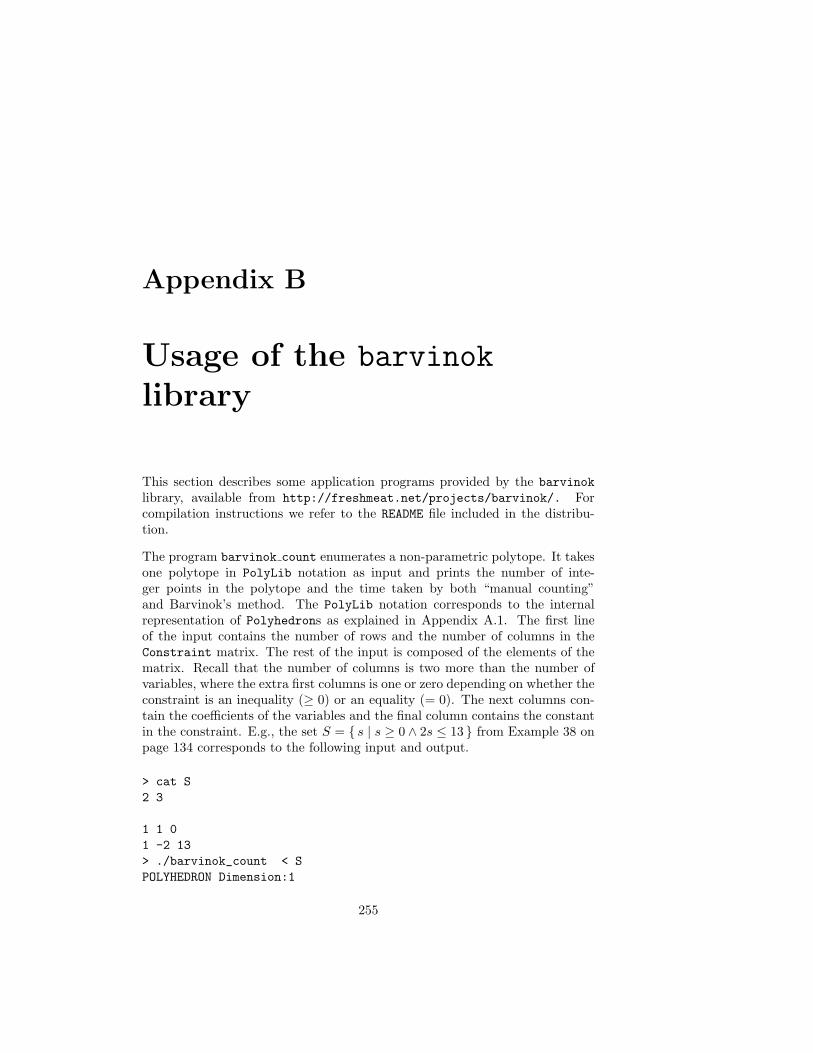
Appendix B
Usage of the barvinok
library
This section describes some application programs provided by the barvinok
library, available from http://freshmeat.net/projects/barvinok/. Forcompilation instructions we refer to the README file included in the distribu-tion.
The program barvinok count enumerates a non-parametric polytope. It takesone polytope in PolyLib notation as input and prints the number of inte-ger points in the polytope and the time taken by both “manual counting”and Barvinok’s method. The PolyLib notation corresponds to the internalrepresentation of Polyhedrons as explained in Appendix A.1. The first lineof the input contains the number of rows and the number of columns in theConstraint matrix. The rest of the input is composed of the elements of thematrix. Recall that the number of columns is two more than the number ofvariables, where the extra first columns is one or zero depending on whether theconstraint is an inequality (≥ 0) or an equality (= 0). The next columns con-tain the coefficients of the variables and the final column contains the constantin the constraint. E.g., the set S = s | s ≥ 0 ∧ 2s ≤ 13 from Example 38 onpage 134 corresponds to the following input and output.
> cat S
2 3
1 1 0
1 -2 13
> ./barvinok_count < S
POLYHEDRON Dimension:1
255
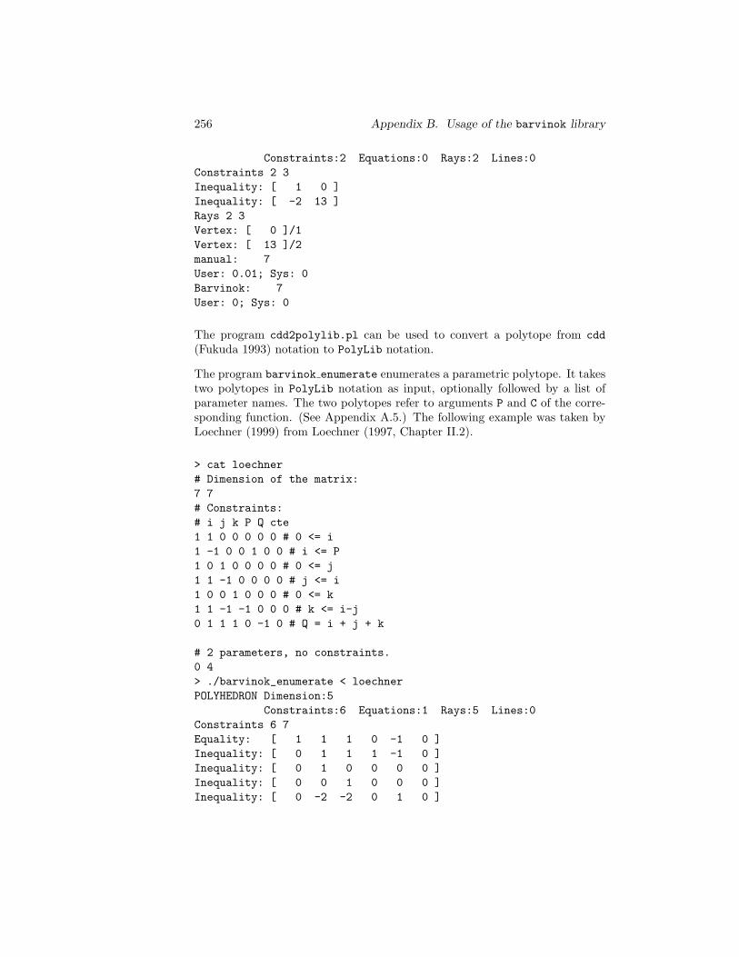
256 Appendix B. Usage of the barvinok library
Constraints:2 Equations:0 Rays:2 Lines:0
Constraints 2 3
Inequality: [ 1 0 ]
Inequality: [ -2 13 ]
Rays 2 3
Vertex: [ 0 ]/1
Vertex: [ 13 ]/2
manual: 7
User: 0.01; Sys: 0
Barvinok: 7
User: 0; Sys: 0
The program cdd2polylib.pl can be used to convert a polytope from cdd
(Fukuda 1993) notation to PolyLib notation.
The program barvinok enumerate enumerates a parametric polytope. It takestwo polytopes in PolyLib notation as input, optionally followed by a list ofparameter names. The two polytopes refer to arguments P and C of the corre-sponding function. (See Appendix A.5.) The following example was taken byLoechner (1999) from Loechner (1997, Chapter II.2).
> cat loechner
# Dimension of the matrix:
7 7
# Constraints:
# i j k P Q cte
1 1 0 0 0 0 0 # 0 <= i
1 -1 0 0 1 0 0 # i <= P
1 0 1 0 0 0 0 # 0 <= j
1 1 -1 0 0 0 0 # j <= i
1 0 0 1 0 0 0 # 0 <= k
1 1 -1 -1 0 0 0 # k <= i-j
0 1 1 1 0 -1 0 # Q = i + j + k
# 2 parameters, no constraints.
0 4
> ./barvinok_enumerate < loechner
POLYHEDRON Dimension:5
Constraints:6 Equations:1 Rays:5 Lines:0
Constraints 6 7
Equality: [ 1 1 1 0 -1 0 ]
Inequality: [ 0 1 1 1 -1 0 ]
Inequality: [ 0 1 0 0 0 0 ]
Inequality: [ 0 0 1 0 0 0 ]
Inequality: [ 0 -2 -2 0 1 0 ]
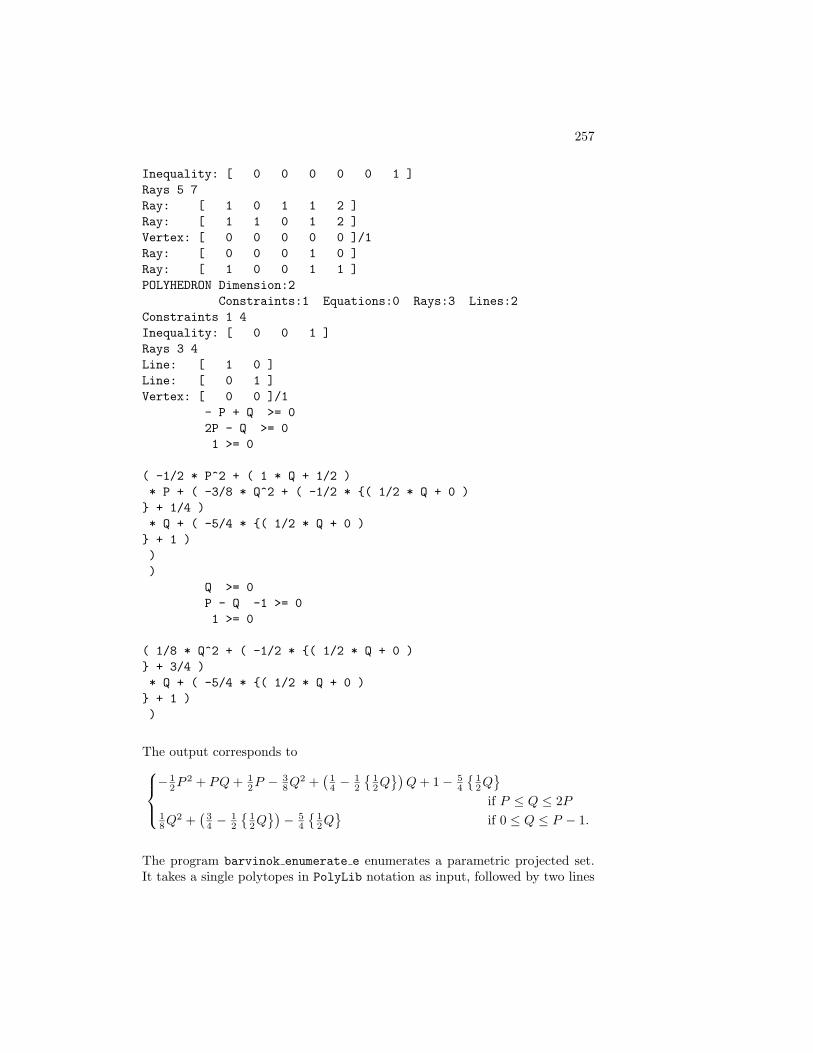
257
Inequality: [ 0 0 0 0 0 1 ]
Rays 5 7
Ray: [ 1 0 1 1 2 ]
Ray: [ 1 1 0 1 2 ]
Vertex: [ 0 0 0 0 0 ]/1
Ray: [ 0 0 0 1 0 ]
Ray: [ 1 0 0 1 1 ]
POLYHEDRON Dimension:2
Constraints:1 Equations:0 Rays:3 Lines:2
Constraints 1 4
Inequality: [ 0 0 1 ]
Rays 3 4
Line: [ 1 0 ]
Line: [ 0 1 ]
Vertex: [ 0 0 ]/1
- P + Q >= 0
2P - Q >= 0
1 >= 0
( -1/2 * P^2 + ( 1 * Q + 1/2 )
* P + ( -3/8 * Q^2 + ( -1/2 * ( 1/2 * Q + 0 )
+ 1/4 )
* Q + ( -5/4 * ( 1/2 * Q + 0 )
+ 1 )
)
)
Q >= 0
P - Q -1 >= 0
1 >= 0
( 1/8 * Q^2 + ( -1/2 * ( 1/2 * Q + 0 )
+ 3/4 )
* Q + ( -5/4 * ( 1/2 * Q + 0 )
+ 1 )
)
The output corresponds to
− 12P 2 + PQ + 1
2P − 38Q2 +
(14 − 1
2
12Q)
Q + 1 − 54
12Q
if P ≤ Q ≤ 2P18Q2 +
(34 − 1
2
12Q)
− 54
12Q
if 0 ≤ Q ≤ P − 1.
The program barvinok enumerate e enumerates a parametric projected set.It takes a single polytopes in PolyLib notation as input, followed by two lines
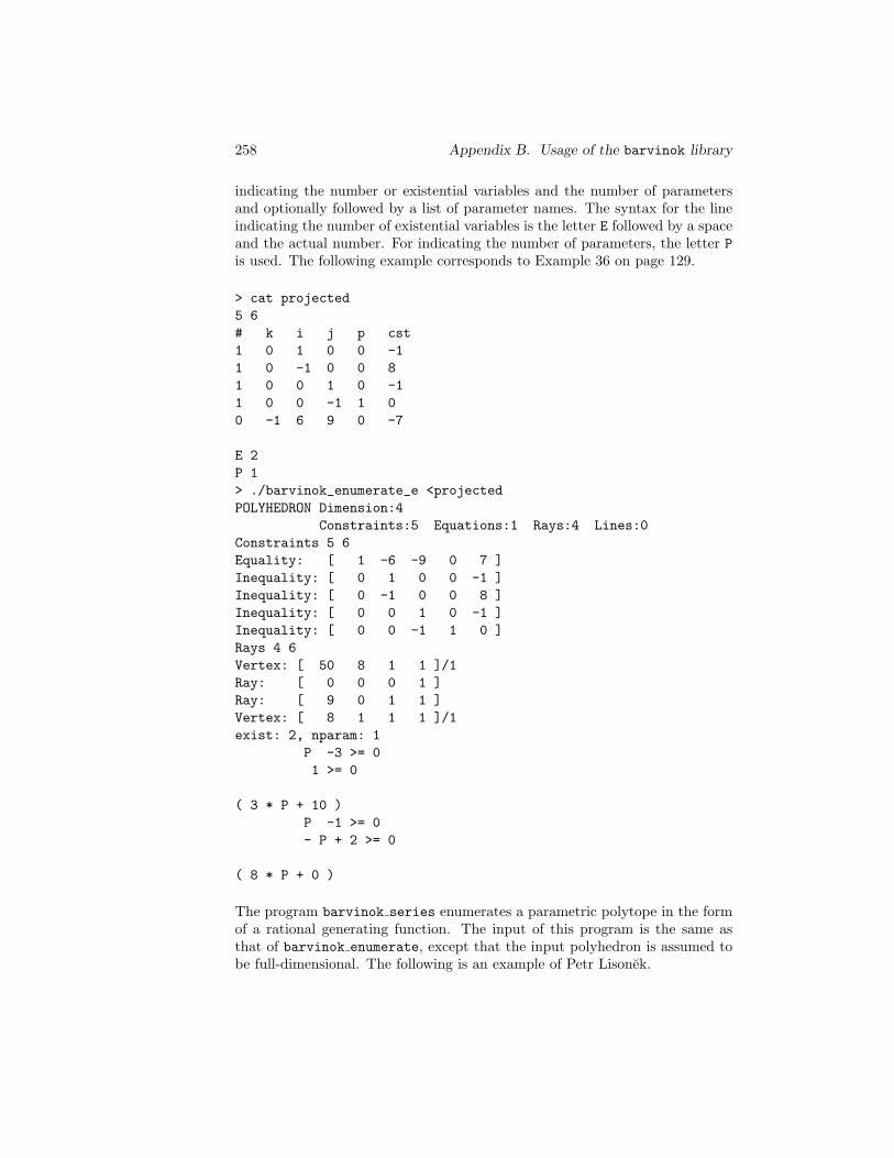
258 Appendix B. Usage of the barvinok library
indicating the number or existential variables and the number of parametersand optionally followed by a list of parameter names. The syntax for the lineindicating the number of existential variables is the letter E followed by a spaceand the actual number. For indicating the number of parameters, the letter Pis used. The following example corresponds to Example 36 on page 129.
> cat projected
5 6
# k i j p cst
1 0 1 0 0 -1
1 0 -1 0 0 8
1 0 0 1 0 -1
1 0 0 -1 1 0
0 -1 6 9 0 -7
E 2
P 1
> ./barvinok_enumerate_e <projected
POLYHEDRON Dimension:4
Constraints:5 Equations:1 Rays:4 Lines:0
Constraints 5 6
Equality: [ 1 -6 -9 0 7 ]
Inequality: [ 0 1 0 0 -1 ]
Inequality: [ 0 -1 0 0 8 ]
Inequality: [ 0 0 1 0 -1 ]
Inequality: [ 0 0 -1 1 0 ]
Rays 4 6
Vertex: [ 50 8 1 1 ]/1
Ray: [ 0 0 0 1 ]
Ray: [ 9 0 1 1 ]
Vertex: [ 8 1 1 1 ]/1
exist: 2, nparam: 1
P -3 >= 0
1 >= 0
( 3 * P + 10 )
P -1 >= 0
- P + 2 >= 0
( 8 * P + 0 )
The program barvinok series enumerates a parametric polytope in the formof a rational generating function. The input of this program is the same asthat of barvinok enumerate, except that the input polyhedron is assumed tobe full-dimensional. The following is an example of Petr Lisonek.

259
> cat petr
4 6
1 -1 -1 -1 1 0
1 1 -1 0 0 0
1 0 1 -1 0 0
1 0 0 1 0 -1
0 3
n
> ./barvinok_series < petr
POLYHEDRON Dimension:4
Constraints:5 Equations:0 Rays:5 Lines:0
Constraints 5 6
Inequality: [ -1 -1 -1 1 0 ]
Inequality: [ 1 -1 0 0 0 ]
Inequality: [ 0 1 -1 0 0 ]
Inequality: [ 0 0 1 0 -1 ]
Inequality: [ 0 0 0 0 1 ]
Rays 5 6
Ray: [ 1 1 1 3 ]
Ray: [ 1 1 0 2 ]
Ray: [ 1 0 0 1 ]
Ray: [ 0 0 0 1 ]
Vertex: [ 1 1 1 3 ]/1
POLYHEDRON Dimension:1
Constraints:1 Equations:0 Rays:2 Lines:1
Constraints 1 3
Inequality: [ 0 1 ]
Rays 2 3
Line: [ 1 ]
Vertex: [ 0 ]/1
(n^3)/((1-n) * (1-n) * (1-n^2) * (1-n^3))

260 Appendix B. Usage of the barvinok library
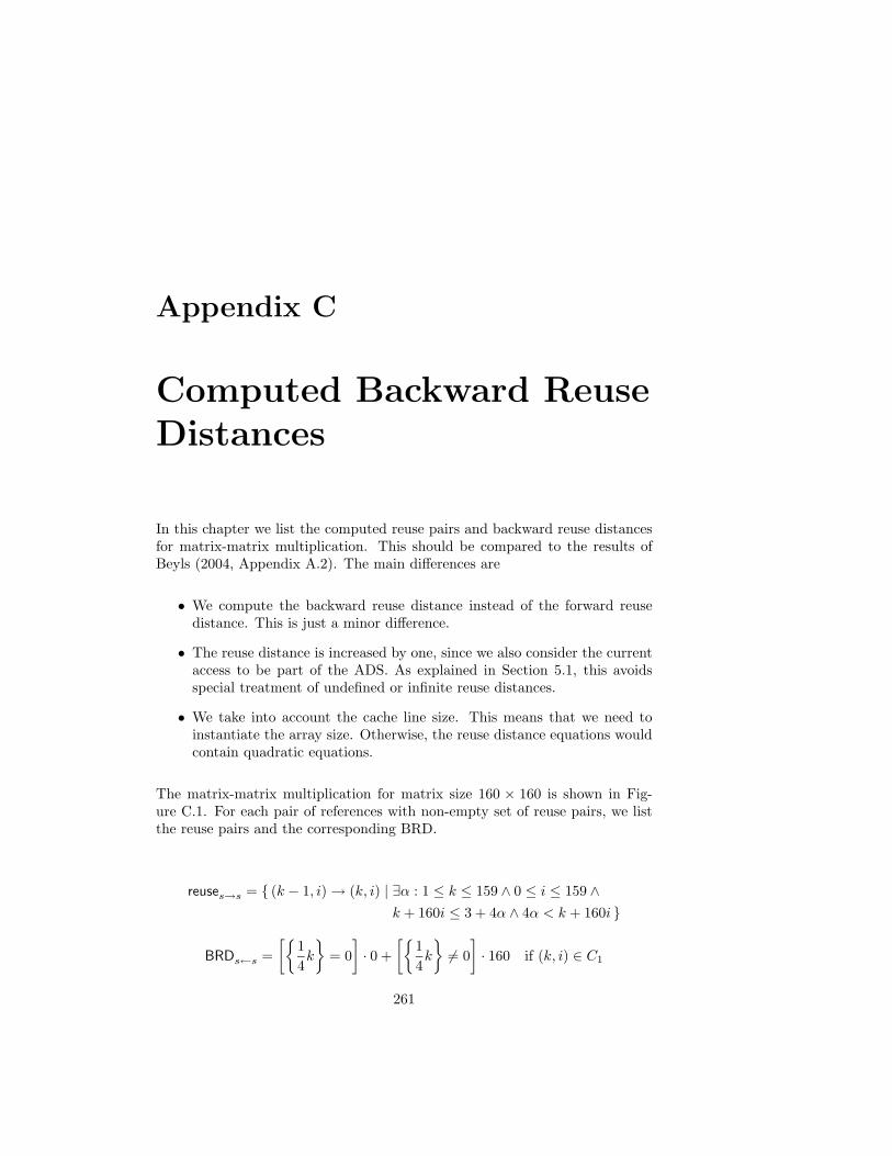
Appendix C
Computed Backward Reuse
Distances
In this chapter we list the computed reuse pairs and backward reuse distancesfor matrix-matrix multiplication. This should be compared to the results ofBeyls (2004, Appendix A.2). The main differences are
• We compute the backward reuse distance instead of the forward reusedistance. This is just a minor difference.
• The reuse distance is increased by one, since we also consider the currentaccess to be part of the ADS. As explained in Section 5.1, this avoidsspecial treatment of undefined or infinite reuse distances.
• We take into account the cache line size. This means that we need toinstantiate the array size. Otherwise, the reuse distance equations wouldcontain quadratic equations.
The matrix-matrix multiplication for matrix size 160 × 160 is shown in Fig-ure C.1. For each pair of references with non-empty set of reuse pairs, we listthe reuse pairs and the corresponding BRD.
reuses→s = (k − 1, i) → (k, i) | ∃α : 1 ≤ k ≤ 159 ∧ 0 ≤ i ≤ 159 ∧
k + 160i ≤ 3 + 4α ∧ 4α < k + 160i
BRDs←s =
[1
4k
= 0
]
· 0 +
[1
4k
6= 0
]
· 160 if (k, i) ∈ C1
261
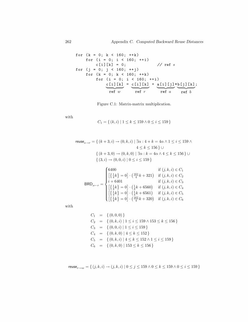
262 Appendix C. Computed Backward Reuse Distances
for (k = 0; k < 160; ++k)
for (i = 0; i < 160; ++i)
c[i][k] = 0; // ref sfor (j = 0; j < 160; ++j)
for (k = 0; k < 160; ++k)
for (i = 0; i < 160; ++i)
c[i][k]︸ ︷︷ ︸
ref w
= c[i][k]︸ ︷︷ ︸
ref r
+ a[i][j]︸ ︷︷ ︸
ref a
*b[j][k]︸ ︷︷ ︸
ref b
;
Figure C.1: Matrix-matrix multiplication.
withC1 = (k, i) | 1 ≤ k ≤ 159 ∧ 0 ≤ i ≤ 159
reuses→r = (k + 3, i) → (0, k, i) | ∃α : 4 + k = 4α ∧ 1 ≤ i ≤ 159 ∧
4 ≤ k ≤ 156 ∪
(k + 3, 0) → (0, k, 0) | ∃α : k = 4α ∧ 4 ≤ k ≤ 156 ∪
(3, i) → (0, 0, i) | 0 ≤ i ≤ 159
BRDs←r =
6400 if (j, k, i) ∈ C1[
14k
= 0]·(
1614 k + 321
)if (j, k, i) ∈ C2
i + 6401 if (j, k, i) ∈ C3[
14k
= 0]·(
14k + 6560
)if (j, k, i) ∈ C4
[14k
= 0]·(
14k + 6561
)if (j, k, i) ∈ C5
[14k
= 0]·(
1614 k + 320
)if (j, k, i) ∈ C6
with
C1 = (0, 0, 0)
C2 = (0, k, i) | 1 ≤ i ≤ 159 ∧ 153 ≤ k ≤ 156
C3 = (0, 0, i) | 1 ≤ i ≤ 159
C4 = (0, k, 0) | 4 ≤ k ≤ 152
C5 = (0, k, i) | 4 ≤ k ≤ 152 ∧ 1 ≤ i ≤ 159
C6 = (0, k, 0) | 153 ≤ k ≤ 156
reuser→w = (j, k, i) → (j, k, i) | 0 ≤ j ≤ 159 ∧ 0 ≤ k ≤ 159 ∧ 0 ≤ i ≤ 159
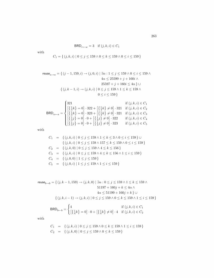
263
BRDr←w = 3 if (j, k, i) ∈ C1
withC1 = (j, k, i) | 0 ≤ j ≤ 159 ∧ 0 ≤ k ≤ 159 ∧ 0 ≤ i ≤ 159
reusea→a = (j − 1, 159, i) → (j, 0, i) | ∃α : 1 ≤ j ≤ 159 ∧ 0 ≤ i ≤ 159 ∧
4α ≤ 25599 + j + 160i ∧
25597 + j + 160i ≤ 4α ∪
(j, k − 1, i) → (j, k, i) | 0 ≤ j ≤ 159 ∧ 1 ≤ k ≤ 159 ∧
0 ≤ i ≤ 159
BRDa←a =
321 if (j, k, i) ∈ C1[
14k
= 0]· 322 +
[14k6= 0]· 321 if (j, k, i) ∈ C2
[14k
= 0]· 323 +
[14k6= 0]· 321 if (j, k, i) ∈ C3
[14j
= 0]· 0 +
[14j6= 0]· 322 if (j, k, i) ∈ C4
[14j
= 0]· 0 +
[14j6= 0]· 323 if (j, k, i) ∈ C5
with
C1 = (j, k, i) | 0 ≤ j ≤ 159 ∧ 1 ≤ k ≤ 3 ∧ 0 ≤ i ≤ 159 ∪
(j, k, i) | 0 ≤ j ≤ 159 ∧ 157 ≤ k ≤ 159 ∧ 0 ≤ i ≤ 159
C2 = (j, k, 0) | 0 ≤ j ≤ 159 ∧ 4 ≤ k ≤ 156
C3 = (j, k, i) | 0 ≤ j ≤ 159 ∧ 4 ≤ k ≤ 156 ∧ 1 ≤ i ≤ 159
C4 = (j, 0, 0) | 1 ≤ j ≤ 159
C5 = (j, 0, i) | 1 ≤ j ≤ 159 ∧ 1 ≤ i ≤ 159
reuseb→b = (j, k − 1, 159) → (j, k, 0) | ∃α : 0 ≤ j ≤ 159 ∧ 1 ≤ k ≤ 159 ∧
51197 + 160j + k ≤ 4α ∧
4α ≤ 51199 + 160j + k ∪
(j, k, i − 1) → (j, k, i) | 0 ≤ j ≤ 159 ∧ 0 ≤ k ≤ 159 ∧ 1 ≤ i ≤ 159
BRDb←b =
4 if (j, k, i) ∈ C1[
14k
= 0]· 0 +
[14k6= 0]· 4 if (j, k, i) ∈ C2
with
C1 = (j, k, i) | 0 ≤ j ≤ 159 ∧ 0 ≤ k ≤ 159 ∧ 1 ≤ i ≤ 159
C2 = (j, k, 0) | 0 ≤ j ≤ 159 ∧ 0 ≤ k ≤ 159
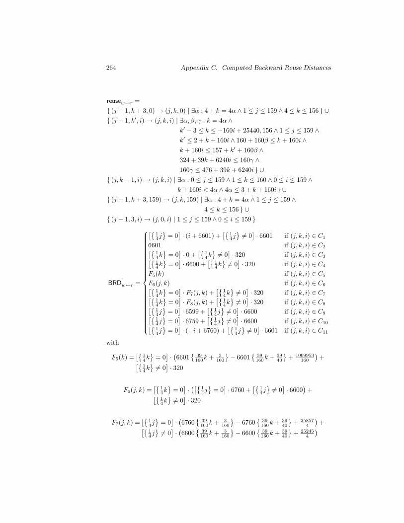
264 Appendix C. Computed Backward Reuse Distances
reusew→r =
(j − 1, k + 3, 0) → (j, k, 0) | ∃α : 4 + k = 4α ∧ 1 ≤ j ≤ 159 ∧ 4 ≤ k ≤ 156 ∪
(j − 1, k′, i) → (j, k, i) | ∃α, β, γ : k = 4α ∧
k′ − 3 ≤ k ≤ −160i + 25440, 156 ∧ 1 ≤ j ≤ 159 ∧
k′ ≤ 2 + k + 160i ∧ 160 + 160β ≤ k + 160i ∧
k + 160i ≤ 157 + k′ + 160β ∧
324 + 39k + 6240i ≤ 160γ ∧
160γ ≤ 476 + 39k + 6240i ∪
(j, k − 1, i) → (j, k, i) | ∃α : 0 ≤ j ≤ 159 ∧ 1 ≤ k ≤ 160 ∧ 0 ≤ i ≤ 159 ∧
k + 160i < 4α ∧ 4α ≤ 3 + k + 160i ∪
(j − 1, k + 3, 159) → (j, k, 159) | ∃α : 4 + k = 4α ∧ 1 ≤ j ≤ 159 ∧
4 ≤ k ≤ 156 ∪
(j − 1, 3, i) → (j, 0, i) | 1 ≤ j ≤ 159 ∧ 0 ≤ i ≤ 159
BRDw←r =
[14j
= 0]· (i + 6601) +
[14j6= 0]· 6601 if (j, k, i) ∈ C1
6601 if (j, k, i) ∈ C2[
14k
= 0]· 0 +
[14k6= 0]· 320 if (j, k, i) ∈ C3
[14k
= 0]· 6600 +
[14k6= 0]· 320 if (j, k, i) ∈ C4
F5(k) if (j, k, i) ∈ C5
F6(j, k) if (j, k, i) ∈ C6[
14k
= 0]· F7(j, k) +
[14k6= 0]· 320 if (j, k, i) ∈ C7
[14k
= 0]· F8(j, k) +
[14k6= 0]· 320 if (j, k, i) ∈ C8
[14j
= 0]· 6599 +
[14j6= 0]· 6600 if (j, k, i) ∈ C9
[14j
= 0]· 6759 +
[14j6= 0]· 6600 if (j, k, i) ∈ C10
[14j
= 0]· (−i + 6760) +
[14j6= 0]· 6601 if (j, k, i) ∈ C11
with
F5(k) =[
14k
= 0]·(6601
39160k + 3
160
− 6601
39160k + 39
40
+ 1009953
160
)+
[14k6= 0]· 320
F6(j, k) =[
14k
= 0]·([
14j
= 0]· 6760 +
[14j6= 0]· 6600
)+
[14k6= 0]· 320
F7(j, k) =[
14j
= 0]·(6760
39160k + 3
160
− 6760
39160k + 39
40
+ 25857
4
)+
[14j6= 0]·(6600
39160k + 3
160
− 6600
39160k + 39
40
+ 25245
4
)
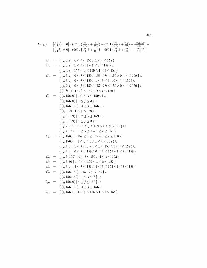
265
F8(j, k) =[
14j
= 0]·(6761
39160k + 3
160
− 6761
39160k + 39
40
+ 1034433
160
)+
[14j6= 0]·(6601
39160k + 3
160
− 6601
39160k + 39
40
+ 1009953
160
)
C1 = (j, 0, i) | 4 ≤ j ≤ 156 ∧ 1 ≤ i ≤ 158
C2 = (j, 0, i) | 1 ≤ j ≤ 3 ∧ 1 ≤ i ≤ 158 ∪
(j, 0, i) | 157 ≤ j ≤ 159 ∧ 1 ≤ i ≤ 158
C3 = (j, k, i) | 0 ≤ j ≤ 159 ∧ 153 ≤ k ≤ 155 ∧ 0 ≤ i ≤ 159 ∪
(j, k, i) | 0 ≤ j ≤ 159 ∧ 1 ≤ k ≤ 3 ∧ 0 ≤ i ≤ 159 ∪
(j, k, i) | 0 ≤ j ≤ 159 ∧ 157 ≤ k ≤ 159 ∧ 0 ≤ i ≤ 159 ∪
(0, k, i) | 1 ≤ k ≤ 159 ∧ 0 ≤ i ≤ 159
C4 = (j, 156, 0) | 157 ≤ j ≤ 159∧ ∪
(j, 156, 0) | 1 ≤ j ≤ 3 ∪
(j, 156, 159) | 4 ≤ j ≤ 156 ∪
(j, 0, 0) | 1 ≤ j ≤ 159 ∪
(j, 0, 159) | 157 ≤ j ≤ 159 ∪
(j, 0, 159) | 1 ≤ j ≤ 3 ∪
(j, k, 159) | 157 ≤ j ≤ 159 ∧ 4 ≤ k ≤ 152 ∪
(j, k, 159) | 1 ≤ j ≤ 3 ∧ 4 ≤ k ≤ 152
C5 = (j, 156, i) | 157 ≤ j ≤ 159 ∧ 1 ≤ i ≤ 158 ∪
(j, 156, i) | 1 ≤ j ≤ 3 ∧ 1 ≤ i ≤ 158 ∪
(j, k, i) | 1 ≤ j ≤ 3 ∧ 4 ≤ k ≤ 152 ∧ 1 ≤ i ≤ 158 ∪
(j, k, i) | 0 ≤ j ≤ 159 ∧ 0 ≤ k ≤ 159 ∧ 1 ≤ i ≤ 159
C6 = (j, k, 159) | 4 ≤ j ≤ 156 ∧ 4 ≤ k ≤ 152
C7 = (j, k, 0) | 4 ≤ j ≤ 156 ∧ 4 ≤ k ≤ 152
C8 = (j, k, i) | 4 ≤ j ≤ 156 ∧ 4 ≤ k ≤ 152 ∧ 1 ≤ i ≤ 158
C9 = (j, 156, 159) | 157 ≤ j ≤ 159 ∪
(j, 156, 159) | 1 ≤ j ≤ 3 ∪
C10 = (j, 156, 0) | 4 ≤ j ≤ 156 ∪
(j, 156, 159) | 4 ≤ j ≤ 156
C11 = (j, 156, i) | 4 ≤ j ≤ 156 ∧ 1 ≤ i ≤ 158

266 Appendix C. Computed Backward Reuse Distances
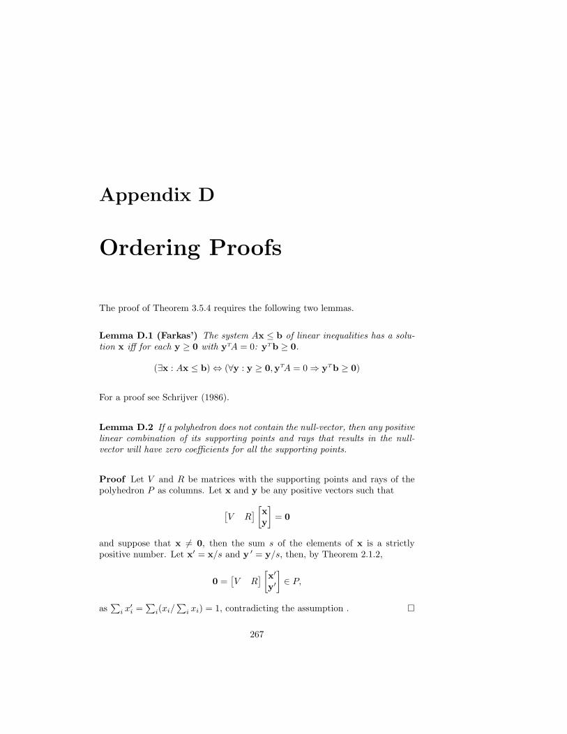
Appendix D
Ordering Proofs
The proof of Theorem 3.5.4 requires the following two lemmas.
Lemma D.1 (Farkas’) The system Ax ≤ b of linear inequalities has a solu-tion x iff for each y ≥ 0 with yTA = 0: yTb ≥ 0.
(∃x : Ax ≤ b) ⇔ (∀y : y ≥ 0,yTA = 0 ⇒ yT b ≥ 0)
For a proof see Schrijver (1986).
Lemma D.2 If a polyhedron does not contain the null-vector, then any positivelinear combination of its supporting points and rays that results in the null-vector will have zero coefficients for all the supporting points.
Proof Let V and R be matrices with the supporting points and rays of thepolyhedron P as columns. Let x and y be any positive vectors such that
[V R
][xy
]
= 0
and suppose that x 6= 0, then the sum s of the elements of x is a strictlypositive number. Let x′ = x/s and y ′ = y/s, then, by Theorem 2.1.2,
0 =[V R
][x′
y′
]
∈ P,
as∑
i x′i =∑
i(xi/∑
i xi) = 1, contradicting the assumption .
267
268 Appendix D. Ordering Proofs
Proof (of Theorem 3.5.4) If DP contains the null-vector, then the validordering polyhedron is empty since πT0 = 0 for any π. This proves that ifDP’s valid ordering polyhedron is non-empty, then DP does not contain thenull-vector.
Conversely, assume that DP does not contain the null-vector and let V [R]be a matrix with the supporting points [rays] in the explicit notation of DP
as columns. Then V T π ≥ 1 ∧ RT π ≥ 0 ensures π ∈ PO, i.e., π should be asolution of
−
[V T
RT
]
π ≤
[−10
]
.
By Farkas’ Lemma (Lemma D.1), this set of equations has a solution iff
∀y : x,y ≥ 0,−[V R
][xy
]
= 0 ⇒[xT yT
][−10
]
≥ 0.
According to Lemma D.2, any pair of vectors satisfying the premise of theimplication will have x = 0, for which the consequent trivially holds.
The proof of Theorem 3.5.10 requires another pair of lemmas.
Lemma D.3 If RG is non-degenerate then RG′ , where the graph G′ is com-puted as combine(G, p1, p2,αp1,p2
), is also non-degenerate iff the offset αp1,p2
between the two nodes p1 and p2 is such that it satisfies the condition (3.47):
αp1,p26∈(RG + VG,(p2,p1)
)∪(−(RG + VG,(p1,p2)
))
Proof We prove that RG′ is degenerate iff α = αp1,p2is a member of the
set in the right hand side of (3.47). First note that any circuit in G′ and itscorresponding indirect distance vectors corresponds to a circuit in G′′, whereG′′ is G with two additional “pseudo-edges”: one between p1 and p2 withDP(p1,p2) = −α and one between p2 and p1 with DP(p2,p1) = α. Such apseudo-edge represents a pseudo-dependence. The graph G′′ has one additionalcircuit, viz. the one composed of the two pseudo-edges.
If RG′ is degenerate then there exists an r ∈ RG′ such that r = 0. Accordingto (3.46) and (3.45), any element from RG′′ is the sum of indirect distancevectors over a circuit, i.e.,
r =∑
k
λkδk λk > 0,∑
k
λk ≥ 1
where each δj is an element of VG′′,(p,p) for some p ∈ VG, excluding the caseof the circuit composed of the two pseudo-edges, and where we have left outthe terms for which λk = 0 as they do not have any influence. Since the path
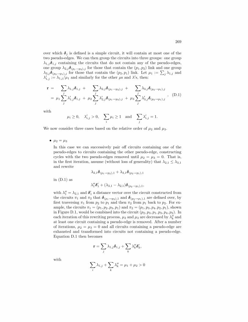
269
over which δj is defined is a simple circuit, it will contain at most one of thetwo pseudo-edges. We can then group the circuits into three groups: one groupλ1,jδ1,j containing the circuits that do not contain any of the pseudo-edges,one group λ2,jδ(p1→p2),j for those that contain the (p1, p2) link and one groupλ3,jδ(p2→p1),j for those that contain the (p2, p1) link. Let µ1 :=
∑
j λ1,j andλ′1,j := λ1,j/µ1 and similarly for the other µs and λ′s, then:
r =∑
j
λ1,jδ1,j +∑
j
λ2,jδ(p1→p2),j +∑
j
λ3,jδ(p2→p1),j
= µ1
∑
j
λ′1,jδ1,j + µ2
∑
j
λ′2,jδ(p1→p2),j + µ3
∑
j
λ′3,jδ(p2→p1),j
, (D.1)
with
µi ≥ 0, λ′i,j > 0,∑
i
µi ≥ 1 and∑
j
λ′i,j = 1.
We now consider three cases based on the relative order of µ2 and µ3.
• µ2 = µ3
In this case we can successively pair off circuits containing one of thepseudo-edges to circuits containing the other pseudo-edge, constructingcycles with the two pseudo-edges removed until µ2 = µ3 = 0. That is,in the first iteration, assume (without loss of generality) that λ2,1 ≤ λ3,1
and rewrite
λ2,1δ(p1→p2),1 + λ3,1δ(p2→p1),1
in (D.1) as
λ′′1δ′1 + (λ3,1 − λ2,1)δ(p2→p1),1,
with λ′′1 = λ2,1 and δ′1 a distance vector over the circuit constructed fromthe circuits π1 and π2 that δ(p1→p2),1 and δ(p2→p1),1 are defined over, byfirst traversing π1 from p2 to p1 and then π2 from p1 back to p2. For ex-ample, the circuits π1 = (p1, p2, p3, p1) and π2 = (p1, p3, p4, p2, p1), shownin Figure D.1, would be combined into the circuit (p2, p3, p1, p3, p4, p2). Ineach iteration of this rewriting process, µ2 and µ3 are decreased by λ′′k andat least one circuit containing a pseudo-edge is removed. After a numberof iterations, µ2 = µ3 = 0 and all circuits containing a pseudo-edge areexhausted and transformed into circuits not containing a pseudo-edge.Equation D.1 then becomes
r =∑
j
λ1,jδ1,j +∑
k
λ′′kδ′k,
with∑
i
λ1,j +∑
k
λ′′k = µ1 + µ2 > 0
270 Appendix D. Ordering Proofs
•
•
•
•
π1
π2
p1
p2
p3
p4
Figure D.1: Pairing off two circuits.
•
• •
•
αp1,p2
p2
p1
Figure D.2: Decomposition of a circuit containing a pseudo-edge.
and each δ′k a distance vector over a circuit and therefore in RG as it isthe sum of distance vectors over simple circuits. We are then left with astrictly positive combination of elements from the original RG. Since byassumption 0 6∈ RG, no strictly positive combination of elements of RG
can result in the null-vector, so in this case r cannot be the null-vector.
• µ2 < µ3
As in the previous case, we can pair off some of the circuits, resulting inan element of RG. This will exhaust the circuits that contain the pseudo-edge (p1, p2), but will leave µ3−µ2 circuits that contain the other pseudo-edge. An indirect distance vector over such a circuit can be decomposedinto α and some element from VG(p1,p2). Such a decomposition is shownin Figure D.2. As a result we have:
r = r′ + (µ3 − µ2)α + (µ3 − µ2)∑
j
λ′3,jδ′j
with r′ ∈ RG and each δ′ ∈ VG(p1,p2). If r = 0 then, since µ3 − µ2 isstrictly positive:
α = −1
µ3 − µ2r′ −
∑
j
λ′3,jδ′j
or
α ∈ −(RG + VG,(p1,p2)
). (D.2)
271
• µ2 > µ3
This case is completely analogous to the previous case and yields:
α ∈ RG + VG,(p2,p1). (D.3)
Conversely, let α be an element of either of the sets in equations (D.2) and (D.3),then RG′ is degenerate. To see this, take (D.3) and let
α = r +∑
j
λjδj (D.4)
with r ∈ RG,∑
j λj = 1 and for each δj : δj ∈ VG,(p2,p1). Obviously α =∑
j λjα, so we can combine each δj with −α and rewrite (D.4) as
0 = r +∑
j
λjδ′j
with δ′j = δj − α ∈ VG′,(p1,p1) and so r′ =∑
j λjδ′j ∈ RG′ . If r = 0 then we
have found an element in RG′ equal to the null-vector. If r is in RG then itis also in RG′ and again we find an element r + r′ in RG′ equal to the null-vector. In the final case r = λr′′ with r′′ ∈ RG′ and 0 < λ < 1, and thenr′′ + λ−1r′ = 0 ∈ RG′ .
Lemma D.4 If d ≥ 2 and if RG is non-degenerate, then the constraint (3.47):
αp1,p26∈(RG + VG,(p2,p1)
)∪(−(RG + VG,(p1,p2)
))
has an (infinite number of) integer solution(s).
Proof If RG is contained in a hyperplane H, then the set(RG + VG,(p2,p1)
)∪
(−(RG + VG,(p1,p2)
))is contained in the same hyperplane. Otherwise we could
take δ1 ∈ VG,(p2,p1) and δ2 ∈ −VG,(p1,p2) with δ2 6∈ δ1 + H. But then RG ∋δ1 − δ2 6∈ H, which contradicts the assumption. Let g be any integer vector,different from the null vector, orthogonal to H and δ1 ∈ VG,(p2,p1), then δ1 +gis not in H and therefore a solution to (3.47).
If RG is not contained in a single hyperplane, then let H1 and H2 be twodistinct supporting hyperplanes of RG:
H1 = x | g T
1x = 0 and H2 = x | g T
2x = 0 ,
with g1 and g2 pointing “outward” (see Figure D.3), i.e.,
RG ⊂ x | g T
1 x ≤ 0 ∩ x | g T
2 x ≤ 0 . (D.5)
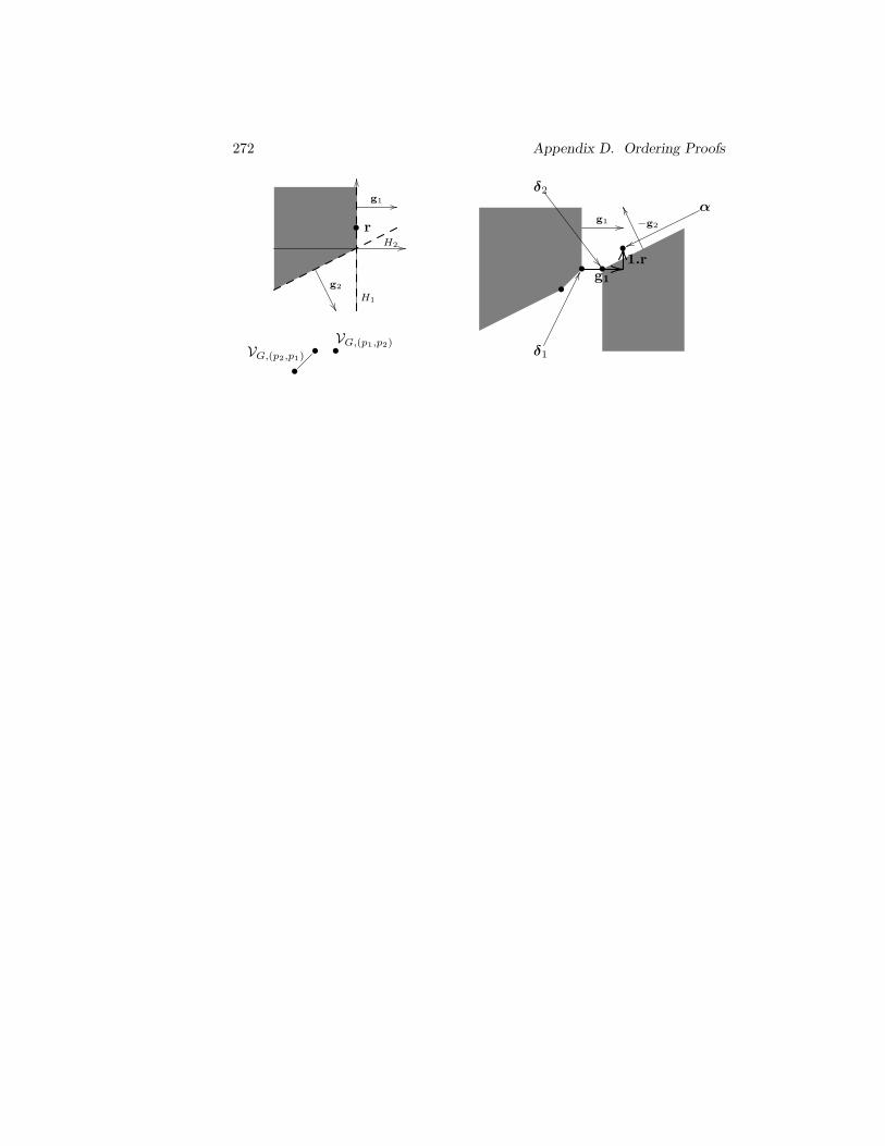
272 Appendix D. Ordering Proofs
g1
g2
• rH2
H1
•
• •VG,(p1,p2)
VG,(p2,p1)
•
•
δ1
•
δ2
•
αg1 −g2
g1
1.r
−g T
2 (x − δ2) = 0
g T
1 (x − δ1) = 0
Figure D.3: Illustration of the proof of Lemma D.4: on the top left the self-dependence full cone, on the bottom left the indirect distance vector polytopesand on the right the illegal regions for the relative offset.
Furthermore, let δ1 and δ2 be defined as follows:
δ1 = argmaxx∈VG,(p2,p1)
g T
1 x δ2 = argmaxx∈−VG,(p1,p2)
−g T
2 x,
then and because of (D.5):
∀x ∈ RG + VG,(p2,p1) : g T
1 (x − δ1) ≤ 0
and similarly
∀x ∈ −(RG + VG,(p2,p1)
): −g T
2 (x − δ2) ≤ 0.
Let r be an arbitrary integer point in H1 \H2, i.e., g T
1 r = 0 and g T
2 r < 0, thenα = δ1 + g1 + nr with
n ≥1 + g T
2 (δ1 − δ2 + g1)
−g T
2 r
is a solution to (3.47) since
g T
1 (δ1 + g1 + nr − δ1) = ||g1||2 + n.0 > 0
and−g T
2 (δ1 + g1 + nr − δ2) ≥ 1.
Proof (of Theorem 3.5.10) The proof follows trivially from Lemma D.4 andLemma D.3.
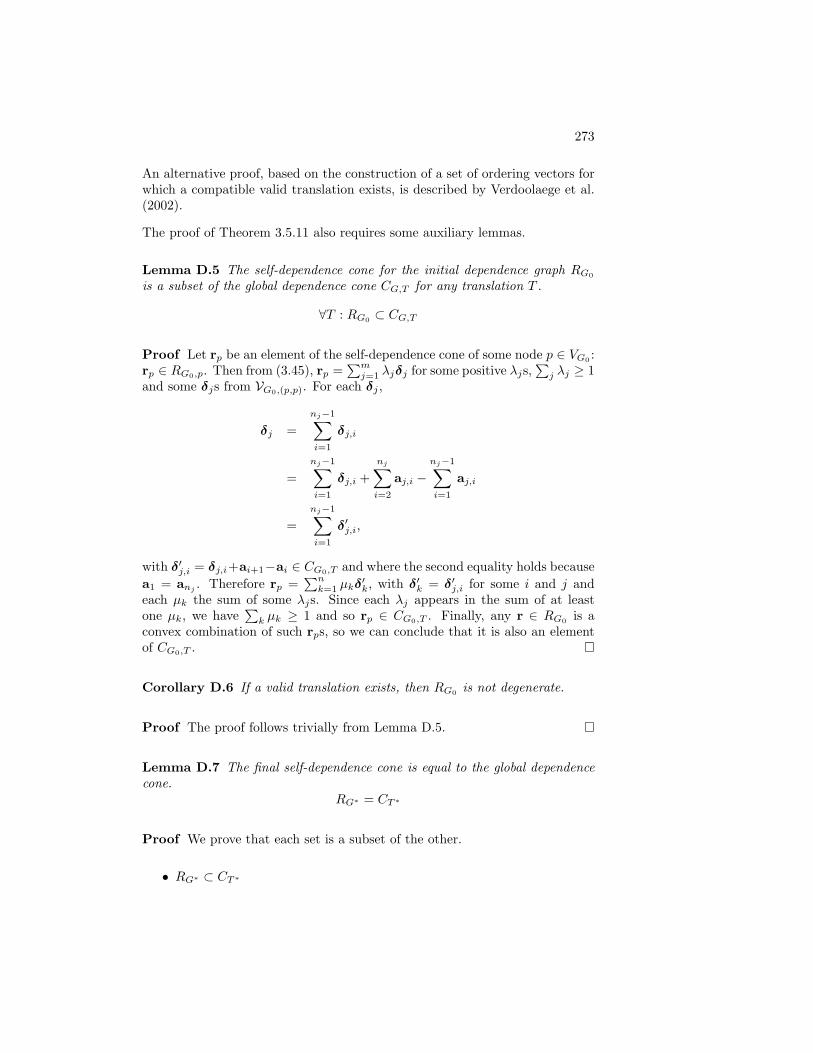
273
An alternative proof, based on the construction of a set of ordering vectors forwhich a compatible valid translation exists, is described by Verdoolaege et al.(2002).
The proof of Theorem 3.5.11 also requires some auxiliary lemmas.
Lemma D.5 The self-dependence cone for the initial dependence graph RG0
is a subset of the global dependence cone CG,T for any translation T .
∀T : RG0⊂ CG,T
Proof Let rp be an element of the self-dependence cone of some node p ∈ VG0:
rp ∈ RG0,p. Then from (3.45), rp =∑m
j=1 λjδj for some positive λjs,∑
j λj ≥ 1and some δjs from VG0,(p,p). For each δj ,
δj =
nj−1∑
i=1
δj,i
=
nj−1∑
i=1
δj,i +
nj∑
i=2
aj,i −
nj−1∑
i=1
aj,i
=
nj−1∑
i=1
δ′j,i,
with δ′j,i = δj,i+ai+1−ai ∈ CG0,T and where the second equality holds because
a1 = anj. Therefore rp =
∑nk=1 µkδ′k, with δ′k = δ′j,i for some i and j and
each µk the sum of some λjs. Since each λj appears in the sum of at leastone µk, we have
∑
k µk ≥ 1 and so rp ∈ CG0,T . Finally, any r ∈ RG0is a
convex combination of such rps, so we can conclude that it is also an elementof CG0,T .
Corollary D.6 If a valid translation exists, then RG0is not degenerate.
Proof The proof follows trivially from Lemma D.5.
Lemma D.7 The final self-dependence cone is equal to the global dependencecone.
RG∗ = CT∗
Proof We prove that each set is a subset of the other.
• RG∗ ⊂ CT∗
274 Appendix D. Ordering Proofs
Each element r in RG∗ can be written as a positive combination of indirectdistance vectors over a circuit r =
∑
j λjrj , with∑
j λj ≥ 1 from thesingle node to itself. By construction, each such distance vector willbe composed of distance vectors corresponding to “real” edges in theoriginal graph G0 and relative offsets corresponding to pseudo-edges inthe original graph. Together they will form a circuit in the original graph.Replace all adjacent pseudo-edges in this circuit by a single pseudo-edgeconnecting the starting node of the first pseudo-edge to the ending node ofthe last pseudo-edge. Insert a pseudo-edge from a node to itself betweeneach pair of adjacent real edges. The resulting circuit alternates betweenreal edges and pseudo-edges and we can rewrite the indirect distancevector as follows:
rj =∑
k
vu2k,u2k+1− αu2k+1,u2k+2
=∑
k
vu2k,u2k+1+ au2k+1
− au2k+2
=∑
k
vu2k,u2k+1+ au2k+1
− au2k
The last equality holds because the first and final nodes are the same andhence have the same offset. The last identity shows that rj ∈ CT∗ andthus r is in CT∗ as well.
• RG∗ ⊃ CT∗
Each element δ in CT∗ can be written as a positive combination of dis-tance vectors with
∑
j λj ≥ 1. Any such distance vector is the sum of adistance vector over an edge (p1, p2) in G0 and the relative offset αp2,p1
between the end points and is therefore an element of RG∗ . As a result,δ is in RG∗ as well.
Proof (of Theorem 3.5.11) The theorem follows almost immediately fromLemma D.7. If a translation exists, then by Corollary D.6 any translationwe construct using αs based on Lemma D.3 will have a non-degenerate RG∗
and will thus be valid. Conversely, for any valid translation, we can in eachstep choose a relative offset that corresponds to this translation. The self-dependence cone RG′ that results from the combination in each step is a su-perset of the one RG prior to combination. I.e., we have
RG0⊂ . . . ⊂ RG ⊂ RG′ ⊂ RG′′ ⊂ . . . ⊂ RG∗ .
Since the final RG∗ is non-degenerate, so will all the others and therefore thosechoices will correspond to valid ones according to Lemma D.3.
References
Alekseevskaya, T. V., I. M. Gel′fand, and A. V. Zelevinskiı (1987). Distri-bution of real hyperplanes and the partition function connected with it.Doklady Akademii Nauk SSSR 297 (6), 1289–1293. [116]
Allen, J. R., D. Callahan, and K. Kennedy (1987). Automatic decomposi-tion of scientific programs for parallel execution. In Proceedings of theFourteenth Annual ACM Symposium on the Principles of ProgrammingLanguages, pp. 63–76. [38]
Amarasinghe, S., J. Anderson, M. S. Lam, and C.-W. Tseng (1995). Anoverview of the SUIF compiler for scalable parallel machines. In Proceed-ings of the Seventh SIAM Conference on Parallel Processing for ScientificComputing, San Francisco, CA. [36]
Anantharaman, S. and S. Pande (1998). Compiler optimizations for realtime execution of loops on limited memory embedded systems. In The19th IEEE Systems Symposium (RTSS98). [209]
Aragon, C. R. and R. G. Seidel (1989). Randomized search trees. In 30thannual Symposium on Foundations of Computer Science, pp. 540–545.
[225]
Aurenhammer, F. and R. Klein (2000). Voronoi diagrams. In J. Sack andG. Urrutia (Eds.), Handbook of Computational Geometry, Chapter V, pp.201–290. Elsevier Science Publishing. [SFB Report F003-092, TU Graz,Austria, 1996]. [143]
Avis, D. (2000). lrs: A revised implementation of the reverse search vertexenumeration algorithm. In G. Kalai and G. Ziegler (Eds.), Polytopes —Combinatorics and Computation, pp. 177–198. Birkhauser-Verlag. DMVSeminar Band 29. [13]
Bagnara, R., E. Ricci, E. Zaffanella, and P. M. Hill (2002). Possibly notclosed convex polyhedra and the Parma Polyhedra Library. In M. V.Hermenegildo and G. Puebla (Eds.), Static Analysis: Proceedings of the9th International Symposium, Volume 2477 of Lecture Notes in Computer
275
276 References
Science, Madrid, Spain, pp. 213–229. Springer-Verlag, Berlin. [13]
Balasa, F., F. Catthoor, and H. De Man (1995, June). Background memoryarea estimation for multidimensional signal processing systems. IEEETransactions on Very Large Scale Integration (VLSI) Systems 3 (2), 157–172. [209]
Balasa, F., F. Catthoor, and H. De Man (1997, February). Practical solutionsfor counting scalars and dependences in atomium – a memory manage-ment system for multi-dimensional signal processing. IEEE Transactionson Computer-aided Design CAD-16 (2), 133–145. [32]
Barber, C. B., D. P. Dobkin, and H. Huhdanpaa (1996). The quickhull al-gorithm for convex hulls. ACM Transactions on Mathematical Software(TOMS) 22 (4), 469–483. [13]
Barvinok, A. (1993, November). A polynomial time algorithm for countingintegral points in polyhedra when the dimension is fixed. In 34th AnnualSymposium on Foundations of Computer Science, pp. 566–572. IEEE.
[105, 106]
Barvinok, A. (1994). Computing the Ehrhart polynomial of a convex latticepolytope. Dicrete Comput. Geom. 12, 35–48. [138, 148, 157]
Barvinok, A. (2002). A Course in Convexity, Volume 54 of Graduate Studiesin Mathematics. Providence, RI: American Mathematical Society. [139]
Barvinok, A. and J. Pommersheim (1999). An algorithmic theory of latticepoints in polyhedra. New Perspectives in Algebraic Combinatorics 38,91–147. [4, 5, 106, 109, 133, 134, 137, 139,142, 143, 153, 158, 163, 165, 172, 173, 185, 318, 321, 323, 329, 335, 337]
Barvinok, A. and K. Woods (2003, April). Short rational generating functionsfor lattice point problems. J. Amer. Math. Soc. 16, 957–979.[4, 6, 106, 132, 157, 180, 185, 193, 240, 241, 318, 323, 325, 329, 338, 341]
Bastoul, C. (2002). Generating loops for scanning polyhedra. Technical Re-port 2002/23, Versailles University. [37, 94]
Bastoul, C., A. Cohen, S. Girbal, S. Sharma, and O. Temam (2003, October).Putting polyhedral loop transformations to work. In LCPC03. [24, 36]
Beck, M. (2004). The partial-fractions method for counting solutions to in-tegral linear systems. Discrete Comp. Geom. 32, 437–446. (special issuein honor of Louis Billera). [182, 207]
Beck, M., J. A. De Loera, M. Develin, J. Pfeifle, and R. P. Stanley (2004,February). Coefficients and Roots of Ehrhart Polynomials. AIM 2004-1.
[112]
References 277
Beck, M. and S. Robins (2006). Computing the Continuous Discretely.Integer-point Enumeration in Polyhedra. Springer Undergraduate Textsin Mathematics. Springer. to appear. [4, 112, 113]
Bednara, M., F. Hannig, and J. Teich (2002). Generation of distributed loopcontrol. In In Embedded Processor Design Challenges: Systems, Archi-tectures, Modeling, and Simulation (SAMOS), Volume 2268 of LectureNotes in Computer Science, pp. 154–170. [210]
Beyls, K. (2004). Software Methods to Improve Data Locality and CacheBehavior. Ph. D. thesis, Ghent University.
[203, 204, 205, 206, 208, 214, 217, 225, 261, 323, 339]
Beyls, K. and E. D’Hollander (2001). Reuse distance as a metric for cachebehavior. In IASTED conference on Parallel and Distributed Computingand Systems 2001 (PDCS01), pp. 617–662. [55]
Bik, A. J. C. (1996). Compiler Support for Sparse Matrix Computations. Ph.D. thesis, University of Leiden, The Netherlands. [93, 123, 188, 253]
Blakley, G. R. (1964). Combinatorial remarks on partitions of a multipartitenumber. Duke Math. J. 31 (2), 335–340. [115]
Boigelot, B. (1999). Symbolic Methods for Exploring Infinite State Spaces.Ph. D. thesis, Faculte des Sciences Appliquees de l’Universite de Liege.
[16]
Boigelot, B. and L. Latour (2004, February). Counting the solutions of Pres-burger equations without enumerating them. Theoretical Computer Sci-ence 313 (1), 17–29. [105, 207, 321, 335]
Bollella, G. and J. Gosling (2000). The real-time specification for Java. Com-puter 33 (6), 47–54. [210]
Bouchebaba, Y. (2002). Optimisation des Transfert de Donnees pour leTraitement du Signal: Pavage, Fusion et Reallocation des Tableaux. Ph.D. thesis, Ecole des Mines de Paris (France). [36, 38]
Boulet, P., A. Darte, T. Risset, and Y. Robert (1994). (Pen)-ultimate tiling?Integration, the VLSI Journal 17, 33–51. [38]
Boulet, P., A. Darte, G.-A. Silber, and F. Vivien (1998). Loop paralleliza-tion algorithms: From parallelism extraction to code generation. ParallelComputing 24 (3–4), 421–444. [42]
Boulet, P. and X. Redon (1998a). Communication pre-evaluation in HPF.In EUROPAR’98, Volume 1470 of LNCS, pp. 263–272. Springer Verlag.
[184, 191, 196, 207, 209, 323, 338]
278 References
Boulet, P. and X. Redon (1998b). Communication pre-evaluation in HPF.Technical report, Universite des Sciences et Technologies de Lille. AS-182. [207, 209]
Boulet, P. and X. Redon (1999, December). Sppoc : fonctionnement et ap-plications. Technical Report 00-04, LIFL. [14]
Braberman, V., D. Garbervetsky, and S. Yovine (2003, October). On synthe-sizing parametric specifications of dynamic memory utilization. TechnicalReport TR-2004-03, VERIMAG. [210]
Brion, M. (1988). Points entiers dans les polyedres convexes. Annales Scien-tifiques de l’Ecole Normale Superieure. Quatrieme Serie 21 (4), 653–663.
[138, 139, 142]
Brockmeyer, E., A. Vandecappelle, and F. Catthoor (2000, Aug.). System-atic cycle budget versus system power trade-off: a new perspective on sys-tem exploration of real-time data-dominated applications. In ProceedingsIEEE International Symposium on Low Power Design, Rapallo, Italy, pp.137–142. [32]
Brockmeyer, E., M. Miranda, H. Corporaal, and F. Catthoor (2003, March).Layer assignment echniques for low energy in multi-layered memory or-ganisations. In 2003 Design, Automation and Test in Europe Conferenceand Exposition (DATE 2003), pp. 11070–11075. [32]
Buck, R. (1943). Partition of space. American Mathematical Monthly 50 (9),541–544. [122]
Carr, S. and K. Kennedy (1992, November). Compiler blockability of numer-ical algorithms. In Supercomputing, Minneapolis, MN, pp. 114–124. [38]
Catthoor, F., F. Franssen, S. Wuytack, L. Nachtergaele, and H. De Man(1994, October). Global communication and memory optimizing trans-formations for low power signal processing systems. In IEEE workshop onVLSI signal processing, La Jolla CA. Also in VLSI Signal Processing VII,J.Rabaey, P.Chau, J.Eldon (eds.), IEEE Press, New York, pp.178–187,1994. [28]
Catthoor, F., M. Janssen, L. Nachtergaele, and H. De Man (1996, October).System-level data-flow transformations for power reduction in image andvideo processing. In International Conference on Electronic Circuits andSystems (ICECS), Rhodos, Greece, pp. 1025–1028. [30]
Catthoor, F., M. Janssen, L. Nachtergaele, and H. De Man (1998a). System-level data-flow transformation exploration and power-area trade-offsdemonstrated on video codecs, special issue on “Systematic trade-offanalysis in signal processing systems design” (eds. M.Ibrahim, W. Wolf).J. of VLSI Signal Processing, Kluwer, Boston 18 (1), 39–50. [30]
References 279
Catthoor, F., S. Wuytack, E. De Greef, F. Balasa, L. Nachtergaele, andA. Vandecappelle (1998b). Custom Memory Management Methodology –Exploration of Memory Organisation for Embedded Multimedia SystemDesign. Boston, USA: Kluwer Academic Publishers. [28, 30, 331]
Catthoor, F. and E. Brockmeyer (2000). “Unified meta-flow summary forlow-power data-dominated applications”, chapter in “Unified low-powerdesign flow for data-dominated multi-media and telecom applications”,F.Catthoor (ed.). Kluwer, Boston. [28, 331]
Catthoor, F., K. Danckaert, C. Kulkarni, E. Brockmeyer, P. Kjeldsberg,T. Van Achteren, and T. Omnes (2002). Data access and storage man-agement for embedded programmable processors. Boston, USA: KluwerAcademic Publishers. [28, 31, 331]
Chatterjee, S., E. Parker, P. J. Hanlon, and A. R. Lebeck (2001). Exactanalysis of the cache behavior of nested loops. In Proceedings of the ACMSIGPLAN 2001 Conference on Programming Language Design and Im-plementation, pp. 286–297. ACM Press. [208]
Christof, T. and A. Lobel (1997). Porta: Polyhedron representation trans-formation algorithm (ver. 1.4.0). [13]
Clauss, P. (1996). Counting solutions to linear and nonlinear constraintsthrough Ehrhart polynomials: Applications to analyze and transformscientific programs. In International Conference on Supercomputing, pp.278–285. [184, 185, 206, 208, 323, 338]
Clauss, P. (1997). Handling memory cache policy with integer points count-ing. In European Conference on Parallel Processing, pp. 285–293. [129]
Clauss, P. and V. Loechner (1998, July). Parametric analysis of polyhedraliteration spaces. Journal of VLSI Signal Processing 19 (2), 179–194.
[XXV, 4, 5, 105,106, 112, 119, 121, 126, 133, 185, 191, 200, 202, 205, 206, 207, 208, 209,239, 240, 241, 243, 318, 321, 323, 324, 325, 329, 335, 337, 338, 339, 341]
Cobham, A. (1969). On the base-dependence of sets of numbers recognizableby finite automata. Math. Systems Theory 3, 186–192. [16]
Cohen, H. (1993). A Course in Computational Algebraic Number Theory.Springer-Verlag New York, Inc. [150]
Cormen, T. H., C. E. Leiserson, and R. L. Rivest (1990). Introduction toAlgorithms. M.I.T. Press, Cambridge, Massachusetts, U.S.A. [45]
Cupak, M., F. Catthoor, and H. De Man (1998, November). Verification ofloop transformations for complex data dominated applications. In Pro-ceedings International High Level Design Validation and Test Workshop,La Jolla, CA, pp. 72–79. [34]
280 References
Dahmen, W. and C. A. Micchelli (1988). The number of solutions to lin-ear diophantine equations and multivariate splines. Trans. Amer. Math.Soc. 308, 509–532. [115]
Danckaert, K. (2001). Loop Transformations for Data Transfer and StorageReduction on Multiprocessor Systems. Ph. D. thesis, Katholieke Univer-siteit Leuven, Leuven, Belgium.
[2, 3, 16, 31, 38, 40, 43, 71, 79, 80, 81, 82, 91, 92, 98,100, 237, 238, 317, 318, 319, 320, 321, 324, 328, 333, 334, 335, 339, 340]
Danckaert, K., F. Catthoor, and H. De Man (2000, November). A prepro-cessing step for global loop transformations for data transfer and storageoptimization. In Compilers, Architectures and Synthesis for EmbeddedSystems (CASES), San Jose, California, United States, pp. 34–40. ACMPress. [80, 93]
Danckaert, K., C. Kulkarni, F. Catthoor, H. De Man, and V. Tiwari (2001,January). A systematic approach for system bus load reduction applied tomedical imaging. In Proc. IEEE Int. Conf. on VLSI Design, Bangalore,India. [2]
Darte, A. (1999). On the complexity of loop fusion. In IEEE PACT, pp.149–157. [41, 42]
Darte, A. and Y. Robert (1992, April). Affine-by-statement scheduling ofuniform loop nests over parametric domains. Technical Report 92-16,Laboratoire de l’Informatique du Parallelisme, Ecole Normale Superieurede Lyon. [37]
Darte, A. and Y. Robert (1995). Affine-by-statement scheduling of uniformand affine loop nests over parametric domains. Journal of Parallel andDistributed Computing 29 (1), 43–59. [102]
Darte, A., G.-A. Silber, and F. Vivien (1997). Combining retiming andscheduling techniques for loop parallelization and loop tiling. ParallelProcessing Letters 7 (4), 379–392. [42, 69]
Darte, A. and F. Vivien (1997). Optimal fine and medium grain parallelismdetection in polyhedral reduced dependence graphs. International Jour-nal of Parallel Programming 25 (6), 447–496. [102]
Darte, A. and G. Huard (2000, May). Loop shifting for loop paralleliza-tion. Technical Report RR2000-22, Laboratoire de l’Informatique du Par-allelisme, Ecole Normale Superieure de Lyon. [45]
Darte, A. and G. Huard (2002a, March). Complexity of multi-dimensionalloop alignment. In 19th International Symposium on Theoretical Aspectsof Computer Science, pp. 179–191. [42]
References 281
Darte, A. and G. Huard (2002b). New results on array contraction. In ASAP2002, pp. 359–370. [42, 103]
Dasygenis, M., E. Brockmeyer, B. Durinck, F. Catthoor, D. Soudris, andA. Thanailakis (2004, June). Power, performance and area explorationfor data memory assignment of multimedia applications. In A. Pimenteland S. Vassiliadis (Eds.), Proc. Systems, Architectures, MOdeling, andSimulation (SAMOS), Volume 3133 of LNCS, pp. 540–549. Springer Ver-lag. [32]
De Greef, E. (1998, January). Storage size reduction for multimedia appli-cations. Ph. D. thesis, Katholieke Universiteit Leuven, Leuven, Belgium.
[33]
De Greef, E., F. Catthoor, and H. De Man (1997). Memory size reductionthrough storage order optimization for embedded parallel multimedia ap-plications. Parallel Computing 23 (12), 1811–1837. [53]
De Loera, J. A. (1995, May). Triangulations of Polytopes and ComputationalAlgebra. Ph. D. thesis, Cornell University. [143]
De Loera, J. A., D. Haws, R. Hemmecke, P. Huggins, B. Sturmfels, andR. Yoshida (2003a, July). Short rational functions for toric algebra andapplications. http://arxiv.org/abs/math.CO/0307350.
[4, 5, 106, 206, 240, 318, 329]
De Loera, J. A., D. Haws, R. Hemmecke, P. Huggins, J. Tauzer, andR. Yoshida (2003b, November). A user’s guide for latte v1.1. softwarepackage LattE is available at http://www.math.ucdavis.edu/∼latte/.
[4, 143, 206]
De Loera, J. A., R. Hemmecke, J. Tauzer, and R. Yoshida (2004). Effectivelattice point counting in rational convex polytopes. The Journal of Sym-bolic Computation 38 (4), 1273–1302.
[4, 5, 106, 133, 143, 148, 150, 157, 159, 160, 207, 239, 321, 335]
De Man, H., F. Catthoor, G. Goossens, J. Vanhoof, J. Van Meerbergen,S. Note, and J. Huisken (1990, February). Architecture-driven synthe-sis techniques for VLSI implementation of DSP algorithms. Proc. of theIEEE, special issue on “The future of computer-aided Design” 78 (2),319–335. [2]
Derrien, S., A. Turjan, C. Zissulescu, B. Kienhuis, and E. Deprettere(2003). Deriving efficient control in Kahn process network. In Proc. ofthe ”Int. Workshop on Systems, Architectures, Modeling, and Simula-tion, (SAMOS 2003)”. [210]
Diaconis, P. and A. Gangolli (1995). Rectangular arrays with fixed mar-gins. In Discrete probability and algorithms (Minneapolis, MN, 1993),Volume 72 of IMA Vol. Math. Appl., pp. 15–41. New York: Springer.
282 References
[115]
Diaz, R. and S. Robins (1996). The ehrhart polynomial of a lattice n-simplex.[112]
Diguet, J. P., S. Wuytack, F. Catthoor, and H. De Man (1997, August). For-malized methodology for data reuse exploration in hierarchical memorymappings. In Proceedings of the IEEE International symposium on lowpower electronics and design, Monterey, CA, pp. 30–35. [31]
Dyer, M. and R. Kannan (1997). On barvinok’s algorithm for counting latticepoints in fixed dimension. Mathematics of Operations Research 22 (3),545–549. [150]
Edelsbrunner, H. (1987). Algorithms in Combinatorial Geometry. Springer-Verlag New York, Inc. [122]
Ehrhart, E. (1962). Sur les polyedres rationnels homothetiques a n dimen-sions. C. R. Acad. Sci. Paris 254, 616–618. [111]
Ehrhart, E. (1977). Polynomes arithmetiques et Methode des Polyedres enCombinatoire, Volume 35 of International Series of Numerical Mathe-matics. Basel/Stuttgart: Birkhauser Verlag. [111, 119]
Ellervee, P., M. Miranda, F. Catthoor, and A. Hemani (2001, Decem-ber). System-level data format exploration for dynamically allocated datastructures. IEEE Transactions on Computer-aided design 20 (12), 1469–1472. [32]
Ellmenreich, N., P. Faber, M. Griebl, R. Gunz, H. Keimer, W. Meisl, S. Wet-zel, C. Wieninger, and A. Wust (2001, December). Loopo - loop paral-lelization in the polytope model. [36]
Euler, L. (1770). De partitione numerorum in partes tam numero quam speciedatas. Novi Commentarii academiae scientiarum Petropolitanae 14, 168–187. [115]
Falk, H., C. Ghez, M. Miranda, and R. Leupers (2003, April). High-levelcontrol flow transformations for performance improvement of address-dominated multimedia applications. In 11th Synthesis And System Inte-gration of Mixed Information technologies (SASIMI), Hiroshima, Japan.
[34]
Falk, H. and P. Marwedel (2003, March). Control flow optimization by loopnest splitting at the source code level. In 6th ACM/IEEE Design and Testin Europe Conference (DATE), Munich, Germany, pp. 410–415. [34]
Falk, H., P. Marwedel, and F. Catthoor (2003). “Control flow driven splittingof loop nests at the source code level”, in “Embedded software for SoC”(eds. A.Jerraya, S.Yoo, D.Verkest, N.Wehn). Boston: Kluwer AcademicPublishers. [34]
References 283
Feautrier, P. (1988). Array expansion. In ICS ’88: Proceedings of the 2ndinternational conference on Supercomputing, pp. 429–441. ACM Press.
[18, 30]
Feautrier, P. (1988). Parametric integer programming. Operationnelle/Oper-ations Research 22 (3), 243–268. [15, 185, 191, 207, 323, 338]
Feautrier, P. (1992a, October). Some efficient solutions to the affine schedul-ing problem. Part I. One-dimensional time. International Journal of Par-allel Programming 21 (5), 313–348. [37, 92, 93, 102]
Feautrier, P. (1992b, December). Some efficient solutions to the affinescheduling problem. Part II. multidimensional time. International Jour-nal of Parallel Programming 21 (6), 389–420. [24, 38, 39, 93]
Feautrier, P. (1996). Automatic parallelization in the polytope model. In TheData Parallel Programming Model, pp. 79–103. [92]
Feautrier, P., J. Collard, and C. Bastoul (2002). Solving systems of affine(in)equalities. Technical report, PRiSM, Versailles University.
[15, 319, 330]
Ferrante, J., V. Sarkar, and W. Thrash (1991, August). On estimating andenhancing cache effectiveness. In U. Banerjee, D. Gelernter, A. Nicolau,and D. Padua (Eds.), Proceedings of the Fourth International Workshopon Languages and Compilers for Parallel Computing, Volume 589 of Lec-ture Notes in Computer Science, pp. 328–343. Springer-Verlag. [208]
Fischer, M. J. and M. O. Rabin (1974). Super-exponential complexity ofpresburger arithmetic. In Proceedings of the SIAM-AMS Symposium inApplied Mathematics, Volume 7, pp. 27–41. [14]
Fortune, S. (1992). Voronoi diagrams and delaunay triangulations. In D.-Z. Du and F. Hwang (Eds.), Computing in Euclidean Geometry, WorldScientific, Lecture Notes Series on Computing – Vol. 1, pp. 193–234.World Scientific. [108]
Fraboulet, A., G. Huard, and A. Mignotte (1999, November). Loop Align-ment for Memory Accesses Optimization. In Twelfth International Sym-posium on System Synthesis Proceedings (ISSS’99), pp. 71–77. IEEEComputer Society Press. [42, 103]
Franke, B. and M. O’Boyle (2003, May). Array recovery and high-level trans-formations for DSP applications. ACM Transactions on Embedded Com-puting Systems 2 (2), 132–162. [30, 177, 205, 210]
Franssen, F., L. Nachtergaele, H. Samsom, F. Catthoor, and H. De Man(1994, February). Control flow optimization for fast system simulationand storage minimization. In 5th ACM/IEEE European Design and TestConference, Paris, France, pp. 20–24. [31]
284 References
Free Software Foundation, Inc.. GMP. Available fromftp://ftp.gnu.org/gnu/gmp. []
Fukuda, K. (1993). cdd.c: C-implementation of the double descrip-tion method for computing all vertices and extremal rays of aconvex polyhedron given by a system of linear inequalities. Tech-nical report, Department of Mathematics, Swiss Federal Insti-tute of Technology, Lausanne, Switzerland. program available fromhttp://www.ifor.math.ethz.ch/ fukuda/fukuda.html. [13, 256]
Fukuda, K. (2004, June). Frequently asked questions in polyhedral compu-tation. [13]
Gao, G. R., R. Olsen, V. Sarkar, and R. Thekkath (1992, August). Collec-tive loop fusion for array contraction. In 1992 Workshop on Languagesand Compilers for Parallel Computing, New Haven, Conn., pp. 281–295.Berlin: Springer Verlag. [42]
Gawrilow, E. and M. Joswig (2001). polymake: an approach to modular soft-ware design in computational geometry. In Proceedings of the 17th AnnualSymposium on Computational Geometry, pp. 222–231. ACM. June 3-5,2001, Medford, MA. [13]
Geigl, M. (1997, March). Parallelization of loop nests with general boundsin the polyhedron model. Master’s thesis, Universitat Passau. [19, 42]
Ghez, C., M. Miranda, A. Vandecappelle, F. Catthoor, and D. Verkest (2000,Oct.). Systematic high-level address code transformations for piece-wiselinear indexing: illustration on a medical imaging algorithm. In Proceed-ings IEEE Workshop on Signal Processing Systems (SIPS), Lafayette LA,pp. 623–632. [34]
Ghosh, S., M. Martonosi, and S. Malik (1999). Cache miss equations: acompiler framework for analyzing and tuning memory behavior. ACMTransactions on Programming Languages and Systems 21 (4), 703–746.
[206, 208]
Gomez, J. I., P. Marchal, S. Verdoolaege, L. Pinuel, and F. Catthoor (2004,September). Optimizing the memory bandwidth with loop morphing. In15th IEEE International Conference on Application-Specific Systems, Ar-chitectures, and Processors (ASAP 2004), pp. 213–223. [38, 42, 297]
Gomory, R. E. (1963). An algorithm for integer solutions to linear program-ming. In R. L. Graves and P. Wolfe (Eds.), Recent Advances in Mathe-matical Programming, New York, pp. 269–302. McGraw-Hill. [16]
Graham, R. L., D. E. Knuth, and O. Patashnik (1989). Concrete Mathemat-ics. Addison-Wesley. [159]
References 285
Grotschel, M., L. Lovasz, and A. Schrijver (1988). Geometric Algorithms andCombinatorial Optimization. Berlin: Springer. [150]
Grunbaum, B. (1967). Convex Polytopes. John Wiley & Sons. [142]
Gunz, R. (1998, August). The new loopo scanner and parser.http://www.infosun.fmi.uni-passau.de/cl/loopo/doc/guenz-p.ps.gz. [36]
Gupta, S., M. Miranda, F. Catthoor, and R. Gupta (2000, April). Analysisof high-level address code transformations for programmable processors.In Proceedings 3rd ACM/IEEE Design and Test in Europe Conf., pp.9–13. [34]
Halbwachs, N., D. Merchat, and C. Parent-Vigouroux (2003, June). Carte-sian factoring of polyhedra in linear relation analysis. In Static AnalysisSymposium, SAS’03, San Diego. LNCS 2694, Springer Verlag. [195]
Hardy, G. H. and E. M. Wright (1979). An Introduction to the Theory ofNumbers (Fifth ed.). Oxford University Press. [115]
Heckman, G. J. (1982). Projections of orbits and asymptotic behavior ofmultiplicities for compact connected Lie groups. Inventiones Mathemat-icae 67 (2), 333–356. [115]
Heine, F. and A. Slowik (2000). Volume driven data distribution for NUMA-machines. In Proceedings from the 6th International Euro-Par Conferenceon Parallel Processing, pp. 415–424. [209]
Henrici, P. (1974). Applied and Computational Complex Analysis. Pure andapplied mathematics. New York: Wiley-Interscience [John Wiley & Sons].Volume 1: Power series—integration—conformal mapping—location ofzeros, Pure and Applied Mathematics. [159, 207]
Hu, Q., E. Brockmeyer, M. Palkovic, P. G. Kjeldsberg, and F. Catthoor(2004a, November). Memory hierarchy usage estimation for global looptransformations. In Proc. IEEE Norchip Conference, pp. 301–304.
[41, 239, 324, 340]
Hu, Q., M. Palkovic, and P. Kjeldsberg (2004b, September). Memory require-ment optimization with loop fusion and loop shifting. In EUROMICROSymposium on Digital System Design (DSD 2004), pp. 272–278. [33]
Irigoin, F. and R. Triolet (1988, January). Supernode partitioning. In 15thAnnual ACM Symposium on Principles of Programming Languages, SanDiego, California, pp. 319–329. [38]
Jeannet, B. (2002, May). The POLKA convex polyhedra library, edition 2.0.http://www.irisa.fr/prive/Bertrand.Jeannet/newpolka.html. [13]
Kandemir, M. T., J. Ramanujam, A. N. Choudhary, and P. Banerjee(2001). A layout-conscious iteration space transformation technique.
286 References
IEEE Transactions on Computers 50 (12), 1321–1335. [102]
Kelly, W. (1996). Optimization within a unified transformation framework.Technical Report CS-TR-3725, Dept. of CS, Univ. of Maryland, CollegePark. [24]
Kelly, W. and W. Pugh (1993a, July). Determining schedules based on per-formance estimation. Technical Report CS-TR-3108, Dept. of CS, Univ.of Maryland, College Park. [102]
Kelly, W. and W. Pugh (1993b, April). A framework for unifying reorderingtransformations. Technical Report CS-TR-3193, Dept. of CS, Univ. ofMaryland, College Park. [92]
Kelly, W. and W. Pugh (1994). Finding legal reordering transformationsusing mappings. In Languages and Compilers for Parallel Computing,pp. 107–124. [102]
Kelly, W., W. Pugh, and E. Rosser (1995). Code generation for multiple map-pings. In Frontiers ’95: The 5th Symposium on the Frontiers of MassivelyParallel Computation, McLean, VA. [36]
Kelly, W., V. Maslov, W. Pugh, E. Rosser, T. Shpeisman, and D. Won-nacott (1996a, December). New user interface for petit and other inter-faces: user guide. Technical report, University of Maryland. Available aspetit/doc/petit.ps in the Omega distribution. [18, 26, 36]
Kelly, W., V. Maslov, W. Pugh, E. Rosser, T. Shpeisman, and D. Wonnacott(1996b, November). The Omega calculator and library. Technical report,University of Maryland. [205]
Kelly, W., V. Maslov, W. Pugh, E. Rosser, T. Shpeisman, and D. Wonnacott(1996c, November). The Omega library. Technical report, University ofMaryland. [14, 36, 319, 330]
Kennedy, K. and K. S. McKinley (1993). Maximizing loop parallelism andimproving data locality via loop fusion and distribution. In 1993 Work-shop on Languages and Compilers for Parallel Computing, Volume 768,Portland, OR, pp. 301–320. Berlin: Springer Verlag. [42, 102]
Kjeldsberg, P. (2001, March). Storage requirement estimation and optimisa-tion for data-intensive applications. Ph. D. thesis, Norwegian Universityof Science and Technology, Trondheim, Norway. [33]
Kozen, D. C. (1992). The Design and Analysis of Algorithms. Springer-VerlagNew York, Inc. [225]
Kuck, D., Y. Muraoka, and S. Chen (1972, December). On the number ofoperations simultaneously executable in fortran-like programs and theirresulting speedup. IEEE Transactions on Computers C-21 (12), 1293–1310. [21]
References 287
Kulkarni, C. (2001, February). Cache optimization for multimedia applica-tions. Ph. D. thesis, Katholieke Universiteit Leuven, Leuven, Belgium.
[33]
Lam, M. S. and M. E. Wolf (1992). Automatic blocking by a compiler. InJ. Dongarra, K. Kennedy, P. Messina, D. C. Sorensen, and R. G. Voigt(Eds.), Proc. of the fifth SIAM Conference on Parallel Processing forScientific Computing, pp. 537–542. [38]
Lamport, L. (1974, February). The parallel execution of DO loops. Commu-nications of the ACM 17 (2), 83–93. [93]
Latour, L. (2004, July). From automata to formulas: Convex integer poly-hedra. In 19th IEEE Symposium on Logic in Computer Science (LICS2004), pp. 120–129. IEEE Computer Society. [16]
Lee, C. W. (1991). Regular triangulations of convex polytopes. Applied Ge-ometry and Discrete Mathematics — The Victor Klee Festschrift 4, 443–456. [143]
Lee, C. W. (1997). Subdivisions and triangulations of polytopes. In Handbookof discrete and computational geometry, pp. 271–290. CRC Press, Inc.
[143]
Lengauer, C. (1993). Loop parallelization in the polytope model. In Inter-national Conference on Concurrency Theory, pp. 398–416. [93]
Lenstra, A. K., H. W. Lenstra, and L. Lovasz (1982). Factoring polynomialswith rational coefficients. Mathematische Annalen 261 (4), 515–534. [150]
Lim, A. W. and M. S. Lam (1997). Maximizing parallelism and minimizingsynchronization with affine transforms. In Proceedings of the Twenty-fourth Annual ACM Symposium on the Principles of Programming Lan-guages, Paris, France, pp. 201–214. ACM Press. [37, 102]
Lim, A. W., S.-W. Liao, and M. S. Lam (2001). Blocking and array con-traction across arbitrarily nested loops using affine partitioning. ACMSIGPLAN Notices 36 (7), 103–112. [102]
Lippens, P., J. van Meerbergen, W. Verhaegh, and A. van der Werf(1993, November). Allocation of multiport memories for hierarchical datastreams. In Proceedings of the IEEE/ACM international conference onComputer-aided design, Santa Clara, California, United States, pp. 728–735. IEEE Computer Society Press. [2]
Lisper, B. (2003, July). Fully automatic, parametric worst-case executiontime analysis. In J. Gustafsson (Ed.), Proc. Third International Workshopon Worst-Case Execution Time (WCET) Analysis, Porto, pp. 77–80.
[209]
288 References
Liveris, N., N. D. Zervas, and C. E. Goutis (2001, September). A codetransformation-based methodology for improving I-cache performance.In Proc. Intnl. Conf. on Electronic Circuits and Systems. [215]
Loechner, V. (1997). Contribution a l’etude des polyedres parametres et ap-plications en parallelisation automatique. Ph. D. thesis, University LouisPasteur, Strasbourg. [256]
Loechner, V. (1999, March). Polylib: A library for manipulating parame-terized polyhedra. Technical report, ICPS, Universite Louis Pasteur deStrasbourg, France. [14, 202, 206, 243, 245, 256]
Loechner, V. and D. K. Wilde (1997, December). Parameterized polyhedraand their vertices. International Journal of Parallel Programming 25 (6),525–549. [124, 127, 243]
Loechner, V., B. Meister, and P. Clauss (2002). Precise data locality opti-mization of nested loops. J. Supercomput. 21 (1), 37–76. [205, 210]
Manjikian, N. and T. Abdelrahman (1995, February). Fusion of loops forparallelism and locality. Technical Report CSRI-315, Computer SystemsResearch Institute, University of Toronto, Canada. [42, 102]
Manocha, D. (1993). Multipolynomial resultant algorithms. Journal of Sym-bolic Computation 15 (2), 99–122. [203]
Marchal, P., J. I. Gomez, S. Verdoolaege, L. Pinuel, and F. Catthoor (2004,September). Optimizing the memory bandwidth with loop fusion. InA. Orailoglu, P. H. Chou, P. Eles, and A. Jantsch (Eds.), Proceedingsof ACM ISSS+CODES, pp. 188–193. [297]
Matousek, J. (2002). Lectures on Discrete Geometry, Volume 212 of GraduateTexts in Mathematics. New York: Springer-Verlag. [122]
McAllister, T. B. and K. Woods (2004, March). The minimum period of theehrhart quasi-polynomial of a rational polytope. [112]
Meister, B. (2004, July). Projecting periodic polyhedra for loop nest analysis.In M. Gerndt and E. Kereku (Eds.), Proceedings of the 11th Workshopon Compilers for Parallel Computers (CPC 04), pp. 13–24. [207]
Miller, E. and B. Sturmfels (2004). Combinatorial Commutative Algebra.Springer Graduate Texts in Math. Springer. [112]
Miranda, M., F. Catthoor, M. Janssen, and H. De Man (1998, December).High-level address optimisation and synthesis techniques for data-transferintensive applications. IEEE Trans. on VLSI Systems 6 (4), 677–686. [34]
Muraoka, Y. (1971, February). Parallelism Exposure and Exploitation in Pro-grams. Ph. D. thesis, Dept. of Computer Science, University of illinois atUrbana-Champaign. [21]
References 289
Nilsson, N. J. (1980). Principles of Artificial Intelligence. Morgan KaufmannPublishers, Inc., Los Altos, CA. [102]
Nookala, S. P. K. and T. Risset (2000, May). A library for Z-polyhedraloperations. Technical Report PI-1330, IRISA, Rennes, France. [14]
Nootaert, B., K. Beyls, and E. D’Hollander (2005, January). On the cal-culation of Erhart polynomials in degenerate domains. Technical ReportR105.001, Ghent University. [203]
Olsen, R. and G. R. Gao (1992, April). Collective analysis and transfor-mation of loop clusters. Technical Report ACAPS Technical Memo 44,McGill University. [102]
Omnes, T. (2001, May). Acropolis: un precompilateur de specification pourl’exploration du transfert et du stockage des donnees en conception desystemes embarques a haut debit. Ph. D. thesis, Ecole des Mines de Paris,Paris, France. [32]
Palkovic, M. (2002). Storage requirement estimation in loop transformationstage of dtse. Symposium Program Acceleration through Application andArchitecture driven Code Transformations, PACT 2002, Edegem, Bel-gium, September 9-10, 2002. [41, 239, 324, 340]
Palkovic, M., E. Brockmeyer, H. Corporaal, F. Catthoor, and J. Vounckx(2004, March). Hierarchical rewriting and hiding of conditions to enableglobal loop transformations. In ODES-2: 2nd Workshop on Optimiza-tions for DSP and Embedded Systems, in conjunction with InternationalSymposium on Code Generation and Optimization (CGO), Palo Alto CA.
[30]
Papadimitriou, C. (1994). Computational Complexity. Reading, MA:Addison-Wesley Publishing Company. [110]
Parker, E. and S. Chatterjee (2004, April). An automata-theoretic algorithmfor counting solutions to Presburger formulas. In Compiler Construction2004, Volume 2985 of Lecture Notes in Computer Science, pp. 104–119.
[15, 105, 207, 321, 335]
Presburger, M. (1929). Uber die Vollstandigkeit eines gewissen Systems derArithmetik ganzer Zahlen, in welchem die Addition als einzige Operationhervortritt. In Comptes Rendus du I congres de Mathematiciens des PaysSlaves, pp. 92–101. [11, 14]
Pugh, W. (1991). The Omega test: a fast and practical integer program-ming algorithm for dependence analysis. In Proceedings of the 1991ACM/IEEE conference on Supercomputing, pp. 4–13. ACM Press. [189]
Pugh, W. (1992). A practical algorithm for exact array dependence analysis.Communications of the ACM 35 (8), 102–114. [189, 202]
290 References
Pugh, W. (1994). Counting solutions to Presburger formulas: How and why.In SIGPLAN Conference on Programming Language Design and Imple-mentation (PLDI’94), pp. 121–134.
[4, 11, 105, 200, 201, 202, 209, 318, 321, 329, 335]
Pugh, W. and D. Wonnacott (1994). Experiences with constraint-based arraydependence analysis. In Principles and Practice of Constraint Program-ming, pp. 312–325. [15, 217]
Quillere, F. and S. Rajopadhye (2000, September). Optimizing memory us-age in the polyhedral model. In ACM Transactions on Programming Lan-guages and Systems (TOPLAS),Volume 22, Issue 5, pp. 773–815. [81]
Quillere, F., S. Rajopadhye, and D. K. Wilde (2000, October). Generation ofefficient nested loops from polyhedra. In International Journal of ParallelProgramming, vol 28, no 5. [36, 37, 94]
Quinton, P., S. Rajopadhye, and D. K. Wilde (1994, May). Using staticanalysis to derive imperative code from ALPHA. Technical Report PI-828, IRISA, Rennes, France. [18]
Ramanujam, J. (1992). A linear algebraic view of loop transformations andtheir interaction. In J. Dongarra, K. Kennedy, P. Messina, D. C. Sorensen,and R. G. Voigt (Eds.), Proc. of the fifth SIAM Conference on ParallelProcessing for Scientific Computing, pp. 543–548. [38]
Rambau, J. (1996, October). Polyhedral Subdivisions and Projections ofPolytopes. Ph. D. thesis, Fachbereich Mathematik, TU-Berlin, Shaker-Verlag, Aachen. [120]
Rijpkema, E., E. Deprettere, and B. Kienhuis (1999). Compilation from mat-lab to process networks. In Second International Workshop on Compilerand Architecture Support for Embedded Systems (CASES’99). [210]
Rivera, G. and C.-W. Tseng (1999, November). Locality optimizations formulti-level caches. In Proceedings of SC’99, Portland, OR. [38]
Rydland, P., M. Palkovic, P. Kjeldsberg, E. Brockmeyer, and F. Catthoor(2003, November). Inter in-place storage size requirement estimation. InNORCHIP Conference, pp. 240–243. [33]
Samsom, H., F. Franssen, F. Catthoor, and H. De Man (1995, September).System-level verification of video and image processing specifications. InProceedings 8th ACM/IEEE International Symposium on System-LevelSynthesis (ISSS), Cannes, France, pp. 144–149. [34]
Sarkar, V. and R. Thekkath (1992). A general framework for iteration-reordering loop transformations (technical summary). In Proceedings ofthe SIGPLAN ’92 Conference on Programming Language Design and Im-plementation, San Francisco, CA, pp. 175–187. [38]
References 291
Schelkens, N., F. Van Eynde, and S. Verdoolaege (2000). The semantics oftemporal adjuncts. In P. Monachesi (Ed.), Computational Linguistics inthe Netherlands 1999 Selected Papers from the Tenth CLIN Meeting, pp.169–179. Post Conference Proceedings. [297]
Schrijver, A. (1986). Theory of Linear and Integer Programming. John Wiley& Sons. [8, 72, 110, 142, 149, 150, 267]
Schuler, F. (1995). The loopo scanner and parser.http://www.uni-passau.de/ loopo/doc/schuler-p.ps.Z. [36]
Seghir, R. (2002, June). Denombrement des point entiers de l’union et del’image des polyedres parametres. Master’s thesis, ICPS, Universite LouisPasteur de Strasbourg, France. [185, 206, 248]
Seghir, R. (2003). Une nouvelle approche pour le calcul des polynomesd’Ehrhart d’un polyedre parametre. unpublished. [5]
Seghir, R. (2004). Personal communication. [124]
Seghir, R., S. Verdoolaege, K. Beyls, and V. Loechner (2004, February).Analytical computation of Ehrhart polynomials and its application incompile-time generated cache hints. Technical Report 118, ICPS, Uni-versite Louis Pasteur de Strasbourg, France. [6, 298, 325, 341]
Semenov, A. L. (1977). Presburgerness of predicates regular in two numbersystems. Siberian Mathematical Journal 18, 403–418. In Russian. Englishtranslation in Siberian J. Math. 18 (1977), 289–300. [16]
Shashidhar, K., A. Vandecappelle, and F. Catthoor (2001, Sep.). Lowpower design of turbo decoder module with exploration of energy-performance trade-offs. In Workshop on Compilers and Operating Sys-tems for Low Power (COLP’01) in conjunction with International Con-ference on Parallel Architectures and Compilation Techniques (PACT),Barcelona, Spain, pp. 10.1–10.6. [32]
Shashidhar, K., M. Bruynooghe, F. Catthoor, and G. Janssens (2002). Geo-metric model checking: An automatic verification technique for loop anddata reuse transformations. In International Workshop on Compilers Op-timization Meets Compiler Verification (COCV’02). Held in conjunctionwith 5th European Joint Conferences on Theory and Practice of Soft-ware (ETAPS’02). In Electronic Notes in Theoretical Computer Science(ENTCS), Elsevier Science, Vol. 65, No.2, Grenoble, France. [34]
Shoup, V. (2004). NTL. Available from http://www.shoup.net/ntl/. [151]
Slock, P., S. Wuytack, F. Catthoor, and G. de Jong (1997, Sep.). Fastand extensive system-level memory exploration for ATM applications. InProceedings 10th ACM/IEEE International Symposium on System-LevelSynthesis (ISSS), Antwerp, Belgium, pp. 74–81. [32]
292 References
Song, Y. and Z. Li (1999). New tiling techniques to improve cache temporallocality. In SIGPLAN Conference on Programming Language Design andImplementation, pp. 215–228. [38]
Song, Y., R. Xu, C. Wang, and Z. Li (2000, November). Performance en-hancement by memory reduction. Technical Report CSD-TR-00-016, De-partment of Computer Sciences, Purdue University. [38]
Song, Y., R. Xu, C. Wang, and Z. Li (2001). Data locality enhancement bymemory reduction. In International Conference on Supercomputing, pp.50–64. [42, 103]
Srivastava, H. M. and H. L. Manocha (1984). A Treatise on Generating Func-tions. Ellis Horwood Series: Mathematics and its Applications. Chich-ester: Ellis Horwood Ltd. [109]
Stanley, R. P. (1986). Enumerative Combinatorics, Volume 1. CambridgeUniversity Press. [111, 112]
Stanley, R. P. (1996). Combinatorics and Commutative Algebra, Second edi-tion, Volume 41 of Progress in Mathematics. Birkhauser, Boston. [115]
Sturmfels, B. (1995). On vector partition functions. J. Comb. Theory Ser.A 72 (2), 302–309. [115, 116, 119]
Turjan, A., B. Kienhuis, and E. Deprettere (2002, July). A compile timebased approach for solving out-of-order communication in Kahn processnetworks. In IEEE 13th International Conference on Aplication-specificSystems, Architectures and Processors (ASAP’2002). [203, 205, 210]
Van Achteren, T. (2004, June). Data Reuse Exploration Techniques forMulti-media Applications. Ph. D. thesis, Katholieke Universiteit Leuven,Leuven, Belgium. [31]
Van Achteren, T., G. Deconinck, F. Catthoor, and R. Lauwereins (2002, 4-8March). Data reuse exploration methodology for loop-dominated applica-tions. In IEEE/ACM Design Automation and Test Conference (DATE),Paris, France. [31]
Van Achteren, T., F. Catthoor, R. Lauwereins, and G. Deconinck (2003).Search space definition and exploration for nonuniform data reuse op-portunities in data-dominant applications. ACM Transactions on DesignAutomation of Electronic Systems (TODAES) 8 (1), 125–139. [31]
Van der Aa, T., F. Barat, M. Jayapala, H. Corporaal, F. Catthoor, andG. Deconinck (2003, March). Software transformations to reduce instruc-tion memory power consumption using a loop buffer. In 1st Workshop onOptimization for DSP and Embedded Systems, ODES. [215]
References 293
van Engelen, R. A. and K. A. Gallivan (2001). An efficient algorithm forpointer-to-array access conversion for compiling and optimizing dsp ap-plications. In Innovative Archs. for Future Gen. High-Perf. Processorsand Systems, pp. 80–89. IEEE. [30, 177]
van Meeuwen, T. (2002). Data cache conflict-miss reduction by high-leveldata-layout transformations. Master’s thesis, T.U.Eindhoven, the Nether-lands. [33]
van Swaaij, M. (1992). Data Flow Geometry: Exploiting Regularity inSystem-level Synthesis. Ph. D. thesis, Katholieke Universiteit Leuven.
[38, 40, 43, 70, 92, 93, 98, 319, 333]
van Swaaij, M., F. Catthoor, and H. D. Man (1990). Deriving asic architec-tures for the hough transform. Parallel Computing 16 (1), 113–121. [37]
van Swaaij, M., F. Franssen, F. Catthoor, and H. De Man (1992a, Octo-ber). Automating high level control flow transformations for DSP mem-ory management. In IEEE workshop on VLSI Signal Processing. [98]
van Swaaij, M., F. Franssen, F. Catthoor, and H. De Man (1992b, March).Modelling data and control flow for high-level memory management. InProceedings of the 3rd ACM/IEEE European Design Automation Con-ference, Brussels, Belgium, pp. 8–13. [31, 37]
Vanbroekhoven, P., G. Janssens, M. Bruynooghe, H. Corporaal, and F. Cat-thoor (2003, April). A step toward a scalable dynamic single assignmentconversion. Report CW 360, K.U.Leuven, Department of Computer Sci-ence. [18, 30]
Verdoolaege, S., M. Denecker, N. Schelkens, D. De Schreye, andF. Van Eynde (2000). Semantic interpretation of temporal informationby abductive inference. In P. Monachesi (Ed.), Computational Linguisticsin the Netherlands 1999 Selected Papers from the Tenth CLIN Meeting,pp. 201–211. Post Conference Proceedings. [297]
Verdoolaege, S., F. Catthoor, M. Bruynooghe, and G. Janssens (2001a,November). A heuristic for improving the regularity of accesses by globalloop transformations in the polyhedral model. Report CW 325, Depart-ment of Computer Science, K.U.Leuven, Leuven, Belgium.
[5, 74, 75, 81, 100, 298, 324, 340]
Verdoolaege, S., M. Denecker, and F. Van Eynde (2001b). Abductive reason-ing with temporal information. In H. Bunt, I. van der Sluis, and E. Thijsse(Eds.), Proceedings of the Fourth International Workshop on Computa-tional Semantics, pp. 351–366. [297]
Verdoolaege, S., F. Catthoor, M. Bruynooghe, and G. Janssens (2002, Octo-ber). Feasibility of incremental translation. Report CW 348, Departmentof Computer Science, K.U.Leuven, Leuven, Belgium.
294 References
[5, 58, 92, 96, 97, 98, 273, 298, 324, 340]
Verdoolaege, S., M. Bruynooghe, G. Janssens, and F. Catthoor (2003a,June). Multi-dimensional incremental loop fusion for data locality. InD. Martin (Ed.), IEEE 14th International Conference on Application-specific Systems, Architectures and Processors, The Hague, The Nether-lands, pp. 17–27. [5, 297, 324, 340]
Verdoolaege, S., K. Danckaert, F. Catthoor, M. Bruynooghe, and G. Jans-sens (2003b, March). An access regularity criterion and regularity im-provement heuristics for data transfer optimization by global loop trans-formations. In 1st Workshop on Optimization for DSP and EmbeddedSystems, ODES. [5, 298, 324, 340]
Verdoolaege, S., K. Beyls, M. Bruynooghe, and F. Catthoor (2004a, Octo-ber). Experiences with enumeration of integer projections of parametricpolytopes. Report CW 395, K.U.Leuven, Department of Computer Sci-ence. [184, 185, 208, 299]
Verdoolaege, S., K. Beyls, M. Bruynooghe, R. Seghir, and V. Loechner(2004b, March). Analytical computation of Ehrhart polynomials and itsapplications for embedded systems. In 2nd Workshop on Optimizationfor DSP and Embedded Systems, ODES-2. [6, 298, 325, 341]
Verdoolaege, S., K. Beyls, M. Bruynooghe, R. Seghir, and V. Loechner(2004c, jan). Analytical computation of Ehrhart polynomials and its ap-plications for embedded systems. Report CW 376, Department of Com-puter Science, K.U.Leuven, Leuven, Belgium. [298]
Verdoolaege, S., R. Seghir, K. Beyls, V. Loechner, and M. Bruynooghe(2004d, September). Analytical computation of Ehrhart polynomials:Enabling more compiler analyses and optimizations. In Proceedings ofInternational Conference on Compilers, Architectures, and Synthesis forEmbedded Systems, Washington D.C., pp. 248–258.
[6, 132, 163, 208, 233, 297, 325, 341]
Verdoolaege, S., K. Beyls, M. Bruynooghe, and F. Catthoor (2005a). Expe-riences with enumeration of integer projections of parametric polytopes.In R. Bodik (Ed.), Proceedings of 14th International Conference on Com-piler Construction, Edinburgh, Scotland. [6, 298, 325, 341]
Verdoolaege, S., K. Woods, M. Bruynooghe, and R. Cools (2005b). Computa-tion and manipulation of enumerators of integer projections of paramet-ric polytopes. Report CW 392, Dept. of Computer Science, K.U.Leuven,Leuven, Belgium. [6, 299, 325, 341]
Weispfenning, V. (1997). Complexity and uniformity of elimination in pres-burger arithmetic. In Proceedings of the 1997 international symposiumon Symbolic and algebraic computation, pp. 48–53. ACM Press. [14]
References 295
Wilde, D. K. (1993). A library for doing polyhedral operations. TechnicalReport 785, IRISA, Rennes, France.http://www.irisa.fr/EXTERNE/bibli/pi/pi785.html.
[13, 14, 142, 243, 244, 319, 330]
Wilkes, M. (2000). The memory gap. In 27th annual International Sympo-sium on Computer Architecture, Keynote speech at Workshop on “Solvingthe Memory Wall problem”, Vancouver BC, Canada. [1, 317, 327]
Wolf, M. E. and M. S. Lam (1991, June). A Data Locality Optimizing Algo-rithm. In Proceedings of the ACM SIGPLAN Conference on ProgrammingLanguage Design and Implementation (PLDI’91), pp. 30–44. [41, 83, 102]
Wolfe, M. J. (1982, October). Optimizing Supercompilers for Supercomput-ers. Ph. D. thesis, Dept. of Computer Science, University of Illinois atUrbana-Champaign. [59]
Wolfe, M. J. (1989, November). More iteration space tiling. In In Supercom-puting ’88, pp. 655–664. [38]
Wolfe, M. J. (1991). Tiny. a loop restructuring research tool. Technical Re-port 19-14-21, Oregon Grad. Inst. of Sc. and Tech., Dept. Comp. Sc. &Eng., Beaverton. [36]
Wolper, P. and B. Boigelot (1995, September). An automata-theoretic ap-proach to presburger arithmetic constraints. In Proc. 2nd Static AnalysisSymposium, Volume 983 of Lecture Notes in Computer Science, pp. 21–32. Springer-Verlag. [16]
Woods, K. (2004, December). Computing the period of an Ehrhart quasi-polynomial. [112, 132, 197, 221]
Wuytack, S., F. Catthoor, G. de Jong, B. Lin, and H. De Man (1996a,November). Flow graph balancing for minimizing the required mem-ory bandwith. In IEEE 9th International Symposium on System Syn-thesis,(ISSS’96), La Jolla, CA, pp. 127–132. [32]
Wuytack, S., F. Catthoor, L. Nachtergaele, and H. De Man (1996b, August).Power exploration for data dominated video applications. In Proc. IEEEIntnl. Symp. on Low Power Design, Monterey CA, pp. 359–364. [2]
Wuytack, S., J. P. Diguet, F. Catthoor, and H. De Man (1998, December).Formalized methodology for data reuse exploration for low-power hierar-chical memory mappings. IEEE Trans. on VLSI Systems 6 (4), 529–537.
[31]
Wuytack, S., F. Catthoor, G. de Jong, and H. De Man (1999, December).Minimizing the required memory bandwidth in vlsi system realizations.IEEE Transactions on VLSI Systems 7 (4), 433–441. [32]
296 References
Yang, Y. (2005). Searching for optimal loop transformations. Master’s thesis,Katholieke Universiteit Leuven. to appear. [76, 239, 325, 340]
Yang, Y.-Q., C. Ancourt, and F. Irigoin (1994). Minimal data dependenceabstractions for loop transformations. In Languages and Compilers forParallel Computing, pp. 201–216. [22, 95]
Yoshida, R. (2004a). Barvinok’s Rational Functions: Algorithms and Appli-cations to Optimization, Statistics, and Algebra. Ph. D. thesis, UC-Davis.
[4, 113, 115, 133]
Yoshida, R. (2004b). Personal communication. [160]
Zhao, Y. and S. Malik (2000, October). Exact memory size estimation forarray computations. IEEE Transactions on Very Large Scale Integration(VLSI) Systems 8 (5), 517–521. [209]
Zima, H. and B. Chapman (1990). Supercompilers for Parallel and VectorComputers. Frontier Series. Addison-Wesley. [18]
List of Publications
Contributions at international conferences, pub-lished in proceedings
Schelkens, N., F. Van Eynde, and S. Verdoolaege (2000). The semanticsof temporal adjuncts. In Computational Linguistics in the Netherlands1999 Selected Papers from the Tenth CLIN Meeting, pp. 169–179. PostConference Proceedings.
Verdoolaege, S., M. Denecker, N. Schelkens, D. De Schreye, and F. Van Eynde(2000). Semantic interpretation of temporal information by abductiveinference. In Computational Linguistics in the Netherlands 1999 SelectedPapers from the Tenth CLIN Meeting, pp. 201–211. Post ConferenceProceedings.
Verdoolaege, S., M. Denecker, and F. Van Eynde (2001). Abductive reasoningwith temporal information. In Proceedings of the Fourth InternationalWorkshop on Computational Semantics, pp. 351–366.
Verdoolaege, S., M. Bruynooghe, G. Janssens, and F. Catthoor (2003, June).Multi-dimensional incremental loop fusion for data locality. In D. Martin(Ed.), IEEE 14th International Conference on Application-specific Sys-tems, Architectures and Processors, The Hague, The Netherlands, pp.17–27.
Gomez, J. I., P. Marchal, S. Verdoolaege, L. Pinuel, and F. Catthoor (2004,September). Optimizing the memory bandwidth with loop morphing.In 15th IEEE International Conference on Application-Specific Systems,Architectures, and Processors (ASAP 2004), pp. 213–223.
Marchal, P., J. I. Gomez, S. Verdoolaege, L. Pinuel, and F. Catthoor (2004,September). Optimizing the memory bandwidth with loop fusion. InProceedings of ACM ISSS+CODES, pp. 188–193.
297
298 List of Publications
Verdoolaege, S., R. Seghir, K. Beyls, V. Loechner, and M. Bruynooghe (2004,September). Analytical computation of Ehrhart polynomials: Enablingmore compiler analyses and optimizations. In Proceedings of Interna-tional Conference on Compilers, Architectures, and Synthesis for Embed-ded Systems, Washington D.C., pp. 248–258.
Verdoolaege, S., K. Beyls, M. Bruynooghe, and F. Catthoor (2005). Experi-ences with enumeration of integer projections of parametric polytopes. InProceedings of 14th International Conference on Compiler Construction,Edinburgh, Scotland.
Contributions at international conferences, notpublished or only as abstract
Verdoolaege, S., K. Danckaert, F. Catthoor, M. Bruynooghe, and G. Janssens(2003, March). An access regularity criterion and regularity improve-ment heuristics for data transfer optimization by global loop transforma-tions. In 1st Workshop on Optimization for DSP and Embedded Systems,ODES.
Verdoolaege, S., K. Beyls, M. Bruynooghe, R. Seghir, and V. Loechner (2004,March). Analytical computation of Ehrhart polynomials and its applica-tions for embedded systems. In 2nd Workshop on Optimization for DSPand Embedded Systems, ODES-2.
Technical Reports
Verdoolaege, S., F. Catthoor, M. Bruynooghe, and G. Janssens (2001, Novem-ber). A heuristic for improving the regularity of accesses by global looptransformations in the polyhedral model. Report CW 325, Departmentof Computer Science, K.U.Leuven, Leuven, Belgium.
Verdoolaege, S., F. Catthoor, M. Bruynooghe, and G. Janssens (2002, Octo-ber). Feasibility of incremental translation. Report CW 348, Departmentof Computer Science, K.U.Leuven, Leuven, Belgium.
Verdoolaege, S., K. Beyls, M. Bruynooghe, R. Seghir, and V. Loechner (2004,jan). Analytical computation of Ehrhart polynomials and its applica-tions for embedded systems. Report CW 376, Department of ComputerScience, K.U.Leuven, Leuven, Belgium.
Seghir, R., S. Verdoolaege, K. Beyls, and V. Loechner (2004, February).Analytical computation of Ehrhart polynomials and its application incompile-time generated cache hints. Technical Report 118, ICPS, Uni-versite Louis Pasteur de Strasbourg, France.
List of Publications 299
Verdoolaege, S., K. Beyls, M. Bruynooghe, and F. Catthoor (2004, October).Experiences with enumeration of integer projections of parametric poly-topes. Report CW 395, K.U.Leuven, Department of Computer Science.
Verdoolaege, S., K. Woods, M. Bruynooghe, and R. Cools (2005). Computa-tion and manipulation of enumerators of integer projections of paramet-ric polytopes. Report CW 392, Dept. of Computer Science, K.U.Leuven,Leuven, Belgium.

300 List of Publications
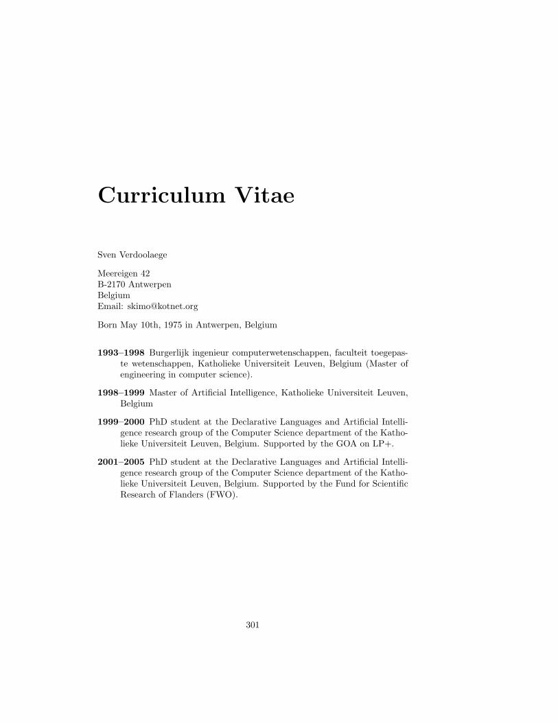
Curriculum Vitae
Sven Verdoolaege
Meereigen 42B-2170 AntwerpenBelgiumEmail: [email protected]
Born May 10th, 1975 in Antwerpen, Belgium
1993–1998 Burgerlijk ingenieur computerwetenschappen, faculteit toegepas-te wetenschappen, Katholieke Universiteit Leuven, Belgium (Master ofengineering in computer science).
1998–1999 Master of Artificial Intelligence, Katholieke Universiteit Leuven,Belgium
1999–2000 PhD student at the Declarative Languages and Artificial Intelli-gence research group of the Computer Science department of the Katho-lieke Universiteit Leuven, Belgium. Supported by the GOA on LP+.
2001–2005 PhD student at the Declarative Languages and Artificial Intelli-gence research group of the Computer Science department of the Katho-lieke Universiteit Leuven, Belgium. Supported by the Fund for ScientificResearch of Flanders (FWO).
301

302 Curriculum Vitae
Index
--disable-incremental, 160--enable-fractional, 245--use-fractional, 225
Abdelrahman, T., 42, 102, 288access function, 19accessed data set, 214Accessed Data Set (ADS), 226, 227,
231, 261active vertex, 125ada.pl, 26add
gen fun::, see gen fun::add
affine function, 12, 19piecewise, see piecewise affine
functionaffine hull, 8, 72Alekseevskaya, T. V., 116, 275algorithm
cutting plane, see cutting planealgorithm
Allen, J. R., 38, 275ALPHA, 18Amarasinghe, S., 36, 275Anantharaman, S., 209, 275Ancourt, C., 296Anderson, J., 275anti-dependence, 26apex, 9approximation theory, 4, 115Aragon, C. R., 225, 275arr, 244array contraction, 42array recovery, 177, 210Atomium, 35Aurenhammer, F., 143, 275
Avis, D., 13, 275
back substitutionsophisticated, see sophisticated
back substitutionBackward Reuse Distance (BRD),
55, 215, 216, 221, 224–226,261
Bagnara, R., 13, 275Balasa, F., 32, 209, 276, 279Banerjee, P., 285Barat, F., 292Barber, C. B., 13, 276barvinok, XIV, 106, 160, 225, 233,
243, 245, 248, 253, 255availability, 255
Barvinok, A., II, III, 4–6, 105, 106,109, 132–134, 137–139, 142,148, 153, 157, 158, 163, 165,172, 173, 180, 185, 193, 240,241, 276, 318, 321, 323, 325,329, 335, 337, 338, 341
barvinok count, 252, 255barvinok enumerate, 252, 256, 258barvinok enumerate e, 225, 252, 257barvinok enumerate ev, 252barvinok enumerate pip, 252barvinok series, 253, 258Basic Group (BG), 32Bastoul, C., 24, 36, 37, 94, 276, 283Beck, M., 4, 112, 113, 182, 207, 276,
277Bednara, M., 210, 277Bellman-Ford algorithm, 45Beyls, K., II, III, 5, 6, 55, 203–206,
208, 214, 217, 225, 233, 261,
303
304 Index
277, 289, 291, 294, 298,299, 323, 338
Bik, A. J. C., 93, 123, 188, 253, 277Blakley, G. R., 115, 277Boigelot, B., 16, 105, 207, 277, 295,
321, 335Bollella, G., 210, 277Bouchebaba, Y., 36, 38, 277Boulet, P., 14, 38, 42, 184, 191, 196,
207, 209, 277, 278, 323,338
Braberman, V., 210, 278Brion’s polarization trick, 142Brion’s Theorem, 139Brion, M., 138, 139, 142, 278Brockmeyer, E., 28, 32, 278, 279,
281, 285, 289, 290, 331Bruynooghe, M., 298, 299Bruynooghe, M., I, III, 5, 6, 291,
293, 294, 297–299Buck, R., 122, 278
cachedata, see data cacheinstruction, see instruction cache
cache analysis, 215cache line, 39cache simulator, 225Callahan, D., 275Carr, S., 38, 278carry, 39Catthoor, F., I, III, 5, 6, 28, 30, 31,
276, 278–285, 288–295, 297–299, 331
causality condition, 39Cavity Detection (CD), 55cdd, 13, 256cdd2polylib.pl, 256cell, 108chamber, 116chamber complex, 170, 179
of a parametric polytope, 120of a polytope projection, 120of a vector partition function,
116
Chapman, B., 18, 296Chatterjee, S., 15, 105, 207, 208,
279, 289, 321, 335Chen, S., 286Chernikova, 252Cholesky factorization, 225, 226, 234Choudhary, A. N., 285Christof, T., 13, 279Chunky Loop Generator (CLooG),
37circular reference, see reference, cir-
cularClauss, P., XXV, 4, 5, 105, 106,
112, 119, 121, 126, 129, 133,184, 185, 191, 200, 202, 205–209, 239–241, 243, 279, 288,318, 321, 323–325, 329, 335,337–339, 341
Cobham, A., 16, 279code generation, 36coeff, 250Cohen, A., 276Cohen, H., 150, 279Collard, J., 283common iteration space, 17, 24common refinement, 107commutative algebra, 4, 115complex
chamber, see chamber complexpolyhedral, see polyhedral com-
plexcompute evalue, 249compute poly, 249cone, 9
dependence, see dependence coneglobal dependence, 273polar, see polar conepolyhedral, see polyhedral coneself dependence, 97self dependence full, 97shifted, see shifted conesimplicial, see simplicial conesupporting, see supporting coneunimodular, see unimodular cone
cone::short vector, 151
Index 305
constituent, 111Constraint, 244, 255consumer, 18context, 251contraction
array, see array contractionconvex hull, 9, 22Cools, R., IV, 6, 294, 299Cormen, T. H., 45, 279Corporaal, H., 278, 289, 292, 293corrector polynomial, 116Cupak, M., 34, 279curve
moment, see moment curvecutting plane algorithm, 15
d, 244, 250D’Hollander, E., 55, 277, 289Dahmen, W., 115, 280Danckaert, K., II, 2, 3, 5, 16, 31,
38, 40, 43, 71, 79–82, 91–93, 98, 100, 237, 238, 279,280, 294, 298, 317–321, 324,328, 333–335, 339, 340
dark shadow, 202Darte, A., IV, 37, 41, 42, 45, 69,
102, 103, 277, 280, 281Dasygenis, M., 32, 281data cache, 215Data Transfer and Storage Explo-
ration (DTSE), 1, 2, 28,34, 36, 41, 92, 103, 239
decompose
decomposer::, see decomposer
::decompose
decomposer::decompose, 151decomposer::handle, 151Deconinck, G., 292degenerate, 96, 96, 268, 271, 273,
274degenerate domain, 203, 233degree
of a piecewise step-polynomial,131
of a step-polynomial, 131
Delaunay triangulation, 143, 144Demoen, B., IVDenecker, M., I, 293, 297dependence
anti-, see anti-dependencecarrying of, 39flow, see flow dependencegroup, see group dependenceoutput, see output dependencepseudo, 46, 47self, see self dependencetrue, see true dependenceuniform, see uniform dependence
dependence analysis, 15, 217dependence cone, 71, 95, 101
global, see global dependencecone
dependence direction vector, 59dependence distance vector, 21dependence domain, 20, 72, 73, 75,
100dependence function, 20, 72, 73, 75,
100dependence graph, 23, 44dependence polytope, 22, 38, 70,
72, 74, 101dependence relation, 19, 72, 74, 83,
100Deprettere, E., 281, 290, 292Derrien, S., 210, 281DESICS, IDevelin, M., 276De Greef, E., 33, 53, 279, 281de Jong, G., 291, 295De Loera, J. A., II–IV, 4, 5, 106,
133, 143, 148, 150, 157, 159,160, 206, 207, 239, 240, 276,281, 318, 321, 329, 335
De Man, H., 2, 276, 278–283, 288,290, 293, 295
De Mot, E., IDe Schreye, D., I, III, 293, 297Diaconis, P., 115, 281Diaz, R., 112, 282difference
306 Index
set, see set differenceDiguet, J. P., 31, 282, 295Dimension, 244dimension, 8
statement-level, see statement-level dimension
direction vector, 59distance vector, 21, 39
indirect, 97lexicographically minimal, see
lexicographically minimaldistance vector
translated, see translated dis-tance vector, 44
Dobkin, D. P., 276Domain, 220domain
degenerate, see degenerate do-main
iteration, see iteration domainpolyhedral, see polyhedral do-
mainvalidity, see validity domain
DomainConstraintSimplify, 253DomainDifference, 14, 182DomainIncludes, 253DomainSimplify, 14DTSE, 39Durinck, B., 281Dyer, M., 150, 282Dynamic Single Assignment (DSA),
18, 20, 24, 30
eadd, 248eadd partitions, 171Edelsbrunner, H., 122, 282edge
pseudo, 46, 271, 273–274eequal, 249Ehrhart polynomial, 112Ehrhart quasi-polynomial, 112Ehrhart series, 112, 206Ehrhart, E., 111, 119, 282Ellervee, P., 32, 282Ellmenreich, N., 36, 282
emask, 176emul, 248emul partitions, 176enode, 244–248Enumeration, 245, 247, 252enumerator, 109envelope
lower, see lower envelopeeor, 248equality
implicit, see implicit equalityesum, 179, 249Euler, L., 115, 282evalue, 244, 247–249, 252evalue combine, 200evalue frac2floor, 245, 249evalue range reduction, 199exclusion-inclusion principle, 221, 227explicit representation, 8, 13external representation, 8
Faber, P., 282face, 8
lower, see lower facefacet, 8
thick, see thick facetFalk, H., 34, 282Feautrier, P., 15, 18, 24, 30, 37–39,
92, 93, 102, 184, 191, 207,283, 319, 323, 330, 338
Ferrante, J., 208, 283fiber, 109finite state machine, 16Fischer, M. J., 14, 283flooring, 246, 249, 250flow dependence, 18, 25Fortune, S., 108, 283Fraboulet, A., IV, 42, 103, 283fractional, 246, 247, 249, 250fractional part, 197Franke, B., 30, 177, 205, 210, 283Franssen, F., 31, 278, 283, 290, 293frd.pl, 225Free Software Foundation, Inc., 284Froyen, L., IV
Index 307
Fukuda, K., 13, 256, 284function, 11
affine, see affine functiongenerating, see generating func-
tionindicator, see indicator functionpartition, see partition function
fundamental parallelepiped, 138, 149
g, 106g1, 181Gunz, R., 36, 282, 285Gallivan, K. A., 30, 177, 293Gangolli, A., 115, 281Gao, G. R., 42, 102, 284, 289Garbervetsky, D., 278Gawrilow, E., 13, 284Geigl, M., 19, 42, 284Gel′fand, I. M., 275gen fun, 251gen fun::add, 183, 251gen fun::operator evalue *, 183,
251generating function, 109
multiple, see multiple generat-ing function
of a sequence, 109of an integer set, 133rational, see rational generat-
ing functiongenerator, 9geometric series, 110, 135Ghez, C., 34, 282, 284Ghosh, S., 206, 208, 284Girbal, S., 276global dependence cone, 96, 96GMP, 206, 243Gomory, R. E., 16, 284Goossens, G., 281Gosling, J., 210, 277Goutis, C. E., 288Grunbaum, B., 142, 285Graham, R. L., 159, 284greatest common divisor (gcd), 93,
94
Griebl, M., 282group dependence, 19group reuse, 20Grotschel, M., 150, 285Gupta, R., 285Gupta, S., 34, 285Gomez, J. I., 38, 42, 284, 288, 297
Hadamard product, 172Halbwachs, N., 195, 285handle
decomposer::, see decomposer
::handle
Hanlon, P. J., 279Hannig, F., 277Hardy, G. H., 115, 285Haws, D., 281Heckman, G. J., 115, 285height, 144Heine, F., 209, 285Hemani, A., 282Hemmecke, R., 281Henrici, P., 159, 207, 285Hill, P. M., 275Hough transform, 37Hu, Q., 33, 41, 239, 285, 340Huard, G., 42, 45, 103, 280, 281,
283Huggins, P., 281Huhdanpaa, H., 276Huisken, J., 281hull
affine, see affine hullconvex, see convex hullpolyhedral, see polyhedral hullpositive, see positive hull
IMEC, I, IV, 1, 28, 34, 35, 98, 317,327
implicit equality, 7implicit representation, 8, 13, 110index, 303–316indicator function, 133, 172indirect self dependence, 44initial counting, 202
308 Index
input dependence, 24input size, 110instruction cache, 215Integer Linear Programming (ILP),
103integer projection, 11internal representation, 8interpolation
Vandermonde, see Vandermondeinterpolation
intersection, 172, 176Irigoin, F., 38, 285, 296Itanium, 36iteration domain, 16iteration space
common, see common iterationspace
iteration vector, 16, 37
Janssen, M., 278, 288Janssens, G., IV, 5, 291, 293, 294,
297, 298Jayapala, M., 292Jeannet, B., 13, 285Joswig, M., 13, 284
Kandemir, M. T., 102, 285Kannan, R., 150, 282Keimer, H., 282Kelly, W., 14, 18, 24, 26, 36, 92,
102, 205, 286, 319, 330Kennedy, K., 38, 42, 102, 275, 278,
286Kienhuis, B., IV, 281, 290, 292Kjeldsberg, P., 33, 279, 285, 286,
290Kjeldsberg, P. G., 285Klein, R., 143, 275Knuth, D. E., 284Kozen, D. C., 225, 286Kuck, D., 21, 286Kulkarni, C., 33, 279, 280, 287
Lobel, A., 13, 279Lam, M. S., 37, 38, 41, 83, 102, 275,
287, 295
Lamport, L., 93, 287LASH, XII, 16Latour, L., 16, 105, 207, 277, 287,
321, 335LattE, II, IV, 4, 115, 143, 160, 206,
207lattice
linearly bounded, see linearlybounded lattice
point, see point latticeLauwereins, R., 292Lebeck, A. R., 279Lee, C. W., 143, 287Leiserson, C. E., 279Lengauer, C., 93, 287Lenstra, A. K., 150, 287Lenstra, H. W., 287Lenstra, Lenstra and Lovasz’ basis
reduction algorithm (LLL),150–152, 154, 156
Leupers, R., 282lexicographical minimum, 13, 15lexicographical order, 13, 24, 38lexicographically minimal distance
vector, 44Li, Z., 38, 292Liao, S.-W., 287library
barvinok, see barvinok
Omega, see Omega
PIP, see PIP
PolyLib, see PolyLib
lifting, 144Lim, A. W., 37, 102, 287Lin, B., 295line, 10linear transformation, 38, 94linearly bounded lattice, 10Linearly Bounded Lattice (LBL), 11,
14, 38Lippens, P., 2, 287Lisonek, P., 258Lisper, B., 209, 287Liveris, N., 215, 288LLL, 151
Index 309
locality, 39, 39spatial, see spatial localitytemporal, see temporal local-
ityLoechner, V., III, XXV, 4, 5, 6, 14,
105, 106, 112, 119, 121, 124,126, 127, 133, 185, 191, 200,202, 205–210, 239–241, 243,245, 256, 279, 288, 291,294, 298, 318, 321, 323–325, 329, 335, 337–339, 341
long long, 220long 4D, 160lookup-table, 234loop alignment, 38loop coalescing, 93loop distribution, 38loop fusion, 33, 38, 41, 99loop interchange, 38loop interleaving, 38loop morphing, 38, 42loop reversal, 38loop shifting, 33, 41loop skewing, 38loop tiling, 38LoopGen, 36, 37LooPo, 36Lovasz, L., 285, 287lower envelope, 144lower face, 144lrs, 13
machinefinite state, see finite state ma-
chinemagic square, 4, 113Malik, S., 209, 284, 296Man, H. D., 293Manjikian, N., 42, 102, 288Manocha, D., 203, 288Manocha, H. L., 109, 292Marchal, P., 284, 288, 297Martonosi, M., 284Marwedel, P., 34, 282masking out, 172, 222
Maslov, V., 286mat ZZ, 250matlab, 210Matousek, J., 122, 288matrix
unimodular, see unimodular ma-trix
McAllister, T. B., 112, 288McKinley, K. S., 42, 102, 286Meisl, W., 282Meister, B., 207, 288Memory Compaction (MC), 53Memory Hierarchy Layer Assignment
(MHLA), 32Merchat, D., 285Micchelli, C. A., 115, 280Mignotte, A., 283Miller, E., 112, 288Minkowski’s First Theorem, 149Miranda, M., 34, 278, 282, 284, 285,
288moment curve, 158monomial substitution, 157morphing
loop, see loop morphingmulti-dimensional schedule, 38multiple generating function, 109multiple sequence, 109Muraoka, Y., 21, 286, 288
n, 250Nachtergaele, L., 278, 279, 283, 295NbBid, 244NbConstraints, 244NbEq, 244NbRays, 244new eadd, 248next, 244Nilsson, N. J., 102, 289Nookala, S. P. K., 14, 289Nootaert, B., 203, 289Note, S., 281NTL, II, 151, 250number
310 Index
regularity, see regularity num-ber
Number Decision Diagram (NDD),16, 221
O’Boyle, M., 30, 177, 205, 210, 283Olsen, R., 102, 284, 289Omega, XII, 11, 13–16, 36, 63, 64,
205, 208, 217, 218, 220–222, 224, 226, 227, 231, 232,286, 319, 323, 330, 339
Omega test, 189, 202Omnes, T., 32, 279, 289Open Research Compiler (ORC), 36operator evalue *
gen fun::, see gen fun::operator
evalue *
orderlexicographical, see lexicograph-
ical orderordering
valid, see valid orderingordering vector, 37orthogonalization, 28Out Of Memory (OOM), 227, 234outer wall, 170
pairreuse, see reuse pair
Palkovic, M., II, IV, 30, 41, 239,285, 289, 290, 324, 340
Pande, S., 209, 275Papadimitriou, C., 110, 289parallelepiped
fundamental, see fundamentalparallelepiped
parameter, 12Parametric Integer Programming (PIP),
15, 184, 191, 192, 207, 209,253, 338
parametric polytope, 12chamber complex, see chamber
complex of a parametric poly-tope
parametric relation, 12
parametric set, 12parametric vertex, 123ParamPolyhedron Reduce, 195Parent-Vigouroux, C., 285Pareto, 41Parker, E., 15, 105, 207, 279, 289,
321, 335partition, 246–250partition function, 115
vector, see vector partition func-tion
Patashnik, O., 284path
fundamental, 96, 97PER in SUIF (pers), 36, 37period, 111, 127periodic, 244, 245periodic number, 111, 127perparse.pl, 36Petit, 26, 36Pfeifle, J., 276piecewise affine function, 12piecewise step-polynomial, 131PIP, XII, 14–16, 222, 226, 227, 231–
233, 240, 319, 323–325, 330,339, 341
Pinuel, L., 284, 288, 297point
supporting, see supporting pointpoint lattice, 10pointer conversion, see array recov-
erypolar cone, 142polka, 13, 14polynomial
step-, see step-polynomialpolyhedral complex, 107polyhedral cone, 9polyhedral domain, 14Polyhedral Extraction Routine (PER),
35–37polyhedral hull, 10, 68Polyhedron, 243, 251, 253–255polyhedron
rational, see rational polyhedron
Index 311
valid ordering, see valid order-ing polyhedron
Polyhedron Enumerate, 252Polyhedron Image Enumerate, 185Polyhedron Polarize, 143, 253Polyhedron Project, 254PolyhedronIncludes, 253PolyLib, II, III, XI, 13–15, 64, 105,
127, 128, 143, 144, 181, 182,185, 195, 196, 202, 206, 225,232, 241, 243, 248, 249, 252,253, 255–257, 319, 325, 330,342
polymake, 13polynomial
corrector, see corrector poly-nomial
Ehrhart, see Ehrhart polyno-mial
polynomial, 244, 245, 250polynomial time complexity, 110polytope, 9
indirect distance vector, 97parametric, see parametric poly-
toperational, see rational polytope
polytope projectionchamber complex, see chamber
complex of a polytope pro-jection
Pommersheim, J., III, 4, 5, 106, 109,133, 134, 137, 139, 142, 143,153, 158, 163, 165, 172, 173,185, 276, 318, 321, 323, 329,335, 337
PORTA, 13pos, 244–246, 248positive hull, 9power, 250power series, 109PPL, 13, 14Presburger formula, 11, 15, 16, 214,
217, 221, 224Presburger set, 11, 14, 15Presburger, M., 11, 14, 289
principleexclusion-inclusion, see exclusion-
inclusion principleprint evalue, 249prism, 195producer, 18product
Hadamard, see Hadamard prod-uct
projected set, 10, 15, 217, 224projection
integer, see integer projectionproper triangulation, 108pseudo-dependence, 268pseudo-edge, 268Pugh, W., 4, 11, 15, 92, 102, 105,
189, 200–202, 209, 217, 286,289, 290, 318, 321, 329,335
qhull, 13quadratic constraint, 196quasi-polynomial
Ehrhart, see Ehrhart quasi-poly-nomial
quasi-polynomial, 111, 127Quillere, F., 36, 37, 81, 94, 290Quinton, P., 18, 290
Rabin, M. O., 14, 283Rajopadhye, S., 81, 290Ramanujam, J., 38, 285, 290Rambau, J., 120, 290random treap, 225rational generating function, 131,
224short, see short rational gener-
ating functionrational polyhedron, 7rational polytope, 8rational unimodular cone, 137Ray, 244ray, 8, 10red substitution
unsafe, see unsafe red substi-tution
312 Index
Redon, X., 14, 184, 191, 196, 207,209, 277, 278, 323, 338
reduce evalue, 198, 249Reduction of Arithmetic Cost of Ex-
pressions (RACE), 34reference
circular, see circular referencerefinement, 107regular triangulation, 143regularity, 40, 40regularity number, 70relation, 11
parametric, see parametric re-lation
relation, 246, 250representation
explicit, see explicit represen-tation
external, see external represen-tation
implicit, see implicit represen-tation
internal, see internal represen-tation
representation theory, 4, 115residue, 159restricted reuse pair, 221reuse
group, see group reuseself, see self reuse
reuse pair, 214restricted, see restricted reuse
pairRicci, E., 275Rijpkema, E., 210, 290Risset, T., 14, 277, 289Rivera, G., 38, 290Rivest, R. L., 279Robert, Y., 37, 102, 277, 280Robins, S., 4, 112, 113, 277, 282Rosser, E., 286Rydland, P., 33, 290
Samsom, H., 33, 283, 290Sarkar, V., 38, 283, 284, 290
schedule, 37, 94multi-dimensional, see multi-di-
mensional scheduleshifted-linear, see shifted-linear
schedulescheduling, 93
affine-by-statement, 37Schelkens, N., I, 291, 293, 297Schrijver, A., 8, 72, 110, 142, 149,
150, 267, 285, 291Schuler, F., 36, 291sda.pl, 24Seghir, R., III, 5, 6, 124, 185, 206,
248, 291, 294, 298, 325,341
Seidel, R. G., 225, 275selection, 172self dependence, 19, 44
indirect, see indirect self depen-dence
self reuse, 20, 20Semenov, A. L., 16, 291sequence, 109
multiple, see multiple sequenceSerebrenik, A., IVseries
Ehrhart, see Ehrhart seriesgeometric, see geometric series
setaccessed data, see accessed data
setparametric, see parametric setPresburger, see Presburger setprojected, see projected set
set difference, 176, 221shadow
dark, see dark shadowSharma, S., 276Shashidhar, K., 32, 34, 291shifted cone, 9shifted-linear schedule, 69short rational generating function,
131short rat, 250short vector
Index 313
cone::, see cone::short vector
Shoup, V., 151, 291Shpeisman, T., 286Silber, G.-A., 277, 280simplicial cone, 108, 116, 143simplify, 220, 227simulator
cache, see cache simulatorsize
input, see input sizesize, 244, 246Slock, P., 32, 291Slowik, A., 209, 285Song, Y., 38, 42, 103, 292sophisticated back substitution, 218,
227sort
topological, see topological sortSoudris, D., 281spatial locality, 39specialization, 157splinter, 202SPPoC, 14square
magic, see magic squareSrivastava, H. M., 109, 292Stanford University Intermediate For-
mat (SUIF), 36, 37Stanley, R. P., 111, 112, 115, 276,
292statement-level dimension, 24, 43,
59, 214statistics, 4, 115step-polynomial, 131
piecewise, see piecewise step-polynomial
Storage Bandwidth Optimization)(SBO), 32
Storage Cycle Budget Distribution(SCBD), 31, 32
stride, 132, 197, 246strongly connected component (SCC),
69, 77, 78Sturmfels, B., 112, 115, 116, 119,
281, 288, 292
subdivision, 108substitution
back, see back substitutionmonomial, see monomial sub-
stitutionred, see red substitution
SUIF Loop Generator (sloog), 37SUIF to C (s2c), 37summary
Chinese, 317–326Dutch, 327–342
summation, 177support, 107supporting cone, 139supporting point, 8
Tauzer, J., 281Teich, J., 277Temam, O., 276temporal locality, 39term, 251Thanailakis, A., 281Thekkath, R., 38, 284, 290thick facet, 185Thrash, W., 283time complexity, 110Tiny, 36Tiwari, V., 280topological sort, 51transformation
valid, see valid transformationtransitive closure, 45translated distance vector, 43translation
incremental, 46valid, see valid translation, 97,
98, 273treap
random, see random treaptriangularize cone, 144triangulation, 108
Delaunay, see Delaunay trian-gulation
proper, see proper triangula-tion
314 Index
regular, see regular triangula-tion
Triolet, R., 38, 285true dependence, 19Tseng, C.-W., 38, 275, 290Turjan, A., 203, 205, 210, 281, 292type, 244
uniform dependence, 40unimodular cone
rational, see rational unimod-ular cone
unimodular matrix, 38, 137, 253unimodular complete, 253union, 176, 248UNKNOWN, 217, 218, 226, 227unsafe red substitution, 219, 227Updating Singular Value Decompo-
sition (USVD), 55, 69, 80–82
valid ordering polyhedron, 94valid transformation, 39valid translation, 96validity domain, 121Value, 243, 249, 252van Engelen, R. A., 30, 177, 293van Meerbergen, J., 287van Meeuwen, T., 33, 293van Swaaij, M., 31, 37, 38, 40, 43,
70, 92, 93, 98, 293, 319,333
Vanbroekhoven, P., IV, 18, 30, 293Vandecappelle, A., IV, 278, 279, 284,
291Vandermonde interpolation, 202Vanhoof, J., 281Van Achteren, T., IV, 31, 279, 292Van Belleghem, K., IVan der Aa, T., 215, 292van der Werf, A., 287Van Eynde, F., I, 291, 293, 297Van Meerbergen, J., 281Van Nuffelen, B., IVan Oudheusden, K., IV
vec ZZ, 250vector
direction, see direction vectordistance, see distance vectoriteration, see iteration vectorordering, see ordering vector
vector partition function, 115, 207chamber complex, see chamber
complex of a vector parti-tion function
Verdoolaege, S., 5, 6, 58, 74, 75, 81,92, 96–98, 100, 132, 163,184, 185, 208, 233, 273, 284,288, 291, 293, 294, 297–299, 324, 325, 340, 341
Verhaegh, W., 287Verkest, D., 284vertex, 8
active, see active vertexparametric, see parametric ver-
texVivien, F., 102, 277, 280Vounckx, J., 289
Wust, A., 282wall
outer, see outer wallWang, C., 292Weispfenning, V., 14, 294Wetzel, S., 282WHIRL, 36, 37WHIRL Loop Generator (WLooG),
37WHIRL to Polyhedra (W2P), 36Wieninger, C., 282Wilde, D. K., 13, 14, 124, 127, 142,
243, 244, 288, 290, 295,319, 330
Wilkes, M., 1, 295, 317, 327Wolf, M. E., 38, 41, 83, 102, 287,
295Wolfe, M. J., 36, 38, 59, 295Wolper, P., 16, 295Wonnacott, D., 15, 217, 286, 290Woods, K., III, IV, 4, 6, 6, 106, 112,
Index 315
132, 157, 180, 185, 193, 197,221, 240, 241, 276, 288,294, 295, 299, 318, 323,325, 329, 338, 341
WRaP-IT, 36, 37Wright, E. M., 115, 285Wuytack, S., 2, 31, 32, 278, 279,
282, 291, 295
x.n, 244x.p, 244Xu, R., 292
Yang, Y., 76, 239, 296, 340Yang, Y.-Q., 22, 95, 296Yoshida, R., 4, 113, 115, 133, 160,
281, 296Yovine, S., 278
Zaffanella, E., 275Zelevinskiı, A. V., 275Zervas, N. D., 288Zhao, Y., 209, 296Zima, H., 18, 296Zissulescu, C., 281ZZ, 250

316 Index
LLL***¬¬¬¢¢¢###¦¦¦¦¦¦kkkjjjøøø\\\
jjj
1 ÓÓÓ
ÿ®ì¦?ûìX3¤Ý0XoÄê×Ä¢?ûì
(Wilkes 2000)ó*ø:°?ûìÄÞ>Q!°\Gê>èÞ>QÇIMEC÷êjâݦ?û (DTSE)0uÀ>?û?R'jZ?ûFÀ>\I"\¬¢#¦Çýý©\IøÇu"
õHbh½"u0ǽBkjrjø\ãÇjj¯~øÓä1ûý©\IÿXêj¦bó£Ï0Zj0Ç, u\Iûh
1.1 òòòµµµ¦¦¦ÄÄÄååå
LLL***¬¬¬¢¢¢###¦¦¦
DTSE0¥ÇZ½4~\¬¢#¦u°jâ?Ru¦Û\uÛ\u4é3jâãÜ'?R--å¬ÝÞå¬ÖBÇãÖ,?ó¬ÿ®ì£?ûìËÌ?ÇYø?ûìÞBÇb4¤Ý°*?R¦?R-å¬BÇ,1²Ã£Ä3?û~u?/jâÇ, >è?ûFu4é?R#FuLÝÞäuÇÙÛ\u4øêÛ\uZu1iǤÙÆÍìS$<jD¬¢#¦,Ça¥#¦ÇÇ1"& DTSE0¥ÇZ½êŵïO$Ça¦ÞLq¬¢#¦
Danckaert (2001)ñ0ä[ä6ÜnÜnǬ¢Ç³S~rju,+Ç?%¬¢#¦1#¦¬¢#rdzSø\u"Þc0ÜÇZ½ÄZ½Õ²Ç¬¢[,+o*nót3³S8-Z½Õû½³S8-#q~Z½ÝiÌD
317
318 L*¬¢#¦¦kjø\j
u"u#¦ZÌDÛ\u²##¦Danckaert (2001)Û Dê"u#¦?÷êugä)ïZÛ\)ïÂ,Ç
ý©ð©Ò4Û"u#¦? ÙÇZ½1""#¦Lu·¢Xyê²##¦"Þ,1Lqb4Ù~&Ç1"/û½q~ÇÒ;ê²##¦1ù"u#¦·¢¤D[hâ"u#¦?óth*Danckaert (2001)ñÂ,ÇXn\Y«G
kkkjjjøøø\\\jjj
|¢ìø\ãÇjuIÛ?®åǾ 3ÞC1.1Ä+Ç°× S1q'j³S#ÞÄHtrÇj
#SN = #
(i, j) ∈ Z2 | 1 ≤ i ≤ N ∧ 1 ≤ j ≤ i
$¥ N 4kjÞc;\¯Ò4
#SN =N(N + 1)
2
éb ÓÇ4d~kj@ä¯ ½b4é/b ÓÇkj4ûój¦°?óYøø\j¯Ç¾à0jÇj
HÏÄÊÄk Pugh (1994)Ý Clauss¦ Loechner (1998)buûø\j¯b4Vtø¤",ÇV?ó-ì¦R¯Barvinok ¦ Pommersheim (1999) ñêÇHj?Barvinok¦Woods (2003)j0êjtøéj" (De Loera| 2003a)7ÿ®óÇIÛ¦°B\Iø\j¯Ç é$HÏÄÊXYç,+
ý©\IÿXêûÇ, óûkjõÁj¯¥"Barvinok¦ Pommersheim (1999)ñ®
1.2 ;;;
ÁÿXê[ä6ÜnL*¬¢#¦0kjø\jZjó¼~嬮Þa~
2 [[[äää666ÜÜÜnnn
[ä6Ün~uIÛ?#¦Ç°õ¬¢,+ǰȪé X Ĭ¢³Srj5ÞȬ¢)#ÞÄ5ÞÄø\w)³S SX¥¬¢Þ4Þ)#Þ¦kj5ó\ÇÞcø\3kjõÁÇý"u0ǽB®jø\rjJõ
3. L*¬¢#¦ 319
Áÿ®?ø\0"ZHzõõÁàw)ºõÁ°rj=kÁ=ø
øê³S1iÇ[ä6ÜnÝ9ܳS-jâ##øδX,Y 4ܳSè SX × SY øøÇã,+ªé³S"ªé³SÇ?½Bê#³S-thq~UÖjâ#Á#Þc#ø~=øu,+#å¬5Þ d = j − iÄ#õÁ DP X,Y ½B
DP X,Y = convd ∈ Zd | ∃(i, j) ∈ δX,Y : d = j − i
#CÝVÍõªéÄÖ#C#a#øÄ
óìJ<Y·¢²³SÝ\³S8-)Ä~Ò4LÇ*ó!X+)°5Þ iB5Þ jÇ5Þ iBj3ÇÆu~
õÿ®õÁ¦Ù#ø\Óä·¢&~ PolyLib (Wilde 1993)u®kjõÁkjºÇ&~ Omega (Kelly| 1996c)uÿ®=ø?&~ PIP (Feautrier| 2002)u®!B
3 LLL***¬¬¬¢¢¢###¦¦¦
3.1 555óó󬬬¢¢¢###¦¦¦
êq¬¢#¦Ç·¢&~[ä6Ün$Ç·¢OÁ³S¦#øÄÜnÇ1ù#¦ÊâÜnOéaÇ·¢\If~.Óäu"
·¢D5ó¬¢#¦Ç=ý·¢~5ó#¦²³Snót3³S8-¦éǪé X dzS#Þ i4~35ó#¦
AX : i 7→ AX(i) = AX i + aX
nóá3³S8-¥q~Ò4¦$#'Çvan Swaaij(1992)Z Danckaert (2001)FóÙÇZ½°ZÇá3~#Þ π$#Þ²³Snót"u-¶
5ó¬¢#¦®Ýiû½Ä"u#¦Ýj AX Z½Zû½Ä²#5
Þ aX Z½YÜÇZ½aD!#¦thu¦uh%hÄ#ún\Ç=ý#¦Äå¬5ÞÑL 0ÇÇ#¦bú½Bthéu ÓDz##¦ÌDÛ\uÇ "u#¦ÌDu
320 L*¬¢#¦¦kjø\j
3.2 ¬¬¬¢¢¢\\\???
¯l²##¦Z½ó"u#¦Z½bqÇb·¢¤4ÿX²##¦ÇOÇR!"u#¦Çý#C°JSÝÄÃ,:zÄå¬5ÞÑaL 0êLq²##¦Ç46Þ® 3.1'³S²#C°ÜÇ\?ó#éå¬O²##¦û½³Sóá3³S8-°#é ÇÄ1Ç"¬¢\?ù¬¢²#
ê&~£®Ç'³S²Ë##ø#jâ!õÜÇ\?óå#éå¬thGã!B 56– 57ÞC 3.15–C3.17,+Þc£®óÛ\u¦?ûF0ÁÛP*
3.3 """uuu###¦¦¦
ztth"u#¦ßIG4ây¦#SÝ°##¦Ýj>
qw 66Þ½® 3.4.3½Góq®ÇX&~#øýüÇÞc½®½;,+o*w
·¢²#õÁj~)ugä)ïó®.<YÇÄ#å¬5Þ#?%jÖ %jÖ°Ç#å¬5Þ-#IÒÖ°÷#ø½B
δpc =
(x,y) ∈ Q2d | Gxx + Gyy = g ∧ Fxx + Fyy ≥ fÇ
72Þ½® 3.4.4Ç~ Ap ¦ Ac#¦éa#õÁj
rd(Ap, Ac) = rank
[−Ap Ac
Gx Gy
]
− rank[Gx Gy
]
74Þ½® 3.4.5Ç,Ä"u#¦¥Äzt!j
Rd := minAp,Ac ,
rd(Ap, Ac) = d − min
(
rank
[Gcl
Gl
]
, rank
[Gcr
Gr
])
Ù¥
Gx =
Gcl
Gl
0
¦ Gy =
Gcl
0Gl
¥jâ#,+o*# DD ¦#<j DF (x) = Dx + d0 ÄÇ®*;
rd(Ap, Ac) = rank
[Ac − ApD
G′
]
− rankG′ ¦ Rd = d − rank
[DG′
]
Ù¥G′,+ DD ¥*Þc rdÛê Danckaert (2001)Ä~gä)ïÇý rK = rank(Ac − ApD)
4. kjø\j 321
Danckaert (2001)÷èÂ,ÇúÛê82Þ, 3.3 ,+[Ûk/Â,ǥijSÇj·¢¤÷êiÜÇÂ,ÇÇ¢X,1/~Çb4èÂ,ÇH
Êâ.Û\ugä)ïÇ·¢ÄXÕa²,:u8ó¬¢*óû½"u#¦DuXDÛ\uÇÒztÆ!*
3.4 ~~~
Danckaert (2001)ÉñêÜÇ~Z½,QuÇiZ½Ì>èìÝÇOÇ&zóÇZ½°&~Í;\S$<jÄ,ÇÇ&YÇ0K/.X7~Ä0bÜÇÕÇóä~Z½0°Ç¬¢#¦,1~õ0*u,+ÖÇY«0ã[S$<j&~ÇbÒ&P*1ztÇ?%¦½Ï#'4ÕÇ&ìÝÿ~Xh½&L²##¦/1q
4 kkkjjjøøø\\\jjj
4.1 ÓÓÓ
õbìJÔGÇjǾÇq¥ÄÖjâÇjY«j¯~"u0ÇuÃcqro*
cS(p) = #Sp = #
x ∈ Zd | ∃y ∈ Zd′ : Ax + Dy + Bp + c ≥ 0
Ù¥ x ∈ Zd ,+RjÔGÇp ∈ Zn ,+ÇjÄ"kjÇy ∈ Zd′ ,
+i?óÞ##Þh d′ = 0ÇÞc¯ÕkjõÁj.®ù"1ûY«¯ (Clauss¦ Loechner 1998)Çb4ý& dû½Ç®! <Y-ìÝÅjo*LéJ¯Ç"ÃÓ*!£ 1!çÕÄå)äúj (Boigelot¦Latour 2004; Parker¦ Chatterjee 2004)7ÿ®Ãkj¯ (n = 0)Ç?! <Y-ìÝ4jo*Pugh (1994)ÃU7ÿ®¯/~®Çb%4®tø¤",Ç?%! <Y-ìÝ4jo*
ý©1\IÉñê Barvinok¦ Pommersheim (1999)®[7~ûkjõÁj¯"Ç1ù1 Clauss¦ Loechner (1998)Z De Loera| (2004)ÏÄ)äú®Ûj*,1~Ü«o*u,+"÷j4û½ÇÜ«,+o*®-ìÝÑQj jõ1*ý©ÿXêÜ«,+o*ìJä®Zéÿ®=øjß
322 L*¬¢#¦¦kjø\j
4.2 ÜÜÜ«««,,,+++ooo***
kjõÁj*,1~Ü«o*u,+Ç=ý<j c : Zn → QZ
ÙÄ<j C<j c#Þ4kjÖ<j#aõÁ°rjãÇj<j cÄ<j C : Cn → C#aÇó Cn :8øBÑ
b¸ÿjÇ*C(x) =
∑
s∈Zn
c(s)xs
ÕÕ¦X3<j#X3b¸ÿj,BÑ3Ä<jÇb4Ç¢óX3 Cn øBÑ
·¢ä&~,+o*4Á½B®Ä<j¦Iã~×õ1*®Ä<j½B
C(x) =∑
i∈I
αixpi
(1 − xbi1)(1 − xbi2) · · · (1 − xbiki )
Ù¥ x ∈ Cn, αi ∈ QÇpi ∈ ZnÇbij ∈ Zn \ 0Iã~×õ1*½BõÁKÄIw)?IóÇ\IÞIã~×õ1*½B
g(s) =m∑
j=1
αj
dj∏
k=1
⌊〈ajk, s〉 + bjk⌋
Ù¥ αj ∈ QÇajk ∈ QnÇbjk ∈ Q
¥²rjø\Äkjø\Ç<j<jkjaø\'j(0Ý 1)#aÄ<jÒw)ø\Ä<j
4.3 Barvinok®®®
iÇBarvinokñõÁj®®ñõÁÄ<jÇlFÄ<jó 1Ä1YøztõÁjÇ4O<jÄ<j¥1jÇ?%1#aõÁ°r
ê®õÁÄ<jÇa²ÇIÄ4UñÙÄ<jÄID²õÁÄ<jUÄ3ºzþ§²ÁoÄõÁ@éÄ<j
®bFZl²ÇõÁ@éUÄîÜ@éQnRFZîÜ@éÄ<j4UñÇOîÜ@é°½B,,+ĽZîÜ@éÄó""u\ZjÞcîÜI4 Barvinok®!Z½Ç?&rÇ®! <Y-ìÝõ1*
Fó 1ÇO4®Ä<j¥Ä1ôb4ÇX4rÇ®Ä<jôO$ÄF<j,1®Äó x = 1ÿbÿj1$·¢j0ê.®®²FõÃÿj1¯ÕtFÃÿj1¯j0®ãq\IF?LFVã®®Ä<j¥Ç11
5. ¼~嬮 323
ê®kjõÁjIã~×õ1*,+o*Ç&~ Clauss ¦Loechner (1998)ñ®u®kj?IóÇ\IÞkjõÁû½kjºlóÇ\IÞ² Barvinok®a~kjºBarvinok¦ Pommersheim (1999)tõÁIÇb-ûÒê®kjõÁj®Ä<j,+o*Ça²kjõÁÄ n + d8-°õÁÇlF#aÄ<j¥ d#Þ\I
4.4 äää®®®
Iã~×õ1*¦®Ä<jÜ«,+o*7qä®Ç¾Æ)ïø\ä®1ùóìKÞqä®Ça/Õ?Iã~×õ1*õÁIä®4ǾéIã~×õ1* ÓÇÆ/;\Öbé®Ä<j ÓÇÆ¥j',uÇé®Ä<j ÓÇêqóìKÞÇa~\IFÖbéIã~×õ1* ÓÇ䮥j·¢yÒêIã~×õ1*Z®Ä<jÜ«,+o*,óõ1*-##¦
4.5 ===kkk
ó$Ç·¢ëÇIã~×õ1*=øj0Ç0Clauss (1996)ñÙ! <Y-ìÝõ1*Çb7ú=ó>V#Þ<YÇ0Êâ;\½=óu>V#ÞÙ)L%Ù! <Y-ìݤõ1*Çb4ÇX,1/~·¢Hb¥j¯eÑ,1~YÇ0uû®Ç0ä Boulet¦ Redon (1998a)ñ0Æ¢0/~Çb4Ù! <Y-ìÝjo*Æ¢0~ PIP (Feautrier 1988)²=øj¯ÕtõÁj¯Çl~ Clauss¦ Loechner (1998)®uûÕ¯·¢~" Barvinok®"¦®ÇÒztÇ"ÞH0!Ç0² Barvinok¦Woods (2003)ñ®Ä<jõ1*u®Z·¢ñõ1*u#¦®\óåBarvinok ¦Woods (2003)ñ®tø¤",
5 ¼¼¼~~~åå嬬¬®®®
¼~å¬4éjâ?RÛ\uÝÞÇ~uÜ°¤¥?qìJ0Á¼~å¬ïh®,1)4·¢jEÇUa~
·¢Ë Beyls (2004)øuÃc¼~å¬0ÇÇb4·¢²Ça~¥?"X 1°¤¥?óY«<YÇ~.ÓäÃ/4 OmegaÄ,¼~å¬0ÇztRjø\Ò1"hêø\X!ä®1Ç·¢÷êc01"¦Þ½ä®óÞc0¥Ç7
324 L*¬¢#¦¦kjø\j
ÿ®·¢.®ñ¼~å¬Ä¾Çb4éǾÇÑ?ó7ÿ®0
é~Þc0ztø\jAèy"êÁzñXé²=øj¯ÕtõÁj¯ ÓÇ;\½¦ PIP&~YÜ«03
ø*#é Clauss¦ Loechner (1998)®"Ç·¢jEêûøÄj¯j*thuúÕÁÜX"ê
6 XXX
6.1 LLL***¬¬¬¢¢¢###¦¦¦
¦¦¦ààà
ý©ð©4ZÛ?j0 Danckaert (2001) ñ\¬¢#¦00Ýi8ù~8Ýi"u#¦ù²##¦Danckaert(2001)ÌDê"u#¦Ç, ztêugä)ïZÛ\)ïÂ,Çb4Â,ÇXD#¦h½u
·¢yÒê²##¦,1Lqñ¥Ù"u#¦ãth*?óÇL*²##¦hâóÙZ½¥¤?óthá3~#Þb4~Xh½&²##¦1qÇ?%ÇXã&~°hS$<jO~#Äu]t*ÇÄ1·¢V«ê~Z½Ç?~/û½~¦V«ê~Z½Ç²##¦l,1LqÇ?%óY«<Y²##¦"¬¢\?ù¬¢²#~;\£®·¢óÛ\u¦?ûF0Á.²ztÛP*
é"u#¦ ÓÇ·¢Ûê Danckaert (2001)ñugä)ï1ù#Â,ÇÛÂ,Çó>è-°ÍP*·¢:êÞcgä)ï¦.#ä6ø$iÇ·¢MsêÇ,+Äzt!Ú*O$ÇX~qAÞÂuztYÇfåê·¢¤&*7aÍP#IÛU%Ç %Dêthu¦Û\u
X©ÕVerdoolaege | (2001a), Verdoolaege | (2002), Verdoolaege |(2003b), Verdoolaege| (2003a)
uuuÓÓÓ***000
¯l·¢L*¬¢#¦®ø4ã&~ÍìS$<jÇb4·¢&~êv;\£®óuÓ*¥Ç·¢aj0&~S$<jPalkovic (2002)Z| (2004a).²DêYǯ¬¢#¦,Ça¥XW!ÇÇ1"& DTSE0¥ÇZ½êŵï
6. X 325
¯l·¢ó®XÞDêthu¦Û\uÇb÷Â,ÇDêuÂ,Ç"½jâ#,+o*#¦#<jIJÂ,Çj0tthuÛ\u1ù#øÒ4ø¦uÓ*ø (í2005)
6.2 kkkjjjøøø\\\jjj
¦¦¦ààà
ý©Éñê Barvinok®a~kjõÁD¾"Ç?éÿ®kjõÁ°rj=kqêjß"ú~¼~嬮"èX"
®kjõÁjIã~×õ1*¦®Ä<jYÜ«,+o*,ó
õ1*-®ñIã~×õ1*®"è,ÒÇ·¢jE®¤ÝîÇkjõÁj"¤ÝOzõ."! <Y-ìÝÅjo*LÇO"¥&~,+o*Åjo*Li®Ä<j Barvinok®"7® EhrhartÿjYǾ
·¢yÒêIã~×õ1*Z®Ä<jÜ«,+o*,óõ1*-
##¦²ÇZ.®Ä<jõ1*u®\óåÇÒzt1Iã~×õ1*õ1*u®Þc®Ä<j®tøe",O$Ç·¢¤ÉñêÜ«,ØS0Ç¢I/~;\½Z PIPu²=øj¯ÕtõÁj¯¯lÇ0X,1/~Ç?%Ç0! <Y-ìÝjo*Çb4"ÞYÜÇ0ÑHÇ %*#3
~.Óä,¼~å¬0ÇztRjø\úy"1"hêø\X!ä®1Ç·¢÷ê¥ØS0¯lǾÇÑ?ó7ÿ®0Çb4Ç04ÙÆ0H!ÄÕ,+ø\X,X4h
X©ÕVerdoolaege| (2004b), Seghir| (2004), Verdoolaege| (2004d),Verdoolaege| (2005a), Verdoolaege| (2005b)
uuuÓÓÓ***000
·¢"è&~êIã~×õ1*,+0óuÓ*¥Ç·¢aéIã~×õ1*¦®Ä<ja~*vóY0ÁÇBarvinok¦Woods (2003)ñ®Ä<jõ1*u=k®"Ó*RÌ:U
¯l Clauss¦ Loechner (1998)ñ®?I®4õ1*uÇå̤4?óiaÏÄX~HõÁEu¦ PolyLibÇ?%aZ;Iã~×õ1*

326 L*¬¢#¦¦kjø\j
!Çé:"u0ǽBkjrjø\jRÄáZLÏÄ|ÊL4
Incrementele
Lustransformaties en
Enumeratie van
Parametrische
Verzamelingen
1 Inleiding
De exponentiele groei van processorsnelheden zonder een evenredige versnel-ling van de toegangstijden tot de achtergrondgeheugens heeft geleid tot eengroeiende “geheugenbarriere” (Wilkes 2000). In ingebedde systemen is het ge-heugen ook het onderdeel geworden met het hoogste vermogenverbruik. Demethodologie voor de exploratie van gegevensoverdracht en -opslag (DTSE)werd ontwikkeld op IMEC om dit vermogenverbruik te verminderen door hetaantal geheugentoegangen en de totale geheugenvereisten te optimaliseren. Eendeel van deze vermindering wordt bekomen door middel van globale lustrans-formaties, het onderwerp van het eerste deel van deze thesis.
Vele optimalisatietechnieken tijdens het compilatieproces vergen de enumeratievan parametrische gehele verzamelingen gedefinieerd door lineaire vergelijkin-gen. Bestaande hulpmiddelen kunnen veel van die problemen niet oplossen. Hettweede deel van de thesis bespreekt een implementatie en verdere uitbreidingvan recente wiskundige technieken die zorgen voor een serieuze verbetering.
327
328 Nederlandse Samenvatting
1.1 Achtergrond en Motivatie
Incrementele Lustransformaties
Een belangrijk deel van de DTSE methodologie bestaat uit de verbeteringvan de regelmaat en de lokaliteit van datatoegangen met behulp van globalelustransformaties. Lokaliteit is een maat voor de afstand in tijd tussen tweetoegangen tot hetzelfde data-element. Bij een korte afstand is de kans grootdat het element zich nog bevindt in een geheugen dicht bij de processor datkleiner en sneller is. Een korte afstand tussen eerste en laatste toegang laattoe om geheugen te hergebruiken voor andere gegevens en vermindert de totalegeheugenvereiste. Regelmaat meet de uniformiteit van toegangsafhankelijkhe-den. Een goede regelmaat helpt bij het optimaliseren van de lokaliteit. Naastlokaliteit en regulariteit dienen ook andere, meer ingewikkelde, kostfunctiesbeschouwd te worden en het resultaat is best niet een enkel getransformeerdprogramma, maar meerdere getransformeerde programma’s die in de volgendestappen van de DTSE methodologie verder geevalueerd kunnen worden. Hetis dan ook belangrijk om de lustransformaties zoveel mogelijk incrementeel uitte voeren.
De methode voorgesteld door Danckaert (2001) is gebaseerd op een geometrischmodel waarin elke iteratie van een lus voorgesteld wordt door een geheel punten een lus getransformeerd wordt door de verzameling van alle iteraties van eenlus als een geheel te manipuleren. Ze bestaat uit een stap die de geometrischevoorstelling van elke lus afbeeldt op een gemeenschappelijke iteratieruimte eneen stap die een uitvoeringsvolgorde bepaalt in deze ruimte. De eerste stap isverder onderverdeeld in een lineaire transformatie gericht op de regelmaat eneen translatie gericht op de lokaliteit. Danckaert (2001) richt zich voorname-lijk op de lineaire transformatie en ontwikkelt een regelmaatscriterium en eenzoekprocedure die dit criterium lokaal optimaliseert.
De oorspronkelijke opzet van deze thesis was het verfijnen van de bestaandelineaire transformatie en het ontwikkelen van de andere stappen zodanig dat eenincrementele toepassing mogelijk is. We hebben aangetoond dat het inderdaadmogelijk is om de translatie incrementeel uit te voeren, maar dat die sterkbemoeilijkt wordt door de daaropvolgende ordeningsstap. Door de ordening opvoorhand vast te leggen, wordt de translatie, en in mindere mate ook de lineairetransformatie, vereenvoudigd. We beschouwen ook hoe we kunnen verzekerendat een geldige oplossing bestaat na de lineaire transformatie. Aan deze vereistewordt niet voldaan door de zoekprocedure van Danckaert (2001).
Enumeratie van Parametrische Verzamelingen
Het tellen van het aantal objecten dat voldoet aan bepaalde kenmerken is eenessentiele stap van vele technieken voor het analyseren en optimaliseren vanprogramma’s. Stel bij voorbeeld dat we willen tellen hoeveel keer opdracht S1
2. Geometrisch Model 329
in het programma in Figuur 1.1 op bladzijde 3 uitgevoerd wordt, waarbij Neen parameter is. Dit probleem kan geformuleerd worden als de enumeratievan de verzameling van waarden die iteratoren doorlopen tijdens te uitvoeringvan het programma, i.e.,
#SN = #
(i, j) ∈ Z2 | 1 ≤ i ≤ N ∧ 1 ≤ j ≤ i
.
Voor dit eenvoudige voorbeeld is de oplossing evident,
#SN =N(N + 1)
2.
Voor sommige technieken hangt het gebruik van parameters (zoals N in hetvoorbeeld) af van het probleem, terwijl bij andere technieken het tellen in-trinsiek parametrisch is. Ook in de wiskundegemeenschap komen dergelijktelproblemen voor, e.g., het tellen van het aantal magische vierkanten.
In de compilergemeenschap worden meestal de technieken van Pugh (1994) ofClauss en Loechner (1998) aangehaald voor het oplossen van telproblemen. Deeerste is echter voor zover bekend nog nooit geımplementeerd en de laatsteis onderhevig aan tijdscomplexiteits- en degeneratieproblemen. Een efficienteteltechniek werd voorgesteld door Barvinok en Pommersheim (1999) en verderuitgebreid door Barvinok en Woods (2003). De tot dusver enige gekende im-plementatie van deze techniek door De Loera e.a. (2003a) is enkel geschikt vooreen kleine subklasse van de telproblemen die voorkomen in de analyse en opti-malisatie van programma’s Bovendien is de vorm waarin de oplossing gegevenwordt, onvertrouwd en lijkt ze niet geschikt voor de compilergemeenschap.
In het tweede deel van deze thesis bespreken we de nodige details voor eenpraktische implementatie van het algoritme van Barvinok en Pommersheim(1999), toegepast op algemene parametrische telproblemen.
1.2 Overzicht
In de rest van deze samenvatting bespreken we achtereenvolgens het geome-trisch model, de methodologie voor incrementele lustransformaties, de enume-ratie van parametrische verzamelingen en een toepassing van deze enumeratieop het berekenen van hergebruiksafstanden.
2 Geometrisch Model
Het geometrisch model wordt veelvuldig gebruikt voor het voorstellen en mani-puleren van lusnesten in programma’s. Aan elke opdracht X in het programmawordt een verzameling SX van gehele vectoren verbonden, waarbij elke vector
330 Nederlandse Samenvatting
overeenkomt met een uitvoering van de opdracht en bestaat uit de waardenvan de iteratoren van omliggende lussen voor die bepaalde uitvoering. Eendergelijke verzameling wordt een iteratiedomein genoemd. Indien de onder- enbovengrenzen van de lussen affiene combinaties zijn van de omliggende lusite-ratoren en mogelijke parameters, dan komt zo’n verzameling overeen met degehele punten in een (parametrische) polytoop, waarbij een polytoop een verza-meling (rationale) getallen is, begrensd door lineaire vergelijkingen. Dergelijkepolytopen zijn eenvoudiger en efficienter te manipuleren dan willekeurige verza-melingen. De uiterste punten van een polytoop worden vertices genoemd. Bijuitbreiding beschouwen we ook projecties van de gehele punten in een polytoop,hetgeen we geprojecteerde verzamelingen noemen.
Naast iteratiedomeinen worden er in het geometrische model ook afhankelijk-heden tussen iteratiedomeinen voorgesteld. Een afhankelijkheidsrelatie δX,Y
is een deelverzameling van het Cartesisch product van twee iteratiedomeinenSX × SY , waarbij elk element van de relatie uitdrukt dat de overeenkomstigeiteratie uit het tweede domein afhangt van de overeenkomstige iteratie uit heteerste domein. Elke afhankelijkheidsrelatie legt een (partiele) orde op aan deiteraties. We spreken van een echte afhankelijkheid als de iteratie uit het tweededomein een gegeven nodig heeft dat berekend wordt in de iteratie van het eer-ste domein. Dergelijke afhankelijkheidsrelaties kunnen ook voorgesteld wordendoor polytopen of geprojecteerde verzamelingen. Aan elke afhankelijkheidsre-latie δX,Y verbinden we ook een afhankelijkheidspolytoop DPX,Y , gedefinieerdals
DPX,Y = convd ∈ Zd | ∃(i, j) ∈ δX,Y : d = j − i
,
de verzameling van alle afstandsvectoren d = j − i. De afhankelijkheidsgraafheeft als knopen een of meerdere opdrachten en heeft een boog tussen tweeknopen indien er een niet-lege afhankelijkheidsrelatie bestaat tussen opdrachtenin de twee knopen.
Het is soms nodig om een volgorde op te leggen aan de elementen van een itera-tiedomein of een hele iteratieruimte. We beschouwen meestal de lexicografischevolgorde, waarbij een vector als kleiner dan een andere wordt beschouwd alsop de eerste positie waar de twee vectoren van elkaar verschillen bij de eerstevector een kleiner getal staat. De lexicografische volgorde komt overeen met devolgorde in het gemodelleerde programma.
Er bestaan vele hulpmiddelen voor het manipuleren van polytopen en gere-lateerde verzamelingen. Voor het berekenen van de (parametrische) verticesvan polytopen gebruiken we PolyLib (Wilde 1993); voor het manipuleren vangeprojecteerde verzamelingen gebruiken we Omega (Kelly e.a. 1996c); en voorhet berekenen van het lexicografisch minimum van parametrische polytopengebruiken we PIP (Feautrier e.a. 2002).
3. Incrementele Lustransformaties 331
3 Incrementele Lustransformaties
3.1 De DTSE methodologie
De DTSE methodologie wordt in detail beschreven door Catthoor e.a. (1998b)en Catthoor e.a. (2002). Hier wordt een korte samenvatting gegeven van dehoofdstappen geıllustreerd in Figuur 3.1.
Het startpunt is een uitvoerbare specificatie van de toepassing (bvb. C code)met toegangen tot multidimensionale gegevens. Het eindpunt is een getrans-formeerde specificatie, mogelijk gecombineerd met een (partiele) netlist vangeheugens als gedeeltelijk-op-maat-gemaakte geheugenarchitecturen het eind-doel zijn. Voor instructie-set processoren wordt de getransformeerde broncodeals invoer gebruikt voor de softwarecompilatie stap. De methodologie is geba-seerd op het idee van orthogonalisatie (Catthoor en Brockmeyer 2000), waarbijin iedere stap een probleem wordt opgelost op een bepaald abstractieniveau.
De eerste stappen zijn platformonafhankelijk. Ze optimaliseren in het algemeende regelmaat en lokaliteit van de gegevenstoegangen en maken de mogelijkhedentot gegevenshergebruik expliciet. De daaropvolgende stappen zijn platformaf-hankelijk. De fysieke eigenschappen van het platform worden nu in rekeninggebracht en de gegevensoverdracht wordt op een kostverlagende manier afge-beeld op het platform.
We beschrijven nu zeer kort de functionaliteit van elk van de hoofdstappen inde DTSE methodologie.
Platformonafhankelijke stappen
1. Voorbereidende bewerkingenDeze stap bereidt de code voor op de eigenlijke DTSE optimalisaties.De code wordt geherstructureerd zodanig dat het gedeelte relevant voorDTSE optimalisaties geısoleerd wordt. Ze wordt in een zodanige vormgegoten dat globale transformaties voor de optimalisatie van de gegevens-overdracht op een eenvoudige manier toegepast kunnen worden.
2. Globale gegevensstroomtransformatiesDeze stap bestaat uit twee categorieen van transformaties. Een eerstecategorie verwijdert overbodige gegevenstoegangen en verkleint de tijde-lijke buffergroottes. Gegevenshergebruik wordt dan enkel toegepast opde overblijvende, noodzakelijke gegevenstoegangen. De tweede catego-rie vermindert de flessenhalzen die de toepassing van lustransformatiesverhinderen.
3. Globale lustransformatiesHet doel van de lustransformaties is de globale levensduur van de signalen
332 Nederlandse Samenvatting
in te korten en de lokaliteit en regelmaat van de gegevenstoegangen teverhogen. Deze stap is het onderwerp van dit deel van de thesis.
4. Exploratie van gegevenshergebruikHet doel van de exploratie van gegevenshergebruik is het invoeren vaneen hierarchische geheugenorganisatie die optimaal gebruik maakt vande tijdslokaliteit in de gegevenstoegangen, geıntroduceerd door de voor-gaande lustransformatiestap, om gegevens die frequent gelezen worden tekunnen lezen uit kleinere en snellere geheugens die ook minder energieverbruiken.
Platformafhankelijke stappen
1. Opslag-tijdsbudget-verdeling (SCBD)Tijdens geheugenhierarchie-niveau-toekenning (MHLA) worden de kopiesvan gegevenshergebruik en de daarbij horende gegevensoverdracht ver-deeld over de verschillende niveaus in de geheugenhierarchie. Hierbijwordt rekening gehouden met de beschikbare bandbreedte en een hoog-niveau schatting van de geheugengrootte. Tijdens opslagbandbreedte-op-timalisatie (SBO) wordt bepaald welke gegevens simultaan toegankelijkmoeten worden gemaakt in de geheugenarchitectuur om aan de reele-tijdsbeperkingen te voldoen met een minimale geheugenkost.
2. Geheugenreservering en -toekenning (MAA)Het doel van de geheugenreservering en -toekenningstap is het bepalenvan een optimale geheugenarchitectuur voor de gegevens. Deze stap be-paalt zowel het aantal en het type van de geheugens in de geheugenar-chitectuur als de toekenning van signalen aan de diverse geheugens.
3. In-plaats-optimalisatieHet doel van de in-plaats-optimalisatiestap is het vinden van een opti-male plaatsing voor de gegevens in hun geheugens zo dat de benodigdegeheugenruimte zo klein mogelijk is.
3.2 Affiene Lustransformaties
We voeren lustransformaties uit op een programma door het manipuleren vanhet overeenkomstige geometrische model. Hiertoe moet eerst een geometrischmodel opgesteld worden bestaande uit iteratieruimten en afhankelijkheden enna transformatie moet het model terug omgezet worden naar een programma.We maken hiervoor gedeeltelijk gebruik van bestaande hulpmiddelen.
We beschouwen enkel affiene lustransformaties, waarbij elk iteratiedomein alseen geheel wordt afgebeeld onder een affiene transformatie op een gemeenschap-pelijke iteratieruimte. Elke iteratie i van een opdracht X wordt dus afgebeeld
3. Incrementele Lustransformaties 333
onder dezelfde affiene transformatie
AX : i 7→ AX(i) = AX i + aX .
De volgorde waarin de iteraties in de gemeenschappelijke iteratieruimte wordenuitgevoerd is de lexicografische. Dit is een verschil met het voorstel van vanSwaaij (1992) en Danckaert (2001), waar, in een volgende stap, nog een bijko-mende gemeenschappelijke ordeningsvector π berekend wordt die elke iteratieafbeeldt op een lineaire tijdsas.
Het berekenen van de affiene lustransformaties wordt onderverdeeld in een stapdie alle lineaire transformatiematrices AX bepaalt en een stap die alle verplaat-singen aX bepaalt. In beide stappen dient rekening gehouden te worden metzowel de geldigheid als de optimaliteit van de uiteindelijke transformatie. Eentransformatie is geldig indien alle afhankelijkheden gerespecteerd worden, het-geen het geval is als alle (getransformeerde) afstandsvectoren lexicografischpositief zijn. Wat optimaliteit betreft, zal de translatie zich vooral richten oplokaliteit, terwijl de lineaire transformatie zich vooral richt op de regelmaat.
3.3 Lusversmelting
Alhoewel de translatie pas na de lineaire transformatie uitgevoerd wordt, be-spreken we ze eerst omdat ze een voorwaarde oplegt aan die lineaire trans-formatie. Die voorwaarde is dat alle (onrechtstreekse) afstandsvectoren overcycli in de afhankelijkheidsgraaf lexicografisch positief moeten zijn. De trans-latie kan dan incrementeel uitgevoerd worden door in elke stap twee knopen inde afhankelijkheidsgraaf samen te voegen met een relatieve verschuiving zoalsbeschreven in Algoritme 3.1 op bladzijde 46. Aangezien tijdens de translatieenkel de relatieve posities van de iteratiedomeinen in de gemeenschappelijkeiteratieruimte bepaald worden, komt ze overeen met een algemene vorm vanlusversmelting en lusverschuiving.
Als eenvoudige lokaliteitsheuristiek stellen we voor om telkens twee knopen sa-men te nemen waarvan de onderlinge afhankelijkheidsrelaties die zijn met hoog-ste aantal betrokken gegevens. De relatieve verschuiving wordt gelijk genomenaan de minimaal toegelaten waarde opgelegd door de geldigheidsvoorwaarde.Figuren 3.15–3.17 op bladzijden 56–57 en Tabel 3.1 op bladzijde 54 tonen aandat met deze eenvoudige heuristiek reeds goede resultaten bekomen worden ophet vlak van de lokaliteit en de uiteindelijke gegeheugenvereisten.
3.4 Lineaire Transformatie
Een voldoende voorwaarde voor het verkrijgen van een geldige lineaire trans-formatie, is ervoor te zorgen dat de eerste rijen van de transformatiematricesbehorende tot knopen die een afhankelijkheidscyclus vormen, op een geschik-te manier gekozen worden en wel zoals voorgeschreven door Stelling 3.4.3 op
334 Nederlandse Samenvatting
bladzijde 66. De berekeningen die hiervoor nodig zijn, hoeven niet uit te gaanvan de afhankelijkheidsrelaties zelf, maar kunnen gebruik maken van een ver-eenvoudigde voorstelling zoals beschreven in de stelling.
Als regelmaatscriterium beschouwen we de dimensie van de afhankelijkheids-polytoop. In het ideale geval zijn immers alle afstandsvectoren gelijk en is dedimensie gelijk aan nul. Hoe hoger de dimensie, hoe groter ook de variatie tus-sen de verschillende afstandsvectoren. Indien de afhankelijkheid gegeven wordtin de vorm van een afhankelijkheidsrelatie
δpc =
(x,y) ∈ Q2d | Gxx + Gyy = g ∧ Fxx + Fyy ≥ f
,
dan wordt de dimensie van de overeenkomstige afhankelijkheidspolytoop natransformatie met Ap en Ac volgens Stelling 3.4.4 op bladzijde 72 gegeven door
rd(Ap, Ac) = rank
[−Ap Ac
Gx Gy
]
− rank[Gx Gy
].
De minimaal haalbare dimensie over alle lineaire transformaties wordt volgensStelling 3.4.5 op bladzijde 74 gegeven door
Rd := minAp,Ac
niet-singulier
rd(Ap, Ac) = d − min
(
rank
[Gcl
Gl
]
, rank
[Gcr
Gr
])
,
met
Gx =
Gcl
Gl
0
en Gy =
Gcl
0Gl
.
Indien de afhankelijkheid gegeven wordt in de vorm van een afhankelijkheidsdo-mein DD en een afhankelijkheidsfunctie DF(x) = Dx+d0, dan vereenvoudigendie formules tot
rd(Ap, Ac) = rank
[Ac − ApD
G′
]
− rankG′ en Rd = d − rank
[DG′
]
,
waarbij G′ de gelijkheden in DD voorstellen. Dit is een verfijning van hetcriterium gebruikt door Danckaert (2001), rK = rank(Ac − ApD).
Ook de zoekprocedure met terugkeer (“backtracking”), eveneens ontwikkelddoor Danckaert (2001), werd verfijnd en aangevuld met twee bijkomende zoek-procedures die niet algemeen toepasbaar zijn, maar wel sneller tot een resultaatkomen. Tabel 3.3 op bladzijde 82 toont het effect van de verfijningen op hetaantal benodigde iteraties van de zoekprocedure.
Uit een herformulering van een gekend lokaliteitscriterium leiden we af dat wede mogelijk overblijvende onregelmaat best in de binnenste lussen plaatsen.Enkel rekening houden met regulariteit en niet met lokaliteit kan leiden totsuboptimale oplossingen.
4. Enumeratie van Parametrische Verzamelingen 335
3.5 Ordening
Als mogelijke voordelen van de extra lineaire ordening werd door Danckaert(2001) aangehaald dat de extra stap de complexiteit zou reduceren omdat inelke stap meer eenvoudige kostfuncties zouden kunnen gebruikt worden en datde extra stap de methodologie onderscheidt van andere methodologieen dieniet automatiseerbaar gebleken zijn. Als nadelen wordt aangehaald dat el-ke transformatie op meerder manieren kan gemodelleerd worden en dat enkelniet-tijdsgerelateerde kostfuncties kunnen gebruikt worden. Dit laatste nadeelmaakt het zeer moeilijk om een goede oplossing te vinden en, in tegenstellingtot de verwachtingen, doet de extra stap de complexiteit eerder stijgen dandalen. Met name het incrementeel uitvoeren van de translatie wordt sterkbemoeilijkt door de onzekerheid over de finale ordening.
4 Enumeratie van Parametrische Verzamelin-
gen
4.1 Inleiding
Veel optimalisatietechnieken maken gebruik van het tellen van bepaalde objec-ten zoals de gegevens die aangesproken worden gedurende de uitvoering vaneen programma. Dergelijke telproblemen kunnen dikwijls geformuleerd wordenaan de hand van lineaire ongelijkheden. De algemene vorm is
cS(p) = #Sp = #
x ∈ Zd | ∃y ∈ Zd′ : Ax + Dy + Bp + c ≥ 0
,
waarbij x ∈ Zd de te tellen objecten voorstellen, p ∈ Zn parameters waarvande enumeratie afhangt en y ∈ Zd′ extra existentieel gekwantificeerde varia-belen. Indien d′ = 0, dan reduceert het probleem zich tot het enumererenvan parametrische polytopen, waarvoor reeds een algoritme en implementa-tie bestaat (Clauss en Loechner 1998), maar waarvan de uitvoeringstijd ex-ponentieel lang kan zijn, zelfs als de dimensie d vastligt, en die in sommigegevallen zelfs geen oplossing levert. Recente automaten-gebaseerde teltechnie-ken (Boigelot en Latour 2004; Parker en Chatterjee 2004) zijn geschikt voorproblemen zonder parameters (n = 0) en zijn ook exponentieel. Pugh (1994)beschrijft een techniek voor het algemene probleem, maar is tot zover bekendnog niet geımplementeerd en is ook exponentieel.
We beschrijven een implementatie van het algoritme van Barvinok en Pom-mersheim (1999) voor het enumereren van parametrische polytopen, waarbijwe enkele verfijningen doorvoeren gebaseerd op het werk van Clauss en Loech-ner (1998) en De Loera e.a. (2004). De enumeratie kan op twee manierenvoorgesteld worden en beide kunnen berekend worden in een tijd die (voor een
336 Nederlandse Samenvatting
vastgelegde dimensie) polynomiaal is in het aantal bits dat nodig is om hetprobleem voor te stellen. Ook enkele operaties op beide voorstellingswijzen enuitbreidingen naar de enumeratie van parametrische geprojecteerde verzame-lingen komen aan bod.
4.2 Twee Voorstellingen
De enumeratie van een parametrische polytoop kan op twee manieren wordenvoorgesteld, als een expliciete functie c : Zn → Q die een vector van parameter-waarden afbeeldt op het aantal gehele punten in de overeenkomstige polytoop ofals de genererende functie C van die expliciete functie. De genererende functievan c is een functie C : Cn → C met een Laurent machtreeksontwikkeling
C(x) =∑
s∈Zn
c(s)xs
die convergeert op een niet-ledige open deelverzameling van Cn. Bemerk hierbijdat verschillende machtreeksen, horende bij verschillende expliciete functies,kunnen convergeren naar dezelfde genererende functie, zij het op verschillendedeelverzamelingen van Cn.
Meer in het bijzonder stellen we een genererende functie voor als een rationalegenererende functie
C(x) =∑
i∈I
αixpi
(1 − xbi1)(1 − xbi2) · · · (1 − xbiki ),
met x ∈ Cn, αi ∈ Q, pi ∈ Zn en bij ∈ Zn \ 0. Een expliciete functie wordtvoorgesteld als een stuksgewijze stapveelterm, bestaande uit een polyhedraleonderverdeling van het functiedomein, de kamerontbinding, met geassocieerdaan elk van de onderdelen een functie van de vorm
g(s) =m∑
j=1
αj
dj∏
k=1
⌊〈ajk, s〉 + bjk⌋ ,
met αj ∈ Q, ajk ∈ Qn and bjk ∈ Q.
Als speciaal geval beschouwen we voor elke verzameling de functie die een geheelpunt afbeeldt op het aantal (0 of 1) voorkomens van dat punt in de verzameling.De overeenkomstige genererende functie wordt kortweg de genererende functievan die verzameling genoemd.
4.3 Barvinoks Algoritme
Het kernidee achter Barvinoks algoritme voor het tellen van de punten in eenpolytoop is om eerst de genererende functie van die polytoop te berekenen en
4. Enumeratie van Parametrische Verzamelingen 337
om die functie dan te evalueren in het punt 1. De functiewaarde is immers gelijkaan het aantal termen in de genererende functie en elke term komt overeen meteen punt in de te tellen polytoop.
Het opstellen van de genererende functie van een polytoop gebeurt door de po-lytoop op te splitsen in delen waarvan de genererende functie triviaal te bepalenis in de vorm van een rationale genererende functie. Eerst wordt de genererendefunctie van de polytoop geschreven als de som over alle vertices van de genere-rende functies van de (polyhedrale) kegels gevormd door de hypervlakken diesamenkomen in een zelfde vertex. Elk van die kegels wordt verder onderver-deeld als een som en verschil van unimodulaire kegels. De genererende functiesvan deze laatste zijn eenvoudiger op te stellen omdat elk geheel punt in eendergelijke kegel bij definitie op een unieke wijze kan geschreven worden als desom van een welbepaald punt en een positieve gehele lineaire combinatie vanzijn generatoren. Voornoemde unimodulaire ontbinding is de cruciale stap vanhet algoritme en is verantwoordelijk voor het polynomiale gedrag.
Het evalueren van een rationale genererende functie in het punt 1 vergt enigebehoedzaamheid omdat dat punt een pool is van elke term in de rationale gene-rerende functie. Het is echter geen pool van de hele functie en de functiewaardekan dus berekend worden als de constante term van de Laurentontwikkelingrond x = 1. We breiden hiervoor een bestaande methode uit die het berekenenvan die term omzet naar het berekenen van de constante term van een reeksin slechts een variabele. De uitbreiding laat toe om ook een partiele evaluatiete berekenen en om de evaluatie incrementeel uit te voeren. Dat laatste zorgtervoor dat de constante term van elke term in de rationale genererende functiealtijd individueel kan berekend worden.
Om een parametrische polytoop te enumereren als een stuksgewijze stapveel-term, wordt eerst een polyhedrale ontbinding van de parameterruimte bere-kend volgens het algoritme van Clauss en Loechner (1998) die zodanig is datde parametrische polytoop in elk gebied een vast aantal parametrische verti-ces heeft. Vervolgens wordt Barvinoks algoritme in elk gebied toegepast opde parametrische vertices. Barvinok en Pommersheim (1999) beschrijven ookde mogelijkheid om een polyhedrale ontbinding te berekenen, zonder die ech-ter verder uit te werken. Om een enumeratie in de vorm van een rationalegenererende functie te berekenen, dient de parametrische polytoop beschouwdte worden als een polyhedron in een ruimte van dimensie n + d en moet deovereenkomstige rationale genererende functie partieel geevalueerd worden inde variabelen die overeenkomen met de dimensies waarin geteld moet worden.
4.4 Operaties
Op zowel rationale genererende functies als stuksgewijze stapveeltermen kun-nen een aantal operaties uitgevoerd worden zoals som, vermenigvuldiging, stan-
338 Nederlandse Samenvatting
daard operaties op verzamelingen en de sommatie over een verzameling. Voorstuksgewijze stapveeltermen moet daarbij bijzondere aandacht geschonken wor-den aan de polyhedrale ontbindingen. Sommige van bovenstaande operatieszijn eenvoudiger dan andere. Zo is vermenigvuldiging triviaal voor stuksge-wijze stapveeltermen, maar moeten er voor rationale genererende functies eenstel telproblemen opgelost worden. Anderzijds is sommatie over een verzame-ling voor rationale genererende functies een eenvoudige toepassing van partieleevaluatie, terwijl er voor stuksgewijze stapveeltermen dan weer een stel telpro-blemen opgelost moeten worden. Als belangrijke bijdrage tonen we aan dat eenstuksgewijze stapveelterm en de bijbehorende rationale genererende functie inpolynomiale tijd in elkaar kunnen omgezet worden.
4.5 Projectie
We beschrijven vier methoden voor het enumereren van parametrische gepro-jecteerde verzamelingen onder de vorm van een stuksgewijze stapveelterm. Deeerste methode, voorgesteld door Clauss (1996), is polynomiaal, maar werktenkel voor het geval waar slechts een variabele weggeprojecteerd moet worden.De tweede, nieuwe methode is gebaseerd op een aantal vereenvoudigingsregels.Ze is meer algemeen en nog steeds polynomiaal, maar is niet toepasbaar isalle gevallen. Voor de telproblemen die voorkomen in de door ons bekekenoptimalisatietechnieken bleek ze echter wel voldoende toepasbaar. De derdemethode, oorspronkelijk voorgesteld door Boulet en Redon (1998a), is alge-meen toepasbaar, maar heeft in het slechtste geval een exponentiele uitvoe-ringstijd. Het oorspronkelijke voorstel combineerde een reductie van het enu-mereren van parametrische geprojecteerde verzamelingen naar parametrischepolytopen met behulp van PIP (Feautrier 1988) met de methode van Clauss enLoechner (1998). Wanneer we die laatste vervangen door onze implementatievan Barvinoks algoritme, verkrijgen we een techniek die in de praktijk zeer goedwerkt. De laatste methode combineert de polynomiale techniek van Barvinoken Woods (2003) voor het berekenen van rationale genererende functies voorparametrische geprojecteerde verzamelingen met onze polynomiale omzetting.Voor zover bekend is de techniek van Barvinok en Woods (2003) tot dusvernog nooit geımplementeerd.
5 Hergebruiksafstandsberekeningen
De hergebruiksafstand is een maat voor de lokaliteit van geheugentoegangenen kan gebruikt worden om bepaalde aspecten van het cachegedrag te model-leren. De exacte berekening van hergebruiksafstanden vormt een interessantetoepassing van onze telbibliotheek.
Voor de beschrijving van de hergebruiksafstandsvergelijkingen volgen we Beyls
6. Besluit 339
(2004), maar passen ze in onze experimenten toe op caches met lijngroottesverschillend van 1. Dit bemoeilijkt het afleiden van de te tellen verzamelin-gen uit de hergebruiksafstandsvergelijkingen met de bestaande hulpmiddelen,Omega in het bijzonder. Na de identificatie van de verschil-operatie als mogelij-ke boosdoener, hebben we verschillende berekeningswijzen uitgedacht die dezeoperatie zoveel mogelijk vermijden. Geen van deze berekeningswijzen werktvoor alle voorbeeldprogramma’s waarvan we de hergebruiksafstanden wenstente bepalen, maar voor elk van deze voorbeeldprogramma’s is er wel minstenseen berekeningswijze die tot resultaten leidt.
Experimenten met de op bovenstaande wijze verkregen telproblemen bevesti-gen de eerder reeds getrokken conclusies. Voor het omzetten van parametrischegeprojecteerde verzamelingen naar parametrische polytopen leveren de omzet-tingsregels en het gebruik van PIP gelijkaardige resultaten. In tegenstelling totde implementatie van de methode van Clauss en Loechner (1998), heeft onzebibliotheek geen moeilijkheden met het enumereren van de resulterende para-metrische polytopen. Het resultaat van de enumeratie werd ook onafhankelijkgeverifieerd met behulp van een simulator.
6 Besluit
6.1 Incrementele Lustransformaties
Samenvatting en Bijdragen
Het oorspronkelijke doel van deze thesis was het verfijnen en uitbreiden van demethodologie van Danckaert (2001) voor globale lustransformaties, bestaandeuit een plaatsing en een ordening. De plaatsing was verder onderverdeeld in eenlineaire transformatie en een translatie. Enkel die lineaire transformatie wasverder uitgewerkt met als resultaat een regelmaatscriterium en een zoekproce-dure voor het lokaal optimaliseren van dit criterium, zonder echter rekening tehouden met de globale geldigheid.
We hebben aangetoond dat het mogelijk is om de translatie incrementeel uitte voeren waarbij we kunnen verzekeren dat er nog een geldige lineaire orde-ning bestaat in de volgende stap, in de veronderstelling dat de voorgaandelineaire transformatie nog een geldige oplossing toelaat. De onzekerheid overde finale ordening zorgt er wel voor dat de translatie moeilijker wordt en datgeen accurate kostfuncties kunnen gebruikt worden. Aangezien het vrij latenvan de ordening geen merkbare voordelen heeft, hebben we de ordeningsstapverwijderd en vervangen door een vooraf bepaalde, vaste ordening. Zonder or-dening kan de translatie nog steeds incrementeel uitgevoerd worden en komtze overeen met een algemene lusversmelting en lusverschuiving. Zelfs met eeneenvoudige heuristiek verkrijgen we significante verbeteringen in de lokaliteit
340 Nederlandse Samenvatting
en de geheugenvereisten.
Wat betreft de lineaire transformatie hebben we zowel het regelmaatscriteriumals de bijbehorende zoekprocedure van Danckaert (2001) verfijnd. Deze verfij-ning levert sterk verbeterde resultaten met minder berekeningen. We hebbenhet verband getoond tussen dit criterium en gekende afhankelijkheidsabstrac-ties en we hebben een formule afgeleid voor de best haalbare waarde zodat ergeen exhaustief zoekproces meer nodig is. De resultaten zijn veralgemeend naareen breder kader voor afhankelijkheidsanalyse en we hebben ook geldigheid enlokaliteit onderzocht.
Publicaties: Verdoolaege e.a. (2001a), Verdoolaege e.a. (2002), Verdoolaege e.a.(2003b), Verdoolaege e.a. (2003a)
Toekomstig Werk
Alhoewel ons algoritme voor incrementele lustransformaties ontworpen is methet oog op het gebruik van meerdere ingewikkelde kostfuncties, hebben weons voorlopig beperkt tot een zeer eenvoudige lokaliteitsheuristiek. Dit dientuitgebreid te worden naar een groter stel kostfuncties waarbij ook een afwegingdient gemaakt te worden tussen de verschillende kostfuncties. Dit onderwerpis reeds aangesneden door Palkovic (2002) en Hu e.a. (2004a). Het resultaatvan het algoritme zou dan een stel Pareto-optimale oplossingen moeten zijn diedan verder geevalueerd kunnen worden in de volgende stappen van de DTSEmethodologie.
De uitgewerkte zoekprocedures houden enkel rekening met regelmaat en nietmet geldigheid en lokaliteit, die we wel theoretisch beschouwd hebben. Deprocedures veronderstellen ook dat de afhankelijkheid kan beschreven wordenmet een koppel van een afhankelijkheidsdomein en een afhankelijkheidsfunctie.Een uitbreiding van de procedures naar zowel validiteit en lokaliteit als meeralgemene afhankelijkheidsrelaties is voorwerp van huidig en toekomend werk(Yang 2005).
6.2 Enumeratie van Parametrische Verzamelingen
Samenvatting en Bijdragen
We hebben de eerste implementatie beschreven van Barvinoks enumeratie-algoritme toegepast op parametrische polytopen met uitbreidingen naar pro-jecties van de gehele punten in parametrische polytopen. Deze implementatieis experimenteel geverifieerd op de berekening van hergebruiksafstanden.
Parametrische polytopen kunnen in polynomiale tijd geenumereerd worden inde vorm van een stuksgewijze stapveelterm of een rationale genererende func-tie. De experimenten waren vooral gericht op de stuksgewijze stapveeltermen
6. Besluit 341
en geven aan dat de berekeningstijd drastisch verkleint in vergelijking met deenige andere implementatie voor de enumeratie van parametrische polytopen,waarvan we hebben aangetoond dat ze in het slechtste geval een exponentieleberekeningstijd nodig heeft omdat de gebruikte voorstelling exponentieel grootkan worden. Een andere implementatie van Barvinoks methode voor het be-rekenen van rationale genererende functies behandelt enkel het speciale gevalvan Ehrhartreeksen.
We hebben voorts aangetoond dat stuksgewijze stapveeltermen en rationalegenererende functies naar elkaar omgezet kunnen worden in polynomiale tijd.Gecombineerd met een bestaand polynomiaal algoritme voor het enumererenvan parametrische geprojecteerde verzamelingen onder de vorm van een ra-tionale genererende functie, levert deze omzetting een polynomiaal algoritmevoor het enumereren van parametrische geprojecteerde verzamelingen onderde vorm van een stuksgewijze stapveelterm. Een implementatie van dit be-staande algoritme vormt echter nog een uitdaging. We hebben daarom ooktwee alternatieven besproken die het probleem reduceren tot het enumererenvan parametrische polytopen door het toepassen van enkele regels of door hetvoorbehandelen met PIP. Alhoewel het eerste alternatief niet algemeen toe-pasbaar is en het tweede in het slechtste geval exponentieel veel tijd vergt,werkten beide redelijk goed tijdens onze experimenten. Beide alternatievenwaren in onze experimenten ook min of meer evenwaardig.
Het afleiden van de te enumereren parametrische verzamelingen uit de herge-bruiksafstandsvergelijkingen voor onze experimenten bleek niet eenvoudig metde bestaande hulpmiddelen. Na de identificatie van de verschil-operatie alsmogelijke boosdoener, hebben we enkele alternatieve berekeningswijzen uit-gewerkt. Alhoewel er voor elk van de voorbeeldprogramma’s wel een bere-keningswijze bestond die gewenste verzamelingen leverde, werkte geen enkeleconsistent beter dan de andere. Het beperkt succes wijst er mogelijk op dat deverschil-operatie niet de enige moeilijkheid is.
Publicaties: Verdoolaege e.a. (2004b), Seghir e.a. (2004), Verdoolaege e.a.(2004d), Verdoolaege e.a. (2005a), Verdoolaege e.a. (2005b)
Toekomstig Werk
Tijdens onze experimenten hebben we vrijwel exclusief gebruik gemaakt vanstuksgewijze stapveeltermen. Het zou interessant zijn om het gebruik van stuks-gewijze stapveeltermen te vergelijken met dat van rationale genererende func-ties. Een implementatie van het polynomiale algoritme van Barvinok en Woods(2003) voor de projectie-operatie op rationale genererende functies zou daarbijnog de meeste interesse genieten.
Alhoewel het algoritme van Clauss en Loechner (1998) voor het berekenenvan de kamerontbinding polynomiaal is, is het misschien toch mogelijk om
342 Nederlandse Samenvatting
dit nog te verbeteren. Het vervangen van PolyLib door een andere, meerefficiente bibliotheek zou ook een verbetering kunnen opleveren als ook eenverder doorgedreven vereenvoudiging van stuksgewijze stapveeltermen.
Als laatste vermelden we dat onderzoek naar de enumeratie van verzamelingengedefinieerd door niet-lineaire vergelijkingen nog een zeer interessante uitdagingvormt.
Related Documents