Increasing Inequality and Financial Fragility in an Agent Based Macroeconomic Model

Electronic copy available at: http://ssrn.com/abstract=2356249

Increasing Inequality and Financial Fragility in an An

Agent Based Macroeconomic Model

Alberto Russo∗1, Luca Riccetti2, and Mauro Gallegati1

1Universita Politecnica delle Marche, Ancona, Italy2Sapienza Universita di Roma, Italy

18th November 2013

Paper prepared for the EMAEE 2013, 8th European Meeting on Applied Evolutionary

Economics, June 10-12 2013, SKEMA Business School, Sophia Antipolis, France

Abstract

The aim of this paper is to investigate the relationship between increasing inequality

and financial fragility in an agent based macroeconomic model. We analyse the effects

of a non-linear relationship between wealth and consumption on the evolution of the

economic system. Preliminary results show that more inequality rises macroeconomic

volatility, increasing the likelihood of observing large unemployment crises.

Keywords: agent-based model, business cycle, inequality, crisis.

JEL classification codes: E21, E32, C63.

∗Corresponding address: Universita Politecnica delle Marche, Department of Economics and Social Sci-

ences, Piazzale Martelli 8, 60121 Ancona (Italy). E-mail: [email protected]

1

Electronic copy available at: http://ssrn.com/abstract=2356249

1 Introduction

Many advanced economies experimented a rise of income and wealth inequality in recent dec-

ades. If consumption grows less than proportionally with wealth, that is the rich consume

relatively less with respect to wealth than the poor, then increasing inequality may result

in insufficient aggregate demand. In a monetary production economy, as the capitalist sys-

tem, this may lower the profit rate, possibly resulting in lower investments and then more

unemployment.

“The aggregate demand deficiency preceded the financial crisis and was due to structural

changes in income distribution. Since 1980, in most advanced countries the median wage has

stagnated and inequalities have surged in favour of high incomes” (Fitoussi and Stiglitz, 2009,

p.3). In other words, “although the crisis may have emerged in the financial sector, its roots

are much deeper and lie in a structural change in income distribution that had been going on

for the past three decades” (Fitoussi and Saraceno, 2010, p.2). All in all, a real cause, that

is the increase of inequality, may result in a financial crisis. Accordingly, the expansion of

finance (for instance through credit consumption) may only postpone the occurrence of the

crisis.

“While several authors have noticed that there might be a link between rising inequality

and the crisis (Stiglitz 2010, Wade 2009, Rajan 2010), there is as of yet little systematic

analysis” (Stockhammer, 2012). The aim of this paper is to contribute to this stream of

literature by analysing the interplay between increasing inequality and financial fragility in

a complex macroeconomic system. First of all, our aim is to assess the effects of a non-

linear relationship between wealth and consumption, and then the consequences of increasing

inequality on the economic system. “From a macroeconomic point of view, the increase

in inequality triggers redistribution from households with high propensity to consume to

households with a lower propensity to consume and/or from households credit constrained to

households without such a constraint. The reasons for this difference in the propensities may

be traced back to the work of Kalecki and Kaldor on income distribution (Kalecki, (1942);

Kaldor, (1955)), and it may be related to a minimum consumption (subsistence) level, to

liquidity or credit constraints, or to satiation phenomena”(Fitoussi and Saraceno, 2010, p.7).

As for the modelling framework, building upon Riccetti et al. (2012), we propose a

macroeconomic microfounded model with heterogeneous agents in which households, firms,

and banks interact according to a decentralized matching process presenting common features

across four markets: goods, labour, credit and deposits. In general, the idea is to start

from simple (adaptive) individual rules of behaviour in order to reproduce the emergence of

aggregate regularities (Tesfatsion and Judd, 2006) from the bottom up (Epstein and Axtell,

1996). In other words, we follow a constructive approach to macroeconomics (Gaffeo et

al. 2007). In our setting, agents are boundedly rational and follow (relatively) simple rules

of behaviour in an incomplete and asymmetric information context: households try to buy

2

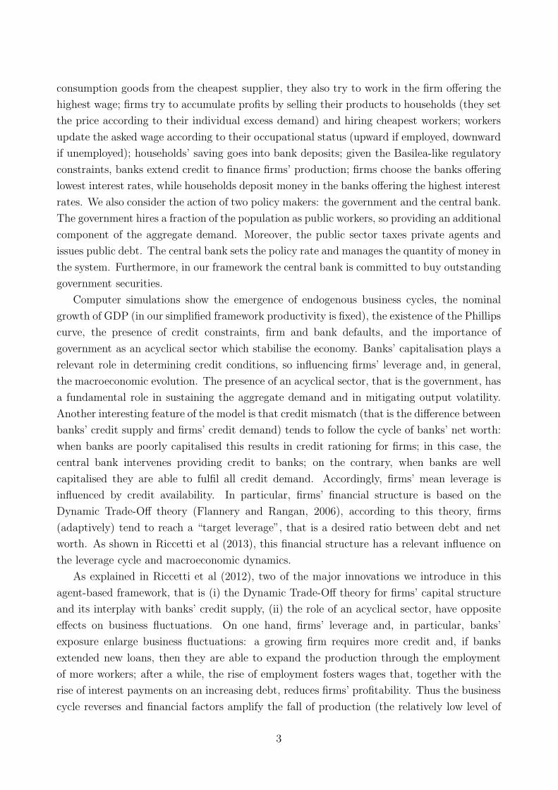
consumption goods from the cheapest supplier, they also try to work in the firm offering the

highest wage; firms try to accumulate profits by selling their products to households (they set

the price according to their individual excess demand) and hiring cheapest workers; workers

update the asked wage according to their occupational status (upward if employed, downward

if unemployed); households’ saving goes into bank deposits; given the Basilea-like regulatory

constraints, banks extend credit to finance firms’ production; firms choose the banks offering

lowest interest rates, while households deposit money in the banks offering the highest interest

rates. We also consider the action of two policy makers: the government and the central bank.

The government hires a fraction of the population as public workers, so providing an additional

component of the aggregate demand. Moreover, the public sector taxes private agents and

issues public debt. The central bank sets the policy rate and manages the quantity of money in

the system. Furthermore, in our framework the central bank is committed to buy outstanding

government securities.

Computer simulations show the emergence of endogenous business cycles, the nominal

growth of GDP (in our simplified framework productivity is fixed), the existence of the Phillips

curve, the presence of credit constraints, firm and bank defaults, and the importance of

government as an acyclical sector which stabilise the economy. Banks’ capitalisation plays a

relevant role in determining credit conditions, so influencing firms’ leverage and, in general,

the macroeconomic evolution. The presence of an acyclical sector, that is the government, has

a fundamental role in sustaining the aggregate demand and in mitigating output volatility.

Another interesting feature of the model is that credit mismatch (that is the difference between

banks’ credit supply and firms’ credit demand) tends to follow the cycle of banks’ net worth:

when banks are poorly capitalised this results in credit rationing for firms; in this case, the

central bank intervenes providing credit to banks; on the contrary, when banks are well

capitalised they are able to fulfil all credit demand. Accordingly, firms’ mean leverage is

influenced by credit availability. In particular, firms’ financial structure is based on the

Dynamic Trade-Off theory (Flannery and Rangan, 2006), according to this theory, firms

(adaptively) tend to reach a “target leverage”, that is a desired ratio between debt and net

worth. As shown in Riccetti et al (2013), this financial structure has a relevant influence on

the leverage cycle and macroeconomic dynamics.

As explained in Riccetti et al (2012), two of the major innovations we introduce in this

agent-based framework, that is (i) the Dynamic Trade-Off theory for firms’ capital structure

and its interplay with banks’ credit supply, (ii) the role of an acyclical sector, have opposite

effects on business fluctuations. On one hand, firms’ leverage and, in particular, banks’

exposure enlarge business fluctuations: a growing firm requires more credit and, if banks

extended new loans, then they are able to expand the production through the employment

of more workers; after a while, the rise of employment fosters wages that, together with the

rise of interest payments on an increasing debt, reduces firms’ profitability. Thus the business

cycle reverses and financial factors amplify the fall of production (the relatively low level of

3

profits with respect to interest payments induces a deleveraging process).

Moreover, model simulations highlight that even extended crises can endogenously emerge.

In these cases, the system may remain trapped in a large unemployment status, without the

possibility to quickly recover unless an exogenous intervention. Indeed, the macroeconomic

system evolves towards an “extended crisis” scenario, where the private sector tends to dis-

appear, that is almost only public workers remain employed. In this case, differently from the

usual business cycle mechanism, the decrease of wages due to growing unemployment does

not reverse the cycle, but rather amplifies the recession due to the lack of aggregate demand.

In other words, the self-adjustment mechanism which spontaneously reverses the business

cycle (e.g., the rise of the unemployment rate reduces the real wage and then the resulting

increase of profits makes room for an expansionary production phase) does not work. Indeed,

real wage lowers excessively boosting a vicious circle for which the fall of purchasing power

prevents firms to sell commodities, then firms reduce production, unemployment continues to

rise, and the system moves towards a large crisis.

We extend the model proposed in Riccetti et al (2012) by considering heterogeneous con-

sumption behaviours. “If propensities to consume differ, then the overall propensity to con-

sume is affected by income distribution, and an increase in inequality causes it to decrease.

The reduction of consumption demand, then, puts downward pressure on aggregate demand

and on income (unless some compensation comes from other items, like government spending

or external demand)” (Fitoussi and Saraceno, 2010, p.2). As a matter of fact, rich people

may accumulate higher wealth while poor people may suffer from low consumption, so cre-

ating negative consequences at the macroeconomic level, as a lack of aggregate demand, so

increasing the likelihood of observing a crisis with large unemployment.

The paper is organised as follows. After this introduction, we provide a brief descrip-

tion of the agent based macroeconomic model in Section 2. In particular, we present the

structure of four markets (credit, labour, goods and deposits) and the mechanisms of agents’

wealth accumulation. In Section 3 we discuss simulation results regarding the baseline model,

and a setting with heterogeneous consumption behaviour. Finally, Section 4 provides some

concluding remarks.

2 The model

In this section we provide a description of the modelling properties which characterise our

agent based macroeconomic model. The economic system is composed of households (h =

1, 2, ..., H), firms (f = 1, 2, ..., F ), banks (b = 1, 2, ..., B), a central bank, and the government,

and it evolves over a time span t = 1, 2, ..., T . Then, the economy is composed of four

markets: (i) credit market; (ii) labour market; (iii) goods market; (iv) deposit market. In

what follows we describe the working of the goods market. Agents are heterogeneous, live in

an incomplete and asymmetric information context, follow simple behavioural rules, and use

4

adaptive expectations.

The interaction between the demand (firms in the credit and labor markets, households

in the goods market, and banks in the deposit market) and the supply (banks in the credit

market, households in the labor and deposit markets, and firms in the goods market) sides of

the four markets follows a common decentralised matching protocol: a random list of agents

in the demand side is set, then the first agent in the list observes a random subset of potential

partners and chooses the cheapest one. After that, the second agent on the list performs the

same activity on a new random subset of the updated potential partner list. The process

iterates till the end of the demand side list. Subsequently, a new random list of agents in the

demand side is set and the whole matching mechanism goes on until either one side of the

market (demand or supply) is empty or no further matchings are feasible.

2.1 Credit market

In the credit market, firms and households are on the demand side, while banks are on the

supply side. Firms aim at financing production and banks may provide credit to this end.

Firm’s f credit demand at time t depends on its net worth Aft and the leverage target lft.

Hence, required credit is:

Bdft = Aft · lft (1)

The evolution of the leverage target depends on the following rule:

lft =

8>>><>>>:lft−1 · (1 + α · U(0, 1)) , if πft−1/(Aft−1 +Bft−1) > ift−1 and yft−1 < ψ · yft−1

lft−1, if πft−1/(Aft−1 +Bft−1) = ift−1 and yft−1 < ψ · yft−1

lft−1 · (1− α · U(0, 1)) , if πft−1/(Aft−1 +Bft−1) < ift−1 or yft−1 ≥ ψ · yft−1

(2)

where α > 0 is a parameter representing the maximum percentage change of the relevant

variable (in this case the target leverage), U(0, 1) is a random number picked from a uniform

distribution in the interval (0,1), πft−1 is the gross profit (realized in the previous period),

Bft−1 is the previous period effective debt, ift−1 is the nominal interest rate paid on previous

debts1, yft−1 represents inventories (that is, unsold goods), 0 ≤ ψ ≤ 1 is a parameter rep-

resenting a threshold for inventories based on previous period production yft−1. Equation 2

means that the leverage target increases (decreases) if the profit rate is higher (lower) than

average interest rate and there is a low (high) level of inventories.

On the supply side, bank b offers a total amount of money Bdbt depending on net worth Abt,

deposits Dbt, central bank credit mbt, and some legal constraints (proxied by the parameters

1It is a mean interest rate calculated as the weighted average of interests paid to the lending banks.

5

γ1 > 0 and 0 ≤ γ2 ≤ 1 that represents respectively the maximum admissible leverage and

maximum percentage of capital to be invested in lending activities):

Bdbt = min(kbt, kbt) (3)

where k = γ1·Abt, k = γ2·Abt+Dbt−1+mbt. Moreover, in order to reduce risk concentration,

banks lend to a single firm up to a maximum fraction β of the total amount of the credit

Bdbt. This behavioural parameter can be also interpreted as a regulatory constraint to avoid

excessive concentration.

Bank b charges an interest rate on the firm f at time t according to the following equation:

ibft = iCBt + ibt + ift (4)

where iCBt is the nominal interest rate set by the central bank at time t, ibt is a bank-

specific component, and ift = ρ lft/100 is a firm-specific component, that is a risk premium

on firm target leverage (with ρ > 0).

The bank-specific component evolves as follows:

ibt =

8<:ibt−1 · (1− α · U(0, 1)) , if Bbt−1 > 0

ibt−1 · (1 + α · U(0, 1)) , if Bbt−1 = 0(5)

where Bbt−1 is the amount of money that the bank did not manage to lend to firms in the

previous period.

As a result of the interaction based on the matching mechanism explained above, each

firm ends up with a credit Bft ≤ Bdft, , and each bank lends to firms an amount Bbt ≤ Bd

bt.

The difference between desired and effective credit is equal to Bdft − Bft = Bft for firms

and Bdbt − Bbt = Bbt for banks. Moreover, we assume that banks ask for an investment in

government securities equal to Γdbt = kbt−Bbt. If the sum of desired government bonds exceeds

the amount of outstanding public debt then the effective investment Γbt is rescaled according

to a factor Γdbt/P

Γdbt. Instead, if public debt exceeds the banks’ desired demand, then the

central bank buys the residual amount.

2.2 Labour market

First of all, the government hires a fraction g of households. The remaining part is available

for working in the firms. Firm’s f labor demand depends on the total capital available:

Aft +Bft. Each worker posts a wage wht which is updated as follows:

wht =

8<:wht−1 · (1 + α · U(0, 1)) , if h employed at time t− 1

wht−1 · (1− α · U(0, 1)) , if h unemployed at time t− 1(6)

6

The required wage has a minimum equal to: θpt−1(1+ τ), where θ is a positive parameter,

p is the maximum price of a single good, and τ is the tax rate on labor income. This means

that a worker asks at least a wage net of taxes able to buy a multiple θ of a good.

As a result of the decentralized matching between labor supply and demand, each firm

ends up with a number of workers nft and a residual cash (insufficient to hire an additional

worker). Obviously, a fraction of households may remain unemployed. In the baseline model,

the wage of unemployed people is set equal to zero.

Then, we remove this assumption by introducing an unemployment benefit paid by the

government. Accordingly, if the h-th worker is unemployed at time t then her income is given

by:

wht = ηpt−1 (7)

where η is a positive parameter. We will explore the role of this parameter on model

behavior in the computational experiments proposed below.

2.3 Goods market

In the goods market households represent the demand side, while firms are the supply side.

Households set the desired consumption, cdht, as follows:

cdht = c1 · wht + c2 · Ac3ht (8)

where wht is the wage gained by household h, 0 < c1 ≤ 1 is the propensity to consume current

income, 0 ≤ c2 ≤ 1 is the propensity to consume the wealth Aht.

In this paper, we add the parameter c3, that was implicitly equal to 1 in Riccetti et al.

(2012). Accordingly, for 0 < c3 < 1 consumption increases less than proportionally whith

wealth, that is the saving rate is higher for wealthier agents. We will investigate the role

of the parameter c3 below, by means of computer simulations, trying to assess the effects

of heterogeneous consumption behaviours on macroeconomic dynamics. In particular, we

consider two different scenarios, one with c3 = 1, that is the baseline scenario, and one with

c3 = 0.5. Accordingly, when c3 = 1 we have the following consumption function:

cdht = c1 · wht + c2 · Aht

Instead, if c3 = 0.5 the consumption function is given by:

cdht = c1 · wht + c2ÈAht

Moreover, if the amount cdht is smaller than the average price of one good p then cdht =

min(p , wht + Aht).

Given the number of hired workers, nft, firms produce consumption goods:

7

yft = φ · nft (9)

where φ ≥ 1 is a productivity parameter (equal for all firms and time-invariant).

Firms try to sell their current period production and previous period inventories. The

selling price increases if in the previous period the firm managed to sell all the output, while

it reduces if it had positive inventories. Moreover, the minimum price at which the firm want

to sell its output is set such that it is at least equal to the average cost of production, that is

ex-ante profits are at worst equal to zero.

At the end of the goods market matching, each household ends up with a residual cash,

which is not enough to buy an additional good and that it will try to deposit in a bank. At

the same time, firms may remain with unsold goods (inventories), that they will try to sell in

the next period.

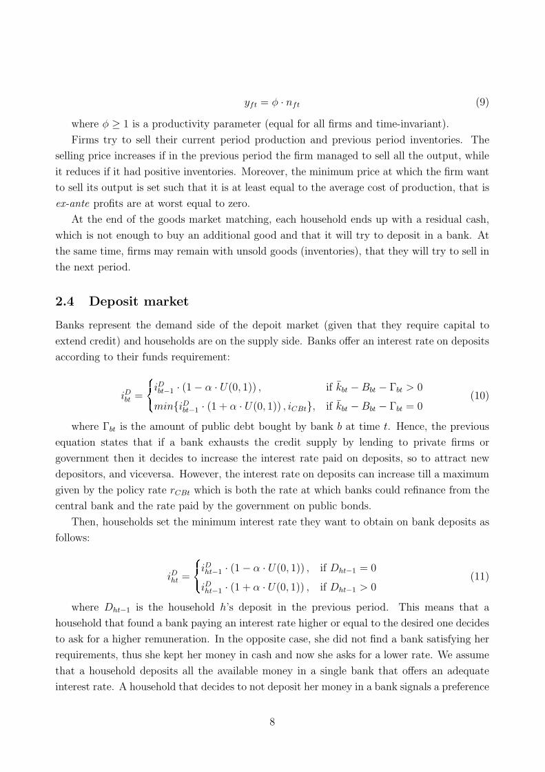
2.4 Deposit market

Banks represent the demand side of the depoit market (given that they require capital to

extend credit) and households are on the supply side. Banks offer an interest rate on deposits

according to their funds requirement:

iDbt =

8<:iDbt−1· (1− α · U(0, 1)) , if kbt −Bbt − Γbt > 0

miniDbt−1· (1 + α · U(0, 1)) , iCBt, if kbt −Bbt − Γbt = 0

(10)

where Γbt is the amount of public debt bought by bank b at time t. Hence, the previous

equation states that if a bank exhausts the credit supply by lending to private firms or

government then it decides to increase the interest rate paid on deposits, so to attract new

depositors, and viceversa. However, the interest rate on deposits can increase till a maximum

given by the policy rate rCBt which is both the rate at which banks could refinance from the

central bank and the rate paid by the government on public bonds.

Then, households set the minimum interest rate they want to obtain on bank deposits as

follows:

iDht =

8<:iDht−1· (1− α · U(0, 1)) , if Dht−1 = 0

iDht−1· (1 + α · U(0, 1)) , if Dht−1 > 0

(11)

where Dht−1 is the household h’s deposit in the previous period. This means that a

household that found a bank paying an interest rate higher or equal to the desired one decides

to ask for a higher remuneration. In the opposite case, she did not find a bank satisfying her

requirements, thus she kept her money in cash and now she asks for a lower rate. We assume

that a household deposits all the available money in a single bank that offers an adequate

interest rate. A household that decides to not deposit her money in a bank signals a preference

8

for liquidity, because she does not accept to deposit her cash for an interest rate below the

desired one.

2.5 Wealth dynamics

2.5.1 Firms

As a result of the outcomes of the credit, labor and goods markets, the firm f ’s profit is equal

to:

πft = pft · yft −Wft − intft (12)

where Wft is the firm f ’s wage bill, that is the sum of wages paid to employed workers,

and intft is the sum of interests paid on bank loans.

Firms pay a proportional tax τ on positive profits; negative profits will be subtracted from

the next positive profits. We indicate net profits with πft.

Finally, firms pay a percentage δft as dividends on positive net profits. The fraction 0 ≤ δft ≤

1 evolves according to the following rule:

δft =

8<:δft−1 · (1− α · U(0, 1)) , if yft = 0 and yft > 0

δft−1 · (1 + α · U(0, 1)) , if yft > 0 or yft = 0(13)

This means that firms distribute less dividends when they need self-financing to expand

production (that is, they do not have inventories) and viceversa. The profit net of taxes and

dividends is indicated by πft. In case of negative profits πft = πft.

Thus, the evolution of firm f ’s net worth is given by:

Aft = (1− τ ′) · [Aft−1 + πft] (14)

where τ ′ is the tax rate on wealth (applied only on wealth exceeding a threshold τ ′ · p,

that is a multiple of the average goods price).

If Aft ≤ 0 then the firm goes bankrupt and a new entrant takes its place. The initial

net worth of the new entrant is a multiple of the average goods price, while the leverage is

one. Moreover, the initial price is equal to the mean price of survival firms. Banks linked

to defaulted firms lose a fraction of their loans (the loss given default rate is calculated as

(Aft +Bft)/Bft).

2.5.2 Banks

According to the operations in the credit and the deposit markets, the bank b’s profit is equal

to:

πbt = intbt + iΓt · Γbt − iDbt−1·Dbt−1 − itCB ·mbt − badbt (15)

9

where intbt represents the interests gained on lending to non-defaulted firms, iΓt is the

interest rate on government securities (Γbt), and badbt is the amount of “bad debt” due to

bankrupted firms, that is non performing loans. Bad debt is the loss given default of the total

loan, that is a fraction 1 − (Aft + Bft)/Bft of the loan to defaulted firm f connected with

bank b.

Banks pay a proportional tax τ on positive profits; negative profits will be subtracted from

the next positive profits. We indicate net profits with πbt.

Finally, banks pay a percentage δbt as dividends on positive net profits. The fraction 0 ≤

δbt ≤ 1 evolves according to the following rule:

δbt =

8<:δbt−1 · (1− α · U(0, 1)) , if Bbt > 0 and Bbt = 0

δbt−1 · (1 + α · U(0, 1)) , if Bbt = 0 or Bbt > 0(16)

Hence, if the bank does not manage to lend the desired supply of credit then it decides to

distribute more dividends (because it does not need high reinvested profits), and viceversa.

The profit net of taxes and dividends is indicated by πbt. In case of negative profits

πbt = πbt.

Thus, the bank b’s net worth evolves as follows:

Abt = (1− τ ′) · [Abt−1 + πbt] (17)

where τ ′ is the tax rate on wealth (applied only on wealth exceeding a threshold τ ′ · p,

that is a multiple of the average goods price).

If Abt ≤ 0 then the bank is in default and a new entrant takes its place. Households linked

to defaulted banks lose a fraction of their deposits (the loss given default rate is calculated as

(Abt +Dbt)/Dbt). The initial net worth of the new entrant is a multiple of the average goods

price. Moreover, the initial bank-specific component of the interest rate (ibt) is equal to the

mean value across banks.

2.5.3 Households

As a result of interaction in the labor, goods, and deposit markets, the household h’s wealth

evolves as follows:

Aht = (1− τ ′) · [Aht−1 + (1− τ) · wht + divht + intDht − cht] (18)

where τ ′ is the tax rate on wealth (applied only on wealth exceeding a threshold τ ′ · p,

that is a multiple of the average goods price), τ is the tax rate on income, wht is the wage

gained by employed workers, divht is the fraction (proportional to the household h’s wealth

compared to overall households’ wealth) of dividends distributed by firms and banks net of

the amount of resources needed to finance new entrants (hence, this value may be negative),

10

intDht represents interests on deposits, and cht ≤ cdht is the effective consumption. Households

linked to defaulted banks lose a fraction of their deposits as already explained.

2.6 Government and central bank

Government’s current expenditure is given by the sum of wages paid to public workers (Gt)

and the interests paid on public debt to banks.2 Moreover, government collects taxes on

incomes and wealth and receives interests gained by the central bank. The difference between

expenditures and revenues is the public deficit Ψt. Consequently, public debt is Γt = Γt−1+Ψt.

Central bank decides the policy rate iCBt and the quantity of money to put into the

system in accordance with the interest rate. In order to do that, the central bank observes

the aggregate excess supply or demand in the credit market and sets an amount of money Mt

to reduce the gap in the subsequent period of time.

3 Simulations

3.1 Baseline scenario

We study the dynamics of the model by means of computer simulations. Table 1 shows the

parameter setting of the baseline simulation. The initial agents’ wealth is set as follows:

Af1 = max0.1, N(3, 1), Ab1 = max0.2, N(5, 1), Ah1 = max0.01, N(0.5, 0.01). The

policy rate iCBt is constant at 1%. For more details see Riccetti et al (2012).

Computer simulations show that endogenous business cycles emerge as a consequence of

the interaction between real and financial factors. When firms’ profits are improving, they try

to expand the production and, if banks extend more credit, this results in more employment;

the decrease of the unemployment rate leads to the rise of wages that, on the one hand,

increases the aggregate demand, while on the other hand reduces firms’ profits, and this

may cause the inversion of the business cycle. Indeed, there is a significant cross-correlation

between the unemployment rate and the firms’ profit rate. First of all, there is a high positive

correlation at lag 0: the profit rate is high when unemployment is high given that firms

save on production costs (e.g., wage bill) but, at the same time, the aggregate demand does

not decrease proportionally, because of public workers’ expenditure and consumption due to

wealth, thus firms can sell their commodities (including inventories) in the goods market.

However, the presence of unemployed people, the tendency of wages to decrease due to the

high unemployment rate, and the reduction of households’ wealth, cause the fall of next period

aggregate demand that, in turn, reduces firms’ profits. Indeed, there is a negative correlation

at lag +1. Instead, the negative correlation at lag -1 means that increasing profits boost the

2It could also spend an amount Ωt for extreme cases in which the government has to intervene to finance

new entrants when private wealth is not enough. However, in our simulations this never happens.

11

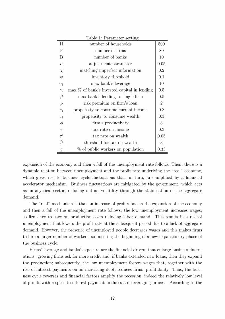
Table 1: Parameter setting

H number of households 500

F number of firms 80

B number of banks 10

α adjustment parameter 0.05

χ matching imperfect information 0.2

ψ inventory threshold 0.1

γ1 max bank’s leverage 10

γ2 max % of bank’s invested capital in lending 0.5

β max bank’s lending to single firm 0.5

ρ risk premium on firm’s loan 2

c1 propensity to consume current income 0.8

c2 propensity to consume wealth 0.3

φ firm’s productivity 3

τ tax rate on income 0.3

τ ′ tax rate on wealth 0.05

τ ′ threshold for tax on wealth 3

g % of public workers on population 0.33

expansion of the economy and then a fall of the unemployment rate follows. Then, there is a

dynamic relation between unemployment and the profit rate underlying the “real” economy,

which gives rise to business cycle fluctuations that, in turn, are amplified by a financial

accelerator mechanism. Business fluctuations are mitigated by the government, which acts

as an acyclical sector, reducing output volatility through the stabilisation of the aggregate

demand.

The “real” mechanism is that an increase of profits boosts the expansion of the economy

and then a fall of the unemployment rate follows; the low unemployment increases wages,

so firms try to save on production costs reducing labor demand. This results in a rise of

unemployment that lowers the profit rate at the subsequent period due to a lack of aggregate

demand. However, the presence of unemployed people decreases wages and this makes firms

to hire a larger number of workers, so boosting the beginning of a new expansionary phase of

the business cycle.

Firms’ leverage and banks’ exposure are the financial drivers that enlarge business fluctu-

ations: growing firms ask for more credit and, if banks extended new loans, then they expand

the production; subsequently, the low unemployment fosters wages that, together with the

rise of interest payments on an increasing debt, reduces firms’ profitability. Thus, the busi-

ness cycle reverses and financial factors amplify the recession, indeed the relatively low level

of profits with respect to interest payments induces a deleveraging process. According to the

12

empirical evidence (for example, Kalemli-Ozcan et al., 2011), there is a negative but mod-

est correlation between firms’ leverage and the unemployment rate, while there is a more

significant negative correlation between banks’ exposure and unemployment. Then, banks’

capitalization is the most important determinant of credit conditions, so influencing firms’

leverage and the macroeconomic evolution.

In some cases, differently from the usual business cycle mechanism, the fall of wages due

to the increase of unemployment does not reverse the cycle, but generates a lack of aggregate

demand that amplifies the recession in a vicious circle: indeed, the fall of purchasing power

prevents firms to sell commodities, then firms decrease production, unemployment continues

to rise, and the recession further deteriorates. In these cases, the system may remain trapped

in an extended crisis.

3.2 Heterogeneous consumption behaviour

Lets’ now compare the result of the baseline model, obtained with a parameter c3 = 1 in

equation 8, with the results of the simulations in which c3 = 0.5. Our aim is to address

the inequality topic in a symplified framework in which all households have the same skills

and they all works in an economy with homogeneous goods. Thus, labour income does not

vary much across households and capital income is distributed to households proportionally

to their share (which in turn depends on households’ wealth). Moreover, all households have

a similar initial wealth. Indeed, in the baseline case (c3 = 1), we obtain a wealth distribution

that is negatively skewed, while in the real world it is highly positively skewed.

Even in this symplified framework, a propensity to consume decreasing with wealth (c3 =

0.5) modifies the household’s wealth distribution. Indeed, in this case we can observe a larger

wealth inequality: wealth distribution not only presents a left tail, but also a right tail, thus

the richest agent has a higher wealth and the skewness becomes about zero (with a mean

slightly higher than the median of households’ wealth); the larger inequality is also signaled

by an increase of the standard deviation; moreover, average wealth increases given that richest

households save more. This analysis on wealth distribution is summarized in table 2.

Table 2: Statistics about wealth distribution at time T=500 in two simulation with different

value of parameter c3: c3 = 1 and c3 = 0.5

Statistic c3 = 1 c3 = 0.5

Mean 1.38 1.61

Standard deviation 0.38 0.54

Skewness -0.72 -0.08

Maximum 2.13 3.28

These results are robust both at different time steps (for instance we check the wealth

13

distribution also at time t=150) and in different simulations. Indeed, we perform a Monte

Carlo with 100 simulations on a time horizon T = 500 (again skipping the first 100 periods,

then we analyse the last 400 time steps).

Table 3 reports some relevant macroeconomic features of the two Monte Carlo simulations

with c3 = 1 and c3 = 0.5.

Table 3: 100 Monte Carlo replications for both c3 = 1 and c3 = 0.5 (data calculated on

time span 101-500). The number of simulations with average unemployment rate and max-

imum unemployment rate above 20% are computed on all 100 simulations. Instead, the other

statistics refers to simulations with average unemployment rate below 20% (that is 98 simula-

tions for both cases); in brackets we add the standard deviation of the corresponding statistic

among the simulations; the last column indicates the p-value of the test on the null hypothesis

that the value of the statistic is equal between the two cases of c3 = 1 and c3 = 0.5.

Variable c3 = 1 c3 = 0.5 p-value H0=0

Sim. with mean(ur) < 20% 98 98

Sim. with max(ur) < 20% 97 90

Unemployment rate % 9.73 (0.87) 9.71 (0.61) 85.2%

Unemployment volatility % 1.84 (0.12) 2.17 (0.18) 0.0%

Firm default rate % 6.21 (0.70) 6.51 (0.60) 0.1%

Bank default rate % 0.40 (0.38) 0.32 (0.37) 13.5%

Firm mean leverage 1.23 (0.31) 1.10 (0.21) 0.1%

Firm leverage volatility 0.23 (0.07) 0.30 (0.07) 0.0%

Interest rate % 8.04 (0.81) 8.51 (0.77) 0.0%

Credit constraint % 4.15 (1.64) 8.79 (2.57) 0.0%

Wage share % 63.7 (0.3) 63.6 (0.2) 0.7%

Public deficit % 3.16 (0.05) 2.96 (0.06) 0.0%

Inflation rate % 1.99 (0.04) 1.99 (0.03) 100%

We can observe that in both cases the economy falls in a large crisis scenario, that is

with a mean unemployment rate above 20%, 2 times over 100 simulations and the mean

unemployment rate is the same. However, the unemployment volatility is much higher when

c3 = 0.5, that is whith larger wealth inequality, and the difference is statistically significant

at 99% level. Therefore, the business cycle is “larger” with a lower minumum and a higher

maximum for the unemployment rate. Indeed, while in the baseline case (c3 = 1) we never

find a time step with unemployment above 20%, but for the two large crisis scenario, in

the inequality case (c3 = 0.5) we detect 10 simulations in which the unemployment peaks

above 20% (the two large crises plus other 8 simulations). If the policy maker considers

the business cycle volatility as a problem to be stabilised, than the reduction of the wealth

inequality seems to be an effective tool to reach this target. Especially, the policy maker could

14

avoid large unemployment crises (e.g., with an unemployment rate above 20%) by reducing

inequality. For instance, in an agent based macroeconomic setting, Dosi et al. (2013) find

that more inquality leads to higher volatility, increasing the likelihood of unemployment crises;

they also show that fiscal policy is an effective countercyclical tool especially when income

distribution is skewed towards profits.

It is worth to note that the percentage of firm defaults increases in the case of c3 = 0.5,

probably due to higher macroeconomic volatility. Indeed, the mean firm leverage is lower in

this case, then the economy should be safer according to this indicator. Instead, this is not the

case given that firm leverage is more volatile, giving rise to the already mentioned “larger”

business cycle, with stronger leveraging and deleveraging processes. Moreover, the higher

volatility, that highlights a riskier economic environment, goes along with higher interest

rates charged by banks to firms, that in turn affects both the mean firm leverage (lower,

because it is less favorable to ask money to banks) and the number of firm defaults (higher,

because of the higher cost of the debt).

We calculate the credit constraint as the percentage of credit required by firms that firms

do not obtain. Given that we observe a correlation above 50% between firm leverage and

credit constraint, and given that in the case of c3 = 0.5 firm leverage is more pro-cyclical, in

this situation there are periods in which the credit constraint is stronger. We can confirm this

analysis computing the average of the standard deviation and the average of the maximum

credit constraint in the two Monte Carlo settings: when c3 = 0.5 the average standard

deviation is 8.16% and the average maximum is 35.08%, while if c3 = 1 the average standard

deviation is 5.75% and the average maximum is 26.97%. Given that the distribution is

truncated at zero (and it often happens that firms receive all the required credit), the longer

right tail of the distribution in the case of c3 = 0.5 explains the higher mean credit constraint.

Moreover, this is another further which can eplains why the mean leverage is lower when

c3 = 0.5. Finally, the relation between firm leverage and credit constraint has both causal

direction: a higher firm leverage implies a higher probability of credit constraint, but also

a higher credit constraint implies a lower leverage, because firms are not able to reach their

desired leverage. The wage share is statistically different between the two Monte Carlo, but

the difference is economically not significant. The similar wage share between the two Monte

Carlo experiments implies a similar pressure to increase wages and thus similar effets on price

dynamics. Indeed, the inflation rate is the same in both cases.

Instead, the public deficit is slightly lower in the case with c3 = 0.5, given that in this

case there are richer households and we assume the presence of a 5% tax rate on wealth (only

above a certain wealth level). However, in both cases the public deficit remains on admissible

values (compared to GDP).

To summarise, we observe a negative impact on the economy of a propensity to con-

sume that decreases with wealth (that also creates an economic system with larger wealth

inequality). Indeed, in this case the business cycle is “larger” and we count a higher number

15

of simulations in which we detect large unemployment crises. This riskier economic envir-

onment with a stronger volatility implies a larger number of firm defaults, a higher mean

interest rates, and a higher mean credit constraint.

4 Concluding remarks

We proposed an analysis of the effects of wealth inequality on macroeconomic dynamics in an

economy composed of heterogeneous households, firms, banks, and two policy makers, that

is the government and the central bank. Preliminary results show that more inequality rises

macroeconomic volatility, increasing the likelihood of observing large unemployment crises.

However, we are just making the first steps towards a better understanding of increasing

inequality on the evolution of a complex macroeconomic system. Next step in this direction

is the introduction of consumer credit, through which the saving of rich can finance the

consumption of poor. Actually, consumer credit and other forms of indebtedness can prevent

the lack of aggregate demand to happen for a while, but probably at the cost of more financial

instability, that may increase the likelihood of large unemployment crises. In other words, in

a context of growing inequality, debt accumulation may increase financial fragility, spreading

in the system through credit interlinkages (Delli Gatti et al, 2010), eventually leading to a

financial collapse. So finance may postpone the crisis due to the lack of aggregate demand,

but it also creates the bases for a later crisis.

16

References

[1] Delli Gatti D., Gallegati M., Greenwald B., Russo A., Stiglitz J.E. (2010), “The financial

accelerator in an evolving credit network”, Journal of Economic Dynamics and Control,

34(9): 1627-1650.

[2] Dosi G., Fagiolo G., Napoletano M., Roventini A. (2013), “Income distribution, credit

and fiscal policies in an agent-based Keynesian model”, Journal of Economic Dynamics

and Control, 37(8): 1598-1625.

[3] Epstein J.M., Axtell R.L. (1996), Growing Artificial Societies: Social Science from the

Bottom Up, MIT Press/Brookings Institution.

[4] Fitoussi J.-P., Saraceno F. (2010), “Inequality and macroeconomic performance”, Doc-

ument de travail de l’OFCE No. 2010-13, Centre de recherche en economie de Sciences

Po.

[5] Flannery M.J., Rangan K.P. (2006), “Partial adjustment toward target capital struc-

tures”, Journal of Financial Economics, 79(3): 469-506.

[6] Gaffeo E., Catalano M., Clementi F., Delli Gatti D., Gallegati M., Russo A. (2007),

“Reflections on modern macroeconomics: Can we travel along a safer road?”, Physica A,

382(1): 89-97.

[7] IMF (2007), World Economic Outlook, “Spillovers and Cycles in the Global Economy”,

chap. 5, International Monetary Fund, April 2007.

[8] Kaldor N. (1955), “Alternative Theories of Distribution”, The Review of Economic Stud-

ies, 23(2): 83-100.

[9] Kalemli-Ozcan S., Sorensen B., Yesiltas S. (2011), “Leverage Across Firms, Banks, and

Countries”, NBER Working Papers 17354, National Bureau of Economic Research.

[10] Kalecki M. (1942), “A Theory of Profits”, The Economic Journal, 52(206/207): 258-67.

[11] Rajan R. (2010), Fault Lines. How Hidden Fractures Still Threaten the World Economy,

Princeton: Princeton University Press.

[12] Riccetti L., Russo A., Gallegati M. (2012), “An Agent Based Decentralized Matching

Macroeconomic Model”, MPRA paper No. 42211, University Library of Munich, Ger-

many.

[13] Riccetti L., Russo A., Gallegati M. (2013), “Leveraged Network-Based Financial Accel-

erator”, Journal of Economic Dynamics and Control, 37(8): 1626-1640.

17

[14] Stiglitz J.E. (2010), Freefall: Free Markets, and the Sinking of the World Economy, New

York: Norton.

[15] Stockhammer E. (2012), “Rising Inequality as a Root Cause of the Present Crisis”,

Working Paper No. 282, Political Economy Research Institute (PERI), University of

Massachussets, Amherst.

[16] Tesfatsion L.S., Judd K.L. (2006), Handbook of Computational Economics: Agent-Based

Computational Economics, Vol. 2, North-Holland.

[17] Wade R. (2009), “The global slump. Deeper causes and harder lessons”. Challenge, 52(5):

5-24.

18