SABANCI UNIVERSITY Incorporating Prior Information in Nonnegative Matrix Factorization for Audio Source Separation by Emad Mounir Grais Girgis A thesis submitted in partial fulfillment for the degree of Doctor of Philosophy in the Faculty of Engineering and Natural Sciences Electronics Engineering June 2013

Welcome message from author
This document is posted to help you gain knowledge. Please leave a comment to let me know what you think about it! Share it to your friends and learn new things together.
Transcript
SABANCI UNIVERSITY
Incorporating Prior Information in
Nonnegative Matrix Factorization for
Audio Source Separation
by
Emad Mounir Grais Girgis
A thesis submitted in partial fulfillment for the
degree of Doctor of Philosophy
in the
Faculty of Engineering and Natural Sciences
Electronics Engineering
June 2013


c©Emad Mounir Grais Girgis 2013
All Rights Reserved

To my God. . .
iii

Acknowledgements
I would like to express my deep and sincere gratitude to my thesis supervisor Assist.
Prof. Hakan Erdogan for his invaluable guidance, tolerance, positiveness, support, and
encouragement throughout my thesis.
I am grateful to my committee members Prof. Mustafa Unel, Assoc. Prof. Ilker
Hamzaoglu, Assoc. Prof. Ali Taylan Cemgil, and Assoc. Prof. Mujdat Cetin for
taking the time to read and comment on my thesis.
I would like to thank Erasmus Mundus for providing the necessary financial support for
the first three years of my PhD study. I also would like to thank Sabancı university and
Turk-Telekom for supporting my research for the remaining period of my PhD study.
My deepest gratitude goes to my family for their unflagging love and support throughout
my life.
I would like to thank all my colleges in VPA laboratory for their great help. Finally,
I would like to thank the international office here at Sabancı university for their help
during my stay in Turkey.
iv
Incorporating Prior Information in Nonnegative Matrix Factorization for Audio Source
Separation
Emad Mounir Grais Girgis
EE, PhD Thesis, 2013
Thesis Supervisor: Hakan Erdogan
Keywords: Single channel source separation, nonnegative matrix factorization,
hidden Markov model, Gaussian mixture model, minimum mean squared error
estimation, model adaptation, orthogonality constraints, discriminative training,
dictionary learning, Wiener filter, spectral masks.
Abstract
In this work, we propose solutions to the problem of audio source separation from a single
recording. The audio source signals can be speech, music or any other audio signals. We
assume training data for the individual source signals that are present in the mixed signal
are available. The training data are used to build a representative model for each source.
In most cases, these models are sets of basis vectors in magnitude or power spectral
domain. The proposed algorithms basically depend on decomposing the spectrogram
of the mixed signal with the trained basis models for all observed sources in the mixed
signal. Nonnegative matrix factorization (NMF) is used to train the basis models for
the source signals. NMF is then used to decompose the mixed signal spectrogram as a
weighted linear combination of the trained basis vectors for each observed source in the
mixed signal. After decomposing the mixed signal, spectral masks are built and used to
reconstruct the source signals.
In this thesis, we improve the performance of NMF for source separation by incorpo-
rating more constraints and prior information related to the source signals to the NMF
decomposition results. The NMF decomposition weights are encouraged to satisfy some
prior information that is related to the nature of the source signals. The priors are
modeled using Gaussian mixture models or hidden Markov models. These priors basi-
cally represent valid weight combination sequences that the basis vectors can receive for
a certain type of source signal. The prior models are incorporated with the NMF cost
function using either log-likelihood or minimum mean squared error estimation (MMSE).

We also incorporate the prior information as a post processing. We incorporate the
smoothness prior on the NMF solutions by using post smoothing processing. We also
introduce post enhancement using MMSE estimation to obtain better separation for the
source signals.
In this thesis, we also improve the NMF training for the basis models. In cases when
enough training data are not available, we introduce two different adaptation methods
for the trained basis to better fit the sources in the mixed signal. We also improve
the training procedures for the sources by learning more discriminative dictionaries for
the source signals. In addition, to consider a larger context in the models, we con-
catenate neighboring spectra together and train basis sets from them instead of a single
frame which makes it possible to directly model the relation between consequent spectral
frames.
Experimental results show that the proposed approaches improve the performance of
using NMF in source separation applications.
Ses Kaynagı Ayrımı icin Negatif Olmayan Matris Ayrıstırma’ya Onsel Bilgilerin Dahil
Edilmesi
EMAD MOUNIR GRAIS GIRGIS
EE, Doktora Tezi, 2013
Tez Danısmanı: Hakan Erdogan
Anahtar Kelimeler: Tek Kanal Kaynak ayrımı, Negatif Olmayan Matris Ayrıstırma
(NOMA), saklı Markov modeli, Gauss karısım modeli, minimum ortalama karesel hata
kestirimi (MOKH), model uyarlama, dikgenlik kısıtları, ayırt edici egitim, sozluk
ogrenme, Wiener filtresi, spektral maskeler.
Ozet
Bu calısmada tek bir kayıttan ses kaynaklarının ayrımı problemine cozum onerilerinde
bulunuyoruz. Ses kaynakları konusma, muzik veya baska ses sinyalleri olabilir. Karısmıs
sinyal icerisindeki ozgun sinyal kaynaklarının egitim verilerinin elimizde mevcut oldugunu
varsayıyoruz. Egitim verileri her kaynak icin ornek model kurmak amacıyla kullanılır.
Genellikle bu modeller spektral uzayda buyukluk veya guc degerlerini acıklayan ta-
ban vektor kumeleridir. Temelde, onerilen algoritma karısmıs sinyalin spektrogramının
karısmıs sinyal icinde bulunan butun kaynak sinyallerin taban egitim modelleriyle ayrıstır-
ılmasına dayanır. Kaynak sinyallerin taban modellerini egitmek icin Negatif Olmayan
Matris Ayrıstırma (NOMA) metodu kullanılır. Daha sonra NOMA, karısmıs sinyal spek-
trogramını, bu sinyal icinde bulunan butun kaynak sinyallerin egitilmis taban vektorlerinin
agırlıklı dogrusal katısımı olarak ayrıstırmakta kullanılır. Karısmıs sinyali ayrıstırdıktan
sonra kaynak sinyali tekrar insa etmek icin spektral maskeler olusturulur.
Bu tezde, NOMA ayrıstırma sonuclarına, kaynak sinyalleriyle baglantılı daha cok kısıt
ve onsel bilgi dahil ederek, kaynak ayrıstırmada NOMA’nın performansını arttırıyoruz.
NOMA ayrıstırmasındaki agırlıklar kaynak sinyallerin dogasına baglı bazı onsel kısıtları
saglamak icin tesvik edilmistir. Kullandıgımız onsel bilgi modelleri Gauss karısımı ya
da saklı Markov modelleridir. Temelde bu onsel modeller her kaynagın tabanlarının
sahip olacakları gecerli agırlık dizilerini ifade ederler. Bu onsel modeller NOMA maliyet
fonksiyonuna log-olabilirlik ya da minimum ortalama karesel hata (MOKH) kestirimi
kullanılarak dahil edilmistir.

Onsel bilgiler ardıl islemler sırasında da dahil edilmistir. Duzgunluk onsel bilgisi basit
bir ardıl duzgunlestirme ile dahil edilmistir. Ayrıca, daha iyi ayrıstırma saglamak icin
MOKH kestirimi kullanarak ardıl iyilestirme metodu da tanıtılmıstır.
Bu tezde aynı zamanda taban modelleri icin NOMA egitimini de iyilestiriyoruz. Yeterli
egitim verisi mevcut olmayan durumlarda karısmıs sinyaldeki kaynaklara daha uygun
tabanlar bulmak amacıyla iki farklı uyarlama metodu sunuyoruz. Diger bir katkı olarak,
kaynak sinyaller icin daha ayırt edici modeller ogrenerek kaynak egitim yordamlarını da
gelistiriyoruz. Baska bir bolumde, modellerimizin cevresel etkileri daha iyi ogrenmesi
icin, komsu spektral verileri birlestirdikten sonra onlardan taban vektorleri egitiyor ve
boylece komsu cerceveler arasındaki bilgileri dogrudan modellemis oluyoruz.
Deneysel sonuclar onerilen metotların kaynak ayrıstırma uygulamalarında NOMA’nın
performansını arttırdıgını gostermistir.
Contents
Acknowledgements iv
Abstract v
Ozet vii
List of Figures xii
List of Tables xiii
Abbreviations xv
1 Introduction 1
1.1 Approaches to single-channel audio source separation . . . . . . . . . . . . 2
1.2 The contributions of this thesis . . . . . . . . . . . . . . . . . . . . . . . . 6
1.3 Organization of this thesis . . . . . . . . . . . . . . . . . . . . . . . . . . . 8
2 Background 9
2.1 Formulation for single-channel source separation . . . . . . . . . . . . . . 9
2.2 Non-negative matrix factorization . . . . . . . . . . . . . . . . . . . . . . . 11
2.3 NMF for single channel source separation . . . . . . . . . . . . . . . . . . 16
2.3.1 Reconstruction of source signals and spectral masks . . . . . . . . 19
2.4 Performance evaluation . . . . . . . . . . . . . . . . . . . . . . . . . . . . 20
3 Regularized NMF using GMM priors 22
3.1 Motivations and overview . . . . . . . . . . . . . . . . . . . . . . . . . . . 22
3.2 The proposed regularized nonnegative matrix factorization approach . . . 25
3.3 Training the source models . . . . . . . . . . . . . . . . . . . . . . . . . . 28
3.3.1 Sequential training . . . . . . . . . . . . . . . . . . . . . . . . . . . 28
3.3.2 Joint training . . . . . . . . . . . . . . . . . . . . . . . . . . . . . . 29
3.3.3 Determining the hyper-parameters . . . . . . . . . . . . . . . . . . 30
3.4 Signal separation . . . . . . . . . . . . . . . . . . . . . . . . . . . . . . . . 31
3.4.1 Reconstruction of source signals and spectral masks . . . . . . . . 33
3.4.2 Signal separation using IS-NMF . . . . . . . . . . . . . . . . . . . 33
3.5 Experiments and discussion . . . . . . . . . . . . . . . . . . . . . . . . . . 34
ix
Contents x
3.5.1 Speech-music separation . . . . . . . . . . . . . . . . . . . . . . . . 34
3.5.2 Speech-speech separation . . . . . . . . . . . . . . . . . . . . . . . 38
3.5.3 Comparison with the use of a conjugate prior . . . . . . . . . . . . 40
3.6 Conclusion . . . . . . . . . . . . . . . . . . . . . . . . . . . . . . . . . . . 42
4 Regularized NMF using HMM priors 44
4.1 Motivations and overview . . . . . . . . . . . . . . . . . . . . . . . . . . . 44
4.2 The proposed regularized NMF using HMM . . . . . . . . . . . . . . . . . 46
4.3 Training the source models . . . . . . . . . . . . . . . . . . . . . . . . . . 50
4.3.1 Initial training . . . . . . . . . . . . . . . . . . . . . . . . . . . . . 50
4.3.2 Joint training . . . . . . . . . . . . . . . . . . . . . . . . . . . . . . 51
4.4 Signal separation . . . . . . . . . . . . . . . . . . . . . . . . . . . . . . . . 52
4.5 Experiments and discussion . . . . . . . . . . . . . . . . . . . . . . . . . . 54
4.5.1 Comparison with other priors . . . . . . . . . . . . . . . . . . . . . 55
4.6 Conclusion . . . . . . . . . . . . . . . . . . . . . . . . . . . . . . . . . . . 57
5 Regularized NMF using MMSE estimates under GMM priors withonline learning for the uncertainties 58
5.1 Motivations and overview . . . . . . . . . . . . . . . . . . . . . . . . . . . 58
5.2 Regularized nonnegative matrix factorization using MMSE estimation . . 59
5.3 The proposed regularized NMF for source separation . . . . . . . . . . . . 65
5.3.1 Signal separation . . . . . . . . . . . . . . . . . . . . . . . . . . . . 65
5.3.2 Source signals reconstruction . . . . . . . . . . . . . . . . . . . . . 68
5.4 Experiments and discussion . . . . . . . . . . . . . . . . . . . . . . . . . . 69
5.4.1 Comparison with other priors . . . . . . . . . . . . . . . . . . . . . 70
5.5 Conclusion . . . . . . . . . . . . . . . . . . . . . . . . . . . . . . . . . . . 72
6 Spectro-temporal post-smoothing 74
6.1 Motivations and overview . . . . . . . . . . . . . . . . . . . . . . . . . . . 74
6.2 Source signals reconstruction and smoothed masks . . . . . . . . . . . . . 75
6.3 Experiments and discussion . . . . . . . . . . . . . . . . . . . . . . . . . . 77
6.3.1 Comparison with regularized NMF with continuity prior . . . . . . 79
6.3.2 Comparison with regularized NMF with MMSE priors . . . . . . . 81
6.3.3 Combining MMSE estimation based regularized NMF with post-smoothing . . . . . . . . . . . . . . . . . . . . . . . . . . . . . . . . 81
6.4 Conclusion . . . . . . . . . . . . . . . . . . . . . . . . . . . . . . . . . . . 82
7 Spectro-temporal post-enhancement using MMSE estimation 84
7.1 Motivations and overview . . . . . . . . . . . . . . . . . . . . . . . . . . . 84
7.2 MMSE estimation for post enhancement . . . . . . . . . . . . . . . . . . . 85
7.2.1 Training the source GMMs . . . . . . . . . . . . . . . . . . . . . . 86
7.2.2 Learning the distortion . . . . . . . . . . . . . . . . . . . . . . . . 87
7.2.3 Calculating MMSE estimates . . . . . . . . . . . . . . . . . . . . . 88
7.3 Experiments and discussion . . . . . . . . . . . . . . . . . . . . . . . . . . 89
7.4 Conclusion . . . . . . . . . . . . . . . . . . . . . . . . . . . . . . . . . . . 91
8 Discriminative nonnegative dictionary learning using cross-coherencepenalties 92

Contents xi
8.1 Motivations and overview . . . . . . . . . . . . . . . . . . . . . . . . . . . 92
8.2 Dictionary learning . . . . . . . . . . . . . . . . . . . . . . . . . . . . . . . 93
8.3 Discriminative learning through cross-coherence penalties . . . . . . . . . 95
8.4 Signal separation . . . . . . . . . . . . . . . . . . . . . . . . . . . . . . . . 98
8.5 Experiments and discussion . . . . . . . . . . . . . . . . . . . . . . . . . . 98
8.6 Conclusion . . . . . . . . . . . . . . . . . . . . . . . . . . . . . . . . . . . 100
9 Adaptation of speaker-specific bases in non-negative matrix factoriza-tion 102
9.1 Motivations and overview . . . . . . . . . . . . . . . . . . . . . . . . . . . 102
9.2 Probabilistic perspective of NMF . . . . . . . . . . . . . . . . . . . . . . . 104
9.3 Basis vectors matrix prior p(B) . . . . . . . . . . . . . . . . . . . . . . . . 105
9.4 Training the bases . . . . . . . . . . . . . . . . . . . . . . . . . . . . . . . 105
9.5 Speech model adaptation . . . . . . . . . . . . . . . . . . . . . . . . . . . 106
9.5.1 Bayesian adaptation of the speech bases . . . . . . . . . . . . . . . 106
9.5.2 Linear transformation adaptation of the speech bases . . . . . . . . 107
9.5.3 Combined adaptation . . . . . . . . . . . . . . . . . . . . . . . . . 108
9.6 Signal separation and reconstruction . . . . . . . . . . . . . . . . . . . . . 108
9.7 Experiments and results . . . . . . . . . . . . . . . . . . . . . . . . . . . . 109
9.8 Conclusion . . . . . . . . . . . . . . . . . . . . . . . . . . . . . . . . . . . 111
10 Nonnegative matrix factorization with sliding windows and spectralmasks 112
10.1 Motivations and overview . . . . . . . . . . . . . . . . . . . . . . . . . . . 112
10.2 Training the bases . . . . . . . . . . . . . . . . . . . . . . . . . . . . . . . 113
10.3 Signal separation and masking . . . . . . . . . . . . . . . . . . . . . . . . 113
10.3.1 Source signals reconstruction and masks. . . . . . . . . . . . . . . 114
10.4 Experiments and discussion . . . . . . . . . . . . . . . . . . . . . . . . . . 115
10.4.1 Comparison with post-smoothing in Chapter 6 and CNMF . . . . 116
10.5 Conclusion . . . . . . . . . . . . . . . . . . . . . . . . . . . . . . . . . . . 118
11 Conclusions and future work 119
11.1 Future work . . . . . . . . . . . . . . . . . . . . . . . . . . . . . . . . . . . 121
12 Appendix A 122
13 Appendix B 130
Bibliography 134
List of Figures
1.1 Single channel source separation (SCSS) . . . . . . . . . . . . . . . . . . . . . 2
1.2 Nonnegative matrix factorization (NMF) . . . . . . . . . . . . . . . . . . . . . 5
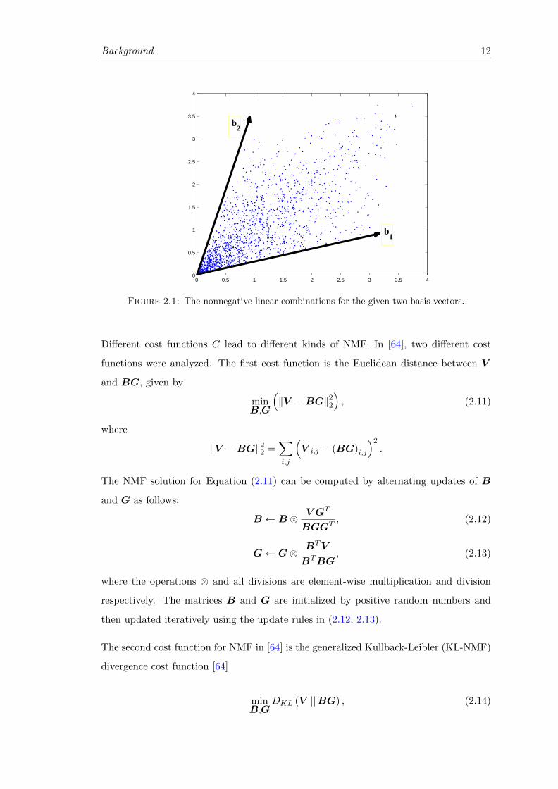
2.1 The nonnegative linear combinations for the given two basis vectors. . . . . . . 12
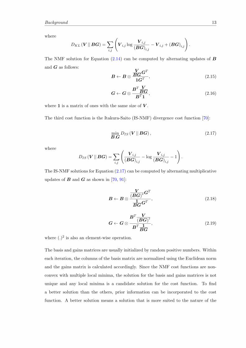
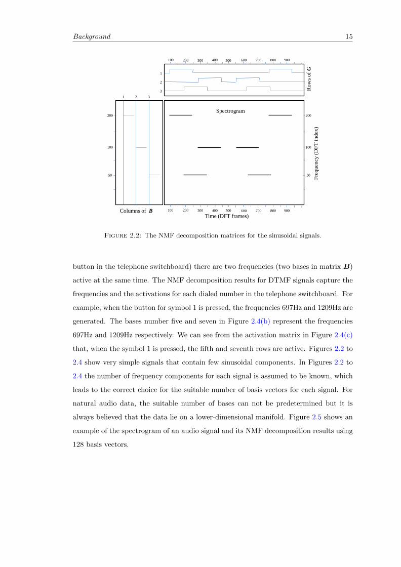
2.2 The NMF decomposition matrices for the sinusoidal signals. . . . . . . . . . . . 15
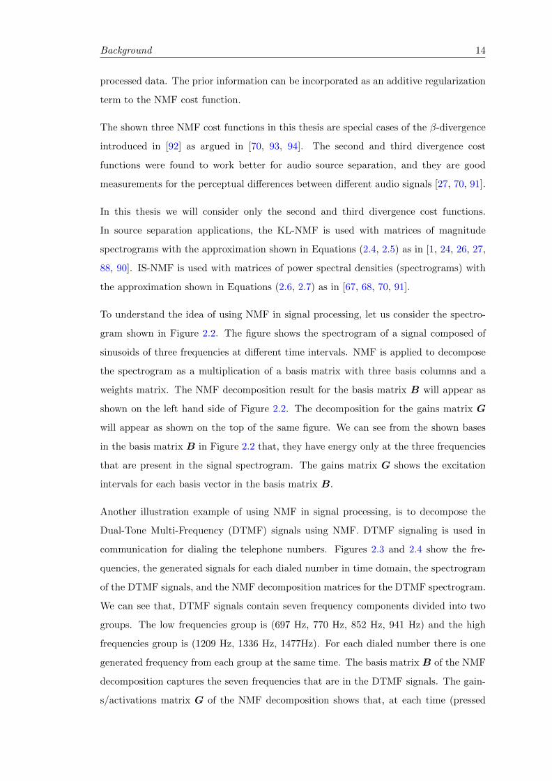
2.3 The DTMF signals. . . . . . . . . . . . . . . . . . . . . . . . . . . . . . . . 16
2.4 The NMF decomposition matrices for the DTMF signals. . . . . . . . . . 17
2.5 The NMF decomposition matrices for a clean speech signal. . . . . . . . . 18
3.1 The cluster structure for the nonnegative linear combinations of the basis vectors. 24
3.2 The effect of changing the number of GMM mixture K for speech-musicseparation using KL-NMF at SMR = −5 dB, λspeech = λmusic = 0.005, λtrain =0.0001. . . . . . . . . . . . . . . . . . . . . . . . . . . . . . . . . . . . . . . 36
3.3 The SIR for the case of using no priors during training and separationstages, the case of using prior only during testing, and the case of usingprior during training and separation stages. . . . . . . . . . . . . . . . . . 39
4.1 The cluster and temporal structures for the nonnegative linear combinations of
the basis vectors. . . . . . . . . . . . . . . . . . . . . . . . . . . . . . . . . . 45
4.2 The graphical model representation of a HMM . . . . . . . . . . . . . . . 48
5.1 The flow chart of using regularized NMF with MMSE estimates underGMM priors for SCSS. The term NMF+MMSE means regularized NMFusing MMSE estimates under GMM priors. . . . . . . . . . . . . . . . . . 66
5.2 The effect of using different prior models on the gains matrix on the SNRvalues. . . . . . . . . . . . . . . . . . . . . . . . . . . . . . . . . . . . . . . 71
5.3 The effect of using different prior models on the gains matrix on the SIRvalues . . . . . . . . . . . . . . . . . . . . . . . . . . . . . . . . . . . . . . 72
5.4 The effect of using different prior models on the gains matrix on the SDRvalues . . . . . . . . . . . . . . . . . . . . . . . . . . . . . . . . . . . . . . 73
7.1 Columns construction and sliding windows with length L frames. . . . . . . . . 86
8.1 The simplified cross-coherence penalty. . . . . . . . . . . . . . . . . . . . . . . 99
8.2 SDR and SIR in dB for the estimated speech signal. . . . . . . . . . . . . 100
10.1 Columns construction and sliding windows with length L frames. . . . . . . . . 113
12.1 The graphical model of the observation model. . . . . . . . . . . . . . . . 122
12.2 Graphical representation of the observation model for a set of N datapoints. . . . . . . . . . . . . . . . . . . . . . . . . . . . . . . . . . . . . . . 127
xii
List of Tables
3.1 SNR in dB for the speech signal for speech-music separation using regu-larized KL-NMF with λtrain = 0 and different values of the regularizationparameters in testing λspeech and λmusic. . . . . . . . . . . . . . . . . . . . 38
3.2 SNR in dB for the speech signal for speech-music separation using reg-ularized KL-NMF with different values of the regularization parametersλspeech, λmusic and λtrain = 0.0001 for last two columns. . . . . . . . . . . 38
3.3 SNR in dB for the speech signal for speech-music separation using reg-ularized IS-NMF with different values of the regularization parametersλspeech and λmusic. . . . . . . . . . . . . . . . . . . . . . . . . . . . . . . . 38
3.4 SNR in dB for the male speech signal for speech-speech separation usingregularized KL-NMF with different values of the regularization parame-ters λmale and λfemale. . . . . . . . . . . . . . . . . . . . . . . . . . . . . . 39
3.5 SNR in dB for the male speech signal for speech-speech separation usingregularized IS-NMF with different values of the regularization parametersλmale and λfemale. . . . . . . . . . . . . . . . . . . . . . . . . . . . . . . . 40
3.6 SNR in dB for the speech signal for speech-music separation using conju-gate prior KL-NMF with different values of the prior parameters. . . . . . 42
4.1 SNR in dB for the estimated speech signal for using different HMM . . . . . . . . . 55
4.2 SNR in dB for the estimated speech signal for using GMM prior models . . . . . . . 56
4.3 SNR in dB for the estimated speech signal for using different prior models . . . . . . 57
5.1 SNR and SIR in dB for the estimated speech signal with regularizationparameters λspeech = λmusic = 1 and different number of Gaussian mixturecomponents K. . . . . . . . . . . . . . . . . . . . . . . . . . . . . . . . . . 69
6.1 SNR in dB for the estimated speech signal using spectral mask without and with
smoothing filter, with different filter types and different filter size a× b. . . . . . . . 77
6.2 SNR in dB for the estimated speech signal using spectral mask after smoothing the
matrix G in the mask, with different filter types and different filter size a× b. . . . . . 77
6.3 SNR in dB for the estimated speech signal with smoothing G without using mask with
different filters with a = 1, b = 3. . . . . . . . . . . . . . . . . . . . . . . . . . . 79
6.4 SNR in dB for the estimated speech signal with smoothing the estimated magnitude
spectrogram of speech signal with different filters with a = 1, b = 3. . . . . . . . . . . 79
6.5 SNR in dB for the estimated speech signal using only NMF and with using regularized
NMF in [1]. . . . . . . . . . . . . . . . . . . . . . . . . . . . . . . . . . . . . 80
6.6 SNR and SIR in dB for the estimated speech signal using spectral maskafter smoothing the matrix G in the mask, with different filter types anddifferent filter size a = 1 and different values for b. . . . . . . . . . . . . . 81
xiii

List of tables xiv
6.7 SNR and SIR in dB for the estimated speech signal using MMSE estimatesbased regularized NMF and smoothed masks for different filter types anddifferent filter size a = 1,K = 16, λ = 1 and different values for b. . . . . . 82
6.8 SNR and SIR in dB for the oracle experiment. . . . . . . . . . . . . . . . 82
7.1 SDR and SIR in dB for the estimated speech signal. . . . . . . . . . . . . 90
8.1 SDR and SIR in dB for the estimated speech signal. . . . . . . . . . . . . 100
9.1 Signal to Noise Ratio (SNR) in dB for the separated speech signal for every
experiment with 10 seconds samples. . . . . . . . . . . . . . . . . . . . . . . . 110
9.2 Signal to Noise Ratio (SNR) in dB for the separated speech signal for every
experiment with 15 seconds samples. . . . . . . . . . . . . . . . . . . . . . . . 111
10.1 SNR in dB for the speech signal using NMF with sliding window andspectral mask with p = 3 for different numbers of bases. . . . . . . . . . . 115
10.2 SNR in dB for the speech signal in case of using NMF with sliding windowand different masks, with Ns = Nm = 642. . . . . . . . . . . . . . . . . . . 116
10.3 SNR in dB for the speech signal in case of using NMF with differentmasks, without sliding window, with Ns = Nm = 128. . . . . . . . . . 116
10.4 The percentage improvement for SNR and SIR in dB for the estimatedspeech signal for using post-smoothing and NMF with sliding windows. . 117
10.5 SNR and SIR in dB for the estimated speech signal in the case of usingNMF with sliding window and CNMF with different L values and p = 2. . 118
Abbreviations
SCSS Single Channel Source Separation
NMF Nonnegative Matrix Factorization
GMM Gaussian Mixtuer Models
HMM Hidden Markov Models
FHMM Factorial Hidden Markov Models
MMSE Minimum Mean Squared Error
PDF Probability Density Function
MFCC Mel-Frequency Cepstral Coefficients
EM Expectation Maximization
SVM Support Vector Machines
SNR Signal to Noise Ratio
SDR Signal to Distortion Ratio
SIR Signal to Interference Ratio
PSD Power Spectral Density
xv

Chapter 1
Introduction
Source separation refers to the problem of separating one or more desired signals from
mixtures of multiple signals. This problem can be encountered in many different applica-
tions such as medical [2, 3, 4], military [5, 6], and multimedia [7, 8]. To perform effective
separation, this problem is usually approached by using multiple sensors each of which
measures a different mixture of the source signals to obtain sufficient information about
the incoming source signals. In most cases, the source signals are assumed to be statis-
tically independent and no extra prior information about the source signals is assumed
available. The problem is treated as blind source separation (BSS) [7, 9], which can
be performed by techniques such as independent component analysis (ICA) [9, 10, 11].
This approach performs well when the number of measuring sensors (channels) are at
least as many as the number of signal sources in the mixed signal.
A more complicated problem is that of separating multiple source signals from a single
measuring of the mixed signal. This problem is usually defined as the single channel
source separation (SCSS) problem. The goal in single-channel source separation (SCSS)
is to recover the original source signals from a single recording of their linear mixture as
shown in Figure 1.1. Since the problem is underspecified, prior knowledge or training
data for the source signals are assumed to be available.
In this thesis we consider the single channel source separation problem for audio signals.
The audio signals can be speech, music, or noise. The single-channel audio source
separation problem is encountered in many applications such as: separating instruments
in music recordings [1, 12, 13, 14], separating speech signals from multiple simultaneous
1
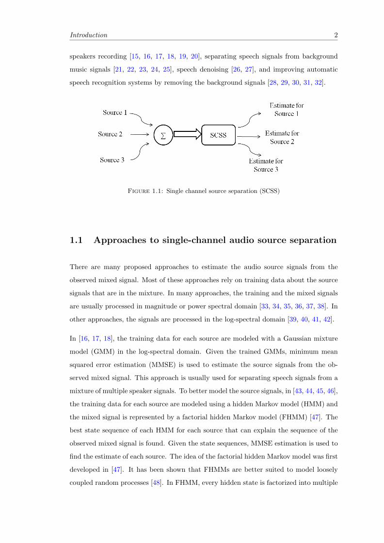
Introduction 2
speakers recording [15, 16, 17, 18, 19, 20], separating speech signals from background
music signals [21, 22, 23, 24, 25], speech denoising [26, 27], and improving automatic
speech recognition systems by removing the background signals [28, 29, 30, 31, 32].
Figure 1.1: Single channel source separation (SCSS)
1.1 Approaches to single-channel audio source separation
There are many proposed approaches to estimate the audio source signals from the
observed mixed signal. Most of these approaches rely on training data about the source
signals that are in the mixture. In many approaches, the training and the mixed signals
are usually processed in magnitude or power spectral domain [33, 34, 35, 36, 37, 38]. In
other approaches, the signals are processed in the log-spectral domain [39, 40, 41, 42].
In [16, 17, 18], the training data for each source are modeled with a Gaussian mixture
model (GMM) in the log-spectral domain. Given the trained GMMs, minimum mean
squared error estimation (MMSE) is used to estimate the source signals from the ob-
served mixed signal. This approach is usually used for separating speech signals from a
mixture of multiple speaker signals. To better model the source signals, in [43, 44, 45, 46],
the training data for each source are modeled using a hidden Markov model (HMM) and
the mixed signal is represented by a factorial hidden Markov model (FHMM) [47]. The
best state sequence of each HMM for each source that can explain the sequence of the
observed mixed signal is found. Given the state sequences, MMSE estimation is used to
find the estimate of each source. The idea of the factorial hidden Markov model was first
developed in [47]. It has been shown that FHMMs are better suited to model loosely
coupled random processes [48]. In FHMM, every hidden state is factorized into multiple
Introduction 3
state variables. The main limitation of using MMSE estimation to separate the source
signals in the log-spectral domain is that, the data used in training and separation stages
are assumed to have the same energy level. In practical cases, the sources are mixed
with a different energy level. There are approaches to fix this limitation [49, 50, 51]. The
basic idea is to express the probability density function (PDF) of the mixture in terms
of the individual speakers PDFs and their corresponding gains. Then, those patterns
and gains which maximize the mixture PDF are selected and used to recover the speech
signals. In [44], a non-linear optimization technique was used to estimate the ratio be-
tween the energy of the two sources. In [52], the expectation-maximization algorithm
(EM) was used to estimate the gains and the other FHMM parameters. In general, these
approaches are computationally complicated with slow performance.
Another approach for SCSS is to decompose the mixed signal spectral frames as a
weighted linear combination of the training data spectral frames. In [53, 54, 55, 56, 57,
58, 59], the mixed signal is decomposed as a linear combination of a number of exemplars
from a large exemplar dictionary of training data for each source signal. In our early
work [23], the magnitude spectrogram frames of the training data for each source were
used as a model or dictionary; then matching pursuit was used to decompose the mixed
signal magnitude spectrogram with the training data magnitude spectrogram frames;
the decomposition results were used to build spectral masks; the spectral masks were
used to estimate the contribution of each source in the mixed signal. These approaches
usually give good results but they require large dictionaries for the source signals.
Instead of using the whole training data as a dictionary, in [14, 22, 60, 61, 62] a set of
representative vectors is used as a dictionary for each source training data. The mixed
signal spectrum is represented as a linear combination of these dictionary entries. In [60],
a non-negative sparse representation is employed, and the sources are reconstructed using
the Wiener filter. In [14], sparse coding with a temporal continuity objective was used
for separating musical instruments. In [63], the training data was modeled in power
spectral density domain by a Gaussian mixture model (GMM) with zero means and
diagonal covariance matrix for each source. Every model was then adapted to better
represent the source signals in the mixed signal. Finally, the adaptive Wiener filter
was used with the adapted models to estimate the source signals in [63]. In our early
work [22], the training data was modeled by clustering the spectrogram of the training
data using K-means algorithms. Coordinate descent was used in [22] to decompose the
Introduction 4
spectrogram of the mixed signal with the K cluster centroids for each source training
data. Sparsity and continuity priors were enforced during the decomposition and the
sources’ STFT were reconstructed in [22] using the Wiener filter.
The most used approach for solving the SCSS problem is nonnegative matrix factoriza-
tion (NMF) [64] to train a set of nonnegative basis vectors (dictionary) for the training
data of each source. In the separation stage, NMF is used to decompose the mixed
signal as a weighted linear combination of the trained basis vectors. The estimate of
each source is found by summing its corresponding trained basis terms from the NMF
decomposition during the separation stage [13, 26, 27, 65]. The NMF is used in this
framework in magnitude spectral or power spectral domain where the nonnegativity
constraint is necessary. The number of the trained basis vectors is usually less than the
dimension of the spectral frames of the training data. Due to the efficient update rule
solutions of NMF [64] and since every source is represented by a few number of basis
vectors, this approach is considered to be fast and very simple which makes it the most
used approach in SCSS. Another advantage of using NMF in SCSS is that there is no
limitation on the energy level for the training and mixed signals. As we will show later,
NMF can be extended to consider more properties for the processed signals.
There are many other methods of using NMF in SCSS. In [12], different NMF decompo-
sitions were done for both training and testing data. The trained basis vectors were used
to learn support vector machines (SVM) classifiers. The trained SVM classifiers were
used to classify the basis vectors of the mixed signal and assign them to different source
signals. An unsupervised NMF with clustering was used in [1] to separate the mixed
signal. In [13], NMF was used to decompose the mixed data by fixed trained basis vec-
tors for each source in one method, and in another method the NMF was used without
trained basis vectors to decompose the mixed data, but it requires human interaction
for clustering the resulting basis vectors into different sources.
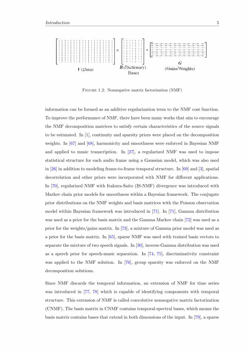
As can be seen in Figure 1.2, NMF is a matrix factorization that decomposes any
nonnegative matrix V into a multiplication of a nonnegative basis matrix/dictionary
B and a nonnegative gains/weights/activations matrix G [64, 66]. The decomposition
matrices are found by minimizing a predefined cost function. Like any optimization
problem, the main goal is to minimize the cost function without considering the nature of
the processed signals. To consider the prior information on the NMF solution, extra prior
Introduction 5
Figure 1.2: Nonnegative matrix factorization (NMF)
information can be formed as an additive regularization term to the NMF cost function.
To improve the performance of NMF, there have been many works that aim to encourage
the NMF decomposition matrices to satisfy certain characteristics of the source signals
to be estimated. In [1], continuity and sparsity priors were placed on the decomposition
weights. In [67] and [68], harmonicity and smoothness were enforced in Bayesian NMF
and applied to music transcription. In [27], a regularized NMF was used to impose
statistical structure for each audio frame using a Gaussian model, which was also used
in [26] in addition to modeling frame-to-frame temporal structure. In [69] and [3], spatial
decorrelation and other priors were incorporated with NMF for different applications.
In [70], regularized NMF with Itakura-Saito (IS-NMF) divergence was introduced with
Markov chain prior models for smoothness within a Bayesian framework. The conjugate
prior distributions on the NMF weights and basis matrices with the Poisson observation
model within Bayesian framework was introduced in [71]. In [71], Gamma distribution
was used as a prior for the basis matrix and the Gamma Markov chain [72] was used as a
prior for the weights/gains matrix. In [73], a mixture of Gamma prior model was used as
a prior for the basis matrix. In [65], sparse NMF was used with trained basis vectors to
separate the mixture of two speech signals. In [30], inverse-Gamma distribution was used
as a speech prior for speech-music separation. In [74, 75], discriminativity constraint
was applied to the NMF solution. In [76], group sparsity was enforced on the NMF
decomposition solutions.
Since NMF discards the temporal information, an extension of NMF for time series
was introduced in [77, 78] which is capable of identifying components with temporal
structure. This extension of NMF is called convolutive nonnegative matrix factorization
(CNMF). The basis matrix in CNMF contains temporal-spectral bases, which means the
basis matrix contains bases that extend in both dimensions of the input. In [79], a sparse
Introduction 6
CNMF was presented. In [80], CNMF was used with exemplar-based robust speech
recognition under noise. In [81], group sparsity is enforced on the CNMF decomposition.
CNMF with basis adaptation was introduced in [38].
1.2 The contributions of this thesis
In this thesis, we improve single channel source separation using NMF by incorporating
prior information about the source signals. The prior information is incorporated during
the NMF decomposition or as a post processing step. We improve the NMF performance
by incorporating more priors to the NMF matrices by using regularized NMF. The prior
information is modeled using statistical models that can capture the characteristics of the
source signals. Unlike [70, 71] the parameters of the used prior models here are trained
from training data for the source signals as opposed to choosing the parameters of the
prior models during the separation/testing stage. We model the prior information about
the NMF gains using rich models like Gaussian mixture models (GMM) and hidden
Markov models (HMM). We also propose a novel approach for applying the prior on the
NMF solutions which aims to evaluate how much the NMF solution needs to rely on
the prior information. In addition, we incorporate prior information based on intuitive
facts like discriminativity of the bases and the smoothness of the source spectra or
gains matrices or spectral masks. Furthermore, we introduce model adaptation where
the source signals are modeled by a nonnegative dictionary. Finally, we consider to
train a set of basis vectors that capture the relations between the consequent spectral
frames. We have disseminated some of our contributions in the following publications
[82, 83, 84, 85, 86, 87, 88, 89].
The contributions of this thesis can be itemized as follows:
• We use a Gaussian mixture model (GMM) to regularize the gains in NMF decom-
position to improve the separation performance. We develop new update rules for
the proposed regularized NMF. In addition, we introduce joint training to learn
both the dictionary and the prior GMM together.
Introduction 7
• To model the dynamic information in source signals, we introduce an HMM as a
regularizer for the gains matrix columns which characterizes the sequential depen-
dence of the temporal activations in a principled manner. We derive the update
rules for the new regularized NMF.
• As a novel idea to improve regularization and to avoid dependence on the regu-
larization parameters, we introduce a new regularization method based on MMSE
estimates under a GMM prior with a distortion model where the distortion co-
variance is estimated online. Based on the estimated covariance of the distortion,
the proposed MMSE estimation based regularized NMF decides how much the
solution relies on the GMM prior.
• We incorporate the smoothness prior information into the estimated source signals
using post-processing. The NMF solutions during the separation stage are used to
build spectral masks which are then smoothed by low pass filters. The smoothed
spectral masks are used to estimate the source signals.
• Instead of incorporating prior information about the NMF matrices, we incorpo-
rate prior information about the spectrogram frames of the source signals. The
GMMs are used to model the priors about the log-spectra of the source signals.
The MMSE estimation is used to enhance the separated signal spectrogram un-
der the trained GMM priors. To consider the temporal information between the
consequent frames of the spectrogram, MMSE estimation is applied to enhance
multiple stacked spectral frames together.
• We introduce a novel method to learn discriminative nonnegative dictionaries for
the source signals. The dictionary for each source is learned to well represent its
own source and penalized from representing the other source signals. We penal-
ize each dictionary from representing the other source signals by minimizing the
projection of each source dictionary into the other source dictionaries.
• We introduce new model adaptation techniques where the training data are mod-
eled using nonnegative dictionaries. The adaptation is used here to overcome the
lack of sufficient training data. A general dictionary is learned for speech signals
and then the proposed adaptation methods are used to adapt the general model
to better fit the speech signals that exist in the mixed signal. The Bayesian and
Introduction 8
linear transformation adaptations are introduced and used to adapt the source
dictionaries.
• The last contribution is to train basis matrices that can capture the relation be-
tween consequent spectral frames. The main idea is to use sliding windows with
NMF to decompose multiple stacked spectral frames together. The NMF decom-
position results are used to build spectral masks to estimate the source signals.
1.3 Organization of this thesis
In Chapter 2, we introduce the mathematical formulation for single channel source sep-
aration (SCSS) and nonnegative matrix factorization (NMF). We also show the conven-
tional use of NMF in SCSS in Chapter 2. In Chapters 3 to 5, we describe our approaches
for incorporating statistical priors to the NMF solution of the gains matrix. In Chapter
3, prior information about the NMF gains matrix is modeled by Gaussian mixture mod-
els (GMM) and this information is incorporated by adding a GMM log-likelihood term
to the NMF divergence cost function. In Chapter 4, prior information about the NMF
gains matrix is modeled by a hidden Markov model (HMM). The NMF solution of the
gains matrix is guided by the prior HMM. In Chapter 5, we incorporate statistical priors
which are modeled using GMM to the NMF solution of the gains matrix after evaluating
the actual need to the prior information by using a novel regularization method based on
MMSE estimation. Chapters 6 and 7 focus on post-processing after NMF-based source
separation. In Chapter 6, the smoothness prior is considered in the estimation of the
sources using simple post processing. Another more complex post processing approach
using MMSE estimation is introduced in Chapter 7 to enhance the separated signals.
In Chapters 8-10, we improve the dictionaries used in source separation. In Chapter 8,
discriminative training for the NMF basis matrices is introduced. In Chapter 9, adap-
tation of the basis matrix to a specific speaker is introduced. Finally, in Chapter 10,
NMF with sliding windows approach is introduced to model the relation between the
sequence of spectral frames.
Chapter 2
Background
2.1 Formulation for single-channel source separation
Single-channel audio source separation (SCSS) aims to find estimates of the original
audio source signals sz(t), ∀z ∈ {1, .., Z} given only a mixed signal y(t). The mixing
process is taken as a sum of the sources as follows:
y(t) =
Z∑z=1
sz(t), (2.1)
where t denotes time and Z is the number of sources in the mixed signal.
This problem is usually solved in the short time Fourier transform (STFT) domain
[1, 22, 28]. Let Y (n, f) be the STFT of y(t), where n represents the frame index and f
is the frequency index. Due to the linearity of the STFT, we have:
Y (n, f) =Z∑z=1
Sz(n, f), (2.2)
where Sz(n, f) is the unknown STFT of source z in the mixed signal. To compute the
STFT of a given audio signal, the signal is divided into overlapping segments (frames).
For each frame, the discrete Fourier transform (DFT) is calculated and a column in the
STFT matrix is obtained. The STFT of a given signal is a matrix of complex numbers
where each column represents a DFT of a segment or frame of the audio signal and the
9
Background 10
rows represent frequency indices. We can rewrite (2.2) as follows:
|Y (n, f)| ejφY (n,f) =
Z∑z=1
|Sz(n, f)| ejφSz (n,f), (2.3)
where φY (n, f) and φSz(n, f) are the phase angles of the mixed and zth source signal
respectively.
To find estimates for the source signals, different approximations for Equation (2.3) are
usually used to avoid dealing with complex numbers which have unknown phase angles
and magnitudes; the phase is known to be less important in audio applications. In [1,
24, 27, 28, 65, 90], it is assumed that the sources have the same phase angle as the mixed
signal, that is φSz(n, f) = φY (n, f), ∀z = 1, .., Z. Thus, the magnitude spectrogram of
the measured signal is approximated as the sum of source signal magnitude spectrograms’
entries as follows:
|Y (n, f)| =Z∑z=1
|Sz(n, f)| . (2.4)
In this approximation, the mixed signal and the source magnitude spectrograms can be
written in matrix form as follows:
Y =
Z∑z=1
Sz. (2.5)
In this first approximation, Y is the magnitude spectrogram of the mixed signal and Sz
represents the unknown magnitude spectrogram of the source signal z.
The second approximation for Equation (2.3) is assuming the sources to be independent
[67, 68, 70, 83, 84]. In those works, the power spectral density (PSD) of the measured
signal is approximated as the sum of source signal PSDs as follows:
σ2y(n, f) =
Z∑z=1
σ2Sz
(n, f), (2.6)
where σ2y(n, f) = E(|Y (n, f)|2). In this approximation, the PSD frames can be written
in matrix form (spectrogram) as follows:
Y =Z∑z=1
Sz. (2.7)
Background 11
In this approximation, Y is the spectrogram (power spectrogram) of the mixed signal
and Sz represents the unknown spectrogram of the source signal z. The PSD for the
measured signal y(t) is calculated by taking the squared magnitude of its STFT.
In this thesis, we mainly use NMF for source separation. We give here an introduction
about different types of NMF cost functions. The conventional approach of using NMF
for source separation is introduced in the following section.
2.2 Non-negative matrix factorization
Non-negative matrix factorization [64] is an algorithm that is used to decompose any
matrix V with nonnegative entries into a nonnegative basis/dictionary matrix B and a
nonnegative weights/gains matrix G as follows:
V ≈ BG. (2.8)
So every column vector in the matrix V is approximated by a nonnegative weighted
linear combination of the basis vectors in the columns of B, where B has fewer columns
than V . The weights for basis vectors appear in the corresponding column of the matrix
G as follows:
vn =D∑j=1
gjnbj , (2.9)
where vn is the column n in matrix V , bj is the column j in matrix B, gjn is its weight
in the gains matrix G, and D is the number of bases in B. The matrix B contains
nonnegative basis vectors that are optimized to allow the data in V to be approximated
as a nonnegative linear combination of its constituent vectors. Figure 2.1 shows a simple
two dimensional example where the number of basis vectors is two. Any nonnegative
linear combinations of the two basis vectors appears in the nonnegative cone between
the two basis vectors as shown in Figure 2.1.
The two matrices B and G in Equation (2.8) can be computed by solving the following
minimization problem:
minB,G
C (V ,BG) , (2.10)
subject to elements of B,G ≥ 0.
Background 12
0 0.5 1 1.5 2 2.5 3 3.5 40
0.5
1
1.5
2
2.5
3
3.5
4
b2
b1
Figure 2.1: The nonnegative linear combinations for the given two basis vectors.
Different cost functions C lead to different kinds of NMF. In [64], two different cost
functions were analyzed. The first cost function is the Euclidean distance between V
and BG, given by
minB,G
(‖V −BG‖22
), (2.11)
where
‖V −BG‖22 =∑i,j
(V i,j − (BG)i,j
)2.
The NMF solution for Equation (2.11) can be computed by alternating updates of B
and G as follows:
B ← B ⊗ V GT
BGGT, (2.12)
G← G⊗ BTV
BTBG, (2.13)
where the operations ⊗ and all divisions are element-wise multiplication and division
respectively. The matrices B and G are initialized by positive random numbers and
then updated iteratively using the update rules in (2.12, 2.13).
The second cost function for NMF in [64] is the generalized Kullback-Leibler (KL-NMF)
divergence cost function [64]
minB,G
DKL (V ||BG) , (2.14)
Background 13
where
DKL (V ||BG) =∑i,j
(V i,j log
V i,j
(BG)i,j− V i,j + (BG)i,j
).
The NMF solution for Equation (2.14) can be computed by alternating updates of B
and G as follows:
B ← B ⊗VBGG
T
1GT, (2.15)
G← G⊗BT V
BGBT1
, (2.16)
where 1 is a matrix of ones with the same size of V .
The third cost function is the Itakura-Saito (IS-NMF) divergence cost function [70]:
minB,G
DIS (V ||BG) , (2.17)
where
DIS (V ||BG) =∑i,j
(V i,j
(BG)i,j− log
V i,j
(BG)i,j− 1
).
The IS-NMF solutions for Equation (2.17) can be computed by alternating multiplicative
updates of B and G as shown in [70, 91]:
B ← B ⊗
V(BG)
2GT
1BGG
T, (2.18)
G← G⊗BT V
(BG)2
BT 1BG
, (2.19)
where (.)2 is also an element-wise operation.
The basis and gains matrices are usually initialized by random positive numbers. Within
each iteration, the columns of the basis matrix are normalized using the Euclidean norm
and the gains matrix is calculated accordingly. Since the NMF cost functions are non-
convex with multiple local minima, the solution for the basis and gains matrices is not
unique and any local minima is a candidate solution for the cost function. To find
a better solution than the others, prior information can be incorporated to the cost
function. A better solution means a solution that is more suited to the nature of the
Background 14
processed data. The prior information can be incorporated as an additive regularization
term to the NMF cost function.
The shown three NMF cost functions in this thesis are special cases of the β-divergence
introduced in [92] as argued in [70, 93, 94]. The second and third divergence cost
functions were found to work better for audio source separation, and they are good
measurements for the perceptual differences between different audio signals [27, 70, 91].
In this thesis we will consider only the second and third divergence cost functions.
In source separation applications, the KL-NMF is used with matrices of magnitude
spectrograms with the approximation shown in Equations (2.4, 2.5) as in [1, 24, 26, 27,
88, 90]. IS-NMF is used with matrices of power spectral densities (spectrograms) with
the approximation shown in Equations (2.6, 2.7) as in [67, 68, 70, 91].
To understand the idea of using NMF in signal processing, let us consider the spectro-
gram shown in Figure 2.2. The figure shows the spectrogram of a signal composed of
sinusoids of three frequencies at different time intervals. NMF is applied to decompose
the spectrogram as a multiplication of a basis matrix with three basis columns and a
weights matrix. The NMF decomposition result for the basis matrix B will appear as
shown on the left hand side of Figure 2.2. The decomposition for the gains matrix G
will appear as shown on the top of the same figure. We can see from the shown bases
in the basis matrix B in Figure 2.2 that, they have energy only at the three frequencies
that are present in the signal spectrogram. The gains matrix G shows the excitation
intervals for each basis vector in the basis matrix B.
Another illustration example of using NMF in signal processing, is to decompose the
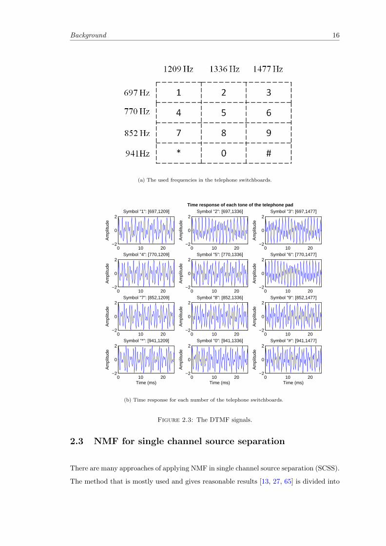
Dual-Tone Multi-Frequency (DTMF) signals using NMF. DTMF signaling is used in
communication for dialing the telephone numbers. Figures 2.3 and 2.4 show the fre-
quencies, the generated signals for each dialed number in time domain, the spectrogram
of the DTMF signals, and the NMF decomposition matrices for the DTMF spectrogram.
We can see that, DTMF signals contain seven frequency components divided into two
groups. The low frequencies group is (697 Hz, 770 Hz, 852 Hz, 941 Hz) and the high
frequencies group is (1209 Hz, 1336 Hz, 1477Hz). For each dialed number there is one
generated frequency from each group at the same time. The basis matrix B of the NMF
decomposition captures the seven frequencies that are in the DTMF signals. The gain-
s/activations matrix G of the NMF decomposition shows that, at each time (pressed
Background 15
200
100
50
1 2 3
1
2
3
200
100
50
Fre
qu
ency
(D
FT
in
dex
))
100 200 300 400 500 600 700 800 900
200 300 400 500 600 700 800 900100
Time (DFT frames)
Spectrogram
Columns of B
Ro
ws
of
G
Figure 2.2: The NMF decomposition matrices for the sinusoidal signals.
button in the telephone switchboard) there are two frequencies (two bases in matrix B)
active at the same time. The NMF decomposition results for DTMF signals capture the
frequencies and the activations for each dialed number in the telephone switchboard. For
example, when the button for symbol 1 is pressed, the frequencies 697Hz and 1209Hz are
generated. The bases number five and seven in Figure 2.4(b) represent the frequencies
697Hz and 1209Hz respectively. We can see from the activation matrix in Figure 2.4(c)
that, when the symbol 1 is pressed, the fifth and seventh rows are active. Figures 2.2 to
2.4 show very simple signals that contain few sinusoidal components. In Figures 2.2 to
2.4 the number of frequency components for each signal is assumed to be known, which
leads to the correct choice for the suitable number of basis vectors for each signal. For
natural audio data, the suitable number of bases can not be predetermined but it is
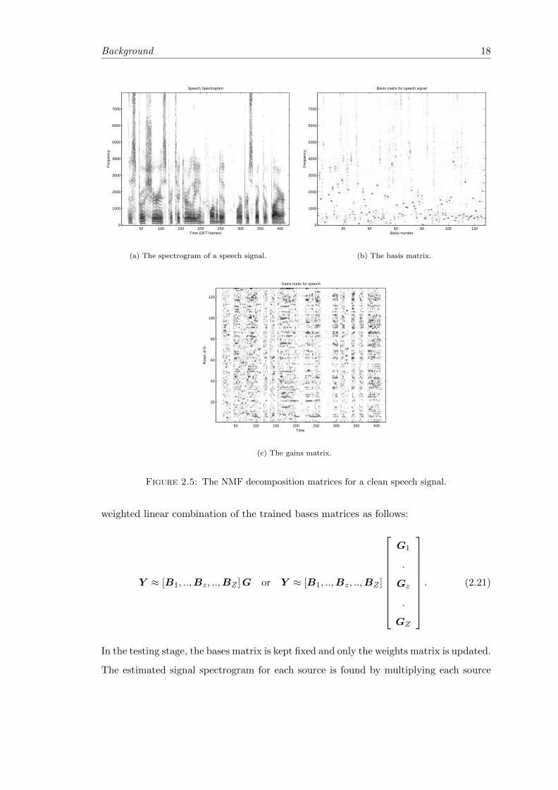
always believed that the data lie on a lower-dimensional manifold. Figure 2.5 shows an
example of the spectrogram of an audio signal and its NMF decomposition results using
128 basis vectors.
Background 16
(a) The used frequencies in the telephone switchboards.
0 10 20−2
0
2Symbol "1": [697,1209]
Am
plitu
de
0 10 20−2
0
2Symbol "2": [697,1336]
Am
plitu
de
0 10 20−2
0
2Symbol "3": [697,1477]
Am
plitu
de
0 10 20−2
0
2Symbol "4": [770,1209]
Am
plitu
de
0 10 20−2
0
2Symbol "5": [770,1336]
Am
plitu
de
0 10 20−2
0
2Symbol "6": [770,1477]
Am
plitu
de
0 10 20−2
0
2Symbol "7": [852,1209]
Am
plitu
de
0 10 20−2
0
2Symbol "8": [852,1336]
Am
plitu
de
0 10 20−2
0
2Symbol "9": [852,1477]
Am
plitu
de
0 10 20−2
0
2Symbol "*": [941,1209]
Am
plitu
de
Time (ms)0 10 20
−2
0
2Symbol "0": [941,1336]
Am
plitu
de
Time (ms)0 10 20
−2
0
2Symbol "#": [941,1477]
Am
plitu
de
Time (ms)
Time response of each tone of the telephone pad
(b) Time response for each number of the telephone switchboards.
Figure 2.3: The DTMF signals.
2.3 NMF for single channel source separation
There are many approaches of applying NMF in single channel source separation (SCSS).
The method that is mostly used and gives reasonable results [13, 27, 65] is divided into
Background 17
Time (DFT frames)
Fre
quen
cy
1 200 400 600 800 1000 1200 1400 1600 1800 2000 2200 24000
500
1000
1500
2000
2500
3000
3500
(a) The spectrogram of the DTMF.
Columns of B
Fre
quen
cy
1 2 3 4 5 6 70
500
1000
1500
2000
2500
3000
3500
(b) The basis matrix for the DTMF.
Time (DFT frames)
Row
s of
G
1 200 400 600 800 1000 1200 1400 1600 1800 2000 2200 2400
1
2
3
4
5
6
7
(c) The activation matrix for the DTMF.
Figure 2.4: The NMF decomposition matrices for the DTMF signals.
two main stages, the training stage and the separation stage. In the training stage, it
is assumed that, there is enough training data for each observed source in the mixed
signal. NMF uses these training data to train a set of basis vectors for each source. The
spectrogram Strainz of the training data of each source z is computed first using STFT.
Then NMF is used to decompose this spectrogram into a basis matrix Bz and a weights
matrix Gtrainz as follows:
Strainz ≈ BzGtrainz . (2.20)
The basis matrix (trained bases) Bz is used as a representative model for the training
data for each source z.
In the testing or separation stage, the trained basis matrices for all sources are concate-
nated in one bases matrix. NMF decomposes the mixed signal spectrogram Y into a
Background 18
Time (DFT frames)
Fre
quen
cy
Speech Spectrogram
50 100 150 200 250 300 350 4000
1000
2000
3000
4000
5000
6000
7000
(a) The spectrogram of a speech signal.
Basis matrix for speech signal
Basis number
Fre
quen
cy
20 40 60 80 100 1200
1000
2000
3000
4000
5000
6000
7000
(b) The basis matrix.
Gains matix for speech
Time
Row
s of
G
50 100 150 200 250 300 350 400
20
40
60
80
100
120
(c) The gains matrix.
Figure 2.5: The NMF decomposition matrices for a clean speech signal.
weighted linear combination of the trained bases matrices as follows:
Y ≈ [B1, ..,Bz, ..,BZ ]G or Y ≈ [B1, ..,Bz, ..,BZ ]
G1
.
Gz
.
GZ
. (2.21)
In the testing stage, the bases matrix is kept fixed and only the weights matrix is updated.
The estimated signal spectrogram for each source is found by multiplying each source
Background 19
basis in the bases matrix with its corresponding weights in the weights matrix as follows:
S1 = B1G1, ..., Sz = BzGz, ..., SZ = BZGZ . (2.22)
2.3.1 Reconstruction of source signals and spectral masks
In our earlier work of using NMF for source separation [24], instead of using the initial
estimates S1, ...., SZ in Equation (2.22) as the final estimates for the source signals, we
used them to build spectral masks. Special cases of this idea appear in [28, 73, 90, 95].
The sum of the estimated spectra Sz, ∀z ∈ {1, .., Z} in (2.22) may not sum up to
the mixed magnitude-spectrogram Y . We usually obtain nonzero decomposition error.
Thus, NMF gives us an approximation:
Y ≈Z∑z=1
Sz.
Assuming noise is negligible in the mixed signal, the component signals’ sum should be
directly equal to the mixed magnitude spectrogram. To make the error zero, we used the
initial estimated magnitude spectrograms Sz, ∀z ∈ {1, .., Z} to build spectral masks as
follows:
Hz =Sz
p∑Zj=1 Sj
p , ∀z ∈ {1, .., Z} (2.23)
where p > 0 is a parameter, the operation (.)p, and the division are element-wise op-
erations. Notice that, the elements of Hz ∈ [0, 1] and using different p values leads to
different kinds of masks. When p = 2 the mask H is a Wiener filter assuming S2z are
estimates of the PSD of the zth source signal and sources are independent. The value of
p controls the saturation level of the ratio in (2.23). When p > 1, the larger source com-
ponent will dominate more in the mixture. At p =∞, we achieve a binary mask (hard
mask) which will choose the larger source component as the only component. These
masks will scale every frequency component in the observed mixed spectrogram Y with
a ratio that explains how much each source contributes in the mixed signal such that:
Sz = Hz ⊗ Y , (2.24)
where Sz is the final estimate of the source z spectrogram, and ⊗ is an element-wise
multiplication. By using this idea we make the approximation error zero, and we can
Background 20
make sure that the estimated signals will add up to the mixed signal. After finding the
contribution of each source in the mixed signal, the estimate for each source signal sz(t)
can be computed by inverse STFT to the estimated source spectrogram Sz with the
phase angle of the mixed signal. In [24], we applied this idea to separate a speech signal
from a background music signal using the KL-NMF cost function. We tried different
values for the number of trained basis vectors for each source basis matrix and different
values for the spectral mask parameter p. We achieved reasonable performance when the
number of basis was 128 basis vectors for each source and p = 3. We also evaluated this
idea in our previous work [96] to improve the audio-visual speech recognition performance
by removing the background music signal from the speech signal. In [96], we achieved
better recognition performance compared to the case when the speech recognition was
done without removing the background signals.
2.4 Performance evaluation
In this thesis, we use different metrics to evaluate our proposed ideas. The metrics are
Source to Distortion Ratio (SDR) and Source to Interference Ratio (SIR) from [97]. We
also use the regular Signal to Noise Ratio (SNR) metric. These metrics are defined as
follows:
SDR = 10 log10
‖starget (t)‖2
‖einterf (t) + eartif (t)‖2, (2.25)
SIR = 10 log10
‖starget (t)‖2
‖einterf (t)‖2, (2.26)
SNR = 10 log10
‖s (t)‖2
‖s (t)− s (t)‖2. (2.27)
The separated signal is a combination of different components as follows:
s (t) = starget (t) + einterf (t) + eartif (t) , (2.28)
where starget (t) is the target signal which is defined as the projection of the predicted
signal onto the original desired signal, einterf (t) is the interference error due to the other
source signals only, and eartif (t) shows artifacts introduced by the separation algorithm.
Background 21
If sw (t) is the desired source signal, sw (t) is its estimated signal, so
starget (t) =< sw (t) , sw (t) >
‖sw‖2sw (t) ,
if the sources are mutually orthogonal,
einterf (t) =
(Z∑w=1
< sw (t) , sw (t) >
‖sw‖2sw
)− < sw (t) , sw (t) >
‖sw‖2sw (t) ,
where < ., . > is the dot product. If the sources are not orthogonal, one can use Gram
Schmidt orthogonalization to find the orthogonal projection onto the subspace spanned
by all the source signals [97],
eartif (t) = sw (t)− starget (t)− einterf (t) ,
The higher the SDR, SIR, and SNR, the better performance we achieve.
In the literature there have been some studies where the improvements appear to be
small. In [98], the SDR improvements were around 0.1 dB. In [1, 73], the improvements
in SNR were between 0.2-0.5 dB. The minimum improvement SIR was 1.5 dB in [60].
Chapter 3
Regularized NMF using GMM
priors
3.1 Motivations and overview
In this chapter, we propose a new regularized NMF algorithm that incorporates the
statistical characteristics of the source signals to steer the optimal solution of the NMF
cost function during the separation process. We propose a new multi-objective cost
function which includes the conventional divergence term for the NMF together with
a prior likelihood term. The first term measures the divergence between the observed
data and the multiplication of basis and gains matrices as shown in Equations (2.14,
2.17). The novel second term encourages the log-normalized gain vectors of the NMF
solution to increase their likelihood under a Gaussian mixture model (GMM) prior which
is used to encourage the gains to follow certain patterns. The normalization of the gains
makes the prior models energy independent, which is an advantage as compared to earlier
proposals [26, 27] where a single Gaussian was used as a prior model. In addition, GMM
is a much richer prior than the previously considered alternatives such as conjugate priors
[71, 99] which may not represent the distribution of the gains in the best possible way.
We introduce novel update rules that solve the optimization problem efficiently for the
new regularized NMF problem. This optimization is challenging due to using energy
normalization and GMM for prior modeling, which makes the problem highly nonlinear
and non-convex.
22
Regularized NMF using GMM priors 23
As shown in Section 2.3, the conventional use of NMF in supervised source separation
is to decompose the magnitude or power spectra of the training data of each source into
a trained basis matrix and a trained gains/weights matrix as in Equation (2.20). In
previous works [24, 65], the columns of the trained basis matrix are usually used as the
only representative model for the training source signals and the trained gains matrices
were usually ignored.
As a simple example to understand the model we introduce here, we can look at the toy
example in Figure 2.4. In Figure 2.4(c), the columns of the gains matrix only appear
in certain patterns in the DTMF signal. We can also see from Figure 2.4 that some
combinations for the basis vectors in the basis matrix are not allowed. For example,
any combination between the basis vectors number two, three, four, and five is not
allowed because these basis vectors represent the lower band frequencies that can not be
combined in DTMF data as shown in Figure 2.3(a). Also any combination between the
basis vectors number one, six, and seven can not be combined because they represent the
higher band frequency components that can not be combined as shown in Figure 2.3(a).
Based on the basis matrix in Figure 2.4(b), there are many different combinations for
the basis vectors in the basis matrix but just 12 of them are only valid combinations as
we can see in Figures 2.3(a) and 2.4(c).
The columns of the trained gains matrix represent the valid weight combination patterns
that the columns in the basis matrix can jointly receive for a specific type of source signal.
A prior distribution can represent the statistical distribution of the gains vector in each
column of the gains matrix and model the correlation between their entries. Since the
trained basis matrix for each source is common in the training and separation stage, the
prior model for the gains matrix for each source can guide the NMF solution to prefer
valid gain patterns during the separation stage. We use a multivariate Gaussian mixture
model (GMM) as a prior model for the gains vector for each frame of each source.
Figure 3.1 shows an example similar to Figure 2.1 but where certain linear combinations
between the two basis vectors are allowed. The figure shows the cases where the clus-
tering structure of the nonnegative linear combinations of the given two basis vectors
can be seen. For example, for speech signals there are a variety of phonetic differences,
which causes a sort of clustering structure for the data. Since the trained basis vectors
are the same during the training and the separation stage, we believe these clustering
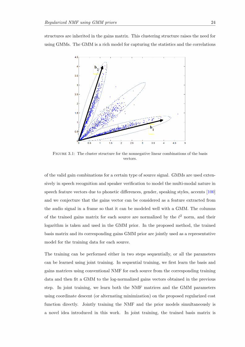
Regularized NMF using GMM priors 24
structures are inherited in the gains matrix. This clustering structure raises the need for
using GMMs. The GMM is a rich model for capturing the statistics and the correlations
Figure 3.1: The cluster structure for the nonnegative linear combinations of the basisvectors.
of the valid gain combinations for a certain type of source signal. GMMs are used exten-
sively in speech recognition and speaker verification to model the multi-modal nature in
speech feature vectors due to phonetic differences, gender, speaking styles, accents [100]
and we conjecture that the gains vector can be considered as a feature extracted from
the audio signal in a frame so that it can be modeled well with a GMM. The columns
of the trained gains matrix for each source are normalized by the `2 norm, and their
logarithm is taken and used in the GMM prior. In the proposed method, the trained
basis matrix and its corresponding gains GMM prior are jointly used as a representative
model for the training data for each source.
The training can be performed either in two steps sequentially, or all the parameters
can be learned using joint training. In sequential training, we first learn the basis and
gains matrices using conventional NMF for each source from the corresponding training
data and then fit a GMM to the log-normalized gains vectors obtained in the previous
step. In joint training, we learn both the NMF matrices and the GMM parameters
using coordinate descent (or alternating minimization) on the proposed regularized cost
function directly. Jointly training the NMF and the prior models simultaneously is
a novel idea introduced in this work. In joint training, the trained basis matrix is
Regularized NMF using GMM priors 25
also changed since the gains matrix is enforced to satisfy the NMF equation guided by
the GMM prior, so that the trained models are more consistent with the GMM prior
assumption. For this reason, we use sequential training for initialization of the model
parameters, but eventually use joint training of the model parameters in this work.
In the separation stage after observing the mixed signal, the proposed regularized NMF
is used to decompose the magnitude or power spectra of the observed mixed signal as
a weighted linear combination of the columns of trained bases matrices for all source
signals that appear in the mixed signal. The decomposition weights are encouraged
to increase their log-likelihood with their corresponding trained prior GMMs using the
regularized cost function.
In this chapter, we apply the proposed regularized NMF using the generalized Kullback-
Leibler (KL-NMF) divergence cost function [64] and the Itakura-Saito (IS-NMF) diver-
gence cost function [70] which are shown in Equations (2.14) and (2.17) respectively.
As shown in Section (2.2), the KL-NMF is used with matrices of magnitude spectro-
grams with the approximation shown in Equations (2.4, 2.5), while IS-NMF is used with
matrices of power spectral densities (spectrograms) with the approximation shown in
Equations (2.6, 2.7). We will show the proposed regularized NMF using KL-NMF first,
then we will state the differences regarding the usage of IS-NMF.
3.2 The proposed regularized nonnegative matrix factor-
ization approach
The goal of regularized NMF is to incorporate prior information on the solutions of the
matrices B and G. We enforce a statistical prior on the solution of the gains matrix
G only. We need the solution of G in Equation (2.8) to minimize the KL-divergence
cost function in Equation (2.14), and the log-normalized columns of the gains matrix
G, namely logg‖g‖2
, to maximize their log-likelihood under a trained GMM prior model.
Hence, the solution of G can be found by minimizing the following regularized KL-
divergence cost function:
C = DKL (V ||BG)− λL(G|θ), (3.1)
Regularized NMF using GMM priors 26
where L(G|θ) is the log-likelihood of the log-normalized columns of the gains matrix
G under the trained prior gain GMM with parameters θ, and λ is a regularization
parameter. The regularization parameter controls the trade-off between the NMF cost
function and the prior log-likelihood. The multivariate Gaussian mixture model (GMM)
with parameters θ = {wk,µk,Σk}Kk=1 for a random variable x is defined as:
p(x|θ) =K∑k=1
wk
(2π)d/2 |Σk|1/2exp
{−1
2(x− µk)
T Σ−1k (x− µk)
}, (3.2)
where K is the number of Gaussian mixture components, wk is the mixture weight, d is
the vector dimension, µk is the mean vector and Σk is the diagonal covariance matrix
of the kth Gaussian model. In this section, we assume GMM parameters θ are given.
We will mention the training of θ in the next section. The normalization is done using
the `2 norm by modeling logg‖g‖2
.
The reason for using the logarithm is because GMM is usually a better fit to the loga-
rithm of the values between 0 and 1 due to wider support as observed in tandem speech
recognition research [101]. The reason for normalization is to make the prior models
insensitive to the change of the energy level of the signals, which makes the same prior
models applicable for a wide range of energy levels and avoids the need to train a different
prior model for different energy levels.
The log-likelihood for the gains matrix G with N columns can be written as follows:
L(G|θ) =N∑n=1
logK∑k=1
ρk,n (θ) , (3.3)
where
ρk,n (θ) =wk
(2π)(d/2) |Σk|1/2exp
{−1
2
(log
gn‖gn‖2
− µk)T
Σ−1k
(log
gn‖gn‖2
− µk)}
,
(3.4)
and gn is the column numbered n in the gains matrix G. The multiplicative update rule
for the basis matrix B for the cost function in Equation (3.1) is the same as in Equation
(2.15). To find the multiplicative update rule for G in Equation (3.1), we follow the
same procedures as in [1] and [67]. We express the gradient with respect to G of the

Regularized NMF using GMM priors 27
cost function ∇GC as the difference of two positive terms ∇+GC and ∇−GC as:
∇GC = ∇+GC −∇
−GC. (3.5)
The cost function is shown to be nonincreasing under the following update rule [1, 67]:
G← G⊗∇−GC∇+GC
, (3.6)
where the operations ⊗ and division are element-wise as in Equation (2.16). We can
write the gradients as:
∇GC = ∇GDKL − λ∇GL(G|θ), (3.7)
where ∇GL(G|θ) is a matrix with the same size of G. The gradient for the KL-cost
function and the prior log-likelihood can also be formed as differences between positive
terms as follows:
∇GDKL = ∇+GDKL −∇−GDKL, (3.8)
∇GL(G|θ) = ∇+GL(G|θ)−∇−GL(G|θ). (3.9)
We can rewrite Equations (3.5, 3.7) as:
∇GC =(∇+GDKL + λ∇−GL(G|θ)
)−(∇−GDKL + λ∇+
GL(G|θ)). (3.10)
The final update rule in Equation (3.6) can be written as follows:
G← G⊗∇−GDKL + λ∇+
GL(G|θ)∇+GDKL + λ∇−GL(G|θ)
, (3.11)
where
∇GDKL = BT
(1− V
(BG)
), (3.12)
∇−GDKL = BT V
(BG), (3.13)
and
∇+GDKL = BT1. (3.14)
Regularized NMF using GMM priors 28
The row j and column n component of the gradient of the prior log-likelihood in Equation
(3.3) can be found as follows:
(∇GL(G|θ))jn =(∇+GL(G|θ)
)jn−(∇−GL(G|θ)
)jn, (3.15)
where
(∇−GL(G|θ)
)jn
=
∑Kk=1
{−ρk,n
(Σkjj
)−1(µkj
gjn+
gjn
‖gn‖2
2
loggjn
‖gn‖2
)}∑K
k=1 ρk,n, (3.16)
(∇+GL(G|θ)
)jn
=
∑Kk=1
{−ρk,n
(Σkjj
)−1(µkjgjn
‖gn‖2
2
+ 1gjn
loggjn
‖gn‖2
)}∑K
k=1 ρk,n. (3.17)
Since the GMMs are trained by log-normalized columns, we know that the values of the
mean vectors µ are always negative. The values of the vectors g are always positive,
so the values from Equations (3.16) and (3.17) will be always positive. We can use
Equations (3.13, 3.14, 3.16, 3.17) to find the total gradients in Equation (3.10) and then
to derive the update rules for G in Equation (3.11). The initialization of the matrix G
is done by running one regular NMF iteration without any prior.
3.3 Training the source models
In the training stage, we aim to train a set of basis vectors for each source and a prior
statistical GMM for the gain patterns that each set of basis vectors can receive for each
source signal.
3.3.1 Sequential training
Given a set of training data for each source signal, the magnitude spectrogram Strainz
for each source z is calculated. The NMF is used to decompose Strainz into basis matrix
Bz and gains matrix Gtrainz . The gains matrix Gtrain
z is then used to train the prior
GMM for each source. KL-NMF is used to decompose the magnitude spectrogram into
Regularized NMF using GMM priors 29
basis and gains matrices as follows:
Strainz ≈ BzGtrainz , (3.18)
Bz,Gtrainz = arg min
B,GDKL
(Strainz ||BG
).
After finding the basis and the gains matrices, the corresponding GMM parameters θz
are then learned as follows:
θz = arg maxθL (Gz|θ) . (3.19)
We use multiplicative update rules in Equations (2.15) and (2.16) to find solutions for
Bz and Gz in Equation (3.18). All the matrices B and Gtrain are initialized by positive
random noise. In each iteration, we normalize the columns of Bz using the `2 norm and
find Gtrainz accordingly. After finding matrices B and Gtrain for all sources, all the basis
matrices B are used in mixed signal decomposition as it is shown in Section 3.4. We
use the gains matrices Gtrain to build statistical prior models. For each matrix Gtrainz ,
we normalize its columns and the logarithm is then calculated. These log-normalized
columns are used to train a gain prior GMM for each source in Equation (3.19) using
the well-known expectation maximization (EM) algorithm [102].
3.3.2 Joint training
In Section 3.3.1, the trained NMF basis and gains matrices for each source are computed
using Equations (2.15, 2.16), and then the prior gain GMMs are trained using the
logarithm of the normalized columns of the trained gains matrix. To match between
the way the trained models are used during training with the way they are used during
separation, we jointly train the basis vectors and the prior models simultaneously to
minimize the regularized cost function:
(Bz,G
trainz , θz
)= arg min
B,G,θDKL
(Strainz ||BG
)− λtrainL (G|θ) . (3.20)
We use the trained NMF and GMM models from Section 3.3.1 as initializations for
the source models, and then we update the model parameters by running alternating
update (coordinate descent) iterations on Bz, Gtrainz and θz parameters. At each NMF
iteration, we update the basis matrix Bz using update rule in (2.15) while keeping Gz
Regularized NMF using GMM priors 30
fixed, and the gains matrix Gtrainz is updated using update rule in (3.11) while keeping
Bz and θz fixed. We use a fixed value for the regularization parameter λtrain during
training. The new gains matrix is then used to train a new GMM with its parameters
θz using the EM algorithm initialized by the previous GMM parameters. By repeating
this procedure at each NMF iteration during training, the basis matrix is learnt in a
consistent way with the clustered structure of the gains matrix due to the usage of the
GMM priors. Since the original NMF problem is non-convex and there may be many
possible local minima, we conjecture that the prior term encourages an NMF solution
which is more consistent with the GMM prior assumption of the gains matrix.
3.3.3 Determining the hyper-parameters
The hyper-parameters in our model are the number of basis vectors d, number of mix-
tures K, and the regularization parameter λtrain. In addition, during testing, we may
use different λ parameters for each source depending on the energy ratios of source sig-
nals (speech-to-music or male-to-female energy ratios in our experiments) which yields
better results than using fixed values as we explain in Sections 3.4 and 3.5.
These hyper-parameters, especially λ value(s), may be learned using a fully Bayesian
treatment by putting priors on them and using the evidence framework or the integrate-
out method [103]. For Bayesian learning of number of mixtures in the GMM and the
number of basis vectors, one needs to use nonparametric Bayesian methods of Dirichlet
process mixtures [104] and Bayesian nonparametric NMF [105] which enable variable
number of mixtures and NMF basis components respectively. This overall Bayesian
treatment is possible since the divergence cost functions DKL and DIS can be seen as
negative log-likelihood functions that depend on the parameters of the NMF decom-
position under the probabilistic interpretations of NMF [70, 106]. However, Bayesian
solutions involve highly complicated computations due to sampling techniques and are
pretty cumbersome to implement. We consider these approaches as out of scope for
this work and leave them as future work. Thus, we take the conventional approach
of determining these parameters using grid search on validation data. Basically, we
perform different experiments with a range of reasonable values for each of these hyper-
parameters and choose the values that provide the best results on validation data.
Regularized NMF using GMM priors 31
3.4 Signal separation
After observing the mixed signal y(t), the magnitude spectrogram Y of the mixed signal
is computed using STFT. To find the contribution of every source in the mixed signal
magnitude spectra, we use KL-NMF to decompose the magnitude spectra Y with the
trained bases matrices B = [B1, ...,Bz, ...,BZ ] that were found from solving Equation
(3.18) as follows:
Y ≈ [B1, ...,Bz, ...,BZ ]G. (3.21)
The only unknown here is the gains matrix G since the matrix B and the trained GMM
parameters Θ = {θ1, ..., θz, ..., θZ} were found during the training stage and they are
fixed in the separation stage. The matrix G is a combination of submatrices, and every
column n of G is a concatenation of subcolumns as follows:
G1
.
.
Gz
.
.
GZ
=
g11 . . g1n . . g1N
. . . . . . .
. . . . . . .
gz1 . . gzn . . gzN
. . . . . . .
. . . . . . .
gZ1. . gZn
. . gZN
, (3.22)
where N is the maximum number of columns in matrix G, and gzn is the column
number n in the gain submatrix Gz for source signal z. Each submatrix represents
the gain combinations that their corresponding basis vectors in the bases matrix have
in the mixed signal. For the log-normalized columns of the submatrix Gz there is a
corresponding trained gain prior GMM. We need the solution of G in Equation (3.21)
to minimize the KL-divergence cost function in Equation (2.14), and the log-normalized
columns of each submatrixGz inG to maximize the log-likelihood with its corresponding
trained gain prior GMM. Combining these two objectives, the solution ofG can be found
by minimizing the following regularized KL-divergence cost function as in Equation (3.1):
C = DKL (Y ||BG)−R(G|Θ), (3.23)
Regularized NMF using GMM priors 32
where R(G) is the weighted sum of the log-likelihoods of the log-normalized columns
of the gain submatrices in matrix G. For each log-likelihood of the gain submatrix Gz
there is a corresponding regularization parameter λz and GMM parameters θz. R(G)
can be written as follows:
R(G|Θ) =
Z∑z=1
λzL(Gz|θz), (3.24)
where L(Gz|θz) is the log-likelihood for the submatrix Gz for source z as in Equation
(3.3). The regularization parameters play an important role in the separation perfor-
mance as we show later. Each source subcolumns[gz1 , .., gzn , .., gzN
]in matrix G in
Equation (3.22) are normalized and treated separately than other subcolumns sets, and
each set of subcolumns is associated with its corresponding trained gain prior GMM.
The multiplicative update rule for G can be found using Equations (3.11, 3.13, 3.14) as
follows:
G← G⊗∇−GDKL +∇+
GR(G|Θ)
∇+GDKL +∇−GR(G|Θ)
, (3.25)
where
∇GR(G|Θ) = ∇+GR(G|Θ)−∇−GR(G|Θ), (3.26)
∇GR(G|Θ) is a matrix with the same size of G and it is a combination of submatrices
as follows:
∇GR(G|Θ) =
λ1∇GL(G1|θ1)
.
.
λz∇GL(Gz|θz)
.
.
λZ∇GL(GZ |θZ)
, (3.27)
and ∇GL(Gz|θz) can be found for each source z using Equations (3.15, 3.16, 3.17).
Normalizing vectors in the prior models slightly increases the derivation complexity and
the computational requirements of the multiplicative update rule of the gains matrix,
but it is beneficial in situations where the source signals occur with varying energy levels.
Normalizing the training and testing gain matrices gives the prior models the chance to
be applicable for any energy level that the source signals can take in the mixed signal
regardless of the energy levels of the training signals. It is important to note that,

Regularized NMF using GMM priors 33
normalization during the separation process is done only for maximizing the prior log-
likelihood. The general solution for the cost function in Equations (3.1) and (3.23) is
not normalized.
After finding the suitable solution for the matrix G, the initial magnitude spectral
estimate of each source z is found as follows:
Sz = BzGz. (3.28)
3.4.1 Reconstruction of source signals and spectral masks
To reconstruct the source signals, we follow the same procedures shown in Section 2.3.1.
We use the initial estimates S from (3.28) to build spectral masks [23, 24, 96] as follows:
Hz =(BzGz)
p∑Zj=1 (BjGj)
p, (3.29)
To be consistent with the literature [28, 73, 90, 95], for KL-NMF we use p = 1 in this
chapter. These masks will scale every time-frequency component in the observed mixed
signal spectrogram in Equation (2.2) with a ratio that determines how much each source
contributes in the mixed signal such that
Sz(n, f) = Hz(n, f)Y (n, f), (3.30)
where Sz(n, f) is the final estimated STFT for Sz(n, f) in Equation (2.2) for source z,
and Hz(n, f) is the column n and row f entry of the spectral mask Hz in Equation
(3.29). As we can see, Sz(n, f) has the same phase angles as Y (n, f) since H is a
real filter. After finding the contribution of each source signal in the mixed signal, the
estimated source signal sz(t) can be found by using inverse STFT of Sz(n, f).
3.4.2 Signal separation using IS-NMF
In case of using IS-NMF rather than using KL-NMF, we only need to replace the gra-
dients in Equations (3.12, 3.13, 3.14) respectively with
∇GDIS = BT 1
BG−BT V
(BG)2 , (3.31)
Regularized NMF using GMM priors 34
∇−GDIS = BT V
(BG)2 , (3.32)
and
∇+GDIS = BT 1
BG. (3.33)
These gradients are used to find the update rules in Equations (3.11, 3.25). It is also
important to note that the gradients in Equations (3.16, 3.17, 3.27) will be the same in
the IS-NMF framework. Training the bases in Section 3.3 is done by using the IS-NMF
update rules. The IS-NMF is used in training and separation stages with power spectral
density (PSD) matrices rather than using magnitude spectra as in the case of KL-NMF.
In practice, we just use the squared magnitude spectra as PSD estimates. By using
IS-NMF, the value Sz = BzGz in Equations (3.28, 3.29) is the PSD of the source z.
The spectral mask that is usually used in IS-NMF is the Wiener filter [70], which means
p = 1 in Equation (3.29) since the values of the product BzGz in IS-NMF represent
PSD estimates for the sources.
3.5 Experiments and discussion
We applied the proposed algorithm to two different problems: the first problem is speech-
music separation, and the second one is speech-speech separation. In each case, we tested
our separation algorithm using both KL-NMF and IS-NMF. This procedure results in
four different sets of experiments. The spectrograms for the training and testing signals
were calculated by using the STFT: A Hamming window with 480 points length and 60%
overlap was used and the FFT was taken at 512 points, the first 257 FFT points only
were used since the conjugate of the remaining 255 points are involved in the first FFT
points. In case of using KL-NMF we chose the value of the spectral mask parameter
p = 1 in Equation (3.29). In case of using IS-NMF we chose the Wiener filter to be the
spectral mask in Equation (3.29) as in [70].
3.5.1 Speech-music separation
In this experiment, we used the proposed algorithm to separate a speech signal from a
background piano music signal. Our main goal was to get a clean speech signal from
Regularized NMF using GMM priors 35
a mixture of speech and piano signals. We simulated our algorithm on a collection of
speech and piano data at 16 kHz sampling rate. For speech data, we used a male Turkish
speech data for a single speaker. The data was recorded using a headset microphone in
a clear office environment. The data contains 560 short utterances with approximate
duration 4 seconds each. For training speech data, we used 540 short utterances, we
used another 20 utterances for validation and testing with 10 utterances each. For music
data, we downloaded piano music data from piano society website [107]. We used 12
pieces with approximately 50 minutes of total duration from different composers but
from a single artist for training and left out one piece for testing. We trained 128 basis
vectors for each source, which makes the size of each matrix Bspeech and Bmusic to be
257× 128.
The simulated mixed data was formed by adding random portions of the test music file
to the 20 speech utterance test and validation files at a different speech-to-music ratio
(SMR) values in dB. The audio power levels of each file were found using the “speech
voltmeter” program from the G.191 ITU-T STL software suite [108]. For each SMR
value, we obtained 20 mixed utterances. The first 10 mixed files for each SMR were
used as a validation set to choose the suitable values for regularization parameters. The
other 10 mixed files were used for testing. The proposed algorithm was run first on the
validation set by using different values for the regularization parameters. We started
with very small value 0.0001 for the regularization parameters, and we gradually in-
creased their values by a multiple of ten as long as the SNR results had been improved,
until the SNR started to decrease, then we searched close to the tried values for the
regularization parameters that gave the highest SNR. The suitable values of the regu-
larization parameters that were found using the validation set were then used on the
test set. The shown results for all experiments are the average SNR of the 10 mixed test
utterances.
The suitable number of mixture components K of the GMMs was chosen by trying
different values as we can see from Figure 3.2. The figure shows the SNR in dB of the
estimated speech signal at SMR = −5 dB, with joint training of the source models as
shown in Section 3.3.2, with λtrain = 0.0001 for both sources, and λspeech = λmusic =
0.005. we tried K ∈ {4, 8, 16, 32}. We got slightly better results for K = 16. We fixed
the value of K = 16 for all other experiments.
Regularized NMF using GMM priors 36
4 8 16 32
5
5.1
5.2
5.3
5.4
Changing the number of GMM mixtures (K)
K
SN
R(d
B)
Figure 3.2: The effect of changing the number of GMM mixture K for speech-musicseparation using KL-NMF at SMR = −5 dB, λspeech = λmusic = 0.005, λtrain = 0.0001.
To show the performance difference between using sequential training in Section 3.3.1
and using joint training in Section 3.3.2, we used KL-NMF with two different training
cases. Table 3.1 shows the SNR of the separated speech signal using KL-NMF and
sequential training for the source models. In this case, the regularization parameters
λtrain = 0 for both sources. Second column shows the separation results of using NMF
without using the GMM gain prior models in training and separation, which means the
regularization parameters for separation λspeech = λmusic = 0. In the third column,
we show the case where the same values for the regularization parameters improve
the separation results for all SMR cases compared to using NMF without any prior
Regularized NMF using GMM priors 37
information. If we know some information about SMR of the mixed signal or estimate
it online, we can choose different values for the regularization parameters for each SMR
case, that can lead to better results as we can see in last column in the same table.
Table 3.2 shows the results with the same data as in Table 3.1 but with joint training
for the source models. Second column in Table 3.2 shows the separation results of using
NMF without using the GMM gain prior models in training and separation, which means
λtrain = 0, λspeech = λmusic = 0 for both sources. In the third column, we show the case
where the same values for the regularization parameters improve the separation results
for all SMR cases. In the last column of the table, better results based on better choices
of the regularization parameters are shown assuming the SMR is known. The values of
the regularization parameters during training stage are λtrain = 0.0001 for both sources
in the third and fourth columns in Table 3.2. We can see that the results of jointly
training the models in Table 3.2 are better than their corresponding results in Table 3.1
for the case of training the models separately.
Figure 3.3 shows the signal to interference ratio (SIR) of the estimated speech signal
for different cases. SIR is defined as the ratio of the target energy to the interference
error due to the music signal only [97]. The line marked with × in the figure shows
the SIR corresponding to the case of using no prior in the second column in Tables
3.1 or 3.2. The SIR corresponding to the third column in Table 3.1 is shown in this
figure with line marked with circles; in this case the priors were used during separation
without performing joint training. The line with square marks in this figure shows the
SIR corresponding to the third column in Table 3.2 where the joint training was applied
with λtrain = 0.0001 for both sources and λspeech = λmusic = 0.005. We can see from
Figure 3.3 and Tables 3.1 and 3.2 that using joint training improves the performance of
the separation process. The shown values of the regularization parameters were selected
based on the validation set. Since the joint training of the source models gives better
results than the sequential training, we used joint training for our other remaining
experiments.
Table 3.3 shows the results with the same data in Table 3.2 with the same values of
λtrain but using IS-NMF with Wiener filter as a spectral mask.
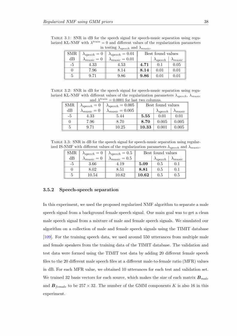
Regularized NMF using GMM priors 38
Table 3.1: SNR in dB for the speech signal for speech-music separation using regu-larized KL-NMF with λtrain = 0 and different values of the regularization parameters
in testing λspeech and λmusic.
SMR λspeech = 0 λspeech = 0.01 Best found valuesdB λmusic = 0 λmusic = 0.01 λspeech λmusic-5 4.33 4.53 4.71 0.1 0.05
0 7.96 8.14 8.14 0.01 0.01
5 9.71 9.86 9.86 0.01 0.01
Table 3.2: SNR in dB for the speech signal for speech-music separation using regu-larized KL-NMF with different values of the regularization parameters λspeech, λmusic
and λtrain = 0.0001 for last two columns.
SMR λspeech = 0 λspeech = 0.005 Best found valuesdB λmusic = 0 λmusic = 0.005 λspeech λmusic-5 4.33 5.44 5.55 0.01 0.01
0 7.96 8.70 8.70 0.005 0.005
5 9.71 10.25 10.33 0.001 0.005
Table 3.3: SNR in dB for the speech signal for speech-music separation using regular-ized IS-NMF with different values of the regularization parameters λspeech and λmusic.
SMR λspeech = 0 λspeech = 0.5 Best found valuesdB λmusic = 0 λmusic = 0.5 λspeech λmusic-5 3.66 4.19 5.09 0.5 0.1
0 8.02 8.51 8.81 0.5 0.1
5 10.54 10.62 10.62 0.5 0.5
3.5.2 Speech-speech separation
In this experiment, we used the proposed regularized NMF algorithm to separate a male
speech signal from a background female speech signal. Our main goal was to get a clean
male speech signal from a mixture of male and female speech signals. We simulated our
algorithm on a collection of male and female speech signals using the TIMIT database
[109]. For the training speech data, we used around 550 utterances from multiple male
and female speakers from the training data of the TIMIT database. The validation and
test data were formed using the TIMIT test data by adding 20 different female speech
files to the 20 different male speech files at a different male-to-female ratio (MFR) values
in dB. For each MFR value, we obtained 10 utterances for each test and validation set.
We trained 32 basis vectors for each source, which makes the size of each matrix Bmale
and Bfemale to be 257× 32. The number of the GMM components K is also 16 in this
experiment.
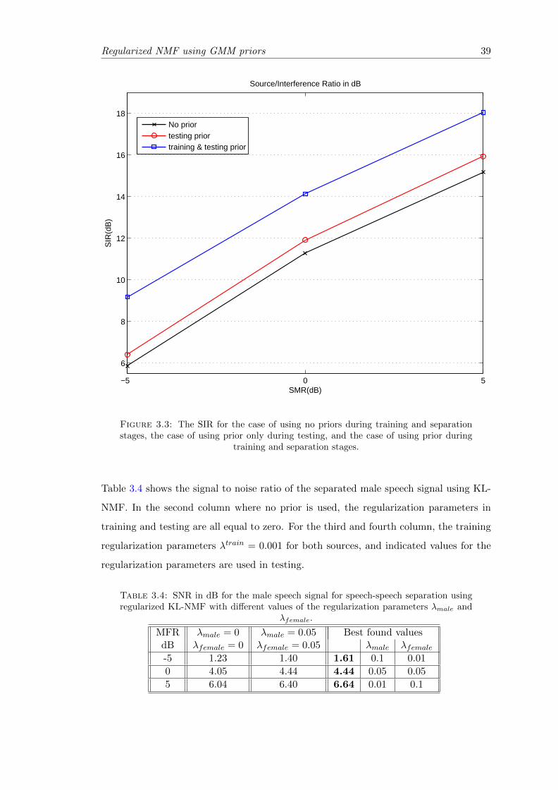
Regularized NMF using GMM priors 39
−5 0 5
6
8
10
12
14
16
18
SMR(dB)
SIR
(dB
)
Source/Interference Ratio in dB
No priortesting priortraining & testing prior
Figure 3.3: The SIR for the case of using no priors during training and separationstages, the case of using prior only during testing, and the case of using prior during
training and separation stages.
Table 3.4 shows the signal to noise ratio of the separated male speech signal using KL-
NMF. In the second column where no prior is used, the regularization parameters in
training and testing are all equal to zero. For the third and fourth column, the training
regularization parameters λtrain = 0.001 for both sources, and indicated values for the
regularization parameters are used in testing.
Table 3.4: SNR in dB for the male speech signal for speech-speech separation usingregularized KL-NMF with different values of the regularization parameters λmale and
λfemale.
MFR λmale = 0 λmale = 0.05 Best found valuesdB λfemale = 0 λfemale = 0.05 λmale λfemale-5 1.23 1.40 1.61 0.1 0.01
0 4.05 4.44 4.44 0.05 0.05
5 6.04 6.40 6.64 0.01 0.1

Regularized NMF using GMM priors 40
Table 3.5 shows the results of using IS-NMF with different values of the regularization
parameters λmale, λfemale, and λtrain = 0.001 for the third and fourth columns.
Table 3.5: SNR in dB for the male speech signal for speech-speech separation usingregularized IS-NMF with different values of the regularization parameters λmale and
λfemale.
MFR λmale = 0 λmale = 1.5 Best found valuesdB λfemale = 0 λfemale = 1.5 λmale λfemale-5 1.59 1.63 1.66 1.5 1
0 3.23 3.29 3.45 1.5 5
5 4.22 4.36 5.64 0.1 10
We can see from the fourth column in Tables 3.4 and 3.5 that, at low MFR we get better
results when the values of λmale is slightly higher than their values at high MFR. This
means, when the male speech signal has less energy in the mixed signal, we rely more
on the prior model for the male speech signal. As the energy level of the male speech
signal increases, the values of the male speech prior parameter decreases and the value
of the female speech prior parameter increases since the energy level of the female speech
signal is decreased.
We can see from all tables that, comparing with no prior case, incorporating statistical
prior information with NMF improves the performance of the separation algorithm. We
also observe that, our proposed algorithm improves the performance of NMF regardless
of the application and the used NMF cost function. In addition we found that, the same
trained GMM prior model works for a range of energy levels avoiding the need to train
different GMM model for each different energy level.
3.5.3 Comparison with the use of a conjugate prior
In this section we compare our proposed method of using GMM as a prior on the
solution of NMF with the conjugate prior models for the case of KL-NMF. Instead of
using GMM as a prior for the solution of the gains matrix during the separation process,
the conjugate prior model is used as a prior for the gains matrix in this section. The
probabilistic conjugate prior model for the solution of the gains matrixG for KL-NMF is
the Gamma distribution as shown in [99]. The probability distribution function (PDF)
of the Gamma distribution with parameters a and b of a random variable x is defined
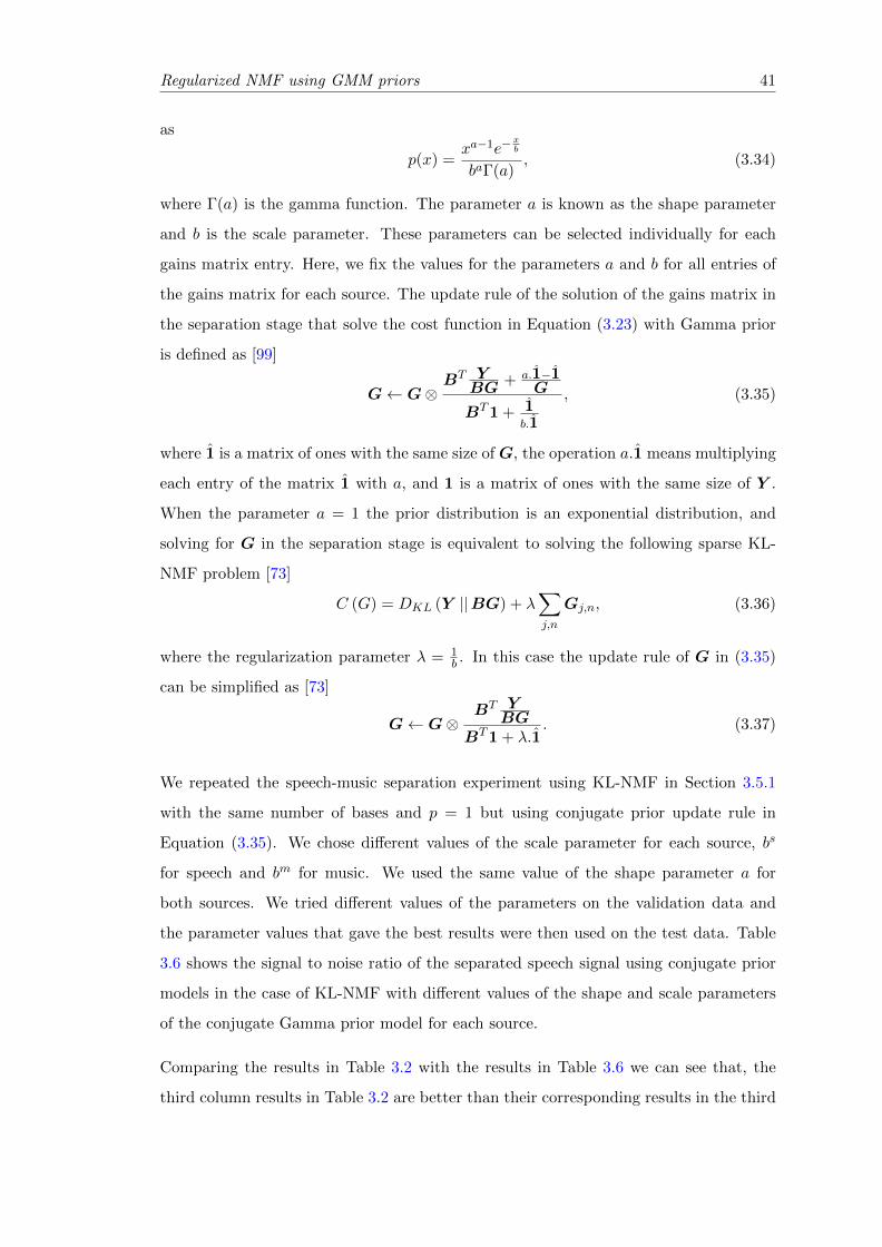
Regularized NMF using GMM priors 41
as
p(x) =xa−1e−
xb
baΓ(a), (3.34)
where Γ(a) is the gamma function. The parameter a is known as the shape parameter
and b is the scale parameter. These parameters can be selected individually for each
gains matrix entry. Here, we fix the values for the parameters a and b for all entries of
the gains matrix for each source. The update rule of the solution of the gains matrix in
the separation stage that solve the cost function in Equation (3.23) with Gamma prior
is defined as [99]
G← G⊗BT Y
BG + a.1−1G
BT1 + 1b.1
, (3.35)
where 1 is a matrix of ones with the same size of G, the operation a.1 means multiplying
each entry of the matrix 1 with a, and 1 is a matrix of ones with the same size of Y .
When the parameter a = 1 the prior distribution is an exponential distribution, and
solving for G in the separation stage is equivalent to solving the following sparse KL-
NMF problem [73]
C (G) = DKL (Y ||BG) + λ∑j,n
Gj,n, (3.36)
where the regularization parameter λ = 1b . In this case the update rule of G in (3.35)
can be simplified as [73]
G← G⊗BT Y
BGBT1 + λ.1
. (3.37)
We repeated the speech-music separation experiment using KL-NMF in Section 3.5.1
with the same number of bases and p = 1 but using conjugate prior update rule in
Equation (3.35). We chose different values of the scale parameter for each source, bs
for speech and bm for music. We used the same value of the shape parameter a for
both sources. We tried different values of the parameters on the validation data and
the parameter values that gave the best results were then used on the test data. Table
3.6 shows the signal to noise ratio of the separated speech signal using conjugate prior
models in the case of KL-NMF with different values of the shape and scale parameters
of the conjugate Gamma prior model for each source.
Comparing the results in Table 3.2 with the results in Table 3.6 we can see that, the
third column results in Table 3.2 are better than their corresponding results in the third

Regularized NMF using GMM priors 42
Table 3.6: SNR in dB for the speech signal for speech-music separation using conju-gate prior KL-NMF with different values of the prior parameters.
SMR No a = 1 Best found valuesdB Prior bs = bm = 103 a bs bm
-5 4.33 4.35 4.35 1 103 103
0 7.96 8.02 8.02 1 103 103
5 9.71 9.80 10.26 1 102 102
column in Table 3.6. Comparing the results in the last columns of both tables, we can
see that using the GMM prior models give better results than using conjugate prior
models at most SMR cases. We conjecture that, the GMM prior gives better results
than the conjugate prior (Gamma prior) since the Gamma distribution is incapable of
capturing the multi-mode structure that are related to the audio signals. For speech
signals in general there is a variety of phonetic, gender, speaking style, and accent
differences which raises the necessity for using many Gaussian components. As we can
see in both cases there are many parameter values to be chosen and exact comparison
can not be achieved since we can not test all possible combinations of the parameters.
From running many experiments, we observed that, the performance in the case of
using conjugate prior is very sensitive to small changes in the combination choices of the
prior parameter values especially the shape parameter a. For each NMF divergence cost
function there is a corresponding conjugate prior distribution that must be chosen. In
case of KL-NMF the conjugate prior distribution is the Gamma distribution, in IS-NMF
case the conjugate prior distribution is the inverse-Gamma PDF [70]. The GMM prior
models can be applied regardless of the type of the NMF cost function.
3.6 Conclusion
In this chapter, we introduced a new regularized NMF algorithm for single channel
source separation. The energy independent prior GMM was used to force the NMF
solution to satisfy the statistical nature of the estimated source signals. The gains
found in NMF solution were encouraged to increase their likelihood with the prior gain
models of the source signals. Gaussian mixture models were used to model the log-
normalized gain prior to improve the separation results. Our experiments indicate that

Regularized NMF using GMM priors 43
the proposed approach is a promising method in single channel speech-music and speech-
speech separation using various target-to-background energy ratios and different NMF
divergence functions.
Chapter 4
Regularized NMF using HMM
priors
4.1 Motivations and overview
The NMF solutions in Section 2.3 do not consider the temporal information between the
consequent frames in the spectrogram. The temporal information between the frames is
important information that can be used to improve any audio signal processing system.
In Chapter 3, Gaussian mixture model (GMM) was used as a prior that guides the NMF
solution of the gains matrix to get better solution for the NMF cost function. A better
solution means a solution that is more compatible with the nature of the source signals.
GMM models the columns of the trained gains matrix without considering the dynamic
structure of the processed audio signals. GMM treats the columns of the trained gains
matrix independently from each other. The temporal structure is important information
that needs to be considered when we model any audio signal.
In this chapter, we try to guide the solution of NMF during the separation stage to
consider temporal and statistical prior information. The columns of the trained gains
matrix represent the valid gain combination sequences for a certain type of source sig-
nal. The gains matrix can be used to train a prior model for the valid weight pattern
sequence for each source. The prior models can guide the NMF decomposition weight-
s/gains during the separation stage to find a solution that can be considered as valid
weight combination sequences for the underlying source signal while minimizing the
44
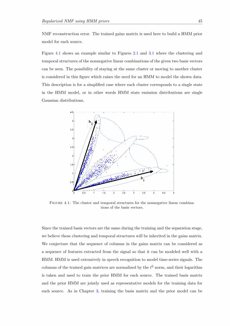
Regularized NMF using HMM priors 45
NMF reconstruction error. The trained gains matrix is used here to build a HMM prior
model for each source.
Figure 4.1 shows an example similar to Figures 2.1 and 3.1 where the clustering and
temporal structures of the nonnegative linear combinations of the given two basis vectors
can be seen. The possibility of staying at the same cluster or moving to another cluster
is considered in this figure which raises the need for an HMM to model the shown data.
This description is for a simplified case where each cluster corresponds to a single state
in the HMM model, or in other words HMM state emission distributions are single
Gaussian distributions.
Figure 4.1: The cluster and temporal structures for the nonnegative linear combina-tions of the basis vectors.
Since the trained basis vectors are the same during the training and the separation stage,
we believe these clustering and temporal structures will be inherited in the gains matrix.
We conjecture that the sequence of columns in the gains matrix can be considered as
a sequence of features extracted from the signal so that it can be modeled well with a
HMM. HMM is used extensively in speech recognition to model time-series signals. The
columns of the trained gain matrices are normalized by the `2 norm, and their logarithm
is taken and used to train the prior HMM for each source. The trained basis matrix
and the prior HMM are jointly used as representative models for the training data for
each source. As in Chapter 3, training the basis matrix and the prior model can be
Regularized NMF using HMM priors 46
done either in two steps sequentially, or all model parameters can be learnt using joint
training.
From the previous chapter we can see that, using joint training gives better results
than using sequential training. To avoid repetitions, we will only consider using joint
training. We use sequential training for initializing the model parameters, then we use
joint training to learn the model parameters. In the separation stage and after observing
the mixed signal, NMF is used to decompose the spectrogram of the mixed signal as a
weighted linear combination of the columns of the trained basis matrices. The sequence
of the decomposition weight combinations are jointly encouraged to increase the log-
likelihood with their corresponding trained prior HMMs. The solution that decreases
the NMF construction error and increases the log-likelihood with the prior HMMs is
computed from solving a regularized NMF cost function. The proposed algorithm models
the prior information using HMM, which is a rich model to represent the statistical
distribution of any sequential training data. Temporal relations between sequential
frames are also modeled in the HMM using transition probabilities among states. Since
the HMMs are trained using normalized data, there is no restriction on the energy level
of the testing data compared to the training data. Moreover, the source signals can
have different energy levels in the mixed signal without any limitations. In the previous
chapter, GMM priors improve the separation performance regardless of the used NMF
cost function. To avoid repetition as in previous chapter, we will apply HMM priors on
the IS-NMF solution only.
4.2 The proposed regularized NMF using HMM
In this chapter, we use the regularized NMF to incorporate dynamic statistical prior
information on the solutions of the gains matrix G. We need the solution of G in
Equation (2.8) to minimize the IS-divergence cost function in Equation (2.17), and
the log-normalized columns of the gains matrix G “logg‖g‖2
”, to maximize their log-
likelihood under a trained HMM prior model. Hence, the solution of G can be found by
minimizing the following regularized IS-divergence cost function:
C = DIS (V ||BG)− λL(G|θ), (4.1)

Regularized NMF using HMM priors 47
where L(G|θ) is the log-likelihood of the log-normalized columns of the gains matrix
G under the trained prior HMM for the gain vectors with parameters θ, and λ is a
regularization parameter. The regularization parameter controls the trade-off between
the NMF cost function and the prior log-likelihood. In this section, we assume HMM
parameters θ are given and in the next section, we will mention the training procedures
of θ. The log-likelihood for the sequence of the log-normalized columns can be written
as follows:
L(G|θ) = log p
(log
g1
‖g1‖2, .., log
gn‖gn‖2
, .., loggN‖gN‖2
|θ), (4.2)
where N is the number of columns in the matrix G. To find the multiplicative update
rule for G in Equation (4.1), we follow the same procedures as in Section 3.2. From
Equations (3.5) to (3.11), we obtain
G← G⊗∇−GDIS + λ∇+L(G|θ)∇+GDIS + λ∇−L(G|θ)
, (4.3)
where
∇GDIS = BT 1
BG−BT V
(BG)2 , (4.4)
∇−GDIS = BT V
(BG)2 , (4.5)
and
∇+GDIS = BT 1
BG. (4.6)
To find the gradients for the log-likelihood in Equation (4.2), let loggn
‖gn‖2= xn, and
given a sequence of data x = {x1, ..,xn, ..,xN}, a HMM state sequence q1, .., qn, .., qN ∈
|Q|, and the trained HMM parameters θ = {A,E, π}, where A is the transition matrix
with entries aij = p (qn+1 = j|qn = i), E is the set of weights, means and covariances
parameters of the GMM emission probabilities, and π = p(q1 = i) is the initial state
probabilities, the likelihood can be calculated as follows:
p(x1:N |θ) =∑q1:N
p (x1:N |q1:N , θ) p (q1:N |θ) , (4.7)
where
p (q1:N |θ) =∏n
p (qn|qn−1, θ)
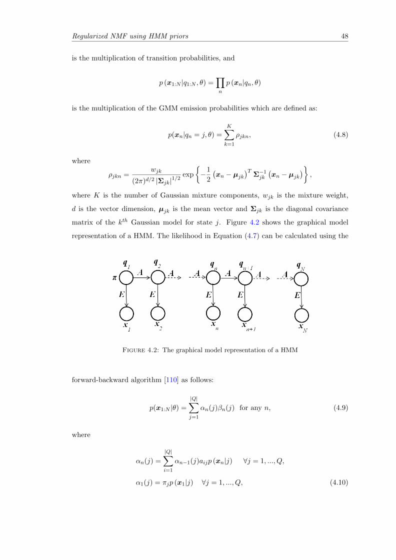
Regularized NMF using HMM priors 48
is the multiplication of transition probabilities, and
p (x1:N |q1:N , θ) =∏n
p (xn|qn, θ)
is the multiplication of the GMM emission probabilities which are defined as:
p(xn|qn = j, θ) =
K∑k=1
ρjkn, (4.8)
where
ρjkn =wjk
(2π)d/2 |Σjk|1/2exp
{−1
2
(xn − µjk
)TΣ−1jk
(xn − µjk
)},
where K is the number of Gaussian mixture components, wjk is the mixture weight,
d is the vector dimension, µjk is the mean vector and Σjk is the diagonal covariance
matrix of the kth Gaussian model for state j. Figure 4.2 shows the graphical model
representation of a HMM. The likelihood in Equation (4.7) can be calculated using the
Figure 4.2: The graphical model representation of a HMM
forward-backward algorithm [110] as follows:
p(x1:N |θ) =
|Q|∑j=1
αn(j)βn(j) for any n, (4.9)
where
αn(j) =
|Q|∑i=1
αn−1(j)aijp (xn|j) ∀j = 1, ..., Q,
α1(j) = πjp (x1|j) ∀j = 1, ..., Q, (4.10)
Regularized NMF using HMM priors 49
and
βn(j) =
|Q|∑i=1
aijp (xn+1|j)βn+1(j) ∀j = 1, ..., Q,
βN (j) = 1, ∀j = 1, ..., Q. (4.11)
The gradient of the log-likelihood in Equation (4.2) can be computed using (4.9). The
gradient with respect to the data point gn of the log-likelihood in Equation (4.9) can be
found as follows:
∇gn[log p(x1:N )] =
∑|Q|j=1 βn(j)∇gn
[αn(j)]∑|Q|j=1 αn(j)βn(j)
, (4.12)
where
∇gn[αn(j)] =
|Q|∑i=1
αn−1(j)aij∇gn[p (xn|j)] . (4.13)
Note that, βn(j) in Equation (4.12) and αn−1(j) in Equation (4.13) are not functions of
gn. The gradient ∇gn[p (xn|j)] can also be written as a difference of two positive terms
∇gn[p (xn|j)] = ∇+
gn[p (xn|j)]−∇−gn
[p (xn|j)] , (4.14)
these gradients can be calculated after replacing xn with loggn
‖gn‖2in Equation (4.8).
The component a of these gradient vectors can be calculated as follows:
∇−gn[p (xn|j)]a =
K∑k=1
−ρjkn (Σjkaa)−1
(µjkagan
+gan
‖gn‖22
loggan‖gn‖2
), (4.15)
∇+gn
[p (xn|j)]a =K∑k=1
−ρjkn (Σkaa)−1
(µjkagan
‖gn‖22
+1
ganlog
gan‖gn‖2
). (4.16)
Since the HMMs are trained by log-normalized columns, the values of the mean vectors
µ will be always negative. Also since the values of the vectors g are always positive, so
the values from Equations (4.15) and (4.16) will be always positive.
We can summarize the procedures of calculating the gradients as follows: first, we
calculate all values of α and β using Equations (4.10, 4.11) for all HMM states and
all observations after replacing each xn with loggn
‖gn‖2. Second, Equations (4.12) to
(4.16) are used to calculate the gradient of each column in the log-likelihood prior term.
We calculate the gradients in Equations (4.5, 4.6) and use them to derive the update
rules for G in Equation (4.3). Calculating the gradient of the log-likelihood in Equation
Regularized NMF using HMM priors 50
(4.12) gives us the chance to scale the values of α and β as shown in [110] to avoid any
numerical problem. Using log-normalized columns helps to keep track of the positive
and negative terms in Equations (4.12) to (4.16).
4.3 Training the source models
The main goal in this stage is to train a set of basis vectors and a prior statistical HMM
for the sequence of gain combination patterns that each set of basis vectors can receive
for each source. The training for the source models can be done in two different ways,
sequential training and joint training. In Chapter 3 it was shown that, joint training
gives better performance than sequential training. In this chapter, we use sequential
training to initialize the source models, then we use joint training to train the NMF
basis vectors and the HMM prior models.
4.3.1 Initial training
The spectrogram Strainz of the available training data for each source signal z is calcu-
lated. IS-NMF is used to decompose Strainz into a basis matrix Bz and a gains matrix
Gtrainz as follows:
Strainz ≈ BzGtrainz ,
where the solution for Bz and Gtrainz can be found by solving the following NMF cost
function:
Bz,Gtrainz = arg min
B,GDIS
(Strainz ||BG
). (4.17)
We use multiplicative update rules in Equations (2.18) and (2.19) to find solutions
for Bz and Gtrainz in Equation (4.17). All the matrices B and Gtrain are initialized by
positive random noise. In each iteration, we normalize the columns ofBz and findGtrainz
accordingly. After finding the basis and the gains matrices, the gains matrix Gtrainz is
then used to train a prior HMM for each source. For each matrix Gtrainz , we normalize
its columns and the logarithm is then computed. These log-normalized columns are
used to train a gain prior HMM for each source. We trained a fully connected HMM
for each source in an unsupervised fashion using the Baum-Welch algorithm [110]. The
Regularized NMF using HMM priors 51
corresponding HMM parameters θz are then learned as follows:
θz = arg maxθL(Gtrainz |θ
), (4.18)
where L(Gtrainz |θ
)is the log-likelihood that is defined in Equation (4.2) for the columns
of the trained gains matrix Gtrainz . After training we hope that HMM learns meaningful
states such as phones or phone groups for speech and the probability of transitions
between them.
4.3.2 Joint training
To match between the way the trained models are used during training with the way they
are used during separation, we jointly train the basis vectors and the prior models. After
finding initial solution for the source parameters in Section 4.3.1, we use joint training
to update the basis and gains matrices with the HMMs parameters simultaneously to
minimize the following regularized cost function:
(Bz,G
trainz , θz
)= arg min
B,G,θDIS
(Strainz ||BG
)− λtrainL (G|θ) . (4.19)
We use the trained NMF and HMM models from Section 4.3.1 as initializations for
the source models, and then we update the model parameters by running alternating
update (coordinate descent) iterations on Bz, Gtrainz and θz parameters. At each NMF
iteration, we update the basis matrix Bz using update rule in (2.18) while keeping Gz
fixed, and the gains matrix Gtrainz is updated using update rule in (4.3) while keeping
Bz and θz fixed. We use a fixed value for the regularization parameter λtrain during
training. The new gains matrix is then used to train a new HMM with its parameters
θz using the Baum-Welch algorithm initialized from their values in the previous NMF
iteration. In joint training, the updating of the basis matrices is consistent with the
clustering structure of the gains matrix due to the usage of the GMMs as an emission
probability in the prior HMM.
After finding the suitable solutions for Equation (4.19), the trained basis matrix and the
prior HMM for each source are then used in the mixed signal decomposition in Equation
(4.21).
Regularized NMF using HMM priors 52
4.4 Signal separation
After observing the mixed signal y(t), we need to find the estimate for each source in
the given mixed signal using NMF with the trained models. The spectrogram Y of
the mixed signal is computed and NMF is used to decompose it with the trained basis
matrices that were found from solving Equation (4.19) as follows:
Y ≈ [B1, ...,Bz, ...,BZ ]
G1
.
Gz
.
GZ
, or Y ≈ BG. (4.20)
Since the bases matrices are given and fixed, the only goal here is to find a suitable
solution for the gains matrix G. The gains matrix G is a combination of submatrices as
shown in Equation (3.22), each submatrix Gz represents the weight combinations that
its corresponding basis vectors in matrix Bz contributes in the mixed signal. For each
submatrix Gz there is a trained prior HMM that models the valid gain combination
sequences that can be seen in the gains matrix for source z. We need to find a solution
for Gz that minimizes the IS-divergence cost function and increases the log-likelihood
for each submatrix Gz with its corresponding trained prior HMM. We can formulate
these objectives using the following regularized NMF:
C (G) = DIS (Y ||BG)−R(G|Θ), (4.21)
where R(G|Θ) is the weighted sum of the log-likelihoods of the log-normalized columns
of the gain submatrices under the trained prior HMMs, and Θ is the set of parameters
for all sources’ prior HMMs. R(G) can be written as follows:
R(G|Θ) =
Z∑z=1
λzL(Gz|θz), (4.22)
where λz is the regularization parameter of the log-likelihood of source z, L(Gz|θz) is
the log-likelihood for the submatrix Gz under the prior HMM with parameters θz that
is defined in Equation (4.2) for source z.
Regularized NMF using HMM priors 53
The multiplicative update rule for G can be found after modifying Equation (4.3) as
follows:
G← G⊗∇−GDIS +∇+
GR(G|Θ)
∇+GDIS +∇−GR(G|Θ)
, (4.23)
where
∇GR(G|Θ) = ∇+GR(G|Θ)−∇−GR(G|Θ), (4.24)
∇+GR(G|Θ) and ∇−GR(G|Θ) are matrices with the same size of G and they are combi-
nations of submatrices. The matrix ∇+GR(G|Θ) can be written as follows:
∇+GR(G|Θ) =
λ1∇+GL(G1|θ1)
.
λz∇+GL(Gz|θz)
.
λZ∇+GL(GZ |θZ)
. (4.25)
We can write∇−GR(G|Θ) similarly as in (4.25) after replacing∇+G with∇−G. The solution
for ∇+GL(Gz|θz) and ∇−GL(Gz|θz) can be found for each source z as shown in Section
4.2. The matrices ∇−GDIS and ∇+GDIS can be computed as shown in Equations (4.5,
4.6).
After finding the suitable solution for the matrix G, the initial spectrogram estimate for
each source z is found as follows:
Sz = BzGz. (4.26)
The final STFT estimate for the source z can be found through the Wiener as follows:
Sz(n, f) = Hz(n, f)Y (n, f), (4.27)
where Hz is the Wiener filter for source z which is defined as [70]:
Hz =(BzGz)∑Zj=1 (BjGj)
, (4.28)
where Sz(n, f) is the final estimated STFT for source Sz(n, f) in Equation (2.2), and
Hz(n, f) is the column n and row f entry of the Wiener filter Hz in Equation (4.28).
The Wiener filter scales the mixed signal STFT entries according to the contribution
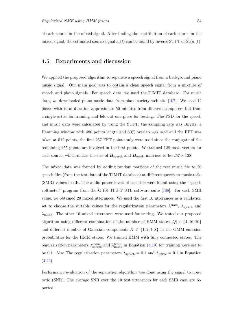
Regularized NMF using HMM priors 54
of each source in the mixed signal. After finding the contribution of each source in the
mixed signal, the estimated source signal sz(t) can be found by inverse STFT of Sz(n, f).
4.5 Experiments and discussion
We applied the proposed algorithm to separate a speech signal from a background piano
music signal. Our main goal was to obtain a clean speech signal from a mixture of
speech and piano signals. For speech data, we used the TIMIT database. For music
data, we downloaded piano music data from piano society web site [107]. We used 12
pieces with total duration approximate 50 minutes from different composers but from
a single artist for training and left out one piece for testing. The PSD for the speech
and music data were calculated by using the STFT: the sampling rate was 16KHz, a
Hamming window with 480 points length and 60% overlap was used and the FFT was
taken at 512 points, the first 257 FFT points only were used since the conjugate of the
remaining 255 points are involved in the first points. We trained 128 basis vectors for
each source, which makes the size of Bspeech and Bmusic matrices to be 257× 128.
The mixed data was formed by adding random portions of the test music file to 20
speech files (from the test data of the TIMIT database) at different speech-to-music ratio
(SMR) values in dB. The audio power levels of each file were found using the “speech
voltmeter” program from the G.191 ITU-T STL software suite [108]. For each SMR
value, we obtained 20 mixed utterances. We used the first 10 utterances as a validation
set to choose the suitable values for the regularization parameters λtrain, λspeech and
λmusic. The other 10 mixed utterances were used for testing. We tested our proposed
algorithm using different combination of the number of HMM states |Q| ∈ {4, 16, 20}
and different number of Gaussian components K ∈ {1, 2, 4, 8} in the GMM emission
probabilities for the HMM states. We trained HMM with fully connected states. The
regularization parameters λtrainspeech and λtrainmusic in Equation (4.19) for training were set to
be 0.1. Also The regularization parameters λspeech = 0.1 and λmusic = 0.1 in Equation
(4.22).
Performance evaluation of the separation algorithm was done using the signal to noise
ratio (SNR). The average SNR over the 10 test utterances for each SMR case are re-
ported.
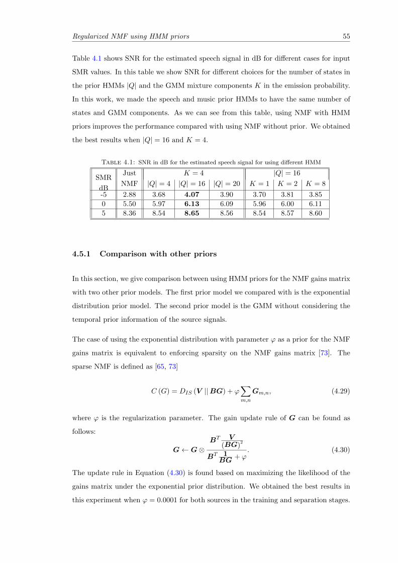
Regularized NMF using HMM priors 55
Table 4.1 shows SNR for the estimated speech signal in dB for different cases for input
SMR values. In this table we show SNR for different choices for the number of states in
the prior HMMs |Q| and the GMM mixture components K in the emission probability.
In this work, we made the speech and music prior HMMs to have the same number of
states and GMM components. As we can see from this table, using NMF with HMM
priors improves the performance compared with using NMF without prior. We obtained
the best results when |Q| = 16 and K = 4.
Table 4.1: SNR in dB for the estimated speech signal for using different HMM
SMRJust K = 4 |Q| = 16
dBNMF |Q| = 4 |Q| = 16 |Q| = 20 K = 1 K = 2 K = 8
-5 2.88 3.68 4.07 3.90 3.70 3.81 3.85
0 5.50 5.97 6.13 6.09 5.96 6.00 6.11
5 8.36 8.54 8.65 8.56 8.54 8.57 8.60
4.5.1 Comparison with other priors
In this section, we give comparison between using HMM priors for the NMF gains matrix
with two other prior models. The first prior model we compared with is the exponential
distribution prior model. The second prior model is the GMM without considering the
temporal prior information of the source signals.
The case of using the exponential distribution with parameter ϕ as a prior for the NMF
gains matrix is equivalent to enforcing sparsity on the NMF gains matrix [73]. The
sparse NMF is defined as [65, 73]
C (G) = DIS (V ||BG) + ϕ∑m,n
Gm,n, (4.29)
where ϕ is the regularization parameter. The gain update rule of G can be found as
follows:
G← G⊗BT V
(BG)2
BT 1BG + ϕ
. (4.30)
The update rule in Equation (4.30) is found based on maximizing the likelihood of the
gains matrix under the exponential prior distribution. We obtained the best results in
this experiment when ϕ = 0.0001 for both sources in the training and separation stages.
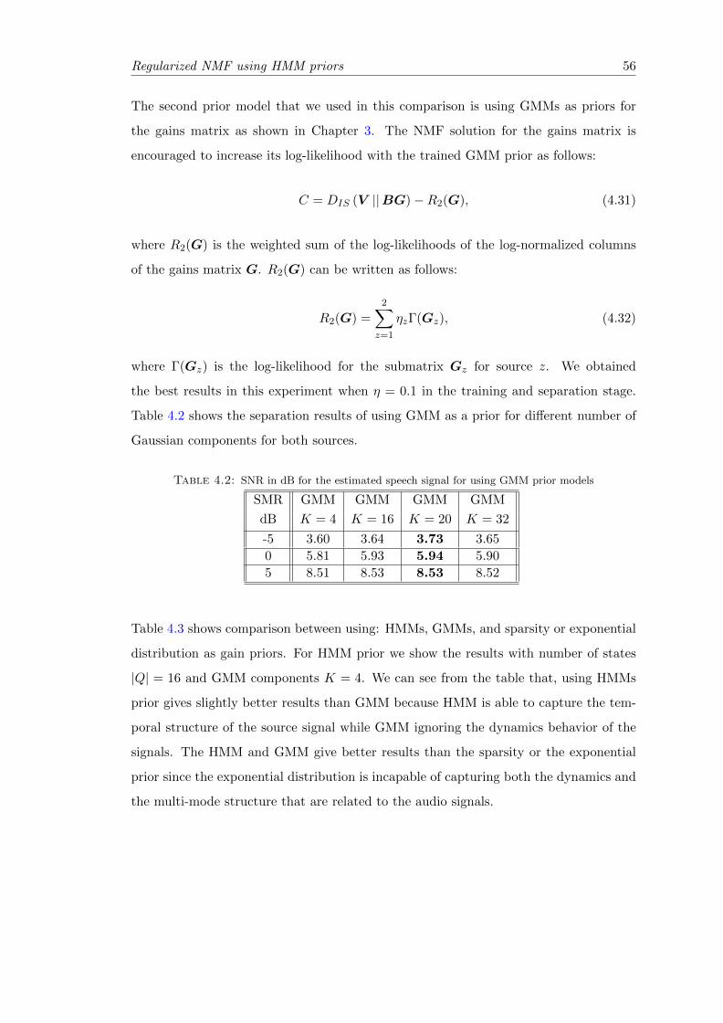
Regularized NMF using HMM priors 56
The second prior model that we used in this comparison is using GMMs as priors for
the gains matrix as shown in Chapter 3. The NMF solution for the gains matrix is
encouraged to increase its log-likelihood with the trained GMM prior as follows:
C = DIS (V ||BG)−R2(G), (4.31)
where R2(G) is the weighted sum of the log-likelihoods of the log-normalized columns
of the gains matrix G. R2(G) can be written as follows:
R2(G) =
2∑z=1
ηzΓ(Gz), (4.32)
where Γ(Gz) is the log-likelihood for the submatrix Gz for source z. We obtained
the best results in this experiment when η = 0.1 in the training and separation stage.
Table 4.2 shows the separation results of using GMM as a prior for different number of
Gaussian components for both sources.
Table 4.2: SNR in dB for the estimated speech signal for using GMM prior models
SMR GMM GMM GMM GMM
dB K = 4 K = 16 K = 20 K = 32
-5 3.60 3.64 3.73 3.65
0 5.81 5.93 5.94 5.90
5 8.51 8.53 8.53 8.52
Table 4.3 shows comparison between using: HMMs, GMMs, and sparsity or exponential
distribution as gain priors. For HMM prior we show the results with number of states
|Q| = 16 and GMM components K = 4. We can see from the table that, using HMMs
prior gives slightly better results than GMM because HMM is able to capture the tem-
poral structure of the source signal while GMM ignoring the dynamics behavior of the
signals. The HMM and GMM give better results than the sparsity or the exponential
prior since the exponential distribution is incapable of capturing both the dynamics and
the multi-mode structure that are related to the audio signals.
Regularized NMF using HMM priors 57
Table 4.3: SNR in dB for the estimated speech signal for using different prior models
SMR Just HMM GMMSparsity
dB NMF |Q| = 16,K = 4 K = 20
-5 2.88 4.07 3.73 3.06
0 5.50 6.13 5.94 5.85
5 8.36 8.65 8.53 8.51
4.6 Conclusion
In this chapter, we introduced a new regularized NMF algorithm for single channel
source separation. The energy independent HMM prior models were incorporated with
NMF solutions to improve the separation performance. In future work, we will consider
supervised training for the prior HMMs.
Chapter 5
Regularized NMF using MMSE
estimates under GMM priors
with online learning for the
uncertainties
5.1 Motivations and overview
In Chapters 3 and 4 the gains matrix during the separation stage was guided to follow
the prior information by maximizing its likelihood with a trained prior model. The prior
model was applied on the NMF solutions without evaluating the actual need for prior
information. From the results in Tables 3.1 to 3.5 in Chapter 3 we can see that, in
many cases when the desired signal has higher energy compared to other sources in the
mixed signal, the NMF solution of the gains matrix relies less on the prior information
for the desired signal and vice versa. This means that, the need for incorporating prior
information in the NMF solution depends on how bad the NMF solution for the gains
matrix is without any prior.
In this chapter, we introduce a new strategy of applying the priors on the NMF solutions
of the gains/weights matrix during the separation stage. The new strategy is based on
evaluating how much the solution of the NMF gains matrix needs to rely on the prior
models. We use here Gaussian mixture models (GMMs) to model the prior information
58
Regularized NMF using MMSE estimates under GMM priors 59
about the gains matrix. The NMF solutions without using priors for the weights matrix
for each source during the separation stage can be seen as a deformed image, and its
corresponding valid gains matrix needs to be estimated under the GMM prior. The
deformation operator parameters which measure the uncertainty of the NMF solution of
the weights matrix are learned directly from the observed mixed signal. The uncertainty
in this work is a measurement of how far the NMF solution of the weights matrix
during the separation stage is from being valid weight patterns that are modeled in the
prior GMM. The learned uncertainties are used with the minimum mean squared error
(MMSE) estimator to find the estimate of the valid weights matrix. The estimated valid
weights matrix should also consider the minimization of the NMF cost function. To
achieve these two goals, a regularized NMF is used to consider the valid weight patterns
that can appear in the columns of the weights matrix while decreasing the NMF cost
function. The uncertainties within MMSE estimates of the valid weight combinations
are embedded in the regularized NMF cost function for this purpose. The uncertainty
measurements play very important role in this work as we will show in next sections.
If the uncertainty of the NMF solution of the weights matrix is high, that means the
regularized NMF needs more support from the prior term. In case of low uncertainty,
the regularized NMF needs less support from the prior term. Including the uncertainty
measurements in the regularization term using MMSE estimate makes the proposed
regularized NMF algorithm decide automatically how much the solution should rely on
the prior GMM term. This is the main advantage of the proposed regularized NMF
compared to the regularization using the log-likelihood of the GMM prior in previous
chapters or other prior distributions [82, 84, 99].
5.2 Regularized nonnegative matrix factorization using MMSE
estimation
In this chapter, we enforce a statistical prior information on the solution of the gain-
s/weights matrix G. We need the solution of G in Equation (2.8) to minimize the
IS-divergence cost function in Equation (2.17), and the columns of the gains matrix G
should form valid weight combinations under a prior GMM model.
Regularized NMF using MMSE estimates under GMM priors 60
The most used strategy for incorporating a prior is by maximizing the likelihood of the
solution under the prior model while minimizing the NMF divergence at the same time.
To achieve this, we usually add these two objectives in a single cost function. In Chapter
3, a GMM was used as the prior model for the gains matrix, and the solution of the
gains matrix was encouraged to increase its log-likelihood with the prior model using
this regularized NMF cost function. The regularization parameters in Chapter 3 were
the only tool to control how much the regularized NMF relies on the prior model. The
value of the regularization parameters were chosen manually in that chapter.
Gaussian mixture model is a rich prior model where we can see the means of the GMM
mixture components as “valid templates” that were observed in the training data. Even,
Parzen density priors [111] can be seen under the same framework. In Parzen density
prior estimation, training examples are seen as “valid templates” and a fixed variance
is assigned to each example. In GMM priors, we learn the templates as cluster means
from training data and we can also estimate the cluster variances from the data. We
can think of the GMM prior as a way to encourage the use of valid templates or cluster
means in the NMF solution during the test phase. This view of the GMM prior will be
helpful in understanding the MMSE method we introduce in this chapter.
We can find a way of measuring how far the conventional NMF solution is from the
trained templates in the prior GMM and call this the error term. Based on this error,
the regularized NMF can decide automatically how much the solution of the NMF needs
help from the prior model. If the conventional NMF solution is far from the templates
then the regularized NMF will rely more on the prior model. If the conventional NMF
solution is close to the templates then the regularized NMF will rely less on the prior
model. By deciding automatically how much the regularized NMF needs to rely on
the prior we conjecture that, we do not need to manually change the values of the
regularization parameter for different energy level for the sources as shown in Tables 3.1
to 3.5 to improve the performance of NMF.
We use the following way of measuring how far the conventional NMF solution is from
the prior templates: We can see the solution of the conventional NMF as distorted
observations of a true/valid template. Given the prior GMM templates, we can learn a
probability distribution model for the distortion that captures how far the observations
in the conventional gains matrix is from the prior GMM. The distortion or the error
Regularized NMF using MMSE estimates under GMM priors 61
model can be seen as a summary of the distortion that exists in all columns in the gains
matrix of the NMF solution.
Based on the prior GMM and the trained distortion model, we can find a better estimate
for the desired observation for each column in the distorted gains matrix. We can
mathematically formulate this by seeing the solution matrix G that only minimizes the
cost function in Equation (2.17) as a distorted image where its restored image needs to
be estimated. The columns of the matrix G are normalized using the `2 norm and their
logarithm is then calculated. Let the log-normalized column n of the gains matrix be
qn. The vector qn is treated as a distorted observation as:
qn = xn + e, (5.1)
where xn is the logarithm of the unknown desired pattern that corresponds to the
observation qn and needs to be estimated under a prior GMM, e is the logarithm of the
multiplicative deformation operator, which is modeled by a Gaussian distribution with
zero mean and diagonal covariance matrix Ψ as N (e|0,Ψ). The GMM prior model for
a random variable x is defined as:
p(x) =K∑k=1
ωk
(2π)d/2 |Σk|1/2exp
{−1
2(x− µk)
T Σ−1k (x− µk)
}, (5.2)
where K is the number of Gaussian mixture components, ωk is the mixture weight, d is
the vector dimension, µk is the mean vector and Σk is the diagonal covariance matrix
of the kth Gaussian model. The GMM prior model for the gains matrix is trained using
log-normalized columns of the trained gains matrix from training data as we show in
Section 3.3.1.
The uncertainty Ψ is trained directly from all observations q = {q1, .., qn, .., qN} which
can be iteratively learned using the expectation maximization (EM) algorithm [102].
Given the learned prior GMM parameters which are considered fixed here, the update
of Ψ is found based on the sufficient statistics zn and Rn as shown in Appendix A and
similar to [112, 113, 114] as follows:
Ψ = diag
{1
N
N∑n=1
(qnq
Tn − qnzTn − znqTn + Rn
)}, (5.3)
Regularized NMF using MMSE estimates under GMM priors 62
where the “diag” operator sets all the off-diagonal elements of a matrix to zero, N is the
number of columns in matrix G, and the sufficient statistics zn and Rn can be updated
using Ψ from the previous iteration as follows:
zn =K∑k=1
γknzkn, (5.4)
and
Rn =
K∑k=1
γknRkn, (5.5)
where
γkn =
[ωkN (qn|µk,Σk + Ψ)∑Kj=1 ωjN
(qn|µj ,Σj + Ψ
)] , (5.6)
Rkn = Σk −Σk (Σk + Ψ)−1 ΣTk + zknz
Tkn, (5.7)
and
zkn = µk + Σk (Σk + Ψ)−1 (qn − µk) . (5.8)
Given the learned uncertainty and the prior GMM, the MMSE estimate of the pattern
xn given the observation qn can be computed as shown in Appendix A and similar to
[112, 113, 114] as follows:
xn = f (qn) =K∑k=1
γkn
[µk + Σk (Σk + Ψ)−1 (qn − µk)
], (5.9)
where
γkn =
[ωkN (qn|µk,Σk + Ψ)∑Kj=1 ωjN
(qn|µj ,Σj + Ψ
)] . (5.10)
The value of Ψ in the term Σk (Σk + Ψ)−1 in Equation (5.9) plays an important role in
this framework. Ψ is considered as the uncertainty measurement of the observations in
matrixG. When the entries of the uncertainty Ψ are very small compared to their corre-
sponding entries in Σk for a certain active GMM component k, the term Σk (Σk + Ψ)−1
tends to be the identity matrix, and MMSE estimate in (5.9) will be the observation qn.
When the entries of the uncertainty Ψ are very high comparing to their corresponding
entries in Σk for a certain active GMM component k, the term Σk (Σk + Ψ)−1 tends
to be a zeros matrix, and MMSE estimate will be the weighted sum of prior templates∑Kk=1 γknµk. In most cases γkn tends to be close to one for one Gaussian component,
Regularized NMF using MMSE estimates under GMM priors 63
and close to zero for the other components. This makes the MMSE estimate in the
case of high Ψ to be one of the mean vectors in the prior GMM, which is considered
as a template pattern for the valid observation. We can rephrase this as follows: When
the uncertainty of the observations q is high, the MMSE estimate of x, relies more on
the prior GMM of x. When the uncertainty of the observations q is low, the MMSE
estimate of x, relies more on the observation qn. In general, the MMSE solution of x
lies between the observation qn and one of the templates in the prior GMM. The term
Σk (Σk + Ψ)−1 controls the distance between xn and qn and also the distance between
xn and one of the template µk assuming that γkn ≈ 1 for a Gaussian component k.
The model in Equation (5.1) expresses the normalized columns of the gains matrix as a
distorted image with a diagonal multiplicative deformation matrix. For the normalized
columnsgn
‖gn‖2there is a deformation matrix Ed with log-normal distribution that is
applied to the correct pattern gn
gn‖gn‖2
= Edgn. (5.11)
The uncertainty for Ed is represented in the covariance matrix Ψ. Given the distorted
matrix G, we find the corresponding MMSE estimate for its log-normalized columns
G. The reason for working in the logarithm domain is that, the gains are constrained
to be nonnegative and the MMSE estimate can be negative so the logarithm of the
normalized gains is an unconstrained variable that we can work with. The estimated
weight patterns in G that are corresponding to the MMSE estimates for the correct
patterns do not consider minimizing the NMF cost function in Equation (2.17), which
is still the main goal. We need the solution of G to consider the pattern shape priors on
the solution of the gains matrix, and also consider the reconstruction error of the NMF
cost function. To consider the combination of the two objectives, we consider using
the regularized NMF. We add a penalty term to the NMF-divergence cost function.
The penalty term tries to minimize the distance between the solution of log-normalized
columns of gn with its corresponding MMSE estimate f(gn) as follows:
loggn‖gn‖2
≈ f(
loggn‖gn‖2
)or
gn‖gn‖2
≈ exp
(f
(log
gn‖gn‖2
)). (5.12)
The regularized IS-NMF cost function is defined as follows:
C = DIS (V ||BG) + λL(G), (5.13)
Regularized NMF using MMSE estimates under GMM priors 64
where
L(G) =N∑n=1
∥∥∥∥ gn‖gn‖2
− exp
(f
(log
gn‖gn‖2
))∥∥∥∥2
2
, (5.14)
f
(log
gn
‖gn‖2
)is the MMSE estimate defined in Equation (5.9), and λ is a regularization
parameter. The regularized NMF can be rewritten in more details as
C =∑m,n
(V m,n
(BG)m,n
− logV m,n
(BG)m,n
− 1
)+ λ
N∑n=1
∥∥∥∥∥ gn‖gn‖2
− exp
(K∑
k=1
γkn
[µk + Σk (Σk + Ψ)−1
(log
gn‖gn‖2
− µk
)])∥∥∥∥∥2
2
.
(5.15)
In Equation (5.15), the MMSE of the desired patterns of the gains matrix is embedded
in the regularized NMF cost function. Note that γkn is also a function of gn in this
equation. The first term in (5.15), decreases the reconstruction error between V and
BG. Given Ψ, we can forget for a while the MMSE estimate concept that leaded
us to our target regularized NMF cost function in (5.15) and see Equation (5.15) as
an optimization problem. We can see from (5.15) that, if the distortion measurement
parameter Ψ is high, the regularized nonnegative matrix factorization solution for the
gains matrix will rely more on the prior GMM for the gains matrix. If the distortion
parameter Ψ is low, the regularized nonnegative matrix factorization solution for the
gains matrix will be close to the ordinary NMF solution for the gains matrix without
considering any prior. The second term in Equation (5.15) is ignored in the case of zero
uncertainty Ψ. In case of high values of Ψ, the second term encourages to decrease
the distance between each normalized columngn
‖gn‖2in G with a corresponding prior
template exp (µk) assuming that γkn ≈ 1 for a certain Gaussian component k. For
different values of Ψ, the penalty term decreases the distance between eachgn
‖gn‖2and
an estimated pattern that lies between a prior template andgn
‖gn‖2.
The multiplicative update rule for B in (5.15) is still the same as in Equation (2.18).
The multiplicative update rule for G can be found by following the same procedures as
in Section 3.2. From Equations (3.5) to (3.11), we obtain
G← G⊗∇−GDIS + λ∇−GL(G)
∇+GDIS + λ∇+
GL(G), (5.16)
where
∇GDIS = BT 1
BG−BT V
(BG)2 , (5.17)
Regularized NMF using MMSE estimates under GMM priors 65
∇−GDIS = BT V
(BG)2 , and ∇+GDIS = BT 1
BG. (5.18)
Note that, in calculating the gradients ∇+GL(G) and ∇−GL(G), the term γkn is also a
function ofG. The gradients ∇+GL(G) and ∇−GL(G) are calculated in Appendix B. Since
all the terms in Equation (5.16) are nonnegative, then the values of G of the update
rule (5.16) are nonnegative.
5.3 The proposed regularized NMF for source separation
Figure 5.1 shows the flow chart that summarizes all stages of applying the proposed
regularized NMF method for single channel source separation (SCSS) problems for only
two sources. The proposed algorithm is used for SCSS in two main stages. The first
stage is to train a set of basis vectors for each source using NMF in Equation (2.17), and
also to train the prior GMM for the valid gain patterns that the trained basis vectors
can possible have for each source as shown in Section 3.3.1 and learning the source’s
models stage in Figure 5.1. The second stage is the separation process which is done
in three main sequential steps. The first step is using NMF in Equation (2.17) to find
the gain matrices by decomposing the mixed signal spectrogram with the trained basis
vectors without using any prior for the gains matrix. The second step is to use the gain
matrices with the prior GMMs to learn the uncertainty parameters, which measure how
far the columns in the gain matrices are in the separation stage from being a valid gain
pattern for each source. These two steps are shown in learning the uncertainties stage
in Figure 5.1. The last step shown in the figure is to use the learned uncertainties and
the prior GMMs with the proposed regularized NMF cost function in Equation (5.15)
to find the final values for the gain matrices.
5.3.1 Signal separation
Lets assume we have only two sources for simplicity. After observing the mixed signal
y(t), NMF is used to decompose the mixed signal spectrogram Y with the trained bases
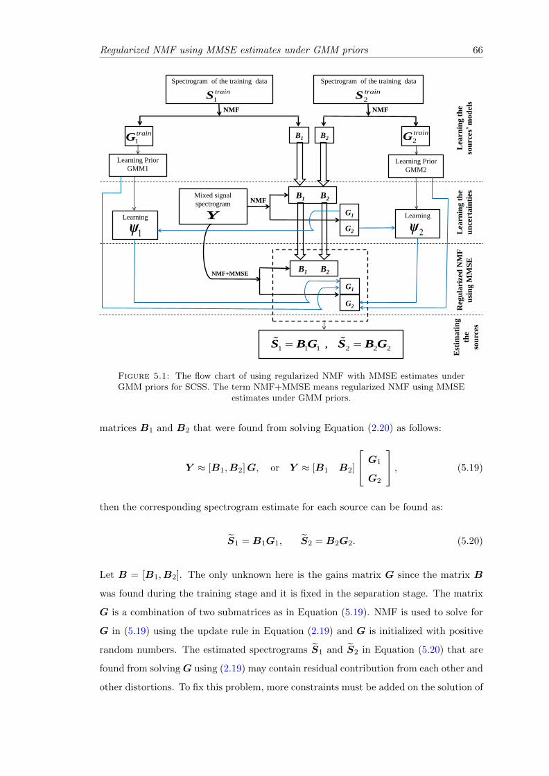
Regularized NMF using MMSE estimates under GMM priors 66
Spectrogram of the training data
1
trainS
Spectrogram of the training data
2
trainS
NMF NMF
B1 B21
trainG 2
trainG
Learning Prior
GMM1Learning Prior
GMM2
Mixed signal
spectrogram
Y G1
G2
NMF
Learning
ψLearning
G1
G2
NMF+MMSE
1 1 1 2 2 2 , S BG S B G
B1 B2
B1 B2
Lea
rn
ing
th
e
sou
rces’
mo
del
s
Lea
rn
ing
th
e
un
certa
inti
es
Reg
ula
rize
d N
MF
usi
ng
MM
SE
Est
ima
tin
g
the
sou
rces
ψ
Figure 5.1: The flow chart of using regularized NMF with MMSE estimates underGMM priors for SCSS. The term NMF+MMSE means regularized NMF using MMSE
estimates under GMM priors.
matrices B1 and B2 that were found from solving Equation (2.20) as follows:
Y ≈ [B1,B2]G, or Y ≈ [B1 B2]
G1
G2
, (5.19)
then the corresponding spectrogram estimate for each source can be found as:
S1 = B1G1, S2 = B2G2. (5.20)
Let B = [B1,B2]. The only unknown here is the gains matrix G since the matrix B
was found during the training stage and it is fixed in the separation stage. The matrix
G is a combination of two submatrices as in Equation (5.19). NMF is used to solve for
G in (5.19) using the update rule in Equation (2.19) and G is initialized with positive
random numbers. The estimated spectrograms S1 and S2 in Equation (5.20) that are
found from solvingG using (2.19) may contain residual contribution from each other and
other distortions. To fix this problem, more constraints must be added on the solution of
Regularized NMF using MMSE estimates under GMM priors 67
each submatrix. Recall that, for each submatrix in G, there is a corresponding trained
GMM prior for the valid weight combinations that its corresponding log-normalized
columns can have. The resulting solution for each submatrix in G using (2.19) does not
consider the prior information on the valid weight combinations that the basis vectors
can possible have for each source. The normalized columns of the submatrices G1 and
G2 can be seen as deformed images as in Equation (5.11) and their restored images are
needed to be estimated. First, we need to learn the uncertainty parameters Ψ1 and Ψ2
for the deformation operators Ed1 and Ed2 respectively for each image. The columns
of the submatrix G1 are normalized and their logarithm are calculated and used with
the GMM prior parameters for the first source to estimate Ψ1 iteratively using the EM
algorithm in Equations (5.3) to (5.8). The log-normalized columns “loggn
‖gn‖2” ofG1 can
be seen as qn in Equations (5.3) to (5.8). We repeat the same procedures to calculate Ψ2
using the log-normalized columns of G2 and the prior GMM for the second source. The
uncertainties Ψ1 and Ψ2 can also be seen as measurements of the remaining distortion
from one source into another source, which also depends on the mixing ratio between the
two sources. For example, if the first source has higher energy than the second source in
the mixed signal, we expect the values of Ψ2 to be higher than the values in Ψ1 and vice
versa. After calculating the uncertainty parameters for both sources Ψ1 and Ψ2, we use
the regularized NMF in (5.13) to solve for G with the prior GMMs for both sources and
the estimated uncertainties Ψ1 and Ψ2 as follows:
C = DIS (Y ||BG) +R(G), (5.21)
where
R(G) = λ1L1(G1) + λ2L2(G2), (5.22)
L1(G1) is defined as in Equation (5.14) for the first source, L2(G2) is for the second
source, λ1, and λ2 are their corresponding regularization parameters. The update rule
in Equation (5.16) can be used to solve for G after modifying it as follows:
G← G⊗∇−GDIS +∇−GR(G)
∇+GDIS +∇+
GR(G), (5.23)
Regularized NMF using MMSE estimates under GMM priors 68
where ∇+GR(G) and ∇−GR(G) are nonnegative matrices with the same size of G and
they are combinations of two submatrices as follows:
∇−GR(G) =
λ1∇−GL(G1)
λ2∇−GL(G2)
, ∇+GR(G) =
λ1∇+GL(G1)
λ2∇+GL(G2)
, (5.24)
where ∇+GL(G1),∇−GL(G1),∇+
GL(G2), and ∇−GL(G2) are calculated as in Section 5.2
for each source.
The normalization of the columns of the gain matrices are used in the prior term R(G)
and its gradient terms only. The general solution for the gains matrix of Equation (5.21)
at each iteration is not normalized. The normalization is done only in the prior term
since the prior models have been trained by normalized data before. Normalization is
also useful in cases where the source signals occur with different energy levels from each
other in the mixed signal. Normalizing the training and testing gain matrices gives the
prior models a chance to work with any energy level that the source signals can take in
the mixed signal regardless of the energy levels of the training signals.
5.3.2 Source signals reconstruction
After finding the suitable solution for the matrix G, the initial estimated spectrograms
S1 and S2 can be calculated from (5.20) and then used to build spectral masks as
follows:
H1 =S1
S1 + S2
, H2 =S2
S1 + S2
, (5.25)
where the divisions are done element-wise. The final estimate of each source STFT can
be obtained as follows:
S1 (n, f) = H1 (n, f)Y (n, f) , S2 (n, f) = H2 (n, f)Y (n, f) , (5.26)
where Y (n, f) is the STFT of the observed mixed signal in Equation (2.2), H1 (n, f)
and H2 (n, f) are the entries at row f and column n of the spectral masks H1 and H2
respectively. The spectral mask entries scale the observed mixed signal STFT entries
according to the contribution of each source in the mixed signal. The spectral masks
can be seen as the Wiener filter as in [70]. The estimated source signals s1(t) and s2(t)
can be found by inverse STFT of its corresponding STFT S1(n, f) and S2(n, f).
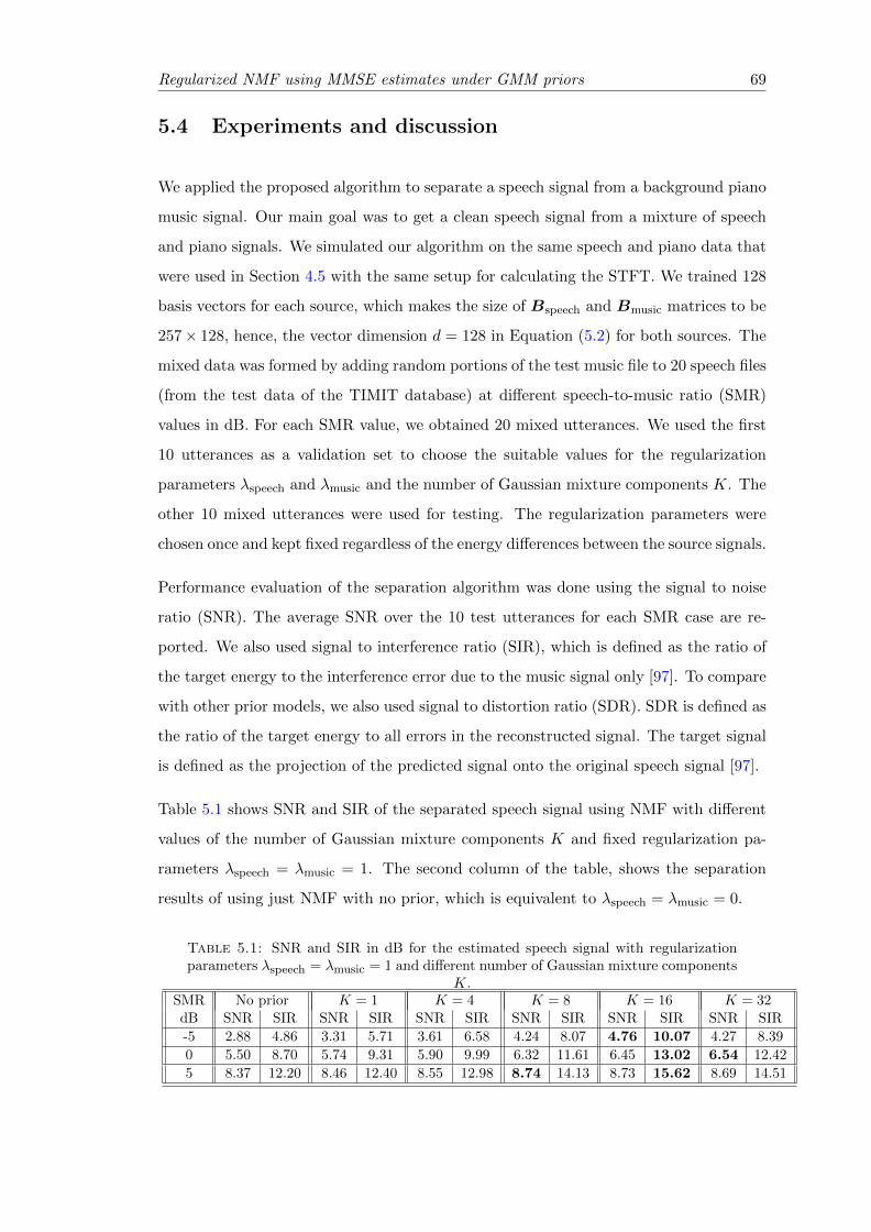
Regularized NMF using MMSE estimates under GMM priors 69
5.4 Experiments and discussion
We applied the proposed algorithm to separate a speech signal from a background piano
music signal. Our main goal was to get a clean speech signal from a mixture of speech
and piano signals. We simulated our algorithm on the same speech and piano data that
were used in Section 4.5 with the same setup for calculating the STFT. We trained 128
basis vectors for each source, which makes the size of Bspeech and Bmusic matrices to be
257× 128, hence, the vector dimension d = 128 in Equation (5.2) for both sources. The
mixed data was formed by adding random portions of the test music file to 20 speech files
(from the test data of the TIMIT database) at different speech-to-music ratio (SMR)
values in dB. For each SMR value, we obtained 20 mixed utterances. We used the first
10 utterances as a validation set to choose the suitable values for the regularization
parameters λspeech and λmusic and the number of Gaussian mixture components K. The
other 10 mixed utterances were used for testing. The regularization parameters were
chosen once and kept fixed regardless of the energy differences between the source signals.
Performance evaluation of the separation algorithm was done using the signal to noise
ratio (SNR). The average SNR over the 10 test utterances for each SMR case are re-
ported. We also used signal to interference ratio (SIR), which is defined as the ratio of
the target energy to the interference error due to the music signal only [97]. To compare
with other prior models, we also used signal to distortion ratio (SDR). SDR is defined as
the ratio of the target energy to all errors in the reconstructed signal. The target signal
is defined as the projection of the predicted signal onto the original speech signal [97].
Table 5.1 shows SNR and SIR of the separated speech signal using NMF with different
values of the number of Gaussian mixture components K and fixed regularization pa-
rameters λspeech = λmusic = 1. The second column of the table, shows the separation
results of using just NMF with no prior, which is equivalent to λspeech = λmusic = 0.
Table 5.1: SNR and SIR in dB for the estimated speech signal with regularizationparameters λspeech = λmusic = 1 and different number of Gaussian mixture components
K.SMR No prior K = 1 K = 4 K = 8 K = 16 K = 32dB SNR SIR SNR SIR SNR SIR SNR SIR SNR SIR SNR SIR
-5 2.88 4.86 3.31 5.71 3.61 6.58 4.24 8.07 4.76 10.07 4.27 8.39
0 5.50 8.70 5.74 9.31 5.90 9.99 6.32 11.61 6.45 13.02 6.54 12.42
5 8.37 12.20 8.46 12.40 8.55 12.98 8.74 14.13 8.73 15.62 8.69 14.51
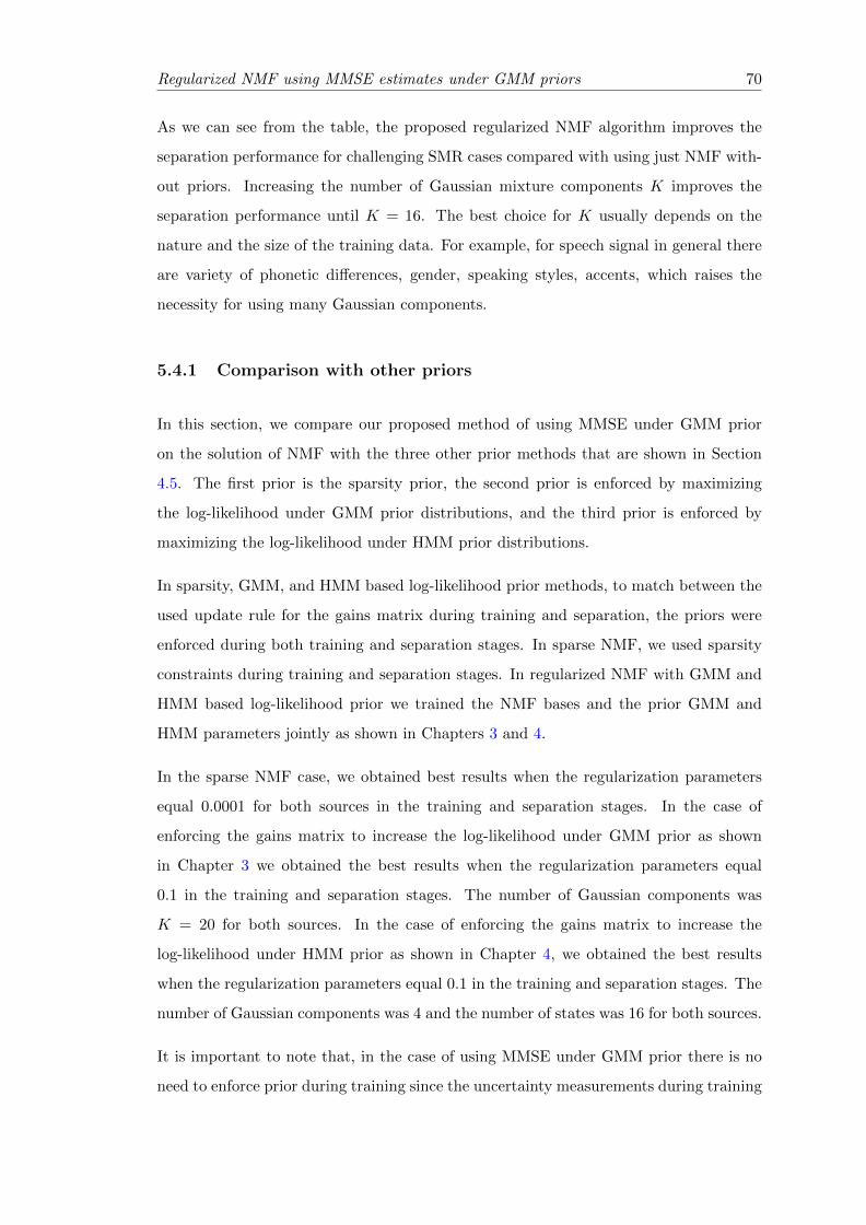
Regularized NMF using MMSE estimates under GMM priors 70
As we can see from the table, the proposed regularized NMF algorithm improves the
separation performance for challenging SMR cases compared with using just NMF with-
out priors. Increasing the number of Gaussian mixture components K improves the
separation performance until K = 16. The best choice for K usually depends on the
nature and the size of the training data. For example, for speech signal in general there
are variety of phonetic differences, gender, speaking styles, accents, which raises the
necessity for using many Gaussian components.
5.4.1 Comparison with other priors
In this section, we compare our proposed method of using MMSE under GMM prior
on the solution of NMF with the three other prior methods that are shown in Section
4.5. The first prior is the sparsity prior, the second prior is enforced by maximizing
the log-likelihood under GMM prior distributions, and the third prior is enforced by
maximizing the log-likelihood under HMM prior distributions.
In sparsity, GMM, and HMM based log-likelihood prior methods, to match between the
used update rule for the gains matrix during training and separation, the priors were
enforced during both training and separation stages. In sparse NMF, we used sparsity
constraints during training and separation stages. In regularized NMF with GMM and
HMM based log-likelihood prior we trained the NMF bases and the prior GMM and
HMM parameters jointly as shown in Chapters 3 and 4.
In the sparse NMF case, we obtained best results when the regularization parameters
equal 0.0001 for both sources in the training and separation stages. In the case of
enforcing the gains matrix to increase the log-likelihood under GMM prior as shown
in Chapter 3 we obtained the best results when the regularization parameters equal
0.1 in the training and separation stages. The number of Gaussian components was
K = 20 for both sources. In the case of enforcing the gains matrix to increase the
log-likelihood under HMM prior as shown in Chapter 4, we obtained the best results
when the regularization parameters equal 0.1 in the training and separation stages. The
number of Gaussian components was 4 and the number of states was 16 for both sources.
It is important to note that, in the case of using MMSE under GMM prior there is no
need to enforce prior during training since the uncertainty measurements during training
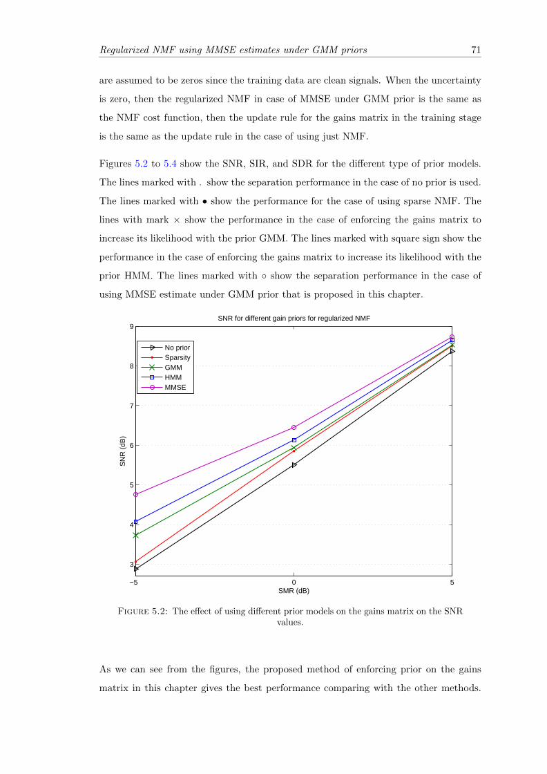
Regularized NMF using MMSE estimates under GMM priors 71
are assumed to be zeros since the training data are clean signals. When the uncertainty
is zero, then the regularized NMF in case of MMSE under GMM prior is the same as
the NMF cost function, then the update rule for the gains matrix in the training stage
is the same as the update rule in the case of using just NMF.
Figures 5.2 to 5.4 show the SNR, SIR, and SDR for the different type of prior models.
The lines marked with . show the separation performance in the case of no prior is used.
The lines marked with • show the performance for the case of using sparse NMF. The
lines with mark × show the performance in the case of enforcing the gains matrix to
increase its likelihood with the prior GMM. The lines marked with square sign show the
performance in the case of enforcing the gains matrix to increase its likelihood with the
prior HMM. The lines marked with ◦ show the separation performance in the case of
using MMSE estimate under GMM prior that is proposed in this chapter.
−5 0 5
3
4
5
6
7
8
9SNR for different gain priors for regularized NMF
SMR (dB)
SN
R (
dB)
No priorSparsityGMMHMMMMSE
Figure 5.2: The effect of using different prior models on the gains matrix on the SNRvalues.
As we can see from the figures, the proposed method of enforcing prior on the gains
matrix in this chapter gives the best performance comparing with the other methods.
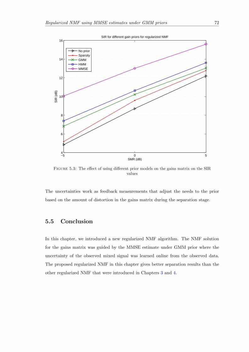
Regularized NMF using MMSE estimates under GMM priors 72
−5 0 54
6
8
10
12
14
16SIR for different gain priors for regularized NMF
SMR (dB)
SIR
(dB
)
No priorSparsityGMMHMMMMSE
Figure 5.3: The effect of using different prior models on the gains matrix on the SIRvalues
The uncertainties work as feedback measurements that adjust the needs to the prior
based on the amount of distortion in the gains matrix during the separation stage.
5.5 Conclusion
In this chapter, we introduced a new regularized NMF algorithm. The NMF solution
for the gains matrix was guided by the MMSE estimate under GMM prior where the
uncertainty of the observed mixed signal was learned online from the observed data.
The proposed regularized NMF in this chapter gives better separation results than the
other regularized NMF that were introduced in Chapters 3 and 4.
Regularized NMF using MMSE estimates under GMM priors 73
−5 0 5
2
3
4
5
6
7
8
SMR (dB)
SD
R (
dB)
SDR for different gain priors for regularized NMF
No priorSparsityGMMHMMMMSE
Figure 5.4: The effect of using different prior models on the gains matrix on the SDRvalues
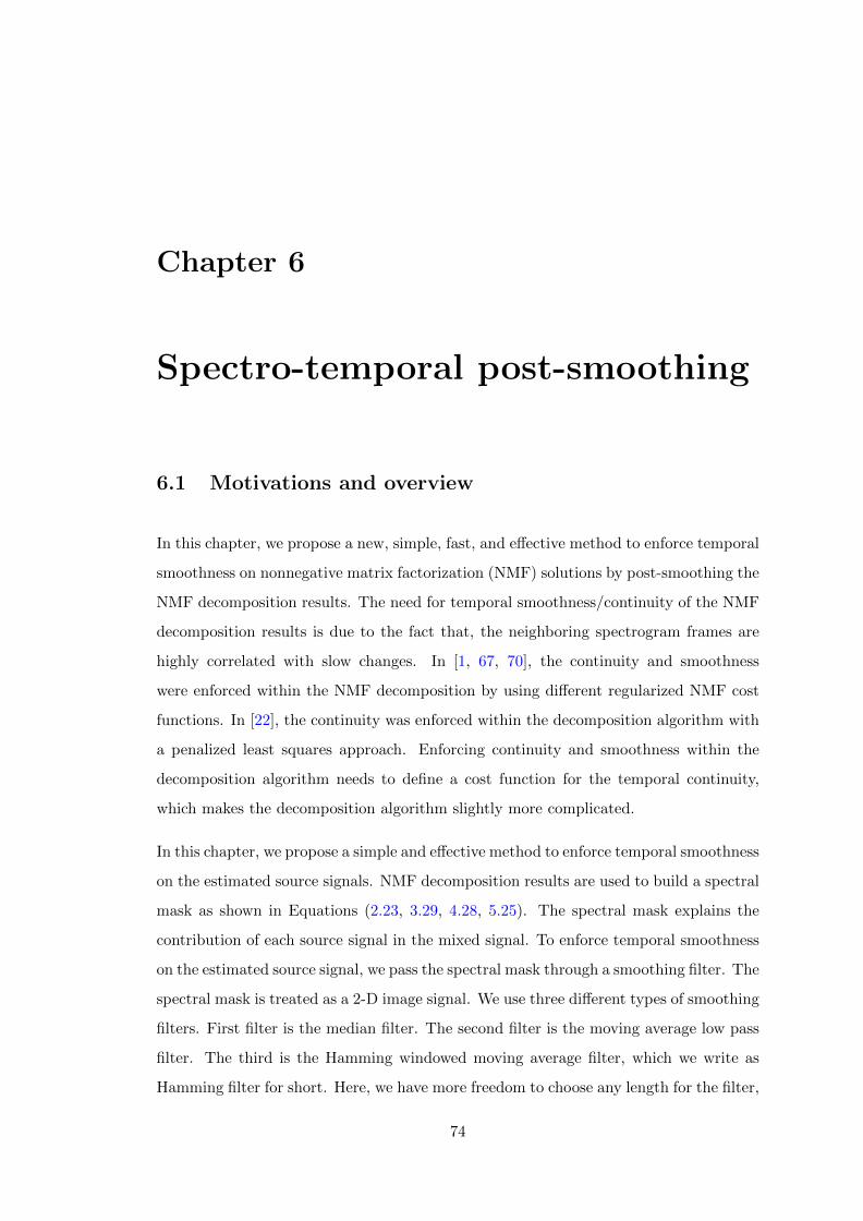
Chapter 6
Spectro-temporal post-smoothing
6.1 Motivations and overview
In this chapter, we propose a new, simple, fast, and effective method to enforce temporal
smoothness on nonnegative matrix factorization (NMF) solutions by post-smoothing the
NMF decomposition results. The need for temporal smoothness/continuity of the NMF
decomposition results is due to the fact that, the neighboring spectrogram frames are
highly correlated with slow changes. In [1, 67, 70], the continuity and smoothness
were enforced within the NMF decomposition by using different regularized NMF cost
functions. In [22], the continuity was enforced within the decomposition algorithm with
a penalized least squares approach. Enforcing continuity and smoothness within the
decomposition algorithm needs to define a cost function for the temporal continuity,
which makes the decomposition algorithm slightly more complicated.
In this chapter, we propose a simple and effective method to enforce temporal smoothness
on the estimated source signals. NMF decomposition results are used to build a spectral
mask as shown in Equations (2.23, 3.29, 4.28, 5.25). The spectral mask explains the
contribution of each source signal in the mixed signal. To enforce temporal smoothness
on the estimated source signal, we pass the spectral mask through a smoothing filter. The
spectral mask is treated as a 2-D image signal. We use three different types of smoothing
filters. First filter is the median filter. The second filter is the moving average low pass
filter. The third is the Hamming windowed moving average filter, which we write as
Hamming filter for short. Here, we have more freedom to choose any length for the filter,
74
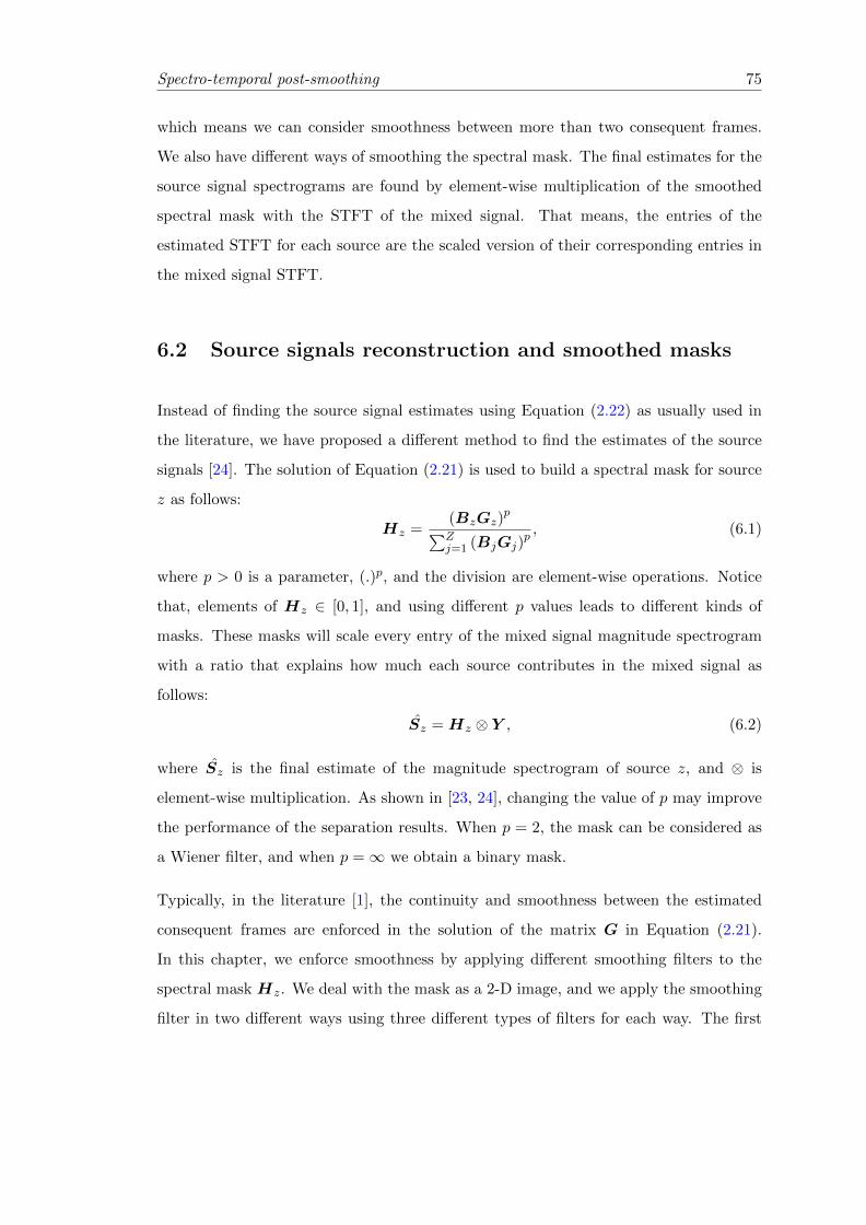
Spectro-temporal post-smoothing 75
which means we can consider smoothness between more than two consequent frames.
We also have different ways of smoothing the spectral mask. The final estimates for the
source signal spectrograms are found by element-wise multiplication of the smoothed
spectral mask with the STFT of the mixed signal. That means, the entries of the
estimated STFT for each source are the scaled version of their corresponding entries in
the mixed signal STFT.
6.2 Source signals reconstruction and smoothed masks
Instead of finding the source signal estimates using Equation (2.22) as usually used in
the literature, we have proposed a different method to find the estimates of the source
signals [24]. The solution of Equation (2.21) is used to build a spectral mask for source
z as follows:
Hz =(BzGz)
p∑Zj=1 (BjGj)
p, (6.1)
where p > 0 is a parameter, (.)p, and the division are element-wise operations. Notice
that, elements of Hz ∈ [0, 1], and using different p values leads to different kinds of
masks. These masks will scale every entry of the mixed signal magnitude spectrogram
with a ratio that explains how much each source contributes in the mixed signal as
follows:
Sz = Hz ⊗ Y , (6.2)
where Sz is the final estimate of the magnitude spectrogram of source z, and ⊗ is
element-wise multiplication. As shown in [23, 24], changing the value of p may improve
the performance of the separation results. When p = 2, the mask can be considered as
a Wiener filter, and when p =∞ we obtain a binary mask.
Typically, in the literature [1], the continuity and smoothness between the estimated
consequent frames are enforced in the solution of the matrix G in Equation (2.21).
In this chapter, we enforce smoothness by applying different smoothing filters to the
spectral mask Hz. We deal with the mask as a 2-D image, and we apply the smoothing
filter in two different ways using three different types of filters for each way. The first
Spectro-temporal post-smoothing 76
way of applying the smoothing filter to the spectral mask is as follows:
Az = ξ
((BzGz)
p∑Zj=1 (BjGj)
p
), (6.3)
where ξ (.) is a smoothing filter and Az is the smoothed mask that is used to estimate
the source z as follows:
Sz = Az ⊗ Y , (6.4)
The second way of applying the smoothing filter to the spectral mask is as follows:
Az =(Bzξ (Gz))
p∑Zj=1 (Bjξ (Gj))
p, (6.5)
which means we apply the smoothing filter on the gains matrices only in the spectral
mask formula.
The first type of filters that are used in this work is the median filter, which replaces
the entry values of the mask by the median of all entries in the neighborhood. The
second filter is the moving average low pass filter. The 1-D moving average low pass
filter coefficients cn′ are defined as
cn′ =1
b, n′ = {1, 2, ...., b} ,
where b is the filter length. The third filter is the Hamming windowed moving average
filter “Hamming filter” for short with 1-D coefficients cn′ defined as
cn′ =1
cwn′ , n′ = {1, 2, ...., b} ,
where c is chosen such that∑
n′ cn′ = 1, and w is the Hamming window with length b.
The direction of the smoothing filter is usually in the time axis, which is the horizontal
axis of the spectral mask. As we elaborate in the next sections, it is important to note
that, both methods of applying the smoothing filters on the spectral mask are neither
similar to applying the same smoothing filter to the gains matrix G without mask, nor
applying the same smoothing filter to the estimated magnitude spectra of the source
signals.
After finding suitable estimates of the magnitude spectrograms of the source signals. The
Spectro-temporal post-smoothing 77
estimated source sz(t) can be found by inverse STFT of the estimated source magnitude
spectrogram Sz with the phase angle of the mixed signal.
6.3 Experiments and discussion
We applied the proposed algorithm to separate a speech signal from a background piano
music signal. Our main goal was to get a clean speech signal from a mixture of speech
and piano music. We simulated our algorithm on a collection of Turkish speech data
and piano music data at 16kHz sampling rate. For training speech data, we used 540
short utterances from a single speaker, we used other 20 utterances of the same speaker
for testing. For music data, we downloaded piano music from piano society web site
[107]. The magnitude spectra of the training speech and music data were calculated
by using the STFT: A Hamming window with 480 points length and 60% overlap was
used and the FFT was taken at 512 points, the first 257 FFT points only were used
since the conjugate of the 255 remaining points are involved in the first FFT points.
The test data was formed by adding random portions of the test music file to the 20
speech utterance files at different speech-to-music ratio (SMR) values in dB. For each
SMR value, we obtained 20 test utterances.
We trained 128 basis vectors for each source in Equation (2.20), which makes the size
of each trained basis matrix Bspeech and Bmusic to be 257 × 128, and we fixed the
parameter p = 3 in Equation (6.1). Those choices gave good results on the same data
set in [24].
Table 6.1: SNR in dB for the estimated speech signal using spectral mask without and withsmoothing filter, with different filter types and different filter size a× b.
SMRJust Median Filter Moving Average Filter Hamming Filter
dBUsing a = 1 a = 1 a = 1 a = 1 a = 2 a = 1 a = 1 a = 1 a = 1 a = 2 a = 1 a = 1 a = 1 a = 1 a = 2
Mask b = 3 b = 5 b = 7 b = 9 b = 3 b = 2 b = 3 b = 5 b = 7 b = 3 b = 3 b = 5 b = 7 b = 9 b = 3
-5 7.05 7.26 7.44 7.45 7.30 7.04 7.18 7.34 7.38 7.32 6.84 7.17 7.39 7.43 7.42 6.72
0 10.37 10.69 10.86 10.82 10.71 10.47 10.56 10.72 10.74 10.57 10.13 10.51 10.76 10.80 10.75 10.01
5 12.46 12.80 12.95 12.92 12.73 12.31 12.60 12.77 12.72 12.44 11.87 12.59 12.81 12.81 12.70 11.78
Table 6.2: SNR in dB for the estimated speech signal using spectral mask after smoothingthe matrix G in the mask, with different filter types and different filter size a× b.
SMRMedian Filter Moving Average Filter Hamming Filter
dBa = 1 a = 1 a = 1 a = 1 a = 1 a = 1 a = 1 a = 1 a = 1 a = 1 a = 1 a = 1 a = 1 a = 1
b = 3 b = 5 b = 7 b = 3 b = 5 b = 7 b = 9 b = 11 b = 3 b = 5 b = 7 b = 9 b = 11 b = 13
-5 7.16 7.17 7.15 7.56 7.79 7.85 7.82 7.74 7.21 7.60 7.76 7.85 7.88 7.89
0 10.46 10.48 10.41 10.95 11.16 11.18 11.12 10.99 10.56 10.97 11.13 11.20 11.22 11.20
5 12.57 12.69 12.57 13.12 13.40 13.48 13.44 13.31 12.67 13.15 13.35 13.46 13.51 13.51
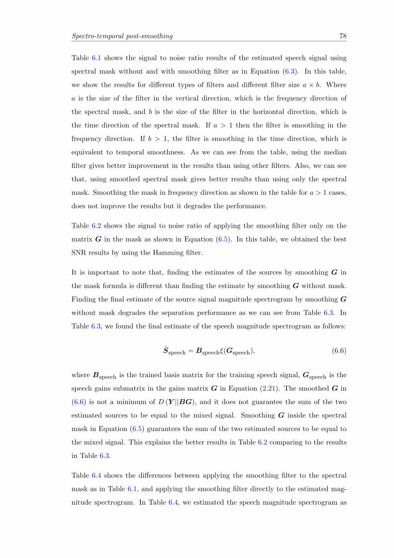
Spectro-temporal post-smoothing 78
Table 6.1 shows the signal to noise ratio results of the estimated speech signal using
spectral mask without and with smoothing filter as in Equation (6.3). In this table,
we show the results for different types of filters and different filter size a × b. Where
a is the size of the filter in the vertical direction, which is the frequency direction of
the spectral mask, and b is the size of the filter in the horizontal direction, which is
the time direction of the spectral mask. If a > 1 then the filter is smoothing in the
frequency direction. If b > 1, the filter is smoothing in the time direction, which is
equivalent to temporal smoothness. As we can see from the table, using the median
filter gives better improvement in the results than using other filters. Also, we can see
that, using smoothed spectral mask gives better results than using only the spectral
mask. Smoothing the mask in frequency direction as shown in the table for a > 1 cases,
does not improve the results but it degrades the performance.
Table 6.2 shows the signal to noise ratio of applying the smoothing filter only on the
matrix G in the mask as shown in Equation (6.5). In this table, we obtained the best
SNR results by using the Hamming filter.
It is important to note that, finding the estimates of the sources by smoothing G in
the mask formula is different than finding the estimate by smoothing G without mask.
Finding the final estimate of the source signal magnitude spectrogram by smoothing G
without mask degrades the separation performance as we can see from Table 6.3. In
Table 6.3, we found the final estimate of the speech magnitude spectrogram as follows:
Sspeech = Bspeechξ(Gspeech), (6.6)
where Bspeech is the trained basis matrix for the training speech signal, Gspeech is the
speech gains submatrix in the gains matrix G in Equation (2.21). The smoothed G in
(6.6) is not a minimum of D (Y ||BG), and it does not guarantee the sum of the two
estimated sources to be equal to the mixed signal. Smoothing G inside the spectral
mask in Equation (6.5) guarantees the sum of the two estimated sources to be equal to
the mixed signal. This explains the better results in Table 6.2 comparing to the results
in Table 6.3.
Table 6.4 shows the differences between applying the smoothing filter to the spectral
mask as in Table 6.1, and applying the smoothing filter directly to the estimated mag-
nitude spectrogram. In Table 6.4, we estimated the speech magnitude spectrogram as
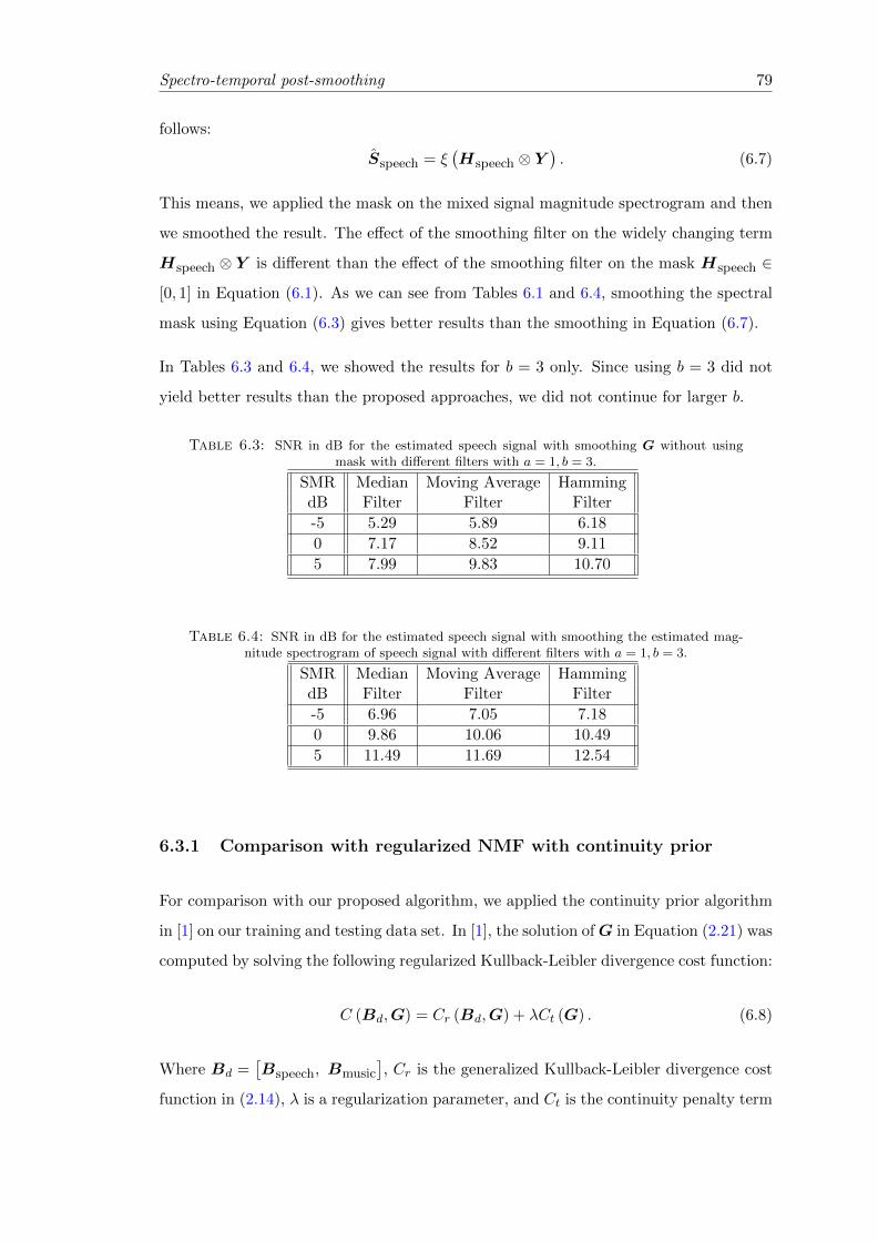
Spectro-temporal post-smoothing 79
follows:
Sspeech = ξ(Hspeech ⊗ Y
). (6.7)
This means, we applied the mask on the mixed signal magnitude spectrogram and then
we smoothed the result. The effect of the smoothing filter on the widely changing term
Hspeech ⊗ Y is different than the effect of the smoothing filter on the mask Hspeech ∈
[0, 1] in Equation (6.1). As we can see from Tables 6.1 and 6.4, smoothing the spectral
mask using Equation (6.3) gives better results than the smoothing in Equation (6.7).
In Tables 6.3 and 6.4, we showed the results for b = 3 only. Since using b = 3 did not
yield better results than the proposed approaches, we did not continue for larger b.
Table 6.3: SNR in dB for the estimated speech signal with smoothing G without usingmask with different filters with a = 1, b = 3.
SMR Median Moving Average HammingdB Filter Filter Filter
-5 5.29 5.89 6.18
0 7.17 8.52 9.11
5 7.99 9.83 10.70
Table 6.4: SNR in dB for the estimated speech signal with smoothing the estimated mag-nitude spectrogram of speech signal with different filters with a = 1, b = 3.
SMR Median Moving Average HammingdB Filter Filter Filter
-5 6.96 7.05 7.18
0 9.86 10.06 10.49
5 11.49 11.69 12.54
6.3.1 Comparison with regularized NMF with continuity prior
For comparison with our proposed algorithm, we applied the continuity prior algorithm
in [1] on our training and testing data set. In [1], the solution ofG in Equation (2.21) was
computed by solving the following regularized Kullback-Leibler divergence cost function:
C (Bd,G) = Cr (Bd,G) + λCt (G) . (6.8)
Where Bd =[Bspeech, Bmusic
], Cr is the generalized Kullback-Leibler divergence cost
function in (2.14), λ is a regularization parameter, and Ct is the continuity penalty term
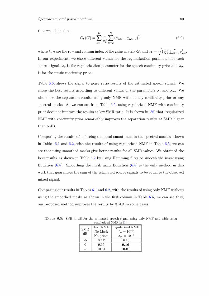
Spectro-temporal post-smoothing 80
that was defined as
Ct (G) =K∑k=1
1
σ2k
N∑n=2
(gk,n − gk,n−1)2 , (6.9)
where k, n are the row and column index of the gains matrixG, and σk =√(
1N
)∑Nn=1 g
2k,n.
In our experiment, we chose different values for the regularization parameter for each
source signal. λs is the regularization parameter for the speech continuity prior and λm
is for the music continuity prior.
Table 6.5, shows the signal to noise ratio results of the estimated speech signal. We
chose the best results according to different values of the parameters λs and λm. We
also show the separation results using only NMF without any continuity prior or any
spectral masks. As we can see from Table 6.5, using regularized NMF with continuity
prior does not improve the results at low SMR ratio. It is shown in [86] that, regularized
NMF with continuity prior remarkably improves the separation results at SMR higher
than 5 dB.
Comparing the results of enforcing temporal smoothness in the spectral mask as shown
in Tables 6.1 and 6.2, with the results of using regularized NMF in Table 6.5, we can
see that using smoothed masks give better results for all SMR values. We obtained the
best results as shown in Table 6.2 by using Hamming filter to smooth the mask using
Equation (6.5). Smoothing the mask using Equation (6.5) is the only method in this
work that guarantees the sum of the estimated source signals to be equal to the observed
mixed signal.
Comparing our results in Tables 6.1 and 6.2, with the results of using only NMF without
using the smoothed masks as shown in the first column in Table 6.5, we can see that,
our proposed method improves the results by 3 dB in some cases.
Table 6.5: SNR in dB for the estimated speech signal using only NMF and with usingregularized NMF in [1].
SMRJust NMF regularized NMF
dBNo Mask λs = 10−5
No priors λm = 10−5
-5 6.17 6.13
0 9.15 9.16
5 10.81 10.81
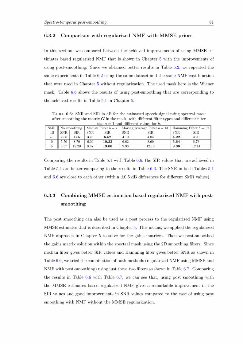
Spectro-temporal post-smoothing 81
6.3.2 Comparison with regularized NMF with MMSE priors
In this section, we compared between the achieved improvements of using MMSE es-
timates based regularized NMF that is shown in Chapter 5 with the improvements of
using post-smoothing. Since we obtained better results in Table 6.2, we repeated the
same experiments in Table 6.2 using the same dataset and the same NMF cost function
that were used in Chapter 5 without regularization. The used mask here is the Wiener
mask. Table 6.6 shows the results of using post-smoothing that are corresponding to
the achieved results in Table 5.1 in Chapter 5.
Table 6.6: SNR and SIR in dB for the estimated speech signal using spectral maskafter smoothing the matrix G in the mask, with different filter types and different filter
size a = 1 and different values for b.SMR No smoothing Median Filter b = 7 Moving Average Filter b = 13 Hamming Filter b = 19dB SNR SIR SNR SIR SNR SIR SNR SIR
-5 2.88 4.86 3.45 6.52 4.19 4.84 4.22 4.90
0 5.50 8.70 6.09 10.33 6.62 8.69 6.64 8.73
5 8.37 12.20 8.87 13.66 9.33 12.13 9.36 12.14
Comparing the results in Table 5.1 with Table 6.6, the SIR values that are achieved in
Table 5.1 are better comparing to the results in Table 6.6. The SNR in both Tables 5.1
and 6.6 are close to each other (within ±0.5 dB differences for different SMR values).
6.3.3 Combining MMSE estimation based regularized NMF with post-
smoothing
The post smoothing can also be used as a post process to the regularized NMF using
MMSE estimates that is described in Chapter 5. This means, we applied the regularized
NMF approach in Chapter 5 to solve for the gains matrices. Then we post-smoothed
the gains matrix solution within the spectral mask using the 2D smoothing filters. Since
median filter gives better SIR values and Hamming filter gives better SNR as shown in
Table 6.6, we tried the combination of both methods (regularized NMF using MMSE and
NMF with post-smoothing) using just these two filters as shown in Table 6.7. Comparing
the results in Table 6.6 with Table 6.7, we can see that, using post smoothing with
the MMSE estimates based regularized NMF gives a remarkable improvement in the
SIR values and good improvements in SNR values compared to the case of using post
smoothing with NMF without the MMSE regularization.

Spectro-temporal post-smoothing 82
Table 6.7: SNR and SIR in dB for the estimated speech signal using MMSE estimatesbased regularized NMF and smoothed masks for different filter types and different filter
size a = 1,K = 16, λ = 1 and different values for b.SMR No smoothing Median Filter Hamming Filter
b = 7 b = 19 b = 7dB SNR SIR SNR SIR SNR SIR SNR SIR
-5 2.88 4.86 5.88 15.23 6.04 9.92 5.67 10.33
0 5.50 8.70 7.18 16.90 7.54 12.81 7.26 13.28
5 8.37 12.20 9.26 18.65 9.69 15.15 9.47 15.73
Comparing the results in Table 5.1 with Table 6.7, we can see that, using post smoothing
with median filters after MMSE estimates based regularized NMF improves both the
SIR and SNR values compared to the case of using regularized NMF only without post
smoothing. For the case of using Hamming filter for smoothing after the regularized
NMF, we obtained better SNR values but slightly better values for SIR when b = 7.
The achieved improvement due to combining MMSE estimates based regularized NMF
with the post-smoothing compared with the case of using just NMF (first column in
Tables 6.6 and 6.7) is considered to be remarkable.
Table 6.8 shows the “oracle” results where we put the correct magnitude of the speech
signal with the phase of the mixed signal. These results represent the gold standard
that can be achieved when the magnitude spectra are recovered exactly. As can be seen
from Tables 6.7 and 6.8, the achieved SIR results of using MMSE estimation in the
regularized NMF followed by smoothed masks are very close to the SIR in the oracle
experiment. The achieved SNR results in Table 6.7 are considered to be good as well
but there is more that can be achieved for the SNR.
Table 6.8: SNR and SIR in dB for the oracle experiment.
SMR OracledB SNR SIR
-5 9.25 15.21
0 11.62 16.90
5 14.46 19.41
6.4 Conclusion
In this chapter, we studied new methods to enforce smoothness on the NMF solutions
rather than using regularized NMF with the continuity prior. The new methods are
Spectro-temporal post-smoothing 83
based on post-smoothing the NMF decomposition results. We also studied the case when
the MMSE estimates based regularized NMF that had been introduced in Chapter 5 was
followed by the post-smoothing process that was presented in this chapter. The achieved
improvements of using post-smoothing for the case of using NMF with and without
MMSE estimates based regularization is considered to be quite large improvements.
Chapter 7
Spectro-temporal
post-enhancement using MMSE
estimation
7.1 Motivations and overview
In Chapter 5, minimum mean squared error (MMSE) estimation was used to improve/-
correct the gains matrix solution of the NMF. MMSE estimate based correction of the
gain matrices was performed using a regularized NMF cost function. In this chapter,
MMSE estimation is used to improve/correct the NMF separated spectrograms. MMSE
estimate based correction of the separated spectrograms is embedded in the Wiener filter
to guarantee that the sum of the estimated sources be equal to the mixed signal. In
Chapter 5, we were trying to improve the IS-NMF solution for the gains matrices only
since the trained basis matrices were assumed to be good in representing the training
data. The trained basis matrix that is usually used as a representative for each source
training data is usually not sufficient to represent all the characteristics of each source.
This representation may be limited since the dynamic information between the frames
is missing and there is no analytical approach for choosing a suitable number of bases
for a given source signal. More information about the sources besides their trained basis
matrices is usually needed.
84
Spectro-temporal post-enhancement using MMSE estimation 85
In this chapter, besides training a basis matrix for each source, the spectrogram for
each training data is directly used to train a Gaussian mixture model (GMM) in the
logarithm domain. The trained basis matrices are used with NMF to compute a spec-
trogram for each source from the mixed signal. The computed spectrogram of each
source is then treated as a 2D distorted signal. The trained GMM and the expectation
maximization algorithm (EM) [102] are used to learn the distortion in each separated
signal spectrogram. The trained GMMs, the learned distortions, the minimum mean
squared error (MMSE) estimates, and the Wiener filters are used to find enhanced ver-
sions of the separated spectrograms. To consider the dynamic information between the
spectrogram frames, we apply the enhancement approach on multiple consequent frames
at once instead of applying it frame by frame.
7.2 MMSE estimation for post enhancement
The assumption that is inherent in the solution of Equations (2.20) to (2.22) in Chapter
1 is that, the trained basis matrix for each source is a sufficient representative for the
training data for each source. Some obvious drawbacks of this assumption are that
the number of bases can not be determined analytically and the trained matrices do
not capture the dynamic information for the source signals. In addition, NMF may
cause high overlap among sources due to accepting the whole span of the bases as
representations. The initial estimated spectrogram Sz in (2.22) for each source z is
treated as a distorted 2D signal (image) that needs to be restored. MMSE estimation
is used as a post process to find better estimates for the source signals.
We first need to build a model for the correct/expected frames that the spectrogram
Sz should have. For example, the sequence of PSD (power spectral density) frames in
the spectrogram Strainz in Equation (2.20) can be seen as valid PSD frames that the
spectrogram of the source z can have. The training signal spectrogram Strainz can be
used to train a Gaussian mixture model GMMz for the valid PSD frames that can be
seen in source z. Then, how far the statistics of the spectrogram Sz from the trained
GMMz is learned which is considered as a measurement of the amount of distortions
that exist in the spectrogram Sz. Based on the amount of the existed distortions and the
GMM that model the valid frames, MMSE estimates are used to find a better solution
for each source spectrogram Sz. To consider the dynamic information of the source
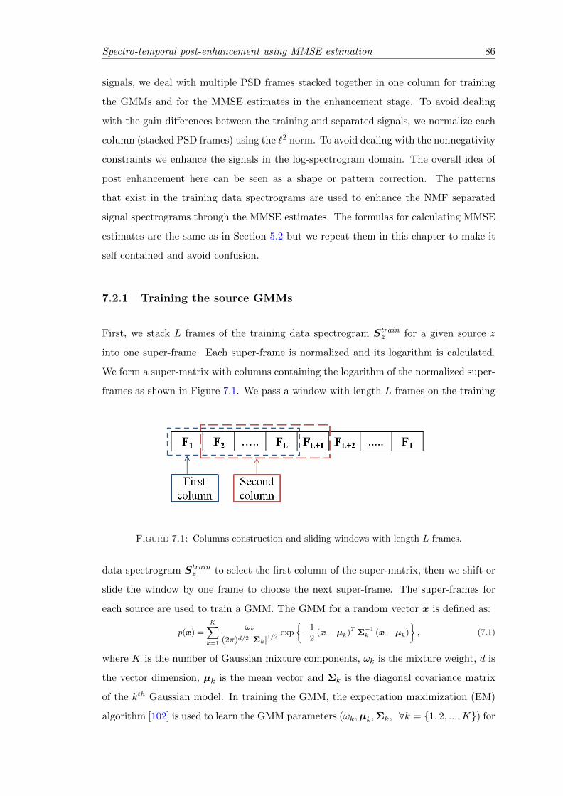
Spectro-temporal post-enhancement using MMSE estimation 86
signals, we deal with multiple PSD frames stacked together in one column for training
the GMMs and for the MMSE estimates in the enhancement stage. To avoid dealing
with the gain differences between the training and separated signals, we normalize each
column (stacked PSD frames) using the `2 norm. To avoid dealing with the nonnegativity
constraints we enhance the signals in the log-spectrogram domain. The overall idea of
post enhancement here can be seen as a shape or pattern correction. The patterns
that exist in the training data spectrograms are used to enhance the NMF separated
signal spectrograms through the MMSE estimates. The formulas for calculating MMSE
estimates are the same as in Section 5.2 but we repeat them in this chapter to make it
self contained and avoid confusion.
7.2.1 Training the source GMMs
First, we stack L frames of the training data spectrogram Strainz for a given source z
into one super-frame. Each super-frame is normalized and its logarithm is calculated.
We form a super-matrix with columns containing the logarithm of the normalized super-
frames as shown in Figure 7.1. We pass a window with length L frames on the training
Figure 7.1: Columns construction and sliding windows with length L frames.
data spectrogram Strainz to select the first column of the super-matrix, then we shift or
slide the window by one frame to choose the next super-frame. The super-frames for
each source are used to train a GMM. The GMM for a random vector x is defined as:
p(x) =
K∑k=1
ωk
(2π)d/2 |Σk|1/2exp
{−1
2(x− µk)T Σ−1
k (x− µk)
}, (7.1)
where K is the number of Gaussian mixture components, ωk is the mixture weight, d is
the vector dimension, µk is the mean vector and Σk is the diagonal covariance matrix
of the kth Gaussian model. In training the GMM, the expectation maximization (EM)
algorithm [102] is used to learn the GMM parameters (ωk,µk,Σk, ∀k = {1, 2, ...,K}) for
Spectro-temporal post-enhancement using MMSE estimation 87
each source given the logarithm of its normalized super-frames as training data. After
training the GMM parameters using each source training data, we will have trained
GMMz for each source z.
7.2.2 Learning the distortion
We need to learn how much the spectrogram Sz for a given source z in (2.22) is distorted
compared with its corresponding trained GMMz. First, we need to form a super-matrix
for each Sz in (2.22). We attach L − 1 frames with values close to zeros to the far left
and right to each spectrogram Sz. Then we start forming super-frames with L stacked
frames for the spectrogram Sz as we did during training the GMMs in Section 7.2.1.
Every super-frame is normalized and its logarithm is calculated and used to form a
super-matrix Qz for its corresponding spectrogram Sz. The normalization values for
the super-frames are saved to be used later. Data corresponding to each PSD frame
in Sz will appear L times in its corresponding super-matrix Qz as sub-vectors in the
corresponding super-frame columns. Each column qn in Qz can be seen as a noisy
observation which can be written as a sum of a clean observation xn and an additive
noise ez as follows:
qn = xn + ez, (7.2)
where xn is the unknown desired pattern that corresponds to the observation qn and
needs to be estimated under a trained GMMz from Section 7.2.1, ez is the logarithm
of a distortion operator, which is modeled here by a Gaussian distribution with zero
mean and diagonal covariance matrix Ψz as N (e|0,Ψz). The uncertainty Ψz is trained
directly from all columns q = {q1, .., qn, .., qN} inQz, where N is the number of columns
in the matrix Qz. The uncertainty Ψz can be iteratively learned using the expectation
maximization (EM) algorithm. Given the GMMz parameters which are considered fixed
here, the update of Ψz is found based on the sufficient statistics zn and Rn as in
Appendix A as follows [112, 113, 114]:
Ψz = diag
{1
N
N∑n=1
(qnq
Tn − qnzTn − znqTn + Rn
)}, (7.3)
where the “diag” operator sets all the off-diagonal elements of a matrix to zero, and the
sufficient statistics zn and Rn can be updated using Ψz from the previous iteration as

Spectro-temporal post-enhancement using MMSE estimation 88
follows:
zn =K∑k=1
γknzkn, and Rn =K∑k=1
γknRkn, (7.4)
where
γkn =
[ωkN (qn|µk,Σk + Ψz)∑Kj=1 ωjN
(qn|µj ,Σj + Ψz
)] , (7.5)
Rkn = Σk −Σk (Σk + Ψz)−1 ΣT
k + zknzTkn, (7.6)
and
zkn = µk + Σk (Σk + Ψz)−1 (qn − µk) . (7.7)
Ψz is considered as a general uncertainty measurement over all the observations in
matrix Qz. Ψz can be seen as a model that summarizes the deformation that exists
in all columns in the super-matrix Qz. Given the trained GMMz, the super-matrix Qz
that is corresponding to the distorted spectrogram Sz, the uncertainty Ψz is calculated
iteratively for each source z using Equations (7.3) to (7.7).
7.2.3 Calculating MMSE estimates
Given the GMMz parameters and the uncertainty measurement Ψz for a given source
signal z, the MMSE estimate of each pattern xn given its observation qn under the
observation model in Equation (7.2) can be found as in Appendix A as follows:
xn =K∑k=1
γkn
[µk + Σk (Σk + Ψz)
−1 (qn − µk)], (7.8)
where
γkn =
[ωkN (qn|µk,Σk + Ψz)∑Kj=1 ωjN
(qn|µj ,Σj + Ψz
)] . (7.9)
The model in Equation (7.2) expresses the normalized super-columns before calculating
the logarithm of the spectrogram Sz as a distorted image with a multiplicative defor-
mation diagonal matrix. For the normalized super-frame columns sn‖sn‖2
of Sz there is
a deformation matrix Edz with log-normal distribution that is applied to the correct
pattern that we need to estimate sn as follows:
sn‖sn‖2
= Edz sn. (7.10)
Spectro-temporal post-enhancement using MMSE estimation 89
The uncertainty for Edz for source z is represented in the covariance matrix Ψz. The
MMSE estimation based post enhancement here can be seen as performing denoising un-
der multiplicative noise. We believe this is beneficial since the additive noise is assumed
to be removed by NMF.
After calculating xn, ∀n ∈ {1, .., N}, we calculate the exponent for each entry of xn, ∀n ∈
{1, .., N} and form a matrix T z by inserting xn’s in its columns. The procedures in
Sections 7.2.2 and 7.2.3 are repeated for each source. The norm for each super-column
that was calculated in Section 7.2.2 is used to scale its corresponding super-column
in T z. The columns of T z are scaled by multiplying each super-frame (column) with
its corresponding norm from Section 7.2.2. The norm rescaling is used to preserve the
energy differences between the two source signals. We convert the scaled super-frames of
T z into the original size of the spectrograms by reframing its super-frames. Since every
PSD frame appears L times in different L consequent super-frames, we take the average
to find the final enhanced spectrogram Sz. The spectrograms Sz, ∀z ∈ {1, .., Z} are
then used in the Wiener filter Hz to find the final source STFTs as follows:
Hz =Sz∑Zl=1 Sl
, (7.11)
Sz (n, f) = Hz (n, f)Y (n, f) , (7.12)
where the divisions are done element-wise. The use of the Wiener filters here is very
important since it is the only way to guarantee that the two estimated source spectro-
grams add up to the mixed signal spectrogram. The estimated source signals sz(t) can
be found by using inverse STFT of Sz(n, f).
7.3 Experiments and discussion
We applied the proposed algorithm to separate a speech signal from a background piano
music signal. Our main goal was to get a clean speech signal from a mixture of speech
and piano signals. We simulated our algorithm on the same training and testing speech
and piano data that were used in Sections 4.5 and 5.4 with the same setup for calculating
the STFT. We trained 128 basis vectors for each source, which makes the size of Bspeech
and Bmusic matrices to be 257× 128.
Spectro-temporal post-enhancement using MMSE estimation 90
Performance evaluation of the separation algorithm was done using the signal to noise
ratio (SNR), signal to distortion ratio (SDR), and the signal to interference ratio (SIR)
that are described in Section 2.4. The average SNR, SDR, and SIR over the 10 test utter-
ances are reported. The higher SNR, SDR, and SIR we measure, the better performance
we achieve.
Table 7.1 shows the SNR, SDR, and SIR of the separated speech signal using IS-NMF
without post enhancement and NMF with post enhancement using MMSE estimates
with different values of GMM components K and the number of the stacked frames L.
The second column of the table shows the separation results of using just NMF with
spectral masks without post enhancement as shown in Equations (2.23) to (2.24). The
third and fourth columns show the results of using NMF with MMSE estimation based
post enhancement with the Wiener filters as shown in Equations (7.11) and (7.12). The
choice for K and L was done by trying different combinations. In this chapter, we
chose the same value for L for both sources and also for K. The shown results are just
examples for the improvements that can be achieved. Better results can be achieved for
different combinations of K and L.
Table 7.1: SDR and SIR in dB for the estimated speech signal.
SMR NMF NMF+Post MMSEL = 11, K = 256 L = 3, K = 32
dB SDR SIR SNR SDR SIR SNR SDR SIR SNR
-5 1.51 4.86 2.88 3.45 9.47 5.25 2.52 6.30 4.05
0 4.53 8.70 5.50 6.05 12.89 6.95 5.61 10.19 6.53
5 7.74 12.20 8.37 8.84 15.76 9.12 8.74 13.45 9.28
As we can see from the table, the proposed NMF with post enhancement using MMSE
estimates improves the separation performance comparing with just using NMF. In-
creasing the value of L improves the performance but it requires increasing the value of
K. The best choice for K usually depends on the nature and the size of the training
data and also on the value of L. It is important to note that, applying MMSE estimates
directly on the mixed signal without using NMF (not shown in the table) gives worse
results than just using NMF because the MMSE estimate post enhancement removes
only the multiplicative noise while the music signal here is considered as an additive
noise.
Spectro-temporal post-enhancement using MMSE estimation 91
Comparing the performance in Table 6.6 of using post smoothing idea that is shown in
Chapter 6 with the performance of using post enhancement idea that is shown in Table
7.1, we can see that, post enhancement gives better results than post smoothing.
Comparing the performance shown in Table 5.1 and Figure 5.4 of using MMSE estima-
tions under GMM prior for regularized NMF that is introduced in Chapter 5 with the
performance of using MMSE estimates as post enhancement that is shown in Table 7.1,
we can see that, MMSE estimates as post enhancement gives better SDR and SNR re-
sults than using MMSE estimates for regularized NMF. Regularized NMF using MMSE
estimates gives better SIR values than using MMSE estimates as post enhancement. In
general, the exact comparison between these two approaches is not guaranteed because
of the many free parameters that need to be chosen for each approach. Using MMSE
estimation as post enhancement considers the temporal structure of the source signals
while the regularized NMF using MMSE does not consider the temporal structure.
7.4 Conclusion
In this chapter, we improved the quality of NMF based source separation by employing a
novel MMSE estimation technique based on trained GMMs. The distortion was learned
online from the NMF separated signal spectrograms. The dynamics or the sequential
information of the sources was considered by enhancing multiple frames of the spec-
trograms at once. The results show that, the proposed MMSE estimation based post
enhancement improves the quality of the NMF separated sources.

Chapter 8
Discriminative nonnegative
dictionary learning using
cross-coherence penalties
8.1 Motivations and overview
In this chapter, we introduce a new discriminative training method for nonnegative
dictionary learning. As shown before, nonnegative matrix factorization (NMF) is used
to learn a dictionary (a set of basis vectors) for each source as in Equation 2.20. NMF
is then used to decompose the mixed signal magnitude spectrogram as a weighted linear
combination of the trained dictionary entries for all sources in the mixed signal. The
estimate for each source is found by summing the decomposition terms that include its
corresponding trained basis vectors as shown in Equations (2.21) and (2.22). One of
the main problems of this framework is that, the trained basis vectors for each source
dictionary can represent the other source signals. When a dictionary of one source is
able to represent the other source signals, the estimated separated signal for this source
in Equation (2.22) will contain signals from the other sources that are in the mixed
signal. A solution for this problem is to learn the entries for each source dictionary to
be more discriminative from the entries of the other sources’ dictionaries. The goal in
this chapter is to train nonnegative discriminative dictionaries simultaneously for the
source signals. Discriminative dictionary for a source signal in this work means that, a
92

Discriminative nonnegative dictionary learning using cross-coherence penalties 93
dictionary that is good in representing this source signal and at the same time is bad
in representing the other source signals [115]. Enforcing the dictionary for each source
signal to poorly represent the other source signals increases the separation capability of
the NMF decomposition of the observed mixed signal.
The NMF solution for training a dictionary for a source signal is usually not unique,
and there are multiple solutions that can be used as a dictionary for the same source.
In this chapter, we are seeking a dictionary for each source during the training that
minimizes the reconstruction error and prevents its bases from representing the other
sources. To prevent the dictionaries from representing the sources of each other, we
propose to minimize the cross-coherence between the source dictionaries. Minimizing
the cross-coherence is equivalent to minimizing the projection of every source signal on
the subspaces that are spanned by the other source’s dictionaries. To achieve good rep-
resentative and discriminative dictionaries with nonnegativity constraints, we formulate
these objectives using a regularized NMF cost function with simplified cross-coherence
penalties. The new update rules for simultaneously training the dictionaries that solve
the regularized NMF cost function are introduced in this chapter.
In this work, we use the generalized Kullback-Leibler divergence cost function in Equa-
tion (2.14) with the approximation shown in (2.4). We also assume that, the number of
sources is two for simplicity.
8.2 Dictionary learning
The matrix B in Equation (2.8) can be seen as a dictionary with nonnegativity con-
straints that represents each column v in V as a weighted linear combination of its
constituent vectors as follows:
vn =D∑j=1
gjnbj , bj ∈ B, (8.1)
where vn is the column n in matrix V , bj is the column j in matrix B and gjn is its
weight in the gains matrix G. One of the main quality measurements of a dictionary is
its coherence [116]. The coherence is a measurement of the redundancy of the dictionary
and small coherence indicates that the dictionary is not far from an orthogonal basis.
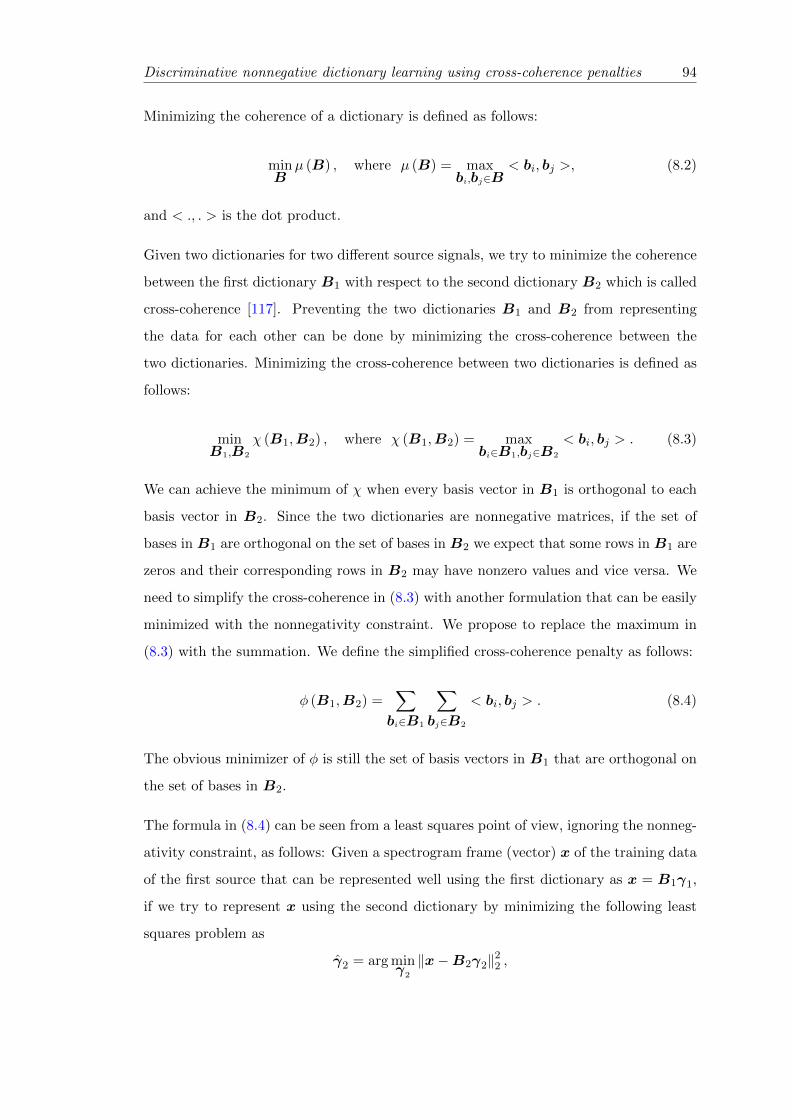
Discriminative nonnegative dictionary learning using cross-coherence penalties 94
Minimizing the coherence of a dictionary is defined as follows:
minB
µ (B) , where µ (B) = maxbi,bj∈B
< bi, bj >, (8.2)
and < ., . > is the dot product.
Given two dictionaries for two different source signals, we try to minimize the coherence
between the first dictionary B1 with respect to the second dictionary B2 which is called
cross-coherence [117]. Preventing the two dictionaries B1 and B2 from representing
the data for each other can be done by minimizing the cross-coherence between the
two dictionaries. Minimizing the cross-coherence between two dictionaries is defined as
follows:
minB1,B2
χ (B1,B2) , where χ (B1,B2) = maxbi∈B1,bj∈B2
< bi, bj > . (8.3)
We can achieve the minimum of χ when every basis vector in B1 is orthogonal to each
basis vector in B2. Since the two dictionaries are nonnegative matrices, if the set of
bases in B1 are orthogonal on the set of bases in B2 we expect that some rows in B1 are
zeros and their corresponding rows in B2 may have nonzero values and vice versa. We
need to simplify the cross-coherence in (8.3) with another formulation that can be easily
minimized with the nonnegativity constraint. We propose to replace the maximum in
(8.3) with the summation. We define the simplified cross-coherence penalty as follows:
φ (B1,B2) =∑bi∈B1
∑bj∈B2
< bi, bj > . (8.4)
The obvious minimizer of φ is still the set of basis vectors in B1 that are orthogonal on
the set of bases in B2.
The formula in (8.4) can be seen from a least squares point of view, ignoring the nonneg-
ativity constraint, as follows: Given a spectrogram frame (vector) x of the training data
of the first source that can be represented well using the first dictionary as x = B1γ1,
if we try to represent x using the second dictionary by minimizing the following least
squares problem as
γ2 = arg minγ2
‖x−B2γ2‖22 ,
Discriminative nonnegative dictionary learning using cross-coherence penalties 95
the pseudo-inverse (least squares) solution for γ2 will be
γ2 =(BT
2B2
)−1BT
2B1γ1.
From the previous formula, if we want x not to be represented byB2 we needBT2B1 = 0.
Minimizing the entries of the multiplication BT2B1 or BT
1B2 minimizes the possibility
of each source dictionary from representing the other sources.
The dictionaries B1 and B2 that minimize φ in (8.4) may not be a good representative
for Strain1 and Strain2 in Equation (2.20) (or Equation (8.5, 8.6) in next section). We use
regularized NMF to find the basis matrices B1 and B2 that can solve Equations (8.5),
and (8.6) and minimizes (8.4) at the same time.
8.3 Discriminative learning through cross-coherence penal-
ties
The available training data for each source signal is used with NMF to train a dictionary
of basis vectors for each source. The trained dictionaries will be used for the mixed signal
decomposition as shown in next section. To train the dictionaries, the magnitude spectra
for each source training data Strain1 and Strain2 are needed to be decomposed into basis
and gains matrices as follows:
Strain1 ≈ B1Gtrain1 , (8.5)
Strain2 ≈ B2Gtrain2 , (8.6)
where Strain1 ∈ <M×N1+ , Gtrain
1 ∈ <D1×N1+ , Strain2 ∈ <M×N2
+ , Gtrain2 ∈ <D2×N2
+ , and the
dictionaries B1 ∈ <M×D1+ , B2 ∈ <M×D2
+ . The NMF can be used to solve Equations
(8.5, 8.6) but we need the two basis matrices to be more discriminative from each other.
To avoid the dictionary of each source from representing the other sources, we need the
projection of the basis vectors of the first source dictionary on the basis vectors of the
second source dictionary to be small. We also need to make sure that the set of bases for
each source is capable of representing its own source signal efficiently. To compromise
Discriminative nonnegative dictionary learning using cross-coherence penalties 96
these two goals we formulate this problem as a regularized NMF problem as follows:
C = DKL
(Strain1 ||B1G
train1
)+ α1DKL
(Strain2 ||B2G
train2
)+ α2
∑i,j
(BT
1B2
)ij, (8.7)
where α1 is a regularization parameter that can be used to balance the energy scale
differences between the two sources training data, α2 is a regularization parameter that
controls the trade-off between the NMF reconstruction error terms and the simplified
cross-coherence penalty term. The last term in Equation (8.7) enforces the discrimina-
tivity between the two dictionaries. The value of α1 can be determined for example from
the ratio between the sum of all entries in matrix Strain1 to the sum of Strain2 entries.
To find the update rule solutions for the basis matrices we follow the same procedures
as in [1, 67, 84]. We express the gradient with respect to B1 of the cost function in
Equation (8.7) as a difference of two positive terms ∇+
B1C and ∇−
B1C as follow:
∇B1C = ∇+
B1C −∇−
B1C. (8.8)
The cost function is shown to be nonincreasing under the following update rule [1, 67]
B1 ← B1 ⊗∇−B1
C
∇+
B1C. (8.9)
The gradient with respect to B1 of the cost function in Equation (8.7) can be calculated
as follows:
∇B1C =
(1− Strain1
B1Gtrain1
)GtrainT
1 + α2B212, (8.10)
where 1 is a matrix of ones with the same size of Strain1 and 12 ∈ <D2×D1+ is a matrix of
ones. The gradient can be divided as in Equation (8.8) as
∇−B1
C =Strain1
B1Gtrain1
GtrainT
1 , (8.11)
∇+
B1C = 1GtrainT
1 + α2B212. (8.12)
Discriminative nonnegative dictionary learning using cross-coherence penalties 97
The final update rule for matrix B1 can be written from Equations (8.9, 8.11, 8.12) as
follows:
B1 ← B1 ⊗Strain
1
B1Gtrain1
GtrainT
1
1GtrainT
1 + α2B212
. (8.13)
The only difference between the update rule in Equation (8.13) and Equation (2.15) is
the additional term in the denominator due to the cross-coherence penalty term.
Following the same procedures, the update rule for B2 is
B2 ← B2 ⊗Strain
2
B2Gtrain2
GtrainT
2
1GtrainT
2 + λB111
, (8.14)
where λ = α2/α1, 11 ∈ <D1×D2+ is a matrix of ones.
To see the effect of adding cross-coherence penalties between the two basis dictionaries,
we can rewrite the update rules in Equations (8.13) and (8.14) in more details as follows:
B1ij ← B1ij
∑kG
train1jk
Strain1ik/(B1G
train1
)ik(∑
mGtrain1jm
)+ α2
∑lB2il
, (8.15)
B2ij ← B2ij
∑kG
train2jk
Strain2ik/(B2G
train2
)ik(∑
mGtrain2jm
)+ λ
∑lB1il
. (8.16)
We can see that, each row entry in matrix B1 is divided over the sum of the entries
of its corresponding row in matrix B2 and vice versa. Since B1 and B2 can not have
negative values, the only way to enforce orthogonality between the two dictionaries is
by making each row entries of one basis dictionary to be much smaller (close to zero)
than the entries of its corresponding row in the other basis dictionary. The extra terms
in the denominators guarantee that, some rows will dominate more in one dictionary
over their corresponding rows in the other dictionary.
The multiplicative update rule solutions for the gains matrices Gtrain1 and Gtrain
2 are
exactly the same as in Equation (2.16). All basis and gain matrices are initialized using
positive random numbers.
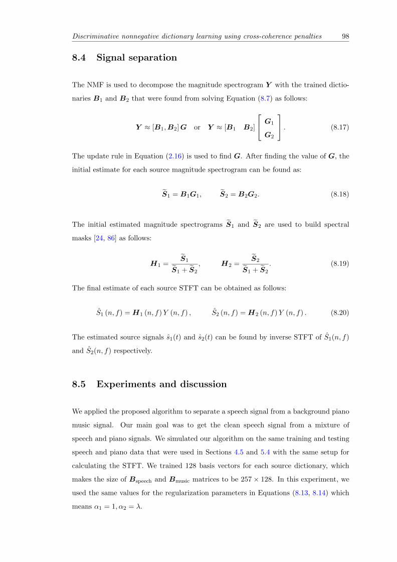
Discriminative nonnegative dictionary learning using cross-coherence penalties 98
8.4 Signal separation
The NMF is used to decompose the magnitude spectrogram Y with the trained dictio-
naries B1 and B2 that were found from solving Equation (8.7) as follows:
Y ≈ [B1,B2]G or Y ≈ [B1 B2]
G1
G2
. (8.17)
The update rule in Equation (2.16) is used to find G. After finding the value of G, the
initial estimate for each source magnitude spectrogram can be found as:
S1 = B1G1, S2 = B2G2. (8.18)
The initial estimated magnitude spectrograms S1 and S2 are used to build spectral
masks [24, 86] as follows:
H1 =S1
S1 + S2
, H2 =S2
S1 + S2
. (8.19)
The final estimate of each source STFT can be obtained as follows:
S1 (n, f) = H1 (n, f)Y (n, f) , S2 (n, f) = H2 (n, f)Y (n, f) . (8.20)
The estimated source signals s1(t) and s2(t) can be found by inverse STFT of S1(n, f)
and S2(n, f) respectively.
8.5 Experiments and discussion
We applied the proposed algorithm to separate a speech signal from a background piano
music signal. Our main goal was to get the clean speech signal from a mixture of
speech and piano signals. We simulated our algorithm on the same training and testing
speech and piano data that were used in Sections 4.5 and 5.4 with the same setup for
calculating the STFT. We trained 128 basis vectors for each source dictionary, which
makes the size of Bspeech and Bmusic matrices to be 257 × 128. In this experiment, we
used the same values for the regularization parameters in Equations (8.13, 8.14) which
means α1 = 1, α2 = λ.
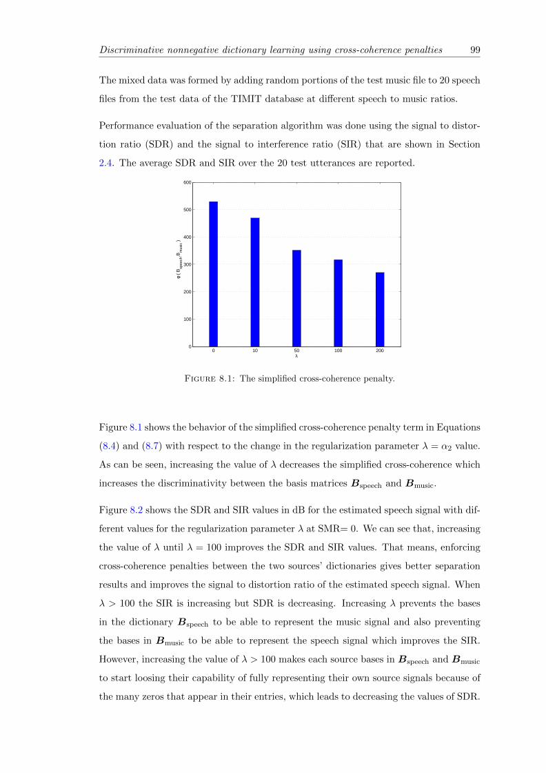
Discriminative nonnegative dictionary learning using cross-coherence penalties 99
The mixed data was formed by adding random portions of the test music file to 20 speech
files from the test data of the TIMIT database at different speech to music ratios.
Performance evaluation of the separation algorithm was done using the signal to distor-
tion ratio (SDR) and the signal to interference ratio (SIR) that are shown in Section
2.4. The average SDR and SIR over the 20 test utterances are reported.
0 10 50 100 2000
100
200
300
400
500
600
λ
φ (
Bsp
eech
,Bm
usic
)
Figure 8.1: The simplified cross-coherence penalty.
Figure 8.1 shows the behavior of the simplified cross-coherence penalty term in Equations
(8.4) and (8.7) with respect to the change in the regularization parameter λ = α2 value.
As can be seen, increasing the value of λ decreases the simplified cross-coherence which
increases the discriminativity between the basis matrices Bspeech and Bmusic.
Figure 8.2 shows the SDR and SIR values in dB for the estimated speech signal with dif-
ferent values for the regularization parameter λ at SMR= 0. We can see that, increasing
the value of λ until λ = 100 improves the SDR and SIR values. That means, enforcing
cross-coherence penalties between the two sources’ dictionaries gives better separation
results and improves the signal to distortion ratio of the estimated speech signal. When
λ > 100 the SIR is increasing but SDR is decreasing. Increasing λ prevents the bases
in the dictionary Bspeech to be able to represent the music signal and also preventing
the bases in Bmusic to be able to represent the speech signal which improves the SIR.
However, increasing the value of λ > 100 makes each source bases in Bspeech and Bmusic
to start loosing their capability of fully representing their own source signals because of
the many zeros that appear in their entries, which leads to decreasing the values of SDR.
Discriminative nonnegative dictionary learning using cross-coherence penalties 100
0 10 50 100 200
4.9
5
5.1
5.2
5.3
5.4
5.5
5.6
λ
SD
R (
dB)
(a) The SDR of the separated speech signal.
0 10 50 100 200
8
8.5
9
9.5
10
10.5
11
11.5
12
12.5
λ
SIR
(dB
)
(b) The SIR of the separated speech signal.
Figure 8.2: SDR and SIR in dB for the estimated speech signal.
According to the shown figure, the good candidate value for λ that improves both SDR
and SIR values for the used data sets is 100. Comparing the results of using only NMF
without any constraint (λ = 0), we can see from the shown figure that, discriminative
training for the source bases models by using cross-coherence penalties can improve the
performance of the separation process.
Table 8.1 shows the separation performance of using NMF without any constraint and
with discriminative learning with λ = 100 for different SMR values.
Table 8.1: SDR and SIR in dB for the estimated speech signal.
SMR Just NMF Regularized NMFλ = 0 λ = 100
dB SDR SIR SDR SIR
-5 2.41 4.94 3.45 7.78
0 4.90 8.28 5.54 11.49
5 8.05 12.30 8.06 14.61
8.6 Conclusion
In this chapter, we introduced a new discriminative training method for NMF dictionary
models. The main idea was to prevent the dictionary of each source from representing

Discriminative nonnegative dictionary learning using cross-coherence penalties 101
the other sources. We trained dictionaries with a set of basis vectors for each source
where the projection between the bases for different sources is small. The proposed
training method improved the performance of source separation.
Chapter 9
Adaptation of speaker-specific
bases in non-negative matrix
factorization
9.1 Motivations and overview
Most algorithms that use NMF to separate source signals from a mixture of source
signals assume that, there is enough training data available for each source. NMF uses
these data in magnitude spectral domain to train a set of basis vectors for each source.
These sets of bases are used with NMF to estimate the source signals from the mixture.
This kind of algorithms produce good results when sufficient training data are available
and the spectral characteristics of the training data are similar to those of the data in
the mixture. In speech-music separation, sometimes finding enough training speech data
for a specific speaker that is in the mixture signal is not easy. Building a source model
using little training data leads to a poor model that is incapable of capturing the actual
characteristics of the source signal. Also using other speakers’ speech signals that are
not in the mixture as a training data leads to a mismatch between the training and the
target data, which decreases the quality of the obtained solution.
Model adaptation is usually an alternative approach that is used to overcome the problem
of the lack of enough training data to accurately model the actual characteristics of any
signal. A general model is built first from general training data, then this model is
102
Adaptation of speaker-specific bases in non-negative matrix factorization 103
adapted to capture the properties of the target data. In speech recognition, adaptation
is used extensively to adapt the parameters of the speech models [118]. Model adaptation
is also used in single channel source separation applications to adapt the source signal
models to better represent the actual properties of the observed signals in the mixed
signal. In [63], Bayesian adaptation was used to adapt the GMM model for each source
signal. The data that was used to adapt the models was estimated from the observed
mixed signal directly in [63]. In [73, 119], the adaptation of the set of basis vectors
that models every source signal was introduced, and the adaptation is done within the
separation process without any need for an extra adaptation stage.
The key idea in this chapter is, rather than using the small training data for a specific
speaker to train a set of basis vectors with more entries to estimate, we train a general
set of basis vectors using enough speech signals from multiple speakers. Then we adapt
these basis vectors to better match the target data. First, we use NMF and training
speech data of many speakers to train a general set of basis vectors. Second, we adapt
these bases using a small amount of training data of a specific speaker to get speaker-
specific bases. The adapted bases are used to separate the speech signal of the same
speaker from the background music. Here, we assume that a small amount of isolated
training speech data of the speaker is available.
This chapter introduces two adaptation algorithms for the nonnegative matrix factor-
ization basis models. The proposed adaptation algorithms are Bayesian adaptation and
linear transformation adaptation. Training speech data for multiple speakers are used
with NMF to train a set of basis vectors as a general model for speech signals. For
the first adaptation method, the probabilistic interpretation of NMF is used to achieve
Bayesian adaptation to adjust the general model. The second adaptation method is
based on linear transform, which changes the subspace that the general model spans to
better match the speech signal that is in the mixed signal.
Adaptation of speaker-specific bases in non-negative matrix factorization 104
9.2 Probabilistic perspective of NMF
As shown in [71, 106], each entry vk,j of the matrix V in (2.14) can be modeled by
Poisson distribution as follows:
p(vk,j |bk,1:I , g1:I,j) = PO(vk,j ;I∑i
bk,igi,j), (9.1)
where bk,1:I denotes the kth row of B, g1:I,j the jth column of G, respectively, and the
Poisson distribution defined as
PO(v;λ) =e−λλv
Γ (v + 1), (9.2)
where Γ (v) is the gamma function. Assuming that each entry vk,j is statistically inde-
pendent conditional on B and G, the model can be denoted by:
p (V |B,G) =∏k,j
e−[BG]
k,j [BG][V ]
k,j
k,j
Γ(
[V ]k,j + 1) . (9.3)
The maximum likelihood solution is found by
(B,G) = arg maxB,G
log p (V |B,G) , (9.4)
where
log p (V |B,G) =∑k,j
− [BG]k,j + [V ]k,j log(
[BG]k,j
)− log
(Γ([V ]k,j + 1)
).
We can see that finding the maximum likelihood solution is equivalent to solving the
objective function (2.14). The advantage of using NMF in probabilistic framework is
the ability to put priors on every entry of the matrices B and G [71]. In this chapter,
we will use the advantage of putting priors only on the entries of the bases matrix B as
we will show in the next sections.
Adaptation of speaker-specific bases in non-negative matrix factorization 105
9.3 Basis vectors matrix prior p(B)
In [71], the prior on each basis vector matrix entry is assumed to be independently drawn
from a Gamma distribution:
p(bk,i) = G(bk,i;αk,i, β−1k,i ) =
bαk,i−1k,i β
αk,i
k,i e−bk,iβk,i
Γ(αk,i). (9.5)
The hyperparameters αk,i and βk,i of the model can be selected individually for each
basis matrix entry. It is also assumed that p(B) =∏Ii=1
∏Fk=1 p(bk,i) then we have
log p(B) =+I∑i=1
F∑k=1
(αk,i − 1) log(bk,i)− bk,iβk,i. (9.6)
Here =+ denotes equal up to irrelevant constant terms (i.e. p ∝ q ⇐⇒ log p =+ log q).
The joint posterior distribution is given by Bayes rule p(B,G|V ) ∝ p(V |B,G)P (B,G)
which factorises to p(V |B,G)P (B)P (G). The MAP estimate can be found as
arg maxB,G
[log p(V |B,G) + log p(G) + log p(B)] . (9.7)
In this chapter, we do not use any prior on the gain matrix p(G). We substitute the
terms in (9.7) with the ones from Equations (9.4) and (9.6). The MAP estimator can be
derived [71], and the update rule for each element in the bases matrix B and the gain
matrix G is given as
bk,i ← bk,i
(αk,i−1)bk,i
+∑K
j=1 gi,jvk,j∑I
i=1 bk,igi,j
βk,i +∑K
j′=1 gi,j′, (9.8)
G← G⊗BT V
BGBT1
. (9.9)
Notice that the update rule (9.8) differs from the basic NMF update (2.15) only by
additive terms in the numerator and denominator, which are due to the priors.
9.4 Training the bases
Given a set of training data for music and speech of multiple speakers signals, The
STFT is computed for each signal, and the magnitude spectrogram Strain and M train
Adaptation of speaker-specific bases in non-negative matrix factorization 106
of speech and music respectively are calculated. Then NMF is used to decompose these
spectrograms into bases and weights matrices as follows:
Strain ≈ BspeechGspeech. (9.10)
M train ≈ BmusicGmusic. (9.11)
The update rules in Equations (2.15) and (2.16) are used to solve Equations (9.10) and
(9.11). We call the trained bases matrix Bspeech a general model for multiple speakers
speech signals, and this matrix needs to be adapted to specific speaker speech signals.
9.5 Speech model adaptation
Given the general speech model which represents multiple speakers speech signalsBspeech,
the goal now is to adapt this model using a small amount of a specific-speaker speech
signals to better match the target speech signal that is in the mixture. We introduce
two adaptation techniques to adapt the speech model. First adaptation algorithm is
the Bayesian adaptation, which is derived from the probabilistic framework of NMF in
Equation (9.8). Second adaptation algorithm which we introduce is derived from maxi-
mum likelihood linear regression (MLLR) adaptation [120], linear regression which aims
to change the subspace of the model to better match the target data.
9.5.1 Bayesian adaptation of the speech bases
In this chapter, we assume that we have a small adaptation data of speaker-specific
speech signal sadapt(t). The goal now is to use the magnitude spectrogram of this new
data Sadapt to adapt the general bases matrix Bspeech to become speaker specific bases
matrix Bs. We will use first the Bayesian adaptation in Equation (9.8) by replacing β−1
values with the entries of Bspeech, and α = 2 everywhere inspired from [71]. This choice
makes the mode of the Gamma distribution equal to the general model bases Bspeech
which means that the general model is used as a prior for Bs, so the update rules will
be as follows:
Bs ← Bs ⊗1′
Bs+Sadapt
BsGaGTa
1′
Bspeech+ 1GT
a
, (9.12)
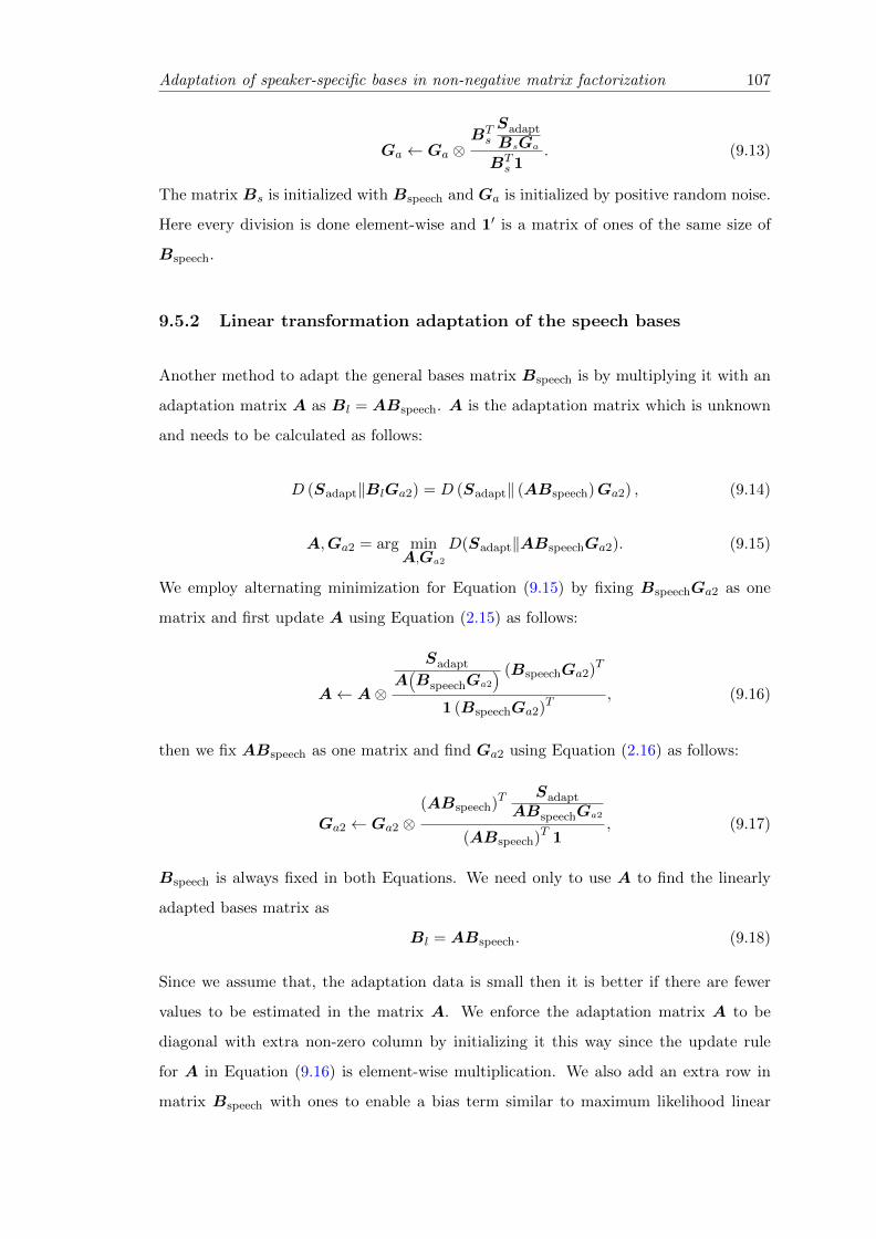
Adaptation of speaker-specific bases in non-negative matrix factorization 107
Ga ← Ga ⊗BTs
Sadapt
BsGa
BTs 1
. (9.13)
The matrix Bs is initialized with Bspeech and Ga is initialized by positive random noise.
Here every division is done element-wise and 1′ is a matrix of ones of the same size of
Bspeech.
9.5.2 Linear transformation adaptation of the speech bases
Another method to adapt the general bases matrix Bspeech is by multiplying it with an
adaptation matrix A as Bl = ABspeech. A is the adaptation matrix which is unknown
and needs to be calculated as follows:
D (Sadapt‖BlGa2) = D (Sadapt‖ (ABspeech)Ga2) , (9.14)
A,Ga2 = arg minA,Ga2
D(Sadapt‖ABspeechGa2). (9.15)
We employ alternating minimization for Equation (9.15) by fixing BspeechGa2 as one
matrix and first update A using Equation (2.15) as follows:
A← A⊗
Sadapt
A(BspeechGa2
) (BspeechGa2)T
1 (BspeechGa2)T, (9.16)
then we fix ABspeech as one matrix and find Ga2 using Equation (2.16) as follows:
Ga2 ← Ga2 ⊗(ABspeech)T
Sadapt
ABspeechGa2
(ABspeech)T 1, (9.17)
Bspeech is always fixed in both Equations. We need only to use A to find the linearly
adapted bases matrix as
Bl = ABspeech. (9.18)
Since we assume that, the adaptation data is small then it is better if there are fewer
values to be estimated in the matrix A. We enforce the adaptation matrix A to be
diagonal with extra non-zero column by initializing it this way since the update rule
for A in Equation (9.16) is element-wise multiplication. We also add an extra row in
matrix Bspeech with ones to enable a bias term similar to maximum likelihood linear
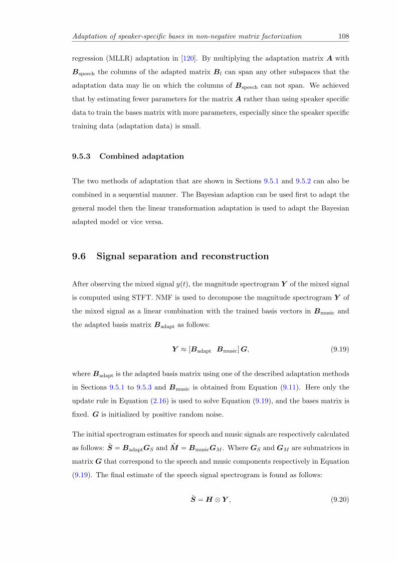
Adaptation of speaker-specific bases in non-negative matrix factorization 108
regression (MLLR) adaptation in [120]. By multiplying the adaptation matrix A with
Bspeech the columns of the adapted matrix Bl can span any other subspaces that the
adaptation data may lie on which the columns of Bspeech can not span. We achieved
that by estimating fewer parameters for the matrix A rather than using speaker specific
data to train the bases matrix with more parameters, especially since the speaker specific
training data (adaptation data) is small.
9.5.3 Combined adaptation
The two methods of adaptation that are shown in Sections 9.5.1 and 9.5.2 can also be
combined in a sequential manner. The Bayesian adaption can be used first to adapt the
general model then the linear transformation adaptation is used to adapt the Bayesian
adapted model or vice versa.
9.6 Signal separation and reconstruction
After observing the mixed signal y(t), the magnitude spectrogram Y of the mixed signal
is computed using STFT. NMF is used to decompose the magnitude spectrogram Y of
the mixed signal as a linear combination with the trained basis vectors in Bmusic and
the adapted basis matrix Badapt as follows:
Y ≈ [Badapt Bmusic]G, (9.19)
where Badapt is the adapted basis matrix using one of the described adaptation methods
in Sections 9.5.1 to 9.5.3 and Bmusic is obtained from Equation (9.11). Here only the
update rule in Equation (2.16) is used to solve Equation (9.19), and the bases matrix is
fixed. G is initialized by positive random noise.
The initial spectrogram estimates for speech and music signals are respectively calculated
as follows: S = BadaptGS and M = BmusicGM . Where GS and GM are submatrices in
matrix G that correspond to the speech and music components respectively in Equation
(9.19). The final estimate of the speech signal spectrogram is found as follows:
S = H ⊗ Y , (9.20)
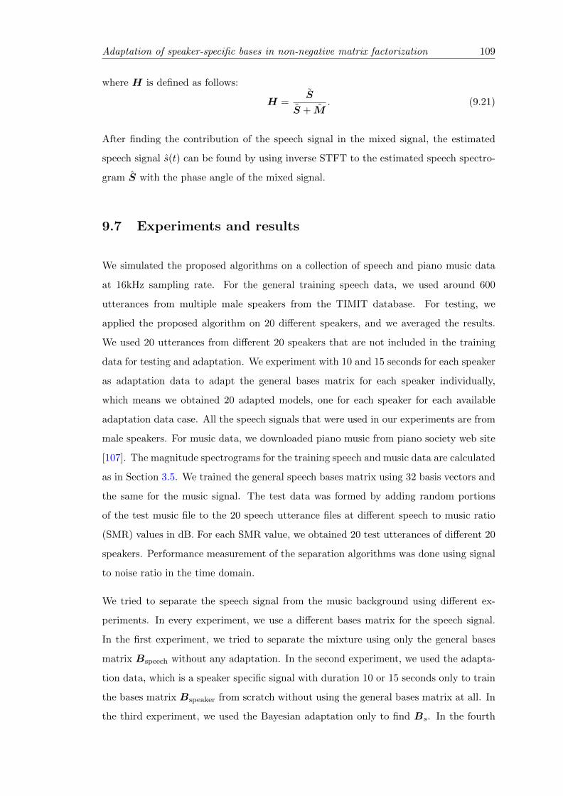
Adaptation of speaker-specific bases in non-negative matrix factorization 109
where H is defined as follows:
H =S
S + M. (9.21)
After finding the contribution of the speech signal in the mixed signal, the estimated
speech signal s(t) can be found by using inverse STFT to the estimated speech spectro-
gram S with the phase angle of the mixed signal.
9.7 Experiments and results
We simulated the proposed algorithms on a collection of speech and piano music data
at 16kHz sampling rate. For the general training speech data, we used around 600
utterances from multiple male speakers from the TIMIT database. For testing, we
applied the proposed algorithm on 20 different speakers, and we averaged the results.
We used 20 utterances from different 20 speakers that are not included in the training
data for testing and adaptation. We experiment with 10 and 15 seconds for each speaker
as adaptation data to adapt the general bases matrix for each speaker individually,
which means we obtained 20 adapted models, one for each speaker for each available
adaptation data case. All the speech signals that were used in our experiments are from
male speakers. For music data, we downloaded piano music from piano society web site
[107]. The magnitude spectrograms for the training speech and music data are calculated
as in Section 3.5. We trained the general speech bases matrix using 32 basis vectors and
the same for the music signal. The test data was formed by adding random portions
of the test music file to the 20 speech utterance files at different speech to music ratio
(SMR) values in dB. For each SMR value, we obtained 20 test utterances of different 20
speakers. Performance measurement of the separation algorithms was done using signal
to noise ratio in the time domain.
We tried to separate the speech signal from the music background using different ex-
periments. In every experiment, we use a different bases matrix for the speech signal.
In the first experiment, we tried to separate the mixture using only the general bases
matrix Bspeech without any adaptation. In the second experiment, we used the adapta-
tion data, which is a speaker specific signal with duration 10 or 15 seconds only to train
the bases matrix Bspeaker from scratch without using the general bases matrix at all. In
the third experiment, we used the Bayesian adaptation only to find Bs. In the fourth
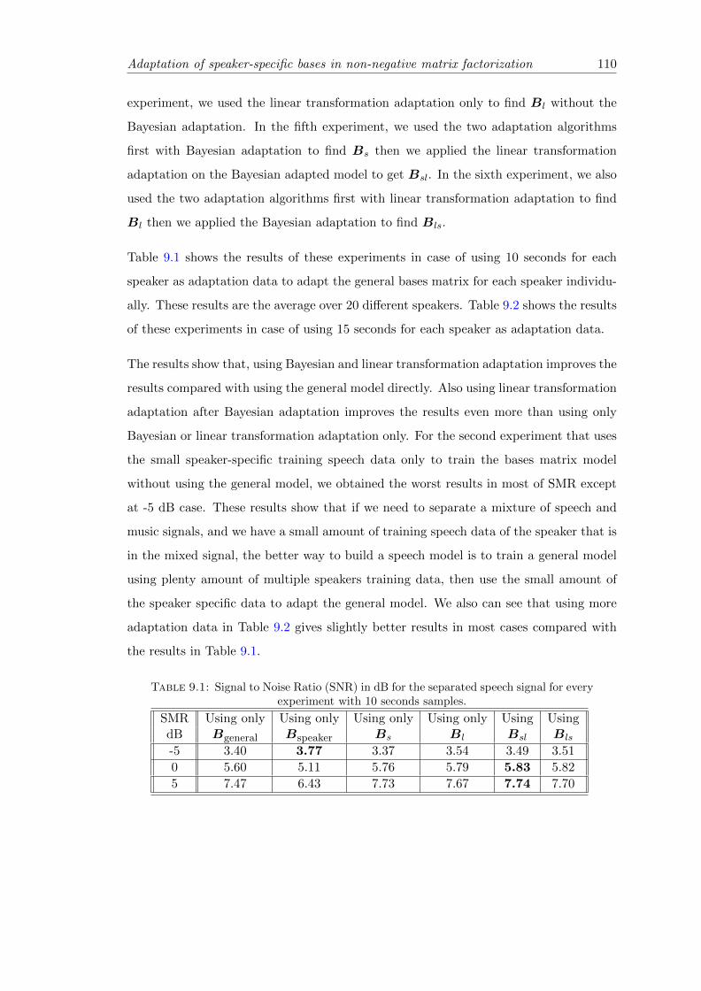
Adaptation of speaker-specific bases in non-negative matrix factorization 110
experiment, we used the linear transformation adaptation only to find Bl without the
Bayesian adaptation. In the fifth experiment, we used the two adaptation algorithms
first with Bayesian adaptation to find Bs then we applied the linear transformation
adaptation on the Bayesian adapted model to get Bsl. In the sixth experiment, we also
used the two adaptation algorithms first with linear transformation adaptation to find
Bl then we applied the Bayesian adaptation to find Bls.
Table 9.1 shows the results of these experiments in case of using 10 seconds for each
speaker as adaptation data to adapt the general bases matrix for each speaker individu-
ally. These results are the average over 20 different speakers. Table 9.2 shows the results
of these experiments in case of using 15 seconds for each speaker as adaptation data.
The results show that, using Bayesian and linear transformation adaptation improves the
results compared with using the general model directly. Also using linear transformation
adaptation after Bayesian adaptation improves the results even more than using only
Bayesian or linear transformation adaptation only. For the second experiment that uses
the small speaker-specific training speech data only to train the bases matrix model
without using the general model, we obtained the worst results in most of SMR except
at -5 dB case. These results show that if we need to separate a mixture of speech and
music signals, and we have a small amount of training speech data of the speaker that is
in the mixed signal, the better way to build a speech model is to train a general model
using plenty amount of multiple speakers training data, then use the small amount of
the speaker specific data to adapt the general model. We also can see that using more
adaptation data in Table 9.2 gives slightly better results in most cases compared with
the results in Table 9.1.
Table 9.1: Signal to Noise Ratio (SNR) in dB for the separated speech signal for everyexperiment with 10 seconds samples.
SMR Using only Using only Using only Using only Using UsingdB Bgeneral Bspeaker Bs Bl Bsl Bls
-5 3.40 3.77 3.37 3.54 3.49 3.51
0 5.60 5.11 5.76 5.79 5.83 5.82
5 7.47 6.43 7.73 7.67 7.74 7.70
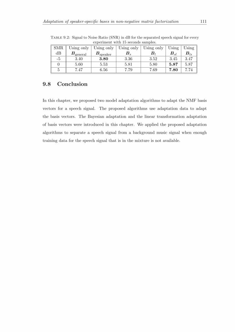
Adaptation of speaker-specific bases in non-negative matrix factorization 111
Table 9.2: Signal to Noise Ratio (SNR) in dB for the separated speech signal for everyexperiment with 15 seconds samples.
SMR Using only Using only Using only Using only Using UsingdB Bgeneral Bspeaker Bs Bl Bsl Bls
-5 3.40 3.80 3.36 3.52 3.45 3.47
0 5.60 5.53 5.81 5.80 5.87 5.87
5 7.47 6.56 7.79 7.69 7.80 7.74
9.8 Conclusion
In this chapter, we proposed two model adaptation algorithms to adapt the NMF basis
vectors for a speech signal. The proposed algorithms use adaptation data to adapt
the basis vectors. The Bayesian adaptation and the linear transformation adaptation
of basis vectors were introduced in this chapter. We applied the proposed adaptation
algorithms to separate a speech signal from a background music signal when enough
training data for the speech signal that is in the mixture is not available.
Chapter 10
Nonnegative matrix factorization
with sliding windows and spectral
masks
10.1 Motivations and overview
In [24, 27, 65], NMF was used with training data to train a set of basis vectors for
each source, then these basis vectors were used with NMF to separate the mixed signal.
The separation was done frame by frame without considering the smoothness transition
and any other information between the consequent frames. To make NMF consider the
relation between the consequent spectral frames in the training and separation stages, we
form the columns of the matrices that need to be decomposed from multiple consequent
spectral frames stacked together in super-frames. Rather than using NMF to directly
decompose the spectrogram of the signals in training and separation stages as shown in
Equations (2.14) to (2.22), we form the matrices to be decomposed as follows: We
stack L spectrogram frames in one vector, we pass a window with length equal to
multiple spectral frames size to select the first column of the matrix, then we shift
or slide the window by one frame to choose the next column as shown in Figure 10.1.
Therefore, NMF is used in this work to decompose matrices with columns that contain
L multiple spectral frames in both training and separation stages. Thus, rather than
decomposing every spectral frame in the spectrogram independently from each other, we
112

Nonnegative matrix factorization with sliding windows and spectral masks 113
Figure 10.1: Columns construction and sliding windows with length L frames.
decompose multiple frames at once in one column. Sliding the window by one frame each
time to get the next column makes every frame decomposed L times with different L
neighbor frames. We take the average of the different decomposion results for each frame
to find an accurate decomposion of the spectrograms. The novelty of this work is in
using NMF with sliding windows and different types of spectral masks. The experiment
results show that using NMF, spectral masks, and sliding windows with multiple spectral
frames improve the separation results compared to using NMF only. We also compare
convolutive nonnegative matrix factorization (CNMF) [77, 78] with the proposed NMF
with sliding windows approach. In this chapter, we assume the number of sources is two
for simplicity.
10.2 Training the bases
The training procedure for training a set of basis vectors for each source here is similar
to the procedure shown in Equation (2.20). The only difference here is that, each column
in the matrices to be decomposed are combined of L consequent frames from the source
spectrograms as shown in Figure 10.1.
10.3 Signal separation and masking
After observing the mixed signal y(t), the magnitude spectrogram Y of the mixed signal
is computed. Instead of using NMF directly to decompose the spectrogram of the mixed
signal, we build a matrix Y 2 with columns that contain L frames of the mixed signal
spectrogram as shown in Figure 10.1. We attach L− 1 frames with zeros values to the
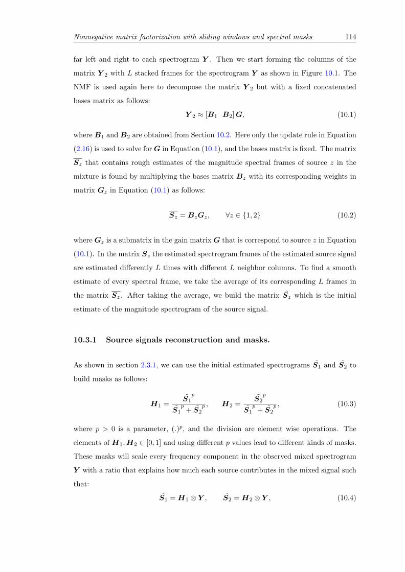
Nonnegative matrix factorization with sliding windows and spectral masks 114
far left and right to each spectrogram Y . Then we start forming the columns of the
matrix Y 2 with L stacked frames for the spectrogram Y as shown in Figure 10.1. The
NMF is used again here to decompose the matrix Y 2 but with a fixed concatenated
bases matrix as follows:
Y 2 ≈ [B1 B2]G, (10.1)
where B1 and B2 are obtained from Section 10.2. Here only the update rule in Equation
(2.16) is used to solve forG in Equation (10.1), and the bases matrix is fixed. The matrix
Sz that contains rough estimates of the magnitude spectral frames of source z in the
mixture is found by multiplying the bases matrix Bz with its corresponding weights in
matrix Gz in Equation (10.1) as follows:
Sz = BzGz, ∀z ∈ {1, 2} (10.2)
where Gz is a submatrix in the gain matrix G that is correspond to source z in Equation
(10.1). In the matrix Sz the estimated spectrogram frames of the estimated source signal
are estimated differently L times with different L neighbor columns. To find a smooth
estimate of every spectral frame, we take the average of its corresponding L frames in
the matrix Sz. After taking the average, we build the matrix Sz which is the initial
estimate of the magnitude spectrogram of the source signal.
10.3.1 Source signals reconstruction and masks.
As shown in section 2.3.1, we can use the initial estimated spectrograms S1 and S2 to
build masks as follows:
H1 =S1
p
S1p
+ S2p , H2 =
S2p
S1p
+ S2p , (10.3)
where p > 0 is a parameter, (.)p, and the division are element wise operations. The
elements of H1,H2 ∈ [0, 1] and using different p values lead to different kinds of masks.
These masks will scale every frequency component in the observed mixed spectrogram
Y with a ratio that explains how much each source contributes in the mixed signal such
that:
S1 = H1 ⊗ Y , S2 = H2 ⊗ Y , (10.4)

Nonnegative matrix factorization with sliding windows and spectral masks 115
where S1 and S2 are the final estimates of the sources spectrograms, and ⊗ is element-
wise multiplication. By using these spectral masks, we can make sure that the two
estimated signals will add up to the mixed signal. After finding the contribution of each
source in the mixed signal, the estimated for each source signal sz(t) can be found by
using inverse STFT to the estimated speech spectrogram Sz with the phase angle of the
mixed signal.
10.4 Experiments and discussion
We applied the proposed algorithm to separate a speech signal from a background piano
music signal. Our main goal was to get the clean speech signal from a mixture of speech
and piano signals. We simulated the proposed algorithms on a collection of speech and
piano music data at 16kHz sampling rate. For speech data, we use the single speaker
(Turkish) database that was used in Section 6.3 and also the music data.
We concatenated every consequent five (L = 5) spectrogram frames of the training
data in one column vector with size (5*257) as we have mentioned in Section 10.2. Each
vector in Strainspeech and Strain
music is in 1285 dimensions (5*257). We trained different number
of bases Ns for training speech signal and Nm for training music signal. Ns and Nm
take values 1285, 642, 321, and 160 bases. The test data was formed by adding random
portions of the test music file to the 20 speech utterance files from the same speaker at
different speech to music ratio (SMR) values in dB.
Table 10.1 shows the separation performance of using NMF with a different number of
bases Ns and Nm. We obtained these results by using the spectral mask with p = 3 in
Equation (10.3) and sliding window with L = 5. Table 10.2 shows the performance of
Table 10.1: SNR in dB for the speech signal using NMF with sliding window andspectral mask with p = 3 for different numbers of bases.
SMR Ns = 1285 Ns = 1285 Ns = 1285 Ns = 642 Ns = 642 Ns = 321 Ns = 321dB Nm = 1285 Nm = 642 Nm = 321 Nm = 642 Nm = 160 Nm = 642 Nm = 160
-5 8.00 7.31 5.33 8.19 4.90 7.84 6.53
0 10.91 10.88 9.05 11.48 8.65 10.60 10.02
5 12.76 13.34 11.99 13.52 11.75 12.05 12.77
using NMF and sliding window without masks and with different kinds of masks, which
shows that, we obtained better results when p = 3 and p = 4 in Equation (10.3).
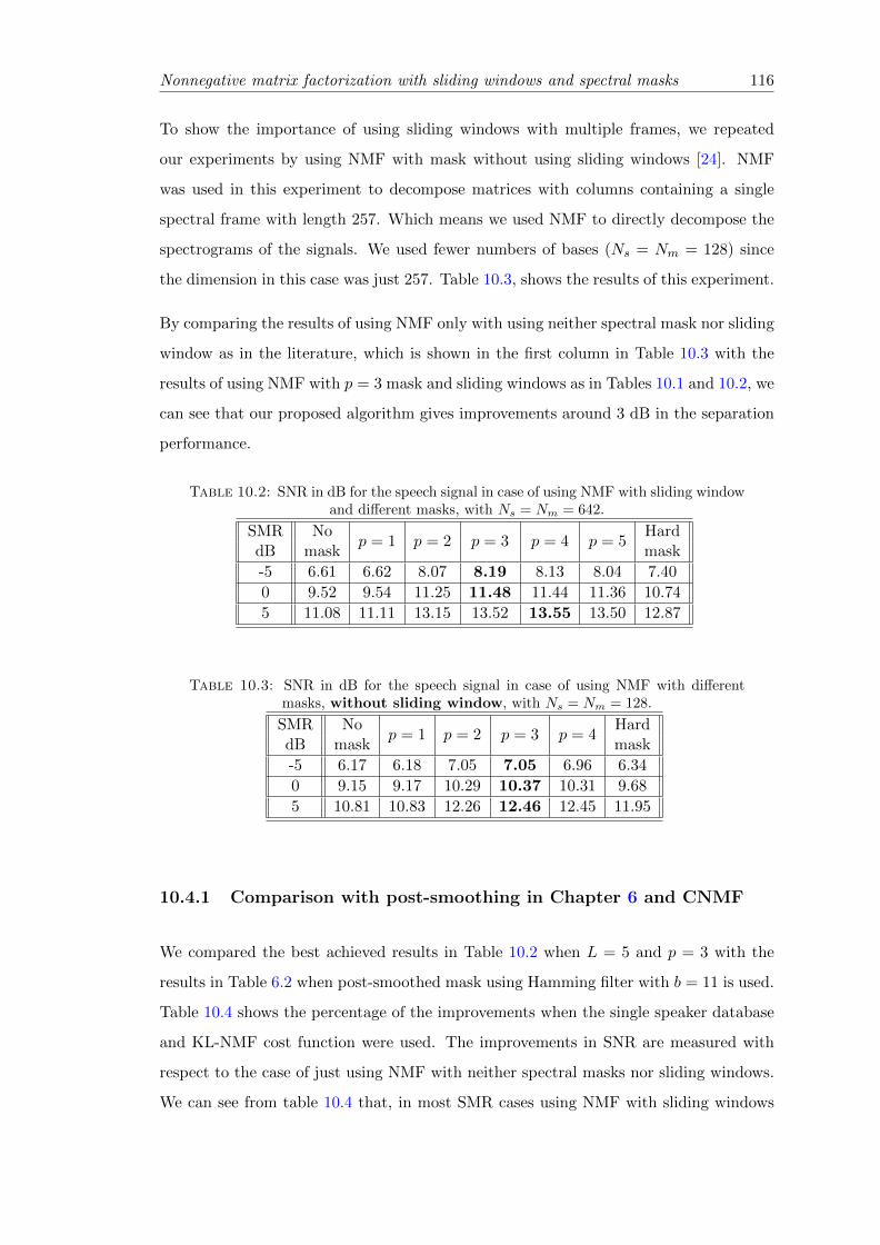
Nonnegative matrix factorization with sliding windows and spectral masks 116
To show the importance of using sliding windows with multiple frames, we repeated
our experiments by using NMF with mask without using sliding windows [24]. NMF
was used in this experiment to decompose matrices with columns containing a single
spectral frame with length 257. Which means we used NMF to directly decompose the
spectrograms of the signals. We used fewer numbers of bases (Ns = Nm = 128) since
the dimension in this case was just 257. Table 10.3, shows the results of this experiment.
By comparing the results of using NMF only with using neither spectral mask nor sliding
window as in the literature, which is shown in the first column in Table 10.3 with the
results of using NMF with p = 3 mask and sliding windows as in Tables 10.1 and 10.2, we
can see that our proposed algorithm gives improvements around 3 dB in the separation
performance.
Table 10.2: SNR in dB for the speech signal in case of using NMF with sliding windowand different masks, with Ns = Nm = 642.
SMR Nop = 1 p = 2 p = 3 p = 4 p = 5
HarddB mask mask
-5 6.61 6.62 8.07 8.19 8.13 8.04 7.40
0 9.52 9.54 11.25 11.48 11.44 11.36 10.74
5 11.08 11.11 13.15 13.52 13.55 13.50 12.87
Table 10.3: SNR in dB for the speech signal in case of using NMF with differentmasks, without sliding window, with Ns = Nm = 128.
SMR Nop = 1 p = 2 p = 3 p = 4
HarddB mask mask
-5 6.17 6.18 7.05 7.05 6.96 6.34
0 9.15 9.17 10.29 10.37 10.31 9.68
5 10.81 10.83 12.26 12.46 12.45 11.95
10.4.1 Comparison with post-smoothing in Chapter 6 and CNMF
We compared the best achieved results in Table 10.2 when L = 5 and p = 3 with the
results in Table 6.2 when post-smoothed mask using Hamming filter with b = 11 is used.
Table 10.4 shows the percentage of the improvements when the single speaker database
and KL-NMF cost function were used. The improvements in SNR are measured with
respect to the case of just using NMF with neither spectral masks nor sliding windows.
We can see from table 10.4 that, in most SMR cases using NMF with sliding windows

Nonnegative matrix factorization with sliding windows and spectral masks 117
Table 10.4: The percentage improvement for SNR and SIR in dB for the estimatedspeech signal for using post-smoothing and NMF with sliding windows.
SMR post-smoothing Sliding windowsdB SNR SIR SNR SIR
-5 27.71% 121.82% 32.74% 124.62%
0 22.62% 66.33% 25.46% 71.09%
5 24.98% 46.15% 25.07% 50.26%
gives better performance than using post-smoothed masks.
We also applied NMF with sliding windows on the same multi-speakers TIMIT dataset
and the same IS-NMF cost function that were used in Table 6.6. The used mask here
is the Wiener mask. We also compared with using convolutive nonnegative matrix
factorization (CNMF) [77, 78] in source separation. CNMF is an extension of NMF for
time series which is capable of identifying components with temporal structure. The
basis matrix in CNMF contains temporal-spectral bases, which means the basis matrix
contains bases that extend in both dimensions of the input. The CNMF approximation,
cost function, and the update rules that corresponds to NMF in Equations (2.8) to (2.19)
are as follows:
V ≈L−1∑l=0
Bl
l→G, (10.5)
Λ =L−1∑l=0
Bl
l→G, (10.6)
DIS =∑i,j
(V i,j
Λi,j− log
V i,j
Λi,j− 1
), (10.7)
Bl ← Bl ⊗VΛ2
l→GT
1Λ
l→GT, (10.8)
G← G⊗BTl
l←(VΛ2
)BTl
1Λ
, (10.9)
∀l ∈ {0, .., L− 1} ,
wherel→(.) is an operator which shifts columns l places to the right, as each column is
shifted to the right the leftmost columns are zero filled.l←(.) is shifting to the left operator.
More details about CNMF can be found in [77, 78].

Nonnegative matrix factorization with sliding windows and spectral masks 118
Table 10.5 shows the results of using IS-NMF with sliding windows and IS-CNMF that
can be compared to the achieved results in Table 6.6 in Chapter 6. Comparing the
Table 10.5: SNR and SIR in dB for the estimated speech signal in the case of usingNMF with sliding window and CNMF with different L values and p = 2.
SMR NMF NMF with sliding-windows CNMFL = 1, Ns = Nm = 128 L = 7, Ns = Nm = 180 L = 7, Ns = Nm = 128
dB SNR SIR SNR SIR SNR SIR
-5 2.88 4.86 5.59 8.46 4.32 6.79
0 5.50 8.70 7.72 12.03 6.77 10.67
5 8.37 12.20 10.28 14.76 9.04 13.34
results in Table 10.5 with Table 6.6 we can see that: using CNMF gives better results
than using NMF with post-smoothed masks; using NMF with sliding windows gives
better results than using CNMF; NMF with sliding windows requires more basis vectors
than CNMF. Using 180 bases in CNMF gave worse results than using 128 bases.
10.5 Conclusion
In this chapter, we introduced single channel source separation using nonnegative ma-
trix factorization (NMF) with sliding windows and spectral masks. We used NMF to
decompose matrices with columns containing multiple spectral frames. We built a spec-
tral mask from the decomposition results to find the contribution of each source signal
in the mixed signal. The proposed algorithm gave better results and more accurate
source separation for both cases when the training and testing data are from the same
or different speakers. It was also shown that, using NMF with sliding windows gives
better results than CNMF.
Chapter 11
Conclusions and future work
In this thesis, we improved the performance of nonnegative matrix factorization (NMF)
for source separation applications. We combined many machine learning and statistical
signal processing approaches to enhance the NMF performance for source separation.
We improved the solution of NMF by incorporating prior information on the basis and
gains matrices. In Chapters 3 to 5, we guided the NMF solution of the gains matrix
by rich prior models to find better suited estimates to the source signals. The priors
were modeled in Chapters 3 and 5 using GMMs and in Chapter 4 using HMMs. The
priors were incorporated into the NMF solution using either log-likelihood as shown in
Chapters 3 and 4 or minimum mean squared error (MMSE) estimation as shown in
Chapter 5. We introduced three different methods to improve the gains matrix solution
of NMF. Guiding the gains matrix solution of NMF using MMSE estimates under GMM
prior gave better results compared to the other prior methods. Using MMSE estimates,
we achieved improvement around 2 dB in SNR and 6 dB in SIR. The usage of the
HMM as a prior model for regularized NMF is considered to be a good idea that can be
improved in future work. In general, the approaches of using GMMs and HMMs as prior
models for the regularized NMF can be improved by using supervised learning for the
source models especially the prior models. For example, training speech signals can be
clustered based on phonemes. The initialization of the parameters for the prior GMMs
and HMMs can be done based on this phoneme clustering to obtain better prior models.
In Chapters 6 and 7, the prior information was incorporated as post processing. In
119
General Conclusion 120
Chapter 6, we incorporated the smoothness prior on the NMF solutions by using post-
smoothing of masks or gains. Although the introduced idea in that chapter is very
simple, the achieved improvements show that it is a very effective approach. In Chapter
7, the MMSE estimation was also used as post processing to enhance the NMF solution
for the spectrograms of the separated source signals. The post enhancement using
MMSE estimation under GMM prior gave better performance than the post-smoothing
approach. The MMSE estimation based post enhancement can be improved by using
HMMs instead of GMMs to model the log-spectra of the training data.
In Chapters 8 and 9 we improved the training procedures for the basis matrices for the
source signals. In Chapter 8 we learned discriminative dictionaries where a dictionary
of one source was penalized from representing the other sources. The achieved improve-
ments in Chapter 8 can be increased by adjusting the energy differences between the
training data of sources. In Chapter 9, we introduced the idea of model adaptation
where the training data were modeled using dictionaries. The model adaptation was
introduced in this thesis to overcome the problem of lack of sufficient training data for a
specific source signal. In Chapter 9, a general nonnegative dictionary model for speech
signals was trained and then adapted to the target speech signals that exist in the mixed
signal to improve the performance of NMF for source separation.
In Chapter 10, we trained basis matrices that consider the relation between consequent
frames by processing multiple stacked frames together. Based on the simplicity of the
proposed approach in Chapter 10, the achieved results in Tables 10.2 and 10.5 are
considered to be very good.
Because of the simplicity of the post-smoothing approach that is shown in Chapter 6, it
can be combined with the other proposed approaches in this thesis. The best achieved
results in this thesis are shown in Table 6.7 where the regularized NMF using MMSE
estimates was combined with the post-smoothed masks. The SNR improvement in Table
6.7 is around 3 dB and the improvement in SIR is around 10 dB which is considered a
remarkable improvement.
In general, a fair comparison between the proposed approaches in this thesis is not guar-
anteed since for each approach there are many free parameters that need to be chosen.
As many machine learning problems, the performance of the proposed approaches in
this thesis can differ based on the type and nature of the processed signals.
General Conclusion 121
11.1 Future work
Many of the proposed approaches in this thesis can be combined to achieve better
separation performance. There are many approaches/ideas that we consider as future
work which can be itemized as follows:
• The idea of using MMSE estimation under GMM prior in regularized NMF that
is introduced in Chapter 5 can be generalized for many other cost functions and
applications as MMSE estimates based regularization.
• The idea of using MMSE estimation under GMM prior in regularized NMF can
be improved by replacing GMMs by HMMs to consider the temporal behavior of
the source signals.
• The idea of using MMSE estimation under GMM prior for post enhancement that
is introduced in Chapter 7 can also be improved by replacing GMMs by HMMs
to consider the temporal behavior of the source signals in a model-based fashion
rather than using multiple spectral frames stacked together.
• Most of the methods that use GMMs and HMMs to model the data in this thesis
can be improved by using supervised learning. For example, the training of HMM
in Chapter 4 for a speech signal can be improved by first clustering the training
speech data into phonemes and using these clusters to initialize the HMM states.
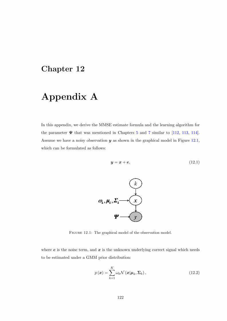
Chapter 12
Appendix A
In this appendix, we derive the MMSE estimate formula and the learning algorithm for
the parameter Ψ that was mentioned in Chapters 5 and 7 similar to [112, 113, 114].
Assume we have a noisy observation y as shown in the graphical model in Figure 12.1,
which can be formulated as follows:
y = x+ e, (12.1)
Figure 12.1: The graphical model of the observation model.
where e is the noise term, and x is the unknown underlying correct signal which needs
to be estimated under a GMM prior distribution:
p (x) =K∑k=1
ωkN (x|µk,Σk) , (12.2)
122

Appendix A 123
the error term e has a Gaussian distribution with zero mean and diagonal covariance
matrix Ψ:
p (e) = N (e|0,Ψ) . (12.3)
The conditional distribution of y is a Gaussian with mean x and diagonal covariance
matrix Ψ:
p(y|x, k) = p(y|x) = N (y|x,Ψ) . (12.4)
The distribution of y given the Gaussian component k is a Gaussian with mean µk and
diagonal covariance matrix Σk + Ψ:
p(y|k) = N (y|µk,Σk + Ψ) . (12.5)
The marginal probability distribution of y is a GMM:
p(y) =
K∑k=1
ωkN (y|µk,Σk + Ψ) , (12.6)
where the expectations E (x) = E (y), and E (e) = 0. Note that, this observation model
has some mathematical similarities but different concepts with factor analysis models
assuming the load matrix is the identity matrix [112, 113, 114].
The MMSE estimate of x can be found by calculating the conditional expectation of
x given the observation y. Given the Gaussian component k, the joint distribution
of x and y is a multivariate Gaussian distribution with conditional expectation and
conditional variance as follows [112, 121]:
E (x|y, k) = µk + ΣkxyΣ−1ky
(y − µk) , (12.7)
var (x|y, k) = Σk −ΣkxyΣ−1ky
ΣTkxy , (12.8)
we know that
Σky = Σk + Ψ, (12.9)
Appendix A 124
and
Σkxy = cov (x,y)
= E(xyT
)− E (x)E
(yT)
= E[x(xT + eT
)]− E (x)E
(yT)
= E(xxT
)+ E (x)E
(eT)− E (x)E
(yT)
= var (x) + E (x)E(xT)− E (x)E
(yT)
= var (x) = Σk. (12.10)
The conditional expectation given the Gaussian component k of the prior model is
E (x|y, k) = µk + Σk (Σk + Ψ)−1 (y − µk)
= xk. (12.11)
We also can find the following conditional expectation given only the observation y as
follows:
E (x|y) =K∑k=1
p (k|y)E (x|y, k)
=
K∑k=1
γkE (x|y, k)
= x, (12.12)
where
p (k|y) =ωkp (y|k)∑Kj=1 ωjp (y|j)
= γk. (12.13)
From equations (12.11, 12.12, 12.13) we can write the final MMSE estimate of x given
the model parameters as follows:
x =K∑k=1
γk
[µk + Σk (Σk + Ψ)−1 (y − µk)
]. (12.14)
Appendix A 125
We need also to find the following sufficient statistics to be used in estimating the model
parameters:
var (x|y, k) = Σk −Σk (Σk + Ψ)−1 ΣTk , (12.15)
E(xxT |y, k
)= var (x|y, k) + E (x|y, k)E (x|y, k)T
= Σk −Σk (Σk + Ψ)−1 ΣTk + xkx
Tk
= Rk, (12.16)
and
E(xxT |y
)=
K∑k=1
p (k|y)E(xxT |y, k
)=
K∑k=1
γkE(xxT |y, k
)=
K∑k=1
γkRk
= R. (12.17)
Parameters learning using the EM algorithm
In the training stage, we assume we have clean data with e = 0. The prior GMM
parameters ω,µ,Σ are learned as regular GMM models. The only parameter that need
to be estimated is Ψ, which is learned from the deformed signal “qn” in Chapters 5 and
7. The parameter Ψ is learned iteratively using maximum likelihood estimation. Given
the data points q = q1, q2, . . . , qn, . . . , qN , and the GMM parameters, we need to find
an estimate for Ψ. We follow the same procedures as in [112, 113, 114].
Let us rewrite the sufficient statistics in Equations (12.13, 12.11, 12.14, 12.16, 12.17)
after replacing x with z (to avoid confusion between calculating the MMSE estimate
Appendix A 126
and training the model parameters) as follows:
γkn =ωkN (qn|µk,Σk + Ψ)∑Kj=1 ωjN
(qn|µj ,Σj + Ψ
) , (12.18)
zkn = Ezn|qn,k(zn|qn, k) = µk + Σk (Σk + Ψ)−1 (qn − µk) , (12.19)
zn = Ezn|qn(zn|qn) =
K∑k=1
γknzkn, (12.20)
Rkn = Ezn|qn,k
(znz
Tn |qn, k
)= Σk −Σk (Σk + Ψ)−1 ΣT
k + zknzTkn, (12.21)
and
Rn = Ezn|qn
(znz
Tn |qn
)=
K∑k=1
γknRkn. (12.22)
We define q = {q1, q2, . . . , qN}, z = {z1, z2, . . . ,zN}, and K = {k1, k2, . . . , kN}. Given
the generative model in Figure 12.2, the complete log-likelihood can be written in a
product form as follows:
l (q, z,K|θ) = log
N∏n=1
p(kn)p(zn|kn)p(qn|zn, kn)
= log
N∏n=1
K∏k=1
[p(k)p(zn|k)p(qn|zn, k)]δk,kn
= logN∏n=1
K∏k=1
[ωkN (zn|µk,Σk)N (qn|zn,Ψ)]δk,kn , (12.23)
where θ = {µ,Σ, ω,Ψ}, δk1,k2 =
1 k1 = k2
0 else
,
l (q, z,K|θ) =
N∑n=1
K∑k=1
δk,kn logωk+
N∑n=1
K∑k=1
δk,kn logN (zn|µk,Σk)+
N∑n=1
K∑k=1
δk,kn logN (qn|zn,Ψ) .
(12.24)
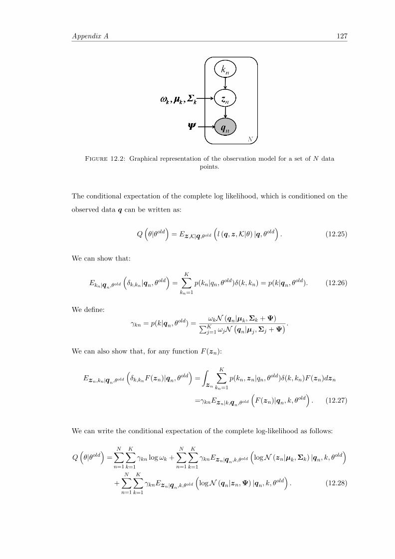
Appendix A 127
Figure 12.2: Graphical representation of the observation model for a set of N datapoints.
The conditional expectation of the complete log likelihood, which is conditioned on the
observed data q can be written as:
Q(θ|θold
)= Ez,K|q,θold
(l (q, z,K|θ) |q, θold
). (12.25)
We can show that:
Ekn|qn,θold
(δk,kn |qn, θold
)=
K∑kn=1
p(kn|qn, θold)δ(k, kn) = p(k|qn, θold). (12.26)
We define:
γkn = p(k|qn, θold) =ωkN (qn|µk,Σk + Ψ)∑Kj=1 ωjN
(qn|µj ,Σj + Ψ
) .We can also show that, for any function F (zn):
Ezn,kn|qn,θold
(δk,knF (zn)|qn, θold
)=
∫zn
K∑kn=1
p(kn, zn|qn, θold)δ(k, kn)F (zn)dzn
=γknEzn|k,qn,θold
(F (zn)|qn, k, θold
). (12.27)
We can write the conditional expectation of the complete log-likelihood as follows:
Q(θ|θold
)=
N∑n=1
K∑k=1
γkn logωk +N∑n=1
K∑k=1
γknEzn|qn,k,θold
(logN (zn|µk,Σk) |qn, k, θold
)+
N∑n=1
K∑k=1
γknEzn|qn,k,θold
(logN (qn|zn,Ψ) |qn, k, θold
). (12.28)
Appendix A 128
For the parameter Ψ, we need to maximize the third part of Equation (12.28) with
respect to Ψ:
Q′ =
N∑n=1
K∑k=1
γknEzn|qn,k,θold
(logN (qn|zn,Ψ) |qn, k, θold
)=
N∑n=1
K∑k=1
γknEzn|qn,k,θold
(log
1
(2π)d2 |Ψ|
12
exp
{−1
2(qn − zn)T Ψ−1 (qn − zn)
}|qn, k, θold
)
=
N∑n=1
K∑k=1
γknEzn|qn,k,θold
(−d2
log (2π)− 1
2log |Ψ| − 1
2(qn − zn)T Ψ−1 (qn − zn) |qn, k, θold
),
(12.29)
the derivative of Q′ with respect to Ψ−1 is set to zero:
∂Q′
∂Ψ−1 =N∑n=1
K∑k=1
γknEzn|qn,k,θold
(1
2Ψ− 1
2(qn − zn) (qn − zn)T |qn, k, θold
)= 0,
(12.30)
Ψ
N∑n=1
K∑k=1
γkn =
N∑n=1
K∑k=1
γknqnqTn −
N∑n=1
qn
K∑k=1
γknEzn|qn,k,θold
(zn|qn, k, θold
)T−
(N∑n=1
qn
K∑k=1
γknEzn|qn,k,θold
(zn|qn, k, θold
)T)T
+N∑n=1
K∑k=1
γknEzn|qn,k,θold
(znz
Tn |qn, k, θold
), (12.31)
we know thatN∑n=1
K∑k=1
γkn = N andK∑k=1
γkn = 1,
thenN∑n=1
qnqTn
K∑k=1
γkn =
N∑n=1
qnqTn ,
and
ΨN∑n=1
K∑k=1
γkn = NΨ.
We can use the values of∑K
k=1 γknEzn|qn,k,θold
(zn|qn, k, θold
)and∑K
k=1 γknEzn|qn,k,θold
(znz
Tn |qn, k, θold
)from Equations (12.20, 12.22) to update the es-
timate of Ψ as follows:

Appendix A 129
Ψ = diag
{1
N
N∑n=1
(qnq
Tn − qnzTn − znqTn + Rn
)}, (12.32)
where the “diag” operator sets all the off-diagonal elements of a matrix to zero.
Chapter 13
Appendix B
In this appendix, we calculate the gradients of the penalty term in the regularized NMF
cost function in Section 5.2. To calculate the update rule for the gains matrix G, the
gradients ∇+GL(G) and ∇−GL(G) are needed to be calculated. Lets recall the regularized
NMF cost function
C (G) = DIS (V ||BG) + αL(G), (13.1)
where
L(G) =
N∑n
∥∥∥∥ gn‖gn‖2
− exp (f (gn))
∥∥∥∥2
2
, (13.2)
f (gn) =
K∑k=1
γkn
[µk + Σk (Σk + Ψ)−1
(log
gn‖gn‖2
− µk)]
, (13.3)
and
γkn =
ωkN(
loggn
‖gn‖2|µk,Σk + Ψ
)∑K
j=1 ωjN(
loggn
‖gn‖2|µj ,Σj + Ψ
) . (13.4)
Since the training data for the GMM models are the logarithm of the normalized vectors,
then the mean vectors of the GMM are always not positive, also the values of loggn
‖gn‖2are also not positive, and gn is always nonnegative.
Let gn = x, and its ath component is gna= xa, and f(gn) = f(x). We can write the
constraint in Equation (13.2) as:
L(x) =
∥∥∥∥ x
‖x‖2− exp (f(x))
∥∥∥∥2
2
. (13.5)
130
Appendix B 131
The a component of the gradient of L(x) is
∂L(x)
∂xa= 2
(xa‖x‖2
− exp (f(xa))
)(1
‖x‖2− x2
a
‖x‖32−∇f(xa) exp (f(xa))
)= ∇L(xa), (13.6)
which can be written as a difference of two positive terms
∇L(xa) = ∇+L(xa)−∇−L(xa). (13.7)
The component a of the gradient of f (x) can be written as a difference of two positive
terms:∂f (x)
∂xa= ∇+f (xa)−∇−f (xa) . (13.8)
The component a of the gradient of L (x) in Equation (13.7) can be written as:
∇+L(xa) = 2
{xa‖x‖2
(1
‖x‖2+ exp (f(xa))∇−f(xa)
)+ exp (f(xa))
(x2a
‖x‖32+ exp (f(xa))∇+f(xa)
)},
(13.9)
and
∇−L(xa) = 2
{xa‖x‖2
(x2a
‖x‖32+ exp (f(xa))∇+f(xa)
)+ exp (f(xa))
(1
‖x‖2+ exp (f(xa))∇−f(xa)
)}.
(13.10)
We need to find the values of∇+f(xa) and∇−f(xa). Note that, the term Σk (Σk + Ψ)−1
forms a diagonal matrix.
Let
H(xa) = µka + Σkaa (Σkaa + Ψaa)−1
(log
xa‖x‖2
− µka
), (13.11)
then f(x) in Equation (13.3) can be written as:
f(x) =K∑k=1
γk(x)H(x). (13.12)
The gradient of f(x) in Equation (13.12) can be written as:
∇f(xa) =K∑k=1
[γk(x)∇H(xa) +H(xa)∇γk(xa)] , (13.13)
Appendix B 132
where
γk(x) =
ωkN(
log x‖x‖2|µk,Σk + Ψ
)∑K
j=1 ωjN(
log x‖x‖2|µj ,Σj + Ψ
) =
Mk(x)
Nk(x). (13.14)
We can also write the gradient components of H(xa) and γk(x) as a difference of two
positive terms
∇H(xa) = ∇+H(xa)−∇−H(xa), (13.15)
and
∇γk(xa) = ∇+γk(xa)−∇−γk(xa). (13.16)
The gradient of f(xa) in Equations (13.8, 13.13) can be written as:
∇+f(xa) =K∑k=1
[γk(x)∇+H(xa) +H+(xa)∇+γk(xa) +H−(xa)∇−γk(xa)
], (13.17)
∇−f(xa) =
K∑k=1
[γk(x)∇−H(xa) +H−(xa)∇+γk(xa) +H+(xa)∇−γk(xa)
], (13.18)
where
∇+H(xa) = Σkaa (Σkaa + Ψaa)−1 1
xa, (13.19)
∇−H(xa) = Σkaa (Σkaa + Ψaa)−1 xa
‖x‖22, (13.20)
and H(xa) can be written as a difference of two positive terms:
H(xa) = H+(xa)−H−(xa), (13.21)
where
H+(xa) = −Σkaa (Σkaa + Ψaa)−1µka , (13.22)
and
H−(xa) = −[µka + Σkaa (Σkaa + Ψaa)
−1 logxa‖x‖2
]. (13.23)
Appendix B 133
We can rewrite γk(x) in Equation (13.14) as:
γk(x) =Mk(x)
Nk(x), (13.24)
note that γk(x),Mk(x), Nk(x) ≥ 0.
The component a of the gradient of γk(x) can be written as:
∇γk(xa) =Nk(x)∇Mk(xa)−Mk(x)∇Nk(xa)
N2k (x)
. (13.25)
We can write the gradients of Mk(x) and Nk(x) as a difference of two positive terms
∇Mk(xa) = ∇+Mk(xa)−∇−Mk(xa), (13.26)
and
∇Nk(xa) =
K∑k=1
∇+Mk(xa)−K∑k=1
∇−Mk(xa). (13.27)
The gradient of γk(xa) in Equation (13.16) can be written as:
∇+γk(xa) =Nk(x)∇M+
k (xa) +Mk(x)∑K
k=1∇−Mk(xa)
N2k (x)
, (13.28)
∇−γk(xa) =Nk(x)∇M−k (xa) +Mk(x)
∑Kk=1∇+Mk(xa)
N2k (x)
, (13.29)
where
∇+Mk(xa) = Mk(x) (Σkaa + Ψaa)−1
[−1
xalog
xa‖x‖2
−µkaxa
‖x‖22
], (13.30)
and
∇−Mk(xa) = Mk(x) (Σkaa + Ψaa)−1
[−µkaxa
− xa
‖x‖22log
xa‖x‖2
]. (13.31)
After finding ∇+γk(xa), and ∇−γk(xa) from Equations (13.28, 13.29), and ∇+H(xa),
and ∇−H(xa) from Equations (13.19, 13.20), we can find the gradients ∇+f(xa), and
∇−f(xa) in Equations (13.17, 13.18), which complete our solution for ∇+L(xa), and
∇−L(xa) in Equations (13.9, 13.10).
Bibliography
[1] T. Virtanen. Monaural sound source separation by non-negative matrix factor-
ization with temporal continuity and sparseness criteria. IEEE Transactions on
Audio, Speech, and Language Processing, 15:1066–1074, March 2007.
[2] T. P. Jung, S. Makeig, C. Humphries, T. W. Lee, M. j. Mckeown, V. Iragui,
and T. j. Sejnowski. Removing electroencephalographic artifacts by blind source
separation. Technical report, Society for Psychophysiological Research. Cambridge
University Press. Printed in the USA., 2000.
[3] A. Cichocki, S. L. Shishkina, T. Musha, Z. Leonowicz, T. Asada, and T. Ku-
rachi. EEG filtering based on blind source separation (BSS) for early detection of
Alzheimers disease. Clinical Neurophysiology, 116:729–737, 2005.
[4] N. Correa, T. Adali, Y. O. Li, and V. D. Calhoun. Comparison of blind source
separation algorithms for FMRI using a new Matlab toolbox: GIFT. In IEEE
International Conference on Acoustics, Speech, and Signal Processing (ICASSP),
2005.
[5] N. Doukas and N. V. Kardimas. A blind source separation based cryptography
scheme for mobile military communication applications. WSEAS transaction on
communications, 7(12):1235–1235, 2008.
[6] J. X. Wang, L. M. Zhang, and Z. G. Zhong. Blind separation of radar signal
based on the estimation of AR model’s order. In 7th International Conference on
Wireless Communications, Networking and Mobile Computing (WiCOM), 2011.
[7] J.C. Bezdec. Blind Speech Separation. Springer, 2007.
134
Bibliography 135
[8] C. H. Choi, W. Chang, and S. Y. Lee. Blind source separation of speech and
music signals using harmonic frequency dependent independent vector analysis.
ELECTRONICS LETTERS, 48(2):124–125, 2012.
[9] J. F. Cardoso. Blind source separation: Statistical principles. Proceedings of the
IEEE, 86(10):2009–2025, 1998.
[10] A. J. Bell and T. J. Sejnowski. An information maximization approach to blind
separation and blind deconvolution. Neural Computation, 7(6):1129–59, 1995.
[11] A. Hyvarinen, J. Karhunen, and E. Oja. Independent component analysis. John
Wiley and Sons, 2001.
[12] M. Helen and T. Virtanen. Separation of drums from polyphonic music using
nonnegative matrix factorization and support vector machine. In European Signal
Processing Conference, 2005.
[13] B. Wang and M. D. Plumbley. Investigating single-channel audio source separation
methods based on non-negative matrix factorization. In International Workshop
of the ICA Research Network, 2006.
[14] T. Virtanen. Sound source separation using sparse coding with temporal continuity
objective. In ICMC, 2003.
[15] J. R. Hershey, S. J. Rennie, P. A. Olsen, and T. T. Kristjansson. Super-human
multi-talker speech recognition: A graphical modeling approach. Computer Speech
and Language, 24(1):45–66, January 2010.
[16] A. M. Reddy and B. Raj. Soft Mask Methods for single-channel speaker separation.
IEEE Transactions on Audio, Speech, and Language Processing, 15, August 2007.
[17] A. M. Reddy and B. Raj. A Minimum Mean squared error estimator for sin-
gle channel speaker separation. In International Conference on Spoken Language
Processing (InterSpeech), 2004.
[18] T. Kristjansson, J. Hershey, and H. Attias. Single microphone source separation
using high resolution signal reconstruction. In IEEE International Conference
Acoustics, Speech and Signal Processing (ICASSP), 2004.
Bibliography 136
[19] B. Raj and P. Smaragdis. Latent variable decomposition of spectrograms for
single channel speaker separation. In IEEE Workshop on Digital Object Identifier
Applications of Signal Processing to Audio and Acoustics, 2005.
[20] M. V. Shashanka, B. Raj, and P. Smaragdis. Sparse overcomplete decomposition
for single channel speaker separation. In IEEE International Conference Acoustics,
Speech and Signal Processing (ICASSP), 2007.
[21] C. Demir, A. T. Cemgil, and M. Saraclar. Catalog-based single-channel speech-
music separation. In Annual Conference of the International Speech Communica-
tion Association (InterSpeech), 2010.
[22] H. Erdogan and E. M. Grais. Semi-blind speech-music separation using sparsity
and continuity priors. In ICPR, 2010.
[23] E. M. Grais and H. Erdogan. Single channel speech-music separation using match-
ing pursuit and spectral masks. In IEEE Conference on Signal Processing and
Communications Applications (SIU), 2011.
[24] E. M. Grais and H. Erdogan. Single channel speech music separation using non-
negative matrix factorization and spectral masks. In International Conference on
Digital Signal Processing, 2011.
[25] C. Demir, M. Saraclar, and A. T. Cemgil. Catalog-based single-channel speech-
music separation with the Itakura-Saito divergence. In European Signal Processing
Conference (EUSIPCO), 2012.
[26] K. W. Wilson, B. Raj, and P. Smaragdis. Regularized non-negative matrix fac-
torization with temporal dependencies for speech denoising. In InterSpeech, 2008.
[27] K. W. Wilson, B. Raj, P. Smaragdis, and A. Divakaran. Speech denoising using
nonnegative matrix factorization with priors. In IEEE International Conference
Acoustics, Speech and Signal Processing (ICASSP), 2008.
[28] B. Raj, T. Virtanen, S. Chaudhure, and R. Singh. Non-negative matrix factor-
ization based compensation of music for automatic speech recognition. In Annual
Conference of the International Speech Communication Association (InterSpeech),
2010.
Bibliography 137
[29] C. Demir, M. Saraclar, and A. T. Cemgil. Single-channel speech-music separation
for robust ASR with mixture models. IEEE Transactions on Audio, Speech, and
Language Processing, 21(4):725–736, 2013.
[30] C. Demir, A. T. Cemgil, and M. Saraclar. Effect of speech priors in single-channel
speech-music separation for ASR. In Annual Conference of the International
Speech Communication Association (InterSpeech), 2012.
[31] C. Demir, A. T. Cemgil, and M. Saraclar. Semi-supervised single-channel speech-
music separation for automatic speech recognition. In Annual Conference of the
International Speech Communication Association (InterSpeech), 2011.
[32] C. Demir, A. T. Cemgil, and M. Saraclar. Catalog-based single-channel speech-
music separation for automatic speech recognition. In European Signal Processing
Conference (EUSIPCO), 2011.
[33] P. Smaragdis, M. V. Shashanka, and B. Raj. Latent Dirichlet decomposition for
single channel speaker separation. In IEEE International Conference Acoustics,
Speech and Signal Processing (ICASSP), 2006.
[34] Z. Duan, G. J. Mysore, and P. Smaragdis. Speech enhancement by online non-
negative spectrogram decomposition in non-stationary noise environments. In 13th
Annual conference of the International Speech Communication Association (Inter-
Speech), 2012.
[35] G. Mysore and P. Smaragdis. A non-negative approach to semi-supervised separa-
tion of speech from noise with the use of temporal dynamics. In IEEE International
Conference Acoustics, Speech and Signal Processing (ICASSP), 2011.
[36] G. Mysore, P. Smaragdis, and B. Raj. Non-negative hidden markov modeling of
audio with application to source separation. In 9th international conference on
Latent Variable Analysis and Signal Separation (LCA/ICA), 2010.
[37] A. Hurmalainen, J. F. Gemmeke, and T. Virtanen. Detection, separation and
recognition of speech from continuous signals using spectral factorization. In Eu-
ropean Signal Processing Conference (EUSIPCO), 2012.
Bibliography 138
[38] M. A. Carlin, N. Malyska, and T. F. Quatien. Speech enhancement using sparse
convolutive nonnegative matrix factorization with basis adaptation. In 13th An-
nual Conference of the International Speech Communication Association (Inter-
Speech), 2012.
[39] M. H. Radfar and R. M. Dansereau. Single channel speech separation using min-
imum mean square error estimation of sources’ log spectra. In in Proc. of IEEE
International Workshop on Machine Learning for Signal Processing (MLSP Thes-
saloniki, Greece), 2007.
[40] M. H. Radfar and R. M. Dansereau. Single Channel speech separation using soft
mask filtering. IEEE Transaction on Audio, Speech, and Language Processing, 15
(8):2299–2310, November 2007.
[41] S. T. Rowies. Factorial models and refiltering for speech separation and denoising.
In EuroSpeech,vol. 7, pp. 1009-1012., May 2003.
[42] M. H. Radfar, A. H. Banihashemi, R. M. Dansereau, and A. Sayadiyan. A non-
linear minimum mean square error estimator for the mixture-maximization ap-
proximation. In Electronic Letters, vol. 42, no. 12, pp.75-76, 2006.
[43] T. Virtanen. Speech recognition using factorial hidden markov models for sep-
aration in the feature space. In International Conference on Spoken Language
Processing (InterSpeech), 2006.
[44] M. H. Radfar, W. Wong, R. M. Dansereau, and W. Y. Chan. Scaled factorial
Hidden Markov Models: a new technique for compensating gain differences in
model-based single channel speech separation. In IEEE International Conference
Acoustics, Speech and Signal Processing (ICASSP), 2010.
[45] S. T. Roweis. One Microphone source separation. Neural Information Processing
Systems, 13, pages 793–799, 2000.
[46] A. N. Deoras and A. H. Johnson. A factorial hmm approach to simultaneous recog-
nition of isolated digits spoken by multiple talkers on one audio channel. In IEEE
International Conference Acoustics, Speech and Signal Processing (ICASSP), 2004.
[47] Z. Ghahramani. Factorial hidden markov models. Machine Learning, 29, pages
245–275, 1997.
Bibliography 139
[48] B. Logan and P. Moreno. Factorial hmms for acoustic modeling. In IEEE Inter-
national Conference Acoustics, Speech and Signal Processing (ICASSP), 1998.
[49] M. H. Radfar, W. Wong, W. Y. Chan, and R. M. Dansereau. Gain estimation
in model-based single channel speech separation. In In proc. IEEE International
Workshop on Machine Learning for Signal Processing (MLSP, Grenoble, France),
September 2009.
[50] M. H. Radfar, R. M. Dansereau, and W. Y. Chan. Monaural speech separation
based on gain adapted minimum mean square error estimation. Journal of Signal
Processing Systems,Springer, 61(1):21–37, 2008.
[51] M. H. Radfar and R. M. Dansereau. Long-term gain estimation in model-based
single channel speech separation. In in Proc. of IEEE Workshop on Applications
of Signal Processing to Audio and Acoustics (WASPAA, New Paltz, NY), 2007.
[52] A. Ozerov, C. Fvotte, and M. Charbit. Factorial scaled hidden markov model for
polyphonic audio representation and source separation. In IEEE Workshop on
Applications of Signal Processing to Audio and Acoustics (WASPAA), Mohonk,
NY, 2009.
[53] J. F. Gemmeke, T. Virtanen, and A. Hurmalainen. Exemplar-based sparse repre-
sentations for noise robust automatic speech recognition. IEEE Transactions on
Audio, Speech, and Language Processing, 19(7), 2011.
[54] H. Kallasjoki, U. Remes, J. F. Gemmeke, T. Virtanen, and K. J. Palomaki. Uncer-
tainty measures for improving exemplar-based source separation. In 12th Annual
Conference of the International Speech Communication Association (InterSpeech),
2011.
[55] A. Hurmalainen, K. Mahkonen, J. F. Gemmeke, and T. Virtanen. Exemplar-
based recognition of speech in highly variable noise. In International Workshop
on Machine Listening in Multisource Environments, 2011.
[56] J. F. Gemmeke, T. Virtanen, and A. Hurmalainen. Exemplar-based speech en-
hancement and its application to noise-robust automatic speech recognition. In
International Workshop on Machine Listening in Multisource Environments, 2011.
Bibliography 140
[57] J. F. Gemmeke, A. Hurmalainen, T. Virtanen, and Y. Sun. Toward-a practical
implementation of exemplar-based noise robust ASR. In 19th European Signal
Processing Conference 2011, 2011.
[58] A. Hurmalainen and T. Virtanen. Modelling spectro-temporal dynamics in
factorisation-based noise-robust automatic speech recognition. In In proc. 37th
International Conference on Acoustics, Speech, and Signal Processing (ICASSP),
2012.
[59] J. F. Gemmeke, T. Virtanen, and Y. Sun. Noise robust exemplar-based connected
digital recognition. In IEEE International Conference on Acoustics, Speech, and
Signal Processing (ICASSP), 2010.
[60] L. Benaroya, L. M. Donagh, F. Bimbot, and R. Gribonval. Non negative sparse
representation for Wiener based source separation with a single sensor. In Proc.
IEEE Conf. Acoust. Speech Sig. Proc., 2003.
[61] L. Benaroya, F. Bimbot, G. Gravier, and G. Gribonval. Experiments in audio
source separation with one sensor for robust speech recognition. Speech Commu-
nication, 48(7):848–54, July 2006.
[62] R. Blouet, G. Rapaport, and C. Fevott. Evaluation of several strategies for single
sensor speech/music separation. In Proc. IEEE Conf. Acoust. Speech Sig. Proc.,
2008.
[63] A. Ozerov, P. Philippe, F. Bimbot, and R. Gribonval. Adaptation of Bayesian
models for single-channel source separation and its application to voice/music sep-
aration in popular songs. IEEE Trans. of Audio, Speech, and Language Processing,
15, 2007.
[64] D. D. Lee and H. S. Seung. Algorithms for non-negative matrix factorization.
Advances in Neural Information Processing Systems, 13:556–562, 2001.
[65] M. N. Schmidt and R. K. Olsson. Single-channel speech separation using sparse
non-negative matrix factorization. In International Conference on Spoken Lan-
guage Processing (InterSpeech), 2006.
[66] D. D. Lee and H. S. Seung. Learning of the parts of objects by non-negative matrix
factorization. Nature, 401:788–791, 1999.
Bibliography 141
[67] N. Bertin, R. Badeau, and E. Vincent. Enforcing harmonicity and smoothness
in bayesian nonnegative matrix factorization applied to polyphonic music tran-
scription. IEEE Transactions on Audio, Speech, and Language Processing, 18(3):
538–549, 2010.
[68] N. Bertin, R. Badeau, and E. Vincent. Fast Bayesian NMF algorithms enforcing
harmonicity and temporal continuity in polyphonic music transcription. In IEEE
Workshop on Applications of Signal Processing to Audio and Acoustics, October
2009.
[69] A. Cichocki, R. Zdunek, and S. Amari. New algorithms for nonnegative matrix
factorization in applications to blind source separation. In IEEE International
Conference on Acoustics, Speech, and Signal Processing (ICASSP), 2006.
[70] C. Fevotte, N. Bertin, and J. L. Durrieu. Nonnegative matrix factorization with the
itakura-saito divergence. With application to music analysis. Neural Computation,
21(3):793–830, 2009.
[71] T. Virtanen, A. T. Cemgil, and S. Godsill. Bayesian extensions to non-negative
matrix factorization for audio signal modeling. In IEEE International Conference
Acoustics, Speech and Signal Processing (ICASSP), 2008.
[72] A. T. Cemgil and O. Dikmen. Conjugate Gamma Markov random fields for mod-
elling nonstationary sources. In International Conference on Independent Compo-
nent Analysis and Signal Separation, 2007.
[73] T. Virtanen and A. T. Cemgil. Mixtures of gamma priors for non-negative matrix
factorization based speech separation. In International Conference on Independent
Component Analysis and Blind Signal Separation, 2009.
[74] G. Naiyang, T. Dacheng, L. Zhigang, and B. Yuan. Manifold regularized dis-
criminative nonnegative matrix factorization with fast gradient descent. IEEE
Transactions on image processing, 20(7), 2011.
[75] N. B. Lewandowski, Y. Bengio, and P. Vincent. Discriminative nonnegative matrix
factorization for multiple pitch estimation. In ISMIR, 2012.
Bibliography 142
[76] A. Lefevre, F. Bach, and C. Fevotte. Itakura-Saito nonnegative matrix factoriza-
tion with group sparsity. In IEEE International Conference Acoustics, Speech and
Signal Processing (ICASSP), 2011.
[77] P. Smaragdis. Non-negative matrix factor deconvolution; extraction of multiple
sound sources from monophonic inputs. In 5th International Conference on Inde-
pendent Component Analysis and Blind Signal Separation, 2004.
[78] P. Smaragdis. Convolutive speech bases and their application to supervised speech
separation. IEEE Transactions on Audio, Speech, and Language Processing, 15(1),
2007.
[79] P. D. O’Grady and B. A. Pearlmutter. Convolutive non-negative matrix factorisa-
tion with a sparseness constraint. In 16th Workshop Machine Learning for Signal
Processing, 2006.
[80] A. Hurmalainen, J. F. Gemmeke, A. T. Virtanen, and Y. Sun. Non-negative
matrix deconvolution in noise robust speech recognition. In IEEE International
Conference on Acoustics, Speech, and Signal Processing (ICASSP), 2011.
[81] A. Hurmalainen, R. Saeidi, and T. Virtanen. Group sparsity for speaker identity
discrimination in factorisation-based speech recognition. In International Confer-
ence on Spoken Language Processing (InterSpeech), 2012.
[82] E. M. Grais and H. Erdogan. Regularized nonnegative matrix factorization using
gaussian mixture priors for supervised single channel source separation. Computer
Speech and Language, 27(3):746–762, May 2013.
[83] E. M. Grais and H. Erdogan. Hidden Markov Models as priors for regularized
nonnegative matrix factorization in single-channel source separation. In Annual
Conference of the International Speech Communication Association (InterSpeech),
2012.
[84] E. M. Grais and H. Erdogan. Gaussian mixture gain priors for regularized nonnega-
tive matrix factorization in single-channel source separation. In Annual Conference
of the International Speech Communication Association (InterSpeech), 2012.
Bibliography 143
[85] E. M. Grais and H. Erdogan. Spectro-temporal post-enhancement using MMSE
estimation in NMF based single-channel source separation. In Annual Conference
of the International Speech Communication Association (InterSpeech), 2013.
[86] E. M. Grais and H. Erdogan. Spectro-temporal post-smoothing in NMF based
single-channel source separation. In European Signal Processing Conference (EU-
SIPCO), 2012.
[87] E. M. Grais and H. Erdogan. Discriminative nonnegative dictionary learning using
cross-coherence penalties for single channel source separation. In Annual Confer-
ence of the International Speech Communication Association (InterSpeech), 2013.
[88] E. M. Grais and H. Erdogan. Single channel speech music separation using non-
negative matrix factorization with sliding window and spectral masks. In Annual
Conference of the International Speech Communication Association (InterSpeech),
2011.
[89] E. M. Grais and H. Erdogan. Adaptation of speaker-specific bases in non-negative
matrix factorization for single channel speech-music separation. In Annual Confer-
ence of the International Speech Communication Association (InterSpeech), 2011.
[90] B. Raj, R. Singh, and T. Virtanen. Phoneme-dependent NMF for speech enhance-
ment in monaural mixtures. In Annual Conference of the International Speech
Communication Association (InterSpeech), 2011.
[91] X. Jaureguiberry, P. Leveau, S. Maller, and J. J. Burred. Adaptation of
source-specific dictionaries in non-negative matrix factorization for source sepa-
ration. In IEEE International Conference Acoustics, Speech and Signal Processing
(ICASSP), 2011.
[92] S. Eguchi and Y. Kano. Robustifying maximum likelihood estimation. Technical
report, Institute of Statistical Mathematics., 2001.
[93] A. Cichocki, S. Amari, R. Zdunek, R. Kompass, G. Hori, and Z. He. Extended
SMART algorithms for non-negative matrix factorization. In International Con-
ference on Artificial Intelligence and Soft Computing (ICAISC), 2006.
[94] A. Cichocki, R. Zdunek, S. Amari, R. Kompass, G. Hori, and Z. He. Csiszars
divergences for non-negative matrix factorization: Family of new algorithms. In

Bibliography 144
International Conference on Independent Component Analysis and Blind Signal
Separation (ICA), 2006.
[95] S. Nakano, K. Yamamoto, and S. Nakagawa. Speech recognition in mixed sound
of speech and music based on vector quantization and non-negative matrix factor-
ization. In Annual Conference of the International Speech Communication Asso-
ciation (InterSpeech), 2011.
[96] E. M. Grais, I. S. Topkaya, and H. Erdogan. Audio-Visual speech recognition with
background music using single-channel source separation. In IEEE Conference on
Signal Processing and Communications Applications (SIU), 2012.
[97] E. Vincent, R. Gribonval, and C. Fevotte. Performance measurement in blind
audio source separation. IEEE Transactions on Audio, Speech, and Language
Processing, 14(4):1462–69, July 2006.
[98] F. Weninger, J. Feliu, and B. Schuller. Supervised and semi-supervised suppres-
sion of background music monaural speech recordings. In IEEE International
Conference Acoustics, Speech and Signal Processing (ICASSP), 2012.
[99] J. Canny. GaP: a factor model for discrete data. In Annual International ACM
SIGIR Conference on Research and Development in Information Retrieval, 2004.
[100] L. Rabiner and B. H. Juang. Fundamentals of Speech Recognition. Prentice Hall,
Englewood Cliffs NJ, 1993.
[101] F. Wessel, R. Schluter, and H. Ney. Using posterior word probabilities for improved
speech recognition. In IEEE International Conference Acoustics, Speech and Signal
Processing (ICASSP), 2000.
[102] A. P. Dempster, N. M. Laird, and D. B. Rubin. Maximum likelihood from in-
complete data via the EM algorithm. Journal of the Royal Statistical Society,
1977.
[103] D. J. C. MacKay. Comparison of approximate methods for handling hyperparam-
eters. Neural Computation, 1999, 11:1035–1068, 1999.
[104] T. S. Ferguson. A Bayesian analysis of some nonparametric problems. The Annals
of Statistics, 1(2), 1973.
Bibliography 145
[105] D. Blei, M. Hoffman, and P. Cook. Bayesian nonparametric matrix factorization
for recorded music. In International Conference on Machine Learning, 2010.
[106] A. T. Cemgil. Bayesian inference in non-negative matrix factorisation mod-
els. Technical report, CUED/F-INFENG/TR.609, University of Cambridge, July
2008.
[107] URL. http://pianosociety.com, 2009.
[108] URL. http://www.itu.int/rec/T-REC-G.191/en, 2009.
[109] W. M. Fisher, G. R. Doddingtion, and K. M. Goudie-Marshall. The DARPA
speech recognition research database: Specifications and status. In DARPA Work-
shop on Speech Recognition, 1986.
[110] L. R. Rabiner. A tutorial on hidden Markov models and selected application in
speech recognition. Proc. IEEE, 77(2):257–285, February 1989.
[111] J. Kim, M. Cetin, and A. S. Willsky. Nonparametric shape priors for active
contour-based image segmentation. Signal Processing, 87:3021–3044, 2007.
[112] A. V. I. Rosti and M. J. F. Gales. Generalised linear gaussian models. Technical
report, CUED/F-INFENG/TR.420, University of Cambridge, 2001.
[113] A. V. I. Rosti and M. J. F. Gales. Factor analysed hidden markov models for
speech recognition. Computer Speech and Language, Issue 2, 18:181–200, 2004.
[114] Z. Ghahramani and G. E. Hinton. The EM algorithm for mixtures of factor ana-
lyzers. Technical report, CRG-TR-96-1, University of Toronto, Canada, February
1997.
[115] J. Mairal, F. Bach, J. Ponce, G. Sapiro, and A. Zisserman. Discriminative learned
dictionaries for local image analysis. In Computer Vision and Pattern Recognition
(CVPR), 2008.
[116] P. Jost, P. Vandergheynst, and P. Frossard. Tree-Based pursuit: Algorithm and
properties. IEEE Trans. Signal Process, 54:4685–4697, December 2006.
[117] K. Schnass and P. Vandergheynst. Dictionary preconditioning for greedy algo-
rithms. IEEE Transactions on Signal Processing, 56(5):1994–2002, 2008.
Bibliography 146
[118] C. H. Lee and Q. Huo. On adaptive decision rules and decision parameter adapta-
tion for automatic speech recognition. Proceedings of the IEEE, 88(8):1241–1269,
2000.
[119] T. Virtanen. Spectral Covariance in prior distributions of non-negative matrix
factorization based speech separation. In EUSIPCO, 2009.
[120] C. J. Leggetter and P. C. Woodland. Maximum likelihood linear regression for
speaker adaptation of continuous density hidden Markov models. Computer Speech
and Language, 9:171–85, 1995.
[121] A. L. Garcia. Probability and random processing for electrical engineering.
Addison-Wesley, 1994.
Related Documents