Incorporating Magnetogram Data into Time-Dependent Coronal Field Models By George Fisher, Bill Abbett, Dave Bercik, Jim McTiernan, and Brian Welsch Space.

Incorporating Magnetogram Data into Time-Dependent Coronal Field Models

By George Fisher, Bill Abbett, Dave Bercik, Jim McTiernan, and Brian Welsch

Space Sciences Laboratory,University of California, Berkeley

Abstract: We briefly review our efforts to incorporate sequences of photospheric vector magnetograms into MHD simulations of coronal evolution, in an effort to create data-driven models of the coronal magnetic field. Such models should improve our understanding of flares and coronal mass ejections (CMEs), and might eventually lead to predictive capabilities.

How can we predict the onset of flares & CMEs?

Free magnetic energy stored in electric currents JC in the coronal magnetic field is thought to drive flares & CMEs.

Measurements of the (vector) coronal field BC , however, are rare & subject to large uncertainties.

Effectively, coronal electric currents cannot be directly measured.

Hence, current forecast methods statistically relate other data (e.g., aspects of the photospheric magnetic field BP) to flares/ CMEs.

Can the essentially statistical character of current flare & CME forecast methods be improved?

In his review article, “Driving major solar flares and eruptions”, Schrijver (2009) notes:

“Whether deterministic forecasting is in principle possible remains to be seen: to date no reliable such forecasts can be made.”

What capabilities must be developed beforedeterministic predictions can be made?

Two possible developments might enable deterministic forecasting.

(i) An observational signature of imminent eruption could be discovered.

But observers have searched long and hard for such a signature, without success.

(ii) A time-dependent model of coronal magnetic field that incorporates data could be used to identify magnetic structures prone to flares/ CMEs.

Here, we review our efforts to develop such a model.

NB: Key aspects of flares and CMEs are “known unknowns” (Rumsfeld 2002). • The magnetic structure of flare- & CME-prone coronal field

configurations is unknown. For instance:

– Are magnetic nulls essential for flares / CMEs? – Must twisted flux ropes exist prior to eruptions?

• What triggers the sudden release of stored free magnetic energy in the corona in flares & CMEs?

Data-driven coronal models must first be used for interpretation before we can make predictions!

Key components of a time-dependent, data-driven model of the coronal magnetic field BC(x,y,z; t) are:

1. A initial state BC(x,y,z; t0) derived from data.

2. A method to incorporate observed data to drive the model forward for t > t0, such as:– measurements of the photospheric field BP

– possibly, coronal EUV or X-ray observations

3. A model that can accurately simulate coronal evolution in response to driving.

Step 1. For the initial coronal field BC, we use a non-linear force-free field (NLFFF), with |JC(x,y,z;t0)|≠ 0.

• Some jargon: - Force-free field: JC x BC = 0; current JC is parallel to BC

- Alpha: coefficient function between JC & BC, JC = αBC

- Linear Force-free field: α is constant in space- Non-linear Force-free field: α varies in space- Potential field: α = 0, JC = 0; also called “current-free”

Since free energy emerges with active region fields (Leka et al. 1996), a realistic initial state will, in general, include currents: |JC( x, y, z; t0)|≠ 0.

We extrapolate NLFFFs via the Optimization Method of Wheatland, Roumeliotis, and Sturrock (2000).

Ideally, the magnetogram would be recorded in a force-free layer of the solar atmosphere.

The solar photosphere is generally not force-free, so extrapolations from the “forced” BP might not represent BC accurately.

(The chromospheric magnetogram shown here is approximately force-free.)

IVM data from T. Metcalf

29 Oct. 2003, 18:46 UT

The Optimization starts from an ambiguity-resolved vector magnetogram of the photospheric field BP.

This image shows field lines from the extrapolated potential field.

The input magnetogram need not be flux balanced, but no current flows on flux that leaves the box.

Note that these field lines do not appear sheared --- they cross polarity inversion lines (PILs) at nearly right angles --- cf., the next figure!

The brighter field lines have stronger Bz at the surface.

The initial field for the Optimization Method is a po-tential field extrapolated from the photospheric Bz.

AR 10486, 29 Oct. 2003

AR 10486, 29 Oct. 2003

NLFFF fields resulting from the Optimization Method differ from the (unique) potential field.

This image shows field lines from the extrapolated NLFFF.

Some field lines here do appear sheared --- they do cross PILs at acute angles, and in some cases run nearly parallel to them.

Note the helical character of some field lines.

Step 2. We use observations of BP(x,y,0; t) for t>t0 to derive time-dependent boundary conditions to evolve BC(x,y,z; t).

• Faraday’s Law enables estimation the photospheric electric field E(x,y,0; t) from evolution of BP(x,y,0; t).

– “Component driving” method exist to estimate E from Bz/t, e.g., ILCT (Welsch et al. 2004), MEF (Longcope 2004)

– Here, we describe the “PTD” method “vector driving,” i.e., inferring E from evolution of the full magnetic vector B/t

• Assuming the resistive component R of the electric field E can be determined from the model’s current state, Ohm’s Law can be used to determine v: E = -(v x B)/c + R (7)

We use a poloidal-toroidal decomposition (PTD) of the vector BP/t to derive E.

A divergence-free (solenoidal) vector field can be decomposed via

where the overdot represents the partial time derivative. From (8), three scalar potentials can be derived:

When solving these Poisson equations, care must be taken with boundary conditions! See Fisher et al. (“nearly submitted”).

€

˙ B =∇ ×∇ × ˙ β ̂ z +∇ × ˙ J ̂ z (8),

€

∇h2 ˙ β = − ˙ Β z (9);

∇ h2˙ J = −

4π ˙ J zc

= −ˆ z ⋅(∇ h × ˙ B h ) (10);

∇ h2 ∂ ˙ β

∂z

⎛

⎝ ⎜

⎞

⎠ ⎟=∇ h ⋅ ˙ B h (11).

Faraday’s Law relates the electric field E related to the PTD scalar potentials,

To derive (13), we have “uncurled” (12), and consequently had to introduce the (unknown) gradient of a scalar potential ψ.

Since the electric field arising from ψ is derived from a gradient, it has no curl, and magnetic evolution does not directly constrain ψ – other information must be used!

€

∇×E =−1

c∇ h

∂ ˙ β

∂z

⎛

⎝ ⎜

⎞

⎠ ⎟−

1

c∇ h × ˙ J ̂ z +

1

c∇ h

2 ˙ β ̂ z (12)

E =−1

c∇ h × ˙ β ˆ z + ˙ J ̂ z ( ) −∇ψ = EI −∇ψ (13)

15

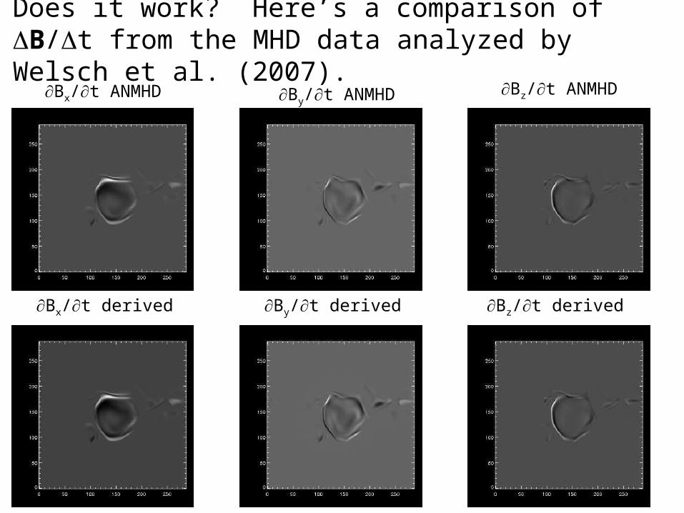
Does it work? Here’s a comparison of B/t from the MHD data analyzed by Welsch et al. (2007).

Bx/t ANMHD By/t ANMHD Bz/t ANMHD

Bz/t derivedBy/t derivedBx/t derived

16

So the magnetic evolution is reproduced, but how well is E recovered? First, try setting ψ=0:

Ex true Ey true Ez true

Ex derived Ey derived Ez derived

Hence, B/t enables recovery of the curl of E, but recovering E itself requires accurately estimating ψ.

We have investigated two approaches to specify ψ:

(a) A relaxation algorithm finds ψ consistent with ideal evol-ution, (E-R)B = ψB; but this doesn’t fully constrain ψ.

(b) A variational method, which can also derive a ψ con-sistent with ideal evolution, as well as Longope’s MEF:

Further details (many!) are provided in Fisher et al. (2009)

€

min dxdyW 2 (ExI −

∂ψ

∂x)2 + (Ey

I −∂ψ

∂y)2 + (E z

I −∂ψ

∂z)2

⎛

⎝ ⎜

⎞

⎠ ⎟∫∫ (14)

Step 3. A useful model of BC

(x,y,z; t) must approximate the physics of the photosphere-to-corona over a large domain.

Modeling the photosphere to corona is challenging: time scales are rapid; length scales are short; radiative transfer plays a key role; temperature & density are highly stratified.

Computational limitations preclude faithful modeling of all of these processes on active region length scales.

Guiding question: What is the simplest algorithm that reasonably approximates the physics of these complex atmospheric layers over a large spatial domain?

Goal: To obtain physically meaningful results by solving the MHD conservation equations on a discretized mesh.

( )

( ) ( )

( ) Qpet

et

B

Bp

t

t

++×∇+⋅∇−=⋅∇+∂

∂

×∇×∇−=−⋅∇+∂

∂

=⎥⎦

⎤⎢⎣

⎡−−⎟⎟

⎠

⎞⎜⎜⎝

⎛++⋅∇+

∂

∂

=⋅∇+∂

∂

φπ

η

η

ρππ

ρρ

ρρ

2

2

4

48

0

Buu

BBuuB

gDBB

Iuuu

u

Currently in RADMHD:Red --- treated explicitlyBlue --- treated implicitlyPurple --- combination of both

In Abbett (2007) we developed a semi-implicit MHD model, RADMHD, that advances the explicit portion of the MHD system (shown above) by means of a third order-accurate CWENO shock capture scheme, and solves the implicit portion of the system via a JFNK technique.

Flows from Step 2. are incorporated into the model as a time-dependent force --- i.e., a source term to the momentum equation.

First, define the physical contribution to the force as defined by the MHD momentum conservation equation:

€

Fphys = −∇ ⋅ ρuu + p +B2

8π

⎛

⎝ ⎜

⎞

⎠ ⎟I +

BB

4π− Π

⎡

⎣ ⎢

⎤

⎦ ⎥ + ρ g (20)

Further, define the forces implied by the data:

€

Fdata =∂ ρ uILCT / MEF

∂t(19)

Then in a single horizontal layer corresponding to the model’s photosphere, we recast the MHD momentum equation in the following form:

€

∂ρu

∂t

⎛

⎝ ⎜

⎞

⎠ ⎟phot

= ξ Fdata( )⊥+ 1−ξ( ) Fphys( )⊥+ Fphys( )||, (20)

where the parallel and perpendicular subscripts denote the forces parallel or perpendicular to the direction of the magnetic field.

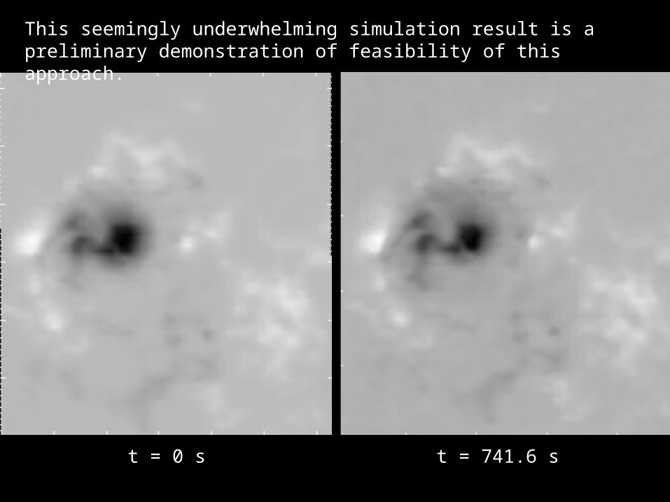
t = 741.6 st = 0 s

This seemingly underwhelming simulation result is a preliminary demonstration of feasibility of this approach.

AR8210 IVM vector magnetogram timeseries

t = 0 s t = 741.6 s

Summary of recent improvements to RADMHD:

We have developed and implemented a computationally efficient method of approximating optically thick radiative cooling in our RADMHD quiet Sun models. The treatment improves upon the ad hoc method presented in Abbett (2007), while still retaining the efficiency necessary to allow for large, active region-scale, convection zone-to-corona computational domains.

The simulations presented here are preliminary. Time will tell whether the new RT treatment is robust, and whether it can maintain the average superadiabatic stratification necessary to sustain solar-like convective turbulence over the long timescales necessary to study the physics of the convective dynamo. However, the initial results are encouraging, and the simulations continue to progress.

1. We are continuing to develop our techniques for determining an initial state for the coronal magnetic field BC(x,y,z; t).

2. We are investigating innovative methods to specify an electric field, E(x,y,0;t), from the evolution of the photospheric field BP(x,y,z; t), which can be used to drive the coronal model forward in time.

3. We have also developed a rudimentary means of assimilating a time series of vector magnetograms into the active zones of an MHD model in a manner that is stable, and does not over-specify the problem.

Conclusion: Capabilities required for data-driven modeling of the coronal magnetic field are still in development, but progress is being made.

Acknowledgements:This ongoing work is supported by NASA, through its Heliophysics Theory and Living With a Star TR&T programs, and the National Science Foundation, though its ATM, SHINE, and National Space Weather programs. Many of the simulations presented here were performed on NASA’s NCCS Discover supercomputer.

Disclaimer:Brian Welsch pressured George Fisher into presenting this poster against George’s will; Brian is also responsible for any inaccurate, objectionable, or cheesy content.