Income Taxes, Sorting, and the Costs of Housing: Evidence ... · Acknowledgements: We thank Comparis.ch for generously providing apartment-level data on housing prices and apartment

Income Taxes, Sorting, and the Costs ofHousing: Evidence from Municipal Boundaries

in Switzerland∗

Christoph BastenETH Zurich

Maximilian von EhrlichUniversity of Bern

Andrea LassmannETH Zurich

July 7, 2014

Abstract

This paper provides novel evidence on the role of income taxesfor residential rents and spatial sorting. Drawing on comprehensiveapartment-level data, we identify the effects of tax differentials acrossmunicipal boundaries in Switzerland. The boundary discontinuity de-sign (BDD) corrects for unobservable location characteristics such asenvironmental amenities or the access to public goods and thereby re-duces the estimated response of housing prices by one half comparedto conventional estimates: we identify an income tax elasticity of rentsof about 0.26. We complement this approach with census data on lo-cal sociodemographic characteristics and show that about one third ofthis effect can be traced back to a sorting of high-income householdsinto low-tax municipalities. These findings are robust to a matchingapproach (MBDD) which compares identical residences on oppositesides of the boundary and a number of further sensitivity checks.

Key words: Local taxation, income taxation, housing prices, incomesorting, boundary discontinuity design, spatial differencing

JEL classification: H71; H24; R21; R38; C14

∗Acknowledgements: We thank Comparis.ch for generously providing apartment-leveldata on housing prices and apartment characteristics, and BFS for providing data fromthe 2000 micro census. We further thank the cantonal tax offices for providing data,Gema Ricart (Swiss Federal Tax Administration) and in particular Raphael Parchet forkindly providing data on local tax burden in the year 2000. We are thankful for numerouscomments from Florian Chatagny and Dirk Drechsel and benefited from comments ofseminar participants at ETH Zurich, University of Hamburg, and from participants of themeeting of the Swiss Society of Economics and Statistics in Bern, and the IIPF in Lugano.Contact : Basten: [email protected]; Ehrlich: [email protected];Lassmann: [email protected].

1 Introduction

Location decisions of individuals depend among others on neighborhood at-tributes as well as on the bundle of taxes and public goods offered by localgovernments. Tiebout (1956) pointed out that mobile citizens weigh thecosts and benefits of public goods provided at the local level and therebyinduce competition among municipalities and regions that ultimately yieldsan efficient provision of public goods and a sorting of households according totheir preferred bundles. Even with a relatively small number of mobile, wellinformed individuals who vote by feet the mechanism should reflect in hous-ing prices. A marginal difference in local taxes between two municipalitiesproviding the same quality of public goods capitalizes in the price for housingas residents have to be compensated for an increase in taxes by a decline inhousing prices. Apart from this direct effect, tax differentials are likely to in-duce a sorting of households across jurisdictions because rich households havea relatively stronger preference for low taxes than poor households if taxesare progressive or preferences are non-homothetic (see Schmidheiny, 2006a).Accordingly, low-tax jurisdictions are characterized by higher incomes whichraises housing prices further.

The empirical relevance of these intuitive mechanisms plays an importantrole for the local provision of public goods and the optimal design of fiscalfederalism. On the one hand, a high elasticity of housing prices with respectto local taxes implies a high degree of mobility and consequently, competitionamong local governments. This should prevent a misuse of public funds. Onthe other hand, a high tax elasticity points to the limitations of fiscal decen-tralization because local income taxes may not be used for redistributionalpolicies and expenditures for goods producing inter-jurisdictional spilloversmay be too low (see e.g. Gordon, 1983). Moreover, as pointed out by Hilber(2011) the extent to which fiscal variables capitalize into local housing priceshas important implications for the evaluation of a wide range of policies. Forinstance, a high degree of capitalization may have adverse consequences forintergovernmental aid or tax deductions.

This paper’s contribution is twofold: first, we identify the causal effectof local income taxes on the costs of housing and second, we isolate the roleplayed by sociodemographic sorting. Our analysis draws on a unique micro-geographic dataset which covers detailed information on the universe of 3.5million rental advertised residences over the period 2005–2012 and acrossalmost all Swiss municipalities. Due to the large degree of regional autonomywhich allows municipalities to charge different income taxes, Switzerland

2

is often referred to as a prime example for fiscal federalism. We matchthe apartment level information with census data about sociodemographiccharacteristics of individual households.

Estimating the response of housing prices to tax changes is complicatedby the fact that capitalization of taxes is conditional on the quality of lo-cal public goods and services which cannot be measured in a satisfactoryway. Moreover, the spatial income distribution and the level of local taxesare determined simultaneously because a larger tax base allows for lowertax rates. This is particularly relevant as (income) sorting may arise forvarious other reasons than taxes. For instance, households being similar interms of sociodemographic characteristics such as income, education, or cul-tural background tend to cluster because of environmental and neighborhoodamenities as well as social interactions (Bayer, Ferreira, and McMillan, 2007;Bayer and McMillan, 2012). Likewise, the distance to the central business dis-trict (CBD) matters because different types of households value commutingcosts differently. Accordingly, sociodemographic variables are intrinsicallycorrelated with unobservable location attributes as well as local taxes. Asa consequence the identification of the tax elasticity is hardly convincing inconventional hedonic regression.

We address these endogeneity problems using a boundary discontinuitydesign and compare residences in a very close neighborhood on both sidesof a municipal boundary. Under the assumption that the distribution ofpotentially confounding variables changes continuously, we can hold localamenities as well as household preferences over neighborhood attributes andpublic goods constant and use the jump in the income tax across municipalboundaries to identify the marginal willingness to pay for living in a low-taxcommunity. The precise georeferencing of households and apartments al-lows us to analyze the variation in rents as well as in sociodemographic andapartment characteristics within a narrow distance band from the municipalboundaries. Features of geographical attractiveness certainly vary contin-uously just as the crime rate, and the population density. Likewise, theaccess to infrastructure and other non-excludable public goods and servicesare continuous functions of distance. We embed our approach in a sortingframework and quantify the degree of income sorting caused by tax differ-ences. This enables us to to disentangle the direct capitalization of taxes inhousing prices from the indirect effect caused by sociodemographic sorting.

Our results provide strong support for a capitalization of income taxesin rents and housing prices. We show that the average elasticity of annualrents with regard to annual income taxes is about 0.26. However, conven-

3

tional hedonic regressions would suggest a much higher rate of about 0.54.Accordingly, unobservable preferences about local public goods and neigh-borhood characteristics that offset the effect of higher taxes are decisive andreduce the estimated elasticity by almost one half. Further accounting for so-ciodemographic characteristics, we show that roughly one third of the higherrents in low-tax municipalities can be attributed to a sorting a high-incomehouseholds.

The remainder of the paper is organized as follows. Section 2 reviews theliterature on taxes and housing prices before we introduce the institutionalbackground in Section 3. Section 4 presents the data and in Section 5 wederive an empirical model for inference about the effect of local income taxeson rents. We describe our key results in Section 6 and perform numeroussensitivity checks in Section 7. The last section concludes with a summaryof the key findings.

2 Local taxes and housing prices

Following Oates (1969) there has been ample empirical research on the effectof taxes on property values, but as a matter of the design of tax institutions inthe majority of countries, most authors have studied the effect of local prop-erty taxes on housing prices (see Ross and Yinger, 1999 and Hilber, 2011for excellent overviews) while empirical evidence regarding local differencesin income taxes and their link to housing prices can hardly be obtained (ex-ceptions are Morger, 2013 and Stull and Stull, 1991).1 Most of these studiesfollow the standard hedonic approach to estimate the valuation of housingcharacteristics and local amenities which however is prone to endogeneitybias resulting from unobservables. Accordingly, in order to address these is-sues the distinction of possible sources for differences in taxation is essential.These include the variation in household preferences, the efficiency of publicgoods provision, and the size of the tax base.

Different tax rates between municipalites may lead to rent differentialsvia the following channels. First, there is a direct effect as disposable in-come increases with lower taxes. Second, tax savings increase with incomeand accordingly high-income individuals have a higher willingness to pay for

1Further empirical tests of Tiebout’s sorting mechanism with regard to changes in envi-ronmental quality and schooling are manifold (e.g., Banzhaf and Walsh, 2008; Rothstein,2006). For a discussion of the estimation of housing prices and demand see Sheppard(1999).

4

housing in the low-tax municipality. With inelastic supply high-income indi-viduals outbid lower income individuals which results in income sorting acrossmunicipalities. Third, fixed migration costs imply that high-income individ-uals are more responsive to tax differences. Suppose there was an exogenousshock to the tax difference between two municipalities. In accordance withthe channels described above, this will boost the demand for housing in thelow-tax municipality. Yet, there are potential feedback mechanisms on localtaxes because a favorable selection of high-income citizens allows for the pro-vision of a given level of public goods at lower tax rates. Similarly, the newselection of citizens may change the set of municipal preferences and strivefor a lower level of government expenditures which will further reduce taxes.

The sorting process outlined above is likely to be incomplete once het-erogeneous preferences are taken into account (Schmidheiny, 2006b). Con-versely, complete income stratification would occur if household preferencesvaried only over income (see e.g., Epple and Platt, 1998; Epple and Sieg,1999). For instance, households may self-segregate in the sense that individ-uals prefer to locate close to other households with similar characteristics.This can explain the clustering of household types within municipalities andacross municipal boundaries (Ioannides, 2004). Moreover, individuals mayfreeride on externalities that local neighborhoods generate across boundariesor exhibit heterogeneous preferences over local public goods. An example forthe latter is the relationship between housing prices and schooling qualitythat has been subject to previous empirical work using similar identificationstrategies (see, e.g. Bayer, Ferreira, and McMillan, 2007; Black, 1999; Fackand Grenet, 2010; Gibbons, Machin, and Silva, 2013). Similar to these stud-ies showing that the inclusion of neighborhood effects reduces the coefficientof school quality in hedonic regressions, we find that disregarding local un-observables produces an upward bias in the elasticity of housing prices withregard to income taxes. Moreover, we show that income sorting explains aconsiderable part of the effect. Empirical evidence in favor of incompleteincome sorting in Switzerland is found in Hodler and Schmidheiny (2006),Schmidheiny (2006a), and Schaltegger, Somogyi, and Sturm (2011). Withincomplete sorting and moving costs income taxes should not fully capitalizein housing prices.

In general, these sources of tax variation raise severe endogeneity prob-lems due to unobserved heterogeneity. Previous work has not been able toaccount for both the variation in neighborhood characteristics that may re-flect individual preferences about the level and quality of public goods andthe local variation in income taxes. Utilizing an institutional background

5

that leads to local differences in income taxes together with detailed georef-erenced data on individual rental prices, apartment types and sociodemo-graphic characteristics we are able to assess the effects of income taxes onhousing prices taking spatial sorting into account.

3 Institutional background: taxes, public goods

and housing prices in Switzerland

By the Constitution of the Swiss Confederation, both the federal state andthe 26 cantons (which are similar to U.S. States and German Bundeslander)are fiscal jurisdictions. It is noticeable that cantons have the main tax au-thority and the federal state’s right to levy taxes is limited both in durationand extent. In practice, cantonal law delegates the authority to levy taxesto the municipalities such that all three state levels – the federal state, thecantons, and the municipalities – are tax jurisdictions, i.e., they set their owntax rates and levy their own income taxes. Elements of direct democracy arepronounced and thus tax rates are set periodically by referenda.2 While thefederal government levies the highest share of total tax revenue (45%), itrelies mostly on indirect taxes and income taxes amount to only 15% of itsrevenue. On the other hand, cantons and municipalities, accounting for 33%and 23% of the total tax revenue respectively, mainly impose direct taxessuch as income taxes, which account for 60% of the cantonal and for 70%of the municipal revenue. The shares in total expenditures are 33%, 41%,and 22%, for the federal, cantonal, and municipal level, respectively.3 Inparticular, the Swiss Constitution allows cantons to set their own incometax schemes, including the degree of tax progression. As a consequence, theheterogeneity across cantons is large. Notably, municipalities have to settheir tax rates as a flat multiple of the cantonal rate such that progression ishomogeneous within cantons.

The unique combination of institutional characteristics leads to hous-ing prices that are endogenously determined through differences in income

2The local (legislative) tax-setting authorities are usually the cantonal parliaments andthe municipality councils but exceptions (including compulsory referenda) exist. Tax ratesare determined annually in most cantons.

3All figures refer to the year 2011 and stem from the Swiss Federal Finance Admin-istration (EFV). Fiscal revenue shares are based on figures for the three levels (federal,cantonal, municipal). Expenditures include fiscal transfers and social security accountsfor the remaining 4% of total expenditures.

6

taxes across jurisdictions that can be traced back exclusively to heteroge-nous preferences and income sorting. The reasons are as follows: first, inter-jurisdictional competition is limited through systems of federal and cantonalfiscal equalization schemes in practice. Second, as pointed out by Hodlerand Schmidheiny (2006), a minimum level and quality of public goods pro-vision is regulated by (mostly) cantonal law. For instance, teacher salariesand school class size are determined by the cantons and tutoring is limitedon the basis of equality considerations, hence not only the level but also thequality of schooling is sufficiently homogeneous. Note also that secondaryeducation (starting at age 13) and tertiary education are completely deter-mined at the cantonal level. Third, the large degree of regional autonomygives rise to yardstick competition as tax rates are set by referendum, rul-ing out large-scale inefficiencies as a source of differences in income taxes.Finally, the Swiss tenancy law is flexible and accordingly, rents can usuallybe adjusted at least once a year.4 In the following section we illustrate thespatial differences that prevail both regarding the tax rates and rents acrosscantons and municipalities.

4 Data

We use three data sources that are combined with geographic informationabout Switzerland. First, the data on housing prices comprise about 3.5 mil-lion postings of residences offered for rent during the period 2005-2012. Thesedata stem from comparis.ch which is the most widely-used price comparisonservice in Switzerland offering among others information on real estate, in-surance, and phone contracts. For their real estate platform comparis.chcollects all offers posted on the 17 most popular apartment search engines inthe Swiss market. According to official statistical sources, the total numberof (owned and rented) apartments was 4,131,342, and the number of inhab-ited apartments was 3,534,508 in 2011, thus the number of vacancies wasabout 600,000.5 The number of unique observations in the same year cov-ered by our sample is about the same. These figures indicate that the datacoverage of our sample is excellent. Our data also reflect the distribution ofresidences across different categories very well. The median apartment in our

4In most cases, rents can be adjusted on first April and first October in any year.The law allows an adjustment to rents customary in a place (allowing for local differenceswithin municipalities) regarding existing and new tenants.

5Source: Swiss Federal Statistical Office (BFS).

7

data has 3.5 rooms and a living space of about 80 square meters. Regardingthe geographic distribution of postings across cantons we observe a strongconcentration of observations (about 20%) in the Canton of Zurich whichis approximately consistent with the population share. In 2011, about 18% of the Swiss population lived in the Canton of Zurich. In addition, thedata provide a good coverage of more rural areas such as the cantons Aargauand Schwyz with 51,259 and 11,223 observations in 2011 (corresponding to8.2% and 1.8% of the total) which fits approximately their population sharesof 7.7% and 1.9%.6 The overall distribution of residences in our sample isshown in Figure 1.

– Figure 1 here –

All prices in the data at our disposal reflect offer prices rather than trans-action prices. To account for the potential measurement error that mightarise from the difference between offer prices and transaction prices, we fo-cus on rents rather than residential property prices.7 Immigration has beenan important factor that led to increasing demand for housing in recent years.As a consequence, rents are almost never negotiated but taken as given bythe tenant. Moreover, real estate brokers offer residences online, in whichcase the advertisement appears in the data at our disposal. In general, bro-kers are very rare in this market because they are regulated to earn a flatrateof 500 Swiss Francs (CHF) for matching a landlord and a customer. Impor-tantly, the rental share is relatively high in Switzerland, amounting to 59%in total inhabited accommodations in 2011.8 Migration costs are likely to belower for tenants than for property owners and thus capitalization should bemore pronounced. Finally, a recent study by Banzhaf and Farooque (2013)for the Los Angeles area has shown that rents capture spatial differences incontemporaneous amenities and income better than property prices.

Second, information on sociodemographic characteristics of individualhouseholds is obtained from census data. It covers information on education,employment status, occupation, age, legal status, native language, etc. The

6Population shares stem from the Swiss Federal Statistical Office (BFS).7Our dataset includes information on residential properties. Yet, we disregard these

data as we believe that the effect can be identified more precisely from rental prices.8The residential property share in Switzerland is particularly low in comparison to

the neighboring countries (56.4% in Austria, 58.1% in France, 45% in Germany, 77.1%in Italy). Sources: Swiss Federal Statistical Office (BFS), Euroconstruct 2013. The lowproperty share is mostly due to the fact that with the exception of Valais, individualapartments could not be purchased until 1965.

8

corresponding dataset was provided by the Swiss Federal Statistical Office(BFS) and can be geolinked by precise addresses.9 We match the informationon real estate and sociodemographics to information about the geographiclocation of municipal boundaries that stem from BFS, and to data on the mu-nicipal tax burden, both spanning the period 2005–2012. The former allowsus to determine the municipality in which individual residences are locatedas well as the distance from each residence to every municipal boundary inevery year. Annual maps are necessary because due to several reforms, thenumber of municipalities diminished from 2,777 in 2005 to 2,495 in 2012.

Third, we calculate the local income tax burden depending on householdtypes and covering the years 2005-2012. Differences in tax legislation implythat the calculation of the tax base varies across cantons (deductions fromgross income are set at the cantonal level). Applying the cantonal tax ratewhich relies on a continuous and progressive tax schedule to the tax baseyields the so-called Einfache Steuer. This sets the basis for calculation ofthe municipal and church taxes, with the corresponding flat tax rate usuallybeing defined in %. More specifically, the overall tax burden is calculated asfollows. We collected data on cantonal, municipal and church tax rates, andon poll and school taxes if applicable for every municipality in all years aswell as the majority religious shares.10 We further use data from the SwissFederal Tax Administration (ESTV) on the total tax burden at the municipallevel. These data cover municipalities with at least 2,000 inhabitants until2010 and all municipalities in later years. Using these data together withthe cantonal tax rates we infer the cantonal tax burden i.e., the EinfacheSteuer. With the cantonal tax burden and the municipal tax multipliers athand we obtain the municipal tax burden which is added to the cantonaltax burden for all years. This computation is done by household statusand income, where we distinguish between single households and marriedhouseholds with 2 children and income= {80; 100; 150; 200; 400} tsd. CHF.11

9We use the year 2000 as this is the last census which built on a questionnaire that theentire population of Switzerland had to answer. Accordingly, it shows the demographic,social, and economic developments at the finest possible spatial scale. Later censuses arebased on samples and data are available at the municipality level only for a few variables.

10The municipal tax multipliers are typically made available on the cantonal or municipalwebpages, and where not available we contacted the respective authorities for information.The majority religious shares at the municipality level stem from the 2000 census. Allresults are robust to using only the observations covered by ESTV data.

11More detailed information on the computation of the municipal tax burden is providedin Appendix A.

9

For reasons of consistency, we apply this approach to all municipalitiesin all years and test the precision of our data by comparing the tax burdenstated by ESTV for municipalities with more than 2,000 inhabitants withour own calculations. The fuzziness resulting from our calculations is minor.Moreover, the ranking of municipalities in terms of their tax level is perfectlymatched by our computations and the negligible deviations in the absolutetax burden are due to the tax authority using slightly different representativecharacteristics for the computation of the tax base.12


In Figure 2 we display the total tax burden across all Swiss municipalitiesusing different colors for the quintiles of the distribution. We plot this mapfor a single person with an annual income of 100 tsd. CHF in 2012. Thewestern part of Switzerland generally exhibits the highest taxes while thecentral part levies relatively low taxes. Overall, we observe a large variation.The minimum tax burden applies in the municipality of Wollerau (Schwyz)and corresponds to 4,806 CHF while the highest tax burden applies in LesPlanchettes (Neuchatel) and corresponds to 19,841. Interestingly, we observemunicipalities in the lowest quantile of tax burden (marked in light yellow)right next to municipalities in the upper quantile of the distribution (markedin dark blue). Many of these cases are municipality pairs belonging to dif-ferent cantons but we find considerable variation within cantons, too. TheCanton of Graubunden displays the largest variance in tax burden acrossmunicipalities for our representative single person household with a rangeof 4,997 (Rongellen) to 17,547 (Schmitten). We have plotted the distribu-tion of municipal taxes in the Canton of Zurich separately in Panel B. Twointeresting observations are immediately evident from the map. First, themost attractive locations at the lake side display very low taxes. Second, thehighest taxes are levied at the border of the canton relatively distant fromthe agglomerations’ core.


How does the distribution of taxes relate to the distribution of rents? Themaps in Figure 3 plot the average rent per square meter in a municipality

12Contrasting the ESTV data about the tax burden for municipalities with more than2,000 inhabitants with our own calculations yields a correlation coefficient of 0.98 and amean difference in the annual tax burden of only 0.6% of annual income across all cantonsand years. The results are robust to using data covered by ESTV only.

10

for Switzerland and for the Canton of Zurich, respectively. Compared to thetax burden, we observe less of a clear regional pattern in the distribution ofrents as the top quintile (marked in dark red) is scattered across western,central and eastern Switzerland. Rents are highest in the agglomerations ofZurich and Geneva but we find other municipalities in the upper quintilein less agglomerated regions such as around Zug, Schwyz or in Graubunden(where taxes tend to be low). Focusing on the Canton of Zurich we observethe highest rents in the lake-side municipalities and the lowest rents at thecantonal borders which corresponds to the inverse of the distribution of taxesas illustrated in Figure 2. Of course we cannot infer the effect of taxes onthe prices of housing from such unconditional correlations because of manyconfounding factors that become evident from the maps. For instance, nu-merous of the high-rent and low-tax municipalities in the Canton of Zurichare located in the most attractive environment close to the lake and in com-muting distance to the city center while the low-rent and high-tax regionstend to be in the hinterland and offer less convenient public transport linksto the city. The municipalities with high rents and low taxes in Graubundenare located in some of the most popular tourist regions while municipalitiesfeaturing low rents and relatively (yet not always) higher taxes tend to belocated in densely populated mountain areas.

5 Estimating the effect of income taxes on

housing prices

This paper’s empirical approach identifies the impact of income taxes onrental prices based on a boundary discontinuity design as developed in Black(1999) and Bayer, Ferreira, and McMillan (2007) and refined by Fack andGrenet (2010) and Gibbons, Machin, and Silva (2013). In contrast to thesestudies focusing on expenditure-side effects – or more precisely, on the val-uation of schooling –, our analysis relates rental prices to public revenues.Unobservable local conditions determine the level of taxes and rents at thesame time which implies that conventional hedonic housing prices regres-sions yield biased estimates of the tax elasticity. With geographic locationcommonly being acknowledged as the key determinant of housing prices itseems advisable to pursue a counterfactual analysis based on observationsthat share the same neighborhood characteristics. For instance, Albouy andEhrlich (Albouy and Ehrlich) conclude that space is a much greater deter-

11

minant of land values than time even when studying data over the housingboom and bust cycle. In urban economic theory and consistent with empiri-cal evidence, the rent gradient typically decreases continuously with distancefrom the economic center, publicly provided amenities, or other attractivelocation fundamentals. In contrast, the tax burden changes discontinuouslyat the municipal boundary in the multijurisdictional tax system of Switzer-land. The analysis of narrow windows around spatial boundaries togetherwith boundary fixed effects can thus be exploited to obtain a causal effect ofincome taxes on rents.13

5.1 Boundary discontinuity design (BDD)

Let us use the following notation. We observe postings of individual resi-dences denoted by i in year t which belong to a municipality m ∈ M . Eachmunicipality levies an annual income tax Taxmt – which can vary acrosshousehold type and income level – from its residents. Using data on ad-ministrative boundaries we can assign each municipality all its neighboringmunicipalities. Restricting our dataset to posts with non-missing and plau-sible values for the residence characteristics reported in Table 1, we obtainM = 1, 989 municipalities.14 We denote by p = {m,m′} a pair of neigh-boring municipalities where each combination of municipalities is consideredonly once and each residence is uniquely assigned to one municipality pairaccording to the minimum distance to the municipal boundary.

The log tax burden is denoted by τmt which refers to a gross income of100 tsd. CHF and to a single person household in our benchmark specifica-tions. This corresponds approximately to 1.5 times the median income of anemployee in Switzerland. In order to insure a sufficient degree of institutionalhomogeneity we restrict the analysis to municipalities belonging to the samecanton. This implies that the results are not affected by the choice of income

13Note that this approach is similar but not equivalent to a spatial regression disconti-nuity design, where identification is based on the continuity of distance as a running (orforcing) variable; e.g., Lalive (2008), Dell (2010); see also Eugster and Parchet (2013),Basten and Betz (2013), Egger and Lassmann (2013) for such designs for Switzerland. Incontrast to most spatial RDD, the distance from the boundary has no uniform economicinterpretation and we match individual residences on both sides of the boundary.

14This refers to the full time period. We assign the respective neighboring municipalitiesfor each year separately according to the corresponding classification and digital mapsof municipalities. As some municipal boundaries were modified over the period underconsideration we use separate digital maps for each year which are available from BFS.

12

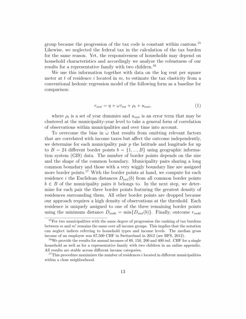
group because the progression of the tax code is constant within cantons.15

Likewise, we neglected the federal tax in the calculation of the tax burdenfor the same reason. Yet, the responsiveness of households may depend onhousehold characteristics and accordingly we analyze the robustness of ourresults for a representative family with two children.16

We use this information together with data on the log rent per squaremeter at t of residence i located in m, to estimate the tax elasticity from aconventional hedonic regression model of the following form as a baseline forcomparison:

rimt = η + ωτmt + ρt + uimt, (1)

where ρt is a set of year dummies and uimt is an error term that may beclustered at the municipality-year level to take a general form of correlationof observations within municipalities and over time into account.

To overcome the bias in ω that results from omitting relevant factorsthat are correlated with income taxes but affect the outcome independently,we determine for each municipality pair p the latitude and longitude for upto B = 24 different border points b = {1, ..., B} using geographic informa-tion system (GIS) data. The number of border points depends on the sizeand the shape of the common boundary. Municipality pairs sharing a longcommon boundary and those with a very wiggly boundary line are assignedmore border points.17 With the border points at hand, we compute for eachresidence i the Euclidean distances Dimt(b) from all common border pointsb ∈ B of the municipality pairs it belongs to. In the next step, we deter-mine for each pair the three border points featuring the greatest density ofresidences surrounding them. All other border points are dropped becauseour approach requires a high density of observations at the threshold. Eachresidence is uniquely assigned to one of the three remaining border pointsusing the minimum distance Dimbt = min{Dimt(b)}. Finally, outcome rimbt

15For two municipalities with the same degree of progression the ranking of tax burdensbetween m and m′ remains the same over all income groups. This implies that the notationcan neglect indices referring to household types and income levels. The median grossincome of an employee was 67,500 CHF in Switzerland in 2012 (see BFS, 2012).

16We provide the results for annual incomes of 80, 150, 200 and 400 tsd. CHF for a singlehousehold as well as for a representative family with two children in an online appendix.All results are stable across different income categories.

17This procedure maximizes the number of residences i located in different municipalitieswithin a close neighborhood.

13

is measured for each residence i located in municipality m and assigned toborder point b at year t.

This procedure allows us to estimate a BDD model which can be statedas follows:

rimbt = α + βτmt + θbt + εimbt, (2)

where β measures the tax elasticity, θbt is the border-point- and year-specificfixed effect that absorbs all variation specific to the neighborhood of theborder-point in both the cross-sectional and the time dimension, and εimbt isan error term which we cluster at the boundary-year level to account for serialcorrelation along boundaries that may be due to both spatial correlation andcorrelation over time.18 By limiting the sample to residences within a smallneighborhood of the border-points we ensure that θbt accurately captureslocation-specific unobservables.

5.2 Matching residences across boundaries (MBDD)

As an alternative approach, we follow Fack and Grenet (2010) and Gibbons,Machin, and Silva (2013) and match each posting i on one side of b in mwith a counterfactual i′ on the other side of b in m′. The counterfactualtransaction ri′m′bt is calculated as the distance-weighted geographic mean ofthe prices of all transactions j that took place within a certain radius andin the same year as transaction i but were located in municipality m′ ratherthan in m:

ri′m′bt =J∑

j=1

1Dij∑Jj=1

1Dij

rjm′bt. (3)

Note that 1Dij

refers to the inverse distance between a residence j and

reference sale i (both posted in the same year).19 Assuming that the ref-erence transaction and the counterfactual are sufficiently close, they share

18Note that in general, a residence i that has n neighbors will be in n pairs and ac-cordingly the error terms of all these n terms will be correlated. This correlation occursbecause the residence-specific error term enters the error of each pair. For this reason eachresidence i is used only once. We assign each i a unique municipality pair according tothe minimum distance to the boundary.

19For the sake of computational ease, we use the inverse distance between postings iand j via the border point. With many border points it can be shown that this yieldsvirtually the same values as computing direct distances.

14

the same unobservable time-varying neighborhood effect and the regressionmodel (referred to as MBDD) becomes:

rimbt − ri′m′bt = γ(τmt − τm′t) + (εimbt − εi′m′bt). (4)

Parameter γ reflects the tax elasticity of rents and can be estimated byregressing the price differential between reference and counterfactual rent onthe corresponding tax differential. Since the identification assumptions aremore likely to be valid for observations with a small distance, we estimate aninverse-distance weighted model. We apply a weight

∑Jj=1

1Dij

to each pair

{i, i′} such that observations in a close neighborhood receive more weight.Standard errors are clustered at the boundary-year level to account for theserial correlation in the error term induced by differencing. Note that this ap-proach differs from the model in equation (2) by eliminating common spatialtrends through spatial differencing and by taking the distance between indi-vidual residences at opposing sides of the boundary into account. Since wepool the data over the years 2005-2012, we additionally allow for a commontime trend λt by including year dummies. While the tax burden differen-tial varies across years, all municipalities within each pair in our boundarysample generally offer the higher/lower tax rate over the full time period.

5.3 Discussion of the identifying assumptions

Under the assumption that unobservable determinants of rents vary contin-uously at the boundary, the parameters β and γ identify the causal effectof interest for observations in the vicinity of the boundary in the BDD andMBDD approaches, respectively. We choose the radius from the municipal-ity boundary such that it guarantees both the consistent estimation of thecoefficients of interest as well as sufficient precision. Hence, all estimatesare reported for three alternative bandwidths: we use samples of residenceslocated within 1 km, 600 meters, and 300 meters from the closest borderpoint. Note that municipality-pair-specific distances instead of border-point-specific distances would be adequate to condition on the commuting costs tothe neighbor municipality but would not capture the local conditions of asmall well defined area: a residence i in m may be as close to the p-boundaryas a residence j located in neighboring municipality m′ but still i and j mightbe distant from each other and located in environments of very different at-tractiveness. In contrast, by way of the chosen design we condition on the

15

proximity of residences i and j as well as on the proximity to the municipalboundary in terms of their proximity to a common border point. Hence, thisapproach allows us to hold neighborhood characteristics constant.

The resulting distribution of observations in space around individual bor-der points is best described in a map as the one in Figure 4. The mapexemplifies for two neighboring municipalities, Kusnacht and Zollikon (Can-ton of Zurich), how individual observations are allocated to and comparedacross municipal border-points on a narrow spatial scale: the first type ofresidences (green) is located at the lakeside, the second type (blue) is locatedclose to the centers and along main traffic routes, and the third type (red)is located outside the center on the hill in both municipalities. Each of thethree border points will be assigned a unique fixed effect and the sample willbe restricted to observations within the bandwidth. Hence, using the 300meter radius the red border point may not be used in the regressions dueto the low density of residences in the northern municipality. In order toavoid differences in the sample composition of border points we restrict allspecifications to border points covered by the 300 meter boundary sample.20

The MBDD framework further improves on the continuity assumption as itattributes a greater weight to those residence pairs that are closer than oth-ers within each circle drawn in Figure 4. Specifically, we construct for eachdot in the southern part of the circle a counterfactual residence which is aweighted average of the dots on the northern side of the boundary and withinthe circle according to equation (3).

The identifying assumptions would be violated if we observed a bunch-ing of residences and postings on the low (or high) tax side of the border.A discontinuity in the density of the observations would point to a system-atic difference in the supply of housing which is correlated with local taxes.As suggested by McCrary (2008), we illustrate the density of our observa-tions in equally sized bins of the distance from the boundary in the upperleft panel of Figure 5. Naturally, the frequency of postings decreases in theclose neighborhood of a municipality boundary which is due to residencesbeing concentrated in the center of a municipality. This process holds truein treated and control municipalities and we observe an almost symmetricshape of the histograms on both sides of the boundary. Even the immedi-

20The distance between municipalities may have implications for strategic tax setting.Accordingly, border points/municipality pairs that enter the sample only for larger dis-tances may be systematically different from others and we restrict our analysis to munic-ipality pairs and border points that display a sufficiently high density of residences withthe smallest bandwidth.

16

ate bins at both sides of zero distance have approximately the same density.Hence, there is no indication of a bias toward more postings on either sideof the threshold.


Finally, our identification strategies rely on the assumption that estimatesof β and γ can be unambiguously attributed to the jump in the income tax.If instead other factors varied discontinuously at b, our estimates could notisolate the effect of taxes. It is not plausible to disentangle the effect of in-come tax differences at cantonal borders from other political, economic andinstitutional differences. For this reason we generally restrict our sample tomunicipal boundaries which do no coincide with cantonal borders. Furtherviolations of the continuity assumption may include: (i) geographic barriersthat separate municipalities at b, (ii) apartment characteristics being system-atically different in m and m′, (iii) asymmetric level and quality of excludablepublic goods between municipalities, and (iv) individual preferences to liveat a particular address in central business districts.

We address these concerns in the following way: (i), we drop pairs thatare separated by rivers and highways or feature a difference in altitude ofmore than 400 meters. In addition we drop pairs split by language borders.21

(ii), we account for apartment characteristics by using residuals obtainedfrom first-stage regressions of the log rent per square meter on a comprehen-sive set of characteristics in all specifications.22 (iii), we exploit tax variationwithin school districts in Section 7 because elementary schools are typicallyfinanced on the municipal level. Other publicly provided goods such as healthservices, roads, cultural events are either not municipality-specific, regulatedon the cantonal and federal level, or not exclusively limited to local residents.In the latter case the usage costs become a continuous function of distance.Identifying the effects only from tax rate variation over time – e.g. addingmunicipality fixed effects – further supports this argument. In order to rule

21German, French, Italian, and Romansh are official languages in Switzerland. Lan-guage borders are defined by the majority of the respective language speakers withinmunicipalities.

22These include the variables summarized in the next section, nonlinear and interactionterms of them as well as year dummies. Moreover, all results remain very robust toalternative specifications of the first-stage. In our preferred first-stage specification, weexplain about 15% of the variation in log rents. The corresponding regression tables aredisplayed in an online appendix.

17

out CBD specific effects (iv), we estimate equations (2) and (4) for obser-vations that exclude the agglomerations of Basel, Bern, Geneva, Lausanne,and Zurich separately.

6 Results

6.1 Descriptive statistics

In total we can assign about 2.5 million postings containing non-missing in-formation on square meters, rents, and many other apartment characteristicsto the municipalities which we consider between the years 2005 and 2012.23

These include information about detailed characteristics of the residence aslisted for the full dataset in columns (1) and (2) of Table 1. Apart from age,number of rooms, and the apartment’s floor these are binary variables thatcapture information on the quality and type of the residence. We use thefollowing sociodemographic covariates: the shares of high- and low-incomepopulation, of high- and low-skilled population, of foreigners, of unemployed,of commuters, as well as the average age. These data are based on individualinformation which is georeferenced and assigned to grids of 1× 1 km. Then,we compute the respective shares and averages on the basis of the total popu-lation within each grid. Income groups are constructed according to detailedoccupation categories and job functions. For details about the tax data andthe sociodemographic variables see Appendices A and B.

Regarding our identification strategy we resort to observations in the closeneighborhood of a municipal boundary. The boundary sub-sample (columns(3) and (4) of Table 1) consists of residences that could be assigned to aborder point b which features at least 2 observations on both sides of theboundary and within a distance of 300 meters. Accordingly, the municipalitycomposition remains stable when restricting the boundary sub-sample toalternative maximum distances of 1 km and 600 meters. All border pointswhich correspond to geographic or linguistic barriers have been dropped.Moreover, we drop municipality pairs with a tax differential of less than 100CHF and we keep only residences that lie in a 1 × 1 km grid which hasa population of at least 50 individuals. The latter should ensure that the

23Note that we loose about one million of postings due the following reasons: First, wedrop observations with missing or non-credible information regarding rents, rooms, andsquare meters. Second, we drop postings offering a rent of less than 5 CHF or more than52 CHF per square meter. These values equal approximately the 1st and 99th percentiles.

18

sociodemographic information is representative of the neighborhood. Taxburden and rents are measured in CHF where T S100

m refers to the annual taxburden of a single household earning 100 thousand CHF per year. In total theboundary sub-sample consists of 151,011 postings in 211 municipalities. Theaverage rent per square meter amounts to 21.1 and and 22.2 CHF in the fullsample and the boundary sub-sample, respectively. Furthermore, the averageannual tax burden (T S100

m ) is about 13,900 CHF in both samples. Whencomparing the boundary sub-sample – which consists of only about 10% ofthe total number of municipalities – to the full dataset, we observe that themoments of the data are remarkably similar not only for the main variablesbut also for the sociodemographic and residence covariates. The boundarysample focuses on 190 border points with sufficiently close residences on bothsides of the boundary and 701 associated grid cells. Accordingly, a borderpoint is assigned on average about 800 observations and 3.6 grid cells (1× 1km).

– Table 1 here –

Table 1 provides further information about the data. The average apart-ment has about 3.5 rooms, is about 40 years old, and is located on the secondfloor. More than 70% of the residences either have a balcony or a terrace and40% have a parquet floor. The share of high-skilled is about 10% and theshare of foreigners amounts to about 23%. Overall, these figures seem rea-sonable and representative. Limiting the sample with respect to a distanceof 600 and 300 meters from the closest border point results in samples of89,058, and 30,980 observations, respectively. Within these distance bands,the observed average rents are 21.8 CHF and 21.4 CHF. The figures for theaverage annual income tax burden of our benchmark household with a grossannual income of 100 thousand CHF amount to 14,113 CHF and to 14,202CHF. In general, our dataset has a remarkable support at the border regionswhich allows us to condition very precisely on the location of residences. Thisis a feature of the data coverage, the relatively small size of municipalities,and the high population density in Switzerland.

6.2 Graphical assessment of boundary discontinuities

In Figure 5 we illustrate the symmetry of the distribution of residences acrossboundaries as described earlier, as well as the deviations in tax burden, rentsper square meter, and residual rents from the border-point averages for ob-servations on the low- and high-tax side of each boundary. Note that we pool

19

all border-points and structure the data such that high-tax municipalities areassigned negative distances whereas low-tax municipalities have positive dis-tances from the boundary. Moreover, the figures show local averages overdistance bins of 100 meters as well as flexible polynomial fits that were esti-mated separately on both sides of the boundary.24 In each figure we restrictthe sample to a distance band of 1 km on either side of the boundary whichcorresponds to the maximum bandwidth used in the estimations.

By construction, the difference in tax burden between municipalities onopposite sides of the boundary features a discontinuity at the boundary (seeupper right panel of Figure 5). On average the difference between taxes(T S100

m in neighboring low- and high-tax municipalities is about 750 CHFor 5% of the sample average in T S100

m . The municipal distance from theboundary is measured by the average distance of observed residences withina municipality. The lower panel of Figure 5 suggests that the jump in therental price per square meter and even more so, the one in residual rents ispronounced at the municipal boundary. We observe an average difference inlog rent per square meter and residual rent of 0.02 and 0.03, respectively. Inboth cases, this corresponds to approximately 1% of the dependent variables’sample average. Accordingly, the figures suggest that a 5% tax differentialresults in a 1% rent difference or a 20% capitalization rate. The 95% con-fidence intervals of the polynomial fits indicate that the discontinuities arehighly significant for all three variables.

Figure 6 visualizes the discontinuity in the share of skilled versus un-skilled and high-income versus low-income individuals in order to shed lighton the extent of sorting across municipalities which is a prominent chan-nel to explain the rent differential. The figures are constructed in the sameway as described above and indicate a clear discontinuity at the boundary.For each variable the jump at the boundary is strongly significant. At theboundary, the share of high-skilled and high-income individuals increases byabout 45 and 50% in the low-tax municipality compared to the high-tax mu-nicipality. Conversely, the share of low-skilled and low income individualsjumps substantially when moving from the low-tax to the high-tax side ofthe boundary. In the next section we analyze the significance of these dif-ferences and quantify the elasticities as well as the relative importance of

24An alternative and qualitatively equivalent way of displaying the discontinuities wouldbe to regress the variable in question on border-point fixed effects and on dummy variablesfor each bin where the coefficients on these distance dummies correspond to points on thepolynomial fit displayed in our figures. We obtain very similar graphs with both approachesand accordingly chose the continuous version.

20

income sorting.

– Figures 5 and 6 here –

6.3 BDD results

Table 2 reports the coefficients and standard errors based on equation (1)in columns (1) and (2) and equation (2) in columns (3)-(8). The table isstructured as follows. We use log rental prices per square meter as outcomein Panel A and residual rents purged of the influence of apartment charac-teristics in Panel B. The latter are derived as the residuals from a first stageregression of log rents on flexible functions of the apartment characteristicsreported in Table 1.25 Uneven columns refer to specifications that includeall municipalities in the chosen sample while even columns exclude the fivelargest agglomerations. This leads to 605 and 522 border points. The dis-tance band around the border points is limited to 1 km in columns (3) and(4). It is reduced to 600 and 300 meters in columns (5)-(6) and columns(7)-(8), respectively. The results may be summarized as follows. First, theelasticities carry a negative sign as expected and are statistically highly sig-nificant. Second, the inclusion of boundary fixed effects – columns (3)-(8)– is able to reduce the bias from the conventional hedonic approach con-siderably and contributes substantially in terms of the models’ explanatorypower. Third, limiting the sample to close distance bands around boundarieslowers the coefficients further. Fourth, taking residence characteristics intoaccount increases the estimates of the tax elasticity slightly and becomesrobust to the results in Panel A the smaller we choose the distance to theboundary. Quantitatively, we find that an increase in the tax burden by 1%lowers rental prices by approximately 0.5% using the conventional approach.This effect reduces to -0.248 and to -0.258 regarding outcomes in Panel Aversus Panel B when accounting for border point fixed effects and limitingthe distance of observations to 300 meters from the boundary. It amountsto -0.282 and -0.311 when excluding observations located in large agglom-erations. Note also that excluding agglomerations does not systematicallyaffect the tax elasticity: while the effect is somewhat more pronounced whenincluding agglomerations in the 600 meter sample the opposite is true for

25We estimate numerous first-stage specifications and account for the fact that the pre-mium attached to apartment characteristics may vary across cantons and may be differentin cities compared to more rural areas. Our results remain robust to these alternativefirst-stages.

21

the 300 meter sample. In any case the difference in the coefficients is negli-gible which suggests that the estimated tax elasticity is not confounded bydifferences of population density or other agglomeration effects.

Overall, the size of the estimates drops by roughly 50% when accountingfor unobservable neighborhood characteristics compared to the conventionalhedonic regressions in columns (1) and (2). Moreover, border fixed effectsexplain about 40% of the variation in the data.

– Table 2 about here –

6.4 MBDD results

Results based on the approach in equation (4) are shown in Table 3. Thestructure of the table and the sample composition is exactly the same asin Table 2. We additionally report the average distance between referenceresidences and the counterfactual that matches observations located in theneighboring municipality. The elasticities are remarkably similar to the onesin Table 2, however, unobservable neighborhood characteristics seem to beabsorbed already for relatively large bandwidths. While the BDD coefficientsdrop further when moving from a bandwidth of 1 km to 300 meters, theMBDD’s coefficients are comparable to the ones in column (8) of Table 2when using the 1 km window. Hence, due to contrasting individual residencesand assigning more weight to nearby units, the MBDD represents the moreefficient approach compared to the BDD. Moreover, the coefficients are quiterobust over all three samples. Our preferred estimates correspond to the 300meter boundary sample which display an income tax elasticity that amountsto roughly -0.253 in Panel A and to -0.264 in Panel B (column (5)). Again,excluding agglomerations does not systematically affect the estimates.


6.5 The role of sociodemographic sorting

Apart from the direct capitalization effect of tax differentials it is evident fromFigure 6 that tax differentials lead to a sorting of households. We quantifythe share of rent differences between high- and low-tax municipalities thatis due to sociodemographic sorting by including the vector of census blockcovariates summarized in Table 1 on the right-hand side of equations (2)and (4). Table 4 reports the coefficients and standard errors from both

22

equations with distance bands restricted to 600 and 300 meters. Comparedto the preferred specifications with 300 meters distance in Table 3 the taxelasticity of rents is reduced by 20-30% and amounts to -0.181 and to -0.199for log rents and residual rents, respectively. The corresponding specificationsdisregarding local sociodemographics yield elasticities of -0.253 and -0.264 forlog rents and residual rents, respectively. This suggests that low taxes attracthigh-income households and accordingly a larger housing budget which drivesup rents in addition to the direct capitalization effect.


7 Sensitivity

Our results have been shown to be very stable across the two approaches. Ingeneral, matching residences to individual counterfactuals in the neighbor-ing municipalities allows for a high degree of precision compared to the BDDeven with relatively larger windows. We test the sensitivity of these resultsand in particular for the preferred MBDD specifications along the followinglines:

The role of schooling. At the municipality level in Switzerland the onlyrelevant public good that appears excludable is elementary schooling. Asmentioned above a large degree of homogeneity across municipalities is guar-anteed in elementary schooling as well. The main reason for differences inschooling should be the composition of pupils. This represents a channel forthe indirect effect of taxes on housing prices via sorting which is captured bythe chosen design. Yet, in principle the quality of elementary schools maychange discontinuously at the municipal boundary and accordingly raisesconcerns about the consistency of our estimates. In order to address thisconcern, we digitalized maps on school districts for cantons where applica-ble: these are the Cantons of Zurich, Bern, Aargau, Fribourg, and Vaud.In these cantons the boundaries of school attendance zones do not alwayscoincide with municipal boundaries. Accordingly we focus on observationsalong boundaries that are located within the same school district yet facedifferent levels of income taxes. The corresponding results are summarizedin Table 5.

Since the number of municipality pairs drops considerably when usingonly boundaries within the same school district we focus on the estimations

23

within the 600 meter window. As has been shown in Tables 2 and 3 this band-width is appropriate to capture neighborhood specific unobservables. PanelsA (log rent per square meter) and B (residual rents) report the coefficientsfor the BDD and MBDD approaches where sociodemographic sorting is ac-counted for in columns (2) and (4). While the coefficients’ magnitude tends toincrease somewhat when accounting for schools and using log rent per squaremeter as the dependent variable, the opposite is true for residual rents. Lim-iting the sample to units within the same school district, the benchmarkMBDD estimate increases from -0.305 to -0.420 and decreases from -0.395 to-0.323 in the log rent and residual rent specifications, respectively. However,in none of the specifications we can reject that the coefficients are identical forthe two samples at conventional levels of significance. Note that restrictingthe sample to residences located in the same school district reduces the num-ber of observations substantially and accordingly raises the standard errorsbut most coefficients remain remarkably significant. Moreover, the estimatesreported in Table 5 are consistent with the finding that about two thirds ofthe tax elasticity are due to direct capitalization effects and approximatelyone third is driven by household sorting. Comparing columns (2) and (1) andcolumns (4) and (3), we observe a reduction of the estimated tax elasticitybetween 13 and 29% when including sociodemographic covariates.


Placebo discontinuities. We address the possibility that rent differentialsare erroneously attributed to tax differentials by shifting municipal bound-aries artificially within both m and m′. For this we set new ’fake’ boundarieswhich are shifted 300 meters from the true boundary point for either mu-nicipality within a (border-point-specific) pair. Then, we reassign the newlytreated observations the low tax rate and the newly non-treated observationsthe high tax rate. Finally, we estimate the BDD model using the new taxburden variable. Table 6 reports the corresponding results for log rents persquare meter as well as residual rents and for a shift of the true bound-ary towards the low- or high-tax municipalities. Hence, in the former casewe contaminate the control units and in the latter case we contaminate thetreated. None of the estimates in Table 6 is significant and the coefficients’magnitudes are far from our benchmark. This falsification exercise adds fur-ther confidence in our results as it shows that spatial trends in unobservablescan be effectively eliminated by spatial differencing.


24

Functional form misspecification. In line with most regression disconti-nuity approaches, we account for spatial trends that lead to average rentdifferences across boundaries by adding flexible forms of distance or coordi-nates to equation (4):

rimbt − ri′m′bt = δ(τmt − τm′t) + f(limbt)− f(li′m′bt) + (νimbt − νi′m′bt), (5)

where f(limbt) and f(li′m′bt) include (i) a cubic polynomial function of distanceto b, and (ii) the geographic coordinates of locations. Results are presentedin columns (1) and (2) of Table 7 and are directly comparable to the onesshown in column (5) of Table 3. The coefficients are nearly identical whichconfirms the robustness of the estimated tax elasticities to the inclusion offlexible forms of distance to the boundary. Note that spatial trends acrossboundaries have been taken into account already by weighting the regressionsusing the inverse distance.

Furthermore, nonlinearities of tax rates may apply. The MBDD approachidentifies the coefficient on (τmt − τm′t) which reflects the tax benefit fromliving in municipality m compared to living in municipality m′. For somemunicipality pairs the tax differential is only minor and may not lead to anaggregate price response, at least as long as the differential is below individ-ual fixed migration costs. Similarly, it may be the case that for sufficientlyhigh levels of taxes all mobile households leave a municipality and only theelderly or other tax-inelastic groups remain. In this scenario, the marginaleffect of a tax increase will be negligible. Accordingly, it seems plausible toexpect a nonlinear relationship between rents and local income taxes. Weapproach the potential nonlinear response by (i) including a quadratic termof the tax differential in equation (4); and by (ii) focusing on comparisons ofobservations i and their counterfactual i′ where the tax differential exceedsthe median tax differential in the sample, amounting to 731 CHF. Columns(3) and (4) suggest that both approaches leave previous results qualitativelyunaffected. At the same time column (3) provides some indication that theelasticity diminishes with high tax differentials.

Endogeneity of municipality boundaries and taxes. Due to municipalitymergers, the data are georeferenced by year. However, if municipality merg-ers are more or less likely for neighbors with large tax differentials this wouldinduce a selection bias. We address the possibility that the tax differentialis simultaneously determined with the tax base by dropping unstable mu-nicipal boundaries as a robustness check. Hence, we focus on the subset of

25

municipalities that maintained their boundaries unchanged over the entiretime horizon in column (5) of Table 7.

A further concern relates to pre-existing spatial differences in the compo-sition of the population which led to the establishment of municipal bound-aries along the current lines and renders taxes endogenous. It seems veryunlikely that the population composition featured discontinuities in the ab-sence of municipal boundaries and natural irregularities as the costs of socialinteractions tend to be a smooth function of distance. Of course, the con-tinuity assumption in the absence of municipal boundaries does not holdif natural geographic barriers such as rivers or mountains prevail. We ad-dress this concern by dropping boundary segments coinciding with naturalirregularities from the sample throughout all regressions. Moreover, we in-clude municipality fixed effects in MBDD specifications. Thereby, we absorball time-invariant differences in the population composition of municipali-ties and identify the tax elasticity exclusively from variation in the level oftaxes over time. The corresponding results are reported in column (6) ofTable 7 and confirm our results. Exploiting exclusively variation over timereduces the efficiency of the estimates but the coefficients remain significantand almost identical in magnitude. Note that municipality fixed effects cap-ture the average sociodemographics which determine the preferences of theelectorate but they do not reflect the distribution of households within mu-nicipalities and in particular the sorting at the boundary as captured by oursociodemographic covariates. Thus, we still observe a reduction of the coef-ficient by about one third when adding the sociodemographic covariates tothe specification with municipality fixed effects.


Heterogeneity in households and residences. As a final sensitivity check westudy the heterogeneity of the tax elasticity with regard to different householdand residence types. In column (7) of Table 7 we report the results for arepresentative married couple with two children and annual income of 100tsd. CHF. We obtained similar results for four additional income choices of80, 150, 200, and 400 tsd. CHF.26 The point estimates remain qualitativelyunchanged compared to our benchmark. This can be explained by the factthat the tax progression across income groups and household types is fairlystable within cantons. Yet, we observe heterogenous responses to income

26These results and a battery of further specifications are made available in an onlineappendix.

26

taxes for different residence types: we split the sample into quartiles basedon apartment size and estimated equation (4) separately for each of the fourquartiles. Table 8 reports the corresponding results and shows throughout allspecifications an increased responsiveness of smaller apartments. This pointsto an increased mobility of smaller households compared to larger ones andis consistent with household size as a determinant of migration cost.


8 Concluding remarks

Local income taxes directly capitalize in housing prices and indirectly affectthe latter through a spatial sorting of households according to income. Thedegree of capitalization and spatial sorting is of key importance for the opti-mal design of many policy measures as well as for the configuration of fiscalfederalism in general. Previous studies have been confined to property taxesand were complicated by unobservable confounding factors such as hetero-geneous household preferences, environmental amenities, and the quality oflocal public goods and services. This paper corrects for unobservable locationcharacteristics and disentangles the direct capitalization effect and the roleof household sorting using comprehensive apartment/household-level dataon rents and sociodemographic characteristics. We identify the income taxelasticity using a boundary discontinuity design and alternatively a matchingapproach. In both cases, we estimate an income tax elasticity of about 0.26which amounts to about one half of the estimate from conventional hedonicregressions and thus points to the important role of unobservable locationcharacteristics. Moreover, our results show that about one third of the over-all effect is due to household sorting whereas two thirds can be attributed todirect capitalization of fiscal variables in housing prices.

27

References

Albouy, D. and G. Ehrlich. The distribution of urban land values: Evidencefrom market transactions. Lincoln Institute Product Code: WP14XX.

Banzhaf, H. S. and O. Farooque (2013). Interjurisdictional housing prices andspatial amenities: Which measures of housing prices reflect local publicgoods? Regional Science and Urban Economics 43 (4), 635–648.

Banzhaf, H. S. and R. P. Walsh (2008). Do people vote with their feet? Anempirical test of Tiebout. American Economic Review 98 (3), 843–63.

Basten, C. and F. Betz (2013). Beyond work ethic: Religion, individual, andpolitical preferences. American Economic Journal: Economic Policy 5 (3),67–91.

Bayer, P., F. Ferreira, and R. McMillan (2007). A unified framework formeasuring preferences for schools and neighborhoods. Journal of PoliticalEconomy 115 (4), 588–638.

Bayer, P. and R. McMillan (2012). Tiebout sorting and neighborhood strat-ification. Journal of Public Economics 96 (11), 1129–1143.

Black, S. E. (1999). Do better schools matter? Parental valuation of elemen-tary education. The Quarterly Journal of Economics 114 (2), 577–599.

Dell, M. (2010). The persistent effects of peru’s mining mita. Economet-rica 78 (6), 1863–1903.

Egger, P. and A. Lassmann (2013). The causal impact of common nativelanguage on international trade: Evidence from a spatial regression dis-continuity design. CEPR Discussion Papers 9441, C.E.P.R. DiscussionPapers.

Epple, D. and G. J. Platt (1998). Equilibrium and local redistribution in anurban economy when households differ in both preferences and incomes.Journal of Urban Economics 43 (1), 23–51.

Epple, D. and H. Sieg (1999). Estimating equilibrium models of local juris-dictions. Journal of Political Economy 107 (4), 645–681.

28

Eugster, B. and R. Parchet (2013). Culture and taxes: Towards identifyingtax competition. Economics Working Paper Series 1339, University of St.Gallen, School of Economics and Political Science.

Fack, G. and J. Grenet (2010). When do better schools raise housing prices?Evidence from Paris public and private schools. Journal of Public Eco-nomics 94 (1-2), 59–77.

Gibbons, S., S. Machin, and O. Silva (2013). Valuing school quality usingboundary discontinuities. Journal of Urban Economics 75 (C), 15–28.

Gordon, R. H. (1983). An optimal taxation approach to fiscal federalism.The Quarterly Journal of Economics 98 (4), 567–586.

Hilber, C. A. L. (2011, October). The Economic implications of house pricecapitalization: A survey of an emerging literature. SERC Discussion Pa-pers 0091, Spatial Economics Research Centre, LSE.

Hodler, R. and K. Schmidheiny (2006). How fiscal decentralization fflattensprogressive taxes. FinanzArchiv: Public Finance Analysis 62 (2), 281–304.

Ioannides, Y. M. (2004). Neighborhood income distributions. Journal ofUrban Economics 56 (3), 435–457.

Lalive, R. (2008). How do extended benefits affect unemployment duration:A regression discontinuity approach. Journal of Econometrics 142 (2), 785–806.

McCrary, J. (2008). Manipulation of the running variable in the regressiondiscontinuity design: A density test. Journal of Econometrics 142 (2),698–714.

Morger, M. (2013). Heterogeneity in income tax capitalization and its effectson segregation within switzerland.

Oates, W. E. (1969). The effects of property taxes and local public spend-ing on property values: An empirical study of tax capitalization and thetiebout hypothesis. Journal of Political Economy 77 (6), 957–971.

Parchet, R. (2012). Are local tax rates strategic complements or substi-tutes? ERSA conference papers ersa12p313, European Regional ScienceAssociation.

29

Ross, S. and J. Yinger (1999). Sorting and voting: A review of the literatureon urban public finance. In P. C. Cheshire and E. S. Mills (Eds.), Handbookof Regional and Urban Economics, Volume 3 of Handbook of Regional andUrban Economics, Chapter 47, pp. 2001–2060. Elsevier.

Rothstein, J. M. (2006). Good principals or good peers? Parental valuationof school characteristics, Tiebout equilibrium, and the incentive effectsof competition among jurisdictions. American Economic Review 96 (4),1333–1350.

Schaltegger, C. A., F. Somogyi, and J.-E. Sturm (2011). Tax competitionand income sorting: Evidence from the zurich metropolitan area. EuropeanJournal of Political Economy 27 (3), 455–470.

Schmidheiny, K. (2006a). Income segregation and local progressive taxation:Empirical evidence from switzerland. Journal of Public Economics 90 (3),429–458.

Schmidheiny, K. (2006b). Income segregation from local income taxationwhen households differ in both preferences and incomes. Regional Scienceand Urban Economics 36 (2), 270–299.

Sheppard, S. (1999). Hedonic analysis of housing markets. In P. C. Cheshireand E. S. Mills (Eds.), Handbook of Regional and Urban Economics, Vol-ume 3 of Handbook of Regional and Urban Economics, Chapter 41, pp.1595–1635. Elsevier.

Stull, W. J. and J. C. Stull (1991). Capitalization of local income taxes.Journal of Urban Economics 29 (2), 182–190.

Tiebout, C. M. (1956). A pure theory of local expenditures. Journal ofPolitical Economy 64, 416.

30

Tables and figures

Figure 1: Distribution of Residences

Note: Each dot refers to one residence for which we observe a posting containing informationon the rent per square meter, and on all covariates listed in Table 1. The lower map focuses onthe Canton of Zurich.

Figure 2: Income tax Burden across Swiss Municipalities

Income tax burden (CHF)4806 - 1278212783 - 1437914380 - 1512615127 - 1584115842 - 19841

Income tax burden (CHF)Canton of Zurich

8741 - 98499850 - 1052310524 - 1090810909 - 1119711198 - 11390

Note: The colors refer to the quintiles of the distribution of income tax burden in Switzerlandand in the Canton of Zurich. Lighter colors correspond to lower tax burden, darker colors tohigher tax burden. The tax burden is calculated for a single household with an annual grossincome of 100,000 CHF in the year 2012.

Figure 3: Rents across Swiss Municipalities

Average rent per sqm (CHF)5 - 1516 - 1718 - 1920 - 2223 - 74

Average rent per sqm (CHF) Canton of Zurich

14 - 1920 - 2122 - 2324 - 2627 - 41

Note: The colors refer to the quintiles of the distribution of rents per square meter in 2012where the upper map plots Switzerland and the lower map focuses on the Canton of Zurich.Lighter colors correspond to lower rents, darker colors to higher rents. We consider only borderpoints that are assigned at least 2 residences. Municipalities that do not feature a border pointwith sufficient observations are dropped from the analysis and are marked white areas in theabove maps.

Figure 4: Residences and Border Points – Example: Zol-likon/Kusnacht

Note: Each dot refers to one residence for which we observe a posting containing information onthe rent per square meter, and on all covariates listed in Table 1. The colors of the dots indicatethe border point that residences were assigned to on the basis of the minimum distance. Notethat Zollikon and Kusnacht are two municipalities in the Canton of Zurich which are situatedat the lake of Zurich. Residences marked in green (border point 1) are very close to the lakeshore while residences marked in red (border point 3) are on a hill.

Figure 5: Taxes, Rents, and the Municipal Border

Distribution of Residences Income tax Burden

Rent per square meter Residual rent

Note: Treated units (lower taxes) are assigned positive distances while control units (highertaxes) are assigned negative distances. We use pooled data for 2005-2012. The figures showlocal averages of variables in equally sized bins of 100 meters which are plotted against thedistance from the respective boundary point within 1 km. Rents per square meter and residualrents are measured in logarithmic terms, and the tax burden in absolute terms. All variablesare measured in terms of the deviation from the respective border-point-year average. We fitlinear predictions for income tax burden and quadratic functions for rent per square meterand residual rent on both sides of the threshold and display the corresponding 95% confidenceintervals.

Figure 6: Taxes, sociodemographic Variables, and the MunicipalBorder

Share of high-skilled individuals Share of low-skilled individuals

Share of high-income individuals Share of low-income individuals

Note: Treated units (lower taxes) are assigned positive distances while control units (highertaxes) are assigned negative distances. The shares are computed on the basis of the populationin 1 × 1 km grids where we require a minimum population of 50. Each residence i is assignedthe sociodemographics of the grid g it is located in. For more details on the classification ofhigh- (low-) income (skill) groups see Appendix B. The figures show local averages of variablesin equally sized bins of 100 meters which are plotted against the distance from the respectiveboundary point within 1 km. Outcomes are measured in shares and as the deviation from therespective boundary-year average. We fit quadratic functions on both sides of the thresholdand display the corresponding 95% confidence intervals.

Table 1: Summary statistics

Full data set Boundary sub-sample

Mean Std. Dev. Mean Std. Dev.

Main Variables

Rent/m2 Ri 21.140 6.261 22.247 6.430Tax burden TS100

m 13,875.760 2,409.827 13,849.775 2,497.446Distance (meter) Dib - - 538.177 244

Sociodemographic Covariates

Share of high-incomeg 0.124 0.061 0.139 0.074Share of low-incomeg 0.111 0.040 0.112 0.046Share of high-skilledg 0.100 0.070 0.117 0.077Share of low-skilledg 0.302 0.088 0.294 0.101Average ageg 39.580 3.496 40.354 3.499Share of foreignersg 0.239 0.115 0.257 0.123Share of unemployedg 0.032 0.017 0.032 0.015Share of commutersg 0.439 0.049 0.433 0.042Populationg 3604.573 3589.298 2811.350 2038.478

Residence CovariatesRoomsi 3.528 1.324 3.507 1.325Agei 32.585 35.746 40.354 3.499Floori 1.933 1.696 1.916 1.755Parqueti 0.376 0.484 0.367 0.482Cellari 0.175 0.380 0.175 0.380Attici 0.041 0.199 0.040 0.195Gardeni 0.098 0.297 0.105 0.307Terracei 0.078 0.268 0.077 0.266Balconyi 0.653 0.476 0.667 0.471Lifti 0.370 0.483 0.347 0.476Renovatedi 0.078 0.269 0.081 0.273Carporti 0.108 0.310 0.098 0.298Lake viewi 0.013 0.113 0.035 0.184Furnishedi 0.042 0.201 0.065 0.247Bathtubi 0.040 0.195 0.045 0.207Dryeri 0.048 0.214 0.042 0.200Washingmi 0.058 0.234 0.048 0.214Dishwashi 0.155 0.362 0.160 0.366Ceramicstovei 0.204 0.403 0.213 0.409Openkitcheni 0.049 0.215 0.043 0.202Floorheati 0.012 0.111 0.010 0.099Fireplacei 0.050 0.218 0.061 0.240

Municipalities M 1,989 211Grids G 8,399 701Border points B 6,193 190Residences I 2,516,518 151,011

Notes: The summary statistics correspond to data pooled over the period 2005-2012. We dropped obser-vations with a rent of less than 5 CHF or more than 52 CHF per square meter, and observations withmissing information on rents, the number of rooms, and square meters. This diminishes the sample fromabout 3.5mn. observations to 2,516,518 observations in the full dataset. The boundary sub-sample consistsof all residences that could be assigned to a border point b which features at least 2 observations on bothsides of the boundary and within a distance of 300 meters. Accordingly, the municipality compositionremains stable when restricting the boundary sub-sample to residences at maximum distances of 600 and300 meters. All border points which correspond to geographic barriers (e.g. rivers) or linguistic barriershave been dropped. Moreover, we drop municipality pairs with a tax differential of less than 100 CHFand we keep only residences that lie within a 1× 1 km grid g with a population of at least 50 individuals.The latter should ensure that the sociodemographic information is representative of the neighborhood.Tax burden and rents are measured in CHF. TS100

m refers to the tax burden of a single household with anannual income of 100,000 CHF. For a detailed definition of the sociodemographic variables and the taxburden see Appendices A and B.

Tab

le2:

BDD

formunicipaltaxesand

rentalprices2005-2012

A.Log

rentperm

2

OL

SB

DD

1km

BD

D0.6

km

BD

D0.3

km

(1)

(2)

(3)

(4)

(5)

(6)

(7)

(8)

Tax

elast

icit

y-0

.489∗∗∗

-0.5

03∗∗∗

-0.3

69∗∗∗

-0.3

77∗∗∗

-0.3

45∗∗∗

-0.2

74∗∗∗

-0.2

48∗∗

-0.2

82∗∗

(0.0

62)

(0.0

35)

(0.0

44)

(0.0

63)

(0.0

62)

(0.0

82)

(0.1

15)

(0.1

42)

Ob

s.260,4

54

165,3

32

151,0

11

120,4

39

89,0

58

75,2

18

30,9

80

26,4

70

No.b,t

––

605

522

605

522

605

522

Agglo

m.

Yes

No

Yes

No

Yes

No

Yes

No

ad

j.R

20.1

24

0.1

86

0.5

06

0.5

05

0.5

21

0.5

09

0.5

47

0.5

51

B.Residualrent

OL

SB

DD

1km

BD

D0.6

km

BD

D0.3

km

(1)

(2)

(3)

(4)

(5)

(6)

(7)

(8)

Tax

elast

icit

y-0

.540∗∗∗

-0.5

25∗∗∗

-0.4

63∗∗∗

-0.4

50∗∗∗

-0.4

56∗∗∗

-0.3

83∗∗∗

-0.2

58∗∗∗

-0.3

11∗∗∗

(0.0

52)

(0.0

35)

(0.0

46)

(0.0

64)

(0.0

64)

(0.0

79)

(0.1

00)

(0.1

17)

Ob

s.260,4

54

165,3

32

151,0

11

120,4

39

89,0

58

75,2

18

30,9

80

26,4

70

No.b,t

––

605

522

605

522

605

522

Agglo

m.

Yes

No

Yes

No

Yes

No

Yes

No

ad

j.R

20.1

43

0.1

85

0.4

65

0.4

81

0.4

84

0.4

87

0.5

22

0.5

41

∗∗∗,∗∗

,∗

den

ote

stati

stic

al

sign

ifica

nce

at

the

1%

,5%

,an

d10%

level

,re

spec

tivel

y.S

tan

dard

erro

rsare

clu

ster

edat

the

mu

nic

ipality

-yea

rle

vel

inco

lum

ns

(1)

an

d(2

)an

dat

the

bord

er-p

oin

t-yea

rle

vel

inco

lum

ns

(3)-

(8).

Th

efi

rst

two

colu

mn

sare

esti

mate

dby

OL

S(i

ncl

ud

ing

yea

rfi

xed

effec

ts)

an

dco

lum

ns

(3)-

(8)

refe

rto

BD

Des

tim

ate

s(i

ncl

ud

ing

bord

er-p

oin

t-yea

rfi

xed

effec

ts).

Each

spec

ifica

tion

isre

port

edfo

ra

sam

ple

of

all

ob

serv

ati

on

sin

un

even

colu

mn

san

don

eex

clu

din

gth

e5

larg

est

agglo

mer

ati

on

sin

even

colu

mn

sco

ver

ing

the

yea

rs2005-2

012.

We

acc

ou

nt

for

605

an

d522

bou

nd

ary

-yea

rgro

up

sin

the

sam

ple

sw

ith

an

dw

ith

ou

tagglo

mer

ati

on

s,re

spec

tivel

y.R

esid

ual

rents

are

ob

tain

edfr

om

are

gre

ssio

nof

the

log

rent

per

squ

are

met

eron

the

resi

den

ceco

vari

ate

slist

edin

Tab

le1

an

din

tera

ctio

ns

bet

wee

nth

em.

Table 3: MBDD for municipal taxes and rental prices 2005-2012

A. Log rent per m2

1km Sample 0.6km Sample 0.3km Sample(1) (2) (3) (4) (5) (6)

Tax elasticity -0.284∗∗∗ -0.263∗∗∗ -0.305∗∗∗ -0.263∗∗∗ -0.253∗∗∗ -0.257∗∗

(0.052) (0.073) (0.067) (0.084) (0.097) (0.116)

Obs. 151,011 120,439 89,058 75,218 30,980 26,470No. b,t 605 522 605 522 605 522Agglom. Yes No Yes No Yes Noadj. R2 0.015 0.011 0.016 0.012 0.009 0.008Avg.dist 1.019 0.988 0.717 0.710 0.411 0.419

B. Residual rent

1km Sample 0.6km Sample 0.3km Sample(1) (2) (3) (4) (5) (6)

Tax elasticity -0.389∗∗∗ -0.363∗∗∗ -0.395∗∗∗ -0.348∗∗∗ -0.264∗∗∗ -0.265∗∗

(0.051) (0.068) (0.066) (0.080) (0.090) (0.103)

Obs. 151,011 120,439 89,058 75,218 30,980 26,470No. b,t 605 522 605 522 605 522Agglom. Yes No Yes No Yes Noadj. R2 0.025 0.019 0.025 0.018 0.010 0.009Avg.dist 1.019 0.988 0.717 0.710 0.411 0.419

∗∗∗, ∗∗, ∗ denote statistical significance at the 1%, 5%, and 10% level, respectively. The sample covers theyears 2005-2012. Standard errors are clustered at the border-point-year level. All regressions include yearfixed effects and are estimated by WLS. The reference observations are spatially differenced with respectto a counterfactual outcome (according to equation (3)) at 605/522 border points. Weights correspondto the inverse distance to the counterfactual (the average distance between the reference unit and allresidences used to construct the counterfactual residence). Each specification is reported for a sampleof all observations in uneven columns and one excluding the 5 largest agglomerations in even columns.Residual rents are obtained from a regression of the log rent per square meter on the residence covariateslisted in Table 1 and interactions between them.

Table 4: Sociodemographic sorting

A. Log rent per m2

BDD MBDD0.6km 0.3km 0.6km 0.3km

(1) (2) (3) (4)Tax elasticity -0.333∗∗∗ -0.226∗ -0.244∗∗∗ -0.181∗

(0.070) (0.126) (0.076) (0.108)

Obs. 89,058 30,980 89,058 30,980No. b,t 605 605 605 605Socio-demog. Yes Yes Yes Yesadj. R2 0.524 0.553 0.052 0.048Avg.dist .717 .411

B. Residual rent

BDD MBDD0.6km 0.3km 0.6km 0.3km

(1) (2) (3) (4)Tax elasticity -0.405∗∗∗ -0.255∗∗ -0.308∗∗∗ -0.199∗∗

(0.068) (0.102) (0.069) (0.097)

Obs. 89,058 30,980 89,058 30,980No. b,t 605 605 605 605Socio-demog. Yes Yes Yes Yesadj. R2 0.486 0.526 0.055 0.037Avg.dist .717 .411

∗∗∗, ∗∗, ∗ denote statistical significance at the 1%, 5%, and 10% level, respectively. The sample coversthe years 2005-2012 and includes agglomerations. Standard errors are clustered at the border-point-yearlevel. Columns (1) and (2) refer to BDD estimates whereas columns (3) and (4) correspond to the MBDDspecifications and are estimated by WLS. Weights correspond to the inverse distance to the counterfactual(the average distance between the reference unit and all residences used to construct the counterfactualresidence). Residual rents are obtained from a regression of the log rent per square meter on the residencecovariates listed in Table 1 and interactions between them. We include linear terms of all sociodemographiccovariates listed in Table 1. These variables are computed on the basis of the population of 1×1 km grids.We locate each residence i in the grid and assign the corresponding sociodemographic covariates.

Table 5: (M)BDD with schooling

A. Log rent per m2

BDD MBDD(1) (2) (3) (4)

Tax elasticity -0.498∗∗ -0.433∗ -0.420∗ -0.306#

(0.227) (0.226) (0.226) (0.209)

Obs. 21,014 21,014 21,014 21,014No. b,t 151 151 151 151Socio-demog. No Yes No Yesadj. R2 0.434 0.444 0.028 0.103Avg.dist 0.689 0.689

B. Residual rent

BDD MBDD(1) (2) (3) (4)

Tax elasticity -0.404∗∗∗ -0.285∗ -0.323∗ -0.244#

(0.144) (0.154) (0.164) (0.157)

Obs. 21,014 21,014 21,014 21,014No. b,t 151 151 151 151Socio-demog. No Yes No Yesadj. R2 0.351 0.359 0.025 0.088Avg.dist 0.689 0.689

∗∗∗, ∗∗, ∗, # denote statistical significance at the 1%, 5%, 10% and 15% level, respectively. The samplecovers the years 2005-2012. Standard errors are clustered at the municipality-year level. All regressionsare based on the sample with agglomerations and a distance limited to 600 meters from the boundarypoint. This yields 150 border-point-year groups of units that lie within the same school district but facedifferent municipal income taxes. Columns (1) and (2) refer to the BDD estimates whereas columns (3)and (4) correspond to the MBDD specifications which are estimates by WLS. Weights correspond to theinverse distance to the counterfactual (the average distance between the reference unit and all residencesused to construct the counterfactual residence). Residual rents are obtained from a regression of thelog rent per square meter on the residence covariates listed in Table 1 and interactions between them.Each specification is reported without (in uneven columns) and with (in even columns) sociodemographiccovariates. These are listed in Table 1.

Table 6: Placebo tests

Border shifted towards treated Border shifted towards control

Log rent/m2 Residual rent Log rent/m2 Residual rentTax elasticity 0.152 -0.041 0.104 -0.022

(0.110) (0.086) (0.089) (0.089)Obs. 54,472 57,548 54,472 57,548No. b,t 522 522 522 522adj. R2 0.551 0.514 0.519 0.498

All standard errors are clustered at the border-point-year level. Regressions are based on the samplewithout agglomerations and a distance limited to 600 meters from the border point.

Tab

le7:

Sensitivity(I)

A.Log

rentperm

2

Dis

tan

ceC

oord

inate

st-

squ

are

dt-

Med

ian

Sta

ble

Mu

nic

ipality

FE

Marr

ied

&2

Ch

ild

ren

(1)

(2)

(3)

(4)

(5)

(6)

(7)

Tax

elast

icit

y-0

.262∗∗∗

-0.2

38∗∗

-0.2

62∗∗∗

-0.2

72∗∗∗

-0.2

39∗∗

-0.2

94∗

-0.2

54∗∗∗

(0.0

96)

(0.0

96)

(0.0

95)

(0.0

97)

(0.1

01)

(0.1

64)

(0.0

97)

Tax

elast

icit

y2

1.0

75∗∗

(0.4

64)

Ob

s.30,9

80

30,9

80

30,9

80

13,4

81

28,1

29

30,9

80

30,9

80

No.b,t

605

605

605

248

594

605

605

ad

j.R

20.0

14

0.0

14

0.0

12

0.0

23

0.0

10

0.2

13

0.0

09

Avg.d

ist

0.4

11

0.4

11

0.4

11

0.4

11

0.4

11

0.4

11

0.4

11

B.Residualrent

Dis

tan

ceC

oord

inate

st-

squ

are

dt-

Med

ian

Sta

ble

Mu

nic

ipality

FE

Marr

ied

&2

Ch

ild

ren

(1)

(2)

(3)

(4)

(5)

(6)

(7)

Tax

elast

icit

y-0

.277∗∗∗

-0.2

46∗∗∗

-0.2

72∗∗∗

-0.2

73∗∗∗

-0.2

42∗∗∗

-0.2

98∗∗

-0.2

64∗∗∗

(0.0

90)

(0.0

86)

(0.0

88)

(0.0

91)

(0.0

93)

(0.1

50)

(0.0

90)

Tax

elast

icit

y2

0.9

94∗∗

(0.4

44)

Ob

s.30,9

80

30,9

80

30,9

80

13,4

81

28,1

29

30,9

80

30,9

80

No.b,t

605

605

605

248

594

605

605

ad

j.R

20.0

15

0.0

17

0.0

13

0.0

26

0.0

10

0.1

91

0.0

10

Avg.d

ist

0.4

11

0.4

11

0.4

11

0.4

11

0.4

11

0.4

11

0.4

11

∗∗∗,∗∗

,∗

den

ote

stati

stic

al

sign

ifica

nce

at

the

1%

,5%

,an

d10%

level

,re

spec

tivel

y.T

he

sam

ple

cover

sth

eyea

rs2005-2

012.

All

stan

dard

erro

rsare

clu

ster

edat

the

bord

er-p

oin

t-yea

rle

vel

.A

llre

gre

ssio

ns

incl

ud

eyea

rfi

xed

effec

tsan

dare

esti

mate

dby

WL

S.

Th

ere

fere

nce

ob

serv

ati

on

sare

spati

ally

diff

eren

ced

wit

hre

spec

tto

aco

unte

rfact

ualou

tcom

e(a

ccord

ing

toeq

uati

on

(3))

at

605/522

bord

erp

oin

ts.

Wei

ghts

corr

esp

on

dto

the

inver

sed

ista

nce

toth

eco

unte

rfact

ual

(th

eaver

age

dis

tan

ceb

etw

een

the

refe

ren

ceu

nit

an

dall

resi

den

ces

use

dto

con

stru

ctth

eco

unte

rfact

ual

resi

den

ce).

Res

idu

al

rents

are

ob

tain

edfr

om

are

gre

ssio

nof

the

log

rent

per

squ

are

met

eron

the

resi

den

ceco

vari

ate

sli

sted

inT

ab

le1

an

din

tera

ctio

ns

bet

wee

nth

em.

Reg

ress

ion

sare

base

don

ad

ista

nce

lim

ited

to300

met

ers

from

the

bord

erp

oin

t.C

olu

mn

(1)

incl

ud

esa

cub

icfu

nct

ion

of

dis

tan

cefr

om

the

bord

erp

oin

t,co

lum

n(2

)in

clu

des

x-

an

dy-c

oord

inate

s,co

lum

n(3

)in

clu

des

asq

uare

dte

rmof

the

tax

diff

eren

tial,

colu

mn

(4)

com

pare

sob

serv

ati

on

sw

ith

ab

ove

med

ian

tax

diff

eren

tial

(i.e

.,>

731

CH

F);

colu

mn

(5)

show

sth

ere

sult

sb

ase

don

asa

mp

leof

mu

nic

ipaliti

esth

at

are

stab

leover

tim

e;co

lum

n(6

)in

clu

des

mu

nic

ipality

fixed

effec

tsin

ad

dit

ion

tob

ord

er-p

oin

t-yea

rfi

xed

effec

ts;

an

dco

lum

n(7

)fo

cuse

son

marr

ied

hou

seh

old

sw

ith

two

child

ren

an

dan

an

nu

al

gro

ssin

com

eof

100,0

00

CH

F.

Table 8: Sensitivity (II)

A. Log rent per m2

1. Quartile 2. Quartile 3. Quartile 4. Quartile(1) (2) (3) (4)

Tax elasticity -0.357∗∗ -0.366∗∗∗ -0.274∗∗ -0.189(0.158) (0.126) (0.117) (0.122)

Obs. 8,055 8,239 7,806 6,880No. b,t 520 513 547 540

adj. R2 0.017 0.023 0.019 0.013Avg.dist 0.411 0.411 0.411 0.411

B. Residual rent

1. Quartile 2. Quartile 3. Quartile 4. Quartile(1) (2) (3) (4)

Tax elasticity -0.414∗∗∗ -0.291∗∗ -0.280∗∗∗ -0.160(0.130) (0.137) (0.103) (0.120)

Obs. 8,055 8,239 7,806 6,880No. b,t 520 513 547 540adj. R2 0.029 0.013 0.023 0.011Avg.dist 0.411 0.411 0.411 0.411

∗∗∗, ∗∗, ∗ denote statistical significance at the 1%, 5%, and 10% level, respectively. The sample coversthe years 2005-2012. All standard errors are clustered at the border-point-year level. All regressionsinclude year fixed effects and are estimated by WLS. The reference observations are spatially differencedwith respect to a counterfactual outcome (according to equation (3)) at 605/522 border points. Weightscorrespond to the inverse distance to the counterfactual (the average distance between the reference unitand all residences used to construct the counterfactual residence). Residual rents are obtained from aregression of the log rent per square meter on the residence covariates listed in Table 1 and interactionsbetween them. Regressions are based on a distance limited to 300 meters from the border point. Columns(1)-(4) show the results for quartiles of apartment size (1st qu.: 15-61, 2nd qu.: 61.5-82, 3rd qu.: 82.3-107,4th qu.: 107.3-230 square meters).

Appendix A: Data on municipal taxes

There are numerous differences in the calculation of taxes across the 26 can-tons. These include differences in deductions, in the cantonal tax rates (pro-gressive versus flat rate), the character of the municipal and church tax rates(percentage, multiple), and the tax base (Einfache Steuer, cantonal tax, tax-able income).

The total income tax from cantonal, municipal and church taxes was cal-culated by canton and year (2005-2012) as follows. We used figures publishedby Eidgenossische Steuerverwaltung (ESTV) for all municipalities with atleast 2,000 inhabitants before 2010 and full information for all municipalitiesfor 2010-12 to trace back the so-called canton-specific Einfache Steuer whichsets the basis for the calculation of the local tax burden. For most cantons,the formula is as follows.

Base =1

G

G∑g=1

Tax− Poll tax

tcant + tmun + tchurch,

where Base is the Einfache Steuer, G denotes the number of municipalities,Tax is the local tax burden published by ESTV, Poll tax is a canton- ormunicipality-specific poll tax, tcant is the cantonal, tmun the municipal,and tchurch the church tax rate.

We used the church tax rate according to the majority confession bymunicipality using 2000 census data (BFS). All calculations are done byyear and canton. We obtained the income tax as the sum of the three andadd the poll tax if applicable for all years 2005-2012. The income tax wascalculated for different levels of annual gross income (80, 100, 150, 200, 400tsd. CHF) and for two different types of households (single households andmarried households with two children). The sources were as follows: cantonaltax rates (ESTV), municipal tax rates (cantonal tax or statistical offices),church tax rates (cantonal tax or statistical offices or local parishes), polltax (cantonal tax offices). The latter were levied by the Cantons of Geneva,Lucerne, Nidwalden, Schaffhausen, Solothurn, Uri, Vaud, and Zurich. Theydiffered by municipality in the Cantons of Vaud and Solothurn. We generallyneglected federal income taxes (note that these are irrelevant anyway as wefocus solely on within-canton comparisons).

Exceptions are explained in the following. Calculations were adjusted forthe Cantons of Appenzell-Innerrhoden and Graubunden, where municipaltaxes were expressed in % of the cantonal tax, for the Canton of Valais,

where the church tax was expressed in % of the municipal tax, and for theCanton of Jura, where the church tax was expressed in % of the cantonaltax. Base was then multiplied accordingly by the cantonal, municipal, andchurch tax rates.

In case municipalities within canton reported non-uniform and positiveschool and/or district tax rates (Schwyz, Zug, Appenzell-Innerrhoden, Thur-gau), we added these tax rates to the municipal tax rate. Note that mu-nicipalities were always a subset of districts. Three municipalities did notlevy income taxes but instead only a school tax (Einsiedeln, Kussnacht amRigi, Gersau) from 2010 onwards. Only 38 administrative municipalitiesin 2 cantons (Appenzell-Innerrhoden and Thurgau) consisted of more thanone (at most 5, on average 2.2) school municipalities and reported differentschool taxes within the administrative municipality (note that there is moremunicipalities but these do not charge varying school taxes).

In the Canton of Uri, taxes were calculated as a percentage of the taxableincome until 2008. To obtain the tax burden, we first regressed the taxburden minus the poll tax on the municipal and the church tax rate and on aconstant and obtained the Einfache Steuer from the latter in all years before2009. This procedure is in line with Parchet (2012). We estimated theseregressions by year. We then calculated the total income tax burden fromcantonal, municipal and church taxes for all municipalities from the followingformula:

Tax = Poll tax + Base× tcant + taxable income× (tmun + tchurch).

The taxable income was obtained by subtracting deductions for public andprivate insurance and pension contributions, business and general expenses.We assumed a typical number of deductions to proxy the taxable incomeand in a next step, calculated the total tax burden due. Specifically, deduc-tions for public insurance schemes were 7.1% of the gross annual income (5%,1.1%, and 1% thereof for public pension, unemployment, and accident insur-ance, respectively), resulting in net income. Deductions for private pensionschemes amounted to 6,192 CHF in the years 2005 and 2006, and to 6,365in 2007 and 2008. In addition, a general insurance deduction of 1,500 CHFwas subtracted. Deductions for general expenses amounted to 2000 CHF.Finally, we deducted business expenses by utilizing the minimum of 3% ofthe net income and 3800 CHF.

For the Canton of Basel-Stadt, we used the income tax burden as pub-lished by ESTV in all years and for all three municipalities of the canton.

Appendix B: Sociodemographic data

Sociodemographic variables stem from the 2000 micro census and were kindlyprovided by the Swiss Federal Statistical Office (BFS). We obtained xy-coordinate-based individual data (anonymized) that we aggregate within spa-tial grids of 1× 1 km. The variables are constructed as follows.

Share of high-income. The share of high-income individuals in the totallaborforce (working plus nonworking population). To construct this vari-able, we used information on socio-professional categories as defined by BFS.High-income individuals are defined as individuals whose job function is topmanagement, independent professions (e.g. physicians, lawyers, architects),other self-employed excluding agriculture, academic jobs, and managerialstaff (Oberstes Management, Freie Berufe, Andere Selbstandige ohne Land-wirtschaft, Akademische Berufe und oberes Kader). We calculate the sum ofhigh-income individuals within the grid and divide it by the total laborforcewithin the grid to obtain the share.

Share of low-income. The share of low-income individuals in the totallaborforce. Low-income individuals are defined as individuals occupying non-skilled job functions (ungelernte Angestellte und Arbeiter). The calculationof the share is otherwise analogous to the share of high-income.

Share of high-skilled. The share of high-skilled individuals in the adultpopulation. To construct this variable, we used information on the highestcompleted educational degree. High-skilled individuals are defined as indi-viduals with a college of higher education or university degree. We calculatethe sum of high-skilled individuals within the grid and divide it by all indi-viduals (excluding missing observations, school-aged, or younger) within thegrid to obtain the share.

Share of low-skilled. The share of low-skilled individuals in the adult pop-ulation. To construct this variable, we used information on the highest com-pleted educational degree. Low-skilled individuals are defined as individualswithout an educational degree and completed compulsory schooling. Thecalculation of the share is otherwise analogous to the share of high-skilled.

Average age. The average of the age of all individuals within the grid.Share of foreigners. The share of non-native born in the total popula-

tion. We calculate the sum of foreigners within the grid and divide it by thepopulation within the grid.

Share of unemployed. The share of unemployed in the total laborforce.We calculate the sum of unemployed within the grid and divide it by thetotal laborforce within the grid.

Share of commuters. The share of commuters in the total adult popula-tion. We calculate the sum of commuters within the grid and divide it bythe population within the grid.

Population. The total number of individuals in the census (7,452,075).

Income Taxes, Sorting, and the Costs of Housing: Evidence ... · Acknowledgements: We thank Comparis.ch for generously providing apartment-level data on housing prices and apartment

Documents