55 OECD 1999 OECD Economic Studies No. 29, 1997/II INCOME DISTRIBUTION AND POVERTY IN 13 OECD COUNTRIES Howard Oxley, Jean-Marc Burniaux, Thai-Thanh Dang and Marco Mira d’Ercole TABLE OF CONTENTS Introduction................................................................................................................................ 56 Data and methodology ............................................................................................................. 57 Data......................................................................................................................................... 57 The income concept ............................................................................................................. 61 Trends in the distribution of disposable income and poverty ........................................... 61 Market income and inequality................................................................................................. 64 The distributional impact of the tax-and-transfer system ................................................... 72 Evaluating the impact of employment status: an MLD decomposition............................. 77 The relative position of individual groups and the impact of the tax-and-transfer system ............................................................................................ 82 Conclusions ................................................................................................................................ 87 Bibliography............................................................................................................................... 92 Statistical Annex ........................................................................................................................ 93 The authors are indebted to Michael Förster, Robert Ford, Peter Scherer, Paul Swaim and numerous other colleagues who have commented on successive drafts. This paper would not have been possible without the help of national experts who prepared the underlying data. These include Robert Urquart and Peter Saunders (Australia), Christian Valenduc and Ive Marx (Belgium), Iain Tyrell and Michael Hatfield (Canada), Lars Pantmann (Denmark), Heikki Viitamäki and Esko Mustonen (Finland), Bernard Legris (France), Markus Grabka (Germany), Marco di Marco (Italy), Fumihira Nishizaki (Japan), Peter Heijmans and Hans de Kleijn (the Netherlands), Jon Epland (Norway), Yvla Andersson and Thomas Pettersson (Sweden) and John Coder and Tim Smeeding (United States). Thanks also goes to Jackie Gardel and Muriel Duluc for secretarial support. The views expressed in this paper are those of the authors and are not necessarily shared by the OECD.

Welcome message from author
This document is posted to help you gain knowledge. Please leave a comment to let me know what you think about it! Share it to your friends and learn new things together.
Transcript
55
OECD 1999
OECD Economic Studies No. 29, 1997/II
INCOME DISTRIBUTION AND POVERTY IN 13 OECD COUNTRIES
Howard Oxley, Jean-Marc Burniaux, Thai-Thanh Dang and Marco Mira d’Ercole
TABLE OF CONTENTS
Introduction................................................................................................................................ 56
Data and methodology............................................................................................................. 57Data......................................................................................................................................... 57The income concept ............................................................................................................. 61
Trends in the distribution of disposable income and poverty ........................................... 61
Market income and inequality................................................................................................. 64
The distributional impact of the tax-and-transfer system ................................................... 72
Evaluating the impact of employment status: an MLD decomposition............................. 77
The relative position of individual groups and the impactof the tax-and-transfer system ............................................................................................ 82
Conclusions ................................................................................................................................ 87
Bibliography............................................................................................................................... 92
Statistical Annex ........................................................................................................................ 93
The authors are indebted to Michael Förster, Robert Ford, Peter Scherer, Paul Swaim and numerousother colleagues who have commented on successive drafts. This paper would not have been possiblewithout the help of national experts who prepared the underlying data. These include Robert Urquartand Peter Saunders (Australia), Christian Valenduc and Ive Marx (Belgium), Iain Tyrell and Michael Hatfield(Canada), Lars Pantmann (Denmark), Heikki Viitamäki and Esko Mustonen (Finland), Bernard Legris(France), Markus Grabka (Germany), Marco di Marco (Italy), Fumihira Nishizaki (Japan), Peter Heijmansand Hans de Kleijn (the Netherlands), Jon Epland (Norway), Yvla Andersson and Thomas Pettersson(Sweden) and John Coder and Tim Smeeding (United States). Thanks also goes to Jackie Gardel andMuriel Duluc for secretarial support. The views expressed in this paper are those of the authors and arenot necessarily shared by the OECD.
02_chap.fm Page 55 Monday, May 3, 1999 4:53 PM
56
OECD 1999
INTRODUCTION
This article reports on developments in income distribution and poverty for13 OECD countries (Australia, Belgium, Canada, Denmark, Finland, France,Germany, Italy, Japan, the Netherlands, Norway, Sweden and the United States), inthe one to two decades ending in the early to mid-1990s.1 There are four broadconclusions:
– Inequality in the distribution of disposable income and poverty haveincreased over the past two decades in some, but by no means all, OECDcountries.
– Market income has become more unequally distributed in most countries,but the relative contribution of earnings and of self-employment and capitalincome varies considerably across countries. Widening wage-rate distribu-tions have been important, but changing patterns of employment at thelevel of the working-age population have also played a role.
– Taxes and transfers substantially reduce income inequality and poverty in agiven year. They have also tended to offset increased inequality of labourand capital income – partly reflecting endogenous response (e.g. of taxes) tochanges at the level of market income. The increase in the share of taxes andtransfers in total income has been an important factor underlying this devel-opment.
– Not all population groups have been affected to the same degree and in thesame manner by the tax-and-transfer system: retirement-age householdsand the unemployed appear to have benefited the most, while childrenhave gained the least. A larger share of the total number of poor may now befound among the working population.
Previous OECD work highlighted several issues which are relevant for thisstudy. Atkinson et al. (1995) examined cross-country differences in income distribu-tion using the Luxembourg Income Study (LIS) data, which have been adjusted tomake them more internationally comparable. However, this study provided lessinformation on changes in income distribution over time.2 The OECD EmploymentOutlook addressed the issue of full-time earnings inequality and low pay (OECD,1993 and 1996a) and earnings mobility (OECD, 1997a). The present study seeks to
02_chap.fm Page 56 Monday, May 3, 1999 4:53 PM
Income Distribution and Poverty in 13 OECD Countries
57
OECD 1999
throw further light on the impact of changes in market income on the overall incomedistribution and on how the tax-and-transfer system has responded.
This study provides additional background material to OECD work onlabour-market reform. The OECD Jobs Study and follow-ups (OECD, 1994 and 1997b)laid out a comprehensive strategy aimed at improving the labour-market performance.Measures to improve labour-market incentives were a major element of the recom-mendations. Higher employment ensuing from such reforms can lead to a narrowing inthe distribution of earnings and income in cases where households move from zero topositive earnings on gaining employment. However, policy makers are faced withpotential policy dilemmas: reforms which permit further widening of wage-rate distri-butions could create a new class of the working poor, while less generousincome-transfer systems would lead to increased difficulties for those without marketincome. This study does not purport to resolve these issues. Rather, it is intended toprovide a clearer idea about what has been happening over the past few decades, pos-sible reasons for these changes and the groups which appear most affected, on average.
This study is organised as follows. Methodological and data issues are raisedin section two, while section three provides a short description of overall trends inthe distribution of disposable income and poverty. The remainder of the study dis-cusses some of the sources of this change in overall inequality and the experienceof some of the groups affected. Section four examines the impact of various compo-nents of market income; and section five focuses on the role and impact of thetax-and-transfer system. Section six provides some evidence on the role of employ-ment. A final section looks at the impact of the tax-and-transfer system on averageincomes and poverty of selected population groups.
DATA AND METHODOLOGY3
Data
This study uses a common approach to analyse national data on the distribu-tion of household income. Data were collected on the basis of a questionnaire com-pleted by national authorities or experts who drew on the country files mostappropriate for comparisons over time. The specific years chosen differed acrosscountries – in most cases reflecting data availability. The maximum time periodcovered is from a year around the mid-1970s to one in the early to mid-1990s, butover half the countries provided data starting in the mid-1980s (Belgium, Denmark,Finland, France, Germany, Italy, Japan and Norway). While broad indicators are pre-sented for the two sub-periods of the mid-1970s to the mid-1980s and themid-1980s to the mid-1990s, detailed analysis focuses on the longest period availablefor each country. These data are representative samples of the population at a
02_chap.fm Page 57 Monday, May 3, 1999 4:53 PM
OECD Economic Review No. 29, 1997/II
58
OECD 1999
Box A. Source and nature of the data
Detailed data on the distribution of household disposable income by type ofincome, age of individuals and a variety of household characteristics have been col-lected through a common questionnaire sent to experts in each country. Data weredrawn from national sources rather than international data sets based on comparabledefinitions – such as those in the Luxembourg Income Study. Nonetheless, a commonclassification of the data was imposed by the questionnaire.
Data were requested for three years: one in the mid- to the end 1970s, one in theearly to mid-1980s and one in the early 1990s (see Table 1 for precise years). However,for Belgium, Denmark, Finland, France, Germany, Italy, Japan and Norway, the earliestyears range from 1979 to 1986 and the time span is limited to around ten years.
The population coverage of the surveys is, in general, the resident non-institutionalpopulation, but sample sizes vary considerably. For countries with particularly smallsamples, e.g. Australia and Germany, or for small changes over time, the movementsmay not be statistically significant. This risk is higher for decompositions by householdtype, particularly when considering the sub-population of the poor.1.
The data are cross-sectional and do not take into account dynamic changes in thesituation of individuals over time. The study uses “ snapshots” of the population whichchange between periods: for example, individuals in the bottom 5 per cent of the dis-tribution in one period are not necessarily the same as those in the second period.
Measurement problems are likely to be particularly important at the extremesof the distribution. Many countries have experienced an increase in the degree ofhomelessness which household surveys usually fail to pick up because they onlyinclude households with a fixed residence.
Problems of under-reporting of incomes exist for all countries, particularlyfor self-employment and capital and property incomes (where there is consid-erable variation in definitions as well)2 and in income transfers (particularly forincome-tested benefits). Under-reporting for capital income may be concentratedin certain groups (Atkinson et al., 1995). In some countries, data on tax payments arederived from simulation models (Germany, Italy and the United States).Self-employment income is included with earnings in Canada and Germany. Muchof capital income is not included in Belgium and, possibly, Italy. For France, marketincome data are net of social security contributions and, consequently, only directtaxes on income are reported.
For two countries there are breaks in data series, due to changes in the incomeconcept or changes in the sampling procedure:
– For the Netherlands, there were changes in the tax system in the early 1990s, butdata for 1985 were made consistent by national authorities with those for lateryears. The change over the entire period was established by linking thegrowth of the various indicators from 1977 to 1985 (old tax system) with thegrowth from 1985 to 1994 (new tax system).
(continued on next page)
02_chap.fm Page 58 Monday, May 3, 1999 4:53 PM
Income Distribution and Poverty in 13 OECD Countries
59
OECD 1999
moment in time. Thus, those individuals included in the sample in the first periodmay not necessarily appear in samples for later periods.
There is less cross-country comparability than with the LIS data, although anumber of problems, described in Box A, are common to both.4 Such problems arealmost certainly less significant for comparisons over time. Nonetheless, availableyears were not always at the same cyclical position. Further, these samples may notalways accurately reflect changes over time at the extremes of the distribution:household surveys usually exclude individuals without a fixed residence anddevelopments such as increased homelessness may not be picked up.5 At the top
(continued)
– For Sweden, there was also a change in the tax system between 1990 and 1991but there was no way of linking the period 1975 to 1990 with the period 1991to 1995. In this case, the change over the entire period was established bylinking the growth of indicators in the earlier period with the growth in thelater period. Changes from 1990 to 1991 are, thus, not included.3
Finally, in Italy, the organisation undertaking the income survey changed in theearly 1990s and this may have improved the sampling and measurement of lowerincome households, thus exaggerating changes over time. There is no way of adjustingfor this effect.
In several countries (Belgium, Germany and the Netherlands), zero householddisposable incomes were eliminated from the sample. This may weaken thecross-country comparability of those inequality indices which are especially sensi-tive to individuals at the bottom of the distribution (such as the MLD). Finally, theremay be differences in the cyclical position of economies in various years. The yearsfor which data were collected are not always at the same cyclical position. For fur-ther details on the data sets see Burniaux et al. (1997), Annex 1.
Additional data drawn from LIS files used national data to examine the impactof taxes and transfers on poverty. These data covered slightly different time periodsbut results appeared broadly consistent with those described above.
1. Confidence intervals for inequality indices and their changes were not estimated.2. Since the last two components have serious measurement problems they have been aggre-
gated together.3. It should also be noted that data for Sweden are affected by the fact that all individuals
over 18 are treated as independent households even when they are living with their par-ents. This means that income distribution indicators may be biased upwards. In addition,the breakdown by age group and by family type are also affected. Since there has been alarge increase in the members of over 18 living with parents, this effect has become magni-fied over time.
02_chap.fm Page 59 Monday, May 3, 1999 4:53 PM
OECD Economic Review No. 29, 1997/II
60
OECD 1999
end of the distribution, households are often assigned an arbitrary income to main-tain confidentiality (top coding) and thus movements at the very top of the distri-bution may be missed or distorted if rules for top coding change, as was the casefor the United States, or major changes in the distribution occur in this segment.Under-reporting or other measurement problems may not remain constant overtime. Finally, breaks in the data occurred for the Netherlands and Sweden, and only
Box B. The income concept: “equivalent disposable income per household member”
All incomes, taxes and benefits are reported on an annual basis. Household dis-posable income (Yi) includes earnings, self-employment incomes, realised prop-erty incomes,1 cash transfers less direct taxes and social security contributions paidby individuals. Current income is deflated by using the consumer price index (CPI)relative to the initial year (all incomes are expressed in national currencies of theinitial year).
The unit of observation is the household, defined as a collection of individualssharing the same housing unit, although the family is used in some countries.Equivalent disposable income per household member is total household dispos-able income divided by household size, with an additional correction to allow forhousehold economies of scale. Each individual is then attributed the adjustedincome of the household. For instance, if Yi denotes the total disposable income ofhousehold i, the “ adjusted” income of each member j of household i (Wij) is:
where Si is the number of members in household i and ε is the correction for house-hold economies of scale, usually referred to as the equivalence-scale elasticity. Thesmaller the value for ε, the higher the assumed economies of scale in consumption.A value of one implies no economies of scale, and is equivalent to per capitaincome. A value less than one implies that household welfare can be maintainedwith a less than proportionate increase in resources as an additional member isadded. A value of zero is equivalent to using household income, i.e. it assumes noincrease in needs with household size. There is no consensus on the correct elas-ticity. This study uses a value of 0.5, but see Burniaux et al. (1998) for the estimateusing an elasticity of one.
1. This component also includes private transfers such as private pension receipts which areimportant, for example in the United States.
WY
Siji
i
= ε,
02_chap.fm Page 60 Monday, May 3, 1999 4:53 PM
Income Distribution and Poverty in 13 OECD Countries
61
OECD 1999
partial corrections were possible. In the case of Italy, because of improvements inthe measurement of low-income households in the early 1990s, the widening in theincome distribution over time may be overstated (Box A). This highlights the needfor caution in interpreting these results.6
The income concept
The key concept for measuring the distribution of income and degree of pov-erty is equivalent household disposable income per individual (Box B). The income of allmembers of the household is combined and then divided by the square-root of thenumber of individuals in the household,7 to allow for differences in household sizeand for the existence of household “ economies of scale” in consumption, i.e. that“ needs” do not rise in direct proportion as the number of persons in the householdincreases.8 On the assumption that households generally pool income, equivalenthousehold disposable income is attributed to each individual in the household.Thus, children are assumed to benefit equally from household income, eventhough only the parents usually receive income in their own right. Individuals werethen ranked according to their equivalent income and the various measures ofincome distribution and poverty were calculated. Equivalent household dispos-able income is broken down into: earnings; self-employment and capital income;transfers received from general government; and direct taxes and social securitycontributions paid by individuals.9 The sum of the first two of these components isreferred to here as “ market income” .
TRENDS IN THE DISTRIBUTION OF DISPOSABLE INCOME AND POVERTY
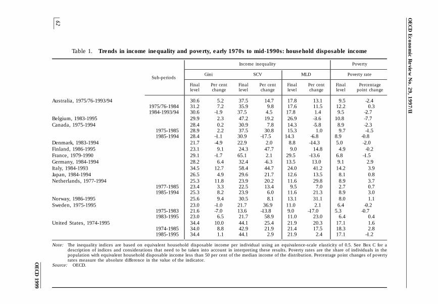
Three widely used inequality indices are presented in the first three columnsof the top panel of Table 1 – the Gini coefficient, the mean log deviation(MLD) index and the squared coefficient of variation (SCV) – to describe changes inthe distribution of equivalent household disposable income (see Box C for furtherdescription of the main features of these indexes). Increases in all three inequalityindices occurred in four of the five countries for which data were available from themid-1970s to the mid-1980s. Over the period from the mid-1980s to the mid-1990s,the indices show a fairly clear increase in seven of the 13 countries shown. For theother six countries, there was no clear trend: either changes in the Gini coefficientwere clustered around zero and/or the different indices point in different direc-tions. In Australia, Canada and, particularly, Sweden, the movements in the earlierperiod (declines in Australia and Sweden, increases in Canada) tended to be offsetin the second, such that inequality changed little over the two decades.
02_chap.fm Page 61 Monday, May 3, 1999 4:53 PM
OE
CD
Eco
no
mic R
evie
w N
o. 2
9, 1
99
7/II
62
OE
CD
1999
Table 1. Trends in income inequality and poverty, early 1970s to mid-1990s: household disposable income
Income inequality Poverty
Gini SCV MLD Poverty rateSub-periods
Final Per cent Final Per cent Final Per cent Final Percentagelevel change level change level change level point change
Australia, 1975/76-1993/94 30.6 5.2 37.5 14.7 17.8 13.1 9.5 –2.41975/76-1984 31.2 7.2 35.9 9.8 17.6 11.5 12.2 0.31984-1993/94 30.6 –1.9 37.5 4.5 17.8 1.4 9.5 –2.7
Belgium, 1983-1995 29.9 2.3 47.2 19.2 26.9 –3.6 10.8 –7.7Canada, 1975-1994 28.4 0.2 30.9 7.8 14.3 –5.8 8.9 –2.3
1975-1985 28.9 2.2 37.5 30.8 15.3 1.0 9.7 –1.51985-1994 28.4 –1.1 30.9 –17.5 14.3 –6.8 8.9 –0.8
Denmark, 1983-1994 21.7 –4.9 22.9 2.0 8.8 –14.3 5.0 –2.0Finland, 1986-1995 23.1 9.1 24.3 47.7 9.0 14.8 4.9 –0.2France, 1979-1990 29.1 –1.7 65.1 2.1 29.5 –13.6 6.8 –1.5Germany, 1984-1994 28.2 6.4 32.4 –6.3 13.5 13.0 9.1 2.9Italy, 1984-1993 34.5 12.7 58.4 44.7 24.0 41.2 14.2 3.9Japan, 1984-1994 26.5 4.9 29.6 21.7 12.6 13.5 8.1 0.8Netherlands, 1977-1994 25.3 11.8 23.9 20.2 11.6 29.8 8.9 3.7
1977-1985 23.4 3.3 22.5 13.4 9.5 7.0 2.7 0.71985-1994 25.3 8.2 23.9 6.0 11.6 21.3 8.9 3.0
Norway, 1986-1995 25.6 9.4 30.5 8.1 13.1 31.1 8.0 1.1Sweden, 1975-1995 23.0 –1.0 21.7 36.9 11.0 2.1 6.4 –0.2
1975-1983 21.6 –7.0 13.6 –13.8 9.0 –17.0 5.3 –0.71983-1995 23.0 6.5 21.7 58.9 11.0 23.0 6.4 0.4
United States, 1974-1995 34.4 10.0 44.1 25.4 21.9 20.3 17.1 1.61974-1985 34.0 8.8 42.9 21.9 21.4 17.5 18.3 2.81985-1995 34.4 1.1 44.1 2.9 21.9 2.4 17.1 –1.2
Note: The inequality indices are based on equivalent household disposable income per individual using an equivalence-scale elasticity of 0.5. See Box C for adescription of indices and considerations that need to be taken into account in interpreting these results. Poverty rates are the share of individuals in thepopulation with equivalent household disposable income less than 50 per cent of the median income of the distribution. Percentage point changes of povertyrates measure the absolute difference in the value of the indicator.
Source: OECD.
02_chap.fm P
age 62 Monday, M
ay 3, 1999 4:53 PM
Income Distribution and Poverty in 13 OECD Countries
63
OECD 1999
The poverty rate (Table 1, right-hand column) – defined as the proportion ofindividuals falling below one half of median equivalent household disposableincome10 – rose in two of the five countries for which data are available since themid-1970s, and in six of the 13 for which data are available since the mid-1980s.11
Thus, while income distribution has widened and poverty rates increased insome countries, these trends are not common to all countries. The nexttwo sections describe some of the sources for these differences, using the longestavailable time period for all countries.
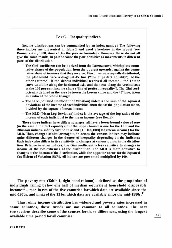
Box C. Inequality indices
Income distributions can be summarised by an index number. The followingthree indices are presented in Table 1 and used elsewhere in the report (seeBurniaux et al., 1988, Annex 1 for the precise formulae). However, these do not allgive the same results, in part because they are sensitive to movements in differentparts of the distribution.
– The Gini coefficient can be derived from the Lorenz curve, which plots cumu-lative shares of the population, from the poorest upwards, against the cumu-lative share of incomes that they receive. If incomes were equally distributed,the plot would trace a diagonal 45° line (“ line of perfect equality” ). At theother extreme – if the richest individual received all income – the Lorenzcurve would lie along the horizontal axis, and then rise along the vertical axisat the 100 per cent income share (“ line of perfect inequality” ). The Gini coef-ficient is defined as the area between the Lorenz curve and the 45° line, takenas a ratio of the whole triangle.
– The SCV (Squared Coefficient of Variation) index is the sum of the squareddeviations of the income of each individual from that of the population mean,divided by the square of mean income.
– The MLD (Mean Log Deviation) index is the average of the log ratios of theincome of each individual to the mean income (see Box E).
These three indices have different ranges: all have a lower bound value of zero(in the case of perfect equality), but the upper bound is one for the Gini and theAtkinson indices, infinity for the SCV and [1 + log(100)] log (mean income) for theMLD. Thus, changes of similar magnitude across the various indices may indicatequite different changes in the degree of inequality depending on the indicator.Each index also differs in its sensitivity to changes at various points in the distribu-tion. Relative to other indices, the Gini coefficient is less sensitive to changes inincome at the two extremes of the distribution. The MLD is more sensitive tochanges at the bottom of the distribution, while the opposite occurs for the SquaredCoefficient of Variation (SCV). All indices are presented multiplied by 100.
02_chap.fm Page 63 Monday, May 3, 1999 4:53 PM
OECD Economic Review No. 29, 1997/II
64
OECD 1999
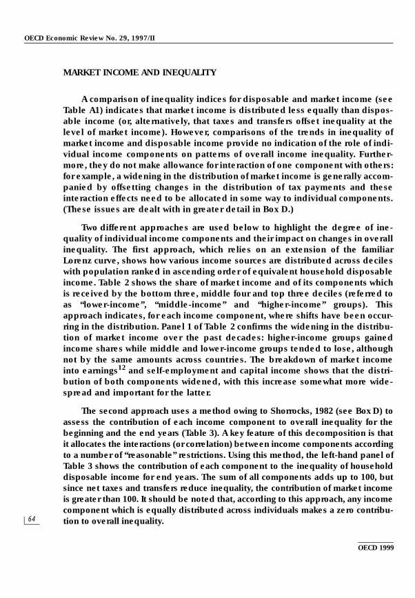
MARKET INCOME AND INEQUALITY
A comparison of inequality indices for disposable and market income (seeTable A1) indicates that market income is distributed less equally than dispos-able income (or, alternatively, that taxes and transfers offset inequality at thelevel of market income). However, comparisons of the trends in inequality ofmarket income and disposable income provide no indication of the role of indi-vidual income components on patterns of overall income inequality. Further-more, they do not make allowance for interaction of one component with others:for example, a widening in the distribution of market income is generally accom-panied by offsetting changes in the distribution of tax payments and theseinteraction effects need to be allocated in some way to individual components.(These issues are dealt with in greater detail in Box D.)
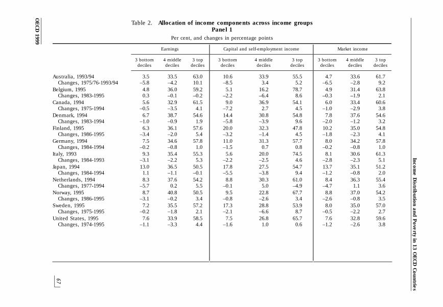
Two different approaches are used below to highlight the degree of ine-quality of individual income components and their impact on changes in overallinequality. The first approach, which relies on an extension of the familiarLorenz curve, shows how various income sources are distributed across decileswith population ranked in ascending order of equivalent household disposableincome. Table 2 shows the share of market income and of its components whichis received by the bottom three, middle four and top three deciles (referred toas “ lower-income” , “ middle-income” and “ higher-income” groups). Thisapproach indicates, for each income component, where shifts have been occur-ring in the distribution. Panel 1 of Table 2 confirms the widening in the distribu-tion of market income over the past decades: higher-income groups gainedincome shares while middle and lower-income groups tended to lose, althoughnot by the same amounts across countries. The breakdown of market incomeinto earnings12 and self-employment and capital income shows that the distri-bution of both components widened, with this increase somewhat more wide-spread and important for the latter.
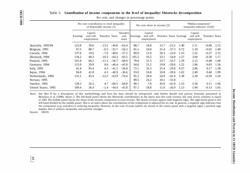
The second approach uses a method owing to Shorrocks, 1982 (see Box D) toassess the contribution of each income component to overall inequality for thebeginning and the end years (Table 3). A key feature of this decomposition is thatit allocates the interactions (or correlation) between income components accordingto a number of “ reasonable” restrictions. Using this method, the left-hand panel ofTable 3 shows the contribution of each component to the inequality of householddisposable income for end years. The sum of all components adds up to 100, butsince net taxes and transfers reduce inequality, the contribution of market incomeis greater than 100. It should be noted that, according to this approach, any incomecomponent which is equally distributed across individuals makes a zero contribu-tion to overall inequality.
02_chap.fm Page 64 Monday, May 3, 1999 4:53 PM
Income Distribution and Poverty in 13 OECD Countries
65
OECD 1999
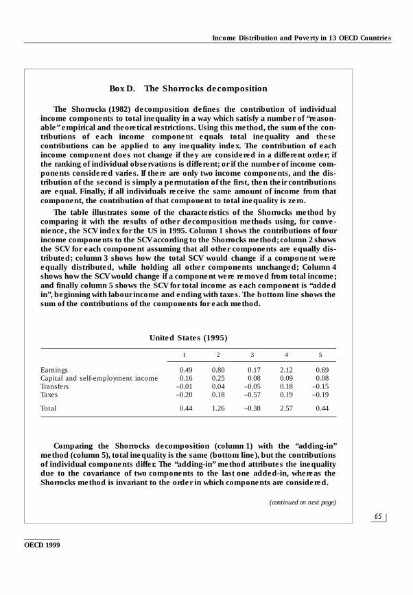
Box D. The Shorrocks decomposition
The Shorrocks (1982) decomposition defines the contribution of individualincome components to total inequality in a way which satisfy a number of “ reason-able” empirical and theoretical restrictions. Using this method, the sum of the con-tributions of each income component equals total inequality and thesecontributions can be applied to any inequality index. The contribution of eachincome component does not change if they are considered in a different order; ifthe ranking of individual observations is different; or if the number of income com-ponents considered varies. If there are only two income components, and the dis-tribution of the second is simply a permutation of the first, then their contributionsare equal. Finally, if all individuals receive the same amount of income from thatcomponent, the contribution of that component to total inequality is zero.
The table illustrates some of the characteristics of the Shorrocks method bycomparing it with the results of other decomposition methods using, for conve-nience, the SCV index for the US in 1995. Column 1 shows the contributions of fourincome components to the SCV according to the Shorrocks method; column 2 showsthe SCV for each component assuming that all other components are equally dis-tributed; column 3 shows how the total SCV would change if a component wereequally distributed, while holding all other components unchanged; Column 4shows how the SCV would change if a component were removed from total income;and finally column 5 shows the SCV for total income as each component is “ addedin” , beginning with labour income and ending with taxes. The bottom line shows thesum of the contributions of the components for each method.
Comparing the Shorrocks decomposition (column 1) with the “ adding-in”method (column 5), total inequality is the same (bottom line), but the contributionsof individual components differ. The “ adding-in” method attributes the inequalitydue to the covariance of two components to the last one added-in, whereas theShorrocks method is invariant to the order in which components are considered.
(continued on next page)
United States (1995)
1 2 3 4 5
Earnings 0.49 0.80 0.17 2.12 0.69Capital and self-employment income 0.16 0.25 0.08 0.09 0.08Transfers – 0.01 0.04 – 0.05 0.18 – 0.15Taxes – 0.20 0.18 – 0.57 0.19 – 0.19
Total 0.44 1.26 – 0.38 2.57 0.44
02_chap.fm Page 65 Monday, May 3, 1999 4:53 PM
OECD Economic Review No. 29, 1997/II
66
OECD 1999
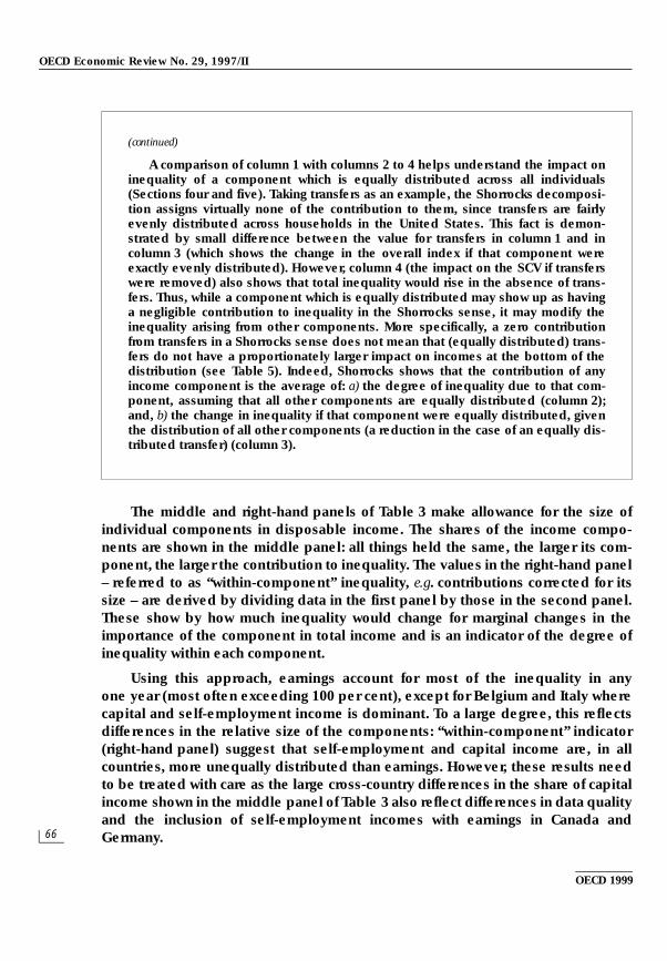
The middle and right-hand panels of Table 3 make allowance for the size ofindividual components in disposable income. The shares of the income compo-nents are shown in the middle panel: all things held the same, the larger its com-ponent, the larger the contribution to inequality. The values in the right-hand panel– referred to as “ within-component” inequality, e.g. contributions corrected for itssize – are derived by dividing data in the first panel by those in the second panel.These show by how much inequality would change for marginal changes in theimportance of the component in total income and is an indicator of the degree ofinequality within each component.
Using this approach, earnings account for most of the inequality in anyone year (most often exceeding 100 per cent), except for Belgium and Italy wherecapital and self-employment income is dominant. To a large degree, this reflectsdifferences in the relative size of the components: “ within-component” indicator(right-hand panel) suggest that self-employment and capital income are, in allcountries, more unequally distributed than earnings. However, these results needto be treated with care as the large cross-country differences in the share of capitalincome shown in the middle panel of Table 3 also reflect differences in data qualityand the inclusion of self-employment incomes with earnings in Canada andGermany.
(continued)
A comparison of column 1 with columns 2 to 4 helps understand the impact oninequality of a component which is equally distributed across all individuals(Sections four and five). Taking transfers as an example, the Shorrocks decomposi-tion assigns virtually none of the contribution to them, since transfers are fairlyevenly distributed across households in the United States. This fact is demon-strated by small difference between the value for transfers in column 1 and incolumn 3 (which shows the change in the overall index if that component wereexactly evenly distributed). However, column 4 (the impact on the SCV if transferswere removed) also shows that total inequality would rise in the absence of trans-fers. Thus, while a component which is equally distributed may show up as havinga negligible contribution to inequality in the Shorrocks sense, it may modify theinequality arising from other components. More specifically, a zero contributionfrom transfers in a Shorrocks sense does not mean that (equally distributed) trans-fers do not have a proportionately larger impact on incomes at the bottom of thedistribution (see Table 5). Indeed, Shorrocks shows that the contribution of anyincome component is the average of: a) the degree of inequality due to that com-ponent, assuming that all other components are equally distributed (column 2);and, b) the change in inequality if that component were equally distributed, giventhe distribution of all other components (a reduction in the case of an equally dis-tributed transfer) (column 3).
02_chap.fm Page 66 Monday, May 3, 1999 4:53 PM
Inco
me
Distrib
utio
n a
nd
Po
verty in
13
OE
CD
Co
un
tries
67
OE
CD
1999
Table 2. Allocation of income components across income groupsPanel 1
Per cent, and changes in percentage points
Earnings Capital and self-employment income Market income
3 bottom 4 middle 3 top 3 bottom 4 middle 3 top 3 bottom 4 middle 3 topdeciles deciles deciles deciles deciles deciles deciles deciles deciles
Australia, 1993/94 3.5 33.5 63.0 10.6 33.9 55.5 4.7 33.6 61.7Changes, 1975/76-1993/94 – 5.8 – 4.2 10.1 – 8.5 3.4 5.2 – 6.5 – 2.8 9.2
Belgium, 1995 4.8 36.0 59.2 5.1 16.2 78.7 4.9 31.4 63.8Changes, 1983-1995 0.3 – 0.1 – 0.2 – 2.2 – 6.4 8.6 – 0.3 – 1.9 2.1
Canada, 1994 5.6 32.9 61.5 9.0 36.9 54.1 6.0 33.4 60.6Changes, 1975-1994 – 0.5 – 3.5 4.1 – 7.2 2.7 4.5 – 1.0 – 2.9 3.8
Denmark, 1994 6.7 38.7 54.6 14.4 30.8 54.8 7.8 37.6 54.6Changes, 1983-1994 – 1.0 – 0.9 1.9 – 5.8 – 3.9 9.6 – 2.0 – 1.2 3.2
Finland, 1995 6.3 36.1 57.6 20.0 32.3 47.8 10.2 35.0 54.8Changes, 1986-1995 – 3.4 – 2.0 5.4 – 3.2 – 1.4 4.5 – 1.8 – 2.3 4.1
Germany, 1994 7.5 34.6 57.8 11.0 31.3 57.7 8.0 34.2 57.8Changes, 1984-1994 – 0.2 – 0.8 1.0 – 1.5 0.7 0.8 – 0.2 – 0.8 1.0
Italy, 1993 9.3 35.4 55.3 5.6 20.0 74.5 8.1 30.6 61.3Changes, 1984-1993 – 3.1 – 2.2 5.3 – 2.2 – 2.5 4.6 – 2.8 – 2.3 5.1
Japan, 1994 13.0 36.5 50.5 17.8 27.5 54.7 13.7 35.1 51.2Changes, 1984-1994 1.1 – 1.1 – 0.1 – 5.5 – 3.8 9.4 – 1.2 – 0.8 2.0
Netherlands, 1994 8.3 37.6 54.2 8.8 30.3 61.0 8.4 36.3 55.4Changes, 1977-1994 – 5.7 0.2 5.5 – 0.1 5.0 – 4.9 – 4.7 1.1 3.6
Norway, 1995 8.7 40.8 50.5 9.5 22.8 67.7 8.8 37.0 54.2Changes, 1986-1995 – 3.1 – 0.2 3.4 – 0.8 – 2.6 3.4 – 2.6 – 0.8 3.5
Sweden, 1995 7.2 35.5 57.2 17.3 28.8 53.9 8.0 35.0 57.0Changes, 1975-1995 – 0.2 – 1.8 2.1 – 2.1 – 6.6 8.7 – 0.5 – 2.2 2.7
United States, 1995 7.6 33.9 58.5 7.5 26.8 65.7 7.6 32.8 59.6Changes, 1974-1995 – 1.1 – 3.3 4.4 – 1.6 1.0 0.6 – 1.2 – 2.6 3.8
02_chap.fm P
age 67 Monday, M
ay 3, 1999 4:53 PM
OE
CD
Eco
no
mic R
evie
w N
o. 2
9, 1
99
7/II
68
OE
CD
1999
Table 2. Allocation of income components across income groups (cont.)Panel 2
Per cent, and changes in percentage points
Transfers Taxes Disposable income
3 bottom 4 middle 3 top 3 bottom 4 middle 3 top 3 bottom 4 middle 3 topdeciles deciles deciles deciles deciles deciles deciles deciles deciles
Australia, 1993/94 58.1 34.6 7.4 1.9 27.8 70.4 13.8 35.1 51.1Changes, 1975/76-1993/94 1.1 5.2 – 6.3 – 7.9 – 6.0 13.9 – 0.4 – 1.0 1.4
Belgium, 1995 30.0 45.7 24.3 2.1 29.3 68.6 13.8 36.6 49.6Changes, 1983-1995 0.0 1.2 – 1.2 – 1.5 0.6 0.9 0.5 – 1.7 1.1
Canada, 1994 41.7 41.0 17.3 2.9 29.2 67.9 14.0 35.9 50.1Changes, 1975-1994 – 7.6 7.2 0.4 – 0.7 – 2.0 2.7 1.2 – 0.9 – 0.4
Denmark, 1994 45.8 37.5 16.7 12.7 36.5 50.8 17.6 38.2 44.2Changes, 1983-1994 3.8 – 1.1 – 2.7 2.1 – 3.0 0.9 0.8 – 0.2 – 0.6
Finland, 1995 39.8 41.4 18.7 9.5 32.9 57.6 17.5 37.2 45.3Changes, 1986-1995 2.4 4.4 – 6.8 0.3 – 1.1 0.8 – 0.6 – 1.2 1.7
Germany, 1994 38.6 40.1 21.3 5.3 31.7 62.9 14.8 36.1 49.1Changes, 1984-1994 – 5.0 4.9 0.1 – 0.5 0.4 0.1 – 1.1 – 0.1 1.2
Italy, 1993 20.8 44.7 34.5 5.8 29.8 64.4 12.1 34.4 53.5Changes, 1984-1993 – 5.8 0.8 5.1 – 4.8 – 2.3 7.1 – 1.9 – 0.7 2.6
Japan, 1994 27.5 37.5 35.0 11.3 29.7 59.0 15.7 36.5 47.8Changes, 1984-1994 – 0.5 4.8 – 4.2 – 1.3 – 1.2 2.4 – 0.6 – 0.2 0.8
Netherlands, 1994 43.6 35.7 20.7 10.7 34.5 54.7 16.2 36.8 47.0Changes, 1977-1994 10.0 – 2.5 – 7.5 – 2.2 0.7 1.5 – 1.6 0.4 1.2
Norway, 1995 47.7 35.3 17.0 8.3 35.4 56.3 16.0 37.2 46.8Changes, 1986-1995 2.3 – 0.9 – 1.4 – 1.8 – 2.4 4.2 – 1.0 – 0.4 1.4
Sweden, 1995 31.4 41.4 27.2 10.7 34.8 54.4 17.2 37.9 44.9Changes, 1975-1995 – 8.3 5.9 2.4 3.5 1.2 – 4.7 0.3 – 0.1 – 0.2
United States, 1995 37.2 38.2 24.6 5.2 26.5 68.2 11.5 35.0 53.5Changes, 1974-1995 – 6.8 3.8 3.0 0.3 – 3.7 3.5 – 1.2 – 1.4 2.6
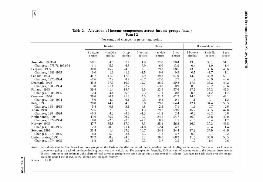
Note: Individuals were broken down into three groups on the basis of the distribution of their equivalent household disposable income. The share of each incomecomponent going to each of the three decile groups was then calculated. For example, for Australia, 13.5 per cent of income went to the bottom three incomedeciles (third from last columns). The share of total earnings going to the same group was 3.5 per cent (first column). Changes for each share over the longestavailable period are shown in the second line for each country.
Source: OECD.
02_chap.fm P
age 68 Monday, M
ay 3, 1999 4:53 PM
Inco
me
Distrib
utio
n a
nd
Po
verty in
13
OE
CD
Co
un
tries
69
OE
CD
1999
Table 3. Contribution of income components to the level of inequality: Shorrocks decompositionPer cent, and changes in percentage points
Per cent contribution to total inequality ‘‘Within-component’’Per cent share in income [2]
of disposable income [1] inequality indicator [1]/[2]
Capital Transfers Capital CapitalEarnings and self- Transfers Taxes and Earnings and self- Transfers Taxes Earnings and self- Transfers Taxes
employment taxes employment employment
Australia, 1993/94 123.8 39.6 –13.5 –49.8 –63.4 88.7 18.8 15.7 –23.2 1.40 2.11 –0.86 2.15Belgium, 1995 67.5 88.7 –0.5 –55.7 –56.2 81.1 24.8 31.4 –37.3 0.72 1.19 –0.02 1.49Canada, 1994 137.6 19.6 –7.6 –49.6 –57.2 89.9 12.9 20.3 –23.0 1.53 1.52 –0.37 2.15Denmark, 1994 134.2 49.3 –19.3 –64.3 –83.5 105.3 16.5 33.1 –54.8 1.27 3.00 –0.58 1.17Finland, 1995 101.8 66.2 –11.3 –56.7 –68.0 78.8 31.3 23.7 –33.7 1.29 2.12 –0.48 1.68Germany, 1994 115.9 29.9 0.6 –46.4 –45.8 94.6 15.2 19.8 –29.6 1.22 1.96 0.03 1.56Italy, 1993 41.4 95.4 4.3 –41.1 –36.8 72.1 32.3 25.4 –29.8 0.57 2.96 0.17 1.38Japan, 1994 94.8 41.8 4.3 –40.9 –36.6 93.0 16.8 10.8 –20.6 1.02 2.49 0.40 1.99Netherlands, 1994 131.1 45.4 –12.5 –63.9 –76.4 95.3 20.8 24.9 –41.0 1.38 2.18 –0.50 1.56Norway, 1995 . . . . . . . . . . 89.5 24.2 18.1 –31.8 . . . . . . . .Sweden, 1995 138.3 26.5 4.7 –69.5 –64.8 90.1 7.8 43.9 –41.8 1.53 3.39 0.11 1.66United States, 1995 109.4 36.4 –1.4 –44.4 –45.8 97.1 18.8 11.0 –26.9 1.13 1.94 –0.13 1.65
Note: See Box D for a description of this methodology and how the data should be interpreted, with further details and precise formulae presented inBurniaux et al. (1998), Annex 2. The left-hand panel shows the Shorrocks contributions in the latest year (for each country, the sum across columns is equalto 100). The middle panel shows the share of the income component in total income. The shares of taxes appear with negative signs. The right-hand panel is theleft-hand divided by the middle panel. This is an index where the contribution of the component is adjusted for its size. In general, a negative sign indicates thatthe component (e.g. transfers) is reducing inequality. However, in the case of taxes (which are shown in the centre panel with a negative sign), a positive signimplies that it reduces inequality and positive changes.
Source: OECD.
02_chap.fm P
age 69 Monday, M
ay 3, 1999 4:53 PM
OECD Economic Review No. 29, 1997/II
70
OECD 1999
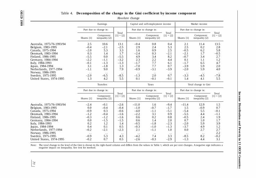
Table 4 uses the information in Table 3 (and equivalent data for the beginningof the period) to calculate an estimate of the “ contribution” of each income compo-nent to the change in total inequality, as measured by the Gini coefficient:13
The data shown in Table 4 are derived as follows:
– First, the Gini coefficient for the beginning and end years are multiplied bythe contributions in the left-hand panel of Table 3. The change in these val-ues over the period (Table 4, third column for each panel) indicates by howmuch the Gini coefficient would have changed if each component is consid-ered independently – i.e. for Australia, the third column shows that earningswould have led to an increase in the Gini coefficient of 13.1 percentagepoints if there had been no changes in the other components.
– Second, using the middle and right-hand panels of Table 3, the impact foreach component (Table 4, third column for each panel) is then decom-posed, using a shift-share approach, into the effect of: a) changes in the shareof each component in total income, holding the “ within-component” ine-quality constant over the period (Table 4, first column for each component);and b) changes in the “ component-specific” inequality (second column)over the period, holding the shares constant. Thus, the first andsecond columns for Australia indicate that a change in the share of earnings,considered alone, would have increased the Gini coefficient by2.5 percentage points, while the change in the “ within-component” inequal-ity would have increased the Gini by 10.6 points.
Table 4 indicates a complex picture with considerable cross-country variation:
– Market income has been the most important factor driving the change in thedistribution of disposable income over the last one to two decades. Thecontribution of market income increased inequality in all countries exceptDenmark and, more notably, Sweden. If only changes in market income wereconsidered, the Gini would have increased by more (or fallen by more in thecase of a decline) than it actually did, in all countries except Denmark.
– In over half the countries, the declining share of market income in totalincome has tended to reduce inequality.
– While measurement problems are important for a number of countries, cap-ital and self-employment income led to a (sometimes substantial) wideningin the distribution of disposable income in all countries except Denmarkand the Netherlands and, to a much lesser degree, the United States.
– Finally, earnings, considered on its own, contributed to a narrowing in thedistribution of income in six of the 13 countries covered. Earnings made alarge positive contribution to the overall change in the Gini only in Australia,the Netherlands and the United States.
02_chap.fm Page 70 Monday, May 3, 1999 4:53 PM
Inco
me
Distrib
utio
n a
nd
Po
verty in
13
OE
CD
Co
un
tries
71
OE
CD
1999
Table 4. Decomposition of the change in the Gini coefficient by income componentAbsolute change
Earnings Capital and self-employment income Market income
Part due to change in: Part due to change in: Part due to change in:Total Total Total
Component Component Component[1] + [2] [1] + [2] [1] + [2]Shares [1] inequality [2] Shares [1] inequality [2] Shares [1] inequality [2]
Australia, 1975/76-1993/94 2.5 10.6 13.1 –0.4 0.8 0.4 2.1 11.4 13.5Belgium, 1983-1995 –0.4 –2.1 –2.5 2.9 2.4 5.3 2.5 0.2 2.8Canada, 1975-1994 –2.0 5.3 3.3 1.6 0.9 2.5 –0.5 6.2 5.8Denmark, 1983-1994 0.3 1.4 1.7 –2.4 0.3 –2.1 –2.1 1.7 –0.5Finland, 1986-1995 –5.5 0.0 –5.5 4.9 3.4 8.2 –0.7 3.4 2.7Germany, 1984-1994 –2.2 –1.1 –3.2 2.3 2.2 4.4 0.1 1.1 1.2Italy, 1984-1993 –0.1 –1.3 –1.3 –1.7 7.7 6.1 –1.7 6.5 4.7Japan, 1984-1994 3.1 –1.8 1.3 –7.0 7.7 0.7 –3.9 5.9 2.0Netherlands, 1977-1994 –1.1 9.0 7.9 –0.9 –3.1 –3.9 –2.0 5.9 4.0Norway, 1986-1995 . . . . . . . . . . . . . . . . . .Sweden, 1975-1995 –2.0 –6.5 –8.5 –1.3 2.0 0.7 –3.3 –4.5 –7.8United States, 1974-1995 1.3 4.2 5.5 0.1 –0.1 –0.1 1.4 4.1 5.5
Transfers Taxes Total change in Gini
Part due to change in: Part due to change in: Part due to change in:Total Total Total
Component Component Component[1] + [2] [1] + [2] [1] + [2]Shares [1] inequality [2] Shares [1] inequality [2] Shares [1] inequality [2]
Australia, 1975/76-1993/94 –2.4 –0.1 –2.6 –11.0 1.6 –9.4 –11.4 12.9 1.5Belgium, 1983-1995 0.0 –0.4 –0.4 –1.0 –0.7 –1.7 1.5 –0.9 0.7Canada, 1975-1994 –0.9 0.3 –0.6 –4.0 –1.1 –5.1 –5.4 5.5 –0.1Denmark, 1983-1994 –1.2 –0.4 –1.6 –2.2 3.1 0.9 –5.5 4.4 –1.1Finland, 1986-1995 –0.3 –1.2 –1.6 0.6 0.2 0.8 –0.5 2.4 1.9Germany, 1984-1994 0.0 –1.5 –1.5 0.6 1.4 2.0 0.7 1.0 1.7Italy, 1984-1993 0.2 1.2 1.4 –0.5 –1.8 –2.3 –2.0 5.9 3.9Japan, 1984-1994 0.4 0.1 0.5 –0.3 –1.0 –1.3 –3.7 4.9 1.2Netherlands, 1977-1994 –0.2 –2.1 –2.3 2.1 –1.1 1.0 0.0 2.7 2.7Norway, 1986-1995 . . . . . . . . . . . . . . . . 2.2Sweden, 1975-1995 –0.9 5.3 4.3 –4.2 7.4 3.3 –8.5 8.2 –0.2United States, 1974-1995 –0.2 0.7 0.5 –2.6 –0.3 –2.9 –1.3 4.4 3.1
Note: The total change in the level of the Gini is shown in the right-hand column and differs from the values in Table 1, which are per cent changes. A negative sign indicates anegative impact on inequality. See text for method.
02_chap.fm P
age 71 Monday, M
ay 3, 1999 4:53 PM
OECD Economic Review No. 29, 1997/II
72
OECD 1999
There has been a considerable debate over the role of earnings (more specif-ically, of full-time earnings differentials) on the changing distribution of income.Other OECD findings (OECD, 1993 and OECD, 1996a) have pointed to a widespreadwidening across countries in the distribution of full-time earnings which are used asa proxy for the wage-rate distribution. But the relation between the distribution offull-time earnings (at the level of individuals) and that of earnings (at the level ofhouseholds) is a complex one. First, at the level of individual workers, changes inhours worked can account for part of the widening in the distribution of full-timeearnings. Second, and more important, changes in the distribution of earningsacross households, as measured in this study, also depend on the distribution ofemployment. For example, Burniaux (1998) finds that increased labour-market par-ticipation among women in the 1980s mainly occurred in households with averageor above-average incomes; as a result, the increase in women’s employment intwo-earner households led to a widening of inequalities. This effect has sometimesbeen magnified (most notably in the United States) by an increased correlationbetween spouses’ earnings (e.g. more high earners living in the same household).At the same time, the increase in the share of no-worker (i.e. zero earnings) house-holds in many countries (Gregg and Wadsworth, 1996) may also have played animportant role in driving changes in income distribution over the past two decades.While these issues will be further elaborated below, the impact of taxes and trans-fers is examined first.
THE DISTRIBUTIONAL IMPACT OF THE TAX-AND-TRANSFER SYSTEM
Tables 2 to 4 may also be used to illustrate the extent to which the redistribu-tive impact of tax-and-transfer systems has modified the trends found at the levelof market income. Table 2, which shows the distribution of taxes and transfersacross deciles, indicates that public transfers do not appear to be heavily targetedtowards lower-income groups, except in Australia. In seven of the twelve countries,the share of transfers received by the middle four deciles is close to or above theirshare in the total population, while in Italy and Japan, more transfers are receivedby the top three deciles than by the bottom three. When looking at changes in thedistribution of public transfers, the share received by the lower-income groups hasfallen over time (or remained broadly stable) in seven countries, while that goingto the middle-income groups and upper-income groups has risen (or remained sta-ble) in nine and five countries, respectively. In contrast, taxes appear to be muchmore concentrated on the higher income groups: the top three deciles pay consid-erably more than their share in the total population, while the middle four and, par-ticularly, the bottom three pay less.14 As the distribution of market income haswidened, this pattern has become more accentuated.
02_chap.fm Page 72 Monday, May 3, 1999 4:53 PM
Income Distribution and Poverty in 13 OECD Countries
73
OECD 1999
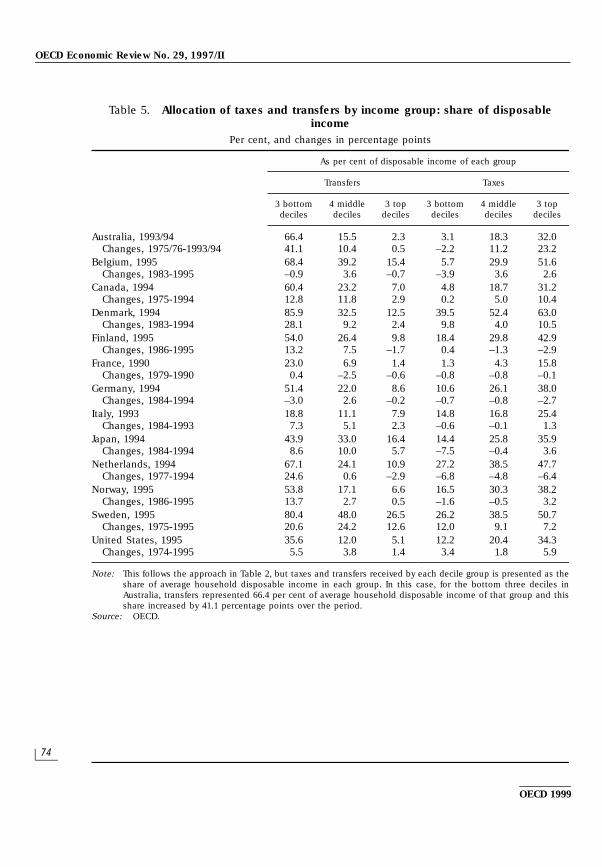
A different perspective is presented in Table 5, which shows taxes and trans-fers for the same three decile groups, but as a share of average income in eachdecile group. This shows that transfers make up a large share of disposable incomein the bottom three deciles, becoming progressively smaller in the middle andhigher-income groups. The opposite is the case for taxes. Seen from this perspec-tive, the tax-and-transfer system appears to have become more progressive overtime. Transfers as a share of disposable income increased substantially forlower-income groups in all countries except Belgium and Germany. At the sametime, the share of taxes in income increased for the upper deciles, while theincrease for the middle-income groups has been smaller and less widespread.15
Taken together, these patterns suggest a significant shift in income structure inthe bottom three deciles away from market income and towards greater depen-dence on transfer income. Even though the share of transfers going to the bottomthree deciles has declined in a number of countries (Table 2), transfers nonethelessmake up an increasing share of total income of these households in all countriesexcept Germany (Table 5). Further evidence (not shown) indicates that this shift hasbeen accompanied by an increase in the share of individuals in the bottomthree deciles, who belong to non-working households. Increasing retirement and,in certain countries, higher unemployment combined with a less equal distributionof employment opportunities account for this shift.
The Shorrocks analysis (Table 3) shows that taxes and transfers, taken together,reduced inequality in the latest year in all countries. Transfers, taken alone, reducedinequality in all but four countries (Germany, Italy, Japan and Sweden) but, generally,its impact was small relative to taxes. This result partly reflected the effect of size –taxes are larger than transfers (middle panel) – but also the fact that a larger share oftaxes are paid by upper-income groups – i.e. that taxes are less equally distributedacross households (right-hand panel) than transfers. As noted (Box D), a componentdoes not contribute to inequality in the Shorrocks sense if it is equally shared by allindividuals. But even a small Shorrocks contribution from transfers is still consistentwith transfers having a proportionately larger impact on the incomes of those at the bot-tom of the distribution of market income. As is shown in Table 5, transfers have madeup a larger share of the (lower) income of these households.
Turning to Table 4 (impact on the change in the Gini coefficient), taxes andtransfers taken together reduced inequality in all countries except Sweden and,possibly, Germany, offsetting the effect of growing inequality in market incomes. Ina majority of countries, the increasing shares of taxes or transfers taken togetherexplain much of this development with no consistent cross-country pattern in termsof the relative importance of the two components.16 In certain countries, taxes andtransfers taken individually contributed to some widening in inequality on aShorrocks basis.
02_chap.fm Page 73 Monday, May 3, 1999 4:53 PM
OECD Economic Review No. 29, 1997/II
74
OECD 1999
Table 5. Allocation of taxes and transfers by income group: share of disposableincome
Per cent, and changes in percentage points
As per cent of disposable income of each group
Transfers Taxes
3 bottom 4 middle 3 top 3 bottom 4 middle 3 topdeciles deciles deciles deciles deciles deciles
Australia, 1993/94 66.4 15.5 2.3 3.1 18.3 32.0Changes, 1975/76-1993/94 41.1 10.4 0.5 –2.2 11.2 23.2
Belgium, 1995 68.4 39.2 15.4 5.7 29.9 51.6Changes, 1983-1995 –0.9 3.6 –0.7 –3.9 3.6 2.6
Canada, 1994 60.4 23.2 7.0 4.8 18.7 31.2Changes, 1975-1994 12.8 11.8 2.9 0.2 5.0 10.4
Denmark, 1994 85.9 32.5 12.5 39.5 52.4 63.0Changes, 1983-1994 28.1 9.2 2.4 9.8 4.0 10.5
Finland, 1995 54.0 26.4 9.8 18.4 29.8 42.9Changes, 1986-1995 13.2 7.5 –1.7 0.4 –1.3 –2.9
France, 1990 23.0 6.9 1.4 1.3 4.3 15.8Changes, 1979-1990 0.4 –2.5 –0.6 –0.8 –0.8 –0.1
Germany, 1994 51.4 22.0 8.6 10.6 26.1 38.0Changes, 1984-1994 –3.0 2.6 –0.2 –0.7 –0.8 –2.7
Italy, 1993 18.8 11.1 7.9 14.8 16.8 25.4Changes, 1984-1993 7.3 5.1 2.3 –0.6 –0.1 1.3
Japan, 1994 43.9 33.0 16.4 14.4 25.8 35.9Changes, 1984-1994 8.6 10.0 5.7 –7.5 –0.4 3.6
Netherlands, 1994 67.1 24.1 10.9 27.2 38.5 47.7Changes, 1977-1994 24.6 0.6 –2.9 –6.8 –4.8 –6.4
Norway, 1995 53.8 17.1 6.6 16.5 30.3 38.2Changes, 1986-1995 13.7 2.7 0.5 –1.6 –0.5 3.2
Sweden, 1995 80.4 48.0 26.5 26.2 38.5 50.7Changes, 1975-1995 20.6 24.2 12.6 12.0 9.1 7.2
United States, 1995 35.6 12.0 5.1 12.2 20.4 34.3Changes, 1974-1995 5.5 3.8 1.4 3.4 1.8 5.9
Note: This follows the approach in Table 2, but taxes and transfers received by each decile group is presented as theshare of average household disposable income in each group. In this case, for the bottom three deciles inAustralia, transfers represented 66.4 per cent of average household disposable income of that group and thisshare increased by 41.1 percentage points over the period.
Source: OECD.
02_chap.fm Page 74 Monday, May 3, 1999 4:53 PM
Inco
me
Distrib
utio
n a
nd
Po
verty in
13
OE
CD
Co
un
tries
75
OE
CD
1999
Table 6. Poverty rates before and after taxes and transfers for five countriesPer cent and changes in percentage points
Before taxes and transfers
By employmentBy age of household head2 By family type3
status1
TotalSingle Single TwoYoung Prime-age Older-age Retired Two adults,
No worker Workers adult with adult, adults withhousehold household household household no children
children no children children
Canada, 1991 70.8 12.7 27.9 15.5 18.5 57.4 67.4 46.3 15.5 20.4 22.9Changes, 1975-1991 –14.0 –0.1 12.4 2.8 –0.9 –10.2 0.2 1.4 2.8 –2.9 0.3
France, 1989 80.6 15.4 24.1 20.7 40.1 84.6 53.0 60.6 24.3 40.1 34.5Changes, 1984/85-1989 1.9 4.2 6.2 2.3 –5.2 –2.8 9.1 0.3 2.1 –0.6 1.6
Germany, 1989 74.5 4.6 14.2 5.2 17.9 70.7 40.5 50.1 4.3 25.4 22.1Changes, 1978-1989 11.8 1.4 4.5 1.7 0.9 0.9 –1.1 –10.9 –0.2 –7.3 1.9
Sweden, 1992 93.7 14.4 37.9 14.5 21.7 90.7 39.3 57.2 12.3 38.9 33.9Changes, 1975-1992 4.7 7.5 22.2 7.6 4.1 –8.4 10.4 4.9 7.3 2.3 7.9
United States, 1994 69.5 15.1 31.5 17.4 18.5 58.1 63.3 44.4 18.8 21.9 25.3Changes, 1974-1994 1.1 4.4 11.9 4.8 1.2 –6.7 –7.6 –5.8 6.4 –0.3 4.5
After taxes and transfers
By employmentBy age of household head2 By family type3
status1
TotalSingle Single TwoYoung Prime-age Older-age Retired Two adults,
No worker Workers adult with adult, adults withhousehold household household household no children
children no children children
Canada, 1991 31.3 6.9 20.9 9.7 10.7 5.1 57.7 23.2 8.7 5.3 11.2Changes, 1975-1991 –24.3 –1.7 8.0 0.1 –3.4 –30.1 2.8 –14.0 –0.3 –5.4 –3.9
France, 1989 22.6 2.3 8.9 6.4 9.3 12.4 29.0 16.3 6.2 7.0 8.2Changes, 1984-1989 –4.9 0.1 0.4 –1.1 –3.6 –7.0 6.9 –1.9 –1.9 –3.8 –2.1
Germany, 1989 15.0 2.4 9.8 3.8 5.1 7.6 30.4 14.4 2.3 3.2 5.5Changes, 1978-1989 –3.7 0.7 1.3 1.5 –0.3 –10.3 1.9 –10.6 0.4 –3.3 –1.0
Sweden, 1992 15.1 3.7 18.1 2.8 2.8 6.3 4.9 17.9 2.3 1.2 6.5Changes, 1975-1992 –4.8 1.4 8.4 0.1 –2.0 –7.1 1.2 –0.4 0.2 –2.4 0.1
02_chap.fm P
age 75 Monday, M
ay 3, 1999 4:53 PM
OE
CD
Eco
no
mic R
evie
w N
o. 2
9, 1
99
7/II
76
OE
CD
1999
Table 6. Poverty rates before and after taxes and transfers for five countries (cont.)Per cent and changes in percentage points
After taxes and transfers
By employmentBy age of household head2 By family type3
status1
TotalSingle Single TwoYoung Prime-age Older-age Retired Two adults,
No worker Workers adult with adult, adults withhousehold household household household no children
children no children children
United States, 1994 40.3 12.4 29.7 15.2 12.4 20.5 57.2 27.9 15.6 9.6 17.7Changes, 1974-1994 –2.4 3.0 10.6 3.6 0.0 –8.5 –7.4 –7.6 4.7 –0.7 2.4
1. Population in households with a working-age head.2. Young, prime-age, older-age and retired refer, respectively, to households with heads below 30, between 30 and below 50, between 50 and 65, and above
65 years old.3. Two-adult households refers to two-or-more adult households.Note: Data drawn from LIS data files and the years do not always correspond to those found in Table 1. Poverty rate by group refers to the number of individuals in a
group with equivalent disposable income below 50 per cent of median equivalent disposable income as a per cent of the total number of individuals in thatgroup. Two-adult households refer to individuals living in households with two or more adults. Young, prime-age, older worker and retirement age refer toindividuals living in households where the household head is less than 30, between 30 and 50, between 51 and 65 and over 65, respectively.
Source: Luxembourg Income Study.
02_chap.fm P
age 76 Monday, M
ay 3, 1999 4:53 PM
Income Distribution and Poverty in 13 OECD Countries
77
OECD 1999
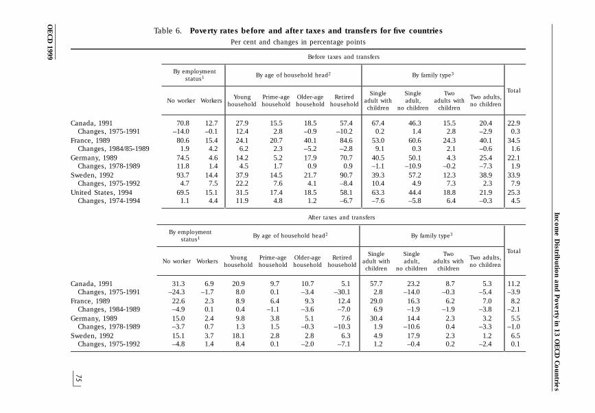
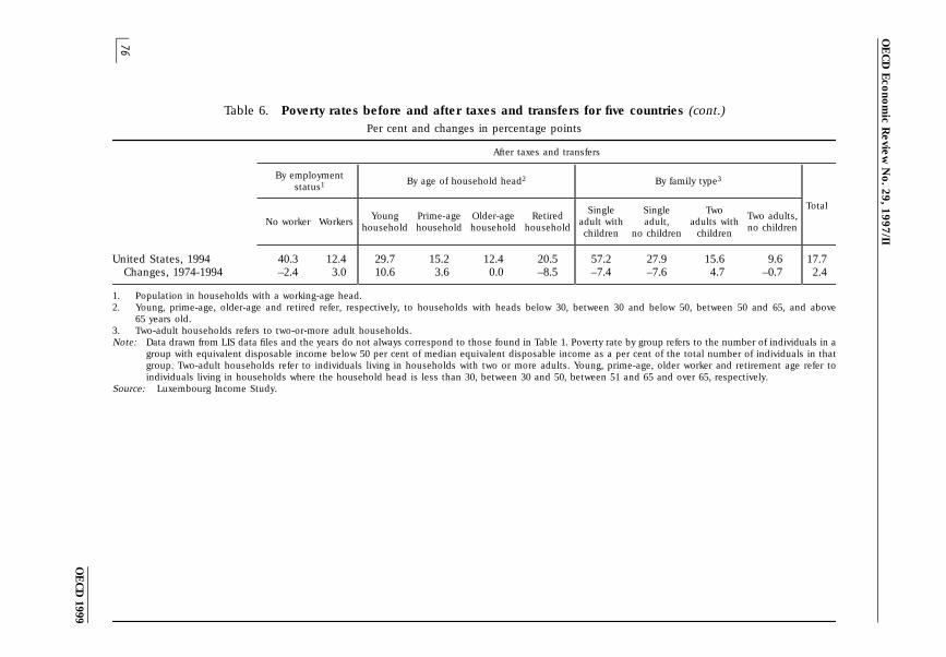
Turning to the impact on poverty, Table 6 (left-hand column) shows poverty rates(head-count ratios) pre- and post-taxes and transfers in the most recent year for whichdata was available, and the change in these rates over time, for five countries. The dataare drawn from the Luxembourg Income Study data files.17 A comparison of the top andbottom panels indicates that taxes and transfers taken together reduced poverty ratessubstantially in all countries. Poverty rates before taxes and transfers increased overthe period in all countries, particularly in Sweden and the United States. Nonetheless,the increasing role of the tax-and-transfer system slowed the growth in poverty ratesafter taxes and transfers in all countries, and led to declines in three.
In judging the impact of taxes and transfers on inequality and poverty, it should benoted that developments at the level of market income reflect, in part, interactionsbetween tax-and-transfer policies and household behaviour. For example, increasedaccess to old-age pensions and higher pension benefits over the period may have ledto earlier withdrawal from the labour market (Blondal and Scarpetta, 1998), a fall in mar-ket incomes of retired households and, thus, increased “poverty” measured beforetaxes and transfers. Increased take-up of transfer programmes among the working-agepopulation may have had similar effects, particularly in Europe; for example, earlyretirement and disability schemes have been used in some countries to provide sup-port to the long-term unemployed, who then withdrew from the labour force (MacFarlanand Oxley, 1996). Such factors may partly explain why poverty rates before taxes andtransfers are lower in North America than, for example, in France and Sweden.18
EVALUATING THE IMPACT OF EMPLOYMENT STATUS: AN MLD DECOMPOSITION
This section provides some further information on the importance of changesin the distribution of employment across households for trends in income distribu-tion. Aggregate changes in inequality can be decomposed into three parts (Box E):
a) The effect of changing shares of each group in the population. For example,if the share of a group that has a wide distribution of income increases, thedegree of overall inequality will also increase. This is referred to as the“ structural” effect.
b) The effect of changing inequality within each group. If the inequality withinindividual groups increases, aggregate inequality will rise over time, popu-lation shares held constant. This is referred to as the “ within-group” effect.
c) Finally, the impact of a widening or narrowing of average incomes of one grouprelative to another. Thus, if two groups have the same “ within-group” distribu-tion,19 but the difference between the average income of each group wid-ens, then the overall distribution also increases (when the populationstructure is held constant). This is called the “ between-group” effect.
02_chap.fm Page 77 Monday, May 3, 1999 4:53 PM
OECD Economic Review No. 29, 1997/II
78
OECD 1999
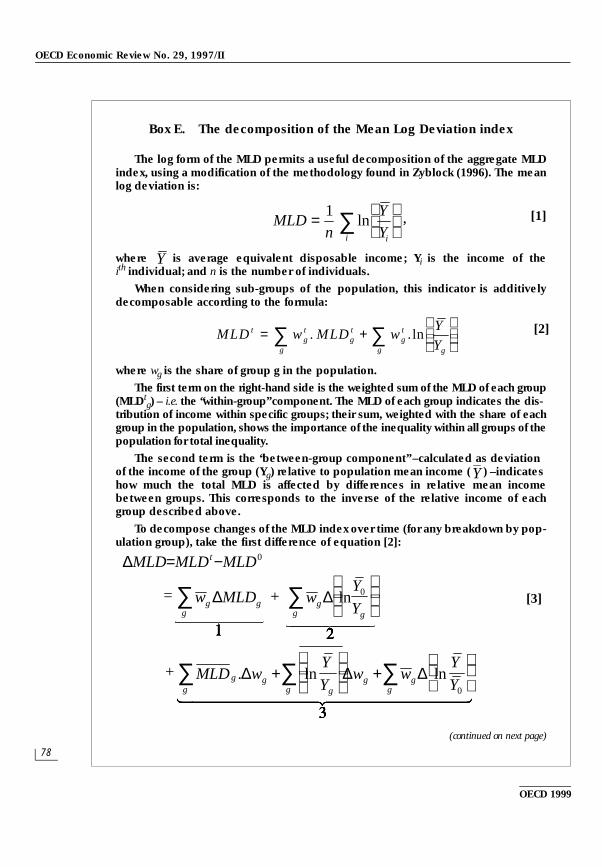
Box E. The decomposition of the Mean Log Deviation index
The log form of the MLD permits a useful decomposition of the aggregate MLDindex, using a modification of the methodology found in Zyblock (1996). The meanlog deviation is:
where is average equivalent disposable income; Yi is the income of theith individual; and n is the number of individuals.
When considering sub-groups of the population, this indicator is additivelydecomposable according to the formula:
where wg is the share of group g in the population.
The first term on the right-hand side is the weighted sum of the MLD of each group(MLDt
g) – i.e. the “within-group” component. The MLD of each group indicates the dis-tribution of income within specific groups; their sum, weighted with the share of eachgroup in the population, shows the importance of the inequality within all groups of thepopulation for total inequality.
The second term is the “between-group component” – calculated as deviationof the income of the group (Yg) relative to population mean income ( ) – indicateshow much the total MLD is affected by differences in relative mean incomebetween groups. This corresponds to the inverse of the relative income of eachgroup described above.
To decompose changes of the MLD index over time (for any breakdown by pop-ulation group), take the first difference of equation [2]:
(continued on next page)
MLDn
Y
Yi i
=
∑1
ln [1],
Y
MLD w MLD wY
Yt
gt
gt
ggt
gg
= +
∑ ∑. . ln [2]
Y
0MLDMLDMLD t−=∆
∑ ∆g
gg MLDw
∆∑
ggg Y
Yw 0ln
∑∑∑
∆+∆
+∆
ggg
g gggg
Y
Yww
Y
YwMLD
0
lnln.
����� �����
�����
[3]= +
+
02_chap.fm Page 78 Monday, May 3, 1999 11:53 AM
Income Distribution and Poverty in 13 OECD Countries
79
OECD 1999
The MLD index is used to isolate these effects as it can be decomposed pre-cisely into these three components (Box E). It should be noted that the MLD ismore sensitive to changes at the bottom of the distribution. However, this is prob-ably consistent with the greater concern attached to these groups by policy makers.
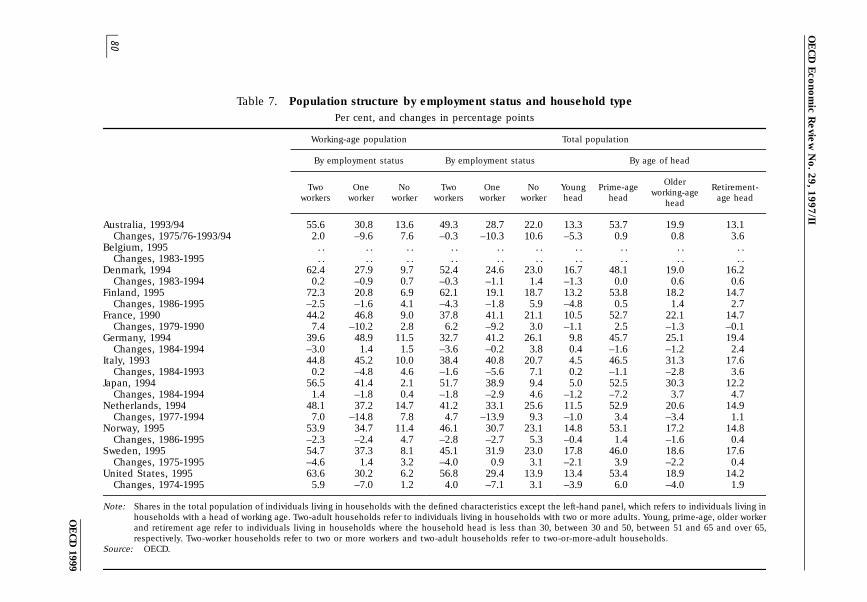
Changes in the structure of the population according to the employment statusof households is an important factor underlying changes in income distribution(Table 7). The left-hand panel considers individuals living in households with aworking-age head (referred to below as the “working-age” population). For thisgroup, the breakdown of the population by the employment status of the house-hold indicates an increase in the share of individuals living in households withno worker. The principal counterpart of this development has been a fall in the share ofindividuals living in one-earner households. The share of households with two earnersincreased in all countries except Finland, Germany, Norway and Sweden.
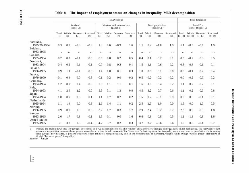
The results presented in Table 8 give some indication of the importance ofchanges in employment status for income distribution. The table shows thechanges in the MLD index over the period as the population is extended progres-sively from households with workers (Panel A) to include, first, non-working house-holds (Panel B) and, then, retired households (Panel C) (Table 8).20 For example, inAustralia the MLD index increases by 0.3 for workers but by 1.3 after non-workinghouseholds are included and 1.1 with the inclusion of the retired. Since the focushere is on the impact of non-working households, the difference when moving fromPanel A to Panel B is highlighted in Panel D.
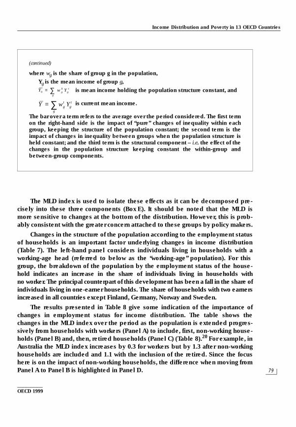
(continued)
where wg is the share of group g in the population,
Yg is the mean income of group g,
is mean income holding the population structure constant, and
is current mean income.
The bar over a term refers to the average over the period considered. The first termon the right-hand side is the impact of “ pure” changes of inequality within eachgroup, keeping the structure of the population constant; the second term is theimpact of changes in inequality between groups when the population structure isheld constant; and the third term is the structural component – i.e. the effect of thechanges in the population structure keeping constant the within-group andbetween-group components.
Y w Ygg
gt
00= ∑
Y w Ygt
ggt= ∑
02_chap.fm Page 79 Monday, May 3, 1999 4:55 PM
OE
CD
Eco
no
mic R
evie
w N
o. 2
9, 1
99
7/II
80
OE
CD
1999
Table 7. Population structure by employment status and household typePer cent, and changes in percentage points
Working-age population Total population
By employment status By employment status By age of head
OlderTwo One No Two One No Young Prime-age Retirement-
working-ageworkers worker worker workers worker worker head head age head
head
Australia, 1993/94 55.6 30.8 13.6 49.3 28.7 22.0 13.3 53.7 19.9 13.1Changes, 1975/76-1993/94 2.0 –9.6 7.6 –0.3 –10.3 10.6 –5.3 0.9 0.8 3.6
Belgium, 1995 . . . . . . . . . . . . . . . . . . . .Changes, 1983-1995 . . . . . . . . . . . . . . . . . . . .
Denmark, 1994 62.4 27.9 9.7 52.4 24.6 23.0 16.7 48.1 19.0 16.2Changes, 1983-1994 0.2 –0.9 0.7 –0.3 –1.1 1.4 –1.3 0.0 0.6 0.6
Finland, 1995 72.3 20.8 6.9 62.1 19.1 18.7 13.2 53.8 18.2 14.7Changes, 1986-1995 –2.5 –1.6 4.1 –4.3 –1.8 5.9 –4.8 0.5 1.4 2.7
France, 1990 44.2 46.8 9.0 37.8 41.1 21.1 10.5 52.7 22.1 14.7Changes, 1979-1990 7.4 –10.2 2.8 6.2 –9.2 3.0 –1.1 2.5 –1.3 –0.1
Germany, 1994 39.6 48.9 11.5 32.7 41.2 26.1 9.8 45.7 25.1 19.4Changes, 1984-1994 –3.0 1.4 1.5 –3.6 –0.2 3.8 0.4 –1.6 –1.2 2.4
Italy, 1993 44.8 45.2 10.0 38.4 40.8 20.7 4.5 46.5 31.3 17.6Changes, 1984-1993 0.2 –4.8 4.6 –1.6 –5.6 7.1 0.2 –1.1 –2.8 3.6
Japan, 1994 56.5 41.4 2.1 51.7 38.9 9.4 5.0 52.5 30.3 12.2Changes, 1984-1994 1.4 –1.8 0.4 –1.8 –2.9 4.6 –1.2 –7.2 3.7 4.7
Netherlands, 1994 48.1 37.2 14.7 41.2 33.1 25.6 11.5 52.9 20.6 14.9Changes, 1977-1994 7.0 –14.8 7.8 4.7 –13.9 9.3 –1.0 3.4 –3.4 1.1
Norway, 1995 53.9 34.7 11.4 46.1 30.7 23.1 14.8 53.1 17.2 14.8Changes, 1986-1995 –2.3 –2.4 4.7 –2.8 –2.7 5.3 –0.4 1.4 –1.6 0.4
Sweden, 1995 54.7 37.3 8.1 45.1 31.9 23.0 17.8 46.0 18.6 17.6Changes, 1975-1995 –4.6 1.4 3.2 –4.0 0.9 3.1 –2.1 3.9 –2.2 0.4
United States, 1995 63.6 30.2 6.2 56.8 29.4 13.9 13.4 53.4 18.9 14.2Changes, 1974-1995 5.9 –7.0 1.2 4.0 –7.1 3.1 –3.9 6.0 –4.0 1.9
Note: Shares in the total population of individuals living in households with the defined characteristics except the left-hand panel, which refers to individuals living inhouseholds with a head of working age. Two-adult households refer to individuals living in households with two or more adults. Young, prime-age, older workerand retirement age refer to individuals living in households where the household head is less than 30, between 30 and 50, between 51 and 65 and over 65,respectively. Two-worker households refer to two or more workers and two-adult households refer to two-or-more-adult households.
Source: OECD.
02_chap.fm P
age 80 Monday, M
ay 3, 1999 4:55 PM
Inco
me
Distrib
utio
n a
nd
Po
verty in
13
OE
CD
Co
un
tries
81
OE
CD
1999
Table 8. The impact of employment status on changes in inequality: MLD decomposition
MLD change First difference
Workers1 Workers and non-workers Total population Panel D =(panel A) (panel B) (panel C) panel B-panel A
Total Within Between Structural Total Within Between Structural Total Within Between Structural Total Within Between Structural[1] [2] [3] [4] [5] [6] [7] [8] [9] [10] [11] [12] [5]-[1] [6]-[2] [7]-[3] [8]-[4]
Australia,1975/76-1984 0.3 0.9 –0.3 –0.3 1.3 0.6 –0.9 1.6 1.1 0.2 –1.0 1.9 1.1 –0.3 –0.6 1.9
Belgium,1983-1995 . . . . . . . . . . . . . . . . . . . . . . . . . . . . . . . .
Canada,1985-1994 0.2 0.2 –0.1 0.0 0.6 0.0 0.2 0.5 0.4 0.1 0.2 0.1 0.5 –0.2 0.3 0.5
Denmark,1983-1994 –0.4 –0.2 –0.1 –0.1 –0.9 –0.8 –0.2 0.1 –1.5 –1.1 –0.6 0.2 –0.5 –0.6 –0.1 0.1
Finland,1986-1995 0.9 1.1 –0.1 0.0 1.4 1.0 0.1 0.3 1.0 0.8 0.1 0.0 0.5 –0.1 0.2 0.4
France,1979-1990 –0.1 0.4 0.0 –0.5 –0.1 0.2 0.0 –0.2 –0.5 –0.2 –0.2 –0.2 0.0 –0.2 0.0 0.2
Germany,1984-1994 1.2 0.9 0.4 0.0 2.3 1.1 1.1 0.1 1.6 1.0 0.4 0.2 1.1 0.2 0.7 0.1
Italy,1984-1993 4.1 2.9 1.2 0.0 5.3 3.1 1.3 0.8 4.5 3.2 0.7 0.6 1.1 0.2 0.0 0.8
Japan,1984-1994 1.0 0.7 0.3 0.1 1.1 0.7 0.2 0.2 1.5 0.7 –0.1 0.9 0.0 0.0 –0.1 0.1
Netherlands,1985-1994 1.1 1.4 0.0 –0.3 2.6 1.4 1.1 0.2 2.5 1.5 1.0 0.0 1.5 0.0 1.0 0.5
Norway,1986-1995 0.9 0.9 0.0 0.0 3.2 1.7 –0.3 1.7 2.9 2.4 –0.2 0.7 2.3 0.9 –0.3 1.8
Sweden,1983-1995 2.6 1.7 0.8 0.1 1.5 –0.1 0.0 1.6 0.6 0.9 –0.8 0.5 –1.1 –1.8 –0.8 1.6
United States,1985-1995 3.1 3.2 0.3 –0.4 4.2 3.7 0.2 0.3 3.7 3.7 –0.6 0.6 1.0 0.5 –0.1 0.7
1. Workers are broken down into two groups: one-earner and two-earner households. The ‘‘within’’ effect indicates changes in inequalities within each group, the ‘‘between’’ effectmeasures inequalities between these groups when the structure is held constant. The ‘‘structural’’ effect captures the inequality component due to population shifts amongthese groups. For instance, a positive structural effect indicates rising inequality due to the combination of increasing weights with: a) high ‘‘within group’’ inequality; orb) high ‘‘between group’’ inequality.
Source: OECD.
02_chap.fm P
age 81 Monday, M
ay 3, 1999 4:55 PM

OECD Economic Review No. 29, 1997/II
82
OECD 1999
The change in the MLD for households with at least one worker was positive in allcountries except for Denmark and France and was very large in Italy, Sweden and theUnited States (Panel A). Part of this increase may reflect widening wage-rate distribu-tions where they occurred.21 However, employment effects have also been importantin explaining the changes in the distribution of disposable income: as can be seen, theaddition of non-workers to the working-age population leads to a further increase in theMLD over the period for all countries except Denmark and Sweden (Panel D,first column). In contrast, the change in the MLD is smaller when the retired householdsare included (compare column 9 with column 5) indicating that this group tended to off-set the widening among the households with a working-age head.
Further evidence of the importance of employment effects is indicated by thebreakdown of the change in inequality into the “ between-group” , “ within-group”and “ structural” effects described above.22
– For working households (Panel A) (which include both single-earner andtwo-or-more-earner households), the main source of the change in inequal-ity has been widening inequality within both one- and two-worker house-holds (“ within-group” effect), although a widening in average incomesbetween the two groups has also played a role, particularly in Italy andSweden (“ between-group” effect). There is no evidence that the increase inthe share of two-earner households (“ structural” effect) has led to a widen-ing in the distribution of income as measured by the MLD.
– The decline in inequality (in all countries except Japan) when the retired areadded in appears to be driven by the “ between-group” effect, suggestingrising mean incomes of the retired as pension schemes matured.
– The “ structural” effect arising from the rising share of non-working house-holds is positive in all countries (last column in Panel D) and is generallymore important than the “ within” and “ between-group” effects.
THE RELATIVE POSITION OF INDIVIDUAL GROUPS AND THE IMPACT OF THE TAX-AND-TRANSFER SYSTEM23
Changes in the position of individual groups relative to developments in thepopulation as a whole – and the degree to which these changes reflect the operation ofthe tax-and-transfer system – are described in two ways. A first approach (Table 6) com-pares poverty rates for different groups in the population before and after taxes andtransfers, broken down by employment status, age of the household head and familytype.24 However, information is limited to a subset of only five countries.
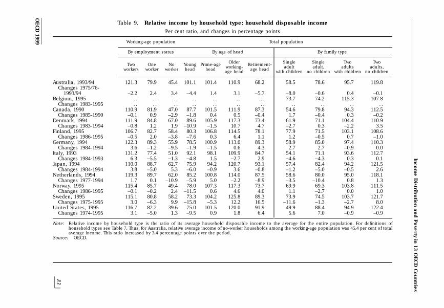
The second approach looks at average income of the same groups relative tothe population average. Table 9 (first line) shows the per cent ratio of average
02_chap.fm Page 82 Monday, May 3, 1999 4:55 PM
Inco
me
Distrib
utio
n a
nd
Po
verty in
13
OE
CD
Co
un
tries
83
OE
CD
1999
Table 9. Relative income by household type: household disposable incomePer cent ratio, and changes in percentage points
Working-age population Total population
By employment status By age of head By family type
Older Single Single Two TwoTwo One No Young Prime-age Retirement-working- adult adult, adults adults,workers worker worker head head age headage head with children no children with children no children
Australia, 1993/94 121.3 79.9 45.4 101.1 101.4 110.9 68.2 58.5 78.6 95.7 119.8Changes 1975/76-
1993/94 –2.2 2.4 3.4 –4.4 1.4 3.1 –5.7 –8.0 –0.6 0.4 –0.1Belgium, 1995 . . . . . . . . . . . . . . 73.7 74.2 115.3 107.8
Changes 1983-1995 . . . . . . . . . . . . . . . . . . . . . .Canada, 1990 110.9 81.9 47.0 87.7 101.5 111.9 87.3 54.6 79.8 94.3 112.5
Changes 1985-1990 –0.1 0.9 –2.9 –1.8 0.4 0.5 –0.4 1.7 –0.4 0.3 –0.2Denmark, 1994 111.9 84.8 67.0 89.6 105.9 117.3 73.4 61.9 71.1 104.4 110.9
Changes 1983-1994 –0.8 1.2 1.9 –10.9 –1.5 10.7 4.7 –2.7 0.3 –2.2 3.5Finland, 1995 106.7 82.7 58.4 80.3 106.8 114.5 78.1 77.9 71.5 103.1 108.6
Changes 1986-1995 –0.5 2.0 –3.8 –7.6 0.3 6.4 1.1 1.2 –0.5 0.7 –1.0Germany, 1994 122.3 89.3 55.9 78.5 100.9 113.0 89.3 58.9 85.0 97.4 110.3
Changes 1984-1994 3.6 –1.2 –9.5 –1.9 –1.5 0.6 4.3 2.7 2.7 –0.9 0.0Italy, 1993 131.2 77.4 51.0 92.1 98.1 109.9 84.7 54.1 71.1 93.6 112.7
Changes 1984-1993 6.3 –5.5 –1.3 –4.8 1.5 –2.7 2.9 –4.6 –4.3 0.3 0.1Japan, 1994 110.0 88.7 62.7 75.9 94.2 120.7 93.1 57.4 82.4 94.2 121.5
Changes 1984-1994 3.8 –5.0 5.3 –6.0 –0.9 3.6 –0.8 –1.2 –5.0 –0.5 2.6Netherlands, 1994 119.3 89.7 62.0 85.2 100.8 114.0 87.5 58.6 80.0 95.0 118.1
Changes 1977-1994 1.7 0.1 –10.9 –5.9 5.0 –2.2 –8.9 –3.5 –10.4 0.8 1.3Norway, 1995 115.4 85.7 49.4 78.0 107.3 117.3 73.7 69.9 69.3 103.8 111.5
Changes 1986-1995 –0.1 –0.2 2.4 –11.5 0.6 4.6 4.0 1.1 –2.7 0.0 1.0Sweden, 1995 115.1 80.8 58.2 73.3 104.2 125.8 89.3 73.9 74.5 103.7 121.7
Changes 1975-1995 3.0 –6.3 9.9 –15.8 –5.3 12.2 16.5 –11.6 –1.3 –2.7 8.0United States, 1995 116.7 82.2 39.6 75.0 101.5 120.0 91.9 49.9 88.4 94.9 122.4
Changes 1974-1995 3.1 –5.0 1.3 –9.5 0.9 1.8 6.4 5.6 7.0 –0.9 –0.9
Note: Relative income by household type is the ratio of its average household disposable income to the average for the entire population. For definitions ofhousehold types see Table 7. Thus, for Australia, relative average income of no-worker households among the working-age population was 45.4 per cent of totalaverage income. This ratio increased by 3.4 percentage points over the period.
Source: OECD.
02_chap.fm P
age 83 Monday, M
ay 3, 1999 4:55 PM
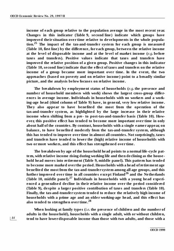
OECD Economic Review No. 29, 1997/II
84
OECD 1999
income of each group relative to the population average in the most recent year.Changes in this indicator (Table 9, second line) indicate which groups haveimproved their situation over time relative to developments in the whole popula-tion.25 The impact of the tax-and-transfer system for each group is measured(Table 10, first line) by the difference, for each group, between the relative incomeat the level of disposable income and at the level of market income (e.g. beforetaxes and transfers). Positive values indicate that taxes and transfers haveimproved the relative position of a given group. Positive changes in this indicator(Table 10, second line) indicate that the effect of taxes and transfers on the relativeincome of a group became more important over time. In the event, the twoapproaches (based on poverty and on relative income) point to a broadly similarpicture, and the analysis below focuses on relative income.
The breakdown by employment status of households (e.g. the presence andnumber of household members with work) shows the largest cross-group differ-ences in average income. Individuals in households with no workers and a work-ing-age head (third column of Table 9) have, in general, very low relative income.They also appear to have benefited the most from the operation of thetax-and-transfer system, as highlighted by the large increase in their relativeincome when shifting from a pre- to post-tax-and-transfer basis (Table 10). How-ever, this positive effect has tended to become more important over time in onlyabout half of the countries. By contrast, households with a single earner appear, onbalance, to have benefited modestly from the tax-and-transfer system, althoughthis has tended to improve over time in almost all countries. Not surprisingly, taxesand transfers have tended to lower the (high) relative income of households withtwo or more workers, and this effect has strengthened over time.
The breakdown by age of the household head points to a normal life-cycle pat-tern, with relative income rising during working life and then declining as the house-hold head moves into retirement (Table 9, middle panel). This pattern has tendedto become more marked over the period. Households with a head of retirement agebenefited the most from the tax-and-transfer system among all age groups, and thisfurther improved over time in all countries except Finland26 and the Netherlands(Table 10, middle panel).27 Individuals in households with a young head experi-enced a generalised decline in their relative income over the period considered(Table 9), despite a larger positive contribution of taxes and transfers (Table 10).Finally, the tax-and-transfer system tended to reduce the relatively high income ofhouseholds with a prime age and an older working-age head, and this effect hasalso tended to strengthen over time.28
When looking at family types (i.e. the presence of children and the number ofadults in the household), households with a single adult, with or without children,tend to have lower disposable income than those with two adults, and those with a
02_chap.fm Page 84 Monday, May 3, 1999 4:55 PM
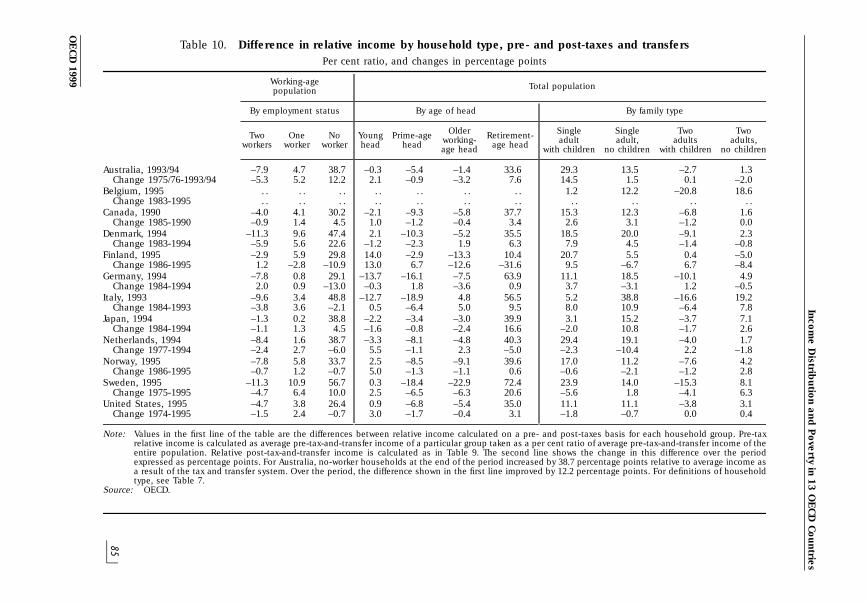
Inco
me
Distrib
utio
n a
nd
Po
verty in
13
OE
CD
Co
un
tries
85
OE
CD
1999
Table 10. Difference in relative income by household type, pre- and post-taxes and transfersPer cent ratio, and changes in percentage points
Working-age Total populationpopulation
By employment status By age of head By family type
Older Single Single Two TwoTwo One No Young Prime-age Retirement-working- adult adult, adults adults,workers worker worker head head age headage head with children no children with children no children
Australia, 1993/94 –7.9 4.7 38.7 –0.3 –5.4 –1.4 33.6 29.3 13.5 –2.7 1.3Change 1975/76-1993/94 –5.3 5.2 12.2 2.1 –0.9 –3.2 7.6 14.5 1.5 0.1 –2.0
Belgium, 1995 . . . . . . . . . . . . . . 1.2 12.2 –20.8 18.6Change 1983-1995 . . . . . . . . . . . . . . . . . . . . . .
Canada, 1990 –4.0 4.1 30.2 –2.1 –9.3 –5.8 37.7 15.3 12.3 –6.8 1.6Change 1985-1990 –0.9 1.4 4.5 1.0 –1.2 –0.4 3.4 2.6 3.1 –1.2 0.0
Denmark, 1994 –11.3 9.6 47.4 2.1 –10.3 –5.2 35.5 18.5 20.0 –9.1 2.3Change 1983-1994 –5.9 5.6 22.6 –1.2 –2.3 1.9 6.3 7.9 4.5 –1.4 –0.8
Finland, 1995 –2.9 5.9 29.8 14.0 –2.9 –13.3 10.4 20.7 5.5 0.4 –5.0Change 1986-1995 1.2 –2.8 –10.9 13.0 6.7 –12.6 –31.6 9.5 –6.7 6.7 –8.4
Germany, 1994 –7.8 0.8 29.1 –13.7 –16.1 –7.5 63.9 11.1 18.5 –10.1 4.9Change 1984-1994 2.0 0.9 –13.0 –0.3 1.8 –3.6 0.9 3.7 –3.1 1.2 –0.5
Italy, 1993 –9.6 3.4 48.8 –12.7 –18.9 4.8 56.5 5.2 38.8 –16.6 19.2Change 1984-1993 –3.8 3.6 –2.1 0.5 –6.4 5.0 9.5 8.0 10.9 –6.4 7.8
Japan, 1994 –1.3 0.2 38.8 –2.2 –3.4 –3.0 39.9 3.1 15.2 –3.7 7.1Change 1984-1994 –1.1 1.3 4.5 –1.6 –0.8 –2.4 16.6 –2.0 10.8 –1.7 2.6
Netherlands, 1994 –8.4 1.6 38.7 –3.3 –8.1 –4.8 40.3 29.4 19.1 –4.0 1.7Change 1977-1994 –2.4 2.7 –6.0 5.5 –1.1 2.3 –5.0 –2.3 –10.4 2.2 –1.8
Norway, 1995 –7.8 5.8 33.7 2.5 –8.5 –9.1 39.6 17.0 11.2 –7.6 4.2Change 1986-1995 –0.7 1.2 –0.7 5.0 –1.3 –1.1 0.6 –0.6 –2.1 –1.2 2.8
Sweden, 1995 –11.3 10.9 56.7 0.3 –18.4 –22.9 72.4 23.9 14.0 –15.3 8.1Change 1975-1995 –4.7 6.4 10.0 2.5 –6.5 –6.3 20.6 –5.6 1.8 –4.1 6.3
United States, 1995 –4.7 3.8 26.4 0.9 –6.8 –5.4 35.0 11.1 11.1 –3.8 3.1Change 1974-1995 –1.5 2.4 –0.7 3.0 –1.7 –0.4 3.1 –1.8 –0.7 0.0 0.4
Note: Values in the first line of the table are the differences between relative income calculated on a pre- and post-taxes basis for each household group. Pre-taxrelative income is calculated as average pre-tax-and-transfer income of a particular group taken as a per cent ratio of average pre-tax-and-transfer income of theentire population. Relative post-tax-and-transfer income is calculated as in Table 9. The second line shows the change in this difference over the periodexpressed as percentage points. For Australia, no-worker households at the end of the period increased by 38.7 percentage points relative to average income asa result of the tax and transfer system. Over the period, the difference shown in the first line improved by 12.2 percentage points. For definitions of householdtype, see Table 7.
Source: OECD.
02_chap.fm P
age 85 Monday, M
ay 3, 1999 4:55 PM
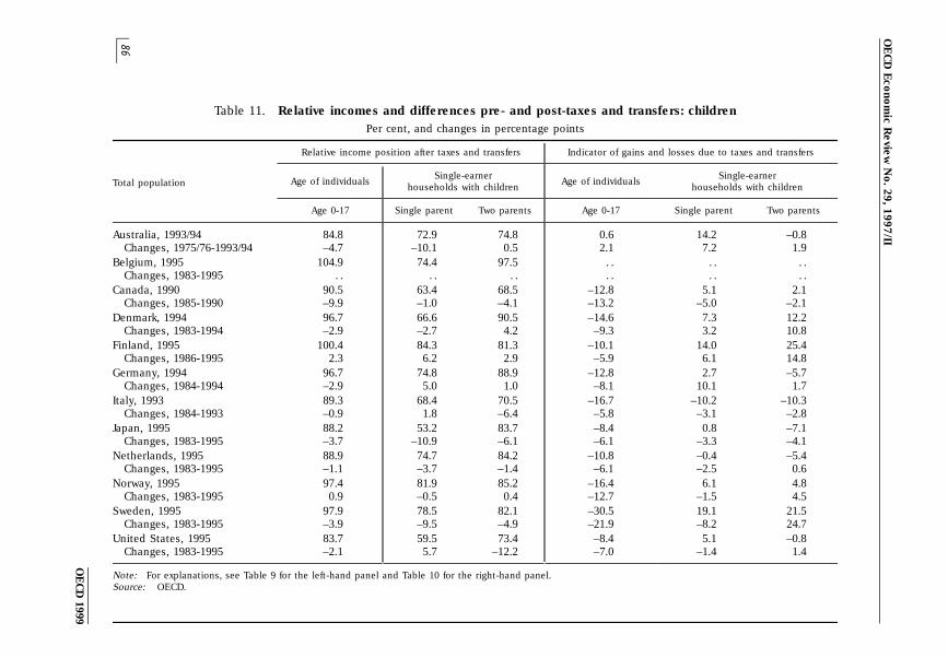
OE
CD
Eco
no
mic R
evie
w N
o. 2
9, 1
99
7/II
86
OE
CD
1999
Table 11. Relative incomes and differences pre- and post-taxes and transfers: childrenPer cent, and changes in percentage points
Relative income position after taxes and transfers Indicator of gains and losses due to taxes and transfers
Single-earner Single-earnerAge of individuals Age of individualsTotal population households with children households with children
Age 0-17 Single parent Two parents Age 0-17 Single parent Two parents
Australia, 1993/94 84.8 72.9 74.8 0.6 14.2 –0.8Changes, 1975/76-1993/94 –4.7 –10.1 0.5 2.1 7.2 1.9
Belgium, 1995 104.9 74.4 97.5 . . . . . .Changes, 1983-1995 . . . . . . . . . . . .
Canada, 1990 90.5 63.4 68.5 –12.8 5.1 2.1Changes, 1985-1990 –9.9 –1.0 –4.1 –13.2 –5.0 –2.1
Denmark, 1994 96.7 66.6 90.5 –14.6 7.3 12.2Changes, 1983-1994 –2.9 –2.7 4.2 –9.3 3.2 10.8
Finland, 1995 100.4 84.3 81.3 –10.1 14.0 25.4Changes, 1986-1995 2.3 6.2 2.9 –5.9 6.1 14.8
Germany, 1994 96.7 74.8 88.9 –12.8 2.7 –5.7Changes, 1984-1994 –2.9 5.0 1.0 –8.1 10.1 1.7
Italy, 1993 89.3 68.4 70.5 –16.7 –10.2 –10.3Changes, 1984-1993 –0.9 1.8 –6.4 –5.8 –3.1 –2.8
Japan, 1995 88.2 53.2 83.7 –8.4 0.8 –7.1Changes, 1983-1995 –3.7 –10.9 –6.1 –6.1 –3.3 –4.1
Netherlands, 1995 88.9 74.7 84.2 –10.8 –0.4 –5.4Changes, 1983-1995 –1.1 –3.7 –1.4 –6.1 –2.5 0.6
Norway, 1995 97.4 81.9 85.2 –16.4 6.1 4.8Changes, 1983-1995 0.9 –0.5 0.4 –12.7 –1.5 4.5
Sweden, 1995 97.9 78.5 82.1 –30.5 19.1 21.5Changes, 1983-1995 –3.9 –9.5 –4.9 –21.9 –8.2 24.7
United States, 1995 83.7 59.5 73.4 –8.4 5.1 –0.8Changes, 1983-1995 –2.1 5.7 –12.2 –7.0 –1.4 1.4
Note: For explanations, see Table 9 for the left-hand panel and Table 10 for the right-hand panel.Source: OECD.
02_chap.fm P
age 86 Monday, M
ay 3, 1999 4:55 PM
Income Distribution and Poverty in 13 OECD Countries
87
OECD 1999
single adult and children have the lowest relative income of all groups. These pat-terns reflect a combination of factors: i) a higher number of workers in householdswith two or more adults; ii) larger size of households with children; and iii) the factthat more lone parents do not work when compared to other groups. In general, thetax-and-transfer system benefits single-adult households the most and two-adulthouseholds with children the least, mirroring differences in relative income(Table 10, right-hand panel).
Table 11 provides additional insight on the situation of children, in terms ofboth relative income (left-hand panel) and the importance of the tax-and-transfersystem (right-hand panel). Children (defined as individuals below the age of 18)enjoyed – in the most recent year available – below-average income in all countriesexcept Belgium and Finland, and their position tended to deteriorate over time inalmost all countries. The tax-and-transfer system has tended to increase, on bal-ance, their relative income, but support appears to have been falling over the pastdecades in most countries (Table 11, right-hand panel). Single parents withoutwork are obviously the most vulnerable group. But relatively low income was alsoexperienced in some countries by two-adult households with a single earner(Table 11, second column); and in a majority of countries taxes and transfers con-tributed to a deterioration of the relative position of this group.
CONCLUSIONS
The results provide some hints as to which factors underlie the increase in in-equality at the level of market income. First, while earnings contribute most to in-equality in any one year, this income component has not always been the largestcontributor to the widening of the distribution of income over the period and, insome cases, earnings did not contribute to the increase in disposable income in-equality at all once interaction effects have been taken into account (Shorrocksmethodology). Capital and self-employment income has contributed significantlyin many countries, sometimes reflecting increased shares. However, measurementproblems argue for caution in interpreting these results.
Decompositions which take into account the changing patterns of employmentand non-employment across households suggest that disposable income inequal-ity increased among employed households. A number of factors probably played arole, including increased wage-rate differentials and a more unequal distribution ofemployment across households. The results showed that increasing shares ofnon-working households within the working-age population contributed to therise in inequality and this increase may have been substantial in a few countries. Incontrast, the increasing share of the retired appears to have contributed to a reduc-tion in inequality.
02_chap.fm Page 87 Monday, May 3, 1999 4:55 PM
OECD Economic Review No. 29, 1997/II
88
OECD 1999
The results also show that the increased importance of taxes and transfers hasbeen quite successful in offsetting the greater inequality in market income –although feedback effects (e.g. earlier retirement as a result of age pensions) cer-tainly explain at least some of the widening in the distribution of market income.There was considerable variation across countries in the relative importance ofthese two components in explaining the change in inequality over the period.Nonetheless, transfers appear to have keen key for helping households at the bot-tom of the distribution. As the share of non-working households in the total popu-lation has increased, incomes of those at the bottom of the distribution have beenincreasingly made up of income-transfer benefits. In this context, retirement-agehouseholds have been particularly favoured and, for a subset of five countries, theyhave experienced the sharpest falls in poverty of all population groups considered.In contrast children, taken as a group, have tended to lose ground.
An unanswered question is how policy should respond to increased inequalityof market income. In this context, it would appear important to consider not onlythe impact of policy on the “ static” distribution (as presented in this study), but alsothe effects on the income of individual households through time. Households at thebottom of the distribution move up the income ladder as they become employedand, as they improve their earning capacity through better education and skills;conversely, those losing jobs or moving into retirement may see their incomes fall.As noted above, some part of the increase in inequality and poverty has reflectedthe increasing share of non-working households among the working-age popula-tion. Policies aimed at narrowing the “ static” distribution of income by increasingtransfer payment may – where they are already generous – limit job creation andreduce the incentive to find work, thereby perpetuating low incomes. At the sametime, policies which lead to a widening in wage rates for the low paid may raiseemployment but lead to an increase in the number of “ working poor” households.Policies need, therefore, to focus both on increasing employment and on measuresto encourage upward earnings mobility through time, possibly supplemented bywork-conditional benefits for low-wage households.
02_chap.fm Page 88 Monday, May 3, 1999 4:55 PM
Income Distribution and Poverty in 13 OECD Countries
89
OECD 1999
NOTES
1. Not all results are available for all countries and periods.
2. While there have been a number of international comparisons (see, inter alia, Gottschalk andSmeeding, 1997), a common methodology has not been used and the range of countries cov-ered is smaller.
3. For a further discussion of data issues and problems see Burniaux et al. (1998).
4. Nonetheless, a comparison of Gini coefficients with those found in Atkinson et al. (1995), basedon LIS data, shows similar rank orderings across countries.
5. Estimates of the number of homeless suggest that this would not make a substantial differenceto the results in terms of the overall distribution, although it might possibly be somewhat moreimportant for measures of poverty (OECD, 1996b).
6. The size of the changes over time for individual components and groups for some countries sug-gest that there may be inconsistencies in data sets which have not been accounted for.
7. This is referred to as an equivalence scale elasticity of 0.5 (or N0.5).
8. To test the sensitivity of the results to this assumption, indicators of distribution and pov-erty were also calculated using per capita income (i.e. household income divided by thenumber of individuals). In the event, changes in overall income distribution show broadlythe same trends over time, though relative rankings of households by characteristic (age,family and employment status) within each country were often different (seeBurniaux et al., 1998).
9. Indirect taxes have not been taken into account. There has been some shifting in taxes fromdirect towards indirect taxes over the period such that the equalising impact of taxes may beoverstated See Leibfritz et al., 1997.
10. Thus, the threshold rises in line with median income. See Burniaux et al. (1998) for resultsusing a threshold which remains unchanged in real terms through the period. On thisbasis, poverty would have fallen in all countries except Australia (where real medianincome fell over the period).
11. Similar results were used found using poverty thresholds set at 40 and 60 per cent of medianincome. See Burniaux et al., 1998.
12. Additional evidence presented in the fifth section shows that the widening in the shares of earn-ings may be related to employment patterns and the rise in the number of no-earner householdswhich are concentrated in the bottom deciles.
13. The contributions of each component to the change in the index can differ depending on theindex chosen. As shown in Table 1, both the sign and the size of the change can vary depending
02_chap.fm Page 89 Monday, May 3, 1999 4:55 PM

OECD Economic Review No. 29, 1997/II
90
OECD 1999
on the index chosen. Nonetheless, the results using the other two indices in Table 1 broadly con-cur with the results presented here. Results using the SCV are shown in Burniaux et al. (1998).
14. This is less the case for Denmark, the Netherlands and Sweden, where most transfer paymentsare taxed as part of income.
15. Taxes also rose sharply for the lower-income group in Denmark and Sweden. This reflected thefact that, as noted, a larger share of transfers is taxable in these two countries and that transfersincreased sharply in both.
16. The large positive contribution of taxes in Sweden partly reflects the effect of tax reforms in theearly 1990s, that changed the definition of taxable income and widened the tax base.
17. A comparison of the poverty rates from the LIS files and the questionnaire suggests thatthe country rankings are broadly the same. The main difference in ranking is Germany,where the poverty rate is much lower in the LIS 1989 data than in the GSOEP datafor 1994.
18. This may also reflect differences in pension arrangements between Europe and the UnitedStates. Private pensions, which are included in market incomes, are more important in theUnited States. This is likely to reduce the number of non-working households with no mar-ket income, leading to a narrower market income distribution and lower poverty ratespre-taxes and transfers.
19. Relative to the mean of each group.
20. To better capture the effects of non-workers, workers and the retired, the population groupshave been recomposed in Table 8 into individuals belonging to households with at leastone worker (of working age and retirement age) (Panel A), individuals belonging to householdswith no workers of working age (Panel B) and individuals belonging to households withnon-workers of retirement age (the retired) (Panel C).
21. However, it is difficult to assess the impact without further information about the impact ofchanging patterns of hours worked across households and the correlation between the incomesof workers in multi-earner households.
22. For example, in Australia the structural effect (i.e. the effect of changing shares of one andtwo-earner households) at the level of working households was -0.3 (column 4), but thisincreased to 1.6 (column 8) when changes in the shares of working and non-working householdsare allowed for – a difference of 1.9 (Panel D). This compares to rise of 1.0 at the level of totalMLD (1.3 in column 5 less 0.3 in column 1).
23. Results for average incomes and poverty rates in this section are particularly sensitive to theequivalence scale used. For example, the use of an equivalence-scale elasticity of 1 (per capitaincome) would raise average equivalent incomes of population groups with a small size (e.g. theretired) relative to those with larger average household size (e.g. two-adult households with chil-dren).
24. Family type refers to the family status – i.e. single or married and with or without children. Theincome unit remains the household.
25. The population structure has been held constant at the end of the period to control for theimpact of changing population structure.
26. The results for Finland may be affected by a shift in the pension system from the public to theprivate sector.
27. Indeed, the relative position of this group improved over time as they cumulated both highermarket incomes relative to the population average and increased benefits from the
02_chap.fm Page 90 Monday, May 3, 1999 4:55 PM

Income Distribution and Poverty in 13 OECD Countries
91
OECD 1999
tax-and-transfer system: for the five countries, poverty rates for retirement-age households felleven before taxes and transfers (Table 6).
28. For the five countries, the share of the poor who belonged to prime-age households increasedover the past two decades and for this group there also appears to have been an increasing num-ber of working poor. This contrasts with the experience of older-worker households whichwork: poverty rates for this group have declined. This pattern for older-worker households isconsistent with increased early retirement or withdrawal from the labour market, particularlyamong those with lower incomes (Table 6).
02_chap.fm Page 91 Monday, May 3, 1999 4:55 PM
OECD Economic Review No. 29, 1997/II
92
OECD 1999
BIBLIOGRAPHY
ATKINSON, A.B., L. RAINWATER and T.M. SMEEDING (1995), “Income distribution in OECDcountries: evidence from the Luxembourg Income Study”, Income Distribution in OECD Countries,OECD Social Policy Studies, No. 18.
BLONDAL, S. and S. SCARPETTA (1999), “The retirement decision in OECD countries”, OECDEconomics Department Working Paper, No. 202.
BURNIAUX, J.M. (1998), “Inégalités et emplois : effet de redistribution lié à la structure familiale”,Economie Internationale, n° 71, 3e trimestre, pp. 101-132.
BURNIAUX, J.M., T.T. DANG, D. FORE, M. FÖRSTER, M. MIRA d’ERCOLE and H. OXLEY (1998),“Income distribution and poverty in selected OECD countries”, OECD Economics DepartmentWorking Paper, No. 189.
GOTTSCHALK, P. and T.M. SMEEDING (1997), “Cross-national comparisons of earnings andincome inequality”, Journal of Economic Literature, No. 2, pp. 633-687.
GREGG, P. and J. WADSWORTH (1996), “It takes two: employment polarisation in the OECD”,London School of Economics, Centre for Economic Performance Discussion Paper, No. 304,September.
LEIBFRITZ, W., J. THORNTON and A. BIBBEE (1997), “Taxation and economic performance”,OECD Economics and Statistics Department Working Paper, No. 176.
MACFARLAN, M. and H. OXLEY (1996), “Social transfers: spending patterns, institutional arrange-ments and policy responses”, OECD Economic Studies, No. 27.
OECD (1993), Employment Outlook, Paris.
OECD (1994), The OECD Jobs Study, Paris.
OECD (1996a), Employment Outlook, Paris.
OECD (1996b), Strategies for Housing and Social Integration in Cities, Paris.
OECD (1997a), Employment Outlook, Chapter 2, Paris.
OECD (1997b), Implementing the OECD Jobs Strategy: Lessons From Member Countries’ Experience,Paris.
SHORROCKS, A.F. (1982), “Inequality decomposition by factor components”, Econometrica, Vol. 50,No. 1.
ZYBLOCK, M. (1996), “Why is family market income inequality increasing in Canada?”, WorkingPaper, Human Resources Development, Canada.
02_chap.fm Page 92 Monday, May 3, 1999 4:55 PM

OECD 1999
STATISTICAL ANNEX
02_chap.fm Page 93 Monday, May 3, 1999 4:55 PM
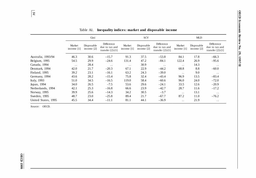
OE
CD
Eco
no
mic R
evie
w N
o. 2
9, 1
99
7/II
94
OE
CD
1999
Table A1. Inequality indices: market and disposable income
Gini SCV MLD
Difference Difference DifferenceMarket Disposable Market Disposable Market Disposable
due to tax and due to tax and due to tax andincome [1] income [2] income [1] income [2] income [1] income [2]
transfer [2]-[1] transfer [2]-[1] transfer [2]-[1]
Australia, 1993/94 46.3 30.6 –15.7 91.3 37.5 –53.8 84.1 17.8 –66.3Belgium, 1995 54.5 29.9 –24.6 131.4 47.2 –84.1 122.4 26.9 –95.6Canada, 1994 . . 28.4 . . . . 30.9 . . . . 14.3 . .Denmark, 1994 42.0 21.7 –20.3 67.1 22.9 –44.2 68.8 8.8 –60.0Finland, 1995 39.2 23.1 –16.1 63.2 24.3 –39.0 . . 9.0 . .Germany, 1994 43.6 28.2 –15.4 75.8 32.4 –43.4 96.9 13.5 –83.4Italy, 1993 51.0 34.5 –16.5 119.0 58.4 –60.6 96.0 24.0 –72.0Japan, 1994 34.0 26.5 –7.5 53.6 29.6 –24.1 33.5 12.6 –20.9Netherlands, 1994 42.1 25.3 –16.8 66.6 23.9 –42.7 28.7 11.6 –17.2Norway, 1995 39.9 25.6 –14.3 34.2 30.5 –3.7 . . 13.1 . .Sweden, 1995 48.7 23.0 –25.8 89.4 21.7 –67.7 87.2 11.0 –76.2United States, 1995 45.5 34.4 –11.1 81.1 44.1 –36.9 . . 21.9 . .
Source: OECD.
02_chap.fm P
age 94 Monday, M
ay 3, 1999 4:55 PM
Related Documents