Inclusion dynamics hybrid automata

Inclusion Dynamics Hybrid Automata ?

Alberto Casagrande a,b,c Carla Piazza a,∗ Alberto Policriti a,c

Bud Mishra d,e

aDIMI, Universita di Udine, Via delle Scienze, 206, 33100 Udine, ItalybDISA, Universita di Udine, Via delle Scienze, 208, 33100 Udine, ItalycIstituto di Genomica Applicata, Via J.Linussio, 51, 33100 Udine, Italy

dCourant Institute of Mathematical Science, NYU, New York, U.S.A.eNYU School of Medicine, 550 First Avenue, New York, 10016 U.S.A.

Abstract

Hybrid systems are dynamical systems with the ability to describe mixed discrete-continuous evolution of a wide range of systems. Consequently, at first glance, hybridsystems appear powerful but recalcitrant, neither yielding to analysis and reasoningthrough a purely continuous-time modeling as with systems of differential equa-tions, nor open to inferential processes commonly used for discrete state-transitionsystems such as finite state automata. A convenient and popular model, called hy-brid automata, was introduced to model them and has spurred much interest onits tractability as a tool for inference and model checking in a general setting. In-tuitively, a hybrid automaton is simply a “finite-state” automaton with each stateaugmented by continuous variables, which evolve according to a set of well-definedcontinuous laws, each specified separately for each state. This article investigatesboth the notion of hybrid automaton and the model checking problem over suchstructure. In particular, it relates first-order theories and analysis results on mul-tivalued maps and reduces the bounded reachability problem for hybrid automatawhose continuous laws are expressed by inclusions (x′ ∈ f(x, t)) to a decidabilityproblem for first-order formulæ over the reals. Furthermore, the paper introducesa class of hybrid automata for which the reachability problem can be decided andshows that the problem of deciding whether a hybrid automaton belongs to thisclass can be again decided using first-order formulæ over the reals. Despite the factthat the bisimulation quotient for this class of hybrid automata can be infinite, weshow that our techniques permit effective model checking for a nontrivial fragmentof CTL.

Key words: Hybrid Automata; First-order Logics over the Reals; Model Checking

Preprint submitted to Information and Computations September 23, 2008

1 Introduction

Over the last century, we have come to accept a discrete description of naturein a quantum mechanical framework, where system configurations are in termsof superpositions of discrete states. Nonetheless, in the meso- or macroscopicworld, we still revert to the classical laws of nature, described in terms ofcontinuous dynamics of continuous variables. For instance, Newton’s equationof gravitation, Maxwell’s laws of electromagnetic theory, or kinetic theoriesbased on statistical mechanics, etc. all describe the macroscopic nature quitefaithfully, albeit approximately, through differential equations describing con-tinuous evolution over real domains. In contrast, many natural and engineeredsystems possessing memory (e.g., digital circuits, or gene regulatory networks),are best described in terms of discrete state-transition systems, where the sys-tem moves from one configuration to a non-neighboring configuration in aninfinitesimally small amount time, while resting in a small neighborhood of aquasi-stable configuration between any two consecutive transitions. In prin-ciple, such discrete-state models can be described by a suitably formulatedcontinuous system, but then such a system would suffer from unacceptable in-tractability. In reality, however, nature often refuses to follow this dichotomyneatly; unfortunately for the mathematical modelers, there do exist many in-teresting systems that can be best described in a mixed discrete-continuousformalism, which can neither be characterized properly using a completely dis-crete model nor a purely continuous model. Such systems consist of a discreteprogram within a continuously changing environment and are dubbed hybridsystems because of this underlying hybrid nature of the dynamics.

In order to model hybrid systems, Alur et al. introduced in [1] the notion ofhybrid automata. Intuitively a hybrid automaton is a “finite-state” automa-ton [2] with continuous variables which evolve according to a set of continuouslaws, called dynamics, characterizing each discrete location. The continuousevolution of the hybrid automaton is ruled in each location by exactly onedynamic and the dynamic may change from location to location. Moreover,each location is characterized by a set of continuous values, called invariant,which defines the allowed continuous part of the state. Each of the hybridautomaton’s states must maintain its continuous part inside (satisfying) theinvariant. Finally, each of the edges, e, of the hybrid automaton is labeled bya pair consisting of a set of continuous states and a map Re, referred to asactivation and reset, respectively. The automaton can cross an edge only if

? This work is partially done in the framework of the HYCON Network of Excel-lence, and supported by NSF’s ITR programs, DARPA’s BioCOMP/Biospice pro-gram, NYU CCPR/DHS program, PRIN’05 program 2005015491, PRIN ”BISCA”2006011235, and regional project BIOCHECK.∗ Corresponding author.

Email address: [email protected] (Carla Piazza).

2

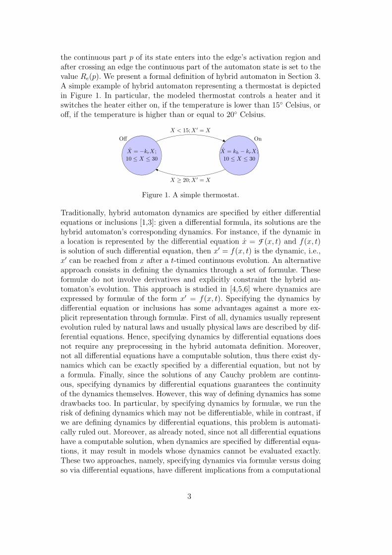
the continuous part p of its state enters into the edge’s activation region andafter crossing an edge the continuous part of the automaton state is set to thevalue Re(p). We present a formal definition of hybrid automaton in Section 3.A simple example of hybrid automaton representing a thermostat is depictedin Figure 1. In particular, the modeled thermostat controls a heater and itswitches the heater either on, if the temperature is lower than 15◦ Celsius, oroff, if the temperature is higher than or equal to 20◦ Celsius.

X = −krX;10 ≤ X ≤ 30

X = kh − krX;10 ≤ X ≤ 30

X < 15; X ′ = X

X ≥ 20; X ′ = X

Off On

Figure 1. A simple thermostat.

Traditionally, hybrid automaton dynamics are specified by either differentialequations or inclusions [1,3]: given a differential formula, its solutions are thehybrid automaton’s corresponding dynamics. For instance, if the dynamic ina location is represented by the differential equation x = F (x, t) and f(x, t)is solution of such differential equation, then x′ = f(x, t) is the dynamic, i.e.,x′ can be reached from x after a t-timed continuous evolution. An alternativeapproach consists in defining the dynamics through a set of formulæ. Theseformulæ do not involve derivatives and explicitly constraint the hybrid au-tomaton’s evolution. This approach is studied in [4,5,6] where dynamics areexpressed by formulæ of the form x′ = f(x, t). Specifying the dynamics bydifferential equation or inclusions has some advantages against a more ex-plicit representation through formulæ. First of all, dynamics usually representevolution ruled by natural laws and usually physical laws are described by dif-ferential equations. Hence, specifying dynamics by differential equations doesnot require any preprocessing in the hybrid automata definition. Moreover,not all differential equations have a computable solution, thus there exist dy-namics which can be exactly specified by a differential equation, but not bya formula. Finally, since the solutions of any Cauchy problem are continu-ous, specifying dynamics by differential equations guarantees the continuityof the dynamics themselves. However, this way of defining dynamics has somedrawbacks too. In particular, by specifying dynamics by formulæ, we run therisk of defining dynamics which may not be differentiable, while in contrast, ifwe are defining dynamics by differential equations, this problem is automati-cally ruled out. Moreover, as already noted, since not all differential equationshave a computable solution, when dynamics are specified by differential equa-tions, it may result in models whose dynamics cannot be evaluated exactly.These two approaches, namely, specifying dynamics via formulæ versus doingso via differential equations, have different implications from a computational

3

viewpoint: in the first case, using formulæ enables one to exploit quantifierelimination and decidability results over first-order logic to directly evaluatereachability (of one state from a given initial state); however, in the later case,i.e., when using differential equations to define dynamics, one first needs somepreprocessing to compute the dynamics themselves whenever it is possible.

Using hybrid automata, we can study hybrid systems and verify properties overthem. In particular, several techniques have been proposed to verify propertiesexpressed in some kind of temporal logic, such as CTL* or TCTL, over hybridautomata, e.g., see [7,1,8,9,10]. These techniques are mainly based on finitestate model checking approaches and exploit equivalence reductions (i.e., sim-ulation or bisimulation) [11,12,13] to reduce the number of system’s states.In particular, if a hybrid automaton has either a finite simulation quotientor a finite bisimulation quotient, then the property can be verified on the re-duced model through standard model checking algorithms. Since simulationpreserves LTL and bisimulation preserves CTL*, if the property holds on thereduced model, then it also holds on the original hybrid automaton. Duringthe last few years, many such techniques had been successfully used to verifyspecifications of communication protocols and controllers [14,15,16,17]. Morerecently there have also been several successful applications and consequentlya growing interest in their use in analyzing biological systems [18,19,20,21].

An interesting verification problem is the one involving safety condition whichrequires checking whether a certain property ϕ, describing all safe situations,never fails during the hybrid automaton’s evolution. Such problem can be nat-urally reduced to a reachability problem over hybrid automata. As a matter offact, to prove that a certain property ϕ is true during the entire evolution ofa hybrid automaton H, we only need to prove that all the states in which ϕ isfalse are not reachable by H. Unfortunately, it has been proven in [22] that thehalting problem for Turing machines can be reduced to a reachability problemfor a particular class of hybrid automata. Hence, the reachability problem isnot decidable in general. However, there have been proposed many non-trivial(or non-degenerate) classes of hybrid automata for which either reachabilityproblem or (more generally) temporal logic verification is decidable. In [9] Aluret al. introduced multirate automata as an extensions of timed automata [23].Such hybrid automata are characterized by resets which are either identity orconstant function zero. Moreover, their continuous variables evolve like clockswith rational rates (i.e., x becomes c · t + x, where c ∈ Q, in time t). In thesame work it has been proven that the reachability problem over multirateautomata is not decidable in general. However, by imposing a restriction ondynamics called simplicity condition, decidability for reachability problem andfinite bisimulation are shown to be achievable. Puri and Varaiya in [3] intro-duced rectangular hybrid automata whose dynamics can be characterized by adifferential inclusion of the type x ∈ [l, u], where l and u are rational numbers.Even if Kopke had proved in [24] that reachability is in general undecidable

4

for such classes of hybrid automata and that three dimensional rectangularautomata have infinite simulation quotient, they showed that, under a condi-tion called initialized condition, reachability can be decided. Finally, Laffer-riere, Pappas and Sastry introduced o-minimal hybrid automata in [25]. Suchclasses of hybrid automata guarantee finite bisimulation quotient, providedthat a constant reset condition is imposed on all of automaton’s edges.

This article aims at studying hybrid automata whose dynamics are inclusiondynamics defined by formulæ. We model hybrid automata having dynamicsof the type x′ ∈ f(x, t) and we reduce model checking problems over themto decidability problems over first-order formulæ. Since in this theory f(x, t)need not be differentiable, such kind of dynamics generalizes dynamics definedby differential inclusions. We show that imposing continuity on f(x, t) withrespect to t does not suffice to guarantee the existence of a proper continu-ous evolution satisfying the dynamics. As a consequence, we propose a set ofstronger conditions, which relies not only on the existence of such evolution,but also on the decidability of satisfiability problem for certain first-order for-mulæ, as described below. Since such results can be achieved using a Michael’sselection theorem [26], if a hybrid automaton satisfies such conditions, it is saidto be in Michael’s form. Exploiting Michael’s form, we present a class of hy-brid automata for which reachability problems can be reduced to a decidabilityproblem for first-order formulæ. We show that even if its bisimulation quotientis infinite and the finiteness of its simulation quotient is still an open problem,model checking over a CTL sub-logic (not preserved under simulation) can bereduced to a decidability problem for first-order formulæ too. We demonstratethat our decidability results cannot be achieved exploiting standard equiva-lence reduction techniques such as simulation and bisimulation. Finally, usingsimilar techniques, we prove that the membership problem of deciding whethera hybrid automaton belongs to this decidable class of automata, is also decid-able, because it can be reduced to the earlier class of decidability problemsfor model checking of hybrid automata. The class of automata we study inthis article is a generalization of o-minimal hybrid automata, since from eachpoint we can have an infinite number of continuous trajectories. This approachallows one to model situations in which the dynamics are not exactly known,e.g., some parameters are missing, as in the case with many models of bio-chemical pathways. Here, we focus only on the computability of the reductionsfrom temporal formula to the associated first-order formula, without placingany particular emphasis on their computational complexity. That is to say, wemake no effort at presenting the most efficient reductions, but merely provethat such reductions can be computed in an effective manner.

More specifically, the article is organized as follows:

Section 2 reviews the notion of first-order theory, describes some importanttheories over real numbers, and presents some decidability results over them.

5

Section 3 introduces the formal definition of hybrid automata.Section 4 shows that not all hybrid automata whose dynamics are continuous

have a continuous evolution. Moreover, it proposes a set of conditions, calledMichael’s form, which lets us reduce the problem of verifying the existence ofsuch evolution to a decidability problem over first-order formulæ and nextit shows how such conditions can be tested. Finally, it gives an effectivereduction from reachability problems over hybrid automata in Michael’sform to decidability problems for first-order formulæ under the assumptionof a finite number of discrete transitions over locations.

Section 5 introduces a class of hybrid automata, called FOCoRe, which arein Michael’s form and whose resets are restricted to constant maps. It showsthat every FOCoRe’s evolution can be reduced to a canonical form compris-ing FOCoRe’s evolution whose number of discrete transitions is bounded bythe number of automaton’s discrete edges and, hence, that the reachabil-ity problem can be decided. Moreover, it proves that FOCoRe automatahave infinite bisimulation quotient in general, and yet model checking overa particular CTL sub-logic, called ΦP , is still decidable.

Section 6 sketches a complex biological that can be modeled by using theproposed methods.

Section 7 ends the article with some comments, some practical applications,and some open problems and future works that remain to be addressed.

Part of the material presented in this paper appeared in [27,28].

2 Theories and Decidability

In this section, we review the notion of first-order theory, we describe someinteresting theories and we introduce some decidability results over them. Fora more detailed treatment of these notions, the reader may refer to [29,30].

2.1 Languages, Theories, and Models

A first-order language L is a tuple L = 〈Var ,Const ,Funct ,Rel ,Ar〉, whereVar is a set of variables, Const is a set of constant values, Funct is a setof functional operators, Rel is a set of relational symbols, and the “arity”function Ar : Funct ∪Rel → (N\{0}) associates to each element of Funct andRel the number of arguments it takes.

A term of L can be defined as:

term ::= X | c | f(term1, . . . , termAr(f))

6

where X is a variable in Var , c is a constant in Const , and f is a function inFunct .

An atomic formula ϕa of L has the form > or ⊥ (standing for true and false,respectively) or R(term1, . . . , termAr(R)), where R is a relational operator inRel and term i is a term of L for all i ∈ [1,Ar(R)]. Moreover, a formula ϕ ofL is defined as follows:

ϕ ::= ϕa | ϕ1 ∨ ϕ2 | ¬ϕ1 | ∀X ϕ1

where ϕa is an atomic formula of L, X is a variable in Var , and ϕi is a formulaof L for all i ∈ {1, 2}. We define ϕ1 ∧ ϕ2 as a short hand for ¬(¬ϕ1 ∨ ¬ϕ2),ϕ1 _ ϕ2 as a short hand for (¬ϕ1) ∨ ϕ2, and ∃X ϕ1 as a short hand for¬∀X ¬ϕ1. The two symbols ∃ and ∀ are called quantifiers.

An occurrence of a variable X ∈ Var is bound or quantified in a formula ϕ, ifit occurs in a ϕ’s sub-formula of the kind either ∀X ϕ or ∃X ϕ. An occurrenceof a variable is free if it is not bound. Modulo renaming we can safely assumethat the variables which occur bound in a formula do not occur free, andvice versa. A sentence is a formula such that all the variable occurrencesare bound. The set of free variables occurring in the first-order formula ϕ isdenoted by Free(ϕ). We will use the notation ϕ[X1, . . . , Xm] (ϕ[X], whereX = (X1, . . . , Xm)) to stress the fact that Free(ϕ) includes the set of variables{X1, . . ., Xm} (the set of components of the vector X, respectively).

A model of a language L is tuple M = 〈M, Const, Funct, Rel〉 where:

• M is a nonempty set called support ;• Const : Const → C ⊆M is an interpretation for (the elements of) Const ;

• Funct : Funct → ⋃∞k=1

(∏ki=1 M →M

), with Funct (f) :

∏Ar(f)i=1 M → M , is

an interpretation for (the elements of) Funct ;

• Rel : Rel → ⋃∞k=1

(∏ki=1 M → {>,⊥}

), with Rel (R) :

∏Ar(R)i=1 M → {>,⊥},

is an interpretation for (the elements of) Rel ;

Let M be a model of L with support M , ϕ[X1, . . . , Xi, . . . , Xm] be a formulaof L, and p ∈ M . The expression obtained by replacing Xi by p is denotedby ϕ[X1, . . . , Xi−1, p,Xi+1, . . . , Xn] and, strictly speaking, is to be intended asobtained after adding a new constant cp to the language. With a slight abuseof notation we will use formulæ to also denote these expressions.

The semantics of L-formulæ with respect to a model M is defined in thestandard way (see [29,30]). In particular, we say that a formula ϕa[p1, . . . , pm],where ϕa is atomic, holds inM if applying the interpretations of the constant,functional, and relational operators we obtain the truth value >. The formulaϕ1[p1, . . . , pm] ∨ ϕ2[p1, . . . , pm] holds in M if either the first or the seconddisjunct holds inM. The formula ¬ϕ1[p1, . . . , pm] holds inM if ϕ1[p1, . . . , pm]

7

does not. The formula ∀X ϕ1[X, p1, . . . , pm] holds inM if for each p ∈M theformula ϕ1[p, p1, . . . , pm] holds. We say that a formula ϕ[X1, . . . , Xm] in L issatisfiable inM if there exist p1, . . . , pm ∈M such that ϕ[p1, . . . , pm] holds inM. Moreover, we say that ϕ[X1, . . . , Xm] is valid if ϕ[p1, . . . , pm] holds in Mfor all p1, . . . , pm ∈ M . When the model M is clear from the context we willsimply say that a formula holds (is satisfiable or is valid, respectively).

When we speak of models over M , where M is a nonempty set, we are referringto those models whose support isM . Besides, when Const : Const → C is clearfrom the context, we use 〈M,C, Funct, Rel〉 to mean 〈M, Const, Funct, Rel〉.

Example 1 Consider the language LR def= 〈Var ,Z, {+, ∗}, {≥},Ar〉. A model

for the language LR is the tuple 〈R,Z, Funct, Rel〉 where Funct and Rel are theusual interpretations for {+, ∗} and {≥}, respectively and we have a constantfor each element in Z.

Notice that such a model can be “simplified” to M0def= 〈R, {0, 1}, Funct, Rel〉,

in the sense that for each formula ϕR in the language LR there exists a for-

mula ϕ0 in the language L0def= 〈Var , {0, 1}, {+, ∗}, {≥},Ar〉 such that ϕR

is satisfiable in MRdef= 〈R,Z, Funct, Rel〉 if and only if ϕ0 is satisfiable in

M0def= 〈R, {0, 1}, Funct, Rel〉.

Given a set Γ of sentences and a sentence ϕ, we say that ϕ is a logical con-sequence of Γ (denoted, Γ |= ϕ) if for each model M it holds that if eachformula of Γ is valid in M (M |= Γ), then ϕ is valid in M. As a conse-quence of completeness of first-order logic, we may equivalently say that ϕ isprovable from Γ (see [29,30]). A theory T is a set of sentences such that ifT |= ϕ, then ϕ ∈ T . Given a language L and a modelM the complete theoryT (M) of M, is the set of all the sentences of L which are valid in M. Givena model 〈M,C, Funct, Rel〉, we also indicate its complete theory by either〈M,C, Funct, Rel〉 or 〈M,C, f0, . . . , fn, r0, . . . rm〉, where Funct = {f0, . . . , fn}and Rel = {r0, . . . , rm}. Notice that for each model M it holds that for eachsentence ϕ, either ϕ ∈ T (M) or ¬ϕ ∈ T (M). Two formulæ ϕ1[X] and ϕ2[Y ],where X and Y are two vectors of variables, are equivalent with respect to atheory T if it holds that T |= ∀X, Y (ϕ1[X] ] ϕ2[Y ]). We say that a theoryT admits the so-called elimination of quantifiers, if, for any formula ϕ, thereexists a quantifier free formula % such that ϕ is equivalent to % with respectto T . If there exists an algorithm for deciding whether a sentence ϕ belongsto T or not, we say that T is decidable. Notice that given a model M, itscomplete theory T (M) is decidable if and only if both the satisfiability andthe validity of formulæ in M are decidable.

Example 2 Consider the formula ϕdef= ∃X (aX2 + bX + C = 0). It is well

known that, in the theory of reals with +, ∗, and ≥, ϕ holds if and only if theunquantified formula b2 − 4ac ≥ 0 holds.

8

In the rest of this paper we will only refer to theories of the form T (M) forsome model M.

2.2 O-Minimal Theories

An interesting class of theories is the class of o-minimal theories [31,32]. Givena language L and a model M of L with support M we say that a set S ⊆Mk is definable if and only if there exists a formula ϕ[X1, . . . , Xk] such thatϕ[p1, . . . , pk] holds in M if and only if (p1, . . . , pk) ∈ S.

Definition 3 (O-Minimal Theory) Let L be a first-order language whoseset of relational symbols includes a binary symbol ≤ and let M be a modelof L in which ≤ is interpreted as a linear order. The theory T (M) is orderminimal, or simply o-minimal, if every set definable in T (M) is a finite unionof points and intervals (with respect to ≤).

The class of o-minimal theories includes many interesting theories over R.Below we recall a few of them.

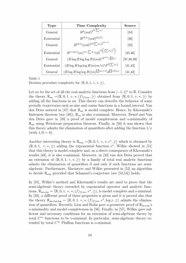
The theory R =〈R, 0, 1,+, ∗,≥〉 is called semi-algebraic theory. In [33], Tarskishowed that such theory admits elimination of quantifiers and that it is decid-able. Unfortunately, Tarski’s algorithm has a computational complexity, whichcould not even be expressed as a bounded tower of exponents of the input size.In [34] Collins presented an algorithm, called Cylindrical Algebraic Decomposi-tion (CAD), to decide the satisfiability of a formula ϕ of LR. Later Hoon Hong,using many useful and practical heuristics, created the first practical quantifierelimination software Qepcad. Alternative CAD-based methods that are doublyexponential in the number of quantifier alternations rather than the numberof variables, have been proposed by Grigorev [35,36] and Renegar [37,38,39].New quantifier elimination approaches have been proposed by Basu, Pollack,and Roy in [40,41,42]. The total time complexity (bit-complexity) [43,44] ofthe semi-algebraic decision procedures, mentioned above, are summarized inTable 1, under the hypothesis that the coefficients of the polynomials can bestored with at most B bits and that the input formulæ have the form:

(Q1X[1])(Q2X

[2]) . . . (QlX [l])(ϕ[X [1], . . . , X [l]])

where Qi ∈ {∀,∃} and Qj 6= Qj+1, X [i] is a partition of all the variables inϕ, with |X [i]| = ni, and ϕ is a quantifier-free formula with atomic formulæconsisting of m polynomials of equalities and inequalities of total degree dhaving the form

gk(X[1], . . . , X [l]) ≥ 0, k = 1, . . . ,m.

9

Type Time Complexity Source

General B3(md)2O(∑

ni) [34]

Existential BO(1)(md)O(n2) [36]

General BO(1)(md)(O(∑

ni))4∗l−2

[35]

Existential B1+o(1)(m)(1+∑

ni)(d)O

((∑

ni)2)

[45,46]

General (B log B log log B)(md)(2O(l))∏ni [37,38,39]

Existential (B log B log log B)m(m/s)sdO(∑

ni) [41,42]

General (B log B log log B)(m)∏

(ni+1)d∏O(ni) [41,42]

Table 1Decision procedure complexity for 〈R, 0, 1, +, ∗,≥〉.

Let an be the set of all the real-analytic functions from [−1, 1]n to R. Considerthe theory Ran =〈R, 0, 1,+, ∗, (f)f∈an,≥〉 obtained from 〈R, 0, 1,+, ∗,≥〉 byadding all the functions in an. This theory can describe the behavior of someperiodic trajectories such as sine and cosine functions in a bound interval. Vanden Dries noticed in [47] that Ran is model complete. Hence, by Khovanskı’sfiniteness theorem (see [48]), Ran is also o-minimal. Moreover, Denef and Vanden Dries gave in [49] a proof of model completeness and o-minimality ofRan using Weirstrass preparation theorem. Finally, in [50] it was shown thatthis theory admits the elimination of quantifiers after adding the function 1/x(with 1/0 = 0).

Another interesting theory is Rexp =〈R, 0, 1,+, ∗, ex,≥〉 which is obtained by(R, 0, 1, +, ∗,≥) adding the exponential function ex. Wilkie showed in [51]that this theory is model complete and, as a direct consequence of Khovanskı’sresults [48], it is also o-minimal. Moreover, in [32] van den Dries proved thatan extension of 〈R, 0, 1,+, ∗,≥〉 by a family of total real analytic functionsadmits the elimination of quantifiers if and only if such functions are semi-algebraic. Furthermore, Macintyre and Wilkie presented in [52] an algorithmto decide Rexp provided that Schanuel’s conjecture (see [53,54]) holds.

In [55], Wilkie’s method and Khovanskı’s results are used to prove that thesemi-algebraic theory extended by exponential operator and analytic func-tions, Ran,exp = 〈R, 0, 1,+, ∗, (f)f∈an, e

x,≥〉, is model complete and o-minimal.In [50], a different proof of these properties is given and it is proved also thatthe theory Ran,exp,log = 〈R, 0, 1,+, ∗, (f)f∈an, e

x, log x,≥〉 admits the elimina-tion of quantifiers. Recently, Lion and Rolin gave a geometric proof of Ran,exp’so-minimality and model completeness in [56]. Finally, in [57], Wilkie gave suf-ficient and necessary conditions for an extension of semi-algebraic theory bytotal C∞ functions to be o-minimal. In particular, semi-algebraic theory ex-tended by total C∞ Pfaffian functions is o-minimal.

10

3 Hybrid Automata

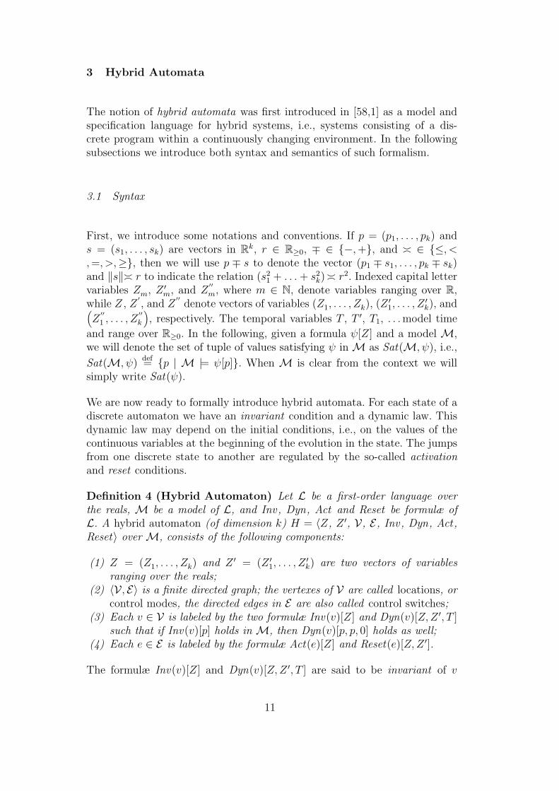
The notion of hybrid automata was first introduced in [58,1] as a model andspecification language for hybrid systems, i.e., systems consisting of a dis-crete program within a continuously changing environment. In the followingsubsections we introduce both syntax and semantics of such formalism.

3.1 Syntax

First, we introduce some notations and conventions. If p = (p1, . . . , pk) ands = (s1, . . . , sk) are vectors in Rk, r ∈ R≥0, ∓ ∈ {−,+}, and � ∈ {≤, <,=, >,≥}, then we will use p ∓ s to denote the vector (p1 ∓ s1, . . . , pk ∓ sk)and ‖s‖� r to indicate the relation (s2

1 + . . .+ s2k)� r2. Indexed capital letter

variables Zm, Z ′m, and Z′′m, where m ∈ N, denote variables ranging over R,

while Z , Z′, and Z

′′denote vectors of variables (Z1, . . . , Zk), (Z ′1, . . . , Z

′k), and(

Z′′1 , . . . , Z

′′k

), respectively. The temporal variables T , T ′, T1, . . . model time

and range over R≥0. In the following, given a formula ψ[Z] and a model M,we will denote the set of tuple of values satisfying ψ inM as Sat(M, ψ), i.e.,

Sat(M, ψ)def= {p | M |= ψ[p]}. When M is clear from the context we will

simply write Sat(ψ).

We are now ready to formally introduce hybrid automata. For each state of adiscrete automaton we have an invariant condition and a dynamic law. Thisdynamic law may depend on the initial conditions, i.e., on the values of thecontinuous variables at the beginning of the evolution in the state. The jumpsfrom one discrete state to another are regulated by the so-called activationand reset conditions.

Definition 4 (Hybrid Automaton) Let L be a first-order language overthe reals, M be a model of L, and Inv, Dyn, Act and Reset be formulæ ofL. A hybrid automaton (of dimension k) H = 〈Z, Z ′, V, E, Inv, Dyn, Act,Reset〉 over M, consists of the following components:

(1) Z = (Z1, . . . , Zk) and Z ′ = (Z ′1, . . . , Z′k) are two vectors of variables

ranging over the reals;(2) 〈V , E〉 is a finite directed graph; the vertexes of V are called locations, or

control modes, the directed edges in E are also called control switches;(3) Each v ∈ V is labeled by the two formulæ Inv(v)[Z] and Dyn(v)[Z,Z ′, T ]

such that if Inv(v)[p] holds in M, then Dyn(v)[p, p, 0] holds as well;(4) Each e ∈ E is labeled by the formulæ Act(e)[Z] and Reset(e)[Z,Z ′].

The formulæ Inv(v)[Z] and Dyn(v)[Z,Z ′, T ] are said to be invariant of v

11

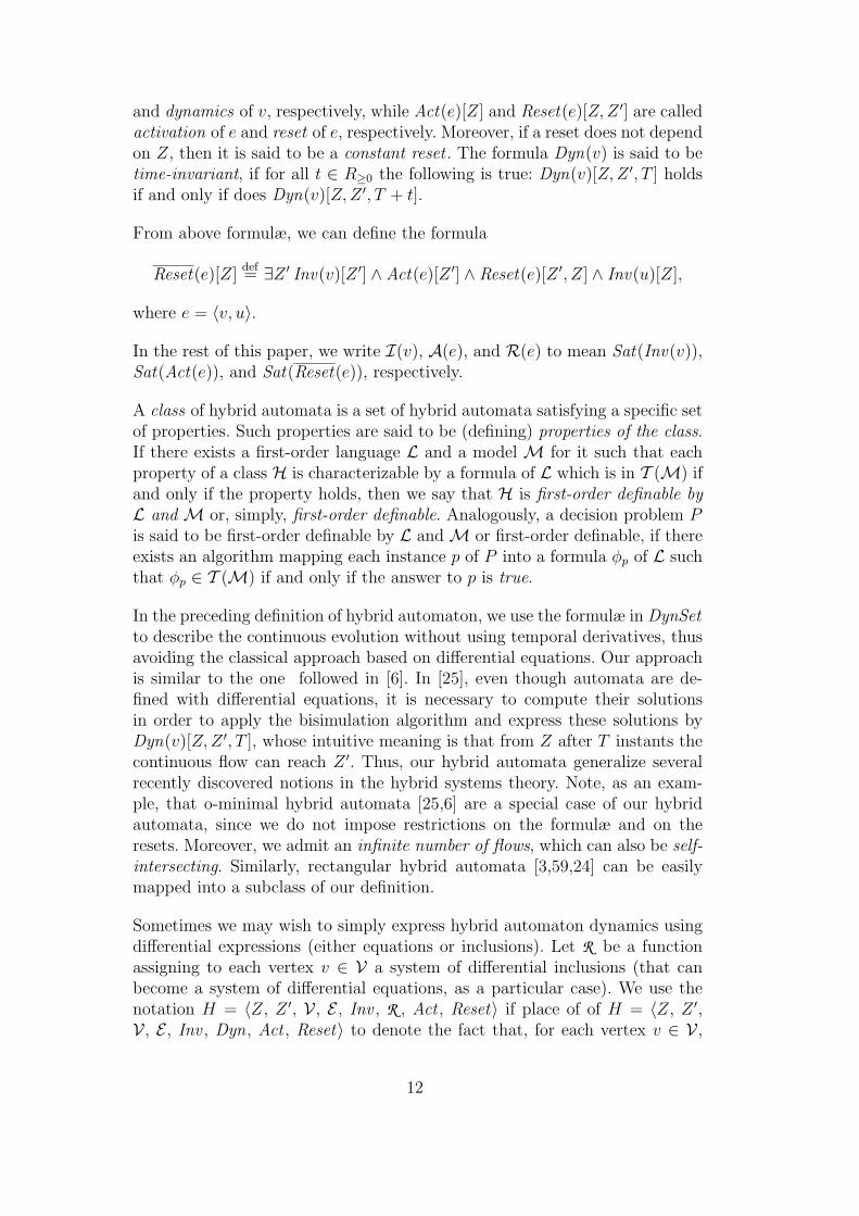
and dynamics of v, respectively, while Act(e)[Z] and Reset(e)[Z,Z ′] are calledactivation of e and reset of e, respectively. Moreover, if a reset does not dependon Z, then it is said to be a constant reset . The formula Dyn(v) is said to betime-invariant, if for all t ∈ R≥0 the following is true: Dyn(v)[Z,Z ′, T ] holdsif and only if does Dyn(v)[Z,Z ′, T + t].

From above formulæ, we can define the formula

Reset(e)[Z]def= ∃Z ′ Inv(v)[Z ′] ∧ Act(e)[Z ′] ∧ Reset(e)[Z ′, Z] ∧ Inv(u)[Z],

where e = 〈v, u〉.

In the rest of this paper, we write I(v), A(e), and R(e) to mean Sat(Inv(v)),Sat(Act(e)), and Sat(Reset(e)), respectively.

A class of hybrid automata is a set of hybrid automata satisfying a specific setof properties. Such properties are said to be (defining) properties of the class.If there exists a first-order language L and a model M for it such that eachproperty of a class H is characterizable by a formula of L which is in T (M) ifand only if the property holds, then we say that H is first-order definable byL and M or, simply, first-order definable. Analogously, a decision problem Pis said to be first-order definable by L andM or first-order definable, if thereexists an algorithm mapping each instance p of P into a formula φp of L suchthat φp ∈ T (M) if and only if the answer to p is true.

In the preceding definition of hybrid automaton, we use the formulæ in DynSetto describe the continuous evolution without using temporal derivatives, thusavoiding the classical approach based on differential equations. Our approachis similar to the one followed in [6]. In [25], even though automata are de-fined with differential equations, it is necessary to compute their solutionsin order to apply the bisimulation algorithm and express these solutions byDyn(v)[Z,Z ′, T ], whose intuitive meaning is that from Z after T instants thecontinuous flow can reach Z ′. Thus, our hybrid automata generalize severalrecently discovered notions in the hybrid systems theory. Note, as an exam-ple, that o-minimal hybrid automata [25,6] are a special case of our hybridautomata, since we do not impose restrictions on the formulæ and on theresets. Moreover, we admit an infinite number of flows, which can also be self-intersecting. Similarly, rectangular hybrid automata [3,59,24] can be easilymapped into a subclass of our definition.

Sometimes we may wish to simply express hybrid automaton dynamics usingdifferential expressions (either equations or inclusions). Let R be a functionassigning to each vertex v ∈ V a system of differential inclusions (that canbecome a system of differential equations, as a particular case). We use thenotation H = 〈Z, Z ′, V , E , Inv , R , Act , Reset〉 if place of of H = 〈Z, Z ′,V , E , Inv , Dyn, Act , Reset〉 to denote the fact that, for each vertex v ∈ V ,

12

the formula Dyn(v)[Z,Z ′, T ] corresponds to the solution of the differentialinclusions R (v) when the starting point is Z.

3.2 Semantics and Reachability

To formalize the semantics of hybrid automata, we first need to introduce theconcept of hybrid automaton’s state.

Definition 5 (States) Let H be a hybrid automaton overM of dimension k.A state q of H is a pair 〈v, r〉, where v ∈ V is a location and r = (r1, . . . , rk) ∈Rk is an assignment of values for the variables of Z. A state 〈v, r〉 is said tobe admissible if Inv(v)[r] holds in M.

Intuitively, an execution of a hybrid automaton corresponds to a sequenceof transitions from one state of the automaton to another. Hybrid automatahave two kinds of transition (and reachability) relations: continuous transition(reachability) relations, capturing the continuous evolution of a state accordingto both formulæ Dyn(v) and Inv(v), and discrete transition (reachability)relation, capturing changes of location driven by the formula Reset(e) and theformula Act(e).

More formally, we can define hybrid automaton semantics as follow.

Definition 6 (Hybrid Automaton - Semantics) Let H be a hybrid au-tomaton over M of dimension k. The continuous reachability transition rela-

tionst−→C between admissible states is defined as follows:

〈v, r〉 t−→C 〈v, s〉 ⇐⇒

there exists f : R≥0 → Rk continuous func-tion such that r = f(0), s = f(t), andfor each t′ ∈ [0, t] the formulæ Inv(v)[f(t′)]and Dyn(v)[r, f(t′), t′] hold inM. f is calledflow function.

The discrete reachability transition relatione−→D, where e ∈ E, between admis-

sible states is defined as follows:

〈v, r〉 〈v,u〉−−→D 〈u, s〉 ⇐⇒〈v, u〉 ∈ E and the formulæ Inv(v)[r],Act(〈v, u〉)[r], Reset(〈v, u〉)[r, s], andInv(u)[s] hold in M.

We use the notation `λ−→ `′ to indicate that either `

λ−→C `′, if λ ∈ R≥0, or

`λ−→D `′, when λ ∈ E . Furthermore, we write ` −→C `′ to denote that there

exists a t such that `t−→C `

′.

13

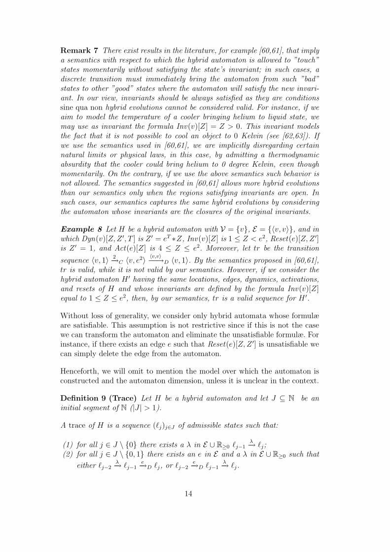
Remark 7 There exist results in the literature, for example [60,61], that implya semantics with respect to which the hybrid automaton is allowed to ”touch”states momentarily without satisfying the state’s invariant; in such cases, adiscrete transition must immediately bring the automaton from such ”bad”states to other ”good” states where the automaton will satisfy the new invari-ant. In our view, invariants should be always satisfied as they are conditionssine qua non hybrid evolutions cannot be considered valid. For instance, if weaim to model the temperature of a cooler bringing helium to liquid state, wemay use as invariant the formula Inv(v)[Z] = Z > 0. This invariant modelsthe fact that it is not possible to cool an object to 0 Kelvin (see [62,63]). Ifwe use the semantics used in [60,61], we are implicitly disregarding certainnatural limits or physical laws, in this case, by admitting a thermodynamicabsurdity that the cooler could bring helium to 0 degree Kelvin, even thoughmomentarily. On the contrary, if we use the above semantics such behavior isnot allowed. The semantics suggested in [60,61] allows more hybrid evolutionsthan our semantics only when the regions satisfying invariants are open. Insuch cases, our semantics captures the same hybrid evolutions by consideringthe automaton whose invariants are the closures of the original invariants.

Example 8 Let H be a hybrid automaton with V = {v}, E = {〈v, v〉}, and inwhich Dyn(v)[Z,Z ′, T ] is Z ′ = eT ∗Z, Inv(v)[Z] is 1 ≤ Z < e2, Reset(e)[Z,Z ′]is Z ′ = 1, and Act(e)[Z] is 4 ≤ Z ≤ e2. Moreover, let tr be the transition

sequence 〈v, 1〉 2−→C 〈v, e2〉 〈v,v〉−−→D 〈v, 1〉. By the semantics proposed in [60,61],tr is valid, while it is not valid by our semantics. However, if we consider thehybrid automaton H ′ having the same locations, edges, dynamics, activations,and resets of H and whose invariants are defined by the formula Inv(v)[Z]equal to 1 ≤ Z ≤ e2, then, by our semantics, tr is a valid sequence for H ′.

Without loss of generality, we consider only hybrid automata whose formulæare satisfiable. This assumption is not restrictive since if this is not the casewe can transform the automaton and eliminate the unsatisfiable formulæ. Forinstance, if there exists an edge e such that Reset(e)[Z,Z ′] is unsatisfiable wecan simply delete the edge from the automaton.

Henceforth, we will omit to mention the model over which the automaton isconstructed and the automaton dimension, unless it is unclear in the context.

Definition 9 (Trace) Let H be a hybrid automaton and let J ⊆ N be aninitial segment of N (|J | > 1).

A trace of H is a sequence (`j)j∈J of admissible states such that:

(1) for all j ∈ J \ {0} there exists a λ in E ∪ R≥0 `j−1λ−→ `j;

(2) for all j ∈ J \ {0, 1} there exists an e in E and a λ in E ∪ R≥0 such that

either `j−2λ−→ `j−1

e−→D `j, or `j−2e−→D `j−1

λ−→ `j.

14

Remark 10 Condition 2 in the above definition has been introduced to definea notion of hybrid trace analogous to the notion of trajectory defined in dynam-ical systems. In particular, if we relax Condition 2, we must assume transitivedynamics. For the sake of concreteness, consider the model of an automaticarcher in a 2-dimensional world. The archer’s goal is to hit a target τ with anarrow. Trajectories of the arrow is defined by two parameters, namely, gravityg and an initial linear velocity of magnitude v, which is assumed, for simplic-ity, to remain same over a succession of attempts by the archer. After eachsuccessive throw, the archer adjusts the angle of next throw according to thefinal position of the arrow: if the arrow lands ahead of target, then the throwingangle will be decreased proportionally, if, on the other hand, the arrow landsbehind target, then the throwing angle will be increased proportionally.

The hybrid automata describing such system consists of one vertex, v, andone edge, e: the arrow trajectories are modeled by the continuous dynamicsin v, while the adjustments of throwing angle are represented by resets on e.The automata has three continuous variables, Xp, Yp, and θ, representing thearrow position with respect to y-axis, the arrow position with respect to x-axis,and the throwing angle, respectively. Assuming the archer in position 〈Xp, Yp〉,Dyn(v)[Z,Z ′, T ]

def= Y ′p = −1

2gT 2+sin θvT+Yp∧X ′p = sin θvT+Xp∧θ′ = θ and

Inv(v)[Z]def= Yp ≥ 0 ∧ θ ∈ [0, π

2), where Z ′ = 〈X ′p, Y ′p , θ′〉 and Z = 〈Xp, Yp, θ〉,

can describe dynamics and invariant on v, respectively. The activation region

can be characterized as Act(e)[Z]def= Xp > 0 ∧ Yp = 0 and the reset can be

Reset(e)[Z,Z ′]def= X ′p = 0 ∧ Y ′p = 0 ∧ θ′ = Φτ (θ,Xp), where Φτ is a function

which updates θ according to the distance by which arrow misses its target.

It is easy to prove that the continuous dynamics of such automaton is not tran-sitive i.e., even if the archer can throw an arrow from 〈Xp, Yp〉 to 〈X ′p, Y ′p〉 andfrom 〈X ′p, Y ′p〉 to 〈X ′′p , Y ′′p 〉 by using the same throwing angle, it is not true thatthe archer can throw an arrow from 〈Xp, Yp〉 to 〈X ′′p , Y ′′p 〉. It is also obviousthat the continuous evolution cannot be split into two or more “sub-evolutions”i.e., even if the archer can throw an arrow from 〈Xp, Yp〉 to 〈X ′p, Y ′p〉 by using athrowing angle θ in time T , it does not hold that there exists a time T ′ ∈ (0, T )such that the archer can throw an arrow from 〈Xp, Yp〉 to 〈X ′′p , Y ′′p 〉 with throw-ing angle θ in time T ′ and from 〈X ′′p , Y ′′p 〉 to 〈X ′p, Y ′p〉 with the same throwingangle in time T − T ′. In particular, the model has an intrinsic interleavingbehavior which does not admit two consecutive transitions of the same kind.

For such reasons such as this, to handle systems lacking autonomous dynam-ics, we imposed Condition 2. Notice that the continuous dynamics of the pro-posed automaton can be turned into a transitive one by adding a variable whichrepresents the evolution of the y-velocity during the arrow trajectory. By doingso, we would increase the complexity of the formulæ involved in the decisionprocedure, even if we would not necessarily improve the accuracy of the model.

15

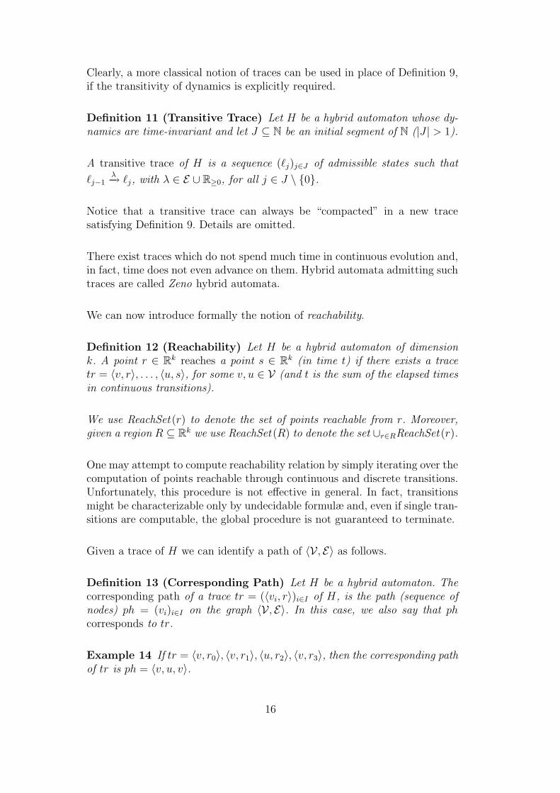
Clearly, a more classical notion of traces can be used in place of Definition 9,if the transitivity of dynamics is explicitly required.

Definition 11 (Transitive Trace) Let H be a hybrid automaton whose dy-namics are time-invariant and let J ⊆ N be an initial segment of N (|J | > 1).

A transitive trace of H is a sequence (`j)j∈J of admissible states such that

`j−1λ−→ `j, with λ ∈ E ∪ R≥0, for all j ∈ J \ {0}.

Notice that a transitive trace can always be “compacted” in a new tracesatisfying Definition 9. Details are omitted.

There exist traces which do not spend much time in continuous evolution and,in fact, time does not even advance on them. Hybrid automata admitting suchtraces are called Zeno hybrid automata.

We can now introduce formally the notion of reachability.

Definition 12 (Reachability) Let H be a hybrid automaton of dimensionk. A point r ∈ Rk reaches a point s ∈ Rk (in time t) if there exists a tracetr = 〈v, r〉, . . . , 〈u, s〉, for some v, u ∈ V (and t is the sum of the elapsed timesin continuous transitions).

We use ReachSet (r) to denote the set of points reachable from r. Moreover,given a region R ⊆ Rk we use ReachSet (R) to denote the set ∪r∈RReachSet (r).

One may attempt to compute reachability relation by simply iterating over thecomputation of points reachable through continuous and discrete transitions.Unfortunately, this procedure is not effective in general. In fact, transitionsmight be characterizable only by undecidable formulæ and, even if single tran-sitions are computable, the global procedure is not guaranteed to terminate.

Given a trace of H we can identify a path of 〈V , E〉 as follows.

Definition 13 (Corresponding Path) Let H be a hybrid automaton. Thecorresponding path of a trace tr = (〈vi, r〉)i∈I of H, is the path (sequence ofnodes) ph = (vi)i∈I on the graph 〈V , E〉. In this case, we also say that phcorresponds to tr.

Example 14 If tr = 〈v, r0〉, 〈v, r1〉, 〈u, r2〉, 〈v, r3〉, then the corresponding pathof tr is ph = 〈v, u, v〉.

16

3.3 Model Checking for Hybrid Systems

To verify specifications on hybrid automata, one may want to consider theirtransition systems and apply classical model checking techniques (see e.g.,[64]). Unfortunately, hybrid automata have infinite state systems and the stan-dard model checking techniques, which work on finite state models, cannot bedirectly applied in this context. To solve this problem, many authors sug-gested the use of equivalence reductions based on relations such as simulationand bisimulation. Since bisimulation preserves branching-time temporal logicssuch as CTL and CTL*, whenever the bisimulation quotient of a system isfinite, we could verify CTL and CTL* properties of the system applying finitemodel checking techniques on its bisimulation quotient. In a similar vein, ifthe simulation quotient is finite we may also attempt to verify LTL propertiesof the system by applying finite model checking techniques on its simulationquotient. Bisimulation has the advantage of preserving more expressive logics,but in many cases it produces infinite quotients. On the other hand, simu-lation preserves less expressive logics, but it can also reduce a significantlylarger class of automata to finite state models.

Since on a single hybrid automaton we can consider both timed and untimedsemantics, we can compute (bi)simulation on both of them. For these reasons,we distinguish between the so called timed-abstract simulations/bisimulations,computed on the untimed semantics, and the timed simulation/bisimulation,evaluated on timed semantics. When we talk about simulation and bisimula-tion, we refer to timed-abstract simulation and bisimulation, respectively.

An interesting instance of the model checking problem is the verification ofsafety properties : given a hybrid automaton H and a property φ, we may wishto test whether φ holds along all of H’s trajectories. Since this is the case ifand only if there is no reachable state in which φ does not hold, the verificationof safety properties naturally reduces to the reachability problem. Even if ithas been proven in [22] that reachability is generally undecidable, many in-teresting classes of hybrid automata over which reachability is decidable havebeen characterized in the literature [24,59,25,6]. A common approach for de-ciding reachability of hybrid automata employs the technique of discretizingthe automata either using equivalence relations which strongly preserve reach-ability (e.g., bisimulation [25]) or using abstractions (e.g., predicate abstrac-tion [65,66]). In this paper, instead, we study reachability on hybrid automataby translating the reachability problem into first-order formulæ over the reals.In particular, we make use of the following results (whose proof is obvious):

Theorem 15 If a class H of hybrid automata is first-order definable by a lan-guage L and a model M, with T (M) decidable, then the membership problemfor a given hybrid automata H in H is decidable.

17

Theorem 16 If the reachability problem for a given hybrid automaton H isfirst-order definable by a language L and a model M, with T (M) decidable,then the reachability problem for H is decidable.

The formulæ we get from the translation include formulæ occurring in theautomata and we are interested in the evaluation of these formulæ in themodel M over which the automaton is defined. Hence, to obtain decidabilityresults we will ultimately exploit properties of the theory T (M).

4 Dynamics and Flow Selections

As remarked in Section 3, we allow the use of first-order formulæ, in placeof differential equations and inclusions, to define hybrid automaton’s flows.In particular, the dynamics are described through formulæ. Since, in general,given a dynamic, we cannot guarantee the existence of a corresponding flowfunction, in this section we introduce and study a set of properties whichensure such existence. The conditions we will impose on dynamics, will allowus to use Michael’s selection theorem (see [26,67]) to translate a reachabilityproblem into a first-order satisfiability problem over the reals.

The novelty of our approach mainly lies in the use of continuous selectionresults [67] which allow us to consider hybrid automata whose dynamics cor-respond to non-autonomous differential inclusions. As a direct consequence ofsuch results, we can derive first-order formulæ to encode reachability problems.

All the formulæ presented in this and in the following sections are built uponInv , Dyn, Act , and Reset by using standard connectives and first-order quan-tifiers. It follows that, if we are considering an automaton over a model M,all the presented formulæ are evaluated with respect to the theory T (M).Hence, whenever T (M) is decidable, the decidability of the problems whichare reduced to such formulæ follows.

4.1 Dynamics and Selection Problem

Assuming the continuity of F , the existence of a continuous solution for theCauchy problem x(t) = F (t, x(t))

x(0) = c(1)

is ensured by Cauchy-Kovalevskaya’s theorem (see [68]). Hence, specifying hy-brid automaton dynamics through differential equations has the side-effect of

18

guaranteeing the existence of a continuous differentiable flow function satis-fying the dynamics. This remark can be exploited when dynamics is specifiedby differential equations, which lead to first-order formula trajectories [25,69].

As remarked we allow the use of formulæ, in place of differential equations andinclusions, to define hybrid automaton’s flows. This choice lets us model hybridautomata whose dynamics are not differentiable, but it does not guarantee theexistence of a continuous flow function satisfying the dynamics. In particular,given two formulæ Dyn(v)[Z,Z ′, T ] and Inv(v)[Z] specifying the dynamicsin a location v and its invariant, respectively, we are not guaranteed that

〈v, p〉 t−→C 〈v, qt〉. This is the case even if for all t ∈ R≥0, there exists a qt ∈ Rk

such that Dyn(v)[p, qt, t] ∧ Inv(v)[qt] holds (see Example 20). Hence, we needto find a set of sufficient conditions for the existence of a continuous functionsatisfying the dynamics. To this end we formulate the flow specification as aselection problem.

In general, given a family of sets {Sx : x ∈ X}, a selection, or choice function,is a function f : X → ⋃

x∈X Sx such that, for each x ∈ X, f(x) ∈ Sx. If X isfinite, then the existence of a selection is obvious. Otherwise, it is necessary toassume (some form of) the axiom of choice[67,70]. The reader should noticethat the axiom of choice does not guarantee continuity. In particular, thereexist families of sets which have no continuous selection.

To find a set of sufficient conditions for the continuity of the selection, weneed to introduce both the notions of lower semi-continuity (see [67]) andα-paraconvexity (see [71]).

Definition 17 (Lower Semi-Continuous Map) Let F : X → 2Y be amap from X to 2Y . We define F to be lower semi-continuous (l.s.c.) if foreach x ∈ X, for each y ∈ F (x), and for each neighborhood Uy of y, there ex-ists a neighborhood Ux of x such that for each x′ ∈ Ux it holds F (x′)∩Uy 6= ∅.

We recall that a Banach space is a normed vector space in which every Cauchysequence has a limit, i.e., the space is complete (see, e.g., [67]).

Definition 18 (α-Paraconvex Set) Let L be a normed linear space withmetric γ and let α be a real number in [0, 1]. A set P ⊆ L is α-paraconvexif γ(q, P ) ≤ α ∗ r for all open sphere, Sr, with radius r, and for all q in theconvex hull of Sr(p) ∩ P .

A set is called paraconvex if it is α-paraconvex for some α < 1. Notice that ifa set is convex, then it is also paraconvex, whereas there exist sets which areparaconvex and non-convex.

Exploiting lower semi-continuity and properties of Banach spaces, Michaelproved the following result (see [71]).

19

+1

−1

Φ(0) Φ(t0)

Φ(t1)

t0 t1

1t1

1t1− |t|

Figure 2. The map Φ of Example 20.

Theorem 19 (Michael’s Selection Theorem) Let X and Y be a metricspace and a Banach space, respectively. Let F be a lower semi-continuousfunction from X into the closed α-paraconvex subsets of Y , with α ∈ [0, 1[.Then there exists a continuous selection function f : X → Y for F , that is fis continuous and ∀x ∈ X we have f(x) ∈ F (x).

The preceding result provides us the sufficient condition we were lookingfor. Notice that the result is proven under the hypothesis that F (x) is α-paraconvex and closed for all x ∈ X. Both the closure and the α-paraconvexityof F (x) are necessary. As a matter of fact, there exists a continuous map fromthe open interval (−1,+1) into closed and not α-paraconvex subsets of R2

which has no continuous selection, as illustrated by Example 20 below.

The first selection theorem identified by Michael in [26] has a simpler formula-tion, but with conditions stricter in comparison to the one above. In particular,it requires convexity, instead of α-paraconvexity, for all y ∈ Y . Despite thisdrawback, we adopt the above version to allow applications to a wider set ofsystems; e.g., systems like the one presented in Section 6.

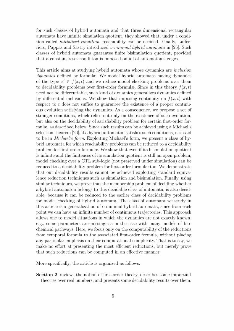
Example 20 (From [67]) Consider the map Φ : (−2π,+2π) → 2R2defined

as follow:

Φ(t)def=

{

(t cos θ, sin θ) | 1t≤ θ ≤ 1

t+ 2π − |t|

}if t 6= 0

{(x, y) | − 1 ≤ y ≤ 1 ∧ x = 0} otherwise

By definition, if t = 0, Φ(t) is the set of points in the segment between (0, 1)and (0,−1). Otherwise, if t 6= 0, Φ(t) is a subset of an ellipsoid in R2 obtainedafter removing the section from angle 1

t− |t| to angle 1

t. Hence, as t gets

smaller, the arc length of the removed section decreases, while the removedsection itself spins around the origin at increasing angular speed. Moreover,the x-width of Φ(t) shrinks to zero as t→ 0, collapsing Φ(t) to Φ(0).

20

The function Φ can be easily proved to be lower semi-continuous over the entireopen interval (−2π,+2π), and yet there is no continuous selection defined onthis interval. As a matter of fact, if we assume for the sake of contradictionthat there exists a selection f(t) continuous in (−2π, 2π), then there shouldexist limt→0 f(t). But by definition of Φ, the second component of f is forced tobounce between 2π and −2π as fast as t gets close to zero. Hence, limt→0 f(t)does not exist and f(t) cannot be continuous.

Notice that, since there exists no α < 1 such that Φ(t) is α-paraconvex for allt, Φ does not satisfy the hypothesis of Theorem 19.

4.2 Michael’s Form

In this section, we exploit Theorem 19 and we present a set of conditions whichguarantee the existence of a valid continuous transition.

First of all, we need to characterize those time instants at which the automata,starting from a point p in a location v, can reach a point q while remaininginside the invariant set of v. We recall that an interval over R≥0 is a set ofthe form {r ∈ R≥0 | a ≺1 r ≺2 b}, where ≺1, ≺2 are in {<, ≤}, a ∈ R≥0,b ∈ R≥0 ∪ {+∞}, and a ≤ b.

The following simple lemma holds since Inv(v)[p] implies Dyn(v)[p, p, 0].

Lemma 21 Let H be a hybrid automaton. Let p ∈ Rk be such that Inv(v)[p]holds. The formula ∃Z ′(Dyn(v)[p, Z ′, 0] ∧ Inv(v)[Z ′]) holds.

The above lemma allows us to focus on the initial segment of time instants,for which there are dynamics that start from p and remain inside the invariantof v—these dynamics are the main foci of our interest.

Definition 22 (IHv,p and FHv,p) Let H be a hybrid automaton. Let v be a lo-

cation of H and p be such that Inv(v)[p] holds. IHv,p is the interval of timeinstants satisfying the following conditions:

• the formula ∀T ∈ IHv,p ∃Z ′(Dyn(v)[p, Z ′, T ] ∧ Inv(v)[Z ′]) holds;• 0 ∈ IHv,p;• IHv,p is maximal with respect to the above requirements.

Define the function FHv,p : IHv,p → 2Rk

as:

FHv,p(t)

def= {q | Dyn(v)[p, q, t] and Inv(v)[q]}.

We now possess all the ingredients to introduce Michael’s Form.

21

Definition 23 (Michael’s Form) Let H be a hybrid automaton. We saythat H is in Michael’s form if for each v ∈ V and for all p such that Inv(v)[p]holds, there exists an α ∈ [0, 1[ such that the function FH

v,p is lower semi-continuous, and, for each t ∈ IHv,p, the set FH

v,p(t) is closed and α-paraconvex.

Definition 23 imposes a certain kind of continuity on the set of trajectoriesand it requires that for each p and for each time instant t, the set of pointsreachable from p at time t is a closed α-paraconvex set. This condition willallow us to exploit Michael’s selection theorem to find valid continuous flows.

Example 24 Let H = 〈Z,Z ′,V , E , Inv ,Dyn,Act , Reset〉 where:

• Z = (Z1, Z2) and Z ′ = (Z ′1, Z′2);

• V = {v} and E = {e}, where e goes form v to v;• Inv(v)[Z] is (0 ≤ Z1 ≤ 1 ∧ 0 ≤ Z2 ≤ 1);• Dyn(v)[Z,Z ′, T ] is (Z ′1 = T + Z1 ∧ Z ′2 ≥ T 2 + Z2);• Act(e)[Z] is (Z1 = 1 ∨ Z2 = (1− Z1)4);• Reset(e)[Z,Z ′] is (Z ′1 = (Z1)3 + 1 ∧ Z ′2 = 1).

The formulæ in H are first-order formulæ over the reals. If p = (p1, p2), with0 ≤ p1, p2 ≤ 1, then the function FH

v,p is defined as FHv,p(t) = {(q1, q2) | q1 =

t + p1, q2 ≥ t2 + p2, and q1, q2 ∈ [0, 1]}. It is easy to see that p ∈ FHv,p(0) and

for each t the set FHv,p(t) is closed and convex, since it is a segment. Moreover,

this function is lower semi-continuous over the interval IHv,p. Hence, H is inMichael’s form.

Notice that all dynamics expressed by not parametric ODE are in Michael’sForm. To see this, simply notice that from each point p and any time t, thereexists just one p′ reachable from p in time t. Hence, the set of all pointsreachable from p in time t is (trivially) closed and convex. Moreover, since thetrajectory is defined by differential equations, the dynamics is continuous and,thus, by definition, it is in Michael’s Form.

We now show how to automatically identify a hybrid automaton in Michael’sform. We present a first-order formula which holds if and only if the hybridautomaton under consideration is in Michael’s form. In order to write thisformula we need to use some standard constants, operators and relations overthe reals, i.e., 0, +, −, ∗, and ≤. We assume that the model M over whichour automaton is defined interprets these symbols in the standard way.

First of all, we need to characterize both IHv,p and FHv,p by some formulæ.

Consider the following formulæ.

φ(H, v)[Z,Z ′, T ]def= Dyn(v)[Z,Z ′, T ] ∧ Inv(v)[Z ′]

ψ(H, v)[Z, T ]def= ∀T ′ (0 ≤ T ′ ≤ T _ (∃Z ′ φ(H, v)[Z,Z ′, T ′]))

22

By definition of FHv,p, it is easy to prove that q ∈ FH

v,p(t) if and only if theformula φ(H, v)[p, q, t] holds. Moreover, by definition of IHv,p, we can deducethat t ∈ IHv,p if and only if the formula ψ(H, v)[p, t] holds.

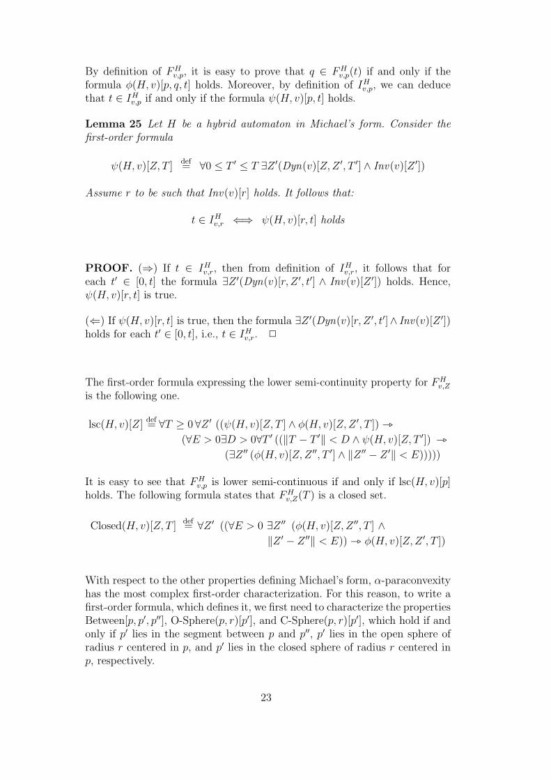
Lemma 25 Let H be a hybrid automaton in Michael’s form. Consider thefirst-order formula

ψ(H, v)[Z, T ]def= ∀0 ≤ T ′ ≤ T ∃Z ′(Dyn(v)[Z,Z ′, T ′] ∧ Inv(v)[Z ′])

Assume r to be such that Inv(v)[r] holds. It follows that:

t ∈ IHv,r ⇐⇒ ψ(H, v)[r, t] holds

PROOF. (⇒) If t ∈ IHv,r, then from definition of IHv,r, it follows that foreach t′ ∈ [0, t] the formula ∃Z ′(Dyn(v)[r, Z ′, t′] ∧ Inv(v)[Z ′]) holds. Hence,ψ(H, v)[r, t] is true.

(⇐) If ψ(H, v)[r, t] is true, then the formula ∃Z ′(Dyn(v)[r, Z ′, t′]∧ Inv(v)[Z ′])holds for each t′ ∈ [0, t], i.e., t ∈ IHv,r. 2

The first-order formula expressing the lower semi-continuity property for FHv,Z

is the following one.

lsc(H, v)[Z]def= ∀T ≥ 0 ∀Z ′ ((ψ(H, v)[Z, T ] ∧ φ(H, v)[Z,Z ′, T ]) _

(∀E > 0∃D > 0∀T ′ ((‖T − T ′‖ < D ∧ ψ(H, v)[Z, T ′]) _(∃Z ′′ (φ(H, v)[Z,Z ′′, T ′] ∧ ‖Z ′′ − Z ′‖ < E)))))

It is easy to see that FHv,p is lower semi-continuous if and only if lsc(H, v)[p]

holds. The following formula states that FHv,Z(T ) is a closed set.

Closed(H, v)[Z, T ]def= ∀Z ′ ((∀E > 0 ∃Z ′′ (φ(H, v)[Z,Z ′′, T ] ∧

‖Z ′ − Z ′′‖ < E)) _ φ(H, v)[Z,Z ′, T ])

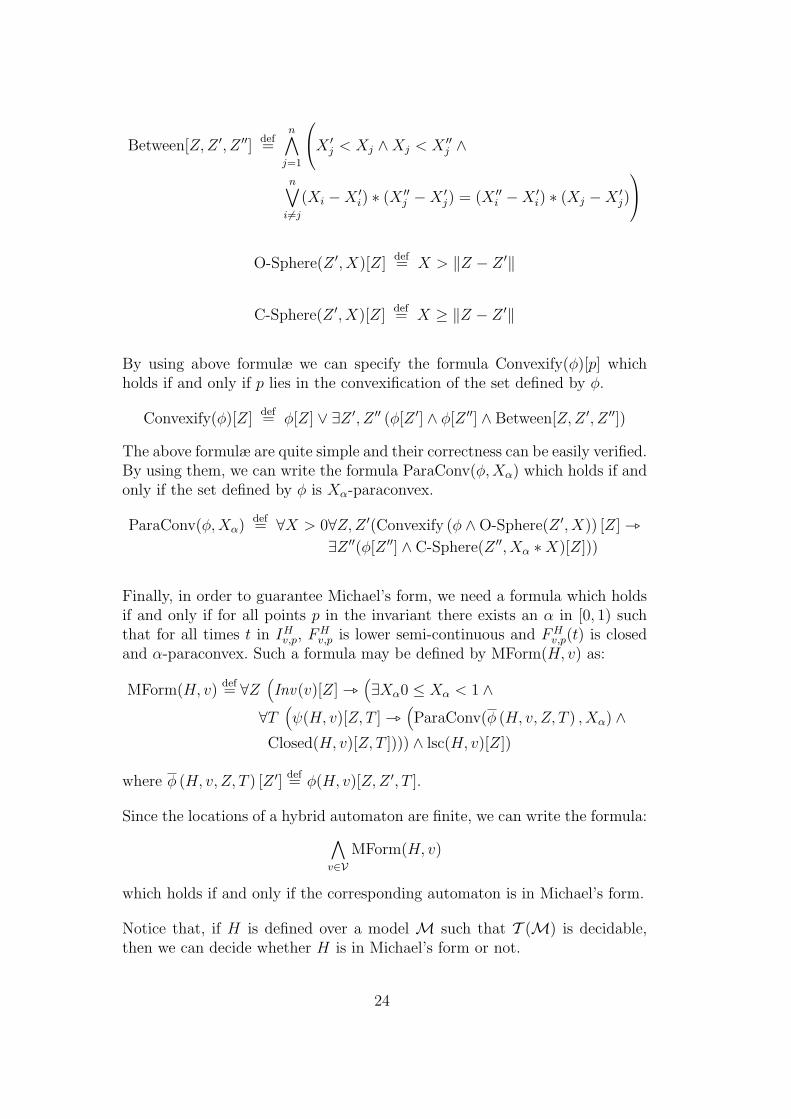
With respect to the other properties defining Michael’s form, α-paraconvexityhas the most complex first-order characterization. For this reason, to write afirst-order formula, which defines it, we first need to characterize the propertiesBetween[p, p′, p′′], O-Sphere(p, r)[p′], and C-Sphere(p, r)[p′], which hold if andonly if p′ lies in the segment between p and p′′, p′ lies in the open sphere ofradius r centered in p, and p′ lies in the closed sphere of radius r centered inp, respectively.

23

Between[Z,Z ′, Z ′′]def=

n∧j=1

X ′j < Xj ∧Xj < X ′′j ∧

n∨i 6=j

(Xi −X ′i) ∗ (X ′′j −X ′j) = (X ′′i −X ′i) ∗ (Xj −X ′j)

O-Sphere(Z ′, X)[Z]def= X > ‖Z − Z ′‖

C-Sphere(Z ′, X)[Z]def= X ≥ ‖Z − Z ′‖

By using above formulæ we can specify the formula Convexify(φ)[p] whichholds if and only if p lies in the convexification of the set defined by φ.

Convexify(φ)[Z]def= φ[Z] ∨ ∃Z ′, Z ′′ (φ[Z ′] ∧ φ[Z ′′] ∧ Between[Z,Z ′, Z ′′])

The above formulæ are quite simple and their correctness can be easily verified.By using them, we can write the formula ParaConv(φ,Xα) which holds if andonly if the set defined by φ is Xα-paraconvex.

ParaConv(φ,Xα)def= ∀X > 0∀Z,Z ′(Convexify (φ ∧O-Sphere(Z ′, X)) [Z] _

∃Z ′′(φ[Z ′′] ∧ C-Sphere(Z ′′, Xα ∗X)[Z]))

Finally, in order to guarantee Michael’s form, we need a formula which holdsif and only if for all points p in the invariant there exists an α in [0, 1) suchthat for all times t in IHv,p, F

Hv,p is lower semi-continuous and FH

v,p(t) is closedand α-paraconvex. Such a formula may be defined by MForm(H, v) as:

MForm(H, v)def= ∀Z

(Inv(v)[Z] _

(∃Xα0 ≤ Xα < 1 ∧

∀T(ψ(H, v)[Z, T ] _

(ParaConv(φ (H, v, Z, T ) , Xα) ∧

Closed(H, v)[Z, T ]))) ∧ lsc(H, v)[Z])

where φ (H, v, Z, T ) [Z ′]def= φ(H, v)[Z,Z ′, T ].

Since the locations of a hybrid automaton are finite, we can write the formula:∧v∈V

MForm(H, v)

which holds if and only if the corresponding automaton is in Michael’s form.

Notice that, if H is defined over a model M such that T (M) is decidable,then we can decide whether H is in Michael’s form or not.

24

4.3 Reachability

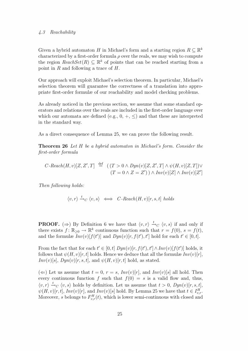
Given a hybrid automaton H in Michael’s form and a starting region R ⊆ Rk

characterized by a first-order formula ρ over the reals, we may wish to computethe region ReachSet (R) ⊆ Rk of points that can be reached starting from apoint in R and following a trace of H.

Our approach will exploit Michael’s selection theorem. In particular, Michael’sselection theorem will guarantee the correctness of a translation into appro-priate first-order formulæ of our reachability and model checking problems.

As already noticed in the previous section, we assume that some standard op-erators and relations over the reals are included in the first-order language overwhich our automata are defined (e.g., 0, +, ≤) and that these are interpretedin the standard way.

As a direct consequence of Lemma 25, we can prove the following result.

Theorem 26 Let H be a hybrid automaton in Michael’s form. Consider thefirst-order formula

C -Reach(H, v)[Z,Z ′, T ]def= ( (T > 0 ∧ Dyn(v)[Z,Z ′, T ] ∧ ψ(H, v)[Z, T ])∨

(T = 0 ∧ Z = Z ′) ) ∧ Inv(v)[Z] ∧ Inv(v)[Z ′]

Then following holds:

〈v, r〉 t−→C 〈v, s〉 ⇐⇒ C -Reach(H, v)[r, s, t] holds

PROOF. (⇒) By Definition 6 we have that 〈v, r〉 t−→C 〈v, s〉 if and only ifthere exists f : R≥0 → Rk continuous function such that r = f(0), s = f(t),and the formulæ Inv(v)[f(t′)] and Dyn(v)[r, f(t′), t′] hold for each t′ ∈ [0, t].

From the fact that for each t′ ∈ [0, t] Dyn(v)[r, f(t′), t′]∧ Inv(v)[f(t′)] holds, itfollows that ψ(H, v)[r, t] holds. Hence we deduce that all the formulæ Inv(v)[r],Inv(v)[s], Dyn(v)[r, s, t], and ψ(H, v)[r, t] hold, as stated.

(⇐) Let us assume that t = 0, r = s, Inv(v)[r], and Inv(v)[s] all hold. Thenevery continuous function f such that f(0) = s is a valid flow and, thus,

〈v, r〉 t−→C 〈v, s〉 holds by definition. Let us assume that t > 0, Dyn(v)[r, s, t],ψ(H, v)[r, t], Inv(v)[r], and Inv(v)[s] hold. By Lemma 25 we have that t ∈ IHv,r.Moreover, s belongs to FH

v,r(t), which is lower semi-continuous with closed and

25

α-paraconvex images. Consider the function F : [0, t]→ 2Rkdefined as:

F (T ) =

{r} if T = 0

FHv,r(T ) if 0 < T < t

{s} if T = t

It is immediately seen that for each t′ ∈ [0, t] F (t′) is closed and α-paraconvex.We prove that F is lower semi-continuous on [0, t]. Let t′ ∈ [0, t]. We need toconsider three distinct cases: (a) t′ = 0; (b) 0 < t′ < t; (c) t′ = t.

(a) If t′ = 0 and y ∈ F (0), then y = r. Let Ur be a neighborhood of r. Since,FHv,r is lower semi-continuous there exists a neighborhood U0 of 0 in IHv,r such

that for each t′′ in U0 it holds that FHv,r(t

′′)∩Ur 6= ∅. Since, [0, t] ⊆ IHv,r we getthat U ′0 = U0 ∩ [0, t) is a neighborhood of 0 in [0, t]. If t′′ ∈ U ′0, there are twopossible subcases: either t′′ = 0 or 0 < t′′ < t. If t′′ = 0, then F (0) ∩ Ur ={r} 6= ∅. If, on the other hand, 0 < t′′ < t, then F (t′′)∩Ur = FH

v,r(t′′)∩Ur 6= ∅.

(b) If 0 < t′ < t and y ∈ F (t′), then y ∈ FHv,r(t

′). Let Uy be a neighborhoodof y. Since FH

v,r is lower semi-continuous, there exists a neighborhood Ut′ oft′ in IHv,r such that for each t′′ in Ut′ it holds that FH

v,r(t′′) ∩ Uy 6= ∅. Since

t′ ∈ (0, t) ⊆ IHv,r, we conclude that U ′t′ = Ut′ ∩ (0, t) is a neighborhood of t′ in

[0, t]. If t′′ ∈ U ′t′ , then F (t′′) ∩ Ur = FHv,r(t

′′) ∩ Ur 6= ∅.

(c) If t′ = t and y ∈ F (t), then y = s. Let Us be a neighborhood of s. SinceFHv,r is lower semi-continuous, there exists a neighborhood Ut of t in IHv,r such

that for each t′′ in Ut, it holds that FHv,r(t

′′) ∩ Us 6= ∅. Since [0, t] ⊆ IHv,r, weget that U ′t = Ut ∩ (0, t] is a neighborhood of t in [0, t]. If t′′ ∈ U ′t , then thereare two possible sub-cases: namely, either t′′ = t or 0 < t′′ < t. If t′′ = t, thenF (0) ∩ Us = {s} 6= ∅. If 0 < t′′ < t, then F (t′′) ∩ Us = FH

v,r(t′′) ∩ Us 6= ∅.

Since F : [0, t] → 2Rkis lower semi-continuous, [0, t] is a metric space, Rk is

a Banach space, and F (t′) is closed and α-paraconvex, for each t′ in [0, t],by Theorem 19, we may deduce the following: there exists f : [0, t] → Rk

continuous selection for F . Hence, by definition of continuous selection (see[67]), f is a continuous function such that for each t′ ∈ [0, t] it holds f(t′) ∈F (t′). From this last statement, we further deduce that: f(0) = r; f(t) = s;for each 0 < t′ < t it holds that f(t′) ∈ FH

v,r(t′), i.e., Dyn(v)[r, f(t′), t′] and

Inv(v)[f(t′)]. Consider the function f : R≥0 → Rk defined as:

f(T ) =

f(T ) if T ∈ [0, t]

s if T > t

We conclude that 〈v, r〉 t−→C 〈v, s〉, as desired. 2

26

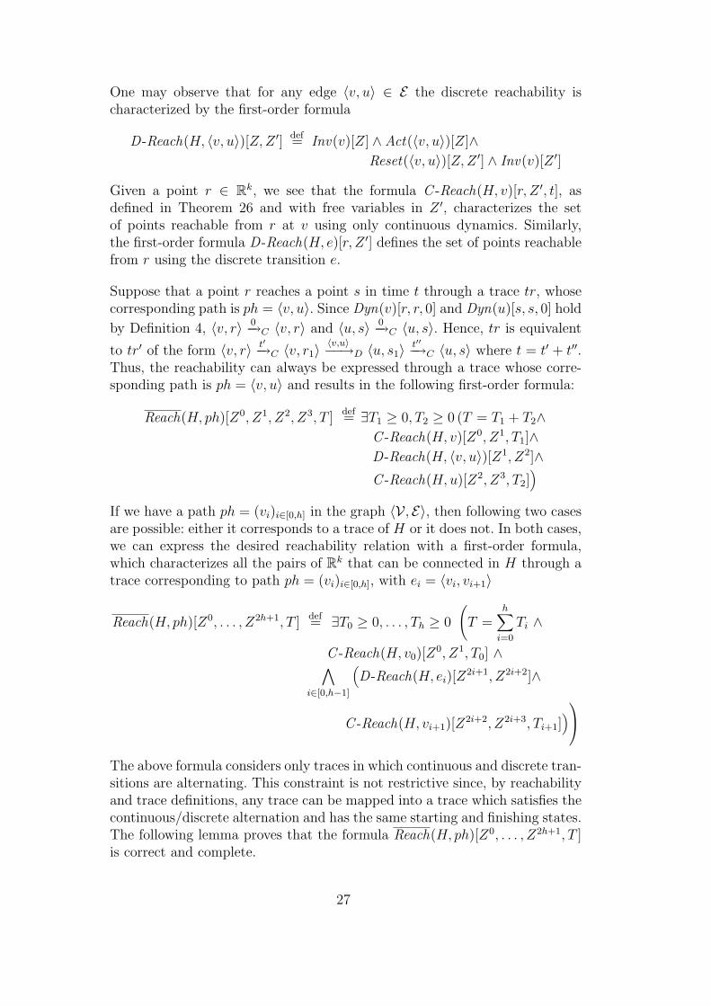
One may observe that for any edge 〈v, u〉 ∈ E the discrete reachability ischaracterized by the first-order formula

D-Reach(H, 〈v, u〉)[Z,Z ′] def= Inv(v)[Z] ∧ Act(〈v, u〉)[Z]∧

Reset(〈v, u〉)[Z,Z ′] ∧ Inv(v)[Z ′]

Given a point r ∈ Rk, we see that the formula C -Reach(H, v)[r, Z ′, t], asdefined in Theorem 26 and with free variables in Z ′, characterizes the setof points reachable from r at v using only continuous dynamics. Similarly,the first-order formula D-Reach(H, e)[r, Z ′] defines the set of points reachablefrom r using the discrete transition e.

Suppose that a point r reaches a point s in time t through a trace tr, whosecorresponding path is ph = 〈v, u〉. Since Dyn(v)[r, r, 0] and Dyn(u)[s, s, 0] hold

by Definition 4, 〈v, r〉 0−→C 〈v, r〉 and 〈u, s〉 0−→C 〈u, s〉. Hence, tr is equivalent

to tr′ of the form 〈v, r〉 t′−→C 〈v, r1〉〈v,u〉−−→D 〈u, s1〉

t′′−→C 〈u, s〉 where t = t′ + t′′.Thus, the reachability can always be expressed through a trace whose corre-sponding path is ph = 〈v, u〉 and results in the following first-order formula:

Reach(H, ph)[Z0, Z1, Z2, Z3, T ]def= ∃T1 ≥ 0, T2 ≥ 0 (T = T1 + T2∧

C -Reach(H, v)[Z0, Z1, T1]∧D-Reach(H, 〈v, u〉)[Z1, Z2]∧C -Reach(H, u)[Z2, Z3, T2]

)If we have a path ph = (vi)i∈[0,h] in the graph 〈V , E〉, then following two casesare possible: either it corresponds to a trace of H or it does not. In both cases,we can express the desired reachability relation with a first-order formula,which characterizes all the pairs of Rk that can be connected in H through atrace corresponding to path ph = (vi)i∈[0,h], with ei = 〈vi, vi+1〉

Reach(H, ph)[Z0, . . . , Z2h+1, T ]def= ∃T0 ≥ 0, . . . , Th ≥ 0

(T =

h∑i=0

Ti ∧

C -Reach(H, v0)[Z0, Z1, T0] ∧∧i∈[0,h−1]

(D-Reach(H, ei)[Z

2i+1, Z2i+2]∧

C -Reach(H, vi+1)[Z2i+2, Z2i+3, Ti+1])

The above formula considers only traces in which continuous and discrete tran-sitions are alternating. This constraint is not restrictive since, by reachabilityand trace definitions, any trace can be mapped into a trace which satisfies thecontinuous/discrete alternation and has the same starting and finishing states.The following lemma proves that the formula Reach(H, ph)[Z0, . . . , Z2h+1, T ]is correct and complete.

27

Lemma 27 Let H = 〈Z, Z ′, V, E, Inv, Dyn, Act, Reset〉 be a hybrid au-tomaton in Michael’s form and ph = (vi)i∈[0,h] be a path in 〈V , E〉. It holdsthat r reaches s in time t through a trace tr whose corresponding path is ph ifand only if Reach(H, ph)[r, Z1, . . . , Z2h, s, t] is satisfiable.

PROOF. (⇒) Let tr = (`i)i∈[0,n] with `0 = 〈v0, r〉 and `n = 〈vn, s〉. Since,by Definition 4, Dyn(v)[r, r, 0] and Dyn(u)[s, s, 0] hold, if there are two con-

secutive discrete transitions `ie−→D `i+1

e′−→D `i+2 in tr, we can replace them

by `ie−→D `i+1

0−→C `i+1e′−→D `i+2. Hence, we may assume that in tr discrete

and continuous transitions are alternated. We may further assume tr startsand ends with a continuous transition, since, otherwise, we may simply add

either `00−→C `0 or `n

0−→C `n or both. Thus, we have that n = 2h. Let`i = 〈vi, ri〉 and consider the valuation, which replaces Zi by ri in the formulaReach(H, ph)[r, Z1, . . . , Z2h, s, t]. By induction on h, we can prove that thisvaluation satisfies Reach(H, ph)[r, Z1, . . . , Z2h, s, t].

(⇐) Since Reach(H, ph)[r, Z1, . . . , Z2h, s, t] is satisfiable, there exists an assign-ment to the Zi’s which satisfies it by replacing Zi with zi. Consider the tracetr = (`i)i∈[0,2h] such that `0 = 〈v, r〉, `2h = 〈vh, s〉, and for each i ∈ [1, h − 1],we have `2i−1 = 〈vi−1, z2i−1〉 and `2i = 〈vi, z2i〉. By induction on the length ofph, we can prove that tr is a trace of H, which connects r to s in time t. 2

Let ph be a path of length h. Consider the formula

Reach(H, ph)[Z,Z ′, T ]def= ∃Z1, . . . , Z2h Reach(H, ph)[Z,Z1, . . . , Z2h, Z ′, T ]

Since Reach(H, ph)[r, s, t] holds if and only if Reach(H, ph)[r, Z1, . . . , Z2h, s, t]is satisfiable, by Lemma 27, r reaches s in time t if and only if there ex-ists a path ph of 〈V , E〉 such that the formula Reach(H, ph)[r, s, t] holds. So,we could characterize reachability for a hybrid automaton in Michael’s form,considering the disjunction of all the formulæ for all the paths of 〈V , E〉. Un-fortunately, if 〈V , E〉 has a cycle, then it has an infinite number of paths andthis straightforward approach fails. In Section 5 we introduce a class of hybridautomata whose traces corresponds to paths of finite length.

5 First-Order Constant Reset Hybrid Automata

In this section we introduce and study a class of hybrid automata, First-OrderConstant Reset hybrid automata (FOCoRe). Such automata are in Michael’sform and their resets are constant as in the class of o-minimal hybrid automata.Even though FOCoRe automata do not admit finite bisimulation quotient, we

28

can translate reachability problems into satisfiability of a particular first-orderformula over the reals. It follows that if the specifying theory is decidable, thenthe reachability problem is decidable.

5.1 FOCoRe Definition

A FOCoRe automaton is simply a hybrid automaton in Michael’s form whoseresets are constant. More formally we can define it as follows.

Definition 28 (First-Order Constant Reset Automata) We say that ahybrid automaton H is a first-order constant reset hybrid automaton, or sim-ply a FOCoRe, if:

(1) H is in Michael’s form;(2) All the resets, Reset(e)[Z,Z ′], of H are constant i.e., if Reset(e)[p, s]

holds, then Reset(e)[r, s] holds too for all p, s, and r in Rk.

Condition 1 will allow us to exploit Theorem 26 to check the existence of a validcontinuous flows. Condition 2 is exactly the condition imposed on o-minimalhybrid automata.

Example 29 Let H = 〈Z,Z ′,V , E , Inv ,Dyn,Act , Reset〉 where:

• Z = (Z1, Z2) and Z ′ = (Z ′1, Z′2);

• V = {v} and E = {e}, where e goes form v to v;• Inv(v)[Z] is (0 ≤ Z1 ≤ 1 ∧ 0 ≤ Z2 ≤ 1);• Dyn(v)[Z,Z ′, T ] is (Z ′1 = T + Z1 ∧ Z ′2 ≥ T 2 + Z2);• Act(e)[Z] is (Z1 = 1 ∨ Z2 = 1);• Reset(e)[Z,Z ′] is (Z ′1 = 1 ∧ Z ′2 = 1).

The formulæ in H are first-order formulæ over the reals. If p = (p1, p2), with0 ≤ p1, p2 ≤ 1, then the function FH

v,p is defined as FHv,p(t) = {(q1, q2) | q1 =

t+ p1, q2 ≥ t2 + p2, and 0 ≤ q1, q2 ≤ 1}. It is easy to see that p ∈ FHv,p(0) and

for each t the set FHv,p(t) is closed and convex, since it is a segment. Moreover,

this function is lower semi-continuous over the interval IHv,p. It follows that His in Michael’s form. Finally, Reset(e)[Z,Z ′] does not depend on Z. Hence,H is a FOCoRe automaton.

O-minimal hybrid automata [25,6] are easily seen as special cases of FOCoReautomata. As a matter of fact, o-minimal hybrid automata allow only onecontinuous flow from each point, hence an o-minimal hybrid automaton is aFOCoRe for which the set FH

v,p(t) reduces to a singleton, which is obviouslyclosed and convex, for each time instant t. The continuity of the flow im-mediately implies the lower semi-continuity of FH

v,p(t) over IHv,p. On the other

29

hand, the class FOCoRe is not included in the class of o-minimal hybrid au-tomata, since from each point we allow a set of flows. Moreover, FOCoRe’sflows are not necessarily solutions of autonomous differential inclusions andtheir dynamics are not o-minimal in general.

Notice that the identification of a FOCoRe automaton can be carried outautomatically. In particular, in the remaining part of the section we presenta first-order formula which holds if and only if a particular automaton underconsideration is a FOCoRe.

As detailed in Section 4.2, a hybrid automaton H is in Michael’s form if andonly if the following formula holds:∧

v∈VMForm(H, v)

Let us consider Condition 2 of FOCoRe definition. We just need to charac-terize the fact that, for all points p, p′, q ∈ Rk, if Reset(e)[p, q] holds, thenReset(e)[p′, q] does too. It is easy to prove that following formula expressesthis fact.

ConstReset(H, e)def= ∀Z1, Z

′, Z2, Z′′ ((Reset(e)[Z1, Z

′] ∧ Reset(e)[Z2, Z′′]) _

Reset(e)[Z1, Z′′])

Since both edges and locations are bounded, we can write the formula:∧v∈V

MForm(H, e) ∧∧e∈E

ConstReset(H, e)

which holds if and only if the corresponding hybrid automaton is a FOCoRe.

5.2 Reachability

Given a FOCoRe automaton H and a starting region R ⊆ Rk characterizedby a first-order formula ρ over the reals, we may wish to compute the regionReachSet (R) ⊆ Rk of points that can be reached starting from a point in Rand following a trace of H.

More generally, given a formula Q of a temporal logic, we may also be inter-ested in determining the points of R which satisfy Q. In the case of o-minimalhybrid automata, reachability as well as other temporal logic properties arechecked through bisimulation. This technique can be applied whenever we con-sider a class C of hybrid automata, which has the finite bisimulation property,i.e., each automaton in C has a finite bisimulation quotient. Unfortunately,the class of FOCoRe does not possess the finite bisimulation property, as wewill show in Section 5.3.

30

Our approach will instead exploit the properties of Michael’s form and con-stant resets. In this section, we demonstrate how the reachability problemover FOCoRe T -automata can be reduced to the satisfiability of a first-orderformula over the theory T . From this note entails the decidability of the reach-ability problem over the FOCoRe which are expressed in a decidable theory.

In Section 4.3, we derived the formula Reach such that if H is a hybrid au-tomaton in Michael’s form, ph = 〈v0, . . . , vh〉 is a path in 〈V , E〉 and r, s ∈ Rk,then r reaches s in time t through a trace tr whose corresponding path is phif and only if the first-order formula Reach(H, ph)[r, Z1, . . . , Z2h, s, t] is satisfi-able. As remarked at the end of the same section, if 〈V , E〉 has a cycle, then ithas an infinite number of paths and, thus the formula Reach cannot be useddirectly to specify an effective method to reduce a reachability problem overH to a satisfiability problem in a first-order theory. In the specific case ofFOCoRe, we can exploit the constant resets feature and ignore all the pathsof 〈V , E〉 whose length exceeds |E|. Below, we denote the set of those pathsin 〈V , E〉 of length at most |E| as P E and we write P E(v) to denote the set ofpath in P E starting from v.

Theorem 30 Let H be a FOCoRe automaton of dimension k. Point s ∈ Rk

is reachable from r ∈ Rk by H if and only if there exists a path ph ∈ P E oflength at most |E| such that the formula ∃T ≥ 0 Reach(H, ph)[r, s, T ] holds.

PROOF. The complete proof of the preceding theorem is reported in Ap-pendix on page 48.

Given a FOCoRe automaton H, if P E is the set of paths of 〈V , E〉 of lengthat most |E|, we can define the first-order formula PH [Z,Z ′] as follows:

PH [Z,Z ′]def=

∨ph∈PE

∃T ≥ 0 Reach(H, ph)[Z,Z ′, T ]

From Theorem 30, it follows that, given a FOCoRe H, s ∈ ReachSet (r) if andonly if the formula PH [r, s] holds. We can now characterize the set of pointsreachable from a first-order definable set R ⊆ Rk.

Corollary 31 Let H be a FOCoRe automaton and ρ[Z] be a first-order for-mula. The set ReachSet (Sat(ρ)) is characterized by the first-order formula

SH(ρ)[Z ′]def= ∃Z (ρ[Z] ∧ PH [Z,Z ′])

Thus we have reduced our reachability problem to that of deciding the satisfi-ability of an existential first-order formula and we get the following corollary.

31

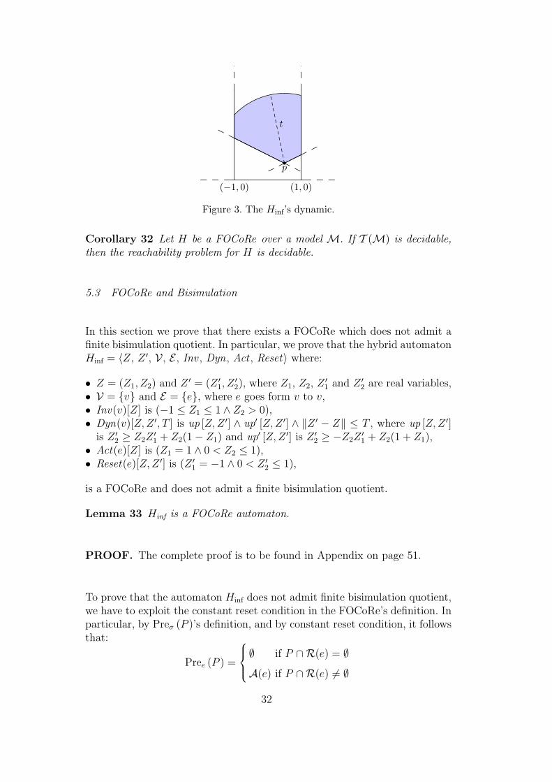
p

(−1, 0) (1, 0)

t

Figure 3. The Hinf’s dynamic.

Corollary 32 Let H be a FOCoRe over a model M. If T (M) is decidable,then the reachability problem for H is decidable.

5.3 FOCoRe and Bisimulation

In this section we prove that there exists a FOCoRe which does not admit afinite bisimulation quotient. In particular, we prove that the hybrid automatonHinf = 〈Z, Z ′, V , E , Inv , Dyn, Act , Reset〉 where:

• Z = (Z1, Z2) and Z ′ = (Z ′1, Z′2), where Z1, Z2, Z ′1 and Z ′2 are real variables,

• V = {v} and E = {e}, where e goes form v to v,• Inv(v)[Z] is (−1 ≤ Z1 ≤ 1 ∧ Z2 > 0),• Dyn(v)[Z,Z ′, T ] is up [Z,Z ′] ∧ up′ [Z,Z ′] ∧ ‖Z ′ − Z‖ ≤ T , where up [Z,Z ′]

is Z ′2 ≥ Z2Z′1 + Z2(1− Z1) and up′ [Z,Z ′] is Z ′2 ≥ −Z2Z

′1 + Z2(1 + Z1),

• Act(e)[Z] is (Z1 = 1 ∧ 0 < Z2 ≤ 1),• Reset(e)[Z,Z ′] is (Z ′1 = −1 ∧ 0 < Z ′2 ≤ 1),

is a FOCoRe and does not admit a finite bisimulation quotient.

Lemma 33 Hinf is a FOCoRe automaton.

PROOF. The complete proof is to be found in Appendix on page 51.

To prove that the automaton Hinf does not admit finite bisimulation quotient,we have to exploit the constant reset condition in the FOCoRe’s definition. Inparticular, by Preσ (P )’s definition, and by constant reset condition, it followsthat:

Pree (P ) =

∅ if P ∩R(e) = ∅

A(e) if P ∩R(e) 6= ∅

32

Thus, as reported in [25], Hinf admits a finite bisimulation quotient if andonly if Algorithm 1 terminates, when the initial partition is the partition Svinduced by the set Av = {I(v)} ∪⋃〈v′,v〉∈E {R(〈v′, v〉)} ∪⋃〈v,v′〉∈E {A(〈v, v′〉)}.

Algorithm 1 Bisimulation algorithm for hybrid systems with constant resets

for v ∈ V doSv ← compute initial partition from(Av)while ∃P, P ′ ∈ Sv such that ∅ 6= P ∩ Prev (P ′) 6= P doP1 ← P ∩ Prev (P ′)P2 ← P \ Prev (P ′)Sv ← (Sv \ {P}) ∪ {P1, P2}

end whileend forX/ ∼← ⋃

v〈v,Sv〉

However, the following results allow us to conclude that Algorithm 1 does notterminate on Hinf and consequently, Hinf does not admit finite bisimulationquotient. Below, we prove that, considering the Hinf automaton, there existstwo sets satisfying the while condition at the end of each cycle of Algorithm 1.In particular, we prove that each of algorithm’s iteration adds to Sv a non-empty set P1 smaller than P such that P1 and P ′ satisfy the while condition.

Theorem 34 The automaton Hinf does not admit finite bisimulation quotient.

PROOF. The complete proof of the preceding theorem is presented in Ap-pendix on page 56.

Next corollary follows from Lemma 33 and Theorem 34.

Corollary 35 There exist FOCoRe automata that do not admit finite bisim-ulation quotient.

PROOF. By Lemma 33, Hinf is a FOCoRe automaton and, by Theorem 34,Hinf does not admit finite bisimulation quotient. 2

To complete our analysis we briefly comment on the connection between FO-CoRe and rectangular automata (see [24]).

It is easy to see that there exist FOCoRe which are not rectangular automataand there exist rectangular automata which are not FOCoRe. In particular,the automaton Hinf introduced above is a FOCoRe which is not rectangular,since its dynamics cannot be expressed as a differential inclusion of the kind

33

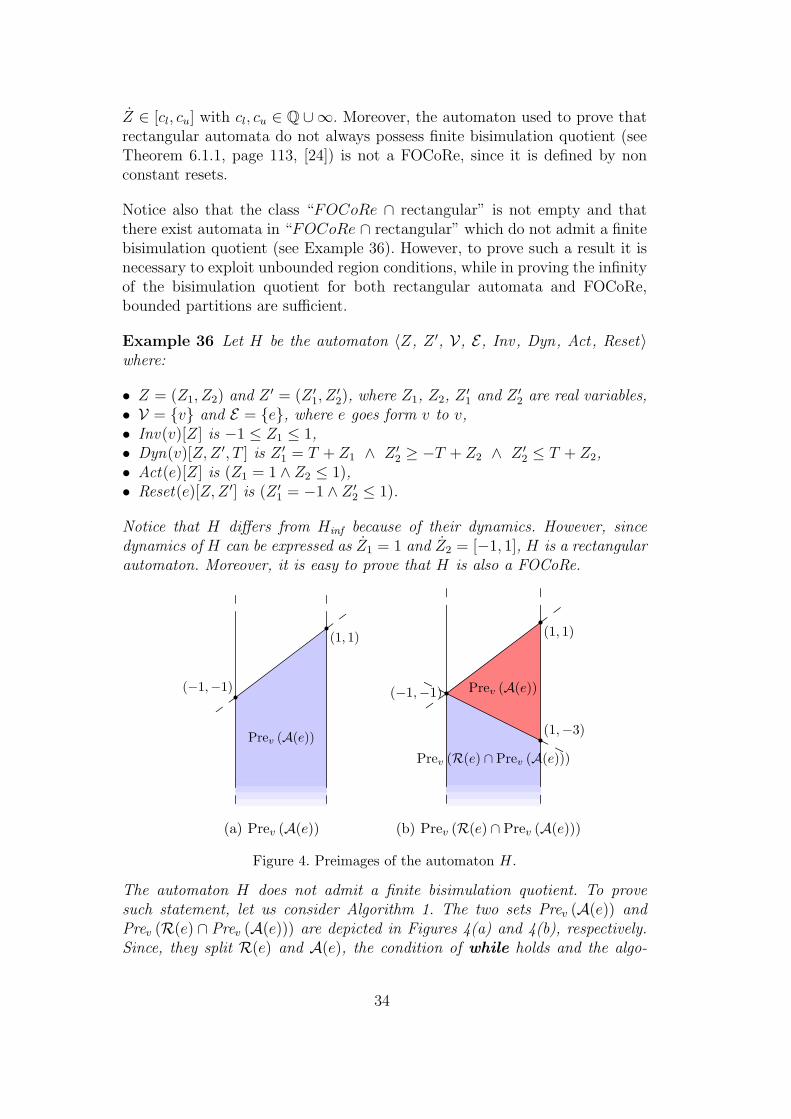
Z ∈ [cl, cu] with cl, cu ∈ Q ∪∞. Moreover, the automaton used to prove thatrectangular automata do not always possess finite bisimulation quotient (seeTheorem 6.1.1, page 113, [24]) is not a FOCoRe, since it is defined by nonconstant resets.

Notice also that the class “FOCoRe ∩ rectangular” is not empty and thatthere exist automata in “FOCoRe ∩ rectangular” which do not admit a finitebisimulation quotient (see Example 36). However, to prove such a result it isnecessary to exploit unbounded region conditions, while in proving the infinityof the bisimulation quotient for both rectangular automata and FOCoRe,bounded partitions are sufficient.

Example 36 Let H be the automaton 〈Z, Z ′, V, E, Inv, Dyn, Act, Reset〉where:

• Z = (Z1, Z2) and Z ′ = (Z ′1, Z′2), where Z1, Z2, Z ′1 and Z ′2 are real variables,

• V = {v} and E = {e}, where e goes form v to v,• Inv(v)[Z] is −1 ≤ Z1 ≤ 1,• Dyn(v)[Z,Z ′, T ] is Z ′1 = T + Z1 ∧ Z ′2 ≥ −T + Z2 ∧ Z ′2 ≤ T + Z2,• Act(e)[Z] is (Z1 = 1 ∧ Z2 ≤ 1),• Reset(e)[Z,Z ′] is (Z ′1 = −1 ∧ Z ′2 ≤ 1).

Notice that H differs from Hinf because of their dynamics. However, sincedynamics of H can be expressed as Z1 = 1 and Z2 = [−1, 1], H is a rectangularautomaton. Moreover, it is easy to prove that H is also a FOCoRe.

(1, 1)

(−1,−1)

Prev (A(e))

(a) Prev (A(e))

(1, 1)

(−1,−1)

(1,−3)

Prev (R(e) ∩ Prev (A(e)))

Prev (A(e))

(b) Prev (R(e) ∩ Prev (A(e)))

Figure 4. Preimages of the automaton H.

The automaton H does not admit a finite bisimulation quotient. To provesuch statement, let us consider Algorithm 1. The two sets Prev (A(e)) andPrev (R(e) ∩ Prev (A(e))) are depicted in Figures 4(a) and 4(b), respectively.Since, they split R(e) and A(e), the condition of while holds and the algo-

34

rithm does not stop. In the same way, at every step of the algorithm, a setof the approximate bisimulation partition will be split into two sets. Since in-variant has no lower bound, we will have the same situation at every step andthe algorithm will never stop. Hence, H does not admit a finite bisimulationquotient.

5.4 Model Checking

Despite the absence of a finite bisimulation result for FOCoRe, we can stillshow, by building upon the decidability of the reachability problem, that asubstantial and interesting fragment of CTL can be decided over FOCoReautomata. Since this fragment is not included in LTL, it is not possible to usesimulation equivalence to reduce the model.

Given a FOCoRe automaton of dimension k, let P = {P1[Z], . . ., Pm[Z]} bea set of atomic propositions whose elements are first-order formulæ over thereals with k free-variables and let ΦP be the set of formulæ defined by:

Q ::= P [Z] | ¬P [Z] |Q1 ∨Q2 | E3Q1 | A2Q1

Notice that the formula E3A2P [Z], which belongs to ΦP , distinguishes modelswhich are simulation equivalent. (see [27]).

We define the semantics of the formulæ of ΦP by structural induction. Oursemantics corresponds to the standard CTL semantics on the transition systemdefined by the untimed semantics of hybrid automata.

Definition 37 (ΦP - Semantics) Let H be a hybrid automaton. Given astate ` = 〈v, r〉 of H, we say that ` satisfies the ΦP formula Q, denoted by` � Q, if and only if:

• ` � P [Z] iff P [r] holds;• ` � Q1 ∨Q2 iff ` � Q1 or ` � Q2;• ` � ¬Q1 iff ` 6� Q1;• ` � E3Q1 iff there exists state `′ reachable from ` such that `′ � Q1;• ` � A2Q1 iff for each state `′ reachable from ` it holds `′ � Q1.

Given a FOCoRe automaton H, an admissible state ` and a formula Q ∈ ΦP ,we can decide ` � Q by reducing the problem to the validity problem for afirst-order formula as follows.

Definition 38 Let H be a FOCoRe, Q be a formula of ΦP , and v be a stateof H. We define the first-order formula % (H,Q, v) [Z] as follows:

35

• % (H,P [Z], v) [Z] is Inv(v)[Z] ∧ P [Z];• % (H,¬P [Z], v) [Z] is Inv(v)[Z] ∧ ¬P [Z];• % (H,Q1 ∨Q2, v) [Z] is % (H,Q1, v) [Z] ∨ % (H,Q2, v) [Z];• % (H, E3Q1, v) [Z] is∨

ph∈PE(v)

(∃Z ′(∃T ≥ 0 Reach(H, ph)[Z,Z ′, T ] ∧ % (H,Q1, uph) [Z ′]));

• % (H, A2Q1, v) [Z] is∧ph∈PE(v)

(∀Z ′(∃T ≥ 0 Reach(H, ph)[Z,Z ′, T ] _ % (H,Q1, uph) [Z ′]));

where we use uph ∈ V to denote the last node of ph ∈ P E(v).

The following theorem associates the validity of the formula % (H,Q, v) withthe ΦP-formula Q.

Theorem 39 Let H be a FOCoRe automaton and Q be a formula of ΦP . Theformula % (H,Q, v) [r] holds if and only if 〈v, r〉 � Q.

PROOF. The complete proof of the preceding theorem is reported in Ap-pendix on page 57.

We can give some partial results over ΦP extended with the operator EU.Consider the following grammar obtained from ΦP by adding such an operator.

Q ::= P [Z] | ¬P [Z] |Q1 ∨Q2 | E3Q1 | A2Q1 | E (Q1UQ2)

In the rest of this section we will call this language ΦU,P .

To define the semantics of the until operator we need to introduce the notionof admissible function. If we have 〈v, r〉 −→C 〈v, s〉, then an admissible functionis a continuous function which leads from r to s satisfying the dynamics andinvariant conditions.

Definition 40 ((r, s, v) admissible function) Let H be a hybrid automatonand let 〈v, r〉 and 〈v, s〉 be two states of H such 〈v, r〉 −→C 〈v, s〉. An (r, s, v)admissible function is a continuous function f : [0, t]→ Rk such that r = f(0),s = f(t), and, for each t′ ∈ [0, t], both Inv(v)[f(t′)] and Dyn(v)[r, f(t′), t′] hold.

Notice that, if 〈v, r〉 −→C 〈v, s〉, there always exists at least one (r, s, v) admis-sible function.

We only define the until operator, since the remaining is defined as in ΦP .

36

Definition 41 (ΦU,P - Semantics) Let H be a hybrid automaton. Given astate `0 = 〈v0, r0〉 of H, we say that `0 satisfies the ΦU,P formula Q1UQ2,denoted by `0 � E (Q1UQ2), if and only if there exists a trace of the form〈v0, r0〉, . . . , 〈vn, rn〉 such that:

• for each i ∈ [0, n− 1] it holds 〈vi, ri〉 � Q1;• 〈vn, rn〉 � Q2;• for each i ∈ [0, n− 1] if 〈vi, ri〉 −→C 〈vi+1, ri+1〉, then there is an (ri, ri+1, vi)

admissible function f : [0, t]→ Rk such that for each t′ ∈ (0, t) it holds that〈vi, f(t′)〉 � Q1.

We can prove the following result.

Theorem 42 Let H = 〈Z,Z ′,V , E , Inv ,Dyn,Act , Reset〉 be a FOCoRe andv ∈ V be a location of H. Moreover, let Q1 and Q2 be two formulæ of ΦU,P andH ′ be the hybrid automaton H ′ = 〈Z,Z ′,V , E , Inv ′, Dyn,Act , Reset〉, wherethe invariants Inv ′ are defined as

Inv ′(v)[Z]def= Inv(v)[Z] ∧ (% (H,Q1, v) [Z] ∨ % (H,Q2, v) [Z])

for all v ∈ V Consider the formula % (H,H ′, E(Q1UQ2), v) [Z] defined by

% (H,H ′, E(Q1UQ2), v) [Z]def=

∃T ≥ 0∃Z ′∨

ph∈PE(v)

Reach(H ′, ph)[Z,Z ′, T ]∧

% (H,Q2, uph) [Z ′]

If the automaton H ′ is a FOCoRe and the formula % (H,H ′, E(Q1UQ2), v) [r]holds, then 〈v, r〉 � E(Q1UQ2).

PROOF. The complete proof of the preceding theorem is presented in Ap-pendix on page 57.

If we consider only transitive dynamics (i.e., dynamics which satisfy the for-mula Dyn(v)[Z,Z ′, T ]∧Dyn(v)[Z ′, Z ′′, T ′] _ Dyn(v)[Z,Z ′′, T + T ′]), then wecan prove the following result.

Theorem 43 Let H = 〈Z,Z ′,V , E , Inv ,Dyn,Act , Reset〉 and v ∈ V be a H’slocation. Moreover, let Q1 and Q2 be two ΦU,P formulæ and H ′ be the hybrid

automaton 〈Z,Z ′,V , E , Inv ′, Dyn, Act ,Reset〉 where Inv ′(v)[Z]def= Inv(v)[Z]∧

% (H,Q1, v) [Z] for all v ∈ V. Consider the formula % (H,H ′, EQ1UQ2, v) [Z]

37

defined by

∃Z ′ ∃T ≥ 0

∀0 ≤ T ′ < T ∃Z ′′

∨ph∈PE(v)

∨ph′∈PE(uph)

(Reach(H ′, ph)[Z,Z ′′, T ′]∧

Reach(H, ph′)[Z ′′, Z ′, T − T ′] ∧ % (H,Q2, uph′) [Z ′])

∨∃T ′ > 0 ∀0 < T ′′ ≤ T ′ ∃Z ′′

∨ph∈PE(v)

∨ph′∈PE(uph)

(Reach(H ′, ph)[Z,Z ′, T ]∧

Reach(H, ph′)[Z ′, Z ′′, T ′′] ∧ % (H,Q2, uph′) [Z ′′])

where we use up ∈ V to denote the last node of a path p. If H and H ′ areFOCoRe, the continuous dynamics is transitive, and % (H,H ′, EQ1UQ2, v) [q]holds, then 〈v, q〉 � EQ1UQ2.

PROOF. The complete proof of the preceding theorem is presented in Ap-pendix on page 61.

Despite the obvious limitations of the above results, in that they do not guar-antee the decidability of ΦU,P , they still give us sufficient conditions to provethe existence of a trajectory (ρi)i∈I leaving a state 〈v, r〉 such that the proper-ties Q1 holds on (ρi)i∈I until the Q2 does. Verifying existence of such propertiesis crucial in safety verification, when we require that a property fails to holdas long as some security states have not been reached. For these reasons, weargue that, even though Theorem 42 and Theorem 43 do not quite succeed inproducing a complete algorithm for deciding 〈v, q〉 � EQ1UQ2, they will stillprove important in practice, especially in safety verification of FOCoRe.

6 A Biological Application

RNA silencing is a mechanism widely used by eukaryotes to suppress theeffects of unwanted gene transcriptions and is believed to have evolved to

38

provide defense against either viruses or transposons. Thus, like a miniatureimmune systems, it protects cells from alien genetic materials in three ways:(a) identifying non-self-elements, (b) producing a specific responses, and (c)raising such responses until the threat is cleared.

Bergstrom et al. provide, in [72], a formal model of RNA silencing and iden-tify 4 main actors in the silencing mechanism: mRNA, dsRNA, RNA-inducedsilencing complex (RISC), and RISC-mRNA complex. In the same papers,the authors also propose the following system of differential equations, ob-tained from mass-action kinetics laws, to model the evolution of the silencingmechanisms.

D(t) = −a ∗D(t) + g ∗ C(t)

R(t) = a ∗ n ∗D(t)− dR ∗R(t)− b ∗R(t) ∗M(t)

C(t) = b ∗R(t) ∗M(t)− (g + dC ∗ (t)) ∗ C(t)

M(t) = h− dM ∗M(t)− b ∗R(t) ∗M(t)

where D, R, C, and M represent dsRNA, RISC, RISC-mRNA, and mRNAquantities, respectively, and a, g, dR, b, dC , h, and dM are environmentalcoefficients which vary because of an assortment of reasons that are left unac-counted for in the model. In particular, it would be more reasonable to assumethat the rate of regeneration of dsRNA is not a fixed constant, but varies ina continuous manner with its value ranging in an interval [gmin, gmax] as thesystem evolves. These ranges may further differ from one transcriptome to an-other depending on the base composition. Consequently, all possible behaviorof the system, modeled as above, cannot be properly inferred from a singlesimulation.

In order to capture the complete set of behaviors of this biological system,we may approximate its solution by a process, essentially “integrating semi-algebraic hybrid automaton”, which roughly mimics the steps of a numericalintegration algorithm by using dynamics to simulate step function togetherwith interleaving steps and resets. The resulting automaton is thus equippedwith just one location and one transition: its dynamics are finite approxima-tions obtained from a suitably truncated Taylor series and its reset is identity.Notice that since the dynamics are polynomial, they are Hausdorff continuous.

Thus, if we constrain g to vary only within a close interval G, then the setof points, F [X,G](t), reachable from any point X with a generic t-timed con-tinuous evolution is closed. Moreover, for all α and all t, there exists a finitepartition, P (G), of G such that F [X,G](t) is α-paraconvex and

F [X,G](t) =⋃

G∈P(G)

F [X,G](t) (2)

for all G ∈ P (G) and all t ∈ [0, t]. It follows that F [X,G] is piece-wise in

39

Michael’s form and, by Lemma 25, we can always deduce the existence of acontinuous flow from X to Y for any Y ∈ F [X,G](t). We omit an exhaustivediscussion of various topics related to this example and postpone a formalproof of these intuitive observations to future work.

Notice that using α-paraconvexity in place of the —less demanding— convex-ity in Definition 23, gave us the possibility of partitioning G as above and,ultimately, of proving that the considered system could be represented by ahybrid automaton in Michael’s form.

Since the dynamics of the automaton arising in this example models the so-lution of an ODE, the fact that the reachability can be solved in this ap-proximate sense is not wholly unexpected. However, the systems of the kind,we encountered in the context of modeling RNA silencing, encompass manyof the subtle issues that arise quite frequently in systems biology. Note thatlike RNA silencing, many biological processes evolve to acquire robustness anduniversality: in other words, these processes work almost equally well for prac-tically all of the genes independent of how these genes and their orthologs inother organisms vary from species to species, and they continue to carry outtheir functional roles irrespective of how their micro-environments fluctuate.Traditionally, the difficulties, posed to the systems biology models by thesestructures, are circumvented by grossly simplifying it to a toy model (e.g., cer-tain environmental properties are assumed to hold constant, etc.). However,by building on the hybrid automata model, developed here, it is seen that onecan reason about rather realistic models without too coarse a simplificationor too idealistic an approximation.

7 Conclusions

In this article, we considered the model checking problem over hybrid au-tomata. We exploited some well known results taken from both logic andanalysis and we gave an example of how a tighter interaction between thesetwo mathematical fields can still bring some interesting results in the fieldof hybrid system verification. As a consequence, we are now convinced thatfurther improvements in this field will only come through a cross-disciplinaryconsilience of many fields such as logic, analysis, algebra, symbolic computa-tion, algorithms, and computer science. Development of more efficient algo-rithms to decide polynomial formulæ and proving the decidability of theoriessuch as 〈R, 0, 1,+, ∗, ex,≥〉 or 〈R, 0, 1,+, ∗, (f)f∈an,≥〉 will become the fun-damental aims of this emerging field in the future. We will benefit in theseefforts if we could identify general analysis results which allow us to reducecontinuous reachability to either small formulæ decidability or low complex-ity methods. Finally, we expect new developments in computer science (e.g.,

40

symbolic computation, computations modeled by dynamical systems, sym-bolic model checking, etc.) will harvest such important breakthrough resultsand discriminatively effective algorithms, which will obviate the mostly futilesemi-decidable heuristics that are now in use.

In particular, in this work we considered hybrid automata whose dynamicsare inclusion dynamics defined by first-order formulæ. We showed that even ifthe automaton’s dynamics are continuous, we cannot guarantee the existenceof a continuous transition satisfying the dynamics themselves. For this reason,we defined a set of conditions which relates the existence of such continuoustransition and the truth value of a first-order formula. Since such results areobtained using the selection theorem of Michael [26], we say that a hybridautomaton satisfying such conditions is in Michael’s form. If H is a hybridautomaton in Michael’s form, then we were able to write the first-order formulaReach(H, ph)[Z,Z ′, T ] which holds if and only if H can reach Z ′ from Z intime T through a trace whose corresponding path is ph. Exploiting this result,we presented the class of First Order Constant Reset automata, FOCoRe. AFOCoRe is a first-order hybrid automaton in Michael’s form whose resets areconstant maps. Aided by the constant reset condition, we were able to provethat we can reduce the general reachability problem over any FOCoRe Hto a simpler reachability problem over the traces of length at most equal tothe number of H’s discrete edges. It follows that the reachability problemfor FOCoRe is decidable. We introduced a CTL sub-logic called ΦP and weproved that model checking problems expressed within ΦP are decidable overFOCoRe. Notice that, since ΦP is not preserved by simulation and since thereexist FOCoRe having infinite bisimulation quotient, our decidability resultscannot be achieved exploiting standard equivalence reduction techniques.

As far as applications of our class of hybrid automata are concerned we brieflydiscuss some cases coming from Systems Biology. KMA (kinetic mass action)based systems of ODE models have begun to be considered limited in their ap-plicability, and it is now felt that their generalizations require many changesto the representation of the underlying mathematical models. These gener-alizations must recognize that a biological cell is not a well-mixed systemand often involve interactions among small number of molecules (low copynumber). They must also account for the enormous amount of uncertaintythat exist about their parameters. Such stochasticities, uncertainties, and un-modeled dependencies on local micro-environment, etc. can be expressed ina system allowing for the non-determinism in the flow and easily representedvia inclusion formalisms.

Hybrid automata have been already used to model different biological systems(see, e.g., [18,19]). In particular, they facilitate modeling of systems whose lawsdrastically change during different developmental stages or epochs of a limitcycle (e.g., cell cycle, circadian or ultradian rhythms, etc.). In this context

41

each phase is modeled through a different state while each phase change cor-responds to a discrete edge. The jumps from one phase to another usuallyoccur when the reactants (e.g., morphogens, transcriptional factors, or mi-croRNAs) reach limit values. One could imagine that the resets in these casesshould be the identity function. However, it is reasonable to introduce somenon-determinism on the jumps, since: (1) the exact jump conditions are notalways exactly/ completely known; (2) they can be subject to variations dueto external conditions. Hence, constant resets from the activation region toitself are quite natural in this context. The continuous dynamics of each statecan be inferred using standard techniques (e.g., Michaelis-Menten, S-systems).Unfortunately, many parameters are necessary to determine a single-functioncontinuous evolution. When some parameters are unknown we can only infera set of possible continuous evolutions for each state. Applying analysis tech-niques, such as Taylor approximation method, we can now approximate thesecontinuous evolutions with polynomials, in order to get a FOCoRe model ofthe system.

Furthermore, biological systems are not time-invariant, nor do they operatein a uniform time-scale. For instance, a cell’s behavior is clearly dependenton its time-dependent micro-environment (e.g., where the organism is in itsdevelopmental processes, etc.). Thus a model that keeps the systems just gen-eral enough can be easily argued to be very prudent, especially in the contextof biology. The faster reactions, mediated by a signaling event (e.g., a ligandbinding to a receptor) or internal state change (e.g., a flagella switching froma CW rotation to CCW), are easily represented by explicitly including thenatural hybrid-ness of the system, although, in this context, they require aneed to go beyond the constant reset constraints.

An interesting general technique which uses hybrid automata to model cellularprocesses has been presented in [73], where the authors proposed a transla-tion of (M,R)-systems [74,75] into hybrid automata. (M,R)-systems modelmetabolic processes always distinguishing four phases: normal phase, repairphase, replication phase, and mutation phase. In each phase environmentalinput are involved and the jumps from one phase to another are highly non-deterministic. In the translation proposed in [73] from (M,R)-systems to hy-brid automata the dependence from environmental inputs is modeled addingparameters to the continuous dynamics, while the non-deterministic jumpsare modeled using constant resets. When the variations of the environmen-tal inputs are not completely known the automata proposed in [73] can beapproximated by FOCoRe automata.

In the future, we plan to further study the expressiveness of first-order theoriesin hybrid automaton context. Since the Michael’s form can guarantee the exis-tence of a continuous transition for any kind of first-order dynamic, we wouldlike to investigate the possibility of relaxing it by restricting the specification

42

theories to o-minimal theories. As a matter of fact, even if Example 20 provesthe existence of a continuous map for which there is no continuous selection,such an example does not satisfy o-minimality. Moreover, we are interested inthe possibility of exploiting first-order theories over reals with restricted vari-ables over naturals to study synchronization problems over hybrid automata.Finally, we will focus, in the near future, on applying the techniques presentedhere to study stability of hybrid systems.

References

[1] R. Alur, C. Courcoubetis, T. A. Henzinger, P.-H. Ho, Hybrid automata: Analgorithmic approach to the specification and verification of hybrid systems, in:R. L. Grossman, A. Nerode, A. P. Ravn, H. Rischel (Eds.), Hybrid Systems,Vol. 736 of LNCS, Springer-Verlag, 1993, pp. 209–229.

[2] J. E. Hopcroft, J. D. Ullman, Introduction to Automata Theory, Languages,and Computation, Addison-Wesley, 1979.

[3] A. Puri, P. Varaiya, Decidability of hybrid systems with rectangular differentialinclusions, in: D. L. Dill (Ed.), Proceedings of International Conference onComputer Aided Verification (CAV’94), Vol. 818 of LNCS, Springer-Verlag,1994, pp. 95–104.

[4] M. Franzle, Analysis of Hybrid Systems: An ounce of realism can save an infinityof states, in: J. Flum, M. Rodrıguez-Artalejo (Eds.), Proceedings of ComputerScience Logic (CSL’99), Vol. 1683 of LNCS, Springer-Verlag, 1999, pp. 126–140.

[5] H. Anai, V. Weispfenning, Reach set computations using real quantifierelimination, in: M. D. D. Benedetto, A. Sangiovanni-Vincentelli (Eds.),Proceedings of Hybrid Systems: Computation and Control (HSCC’01), Vol.2034 of LNCS, Springer-Verlag, 2001, pp. 232–246.

[6] T. Brihaye, C. Michaux, C. Riviere, C. Troestler, On O-Minimal HybridSystems, in: R. Alur, G. J. Pappas (Eds.), Proceedings of Hybrid Systems:Computation and Control (HSCC’04), Vol. 2993 of LNCS, Springer-Verlag,2004, pp. 219–233.

[7] X. Nicollin, A. Olivero, J. Sifakis, S. Yovine, An approach to the descriptionand analysis of hybrid systems, in: R. L. Grossman, A. Nerode, A. P. Ravn,H. Rischel (Eds.), Hybrid Systems, Vol. 736 of LNCS, Springer-Verlag, 1993,pp. 149–178.

[8] R. Alur, C. Courcoubetis, D. Dill, Model-checking in dense real-time,Information and Computation 104 (1) (1993) 2–34.

[9] R. Alur, C. Courcoubetis, N. Halbwachs, T. A. Henzinger, P.-H. Ho, X. Nicollin,A. Olivero, J. Sifakis, S. Yovine, The algorithmic analysis of hybrid systems,Theoretical Computer Science 138 (1) (1995) 3–34.

43

[10] P. Tabuada, G. J. Pappas, Model checking ltl over controllable linear systems isdecidable., in: O. Maler, A. Pnueli (Eds.), HSCC, Vol. 2623 of LNCS, Springer-Verlag, 2003, pp. 498–513.

[11] R. Milner, An algebraic definition of simulation between programs, Tech. rep.,Stanford University (1971).

[12] J. van Benthem, Modal Correspondence Theory, Ph.D. thesis, Department ofMathematics, University of Amsterdam, advisers - M. H. L and S. K. Thomassen(1978).

[13] R. Alur, C. Courcoubetis, N. Halbwachs, D. Dill, H. Wong-Toi, Minimizationof timed transition systems (extended abstract), in: Proceedings of the ThirdInternational Conference on Concurrency Theory (CONCUR’92), Vol. 630,Springer-Verlag, 1992, pp. 340–354, lNCS.

[14] K. G. Larsen, M. Mikucionis, B. Nielsen, A. Skou, Testing real-time embeddedsoftware using uppaal-tron: an industrial case study, in: Proceedings of the FifthACM international conference on Embedded software (EMSOFT’05), ACMPress, 2005, pp. 299–306.

[15] J.-R. Abrial, E. Borger, H. Langmaack, The steam boiler case study:Competition of formal program specification and development methods, in: J.-R. Abrial, E. Borger, H. Langmaack (Eds.), Formal Methods for IndustrialApplications, Vol. 1165 of LNCS, Springer-Verlag, 1996, pp. 1–12.

[16] M. Archer, C. Heitmeyer, Verifying hybrid systems modeled as timed automata:A case study, in: O. Maler (Ed.), Proceedings of the Conference on Hybrid andReal-Time Systems (HART’97), Vol. 1201 of LNCS, Springer-Verlag, 1997, pp.171–185.

[17] A. Balluchi, L. Benvenuti, M. D. Di Benedetto, G. M. Miconi, U. Pozzi, T. Villa,H. Wong-Toi, A. L. Sangiovanni-Vincentelli, Maximal safe set computation foridle speed control of an automotive engine, in: N. A. Lynch, B. H. Krogh (Eds.),HSCC, Vol. 1790 of LNCS, Springer-Verlag, 2000, pp. 32–44.

[18] R. Alur, C. Belta, F. Ivancic, V. Kumar, M. Mintz, G. J. Pappas, H. Rubin,J. Schug, Hybrid Modeling and Simulation of Biomolecular Networks, in:Proceedings of Hybrid Systems: Computation and Control (HSCC’01), Vol.2034 of LNCS, Springer-Verlag, 2001, pp. 19–32.

[19] R. Ghosh, A. Tiwari, C. Tomlin, Automated Symbolic Reachability Analysis;with Application to Delta-Notch Signaling Automata, in: O. Maler, A. Pnueli(Eds.), Proceedings of Hybrid Systems: Computation and Control (HSCC’03),Vol. 2623 of LNCS, Springer-Verlag, 2003, pp. 233–248.

[20] M. Antoniotti, C. Piazza, A. Policriti, M. Simeoni, B. Mishra, Taming theComplexity of Biochemical Models through Bisimulation and Collapsing:Theory and Practice, Theoretical Computer Science 325 (1) (2004) 45–67.

[21] C. Piazza, M. Antoniotti, V. Mysore, A. Policriti, F. Winkler, B. Mishra,Algorithmic Algebraic Model Checking I: Challenges from Systems Biology, in:

44

K. Etessami, S. K. Rajamani (Eds.), Proceedings Computer Aided Verification(CAV’05), No. 3576 in LNCS, Springer-Verlag, 2005, pp. 5–19.

[22] T. A. Henzinger, P. W. Kopke, A. Puri, P. Varaiya, What’s decidableabout hybrid automata?, in: Proceedings of the Twenty-Seventh Annual ACMSymposium on the Theory of Computing (STOC ’95), ACM Press, 1995, pp.373–382.

[23] R. Alur, D. L. Dill, A theory of timed automata, Theoretical Computer Science126 (2) (1994) 183–235.

[24] P. W. Kopke, The theory of rectangular hybrid automata, Ph.D. thesis, Facultyof the Graduate School, Cornell University, advisor - T. A. Henzinger (1996).

[25] G. Lafferriere, G. J. Pappas, S. Sastry, O-Minimal Hybrid Systems,Mathematics of Control, Signals, and Systems 13 (2000) 1–21.

[26] E. Michael, Continuous selections I, Annals of Mathematica 63 (1956) 361–382.

[27] A. Casagrande, C. Piazza, B. Mishra, Semi-Algebraic Constant Reset HybridAutomata - SACoRe, in: Proceedings of the 44rd Conference on Decision andControl and European Control Conference (CDC-ECC’05), IEEE ComputerSociety Press, 2005, pp. 678–683.

[28] A. Casagrande, Hybrid Systems: A First-Order Approach to Verification andApproximation Techniques, Ph.D. thesis, Department of Mathematics andComputer Science, University of Udine, Udine, Italy, advisers - Prof. AlbertoPolicriti and Prof. Tiziano Villa (March 2006).

[29] H. B. Enderton, A Mathematical Introduction to Logic, ii Edition,Harcourt/Academic Press, 2001.

[30] E. Mendelson, Introduction to Mathematical Logic, iv Edition, CRC Press,1997.

[31] L. van den Dries, C. Miller, Geometric categories and o-minimal structures,Duke Math. Journal 84 (1996) 497–540.

[32] L. van den Dries, Tame topology and O-minimal structures, Vol. 248 of LondonMathematical Society Lecture Note Series, Cambridge University Press, 1998.

[33] A. Tarski, A Decision Method for Elementary Algebra and Geometry, Univ.California Press, 1951.

[34] G. E. Collins, Quantifier Elimination for the Elementary Theory of Real ClosedFields by Cylindrical Algebraic Decomposition, in: Proceedings of the SecondGI Conference on Automata Theory and Formal Languages, Vol. 33 of LNCS,Springer-Verlag, 1975, pp. 134–183.

[35] D. Grigorev, Complexity of deciding tarski algebra, Journal of SymbolicComputation 5 (1-2) (1988) 65–108.

[36] D. Grigorev, N. Vorobjov, Counting connected components of a semialgebraicset in subexponential time, Computational Complexity 2 (2) (1992) 133–186.

45

[37] J. Renegar, On the computational complexity and geometry of the first-ordertheory of the reals. Part I: Introduction. Preliminaries. The geometry of semi-algebraic sets. The decision problem for the existential theory of the reals,Journal of Symbolic Computation 13 (3) (1992) 255–299.

[38] J. Renegar, On the computational complexity and geometry of the first-ordertheory of the reals. Part II: The general decision problem. Preliminaries forquantifier elimination, Journal of Symbolic Computation 13 (3) (1992) 301–327.

[39] J. Renegar, On the computational complexity and geometry of the first-ordertheory of the reals. Part III: Quantifier elimination, Journal of SymbolicComputation 13 (3) (1992) 329–352.

[40] S. Basu, Algorithms in semi-algebraic geometry, Ph.D. thesis, Department ofComputer Science, New York University, adviser - Richard Pollack (1996).

[41] S. Basu, An improved algorithm for quantifier elimination over real closed fields,in: Proceedings of the Thirty-Eighth Annual Symposium on Foundations ofComputer Science (FOCS ’97), IEEE Computer Society Press, 1997, pp. 56–65.

[42] S. Basu, R. Pollack, M.-F. Roy, On the combinatorial and algebraic complexityof quantifier elimination, Journal of the Association for Computing Machinery43 (6) (1996) 1002–1045.

[43] B. Mishra, Algorithmic Algebra, Springer-Verlag New York, Inc., 1993.

[44] B. Mishra, Computational real algebraic geometry, in: J. E. Goodman,J. O’Rourke (Eds.), Handbook of Discrete and Computational Geometry:(Second Edition), CRC Press, Boca Raton, FL, 2004, pp. 740–764.

[45] J. Canny, Some algebraic and geometric computations in PSPACE, in:Proceedings of the Twentieth annual ACM symposium on Theory of computing(STOC ’88), ACM Press, 1988, pp. 460–469.

[46] J. Canny, Improved algorithms for sign determination and existential quantifierelimination, The Computer Journal 36 (5) (1993) 409–418.URL citeseer.ist.psu.edu/canny93improved.html

[47] L. van den Dries, A generalization of the Tarski-Seidenberg theorem and somenondefinability results, Bulletin of American Mathematical Society (New Series)15 (2) (1986) 189–193.

[48] A. G. Khovanskiı, On a class of systems of transcendental equations, SovietMath. Dokl. 22 (1980) 762–765.

[49] J. Denef, L. van den Dries, p-adic and real subanalytic sets, Annals ofMathematica 128 (1) (1988) 79–138.

[50] L. van den Dries, A. Macintyre, D. Marker, The elementary theory of restrictedanalytic functions with exponentiation, Annals of Mathematica 140 (1) (1994)183–205.

46

[51] A. J. Wilkie, Model completeness results for expansions of the ordered fieldof real numbers by restricted Pfaffian functions and the exponential function,Journal of the American Mathematical Society 9 (4) (1996) 1051–1094.

[52] A. Macintyre, A. J. Wilkie, On the decidability of the real exponential field,in: P. G. Odifreddi (Ed.), Kreiseliana, about and around Georg Kreisel,A. K. Peters, 1996, pp. 441–467.

[53] G. V. Chudnovsky, Contributions to the Theory of Transcendental Numbers,No. 19 in Mathematical Surveys and Monographs, American MathematicalSociety, 1984.

[54] A. Macintyre, Schanuel’s conjecture and free exponential rings., Annals of Pureand Applied Logic 51 (3) (1991) 241–246.

[55] L. van den Dries, C. Miller, On the real exponential field with restricted analyticfunctions, Israel Journal of Mathematics 85 (1-3) (1994) 19–56.

[56] J.-M. Lion, J.-P. Rolin, Theoreme de preparation pour les fonctionslogarithmico-exponentielles, Annales de l’institut Fourier 47 (3) (1997) 859–884.

[57] A. J. Wilkie, A theorem of the complement and some new O-minimal structures,Selecta Mathematica, New Series 5 (4) (1999) 397–421.

[58] O. Maler, Z. Manna, A. Pnueli, From timed to hybrid systems, in: J. W.de Bakker, C. Huizing, W. P. de Roever, G. Rozenberg (Eds.), Real-Time:Theory in Practice, Vol. 600, Springer-Verlag, 1991, pp. 447–484.URL citeseer.nj.nec.com/maler92from.html

[59] T. A. Henzinger, P. W. Kopke, State Equivalences for Rectangular HybridAutomata, in: U. Montanari, V. Sassone (Eds.), Proceedings of InternationalConference on Concurrency Theory (Concur’96), Vol. 1119 of LNCS, Springer-Verlag, 1996, pp. 530–545.

[60] T. A. Henzinger, The Theory of Hybrid Automata, in: Proceedings of theEleventh Symposium on Logic in Computer Science (LICS’96), IEEE ComputerSociety Press, 1996, pp. 278–292.

[61] J. Lygeros, K. H. Johansson, S. N. Simic, J. Zhang, S. Sastry, Continuity andinvariance in hybrid automata, in: Proceedings of the Fortieth IEEE Conferenceon Decision and Control (CDC ’01), IEEE Computer Society Press, 2001, pp.340–345.

[62] H. B. Callen, Thermodynamics, John Wiley & Sons, Inc., 1960.

[63] E. Fermi, Thermodynamics, Dover Publications, 1937.

[64] E. M. Clarke, O. Grumberg, D. A. Peled, Model checking, MIT Press, 1999.

[65] R. Alur, T. Dang, F. Ivancic, Reachability analysis of hybrid systems viapredicate abstraction., in: C. Tomlin, M. R. Greenstreet (Eds.), Hybrid Systems:Computation and Control, 5th International Workshop, HSCC 2002, March 25-27, 2002, Proceedings, Vol. 2289 of LNCS, Springer-Verlag, 2002, pp. 35–48.

47

[66] A. Tiwari, G. Khanna, Series of Abstraction for Hybrid Automata, in:C. Tomlin, M. R. Greenstreet (Eds.), Hybrid Systems: Computation andControl, 5th International Workshop, HSCC 2002, March 25-27, 2002,Proceedings, Vol. 2289 of LNCS, Springer-Verlag, 2002, pp. 465–478.

[67] J. P. Aubin, A. Cellina, Differential Inclusions, Vol. 264 of A Series ofComprehensive Studies in Mathematics, Springer-Verlag, 1984.

[68] M. Safonov, The abstract Cauchy-Kovalevskaya theorem in a weighted Banachspace, Communications on Pure and Applied Mathmatics 48 (1995) 629–643.

[69] G. Lafferriere, G. J. Pappas, S. Yovine, Symbolic Reachability Computationfor Families of Linear Vector Fields, Journal of Symbolic Computation 32 (3)(2001) 231–253.

[70] T. Jech, The Axiom of Choice, North Holland, 1973.

[71] E. Michael, Paraconvex sets, Mathematica Scandinavica 7 (2) (1959) 372–375.

[72] R. A. Carl T. Bergstrom, Erin McKittrick, Mathematical models of rnasilencing: Unidirectional amplification limits accidental self-directed reactions,PNAS 100 (10) (2003) 11511–11516.

[73] K. H. Cho, K. H. Johansson, O. Wolkenhauer, A hybrid systems framework forcellular processes, BioSystems 80 (2005) 273–282.

[74] R. Rosen, Some realizations of (m,r)-systems and their interpretation, Bull.Math. Biophys. 33 (1971) 303–319.

[75] J. L. Casti, The theory of metabolism-repair systems, Appl. Math. Comput. 28(1988) 113–154.

Appendix

Proof of Theorem 30

PROOF. (⇐) If there exists a path such that ∃T ≥ 0 Reach(H, ph)[r, s, T ]holds, then, by definition of Reach, ∃T ≥ 0 Reach(H, ph)[r, Z1, . . . , Z2|ph|, s, T ]is satisfiable and, by Lemma 27, r reaches s in H.

(⇒) Conversely, if s ∈ ReachSet (r), by Lemma 27, there exists a path ph suchthat the formula ∃T ≥ 0 Reach(H, ph)[r, Z1, . . . , Z2|ph|, s, T ] is satisfiable; letph be one such path of minimal length. Thus, by definition of Reach, theformula ∃T ≥ 0 Reach(H, ph)[r, s, T ] holds. Moreover, if the length of ph isless than or equal to |E|, then ph ∈ P E and we are done. If, on the otherhand, ph is longer than |E|, then ph is of the form 〈v0, v1, . . . , vh〉 with h > |E|.Hence, by the pigeonhole principle applied to edges, there must exist at least

48

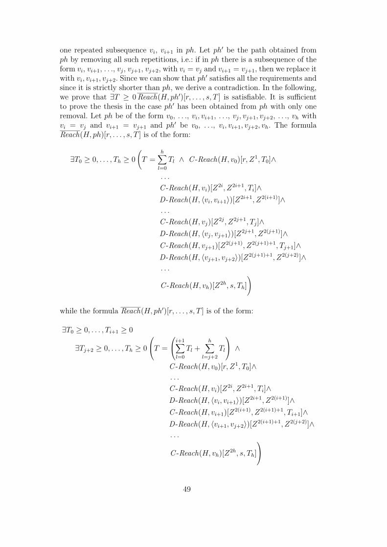
one repeated subsequence vi, vi+1 in ph. Let ph′ be the path obtained fromph by removing all such repetitions, i.e.: if in ph there is a subsequence of theform vi, vi+1, . . ., vj, vj+1, vj+2, with vi = vj and vi+1 = vj+1, then we replace itwith vi, vi+1, vj+2. Since we can show that ph′ satisfies all the requirements andsince it is strictly shorter than ph, we derive a contradiction. In the following,we prove that ∃T ≥ 0 Reach(H, ph′)[r, . . . , s, T ] is satisfiable. It is sufficientto prove the thesis in the case ph′ has been obtained from ph with only oneremoval. Let ph be of the form v0, . . ., vi, vi+1, . . ., vj, vj+1, vj+2, . . ., vh withvi = vj and vi+1 = vj+1 and ph′ be v0, . . ., vi, vi+1, vj+2, vh. The formulaReach(H, ph)[r, . . . , s, T ] is of the form:

∃T0 ≥ 0, . . . , Th ≥ 0

(T =

h∑l=0

Tl ∧ C -Reach(H, v0)[r, Z1, T0]∧

. . .

C -Reach(H, vi)[Z2i, Z2i+1, Ti]∧

D-Reach(H, 〈vi, vi+1〉)[Z2i+1, Z2(i+1)]∧. . .

C -Reach(H, vj)[Z2j, Z2j+1, Tj]∧

D-Reach(H, 〈vj, vj+1〉)[Z2j+1, Z2(j+1)]∧C -Reach(H, vj+1)[Z2(j+1), Z2(j+1)+1, Tj+1]∧D-Reach(H, 〈vj+1, vj+2〉)[Z2(j+1)+1, Z2(j+2)]∧. . .

C -Reach(H, vh)[Z2h, s, Th]

)

while the formula Reach(H, ph′)[r, . . . , s, T ] is of the form:

∃T0 ≥ 0, . . . , Ti+1 ≥ 0

∃Tj+2 ≥ 0, . . . , Th ≥ 0

T =

i+1∑l=0

Tl +h∑

l=j+2

Tl

∧C -Reach(H, v0)[r, Z1, T0]∧. . .

C -Reach(H, vi)[Z2i, Z2i+1, Ti]∧

D-Reach(H, 〈vi, vi+1〉)[Z2i+1, Z2(i+1)]∧C -Reach(H, vi+1)[Z2(i+1), Z2(i+1)+1, Ti+1]∧D-Reach(H, 〈vi+1, vj+2〉)[Z2(i+1)+1, Z2(j+2)]∧. . .

C -Reach(H, vh)[Z2h, s, Th]

49

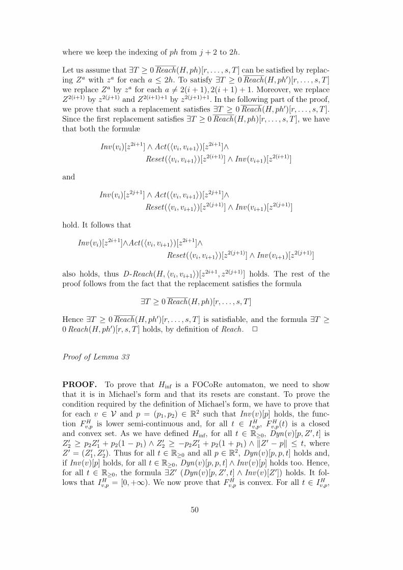
where we keep the indexing of ph from j + 2 to 2h.

Let us assume that ∃T ≥ 0 Reach(H, ph)[r, . . . , s, T ] can be satisfied by replac-ing Za with za for each a ≤ 2h. To satisfy ∃T ≥ 0 Reach(H, ph′)[r, . . . , s, T ]we replace Za by za for each a 6= 2(i + 1), 2(i + 1) + 1. Moreover, we replaceZ2(i+1) by z2(j+1) and Z2(i+1)+1 by z2(j+1)+1. In the following part of the proof,we prove that such a replacement satisfies ∃T ≥ 0 Reach(H, ph′)[r, . . . , s, T ].Since the first replacement satisfies ∃T ≥ 0 Reach(H, ph)[r, . . . , s, T ], we havethat both the formulæ

Inv(vi)[z2i+1] ∧ Act(〈vi, vi+1〉)[z2i+1]∧

Reset(〈vi, vi+1〉)[z2(i+1)] ∧ Inv(vi+1)[z2(i+1)]

and

Inv(vi)[z2j+1] ∧ Act(〈vi, vi+1〉)[z2j+1]∧

Reset(〈vi, vi+1〉)[z2(j+1)] ∧ Inv(vi+1)[z2(j+1)]

hold. It follows that

Inv(vi)[z2i+1]∧Act(〈vi, vi+1〉)[z2i+1]∧

Reset(〈vi, vi+1〉)[z2(j+1)] ∧ Inv(vi+1)[z2(j+1)]

also holds, thus D-Reach(H, 〈vi, vi+1〉)[z2i+1, z2(j+1)] holds. The rest of theproof follows from the fact that the replacement satisfies the formula

∃T ≥ 0 Reach(H, ph)[r, . . . , s, T ]

Hence ∃T ≥ 0 Reach(H, ph′)[r, . . . , s, T ] is satisfiable, and the formula ∃T ≥0 Reach(H, ph′)[r, s, T ] holds, by definition of Reach. 2

Proof of Lemma 33

PROOF. To prove that Hinf is a FOCoRe automaton, we need to showthat it is in Michael’s form and that its resets are constant. To prove thecondition required by the definition of Michael’s form, we have to prove thatfor each v ∈ V and p = (p1, p2) ∈ R2 such that Inv(v)[p] holds, the func-tion FH

v,p is lower semi-continuous and, for all t ∈ IHv,p, FHv,p(t) is a closed

and convex set. As we have defined Hinf, for all t ∈ R≥0, Dyn(v)[p, Z ′, t] isZ ′2 ≥ p2Z

′1 + p2(1 − p1) ∧ Z ′2 ≥ −p2Z

′1 + p2(1 + p1) ∧ ‖Z ′ − p‖ ≤ t, where

Z ′ = (Z ′1, Z′2). Thus for all t ∈ R≥0 and all p ∈ R2, Dyn(v)[p, p, t] holds and,

if Inv(v)[p] holds, for all t ∈ R≥0, Dyn(v)[p, p, t] ∧ Inv(v)[p] holds too. Hence,for all t ∈ R≥0, the formula ∃Z ′ (Dyn(v)[p, Z ′, t] ∧ Inv(v)[Z ′]) holds. It fol-lows that IHv,p = [0,+∞). We now prove that FH

v,p is convex. For all t ∈ IHv,p,

50

FHv,p is such that FH

v,p(t) = {q | Dyn(v)[p, q, t] ∧ Inv(v)[q]}, where q = (q1, q2).Hence, by Dyn’s definition, FH

v,p(t) = Sat(up [p, Z] ∧ up′ [p, Z])∩Sat(Inv(v))∩Sat(‖p− Z‖ ≤ t). Since the intersection of convex sets is convex, to deduce theconvexity of FH

v,p(t), we will prove the convexity of Sat(up [p, Z] ∧ up′ [p, Z])∩Sat(Inv(v)), and Sat(‖p− Z‖ ≤ t). A set S is convex if and only if for allq, q ∈ S, all points of the segment between q and q are contained in S. Theconvexity of Sat(‖p− Z‖ ≤ t) is obvious, hence we have to prove the con-vexity of Sat(up [p, Z] ∧ up′ [p, Z]) ∩ Sat(Inv(v)). In particular, we need toprove that for all p = (p1, p2), q = (q1, q2), r = (r1, r2) ∈ R2, and for allα ∈ [0, 1], if q, r ∈ Sat(up [p, Z] ∧ up′ [p, Z]) ∩ Sat(Inv(v)) then (s1, s2) ∈Sat(up [p, Z] ∧ up′ [p, Z]) ∩ Sat(Inv(v)), where s1 = (1− α)q1 + αr1 and s2 =(1−α)q2+αr2. If q ∈ Sat(up [p, Z] ∧ up′ [p, Z]) then q2 ≥ p2q1+p2(1−p1)∧q2 ≥−p2q1 + p2(1 + p1) and if r ∈ Sat(up [p, Z] ∧ up′ [p, Z]) then r2 ≥ p2r1 + p2(1−p1) ∧ r2 ≥ −p2r1 + p2(1 + p1). Thus:

s2 = (1− α)q2 + αr2

≥ (1− α) (p2q1 + p2(1− p1)) + α (p2r1 + p2(1− p1))

≥ p2 ((1− α)q1 + αr1) + p2(1− p1) ((1− α) + α) .

But, s1 = (1− α)q1 + αr1 hence:

s2 ≥ p2 ((1− α)q1 + αr1) + p2(1− p1) ((1− α) + α)

≥ p2 ((1− α)q1 + αr1) + p2(1− p1)

≥ p2s1 + p2(1− p1).

Symmetrically:

s2 = (1− α)q2 + αr2

≥ (1− α) (p2(1 + p1)− p2q1) + α (p2(1 + p1)− p2q1)

≥ −p2 ((1− α)q1 + αr1) + p2(1 + p1) ((1− α) + α)

≥ −p2s1 + p2(1 + p1),

thus, for all s lying on the segment between q and r, the formula up [p, s] ∧up′ [p, s] holds. Moreover, if Inv(v)[q] and Inv(v)[r] then −1 ≤ q1 ≤ 1 ∧ q2 >0 and −1 ≤ r1 ≤ 1 ∧ r2 > 0, thus s2 = (1 − α)q2 + αr2 ≥ (1 − α)0 +α0 ≥ 0. Furthermore, s1 = (1 − α)q1 + αr1 ≥ −(1 − α) − α ≥ −1 ands1 = (1 − α)q1 + αr1 ≤ (1 − α) + α ≤ 1 and hence, for all s belongingto the segment between q and r, the formula Inv(v)[s] holds. Thus for allq, r ∈ Sat(up [p, Z] ∧ up′ [p, Z]) ∩ Sat(Inv(v)) and for all s belonging to thesegment between q and r, s ∈ Sat(up [p, Z] ∧ up′ [p, Z]) ∩ Sat(Inv(v)). Hencewe have demonstrated the convexity of FH

v,p(t).

We now prove that FHv,p is lower semi-continuous. By Definition 17, FH

v,p islower semi-continuous if and only if for all q ∈ FH

v,p(t) and for all neighborhoodsUq,ε = {q′ | ‖q′−q‖ < ε} of q there exists a neighborhood Ut,δ = {t′ | |t′−t| < δ}

51

of t such that ∀t′ ∈ Ut,δ the set (FHv,p(t

′) ∩ Uq,ε) is not empty. Now we provethat, for all q ∈ FH

v,p(t) and for all ε > 0, δ = ε2

is such that ∀t′ ∈ Ut,δr ∈ (FH

v,p(t′)∩Uq,ε), where r is the point in the segment between p and q such

that ‖r− q‖ = 2ε3

. Since FHv,p(t) is convex and both q and p are in FH

v,p(t), thenr ∈ FH

v,p(t). Notice that, since FHv,p(t) = Sat(up [p, Z] ∧ up′ [p, Z] ∧ Inv(v)) ∩

Sat(‖p− Z‖ ≤ t), it holds that if t′ ≥ t, then FHv,p(t

′) ⊇ FHv,p(t). Thus if t′ ≥ t,

then r ∈ FHv,p(t

′). So assume that t′ < t. By definition of r, it follows directlythat ‖r − q‖ + ‖p − r‖ = ‖p − q‖. Moreover, since by hypothesis q ∈ FH

v,p(t),‖p− q‖ ≤ t. Hence 2ε

3+ ‖p− r‖ ≤ t holds, but this formula holds if and only

if ‖p − r‖ ≤ t − 2ε3

. Furthermore, by hypothesis ‖t′ − t‖ < ε2

and t′ < t, thust < t′+ ε

2. It follows that ‖p−r‖ ≤ t− 2ε

3< t′− ε

6. But ε > 0 then ‖p−r‖ ≤ t′.

Moreover, since r ∈ FHv,p(t), the formula up [p, r] ∧ up′ [p, r] ∧ Inv(v)[r] holds.

Hence r ∈ Sat(up [p, Z] ∧ up′ [p, Z] ∧ Inv(v)) ∩ Sat(‖p− Z‖ ≤ t′) = FHv,p(t

′)and the function FH

v,p is lower semi-continuous. We now need to prove that,for all p and for all t ∈ IHv,p, the set FH

v,p(t) is closed. By definition, FHv,p(t) =

Sat(up [p, Z] ∧ up′ [p, Z]) ∩ Sat(Inv(v)) ∩ Sat(‖p− Z‖ ≤ t). By definition ofour automaton, if p = (p1, p2) and q = (q1, q2), then up [p, q] ∧ up′ [p, q] isq2 ≥ p2q1 + p2(1− p1) ∧ q2 ≥ −p2q1 + p2(1 + p1) ∧ ‖p− q‖ ≤ t. Moreover, theformula q2 ≥ −p2q1 + p2(1 + p1) holds if and only if p2q1 ≥ −q2 + p2(1 + p1)holds. Thus, from Dyn(v)[p, q, t], it follows that:

q2 ≥ p2q1 + p2(1− p1)

≥ −q2 + p2(1 + p1) + p2(1− p1)

≥ −q2 + 2p2,

and then q2 ≥ p2. Since Inv(v)[q] is−1 ≤ q1 ≤ 1∧q2 > 0 and q2 > p2∧Inv(v)[p]implies q2 > 0, for all p ∈ R2 such that Inv(v)[p] and for all t ∈ IHv,p, FH

v,p(t) ={q |q2 ≥ p2q1 +p2(1−p1)∧q2 ≥ −p2q1 +p2(1+p1)∧−1 ≤ q1 ≤ 1∧‖p−q‖ ≤ t},where q = (q1, q2). Hence, since FH

v,p(t) is an intersection of closed sets, FHv,p(t)

is a closed set. It follows that Hinf is a FOCoRe automaton. 2

Lemma 44 For the automaton Hinf, if the formula Inv(v)[p] holds then, foreach t ∈ R≥0, ψ(H, v)[p, t] holds.

PROOF. By definition, ψ(H, v)[p, t] is ∀0 ≤ T ′ ≤ t ∃Z ′Dyn(v)[p, Z ′, T ′] ∧Inv(v)[Z ′]. Moreover, by Hinf’s definition, Dyn(v)[p, Z ′, T ] is Z ′2 ≥ p2Z

′1 +

p2(1 − p1) ∧ Z ′2 ≥ −p2Z′1 + p2(1 + p1) ∧ ‖p − Z ′‖ ≤ T and Inv(v)[p] is −1 ≤

p1 ≤ 1 ∧ p2 > 0, where p = (p1, p2) and Z ′ = (Z ′1, Z′2). It follows that,

for all t ∈ R≥0, Dyn(v)[p, p, t] holds. Thus if Inv(v)[p] holds then, for allt ∈ R≥0, ∃Z ′Dyn(v)[p, Z ′, t] ∧ Inv(v)[Z ′] holds. Hence, by definition of theformula ψ(H, v)[p, t], if Inv(v)[p] holds then, for all t ∈ R≥0, ψ(H, v)[p, t]holds too. 2

52

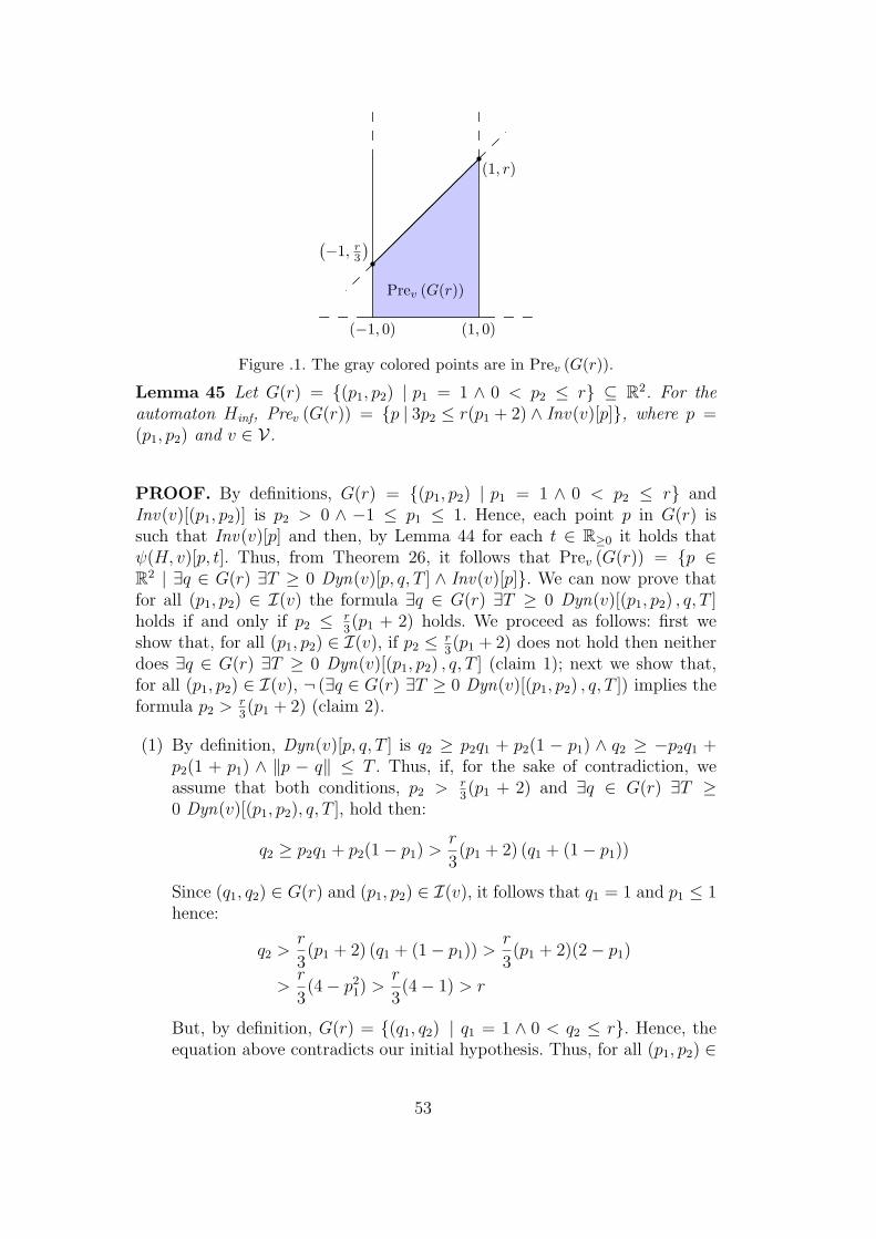
(1, r)

(−1, r

3

)Prev (G(r))

(−1, 0) (1, 0)

Figure .1. The gray colored points are in Prev (G(r)).

Lemma 45 Let G(r) = {(p1, p2) | p1 = 1 ∧ 0 < p2 ≤ r} ⊆ R2. For theautomaton Hinf, Prev (G(r)) = {p | 3p2 ≤ r(p1 + 2) ∧ Inv(v)[p]}, where p =(p1, p2) and v ∈ V.

PROOF. By definitions, G(r) = {(p1, p2) | p1 = 1 ∧ 0 < p2 ≤ r} andInv(v)[(p1, p2)] is p2 > 0 ∧ −1 ≤ p1 ≤ 1. Hence, each point p in G(r) issuch that Inv(v)[p] and then, by Lemma 44 for each t ∈ R≥0 it holds thatψ(H, v)[p, t]. Thus, from Theorem 26, it follows that Prev (G(r)) = {p ∈R2 | ∃q ∈ G(r) ∃T ≥ 0 Dyn(v)[p, q, T ] ∧ Inv(v)[p]}. We can now prove thatfor all (p1, p2) ∈ I(v) the formula ∃q ∈ G(r) ∃T ≥ 0 Dyn(v)[(p1, p2) , q, T ]holds if and only if p2 ≤ r

3(p1 + 2) holds. We proceed as follows: first we

show that, for all (p1, p2) ∈ I(v), if p2 ≤ r3(p1 + 2) does not hold then neither

does ∃q ∈ G(r) ∃T ≥ 0 Dyn(v)[(p1, p2) , q, T ] (claim 1); next we show that,for all (p1, p2) ∈ I(v), ¬ (∃q ∈ G(r) ∃T ≥ 0 Dyn(v)[(p1, p2) , q, T ]) implies theformula p2 >

r3(p1 + 2) (claim 2).

(1) By definition, Dyn(v)[p, q, T ] is q2 ≥ p2q1 + p2(1 − p1) ∧ q2 ≥ −p2q1 +p2(1 + p1) ∧ ‖p − q‖ ≤ T . Thus, if, for the sake of contradiction, weassume that both conditions, p2 > r

3(p1 + 2) and ∃q ∈ G(r) ∃T ≥

0 Dyn(v)[(p1, p2), q, T ], hold then:

q2 ≥ p2q1 + p2(1− p1) >r

3(p1 + 2) (q1 + (1− p1))

Since (q1, q2) ∈ G(r) and (p1, p2) ∈ I(v), it follows that q1 = 1 and p1 ≤ 1hence:

q2 >r

3(p1 + 2) (q1 + (1− p1)) >

r

3(p1 + 2)(2− p1)

>r

3(4− p2

1) >r

3(4− 1) > r

But, by definition, G(r) = {(q1, q2) | q1 = 1 ∧ 0 < q2 ≤ r}. Hence, theequation above contradicts our initial hypothesis. Thus, for all (p1, p2) ∈

53

I(v), if p2 >r3(p1 +2) holds then ∃q ∈ G(r) ∃T ≥ 0 Dyn(v)[(p1, p2) , q, T ]

does not.(2) By definition, Dyn(v)[p, q, T ] is q2 ≥ p2q1 + p2(1 − p1) ∧ q2 ≥ −p2q1 +

p2(1 + p1)∧ ‖p− q‖ ≤ T , and if, for the sake of contradiction, we assumethat both formulæ ∀q ∈ G(r) ∀T ≥ 0 ¬Dyn(v)[p, q, T ] and p2 ≤ r

3(p1 +2)

hold then either q2 < p2q1 + p2(1 − p1), q2 < −p2q1 + p2(1 + p1) or∀q ∈ G(r)∀T ≥ 0 ‖p− q‖ > T . If the formula q2 < p2q1 + p2(1− p1) holdsthen:

q2 < p2q1 + p2(1− p1) <r

3(p1 + 2) (q1 + (1− p1))

Since (q1, q2) ∈ G(r) and (p1, p2) ∈ I(v), it follows that q1 = 1 andp1 ≥ −1 hence:

q2 <r

3(p1 + 2) (q1 + (1− p1)) <

r

3(p1 + 2)(2− p1)

<r

3(4− p2

1) <r

3(4− 1) < r

But, by definition, G(r) = {(q1, q2) | q1 = 1∧ 0 < q2 ≤ r} and, in partic-ular, (1, r) ∈ G(r). Hence, the formula q2 < p2q1 + p2(1− p1) contradictsour hypothesis.

Let us assume that the formula q2 < −p2q1 + p2(1 + p1) holds. Since(q1, q2) ∈ G(r) and (p1, p2) ∈ I(v), by hypothesis, q1 = 1 and p1 ≤ 1. Itfollows that

q2 < −p2q1 + p2(1 + p1) < −p2 + p2(1 + 1) = p2

Moreover, the formula p2 ≤ r3(p1 + 2) holds by hypothesis, thus

q2 < p2 ≤r

3(p1 + 2) ≤ r

3= r

But by definition, G(r) = {(q1, q2) | q1 = 1 ∧ 0 < q2 ≤ r} and, inparticular, (1, r) ∈ G(r). Hence, the formula q2 < −p2q1 + p2(1 + p1)contradicts our hypothesis.

Let us first assume that ∀q ∈ G(r)∀T ≥ 0 ‖p − q‖ > T holds. Let usover-estimate the maximum of ‖p − q‖ when p ∈ I(v), q ∈ G(r), andp2 ≤ r

3(p1 + 2).

max ‖p− q‖ ≤ max2√

(p1 − q1)2 + (p2 − q2)2

≤ 2√

max (p1 − q1)2 + max (p2 − q2)2

≤ 2√

max (max p1 −min q1,min p1 −max q1)2 + max (p2 − q2)2

Since (q1, q2) ∈ G(r), (p1, p2) ∈ I(v), and p2 ≤ r3(p1 + 2) by hypothesis,

54

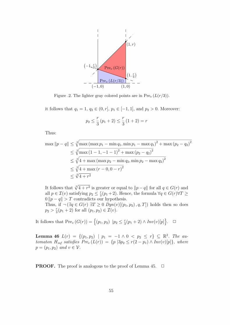
(1, r)

(−1, r

3

)(1, r

9

)Prev (L(r/3))

Prev (G(r))

(−1, 0) (1, 0)

Figure .2. The lighter gray colored points are in Prev (L(r/3)).

it follows that q1 = 1, q2 ∈ (0, r], p1 ∈ [−1, 1], and p2 > 0. Moreover:

p2 ≤r

3(p1 + 2) ≤ r

3(1 + 2) = r

Thus:

max ‖p− q‖ ≤ 2√

max (max p1 −min q1,min p1 −max q1)2 + max (p2 − q2)2

≤ 2√

max (1− 1,−1− 1)2 + max (p2 − q2)2

≤ 2√

4 + max (max p2 −min q2,min p2 −max q2)2

≤ 2√

4 + max (r − 0, 0− r)2

≤ 2√

4 + r2

It follows that 2√

4 + r2 is greater or equal to ‖p− q‖ for all q ∈ G(r) andall p ∈ I(v) satisfying p2 ≤ r

3(p1 +2). Hence, the formula ∀q ∈ G(r)∀T ≥

0 ‖p− q‖ > T contradicts our hypothesis.Thus, if ¬ (∃q ∈ G(r) ∃T ≥ 0 Dyn(v)[(p1, p2) , q, T ]) holds then so doesp2 >

r3(p1 + 2) for all (p1, p2) ∈ I(v).

It follows that Prev (G(r)) ={

(p1, p2) |p2 ≤ r3(p1 + 2) ∧ Inv(v)[p]

}. 2

Lemma 46 L(r) = {(p1, p2) | p1 = −1 ∧ 0 < p2 ≤ r} ⊆ R2. The au-tomaton Hinf satisfies Prev (L(r)) = {p |3p2 ≤ r(2− p1) ∧ Inv(v)[p]}, wherep = (p1, p2) and v ∈ V.

PROOF. The proof is analogous to the proof of Lemma 45. 2

55

Proof of Theorem 34

PROOF. Our proof that Hinf does not admit finite bisimulation quotient re-lies on showing that Algorithm 1 does not terminate on Hinf. At the beginningof the computation, Algorithm 1 uses Sv = {R(e),A(e), I(v) \ (R(e) ∪ A(e))}as initial partition. Since L(1) = R(e) and G(1) = A(e), we have thatSv = {L(1), G(1), I(v) \ (L(1) ∪G(1))}. If p = (p1, p2) then, by Lemma 46and G’s definition:

Prev (L(r)) ∩G(r′) = {Z |p2 ≤r

3(2− p1) ∧ Inv(v)[Z] ∧ p1 = 1 ∧ 0 < p2 ≤ r′}

= {Z |p2 ≤r

3∧ Inv(v)[Z] ∧ p1 = 1 ∧ 0 < p2 ≤ r′}

= G(r

3

)

Similarly, by Lemma 45 and L’s definition: Prev (G(r′))∩L(r) = L(r′

3

). Thus,

if r < 3r′ and r, r′ ∈ R≥0 then ∅ 6= Prev (L(r)) ∩ G(r′) 6= G(r′) and then the

algorithm removes G(r′) from Sv and it inserts the sets G(r3

)and G(r′)\G

(r3

)in Sv. Otherwise, r ≥ 3r′ holds and if r, r′ ∈ R≥0 then 3r > r ≥ 3r′ > r′. Itfollows that ∅ 6= Prev (G(r′)) ∩ L(r) 6= L(r) and then the algorithm removes

L(r) from Sv and it inserts the sets L(r′

3

)and L(r) \ L

(r′

3

)in Sv. Hence,

since the initial partition contains both L(1) and G(1), during the subsequentcomputation steps, there will exist r, r′ ∈ (0, 1] such that L(r), G(r′) ∈ Sv.Moreover, at each computation steps ∃P, P ′ ∈ Sv | ∅ 6= Prev (P ) ∩ P ′ 6= P ′

in particular, if r < 3r′ then P = L(r) and P ′ = G(r′), since, Otherwise,P = G(r′) and P ′ = L(r). It follows then that Algorithm 1 does not terminate,leading to the conclusion that Hinf does not admit finite bisimulation. 2

Proof of Theorem 39

PROOF. We proceed by structural induction on Q. The only interestingcases are the formulæ E3Q1 and A2Q1. We prove the statement in the caseE3Q1, since the other case has a similar proof.

(⇒) By Definition 37, 〈v, r〉 � E3Q1 holds if and only if, for some state 〈v′, s〉reachable from 〈v, r〉, it holds that 〈v′, s〉 � Q1. But, by Lemma 30, we candeduce that 〈v′, s〉 is reachable from 〈v, r〉 if and only if there exists a ph ∈P E(v) such that ∃T ≥ 0 Reach(H, ph)[r, s, T ] holds and v′ = uph. Moreover, byinductive hypothesis, 〈v′, Z〉 � Q1 holds if and only if % (H,Q1, v

′) [Z] holds.Thus 〈v, r〉 � E3Q1 holds if and only if there exists a ph ∈ P E(v) such that∃Z ′(∃T ≥ 0 Reach(H, ph)[r, Z ′, T ]∧ % (H,Q1, uph) [Z ′]) holds, and then, if andonly if % (H, E3Q1, v) [r].

56

(⇐) If % (H, E3Q1, v) [r] holds, then one of its disjoint clauses must hold. Letph be the path whose disjoint holds. By Lemma 30, we can deduce that ifthe formula ∃T ≥ 0 Reach(H, ph)[r, s, T ] holds, and ph ∈ P E(v), then 〈uph, s〉is reachable from 〈v, r〉. Moreover, by inductive hypothesis, 〈uph, Z〉 � Q1

holds if and only if % (H,Q1, uph) [Z] holds. Hence, by ΦP ’s semantics, if% (H, E3Q1, v) [r] holds, then 〈uph, s〉 is reachable from 〈v, r〉 and 〈uph, s〉 �Q1. It follows that 〈v, r〉 � E3Q1 holds. 2

Proof of Theorem 42

PROOF. By Lemma 27 and by Reach’s definition, if H ′ is a FOCoRe, thenthe formula Reach(H ′, ph)[p, q, t] holds if and only if H ′ reaches q from p intime t through a trace whose corresponding path is ph. Moreover, by hy-

pothesis, Inv ′(v)[Z]def= Inv(v)[Z] ∧ (% (H,Q1, v) [Z] ∨ % (H,Q2, v) [Z]) for all

v ∈ V . Hence if the formula Reach(H ′, ph)[p, q, t] holds, then during the evolu-tion from p to q satisfy either % (H,Q1, v) [Z] or % (H,Q2, v) [Z]. Furthermore,since H and H ′ have the same dynamics, activations, and resets, if the formulaReach(H ′, ph)[p, q, t] holds, then Reach(H, ph)[p, q, t] holds too. Now considerthe formula % (H,H ′, E(Q1UQ2), v) [Z]. If % (H,H ′, E(Q1UQ2), v) [r] holds, then

∃T ≥ 0∃Z ′∨

ph∈PE(v)

Reach(H ′, ph)[r, Z ′, T ] ∧ % (H,Q2, uph) [Z ′]

holds too. By above considerations, it follows that there exists an evolution ofH from r to p satisfying % (H,Q2, uph) [p] such that during all the evolutioneither % (H,Q1, uph) [Z] or % (H,Q2, uph) [Z] holds. Thus 〈v, r〉 � E(Q1UQ2)by Theorem 39 and by ΦU,P semantics. 2

Lemma 47 Let H be a hybrid automaton. If Dyn is a transitive dynamics,then C -Reach(H, v)[r, s, t] holds if and only if the following formula holds

∃Z ′′ ∃0 ≤ T ′ ≤ t (C -Reach(H, v)[r, Z ′′, T ′] ∧ C -Reach(H, v)[Z ′′, s, t− T ′])

PROOF. (⇒) By Dyn’s definition, the formula C -Reach(H, v)[r, r, 0] holdsfor all r. Hence if the formula C -Reach(H, v)[r, s, t] holds, then

C -Reach(H, v)[r, s, t] ∧ C -Reach(H, v)[s, s, 0]

holds too. It follows that there exist a w and a t′ ≥ 0 such that the followingholds

C -Reach(H, v)[r, w, t′] ∧ C -Reach(H, v)[w, s, t− t′]In particular, this holds with w = s and t′ = t.

57

(⇐) Consider the formula

φ[Z,Z ′, T ]def= ∃Z ′′ ∃0 ≤ T ′ ≤ T (C -Reach(H, v)[Z,Z ′′, T ′]∧

C -Reach(H, v)[Z ′′, Z ′, T − T ′])

If there exist p, q and t, t′ ≥ 0 such that both t = t′ and φ[p, q, t] hold,then C -Reach(H, v)[p, q, t] ∧ C -Reach(H, v)[q, q, 0], and thus φ[p, q, t] impliesthat it holds C -Reach(H, v)[p, q, t]. Moreover, if there exist p, q and t, t′ ≥0 such that both t′ = 0 and φ[p, q, t] hold, then C -Reach(H, v)[p, p, 0] ∧C -Reach(H, v)[p, q, t], indeed φ[p, q, t] implies C -Reach(H, v)[p, q, t]. Hence,in the following part of the proof, we consider the case in which both T ′ 6= Tand T ′ 6= 0 hold. By C -Reach’s definition, C -Reach(H, v)[r, s, t] holds if andonly if it holds that

( (t > 0 ∧ Dyn(v)[r, s, t] ∧ ψ(H, v)[r, t])∨(t = 0 ∧ r = s) ) ∧ Inv(v)[r] ∧ Inv(v)[s]

Hence the formula

∃Z ′′ ∃0 ≤ T ′ ≤ t (C -Reach(H, v)[r, Z ′′, T ′] ∧ C -Reach(H, v)[Z ′′, s, t− T ′])

holds if and only if the following statement holds

∃Z ′′ ∃0 ≤ T ′ ≤ t ((( (T ′ > 0 ∧ Dyn(v)[r, Z ′′, T ′] ∧ ψ(H, v)[r, T ′])∨(T ′ = 0 ∧ r = Z ′′) ) ∧ Inv(v)[r] ∧ Inv(v)[Z ′′])

∧( (t− T ′) > 0 ∧ Dyn(v)[Z ′′, s, t− T ′]∧ψ(H, v)[Z ′′, t− T ′]) ∨ ((t− T ′) = 0∧Z ′′ = s) ) ∧ Inv(v)[Z ′′] ∧ Inv(v)[s]))

As noted earlier, we are considering the case in which both T ′ 6= t and T ′ 6= 0hold. In this case, it is easy to prove that the above formula is equivalent to

∃Z ′′ ∃0 ≤ T ′ ≤ T (( (T ′ > 0 ∧ Dyn(v)[r, Z ′′, T ′] ∧ ψ(H, v)[r, T ′]∧(t− T ′) > 0 ∧ Dyn(v)[Z ′′, s, t− T ′]∧ψ(H, v)[Z ′′, t− T ′]) ∧ Inv(v)[r] ∧ Inv(v)[Z ′′]∧Inv(v)[s])

Moreover, by ψ’s definition, if the formulæ ψ(H, v)[Z ′′, t− T ′], ψ(H, v)[r, T ′],and C -Reach(H, v)[r, Z ′′, T ′] are satisfiable, then ψ(H, v)[r, t] holds. Hence,since Dyn is transitive, it easily follows that if the formula

∃Z ′′ ∃0 ≤ T ′ ≤ t (C -Reach(H, v)[r, Z ′′, T ′] ∧ C -Reach(H, v)[Z ′′, s, t− T ′])

holds, then C -Reach(H, v)[r, s, t] holds too. 2

58

Lemma 48 Let H be a hybrid automaton. Moreover, let ph = (vi)i∈[0,h] andph′ = (v′i)i∈[0,h′] be two paths in 〈V , E〉 such that vh = v′0. If Dyn is a transitivedynamics, then Reach(H, ph′′)[r, s, t] holds if and only if it holds that

∃Z ′′ ∃0 ≤ T ′ ≤ t (Reach(H, ph)[r, Z ′′, T ′] ∧ Reach(H, ph)[Z ′′, s, t− T ′])

where ph′′ = ph · ph′.

PROOF. Let h′′ be the length of ph · ph′ (i.e., h′′ = |ph · ph′|) and ph · ph′ bethe path (vi)i∈[0,h′′]. By Reach’s definition, Reach(H, ph′′)[r, s, t] is equivalentto

∃Z1, . . . , Z2h′′ Reach(H, ph′′)[r, Z1, . . . , Z2h′′ , s, t]

Hence, by Reach’s definition, the formula Reach(H, ph′′)[Z0, Z2h′′+1, T ] is sat-isfied by (r, s, t) if and only if the following formula is satisfied by (r, s, t)

∃Z1, . . . , Z2h′′ ∃T0 ≥ 0, . . . , Th′′ ≥ 0T =h′′∑i=0

Ti ∧ C -Reach(H, v0)[Z0, Z1, T0] ∧∧

i∈[0,h′′−1]

(D-Reach(H, 〈vi, vi+1〉)[Z2i+1, Z2i+2]∧

C -Reach(H, vi+1)[Z2i+2, Z2i+3, Ti+1])

By Lemma 47, it follows that Reach(H, ph′′)[Z0, Z2h′′+1, T ] is satisfied by(r, s, t) if and only if the following formula is satisfied by (r, s, t)

∃Z ′′ ∃0 ≤ T ′ ≤ T ∃Z1, . . . , Z2h′′ ∃T0 ≥ 0 . . . ∃Th′′ ≥ 0

∃T ′h ≥ 0∃T ′′h ≥ 0Th = T ′h + T ′′h(T ′ = T ′h +

h−1∑i=0

Ti ∧ C -Reach(H, v0)[Z0, Z1, T0] ∧∧i∈[0,h−2]

(D-Reach(H, 〈vi, vi+1〉)[Z2i+1, Z2i+2]∧

C -Reach(H, vi+1)[Z2i+2, Z2i+3, Ti+1])∧

D-Reach(H, 〈vh−1, vh〉)[Z2h−1, Z2h]∧

C -Reach(H, vh)[Z2h, Z ′′, T ′h]

)∧T − T ′ = T ′′h +

h′′∑i=h+1

Ti ∧

C -Reach(H, vh)[Z′′, Z2h+1, T ′′h ] ∧

59

∧i∈[h,h′′−1]

(D-Reach(H, 〈vi, vi+1〉)[Z2i+1, Z2i+2]∧

C -Reach(H, vi+1)[Z2i+2, Z2i+3, Ti+1])

This last formula is equivalent to

∃Z ′′ ∃0 ≤ T ′ ≤ T (Reach(H, ph)[Z,Z ′′, T ′] ∧ Reach(H, ph′)[Z ′′, Z ′, T − T ′])

Hence, the thesis holds. 2

Proof of Theorem 43

PROOF. If % (H,H ′, EQ1UQ2, v) [q] holds, then there exist two paths ph ∈P E(v) and ph′ ∈ P E(uph) such that either

φ1def=∃Z ′ ∃T ≥ 0 (∀0 ≤ T ′ < T ∃Z ′′ (Reach(H ′, ph)[Z,Z ′′, T ′]∧

Reach(H, ph′)[Z ′′, Z ′, T − T ′] ∧ % (H,Q2, uph′) [Z ′]))

or

φ2def=∃Z ′ ∃T ≥ 0 (∃T ′ > 0 ∀0 < T ′′ ≤ T ′ ∃Z ′′ (Reach(H ′, ph)[Z,Z ′, T ]∧

Reach(H, ph′)[Z ′, Z ′′, T ′′] ∧ % (H,Q2, uph′) [Z ′′]))

holds. If φ1 holds, then there exist a Z ′ and a T ≥ 0 such that for all T ′ ∈ [0, T )the formula

∃Z ′′ (Reach(H ′, ph)[Z,Z ′′, T ′]∧Reach(H, ph′)[Z ′′, Z ′, T − T ′] ∧ % (H,Q2, uph′) [Z ′])

holds too. Hence, since Dyn is transitive by hypothesis, if φ1 holds, then thereexist a Z ′ and a T ≥ 0 such that the formula Reach(H ′, ph · ph′)[Z,Z ′, T ] ∧% (H,Q2, uph·ph′) [Z ′] holds by Lemma 48. By Lemma 27 and by Reach’s def-inition, if m = |ph · ph′|, there exist a trace tr = (〈vi, ri〉)i∈[0,...,2∗m−1] of Hand a sequence (fi :)i∈[0,...,m−1] of functions such that fi : [0, ti] → Rn is(r2∗i, r2∗i+1, v2∗i) admissible in H for all i ∈ [0, . . . ,m − 1] and H reaches〈v, Z〉 from 〈uph·ph′ , Z ′〉 through tr (i.e., 〈v, Z〉 = 〈v0, r0〉 and 〈uph·ph′ , Z ′〉 =〈vm, rm〉). Hence, by Theorem 39, 〈uph·ph′ , Z ′〉 � Q2. Moreover, if m = 2 ∗|ph| − 1, we can deduce that H ′ reaches 〈v, Z〉 from 〈uph·ph′ , Z ′〉 throughtr′ = 〈v0, r0〉, . . . , 〈vm, rm〉, 〈uph, Z ′′〉, fi is (r2∗i, r2∗i+1, v2∗i) admissible in H ′

for all i ∈ [0, . . . ,m−1], and fm is (r2∗m, Z′′, v2∗m) admissible in H ′. Hence, by

H ′’s definition and by Theorem 39, 〈v2∗i, fi(t)〉 � Q1 for all i ∈ [0, . . . ,m− 1]and for all t ∈ [0, ti). It follows that 〈v, q〉 � EQ1UQ2. In an analogous way,we can prove the same result if φ2 holds. 2

60