Author’s preprint version. Published 2014 in Laboratory Phonology (5)1, 195-230. 1 Incipient tonogenesis in Phnom Penh Khmer: Computational studies James P. Kirby School of Philosophy, Psychology and Language Sciences, University of Edinburgh, Dugald Stewart Building, 3 Charles Street, Edinburgh EH9 8AD UK Abstract In the colloquial Phnom Penh dialect of Khmer (Cambodian), lexical use of F 0 is emerging together with an intermediate VOT category and breathy phonation following the loss of /r/ in onsets (e.g. ក# /kruː/ ‘teacher’ > [kʰṳ̀ː]). I show how this incipient tonogenesis might arise in a series of computational simulations tracing the evolution of multivariate phonetic category distributions in a population of ideal observers. Acoustic production data from a fieldwork study conducted in Phnom Penh was used as the starting point for the simulations. After establishing that the basic framework predicted relative stability over time, two possible responses to a phonetic production bias were considered: one in which agents correctly identified the source of (and thereby compensated for) the effects of the bias, and one in which agents misattributed the acoustic effects of the bias as a property of the onset. Good qualitative fits to the empirical production data were found for the latter group of learners, while the outcome for compensating learners resembled production data from a related dialect. These results are consistent with the sudden and discontinuous nature of many sound changes, and suggest that what appear to be enhancement effects may also emerge under different assumptions about the number of cue dimensions accessible to or deemed relevant by the learner. 1 Introduction A topic of central interest for researchers studying the evolution of sound systems is PHONOLOGIZATION (Hyman, 1976), the historical process whereby the distribution of a predictable and phonetically natural process becomes phonologically determined. A familiar example is the idea that lexical tone contrasts can trace their origins to the pitch perturbations conditioned by differences in obstruent voicing (Matisoff,

Welcome message from author
This document is posted to help you gain knowledge. Please leave a comment to let me know what you think about it! Share it to your friends and learn new things together.
Transcript
Author’s preprint version. Published 2014 in Laboratory Phonology (5)1, 195-230.
1
Incipient tonogenesis in Phnom Penh Khmer: Computational studies
James P. Kirby
School of Philosophy, Psychology and Language Sciences, University of Edinburgh, Dugald Stewart
Building, 3 Charles Street, Edinburgh EH9 8AD UK
Abstract
In the colloquial Phnom Penh dialect of Khmer (Cambodian), lexical use of F0 is
emerging together with an intermediate VOT category and breathy phonation
following the loss of /r/ in onsets (e.g. ក# /kruː/ ‘teacher’ > [kʰu ː]). I show how this
incipient tonogenesis might arise in a series of computational simulations tracing
the evolution of multivariate phonetic category distributions in a population of
ideal observers. Acoustic production data from a fieldwork study conducted in
Phnom Penh was used as the starting point for the simulations. After establishing
that the basic framework predicted relative stability over time, two possible
responses to a phonetic production bias were considered: one in which agents
correctly identified the source of (and thereby compensated for) the effects of the
bias, and one in which agents misattributed the acoustic effects of the bias as a
property of the onset. Good qualitative fits to the empirical production data were
found for the latter group of learners, while the outcome for compensating learners
resembled production data from a related dialect. These results are consistent with
the sudden and discontinuous nature of many sound changes, and suggest that what
appear to be enhancement effects may also emerge under different assumptions
about the number of cue dimensions accessible to or deemed relevant by the
learner.
1 Introduction
A topic of central interest for researchers studying the evolution of sound systems is PHONOLOGIZATION
(Hyman, 1976), the historical process whereby the distribution of a predictable and phonetically natural
process becomes phonologically determined. A familiar example is the idea that lexical tone contrasts can
trace their origins to the pitch perturbations conditioned by differences in obstruent voicing (Matisoff,
Author’s preprint version. Published 2014 in Laboratory Phonology (5)1, 195-230.
2
1973; Hombert et al., 1979). A schematized account of this process is sketched in Table 1. First, intrinsic
differences in vowel F0 (Stage I) become a perceptual cue to the identity of the initial consonant (Stage
II). If other cues to the contrast between initial consonants are lost, the contrast may be maintained solely
by differences in F0 (Stage III), setting the stage for a reanalysis of pitch as a contrastive phonological
feature. Similar accounts have been sketched for the development of contrastive vowel length
(Kavitskaya, 2002), vowel quality (Moreton and Thomas, 2007), nasalization (Beddor, 2009) and
consonant voicing (Johnsen, 2011).
Table 1: Tonogenesis as phonologization F0 (after Hyman, 1976). Sparklines show time course of F0 production.
Stage I Stage II Stage III
pá pá pá
bá bǎ pǎ
Phonologization often involves multiple phonetic features. An example is provided by the case of
incipient tonogenesis in Phnom Penh Khmer, an Austroasiatic language of Cambodia. As shown in Table
2, Standard Khmer contrasts plain with aspirated stops in onsets; it also allows a large number of onset
clusters, of which one in particular, /Cr/, will be of interest here. It has long been noted that in the
colloquial speech of the capital Phnom Penh (hereafter PP), words such as ក# /kruː/ ‘teacher’, realized as
[kruː] in Standard Khmer, are produced in PP as something like [kùː], [kʰǔː], or [kṳː]: that is, realized with
a falling or falling-rising pitch contour along with increased post-release aspiration and/or breathy
phonation in place of the trill (Noss, 1966; Huffman, 1967; Wayland and Guion, 2005; Filippi and
Vicheth, 2009). Thus the contrast between colloquial forms of words such as ក# /kruː/ ‘teacher’ and ក
/kuː/ ‘pair’, or ត /taː/ ‘grandfather’ and ត /traː/ ‘seal, stamp’, is presumably being maintained primarily
by differences in the phonetic realization of the nucleus.

Author’s preprint version. Published 2014 in Laboratory Phonology (5)1, 195-230.
3
Table 2: Plain, aspirated, and plain stop+trill onset clusters in Standard Khmer.
ប"# /paː/ ‘father’ ផ /pʰaː/ ‘cloth’ ប /praː/ ‘kind of fish’
ត /taː/ ‘grandfather’ ថ /tʰaː/ ‘to say’ ត /traː/ ‘seal, stamp’
ក /kuː/ ‘pair’ ឃរ /kʰuː/ ‘old’ ក# /kruː/ ‘teacher’
In an acoustic investigation of this sound change, Wayland and Guion (2002, 2005) found that /r/-loss
in PP Khmer was characterized by the development of increased post-release aspiration along with a
falling-rising pitch contour in two speakers. More recently, I explored the perception and production of
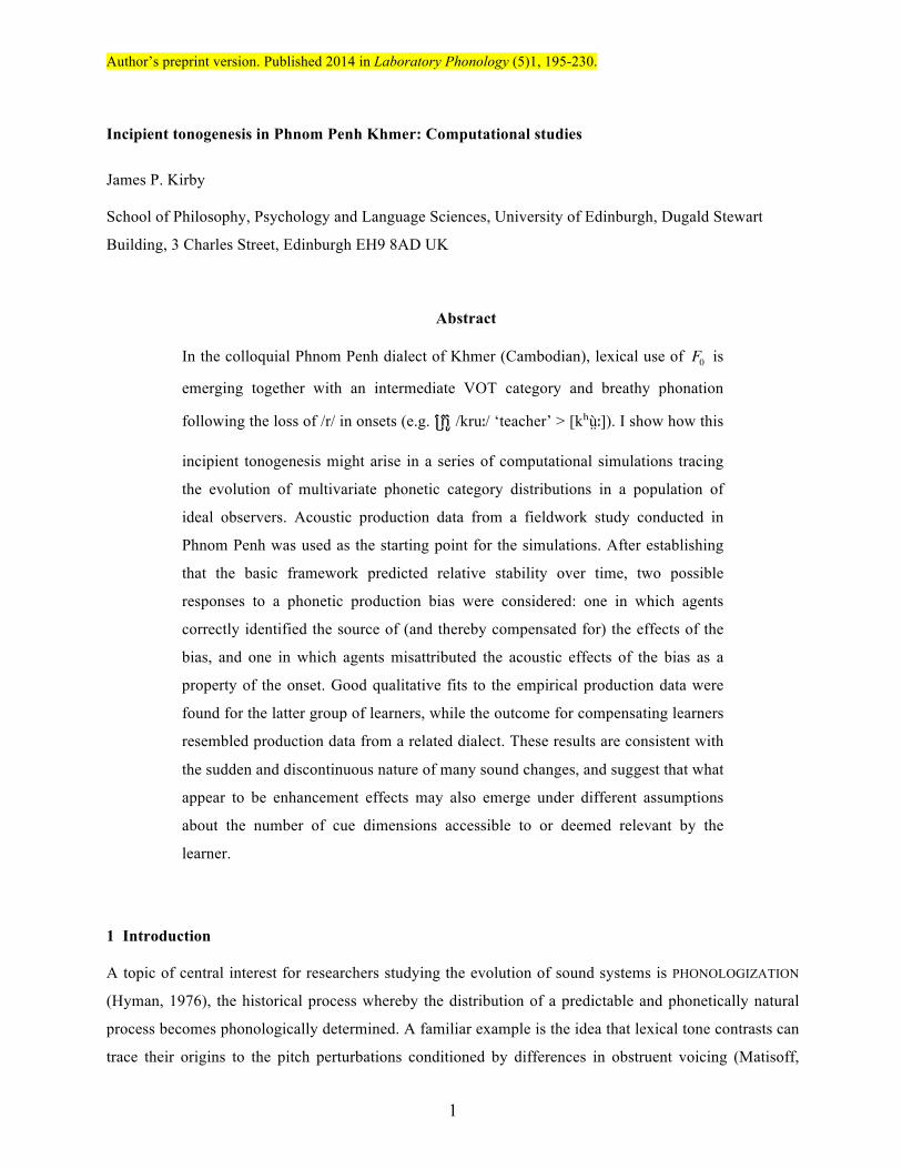
this contrast in 20 native speaking participants of PP Khmer (Kirby under review). Figure 1 plots F0 (in
Hz) over the time course of the vowel for male and female speakers’ productions of /CrV/ forms in both
reading (Standard Khmer) and colloquial (PP) conditions. For speakers of both sexes, F0 of words
produced in the colloquial condition was consistently lower (by 20-30 Hz) than F0 of words produced in
the standard/reading condition at all timepoints; however, the steepness of the F0 drop was not
significantly greater in /CrV/ onsets compared to /CV/ or /CʰV/ onsets. Items were also examined for
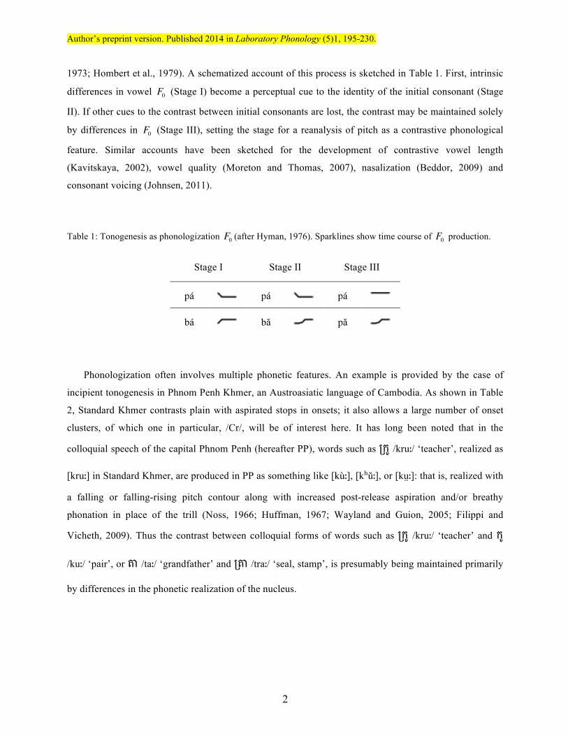
evidence of a phonation type distinction by measuring the amplitude differential between the first and
second harmonics (H1-H2) and the difference between the amplitude of the first harmonic and the
amplitude of the most prominent harmonic of the third formant (H1−A3), both corrected for the influence
of vowel height using the method of Iseli and Alwan (2004). The results indicate that both H1*−H2* and
H1*−A3* are generally higher in colloquial speech than in standard speech; however for both measures
this difference is primarily manifested at onset and offset of the vowel (Figure 2).
Author’s preprint version. Published 2014 in Laboratory Phonology (5)1, 195-230.
4
Figure 1: Average F0 (in Hz) by sex (left: female, right: male) and condition for /CrV/ items. Bars show standard
error of the mean. After Kirby (under review).
Figure 2: Average H1*−H2* (left) and H1*−A3* (right) by condition (standard: solid, colloquial: dashed) for /CrV/
items. Bars show standard error of the mean. After Kirby (under review).
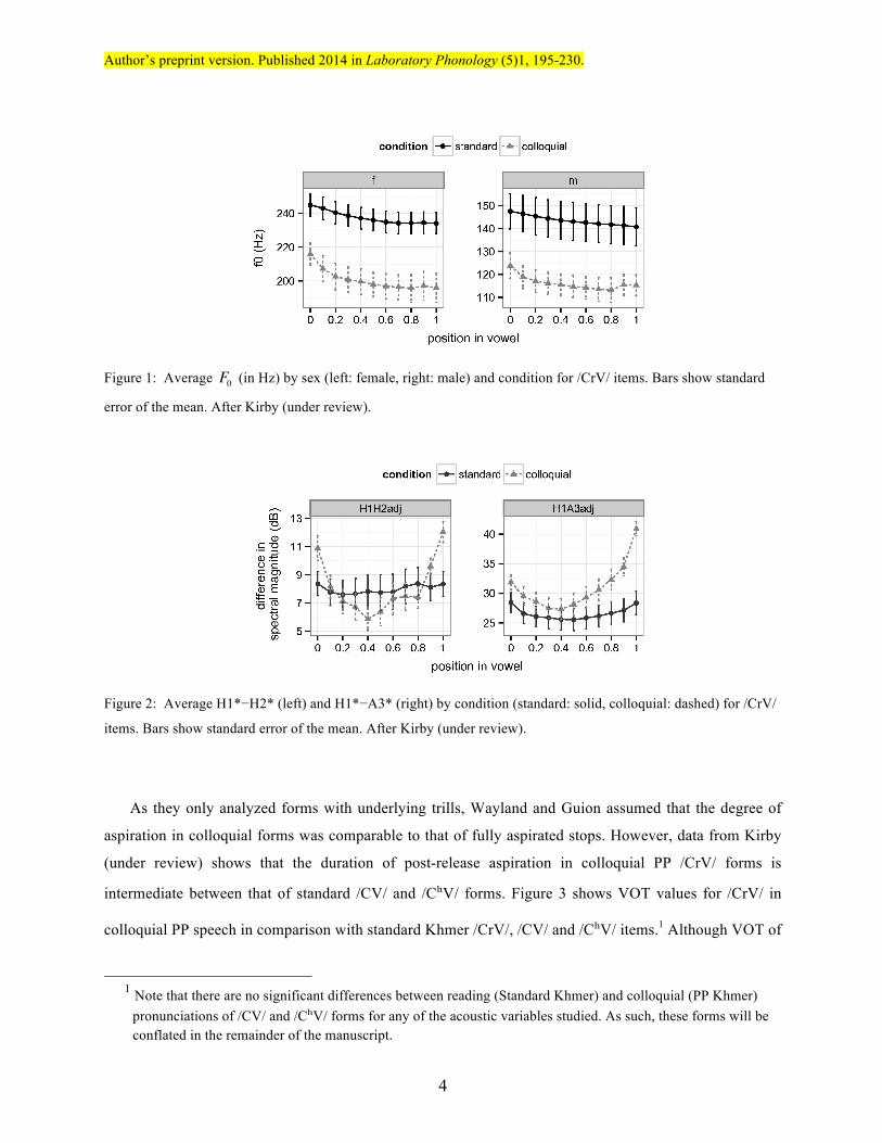
As they only analyzed forms with underlying trills, Wayland and Guion assumed that the degree of
aspiration in colloquial forms was comparable to that of fully aspirated stops. However, data from Kirby
(under review) shows that the duration of post-release aspiration in colloquial PP /CrV/ forms is
intermediate between that of standard /CV/ and /CʰV/ forms. Figure 3 shows VOT values for /CrV/ in
colloquial PP speech in comparison with standard Khmer /CrV/, /CV/ and /CʰV/ items.1 Although VOT of
1 Note that there are no significant differences between reading (Standard Khmer) and colloquial (PP Khmer)
pronunciations of /CV/ and /CʰV/ forms for any of the acoustic variables studied. As such, these forms will be conflated in the remainder of the manuscript.
Author’s preprint version. Published 2014 in Laboratory Phonology (5)1, 195-230.
5
colloquial /CrV/ forms is indeed increased relative to the reading pronunciation of those same forms, it is
not as extensive as in reading condition /CʰV/ forms. A multilevel regression model estimates the VOT of
aspirated stops in reading condition to be, on average, nearly twice as long as the VOT of plain stops in
/CrV/ sequences when produced colloquially. Thus it appears that, rather than merging with one of the
existing categories, the loss of /r/ in PP has triggered the emergence of a novel phonetic (if not yet
phonological) category.
Figure 3: VOT by onset in standard (open) and colloquial /CrV/ forms (shaded). From Kirby (under review).
To explore perceptual sensitivity to cues distinguishing colloquial PP forms like ក# /kruː/ ‘teacher’
from ក /kuː/ ‘pair’, Kirby (under review) employed a two-alternative forced choice (2AFC) listening
paradigm to test listener sensitivity to three potential cues distinguishing standard from colloquial
pronunciations: F0 , VOT, and breathy voice quality. The perception tests employed synthesized stimuli of
quasi-continuously varying F0 and categorically varying differences in VOT and breathiness. The results
indicate that F0 has become a sufficient cue distinguishing colloquial /CrV/ forms from /CV/ forms, but
that increased aspiration and breathy voice quality may also used by listeners as cues to this contrast.
These findings confirm that, to the extent that colloquial PP realizations like [kʰu ː ] can be assumed to
be the end result of a historical process of change starting from Standard Khmer forms like /kruː/, the
contrast appears to have transphonologized: in this case, the loss of the trill has been compensated for by
Author’s preprint version. Published 2014 in Laboratory Phonology (5)1, 195-230.
6
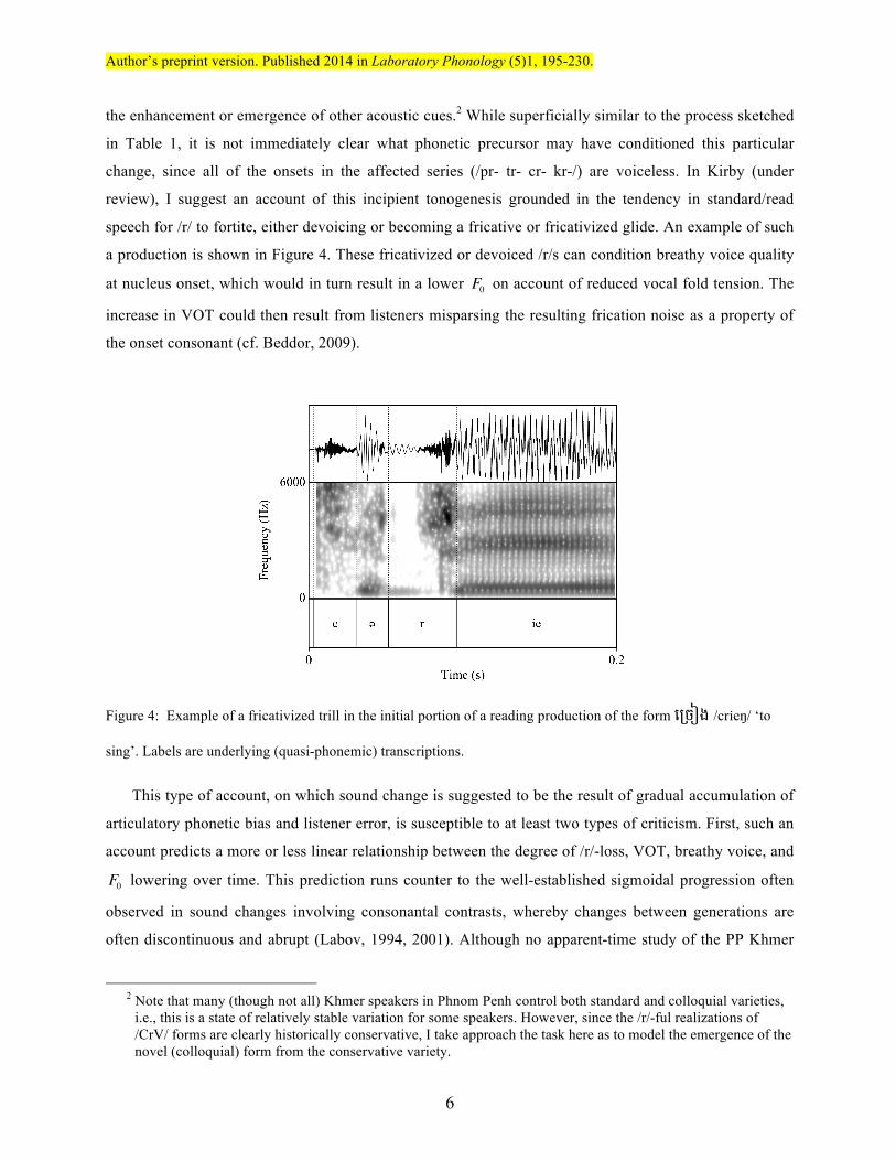
the enhancement or emergence of other acoustic cues.2 While superficially similar to the process sketched
in Table 1, it is not immediately clear what phonetic precursor may have conditioned this particular
change, since all of the onsets in the affected series (/pr- tr- cr- kr-/) are voiceless. In Kirby (under
review), I suggest an account of this incipient tonogenesis grounded in the tendency in standard/read
speech for /r/ to fortite, either devoicing or becoming a fricative or fricativized glide. An example of such
a production is shown in Figure 4. These fricativized or devoiced /r/s can condition breathy voice quality
at nucleus onset, which would in turn result in a lower F0 on account of reduced vocal fold tension. The
increase in VOT could then result from listeners misparsing the resulting frication noise as a property of
the onset consonant (cf. Beddor, 2009).
Figure 4: Example of a fricativized trill in the initial portion of a reading production of the form េចៀង /crieŋ/ ‘to
sing’. Labels are underlying (quasi-phonemic) transcriptions.
This type of account, on which sound change is suggested to be the result of gradual accumulation of
articulatory phonetic bias and listener error, is susceptible to at least two types of criticism. First, such an
account predicts a more or less linear relationship between the degree of /r/-loss, VOT, breathy voice, and
F0 lowering over time. This prediction runs counter to the well-established sigmoidal progression often
observed in sound changes involving consonantal contrasts, whereby changes between generations are
often discontinuous and abrupt (Labov, 1994, 2001). Although no apparent-time study of the PP Khmer
2 Note that many (though not all) Khmer speakers in Phnom Penh control both standard and colloquial varieties,
i.e., this is a state of relatively stable variation for some speakers. However, since the /r/-ful realizations of /CrV/ forms are clearly historically conservative, I take approach the task here as to model the emergence of the novel (colloquial) form from the conservative variety.

Author’s preprint version. Published 2014 in Laboratory Phonology (5)1, 195-230.
7
case has yet been conducted, there is no evidence, anecdotal or otherwise, to suggest that differences in
the realization of e.g. the form of ក# /kruː/ ‘teacher’ in Standard Khmer (where /kruː/ > [kruː]) and
colloquial PP Khmer (where /kruː/ > [kʰu ː ]) are anything but categorical.
Second, this account fails to explain why F0 , and not phonation type or VOT, has become the primary
perceptual cue to the contrast in PP Khmer. Indeed, the process by which Khmer is thought to have
acquired its sizeable inventory of diphthongs and two contrasting consonantal registers almost certainly
involved a stage of contrastive voice quality (Henderson, 1952; Ferlus, 1992), and several scholars have
proposed that the canonical path to tone is similarly mediated by phonation type contrasts (Pulleyblank,
1978; Diffloth, 1989; Thurgood, 2002). This hypothesis is complicated by the existence of languages or
dialect clusters that show evidence for a range of different outcomes of a cue restructuring process. A
good example is that of Kammu dialects, which provide evidence for a number of possible evolutionary
outcomes (Svantesson and House, 2006; Abramson et al., 2007). As shown in Table 3, while the
conservative Eastern dialects retained a voicing contrast in initial consonants, this contrast
transphonologized differently in each of the three Western dialects. The result is a dialect continuum
suggesting several evolutionary trajectories, or stopping points along a single trajectory.
Table 3: Evolution of initial obstruent voicing in Kammu (after Premsrirat, 2001).
E. Kammu W. Kammu W. Kammu W. Kammu gloss (tone 1) (tone 2) (register) buːc pùːc pʰùːc pṳc ‘rice wine’
puːc pûːc pʰúːc pûc ‘to take off clothes’
glaːŋ klàːŋ kʰlàːŋ kla ː ŋ ‘stone’
klaːŋ klâːŋ kʰláːŋ klâːŋ ‘eagle’
In the case of tone and voice quality, it is also not clear why languages would necessarily have to
‘pass through’ a stage of contrastive voice quality, rather than simply employing both cues
simultaneously. Indeed, the frequency with which phonologization of one cue seems to entail the
dephonologization of another is actually unexpected from a perceptual point of view, since considerable
redundancy is the typical state of a phonetic contrast (Lisker, 1978). If phonologization is the end result of
an enhancement of subphonemic cues, what conditions this enhancement, and what governs the selection
of one phonetic dimension for enhancement and not another?

Author’s preprint version. Published 2014 in Laboratory Phonology (5)1, 195-230.
8
In this paper, I pursue an account of phonologization that is based around the conception of the learner
as an IDEAL OBSERVER (Green and Swets, 1966; Geisler and Diehl, 2002; Clayards, 2008; Kirby, 2013a).
On this account, the catalyst of subphonemic reorganization is a loss of contrast precision at the level of
sublexical categorization, driven by a sufficiently actuated phonetic bias. Shifts in the magnitude of the
cue realizations are then predicted to result from the application of an optimal or near-optimal
categorization strategy. On this approach it is straightforward to represent the multivariate richness of the
acoustic signal and to reason about the categorization behavior of learners under different scenarios using
empirical production data of the sort just reviewed. In what follows, I outline the fundamentals of this
approach, and then illustrate its application to the case of incipient tonogenesis in PP Khmer.
2 Modeling phonetic category acquisition
The basic problem of speech perception finds a useful metaphor in the ‘noisy channel’ familiar from
information theory (Shannon and Weaver, 1949). At one end of the channel is the speaker, who is
attempting to send a message to the listener at the other end. However, even under relatively ideal
conditions, speech communication is fraught with difficulties, and a number of factors – including, but by
no means limited to, the influence of physiological, social, and cognitive constraints on speech production
and perception – can introduce variability into the acoustic realization, potentially obscuring the speaker’s
intended message. Here, such influences will collectively be referred to as BIAS FACTORS. Setting aside
for the moment questions about the source, nature, and influence of these bias factors (but see Garrett and
Johnson, 2013), it is enough to simply note that many different types of bias can have a similar effect:
namely, they introduce additional asymmetric variability into the speech signal.
To make this a bit more concrete, we may conceive of the speaker’s goal as being to transmit to the
listener a sequence of labels, representing phonetic categories, each one signaled along multiple acoustic-
phonetic dimensions. The listener’s task is to recover the speaker’s intended sequence of labels based on
the acoustic-phonetic information they receive. All else being equal, the speaker’s success is to some
extent dependent on the PRECISION of the contrasts being transmitted – precision being determined based
on the statistical distribution of acoustic-phonetic cues to the contrast in question. Precision may be
reduced for a variety of reasons, including channel noise introduced by bias factors, or changes in the
system of contrast at the structural level, which may result in an increase or decrease in the number of
categories competing over some acoustic-phonetic space.
This formulation allows us to address the question of how learners might respond in general to
variation in the degree of contrast precision, abstracting away from the precise causes of such variation.
The basic premise of the model of category acquisition outlined here is that learners attempt to parse this

Author’s preprint version. Published 2014 in Laboratory Phonology (5)1, 195-230.
9
potentially noisy speech input in an optimal fashion. This requires that we make explicit the mechanism
by which learners (re)construct category structure on the basis of multivariate acoustic input.
2.1 Representational scheme for phonetic categories
If the speech signal is inherently multidimensional, then any representational scheme for sublexical
categories must be capable of handling multiple dimensions. One formal representation meeting this
description is a FINITE MIXTURE MODEL (McLachlan and Peel, 2000; Rosseel, 2002), which models a
statistical distribution as a weighted sum of other distributions. Mixture models have a long history in
speech research and have been used in work on speech perception (Lisker and Abramson, 1970; Nearey
and Hogan, 1986; Pierrehumbert, 2001; Clayards, 2008), the perceptual integration of acoustic cues
(McMurray et al., 2009; Toscano and McMurray, 2010), and the unsupervised induction of phonetic
category structure (de Boer and Kuhl, 2003; Vallabha et al., 2007; Kirby, 2011).
For computational simplicity, and in line with much previous work, we assume that the underlying
probability distributions of the mixture components (i.e., the cue dimensions) are normal (Gaussian);
however, there is nothing in the following that relies crucially on this assumption, so other distributions
(log-normal, gamma, etc.) could be substituted if it is determined they are more appropriate for some of
the particular cues investigated here. In a GAUSSIAN MIXTURE MODEL (GMM), a D-dimensional
observation vector x = (x1,…, xD ) is assumed to be independently generated by an underlying
distribution with a probability density function
f (x;Θ) = π k
k=1
K
∑ N (x | µk ,Σ k ) (1)
where Θ = (θ1,…,θK ) = ((π1,µ1,Σ1),…,(π K ,µK ,ΣK )) is a K(D+2)-parameter structure containing the
component weights π k ,mean vectors µk , and covariance matrices Σ k of the D-dimensional Gaussian
densities
N (x | µk ,Σ k ) =
1(2π )D/2 | Σ k |
1/2 exp − 12(x − µk )
T Σ k−1(x − µk )
⎧⎨⎩
⎫⎬⎭
(2)
Note that the component weights π1,…,π K must sum to 1.
To make this more concrete, we may think of x as a set of cue values representing an instance of
phonetic category c; of D as representing the number of cue dimensions (x1, x2,…, xD ) relevant to the
perception of that category; and of K as representing the total number of category labels (c1,c2,…,cK )

Author’s preprint version. Published 2014 in Laboratory Phonology (5)1, 195-230.
10
competing over the region of phonetic space defined by D. For example, for a language with three initial
stops (K=3) cued along four dimensions (D=4), we might have c1 = /b/, c2 = /p/, c3 = /pʰ/ and x1 =
VOT, x2 = amplitude of release burst, x3 = F0 , and x4 = spectral tilt. A given utterance x will thus
consist of four columns, each one providing a value for one of these cues.
2.1.1 Production: sampling
A great conceptual and practical advantage of representing sublexical categories with GMMs is that a
single representation can serve as the basis for production as well as perception, thus providing a formal
link between production data and categorization behavior (Nearey and Hogan, 1986; Solé, 2003). This
allows a learner’s experience to form the basis for both the production of instances of a category as well as
for determining the category label of novel instances. Formally, production is modeled by taking a point
estimate from the approximate cumulative distribution function of the multivariate density as given in
Equation 2. Because the cue distributions are continuous, the true probability of any given value of x is in
fact 0. However, we can define the probability of x falling into some interval of the cue space [a,b] as
P[a ≤ X ≤ b]= fa
b
∫ (x)dx (3)
for some arbitrarily small difference between a and b. In practice, the selection of a particular value may
be achieved by methods such as inversion sampling (where the cumulative distribution function is equated
to that of a pseudo random number generator) or rejection sampling (see Devroye, 1986 for details).
2.1.2 Perception: the ideal observer
The GMM for a given category c defines a probability density function f (x | c) ; as illustrated above,
sampling from this density may be used as a coarse approximation of the output of speech production. The
task of the listener can be modeled as the inverse problem: determining the likelihood of a given category
label c given an observation vector x. If we consider the task of a listener to be choosing the speaker’s
most likely intended message given a set of cue values, and under certain assumptions about the
information in the speech signal available to the listener, we can construct a model of the behavior that
would optimize this task. This is sometimes referred to as an IDEAL OBSERVER model, a type of Bayesian
classifier. Ideal observer models have been used to successfully model perception in a variety of domains
and contexts including visual discrimination (Geisler, 1989), reading (Norris, 2006), word segmentation
(Goldwater et al., 2009) and auditory word recognition (Clayards et al., 2008).

Author’s preprint version. Published 2014 in Laboratory Phonology (5)1, 195-230.
11
In order to assign a category label c to an utterance x , the ideal observer requires access to two
sources of information: p(c) (the prior probability of the category c) and p(x|c) (the probability of the
observation, given that it is a member of category c). If we assume these probabilities can be estimated
from the statistical distributions of speech cues (Maye et al., 2002; Clayards et al., 2008), the probability
that the speaker intended an instance of category ci given a particular vector of cue values x is given by
Bayes rule as
p(ci | x) =p(x | ci )p(ci )
pk=1
K
∑ (x | ck )p(ck ) (4)
The optimal classifier is then one in which classification accuracy is maximized. Formally, this means that
a given observation vector x is assigned to a category ci in such a way that p(ci | x) is maximized.
Assuming that the a priori probabilities of the category indicesn and the class-conditional likelihoods
p(x | ck ) for k = [1,…,K ] are known (or can be estimated from the data), and that each dimension
attribute is independent of every other, the posterior probability of each category index can be computed
as:
P(ci | x = x1,…, xD ) =p(x1 | ci )p(x2 | ci ),…, p(xD | ci )p(ci )
pk=1
K
∑ (x1 | ck )p(x2 | ck ),…, p(xD | ck )p(ck ) (5)
A deterministic classification rule assigns x the category label ck with the highest maximum a posteriori
probability:
ck = argmaxk=[1,…,K ][p(ck | x1,…,kD )p(ck )] (6)
This classifier is sometimes called a BAYES OPTIMAL CLASSIFIER (Duda et al., 2000). The error rate of this
classifier may be expressed as
= 1− p∫
k=1
K
∑ (x | ck )p(ck )dx (7)
Although optimal classifiers make strong assumptions and their predictions are not always in line with
human classification behavior (Ashby and Maddox, 1993), they provide a lower bound on the error rate
that can be obtained for a given classification problem. Given an ideal observer model of a classification
task, one can then degrade the performance in a systematic fashion by introducing known or hypothesized
sources of noise, altering the decision process, and/or simulating physiological constraints that could limit
performance (Geisler and Diehl, 2002).

Author’s preprint version. Published 2014 in Laboratory Phonology (5)1, 195-230.
12
3 Simulating sound change: Case studies
Several recent computational treatments of language change (Niyogi and Berwick, 1995, 2009; Baker,
2008a) argue that the sigmoidal or discontinuous nature of change can only be modeled by characterizing
the behavior of populations, noting that models where individuals receive input from a single teacher
(e.g., S. Kirby et al., 2007) have a linear dynamics that converge to a single stable state from all initial
conditions. Most of this work has focused on modeling either lexical or syntactic change, where the task is
usually cast as deciding between competing discrete representation, e.g. different grammars (Baker,
2008b). A similar approach is often taken in models of the evolution of sound patterns, where the learning
problem is cast as one of deciding between discrete pronunciation variants (Niyogi, 2006).
The problem considered here, on the other hand, requires estimation of continuous phonetic
parameters. Kirby and Sonderegger (2013) provide a simple computational framework for simulating the
evolution of a continuous phonetic parameter in a population of learners. Here, I extend that framework in
order to consider an additional source of potential discontinuity between teacher and learner: changes in
attention to cue. It is well known that speakers often produce impressionistically homophonous categories
that can nonetheless be reliably distinguished at the phonetic level (Hewlett, 1988; Labov et al., 1991; Yu,
2007). However, statistical separability along a given acoustic dimension does not guarantee that a learner
will attend to that dimension when forming a judgment about category membership (Francis and
Nusbaum, 2002). In Kirby (2010, 2011) I demonstrate how, for a fixed set of input data, varying the
number of cue dimensions considered by a statistical learner can impact the category structure induced by
that learner in a somewhat unpredictable fashion. This suggests that changes in attention to the number of
cue dimensions relevant to a contrast could potentially condition abrupt changes in classification behavior
across generations of learners.
In this section, I explore this hypothesis using acoustic data from PP Khmer. Rather than a binomial
model where a specific variant is either adopted or not adopted, I propose a model that directly represents
the multidimensional makeup of phonetic categories, and consider a learning regimen that operates over
these representations. By allowing for the possibility that a learner may consider only a subset of the
available cue dimensions, substantive and abrupt shifts in the acquired cue distributions become possible.
Returning to the case of PP Khmer discussed in Section 1, there are several empirical findings for
which an explanation is desirable. As reviewed above, the loss of /r/ appears to have catalyzed the
transphonologization of pitch, aspiration and voice quality in PP Khmer, though to different degrees: F0
seems to have become the most salient cue to the contrast between /CV/ and (underlyingly) /CrV/ forms,
although the distribution of other cues has changed as well. Is it possible for a model to predict this
asymmetry without explicitly building it in, for instance in the form of a priori constraint weightings?

Author’s preprint version. Published 2014 in Laboratory Phonology (5)1, 195-230.
13
Similarly, what accounts for the emergence of a phonetically intermediate VOT category in the colloquial
production of /CrV/ forms, instead of merging with either the plain or aspirated forms?
To try and answer these questions, we can consider the evolution of a population of ideal observers in
a computational setting.3 Assume a population of L learners, each of who receives N training samples
from a population of P teachers; furthermore, assume the population is perfectly mixed, such that each
training example is equally likely to come from any teacher in population. For the simulations reported
here, L=P=100 and N=1000, but the results do not depend crucially on these parameter values.4
At initialization, the population is described by the means and covariance matrices of a D-dimensional
multivariate normal mixture with K components. This mixture is used to generate the initial population of
P teacher agents, each consisting of an N-length list of D-dimensional exemplars; thus, the state of the
population at time t may be described by a list with N × P rows, which may be subdivided by mixture
component (category label) into three matrices C1,C2 ,C3 with N /K × P rows each. At each iteration, a
training sample XT = (x1,…,xN ) is generated for each learner by sampling at random from these matrices.
More precisely, the means and sample covariance matrices of each of the C matrices are used to
independently generate N/3 D-dimensional examples of each category using the quasi-randomized Monte
Carlo procedure of Genz and Bretz (2009). Each learner then classifies their training sample using the
Bayes optimal classifier described in Section 2, applying Equations (5) and (6) to assign each exemplar
the maximum a posteriori likely category label.
The resulting lists of exemplars and their assigned category labels are then aggregated and used to
compute unbiased estimates of the mixture means and covariance matrices, from which samples for the
next generation of learners are generated. This requires that learners recover
Θ = (θ1,…,θK ) = ((π1,µ1,Σ1),…,(π K ,µK ,ΣK )) , the parameter structure containing the component weights,
mean vectors, and covariance matrices of the GMM from the training sample. Here, Θ is found by
maximizing the log-likelihood (8):
log p(x1,x2 ,…,xN | µ,Σ) = log
n=1
N
∑ π kk=1
K
∑ N (xn | µk ,Σ k ) (8)
Since this cannot be solved in closed form, iterative techniques such as the expectation-maximizaton
(EM) algorithm (Dempster et al., 1977) are often employed, although other methods (such as Gibbs
3 Data and simulation code available at http://lel.ed.ac.uk/�jkirby/khmer. 4 An important assumption made here is that changes in the phonetic realization of forms are initiated by adult
language users, and that these (possibly biased) forms form the input for language learners. This assumption is consistent with findings that phonetic realization of categories can indeed change over the lifetime (Harrington et al., 2000; Harrington, 2006; Sankoff and Blondeau, 2007) but also allows for the fact that children often acquire qualitatively different grammars from those of their parents (Sankoff and Laberge, 1973; Payne, 1976, 1980; Hudson Cam and Newport, 2005; cf. Foulkes and Vihman, in press).

Author’s preprint version. Published 2014 in Laboratory Phonology (5)1, 195-230.
14
sampling) may also be used (Bishop, 2006). Starting from an initial guess about Θ , the EM algorithm
alternates between computing a probability distribution over completions of missing data given the
current model (the E-step) and then re-estimating the model parameters using these completions (the M-
step). The E-step computes the conditional probability zik that observation xi belongs to the kth
component:
zik =π kN (x | µk ,Σ k )
π jj=1
K
∑ N (x | µk ,Σ j ) (9)
In the M-step, the parameters Θ are then re-estimated based on these conditional probabilities. For more
details on EM-based parameter estimation for multivariate Gaussian mixtures, see McLachlan and Peel
(2000).
A further assumption made in the present work is that the learner knows the number of category labels
in advance. This is a common assumption made in work applying mixture models to the task of phonetic
category learning (de Boer and Kuhl, 2003; Lin, 2005), in part because of the difficulty involved with
jointly inferring both the number of mixture components and the parameters of those components. The
criterion of maximum likelihood in and of itself does little to address the issue, as maximum likelihood
may be achieved by associating each observation with its own Gaussian, leading to a model with as many
Gaussians as it has data points. This kind of overfitting may potentially be avoided by finding the optimal
trade-off between data likelihood and model complexity, a process sometimes termed REGULARIZATION
(Hastie et al., 2008). One approach to regularization is to pick the simplest model consistent with the data,
where ‘simplest’ is defined with respect to the number of parameters in the model. Kirby (2010) provides
an illustration of how the BAYESIAN INFORMATION CRITERION (BIC: Schwarz, 1978) can be used to
perform model selection in the induction of phonetic categories, by fitting a number of models with
increasing numbers of mixture components K and selecting the model with the smallest BIC. Vallabha
et al. (2007) and McMurray et al. (2009) take a ‘winner-takes-all’ approach to the model selection
problem: starting from some suitably large K, the mixture parameters are updated after each input, but the
component weight is updated only for the most likely component. Feldman et al. (2009) and Dillon et al.
(2013) take an explicitly non-parametric Bayesian approach to the problem of phonetic category
induction, allowing a potentially infinite number of components K but imposing a prior that is biased
toward mixtures with smaller numbers of categories (Rasmussen, 2000; Teh et al., 2006). A comparison
of regularization mechanisms for the categorization and density estimation of phonetic categories is left
for future work.

Author’s preprint version. Published 2014 in Laboratory Phonology (5)1, 195-230.
15
To best try and understand the specifics of a particular instance as well as the more general properties
governing models of sound change, the simulations reported here use as their starting point the empirical
parameter estimates for D=4 cues ( F0 , VOT, H1*−H2*, and duration of /r/) distinguishing the K=3
categories /CV/, /CʰV/ and /CrV/ of Standard Khmer, as reported in Kirby (under review). Without loss of
generality, we consider here only data from the velar series /k kʰ kr/, with F0 estimates drawn from male
talker productions, though this could be generalised to apply across categories by normalizing the cue
dimensions. For reference, density estimates of these cues are plotted in Figure 5.
Figure 5: Density estimates for the initial state of D=4 cues (VOT, F0 , H1*−H2*, and duration of /r/) for K=3
phonetic categories /k kʰ kr/. Based on data from Kirby (under review).
In the following sections, I report the results of three types of simulations, each seeded from this same
initial configuration. The first series establishes the basic stability of this procedure in the absence of
perturbing bias (3.1). The second series describes a scenario where a perturbing bias is introduced and
learners misparse its acoustic consequences. (Section 3.2). Finally, the third series describes the results of
a similar simulation in which listeners compensate for the effects of the bias (Section 3.3).
3.1 Series I: Stability
To establish the basic efficacy of this regime, consider the evolution of these cue distributions over 50
generations in populations of size 100. The lexicon consists of just three items (arbitrarily labeled /kuː/,
/kʰuː/ and /kruː/) with equal frequencies, seeded with the data presented in Kirby (under review), given in
Figure 5.

Author’s preprint version. Published 2014 in Laboratory Phonology (5)1, 195-230.
16
Figure 6: Stability in the evolution of phonetic cue distributions over 50 rounds of sampling and estimation.
Classification error rate at generation 0: 0.001; generation 50: 0.002.
Figure 6 shows the evolution of the mean and variance in a representative simulation. Visual
inspection suggests no significant changes in the mean between the initial and final distributions; this is
corroborated by the results of Hotelling’s two-sample T 2 test, the multivariate analog of the t test
(p<0.0001). Error rates are similarly stable over the course of the simulation, never rising above 0.01%.
What does change slightly over the course of iterating this sampling/estimation regime is the variance of
the mixture components, especially those with well-separated means (VOT of the /kʰuː/ class and duration
of /r/ for the /kruː/ class). This is to be expected due to the interaction of the optimizing nature of the
learning rule, which seeks to maximize the classification accuracy of the learner, and the finite number of
samples drawn from the distribution at each iteration.5 This is consistent with the analytic results of Boyd
5 Recall that a sample estimator µ of a normally distributed random variable is itself distributed N (µ,σ 2 / n) ,
converging to µ as n→∞ ; the unbiased estimator of the sample standard deviation s2 =1
n −1(xi − x )
2
i=1
n
∑ is
similarly asymptotically normal, approaching the true standard deviation with large n.

Author’s preprint version. Published 2014 in Laboratory Phonology (5)1, 195-230.
17
and Richerson (1985), who show how such cases of ‘blending inheritance’ reduce the variance of a
quantitative trait over time (Boyd and Richerson 1985: 75; cf. Kirby and Sonderegger, 2013).
The results of Series I suggest that transphonologization of F0 is unlikely to emerge spontaneously.
This is perhaps unsurprising given that, with large training samples and strong parametric assumptions,
statistical learners are extremely accurate at estimating the parameters of the distribution which generated
their training data. Nonetheless, it is important to establish that the system predicts (relative) stability in
the absence of a perturbing bias.
3.2 Series II: Misparsing the acoustic effects of bias
Where this becomes interesting is when we introduce a bias factor impacting the production of /r/. The
two main variants observed in the data in Kirby (under review), devoiced taps/trills and (voiced)
fricatives, accounted for around 20-25% of all reading condition (i.e., Standard Khmer) productions of /r/.
Here, I assume roughly this percentage of tokens are realized in this way. This was implemented by
reducing the perceived duration of /r/ in some /CrV/ tokens by a random percentage ρ , which was then
added to the VOT of those same tokens (see Figure 7). Over time, this has the effect of reducing the
perceived duration of /r/ and increasing the perceived duration of the onset.
Figure 7: Illustration of how misparsing is implemented in the simulations, using the example of េចៀង /crieŋ/ ‘to
sing’ from Figure 4. Region (a) is the original onset burst (28 ms); region (c) is the misparsed portion of /r/ (25 ms);
and region (b) is the ‘correctly’ parsed portion of /r/ (20 ms). In this example, the onset would be perceived as 53 ms
in length, and the /r/ just 20 ms.

Author’s preprint version. Published 2014 in Laboratory Phonology (5)1, 195-230.
18
Applied continuously, it is clear that this type of bias will eventually result in the duration of /r/ in
/CrV/ training examples approaching zero at a rate proportional to the strength of the bias. It stands to
reason that at some point, the acoustic presence of the trill will be so degraded in the input that learners
will no longer consider this dimension when making category assignments. In the absence of any data on
the minimum duration of a perceptible trill, I adopt a somewhat arbitrary, but empirically derived cutoff:
when the mean duration of /r/ in the training sample falls below 2 standard deviations away from the mean
of the initial sample (i.e., from the empirical reading production data), a learner will no longer regard this
cue dimension as relevant for the purposes of categorization. In the present case, this generally meant a
cutoff of 4-5 ms. Altering this cutoff point changes the rate at which the qualitative shift in attention to
cue takes place, but otherwise does not substantively change the predictions of the model as described
below.
Figure 8: Evolution of means and variance of cues to category distributions after 50 generations in a population that
misattributes ρ proportion of 20% of /r/s as increased VOT (see also Table 4). Lines indicate category means;
shading shows two standard deviations around the mean. Note the abrupt changes in variance at generation 9,
especially for the duration of /r/, which is the point in this simulation run at which this dimension becomes ignored
by the learner.

Author’s preprint version. Published 2014 in Laboratory Phonology (5)1, 195-230.
19
Table 4: Evolution of means and standard deviations of F0 ,VOT, H1*-H2*, and duration of /r/ at t = 1, 5, 10, 20,
and 50 generations in a population that misparses ρ proportion of 20% of /r/s as increased VOT. ‘emp’ = empirical
results from Kirby (under review).
t VOT (ms) F0 (Hz) H1*-H2* (dB) duration of /r/ (ms)
/CV/
1 25 (8.1) 132 (6.7) -0.20 (2.6) - 5 25 (8.0) 132 (6.7) -0.23 (2.6) - 10 22 (5.9) 133 (6.1) -0.59 (2.6) - 20 22 (4.6) 133 (7.1) -0.25 (2.9) - 50 21 (4.2) 132 (7.3) -0.19 (2.9) -
emp 25 (8.0) 132 (6.7) -0.20 (2.6) -
/CʰV/
1 83 (18.5) 135 (8.2) -0.06 (3.1) - 5 85 (16.0) 135 (8.4) -0.11 (3.1) - 10 85 (14.7) 135 (8.4) -0.08 (3.2) - 20 86 (14.0) 135 (8.3) -0.08 (3.3) - 50 83 (12.6) 135 (8.3) -0.07 (3.3) -
emp 83 (18.3) 135 (8.2) -0.09 (3.1) -
/CrV/
1 26 (9.1) 130 (6.0) 0.33 (2.4) 18.6 (4.9) 5 29 (9.2) 130 (6.0) 0.38 (2.4) 10.1 (6.7) 10 26 (6.2) 127 (5.1) 1.09 (2.1) 6.6 (4.9) 20 40 (3.6) 127 (4.4) 1.03 (1.9) 3.5 (2.4) 50 41 (2.7) 126 (4.0) 1.14 (1.9) 0.4 (0.3)
emp 61 (26.9) 120 (9.6) 2.30 (3.8)
The result is a bifurcation in the learning chain. Figure 8 shows the evolution of the mean and
variance over 50 generations for a representative simulation where 20% of /kruː/ tokens were
devoiced/fricated by a random percentage in each training sample at each iteration. For the first few
generations there is little qualitative change in the mixtures learned, but at generation 9, the number of
dimensions used for classification changes from 4 to 3, and as a result the category labels assigned by the
learner are significantly different than those intended by the teacher. This coincides with a spike in the
classification error rate (see Figure 12). The marginal mixture distribution estimates learned by the
following generation further serve to find separations in this multidimensional cue space due to the
objective function being optimized by the decision rule. The result is that F0 drops for the /kruː/ category,
while H1*−H2* rises slightly and an intermediate VOT category emerges. After 50 generations or so the
simulation tends to stabilize, as seen in Figure 8 and assessed by non-significant (p>0.3) results of
Hotelling’s T 2 tests comparing distributions at adjacent timepoints.

Author’s preprint version. Published 2014 in Laboratory Phonology (5)1, 195-230.
20
Figure 9: Top row: density estimates for 3 cues in a population that misattributes ρ proportion of 20% of /r/s as increased VOT after 50 generations (duration of /r/ = 0). Classification error rate at generation 50: 0.002. Bottom row: empirical cue distributions for colloquial pronunciations of /kuː/, /kʰuː/, and /kruː/ forms (after Kirby under review). Classification error rate: 0.006.
These results can be compared with the empirical distributions taken from the colloquial production
data of Kirby (under review), given in Figure 9 and Table 4. These indicate good qualitative, if not
quantitative fits; the ideal observer seeks to maximize differences in category structure, whereas the
empirical data display a greater range of variance, especially in terms of the VOT distribution for /CrV/
forms. As noted above, the ideal observer estimates represent optimal, rather than actual, performance; it
is therefore encouraging that the effect is broadly compatible with the empirical findings. Greater
approximation to the empirical distributions might be obtained by degrading the input or learning
procedure in some principled manner (Section 2.1.2).
3.3 Series III: Compensation for coarticulation
In the simulations described above, it was assumed that the devoiced/fricated proportion ρ of /r/ was
misparsed by learners as increased VOT. That is, the assumption is that learners failed to compensate for
what is in some sense an effect of coarticulation. It is instructive to consider the outcome if we do not
make this assumption. This is broadly in the spirit of Labov’s (1994: 586) suggestion that ‘misunderstood
tokens may never form part of the pool of tokens that are used to establish probabilities’ (see also Kroch,
1989; Garrett and Johnson, 2013), or what is sometimes referred to as ‘input filtering’. In this set of
Author’s preprint version. Published 2014 in Laboratory Phonology (5)1, 195-230.
21
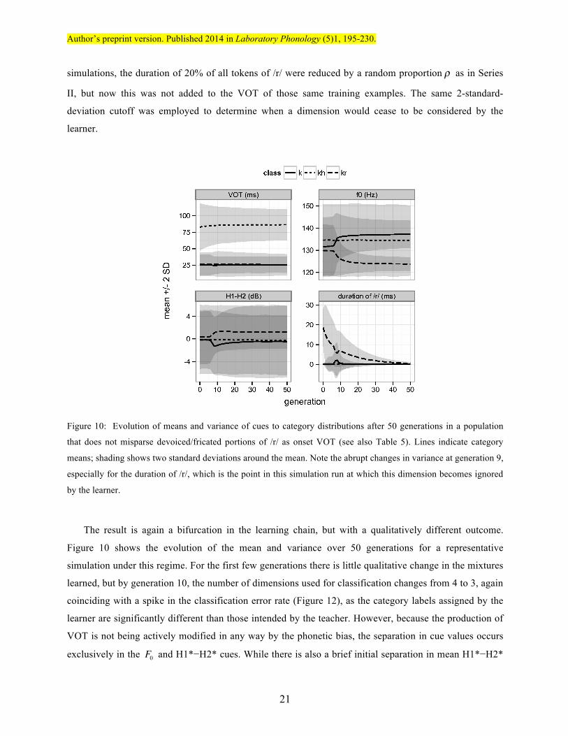
simulations, the duration of 20% of all tokens of /r/ were reduced by a random proportion ρ as in Series
II, but now this was not added to the VOT of those same training examples. The same 2-standard-
deviation cutoff was employed to determine when a dimension would cease to be considered by the
learner.
Figure 10: Evolution of means and variance of cues to category distributions after 50 generations in a population
that does not misparse devoiced/fricated portions of /r/ as onset VOT (see also Table 5). Lines indicate category
means; shading shows two standard deviations around the mean. Note the abrupt changes in variance at generation 9,
especially for the duration of /r/, which is the point in this simulation run at which this dimension becomes ignored
by the learner.
The result is again a bifurcation in the learning chain, but with a qualitatively different outcome.
Figure 10 shows the evolution of the mean and variance over 50 generations for a representative
simulation under this regime. For the first few generations there is little qualitative change in the mixtures
learned, but by generation 10, the number of dimensions used for classification changes from 4 to 3, again
coinciding with a spike in the classification error rate (Figure 12), as the category labels assigned by the
learner are significantly different than those intended by the teacher. However, because the production of
VOT is not being actively modified in any way by the phonetic bias, the separation in cue values occurs
exclusively in the F0 and H1*−H2* cues. While there is also a brief initial separation in mean H1*−H2*

Author’s preprint version. Published 2014 in Laboratory Phonology (5)1, 195-230.
22
between /kʰuː/ and /kruː/, this becomes lost by around 40 generations, with F0 and H1*−H2* serving only
to distinguish /kruː/-class from /kuː/-class forms.
Table 5: Evolution of means and standard deviations of F0 ,VOT, H1*-H2* ,and duration of /r/ at t = 1, 5, 10, 20,
and 50 generations in a population that misparses ρ proportion of 20% of /r/s as increased VOT. ‘emp’ = empirical
results from Kirby (under review).
t VOT (ms) F0 (Hz) H1*-H2* (dB) duration of /r/ (ms)
/CV/
1 25 (8.1) 131 (6.9) -0.19 (2.6) - 5 25 (8.0) 132 (6.9) -0.18 (2.6) - 10 25 (6.5) 136 (5.1) -1.15 (2.7) - 20 26 (6.3) 137 (4.5) -0.60 (3.1) - 50 26 (6.3) 137 (3.2) -0.47 (3.2) -
emp 28 (11.3) 106 (1.3) -8.3 (7.5) -
/CʰV/
1 83 (18.3) 135 (8.2) -0.10 (3.1) - 5 85 (15.8) 135 (8.3) -0.08 (3.1) - 10 85 (14.5) 134 (8.2) -0.09 (3.1) - 20 86 (13.3) 134 (8.3) -0.21 (3.2) - 50 86 (11.9) 134 (8.1) -0.25 (3.2) -
emp 66 (9.9) 110 (3.5) -6.50 (6.2) -
/CrV/
1 26 (9.1) 130 (6.0) 0.32 (2.4) 15.3 (4.9) 5 26 (9.0) 130 (5.9) 0.35 (2.4) 9.9 (7.5) 10 27 (9.8) 126 (3.7) 1.31 (1.9) 6.5 (5.5) 20 26 (9.3) 126 (2.2) 1.27 (1.6) 3.7 (3.1) 50 26 (8.3) 124 (1.6) 1.21 (1.5) 0.2 (0.3)
emp 25 (10.3) 96 (5.2) -5.8 (7.2) -
It is interesting to consider the predictions of this model in light of the empirical facts of a different
Khmer dialect, that spoken in Kiên Giang (KG) province in neighboring Vietnam. Thạch Ngọc Minh
(1999) reports a development of a falling F0 contour following loss of /r/, but does not transcribe any
subsequent increase in aspiration, giving examples such as Standard Khmer /krɑː/ ∼ KG Khmer [krɑː]
‘poor’ (otherwise homophonous with /kɑː/ ‘neck’), Standard Khmer /craːn/ ∼ KG Khmer [càːn] ‘to push’
(otherwise homophonous with /caːn/ ‘bowl’), etc. Preliminary analysis of data from an acoustic/perceptual
study of this variety confirm that while KG lexical items pronounced with trills in Standard Khmer have a
lower F0 compared to their Standard Khmer counterparts, there is no accompanying increase in VOT
(Kirby, 2013b). This can be seen from Table 5 and the density plots in the bottom row of Figure 11, which

Author’s preprint version. Published 2014 in Laboratory Phonology (5)1, 195-230.
23
show empirical cue distributions for the productions of forms with onsets /k/ /kʰ/ /kr/ from a
representative speaker in the study. At least in this speaker, there does not appear to be any evidence of
breathy voice quality, but average F0 is clearly much lower in /CrV/ forms. Although the data are still
being analyzed, it is encouraging that the results of changing a single parameter setting in the model
framework appear to correspond to empirically attested stable states. Nonetheless, it remains to be
demonstrated that the productions of this speaker are representative of the population in question.
Figure 11: Top row: density estimates for cues of a population that does not misattribute devoiced /r/ to onset VOT.
Classification error rate at generation 50: 0.002. Bottom row: empirical cue distributions for productions of /kuː/,
/kʰuː/, and /kruː/ forms forms based on recordings of a representative male speaker of KG Khmer (after Kirby,
2013b). Classification error rate: 0.05.
Figure 12: Evolution of error rates for each of the three simulation series. Series I: stable evolution, no bias. Series
II: bias misparsed as a property of the onset. Series III: bias plus input filtering (no misparsing).

Author’s preprint version. Published 2014 in Laboratory Phonology (5)1, 195-230.
24
4 Discussion
The simulations reported above show how learners modeled as ideal observers in a social learning
environment, given Standard Khmer cue distributions as input, will converge on a set of cue distributions
that qualitatively resemble the empirical distributions observed in actual PP Khmer data. In addition,
whether or not learners were assumed to misattribute the acoustic result of a phonetic bias factor was seen
to have a dramatic impact on the evolution of the phonetic category structures.
Given a reasonably accurate characterization of a synchronic start state and a hypothesized phonetic
bias factor, this type of model enables predictions about directionality in phonologization from a point in
time when the ‘seeds’ of the change still lie below the threshold of perceptibility. In the Khmer case
examined here, it may be that the pre-existing bias towards slightly lowered F0 and slightly higher
H1*−H2* in /CrV/ forms became ‘amplified’ or enhanced when the contrast became endangered. Of
course, things need not have turned out this way, and the precise outcome illustrated here is in some ways
dependent on other assumptions about the makeup of the population, the rate of fortition, and the
threshold at which attention to cue will shift. Nonetheless, the finding that under relatively realistic
assumptions the model’s prediction is broadly in line with the empirical findings suggests that this is a
promising approach worthy of further investigation.
4.1 Independence of phonetic dimensions
In the Introduction, I referred to an account of incipient tonogenesis in PP Khmer grounded in the
tendency for /r/ to devoice or fricativize, conditioning breathy voice quality which would in turn result in
a lower F0 . In the ideal observer model, however, all cue dimensions are treated as independent. While
not wholly unmotivated (Clayards, 2008), such independence assumptions are almost certainly not
warranted in every case: that is, there are some cues which are not independent for physiological reasons,
such as breathy voice quality and lowered F0 (which share the articulatory setting of reduced vocal fold
tension). One way to capture such dependencies would be to relax the independence assumption of the
naive Bayes classifier used here. Completely removing this assumption entails estimating the entire
covariance matrix, which can be problematic in multivariate settings. One potential compromise would be
the use of a BAYESIAN BELIEF NETWORK (Pearl, 1988), a probabilistic model where conditional
dependencies are represented by edges in a directed acyclic graph. Due in part to the existence of efficient
learning and inference algorithms for Bayes nets, they have become increasingly popular in automatic
speech recognition applications (Zweig, 1998; Livescu et al., 2003; King et al., 2007), where they provide
an attractive and tractable way to capture all and only the relevant dependencies between cue dimensions.

Author’s preprint version. Published 2014 in Laboratory Phonology (5)1, 195-230.
25
4.2 Compensation for coarticulation and population diversity
The implementation of the phonetic precursor discussed here is closely related to the proposal of Beddor
(2009), who shows how a gesture initially associated with one segment can come to be interpreted
distinctively with a different segment. Beddor’s study focuses on the emergence of contrastive
nasalization, whereby the acoustic effects of velum lowering initially associated with a nasal come to be
associated with a following vowel, but it is conceptually very similar to the temporal exchange between
duration of /r/ and onset VOT hypothesized here. It would be interesting to see if Khmer listeners are
sensitive to experimental manipulations of this covariation in the same way that participants in Beddor’s
study were sensitive to covariation in the duration of nasals and the degree of anticipatory vowel
nasalization.
In the third set of simulations discussed above, however, the assumption was made that listeners were
disregarding coarticulatory effects when they resulted from the application of a phonetic production bias.
This too is a commonly held assumption: Garrett and Johnson (2013) for example state that “[i]t seems
reasonable to assume that variants produced by phonetic bias factors are usually ‘corrected’, either by
perceptual processes like compensation or by rejection of speech errors” (73). The degree to which this
type of correction might be applied presumably needs to be related to the strength of the bias factor in
some fashion, given that perceptual learning is known to generalize across speakers (Kraljic and Samuel,
2006) and that variation in cognitive processing styles can give rise to differential rates of compensation
for coarticulation in a neurotypical population (Yu, 2010). Moreover, the findings of Labov, Sankoff,
Harrington, and others indicate that the phonetic realization of phonological categories can and does
change over the lifespan, and that social factors (such as the desire to distinguish oneself or one’s group
identity via linguistic means) are sure to play an important role. Future extensions of this framework
should therefore explore the space of outcomes under a more varied and realistic set of assumptions about
the incidence and causes of compensation for coarticulation in the population.
4.3 Actuation and stability
The role of population diversity is also important for the issue of actuation in sound change, an issue not
directly addressed in the present simulations. Although stability is predicted when no bias factor is
present, the introduction of a bias factor begins an inevitable progression towards a qualitative change in
the distributions learned. As noted repeatedly at least since Weinrich et al. (1968), this is problematic
given that the general state of sound systems appears to be one of stability rather than constant change,
even (or especially) in the presence of bias. Baker (2008a) goes so far to assert that ‘phonologization-of-
Author’s preprint version. Published 2014 in Laboratory Phonology (5)1, 195-230.
26
coarticulation’ models are completely empirically inadequate (32) because they predict sound change to
occur “whenever possible, in every language, and at every time” (31).
However, there are reasons to think it may be premature to reject this mechanism of change entirely.
Besides studies that do appear to show incremental change across the lifespan, other mechanisms may
impact the likelihood of phonologization of phonetic variability. In addition to mechanisms that warp the
perceptual space prior to categorization (Iverson and Kuhl, 1995), learners may be biased towards existing
or smaller numbers of categories (Pothos and Close, 2008; Pothos and Bailey, 2009), which may inhibit
the phonologization of intermediate variants; aspects of population diversity and dynamics reviewed
above surely play a central role as well (Baker et al., 2011; Kirby and Sonderegger, 2013).
4.4 Relation to other models
The model sketched above employs a relatively simple characterization of the relationship between
teachers and learners, whereby each learner receives independent and identically distributed random
samples from its teachers and uses these to compute maximum likelihood estimates by making strong
assumptions about the form of the distributions. Different approaches are of course possible. If the
distributional assumptions were relaxed, one might instead simulate draws from the posterior distribution
using some type of Monte Carlo sampling technique (rejection sampling, Gibbs sampling, etc.). The
implementation of such techniques for multivariate mixtures with possibly differing covariance matrices
is challenging, however, and in this instance it is not immediately clear how the added complexity of such
a model would shed greater light on the issues of interest here. Despite differences in the basic
assumptions about the source of data, results from the iterated learning literature are likely to be relevant
here (Griffiths and Kalish, 2007; S. Kirby et al. 2007; Burkett and Griffiths, 2010).
The learning method sketched here is also related to several other previously proposed models of
phonological change. While space precludes a detailed comparison, several observations are worth noting.
A number of authors have considered sound change from within the general framework of exemplar
models (Johnson, 1997; Kirchner, 1998; Pierrehumbert, 2001; Wedel, 2006), which have close analogs to
statistical methods of probability density estimation of the kind employed in the present work (Estes,
1986; Ashby and Maddox, 1993; Rosseel, 2002). In particular, many models of classification can be
shown to be equivalent to an inductive process by which the observer estimates the likelihood that a novel
stimulus x belongs to one of K categories (Ashby and Alfonso-Reese, 1995). The difference between
‘true’ exemplar models and density estimation models of the type described here is less important than the
distinction between whether the classifiers are assumed to be parametric or nonparametric - that is,

Author’s preprint version. Published 2014 in Laboratory Phonology (5)1, 195-230.
27
whether or not the distribution of the observed data is assumed to have been generated by a distribution
easily described by just a few parameters, such as the mean and variance.
While some research (most of it involving the classification of visual stimuli) argues in favor of
nonparametric models of human categorization behavior, there are other empirical domains (such as
speech) where the relevant distributions do appear to follow well-known parameterized distributions. In
addition, nonparametric approaches predict that, given enough training experience, human classification
behavior should eventually come to resemble that of the underlying category structure, no matter how
arbitrary. This is probably not the case, since human classification behavior clearly is limited, or at least
preferentially constrained. For instance, McKinley and Nosofsky (1995) conducted an experiment in
which they had participants categorize visual stimuli for which the optimal likelihood classification
boundary was both highly nonquadratic and not possible to characterize as a simple continuous curve.
Even with continuous corrective feedback, only one-third of the participants in this experiment were able
to exceed the classification accuracy of a quadratic (parametric) classifier, and another third were unable
to even perform as well as a simple linear classifier. In their computational work on English and Japanese
vowel category learning, Vallabha et al. (2007) compared parametric and nonparametric versions of an
online mixture estimation algorithm. They found the parametric algorithm significantly outperformed the
nonparametric one, which they attributed to the nonparametric estimator’s inherent lack of constraints on
the underlying category structure.
These types of results suggest that nonparametric density estimators may be too powerful a model of
human classification behavior. This is especially true in the case of speech sounds, where most evidence
suggests that variability in the speech signal is accessible to and used by speakers and listeners in forming
category judgments (Pisoni and Tash, 1974; Miller and Volaitis, 1989; McMurray et al., 2002; Clayards
et al., 2008). As the notion of category is ill-defined in exemplar-based approaches – the categories are, in
a very real sense, defined by the experienced tokens themselves – it is not clear how variability in the
signal should become information for the listener in such a model.
Another approach to phonological category learning and change from a non-exemplar perspective is
Boersma and Hamann (2008), who consider the evolution of phonological categories in a constraint-based
framework. In order to avoid computing auditory distances, their model discretizes the continuous
auditory cue space into an arbitrary number of cue constraints, which are then ranked using a standard
constraint-demotion algorithm. However, this approach requires that the cue constraints be ranked relative
to a universal ‘ease of articulation’ curve, a concept that has proven particularly difficult to rigorously
quantify (Pouplier, 2003). In addition, since the authors’ primary focus was on accounting for auditory
dispersion, they do not explore the question of how multiple phonetic cues would interact in their model.
Author’s preprint version. Published 2014 in Laboratory Phonology (5)1, 195-230.
28
In spite of the difference between these models, superficial and otherwise, it is important to point out
that their basic predictions are all consistent with the idea that changes to phonological systems may be
emergent, rather than explicitly goal-oriented. The main contribution of the present formulation is provide
an explicit characterization of categorization in the multivariate case, and to show how changes in
attention to one phonetic cue can have abrupt and substantive impact on the realization of others.
4.4.1 Lexical competition effects
In the simulations reported above, the number of category labels K is assumed to be fixed and
unchanging. Looking at the degree to which some of the cue distributions overlap, however, one might
wonder why transphonologization, and not category merger, should be the outcome in this case. One
reason might involve some type of systemic pressure for lexical distinctiveness. Blevins and Wedel
(2009) propose a model in which VARIANT TRADING promotes separation between competing adjacent
categories. The degree to which variant trading plays a role is mediated by the disambiguating influence
of both word-external factors, such as discourse context, as well as word-internal factors, such as
distributional overlap in phonetic cues. In fact, in this model, any factor that reduces categorization error
promotes greater contrast between categories over time.
For Blevins and Wedel, variant trading provides a principled, non-teleological mechanism for
explaining the avoidance of sound change in just those cases where it would create ‘pernicious’
homophony, such as in inflectional paradigms. As Khmer is not an inflecting language, it is not obvious
that ambiguity in word-internal dimensions should outstrip the disambiguating effects of the relevant
word-external factors: ‘father’ and ‘kind of fish’ seem unlikely to be confused, even if pronounced
identically. Furthermore, while variant trading should promote the distinctiveness of existing covert
contrasts, it is not clear how it would drive the emergence of an intermediate VOT category. Nevertheless,
this approach suggests a promising avenue for additional modeling work.
4.4.2 A role for probabilistic enhancement?
In Kirby (2010, 2013a) I outlined a similar computational model of sound change, arguing that bias-
induced loss of contrast precision alone is not enough to induce transphonologization; at least in some
cases, (probabilistic) enhancement of subphonemic cues also appears to be necessary. I proposed that
degree of enhancement is a probabilistic function of contrast precision, while the probability with which a
given cue is enhanced is related directly to its informativeness or reliability – the degree to which it
contributes to accurate identification of a speech sound. This approach was successfully used to model the
emergence of contrastive F0 in Seoul Korean (Kirby, 2010, 2013a), and the incipient tonogenesis in PP

Author’s preprint version. Published 2014 in Laboratory Phonology (5)1, 195-230.
29
Khmer looks on the surface to be a similar scenario: a phonetic bias factor (here, fortition of /r/) affects a
loss of precision (here, between /CrV/ and /CV/ or /CʰV/ forms). This loss of precision would then be
predicted to drive probabilistic enhancement of other available cues, such as the degree of F0 drop or
breathy phonation. Thus, it is perhaps surprising that a qualitative approximation of the empirical results
obtains in the Khmer case without this mechanism. Indeed, when the procedure outlined above was
augmented with a probabilistic enhancement mechanism, the results were more or less identical.
Why should this be the case? There are several differences between the two procedures that may play
a role, but the most important is probably that the two approaches model the acquisition and classification
of categories in fundamentally different ways. First, Kirby (2010, 2013a) simulates an ‘online’ learning
scenario in which two adult speakers exchange speech tokens one at a time. In the face of bias, the
probabilistic enhancement strategy works to rein in this bias, promoting stability of the status quo. In the
present work, learners operate in ‘batch mode’, performing classification and density estimation
simultaneously with access to the sum total of experienced tokens. The second major difference is the
introduction here of the potential for a shift in the number of cue dimensions used to perform
categorization. It is interesting to note that changing the number of dimensions has much the same effect
as probabilistic enhancement, but without having to track incremental changes in cue distributions within
a single learner. The present model therefore predicts (near-)categorical discontinuities between
generations, as has often been empirically observed. While this does not mean that listener-oriented
enhancement plays no role whatsoever in sound change (cf. Lindblom, 1990; Lindblom et al., 1995;
Diehl, 2008), it does suggest that its impact on the process of cross-generational change may be
constrained or obscured relative to the role played by categorization behavior and attention to cue.
5 Conclusions
This paper has described a computational modeling framework that can shed light on the dynamics of
transphonologization. We have examined the case of incipient tonogenesis in Phnom Penh Khmer and
seen how, by making minimal assumptions about learners, transphonologization results from the
application of phonetic production bias in a population of ideal observer agents. In particular, abrupt
changes in the distribution of acoustic cues to category membership coincided with changes in attention to
cue. These results are consistent with the sudden and discontinuous nature of many sound changes, and
suggest that what appear to be enhancement effects may also emerge from different assumptions about the
number of cue dimensions accessible to or deemed relevant by the learner.

Author’s preprint version. Published 2014 in Laboratory Phonology (5)1, 195-230.
30
References
Abramson, Arthur S., Patrick W. Nye, and Theraphan Luangthongkum. 2007. Voice register in Khmu’:
Experiments in production and perception. Phonetica 64:80–104.
Ashby, F. Gregory, and Leola A. Alfonso-Reese. 1995. Categorization as probability density estimation.
Journal of Mathematical Psychology 39:216–233.
Ashby, F. Gregory, and W. Todd Maddox. 1993. Relations between prototype, exemplar, and decision
bound models of categorization. Journal of Mathematical Psychology 37:372–400.
Baker, Adam. 2008a. Addressing the actuation problem with quantitative models of sound change. In
Proceedings of the 31st Annual Penn Linguistics Colloquium, volume 14(1), 29–41.
Baker, Adam. 2008b. Computational approaches to the study of language change. Language and
Linguistics Compass 2:289–307.
Baker, Adam, Diana Archangeli, and Jeff Mielke. 2011. Variability in American English s-retraction
suggests a solution to the actuation problem. Language Variation and Change 23:347–374.
Beddor, Patrice Speeter. 2009. A coarticulatory path to sound change. Language 85:785–821.
Bishop, Christopher M. 2006. Pattern recognition and machine learning. New York: Springer Verlag.
Blevins, Juliette, and Andrew Wedel. 2009. Inhibited sound change: An evolutionary approach to lexical
competition. Diachronica 26:143–183.
de Boer, Bart, and Patricia Kuhl. 2003. Investigating the role of infant-directed speech with a computer
model. Acoustics Research Letters On-line 4:129–134.
Boersma, Paul, and Silke Hamann. 2008. The evolution of auditory dispersion in bidirectional constraint
grammars. Phonology 25:217–270.
Boyd, Robert, and Peter J. Richerson. 1985. Culture and the evolutionary process. Chicago: University of
Chicago Press.
Burkett, David, and Thomas L. Griffiths. 2010. Iterated learning of multiple languages from multiple
teachers. In Andrew D. M. Smith, Marieke Schouwstra, Bart de Boer, and Kenny Smith (eds.), The
evolution of language: Proceedings of the 8th international conference (EVOLANG 8), 58–65.
Singapore: World Scientific.
Clayards, Meghan. 2008. The ideal listener: Making optimal use of acoustic-phonetic cues for word
recognition. Ph.D. dissertation, University of Rochester.
Clayards, Meghan, Michael K. Tanenhaus, Richard Aslin, and Robert A. Jacobs. 2008. Perception of
speech reflects optimal use of probabilistic speech cues. Cognition 108:804–809.
Dempster, Arthur P., Nan M. Laird, and Donald B. Rubin. 1977. Maximum likelihood from incomplete
data via the EM algorithm. Journal of the Royal Statistical Society, Series B (Methodological)
39:1–38.

Author’s preprint version. Published 2014 in Laboratory Phonology (5)1, 195-230.
31
Devroye, Luc. 1986. Non-uniform random variate generation. New York: Springer Verlag. Online edition
retrieved January 23, 2007 from http://cg.scs.carleton.ca/�luc/rnbookindex.html.
Diehl, Randy L. 2008. Acoustic and auditory phonetics: The adaptive design of speech sound systems.
Philosophical Transactions of the Royal Society 363:965–978.
Diffloth, Gérard. 1989. Proto-Austroasiatic creaky voice. Mon-Khmer Studies 15:139–154.
Dillon, Brian W., Ewan Dunbar, and William Idsardi. 2013. A single stage approach to learning
phonological categories: Insights from Inuktitut. Cognitive Science 37(2):344–377.
Duda, Richard O., Peter E. Hart, and David G. Stork. 2000. Pattern classification. New York: John Wiley
and Sons.
Estes, William K. 1986. Array models for category learning. Cognitive Psychology 18:500–549.
Feldman, Naomi H., Thomas L. Griffiths, and James L. Morgan. 2009. Learning phonetic categories by
learning a lexicon. In Niels Taatgen and Hedderik van Rijn (eds.), Proceedings of the 31st Annual
Conference of the Cognitive Science Society, 2208–2213. Austin, TX: Cognitive Science Society.
Ferlus, Michel. 1992. Essai de phonétique historique du khmer. Mon-Khmer Studies 21:57–89.
Filippi, Jean-Michel, and Hiep Chan Vicheth. 2009. Dictionnaire de la pronunciation du Khmer: Khmer
standard et dialecte phnompenhois. Phnom Penh: Editions Funan.
Foulkes, Paul, and Marianne Vihman. In press. First language acquisition and phonological change. In
Patrick Honeybone and Joseph C. Salmons (eds.), Oxford handbook of historical phonology.
Oxford: Oxford University Press.
Francis, Alexander L. and Howard Nusbaum. 2002. Selective attention and the acquisition of new
phonetic categories. Journal of Experimental Psychology: Human Perception and Performance
28(2):349–366.
Garrett, Andrew, and Keith Johnson. 2013. Phonetic bias in sound change. In Alan C. L. Yu (ed.), Origins
of sound patterns: Approaches to phonologization, 51–97. Oxford: Oxford University Press.
Geisler, Wilson S. 1989. Sequential ideal-observer analysis of visual discrimination. Psychological
Review 96:267–314.
Geisler, Wilson S., and Randy L. Diehl. 2002. Bayesian natural selection and the evolution of perceptual
systems. Philosophical Transactions of the Royal Society of London B 357:419–448.
Genz, Alan, and Frank Bretz. 2009. Computation of multivariate normal and t probabilities. Lecture
Notes in Statistics. Heidelberg: Springer-Verlag.
Goldwater, Sharon, Thomas L. Griffiths, and Mark Johnson. 2009. A Bayesian framework for word
segementation: Exploring the effects of context. Cognition 112:21–54.
Green, David M., and John A. Swets. 1966. Signal detection theory and psychophysics. New York: Wiley.
Author’s preprint version. Published 2014 in Laboratory Phonology (5)1, 195-230.
32
Griffiths, Thomas L., and Michael L. Kalish. 2007. Language evolution by iterated learning with Bayesian
agents. Cognitive Science 31:441–480.
Harrington, Jonathan. 2006. An acoustic analysis of ‘happy-tensing’ in the Queen’s Christmas broadcasts.
Journal of Phonetics 34:439–457.
Harrington, Jonathan, Sallyanne Palethorpe, and Cathiner I. Watson. 2000. Monophthongal vowel
changes in Received Pronunciation: An acoustic analysis of the Queen’s Christmas broadcasts.
Journal of the International Phonetic Association 30:63–78.
Hastie, Trevor, Robert Tibshirani, and Jerome Friedman. 2008. The elements of statistical learning: Data
mining, inference, and prediction (2nd edition). New York: Springer Verlag.
Henderson, Eugénie J. A. 1952. The main features of Cambodian pronunciation. Bulletin of the School of
Oriental and African Studies, University of London 14:149–174.
Hewlett, Nigel. 1988. Acoustic properties of /k/ and /t/ in normal and phonologically disorderd speech.
Clinical Linguistics and Phonetics 2:29–45.
Hombert, Jean-Marie, John J. Ohala, and William G. Ewan. 1979. Phonetic explanations for the
development of tones. Language 55:37–58.
Hudson Cam, Carla L., and Elissa L. Newport. 2005. Regularizing unpredictable variation: The roles of
adult and child learners in language formation and change. Language Learning and Development
1:151–195.
Huffman, Franklin E. 1967. An outline of Cambodian grammar. Ph.D. dissertation, Department of
Linguistics, Cornell University.
Hyman, Larry M. 1976. Phonologization. In Alphonse Juilland (ed.), Linguistic studies presented to
Joseph H. Greenberg, 407–418. Saratoga: Anma Libri.
Iseli, Markus, and Abeer Alwan. 2004. An improved correction formula for the estimation of harmonic
magnitudes and its application to open quotient estimation. In Proc. ICASSP, 669–672. Montreal.
Iverson, Paul, and Patricia K. Kuhl. 1995. Mapping the perceptual magnet effect for speech using signal
detection theory and multidimensional scaling. Journal of the Acoustical Society of America
97:553–562.
Johnsen, Sverre Stausland. 2011. The phonetics and phonologization of Verner’s law. In Thomas Krisch
and Thomas Lindner (eds.), Indogermanistik und Linguistik im Dialog, 232–241. Wiesbaden:
Reichert Verlag.
Johnson, Keith. 1997. Speech perception without speaker normalization. In John W. Mullenix (ed.),
Talker variability in speech processing, 145–166. San Diego: Academic Press.
Kavitskaya, Darya. 2002. Compensatory lengthening: Phonetics, phonology, diachrony. New York:
Routledge.

Author’s preprint version. Published 2014 in Laboratory Phonology (5)1, 195-230.
33
King, Simon, Joe Frankel, Karen Livescu, Erik McDermott, Korin Richmond, and Mirjam Wester. 2007.
Speech production knowledge in automatic speech recognition. Journal of the Acoustical Society of
America 121:723–742.
Kirby, James. 2010. Cue selection and category restructuring in sound change. Ph.D. dissertation,
Department of Linguistics, University of Chicago.
Kirby, James. 2011. Modeling the acquisition of covert contrast. In Wai-Sum Lee and Eric Zee (eds.),
Proceedings of the Seventeenth International Conference of the Phonetic Sciences, 1090–1093.
Kirby, James. 2013a. The role of probabilistic enhancement in phonologization. In Alan C. L. Yu (ed.),
Origins of sound patterns: Approaches to phonologization, 228–246. Oxford: Oxford University
Press.
Kirby, James. 2013b. Tonogenesis in Khmer: A cross-dialect comparison. Paper presented at the 23rd
Annual Meeting of the Southeast Asian Lingustic Society, Bangkok. Handout online at
http://jseals.org/seals23/kirby2013tonogenesis.pdf.
Kirby, James. Under review. Incipient tonogenesis in Phnom Penh Khmer: Acoustic and perceptual
studies. Journal of Phonetics.
Kirby, James, and Morgan Sonderegger. 2013. A model of population dynamics applied to phonetic
change. In Markus Knauff, Michael Pauen, Natalie Sebanz and Ipke Wachsmuth (eds.),
Proceedings of the 35th Annual Conference of the Cognitive Science Society, 776–781. Austin, TX:
Cognitive Science Society.
Kirby, Simon, Mike Dowman, and Thomas L. Griffiths. 2007. Innateness and culture in the evolution of
language. Proceedings of the National Academy of Sciences of the USA 104:5241–5245.
Kirchner, Robert. 1998. Preliminary thoughts on “phonologization” within an exemplar-based speech
processing system. In Matthew Gordon (ed.), UCLA Working Papers in Linguistics (volume 1 of
Papers in phonology 2), 205–231.
Kraljic, T., and A. G. Samuel. 2006. Generalization in perceptual learning for speech. Psychonomic
Bulletin & Review 13:262–268.
Kroch, Anthony. 1989. Reflexes of grammar in patterns of language change. Language Variation and
Change 1:199–244.
Labov, William. 1994. Principles of linguistic change vol. 1: Internal factors. Oxford: Oxford University
Press.
Labov, William. 2001. Principles of linguistic change vol. 2: Social factors. Oxford: Oxford University
Press.
Labov, William, Mark Karen, and Corey Miller. 1991. Near-mergers and the suspension of phonemic
contrast. Language Variation and Change 3:33–74.

Author’s preprint version. Published 2014 in Laboratory Phonology (5)1, 195-230.
34
Lin, Ying. 2005. Learning features and segments from waveforms: A statistical model of early
phonological acquisition. Ph.D. dissertation, UCLA.
Lindblom, Björn. 1990. Explaining phonetic variation: A sketch of the H & H theory. In William J.
Hardcastle and Alain Marchal (eds.), Speech production and speech modeling, 403–439. Dordrecht:
Kluwer.
Lindblom, Björn, Susan Guion, Susan Hura, Seung-Jae Moon, and Raquel Willerman. 1995. Is sound
change adaptive? Rivista di Linguistica 7:5–37.
Lisker, Leigh. 1978. Rapid vs. rabid: A catalogue of acoustic features that may cue the distinction. In
Haskins Laboratories Status Report on Speech Research SR-54, 128–32.
Lisker, Leigh, and Arthur Abramson. 1970. The voicing dimension: Some experiments in comparative
phonetics. In Proceedings of the Sixth International Congress of Phonetic Sciences, 563–567.
Prague: Academia Publishing House of the Czechoslovak Academy of Sciences.
Livescu, Karen, James Glass, and Jeff Blimes. 2003. Hidden feature modeling for speech recognition
using dynamic Bayesian networks. In Proc. EUROSPEECH, volume 4, 2529–2532.
Matisoff, James A. 1973. Tonogenesis in Southeast Asia. In Larry Hyman (ed.), Consonant types and
tone, 71–95. Los Angeles: University of Southern California.
Maye, Jessica, Janet F. Werker, and LouAnn Gerken. 2002. Infant sensitivity to distributional information
can affect phonetic discrimination. Cognition 82:B101–B111.
McKinley, Stephen C., and Robert M. Nosofsky. 1995. Investigations of exemplar and decision bound
models in large, ill-defined category structures. Journal of Experimental Psychology: Human
Perception and Performance 21:128–148.
McLachlan, Geoffry J., and David Peel. 2000. Finite mixture models. New York: Wiley.
McMurray, Bob, Richard N. Aslin, and Joseph C. Toscano. 2009. Statistical learning of phonetic
categories: Insights from a computational approach. Developmental Science 12:369–378.
McMurray, Bob, Michael K. Tanenhaus, and Richard N. Aslin. 2002. Gradient effects of within-category
phonetic varition on lexical access. Cognition 86:B33–B42.
Miller, Joanne L., and Lydia E. Volaitis. 1989. Effect of speaking rate on the perceptual structure of a
phonetic category. Perception & Psychophysics 46:505–512.
Moreton, Elliott, and Erik R. Thomas. 2007. Origins of Canadian Raising in voiceless-coda effects: a case
study in phonologization. In Jennifer S. Cole and José Ignacio Hualde (eds.), Laboratory phonology
9, 37–64. Berlin: Mouton de Gruyter.
Nearey, Terrance, and John T. Hogan. 1986. Phonological contrast in experimental phonetics: Relating
distributions of production data to perceptual categorization curves. In John J. Ohala and Jeri J.
Jaeger (eds.), Experimental phonology, 141–162. Orlando: Academic Press.

Author’s preprint version. Published 2014 in Laboratory Phonology (5)1, 195-230.
35
Niyogi, Partha. 2006. The computational nature of language learning and evolution. Cambridge: The
MIT Press.
Niyogi, Partha, and Robert C. Berwick. 1995. The logical problem of language change. Technical Report
AI Memo 1516 / CBCL Paper 115, Massachusetts Institute of Technology. MIT AI Laboratory and
Center for Biological and Computational Learning, Department of Brain and Cognitive Sciences.
Niyogi, Partha, and Robert C. Berwick. 2009. The proper treatment of language acquisition and change in
a population setting. Proceedings of the National Academy of Sciences 106:10124–10129.
Norris, Dennis. 2006. The Bayesian reader: Explaining word recognition as an optimal Bayesian decision
process. Psychological Review 113:327–257.
Noss, Richard B. 1966. The treatment of */r/ in two modern Khmer dialects. In Norman H. Zide (ed.),
Studies in comparative Austroasiatic linguistics, 89–95. London: Mouton & Co.
Payne, Arvilla. 1976. The acquisition of the phonological system of a second dialect. Ph.D. dissertation,
University of Pennsylvania.
Payne, Arvilla. 1980. Factors controlling the acquisition of the Philadelphia dialect by out-of-state
children. In William Labov (ed.), Locating language in time and space, 143–178. New York:
Academic Press.
Pearl, Judea. 1988. Probabilistic reasoning in intelligent systems. San Francisco, CA: Morgan Kaufmann.
Pierrehumbert, Janet. 2001. Exemplar dynamics: Word frequency, lenition, and contrast. In Joan Bybee
and Paul Hopper (ed.s.), Frequency effects and the emergence of linguistic structure, 137–157.
Amsterdam: John Benjamins.
Pisoni, David B., and Jeffrey Tash. 1974. Reaction times to comparisons within and across phonetic
categories. Perception and Psychophysics 15:285–290.
Pothos, Emmanuel M., and Todd M. Bailey. 2009. Predicting category intuitiveness with the rational
model, the simplicity model, and the Generalized Context Model. Journal of Experimental
Psychology: Learning, Memory, and Cognition 35:1062–1080.
Pothos, Emmanuel M., and James Close. 2008. One or two dimensions in spontaneous classification: A
simplicity approach. Cognition 107:581–602.
Pouplier, Marianne. 2003. The dynamics of error. In Maria-Josep Solé, Daniel Recasens, and Joaquín
Romero (eds.), Proceedings of the Fifteenth International Congress of the Phonetic Sciences,
2245–2248. Barcelona: Universitat Autonoma de Barcelona.
Premsrirat, Suwilai. 2001. Tonogenesis in Khmu dialects of SEA. Mon-Khmer Studies 31:47–56.
Pulleyblank, Edwin G. 1978. The nature of Middle Chinese tones and their development to Early
Mandarin. Journal of Chinese Linguistics 6:173–203.
Author’s preprint version. Published 2014 in Laboratory Phonology (5)1, 195-230.
36
Rasmussen, Carl E. 2000. The infinite Gaussian mixture model. In Sara A. Solla, Todd K. Leen and
Klaus-Robert Müller (eds.), Advances in Neural Information Processing Systems 12, 554–560.
Cambridge, MA: MIT Press.
Rosseel, Yves. 2002. Mixture models of categorization. Journal of Mathematical Psychology 46:178–210.
Sankoff, Gillian, and Hélène Blondeau. 2007. Language change across the lifespan: /r/ in Montreal
French. Language 3:560–588.
Sankoff, Gillian, and Suzanne Laberge. 1973. On the acquisition of native speakers by a language. Kivung
1973:32–47.
Schwarz, Gideon E. 1978. Estimating the dimension of a model. Annals of Statistics 6:461–464.
Shannon, Claude E., and Warren Weaver. 1949. A mathematical theory of communication. Urbana:
University of Illinois Press.
Solé, Maria-Josep. 2003. Is variation encoded in phonology? In Daniel Recasens, Maria-Josep Solé, and
Joaquín Romero (eds.), Proceedings of the Fifteenth International Congress of the Phonetic
Sciences, 289–292. Barcelona: Universitat Autonoma de Barcelona.
Svantesson, Jan-Olaf, and David House. 2006. Tone production, tone perception and Kammu tonogenesis.
Phonology 23:309–333.
Teh, Yee Whye, Michael I. Jordan, Matthew J. Beal, and David M. Blei. 2006. Hierarchical Dirichlet
processes. Journal of the American Statistical Association 101:1566–1581.
Thạch Ngọc Minh. 1999. Monosyllabization in Kiengiang Khmer. Mon-Khmer Studies 29:81–95.
Thurgood, Graham. 2002. Vietnamese and tonogenesis: revising the model and the analysis. Diachronica
19:333–363.
Toscano, Joseph C., and Bob McMurray. 2010. Cue integration with categories: Weighting acoustic cues
in speech using unsupervised learning and distributional statistics. Cognitive Science 34:434–464.
Vallabha, Gautam K., James L. McClelland, Ferran Pons, Janet F. Werker, and Shigeaki Amano. 2007.
Unsupervised learning of vowel categories from infant-directed speech. Proceedings of the
National Academy of Sciences 104:13273–13278.
Wayland, Ratree, and Susan Guion. 2002. Tonogenesis in Khmer. In Ratree Wayland, John Hartmann,
and Paul Sidwell (eds.), Papers from the 12th Meeting of the Southeast Asian Linguistics Society
(2002), 145–152. Canberra: Pacific Linguistics.
Wayland, Ratree P., and Susan G. Guion. 2005. Sound changes following the loss of /r/ in Khmer: A new
tonogenetic mechanism? Mon-Khmer Studies 35:55–82.
Wedel, Andrew B. 2006. Exemplar models, evolution and language change. The Linguistic Review
23:247–274.
Author’s preprint version. Published 2014 in Laboratory Phonology (5)1, 195-230.
37
Weinrich, Uriel, William Labov, and Marvin Herzog. 1968. Empirical foundations for a theory of
language change. In Winifred P. Lehmann and Yakov Malkiel (eds.), Directions for Historical
Linguistics, 95–195. Austin: University of Texas.
Yu, Alan C. L. 2007. Understanding near mergers: the case of morphological tone in Cantonese.
Phonology 24:187–214.
Yu, Alan C. L. 2010. Perceptual compensation is correlated with individuals’ “autistic” traits:
Implications for models of sound change. PLoS ONE 5:e11950.
Zweig, Geoffrey. 1998. Speech recognition using Dynamic Bayesian Networks. Ph.D. dissertation,
University of California-Berkeley.
Related Documents