Incentive Design for Operations-Marketing Multitasking Tinglong Dai * Rongzhu Ke † Christopher Thomas Ryan ‡ * Carey Business School, Johns Hopkins University, Baltimore, Maryland 21202, [email protected] † Department of Economics, Hong Kong Baptist University, Kowloon, Hong Kong, [email protected] ‡ Sauder School of Business, University of British Columbia, Vancouver, Canada, [email protected] Forthcoming in Management Science A firm hires an agent (e.g., store manager) to undertake both operational and marketing tasks. Marketing tasks boost demand, but for demand to translate into sales, operational effort is required to maintain adequate inventory. The firm designs a compensation plan to induce the agent to put effort into both marketing and operations while facing “demand censoring” (i.e., demand in excess of available inventory is unobservable). We formulate this incentive-design problem in a principal-agent framework with a multitasking agent subject to a censored signal. We develop a bang-bang optimal control approach, with a general optimality structure applicable to a broad class of incentive-design problems. Using this approach, we characterize the optimal compensation plan, with a bonus region resembling a “mast” and “sail,” such that a bonus is paid when either all inventory above a threshold is sold or the sales quantity meets an inventory-dependent target. The optimal “mast and sail” compensation plan implies non-monotonicity, where the agent can be less likely to receive a bonus for achieving a better outcome. This gives rise to an ex post moral hazard issue where the agent may “hide” inventory to earn a bonus. We show this ex post moral hazard issue is a result of demand censoring. If available information includes a waitlist (or other noisy signals) to gauge unsatisfied demand, no ex post moral hazard issues remain. Key words : Marketing-operations interface, multitasking, moral hazard, retail operations, optimal control 1. Introduction The impetus for studying the interface of operations and marketing is the contention that each function cannot be managed without careful consideration of the other (Shapiro 1977; Ho and Tang 2004). This reality is acutely apparent in retail settings, where a single manager oversees both operational and marketing tasks. A search on the online employment platform Monster.com returns over 8,500 retail store manager job listings with “multitasking” as a core skill. Echoing this requirement, DeHoratius and Raman (2007, p. 523) contend the store manager is a “multitasking agent who allocates effort to different activities based on the rewards that accrue from, and the cost of pursuing, each of these activities” [emphasis added]. Stated differently, the multitasking store manager must allocate efforts across both functions, and the effectiveness of this “balance of effort” is critical to the success of the store. We focus on two activities of a store manager: (a) marketing (i.e., bolstering customer demand) and (b) operations (i.e., ensuring inventory can be put in the hands of customers, where it belongs,

Welcome message from author
This document is posted to help you gain knowledge. Please leave a comment to let me know what you think about it! Share it to your friends and learn new things together.
Transcript

Incentive Design for Operations-Marketing Multitasking
Tinglong Dai∗ Rongzhu Ke† Christopher Thomas Ryan‡∗Carey Business School, Johns Hopkins University, Baltimore, Maryland 21202, [email protected]
†Department of Economics, Hong Kong Baptist University, Kowloon, Hong Kong, [email protected]‡Sauder School of Business, University of British Columbia, Vancouver, Canada, [email protected]
Forthcoming in Management Science
A firm hires an agent (e.g., store manager) to undertake both operational and marketing tasks. Marketing
tasks boost demand, but for demand to translate into sales, operational effort is required to maintain adequate
inventory. The firm designs a compensation plan to induce the agent to put effort into both marketing and
operations while facing “demand censoring” (i.e., demand in excess of available inventory is unobservable).
We formulate this incentive-design problem in a principal-agent framework with a multitasking agent subject
to a censored signal. We develop a bang-bang optimal control approach, with a general optimality structure
applicable to a broad class of incentive-design problems. Using this approach, we characterize the optimal
compensation plan, with a bonus region resembling a “mast” and “sail,” such that a bonus is paid when
either all inventory above a threshold is sold or the sales quantity meets an inventory-dependent target. The
optimal “mast and sail” compensation plan implies non-monotonicity, where the agent can be less likely to
receive a bonus for achieving a better outcome. This gives rise to an ex post moral hazard issue where the
agent may “hide” inventory to earn a bonus. We show this ex post moral hazard issue is a result of demand
censoring. If available information includes a waitlist (or other noisy signals) to gauge unsatisfied demand,
no ex post moral hazard issues remain.
Key words : Marketing-operations interface, multitasking, moral hazard, retail operations, optimal control
1. Introduction
The impetus for studying the interface of operations and marketing is the contention that each
function cannot be managed without careful consideration of the other (Shapiro 1977; Ho and
Tang 2004). This reality is acutely apparent in retail settings, where a single manager oversees
both operational and marketing tasks. A search on the online employment platform Monster.com
returns over 8,500 retail store manager job listings with “multitasking” as a core skill. Echoing this
requirement, DeHoratius and Raman (2007, p. 523) contend the store manager is a “multitasking
agent who allocates effort to different activities based on the rewards that accrue from, and the
cost of pursuing, each of these activities” [emphasis added]. Stated differently, the multitasking
store manager must allocate efforts across both functions, and the effectiveness of this “balance of
effort” is critical to the success of the store.
We focus on two activities of a store manager: (a) marketing (i.e., bolstering customer demand)
and (b) operations (i.e., ensuring inventory can be put in the hands of customers, where it belongs,
2 Dai, Ke, and Ryan: Incentive Design for Operations-Marketing Multitasking
instead of being misplaced, damaged, spoiled, or stolen through mismanagement).1 How to design
compensation plans to get the most out of their store managers, in light of these two competing
areas of focus? Such a question is a critical concern for those running decentralized retail chains.
The challenge of compensation design for retail store managers is the subject of business school
case studies (Krishnan and Fisher 2005) and empirical research (DeHoratius and Raman 2007).
The vast majority of compensation models consider single-tasking agents, most prominently in
the salesforce compensation literature (see Section 2 for more detail). When it comes to multi-
tasking agents, the research typically restricts attention to linear contracts in settings where the
outcomes of each task are perfectly observable. The former belies an interest in non-optimal con-
tracts (the optimality of linear contracts is only established in very restrictive settings), whereas the
latter is unsuitable for our setting. To translate demand generated through marketing effort into
sales requires sufficient inventory, an outcome of operational effort. When inventory is insufficient,
unmet demand is lost and unobservable, a phenomenon known as demand censoring. Accordingly,
the outcomes of the associated tasks in our setting lack observability.
Demand censoring is widely seen in practice and well studied in economics (e.g., Conlon and
Mortimer 2013), marketing (e.g., Anupindi et al. 1998), and operations management (e.g., Besbes
and Muharremoglu 2012). Its negative implications for sales performance is well known, largely
because censoring complicates the forecasting of demand and the planning of inventory. However,
the effect of demand censoring on contract design has not been studied in the multitasking setting.
A major takeaway of this paper is that demand censoring—a defining feature of the interplay
between operations and marketing—has inherent and perplexing implications for compensation
design. We come to this conclusion as follows. Practically implementable compensation plans typi-
cally have simple structures. Two prime examples are quota-bonus contracts and linear commission
contracts in salesforce compensation. A pivotal property of these contracts, in addition to being
easily understood by salespeople, is that they are monotone, meaning that an increase in sales
weakly increases compensation. It would strike a salesperson as strange if an additional sale reduced
their compensation. However, establishing the monotonicity of optimal contracts proves difficult.
In single-tasking salesforce compensation, researchers have examined the optimality of quota-
bonus and linear commission contracts. Rogerson (1985), for example, shows monotonicity using the
so-called “first-order approach.” The first-order approach—a standard procedure used in deriving
the optimal compensation plan in moral hazard problems—is not without controversy. Laffont and
Martimort (2009, p. 200) state that “the first-order approach has been one of the most debated
1 Among the main sources of the discrepancy of recorded inventory and available inventory are shrinkage and mis-placement (Atalı et al. 2009; Ton and Raman 2004). Beck and Peacock (2009) estimate retailers around the globesuffer a $232 billion annual loss from inventory shrinkage.

Dai, Ke, and Ryan: Incentive Design for Operations-Marketing Multitasking 3
issues in contract theory” and “when the first-order approach is not valid, using it can be very
misleading.” In particular, the convex distribution function condition (CDFC), often assumed in the
moral hazard principal-agent literature to support the first-order approach, is satisfied by essentially
no familiar distributions. The validity of the first-order approach is particularly troubling under a
multitasking setting, with a multidimensional effort and a multidimensional output signal.2
To overcome these technical challenges, we develop a “bang-bang” optimal control approach that
applies to a broad class of incentive-design problems that significantly relaxes conditions needed to
establish optimality. This approach allows for most of the commonly used families of distributions
on both the operational and marketing sides. Using this approach, we characterize the optimal
compensation plan for a multitasking agent subject to a censored signal. The optimal compensation
plan we derive is analogous to the quota-bonus contracts of the salesforce literature, except now
a bonus region for sales and inventory realizations exists: if sales and inventory realize in this
region, a bonus is granted; otherwise, the store manager gets only her salary. Concretely, we find
an optimal compensation plan for the multitasking store manager, under the monotone likelihood
ratio property (MLRP) that is commonly assumed in the principal-agent literature (see Laffont and
Martimort 2009, pp. 164–165), that consists of a base salary and a bonus paid to the store manager
when either (i) inventory does not clear and the sales quantity exceeds an inventory-dependent
threshold or (ii) inventory clears and the realized inventory level exceeds a threshold.
Intriguingly, the structure of such a bonus region gives rise to inherent non-monotonicity of
the optimal compensation plan—given the same sales outcome, scenarios exist in which the store
manager receives the bonus at some inventory level, but no longer so at a higher inventory level.
In other words, ceteris paribus, the store manager seems to be penalized for better inventory
performance. This nonintuitive result can be understood as follows. When inventory is cleared,
the realized demand is unobservable and capped by the inventory level. The firm’s observed sales
quantity is a lower bound on realized demand. Given the same sales quantity, as inventory increases,
the sales manager no longer clears the inventory. The observed sales quantity is equal to (as opposed
to a lower bound of) realized demand. Increased inventory is informative of the store manager not
exerting high marketing effort. This informational reasoning justifies a loss of the bonus.
Our derivation of the optimal compensation plan restricts attention to ex ante moral hazard
(i.e., the agent’s effort after entering into the compensation plan is not observable). This focus is
standard in the literature—the vast majority of the moral hazard literature ignores any ex post
moral hazard (i.e., after exerting effort, the agent does not manipulate the realized outcome). A
non-monotone optimal compensation plan evokes the speculation that, in certain cases, a store
2 The multitasking literature (e.g., Holmstrom and Milgrom 1991; Feltham and Xie 1994; Dewatripont et al. 1999)focuses on deriving optimal parameters of linear compensation schemes, without establishing their optimality.
4 Dai, Ke, and Ryan: Incentive Design for Operations-Marketing Multitasking
manager may “hide” inventory to represent a stockout to the firm, thereby hiding a potential
deficiency in marketing effort. In other words, in the presence of the additional consideration of ex
post moral hazard, demand censoring further confounds operations-marketing multitasking.
Of course, the incentive to “hide” inventory could be monitored by the company. However, the
need for such careful monitoring runs against the principle of effective incentive design: if incentives
are appropriately designed, employees have the “right” incentives to manage their own behavior. If
monitoring can capture the overstating of inventory losses (i.e., ex post moral hazard), can we not
also monitor operational and marketing effort (i.e., ex ante moral hazard)? This reveals an “agency
conundrum”: because of the firm’s inability to monitor customer intentions (i.e., not observing all
of demand due to inventory shortfalls), it is unable to design intuitive compensation schemes that
preclude the need for the monitoring of employee intentions, either their conscientiousness in sales
and operational activities or in their honesty in representing the level of inventory in the store.
This conundrum has important implications for incentive design in the retail setting.
We believe this agency conundrum (the result of demand censoring and non-monotone contracts)
is at the core of multitasking with censored signals. Further analysis and numerical investigations
show several intuitive, monotone compensation plans fail to be optimal. A natural first idea, given
the two output signals (demand and inventory), is to give the store manager a bonus if each signal
meets some minimum threshold. We call such compensation plans “corner” compensation plans,
because the two thresholds form a corner in the outcome space. The logic of corner compensation
plans finds its trace in practice (e.g., Krishnan and Fisher 2005; DeHoratius and Raman 2007)
and is in line with known results in the single-tasking contract theory literature (e.g., Oyer 2000).
Nonetheless, we show such plans cannot be optimal and furthermore exhibit natural cases where
they perform arbitrarily poorly. Other simple (and monotone) compensation plans, like linear
compensation, do not fare any better in our numerical experiments.
Our resolution of the agency conundrum is also telling. The trap of both ex ante and ex post moral
hazard is not overcome by further monitoring of employees, but instead by improved monitoring of
customer intentions, even to a modest degree. If the firm can noisily gauge unsatisfied demand, for
example, through a waitlist where an unknown but nonzero proportion of unsatisfied demand is
recorded, an optimal compensation plan be constructed to handle both ex ante and ex post moral
hazard issues. Remarkably, going from complete demand censoring to “partial” demand censoring
greatly alleviates the challenge of managing inventory, here indirectly through incentive design.
Taken together, our results allude to a novel connection between customer intention and employee
effort. The visibility of customer behavior (i.e., their demand) and the visibility of employees behav-
ior (i.e., their effort) are linked through employee compensation. Monitoring employee behavior
in order to improve employee effort is unnecessary; improved monitoring of customers can suffice.

Dai, Ke, and Ryan: Incentive Design for Operations-Marketing Multitasking 5
This interplay between customer behavior and operational planning goes to the very heart of what
makes the operations-marketing interface compelling to study.
2. Related Literature
The retail operations literature has empirically documented the importance of incentive design for
store managers. DeHoratius and Raman (2007) empirically study store managers as multitasking
agents who function as both an inventory-shrinkage controller and a salesperson. DeHoratius and
Raman (2007) substantiate the view that store managers makes their effort decision across both job
functions in response to incentives. Krishnan and Fisher (2005) provide a process view of the range
of a retail manager’s responsibilities and detail the impact of incentive design on operational and
marketing efforts, counting spoilage and shrinkage control as crucial areas of managerial control.
To the best of our knowledge, our paper is the first analytical treatment of optimal incentive design
for a multitasking store manager. Accordingly, we are the first to provide an optimal benchmark
to assess losses due to demand censoring and multitasking. Our findings shed light on the nature
of the relationship between marketing and operations, an issue that has inspired a voluminous
literature (e.g., Shapiro 1977; Ho and Tang 2004; Jerath et al. 2007).
Salesforce compensation has been studied in the economics, marketing, and operations manage-
ment literature (see, e.g., Lal and Srinivasan 1993; Raju and Srinivasan 1996; Oyer 2000; Misra
et al. 2004; Herweg et al. 2010; Jain 2012; Chen et al. 2019; Long and Nasiry 2019). Much of this
literature focuses on two types of contracts, linear commission and quota-bonus (i.e., the salesper-
son receives a bonus for meeting a sales quota). The optimality of linear commission contracts has
various caveats—its primary justification assumes a normally distributed outcome and a constant
absolute risk-aversion (CARA) agent utility. By contrast, the optimality of quota-bonus contracts
has followed from less restrictive conditions, namely, risk neutrality, limited liability, and a general
outcome distributions. (Limited liability captures an agent’s aversion to downside risk and can be
viewed as a type of risk aversion.) We follow the latter tradition and derive optimal contracts in a
spirit similar to quota-bonus contracts, although with important differences.
The salesforce compensation literature had, until recently, assumed unlimited inventory meets
demand generated by the salesperson. A recent stream of literature (Chu and Lai 2013; Dai and
Jerath 2013, 2016, 2019) incorporates demand censoring due to limited inventory into the single-
tasking model. We study the compensation of a store manager who undertakes operational effort
to increase the realized inventory level, in addition to marketing effort to influence demand. As a
result, our optimal compensation plan exhibits a structure that does not immediately generalize
the well-studied quota-bonus contract from the single-tasking setting. Indeed, we show several
“intuitive” generalizations, including that corner compensation plans are not optimal and can
perform poorly relative to the optimal compensation plan.
6 Dai, Ke, and Ryan: Incentive Design for Operations-Marketing Multitasking
Our paper also relates to the accounting and economics literature (e.g., Holmstrom and Milgrom
1991; Feltham and Xie 1994; Dewatripont et al. 1999) on multitasking. The seminal work here is
Holmstrom and Milgrom’s (1991) model of a multitasking agent whose job consists of multiple,
concurrent activities that jointly produce a multidimensional output. They focus on a linear com-
pensation scheme and show varying the weights of the compensation plan elicits changes in the
agent’s effort allocation. Our work departs from this setting in several ways. First, our multidi-
mensional output affects the principal’s utility in a nonlinear fashion. Second, our paper derives
the optimal compensation plan, whereas the literature (following Holmstrom and Milgrom (1991))
mostly assumes a linear compensation scheme without careful justification of optimality. Third,
the observability of our multidimensional output signal is imperfect, microfounded through demand
censoring. By contrast, the literature typically assumes perfect observability on all dimensions of
the output signal. As we reveal, unobservability provides rich managerial implications.
Thematically, demand censoring plays a significant role in our analysis.3 By providing a novel
connection between understanding customer demand and designing compensation plans, our paper
enriches a stream of literature on demand censoring. In particular, Besbes and Muharremoglu
(2013) show an exploration–exploitation trade-off in a multi-period inventory control problem with-
out moral hazard. They show in the case of a discrete demand distribution that the lost-sales
indicator voids the need for active exploration. Jain et al. (2015) study another multi-period inven-
tory control problem (also without moral hazard) and numerically show the timing information
of stock-out can help recover much of the inefficiency from demand censoring. Related to this
literature, we show a noisy signal of the lost demand can resolve ex post moral hazard issues.
Finally, we advance the methodology of principal-agent theory by using a “bang-bang” approach
to solve risk-neutral, limited-liability moral hazard problems with finitely many actions. Although
optimal control is a classical tool in economics, marketing, and operations (see, e.g., Sethi and
Thompson 2000; Crama et al. 2008), to our knowledge, the application of this type of logic in the
moral hazard literature is limited. We model the risk-neutral setting, which makes the problem
linear, so optimality is based on extremal solutions with a bang-bang structure. We explore this
approach generally to provide a methodological understanding of the approach that we believe may
be of separate interest for contract theory researchers. Our work applies results from a particularly
cogent presentation of optimization in L∞ spaces in Barvinok (2002, Sections III.5 and IV.12).
This general setup treats linear optimal control as a special case.
3 The operations management and accounting literature (e.g., Chao et al. 2009; Baiman et al. 2010; Krishnan andWinter 2012, Section 8.1; Nikoofal and Gumus 2018) has studied similar settings where the outcome of a product isdetermined by the weakest of its several components, such as demand and inventory in our setting.
Dai, Ke, and Ryan: Incentive Design for Operations-Marketing Multitasking 7
3. Model
Consider a multitasking store manager (the agent) hired by a firm (the principal) to make oper-
ational effort eo and marketing effort em. We assume eo and em take on at most finitely many
values. Operational effort concerns increasing available inventory, and marketing effort concerns
increasing demand. The principal cannot directly observe the effort choices of the store manager;
they can only be indirectly inferred by observing inventory and demand realizations.
Let us be more precise about the mechanics of operational effort and realized inventory. The firm
supplies the store manager with an initial inventory level I. The realized inventory I ≤ I is all that
is available to meet demand. The difference I−I is unavailable to meet demand due to a variety of
factors, including theft, damage, spoilage, and misshelving. Operational effort stochastically affects
these factors to improve realized inventory. Until Section 9.2, we focus on the underlying incentive
issues for effectively handling a given stock of inventory (i.e., I is exogenous).
The cumulative distribution function of realized available inventory I is F (i|eo) with probability
density function f(i|eo), where i ∈ [0, I]. We denote demand by Q, its cumulative distribution
function by G(q|em), and its probability density function by g(q|em) for q ∈ [0, Q], where Q is an
upper bound on demand.4 These assumptions imply operational effort does not affect demand and
marketing effort does not affect the realization of available inventory. Accordingly, for every effort
level, the random variables I and Q are independent. Both density functions f and g are continuous
functions of their first argument. We make a standard assumption (see, e.g., Grossman and Hart
1983; Rogerson 1985) that the output distributions f(I|eo) and g(Q|em) satisfy the monotone
likelihood ratio property (MLRP); that is,
f(i|eo)
f(i|eo)nonincreasing in i for eo < eo and g(s|em)
g(s|em)nonincreasing in s for em < em. (1)
The MLRP implies a better inventory (demand) outcome is more informative of the fact that the
store manager has exerted operational (marketing) effort. The MLRP is satisfied by most of the
commonly used families of distributions.
The (random) sales outcome is denoted S ,min{I,Q}. To reflect the phenomenon of demand
censoring, we assume both the firm and store manager observe the realized inventory level and
sales outcome, but neither can observe the realized demand in excess of the realized inventory level.
We assume Q≥ I to allow for the possibility that demand is censored at its highest level.
The store manager is effort averse. Her disutility from exerting efforts (eo, em) is given by
c(eo, em). We assume c(eo, em) is increasing in both dimensions of effort.
4 Consistent with most of the moral hazard literature, we use a constant support for both demand and inventoryoutcomes. If either support moves with effort, the well-known “Mirrlees argument” applies: The firm can detect, witha positive likelihood, that the store manager has deviated from the desired action (Mirrlees 1999).

8 Dai, Ke, and Ryan: Incentive Design for Operations-Marketing Multitasking
The firm designs a compensation plan w(I,S) to maximize its total expected revenue less the
total expected compensation to the store manager. We assume both the firm and store manager
are risk neutral but with limited liability, bounding w below by¯w and above by w. The lower
bound on compensation (¯w) is normalized to zero without loss. The latter (w) implies the firm is
budget constrained and cannot compensate beyond w. This budget w is known to both the firm and
the store manager. Assuming an upper bound for the compensation level is fairly common in the
contract theory literature (e.g., Holmstrom 1979; Innes 1990; Arya et al. 2007; Jewitt 2008; Bond
and Gomes 2009). In particular, Bond and Gomes (2009, p. 177) provide a variety of motivations
for it, such as “a desire to limit the pay of an employee to less than his/her supervisor.” We take w
as given until Section 9.1, in which we generalize the upper bound on w(i, s) to be a more general
resource constraint that is an integrable function of i and s.
The sequence of events is as follows. First, the firm offers a compensation plan w(i, s) to the
store manager who either takes it or leaves it. Second, if the compensation plan is accepted,
the store manager chooses an operational effort eo and a marketing effort em. Both efforts are
exerted simultaneously. Third, inventory I and demand Q outcomes are simultaneously realized
and inventory and sales S = min{Q,I} are observed. Each unit of met demand yields the principal
a margin of r, unmet demand is lost and unobserved, and unused inventory is salvaged at a return
normalized to zero. Fourth, the firm compensates the store manager according to w(·, ·). Because
initial inventory I is given, the cost of procuring inventory is sunk. Accordingly, we may formulate
the firm’s problem as
maxw,e∗o,e∗m
rE[S|e∗o, e∗m]−E[w(I,S)|e∗o, e∗m] (2a)
subject to S = min{Q,I} (2b)
E[w(I,S)|e∗o, e∗m]− c(e∗o, e∗m)≥¯U (2c)
E[w(I,S)|e∗o, e∗m]−E[w(I,S)|eo, em]≥ c(e∗o, e∗m)− c(eo, em) for all (eo, em) (2d)
0≤w(i, s)≤ w for all (i, s), (2e)
where the expectation E[·|eo, em] is taken over the joint distribution of I and S at effort levels eo
and em. The participation constraint (2c) ensures the store manager’s expected net payoff is no
lower than a reservation utility¯U , and the incentive compatibility (IC) constraint (2d) ensures
choosing (e∗o, e∗m) over all other effort levels is optimal for the store manager.
We refer to problem (2) as a multitasking store manager problem. This problem is conceptually
challenging. Indeed, it is a bilevel optimization problem with an infinite-dimensional decision vari-
able w. Deriving the form of an optimal compensation plan w(·, ·) requires a methodical exploration
of optimality conditions in this setting.

Dai, Ke, and Ryan: Incentive Design for Operations-Marketing Multitasking 9
4. A Bang-Bang Optimal Control Approach
In this section, we study a general class of risk-neutral moral hazard problems with finite agent
action sets. Our approach applies more broadly than the multitasking store manager setting, so
we describe it in a general notation not overly specific to its use in this paper.
Consider a moral-hazard problem between one principal and one agent. The agent has a finite set
of actionsA= {~a1,~a2, . . . ,~am}; we use the “arrow” notation ~a to denote a vector. In the multitasking
setting, this assumption implies a finite number of operational effort levels eo, a finite number of
marketing effort levels em, and each action ~a∈A is a pair of efforts ~a= (eo, em).
The agent incurs a cost c(~a) for taking action ~a ∈ A, where we assume c(~a) is increasing in ~a.
The output is a vector ~x∈X , where X is a compact subset of Rn, for some integer n.5 The random
output X has a density function f(~x|~a), where f(·|~a) is in L1(X ) for all ~a ∈A and f(~x|~a)> 0 for
all ~x ∈ X and ~a ∈ A; the notation L1(X ) denotes the space of all absolutely integrable functions
on X with respect to Lebesgue measure on Rn. This general formulation allows the signals to be
correlated and depend on combinations of efforts.
The principal offers the agent the wage contract w :X →R that pays out according to the realized
outcome. The principal values outcome ~x∈X according to the valuation function π :X →R. The
agent has limited liability and must receive a minimum wage of¯w almost surely. We normalize
¯w to
zero. Moreover, the principal has a constraint that tops compensation out at w; that is, w(x)≤ w
for almost all x∈X . Finally, the agent has a reservation utility¯U for her next-best alternative.
Both the principal and agent are risk neutral. The expected utility of the principal is
denoted V (w,~a),∫x∈X (π(~x)−w(~x))f(~x|~a)dx, and the expected utility of the agent is U(w,~a),∫
~x∈X w(~x)f(~x|~a)d~x− c(~a). We formulate the moral hazard problem as
maxw,~a
V (w,~a) (3a)
subject to U(w,~a)≥¯U (3b)
U(w,~a)−U(w,~ai)≥ 0 for i= 1,2, . . . ,m (3c)
0≤w≤w. (3d)
Following the two-step solution approach developed by Grossman and Hart (1983), we suppose
an implementable target action ~a∗ has been identified. This approach reduces the problem to
minw
∫~x∈X
w(~x)f(~x|~a∗)d~x (4a)
5 The compactness condition of X is not overly restrictive. If the original space of signals is unbounded, for instance,a transformation of the signal could make the signal space compact. For instance, tasking the transformation ex
1+ex
of the original signal x, in each dimension, can achieve the desired goal.
10 Dai, Ke, and Ryan: Incentive Design for Operations-Marketing Multitasking
subject to
∫~x∈X
w(~x)f(~x|~a∗)d~x≥¯U (4b)
∫~x∈X
Ri(~x)w(~x)f(~x|~a∗)d~x≥ c(~a∗)− c(~ai) for i∈ {1,2, . . . ,m} such that ~ai 6=~a∗ (4c)
0≤w≤w, (4d)
where we use the fact that V (w,~a) =E[π(~x)|~a∗]−∫~x∈X w(~x)f(~x|~a∗)d~x, drop the constant E[π(~x)|~a∗]
from the objective, convert to a minimization problem, and simplify the constraint (3c) by defining
Ri(~x), 1− f(~x|~ai)f(~x|~a∗) (5)
for i= 1,2, . . . ,m. Finally, we drop the IC constraint for ~ai =~a∗, because this constraint is always
satisfied with equality.
A bang-bang contract is a feasible solution to (4), where w(~x)∈ {0,w} for almost all ~x∈X .
Theorem 1. An optimal bang-bang contract for (4) exists.
Next, we characterize when an optimal bang-bang contract takes the value of 0 and when it
takes the value w. This characterization is associated with a trigger value of a weighted sum of
appropriately defined covariances of the contract with the likelihoods of outcomes under different
actions. Our analysis uses tools found in Barvinok (2002, Section IV.12).
Theorem 2. There exist nonnegative multipliers ωi and a “target” t such that an optimal solu-
tion to (4) of the following form exists:6
w∗(~x) =
{w if
∑m
i=1ωiRi(~x)≥ t0 otherwise
, (6)
where∑m
i=1ωi = 1 holds.
Let B , {~x∈X :∑m
i=1ωiRi(~x)≥ t} denote the bonus region of the compensation plan w∗. In
other words, w∗(~x) evaluates to w inside B and zero outside B.
The contract in (6) has a compelling economic interpretation. Consider the condition
m∑i=1
ωiRi(~x)≥ t (7)
that defines the bonus region B. Because the ωi are nonnegative and sum to 1, the left-hand side
is a weighted sum of likelihood ratios that can be viewed as a measure of the information value (or
6 This assumes the function∑m
i=1 ωiRi(~x) has zero mass at the cutoff t. If positive mass exists at the cutoff, a lotterywith payouts on 0 and w can characterize an optimal contract. We assume zero mass at the cutoff to avoid thisadditional complication.

Dai, Ke, and Ryan: Incentive Design for Operations-Marketing Multitasking 11
informativeness) of outcome ~x for determining if the agent took the target action ~a∗. For the given
outcome ~x, larger values of Ri(~x) are associated with actions ~ai, where the outcome ~x is less likely
under action ~ai than action ~a∗. Thus, the larger∑m
i=1ωiRi(~x) is, the less likely the agent is to have
deviated from ~a∗. The trigger condition (7) rewards outcomes whose informativeness exceeds the
given threshold t. The weights ωi fine-tune how we measure this informativeness and are determined
through solving a dual problem that “prices” the significance of deviations to different actions.
In light of this logic, we refer to contracts of the form (6) as information-trigger contracts (or
simply trigger contracts). If the information value (as measured by∑m
i=1ωiRi(~x)) exceeds some
trigger value, the agent is rewarded for that outcome.
The proof of Theorem 2 derives ωi and t from solving a dual optimization problem. However,
another approach is to solve a restricted class of the primal moral hazard problem (4), where
contracts are information-trigger contracts of the form (6). If w is an information-trigger contract,
V (w,~a∗) = w
∫~x∈X subject to∑m
i=1 ωiRi(~x)≥t
f(~x|~a∗)d~x= wP
[m∑i=1
ωiRi( ~X)≥ t
]
and ∫~x∈X subject to∑m
i=1 ωiRi(~x)≥t
Ri(~x)w(~x)f(~x|~a)d~x= wE
[Ri( ~X)
∣∣∣∣ m∑i=1
ωiRi( ~X)≥ t
],
where P[·] is the probability measure and E[·] is the expectation operator associated with f(·|~a∗).Using this notation, the restriction of (4) over trigger contracts of the form (6) is
minω,t
wP
[m∑i=1
ωiRi( ~X)≥ t
](8a)
subject to wP
[m∑i=1
ωiRi( ~X)≥ t
]≥
¯U (8b)
wE
[Ri( ~X)
∣∣∣∣ m∑i=1
ωiRi( ~X)≥ t
]≥ c(~a∗)− c(~ai) for i∈ {1,2, . . . ,m} (8c)
m∑i=1
ωi = 1 (8d)
ωi ≥ 0 for all i∈ {1,2, . . . ,m}. (8e)
The next result relates optimality in this problem to the original problem (4).
Theorem 3. Problem (8) has the same optimal value as (4). Moreover, an optimal solution to
(8) corresponds to an optimal solution to (4).
Theorem 3 says that it suffices to solve the finite-dimensional problem (8) to solve the original
moral hazard problem.

12 Dai, Ke, and Ryan: Incentive Design for Operations-Marketing Multitasking
5. Analyzing the Multitasking Store Manager Problem
We now study store manager problem introduced in Section 3 using the bang-bang approach of
the previous section.
5.1. General Optimality Structure
Theorem 2 applies directly to the store manager problem (2). A critical object needed to define
information-trigger compensation plans of the form (6) is the joint distribution of S and I. Demand
Q and inventory I are assumed to be independent, and hence deriving their joint distribution is
straightforward. Deriving the joint distribution of the sales and inventory is more difficult because
of demand censoring. The following lemma provides the joint cumulative distribution function
Pr(I ≤ i,S ≤ s|eo, em) of I and S.
Lemma 1. The joint cumulative distribution function
Pr(I ≤ i,S ≤ s|eo, em) =
{F (s|eo) +G(s|em)[F (i|eo)−F (s|eo)] if s < i
F (i|eo) if s= i.
Before deriving the joint probability density function, we briefly discuss the domain of compen-
sation plans. Note D ,{
(i, s) : 0≤ s≤ i and 0≤ i≤ I}
is the domain of any feasible compensa-
tion plan because of demand censoring. We also denote by DNSO , {(i, s)∈D : s < i} and DSO ,
{(i, s)∈D : s= i} the regions of the domain where no stockout occurs and stockout occurs, respec-
tively. For simplicity, we denote by w(i) the compensation level when s = i; that is, we shorten
w(i, i) to w(i).
The underlying measure of tuples (i, s) is absolutely continuous when s < i, whereas along the
45◦ line for each i, a point mass of weight 1−G(i|em) at (i, i) is present. The joint probability
density function of S and I is thus h(i, s|eo, em) = f(i|eo)g(s|em) for s < i, and h(i, i|eo, em) =
f(i|eo)(1−G(i|em)) when s= i.
Given this density function, using (5), we represent the ratio function Reo,em(i, s) as
Reo,em(i, s) = 1− I[i > s]f(i|eo)g(s|em) + δ(i= s)f(i|eo)(1−G(i|em)
I[i > s]f(i|e∗o)g(s|e∗m) + δ(i= s)f(i|e∗o)(1−G(i|e∗m),
where I[·] is the indicator function and δ(i= s) is a Dirac function at i. We describe an optimal
information-trigger compensation plan in two different scenarios: (i) where i > s (no stockout) and
(ii) where i= s (stockout), by defining appropriate ratio functions. In the nonstockout (NSO) case,
RNSOeo,em
(i, s) = 1− f(i|eo)g(s|em)
f(i|e∗o)g(s|e∗m), (9)
and in the stockout (SO) case,
RSOeo,em
(i) = 1− f(i|eo)(1−G(i|em)
f(i|e∗o)(1−G(i|e∗m). (10)
Dai, Ke, and Ryan: Incentive Design for Operations-Marketing Multitasking 13
Theorem 2 implies an optimal compensation plan takes the following form:
w∗(i, s) =
{wNSO(i, s) if (i, s)∈DNSO
wSO(i) if (i, s)∈DSO, (11)
where
wNSO(i, s) =
w if∑eo,em
ωeo,emRNSOeo,em
(i, s)≥ t
0 otherwiseand wSO(i) =
w if∑eo,em
ωeo,emRSOeo,em
(i)≥ t
0 otherwise,
for some choice of t and nonnegative ωeo,em satisfying∑
eo,emωeo,em = 1.
Recall that B denotes the bonus region of the information-trigger compensation plan w∗ defined
in (6). We adopt that notation here and refine it further by setting
BNSO ,
{(i, s)∈DNSO :
∑eo,em
ωeo,emRNSOeo,em
(i, s)≥ t
}, (12)
BSO ,
{(i, s)∈DSO :
∑eo,em
ωeo,emRSOeo,em
(i, s)≥ t
}. (13)
A key observation here is that the bonus region BNSO is possibly a full-dimensional subset of
the nonstockout region of the domain DSO, whereas the bonus region BSO is a one-dimensional set
along the 45◦ line DSO.
5.2. Mast-and-Sail Compensation Plans
Throughout the rest of paper, we make more concrete the structure of the optimal com-
pensation plan (11) in a special multitasking setting with two levels—“high” (H) and “low”
(L)—for each of the operational and marketing efforts. In the notation of Section 4, A =
{(eHo , eHm), (eHo , eLm), (eLo , e
Hm), (eLo , e
Lm)}. We also assume the target action is (eHo , e
Hm), that is, for
the store manager to make her best effort in both operations and marketing. For a discussion of
scenarios where other effort levels may be targeted, see Section OA.6.
We first look into the structure of BNSO under these assumptions.
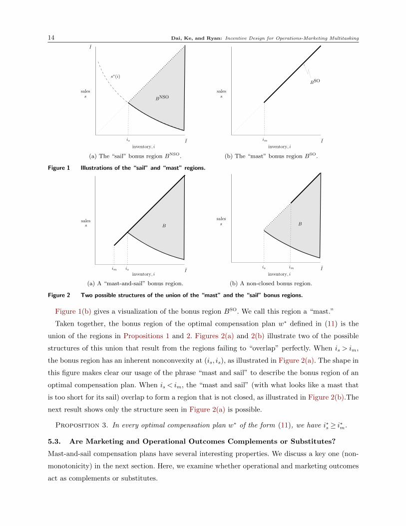
Proposition 1. A nonincreasing and continuous function s∗ and is ∈ (0, I] exist such that
BNSO = {(i, s) : i≥ is and s∗(i)≤ s < i}.7
Because s∗(i) is a nonincreasing and continuous function of i on its domain, the bonus region
resembles the one shown in Figure 1(a). We call the shape of this region a “sail.”
Proposition 2. An inventory value im ∈ (0, I] exists, such that BSO = {(i, s) : s= i≥ im}.
7 Observe that BNSO can be empty under this definition when the function s∗ only takes values in (I , Q], in whichcase is = I, which is not optimal. For this reason, in figures like Figure 1(a), we restrict the vertical axis to be between0 and I, as opposed to 0 and Q.
14 Dai, Ke, and Ryan: Incentive Design for Operations-Marketing Multitasking
I
s
I
inventory, i
sales
is
s∗(i)
BNSO
(a) The “sail” bonus region BNSO.
I
s
inventory, i
sales
im
BSO
(b) The “mast” bonus region BSO.
Figure 1 Illustrations of the “sail” and “mast” regions.
I
s
iminventory, i
sales
is
B
(a) A “mast-and-sail” bonus region.
I
s
im
inventory, i
sales
is
B
(b) A non-closed bonus region.
Figure 2 Two possible structures of the union of the “mast” and the “sail” bonus regions.
Figure 1(b) gives a visualization of the bonus region BSO. We call this region a “mast.”
Taken together, the bonus region of the optimal compensation plan w∗ defined in (11) is the
union of the regions in Propositions 1 and 2. Figures 2(a) and 2(b) illustrate two of the possible
structures of this union that result from the regions failing to “overlap” perfectly. When is > im,
the bonus region has an inherent nonconvexity at (is, is), as illustrated in Figure 2(a). The shape in
this figure makes clear our usage of the phrase “mast and sail” to describe the bonus region of an
optimal compensation plan. When is < im, the “mast and sail” (with what looks like a mast that
is too short for its sail) overlap to form a region that is not closed, as illustrated in Figure 2(b).The
next result shows only the structure seen in Figure 2(a) is possible.
Proposition 3. In every optimal compensation plan w∗ of the form (11), we have i∗s ≥ i∗m.
5.3. Are Marketing and Operational Outcomes Complements or Substitutes?
Mast-and-sail compensation plans have several interesting properties. We discuss a key one (non-
monotonicity) in the next section. Here, we examine whether operational and marketing outcomes
act as complements or substitutes.
Dai, Ke, and Ryan: Incentive Design for Operations-Marketing Multitasking 15
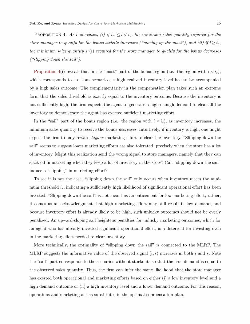
Proposition 4. As i increases, (i) if im ≤ i < is, the minimum sales quantity required for the
store manager to qualify for the bonus strictly increases (“moving up the mast”), and (ii) if i≥ is,
the minimum sales quantity s∗(i) required for the store manager to qualify for the bonus decreases
(“slipping down the sail”).
Proposition 4(i) reveals that in the “mast” part of the bonus region (i.e., the region with i < is),
which corresponds to stockout scenarios, a high realized inventory level has to be accompanied
by a high sales outcome. The complementarity in the compensation plan takes such an extreme
form that the sales threshold is exactly equal to the inventory outcome. Because the inventory is
not sufficiently high, the firm expects the agent to generate a high-enough demand to clear all the
inventory to demonstrate the agent has exerted sufficient marketing effort.
In the “sail” part of the bonus region (i.e., the region with i≥ is), as inventory increases, the
minimum sales quantity to receive the bonus decreases. Intuitively, if inventory is high, one might
expect the firm to only reward higher marketing effort to clear the inventory. “Slipping down the
sail” seems to suggest lower marketing efforts are also tolerated, precisely when the store has a lot
of inventory. Might this realization send the wrong signal to store managers, namely that they can
slack off in marketing when they keep a lot of inventory in the store? Can “slipping down the sail”
induce a “slipping” in marketing effort?
To see it is not the case, “slipping down the sail” only occurs when inventory meets the mini-
mum threshold is, indicating a sufficiently high likelihood of significant operational effort has been
invested. “Slipping down the sail” is not meant as an enticement for low marketing effort; rather,
it comes as an acknowledgment that high marketing effort may still result in low demand, and
because inventory effort is already likely to be high, such unlucky outcomes should not be overly
penalized. An upward-sloping sail heightens penalties for unlucky marketing outcomes, which for
an agent who has already invested significant operational effort, is a deterrent for investing even
in the marketing effort needed to clear inventory.
More technically, the optimality of “slipping down the sail” is connected to the MLRP. The
MLRP suggests the informative value of the observed signal (i, s) increases in both i and s. Note
the “sail” part corresponds to the scenarios without stockouts so that the true demand is equal to
the observed sales quantity. Thus, the firm can infer the same likelihood that the store manager
has exerted both operational and marketing efforts based on either (i) a low inventory level and a
high demand outcome or (ii) a high inventory level and a lower demand outcome. For this reason,
operations and marketing act as substitutes in the optimal compensation plan.
16 Dai, Ke, and Ryan: Incentive Design for Operations-Marketing Multitasking
s
inventory, i
sales
(im, im)
(is, is)
(i, s)
(i◦, s◦)
Figure 3 An illustration of the lack of joint monotonicity of an optimal compensation plan.
6. Ex Post Moral Hazard in Mast-and-Sail Compensation Plans
In this section, we explore the monotonicity of the mast-and-sail structure. To make things concrete,
and because a compensation plan has two arguments (i and s), we start with carefully defining
monotonicity. We say w(i, s) is monotone in i if w(i′, s)≤ w(i′′, s) for every (i′, s), (i′′, s) ∈D and
i′ ≤ i′′. Similarly, we say w(i, s) is monotone in s if w(i, s′) ≤ w(i, s′′) for every (i, s′), (i, s′′) ∈D
and s′ ≤ s′′. Finally, we say w(i, s) is (strictly) jointly monotone if w(i′, s′) ≤ w(i′′, s′′) for all
(i′, s′), (i′′, s′′)∈D with i′ < i′′ and s′ < s′′.8
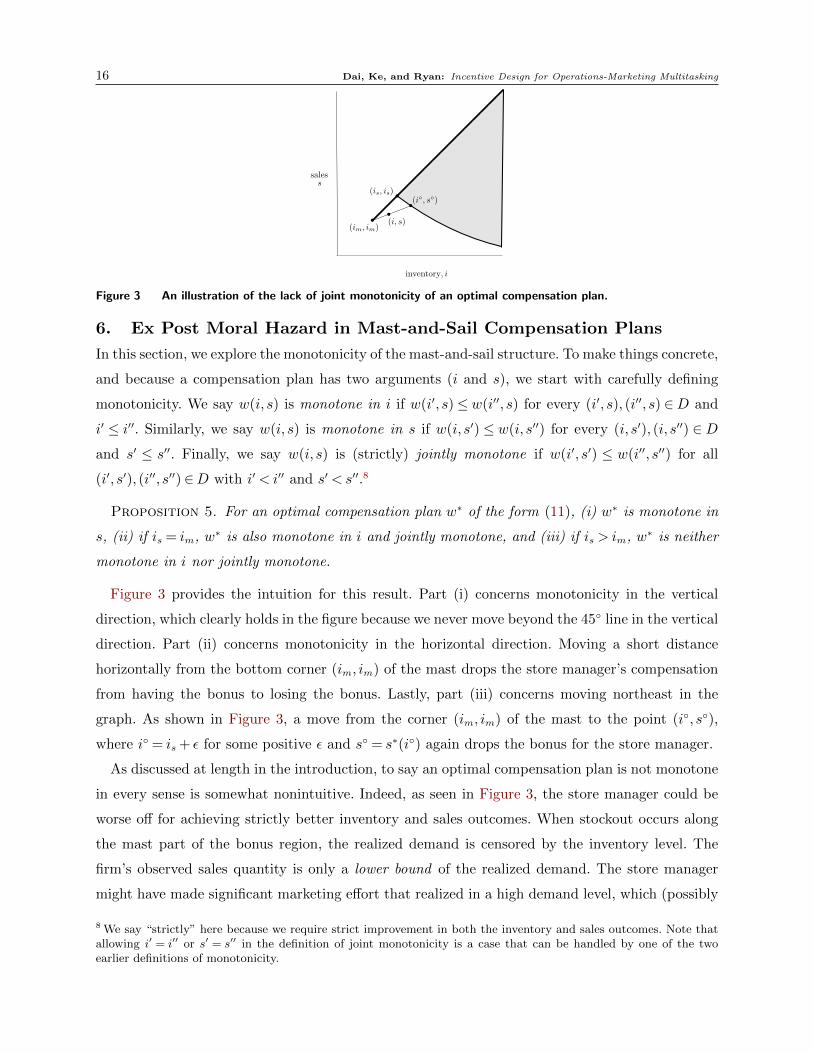
Proposition 5. For an optimal compensation plan w∗ of the form (11), (i) w∗ is monotone in
s, (ii) if is = im, w∗ is also monotone in i and jointly monotone, and (iii) if is > im, w∗ is neither
monotone in i nor jointly monotone.
Figure 3 provides the intuition for this result. Part (i) concerns monotonicity in the vertical
direction, which clearly holds in the figure because we never move beyond the 45◦ line in the vertical
direction. Part (ii) concerns monotonicity in the horizontal direction. Moving a short distance
horizontally from the bottom corner (im, im) of the mast drops the store manager’s compensation
from having the bonus to losing the bonus. Lastly, part (iii) concerns moving northeast in the
graph. As shown in Figure 3, a move from the corner (im, im) of the mast to the point (i◦, s◦),
where i◦ = is + ε for some positive ε and s◦ = s∗(i◦) again drops the bonus for the store manager.
As discussed at length in the introduction, to say an optimal compensation plan is not monotone
in every sense is somewhat nonintuitive. Indeed, as seen in Figure 3, the store manager could be
worse off for achieving strictly better inventory and sales outcomes. When stockout occurs along
the mast part of the bonus region, the realized demand is censored by the inventory level. The
firm’s observed sales quantity is only a lower bound of the realized demand. The store manager
might have made significant marketing effort that realized in a high demand level, which (possibly
8 We say “strictly” here because we require strict improvement in both the inventory and sales outcomes. Note thatallowing i′ = i′′ or s′ = s′′ in the definition of joint monotonicity is a case that can be handled by one of the twoearlier definitions of monotonicity.

Dai, Ke, and Ryan: Incentive Design for Operations-Marketing Multitasking 17
unluckily) available inventory was not able to meet. Given the same sales quantity, as inventory
increases, the firm no longer experiences stockouts. The observed sales quantity is equal to (as
opposed to a lower bound of) the realized demand. Thus, an increased realized inventory level
may be informative of the fact that the store manager has not exerted high marketing effort. In
other words, to encourage greater marketing effort, the firm is rewarding the possibility of a high
demand realization when inventory stocks out. When the uncertainty surrounding realized demand
(as opposed to sales) is removed, better performance is required to warrant the bonus.
Interesting as the above non-monotonicity property is, it may raise implementability concerns. If
inventory can be “hidden” from the principal ex post, which does not seem entirely inconceivable,
the compensation plan becomes faulty. To see this possibility concretely, suppose a store manager
realizes inventory and sales (i′, s′) with i′ > im but does not receive a bonus. This scenario occurs,
for instance, when i′ ∈ (im, is) and i′ < s′ < s∗(i′). If the store manager could hide some of the
realized inventory (or claim it was “shrunk”) to reveal an output of (i′, i′), she would receive a
bonus. In other words, the store manager is effectively rewarded for disposing of inventory, meaning
ex post moral hazard issue is inherent with contracts that are non-monotone in inventory.
In practice, inventory can neither be freely “hidden” nor perfectly observed. The ex post moral
hazard problem of manipulating inventory is thus similar to “costly state falsification” problems
studied in the accounting and economics literature (see, e.g., Lacker and Weinberg 1989, Beyer et
al. 2014). Monitoring ex post manipulation by the firm is itself limited, and penalties are difficult
to enforce. Indeed, the setup of our problem supposes marketing and operational effort of the store
manager are not observable to the firm. This setup suggests monitoring of inventory is limited for
the same reasons. To the extent that a careful accounting of realized inventory and assessment of
store manager effort are confounded, the non-monotonicity of the mast-and-sail compensation plan
is an endemic issue. If, under some method, inventory realizations can be observed and operational
effort remains hidden, the non-monotonicity of the mast-and-sail compensation plan is less of a
concern. However, we are unaware of such tools for use in practice.
In the rest of the paper, we search for alternate compensation plans that resolve the ex post
moral hazard issue of inventory manipulation.
7. Monotone (But Not Optimal) Compensation Plans
In the previous two sections, we have characterized an optimal mast-and-sail compensation plan,
but these compensation plans suffer from non-monotonicity, limiting their practicality in the pres-
ence of ex post moral hazard over the hiding of inventory.9 This issue motivates interest in exploring
the performance of classes of implementable compensation plans that are monotone.
9 It is worth noting that the non-monotonicity issue disappears if demand is fully observed. We explore this issue inSection OA.4, where we also explore the dead-weight loss due to demand censoring.
18 Dai, Ke, and Ryan: Incentive Design for Operations-Marketing Multitasking
I
s
b
I
inventory, i
sales
a
βbonus
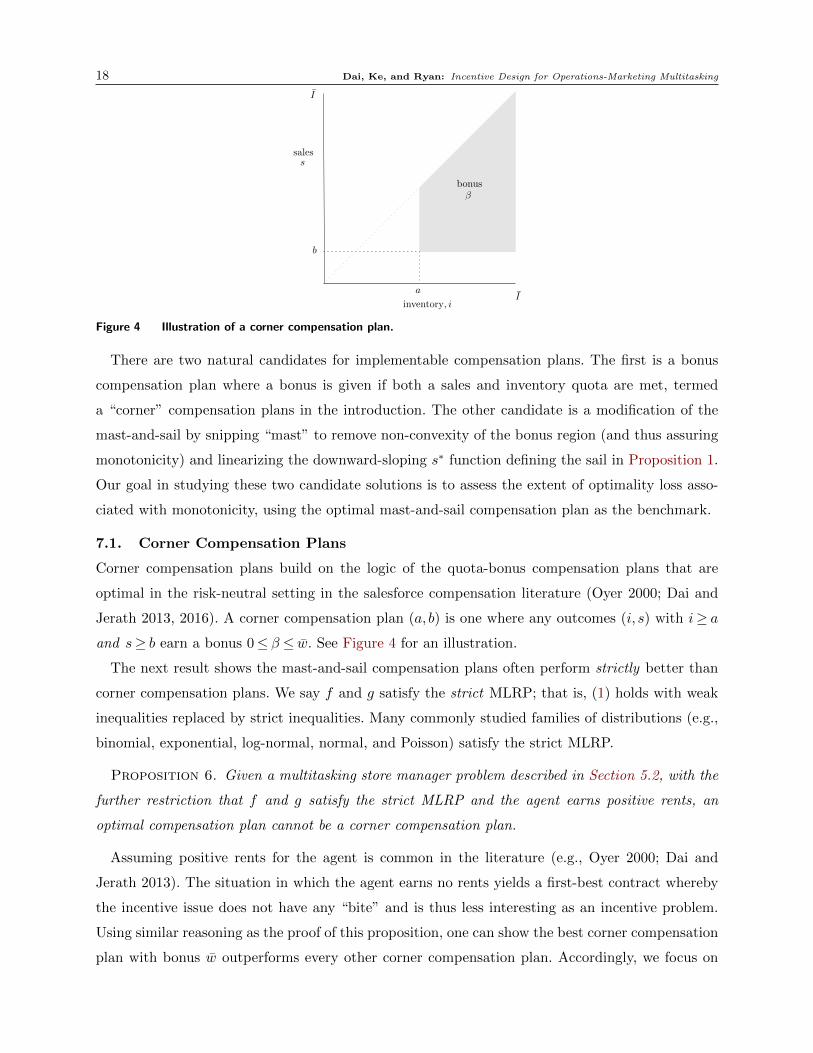
Figure 4 Illustration of a corner compensation plan.
There are two natural candidates for implementable compensation plans. The first is a bonus
compensation plan where a bonus is given if both a sales and inventory quota are met, termed
a “corner” compensation plans in the introduction. The other candidate is a modification of the
mast-and-sail by snipping “mast” to remove non-convexity of the bonus region (and thus assuring
monotonicity) and linearizing the downward-sloping s∗ function defining the sail in Proposition 1.
Our goal in studying these two candidate solutions is to assess the extent of optimality loss asso-
ciated with monotonicity, using the optimal mast-and-sail compensation plan as the benchmark.
7.1. Corner Compensation Plans
Corner compensation plans build on the logic of the quota-bonus compensation plans that are
optimal in the risk-neutral setting in the salesforce compensation literature (Oyer 2000; Dai and
Jerath 2013, 2016). A corner compensation plan (a, b) is one where any outcomes (i, s) with i≥ a
and s≥ b earn a bonus 0≤ β ≤ w. See Figure 4 for an illustration.
The next result shows the mast-and-sail compensation plans often perform strictly better than
corner compensation plans. We say f and g satisfy the strict MLRP; that is, (1) holds with weak
inequalities replaced by strict inequalities. Many commonly studied families of distributions (e.g.,
binomial, exponential, log-normal, normal, and Poisson) satisfy the strict MLRP.
Proposition 6. Given a multitasking store manager problem described in Section 5.2, with the
further restriction that f and g satisfy the strict MLRP and the agent earns positive rents, an
optimal compensation plan cannot be a corner compensation plan.
Assuming positive rents for the agent is common in the literature (e.g., Oyer 2000; Dai and
Jerath 2013). The situation in which the agent earns no rents yields a first-best contract whereby
the incentive issue does not have any “bite” and is thus less interesting as an incentive problem.
Using similar reasoning as the proof of this proposition, one can show the best corner compensation
plan with bonus w outperforms every other corner compensation plan. Accordingly, we focus on
Dai, Ke, and Ryan: Incentive Design for Operations-Marketing Multitasking 19
corner compensation plans with bonus w. Moreover, observe that compensation plans rewarding
sales only are achieved by setting a= b, and those rewarding inventory only are achieved by setting
b= 0. Single-tasking compensation plans are special cases of corner compensation plans and so are
(weakly) dominated by the optimal corner compensation plan.
Additional analytical performance bounds are hard to come by, in no small part because of the
challenging nature of computing the parameters of the optimal compensation plan. The difficulty
is that the weights ωi and t in (12) and (13) must be computed to get a sense of the shape of the
mast and sail. Problem (8) and Theorem 3 provide our best hope for computing ωi and t in general.
However, (8) is a challenging optimization problem and, to our knowledge, does not readily admit
analytical characterizations that can be used to provide bounds. For this reason, we primarily use
numerical calculations to further compare various compensation plans.
To numerically quantify the performance loss of corner compensation plans, we need to describe
the structure of an optimal corner compensation plan. Luckily, the analysis under a corner com-
pensation problem greatly simplifies, as evidenced by the following simple result.
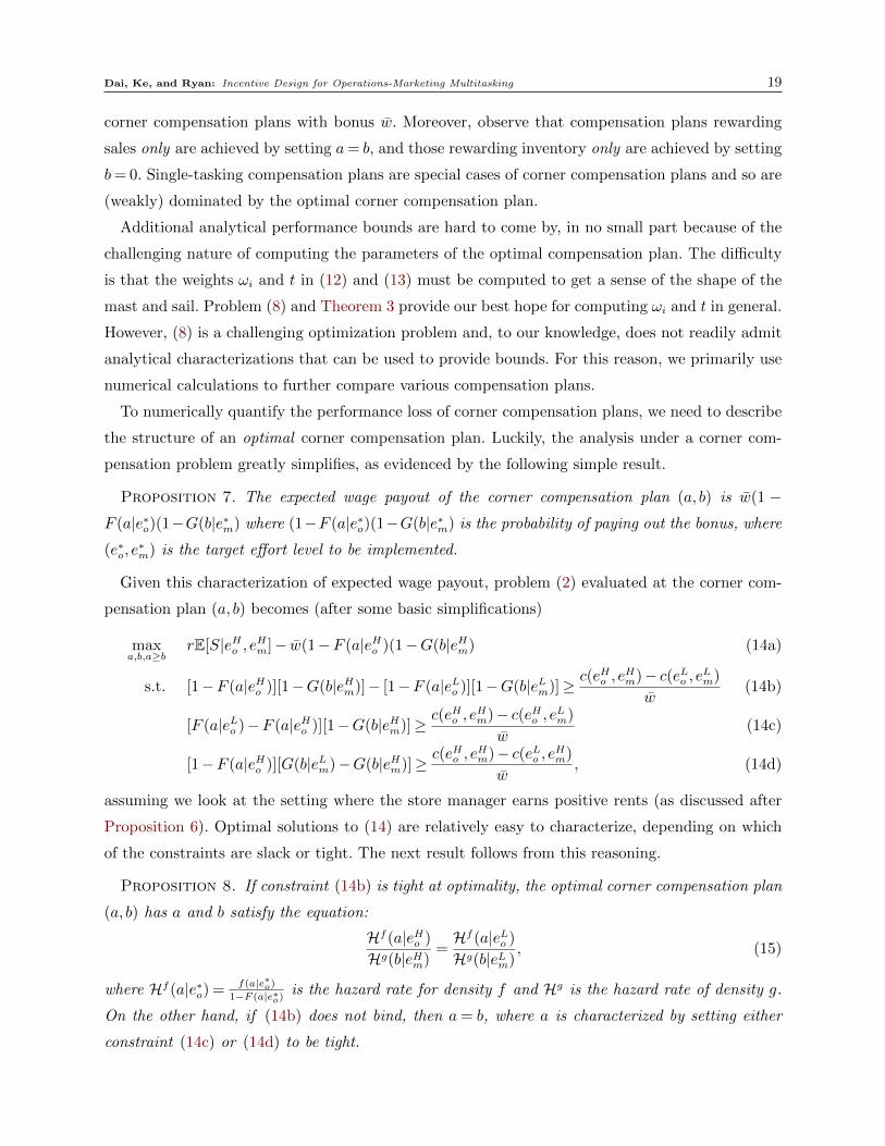
Proposition 7. The expected wage payout of the corner compensation plan (a, b) is w(1 −F (a|e∗o)(1−G(b|e∗m) where (1−F (a|e∗o)(1−G(b|e∗m) is the probability of paying out the bonus, where
(e∗o, e∗m) is the target effort level to be implemented.
Given this characterization of expected wage payout, problem (2) evaluated at the corner com-
pensation plan (a, b) becomes (after some basic simplifications)
maxa,b,a≥b
rE[S|eHo , eHm]− w(1−F (a|eHo )(1−G(b|eHm) (14a)
s.t. [1−F (a|eHo )][1−G(b|eHm)]− [1−F (a|eLo )][1−G(b|eLm)]≥ c(eHo , eHm)− c(eLo , eLm)
w(14b)
[F (a|eLo )−F (a|eHo )][1−G(b|eHm)]≥ c(eHo , eHm)− c(eHo , eLm)
w(14c)
[1−F (a|eHo )][G(b|eLm)−G(b|eHm)]≥ c(eHo , eHm)− c(eLo , eHm)
w, (14d)
assuming we look at the setting where the store manager earns positive rents (as discussed after
Proposition 6). Optimal solutions to (14) are relatively easy to characterize, depending on which
of the constraints are slack or tight. The next result follows from this reasoning.
Proposition 8. If constraint (14b) is tight at optimality, the optimal corner compensation plan
(a, b) has a and b satisfy the equation:
Hf (a|eHo )
Hg(b|eHm)=Hf (a|eLo )
Hg(b|eLm), (15)
where Hf (a|e∗o) = f(a|e∗o)
1−F (a|e∗o)is the hazard rate for density f and Hg is the hazard rate of density g.
On the other hand, if (14b) does not bind, then a= b, where a is characterized by setting either
constraint (14c) or (14d) to be tight.

20 Dai, Ke, and Ryan: Incentive Design for Operations-Marketing Multitasking
1 1.05 1.1 1.15 1.2 1.25 1.3 1.35 1.4 1.45 1.50.6%
0.65%
0.7%
0.75%
0.8%
0.85%
0.9%
Effi
cien
cy lo
ss r
elat
ive
to th
e op
timal
mas
t-an
d-sa
il co
mpe
nsat
ion
plan
(a) Parameters: w= 10, c(eHo , eLm) = c(eLo , e
Hm) = 3.0,
c(eHo , eHm) = 3.5, c(eLo , e
Lm) between 1 and 1.5.
1.5 1.55 1.6 1.65 1.7 1.75 1.80%
2%
4%
6%
8%
10%
12%
14%
16%
18%
20%
Effi
cien
cy lo
ss r
elat
ive
to th
e op
timal
mas
t-an
d-sa
il co
mpe
nsat
ion
plan
(b) Parameters: w = 10, c(eLo , eLm) = 1, c(eLo , e
Hm) =
1.8, c(eHo , eHm) = 3.5, c(eHo , e
Lm) between 1.5 and 1.8.
Figure 5 Performance of optimal corner compensation plan versus optimal mast-and-sail compensation plan. We
assume F (i|eo) = (H(i))eo and G(s|em) = (L(s))em , where H(i) = i and L(s) = s.
This structure assists us in running numerical experiments to evaluate the performance of optimal
corner compensation plans. For an illustration of how to use these results, see a concrete numerical
example in Section OA.3. Here, we present two representative and contrasting scenarios in Fig-
ures 5(a) and 5(b). Figure 5(a) shows the performance of the corner compensation plan is close to
optimal (within 1%) when the marketing and operational activities are highly complementary in
terms of the agent’s cost structure. By contrast, Figure 5(a) shows when the marketing and oper-
ational activities are not sufficiently complementary, the performance of the corner compensation
plan is far from optimal, with a gap of up to 18%.
In certain cases, the corner compensation plan fails to induce the target action achievable under
the optimal compensation plan. Example 1 provides one such example. Although the corner com-
pensation plan may lead to a lower expected compensation than the optimal compensation plan,
the firm’s expected sales quantity is also lower because of the store manager’s lower effort than
the desired one. Thus, under a sufficiently high unit revenue (so that the target action entails high
effort in both operational and marketing activities), the firm’s expected profit is higher under the
mast-and-sail compensation plan. Indeed, for this type of scenario, we can show the efficiency loss
under the corner compensation plan increases linearly in the unit revenue. In other words, the
worst-case loss in performance of corner compensation plans is arbitrarily large.
Example 1. Consider the following instance where eo ∈ {eLo , eHo } and em ∈ {eLm, eHm} where eLo =
eLm = 1 and eHo = eHm = 2. The target action is (eHo , eHm) = (2,2). The cost function is c(eHo , e
Hm) = 3.1,
c(eHo , eLm) = 1, c(eLo , e
Hm) = 1.6, and c(eLo , e
Lm) = 0.1. The resource constraint for the firm has w= 10.
For this instance, we can show the firm can use a mast-and-sail compensation plan with ω∗eLo ,e
Lm
=
0, ω∗eHo ,e
Lm
= 0.8602, ω∗eLo ,e
Hm
= 0.1398, and t∗ = 0.1817 to induce the target action, under which the
store manager’s probability of receiving the bonus is 58.70%. However, no corner compensation plan

Dai, Ke, and Ryan: Incentive Design for Operations-Marketing Multitasking 21
50 100 150 200
r
20
30
40
50
60
70
80
90
100
The
firm
' exp
ecte
d pr
ofit
Under mast-and-sail compensation planUnder corner compensation plan
Figure 6 Expected profits under the mast-and-sail and corner compensation plans versus revenue rate r.
exists that can induce the target action. Indeed, the best that the corner compensation plan can
achieve is to induce (eHo , eLm) with parameters of a∗ = b∗ = 0.6186, under which the store manager’s
probability of receiving the bonus is 23.55%. We illustrate the firm’s expected profits under both
types of compensation plans in Figure 6, as a function of the per-unit revenue rate r.
7.2. Modifying Mast-and-Sail Compensation Plans for Implementability
In the previous subsection, we used a single-tasking logic to construct and evaluate corner com-
pensation plans, with the sales-quota-bonus compensation plan being the simplest case, and found
its performance depends on the store manager’s cost structure and can be far from optimal. We
now switch gears to using our mast-and-sail compensation plan as inspiration for designing ex
post implementable compensation plans. We do so in two directions: (i) removing the mast (i.e.,
setting im = is and (ii) linearizing the downward-sloping function s∗ in Proposition 1. Removing
the mast assures monotonicity of the compensation plan and linearizing s∗ makes communicating
the compensation plan to sales managers easier in practice.10
Together this effort amounts to finding the best compensation plan where the bonus region is
characterized by a downward-sloping line (creating a “triangular sail” like that in Figure 7). We
call such compensation plans weighted-sum threshold compensation plans because the payout of
the bonus is determined by the weighted sum of the sales quantity and inventory level. Specifically,
the agent receives a bonus if the realized sales quantity s and inventory level i satisfy s+κ1 · i≥ κ2,
for some κ1, κ2 ≥ 0.11 To find the optimal weighted-sum threshold compensation plan, one searches
over the values of κ1 and κ2 that give the best payoff to the firm.Numerical results (see Figure 8) show the optimal weighted-sum threshold compensation plans
10 In Section OA.5 we additionally explore non-monotone approximations of mast-and-sail compensation plans, forthe purpose of examining what aspects of the mast-and-sail structure drive optimality. There we show via extensivenumerical experiments that there is little optimality loss by replacing s∗ by a linear function. By contrast, removingthe mast can have a significant impact.
11 We restrict attention to nonnegative κ1 and κ2 to ensure the “triangular sail” is described by a downward-slopingline and the 45◦ line. Recall the function s∗ in mast-and-sail compensation plans was downward sloping. Moreover,an upward-sloping triangular sail itself is non-monotone, despite its simplicity, and thus susceptible to the ex postmoral hazard of hiding inventory. For these reasons, we restrict attention to nonnegative κ1 and κ2.

22 Dai, Ke, and Ryan: Incentive Design for Operations-Marketing Multitasking
I
s
inventory, i
sales
κ2
κ2
κ1+1
Figure 7 An illustration of a weighted-sum-threshold compensation plan.
1.5 1.55 1.6 1.65 1.7 1.75 1.80%
2%
4%
6%
8%
10%
12%
14%
16%
18%
Effi
cien
cy lo
ss r
elat
ive
to th
e op
timal
mas
t-an
d-sa
il co
mpe
nsat
ion
plan Corner compensation plan
Weighted-sum threshold compensation plan
Figure 8 Expected profits under the mast-and-sail and corner compensation plans versus c(eHo , eLm)
also perform poorly (indeed, as poorly as corner compensation plans) in bad cases (losses of up to
18% in this example). We conclude the “loss due to monotonicity” that is captured by the ex post
moral hazard issue that afflicts mast-and-sail contracts has no easy fix. The next section shows,
however, with some additional information, this issue can be resolved.
8. Resolving Ex Post Moral Hazard through Gauging UnsatisfiedDemand12
In previous sections, we assumed any demand in excess of inventory cannot be observed. We now
consider a more general setting where partial information is revealed when demand exceeds sales.
In particular, we assume some random (and unknown) fraction of customers who do not receive
the product express interest via a waitlist (or some other method of capturing unsatisfied demand).
We introduce a new random variable13
Θ := Λ(Q− I) + I, (16)
12 We thank an anonymous reviewer for suggesting this direction of analysis to tackle ex post moral hazard.
13 In fact, our analysis allows for Θ to be defined by a general function of Γ, Q, and I that satisfies sufficientmonotonicity properties. We study the linear version due to its intuitive nature.

Dai, Ke, and Ryan: Incentive Design for Operations-Marketing Multitasking 23
where Λ is a continuous random variable distributed on (0,1). When Q, I, and Λ realize to outcome
(q, i, λ), where q > i, λ can be interpreted as the fraction of customers who sign the waitlist when
facing stockout. We call Λ the random fraction of captured demand (or simply the fraction).
We define a new random variable,
Z :=Z(I,Q,Θ) =
{Q if Q≤ IΘ if Q> I
, (17)
that captures what demand information can be observed. We cannot observe Q when Q> I and
we cannot observe Θ when Q≤ I. We assume the conditional density function γ(θ|q, i) for all q, i
such that q > i is known to both the firm and store manager. This assumption amounts to knowing
the probability density function ϕ of the fraction Λ, because in this case, γ(θ|q, i) = 1q−iϕ
(θ−iq−i
).
The firm and store manager observe I and Z. When Z = Θ, the product Λ(Q−I) can be observed
(since I is also observable) but knowledge of this product does not reveal Λ or Q directly. That is,
the proportion of unsatisfied customers that sign up for the waitlist is not observable. The derived
signal Z captures intermediate degrees of demand censoring. In the classical censoring case, Θ is
precisely I with Λ a constant at 0. Accordingly, Z becomes the random variable S studied in earlier
sections. Similarly, the situation where demand is observed sets Θ =Q with Λ a constant at 1; this
full information case is explored in Section OA.4 of the online appendix.
Because the firm and store manager observe I and Z, the compensation plan w is a function of
I and Z. The same bang-bang methodology applies to this new setting, as the underlying problem
remains linear in w. The optimal compensation plan is therefore defined by characterizing its bonus
region where the store manager receives w, using the methodology of Section 4.
To get a sense of the bonus region, we need to understand the domain of w. According to (17),
two regions of the domain need to be considered: (i) the “no lost sales” (NLS) region (where Z ≤ I)
and (ii) the lost-sales (LS) region (where Z > I). As before, we may construct the bonus region in
the two “chunks” of the underlying domain, the NLS region and the LS region. The joint density
function of (I,Z) can be expressed over these two regions as follows:
h(i, z|eo, em) :=
{f(i|eo)g(z|em) if z ≤ i∫ Qq=i
γ(z|q, i)g(q|em)dqf(i|eo) if z > i.(18)
Using the joint density function in (18), we define the bonus regions in the NLS and LS regions in
terms of likelihood ratio functions as follows:
RNLSeo,em
(i, z) = 1− g(z|em)
g(z|e∗m)· f(i|eo)f(i|e∗o)
(19)
RLSe0,em
(i, z) = 1−∫ Qq=i
γ(z|q, i)g(q|em)dq∫ Qq=i
γ(z|q, i)g(q|e∗m)dq︸ ︷︷ ︸(∗)
·f(i|eo)f(i|e∗o)
, (20)
24 Dai, Ke, and Ryan: Incentive Design for Operations-Marketing Multitasking
where e∗o and e∗m are the target effort levels.
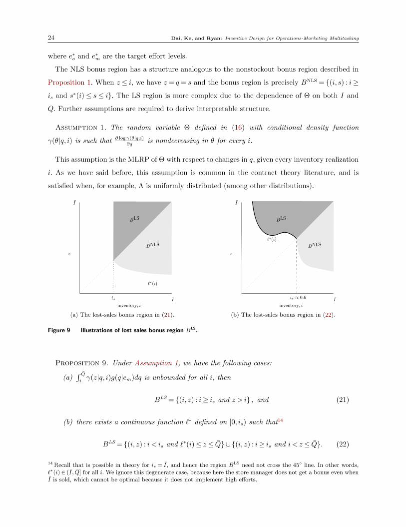
The NLS bonus region has a structure analogous to the nonstockout bonus region described in
Proposition 1. When z ≤ i, we have z = q = s and the bonus region is precisely BNLS = {(i, s) : i≥
is and s∗(i)≤ s≤ i}. The LS region is more complex due to the dependence of Θ on both I and
Q. Further assumptions are required to derive interpretable structure.
Assumption 1. The random variable Θ defined in (16) with conditional density function
γ(θ|q, i) is such that ∂ logγ(θ|q,i)∂q
is nondecreasing in θ for every i.
This assumption is the MLRP of Θ with respect to changes in q, given every inventory realization
i. As we have said before, this assumption is common in the contract theory literature, and is
satisfied when, for example, Λ is uniformly distributed (among other distributions).
I
z
I
inventory, i
is
`∗(i)
BLS
BNLS
(a) The lost-sales bonus region in (21).
I
z
I
inventory, i
is ≈ 0.6
`∗(i)
BLS
BNLS
(b) The lost-sales bonus region in (22).
Figure 9 Illustrations of lost sales bonus region BLS.
Proposition 9. Under Assumption 1, we have the following cases:
(a)∫ Qiγ(z|q, i)g(q|em)dq is unbounded for all i, then
BLS = {(i, z) : i≥ is and z > i} , and (21)
(b) there exists a continuous function `∗ defined on [0, is) such that14
BLS = {(i, z) : i < is and `∗(i)≤ z ≤ Q}∪ {(i, z) : i≥ is and i < z ≤ Q}. (22)
14 Recall that is possible in theory for is = I, and hence the region BLS need not cross the 45◦ line. In other words,`∗(i)∈ (I , Q] for all i. We ignore this degenerate case, because here the store manager does not get a bonus even whenI is sold, which cannot be optimal because it does not implement high efforts.
Dai, Ke, and Ryan: Incentive Design for Operations-Marketing Multitasking 25
An important fact used in this proof is that Λ ∈ (0,1). When we can infer that Q = I (i.e.,
stockout occurs) when Z = I because this implies Λ(Q− I) = 0 and Λ never realizes to 0. In other
words, when the signal Θ is equal to I, no demand is lost. This ensures the LS and NLS bonus
regions meet at the same point on the 45◦ line (is).
Figure 9 gives a visualization of the bonus regions BLS and BNLS in cases (a) and (b) of Proposi-
tion 9. Figure 9(a) was generated assuming Λ is a power law distribution with cumulative distribu-
tion function λα, where α≤ 1. It is straightforward that this class of distributions (which includes
the uniform distribution) satisfies the conditions of Proposition 9(a). We generated Figure 9(b) by
considering the case in which Λ was distributed, so that − log Λ is a Gamma(α,β) distribution.
This ensures Λ ∈ (0,1). It is straightforward to check that the conditions of Proposition 9(b) are
satisfied for this setting. To generate the figure, we took α= 2 and β = 1/2.
The two different cases for the bonus region have interesting implications for the question of
monotonicity and ex post moral hazard. Observe that in Figure 9(a), the bonus region is jointly
monotone in z and i. This case is not trivial, because it includes the uniform distribution and
general power law distributions for the fraction Λ of captured demand. The intuition here is that
by including waitlist information, the old “mast” region disappears. The waitlist reveals sufficient
information about marketing effort, so that it is no longer necessary to reward low sales outcomes.
The essential message here is that the bonus region is now monotone; therefore, ex post moral
hazard issue of hiding inventory no longer exists. Indeed, the feasible region BLS is monotone in z
and so even if we allow downward manipulation of the waitlist, there is no incentive to do so.
By contrast, in the bonus region in Figure 9(b), the waitlist signal is sufficiently correlated with
marketing effort to offer bonuses if the waitlist is sufficiently large, even when the sales target is
is not met. This scenario may lead to bonus regions that are not jointly monotone in z and i,
a result coming from the fact that Assumption 1 does not require monotonicity properties of Θ
with respect to changes in i. It is important to point out that it does, nonetheless, preclude any
ex post moral hazard issue of hiding inventory. In the nonstockout region of the domain (s < i),
the store manager has no incentive to hide inventory, due to monotonicity in i: the bonus region is
monotone below the 45◦ line. The area above the 45◦ line captures scenarios with lost sales, and so
no inventory is left to “hide.” Assuming also that the signal Θ cannot be manipulated by the store
manager (e.g., the waitlist captures that the unique identity of customers can be directly verified
by the firm), no ex post moral hazard arises.
Of course, one may still argue that compensation plans with bonus regions such as in Figure 9(b)
are not completely intuitive. In practice, a store manager might wonder why a lower level of sales
requires a smaller waitlist signal to get a bonus, whereas a higher sales level requires a larger
bonus. The fact that no scope exists for ex post manipulation does not change the fact it could be

26 Dai, Ke, and Ryan: Incentive Design for Operations-Marketing Multitasking
I
s
I
inventory, i
sales
is = i`
BLS
BNLS
Figure 10 The “double sail” bonus region BNLS ∪BLS under Assumption 1.
hard to explain such compensation plans to store managers. This lack of joint monotonicity above
the 45◦ line can be removed under the following assumption.
Assumption 2. The random variable Θ defined in (16) with conditional density function
γ(θ|q, i) is such that ∂ logγ(θ|q,i)∂q
is nondecreasing in i for every θ.
Proposition 10. Under Assumptions 1 and 2, a continuous and nonincreasing function `∗(i)
exists such that BLS = {(i, z) : i ≤ is and `∗(i) ≤ z ≤ Q} ∪ {(i, z) : i ≥ is and i ≤ z ≤ Q}, implying
that BNLS ∪BLS has the “double sail” structure depicted in Figure 10.
It is straightforward to observe that the resulting optimal contract is w∗(i, z), where w∗(i, z) = w
when (i, z)∈BNLS ∪BNLS and 0 otherwise, is jointly monotone. In other words, under the waitlist
approach for gauging unsatisfied demand (and given the above technical conditions), an optimal
“double sail” compensation plan exists that is monotone. This avoids the ex post moral hazard
hiding of inventory that afflicted the “mast-and-sail” compensation plan, and has a more intuitive
structure than what we see in Figure 9(b).
One may ask how restrictive Assumptions 1 and 2 are on the distribution of the signal Θ. Note
that distributions that satisfy the condition of Proposition 9(a) fail this condition, but nonetheless
give rise to jointly monotone bonus regions. We saw in Figure 9 that gamma distributions can give
rise to scenarios with non-monotone lost-sales bonus regions. However, one can also check that
non-monotonicity does not hold for all parameter values. Indeed, an algebra exercise can verify
that when Λ is such that − log Λ is a Gamma(α,β), where α− 1 ≥ 4e2+1
( 1β
+ 1), Assumptions 1
and 2 hold and the resulting contract is monotone (by Proposition 10).
9. Further Discussions
In this section, we include some additional discussion on the flexibility of our analytical framework.
In particular, we are able to relax some of the assumptions of the base model that were included for
ease of discussion and presentation. Although not central to our managerial takeaways regarding the

Dai, Ke, and Ryan: Incentive Design for Operations-Marketing Multitasking 27
connection between demand censoring, non-monotonicity, and ex post moral hazard, we nonetheless
consider these extentions worthy of further discussion.
9.1. The Role of w and More General Resource Constraints
The role of the upper bound w on compensation is a delicate one. As mentioned in Section 3, the
assumption is not uncommon in the literature and has been justified elsewhere. However, because
w is exogenous to the model, a question remains of how to interpret it. Can the firm set w? If so,
how high or low should it be set? How does w change the optimal compensation plan?
Changing w does not change the optimality of the mast-and-sail compensation plan, but may
change the relative length of the mast and shape of the sail and the probability of the agent
receiving the bonus under the target actions. If we view w purely as a choice of the firm, and
consider its optimization over the choice of w, larger choices of w are obviously better. Indeed,
w only enters in the constraint w(i, s) ≤ w, and so increasing w can only improve the objective
value of the firm. This slope is a slippery one. If the choice of w is unconstrained, it will be sent
to infinity. When w = +∞, an optimal compensation plan need not exist in general. This issue
is discussed at length in the economics literature (see, e.g., Chu and Sappington 2009). We find
it natural that, in practice, a natural upper bound for w would exist that avoids this theoretical
issue. One possible justification is provided in Section OA.8.
We consider here a more general upper bound than w. Let m(i, s) be the available resources for
compensation by the firm when outcome (i, s) prevails. That is, constraint w(i, s)≤ w is replaced
by constraint w(i, s)≤m(i, s) for almost all (i, s). As an example of m(i, s), consider the following
description from DeHoratius and Raman (2007): “BMS [the company they study] store managers
were offered a bonus for generating sales that ranged from 0.2% to 5% of the sales dollars above
store-specific targets.” In this case, m(i, s) is as fixed proportion of the store revenue less a store-
specific target. In other words, m(i, s) = α · r ·s−C, where r is the per-unit revenue and C denotes
the store-specific target. The range of α in this case ranges from 0.2% to 5%.
Our model can be adjusted to the setting with resource constraint w(i, s) ≤m(i, s), assuming
m(i, s) is an L1 function. Define a new variable β(i, s) where w(i, s) = β(i, s)m(i, s) and β(i, s) ∈
[0,1] for almost all (i, s). The new function β can be interpreted as the percentage of the resource
given to the store manager as a bonus. The problem becomes
maxβ
r
∫i
∫s
sf(i|e∗o)g(s|e∗m)dids−∫i
∫s
β(i, s)m(i, s)f(i|e∗o)g(s|e∗m)dids (23a)
s.t.
∫i
∫s
β(i, s)m(i, s)f(i|e∗o)g(s|e∗m)dids− c(e∗o, e∗m)≥¯U (23b)∫
i
∫s
β(i, s)m(i, s)f(i|e∗o)g(s|e∗m)dids−∫i
∫s
β(i, s)m(i, s)f(i|eo)g(s|em)dids (23c)

28 Dai, Ke, and Ryan: Incentive Design for Operations-Marketing Multitasking
≥ c(e∗o, e∗m)− c(eo, em) for all (eo, em)
0≤ β(i, s)≤ 1 for all (i, s). (23d)
This problem is of the form (4) interpreting f(x|a∗) in that formulation as m(i, s)f(i|eo)g(s|em).
Thus, an optimal bang-bang contract exists for (23) with a similarly nice structure.
Proposition 11. If m is an L1 function, nonnegative multipliers ωi and a “target” t exist such
that an optimal solution to (23) of the following form exists:15
w∗(i, s) =
{m(i, s) if
∑eo,em
ωeo,emReo,em(i, s)≥ t.0 otherwise
,
where
Reo,em(i, s) = 1− I[i > s]f(i|eo)g(s|em) + δ(i= s)f(i|eo)(1−G(i|em)
I[i > s]f(i|e∗o)g(s|e∗m) + δ(i= s)f(i|e∗o)(1−G(i|e∗m).
Under the compensation plan specified by Proposition 11, the store manager’s compensation is
monotone nondecreasing in s, as long as m(i, s) does not decrease in s.
9.2. Endogenizing Initial Inventory
In this section, we endogenize the choice of initial inventory I. Whether it is more natural for I
to be under the control of the firm or the store manager is a matter of debate. In this paper, we
analyze the former. This perspective particularly applies in settings where the firm oversees a large
chain of stores where ordering is done centrally. Allowing the store manager to decide the initial
inventory level gives rise to additional incentive issues that go beyond our scope.
To set the benchmark, suppose we can ignore the incentive compatibility constraint of the store
manager and pay her a constant wage to meet the minimum utility¯U to work at effort level (eHo , e
Hm).
Under this assumption, the firm’s problem is maxI rE[S|I]−C(I), where C(·) is a convex increasing
cost for procuring inventory I and E[·] is the conditional expectation given inventory I. Thus, the
optimal inventory level is the classical newsvendor solution INV that solves r ddI
E[S|INV] =C ′(INV).
As for the second-best compensation plan, where the store manager’s incentives must be taken
into consideration, the firm’s inventory decision becomes
maxIrE[S|I]−W (I)−C(I), (24)
where
W (I),minw
E[w(I,S)|eHo , eHm]
s.t. E[w(I,S)|eHo , eHm]− c(eHo , eHm)≥¯U
15 Again, this assumes the function∑m
i=1 ωiRi(~x) has zero mass at the cutoff t.

Dai, Ke, and Ryan: Incentive Design for Operations-Marketing Multitasking 29
E[w(I,S)|eHo , eHm]−E[w(I,S)|eo, em]≥ c(eHo , eHm)− c(eo, em) for all (eo, em)
0≤w(i, s)≤ w for all (i, s)
is the optimal value function when (eHo , eHm) is the target effort level.
Proposition 12. (i) Under the assumption that (eHo , eHm) is the target effort level and f and g
satisfy the MLRP, we have ddIW (I)< 0 for all I. That is, an increase in I leads to a decrease
in the expected payout to the store manager.
(ii) The firm’s optimal inventory level, by accounting for the multitasking store manager problem,
is higher than that in the newsvendor problem, which helps the firm achieve a lower expected
payment to the store manager than otherwise.
The intuition behind Proposition 12(i) is as follows. Because the firm is more likely to pay a
bonus if the inventory is cleared (as long as sales are greater than im), increasing inventory reduces
the chance of inventory clearing and thus the chance of paying out the bonus.
Proposition 12(ii) entails optimizing the initial inventory level I. Let I∗ be the optimal inventory
choice in (24). The first-order condition of (24) yields the necessary optimality condition for I∗:
rd
dIE[S|I∗]− d
dIW (I∗) =C ′(I∗). (25)
In light of (24) and (25), and because ddIW (I∗)< 0 (by Proposition 12) and C is a convex increasing
function, we can conclude I∗ > INV . In other words, the firm over-invests in inventory as compared
to the classical newsvendor setting without agency issues. This result echoes the view of Dai and
Jerath (2013, 2019) that a higher inventory level mitigates the possibility of demand censoring and
hence benefits the firm by reducing the complications in contract design.
10. Conclusion
In this paper, we examined incentive issues at the intersection of operations and marketing. We
show the censoring of marketing outcomes (i.e., demand censoring) gives rise to a vexing incentive
issue of both ex ante and ex post moral hazard. Addressing ex ante moral hazard alone leads to
an optimal compensation plan that does not overcome the ex post issue. Only by providing for an
additional signal of unsatisfied demand (e.g., via a waitlist) can we construct a compensation plan
that is both optimal and resolve the ex ante and ex post moral hazard issues.
Taken together, our research provides a compelling narrative linking customer and employee
behavior in the retail setting. Because of its inability to monitor customer intentions (i.e., not
observing all of demand), for the firm to design intuitive compensation schemes, it has to monitor
employee intentions (i.e., their conscientiousness in sales and operational activities or in accurately
representing the level of inventory in the store). In effect, an arms-length company cannot stop the

30 Dai, Ke, and Ryan: Incentive Design for Operations-Marketing Multitasking
employee from using its lack of understanding of customer demand to benefit employee compensa-
tion. Employees incur a rent from the company’s lack of visibility over customers. Only additional
information about customer intentions removes this rent-seeking opportunity.
Our novel methodology (i.e., the bang-bang optimal control approach) transcends the limitations
of classical solution approaches in contract theory and is applicable to a broad set of incentive
design problems. In addition, we hope our work will inspire future research into this immensely
exciting venue. For example, instead of having a single manager in charge of both operations
and marketing, one could imagine two managers responsible for one of each task. The nature of
the relationship between these two managers, and their compensation plans, should also include
aspects of customer demand and behavior. Another scenario involves a store manager who has
operational responsibilities not only for execution (i.e., maintaining inventory), but also in making
operational decisions, such as inventory stocking levels (see, e.g., Sen and Alp 2019). Stockouts—
and the associated incentive complications—will be likely even more prevalent in a decentralized
supply chain because of double marginalization. An interesting research question would be whether
agency issues make optimal order quantities more or less conservative.
Acknowledgments
The authors are grateful to the Department Editor, Associate Editor, and three anonymous reviewers for the
constructive review process. They also appreciate Anil Arya, Maqbool Dada, Nicole DeHoratius, Vishal Gaur,
Jonathan Glover, Xiaoyang Long, Suresh Sethi, Christopher S. Tang, Fuqiang Zhang, and Gaoqing Zhang for
their valuable suggestions. Seminar participants at Boston College, Cornell University, Duke University, Hong
Kong Baptist University, INSEAD, National University of Singapore, Singapore Management University,
University of Alberta, University of California Los Angeles, University of Florida, University of Michigan,
University of Rochester, University of Texas at Austin, University of Texas at Dallas, University of Virginia,
University of Wisconsin–Madison, Wake Forest University, and Washington University in St. Louis provided
helpful comments for various versions of the paper. The authors also benefited from interacting with session
participants at the 2018 MSOM Conference (Dallas, Texas), 2019 INFORMS Marketing Science Conference
(Rome, Italy), 2019 POMS International Conference (Brighton, UK), and INFORMS 2019 Annual Meeting
(Seattle, Washington). The authors contributed equally, with names listed in alphabetical order; Rongzhu
Ke is the corresponding author of the paper.
References
Anupindi, R., M. Dada, S. Gupta. 1998. Estimation of consumer demand with stock-out based substitution:
An application to vending machine products. Marketing Sci. 17(4) 406–423.
Arya, A., J. Glover, B. Mittendorf. 2007. Aligning incentives by capping bonuses. Antle, R., F. Gjesdal, P.
J. Liang, eds. Essays in Accounting Theory in Honour of Joel S. Demski (New York, NY: Springer)
169–182.
Dai, Ke, and Ryan: Incentive Design for Operations-Marketing Multitasking 31
Atalı, A., H. L. Lee, and O. Ozer. 2009. If the inventory manager knew: Value of visibility and RFID under
imperfect inventory information. Stanford University Working Paper.
Baiman, S., S. Netessine, R. Saouma. 2010. Informativeness, incentive compensation, and the choice of
inventory buffer. Accounting Rev. 85(6) 1839–1860.
Barvinok, A. 2002. A Course in Convexity. Graduate Studies in Mathematics 54. Providence, RI: American
Mathematical Society.
Beck, A., C. Peacock. 2009. New Loss Prevention: Redefining Shrinkage Management. Basingstoke, United
Kingdom: Palgrave Macmillan.
Besbes, O., A. Muharremoglu. 2013. On implications of demand censoring in the newsvendor problem.
Management Sci. 59(6) 1407–1424.
Beyer, A., I. Guttman, I. Marinovic. 2014. Optimal contracts with performance manipulation. J. Accounting
Res. 52(4) 817–847.
Bond, P., A. Gomes. 2009. Multitask principal-agent problems: Optimal contracts, fragility, and effort mis-
allocation. J. Econom. Theory 144(1) 175-211.
Chao, G. H., S. M. R. Iravani, R. C. Savaskan. 2009. Quality improvement incentives and product recall cost
sharing contracts. Management Sci. 55(7) 1122–1138.
Chen, K.-Y., S. Li, Y. Rong. 2019. The behavioral promise and pitfalls in compensating store managers.
Management Sci. Forthcoming.
Chu, L. Y., G. Lai. 2013. Salesforce contracting under demand censorship. Manufacturing Service Oper.
Management 15(2) 320–334.
Chu, L. Y., D. E. M. Sappington. 2009. Implementing high-powered contracts to motivate intertemporal
effort supply. RAND J. Econom. 40(2) 296–316.
Conlon, C. T., J. H. Mortimer. 2013. Demand estimation under incomplete product availability. Amer.
Econom. J.: Microeconomics 5(4) 1–30.
Crama, P., Reyck, B.D. and Degraeve, Z., 2008. Milestone payments or royalties? Contract design for R&D
licensing. Oper. Res. 56(6) 1539–1552.
Dai, T., K. Jerath. 2013. Salesforce compensation with inventory considerations. Management Sci. 59(11)
2490–2501.
Dai, T., K. Jerath. 2016. Impact of inventory on quota-bonus contracts with rent sharing. Oper. Res. 64(1)
94–98.
Dai, T., K. Jerath. 2019. Salesforce contracting under uncertain demand and supply: Double moral hazard
and optimality of smooth contracts. Marketing Sci. 38(5) 852–870.
DeHoratius, N., A. Raman. 2007. Store manager incentive design and retail performance: An exploratory
investigation. Manufacturing Service Oper. Management 9(4) 518–534.
32 Dai, Ke, and Ryan: Incentive Design for Operations-Marketing Multitasking
Dewatripont, M., I. Jewitt, J. Tirole. 1999. The economics of career concerns, Part II: Application to missions
and accountability of government agencies. Rev. Econom. Stud. 66(1) 199–217.
Feiler, D. C., J. D. Tong, R. Larrick. 2013. Biased judgment in censored environments. Management Sci.
59(3) 573–591.
Feltham, G. A., J. Xie. 1994. Performance measure congruity and diversity in multi-task principal/agent
relations. Accounting Rev. 69(3) 429–453.
Grossman, S. J., O. D. Hart. 1983. An analysis of the principal-agent problem. Econometrica 51(1) 7–45.
Herweg, F., D. Muller, P. Weinschenk. 2010. Binary payment schemes: moral hazard and loss aversion. Amer.
Econom. Rev. 100(5) 2451–2477.
Ho, T. H., C. S. Tang. 2004. Introduction to the special issue on marketing and operations management
interfaces and coordination. Management Sci. 50(4) 429–430.
Holmstrom, B. 1979. Moral hazard and observability. Bell J. Econom. 10(1) 74–91.
Holmstrom, B., P. Milgrom. 1991. Multitask principal-agent analyses: Incentive contracts, asset ownership,
and job design. J. Law Econom. Organ. 7(Sp) 24–52.
Huh, W. T., R. Levi, P. Rusmevichientong, J. B. Orlin. 2011. Adaptive data-driven inventory control with
censored demand based on Kaplan-Meier estimator. Oper. Res. 59(4) 929–941.
Innes, R. D. 1990. Limited liability and incentive contracting with ex-ante action choices. J. Econom. Theory
52 45–67.
Jain, S. 2012. Self-control and incentives: An analysis of multiperiod quota plans. Marketing Sci. 31(5)
855–869.
Jain, A., N. Rudi, T. Wang. 2014. Demand estimation and ordering under censoring: Stock-out timing is
(almost) all you need. Oper. Res. 63(1) 134–150.
Jerath, K., S. Netessine, Z. J. Zhang. 2007. Can we all get along? incentive contracts to bridge the marketing
and operations divide. University of Pennsylvania Working Paper.
Jerath, K., S.-H. Kim, R. Swinney. 2017. Product quality in a distribution channel with inventory risk.
Marketing Sci. 36(5) 747–761.
Jewitt, I. 2008. Moral hazard with bounded payments. J. Econom. Theory 143(1) 59–82.
Ke, R., C. T. Ryan. 2018. Monotonicity of optimal contracts without the first-order approach. Oper. Res.
66(4 ) 1101–1118.
Krishnan, H., R. A. Winter. 2012. The economic foundations of supply chain contracting. Foundations and
Trends in Technology, Information and Operations Management 5(3–4) 147–309.
Krishnan, J., M. Fisher. 2005. Store level execution at Wawa. Case study, University of Pennsylvania.
Lacker, J. M., J. A. Weinberg. 1989. Optimal contracts under costly state falsification. J. Political Econom.
97(6) 1345–1363.
Dai, Ke, and Ryan: Incentive Design for Operations-Marketing Multitasking 33
Laffont, J. J., D. Martimort. 2009. The Theory of Incentives: The Principal-Agent Model. Princeton, NJ:
Princeton University Press.
Lal, R., V. Srinivasan. 1993. Compensation plans for single-and multi-product salesforces: An application of
the Holmstrom-Milgrom model. Management Sci. 39(7) 777–793.
Long, X, J. Nasiry. 2019. Wage transparency and social comparison in salesforce compensation. Management
Sci. Forthcoming.
Mirrlees, J. A. 1999. The theory of moral hazard and unobservable behaviour: Part I. Rev. Econom. Stud.
66(1) 3–21.
Misra, S., E. J. Pinker, R. A. Shumsky. 2004. Salesforce design with experience-based learning. IIE Trans-
actions 36(10) 941–952.
Nikoofal, M. E., M. Gumus. 2018. Quality at the source or at the end? Managing supplier quality under
information asymmetry. Manufacturing Service Oper. Management 20(3) 498–516.
Oyer, P. 2000. A theory of sales quotas with limited liability and rent sharing. J. Labor Econom. 18(3)
405–426.
Raju, J. S., V. Srinivasan. 1996. Quota-based compensation plans for multiterritory heterogeneous salesforces.
Management Sci. 42(10) 1454–1462.
Rogerson, W. P. 1985. The first-order approach to principal-agent problems. Econometrica 53(6) 1357–1367.
Rudi, N., D. Drake. 2014. Observation bias: The impact of demand censoring on newsvendor level and
adjustment behavior. Management Sci. 60(5) 1334–1345.
Sen, A., O. Alp. 2019. Delegation of stocking decisions under asymmetric demand information. Manufacturing
Service Oper. Management. Forthcoming.
Sethi, S. P., G. L. Thompson. 2000. Optimal Control Theory: Applications to Management Science and
Economics. New York, NY: Springer.
Shapiro, B. P. 1977. Can marketing and manufacturing coexist? Harvard Bus. Rev. 55(5) 104–114.
Ton, Z., A. Raman. 2004. The effect of product variety and inventory levels on misplaced products at retail
stores: A longitudinal study. Harvard Business School Working Paper.

Online Appendix to: Incentive Design for Operations-Marketing Multitasking oa1
Online Appendix to“Incentive Design for Operations-Marketing Multitasking”
In this online appendix, we provide proofs of the results in the main body, additional technical
details, and robustness checks.
OA.1. Proofs of Results Stated in the Paper
Proof of Theorem 1: We need the following two lemmas.
Lemma OA1. An optimal contract for (4) exists.
Proof of Lemma OA1. Due to constraint (4d), we may assume w is a function in L∞(X ), the
space of uniformly bounded functions on X . Moreover, those same constraints ensure the feasible
region of (4) is bounded in the norm on L∞(X ). Hence, by Alaoglu’s Theorem (see Theorem
5.105 in Aliprantis and Border 2006), the set {w : 0≤w(~x)≤w} is compact in the weak topology
σ(L∞(X ),L1(X )) (for a definition of this weak topology, see Section 5.14 of Aliprantis and Border
(2006)). Because f(·|~a) is in L1(X ) for all ~a ∈ A, the constraints (4b) and (4c) are continuous in
the σ(L∞(X ),L1(X )) topology, and so the feasible region is a closed subset of {w : 0≤w(~x)≤w}
and thus also compact in the σ(L∞(X ),L1(X )) topology. Moreover, the objective function V (w,a)
is continuous in the σ(L∞(X ),L1(X )) topology, and so, by Weierstrass’s Theorem (see Theorem
2.35 in Aliprantis and Border 2006), an optimal contract exists. �
Let W denote the set of feasible contracts to (4). An extremal contract of W is a contract that
cannot be written as the convex combination of two other feasible contracts. That is, w ∈W is
an extremal contract if w1,w2 ∈W , and λ1, λ2 ∈ (0,1) with λ1 + λ2 = 1 do not exist such that
w= λ1w1 +λ2w
2. The next result is a consequence of Barvinok (2002, Proposition III.5.3).
Lemma OA2. Every extremal feasible contract to (4) is a bang-bang contract.
Proof of Lemma OA2. This argument can be adapted from Proposition III.5.3 in Barvinok (2002).
Our problem (4) is a linear program in L∞(X ) with finitely many constraints. Proposition III.5.3
in Barvinok (2002) shows that in linear programs in L∞[0,1], extremal solutions have a bang-bang
structure. This result can be adjusted to the multidimensional setting over the compact set X
using standard arguments. Details are omitted. �
Bauer’s Maximum Principle (see Theorem 7.69 in Aliprantis and Border (2006)) states that every
lower semicontinuous concave function has an extreme-point minimizer over a compact convex set.
The feasible region W is convex because all constraints are linear. The compactness of W and
the continuity of the objective of (4) were argued in the proof of Lemma OA1. Hence, by Bauer’s

oa2 Online Appendix to: Incentive Design for Operations-Marketing Multitasking
Maximum Principle, an optimal extremal contract exists. Therefore, by Lemma OA2, an optimal
bang-bang contract exists. �
Proof of Theorem 2. We use Barvinok (2002) Proposition IV.12.6, which is based on duality and
complementary slackness, to characterize the structure of an optimal solution to our linear program
over L∞[0,1]. Adapted to our setting, this method involves setting a Lagrange multiplier µ for
the IR constraint (4b) and Lagrange multipliers λ1, λ2, . . . , λm for the constraints in (4c). Given a
choice of nonnegative dual multipliers µ and λi, we define a function
p(~x),max{0,−f(~x|~a∗) +µf(~x|~a∗) +m∑i=1
λiRi(~x)f(~x|~a∗)} (OA1)
and, by Barvinok (2002, Proposition IV.12.6), an optimal bang-bang contract has the form
w∗(~x) =
{w if p(~x)> 0
0 if p(~x) = 0, (OA2)
assuming {~x :−f(~x|~a∗) +µf(~x|~a∗) +∑m
i=1 λiRi(~x)f(~x|~a∗) = 0} has measure zero.
Observe that p(~x)> 0 if and only if
− 1 +µ+m∑i=1
λiRi(~x)> 0, (OA3)
which can be rewritten as
m∑i=1
ωiRi(~x)> 1−µ∑mi=1 λi
,
where ωi ,λi∑mi=1 λi
. In the first step, we divide both sides of the argument in the “max” in (OA1)
by f(~x|~a∗), which is positive for all ~x∈X . In the last step, we divide through by∑m
i=1 λi which we
assume is nonzero. This assumption is without loss, because otherwise λi = 0 for all i, and so (OA3)
either holds for all x or no x. Thus, if∑m
i=1 λi = 0, the extremal contract is either constant at 0 or
constant at w. In either case, the contract is either not feasible (violates IR) or not optimal (pays
out the maximum) and thus can be excluded from consideration. Observe that ωi is nonnegative
because λi is nonnegative for all i. Using this equivalence and defining
t, 1−µ∑mi=1 λi
,
we may re-express the optimal bang-bang contract in (OA2) as16
w∗(~x) =
{w if
∑m
i=1ωiRi(~x)≥ t.0 otherwise.
16 Note we change the strict inequality in (OA2) to a weak inequality here. Because p(~x) = 0 is assumed to be ameasure-zero event, this change can be made without loss.
Online Appendix to: Incentive Design for Operations-Marketing Multitasking oa3
This completes the proof. �
Proof of Theorem 3. By Theorem 2, an optimal contract to (4) exists that is feasible to (8). Thus,
the optimal value of (8) is at least the optimal value of (4). Moreover, because the feasible region
of (8) is a restriction of the feasible region of (4) (i.e., it restricts to information-trigger contracts),
the value of the former cannot exceed the value of latter. Together, this implies both problems
have the same optimal value. An optimal solution (ω∗, t∗) of (8) yields the trigger contract
w∗(~x) =
{w if
∑m
i=1ω∗iRi(~x)≥ t∗
0 otherwise,
which is a feasible solution to (4). Moreover, w∗ attains the optimal value of (4) because (ω∗, t∗)
is optimal to (8) and the values of both problems are equal. Therefore, w∗ is optimal to (4). �
Proof of Lemma 1. When the context is clear, we lighten notation to Pr(I ≤ i,S ≤ s). First, note
Pr(I ≤ i,S ≤ s) = Pr(I ≤ i,min{Q,I} ≤ s) = Pr(I ≤ i,Q< I,Q≤ s) + Pr(I ≤ s,Q≥ I)
because s≤ i. We can develop this derivation further by noting that
Pr(I ≤ i,Q< I,Q≤ s) = Pr(Q< I ≤ i,Q≤ s)
=
∫ s
0
∫ i
q
f(j|eo)g(q|em)djdq
=
∫ s
0
(F (i|eo)−F (q|eo))g(q|em)dq
= F (i|eo)∫ s
o
g(q|em)dq−∫ s
0
F (q|eo)g(q|em)dq
= F (i|eo)G(s|em)−∫ s
0
F (q|eo)g(q|em)dq.
It is useful to further analyze this by integration by parts to conclude that
Pr(I ≤ i,Q< I,Q≤ s) = F (i|eo)G(s|em)−F (s|eo)G(s|em) +
∫ s
0
G(q|em)f(q|eo)dq. (OA4)
Moreover,
Pr(I ≤ s,Q≥ I) =
∫ s
0
(∫ Q
j
g(q|em)dq
)f(j|eo)dj
=
∫ s
0
(1−G(j|em))f(j|eo)dj
= F (s|eo)−∫ s
0
G(j|em)f(j|eo)dj. (OA5)
From (OA4) and (OA5), we can conclude that
Pr(I ≤ i,S ≤ s) = Pr(I ≤ i,Q< I,Q≤ s) + Pr(I ≤ s,Q≥ I)
oa4 Online Appendix to: Incentive Design for Operations-Marketing Multitasking
= F (i|eo)G(s|em)−F (s|eo)G(s|em) +
∫ s
0
G(q|em)f(q|eo)dq+F (s|eo)−∫ s
0
G(j|em)f(j|eo)dj
= F (s|eo) +G(s|em)[F (i|eo)−F (s|eo)]
for s < i, and that if s= i,
Pr(I ≤ i,S ≤ s) = F (i|eo).
To conclude, we have derived the joint cumulative distribution function as
Pr(I ≤ i,S ≤ s) =
{F (s|eo) +G(s|em)[F (i|eo)−F (s|eo)] if s < i
F (i|eo) if s= i
and complete the proof. �
Proof of Proposition 1. This follows from implications of the MLRP assumptions stated in Section 3.
To explore the implications of the MLRP assumption, it is useful to represent RNSOeo,em
(i, s) and
RSOeo,em
explicitly:
RNSOeHo ,e
Lm
(i, s) = 1− g(s|eLm)
g(s|eHm), RNSO
eLo ,eHm
(i, s) = 1− f(i|eLo )
f(i|eHo ), and RNSO
eLo ,eLm
(i, s) = 1− f(i|eLo )g(s|eLm)
f(i|eHo )g(s|eHm); (OA6)
RSOeHo ,e
Lm
(i) = 1− 1−G(i|eLm)
1−G(i|eHm), RSO
eLo ,eHm
(i) = 1− f(i|eLo )
f(i|eHo ), and RSO
eLo ,eLm
(i) = 1− f(i|eLo )(1−G(i|eLm))
f(i|eHo )(1−G(i|eHm)). (OA7)
The MLRP lends monotonicity to the ratios on the right-hand sides of (9) and (10) that allows us
to reveal the structure of the bonus regions BNSO and BSO defined in (12) and (13), respectively.
We state these implications in the following lemma.
Lemma OA3. The following hold: (i) both f(i|eLo )
f(i|eHo )and 1−G(i|eLm)
1−G(i|eLm)are nonincreasing and noncon-
stant in i; and (ii) g(s|eLm)
g(s|eHm)is nonincreasing and nonconstant in s.
Finally, note RNSOeHo ,e
Lm
(i, s) is constant in i and RNSOeLo ,e
Hm
(i, s) is constant in s.
Returning to the proof of the proposition, let
s∗(i),min{s :ϕNSO(i, s) = t}, (OA8)
where
ϕNSO(i, s),∑eo,em
ωeo,emRNSO(i, s). (OA9)
These objects are illustrated in Figure OA.1. The critical inventory value is is the unique fixed
point of s∗. That is, it is defined by
s∗(is) = is. (OA10)
We first note the domain of s∗ need not be all [0, I], because for a given i, an s might not exist
such that ϕNSO(i, s) = t. However, properties on the RNSOeo,em
imply that once some i and s exist such

Online Appendix to: Incentive Design for Operations-Marketing Multitasking oa5
s
inventory, i
sales
s∗(i)
{(i, s) : ϕ(i, s) = t}
Figure OA.1 Illustration of the level set {(i, s) : ϕNSO(i, s) = t} of the function ϕNSO (defined in (OA9)) and the
function s∗(i) (defined in (OA8).
that ϕ(i, s) = t is nonempty, the same is true for any i larger than i. That is, the domain of s∗ is
an interval of the form [i, I].
Next, we show the mapping s∗(i) is well behaved. Specifically, it is a nonincreasing, continuous,
and almost everywhere differentiable function of i on its domain. The reasoning is as follows. As
described in the paragraph above (OA8), each of the RNSOeo,em
(i, s) are continuous, nonincreasing,
and nonconstant in each of its coordinates. Hence, the same is true of the function ϕ(i, s). Hence
the level set {(i, s) : ϕ(i, s) = t} has the structure illustrated in Figure OA.1. That is, the level set
{(i, s) :ϕ(i, s) = t} is the region between two nonincreasing and continuous functions. Observe that
the graph of s∗(i) in (i, s)-space is precisely the lower envelope of {(i, s) :ϕ(i, s) = t}. Thus, we can
conclude s∗ is a nonincreasing, continuous, and almost everywhere differentiable function of i.
Finally, we prove the existence of uniqueness of is. Because s∗(i) is a nonincreasing and continuous
function of i and we have assumed BNSO has a positive measure, the arg min in (OA10) is nonempty
(by Brouwer’s Fixed Point Theorem (Corollary 17.56 in Aliprantis and Border (2006)) and is a
singleton (because s∗ is nonincreasing and the 45◦ line is strictly increasing). Hence, a unique choice
exists for is. �
Proof of Proposition 2. When BSO has positive measure, we set
im = min{i :ϕSO(i) = t
},
where
ϕSO(i),∑eo,em
ωeo,emRSOeo,em
(i).
oa6 Online Appendix to: Incentive Design for Operations-Marketing Multitasking
If BSO has zero measure, we simply set im = I.
To see that the set of i such that ϕSO(i) = t is nonempty, observe that ϕSO(I)≥ t because (I , I)
must be in every bonus region, and an i exists such that ϕSO(i) < 0. The latter follows because
properties (OA6) and (OA7) imply∫DSO R
SOeo,em
(i, s)f(i|eo)g(i|em)dsdi≤ 0 for all eo, em, and so for
all eo, em, an i exists such that RSOeo,em
(i)< 0 . Hence, by this continuity of ϕSO(i), the set of i such
that ϕSO(i) = t is nonempty. Again, from the monotonicity properties of ϕSO, the bonus region in
the stockout case is precisely as defined in Proposition 2. �
Proof of Proposition 3. From the definition of s∗(i), is, and im, the following holds for every valid
choice of t and (ωeHo ,eLm , ωeLo ,eLm):
1− t= ωeHo ,eLm1−G(im|eLm)
1−G(im|eHm)+ωeLo ,eHm
f(im|eLo )
f(im|eHo )+ωeLo ,eLm
f(im|eLo )(1−G(im|eLm))
f(im|eHo )(1−G(im|eHm))
= ωeHo ,eLmg(s∗(is)|eLm)
g(s∗(is)|eHm)+ωeLo ,eHm
f(is|eLo )
f(is|eHo )) +ωeLo ,eLm
f(is|eLo )g(s∗(is)|eLm)
f(is|eHo )g(s∗(is)|eHm)
= ωeHo ,eLmg(is|eLm)
g(is|eHm)+ωeLo ,eHm
f(is|eLo )
f(is|eHo )) +ωeLo ,eLm
f(is|eLo )g(is|eLm)
f(is|eHo )g(is|eHm),
where the second equality follows because s∗(is) = is. MRLP distributions also have increasing
failure rates, so we have 1−G(·|eLm)
1−G(·|eHm)< g(·|eLm)
g(·|e∗m), which implies
ωeHo ,eLmg(is|eLm)
g(is|eHm)+ωeLo ,eHm
f(is|eLo )
f(is|eHo )) +ωeLo ,eLm
f(is|eLo )g(is|eLm)
f(is|eHo )g(is|eHm)
≤ ωeHo ,eLmg(im|eLm)
g(im|eHm)+ωeLo ,eHm
f(im|eLo )
f(im|eHo )) +ωeLo ,eLm
f(im|eLo )g(im|eLm)
f(im|eHo )g(im|eHm). �
Because f and g satisfy the MLRP, ωeHo ,eLmg(i|eLm)
g(i|eHm)+ωeLo ,eHm
f(i|eLo )
f(i|eHo ))+ωeLo ,eLm
f(i|eLo )g(i|eLm)
f(i|eHo )g(i|eHm)is a decreasing
function of i. As result, we can conclude i∗1 ≥ i∗2.
Proof of Proposition 5. We first prove (i). For i < im, notice that w∗(s′, i) = w∗(s′′, i) = 0 for all
(i, s′), (i, s′′) ∈D with s′ ≤ s′′. For i ∈ [im, is], observe that w(s, i) = 0 if s < i and w if s= i. Thus,
w∗(s′, i)≤w∗(s′′, i) = 0 for all (i, s′), (i, s′′)∈D with s′ ≤ s′′. Finally, suppose i > is. By the structure
of BNSO and BSO in Propositions 1 and 2, w∗(s, i) = w if s∗(i) ≤ s ≤ i, and 0 otherwise. Hence,
again, w∗(s′, i)≤w∗(s′′, i) = 0 for all (i, s′), (i, s′′)∈D with s′ ≤ s′′. This implies w∗ is monotone in
s. We now show (ii). First, we show w∗ is monotone in i. Suppose s≥ is. This implies w(i, s) = w
for all i ≥ s (which is needed for (i, s) ∈D) and so w∗ is monotone in i in this region. Suppose
otherwise that s < is. In this case, w(i, s) = 0 for i≤min(s∗)−1(s) and w otherwise, which again
yields monotonicity in i. Joint monotonicity now follows from monotonicity in both direction i and
s. Turning now to (iii), if im < is, an ε > 0 exists such that w∗(im, im) = w but w∗(im + ε, im) = 0,
and thus w∗ is not monotone in i.
Finally, we show w∗ also fails joint monotonicity when im < is. Consider the point (i◦, s◦) ,
(is + ε, s∗(i1 + ε)) on the graph of s∗. This means w∗(i◦, s◦) = w because the graph of s∗ for i≥ is
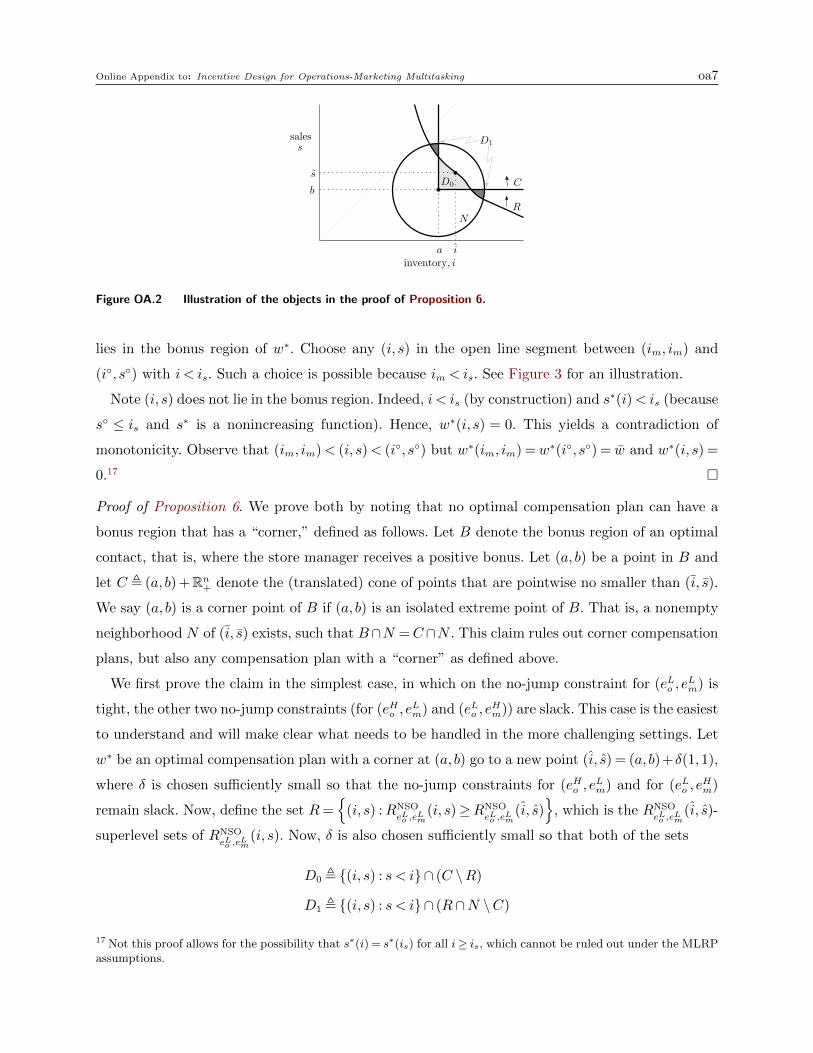
Online Appendix to: Incentive Design for Operations-Marketing Multitasking oa7
s
b
inventory, i
sales
a i
s
NR
CD0
D1
Figure OA.2 Illustration of the objects in the proof of Proposition 6.
lies in the bonus region of w∗. Choose any (i, s) in the open line segment between (im, im) and
(i◦, s◦) with i < is. Such a choice is possible because im < is. See Figure 3 for an illustration.
Note (i, s) does not lie in the bonus region. Indeed, i < is (by construction) and s∗(i)< is (because
s◦ ≤ is and s∗ is a nonincreasing function). Hence, w∗(i, s) = 0. This yields a contradiction of
monotonicity. Observe that (im, im)< (i, s)< (i◦, s◦) but w∗(im, im) =w∗(i◦, s◦) = w and w∗(i, s) =
0.17 �
Proof of Proposition 6. We prove both by noting that no optimal compensation plan can have a
bonus region that has a “corner,” defined as follows. Let B denote the bonus region of an optimal
contact, that is, where the store manager receives a positive bonus. Let (a, b) be a point in B and
let C , (a, b) +Rn+ denote the (translated) cone of points that are pointwise no smaller than (i, s).
We say (a, b) is a corner point of B if (a, b) is an isolated extreme point of B. That is, a nonempty
neighborhood N of (i, s) exists, such that B∩N =C∩N . This claim rules out corner compensation
plans, but also any compensation plan with a “corner” as defined above.
We first prove the claim in the simplest case, in which on the no-jump constraint for (eLo , eLm) is
tight, the other two no-jump constraints (for (eHo , eLm) and (eLo , e
Hm)) are slack. This case is the easiest
to understand and will make clear what needs to be handled in the more challenging settings. Let
w∗ be an optimal compensation plan with a corner at (a, b) go to a new point (i, s) = (a, b)+δ(1,1),
where δ is chosen sufficiently small so that the no-jump constraints for (eHo , eLm) and for (eLo , e
Hm)
remain slack. Now, define the set R={
(i, s) :RNSOeLo ,e
Lm
(i, s)≥RNSOeLo ,e
Lm
(i, s)}
, which is the RNSOeLo ,e
Lm
(i, s)-
superlevel sets of RNSOeLo ,e
Lm
(i, s). Now, δ is also chosen sufficiently small so that both of the sets
D0 , {(i, s) : s < i}∩ (C \R)
D1 , {(i, s) : s < i}∩ (R∩N \C)
17 Not this proof allows for the possibility that s∗(i) = s∗(is) for all i≥ is, which cannot be ruled out under the MLRPassumptions.
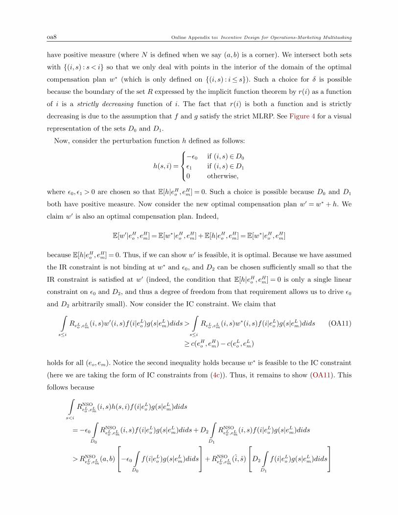
oa8 Online Appendix to: Incentive Design for Operations-Marketing Multitasking
have positive measure (where N is defined when we say (a, b) is a corner). We intersect both sets
with {(i, s) : s < i} so that we only deal with points in the interior of the domain of the optimal
compensation plan w∗ (which is only defined on {(i, s) : i≤ s}). Such a choice for δ is possible
because the boundary of the set R expressed by the implicit function theorem by r(i) as a function
of i is a strictly decreasing function of i. The fact that r(i) is both a function and is strictly
decreasing is due to the assumption that f and g satisfy the strict MLRP. See Figure 4 for a visual
representation of the sets D0 and D1.
Now, consider the perturbation function h defined as follows:
h(s, i) =
−ε0 if (i, s)∈D0
ε1 if (i, s)∈D1
0 otherwise,
where ε0, ε1 > 0 are chosen so that E[h|eHo , eHm] = 0. Such a choice is possible because D0 and D1
both have positive measure. Now consider the new optimal compensation plan w′ = w∗ + h. We
claim w′ is also an optimal compensation plan. Indeed,
E[w′|eHo , eHm] =E[w∗|eHo , eHm] +E[h|eHo , eHm] =E[w∗|eHo , eHm]
because E[h|eHo , eHm] = 0. Thus, if we can show w′ is feasible, it is optimal. Because we have assumed
the IR constraint is not binding at w∗ and ε0, and D2 can be chosen sufficiently small so that the
IR constraint is satisfied at w′ (indeed, the condition that E[h|eHo , eHm] = 0 is only a single linear
constraint on ε0 and D2, and thus a degree of freedom from that requirement allows us to drive ε0
and D2 arbitrarily small). Now consider the IC constraint. We claim that∫s≤i
ReLo ,eLm(i, s)w′(i, s)f(i|eLo )g(s|eLm)dids >
∫s≤i
ReLo ,eLm(i, s)w∗(i, s)f(i|eLo )g(s|eLm)dids (OA11)
≥ c(eHo , eHm)− c(eLo , eLm)
holds for all (eo, em). Notice the second inequality holds because w∗ is feasible to the IC constraint
(here we are taking the form of IC constraints from (4c)). Thus, it remains to show (OA11). This
follows because∫s<i
RNSOeLo ,e
Lm
(i, s)h(s, i)f(i|eLo )g(s|eLm)dids
=−ε0∫D0
RNSOeLo ,e
Lm
(i, s)f(i|eLo )g(s|eLm)dids+D2
∫D1
RNSOeLo ,e
Lm
(i, s)f(i|eLo )g(s|eLm)dids
>RNSOeLo ,e
Lm
(a, b)
−ε0 ∫D0
f(i|eLo )g(s|eLm)dids
+RNSOeLo ,e
Lm
(i, s)
D2
∫D1
f(i|eLo )g(s|eLm)dids
Online Appendix to: Incentive Design for Operations-Marketing Multitasking oa9
>R(a, b)
−ε0 ∫D0
f(i|eLo )g(s|eLm)dids+D2
∫D1
f(i|eLo )g(s|eLm)dids
= 0,
where the key fact in each step is that RNSOeLo ,e
Lm
(i, s) is coordinatewise strictly increasing. This implies
(OA11). Indeed, observe that it suffices to integrate in the region s < i to conclude the IC constraints
bind for w′ because w′(i, s) =w∗(i, s) for i= s (due to h(i, s) = 0 for i= s). We thus conclude w′ is
an optimal compensation plan.
In fact, we have shown something more in (OA11): the IC constraints are slack at optimal
compensation plan w′. However, because problem (2) is linear, every optimal compensation plan
must be on the boundary of the feasible region. This implies either w′ must bind the IR constraint,
which violates our assumption of positive rents, which is a contradiction. This completes the proof
in the special case of the argument in which only the no-jump constraint for (eLo , eLm) was initially
tight.
We now allow the possibility that at least one of the other two no-jump constraints is tight at
(a, b). In the case in which exactly one of the no-jump constraints for (eHo , eLm) or (eLo , e
Hm) is tight, an
argument largely analogous to the previous one can be conducted. Here, the region D1 will consist
of only one “piece” (the D1 in Figure OA.2 has two distinct pieces) because the no-jump constraints
for (eHo , eLm) or (eLo , e
Hm) correspond to horizontal and vertical superlevel sets for RNSO
eo,em(i, s) from
the discussion following (OA7). The difficulty here is that when both of the no-jump constraints for
(eHo , eLm) or (eLo , e
Hm) are tight, “room” remains to construct D1 as in Figure OA.2. In this setting,
we need to construct three regions, D0, D1, and D2, where a tradeoff exists between the value of
the perturbation in regions D1 and D2 to lead to a strictly increasing covariance as we were able
to show in (OA11).
To make this argument, we need the following definitions. We also move a distance δ along (1,1)
to the point (i, s). The superlevel set R and the region D0 are defined exactly as before. To define
D1 and D2, we need the following concepts. At (a, b), ReHo ,eLm(i, s) , R2(s) is constant in i at b
with value R1(b) and so we consider the horizontal line through the point (a, b). Where this line
intersects R is denoted (i1, b). The region D1 is chosen below the horizontal line to the right of
(i1, b), above R, and inside N . Similarly, ReLo ,eHm(i, s) , R2(i) is constant in s at a (at the value
R2(a)). The region D2 is chosen to the left of the vertical line above (a, s2) and above the lower
envelope of R. The specific sets D1 and D2 and δ are chosen so that an ε > 0 exists such that
E[R1(s)|D1]−R1(b)≤ ε and E[R2(i)|D2]−R2(a)≤ ε,
where (as used above) E[·] is the expectation with respect to distributions with effort (eHo , eHm).
From the regions D0, D1, and D2, we define the perturbation

oa10 Online Appendix to: Incentive Design for Operations-Marketing Multitasking
h(i, s) =
−ε0 if (i, s)∈D0
ε1 if (i, s)∈D1
ε2 if (i, s)∈D2
0 otherwise.
Using a logic similar to the simpler case above, it suffices to show that E[h(S, I)] = 0 and
E[R(S, I)h(S, I)]> 0. We now have three degrees of freedom, and so this is possible. For the con-
dition E[h(S, I)] = 0, this only requires
ε0P(D0) = ε1P(D1) + ε2P(D2),
where P[·] is the probability measure with respect to distributions with effort (eHo , eHm). As for the
covariance condition E[R(S, I)h(S, I)]> 0, this analysis is more delicate. We first show how to find
ε1 and ε2 such that
∫D0
R1(s)g(s)f(i)dsdi∫D0
g(s)f(i)dsdi
(ε1
∫D1
g(s)f(i)dsdi+ ε2
∫D2
g(s)f(i)dsdi
)< ε1
∫D1
R1(s)g(s)f(i)dsdi+ ε2
∫D2
R1(s)g(s)f(i)dsdi
and
∫D0
R2(i)g(s)f(i)dsdi∫D0
g(s)f(i)dsdi
(ε1
∫D1
g(s)f(i)dsdi+ ε2
∫D2
g(s)f(i)dsdi
)< ε1
∫D1
R2(i)g(s)f(i)dsdi+ ε2
∫D2
R2(i)g(s)f(i)dsdi.
To see that, we note the coefficient of ε1 in the first inequality is∫D1
R1(s)g(s)f(i)dsdi−∫D0
R1(s)g(s)f(i)dsdi∫D0
g(s)f(i)dsdi
∫D1
g(s)f(i)dsdi > 0,
and the coefficient of ε1 in the second inequality is∫D1
R2(i)g(s)f(i)dsdi−∫D0
R2(i)g(s)f(i)dsdi∫D0
g(s)f(i)dsdi
∫D1
g(s)f(i)dsdi < 0.
Therefore, the existence of such ε1 and ε2 depends on
∫D0
R2(i)g(s)f(i)dsdi∫D0
g(s)f(i)dsdi
∫D2g(s)f(i)dsdi−
∫D2R2(i)g(s)f(i)dsdi∫
D1R2(i)g(s)f(i)dsdi−
∫D0
R2(i)g(s)f(i)dsdi∫D0
g(s)f(i)dsdi
∫D1g(s)f(i)dsdi
>ε1ε2>
∫D0
R1(s)g(s)f(i)dsdi∫D0
g(s)f(i)dsdi
∫D2g(s)f(i)dsdi−
∫D2R1(s)g(s)f(i)dsdi∫
D1R1(s)g(s)f(i)dsdi−
∫D0
R1(s)g(s)f(i)dsdi∫D0
g(s)f(i)dsdi
∫D1g(s)f(i)dsdi
.

Online Appendix to: Incentive Design for Operations-Marketing Multitasking oa11
The sufficient condition is∫D2
R2(i)g(s)f(i)dsdi∫D2
g(s)f(i)dsdi−
∫D0
R2(i)g(s)f(i)dsdi∫D0
g(s)f(i)dsdi∫D0
R2(i)g(s)f(i)dsdi∫D0
g(s)f(i)dsdi−
∫D1
R2(i)g(s)f(i)dsdi∫D1
g(s)f(i)dsdi
>
∫D0
R1(s)g(s)f(i)dsdi∫D0
g(s)f(i)dsdi−
∫D2
R1(s)g(s)f(i)dsdi∫D2
g(s)f(i)dsdi∫D1
R1(s)g(s)f(i)dsdi∫D1
g(s)f(i)dsdi−
∫D0
R1(s)g(s)f(i)dsdi∫D0
g(s)f(i)dsdi
.
We can choose D0 such that∫D0R2(i)g(s)f(i)dsdi∫D0g(s)f(i)dsdi
−R2(a)≤ ε and
∫D0R1(s)g(s)f(i)dsdi∫D0g(s)f(i)dsdi
−R1(b)≤ ε.
Choose D1 and D2 to make∫D2
R2(i)g(s)f(i)dsdi∫D2
g(s)f(i)dsdias large as possible and
∫D1
R2(i)g(s)f(i)dsdi∫D1
g(s)f(i)dsdias close to
R2(a) as possible (indeed the distance is also controlled by ε), and∫D2
R1(s)g(s)f(i)dsdi∫D2
g(s)f(i)dsdias large as
possible. Then, it suffices to have∫D2
R2(i)g(s)f(i)dsdi∫D2
g(s)f(i)dsdi−
∫D0
R2(i)g(s)f(i)dsdi∫D0
g(s)f(i)dsdi∫D0
R2(i)g(s)f(i)dsdi∫D0
g(s)f(i)dsdi−R2(a) + ε
>
∫D0
R1(s)g(s)f(i)dsdi∫D0
g(s)f(i)dsdi− (R1(s)− ε)∫
D1R1(s)g(s)f(i)dsdi∫D1
g(s)f(i)dsdi−
∫D0
R1(s)g(s)f(i)dsdi∫D0
g(s)f(i)dsdi
.
Note both∫D2
R2(i)g(s)f(i)dsdi∫D2
g(s)f(i)dsdiand
∫D2
R1(s)g(s)f(i)dsdi∫D1
g(s)f(i)dsdican be sufficiently large. In the limit case, we
can make ∫D2
R2(i)g(s)f(i)dsdi∫D2
g(s)f(i)dsdi−R2(a)
2ε>
2ε∫D1
R1(s)g(s)f(i)dsdi∫D1
g(s)f(i)dsdi−R1(b)
,
which is always possible. �
Proof of Proposition 9: The proof of parts (i) and (ii) are similar to that of Proposition 1. Due to
Theorem 2 there exists an optimal information trigger contract involving likelihood ratio functions
Reo,em(i, z) as described in (19) and (20).
For part (i), note that (∗) equals∫ Qi
1q−iϕ( z−i
q−i )g(q|eLm)dq∫ Qi
1q−iϕ( z−i
q−i )g(q|eHm)dq=
∫ Qi
1q−iϕ( z−i
q−i )g(q|eLm)dq∫ Qi
1q−iϕ( z−i
q−i )g(q|eHm)
g(q|eLm)g(q|eLm)dq
≤ 1g(i|eHm)
g(i|eLm)
,
which is bounded, where g(q|eHm)
g(q|eLm)≥ g(i|eHm)
g(i|eLm)by MLRP. Now, as
∫ Qi
1q−iϕ( z−i
q−i )g(q|eLm)dq→∞, it must
be that∫ Qi
1q−iϕ( z−i
q−i )g(q|eHm)
g(q|eLm)g(q|eLm)dq→∞ as well. First, by changes of varibles, ς = q− i,∫ Q−i
01ςϕ( z−i
ς)g(ς + i|eLm)dς∫ Q
01ςϕ( z−i
ς)g(ς + i|eHm)dς
= limε→0
∫ Q−iε
1ςϕ( z−i
ς)g(ς + i|eLm)dς∫ Q
ε1ςϕ( z−i
ς)g(ς + i|eHm)dς
.
Therefore, by L’Hopital’s rule, we have
limε→0
∫ Q−iε
1ςϕ( z−i
ς)g(ς + i|eLm)dς∫ Q
ε1ςϕ( z−i
ς)g(ς + i|eHm)dς
= limε→0
1εϕ( z−i
ε)g(ε+ i|eLm)
1εϕ( z−i
ε)g(ε+ i|eHm)
=g(i|eLm)
g(i|eHm),
oa12 Online Appendix to: Incentive Design for Operations-Marketing Multitasking
which is independent of z. This establishes the result, because it also implies RLSeo,em
(i, z) =
RNLSeo,em
(i, z) at z = i, and so BNLS has the structure expressed in the result.
For part (ii), we show RLS(i, z|eo, em) is nondecreasing in z. This suffices to show an i` ∈ (0, I]
exists such that
BLS = {(i, z) : i≤ i` and `∗(i)≤ z ≤ Q}∪ {(i, z) : i≥ i` and i≤ z ≤ Q},
using an argument analogous to that of Proposition 1. The final part of the proof argues i` = is,
establishing the result.
To establish the first part of the argument, we first claim (∗) in (20) is nonincreasing in z under
Assumption 1. First, we can write∫ Q
i
γ′(z|q, i)g(q|em)dq=
∫ Q
i
γ′(z|q, i)γ(z|q, i)
g(q|em)
g(q|e∗m)γ(z|q, i)g(q|e∗m)dq.
Note γ′(z|q,i)γ(z|q,i) is nondecreasing in q by Assumption 1, g(q|em)
g(q|e∗m)is nonincreasing in q. Therefore, the
two functions γ′(z|q,i)γ(z|q,i) and g(q|em)
g(q|e∗m)are negatively correlated given any z. Therefore,∫ Q
i
γ′(z|q,i)γ(z|q,i)
g(q|em)
g(q|e∗m)γ(z|q, i)g(q|e∗m)dq∫ Q
iγ(z|q, i)g(q|e∗m)dq
≤∫ Qi
γ′(z|q,i)γ(z|q,i) γ(z|q, i)g(q|e∗m)dq∫ Qiγ(z|q, i)g(q|e∗m)dq
∫ Qi
g(q|em)
g(q|e∗m)γ(z|q, i)g(q|e∗m)dq∫ Q
iγ(z|q, i)g(q|e∗m)dq
.
By canceling out one of the∫ Qiγ(z|q, i)g(q|e∗m)dq in the denominator, we obtain∫ Q
i
γ′(z|q, i)γ(z|q, i)
g(q|em)
g(q|e∗m)γ(z|q, i)g(q|e∗m)dq ≤
∫ Q
i
γ′(z|q, i)γ(z|q, i)
γ(z|q, i)g(q|e∗m)dq
∫ Qi
g(q|em)
g(q|e∗m)γ(z|q, i)g(q|e∗m)dq∫ Q
iγ(z|q, i)g(q|e∗m)dq
=
∫ Q
i
γ′(z|q, i)g(q|e∗m)dq
∫ Qiγ(z|q, i)g(q|em)dq∫ Q
iγ(z|q, i)g(q|e∗m)dq
.
It remains to show is and i` are equal. This requires that RLSeo,em
(i, i) =RNSLeo,em
(i, i), which occurs
if ∫ qiγ(i|q, i)g(q|em)dq∫ q
iγ(z|q, i)g(q|e∗m)dq
=g(i|em)
g(i|e∗m).
But this holds because Λ∈ (0,1), and so γ(i|q, i)dq is the Dirac measure δ(i= q), thus yielding the
result.
Proof of Proposition 10: It suffices to show∫ Qi γ(z|q,i)g(q|em)dq∫ Qi γ(z|q,i)g(q|e∗m)dq
is nonincreasing in i. We need
∂
∂i
[∫ Qiγ(z|q, i)g(q|em)dq∫ Q
iγ(z|q, i)g(q|e∗m)dq
]≤ 0.
It is equivalent to show
−h(i|q, i)g(i|em) +∫ Qi
∂∂iγ(z|q, i)g(q|em)dq∫ Q
iγ(z|q, i)g(q|em)dq
−−h(i|q, i)g(i|e∗m) +
∫ Qi
∂∂iγ(z|q, i)g(q|e∗m)dq∫ Q
iγ(z|q, i)g(q|e∗m)dq
≤ 0.

Online Appendix to: Incentive Design for Operations-Marketing Multitasking oa13
The fact that
−h(i|q, i)g(i|em)∫ Qiγ(z|q, i)g(q|em)dq
+h(i|q, i)g(i|e∗m)∫ Q
iγ(z|q, i)g(q|e∗m)dq
< 0
is due to Assumption 1: ∫ Qiγ(z|q, i)g(q|e∗m)dq∫ Q
iγ(z|q, i)g(q|em)dq
>g(i|e∗m)
g(i|em).
It remains to show ∫ Qi
∂∂iγ(z|q, i)g(q|em)dq∫ Q
iγ(z|q, i)g(q|em)dq
≤∫ Qi
∂∂iγ(z|q, i)g(q|e∗m)dq∫ Q
iγ(z|q, i)g(q|e∗m)dq
.
By Young’s Theorem, Assumption 2 implies∂∂iγ(z|q,i)γ(z|q,i) is nondecreasing in q, and so we have
∫ Q
i
∂
∂iγ(z|q, i)g(q|em)dq
=
∫ Q
i
∂∂iγ(z|q, i)γ(z|q, i)
g(q|em)
g(q|e∗m)γ(z|q, i)g(q|e∗m)dq
≤∫ Q
i
∂∂iγ(z|q, i)γ(z|q, i)
γ(z|q, i)g(q|e∗m)dq
∫ Qi
g(q|em)
g(q|e∗m)γ(z|q, i)g(q|e∗m)dq∫ Q
iγ(z|q, i)g(q|e∗m)dq
=
∫ Q
i
∂
∂iγ(z|q, i)g(q|e∗m)dq
∫ Qiγ(z|q, i)g(q|em)dq∫ Q
iγ(z|q, i)g(q|e∗m)dq
,
which shows the desired inequality.
Proof of Proposition 12. First, note f(i|eo) may potentially involve I, so we do some transformation.
Let τ = i/I be the ratio. Suppose τ ∈ [0,1] has a distribution F (τ |eo), which is independent of I.
Then, F (i|eo) = F (i/I|eo) and f(i|eo) = 1If(i/I|eo).
We denote s(µ,λ, τ) as the cut-off solving µ+∑
j λj(1−g(s|ejm)f(τ |ejo)
g(s|e∗m)f(τ |e∗o)) = 1 for s < τ I, where j is the
index for the j-th IC constraint. And denote τs(µ,λ) as the minimum solution for s(µ,λ, τ) = τ I,
τm(µ,λ) as the minimum solution for µ+∑
j λj(1−(1−G(τI|ejm))f(τ |ejo)
(1−G(τIs|e∗m))f(τ |e∗o)) = 1.
By strong duality, and Theorem 2, we have
−W (I) = minµ,λ
φ(µ,λ, I)
= minµ,λ
∫ 1
τs(µ,λ)
∫ τI
s(µ,λ,τ)
(−1 +µ+
∑j
λj(1−g(s|ejm)f(τ |ejo)g(s|e∗m)f(τ |e∗o)
)
)g(s|e∗m)f(τ |e∗o)dsdτ
+
∫ 1
τm(µ,λ)
(−1 +µ+
∑j
λj(1−(1−G(τ I|ejm))f(τ |ejo)(1−G(τ Is|e∗m))f(τ |e∗o)
)
)(1−G(τ Is|e∗m))f(τ |e∗o)dτ
−∑j
λj[c(e∗)− c(ej)]−µ[c(e∗) +U ].

oa14 Online Appendix to: Incentive Design for Operations-Marketing Multitasking
Note the dual is convex in (µ,λ). Let (µ∗, λ∗) be the solution of the dual minimization. Then, by
the envelope theorem, we have
−dW (I)
dI=
∂
∂Iφ(µ∗, λ∗, I)
=
∫ 1
τs(µ∗,λ∗)τ
(−1 +µ∗+
∑j
λ∗j (1−g(τ I|ejm)f(τ |ejo)g(τ I|e∗m)f(τ |e∗o)
)
)g(τ I|e∗m)f(τ |e∗o)dτ
−∫ 1
τm(µ∗,λ∗)τ
((−1 +µ∗)g(τ I|e∗m)f(τ |e∗o) +
∑j
λ∗j [g(τ I|e∗m)f(τ |e∗o)− g(τ I|ejm))f(τ |ejo)]
)dτ
= −∫ τs(µ∗,λ∗)
τm(µ∗,λ∗)τ
(−1 +µ∗+
∑j
λ∗j (1−g(τ I|ejm)f(τ |ejo)g(τ I|e∗m)f(τ |e∗o)
)
)g(τ I|e∗m)f(τ |e∗o)dτ
> −
(−1 +µ∗+
∑j
λ∗j (1−g(τs(µ
∗, λ∗)I|ejm)f(τs(µ∗, λ∗)|ejo)
g(τs(µ∗, λ∗)I|e∗m)f(τs(µ∗, λ∗)|e∗o))
)∫ τs(µ∗,λ∗)
τm(µ∗,λ∗)τg(τ I|e∗m)f(τ |e∗o)dτ = 0,
where the inequality is by MLRP and τs(µ∗, λ∗)≥ τm(µ∗, λ∗).
OA.2. Numerical Illustration of a Mast-and-Sail Compensation Plan
We now use a numerical example to illustrate an optimal bonus region of the “mast and sail”
structure (as seen in Figure 2(a)) in the case of outcome distributions that satisfy the MLRP.
This example shows the delicacy of numerical computation in this setting, which is typical of
moral hazard problems. Our extensive numerical simulations use similar logic to that found in this
example.
Example OA.1. Consider the following instance of the multitasking store manager. The distri-
bution functions of operating and marketing effort are F (i|eo) = ieo and G(s|em) = sem , respectively,
where eo ∈ {eLo , eHo } and em ∈ {eLm, eHm}, where eLo = eLm = 1 and eHo = eHm = 2. The target action is
(eHo , eHm) = (2,2). The cost function is c(eHo , e
Hm) = 5, c(eHo , e
Lm) = c(eLo , e
Hm) = 4 and c(eLo , e
Lm) = 2.
The resource constraint for the firm has w= 10.
For now, we suppose an optimal choice of ω (as guaranteed to exist by Theorem 2) has ωeLo ,eLm = 1
and ωeHo ,eLm = ωeLo ,eHm = 0. We construct the associated trigger value t below, and also show the
resulting compensation plan with these choices of parameters is indeed feasible to (4) and thus
optimal.
The condition RNSOeo,em
(i, s)≥ t can be expressed as
1− t≥ f(i|eo)g(s|em)
f(i|eHo )g(s|eHm)= eo
eHo
emeHmieo−e
Ho sem−e
Hm
and the condition RSOeo,em
(i)≥ t amounts to
1− t≥ eoieo−1(1−iem )
eHo ieHo −1(1−ieHm )
.
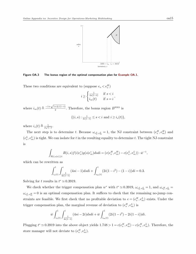
Online Appendix to: Incentive Design for Operations-Marketing Multitasking oa15
s
.5355 = iminventory, i
sales
is = .6412
B
1
Figure OA.3 The bonus region of the optimal compensation plan for Example OA.1.
These two conditions are equivalent to (suppose eo < eHo )
i≥
{1
4s(1−t) if s < i
im(t) if s= i,
where im(t),−1+√
1+2/(1−t)2
. Therefore, the bonus region BNSO is
{(i, s) : 14i(1−t) ≤ s < i and i≥ is(t)},
where is(t), 12√
1−t .
The next step is to determine t. Because ωeLo ,eLm = 1, the NJ constraint between (eHo , eHm) and
(eLo , eLm) is tight. We can isolate for t in the resulting equality to determine t. The tight NJ constraint
is ∫R(i,s|e)≥t
R(i, s)f(i|e∗o)g(s|e∗m)dsdi= (c(eHo , eHm)− c(eLo , eLm)) · w−1,
which can be rewritten as∫ 1
is(t)
∫ i
14i(1−t)
(4si− 1)dsdi+
∫ 1
im(t)
(2i(1− i2)− (1− i))di= 0.3.
Solving for t results in t∗ ' 0.3919.
We check whether the trigger compensation plan w∗ with t∗ ' 0.3919, ωeLo ,eLm = 1, and ωeHo ,eLm =
ωeLo ,eHm = 0 is an optimal compensation plan. It suffices to check that the remaining no-jump con-
straints are feasible. We first check that no profitable deviation to e= (eHo , eLm) exists. Under the
trigger compensation plan, the marginal revenue of deviation to (eHo , eLm) is
w
∫ 1
is(t)
∫ i
14i(1−t)
(4si− 2i)dsdi+ w
∫ 1
im(t)
(2i(1− i2)− 2i(1− i))di.
Plugging t∗ ' 0.3919 into the above object yields 1.748> 1 = c(eHo , eHm)− c(eHo , eLm). Therefore, the
store manager will not deviate to (eHo , eLm).

oa16 Online Appendix to: Incentive Design for Operations-Marketing Multitasking
Similarly, the store manager’s marginal revenue of deviation to (eLo , eHm) is
w
∫ 1
is(t)
∫ i
14i(1−t)
(4si− 2s)dsdi+ w
∫ 1
im(t)
(2i(1− i2)− (1− i2))di.
Plugging t∗ ' 0.3919 into the above object yields 1.864 > 1 = c(eHo , eHm) − c(eLo , eHm). Therefore,
the store manager will not deviate to (eLo , eHm). The bonus region is illustrated in Figure OA.3.
Note im(t∗) = 0.5355< is(t∗) = 0.6412, and so we have a mast-and-sail bonus region as plotted in
Figure OA.3. Under this optimal compensation plan, the probability of payout under the optimal
mast-and-sail compensation plan is 51.96%.
OA.3. Numerical Illustrations of Corner Compensation Plans
To give a sense of how to compute the optimal corner compensation plan we give two concrete
examples. These examples refer to some auxiliary results in the same online appendix that help us
analyze corner compensation plans.
Example OA.2 (Example OA.1 continued). Returning to the set up in Example OA.1, the
optimal corner compensation plan solves problem (14) and can be simply stated as:
mina,b
(1− b2)(1− a2)
s.t. (1− b2)(1− a2)− (1− b)(1− a)≥ 0.3
(1− b2)(1− a2)− (1− b2)(1− a)≥ 0.2
(1− b2)(1− a2)− (1− b)(1− a2)≥ 0.2
b≤ a.
Note we have formulated the objective to minimize the expected probability of paying out the
bonus w (following Proposition 7), which is equivalent to the objective function (14a).
Now, the optimality condition for the optimal corner compensation plan
Hf (a|e∗o)Hg(b|e∗m)
=Hf (a|eo)Hg(b|em)
from equation (15) implies
2a(1−a2)
2b(1−b2)
=
1(1−a)
1(1−b)
,
which yields a = b. Combined with the other case of Proposition 8, we have a = b in optimality.
In this case, we can show the optimal choice of ω has ωeLo ,eLm = 1 and ωeHo ,eLm = ωeLo ,eHm = 0. The
optimal corner compensation plan can be obtained through solving (1− b2)(1− b2)− (1− b)2 = 0.3,
which yields b∗ = 0.5234. Under the optimal corner compensation plan, the probability of payout
is 0.5271. By comparison, the probability of payout under the optimal mast-and-sail compensation
plan is 0.5196. So the performance gap is (0.5271-0.5196)/0.5196=1.44%.
Online Appendix to: Incentive Design for Operations-Marketing Multitasking oa17
Example OA.3. Consider an instance with the same setting as in Example OA.1 except that
the cost functions are as follows: c(eHo , eHm) = 3.4, c(eHo , e
Lm) = 1.5, c(eLo , e
Hm) = 1.8, and c(eLo , e
Lm) = 1.
In this case, we can show the optimal choice of ω has ωeHo ,eLm = 1 and ωeLo ,eLm = ωeLo ,eHm = 0. Thus,
we can solve for b∗ by setting (1− b2)(1− b2)− (1− b2)(1− b) = 0.19, which yields b∗ = 0.4896,
which corresponds to a probability of payout of 0.5781. By comparison, the optimal mast-and-sail
compensation plan has a probability of payout of 0.5148. Thus, using a corner compensation plan
leads to an efficiency loss of (0.5781− 0.5148)/0.5148 = 12.30%.
OA.4. Fully Observed Demand
A natural benchmark is to look at the scenario where demand is fully observed and not censored by
inventory; that is, both the firm and store manager can observe Q. This situation is much simpler
than the case of censored demand. The analysis in Section 4 still applies and it can be shown that
Reo,em(i, q) = 1− f(i|eo)g(q|em)
f(i|e∗o)g(q|e∗m), which is precisely what we analyzed before as RNSO
eo,em(i, s) in (9) for
s≤ i. Similar reasoning thus yields the result:
Proposition OA1. A nonincreasing and continuous function qf exists such that an optimal
contract wf to the fully observed demand exists with the form
wf (i, q) =
{w if (i, q)∈Bf
0 otherwise,
where Bf = {(i, q) : q≥ qf (i)}.
Recall, just as in Proposition 1 for s∗, the domain of the function qf need not be all of [0, I], and
an i may exist such that Bf ⊆ [i, I]× [0, Q]. Thus, the bonus region of the optimal contract in the
fully observed demand case is an “expanded sail” that is not truncated by the 45◦ line.
Next, we use a numerical experiment to demonstrate the efficiency loss due to demand censoring,
by comparing the firm’s expected additional payment to the store manager — compared to the
first-best scenario — for inducing the same effort level. We illustrate our result in Figure OA.4.
OA.5. Approximating Mast-and-Sail Contracts
In this section, we consider approximating mast-and-sail contracts when we allow these contracts to
be nonmonotone in nature, in contrast to Section 7.2, where attention was restricted to monotone
approximations. The purpose of this exercise is to understand what aspects of the mast-and-sail
structure are driving optimality.
We consider the following three nonmonotone approximations, in addition to weighted-sum
threshold policies:
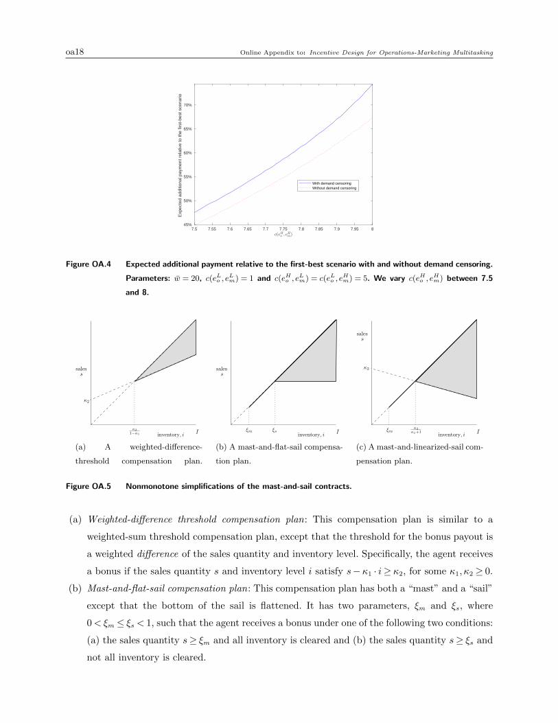
oa18 Online Appendix to: Incentive Design for Operations-Marketing Multitasking
7.5 7.55 7.6 7.65 7.7 7.75 7.8 7.85 7.9 7.95 845%
50%
55%
60%
65%
70%
Exp
ecte
d ad
ditio
nal p
aym
ent r
elat
ive
to th
e fir
st-b
est s
cena
rioWith demand censoringWithout demand censoring
Figure OA.4 Expected additional payment relative to the first-best scenario with and without demand censoring.
Parameters: w = 20, c(eLo , eLm) = 1 and c(eHo , e
Lm) = c(eLo , e
Hm) = 5. We vary c(eHo , e
Hm) between 7.5
and 8.
κ2
1−κ1 I
s
inventory, i
sales
κ2
(a) A weighted-difference-
threshold compensation plan.
I
s
inventory, i
sales
ξsξm
(b) A mast-and-flat-sail compensa-
tion plan.
I
s
inventory, i
sales
κ2
κ1+1ξm
κ2
(c) A mast-and-linearized-sail com-
pensation plan.
Figure OA.5 Nonmonotone simplifications of the mast-and-sail contracts.
(a) Weighted-difference threshold compensation plan: This compensation plan is similar to a
weighted-sum threshold compensation plan, except that the threshold for the bonus payout is
a weighted difference of the sales quantity and inventory level. Specifically, the agent receives
a bonus if the sales quantity s and inventory level i satisfy s−κ1 · i≥ κ2, for some κ1, κ2 ≥ 0.
(b) Mast-and-flat-sail compensation plan: This compensation plan has both a “mast” and a “sail”
except that the bottom of the sail is flattened. It has two parameters, ξm and ξs, where
0< ξm ≤ ξs < 1, such that the agent receives a bonus under one of the following two conditions:
(a) the sales quantity s≥ ξm and all inventory is cleared and (b) the sales quantity s≥ ξs and
not all inventory is cleared.
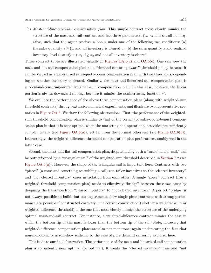
Online Appendix to: Incentive Design for Operations-Marketing Multitasking oa19
(c) Mast-and-linearized-sail compensation plan: This simple contract most closely mimics the
structure of the mast-and-sail contract and has three parameters, ξm, κ1 and κ2, all nonneg-
ative, such that the agent receives a bonus under one of the following two conditions: (a)
the sales quantity s≥ ξm and all inventory is cleared or (b) the sales quantity s and realized
inventory level i satisfy s+κ1 · i≥ κ2 and not all inventory is cleared.
These contract types are illustrated visually in Figures OA.5(a) and OA.5(c). One can view the
mast-and-flat-sail compensation plan as a “demand-censoring-aware” threshold policy because it
can be viewed as a generalized sales-quota-bonus compensation plan with two thresholds, depend-
ing on whether inventory is cleared. Similarly, the mast-and-linearized-sail compensation plan is
a “demand-censoring-aware” weighted-sum compensation plan. In this case, however, the linear
portion is always downward sloping, because it mimics the nonincreasing function s∗.
We evaluate the performance of the above three compensation plans (along with weighted-sum
threshold contracts) through extensive numerical experiments, and illustrate two representative sce-
narios in Figure OA.6. We draw the following observations. First, the performance of the weighted-
sum threshold compensation plan is similar to that of the corner (or sales-quota-bonus) compen-
sation plan in that it is near optimal when the marketing and operational activities are sufficiently
complementary (see Figure OA.6(a)), yet far from the optimal otherwise (see Figure OA.6(b)).
Interestingly, the weighted-difference threshold compensation plan performs reasonably well in the
latter case.
Second, the mast-and-flat-sail compensation plan, despite having both a “mast” and a “sail,” can
be outperformed by a “triangular sail” of the weighted-sum threshold described in Section 7.2 (see
Figure OA.6(a)). However, the shape of the triangular sail is important here. Contracts with two
“pieces” (a mast and something resembling a sail) can tailor incentives to the “cleared inventory”
and “not cleared inventory” cases in isolation from each other. A single “piece” contract (like a
weighted threshold compensation plan) needs to effectively “bridge” between these two cases by
designing the transition from “cleared inventory” to “not cleared inventory.” A perfect “bridge” is
not always possible to build, but our experiments show single-piece contracts with strong perfor-
mance are possible if constructed correctly. The correct construction (whether a weighted-sum or
weighted-difference threshold) is the one that most closely mimics the structure of the underlying
optimal mast-and-sail contract. For instance, a weighted-difference contract mimics the case in
which the bottom tip of the mast is lower than the bottom tip of the sail. Note, however, that
weighted-difference compensation plans are also not monotone, again underscoring the fact that
non-monotonicity is somehow endemic to the case of pure demand censoring explored here.
This leads to our final observation. The performance of the mast-and-linearized-sail compensation
plan is consistently near optimal (or optimal). It treats the “cleared inventory” case and “not
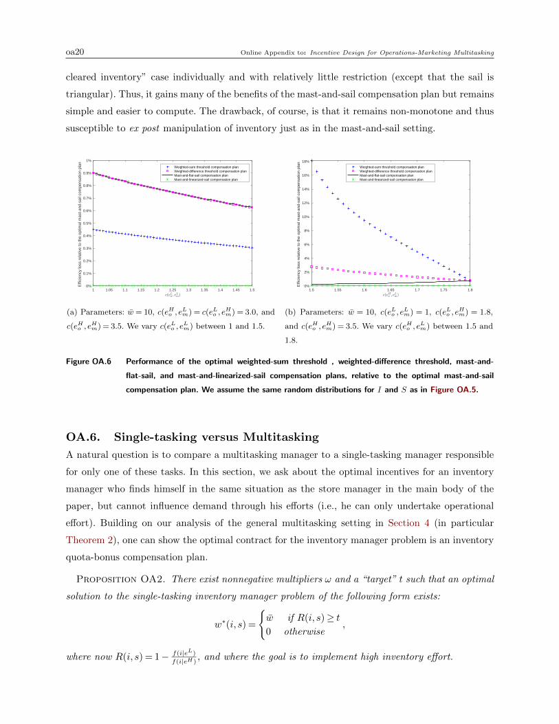
oa20 Online Appendix to: Incentive Design for Operations-Marketing Multitasking
cleared inventory” case individually and with relatively little restriction (except that the sail is
triangular). Thus, it gains many of the benefits of the mast-and-sail compensation plan but remains
simple and easier to compute. The drawback, of course, is that it remains non-monotone and thus
susceptible to ex post manipulation of inventory just as in the mast-and-sail setting.
1 1.05 1.1 1.15 1.2 1.25 1.3 1.35 1.4 1.45 1.50%
0.1%
0.2%
0.3%
0.4%
0.5%
0.6%
0.7%
0.8%
0.9%
1%
Effi
cien
cy lo
ss r
elat
ive
to th
e op
timal
mas
t-an
d-sa
il co
mpe
nsat
ion
plan Weighted-sum threshold compensation plan
Weighted-difference threshold compensation planMast-and-flat-sail compensation planMast-and-linearized-sail compensation plan
(a) Parameters: w = 10, c(eHo , eLm) = c(eLo , e
Hm) = 3.0, and
c(eHo , eHm) = 3.5. We vary c(eLo , e
Lm) between 1 and 1.5.
1.5 1.55 1.6 1.65 1.7 1.75 1.80%
2%
4%
6%
8%
10%
12%
14%
16%
18%
Effi
cien
cy lo
ss r
elat
ive
to th
e op
timal
mas
t-an
d-sa
il co
mpe
nsat
ion
plan Weighted-sum threshold compensation plan
Weighted-difference threshold compensation planMast-and-flat-sail compensation planMast-and-linearized-sail compensation plan
(b) Parameters: w = 10, c(eLo , eLm) = 1, c(eLo , e
Hm) = 1.8,
and c(eHo , eHm) = 3.5. We vary c(eHo , e
Lm) between 1.5 and
1.8.
Figure OA.6 Performance of the optimal weighted-sum threshold , weighted-difference threshold, mast-and-
flat-sail, and mast-and-linearized-sail compensation plans, relative to the optimal mast-and-sail
compensation plan. We assume the same random distributions for I and S as in Figure OA.5.
OA.6. Single-tasking versus Multitasking
A natural question is to compare a multitasking manager to a single-tasking manager responsible
for only one of these tasks. In this section, we ask about the optimal incentives for an inventory
manager who finds himself in the same situation as the store manager in the main body of the
paper, but cannot influence demand through his efforts (i.e., he can only undertake operational
effort). Building on our analysis of the general multitasking setting in Section 4 (in particular
Theorem 2), one can show the optimal contract for the inventory manager problem is an inventory
quota-bonus compensation plan.
Proposition OA2. There exist nonnegative multipliers ω and a “target” t such that an optimal
solution to the single-tasking inventory manager problem of the following form exists:
w∗(i, s) =
{w if R(i, s)≥ t0 otherwise
,
where now R(i, s) = 1− f(i|eL)
f(i|eH ), and where the goal is to implement high inventory effort.
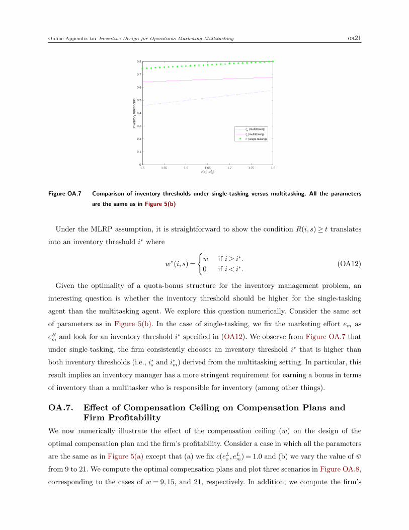
Online Appendix to: Incentive Design for Operations-Marketing Multitasking oa21
1.5 1.55 1.6 1.65 1.7 1.75 1.80
0.1
0.2
0.3
0.4
0.5
0.6
0.7
0.8
Inve
ntor
y th
resh
olds
im (multitasking)
is (multitasking)
i (single-tasking)
Figure OA.7 Comparison of inventory thresholds under single-tasking versus multitasking. All the parameters
are the same as in Figure 5(b)
Under the MLRP assumption, it is straightforward to show the condition R(i, s)≥ t translates
into an inventory threshold i∗ where
w∗(i, s) =
{w if i≥ i∗.0 if i < i∗.
(OA12)
Given the optimality of a quota-bonus structure for the inventory management problem, an
interesting question is whether the inventory threshold should be higher for the single-tasking
agent than the multitasking agent. We explore this question numerically. Consider the same set
of parameters as in Figure 5(b). In the case of single-tasking, we fix the marketing effort em as
eHm and look for an inventory threshold i∗ specified in (OA12). We observe from Figure OA.7 that
under single-tasking, the firm consistently chooses an inventory threshold i∗ that is higher than
both inventory thresholds (i.e., i∗s and i∗m) derived from the multitasking setting. In particular, this
result implies an inventory manager has a more stringent requirement for earning a bonus in terms
of inventory than a multitasker who is responsible for inventory (among other things).
OA.7. Effect of Compensation Ceiling on Compensation Plans andFirm Profitability
We now numerically illustrate the effect of the compensation ceiling (w) on the design of the
optimal compensation plan and the firm’s profitability. Consider a case in which all the parameters
are the same as in Figure 5(a) except that (a) we fix c(eLo , eLm) = 1.0 and (b) we vary the value of w
from 9 to 21. We compute the optimal compensation plans and plot three scenarios in Figure OA.8,
corresponding to the cases of w = 9,15, and 21, respectively. In addition, we compute the firm’s
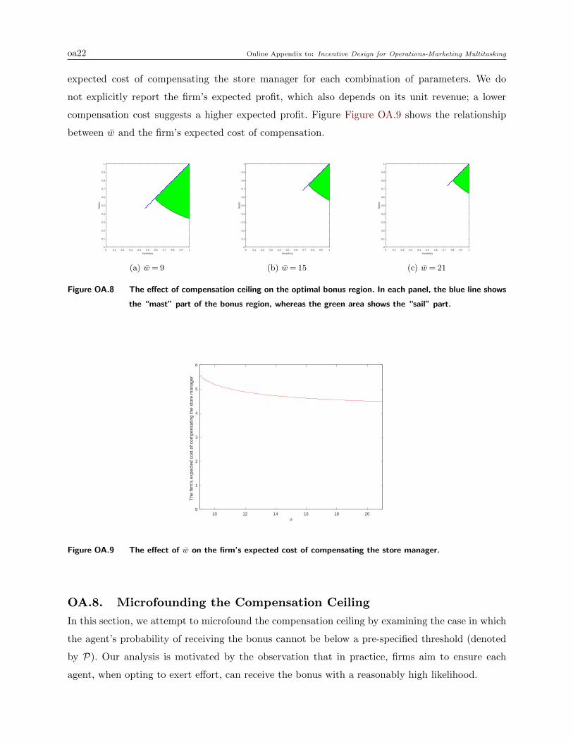
oa22 Online Appendix to: Incentive Design for Operations-Marketing Multitasking
expected cost of compensating the store manager for each combination of parameters. We do
not explicitly report the firm’s expected profit, which also depends on its unit revenue; a lower
compensation cost suggests a higher expected profit. Figure Figure OA.9 shows the relationship
between w and the firm’s expected cost of compensation.
0 0.1 0.2 0.3 0.4 0.5 0.6 0.7 0.8 0.9 1
Inventory
0
0.1
0.2
0.3
0.4
0.5
0.6
0.7
0.8
0.9
1
Sal
es
(a) w= 9
0 0.1 0.2 0.3 0.4 0.5 0.6 0.7 0.8 0.9 1
Inventory
0
0.1
0.2
0.3
0.4
0.5
0.6
0.7
0.8
0.9
1
Sal
es
(b) w= 15
0 0.1 0.2 0.3 0.4 0.5 0.6 0.7 0.8 0.9 1
Inventory
0
0.1
0.2
0.3
0.4
0.5
0.6
0.7
0.8
0.9
1
Sal
es
(c) w= 21
Figure OA.8 The effect of compensation ceiling on the optimal bonus region. In each panel, the blue line shows
the “mast” part of the bonus region, whereas the green area shows the “sail” part.
10 12 14 16 18 200
1
2
3
4
5
6
The
firm
's e
xpec
ted
cost
of c
ompe
nsat
ing
the
stor
e m
anag
er
Figure OA.9 The effect of w on the firm’s expected cost of compensating the store manager.
OA.8. Microfounding the Compensation Ceiling
In this section, we attempt to microfound the compensation ceiling by examining the case in which
the agent’s probability of receiving the bonus cannot be below a pre-specified threshold (denoted
by P). Our analysis is motivated by the observation that in practice, firms aim to ensure each
agent, when opting to exert effort, can receive the bonus with a reasonably high likelihood.
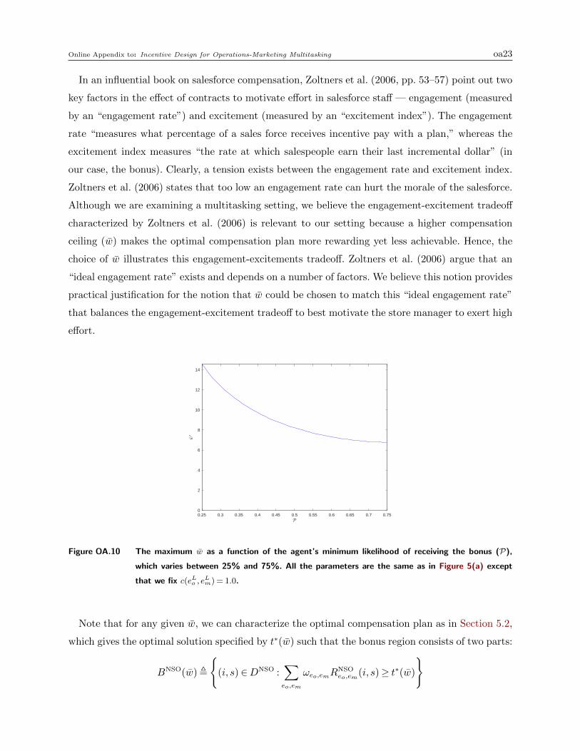
Online Appendix to: Incentive Design for Operations-Marketing Multitasking oa23
In an influential book on salesforce compensation, Zoltners et al. (2006, pp. 53–57) point out two
key factors in the effect of contracts to motivate effort in salesforce staff — engagement (measured
by an “engagement rate”) and excitement (measured by an “excitement index”). The engagement
rate “measures what percentage of a sales force receives incentive pay with a plan,” whereas the
excitement index measures “the rate at which salespeople earn their last incremental dollar” (in
our case, the bonus). Clearly, a tension exists between the engagement rate and excitement index.
Zoltners et al. (2006) states that too low an engagement rate can hurt the morale of the salesforce.
Although we are examining a multitasking setting, we believe the engagement-excitement tradeoff
characterized by Zoltners et al. (2006) is relevant to our setting because a higher compensation
ceiling (w) makes the optimal compensation plan more rewarding yet less achievable. Hence, the
choice of w illustrates this engagement-excitements tradeoff. Zoltners et al. (2006) argue that an
“ideal engagement rate” exists and depends on a number of factors. We believe this notion provides
practical justification for the notion that w could be chosen to match this “ideal engagement rate”
that balances the engagement-excitement tradeoff to best motivate the store manager to exert high
effort.
0.25 0.3 0.35 0.4 0.45 0.5 0.55 0.6 0.65 0.7 0.750
2
4
6
8
10
12
14
Figure OA.10 The maximum w as a function of the agent’s minimum likelihood of receiving the bonus (P),
which varies between 25% and 75%. All the parameters are the same as in Figure 5(a) except
that we fix c(eLo , eLm) = 1.0.
Note that for any given w, we can characterize the optimal compensation plan as in Section 5.2,
which gives the optimal solution specified by t∗(w) such that the bonus region consists of two parts:
BNSO(w),
{(i, s)∈DNSO :
∑eo,em
ωeo,emRNSOeo,em
(i, s)≥ t∗(w)
}

oa24 Online Appendix to: Incentive Design for Operations-Marketing Multitasking
and
BSO(w),
{(i, s)∈DSO :
∑eo,em
ωeo,emRSOeo,em
(i, s)≥ t∗(w)
}.
Thus, the problem is equivalent to finding the maximum w that satisfies
Pr
(∑eo,em
ωeo,emRNSOeo,em
(i, s)≥ t∗(w)
)+ Pr
(∑eo,em
ωeo,emRSOeo,em
(i, s)≥ t∗(w)
)≥P. (OA13)
Using (OA13) as an additional constraint and endogenously choosing w, we conduct a numerical
experiment and illustrate in Figure OA.10 a sensitivity analysis showing how P restricts the range
of w in the incentive-design problem. Our experiment shows that as such a likelihood increases,
as one would expect, the value of w decreases. Thus, by incorporating the agent’s likelihood of
receiving a bonus, this extension can be viewed as a natural way of microfounding w.
References
Aliprantis, C.D., K.C. Border. 2006. Infinite Dimensional Analysis: A Hitchhiker’s Guide, Second Edition.
New York, NY: Springer.
Barvinok, A. 2002. A Course in Convexity. Graduate Studies in Mathematics 54. Providence, RI: American
Mathematical Society.
Zoltners, A. A., P. Sinha, G. A. Zoltners. 2006. The Complete Guide to Sales Force Incentive Compensation:
How to Design and Implement Plans that Work. AMACOM, New York, NY.
Related Documents