In The Name of God The Most Compassionate, The Most Mercifulen.sutech.ac.ir/eee/wp-content/uploads/my_user... · 5 Transient Response and Steady-State Response • The time response

Linear Control Systems

2017 Shiraz University of Technology Dr. A. Rahideh

In The Name of God The Most

Compassionate, The Most Merciful

2

Table of Contents

1. Introduction to Control Systems

2. Mathematical Modelling of Dynamic Systems

3. Steady State and Transient Response Analysis

4. Root Locus Analysis

5. Frequency Response Analysis


3

Chapter 3 Steady State and Transient Response Analysis

3.1. First-Order Systems

3.2. Second-Order Systems

3.3. Higher-Order Systems

3.4. Routh’s Stability Criterion

3.5. Effects of Integral and Derivative Control Actions

3.6. Steady-State Error in Unity Feedback Control Systems


4

Introduction • As mentioned, the first step in analyzing a control system was

to derive a mathematical model of the system.

• Once such a model is obtained, various methods are available for the analysis of system performance.

• Typical Test Signals • Step functions

• Ramp functions

• acceleration functions

• impulse functions

• sinusoidal functions

• White noise


5

Transient Response and Steady-State Response

• The time response of a control system consists of two parts: • the transient response and • the steady-state response.

• Transient response means the part of response goes from the

initial state to the final state.

• By steady-state response, we mean the manner in which the system output behaves as t approaches infinity.

• Thus the system response c(t) may be written as

)()()( tctctc sstr


6

Stability of LTI Systems

• A control system is in equilibrium if, in the absence of any disturbance or input, the output stays in the same state.

• A linear time-invariant control system is stable if the output eventually comes back to its equilibrium state when the system is subjected to an initial condition.

• A linear time-invariant control system is critically stable if oscillations of the output continue forever.

• It is unstable if the output diverges without bound from its equilibrium state when the system is subjected to an initial condition.


7

First-Order System

Consider the first-order system shown below. Physically, this system may represent an RC circuit.

1

1

)(

)(

TssR

sC

)(sE )(sC )(sR

+ _ Ts

1

)(sC )(sR

1

1

Ts

sv C i

+ _

R

+

cv

_

)()( sVsC c

)()( sVsR s

RCT


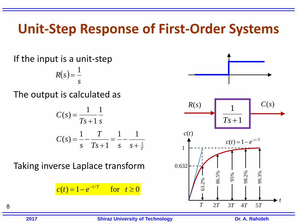
If the input is a unit-step The output is calculated as Taking inverse Laplace transform

8

Unit-Step Response of First-Order Systems

s

sR1

sTssC

1

1

1)(

)(sC )(sR

1

1

Ts

TssTs

T

ssC

1

11

1

1)(

0for1)( / tetc Tt

t

)(tc

T 2T 3T 5T 4T

1

0.632

63.2

%

86.5

%

95%

98.2

%

99.3

%

Ttetc /1)(


If the input is a unit-ramp The output is calculated as Taking inverse Laplace transform

9

Unit-Ramp Response of First-Order Systems

2

1

ssR

2

1

1

1)(

sTssC

)(sC )(sR

1

1

Ts

1

1)(

2

2

Ts

T

s

T

ssC

0for)( / tTeTttc Tt

T

t

)(tc

T 2T 3T 5T 4T

TtTeTttc /)(

6T

T

2T

3T

5T

4T

6T

ttr )(

T


If the input is a unit-ramp The output is calculated as Taking inverse Laplace transform

10

Unit-Impulse Response of First-Order Systems

1sR

1

1)(

TssC

)(sC )(sR

1

1

Ts

0for1

)( / teT

tc Tt

t

)(tc

T 2T 3T 5T 4T

TteT

tc /1)(

6T

T

1


Assume that the error is defined as And the steady-state error is calculated by

11

Steady-State Error First-Order Systems

tctrte

tctret

ss

lim

Input signal Error Steady-state error

Unit-Step

Unit-Ramp

Unit-Impulse

TteTte /1 Tess

Ttete / 0for1 ttr

0for tttr

ttr

0sse

Tt

Tette /1 0sse

)(sE )(sC )(sR

+ _ Ts

1


Using unit-impulse, unit-step, unit-ramp the following outputs are obtained: Since unit-impulse is the derivative of unit-step and unit-step is the derivative of unit-ramp, the corresponding outputs have the same relation in LTI systems: 12

Important Property of LTI Systems

0for12 ttr

0for3 tttr

otherwise0

01

tttr

0for1)( /

2 tetc Tt

0for)( /

3 tTeTttc Tt

0for1

)( /

1 teT

tc Tt

trdt

dtr 21 tc

dt

dtc 21

trdt

dtr 32 tc

dt

dtc 32


• Superposition

• Homogeneity or Scaling

• Derivative

• Integration

13

Important Property of LTI Systems

Linear

System

Input Output

)(1 tu )(1 ty

Linear

System

Input Output

)(2 tu )(2 ty

Linear

System

Input Output

)()( 21 tutu )()( 21 tyty

Linear

System

Input Output

)(1 tu )(1 ty

Linear

System

Input Output

)(1 tu )(1 ty

Linear

System

Input Output

)(1 tu )(1 ty

Linear

System

Input Output

)(1 tudt

d )(1 tydt

d

Linear

System

Input Output

)(1 tu )(1 ty

Linear

System

Input Output

dtu 1 dty1


14

Second-Order System

Consider the second-order system shown below. Physically, this system may represent DC servo drive system.

: Undamped natural frequency : Damping ratio

22

2

2)(

)(

nn

n

sssR

sC

av ai

+ _

aR

+

ae

_

aL

J

B

fi fL

fR

fv +

_

)(sE )(sC )(sR

+ _ n

n

ss

2

2

n

Standard Form

)(sC )(sR

22

2

2 nn

n

ss


15

Second-Order System

The dynamic behaviour of the second-order system can be described in terms of two parameters and n.

1. Undamped case

2. Under-damped case

3. Critically damped case

4. Over-damped case

22

2

2)(

)(

nn

n

sssR

sC

10

1

1

0


16

Second-Order System 1. Undamped case

In this the oscillation continues indefinitely. The roots of the denominator are on the imaginary axis

The unit-step response is obtained as

22

2

)(

)(

n

n

ssR

sC

0

njs 1 njs 2

nj

nj

)Im(s

)Re(s

sssC

n

n 1)(

22

2

ssR

1)( 0forcos1)( tttc n

tn

2

)(tc

Step response


17

Second-Order System 2. Under-damped case

• In this case the closed-loop poles are complex conjugates and lie in the left-half s plane.

• The transient response is oscillatory.

• The closed-loop transfer function can be written as

where is called the damped natural frequency.

10

22

2

2)(

)(

nn

n

sssR

sC

dndn

n

jsjssR

sC

2

)(

)(

21 nd

dn j

)Im(s

)Re(s

dn j

n

d

dn js 1

dn js 1

Step response


18

Second-Order System 2. Under-damped case

The unit-step response of this case is as follows

sss

sCnn

n 1

2)(

22

2

ssR

1)(

10

2222

1)(

dn

n

dn

n

ss

s

ssC

0forsin1

cos1)(2

tttetc dd

tn

0for1

tansin1

1)(2

1

2

tte

tc d

tn

Step response


19

Second-Order System 3. Critically-damped case

• In this case the two poles are equal.


• The unit-step response of this case is as follows

22

2

2)(

)(

nn

n

sssR

sC

2

2

)(

)(

n

n

ssR

sC

nss 21

1

)Im(s

)Re(s n

sssC

n

n 1)(

2

2

0for11)(

ttetc n

tn

ssR

1)(

Step response


20

Second-Order System 4. Over-damped case

In this case the two poles are negative real and unequal.



22

2

2)(

)(

nn

n

sssR

sC

11)(

)(

22

2

nnnn

n

sssR

sC ns 12

1

ssR

1)(

1

)Im(s

)Re(s 1s

2s

ns 12

2

sss

sC

nnnn

n

11

)(22

2

Step response


21

Second-Order System 4. Over-damped case


• Taking inverse Laplace transform yields

ssR

1)(

1

sss

sC

nnnn

n

11

)(22

2

0for1112

11)(

2

1

2

1

2

22

tee

tc

tt nn

Step response


22

Definitions of Transient-Response Specifications

In specifying the transient-response characteristics of a control system to a unit-step input, it is common to specify the following: 1. Delay time, td

2. Rise time, tr

3. Peak time, tp

4. Maximum overshoot, Mp

5. Settling time, ts

Step response


1. Delay time, td :The delay time is the time required for the response to reach half the final value the very first time.

23


Step response


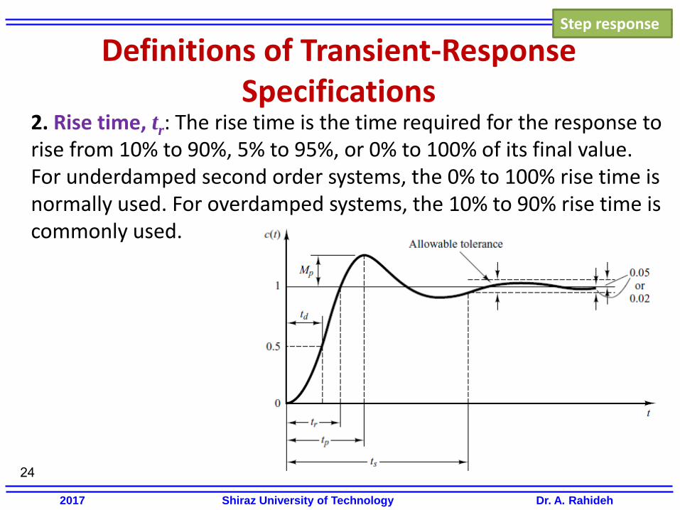
2. Rise time, tr: The rise time is the time required for the response to rise from 10% to 90%, 5% to 95%, or 0% to 100% of its final value. For underdamped second order systems, the 0% to 100% rise time is normally used. For overdamped systems, the 10% to 90% rise time is commonly used.

24


Step response


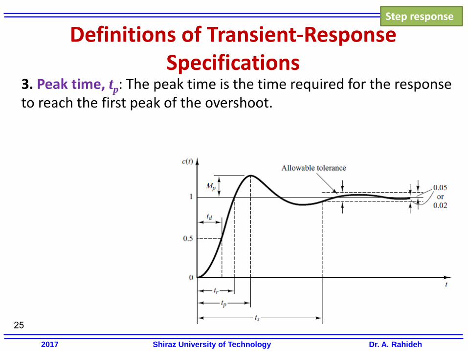
3. Peak time, tp: The peak time is the time required for the response to reach the first peak of the overshoot.

25


Step response


4. Maximum overshoot, Mp: The maximum overshoot is the maximum peak value of the response curve measured from unity. If the final steady-state value of the response differs from unity, then it is common to use the maximum percent overshoot. It is defined by

26


100%

c

ctcM

p

p

Step response


5. Settling time, ts: The settling time is the time required for the response curve to reach and stay within a range about the final value of size specified by absolute percentage of the final value (usually 2% or 5%). The settling time is related to the largest time constant of the control system.

27


Step response


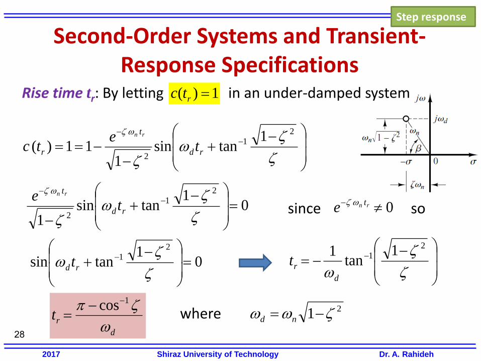
Rise time tr: By letting in an under-damped system since so

where 28

Second-Order Systems and Transient-Response Specifications

21

2

1tansin

111)( rd

t

r te

tcrn

1)( rtc

01

tansin1

21

2

rd

t

te rn

0 rn t

e

01

tansin2

1

rd t

21 nd

21 1

tan1

d

rt

d

rt

1cos

Step response


Peak time tp: Assume again the system is under-damped

29


21

2

21

2

1tancos

1

1tansin

1

te

te

dt

dc

d

t

d

d

t

n

n

n

0 pttdt

dc

0sin1 2

pd

tn

tt

tedt

dcn

p

d

pt

0sin pd t

3,2,,0pd t

1st peak

Step response


Maximum overshoot Mp: Assume again the system is under-damped

30


1)( pp tcM

21

2

1tansin

1

pn t

p

eM

)/( dneM p

21/

eM p

21

21

2

1tansincos

1tancossin

1

pn t

p

eM

0 21

Step response


Settling time ts: Assume again the system is under-damped Consider the time constant is (2% criterion)

(5% criterion)

31


n

s Tt

44

0for1

tansin1

1)(2

1

2

tte

tc d

tn

n

s Tt

33

n

T

1

Step response


Example: Consider a system with the following block diagram. Calculate k and kg so that the maximum overshoot remains under 20% and the peak time happens before the first second for a unit-step input.

32

Second-Order Systems

)1( ss

k c r

+ _

sk g1


Example: to have and

33


)1( ss

k c r

+ _

sk g1

?k ?gk %20pM 1pt

kskks

k

skss

k

ss

k

gg

r

c

)1()1(

)1(1

)1(2

22

2

2 nn

n

r

c

ss

kn 2 kn

gn kk12k

kkg

2

1



34


)1( ss

k c r

+ _

sk g1

?k ?gk %20pM 1pt

kn k

kkg

2

1

%20pM 2.021/

eM p456.0

1pt 11 2

n

pt21

n

rad/s53.3n



35


)1( ss

k c r

+ _

sk g1

?k ?gk %20pM 1pt

kn

k

kkg

2

1

456.0

rad/s53.3n53.3k 5.12k

456.02

1

k

kkg

k

kkg

12456.0


36

Second-Order System The unit-impulse response of the second-order system can be easily

obtained by the inverse Laplace transform of

• For

• For

• For

10

22

2

2)(

nn

n

sssC

Impulse response

0forsin1

)(2

tte

tc d

t

nn

1

0for)( 2

tettct

nn

1

0for12

)(11

2

22

teetctt

n nn

21 nd


The maximum overshoot for the unit-impulse response of the under-damped system occurs at The maximum overshoot is

37


10where1

1tan

2

21

n

peakt

Impulse response

10where1

tan1

exp)(2

1

2max

ntc


The peak time (tp) and maximum overshoot (Mp) of a unit-step response can be obtained from the unit-impulse response

38


Impulse response


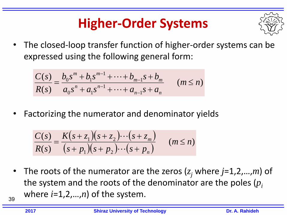
• The closed-loop transfer function of higher-order systems can be expressed using the following general form:

• Factorizing the numerator and denominator yields • The roots of the numerator are the zeros (zj where j=1,2,…,m) of

the system and the roots of the denominator are the poles (pi where i=1,2,…,n) of the system.

39

Higher-Order Systems

)()(

)(

1

1

10

1

1

10 nmasasasa

bsbsbsb

sR

sC

nn

nn

mm

mm

)()(

)(

21

21 nmpspsps

zszszsK

sR

sC

n

m


• Assuming all poles are real and distinct, for a unit-step input the output is

where ai is the residue of the pole at s = -pi

• If the system involves multiple poles, then C(s) will have multiple-

pole terms.

40


n

i i

i

ps

a

s

asC

1

)(


• If all closed-loop poles lie in the left-half s plane, the relative magnitudes of the residues determine the relative importance of the components in the expanded form of C(s).

• If there is a closed-loop zero close to a closed-loop pole, then the residue at this pole is small and the coefficient of the transient-response term corresponding to this pole becomes small.

• A pair of closely located poles and zeros will effectively cancel each other.

41


If a pole is close to a zero, the effect of that pole is low.


• If a pole is located very far from the origin, the residue at this pole may be small.

• The transients corresponding to such a remote pole are small and last a short time.

• Terms in the expanded form of C(s) having very small residues contribute little to the transient response, and these terms may be neglected.

• If this is done, the higher-order system may be approximated by a lower-order one.

42


Far poles from the origin have low effects.


• Consider the case where the poles of C(s) consist of distinct real poles and pairs of complex-conjugate poles. Therefore we have

• The unit-step response c(t) is then

• If all poles have negative real part, the system is stable and 43


)2(

2

1)(

122

2

1

nrqss

csb

ps

a

s

asC

r

k kkk

kkkkkkq

j j

j

r

k

kk

t

k

r

k

kk

t

k

q

j

tp

j

tec

tebeaatc

kk

kkj

1

2

1

2

1

1sin

1cos)(

ac )(


• If the ratios of the real parts of the poles exceed 5 and there are no zeros nearby, the poles nearest the j axis will dominate the transient response behaviour.

• Example: In the following system the dominant pole is 0.5, because there is no zero nearby (near 0.5) and the ratio of poles is 6 which exceeds 5.

• Example: In the following system a zero is near the pole 0.5 therefore the dominant pole is not 0.5 but it is 3.

44

Dominant Closed-Loop Poles

5.03

)5(7

)(

)(

ss

s

sR

sC

5.03

)48.0(

)(

)(

ss

ss

sR

sC


• If all closed-loop poles lie in the left-half s plane, the system is stable.

• If any of the closed-loop poles lie in the right-half s plane, the system is unstable.

45

Stability Analysis in the Complex Plane

5.03

)5(7

)(

)(

ss

s

sR

sC

5.03

)5(7

)(

)(

ss

s

sR

sC


Routh’s stability criterion tells us whether or not there are unstable roots in a polynomial equation without actually solving for them. The procedure is as follows: 1. Consider the following close-loop system

2. Write the characteristics equation Where the coefficients are real quantities. We assume that an is not zero; i.e. any zero root has been removed. 46

Routh’s Stability Criterion

nn

nn

mm

mm

asasasa

bsbsbsb

sR

sC

1

1

10

1

1

10

)(

)(

01

1

10

nn

nn asasasa


3. If any of the coefficients are zero or negative in the presence of at least one positive coefficient, a root or roots exist that are imaginary or that have positive real parts. Therefore, in such a case, the system is not stable.

4. If all coefficients are positive, arrange the coefficients of the polynomial in rows and columns according to the following pattern:

The number of rows is n+1.

47


0

3

2

7531

1

6420

s

s

s

aaaas

aaaas

n

n

n

n


01

1

10

nn

nn asasasa

5. The coefficients to be calculated are listed in the table

where

48


1

0

4321

3

4321

2

7531

1

6420

gs

ccccs

bbbbs

aaaas

aaaas

n

n

n

n

1

30211

a

aaaab

1

50412

a

aaaab

1

70613

a

aaaab

1

21311

b

baabc

1

31512

b

baabc

1

41713

b

baabc


01

1

10

nn

nn asasasa

• To simplify the calculation an entire row may be divided or multiplied by a positive number, e.g. k > 0.

• Routh’s stability criterion states that the number of roots with positive real parts is equal to the number of changes in sign of the coefficients of the first column of the array.

• The necessary and sufficient condition that all roots lie in the left-half s plane is that all terms in the first column of the array have positive signs. 49


1

0

4321

3

4321

2

7531

1

6420

gs

ccccs

kbkbkbkbs

aaaas

aaaas

n

n

n

n


Example: Apply Routh’s stability criterion to the following polynomial: 1. Form the table and simplify (second row is divided by 2)

50


05432 234 ssss

0

1

2

3

4

042

531

s

s

s

s

s

01

1

10

nn

nn asasasa

0

3

2

7531

1

6420

s

s

s

aaaas

aaaas

n

n

n

n

0

1

2

3

4

021

531

s

s

s

s

s


Solution: 2. Calculate the remaining coefficients

51


5

3

51

021

531

0

1

2

3

4

s

s

s

s

s

1

0

4321

3

4321

2

7531

1

6420

gs

ccccs

bbbbs

aaaas

aaaas

n

n

n

n

11

21311

b

1

50412

a

aaaab

31

51211

c

1

30211

a

aaaab

51

01512

b

1

21311

b

baabc

53

01531

d

1

21211

c

cbbcd


Solution: • The first column numbers have changed their signs twice;

therefore there are two roots with positive real parts. • The system is therefore unstable.

52


5

3

51

021

531

0

1

2

3

4

s

s

s

s

s


Special Case 1: If a first-column term in any row is zero, but the remaining terms are not zero or there is no remaining term, then the zero term is replaced by a very small positive number e and the rest of the array is evaluated. Example: If the sign of the coefficient above the zero (e) is the same as that below it, it indicates that there are a pair of imaginary roots. Actually, This example has two roots at . 53


022 23 sss

2

0

22

11

0

1

2

3

s

s

s

s

e

js


If, however, the sign of the coefficient above the zero (e ) is opposite that below it, it indicates that there is one sign change. Example: There are two sign changes of the coefficients in the first column. So there are two roots in the right-half s plane. This agrees with the correct result indicated by the factored form of the polynomial equation. 54


0212323 ssss

2

3

20

31

0

21

2

3

s

s

s

s

e

e


Special Case 2: If all the coefficients in any derived row are zero, it indicates that there are roots of equal magnitude lying radially opposite in the s plane (that is, two real roots with equal magnitudes and opposite signs and/or two conjugate imaginary roots). In such a case, the evaluation of the rest of the array can be continued by forming an auxiliary polynomial with the coefficients of the last row and by using the coefficients of the derivative of this polynomial in the next row. Such roots with equal magnitudes and lying radially opposite in the s plane can be found by solving the auxiliary polynomial, which is always even. For a 2n-degree auxiliary polynomial, there are n pairs of equal and opposite roots. 55



Example:

• The terms in the s3 row are all zero. (Such a case occurs only in an odd-numbered row.)

• The auxiliary polynomial is formed from the coefficient of the s4 row:

• which indicates that there are two pairs of roots of equal magnitude and opposite sign (that is, two real roots with the same magnitude but opposite signs or two complex conjugate roots on the imaginary axis). 56

Routh’s Stability Criterion 0502548242 2345 sssss

00

50482

25241

3

4

5

s

s

s

Auxiliary polynomial P(s)

50482)( 24 sssP


Solution: • The derivative of P(s) with respect to s is • The terms in the s3 row are replaced by the coefficients of the

last equation, i.e. 8 and 96.

57


Coefficients of dP(s) / dt

ssds

sdP968

)( 3

50

0113

5024

968

50482

25241

0

1

2

3

4

5

s

s

s

s

s

s


Solution: • We see that there is one change in sign in the first column of

the new array. • Thus, the original equation has one root with a positive real

part.

58


50

0113

5024

968

50482

25241

0

1

2

3

4

5

s

s

s

s

s

s


Example: Consider the following system. Determine the range of K for stability. • The characteristics equations is • The array of coefficients becomes

59

Application of Routh’s Stability Criterion to Control-System Analysis

Kssss

K

sR

sC

233)(

)(234

0233 234 Kssss

Ks

Ks

Ks

s

Ks

0

791

372

3

4

2

023

31

0279 K

0K

09

14 K

The numbers on the first column should all be positive:


1. Steady-State Response

2. Steady-State Error

or

60

Some Definitions

)(lim)()( tcctct

ss

)(lim)( tetet

ss

)(lim)(0

ssEtes

ss

G(s) )(sE )(sC )(sR

+ _


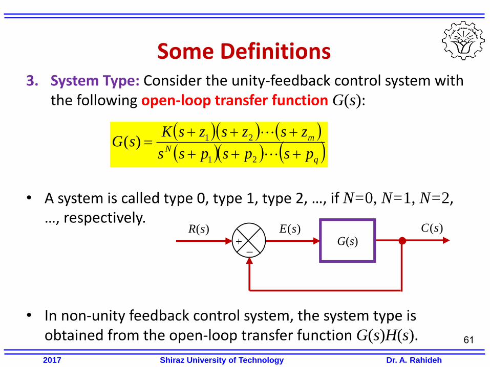
3. System Type: Consider the unity-feedback control system with the following open-loop transfer function G(s):

• A system is called type 0, type 1, type 2, …, if N=0, N=1, N=2,

…, respectively. • In non-unity feedback control system, the system type is

obtained from the open-loop transfer function G(s)H(s). 61

Some Definitions

q

N

m

pspspss

zszszsKsG

21

21)(

G(s) )(sE )(sC )(sR

+ _


1. Proportional controller (P)

2. Proportional-Integral controller (PI)

3. Proportional-Derivative controller (PD)

4. Proportional-Integral-Derivative controller (PID)

62

Different Types of Controllers

Controller C R

+ _ Plant E U


1. Proportional controller (P)

63


)()( teKtu p )()( sEKsU p

C R

+ _ Plant E U

pK


2. Proportional-Integral controller (PI)

Or

64


t

ip deKteKtu0

)()()( )()( sEs

KKsU i

p

t

i

p deT

teKtu0

)(1

)()( )(1

1)( sEsT

KsUi

p

i

p

iT

KK

C R

+ _ Plant E U

sTK

i

p

11


3. Proportional-Derivative controller (PD)

Or

65


dt

tdeKteKtu dp

)()()( )()( sEsKKsU dp

dt

tdeTteKtu dp

)()()( )(1)( sEsTKsU dp

dpd TKK

C R

+ _ Plant E U

sTK dp 1


4. Proportional-Integral-Derivative controller (PID)

Or

66


dt

tdeKdeKteKtu d

t

ip

)()()()(

0 )()( sEsK

s

KKsU d

ip

dt

tdeTde

TteKtu d

t

i

p

)()(

1)()(

0 )(

11)( sEsT

sTKsU d

i

p

C R

+ _ Plant E U

sT

sTK d

i

p

11

dpd TKK

i

p

iT

KK


Integral control action: • In the proportional control of a plant whose transfer function

does not possess an integrator 1/s, there is a steady-state error, or offset, in the response to a step input. Such an offset can be eliminated if the integral control action is included in the controller.

• Note that integral control action, while removing steady-state error, may lead to oscillatory response of slowly decreasing amplitude or even increasing amplitude, both of which are usually undesirable.

67


Controller C R

+ _ Plant E U


Derivative control action: Derivative control action, when added to a proportional controller, provides a means of obtaining a controller with high sensitivity. An advantage of using derivative control action is that it responds to the rate of change of the actuating error and can produce a significant correction before the magnitude of the actuating error becomes too large. Derivative control thus anticipates the actuating error, initiates an early corrective action, and tends to increase the stability of the system.

68


Controller C R

+ _ Plant E U


Unit step input: where kp is the static position error constant

69

Steady-State Errors in Unity-Feedback Control Systems

G(s) )(sE )(sC )(sR

+ _

)()()( sCsRsE )(1

)()()()(

sG

sGsRsRsE

)(1

)()(

sG

sRsE

)(1

)(lim

0 sG

sRse

sss

ssR

1)(

ssGse

sss

1

)(1

1lim

0

)0(1

1

Gess

p

ssk

e

1

1

)0()(lim0

GsGks

p


Unit ramp input: where kv is the static velocity error constant

70


G(s) )(sE )(sC )(sR

+ _

)(1

)(lim

0 sG

sRse

sss

2

1)(

ssR

20

1

)(1

1lim

ssGse

sss

)(

1lim

0 ssGe

sss

v

ssk

e1

)(lim0

ssGks

v


Unit parabolic input: where ka is the static acceleration error constant

71


G(s) )(sE )(sC )(sR

+ _

)(1

)(lim

0 sG

sRse

sss

3

1)(

ssR

30

1

)(1

1lim

ssGse

sss

)(

1lim

20 sGse

sss

a

ssk

e1

)(lim 2

0sGsk

sa


input System type

Unit step Unit ramp Unit Parabolic

0

1

2

3

Effects of the system type on the steady-state error:

72


pk1

1

vk

1

ak

1

0

0 0

0 0 0


Example: In the following system, calculate the gain K to have steady-state error not more than 5% in response to a unit step input.

73


C R

+ _

E U K

1

05.0

s

s

KsG

1

05.0)(

p

ssk

e

1

1

KsGks

p 05.0)(lim0

05.005.01

1

Kess 380K

ssR

1)( 05.0sse


In The Name of God The Most Compassionate, The Most Mercifulen.sutech.ac.ir/eee/wp-content/uploads/my_user... · 5 Transient Response and Steady-State Response • The time response

Documents