In-Situ Monitoring and Testing of IBRC Bridges in Wisconsin

mro

gram

In-Situ Monitoring andTesting of IBRC Bridgesar

chP

g gIn Wisconsin

Res

eahw

ay SPR # 0092-05-02

inH

ig

Christopher M. Foley, PhD, PE; Baolin Wan, PhD; Carl Schneeman, MS; Kristine Barnes, MS; Jordan Komp, MS; Junshan Liu, MS; Andrew Smith, MS

Marquette UniversityDepartment of Civil & Environmental Engineering

June 2010scon

s

June 2010

WHRP 10-09 Wis

Technical Report Documentation Page 1. Report No. WHRP 10-09

2. Government Accession No

3. Recipient’s Catalog No

4. Title and Subtitle In-Situ Monitoring and Testing of IBRC Bridges in Wisconsin

5. Report Date June 2010 6. Performing Organization Code Wisconsin Highway Research Program

7. Authors Christopher Foley, PhD, PE; Baolin Wan, PhD; Carl Schneeman, MS; Kristine Barnes, MS; Jordan Komp, MS; Junshan Liu, MS; Andrew Smith, MS

8. Performing Organization Report No.

9. Performing Organization Name and Address Marquette University Department of Civil & Environmental Engineering Milwaukee, Wisconsin

10. Work Unit No. (TRAIS) 11. Contract or Grant No. WisDOT SPR# 0092-05-02

12. Sponsoring Agency Name and Address Wisconsin Department of Transportation Division of Business Services Research Coordination Section 4802 Sheboygan Ave. Rm 104 Madison, WI 53707

13. Type of Report and Period Covered

Final Report, 2004-2010 14. Sponsoring Agency Code

15. Supplementary Notes 16. Abstract This study examines two highway bridges constructed using novel fiber-reinforced polymer (FRP) composite stay-in-place formwork and an FRP grillage reinforcement system. Both bridge superstructures rely on the FRP components as bridge deck reinforcement. These bridges were monitored in-situ for a period of five years. The monitoring included a series of in-situ load test as well as non-destructive evaluation (NDE). Laboratory investigations accompanied and guided the load testing and NDE implemented. Finite element simulations were employed to evaluate the likely causes of premature deck cracking seen in the traditionally-constructed bridge and the FRP-component superstructures. The study identifies sources of potential deterioration, identifies aspects of the bridge superstructures likely to enhance durability, and quantifies the effectiveness and potential for deterioration of the load transfer mechanisms present in the FRP-component superstructures.

17. Key Words

18. Distribution Statement

No restriction. This document is available to the public through the National Technical Information Service 5285 Port Royal Road Springfield VA 22161

19. Security Classif.(of this report) Unclassified

19. Security Classif. (of this page) Unclassified

20. No. of Pages 232

21. Price

Form DOT F 1700.7 (8-72) Reproduction of completed page authorized

Disclaimer This research was funded through the Wisconsin Highway Research Program by the

Wisconsin Department of Transportation and the Federal Highway Administration under

Project 0092-05-02. The contents of this report reflect the views of the authors who are

responsible for the facts and accuracy of the data presented herein. The contents do not

necessarily reflect the official views of the Wisconsin Department of Transportation or

the Federal Highway Administration at the time of publication.

This document is disseminated under the sponsorship of the Department of

Transportation in the interest of information exchange. The United States Government

assumes no liability for its contents or use thereof. This report does not constitute a

standard, specification or regulation.

The United States Government does not endorse products or manufacturers.

Trade and manufacturers’ names appear in this report only because they are considered

essential to the object of the document.

i

Table of Contents Acknowledgements ............................................................................................................................................ iii Executive Summary ............................................................................................................................................ vi Chapter 1 – Introduction, Literature Review and Synthesis ................................................................................ 1 1.1 Introduction ...................................................................................................................................... 1 1.2 Motivations for Present Research Effort .......................................................................................... 2 1.3 Bridges B-20-133/134 – Waupun, Wisconsin ................................................................................. 4 1.4 Bridges B-20-148/149 – Fond du Lac, Wisconsin ........................................................................... 6 1.5 Literature Review ............................................................................................................................. 8 1.6 Literature Synthesis ....................................................................................................................... 22 1.7 Layout of Research Report ............................................................................................................ 25 1.8 References ...................................................................................................................................... 26 Chapter 2 – Sensor Development and Laboratory Studies ................................................................................ 35 2.1 Introduction .................................................................................................................................... 35 2.2 Development of Portable Strain Sensors ....................................................................................... 35 2.3 Freeze Thaw Testing ...................................................................................................................... 46 2.4 Conclusions .................................................................................................................................... 52 2.5 References ...................................................................................................................................... 53 Chapter 3 – In-Situ Monitoring and Non-Destructive Evaluation ..................................................................... 67 3.1 Introduction .................................................................................................................................... 67 3.2 Benchmark Condition Evaluation of B-20-133/134 ...................................................................... 67 3.3 Benchmark Condition Evaluation of B-20-148/149 ...................................................................... 70 3.4 Evaluation of NDE Techniques ..................................................................................................... 72 3.5 In-Situ Moisture Evaluation in Waupun Bridges ........................................................................... 78 3.6 Conclusions .................................................................................................................................... 80

ii

3.7 References ..................................................................................................................................... 81 Chapter 4 – In-Situ Load Testing .................................................................................................................... 117 4.1 Introduction ................................................................................................................................. 117 4.2 In-Situ Instrumentation ................................................................................................................ 117 4.3 In-Situ Load Test Protocols ......................................................................................................... 121 4.4 Load Testing Results and Discussion .......................................................................................... 122 4.5 Wheel Load Distribution within Bridge Deck ............................................................................. 131 4.6 Concluding Remarks ................................................................................................................... 138 4.7 References ................................................................................................................................... 140 Chapter 5 – Numerical Simulation of Shrinkage-Induced and Vehicle-Induced Stresses .............................. 183 5.1 Introduction ................................................................................................................................. 183 5.2 FE Modeling of Bridge Superstructure ....................................................................................... 183 5.3 Simulation and Evaluation of Shrinkage-Induced Strains ........................................................... 186 5.4 Simulation and Evaluation of Vehicle-Induced Strains............................................................... 197 5.5 Concluding Remarks ................................................................................................................... 199 5.6 References ................................................................................................................................... 201 Chapter 6 – Summary, Conclusions, and Recommendations .......................................................................... 221 6.1 Summary ..................................................................................................................................... 22x 6.2 Conclusions ................................................................................................................................. 22x 6.3 Recommendations ....................................................................................................................... 22x

iii

ACKNOWLEDGEMENTS

The authors would like to acknowledge the support and help from the following individuals at the Wisconsin

Department of Transportation: Travis McDaniel, Bruce Karow. The authors would also like to acknowledge

the help of Professor Jian Zhao, University of Wisconsin at Milwaukee and Dr. Nicholas Hornyak of Collins

Engineers, Inc. The research team is also grateful for the help of Stu Kastein at Fond du Lac County

Highway Department and all the summer work crews at Fond du Lac County for their terrific help in

conducting the load testing. The authors would also like to acknowledge the help of the Fond du Lac County

Sheriff's Office.

iv

EXECUTIVE SUMMARY

This report outlines activities undertake during a five-year monitoring study of Wisconsin's first IBRC bridges

(B-20-133/134 and B-20-148/149). It provides detailed background on the IBRC program and the bridge

superstructures constructed in Waupun, WI and Fond du Lac, WI. The five-year research effort completed

several related, yet distinct, studies designed to assess the likely long-term performance of Wisconsin's IBRC

structures and also provide direction with regard to further investigation into the performance of these

structural systems so that the technologies fostered by them can be introduced in bridge superstructure design

going forward.

The report describes the design and calibration of portable strain sensors suitable for use in the

proposed research effort and a laboratory-based experimental program designed to evaluate the impact of

moisture and freeze-thaw cycling on the shear strength at the interface between the FRP-SIP formwork and

concrete. The laboratory studies completed indicates that freeze-thaw cycling and the presence of water could

be detrimental to the FRP-SIP-formwork-concrete interfacial shear strength. Simplified finite element

modeling and analysis of a similar FRP-SIP deck system suggests that shear demands at the concrete FRP-SIP

interface are very low and not of sufficient magnitude to cause concerns regarding long-term performance of

of the stay-in-place FRP system. The reduction in strength due to moisture presence and freeze-thaw cycling

seen in the laboratory studies is significant, but does not bring the shear strength at the interface down to

levels where the system would be compromised. The laboratory studies conducted to evaluate the reduction

in shear strength resulting from freeze-thaw cycling and moisture presence were very conservative and do not

fully represent the situation present in the field. In other words, the laboratory testing setup is an extreme

scenario that is an approximation of the field conditions. Field conditions are likely to be much more

favorable and the resistance to freeze-thaw degradation is felt to be much higher in the actual structure.

The report outlines a thorough visual benchmark condition evaluation of the bridges at Waupun and

Fond du Lac. Common NDE methods were reviewed for their potential application in the present research

effort and future evaluation of these bridges. A laboratory-based evaluation of the infrared thermography

technique for application in the present research effort was conducted. Tap testing with an impact hammer

v

was shown to be the most useful method for monitoring the IBRC bridges. Infrared thermography was found

to be the least likely to yield useful results.

The presence of moisture accumulation at the interface between the FRP-SIP formwork and concrete

in the Waupun bridge system was assess using a digital hygrometer. No moisture was found when drilling

the hygrometer probe holes so there is no concern that moisture is actually accumulating at the interface of the

FRP-SIP formwork and the concrete deck as of the date of this report. It should be understood that relative

humidity is one measure of the tendency for the FRP-SIP formwork to inhibit moisture egress from within the

deck and may be an indicator for the tendency for moisture to accumulate at the interface. However, the

ability of humidity readings to reliably indicate levels of moisture to expect at the interface remains to be

definitively proven. It is recommended that further analysis with regard to relative humidity be undertaken in

future research efforts as it may be a useful tool for long-term evaluation of bridge decks with FRP-SIP

formwork.

The report describes two in-situ load tests of bridges B-20-133 and B-20-148 conducted to evaluate

critical load transfer mechanisms that could give the research team indication of degradation with time.

Bridge deck displacements relative to the girders in both bridges did not change significantly over the two-

year period of evaluation. It was found that the wheel load distribution widths present in the FRP-SIP bridge

deck system of B-20-133 could be predicted using procedures found in U.S. design specifications.

Furthermore, this load transfer mechanism did not change significantly (if at all) over the two year evaluation

period. Although not fully evaluated in the present research report, the in-situ testing conducted illustrated

that the wheel load distribution widths in B-20-148 are consistent, but narrower, than that in B-20-133. Strain

gradients over the height of the girders in the Fond du Lac bridge load tested clearly exhibit composite

behavior and this behavior did not significantly (if at all) change with time. Lane load distribution factors for

wide-flange bulb-tee composite bridge girder systems (e.g. that used in B-20-148) can be computed

accurately with standard design/analysis procedures found in modern U.S. bridge design specifications.

These lane load distribution factors did not change from the original July 2005 load tests and the July 2007

load test conducted in this research study. The in-situ load testing conducted indicates that the long-term

vi

performance of the IBRC bridges are expected to be no different than any other traditionally constructed

bridge of similar superstructure configuration.

The finite element simulations conducted indicate that drying shrinkage appears to be capable of

causing transverse (and possibly longitudinal) bridge deck cracking at very early stages in the life of the decks

in the Waupun bridges. The simulations conducted indicate that cracking may occur as early as 4-8 days after

bridge deck placement. An FE simulation of the tensile strains and stresses induced by HL-93 vehicle-type

loading was conducted and it was found that tensile stresses induced by HL-93 vehicle loading were found to

be on the order of 20% of the typical magnitudes assumed for the tensile strength of concrete material. When

these are superimposed onto the states of stress likely present 10-days after casting the bridge deck, it is likely

that the combined effects of vehicle-induced stresses and shrinkage-induced stresses will result in transverse

cracking over the interior pier supports in the bridges in Waupun. The FE simulations conducted as part of

this effort clearly support idea that there should be no difference between and IBRC bridge and its counterpart

with regard to behavior leading to cracking since shrinkage-induced straining and traffic loading are the likely

reasons for the transverse cracking. Furthermore, the deck connection detail at the central diaphragms (over

the interior piers) in the FRP-SIP formwork bridge at Waupun is expected to neither improve nor detract from

the behavior with regard to cracking.

1

Chapter 1

Introduction, Literature Review and Synthesis

1.1 Introduction

Across the United States a massive network of transportation infrastructure exists. This network evolved

to include a web of iron rail lines spurned by the industrial revolution and eventually concrete and asphalt

roads for the automobile. Throughout this progression the highway bridge has evolved to meet these

demands. These highway bridges have become increasingly complex, relying on the development of

modern materials, changing economic conditions, and advanced engineering to meet project goals.

Acknowledging the importance of fostering new materials and engineering methods, the United

States Department of Transportation (USDOT) initiated the Innovative Bridge Research and Construction

(IBRC) program under the Transportation Equity Act for the 21st Century (TEA-21) as a venue for the

demonstration of new and groundbreaking material used in the construction of transportation structures

(FHWA 2005). This program fostered development of numerous novel materials and their applications in

bridge engineering and their future use in construction. The first installment of funding was allocated for

the period between 1998 and 2004 and accounted for $7 million in research and development projects and

$122 million of construction projects (Conachen 2005).

Evaluation of fiber-reinforced polymer (FRP) materials has happened frequently in the IBRC

program. Although the material has been in use for a number of years, its implementation in

infrastructure has been slow. Sources of this delay stem from inconsistency in material properties, non-

ductile failure mechanisms, general unfamiliarity among designers, and cost. FRP composites are

composed of oriented fibers, typically carbon or glass, embedded in a polymeric resin and cured to form a

single composite material. The matrix of resin and fiber is usually drawn through a die during a process

called pultrusion, pressed into the desired shape prior to the set-up or curing of the resin, or cured in the

final shape intended for the application. Often this process can be costly as the machinery required may

2 not be readily available to industry and set up of the pultrusion process can be labor intensive. However,

large-scale production can be rapid and very little preparation is required after the curing process.

FRP bars or multi-directional grillages have many advantages and can be used in lieu of steel

reinforcing bars in reinforced concrete. The tendency for conventional steel reinforcement to corrode

within a bridge component (e.g. deck) suggests that FRP reinforcement is an ideal substitute for mild-

steel reinforcing bars in concrete. In 2002, 27.1% of the bridges in the United States were classified by

the DOT as structurally deficient or functionally obsolete (ASCE 2005). A major cause of deficiency for

these structures is gradual deterioration of the steel reinforcing contained within concrete decks and the

concrete spalling that follows. Penetration of water through the concrete decking in conjunction with

high concentrations of chlorides commonly found in salts used for de-icing and snow removal facilitate

this corrosion. FRP systems are generally not affected by corrosion and are immune to the effects of

chlorides and therefore can be a major source for combating this deterioration (Jacobson 2004a).

FRP materials are also capable of developing significantly larger tensile stresses than mild steel.

Currently, common strengths of steel reinforcing bars reach a maximum of 75 ksi, while glass-fiber

reinforced polymers (GFRP) and carbon-fiber reinforced polymers (CFRP) have been found to achieve

maximum stresses of 230 and 535 ksi, respectively (Dietsche 2002b). These higher stress levels

combined with the lower density of FRP relative to that of steel, may allow for less material used in

design and, in turn, offer cost savings.

1.2 Motivations for Present Research Effort

The Innovative Bridge Research and Construction (IBRC) program was created to find innovative

materials for highway bridges, demonstrate their application in infrastructure projects, monitor their

performance, and create a research, development, and technology-transfer program. The primary goal of

the IBRC program was to develop and demonstrate new, cost-effective, highway bridge applications of

innovative materials (IBRC 2006). There is/was an expectation that this program would result in new,

3

more durable structures that need less frequent maintenance and rehabilitation with shorter work times for

improvements, and, lower costs with an improved load capacity.

The Wisconsin Department of Transportation; along with the University of Wisconsin – Madison,

a structural engineering consultant (Alfred Benesch and Co.), and a bridge construction contractor (Lunda

Construction, Inc.), took a significant step in the direction of formalizing the use of novel structural

engineering systems for bridges when they successfully proposed and received funding through the IBRC

Program. The goals of this program pertinent to the present research effort are:

• develop new, cost-effective innovative material applications in highway bridges;

• develop engineering design criteria for innovative products and materials for use in highway

bridges and structures.

To meet these goals, WisDOT and the University of Wisconsin at Madison conducted experimental

validation of a novel fiber-reinforced polymer (FRP) composite stay-in-place form system; a novel FRP

grillage system for bridge deck reinforcement; and a deck replacement scenario involving precast

prestressed concrete bridge deck panels. All of these were designed to be innovative, economical, and

durable substitutes for traditional concrete deck components and rehabilitation techniques used in

highway bridges. The experimental efforts supported tentative guidelines for design that then supported

generation of construction drawings.

With experimental validation of the innovative systems completed; design of the innovative

bridge superstructures completed, construction of two of the bridges completed in fall 2005, a significant

final step required was to “close the loop” in the innovation process. The innovative bridges constructed

require a monitoring period (e.g. 5 years) to evaluate durability of the new systems when compared to

traditional deck systems after imposition of traffic loading. Furthermore, in-situ load testing of the

innovative bridges was required to validate the load transfer mechanisms used in the design phase with

field-obtained data.

In order to complete WisDOT’s process of innovation in bridge deck design, the proposed

research effort set out to complete the following for WisDOT’s IBRC bridges:

4

• evaluate the extent of annual bridge deck deterioration;

• identify the sources of deterioration in the innovative systems;

• validate the load transfer mechanisms present using field-acquired data;

• identify changes in the innovative deck design procedure that will enhance deck durability;

• identify changes in the innovative deck design procedure that will result in design methodologies

that more closely resemble the in-situ behavior;

• quantify the effect of bridge deck-to-diaphragm connection variations;

• provide recommendations for designing and prolonging the life of FRP reinforced bridge decks.

Sources of cracking in the “traditional” deck systems that have been paired with the innovative systems

were found to be important as they aided in the proposed research efforts goal of identifying sources of

deterioration in the innovative systems. In-situ testing of only the innovative deck systems was carried out. The

traditional systems have had a long history of design and construction and therefore, validation of load transfer

mechanisms in these structures is not necessary.

The Wisconsin Department of Transportation (WisDOT) IBRC bridges that are the focus of the present

research effort are bridges B-20-133/134 in Waupun, Wisconsin and bridges B-20-148/149 in Fond du Lac,

Wisconsin. Each bridge group is a traditionally constructed superstructure and a novel FRP-based superstructure.

The following sections in the report outline pertinent details of these bridge pairs that set the foundation for the

present research effort.

1.3 Bridges B-20-133/134 – Waupun, Wisconsin

The first pair of bridges is located in Waupun, WI. Their WisDOT designations are B-20-133 for the

IBRC bridge and B-20-134 for the conventional steel-reinforced bridge deck. An overview photo of the

pair of two-span continuous superstructures is shown in Figure 1.1. These bridges are part of the

overpass for US 151 above State Highway 26. The location is schematically shown in Figure 1.2. The

deck in bridge B-20-133 uses FRP grid reinforcement and FRP stay-in-place (SIP) forms that are coated

with an adhesive called Concresive® (Degussa 2010) and 1/4" (maximum) aggregate. The aggregate

5

adhered to the SIP form is intended interlock with the concrete poured on top of it so the SIP form can act

as positive moment reinforcement for the deck. A mock up is shown in Figure 1.3. The typical bridge

deck cross-section is shown in Figure 1.4 and the aggregate-adhered FRP-SIP formwork is shown in

Figure 1.5.

The girders in these bridges are two-span continuous precast prestressed concrete girders that act

compositely with the bridge deck. Each of the continuous spans is approximately 110 feet long. The

girders are standard Wisconsin 54-inch deep I-girders. The two-span superstructure configuration is

accomplished by using glass fiber-reinforced polymer reinforcing bars in the bridge deck at the interior

pier location. Standard WisDOT continuous barriers are present and the reinforcement at the overhangs

and the barriers are conventional mild-steel reinforcing bars.

Evaluation of the structural performance of this deck configuration was done at UW-Madison

(Dieter 2002; Dieter et al. 2002). Deck panels were tested to determine critical modes of failure and

strength safety factors. Positive moment beams, negative moment beams were also tested for ultimate

strengths, and two span fatigue beams were used to test the fatigue strength of the FRP system. Deck

panels tested showed the ultimate strength due to punching shear with decks using full coverage, gave a

factor of safety exceeding 8. (Dieter 2002; Dieter et al. 2002). The deck system was subjected to 2

million loading cycles in the fatigue beam tests without distress (Dieter 2002; Dieter et al. 2002).

The FRP materials for the SIP form and grid were broken into 3 categories. GV1, GV2, and GV3,

GV being an abbreviation for glass/vinylester. The FRP grid used in B-20-133/134 is classified as GV2

and the FRP form is classified as both GV2 and GV3. The areas for this material characterization and

analysis are shown in Figure 1.6. Areas 1, 3, 6, and 7 were classified as GV2 material, and areas 2, 4, and

5 are classified as GV3 material (Dietsche 2002a).

Various ASTM tests were conducted to determine the mechanical properties of the FRP grid and

SIP forms to establish the criteria needed to develop the IBRC specifications. The FRP grid met all of the

IBRC specifications, and the FRP deck GV2 materials performed very well, but the GV3 portions fell

short in a number of areas including longitudinal tensile and compressive strength, longitudinal short

6 beam shear strength, and longitudinal tensile modulus. The GV3 material was thought to have performed

at a level less than the target level because of issues that came up during testing (Dietsche 2002a). It was

recommended that there be more testing done to improve quality control of FRP manufactured elements

and that the material specifications be standardized (Dietsche 2002a).

University of Wisconsin at Madison researchers also evaluated the effects of freeze/thaw on the

shear strength of the aggregate coated formwork (Helmueller et al. 2002). Because the SIP FRP forms

are expected to act as the positive moment reinforcement for the bridge deck, it is important to understand

how the aggregate/concrete interlock will work after freeze-thaw cycles are endured. To show a

difference between control coating and full coating (what is applied in the actual system), specimens were

made that experienced no freeze/thaw cycles with no aggregate coating, control aggregate coating, and

full aggregate coating. All freeze thaw specimens were tested with the control coating. After

experiencing 0 (control), 100, 150, or 200 freeze/thaw cycles while immersed in water. The freeze/thaw

control group with control coating showed an ultimate bond stress of 310 psi. Freeze-thaw cycles of 100,

150, and 200, had ultimate bond stresses of 280, 280, and 200 psi, respectively. The results of the

experimental testing indicated that a decrease in the available bond strengths from freeze/thaw effects is

likely.

Initial in-situ load tests of B-20-133/134 have been conducted by the University of Missouri –

Rolla (Hernandez et al. 2005a). Deflections of the girders and deck under loading induced by three-axle

dump trucks were measured. Strain gauges were also mounted in the bridge deck on the FRP grid during

construction, but the readings from the strain gauges were unreliable. Deflections for both bridges were

found to be below the AASHTO limit of L/800.

1.4 Bridges B-20-148/149 – Fond du Lac, Wisconsin

The De Neveu Creek IBRC Bridges (B-20-148/149) are located on U.S. Highway 151 south of Fond du

Lac, Wisconsin and is part of a new bypass system around the City. A photograph of the structure can be

found in Figure 1.7 and its location is illustrated in the map shown in Figure 1.8. Each bridge

7

superstructure configuration is simple-span with length of approximately 130 feet. Each bridge carries

two lanes of highway traffic. The structure is skewed approximately 25 degrees and contains minimal

super-elevation. Seven prestressed concrete stringers support the 8” thick FRP-grillage-reinforced

concrete deck. The overhangs in the bridge deck are reinforced with traditional epoxy-coated mild-steel

reinforcement and the barriers included steel reinforcement as well. The girders are intended to act

compositely with the FRP-reinforced deck. Shear transfer is provided by epoxy-coated mild-steel

reinforcing bars. Stringers are of WisDOT type 54W precast prestressed concrete and spaced transversely

6’-5” on center. Figure 1.9 provides a cross section of the bridge and illustrates this narrow spacing of the

stringers.

The FRP grillage reinforcement is a system of pultruded FRP I-bars developed for

implementation in bridges B-20-133 and B-20-148. The FRP reinforcement is a bi-directional grating

system consisting of two individual layers of reinforcement, with one layer placed directly over the other

layer. Figure 1.10 illustrates the double-mat FRP grillage. Each grating layer contains two separate types

of pultruded FRP elements. The primary reinforcing member is an I-bar positioned in the transverse

direction of the deck, perpendicular to the traffic lane. Orthogonal to the I-bars, or parallel to the

direction of traffic, are cross-rods. Each cross-rod is constructed of three independently pultruded

elements, which are assembled in the manufacturing facility. Figure 1.11 illustrates the grillage

components. Further details with regard to the grillage system and material properties are available

(Jacobson 2004a). The bi-directional grid was found to have met all the IBRC specifications for use as a

reinforcing material (Dietsche 2002a).

Tests were done on slabs and beams made using the double layer of grids. Slabs were made to

test punching shear capacity, service load performance, fatigue cycling, and load distribution. In addition,

beams were created to test negative moment capacity and fatigue. Punching shear and service load

performance was tested in several different configurations: simply supported; two-span conditions; and

using supports that simulate the 54W precast girder flanges (Jacobson 2004b).

8

All slabs failed in punching shear though quite a bit of flexural cracking was observed in all the

tests. A flexurally restrained system, which was assumed to be the best representation of bridge B-20-148,

had factors of safety exceeding 10 when compared to HS-20 wheel loads and fatigue damage after 2

million cycles was found to be negligible (Jacobson 2004b). The beam tests conducted indicated shear

was the mode of failure. The FRP I-bar reinforcement also exhibited shear failures. Prior to shear failure,

beam tests showed the FRP deck system had a negative moment capacity 2.5 times greater than the ACI

nominal moment capacity (Jacobson 2004b).

Initial in-situ load testing was again done by the University of Missouri – Rolla (Hernandez et al.

2005b). Similar magnetically mounted prisms were used to measure deflection of the girders and deck

under loading induced by three-axle dump trucks. Readings from internal strain gauges installed during

construction were unreliable. Trucks were placed in several configurations to generate maximum

deflections. Deflections were found to be under the AASHTO L/800 limit.

1.5 Literature Review

The previous IBRC research efforts described earlier sets the table for the present long-term monitoring

effort. It is prudent to review literature that can aid in influencing the development of the methodology

used to conduct the present five-year monitoring program. The present section of the report outlines

previous research efforts related to construction and monitoring of bridge superstructures and components

that involve full-depth FRP panel decks. Research efforts that involve stay-in-place formwork and the

impact of freeze-thaw cycling on performance are reviewed. Finally, recent research efforts involving

instrumentation and in-situ monitoring of bridge superstructure and superstructure components are

described.

Full Depth FRP Panel Decks

The Tech 21 Bridge in Butler County, OH started as a U.S. Department of Defense contract to design a

short-span composite bridge that would be able to withstand military tank loading (Foster et al. 2000).

9

The bridge deck was composed of three sections in a trapezoidal box beam shape. The bridge deck was

covered with an asphalt wearing surface weighing more than the bridge itself. The bridge was

continuously monitored by an instrumentation system. It used 120 sensors to measure chemical or water

incursion in the epoxy adhesive as well as strains. The sensors are hooked up to a data acquisition box

just off the bridge that records data 24 hours a day. In August of 1998, load tests were done to measure

strain and deflection. The tests subjected the bridge to live loads just under the AASHTO HS-20 truck

with deflections were under the AASHTO limit.

Another bridge deck using only GFRP that was heavily monitored and instrumented was

constructed in South Carolina (Coogler et al. 2005). The deck was composed of pultruded GFRP tubes

that were sandwiched between top and bottom face plates. The tubes and face plates were assembled

using adhesive. It was instrumented to measure longitudinal and transverse strain as well as deflection

during a long-term monitoring project.

The Salem Avenue Bridge, which was built with four different types of FRP reinforcement, was

an experimental venture into bridge deck composites (Reising et al. 2004). The bridge was divided into

four regions and a different FRP manufacturer provided an FRP reinforcement system for each region.

Out of six manufactures that were invited to participate in the construction, four agreed to participate.

Each company provided an FRP system for one fourth of the bridge deck. One company supplied

pultruded FRP stay-in-place deck panels that were used as the positive moment reinforcement. The

system is very similar to the system used in B-20-133 studied in this thesis. The rest of the systems relied

on FRP systems that would have an overlay to protect the surface of the panels. The Salem Avenue

Bridge is a five-span continuous haunched steel plate girder. A monitoring program was designed to

compare the performance of the four deck panels over two years with static and high-speed truckload test.

The three full depth FRP decks showed loss in composite action with the girders shortly after installation.

The hybrid system with stay-in-place forms was found to perform very well and exhibit composite action

with the girders, similar to the original reinforced concrete deck. However, it was noted, that it did not

have the same benefits as the all FRP deck systems including dead load reduction and reduced

10 construction time (Reising et al. 2004). More on the static testing of the FRP deck panels can be found in

(Harik et al. 1999).

Stay-in-Place (SIP) Formwork

Stay-in-place metal formwork (SIPMF) has been used in many states across the country. Inspection

techniques for SIPMF and the deterioration of these bridges have been recommended (Grace and Hanson

2004). A survey of the Departments of Transportation in each state was conducted to find out if they used

SIPMF and if not, why they did not. The most common reason for not using SIMPF was due to the

difficulty of inspecting the underside of the deck. With SIPMF it is impossible to use traditional visual

indicators of deterioration. Other Non-Destructive Evaluation (NDE) techniques have to be used to

determine the condition of the concrete and the extent of potential damage. Other problems indicated

were the potential for increased freeze-thaw damage due to the possibility of moisture retention on the

SIPMF and the possible corrosion of the forms over time (Grace and Hanson 2004).

Ten bridges were inspected in the state of Michigan (Grace and Hanson 2004), five had SIPMF

and five were conventionally formed with wood. Five full depth cores were obtained from the top of the

decks in each bridge depending on accessibility for a total of 50 core specimens. One core from each

bridge was visually inspected, two cores were compression tested with vertical strain gauges attached to

determine the compressive strength of the concrete, and two were tested with ultrasonic testing using

commercial hardware on 1-3in thick slices. Ultrasonic testing was done to find variation in the quality of

the concrete through the depth of the deck since this is not possible to find using compression tests. From

the cores, the ultrasonic tests showed that both bridge systems had similar pulse velocities in the slices.

There were no adverse effects found from the SIPMF through the depth of the deck. The compressive

strength tests showed that the concrete used in the decks with SIPMF and without SIPMF were similar as

well. The average compressive strength of a deck core without SIPMF was 6.98 ksi and the deck with

SIPMF reached 6.65 ksi. The modulus of elasticity was found to be 4,800 ksi without SIPMF and 4,090

ksi with SIPMF (Grace and Hanson 2004).

11

In addition to the cores, crack density comparisons were made between the decks with and

without SIPMF. Crack densities were calculated as length of cracks (in.) per unit area of deck (sq. ft.).

The field inspection showed the decks without SIPMF had a slightly higher, but not significantly higher,

crack density at 1.7in/ft2 where the decks with SIPMF had a crack density of 1.5in/ft2 (Grace and Hanson

2004). A second independent study suggested that SIPMF does not have an adverse effect on the quality

of the concrete, but can enhance corrosion effects (Guthrie et al. 2006). Non-corrosive SIP formwork

such as the one used in the Waupun Bridge B-20-133 would not have this potentially negative impact.

Impact of Freeze-Thaw Cycles

In order to gauge the impact of freeze/thaw cycles on FRP systems it is necessary to look at previous

freeze/thaw testing done on bridge components using FRP materials and systems as well as methods to

determine the number of freeze/thaw cycles a bridge in the field will likely see during its service life. The

first part of this section will look at previous freeze/thaw testing done on decks made with SIPMF and

concrete retrofitted with bonded FRP. Retrofitting in this case means the FRP was bonded to existing

concrete components using epoxy adhesive. The second part will look at an algorithm developed to

estimate the annual number of freeze/thaw cycles that will occur in a bridge deck based on observed

weather data.

In addition to looking at how stay-in-place forms affected the concrete quality as previously

described test specimens were made in the lab for freeze-thaw and saltwater tests to look at the contact

and bond between the concrete and the SIPMF (Grace and Hanson 2004). Pulse echo tests done before

freeze-thaw cycling were used to determine the contact quality between the SIPMF and concrete deck on

experimental slabs made in the lab. After the initial loading and cracking, specimens were placed in a

holding tank that could fit eight slabs at a time located inside an environmental chamber. The holding

tank was filled with water and the temperature was cycled according to ASTM C666 to 300 and 600

cycles. Pulse echo tests done on specimens after 300 freeze-thaw cycles showed a complete loss of

12 contact. However, they regained contact again after 600 cycles, which was attributed to the accumulation

of mineral precipitate between the SIPMF and the concrete (Grace and Hanson 2004).

Retrofitting damaged or cracked concrete structures often involves adhesively bonded FRP plates

or sheets. The FRP plates then become tensile reinforcement or confinement for the concrete. One

concern about this retrofitting practice is the bond strength between the FRP plate and the concrete

especially after freeze/thaw induced strains from thermal expansion and contraction (Bisby and Green

2002). With this retrofitting technique catching on in Canada and the Northern United States, freeze/thaw

bond deterioration is a significant concern. The impact of freeze-thaw on this bond was tested through

flexural tests done on beams that were reinforced on the bottom with FRP. Four different types of FRP

plates from three different manufacturers were used. To ensure that there was no deterioration in the

concrete due to freeze-thaw, the concrete mix was designed using accepted admixtures to mitigate

freeze/thaw damage (including approximately 7% air entrainment). The specimens were subjected to 0,

50, 150, 200, or 300 freeze/thaw cycles after which they were tested until failure in four point bending.

The experimental results indicated that freeze/thaw did not significantly damage the adhesive

bond. In several cases it was seen that the bond strength decreased between the initial test with no

freeze/thaw cycles and 50 freeze/thaw cycles. After that, the bond strength increased slightly with more

and more freeze thaw cycles in all cases. The failure mode was also documented for each specimen. Some

specimens experienced failure with shear peeling where a layer of concrete between the FRP plate and

internal steel peeled away. Others experienced debonding at the epoxy-concrete interface where a thin

layer of concrete substrate was pulled off with the epoxy. Glass FRP (GFRP) strip system failures varied

with some failing by debonding, and some failing in sheet tensile rupture after partial debonding (Bisby

and Green 2002).

Instrumentation and In-Situ Monitoring

As state or federal governments own a majority of bridge structures in the United States, a number of

government agencies have produced documents recommending procedures for their instrumentation and

13

monitoring. As of recent times, the Federal Highway Administration (FHWA) produced guidelines for

the instrumentation of bridges, specifically those utilizing high performance concretes in their

construction (FHWA 1996). Similarly, the National Cooperative Highway Research Program (NCHRP)

has developed research initiatives aimed at identifying guidelines for load testing when rating bridges

(NCHRP 1998). Conforming to these guidelines, academia frequently carries out the load testing of

structures. An excellent summary documenting the need for diagnostic bridge testing and

recommendations for the instrumentation of structures is available (Farhey 2005).

The FHWA publication (FHWA 1996) was created in response to the ever-expanding use of high

performance concretes in practice and the corresponding lack of pertinent research on the material. The

document notes that there are a number of methods available for the instrumentation of structures;

however, this discussion is limited to short-term monitoring only. For clarity, short-term monitoring is

focused on testing that imposes loads on a structure over a period of a few hours. Specifically, both static

and dynamic live load testing can be considered short-term monitoring. Furthermore, long-term loading

involves monitoring a structure over a significantly longer period, typically months or years. Long-term

monitoring typically focuses on effects due to shrinkage of concrete, creep of a structure, effects due to

cyclic changes in temperature, other time-dependent effects, and fatigue.

Both the FHWA and NCHRP recommend that short-term strain acquisition be performed by

electrical resistance type gauges. Vibrating-wire type gauges are not capable of rapid acquisition, but are

best suited for long-term monitoring of strains that result from temperature-induced effects. Field

attachment of strain gauges can be difficult. Weldable strain gauges are very good alternatives for

structural steel applications. If monitoring strain in concrete reinforcement is desired, it is recommended

that that gauges should be adequately protected from both the placement of concrete and the fresh

concrete itself. As each manufacturer produces strain gauges of differing specifications, protection

should adhere to the manufacturer’s recommendations. Furthermore, the FHWA acknowledges that

gauges can be mounted to exterior surfaces of hardened concrete. Although more difficult to perform

successfully, gauges can be bonded to smooth surfaces, which typically provide an adequate substrate.

14 Troweled, broom finish and other rough finished surfaces can be more difficult to install gauges and

require surface preparation, but have been performed successfully in the past.

Temperature fluctuations are also of importance when obtaining measurements. Typically

electrical resistance strain gauges are available with a temperature-compensated backing to match the

intended substrate being monitored. While this backing eliminates much of the potential thermal effect,

no two materials have exactly the same coefficient of thermal expansion allowing for the possibility of

thermal differences between them. Compensation for these differences is prudent and should be

employed for both measuring instruments and also for any changes in the substrate itself (NCHRP 1998).

A simple solution recommended to address temperature changes is to conduct testing near sunrise as

temperature gradients are at a minimum (FHWA 1996).

Finally, instruments used in any monitoring project require that an appropriate level of resolution

be available. In short-term monitoring values of strain smaller than 100 με are common (FHWA 1996).

Usage of high impedance strain gauges, typically 350 or 1000 ohms, improves the signal-to-noise ratio of

measurements (NCHRP 1998). Resolution of instruments also requires analysis of region of the substrate

to be sampled. When monitoring a heterogeneous substrate, e.g. reinforced or prestressed concrete, large

gage lengths are required to eliminate local effects (Farhey 2005). Although use of a larger gage length

averages measurements over a region, it also limits local effects that may omit valuable readings.

A single, reliable method of measuring displacement was felt to be non-existent for bridge girders

(FHWA 1996). However, the use of calibrated surveying equipment or taut-wire measurement has

proven to be successful in practice. Taut-wire measurements require the installation of a wire, stretched

between two known points of reference with a known tensioning force. Measuring the movement of

girder relative to the wire can produce displacement values. However, utilization of precise surveying

equipment may offer greater flexibility when site conditions limit physical contact-type measurement of

displacements on a bridge. Placement of optical sensors, prisms, or other similar surveying equipment on

the structure allow for it to be observed from a distance using a calibrated surveying station.

Displacements can also be measured with electrical transducers, e.g. potentiometers, linear variable

15

differential transformers (LVDT’s) or dial gauges but require a stable mounting location. These methods

are typically not practical for displacement monitoring of long-span girders and best suited for local

measurements.

Specific product recommendations (FHWA 1996). The following instruments are recommended

for use in the instrumentation of structures and monitoring of bridge superstructures and substructures.

Short-term monitoring:

Internal adhered gauges on steel reinforcement -

• Micro Measurements CEA-06-250-UW-350 or CEA-06-250-UW-120

• Micro Measurements CEA-06-250-AE-350

External adhered gauges on hardened concrete -

• Micro Measurements EA-05-20CBW-120 or EA-06-20CBW-120

• Micro Measurements EA-05-40CBY-120 or EA-06-40CBY-120

External weldable gauges on structural steel -

• Texas Measurements TML AWC-8B

Long-Term Monitoring:

Vibrating Wire Gauges –

• Geokon VCE-4200 or VCE-4210

• Roctest EM-5

It should be noted that a substantial body of knowledge regarding bridge monitoring and

instrumentation exists in the form of various journal articles, research papers and other engineering

publications. In fact, a substantial portion of mechanical measurement curricula may be applied to

diagnostic bridge monitoring in the form of displacement and strain measurement. The documents

presented in this section are intended to illustrate that significant efforts focusing on structural bridge

monitoring have previously been performed by a number of agencies and organizations, and those

reviewed are most pertinent to the current effort.

16

The Ohio Bridge (HAM-126-0881) is a three-span steel girder bridge with a conventionally

reinforced concrete deck (Lenett et al. 2001). Construction of the bridge started in 1995 and it was

commissioned in 1997. With a goal being to produce a complete scientific view of the loads typical

bridge structures endure over the course of their service lives, researchers monitored loads and

displacements present in the bridge for nearly all aspects of the project (Lenett et al. 2001). Data was

recorded during fabrication of the steel stringers, during transportation to the jobsite, and through

erection. Long-term strains and temperature data are still being monitored today through a permanent

data acquisition system. The effort put forth by the researchers for this investigation and subsequent

evaluation was exhaustive and included a multitude of topics related to conventionally-constructed steel

stringer bridge structures. For this reason, only aspects of the project’s instrument evaluation and

selection and live load testing were reviewed.

The researchers conducted an extensive evaluation of commercially available instrumentation

equipment citing a number of conclusions. Extensive discussion of the instrumentation implemented was

provided (Lenett et al. 2001). Instrumentation devices intended to monitor slowly-varying phenomena

were read using a Campbell Scientific CR-10 system. The unit was capable of scanning one channel at a

time and obtains data at 64 Hz. High-speed devices were read using a MEGADAC system produced by

Optimum Electronics. The system utilized a high-speed interface (up to 25 kHz) between the analog-to-

digital converter and a computer. This allowed sampling of data during higher speed testing. This system

was limited to the high-speed devices and installed in a permanent structure located near the bridge.

Displacement transducers used for the project were Celesco PT101-SWP string potentiometers and Trans-

Tek 244 DC-LVDT linearly variable differential transformers (LVDTs).

Electrical resistance gauges selected for the high-speed data acquisition varied according to their

installation locations (Lenett et al. 2001). Gauges to be mounted on the steel stringers were of weldable

and manufactured by Texas Electronics. Strain gauges of this type were also located on the transverse

diaphragms, or cross-frames, of the bridge in multiple locations. Gauges to be installed in the concrete

deck were of embedded type and cast directly into specified location in the concrete. Special care was

17

taken during casting of the deck to ensure correct location of each sensor. The embedded sensors were

Micro Measurements EGP series gauges.

Two live load tests were conducted. Vehicles specified for testing were two three-axle dump

trucks, of which the independent loads were documented at the time of testing (Lenett et al. 2001). It was

acknowledged that the weight of each truck pair varied from the benchmark to in-service tests and

properly recognized in all following results. The first test was a static, post-construction test to

benchmark the load and displacement data of the structure prior to traffic loading. Eleven different load

cases were conducted at varying locations to profile the strain response of the structure. Each load case

consisted of locating the test vehicles at points of interest along the spans. The trucks were always

positioned adjacent to each other, or longitudinally in a tailgate-to-tailgate fashion.

A follow-up load test was conducted once the structure had been in service for over one year

(Lenett et al. 2001). Similar truck positions were utilized as the benchmark test; however, the in-service

condition prohibited locating trucks adjacent to each other. In order to conduct each load case, control

measures were installed to limit traffic to only a single lane of the bridge. To obtain data for each load

case, the test vehicle was positioned in the closed lane next to the open traffic lane. When ready,

temporary traffic stops were imposed to eliminate transient loading from passing vehicles and data

collected. As only a single lane of the bridge was loaded with a test vehicle, as opposed to the twin

loading of the benchmark test, corresponding results were then superimposed for comparison.

Results from the two sets of load tests yielded the following conclusions. The intermediate cross-

frames contributed to the internal redundancy of the structure and spread the distribution of loads laterally

throughout the structure. These frames were located at 14’ intervals between all stringers. Composite

action of the stringers and deck exists throughout the center span, which was intended for in design.

Partial composite action was observed in exterior spans during the benchmark load test. This partial

composite behavior, although common in structures of this type, was not intended. However, after

completion of the second load test, the eastern exterior span had lost all indication of partial composite

action while the western exterior span had decreased its degree of this behavior.

18

The new Route S655 Bridge over the Norfolk/Southern rail line near Landrum, South Carolina,

replaced an antiquated steel and timber deck structure. The previous two-lane structure had been in

service as early as 1946 and was not in sufficient condition to safely carry two lanes of modern traffic.

Completed in 2001, the new structure spans 60 feet with five steel stringers and a unique glass-fiber

reinforced polymer (GFRP) deck (Turner 2003). Steel wide-flanged stringers are located with an 8’-

0”center-to-center spacing, which, as indicated by the author is intended to challenge the limits of the

GFRP deck (Turner 2003).

The commercially available deck panels are composed entirely of built up sections, each

consisting of approximately ten pultruded elements (Turner 2003). The Duraspan® panels were

produced by Martin Marietta Composites (www.martinmarietta.com/Products/ composites.asp). Each

element is connected to adjacent elements with an adhesive resin. Pre-assembled panels composed of

these elements were delivered to the site and installed longitudinally atop each stringer (Turner 2003).

Additionally, each deck panel was intended to act compositely with the steel stringers and thus significant

investigation of the connection’s shear transfer performance is documented (Turner 2003). The

experimental testing incorporated composite behavior the stringers but the steel stringers were designed to

act in a non-composite manner.

A variety of instruments were installed on the bridge for the data acquisition during load tests

(Turner 2003). Duplicate electrical resistance strain gauges were installed at eighth points along the span.

Weldable gauges were installed on the steel girders and oriented longitudinally to obtain strain

distribution through the depth of the stringers. Complementing the weldable gauges, adhesive-applied

gauges were installed on the GFRP deck in both longitudinal and transverse directions. The transverse

gauges on the deck were intended to provide strain data relating to the behavior of the deck in resisting

wheel loads. Longitudinal gauges were intended to produce strain data that would relay information

pertinent to the degree of composite behavior of the deck and stringers. In addition to the strain gauges,

draw wire transducers (DWT) were installed to measure vertical deflection of the deck relative to the top

19

of the stringers. Finally, surveying prisms were installed at locations along the lower flange of the

stringers to monitor the deflection.

In-situ load testing utilized three-axle dump trucks classified between an AASHTO HS23-44 and

HS25-44 load (Turner 2003). Five load testing scenarios were conducted. The objectives of these load

tests were to determine behavior in both instrumented and un-instrumented areas of the structure; to

determine behavior of the GFRP panels under two-lane loading; quantifying the negative bending

behavior of the GFRP deck over an interior stringer; and to determine positive bending response of the

GFRP deck between stringers (Turner 2003).

Strain distribution through the depth of the cross-section was analyzed to evaluate the degree of

composite action between girders and GFRP decking (Turner 2003). It was noted that the magnitude of

many of the values recorded in these load tests were equal to or smaller than the accuracy of the data

acquisition system. The in-situ load testing indicated that partial composite action was present between

the girders and deck. Measured lane-load moment distribution factors of the steel stringers were also

evaluated and compared to design procedures found in the U.S. design specifications (AASHTO 2002;

AASHTO 2006). The in-situ load testing results indicated that load distribution factors were consistent

with values predicted by expressions found in these specifications (Turner 2003).

The Fairground Road Bridge is a three-span, two-lane structure spanning the Little Miami River

in Greene County, Ohio (BDI 2002). The tested structure is composed of structural steel stringers and the

same GFRP deck panels utilized in the S655 Bridge (Turner 2003). Composite action is achieved steel

studs in a cellular pocket filled with high strength grout. The focus of investigation for this project was

primarily the analysis of composite behavior between the FRP deck panels and steel stringers and load

rating of the structure.

To study the composite behavior of the deck system and stringers, strain transducers

manufactured by Bridge Diagnostics Incorporated (www.bridgetest.com/index.htm) were installed on the

stringers of the structure with a small number of transducers installed directly on the FRP deck panels for

verification of results. These strain transducers are shown in Figure 1.16. Four locations along the length

20 of the bridge were selected as instrumentation points. These locations leverage symmetry of the

superstructure to reduce the cost of installation. A top and bottom flange longitudinal transducer was

installed on each of the stringers at instrumentation points for a total of 32 units. Verification of strain

distribution through the bridge cross-section was conducted via two additional longitudinal transducers

installed on the FRP deck near the top flange of an interior stringer at mid-span of the outer span. Also,

two transducers were installed transversely on the FRP deck between stringers to monitor the bending

behavior of the FPR deck itself. Vertical displacement of the FRP deck was monitored using linearly

varying differential transformers (LVDT) were installed atop the pier as well (BDI 2002).

The load test consisted of slowly moving (less than 5 mph) three-axle dump truck across the

structure in a series of four prescribed paths. The authors did not disclose detail of load location but did

note that duplicate runs were performed to check consistency of data. Stationary, static load testing of the

structure was not performed. While truck passes were being made, continuous monitoring of the sensors

occurred. Relative distance of the vehicle along the bridge was also monitored. It is of note that data

acquisition of the live load test was sampled at a rate of 40 Hz. A final high-speed test was also

conducted with the test vehicle moving at approximately 45 miles-per-hour to estimate the impact effect

of design vehicles.

The data collected produced a number of interesting results. Using the assumption of elastic

response the authors calculated the neutral axis of each stringer based on the strain readings recorded.

The location of the neutral axis of each stringer was found to be consistent with others in the structure and

also indicated some degree of composite action (BDI 2002).

Structure B of the Bridge Street Bridge in Southfield, Michigan utilizes a double-tee beam

stringer system that utilizes CFRP tendons in lieu of conventional steel prestressing tendons (Grace et al.

2002; Grace et al. 2005). Additionally, external post-tensioned carbon fiber cables were draped along the

lengths of each beam to provide supplementary longitudinal strength while similar carbon fiber cables

were post-tensioned transversely at each stringer diaphragm. The concrete deck is reinforced with CFRP

grids, which is topped with a conventional concrete wearing surface. The only conventional

21

reinforcement present in each beam is mild steel shear stirrups located throughout the web of each

double-tee. Six of the beams on Structure B were instrumented for long-term monitoring and subjected to

an in-situ load test to study their behavior relative to AASHTO design specification procedures

(AASHTO 2002; AASHTO 2006).

Each of the three superstructure spans consists of four adjacent double-tee beams each reinforced

longitudinally using LeadlineTM prestressing tendons (www.mkagaku.co.jp/english/corporate/008.html)

and four external, post-tensioned carbon-fiber composite cables (CFCCTM,

www.tokyorope.co.jp/english/). All four girders in a span were also post-tensioned transversely with

CFCC tendons. A lateral diaphragm cast into each girder provides anchorage for each tendon. Horizontal

deck reinforcement is composed of multiple bi-directional NEFMACTM

(www.autoconcomposites.com/index.html) grids of 0.394” diameter carbon fiber reinforcing bars.

Specified 28-day concrete strengths were 7,500 psi for the girders and 5,500 psi for concrete deck

topping.

As monitoring of this structure was conducted from fabrication through to construction and

beyond, a majority of all instruments were installed at the precast facility. All twelve double-tee beams

were instrumented to monitor stress levels during fabrication and prestressing. However, only six beams

were instrumented with long-term monitoring equipment for in-situ observation. Beams to be monitored

in the field contained both internal and external vibrating-wire strain gauges installed at the mid- and

quarter-span points of each beam, as well as displacement sensors. At each strain monitoring section,

(quarters and mid-span) gauges were installed up both webs of the double-tees. Gauges were located near

the bottom of each web, at mid-height, near the top in the decking, and one in the concrete topping. Each

beam contains a total of 30 gauges with only the nine concrete topping sensors installed in the field.

Positioning of the six long-term instrumented beams was such that the width of one entire span

was instrumented and a single representative beam was instrumented in the other two spans. Although

not relevant to the scope of this discussion, it is interesting to note that a load cell was installed for each

22 longitudinal external post-tensioned cable for the instrumented beams to monitor their levels of

prestressing force throughout the life of the structure.

Two three-axle dump trucks were used in four separate load cases during the in-situ (field) load

testing. Each test required multiple readings because the vibrating-wire strain gauges needed to "settle".

Vehicles were located in their desired position and remained in place for a period no less than five

minutes to obtain adequate strain readings. During the interior beam tests, trucks were positioned for

maximum positive bending moment adjacent to the sidewalk on the span. The sidewalk limits the

distance in which a vehicle may approach the exterior beams. One test was conducted in the fully

instrumented north span another was carried out in the complimentary south span. For the exterior load

test the trucks were positioned to produce maximum positive bending moment near the exterior parapet of

the span. Similar to the interior beam tests, the exterior load tests were conducted in the fully

instrumented north span and also the middle span for comparison.

The authors combined the data from the interior and exterior load tests through superposition of

strain readings on each beam to compute distribution factors for the girders. Distribution factors were

calculated based on total strain in a specific beam relative to total strain of all beams. The calculated

distribution factors agreed very well with distribution factors obtained using U.S. design specifications

(AASHTO 2002; AASHTO 2006; Grace et al. 2002; Grace et al. 2005). It was recommended that usage

of the AASHTO specifications (AASHTO 2002; AASHTO 2006) was appropriate for design of

prestressed concrete beams externally reinforced with carbon-fiber reinforcement (Grace et al. 2002;

Grace et al. 2005).

1.6 Literature Synthesis

The use of Fiber-Reinforced Polymer (FRP) components in bridges has significantly advanced from

complete FRP bridge decks to integrating FRP into the concrete bridge deck and girders. With regard to

Wisconsin's IBRC bridges, experimental testing prior to construction showed that the FRP materials can

meet the requirements for use as reinforcement in a concrete bridge deck with material standardization. In

23

addition, specimens tested showed a capacity above what would be required in the field with factors of

safety approaching 5-10 for the different deck configurations. Therefore, the strength of the deck systems

are more than adequate, but their long-term performance and the impact of environmental conditions on

their performance remain uncertain.

Research done by others indicated that steel stay-in-place formwork was found to have a

negligible effect on the quality of concrete in a bridge deck. Even though these steel forms were not

expected to act as reinforcement, the concrete appeared to bond to the metal forms after exposure to

freeze-thaw cycles. Once the test specimen cracked, the bond between the steel SIP form and concrete

was almost non-existent. Therefore, the steel-SIP form deck is not expected to hurt the quality of the

concrete, but simple cracking can break the bond between the SIP form and concrete. This indicates that

there is the potential for reduction in shear strength at this same interface when FRP-SIP form is utilized.

The presence of the bonded aggregate on the FRP-SIP form will help resist this bond-breaking scenario,

but former research suggests that this needs further evaluation.

Freeze-thaw testing done on FRP retrofitted to concrete has shown varying results. In the case of

externally bonded FRP plates, freeze-thaw cycling appeared to increase the bond capacity. This, however,

is a very different scenario from how the new decks are constructed with FRP reinforcement. Testing

done using specimens modeled the system in bridge B-20-133 indicated that freeze-thaw cycling had

some impact on the shear strength at the FRP formwork - concrete interface, but the results were largely

inclusive as a result of the testing arrangement. The effects of freeze-thaw cycling on a deck with FRP-

SIP forms and the understanding that water will get down to the level of the FRP-concrete interface

remains a critical issue to be understood in order to assess the long-term performance of the FRP-SIP

deck system.

A great deal of information exists pertaining to the topic of bridge monitoring. However,

information directly related to the static, live load testing of structures is not easily obtained. A vast

majority of bridges in the United States are inspected from a visual perspective only as the initial cost of

instrumentation often prohibits the scientific evaluation of them. Structures selected for monitoring are

24 limited among the bridge inventory, but this monitoring has proven to provide valuable insight into their

performance. Review of these monitoring efforts also offered insight into procedures used for successful

monitoring of the IBRC structures. Methods of interpreting data relating to the distribution of vehicle

loads among bridge stringers and evaluation of the composite nature of each different structure are

presented in the research carried out, providing a rational basis for implementation on the IBRC structure

of this study.

The successes of these projects provide a proving ground for use of commercially available

instruments. The monitoring efforts reviewed illustrate the preference of electrical-resistance strain

gauges for short-term load testing, as well as the use of high-speed data acquisition systems for data

collection. Additionally, testing illustrated the benefits of vibrating-wire gauges, but also the lengthy

acquisition process required if they are used. The use of removable strain sensors composed of electrical

resistance gauges appears very beneficial for the present monitoring effort.. Extensive amounts of labor

were required for the attachment of electrical resistance gauges. Experiences of the WisDOT IBRC team

(e.g. inconclusive strain gauge instrumentation of the De Neveu Creek Bridge) indicate that it is

exceedingly difficult and unreliable to use field-bonded strain gauges. Thus, removable sensors are

preferred for the present monitoring effort to ensure their repeated use over time. Fabrication of strain

sensors in a controlled environment increases consistency among the sensors and also limits possible

damage from peripheral sources, e.g. the environment, wildlife and possibly vandals.

The previous research efforts suggest that cost of instrumentation is also of concern. The suite of

equipment utilized in the four monitoring projects reviewed noted incorporated a substantial financial

investment. The budget for the present five-year monitoring effort is very, very low. Use of compact

electrical-resistance strain gauges bonded directly to the superstructure produces valuable information at a

low cost when the substrate is composed of homogenous materials such as steel stringers. However,

experience has proven that larger, more costly instruments are required for satisfactory strain data

collection on heterogeneous materials such as concrete. The cost of larger gauges or removable sensors

frequently exceeds $500 per instrument, commanding a significant per-gauge investment. The instrument

25

array specified for this project, which will be outlined later in this report, includes 32 locations of strain

gauges. Considering the per-instrument cost of commercially available sensors and the financial capital

available for this project development of an alternative, a cost effective instrument is imperative.

Finally, the previous work conducted on the Waupun and De Neveu Creek IBRC bridges

provides a baseline for analysis of new data generated in the present effort. The load deflection data

obtained in these previous efforts illustrates global performance of the structure and performance

conforming to conventional U.S. design specifications. Collection of further data is requires as a number

of performance aspects of the novel structures are not fully understood. For example, it would be very

beneficial to have information describing the strain profile of the girders and concrete deck will allow for

assessment of composite action between the superstructure elements. Documentation of any variation in

the strain profile of the structure is important and provides insight into its performance over time.

Observation of the transverse behavior of the FRP-reinforced concrete decking with very closely-spaced

concrete wide-flange girders is also required. Assumptions made in the design of the concrete deck

require verification if the system is to be implemented elsewhere. Finally, an understanding of the strip

widths of bridge deck with FRP-SIP formwork as positive moment reinforcement requires further

evaluation.

1.7 Layout of Research Report

This research report outlines activities conducted during a five-year monitoring program of two of three

Wisconsin IBRC bridges. The development of reliable and portable strain sensors is reviewed in detail.

Experimental testing designed to quantify the degradation in bond between concrete and the FRP-SIP

formwork that results from freeze-thaw cycling is outlined. Statistical evaluation of this bond strength is

discussed and 95% confidence shear strengths are given for scenarios that involve freeze-thaw cycling.

The benchmark condition evaluation of bridges B-20-133/134 and B-20-148/149 is discussed.

Thorough evaluation of nondestructive evaluation (NDE) methodologies and equipment is conducted and

recommendations related to the appropriate use of NDE methods as part of the present effort are made.

26 Detailed discussion of the in-situ instrumentation and load testing protocols are provided. Two in-situ

load tests conducted in July 2007 and July 2009 are outlined. Comparison of lane load girder distribution

factors measured to those recommended using U.S. design specifications is made. Measured wheel load

distribution widths within the FRP-SIP bridge deck are compared to those computed using U.S. design

specification procedures and strain profiles over the height of girders validating composite behavior is

also provided. Comparisons of the load testing results with those of previous IBRC efforts and those

obtained over the two-year interval between in-situ load tests that were included in this effort are also

given.

Finally, the initial condition of the Waupun IBRC bridge decks suggests that the significant

transverse cracking present in both bridge decks may be caused by shrinkage-induced cracking.

Therefore, an analytical effort designed to simulate the effects of traffic-induced loading and shrinkage-

induced strains on bridge deck behavior is undertaken and described in detail.

1.8 References

AASHTO. (2002). Standard Specifications for Highway Bridges, Customary Units, 17th Edition,

American Association of State Highway and Transportation Officials, Washington, DC.

AASHTO. (2006). AASHTO LRFD Bridge Design Specifications Including 2006 Interim Revisions,

Customary U.S. Units, 3rd Edition, American Association of State Highway and Transportation

Officials, Washington, DC.

ASCE. (2005). "Report Card for America's Infrastructure." American Society of Civil Engineers, Reston,

VA.

BDI. (2002). "Load Test and Rating Report - Fairground Road Bridge, Greene County, Ohio." Bridge

Diagnostics, Inc. (www.bridgetest.com/index.htm)

Berg, A. C., Bank, L. C., Oliva, M. G., Russell, J. S., and Jeffrey, S. (2004). "Construction of a FRP

Reinforced Bridge Deck on U.S. Highwy 151 in Wisconsin." 83rd Annual Meeting of the

27

Transportation Research Board, National Research Council, Transportation Research Board,

Washington, DC, CD-ROM.

Bisby, L. A., and Green, M. F. (2002). "Resistance to Freezing and Thawing of Fiber-Rinforced Polymer-

Concrete Bond." ACI Structural Journal, 99(2), 215-223.

Conachen, M. J. (2005). "Modular 3-D FRP Reinforcing System for a Bridge Deck in Fond du Lac,

Wisconsin," University of Wisconsin, Madison, WI.

Coogler, K., Harries, K. A., Wan, B., Rizos, D. C., and Petrou, M. F. (2005). "Critical Evaluation of

Strain Measurements in Glass Fiber-Reinforced Polymer Bridge Decks." Journal of Bridge

Engineering, 10(6 November/December), 704-712.

Degussa. (2010). "Concresive® 1090 Technical Data Guide."

http://www.mullerconstructionsupply.com/EpoxyAndGrout.html.

Dieter, D. A. (2002). "Experimental and Analytical Study of Concrete Bridge Decks Constructed with

FRP Stay-In-Place Forms and Grid Reinforcing," MS Thesis, University of Wisconsin at

Madison, Madison, WI.

Dieter, D. A., Dietsche, J. S., Bank, L. C., Oliva, M. G., Russell, J. S., and Jeffrey, S. (2002). "Concrete

Bridge Decks Constructed with Fiber-Reinforced Polymer Stay-In-Place Forms and Grid

Reinforcing." 81st Annual Meeting of the Transportation Research Board, National Research

Council, Transportation Research Board, Washington, DC, CD-ROM.

Dietsche, J. S. (2002a). "Development of Material Specifications for FRP Structural Elements for hte

Reinforcing of a Concrete Bridge Deck," MS Thesis, University of Wisconsin at Madison,

Madison, WI.

Dietsche, J. S. (2002b). "Development of Material Specifications for FRP Structural Elements for the

Reinforcing of a Concrete Bridge Deck," University of Wisconsin-Madison, Madison, WI.

Farhey, D. N. (2005). "Bridge Instrumentation and Monitoring for Structural Diagnostics." Structural

Health Monitoring, 4(4), 301-318.

28 FHWA. (1996). "Implementation Program on High Performance Concrete - Guidelines for

Instrumentation of Bridges." FHWA-SA-96-075, Federal Highway Administration, Washington,

DC.

FHWA. (2005). "IBRC Program Information, http://ibrc.fhwa.dot.gov/know/program.cfm." FHWA, ed.

Foster, D. C., Richards, D., and Bogner, B. R. (2000). "Design and Installation of Fiber-Reinforced

Polymer Composite Bridge." Journal of Composites for Construction, 4(1), 33-37.

Grace, N., and Hanson, J. (2004). "Inspection and Deterioration of Bridge Decks Constructed using Stay-

In-Place Metal Forms and Epoxy-Coated Reinforcement." Department of Civil Engineering,

Lawrence Technological University, Southfield, MI.

Grace, N., Navarre, F. C., Nacey, R. B., Bonus, W., and Collavino, L. (2002). "Design-Construction of

Bridge Street Bridge - First CFRP Bridge in the United States." PCI Journal, 47(5), 20-35.

Grace, N. F., Roller, J. J., Nacey, R. B., Navarre, F. C., and Bonus, W. (2005). "Truck Load Distribution

Behavior of the Bridge St. Bridge, Southfield, Michigan." PCI Journal, 50(2), 77-89.

Guthrie, W. S., Frost, S. L., Birdsall, A. W., Linford, E. T., Ross, L. A., Crane, R. A., and Eggert, D. L.

"Effect of Stay-In-Place Metal Forms On Performanc of Concrete Bridge Decks. ."

Transportation Research Board Annual Meeting, Washington, DC, (CD-ROM).

Harik, I., Alagusundaramoorthy, P., Siddiqui, R., Lopez-Anido, R., Morton, S., Dutta, P., and Shahrooz,

B. "Static Testing on FRP Bridge Deck Panels." International Society for the Advancement of

Material and Process Engineering Symposium & Exhibition, 1643-1654.

Helmueller, E. J., Bank, L. C., Dieter, D. A., Dietsche, J. A., Oliva, M. G., and Russell, J. S. (2002). "The

Effect of Freeze-Thaw on Bond Between FRP Stay-In-Place Deck Forms and Concrete." CDCC

2002, 2nd International Conference on Durability of Fiber Reinforced Polymer (FRP) Composites

for Construction, Montreal, Quebec, CAN, 1643-1654.

Hernandez, E., Galati, N., and Nanni, A. (2005a). "In-situ load testing of Bridges B-20-133 and B-20-134,

Waupun, WI. ." Center for Infrastructure Engineering Studies, University of Missouri – Rolla.

29

Hernandez, E., Galati, N., and Nanni, A. (2005b). "In-situ load testing of Bridges B-20-148 and B-20-

149, Fond du Lac, WI. ." Center for Infrastructure Engineering Studies, University of Missouri –

Rolla.

Jacobson, D. A. (2004a). "Experimental and Analytical Study of Fiber Reinforced Polymer (FRP) Grid-

Reinforced Concrete Bridge Decking," University of Wisconsin-Madison, Madison, WI.

Jacobson, D. A. (2004b). "Experimental and Analytical Study of Fiber Reinforced Polymer (FRP) Grid-

Reinforced Concrete Bridge Decking," MS Thesis, University of Wisconsin, Madison,

Wisconsin.

Lenett, M. S., Hunt, V. J., Helmicki, A. J., and Aktan, A. E. (2001). "Instrumentation, testing, and

monitoring of a newly constructed reinforced concrete deck-on-steel girder bridge- Phase III."

Research Report UC-CII-01/1, University of Cincinnati, Cincinnati, OH.

NCHRP. (1998). "Manual for Bridge Rating Through Load Testing." Research Results Digest 234,

National Cooperative Highway Research Program.

Reising, R., Shahrooz, B., Hunt, V., Neumann, A., and Helmicki, A. (2004). "Performance Comparison of

Four Fiber-Reinforced Polymer Deck Panels." Journal of Composites for Construction, 8(3 - June

), 265-274.

Turner, M. K. (2003). "In-situ Evaluation of Demonstration GFRP Bridge Deck System Installed on

South Carolina Route S655." University of South Carolina.

30

Figure 1.1 South Side of US 151 Overpass bridge, B-20-133

Figure 1.2 Location of B-20-133/134

Figure 1.3 Mock-Up of the SIP FRP Form and FRP Reinforcement (Dieter et al. 2002)

31

Figure 1.4 Cross-Section of B-20-133 Bridge Deck (Dieter et al. 2002)

Figure 1.5 Stay-in-place Decking with Concresive and Aggregate (Berg et al. 2004).

Figure 1.6 Areas of FRP SIP Form (Dieter et al. 2002)

32

Figure 1.7 The De Neveu Creek Bridge, WI B-20-148.

The De Neveu Creek IBRC Bridge

Figure 1.8 Wisconsin Highways 151 before (left) the bypass and after (right). Adapted from

(Conachen 2005).

Figure 1.9 Cross section of the De Neveu Creek Bridge.

33

Figure 1.10 Assembled FRP grillage (Conachen 2005).

Figure 1.11 Cross sections of FRP materials used (Conachen 2005).

Figure 1.12 Bridge Diagnostics Strain Transducer (BDI 2002).

34

This page has intentionally been left blank.

35  

Chapter 2

Sensor Development and Laboratory Studies

2.1 Introduction

Although the majority tasks of this research were focused on in-situ monitoring and load testing of

bridges associated with the IBRC effort, laboratory work was also performed to develop in-situ load test

sensors and seek understanding of potential long-term performance issues and parameters related to the

IBRC bridge superstructure configurations and components. A novel portable strain sensor was

developed and tested in laboratory. In order to understand the deterioration of the deck using FRP sit-in-

place formwork subjected to freeze-thaw attack which is a potential cause for deterioration in Wisconsin,

concrete prisms bonded with FRP strips were subjected freeze-thaw cycles and tested under direct shear

force. Several Non-Destructive Evaluation (NDE) methods were studied and evaluated through literature

review and Infrared Thermography (IRT) was used to test a prototype bridge deck with FRP sit-in-place

formwork to evaluate their likelihood in detecting damage and deterioration in the IBRC bridge decks.

This chapter of the research report outlines details related to these initiatives.

2.2 Development of Portable Strain Sensors

In order to properly monitor the strain response of the IBRC bridges over the long term, proper

instruments to measure the strain should be selected. Normally, electrical resistance strain gages are the

best instruments to measure strain if the short-term behavior of the structure is of interest. However,

installation of individual electrical resistance gauges directly to the structure has a number of drawbacks.

Primarily, the labor involved in properly bonding the gauges to a structure is significant. The reliability of

field applied gauges is also questionable. Previous attempts to record strain response of the IBRC bridges

by other researchers testify to this. Additionally, gauges installed directly on the structure are not

removable and are vulnerable to environmental degradation and damage. After consulting manufacturers

36  of portable strain instrumentation devices within the industry, it was found that the cost to implement the

proposed instrumentation plan would be prohibitive if a pre-manufactured system was utilized. As a result,

it was decided that development of a new cost effective, reliable and removable strain sensor would be the

best option for the present research effort.

The Portable Sensors

The quarter bridge configuration of the Wheatstone bridge can be constructed rapidly and offers an

acceptable degree of precision. It was felt that the additional sensitivity gained by implementation of a

half or full bridge circuit did not justify the increased expense and labor associated with these

configurations. For example, implementation of a full bridge circuit requires more sensors and the

installation of three additional strain gages. While the expense of additional strain gauges is directly offset

by the elimination of completion resistors used in a quarter bridge circuit, the installation of the additional

gauges incorporates added labor. This stems from the fact that installation of circuit completion resistors

is quite simple relative to the installation of four gauges in the field. Bonding of multiple strain gages in a

constrained region becomes increasingly difficult and leaves significantly less room for error. Thus, there

is additional labor cost and installation time with full and half bridge circuits. If sources of error and

signal conditioning are addressed (e.g. lead wire resistance, temperature compensation) the quarter bridge

configuration can provide satisfactory measurements at low cost. Using this rationale, the quarter bridge

configuration was selected for the new strain sensor.

The strain gages selected were Micro-Measurements CEA-06-250UN-350 gauges. These 350-

ohm gages offer an increased electrical sensitivity over conventional 120-ohm gages. Also, a thin coating

is installed over the foil resistive array by the manufacturer, adding increased protection. It is important to

note that all strain gages were bonded according to the procedures outlined by the manufacturer in a low

modulus carrier to be described in greater detail. All gauges used for this project were bonded to their

substrate carrier with Micro-Measurements M-Bond 200 adhesive.

The portable strain sensor is really nothing more than a low-modulus of elasticity material carrier

for the strain gauges and conventional Vishay strain gauges. A number of materials were evaluated

37  before final selection for the strain gauge carrier. To achieve the objective of developing a removable and

portable strain sensor, it was decided that the quarter bridge strain gage needed to be bonded to a suitable

carrier that could be installed and removed each time a load test was executed. This carrier would then be

bolted to the structural component, transmitting any strain to the carrier then the strain gage. A wide array

of materials for embedded and externally mounted sensors are available, however, they are most often

polymer composites and low modulus metals (e.g. Aluminum).

Based on the preliminary research conducted (Schneeman 2006), a prototype sensor constructed

of Series 6/6 Nylon was manufactured by ROMUS, Incorporated (ROMUS 2005). Its low modulus

(approximately 400,000 psi) and relatively low cost was ideal for both performance and mass-production

of sensors. The material is also easily machined allowing for detailed designs to be translated into

prototypes. The prototype of the sensor was a rectangular bar 1.00” wide by 4.00” long with a thickness

of 0.25.” Figure 2.1 illustrates the final geometry of the prototype while Figure 2.2 shows completed

strain sensors without their protective external coating or electrical connector tabs.

Two 0.386 in. diameter holes were located 0.50” from each end centered on the width of the

sensor carrier, allowing for mechanical anchorage via epoxy-adhered threaded studs. These holes define

the effective gage length of the sensor to be 3.00.” Additionally, a central depression 0.50” wide by 1.50”

long was machined 0.20” into the sensor. A secondary depression 0.20” deep and 0.25” wide was

machined into a single end of the main depression to allow for strain relief of the lead wires. Strain relief

is achieved by bending the lead wires into the depression and anchoring them with a quickset epoxy.

These depressions allow for the strain gage, necessary soldering and lead wire adhesive to be below the

surface of the sensor, reducing the risk of accidental damage to the gage. Further detail of the sensors can

be found in Schneeman (2006).

To attain a satisfactory level of environmental protection, the central depression of each sensor is

filled with a rubber-like compound, M-Coat J, manufactured by Micro-Measurements. This material is a

two-part polysulfide liquid polymer that completely seals the gage (Micro-Measurements 2004). The

polymer is relatively soft and will not affect the strain response of the sensors. Care was taken to isolate

the exposed lead wires and gage from the M-Coat with a Teflon-adhesive tape provided by Micro-

38  Measurements. Additionally, to ensure rapid deployment of each sensor, individual lead wires exiting the

strain sensor contain an individual, insulated quick-disconnect tab. These connections can be made

quickly and repetitively without an appreciable amount of electrical resistance. Male tabs were soldiered

to the lead wires on the sensor to ensure a durable connection, while the female tabs will be installed on

the lead wires of the bridge by crimping.

Anchorage of the Sensor

Mechanical anchorage for each sensor is to be provided by two 1/4” diameter, 3” long bolts with standard

plain washers on each face of the sensor. Each stud utilized 1-inch embedment into the cover concrete.

Each bolt was A307 steel. An appropriate size nut with 120 lb-in of torque, confines the washers and

sensor. Deformed washers, also called star washers, are not recommended, as they will significantly scar

and deform the nylon when tightened. Each bolt is to be set in a 5/16” diameter hole and adhered with a

high strength construction epoxy. Figure 2.3 is a schematic depicting typical field installation. Transfer of

load is accomplished by friction between the substrate, washers, and the nylon strain gauge carrier. It

does not rely on bearing of bolts. Each attachment hole on the sensor is oversized for two primary reasons.

The over-sizing eliminates the possibility of the bolts bearing directly on the nylon. Through laboratory

testing and numerical modeling it was found that bolt bearing causes significant local deformations,

ovaling of the hole, and disrupting strain distribution through the sensor. Figure 2.4 illustrates this effect.

Additionally, use of slightly oversized holes allows for reasonable out-of-plumb tolerances for the field

installation of the threaded studs.

Laboratory Validation

To provide a consistent venue for evaluating the performance of sensors, a constant-moment bending test

was developed. This configuration produces a constant curvature over a user-controlled length of the

beam thus providing a constant strain at any fiber along the entire length of the constant moment section.

Figure 2.5 shows the test frame and beam configuration used while Figure 2.6 provides further detail.

39  

The primary bending member was a W6x20 shape, approximately 9’ long, bent about its minor

axis. Minor-axis bending was utilized to eliminate any lateral-torsional buckling/instability effects when

subjecting a segment of the beam to pure bending. Load was applied by a hand-actuated hydraulic ram,

which was monitored by a calibrated electronic load cell. Mid-span deflections of the primary beam were

monitored throughout testing. A linear displacement sensor (LDS) and a dial gage were located on the

beam for verification of displacements. The LDS monitored the displacement of the beam web, 4’ from

each support and at mid-span of the W6. Spatial constraints forced locating the dial gage 4’ from each

support but on the bottom exterior flange of the primary beam. The load cell and the LDS were connected

to a common data acquisition module facilitating synchronized load and strain readings.

Two sets of holes, 21/64” in diameter, were machined into a single flange of the W6 beam. Each

set of holes was offset vertically 1.76” from the centerline of the web and centered at the mid-span of the

beam as shown in Figure 2.7. The holes were set at a gage of 3”. Each sensor was attached with two

Grade 8 bolts with 5/16” diameter. The tightening nuts were then gradually torqued in an alternating

fashion to 120 lb-in using a calibrated torque wrench. Special care was given to sensor location when

tightening the nuts. If during the tightening process the sensor moved from its intended location, the nuts

would be loosened and re-tightened with the sensor in its appropriate location. This was done to ensure

that the sensors were oriented parallel to the flanges of the test beam at the target 1.76” locations.

Complementing these holes for strain sensor attachment were standard strain gages, bonded directly to the

beam on the opposite flange and centered in the same locations (Figure 2.7). This series of sensors

produces a tensile/compressive pair of readings, each with a bonded gage complementing a strain sensor

for a total of four strain channels.

After the beam testing was setup in the lab, several parameters were evaluated to find the best

installation method for the sensors. First, the torque level on the sensor’s bolts was evaluated. Two strain

sensors were installed on the test W6 beam and tightened to a pretension corresponding to a torque of 120

lb-in. The test beam was then loaded to 5 kips and strain, load, and deflection data were recorded. The

frame was unloaded and sensors were removed and re-installed with a pretension corresponding to 180

lb-in torque. The beam was loaded again to 5 kips. This process was carried out for three additional pairs

40  of sensors. All specimens were attached to the beam with a washer only on the outside face of the sensor

while the inside face was in direct contact with the beam. A total of four tests were conducted at the 120

lb-in setting and four at the 180 lb-in setting. The tensile and compressive values for the sensors and

complementary strain gages were then averaged and compared. It was observed that for tensile readings

no change occurred. On the other hand, compressive readings strain sensor values were 4% closer to the

bare gage values at the higher, 180 lb-in setting than the lower torque setting, albeit with greater

uncertainty (Schneeman 2006). While the higher pretension value did return results closer to the bare

gage values, implementation of this pretension in the field would require an embedment length greater

than 1”. This deeper embedment is not recommended as it may penetrate the prestressing steel of the

girders. Additionally, the higher threaded stud pretension setting tended to significantly deform the soft

nylon sensor material, which may lead to long term differences in individual sensor response as the

instrument is removed and reinstalled. Therefore, 120 lb-in torque was used in the field installation.

A test was performed to evaluate the effect that various support conditions had on the strain

sensors. Two conditions were selected in the evaluation: one with a standard washer on each surface of

the nylon strain sensor, and another with a single washer on the outside of the sensor. In the latter case,

the sensor is closer to the substrate being monitored, but is also rigidly supported in compression by the

substrate. Data for this case was recorded during the torque level load test. Four pairs of sensors were

attached to the test beam, all with 120 lb-in torque levels but with washers on both nylon surfaces. The

beam was then loaded to 5 kips and data recorded. It was found that the tensile response of the sensors

was nearly identical for each washer condition. However, the double washer condition produced results

closer in magnitude in compression to the corresponding tensile case. Having sensors that behave

similarly in tension and compression is desirable and therefore, all sensors used in this project utilize a

washer on both faces of the polymer strain gauge carrier.

Heating due to the excited voltage can affect the reading of the strain gages. As a precautionary

measure, a test was conducted to evaluate if the excitation voltage level selected for the sensors was in

fact appropriate. Four independent strain sensors were configured in a temperature-compensating half

bridge circuit and tested using bolt pretensions outlined previously. The half bridge configuration (Figure

41  2.8) eliminates temperature effects as both sensors experience equal resistive changes due to any heating.

The experiments conducted were subjected to 2.5 volts of exciting voltage for a minimum of 20 minutes

to allow long-term heating to take place in the sensors. Each half bridge circuit contained a sensor

subjected to deformation by the bending test (RSENSOR) while the other sensor (RDummy) was undisturbed.

All sensors attached to the test beam were tightened to 120 lb-in and were installed with only a

single washer on the outside face of the sensor, even though double washers are recommended for field

implementation. Strain values recorded during this test were then compared to data recorded from the

other tests that were configured in the standard, quarter bridge circuit that does not compensate for

temperature effects. Overall, no difference was observed between the temperature compensated half

bridge sensors and the standard quarter bridge sensors. Thus, the excitation level (2.5 volts) used for this

project is valid and is not expected to produce error in strain readings.

Finite Element Analysis

To verify the response of the strain sensors from the constant-moment beam test, a series of finite element

models were constructed using the finite element analysis software package ANSYS (ANSYS 2005).

Both three-dimensional (3D) models of the W6 test beam and the nylon strain sensor were constructed.

The material model used for beam model included a modulus of elasticity of 28,500 ksi and a

Poisson’s ratio of 0.30. The modulus of elasticity was back-calculated from observed deflection values of

the test beam and assumed cross-sectional properties. Additionally, these values are similar to typical

values for steel material. The geometry of the beam was modeled using dimensions for a W6x20 found in

the AISC manual (AISC 2001). These dimensions were input in a two-dimensional (2D) plane and

meshed using PLANE42 elements. Once the 2D model of the beam’s cross-section was constructed with

an appropriate arrangement of elements, it was extruded longitudinally, creating the third dimension of

the model. The 3D elements used were of type SOLID95, of which every element contains 20-nodes has

three degrees of freedom (DOF) per node – translation in the nodal X, Y, and Z directions. These 20-node

“brick” elements were used throughout the FE model.

42  

Boundary conditions of the beam model were provided at individual nodes for support and

loading conditions. Nodes representing the roller supports at beam-ends were restrained in the vertical (Y)

direction. Also, one end of the beam was restrained in both the horizontal (X) and longitudinal (Z)

directions. Figure 2.9 illustrates the boundary conditions imposed on the beam model.

Loads were also applied directly to the nodes at locations where the W8 spreader beam contacts

the main test beam. Idealized as roller supports, an aggregate load of 5,000 lbf was applied to the twelve

nodes contacting the spreader beam. A force of 416.67 lbf was applied to each node in four groups of

three, simulating the total force applied by the hydraulic ram. After the FE model was constructed and

configured, a solution was produced. Maximum vertical deflection was recorded at mid-span with a

magnitude of 0.2 inches (downward). This value agrees well with deflections recorded during laboratory

testing at mid-span of the beam, which had a range of 0.19 to 0.20 inches.

The FE simulation indicated that the strains at the level corresponding to the location of the

bonded gages on the test beam were ±350 με. These values are similar to those strains observed in testing

(364 με compression and 380 με tension). Therefore, both the strain and deflection values validated that

the strain gages bonded to the steel test beam were adequately shunt calibrated and working properly.

In order to better understand the behavior of the portable strain sensors, an FE model of the strain

sensor was developed. The strain sensor behavior under different support conditions (washer presence in

tests) and under varying pretensions (torque level tests) was not made clear during laboratory testing. It

was of great importance that a FE model of the sensor be created, providing an alternative venue for

comparison and evaluation. As the geometry of the sensor is asymmetrical, a detailed FEM was created in

a similar manner as the beam model.

The material model used for modeling the strain sensor included a modulus of elasticity of 400

ksi and a Poisson’s ratio of 0.38. These properties were chosen, as they are common values for the

sensor’s base material, Nylon 6/6. Initially, a 2D model of the strain sensor was created using

PLANAR82 elements and mapped meshing. All geometric details to be encountered within the sensor

were incorporated into this 2D model. This was done so that extrusion of areas could be performed in

stages, replicating the geometry of the sensor. An illustration of the extrusion process is given in Figure

43  2.10. As with the beam model, all 3D elements were SOLID95 elements, composed of 20-nodes and of

brick shape. Further details of the FE model development can be found in Schneeman (2006).

The boundary conditions of the sensor model varied greatly as it is difficult to simulate the actual

loading of the sensor through the washers and threaded studs. Recall that all load transfer is to be

achieved by the friction between nylon and washer; the magnitude of such a friction force is challenging

to reproduce. In lieu of applying loads to the sensor model, it was decided that applying a prescribed

longitudinal displacement to the sensor model would accurately simulate the beam test. A single end

would be displaced while the other would be restrained from displacement. This displacement of

±0.00111 in. represents the displacement of the bolts anchored in the test beam and was calculated using a

strain of ±370 με, which is an approximate midpoint for the strains experienced by the strain gauges

bonded to the test beam during laboratory testing.

By displacing the nodes in the FE model of the sensor by ±0.00111 in., the model could simulate

the sensor deformation seen in the laboratory tests. However, how to apply this displacement was not

originally clear. It was decided that creating a suite of various boundary conditions could “envelope” the

true behavior of the sensor, providing a venue for comparison. Further, these variations in boundary

conditions could help explain the results seen during the testing done to evaluate the presence of washers

on the sensor and the results of the torque level tests. To envelope the proper boundary conditions of the

FE model of the sensor, a number of trials were conducted focusing on evaluating two primary situations.

First, the regions affected by bolt hole displacement were addressed. By systematically adjusting the

boundary conditions around the bolt holes, an accurate simulation of the contact each washer has on the

sensor was developed. Additionally, the interaction between the sensor and the steel beam was addressed.

Manipulation of the boundary conditions on the surface between the sensor and the steel beam were

varied to study the presence washers have on the behavior of the sensor. The condition where no washers

were present between the steel beam and the sensor was evaluated, as well as the condition where they

were separated by a washer. Six models were evaluated (Schneeman 2006) and it was found that the

boundary conditions illustrated in Figure 2.11 had best correlation with the experimental results.

44  

The strain contour of the model is shown in Figure 2.12. The magnitude of strain produced by the

final sensor model compares relatively well to that reported during laboratory testing. In tension, the

mean strain value recorded when using washers on all faces of the sensor was 399 με. The compression

case observed a mean value of 419 με. While the tension value is quite similar to the FEM results, the

slightly larger difference for compression is deemed satisfactory given the complex interaction of the

sensor and washers under compression. As the finite element model of the strain sensor produced

consistent results it is felt that the constant-moment beam test would be an appropriate method to

document the individual behavior of the strain sensors.

Calibration of Individual Strain Sensors for Field Implementation

To ensure accurate performance of the strain sensors in the field, a calibration procedure was performed

documenting the unique response of each individual sensor manufactured under tensile and compressive

loads. Individual calibration is required for all of the strain sensors as irregularities in manufacturing

produce behavior distinctive to each specific instrument.

To ensure similar performance of the test frame and beams during the many load tests, each roller

support was welded to a primary member. Each roller received two tack welds per side of the beams

using a small wire welder. Welding the roller supports to beams eliminated the possibility for independent

movement but did not provide any rotational restraint to the system. Figure 2.13 illustrates locations of

welds. Additionally, locations of members in the test frame were continuously monitored, limiting the

possibility of any relative movement that could introduce error into the recorded data.

All of the load tests were conducted in the following manner. Two sensors per test were mounted

to the W6x20 test beam, with one in compression and the other tension. Each individual nylon strain

sensor was installed on the flange with two Grade 8 5/16” diameter bolts. Washers were placed on the

inner and outer surface of the nylon so that neither the beam nor the fastening nut contacted the sensor.

Each nut was then tightened to a torque of 120 lb-in in alternating fashion. The lead wires of each sensor

were then connected to an additional length of wire, which was connected to the data acquisition module.

The other strain sensor was then installed in a similar manner. As was done with the load tests conducted

45  during development and experimentation of the nylon strain sensor, complementary strain gages were

bonded directly to the opposite flange of the main test beam. The centerlines of these gages were located

at the same elevation, which, in theory, should produce similar magnitudes of strain. Also similar to

previous load tests, load and displacement were continuously monitored during testing by a calibrated

load cell, linear position sensor (LPS), and dial gage. The load cell was located directly under the loading

ram on the W8x31 spreader beam while the LPS and dial gage were located at mid-span of the main test

beam.

Prior to load tests, calculated values for shunt calibration of the strain gages and sensors were

produced. Individual resistances of the four strain channels (two 120-ohm bonded gages, two 350-ohm

strain sensors) were read with a multi-meter and recorded. The simulated tensile strain was then

calculated using the measured resistance of each shunt resistor and the manufacturer’s gauge factor. The

hydraulic ram was hand operated, increasing the load level as uniformly as possible until a maximum load

of approximately 3-kips was reached. Data acquisition was then suspended and the beam slowly unloaded.

Strain sensors were then removed and reinstalled in reverse locations to record their opposite strain

response, or removed entirely for two new sensors to be tested. A total of 35 sensors were tested in both

compression and tension. Further details of the calibration procedure can be found in Schneeman (2006).

In order to quantify individual strain sensor response relative to the bonded strain gauges, a

calibration factor was developed. Given the predominantly linear response of the strain sensors, it was

decided that a simple coefficient multiplier would be satisfactory. The following expression illustrates the

calibration factor used,

where (εSENSOR)i is the strain recorded in nylon sensor “i”, and εGage is the strain recorded in the

corresponding bonded strain gauge. The typical measured strain response of both the bonded strain gages

and the portable sensor is shown in Figure 2.14.

It can be seen from this figure that the strain sensors and gages (solid lines) very nearly match

their linear trend lines (dotted), which pass through the origin. Further, the R-squared values for a linear

46  fit of the measured data are noted, indicating that the trend lines are very nearly equal. On the other hand,

slight discrepancies exist. .

To produce the calibration factors for each gage, a load level of 2,500 lbf was arbitrarily selected

at which strain readings would be analyzed. From Figure 2.14 it can be seen that when loaded at an

appropriate rate the data forms a nearly linear line (R2 = 0.99), thus any load level would be appropriate to

select data from. At this load, three strain values (the sensors mounted to the beam and both bonded strain

gauges) were sampled and averaged. The ratios for compression and tensile response of the strain sensor

under loading were computed. Table 2.1 illustrates typical calculations performed for each load test,

producing calibration factors for two gages simultaneously.

Calibration factors developed for use with field-acquired data are listed in Table 2.2. If a reading

is indicated as compressive, multiplication of the recorded strain reading by the compressive calibration

factor unique to that gage will produce the corrected strain reading. Likewise, the opposite is true for

tensile readings. It can be seen that for a majority of the strain sensors, tensile and compressive response

is similar. From the results of the FE sensor model, calibration factors should theoretically be identical

between tension and compression. However, the anchorage behaves differently in compression relative to

tension, resulting in variation in the response of the strain sensors. Overall, the calibration factors for most

sensors are relatively similar. It can be seen that in all but three sensors below, the compression

calibration factor was larger than the tensile factor, indicating a consistently different response.

2.3 Freeze-Thaw Testing

Bridge B-20-133 uses FRP grid reinforcement and FRP Stay-in-Place (SIP) forms that are coated with an

adhesive called Concresive® (to bond 6.35 mm aggregate to the FRP form (Berg 2004). The aggregate

adhered to the SIP form is intended to interlock with the concrete poured on top of it so the SIP form can

act as positive moment flexural reinforcement for the bridge deck. Full-depth cracking was observed in

this bridge deck (Martin 2006) and as a result, it is reasonable to assume that water has a direct path to the

FRP-concrete interface. With the FRP formwork in place, the water does not have a way to be removed

from the system. This indicates that there is potential for water to be trapped between the FRP and

47  concrete, which could have a detrimental effect during a freezing event. Because the SIP FRP forms are

expected to act as the positive moment reinforcement for the bridge deck, it is important to understand

how the aggregate/concrete interlock is affected by cyclic freezing and thawing. Hygrometer testing

discussed in other chapters of this report sheds further light on the potential for moisture to accumulate at

the concrete FRP-SIP interface.

Freeze-thaw testing done on FRP retrofitted concrete components has shown varying results

(Bisby and Green 2002; Krishnaswamy and Lopez 2006). In a case of externally bonded FRP plates,

freeze-thaw cycling appeared to increase the bond capacity (Bisby and Green 2002). Testing done using

specimens intended to simulate the system in bridge B-20-133 indicated that freeze-thaw cycling had

some impact on the shear strength at the FRP formwork - concrete interface, but the results were largely

inconclusive (Helmueller et al. 2002). Therefore, the effects of freeze-thaw cycling on a deck with FRP-

SIP forms remains a critical issue to be understood in order to assess the long-term performance of the

FRP-SIP deck system and rationally plan inspection methods to monitor long-term behavior.

Materials

The concrete used in this part of research was ready-mixed with a mix design targeted to correspond to

WisDOT Class D concrete, which is used for bridge decks. The slump of the concrete was 114 mm and

air entrainment was 6±0.5%. The entrained air ensured that there was minimal deterioration in the

concrete due to freeze-thaw cycles. Five cylinders were tested at 28-day curing times and the average

compressive strength was 44.6 MPa. FRP strips were cut from the FRP-SIP sheets between the void

space boxes (Berg 2004) using an abrasive blade in a table saw. They were then cut to length using an

abrasive blade in a miter saw. Strips of FRP used in the specimens were 63.5 mm wide and 254 mm long.

Further details of the materials and specimen fabrication can be found in Martin (2006).

Single-Shear Specimens

Epoxy adhesive, trade named Concresive®, was prepared as required by the manufacture and applied to

the FRP strips. The 6.35 mm aggregate supply was obtained through sieving and it was randomly applied

48  on the FRP surface before the adhesive cured in a manner that met the bridge deck specifications. The

aggregate covered 35%-45% of the surface as required in the specifications (Berg 2004). After the

adhesive cured, the FRP strips were laid flat at the bottom of formwork and the side with aggregate was

faced up. Concrete was then placed on top of the FRP sheets in the forms. The specimens were 63.5 mm

wide, 88.9 mm high and 355.6 mm long. The concrete block of the specimens was 254 mm long as

shown in Figure 2.15.

The forms were stripped after 2 days and the specimens were then covered with plastic and left to

cure. After 26 days (28-day total cure time), the specimens were randomly placed into three groups. The

first group was tested in a direct shear apparatus (Figure 2.16) without any exposure to moisture or freeze-

thaw cycles (C-group); one was placed in the freeze-thaw chamber submersed in water and subjected to

freeze-thaw cycles (F-group), and one was placed in room temperature water in concrete cylinder molds

for a time-period equivalent to that required to attain the necessary number freeze-thaw cycles in the F-

group specimens (W-group). Further details are available (Martin 2006).

Test Setup

The test setup (Figure 2.16) was designed to simulate direct shear at the concrete-FRP interface. The

plates that pinched the FRP strip to pull it off were knurled on the inside to inhibit slipping. A calibrated

load cell and a data acquisition system were used to record the load during the test. Throughout the testing,

a slow rate of loading (approximately 74 N/s) was used. Before specimens were tested, the ends of the

concrete were squared off with an abrasive saw as depicted schematically in Figure 2.17. This ensured

that the specimens were tightly clamped in the apparatus with nearly uniform compression thereby

minimizing horizontal slip. Each specimen, after this initial cutting, was placed in a Riehle UTM and

clamped into place by tightening the bolts after leveling the specimen and making sure it was in line with

the load cell and plates that pinched the FRP strip (Figure 2.16). The bolts pinching the plates together

were tightened with extreme care to prevent twisting the FRP strip relative to the concrete block. The

FRP strip was also as close to vertical as possible so direct peeling forces on the FRP plate were

49  minimized. Photographs and further details of the experimental testing apparatus and the testing protocol

are available in Martin (2006).

Freeze-Thaw Cycles

Weather data and heat transfer theory can be used to predict the number of freeze/thaw cycles concrete

bridge decks and concrete pavements may experience in a typical year (Greenfield et al. 2003; Bentz

2000). This study used the algorithm developed by Bentz (2000) to estimate the number of freeze-thaw

cycles expected in the bridge deck considered. Two cities that are the closest to Waupun geographically

are Alpena, MI and Waterloo, IA. B-20-133 in Waupun lies between these two cities. Alpena, MI

concrete pavements are expected to experience 102 freeze-thaw (F/T) cycles per year and concrete bridge

decks are expected to see 107 annual F/T cycles. Simulations for Waterloo, IA indicated that 72 F/T

cycles could be expected for pavements and 86 cycles could be expected for bridge decks. Using the

latitude proximity of Waupun, WI to these two locations as a basis for prediction, it was assumed that the

bridge deck in Waupun could see 90-100 annual F/T events. Estimates for the number of F/T cycles give

meaning to the number of freeze-thaw cycles used in the lab. The experiments conducted in this research

assumed that any damage done to specimens with 100 F/T cycles would give indication of the damage

that could be expected after a typical year. Cumulative damage expected after multiple years of exposure

should not be extrapolated using the research results reported here.

The freeze-thaw testing was conducted using the ASTM C666 standard procedure A (ASTM

2003). Using this procedure, the specimen is completely immersed in water during the freeze-thaw cycles.

The specimens in an ASTM-compatible freeze-thaw chamber were placed so the FRP strips were on top

in the bins. Each compartment was filled with water so the FRP was completely submerged. Containers

were refilled throughout the freeze-thaw process so the FRP would remain submerged during all 100

cycles. The chamber was set to cycle from 4.4º and -17.8º C then from -17.8º to 4.4º C. Further details

regarding the chamber and testing protocol are available (Martin 2006).

50  Freeze-Thaw Testing Results

The majority of specimens exhibited the failure mechanisms shown in Figure 2.18(a). Very few stones

were sheared and even fewer were pulled out of the Concresive®. Because of an inherent eccentricity in

the testing set up, the specimens were not experiencing pure shear stress. Small normal forces were

always present in the bottom of the specimen, which will start the FRP sheet peeling away from the

concrete near the strength limit state. This was observed during every test. Once this happened, the FRP

was quickly pulled off. It is therefore recognized that the shear strength calculated is not a true

measurement of the shear capacity at the interface, but it will be defined as the nominal shear strength to

facilitate comparisons. An effective area was defined individually for each specimen. If a specimen had

areas of honeycombing, those areas were not included in the computed area over which the shear stress

was assumed to act. Every specimen was reduced slightly to account for the area around the edges or

other casting defects. The nominal shear was calculated using maximum load divided by this effective

area. Table 2.3 presents the load at failure of the specimen, the effective bond area observed, the nominal

shear stress calculated, and the number of aggregates on a 254 mm line (Figure 2.18b).

After the freeze-thaw specimens were removed from their containers, it was discovered that five

of the thirteen specimens had the FRP sheets separated from their concrete blocks. This was expected as

the water was allowed to completely and easily penetrate the FRP-concrete interface and F/T could cause

direct expansion and separation of the FRP sheet from the concrete block. The remaining specimens were

numbered F1-F8 and prepared for testing. It is important to note that 38% of the specimens suffered

complete bond failure prior to testing. However, the freeze-thaw chamber immersion scenario is not

indicative of the actual condition likely to be seen in the bridge. Therefore, while it is noteworthy that 5

specimens did not survive the freeze-thaw cycling, these results were not used in the statistical analysis of

the experimental results.

One other observation made during testing was that the interface surface on the concrete in

contact with the FRP strip was very shiny. One of the tested specimens was cut to evaluate the

distribution of course aggregates through the specimen with special interest being at the FRP-concrete

interface. It was observed that the shininess seen in the concrete blocks at the interface between the

51  concrete and FRP was caused by the Concresive® surface it was cured against. The course aggregates

were adequately dispersed in the block and over-vibration in the specimens did not occur.

Statistical Analysis

Using the statistical analysis packages in Excel, each set of data was tested against a normal and

lognormal Cumulative Distribution Function (CDF) model using a Kolmogorov-Smirnov (K-S) test. A

K-S test of good fit compares the observed cumulative frequency and the theoretical cumulative

distribution function using a user-defined probability density function. In this study, lognormal and

normal probability density functions were considered. The maximum difference, Sn, between the

observed and theoretical distribution is compared to a value based on a set significance level and the

sample size, Dnα. All tests were done assuming a significance level of α = 0.05. If the maximum

difference, Sn, is less than Dnα, the assumed distribution is acceptable (Haldar and Mahadevan 2000).

It was found that all three groups of data could be modeled using a normal distribution or a

lognormal distribution. However, the maximum difference in the lognormal model was less than the

maximum difference in the normal model. Normal and lognormal distributions are very similar to one

another, and when the same mean and standard deviation is used there is almost no difference between

them (Haldar and Mahadevan 2000). For this reason, it was decided to model the experimental data using

a normal distribution (Martin 2006).

In design, magnitudes of strength or demand are often quantified at 95% confidence levels and

therefore this confidence level was selected in this research for comparison. Table 2.4 presents mean

values and 95% confidence values (assuming a normal probability density function) for the nominal shear

strength at the FRP-concrete interface. The mean nominal shear stress was reduced 13% by water

exposure only and 16% by 100 freeze-thaw cycles. However, the 95% confidence level was dropped 20%

by water exposure and 40% by freeze-thaw as a result of the increased variability in the experimental

results.

Finite element analysis conducted by Martin (2006) using a simplified model of the bridge FRP-

SIP bridge deck system indicated that the service-level shear-strength (non-cyclic) demand for fully

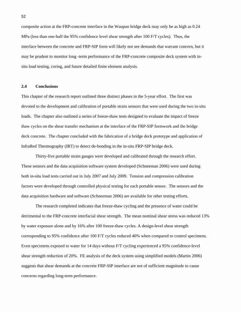
52  composite action at the FRP-concrete interface in the Waupun bridge deck may only be as high as 0.24

MPa (less than one-half the 95% confidence level shear strength after 100 F/T cycles). Thus, the

interface between the concrete and FRP-SIP form will likely not see demands that warrant concern, but it

may be prudent to monitor long -term performance of the FRP-concrete composite deck system with in-

situ load testing, coring, and future detailed finite element analysis.

2.4 Conclusions

This chapter of the research report outlined three distinct phases in the 5-year effort. The first was

devoted to the development and calibration of portable strain sensors that were used during the two in-situ

loads. The chapter also outlined a series of freeze-thaw tests designed to evaluate the impact of freeze

thaw cycles on the shear transfer mechanism at the interface of the FRP-SIP formwork and the bridge

deck concrete. The chapter concluded with the fabrication of a bridge deck prototype and application of

InfraRed Thermography (IRT) to detect de-bonding in the in-situ FRP-SIP bridge deck.

Thirty-five portable strain gauges were developed and calibrated through the research effort.

These sensors and the data acquisition software system developed (Schneeman 2006) were used during

both in-situ load tests carried out in July 2007 and July 2009. Tension and compression calibration

factors were developed through controlled physical testing for each portable sensor. The sensors and the

data acquisition hardware and software (Schneeman 2006) are available for other testing efforts.

The research completed indicates that freeze-thaw cycling and the presence of water could be

detrimental to the FRP-concrete interfacial shear strength. The mean nominal shear stress was reduced 13%

by water exposure alone and by 16% after 100 freeze-thaw cycles. A design-level shear strength

corresponding to 95% confidence after 100 F/T cycles reduced 40% when compared to control specimens.

Even specimens exposed to water for 14 days without F/T cycling experienced a 95% confidence-level

shear strength reduction of 20%. FE analysis of the deck system using simplified models (Martin 2006)

suggests that shear demands at the concrete FRP-SIP interface are not of sufficient magnitude to cause

concerns regarding long-term performance.

53   The laboratory studies conducted to evaluate the reduction in shear strength resulting from freeze-

thaw cycling and moisture presence were very conservative and do not fully represent the situation

present in the field. In other words, the laboratory testing setup is an extreme scenario that is a relatively

crude approximation of the field conditions. Field conditions are likely to be much more favorable and

the resistance to freeze-thaw degradation is felt to be much higher in the actual structure.

2.5 References

AISC (2001). “LRFD Manual of Steel Construction - 3rd Edition,” American Institute of Steel

Construction, Chicago, IL.

ANSYS. (2005). “ANSYS University Intermediate, Release 10.0.”, ANSYS, Inc, Canonsburg, PA.

ASTM (2003). “Standard Test Method for Resistance of Concrete to Rapid Freezing and Thawing,”

ASTM C 666/C 666M – 03, West Conshohocken, PA, 2003.

Bentz, D.P. (2000). “A Computer Model to Predict the Surface Temperature and Time-of-Wetness of

Concrete Pavements and Bridge Decks,” NISTIR 6551, U.S. Department of Commerce, 2000.

Berg, A.C. (2004). “Analysis of a Bridge Deck Built on U.S. Highway 151 with FRP Stay-In-Place

Forms, FRP Grids, and FRP Rebars,” Master’s Thesis, University of Wisconsin – Madison, 2004.

Bisby, L.A. and Green, M.F. (2002). “Resistance to Freezing and Thawing of Fiber-Reinforced Polymer-

Concrete Bond,” ACI Structural Journal, 99(2), 2002, 215-223.

Greenfield, T., Takle, E., Tentinger, B., Alamo, J., Burkheimer, D. and McCauley, D.(2003). “Bridge

Frost: Observations and Forecast by Numerical Methods,” Proceedings of the 2003 Mid-

Continent Transportation Research Symposium, Ames, IA., 2003, CD-ROM.

Haldar, A. and Mahadevan, S. (2000). “Probability, Reliability, and Statistical Methods in Engineering

Design,” John Wiley and Sons, Inc., 2000.

Helmueller, E.J., Bank, L.C., Dieter, D.A., Dietsche, J.S., Oliva, M.G. and Russell, J.S. (2002). “The

Effect of Freeze-Thaw on Bond Between FRP Stay-In-Place Deck Forms and Concrete,”

Proceedings of CDCC 2002, 2nd International Conference on Durability of Fiber Reinforced

Polymer (FRP) Composites for Construction, Montreal, CANADA, May 29-31, pp. 141-152.

54  Krishnaswamy, R. and Lopez M.M.(2006). “Time Performance of Concrete-CFRP Bond under the

Effects of Freeze-Thaw Cycles and Sustained Loading,” TRB 2006 Annual Meeting CD-ROM.

Martin, K.M. (2006). “Impact of Environmental Effects on, and Condition Assessment of, IBRC Bridge

Decks in Wisconsin,” Master’s Thesis, Marquette University, 2006.

Micro-Measurements (2004). “Instruction Bulletin B-147-4.” Application of M-Coat J Protective Coating,

Vishay Micro-Measurements, Revised March, 1996.

ROMUS (2005). “Strain Sensor Shop Drawings." ROMUS Incorporated, Milwaukee, WI.

Schneeman, C.L. (2006). “Development and Evaluation of a Removable and Portable Strain Sensor for

Short-term Live Loading of Bridge Structures,” Master’s Thesis, Marquette University, 2006.

55  

Table 2.1 Calculation of Portable Sensor Calibration Factors

Table 2.2 Calibration Factors for Portable Sensors.

 Top Nylon [uStrain] Top gage [uStrain] Bot. Nylon [uStrain] Bot. gage [uStrain]

-172.4567 -174.029 183.514 180.1114-172.4568 -174.0334 183.5069 180.1181-172.4558 -174.0382 183.4995 180.125

Average = -172.46 -174.03 183.51 180.12St Dev = 0.00 0.00 0.01 0.01

Calibration Factor = 0.991 1.019

Sensor #005 Sensor #006

  Sensor Compression Tension001 1.064 0.964002 1.093 0.965003 1.093 1.159004 1.145 1.045005 0.991 0.925006 1.026 1.019007 1.006 0.975008 0.877 0.786009 1.053 1.070010 1.123 1.091011 1.080 1.043012 1.020 0.999013 1.139 1.028014 1.151 1.073015 1.069 1.013016 1.036 0.999017 1.069 0.967018 0.983 0.935019 1.064 0.972020 1.129 1.044021 0.978 0.934022 0.911 0.851023 1.079 1.044024 0.999 0.945025 1.073 1.026026 1.103 1.026027 1.020 0.959028 1.131 1.033029 1.049 0.985030 0.952 0.922031 0.957 0.940032 0.979 0.923033 0.962 0.910034 1.111 1.026035 0.989 0.997

Average 1.043 0.988

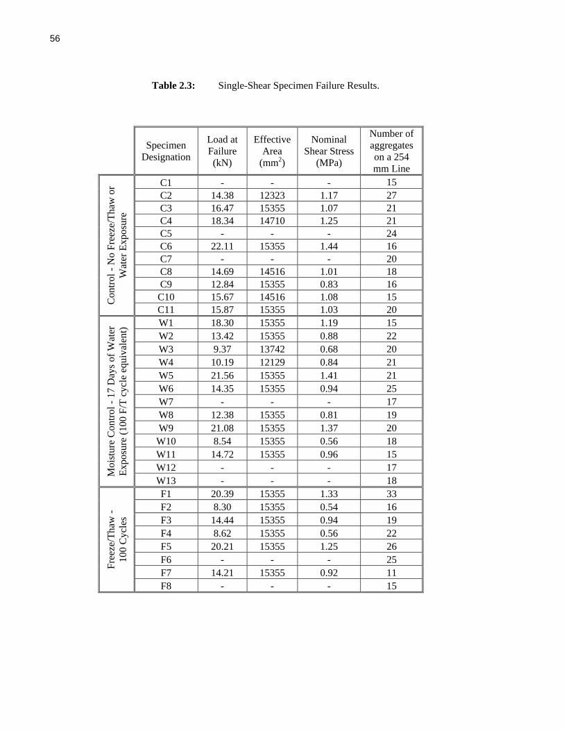
56  

Table 2.3: Single-Shear Specimen Failure Results.

Specimen Designation

Load at Failure (kN)

Effective Area

(mm2)

Nominal Shear Stress

(MPa)

Number of aggregates on a 254 mm Line

Con

trol -

No

Free

ze/T

haw

or

Wat

er E

xpos

ure

C1 - - - 15 C2 14.38 12323 1.17 27 C3 16.47 15355 1.07 21 C4 18.34 14710 1.25 21 C5 - - - 24 C6 22.11 15355 1.44 16 C7 - - - 20 C8 14.69 14516 1.01 18 C9 12.84 15355 0.83 16

C10 15.67 14516 1.08 15 C11 15.87 15355 1.03 20

Moi

stur

e C

ontro

l - 1

7 D

ays o

f Wat

er

Expo

sure

(100

F/T

cyc

le e

quiv

alen

t)

W1 18.30 15355 1.19 15 W2 13.42 15355 0.88 22 W3 9.37 13742 0.68 20 W4 10.19 12129 0.84 21 W5 21.56 15355 1.41 21 W6 14.35 15355 0.94 25 W7 - - - 17 W8 12.38 15355 0.81 19 W9 21.08 15355 1.37 20

W10 8.54 15355 0.56 18 W11 14.72 15355 0.96 15 W12 - - - 17 W13 - - - 18

Free

ze/T

haw

- 10

0 C

ycle

s

F1 20.39 15355 1.33 33 F2 8.30 15355 0.54 16 F3 14.44 15355 0.94 19 F4 8.62 15355 0.56 22 F5 20.21 15355 1.25 26 F6 - - - 25 F7 14.21 15355 0.92 11 F8 - - - 15

57  

Table 2.4: Single-shear means and 95% confidence levels.

Specimen Group Nominal Shear Stress (MPa) Mean 95% Confidence

Control 1.11 0.96 Moisture Control 0.96 0.76

Freeze/Thaw 0.94 0.57

58  

Figure 2.1: Configuration of the strain sensor.

Figure 2.2: Constructed strain sensors without connection tabs or protective coating.

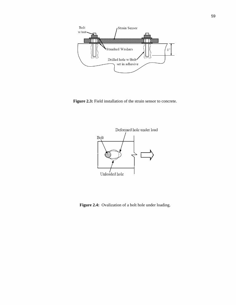
59  

Figure 2.3: Field installation of the strain sensor to concrete.

Figure 2.4: Ovalization of a bolt hole under loading.

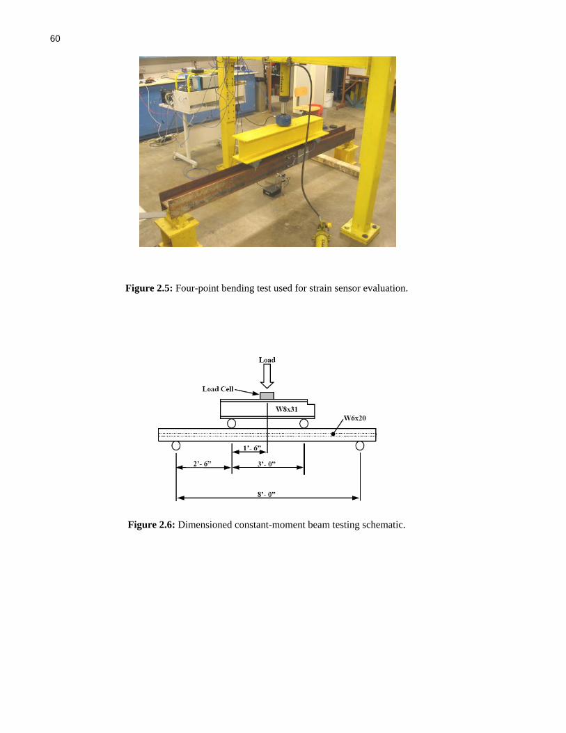
60  

Figure 2.5: Four-point bending test used for strain sensor evaluation.

Figure 2.6: Dimensioned constant-moment beam testing schematic.

61  

Figure 2.7: Mid-span layout of Strain sensors and complementary strain gages.

Figure 2.8: Half bridge temperature compensating circuit.

62  

Figure 2.9: Boundary conditions of the 3D beam model.

Figure 2.10: The extrusion process uses to build a 3D model of the sensor. It can be seen that from figure (a) the entire 2D planar mesh is extruded 0.05” in figure (b). The center depression is then created in figure (c) by extruding all areas around the depression.

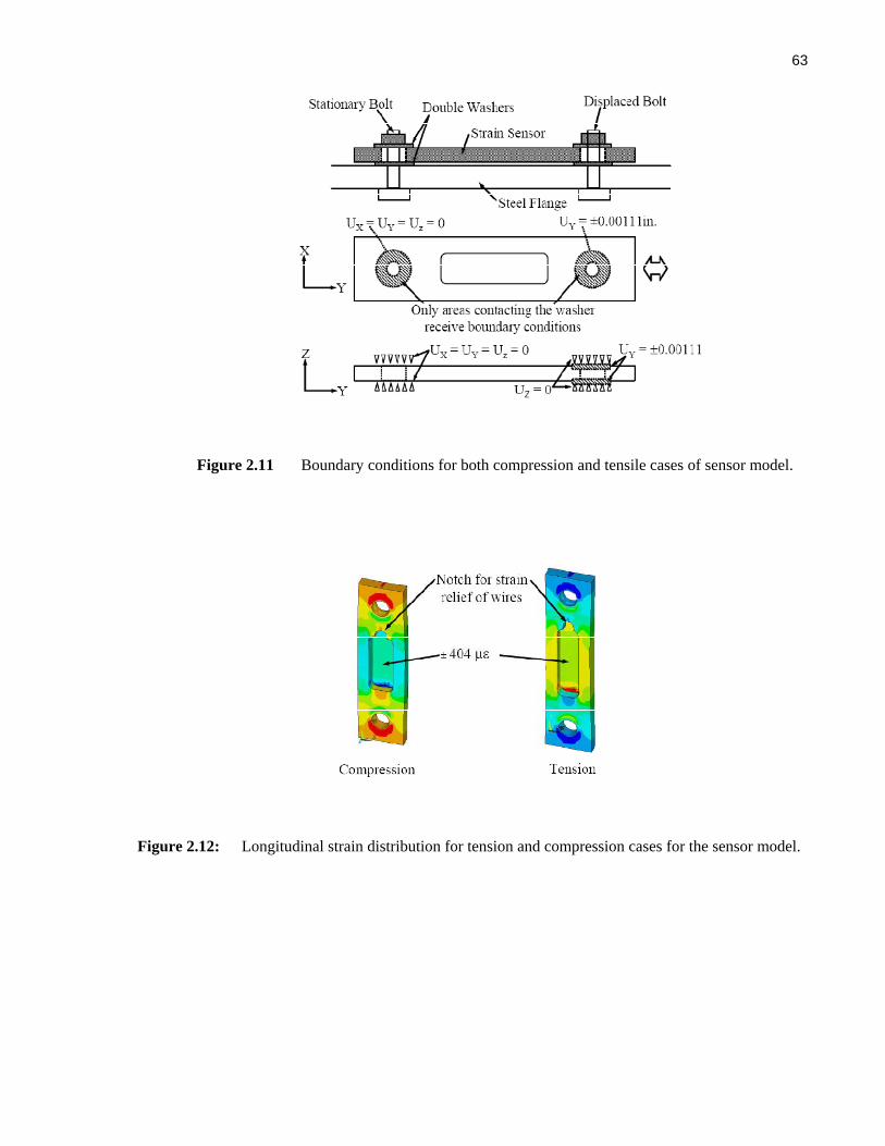
63  

Figure 2.11 Boundary conditions for both compression and tensile cases of sensor model.

Figure 2.12: Longitudinal strain distribution for tension and compression cases for the sensor model.

64  

Figure 2.13: Weld locations on beam members for the constant-moment load test.

Figure 2.14: Typical response of strain gages and sensors under applied loading.

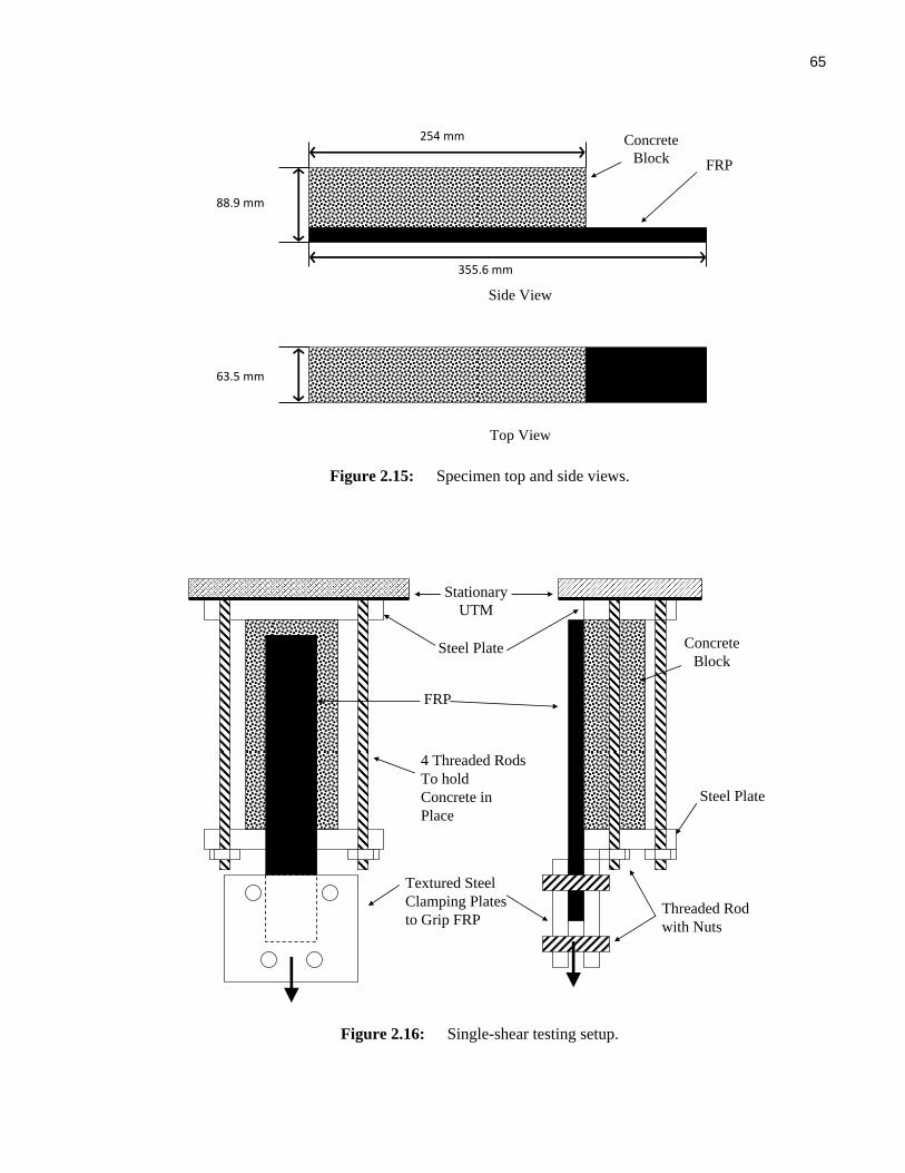
65  

Figure 2.15: Specimen top and side views.

Figure 2.16: Single-shear testing setup.

FRP

Concrete Block

4 Threaded Rods To hold Concrete in Place

Textured Steel Clamping Plates to Grip FRP

Threaded Rod with Nuts

Steel Plate

Steel Plate

Stationary UTM

10”

14”

3.5”

Side View

Top View

2.5”

FRP

Concrete Block

254 mm 

88.9 mm 

355.6 mm 

63.5 mm 

66  

Figure 2.17: Cuts on each end of the concrete block to square it with the FRP.

(a) (b)

Figure 2.18 : Typical single-shear specimen failure: (a) failure surfaces; (b) typical 254 mm line drawn to check aggregate coverage (Berg 2004).

gCutCut

67  

Chapter 3

In-Situ Monitoring and Non-Destructive Evaluation

3.1 Introduction

The IBRC monitoring project for bridges B-20-133/134 and B-20-148/149 was a five year program that

involved in-situ load testing, laboratory work, and numerical simulation of superstructure response. An

in-situ monitoring program was conducted to establish benchmark condition of the bridge superstructure

systems, evaluate nondestructive evaluation (NDE) techniques that may facilitate gathering information

suitable for quantifying long-term performance, and gather information related to egress of moisture into

the FRP-SIP bridge deck system utilized in bridge B-20-133. This chapter in the report is, in large part,

based upon the graduate research work of Martin (2006). Further details regarding the information in the

chapter are available (Martin 2006).

This chapter of the report outlines initiatives in these three areas carried out during the IBRC

monitoring project and provides a detailed benchmark condition evaluation of each bridge superstructure

system, makes recommendations regarding the suitability of various NDE methods in attaining

information pertinent to long-term performance assessment, and discusses data gathered to evaluate the

severity of moisture egress into the FRP-SIP formwork deck system.

3.2 Benchmark Condition Evaluation of B-20-133/134

A day was spent at bridges B-20-133/134 to document an initial crack map and the overall condition of

each bridge. MU-IBRC team members visited B-20-133/134 on October 25, 2005. Visual inspection of

the bridge superstructures was completed and pictures were taken to document the condition of key

superstructure elements. The bridges examined are shown in Figure 3.1. Bridge B-20-133 is the IBRC

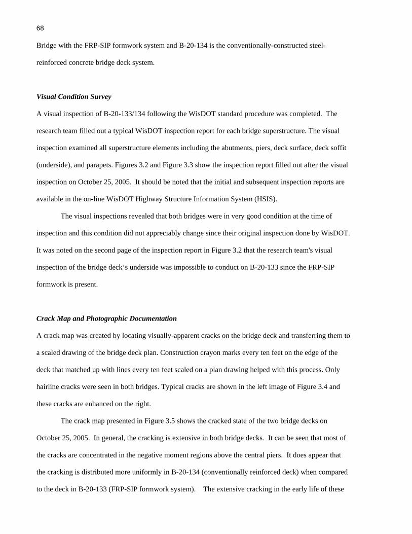
68  Bridge with the FRP-SIP formwork system and B-20-134 is the conventionally-constructed steel-

reinforced concrete bridge deck system.

Visual Condition Survey

A visual inspection of B-20-133/134 following the WisDOT standard procedure was completed. The

research team filled out a typical WisDOT inspection report for each bridge superstructure. The visual

inspection examined all superstructure elements including the abutments, piers, deck surface, deck soffit

(underside), and parapets. Figures 3.2 and Figure 3.3 show the inspection report filled out after the visual

inspection on October 25, 2005. It should be noted that the initial and subsequent inspection reports are

available in the on-line WisDOT Highway Structure Information System (HSIS).

The visual inspections revealed that both bridges were in very good condition at the time of

inspection and this condition did not appreciably change since their original inspection done by WisDOT.

It was noted on the second page of the inspection report in Figure 3.2 that the research team's visual

inspection of the bridge deck’s underside was impossible to conduct on B-20-133 since the FRP-SIP

formwork is present.

Crack Map and Photographic Documentation

A crack map was created by locating visually-apparent cracks on the bridge deck and transferring them to

a scaled drawing of the bridge deck plan. Construction crayon marks every ten feet on the edge of the

deck that matched up with lines every ten feet scaled on a plan drawing helped with this process. Only

hairline cracks were seen in both bridges. Typical cracks are shown in the left image of Figure 3.4 and

these cracks are enhanced on the right.

The crack map presented in Figure 3.5 shows the cracked state of the two bridge decks on

October 25, 2005. In general, the cracking is extensive in both bridge decks. It can be seen that most of

the cracks are concentrated in the negative moment regions above the central piers. It does appear that

the cracking is distributed more uniformly in B-20-134 (conventionally reinforced deck) when compared

to the deck in B-20-133 (FRP-SIP formwork system). The extensive cracking in the early life of these

69  

bridge decks is of concern and subsequent simulation efforts conducted by the research team to help

quantify reasons for this will be discussed in later chapters of this report. Both bridge decks exhibit

typical cracking at acute corners in skewed superstructures that result from free shrinkage restraint in the

bridge deck.

The plan views shown in Figure 3.6 constitute a picture index for bridges B-20-133/134. It shows

the intended target location and direction of the pictures taken to document the bridge condition. The

number in the circle on the index corresponds to the photo number in parenthesis in each figure caption.

The arrow accompanying each number shows the direction the photo was taken.

Bridge B-20-134, the sister bridge to B-20-133, serves as a comparison for the innovative use of

FRP. Bridge B-20-133 is the innovative bridge using FRP SIP formwork and a single layer of FRP

grillage reinforcement. In the pictures for B-20-133, the most southern girder is labeled #1 and the

northern most girder, #3. All pictures from the inspection are included in Figures 3.7 through 3.17. It

should be noted that not all photos indexed in Figure 3.6 are included in this report. All photos can be

found in Martin (2006).

Hairline cracks in the bridge decks have propagated to and through the parapet with efflorescence

showing on the underside of the overhang of each bridge deck shown in Figure 3.7 and 3.8. As seen in

Figure 3.6, cracking on both bridges is primarily located near the abutments and the central pier. Bridge

B-20-133 appears to have less frequent cracking at the mid-span location between the abutment and

central pier. This may be a result of the SIP FRP formwork restraining shrinkage of the deck as well as

the tight spacing of the FRP grillage. Both the innovative and traditionally constructed twin has

significant efflorescent cracks in the bridge deck overhang.

Figures 3.10 and Figure 3.11 show the interior diaphragm looking east and west at the southern

sides of the central piers. There is similar cracking seen around the interface between the girders and the

central diaphragm. The northern parapets also show cracks around the central pier and efflorescence on

the underside of the bridge deck soffit as seen in Figure 3.11 and 3.12. The northern parapets within the

70  spans pictured in Figures 3.13 and 3.14 do not show cracking and efflorescence to the same extent as the

parapets around the central pier.

The only thing quite different about the two bridges is the underside of the decks. Bridge B-20-

133 has FRP-SIP formwork so inspecting the concrete deck condition from the underside is impossible.

Accumulation of moisture at the interface of the concrete deck and FRP-SIP formwork was of concern

and this is evaluated more thoroughly in a subsequent section of this chapter. Figure 3.15 shows typical

and sporadically located blistering in the FRP formwork sheets found in the benchmarks inspection. This

blistering is naturally occurring resin defects arising from the manufacturing process. Excess glue or

sealant used between FRP SIP sheets during construction can also be seen in Figure 3.15. This is not

detrimental.

The underside of B-20-134 is unobstructed and cracks with efflorescence are prevalent on the

underside of the bridge deck. Figure 3.16 shows full depth diagonal and transverse cracks near the

abutment. Full depth cracks are seen through the entirety of the bridge deck. Figure 3.17 shows transverse

full depth cracks along the west span of B-20-134 going all the way to the central pier. It is suspected that

full-depth cracks in the FRP-SIP formed deck are also present, but this was never confirmed.

3.3 Benchmark Condition Evaluation of B-20-148/149

An initial crack map for bridges B-20-148/149 was also generated to document the condition of these

bridge superstructures. On October 27, 2005, MU-IBRC team members performed a visual inspection of

bridges B-20-148/149. Figure 3.19 is an overview photograph showing the bridges in October 2005. It

should be noted that traffic in 2005 was relatively light (much less than it is currently). The visual

inspection included a walk-around under and on the bridges. Photographs were taken to document the

condition of key elements in the bridge superstructures.

Visual Condition Survey

The visual inspection was performed in a manner similar to that of B-20-133/134. In addition, WisDOT

standard bridge inspection report forms were filled out by the research team. These completed forms

71  

serve as supplemental information to that obtained in the regularly scheduled WisDOT inspections, which

are available on the HSIS website. Figure 3.19 includes the completed WisDOT inspection reports for

the two bridges done on October 27, 2005. The MU research team found that the bridge superstructures

were in excellent condition and very little (if any) changes occurred since the initial inspection recorded

in the HSIS database. Bridge B-20-148 is the IBRC Bridge with FRP grillage reinforcement and B-20-

149 is the conventionally reinforced bridge.

Crack Map and Photographic Documentation

A crack map similar to that generated for B-20-133/134 was also generated for B-20-148/149. These two

bridge decks were remarkably free of cracking at the time of this inspection. A typical crack is shown in

Figure 3.21. The overall crack maps for both bridge decks shown in Figure 3.22 indicate that the bridges

have very little cracking at this point in their service life. Only small cracks were found in B-20-149, the

mild-steel reinforced bridge, near the abutment joints and on the parapet.

It is interesting to note that the cracking in these simply-supported superstructures is limited to

locations near the abutments where shrinkage restraint is more likely to be present. The overall span of

these bridge superstructures is similar to the spans found in the continuous superstructures of bridges B-

20-133/134. However, the extent of cracking in the simply supported configuration is much less than the

continuous configuration. This suggests that shrinkage-induced cracking is much more likely in

continuous-span superstructures and that live loading-induced tensile strains in the deck resulting from

the continuous-span configuration. This likelihood is evaluated more thoroughly using finite element

simulation in another chapter of this report.

Bridge deck schematics for B-20-148/149 with picture indices that document photograph

numbers and direction it was taken are given in Figure 3.23. The photographs illustrate the condition of

key bridge elements at the time of the visual inspection (late October 2005). A complete set of photos and

index is available (Martin 2006). Figures 3.24 and 3.25 show overall road surface condition and typical

traffic flow/content on the day of the visual inspection.

72  

Figure 3.26 and 3.27 show the north side of the eastern abutments of each bridge. Figure 3.27

also illustrates the location of the data acquisition junction box that was used for wiring data acquisition

instruments the load testing conducted during the research effort. Figures 3.28 and 3.29 document the

northern parapets of each bridge. Bridge B-20-149 (Figure 3.28), the steel-reinforced bridge deck,

features a pedestrian walk way on the North side of the bridge deck. No cracking was found through the

visual inspection at the overhanging portion of the decks for either bridge.

The concrete diaphragms at the abutments for both bridges were in excellent condition. Figures

3.30 and 3.31 illustrate the condition of these superstructure components on the day of the benchmark

condition survey. Figures 3.32 and 3.33 illustrate the condition of the underside of the bridge deck in the

vicinity of the steel diaphragms. No cracking is seen in the underside of the deck, and the galvanized

steel diaphragms have no signs of deterioration.

The only cracks found through the visual inspection were in the steel-reinforced bridge (B-20-

149). Figure 3.34 documents one of the few cracks found in the parapets of these bridges. In general, the

cracks were of hairline width and they did not project down into the bridge deck overhang. Therefore, it

can be surmised that these cracks were simply shrinkage cracks arising from the slip forming of the

parapet and were not shrinkage cracking in the deck projecting into the parapet wall.

3.4 Evaluation of NDE Techniques

The initial condition of bridges B-20-133/134 and B-20-148/149 fostered examination of non-destructive

evaluation (NDE) methodologies to help understand the likely causes of the initial cracking, evaluating

the extent to which further deterioration is progressing and perhaps most importantly, generating and

understanding the impact of moisture penetration in the bridge deck with FRP-SIP formwork (B-20-133).

This section of the report outlines a review of NDE techniques that may be suitable for

understanding long-term degradation within the bridge superstructures considered in this research effort.

It also outlines a short study to evaluate the extent to which moisture has penetrated the FRP-SIP

formwork bridge deck when compared to the conventionally constructed bridge deck.

73  

Chain Dragging

Chain dragging is a popular acoustic-emission-based technique for locating subsurface delamination in

the concrete above bridge deck reinforcement and stratification-type delamination in concrete (Guthrie, et

al. 2006). To date, chain dragging is the only NDE tool capable of detecting locations of potential

delamination. A typical implementation of chain dragging employs a steel chain being dragged along the

deck or test area in a carefully determined path. A technician listens for changes in the acoustic response

of the deck. Since this is only a location test, another test must be used to determine the size of the

delaminated area. Usually a hammer or tap test follows the chain dragging and this follow-on test is

described in the next section.

It is difficult to say if chain dragging would be useful for locating delamination present on the

bottom of an 8” deck with FRP-SIP formwork. In most cases, delamination of the concrete above

reinforcing steel is in the upper section of the deck. Further testing would be needed to show this as a

valid approach to finding potentially un-bonded areas in the FRP-SIP formwork bridge decks. However,

the technique is likely to remain useful in determining delamations in the concrete matrix near the surface

of the deck that may or may not result from the very closely spaced FRP grillage reinforcement. The

close proximity of the grillage reinforcement near the surface of the deck may have resulted in difficulty

in properly consolidating the concrete during placement. However, it should be noted that this tendency

is no different than that for the conventionally reinforced bridge deck. Attempting to detect delaminations

at the interface between the FRP-SIP formwork and concrete deck is not within the realm of practicality

with the chain dragging NDE technique and therefore, it was not implemented in this study.

Once a bridge deck is in service, carrying out chain dragging on the bridge deck would require

that lane closures be executed. This traffic control was not accounted for in the project budget and

therefore, it was a second difficulty associated with implementing chain dragging in the present study.

These two difficulties associated with chain dragging coupled with its lack of perceived benefit in

assessing the tendency for delamination at critical interfaces in the FRP-SIP bridge deck system suggested

that it would not be a useful NDE methodology for the present study.

74  Tap Testing

Traditional tap testing or coin tap testing is one of the simplest NDE tests to execute, but is also the

hardest to quantitatively interpret. The test simply requires the inspector to tap a small coin-like disk on

the structure in question. The tap test has traditionally been qualitative, relying on an inspectors hearing to

detect defective regions (Starnes and Carino 2003). The other problem with using it on large structures is

that it is a point test. It would be very time consuming to tap the entirety of the underside of a bridge deck.

The research team did identify a research group attempting to create a quantitative and automated

coin tap method. At the time of the research conducted by Martin (2006), a team at the Center for Non-

Destructive Evaluation at Iowa State University was working on improving the coin tap test and to

develop a Computer-Aided Tap Tester (CATT). The system uses and accelerometer to measure the

amount of contact time the tip has with the material in question. For composites, debonding would be

indicated by a longer contact time because the material is more flexible than a bonded composite material.

The instrumented tapping system is intended to have imaging capabilities that would be able to

quantitatively relate to the local stiffness of the structure to potential delamination. The methodology

and procedure was developed to inspect the integrity of airplane and helicopter components. The system

was intended to be simple to apply; would have low cost to implement; and inspectors would not need

extensive training (CNDE 1999). A visit to the CNDE in Ames, IA by Martin (2006) showed that the

CATT would not be a very good choice for the present research effort because the tip of the CATT is

extremely small and intended for very thick composite materials and not reinforced concrete bridge decks.

Figure 3.35 illustrates the typical CATT equipment and images obtained through implementation.

The company that makes the accelerometer tip that is used in the CATT system also

manufactures impact hammers. These hammers in the vibration division of the company can be used for

modal analysis, structural testing, resonance determination, and civil infrastructure health determination

(PCB 2006). The hammers use the same principle as the coin tapping test and the CATT, but a larger

mass to deliver the initial impact. Typical hammers are shown in Figure 3.36. The tip of each hammer

has a response accelerometer attached to it which measures the motion of the test specimen as a result of

75  

the impulse force provided by the hammer. They have the ability to include computer-based data

acquisition while inspecting a structure.

If the FRP-SIP formwork on the bottom of the bridge deck is separating from the concrete deck

(i.e. delaminating), it should be more flexible and show a longer contact time when hit with an impact

hammer. This would be a good test to use to quantify the degree to which debonding has taken place

between the FRP-SIP formwork and the concrete bridge deck. An expected contact time for a good bond

scenario would have to be established to compare the values found on the bridge deck. The present

research effort did not have funds sufficient to calibrate this methodology for use in bridge infrastructure

systems and therefore, it was not applied in the present effort. It should be noted that implementing tap

testing on the underside of the bridge deck is feasible and it is recommended that a research effort be

undertaken to quantify the capabilities of this method for determining the extent to which debonding is

present in the FRP-SIP bridge deck system.

Ultrasonic Testing

Ultrasonic testing measures the speed of waves traveling through materials. Ultrasonic systems, digital or

analog, typically have four components: transducer, pulse generator (clock), receiver/amplifier, and a

display (screen). Figure 3.37 schematically illustrates these components. The clock or pulse generator

sends voltage to the transducer which creates an impulse that excites the material being tested. The

material reflects the wave created by the impulse back to the transducer. The transducer then sends a

voltage signal to the receiver or amplifier. These are all recorded on a screen that displays the time

between the transducer sending the impulse and receiving the reflected wave. This time can then be

related to the pulse velocity when the thickness of the testing material is known. It has been reported that

pulse velocities can then be correlated to material quality or bond quality (Hellier 2001).

Because transducers are used to generate and intercept the pulses on either side of a specimen, it

is more difficult to do this test in-situ on a bridge deck. For example, to determine the quality of concrete,

cores would have to be taken from the bridge to be evaluated. As the quality of concrete decreases so

76  does the pulse velocity. Testing has shown that pulse velocities over 4,600 m/s (15,100 ft/s) indicate very

good quality concrete where velocities lower than 2,100 m/s (6,900 ft/s) indicate very poor quality

concrete (Grace and Hanson, 2004). These velocities can also be used to estimate the unconfined

compressive strength of concrete.

Ultrasonic testing could be useful on a predetermined problem area from chain dragging or tap

testing. This would be another way to quantify delaminations after the delamination has been located.

Typically the transducers used are small and it would be unrealistic to use them to examine the entire

underside of the deck. Testing would have to be done to correlate the pulse velocities to the FRP-SIP

being bonded or un-bonded. Overall, it is unlikely that ultrasonic testing would be a useful tool in

assessing the long-term performance of the IBRC bridge superstructures.

Infrared Thermography

Infrared thermography (IRT) is based on the principle that subsurface defects affect the heat flow in a

material (Rens, Nogueirea and Transue 2005). The technique became a recognized standard method for

NDE by the American Society for Nondestructive Testing in 1992. As conduction occurs in a bridge deck,

any discontinuities in the material will interrupt the heat transfer and show a localized temperature change.

Infrared systems such as cameras and scanners are used to detect these differences. Most of these

applications require a trained professional interpretation because of the many variables that go into IRT

such as emissivity, thermal coefficients of constituent materials, and temperature are difficult to

definitively establish. Even though training is required to interpret results, IRT is fast and it can create

images almost immediately. In theory, a trained thermographer can determine the condition of the

structure very quickly (Hellier 2001).

The key to infrared thermography in bridge decks is that there must be void space in the material

that will transfer heat differently thereby facilitating detection. Concrete is an ideal material for this

because, although it has a low thermal conductivity, it is able to retain heat for a long period of time. For

bridge decks, the conditions just after sunrise or sunset create an environment where the concrete deck

has a different temperature than the surrounding ambient air (Chowdhury et al. 2004).

77  

Debonding between the FRP-SIP formwork and the concrete deck is possible to detect with

infrared thermography, but is harder to detect since the two materials may have lost bond but could still

be in contact with each other. This situation will not provide the necessary void to disrupt the heating

flow. IRT has been used in the aerospace industry to detect de-bonded lamina in composite structures

because of its sensitivity to voids (Nokes and Hawkins 2001). Theoretically, this technique could be used

to show debonding in a bridge deck with the FR-SIP reinforcement.

Bridge decks and test specimens can be heated in a variety of ways. Typically, a bridge deck

tested in-situ is allowed to heat in the morning on a sunny day and they are then scanned in the early

afternoon. An experiment involving a specimen made of FRP tubes bonded together with adhesive was

heated using a hairdryer that piped hot air into the tubular void space. Debonded with void space around

it can be found as a cool spot with an infrared scanner or camera. Other ways of heating specimens

include heated water and heat lamps (Miceli 2000).

Debonding can be confirmed by a tap test once found by an IRT camera or scanner. Tests using

this technique in Ohio showed that IRT was successful in finding debonding in composite retrofit systems

(Nokes and Hawkins 2001). The tap test was found to be essential in minimizing false positive debonded

areas found by the IRT scanner. IRT could identify and monitor debonding; however it was found that a

debonded area must change by 50% to confidently indicate growth in the debonded area (Nokes and

Hawkins 2001).

Marquette University tested out IRT on a scale-model section of the FRP-SIP bridge deck with

FRP grillage reinforcement (Martin 2006). The full-scale prototype was used for this evaluation prior to

load testing. The bridge deck is shown in Figure 3.38. Planned locations of debonded formwork were

fabricated into the bridge-deck prototype. The FRP-SIP formwork was covered in Concresive® and

aggregate as formulated in the original design specifications with the exception of several locations

intentionally masked to create areas un-bonded areas. These un-bonded areas were then intended to be

test locations for the IRT method. Additional details related to the means of establishing un-bonded

zones within the bridge deck prototype are available (Martin 2006).

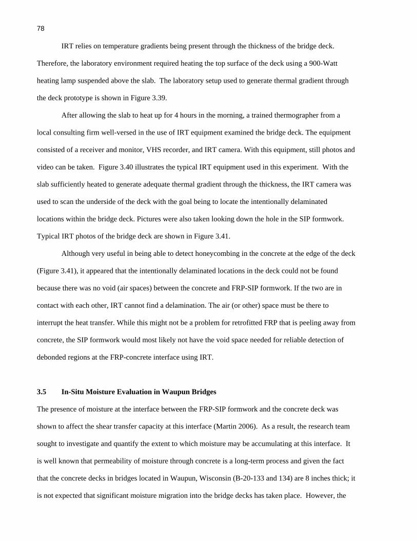
78  

IRT relies on temperature gradients being present through the thickness of the bridge deck.

Therefore, the laboratory environment required heating the top surface of the deck using a 900-Watt

heating lamp suspended above the slab. The laboratory setup used to generate thermal gradient through

the deck prototype is shown in Figure 3.39.

After allowing the slab to heat up for 4 hours in the morning, a trained thermographer from a

local consulting firm well-versed in the use of IRT equipment examined the bridge deck. The equipment

consisted of a receiver and monitor, VHS recorder, and IRT camera. With this equipment, still photos and

video can be taken. Figure 3.40 illustrates the typical IRT equipment used in this experiment. With the

slab sufficiently heated to generate adequate thermal gradient through the thickness, the IRT camera was

used to scan the underside of the deck with the goal being to locate the intentionally delaminated

locations within the bridge deck. Pictures were also taken looking down the hole in the SIP formwork.

Typical IRT photos of the bridge deck are shown in Figure 3.41.

Although very useful in being able to detect honeycombing in the concrete at the edge of the deck

(Figure 3.41), it appeared that the intentionally delaminated locations in the deck could not be found

because there was no void (air spaces) between the concrete and FRP-SIP formwork. If the two are in

contact with each other, IRT cannot find a delamination. The air (or other) space must be there to

interrupt the heat transfer. While this might not be a problem for retrofitted FRP that is peeling away from

concrete, the SIP formwork would most likely not have the void space needed for reliable detection of

debonded regions at the FRP-concrete interface using IRT.

3.5 In-Situ Moisture Evaluation in Waupun Bridges

The presence of moisture at the interface between the FRP-SIP formwork and the concrete deck was

shown to affect the shear transfer capacity at this interface (Martin 2006). As a result, the research team

sought to investigate and quantify the extent to which moisture may be accumulating at this interface. It

is well known that permeability of moisture through concrete is a long-term process and given the fact

that the concrete decks in bridges located in Waupun, Wisconsin (B-20-133 and 134) are 8 inches thick; it

is not expected that significant moisture migration into the bridge decks has taken place. However, the

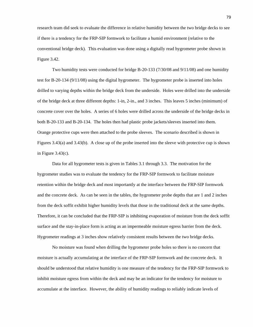
79  

research team did seek to evaluate the difference in relative humidity between the two bridge decks to see

if there is a tendency for the FRP-SIP formwork to facilitate a humid environment (relative to the

conventional bridge deck). This evaluation was done using a digitally read hygrometer probe shown in

Figure 3.42.

Two humidity tests were conducted for bridge B-20-133 (7/30/08 and 9/11/08) and one humidity

test for B-20-134 (9/11/08) using the digital hygrometer. The hygrometer probe is inserted into holes

drilled to varying depths within the bridge deck from the underside. Holes were drilled into the underside

of the bridge deck at three different depths: 1-in, 2-in., and 3 inches. This leaves 5 inches (minimum) of

concrete cover over the holes. A series of 6 holes were drilled across the underside of the bridge decks in

both B-20-133 and B-20-134. The holes then had plastic probe jackets/sleeves inserted into them.

Orange protective cups were then attached to the probe sleeves. The scenario described is shown in

Figures 3.43(a) and 3.43(b). A close up of the probe inserted into the sleeve with protective cup is shown

in Figure 3.43(c).

Data for all hygrometer tests is given in Tables 3.1 through 3.3. The motivation for the

hygrometer studies was to evaluate the tendency for the FRP-SIP formwork to facilitate moisture

retention within the bridge deck and most importantly at the interface between the FRP-SIP formwork

and the concrete deck. As can be seen in the tables, the hygrometer probe depths that are 1 and 2 inches

from the deck soffit exhibit higher humidity levels that those in the traditional deck at the same depths.

Therefore, it can be concluded that the FRP-SIP is inhibiting evaporation of moisture from the deck soffit

surface and the stay-in-place form is acting as an impermeable moisture egress barrier from the deck.

Hygrometer readings at 3 inches show relatively consistent results between the two bridge decks.

No moisture was found when drilling the hygrometer probe holes so there is no concern that

moisture is actually accumulating at the interface of the FRP-SIP formwork and the concrete deck. It

should be understood that relative humidity is one measure of the tendency for the FRP-SIP formwork to

inhibit moisture egress from within the deck and may be an indicator for the tendency for moisture to

accumulate at the interface. However, the ability of humidity readings to reliably indicate levels of

80  moisture to expect at the interface remains to be definitively proven. It is recommended that further

analysis with regard to relative humidity be undertaken in future research efforts as it may be a useful tool

for long-term evaluation.

3.6 Conclusions

Three major items were discussed in the present chapter. Initial benchmark condition assessments of the

IBRC bridge superstructures were described in detail. Evaluation of available NDE techniques, including

a laboratory evaluation test for IRT, was conducted. Finally, in-situ moisture testing through use of

digital hygrometer was described.

After approximately one year of traffic loading, bridges B-20-133/134 showed significant

transverse cracking around the central piers and along the abutment joints. Therefore, it is likely that

moisture has a direct path to the zone where aggregate interlock between the FRP-SIP formwork and

concrete is needed to accomplish the shear transfer needed to ensure that positive tension reinforcement

for the bridge deck exists. Without a way to escape, moisture may freeze and thaw as the climate changes

during the seasons.

Bridges B-20-148/149 are in excellent condition. These bridges show virtually no signs of deck

cracking other than a few hairline cracks located at the abutments and in the parapet(s). The bridge deck

with FRP reinforcement showed no cracks. No cracks were observed to extend through the bridge deck

thickness. The lack of cracking present in the simply-supported superstructure when compared to the

two-span continuous superstructures found in bridges B-20-133/134 suggests that further study of the

continuous superstructure configuration is warranted. Further evaluation of the simply supported bridge

superstructures (B-20-148/149) is not warranted.

The NDE techniques of infrared thermography, chain dragging, tap testing, and ultrasonic testing,

were reviewed. Tap testing with an impact hammer appears to be the most useful methods for monitoring

the bridges studied in the present effort. Infrared thermography is the least likely to yield useful results

for monitoring the IBRC bridges. Without an air void at the interface between FRP-SIP form and the

concrete deck, there will not be a disruption of the heat transfer and IRT will not show debonding.

81  

Whichever NDE method is chosen to inspect the bridge decks with FRP-SIP, it must be realized

that any NDE technique will only be able to look at about half of the FRP area in contact with concrete.

The tops of the void spaces that result from the FRP-tubes in the SIP formwork will be impossible to

inspect because of the layer of FRP below the openings. This makes it very difficult to get a good idea of

how much area is adequately interlocked once a test has been established to determine the quality of the

interlock between the aggregate and FRP. It may be that coring the bridge deck and examining the

resulting concrete quality and the interface between the concrete and FRP-SIP formwork is the most

useful NDE/NDT methodology for the IBRC bridge at Waupun. It is conceivable that cores can be taken

at regular intervals and monitored using procedures employed in Grace and Hanson (2004).

No moisture was found when drilling the hygrometer probe holes so there is no concern that

moisture is actually accumulating at the interface of the FRP-SIP formwork and the concrete deck as of

the date of this report. It should be understood that relative humidity is one measure of the tendency for

the FRP-SIP formwork to inhibit moisture egress from within the deck and may be an indicator for the

tendency for moisture to accumulate at the interface. However, the ability of humidity readings to

reliably indicate levels of moisture to expect at the interface remains to be definitively proven. It is

recommended that further analysis with regard to relative humidity be undertaken in future research

efforts as it may be a useful tool for long-term evaluation.

3.7 References

Chowdhury, R., Attanayaka, A.M.U.B., Aktan, H.M. (2005). "Non-Destructive Evaluation of Concrete

Components Using Infrared (IR) Thermography for Void Detection and Moisture Evaluation",

Transportation Research Board Annual Meeting, National Academies, (CD-ROM).

CNDE (1999). "Tap Test Improved by Instrumentation Development" Center for NDE News, Volume 10,

Issue 2, Iowa State University, Ames, Iowa.

Grace, N. and Hanson, J. (2004). Inspection and Deterioration of Bridge Decks Constructed Using Stay-

In-Place Metal Forms and Epoxy-Coated Reinforcement, Department of Civil Engineering,

82  

Lawrence Technological University, Southfield, MI.

Guthrie, W.S., Frost, S.L., Birdsall, A.W., Linford, E.T., Ross, L.A., Crane, R.A., Eggert, D.L. (2006).

"Effect of Stay-In-Place Metal Forms on Performance of Concrete Bridge Decks", Transportation

Research Board Annual Meeting, National Academies, (CD-ROM).

Hellier, C. (2001). Handbook of Nondestructive Evaluation, McGraw Hill.

Martin, K.E. (2006). Impact of Environmental Effects On, and Condition Assessment Of, IBRC Bridge

Decks in Wisconsin, MS Thesis, Marquette University, Milwaukee, Wisconsin, May.

Miceli, M. (2000). Assessment of Infrared Thermography as NDE method for Investigation of FRP

Bridge Decks, MS Thesis, Virginia Polytechnic Institute and State University, Blacksburg,

Virginia.

Nokes, J.P. and Hawkins, G.F. (2001). Infrared Inspection of Composite Reinforced Concrete Structures,

Ohio Department of Transportation, Columbus, OH.

PCB (2006). PCB Piezotronics, http://www.pcb.com, accessed January through April 2006.

Rens, K.L., Nogueira, C.L., Transue, D.J. (2005). "Bridge Management and Nondestructive Evaluation",

Journal of Performance of Constructed Facilities, Volume 19, No. 1, February, pp. 3-16.

Starnes, M.A. and Carino, N.J. (2003). Infrared Thermography for Nondestructive Evaluation of Fiber

Reinforced Polymer Composites Bonded to Concrete, NISTIR 6949, U.S. Department of

Commerce, Washington, D.C.

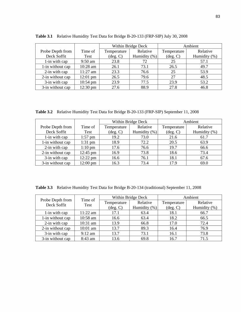
83  

Table 3.1 Relative Humidity Test Data for Bridge B-20-133 (FRP-SIP) July 30, 2008

Probe Depth from Deck Soffit

Time of Test

Within Bridge Deck Ambient Temperature

(deg. C) Relative

Humidity (%)Temperature

(deg. C) Relative

Humidity (%) 1-in with cap 9:50 am 23.8 72 25 57.1

1-in without cap 10:28 am 26.1 73.1 26.5 49.7 2-in with cap 11:27 am 23.3 76.6 25 53.9

2-in without cap 12:01 pm 26.5 79.6 27 48.5 3-in with cap 10:54 pm 23.9 77.5 23.9 53.2

3-in without cap 12:30 pm 27.6 88.9 27.8 46.8

Table 3.2 Relative Humidity Test Data for Bridge B-20-133 (FRP-SIP) September 11, 2008

Probe Depth from Deck Soffit

Time of Test

Within Bridge Deck Ambient Temperature

(deg. C) Relative

Humidity (%)Temperature

(deg. C) Relative

Humidity (%) 1-in with cap 1:57 pm 19.2 73.0 21.6 61.7

1-in without cap 1:31 pm 18.9 72.2 20.5 63.9 2-in with cap 1:10 pm 17.6 76.6 19.7 66.6

2-in without cap 12:45 pm 16.9 73.8 18.6 73.4 3-in with cap 12:22 pm 16.6 76.1 18.1 67.6

3-in without cap 12:00 pm 16.3 73.4 17.9 69.0

Table 3.3 Relative Humidity Test Data for Bridge B-20-134 (traditional) September 11, 2008

Probe Depth from Deck Soffit

Time of Test

Within Bridge Deck Ambient Temperature

(deg. C) Relative

Humidity (%)Temperature

(deg. C) Relative

Humidity (%) 1-in with cap 11:22 am 17.1 63.4 18.1 66.7

1-in without cap 10:58 am 16.6 63.4 18.2 66.5 2-in with cap 10:31 am 13.9 66.8 17.0 72.4

2-in without cap 10:01 am 13.7 89.3 16.4 76.9 3-in with cap 9:12 am 13.7 73.1 16.1 73.8

3-in without cap 8:43 am 13.6 69.8 16.7 71.5

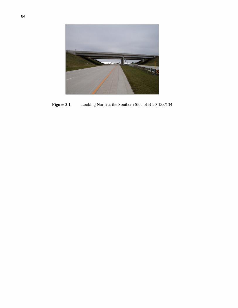
84  

Figure 3.1 Looking North at the Southern Side of B-20-133/134

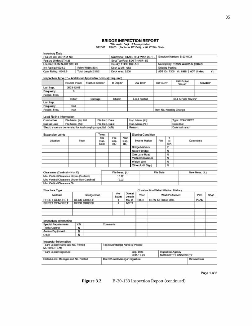
85  

Figure 3.2 B-20-133 Inspection Report (continued)

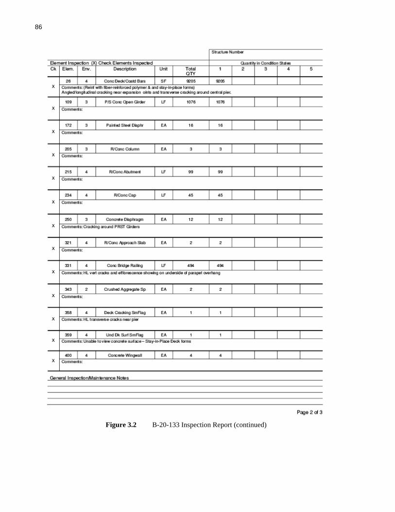
86  

Figure 3.2 B-20-133 Inspection Report (continued)

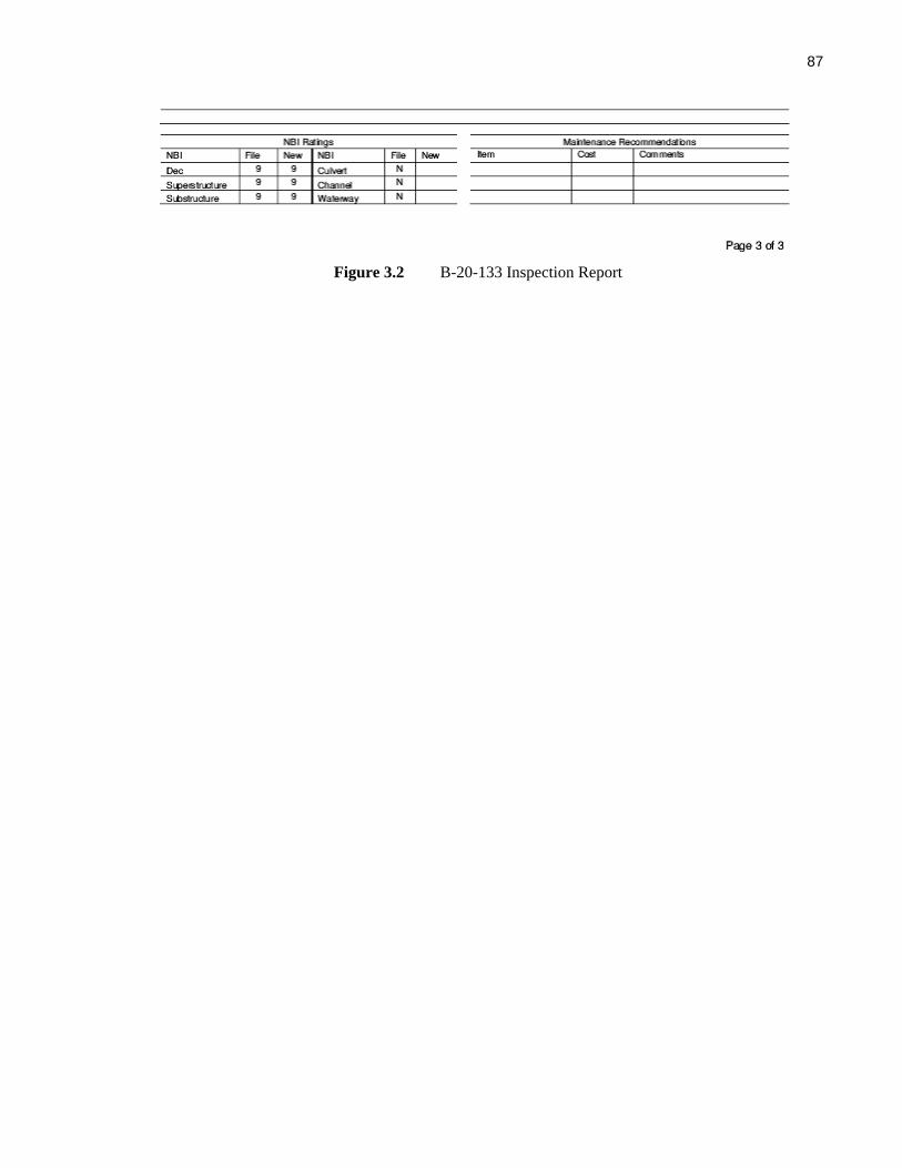
87  

Figure 3.2 B-20-133 Inspection Report

88  

Figure 3.3 B-20-134 Inspection Report (continued)

89  

Figure 3.3 B-20-134 Inspection Report (continued)

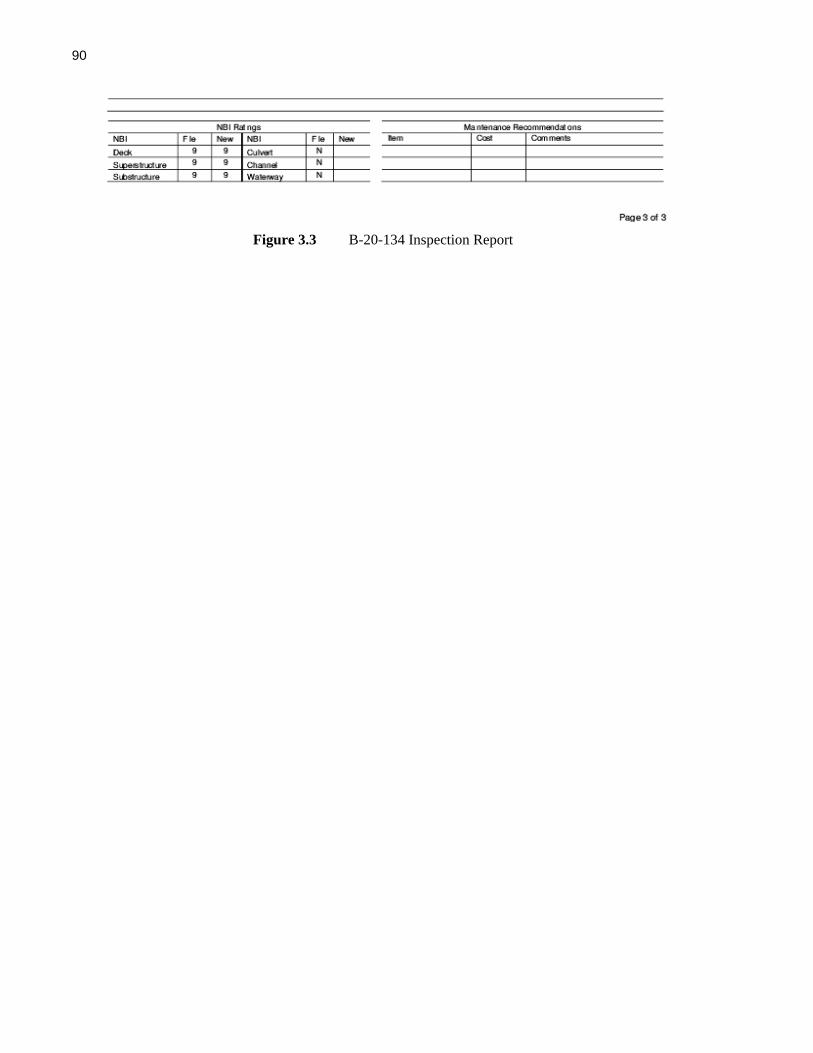
90  

Figure 3.3 B-20-134 Inspection Report

91  

Figure 3.4 Hairline Cracks Near the Bridge/Abutment Joint

92  

Figure 3.5 Crack Map of B-20-133/134

93  

Figure 3.6 Picture Index of B-20-133/134

94  

Figure 3.7 (3) Cracking with Efflorescence South Side of B-20-133 Above Central Pier

Figure 3.8 (17) East Side of Central Pier on the Southern Side of B-20-134

95  

Figure 3.9 (4) Interior Diaphragm of B-20-133 Above Pier, at Girder 2 Looking West

Figure 3.10 (20) Pier Diaphragm Looking West Between Girder 1 and 2, B-20-134

96  

Figure 3.11 (12) North Side Pier B-20-133

Figure 3.12 (36) Center Pier Exterior on North Side, B-20-134

97  

Figure 3.13 (11) West Span B-20-133, North Side

Figure 3.14 (38) West Span B-20-134, North Side

98  

Figure 3.15 (9) West Span Blisters and Sealant Seep-Through in FRP-SIP Deck Between Girder 3

and 4 Near West Abutment, B-20-133

Figure 3.16 (24) Underside of Bridge Deck at North Abutment, Girders (From Left to Right) 1, 2, and

3, B-20-134

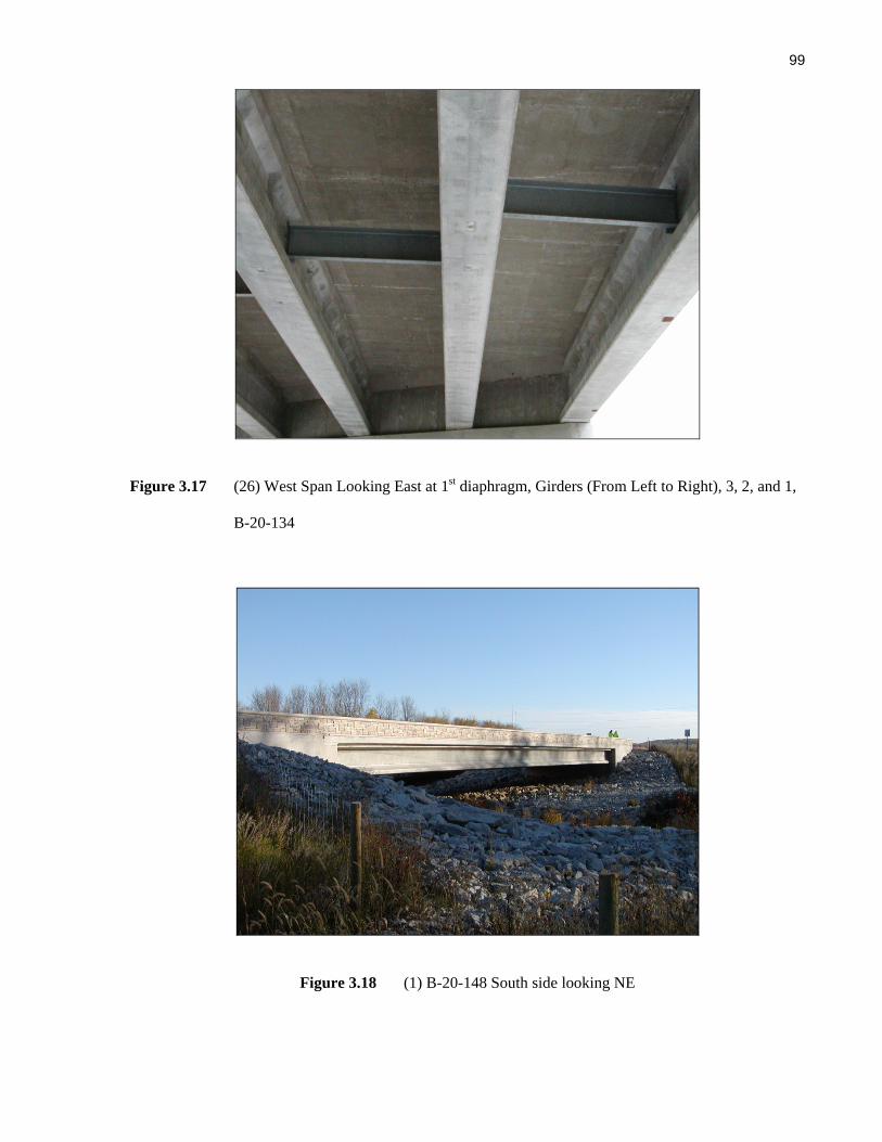
99  

Figure 3.17 (26) West Span Looking East at 1st diaphragm, Girders (From Left to Right), 3, 2, and 1,

B-20-134

Figure 3.18 (1) B-20-148 South side looking NE

100  

Figure 3.19 B-20-148 Inspection Report

101  

Figure 3.19 B-20-148 Inspection Report (continued)

102  

Figure 3.20 B-20-149 Inspection Report

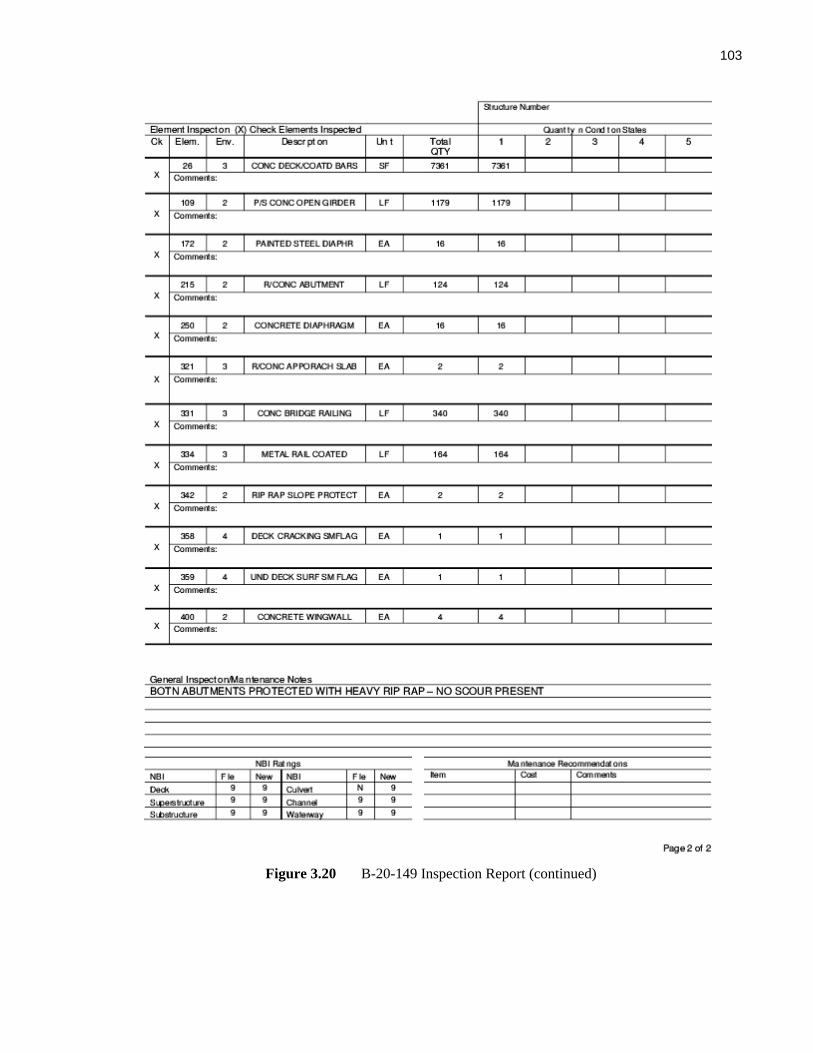
103  

Figure 3.20 B-20-149 Inspection Report (continued)

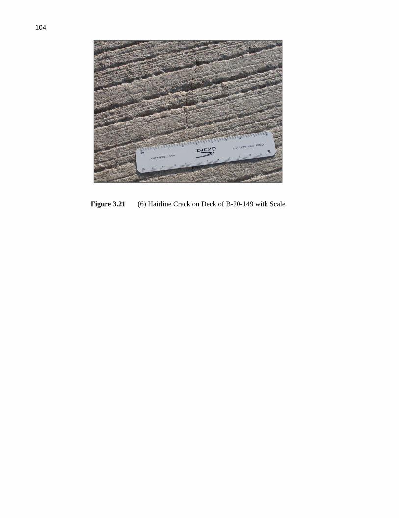
104  

Figure 3.21 (6) Hairline Crack on Deck of B-20-149 with Scale

105  

Figure 3.22 B-20-148/149 Initial Crack Map

106  

Figure 3.23 Picture Map For B-20-148/149

107  

Figure 3.24 (3) Deck of B-20-148 with Traffic Looking West

Figure 3.25 (4) Deck of B-20-149 with Traffic Looking West

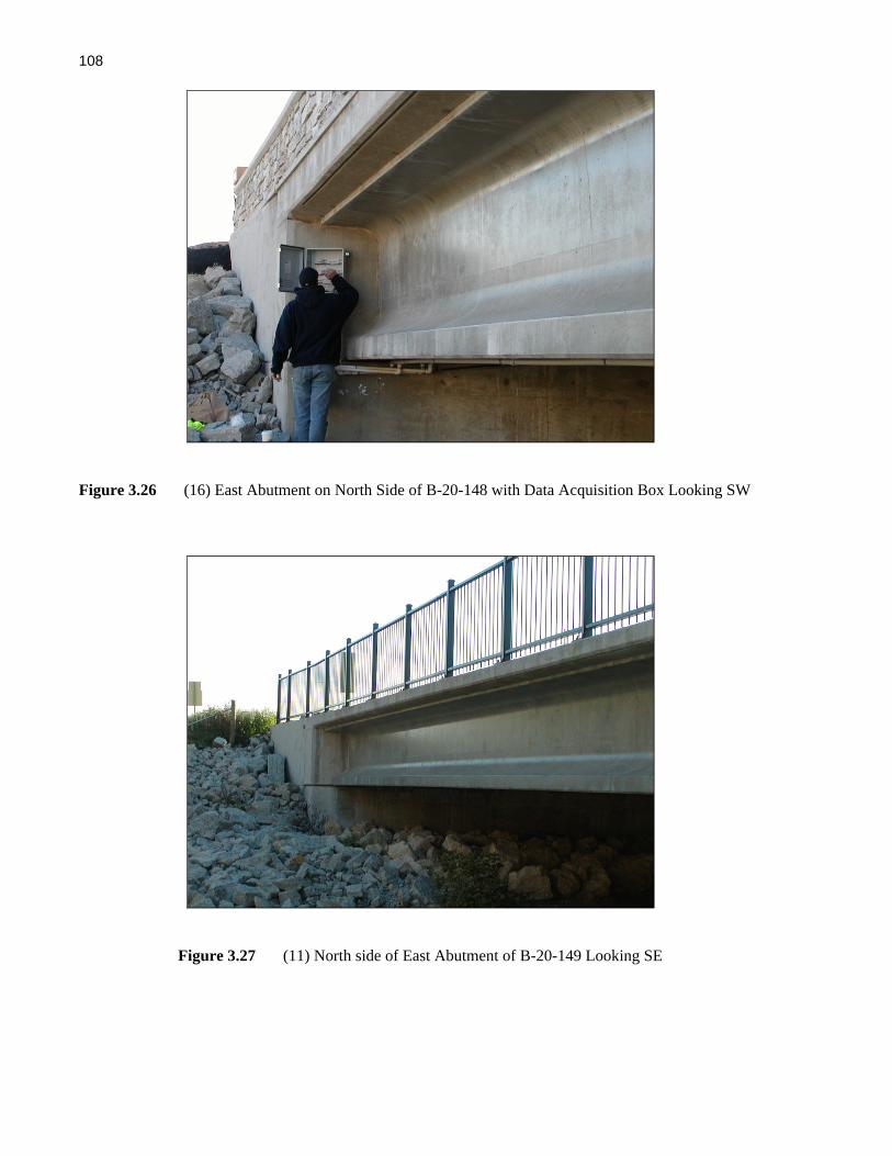
108  

Figure 3.26 (16) East Abutment on North Side of B-20-148 with Data Acquisition Box Looking SW

Figure 3.27 (11) North side of East Abutment of B-20-149 Looking SE

109  

Figure 3.28 (15) Exterior Girder (#7) on North Side of B-20-148 Looking South

Figure 3.29 (13) Underside of Pedestrian Walkway on North Side of B-20-149

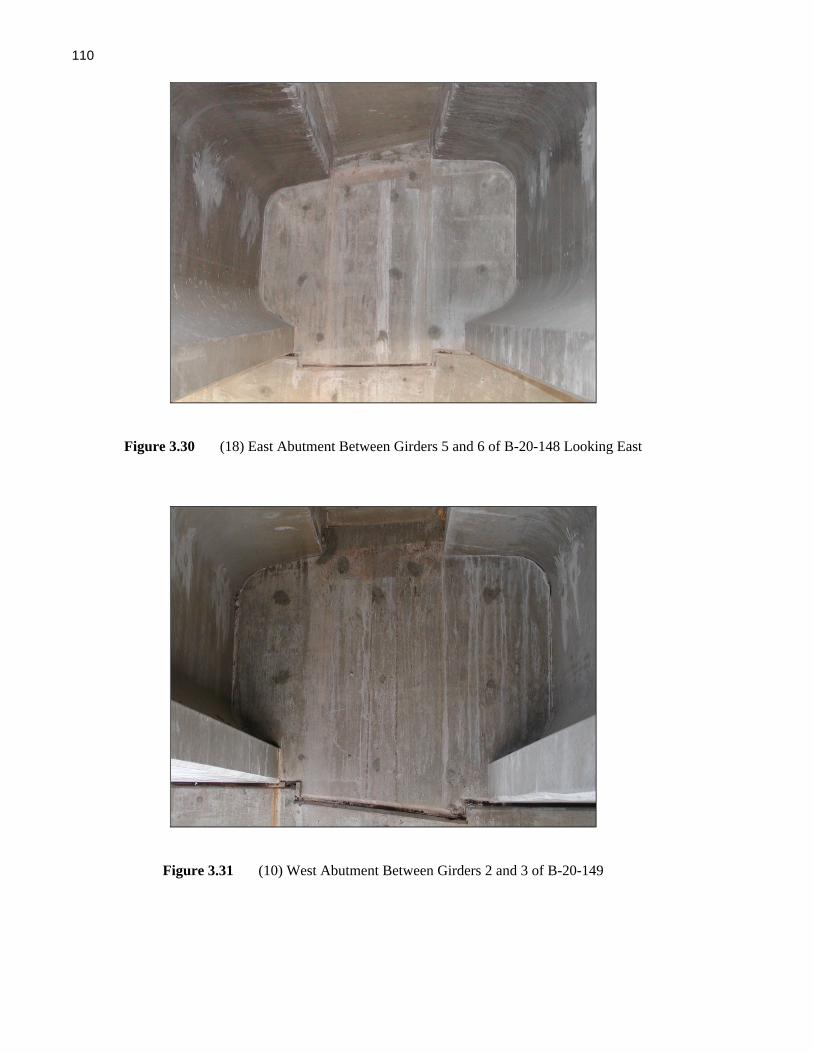
110  

Figure 3.30 (18) East Abutment Between Girders 5 and 6 of B-20-148 Looking East

Figure 3.31 (10) West Abutment Between Girders 2 and 3 of B-20-149

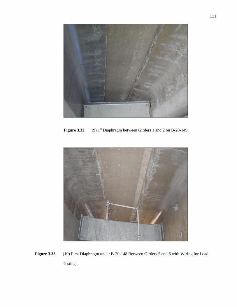
111  

Figure 3.32 (9) 1st Diaphragm between Girders 1 and 2 on B-20-149

Figure 3.33 (19) First Diaphragm under B-20-148 Between Girders 5 and 6 with Wiring for Load

Testing

112  

Figure 3.34 (5) Northern Parapet Crack on B-20-149

Figure 3.35 Computer Aided Tap Tester (CATT) and Testing a Heater Blanket of an American

Airline MD80 (UCOMPO 2006)

Figure 3.36 Modally Tuned® ICP® Impact Hammers (PCB 2006)

113  

Figure 3.37 Ultrasonic Analog Diagram (Hellier 2001).

Figure 3.38 Deck Slab with SIP FRP Forms and FRP Reinforcement

Figure 3.39 Heating up the Slab

114  

Figure 3.40 IRT Monitor and VHS Recorder and Camera

Figure 3.41 IRT Scans of the FRP SIP Form Slab

(a) (b)

Figure 3.42 Digital Hygrometer with Probe: (a) Complete Hygrometer Instrument; (b) Probe with Cord

Lead.

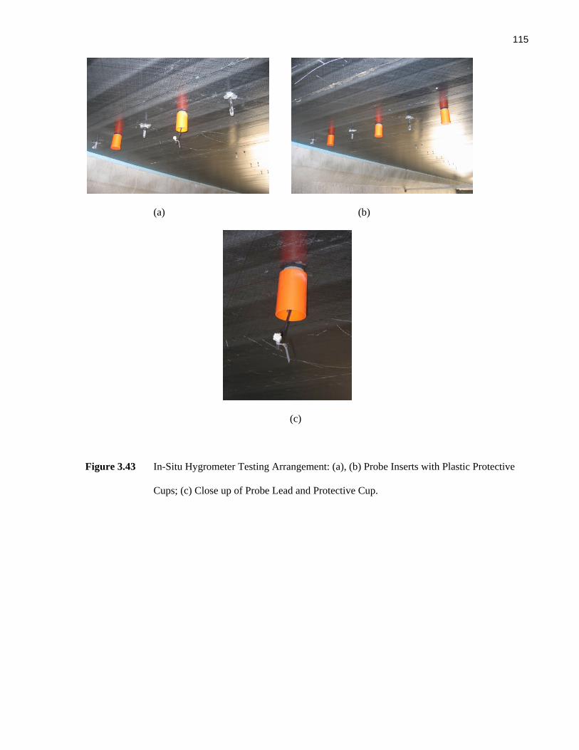
115  

(a) (b)

(c)

Figure 3.43 In-Situ Hygrometer Testing Arrangement: (a), (b) Probe Inserts with Plastic Protective

Cups; (c) Close up of Probe Lead and Protective Cup.

116  

This Page Has Been Intentionally Left Blank

117  

Chapter 4

In-Situ Load Testing  4.1 Introduction

The research project included a component relate to in-situ load testing of the bridges. Two in-situ load

tests were performed on each of the two IBRC bridges. The in-situ load testing was limited to tests done

on the innovative bridges: B-20-133 and B-20-148. The traditionally constructed bridges were not

subjected to in-situ load testing.

The load testing included acquisition of strain and deflection data related to the bridge decks and

girders. The in-situ load testing was conducted with a two-year separation with the goal being to evaluate

changes in response over this period, which may indicate degradation in the superstructure. Performance

parameters evaluated through the load testing to track degradation include: wheel load distribution within

the bridge deck, composite action in the girders, and bridge deck deflections relative to the girders. This

chapter of the report outlines the in-situ instrumentation arrangement, the load testing protocols used, data

acquired from the two in-situ load tests, and discussion of the test data.

4.2 In-Situ Instrumentation

The strain sensors developed as part of the research effort were used in the load testing conducted. Draw

Wire Transducers (DWT's) were also incorporated into the load testing program. The objectives of in-

situ load testing included determination of:

1. the strain profile through the precast girders and the bridge deck;

2. the transverse distribution of wheel loads in bridge deck;

3. the longitudinal distribution of lane loading among the girders within the superstructure;

4. the deflection of the bridge deck relative to the precast girders.

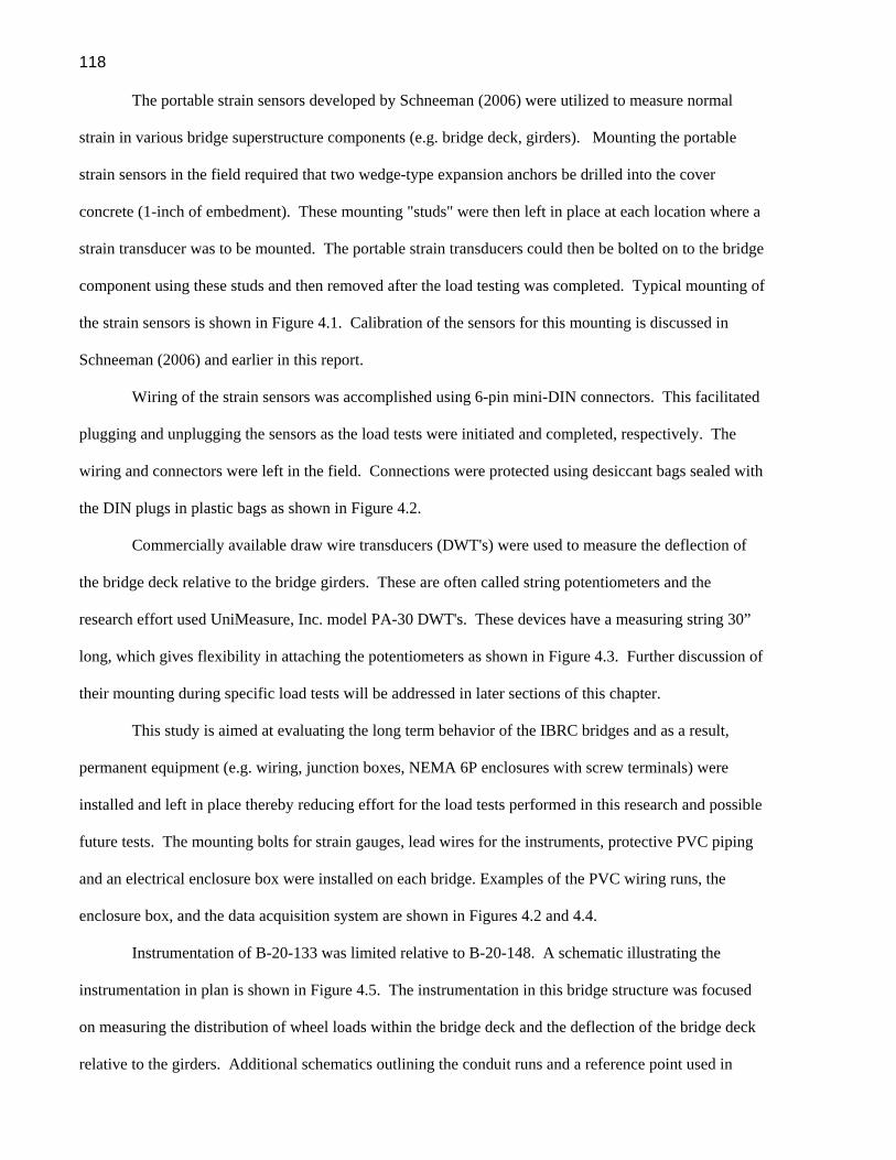
118  

The portable strain sensors developed by Schneeman (2006) were utilized to measure normal

strain in various bridge superstructure components (e.g. bridge deck, girders). Mounting the portable

strain sensors in the field required that two wedge-type expansion anchors be drilled into the cover

concrete (1-inch of embedment). These mounting "studs" were then left in place at each location where a

strain transducer was to be mounted. The portable strain transducers could then be bolted on to the bridge

component using these studs and then removed after the load testing was completed. Typical mounting of

the strain sensors is shown in Figure 4.1. Calibration of the sensors for this mounting is discussed in

Schneeman (2006) and earlier in this report.

Wiring of the strain sensors was accomplished using 6-pin mini-DIN connectors. This facilitated

plugging and unplugging the sensors as the load tests were initiated and completed, respectively. The

wiring and connectors were left in the field. Connections were protected using desiccant bags sealed with

the DIN plugs in plastic bags as shown in Figure 4.2.

Commercially available draw wire transducers (DWT's) were used to measure the deflection of

the bridge deck relative to the bridge girders. These are often called string potentiometers and the

research effort used UniMeasure, Inc. model PA-30 DWT's. These devices have a measuring string 30”

long, which gives flexibility in attaching the potentiometers as shown in Figure 4.3. Further discussion of

their mounting during specific load tests will be addressed in later sections of this chapter.

This study is aimed at evaluating the long term behavior of the IBRC bridges and as a result,

permanent equipment (e.g. wiring, junction boxes, NEMA 6P enclosures with screw terminals) were

installed and left in place thereby reducing effort for the load tests performed in this research and possible

future tests. The mounting bolts for strain gauges, lead wires for the instruments, protective PVC piping

and an electrical enclosure box were installed on each bridge. Examples of the PVC wiring runs, the

enclosure box, and the data acquisition system are shown in Figures 4.2 and 4.4.

Instrumentation of B-20-133 was limited relative to B-20-148. A schematic illustrating the

instrumentation in plan is shown in Figure 4.5. The instrumentation in this bridge structure was focused

on measuring the distribution of wheel loads within the bridge deck and the deflection of the bridge deck

relative to the girders. Additional schematics outlining the conduit runs and a reference point used in

119  

locating the instrumentation in plan is shown in Figure 4.6. Figure 4.6(a) also includes a schematic

illustrating how the DWT's were mounted to measure deck deflections.

Figure 4.7 illustrates the data acquisition system (DAQ) with enclosure. The enclosure contains

terminal bars with 6-pin DIN connector pig-tails that were plugged into the back of the portable DAQ

system. The enclosure is water tight and is permanently mounted to the abutment diaphragm.

The DWT mounting arrangement is shown in Figure 4.7(b). The DWT string was attached to an

eye bolt that was permanently mounted to the underside of the bridge deck using a wedge-type expansion

anchor. Aluminum UniStrut cross members were mounted to the girders using wedge-type expansion

anchors and steel angles. These horizontal members are shown in Figure 4.7(b) and the DWT is attached

to this cross-member with the string extended vertically to the underside of the bridge deck. The DWT

string is located within a relatively sheltered region under the bridge deck. As a result, the strings are not

exposed to wind, which can disturb the deflection readings as a result of the string vibrating in the wind

stream. While the area between the girders and under the deck soffit is not completely sheltered, it did

limit vibrations induced in the DWT strings due to wind. Threaded studs for mounting the portable strain

tranducers are also shown in Figure 4.7(b).

The instrumentation for bridge B-20-148 is a bit more extensive than bridge B-20-133. A

schematic of the instrumentation in plan is given in Figures 4.8, 4.9, and 4.10. The focus of the load

testing on this bridge is to experimentally determine the following: (a) bridge deck deflection relative to

the girders (DWT instruments); (b) girder lane load distribution factors (LM and LT instruments); (c)

transverse wheel loading distribution widths (TW instruments); (d) strain distribution over the height of

the girder-deck composite section (LM and SP instruments).

Longitudinal distribution of load between the girders was conducted by attaching individual strain

sensors to the underside of bridge girders at mid-span (LM strain gauges) and a third-point of the span

(LT strain gauges). As there are seven girders, fourteen individual sensors were installed with each sensor

being centered transversely on the girder. The location and distribution of these sensors in the

superstructure is shown in Figure 4.8

120  

The strain profile of the bridge deck and girders is important to verify that composite action of

exists between the deck and girders. The B-20-148 super-structure was designed assuming composite

action and verification of such behavior is required. Additionally, any degradation of this composite

behavior over time wanted to be measured. By locating the strain sensors at the girder bottom flange,

girder top flange, and on the FRP-reinforced deck as indicated in Figure 4.11, the strain variation over the

height can be recorded. Girders G1 and G2 were installed strain sensors as in Figure 4.10(a) for this

purpose.

The FRP grillage used for primary reinforcement of the concrete bridge deck is a new material

and structural system. Significant laboratory testing has been conducted to date (Bank et al. 1992a; Bank

et al. 1992b; Jacobson 2004), but in-situ validation is lacking. Work by Conachen (2005) attempted to

address the issue, but due to the failure of instruments, little insight into the transverse behavior of the

bridge’s deck resulted. Thus, an array of strain sensors was installed on the underside of the bridge deck

between Girders G2 and G3 (see Figures 4.8 and 4.9a) to evaluate wheel load distribution in the deck.

The sensor array located between mid- and third-span of the bridge and was significantly far from the

abutments. Therefore, the bridge’s skew is not expected to have any effect on the test data of the deck at

the location of the sensor array. The study of University of Wisconsin at Madison (Dieter 2002) indicated

that the effective distribution region of a single HS¬20 wheel load (approximately 20.8 kips) on this FRP

reinforced concrete deck was no more than 36” in either direction from the contact area. Therefore, the

five strain sensors were spaced at intervals of 18 inches in 72 inches of deck in longitudinal direction.

An enclosure similar to that used in B-20-133 was used in this bridge and Figure 4.12(a)

illustrates the mounting of this enclosure to the east abutment on the bridge. Figure 4.8 illustrates the

location of the enclosure in plan. Six-pin DIN plug pigtails were also used to attach to the data

acquisition (DAQ) system. These pigtail connectors are also housed within the NEMA 6P water tight

enclosure and serve as a permanent repository of sensor wiring.

Figure 4.12(b) illustrates the DWT mounting system. This system is identical to that used in

Bridge B-20-133. The DWT string is also protected from wind as a result of the DWT being mounted

between the girders and below the bridge deck soffit. Typical mounting of portable strain sensors to the

121  

lower flange of the girders is shown in Figure 4.12(c). Conduit runs used to facilitate long-term wiring

runs for the load testing are shown in Figure 4.12(d).

4.3 In-Situ Load Test Protocols

The load testing involved protocols designed to gather the desired load transfer characteristic information

for both bridges. The first involved marking the bridge decks with wheel targets for the drivers. This

pavement marking was done each time load testing was conducted and it involved simple paint marking

on the bridge deck. The deck surface marking and method used to position the truck wheels on the bridge

deck are shown in Figure 4.13.

Calibrated (i.e. weighed) tri-axle dump trucks were utilized during all load tests. Six dump trucks

were used. Figure 4.14 illustrates important information for vehicles used during the July 2007 load test.

Trucks used in July 2007 had gross vehicle weights ranging from 54,480 lbs to 58,700 lbs. Front axles

were weighed and the entire vehicle was weighed. These to weights were used to compute rear axle loads

(assumed equally distributed between tandem axles). Figure 4.14 also illustrates vehicle tire contact

patches measured prior to load testing. Figure 4.15 illustrates information for vehicles used in the July

2009 load testing. The dump trucks used for the July 2009 load test had gross vehicle weights ranging

from 64,800 lbs to 66,900 lbs. The weights of these vehicles (on average) are 16% more than the July

2007 load test (56,767 versus 65,933 lbs). The fourth axles were maintained in the up position during all

load testing and therefore, the loads on these axles was not accounted for or included.

Figure 4.16 illustrates the loading protocol used to examine the wheel load distributions within

the bridge deck of bridge B-20-133. This loading protocol is known as "travel path 1" and the data

acquisition file used to plot/reference the data is File1. It should be noted that the exterior deck span

strain and deflections are being evaluated with this loading protocol and as a result, the left front wheel of

the truck is positioned along a longitudinal line at mid-span of this exterior bridge deck span.

Loading protocol two for bridge B-20-133 is shown in Figure 4.17. This loading protocol is

termed "truck travel path 2" and it is intended to measure deck deflection and wheel load distribution

122  within the first interior deck span in the superstructure. The data acquisition file used to reference data

for this load testing protocol is File2. The right front wheel of the truck is used as the target wheel for the

load testing. The truck driver was required to hit painted marks (Figure 4.13) on the bridge deck surface.

It should be noted that all load testing was done under live traffic with the passing lane subjected

to closure. This limited truck positioning on the bridge deck surface to locations where the calibrated

vehicle would remain exclusively in the passing lane.

The loading protocols used for bridge B-20-148 are shown in Figures 4.18, 4.19, 4.20, and 4.21.

Loading protocol 1 shown in Figure 4.18 was used to establish maximum deflections relative to the girder

due to front wheel loads in the exterior bridge deck span. Loading protocol 2 shown in Figure 4.19 was

used to establish maximum deck deflections in the first interior span of the bridge deck. Loading protocol

3 shown in Figure 4.20 was established to examine the distribution of wheel loading within the bridge

deck in the first interior bridge deck span. The final loading protocol (number 4) used for this bridge is

shown in Figure 4.21 and it was used to establish lane loading distribution factors for the bridge

superstructure.

Position of trucks during load testing protocol 4 in Figure 4.21 is shown in Figure 4.22(a). The

lead truck in this grouping was given pavement markings on which to land the front wheel of the vehicle.

The remaining two trucks in the train were simply instructed to align themselves with the lead truck and

position themselves bumper to bumper. Typical wheel loading positions for the wheel load distribution

protocols were accomplished using paint markings on the deck as shown in Figure 4.22(b).

4.4 Load Testing Results and Discussion

Two load tests were conducted as part of the monitoring effort: July 2007 and July 2009. This section of

the report outlines the results of the two load tests conducted. It should be noted that the two load tests

conducted two years apart were intended to capture significant structural load transfer mechanism

changes over this two year period and therefore, identify any significant changes that would warrant

degradation within the superstructure systems. Similarly, any lack of change in these load transfer

mechanisms would suggest that no degradation has occurred over this two-year period.

123  

4.4.1 Bridge B-20-133

Figure 4.23 illustrates the bridge deck deflections relative to the girders seen in the two load tests. The

vehicle travel paths used to generate this data was travel path 1 shown in Figure 4.16. Figure 4.23(a) and

4.23(b) illustrate the deck deflections measured in the July 2007 and July 2009 load tests, respectively.

DWT-1 is the draw wire transducer intended to measure exterior deck span deflections and DWT-2 is

intended to measure the deflections in the first interior span of the deck. Front wheels for the vehicles

were intended to be positioned at mid-span of the exterior deck span. As a result, it was expected that

DWT-1 data would have larger magnitude displacements.

Peak deck deflections measured by DWT-1 during the two load tests are comparable to one

another with the peak magnitudes on the order of 0.015 inches. Measurements obtained via DWT-2

exhibit significant difference owing to the difficulty in positioning vehicles upon the bridge deck with

respect to the locations of the sensors. However, the peak deformations within the first interior bridge

deck span are on the order of 0.005 inches during the July 2009 load test and 0.010 inches during the July

2007 load test. The peak deformations do not illustrate any significant difference over the two year

period and therefore, one can conclude that there has been no significant change in the flexure load

transfer mechanism in the bridge deck.

Vehicle travel path two is shown in Figure 4.17 and the DWT results for the two loading tests are

shown in Figure 4.24. Peak vertical deck displacements relative to the girders during the July 2007 and

2009 load tests were on the order of 0.01 to 0.015 inches. DWT-1 (exterior deck span) magnitudes are

larger than those of DWT-2. Furthermore, DWT-2 results (interior deck span) should have been larger in

the research team's opinion since the vehicle wheels were thought to be at mid-span of the first interior

deck span. However, the magnitudes of DWT-2 readings were less than those of DWT-1. This can be

attributed to the difficulty of positioning the vehicles directly over the deck sensors. However, the

magnitudes have not significantly changed from one another during the two load tests and therefore, it

can be concluded that significant changes in the load transfer mechanism have not occurred and therefore,

there is a very low likelihood of degradation within time. It should be noted that the negative deck

124  deflection readings in Figures 4.23 and 4.24 are a result of bridge deck rebound as the vehicles rapidly

exited the bridge deck in reverse.

The wheel load distribution within the bridge deck was also measured. The loading protocol

included vehicles entering the bridge, stopping at pre-defined locations labeled on the bridge deck as

shown in Figure 4.13(c), being held in place for a set period of time, and them migrating on to the next

stop location. Personnel on the bridge deck guided vehicle operators in these sequences.

Figure 4.25 illustrates the bridge deck flexural strains measured in the load tests. Load travel

paths used in these load tests are shown in Figure 4.17. TW1 sensors are located along a line centered at

mid-span of the exterior deck span. TW2 sensors are located along a line centered at mid-span of the first

interior deck span. Travel path 1 is intended to generate larger strains in the TW1 sensors (relative to the

TW2 sensors) and travel path 2 is intended to generate larger strains in the TW2 sensors (relative to the

TW1 sensors). This difference in sensor strains can be seen when comparing Figure 4.25(a) to Figure

4.26(a) for the July 2007 load test. It is also seen when comparing strain results shown in Figures 4.27(a)

and 4.28(a).

Figure 4.25(a) illustrates the wheel load strain distribution at mid-span of the exterior deck span

(TW1 sensors) obtained during the July 2007 load test when truck travel path 1 was implemented.

Figure 4.26(a) illustrates the strains seen in the TW2 sensors (mid-span of first interior deck span) during

that same load test. As expected, there is a variation in peak strains measured at these two sensor lines.

The skew present in the bridge superstructure results in TW1 and TW2 sensors not aligning themselves

across from one another. Therefore, only carefully drawn conclusions can be made regarding the data

seen in the TW2 sensors when travel path 1 is utilized and the TW1 sensors when travel path 2 is utilized.

Therefore, discussion will be limited to data obtained in the TW1 sensors and travel path 1 and the data

obtained in TW2 sensors and travel path 2.

Figure 4.25 illustrates the wheel load strain distributions seen in the TW1-series sensors measured

during the July 2007 and 2009 load tests. Figure 4.25(a) illustrates the expected stepped variation in

strain readings from sensor TW1-E2 through TW1-W2. When the vehicle wheel is intended to be placed

over TW-W2, this sensor experiences the largest tensile strain. When the wheel is intended to be over

125  

TW1-E2 (far right of figure), sensor TW1-W2 reads the smallest tensile strain. This is consistent with the

sensor layouts within the exterior deck span shown in Figure 4.5. The fact that TW1-E1 and TW-E2 read

nearly the same strain magnitude at the vehicle stopping points corresponding to data points 3,000

through 3,500 is indicative of the difficulty in positioning wheel loads directly over the top of sensors (see

Figure 4.13c).

Comparison on Figures 4.25(a) and 4.25(b) illustrates that there is significant difference in the

load testing results in the July 2007 and July 2009 load tests. The differences in the data obtained in these

two load tests arise from vehicle positioning and ambient vehicle traffic and not load transfer mechanisms

within the superstructure. The vehicles during the July 2009 load test were not positioned in the same

locations as in the July 2007 load test. Pauses in vehicle movement seen in Figure 4.25(a) are also not

present in Figure 4.25(b) indicating the impact of ambient traffic on the strain sensors.

The load tests were conducted under live traffic with the passing lane temporarily closed for test

vehicle positioning. Ambient traffic loading in the driving lane was significantly heavier in July 2009

versus July 2007. As a result, there was significantly more truck and car traffic in the driving lane present

nearly continually during the July 2009 load test. The relatively recent opening of USH 151 at the time of

the July 2007 load test significantly reduced the volume of ambient traffic present on the bridge when the

testing was conducted. As a result, ambient traffic appears to have affected the load testing in July 2009.

Figure 4.26 illustrates the strain distributions measured in TW2 sensors during travel path 1 in the

July 2007 and July 2009 load tests. As outlined earlier, the TW1 and TW2 sensors are offset from one

another as a result of the skew in the bridge superstructure and as a result, their descriptive use is limited.

The results in Figure 4.25(b) and Figure 4.26(b) illustrate strong suspicion that vehicles were not located

properly during travel path 1 in the July 2009 load test. Furthermore, the presence of ambient traffic

significantly affected the strain readings in the bridge deck during the testing.

Figure 4.27 illustrates the strains measured in the TW1 sensors during travel path 2 in the July

2007 and 2009 load tests. Figures 4.27(a) and (b) clearly indicate the vehicle pause points (i.e. the "flat"

segments) and both are devoid of significant evidence of ambient traffic on the bridge at the time of the

126  test travel path execution. The peak strains seen in each of the two load tests are on the order of 50 με

indicating that there is no fundamental changes in the load transfer mechanisms in the deck over the

elapsed two year period. Rebound loading is significantly greater during the July 2009 load test, but this

is simply attributed to driver change during the latter load test. Figure 4.27 illustrates that there is no

significant change in strain readings and therefore, there is no degradation in the load transfer mechanism

in the bridge deck.

Figure 4.28 illustrates the strains measured in TW2 series sensors for vehicle travel path 2.

Unfortunately, Figure 4.28(b) illustrates that the vehicles were likely not positioned correctly during the

July 2009 load test and that there was a significant level of ambient traffic loading present at the time the

vehicle load path was executed during the testing.

Figure 4.17 illustrates that dump truck 100 was used in the July 2007 load testing and dump truck

111 was used in the July 2009 load testing. The separation between front and middle axles for these

dump trucks (Figures 4.14 and 4.15) is 179 inches and 188 inches, respectively. Therefore, it can be

expected that when the front axle is near strain sensor TW-E2, the rear tandem axle group is nearing

sensor TW-W2. Therefore, it can be expected that the rear tandem axle group will influence the strain

readings throughout all sensors in a line. The extent to which this influence affects the strain readings

was impossible to determine with the loading testing protocols used.

Figures 4.29 and 4.30 illustrate the deck deflections measured at DWT-1 and DWT-2 during the

2007 and 2009 load tests. The DWT-1 sensor was located in the exterior deck span and the DWT-2

sensor was located in the first interior deck span. Truck position 1 was intended to generate peak deck

displacements in the exterior span and truck position 2 was intended to generate peak deck displacements

in the first interior deck span. It should be noted that the separation (longitudinally) between DWT-1 and

DWT-2 in the bridge deck is on the order of 100 inches. The spacing between the front axle and middle

axle on the load test dump trucks 91 (used in July 2007) and 111 (used in July 2009) is 179 inches and

188 inches, respectively. Therefore, it can be expected that the front and middle axle wheel loads will

affect displacement readings in the same way as strain readings likely were affected.

127  

Figure 4.29 indicates that peak deflections at DWT-1 were on the order of 0.003 inches in the

July 2007 load test and an upward deflection of approximately 0.005 inches in the July 2009 load test.

The upward deflection most likely indicates that the vehicle may not have been in the intended position

within the bridge deck. The peak displacement seen during truck load travel path 1 was 0.012 inches in

July 2007 and the peak downward displacement measured in July 2009 was on the order of 0.003 inches.

Figure 4.30 indicates that truck travel path 2 contains a bit more consistency with regard to DWT-2 with a

peak downward deflection measured in July 2007 of 0.014 inches and a peak downward deflection

measured in July 2009 of 0.002 inches. Slight upward deflection (e.g. 0.004 inches) at DWT-1 measured

in July 2009 makes some intuitive sense as this sensor is a significant distance longitudinally away from

(ahead of) sensor DWT-2 and an upward deflection in the bridge deck is conceivable. No significant

changes in the peak (magnitude of) deflections occurred in the two load tests, two years apart, and

therefore, it is expected that no significant (at least) measurable degradation in the bridge deck load

transfer mechanism is present.

4.4.2 Bridge B-20-148

Bridge B-20-148 in Fond du Lac, Wisconsin was also load tested at two times: July 2007 and July 2009.

As outlined earlier, the instrumentation and sensor layout was significantly different for this bridge when

compared to bridge B-20-133. The present section outlines the load testing results obtained for this

bridge and provides observations with regard to what these load tests results mean in relation to bridge

superstructure performance.

Figure 4.31 illustrates the bridge deck strain sensor measurements that were intended to quantify

the variation in strains longitudinally along the bridge deck indicating how much bridge deck resists

vehicle wheel loads. It should be emphasized that sensor TW-E2 was faulty as a result of the data

acquisition system port failing and therefore, this sensor as shown in Figure 4.8 was not included in the

testing. The load testing conducted in July 2007 (Figure 4.31a) indicates that the vehicle positions were

not as intended. The peak tensile strains measured in the bridge deck were approximately 40 με in July

128  2007 and the same magnitude in July 2009. A peak tensile strain at the underside of the bridge deck of

this magnitude is really quite low given that tensile cracking strengths for typical deck concrete will be on

the order of 130 με . Therefore, one expects that typical vehicle wheel loadings will not cause cracking

in the bridge deck.

Bridge B-20-148 also included strain sensors mounted to measure the distribution of lane loading

amongst the girders within the superstructure. The sensors designated as LM-1 through LM-7 and LT-1

through LT-7 provide strain measurements that aid in quantifying the lane load distribution factors at

mid-span and third points, respectively. Unfortunately, load testing data obtained in July 2009 (Figures

4.32b and 4.33b) were tainted by unexplained spikes in strain data that may have been caused by faulty

strain sensor mounting. The reason that faulty sensor mounting is suspected is that the magnitude of

tensile and compression strains measured are simply beyond rational magnitudes.

Figure 4.32(a) illustrates that the tensile strains for girders LM-1 through LM-7 range from 60

με tension to essentially zero microstrain. The position of the vehicles illustrated in Figure 4.21

suggests that peak tension strains should exist at the bottom of girders G2. This means that one can

expect maximum tensile strains in sensor LM-2 to be obtained. This is indeed the case in the results

measured. It is disappointing that the strain data obtained during the July 2009 was corrupted. There are

several reasons for this that will be outlined later on in this chapter of the report. However, several very

important conclusions regarding degradation in the superstructure can be made with data that was

obtained in the July 2009 load test.

The measured strains plotted in Figures 4.32(a) and 4.33(a) can be used to gain estimates of lane-

loading distribution factors to compare with design specifications (AASHTO 2006). One can use tension

strains measured across all girders in the superstructure to evaluate a lane load distribution factors as

follows (SC FRP Research):

1

G

ii N

nn

mgμε

με=

=

∑ (4.1)

where:

129  

iμε is the strain measured in girder i

1

GN

nn

με=∑ is the sum of all strains read across all girders in the superstructure.

Using the strain data given in Figure 4.32(a), the a lane load distribution factor for the mid-span location

can be computed as,

62 0.2962 55 37 37 16 10LMmg = =

+ + + + +

Using the strain data given in Figure 4.33(a), the a lane load distribution factor for the mid-span location

can be computed as,

58 0.2758 52 42 25 25 10LTmg = =

+ + + + +

The moment distribution factor at mid-span is slightly larger than that at the 1/3 points and this is

consistent with the known behavior for skews nearing 30-degrees (AASHTO 2006).

A distribution factor was also computed as part of the baseline load testing conducted after B-20-

148 was completed (Hernandez, et al 2005). This distribution factor was computed using beam

deflections across the superstructure and its magnitude was reported to be,

0.23measLMmg =

This is very close and agreeable to the data obtained through the present research effort. As a result, one

can say that the lane load distribution factor did not change from xxxx 2005 to July 2007 and therefore,

there has been no degradation or change in the load transfer mechanism in the superstructure in this

regard.

The AASHTO (2006) specifications also contain procedures for estimating how much of the

design lane will be carried by a single girder within the bridge superstructure. These calculations

performed for girder G2 in the present system are as follows,

0.10.4 0.3

3

1 0.06 0.311.20 14 12.0

gSmI

s

KS SmgL Lt

⎡ ⎤⎛ ⎞⎛ ⎞ ⎛ ⎞⎢ ⎥= + =⎜ ⎟⎜ ⎟ ⎜ ⎟⎢ ⎥⎝ ⎠ ⎝ ⎠ ⎝ ⎠⎣ ⎦

for a single lane loaded situation. The distribution factors computed using strain readings in the present

130  research are in excellent agreement with the distribution factor estimated using bridge specification

expression s (AASHTO 2006).

It was felt to be very important to make an attempt at quantifying the change in strain readings

over the height of the composite girders within the superstructure with time. This would give yet another

indication that the load transfer mechanisms within the bridge superstructure were changing with time.

Figures 4.34 and 4.35 provide data illustrating the variation in strain at three sensor locations over the

height of the girder and the underside of the bridge deck (see Figure 4.11). Figure 4.34(b) and 4.35(b)

illustrates some rather puzzling spikes in strain history outside relatively nice strain trajectories that

compare well with those in Figure 4.34(a) and 4.35(a). The source of these spikes could not be

confidently quantified and therefore, they were ignored in the strain trace.

The peak strain data (plateau portions of the strain trace) in Figures 4.34 and 4.35 were

transcribed onto a strain diagram over the height of the cross-section as shown in Figure 4.36. A

theoretical composite section should have a linear strain diagram over the height of the cross-section.

Furthermore, if the girders and deck were NOT acting compositely with one another, the underside of the

deck (sensors SP1 and SP2) would not be in compression. Figure 4.36 clearly indicates that composite

behavior is occurring in these girders. The data for girder G1 indicates virtually no change in composite

behavior from July 2007 to July 2009. Furthermore, the strain readings above the neutral axis for girder

G2 had virtually no change from July 2007 to July 2009. The strain readings at the bottom flange of

girder G2 were unexpected. While the July 2007 load test yielded expected strain readings, the July 2009

load test results were surprising. A reading of 155 με would indicate significant behavioral change

within the system. However, the response seen in girder G1 during this same load test suggests that this

extreme strain reading was caused by improper installation of the strain gauge. This will be discussed

later in this chapter of the report.

Overall, the data in Figure 4.36 supports the conclusion that there has been no change in the

composite stringer-deck load transfer mechanism from July 2007 to July 2009 and therefore, there has

been no degradation in the system in this regard.

131  

4.5 Wheel Load Distribution within Bridge Deck

The load testing conducted afforded the opportunity to evaluate wheel load distribution widths within the

novel FRP-SIP bridge deck system used in B-20-133. The research team outlined a procedure to compare

AASHTO-LRFD (AASHTO 2006) wheel load distribution widths with those suggested using data

obtained during the load tests in an earlier research paper (Foley et al 2008). The present section provides

an overview of this work and further details are available (Foley et al 2008).

The distribution of wheel loading within a bridge deck is dependent on three major factors: (a) the

deck span length; (b) the restraint characteristics at the ends of the deck span; and (c) the girder stiffness.

Experimental evidence (Allen 1991; Batchelor et al. 1978; Beal 1982; Csagoly et al. 1978) indicates that

there is a significant level of membrane arching action present in many bridge decks and flexural models

may not be the most appropriate method to compute maximum positive and negative moment stresses

within bridge decks. Furthermore, studies have indicated that the stiffness of the girders plays a vital role

in limiting the transverse negative bending moments over the girders (Batchelor et al. 1978; Beal 1982;

Cao et al. 1996; Cao and Shing 1999; Csagoly et al. 1978; Fang et al. 1990; Newmark 1949).

Experiments carried out on scale models (Beal 1982; Fang et al. 1990) and full-scale models

(Fang et al. 1990) have been very valuable in understanding wheel load distribution and have led to

validation of analytical procedures to predict stresses within the bridge deck. However, these previous

efforts focused on isotropic reinforcement layouts and traditional cast-in-place construction. There has

been no data generated to date that supports the validity of applying analysis methods developed for CIP

construction to deck systems that utilize stay-in-place FRP formwork as positive moment reinforcement.

The present research effort allowed experimental data to be generated in this regard.

The methods for computing live load moments within bridge decks have changed very little from

the first proposal formulated by Westergaard (1930). Further work by Newmark (1949) resulted in the

basis for the Standard Specification design procedure for bridge deck analysis (AASHTO 2002). The

procedure used is quite straightforward. A bridge deck live load moment (per unit width of slab) for a

simple span condition is estimated using (AASHTO 2002),

132  

232LLM w

SM P +⎡ ⎤= ⎢ ⎥⎣ ⎦ (units are lbs and feet with result being lb-ft/ft) (4.2)

where: wP is the wheel loading (HS20 or HS15 using standard specification live load models); and S is

the span of the bridge deck (conservatively can be taken as the spacing of the girders if flange widths are

relatively small compared to the span). It should be noted that 1 lb-ft/ft is 4.448 N-m/m and equation (4.2)

is taken from the U.S. customary units version of the specifications. Bridge decks are often continuous

over multiple interior girders and therefore, the simple-span moment per unit width is modified by a

continuity factor (AASHTO 2002),

20.8032LLM w

SM P +⎡ ⎤= ⋅ ⎢ ⎥⎣ ⎦ (4.3)

The positive and negative live load bending moments are taken to be the same within the bridge deck and

this requires that the structural engineer provide equal mats of steel reinforcement in the top and bottom

layers. It should also be noted that equations (4.2) and (4.3) make no distinction of interior and exterior

deck span and therefore, are intended to be conservative for interior span bending moment estimations

when compared to those estimates generated for exterior deck span conditions.

The procedure implied by equations (4.2) and (4.3) was felt to be over-simplistic by many

researchers and experimental and analytical evidence showed that the flexibility of the girders within the

superstructure system affects the state of stress within the deck (Batchelor et al. 1978; Beal 1982; Cao et

al. 1996; Cao and Shing 1999; Csagoly et al. 1978; Fang et al. 1990) and that simplistic computations

may over-estimate negative moment tensile stresses over the girders in the bridge deck. Nonetheless,

equations (4.2) and (4.3) were used successfully for decades and the Load and Resistance Factor Design

(LRFD) specifications included a significant departure from the former procedure.

The LRFD procedure for bridge decks is very similar to the long-standing distribution-factor

procedure used for bridge girder analysis. The LRFD procedure includes definition of a strip width used

to facilitate use of bending moments computed using one-dimensional analysis. In other words, the

structural engineer conducts an analysis of the bridge deck assuming it is a one-dimensional continuous

beam with movable wheel loads within traffic lanes and then converts the bending moments to unit-width

133  

quantities using the strip width. Two strip widths are defined in cast-in-place bridge deck slabs

(AASHTO 2006),

Positive Moment Strip Width

26.0 6.6SW S+ = + ⋅ (4.4)

Negative Moment Strip Width

48.0 3.0SW S− = + ⋅ (4.5)

The LRFD procedure affords the structural engineer the opportunity to utilize statically indeterminate

analysis models and therefore, there is the ability to generate more accurate analysis results through these

models. The assumption that bending moment magnitudes be determined through structural analysis was

a significant departure from earlier specification procedures. To the authors' knowledge, there is no

experimental evidence that demonstrates in-situ bridge behavior of deck systems utilizing the FRP-SIP

formwork systems is appropriately modeled using equations (4.4) and (4.5).

The strain measurements from the July 2007 load test were used as the basis for computing

estimates for the amount of bridge deck width that resists wheel loading. Truck 100 in the July 2007 load

test shown in Figure 4.14 was the vehicle used during loading protocol 1 in Figure 4.16. The strain

measurements used as the basis for computations are given in Figures 4.25(a) and 4.28(a).

An influence surface along the TW1 and TW2 sensor arrays (see Figure 4.5) were generated

using the data acquired during the load testing. Five strain sensors were used during the testing along

each line. The truck wheel was targeted to stop directly above each of these sensors as shown in Figure

4.39. The targeted stops were (in succession): W2, W1, M, E1, and E2. When the calibrated truck wheel

was above W2, there were strain readings at the remaining four sensors. It was assumed that this data

could be used to generate a symmetric (extrapolated) layout of four additional strain readings to locations

with 17.5-inch intervals behind (or in front of) the truck wheel. As a result, five strain readings and four

extrapolated symmetric strain readings were generated where applicable.

Figure 4.14(c) indicates that the front and first-rear-tandem axle are separated by 195 inches.

Thus, when the front wheel is over sensor E2, the first rear-tandem axle is nearly 10 feet from sensor W2.

134  An average strain value for each stop (the plateaus in Figures 4.25a and 4.28a) were used as the basis for

sensor readings. Table 4.1 illustrates these average values obtained at each sensor location and

symmetric extrapolated sensor location values. The bold font values are the strain readings taken in the

field and the italicized-font values are the magnitudes at symmetric locations extrapolated from the

measured data.

The truck motion can be mentally pictured using the data values in Table 4.1. The exterior span

can be considered as an illustrative example. When the front wheel is over sensor TW1-E2, the fifth row

in the exterior span segment of the table is referenced. The strain reading for the front wheel at this

location is then 75 με . There are four strain sensor readings behind the front wheel that provide

measured strain data. The four strain readings ahead of the front wheel are therefore, projected

(extrapolated) assuming symmetry. When the front wheel is over sensor TW1-M, there are two strain

sensors behind and in front of the wheel. As a result, no extrapolation can be done and projected readings

at +/- 70 in. and +/- 52.5 in. are not available. In other words, full symmetry with 140-inches of length

adjacent to the wheel loading could only be obtained for cases where the front axle was over sensor W2

or E2 (first or last stop on sensors).

The strain readings were used to generate equivalent bending moment magnitudes assuming

fully-composite behavior between the FRP-SIP formwork and the concrete deck. Preliminary FEA

indicated that this is a reasonable assumption for service-level loads (Martin 2006). The strain readings at

the bottom surface of the FRP-SIP formwork were converted to strains using Bernoulli beam theory

assumptions,

comp comp

bot

E IM

yε

= (4.6)

compE is the modulus used for the transformed section assuming that the concrete material has been

transformed to equivalent FRP material ( 5.73 6e psi ). The modular ratio used for the computations was

1.56. compI is the second moment of area for the composite cross-section ( 4474.2 in ). Its magnitude was

computed using a 17.5-inch width and data related to the FRP grid and the FRP-SIP formwork panels

135  

(Berg 2004; Dieter 2002; Dietsche 2002). The total height of the in-situ bridge deck is 8 inches. ε is the

measured (or extrapolated) strain from Table 4.1 and boty is the distance from the centroid of the

transformed composite deck cross-section to the bottom surface of the FRP-SIP formwork ( 4.09 in ).

The strain readings from Table 4.1 are used to generate bending moment magnitudes acting in the

vicinity of the strain sensor and these magnitudes are assumed to be an average across the 17.5-inch width

adjacent to the strain sensor (see Table 4.2). The total positive moment resisted within the linear

influence surface adjacent to the wheel loads is simply the summation of all moment magnitudes

computed using the measured strains. These total moments, designated as TM + are given in Table 4.3.

The total moments are then divided by the linear distance defining the area of influence to generate an

average positive bending moment per unit width. This average positive bending moment is given in

Table 4.3 as well. It should be noted that length of influence for W2, W1, M, E1, E2 is 157.5-in., 122.5-

in., 87.5-in., 122.5-in., and 157.5-in., respectively.

The bending moments per unit width of length found in Table 4.3 can be compared to the positive

bending moment that would be computed for a 10.93-kip wheel load using equation (4.3). This wheel

load magnitude is approximately 37% greater than an HL-93 or HS20 truck loading. Table 4.3 illustrates

the positive design live load moments that would result if the deck span was taken as 8-foot, 8-inches (see

Figure 4.5). As shown in the Table, the Standard specification (AASHTO 2002) methodology

conservatively estimates the bending moment per foot of width that would be seen in the deck. As

expected, the exterior span would control the positive bending moment magnitude used for design and the

Standard specification procedure is more conservative for the interior span. One could use the Standard

specification procedure (AASHTO 2002) to conservatively analyze the FRP-SIP bridge deck at load

levels slightly above service-level loading using the standard specification procedure.

Developing a comparison of field acquired strip widths with that recommended in the LRFD

methodology (AASHTO 2006) is a little bit more cumbersome. First of all, a structural analysis is

required to determine the bending moments that would be present in a one-dimensional continuous beam

model of the deck. The present work takes a relatively simplistic approach. The peak positive bending

136  moment within the exterior span of the deck is determined with the assumption that the outside support is

a roller, and the first interior support is fixed. This model is justified because there are two equal

magnitude wheel loads placed in a nearly symmetric fashion on either side of the first interior girder (see

Figure 4.16a). Therefore, there will be very little tendency for the deck to rotate over this interior support.

If this assumption is made, the maximum positive bending moment, maxM + , in the exterior span with a

single concentrated load, P , at mid-span is;

max5

32M P S+ = ⋅ ⋅ (4.6)

The maximum positive bending moment strip width, SW + , for the exterior span can then be computed as

follows;

( )

maxmax

5 5532 32 32

w wP SW S P SPSM SW

M

+

+ ++

= = ⇒ = (4.7)

In the case of the interior span, the process is the same, but the structural analysis bending moment is

computed using,

( )

max 8 8wP SW SPSM

+

+ = = (4.8)

as a result of the fixed-fixed end conditions (see Figure 4.16a). The positive moment strip width for the

interior span condition is therefore,

max8

wP SSW

M+

+=

Strip widths computed using the measured strain data and comparison to the positive moment strip widths

computed using equation (4.4) are given in Table 4.3. The average positive moment strip width, SW + ,

for the exterior span computed using the measured strains is approximately 126 inches (3.22 m). The

positive moment strip width computed using the LRFD specifications (AASHTO 2006) is 83.4 inches.

The average positive bending moment strip width for the interior span condition computed using the

field-measured strain magnitudes is larger indicating a greater width of bridge deck resisting wheel loads.

137  

The Standard Specifications (AASHTO 2002) and LRFD Specifications (AASHTO 2006)

assume that the predominant load-transfer mechanism in the bridge deck is flexure. Recent research

efforts are indicating arching action as a major load-transfer mechanism in many bridge deck

configurations. Assuming the concentrated wheel load is at mid-span results in a shear-span-to-depth

ratio for the deck of approximately 6.5. This would justify flexural behavior as the dominant load transfer

mechanism in the bridge deck and acceptance of Bernoulli beam theory as a model for deck behavior.

However, the edge conditions on the slab strip perpendicular to traffic assumed in the development of

equations (4.3), (4.4), and (4.5) are likely not seen in the real bridge. As a result, differences in the strip

widths computed using measured strains are expected. However, the important item to note is that the

AASHTO analysis procedures result in conservative estimates for bending moment on a per-foot basis.

The width of slab assumed to resist wheel loading in the LRFD specifications is smaller than that

computed using experimentally determined strains from the in-situ testing. Therefore, designers will be

evaluating service-level and near service-level behavior in a conservative manner using the specifications

as the bending moments on a per-foot basis for design will exceed those likely seen in the bridge.

The AASHTO LRFD design specifications (AASHTO 2006) also include an empirical (tabulated)

procedure for conducting live load analysis for bridge decks of "usual" configuration. The conditions

defining the typical configuration pertinent to comparisons with the values measured during the in-situ

load test are (AASHTO 2006):

• The bridge deck is supported on parallel girders.

• Multiple presence factors and dynamic load allowances are included in the tabular values.

• The bridge deck supported on at least 3 girders.

• The width of the bridge deck is not less than 14 feet between centerlines of the exterior girders.

• The moments in the table are “upper-bounds” for the moments in the interior regions of the slab.

The empirical design method (AASHTO 2006) is applicable for the present bridge deck. However,

several assumptions are required in order to make a comparison with the measured values discussed in

this manuscript. First of all, an impact modifier equal to 1.33 will be assumed. Secondly, the spacing of

138  the girders (8 ft 8 inches) and the width of the bridge deck (39 feet) indicate that one design lane will

control the magnitudes of the bending moments present in the bridge deck. Therefore, a multiple-

presence factor of 1.20 should be considered. Finally, the empirical procedure assumes that a 8-kip wheel

load generates the bending moments. The wheel loading in the present in-situ test is 10.93 kips.

The magnitude of the positive bending moment taken from the AASHTO empirical procedure

table is 6.09 k-ft for an 8.67 foot span. Accounting for the multiple presence factor, the impact modifier

and the wheel load difference built into the tabular value results in an empirical estimate for bending

moment equal to,

10.93 1 16.09 5.21 7.18.00 1.20 1.33empM k ft kN m+ ⎛ ⎞ ⎛ ⎞ ⎛ ⎞= = − = −⎜ ⎟⎜ ⎟⎜ ⎟

⎝ ⎠⎝ ⎠⎝ ⎠

As expected, the empirical design procedure provides a conservative estimate for the interior bending

moments within the bridge deck. The process also provides a conservative estimate for the bending

moments in the exterior span. It is also interesting to note that the present wheel loading is 37% greater

than the HL-93 truck wheel loading. As a result, the bending moments used at near service-level

evaluations of bridge deck response are conservative when compared to the in-situ magnitudes estimated

using the methodology developed in the present study.

4.6 Concluding Remarks

There are two major motivations for the present section within the research report. The first is to

summarize what was outlined in the chapter and draw conclusions regarding the information gleaned

from the load testing. The second is to provide general comments regarding lessons learned from the load

testing and provide insights into improving future load tests to add to the database of information being

constructed for these bridges.

The load testing of bridges B-20-133 and B-20-148 was conducted to evaluate several critical

load transfer mechanisms that could give the research team indication of degradation with time. As

outlined earlier, two load tests were conducted: one in July 2007 and another in July 2009. The load

transfer mechanisms evaluated were: (a) wheel load distribution within the bridge deck; (b) composite

139  

beam behavior in the superstructure; (c) lane load distribution within the superstructure; and (d) bridge

deck deflection relative to the girders.

Bridge deck displacements relative to the girders in both bridges did not change significantly with

time as exhibited in Figures 4.23, 4.24, 4.29, and 4.30. As a result, one can conclude that there has not

been a significant change in the bridge deck load transfer mechanism over the two-year period of

evaluation and therefore, no degradation in this load transfer mechanism has occurred.

The wheel load distribution widths present in the FRP-SIP bridge deck system of B-20-133 can

be predicted using standard design/analysis procedures (AASHTO 2006). Figure 4.27 illustrates that this

load transfer mechanism did not change significantly (if at all) over the two year evaluation period and

thus, the wheel load distribution within this superstructure did not degrade. Although not fully evaluated

in the present research report, Figure 4.31(b) illustrates that the wheel load distribution widths in B-20-

148 are consistent, but narrower, than that in B-20-133. This is to be expected since common models for

strip width (AASHTO 2006) given by equations (5.4) and (5.5) are functions of beam spacing. The

spacing of the girders in B-20-133 (Figures 4.5 and 4.6) is wider than the spacing of the girders in B-20-

148 (Figures 4.9 and 4.10) and therefore, this narrower strip width is expected.

Strain gradients over the height of the girders (Figures 4.36) clearly exhibit composite behavior.

Furthermore, the strain gradients did not significantly (if at all) change with time and therefore, one can

conclude that there was no change in the composite beam load transfer mechanism within bridge B-20-

148 over the two-year monitoring period and therefore, no degradation in this regard.

Lane load distribution factors for wide-flange bulb-tee composite bridge girder systems (e.g. that

used in B-20-148) can be computed accurately with standard design/analysis procedures found in modern

bridge specifications (AASHTO 2006). Furthermore, these lane load distribution factors did not change

from July 2005 (Hernandez, et al 2005) and the July 2007 load test in this research study. As a result,

there was no degradation measured in this regard.

The in-situ load testing conducted as part of the present research effort and a recently completed

effort (Hernandez, et al 2005) indicate that there has been no observable degradation in the load transfer

140  mechanisms within the bridge superstructure. The innovative bridges constructed as part of this program,

therefore, are performing as expected.

The in-situ load testing conducted was not without difficulty. The portable strain sensors did a

terrific job in providing strain readings in a relatively reliable manner. However, there were two glaring

difficulties that arose with the instrumentation and the load testing protocols. This section of the report

intends to outline some of these difficulties encountered with a eye to future load testing of these and

other bridges.

The low modulus polymer strain sensors developed performed very, very well during the research

effort. However, there were some installation issues that may have lead to elevated strain readings

encountered during the July 2009 load test (especially at B-20-148). The low modulus polymer carrier

for the strain gauges was bolted in place. This bolting procedure may have resulted in non-straight

orientations for the sensors (see Figure 4.37). As straining in the base material occurred, the studs and

may have introduced significant bending strains into the sensors. As a remedy to this, it is recommended

that the washers beneath the sensors be better able to bridge the slight spalling that normally accompanies

the installation of the threaded studs.

Positioning the wheel loading was perhaps the most difficult task to accurately complete during

the load testing. Figure 4.38 illustrates how sensitive the location of the centerline of the truck wheel can

be relative to the 17.5-inch spacing of the sensors below the deck. It may have been better off to space

out the sensors further than the 17.5 inches used. It also may have been prudent to explore more exact

(GPS-based) deck marking procedures. This would have helped to ensure that wheels on the bridge deck

were positioned as close as possible to locations directly above the bridge deck sensors below.

4.7 References

AASHTO. (2002). Standard Specifications for Highway Bridges, Customary Units, 17th Edition,

American Association of State Highway and Transportation Officials, Washington, DC.

141  

AASHTO. (2006). AASHTO LRFD Bridge Design Specifications Including 2006 Interim Revisions,

Customary U.S. Units, 3rd Edition, American Association of State Highway and Transportation

Officials, Washington, DC.

Allen, J. H. (1991). "Cracking, Serviceability, and Strength of Concrete Bridge Decks." Transportation

Research Record, No. 1290, 152-171.

Bank, L. C., Oliva, M. G., and Russell, J. S. (2005). "In-Situ Load Testing of IBRC Bridge." Wisconsin

Department of Transportation, Federal Highway Administration, Madison, WI.

Batchelor, B., Hewitt, B. E., Csagoly, P., and Holowka, M. (1978). "Investigation of hte Ultimate

Strength of Deck Slabs of Composite Steel/Concrete Bridges." Transportation Research Record,

No. 664, 162-170.

Beal, D. B. (1982). "Load Capacity of Concrete Bridge Decks." Journal of the Structural Division,

108(ST4), 814-832.

Berg, A. C. (2004). "Analysis of a Bridge Deck Built on U.S. Highway 151 with FRP Stay-In-Place

Forms, FRP Grids, and FRP Rebars," MS Thesis, University of Wisconsin at Madison, Madison,

WI.

Berg, A. C., Bank, L. C., Oliva, M. G., Russell, J. S., and Jeffrey, S. (2004). "Construction of a FRP

Reinforced Bridge Deck on U.S. Highwy 151 in Wisconsin." 83rd Annual Meeting of the

Transportation Research Board, National Research Council, Transportation Research Board,

Washington, DC, CD-ROM.

Cao, L. C., Allen, J. H., Shing, P. B., and Woodham, D. (1996). "Behavior of RC Bridge Decks with

Flexible Girders." Journal of Structural Engineering, 122(1), 11-19.

Cao, L. C., and Shing, P. B. (1999). "Simplified Analysis Method for Slab-On-Girder Highway Bridges."

Journal of Structural Engineering, 125(1), 49-59.

Csagoly, P., Holowka, M., and Dorton, R. (1978). "The True Behavior of Thin Concrete Bridge Slabs."

Transportation Research Record, No. 664, 171-179.

142  Dieter, D. A. (2002). "Experimental and Analytical Study of Concrete Bridge Decks Constructed with

FRP Stay-In-Place Forms and Grid Reinforcing," MS Thesis, University of Wisconsin at

Madison, Madison, WI.

Dieter, D. A., Dietsche, J. A., Bank, L. C., Oliva, M. G., and Russell, J. S. (2002a). "Concrete Bridge

Decks Constructed with Fiber-Reinforced Polymer Stay-In-Place Forms and Grid Reinforcing."

Annual Meeting of the Transportation Research Board, National Research Council,

Transportation Research Board, Washington, D.C., CD-ROM.

Dieter, D. A., Dietsche, J. S., Bank, L. C., Oliva, M. G., Russell, J. S., and Jeffrey, S. (2002b). "Concrete

Bridge Decks Constructed with Fiber-Reinforced Polymer Stay-In-Place Forms and Grid

Reinforcing." 81st Annual Meeting of the Transportation Research Board, National Research

Council, Transportation Research Board, Washington, DC, CD-ROM.

Dietsche, J. S. (2002). "Development of Material Specifications for FRP Structural Elements for hte

Reinforcing of a Concrete Bridge Deck," MS Thesis, University of Wisconsin at Madison,

Madison, WI.

Fang, I. K., Worley, J., Burns, N. H., and Klingner, R. E. (1990). "Behavior of Isotropic R/C Bridge

Decks on Steel Girders." Journal of the Structural Division, 116(3), 659-678.

Helmueller, E. J., Bank, L. C., Dieter, D. A., Dietsche, J. A., Oliva, M. G., and Russell, J. S. (2002). "The

Effect of Freeze-Thaw on Bond Between FRP Stay-In-Place Deck Forms and Concrete." CDCC

2002, 2nd International Conference on Durability of Fiber Reinforced Polymer (FRP) Composites

for Construction, Montreal, Quebec, CAN, 1643-1654.

Martin, K. E. (2006). "Impact of Environmental Effects on, and Condition Assessment of IBRC Bridge

Decks in Wisconsin," M.S. Thesis, Marquette University, Milwaukee, WI.

Newmark, N. M. (1949). "Design of I-Beam Bridges." Transactions of the ASCE, 114, 997-1022.

Ringelstetter, T. E., Bank, L. C., Oliva, M. G., Russell, J. S., Matta, F., and Nanni, A. (2006).

"Development of a Cost-Effective Structural FRP Stay-In-Place Formwork System for

Accelerated and Durable Bridge Deck Construction." Annual Meeting of the Transportation

Research Board, National Research Council, Transportation Research Board, Washington, DC.

143  

Schneeman. (2006). "Development and Evaluation of a Removable and Portable Strain Sensor for Short-

Term Live Loading of Bridge Structures," M.S. Thesis, Marquette University, Milwaukee, WI.

Wan, B., Foley, C. M., and Martin, K. E. "Freeze-Thaw Cycling Effects on Shear Transfer Between FRP

Stay-in-Place Formwork and Concrete." The Third International Conference on Durability and

Field Applications of Fiber Reinforced Polymer (FRP) Composites for Construction, CDCC 2007,

Quebec City, CAN, 227-234.

Westergaard, H. M. (1930). "Computation of Stresses in Bridge Slabs Due to Wheel Loads." Public

Roads, March, 1-23.

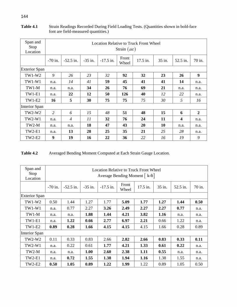
144  Table 4.1 Strain Readings Recorded During Field Loading Tests. (Quantities shown in bold-face

font are field-measured quantities.)

Span and Stop

Location

Location Relative to Truck Front Wheel Strain ( )με

-70 in. -52.5 in. -35 in. -17.5 in. Front Wheel 17.5 in. 35 in. 52.5 in. 70 in.

Exterior Span TW1-W2 9 26 23 32 92 32 23 26 9 TW1-W1 n.a. 14 41 59 45 41 41 14 n.a. TW1-M n.a. n.a. 34 26 76 69 21 n.a. n.a. TW1-E1 n.a. 22 12 50 126 40 12 22 n.a. TW1-E2 16 5 30 75 75 75 30 5 16

Interior Span TW2-W2 2 6 15 48 51 48 15 6 2 TW2-W1 n.a. 4 11 32 76 24 11 4 n.a. TW2-M n.a. n.a. 18 47 43 20 10 n.a. n.a. TW2-E1 n.a. 13 28 25 35 21 25 28 n.a. TW2-E2 9 19 16 22 36 22 16 19 9

Table 4.2 Averaged Bending Moment Computed at Each Strain Gauge Location.

Span and Stop

Location

Location Relative to Truck Front Wheel Average Bending Moment [ ]k-ft

-70 in. -52.5 in. -35 in. -17.5 in. Front Wheel 17.5 in. 35 in. 52.5 in. 70 in.

Exterior Span TW1-W2 0.50 1.44 1.27 1.77 5.09 1.77 1.27 1.44 0.50 TW1-W1 n.a. 0.77 2.27 3.26 2.49 2.27 2.27 0.77 n.a. TW1-M n.a. n.a. 1.88 1.44 4.21 3.82 1.16 n.a. n.a. TW1-E1 n.a. 1.22 0.66 2.77 6.97 2.21 0.66 1.22 n.a. TW1-E2 0.89 0.28 1.66 4.15 4.15 4.15 1.66 0.28 0.89

Interior Span TW2-W2 0.11 0.33 0.83 2.66 2.82 2.66 0.83 0.33 0.11 TW2-W1 n.a. 0.22 0.61 1.77 4.21 1.33 0.61 0.22 n.a. TW2-M n.a. n.a. 1.00 2.60 2.38 1.11 0.55 n.a. n.a. TW2-E1 n.a. 0.72 1.55 1.38 1.94 1.16 1.38 1.55 n.a. TW2-E2 0.50 1.05 0.89 1.22 1.99 1.22 0.89 1.05 0.50

145  

Table 4.3 Bending Moment (per foot) and Strip Width Comparison.

Span and Stop Location

TM +

[ ]k-ft avgM +

[ ]k-ft/ft STDM

[ ]k-ft/ft SW + [ ]in.

LRFDSW −

[ ]in. LRFDSW +

[ ]in.

Exterior Span TW1-W2 15.05 1.15

2.92

155.4

74.08 83.38 TW1-W1 14.11 1.38 128.9 TW1-M 12.51 1.72 103.9 TW1-E1 15.72 1.54 115.7 TW1-E2 18.09 1.38 129.2

Interior Span TW2-W2 10.68 0.81

2.92

175.2

74.08 83.38 TW2-W1 8.96 0.88 162.3 TW2-M 7.64 1.05 136.1 TW2-E1 9.68 0.95 150.3 TW2-E2 9.30 0.71 201.2

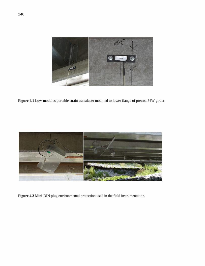
146  

Figure 4.1 Low-modulus portable strain transducer mounted to lower flange of precast 54W girder.

Figure 4.2 Mini-DIN plug environmental protection used in the field instrumentation.

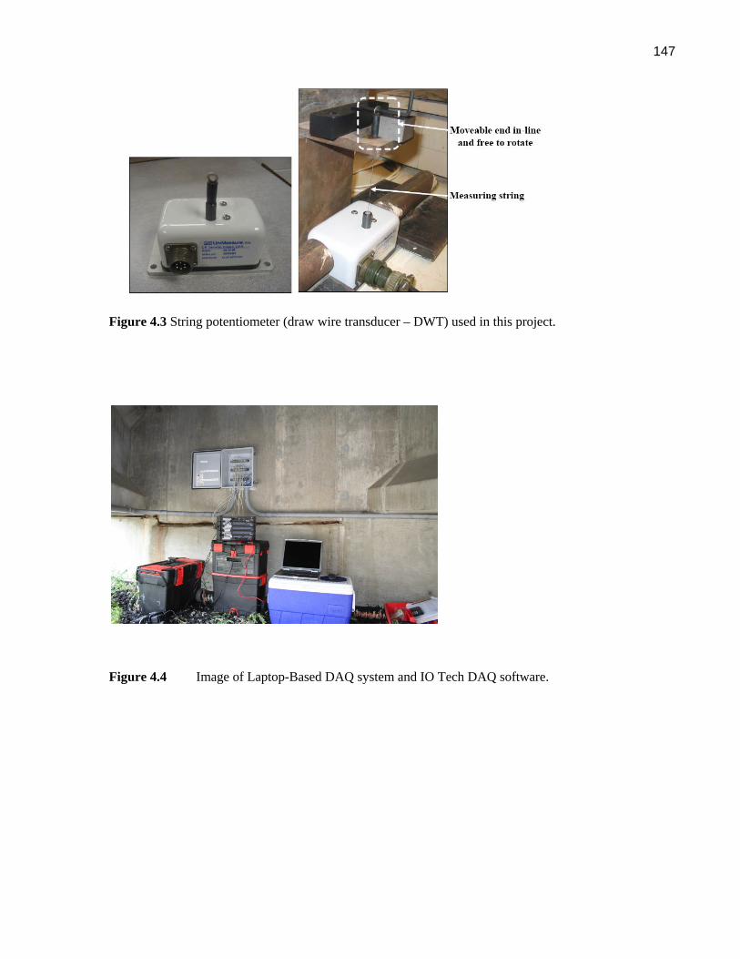
147  

Figure 4.3 String potentiometer (draw wire transducer – DWT) used in this project.

Figure 4.4 Image of Laptop-Based DAQ system and IO Tech DAQ software.

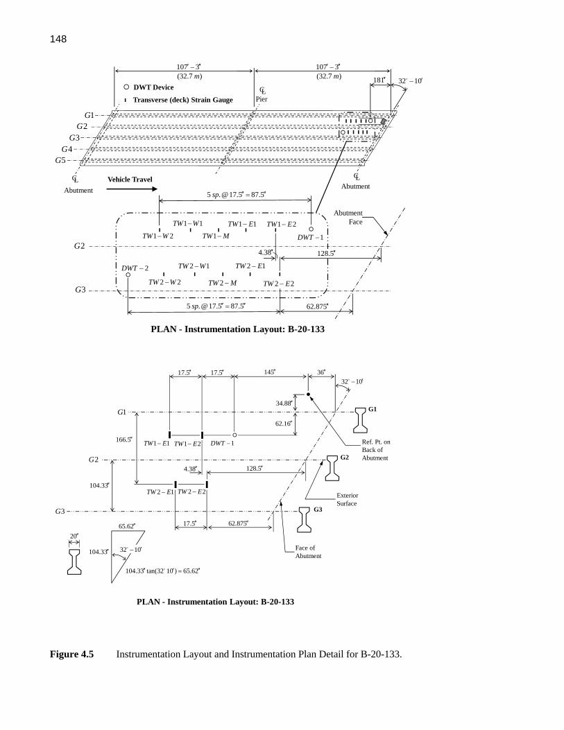
148  

Figure 4.5 Instrumentation Layout and Instrumentation Plan Detail for B-20-133.

1G2G

3G4G

5G

32 10′−

1 2TW W−

1 1TW W−

1TW M−

1 1TW E− 1 2TW E−

1DWT −

2DWT −

Abutment

Pier

Abutment

2 2TW W−

2 1TW W−

2TW M−

2 1TW E−

2 2TW E−

DWT Device

Transverse (deck) Strain Gauge

Vehicle Travel

PLAN - Instrumentation Layout: B-20-133

CL

CL

CL

AbutmentFace

2G

3G

5 [email protected] 87.5sp ′′ ′′=

4.38′′ 128.5′′

5 [email protected] 87.5sp ′′ ′′=

62.875′′

181′′

107 3(32.7 )m

′ ′′−107 3(32.7 )m

′ ′′−

Face ofAbutment

PLAN - Instrumentation Layout: B-20-133

G1

G2

G3

2 1TW E−

1 1TW E− 1DWT −

ExteriorSurface

Ref. Pt. onBack ofAbutment

1G

2G

3G

4.38′′

34.88′′

32 10′−

20′′

62.16′′

1 2TW E−

2 2TW E−

36′′

128.5′′

145′′

65.62′′

104.33 tan(32 10 ) 65.62′′ ′ ′′=

104.33′′

17.5′′17.5′′

62.875′′

32 10′−

17.5′′

104.33′′

166.5′′

149  

(a)

      (b)

Figure 4.6 B-20-133 Cross-Sections Illustrating Instrument Layout: (a) Conduit Runs and Draw

Wire Transducer Mounting; (b) Reference Point Location for Instrumentation.

1G 2G 3G 4G 5G

Section Indicating DWT Device Mounting

1G 2G 3G 4G 5G

Section Showing Conduit Runs

1DWT − 2DWT −

1G 2G 3G 4G 5G

Section Showing Gages Relative Locations in Transverse Direction

32.75''

104.33''

(2650 mm)

104.33''

(2650 mm)

Reference Point

Measured in field: 32.75''Calculated from drawing: 34.882''

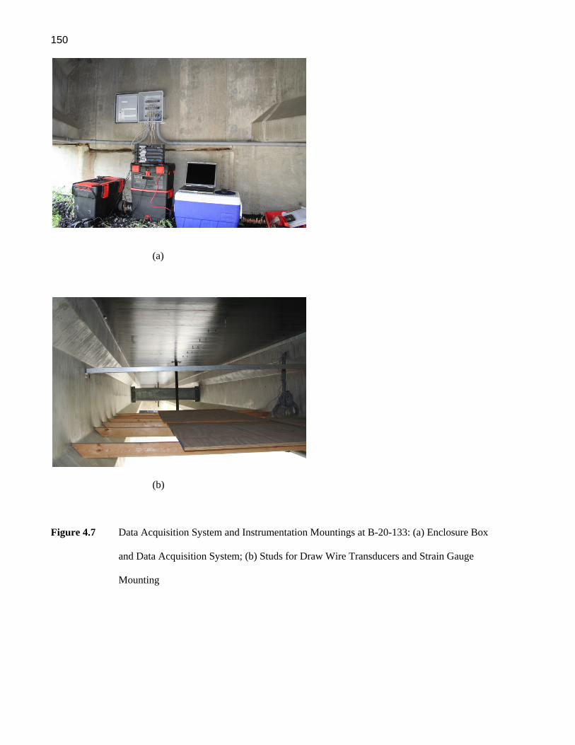
150  

(a)

(b)

Figure 4.7 Data Acquisition System and Instrumentation Mountings at B-20-133: (a) Enclosure Box

and Data Acquisition System; (b) Studs for Draw Wire Transducers and Strain Gauge

Mounting

151  

Figure 4.8 B-20-148 Instrumentation Plan with Sensor Locations, PVC Conduit Runs and Enclosure

Box Location.

DWT DeviceLongitudinal Strain Gauge

Transverse (deck) Strain Gauge

C BearingL

Face ofAbutment

G1G2

G3

G4

G5

G6

G7

63 7.5′′′ −

42 5′ ′′−44 2.5′ ′′−

C BearingL 130 0′ ′′−

Vehicle Travel

25 4 . @ 18sp ′′Enclosure

Box

PVC Conduit Run

PLAN - Instrumentation Layout: B-20-148

1LM −

2LM −

3LM −

4LM −

5LM −

6LM −

7LM −

1DWT −

2DWT −1LT −

2LT −

3LT −

4LT −

5LT −

6LT −

7LT −

2TW W−

1TW W−

TW M−

1TW E−

2TW E−

152  

(a)

(b)

Figure 4.9 B-20-148 Instrumentation Layout in Plan: (a) Bridge Deck Sensor Layout; (b) Lane Load

Distribution Factor Gauge Locations.

Face ofAbutment

PLAN - Instrumentation Layout: B-20-148

G1

G2

G3

Exterior Faceof Flange

Ref. Pt. on Back Edge Parapet Wall

25

G1

63 7.5′′′ −

2TW E−

2DWT −

1DWT −

Girder Center

Deck Span Center

38.5 tan(25)17.95′′

′′=

77 2 38.50′′ ′′=

5 0′ ′′254.5 21 2.5′′ ′ ′′=42 5 7 5 0 456

38′ ′′ ′′ ′ ′′ ′′+ − =

′=

15′′

22.625′′

77′′

77′′

35.91′′

38.5′′

38.5′′

17.95′′

17.95′′

39.45′′17.95′′

21.5′′ 25

2TW W−

204′′

G3-2G3-3 G3-1

G1-2G1-3 G1-1

G2-2G2-3 G2-1

37.625′′

Face ofAbutment

PLAN - Instrumentation Layout: B-20-148

G1

G2

G3

Exterior Faceof Flange

Ref. Pt. on BackEdge of ParapetWall

25

G1

63 7.5′′′ −

Ext. FaceGirder G1 25

CenterlineGirder G1

15 tan(25)7′′′′=

15′′

5 0′ ′′254.5 21 2.5′′ ′ ′′=42 5 7 5 0 456

38′ ′′ ′′ ′ ′′ ′′+ − =

′=

15′′

22.625′′

77′′

77′′35.91′′

1LT −

2LT −

3LT −

1LM −

2LM −

3LM −

35.91′′

35.91′′35.91′′

153  

(a0

(b)

Figure 4.10 B-20-148 Cross-Sections with Instrumentation Locations and Layout: (a) Sensor

Locations within Bridge Cross-Section; (b) Reference Point Location Used to Locate

Sensors.

Strain Gauges“Rigid” Strut

G1 G2 G3 G4 G5 G6 G7

BRIDGE SECTION - Mid-Span

1LM − 2LM − 3LM − 4LM − 5LM − 6LM − 7LM −

1DWT − 2DWT −

1 1SP −

1 2SP −

2 1SP −

2 2SP −

Strain Gauges

G1 G2 G3 G4 G5 G6 G7

B-20-148 BRIDGE SECTION - Mid-Span

1LM − 2LM − 3LM − 4LM − 5LM − 6LM − 7LM −

30''

Ref. Pt.

2′′

22.625′′15′′

77′′

154  

Figure 4.11 B-20-148 Strain Sensor Locations used to Measure Strain Distribution Over Height of

Girders.

3.125′′

3.0′′

3.875′′

3.0′′

1, 2G G

7.23′′

53.64′′

1LM −2LM −

1 1SP −

1 2SP −

2 1SP −

2 2SP −

155  

(a) (b)

(c) (d)

Figure 4.12 B-20-148 Data Acquisition System and Instrumentation: (a) Data Acquisition System and

Enclosure; (b) Draw Wire Transducer Installation; (c) Strain Gauge Installation; (d)

Sensor Wiring Runs and Sensor Installation.

156  

(a)

(b)

(c)

Figure 4.13 Typical Pavement Marking for Load Testing: (a) Bridge B-20-133; (b) Bridge B-20-148;

(c) Truck Positioning Guided by Pavement Marking at B-20-133.

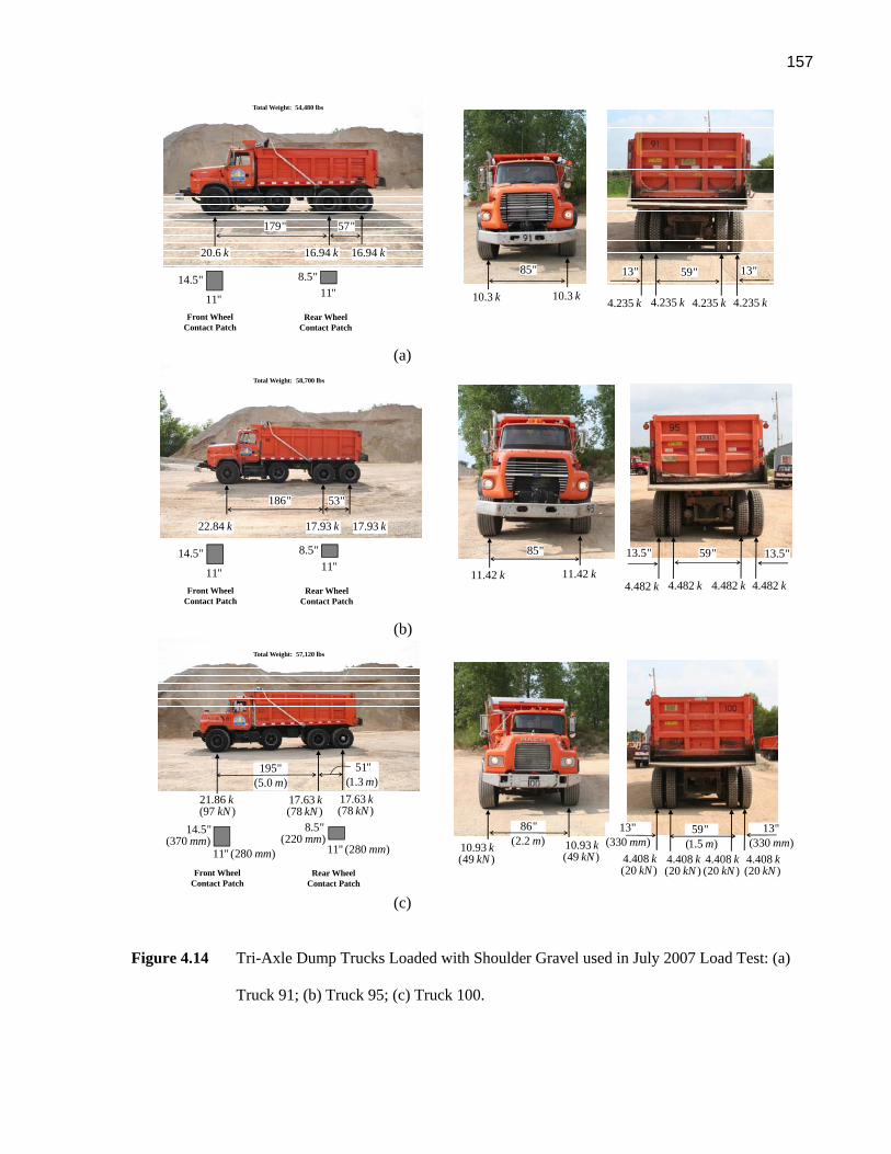
157  

(a)

(b)

(c) Figure 4.14 Tri-Axle Dump Trucks Loaded with Shoulder Gravel used in July 2007 Load Test: (a)

Truck 91; (b) Truck 95; (c) Truck 100.

16.94 k 16.94 k20.6 k

57"179"

11"8.5"

11"

14.5"

Front WheelContact Patch

Rear WheelContact Patch

Total Weight: 54,480 lbs

10.3 k 10.3 k

85"

4.235 k

59"13" 13"

4.235 k4.235 k 4.235 k

17.93 k 17.93 k22.84 k

53"186"

11"8.5"

11"

14.5"

Front WheelContact Patch

Rear WheelContact Patch

Total Weight: 58,700 lbs

11.42 k 11.42 k

85"

4.482 k

59"13.5" 13.5"

4.482 k4.482 k 4.482 k

17.63(78 )

kkN

21.86(97 )

kkN

51"(1.3 )m

195"(5.0 )m

11" (280 )mm

8.5"(220 )mm

14.5"(370 )mm

Front WheelContact Patch

Rear WheelContact Patch

17.63(78 )

kkN

11" (280 )mm

Total Weight: 57,120 lbs

10.93(49 )

kkN

86"(2.2 )m

59"(1.5 )m

13"(330 )mm

4.408(20 )

kkN

10.93(49 )

kkN 4.408

(20 )k

kN4.408(20 )

kkN

4.408(20 )

kkN

13"(330 )mm

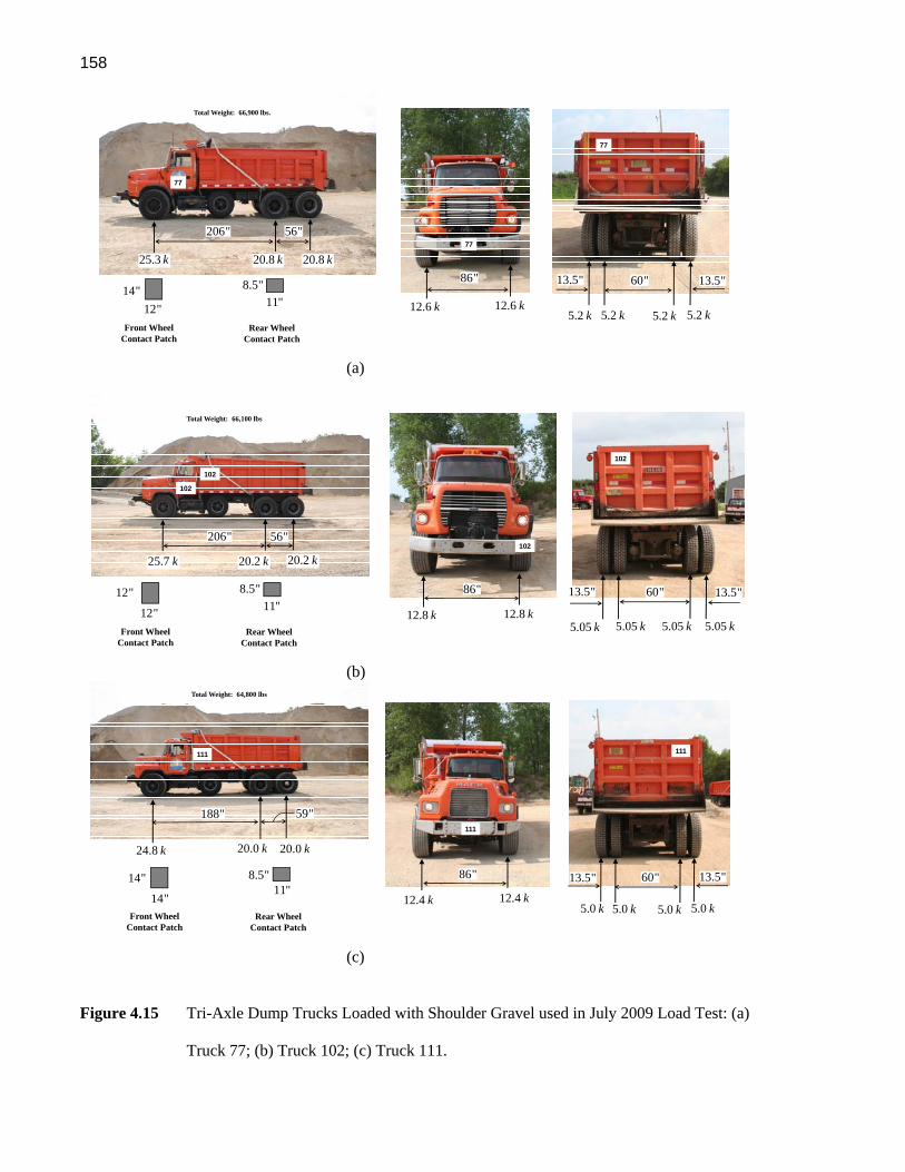
158  

(a)

(b)

(c) Figure 4.15 Tri-Axle Dump Trucks Loaded with Shoulder Gravel used in July 2009 Load Test: (a)

Truck 77; (b) Truck 102; (c) Truck 111.

20.8 k 20.8 k25.3 k

56"206"

11"8.5"

12"14"

Front WheelContact Patch

Rear WheelContact Patch

77

Total Weight: 66,900 lbs.

12.6 k 12.6 k

86"

5.2 k

60"13.5" 13.5"

5.2 k5.2 k 5.2 k

77

77

20.2 k 20.2 k25.7 k

56"206"

11"8.5"

12"

12"

Front WheelContact Patch

Rear WheelContact Patch

102

102

Total Weight: 66,100 lbs

12.8 k 12.8 k

86"

5.05 k

60"13.5" 13.5"

5.05 k5.05 k 5.05 k

102

102

20.0 k24.8 k

59"188"

11"8.5"14"

Front WheelContact Patch

Rear WheelContact Patch

20.0 k

14"

111

Total Weight: 64,800 lbs

12.4 k

86" 60"13.5"

5.0 k12.4 k

5.0 k5.0 k 5.0 k

13.5"

111

111

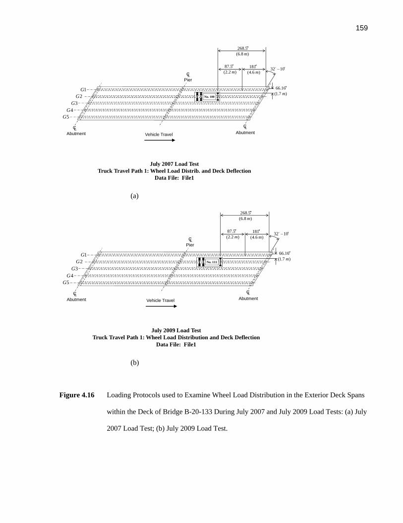
159  

(a)

(b)

Figure 4.16 Loading Protocols used to Examine Wheel Load Distribution in the Exterior Deck Spans

within the Deck of Bridge B-20-133 During July 2007 and July 2009 Load Tests: (a) July

2007 Load Test; (b) July 2009 Load Test.

1G2G

3G4G

5G

32 10′−

Abutment

Pier

Abutment Vehicle TravelCL

CL

CL

181(4.6 )m

′′

66.16(1.7 )m

′′

268.5(6.8 )m

′′

87.5(2.2 )m

′′

No. 100

July 2007 Load TestTruck Travel Path 1: Wheel Load Distrib. and Deck Deflection

Data File: File1

1G2G

3G4G

5G

32 10′−

Abutment

Pier

Abutment Vehicle TravelCL

CL

CL

181(4.6 )m

′′

66.16(1.7 )m

′′

268.5(6.8 )m

′′

87.5(2.2 )m

′′

No. 111

July 2009 Load TestTruck Travel Path 1: Wheel Load Distribution and Deck Deflection

Data File: File1

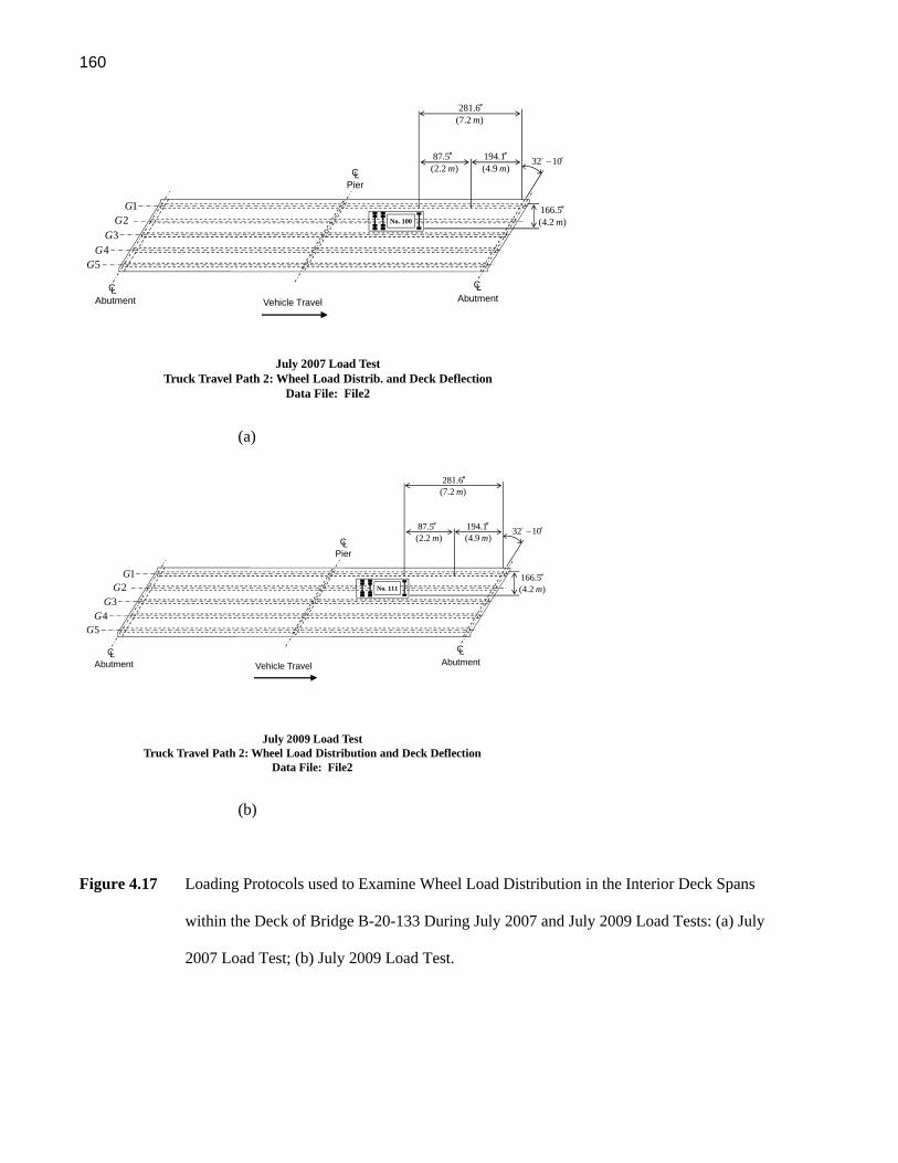
160  

(a)

(b)

Figure 4.17 Loading Protocols used to Examine Wheel Load Distribution in the Interior Deck Spans

within the Deck of Bridge B-20-133 During July 2007 and July 2009 Load Tests: (a) July

2007 Load Test; (b) July 2009 Load Test.

1G2G

3G4G

5G

32 10′−

Abutment

Pier

Abutment Vehicle TravelCL

CL

CL

194.1(4.9 )m

′′

166.5(4.2 )m

′′

281.6(7.2 )m

′′

87.5(2.2 )m

′′

No. 100

July 2007 Load TestTruck Travel Path 2: Wheel Load Distrib. and Deck Deflection

Data File: File2

1G2G

3G4G

5G

32 10′−

Abutment

Pier

Abutment Vehicle TravelCL

CL

CL

194.1(4.9 )m

′′

166.5(4.2 )m

′′

281.6(7.2 )m

′′

87.5(2.2 )m

′′

No. 111

July 2009 Load TestTruck Travel Path 2: Wheel Load Distribution and Deck Deflection

Data File: File2

161  

(a)

(b) Figure 4.18 Loading Protocols used to Examine Deck Deflection in the Exterior Deck Spans within

the Deck of Bridge B-20-148 During July 2007 and July 2009 Load Tests: (a) July 2007

Load Test; (b) July 2009 Load Test.

60 8.5′ ′′

Vehicle Travel

25

July 2007 Load TestTruck Position Number 1 - Deck Deflection

DWT-2 is target: Data File: File1

G3

G1G2

Ref. Pt. on Backof Parapet Wall

76.125′′

No. 91

60 8.5′ ′′

Vehicle Travel

25

July 2009 Load TestTruck Position Number 1 - Deck Deflection

DWT-2 is target: Data File: File1

G3

G1G2

Ref. Pt. on Backof Parapet Wall

76.125′′

No. 111

162  

(a)

(b)

Figure 4.19 Loading Protocols used to Examine Deck Deflection in the Interior Deck Spans within

the Deck of Bridge B-20-148 During July 2007 and July 2009 Load Tests: (a) July 2007

Load Test; (b) July 2009 Load Test.

Vehicle Travel

25

July 2007 Load TestTruck Position 2 - Deck DeflectionDWT-1 Target: Data File: File2

G3

G1G2

Ref. Pt. on Backof Parapet Wall

153.125′′

63 8.4′ ′′

No. 91

Vehicle Travel

25

July 2009 Load TestTruck Position 2 - Deck DeflectionDWT-1 Target: Data File: File2

G3

G1G2

Ref. Pt. on Backof Parapet Wall

153.125′′

63 8.4′ ′′

No. 111

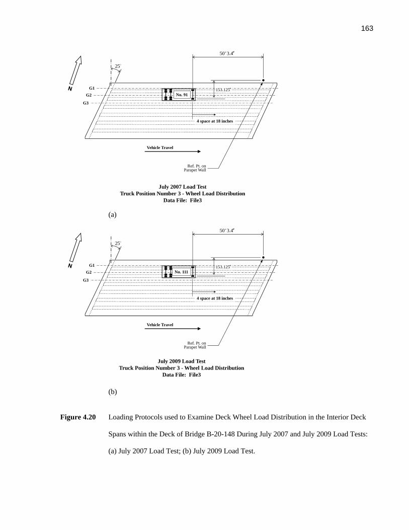
163  

(a)

(b) Figure 4.20 Loading Protocols used to Examine Deck Wheel Load Distribution in the Interior Deck

Spans within the Deck of Bridge B-20-148 During July 2007 and July 2009 Load Tests:

(a) July 2007 Load Test; (b) July 2009 Load Test.

Vehicle Travel

25

July 2007 Load TestTruck Position Number 3 - Wheel Load Distribution

Data File: File3

G3

G1G2

Ref. Pt. onParapet Wall

50' 3.4′′

153.125′′

4 space at 18 inches

No. 91

Vehicle Travel

25

July 2009 Load TestTruck Position Number 3 - Wheel Load Distribution

Data File: File3

G3

G1G2

Ref. Pt. onParapet Wall

50' 3.4′′

153.125′′

4 space at 18 inches

No. 111

164  

(a)

(b)

Figure 4.21 Loading Protocols used to Examine Lane Load Distribution among the Girders in Bridge

B-20-148 During July 2007 and July 2009 Load Tests: (a) July 2007 Load Test; (b) July

2009 Load Test.

25′

Vehicle Travel

25

G3

G1G2

Ref. Pt. on Backof Parapet Wall

70.125′′

July 2007 Load TestTruck Position Number 4 - Lane Load Distribution

Data File: File4

78 6′ ′′−

No. 91No. 95 No. 100

25′

Vehicle Travel

25

G3

G1G2

Ref. Pt. on Backof Parapet Wall

70.125′′

July 2009 Load TestTruck Position Number 4 - Lane Load Distribution

Data File: File4

78 6′ ′′−

No. 111No. 77 No. 102

165  

(a)

(b)

Figure 4.22 Typical Truck Positioning during Load Testing: (a) Bridge B-20-148 Lane Load

Distribution Loading Protocol; (b) Bridge B-20-133 Wheel Load Distribution Loading

Protocol.

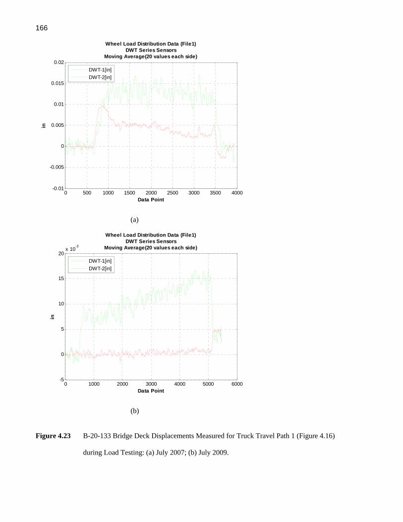
166  

(a)

(b)

Figure 4.23 B-20-133 Bridge Deck Displacements Measured for Truck Travel Path 1 (Figure 4.16)

during Load Testing: (a) July 2007; (b) July 2009.

0 500 1000 1500 2000 2500 3000 3500 4000-0.01

-0.005

0

0.005

0.01

0.015

0.02

Data Point

inWheel Load Distribution Data (File1)

DWT Series SensorsMoving Average(20 values each side)

DWT-1[in]DWT-2[in]

0 1000 2000 3000 4000 5000 6000-5

0

5

10

15

20x 10

-3

Data Point

in

Wheel Load Distribution Data (File1)DWT Series Sensors

Moving Average(20 values each side)

DWT-1[in]DWT-2[in]

167  

(a)

(b)

Figure 4.24 B-20-133 Bridge Deck Displacements Measured for Truck Travel Path 2 (Figure 4.17)

during Load Testing: (a) July 2007; (b) July 2009.

0 500 1000 1500 2000 2500 3000 3500 4000 4500-5

0

5

10

15

20x 10

-3

Data Point

in

Wheel Load Distribution Data (File2)DWT Series Sensors

Moving Average(20 values each side)

DWT-1[in]DWT-2[in]

0 1000 2000 3000 4000 5000 6000-0.015

-0.01

-0.005

0

0.005

0.01

0.015

Data Point

in

Wheel Load Distribution Data (File2)DWT Series Sensors

Moving Average(20 values each side)

DWT-1[in]DWT-2[in]

168  

(a)

(b)

Figure 4.25 B-20-133 Wheel Load Strain Distribution Measurements in the Exterior Bridge Deck

Span during Truck Travel Path 1 (Figure 4.16): (a) July 2007; (b) July 2009.

0 500 1000 1500 2000 2500 3000 3500 4000-20

0

20

40

60

80

100

120

140

Data Point

με

Wheel Load Distribution Data (File1)TW1 Series Sensors

Moving Average(20 values each side)Modified by Correction Factor

TW1-E2[με]TW1-E1[με]TW1-M[με]TW1-W1[με]TW1-W2[με]

0 1000 2000 3000 4000 5000 6000-20

-15

-10

-5

0

5

10

15

20

Data Point

με

Wheel Load Distribution Data (File1)TW1 Series Sensors

Moving Average(20 values each side)Modified by Correction Factor

TW1-E2[με]TW1-E1[με]TW1-M[με]TW1-W1[με]TW1-W2[με]

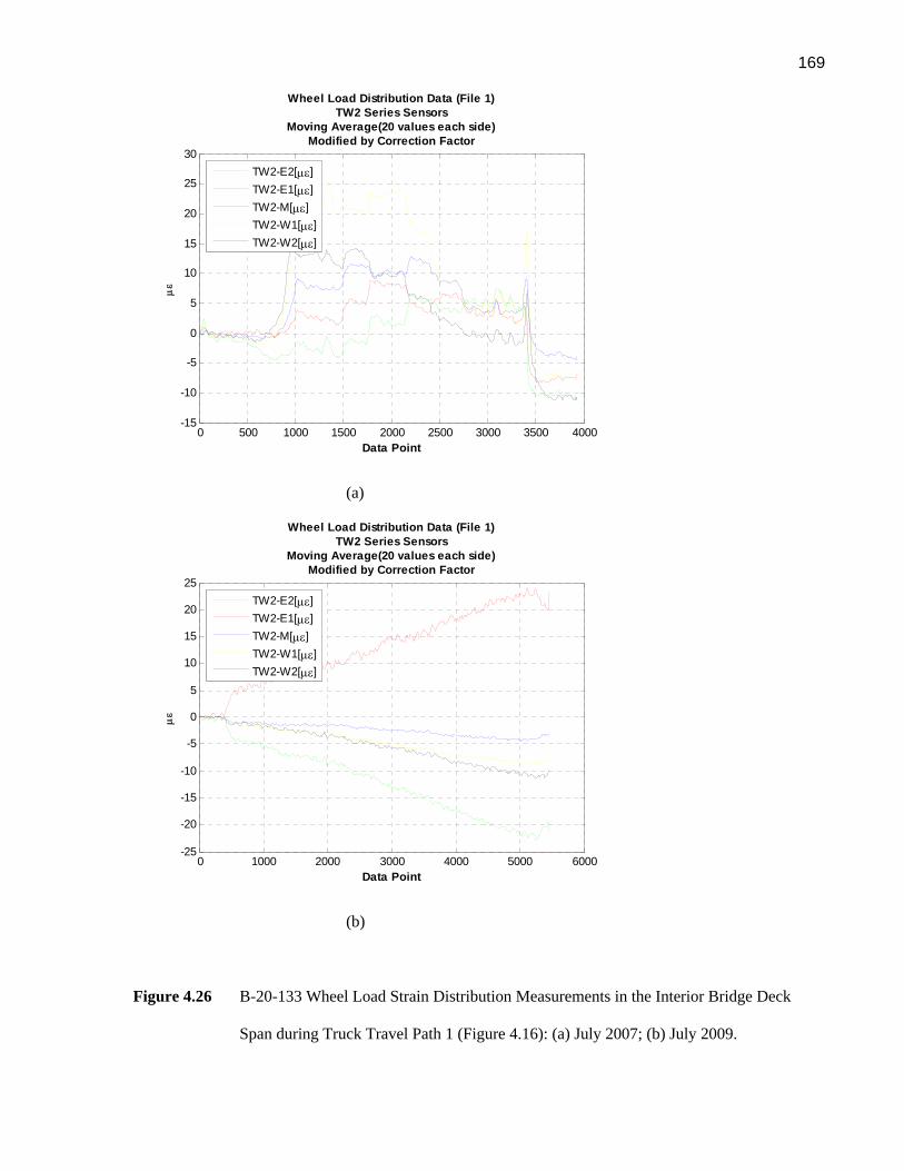
169  

(a)

(b)

Figure 4.26 B-20-133 Wheel Load Strain Distribution Measurements in the Interior Bridge Deck

Span during Truck Travel Path 1 (Figure 4.16): (a) July 2007; (b) July 2009.

0 500 1000 1500 2000 2500 3000 3500 4000-15

-10

-5

0

5

10

15

20

25

30

Data Point

με

Wheel Load Distribution Data (File 1)TW2 Series Sensors

Moving Average(20 values each side)Modified by Correction Factor

TW2-E2[με]TW2-E1[με]TW2-M[με]TW2-W1[με]TW2-W2[με]

0 1000 2000 3000 4000 5000 6000-25

-20

-15

-10

-5

0

5

10

15

20

25

Data Point

με

Wheel Load Distribution Data (File 1)TW2 Series Sensors

Moving Average(20 values each side)Modified by Correction Factor

TW2-E2[με]TW2-E1[με]TW2-M[με]TW2-W1[με]TW2-W2[με]

170  

(a)

(b)

Figure 4.27 B-20-133 Wheel Load Strain Distribution Measurements in the Exterior Bridge Deck

Span during Truck Travel Path 2 (Figure 4.17): (a) July 2007; (b) July 2009.

0 500 1000 1500 2000 2500 3000 3500 4000 4500-20

-10

0

10

20

30

40

50

Data Point

με

Wheel Load Distribution Data (File 2)TW1 Series Sensors

Moving Average(20 values each side)Modified by Correction Factor

TW1-E2[με]TW1-E1[με]TW1-M[με]TW1-W1[με]TW1-W2[με]

0 1000 2000 3000 4000 5000 6000 7000-30

-20

-10

0

10

20

30

40

50

60

Data Point

με

Wheel Load Distribution Data (File 2)TW1 Series Sensors

Moving Average(20 values each side)Modified by Correction Factor

TW1-E2[με]TW1-E1[με]TW1-M[με]TW1-W1[με]TW1-W2[με]

171  

(a)

(b)

Figure 4.28 B-20-133 Wheel Load Strain Distribution Measurements in the Interior Bridge Deck

Span during Truck Travel Path 2 (Figure 4.17): (a) July 2007; (b) July 2009.

0 500 1000 1500 2000 2500 3000 3500 4000 4500-10

0

10

20

30

40

50

60

70

80

Data Point

με

Wheel Load Distribution Data (File2)TW2 Series Sensors

Moving Average(20 values each side)Modified by Correction Factor

TW2-E2[με]TW2-E1[με]TW2-M[με]TW2-W1[με]TW2-W2[με]

0 1000 2000 3000 4000 5000 6000 7000-25

-20

-15

-10

-5

0

5

10

15

20

25

Data Point

με

Wheel Load Distribution Data (File2)TW2 Series Sensors

Moving Average(20 values each side)Modified by Correction Factor

TW2-E2[με]TW2-E1[με]TW2-M[με]TW2-W1[με]TW2-W2[με]

172  

(a)

(b)

Figure 4.29 B-20-148 Deck Displacements for Truck Position 1 (Figure 4.18): (a) July 2007; (b) July

2009.

0 100 200 300 400 500 600 700 800 900-6

-4

-2

0

2

4

6

8

10

12

14x 10

-3

Data Point

inDeck Deflection (File 1)

DWT Series SensorsMoving Average(20 values each side)

DWT-1[in]DWT-2[in]

0 200 400 600 800 1000 1200 1400 1600 1800-8

-6

-4

-2

0

2

4x 10

-3

Data Point

in

Deck Deflection (File 1)DWT Series Sensors

Moving Average(20 values each side)

DWT-1[in]DWT-2[in]

173  

(a)

(b)

Figure 4.30 B-20-148 Deck Displacements for Truck Position 2 (Figure 4.19): (a) July 2007; (b) July

2009.

0 200 400 600 800 1000 1200 1400 1600 1800-4

-2

0

2

4

6

8

10

12

14

16x 10

-3

Data Point

in

Deck Deflection (File 2)DWT Series Sensors

Moving Average(20 values each side)

DWT-1[in]DWT-2[in]

0 200 400 600 800 1000 1200 1400 1600-5

-4

-3

-2

-1

0

1

2

3

4x 10

-3

Data Point

in

Deck Deflection (File 2)DWT Series Sensors

Moving Average(20 values each side)

DWT-1[in]DWT-2[in]

174  

(a)

(b)

Figure 4.31 B-20-148 Wheel Load Distribution Strains Measured for Truck Position 3 (Figure 4.20):

(a) July 2007; (b) July 2009.

0 500 1000 1500 2000 2500 3000 3500 4000 4500-10

-5

0

5

10

15

20

25

30

35

40

Data Point

με

DECK (File3)TW Series Sensors

Moving Average(20 values each side)Modified by Correction Factor

TW-W2 [με]TW-W1 [με]TW-M [με]TW-E1 [με]

0 500 1000 1500 2000 2500 3000 3500 4000 4500 5000-20

-10

0

10

20

30

40

50

Data Point

με

DECK (File3)TW Series Sensors

Moving Average(20 values each side)Modified by Correction Factor

TW-W2 [με]TW-W1 [με]TW-M [με]TW-E1 [με]

175  

(a)

(b)

Figure 4.32 B-20-148 Lane Load Distribution Strains at Mid-Span of Girders for Truck Position 4

(Figure 4.21) Measured During Load Tests: (a) July 2007; (b) July 2009.

0 500 1000 1500 2000 2500 3000 3500 4000 4500 5000-10

0

10

20

30

40

50

60

70

Data Point

με

Lane Load Distribution (File 4)LM Series Sensors

Moving Average(20 values each side)Modified by Correction Factor

LM-1[με]LM-2[με]LM-3[με]LM-4[με]LM-5[με]LM-6[με]LM-7[με]

0 500 1000 1500 2000 2500 3000 3500 4000 4500 5000-12000

-10000

-8000

-6000

-4000

-2000

0

2000

Data Point

με

Lane Load Distribution (File 4)LM Series Sensors

Moving Average(20 values each side)Modified by Correction Factor

LM-1[με]LM-2[με]LM-3[με]LM-4[με]LM-5[με]LM-6[με]LM-7[με]

176  

(a)

(b)

Figure 4.33 B-20-148 Lane Load Distribution Strains at One-Third-Span of Girders for Truck

Position 4 (Figure 4.21) Measured During Load Tests: (a) July 2007; (b) July 2009.

0 500 1000 1500 2000 2500 3000 3500 4000 4500 5000-30

-20

-10

0

10

20

30

40

50

60

Data Point

mue

xcel

onLane Load Distribution (File 4)

LT Series SensorsMoving Average(20 values each side)

Modified by Correction Factor

LT-1[με]LT-2[με]LT-3[με]LT-4[με]LT-5[με]LT-6[με]LT-7[με]

0 500 1000 1500 2000 2500 3000 3500 4000 4500 5000-0.5

0

0.5

1

1.5

2

2.5x 10

4

Data Point

με

Lane Load Distribution (File 4)LT Series Sensors

Moving Average(20 values each side)Modified by Correction Factor

LT-1[με]LT-2[με]LT-3[με]LT-4[με]LT-5[με]LT-6[με]LT-7[με]

177  

(a)

(b)

Figure 4.34 B-20-148 Strains over Girder Height for Girder G1 and Truck Position 4 (Figure 4.21)

Measured During Load Tests: (a) July 2007; (b) July 2009.

0 500 1000 1500 2000 2500 3000 3500 4000 4500 5000-30

-20

-10

0

10

20

30

40

Data Point

με

Girder #1 (File4)Strain Over Height

Moving Average(20 values each side)Modified by Correction Factor

LM-1 [με]SP1-2 [με]SP1-1 [με]

0 500 1000 1500 2000 2500 3000 3500 4000 4500 5000-1000

-800

-600

-400

-200

0

200

Data Point

με

Girder #1 (File4)Strain Over Height

Moving Average(20 values each side)Modified by Correction Factor

LM-1 [με]SP1-2 [με]SP1-1 [με]

178  

(a)

(b)

Figure 4.35 B-20-148 Strains over Girder Height for Girder G2 and Truck Position 4 (Figure 4.21)

Measured During Load Tests: (a) July 2007; (b) July 2009.

0 500 1000 1500 2000 2500 3000 3500 4000 4500 5000-30

-20

-10

0

10

20

30

40

50

60

70

Data Point

με

Girder #2(File4)Strain Over Height

Moving Average(20 values each side)Modified by Correction Factor

LM-2 [με]SP2-2 [με]SP2-1 [με]

0 500 1000 1500 2000 2500 3000 3500 4000 4500 5000-400

-300

-200

-100

0

100

200

Data Point

με

Girder #2(File4)Strain Over Height

Moving Average(20 values each side)Modified by Correction Factor

LM-2 [με]SP2-2 [με]SP2-1 [με]

179  

(a)

(b)

Figure 4.36 B-20-148 Strains over Girder Height for Girders G1 and G2 for Truck Position 4 (Figure

4.21) Measured During Load Tests: (a) Girder G1; (b) Girder G2.

1, 2G G

15 με−

8 με−

40 με+

Girder G1July 2007

20 με−

5 με−

41με+

Girder G1July 2009

1, 2G G

19 με−

8 με−

62 με+

Girder G2July 2007

17 με−

3 με−

155 με+

Girder G2July 2009

180  

Figure 4.37 Strain Sensor Installation Error with Potential to Cause Error in Strain Readings.

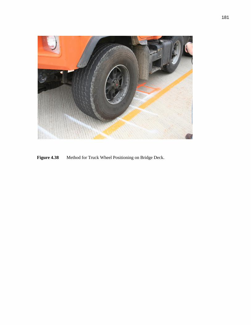
181  

Figure 4.38 Method for Truck Wheel Positioning on Bridge Deck.

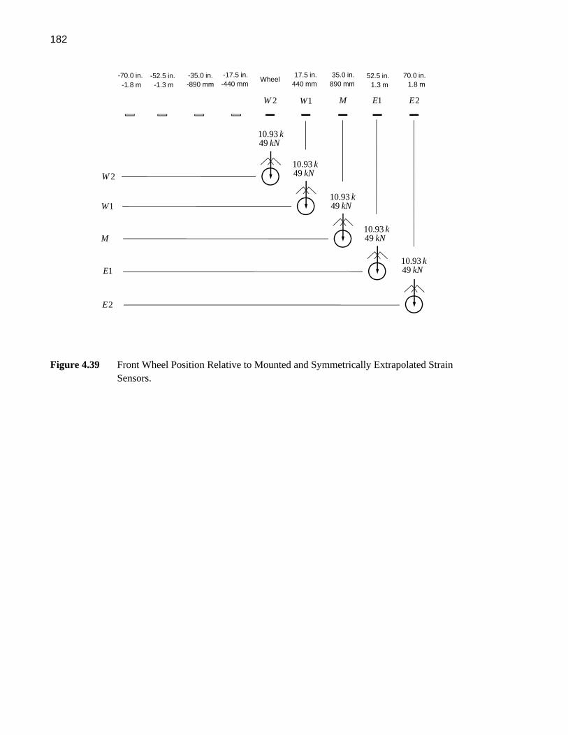
182  

Figure 4.39 Front Wheel Position Relative to Mounted and Symmetrically Extrapolated Strain Sensors.

Wheel-17.5 in.-35.0 in.-52.5 in.-70.0 in. 17.5 in. 35.0 in. 52.5 in. 70.0 in.

2W 1W M 1E 2E

10.9349

kkN

2W

1W

M

1E

2E

-1.8 m -1.3 m -890 mm -440 mm 1.8 m1.3 m890 mm440 mm

10.9349

kkN

10.9349

kkN

10.9349

kkN

10.9349

kkN

183  

Chapter 5

Numerical Simulation of Shrinkage-Induced and Vehicle-Induced Stresses 5.1 Introduction

The present chapter outlines finite element (FE) simulation that is used as the foundation for assessing the

cause and impact of the cracking that exists throughout the bridge deck in the bridges at Waupun,

Wisconsin (bridges B-20-133/134). The simulation results presented here are (in large part) based upon

an MS thesis written to assess bridge deck cracking (Komp 2009). The results present here are intended

to outline the FE simulation used to document the cause of cracking in these bridge decks. Two sources

are examined: (a) shrinkage-induced tensile strains; and (b) typical HL-93 design truck loading. Further

detailed discussion of the modeling is available elsewhere (Komp 2009).

5.2 FE Modeling of Bridge Superstructure

The FE simulation conducted in this research was done using the ANSYS Finite Element Analysis

System (ANSYS 2007). All structural simulations were conducted using linear-elastic analysis and

elements that are standard within the software program. The present section will discuss general

modeling approaches used including the elements utilized.

The bridge prototype was modeling after structure B-20-134, located in Waupun, Wisconsin.

Figure 5.1 provides an overview photograph of the bridge superstructure. The finite element model was

developed using planar elements and subsequent extrusion to solid elements. The three-dimensional solid

modeling of the concrete components of the bridge cross-section was done using SOLID 45 elements

(ANSYS 2007). The bridge plan is shown in Figure 5.2. To create the skew, each girder and associated

deck/barrier was staggered by 1,500 mm (4.9 feet), as shown in Figure 5.2. A close up view of the

staggered model (with modeling volumes shown – not elements) is shown in Figure 5.3. The bridge

cross-section and area modeling prior to extrusion are shown in Figure 5.4.

184  

The bearing plates for the precast concrete girders were modeled using steel material in lieu of the

complex elastomeric bearing materials. The original elastomeric pads had dimensions of 0.50x6.0x30.0

inches and the steel bearing pads in the FE model closely followed these dimensions (within allowable

meshing constraints). The bearing pads were given a modulus of elasticity of 29,000 ksi and Poisson’s

ratio of 0.25. Once modeled, the pads were then centered under the ends of each girder.

The exact restraints at the ends of the bridge are difficult to quantify, and therefore pin-roller

supports were assumed for each span. The plates at the exterior support locations in the bridge were

modeled with “pin supports” (translational restraints applied at each of the 12 nodes on the center-base of

the plates), while the interior support locations included “roller supports” (translational restraints), which

were applied at similar locations (Figure 5.5).

Each of the 5 prestressed concrete girders within a given span was modeled using 3D solid

elements. These girders span 107'-4" centerline to centerline. The girder spacing was 8'-8" and a 12

inch long space at the ends of the girders was included to accommodate the diaphragms at the interior

pier. Solid FE modeling of the girders and their overall dimensions are shown in Figure 5.6. The bridge

deck is the primary concern in this thesis, and the girders were modeled without steel reinforcement, and

were given a modulus of elasticity consistent with a defined 28-day unconfined compressive strength of

9,000 psi. A Poisson’s ratio of 0.2 was selected. (Kachlakev 2001).

Concrete barriers were also modeled using solid elements. Barrier modeling and dimensions are

shown in Figure 5.7. The barriers included no reinforcement, were given a Poisson’s ratio of 0.2, and a

modulus of elasticity consistent with a 28-day unconfined compressive strength equal to 4,000 psi.

For portions of the study targeted toward studying drying shrinkage, the deck was analyzed

before the placement of the barriers, and therefore the barriers were either removed completely, or given

zero density and very small modulus of elasticity set by trial and error. Details can be found in Komp

(2009).

Concrete diaphragms or pilasters were modeled in the 12-inch space between the 5 sets of girders

which connect the two spans. The diaphragms were initially modeled using the same shape and physical

185  

characteristics as the concrete girders. The actual dimensions of the diaphragms and the modeling

characteristic are given in Figure 5.5 and 5.8.

At the ends of the bridge girders and between girder spans, the lateral stability characteristics of

the concrete diaphragms were modeled using nodal restraints. A 6-inch length of the girders was given

transverse displacement restraints. The restraints were applied on the exterior nodes on either side of the

girder, excluding the nodes that were connected to either the deck or the steel plates (Figure 5.9). In

reality, the concrete diaphragms would be cast at an angle similar to that of the skew.

The steel diaphragms present at approximate third points along the girder spans were modeled

using a pin-connected model composed of 3D spar (link) elements. These elements are only capable of

supporting axial forces. The original diaphragms were channel members (MC-shape) as shown in Figure

5.4. The resulting truss model for the diaphragms is schematically shown in Figure 5.10. The horizontal

truss elements were given an area consistent with that of the area of the original MC flanges. The

diagonal elements in the truss were assigned using consistent shear deformation characteristics between

the channel and truss. The link elements representing steel diaphragms were then added between the

girders at approximate third points along the span. The spacing of the X-braced diaphragms in the finite

element model is given in Figure 5.10.

The bridge deck was modeled using 3D solid elements. Figure 5.11 illustrates the deck modeling

approach utilized. The haunches between the deck soffit and girder top surface s have been omitted in the

FE model. In addition, the super elevation of the deck and the rebar (in some cases) were also eliminated

to simplify the model. The deck elements were given a Poisson’s ratio of 0.2 and a modulus of elasticity

consistent with a given unconfined compressive strength (dependent on time). In the linear analysis, the

analysis was only carried out until first cracking (modulus of rupture is reached). In general, it is accurate

to assume linear behavior until this point, as concrete shows relatively linear behavior up until a stress

level near 0.3fc’, which is less than the modulus of rupture (Kachlakev 2001).

Steel rebar was modeled using 3D spar (link) elements. The spacing of rebar was set at 6 inches

in the longitudinal direction of the bridge model to represent the longitudinal steel based on the nodal

186  spacing previously created. The area of these elements could be determined by calculating the total

amount of longitudinal steel (length*area) originally used in the deck, and altering it based on the

previously determined element spacing in the finite element model. The same process was used for the

transverse steel. In general, the addition of steel reinforcement to the model required quite a significant

amount of computer memory, and therefore it was neglected in some of the linear analyses (Komp 2009).

5.3 Simulation and Evaluation of Shrinkage-Induced Strains

The current section examines the effects of drying shrinkage-induced strains on the concrete bridge deck

in bridge B-20-134. The magnitude of shrinkage-induced strains was defined using previous research

efforts reviewed in this section. Shrinkage strain magnitudes were then converted into equivalent

temperature loads to facilitate FE simulation. The shrinkage strains accumulated over a given day were

run as independent linear elastic models. This section of the report outlines the modeling process that was

used to simulate the effects of shrinkage-induced strains in the bridge deck.

5.3.1 Shrinkage Strain Model

A representative value of shrinkage strain was developed using the work of Tadros and Al-Omaishi

(2003). Shrinkage of the concrete is defined as a decrease in volume under constant temperature due to

loss of moisture after concrete has hardened (drying shrinkage). Parametric studies typically focus on

water content, type of cement, type of aggregate, ambient conditions (temperature, humidity, and wind

velocity) at the time of placement, the curing procedure, the amount of reinforcement, and the

volume/surface area ratio of the concrete. The following empirical model has been recommended to

model shrinkage-induced strain magnitude (Tadros and Al-Omaishi 2003; Saadeghvaziri et al. 2002);

1.2 (0.00078)sh vs hs f tdk k k kε ⋅ ⋅ ⋅= − ⋅ (6.1)

The parameter shε is the strain due to shrinkage of the concrete an exposed surface. The constant,

0.00078, represents an estimate for the ultimate shrinkage strain in the concrete. Each component in the

shrinkage strain model depends upon many parameters related to concrete compressive strength and time.

187  

This section of the report describes the parameters used to formulate the shrinkage strain model for the

finite element simulations.

The first parameter addressed, vsk , intends to account for the effect of the volume-to-surface

ratio of the concrete:

( )1.45 0.13 1.0vsk V S= − ≥

where: V = volume of concrete; and S = surface area of concrete. The volume to surface ratio for the

deck in bridge B-20-133 used to establish this coefficient was 3.876 (Komp 2009). With this value of

volume to surface ratio, the volume to surface coefficient is 0.95 (not less than 1.0). Thus, the value of

this coefficient is taken to be 1.0.

The second parameter, hsk , accounts for the fact that shrinkage is greater in dryer climates than

wet climates;

2.00 0.014hsk H= − ⋅

where: H = relative humidity (%). If the humidity at the site is unknown, the following, Figure 5.12 can

be used to estimate the relative humidity at the site. It is felt that the relative humidity within the bridge

deck should be higher than that at the external surfaces of the bridge deck (especially early on in the

bridge deck's service life). The relative humidity readings in the deck of B-20-133 confirm this.

Relative humidity data for the bridge deck's early life was not available and the research team

was forced to make rational assumptions in this regard. The exterior surface of the bridge deck (top) was

assumed to be at 70 percent relative humidity consistent with Figure 5.12. The center of the bridge deck

was assumed to be at 80% relative humidity. Using these values, the humidity parameters are:

( ) 1.02hs topk = and ( ) 0.88hs center

k = . The points at 1/3 from the bottom, 2/3 from the bottom and the

bottom of the bridge deck are interpolated and extrapolated using these values. The magnitudes of the

humidity coefficient are given in Table 5.1.

The parameter fk is a factor to take into consideration the effect of concrete strength and can be

expressed as;

188  

51f

ci

kf

=′+

where: cif ′ is the specified unconfined compressive strength of concrete at the time of prestressing for

pretensioned members and at the time of initial loading for non-prestressed members (ksi). Assuming

that the 28-day strength of the concrete is 4.06 ksi and it achieves 80% of its 28-day strength at 7 days

curing time, this coefficient at 7 days is: 1.19fk = .

The final parameter in the shrinkage strain model is the time-dependent factor, tdk . It is

expressed as;

61 4td

ci

tkf t

=′− +

where: t is the maturity of the concrete (in days). Maturity is defined as the age of concrete between the

end of curing and the time being considered. However, for bridge decks where the curing time may be

unknown (or varying), the time immediately following placement is used as an initial time. In general,

higher strength concretes will produce accelerated early shrinkage.

The concrete strength at the time of loading will again be taken as 7 days and the 28-day

unconfined compression strength for the deck concrete is 4.06 ksi. Assuming cif ′ of 80% of the 28-day

unconfined compression strength leads to the data in Table 5.2 for tdk for a 14-day interval.

The shrinkage strain can now be represented as a function of time using equation (6.1). The

concrete shrinkage can be extended to an entire year interval to gain appreciation for the rapidity of

shrinkage strains forming in the concrete deck. The shrinkage model for a 365-day interval is shown in

Figure 5.13. This figure indicates that the model for concrete shrinkage increases greatly during the first

50 days, and then asymptotically reaches a peak value near -0.936*10-3. As expected, this value

represents the ultimate shrinkage strain (-0.78*10-3) multiplied by a factor of 1.2 (for immediate drying).

189  

5.3.2 Time-Varying Model for Concrete Strength and Stiffness

In order to analyze the effects of shrinkage strains in a bridge deck with time, it is necessary to understand

the change in compressive strength and stiffness of the constituent concrete with time. However, due to

variations in mix design (material properties), sites conditions, construction procedures, and design

specifications, a generalized scenario was created. Figure 5.14 represents schematic variation in

unconfined compressive strength of concrete with time assuming the following: water-to-cement ratio of

0.41; air content of 4.5%; Type 1 cement; 73-deg F temperature during curing for the 28 days. It should

be noted that Figure 5.14 suggests that at “time 0”, the concrete will have nearly 20% of its 28-day

compressive strength. In general, it is accepted that this value of strength is not reached until day one

(Nilson and Darwin 2004), and therefore it was assumed that “time 0” represented day one.

The data in Figure 5.14 and logarithmic interpolation can be used to generate a model for the

variation in unconfined compression strength over a 365-day time period. Figure 5.15 illustrates the

compression strength model superimposed on a single graph with the shrinkage strain model. As

expected, the compression strength of the concrete rises much more rapidly than the shrinkage strain over

an initial 14-day period. If the compression strength increases in the manner shown in Figure 5.15, the

tension strength of the concrete will increase in much the same rate. In fact, it is often assumed that the

tension strength of the concrete is roughly 10% of the compression strength.

The modulus of elasticity is generally known to be related to the unconfined compression strength

of the concrete. For moderate unconfined compression strengths, the modulus of elasticity can be

computed using the following;

57,000 cE f ′=

The increase in the compression strength and the modulus of elasticity over the initial 14-day is shown in

the data found in Table 5.3. The compressive strength model illustrates that approximately 80% of the

28-day unconfined compression strength is achieved at 7-8 days. This is consistent with the strengths

used in the shrinkage strain model discussed earlier.

190  5.3.3 Modeling Shrinkage Strain via Temperature Change

Komp (2009) confirmed that shrinkage strains can be accurately represented by applied temperature

loadings (change) within finite element analysis. The strain resulting from temperature change is written

using the classic relationship below;

Tε α= ⋅ Δ (6.2)

where: α is coefficient of thermal expansion for the concrete material ( 66.6 10 / deg F−× ); and TΔ is the

temperature change. It should be noted that the coefficient of thermal expansion for concrete materials is

thought to range between 65 10 / deg F−× to 69 10 / deg F−× . The magnitude of α is important, but not

critical. The reason for this is that target shrinkage strains are sought and a combination of coefficient of

thermal expansion and temperature change is chosen to meet the shrinkage strain target.

5.3.4 Transient Shrinkage Strain Modeling through Bridge Deck

While empirical equation (6.1) provides an estimate with regard to the shrinkage strain magnitude, this

shrinkage is only representative of exposed concrete surfaces. Therefore, while the strain in the concrete

at the top and bottom surface can be estimated, nothing is known about values of shrinkage strain across

the thickness of the deck, or its variation. Unfortunately, very little research has been done to describe the

variation of shrinkage strains throughout the thickness of concrete.

Some research suggests that the gradient of shrinkage strain through the bridge deck thickness

can be assumed to be linear with the top surface having the largest value of strain (Krauss and Rogalla

1996). However, other research shows that drying strains (neglecting the effects of ambient thermal

heating) within the deck will be equal at the exposed surfaces (top and bottom), thereby creating

compression stresses at the center of the deck (Tadros and Al-Omaishi 2003). Assuming the concrete

deck formwork will remain in place for some finite time duration during the concrete curing, the linear

strain distribution appears logical.

The present study included estimates of relative humidity through the deck thickness. The slope

of the shrinkage strain distribution through the thickness of the bridge deck is assumed to be linear. Two

191  

shrinkage-strain magnitudes within the bridge deck (top surface and center) are used to develop a

shrinkage strain gradient through the height. The FE model of the bridge deck includes three elements

through the deck thickness. Thus, these two points are used to formulate a linear variation for

extrapolation and interpolation to these points. Schematic illustration of the interpolation and

extrapolation procedure is shown in Figure 5.16.

Modeling the transient shrinkage strain through the thickness of the bridge deck using

temperature change gradients begins with assigning target shrinkage strains at points within the bridge

deck. This is done using equation (6.1) and the linear interpolation procedure discussed earlier. Table 5.4

contains shrinkage strain variation over the first 14 days after casting. Once these target shrinkage strains

are known, temperature changes corresponding to these shrinkage strains can be computed using equation

(6.2). Table 5.5 contains the temperature change variation with time that will result in the target

shrinkage strains at the four locations within the bridge deck.

5.3.5 FE Modeling Assumptions

In creating a finite model to analyze the affects of concrete shrinkage, three significant assumptions were

made. These assumptions are described in the following. Further details regarding the assumptions made

are available (Komp 2009). The first significant assumption made is that mild steel reinforcement in the

bridge deck was neglected. Cracks generally form above and parallel to transverse and longitudinal

reinforcement (Schmitt and Darwin 1995, 1999). It was deemed impractical to model the bonding

relationship between rebar and concrete and the actual dimensionality of the rebar within the bridge deck

and as such, settlement cracking cannot be captured in the FEA. From a first-principles standpoint, the

rebar would have little impact on the stress throughout the deck until cracking occurs. The reinforcement

in the deck would lead to a slightly higher composite moment of inertia for the bridge deck, but this

amount is small and it was felt that using pure concrete cross-section was sufficient to study bending

induced strains.

192   The self-weight of the bridge superstructure (girders and deck) was neglected. In general, when a

bridge deck is placed, the concrete is in a viscous-fluid state, and therefore, formwork is required. The

formwork usually consists of a shored plywood formwork system supported on the girders. Therefore,

the girders will deflect under the self-weight of the deck. Because the concrete is still fluid, the deck

concrete conforms to the shape of the deflected girders without generating large tensile stresses (small or

no compression strength and therefore, small tensile strength and very low modulus). Thus, it has been

assumed that the concrete deck deforms in a plastic state without inducing significant tensile stresses. It

should be noted however, that consideration of concrete placement-sequence or placement-rate is omitted.

The continuous slip-formed barriers were removed in the shrinkage analysis. The variability in

barrier placement makes the effects of the barriers on the early life of the bridge deck difficult to

determine. In general, barriers are placed at least 3 days after deck casting. However, the exact time is

quite variable and unknown. Therefore, there is a finite amount of time (at least 3 days), in which the

barriers are not present. Figure 5.13 illustrates that majority of shrinkage-induced straining occurs over a

150-day period for the model employed. Thus, the barriers would likely be cast during a window where

large shrinkage strains are occurring. The crack maps discussed earlier in this report indicate transverse

cracking occurs across the entire bridge deck width. It is unlikely that barriers at the extreme edges are

capable of providing more shrinkage restraint to the deck than the girders below and therefore, the

barriers were omitted from the shrinkage-induced strain analysis.

The shrinkage-induced strains were introduced into the FE model via temperature loads (negative

temperature changes were used to generate shortening of the material fibers. Nodes in the FE model

were selected as the temperature loading sites. There is a set of common nodes at the interface of the

bridge deck and the top surface of the precast girders. In order to ensure that the temperature loading did

not affect the girders, the girder material was given a coefficient of thermal expansion equal to zero. As a

result, the precast girders did not shrink as a result of the temperature loading.

Figure 5.17 illustrates the application of temperature loading into the FE model. As discussed

earlier, temperature changes were applied at the top surface, 1/3 the bridge deck height, 2/3 the bridge

193  

deck height, and at the bridge deck bottom surface. As a result, there was a simulation of shrinkage-

induced strains throughout the bridge deck height.

A linear elastic analysis was run for the temperature gradient loading case. Upon completion of

this analysis, the self-weight of the precast girders and deck were applied. This second analysis was also

linear elastic and as a result, superposition of strains is appropriate. Komp (2009) validated this

superposition process. The self-weight was based upon a material density equal to 150 pounds per cubic

foot.

Nine discrete points in the FE model were utilized to evaluate the results of the shrinkage-induced

strain loading scenario. Figure 5.18 illustrates the location of these points with respect to the interior

diaphragm and near centerline location of the precast girders. The FEA results are based upon a selection

of the bridge deck that is 9,600 mm long 31.4 feet long.

5.3.6 Finite Element Analysis Results and Discussion

Once a cast-in-place bridge deck is placed, the concrete material is consistently gaining strength. The

strains resulting from shrinkage in the concrete material is also increasing. Thus, concrete strength and

concrete shrinkage are simultaneously increasing (at different rates) during the early life of the bridge

deck. The incremental increases in strength and shrinkage were modeled in the present FEA. The strains

were applied at discrete time instances in such a manner that the shrinkage strain model (equation 5.1)

would be simulated. For simplicity, the strains were lumped into a step function that assumed strains

would occur in discrete daily intervals. Figure 5.16 illustrates the step modeling of shrinkage strain

assumed in the FE analysis.

Tables 5.3, 5.4, and 5.5 contain the transient variation in concrete material modulus, shrinkage

strains, and the corresponding temperature changes used in the 14-day FE simulation. The temperature

changes simulating shrinkage strains were applied at the surface, 1/3 down, 2/3 down and the bottom of

the bridge deck.

194  

A separate FE simulation was run for each day and with corresponding temperature changes and

corresponding changes to the elastic material modulus. After each daily simulation is completed, the

stresses developed from each is superimposed (added together) to give the total accumulated stress over

the 14-day time period. Therefore, in this way, the FEA simulates the first 14 days in the life of the

bridge deck and bridge superstructure.

Figure 5.20 illustrates the longitudinal stress contours in the bridge deck top surface at day 10 in

the simulation. The segment of bridge deck used for the contour boundaries is illustrated schematically

in Figure 5.18. In general, the girders provide restraint from free bridge deck volume change, and

therefore it comes as no surprise that the stresses above the girders are slightly larger. The exception to

this appears to occur in two spots directly between the girder spans on the edges between the top and side

surface of the deck.

Table 5.6 provides the numerical results for the bridge deck section defined in Figure 5.18. The

data in the table is from the finite element simulation for the first 10 days after casting taking into

consideration normal stresses in the longitudinal direction and their potential to cause transverse cracking

across the width of the bridge deck. Several observations can be made using the data in the table. First of

all, there is an increase in stress on the bridge deck directly over girders. The data in the table for these

locations corresponds to FE model nodes 1, 3, 5, 7, and 9 in Figure 5.18. It is clear that of the nine

reference points selected, the five points directly over the girders have nearly 15% more stress than their

four counterparts located in-between the girder spacing.

The finite element simulation of the first 10 days after casting illustrates the concrete will be

susceptible to the largest tensile stresses during day 4 after casting (Table 5.6). From the instant the deck

is cast, the deck is continuously gaining strength, while at the same time becoming subject to an

increasing level of strain resulting from shrinkage as the concrete cures. Depending on the rate at which

these two factors vary with time and synergistically interact with one another in the simulation, it would

seem logical that there would be a time in which the combination of increased rigidity and shrinkage

strains would cause the largest amount of stress. From day 5 onward, there is a slight decrease in average

daily stress moving toward day 10.

195  

Concrete gains a majority of its strength (90%) in the first 14 days, while a majority of shrinkage

strains (80%) develop in the first 100 days. Therefore, it makes sense that the maximum stresses would

occur early in the life of the bridge deck. This is not to say that additional stresses after day four may

play a larger role in deck cracking. However, the large early stresses seen in the finite element simulations

suggest a need for special attention during the days immediately following casting.

The data in Table 5.6 is founded upon a summation of the stresses from ten individual finite

element simulations. The average daily stress is the average tensile stress that occurs at the 9 points

across the bridge deck. The cumulative stress is the summation of average stresses up to and including

the day in question. There are two common models used for assessing the cracking (tensile) strength of

concrete. These are the modulus of rupture and 10% of the unconfined compression strength expressed

simply as,

7.5t r cf f f ′= =

0.10t cf f ′=

The models for compression strength gain illustrated in Figure 5.15 and Table 5.3 indicate that the

unconfined compression strength for the concrete deck material increases daily. As a result, the tensile

strength of the concrete defined using both expressions above will change accordingly. Both of these

tensile strength models were used to evaluate the tendency for the bridge deck concrete to crack at

varying stages during the simulation.

The information in Table 5.6 suggests that if 10% of the concrete’s compressive strength were

used to define the concrete’s tensile strength, the concrete would crack (tensile stress exceeds tensile

strength), after four days. If the modulus of rupture was used to characterize the tensile rupture strength

of the concrete, it appears as though deck cracks would appear after eight days. Therefore, the finite

element simulations indicate that transverse cracking in the bridge deck over the interior pier could be

expecting 4-8 days after casting. The type, location, and time frame all agree with actual results, as

shown in Figure 5.21.

196   While the purpose of the simulation discussed here was to evaluate the effects of shrinkage

strains on creating stresses that cause early-age transverse cracking in bridge decks, it is also possible to

analyze the stresses that would cause longitudinal cracking as well. Figure 5.22 provides a representative

finite element stress contour of the transverse direction stresses at the center of the deck.

There are several areas of peak stress represented in the figure. In each case, these areas are

centered just to the right (or left) of a girder, and are elongated in the longitudinal (z) direction. This is

most likely caused by the modeling of the concrete diaphragms at the center pier in the bridge

superstructure. The diaphragm would most likely be cast at an angle consistent with the skew of the

bridge superstructure.

However, in the finite element model, the diaphragms at the central pier and abutments were

modeled with displacement restraint conditions in the transverse direction. The restraint directions were

perpendicular to the girder longitudinal axes instead of to parallel to the skew. As a result, it appears as

though the increased stress contours tend to be distorted in a longitudinal direction, as they follow the

skewed shape of the bridge. Therefore, the modeling of the diaphragms may cause a slight increase in

stress at those locations.

The transverse stresses were found to be generally less than twice the magnitude of the

longitudinal stresses. However, this does not imply that the transverse stresses are not important. In fact,

it is likely that while not in the same direction, the longitudinal and transverse stresses in combination

will cause the deck to crack earlier than either would predict on their own. In analyzing the principle

tensile stress over the center girder on the fourth day, a stress of 66 psi was found (compared to 64 psi

found in Table 5.6 for node 5 on day 4). Therefore, the principle tensile stress is approximately 3% larger

than the longitudinal stress at that same location. However, it is clear that the longitudinal stresses

(causing transverse cracking) are still the predominant stresses in the deck.

Figure 5.23 illustrates normal typical transverse stress contour at the underside of the bridge deck.

The transverse stresses at the bottom of the deck can be quite large, specifically at locations where the

concrete diaphragm, girder, and deck meet. For the strains that develop over day four alone, there is a

peak tensile stress of near 406 psi. It should be stressed that a relatively coarse mesh was used in the

197  

finite element analysis, and the peak stress location is directly on an edge between the girder, diaphragm,

and deck. This is a location that likely contains a very complicated strain and stress field. The yellow

areas on the contour map in Figure 5.22, (slightly removed from the edge) are more representative of the

stresses seen in the actual deck. However, these areas still represent a tensile stress of 73 psi, which is

still quite significant. These transverse tensile stresses on the underside of the deck are larger than the

longitudinal tensile stresses on the top of the deck, and therefore it is possible that cracking may occur on

the underside of the deck before the transverse cracks are seen on the top of the deck. Due to memory

and computing constraints, no further (more detailed) analysis with refined meshes could be carried out

for the bridge. It is recommended that sub-modeling be investigated to further study stresses in these

areas.

5.4 Simulation and Evaluation of Vehicle-Induced Strains

Previous research indicates that transverse cracking, specifically over interior piers, appears to be the

most prevalent form of early-age cracking seen on bridge decks. The FE simulations discussed in the

previous section indicates that concrete shrinkage alone may cause transverse cracking over interior

supports early in the life of the bridge superstructure. The impact of vehicle loading in relation to

generating early age cracking in the bridge decks at Waupun are now evaluated using FE simulation.

The finite element analysis once again focused on the two lane (one direction of traffic) bridge

structure, B-20-134 in Waupun, Wisconsin. Two HL-93 design trucks (AASHTO 2006), whose

configuration is shown in Figure 5.24, were used as the vehicle loading scenario. The positioning of the

trucks was determined through the use of an influence line for a two span continuous-girder

superstructure configuration and locations that would produce maximum negative bending moment in the

girders over the interior pier support. Figure 5.25 shows the vehicle load positioning used as the basis of

the loading in the FE simulation.

The HL-93 concentrated wheel loads were then converted into pressures that would act over

uniformly over tire contact areas. The dimensions of the contact patches for HL-93 design truck model

198  tires are not defined. As a result, tire contact areas similar to those of the tri-axle dump trucks used in the

in-situ load testing were implemented. However, the FE model mesh dictated the size and placement

wheel contact areas. Figures 5.26 and 5.27 illustrate the loading magnitudes and the tire contact areas,

respectively. It should be noted that 25.4 mm equals 1 inch, 4.445 N equals 1 pound, and 145.143

pounds-per-square-inch is 1 MPa.

A slightly smaller length of bridge deck was used to evaluate tensile strains induced by vehicle

loading. The 8,300 mm (27.2 feet) long segment of bridge deck for contour plot reference is given in

Figure 5.28. The nodes selected for strain evaluations are the same as those used in the shrinkage

simulations.

A linear-elastic analysis was then run with the given tire pressure loadings using an FE model that

included girders, deck, and continuous barriers. Mild steel reinforcement in the bridge deck was omitted

in the finite element model. Once the linear elastic analysis was completed, the longitudinal tensile

stresses in the top surface of the deck were examined. Figure 5.29 illustrates the longitudinal stress

contour for the entire bridge deck.

As expected, there are areas of tensile stress are concentrated over the interior pier supports,

while the remainder of the top surface is in compression. The girders, deck and barriers act compositely

with one another. There are some tension strains at the abutment locations within the bridge deck and this

is a result of artificial restraints introduced through diaphragm modeling. The tensile strains are

concentrated within a 12,000 mm (39.4 feet) to the left and right of the interior pier support. Figure 5.30

illustrates the stress contour. The tensile stresses also follow the skewed support configuration.

The longitudinal tensile stress contour in the bridge deck is shown in Figure 5.31. The nodal

locations are superimposed on this stress contour. Each nodal location corresponds to a centerline

location for the longitudinal girders. There are two concentrated areas of peak tensile stress near points 3

and 5. The girder centerlines corresponding to these points are nearest to the wheel lines for the vehicle

loading (Figure 5.25). Thus, the design lane loading resides in the region bounded by nodal locations 3,

4, 5, 6, and 7.

199  

Table 5.6 includes the cumulative stress magnitudes resulting from shrinkage-induced strains

over the 10-day period immediately following casting the bridge deck. There are now stress results

available for HL-93 vehicle effects that can be superimposed onto these previous results. Since the

cumulative shrinkage-induced tensile strains are maximum at 10-days after casting, it is interesting to

examine the superposition of vehicle-induced tensile strains. One must assess when vehicles are likely to

be placed on the superstructure after casting. The likely scenario is that the bridge deck will remain

unloaded by barriers and vehicles for at least 10 days. Thus, the present comparison of stresses assumes

that barriers and vehicle loading will be present 10 days after casting. This is not likely, but it is a

convenient point to freeze tensile stress magnitudes resulting from shrinkage. Table 5.6 illustrates that

there is a reduction in daily tensile stresses occurring and this reduction will continue.

Table 5.6 illustrates that the maximum tensile strain resulting from shrinkage 10-days after

casting is 591 psi. The peak tensile strain resulting from vehicle loading in the present FE simulation is

115 psi. The superposition of these two stress magnitudes gives 706 psi. If we assume that the tensile

strength of concrete is based upon the 28-day unconfined compression strength, the tensile strength of the

concrete at the time the vehicle loading is applied is one of two values depending upon the model used,

7.5 7.5 4,000 474t r cf f f psi′= = = =

0.10 0.10(4,000) 400t cf f psi′= = =

Thus, the superposition of vehicle tensile strains and shrinkage-induced tensile strains results in tensile

stress magnitudes are two times the tension strength magnitude using typical models for the concrete.

From the finite element analysis, it would appear as though the combination of traffic loading

(HL-93 trucks) and concrete shrinkage is likely to cause transverse cracking in the bridge deck over the

interior supports in this bridge.

5.5 Concluding Remarks

A model for the maximum shrinkage strain at the top of the concrete deck bridge deck (Tadros and Al-

Omaishi 2003) was used as the foundation for an FE simulation of the early-life behavior of a concrete

200  bridge deck. This shrinkage strain model was founded upon common parameters: volume-to-surface ratio

of the concrete; the average humidity at the bridge location; the unconfined compressive strength of the

concrete; and the time over which the concrete cured. The relative humidity of the concrete was obtained

through field hygrometer measurements at mid-thickness of the concrete. Based on the relative humidity

at mid-depth, the magnitude of shrinkage strain was linearly interpolated throughout the remaining

thickness at points that were convenient and consistent with the FE model devloped.

The shrinkage strain magnitudes were converted to equivalent temperature loadings suitable for

implementation in the finite element software used (ANSYS 2007). The amount of shrinkage strain that

would occur over a given day was estimated, and 10 independent linear elastic simulations were run.

Only the temperature loads were considered (no self-weight) and the barriers were not included in the

finite element model. Further details of the simulations are available (Komp 2009).

The finite element simulations conducted indicate that drying shrinkage appears to be capable of

causing transverse (and possibly longitudinal) bridge deck cracking at very early stages in the life of the

bridge deck. The simulations conducted indicate that cracking may occur as early as 4-8 days after bridge

deck placement. However, this does not take into consideration the principle stress state, or traffic

loading. Superposition of shrinkage-related stresses and traffic induced stress may cause the deck to

crack at an earlier age. This will be evaluated in the next section of the report.

An FE simulation of the tensile strains and stresses induced by HL-93 vehicle-type loading was

conducted. The FE model included precast girders, the bridge deck and barriers. Tensile stresses induced

by HL-93 vehicle loading were found to be on the order of 20% of the typical magnitudes assumed for the

tensile strength of concrete material. When these are superimposed onto the states of stress likely present

10-days after casting the bridge deck, it is likely that the combined effects of vehicle-induced stresses and

shrinkage-induced stresses will result in transverse cracking over the interior pier supports in the bridges

in Waupun. The crack maps discussed earlier in this report confirm this behavior.

201  

5.6 References

AASHTO (2006). “AASHTO LRFD Bridge Design Specifications”, 2006 Interim Revisions, 3rd Edition,

Washington D.C.

ANSYS (2007) ANSYS Finite Element Analysis System, Release 11.0.

Darwin, D., Nilson, A.H., Dolan, C.W. (2004). Design of Concrete Structures, 13th Edition, McGraw-

Hill Companies, New York.

Kachlakev, D., Miller, T., Yim, S., (2001). Finite Element Modeling of Reinforced Concrete Structures

Strengthened with FRP Laminates, Final Report, Oregon Department of Transportation Research

Group.

Komp, J.T. (2009). Evaluation Of Premature Cracking In Concrete Bridge Decks Using Finite Element

Analysis, MS Thesis, Marquette University, Milwaukee, WI, May.

Krauss, P.D. and Rogalla, E.A. (1996). Transverse Cracking in Newly Constructed Bridge Decks,

NCHRP Report 380, Transportation Research Board, National Academies, Washington, DC.

Martin, K.E. (2006). Impact of Environmental Effects on, and Condition Assessment of IBRC Bridge

Decks in Wisconsin, MS Thesis, Marquette University, Milwaukee, WI, May.

Saadeghvaziri, M.A. (2002). Cause and Control of Transverse Cracking in Bridge Decks, Department of

Transportation Division of Research and Technology, Final Report.

Tadros, M.K., and Al-Omaishi, N. (2003). Prestress Losses in Pretensioned High-Strength Concrete

Bridge Girders, NCHRP Report 496, National Cooperative Highway Research Program,

Transportation Research Board, National Academies, Washington, DC.

Schmitt, T.R. and D. Darwin, D.W. (1995). Cracking in Concrete Bridge Decks, Report No. K-TRAN:

KU-94-l, Final Report, Kansas Department of Transportation.

Schmitt, T.R. and D. Darwin, D.W. (1999). “Effect of Material Properties on Cracking in Bridge Decks",

Journal of Bridge Engineering, Vol. 4, No. 1, American Society of Civil Engineers, pp. 8-13.

202  

Table 5.1 Variation in Humidity Coefficient throughout the Deck Thickness (Komp 2009).

Location hsk Top of Deck 1.02

1/3 Down 0.927 2/3 Down 0.833

Bottom of Deck 0.74

Table 5.2 Variation in Time Dependent Shrinkage Coefficient (Komp 2009).

Time (days) tdk 1 0.020 2 0.040 3 0.059 4 0.077 5 0.094 6 0.111 7 0.127 8 0.143 9 0.158 10 0.172 11 0.186 12 0.200 13 0.213 14 0.226

Table 5.3 Increase in Modulus of Elasticity with Time for 4,000cf psi′ = (Komp 2009).

Time (days) Compression Strength

(fraction of cf ′ ) tE (psi)

1 0.210 1,652,017 2 0.400 2,280,000 3 0.540 2,649,121 4 0.630 2,861,377 5 0.687 2,988,018 6 0.740 3,101,135 7 0.770 3,163,372 8 0.800 3,224,407 9 0.827 3,277,773 10 0.853 3,339,503 11 0.873 3,368,309 12 0.893 3,406,674 13 0.904 3,427,592 14 0.913 3,444,611

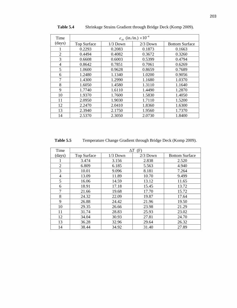
203  

Table 5.4 Shrinkage Strains Gradient through Bridge Deck (Komp 2009).

Time (days)

shε (in./in.) 410−× Top Surface 1/3 Down 2/3 Down Bottom Surface

1 0.2293 0.2083 0.1873 0.1663 2 0.4494 0.4082 0.3672 0.3260 3 0.6608 0.6003 0.5399 0.4794 4 0.8642 0.7851 0.7061 0.6269 5 1.0600 0.9628 0.8659 0.7689 6 1.2480 1.1340 1.0200 0.9056 7 1.4300 1.2990 1.1680 1.0370 8 1.6050 1.4580 1.3110 1.1640 9 1.7740 1.6110 1.4490 1.2870 10 1.9370 1.7600 1.5830 1.4050 11 2.0950 1.9030 1.7110 1.5200 12 2.2470 2.0410 1.8360 1.6300 13 2.3940 2.1750 1.9560 1.7370 14 2.5370 2.3050 2.0730 1.8400

Table 5.5 Temperature Change Gradient through Bridge Deck (Komp 2009).

Time (days)

TΔ (F) Top Surface 1/3 Down 2/3 Down Bottom Surface

1 3.474 3.156 2.838 2.520 2 6.809 6.185 5.563 4.940 3 10.01 9.096 8.181 7.264 4 13.09 11.89 10.70 9.499 5 16.06 14.59 13.12 11.65 6 18.91 17.18 15.45 13.72 7 21.66 19.68 17.70 15.72 8 24.32 22.09 19.87 17.64 9 26.88 24.42 21.96 19.50 10 29.35 26.66 23.98 21.29 11 31.74 28.83 25.93 23.02 12 34.04 30.93 27.81 24.70 13 36.28 32.96 29.64 26.32 14 38.44 34.92 31.40 27.89

204  

Table 5.6 Longitudinal Bridge Deck Stress (psi) Variation with Location (Komp 2009).

Node Location

Day 1 2 3 4 5 6 7 8 9 10

1 49 64 71 73 73 73 71 70 69 67 2 40 52 57 59 59 58 57 56 55 54 3 45 57 62 64 64 63 62 61 60 58 4 40 52 56 58 58 57 56 55 54 53 5 44 57 62 64 63 63 62 60 59 58 6 40 52 56 58 58 57 56 55 54 53 7 44 57 63 64 64 64 63 61 60 59 8 40 52 57 59 59 58 57 56 55 54 9 49 64 71 74 74 73 72 71 69 68

Average Stress 44 56 62 64 63 63 62 61 59 58

Cum. Avg. Stress 44 100 162 225 289 352 414 474 533 591

7.5 cf ′ (psi) 264 364 423 457 477 496 505 515 524 532 0.10 cf ′ (psi) 85 163 219 256 279 301 313 325 336 347

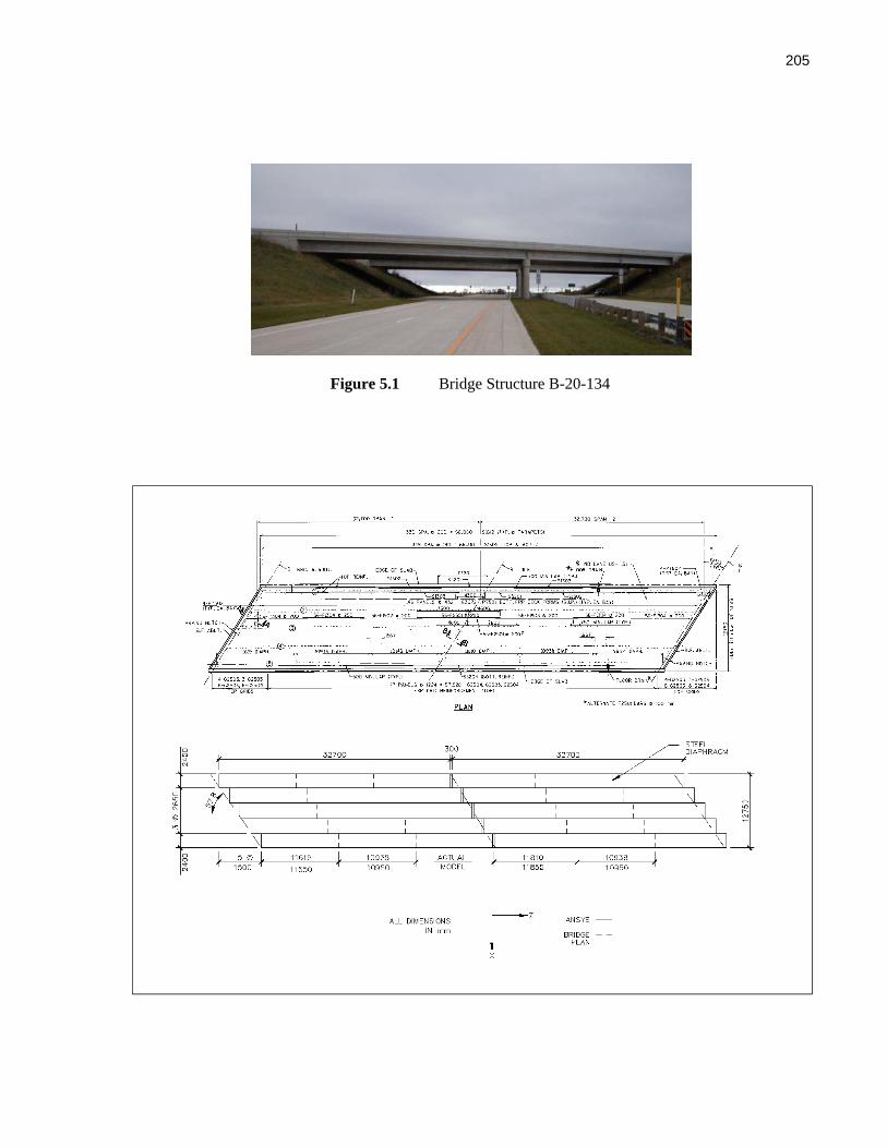
205  

Figure 5.1 Bridge Structure B-20-134

206  

Figure 5.2 Bridge B-20-134 Plan and Plan View of Deck Finite Element Modeling (Komp 2009).

Figure 5.3 Stepped Deck and Girder Terminations to Accommodate Skew (Komp 2009).

Figure 5.4 Bridge B-20-134 Cross Section (Komp 2009).

•Keypoint of deck intersects area of adjacent deck

207  

Figure 5.5 Steel Base Plate Modeling (Komp 2009).

Figure 5.6 Modeling of Standard WisDOT 54’’ Deep Precast Girder (Komp 2009).

208  

Figure 5.7 Concrete Barrier Modeling (Komp 2009).

Figure 5.8 Modeling Approach for Concrete Diaphragms at Interior Piers (Komp 2009).

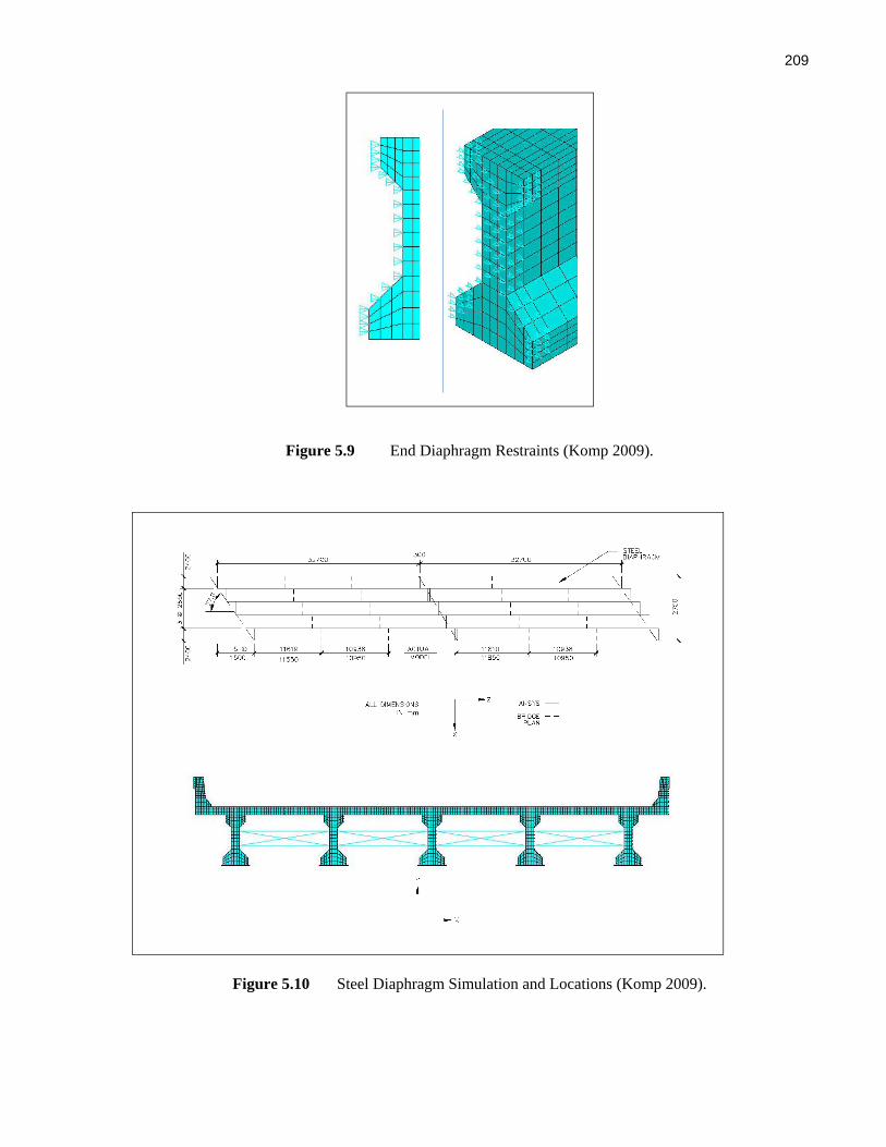
209  

Figure 5.9 End Diaphragm Restraints (Komp 2009).

Figure 5.10 Steel Diaphragm Simulation and Locations (Komp 2009).

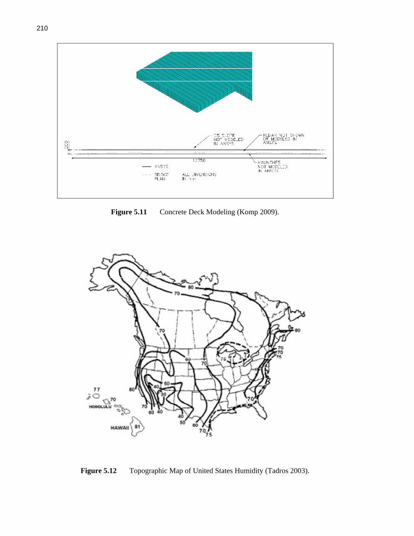
210  

Figure 5.11 Concrete Deck Modeling (Komp 2009).

Figure 5.12 Topographic Map of United States Humidity (Tadros 2003).

211  

Figure 5.13 Concrete Shrinkage with Respect to Time (Komp 2009).

Figure 5.14 Concrete Compressive Strength with Time (MacGregor and Wight 2005).

0

0.0002

0.0004

0.0006

0.0008

0.001

0.0012

0 50 100 150 200 250 300 350

Shrinkage (‐)

t‐Time (days)

Concrete Shrinkage

212  

Figure 5.15 Variation of Shrinkage Strain and Compressive Strength (Komp 2009).

Figure 5.16 Shrinkage Strain Distribution throughout the Deck (Komp 2009).

0

500

1000

1500

2000

2500

3000

3500

4000

0

0.00005

0.0001

0.00015

0.0002

0.00025

0.0003

1 3 5 7 9 11 13

Variation of Shrinkage and Compressive Strength w/ Time (fc'=4,000 psi)

Shrinkage Strain Compressive Strength

Con

cret

e St

rain

(in/

in)

Com

pres

sive

Stre

ngth

(psi

)

Time (days)

sh topε −

sh RHcenterε −

1/3shε −

2/3shε −

sh botε −

213  

Figure 5.17 Temperature Distribution throughout the Finite Element Model (Komp 2009).

Figure 5.18 Finite Element Model Deck Coordinate Locations (Komp 2009).

214  

Figure 5.19 Step-Modeling Shrinkage Strain Variation with Time (Komp 2009).

Figure 5.20 Longitudinal Stress Contour at Day 10 in Simulation (Komp 2009).

Girder Center-Lines

Concrete Diaphragms

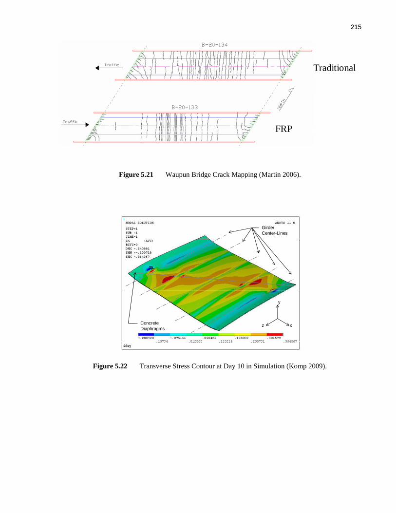
215  

Figure 5.21 Waupun Bridge Crack Mapping (Martin 2006).

Figure 5.22 Transverse Stress Contour at Day 10 in Simulation (Komp 2009).

FRP

Traditional

Concrete Diaphragms

Girder Center-Lines

x

y

z

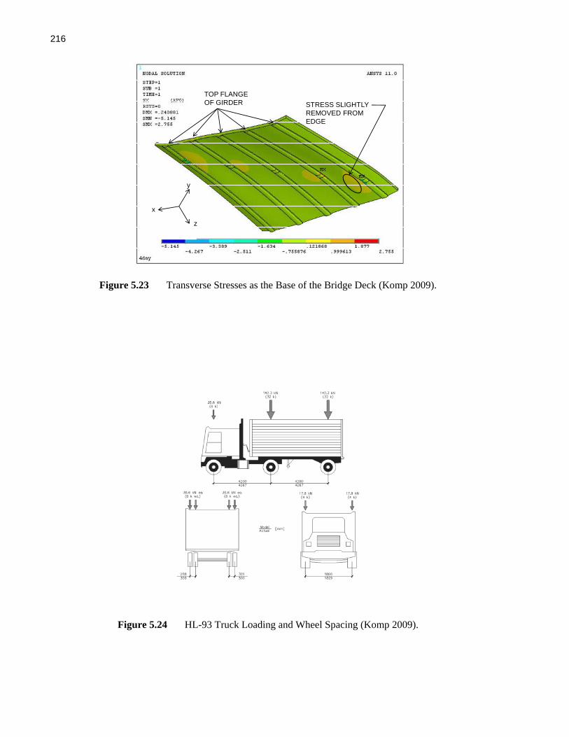
216  

Figure 5.23 Transverse Stresses as the Base of the Bridge Deck (Komp 2009).

Figure 5.24 HL-93 Truck Loading and Wheel Spacing (Komp 2009).

TOP FLANGEOF GIRDER

x

y

z

STRESS SLIGHTLYREMOVED FROM EDGE

217  

Figure 5.25 Plan View of HL-93 Loading Locations (Komp 2009).

Figure 5.26 Tire Pressure Loading Based on Contact Areas (Komp 2009).

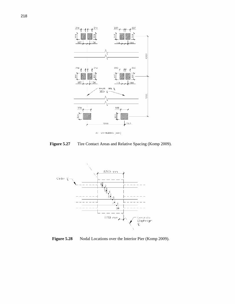
218  

Figure 5.27 Tire Contact Areas and Relative Spacing (Komp 2009).

Figure 5.28 Nodal Locations over the Interior Pier (Komp 2009).

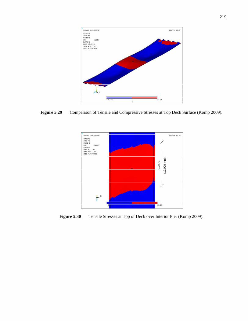
219  

Figure 5.29 Comparison of Tensile and Compressive Stresses at Top Deck Surface (Komp 2009).

Figure 5.30 Tensile Stresses at Top of Deck over Interior Pier (Komp 2009).

0.36

7L

(12,

000

mm

)

220  

Figure 5.31 Contour Plot of Longitudinal Normal Stresses at the Interior Pier (Komp 2009).

TOP GIRDERFLANGES z

y

x

BASE OFBARRIERS

1 243

5 6 7 8 9

221

Chapter 6

Summary, Conclusions and Recommendations

6.1 Summary

This report outlines activities undertake during a five-year monitoring study of Wisconsin's first IBRC

bridges. The report provides detailed background on the IBRC program and the bridge superstructures

constructed in Waupun, WI and Fond du Lac, WI. A detailed review of literature related to the objectives

of the present research effort was provided. A synthesis of the literature was generated to guide the

activities undertaken as part of the present effort.

The development of portable strain sensors suitable for use in the proposed research effort was

described in detail. Calibration factors for these sensors were also developed. A laboratory-based

experimental program designed to evaluate the impact of moisture and freeze-thaw cycling on the shear

strength at the interface between the FRP-SIP formwork and concrete was undertaken.

Thorough visual benchmark condition evaluation of the bridges at Waupun and Fond du Lac was

conducted. Common NDE methods were reviewed for application in the present research effort. A

laboratory-based evaluation of the infrared thermography technique for application in the present research

effort was conducted. Finally, the presence of moisture accumulation at the interface between the FRP-

SIP formwork and concrete in the Waupun bridge system was assess using a digital hygrometer.

Two in-situ load tests were conducted. The first occurred in July 2007 and the second occurred in

July 2009. Detailed discussion of the data acquisition system and instrumentation was provided.

Thorough discussion of all load testing results and insights with regard to degradation of performance

with time were given. Finite Element (FE) simulation of shrinkage-induced and vehicle-induced stresses

was conducted using commercial-grade FE software.

222 6.2 Conclusions and Recommendations

The five-year research effort completed several related, yet distinct, studies designed to assess the likely

long-term performance of Wisconsin's IBRC structures and also provide direction with regard to further

investigation into the performance of these structural systems so that the technologies fostered by them

can be introduced in bridge superstructure design going forward. This section of the report outlines

conclusions drawn by the research team and makes recommendations regarding further investigation

designed to assess long-term performance of these structures and improve the technologies developed.

Impact of Freeze-Thaw Cycling

The research completed indicates that freeze-thaw cycling and the presence of water could be detrimental

to the FRP-SIP-formwork-concrete interfacial shear strength. Experimental studies indicated that the

mean nominal shear strength at this interface was reduced 13% by water exposure alone and by 16% after

100 freeze-thaw cycles. A design-level shear strength corresponding to 95% confidence after 100 F/T

cycles reduced 40% when compared to control specimens. Even specimens exposed to water for 14 days

without F/T cycling experienced a 95% confidence-level shear strength reduction of 20%. FE analysis of

the deck system using simplified models suggests that shear demands at the concrete FRP-SIP interface

are not of sufficient magnitude to cause concerns regarding long-term performance even with the

reduction in strength due to moisture presence and freeze-thaw cycling.

NDE Evaluation

After approximately four years of traffic loading, bridges B-20-133/134 showed significant transverse

cracking around the central piers and along the abutment joints. Therefore, it is likely that moisture has a

direct path to the zone where aggregate interlock between the FRP-SIP formwork and concrete is needed

to accomplish the shear transfer needed to ensure that positive tension reinforcement for the bridge deck

exists. Without a way to escape, moisture may freeze and thaw as the climate changes during the seasons.

223

The laboratory freeze-thaw testing indicates that this is likely not of concern, but laboratory testing is

limited in its ability to simulate real-world behavior.

Bridges B-20-148/149 are in excellent condition with minor cracking present. At the time of the

2005 visual inspection, these bridges showed virtually no signs of deck cracking other than a few hairline

cracks located at the abutments and in the parapet(s). The bridge deck with FRP reinforcement showed no

cracks. No cracks were observed to extend through the bridge deck thickness. The lack of cracking

present in the simply-supported superstructure when compared to the two-span continuous superstructures

found in bridges B-20-133/134 suggests that further study of the continuous superstructure configuration

is warranted. Further evaluation of the simply supported bridge superstructures (B-20-148/149) is not

warranted.

The NDE techniques of infrared thermography, chain dragging, tap testing, and ultrasonic testing,

were reviewed. Tap testing with an impact hammer appears to be the most useful methods for monitoring

the bridges studied in the present effort. Infrared thermography is the least likely to yield useful results

for monitoring the IBRC bridges. Without an air void at the interface between FRP-SIP form and the

concrete deck, there will not be a disruption of the heat transfer and IRT will not show debonding.

Whichever NDE method is chosen to inspect the bridge decks with FRP-SIP, it must be realized

that any NDE technique will only be able to look at about half of the FRP area in contact with concrete.

The tops of the void spaces that result from the FRP-tubes in the SIP formwork will be impossible to

inspect because of the layer of FRP below the openings. This makes it very difficult to get a good idea of

how much area is adequately interlocked once a test has been established to determine the quality of the

interlock between the aggregate and FRP. It may be that coring the bridge deck and examining the

resulting concrete quality and the interface between the concrete and FRP-SIP formwork is the most

useful NDE/NDT methodology for the IBRC bridge at Waupun.

No moisture was found when drilling the hygrometer probe holes so there is no concern that

moisture is actually accumulating at the interface of the FRP-SIP formwork and the concrete deck as of

the date of this report. It should be understood that relative humidity is one measure of the tendency for

224 the FRP-SIP formwork to inhibit moisture egress from within the deck and may be an indicator for the

tendency for moisture to accumulate at the interface. However, the ability of humidity readings to

reliably indicate levels of moisture to expect at the interface remains to be definitively proven. It is

recommended that further analysis with regard to relative humidity be undertaken in future research

efforts as it may be a useful tool for long-term evaluation of bridge decks with FRP-SIP formwork.

In-Situ Load Testing

In-situ load testing of bridges B-20-133 and B-20-148 was conducted to evaluate several critical load

transfer mechanisms that could give the research team indication of degradation with time. Two load

tests were conducted: July 2007 and July 2009. The load transfer mechanisms evaluated were: (a) wheel

load distribution within the bridge deck; (b) composite beam behavior in the superstructure; (c) lane load

distribution within the superstructure; and (d) bridge deck deflection relative to the girders.

Bridge deck displacements relative to the girders in both bridges did not change significantly with

time. As a result, one can conclude that there has not been a significant change in the bridge deck load

transfer mechanism over the two-year period of evaluation and therefore, no degradation in this load

transfer mechanism has occurred. The IBRC bridge decks are performing in a manner that is satisfactory

and expected.

The wheel load distribution widths present in the FRP-SIP bridge deck system of B-20-133 can

be predicted using standard design/analysis procedures found in U.S. design specifications. The in-situ

load testing found that this load transfer mechanism did not change significantly (if at all) over the two

year evaluation period and thus, the wheel load distribution within this superstructure did not degrade.

Although not fully evaluated in the present research report, the in-situ testing illustrates that the wheel

load distribution widths in B-20-148 are consistent, but narrower, than that in B-20-133. This is to be

expected since common models for strip width found in U.S. design specifications are functions of beam

spacing. The spacing of the girders in B-20-133 is wider than the spacing of the girders in B-20-148 and

therefore, this narrower strip width is expected. The lack of significant change in strip widths over the

225

two-year interval suggest that the load transfer mechanisms in the bridge deck have not changed and

therefore, there is no reason to suspect degradation and reduced expectations for quality long term

performance.

Strain gradients over the height of the girders in the Fond du Lac bridge load tested clearly

exhibit composite behavior. Furthermore, the strain gradients did not significantly (if at all) change with

time and therefore, one can conclude that there was no change in the composite beam load transfer

mechanism within bridge B-20-148 over the two-year monitoring period and therefore, no degradation in

this regard.

Lane load distribution factors for wide-flange bulb-tee composite bridge girder systems (e.g. that

used in B-20-148) can be computed accurately with standard design/analysis procedures found in modern

U.S. bridge design specifications. Furthermore, these lane load distribution factors did not change from

the original July 2005 load tests and the July 2007 load test conducted in this research study. As a result,

there was no degradation measured in this regard and the long-term performance of this bridge system is

expected to be no different than any other traditionally constructed bridge of similar superstructure

configuration.

The in-situ load testing conducted was not without difficulty. The portable strain sensors design

and fabricated did a terrific job in providing strain readings in a relatively reliable manner. However,

there were two glaring difficulties that arose with the instrumentation and the load testing protocols.

There were some installation issues that may have lead to elevated strain readings encountered during the

July 2009 load test (especially at B-20-148). The low modulus polymer carrier for the strain gauges was

bolted in place and this bolting procedure may have resulted in non-straight orientations for the sensors.

As a result, the studs and may have introduced significant bending strains into the sensors. As a remedy

to this, it is recommended that the washers beneath the sensors be better able to bridge the slight spalling

that normally accompanies the installation of the threaded studs.

Positioning the wheel loading was perhaps the most difficult task to accurately complete during

the load testing. It may have been better off to space out the wheel load distributions sensors at the

226 underside of the bridge deck further than the 17.5 inches used. It also may have been prudent to explore

more exact (GPS-based) deck marking procedures. This would have helped to ensure that wheels on the

bridge deck were positioned as close as possible to locations directly above the bridge deck sensors

below.

Numerical Simulation

The finite element simulations conducted indicate that drying shrinkage appears to be capable of causing

transverse (and possibly longitudinal) bridge deck cracking at very early stages in the life of a bridge

deck. The simulations conducted indicate that cracking may occur as early as 4-8 days after bridge deck

placement.

An FE simulation of the tensile strains and stresses induced by HL-93 vehicle-type loading was

conducted. The FE model included precast girders, the bridge deck and barriers. Tensile stresses induced

by HL-93 vehicle loading were found to be on the order of 20% of the typical magnitudes assumed for the

tensile strength of concrete material. When these are superimposed onto the states of stress likely present

10-days after casting the bridge deck, it is likely that the combined effects of vehicle-induced stresses and

shrinkage-induced stresses will result in transverse cracking over the interior pier supports in the bridges

in Waupun.

The crack maps developed in the benchmark condition assessment of the bridges in Waupun and

Fond du Lac indicate that there is no difference between crack patterns developed in the FRP bridges

versus the traditionally constructed counterparts. The FE simulations conducted as part of this effort

clearly support that there should be no difference in behavior leading to cracking since shrinkage-induced

straining and traffic loading are the likely reasons for the transverse cracking. Furthermore, the deck

connection detail at the central diaphragms (over the interior piers) in the FRP-SIP formwork bridge at

Waupun is expected to neither improve nor detract from the behavior with regard to cracking.

Wisconsin Highway Research Program

University of Wisconsin-Madison 1415 Engineering Drive

Madison, WI 53706 608/262-2013 www.whrp.org