In Search of the Well Tie Without Sonic Copia

8/9/2019 In Search of the Well Tie Without Sonic Copia

http://slidepdf.com/reader/full/in-search-of-the-well-tie-without-sonic-copia 1/4



Figure 2. Log data from the Texas Gulf Coast, Lavaca County: Gamma ray, resistivity, roughly estimated lithology,estimated sonic logs (blue) using the time average Faust and Smith equations overlain on the actual sonic data (magenta).Differences between sonic log data (DT) and estimated values (Tavg, Faust, Smith) are shown beside these overlays. Thezero line (orange) in these difference plots means zero error in estnnating the sonic data.

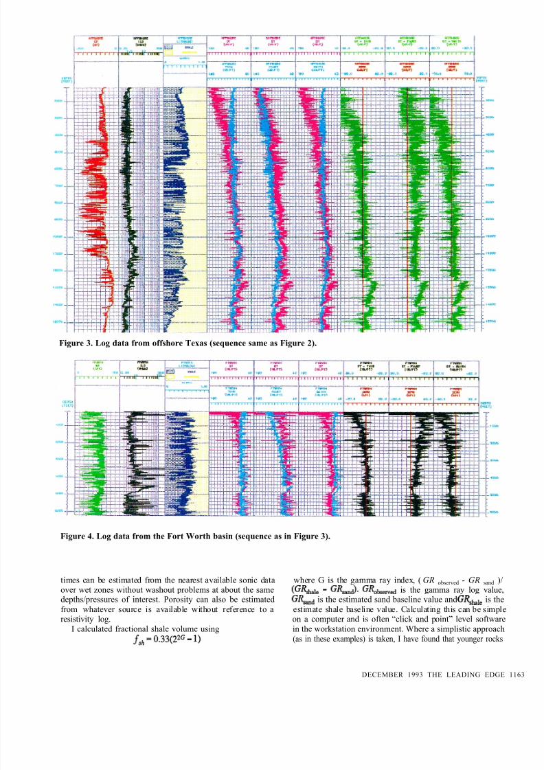
methods from Table 1 (blue) overlain on the actual sonic data(magenta). Differences between sonic log data and estimatedvalues (DT minus the estimated sonic data) are shown beside

these overlays. The zero line (red) in these difference plots

means zero error in estimating the sonic data. Figure 6 is an

expanded view of a portion of Figure 5.

Errors in estimating traveltime using resistivity are espe-cially large where average sonic traveltimes exceed about 100ps/ft (usually the shallower well data). This is well demon-strated by the large residual errors left by all three methodsfor shallow intervals of log data. The depth term,

z-l/6,

in theFaust equation does help a little in reducing the transit timeerror in the shallower log intervals (Figure 2) which is not particularly surprising, since all Faust’s data were over very

shallow log depths by today’s standards. Faust’s depth termacts as a low-frequency correction that I have found can bemore accurately defined by checkshot correcting the estimatedsonic logs with seismic stacking velocities near the well.Basically, the resistivity (porosity) and lithology data provide

the high frequency information, while the checkshot suppliesthe low-frequency trend in the estimation of the sonic log.

Appendix. The two-lithology matrix form of the time aver-age equation I used in these examples is

AT

AT fR v

s AT

1 f,h>l 1 fR

whereAT

is traveltime, f R is fractional porosity (the decimalequivalent of the percentage of total volume) calculated from

deep induction resistivity,AT

is traveltime representing the

shale portion of the matrix,AT

is traveltime representing the

sandy portion of the matrix, ATF is traveltime representingthe pore fluid, and f sh is the fractional shale volume calculated

from gamma ray data. The examples in Figures 2-6 have hadtraveltime specifically estimated using

AT=

89f

[9Of

l

1

fR

I calculated fractional porosity, f R , from resistivity (to make

the comparisons more meaningful) at each log sample, usingArchie’s equations with n = 1, a = 2, m = 0.81, and assuming

100 percent saltwater saturation with a constant resistivity R,,, = 0.045

Q m

The specific equation I used here was

fR

= O.l9/?R

where R is the deep induction resistivity values withoutcorrection.

In practice, I choose constants on the basis of the nearest

available data and occasionally make corrections for Rw as afunction of depth. Matrix (in this case sand and shale) transit

162 THE LEADING EDGE DECEMBER 1993



Figure 3. Log data from offshore Texas (sequence same as Figure 2).

Figure 4. Log data from the Fort Worth basin (sequence as in Figure 3).

times can be estimated from the nearest available sonic data where G is the gamma ray index, ( GR observed - GR sand )/over wet zones without washout problems at about the same

GR ,

hale

G and)a

GR served

is the gamma ray log value,depths/pressures of interest. Porosity can also be estimated

d

is the estimated sand baseline value andhle

is the

from whatever resistivity log.

source is available without reference to a estimate shale baseline value. Calculating this can be simpleon a computer and is often “click and point” level software

I calculated fractional shale volume using

fssh

=

0.33 22G

in the workstation environment. Where a simplistic approach

(as in these examples) is taken, I have found that younger rocks

DECEMBER 1993 THE LEADING EDGE



Figure 5. Log data from East Texas basin.

Figure 6. Expanded view of a portion of the log data in Figure 5.

require a faster shale baseline value or, as shown here, anunreasonably high sand content in the lithology estimate.

The ability to control meaningful lithological parameterswhen estimating the sonic response makes this a very useful

tool for stratigraphic modeling. Over intervals of a few hun-dred feet, the assumption used in these examples will often provide a good fit to sonic data after application of a small bulk shift.

Steve Adcock earned BS degrees in physics (Louisiana State University) and in geology (Centenary College),and on MS in geophysics (Uni versity of

Houston). He starred in the oil business

as a geophysicist wi th Texaco’s Hour-

ton ofice and now works for M itchell Energy as a senior staff geophysicist.

1164 THE LEADING EDGE DECEMBER 1993

In Search of the Well Tie Without Sonic Copia

Documents