Impulse response analysis in linear multivariate models

Generalized Impulse Response Analysis in LinearMultivariate Models¤

M. Hashem PesaranTrinity College, Cambridge

Yongcheol ShinDepartment of Applied Economics, University of Cambridge

May 1997Revised July 1997

Abstract

Building on Koop, Pesaran and Potter (1996), we propose the `generalized' impulseresponse analysis for unrestricted vector autoregressive (VAR) and cointegrated VARmodels. Unlike the traditional impulse response analysis, our approach does not requireorthogonalization of shocks and is invariant to the ordering of the variables in the VAR.The approach is also used in the construction of order-invariant forecast error variancedecompositions.

Keywords: Generalized impulse responses; Forecast error variance decompositions; VAR;CointegrationJEL classi¯cation: C13; C32; C51

¤Correspondence: M. Hashem Pesaran, Faculty of Economics and Politics, University of Cam-bridge, Austin Robinson Building, Sidgwick Avenue, Cambridge CB3 9DD, United Kingdom. Tele-phone: +44 1223 335216. Fax: +44 1223 335471. E-mail: [email protected] Internet:httpnnwww.econ.cam.ac.uknfacultynpesarann

1 Introduction

Following Sims' (1980) seminal paper, dynamic analysis of vector autoregressive (VAR) mod-els is routinely carried out using the `orthogonalized' impulse responses, where the underlyingshocks to the VAR model are orthogonalized using the Cholesky decomposition before im-pulse responses, or forecast error variance decompositions are computed. This approachis not, however, invariant to the ordering of the variables in the VAR. See, for example,LÄutkepohl (1991, Section, 2.3.2).In this note, building on Koop et al. (1996), we propose an alternative approach to

impulse response analysis which does not have the above shortcoming. We refer to this asthe generalized impulse response analysis. In particular, we show that for a non-diagonalerror variance matrix the orthogonalized and the generalized impulse responses coincide onlyin the case of the impulse responses of the shocks to the ¯rst equation in the VAR. In Section4 the proposed approach is applied to cointegrated VAR models, and it is shown that themaximum likelihood estimator of the generalized impulse responses is

pT -consistent and

asymptotically normally distributed.We provide an empirical illustration of the substantial di®erences that could exist between

the two approaches, using a trivariate VAR model containing U.S. quarterly observations onreal investment and consumption expenditures and output over 1948(1)-1988(4).

2 The Generalized Impulse Response Functions

Consider the augmented vector autoregressive model,

xt =

pXi=1

©ixt¡i +ªwt + "t; t = 1; 2; :::; T; (2.1)

where xt = (x1t; x2t; :::; xmt)0 is an m £ 1 vector of jointly determined dependent variables,

wt is a q£ 1 vector of deterministic and/or exogenous variables, and f©i; i = 1; 2; :::; pg andª are m£m and m£ q coe±cient matrices. We make the following standard assumptions:(see, for example, LÄutkepohl (1991, Chapter 2) and Pesaran and Pesaran (1997, Section19.3))]

Assumption 2.1 E("t) = 0, E("t"0t) = § for all t, where § =f¾ij; i; j = 1; 2; ; :::;mg is an

m£m positive de¯nite matrix, E("t"0t0) = 0 for all t = t

0 and E("tjwt) = 0.

Assumption 2.2 All the roots of jIm ¡Pp

i=1©izij = 0 fall outside the unit circle.

Assumption 2.3 xt¡1;xt¡2; :::;xt¡p;wt, t = 1; 2; :::; T , are not perfectly collinear.

Under Assumption 2.2, xt would be covariance-stationary, and (2.1) can be rewritten asthe in¯nite moving average representation,

xt =

1Xi=0

Ai"t¡i +1Xi=0

Giwt¡i; t = 1; 2; :::; T; (2.2)

[1]

where the m £ m coe±cient matrices Ai can be obtained using the following recursiverelations:

Ai = ©1Ai¡1 +©2Ai¡2 + ¢ ¢ ¢+©pAi¡p; i = 1; 2; :::; (2.3)

with A0 = Im and Ai = 0 for i < 0, and Gi = Aiª.An impulse response function measures the time pro¯le of the e®ect of shocks at a given

point in time on the (expected) future values of variables in a dynamical system. The bestway to describe an impulse response is to view it as the outcome of a conceptual experimentin which the time pro¯le of the e®ect of a hypothetical m £ 1 vector of shocks of size± = (±1; :::; ±m)

0, say, hitting the economy at time t is compared with a base-line pro¯leat time t + n, given the economy's history. There are three main issues: (i) The types ofshocks hitting the economy at time t; (ii) the state of the economy at time t¡1 before beingshocked; and (iii) the types of shocks expected to hit the economy from t+ 1 to t+ n.Denoting the known history of the economy up to time t ¡ 1 by the non-decreasing

information set ­t¡1, the generalized impulse response function of xt at horizon n, advancedin Koop et al. (1996), is de¯ned by

GIx(n; ±;­t¡1) = E (xt+nj"t = ±;­t¡1)¡ E (xt+nj­t¡1) : (2.4)

Using (2.4) in (2.2), we have GIx(n; ±;­t¡1) = An±, which is independent of ­t¡1, butdepends on the composition of shocks de¯ned by ±.1

Clearly, the appropriate choice of hypothesized vector of shocks, ±, is central to the prop-erties of the impulse response function. The traditional approach, suggested by Sims (1980),is to resolve the problem surrounding the choice of ± by using the Cholesky decompositionof §:

PP0 = §; (2.5)

where P is an m£m lower triangular matrix. Then, (2.2) can be rewritten as

xt =

1Xi=0

(AiP)(P¡1"t¡i) +

1Xi=0

Giwt¡i =1Xi=0

(AiP)»t¡i +1Xi=0

Giwt¡i; t = 1; 2; :::; T; (2.6)

such that »t = P¡1"t are orthogonalized; namely, E(»t»

0t) = Im. Hence, the m£ 1 vector of

the orthogonalized impulse response function of a unit shock to the jth equation on xt+n isgiven by

Ãoj(n) = AnPej; n = 0; 1; 2; :::; (2.7)

where ej is an m£ 1 selection vector with unity as its jth element and zeros elsewhere.An alternative approach would be to use (2.4) directly, but instead of shocking all the

elements of "t; we could choose to shock only one element, say its jth element, and integrateout the e®ects of other shocks using an assumed or the historically observed distribution ofthe errors. In this case we have

GIx(n; ±j ;­t¡1) = E (xt+nj"jt = ±j;­t¡1)¡ E (xt+nj­t¡1) : (2.8)

1This history invariance property of the impulse response is speci¯c to linear systems and does not carryover to non-linear models.

[2]

Assuming that "t has a multivariate normal distribution, it is now easily seen (see alsoKoop et al. (1996)) that2

E ("tj"jt = ±j) = (¾1j; ¾2j; :::; ¾mj)0 ¾¡1jj ±j = §ej¾¡1jj ±j:Hence, the m £ 1 vector of the (unscaled) generalized impulse response of the e®ect of ashock in the jth equation at time t on xt+n is given byµ

An§ejp¾jj

¶µ±jp¾jj

¶; n = 0; 1; 2; ::: : (2.9)

By setting ±j =p¾jj , we obtain the scaled generalized impulse response function by

Ãgj(n) = ¾¡ 12

jj An§ej; n = 0; 1; 2; :::; (2.10)

which measures the e®ect of one standard error shock to the jth equation at time t onexpected values of x at time t+ n.Finally, the above generalized impulses can also be used in the derivation of the forecast

error variance decompositions, de¯ned as the proportion of the n-step ahead forecast errorvariance of variable i which is accounted for by the innovations in variable j in the VAR.For an analysis of the forecast error variance decompositions based on the orthogonalizedimpulse responses see LÄutkepohl (1991, Section 2.3.3). Denoting the orthogonalized and thegeneralized forecast error variance decompositions by µoij(n) and µ

gij(n), respectively, then

for n = 0; 1; 2; :::;

µoij(n) =

Pn`=0 (e

0iA`Pej)

2Pn`=0

¡e0iA`§A0

`ei¢ ; µgij(n) = ¾¡1ii

Pn`=0 (e

0iA`§ej)

2Pn`=0 e

0iA`§A

0`ei

; i; j = 1; :::;m:

Notice that by constructionPm

j=1 µoij(n) = 1. However, due to the non-zero covariance

between the original (non-orthogonalized) shocks, in generalPm

j=1 µgij(n) 6= 1.3

3 The Relationship between Generalized and Orthog-

onalized Impulse Responses

The orthogonalized and the generalized impulse response functions, Ãoj(n) and Ãgj(n), di®er

in a number of respects. The generalized impulse responses are invariant to the reorderingof the variables in the VAR, but this is not the case with the orthogonalized ones. Typ-ically there are many alternative reparameterizations that could be employed to computeorthogonalized impulse responses, and there is no clear guidance as to which one of thesepossible parameterizations should be used. In contrast, the generalized impulse responses

2When the distribution of the errors "t are non-normal, one could obtain the conditional expectationsE ("tj"jt = ±j) by stochastic simulations, or by resampling techniques if the distribution of errors is notknown.

3For a further discussion of the generalised forecast error variance decompositions see Pesaran and Pesaran(1997, Section 19.5).

[3]

are unique and fully take account of the historical patterns of correlations observed amongstthe di®erent shocks.The relationship between the two impulse responses are set out in the following proposition:4

Proposition 3.1 The generalized and the orthogonalized impulse responses coincide if § isdiagonal. In the case where § is non-diagonal,

Ãgj(n) 6= Ãoj(n) for j = 2; 3; :::;m;

and the two impulse responses are the same only for j = 1.

Proof. The ¯rst part of Proposition 3.1 holds trivially. Next, rewrite Ãgj(n) and Ãoj(n) as

Ãgj(n) = An'gj ; Ã

oj(n) = An'

oj ;

such that 'gj = ¾¡ 12

jj §ej and 'oj = Pej. Noticing that

'gj = ¾¡ 12

jj (¾1j; ¾2j; :::; ¾mj)0 ; for j = 1; 2; :::;m;

'o1 = (p11; p21; :::; pm1)0 ; :::;'oj = (0; :::; 0; pjj ; :::; pmj)

0 ; :::;'om = (0; :::; 0; pmm)0 ;

it is then easily seen that

'gj 6= 'oj and Ãgj 6= Ãoj for j = 2; :::;m:

When j = 1,

'g1 = ¾¡ 12

11 (¾11; ¾21; :::; ¾m1)0 : (3.1)

Using the equality PP0 = §, we have

p211 = ¾11; (¾11; ¾21; :::; ¾m1)0 =

¡p211; p11p21; :::; p11pm1

¢0: (3.2)

Using (3.2) in (3.1), we obtain 'g1 = 'o1 and Ã

g1 = Ã

o1.

4 The Generalized Impulse Response Analysis in A

Cointegrated VAR Model

In this section we extend the generalized impulse analysis to a cointegrated VAR model, alsoknown as a vector error correction (VEC) model. The econometric issues surrounding theanalysis of VEC model are discussed, for example, in Johansen (1995) and Pesaran, Shinand Smith (1997). Here we provide only a brief outline of the estimation issues, focusingattention on the generalized impulse response functions.To deal with unit roots and cointegration, we replace Assumption 2.2 by

4Proposition 3.1 also applies to the relationship between the generalised and the orthogonalised forecasterror decompositions.

[4]

Assumption 4.1 The roots of jIm ¡Pp

i=1©izij = 0 satisfy jzj > 1 or z = 1.

In this case (2.1) can be transformed into the VEC form:

¢xt = ¡¦xt¡1 +p¡1Xi=1

¡i¢xt¡i +¦¤wt + "t; t = 1; 2; :::; T; (4.1)

where ¦ = Im¡Pp

i=1©i, ¡i = ¡Pp

j=i+1©j for i = 1; :::; p¡ 1, and ¤ is an m£ g matrix ofunknown coe±cients. The relationships between parameters in (2.1) and (4.1) can also berewritten as

©1 = Im ¡¦+ ¡1; ©i = ¡i ¡ ¡i¡1 for i = 2; :::; p¡ 1; ©p = ¡¡p¡1: (4.2)

Suppose that the system (4.1) is cointegrated in the sense that there exists an m £ rmatrix ¯ such that the r £ 1 vector zt = ¯0xt is stationary, where 1 · r < m. Thecointegrating restrictions can be formally expressed as

¦ = ®¯0; (4.3)

where ® and ¯ are m £ r matrices of full rank r; that is, rank(¦) = r. Finally, to ensurethat the underlying variables in xt are at most I(1); we assume:

Assumption 4.2 ®0?¡¯? has full rank, where ¡ = Im ¡Pp¡1

i=1 ¡i; and ®? and ¯? arem£ (m¡ r) matrices of full column rank such that ®0®? = 0 and ¯0¯? = 0.Under Assumptions 4.1 and 4.2, and (4.3), xt will be ¯rst-di®erence stationary, and

therefore, ¢xt can be written as the in¯nite moving average representation (see, for example,Johansen (1995, Chapter 4)),

¢xt =1Xi=0

Ci"t¡i +1Xi=0

Ci¦¤wt¡i; t = 1; 2; :::; T: (4.4)

Applying the de¯nition of the scaled generalized impulse responses (see (2.10)) to (4.4),we obtain

Ãg¢x;j(n) = ¾¡ 12

jj Cn§ej ; n = 0; 1; 2; :::; (4.5)

which measures the e®ect of the shock to the jth equation in (4.4) on ¢xt+n. We also obtainthe generalized impulse response functions of xt+n with respect to a shock in the jth equationby

Ãgx;j(n) = ¾¡ 12

jj Bn§ej ; n = 0; 1; 2; :::; (4.6)

where Bn =Pn

j=0Cj is the `cumulative e®ect' matrix with B0 = C0 = Im.

A necessary and su±cient condition for cointegration is given by ¯0C(1) = 0, whereC(1) =

P1i=0Ci with rank[C(1)] = m ¡ r (see Engle and Granger (1987)). Then, the

cointegrating relations can be written as

zt = ¯0xt =

1Xi=0

¯0Bi"t¡i +1Xi=0

¯0Bi¦¤wt¡i: (4.7)

[5]

Hence, the generalized impulse response functions of zt with respect to a shock in the jthequation is given by

Ãgz;j(n) = ¾¡ 12

jj ¯0Bn§ej; n = 0; 1; 2; ::: : (4.8)

Similarly, the orthogonalized impulse response functions of xt and zt with respect to avariable-speci¯c shock in the jth equation are given by

Ãox;j(n) = BnPej ; Ãoz;j(n) = ¯

0BnPej ; n = 0; 1; 2; ::: : (4.9)

In the present case it is important to note that the parametric restrictions implied by thede¯ciency in the rank of ¦ is taken into account, and therefore, the e®ects of shocks on theindividual variables will be persistent, but these e®ects eventually vanish on the cointegratingrelations, zt = ¯

0xt.5

The matrices fBn; n = 1; 2; :::g can be computed from the underlying VAR coe±cientmatrices f©i; i = 1; :::; pg using the following recursive relations (see Pesaran and Shin(1996)):

Bn = ©1Bn¡1 +©2Bn¡2 + ¢ ¢ ¢+©pBn¡p; n = 1; 2; :::; (4.10)

where B0 = Im and Bn = 0 for n < 0.The ML estimators obtained from (4.1) can be used to obtain the ML estimators of

Ãgx;j(n) and Ãgz;j(n), which we denote by Ã̂

g

x;j(n) and Ã̂g

z;j(n), respectively.6 Moreover, as

shown in the Appendix, for n = 0; 1; 2; :::;

pThÃ̂g

x;j(n)¡Ãgx;j(n)ia» N f0;§x(n; j)g ; (4.11)

pThÃ̂g

z;j(n)¡Ãgz;j(n)ia» N f0;§z(n; j)g ; (4.12)

where `a»' denotes asymptotic equality in distribution, and §x(n; j) and §z(n; j) are given

respectively by (A.15) and (A.17) in the Appendix.

5 An Empirical Illustration

In this section we illustrate our approach by estimating impulse response functions for thetrivariate VAR model in investment, consumption and output previously analyzed by King,Plosser, Stock and Watson (KPSW, 1991) on the U.S. quarterly data. All three variablesare in logarithms, measured on a per capita basis, and denoted by i, c, and y.We ¯rst analyze the unrestricted VAR(4) model,

xt = a0 + a1t+4Xj=1

©jxt¡j + "t; (5.1)

where the ordering of the variables in x is chosen to be (i; c; y), a0 and a1 are 3£ 1 vectorsof coe±cients, ©j ; j = 1; 2; 3; 4; are 3 £ 3 matrices of coe±cients, and t is running from1948(1) to 1988(4).

5Notice that B1 = C(1); and therefore ¯0B1 = 0:6For more details see LÄutkepohl and Reimers (1992) and Pesaran and Shin (1996).

[6]

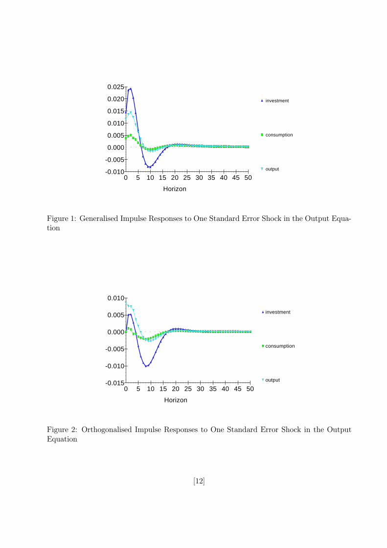
After estimating the parameters in (5.1) consistently by OLS, we turn to estimate theorthogonalized and the generalized impulse response functions with respect to one standarderror shock to the output equation using (2.7) and (2.10), respectively.7 The results forthe generalized and orthogonalized impulse responses are presented in Figures 1 and 2,respectively. Figure 1 shows that the output shocks have larger and more persistent e®ectson investment, followed by output then consumption. After over-shooting, the e®ects onoutput and consumption tend to die out after about 7 quarters. But, the responses ofinvestment to the output shock shows a cyclical pattern over a relatively protracted periodof time; its impact response is 1.5%, rising to 2.5 % in the 2nd quarter, then declining sharplyto {1% around the 10th quarter, and ¯nally gradually tending towards 0.A markedly di®erent picture emerges from Figure 2, which displays the orthogonalized

impulse responses with output shock having much larger impacts on itself than on investmentin the ¯rst few quarters after the shock. Notice also that by construction the impact e®ectsof orthogonalized output shocks on investment and consumption are zero. In general, theshape and the size of the two impulse responses are quite di®erent.8

Next, following KPSW, we assume that all the three variables, are I(1), and so analyze thethree variables in the context of a cointegrated VAR(4) model with unrestricted interceptsand restricted-trend coe±cients,9

¢xt = a0 + a1t¡¦xt¡1 +3Xj=1

¡j¢xt¡j + "t; t = 1948(1)¡ 1988(4); (5.2)

where a1 = ¦° with ° being a 3£ 1 vector of unknown coe±cients.KPSW identify two cointegrating relations between the three variables, namely, i¡y and

c ¡ y, which are also referred to as `great ratios'. With the two cointegrating relations oneneeds four restrictions (two per each cointegrating vector) to exactly identify them. Supposethat the four exactly-identifying restrictions are given by

HE :

icy

trend

2664¯11 ¯12¯21 ¯22¯31 ¯32¯41 ¯42

3775 =26641 00 1¤ ¤¤ ¤

3775 :Under HE, the ML estimates of the two cointegrating vectors obtained from (5.2) subjectto the cointegrating restrictions, namely, rank(¦) = 2, are as follows (see Pesaran and Shin(1997)):

^̄ =

26641 00 1

¡1:028 (:27) ¡1:046 (:13):00017 (:0011) ¡:00008 (:00054)

3775 ; LL = 1552:1;7Detailed estimation results are available upon request. All the computations reported in this section

have been carried out using Micro¯t 4.0 [Pesaran and Pesaran (1997)].8Clearly, the two impulse responses would have coincided if output was speci¯ed to be the ¯rst variable

in the VAR. See Proposition 3.1.9For more details on the choice of intercepts and trends in cointegrated VAR models see Pesaran and

Pesaran (1997) and Pesaran, Shin and Smith (1997).

[7]

where the asymptotic standard errors are given in bracket, and LL is the maximized log-likelihood. Imposition of the full set of restrictions implied by two great ratios yields themaximized log-likelihood of 1548:8, resulting in the log-likelihood ratio statistic of 6:74, whichis below the 95% critical value of the Â2(4) distribution. Thus the `great-ratio' hypothesiscannot be rejected, a ¯nding which is in accordance with KPSW's conclusion.Based on these two cointegrating relations, the generalized and orthogonalized impulse

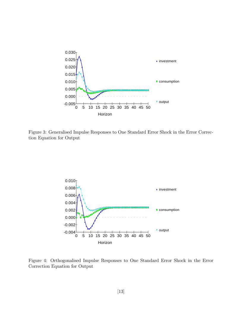
responses with respect to the output shocks can be estimated by (4.6), and (4.9), using theML estimates. The time pro¯les of these impulse responses are displayed in Figures 3 and4, and give a very similar pattern to those obtained in the case of the unrestricted VARmodel. A comparison of these ¯gures further illustrates substantial di®erences that couldexist between the two impulse responses.

Acknowledgments

We are grateful to James Mitchell and Ron Smith for helpful comments. Partial ¯nancialsupport from the ESRC (grant No. L116251016) and the Isaac Newton Trust of TrinityCollege, Cambridge, is gratefully acknowledged.

[8]

A Appendix: Proofs of (4.11) and (4.12)

Let ¡̂, ®̂, ^̄ and §̂ be the maximum likelihood estimators of ¡, ®, ¯ and § in the VEC model (4.1). Usingthe results in LÄutkepohl and Reimers (1992) and Pesaran and Shin (1996), then the following asymptoticresults (as T !1) can be established:10

pTvec

nh¡̂;¡®̂^̄

i¡ [¡;¡®¯]

oa» N(0;§CO); (A.1)

pTvec(§̂¡§) a» N f0; 2PD(§­§)g ; (A.2)

where§CO = (FS

¡1F0)­§; (A.3)

F =

·Im(p¡1) 00 ¯

¸; S =Plim

T!1

·T¡1YY0 T¡1YX0

¡1¯T¡1¯0X¡1Y T¡1¯0X¡1X0¡1¯

¸;

Yt = [¢x0t¡1; :::;¢x0t¡p+1]0, Y = [Y1; :::;YT ], X¡1 = [x0;x1; :::;xT¡1], ¡ = [¡1; :::;¡p¡1], and PD =Dm(D0

mDm)¡1D0m is the projection matrix based on the duplication matrix, Dm.

De¯ning an m2p £ 1 vector, Á = vec(©1;©2; :::;©p), and using (A.1), (A.2), (4.2) and (4.10), it isstraightforward to show that p

Tvec(Á̂¡Á) a» N f0;§Ág ; (A.4)pTvec(B̂n ¡Bn) a» N f0;§Bn =Kn§ÁK

0ng ; n = 1; 2; :::; (A.5)

where

§Á = (W0FS¡1F0W)­§; Kn =

n¡1Xi=0

J(©0)n¡1¡i ­Bi; (A.6)

Wmp£mp

=

266666664

Im ¡Im 0 ¢ ¢ ¢ 0 00 Im ¡Im ¢ ¢ ¢ 0 00 0 Im ¢ ¢ ¢ 0 0...

......

...::

...0 0 0 ¢ ¢ ¢ Im ¡Im0 0 0 ¢ ¢ ¢ 0 Im

377777775 ; ©mp£mp

=

266666664

©1 ©2 ©3 ¢ ¢ ¢ ©p¡1 ©pIm 0 0 ¢ ¢ ¢ 0 00 Im 0 ¢ ¢ ¢ 0 0...

...::

......

...0 0 0 ¢ ¢ ¢ 0 00 0 0 ¢ ¢ ¢ Im 0

377777775and J = (Im;0; :::;0) is an m£mp matrix.

Based on these results, we now derive the asymptotic distribution of the estimator of generalized impulseresponses. First, consider

Ã̂g

x;j(n)¡Ãgx;j(n) =B̂n§̂ej

¡e0j§ej

¢ 12 ¡Bn§ej

³e0j§̂ej

´ 12

³e0j§̂ej

´ 12 ¡e0j§ej

¢ 12

´ NG

DG; (A.7)

where ej is an m£ 1 selection vector, ¾jj = e0j§ej and ¾̂jj = e0j§̂ej . Notice also that

NG =³B̂n§̂¡Bn§

´ej¡e0j§ej

¢ 12 +Bn§ej

·¡e0j§ej

¢ 12 ¡

³e0j§̂ej

´ 12

¸; (A.8)

B̂n§̂¡Bn§ =³B̂n ¡Bn

´³§̂¡§

´+Bn

³§̂¡§

´+³B̂n ¡Bn

´§; (A.9)

10In the context of the VEC model (4.1), the ML estimators of the short-run parameters (¡ and ®) and ofthe long-run parameters (¯) are

pT -consistent and T -consistent, respectively. For a proof see, for example,

Pesaran and Shin (1997).

[9]

and by the Taylor series expansion³e0j§̂ej

´ 12

=¡e0j§ej

¢ 12 +

1

2

¡e0j§ej

¢¡ 12¡e0j­e0j

¢vec(§̂¡§) +R; (A.10)

where R is a scalar remainder term which in view of the consistency of the ML estimators can be shown tobe of op(1) order. Using (A.9) and (A.10) in (A.8), we have

NG =h³B̂n ¡Bn

´³§̂¡§

´+Bn

³§̂¡§

´+³B̂n ¡Bn

´§iej¡e0j§ej

¢ 12 (A.11)

¡Bn§ej·1

2

¡e0j§ej

¢¡ 12¡e0j­e0j

¢vec(§̂¡§) +R

¸;

and also

DG =¡e0j§ej

¢+1

2

¡e0j­e0j

¢vec(§̂¡§) +R¤ = ¾jj + op(1); (A.12)

where R¤ is another scalar remainder term of op(1) order. Multiplying (A.11) bypT and vectorizing the

result,

pTNG =

h¡e0j§­ Im

¢pTvec

³B̂n ¡Bn

´+¡e0j ­Bn

¢pTvec

³§̂¡§

´i¾12jj (A.13)

¡12Ãgx;j(n)

¡e0j­e0j

¢pTvec(§̂¡§) + op(1):

Therefore, multiplying (A.7) bypT and using (A.12) and (A.13), we have

pThÃ̂g

x;j(n)¡Ãgx;j(n)i=

h¡e0j§­ Im

¢;¡e0j ­Bn

¢¡ 12¾

¡ 12

jj Ãgx;j(n)

¡e0j­e0j

¢ip¾jj

· pTvec(B̂n ¡Bn)pTvec(§̂¡§)

¸+op(1):

(A.14)Notice that the asymptotic distributions of

pT (§̂ ¡§) and pT (B̂n ¡ Bn) are independent but normally

distributed. Then, using (A.2) and (A.5) we obtain (4.11), and §x(n; j) is given by

§x(n; j) =1

¾jjfVx

1n§BnVx01n +V

x2n[2PD(§­§)]Vx0

2ng ; (A.15)

where

Vx1n = e

0j§­ Im; Vx

2n =¡e0j ­Bn

¢¡ 12¾¡ 12

jj Ãgx;j(n)

¡e0j­e0j

¢:

Similarly, we obtain

pThÃ̂g

z;j(n)¡Ãgz;j(n)i=

h¡e0j§­ ¯0

¢;¡e0j ­ ¯0Bn

¢¡ 12¾

¡ 12

jj Ãgz;j(n)

¡e0j­e0j

¢ip¾jj

· pTvec(B̂n ¡Bn)pTvec(§̂¡§)

¸+op(1):

(A.16)and

§z(n; j) =1

¾jjfVz

1n§BnVz01n +V

z2n[2PD(§­§)]Vz0

2ng ; (A.17)

where

Vz1n = e

0j§­ ¯0; Vz

2n =¡e0j ­ ¯0Bn

¢¡ 12¾¡ 12

jj Ãgz;j(n)

¡e0j­e0j

¢:

This establishes (4.12). Notice that (A.16) is asymptotically valid irrespective of whether we use the truevalue of ¯ or its T -consistent estimator, ^̄. (See Corollary 1 in Pesaran and Shin (1996)).

[10]

References[1] Engle, R.F. and C.W.J. Granger, 1987, Cointegration and error correction representation: estimation

and testing, Econometrica 55, 251-276.

[2] Johansen, S., 1995, Likelihood-based inference in cointegrated vector autoregressive models (OxfordUniversity Press, Oxford).

[3] King, R.G., C.I. Plosser, J.H. Stock and M.W. Watson, 1991, Stochastic trends and economic °uctua-tions, American Economic Review 81, 819-40.

[4] Koop, G., M.H. Pesaran and S.M. Potter, 1996, Impulse response analysis in nonlinear multivariatemodels, Journal of Econometrics 74, 119-47.

[5] LÄutkepohl, H., 1991, Introduction to multiple time series analysis (Springer-Verlag, Berlin).

[6] LÄutkepohl, H. and H.E. Reimers, 1992, Impulse response analysis of cointegrated systems, Journal ofEconomic and Dynamic Controls 16, 53-78.

[7] Pesaran, M.H. and B. Pesaran, 1997, Working with Micro¯t 4.0: An interactive econometric softwarepackage (DOS and Windows versions), (Oxford University Press, Oxford).

[8] Pesaran, M.H. and Y. Shin, 1997, Long-run structural modelling, unpublished manuscript, Universityof Cambridge. (Internet: httpnnwww.econ.cam.ac.uknfacultynpesarann)

[9] Pesaran, M.H. and Y. Shin, 1996, Cointegration and speed of convergence to equilibrium, Journal ofEconometrics 71, 117-43.

[10] Pesaran, M.H., Y. Shin and R.J. Smith, 1997, Structural analysis of vector autoregressive models withexogenous I(1) variables, DAEWorking Papers Amalgamated Series No. 9706, University of Cambridge.(Internet: httpnnwww.econ.cam.ac.uknfacultynpesarann)

[11] Sims C., 1980, Macroeconomics and Reality, Econometrica 48, 1-48.

[11]

investment

consumption

output

Horizon

-0.005

-0.010

0.000

0.005

0.010

0.015

0.020

0.025

0 5 10 15 20 25 30 35 40 45 50

Figure 1: Generalised Impulse Responses to One Standard Error Shock in the Output Equa-tion

investment

consumption

output

Horizon

-0.005

-0.010

-0.015

0.000

0.005

0.010

0 5 10 15 20 25 30 35 40 45 50

Figure 2: Orthogonalised Impulse Responses to One Standard Error Shock in the OutputEquation

[12]

investment

consumption

output

Horizon

-0.005

0.000

0.005

0.010

0.015

0.020

0.025

0.030

0 5 10 15 20 25 30 35 40 45 50

Figure 3: Generalised Impulse Responses to One Standard Error Shock in the Error Correc-tion Equation for Output

investment

consumption

output

Horizon

-0.002

-0.004

0.000

0.002

0.004

0.006

0.008

0.010

0 5 10 15 20 25 30 35 40 45 50

Figure 4: Orthogonalised Impulse Responses to One Standard Error Shock in the ErrorCorrection Equation for Output

[13]