Improving Turbidity-Based Estimates of Suspended Sediment Concentrations and Loads John Dietrich Jastram Thesis submitted to the faculty of the Virginia Polytechnic Institute and State University in partial fulfillment of the requirements for the degree of Master of Science In Environmental Science and Engineering Department of Crop and Soil Environmental Sciences Dr. Carl Zipper, Chair Dr. Lucian Zelazny Dr. Kenneth Hyer Dr. Dan Spitzner May 4, 2007 Blacksburg, VA Keywords: Turbidity, sediment, continuous monitoring, sediment transport modeling, Roanoke River

Welcome message from author
This document is posted to help you gain knowledge. Please leave a comment to let me know what you think about it! Share it to your friends and learn new things together.
Transcript
Improving Turbidity-Based Estimates of Suspended
Sediment Concentrations and Loads
John Dietrich Jastram
Thesis submitted to the faculty of the Virginia Polytechnic Institute and State University in partial fulfillment of the requirements for the degree of
Master of Science In
Environmental Science and Engineering
Department of Crop and Soil Environmental Sciences
Dr. Carl Zipper, Chair Dr. Lucian Zelazny Dr. Kenneth Hyer Dr. Dan Spitzner
May 4, 2007 Blacksburg, VA
Keywords: Turbidity, sediment, continuous monitoring, sediment transport modeling, Roanoke River
ii
Improving Turbidity-Based Estimates of Suspended
Sediment Concentrations and Loads
John Dietrich Jastram Abstract As the impacts of human activities increase sediment transport by aquatic systems the need to accurately quantify this transport becomes paramount. Turbidity is recognized as an effective tool for monitoring suspended sediments in aquatic systems, and with recent technological advances turbidity can be measured in-situ remotely, continuously, and at much finer temporal scales than was previously possible. Although turbidity provides an improved method for estimation of suspended-sediment concentration (SSC), compared to traditional discharge-based methods, there is still significant variability in turbidity-based SSC estimates and in sediment loadings calculated from those estimates. The purpose of this study was to improve the turbidity-based estimation of SSC. Working at two monitoring sites on the Roanoke River in southwestern Virginia, stage, turbidity, and other water-quality parameters and were monitored with in-situ instrumentation, suspended sediments were sampled manually during elevated turbidity events; those samples were analyzed for SSC and for physical properties; rainfall was quantified by geologic source area. The study identified physical properties of the suspended-sediment samples that contribute to SSC-estimation variance and hydrologic variables that contribute to variance in those physical properties. Results indicated that the inclusion of any of the measured physical properties, which included grain-size distributions, specific surface-area, and organic carbon, in turbidity-based SSC estimation models reduces unexplained variance. Further, the use of hydrologic variables, which were measured remotely and on the same temporal scale as turbidity, to represent these physical properties, resulted in a model which was equally as capable of predicting SSC. A square-root transformed turbidity-based SSC estimation model developed for the Roanoke River at Route 117 monitoring station, which included a water level variable, provided 63% less unexplained variance in SSC estimations and 50% narrower 95% prediction intervals for an annual loading estimate, when compared to a simple linear regression using a logarithmic transformation of the response and regressor (turbidity). Unexplained variance and prediction interval width were also reduced using this approach at a second monitoring site, Roanoke River at Thirteenth Street Bridge; the log-based transformation of SSC and regressors was found to be most appropriate at this monitoring station. Furthermore, this study demonstrated the potential for a single model, generated from a pooled set of data from the two monitoring sites, to estimate SSC with less variance than a model generated only from data collected at this single site. When applied at suitable locations, the use of this pooled model approach could provide many benefits to monitoring programs, such as developing SSC-estimation models for multiple sites which individually do not have enough data to generate a robust model or extending the model to monitoring sites between those for which the model was developed and significantly reducing sampling costs for intensive monitoring programs.

iii
Acknowledgements I would like to express my utmost appreciation for the love and support that my wife, Sarah, has given me throughout our journey towards fulfilling my goal of obtaining a Masters Degree. Her enduring spirit through challenging times has been an inspiration. It is to her that I dedicate this work.
Heartfelt thanks to Ken Hyer and Doug Moyer for being great mentors and friends, and for opening my eyes to the opportunities that would come with earning a Masters Degree.
I would like to thank my advisor, Dr. Carl Zipper, for ensuring that my graduate school
experience fulfilled my goals and provided a strong foundation for my professional career. Dr. Lucian Zelazny has taught me the importance of understanding the “hang-ups”; the
lessons Dr Z. teaches go far beyond Soil Chemistry and Clay Mineralogy and every young scientist could benefit from a semester or two with him – Thanks Dr. Z.
Thanks to Dr. Dan Spitzner for serving on my committee and providing valuable
statistical support for this thesis research. Thanks to the United States Geological Survey and the United States Army Corps of
Engineers for providing financial support for this research.
Finally, I would like to thank all of my family and all of my friends for their love and support, and for being interested in what I was working on even if they had no idea what Turbidity-based SSC estimation means.

iv
Table of Contents Abstract........................................................................................................................................... ii Acknowledgements ...................................................................................................................... iii Table of Contents ......................................................................................................................... iv List of Tables ................................................................................................................................ vi List of Figures.............................................................................................................................. vii Introduction................................................................................................................................... 1
Fluvial Sediment Transport................................................................................................. 1 Impacts of Excessive Fluvial Sediment Transport.............................................................. 1
Literature Review ......................................................................................................................... 3 Quantifying Fluvial Sediment Flux .................................................................................... 3 Spatial and Temporal Variability of Sediment Transport................................................... 4 Collection of Suspended Sediment Samples....................................................................... 5 Sediment Monitoring Methods ........................................................................................... 7
Single-Stage Sampler.............................................................................................. 8 Automatic Pump Sampler ....................................................................................... 9
Surrogate Methods ............................................................................................................ 12 Rating Curve Method............................................................................................ 12 Acoustic Backscatter............................................................................................. 13 Laser Diffraction................................................................................................... 14 Turbidity ............................................................................................................... 16
Research Background................................................................................................................. 18 Research Objectives.................................................................................................................... 19 References.................................................................................................................................... 21 Methods........................................................................................................................................ 28 Introduction................................................................................................................................. 28 Field Methods .............................................................................................................................. 28
Turbidity Measurement..................................................................................................... 28 Stage Measurement........................................................................................................... 29 Sample Collection............................................................................................................. 30
Lab Methods................................................................................................................................ 31 Sample Pre-processing and Storage.................................................................................. 31 Concentration and Sand-Fine Split Analysis .................................................................... 32 Sediment Characteristics................................................................................................... 32 Particle Size Analysis ....................................................................................................... 33 Organic Carbon Analysis.................................................................................................. 34 Specific Surface Area Analysis ........................................................................................ 35
Radar Derived Rainfall Estimation........................................................................................... 35 References.................................................................................................................................... 37 Improving Turbidity-based Estimates of Suspended Sediment Concentrations and Loads39 Abstract......................................................................................................................................... 39 Introduction................................................................................................................................. 40 Methods........................................................................................................................................ 43
Hydrologic and Water-Quality Monitoring ...................................................................... 44 Sediment Sampling and Analysis ..................................................................................... 45 Data analysis ..................................................................................................................... 46
v
Results .......................................................................................................................................... 49 SSC Estimation ................................................................................................................. 49 Effect of Turbidity Measurement Point on SSC Estimation Precision............................. 51 Suspended Sediment Load Estimation.............................................................................. 52
Discussion..................................................................................................................................... 52 Conclusions.................................................................................................................................. 56 References.................................................................................................................................... 57 Pooling Data from Multiple Monitoring Stations to Improve Turbidity-based SSC-estimation..................................................................................................................................... 73 Introduction................................................................................................................................. 73 Methods........................................................................................................................................ 74
Thirteenth Street (site-specific) Model ............................................................................. 74 Pooled Model .................................................................................................................... 74
Results .......................................................................................................................................... 76 Thirteenth Street (site-specific) Model ............................................................................. 76 Pooled Model .................................................................................................................... 78
Discussion..................................................................................................................................... 79 Thirteenth Street Model .................................................................................................... 79 Pooled Model .................................................................................................................... 80
Conclusions.................................................................................................................................. 82 References.................................................................................................................................... 84 Conclusions.................................................................................................................................. 92
References......................................................................................................................... 96 Appendix A. Data for samples collected ................................................................................... 97 Appendix B. Miscellaneous Data ............................................................................................. 101
vi
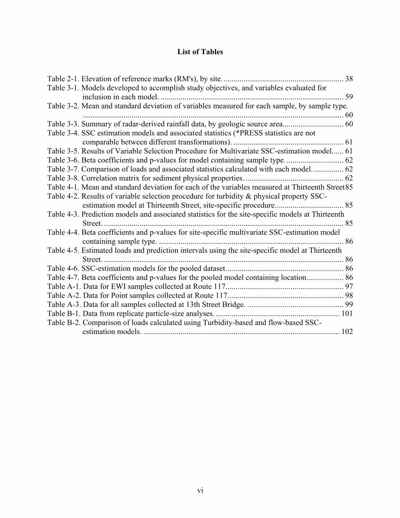
List of Tables
Table 2-1. Elevation of reference marks (RM's), by site. ............................................................. 38 Table 3-1. Models developed to accomplish study objectives, and variables evaluated for
inclusion in each model. ............................................................................................. 59 Table 3-2. Mean and standard deviation of variables measured for each sample, by sample type.
..................................................................................................................................... 60 Table 3-3. Summary of radar-derived rainfall data, by geologic source area............................... 60 Table 3-4. SSC estimation models and associated statistics (*PRESS statistics are not
comparable between different transformations). ........................................................ 61 Table 3-5. Results of Variable Selection Procedure for Multivariate SSC-estimation model...... 61 Table 3-6. Beta coefficients and p-values for model containing sample type. ............................. 62 Table 3-7. Comparison of loads and associated statistics calculated with each model. ............... 62 Table 3-8. Correlation matrix for sediment physical properties. .................................................. 62 Table 4-1. Mean and standard deviation for each of the variables measured at Thirteenth Street85 Table 4-2. Results of variable selection procedure for turbidity & physical property SSC-
estimation model at Thirteenth Street, site-specific procedure................................... 85 Table 4-3. Prediction models and associated statistics for the site-specific models at Thirteenth
Street. .......................................................................................................................... 85 Table 4-4. Beta coefficients and p-values for site-specific multivariate SSC-estimation model
containing sample type. .............................................................................................. 86 Table 4-5. Estimated loads and prediction intervals using the site-specific model at Thirteenth
Street. .......................................................................................................................... 86 Table 4-6. SSC-estimation models for the pooled dataset. ........................................................... 86 Table 4-7. Beta coefficients and p-values for the pooled model containing location................... 86 Table A-1. Data for EWI samples collected at Route 117............................................................ 97 Table A-2. Data for Point samples collected at Route 117........................................................... 98 Table A-3. Data for all samples collected at 13th Street Bridge. ................................................. 99 Table B-1. Data from replicate particle-size analyses. ............................................................... 101 Table B-2. Comparison of loads calculated using Turbidity-based and flow-based SSC-
estimation models. .................................................................................................... 102
vii
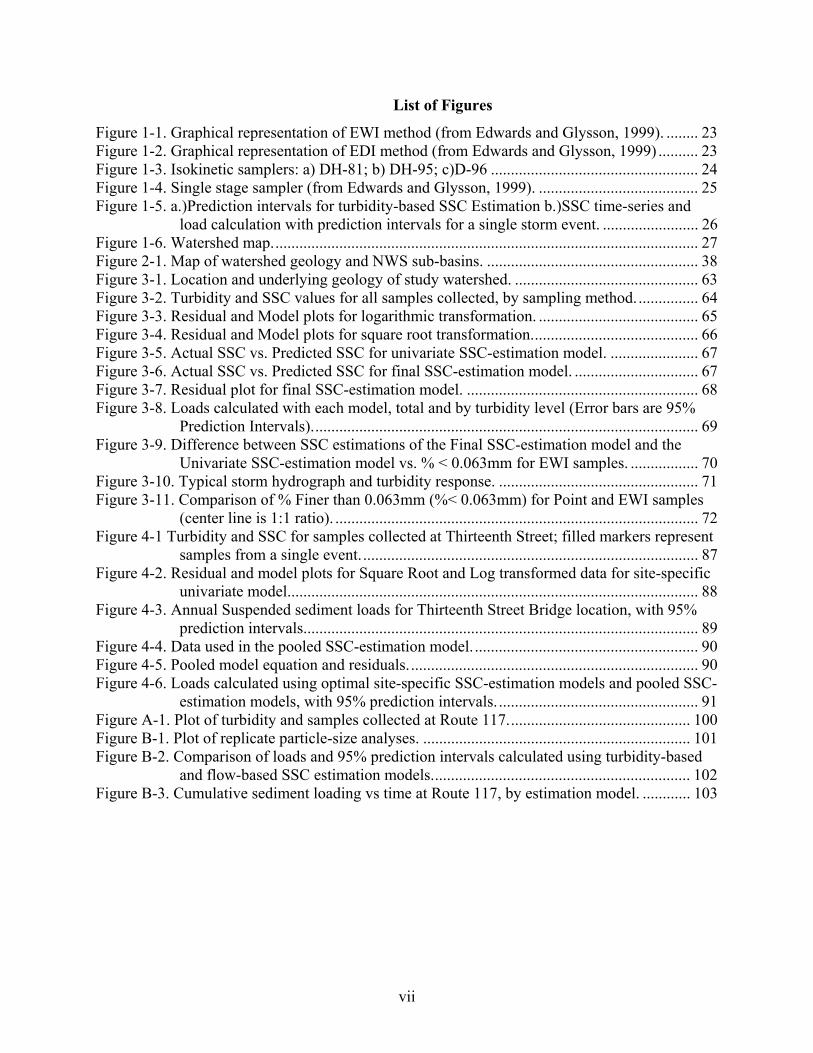
List of Figures
Figure 1-1. Graphical representation of EWI method (from Edwards and Glysson, 1999). ........ 23 Figure 1-2. Graphical representation of EDI method (from Edwards and Glysson, 1999) .......... 23 Figure 1-3. Isokinetic samplers: a) DH-81; b) DH-95; c)D-96 .................................................... 24 Figure 1-4. Single stage sampler (from Edwards and Glysson, 1999). ........................................ 25 Figure 1-5. a.)Prediction intervals for turbidity-based SSC Estimation b.)SSC time-series and
load calculation with prediction intervals for a single storm event. ........................ 26 Figure 1-6. Watershed map........................................................................................................... 27 Figure 2-1. Map of watershed geology and NWS sub-basins. ..................................................... 38 Figure 3-1. Location and underlying geology of study watershed. .............................................. 63 Figure 3-2. Turbidity and SSC values for all samples collected, by sampling method................ 64 Figure 3-3. Residual and Model plots for logarithmic transformation. ........................................ 65 Figure 3-4. Residual and Model plots for square root transformation.......................................... 66 Figure 3-5. Actual SSC vs. Predicted SSC for univariate SSC-estimation model. ...................... 67 Figure 3-6. Actual SSC vs. Predicted SSC for final SSC-estimation model. ............................... 67 Figure 3-7. Residual plot for final SSC-estimation model. .......................................................... 68 Figure 3-8. Loads calculated with each model, total and by turbidity level (Error bars are 95%
Prediction Intervals)................................................................................................. 69 Figure 3-9. Difference between SSC estimations of the Final SSC-estimation model and the
Univariate SSC-estimation model vs. % < 0.063mm for EWI samples. ................. 70 Figure 3-10. Typical storm hydrograph and turbidity response. .................................................. 71 Figure 3-11. Comparison of % Finer than 0.063mm (%< 0.063mm) for Point and EWI samples
(center line is 1:1 ratio). ........................................................................................... 72 Figure 4-1 Turbidity and SSC for samples collected at Thirteenth Street; filled markers represent
samples from a single event..................................................................................... 87 Figure 4-2. Residual and model plots for Square Root and Log transformed data for site-specific
univariate model....................................................................................................... 88 Figure 4-3. Annual Suspended sediment loads for Thirteenth Street Bridge location, with 95%
prediction intervals................................................................................................... 89 Figure 4-4. Data used in the pooled SSC-estimation model. ........................................................ 90 Figure 4-5. Pooled model equation and residuals......................................................................... 90 Figure 4-6. Loads calculated using optimal site-specific SSC-estimation models and pooled SSC-
estimation models, with 95% prediction intervals. .................................................. 91 Figure A-1. Plot of turbidity and samples collected at Route 117.............................................. 100 Figure B-1. Plot of replicate particle-size analyses. ................................................................... 101 Figure B-2. Comparison of loads and 95% prediction intervals calculated using turbidity-based
and flow-based SSC estimation models................................................................. 102 Figure B-3. Cumulative sediment loading vs time at Route 117, by estimation model. ............ 103
1
Chapter 1 Introduction
Fluvial Sediment Transport
Fluvial transport of eroded materials is a key factor in the creation of the landscape
that surrounds us. Additionally, the transport of these materials is necessary for aquatic
systems to maintain hydrologic, geomorphologic, and ecologic functions (Owens et. al.,
2005). These eroded fragmentary materials which originate mostly from weathering of
rocks, but also include chemical and biological precipitates and decomposed organic
material, are termed fluvial sediment when transported by, suspended in, or deposited
from water (Edwards and Glysson, 1999).
Fluvial transport of sediment has occurred throughout geologic time. Hydrologic
systems and aquatic communities have evolved such that extreme events of sediment
transport can be tolerated while a specific base level of sediment transport is required to
maintain balance in the system. Currently, on a global scale, anthropogenic activities
disrupt this balance by accelerating fluvial sediment transport (Owens et. al., 2005).
Impacts of Excessive Fluvial Sediment Transport Elevated suspended sediment concentrations (SSC) are major water-pollution
concerns in Virginia, the USA, and the world. Channel sedimentation was listed as the
primary stressor of streams in the Mid-Atlantic Highlands by the EPA in 2000 (EPA,
2000); siltation ranked second on EPA’s 305b list of stressors causing stream
impairments nationwide (EPA, 2002).

2
The negative effects of sediment transport are apparent in both the terrestrial
environments that serve as sediment sources as well as the aquatic environments to which
the sediments are delivered. Terrestrial impacts of soil erosion (the source of most fluvial
sediments) include the erosion of surficial soil, loss of soil nutrients, degradation of soil
structure, reduction of tillable land, and the ultimate reduction of agricultural productivity
(Walling and Collins, 2000).
The impacts of excessive sedimentation to the aquatic systems receiving the eroded
sediments range from ecological degradation to economic expenses. Ecologically,
suspended sediments harm aquatic ecosystems by decreasing light penetration into the
water column – reducing photosynthesis, smothering benthic habitats, delivering excess
nutrients, and potentially delivering soil-bound contaminants (Davies-Colley and Smith,
2001). Furthermore, toxic materials, including pesticides, metals, and radionuclides, may
adsorb strongly to sediment particles; thus, introduction of excessive amounts of
sediment to a water body from source areas where such materials are present may lead to
toxic conditions for the biota which utilize the resource (Meade and Parker, 1984).
Economically, accelerated transport of suspended sediments increases the costs of
water treatment for human use and may decrease profits from waterways used for
recreational purposes, as people typically perceive sediment laden or turbid water as less
desirable for recreation than clearer waters (Davies-Colley and Smith, 2001). Perhaps
more importantly, sediment accumulation within channels increases the streambed
elevation, leading to more damaging and life-threatening floods as the stormflow carrying
capacity of the channel is decreased (Meade and Parker, 1984). Yet another economic
cost related to sediment can be seen in the increased maintenance needs of structures
3
within waterways carrying elevated sediment concentrations; most reservoirs in the
United States trap at least half of the sediment transported by the river, with larger dams
trapping virtually the entire sediment load carried by the river (Meade and Parker, 1984).
The reduction of reservoir capacity as sediment accumulates introduces multiple
expenses - a filling reservoir may no longer serve the intended purpose and the costs of
maintenance may be compounded by contaminated sediments, preventing removal or
making sediment removal extremely costly. A study in the early 1990’s estimated that
damage from erosion-related pollutants costs over sixteen billion dollars annually in
North America alone (Osterkamp et. al., 1998). Globally, erosion of soils and sediment
transport are major issues, most notably in developing nations where the demands on
marginal farmland and water resources are greatest (Walling and Collins, 2000).
Literature Review
Quantifying Fluvial Sediment Flux Given the consequences of elevated SSC and the need for accurate and precise data to
aid management strategies aiming to reduce the problems associated with accelerated
erosion and sediment transport, the scientific community has sought to understand and
characterize the fluvial transport of sediment. However, understanding and managing
movement of suspended sediment has been challenging, as sediment transport is highly
variable in time, across landscapes, and within stream channels. In order to quantify
suspended sediment transport within a stream channel at a given point in time, personnel
must be on-site sampling with specialized equipment and proper methods during the
sediment transport event. This effort can be especially difficult as most sediment
transport is triggered and sustained by stormflow events (Wolman and Miller, 1960).
Previous studies have demonstrated that as much as 98% of a rivers’ sediment load can
4
be transported during just 10% of the time of record, with as much as 60% of the load
being discharged in only 1% of the time (Meade et. al., 1990). Thus, it is critical for
monitoring programs to quantify sediment-transport during stormflow events.
Spatial and Temporal Variability of Sediment Transport Sediment concentrations and properties vary significantly within the cross-section
of a stream channel. Variability within a cross-section at a single point in time may be
attributed to incomplete mixing of tributary inflows, point-source inputs, groundwater
seepage, and variations in velocity within the cross-section (Martin, 1992).
Variability in sediment concentration and grain-size distribution within a cross-
section is influenced greatly by particle mass. Particles with greater mass require more
energy for entrainment and continued suspension than particles of lesser mass. Small
particles, such as those in the clay and silt fraction, are typically well distributed within
the cross-section (Horowitz et. al., 1990; Gordon et. al., 2004) as the conditions required
for suspension of these particles are more easily met throughout the channel. Sediments
within this category are often referred to as wash load, as these particles are readily
carried through the system and may never settle out (Gordon et.al, 2004; Chang, 2002).
Larger particles, however, may only become entrained during high velocity events, and
even at these times the larger particles will be concentrated near the streambed, with
concentrations and mean grain-size decreasing with distance from the bed (Gordon et. al.,
2004).
Sediment transport within a stream channel may also vary significantly on a
temporal scale, whether the scale is the duration of a stormflow event, seasons, or longer
(Gippel, 1995). Variability within a single stormflow event may be attributed to different
5
sediment source areas contributing to point of measurement at different times. This may
be due to differing times of travel from the source area or varying rainfall patterns over
the source areas. Seasonal variations in sediment properties may be attributed to
sediment availability during certain seasons, such as the increased availability of
sediment in agricultural areas during tillage season. Furthermore, seasonal effects may
be attributed to climatic factors, such as frozen or snow covered soils during winter
months which become available for erosion when thawed in warmer months. Finally,
variability in sediment properties may be observed over longer time frames as land use
changes within the watershed induce or prevent further erosion.
Collection of Suspended Sediment Samples Suspended sediments are rarely distributed uniformly throughout the width and
depth of a channel cross-section; therefore, sampling methods that collect a sample that
represents the average conditions in the entire area of the sampled cross section must be
utilized to minimize potential bias (Edwards and Glysson, 1999). Failure to collect
representative samples is often the largest source of error in water-quality data (Martin et.
al., 1992). Two representative sampling methods, routinely used for sample collection by
the U.S. Geological Survey (USGS) and other agencies, are the Equal Width Increment
(EWI) and Equal Discharge Increment (EDI) (Edwards and Glysson, 1999).
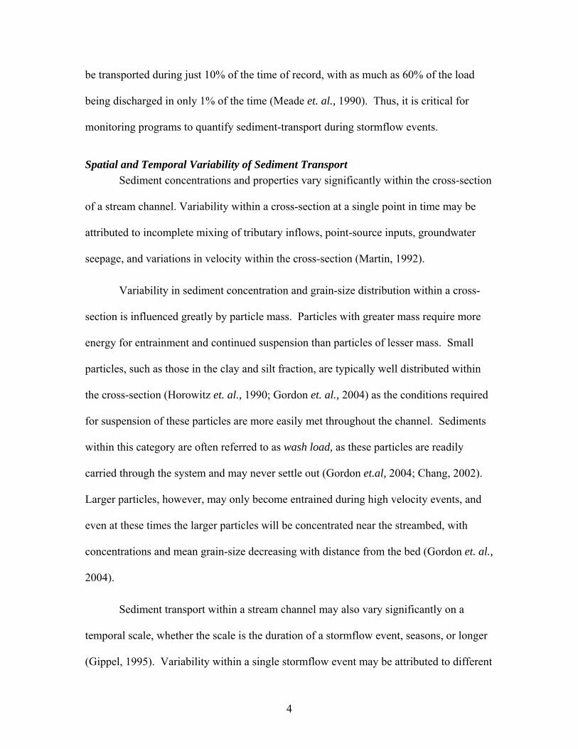
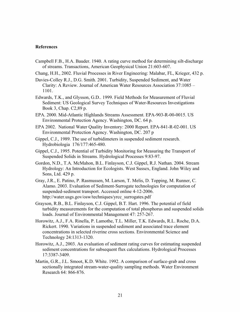
Perhaps the most widely applied SSC-sampling method is the EWI method,
illustrated in Figure 1-1. This approach involves separating the cross-sectional flow into
multiple increments of equal width and collecting a depth-integrated sample at the center
of each increment. Such a sample is obtained by lowering the sampler from the water
surface to the stream bottom, then raising the sampler back to the water surface, at a
6
constant vertical transit rate. This constant rate results in variable sample volumes from
each vertical, thus the sample represents the flow weighted sediment contribution. The
subsamples from each section are typically composited to generate one composite sample
which represents “average” conditions in the entire channel cross section. Alternatively,
each subsample may be analyzed separately to quantify the variation within the cross-
section, as conditions may vary substantially from point to point. A benefit of the EWI
approach is that no prior knowledge of the site is required; one only needs the ability to
measure the width of the cross-section and calculate the locations of the sampling points.
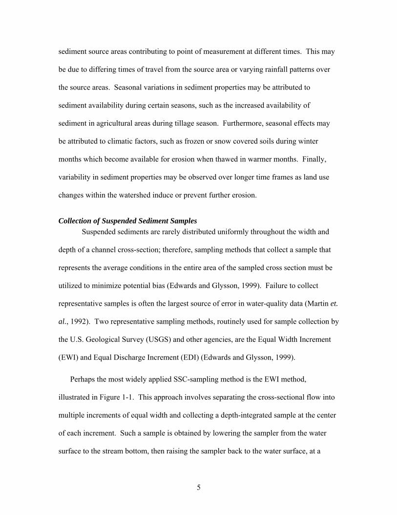
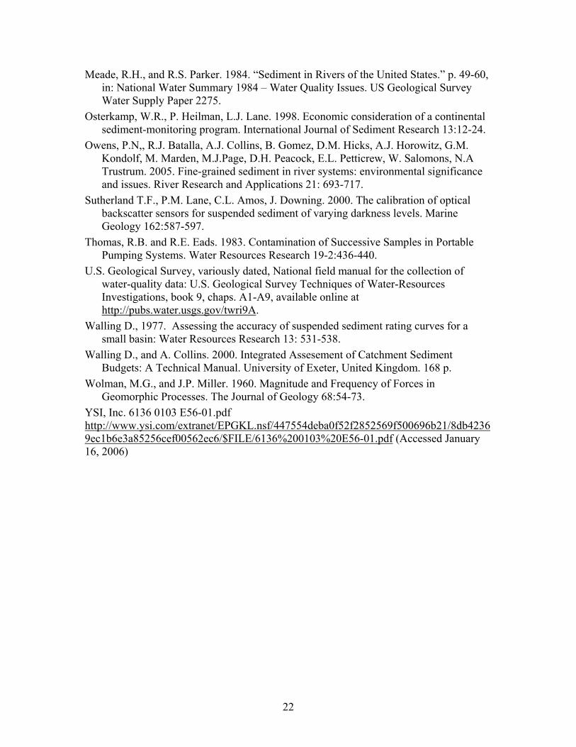
An alternative method, which provides results identical to the EWI method, is the
Equal Discharge Increment (EDI) method (Edwards and Glysson, 1999; Figure 1-2).
This method requires additional understanding of the flow characteristics in the cross-
section, as vertical sampling locations are determined based on the total streamflow. This
understanding can be accomplished by measuring the discharge immediately prior to
sample collection or based on historical discharge measurements for similar flow
conditions at the sampling site. Samples are collected at the center of width intervals
representing 1/nth of the total flow, where n is the number of verticals to be sampled.
Since each vertical section represents the same volume of streamflow, the same volume
of sample is acquired from each section to represent the flow-weighted sample. To
obtain the same volume from each vertical the transit rate must vary according to the
depth and velocity at each sampling point.
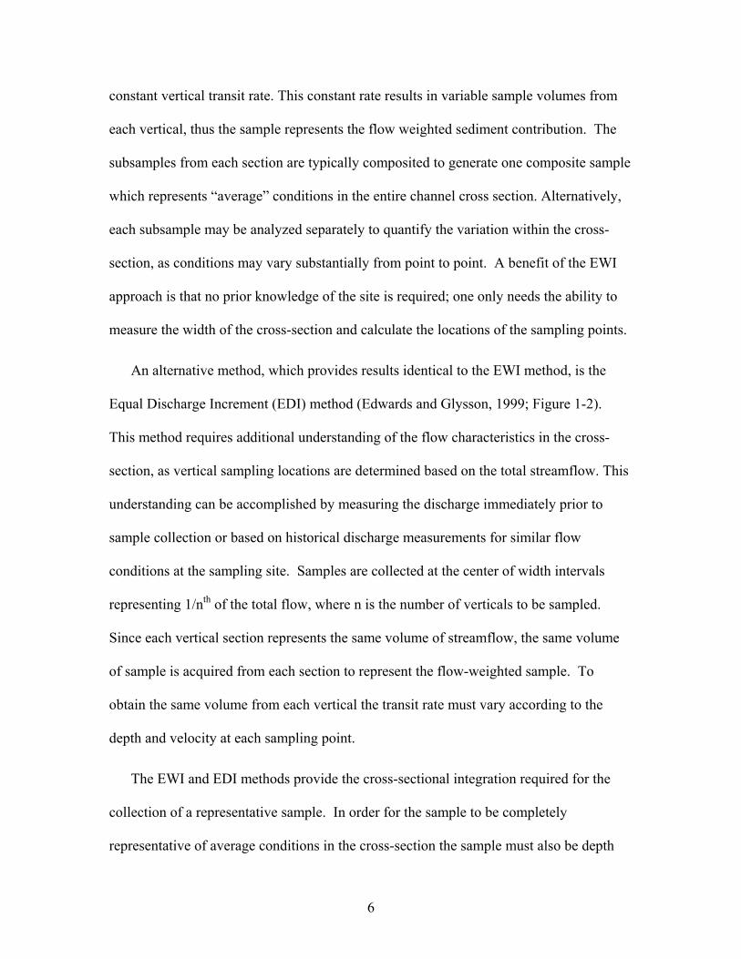
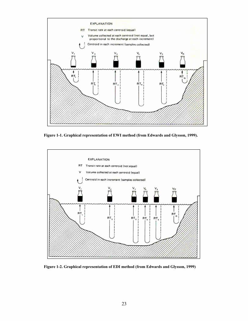
The EWI and EDI methods provide the cross-sectional integration required for the
collection of a representative sample. In order for the sample to be completely
representative of average conditions in the cross-section the sample must also be depth
7
integrated. To accomplish depth integration an isokinetic sampler, designed such that the
ambient stream velocity is maintained as the sample enters the sampler, must be used.
This design is imperative for the collection of representative samples because changes in
velocity as the sample enters the device potentially bias the sample. If ambient velocity
is not maintained, sediment could settle out or be drawn in preferentially from
surrounding flow, thus decreasing or increasing the sampled concentration relative to the
actual concentration in the water body. Isokinetic samplers are effective for specific
depth and velocity ranges; outside of the range for which it is designed, a given isokinetic
sampler will not provide representative data. Isokinetic samplers have been developed by
the Federal Interagency Sedimentation Program (FISP); commonly used samplers include
the DH-81, DH-95, and D-96 (Figure 1-3).
Sediment Monitoring Methods Manual sampling programs can sample only specific points in time, thus a
common problem is that most time periods remain un-sampled. This leads to significant
errors in load estimation because of the temporal variability of suspended sediment
concentrations. In an effort to augment data collected by manual sampling programs,
researchers have developed and employed numerous methods for collecting samples of
suspended sediment during events when personnel are not onsite. The following is a
review of these methods.
The first classification of sediment monitoring methods presented herein includes
methods in which samples are collected without human interaction. These samples are
often collected in response to changing hydrologic conditions or at pre-determined time
intervals, and are subsequently analyzed for the sediment properties of interest.
8
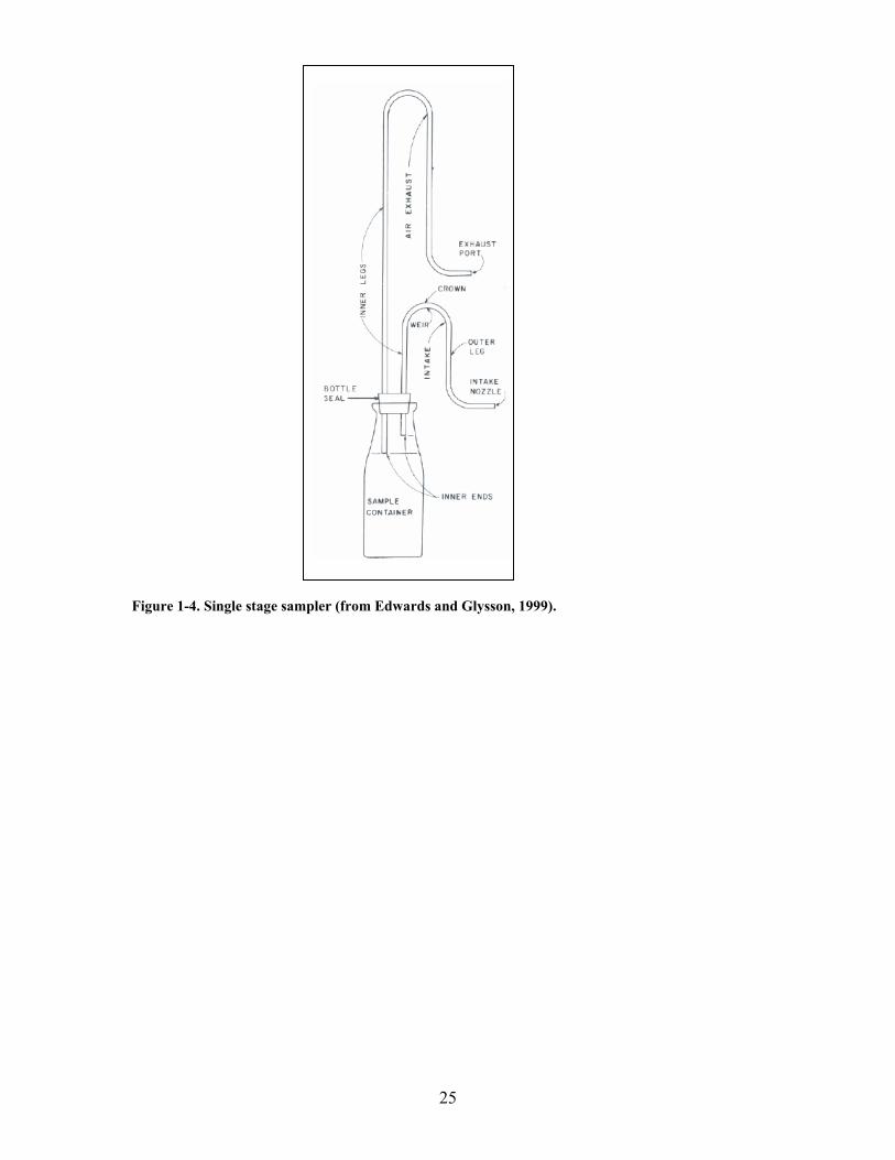
Single-Stage Sampler The single-stage sampler, or siphon sampler, is an inexpensive sampler capable of
sampling the near-surface zone of the water column during rising stages. The basic
design of this sampler, as described by Edwards and Glysson (1999), consists of a sample
container with an intake tube and a vent tube (see Figure 1-4). The assembly is mounted
on the stream bank such that when the water level reaches the intake tube the sampler
begins to fill. As the sampler fills the displaced air is trapped in the intake and exhaust
tubes, resulting in cessation of filling and prevention of outflow. It is critical for the
device to create this air trap so that once one volume of sediment-water mixture is
collected flow into, and out of, the sampler will cease and the concentration will not be
altered by flow through the device. Multiple samplers are often deployed at various
elevations to sample multiple stages on the rising limb of the hydrograph.
The inexpensive nature and the ability to “catch” samples on flashy streams which
may not otherwise be collected are attractive features of the single-stage sampler, and
studies have shown no statistically significant differences between data collected by this
device and another commonly used device - automatic pump samplers (Graczyk et. al.,
2000).
Such samplers also have limitations. The samples collected by this sampler
represent the surface of the flow; therefore, the samples are likely to be biased towards
the fine fraction of the sediment size distribution, as coarser materials are generally
concentrated near the streambed (Horowitz et. al., 1990; Walling and Moorehead, 1989)
and will not be incorporated into the sample. For streams carrying mostly fine sediments
this may not be an issue, however, if a significant portion of the sediment load is coarse
9
material the samples may not be representative. Also, the samplers are only capable of
collecting samples during the rising limb of the storm hydrograph. If one is interested in
characterizing sediment throughout the hydrograph, as is typically the case, alternative
methods must be employed. Finally, these devices must be installed within the stream
channel, typically on the bank, so that the intake is in contact with the flow, increasing
vulnerability to damage from debris or the flow velocity. For these reasons, siphon
samplers are usually reserved for use on small, flashy streams where debris flows may be
of less concern.
Automatic Pump Sampler The automatic pump sampler, commonly called the ISCO® Sampler after the most
prominent manufacturer, is similar to the single-stage sampler in that it collects a
sediment-water sample from a single point in the channel. The pump sampler is more
advanced than the single-stage sampler as it provides the ability to collect multiple
discrete samples over a period of time. The typical pump sampler consists of a pump,
computerized control unit, one or more sample containers, a sampling tube linking the
sampler to the flow, and a power source. When specified conditions, such as stage or
time interval, are met, the pump initiates, first purging the sample tube, then delivering
sample to the container as instructed in the user-defined program.
The samples collected represent only the point within the stream’s cross-section
that is sampled by the intake tube. To obtain estimates of the cross-sectional sediment
concentration, manual width- and depth-integrated samples must be collected
simultaneously with a subset of the automatically collected samples. Relating the
manually collected full-channel samples to the pumped point samples allows for the
10
determination of a coefficient which may be applied to the point samples to estimate the
representative cross-sectional sediment concentration. For this reason, the location of the
intake should ideally represent the mean suspended sediment concentration in the cross
section (Edwards and Glysson, 1999).
Automatic pump samplers provide greatly improved temporal resolution than is
achievable with manual sample collection as they can be programmed to collect samples
according to a variety of sampling regimes (such as storms only, various time increments,
various flow increments, various water-quality parameter increments) and for these
reasons automatic samplers are widely used in studies of sediment transport and water-
quality. Additionally, models of these devices are manufactured for ease of transport and
deployment, reducing the cost of application and enabling users to easily deploy a
sampler for a short period of study (Teledyne-Isco, 2006).
While providing the benefit of collecting multiple samples throughout the
stormflow period, there are many factors which must be accounted for in order for an
auto-sampling program to be successful. These considerations include locating the
sampler in an accessible, sheltered location above high flows, the ability to provide
power to operate the machinery, and the ability to deploy the equipment in a manner
which does not bias the samples collected (Edwards and Glysson, 1999). Situating the
sampler above high water elevation can create a sample bias resulting from coarse
sediments settling in the collection tube, causing the collected sample to be non-
representative of suspended sediments in the stream at the collection point. Because this
source of sampling bias increases with the autosamplers elevation above its’ intake,
which typically increases with stream size, use of autosamplers on larger streams can be
11
problematic. Further complicating sample collection is the possibility of cross-
contamination when residual material is not sufficiently flushed from the intake tube and
is incorporated into successive samples, which typically occurs with rapidly changing
sediment concentrations, and when sand size particles are present (Thomas and Eads,
1983). Additionally, the orientation of the sample intake may bias the particle-size
characteristics of the sample, or may make the sampling tube prone to capturing or
becoming fouled by water-borne debris, thus altering the intake waters’ sediment
concentrations. Research has shown that the most effective orientation for the intake
occurs when the intake is normal to flow terminated by a 90° elbow directed downstream
(Winterstein and Stefan, 1983).
A significant limitation of automatic pump samplers is that personnel must
retrieve the samples collected in order for the sampler to continue operation – the
samplers have a limited sample-holding capacity and sampling will cease once the
capacity is met. This cessation of sampling could lead to missed samples during critical
periods of sediment transport, such as the recession of a large stormflow event.
Furthermore, the samples must be analyzed in the lab in order to determine the SSC and
the expense of labor required to complete these steps can be significant.
The effort required to account for these potential sources of error when
establishing an autosampling program on large rivers may result in significant time
investments. Therefore, the use of autosamplers is best suited for smaller streams
carrying fine sediments.

12
Surrogate Methods The previous category of methods relies upon a device to collect a sample when
specified conditions are met. As there are many severe limitations to the application of
those methods recent research has focused on the development of effective surrogate
monitoring instruments and methods.
As an alternative to traditional, manual sediment monitoring programs, variables
which have a high correlation with SSC and can be measured continuously and remotely
are used as surrogates for estimating SSC. Advantages of using SSC surrogates include
the collection of data during all hydrologic conditions and a reduction in the need for
time-intensive manual sampling. Because SSC varies dramatically with hydrologic
conditions, use of SSC-surrogate monitoring methods can increase both the precision of
SSC loading estimates (Walling, 1977) and scientific understanding of SSC variability in
monitored systems.
Rating Curve Method Perhaps the oldest and most widely applied surrogate method, first presented by
Campbell and Bauder (1940), is the use of stream discharge as a surrogate for sediment
concentration. The common use of this approach, also known as the rating-curve
approach, is likely attributed to the relative ease of streamgage operation and the density
of the streamgaging network in the U.S. Furthermore, there exists a fundamental link
between discharge and sediment transport, as the runoff responsible for increasing
discharge is typically responsible for a large portion of the soil erosion which contributes
to sediment transport. Finally, stream discharge is a requisite for the calculation of
sediment flux (mass transported per unit time), so this method minimizes the number of
parameters which must be measured in order to estimate sediment loading.
13
Although easily implemented, this method may provide results with large error
terms when applied without regard for the complex nature of the relation and the
underlying fundamental concepts (Walling, 1977b). For example, Horowitz (2003)
found that for multiple watersheds in the USA and Europe, ranging in size from <1x10³
km2 to >1x10⁶ km2, high sediment concentrations are often under predicted and low
sediment concentrations are often over predicted, partly as a result of the differing
relation between SSC and discharge on the rising and falling limbs of the stormflow
hydrograph (hysteresis). Although short duration studies applying the rating curve
method are subject to the largest errors, longer duration studies calculating annual
sediment loads have been reported to have errors as high as 280% (Walling, 1977).
Factors such as seasonality and hydrograph position are often incorporated into these
calculations to account for seasonal variation and hysteresis observed over the period of a
storm hydrograph.
Acoustic Backscatter The application of Acoustic Doppler Current Profilers (ADCP’s) for measuring
stream discharge has gained popularity in recent years as technology has developed
making measurements with ADCP’s faster and more accurate than traditional methods
(Simpson, 2001). Furthermore, these instruments may be deployed in-situ to provide a
time-series of discharge values, eliminating the need for discharge rating-curve
development.
ADCP’s measure stream velocity by measuring the Doppler shift in sound waves
transmitted by the instrument and echoed back by particles in suspension (Filizola and
Guyot, 2004). The quality of the velocity measurement is dependent upon the amount of

14
particles scattering the signal; therefore, the instruments record a backscatter value for
assessment of the accuracy of the velocity data. This backscatter value has obvious
connections to suspended sediment concentrations and particle size distributions, and this
link has been evaluated by several investigators. Coefficients of determination (R2) for
regressions estimating suspended sediment from acoustic backscatter have been reported
as high as 0.91 (Gray, et. al., 2003).
Although the potential exists for effectively monitoring stream discharge and
sediment discharge simultaneously with these instruments, the computation of sediment
concentration is quite difficult. Significant data processing is required to obtain values
required for sediment concentration estimation, and the effects of water temperature,
salinity, and pressure must be accounted for in the regression equation (Gartner and Gray,
2006). It is for these reasons that the use of acoustic backscatter as a sediment surrogate
has not yet gained wide acceptance in the scientific community.
Laser Diffraction One of the more recently developed surrogates that demonstrates potential for
widespread application in sediment monitoring is laser diffraction. Laser diffraction
instruments are commonly used in the lab for the determination of particle size
distribution, but until recently these instruments have not been designed for field use.
Recent technological advances have enabled the development of field deployable
instruments capable of measuring suspended sediment concentrations and particle size
distributions; these devices are generally referred to by the acronym LISST (Laser In-Situ
Scattering & Transmissometry) and are manufactured by Sequoia Scientific, Inc.

15
The LISST devices operate by measuring the scattering of a laser beam (light) by
particles in suspension. Laser beams are directed into the sample and the optical
diffraction of the beam is measured and used to estimate the sizes of the particles in
suspension (Agrawal and Pottsmith, 2000). A summation of the sizes of the particles
results in a volumetric suspended sediment concentration, this concentration must then be
converted to a mass concentration by estimation, or measurement, of the density of the
sediment grains (Agrawal and Pottsmith, 2000).
Extensive testing of the LISST devices was conducted by Melis et. al. (2003) on
the Colorado River in Arizona. This study found good agreement between sediment
concentrations and particle size distributions at the point measured by the LISST and
cross-sectional samples collected using isokinetic samplers (R2 values of 0.82 – 0.97).
Difficulties associated with the use of the LISST instruments were related to exceedance
of the instrument’s concentration range during extreme events and fouling of the optics.
The benefit of employing laser diffraction devices in sediment monitoring studies
is that these sensors measure the sediment concentration of the water passing through
them, eliminating the need to develop a relation between the sensed values and the
sediment concentration. The variability in the resulting cross sectional estimations is due
to variability between the cross sectional sample and point measurement, which is a
potential source of variability in many surrogate methods. Additionally, these units
provide grain size distribution data, which is not offered by and is a potential source of
variance in other surrogates.
The limitations to this approach include the concentration range (10mg/L –
3,000mg/L), frequent servicing to limit fouling (Melis et. al., 2003), and cost. According
16
to the manufacturer, Sequoia Scientific, the cost of these instruments ranges from
approximately $5,000 to $30,000 depending on the application and data desired (i.e.
concentration plus particle size vs. concentration only).
Turbidity Turbidity is a measure of the optical clarity of water, and is thus largely controlled
by suspended particulate material, such as fine sediments, which scatter light and reduce
optical clarity (Davies-Colley and Smith, 2001). Turbidity has long been recognized as
an effective surrogate for estimating in-stream sediment concentrations (Walling, 1977a)
and recent technological advances have produced turbidity sensors that can be operated
in-situ for the purpose of generating a continuous record.
The approach of using turbidity as a surrogate for suspended sediment provides
improved estimates of sediment concentration and loads compared to the streamflow
surrogate method (Gippel, 1989; Grayson et al, 1996;). Gippel (1989) reports R2 values
for turbidity-sediment regressions at different monitoring sites ranging from 0.71 to 0.94,
with other investigators reporting R2 values in this same range (Grayson et. al., 1996;
Rasmussen et. al., 2005; Christensen et. al., 2000).
Turbidity, however, is not a perfect surrogate for suspended sediment. Variability
in the relationship between suspended sediment and turbidity may be caused by
characteristics of the sediment in suspension during stormflow events (Gippel, 1995;
Davies-Colley, Smith, 2001; Sutherland et al 2000). The sediment characteristics may be
controlled by hydrologic factors such as stage (water-level), sub-watersheds’
proportionate contributions to SSC at the monitoring point, and/or temporal factors
affecting the sources of the sediment (Gippel, 1995). Sediment properties which
17
contribute to variance in the turbidity-sediment relationship include grain-size
distribution, organic matter content, specific surface area, and particle density. The effect
of grain-size distribution on turbidity is attributed to variations in surface area as size
distributions change (Gippel, 1989; Davies-Colley, Smith, 2001). The effect of
suspended particles on turbidity is determined by surface area, while sediment
concentration is a mass function. Studies have suggested that for samples of the same
concentration of suspended sediment, variations in the particle size may alter turbidity by
as much as a factor of four (Gippel, 1995). To confound this effect, particle-size
distributions have been documented to change seasonally and within single storm events
(Gippel, 1995). Furthermore, particle-size may vary spatially within a watershed, leading
to changing distributions with variations in source area (Gippel, 1995). Additionally,
organic matter has different density, surface area, and light-scattering characteristics than
mineral components, so the fraction of these materials present can be expected to affect
the turbidity-SCC relationship (Gippel, 1989). Other characteristics of the sediment, such
as color, and of the water matrix, such as coloration from dissolved organics, have been
shown to have varied effects on measured turbidity (Gippel, 1989; Sutherland, et al,
2000; U.S. Geological Survey, 2004).
It is important to note that multiple types of turbidity sensors exist, some measuring
light scattering while others measure light transmittance, and that these various sensor
configurations are affected differently by the factors listed above, as each has been
developed to minimize the effects of given factors (Anderson, 2005). Despite the errors
attributed to the factors above, turbidity is the most commonly applied sediment
surrogate technology in the United States (Gray, et. al., 2003).
18
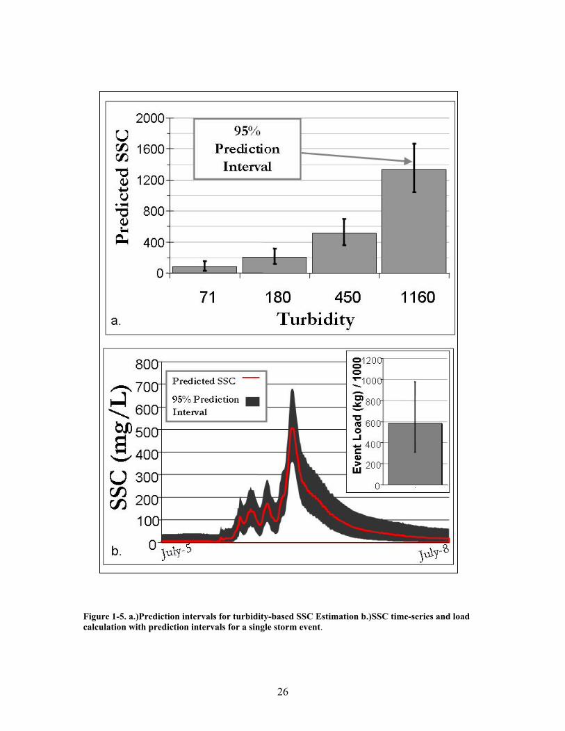
The influence of variance-inducing effects may not be particularly evident in discrete
estimations of SSC from turbidity measurements, as reported statistics indicate the
turbidity-based SSC predictions are very effective. However, individual measures of
SSC are rarely of interest; SSC data are typically used to calculate loads and yields over
various time scales. When estimated SSC data are multiplied by streamflow and summed
over the time period of interest, the estimation errors are compounded and result in loads
and yields with large uncertainty. For example, Figure 1-5a. depicts the 95% prediction
interval for various values of turbidity predicted SSC and Figure 1-5b illustrates the
effect of compounding errors when calculating the suspended sediment load for a single
storm event. Accounting for the variance-inducing effects and thereby reducing variance
in the turbidity-based SSC estimation model would result in more accurate and precise
estimations of sediment load and yield. Improved load and yield estimations would
improve the scientific understanding of aquatic systems transporting sediment and could
also lead to more effective policy as decisions would be based on a more accurate
understanding of sediment transport.
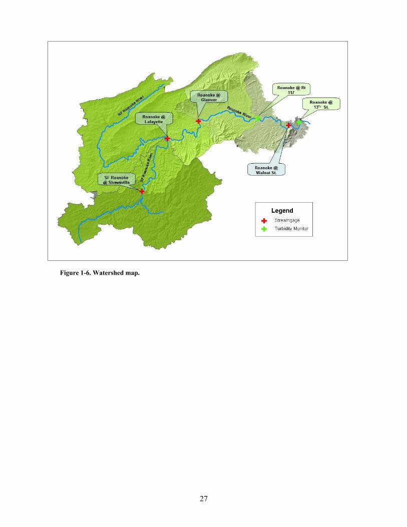
Research Background The United States Geological Survey (USGS) is currently monitoring turbidity at four
locations along the Roanoke River in the Roanoke, VA in an effort to evaluate the effect
of the Roanoke River Flood Reduction Project on suspended sediment concentrations
(SSC) in the river. To accomplish this objective turbidity is monitored at a point directly
upstream of the construction reach, the Route 117 Bridge, and at the downstream extent
of the construction, the 13th Street Bridge (see Figure 1-6). These two monitoring
stations are the focus of the research reported in this document.

19
In addition to these two sites additional monitors are positioned to measure conditions
directly upstream and downstream of the reach under construction (construction is
limited to one 4000 foot reach at a time).
Research Objectives This research investigated the potential to improve turbidity-based SSC and sediment
loading estimates by incorporating hydrologic variables, which can be monitored
remotely and continuously, into turbidity-based SSC estimations. Furthermore, the
applicability of a single estimation model for multiple turbidity-monitoring stations on a
single river reach was explored. The research was initiated by establishing the following
objectives:
1) Determine which physical properties contribute to variance in turbidity-based SSC estimation at the Route 117 monitoring station.
2) Determine if those physical properties can be modeled using hydrologic variables which can be measured remotely and on the same temporal scale as turbidity.
3) Determine if incorporation of hydrologic variables into turbidity-based SSC estimation models can improve the precision of those models and of derived loading estimates.
4) Use the approach outlined in Objectives 1-3 to develop a turbidity-based SSC-estimation model for the Roanoke River at 13th Street Monitoring Station.
5) Determine if a single turbidity-based SSC-estimation model, developed by combining data from the Route 117 and 13th Street monitoring stations (“pooled model”), can effectively estimate SSC at those two locations.
6) If Objective 2 concludes that a multiple-location SSC-estimation model is feasible: compare the capabilities of models developed through Objectives 1 and 2 to estimate sediment loadings.
The remainder of this thesis is contained in four chapters. Chapter Two addresses the
overall study design and methods employed. Chapter Three addresses Objectives 1 -3

20
and Chapter Four addresses Objectives 4 – 6. Conclusions from the entire study are
summarized in Chapter Five.
21
References Campbell F.B., H.A. Bauder. 1940. A rating curve method for determining silt-discharge
of streams. Transactions, American Geophysical Union 21:603-607. Chang, H.H., 2002. Fluvial Processes in River Engineering: Malabar, FL, Krieger, 432 p. Davies-Colley R.J., D.G. Smith. 2001. Turbidity, Suspended Sediment, and Water
Clarity: A Review. Journal of American Water Resources Association 37:1085 – 1101.
Edwards, T.K., and Glysson, G.D.. 1999. Field Methods for Measurement of Fluvial Sediment: US Geological Survey Techniques of Water-Resources Investigations Book 3, Chap. C2,89 p.
EPA. 2000. Mid-Atlantic Highlands Streams Assessment. EPA-903-R-00-0015. US Environmental Protection Agency. Washington, DC. 64 p.
EPA 2002. National Water Quality Inventory: 2000 Report. EPA-841-R-02-001. US Environmental Protection Agency. Washington, DC. 207 p
Gippel, C.J., 1989. The use of turbidimeters in suspended sediment research. Hydrobiologia 176/177:465-480.
Gippel, C.J., 1995. Potential of Turbidity Monitoring for Measuring the Transport of Suspended Solids in Streams. Hydrological Processes 9:83-97.
Gordon, N.D., T.A. McMahon, B.L. Finlayson, C.J. Gippel, R.J. Nathan. 2004. Stream Hydrology: An Introduction for Ecologists. West Sussex, England. John Wiley and Sons, Ltd. 429 p.
Gray, J.R., E. Patino, P. Rasmussen, M. Larson, T. Melis, D. Topping, M. Runner, C. Alamo. 2003. Evaluation of Sediment-Surrogate technologies for computation of suspended-sediment transport. Accessed online 4-12-2006. http://water.usgs.gov/osw/techniques/yrcc_surrogates.pdf
Grayson, R.B., B.L. Finlayson, C.J. Gippel, B.T. Hart. 1996. The potential of field turbidity measurements for the computation of total phosphorus and suspended solids loads. Journal of Environmental Management 47: 257-267.
Horowitz, A.J., F.A. Rinella, P. Lamothe, T.L. Miller, T.K. Edwards, R.L. Roche, D.A. Rickert. 1990. Variations in suspended sediment and associated trace element concentrations in selected riverine cross sections. Environmental Science and Technology 24:1313-1320.
Horowitz, A.J., 2003. An evaluation of sediment rating curves for estimating suspended sediment concentrations for subsequent flux calculations. Hydrological Processes 17:3387-3409.
Martin, G.R., J.L. Smoot, K.D. White. 1992. A comparison of surface-grab and cross sectionally integrated stream-water-quality sampling methods. Water Environment Research 64: 866-876.
22
Meade, R.H., and R.S. Parker. 1984. “Sediment in Rivers of the United States.” p. 49-60, in: National Water Summary 1984 – Water Quality Issues. US Geological Survey Water Supply Paper 2275.
Osterkamp, W.R., P. Heilman, L.J. Lane. 1998. Economic consideration of a continental sediment-monitoring program. International Journal of Sediment Research 13:12-24.
Owens, P.N,, R.J. Batalla, A.J. Collins, B. Gomez, D.M. Hicks, A.J. Horowitz, G.M. Kondolf, M. Marden, M.J.Page, D.H. Peacock, E.L. Petticrew, W. Salomons, N.A Trustrum. 2005. Fine-grained sediment in river systems: environmental significance and issues. River Research and Applications 21: 693-717.
Sutherland T.F., P.M. Lane, C.L. Amos, J. Downing. 2000. The calibration of optical backscatter sensors for suspended sediment of varying darkness levels. Marine Geology 162:587-597.
Thomas, R.B. and R.E. Eads. 1983. Contamination of Successive Samples in Portable Pumping Systems. Water Resources Research 19-2:436-440.
U.S. Geological Survey, variously dated, National field manual for the collection of water-quality data: U.S. Geological Survey Techniques of Water-Resources Investigations, book 9, chaps. A1-A9, available online at http://pubs.water.usgs.gov/twri9A.
Walling D., 1977. Assessing the accuracy of suspended sediment rating curves for a small basin: Water Resources Research 13: 531-538.
Walling D., and A. Collins. 2000. Integrated Assesement of Catchment Sediment Budgets: A Technical Manual. University of Exeter, United Kingdom. 168 p.
Wolman, M.G., and J.P. Miller. 1960. Magnitude and Frequency of Forces in Geomorphic Processes. The Journal of Geology 68:54-73.
YSI, Inc. 6136 0103 E56-01.pdf http://www.ysi.com/extranet/EPGKL.nsf/447554deba0f52f2852569f500696b21/8db42369ec1b6e3a85256cef00562ec6/$FILE/6136%200103%20E56-01.pdf (Accessed January 16, 2006)
23
Figure 1-1. Graphical representation of EWI method (from Edwards and Glysson, 1999).
Figure 1-2. Graphical representation of EDI method (from Edwards and Glysson, 1999)
24
Figure 1-3. Isokinetic samplers: a) DH-81; b) DH-95; c)D-96
a) b)
c)
25
Figure 1-4. Single stage sampler (from Edwards and Glysson, 1999).
26
Figure 1-5. a.)Prediction intervals for turbidity-based SSC Estimation b.)SSC time-series and load calculation with prediction intervals for a single storm event.
27
Figure 1-6. Watershed map.

28
Chapter 2 Methods
Introduction The purpose of this chapter is to describe the field and laboratory methods
employed in this research. The methods presented apply to data collected at both the
Roanoke River at Rt. 117 and Roanoke River at 13th Street Bridge monitoring stations.
Field Methods
Turbidity Measurement Turbidity was measured in-situ by a Yellow Springs Instruments (YSI) 6136
turbidity sensor installed on a YSI 6920 multiparameter sonde. This sonde was
programmed to measure the in-stream turbidity, as well as water temperature, specific
conductance, and pH, on fifteen minute intervals. The data were stored onsite by a
Campbell Scientific CR-10X datalogger, and transmitted via cellular modem to the
United States Geological Survey (USGS) National Water Information System (NWIS)
and subsequently made available in near real-time on the internet
(http://waterdata.usgs.gov/va/nwis/rt ).
The sonde was suspended from the bridge so that the sensors remained submerged
during low flows while also allowing the sonde to maintain a position near the water
surface during elevated flow events. This deployment design was intended to prevent the
sensors from being located in the bedload transport zone during storm events and to
29
reduce the risk of damage or fouling by debris, as the sonde can slide over debris being
transported downstream.
The turbidity sensor was operated, and data were stored, computed, and corrected,
in cooperation with USGS according to the guidelines for operation set forth in Wagner
et. al. (2006). The operation of the instrument was maintained through monthly
servicing, which included sensor drift and fouling determinations and re-calibration.
Stage Measurement Stage (water surface elevation) was measured in-situ by Onset® HOBO® Water
Level Loggers. These instruments measure the total pressure exerted on the sensor, thus
the total pressure exerted on the sensor varies with hydraulic head above the sensor. The
total pressure is also influenced by barometric pressure; therefore an additional HOBO®
was used to record barometric pressure at the Roanoke River at Rt. 117 site.
The HOBO® instruments recorded pressure and temperature on the same time
interval as the turbidity data. The instruments were serviced every four to six weeks, at
which time manual stage measurements were made, data were downloaded to a laptop
computer, and the instrument was thoroughly cleaned. Instrument setup, data download,
and data processing was completed using HOBOware® software.
The instruments were housed in PVC stilling wells mounted to a stable tree on the
riverbank such that the instrument was submerged during all flow conditions. Two
reference marks (RM’s) were established at each deployment site; each RM was assigned
a stage (Table 2-1) and all measurements by the HOBO® were referenced to these RM’s.
30
Sample Collection Full channel width- and depth-integrated samples were collected with the DH-95 or
D-96 isokinetic samplers using the Equal Width Interval (EWI) method as described by
Edwards and Glysson (1999). The use of this equipment and methodology ensured that
the samples collected accurately represented the sediment transported in suspension
throughout the width and depth of the channel cross-section.
Suspended sediment samples were collected at the point of turbidity measurement
with the 3- liter frame sampler; the heavier D-96 sampler was used during extremely high
flows to counter excessive velocities. These samplers allowed the collection of up to 3-
liters of sample per lowering; therefore the volume necessary could be collected more
rapidly than with the 1-liter DH-95. The sample was collected by lowering the sampler
to a point adjacent to the turbidity monitor and allowing it to fill at this single point.
For both the EWI and point sample collections, sub-samples were composited into
separate 8-liter churn splitters, and aliquots for analysis of SSC were drawn from these
composite samples according to methods prescribed by the USGS (USGS, 1999). The
SSC-analysis aliquots were deposited into glass 1-pint sediment sample containers for
shipment to the USGS Eastern Region Sediment Lab in Louisville, Kentucky. The
remainder of the composited sample was retained for analysis of sediment properties, and
was deposited into a 13-liter container for delivery to the Crop and Soil Environmental
Sciences (CSES) labs at Virginia Tech.
31
Lab Methods
Sample Pre-processing and Storage The 1-pint containers (SSC-analysis aliquots) were stored in refrigeration (5° -
10° C) until shipment to the USGS Eastern Region Sediment Lab for SSC analysis; the
resultant SSC data were recorded in the USGS NWIS database, as well as used for this
research.
The sample volumes retained for analysis of sediment properties were refrigerated
(5° - 10° C) for an initial period of at least 5 days, allowing the majority of the sediments
in suspension to settle to the bottom of the container. After this period the samples were
frozen at approximately -10°C for a sufficient period to allow the entire volume to freeze
solid (typically 3-5 days). Once frozen, the samples were returned to the refrigerator
where they were allowed to thaw completely. At this time, nearly all of the sediment
would have settled to the bottom of the container. However, in order to prevent re-
suspension when moving the containers to the lab for further processing, the samples
were frozen once again. The samples were transported to the lab while frozen, and
allowed to thaw completely without additional movement (thus avoiding re-suspension of
the sediments), and excess water was removed via siphoning.
Excess water removal required careful siphoning of the water, taking caution not to
disrupt and remove any of the sediment from the sample. Minimal sediment removal was
ensured by filtration of the decanted water through a 0.45µm glass fiber filter. If large
sediment particles were inadvertently siphoned from the sample they were retained on the
surface of this filter and washed back into the container. Smaller particles, however,
would be trapped within the fibers of the filter and considered lost. The filters were dried
and weighed to ensure that a significant amount of sediment was not lost through this
32
process; the mass of sediment lost ranged from 0 - 15mg for samples containing 0.5 – 8g.
Once a sufficient volume of water was removed, the remaining samples were transferred
into 125mL plastic sample containers for storage until analysis.
Concentration and Sand-Fine Split Analysis Analysis of suspended sediment concentration (SSC) and sand-fine split (%
<0.063mm) was performed by staff at the USGS Eastern Region Sediment Lab in
Louisville, KY. This analysis was performed according to the procedures documented by
Guy (1969), ASTM (2002), and Shreve and Downs (2005). The analysis of SSC and
sand-fine split was performed simultaneously, as the sample was wet-sieved to separate
sands (>0.063mm) and the material passing through the sieve was filtered onto a 0.45µm
filter. Both fractions were oven dried and weighed; SSC was calculated as the sum of the
mass of the two fractions divided by the initial sample volume and % <0.063mm was
calculated as the mass <0.063 divided by the sum of the mass of the two fractions.
Sediment Characteristics Sediment quantities retained for analysis of sediment characteristics (particle size
distributions, surface area, and organic carbon) ranged from 500mg to 8g. The entire
mass of sediment was used to determine particle-size distributions; samples with the
greatest mass of sediment were split and particle-size analysis was performed on each
portion of the split. The samples were then dried and 100mg of each was separated for
Organic C analysis. The mass remaining after removal of the aliquot for Organic C was
used for surface area analysis.
33
Particle Size Analysis The analysis of particle-size distribution was performed via sieve-pipet method as
described by Guy (1969). Wet sieving was used to separate the sand sized particles from
the silt and clay sized particles of the sample. The pipet method, founded upon Stokes’
Law, is used to fractionate the silts and clays.
The sample was dispersed, to reduce errors introduced by flocculation, by the
addition of 1mL of 5% Calgon solution per 100mL of water/sediment mixture. Samples
were mechanically shaken overnight to ensure complete dispersion.
The sand fraction was separated via wet sieving through a 53µm stainless steel
sieve and the silts and clays were simultaneously washed into a 250mL graduated
cylinder for pipet analysis. The sands retained on the sieve were washed into a pre-tared
beaker to be oven dried (110°C, overnight) and weighed.
A water bath with pipet rack assembly, as described by Guy (1969), was used to
make the pipet withdrawals from the 250mL cylinder; withdrawals were made at a depth
of 3 cm using 25 mL pipettes. The temperature was maintained at 27°C to reduce errors
related to variation in settling velocity with temperature. The sample was stirred for 1
minute to ensure uniform dispersion of the sample in the cylinders, then aliquots were
withdrawn at 6 minutes 31 seconds and 2 hours 5 minutes after stirring, representing the
16 µm and 2 µm size fractions, respectively. The aliquots were dispensed into pre-tared
50mL beakers, oven dried, and weighed. Additionally, the sediment remaining in the
cylinder after the withdrawals was washed into a pre-tared 400 mL beaker, oven dried,
and weighed.
Particle-size distribution was calculated as “% finer than” for each fraction
measured. This was accomplished by summing the mass of all fractions, including the
34
material remaining in the cylinder after withdrawals, and calculating the percentage of
the total mass represented by each fraction. The mass of sediment in each size class was
calculated as
MS = MB+S – MB – C x P
where:
MS = Mass of Sediment in given size fraction
MB+S = Mass of Beaker + Sediment
MB = Mass of Beaker
C = Calgon correction factor = 0.0068mg
P = Cylinder volume / Pipet volume = 10
The Calgon correction factor (C) is the mass of Calgon that is present in each
withdrawal, as determined using a blank sample (distilled water) prepared and analyzed
in the same manner as a true sample. The Cylinder volume / Pipet volume (P) scales the
mass of sediment in the withdrawal to represent the mass of that fraction in the entire
sample. Since only 25mL of sample is withdrawn the mass must be multiplied by P=10
to represent the mass present in the entire 250mL slurry.
A subset of the samples was mechanically split prior to analysis to allow the
analysis of duplicate samples for QC purposes. The results of the QC procedures, as well
as the data for all samples analyzed, are contained in Appendix B.
Organic Carbon Analysis All samples were pretreated with sulfurous acid (H2SO3) prior to analysis to
remove inorganic carbon. Organic carbon was determined using the high-temperature
induction furnace method described by Nelson and Sommers (1996). This analysis was
35
performed by Dr. Steve Phillips using the Carlo Erba NA1500 CHN analyzer located at
the Virginia Tech Eastern Shore Agricultural Research Center. This instrument combusts
the sample at 900°C, evolving all carbon present as CO2 gas; the evolved gasses are
subsequently analyzed to determine the total amount of carbon evolved from the sample
(Nelson and Sommers, 1996).
Specific Surface Area Analysis Specific surface area (surface area per unit mass) was determined using the
Micromeritics ASAP 2010 surface area analyzer located in the CSES Mineralogy lab.
This analysis was conducted on the entire mass of sample remaining after the aliquot for
organic carbon analysis was removed. The samples were lightly ground using an agate
mortar and pestle to disaggregate the sample prior to analysis. Specific surface area was
calculated using BET adsorption isotherms for nitrogen adsorbed to the external surfaces
of the sediment particles at the temperature of liquid nitrogen (Pennell, 2002). .
Radar Derived Rainfall Estimation Estimations of average basin rainfall (ABR) were computed for 111 sub-
watersheds within the study watershed (Figure 2-1). These ABR estimations were
computed by National Weather Service staff using the Areal Mean Basin Estimated
Rainfall (AMBER) algorithm with data from the WSR-88D radar system. For the
purposes of this study, the accumulated rainfall, from the beginning of the storm until the
time of sample collection, was used to represent each rainfall event.
The ABR data for each event was used to determine the percentage of total
rainfall received by the watershed occurring over each of four geologic categories. The
geologic categories, carbonate, metamorphic, shale-dominated sedimentary, and other

36
sedimentary, were classified using data from the Virginia Department of Mineral
Resources (2003) (Figure 2-1). Using ArcView GIS software, the AMBER sub-basins
were divided according to the underlying geology. The data were then exported to an
Excel spreadsheet where the percentage of total rainfall occurring over each geologic
category was calculated using Pivot Table functions.
37
References American Society for Testing and Materials, 2002, D3977-97, Standard Test Methods for
Determining Sediment Concentration in Water Samples, ASTM International Edwards, T.K., and Glysson, G.D.. 1999. Field Methods for Measurement of Fluvial
Sediment: US Geological Survey Techniques of Water-Resources Investigations Book 3, Chap. C2,89 p.
Guy, H.P. 1969. Laboratory theory and methods for sediment analysis in Techniques of Water-Resources Investigations of the United States Geological Survey, Book 5, Chapter C1. United States Government Printing Office, Washington D.C.
Nelson, D.W. and L.E. Sommers. 1996. Total Carbon, Organic Carbon, and Organic Matter. P 961-1010, in: D.L. Sparks et. al. (eds.) Methods of soil analysis. Part 3, Chemical Methods. Soil Science Society of America, Madison, Wisconsin.
Pennell, K.D. 2002. Specific Surface Area. P 295-315, in: J.H. Dane and G.C. Topp (eds.) Methods of soil analysis. Part 4, Physical methods. Soil Science Society of America, Madison, Wisconsin.
Shreve, E.A. and A.C. Downs. 2005. Quality-Assurance Plan for the Analysis of Fluvial Sediment by the U.S. Geological Survey Kentucky Water Science Center Sediment Laboratory. U.S. Geological Survey Open-File Report 2005-1230.
U.S. Geological Survey, variously dated, National field manual for the collection of water-quality data: U.S. Geological Survey Techniques of Water-Resources Investigations, book 9, chaps. A1-A9, available online at http://pubs.water.usgs.gov/twri9A.
Virginia Division of Mineral Resources. 2003. Digital representation of the 1993 Geologic Geologic map of Virginia: Virginia Division of Mineral Resources Publication 174 [CD-ROM; 2003, December 31]. Adapted from Virginia Division of Mineral Resources, 1993, Geologic Map of Virginia: Virginia Division of Mineral Resources, scale 1:500,000.
Wagner, R.J., R.W. Boulger Jr., C.J. Oblinger, B.A. Smith. 2006. Guidelines and Standard Procedures for Continuous Water-Quality Monitors: Station Operation, Record Computaiton, and Data Reporting. U.S. Geological Survey Techniques and Methods 1-D3.
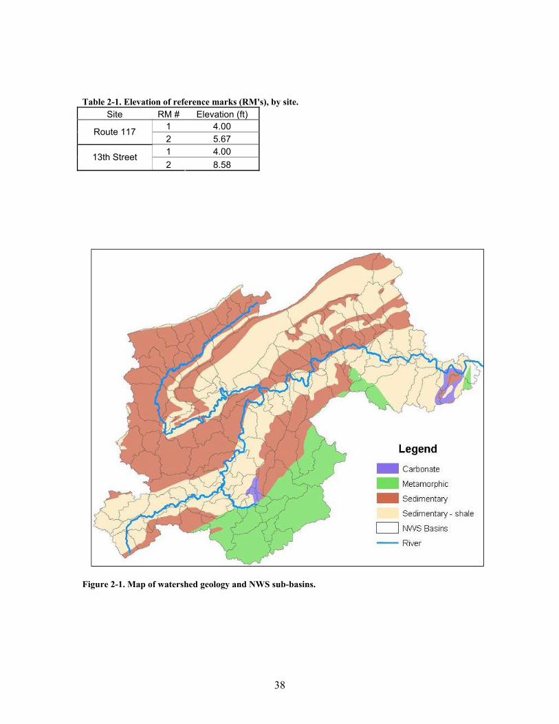
38
Table 2-1. Elevation of reference marks (RM's), by site.
Site RM # Elevation (ft) 1 4.00 Route 117 2 5.67 1 4.00 13th Street 2 8.58
Figure 2-1. Map of watershed geology and NWS sub-basins.
39
Chapter 3 Improving Turbidity-based Estimates of Suspended Sediment Concentrations and Loads
Abstract As the impacts of human activities increase sediment transport by aquatic systems the need to accurately quantify this transport becomes paramount. Turbidity is recognized as an effective tool for monitoring suspended sediments in aquatic systems, and with recent technological advances turbidity can be measured in-situ remotely, continuously, and at much finer temporal scales than was previously possible. Although turbidity provides an improved method for estimation of suspended-sediment concentration (SSC), compared to traditional discharge-based methods, there is still significant variability in turbidity-based SSC estimates and in sediment loadings calculated from those estimates. The purpose of this study was to improve the turbidity-based estimation of SSC. Working at a monitoring site on the Roanoke River in southwestern Virginia, stage, turbidity, and other water-quality parameters were monitored with in-situ instrumentation, suspended sediments were sampled manually during elevated turbidity events; those samples were analyzed for SSC and for physical properties including grain-size distribution and organic carbon content; and rainfall was quantified by geologic source area. The study identified physical properties of the suspended-sediment samples that contribute to SSC-estimation variance and hydrologic variables that contribute to variance in those physical properties. Results indicated that the inclusion of any of the measured physical properties, which included grain-size distributions, specific surface-area, and organic carbon, in turbidity-based SSC estimation models reduces unexplained variance. Further, the use of hydrologic variables, which were measured remotely and on the same temporal scale as turbidity, to represent these physical properties resulted in a model which was equally as capable of predicting SSC. A square-root transformed turbidity-based SSC estimation model, which included a water level variable, provided 63% less unexplained variance in SSC estimations and 50% narrower 95% prediction intervals for an annual loading estimate, when compared to a simple linear regression using a logarithmic transformation of the response and regressor (turbidity).

40
Introduction
Sediment transport is often accelerated by human activities and presents an
environmental monitoring challenge because of its high variability in both space and time. As an
alternative to traditional manual sediment monitoring programs, variables correlated with
suspended sediment concentration (SSC) which can be measured continuously and remotely are
used as surrogates for estimating SSC. Advantages of using SSC surrogates include the
collection of data during all hydrologic conditions and a reduction in the need for time-intensive
manual sampling. Because SSC varies dramatically with hydrologic conditions, use of SSC-
surrogate monitoring methods can increase both the accuracy of SSC loading estimates (Walling,
1977) and scientific understanding of SSC variability in monitored systems.
Turbidity is a measure of the optical clarity of water, which is largely controlled by
suspended particles that scatter light and decrease optical clarity (Davies-Colley and Smith,
2001). Turbidity has long been recognized as an effective surrogate for estimating in-stream
SSC (Walling, 1977) and is the most commonly applied sediment surrogate technology in the
United States today (Gray, et. al., 2003). Current technology allows in-situ deployment of
turbidity sensors and generation of a continuous record of data, typically collected at 15-minute
intervals.
41
Traditionally, streamflow has been used has an SSC surrogate (Campbell and Bauder,
1940). The approach of using turbidity as a surrogate for suspended sediment provides improved
estimates of sediment concentration and loads compared to the traditionally applied streamflow
surrogate method (Gippel, 1989; Grayson et al, 1996). Gippel (1989) reports coefficients of
determination (R2) for turbidity-sediment regressions at various monitoring sites ranging from
0.71 to 0.94, with other investigators reporting R2 values in this same range (Grayson et. al.,
1996; Rasmussen et. al., 2005; Christensen et. al., 2000).
Turbidity, however, is not a perfect surrogate for SSC. Variance in the SSC-turbidity
relationship is caused by changes in suspended-sediment characteristics. Sediment properties
which contribute to variance in the turbidity-SSC relationship include grain-size distribution,
organic matter content, specific surface area, and particle density (Gippel, 1995; Davies-Colley,
Smith, 2001; Sutherland et al 2000). These sediment characteristics may be controlled by
hydrologic factors such as stage (water-level), sub-watersheds’ proportionate contributions to
SSC at the monitoring point, and/or temporal factors affecting the sources of the sediment
(Gippel, 1995).
Grain-size distribution of suspended sediments affects the relationship between SSC and
turbidity (Gippel, 1989; Davies-Colley, Smith, 2001) because turbidity is a function of the
suspended particles’ surface area, while sediment concentration is a function of particle mass.
Studies have suggested that for samples of identical SSC, particle size variations may alter
turbidity by as much as a factor of four (Gippel, 1995). Particle-size distributions of suspended
sediments, in turn, are affected by environmental and hydrologic factors such as season and
hydrologic stage (Horowitz et. al., 1990; Gippel, 1995). Particle-size characteristics of
sediment-source materials may vary spatially within a watershed, leading to changing particle-
42
size distributions as suspended sediments are delivered from differing source areas (Gippel,
1995). Organic matter has different density, surface area, and light-scattering characteristics than
mineral components, so the fraction of these materials present can be expected to affect the
turbidity-SSC relationship (Gippel, 1989). Other characteristics such as color of sediments and
coloration of the water matrix from dissolved organics have been shown to affect turbidity
measurements (Gippel, 1989; Sutherland, et al, 2000; U.S. Geological Survey, 2004).
Another potential contributor to variance in the turbidity-based SSC estimation is
differences in sediment concentration and characteristics between the single point of turbidity
measurement and the cross-section where width- and depth-integrated samples are collected.
Studies have indicated that samples collected at a single point may have a significantly different
SSC and particle-size distribution than samples collected using width- and depth-integration
techniques to represent the entire cross-section (Horowitz et. al., 2000; Martin et. al., 1992).
Martin et. al. (1992) report differences between point samples and width- and depth-integrated
samples as high as 33% for SSC and 58% for the particle-size fraction larger than 62µm, with the
concentrations of both being greater in integrated samples. Such variability may be attributed to
velocity variations within the cross-section and incomplete mixing of tributary inflows, point-
source inputs, and groundwater seepage (Martin, 1992).
SSC and suspended sediments’ grain-size distributions are affected by streamflow. As
streamflow increases, the energy available for entrainment – and thus the maximum sized
particle that can be carried -- increases. Small particles, such as clays and finer-silts, are
typically well distributed within the cross-section (Horowitz et. al., 1990) as the conditions
required for suspension of these particles are more easily met throughout the channel. Larger
particles, however, may become entrained only during high energy events, and will generally be

43
concentrated near the streambed and in those portions of the channel where velocity is highest.
While positive relationships between average suspended particle size and streamflow are
common, instances where increasing streamflow leads instead to increasing proportions of fines
or no change in particle-size distribution have been documented, indicating that sediment load is
controlled by sediment supply rather than streamflow (Walling and Moorehead, 1989).
Because SSC within a flowing stream varies temporally, individual measures of SSC are
rarely of interest; SSC data are typically used to calculate sediment loads and yields over various
time scales. When estimated SSCs are multiplied by streamflow and integrated over time to
calculate load, estimation errors are compounded and produce large uncertainty. A capability to
generate turbidity-based SSC estimates with greater precision would produce more accurate and
precise estimations of sediment load and yield. Improved load and yield estimations would
improve the scientific understanding of fluvial sediment transport and could also lead to more
effective policy as decisions could be based on an improved understanding of sediment transport.
This research investigated the potential to improve turbidity-based SSC and sediment loading
estimates by incorporating hydrologic variables, which can be monitored remotely and
continuously, into turbidity-based SSC estimations. The research was initiated by establishing
the following objectives:
1) Determine which physical properties contribute to variance in turbidity-based SSC estimation.
2) Determine if those physical properties can be modeled using hydrologic variables which can be measured remotely and on the same temporal scale as turbidity.
3) Determine if incorporation of hydrologic variables into turbidity-based SSC estimation models can improve the precision of those models and of derived loading estimates.
Methods
44
This study was conducted at the United States Geological Survey (USGS) Roanoke River
at Route 117 at Roanoke, Virginia (02054750) monitoring station. The 352 square mile
watershed is located in the Blue Ridge and Valley and Ridge physiographic provinces and is
underlain by various types of geology which potentially influence turbidity-SSC relations
(Figure 3-1).
Hydrologic and Water-Quality Monitoring
Turbidity was measured in-situ by a Yellow Springs Instruments (YSI) 6136 turbidity
sensor installed on a YSI 6920 multiparameter sonde. The 6136 turbidity sensor utilizes
wavelengths greater than 900nm, thus eliminating the effect of water color from dissolved
organics on turbidity measurements (Gippel, 1995; U.S. Geological Survey, 2004). The sonde
was programmed to measure in-stream turbidity, as well as water temperature, specific
conductance, and pH, on fifteen minute intervals – termed “continuous data”. The sonde was
suspended from a bridge so that the sensors remained submerged during low flows while also
allowing the sonde to maintain a position near the water surface during elevated flow events.
Stage (water-surface elevation) was measured in-situ by an Onset® HOBO® Water Level
Logger on the same time interval as turbidity.
Radar-derived rainfall estimates were obtained from the National Weather Service. The
rainfall estimates were calculated using the Areal Mean Basin Estimated Rainfall (AMBER)
algorithm with data from the WSR-88D radar system. This algorithm estimates the average
basin rainfall (ABR) for 111 sub-watersheds within the study watershed. The rainfall data were
used to determine the percentage of total rainfall occurring over each of four geologic source-
area categories (metamorphic, carbonate, shale-dominated sedimentary, and other sedimentary;
45
Figure 3-1) for time periods extending from the beginning of each sampled rainfall event until
each time of sampling.
Sediment Sampling and Analysis
Samples were collected during elevated turbidity events (> 45 Formazin Nephelometric
Units (FNU)) according to the methods for sampling presented by Edwards and Glysson (1999).
The full channel width- and depth-integrated samples were collected using a DH-95 or D-96
isokinetic sampler and the Equal Width Interval (EWI) method (Edwards and Glysson, 1999).
High turbidity / high SSC events were targeted by the sampling program to ensure that samples
contained sufficient sediments to allow analysis of physical properties. Sub-samples were
composited into an 8-liter churn splitter. For each sampling event, a second sample was collected
at the point of turbidity measurement using a 3- liter frame sampler or D-96 sampler. The point
sample was collected by lowering the sampler to a point adjacent to the turbidity monitor and
allowing it to fill. Multiple sub-samples were collected in this manner and composited in an 8-
liter churn splitter until a sufficient volume for analysis of sediment properties was obtained.
Approximately 400mL of sample was split from the composited sample, using the churn
splitter, and shipped to the USGS Eastern Region Sediment Lab for analysis of SSC and % <
0.063mm (sand/fine break) using methods described by Guy (1969), ASTM (2002), and Shreve
and Downs (2005). Particles larger than 0.063mm were separated and quantified via sieving
while the finer particles were quantified via filtration onto a 0.45µm filter.
The sample remaining after withdrawal of the 400mL aliquot, approximately 6-7 L, was
transferred to a 13 L container. The sediments were removed from the water matrix using a
sequence of freeze/thaw and siphoning. The siphoned liquid was filtered through a 0.45µm filter
46
to ensure no sediment was lost in the process. The mass of sediments retained for analysis
ranged from approximately 0.5 – 8.8 g, depending on sample volume and concentration.
Particle-size distribution of the extracted sediments was determined via sieve-pipet
method, as described by Guy (1969). Sand (0.054mm) was wet-sieved from the sample, then
pipet withdrawals were taken for the silt (0.016mm) and clay (0.002mm) fractionations. Size-
distribution variables were calculated as the proportion of particle mass smaller than 0.054 mm
(% < 0.054), 0.016mm (%< 0.016), and 0.002mm (%< 0.002).
Organic carbon was determined using the high-temperature induction furnace method
(Nelson and Sommers, 1996) on a Carlo Erba NA1500 CHN analyzer. All samples were
pretreated with sulfurous acid (H2SO3) prior to analysis to remove inorganic carbon (Nelson and
Sommers, 1996).
Specific surface area (surface area per unit mass) was determined using a Micromeritics
ASAP 2010 surface area analyzer. Specific surface area was calculated using BET adsorption
isotherms for nitrogen adsorbed to the external surfaces of the sediment particles at liquid
nitrogen temperature (Pennell, 2002).
Data analysis
SSC estimation models were developed and compared using SAS for Windows Version 9.1.3
and JMP 6.0 software (SAS Institute; Cary, NC). Multivariate models were generated using
best-subsets regression, which ranks all 2k possible regressions (where k is the number of
explanatory variables evaluated) according to user specified statistics; Mallow’s Cp and the
PRESS statistic were used in this study. Minimizing Mallow’s Cp provides a model which
compromises between explaining the most variance possible in the response through
incorporation of all relevant regressors and minimizing the variance of the estimates by
47
minimizing the number of regressors (Helsel and Hirsch, 2002). The PRESS statistic is the sum
of the squared prediction errors, or residuals; therefore, the model with the lowest PRESS
statistic has the lowest error in prediction of future observations (Helsel and Hirsch, 2002).
Transformations of the regressor (turbidity) and response (SSC) variables were required to
generate normally distributed residuals with approximately constant variance (homoscedasticity),
as these are assumptions inherent in linear regression (Helsel and Hirsch, 2002). Logarithmic and
square root transformations were investigated; logarithmic transformations are commonly
applied for turbidity-based estimations of SSC (Rasmussen et. al., 2005; Christensen et. al.,
2000), as a logarithmic transform is often the best suited transformation of hydrologic data. The
models used to evaluate transformations, and generate a baseline for comparison of other models
developed in the study, are given in Table 3-1 as univariate SSC-estimation models. The
transformation found to satisfy the assumptions of regression and provide the best predictive
model at this stage of model generation was utilized in the remainder of the study.
The potential for the sediment physical properties to improve SSC-estimation was
investigated (multivariate SSC-estimation model, Table 3-1). Upon determination of which
physical properties reduce variance in the turbidity-based SSC estimation, a model was
generated to determine the capability to estimate those physical properties using hydrologic
variables which can be measured remotely and continuously (sediment properties estimation,
Table 3-1). The variable ∆Stage and ∆Turbidity were calculated as the rate of change of each
variable during the 15- and 30-minute period prior to sample collection. Once the ability to
explain a portion of the variance in the sediment physical properties with hydrologic variables
was established, a turbidity-based SSC estimation model was generated which included these
48
hydrologic variables to explain variance induced by the physical properties (final SSC estimation
model, Table 3-1).
The investigation of whether differences in SSC or sediment properties between the point
of turbidity measurement and the entire cross section contribute to turbidity-based SSC-
estimation variance was conducted by pooling the point and cross-sectional sample data and
generating a model for this pooled dataset similar to the final SSC-estimation model. An
indicator variable to represent sample type, and variables to represent interactions between
sample type and each of the other regressors, were added to the model. Statistically significant
interaction terms would indicate that sample type affects the dependence of SSC on the
explanatory variables. The form of the overall model is given in Equation 1, where “type” is an
indicator variable set to =0 for the cross-sectional sample and =1 for the point sample, and X2
represents any additional regressor (such as a hydrologic property). Equations 2 and 3
demonstrate the effect of the indicator variable in the case of a cross-sectional sample (type = 0)
and point sample (type = 1), respectively. These equations would not be employed in the
estimation of SSC if the interaction terms were not statistically significant.
√SSC = β0 + β1√Turbidity + β2 X2 + β3Type + β4(√Turbidity x Type) + β5(X2 x Type) (1)
√SSC = β0 + β1√Turbidity + β2 X2 (2)
√SSC = (β0 + β3) + (β1 + β4)√Turbidity + (β2 + β5) X2 (3)
Suspended sediment loads were calculated using each of the SSC-estimation models for
the period of March 24, 2006 to March 24, 2007. The total load for this period, as well as the
portions of the load transported during elevated turbidity (>50 FNU) and baseline turbidity
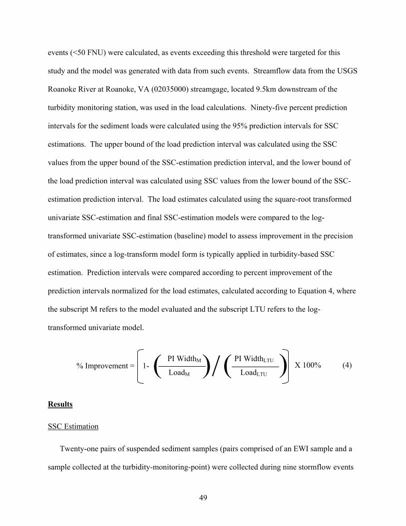
49
events (<50 FNU) were calculated, as events exceeding this threshold were targeted for this
study and the model was generated with data from such events. Streamflow data from the USGS
Roanoke River at Roanoke, VA (02035000) streamgage, located 9.5km downstream of the
turbidity monitoring station, was used in the load calculations. Ninety-five percent prediction
intervals for the sediment loads were calculated using the 95% prediction intervals for SSC
estimations. The upper bound of the load prediction interval was calculated using the SSC
values from the upper bound of the SSC-estimation prediction interval, and the lower bound of
the load prediction interval was calculated using SSC values from the lower bound of the SSC-
estimation prediction interval. The load estimates calculated using the square-root transformed
univariate SSC-estimation and final SSC-estimation models were compared to the log-
transformed univariate SSC-estimation (baseline) model to assess improvement in the precision
of estimates, since a log-transform model form is typically applied in turbidity-based SSC
estimation. Prediction intervals were compared according to percent improvement of the
prediction intervals normalized for the load estimates, calculated according to Equation 4, where
the subscript M refers to the model evaluated and the subscript LTU refers to the log-
transformed univariate model.
Results
SSC Estimation
Twenty-one pairs of suspended sediment samples (pairs comprised of an EWI sample and a
sample collected at the turbidity-monitoring-point) were collected during nine stormflow events
X 100% (4) % Improvement = 1- ( () ) / PI WidthM PI WidthLTU
LoadM LoadLTU
50
over one year. The samples collected represent a variety of conditions, as is indicated by the
distributions of water-quality parameters and sediment properties (Table 3-2); slight differences
are seen in the variables for EWI samples versus point samples because point samples were
collected immediately prior to EWI samples, and conditions during storm events change rapidly.
Turbidity, SC, pH, and water temperature were only collected at the single point in the channel
where the water-quality monitor is located, so differences in these parameters between point and
EWI samples are indicative of temporal variation and not cross-sectional variation. The range of
turbidity values was 45-1160 FNU, and the corresponding SSC range was 44-1310 mg L-1
(Figure 3-2). The mean rainfall contribution from each geologic source area approximated the
source areas’ proportion of the watershed area, but individual storm events exhibited substantial
variation from the means (Table 3-3).
The first step in data analysis was to generate the univariate SSC-estimation model SSCX =
f(Turbidity) using the EWI sampling data. Both logarithmic and square root transformations of
turbidity and SSC provided approximately homoscedastic and normally distributed residuals
(Figure 3-3, Figure 3-4), while the square root transformation provided reduced variance in the
estimation of new values, as indicated by an increased coefficient of determination (Table 3-4,
Figure 3-5); therefore, the square-root transformation was used to generate the univariate SSC-
estimation model. The square root transformed univariate SSC-estimation model had 42% less
unexplained variance (i.e., increased Adjusted R2 from 0.921 to 0.954) than the univariate log-
transformed model (“baseline model”; Table 3-4). The log-transformed (baseline) model is used
as the base for comparison of all future models, as this transformation provided nearly
homoscedastic residuals and is often an appropriate transform for turbidity-based SSC-
estimation.
51
The best-subsets regression process used in development of the multivariate SSC-estimation
model indicated that the addition of any of the measured physical properties, or combination of
those properties, provides an additional 35% - 50% reduction in unexplained variance (relative to
the square-root transformed univariate model) as the Adjusted R2 was increased from 0.954 to
0.970-0.977, with the optimal model containing the %<0.063mm size-fraction variable (Table 3-
5).
The sediment-properties estimation model was developed to estimate % <0.063mm using
continuously measured hydrologic properties as potential explanatory variables. A model
incorporating water temperature and stage was found to explain 45% of the variation in %
<0.063mm (Table 3-4). The radar-derived rainfall estimates for geologic source-areas were
included in the model selection procedure, but did not produce a model with greater predictive
ability than the model given.
Based on this result, we evaluated an SSC estimation model that included turbidity, water
temperature, and stage as independent variables but found that water temperature was not
statistically significant (p< .05). The final SSC-estimation model, which includes turbidity and
stage as independent variables, explains 97.1% of the variance in SSC, a 37% reduction in
unexplained variance relative to the square-root transformed univariate SSC-estimation model
(Adjusted R2 increased from 0.954 to 0.971; Table 3-4, Figure 3-6). Residuals of this model
indicate the addition of stage to the univariate SSC-estimation model did not alter the distribution
of residuals from the univariate SSC-estimation model (Figure 3-7).
Effect of Turbidity Measurement Point on SSC Estimation Precision
Incorporation of the indicator variable (type) and interaction variables (type x turbidity;
type x stage) into the final SSC-estimation model failed to demonstrate a significant difference in
52
the relationships between the explanatory variables and SSC for samples collected at the point of
turbidity measurement versus the entire cross-section (p<.05; Table 3-6). The p-value for the
categorical variable (Type), however, demonstrates significance at a 95% confidence level,
indicating that the intercepts are different for the point and cross-sectional SSC. The intercept of
the model is the value of SSC when turbidity is at its’ minimum value (0), thus differences in
intercept represent a difference in SSC, between the point of turbidity measurement and the
cross-section, for a given value of turbidity.
Suspended Sediment Load Estimation
Total suspended sediment load estimations (Figure 3-8) constructed using the square-
root transformed univariate SSC-estimation model and the final SSC-estimation model are more
precise (have narrower 95% confidence intervals) than the baseline model estimate; the increased
precision is especially pronounced under high-turbidity (>50 NTU) conditions, while the
baseline model produces estimates with the least variance under low-turbidity conditions. All
three SSC-estimation model formulations show that the high turbidity events contributed ≥90%
of total loadings (Figure 3-8, Table 3-7); this contribution to the total load was achieved in less
than 4% of the time-period for which the loads were calculated. The final model showed
improvement in precision, relative to the univariate model, for total and high turbidity (>50
NTU) loadings.
Discussion
It is well documented that turbidity-based SSC-estimation is an improvement over
commonly employed discharge-based procedures (Gippel, 1989; Grayson et al, 1996).
Generally, turbidity-based estimation models are constructed using a logarithmic transform, yet
these data demonstrate a substantial improvement in precision through use of a square-root

53
transform for the study period at this monitoring station. Further improvement is realized through
the addition of variables to represent changes in the particle-size distribution of suspended
sediments.
The results also demonstrate that any variable representing sediment particle-size
properties or organic carbon content can further improve turbidity-based SSC estimation. It is
logical that all of these variables provide a similar capability to reduce SSC-estimation variance,
given their significant correlations (Table 3-8) and the physical relationship between particle-size
and turbidity. This fact is of potential significance to future investigations of this type, given that
the particle-size variable that we found to be optimal in reducing variance can be determined by
sieving, a less time- and resource-intensive procedure than sedimentation-based methods
commonly used to fractionate finer particles.
Hydrologic conditions influence sediment physical properties, and these results indicate
that average particle size tends to increase with increasing stage. This statistical relationship
demonstrates the well-known physical principal: that faster-moving water is capable of
entraining larger particles. Furthermore, the results indicate that water temperature has an affect
on particle-size, and this result is interpreted as a seasonal effect representing sediment
availability and/or variation related to the effect of temperature on particles’ settling velocities,
as the coarse fraction tends to be greater at lower temperatures when water viscosity is greatest
and settling velocities are slower.
We have used the physical relationship between hydrologic conditions and sediment
properties to improve the precision of turbidity-based SSC estimation. Use of a multivariate
SSC-estimation model, which includes √ turbidity and √ stage as explanatory variables,
decreased the unexplained variance of SSC estimations from the square-root transformed
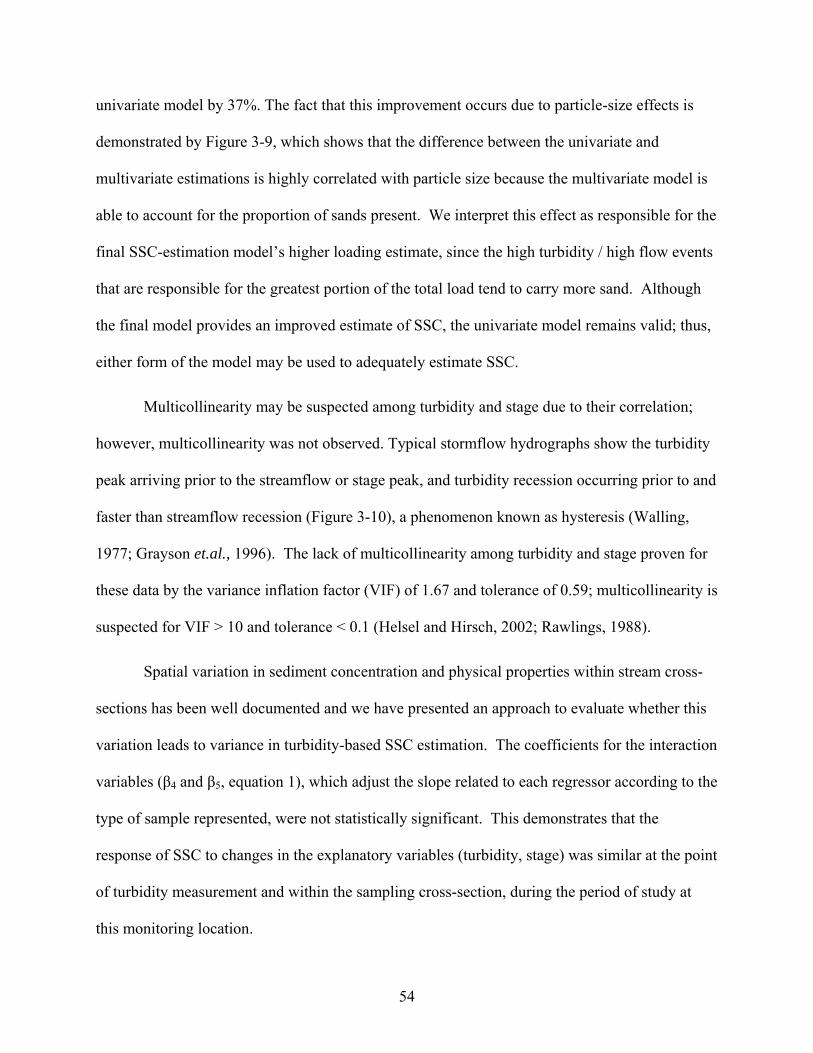
54
univariate model by 37%. The fact that this improvement occurs due to particle-size effects is
demonstrated by Figure 3-9, which shows that the difference between the univariate and
multivariate estimations is highly correlated with particle size because the multivariate model is
able to account for the proportion of sands present. We interpret this effect as responsible for the
final SSC-estimation model’s higher loading estimate, since the high turbidity / high flow events
that are responsible for the greatest portion of the total load tend to carry more sand. Although
the final model provides an improved estimate of SSC, the univariate model remains valid; thus,
either form of the model may be used to adequately estimate SSC.
Multicollinearity may be suspected among turbidity and stage due to their correlation;
however, multicollinearity was not observed. Typical stormflow hydrographs show the turbidity
peak arriving prior to the streamflow or stage peak, and turbidity recession occurring prior to and
faster than streamflow recession (Figure 3-10), a phenomenon known as hysteresis (Walling,
1977; Grayson et.al., 1996). The lack of multicollinearity among turbidity and stage proven for
these data by the variance inflation factor (VIF) of 1.67 and tolerance of 0.59; multicollinearity is
suspected for VIF > 10 and tolerance < 0.1 (Helsel and Hirsch, 2002; Rawlings, 1988).
Spatial variation in sediment concentration and physical properties within stream cross-
sections has been well documented and we have presented an approach to evaluate whether this
variation leads to variance in turbidity-based SSC estimation. The coefficients for the interaction
variables (β4 and β5, equation 1), which adjust the slope related to each regressor according to the
type of sample represented, were not statistically significant. This demonstrates that the
response of SSC to changes in the explanatory variables (turbidity, stage) was similar at the point
of turbidity measurement and within the sampling cross-section, during the period of study at
this monitoring location.
55
The β3 coefficient (equation 1), which represents the effect of sampling method on the
regression intercept, was significant. This term shifts the regression line upward for the cross-
sectional SSC compared to the point SSC, without affecting its slope; therefore, the SSC at the
turbidity measuring point, near the water surface, is typically less than the stream’s depth- and
width-integrated (EWI) SSC. Fewer large particles occur near the surface than at depth, due to
gravitational effects, as indicated by the fact that % <0.063mm is generally greater in the point-
of-turbidity-measurement samples than in the EWI samples (Figure 3-11), The “upward shift”
does not introduce additional variance in the SSC-estimation since this shift does not alter the
rate at which SSC responds to explanatory variables.
Although the improvement in SSC-estimation precision may not appear to be of great
significance in relation to a single estimation (R2 = 0.954 for the univariate estimation vs. 0.971
for the multivariate estimation), this improvement becomes more significant when using the
SSC-estimates for load estimation. The comparison of suspended sediment loads calculated
using each of the models developed clearly demonstrates the improvement realized through the
further explanation of variance in the turbidity-based SSC estimation model. The largest
improvement was realized through the application of a square root transformation, instead of a
logarithmic transformation, due to the greatly reduced estimation errors during periods of
elevated turbidity, which typically coincide with elevated streamflow and greater loadings.
Although the prediction interval for the square root transformed data are much wider at lower
turbidity values, as compared to the logarithmic transformation, these errors contribute little to
the total error in load calculation as flow, and therefore loading, is also low during these periods.
The comparison of load estimations and associated prediction intervals also demonstrates the
56
importance of explaining as much variance as possible, as even the best model has a large 95%
prediction interval.
Conclusions
As anthropogenic landscape influences increase sediment transport within waterways, the
importance of accurately quantifying this transport is vital. The precision of a widely employed
SSC monitoring method, which uses turbidity as a surrogate for SSC, can be improved if the
physical properties of the suspended sediments, and variation in those properties, are known.
This research has shown that hydrologic variables which can be measured remotely and at the
same temporal scale as turbidity can be used to estimate suspended-sediment physical properties,
and that inclusion of these variables in an SSC-estimation model improved that model’s
precision. The hydrologic variable found to represent changes in physical properties of sediment
was stage, which is commonly measured when a turbidity monitoring device is employed,
meaning that the improvement in SSC-estimation can be realized without additional costs.
57
References
American Society for Testing and Materials, 2002, D3977-97, “Standard Test Methods for Determining Sediment Concentration in Water Samples”, ASTM International.
Christensen, V.D., X. Jian, A.C. Ziegler. 2000. Regression Analysis and Real-Time Water-Quality Monitoring to Estimate Constituent Concentrations, Loads, and Yields in the Little Arkansas River, South Central Kansas. United States Geological Survey Water-Resources Investigations Report 00-4126.
Davies-Colley R.J., D.G. Smith. 2001. Turbidity, Suspended Sediment, and Water Clarity: A Review. Journal of American Water Resources Association. 37:1085 – 1101.
Edwards, T.K., and Glysson, G.D.. 1999. Field Methods for Measurement of Fluvial Sediment: US Geological Survey Techniques of Water-Resources Investigations Book 3, Chap. C2,89 p.
Gippel, C.J., 1989. The use of turbidimeters in suspended sediment research. Hydrobiologia 176/177:465-480.
Gippel, C.J., 1995. Potential of Turbidity Monitoring for Measuring the Transport of Suspended Solids in Streams. Hydrological Processes 9:83-97.
Gray, J.R., E. Patino, P. Rasmussen, M. Larson, T. Melis, D. Topping, M. Runner, C. Alamo. 2003. Evaluation of Sediment-Surrogate technologies for computation of suspended-sediment transport. Accessed online 4-12-2006. http://water.usgs.gov/osw/techniques/yrcc_surrogates.pdf
Grayson, R.B., B.L. Finlayson, C.J. Gippel, B.T. Hart. 1996. The potential of field turbidity measurements for the computation of total phosphorus and suspended solids loads. Journal of Environmental Management 47: 257-267.
Guy, H.P. 1969. Laboratory theory and methods for sediment analysis in Techniques of Water-Resources Investigations of the United States Geological Survey, Book 5, Chapter C1. United States Government Printing Office, Washington D.C.
Grayson, R.B., B.L. Finlayson, C.J. Gippel, B.T. Hart. 1996. The potential of field turbidity measurements for the computation of total phosphorus and suspended solids loads. Journal of Environmental Management 47: 257-267.
Helsel, D.R., R.M. Hirsch. 2002. Statistical Methods in Water Resources in Techniques of Water-Resources Investigations of the United States Geological Survey: Book 4, Chapter A3. United States Government Printing Office, Washington D.C.
Horowitz, A.J., F.A. Rinella, P. Lamothe, T.L. Miller, T.K. Edwards, R.L. Roche, D.A. Rickert. 1990. Variations in suspended sediment and associated trace element concentrations in selected riverine cross sections. Environmental Science and Technology 24:1313-1320.
Martin, G.R., J.L. Smoot, K.D. White. 1992. A comparison of surface-grab and cross sectionally integrated stream-water-quality sampling methods. Water Environment Research 64: 866-876.
Nelson, D.W. and L.E. Sommers. 1996. Total Carbon, Organic Carbon, and Organic Matter. P 961-1010, in: D.L. Sparks et. al. (eds.) Methods of soil analysis. Part 3, Chemical Methods. Soil Science Society of America, Madison, Wisconsin.
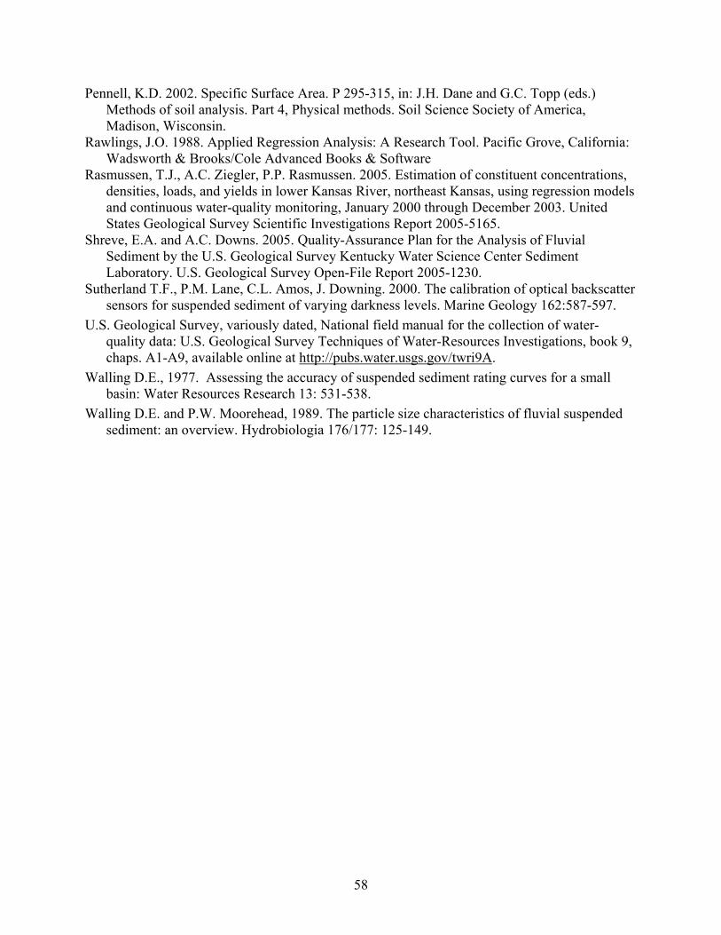
58
Pennell, K.D. 2002. Specific Surface Area. P 295-315, in: J.H. Dane and G.C. Topp (eds.) Methods of soil analysis. Part 4, Physical methods. Soil Science Society of America, Madison, Wisconsin.
Rawlings, J.O. 1988. Applied Regression Analysis: A Research Tool. Pacific Grove, California: Wadsworth & Brooks/Cole Advanced Books & Software
Rasmussen, T.J., A.C. Ziegler, P.P. Rasmussen. 2005. Estimation of constituent concentrations, densities, loads, and yields in lower Kansas River, northeast Kansas, using regression models and continuous water-quality monitoring, January 2000 through December 2003. United States Geological Survey Scientific Investigations Report 2005-5165.
Shreve, E.A. and A.C. Downs. 2005. Quality-Assurance Plan for the Analysis of Fluvial Sediment by the U.S. Geological Survey Kentucky Water Science Center Sediment Laboratory. U.S. Geological Survey Open-File Report 2005-1230.
Sutherland T.F., P.M. Lane, C.L. Amos, J. Downing. 2000. The calibration of optical backscatter sensors for suspended sediment of varying darkness levels. Marine Geology 162:587-597.
U.S. Geological Survey, variously dated, National field manual for the collection of water-quality data: U.S. Geological Survey Techniques of Water-Resources Investigations, book 9, chaps. A1-A9, available online at http://pubs.water.usgs.gov/twri9A.
Walling D.E., 1977. Assessing the accuracy of suspended sediment rating curves for a small basin: Water Resources Research 13: 531-538.
Walling D.E. and P.W. Moorehead, 1989. The particle size characteristics of fluvial suspended sediment: an overview. Hydrobiologia 176/177: 125-149.
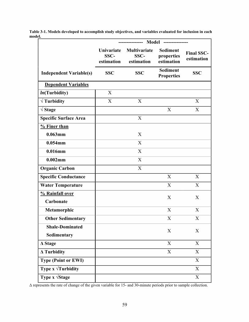
59
Table 3-1. Models developed to accomplish study objectives, and variables evaluated for inclusion in each model.
--------------- Model ---------------
Univariate
SSC-estimation
Multivariate SSC-
estimation
Sediment properties estimation
Final SSC- estimation
Independent Variable(s) SSC SSC Sediment Properties SSC
Dependent Variables
ln(Turbidity) X
√ Turbidity X X X
√ Stage X X
Specific Surface Area X
% Finer than
0.063mm
X
0.054mm X
0.016mm X
0.002mm X
Organic Carbon X
Specific Conductance X X
Water Temperature X X
% Rainfall over
Carbonate
X X
Metamorphic X X
Other Sedimentary X X
Shale-Dominated
Sedimentary
X X
∆ Stage X X
∆ Turbidity X X
Type (Point or EWI) X
Type x √Turbidity X
Type x √Stage X ∆ represents the rate of change of the given variable for 15- and 30-minute periods prior to sample collection.
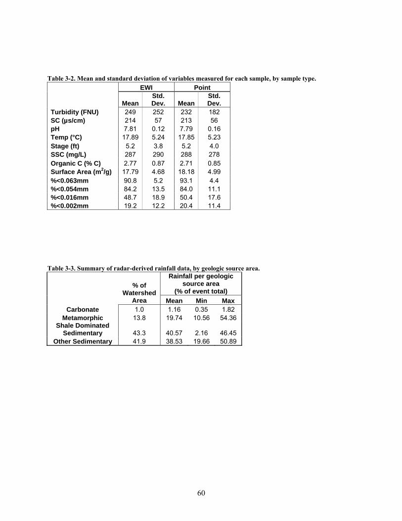
60
Table 3-2. Mean and standard deviation of variables measured for each sample, by sample type.
EWI Point
Mean Std. Dev. Mean
Std. Dev.
Turbidity (FNU) 249 252 232 182 SC (µs/cm) 214 57 213 56 pH 7.81 0.12 7.79 0.16 Temp (°C) 17.89 5.24 17.85 5.23 Stage (ft) 5.2 3.8 5.2 4.0 SSC (mg/L) 287 290 288 278 Organic C (% C) 2.77 0.87 2.71 0.85 Surface Area (m2/g) 17.79 4.68 18.18 4.99 %<0.063mm 90.8 5.2 93.1 4.4 %<0.054mm 84.2 13.5 84.0 11.1 %<0.016mm 48.7 18.9 50.4 17.6 %<0.002mm 19.2 12.2 20.4 11.4
Table 3-3. Summary of radar-derived rainfall data, by geologic source area.
Rainfall per geologic source area
(% of event total)
% of Watershed
Area Mean Min Max Carbonate 1.0 1.16 0.35 1.82
Metamorphic 13.8 19.74 10.56 54.36 Shale Dominated
Sedimentary 43.3 40.57 2.16 46.45 Other Sedimentary 41.9 38.53 19.66 50.89
61
Table 3-4. SSC estimation models and associated statistics (*PRESS statistics are not comparable between different transformations).
Model Adjusted R2 PRESS
Baseline SSCX = exp [0.2012 + 0.9863 ( ln Turbidity)] 0.921 *
Univariate SSC-estimation SSCX = [0.1036 + 1.064 (√Turbidity)]2 0.954 52.31
Multivariate SSC-estimation
SSCX = [18.7537 + 1.0837 (√Turbidity) – 20.8465 (%<0.063mm)]2 0.977 33.39
Sediment Properties estimation
%<0.063 = 0.8675 + 0.0054 (Water Temperature) – 0.0261 (√Stage) 0.450 0.034
Final SSC-estimation
SSCX = [-1.7579 + 0.9567 (√Turbidity) + 1.5699 (√Stage)]2 0.971 38.17
Table 3-5. Results of Variable Selection Procedure for Multivariate SSC-estimation model. Variables in Model CP R2 Adjusted R2
√Turbidity % < 0.063mm 0.58 0.979 0.977
√Turbidity % < 0.016mm 2.32 0.977 0.974
√Turbidity % < 0.002mm 4.19 0.974 0.972
√Turbidity Organic C 4.23 0.974 0.972
√Turbidity % < 0.054mm 4.37 0.974 0.971
√Turbidity Surface Area 5.53 0.973 0.970
√Turbidity 15.51 0.957 0.954
Note: All possible combinations of multiple physical properties were evaluated, these combinations produced models which ranked within the range of those shown above, yet did not exceed the predictive capability of the optimal model given.
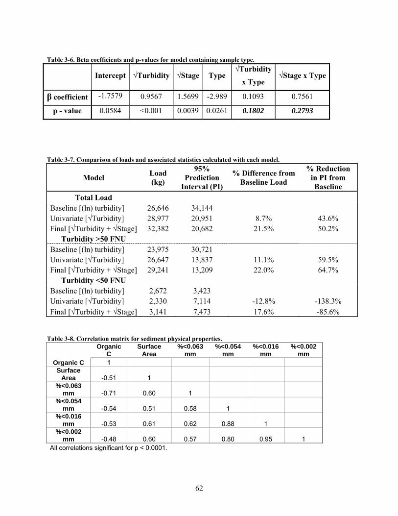
62
Table 3-6. Beta coefficients and p-values for model containing sample type.
Intercept √Turbidity √Stage Type √Turbidity
x Type √Stage x Type
β coefficient -1.7579 0.9567 1.5699 -2.989 0.1093 0.7561
p - value 0.0584 <0.001 0.0039 0.0261 0.1802 0.2793
Table 3-7. Comparison of loads and associated statistics calculated with each model.
Model Load (kg)
95% Prediction
Interval (PI)
% Difference from Baseline Load
% Reduction in PI from Baseline
Total Load Baseline [(ln) turbidity] 26,646 34,144 Univariate [√Turbidity] 28,977 20,951 8.7% 43.6% Final [√Turbidity + √Stage] 32,382 20,682 21.5% 50.2%
Turbidity >50 FNU Baseline [(ln) turbidity] 23,975 30,721 Univariate [√Turbidity] 26,647 13,837 11.1% 59.5% Final [√Turbidity + √Stage] 29,241 13,209 22.0% 64.7%
Turbidity <50 FNU Baseline [(ln) turbidity] 2,672 3,423 Univariate [√Turbidity] 2,330 7,114 -12.8% -138.3% Final [√Turbidity + √Stage] 3,141 7,473 17.6% -85.6%
Table 3-8. Correlation matrix for sediment physical properties.
Organic
C Surface
Area %<0.063
mm %<0.054
mm %<0.016
mm %<0.002
mm Organic C 1 Surface
Area -0.51 1 %<0.063
mm -0.71 0.60 1 %<0.054
mm -0.54 0.51 0.58 1 %<0.016
mm -0.53 0.61 0.62 0.88 1 %<0.002
mm -0.48 0.60 0.57 0.80 0.95 1 All correlations significant for p < 0.0001.
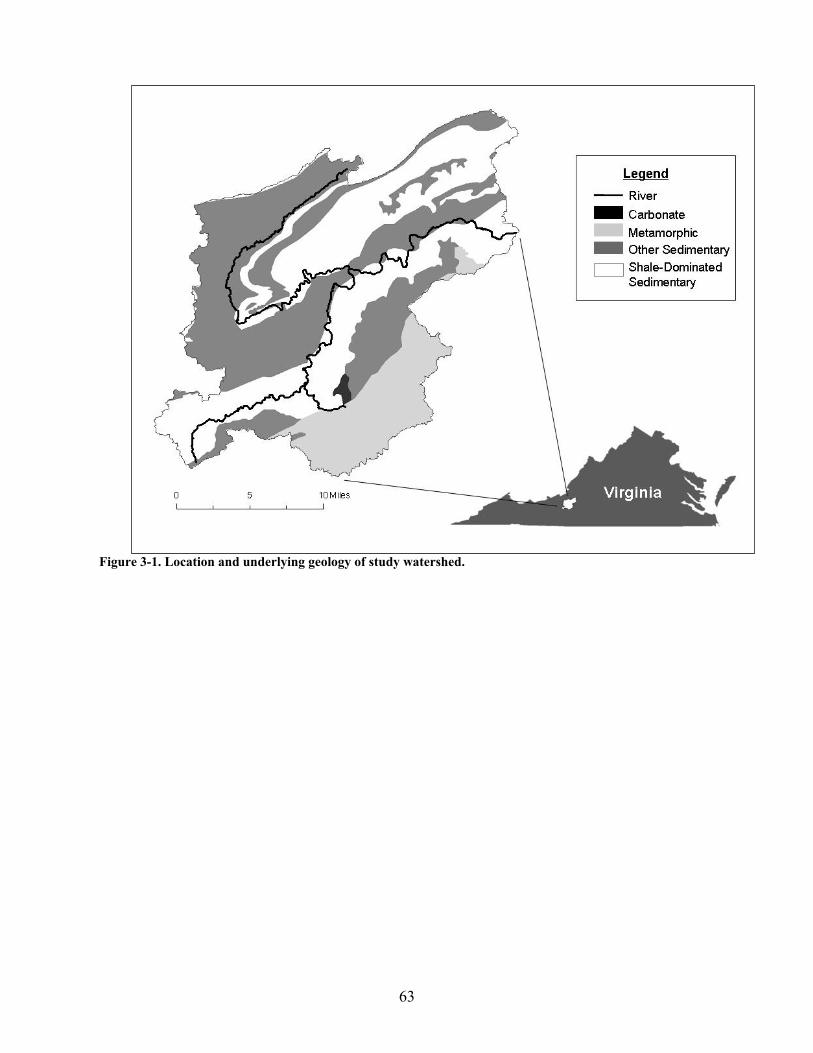
63
Figure 3-1. Location and underlying geology of study watershed.
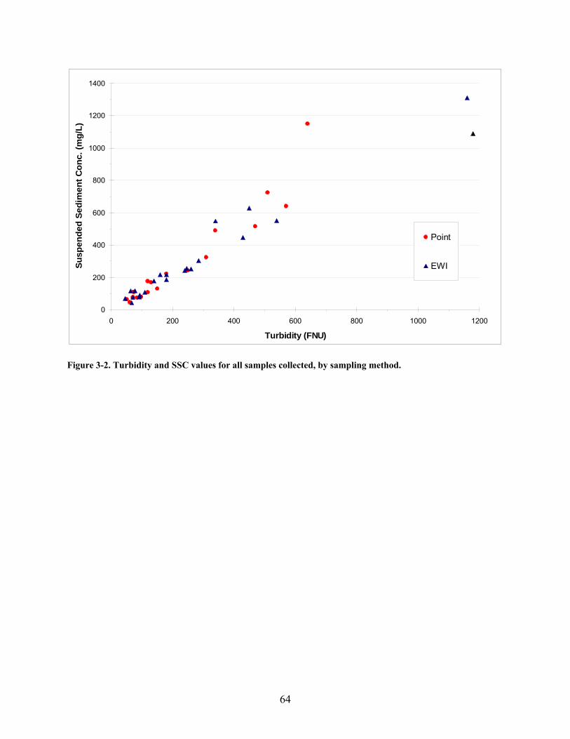
64
0
200
400
600
800
1000
1200
1400
0 200 400 600 800 1000 1200
Turbidity (FNU)
Susp
ende
d Se
dim
ent C
onc.
(mg/
L)
Point
EWI
Figure 3-2. Turbidity and SSC values for all samples collected, by sampling method.
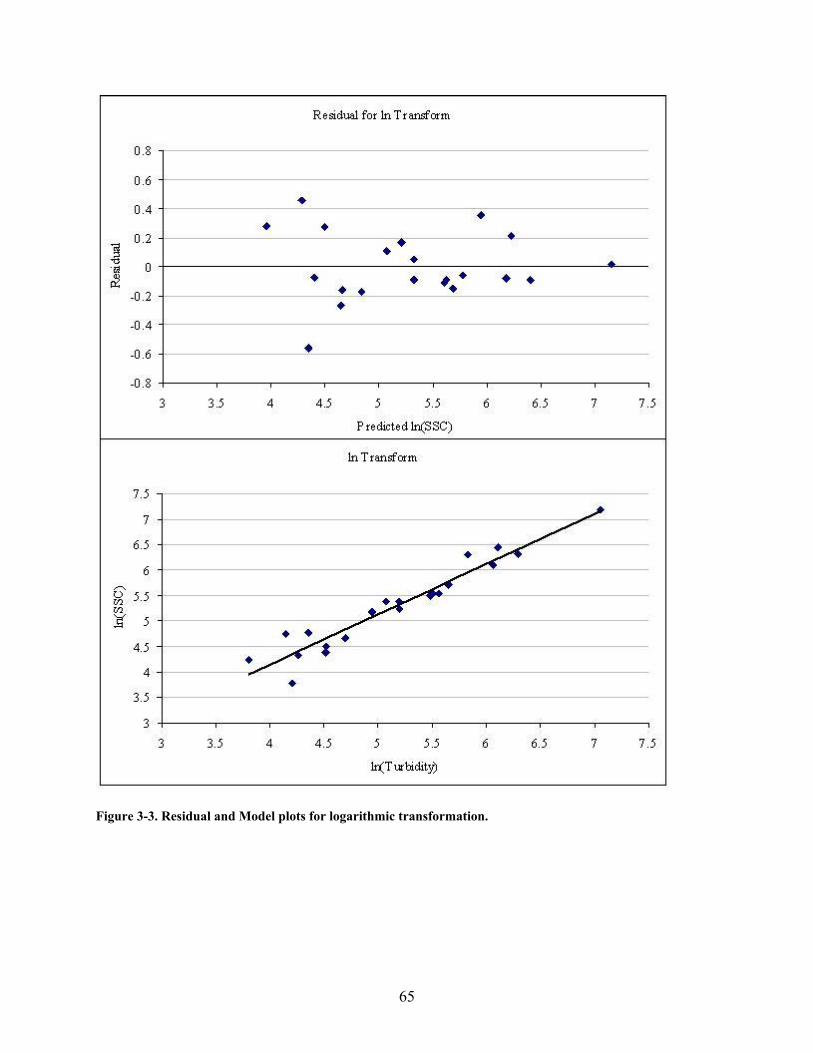
65
Figure 3-3. Residual and Model plots for logarithmic transformation.
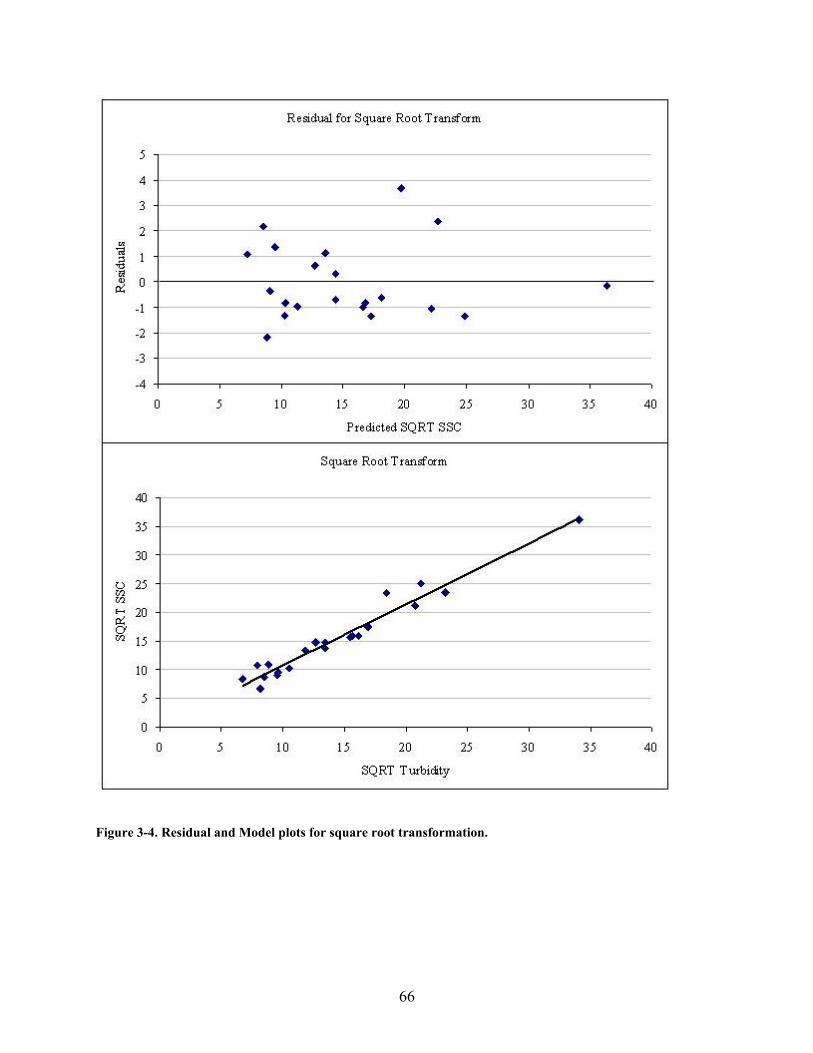
66
Figure 3-4. Residual and Model plots for square root transformation.
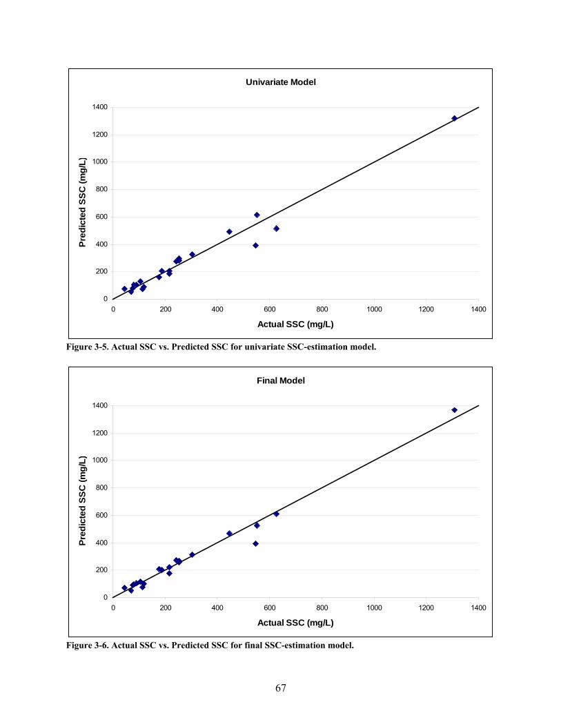
67
Univariate Model
0
200
400
600
800
1000
1200
1400
0 200 400 600 800 1000 1200 1400
Actual SSC (mg/L)
Pred
icte
d SS
C (m
g/L)
Figure 3-5. Actual SSC vs. Predicted SSC for univariate SSC-estimation model.
Final Model
0
200
400
600
800
1000
1200
1400
0 200 400 600 800 1000 1200 1400
Actual SSC (mg/L)
Pred
icte
d SS
C (m
g/L)
Figure 3-6. Actual SSC vs. Predicted SSC for final SSC-estimation model.
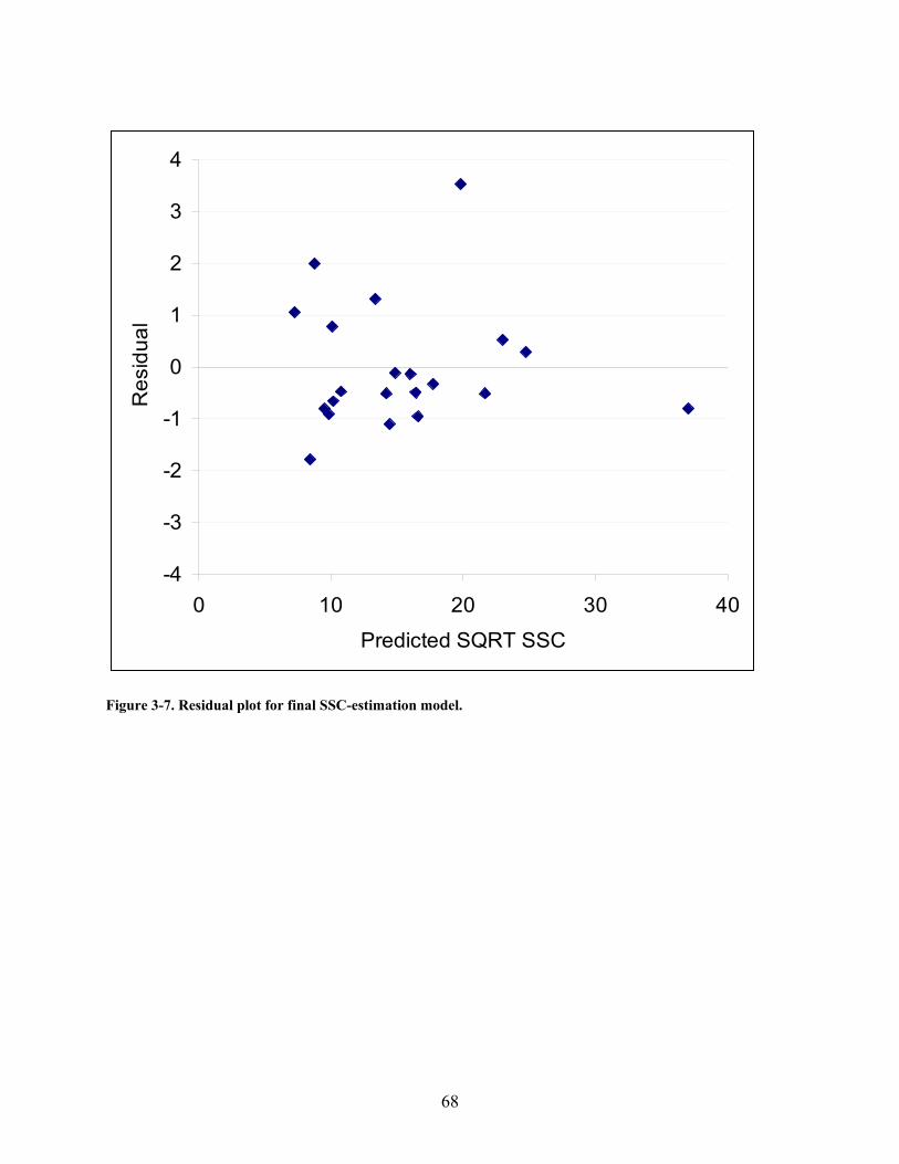
68
-4
-3
-2
-1
0
1
2
3
4
0 10 20 30 40
Predicted SQRT SSC
Res
idua
l
Figure 3-7. Residual plot for final SSC-estimation model.
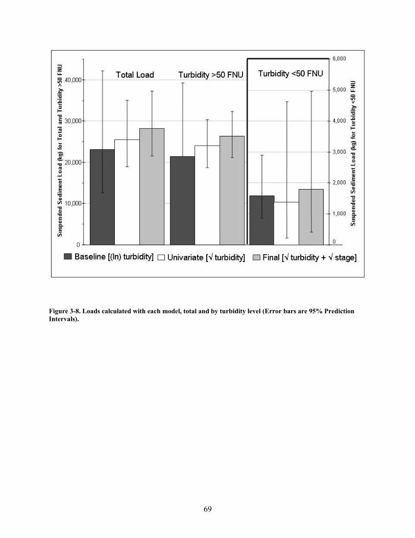
69
Figure 3-8. Loads calculated with each model, total and by turbidity level (Error bars are 95% Prediction Intervals).
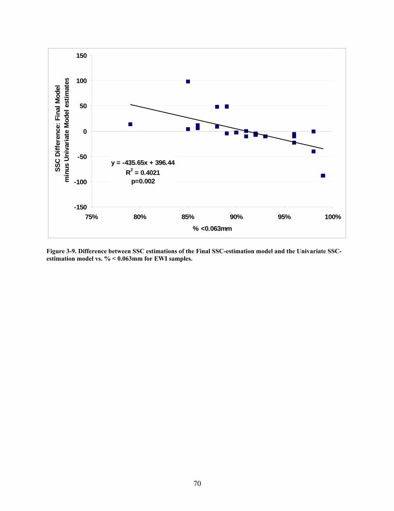
70
y = -435.65x + 396.44R2 = 0.4021
p=0.002
-150
-100
-50
0
50
100
150
75% 80% 85% 90% 95% 100%
% <0.063mm
SSC
Diff
eren
ce: F
inal
Mod
elm
inus
Uni
vari
ate
Mod
el e
stim
ates
Figure 3-9. Difference between SSC estimations of the Final SSC-estimation model and the Univariate SSC-estimation model vs. % < 0.063mm for EWI samples.
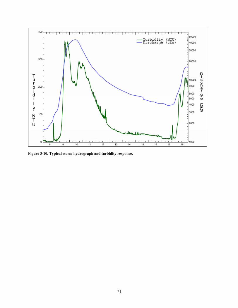
71
Figure 3-10. Typical storm hydrograph and turbidity response.
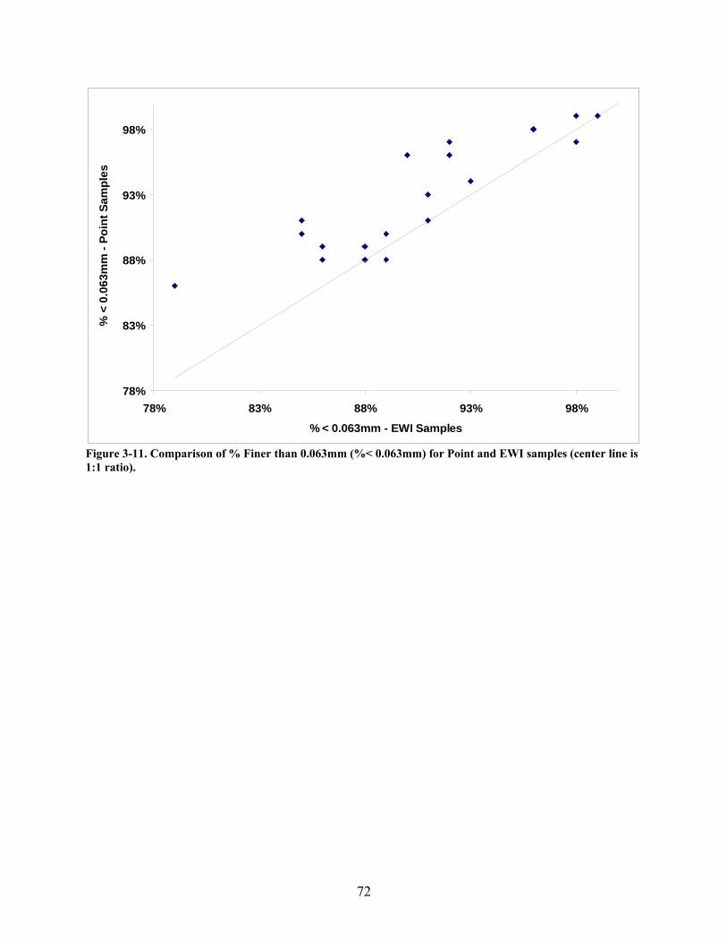
72
78%
83%
88%
93%
98%
78% 83% 88% 93% 98%
% < 0.063mm - EWI Samples
% <
0.0
63m
m -
Poin
t Sam
ples
Figure 3-11. Comparison of % Finer than 0.063mm (%< 0.063mm) for Point and EWI samples (center line is 1:1 ratio).

73
Chapter 4 Pooling Data from Multiple Monitoring Stations to Improve Turbidity-based SSC-estimation
Introduction The United States Army Corps of Engineers (USACOE) is currently constructing the
Roanoke River Flood Reduction Project (RRFRP) along the Roanoke River within the City of
Roanoke, VA. These flood reduction measures require creation of bench cuts, removal of
earthen material within the floodplain, and removal of flow constricting structures and
vegetation. The purpose of these actions is to increase the storage capacity of the river channel
and its’ floodplain to facilitate conveyance of flood waters.
Because of the increased availability of sediment along the river banks during
construction and the potential harm to the aquatic ecosystems if this sediment were to enter the
river, the United States Geological Survey is monitoring turbidity, a commonly applied surrogate
for suspended sediment concentration (SSC), in the river at multiple locations within the
construction reach.
Research was conducted at the Roanoke River at Route 117 monitoring station in order to
maximize the predictive ability of the models used to relate turbidity to SSC (see Chapter 3),
while this Chapter describes an application of the method derived in Chapter 3 at a second
location. Specific objectives for this portion of the study are to:
1) Use the approach outlined in Chapter 3 to develop a turbidity-based SSC-estimation
model for the Roanoke River at 13th Street Monitoring Station.
74
2) Determine if a single turbidity-based SSC-estimation model, developed by combining data from the Route 117 and 13th Street monitoring stations (“pooled model”), can effectively estimate SSC at those two locations.
3) If Objective 2 concludes that a multiple-location SSC-estimation model is feasible: compare the capabilities of models developed through Objectives 1 and 2 to estimate sediment loadings.
Methods
Thirteenth Street (site-specific) Model This portion of the study was conducted at the USGS Roanoke River at Thirteenth Street
Bridge at Roanoke, VA (02055080) monitoring station, downstream of the RRFRP construction
reach and approximately 13 river km downstream of the Route 117 monitoring station, which
was the subject of study described on Chapter 3.
The methods described in Chapters 2 and 3 regarding sample collection, hydrologic data
collection, water-quality (turbidity, SC, pH, water temperature) data collection, lab analyses, and
data analyses were employed in this study. A SSC-estimation model was developed for data
collected at Thirteenth Street using the same variables and procedures described in Chapter 3
(site-specific model). Annual suspended-sediment loads were estimated for Thirteenth Street
using the site-specific multivariate model for the time period of March 28, 2006 (the first date for
which stage data were available at Thirteenth Street) to March 27, 2007. Streamflow data from
the USGS Roanoke River at Roanoke, VA (02055000) streamgage, located 3.5km upstream of
the turbidity monitoring station, were used in the load calculation.
Pooled Model The statistical procedure used to develop and evaluate a single SSC-estimation model
using data collected at both Route 117 and Thirteenth Street (“pooled model”) was similar to the
procedure used to determine potential differences between the point of turbidity measurement
75
and the entire cross-section at a single monitoring location (Chapter 3). This determination was
conducted by pooling the data from the EWI samples at both monitoring locations and
generating a model for this pooled dataset. The pooled dataset consisted of data collected for the
purposes of this study and data collected for the RRFRP monitoring program. Data collected for
the RRFRP monitoring program were collected and analyzed using the same methods as were
used for this study; however, only SSC and % <0.063mm analyses were completed and stage
was not measured.
Square-root and logarithmic transformations of turbidity were evaluated to determine the
appropriate transformation for use in construction of this pooled model. Since the individual
estimation models for each location include turbidity and stage, the pooled model was expected
to require these same variables. However, stage measurement at the two monitoring locations is
based on different base elevations (datums) and channel geometry differs between the two
stations; therefore, stage is not comparable between stations. Discharge, measured at the
Roanoke River at Roanoke, VA (02055000) streamgage (located between the two stations) was
used as the hydrologic variable in the combined model.
Upon determination of the appropriate model, an indicator variable and two interaction
terms were added to evaluate the effect of sampling location on SSC estimation. The indicator
variable represents the sampling location with a value of zero for Route 117 and a value of one
for Thirteenth Street. The interaction variables are the products of the indicator variable and
each of the other explanatory variables (turbidity and discharge). Tests of significance of the
indicator and interaction terms were used to determine if the differences between the locations
were significant. If the interaction terms were not determined to be statistically significant, the
conclusion would be that the relationship between the explanatory variables and SSC was similar
76
at both locations. If the indicator terms were not determined to be statistically significant the
conclusion would be that the model intercepts were similar at each monitoring location. If none
of the interaction or indicator terms were statistically significant, the conclusion would be that it
was acceptable to apply the pooled model at both locations. The form of the overall model is
given in Equation 1 (where Q represents discharge), while Equations 2 and 3 demonstrate the
effect of the indicator and interaction terms on the overall model. Equation 2 demonstrates the
case when Location = 0, representing Route 117. Equation 3 demonstrates the case when
Location = 1, indicating that the sample was collected at Thirteenth Street; note that the value of
one for Location results in β3 being added to the intercept while β4 and β5 are added to the slope
of Turbidity and Discharge, respectively.
√SSC = β0 + β1(√Turbidity) + β2(Q) + β3(Location) + β4(√Turbidity x Location) +
β5(Q x Location) (1)
√SSC = β0 + β1 (√Turbidity) + β2 (Q) (2)
√SSC = (β0 + β3) + (β1 + β4)√Turbidity + (β2 + β5)Q (3)
Annual suspended sediment loads were calculated for each monitoring location using the
pooled model and streamflow data from the Roanoke River at Roanoke, VA (02055000)
streamgage; these loads, and associated 95% prediction intervals, were compared to the loads
and prediction intervals calculated using the site-specific models.
Results
Thirteenth Street (site-specific) Model Eleven pairs of samples (point and cross-section pairs) were collected at Thirteenth Street
during periods of elevated turbidity over one-year (Figure 4-1). The samples collected
represented a range of conditions (Table 4-1); slight differences are seen in the variables for EWI
samples versus Point samples because point samples were collected immediately prior to EWI
77
samples, and conditions during storm events change rapidly. Turbidity, SC, pH, and water
temperature were only measured at the point in the channel where the water-quality monitor is
located, so differences in these parameters between point and EWI samples are indicative of
temporal variation not cross-sectional variation. Five of the eleven sample pairs were collected
during a single storm event lasting three days, thus the results of this model generation process
may be biased towards this event and would ideally be verified with data collected in the future.
The initial step of site-specific model generation indicated that the log-based transform is
more appropriate for this dataset than the square-root transform (Figure 4-2). The results of the
best-subsets regression procedure used to determine if additional variance in the turbidity-based
SSC prediction can be explained by incorporating physical properties of the suspended sediments
indicates that an improvement in model precision is realized through this process. Two models
incorporating sediment physical properties were found to be superior to the site-specific
univariate-SSC estimation model, with the best model containing the organic C variable (Table
4-2). The turbidity and physical property SSC-estimation model (adjusted R2 = 92.4%; Table 4-
3) demonstrates a 24% decrease in unexplained variance compared to the univariate SSC-
estimation model (Increased adjusted R2 from 90.0% to 92.4%). The site-specific multivariate
SSC-estimation model, developed by evaluating those variables capable of predicting the organic
C includes turbidity and stage (Table 4-3). The multivariate model provides a 43% reduction in
the unexplained variance present in the univariate SSC-estimation model, as the amount of
explained variance (adjusted R2) is increased from 90.0% to 94.3% (Table 4-3).
When using both the point-sample and EWI-sample data collected at Thirteenth Street,
incorporation of indicator (type) and interaction ( ln(turbidity) x type, ln(stage) x type) variables
into the multivariate SSC-estimation model demonstrated that there is no sample type effect on
78
the estimation of SSC, as the interaction terms were not significant (Table 4-4). Furthermore, the
indicator variable was not significant, demonstrating that a difference in baseline SSC values
between the point and the entire cross-section is not statistically detectable in the available data
(Table 4-4).
Annual loads estimated using the univariate SSC-estimation model and multivariate SSC-
estimation model demonstrate a 22% increase in the estimated load and 27% decrease in the
width of the 95% prediction band as a result of the addition of stage in the multivariate SSC-
estimation model (Table 4-5, Figure 4-3).
Pooled Model Because of the limitations of the small dataset for Thirteenth Street, in which nearly half
the observations represent a single event, the pooled model was generated using data collected
for the purposes of this research supplemented with data collected for the purposes of the
RRFRP monitoring program, resulting in 27 samples for Route 117 and 31 samples for
Thirteenth Street (Figure 4-4).
Investigation into the proper transformation for the pooled model revealed that the log-
based transformation provided a better distribution of residuals (Figure 4-5) and greater
explanatory power, when compared to the square-root transformation (Table 4-6). Addition of
discharge, measured at the Walnut Street streamgage, provided improved estimates of SSC in
comparison to the univariate turbidity-based SSC-estimation model (Table 4-6), as indicated by
the 26% decrease in unexplained variance (Adj. R2 increased from 95.4% to 96.6%) and the
decrease in PRESS from 5.24 to 3.89.
Since the pooled model was determined to be effective for estimating SSC, the
investigation of whether differences exist between the two monitoring locations, which would
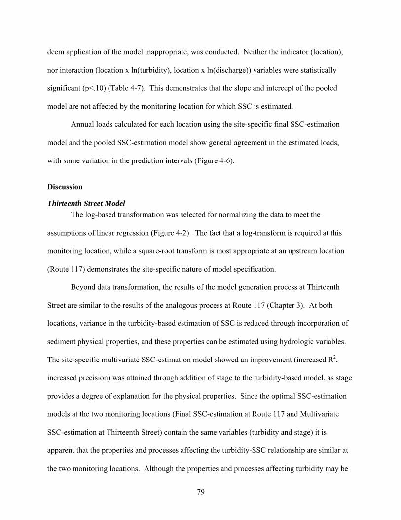
79
deem application of the model inappropriate, was conducted. Neither the indicator (location),
nor interaction (location x ln(turbidity), location x ln(discharge)) variables were statistically
significant (p<.10) (Table 4-7). This demonstrates that the slope and intercept of the pooled
model are not affected by the monitoring location for which SSC is estimated.
Annual loads calculated for each location using the site-specific final SSC-estimation
model and the pooled SSC-estimation model show general agreement in the estimated loads,
with some variation in the prediction intervals (Figure 4-6).
Discussion
Thirteenth Street Model The log-based transformation was selected for normalizing the data to meet the
assumptions of linear regression (Figure 4-2). The fact that a log-transform is required at this
monitoring location, while a square-root transform is most appropriate at an upstream location
(Route 117) demonstrates the site-specific nature of model specification.
Beyond data transformation, the results of the model generation process at Thirteenth
Street are similar to the results of the analogous process at Route 117 (Chapter 3). At both
locations, variance in the turbidity-based estimation of SSC is reduced through incorporation of
sediment physical properties, and these properties can be estimated using hydrologic variables.
The site-specific multivariate SSC-estimation model showed an improvement (increased R2,
increased precision) was attained through addition of stage to the turbidity-based model, as stage
provides a degree of explanation for the physical properties. Since the optimal SSC-estimation
models at the two monitoring locations (Final SSC-estimation at Route 117 and Multivariate
SSC-estimation at Thirteenth Street) contain the same variables (turbidity and stage) it is
apparent that the properties and processes affecting the turbidity-SSC relationship are similar at
the two monitoring locations. Although the properties and processes affecting turbidity may be
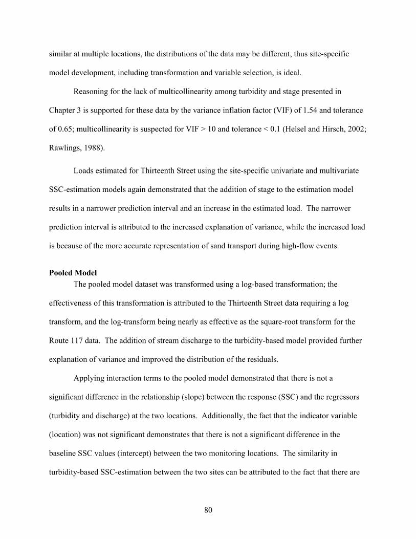
80
similar at multiple locations, the distributions of the data may be different, thus site-specific
model development, including transformation and variable selection, is ideal.
Reasoning for the lack of multicollinearity among turbidity and stage presented in
Chapter 3 is supported for these data by the variance inflation factor (VIF) of 1.54 and tolerance
of 0.65; multicollinearity is suspected for VIF > 10 and tolerance < 0.1 (Helsel and Hirsch, 2002;
Rawlings, 1988).
Loads estimated for Thirteenth Street using the site-specific univariate and multivariate
SSC-estimation models again demonstrated that the addition of stage to the estimation model
results in a narrower prediction interval and an increase in the estimated load. The narrower
prediction interval is attributed to the increased explanation of variance, while the increased load
is because of the more accurate representation of sand transport during high-flow events.
Pooled Model The pooled model dataset was transformed using a log-based transformation; the
effectiveness of this transformation is attributed to the Thirteenth Street data requiring a log
transform, and the log-transform being nearly as effective as the square-root transform for the
Route 117 data. The addition of stream discharge to the turbidity-based model provided further
explanation of variance and improved the distribution of the residuals.
Applying interaction terms to the pooled model demonstrated that there is not a
significant difference in the relationship (slope) between the response (SSC) and the regressors
(turbidity and discharge) at the two locations. Additionally, the fact that the indicator variable
(location) was not significant demonstrates that there is not a significant difference in the
baseline SSC values (intercept) between the two monitoring locations. The similarity in
turbidity-based SSC-estimation between the two sites can be attributed to the fact that there are
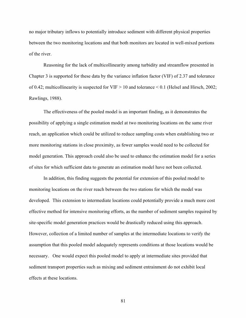
81
no major tributary inflows to potentially introduce sediment with different physical properties
between the two monitoring locations and that both monitors are located in well-mixed portions
of the river.
Reasoning for the lack of multicollinearity among turbidity and streamflow presented in
Chapter 3 is supported for these data by the variance inflation factor (VIF) of 2.37 and tolerance
of 0.42; multicollinearity is suspected for VIF > 10 and tolerance < 0.1 (Helsel and Hirsch, 2002;
Rawlings, 1988).
The effectiveness of the pooled model is an important finding, as it demonstrates the
possibility of applying a single estimation model at two monitoring locations on the same river
reach, an application which could be utilized to reduce sampling costs when establishing two or
more monitoring stations in close proximity, as fewer samples would need to be collected for
model generation. This approach could also be used to enhance the estimation model for a series
of sites for which sufficient data to generate an estimation model have not been collected.
In addition, this finding suggests the potential for extension of this pooled model to
monitoring locations on the river reach between the two stations for which the model was
developed. This extension to intermediate locations could potentially provide a much more cost
effective method for intensive monitoring efforts, as the number of sediment samples required by
site-specific model generation practices would be drastically reduced using this approach.
However, collection of a limited number of samples at the intermediate locations to verify the
assumption that this pooled model adequately represents conditions at those locations would be
necessary. One would expect this pooled model to apply at intermediate sites provided that
sediment transport properties such as mixing and sediment entrainment do not exhibit local
effects at these locations.

82
Comparison of the load estimations performed using the optimal site-specific final SSC-
estimation models and the pooled SSC-estimation model demonstrate the effectiveness of the
pooled model. The estimations of load are comparable at each location, and the prediction
interval at Thirteenth Street is narrower when using the pooled model. The wider prediction
interval for the site-specific model (at Thirteenth Street) is reflective of the small number of data
points used in specification of this model. The wider prediction interval of the pooled model at
Route 117 exists for those reasons discussed in Chapter 3 regarding square-root versus log-based
transformations.
Conclusions
This study has shown that while the physical properties and processes leading to variance
in turbidity-based estimation of SSC may be similar at various monitoring locations, data
distributions may vary by location and therefore a comprehensive model generation process,
including variable and transformation selection, should be employed when developing estimation
models for individual monitoring stations.
Additionally, this study has demonstrated that a single model can adequately estimate
SSC for multiple monitoring locations when that model is generated using a pool of data
collected from those monitoring stations. The monitoring stations used to generate this pooled
model were located in close proximity to one another on the same river with no major
tributaries/sediment sources between the two sites; thus, the monitoring stations were sensing the
“same” sediments. It may be anticipated that this approach would be successful on rivers with
similar characteristics (i.e. close proximity of monitors with no major tributaries between), but
there is no indication that a more general model would apply at sites in different rivers. This

83
approach warrants future investigation as it may provide a cost effective tool for intensive
sediment monitoring.

84
References
Helsel, D.R., R.M. Hirsch. 2002. Statistical Methods in Water Resources in Techniques of
Water-Resources Investigations of the United States Geological Survey: Book 4, Chapter A3. United States Government Printing Office, Washington D.C.
Rawlings, J.O. 1988. Applied Regression Analysis: A Research Tool. Pacific Grove, California: Wadsworth & Brooks/Cole Advanced Books & Software
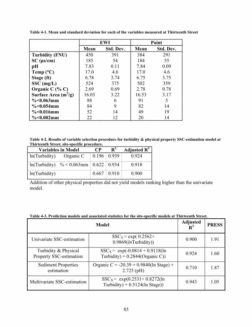
85
Table 4-1. Mean and standard deviation for each of the variables measured at Thirteenth Street
EWI Point Mean Std. Dev. Mean Std. Dev. Turbidity (FNU) 450 391 384 291 SC (µs/cm) 185 54 184 55 pH 7.83 0.11 7.84 0.09 Temp (°C) 17.0 4.6 17.0 4.6 Stage (ft) 6.78 3.74 6.75 3.75 SSC (mg/L) 524 375 502 359 Organic C (% C) 2.69 0.69 2.78 0.78 Surface Area (m2/g) 16.03 3.22 16.53 3.17 %<0.063mm 88 6 91 5 %<0.054mm 84 9 82 14 %<0.016mm 52 14 49 19 %<0.002mm 22 12 20 14
Table 4-2. Results of variable selection procedure for turbidity & physical property SSC-estimation model at Thirteenth Street, site-specific procedure.
Variables in Model CP R2 Adjusted R2
ln(Turbidity) Organic C 0.196 0.939 0.924
ln(Turbidity) % < 0.063mm 0.622 0.934 0.918
ln(Turbidity) 0.667 0.910 0.900
Addition of other physical properties did not yield models ranking higher than the univariate model.
Table 4-3. Prediction models and associated statistics for the site-specific models at Thirteenth Street.
Model Adjusted R2 PRESS
Univariate SSC-estimation SSCX = exp( 0.2562+ 0.9869(lnTurbidity)) 0.900 1.91
Turbidity & Physical Property SSC-estimation
SSCX = exp(-0.0814 + 0.9118(ln Turbidity) + 0.2844(Organic C)) 0.924 1.60
Sediment Properties estimation
Organic C = -20.39 + 0.9840(ln Stage) + 2.725 (pH) 0.710 1.87
Multivariate SSC-estimation SSCX = exp(0.2531+ 0.8272(ln Turbidity) + 0.5124(ln Stage)) 0.943 1.05
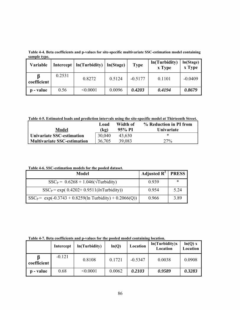
86
Table 4-4. Beta coefficients and p-values for site-specific multivariate SSC-estimation model containing sample type.
Variable Intercept ln(Turbidity) ln(Stage) Type ln(Turbidity)x Type
ln(Stage) x Type
β coefficient
0.2531 0.8272 0.5124 -0.5177 0.1101 -0.0409
p - value 0.56 <0.0001 0.0096 0.4203 0.4194 0.8679 Table 4-5. Estimated loads and prediction intervals using the site-specific model at Thirteenth Street.
Model Load (kg)
Width of 95% PI
% Reduction in PI from Univariate
Univariate SSC-estimation 30,040 43,630 * Multivariate SSC-estimation 36,705 39,083 27%
Table 4-6. SSC-estimation models for the pooled dataset.
Model Adjusted R2 PRESS
SSCP = 0.6268 + 1.046(√Turbidity) 0.939 *
SSCP = exp( 0.4202+ 0.9511(lnTurbidity)) 0.954 5.24
SSCP = exp(-0.3743 + 0.8259(ln Turbidity) + 0.2066(Q)) 0.966 3.89
Table 4-7. Beta coefficients and p-values for the pooled model containing location.
Intercept ln(Turbidity) ln(Q) Location ln(Turbidity)x Location
ln(Q) x Location
β coefficient
-0.121 0.8108 0.1721 -0.5347 0.0038 0.0908
p - value 0.68 <0.0001 0.0062 0.2103 0.9589 0.3283
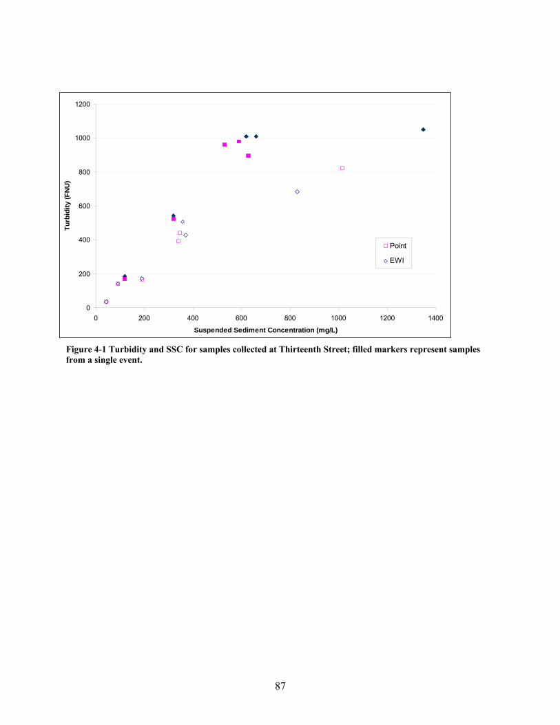
87
Figure 4-1 Turbidity and SSC for samples collected at Thirteenth Street; filled markers represent samples from a single event.
0
200
400
600
800
1000
1200
0 200 400 600 800 1000 1200 1400
Suspended Sediment Concentration (mg/L)
Turb
idity
(FN
U)
Point
EWI
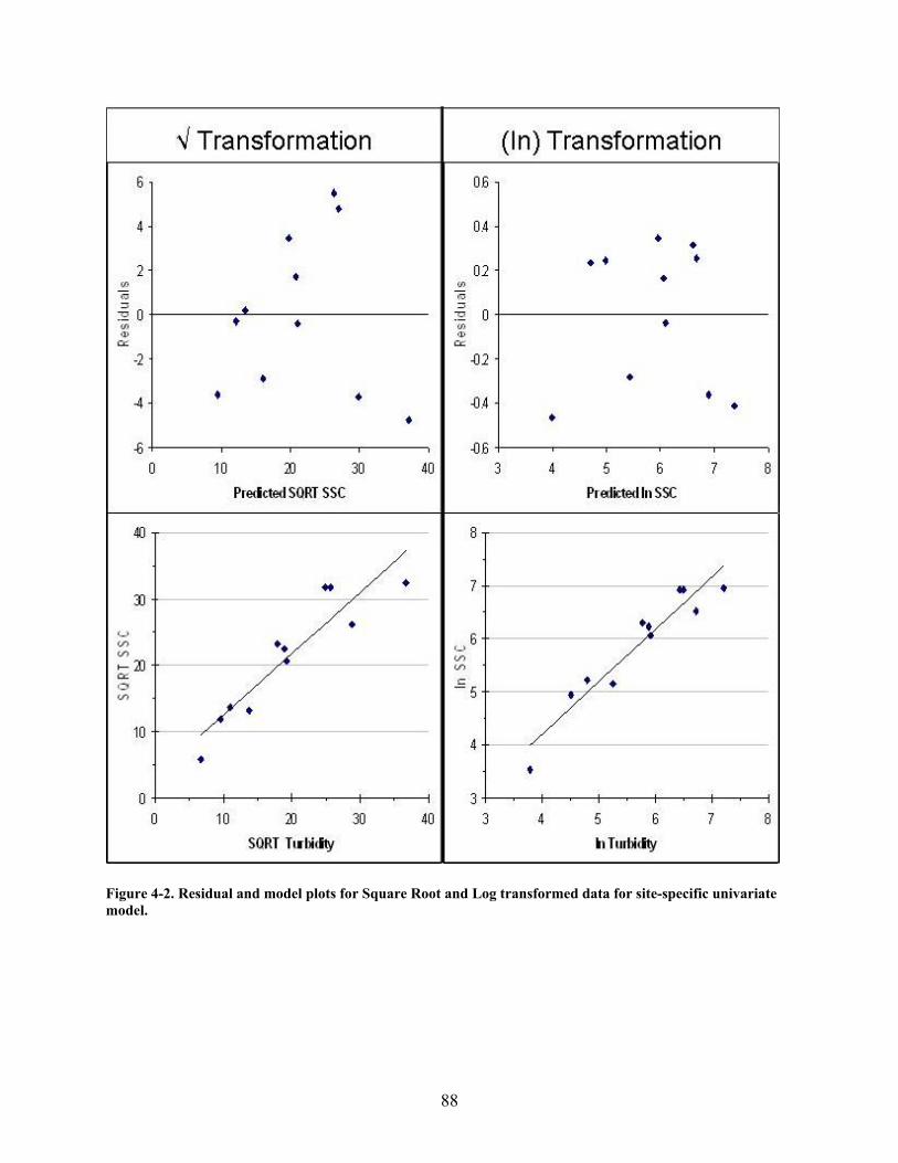
88
Figure 4-2. Residual and model plots for Square Root and Log transformed data for site-specific univariate model.
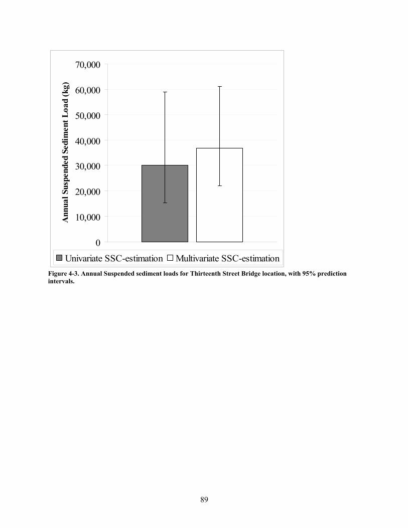
89
0
10,000
20,000
30,000
40,000
50,000
60,000
70,000A
nnua
l Sus
pend
ed S
edim
ent L
oad
(kg)
Univariate SSC-estimation Multivariate SSC-estimation
Figure 4-3. Annual Suspended sediment loads for Thirteenth Street Bridge location, with 95% prediction intervals.
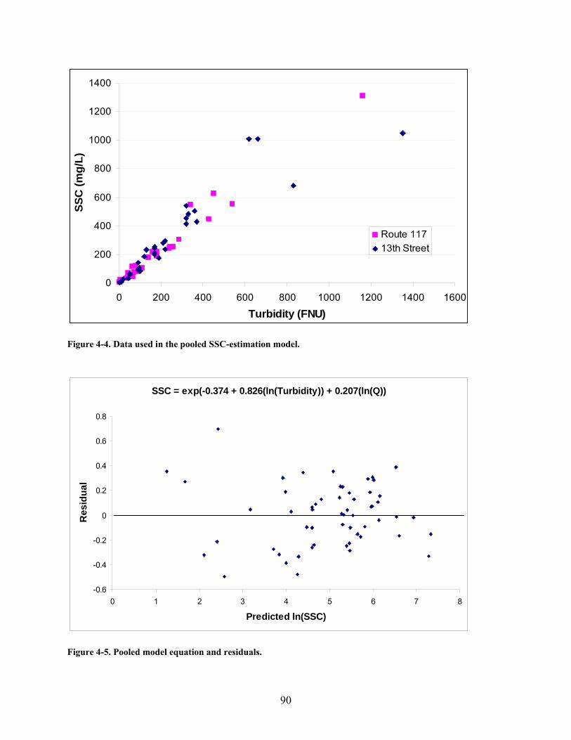
90
0
200
400
600
800
1000
1200
1400
0 200 400 600 800 1000 1200 1400 1600
Turbidity (FNU)
SSC
(mg/
L)
Route 11713th Street
Figure 4-4. Data used in the pooled SSC-estimation model.
Figure 4-5. Pooled model equation and residuals.
SSC = exp(-0.374 + 0.826(ln(Turbidity)) + 0.207(ln(Q))
-0.6
-0.4
-0.2
0
0.2
0.4
0.6
0.8
0 1 2 3 4 5 6 7 8
Predicted ln(SSC)
Res
idua
l
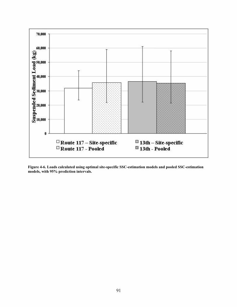
91
Figure 4-6. Loads calculated using optimal site-specific SSC-estimation models and pooled SSC-estimation models, with 95% prediction intervals.
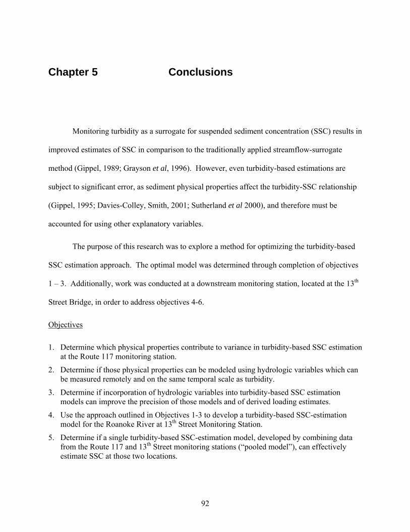
92
Chapter 5 Conclusions
Monitoring turbidity as a surrogate for suspended sediment concentration (SSC) results in
improved estimates of SSC in comparison to the traditionally applied streamflow-surrogate
method (Gippel, 1989; Grayson et al, 1996). However, even turbidity-based estimations are
subject to significant error, as sediment physical properties affect the turbidity-SSC relationship
(Gippel, 1995; Davies-Colley, Smith, 2001; Sutherland et al 2000), and therefore must be
accounted for using other explanatory variables.
The purpose of this research was to explore a method for optimizing the turbidity-based
SSC estimation approach. The optimal model was determined through completion of objectives
1 – 3. Additionally, work was conducted at a downstream monitoring station, located at the 13th
Street Bridge, in order to address objectives 4-6.
Objectives
1. Determine which physical properties contribute to variance in turbidity-based SSC estimation at the Route 117 monitoring station.
2. Determine if those physical properties can be modeled using hydrologic variables which can be measured remotely and on the same temporal scale as turbidity.
3. Determine if incorporation of hydrologic variables into turbidity-based SSC estimation models can improve the precision of those models and of derived loading estimates.
4. Use the approach outlined in Objectives 1-3 to develop a turbidity-based SSC-estimation model for the Roanoke River at 13th Street Monitoring Station.
5. Determine if a single turbidity-based SSC-estimation model, developed by combining data from the Route 117 and 13th Street monitoring stations (“pooled model”), can effectively estimate SSC at those two locations.
93
6. If Objective 2 concludes that a multiple-location SSC-estimation model is feasible: compare the capabilities of models developed through Objectives 1 and 2 to estimate sediment loadings.
This study has demonstrated that the addition of any variable representing the suspended
sediments’ particle size distribution or organic matter content to the turbidity-based SSC-
estimation model improves the model by reducing unexplained variance. At the Route 117 site,
unexplained variance was reduced by as much as 50%, through addition of an easily attainable
measurement of particle-size distribution - % <0.063mm. The finding that particle-size
distributions are a key to reducing unexplained variance in turbidity-based SSC-estimation led to
the successful completion of Objectives 2 & 3, as the physical relationship between particle-size
and hydrologic conditions is well documented. Our findings agreed with the common
understanding that mean particle-size increases with stage, as a model which incorporated stage
and water temperature was capable of explaining nearly half of the variance in the sediments’ %
<0.063mm size fraction. Water temperature contributed to the estimation of this particle-size
variable, possibly as a seasonal effect, which is likely related to sediment availability or settling
velocity. Finally, a more accurate and precise estimation of SSC was realized through the
addition of stage to the turbidity-based model, as stage provides some explanation of the
variance attributed to particle-size effects.
Additional improvement in the estimation of SSC at this monitoring site was realized
through the use of a square-root transformation, instead of the often appropriate log-based
transformation. This improvement resulted from reduced variance in the estimation elevated
turbidity/SSC events, which are highly influential in the calculation of sediment loading.
The improvement in SSC estimation at Route 117 was further demonstrated by reduction
of the 95% prediction interval for an annual suspended sediment load. We have demonstrated

94
that, although the coefficient of variation (R2) and other model statistics may indicate that the
model is quite effective at estimating new values, there may be significant uncertainty in load
estimations even when SSC-estimation equations are characterized by high R2 values.
Practitioners can evaluate this uncertainty and gain a better understanding the limitations of the
model they generate.
Extension of the approach developed at the Route 117 monitoring site to the Thirteenth
Street Bridge site, which is located downstream, yielded similar results, confirming that
sediment physical properties lead to variance in the turbidity-based estimation of SSC and that
physical properties may be estimated using hydrologic variables. The model developed for this
downstream site was more appropriately specified using a log-based transformation, as opposed
to the square-root transformation applied at the upstream site. This transformation selection was
confirmed when the dataset collected through this study was supplemented with additional data
collected at this site for the Roanoke River Flood Reduction Project monitoring program. The
difference in transformations for monitoring sites thirteen kilometers apart on the same river
indicates that estimation models are site specific and best results will be obtained when models
are individually specified for each monitoring station.
The hypothesis that the turbidity-based estimation of SSC may be similar for two
monitoring stations on the same river reach prompted the investigation into whether a model
generated using a pool of data, which includes samples collected at both the upstream and
downstream sites, could be utilized for SSC-estimation. This study concluded that this pooled
model approach was valid, as an effective model was generated using the pooled data with no
statistically significant location effect. Although site specific models are ideal, this approach
provides the capability to build an effective model for a pair of locations that may not have

95
sufficient data to produce robust individual models, provided the lack of locational effects can be
confirmed. Furthermore, this finding leads to the potential for application of the pooled model to
monitoring locations between the sites used in model development, if samples can be collected at
those intermediate locations to confirm the effectiveness of the pooled model. This pooled
model approach could potentially lead to a significant reduction in costs for intensive monitoring
programs on a single river reach as a full model-development dataset would not be required at
each turbidity monitoring station.
Finally, this study has concluded that the precision of turbidity-based SSC estimations
may be significantly improved using stage or discharge data which are commonly collected in
association with turbidity monitoring programs. However, even the best models generated in
this study produce estimates of SSC with considerable uncertainty, and load estimates based on
these SSC estimates have even greater uncertainty. Therefore, further investigation into the
improvement of this method, or development of new methods, is necessary.

96
References Davies-Colley R.J., D.G. Smith. 2001. Turbidity, Suspended Sediment, and Water Clarity: A
Review. Journal of American Water Resources Association. 37:1085 – 1101. Gippel, C.J., 1989. The use of turbidimeters in suspended sediment research. Hydrobiologia
176/177:465-480. Sutherland T.F., P.M. Lane, C.L. Amos, J. Downing. 2000. The calibration of optical backscatter
sensors for suspended sediment of varying darkness levels. Marine Geology 162:587-597.
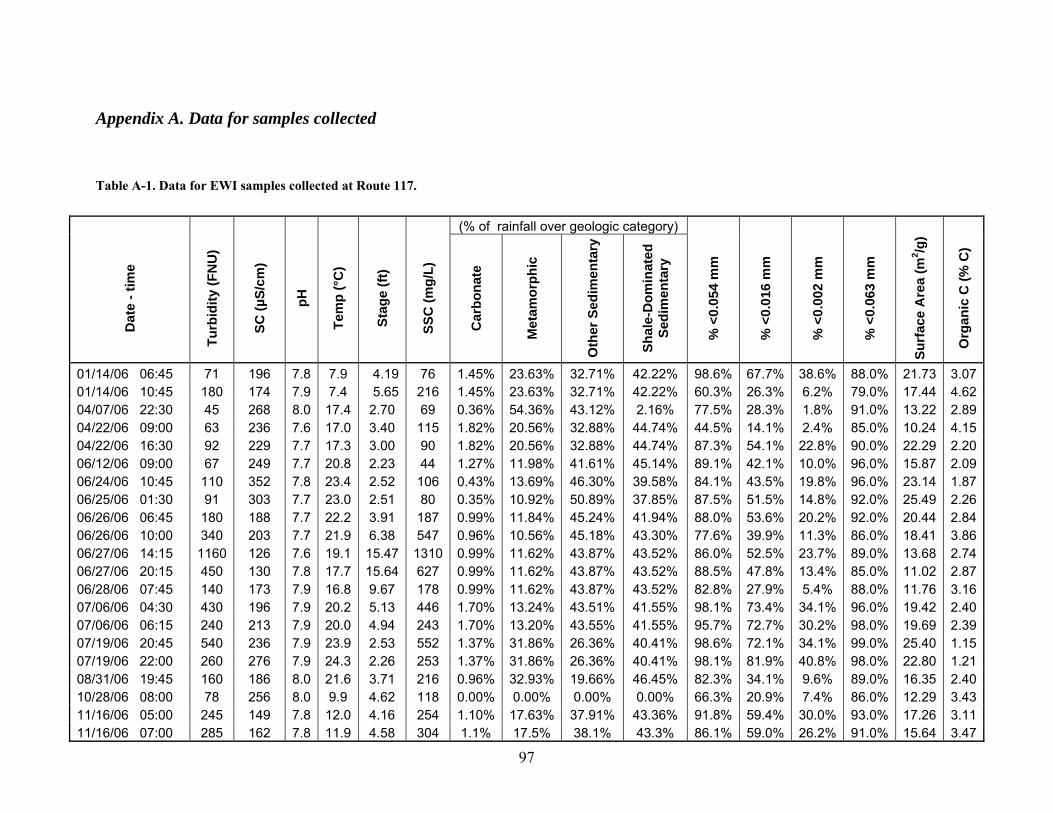
97
Appendix A. Data for samples collected Table A-1. Data for EWI samples collected at Route 117.
(% of rainfall over geologic category)
Dat
e - t
ime
Turb
idity
(FN
U)
SC (µ
S/cm
)
pH
Tem
p (°
C)
Stag
e (ft
)
SSC
(mg/
L)
Car
bona
te
Met
amor
phic
Oth
er S
edim
enta
ry
Shal
e-D
omin
ated
Se
dim
enta
ry
% <
0.05
4 m
m
% <
0.01
6 m
m
% <
0.00
2 m
m
% <
0.06
3 m
m
Surf
ace
Are
a (m
2 /g)
Org
anic
C (%
C)
01/14/06 06:45 71 196 7.8 7.9 4.19 76 1.45% 23.63% 32.71% 42.22% 98.6% 67.7% 38.6% 88.0% 21.73 3.0701/14/06 10:45 180 174 7.9 7.4 5.65 216 1.45% 23.63% 32.71% 42.22% 60.3% 26.3% 6.2% 79.0% 17.44 4.6204/07/06 22:30 45 268 8.0 17.4 2.70 69 0.36% 54.36% 43.12% 2.16% 77.5% 28.3% 1.8% 91.0% 13.22 2.8904/22/06 09:00 63 236 7.6 17.0 3.40 115 1.82% 20.56% 32.88% 44.74% 44.5% 14.1% 2.4% 85.0% 10.24 4.1504/22/06 16:30 92 229 7.7 17.3 3.00 90 1.82% 20.56% 32.88% 44.74% 87.3% 54.1% 22.8% 90.0% 22.29 2.2006/12/06 09:00 67 249 7.7 20.8 2.23 44 1.27% 11.98% 41.61% 45.14% 89.1% 42.1% 10.0% 96.0% 15.87 2.0906/24/06 10:45 110 352 7.8 23.4 2.52 106 0.43% 13.69% 46.30% 39.58% 84.1% 43.5% 19.8% 96.0% 23.14 1.8706/25/06 01:30 91 303 7.7 23.0 2.51 80 0.35% 10.92% 50.89% 37.85% 87.5% 51.5% 14.8% 92.0% 25.49 2.2606/26/06 06:45 180 188 7.7 22.2 3.91 187 0.99% 11.84% 45.24% 41.94% 88.0% 53.6% 20.2% 92.0% 20.44 2.8406/26/06 10:00 340 203 7.7 21.9 6.38 547 0.96% 10.56% 45.18% 43.30% 77.6% 39.9% 11.3% 86.0% 18.41 3.8606/27/06 14:15 1160 126 7.6 19.1 15.47 1310 0.99% 11.62% 43.87% 43.52% 86.0% 52.5% 23.7% 89.0% 13.68 2.7406/27/06 20:15 450 130 7.8 17.7 15.64 627 0.99% 11.62% 43.87% 43.52% 88.5% 47.8% 13.4% 85.0% 11.02 2.8706/28/06 07:45 140 173 7.9 16.8 9.67 178 0.99% 11.62% 43.87% 43.52% 82.8% 27.9% 5.4% 88.0% 11.76 3.1607/06/06 04:30 430 196 7.9 20.2 5.13 446 1.70% 13.24% 43.51% 41.55% 98.1% 73.4% 34.1% 96.0% 19.42 2.4007/06/06 06:15 240 213 7.9 20.0 4.94 243 1.70% 13.20% 43.55% 41.55% 95.7% 72.7% 30.2% 98.0% 19.69 2.3907/19/06 20:45 540 236 7.9 23.9 2.53 552 1.37% 31.86% 26.36% 40.41% 98.6% 72.1% 34.1% 99.0% 25.40 1.1507/19/06 22:00 260 276 7.9 24.3 2.26 253 1.37% 31.86% 26.36% 40.41% 98.1% 81.9% 40.8% 98.0% 22.80 1.2108/31/06 19:45 160 186 8.0 21.6 3.71 216 0.96% 32.93% 19.66% 46.45% 82.3% 34.1% 9.6% 89.0% 16.35 2.4010/28/06 08:00 78 256 8.0 9.9 4.62 118 0.00% 0.00% 0.00% 0.00% 66.3% 20.9% 7.4% 86.0% 12.29 3.4311/16/06 05:00 245 149 7.8 12.0 4.16 254 1.10% 17.63% 37.91% 43.36% 91.8% 59.4% 30.0% 93.0% 17.26 3.1111/16/06 07:00 285 162 7.8 11.9 4.58 304 1.1% 17.5% 38.1% 43.3% 86.1% 59.0% 26.2% 91.0% 15.64 3.47
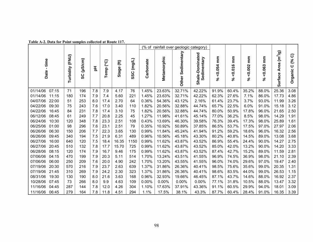
98
Table A-2. Data for Point samples collected at Route 117. (% of rainfall over geologic category)
Dat
e - t
ime
Turb
idity
(FN
U)
SC (µ
S/cm
)
pH
Tem
p (°
C)
Stag
e (ft
)
SSC
(mg/
L)
Car
bona
te
Met
amor
phic
Oth
er S
edim
enta
ry
Shal
e-D
omin
ated
Se
dim
enta
ry
% <
0.05
4 m
m
% <
0.01
6 m
m
% <
0.00
2 m
m
% <
0.06
3 m
m
Surf
ace
Are
a (m
2 /g)
Org
anic
C (%
C)
01/14/06 07:15 71 196 7.8 7.9 4.17 76 1.45% 23.63% 32.71% 42.22% 91.9% 60.4% 35.2% 88.0% 25.36 3.08 01/14/06 11:15 180 174 7.9 7.4 5.60 221 1.45% 23.63% 32.71% 42.22% 62.3% 27.6% 7.1% 86.0% 17.73 4.86 04/07/06 22:00 51 253 8.0 17.4 2.70 64 0.36% 54.36% 43.12% 2.16% 61.4% 23.7% 3.7% 93.0% 11.99 3.26 04/22/06 09:30 75 243 7.6 17.0 3.40 110 1.82% 20.56% 32.88% 44.74% 65.7% 22.5% 6.0% 91.0% 15.18 3.12 04/22/06 16:45 84 231 7.8 17.4 3.10 75 1.82% 20.56% 32.88% 44.74% 80.0% 50.9% 17.8% 96.0% 21.65 2.50 06/12/06 08:45 61 249 7.7 20.8 2.25 45 1.27% 11.98% 41.61% 45.14% 77.0% 36.2% 8.5% 98.0% 14.29 1.91 06/24/06 10:30 120 348 7.8 23.3 2.51 108 0.43% 13.69% 46.30% 39.58% 76.3% 39.4% 17.3% 98.0% 25.89 1.61 06/25/06 01:00 98 296 7.6 23.1 2.51 79 0.35% 10.92% 50.89% 37.85% 86.5% 53.7% 17.5% 97.0% 27.97 2.06 06/26/06 06:30 150 206 7.7 22.3 3.65 130 0.99% 11.84% 45.24% 41.94% 91.2% 59.2% 18.6% 96.0% 16.32 2.56 06/26/06 09:45 340 194 7.5 21.9 6.31 489 0.96% 10.56% 45.18% 43.30% 80.2% 40.8% 14.5% 89.0% 13.08 3.68 06/27/06 16:00 640 120 7.5 18.4 16.35 1150 0.99% 11.62% 43.87% 43.52% 86.9% 55.4% 24.4% 90.0% 14.27 2.75 06/27/06 20:45 510 132 7.8 17.7 15.70 725 0.99% 11.62% 43.87% 43.52% 85.0% 42.0% 13.2% 90.0% 14.20 3.33 06/28/06 08:15 120 174 7.9 16.7 9.46 175 0.99% 11.62% 43.87% 43.52% 87.4% 42.7% 15.2% 89.0% 11.59 2.81 07/06/06 04:15 470 199 7.9 20.3 5.11 514 1.70% 13.24% 43.51% 41.55% 96.9% 74.5% 36.9% 98.0% 21.10 2.39 07/06/06 06:00 250 209 7.6 20.0 4.90 242 1.70% 13.20% 43.55% 41.55% 96.0% 74.0% 29.6% 97.0% 19.47 2.40 07/19/06 20:30 570 216 7.9 23.7 2.63 639 1.37% 31.86% 26.36% 40.41% 98.5% 75.6% 35.6% 99.0% 20.35 1.31 07/19/06 21:45 310 269 7.9 24.2 2.30 323 1.37% 31.86% 26.36% 40.41% 98.6% 83.5% 44.0% 99.0% 26.53 1.15 08/31/06 19:30 130 190 8.0 21.6 3.63 168 0.96% 32.93% 19.66% 46.45% 87.1% 43.7% 14.6% 88.0% 16.92 2.37 10/28/06 07:45 73 266 8.0 9.9 4.63 109 0.00% 0.00% 0.00% 0.00% 77.1% 31.8% 10.5% 88.0% 13.47 3.32 11/16/06 04:45 287 144 7.8 12.0 4.26 304 1.10% 17.63% 37.91% 43.36% 91.1% 60.5% 29.9% 94.0% 18.01 3.09 11/16/06 06:45 279 164 7.8 11.8 4.51 294 1.1% 17.5% 38.1% 43.3% 87.7% 60.4% 28.4% 91.0% 16.35 3.39
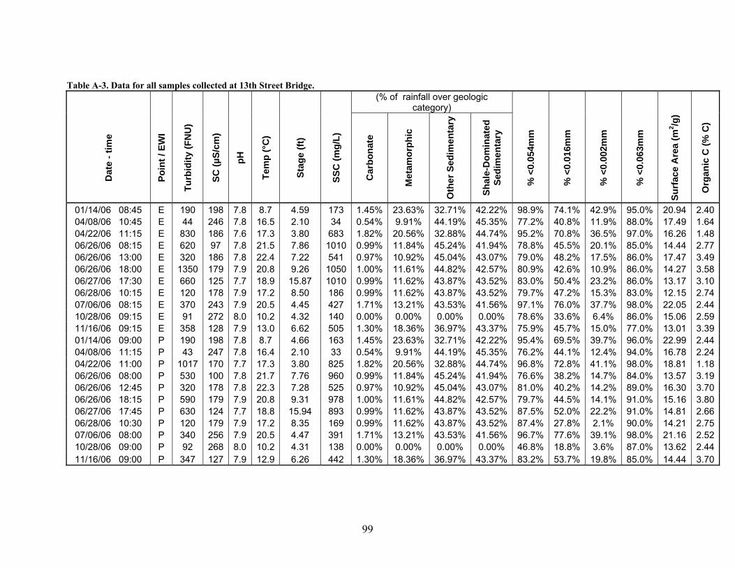
99
Table A-3. Data for all samples collected at 13th Street Bridge.
(% of rainfall over geologic
category) D
ate
- tim
e
Poin
t / E
WI
Turb
idity
(FN
U)
SC (µ
S/cm
)
pH
Tem
p (°
C)
Stag
e (ft
)
SSC
(mg/
L)
Car
bona
te
Met
amor
phic
Oth
er S
edim
enta
ry
Shal
e-D
omin
ated
Se
dim
enta
ry
% <
0.05
4mm
% <
0.01
6mm
% <
0.00
2mm
% <
0.06
3mm
Surf
ace
Are
a (m
2 /g)
Org
anic
C (%
C)
01/14/06 08:45 E 190 198 7.8 8.7 4.59 173 1.45% 23.63% 32.71% 42.22% 98.9% 74.1% 42.9% 95.0% 20.94 2.40 04/08/06 10:45 E 44 246 7.8 16.5 2.10 34 0.54% 9.91% 44.19% 45.35% 77.2% 40.8% 11.9% 88.0% 17.49 1.64 04/22/06 11:15 E 830 186 7.6 17.3 3.80 683 1.82% 20.56% 32.88% 44.74% 95.2% 70.8% 36.5% 97.0% 16.26 1.48 06/26/06 08:15 E 620 97 7.8 21.5 7.86 1010 0.99% 11.84% 45.24% 41.94% 78.8% 45.5% 20.1% 85.0% 14.44 2.77 06/26/06 13:00 E 320 186 7.8 22.4 7.22 541 0.97% 10.92% 45.04% 43.07% 79.0% 48.2% 17.5% 86.0% 17.47 3.49 06/26/06 18:00 E 1350 179 7.9 20.8 9.26 1050 1.00% 11.61% 44.82% 42.57% 80.9% 42.6% 10.9% 86.0% 14.27 3.58 06/27/06 17:30 E 660 125 7.7 18.9 15.87 1010 0.99% 11.62% 43.87% 43.52% 83.0% 50.4% 23.2% 86.0% 13.17 3.10 06/28/06 10:15 E 120 178 7.9 17.2 8.50 186 0.99% 11.62% 43.87% 43.52% 79.7% 47.2% 15.3% 83.0% 12.15 2.74 07/06/06 08:15 E 370 243 7.9 20.5 4.45 427 1.71% 13.21% 43.53% 41.56% 97.1% 76.0% 37.7% 98.0% 22.05 2.44 10/28/06 09:15 E 91 272 8.0 10.2 4.32 140 0.00% 0.00% 0.00% 0.00% 78.6% 33.6% 6.4% 86.0% 15.06 2.59 11/16/06 09:15 E 358 128 7.9 13.0 6.62 505 1.30% 18.36% 36.97% 43.37% 75.9% 45.7% 15.0% 77.0% 13.01 3.39 01/14/06 09:00 P 190 198 7.8 8.7 4.66 163 1.45% 23.63% 32.71% 42.22% 95.4% 69.5% 39.7% 96.0% 22.99 2.44 04/08/06 11:15 P 43 247 7.8 16.4 2.10 33 0.54% 9.91% 44.19% 45.35% 76.2% 44.1% 12.4% 94.0% 16.78 2.24 04/22/06 11:00 P 1017 170 7.7 17.3 3.80 825 1.82% 20.56% 32.88% 44.74% 96.8% 72.8% 41.1% 98.0% 18.81 1.18 06/26/06 08:00 P 530 100 7.8 21.7 7.76 960 0.99% 11.84% 45.24% 41.94% 76.6% 38.2% 14.7% 84.0% 13.57 3.19 06/26/06 12:45 P 320 178 7.8 22.3 7.28 525 0.97% 10.92% 45.04% 43.07% 81.0% 40.2% 14.2% 89.0% 16.30 3.70 06/26/06 18:15 P 590 179 7.9 20.8 9.31 978 1.00% 11.61% 44.82% 42.57% 79.7% 44.5% 14.1% 91.0% 15.16 3.80 06/27/06 17:45 P 630 124 7.7 18.8 15.94 893 0.99% 11.62% 43.87% 43.52% 87.5% 52.0% 22.2% 91.0% 14.81 2.66 06/28/06 10:30 P 120 179 7.9 17.2 8.35 169 0.99% 11.62% 43.87% 43.52% 87.4% 27.8% 2.1% 90.0% 14.21 2.75 07/06/06 08:00 P 340 256 7.9 20.5 4.47 391 1.71% 13.21% 43.53% 41.56% 96.7% 77.6% 39.1% 98.0% 21.16 2.52 10/28/06 09:00 P 92 268 8.0 10.2 4.31 138 0.00% 0.00% 0.00% 0.00% 46.8% 18.8% 3.6% 87.0% 13.62 2.44 11/16/06 09:00 P 347 127 7.9 12.9 6.26 442 1.30% 18.36% 36.97% 43.37% 83.2% 53.7% 19.8% 85.0% 14.44 3.70
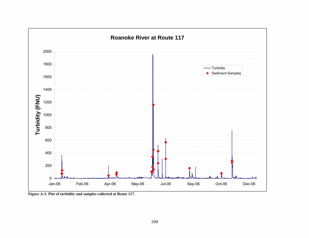
100
Figure A-1. Plot of turbidity and samples collected at Route 117.
Roanoke River at Route 117
0
200
400
600
800
1000
1200
1400
1600
1800
2000
Jan-06 Feb-06 Apr-06 May-06 Jul-06 Sep-06 Oct-06 Dec-06
Turb
idity
(FN
U)
TurbiditySediment Samples
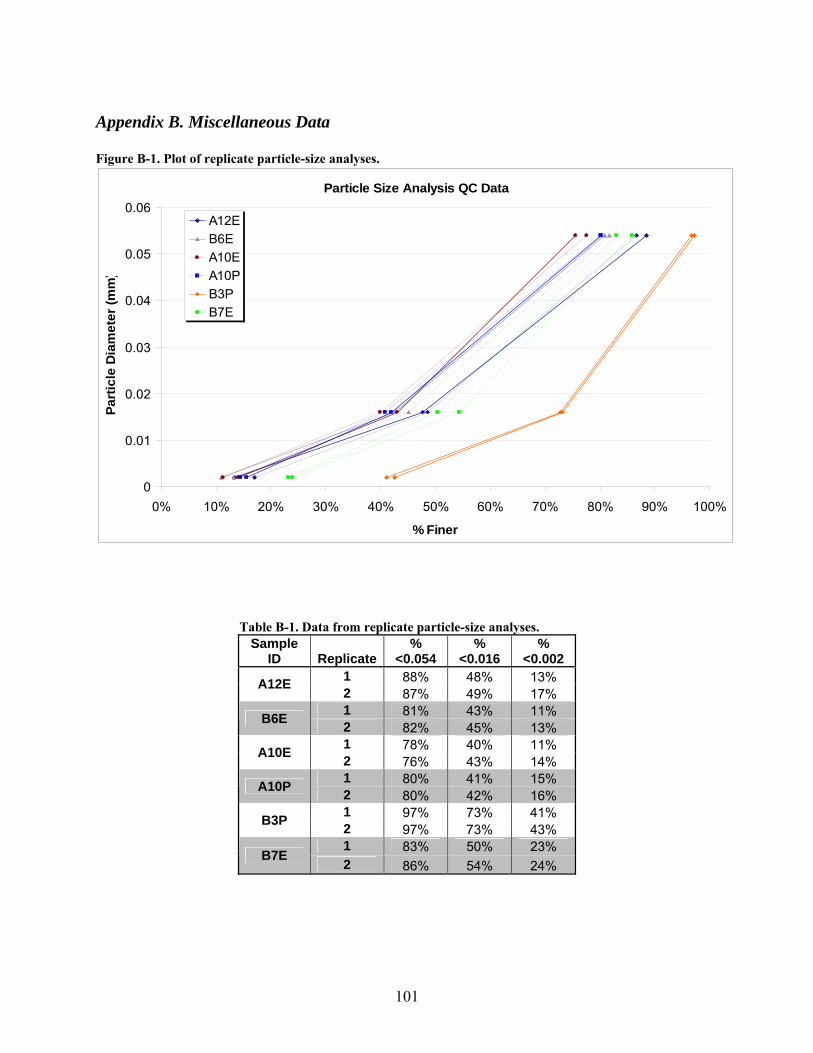
101
Appendix B. Miscellaneous Data Figure B-1. Plot of replicate particle-size analyses.
Particle Size Analysis QC Data
0
0.01
0.02
0.03
0.04
0.05
0.06
0% 10% 20% 30% 40% 50% 60% 70% 80% 90% 100%
% Finer
Part
icle
Dia
met
er (m
m)
A12EB6EA10EA10PB3PB7E
Table B-1. Data from replicate particle-size analyses. Sample
ID Replicate%
<0.054 %
<0.016 %
<0.002 1 88% 48% 13% A12E 2 87% 49% 17% 1 81% 43% 11% B6E 2 82% 45% 13% 1 78% 40% 11% A10E 2 76% 43% 14% 1 80% 41% 15% A10P 2 80% 42% 16% 1 97% 73% 41% B3P 2 97% 73% 43% 1 83% 50% 23% B7E 2 86% 54% 24%
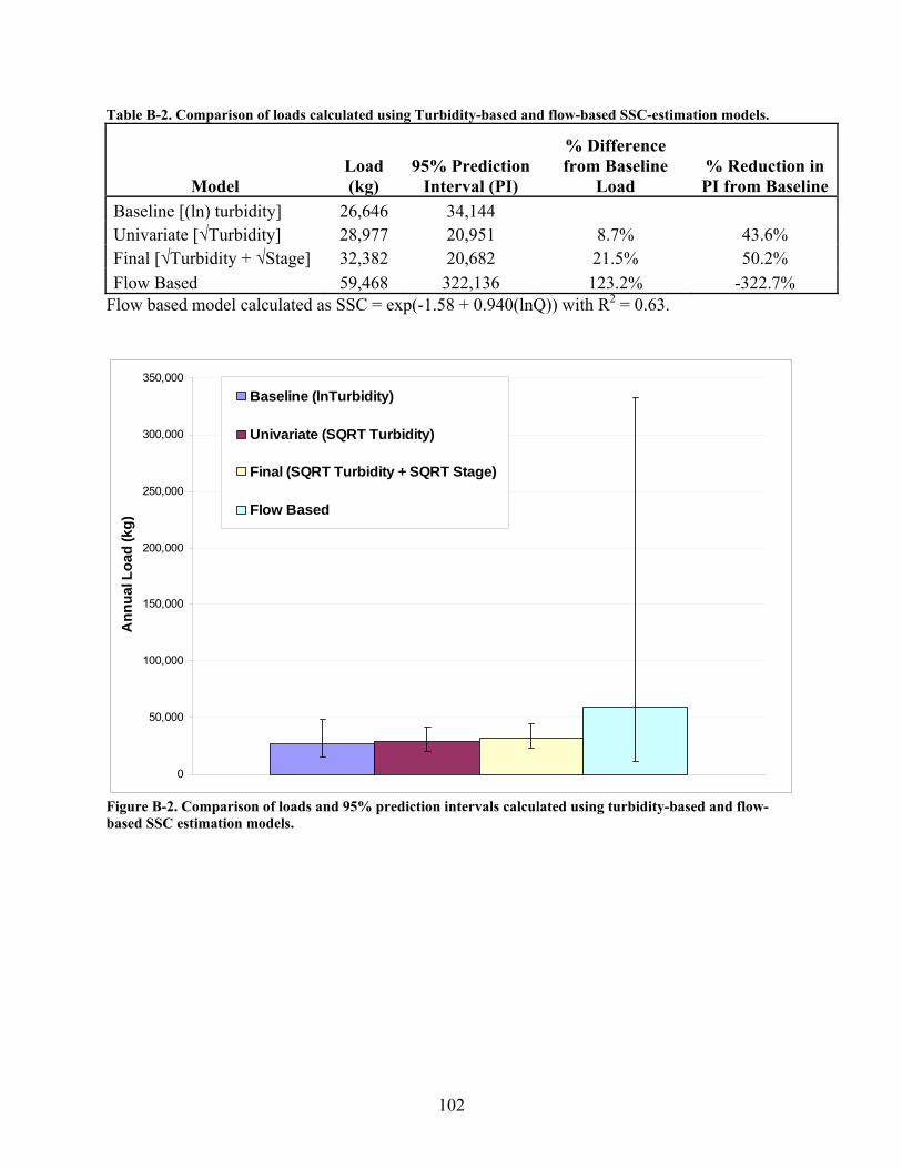
102
Table B-2. Comparison of loads calculated using Turbidity-based and flow-based SSC-estimation models.
Model Load (kg)
95% Prediction Interval (PI)
% Difference from Baseline
Load % Reduction in PI from Baseline
Baseline [(ln) turbidity] 26,646 34,144 Univariate [√Turbidity] 28,977 20,951 8.7% 43.6% Final [√Turbidity + √Stage] 32,382 20,682 21.5% 50.2% Flow Based 59,468 322,136 123.2% -322.7%
Flow based model calculated as SSC = exp(-1.58 + 0.940(lnQ)) with R2 = 0.63.
0
50,000
100,000
150,000
200,000
250,000
300,000
350,000
Ann
ual L
oad
(kg)
Baseline (lnTurbidity)
Univariate (SQRT Turbidity)
Final (SQRT Turbidity + SQRT Stage)
Flow Based
Figure B-2. Comparison of loads and 95% prediction intervals calculated using turbidity-based and flow-based SSC estimation models.
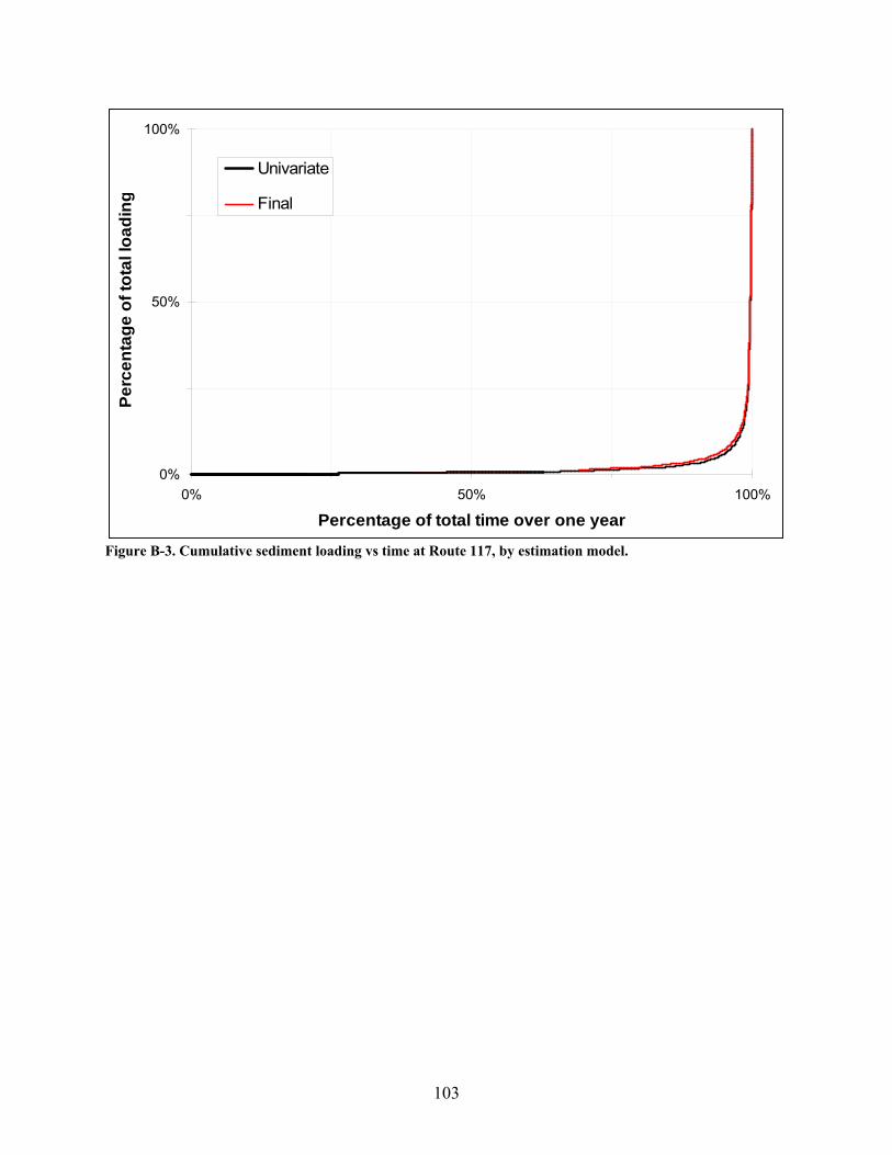
103
0%
50%
100%
0% 50% 100%
Percentage of total time over one year
Perc
enta
ge o
f tot
al lo
adin
g
Univariate
Final
Figure B-3. Cumulative sediment loading vs time at Route 117, by estimation model.
Related Documents