Improving Timbre Similarity : How high's the sky

ACCEPTED FOR PUBLICATION: JNRSAS, (IN PRESS) 1

Improving Timbre Similarity : How high’s the sky ?Jean-Julien Aucouturier Francois Pachet

Abstract—We report on experiments done in an attemptto improve the performance of a music similarity mea-sure which we introduced in [2]. The technique aims atcomparing music titles on the basis of their global “tim-bre”, which has many applications in the field of MusicInformation Retrieval. Such measures of timbre similar-ity have seen a growing interest lately, and every contri-bution (including ours) is yet another instantiation of thesame basic pattern recognition architecture, only with dif-ferent algorithm variants and parameters. Most give en-couraging results with a little effort, and imply that near-perfect results would just extrapolate by fine-tuning thealgorithms’ parameters. However, such systematic testingover large, inter-dependent parameter spaces is both diffi-cult and costly, as it requires to work on a whole generalmeta-database architecture. This paper contributes in twoways to the current state of the art. We report on exten-sive tests over very many parameters and algorithmic vari-ants, either already envisioned in the literature or not. Thisleads to an improvement over existing algorithms of about15% R-precision. But most importantly, we describe manyvariants that surprisingly do not lead to any substancialimprovement. Moreover, our simulations suggest the exis-tence of a “glass ceiling” at R-precision about 65% whichcannot probably be overcome by pursuing such variationson the same theme.

I. Introduction

The domain of Electronic Music Distribution has gainedworldwide attention recently with progress in middleware,networking and compression. However, its success dependslargely on the existence of robust, perceptually relevantmusic similarity relations. It is only with efficient contentmanagement techniques that the millions of music titlesproduced by our society can be made available to its mil-lions of users.

A. Timbre Similarity

In [2], we have proposed to computing automatically mu-sic similarities between music titles based on their globaltimbre quality. The motivation for such an endeavour wastwo fold. First, although it is difficult to define preciselymusic taste, it is quite obvious that music taste is often cor-related with timbre. Some sounds are pleasing to listeners,other are not. Some timbres are specific to music periods(e.g. the sound of Chick Corea playing on an electric pi-ano), others to musical configurations (e.g. the sound of asymphonic orchestra). In any case, listeners are sensitiveto timbre, at least in a global manner.

The second motivation is that timbre similarity is a verynatural way to build relations between music titles. Thevery notion of two music titles that “sound the same”seems to make more sense than, for instance, query by

Jean-Julien Aucouturier is assistant researcher in Sony ComputerScience Laboratory, Paris, France (Phone: (+33)144080511, Email:[email protected])

Francois Pachet is researcher in Sony Computer ScienceLaboratory, Paris, France (Phone: (+33)144080516, Email:[email protected])

humming. Indeed, the notion of melodic similarity is prob-lematic, as a change in a single note in a melody can dra-matically impact the way it is perceived (e.g. change frommajor to minor). Conversely, small variations in timbrewill not affect the timbre quality of a music title, consid-ered in its globality. Typical examples of timbre similarityas we define it are :

• a Schumann sonata (“Classical”) and a Bill Evanspiece (“Jazz”) are similar because they both are ro-mantic piano pieces,

• A Nick Drake tune (“Folk”), an acoustic tune by theSmashing Pumpkins (“Rock”), a bossa nova piece byJoao Gilberto (“World”) are similar because they allconsist of a simple acoustic guitar and a gentle malevoice, etc.

B. State of the Art

Timbre Similarity has seen a growing interest in the Mu-sic Information Retrieval community lately ([4], [5], [7],[12], [13], [18], [22], [25], [32]).

Each contribution often is yet another instantiation ofthe same basic pattern recognition architecture, only withdifferent algorithm variants and parameters. The signal iscut into short overlapping frames (usually between 20 and50ms and a 50% overlap), and for each frame, a feature vec-tor is computed, which usually consists of Mel Frequencycepstrum Coefficients (MFCC, see section II for more de-tails). The number of MFCCs is an important parameter,and each author comes up with a different number: 8([2]),12([12]), 13 ([4]),14([18]), 19([22]), 20([7].

Then a statistical model of the MFCCs’ distribution iscomputed. K-means are used in [4], [7], [13], [22], [25],and GMMs in [2], [7], [18]. Once again, the number ofkmean or GMM centres is a discussed parameter which hasreceived a vast number of answers : 3 ([2]), 8 ([7]), 16 ([4],[7], [22]), 32([7], [18]), 64([7]). [25] uses a computationallysimpler histogram approach computed from Bark Loudnessrepresentation, and [12] uses a supervised algorithm (tree-based vector quantizer) that learns the most distinctivedimensions in a given corpus.

Finally, models are compared with different techniques:sampling ([2]), Earth Mover’s distance ([4], [7], [22]),Asymptotic Likelihood Approximation ([7]).

All these contributions (including ours) give encouragingresults with a little effort and imply that near-perfect re-sults would just extrapolate by fine-tuning the algorithms’parameters.

We should make clear here that this study is only con-cerned with timbre similarity, and that we do not claimthat its conclusions extend to music similarity in general(whatever this may mean), or related tasks like classifica-tion or identification. Recent research in automatic genreclassification and artist identification, for instance, have

2 ACCEPTED FOR PUBLICATION: JNRSAS, (IN PRESS)

shown that the incorporation of other features such as beatand tempo information ([30]), singing voice segmentation([17], [6]) and community metadata ([33]) could improvethe performance. However, such techniques are not ex-plored here as they go beyond the scope of timbre percep-tion.

C. Evaluation

This article reports on experiments done in an attemptto improve the performance of the class of algorithms de-scribed above. Such extensive testing over large, depen-dent parameter spaces is both difficult and costly.

Subjective evaluations are somewhat unreliable and notpractical in a systematic way: in the context of timbre sim-ilarity, we have observed that the conditions of experimentinfluence the estimated precision a lot. It is difficult forthe users not to take account of a priori knowledge aboutthe results. For instance, if the nearest neighbor to a jazzpiece is also a piece by another famous jazz musician, thenthe user is likely to judge it relevant, even if the two piecesbear no timbre similarity. As a consequence of this, a samesimilarity measure may be judged differently depending onthe application context.

Objective evaluation is also problematic, because of thechoice of a ground truth to compare the measure to. In [1],we have projected our similarity measure on genre meta-data to study its agreement to the class information, us-ing the Fisher coefficient. We concluded that there werevery little overlap with genre clusters, but it is unclearwhether this is because the precision of the timbre simi-larity is poor, or because timbre is not a good classifica-tion criteria for genre. Several authors have studied theproblem of choosing an appropriate ground truth : [22]considers as a good match a song which is from the “samealbum”, “same artist”, “same genre” as the seed song. [25]also proposes to use “styles” (e.g. Third Wave ska revival)and “tones” (e.g. energetic) categories from the All MusicGuide AMG 1. [7] pushes the quest for ground truth onestep further by mining the web to collect human similarityratings.

The algorithm used for timbre similarity comes with verymany variants, and has very many parameters to select. Atthe time of [2], the systematic evaluation of the algorithmwas so unpractical that the chosen parameters resultedfrom hand-made parameter twitching. In more recent con-tributions, such as [4], [25], our measure is compared toother techniques, with similarly fixed parameters that alsoresult from little if any systematic evaluation. More gen-erally, attempts at evaluating different measures in the lit-erature tend to compare individual contributions to oneanother, i.e. particular, discrete choices of parameters, in-stead of directly testing the influence of the actual parame-ters. For instance, [25], [5] compares the settings in [22](19MFCCs+16Kmeans) to those of [2](8 MFCCs+3GMM).

Finally, conducting such a systematic evaluation is adaunting task, since before doing so, it requires building a

1 www.allmusic.com

general architecture that is able to :• access and manage the collection of music signals the

measures should be tested on• store each result for each song (or rather each duplet

of songs as we are dealing with a binary operationdist(a,b) = d and each set of parameters

• compare results to a ground truth, which should alsobe stored

• build or import this ground truth on the collection ofsongs according to some criteria

• easily specify the computation of different measures,and to specify different parameters for each algorithmvariant, etc...

In the context of the European project Cuidado, the mu-sic team at SONY CSL Paris has built a fully-fledged EMDsystem, the Music Browser ([24]), which is to our knowl-edge the first system able to handle the whole chain ofEMD from metadata extraction to exploitation by queries,playlists,etc. Metadata about songs and artists are storedin a database, and similarities can be computed on-the-flyor pre-computed into similarity tables. Its open architec-ture makes it easy to import and compute new similar-ity measures. Similarity measures themselves are objectsstored in the database, for which we can describe the exe-cutables that need to be called, as well as the arguments ofthese executables. Using the Music Browser, we were ableto easily specify and launch all the simulations that we de-scribe here, directly from the GUI, without requiring anyadditional programming or external program to bookkeepthe computations and their results.

This paper contributes in two ways to the current stateof the art. We report on extensive tests over very manyparameters and algorithmic variants, some of which havealready been envisioned in the literature, some others be-ing inspired from other domains such as Speech Recogni-tion. This leads to an absolute improvement over existingalgorithms of about 15% R-precision. But most impor-tantly, we describe many variants that surprisingly do notlead to any substancial improvement of the measure’s pre-cision. Moreover, our simulations suggest the existence ofa “glass ceiling” at R-precision about 65% which probablycannot be overcome by pursuing such variations on thesame theme.

II. Framework

In this section, we present the evaluation framework forthe systematic exploration of the parameter space and vari-ants of the algorithm we introduced in [2]. We first describethe initial algorithm, and then describe the evaluation pro-cess.

A. The initial algorithm

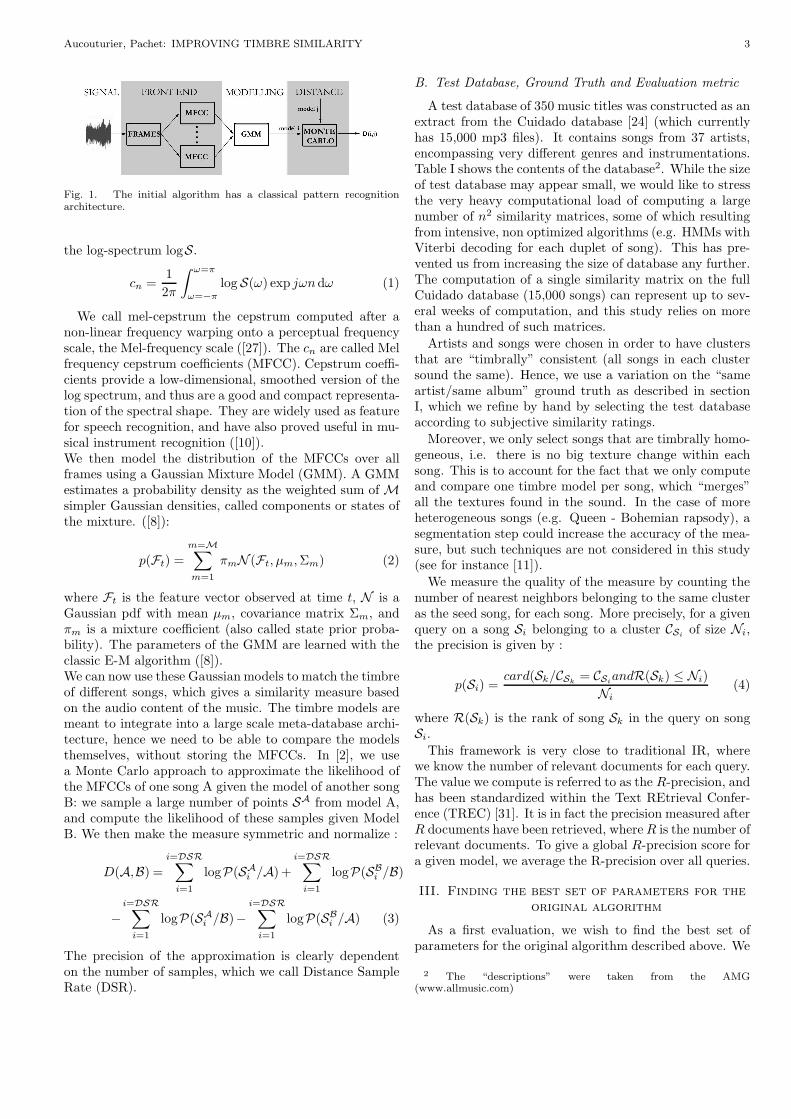
Here we sum up the original algorithm as presented in[2]. As can be seen in Figure 1, it has a classical pat-tern recognition architecture. The signal is first cut intoframes. For each frame, we estimate the spectral envelopeby computing a set of Mel Frequency Cepstrum Coeffi-cients. The cepstrum is the inverse Fourier transform of

Aucouturier, Pachet: IMPROVING TIMBRE SIMILARITY 3

Fig. 1. The initial algorithm has a classical pattern recognitionarchitecture.

the log-spectrum logS.

cn =1

2π

∫ ω=π

ω=−π

log S(ω) exp jωndω (1)

We call mel-cepstrum the cepstrum computed after anon-linear frequency warping onto a perceptual frequencyscale, the Mel-frequency scale ([27]). The cn are called Melfrequency cepstrum coefficients (MFCC). Cepstrum coeffi-cients provide a low-dimensional, smoothed version of thelog spectrum, and thus are a good and compact representa-tion of the spectral shape. They are widely used as featurefor speech recognition, and have also proved useful in mu-sical instrument recognition ([10]).We then model the distribution of the MFCCs over allframes using a Gaussian Mixture Model (GMM). A GMMestimates a probability density as the weighted sum of Msimpler Gaussian densities, called components or states ofthe mixture. ([8]):

p(Ft) =

m=M∑m=1

πmN (Ft, µm, Σm) (2)

where Ft is the feature vector observed at time t, N is aGaussian pdf with mean µm, covariance matrix Σm, andπm is a mixture coefficient (also called state prior proba-bility). The parameters of the GMM are learned with theclassic E-M algorithm ([8]).We can now use these Gaussian models to match the timbreof different songs, which gives a similarity measure basedon the audio content of the music. The timbre models aremeant to integrate into a large scale meta-database archi-tecture, hence we need to be able to compare the modelsthemselves, without storing the MFCCs. In [2], we usea Monte Carlo approach to approximate the likelihood ofthe MFCCs of one song A given the model of another songB: we sample a large number of points SA from model A,and compute the likelihood of these samples given ModelB. We then make the measure symmetric and normalize :

D(A,B) =

i=DSR∑i=1

logP(SAi /A)+

i=DSR∑i=1

logP(SBi /B)

−i=DSR∑

i=1

logP(SAi /B)−

i=DSR∑i=1

logP(SBi /A) (3)

The precision of the approximation is clearly dependenton the number of samples, which we call Distance SampleRate (DSR).

B. Test Database, Ground Truth and Evaluation metric

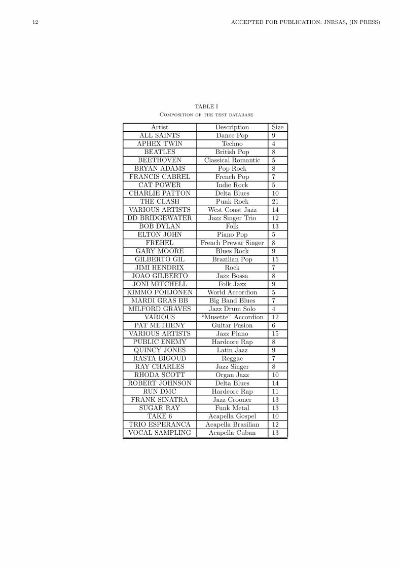
A test database of 350 music titles was constructed as anextract from the Cuidado database [24] (which currentlyhas 15,000 mp3 files). It contains songs from 37 artists,encompassing very different genres and instrumentations.Table I shows the contents of the database2. While the sizeof test database may appear small, we would like to stressthe very heavy computational load of computing a largenumber of n2 similarity matrices, some of which resultingfrom intensive, non optimized algorithms (e.g. HMMs withViterbi decoding for each duplet of song). This has pre-vented us from increasing the size of database any further.The computation of a single similarity matrix on the fullCuidado database (15,000 songs) can represent up to sev-eral weeks of computation, and this study relies on morethan a hundred of such matrices.

Artists and songs were chosen in order to have clustersthat are “timbrally” consistent (all songs in each clustersound the same). Hence, we use a variation on the “sameartist/same album” ground truth as described in sectionI, which we refine by hand by selecting the test databaseaccording to subjective similarity ratings.

Moreover, we only select songs that are timbrally homo-geneous, i.e. there is no big texture change within eachsong. This is to account for the fact that we only computeand compare one timbre model per song, which “merges”all the textures found in the sound. In the case of moreheterogeneous songs (e.g. Queen - Bohemian rapsody), asegmentation step could increase the accuracy of the mea-sure, but such techniques are not considered in this study(see for instance [11]).

We measure the quality of the measure by counting thenumber of nearest neighbors belonging to the same clusteras the seed song, for each song. More precisely, for a givenquery on a song Si belonging to a cluster CSi

of size Ni,the precision is given by :

p(Si) =card(Sk/CSk

= CSiandR(Sk) ≤ Ni)

Ni

(4)

where R(Sk) is the rank of song Sk in the query on songSi.

This framework is very close to traditional IR, wherewe know the number of relevant documents for each query.The value we compute is referred to as the R-precision, andhas been standardized within the Text REtrieval Confer-ence (TREC) [31]. It is in fact the precision measured afterR documents have been retrieved, where R is the number ofrelevant documents. To give a global R-precision score fora given model, we average the R-precision over all queries.

III. Finding the best set of parameters for theoriginal algorithm

As a first evaluation, we wish to find the best set ofparameters for the original algorithm described above. We

2 The “descriptions” were taken from the AMG(www.allmusic.com)

4 ACCEPTED FOR PUBLICATION: JNRSAS, (IN PRESS)

TABLE II

Influence of signal’s sample rate

SR R-Precision11kHz 0.48822kHz 0.50244kHz 0.521

explore the space constituted by the following parameters:

• Signal Sample Rate (SR): The sample rate of the mu-sic signal. The original value in the system in [2] is11KHz. This value was chosen to reduce the CPUtime.

• Number of MFCCs (N): The number of the MFCCsextracted from each frame of data. The more MFCCs,the more precise the approximation of the signal’sspectrum, which also means more variability on thedata. As we are only interested in the spectral en-velopes, not in the finer, faster details like pitch, alarge number may not be appropriate. The originalvalue used in [2] is 8.

• Number of Components (M): The number of gaussiancomponents used in the GMM to model the MFCCs.The more components, the better precision on themodel. However, depending on the dimensionality ofthe data (i.e. the number of MFCCs), more precisemodels may be underestimated. The original value is3.

• Distance Sample Rate (DSR): The number of pointsused to sample from the GMMs in order to estimatethe likelihood of one model given another. The morepoints, the more precision on the distance, but thisincreases the required CPU time linearly.

• Alternative Distance : Many authors ([22], [7]) pro-pose to compare the GMMs using the Earth Mover’sdistance (EMD), a distance measure meant to com-pare histograms with disparate bins ([28]). EMD com-putes a general distance between GMMs by combiningindividual distances between gaussian components.

• Window Size :The size of the frames on which we com-pute the MFCCs.

As this 6-dim space is too big to explore completely,we make the hypothesis that the influence of SR, DSR,EMD and Window Size are both independent of the influ-ence of N and M. However, it is clear from the start thatN and M are linked: there is an optimal balance to befound between high dimensionality and high precision ofthe modeling (curse of dimensionality).

A. influence of SR

To evaluate SR, we fix N, M and DSR to their defaultvalues used in [2] (8,3 and 2000 resp.). In Table II, wesee that the SR has a positive influence on the precision.This is probably due to the increased bandwidth of thehigher definition signals, which enables the algorithm touse higher frequency components than with low SR.

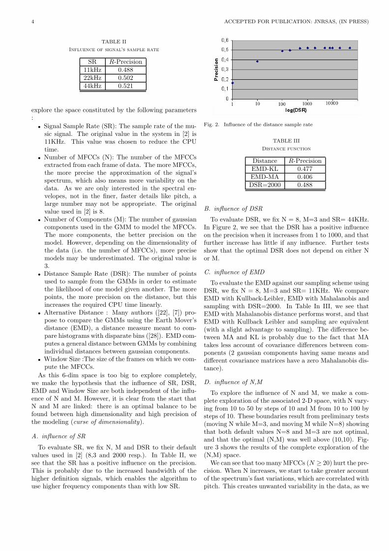
Fig. 2. Influence of the distance sample rate

TABLE III

Distance function

Distance R-PrecisionEMD-KL 0.477EMD-MA 0.406DSR=2000 0.488

B. influence of DSR

To evaluate DSR, we fix N = 8, M=3 and SR= 44KHz.In Figure 2, we see that the DSR has a positive influenceon the precision when it increases from 1 to 1000, and thatfurther increase has little if any influence. Further testsshow that the optimal DSR does not depend on either Nor M.

C. influence of EMD

To evaluate the EMD against our sampling scheme usingDSR, we fix N = 8, M=3 and SR= 11KHz. We compareEMD with Kullback-Leibler, EMD with Mahalanobis andsampling with DSR=2000. In Table In III, we see thatEMD with Mahalanobis distance performs worst, and thatEMD with Kullback Leibler and sampling are equivalent(with a slight advantage to sampling). The difference be-tween MA and KL is probably due to the fact that MAtakes less account of covariance differences between com-ponents (2 gaussian components having same means anddifferent covariance matrices have a zero Mahalanobis dis-tance).

D. influence of N,M

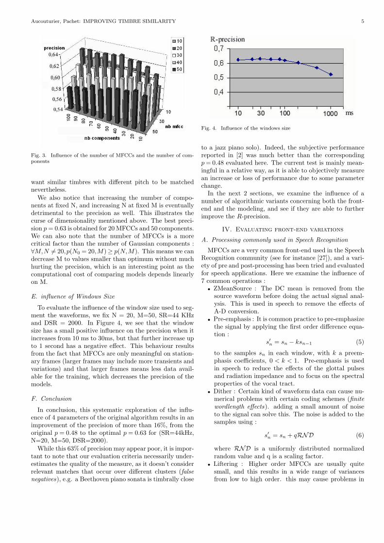
To explore the influence of N and M, we make a com-plete exploration of the associated 2-D space, with N vary-ing from 10 to 50 by steps of 10 and M from 10 to 100 bysteps of 10. These boundaries result from preliminary tests(moving N while M=3, and moving M while N=8) showingthat both default values N=8 and M=3 are not optimal,and that the optimal (N,M) was well above (10,10). Fig-ure 3 shows the results of the complete exploration of the(N,M) space.

We can see that too many MFCCs (N ≥ 20) hurt the pre-cision. When N increases, we start to take greater accountof the spectrum’s fast variations, which are correlated withpitch. This creates unwanted variability in the data, as we

Aucouturier, Pachet: IMPROVING TIMBRE SIMILARITY 5

Fig. 3. Influence of the number of MFCCs and the number of com-ponents

want similar timbres with different pitch to be matchednevertheless.

We also notice that increasing the number of compo-nents at fixed N, and increasing N at fixed M is eventuallydetrimental to the precision as well. This illustrates thecurse of dimensionality mentioned above. The best preci-sion p = 0.63 is obtained for 20 MFCCs and 50 components.We can also note that the number of MFCCs is a morecritical factor than the number of Gaussian components :∀M,N 6= 20,p(N0 = 20,M)≥ p(N,M). This means we candecrease M to values smaller than optimum without muchhurting the precision, which is an interesting point as thecomputational cost of comparing models depends linearlyon M.

E. influence of Windows Size

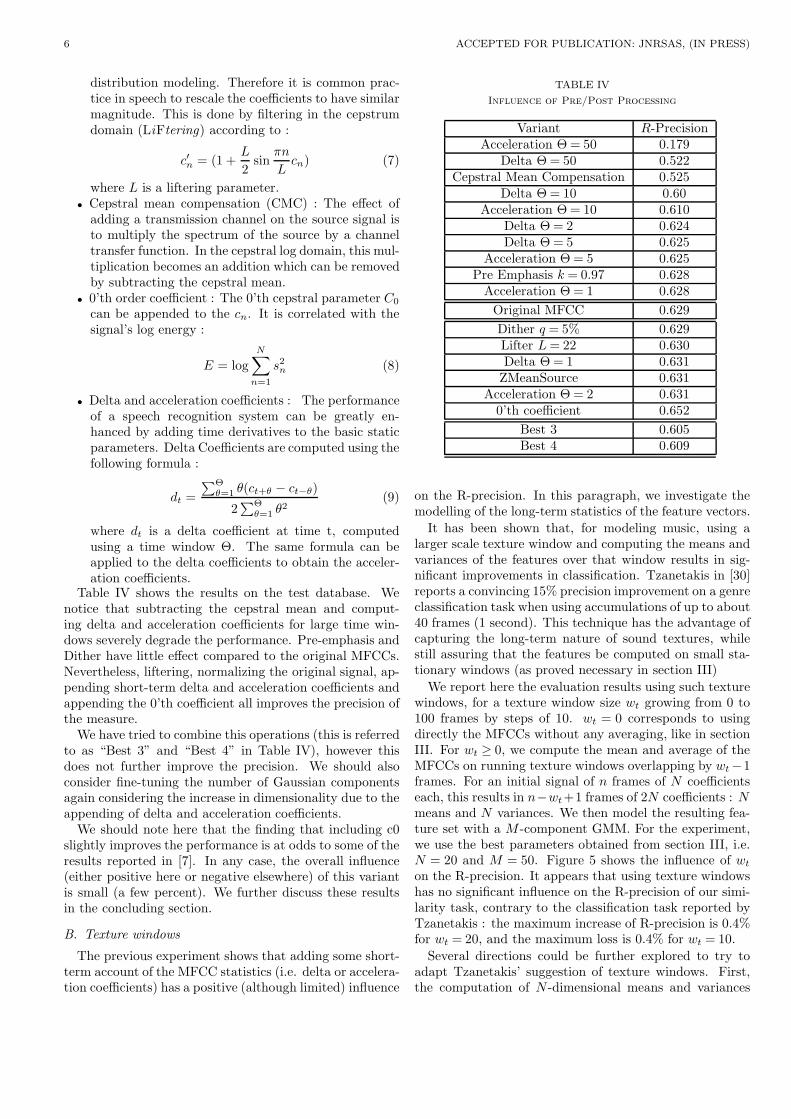
To evaluate the influence of the window size used to seg-ment the waveforms, we fix N = 20, M=50, SR=44 KHzand DSR = 2000. In Figure 4, we see that the windowsize has a small positive influence on the precision when itincreases from 10 ms to 30ms, but that further increase upto 1 second has a negative effect. This behaviour resultsfrom the fact that MFCCs are only meaningful on station-ary frames (larger frames may include more transients andvariations) and that larger frames means less data avail-able for the training, which decreases the precision of themodels.

F. Conclusion

In conclusion, this systematic exploration of the influ-ence of 4 parameters of the original algorithm results in animprovement of the precision of more than 16%, from theoriginal p = 0.48 to the optimal p = 0.63 for (SR=44kHz,N=20, M=50, DSR=2000).

While this 63% of precision may appear poor, it is impor-tant to note that our evaluation criteria necessarily under-estimates the quality of the measure, as it doesn’t considerrelevant matches that occur over different clusters (falsenegatives), e.g. a Beethoven piano sonata is timbrally close

Fig. 4. Influence of the windows size

to a jazz piano solo). Indeed, the subjective performancereported in [2] was much better than the correspondingp = 0.48 evaluated here. The current test is mainly mean-ingful in a relative way, as it is able to objectively measurean increase or loss of performance due to some parameterchange.

In the next 2 sections, we examine the influence of anumber of algorithmic variants concerning both the front-end and the modeling, and see if they are able to furtherimprove the R-precision.

IV. Evaluating front-end variations

A. Processing commonly used in Speech Recognition

MFCCs are a very common front-end used in the SpeechRecognition community (see for instance [27]), and a vari-ety of pre and post-processing has been tried and evaluatedfor speech applications. Here we examine the influence of7 common operations :

• ZMeanSource : The DC mean is removed from thesource waveform before doing the actual signal anal-ysis. This is used in speech to remove the effects ofA-D conversion.

• Pre-emphasis : It is common practice to pre-emphasizethe signal by applying the first order difference equa-tion :

s′n = sn − ksn−1 (5)

to the samples sn in each window, with k a preem-phasis coefficients, 0 < k < 1. Pre-emphasis is usedin speech to reduce the effects of the glottal pulsesand radiation impedance and to focus on the spectralproperties of the vocal tract.

• Dither : Certain kind of waveform data can cause nu-merical problems with certain coding schemes (finite

wordlength effects). adding a small amount of noiseto the signal can solve this. The noise is added to thesamples using :

s′n = sn + qRND (6)

where RND is a uniformly distributed normalizedrandom value and q is a scaling factor.

• Liftering : Higher order MFCCs are usually quitesmall, and this results in a wide range of variancesfrom low to high order. this may cause problems in

6 ACCEPTED FOR PUBLICATION: JNRSAS, (IN PRESS)

distribution modeling. Therefore it is common prac-tice in speech to rescale the coefficients to have similarmagnitude. This is done by filtering in the cepstrumdomain (LiFtering) according to :

c′n = (1 +L

2sin

πn

Lcn) (7)

where L is a liftering parameter.• Cepstral mean compensation (CMC) : The effect of

adding a transmission channel on the source signal isto multiply the spectrum of the source by a channeltransfer function. In the cepstral log domain, this mul-tiplication becomes an addition which can be removedby subtracting the cepstral mean.

• 0’th order coefficient : The 0’th cepstral parameter C0

can be appended to the cn. It is correlated with thesignal’s log energy :

E = log

N∑n=1

s2n (8)

• Delta and acceleration coefficients : The performanceof a speech recognition system can be greatly en-hanced by adding time derivatives to the basic staticparameters. Delta Coefficients are computed using thefollowing formula :

dt =

∑Θθ=1 θ(ct+θ − ct−θ)

2∑Θ

θ=1 θ2(9)

where dt is a delta coefficient at time t, computedusing a time window Θ. The same formula can beapplied to the delta coefficients to obtain the acceler-ation coefficients.

Table IV shows the results on the test database. Wenotice that subtracting the cepstral mean and comput-ing delta and acceleration coefficients for large time win-dows severely degrade the performance. Pre-emphasis andDither have little effect compared to the original MFCCs.Nevertheless, liftering, normalizing the original signal, ap-pending short-term delta and acceleration coefficients andappending the 0’th coefficient all improves the precision ofthe measure.

We have tried to combine this operations (this is referredto as “Best 3” and “Best 4” in Table IV), however thisdoes not further improve the precision. We should alsoconsider fine-tuning the number of Gaussian componentsagain considering the increase in dimensionality due to theappending of delta and acceleration coefficients.

We should note here that the finding that including c0slightly improves the performance is at odds to some of theresults reported in [7]. In any case, the overall influence(either positive here or negative elsewhere) of this variantis small (a few percent). We further discuss these resultsin the concluding section.

B. Texture windows

The previous experiment shows that adding some short-term account of the MFCC statistics (i.e. delta or accelera-tion coefficients) has a positive (although limited) influence

TABLE IV

Influence of Pre/Post Processing

Variant R-PrecisionAcceleration Θ = 50 0.179

Delta Θ = 50 0.522Cepstral Mean Compensation 0.525

Delta Θ = 10 0.60Acceleration Θ = 10 0.610

Delta Θ = 2 0.624Delta Θ = 5 0.625

Acceleration Θ = 5 0.625Pre Emphasis k = 0.97 0.628

Acceleration Θ = 1 0.628

Original MFCC 0.629

Dither q = 5% 0.629Lifter L = 22 0.630Delta Θ = 1 0.631

ZMeanSource 0.631Acceleration Θ = 2 0.631

0’th coefficient 0.652

Best 3 0.605Best 4 0.609

on the R-precision. In this paragraph, we investigate themodelling of the long-term statistics of the feature vectors.

It has been shown that, for modeling music, using alarger scale texture window and computing the means andvariances of the features over that window results in sig-nificant improvements in classification. Tzanetakis in [30]reports a convincing 15% precision improvement on a genreclassification task when using accumulations of up to about40 frames (1 second). This technique has the advantage ofcapturing the long-term nature of sound textures, whilestill assuring that the features be computed on small sta-tionary windows (as proved necessary in section III)

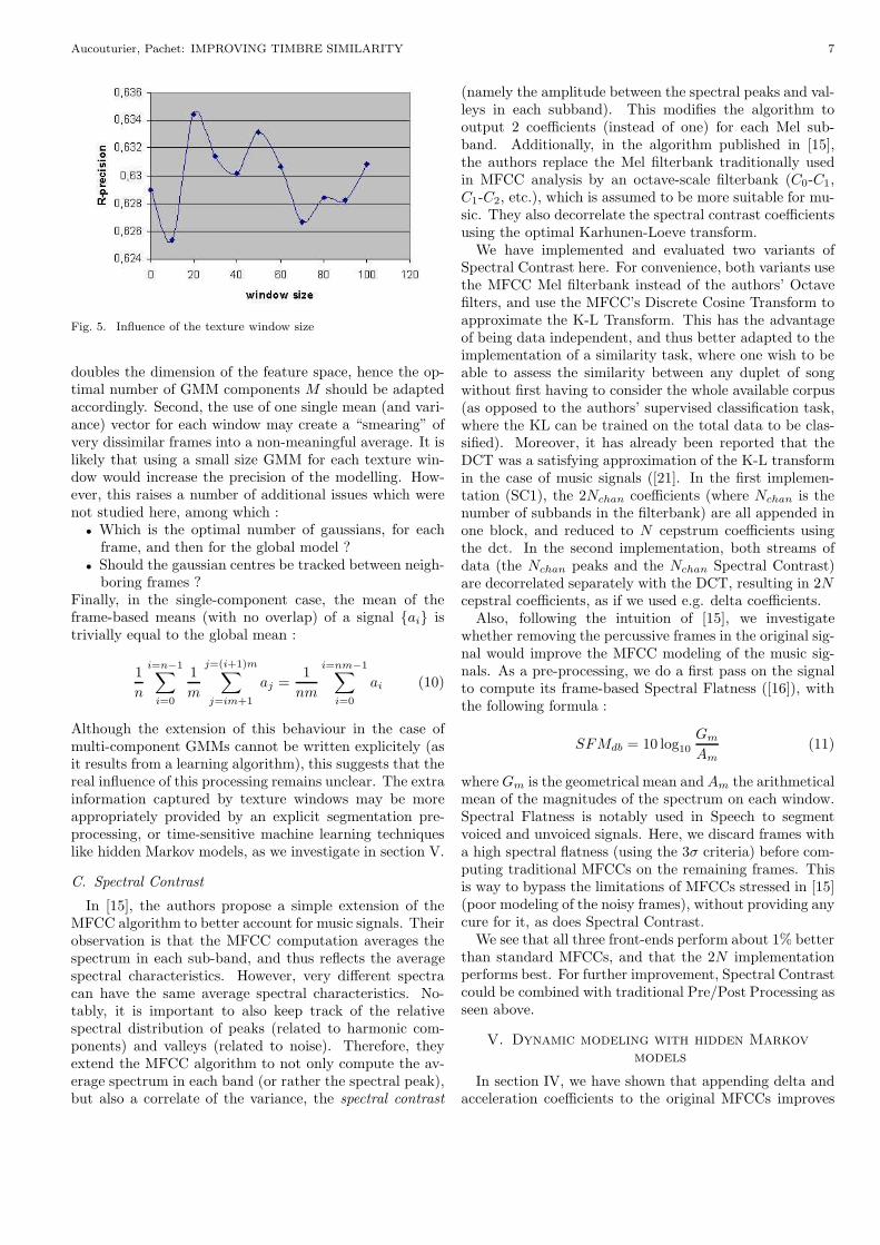
We report here the evaluation results using such texturewindows, for a texture window size wt growing from 0 to100 frames by steps of 10. wt = 0 corresponds to usingdirectly the MFCCs without any averaging, like in sectionIII. For wt ≥ 0, we compute the mean and average of theMFCCs on running texture windows overlapping by wt−1frames. For an initial signal of n frames of N coefficientseach, this results in n−wt+1 frames of 2N coefficients : Nmeans and N variances. We then model the resulting fea-ture set with a M -component GMM. For the experiment,we use the best parameters obtained from section III, i.e.N = 20 and M = 50. Figure 5 shows the influence of wt

on the R-precision. It appears that using texture windowshas no significant influence on the R-precision of our simi-larity task, contrary to the classification task reported byTzanetakis : the maximum increase of R-precision is 0.4%for wt = 20, and the maximum loss is 0.4% for wt = 10.

Several directions could be further explored to try toadapt Tzanetakis’ suggestion of texture windows. First,the computation of N -dimensional means and variances

Aucouturier, Pachet: IMPROVING TIMBRE SIMILARITY 7

Fig. 5. Influence of the texture window size

doubles the dimension of the feature space, hence the op-timal number of GMM components M should be adaptedaccordingly. Second, the use of one single mean (and vari-ance) vector for each window may create a “smearing” ofvery dissimilar frames into a non-meaningful average. It islikely that using a small size GMM for each texture win-dow would increase the precision of the modelling. How-ever, this raises a number of additional issues which werenot studied here, among which :

• Which is the optimal number of gaussians, for eachframe, and then for the global model ?

• Should the gaussian centres be tracked between neigh-boring frames ?

Finally, in the single-component case, the mean of theframe-based means (with no overlap) of a signal {ai} istrivially equal to the global mean :

1

n

i=n−1∑i=0

1

m

j=(i+1)m∑j=im+1

aj =1

nm

i=nm−1∑i=0

ai (10)

Although the extension of this behaviour in the case ofmulti-component GMMs cannot be written explicitely (asit results from a learning algorithm), this suggests that thereal influence of this processing remains unclear. The extrainformation captured by texture windows may be moreappropriately provided by an explicit segmentation pre-processing, or time-sensitive machine learning techniqueslike hidden Markov models, as we investigate in section V.

C. Spectral Contrast

In [15], the authors propose a simple extension of theMFCC algorithm to better account for music signals. Theirobservation is that the MFCC computation averages thespectrum in each sub-band, and thus reflects the averagespectral characteristics. However, very different spectracan have the same average spectral characteristics. No-tably, it is important to also keep track of the relativespectral distribution of peaks (related to harmonic com-ponents) and valleys (related to noise). Therefore, theyextend the MFCC algorithm to not only compute the av-erage spectrum in each band (or rather the spectral peak),but also a correlate of the variance, the spectral contrast

(namely the amplitude between the spectral peaks and val-leys in each subband). This modifies the algorithm tooutput 2 coefficients (instead of one) for each Mel sub-band. Additionally, in the algorithm published in [15],the authors replace the Mel filterbank traditionally usedin MFCC analysis by an octave-scale filterbank (C0-C1,C1-C2, etc.), which is assumed to be more suitable for mu-sic. They also decorrelate the spectral contrast coefficientsusing the optimal Karhunen-Loeve transform.

We have implemented and evaluated two variants ofSpectral Contrast here. For convenience, both variants usethe MFCC Mel filterbank instead of the authors’ Octavefilters, and use the MFCC’s Discrete Cosine Transform toapproximate the K-L Transform. This has the advantageof being data independent, and thus better adapted to theimplementation of a similarity task, where one wish to beable to assess the similarity between any duplet of songwithout first having to consider the whole available corpus(as opposed to the authors’ supervised classification task,where the KL can be trained on the total data to be clas-sified). Moreover, it has already been reported that theDCT was a satisfying approximation of the K-L transformin the case of music signals ([21]. In the first implemen-tation (SC1), the 2Nchan coefficients (where Nchan is thenumber of subbands in the filterbank) are all appended inone block, and reduced to N cepstrum coefficients usingthe dct. In the second implementation, both streams ofdata (the Nchan peaks and the Nchan Spectral Contrast)are decorrelated separately with the DCT, resulting in 2Ncepstral coefficients, as if we used e.g. delta coefficients.

Also, following the intuition of [15], we investigatewhether removing the percussive frames in the original sig-nal would improve the MFCC modeling of the music sig-nals. As a pre-processing, we do a first pass on the signalto compute its frame-based Spectral Flatness ([16]), withthe following formula :

SFMdb = 10 log10

Gm

Am

(11)

where Gm is the geometrical mean and Am the arithmeticalmean of the magnitudes of the spectrum on each window.Spectral Flatness is notably used in Speech to segmentvoiced and unvoiced signals. Here, we discard frames witha high spectral flatness (using the 3σ criteria) before com-puting traditional MFCCs on the remaining frames. Thisis way to bypass the limitations of MFCCs stressed in [15](poor modeling of the noisy frames), without providing anycure for it, as does Spectral Contrast.

We see that all three front-ends perform about 1% betterthan standard MFCCs, and that the 2N implementationperforms best. For further improvement, Spectral Contrastcould be combined with traditional Pre/Post Processing asseen above.

V. Dynamic modeling with hidden Markovmodels

In section IV, we have shown that appending delta andacceleration coefficients to the original MFCCs improves

8 ACCEPTED FOR PUBLICATION: JNRSAS, (IN PRESS)

TABLE V

Influence of Spectral Contrast

Implementation R-PrecisionSC1 0.640SC2 0.656SFN 0.636

standard MFCC 0.629

the precision of the measure. This suggests that the short-term dynamics of the data is also important.

Short-term dynamical behavior in timbre may describee.g. the way steady-state textures follow noisy transientparts. These dynamics are obviously important to com-pare timbres, as can be shown e.g. by listening to revertedguitar sounds used in some contemporary rock songs whichbear no perceptual similarity to normal guitar sounds(same static content, different dynamics). Longer-termdynamics describe how instrumental textures follow eachother, and also account for the musical structure of thepiece (chorus/ verse, etc.). As can be seen in section IV,taking account of these longer-term dynamics (e.g. by us-ing very large delta coefficients) is detrimental to the sim-ilarity measure, as different pieces with same “sound” canbe pretty different in terms of musical structure.

To explicitly model this short-term dynamical behaviorof the data, we try replacing the GMMs by hidden Markovmodels (HMMs, see [26]). A HMM is a set of GMMs (alsocalled states) which are linked with a transition matrixwhich indicates the probability of going from state to an-other in a Markovian process. During the training of theHMM, done with the Baum-Welsh algorithm, we simul-taneously learn the state distributions and the markovianprocess between states.

To compare HMMs with one another, we adapt theMonte Carlo method used for GMMs : we sample fromeach model a large number NS of sequences of size NF ,and compute the log likelihood of each of these sequencesgiven the other models, using equation 3. The probabilitiesP(SA

i /B) are computed by Viterbi decoding.

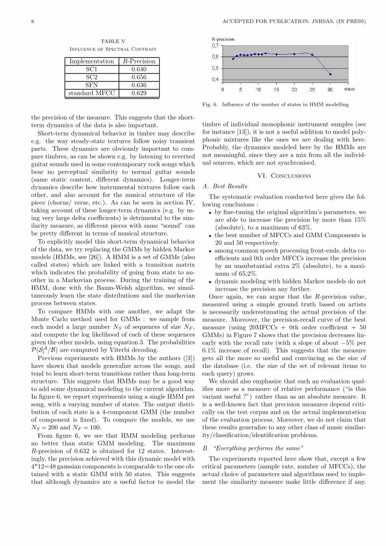
Previous experiments with HMMs by the authors ([3])have shown that models generalize across the songs, andtend to learn short-term transitions rather than long-termstructure. This suggests that HMMs may be a good wayto add some dynamical modeling to the current algorithm.In figure 6, we report experiments using a single HMM persong, with a varying number of states. The output distri-bution of each state is a 4-component GMM (the numberof component is fixed). To compare the models, we useNS = 200 and NF = 100.

From figure 6, we see that HMM modeling performsno better than static GMM modeling. The maximumR-precision of 0.632 is obtained for 12 states. Interest-ingly, the precision achieved with this dynamic model with4*12=48 gaussian components is comparable to the one ob-tained with a static GMM with 50 states. This suggeststhat although dynamics are a useful factor to model the

Fig. 6. Influence of the number of states in HMM modelling

timbre of individual monophonic instrument samples (seefor instance [13]), it is not a useful addition to model poly-phonic mixtures like the ones we are dealing with here.Probably, the dynamics modeled here by the HMMs arenot meaningful, since they are a mix from all the individ-ual sources, which are not synchronised.

VI. Conclusions

A. Best Results

The systematic evaluation conducted here gives the fol-lowing conclusions :

• by fine-tuning the original algorithm’s parameters, weare able to increase the precision by more than 15%(absolute), to a maximum of 63%.

• the best number of MFCCs and GMM Components is20 and 50 respectively.

• among common speech processing front-ends, delta co-efficients and 0th order MFCCs increase the precisionby an unsubstantial extra 2% (absolute), to a maxi-mum of 65,2%.

• dynamic modeling with hidden Markov models do notincrease the precision any further.

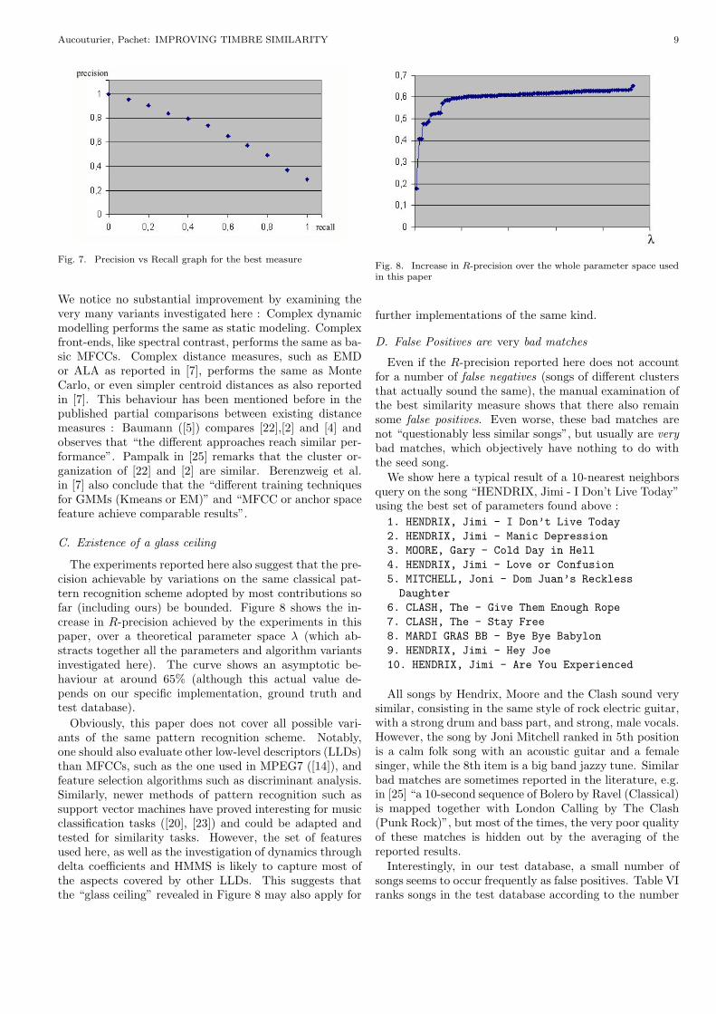
Once again, we can argue that the R-precision value,measured using a simple ground truth based on artistsis necessarily underestimating the actual precision of themeasure. Moreover, the precision-recall curve of the bestmeasure (using 20MFCCs + 0th order coefficient + 50GMMs) in Figure 7 shows that the precision decreases lin-early with the recall rate (with a slope of about −5% per0.1% increase of recall). This suggests that the measuregets all the more so useful and convincing as the size ofthe database (i.e. the size of the set of relevant items toeach query) grows.

We should also emphasize that such an evaluation qual-ifies more as a measure of relative performance (“is thisvariant useful ?”) rather than as an absolute measure. Itis a well-known fact that precision measures depend criti-cally on the test corpus and on the actual implementationof the evaluation process. Moreover, we do not claim thatthese results generalize to any other class of music similar-ity/classification/identification problems.

B. “Everything performs the same”

The experiments reported here show that, except a fewcritical parameters (sample rate, number of MFCCs), theactual choice of parameters and algorithms used to imple-ment the similarity measure make little difference if any.

Aucouturier, Pachet: IMPROVING TIMBRE SIMILARITY 9

Fig. 7. Precision vs Recall graph for the best measure

We notice no substantial improvement by examining thevery many variants investigated here : Complex dynamicmodelling performs the same as static modeling. Complexfront-ends, like spectral contrast, performs the same as ba-sic MFCCs. Complex distance measures, such as EMDor ALA as reported in [7], performs the same as MonteCarlo, or even simpler centroid distances as also reportedin [7]. This behaviour has been mentioned before in thepublished partial comparisons between existing distancemeasures : Baumann ([5]) compares [22],[2] and [4] andobserves that “the different approaches reach similar per-formance”. Pampalk in [25] remarks that the cluster or-ganization of [22] and [2] are similar. Berenzweig et al.in [7] also conclude that the “different training techniquesfor GMMs (Kmeans or EM)” and “MFCC or anchor spacefeature achieve comparable results”.

C. Existence of a glass ceiling

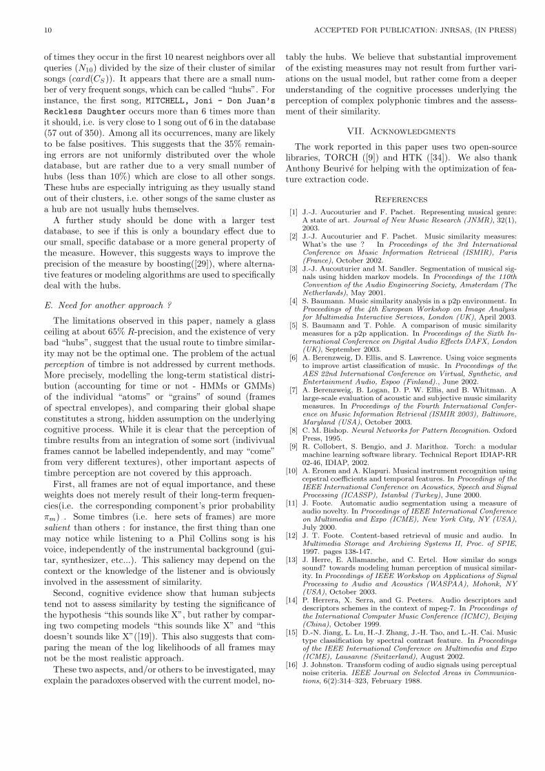
The experiments reported here also suggest that the pre-cision achievable by variations on the same classical pat-tern recognition scheme adopted by most contributions sofar (including ours) be bounded. Figure 8 shows the in-crease in R-precision achieved by the experiments in thispaper, over a theoretical parameter space λ (which ab-stracts together all the parameters and algorithm variantsinvestigated here). The curve shows an asymptotic be-haviour at around 65% (although this actual value de-pends on our specific implementation, ground truth andtest database).

Obviously, this paper does not cover all possible vari-ants of the same pattern recognition scheme. Notably,one should also evaluate other low-level descriptors (LLDs)than MFCCs, such as the one used in MPEG7 ([14]), andfeature selection algorithms such as discriminant analysis.Similarly, newer methods of pattern recognition such assupport vector machines have proved interesting for musicclassification tasks ([20], [23]) and could be adapted andtested for similarity tasks. However, the set of featuresused here, as well as the investigation of dynamics throughdelta coefficients and HMMS is likely to capture most ofthe aspects covered by other LLDs. This suggests thatthe “glass ceiling” revealed in Figure 8 may also apply for

Fig. 8. Increase in R-precision over the whole parameter space usedin this paper

further implementations of the same kind.

D. False Positives are very bad matches

Even if the R-precision reported here does not accountfor a number of false negatives (songs of different clustersthat actually sound the same), the manual examination ofthe best similarity measure shows that there also remainsome false positives. Even worse, these bad matches arenot “questionably less similar songs”, but usually are very

bad matches, which objectively have nothing to do withthe seed song.

We show here a typical result of a 10-nearest neighborsquery on the song “HENDRIX, Jimi - I Don’t Live Today”using the best set of parameters found above :

1. HENDRIX, Jimi - I Don’t Live Today

2. HENDRIX, Jimi - Manic Depression

3. MOORE, Gary - Cold Day in Hell

4. HENDRIX, Jimi - Love or Confusion

5. MITCHELL, Joni - Dom Juan’s Reckless

Daughter

6. CLASH, The - Give Them Enough Rope

7. CLASH, The - Stay Free

8. MARDI GRAS BB - Bye Bye Babylon

9. HENDRIX, Jimi - Hey Joe

10. HENDRIX, Jimi - Are You Experienced

All songs by Hendrix, Moore and the Clash sound verysimilar, consisting in the same style of rock electric guitar,with a strong drum and bass part, and strong, male vocals.However, the song by Joni Mitchell ranked in 5th positionis a calm folk song with an acoustic guitar and a femalesinger, while the 8th item is a big band jazzy tune. Similarbad matches are sometimes reported in the literature, e.g.in [25] “a 10-second sequence of Bolero by Ravel (Classical)is mapped together with London Calling by The Clash(Punk Rock)”, but most of the times, the very poor qualityof these matches is hidden out by the averaging of thereported results.

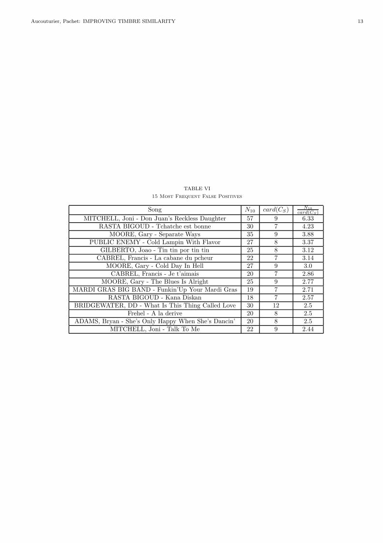
Interestingly, in our test database, a small number ofsongs seems to occur frequently as false positives. Table VIranks songs in the test database according to the number

10 ACCEPTED FOR PUBLICATION: JNRSAS, (IN PRESS)

of times they occur in the first 10 nearest neighbors over allqueries (N10) divided by the size of their cluster of similarsongs (card(CS)). It appears that there are a small num-ber of very frequent songs, which can be called “hubs”. Forinstance, the first song, MITCHELL, Joni - Don Juan’s

Reckless Daughter occurs more than 6 times more thanit should, i.e. is very close to 1 song out of 6 in the database(57 out of 350). Among all its occurrences, many are likelyto be false positives. This suggests that the 35% remain-ing errors are not uniformly distributed over the wholedatabase, but are rather due to a very small number ofhubs (less than 10%) which are close to all other songs.These hubs are especially intriguing as they usually standout of their clusters, i.e. other songs of the same cluster asa hub are not usually hubs themselves.

A further study should be done with a larger testdatabase, to see if this is only a boundary effect due toour small, specific database or a more general property ofthe measure. However, this suggests ways to improve theprecision of the measure by boosting([29]), where alterna-tive features or modeling algorithms are used to specificallydeal with the hubs.

E. Need for another approach ?

The limitations observed in this paper, namely a glassceiling at about 65% R-precision, and the existence of verybad “hubs”, suggest that the usual route to timbre similar-ity may not be the optimal one. The problem of the actualperception of timbre is not addressed by current methods.More precisely, modelling the long-term statistical distri-bution (accounting for time or not - HMMs or GMMs)of the individual “atoms” or “grains” of sound (framesof spectral envelopes), and comparing their global shapeconstitutes a strong, hidden assumption on the underlyingcognitive process. While it is clear that the perception oftimbre results from an integration of some sort (indivivualframes cannot be labelled independently, and may “come”from very different textures), other important aspects oftimbre perception are not covered by this approach.

First, all frames are not of equal importance, and theseweights does not merely result of their long-term frequen-cies(i.e. the corresponding component’s prior probabilityπm) . Some timbres (i.e. here sets of frames) are moresalient than others : for instance, the first thing than onemay notice while listening to a Phil Collins song is hisvoice, independently of the instrumental background (gui-tar, synthesizer, etc...). This saliency may depend on thecontext or the knowledge of the listener and is obviouslyinvolved in the assessment of similarity.

Second, cognitive evidence show that human subjectstend not to assess similarity by testing the significance ofthe hypothesis “this sounds like X”, but rather by compar-ing two competing models “this sounds like X” and “thisdoesn’t sounds like X”([19]). This also suggests that com-paring the mean of the log likelihoods of all frames maynot be the most realistic approach.

These two aspects, and/or others to be investigated, mayexplain the paradoxes observed with the current model, no-

tably the hubs. We believe that substantial improvementof the existing measures may not result from further vari-ations on the usual model, but rather come from a deeperunderstanding of the cognitive processes underlying theperception of complex polyphonic timbres and the assess-ment of their similarity.

VII. Acknowledgments

The work reported in this paper uses two open-sourcelibraries, TORCH ([9]) and HTK ([34]). We also thankAnthony Beurive for helping with the optimization of fea-ture extraction code.

References

[1] J.-J. Aucouturier and F. Pachet. Representing musical genre:A state of art. Journal of New Music Research (JNMR), 32(1),2003.

[2] J.-J. Aucouturier and F. Pachet. Music similarity measures:What’s the use ? In Proceedings of the 3rd InternationalConference on Music Information Retrieval (ISMIR), Paris(France), October 2002.

[3] J.-J. Aucouturier and M. Sandler. Segmentation of musical sig-nals using hidden markov models. In Proceedings of the 110thConvention of the Audio Engineering Society, Amsterdam (TheNetherlands), May 2001.

[4] S. Baumann. Music similarity analysis in a p2p environment. InProceedings of the 4th European Workshop on Image Analysisfor Multimedia Interactive Services, London (UK), April 2003.

[5] S. Baumann and T. Pohle. A comparison of music similaritymeasures for a p2p application. In Proceedings of the Sixth In-ternational Conference on Digital Audio Effects DAFX, London(UK), September 2003.

[6] A. Berenzweig, D. Ellis, and S. Lawrence. Using voice segmentsto improve artist classification of music. In Proceedings of theAES 22nd International Conference on Virtual, Synthetic, andEntertainment Audio, Espoo (Finland)., June 2002.

[7] A. Berenzweig, B. Logan, D. P. W. Ellis, and B. Whitman. Alarge-scale evaluation of acoustic and subjective music similaritymeasures. In Proceedings of the Fourth International Confer-ence on Music Information Retrieval (ISMIR 2003), Baltimore,Maryland (USA), October 2003.

[8] C. M. Bishop. Neural Networks for Pattern Recognition. OxfordPress, 1995.

[9] R. Collobert, S. Bengio, and J. Marithoz. Torch: a modularmachine learning software library. Technical Report IDIAP-RR02-46, IDIAP, 2002.

[10] A. Eronen and A. Klapuri. Musical instrument recognition usingcepstral coefficients and temporal features. In Proceedings of theIEEE International Conference on Acoustics, Speech and SignalProcessing (ICASSP), Istanbul (Turkey), June 2000.

[11] J. Foote. Automatic audio segmentation using a measure ofaudio novelty. In Proceedings of IEEE International Conferenceon Multimedia and Expo (ICME), New York City, NY (USA),July 2000.

[12] J. T. Foote. Content-based retrieval of music and audio. InMultimedia Storage and Archiving Systems II, Proc. of SPIE,1997. pages 138-147.

[13] J. Herre, E. Allamanche, and C. Ertel. How similar do songssound? towards modeling human perception of musical similar-ity. In Proceedings of IEEE Workshop on Applications of SignalProcessing to Audio and Acoustics (WASPAA), Mohonk, NY(USA), October 2003.

[14] P. Herrera, X. Serra, and G. Peeters. Audio descriptors anddescriptors schemes in the context of mpeg-7. In Proceedings ofthe International Computer Music Conference (ICMC), Beijing(China), October 1999.

[15] D.-N. Jiang, L. Lu, H.-J. Zhang, J.-H. Tao, and L.-H. Cai. Musictype classification by spectral contrast feature. In Proceedingsof the IEEE International Conference on Multimedia and Expo(ICME), Lausanne (Switzerland), August 2002.

[16] J. Johnston. Transform coding of audio signals using perceptualnoise criteria. IEEE Journal on Selected Areas in Communica-tions, 6(2):314–323, February 1988.

Aucouturier, Pachet: IMPROVING TIMBRE SIMILARITY 11

[17] Y. E. Kim and B. Whitman. Singer identification in popular mu-sic recordings using voice coding features. In Proceedings of the3rd International Conference on Music Information Retrieval(ISMIR), Paris (France), October October 2002.

[18] V. Kulesh, I. Sethi, and P. V. Indexing and retrieval of mu-sic via gaussian mixture models. In Proceedings of the 3rd In-ternational Workshop on Content-Based Multimedia Indexing(CBMI), Rennes (France), 2003.

[19] M. D. Lee, B. Pincombre, S. Dennis, and P. Bruza. A psycho-logical approach to text document classification. In Proceedingsof the Defence Human Factors Special Interest Group Meeting,October October 2000.

[20] T. Li and G. Tzanetakis. Factors in automatic musical genreclassification of audio signals. In Proceedings of the IEEE Work-shop on Applications of Signal Processing to Audio and Acous-tics (WASPAA) New Paltz, NY (USA), October 2003.

[21] B. Logan. Mel frequency cepstral coefficients for music model-ing. In Proceedings of the 1st International Symposium of Mu-sic Information Retrieval (ISMIR), Plymouth, Massachusetts(USA), October 2000.

[22] B. Logan and A. Salomon. A music similarity function based onsignal analysis. In in proceedings IEEE International Confer-ence on Multimedia and Expo (ICME), Tokyo (Japan ), August2001.

[23] N. C. Maddage, C. Xu, and Y. Wang. A svm-based classifica-tion approach to musical audio. In Proceedings of the 4th Inter-national Conference on Music Information Retrieval (ISMIR),Baltimore, Maryland (USA), October October 2003.

[24] F. Pachet, A. LaBurthe, A. Zils, and J.-J. Aucouturier. Popularmusic access: The sony music browser. Journal of the Amer-ican Society for Information (JASIS), Special Issue on MusicInformation Retrieval, 2004.

[25] E. Pampalk, S. Dixon, and G. Widmer. On the evaluation ofperceptual similarity measures for music. In Proceedings of theSixth International Conference on Digital Audio Effects DAFX,London (UK), September 2003.

[26] L. Rabiner. A tutorial on hidden markov models and selectedapplications in speech recognition. Proceedings of the IEEE,77(2), 1989.

[27] L. Rabiner and B. Juang. Fundamentals of speech recognition.Prentice-Hall, 1993.

[28] Y. Rubner, C. Tomasi, and L. Guibas. The earth movers dis-tance as a metric for image retrieval. Technical report, StanfordUniversity, 1998.

[29] R. Schapire. A brief introduction to boosting. In Proceedings ofthe Sixteenth International Joint Conference on Artificial In-telligence (IJCAI), Stockholm (Sweden), August 1999.

[30] G. Tzanetakis and P. Cook. Musical genre classification of audiosignals. IEEE Transactions on Speech and Audio Processing,10(5), July 2002.

[31] E. Voorhes and D. Harman. Overview of the eighth text retrievalconference. In Proceedings of the Eighth Text Retrieval Confer-ence (TREC), Gaithersburg, Maryland (USA), November 1999.http://trec.nist.gov.

[32] M. Welsh, N. Borisov, J. Hill, R. von Behren, and A. Woo.Querying large collections of music for similarity. Technical Re-port Technical Report UCB/CSD00 -1096, U.C. Berkeley Com-puter Science Division, 1999.

[33] B. Whitman and P. Smaragdis. Combining musical and culturalfeatures for intelligent style detection. In Proceedings of the3rd International Conference on Music Information Retrieval(ISMIR), Paris (France), October October 2002.

[34] S. Young. The htk hidden markov model toolkit. TechnicalReport TR152, Cambridge University Engineering DepartmentCUED, 1993.

12 ACCEPTED FOR PUBLICATION: JNRSAS, (IN PRESS)

TABLE I

Composition of the test database

Artist Description SizeALL SAINTS Dance Pop 9

APHEX TWIN Techno 4BEATLES British Pop 8

BEETHOVEN Classical Romantic 5BRYAN ADAMS Pop Rock 8

FRANCIS CABREL French Pop 7CAT POWER Indie Rock 5

CHARLIE PATTON Delta Blues 10THE CLASH Punk Rock 21

VARIOUS ARTISTS West Coast Jazz 14DD BRIDGEWATER Jazz Singer Trio 12

BOB DYLAN Folk 13ELTON JOHN Piano Pop 5

FREHEL French Prewar Singer 8GARY MOORE Blues Rock 9GILBERTO GIL Brazilian Pop 15JIMI HENDRIX Rock 7

JOAO GILBERTO Jazz Bossa 8JONI MITCHELL Folk Jazz 9

KIMMO POHJONEN World Accordion 5MARDI GRAS BB Big Band Blues 7

MILFORD GRAVES Jazz Drum Solo 4VARIOUS “Musette” Accordion 12

PAT METHENY Guitar Fusion 6VARIOUS ARTISTS Jazz Piano 15PUBLIC ENEMY Hardcore Rap 8QUINCY JONES Latin Jazz 9RASTA BIGOUD Reggae 7RAY CHARLES Jazz Singer 8RHODA SCOTT Organ Jazz 10

ROBERT JOHNSON Delta Blues 14RUN DMC Hardcore Rap 11

FRANK SINATRA Jazz Crooner 13SUGAR RAY Funk Metal 13

TAKE 6 Acapella Gospel 10TRIO ESPERANCA Acapella Brasilian 12VOCAL SAMPLING Acapella Cuban 13

Aucouturier, Pachet: IMPROVING TIMBRE SIMILARITY 13

TABLE VI

15 Most Frequent False Positives

Song N10 card(CS) N10

card(CS)

MITCHELL, Joni - Don Juan’s Reckless Daughter 57 9 6.33RASTA BIGOUD - Tchatche est bonne 30 7 4.23

MOORE, Gary - Separate Ways 35 9 3.88PUBLIC ENEMY - Cold Lampin With Flavor 27 8 3.37

GILBERTO, Joao - Tin tin por tin tin 25 8 3.12CABREL, Francis - La cabane du pcheur 22 7 3.14

MOORE, Gary - Cold Day In Hell 27 9 3.0CABREL, Francis - Je t’aimais 20 7 2.86

MOORE, Gary - The Blues Is Alright 25 9 2.77MARDI GRAS BIG BAND - Funkin’Up Your Mardi Gras 19 7 2.71

RASTA BIGOUD - Kana Diskan 18 7 2.57BRIDGEWATER, DD - What Is This Thing Called Love 30 12 2.5

Frehel - A la derive 20 8 2.5ADAMS, Bryan - She’s Only Happy When She’s Dancin’ 20 8 2.5

MITCHELL, Joni - Talk To Me 22 9 2.44