Improving the MVA-km Method for Transmission Cost ...

Journal of Information Sciences and Computing Technologies(JISCT)

ISSN: 2394-9066

Volume 5, Issue 1 available at www.scitecresearch.com/journals/index.php/jisct 364|

SCITECH Volume 5, Issue 1

RESEARCH ORGANISATION| October 26, 2015

Journal of Information Sciences and Computing Technologies www.scitecresearch.com/journals

Improving the MVA-km Method for Transmission Cost

Allocation Using Counter-Flow Approaches

Ali Mokhtarizadeh 1, Alireza Sedaghati

2

1 Shahab-Danesh Institute of Higher Education, MS. Student in Electrical Engineering,

2 Shahab-Danesh Institute of Higher Education, PhD in Electrical Engineering.

Abstract.

Today with restructuring in power systems and the emergence of competitive electricity markets, operation of the power system have been many changes one of the challenges facing the electricity markets, is transmission pricing. transmission pricing has great impact on the network return on investment, competition and attracting new investors. In this paper, transfer pricing is performed by combination of Zbus and MVA-km methods. The Zbus method is used to determine the contribution of participant of lines transmission power and MVA-km method is used to determine the cost of participant transmission. Lines average apparent power flow is used in MVA-km method. three approaches to using MVA-km is defined in order to investigate the effect of reverse power of lines and how to calculate costs is presented by each approach. Simulation of the proposed method on the test network of 12 Bass is done. and the results of MW-km is compared with MVA-km. also, the results of these three approaches of MVA-km method were compared together and analysis their advantages and disadvantages.

Keywords: Electricity markets; network transmission; transmission pricing; MW-km method; MVA-km

method; Zbus method;

1. Introduction

In recent years, restructuring power systems and the emergence of competitive electricity markets around the world

create the clear differences on operation of power systems. One of the most important characteristics of electricity

markets is the technical characteristics of the transmission network, compared with other markets. accepted

producers of market, are required to use the network transmission for transmission the productive power to

consumers. Therefore, open access to network transmission plays an important role in the competitive electricity

market [1, 2].

One of the most important challenges in the electricity market is the allocation of costs of the transmission network

between market players [3]. In the electricity market, the productive power can't deliver consumer through specific

path, due to the technical characteristics of the transmission network and the theory of electrical circuits, it's not

possible to deliver consumer, productive power from a specific path, but in the transmission network, the

production power of a network inject by manufacturer and it is picked up from the other side, by the consumer and

meanwhile, all of the other powers of production and consuming, can affect the exchange. In other words, passing

power of transmission lines don’t follow the markets financial laws, but follow the laws of load flow [2]. Due to

this theme, determine the transmission network pricing mechanism, is required the specific characteristics of the

electricity industry. Transmission pricing plays a significant role in the presentation of correct economic

information, network utilization and capacity of existing network. Also the transfer pricing plays an important role

to enhance and develop the transmission network in future investment. An appropriate mechanism for transfer

pricing, may cause optimal resource allocation in the network, in long-term [3, 4]. Transfer pricing mechanism

should pursue the following objectives [5]:

http://www.scitecresearch.com/journals


ISSN: 2394-9066


To compensate the cost of transmission system and expected income of investors of transmission

system.

Fair and equitable division of costs between all subscribers transfer system

Improve and increase economic efficiency of network

Up to now various methods is provided for transfer pricing in electricity markets. References [6-9] have conducted

a review of types of the network pricing. These methods fit in two general categories: "incremental cost

transmission pricing (marginal)" and " embedded cost transmission pricing ". incremental cost transmission pricing

(marginal), are methods which to transition pricing, consider only short-term (operational) network [8]. This

category includes nodal pricing method, [10,11], zonal method [12,13] and regional method [9]. in nodal pricing

method, the electricity market settlement is done by using locational marginal pricing method and for this reason,

market price of electricity on different buses of system will vary each other. the difference is the base of transition

pricing, in the nodal method. On zonal and regional pricing methods, transition pricing is done based on the

difference in energy prices between zones and regions in the system. on embedded cost transmission pricing

methods, the costs of long-term (investment) of network is considered for transition pricing [8]. this category

includes pricing methods such as, postage stamp [14], contract path [1,15], MW-Mile or MW-km, power

distribution coefficients[18] and Zbus [19]. In the postage stamp method, based on investment costs of the network,

is received a fixed and same fee of all participant. In the contract path, a financial path is considered for flowing the

power in the network and accordingly, the cost of using the network is calculated. In the MW-mile method, the

contribution of each of the participant from the active power flow through any of the lines is calculated using dc

load flow calculations and accordingly, the allocation of the costs of the transition network are done. The principles

of methods of power distribution coefficients and Zbus MW-mile are similar, Principles and methods of power

distribution coefficients Zbus MW-mile method is similar, with the difference that in the method of power

distribution coefficients for calculating the contribution of the participants from lines power flow is used "

Generation Power Shift Distribution Coefficients » (GSDF) and in Zbus method, is used the theory of electrical

circuits and network impedance matrix.

The transmission pricing mechanism addition to ensuring the return of all costs of the transmission network, it must

distribute costs between network subscribers fairly. Some methods, such as the postage stamp method, even though

satisfy all the costs of the transmission network, but the costs are distributed between network subscribers, unfairly,

because don't consider the location of the participant in the network and their distance from the centers of

production and power consumption. On the other hand, it is possible that some methods such as nodal pricing

method, with fairness, receive the cost of network subscribers much more or less than the actual cost of the

transmission network. From another point of view, disadvantage of more transmission pricing methods is that only

lines active power flow are considered in pricing, while the lines reactive power flow, have an important role in

occupying of line capacity and congestion on the transmission lines [20]. In the meantime, just MVA-km method

and Zbus method consider the lines reactive power flow. The MVA-km method is similar to MW-km, with the

difference that the reactive power consider in calculation of transmission cost in MVA-km method [8]. in this

method the results are low accuracy because the laws governing the load flow is considered to be linear. Although

Zbus method calculates contribution of each participant of active and reactive power, as well, but on calculation of

the cost of transmission method, does not consider the difference between sent and receive lines power and the

counter-flow powers role [21, 22]. In this article, the cost allocation of using of the transmission network performs

using MVA-km improved method. In the proposed method on this article to calculate contribution of network

participants from lines flow powers, use the Zbus method, to obtain more accurate responses. The average amount

of sent and received line powers is used to calculate the transmission costs. Also, three approaches are defined for

MVA-km method according to the inverse powers of the network and mathematical relationships of calculating cost

will present for each of the approaches. The rest of this article is as follows: In the second section, will express how

to calculate the participant contribution of the network lines power flow by Zbus method and how to calculate costs

by MVA-km method. The proposed approaches for calculating the cost of transmission by MVA-km method are

introduced in the third section. A case study was done on test network of 12 bus and are analyzed the results in the

fourth section. The results are presented in the fifth section.

2. Allocation of transmission costs by the combination of Zbus and MVA-km methods

2.2. Zbus method

In current section, with using Zbus method, the contribution of each participant is calculated in the network lines

power flow. In Zbus method, π equivalent circuit used for network modeling. π equivalent circuit shown in Figure

1. apparent power flow of j-k transmission line that is caused by an injection of current in the network i bus is

calculated as follow [21,22]:


ISSN: 2394-9066


𝑆𝑗𝑘𝑖 = 𝑈𝑗 . 𝐼𝑗𝑘

𝑖∗ (1)

𝑆𝑗𝑘𝑖

: j-k line apparent power flow from j-bus to k-bus resulting of current injection in the i-bus

𝑈𝑗 : the voltage of j-bus

𝐼𝑗𝑘𝑖

: current flow of j-k line from j-bus to k-bus resulting of the injection at i-bus

Figure 1. π equivalent circuit of j-k line

Note: the asterisk * means conjugate of complex number

Using mathematical equations that are presented in [21, 22]:

𝐼 𝑗𝑘𝑖 = 𝐷 𝑗𝑘

𝑖 . 𝐼 𝑖 (2)

𝐷 𝑗𝑘𝑖 = 𝑍 𝑗𝑖 − 𝑍 𝑘𝑖 . 𝑌 𝑙𝑗𝑘 + 𝑍 𝑗𝑖 .

𝑌 𝑡𝑗𝑘

2 (3)

𝐼 𝑖 : injected current in the i-bus

𝐷 𝑗𝑘𝑖

: electrical distance between i-bus and j & k-buses

Z ji : elements of j row and i column of network impedance matrix

𝑍 𝑘𝑖 : elements k row and i column of network impedance matrix

𝑌 𝑙𝑗𝑘 : admittance of transmission line j-k

𝑌 𝑡𝑗𝑘 : susceptance of entire of transmission line

Now, by substituting equation (2) in (1), apparent power flow through the jk line resulting of the injection in the i

bus is obtained as follows:

𝑆 𝑗𝑘𝑖 = 𝑈 𝑗 . 𝐷 𝑗𝑘

𝑖∗ . 𝐼𝑖∗ (4)

By substituting 𝐷 𝑗𝑘𝑖∗

in (4), flowing active and reactive power through the jk line from j to k, resulting of power

injection in i bus is calculated as follows. In the presented equations in [21, 22], instead the 𝐼𝑖∗ in equation (4),

𝑆𝑖∗

𝑈𝑖∗

is placed in the wrong way. Because according to general equation Si = UiIi∗, proper equivalent of Ii

∗ is

equivalent S i

U i . This bug is removed in the following equations:

𝑃 𝑗𝑘𝑖 = 𝑅𝑒 𝑈 𝑗 . 𝑍 𝑗𝑖

∗ − 𝑍 𝑘𝑖∗ .𝑌 𝑙𝑗𝑘

∗ + 𝑍 𝑗𝑖∗ .

𝑌 𝑡𝑗𝑘∗

2 .

𝑆 𝑖

𝑈 𝑖 (5)

𝑄 𝑗𝑘𝑖 = 𝐼𝑚 𝑈 𝑗 . 𝑍 𝑗𝑖

∗ − 𝑍 𝑘𝑖∗ . 𝑌 𝑙𝑗𝑘

∗ + 𝑍 𝑗𝑖∗ .


2 .

𝑆 𝑖

𝑈 𝑖 (6)


ISSN: 2394-9066


𝑃 𝑘𝑗𝑖 = 𝑅𝑒 𝑈 𝑘 . 𝑍 𝑘𝑖

∗ − 𝑍 𝑗𝑖∗ .𝑌 𝑙𝑗𝑘

∗ + 𝑍 𝑘𝑖∗ .


2 .

𝑆 𝑖

𝑈 𝑖 (7)

𝑄 𝑘𝑗𝑖 = 𝐼𝑚 𝑈 𝑘 . 𝑍 𝑘𝑖

∗ − 𝑍 𝑗𝑖∗ .𝑌 𝑙𝑗𝑘

∗ + 𝑍 𝑘𝑖∗ .


2 .

𝑆 𝑖

𝑈 𝑖 (8)

𝑃 𝑗𝑘𝑖

: jk line active power flow from j-bus to k-bus resulting from flow injection in the i-bus

𝑄 𝑗𝑘𝑖 : jk line reactive power flow from j-bus to k-bus resulting from flow injection in the i-bus

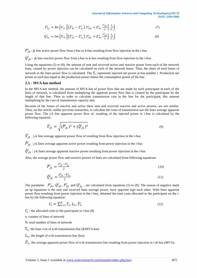
Using the equations (5) to (8), the amount of sent and received active and reactive power from each of the network

lines, caused by power injection can be calculated on each of the network buses. Thus, the share of each buses of

network in the lines power flow is calculated. The S i represents injected net power at bus number i. Production net

power in each bus equal to the production power minus the consumption power of the bus.

2.3. - MVA-km method

In the MVA-km method, the amount of MVA-km of power flow that are made by each participant in each of the

lines of network, is calculated from multiplying the apparent power flow that is created by the participant by the

length of that line. Then in order to calculate transmission cost in the line for the participant, this amount

multiplying by the cost of transmission capacity unit.

Because of the losses of reactive and active then, sent and received reactive and active powers, are not similar.

Then, on this article, unlike previous researches, to calculate the costs of transmission use the lines average apparent

power flow. The j-k line apparent power flow of, resulting of the injected power in i-bus is calculated by the

following equation:

𝑆 𝑗𝑘𝑖 = (𝑃 𝑗𝑘

𝑖 )2 + (𝑄 𝑗𝑘𝑖 )2 (9)

𝑆 𝑗𝑘𝑖

: j-k line average apparent power flow of resulting from flow injection in the i-bus

𝑃 𝑗𝑘𝑖

: j-k lines average apparent active power resulting from power injection in the i-bus

𝑄 𝑗𝑘𝑖

: j-k lines average apparent reactive power resulting from power injection in the i-bus

Also, the average power flow and reactive powers of lines are calculated from following equations:

𝑃 𝑗𝑘𝑖 =

𝑃 𝑗𝑘𝑖 −𝑃 𝑘𝑗

𝑖

2 (10)

𝑄 𝑗𝑘𝑖 =

𝑄 𝑗𝑘𝑖 −𝑄 𝑘𝑗

𝑖

2 (11)

The parameter 𝑃 𝑗𝑘𝑖

, 𝑄 𝑗𝑘𝑖

, 𝑃 𝑘𝑗𝑖

and 𝑄 𝑘𝑗𝑖

, are calculated from equations (5) to (8). The reason of negative mark

on up equations is the sent and received lines average power, have opposite sign each other. With lines apparent

power flow resulting from power injection in the i-bus, obtained the total costs allocated to the participant on the i-

bus by the following equation:

𝐶𝑖 = 𝑇𝑛 . 𝐿𝑛 . 𝑆 𝑛𝑖𝑁

𝑛=1 (12)

𝐶𝑖 : the allocated costs to the participant in i-bus ($)

n: counter of lines of network

N: total number of lines of network

𝑇𝑛 : the base cost of n-th transmission line ($/MVA.km)

𝐿𝑛 : the length of n-th transmission line (km)

𝑆 𝑛𝑖 : the average apparent power flow of n-th transmission line resulting from power injection in i-th bus (MVA).


ISSN: 2394-9066


3. Proposed methods for calculating the cost of transmission by counter flow approaches

In the previous section, how to calculate the allocated costs to each of the participant was shown by the combination

of Zbus and MVA-km methods. As it was seen in MVA-km conventional method for calculating the cost of

transmission, in equation (12), the of the line apparent power flow average amount was used. In a power system,

lines average power flow caused generation or consumption of power by participants, may be in opposite direction

to each other, always. In these conditions, power flow share of one participant of one line may neutralize power

flow share of another participant and thus reduce net power flow of transmission line and will increase power

transmission capacity of line. If the power flow share of a participant from one line be opposite direction of line net

power flow, that named '' counter power ''. In [14, 23], based on the lines counter power, three different approaches

introduced for MW-km method: since the MVA-km method, unlike MW-km method, is considered active and

reactive power simultaneously, it is needed to improve the MVA-km method, according to the lines counter power.

In this section as an innovation, proposed method for taking into account the lines counter power in the calculation

of costs by MVA-km method are presented, in three approaches, as below:

3.1. Absolute MVA-km approach

In this approach, the transmission costs is calculated regardless of the power direction of transmission lines, based

on the absolute amount of MVA-km of each of the network participants. Thus, for each of transmission lines, by

substituting of participant share in lines apparent power flow ( 𝑆 𝑗𝑘𝑖

), in equation 12, the cost of transmission will

calculate and cash out the participant.

3.2. Reverse MVA-km approach

In this approach, the costs of transmission will be counted, based on, the net amount of lines apparent power flow.

Also those participants who cause power flow that opposing main power of lines and thereby, reduce the lines net

power flow, they will be charged for this work. In this approach, four modes may occur:

Mode 1: the participant share of lines active and reactive powers, is in the same direction of line active and reactive

power flow. In this mode, the costs are calculated and are cashed out from the participant by substituting the

participant share in the lines apparent power flow 𝑆 𝑗𝑘𝑖

, in equation (12).

Mode 2: the share of participant in lines active and reactive powers, is opposite direction of line active and reactive

powers flow. In this mode, the costs are calculated and are paid the participant by substituting the participant share

in the lines apparent power flow 𝑆 𝑗𝑘𝑖

, in equation (12).

Mode 3: the share of participant in active power is same direction by line active power and the share of participant

in reactive power is opposite direction of lines apparent power flow. In this mode, the cost of transmission of active

power is calculated and is cashed out from the participant by substituting the participant share in the lines active

power flow of 𝑃 𝑗𝑘𝑖

, in equation (12). Also, cost of transmission of reactive power is calculated and is paid the

participant, by substituting the participant share in the lines reactive power flow of 𝑄 𝑗𝑘𝑖

, in equation (12).

Mode 4: the share of participant in reactive power is same direction of line active power and the share of participant

in active power is opposite direction of line average apparent power flow. In this mode, the cost of transmission of

active power is calculated and is paid to the participant by substituting the participant share in the lines apparent

power flow 𝑃 𝑗𝑘𝑖

, in equation (12). Also, cost of transmission of reactive power is calculated and is cashed out from

the participant, by substituting the participant share in the line reactive power flow 𝑄 𝑗𝑘𝑖

, in equation (12).

3.3. Zero counter-flow MVA-km approach

In this approach, the transmission costs are calculated based on the net amount of lines apparent power flow. In this

approach, unlike absolute MVA-km approach, the participants who caused the counter power in the network, do not

pay cost for using the network. On the other hand, unlike inverse MVA-km approach, do not pay any cost to this

category of participants for this counter power. In this approach, four modes may occur:

Mode 1: the participant share of line active and reactive powers, is same direction of line active and reactive powers

flow. In this mode, the cost of transmission is calculated and is cashed out from the participant, by substituting the

participant share in the lines apparent power flow 𝑆 𝑗𝑘𝑖

, in equation (12).

Mode 2: the share of participant in lines active and reactive powers, is opposite direction of line active and reactive

powers. In this mode, no cost is paid to the participant or is cashed out from participant for transmission.


ISSN: 2394-9066


Mode 3: the share of participant in active power is same direction by line active power and the share of participant

in reactive power is opposite direction of line reactive power flow. In this mode, the cost of transmission of active

power is calculated and is cashed out from the participant by substituting the participant share in the lines active

power flow 𝑃 𝑗𝑘𝑖

, in equation (12). Also, no cost is paid or cashed out for transmission of reactive power.

Mode 4: the share of participant in reactive power is same direction of line active power and the share of participant

in active power is opposite direction of line reactive power. In this mode, no cost is paid or cashed out for

participant for transmission of active power. the cost of transmission of reactive power is calculated and is cashed

out from the participant, by substituting the participant share in the lines active power flow 𝑄 𝑗𝑘𝑖

, in equation (12).

In the future section, these three approaches have been tested on the test network and the results are compared each

other.

Figure 2. Single-line diagram of test network of 12 bus

Table1. The information of test network buses of 12 bus

Number

of the bus

Type of

the bus

Amount of

voltage

(p.u.)

Voltage

angle

(deg)

Productive

active power

(MW)

Productive

reactive

power

(MW)

Consumption

active power

(MW)

Consumption

active power

(MW)

1 slack 1.05 0 - - 0 0

2 PV 1 - 375.56 -129.38 300 35

3 PV 1 - 350 13.43 0 0

4 PV 1 - 303.71 40.51 0 0

5 PV 1 - 600 -15.71 350 25

6 PV 1 - 200 125.73 230 60

7 PQ - - 0 0 350 38

8 PQ - - 0 0 300 25

9 PQ - - 0 0 208 30

10 PQ - - 0 0 170 20

11 PQ - - 0 0 210 23

12 PQ - - 0 0 130 15


ISSN: 2394-9066


4. Case study

4.1. Information of test network

In this section, simulation of proposed method is done for calculating the cost of transmission on 12 bus sample

network. Its network diagram is shown in figure 2. This network has 6 generators and 17 transmission line.

Information of buses and lines of the network, are taken of references [21, 22], are presented on table 1 and table 2,

respectively. The amount of 𝑇𝑛 (the base cost of n-th transmission line) that is used in equation 12 is considered

2$/MVA-km for all of lines, according to reference [21].

Table 2. The information of test network lines of 12 bus

Number

of line

Initial

bus

End

bus

Line resistance

(p.u.)

The reactance

of line (p.u.)

The susceptances

of line (p.u.)

The length

of line

(km)

1 1 2 0.00415 0.025 0.04 30

2 1 6 0.00969 0.05838 0.0949 70

3 1 7 0.0166 0.1 0.16132 120

4 2 8 0.00415 0.025 0.04 30

5 3 7 0.00526 0.03169 0.0511 38

6 8 3 0.00623 0.03752 0.06 45

7 5 4 0.0083 0.05 0.08 60

8 7 4 0.00387 0.02335 0.03765 28

9 4 11 0.0083 0.05 0.08 60

10 6 5 0.00554 0.03335 0.05379 40

11 6 9 0.002075 0.0125 0.02 30

12 6 11 0.00692 0.0417 0.06725 50

13 10 7 0.00554 0.03335 0.05379 40

14 9 10 0.00277 0.01667 0.0269 20

15 10 11 0.00692 0.0417 0.06725 50

16 10 12 0.00484 0.02912 0.047 34

17 11 12 0.00346 0.0208 0.0336 25

Simulation of the proposed method by software package of matpower5.1 in MATLAB software environment is

done. On this software for load flow of ac, is used the Newton - Raphson method [24].

4.2. Results of ac load flow

In this section, ac load flow results are presented on the test network. The related results to network buses are

presented in table 3 and the related results to network lines are presented in table 4.

Table 3. The information of buses of test network from load flow results

Number

of the bus

Amount

of voltage

(p.u.)

Voltage

angle

(deg)

Productive

active power

(MW)

Productive

reactive power

(MW)

Consumption

active power

(MW)

Consumption

reactive power

(MW)

1 1.05 0 443.43 290.05 0 0

2 1 -1.16 375.56 -129.38 300 35


ISSN: 2394-9066


3 1 -1.48 350 13.43 0 0

4 1 -3.67 303.71 40.51 0 0

5 1 -2.40 600 -15.71 350 25

6 1 -6.44 200 125.73 230 60

7 0.99055 -5.85 0 0 350 38

8 0.98837 -3.87 0 0 300 25

9 0.98742 -8.36 0 0 208 30

10 0.98195 -8.97 0 0 170 20

11 0.98207 -8.96 0 0 210 23

12 0.97783 -9.89 0 0 130 15

Table 4. The information of test network lines from load flow results

number of

line

Initial

bus

End

bus

Active power

of initial of

line (MW)

Active power

of end of line

(MW)

Reactive power

of initial of line

(MVAR)

Reactive power

of end of line

(MVAR)

1 1 2 116.56 -114.67 189.30 -182.11

2 1 6 212.75 -208.39 60.74 -44.44

3 1 7 114.12 -111.80 40.01 -42.83

4 2 8 190.23 -188.72 17.38 -12.19

5 3 7 237.92 -234.94 -3.14 16.02

6 8 3 -111.28 112.08 -12.81 11.67

7 5 4 43.26 -43.10 -10.69 3.65

8 7 4 -162.68 163.72 -11.93 14.52

9 4 11 183.09 -180.29 9.80 -0.80

10 6 5 -204.33 206.74 38.70 -29.58

11 6 9 274.89 -273.25 58.47 -50.56

12 6 11 107.83 -106.98 24.00 -25.44

13 10 7 -157.98 159.41 2.66 0.74

14 9 10 65.25 -65.11 20.56 -22.36

15 10 11 -0.67 0.67 -3.43 -3.06

16 10 12 53.76 -53.61 3.12 -6.75

17 11 12 76.60 -76.39 6.30 -8.25

Using of obtained information from the load flow and by equations (5) to (8), will obtain the share of each of the

network participants of active and reactive powers of initial and end of network lines. For this purpose, according

to the method that is used in the reference [21], it is assumed that each of the participants, are placed in a buses of

network. Thus, in the studied test network, there are 12 participants that each of them are placed on one of the buses

1 to 12. Because of huge amount of resulting for share of network participants in lines active and reactive powers

flow, it is ignored presenting these results, on this article.


ISSN: 2394-9066


4.3. The comparison of the results of calculating the cost of transmission by using MW-km and

MVA-km methods

In this section transmission cost of market participants calculates and compares using MW-km and MVA-km

methods. For the use of MVA-km method, is used absolute MVA-km approach because the results be comparable

with MW-km method. Allocated transmission costs to each of the participants in the network buses are shown on

table 5 and figure 3.

Table 5. The allocated transmission cost to network participants by absolute MW-km and MVA-km methods

Bus

number

Transmission cost by

MW-km approach ($)

Transmission cost by

absolute MW-km approach

($)

1 89,461 103,484

2 16,372 42,039

3 64,457 64,546

4 48,230 48,362

5 46,694 47,675

6 4,611 12,031

7 48,216 48,724

8 69,144 69,528

9 33,977 34,545

10 25,724 26,043

11 36,267 36,676

12 24,577 24,911

Sum 507,728 558,565

Figure 3. The comparison of cost of transmission of participants by MW-km and absolute MVA-km approaches

As shown in table 5, the total transmission costs that is delivered from network participants at MW-km method is

US $ 507,728 and at absolute MVA-km method is US $ 558,565. As a result, the total cost of transmission of

absolute MVA-km method is higher about 50,837 $ (about 10%) than the MW-km method. As shown in figure 3,

0

20,000

40,000

60,000

80,000

100,000

120,000

1 2 3 4 5 6 7 8 9 10 11 12

cost of transmission by MW-km method

cost of transmissionby the absolute MVA-km method


ISSN: 2394-9066


transmission cost calculated by MVA-km method, is greater than the calculated transmission cost by MW-km

method, because MVA-km method use from apparent power for calculating the cost of transmission, which is

always greater than or equal active power. In the MW-km method, transmission cost is calculated based on the

active power and in MVA-km method is calculated based on lines apparent power flow. Since capacity of

transmission lines is determined based on the its apparent power flow, using of MW-km method makes the received

cost of network participants be less than actual amount of network lines capacity. As a result, the MW-km method

may be disable to cover the costs of investment in long-term and therefore not compensated the costs of

transmission network. In case if just the active power is used to calculate the costs, the obtained cost don't indicate

the exact amount of the cost of using participants of network lines and allocated costs are not fair.

4.4. Comparison of the results of the three approaches that use MVA-km.

In this section, the results of the simulation of the three proposed approaches for MVA-km method are presented

and the results are compared together. So is investigated effect of counter-powers on the cost of transmission. The

cost of calculated transmission by the three absolute, inverse and zero counter-flow MVA-km approaches are

presented in Table 6 and Figure 4.

As shown on table 6, and is expected, the transmission cost of first approach is maximum amount and the

transmission cost of second approach is minimum amount. The calculated transmission cost by first approach, is

558,565 $ that is maximum, because always use from the absolute value of apparent power and don't consider the

direction of powers flow. In case lines inverse powers flow, in second approach, not only participants don’t pay any

cost but also cashed out cost. Then it's expectable that the transmission cost of second approach be minimum. Its

cost is 208,034 $. In the third approach, unlike the first and the second approaches, don’t pay or cashed out any cost

for lines counter power flow, then, the transmission cost of the third approach is less than first approach, but is more

than the second approach, the cost of third approach is 398,796 $.

The cost of network participants transmission in the three different approaches, were compared in Figure 4. As can

be seen, costs of some participants, including participants at the buses 6, 10 and 12, at the first and third approaches,

have no significant difference. While some other participants, such as participants at the buses 2 and 8, the cost that

is calculated on different approaches have huge difference together.

Table 6. The calculated transmission cost by the approaches of MVA-km method

Bus number Approach 1:

Absolute MVA-km

Approach 2:

inverse MVA-km

Approach 3:

zero counter-flow MVA-km

1 103,484 70,724 89,009

2 42,039 -193 26,493

3 64,546 20,625 43,051

4 48,362 4,729 27,197

5 47,675 24,915 38,392

6 12,031 2,585 8,563

7 48,724 13,245 31,927

8 69,528 3,147 36,876

9 34,545 12,480 24,287

10 26,043 18,914 22,992

11 36,676 17,135 27,342

12 24,911 19,727 22,666

sum 558,565 208,034 398,796


ISSN: 2394-9066


Figure 4. The comparison of costs of participants transmission by the approaches of MVA-km method

For detailed review, consider he participant located in the second bus this participant should pay, in approaches 1

and 3, 42039 $ and 26493 $ respectively, while on third approach, not only pay any cost, but also receive 193 $.

This indicates the position of this participant in the network is such that its productive active and reactive power, is

in the opposite direction of lines power flow and therefore generation of power by this participant, not only don’t

occupy the lines capacity but also can reduce lines power flow and it can open the capacity of lines for using by

other participant s. So if we want examine the approaches of MVA-km from fairness perspective of pricing schemes

of transmission, the second approach is most fairly and after that, third approach is best. On the other hand, if we

look from the perspective of returning investment costs of the transmission network, the first approach, second and

third greatest return on investment, and would make extra motivation for new investment in the transmission

network. From the perspective of investment in the transmission network, may be unreasonable that payment cost to

participants that cause extra power in network and in the long term, wouldn’t cause compensation of investment

costs of some lines. In general, it can be concluded that the first approach has the greatest return on investment, but

the most unfair practice. The second approach is the most fair, but makes the lowest return on investment. The third

approach, have positive characteristics of the other two approaches, and can be a more reasonable option for

selection by policy of electricity market. Prefer one of this method over other approaches, need detailed study of

variable and fixed costs of transmission lines for each network separately, so that be able to select best approach for

calculating of transmission cost.

5. Conclusion

In this article, for pricing of transmission services, used MVA-km and Zbus methods. Also to evaluate the effect of

lines counter power, three new approaches were introduced for MVA-km method and were presented necessary

equations. Simulation of proposed method was done on the test network of 12 Bus. Results of MW-km method

were compared with absolute MVA-km method. The results of this comparison showed that the received

transmission cost by the MVA-km method was more and caused more compensation of costs of transmission

investments and caused extra motivation to new investment. Also due to the occupation of capacity of lines by the

apparent power and not by active power, transmission pricing by MVA-km method is fairer. Then were compared

the results of the three approaches that were proposed for MVA-km method. The result of this comparison showed

that although absolute MVA-km approach makes more investment returns, but this approach is not fair. Also found

that inverse MVA-km approach caused the highest investment return, but not fairly. Finally, it was shown that zero

counter-flow MVA-km approach, with the benefits of the other two approaches, can be better choice for the pricing

of transmission network.

-10,000

10,000

30,000

50,000

70,000

90,000

110,000

1 2 3 4 5 6 7 8 9 10 11 12

the cost of transmission by approach 1




ISSN: 2394-9066


References

[1] Daniel S. Kirschen, Goran Strbac, Fundamentals of Power System Economics, John Wiley & Sons, Ltd, 2004.

[2] S. Stoft, Power System Economics; Designing Markets for Electricity, IEEE Press, 2002.

[3] Tarjei Kristiansen, “Comparison of transmission pricing models”, International Journal of Electrical Power &

Energy Systems, Vol. 33, May 2011, pp. 947-953.

[4] Garg, N.K., Palwalia, D.K., Sharma, H., “Transmission pricing practices: A review”, Proceeding on Nirma

University International Conference on Engineering (NUiCONE), 2013, pp. 1-6.

[5] M. Cannella, E. Disher, R. Gagliardi, “Beyond The Contract Path: A Realistic Approach to Transmission

Pricing”, The Electricity Journal, Vol. 9, Iss. 9, 1996, pp. 26-33.

[6] F.Hussin, M.Y.Hassan, K.L.Lo, “Transmission Congestion Management Assessment in Deregulated Electricity

Market”, Proceeding on Conference on Research and Development (SCOReD), Selangor, MALAYSIA, Jun.

2006, pp. 1-6.

[7] Delberis A. Lima, Antonio Padilha-Feltrin, Javier Contreras, “An overview on network cost allocation

methods”, Electric Power Systems Research, Vol. 79, May 2009, pp. 750-758.

[8] Murali, M., Kumari, M.S., Sydulu, M., “A comparison of embedded cost based transmission pricing methods”,

Proceeding on International Conference on Energy, Automation, and Signal (ICEAS), 2011, pp. 1-6.

[9] Sarfati, M., Hesamzadeh, M.R., “Pricing schemes for dealing with limited transmission capacity - A

comparative study”, Proceeding on IEEE Power and Energy Society General Meeting (PES), 2013, pp. 1-5.

[10] M.D. Simoni, A.J. Pel, R.A. Waraich, S.P. Hoogendoorn, “Marginal cost congestion pricing based on the

network fundamental diagram”, Transportation Research Part C: Emerging Technologies, Vol. 56, Jul. 2015,

pp. 221-238.

[11] Tarjei Kristiansen, “Comparison of transmission pricing models”, International Journal of Electrical Power &

Energy Systems, Vol. 33, May 2011, pp. 947-953.

[12] Anusha Pillay, S. Prabhakar Karthikeyan, D.P. Kothari, “Congestion management in power systems – A

review”, Electrical Power and Energy Systems, Vol. 70, Sep. 2015, pp. 83–90.

[13] Savagave NG., Inamdar HP., “Price area congestion management in radial system under de-regulated

environment – a case study”, International Journal of Electrical Engineering & Technology (IJEET), Vol. 4,

Jan.–Feb. 2013, pp. 100-108.

[14] Orfanos, G.A., Tziasiou, G.T., Georgilakis, P.S., Hatziargyriou, N.D., “Evaluation of transmission pricing

methodologies for pool based electricity markets”, Proceeding on IEEE Trondheim PowerTech, 2011, pp. 1-8.

[15] Milos Pantos, Ferdinand Gubina, “Ex-ante transmission-service pricing via power-flow tracing”, International

Journal of Electrical Power & Energy Systems, Vol. 26, Sep. 2004, pp. 509-518.

[16] Nojeng, S., Hassan, M.Y., Said, D.M., Abdullah, M.P., Hussin, F., “Improving the MW-Mile Method Using

the Power Factor-Based Approach for Pricing the Transmission Services”, IEEE Transactions on Power

Systems, Sep. 2014, pp. 2042 – 2048.

[17] Kharbas, B., Fozdar, M., Tiwari, H., “Transmission tariff allocation using combined MW-Mile & Postage

stamp methods”, Proceeding on IEEE PES Innovative Smart Grid Technologies - India (ISGT India), Dec.

2011, pp. 6-11.

[18] Kilyeni, S., Pop, O., Slavici, T., Craciun, C., Andea, P., Mnerie, D., “Transmission cost allocation using the

distribution factors method”, Proceeding on IEEE Mediterranean Electrotechnical Conference MELECON,

2010, pp. 1093 – 1098.

[19] Conejo, A.J., Contreras, J., Lima, D.A., Padilha-Feltrin, A., “Zbus Transmission Network Cost Allocation”,

IEEE Transactions on Power Systems, Feb. 2007, 342 – 349.

[20] Kharbas, B., Fozdar, M., Tiwari, H., “Comparative assessment of MW-mile and MVA-mile methods of

transmission tariff allocation and revenue reconciliation”, Proceeding on IEEE Power and Energy Society

General Meeting (PES), Jul. 2011, pp. 1-5.

[21] Oana Pop, Florin Solomonesc, Constantin Barbulescu, Stefan Kilyeni, “Allocation of Transmission Cost for

Reactive Power Using System Matrices Method”, Proceedings on International Universities' Power

Engineering Conference (UPEC), 2011, pages 1-6.


ISSN: 2394-9066


[22] Kilyeni, S., Pop, O., Prostean, G., Craciun, C., “Transmission cost allocation based on power flow tracing using

Z bus matrix”, Proceeding on International Conference on Harmonics and Quality of Power (ICHQP), 2010,

pp. 1-6.

[23] Almaktar, M.A., Hassan, M.Y., Abdullah, M.P., Hussin, F., Majid, M.S., “Charge of transmission usage and

losses in pool electricity market”, Proceeding on International Power Engineering and Optimization

Conference (PEOCO), 2010, pp. 557 – 562.

[24] Ray D. Zimmerman, Carlos E. Murillo-Sanchez, “Matpower 5.1 - User's Manual”, Power Systems Engineering

Research Center (Pserc), Mar. 2015.

Improving the MVA-km Method for Transmission Cost ...

Documents