Improving the Foundation Layers for Concrete Pavements

Improving the Foundation Layers for Concrete Pavements

TECHNICAL REPORT: Pavement Foundation Layer Reconstruction – Pennsylvania US 22 Field Study

June 2016

Sponsored byFederal Highway Administration (DTFH 61-06-H-00011 (Work Plan #18))FHWA TPF-5(183): California, Iowa (lead state), Michigan, Pennsylvania, Wisconsin

About the National CP Tech Center

The mission of the National Concrete Pavement Technology (CP Tech ) Center is to unite key transportation stakeholders around the central goal of advancing concrete pavement technology through research, tech transfer, and technology implementation.

About CEER

The mission of the Center for Earthworks Engineering Research (CEER) at Iowa State University is to be the nation’s premier institution for developing fundamental knowledge of earth mechanics, and creating innovative technologies, sensors, and systems to enable rapid, high quality, environmentally friendly, and economical construction of roadways, aviation runways, railroad embankments, dams, structural foundations, fortifications constructed from earth materials, and related geotechnical applications.

Disclaimer Notice

The contents of this report reflect the views of the authors, who are responsible for the facts and the accuracy of the information presented herein. The opinions, findings and conclusions expressed in this publication are those of the authors and not necessarily those of the sponsors.

The sponsors assume no liability for the contents or use of the information contained in this document. This report does not constitute a standard, specification, or regulation.

The sponsors do not endorse products or manufacturers. Trademarks or manufacturers’ names appear in this report only because they are considered essential to the objective of the document.

Iowa State University Non-Discrimination Statement

Iowa State University does not discriminate on the basis of race, color, age, ethnicity, religion, national origin, pregnancy, sexual orientation, gender identity, genetic information, sex, marital status, disability, or status as a U.S. veteran. Inquiries regarding non-discrimination policies may be directed to Office of Equal Opportunity, Title IX/ADA Coordinator, and Affirmative Action Officer, 3350 Beardshear Hall, Ames, Iowa 50011, 515-294-7612, email [email protected].

Iowa Department of Transportation Statements

Federal and state laws prohibit employment and/or public accommodation discrimination on the basis of age, color, creed, disability, gender identity, national origin, pregnancy, race, religion, sex, sexual orientation or veteran’s status. If you believe you have been discriminated against, please contact the Iowa Civil Rights Commission at 800-457-4416 or the Iowa Department of Transportation affirmative action officer. If you need accommodations because of a disability to access the Iowa Department of Transportation’s services, contact the agency’s affirmative action officer at 800-262-0003.

The preparation of this report was financed in part through funds provided by the Iowa Department of Transportation through its “Second Revised Agreement for the Management of Research Conducted by Iowa State University for the Iowa Department of Transportation” and its amendments.

The opinions, findings, and conclusions expressed in this publication are those of the authors and not necessarily those of the Iowa Department of Transportation or the U.S. Department of Transportation Federal Highway Administration.

Technical Report Documentation Page

1. Report No. 2. Government Accession No. 3. Recipient’s Catalog No. DTFH 61-06-H-00011 Work Plan 18

4. Title and Subtitle 5. Report Date Improving the Foundation Layers for Concrete Pavements: Pavement Foundation Layer Reconstruction – Pennsylvania US 22 Field Study

June 2016 6. Performing Organization Code

7. Author(s) 8. Performing Organization Report No. David J. White, Pavana Vennapusa, Jia Li, Alexander Wolfe, Caleb Douglas InTrans Project 09-352 9. Performing Organization Name and Address 10. Work Unit No. (TRAIS) National Concrete Pavement Technology Center and Center for Earthworks Engineering Research (CEER) Iowa State University 2711 South Loop Drive, Suite 4700 Ames, IA 50010-8664

11. Contract or Grant No.

12. Sponsoring Organization Name and Address 13. Type of Report and Period Covered Federal Highway Administration U.S. Department of Transportation 1200 New Jersey Avenue SE Washington, DC 20590

Technical Report 14. Sponsoring Agency Code TPF-5(183)

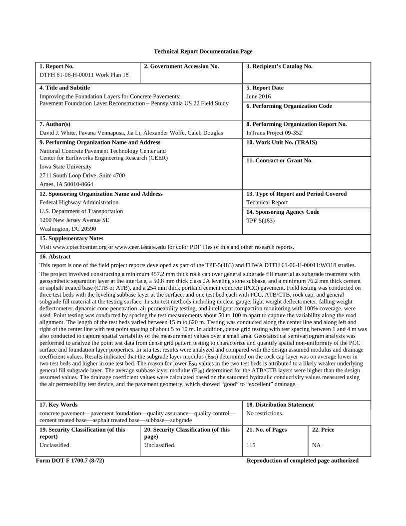
15. Supplementary Notes Visit www.cptechcenter.org or www.ceer.iastate.edu for color PDF files of this and other research reports. 16. Abstract This report is one of the field project reports developed as part of the TPF-5(183) and FHWA DTFH 61-06-H-00011:WO18 studies. The project involved constructing a minimum 457.2 mm thick rock cap over general subgrade fill material as subgrade treatment with geosynthetic separation layer at the interface, a 50.8 mm thick class 2A leveling stone subbase, and a minimum 76.2 mm thick cement or asphalt treated base (CTB or ATB), and a 254 mm thick portland cement concrete (PCC) pavement. Field testing was conducted on three test beds with the leveling subbase layer at the surface, and one test bed each with PCC, ATB/CTB, rock cap, and general subgrade fill material at the testing surface. In situ test methods including nuclear gauge, light weight deflectometer, falling weight deflectometer, dynamic cone penetration, air permeability testing, and intelligent compaction monitoring with 100% coverage, were used. Point testing was conducted by spacing the test measurements about 50 to 100 m apart to capture the variability along the road alignment. The length of the test beds varied between 15 m to 620 m. Testing was conducted along the center line and along left and right of the center line with test point spacing of about 5 to 10 m. In addition, dense grid testing with test spacing between 1 and 4 m was also conducted to capture spatial variability of the measurement values over a small area. Geostatistical semivariogram analysis was performed to analyze the point test data from dense grid pattern testing to characterize and quantify spatial non-uniformity of the PCC surface and foundation layer properties. In situ test results were analyzed and compared with the design assumed modulus and drainage coefficient values. Results indicated that the subgrade layer modulus (ESG) determined on the rock cap layer was on average lower in two test beds and higher in one test bed. The reason for lower ESG values in the two test beds is attributed to a likely weaker underlying general fill subgrade layer. The average subbase layer modulus (ESB) determined for the ATB/CTB layers were higher than the design assumed values. The drainage coefficient values were calculated based on the saturated hydraulic conductivity values measured using the air permeability test device, and the pavement geometry, which showed “good” to “excellent” drainage.

17. Key Words 18. Distribution Statement concrete pavement—pavement foundation—quality assurance—quality control—cement treated base—asphalt treated base—subbase—subgrade

No restrictions.

19. Security Classification (of this report)

20. Security Classification (of this page)

21. No. of Pages 22. Price

Unclassified. Unclassified. 115 NA

Form DOT F 1700.7 (8-72) Reproduction of completed page authorized

IMPROVING THE FOUNDATION LAYERS FOR CONCRETE PAVEMENTS:

PAVEMENT FOUNDATION LAYER RECONSTRUCTION – PENNSYLVANIA US 22 FIELD STUDY

Technical Report June 2016

Research Team Members Tom Cackler, David J. White, Jeffrey R. Roesler, Barry Christopher, Andrew Dawson,

Heath Gieselman, and Pavana Vennapusa

Report Authors David J. White, Pavana K. R. Vennapusa, Jia Li, Alexander J. Wolfe, Caleb Douglas

Iowa State University

Sponsored by the Federal Highway Administration (FHWA)

DTFH61-06-H-00011 Work Plan 18 FHWA Pooled Fund Study TPF-5(183): California, Iowa (lead state),

Michigan, Pennsylvania, Wisconsin

Preparation of this report was financed in part through funds provided by the Iowa Department of Transportation

through its Research Management Agreement with the Institute for Transportation (InTrans Project 09-352)

National Concrete Pavement Technology Center and Center for Earthworks Engineering Research (CEER)

Iowa State University 2711 South Loop Drive, Suite 4700

Ames, IA 50010-8664 Phone: 515-294-5768

www.cptechcenter.org and www.ceer.iastate.edu

v

TABLE OF CONTENTS

ACKNOWLEDGMENTS ............................................................................................................. xi

LIST OF ACRONYMS AND SYMBOLS .................................................................................. xiii

EXECUTIVE SUMMARY ...........................................................................................................xv

CHAPTER 1. INTRODUCTION ....................................................................................................1

CHAPTER 2. PROJECT INFORMATION AND SPECIFICATIONS ..........................................3

Project Background ..............................................................................................................3 Pavement Design Input Parameter Selection and Assumptions ..........................................8

CHAPTER 3. EXPERIMENTAL TESTING METHODS ............................................................10

Laboratory Testing Methods ..............................................................................................10 Particle Size Analysis and Index Properties ..........................................................10 Frost Heave and Thaw Weakening Test ................................................................11

In Situ Testing Methods .....................................................................................................15 Real-Time Kinematic Global Positioning System .................................................16 Zorn Light Weight Deflectometer .........................................................................17 Dynatest Light Weight Deflectometer ...................................................................17 Dynamic Cone Penetrometer .................................................................................17 Kuab Falling Weight Deflectometer ......................................................................18 Humboldt Nuclear Gauge ......................................................................................24 Rapid Air Permeameter Test (APT Device) ..........................................................24 Roller-Integrated Compaction Measurements .......................................................25 Machine Drive Power (MDP) Value .....................................................................26 Compaction Meter Value (CMV) ..........................................................................27

Geostatistical Data Analysis ..............................................................................................27

CHAPTER 4. LABORATORY TEST RESULTS ........................................................................29

Soil Index Properties ..........................................................................................................29 Frost-Heave and Thaw-Weakening Susceptibility ............................................................32

CHAPTER 5. IN-SITU TEST RESULTS .....................................................................................36

Description of Test Beds ....................................................................................................36 TB1: Class 2A Leveling Stone Subbase ............................................................................37 TB2: Class 2A Leveling Stone Subbase ............................................................................43 TB3: Asphalt Treated Base ................................................................................................49 TB4: Cement Treated Base ................................................................................................55 TB5: Rock Cap (Subgrade Treatment) ..............................................................................62 TB6: General Fill Subgrade ...............................................................................................66 TB7: PCC Pavement Surface .............................................................................................73 Summary of In Situ Measurement Values and Comparison with Design Assumptions .......................................................................................................................86

Subgrade Resilient Modulus (ESG or Mr) ...............................................................86 Base Layer Elastic Modulus (ESB): ........................................................................87

vi

Composite Modulus of Subgrade Reaction (kcomp) ................................................87 Drainage Coefficient (Cd) ......................................................................................87

CHAPTER 6. SUMMARY AND CONCLUSIONS .....................................................................91

REFERENCES ..............................................................................................................................93

APPENDIX: 1993 AASHTO RIGID PAVEMENT DESIGN CRITERIA ..................................97

vii

LIST OF FIGURES

Figure 1. Cross-section profile of the new pavement surface and foundation layers at the SR22 project.........................................................................................................................4

Figure 2. Surface of general embankment fill .................................................................................5 Figure 3. Surface of rock cap (subgrade treatment) layer ................................................................5 Figure 4. Rock cap material sampled for gradation analysis ...........................................................6 Figure 5. Side view of embankment constructed with rock cap over general embankment

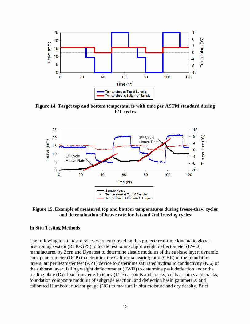
fill and geosynthetic separation layer between the two layers .............................................6 Figure 6. Surface of Class 2A leveling stone layer ..........................................................................7 Figure 7. Surface of ATB layer........................................................................................................7 Figure 8. Construction of CTB layer ...............................................................................................8 Figure 9. Illustration of frost-heave and thaw-weakening test assembly.......................................12 Figure 10. Three-dimensional illustration of frost-heave and thaw-weakening test assembly ......12 Figure 11. View of frost-heave and thaw-weakening test compaction mold with six rings ..........13 Figure 12. Frost-heave and thaw-weakening test compaction mold setup with collar ..................13 Figure 13. Temperature control water baths used to freeze and thaw samples .............................14 Figure 14. Target top and bottom temperatures with time per ASTM standard during

F/T cycles ...........................................................................................................................15 Figure 15. Example of measured top and bottom temperatures during freeze-thaw cycles

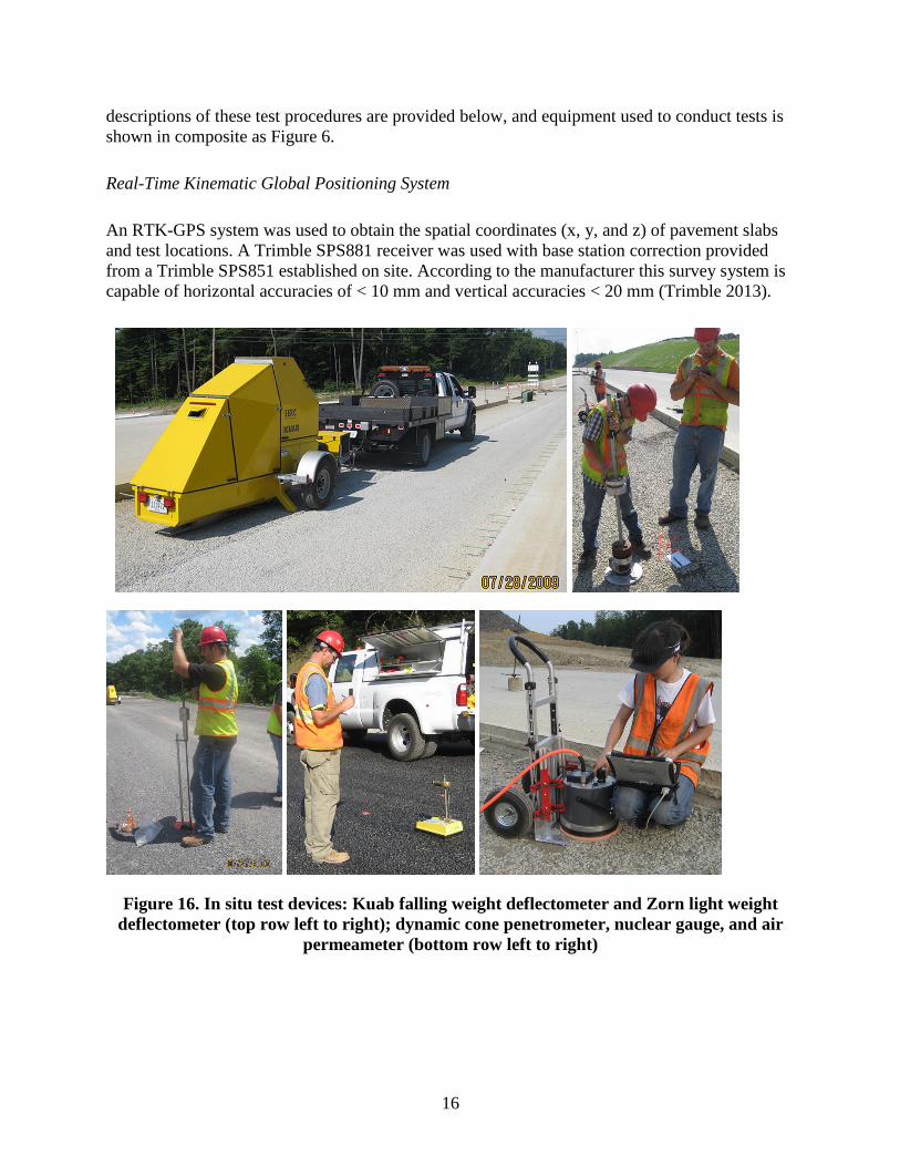
and determination of heave rate for 1st and 2nd freezing cycles .......................................15 Figure 16. In situ test devices: Kuab falling weight deflectometer and Zorn light weight

deflectometer (top row left to right); dynamic cone penetrometer, nuclear gauge, and air permeameter (bottom row left to right) .................................................................16

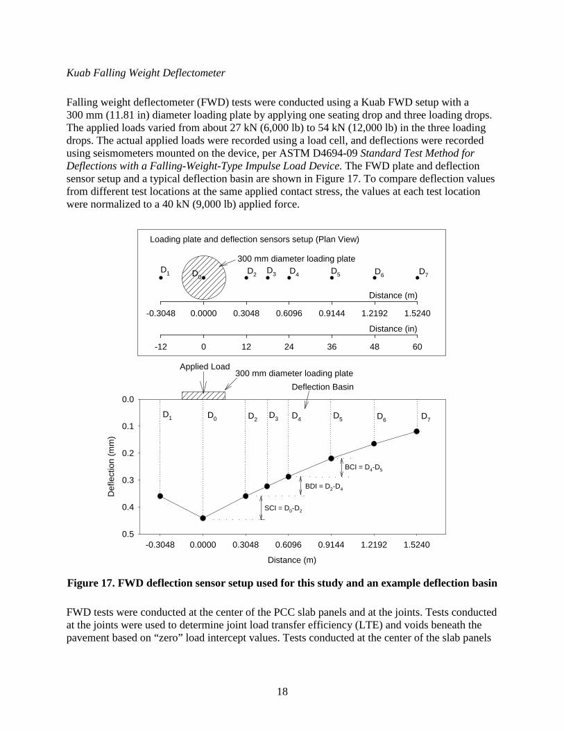
Figure 17. FWD deflection sensor setup used for this study and an example deflection basin ...................................................................................................................................18

Figure 18. Void detection using load-deflection data from FWD test ...........................................19 Figure 19. Static kPLT values versus kFWD-Dynamic measurements reported in literature ..................22 Figure 20. Caterpillar CS683 vibratory smooth drum IC roller .....................................................25 Figure 22. Particle size distribution of TS6 subgrade material ......................................................30 Figure 23. Particle size distribution of TS5 rock cap material ......................................................30 Figure 24. Particle size distribution of TS2 Class A subbase material ..........................................31 Figure 25. Laboratory moisture-density relationships of TS2 Class 2A subbase material ............32 Figure 26. Laboratory moisture-density relationships of TS6 subgrade material .........................32 Figure 27. Frost heave time plots for TS6 subgrade material ........................................................34 Figure 28. Moisture content profiles of TS6 subgrade material ....................................................35 Figure 29. TB 1: Picture of the test area ........................................................................................37 Figure 30. TB 1: Local coordinates of in situ test locations ..........................................................38 Figure 31. TB1: Kriged spatial contour map (top), measurements longitudinally along the

test section (middle), histogram (bottom left), and semivariogram (bottom right) of ELWD-Z3 measurements .......................................................................................................39

Figure 32. TB1: Kriged spatial contour map (top), measurements longitudinally along the test section (middle), histogram (bottom left), and semivariogram (bottom right) of EFWD-K3 measurements .......................................................................................................40

viii

Figure 33. TB1: Kriged spatial contour map (top), measurements longitudinally along the test section (middle), histogram (bottom left), and semivariogram (bottom right) of γd .........................................................................................................................................41

Figure 34. TB1: Kriged spatial contour map (top), measurements longitudinally along the test section (middle), histogram (bottom left), and semivariogram (bottom right) of w .........................................................................................................................................42

Figure 35. TB1: DCP-CBR profiles along all four tracks in longitudinal direction from Sta. 566+50 to Sta. 570+10 .......................................................................................................43

Figure 36. TB 2: Picture of the test bed area .................................................................................44 Figure 37. TB 2: Local coordinates of in situ test locations ..........................................................44 Figure 38. TB 2: Color-coded map of georeferenced CMV map ..................................................45 Figure 39. TB 2: Color-coded map of georeferenced MDP* map ................................................46 Figure 40. TB 2: In situ test results (a) ELWD-Z3, (b) EFWDK3, (c) γd, (d) w, and (e) Ksat along

an about 107 m test section in longitudinal direction ........................................................47 Figure 41. TB 2: Histograms of in situ test measurements (a) ELWD-Z3, (b) EFWDK3, (c) γd,

(d) w, and (e) Ksat ...............................................................................................................48 Figure 42. TB 2: DCP-CBR profiles along all four tracks in longitudinal direction .....................49 Figure 43. TB 3: Picture of the test bed area .................................................................................50 Figure 44. TB 3: Local coordinates of in situ test locations ..........................................................50 Figure 45. TB 3: In situ test results (a) EFWDK3, (b) Uncorrected ESG, (c) ESB, and (d)

Corrected ESG along an about 13 m test section in longitudinal direction .........................51 Figure 46. TB 3: Histograms of in situ test measurements (a) EFWDK3, (b) Uncorrected ESG,

(c) ESB, and (d) Corrected ESG ...........................................................................................52 Figure 47. TB3: Kriged spatial contour map (top), semivariogram (middle), and histogram

(bottom) plots of Ksat measurements [left semi-varaiogram and histogram plots represent measurements on the ATB layer and the right plots represent measurements on the granular subbase layer] ...................................................................54

Figure 48. TB 4: Picture of the test bed area (left side of the black line shows the N [North] area and the right side shows the S [South] area of the test bed).......................................55

Figure 49. TB 4A: Local coordinates of in situ test locations on CTB .........................................56 Figure 50. TB 4A: In situ test results (a) EFWDK3, (b) γd, and (c) w along an about 160 m

test section in longitudinal direction on CTB ....................................................................57 Figure 51. TB 4A: In situ test results (d) Uncorrected ESG, (e) ESB, and (f) Corrected ESG

along an about 160 m test section in longitudinal direction on CTB.................................58 Figure 52. TB 4A: Histograms of in situ test measurements (a) EFWDK3, (b) γd, (c) w, (d)

Uncorrected ESG, (e) ESB, and (f) Corrected ESG ...............................................................59 Figure 53. TB 4A: DCP-CBR profiles along two tracks in longitudinal direction .......................60 Figure 54. TB4B: Kriged spatial contour map (top), semivariogram (middle), and

histogram (bottom) plots of Ksat measurements .................................................................61 Figure 55. TB 5: Picture of the test bed area .................................................................................62 Figure 56. TB 5: Local coordinates of in situ test locations ..........................................................63 Figure 57. TB 5: Color-coded map of georeferenced CMV map ..................................................64 Figure 58. TB 5: Color-coded map of georeferenced MDP* map ................................................65 Figure 59. TB 5: Measurements of ELWD-D3 (top) and measurements of EFWD-K3 (middle)

longitudinally along the test section, histogram of ELWD-D3 (bottom left), and histogram of EFWD-K3 (bottom right) of the measurements ................................................66

ix

Figure 60. TB 6: Picture of the test bed area during IC rolling .....................................................67 Figure 61. TB 6: Local coordinates of in situ test locations on subgrade ......................................67 Figure 62. TB 6: Color-coded map of georeferenced CMV map ..................................................69 Figure 63. TB 6: Color-coded map of georeferenced MDP* map ................................................70 Figure 64. TB 6: In situ test results (a) ELWD-Z3, (b) γd, and (c) w along an about 610 m test

section in longitudinal direction.........................................................................................71 Figure 65. TB 6: Histograms of in situ test measurements (a) ELWD-Z3, (b) γd, and (c) w .............72 Figure 66. TB 6: DCP-CBR profiles along all four tracks in longitudinal direction .....................73 Figure 67. TB 7: Picture of the test area ........................................................................................74 Figure 68. TB 7A: Local coordinates of in situ test locations on PCC [dense testing] .................74 Figure 69. TB 7B: Local coordinates of in situ test locations on PCC [mid panel testing] ...........75 Figure 70. TB 7A: Kriged spatial contour map (top), measurements longitudinally along

the test section (middle), histogram (bottom left), and semivariogram (bottom right) of D0 measurements [dense testing] ...................................................................................76

Figure 71. TB 7A: Kriged spatial contour map (top), measurements longitudinally along the test section (middle), histogram (bottom left), and semivariogram (bottom right) of SCI measurements [dense testing] .................................................................................77

Figure 72. TB 7A: Kriged spatial contour map (top), measurements longitudinally along the test section (middle), histogram (bottom left), and semivariogram (bottom right) of BDI measurements [dense testing] ................................................................................78

Figure 73. TB 7A: Kriged spatial contour map (top), measurements longitudinally along the test section (middle), histogram (bottom left), and semivariogram (bottom right) of BCI measurements [dense testing] .................................................................................79

Figure 74. TB 7A: Kriged spatial contour map (top), measurements longitudinally along the test section (middle), histogram (bottom left), and semivariogram (bottom right) of Area Factor measurements [dense testing] ....................................................................80

Figure 75. TB 7A: Kriged spatial contour map (top), measurements longitudinally along the test section (middle), histogram (bottom left), and semivariogram (bottom right) of Intercept measurements [dense testing] .........................................................................81

Figure 76. TB 7A: Kriged spatial contour map (top), measurements longitudinally along the test section (middle), histogram (bottom left), and semivariogram (bottom right) of kFWD-S_Corr measurements [dense testing] .......................................................................82

Figure 77. TB 7B: FWD tests results on PCC [mid panel testing] ................................................83 Figure 78. TB 7B: FWD tests results on PCC continue [mid panel testing] .................................84 Figure 79. TB 7B: Histograms of FWD test measurements [mid panel testing] ...........................85 Figure 80. TB 7B: Histograms of FWD test measurements continue [mid panel testing] ............86

x

LIST OF TABLES

Table 1. Summary of pavement thickness design input parameters and assumptions (AASHTO 1993 method) .....................................................................................................9

Table 2. Frost susceptibility classifications (ASTM D5918-06) ...................................................11 Table 3. Caterpillar CS683 vibratory smooth drum IC roller features ..........................................26 Table 4. Summary of material index properties.............................................................................29 Table 5. Frost-heave and thaw-weakening test results of TS6 subgrade .......................................35 Table 6. Summary of test beds and in situ testing .........................................................................36 Table 7. Summary of univariate statistics of in situ test results on pavement foundation

layer materials ....................................................................................................................89 Table 8. Summary of design, in situ measured, and laboratory measured values .........................90

xi

ACKNOWLEDGMENTS

This research was conducted under Federal Highway Administration (FHWA) DTFH61-06-H-00011 Work Plan 18 and the FHWA Pooled Fund Study TPF-5(183), involving the following state departments of transportation:

• California • Iowa (lead state) • Michigan • Pennsylvania • Wisconsin

The authors would like to express their gratitude to the National Concrete Pavement Technology (CPTech) Center, the FHWA, the Iowa Department of Transportation (DOT), and the other pooled fund state partners for their financial support and technical assistance.

Joshua Freeman, Lydia Peddicord, Mark Kmetz and several others from Pennsylvania DOT provided assistance in identifying the project and providing access during testing on the project site. We greatly appreciate their help. We also thank Jiake Zhang, Stephen Quist, and Luke Johanson of the Center for Earthworks Engineering Research (CEER) at Iowa State University for help with laboratory and field testing and Christianna White, also of CEER, for comments and editorial assistance.

xii

xiii

LIST OF ACRONYMS AND SYMBOLS

A′ Machine acceleration AF Area factor APT Air permeameter A2Ω Acceleration of the first harmonic component of the roller vibration AΩ Acceleration of the fundamental component of the roller vibration ATB Asphalt treated base material BCI Base curvature index BDI Base damage index CBR California bearing ratio C Constant (300) for calculating CMV Cd Drainage coefficient CMV Compaction meter value COV Coefficient of variation CTB Cement treated base material D0 Deflection measured under the plate D1 to D7 Deflections measured away from the plate at various set distances DSB Subbase layer thickness DCP Dynamic cone penetration test DCP-CBR California bearing ratio calculated from dynamic cone penetration values DPI Dynamic penetration index E Elastic modulus Ec Modulus of elasticity of concrete Esg Modulus of elasticity of subgrade EFWD-K3 Surface modulus determined using 300 mm diameter plate Kuab falling

weight deflectometer ELWD-Z2 Elastic modulus determined from 200 mm diameter plate light weight

deflectometer Es Dynamic secant modulus ESB Elastic modulus of the subbase ESG Elastic modulus of the subgrade F Shape factor FWD Falling weight deflectometer F/T Freeze/thaw g Acceleration due to gravity Go Geometric factor IC Intelligent compaction k Modulus of subgrade reaction kcomp Composite modulus of subgrade reaction keff Effective modulus of subgrade reaction kFWD-Dynamic Dynamic modulus of subgrade reaction from FWD test kFWD-Static-Corr Static modulus of subgrade reaction from FWD test Ksat Saturated hydraulic conductivity determined using rapid gas permeameter test

device I Intercept value

xiv

J Load transfer coefficient L Radius of relative stiffness LL Liquid limit LI Plasticity index LTE Load transfer efficiency LS Loss of support LWD Light weight deflectometer m and b Machine internal loss coefficients specific to a particular machine MDP Machine drive power MET Method of equivalent thickness Mr Resilient modulus MV Measurement value NG Nuclear gauge Po(g) Gauge pressure of the gas at the orifice outlet P1 Absolute gas pressure on the soil surface P2 Pressure app Pg Gross power needed to move the IC machine PID Proportional-integral-derivative controller PL Plastic limit R2 Coefficeint of determination Q Volumetric flow rate r Plate radius (LWD test) r Radius at the outlet (for APT test) RTK-GPS Real-time kinematic global positioning system Sc PCC modulus of rupture S Water saturation Se Effective water saturation Sr Residual water saturation SCI Surface curvature index v Roller velocity W Roller weight α Slope angle determined from roller pitch from a sensor γ(h) Plot of the average squared differences between data values as a function of

separation distance δ Depth to impervious layer γd Dry unit weight determined from Humboldt nuclear gauge λ Brooks-Corey pore size distribution index µ Statistical mean or average µair Dynamic viscosity of air µwater Absolute viscosity of water η Poisson’s ratio σ Statistical standard deviation σ0 Applied stress ρ Density of water w Moisture content determined from Humboldt nuclear gauge wopt Optimum moisture content

xv

EXECUTIVE SUMMARY

Quality foundation layers (the natural subgrade, subbase, and embankment) are essential to achieving excellent pavement performance. Unfortunately, many pavements in the United States still fail due to inadequate foundation layers. To address this problem, a research project, Improving the Foundation Layers for Pavements (FHWA DTFH 61-06-H-00011 WO #18; FHWA TPF-5(183)), was undertaken by Iowa State University to identify, and provide guidance for implementing, best practices regarding foundation layer construction methods, material selection, in situ testing and evaluation, and performance-related designs and specifications. As part of the project, field studies were conducted on several in-service concrete pavements across the country that represented either premature failures or successful long-term pavements. A key aspect of each field study was to tie performance of the foundation layers to key engineering properties and pavement performance. In situ foundation layer performance data, as well as original construction data and maintenance/rehabilitation history data, were collected and geospatially and statistically analyzed to determine the effects of site-specific foundation layer construction methods, site evaluation, materials selection, design, treatments, and maintenance procedures on the performance of the foundation layers and of the related pavements. A technical report was prepared for each field study.

This report presents results and analysis from a field study conducted on SR-22 near Clyde in Indiana County, Pennsylvania. The project consisted of reconstruction of pavement foundation layers (subbase and subgrade) of the east and west bound lanes of the highway. The total length of the reconstruction project was about 7.74 km (4.81 miles).

The pavement foundation layers consisted of a minimum 457.2 mm (18 in.) thick rock cap that was placed and compacted on the subgrade and is referred to as subgrade treatment in the project plans. The subgrade beneath the rock cap consisted of general embankment fill consisted of rocky subgrade material obtained from cuts. A geosynthetic separation layer was installed at the subgrade rockcap interface. A 50.8 mm (2 in.) thick Class 2A levelling stone consisting of crushed limestone material was placed as granular leveling course layer over the rock cap. A minimum 76.2 mm (3 in.) thick asphalt treated base (ATB) or cement treated base (CTB) layer was installed over the granular subbase layer. A 254 mm (10 in.) thick new jointed PCC layer was installed over the CTB/ATB layer. The pavement section was designed in accordance with the AASHTO design guide for design of pavement structures (AASHTO 1993) rigid pavement design.

The Iowa State University (ISU) research team was present at the project site from July 27 to 29, 2009, during the construction process to conduct a field study on foundation layers and the newly constructed PCC surface layer. Field testing was conducted on seven test beds (TBs). Two test beds consisted of levelling stone subbase layer at the surface, and one test bed each consisted of PCC, CTB, ATB, rock cap layer, and general subgrade fill at the testing surface. Field testing involved falling weight deflectometer (FWD), Zorn and Dynatest light weight deflectometer (LWD), nuclear gauge (NG), dynamic cone penetrometer (DCP), and air permeability test (APT) point testing and intelligent compaction (IC) measurements. Laboratory testing was conducted on the materials collected from the field to characterize the index properties (i.e., gradation,

xvi

compaction, specific gravity, soil classification) and frost-heave and thaw-weakening susceptibility of the subgrade general fill materials.

The length of the test beds varied between 15 m to 620 m. Testing was conducted along the center line and along left and right of the center line with test point spacing of about 5 to 10 m. In addition, dense grid testing with test spacing between 1 and 4 m was also conducted to capture spatial variability of the measurement values over a small area. Geostatistical semivariogram analysis was performed to analyze the point test data from dense grid pattern testing to characterize and quantify spatial non-uniformity of the PCC surface and foundation layer properties.

Comparing measured properties from laboratory and in situ testing with the design assumed values revealed the following:

• Average subgrade layer moduli (ESG) was determined based testing on the rock cap layer from three TBs. Average ESG from TBs 1 and 2 from LWD and FWD testing was 71.5 MPa and 120.2 MPa, respectively, which were lower than the design assumed ESG of 206.8 MPa. Average ESG from TB 5 from LWD and FWD measurements were 303.4 and 407.2 MPa, which were higher than the design assumed ESG of 206.8 MPa. Possible reasons for lower ESG values in TBs 1 and 2 can be due to weaker general fill material, as evidenced in TB6 with average moduli of 18.1 MPa. It must be noted that LWD and FWD measurements provide a composite response of materials within its measurement influence depth ranging between 1.5 to 2 times the dimeter of the plate (450 to 600 mm depth).

• Average subbase layer moduli (ESB) values for the CTB and ATB layers were 721 and 4,467 MPa, which are 3.5 to 21.6 times higher than the design assumed ESB of 206.8 MPa. It must be noted that the ATB layer tested in this study was placed one day prior to testing, while the CTB layer was placed several months prior to testing. Additional curing of the ATB material can potentially increase the moduli values of the layer.

• For section with ATB, the composite modulus of subgrade reaction (kcomp) values ranged between 196.8 kPa/mm (based on LWD measurements for ESG) and 282.3 kPa/mm (based on FWD measurements for ESG) and were about 1.2 to 1.7 times lower than the design target kcomp of 340 kPa/mm. Again, it must be noted that additional curing of the ATB material can potentially increase the ESB values and the resulting kcomp values.

• For section with CTB, the estimated kcomp value ranged between 252.4 kPa/mm (based on LWD measurements for ESG) and 367.5 kPa/mm (based on FWD measurements for ESG) and were about 1.3 times lower and 1.1 times higher than the design target kcomp of 340 kPa/mm.

• The drainage coefficient (Cd) value was assumed in the design as 1.0, which represents that the quality of drainage is rated as “good”. Based on the pavement geometry (i.e.,

xvii

cross slope, width of the pavement, thickness of the base layer), the measured Ksat values from the field, and assuming an effective porosity = 0.3, the time for a target 90% drainage was calculated. Based on APT tests conducted on the CTB layer, the time for 90% drainage was estimated as 1.0 day for Ksat = 0.2 cm/s (CTB contaminated with fines) to < 1 hour for Ksat = 7 cm/s (CTB uncontaminated). Based on tests conducted on the ATB layer the time for 90% drainage was estimated < 1 hour for Ksat = 4.6 cm/s. Based on these estimates, the quality of drainage can be rated as “good” to “excellent” for the ATB and CTB layers and does meet the design requirements.

The findings from the field studies under the Improving the Foundation Layers for Concrete Pavements research project will be of significant interest to researchers, practitioners, and agencies dealing with design, construction, and maintenance of PCC pavements. The technical reports are included in Volume II (Appendices) of the Final Report: Improving the Foundation Layers for Pavements. Data from the field studies are used in analyses of performance parameters for pavement foundation layers in the Mechanistic-Empirical Pavement Design Guide (MEPDG) program. New knowledge gained from this project will be incorporated into the Manual of Professional Practice for Design, Construction, Testing and Evaluation of Concrete Pavement Foundations published in 2016.

1

CHAPTER 1. INTRODUCTION

This report presents results and analysis from a field study conducted on State Route 22 (SR-22) near Clyde in Indiana County, Pennsylvania. The project consisted of reconstruction of pavement foundation layers (subbase and subgrade) of the east and west bound lanes of the highway. The total length of the reconstruction project was about 7.74 km (4.81 miles).

The existing pavement consisted of bituminous pavement of varying depths along the project and was removed and undercut down to the desired subgrade elevation and in some areas fill was required to build up to the subgrade elevation. General embankment fill consisting of rocky subgrade material was used in the fill areas. A minimum 457.2 mm (18 in.) thick rock cap was placed and compacted on the subgrade and is referred to as subgrade treatment in the project plans. A geosynthetic separation layer was installed at the subgrade rockcap interface. A 50.8 mm (2 in.) thick Class 2A levelling stone consisting of crushed limestone material was placed as granular leveling course layer over the rock cap. A minimum 76.2 mm (3 in.) thick asphalt treated base (ATB) or cement treated base (CTB) layer was installed over the granular subbase layer. A 254 mm (10 in.) thick new jointed PCC layer was installed over the CTB/ATB layer. The pavement section was designed in accordance with the AASHTO design guide for design of pavement structures (AASHTO 1993) rigid pavement design.

The Iowa State University (ISU) research team was present at the project site from July 27 to 29, 2009, during the construction process to conduct a field study on foundation layers and the newly constructed PCC surface layer. Field testing involved: Kuab falling weight deflectometer (FWD) to determine elastic modulus and deflection basin parameters; Zorn and Dynatest light weight deflectometer (LWD) to determine elastic modulus; dynamic cone penetrometer (DCP) to estimate California bearing ratio values; Humboldt nuclear gauge (NG) to determine moisture and dry unit weight; rapid air permeameter test (APT) device to measure saturated hydraulic conductivity; and roller-integrated compaction monitoring or intelligent compaction (IC) measurements to obtain 100% coverage of compacted material properties. The spatial northing and easting of all test measurement locations were obtained using a real-time kinematic (RTK) global positioning system (GPS).

Laboratory testing was conducted on the materials collected from the field to characterize the index properties (i.e., gradation, compaction, specific gravity, soil classification) and frost-heave and thaw-weakening susceptibility of the subgrade general fill materials.

Field testing was conducted on seven test beds (TBs). TBs 1 and 2 consisted of class 2A levelling stone subbase placed over the rock cap subgrade treatment, TB3 consisted of ATB, TB4 consisted of CTB, TB5 consisted of rock cap subgrade treatment, TB6 consisted of general subgrade fill, and TB7 consisted of the newly constructed PCC layer at the surface. TB2 was located on SR259, which was also being reconstructed as part of this project, while all remaining TBs were located on SR22 mainline. Except TB3, all other TBs were located just east or west of SR259 near Clyde, PA. TB3 was located on an adjacent project site near Blairsville, PA and was tested to evaluate ATB material properties in comparison with the CTB layer properties.

2

The length of the test beds varied between 15 m to 620 m. Testing was conducted along the center line and along left and right of the center line with test point spacing of about 5 to 10 m. In addition, dense grid testing with test spacing between 1 and 4 m was also conducted to capture spatial variability of the measurement values over a small area. Geostatistical semivariogram analysis was performed to analyze the point test data from dense grid pattern testing to characterize and quantify spatial non-uniformity of the PCC surface and foundation layer properties.

This report contains six chapters. Chapter 2 provides background information about the project and photographs documenting the construction procedures; and AASHTO (1993) pavement design input parameters. Chapter 3 presents an overview of the laboratory and in situ testing methods followed in this project. Chapter 4 presents results from laboratory testing. Chapter 5 presents results from in situ testing and analysis and compares laboratory and in situ measured values with the design assumed values. Chapter 6 presents key findings and conclusions from the field study.

The findings from this report should be of significant interest to researchers, practitioners, and agencies who deal with design, construction, and maintenance aspects of PCC pavements. This project report is one of several field project reports developed as part of the TPF-5(183) and FHWA DTFH 61-06-H-00011:WO18 studies.

3

CHAPTER 2. PROJECT INFORMATION AND SPECIFICATIONS

This chapter presents brief background information on the project, photos taken of pavement foundation layer construction during ISU testing, and pavement thickness design parameter selection and assumptions during the design phase of the project.

Project Background

This project is located on SR-22 near Clyde in Indiana County, Pennsylvania, and consisted of reconstruction of pavement foundation layers (subbase and subgrade) of the east and west bound lanes of the highway between Sta. 311+00 and 577+00 (Section 494, Federal Project No. X104-204-L980). The total length of the reconstruction project was about 7.74 km (4.81 miles).

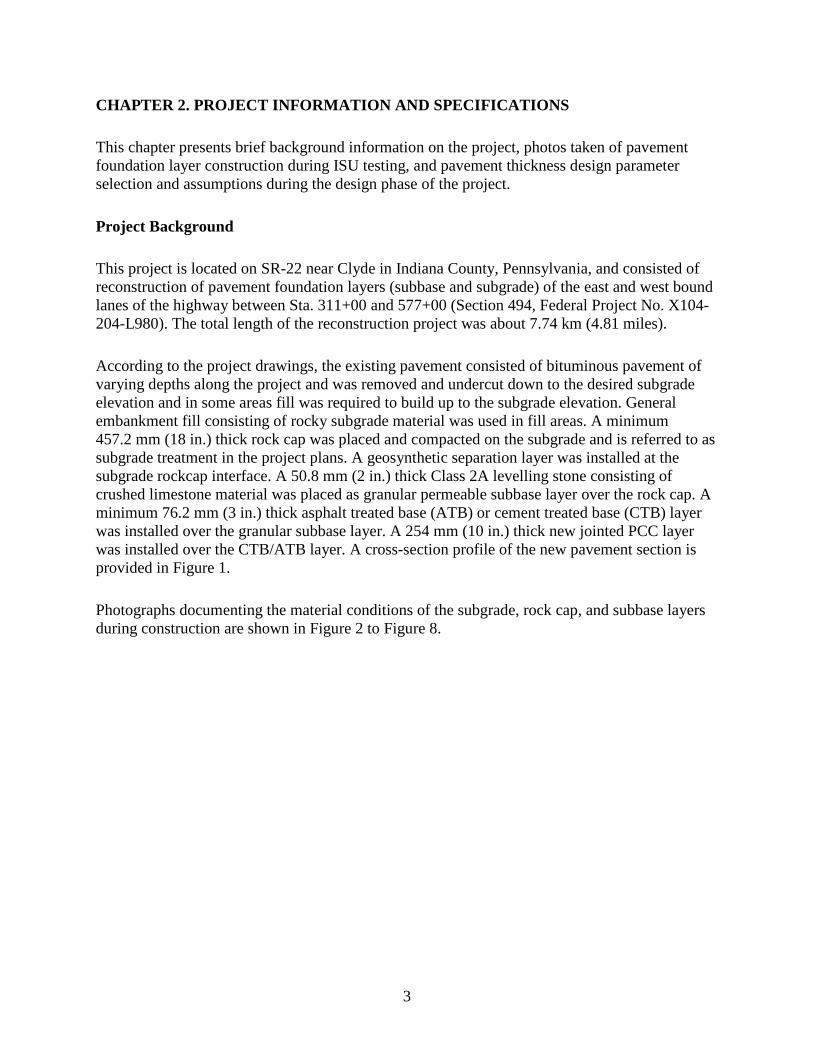
According to the project drawings, the existing pavement consisted of bituminous pavement of varying depths along the project and was removed and undercut down to the desired subgrade elevation and in some areas fill was required to build up to the subgrade elevation. General embankment fill consisting of rocky subgrade material was used in fill areas. A minimum 457.2 mm (18 in.) thick rock cap was placed and compacted on the subgrade and is referred to as subgrade treatment in the project plans. A geosynthetic separation layer was installed at the subgrade rockcap interface. A 50.8 mm (2 in.) thick Class 2A levelling stone consisting of crushed limestone material was placed as granular permeable subbase layer over the rock cap. A minimum 76.2 mm (3 in.) thick asphalt treated base (ATB) or cement treated base (CTB) layer was installed over the granular subbase layer. A 254 mm (10 in.) thick new jointed PCC layer was installed over the CTB/ATB layer. A cross-section profile of the new pavement section is provided in Figure 1.

Photographs documenting the material conditions of the subgrade, rock cap, and subbase layers during construction are shown in Figure 2 to Figure 8.

4

Figure 1. Cross-section profile of the new pavement surface and foundation layers at the SR22 project

5

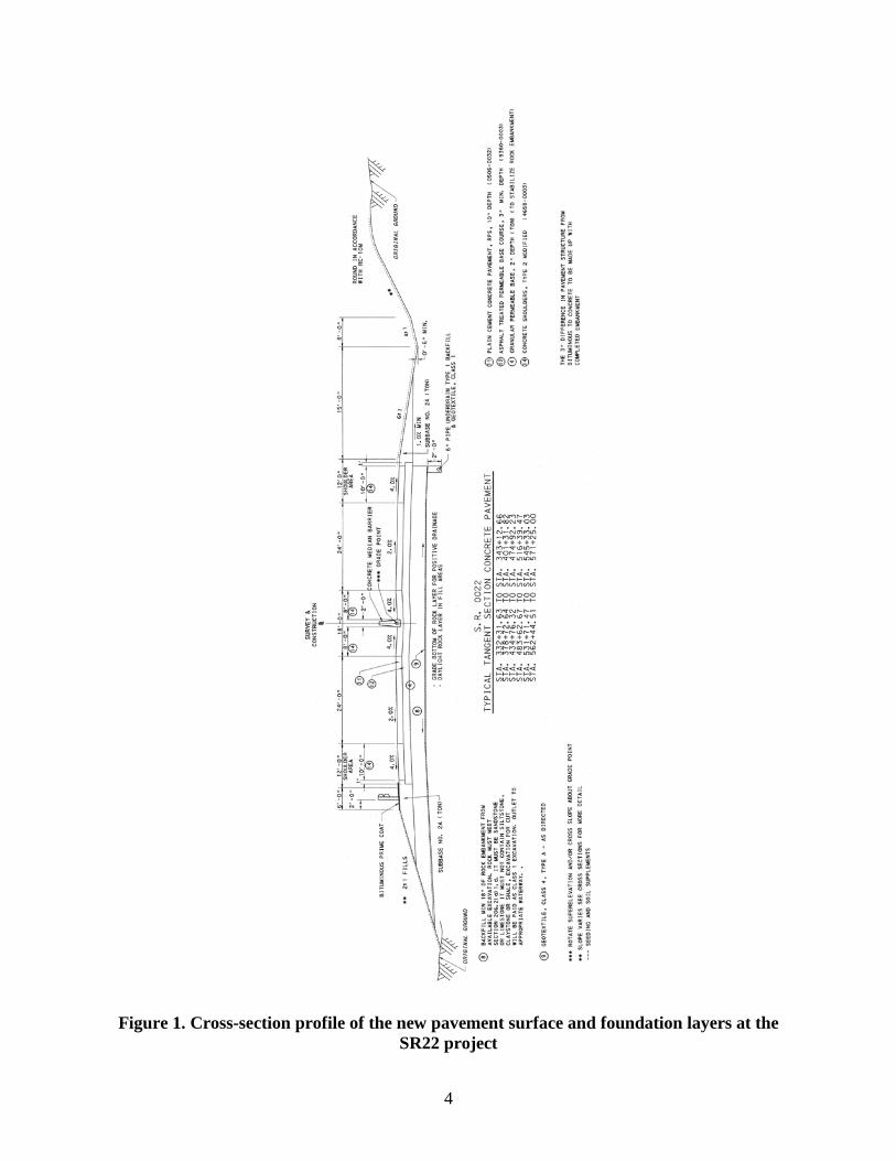
Figure 2. Surface of general embankment fill

Figure 3. Surface of rock cap (subgrade treatment) layer

6

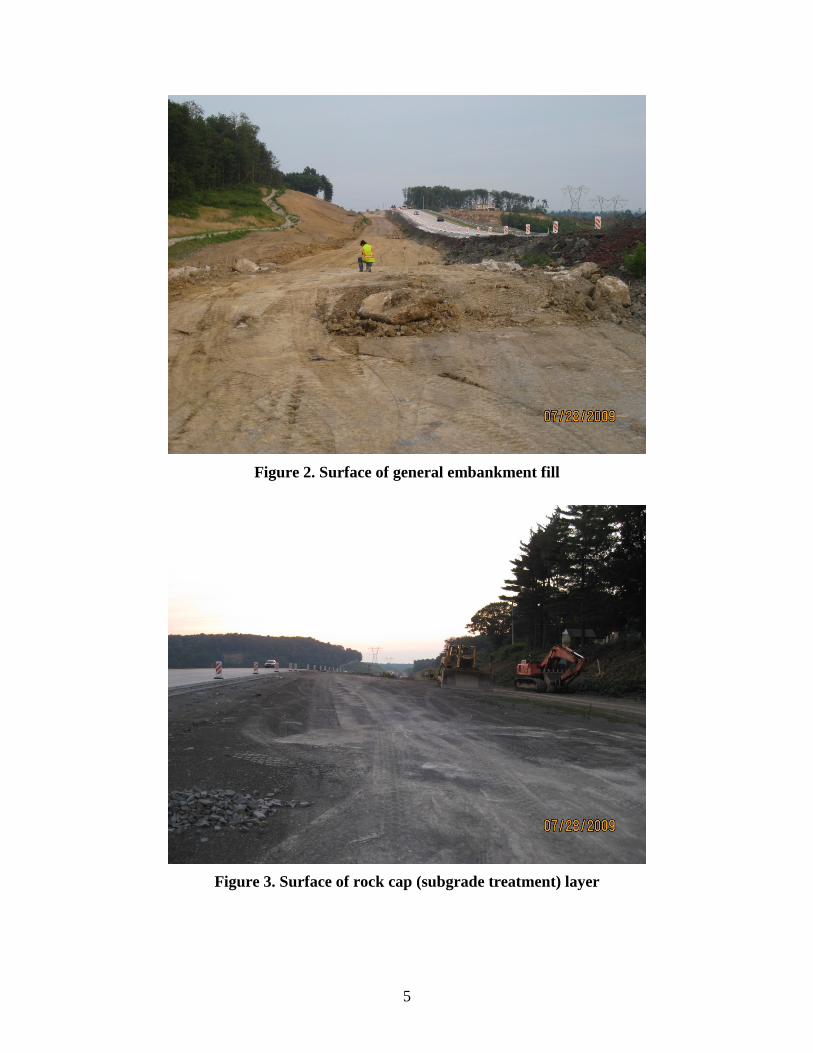
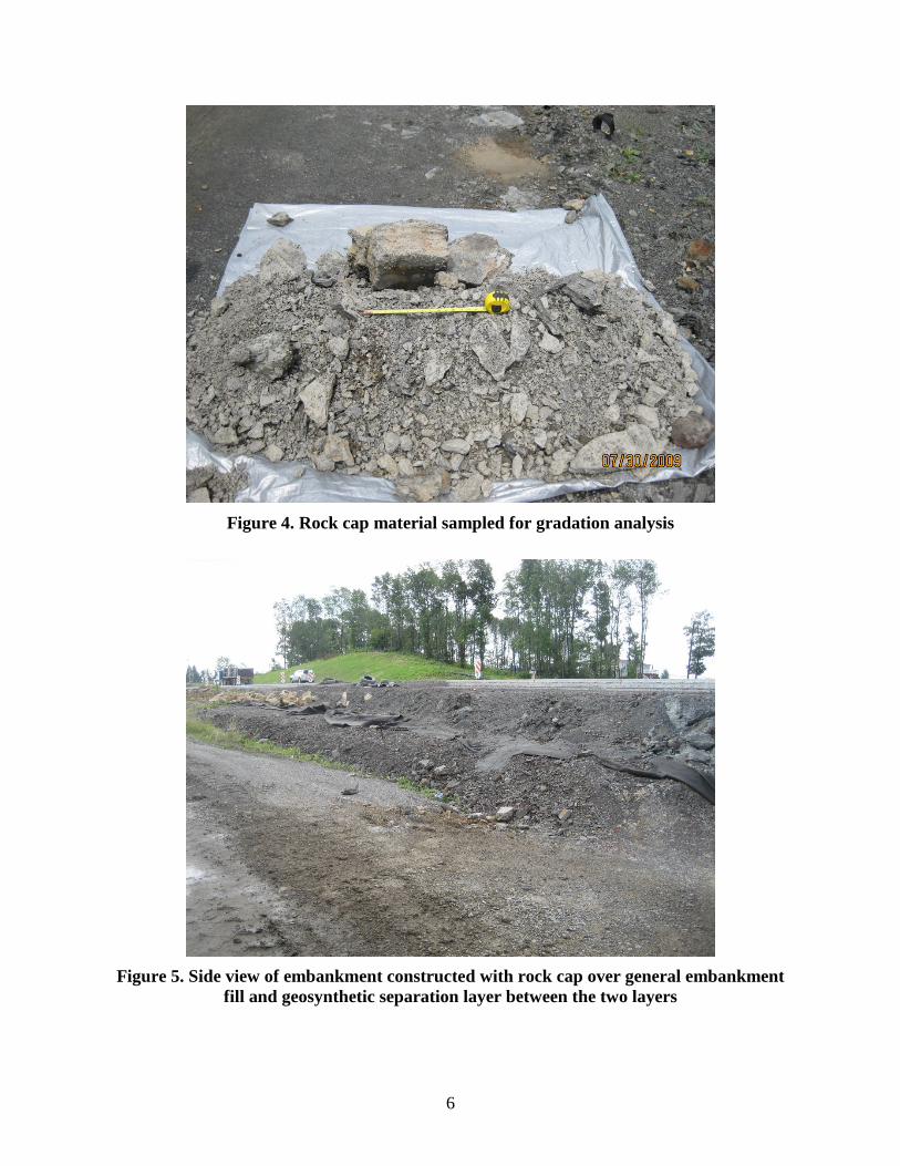
Figure 4. Rock cap material sampled for gradation analysis

Figure 5. Side view of embankment constructed with rock cap over general embankment

fill and geosynthetic separation layer between the two layers

7

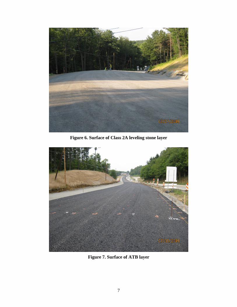
Figure 6. Surface of Class 2A leveling stone layer

Figure 7. Surface of ATB layer

8

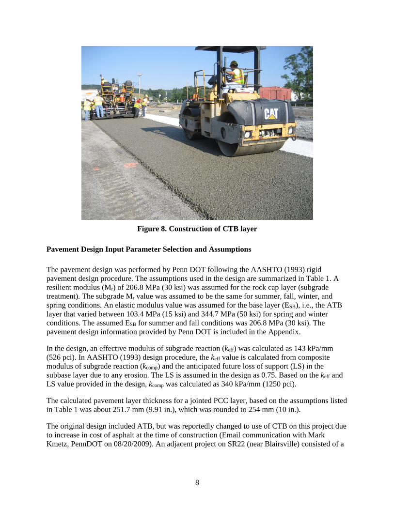
Figure 8. Construction of CTB layer

Pavement Design Input Parameter Selection and Assumptions

The pavement design was performed by Penn DOT following the AASHTO (1993) rigid pavement design procedure. The assumptions used in the design are summarized in Table 1. A resilient modulus (Mr) of 206.8 MPa (30 ksi) was assumed for the rock cap layer (subgrade treatment). The subgrade Mr value was assumed to be the same for summer, fall, winter, and spring conditions. An elastic modulus value was assumed for the base layer (ESB), i.e., the ATB layer that varied between 103.4 MPa (15 ksi) and 344.7 MPa (50 ksi) for spring and winter conditions. The assumed ESB for summer and fall conditions was 206.8 MPa (30 ksi). The pavement design information provided by Penn DOT is included in the Appendix.

In the design, an effective modulus of subgrade reaction (keff) was calculated as 143 kPa/mm (526 pci). In AASHTO (1993) design procedure, the keff value is calculated from composite modulus of subgrade reaction (kcomp) and the anticipated future loss of support (LS) in the subbase layer due to any erosion. The LS is assumed in the design as 0.75. Based on the keff and LS value provided in the design, kcomp was calculated as 340 kPa/mm (1250 pci).

The calculated pavement layer thickness for a jointed PCC layer, based on the assumptions listed in Table 1 was about 251.7 mm (9.91 in.), which was rounded to 254 mm (10 in.).

The original design included ATB, but was reportedly changed to use of CTB on this project due to increase in cost of asphalt at the time of construction (Email communication with Mark Kmetz, PennDOT on 08/20/2009). An adjacent project on SR22 (near Blairsville) consisted of a

9

similar design and included ATB (Figure 7) and was selected for testing to compare with CTB layer properties measured during this field study.

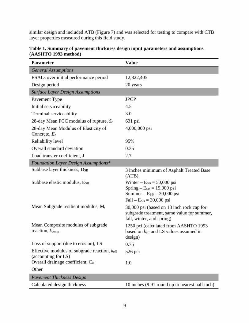
Table 1. Summary of pavement thickness design input parameters and assumptions (AASHTO 1993 method)

Parameter Value General Assumptions ESALs over initial performance period 12,822,405 Design period 20 years Surface Layer Design Assumptions Pavement Type JPCP Initial serviceability 4.5 Terminal serviceability 3.0 28-day Mean PCC modulus of rupture, Sc 631 psi 28-day Mean Modulus of Elasticity of Concrete, Ec

4,000,000 psi

Reliability level 95% Overall standard deviation 0.35 Load transfer coefficient, J 2.7 Foundation Layer Design Assumptions* Subbase layer thickness, DSB 3 inches minimum of Asphalt Treated Base

(ATB) Subbase elastic modulus, ESB Winter – ESB = 50,000 psi

Spring – ESB = 15,000 psi Summer – ESB = 30,000 psi Fall – ESB = 30,000 psi

Mean Subgrade resilient modulus, Mr 30,000 psi (based on 18 inch rock cap for subgrade treatment, same value for summer, fall, winter, and spring)

Mean Composite modulus of subgrade reaction, kcomp

1250 pci (calculated from AASHTO 1993 based on keff and LS values assumed in design)

Loss of support (due to erosion), LS 0.75 Effective modulus of subgrade reaction, keff (accounting for LS)

526 pci

Overall drainage coefficient, Cd 1.0 Other Pavement Thickness Design Calculated design thickness 10 inches (9.91 round up to nearest half inch)

10

CHAPTER 3. EXPERIMENTAL TESTING METHODS

Experimental testing in this research study involved laboratory testing of foundation layer materials, in situ testing to evaluate the properties of the pavement surface and underlying foundation layers, and in-ground instrumentation to monitor temperatures.

This chapter presents a summary of the laboratory and in situ testing methods, and the statistical analysis methods used in this study.

Laboratory Testing Methods

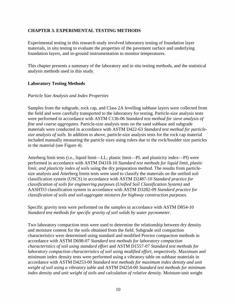
Particle Size Analysis and Index Properties

Samples from the subgrade, rock cap, and Class 2A levelling subbase layers were collected from the field and were carefully transported to the laboratory for testing. Particle-size analysis tests were performed in accordance with ASTM C136-06 Standard test method for sieve analysis of fine and coarse aggregates. Particle-size analysis tests on the sand subbase and subgrade materials were conducted in accordance with ASTM D422-63 Standard test method for particle-size analysis of soils. In addition to above, particle-size analysis tests for the rock cap material included manually measuring the particle sizes using rulers due to the rock/boulder size particles in the material (see Figure 4).

Atterberg limit tests (i.e., liquid limit—LL; plastic limit—PL and plasticity index—PI) were performed in accordance with ASTM D4318-10 Standard test methods for liquid limit, plastic limit, and plasticity index of soils using the dry preparation method. The results from particle-size analysis and Atterberg limits tests were used to classify the materials on the unified soil classification system (USCS) in accordance with ASTM D2487-10 Standard practice for classification of soils for engineering purposes (Unified Soil Classification System) and AASHTO classification system in accordance with ASTM D3282-09 Standard practice for classification of soils and soil-aggregate mixtures for highway construction purposes.

Specific gravity tests were performed on the samples in accordance with ASTM D854-10 Standard test methods for specific gravity of soil solids by water pycnometer.

Two laboratory compaction tests were used to determine the relationship between dry density and moisture content for the soils obtained from the field. Subgrade soil compaction characteristics were determined using standard and modified Proctor compaction methods in accordance with ASTM D698-07 Standard test methods for laboratory compaction characteristics of soil using standard effort and ASTM D1557-07 Standard test methods for laboratory compaction characteristics of soil using modified effort, respectively. Maximum and minimum index density tests were performed using a vibratory table on subbase materials in accordance with ASTM D4253-00 Standard test methods for maximum index density and unit weight of soil using a vibratory table and ASTM D4254-00 Standard test methods for minimum index density and unit weight of soils and calculation of relative density. Moisture-unit weight

11

relationships of subbase materials were determined by performing maximum index density tests by incrementally increasing the moisture content by approximately 1.5% for each test.

Frost Heave and Thaw Weakening Test

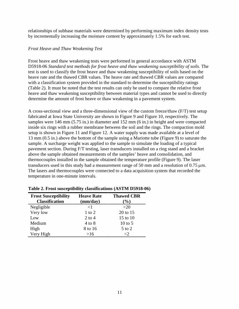
Frost heave and thaw weakening tests were performed in general accordance with ASTM D5918-06 Standard test methods for frost heave and thaw weakening susceptibility of soils. The test is used to classify the frost heave and thaw weakening susceptibility of soils based on the heave rate and the thawed CBR values. The heave rate and thawed CBR values are compared with a classification system provided in the standard to determine the susceptibility ratings (Table 2). It must be noted that the test results can only be used to compare the relative frost heave and thaw weakening susceptibility between material types and cannot be used to directly determine the amount of frost heave or thaw weakening in a pavement system.

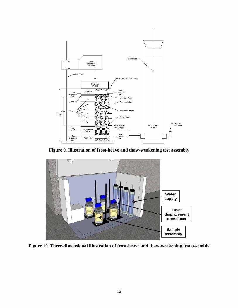
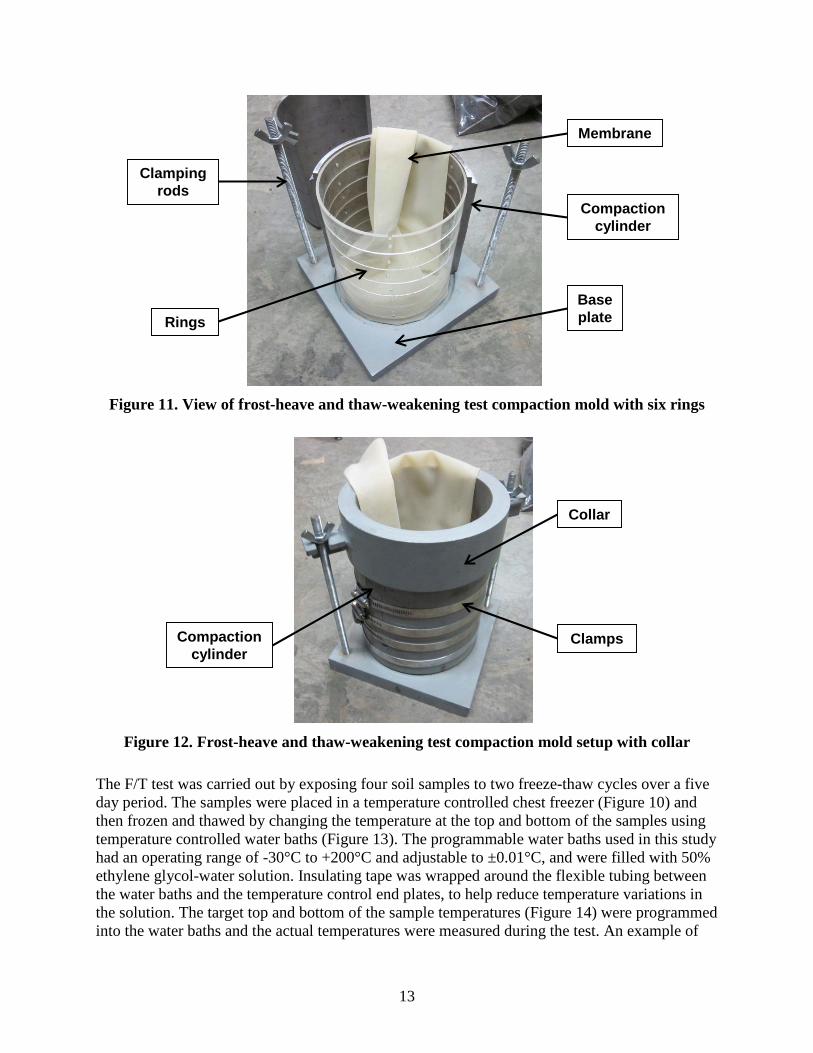
A cross-sectional view and a three-dimensional view of the custom freeze/thaw (F/T) test setup fabricated at Iowa State University are shown in Figure 9 and Figure 10, respectively. The samples were 146 mm (5.75 in.) in diameter and 152 mm (6 in.) in height and were compacted inside six rings with a rubber membrane between the soil and the rings. The compaction mold setup is shown in Figure 11 and Figure 12. A water supply was made available at a level of 13 mm (0.5 in.) above the bottom of the sample using a Mariotte tube (Figure 9) to saturate the sample. A surcharge weight was applied to the sample to simulate the loading of a typical pavement section. During F/T testing, laser transducers installed on a ring stand and a bracket above the sample obtained measurements of the samples’ heave and consolidation, and thermocouples installed in the sample obtained the temperature profile (Figure 9). The laser transducers used in this study had a measurement range of 50 mm and a resolution of 0.75 µm. The lasers and thermocouples were connected to a data acquisition system that recorded the temperature in one-minute intervals.

Table 2. Frost susceptibility classifications (ASTM D5918-06) Frost Susceptibility

Classification Heave Rate (mm/day)

Thawed CBR (%)

Negligible <1 >20 Very low 1 to 2 20 to 15 Low 2 to 4 15 to 10 Medium 4 to 8 10 to 5 High 8 to 16 5 to 2 Very High >16 <2

12

Figure 9. Illustration of frost-heave and thaw-weakening test assembly

Figure 10. Three-dimensional illustration of frost-heave and thaw-weakening test assembly

Water supply

Sample assembly

Laser displacement

transducer

13

Figure 11. View of frost-heave and thaw-weakening test compaction mold with six rings

Figure 12. Frost-heave and thaw-weakening test compaction mold setup with collar

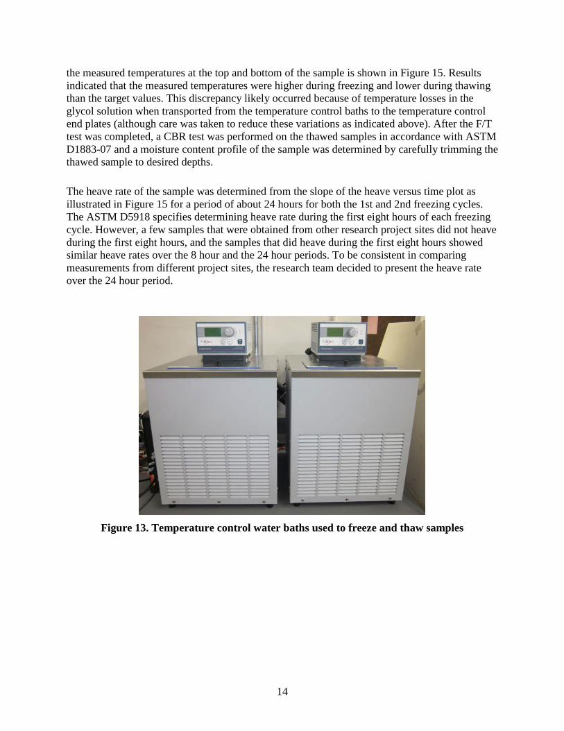
The F/T test was carried out by exposing four soil samples to two freeze-thaw cycles over a five day period. The samples were placed in a temperature controlled chest freezer (Figure 10) and then frozen and thawed by changing the temperature at the top and bottom of the samples using temperature controlled water baths (Figure 13). The programmable water baths used in this study had an operating range of -30°C to +200°C and adjustable to ±0.01°C, and were filled with 50% ethylene glycol-water solution. Insulating tape was wrapped around the flexible tubing between the water baths and the temperature control end plates, to help reduce temperature variations in the solution. The target top and bottom of the sample temperatures (Figure 14) were programmed into the water baths and the actual temperatures were measured during the test. An example of

Base plate

Compaction cylinder

Rings

Clamping rods

Membrane

Clamps

Collar

Compaction cylinder

14

the measured temperatures at the top and bottom of the sample is shown in Figure 15. Results indicated that the measured temperatures were higher during freezing and lower during thawing than the target values. This discrepancy likely occurred because of temperature losses in the glycol solution when transported from the temperature control baths to the temperature control end plates (although care was taken to reduce these variations as indicated above). After the F/T test was completed, a CBR test was performed on the thawed samples in accordance with ASTM D1883-07 and a moisture content profile of the sample was determined by carefully trimming the thawed sample to desired depths.

The heave rate of the sample was determined from the slope of the heave versus time plot as illustrated in Figure 15 for a period of about 24 hours for both the 1st and 2nd freezing cycles. The ASTM D5918 specifies determining heave rate during the first eight hours of each freezing cycle. However, a few samples that were obtained from other research project sites did not heave during the first eight hours, and the samples that did heave during the first eight hours showed similar heave rates over the 8 hour and the 24 hour periods. To be consistent in comparing measurements from different project sites, the research team decided to present the heave rate over the 24 hour period.

Figure 13. Temperature control water baths used to freeze and thaw samples

15

Figure 14. Target top and bottom temperatures with time per ASTM standard during

F/T cycles

Figure 15. Example of measured top and bottom temperatures during freeze-thaw cycles

and determination of heave rate for 1st and 2nd freezing cycles

In Situ Testing Methods

The following in situ test devices were employed on this project: real-time kinematic global positioning system (RTK-GPS) to locate test points; light weight deflectometer (LWD) manufactured by Zorn and Dynatest to determine elastic modulus of the subbase layer; dynamic cone penetrometer (DCP) to determine the California bearing ratio (CBR) of the foundation layers; air permeameter test (APT) device to determine saturated hydraulic conductivity (Ksat) of the subbase layer; falling weight deflectometer (FWD) to determine peak deflection under the loading plate (D0), load transfer efficiency (LTE) at joints and cracks, voids at joints and cracks, foundation composite modulus of subgrade reaction, and deflection basin parameters; and calibrated Humboldt nuclear gauge (NG) to measure in situ moisture and dry density. Brief

1st Cycle Heave Rate

2nd Cycle Heave Rate

16

descriptions of these test procedures are provided below, and equipment used to conduct tests is shown in composite as Figure 6.

Real-Time Kinematic Global Positioning System

An RTK-GPS system was used to obtain the spatial coordinates (x, y, and z) of pavement slabs and test locations. A Trimble SPS881 receiver was used with base station correction provided from a Trimble SPS851 established on site. According to the manufacturer this survey system is capable of horizontal accuracies of < 10 mm and vertical accuracies < 20 mm (Trimble 2013).

Figure 16. In situ test devices: Kuab falling weight deflectometer and Zorn light weight deflectometer (top row left to right); dynamic cone penetrometer, nuclear gauge, and air

permeameter (bottom row left to right)

17

Zorn Light Weight Deflectometer

Zorn LWD tests were performed on granular subbase and subgrade layers. The LWD was set up with a 300 mm diameter plate and 72 cm drop height to provide a calibrated applied stress of 0.1 MPa. The tests were performed following manufacturer recommendations (Zorn 2003) with three seating drops following by three measurement drops, and the elastic modulus values were determined using Equation 3:

FD

r)1(E

0

02

×ση−

= (3)

where E = elastic modulus (MPa); D0 = measured deflection under the plate (mm); η = Poisson’s ratio (0.4); σ0 = applied stress (MPa); r = radius of the plate (mm); and F = shape factor depending on stress distribution (assumed as 8/3) (see Vennapusa and White 2009). According to the manufacturer, the Zorn LWD has D0 measurement range of 0.2 mm to 30 mm.

The results are reported as ELWD-Z3 (Z represents Zorn LWD and 3 represents 300 mm diameter plate).

Dynatest Light Weight Deflectometer

Dynatest LWD tests were performed on rock cap material using the same procedure as the Zorn LWD. The LWD was set up with a 300 mm diameter plate. The Dynatest LWD measures both applied stress and deformation values, which were measured and used in Eq. 3 to determine the elastic modulus values. According to the manufacturer, the Dynatest LWD has a D0 measurement range of 0 to 2.2 mm (see Vennapusa and White 2009).

The results are reported as ELWD-D3 (D represents Dynatest LWD and 3 represents 300 mm diameter plate).

Dynamic Cone Penetrometer

DCP (Figure 16) tests were performed in accordance with ASTM D6951-03 Standard Test Method for Use of the Dynamic Cone Penetrometer in Shallow Pavement Applications to determine dynamic penetration index (DPI) and calculate California bearing ratio (CBR) using Eq. 8. The DCP test results are presented in this report as CBR with depth profiles at each test location. The CBR values were calculation using Equation 5:

12.1DPI292CBR =

(4)

18

Kuab Falling Weight Deflectometer

Falling weight deflectometer (FWD) tests were conducted using a Kuab FWD setup with a 300 mm (11.81 in) diameter loading plate by applying one seating drop and three loading drops. The applied loads varied from about 27 kN (6,000 lb) to 54 kN (12,000 lb) in the three loading drops. The actual applied loads were recorded using a load cell, and deflections were recorded using seismometers mounted on the device, per ASTM D4694-09 Standard Test Method for Deflections with a Falling-Weight-Type Impulse Load Device. The FWD plate and deflection sensor setup and a typical deflection basin are shown in Figure 17. To compare deflection values from different test locations at the same applied contact stress, the values at each test location were normalized to a 40 kN (9,000 lb) applied force.

Figure 17. FWD deflection sensor setup used for this study and an example deflection basin

FWD tests were conducted at the center of the PCC slab panels and at the joints. Tests conducted at the joints were used to determine joint load transfer efficiency (LTE) and voids beneath the pavement based on “zero” load intercept values. Tests conducted at the center of the slab panels

Distance (m)

-0.3048 0.0000 0.3048 0.6096 0.9144 1.2192 1.5240

Distance (in)

-12 0 12 24 36 48 60

300 mm diameter loading plate

D0D1 D2 D3 D4 D5 D6 D7

Loading plate and deflection sensors setup (Plan View)

Distance (m)

-0.3048 0.0000 0.3048 0.6096 0.9144 1.2192 1.5240

Def

lect

ion

(mm

)

0.0

0.1

0.2

0.3

0.4

0.5

SCI = D0-D2

Applied Load

D0D1 D2 D3 D4 D5 D6 D7

BDI = D2-D4

BCI = D4-D5

Deflection Basin300 mm diameter loading plate

19

were used to determine modulus of subgrade reaction (k) values and the intercept values. The procedure used to calculate these parameters are described below.

LTE was determined by obtaining deflections under the plate on the loaded slab (D0) and deflections of the unloaded slab (D1) using a sensor positioned about 305 mm (12 in.) away from the center of the plate (Figure 17). The LTE was calculated using Equation 5.

100(%)0

1 ×=DDLTE (5)

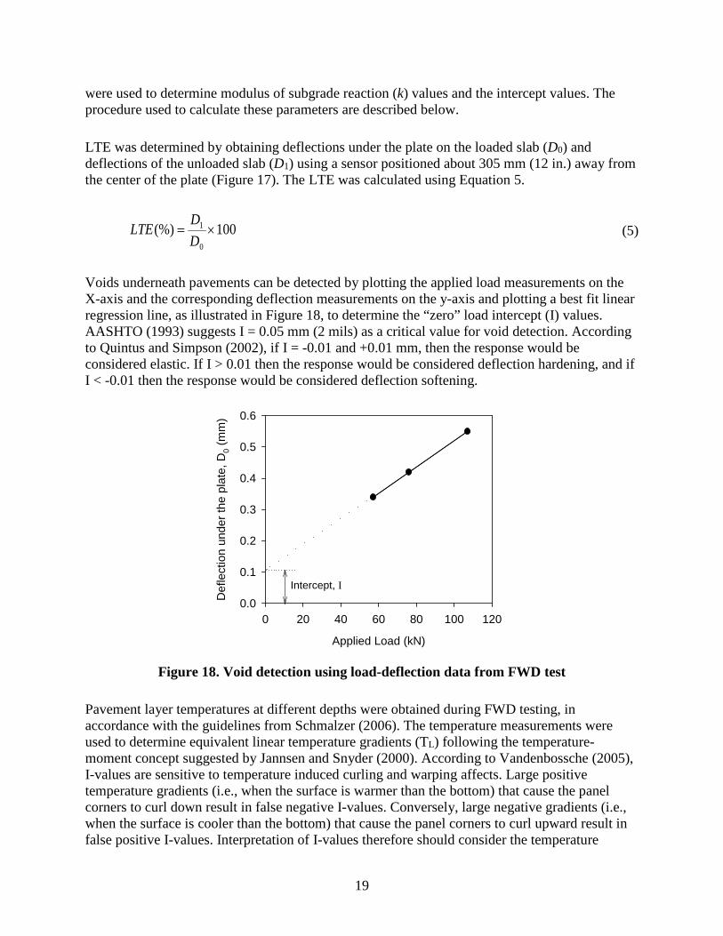
Voids underneath pavements can be detected by plotting the applied load measurements on the X-axis and the corresponding deflection measurements on the y-axis and plotting a best fit linear regression line, as illustrated in Figure 18, to determine the “zero” load intercept (I) values. AASHTO (1993) suggests I = 0.05 mm (2 mils) as a critical value for void detection. According to Quintus and Simpson (2002), if I = -0.01 and +0.01 mm, then the response would be considered elastic. If I > 0.01 then the response would be considered deflection hardening, and if I < -0.01 then the response would be considered deflection softening.

Figure 18. Void detection using load-deflection data from FWD test

Pavement layer temperatures at different depths were obtained during FWD testing, in accordance with the guidelines from Schmalzer (2006). The temperature measurements were used to determine equivalent linear temperature gradients (TL) following the temperature-moment concept suggested by Jannsen and Snyder (2000). According to Vandenbossche (2005), I-values are sensitive to temperature induced curling and warping affects. Large positive temperature gradients (i.e., when the surface is warmer than the bottom) that cause the panel corners to curl down result in false negative I-values. Conversely, large negative gradients (i.e., when the surface is cooler than the bottom) that cause the panel corners to curl upward result in false positive I-values. Interpretation of I-values therefore should consider the temperature

Applied Load (kN)

0 20 40 60 80 100 120

Def

lect

ion

unde

r the

pla

te, D

0 (m

m)

0.0

0.1

0.2

0.3

0.4

0.5

0.6

Intercept, I

20

gradient. Concerning LTE measurements for doweled joints, the temperature gradient is reportedly not a critical factor (Vandenbossche 2005).

The k values were determined using the AREA4 method described in AASHTO (1993). Since the k value determined from FWD test represents a dynamic value, it is referred to here as kFWD-Dynamic. Deflections obtained from four sensors (D0, D2, D4, and D5 shown in Figure 17) were used in the AREA4 calculation. The AREA method was first proposed by Hoffman and Thompson (1981) for flexible pavements and has since been applied extensively for concrete pavements (Darter et al. 1995). AREA4 is calculated using Equation 6 and has dimensions of length (in inches), as it is normalized with deflections under the center of the plate (D0):

×+

×+

×+=

0

5

0

4

0

24 612126

DD

DD

DDAREA (6)

where D0 = deflections measured directly under the plate; D2 = deflections measured at 305 mm (12 in.) away from the plate center ; D4 = deflections measured at 610 mm (24 in.) away from the plate center; and D5 = deflections measured at 914 mm (36 in.) away from the plate center. The AREA4 method can also be calculated using different sensor configurations and setups, (i.e., using deflection data from 3, 5, or 7 sensors), and those methods are described in detail in the literature (Substad et al. 2006, Smith et al. 2007)

In early research conducted using the AREA method, the ILLI-SLAB finite element program was used to compute a matrix of maximum deflections at the plate center and the AREA values by varying the subgrade k, the modulus of the PCC layer, and the thickness of the slab (ERES Consultants, Inc. 1982). Measurements obtained from FWD tests were then compared with the ILLI-SLAB program results to determine the k values through back calculation. Barenberg and Petros (1991) and Ioannides (1990) proposed a forward solution procedure based on Westergaard’s solution for loading on an infinite plate to replace the back calculation procedure. This forward solution presented a unique relationship between AREA value (for a given load and sensor arrangement) and the dense liquid radius of relative stiffness (L) in which subgrade is characterized by the k value. The radius of relative stiffness (L) is estimated using Equation 7:

4

3

2

41lnx

xxAREAx

L

−

= (7)

where x1 = 36, x2 = 1812.279, x3 = -2.559, x4 = 4.387. It must be noted that the x1 to x4 values vary with the sensor arrangement and these values are only valid for the AREA4 sensor setup. Once, the L value is known, the kFWD-Dynamic value can be estimated using Equation 8:

20

*0)(

LDPDpcik DynamicFWD =− (8)

21

where P = applied load (lbs), D0 = deflection measured at plate center (inches), and D0* = non-

dimensional deflection coefficient calculated using Equation 9:

cLbeeaD−−⋅=*

0 (9)

where a = 0.12450, b = 0.14707, c = 0.07565. It must be noted that these equations and coefficients are valid for an FWD setup with an 11.81 in. diameter plate.

The advantages of the AREA4 method are the ease of use without back calculations and the use of multiple sensor data. The disadvantages are that the process assumes that the slab and the subgrade are horizontally infinite. This assumption leads to underestimating the k values of jointed pavements. Crovetti (1993) developed the following slab size corrections for a square slab that is based on finite element analysis conducted using the ILLI-SLAB program and is for use in the kFWD-Dynamic:

𝐴𝐴𝐴𝐴𝐴𝐴𝐴𝐴𝐴𝐴𝐴𝐴𝐴𝐴𝐴𝐴 𝐷𝐷0 = 𝐷𝐷0 1 − 1.15085𝐴𝐴−0.71878𝐿𝐿′

𝐿𝐿 0.80151

(10)

𝐴𝐴𝐴𝐴𝐴𝐴𝐴𝐴𝐴𝐴𝐴𝐴𝐴𝐴𝐴𝐴 𝐿𝐿 = 𝐿𝐿 1 − 0.89434𝐴𝐴−0.61662𝐿𝐿′

𝐿𝐿 1.04831

(11)

where L′ = slab size (smaller dimension of a rectangular slab, length or width). This procedure also has limitations: (1) it considers only a single slab with no load transfer to adjacent slabs, and (2) it assumes a square slab. The square slab assumption is considered to produce sufficiently accurate results when the smaller dimension of a rectangular slab is assumed as L′ (Darter et al. 1995). Darter et al. 1995 suggested using 𝐿𝐿′ = 𝐿𝐿𝐴𝐴𝐿𝐿𝐿𝐿𝐴𝐴ℎ × 𝑊𝑊𝑊𝑊𝐴𝐴𝐴𝐴ℎ to further refine slab size corrections. However, no established procedures for correcting for load transfer to adjacent slabs have been reported so accounting for load transfer remains as a limitation of this method.

AASHTO (1993) suggests dividing the kFWD-Dynamic value by a factor of 2 to determine the equivalent kFWD-Static value. The origin of this factor 2 dates back to Foxworthy’s work in the 1980’s. Foxworthy (1985) reported comparisons between the kFWD-Dynamic values obtained using Dynatest model 8000 FWD and the Static k values (Static kPLT) obtained from 30 in. diameter plate load tests (the exact procedure followed to calculate the Static kPLT is not reported in Foxworthy 1985). Foxworthy used the AREA based back calculation procedure using the ILLI-SLAB finite element program. Results obtained from Foxworthy’s study (Figure 19) are based on 7 FWD tests conducted on PCC pavements with slab thicknesses varying from about 10 in. to 25.5 in. and plate load tests conducted on the foundation layer immediately beneath the pavement over a 4 ft x 5 ft test area. A few of these sections consisted of a 5 to 12 in. thick base course layer and some did not. The subgrade layer material consisted of CL soil from Sheppard Air Force Base in Texas, SM soil from Seymour-Johnson Air Force Base in North Carolina, and

22

an unspecified soil type from McDill Air Force base in Florida. No slab size correction was performed on this dataset.

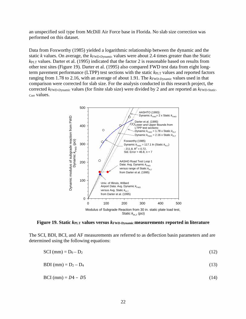
Data from Foxworthy (1985) yielded a logarithmic relationship between the dynamic and the static k values. On average, the kFWD-Dynamic values were about 2.4 times greater than the Static kPLT values. Darter et al. (1995) indicated that the factor 2 is reasonable based on results from other test sites (Figure 19). Darter et al. (1995) also compared FWD test data from eight long-term pavement performance (LTPP) test sections with the static kPLT values and reported factors ranging from 1.78 to 2.16, with an average of about 1.91. The kFWD-Dynamic values used in that comparison were corrected for slab size. For the analysis conducted in this research project, the corrected kFWD-Dynamic values (for finite slab size) were divided by 2 and are reported as kFWD-Static-

Corr values.

Figure 19. Static kPLT values versus kFWD-Dynamic measurements reported in literature

The SCI, BDI, BCI, and AF measurements are referred to as deflection basin parameters and are determined using the following equations:

SCI (mm) = D0 – D2 (12)

BDI (mm) = D2 – D4 (13)

BCI (mm) = 𝐷𝐷4 – 𝐷𝐷5 (14)

Modulus of Subgrade Reaction from 30 in. static plate load test, Static kPLT (pci)

0 100 200 300 400 500

Dyn

amic

mod

ulus

of s

ubgr

ade

reac

tion

from

FW

DD

ynam

ic k

FWD (p

ci)

0

100

200

300

400

500

Dynamic kFWD = 117.1 ln (Static kPLT) - 211.8, R2 = 0.72, Std. Error = 46.8, n = 7

AASHO Road Test Loop 1 Data: Avg. Dynamic kFWD

versus range of Static kPLT

from Darter et al. (1995)

Univ. of Illinois, Willard Airport Data: Avg. Dynamic kFWD

versus Avg. Static kPLT

from Darter et al. (1995)

Foxworthy (1985)

AASHTO (1993): Dynamic kFWD= 2 x Static kFWD

Darter et al. (1995)Lower and Upper Bounds from LTPP test sections:Dynamic kFWD = 1.78 x Static kPLT

Dynamic kFWD = 2.16 x Static kPLT

23

AF (mm) 0

5420

D)D2D2D(D152.4 +++×

= (15)

where, D0 = peak deflection measured directly beneath the plate, D2 = peak deflection measured at 305 mm away from the plate center, D4 = peak deflection measured at 510 mm away from the plate centre, and D5 = peak deflection measured at 914 mm away from the plate centre.

According to Horak (1987), the SCI parameter provides a measure of the strength/ stiffness of the upper portion (base layers) of the pavement foundation layers (Horak 1987). Similarly, BDI represents layers between 300 mm and 600 mm depth (base and subbase layers) and BCI represents layers between 600 mm and 900 mm depth (subgrade layers) from the surface (Kilareski and Anani 1982). The AF is primarily the normalized (with D0) area under the deflection basin curve up to sensor D5 (AASHTO 1993). AF has been used to characterize variations in the foundation layer material properties by some researchers (e.g., Stubstad 2002). Comparatively, lower SCI or BDI or BCI or AF values indicate better support conditions (Horak 1987).

A composite modulus value (EFWD-K3) was calculated using the D0 corresponding to an applied contact force, and Equation 3. Shape factor F = 2 was used in the calculations assuming a uniform stress distribution (see Vennapusa and White 2009). According to the FWD manufacturer, the segmented plate used results in a uniform stress distribution.

For tests conducted on the CTB or ATB layers, the subgrade layer modulus (ESG) was determined using Equation 16, per AASHTO (1993):

iiSG Dd

rE

20

2 )1( ση−= (16)

where: Di = measured deflection at distance di (mm); and di = radial distance of the sensor away from the center of the loading plate.

According to AASHTO (1993), the modulus values estimated from FWD tests exceed the laboratory measured resilient modulus values by a factor of three or more. Therefore an adjustment factor C ≤ 0.33 is recommended to correct ESG determined from Equation 27. In this study, corrected ESG values are calculated using C = 0.33:

SGSG ECorrectedE ×= 33.0 (17)

AASHTO (1993) suggests that the di must be far enough away that it provides a good estimate of the subgrade modulus, independent of the effects of any layers above, but also close enough that it does not result in a too small value. A graphical solution is provided in AASHTO (1993) to

24

estimate the minimum radial distance based on an assumed effective modulus of all layers above the subgrade and the d0 value. Salt (1998) indicated that if ESG values are plotted against radial distance, in linear elastic materials such as sands and gravels, the modulus values decrease with increasing distance and then level off after a certain distance. The deformations at the distance at which the modulus values level off can be used to represent ESG. In some cases the modulus values decrease and then increase with distance. Such conditions represent either soils with moderate to high moduli with poor drainage at the top of the subgrade or soft soils with low moduli. In those cases the distance where the modulus is low is represented as ESG.

Ullidtz (1987) described the Odemark’s method of equivalent thickness (MET) concept and is used in AASHTO (1993). According to the MET concept, a two-layered system with the top layer modulus higher than the bottom layer, can be transformed into a single layer of equivalent thickness with properties of the bottom layer. Using this concept and the modulus of the bottom layer (ESG), the top layer modulus (ESB) can be back-calculated.

In this study, tests conducted on the ATB and the CTB layer were used to calculate ESG and back-calculate ESB values and compare with the design assumptions.

Humboldt Nuclear Gauge

A calibrated nuclear moisture-density gauge (NG) device (Figure 16) was used to provide rapid measurements of soil dry unit weight (γd) and moisture content (w) in the base materials. Tests were performed following ASTM D6938-10 Standard Test Method for In-Place Density and Water Content of Soil and Soil-Aggregate by Nuclear Methods (Shallow Depth). Back-scattering procedure was used in obtaining the measurements. Two measurements of moisture and dry unit weight were obtained at a particular location and the average value is reported.

Rapid Air Permeameter Test (APT Device)

The APT device is a recently developed rapid in situ permeability testing device (White et al. 2014) that uses air as a permeating fluid to determine saturated hydraulic conductivity (Ksat). The APT consists of a self-contained pressurized gas system with a self-sealing base plate and uses a theoretical algorithm to determine the Ksat. The test involves measuring air pressure on the inlet and outlet sides of a precision orifice, calculating gas flow rate, and assuming material properties (i.e., degree of saturation of the material, residual saturation of the material, and pore-size distribution properties of the material), to determine Ksat. The Ksat was calculated using Equation 18 (White et al. 2014):

( ) )S1()S1(g

PPrGQP2

K )/)2((e

2ewater

22

210

1airsat λλ+−−µ

ρ⋅

−µ

= (18)

where Ksat = saturated hydraulic conductivity (cm/s); µair = dynamic viscosity of air (Pas); Q = volumetric flow rate (cm3/s); P1 = absolute gas pressure on the soil surface, Po(g) x 9.81 +

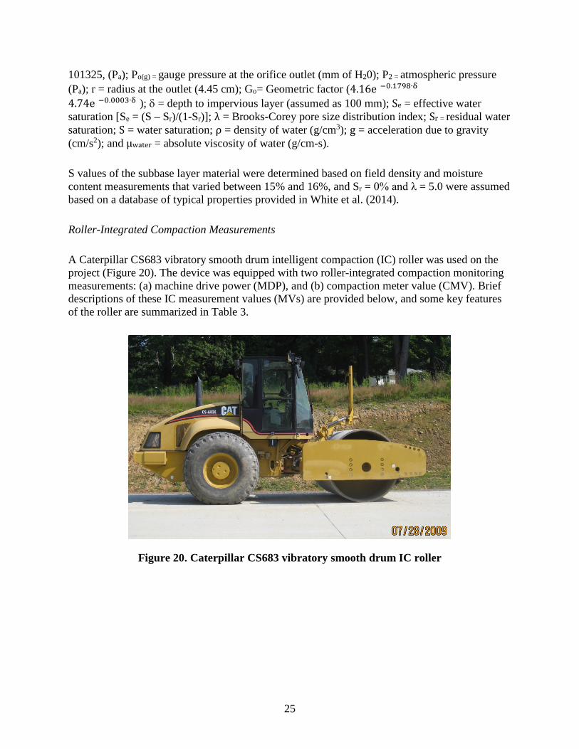
25

101325, (Pa); Po(g) = gauge pressure at the orifice outlet (mm of H20); P2 = atmospheric pressure (Pa); r = radius at the outlet (4.45 cm); Go= Geometric factor (4.16e(−0.1798∙δ) +4.74e(−0.0003∙δ)); δ = depth to impervious layer (assumed as 100 mm); Se = effective water saturation [Se = (S – Sr)/(1-Sr)]; λ = Brooks-Corey pore size distribution index; Sr = residual water saturation; S = water saturation; ρ = density of water (g/cm3); g = acceleration due to gravity (cm/s2); and µwater = absolute viscosity of water (g/cm-s).

S values of the subbase layer material were determined based on field density and moisture content measurements that varied between 15% and 16%, and Sr = 0% and λ = 5.0 were assumed based on a database of typical properties provided in White et al. (2014).

Roller-Integrated Compaction Measurements

A Caterpillar CS683 vibratory smooth drum intelligent compaction (IC) roller was used on the project (Figure 20). The device was equipped with two roller-integrated compaction monitoring measurements: (a) machine drive power (MDP), and (b) compaction meter value (CMV). Brief descriptions of these IC measurement values (MVs) are provided below, and some key features of the roller are summarized in Table 3.

Figure 20. Caterpillar CS683 vibratory smooth drum IC roller

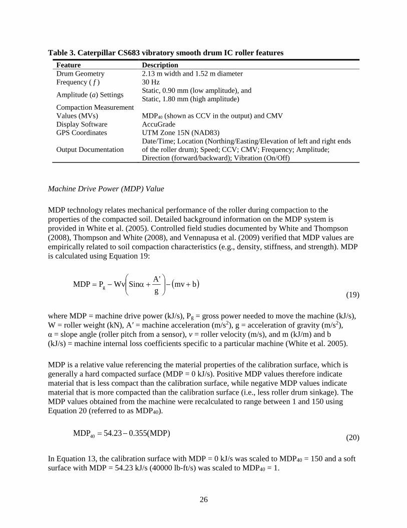
26

Table 3. Caterpillar CS683 vibratory smooth drum IC roller features Feature Description Drum Geometry 2.13 m width and 1.52 m diameter Frequency ( f ) 30 Hz

Amplitude (a) Settings Static, 0.90 mm (low amplitude), and Static, 1.80 mm (high amplitude)

Compaction Measurement Values (MVs) MDP40 (shown as CCV in the output) and CMV Display Software AccuGrade GPS Coordinates UTM Zone 15N (NAD83)

Output Documentation Date/Time; Location (Northing/Easting/Elevation of left and right ends of the roller drum); Speed; CCV; CMV; Frequency; Amplitude; Direction (forward/backward); Vibration (On/Off)

Machine Drive Power (MDP) Value

MDP technology relates mechanical performance of the roller during compaction to the properties of the compacted soil. Detailed background information on the MDP system is provided in White et al. (2005). Controlled field studies documented by White and Thompson (2008), Thompson and White (2008), and Vennapusa et al. (2009) verified that MDP values are empirically related to soil compaction characteristics (e.g., density, stiffness, and strength). MDP is calculated using Equation 19:

(19)

where MDP = machine drive power (kJ/s), Pg = gross power needed to move the machine (kJ/s), W = roller weight (kN), A′ = machine acceleration (m/s2), g = acceleration of gravity (m/s2), α = slope angle (roller pitch from a sensor), v = roller velocity (m/s), and m (kJ/m) and b (kJ/s) = machine internal loss coefficients specific to a particular machine (White et al. 2005).

MDP is a relative value referencing the material properties of the calibration surface, which is generally a hard compacted surface (MDP = 0 kJ/s). Positive MDP values therefore indicate material that is less compact than the calibration surface, while negative MDP values indicate material that is more compacted than the calibration surface (i.e., less roller drum sinkage). The MDP values obtained from the machine were recalculated to range between 1 and 150 using Equation 20 (referred to as MDP40).

(20)

In Equation 13, the calibration surface with MDP = 0 kJ/s was scaled to MDP40 = 150 and a soft surface with MDP = 54.23 kJ/s (40000 lb-ft/s) was scaled to MDP40 = 1.

( )bmvg

'ASinWvPMDP g +−

+α−=

)MDP(355.023.54MDP40 −=

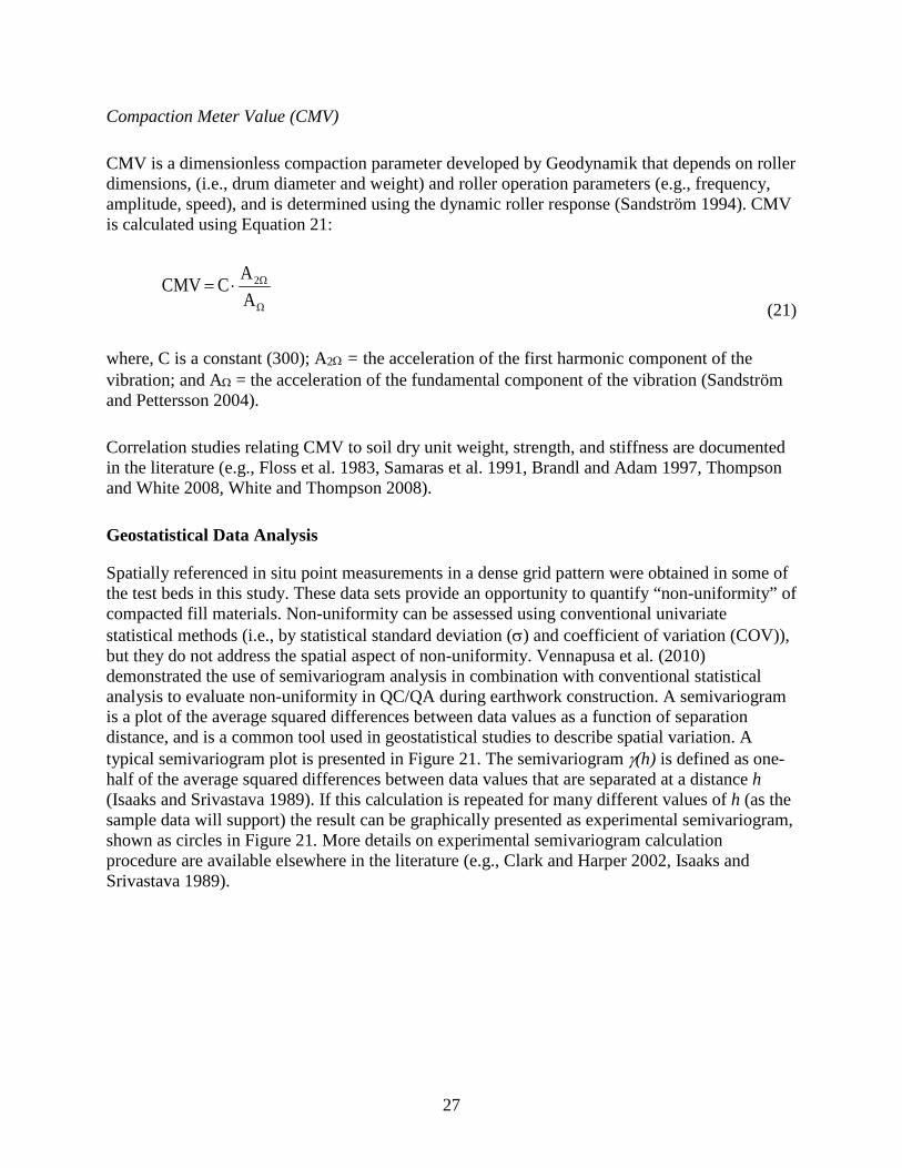
27

Compaction Meter Value (CMV)

CMV is a dimensionless compaction parameter developed by Geodynamik that depends on roller dimensions, (i.e., drum diameter and weight) and roller operation parameters (e.g., frequency, amplitude, speed), and is determined using the dynamic roller response (Sandström 1994). CMV is calculated using Equation 21:

(21)

where, C is a constant (300); A2Ω = the acceleration of the first harmonic component of the vibration; and AΩ = the acceleration of the fundamental component of the vibration (Sandström and Pettersson 2004).

Correlation studies relating CMV to soil dry unit weight, strength, and stiffness are documented in the literature (e.g., Floss et al. 1983, Samaras et al. 1991, Brandl and Adam 1997, Thompson and White 2008, White and Thompson 2008).

Geostatistical Data Analysis

Spatially referenced in situ point measurements in a dense grid pattern were obtained in some of the test beds in this study. These data sets provide an opportunity to quantify “non-uniformity” of compacted fill materials. Non-uniformity can be assessed using conventional univariate statistical methods (i.e., by statistical standard deviation (σ) and coefficient of variation (COV)), but they do not address the spatial aspect of non-uniformity. Vennapusa et al. (2010) demonstrated the use of semivariogram analysis in combination with conventional statistical analysis to evaluate non-uniformity in QC/QA during earthwork construction. A semivariogram is a plot of the average squared differences between data values as a function of separation distance, and is a common tool used in geostatistical studies to describe spatial variation. A typical semivariogram plot is presented in Figure 21. The semivariogram γ(h) is defined as one-half of the average squared differences between data values that are separated at a distance h (Isaaks and Srivastava 1989). If this calculation is repeated for many different values of h (as the sample data will support) the result can be graphically presented as experimental semivariogram, shown as circles in Figure 21. More details on experimental semivariogram calculation procedure are available elsewhere in the literature (e.g., Clark and Harper 2002, Isaaks and Srivastava 1989).

Ω

Ω⋅=AAC CMV 2

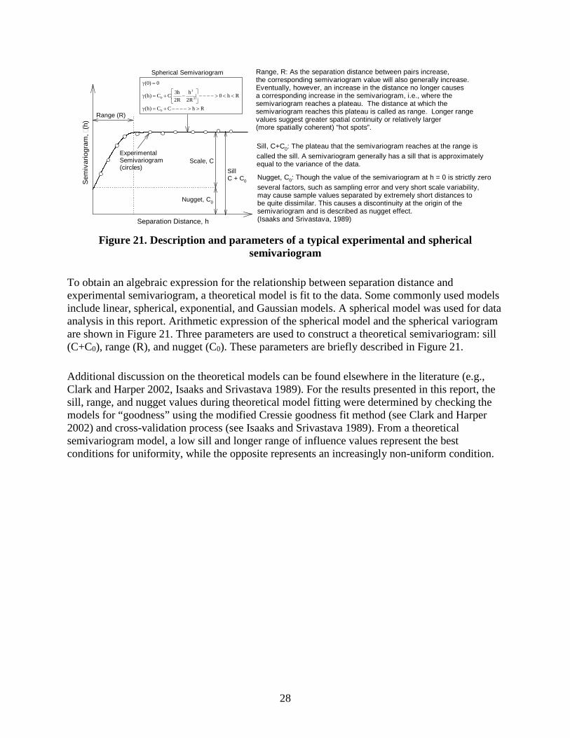
28

Figure 21. Description and parameters of a typical experimental and spherical

semivariogram

To obtain an algebraic expression for the relationship between separation distance and experimental semivariogram, a theoretical model is fit to the data. Some commonly used models include linear, spherical, exponential, and Gaussian models. A spherical model was used for data analysis in this report. Arithmetic expression of the spherical model and the spherical variogram are shown in Figure 21. Three parameters are used to construct a theoretical semivariogram: sill (C+C0), range (R), and nugget (C0). These parameters are briefly described in Figure 21.

Additional discussion on the theoretical models can be found elsewhere in the literature (e.g., Clark and Harper 2002, Isaaks and Srivastava 1989). For the results presented in this report, the sill, range, and nugget values during theoretical model fitting were determined by checking the models for “goodness” using the modified Cressie goodness fit method (see Clark and Harper 2002) and cross-validation process (see Isaaks and Srivastava 1989). From a theoretical semivariogram model, a low sill and longer range of influence values represent the best conditions for uniformity, while the opposite represents an increasingly non-uniform condition.

Range (R)

Scale, C

Nugget, C0

SillC + C0

Range, R: As the separation distance between pairs increase, the corresponding semivariogram value will also generally increase. Eventually, however, an increase in the distance no longer causes a corresponding increase in the semivariogram, i.e., where the semivariogram reaches a plateau. The distance at which the semivariogram reaches this plateau is called as range. Longer range values suggest greater spatial continuity or relatively larger (more spatially coherent) “hot spots”.

Sill, C+C0: The plateau that the semivariogram reaches at the range is called the sill. A semivariogram generally has a sill that is approximately equal to the variance of the data.

Nugget, C0: Though the value of the semivariogram at h = 0 is strictly zero, several factors, such as sampling error and very short scale variability, may cause sample values separated by extremely short distances to be quite dissimilar. This causes a discontinuity at the origin of the semivariogram and is described as nugget effect.(Isaaks and Srivastava, 1989)

Spherical Semivariogram

ExperimentalSemivariogram(circles)

RhCC)h(

Rh0R2h

R2h3CC)h(

0)0(

0

3

3

0

>>−−−−+=γ

<<>−−−−

−+=γ

=γS

emiv

ario

gram

, (h

)

Separation Distance, h

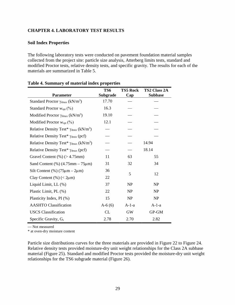
29

CHAPTER 4. LABORATORY TEST RESULTS

Soil Index Properties

The following laboratory tests were conducted on pavement foundation material samples collected from the project site: particle size analysis, Atterberg limits tests, standard and modified Proctor tests, relative density tests, and specific gravity. The results for each of the materials are summarized in Table 5.

Table 4. Summary of material index properties

Parameter TS6

Subgrade TS5 Rock

Cap TS2 Class 2A

Subbase Standard Proctor γdmax (kN/m3) 17.70 — —

Standard Proctor wopt (%) 16.3 — —

Modified Proctor γdmax (kN/m3) 19.10 — —

Modified Proctor wopt (%) 12.1 — —

Relative Density Test* γdmin (kN/m3) — — —

Relative Density Test* γdmin (pcf) — — —

Relative Density Test* γdmax (kN/m3) — — 14.94

Relative Density Test* γdmax (pcf) — — 18.14 Gravel Content (%) (> 4.75mm) 11 63 55

Sand Content (%) (4.75mm – 75µm) 31 32 34

Silt Content (%) (75µm – 2µm) 36 5 12

Clay Content (%) (< 2µm) 22 Liquid Limit, LL (%) 37 NP NP Plastic Limit, PL (%) 22 NP NP Plasticity Index, PI (%) 15 NP NP AASHTO Classification A-6 (6) A-1-a A-1-a USCS Classification CL GW GP-GM Specific Gravity, Gs 2.78 2.70 2.82

— Not measured * at oven-dry moisture content

Particle size distributions curves for the three materials are provided in Figure 22 to Figure 24. Relative density tests provided moisture-dry unit weight relationships for the Class 2A subbase material (Figure 25). Standard and modified Proctor tests provided the moisture-dry unit weight relationships for the TS6 subgrade material (Figure 26).

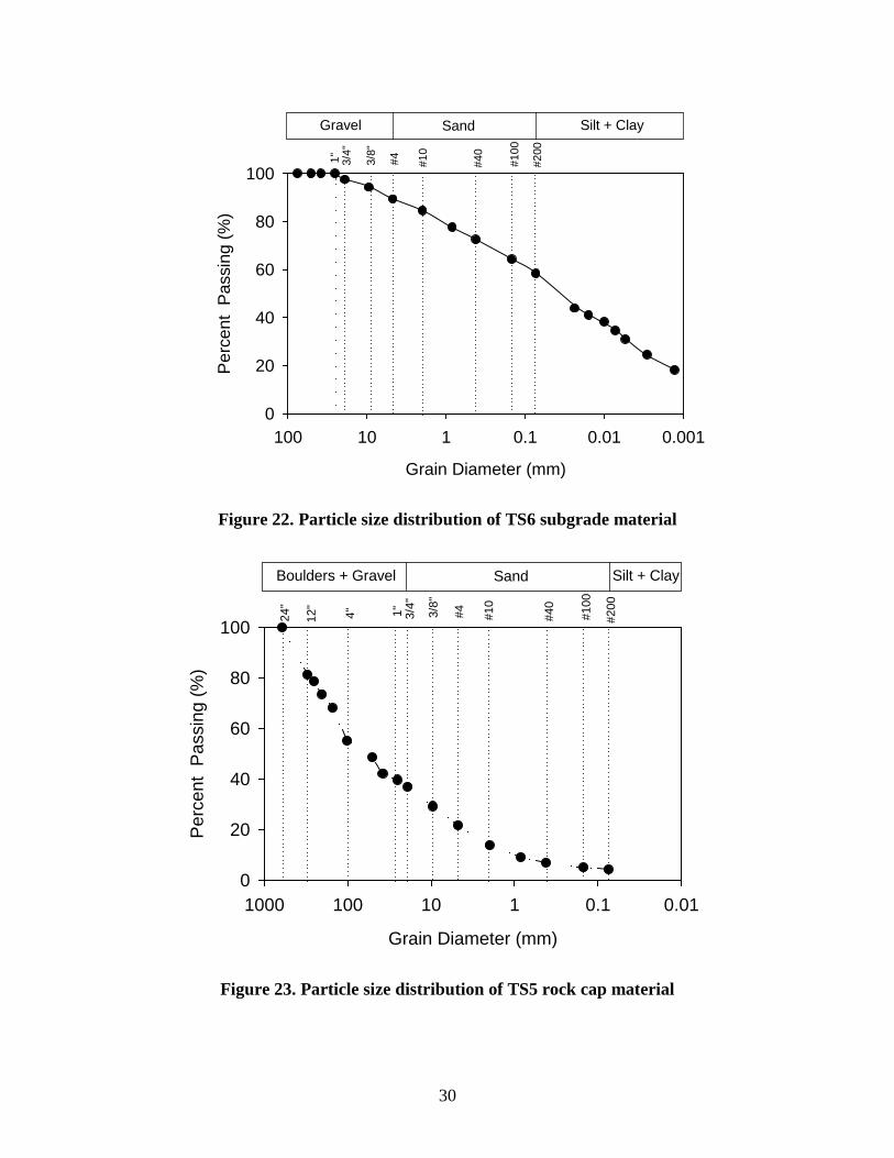
30

Figure 22. Particle size distribution of TS6 subgrade material

Figure 23. Particle size distribution of TS5 rock cap material

#10

#40

#100

#200

#43/8"

3/4"

SandGravel Silt + Clay

Grain Diameter (mm)

0.0010.010.1110100

Per

cent

Pas

sing

(%)

0

20

40

60

80

100

1"

#10

#40

#100

#200

#43/8"

3/4"

Sand Silt + Clay

Grain Diameter (mm)

0.010.11101001000

Per

cent

Pas

sing

(%)

0

20

40

60

80

100

1"24"

12"

4"

Boulders + Gravel

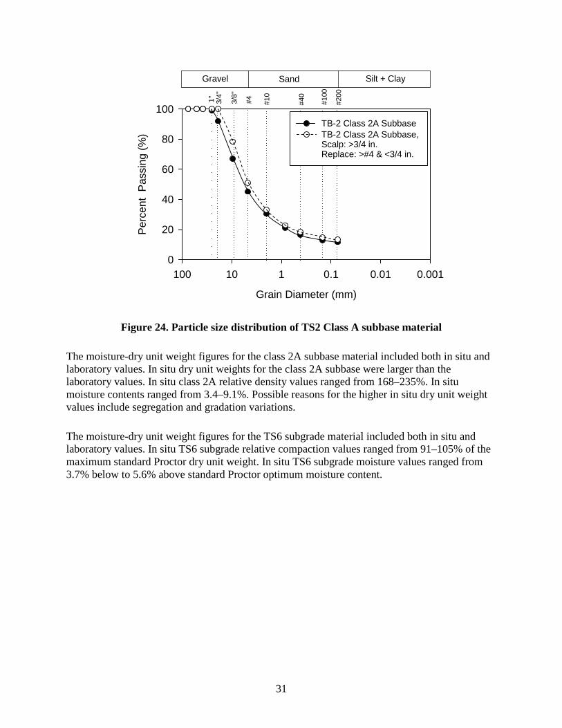
31

Figure 24. Particle size distribution of TS2 Class A subbase material

The moisture-dry unit weight figures for the class 2A subbase material included both in situ and laboratory values. In situ dry unit weights for the class 2A subbase were larger than the laboratory values. In situ class 2A relative density values ranged from 168–235%. In situ moisture contents ranged from 3.4–9.1%. Possible reasons for the higher in situ dry unit weight values include segregation and gradation variations.

The moisture-dry unit weight figures for the TS6 subgrade material included both in situ and laboratory values. In situ TS6 subgrade relative compaction values ranged from 91–105% of the maximum standard Proctor dry unit weight. In situ TS6 subgrade moisture values ranged from 3.7% below to 5.6% above standard Proctor optimum moisture content.

#10

#40

#100

#200

#43/8"

3/4"

SandGravel Silt + Clay

Grain Diameter (mm)

0.0010.010.1110100

Per

cent

Pas

sing

(%)

0

20

40

60

80

100TB-2 Class 2A SubbaseTB-2 Class 2A Subbase, Scalp: >3/4 in. Replace: >#4 & <3/4 in.

1"

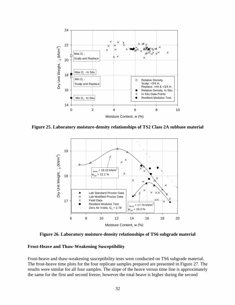
32

Figure 25. Laboratory moisture-density relationships of TS2 Class 2A subbase material

Figure 26. Laboratory moisture-density relationships of TS6 subgrade material

Frost-Heave and Thaw-Weakening Susceptibility

Frost-heave and thaw-weakening susceptibility tests were conducted on TS6 subgrade material. The frost-heave time plots for the four replicate samples prepared are presented in Figure 27. The results were similar for all four samples. The slope of the heave versus time line is approximately the same for the first and second freeze; however the total heave is higher during the second

Moisture Content, w (%)

0 2 4 6 8 10

Dry

Uni

t Wei

ght, d

(kN

/m3 )

14

16

18

20

22

24

Relative Density, Scalp: >3/4 in. Replace: >#4 & <3/4 in.Relative Density, In SituIn Situ Data PointsResilient Modulus TestMin Dr - In Situ

Min Dr - Scalp and Replace

Max Dr - In Situ

Max Dr - Scalp and Replace

Moisture Content, w (%)

6 8 10 12 14 16 18 20

Dry

Uni

t Wei

ght, d

(kN

/m3 )

17

18

19

Lab Standard Proctor DataLab Modified Proctor DataField DataResilient Modulus TestZero Air Voids, Gs = 2.78

dmax = 17.70 kN/m3

wopt = 16.3 %

dmax = 19.10 kN/m3

wopt = 12.1 %

33

freeze because the samples did not return to their original height after the first freeze-thaw cycle. The samples reached a peak heave after the first freeze and never consolidated during thawing. The sample height also increased after the second freeze-thaw cycle.

The moisture content profiles after thawing are presented in Figure 28.The moisture content increased after freeze-thaw cycling compared to the initial moisture content. There are no trends showing redistribution of water in the samples, which would indicate that there was no sufficient capillary action to draw water to the top of the sample.

The frost-heave and thaw-weakening results are summarized in Table 5. The CBR after freeze-thaw cycling was lower than the standard CBR. The thaw-weakening susceptibility rating is high for the material. The frost-heave rate increased slightly from the first to the second freeze cycle. The frost-susceptibility rating for the first freeze is low and medium for the second freeze.

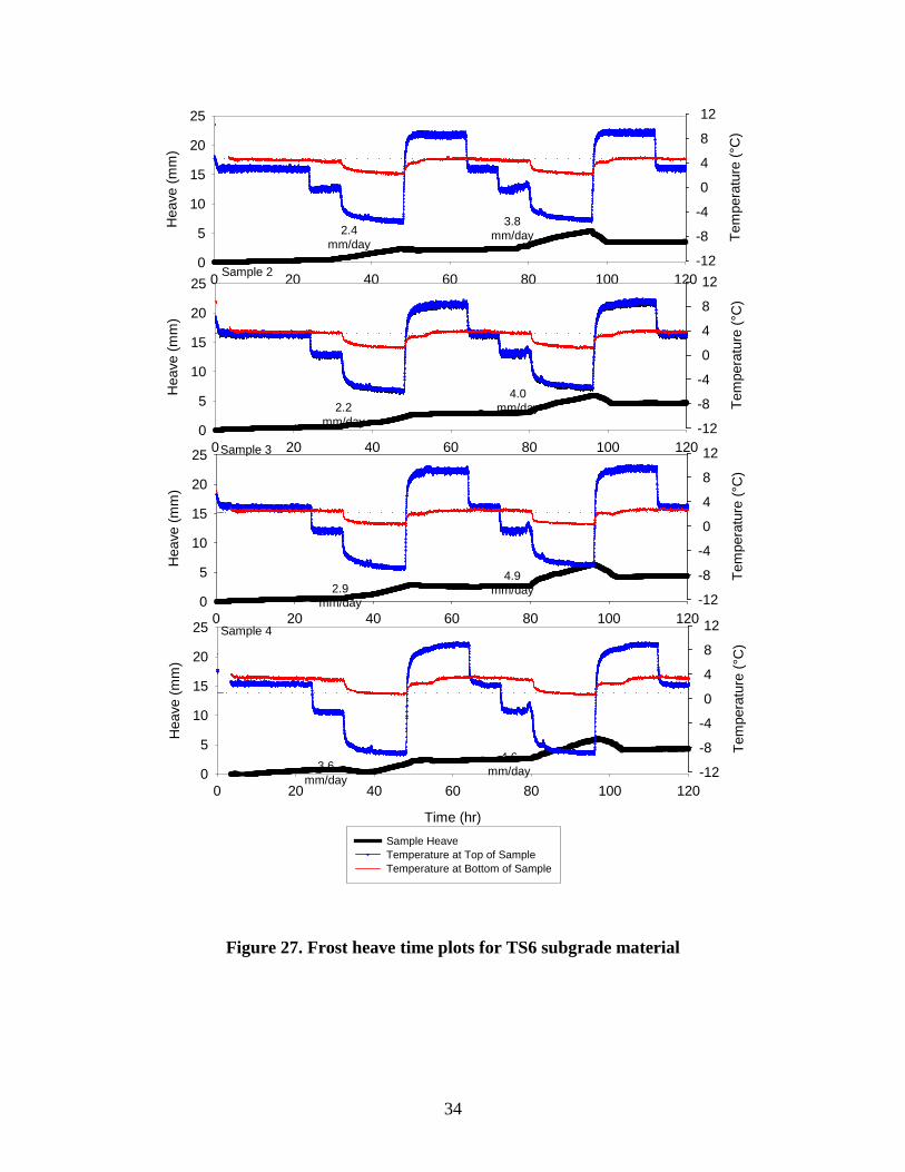
34

Figure 27. Frost heave time plots for TS6 subgrade material

0 20 40 60 80 100 120

Hea

ve (m

m)

0

5

10

15

20

25

Tem

pera

ture

(°C

)

-12

-8

-4

0

4

8

12

0 20 40 60 80 100 120

Hea

ve (m

m)

0

5

10

15

20

25

Tem

pera

ture

(°C

)

-12

-8

-4

0

4

8

12

0 20 40 60 80 100 120

Hea

ve (m

m)

0

5

10

15

20

25

Tem

pera

ture

(°C

)

-12

-8

-4

0

4

8

12

Time (hr)

0 20 40 60 80 100 120

Hea

ve (m

m)

0

5

10

15

20

25

Tem

pera

ture

(°C

)

-12

-8

-4

0

4

8

12

Sample HeaveTemperature at Top of SampleTemperature at Bottom of Sample

Sample 2

Sample 3

Sample 4

2.4mm/day

3.6mm/day

4.6mm/day

2.9mm/day

4.9mm/day

2.2mm/day

4.0mm/day

3.8mm/day

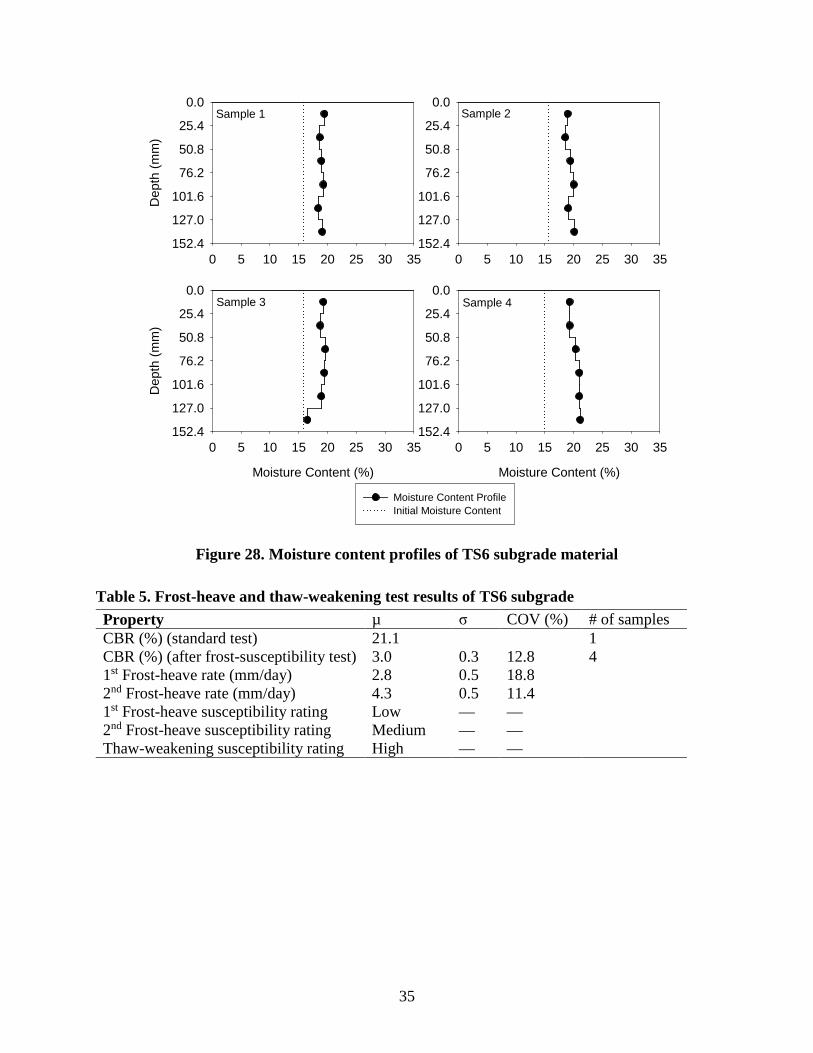
35

Figure 28. Moisture content profiles of TS6 subgrade material

Table 5. Frost-heave and thaw-weakening test results of TS6 subgrade Property µ σ COV (%) # of samples CBR (%) (standard test) 21.1 1 CBR (%) (after frost-susceptibility test) 3.0 0.3 12.8 4 1st Frost-heave rate (mm/day) 2.8 0.5 18.8 2nd Frost-heave rate (mm/day) 4.3 0.5 11.4 1st Frost-heave susceptibility rating Low — — 2nd Frost-heave susceptibility rating Medium — — Thaw-weakening susceptibility rating High — —

0 5 10 15 20 25 30 35

Dep

th (m

m)

0.0

25.4

50.8

76.2

101.6

127.0

152.4

Moisture Content (%)

0 5 10 15 20 25 30 35

0.0

25.4

50.8

76.2

101.6

127.0

152.4

Moisture Content (%)

0 5 10 15 20 25 30 35

Dep

th (m

m)

0.0

25.4

50.8

76.2

101.6

127.0

152.4

Moisture Content ProfileInitial Moisture Content

0 5 10 15 20 25 30 35

0.0

25.4

50.8

76.2

101.6

127.0

152.4

Sample 1 Sample 2

Sample 3 Sample 4

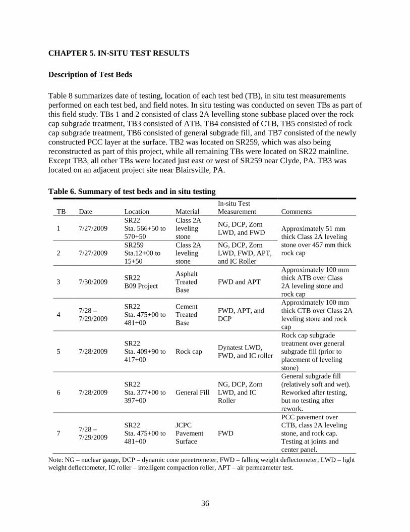
36

CHAPTER 5. IN-SITU TEST RESULTS

Description of Test Beds

Table 8 summarizes date of testing, location of each test bed (TB), in situ test measurements performed on each test bed, and field notes. In situ testing was conducted on seven TBs as part of this field study. TBs 1 and 2 consisted of class 2A levelling stone subbase placed over the rock cap subgrade treatment, TB3 consisted of ATB, TB4 consisted of CTB, TB5 consisted of rock cap subgrade treatment, TB6 consisted of general subgrade fill, and TB7 consisted of the newly constructed PCC layer at the surface. TB2 was located on SR259, which was also being reconstructed as part of this project, while all remaining TBs were located on SR22 mainline. Except TB3, all other TBs were located just east or west of SR259 near Clyde, PA. TB3 was located on an adjacent project site near Blairsville, PA.

Table 6. Summary of test beds and in situ testing

TB Date Location Material In-situ Test Measurement Comments

1 7/27/2009 SR22 Sta. 566+50 to 570+50

Class 2A leveling stone

NG, DCP, Zorn LWD, and FWD Approximately 51 mm

thick Class 2A leveling stone over 457 mm thick rock cap 2 7/27/2009

SR259 Sta.12+00 to 15+50

Class 2A leveling stone

NG, DCP, Zorn LWD, FWD, APT, and IC Roller

3 7/30/2009 SR22 B09 Project

Asphalt Treated Base

FWD and APT

Approximately 100 mm thick ATB over Class 2A leveling stone and rock cap

4 7/28 – 7/29/2009

SR22 Sta. 475+00 to 481+00

Cement Treated Base

FWD, APT, and DCP

Approximately 100 mm thick CTB over Class 2A leveling stone and rock cap

5 7/28/2009 SR22 Sta. 409+90 to 417+00

Rock cap Dynatest LWD, FWD, and IC roller

Rock cap subgrade treatment over general subgrade fill (prior to placement of leveling stone)

6 7/28/2009 SR22 Sta. 377+00 to 397+00

General Fill NG, DCP, Zorn LWD, and IC Roller

General subgrade fill (relatively soft and wet). Reworked after testing, but no testing after rework.

7 7/28 – 7/29/2009

SR22 Sta. 475+00 to 481+00

JCPC Pavement Surface

FWD

PCC pavement over CTB, class 2A leveling stone, and rock cap. Testing at joints and center panel.

Note: NG – nuclear gauge, DCP – dynamic cone penetrometer, FWD – falling weight deflectometer, LWD – light weight deflectometer, IC roller – intelligent compaction roller, APT – air permeameter test.

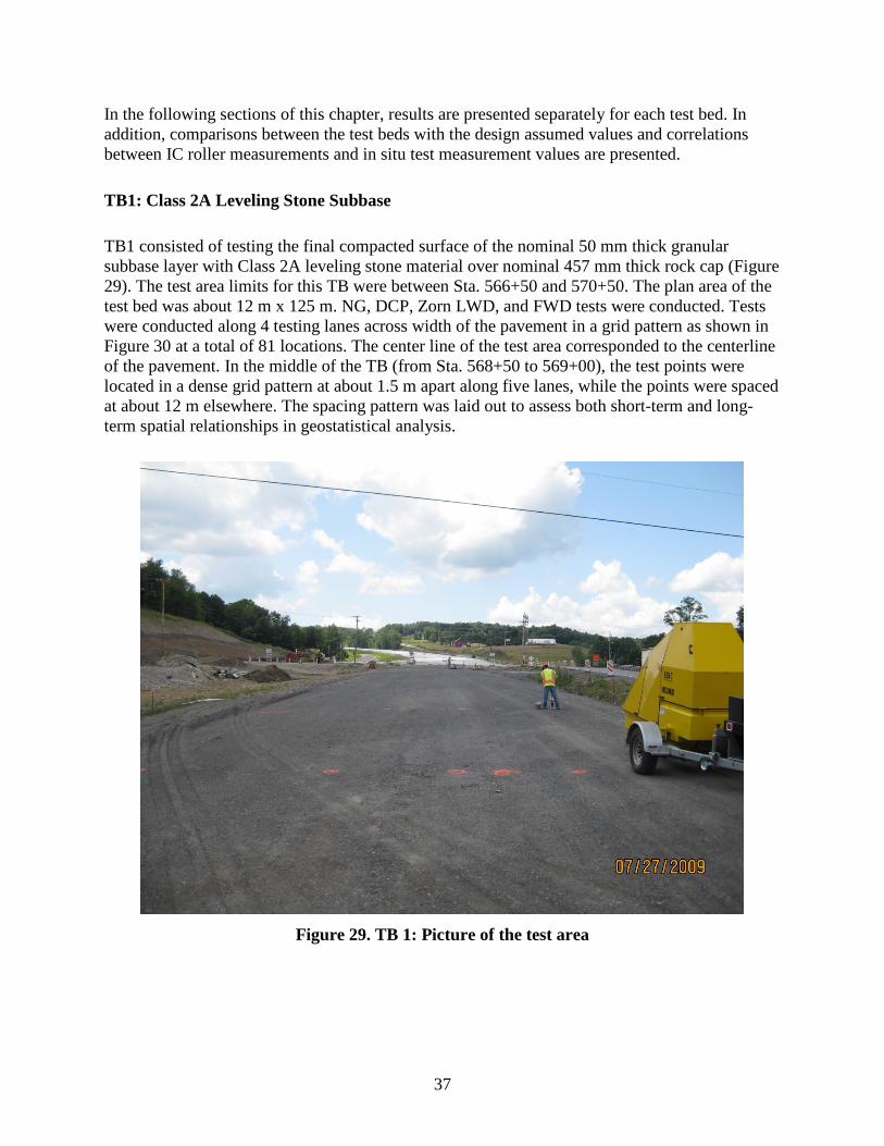
37

In the following sections of this chapter, results are presented separately for each test bed. In addition, comparisons between the test beds with the design assumed values and correlations between IC roller measurements and in situ test measurement values are presented.

TB1: Class 2A Leveling Stone Subbase

TB1 consisted of testing the final compacted surface of the nominal 50 mm thick granular subbase layer with Class 2A leveling stone material over nominal 457 mm thick rock cap (Figure 29). The test area limits for this TB were between Sta. 566+50 and 570+50. The plan area of the test bed was about 12 m x 125 m. NG, DCP, Zorn LWD, and FWD tests were conducted. Tests were conducted along 4 testing lanes across width of the pavement in a grid pattern as shown in Figure 30 at a total of 81 locations. The center line of the test area corresponded to the centerline of the pavement. In the middle of the TB (from Sta. 568+50 to 569+00), the test points were located in a dense grid pattern at about 1.5 m apart along five lanes, while the points were spaced at about 12 m elsewhere. The spacing pattern was laid out to assess both short-term and long-term spatial relationships in geostatistical analysis.

Figure 29. TB 1: Picture of the test area

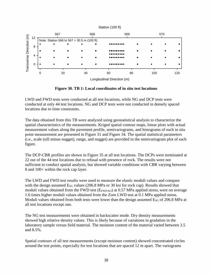
38

Figure 30. TB 1: Local coordinates of in situ test locations

LWD and FWD tests were conducted at all test locations, while NG and DCP tests were conducted at only 44 test locations. NG and DCP tests were not conducted in densely spaced locations due to time constraints.

The data obtained from this TB were analyzed using geostatistical analysis to characterize the spatial characteristics of the measurements. Kriged spatial contour maps, linear plots with actual measurement values along the pavement profile, semivariograms, and histograms of each in situ point measurement are presented in Figure 31 and Figure 34. The spatial statistical parameters (i.e., scale (sill minus nugget), range, and nugget) are provided in the semivariogram plot of each figure.

The DCP-CBR profiles are shown in Figure 35 at all test locations. The DCPs were terminated at 22 out of the 44 test locations due to refusal with presence of rock. The results were not sufficient to conduct spatial analysis, but showed variable conditions with CBR varying between 8 and 100+ within the rock cap layer.

The LWD and FWD test results were used to measure the elastic moduli values and compare with the design assumed ESG values (206.8 MPa or 30 ksi for rock cap). Results showed that moduli values obtained from the FWD test (EFWD-K3) at 0.57 MPa applied stress, were on average 1.6 times higher moduli values obtained from the Zorn LWD test at 0.1 MPa applied stress. Moduli values obtained from both tests were lower than the design assumed ESG of 206.8 MPa at all test locations except one.

The NG test measurements were obtained in backscatter mode. Dry density measurements showed high relative density values. This is likely because of variations in gradation in the laboratory sample versus field material. The moisture content of the material varied between 3.5 and 8.5%.

Spatial contours of all test measurements (except moisture content) showed concentrated circles around the test points, especially for test locations that are spaced 12 m apart. The variograms

Longitudinal Direction (m)

0 20 40 60 80 100 120Tran

sver

se D

irect

ion

(m)

0

4

8

12

Station (100 ft)

567 568 569 570

Note: Station 566 to 567 = 30.5 m (100 ft)

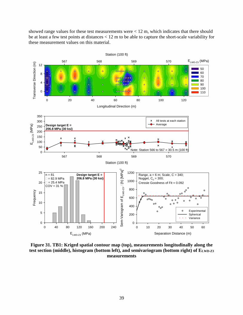
39

showed range values for these test measurements were < 12 m, which indicates that there should be at least a few test points at distances < 12 m to be able to capture the short-scale variability for these measurement values on this material.

Figure 31. TB1: Kriged spatial contour map (top), measurements longitudinally along the test section (middle), histogram (bottom left), and semivariogram (bottom right) of ELWD-Z3

measurements

Station (100 ft)

567 568 569 570

E LWD

-Z3 (

MPa

)

050

100150200250300350

All tests at each stationAverage

Note: Station 566 to 567 = 30.5 m (100 ft)

Design target E =206.8 MPa (30 ksi)

ELWD-Z3 (MPa)

0 40 80 120 160 200 240

Freq

uenc

y

0

5

10

15

20

25n = 81 = 82.9 MPa = 25.4 MPaCOV = 31 %

Design target E =206.8 MPa (30 ksi)

ELWD-Z3 (MPa)

Longitudinal Direction (m)

0 20 40 60 80 100 120Tran

sver

se D

irect

ion

(m)

0

4

8

1250 60 70 80 90 100 110

Station (100 ft)

567 568 569 570

Separation Distance (m)

0 10 20 30 40 50 60Sem

-Var

iogr

am o

f ELW

D-Z

3, (

h) [M

Pa]2

0

200

400

600

800

1000

1200

ExperimentalSphericalVariance

Range, a = 6 m; Scale, C = 340; Nugget, C0 = 300;Cressie Goodness of Fit = 0.092

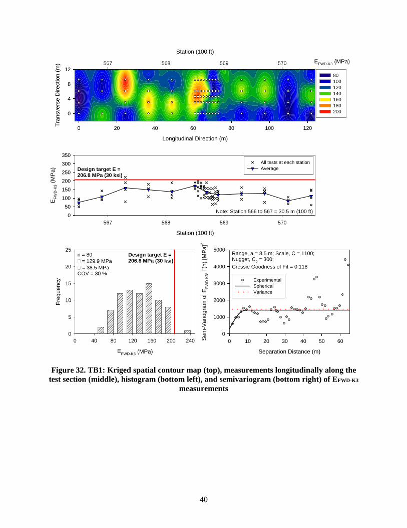
40

Figure 32. TB1: Kriged spatial contour map (top), measurements longitudinally along the test section (middle), histogram (bottom left), and semivariogram (bottom right) of EFWD-K3

measurements

Station (100 ft)

567 568 569 570

E FWD

-K3 (

MPa

)

050

100150200250300350

All tests at each stationAverage

Note: Station 566 to 567 = 30.5 m (100 ft)

Design target E =206.8 MPa (30 ksi)

EFWD-K3 (MPa)

0 40 80 120 160 200 240

Freq

uenc

y

0

5

10

15

20

25n = 80 = 129.9 MPa = 38.5 MPaCOV = 30 %

Design target E =206.8 MPa (30 ksi)

EFWD-K3 (MPa)

Longitudinal Direction (m)

0 20 40 60 80 100 120Tran

sver

se D

irect

ion

(m)

0

4

8

1280 100 120 140 160 180 200

Station (100 ft)

567 568 569 570

Separation Distance (m)

0 10 20 30 40 50 60Sem

-Var

iogr

am o

f EFW

D-K

3, (

h) [M

Pa]2

0

1000

2000

3000

4000

5000

ExperimentalSphericalVariance

Range, a = 8.5 m; Scale, C = 1100; Nugget, C0 = 300;Cressie Goodness of Fit = 0.118

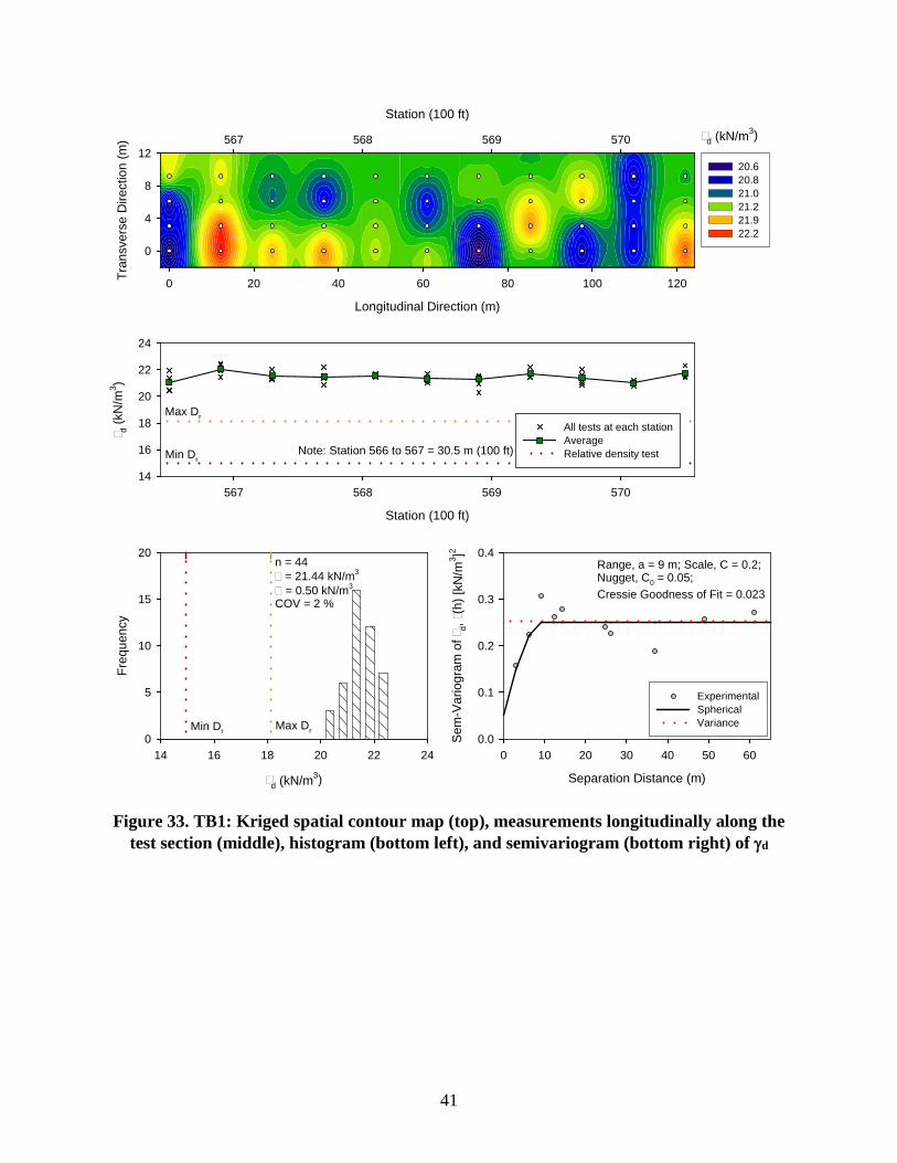
41

Figure 33. TB1: Kriged spatial contour map (top), measurements longitudinally along the test section (middle), histogram (bottom left), and semivariogram (bottom right) of γd

Station (100 ft)

567 568 569 570

d (k

N/m

3 )

14

16

18

20

22

24

All tests at each stationAverageRelative density testNote: Station 566 to 567 = 30.5 m (100 ft)

Max Dr

Min Dr

d (kN/m3)

14 16 18 20 22 24

Freq

uenc

y

0

5

10

15

20n = 44 = 21.44 kN/m3

= 0.50 kN/m3

COV = 2 %

Min Dr Max Dr

d (kN/m3)

Longitudinal Direction (m)

0 20 40 60 80 100 120Tran

sver

se D

irect

ion

(m)

0

4

8

1220.6 20.8 21.0 21.2 21.9 22.2

Station (100 ft)

567 568 569 570

Separation Distance (m)

0 10 20 30 40 50 60

Sem

-Var

iogr

am o

f d, (

h) [k

N/m

3 ]2

0.0

0.1

0.2

0.3

0.4

ExperimentalSphericalVariance

Range, a = 9 m; Scale, C = 0.2; Nugget, C0 = 0.05;Cressie Goodness of Fit = 0.023

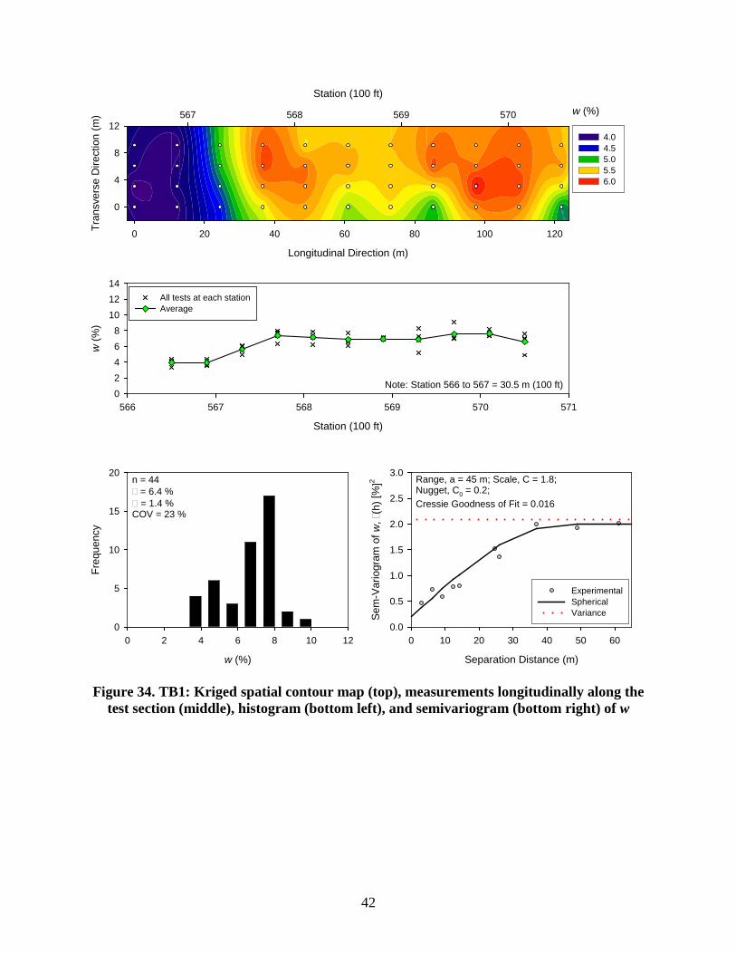
42

Figure 34. TB1: Kriged spatial contour map (top), measurements longitudinally along the test section (middle), histogram (bottom left), and semivariogram (bottom right) of w

w (%)

Longitudinal Direction (m)

0 20 40 60 80 100 120Tran

sver

se D

irect

ion

(m)

0

4

8

124.0 4.5 5.0 5.5 6.0

Station (100 ft)

567 568 569 570

Station (100 ft)

566 567 568 569 570 571

w (%

)

02468

101214

All tests at each stationAverage

Note: Station 566 to 567 = 30.5 m (100 ft)

w (%)

0 2 4 6 8 10 12

Freq

uenc

y

0

5

10

15

20n = 44 = 6.4 % = 1.4 %COV = 23 %

Separation Distance (m)

0 10 20 30 40 50 60

Sem

-Var

iogr

am o

f w,

(h) [

%]2

0.0

0.5

1.0

1.5

2.0

2.5

3.0

ExperimentalSphericalVariance

Range, a = 45 m; Scale, C = 1.8; Nugget, C0 = 0.2;Cressie Goodness of Fit = 0.016

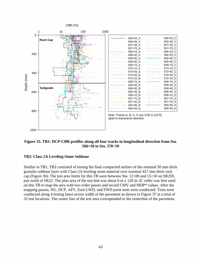
43

Figure 35. TB1: DCP-CBR profiles along all four tracks in longitudinal direction from Sta. 566+50 to Sta. 570+10

TB2: Class 2A Leveling Stone Subbase

Similar to TB1, TB2 consisted of testing the final compacted surface of the nominal 50 mm thick granular subbase layer with Class 2A leveling stone material over nominal 457 mm thick rock cap (Figure 36). The test area limits for this TB were between Sta. 12+00 and 15+50 on SR259, just north of SR22. The plan area of the test bed was about 6 m x 120 m. IC roller was first used on this TB to map the area with two roller passes and record CMV and MDP* values. After the mapping passes, NG, DCP, APT, Zorn LWD, and FWD point tests were conducted. Tests were conducted along 4 testing lanes across width of the pavement as shown in Figure 37 at a total of 32 test locations. The center line of the test area corresponded to the centerline of the pavement.

CBR (%)

1 10 100 1000

Dep

th (m

m)

0

200

400

600

800

1000

Rock Cap

Subgrade

566+50_A566+90_A567+30_A567+70_A568+10_A568+50_A568+90_A569+30_A569+70_A570+10_A570+50_A570+50_B570+10_B569+70_B569+30_B568+90_B568+50_B568+10_B567+70_B567+30_B566+90_B566+50_B

566+50_C566+90_C567+30_C567+70_C568+10_C568+50_C568+90_C569+30_C569+70_C570+10_C570+50_C570+50_D570+10_D569+70_D569+30_D568+90_D568+50_D568+10_D567+70_D567+30_D566+90_D566+50_D

Note: Tracks A, B, C, D are 3.05 m (10 ft) apart in transverse direction

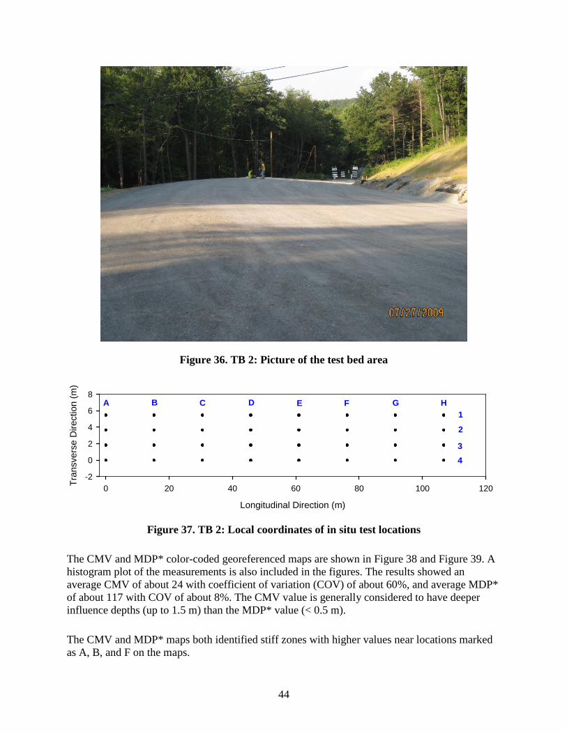
44

Figure 36. TB 2: Picture of the test bed area

Figure 37. TB 2: Local coordinates of in situ test locations

The CMV and MDP* color-coded georeferenced maps are shown in Figure 38 and Figure 39. A histogram plot of the measurements is also included in the figures. The results showed an average CMV of about 24 with coefficient of variation (COV) of about 60%, and average MDP* of about 117 with COV of about 8%. The CMV value is generally considered to have deeper influence depths (up to 1.5 m) than the MDP* value (< 0.5 m).

The CMV and MDP* maps both identified stiff zones with higher values near locations marked as A, B, and F on the maps.

Longitudinal Direction (m)

0 20 40 60 80 100 120Tran

sver

se D

irect

ion

(m)

-2

0

2

4

6

8A H

1

4

B C D E F G

2

3

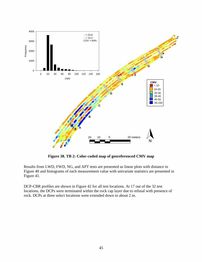
45

Figure 38. TB 2: Color-coded map of georeferenced CMV map

Results from LWD, FWD, NG, and APT tests are presented as linear plots with distance in Figure 40 and histograms of each measurement value with univariate statistics are presented in Figure 41.

DCP-CBR profiles are shown in Figure 42 for all test locations. At 17 out of the 32 test locations, the DCPs were terminated within the rock cap layer due to refusal with presence of rock. DCPs at three select locations were extended down to about 2 m.

CMV

0 20 40 60 80 100 120 140 160

Freq

uenc

y

0

1000

2000

3000

4000 = 23.8 = 14.2COV = 60%

20 10 0 20 meters

A

B

C

D

E

F

G

H

< 1010-2020-3030-4040-5050-150

CMV

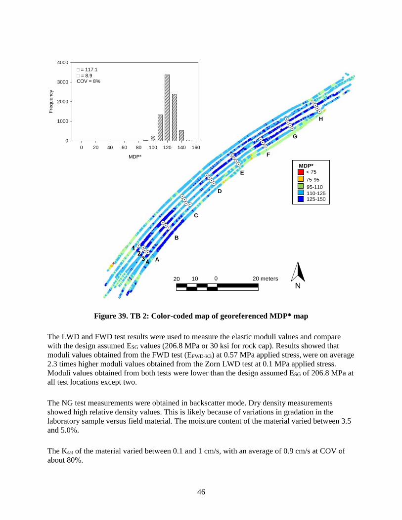
46

Figure 39. TB 2: Color-coded map of georeferenced MDP* map

The LWD and FWD test results were used to measure the elastic moduli values and compare with the design assumed ESG values (206.8 MPa or 30 ksi for rock cap). Results showed that moduli values obtained from the FWD test (EFWD-K3) at 0.57 MPa applied stress, were on average 2.3 times higher moduli values obtained from the Zorn LWD test at 0.1 MPa applied stress. Moduli values obtained from both tests were lower than the design assumed ESG of 206.8 MPa at all test locations except two.

The NG test measurements were obtained in backscatter mode. Dry density measurements showed high relative density values. This is likely because of variations in gradation in the laboratory sample versus field material. The moisture content of the material varied between 3.5 and 5.0%.

The Ksat of the material varied between 0.1 and 1 cm/s, with an average of 0.9 cm/s at COV of about 80%.

20 10 0 20 meters

A

B

C

D

E

F

G

H

MDP*

0 20 40 60 80 100 120 140 160

Freq

uenc

y

0

1000

2000

3000

4000 = 117.1 = 8.9COV = 8%

< 7575-9595-110110-125125-150

MDP*

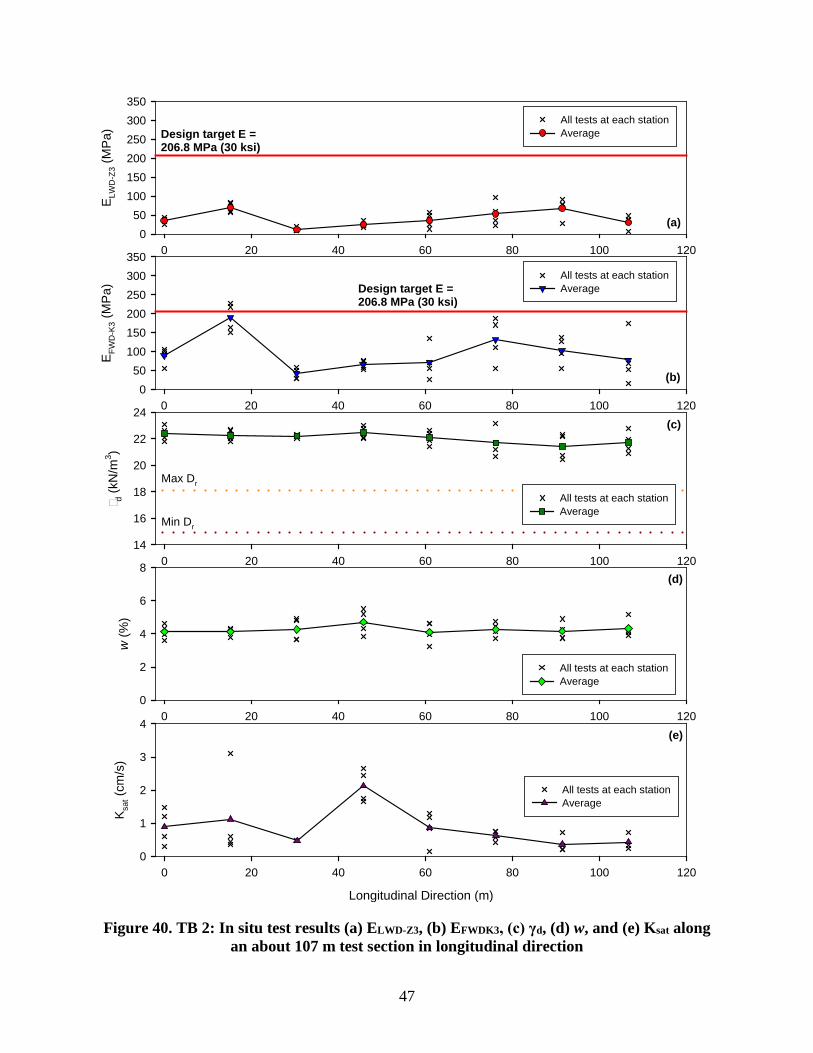
47

Figure 40. TB 2: In situ test results (a) ELWD-Z3, (b) EFWDK3, (c) γd, (d) w, and (e) Ksat along an about 107 m test section in longitudinal direction

0 20 40 60 80 100 120

E LWD

-Z3 (

MPa

)

050

100150200250300350

All tests at each stationAverageDesign target E =

206.8 MPa (30 ksi)

0 20 40 60 80 100 120

E FWD

-K3 (

MPa

)

050

100150200250300350

All tests at each stationAverageDesign target E =

206.8 MPa (30 ksi)

0 20 40 60 80 100 120

d (k

N/m

3 )

14

16

18

20

22

24

All tests at each stationAverage

Max Dr

Min Dr

0 20 40 60 80 100 120

w (%

)

0

2

4

6

8

All tests at each stationAverage

(a)

(b)

(c)

(d)

Longitudinal Direction (m)

0 20 40 60 80 100 120

K sat (

cm/s

)

0

1

2

3

4

All tests at each stationAverage

(e)

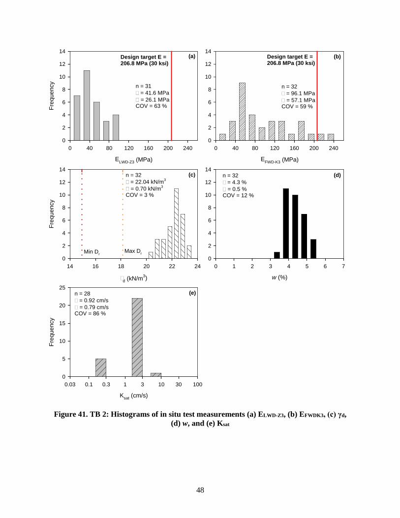
48

Figure 41. TB 2: Histograms of in situ test measurements (a) ELWD-Z3, (b) EFWDK3, (c) γd, (d) w, and (e) Ksat

ELWD-Z3 (MPa)

0 40 80 120 160 200 240

Freq

uenc

y

0

2

4

6

8

10

12

14

n = 31 = 41.6 MPa = 26.1 MPaCOV = 63 %

Design target E =206.8 MPa (30 ksi)

EFWD-K3 (MPa)

0 40 80 120 160 200 2400

2

4

6

8

10

12

14

n = 32 = 96.1 MPa = 57.1 MPaCOV = 59 %

Design target E =206.8 MPa (30 ksi)

d (kN/m3)

14 16 18 20 22 24

Freq

uenc

y

0

2

4

6

8

10

12

14n = 32 = 22.04 kN/m3

= 0.70 kN/m3

COV = 3 %

Min DrMax Dr

w (%)

0 1 2 3 4 5 6 70

2

4

6

8

10

12

14n = 32 = 4.3 % = 0.5 %COV = 12 %

(a) (b)

(c) (d)

Ksat (cm/s)

0.03 0.1 0.3 1 3 10 30 100

Freq

uenc

y

0

5

10

15

20

25n = 28 = 0.92 cm/s = 0.79 cm/sCOV = 86 %

(e)

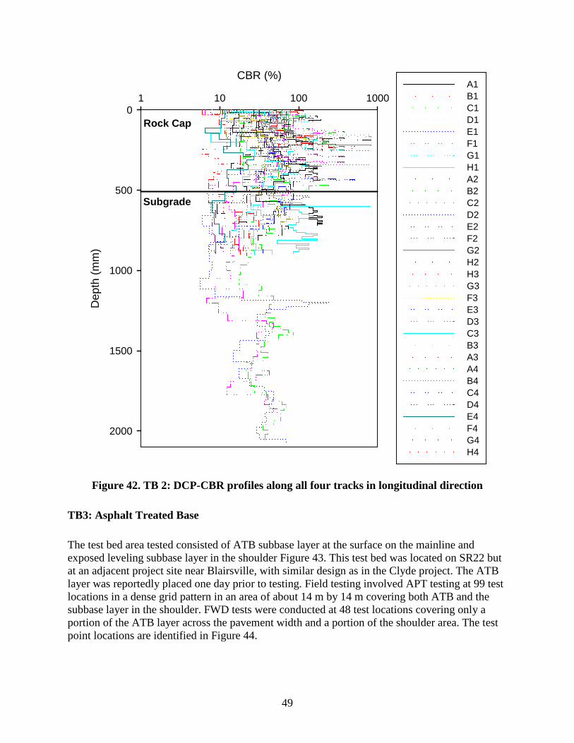
49

Figure 42. TB 2: DCP-CBR profiles along all four tracks in longitudinal direction

TB3: Asphalt Treated Base

The test bed area tested consisted of ATB subbase layer at the surface on the mainline and exposed leveling subbase layer in the shoulder Figure 43. This test bed was located on SR22 but at an adjacent project site near Blairsville, with similar design as in the Clyde project. The ATB layer was reportedly placed one day prior to testing. Field testing involved APT testing at 99 test locations in a dense grid pattern in an area of about 14 m by 14 m covering both ATB and the subbase layer in the shoulder. FWD tests were conducted at 48 test locations covering only a portion of the ATB layer across the pavement width and a portion of the shoulder area. The test point locations are identified in Figure 44.

CBR (%)

1 10 100 1000D

epth

(mm

)0

500

1000

1500

2000

A1B1C1D1E1F1G1H1A2B2C2D2E2F2G2H2H3G3F3E3D3C3B3A3A4B4C4D4E4F4G4H4

Rock Cap

Subgrade

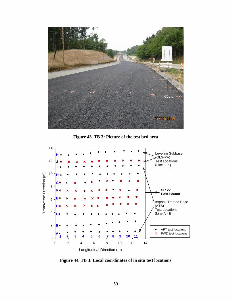
50

Figure 43. TB 3: Picture of the test bed area

Figure 44. TB 3: Local coordinates of in situ test locations

Longitudinal Direction (m)

0 2 4 6 8 10 12 14

Tran

sver

se D

irect

ion

(m)

0

2

4

6

8

10

12

14

APT test locationsFWD test locationsA

B

C

D

E

F

G

H

IJ

K

1 2 3 4 5 6 7 8 9 10 11

SR 22East Bound

Leveling Subbase(OLS-PA)Test Locations(Line J, K)

Asphalt Treated Base(ATB)Test Locations(Line A - I)

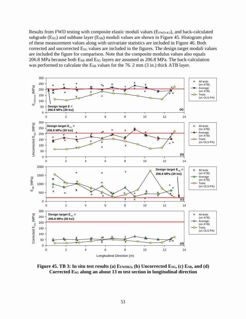
51

Results from FWD testing with composite elastic moduli values (EFWD-K3), and back-calculated subgrade (ESG) and subbase layer (ESB) moduli values are shown in Figure 45. Histogram plots of these measurement values along with univariate statistics are included in Figure 46. Both corrected and uncorrected ESG values are included in the figures. The design target moduli values are included the figure for comparison. Note that the composite modulus values also equals 206.8 MPa because both ESB and ESG layers are assumed as 206.8 MPa. The back-calculation was performed to calculate the ESB values for the 76. 2 mm (3 in.) thick ATB layer.

Figure 45. TB 3: In situ test results (a) EFWDK3, (b) Uncorrected ESG, (c) ESB, and (d) Corrected ESG along an about 13 m test section in longitudinal direction

0 2 4 6 8 10 12 14

E FWD

-K3 (

MPa

)

0

50

100

150

200

250

300All tests(on ATB) Average(on ATB)Tests(on OLS-PA)

Design target E =206.8 MPa (30 ksi)

0 2 4 6 8 10 12 14

Unc

orre

cted

ES

G (M

Pa)

0

50

100

150

200

250

300All tests(on ATB) Average(on ATB)Tests(on OLS-PA)

Design target ESG =206.8 MPa (30 ksi)

0 2 4 6 8 10 12 14

E SB

(MPa

)

0

500

1000

1500

2000All tests(on ATB)Average(on ATB)Tests(on OLS-PA)

Design target ESB =206.8 MPa (30 ksi)

Longitudinal Direction (m)

0 2 4 6 8 10 12 14

Cor

rect

ed E

SG (M

Pa)

0

50

100

150

200

250

300All tests(on ATB)Average(on ATB)Tests(on OLS-PA)

Design target ESG =206.8 MPa (30 ksi)

(a)

(b)

(c)

(d)

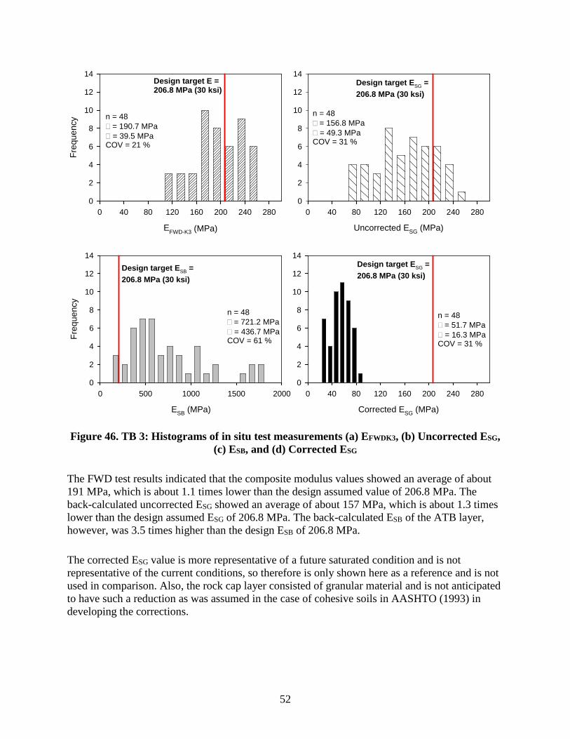
52

Figure 46. TB 3: Histograms of in situ test measurements (a) EFWDK3, (b) Uncorrected ESG, (c) ESB, and (d) Corrected ESG

The FWD test results indicated that the composite modulus values showed an average of about 191 MPa, which is about 1.1 times lower than the design assumed value of 206.8 MPa. The back-calculated uncorrected ESG showed an average of about 157 MPa, which is about 1.3 times lower than the design assumed ESG of 206.8 MPa. The back-calculated ESB of the ATB layer, however, was 3.5 times higher than the design ESB of 206.8 MPa.

The corrected ESG value is more representative of a future saturated condition and is not representative of the current conditions, so therefore is only shown here as a reference and is not used in comparison. Also, the rock cap layer consisted of granular material and is not anticipated to have such a reduction as was assumed in the case of cohesive soils in AASHTO (1993) in developing the corrections.

EFWD-K3 (MPa)

0 40 80 120 160 200 240 280

Freq

uenc

y

0

2

4

6

8

10

12

14

n = 48 = 190.7 MPa = 39.5 MPaCOV = 21 %

Design target E =206.8 MPa (30 ksi)

Uncorrected ESG (MPa)

0 40 80 120 160 200 240 2800

2

4

6

8

10

12

14

n = 48 = 156.8 MPa = 49.3 MPaCOV = 31 %

Design target ESG =206.8 MPa (30 ksi)

ESB (MPa)

0 500 1000 1500 2000

Freq

uenc

y

0

2

4

6

8

10

12

14

n = 48 = 721.2 MPa = 436.7 MPaCOV = 61 %

Design target ESB =206.8 MPa (30 ksi)

Corrected ESG (MPa)

0 40 80 120 160 200 240 2800

2

4

6

8

10

12

14

n = 48 = 51.7 MPa = 16.3 MPaCOV = 31 %

Design target ESG =206.8 MPa (30 ksi)

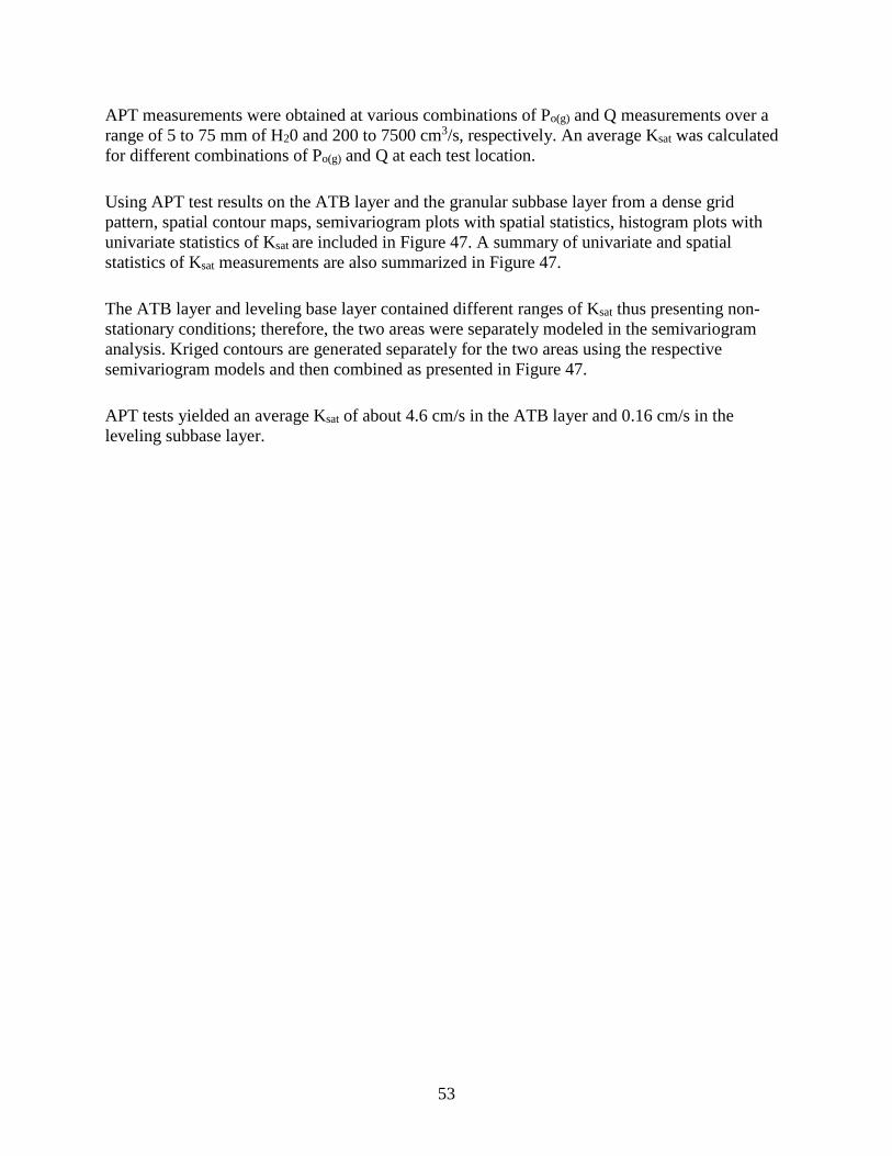
53

APT measurements were obtained at various combinations of Po(g) and Q measurements over a range of 5 to 75 mm of H20 and 200 to 7500 cm3/s, respectively. An average Ksat was calculated for different combinations of Po(g) and Q at each test location.

Using APT test results on the ATB layer and the granular subbase layer from a dense grid pattern, spatial contour maps, semivariogram plots with spatial statistics, histogram plots with univariate statistics of Ksat are included in Figure 47. A summary of univariate and spatial statistics of Ksat measurements are also summarized in Figure 47.

The ATB layer and leveling base layer contained different ranges of Ksat thus presenting non-stationary conditions; therefore, the two areas were separately modeled in the semivariogram analysis. Kriged contours are generated separately for the two areas using the respective semivariogram models and then combined as presented in Figure 47.

APT tests yielded an average Ksat of about 4.6 cm/s in the ATB layer and 0.16 cm/s in the leveling subbase layer.

54

Figure 47. TB3: Kriged spatial contour map (top), semivariogram (middle), and histogram (bottom) plots of Ksat measurements [left semi-varaiogram and histogram plots represent

measurements on the ATB layer and the right plots represent measurements on the granular subbase layer]

Longitudinal Direction (m)

0 2 4 6 8 10 12 14

Tran

sver

se D

irect

ion

(m)

0

2

4

6

8

10

12

14

0.10.31310

Separation Distance (m)

0 1 2 3 4 5Sem

i-Var

iogr

am o

f Log

(Ksa

t),

(h) [

cm/s

]2

0.00

0.02

0.04

0.06

0.08

0.10ExperimentalSpherical

Separation Distance (m)

0 1 2 3 4 5Sem

i-Var

iogr

am o

f Log

(Ksa

t),

(h) [

cm/s

]2

0.00

0.02

0.04

0.06

0.08

0.10ExperimentalSpherical

Ksat (cm/s)

ATBRange, a = 4.0 m;Scale, C = 0.03; Nugget, C0 = 0;Cressie Goodness of Fit = 0.031

Ksat (cm/s)

Freq

uenc

y

0

20

40

60

80

0.03 0.1 0.3 1 3 10 30 100

N = 99 = 4.6 cm/s = 1.9 cm/sCOV = 42%

OLS-PARange, a = 2.0 m;Scale, C = 0.04;Nugget, C0 = 0;Cressie Goodness of Fit = 0.075

Ksat (cm/s)

Freq

uenc

y

0

5

10

15

20

25

30

0.03 0.1 0.3 1 3 10 30 100

N = 22 = 0.16 cm/s = 0.06 cm/sCOV = 40%

ATB OLS-PA

Leveling Subbase(OLS-PA)Test Locations

Asphalt Treated Base(ATB)Test Locations

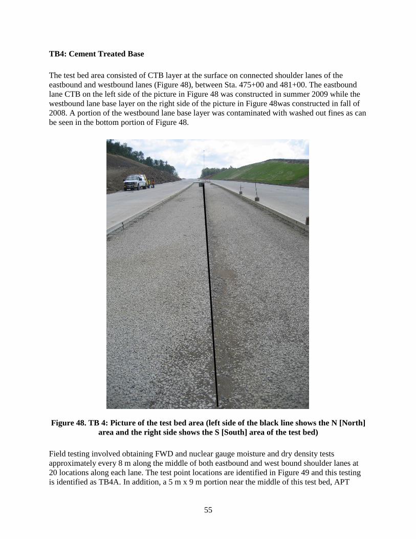
55

TB4: Cement Treated Base

The test bed area consisted of CTB layer at the surface on connected shoulder lanes of the eastbound and westbound lanes (Figure 48), between Sta. 475+00 and 481+00. The eastbound lane CTB on the left side of the picture in Figure 48 was constructed in summer 2009 while the westbound lane base layer on the right side of the picture in Figure 48was constructed in fall of 2008. A portion of the westbound lane base layer was contaminated with washed out fines as can be seen in the bottom portion of Figure 48.

Figure 48. TB 4: Picture of the test bed area (left side of the black line shows the N [North] area and the right side shows the S [South] area of the test bed)

Field testing involved obtaining FWD and nuclear gauge moisture and dry density tests approximately every 8 m along the middle of both eastbound and west bound shoulder lanes at 20 locations along each lane. The test point locations are identified in Figure 49 and this testing is identified as TB4A. In addition, a 5 m x 9 m portion near the middle of this test bed, APT

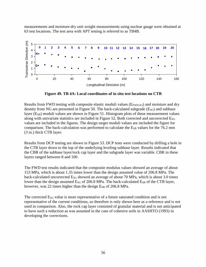
56

measurements and moisture-dry unit weight measurements using nuclear gauge were obtained at 63 test locations. The test area with APT testing is referred to as TB4B.

Figure 49. TB 4A: Local coordinates of in situ test locations on CTB

Results from FWD testing with composite elastic moduli values (EFWD-K3) and moisture and dry desnity from NG are presented in Figure 50. The back-calculated subgrade (ESG) and subbase layer (ESB) moduli values are shown in Figure 51. Histogram plots of these measurement values along with univariate statistics are included in Figure 52. Both corrected and uncorrected ESG values are included in the figures. The design target moduli values are included the figure for comparison. The back-calculation was performed to calculate the ESB values for the 76.2 mm (3 in.) thick CTB layer.

Results from DCP testing are shown in Figure 53. DCP tests were conducted by drilling a hole in the CTB layer down to the top of the underlying leveling subbase layer. Results indicated that the CBR of the subbase layer/rock cap layer and the subgrade layer was variable. CBR in these layers ranged between 8 and 100.

The FWD test results indicated that the composite modulus values showed an average of about 153 MPa, which is about 1.35 times lower than the design assumed value of 206.8 MPa. The back-calculated uncorrected ESG showed an average of about 70 MPa, which is about 3.0 times lower than the design assumed ESG of 206.8 MPa. The back-calculated ESB of the CTB layer, however, was 22 times higher than the design ESB of 206.8 MPa.

The corrected ESG value is more representative of a future saturated condition and is not representative of the current conditions, so therefore is only shown here as a reference and is not used in comparison. Also, the rock cap layer consisted of granular material and is not anticipated to have such a reduction as was assumed in the case of cohesive soils in AASHTO (1993) in developing the corrections.

Longitudinal Direction (m)

0 20 40 60 80 100 120 140 160Tran

sver

se D

irect

ion

(m)

0

1

2

3

4

5

N

S

0 201 2 3 4 5 6 7 8 9 10 11 12 13 14 15 16 17 18 19

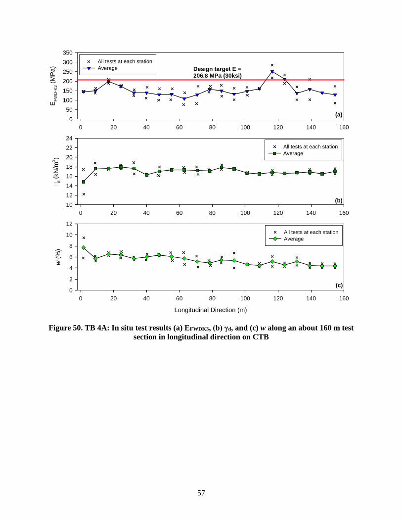
57

Figure 50. TB 4A: In situ test results (a) EFWDK3, (b) γd, and (c) w along an about 160 m test section in longitudinal direction on CTB

0 20 40 60 80 100 120 140 160

E FWD

-K3 (

MPa

)

050

100150200250300350

All tests at each stationAverage Design target E =

206.8 MPa (30ksi)

0 20 40 60 80 100 120 140 160

d (k

N/m

3 )

1012141618202224

All tests at each stationAverage

Longitudinal Direction (m)

0 20 40 60 80 100 120 140 160

w (%

)

0

2

4

6

8

10

12All tests at each stationAverage

(a)

(b)

(c)

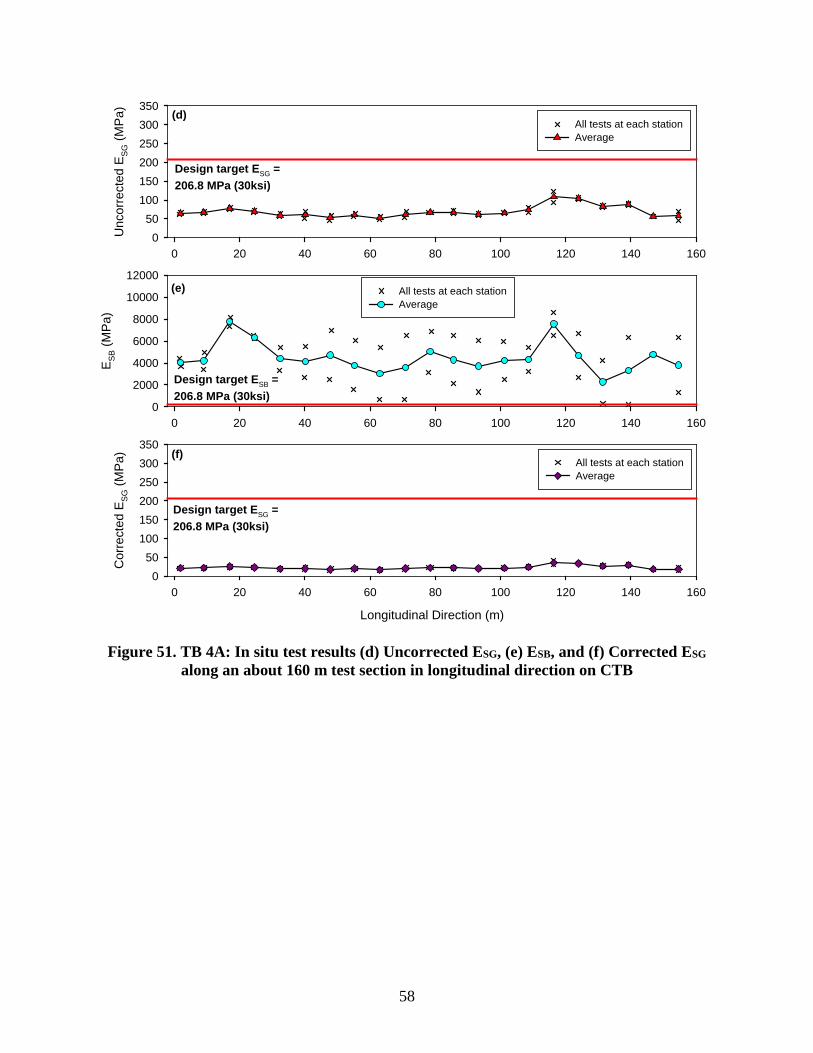
58

Figure 51. TB 4A: In situ test results (d) Uncorrected ESG, (e) ESB, and (f) Corrected ESG along an about 160 m test section in longitudinal direction on CTB

0 20 40 60 80 100 120 140 160

Unc

orre

cted

ESG

(MPa

)

050

100150200250300350

All tests at each stationAverage

Design target ESG =206.8 MPa (30ksi)

0 20 40 60 80 100 120 140 160

E SB (M

Pa)

0

2000

4000

6000

8000

10000

12000All tests at each stationAverage

Design target ESB =206.8 MPa (30ksi)

Longitudinal Direction (m)

0 20 40 60 80 100 120 140 160

Cor

rect

ed E

SG (M

Pa)

050

100150200250300350

All tests at each stationAverage

Design target ESG =206.8 MPa (30ksi)

(d)

(e)

(f)

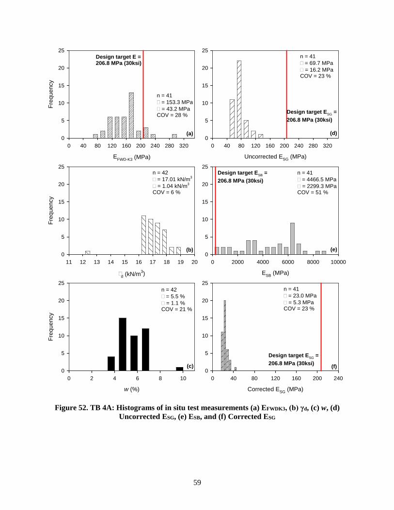
59

Figure 52. TB 4A: Histograms of in situ test measurements (a) EFWDK3, (b) γd, (c) w, (d) Uncorrected ESG, (e) ESB, and (f) Corrected ESG

EFWD-K3 (MPa)

0 40 80 120 160 200 240 280 320

Freq

uenc

y

0

5

10

15

20

25

n = 41 = 153.3 MPa = 43.2 MPaCOV = 28 %

Design target E =206.8 MPa (30ksi)

d (kN/m3)

11 12 13 14 15 16 17 18 19 20

Freq

uenc

y

0

5

10

15

20

25n = 42 = 17.01 kN/m3

= 1.04 kN/m3

COV = 6 %

w (%)

0 2 4 6 8 10

Freq

uenc

y

0

5

10

15

20

25n = 42 = 5.5 % = 1.1 %COV = 21 %

Uncorrected ESG (MPa)

0 40 80 120 160 200 240 280 3200

5

10

15

20

25n = 41 = 69.7 MPa = 16.2 MPaCOV = 23 %

Design target ESG =206.8 MPa (30ksi)

ESB (MPa)

0 2000 4000 6000 8000 100000

5

10

15

20

25n = 41 = 4466.5 MPa = 2299.3 MPaCOV = 51 %

Design target ESB =206.8 MPa (30ksi)

Corrected ESG (MPa)

0 40 80 120 160 200 2400

5

10

15

20

25n = 41 = 23.0 MPa = 5.3 MPaCOV = 23 %

Design target ESG =206.8 MPa (30ksi)

(a)

(b)

(c)

(d)

(e)

(f)

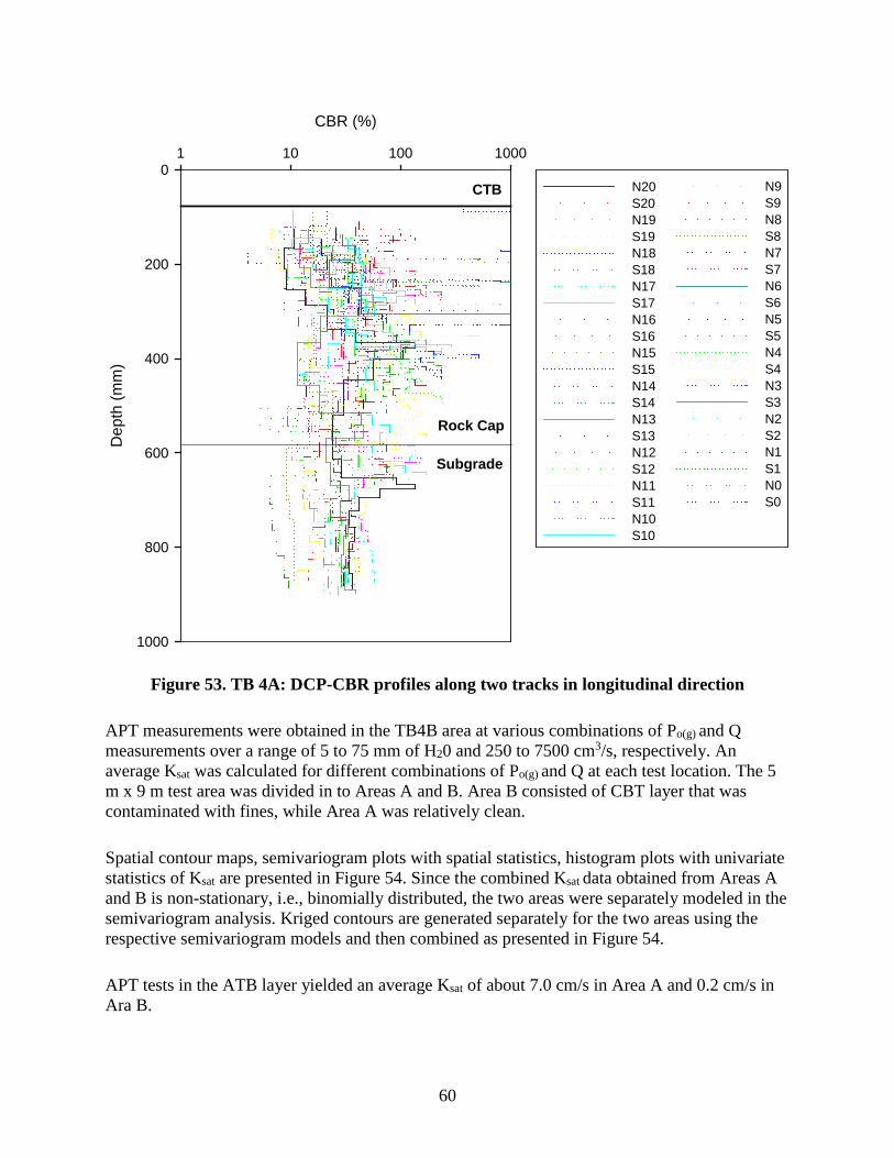
60

Figure 53. TB 4A: DCP-CBR profiles along two tracks in longitudinal direction

APT measurements were obtained in the TB4B area at various combinations of Po(g) and Q measurements over a range of 5 to 75 mm of H20 and 250 to 7500 cm3/s, respectively. An average Ksat was calculated for different combinations of Po(g) and Q at each test location. The 5 m x 9 m test area was divided in to Areas A and B. Area B consisted of CBT layer that was contaminated with fines, while Area A was relatively clean.

Spatial contour maps, semivariogram plots with spatial statistics, histogram plots with univariate statistics of Ksat are presented in Figure 54. Since the combined Ksat data obtained from Areas A and B is non-stationary, i.e., binomially distributed, the two areas were separately modeled in the semivariogram analysis. Kriged contours are generated separately for the two areas using the respective semivariogram models and then combined as presented in Figure 54.

APT tests in the ATB layer yielded an average Ksat of about 7.0 cm/s in Area A and 0.2 cm/s in Ara B.

CBR (%)

1 10 100 1000

Dep

th (m

m)

0

200

400

600

800

1000

Rock Cap

Subgrade

CTB N20S20N19S19N18S18N17S17N16S16N15S15N14S14N13S13N12S12N11S11N10S10

N9S9N8S8N7S7N6S6N5S5N4S4N3S3N2S2N1S1N0S0

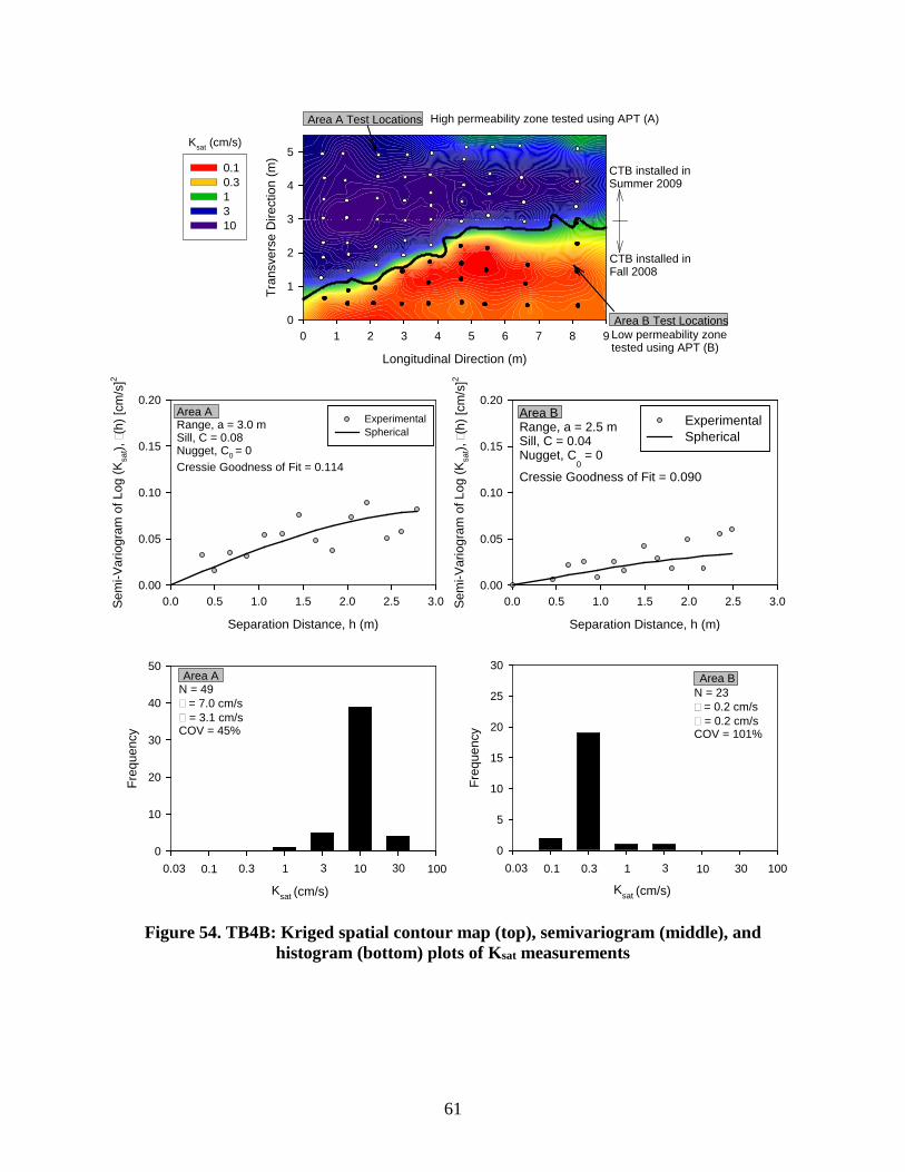
61

Figure 54. TB4B: Kriged spatial contour map (top), semivariogram (middle), and histogram (bottom) plots of Ksat measurements

Longitudinal Direction (m)

0 1 2 3 4 5 6 7 8 9

Tran

sver

se D

irect

ion

(m)

0

1

2

3

4

50.10.31310

Separation Distance, h (m)

0.0 0.5 1.0 1.5 2.0 2.5 3.0Sem

i-Var

iogr

am o

f Log

(Ksa

t),

(h) [

cm/s

]2

0.00

0.05

0.10

0.15

0.20

ExperimentalSpherical

Separation Distance, h (m)

0.0 0.5 1.0 1.5 2.0 2.5 3.0Sem

i-Var

iogr

am o

f Log

(Ksa

t),

(h) [

cm/s

]2

0.00

0.05

0.10

0.15

0.20ExperimentalSpherical

Ksat (cm/s)

Area ARange, a = 3.0 mSill, C = 0.08 Nugget, C0 = 0 Cressie Goodness of Fit = 0.114

Ksat (cm/s)

Freq

uenc

y

0

10

20

30

40

50

0.03 0.1 0.3 1 3 10 30 100

N = 49 = 7.0 cm/s = 3.1 cm/sCOV = 45%

Area BRange, a = 2.5 mSill, C = 0.04 Nugget, C

0 = 0

Cressie Goodness of Fit = 0.090

Ksat (cm/s)

Freq

uenc

y

0

5

10

15

20

25

30

0.03 0.1 0.3 1 3 10 30 100

N = 23 = 0.2 cm/s = 0.2 cm/sCOV = 101%

Area B Test Locations

High permeability zone tested using APT (A)

Low permeability zonetested using APT (B)

Area A Area B

CTB installed inSummer 2009

CTB installed inFall 2008

Area A Test Locations

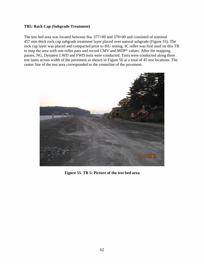
62

TB5: Rock Cap (Subgrade Treatment)

The test bed area was located between Sta. 377+00 and 379+00 and consisted of nominal 457 mm thick rock cap subgrade treatment layer placed over natural subgrade (Figure 55). The rock cap layer was placed and compacted prior to ISU testing. IC roller was first used on this TB to map the area with one roller pass and record CMV and MDP* values. After the mapping passes, NG, Dynatest LWD and FWD tests were conducted. Tests were conducted along three test lanes across width of the pavement as shown in Figure 56 at a total of 45 test locations. The center line of the test area corresponded to the centerline of the pavement.

Figure 55. TB 5: Picture of the test bed area

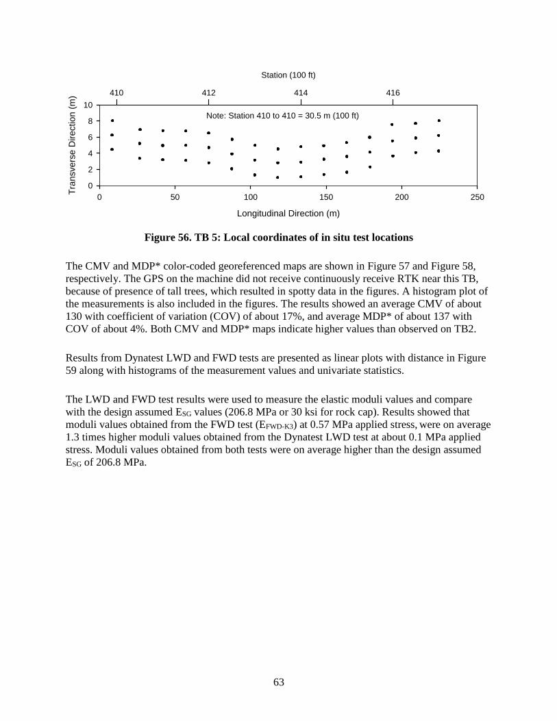
63

Figure 56. TB 5: Local coordinates of in situ test locations

The CMV and MDP* color-coded georeferenced maps are shown in Figure 57 and Figure 58, respectively. The GPS on the machine did not receive continuously receive RTK near this TB, because of presence of tall trees, which resulted in spotty data in the figures. A histogram plot of the measurements is also included in the figures. The results showed an average CMV of about 130 with coefficient of variation (COV) of about 17%, and average MDP* of about 137 with COV of about 4%. Both CMV and MDP* maps indicate higher values than observed on TB2.

Results from Dynatest LWD and FWD tests are presented as linear plots with distance in Figure 59 along with histograms of the measurement values and univariate statistics.

The LWD and FWD test results were used to measure the elastic moduli values and compare with the design assumed ESG values (206.8 MPa or 30 ksi for rock cap). Results showed that moduli values obtained from the FWD test (EFWD-K3) at 0.57 MPa applied stress, were on average 1.3 times higher moduli values obtained from the Dynatest LWD test at about 0.1 MPa applied stress. Moduli values obtained from both tests were on average higher than the design assumed ESG of 206.8 MPa.

Longitudinal Direction (m)

0 50 100 150 200 250Tran

sver

se D

irect

ion

(m)

0

2

4

6

8

10

Station (100 ft)

410 412 414 416

Note: Station 410 to 410 = 30.5 m (100 ft)

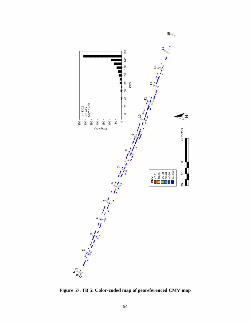
64

Figure 57. TB 5: Color-coded map of georeferenced CMV map

CM

V

020

4060

8010

012

014

016

0

Frequency

050100

150

200

250

300

350

=

130.

2

= 22

.0C

OV

= 1

7%

2010

020

met

ers

AB C

1

2

3

4

5

6

7

8

10

11

12

9

13

14

15

< 10

10-2

020

-30

30-4

040

-50

50-1

50

CM

V

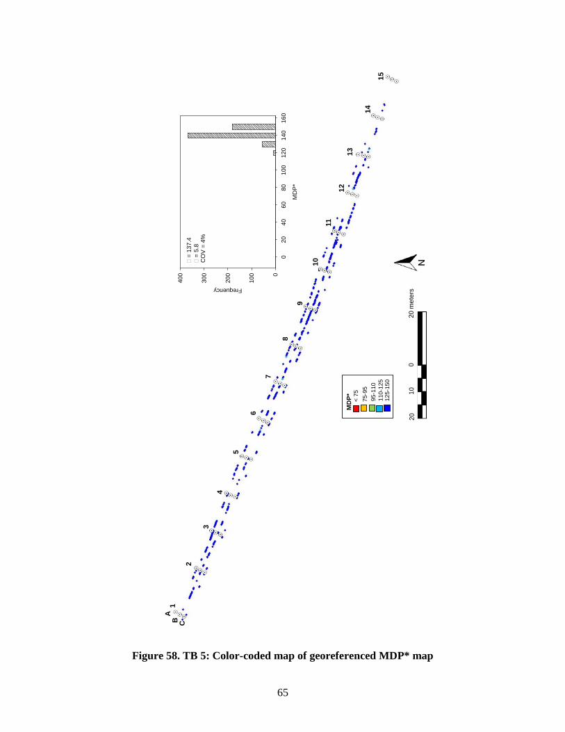
65

Figure 58. TB 5: Color-coded map of georeferenced MDP* map

2010

020

met

ers

AB C

1

2

3

4

5

6

7

8

10

11

12

9

13

14

15

MD

P*

020

4060

8010

012

014

016

0

Frequency

0

100

200

300

400

=

137.

4

= 5.

8C

OV

= 4

%

< 75

75-9

595

-110

110-

125

125-

150

MD

P*

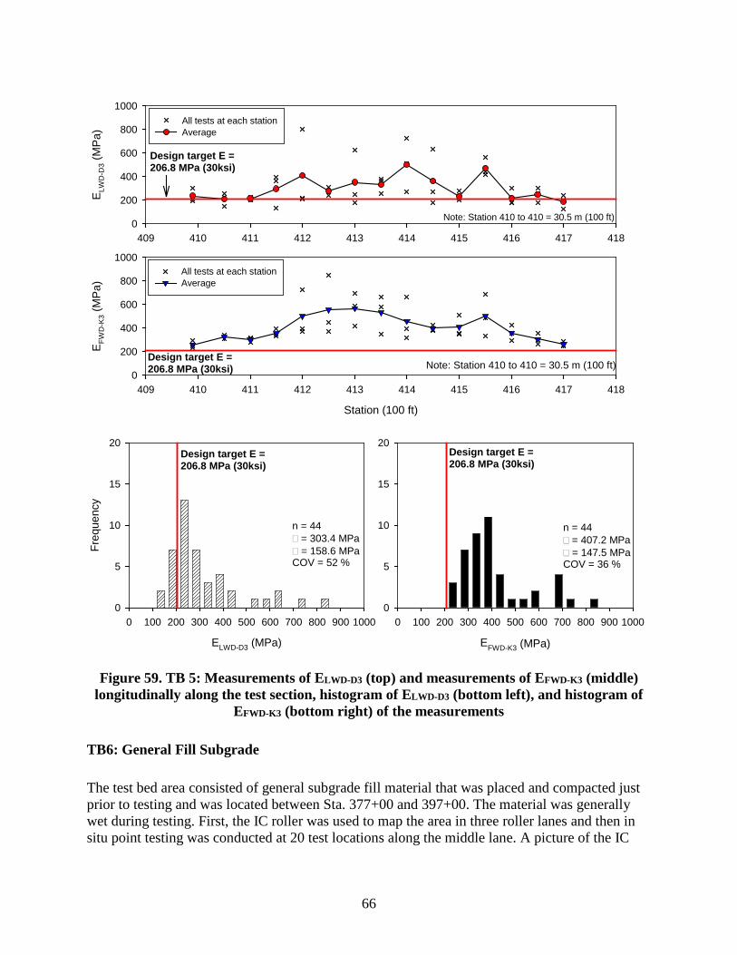
66

Figure 59. TB 5: Measurements of ELWD-D3 (top) and measurements of EFWD-K3 (middle) longitudinally along the test section, histogram of ELWD-D3 (bottom left), and histogram of

EFWD-K3 (bottom right) of the measurements

TB6: General Fill Subgrade

The test bed area consisted of general subgrade fill material that was placed and compacted just prior to testing and was located between Sta. 377+00 and 397+00. The material was generally wet during testing. First, the IC roller was used to map the area in three roller lanes and then in situ point testing was conducted at 20 test locations along the middle lane. A picture of the IC

409 410 411 412 413 414 415 416 417 418

ELW

D-D

3 (M

Pa)

0

200

400

600

800

1000All tests at each stationAverage

Design target E =206.8 MPa (30ksi)

Note: Station 410 to 410 = 30.5 m (100 ft)

Station (100 ft)

409 410 411 412 413 414 415 416 417 418

EFW

D-K

3 (M

Pa)

0

200

400

600

800

1000All tests at each stationAverage

Design target E =206.8 MPa (30ksi) Note: Station 410 to 410 = 30.5 m (100 ft)

ELWD-D3 (MPa)

0 100 200 300 400 500 600 700 800 900 1000

Freq

uenc

y

0

5

10

15

20

n = 44 = 303.4 MPa = 158.6 MPaCOV = 52 %

Design target E =206.8 MPa (30ksi)

EFWD-K3 (MPa)

0 100 200 300 400 500 600 700 800 900 10000

5

10

15

20

n = 44 = 407.2 MPa = 147.5 MPaCOV = 36 %

Design target E =206.8 MPa (30ksi)

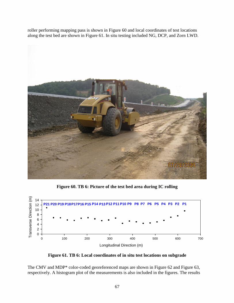
67

roller performing mapping pass is shown in Figure 60 and local coordinates of test locations along the test bed are shown in Figure 61. In situ testing included NG, DCP, and Zorn LWD.

Figure 60. TB 6: Picture of the test bed area during IC rolling

Figure 61. TB 6: Local coordinates of in situ test locations on subgrade

The CMV and MDP* color-coded georeferenced maps are shown in Figure 62 and Figure 63, respectively. A histogram plot of the measurements is also included in the figures. The results

Longitudinal Direction (m)

0 100 200 300 400 500 600 700Tran

sver

se D

irect

ion

(m)

02468

101214

P1P2P3P4P5P6P7P8P9P10P11P12P13P14P15P16P21 P20 P19 P17P18

68

showed an average CMV of about 47 with coefficient of variation (COV) of about 67%, and average MDP* of about 91 with COV of about 18%. The CMV and MDP* values measured on this TB were comparatively lower than measured in TB 2 (subbase) and TB5 (rock cap), as expected.

Results from LWD and NG tests are presented as linear plots with distance in Figure 65 and histograms of each measurement value with univariate statistics are presented in Figure 66.

DCP-CBR profiles are shown in Figure 42 for all test locations. At some test locations, the DCPs were terminated at shallow depths (< 0.5 m) due to refusal with presence of rock in the fill material. CBR values varied between 2 and 100, representing variable conditions in the fill material.

The LWD test results were used to measure the elastic moduli values. It must be noted that the ESG value was assigned to the rock cap layer in the design and not the subgrade layer itself, as the rock cap layer was considered to be subgrade treatment. The design ESG value is shown in Figure 64 for reference only. Results of Zorn LWD testing yielded an average elastic modulus of about 18.1 MPa in this TB with a COV of about 65%.

The NG test measurements were obtained with 304.8 mm (12 in.) measuring depth. In situ relative compaction values ranged from 91–105% of the maximum standard Proctor dry unit weight and in situ moisture values ranged from 3.7% below to 5.6% above standard Proctor optimum moisture content.

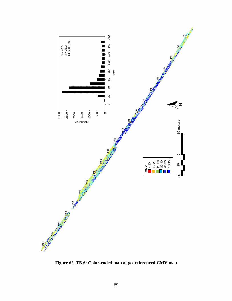
69

Figure 62. TB 6: Color-coded map of georeferenced CMV map

5025

050

met

ers

CM

V

020

4060

8010

012

014

016

0

Frequency

0

500

1000

1500

2000

2500

3000

=

46.6

=

31.3

CO

V =

67%

< 10

10-2

020

-30

30-4

040

-50

50-1

50

CM

V

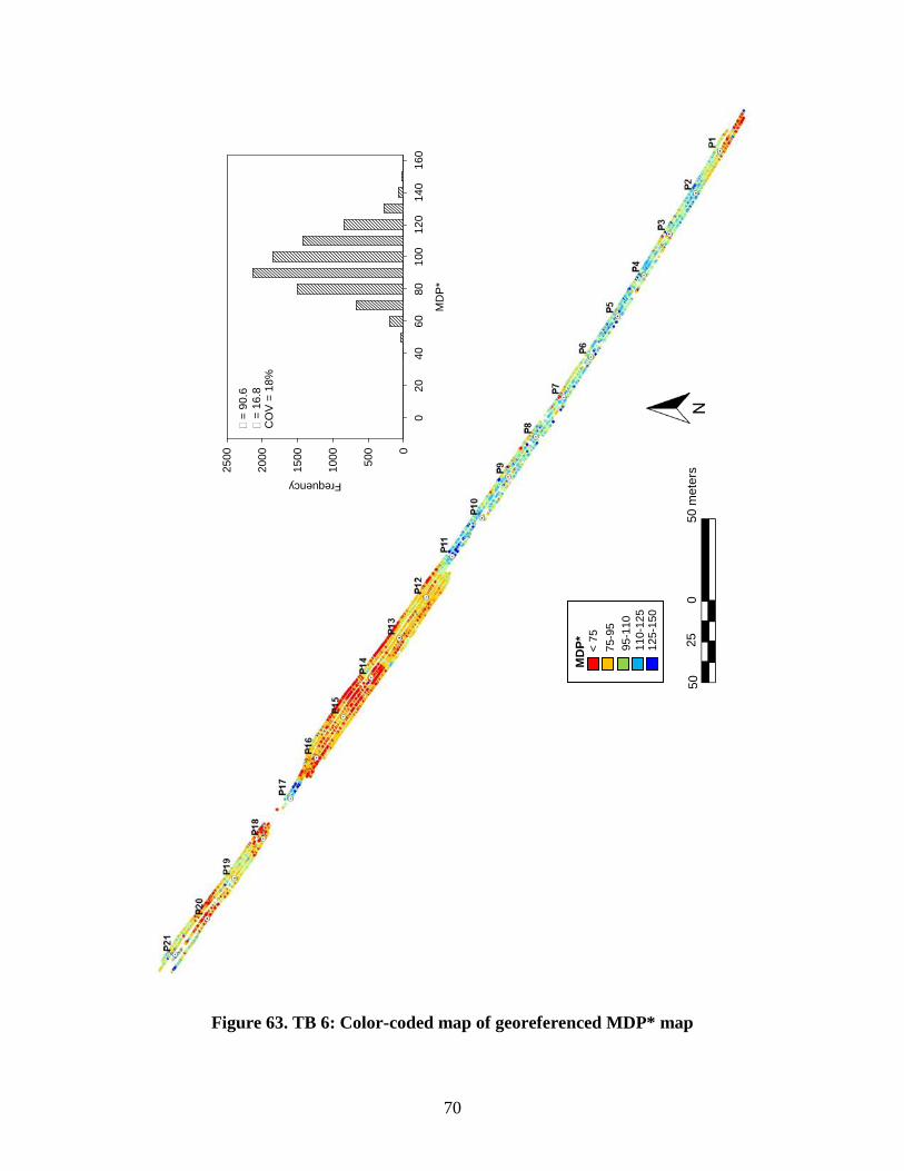
70

Figure 63. TB 6: Color-coded map of georeferenced MDP* map

5025

050

met

ers

MD

P*

020

4060

8010

012

014

016

0

Frequency

0

500

1000

1500

2000

2500

=

90.6

=

16.8

CO

V =

18%

< 75

75-9

595

-110

110-

125

125-

150

MD

P*

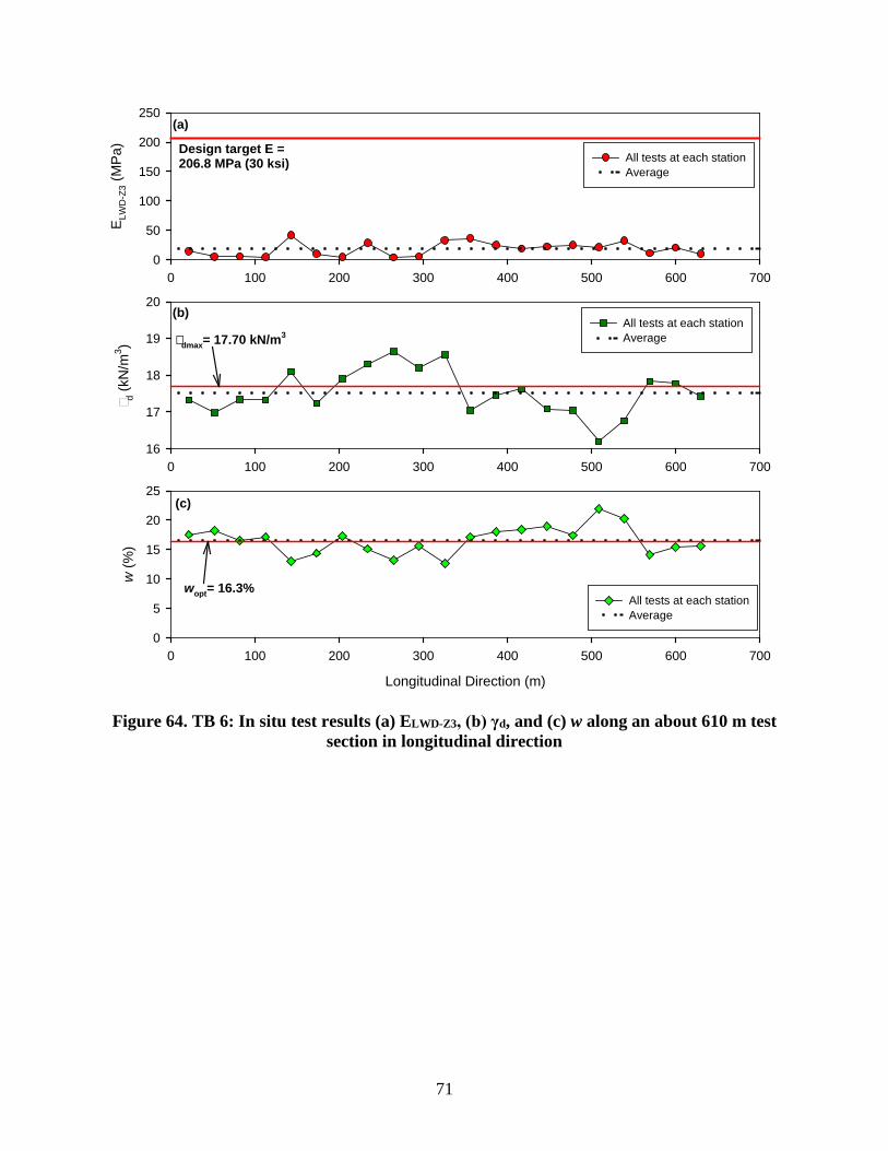
71

Figure 64. TB 6: In situ test results (a) ELWD-Z3, (b) γd, and (c) w along an about 610 m test section in longitudinal direction

0 100 200 300 400 500 600 700

E LWD

-Z3 (

MPa

)

0

50

100

150

200

250

All tests at each stationAverage

Design target E =206.8 MPa (30 ksi)

0 100 200 300 400 500 600 700

d (k

N/m

3 )

16

17

18

19

20All tests at each stationAveragedmax= 17.70 kN/m3

Longitudinal Direction (m)

0 100 200 300 400 500 600 700

w (%

)

0

5

10

15

20

25

All tests at each stationAverage

wopt= 16.3%

(a)

(b)

(c)

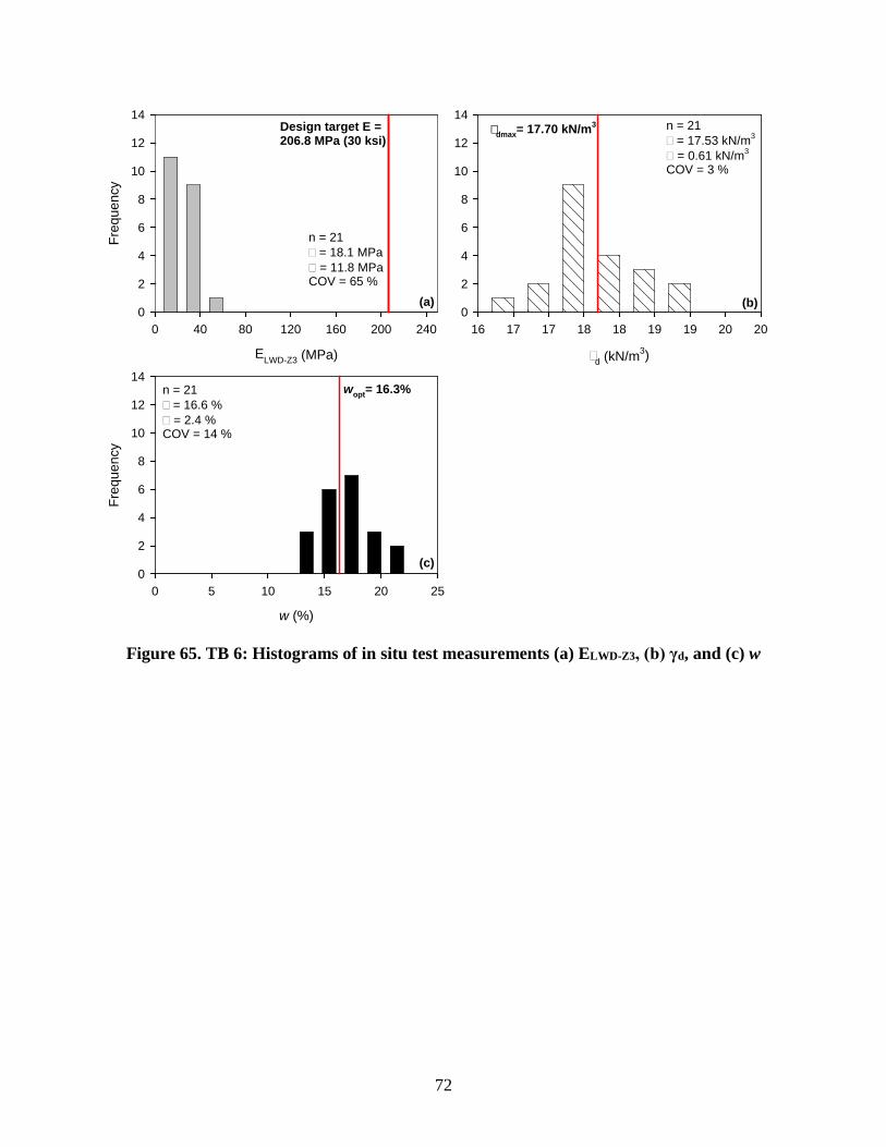
72

Figure 65. TB 6: Histograms of in situ test measurements (a) ELWD-Z3, (b) γd, and (c) w

ELWD-Z3 (MPa)

0 40 80 120 160 200 240

Freq

uenc

y

0

2

4

6

8

10

12

14

n = 21 = 18.1 MPa = 11.8 MPaCOV = 65 %

Design target E =206.8 MPa (30 ksi)

d (kN/m3)

16 17 17 18 18 19 19 20 200

2

4

6

8

10

12

14n = 21 = 17.53 kN/m3

= 0.61 kN/m3

COV = 3 %

dmax= 17.70 kN/m3

w (%)

0 5 10 15 20 25

Freq

uenc

y

0

2

4

6

8

10

12

14n = 21 = 16.6 % = 2.4 %COV = 14 %

wopt= 16.3%

(a) (b)

(c)

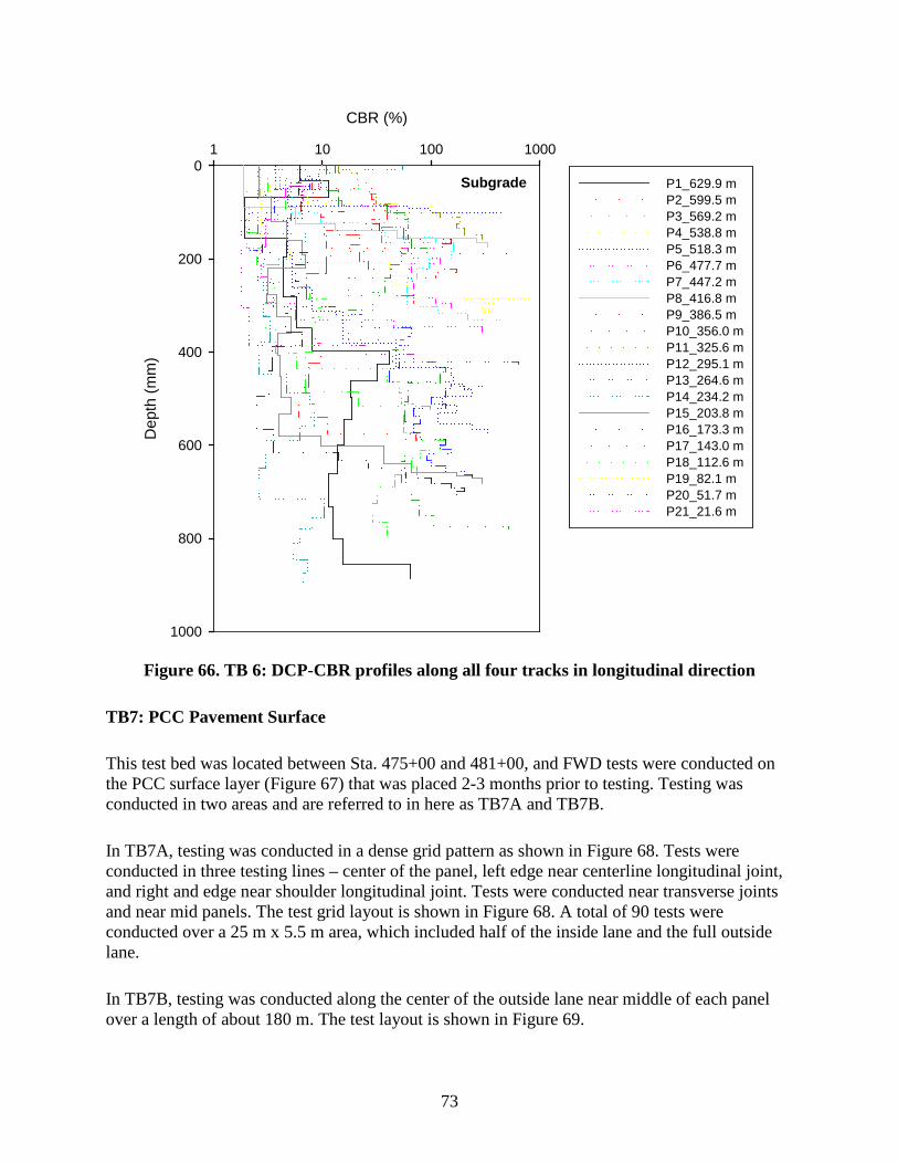
73

Figure 66. TB 6: DCP-CBR profiles along all four tracks in longitudinal direction

TB7: PCC Pavement Surface

This test bed was located between Sta. 475+00 and 481+00, and FWD tests were conducted on the PCC surface layer (Figure 67) that was placed 2-3 months prior to testing. Testing was conducted in two areas and are referred to in here as TB7A and TB7B.

In TB7A, testing was conducted in a dense grid pattern as shown in Figure 68. Tests were conducted in three testing lines – center of the panel, left edge near centerline longitudinal joint, and right and edge near shoulder longitudinal joint. Tests were conducted near transverse joints and near mid panels. The test grid layout is shown in Figure 68. A total of 90 tests were conducted over a 25 m x 5.5 m area, which included half of the inside lane and the full outside lane.

In TB7B, testing was conducted along the center of the outside lane near middle of each panel over a length of about 180 m. The test layout is shown in Figure 69.

CBR (%)

1 10 100 1000D

epth

(mm

)0

200

400

600

800

1000

P1_629.9 mP2_599.5 mP3_569.2 mP4_538.8 mP5_518.3 mP6_477.7 mP7_447.2 mP8_416.8 mP9_386.5 mP10_356.0 mP11_325.6 mP12_295.1 mP13_264.6 mP14_234.2 mP15_203.8 mP16_173.3 mP17_143.0 mP18_112.6 mP19_82.1 mP20_51.7 mP21_21.6 m

Subgrade

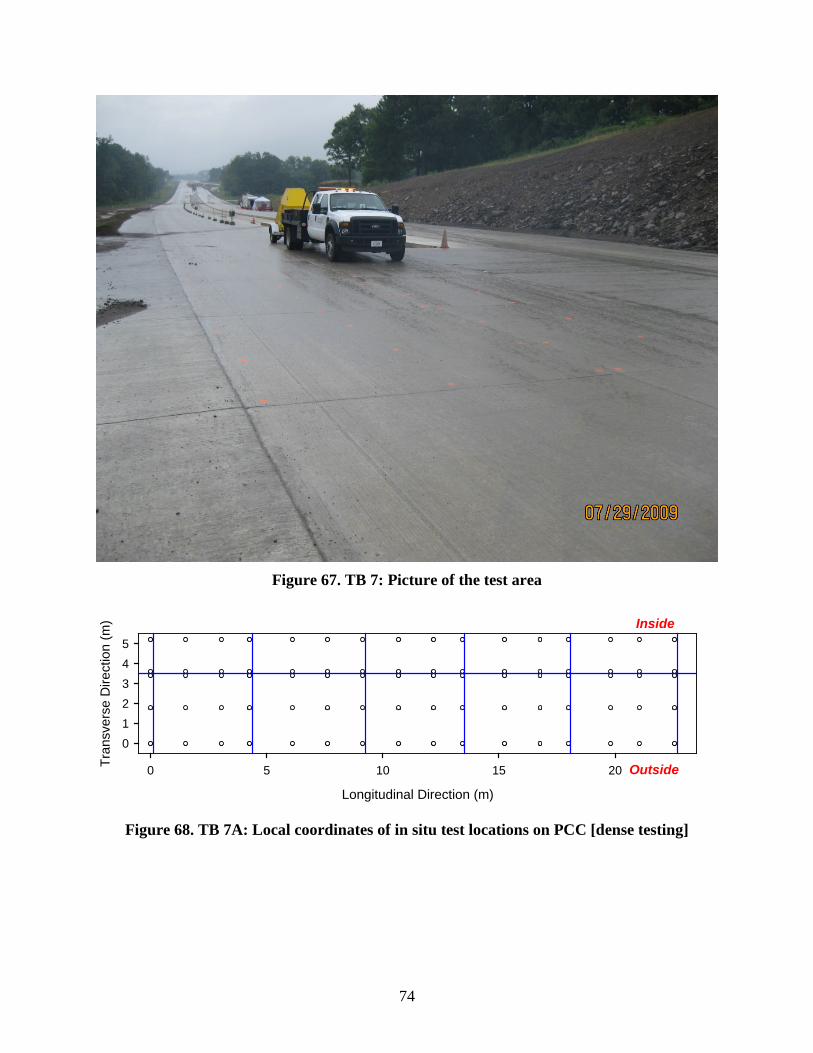
74

Figure 67. TB 7: Picture of the test area

Figure 68. TB 7A: Local coordinates of in situ test locations on PCC [dense testing]

Longitudinal Direction (m)

0 5 10 15 20Tran

sver

se D

irect

ion

(m)

012345

Inside

Outside

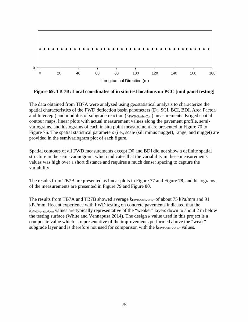
75

Figure 69. TB 7B: Local coordinates of in situ test locations on PCC [mid panel testing]

The data obtained from TB7A were analyzed using geostatistical analysis to characterize the spatial characteristics of the FWD deflection basin parameters (D0, SCI, BCI, BDI, Area Factor, and Intercept) and modulus of subgrade reaction (kFWD-Static-Corr) measurements. Kriged spatial contour maps, linear plots with actual measurement values along the pavement profile, semi-variograms, and histograms of each in situ point measurement are presented in Figure 70 to Figure 76. The spatial statistical parameters (i.e., scale (sill minus nugget), range, and nugget) are provided in the semivariogram plot of each figure.

Spatial contours of all FWD measurements except D0 and BDI did not show a definite spatial structure in the semi-varaiogram, which indicates that the variability in these measurements values was high over a short distance and requires a much denser spacing to capture the variability.

The results from TB7B are presented as linear plots in Figure 77 and Figure 78, and histograms of the measurements are presented in Figure 79 and Figure 80.

The results from TB7A and TB7B showed average kFWD-Static-Corr of about 75 kPa/mm and 91 kPa/mm. Recent experience with FWD testing on concrete pavements indicated that the kFWD-Static-Corr values are typically representative of the “weaker” layers down to about 2 m below the testing surface (White and Vennapusa 2014). The design k value used in this project is a composite value which is representative of the improvements performed above the “weak” subgrade layer and is therefore not used for comparison with the kFWD-Static-Corr values.

Longitudinal Direction (m)

0 20 40 60 80 100 120 140 160 1800

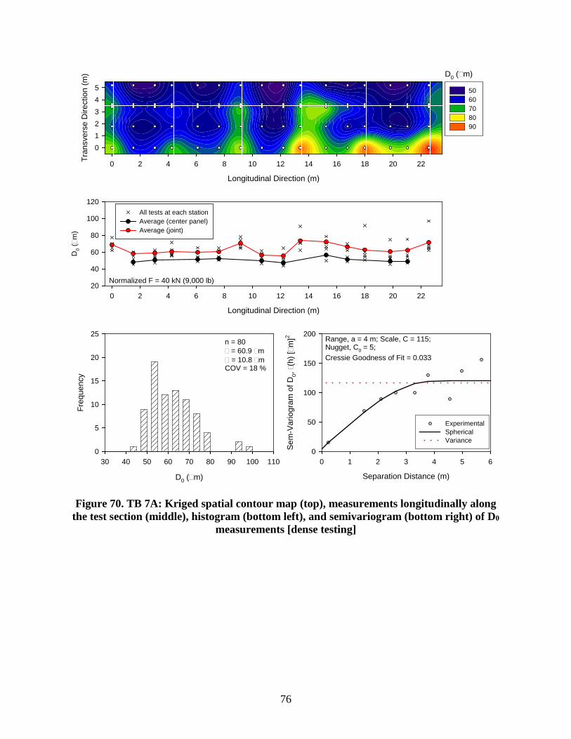
76

Figure 70. TB 7A: Kriged spatial contour map (top), measurements longitudinally along the test section (middle), histogram (bottom left), and semivariogram (bottom right) of D0

measurements [dense testing]

D0 (m)

Longitudinal Direction (m)

0 2 4 6 8 10 12 14 16 18 20 22Tran

sver

se D

irect

ion

(m)

012345 50

60 70 80 90

Longitudinal Direction (m)

0 2 4 6 8 10 12 14 16 18 20 22

D0 (m

)

20

40

60

80

100

120All tests at each stationAverage (center panel)Average (joint)

Normalized F = 40 kN (9,000 lb)

D0 (m)

30 40 50 60 70 80 90 100 110

Freq

uenc

y

0

5

10

15

20

25n = 80 = 60.9 m = 10.8 mCOV = 18 %

Separation Distance (m)

0 1 2 3 4 5 6

Sem

-Var

iogr

am o

f D0, (

h) [

m]2

0

50

100

150

200

ExperimentalSphericalVariance

Range, a = 4 m; Scale, C = 115; Nugget, C0 = 5;Cressie Goodness of Fit = 0.033

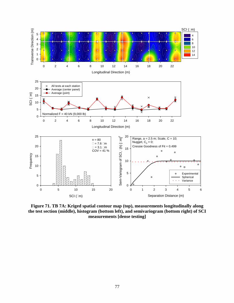
77

Figure 71. TB 7A: Kriged spatial contour map (top), measurements longitudinally along the test section (middle), histogram (bottom left), and semivariogram (bottom right) of SCI

measurements [dense testing]

SCI (m)

Longitudinal Direction (m)

0 2 4 6 8 10 12 14 16 18 20 22

Tran

sver

se D

irect

ion

(m)

012345 4

6 8 10 12 14

Longitudinal Direction (m)

0 2 4 6 8 10 12 14 16 18 20 22

SCI ( m

)

0

5

10

15

20

25All tests at each stationAverage (center panel)Average (joint)

Normalized F = 40 kN (9,000 lb)

SCI (m)

0 5 10 15 20

Freq

uenc

y

0

5

10

15

20

25n = 80 = 7.6 m = 3.1 mCOV = 41 %

Separation Distance (m)

0 1 2 3 4 5 6

Sem

-Var

iogr

am o

f SC

I , (

h) [

m]2

0

5

10

15

20

ExperimentalSphericalVariance

Range, a = 2.5 m; Scale, C = 10; Nugget, C0 = 0;Cressie Goodness of Fit = 0.499

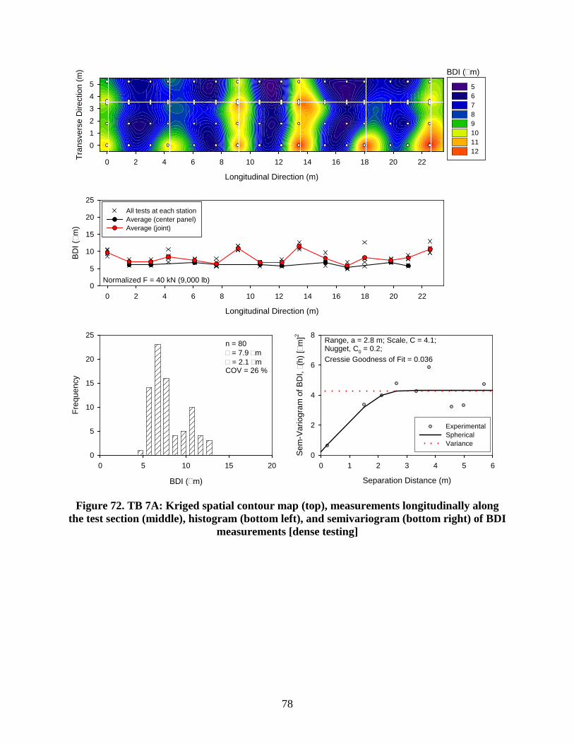
78

Figure 72. TB 7A: Kriged spatial contour map (top), measurements longitudinally along the test section (middle), histogram (bottom left), and semivariogram (bottom right) of BDI

measurements [dense testing]

BDI (m)

Longitudinal Direction (m)

0 2 4 6 8 10 12 14 16 18 20 22Tran

sver

se D

irect

ion

(m)

012345 5

6 7 8 9 10 11 12

Longitudinal Direction (m)

0 2 4 6 8 10 12 14 16 18 20 22

BDI ( m

)

0

5

10

15

20

25All tests at each stationAverage (center panel)Average (joint)

Normalized F = 40 kN (9,000 lb)

BDI (m)

0 5 10 15 20

Freq

uenc

y

0

5

10

15

20

25n = 80 = 7.9 m = 2.1 mCOV = 26 %

Separation Distance (m)

0 1 2 3 4 5 6

Sem

-Var

iogr

am o

f BD

I , (

h) [

m]2

0

2

4

6

8

ExperimentalSphericalVariance

Range, a = 2.8 m; Scale, C = 4.1; Nugget, C0 = 0.2;Cressie Goodness of Fit = 0.036

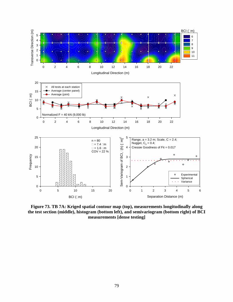
79

Figure 73. TB 7A: Kriged spatial contour map (top), measurements longitudinally along the test section (middle), histogram (bottom left), and semivariogram (bottom right) of BCI

measurements [dense testing]

BCI (m)

Longitudinal Direction (m)

0 2 4 6 8 10 12 14 16 18 20 22Tran

sver

se D

irect

ion

(m)

012345 6

7 8 9 10 11

Longitudinal Direction (m)

0 2 4 6 8 10 12 14 16 18 20 22

BCI ( m

)

0

5

10

15

20All tests at each stationAverage (center panel)Average (joint)

Normalized F = 40 kN (9,000 lb)

BCI (m)

0 5 10 15 20

Freq

uenc

y

0

5

10

15

20

25n = 80 = 7.4 m = 1.6 mCOV = 22 %

Separation Distance (m)

0 1 2 3 4 5 6

Sem

-Var

iogr

am o

f BC

I , (

h) [

m]2

0

1

2

3

4

5

ExperimentalSphericalVariance

Range, a = 3.2 m; Scale, C = 2.4; Nugget, C0 = 0.4;Cressie Goodness of Fit = 0.017

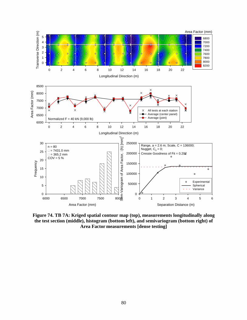
80

Figure 74. TB 7A: Kriged spatial contour map (top), measurements longitudinally along the test section (middle), histogram (bottom left), and semivariogram (bottom right) of

Area Factor measurements [dense testing]

Area Factor (mm)

Longitudinal Direction (m)

0 2 4 6 8 10 12 14 16 18 20 22Tran

sver

se D

irect

ion

(m)

012345 6800

7000 7200 7400 7600 7800 8000 8200

Longitudinal Direction (m)

0 2 4 6 8 10 12 14 16 18 20 22

Area

Fac

tor (

mm

)

6000

6500

7000

7500

8000

8500

All tests at each stationAverage (center panel)Average (joint)Normalized F = 40 kN (9,000 lb)

Area Factor (mm)

6000 6500 7000 7500 8000

Freq

uenc

y

0

5

10

15

20

25

30n = 80 = 7431.0 mm = 365.2 mmCOV = 5 %

Separation Distance (m)

0 1 2 3 4 5 6Sem

-Var

iogr

am o

f Are

a Fa

ctor

, (h

) [m

m]2

0

50000

100000

150000

200000

250000

ExperimentalSphericalVariance

Range, a = 2.6 m; Scale, C = 136000; Nugget, C0 = 0;Cressie Goodness of Fit = 0.202

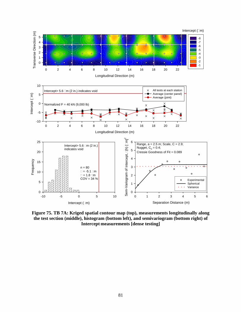
81

Figure 75. TB 7A: Kriged spatial contour map (top), measurements longitudinally along the test section (middle), histogram (bottom left), and semivariogram (bottom right) of

Intercept measurements [dense testing]

Intercept (m)

Longitudinal Direction (m)

0 2 4 6 8 10 12 14 16 18 20 22Tran

sver

se D

irect

ion

(m)

012345 -8

-7 -6 -5 -4 -3 -2 -1

Longitudinal Direction (m)

0 2 4 6 8 10 12 14 16 18 20 22

Inte

rcep

t ( m

)

-10

-5

0

5

10All tests at each stationAverage (center panel)Average (joint)

Normalized F = 40 kN (9,000 lb)

Intercept> 5.6 m (2 in.) indicates void

Intercept (m)

-10 -5 0 5 10

Freq

uenc

y

0

5

10

15

20

25

n = 80 = -5.1 m = 1.8 mCOV = 34 %

Intercept> 5.6 m (2 in.)indicates void

Separation Distance (m)

0 1 2 3 4 5 6Sem

-Var

iogr

am o

f Int

erce

pt,

(h) [ m

]2

0

1

2

3

4

5

6

ExperimentalSphericalVariance

Range, a = 2.5 m; Scale, C = 2.9; Nugget, C0 = 0.4;Cressie Goodness of Fit = 0.089

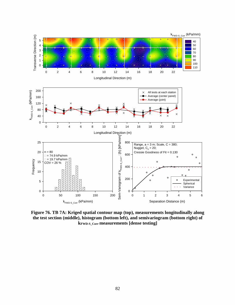
82

Figure 76. TB 7A: Kriged spatial contour map (top), measurements longitudinally along the test section (middle), histogram (bottom left), and semivariogram (bottom right) of

kFWD-S_Corr measurements [dense testing]

kFWD-S_Corr (kPa/mm)

Longitudinal Direction (m)

0 2 4 6 8 10 12 14 16 18 20 22Tran

sver

se D

irect

ion

(m)

012345 40

50 60 70 80 90 100 110

Longitudinal Direction (m)

0 2 4 6 8 10 12 14 16 18 20 22

k FWD

-S_C

orr (

kPa/

mm

)

0

40

80

120

160

200 All tests at each stationAverage (center panel)Average (joint)

kFWD-S_Corr (kPa/mm)

0 50 100 150 200

Freq

uenc

y

0

5

10

15

20

25

n = 80 = 74.9 kPa/mm = 19.7 kPa/mmCOV = 26 %

Separation Distance (m)

0 1 2 3 4 5 6

Sem

-Var

iogr

am o

f kFW

D-S

_Cor

r, (

h) [k

Pa/

mm

]2

0

200

400

600

800

ExperimentalSphericalVariance

Range, a = 3 m; Scale, C = 380; Nugget, C0 = 20;Cressie Goodness of Fit = 0.130

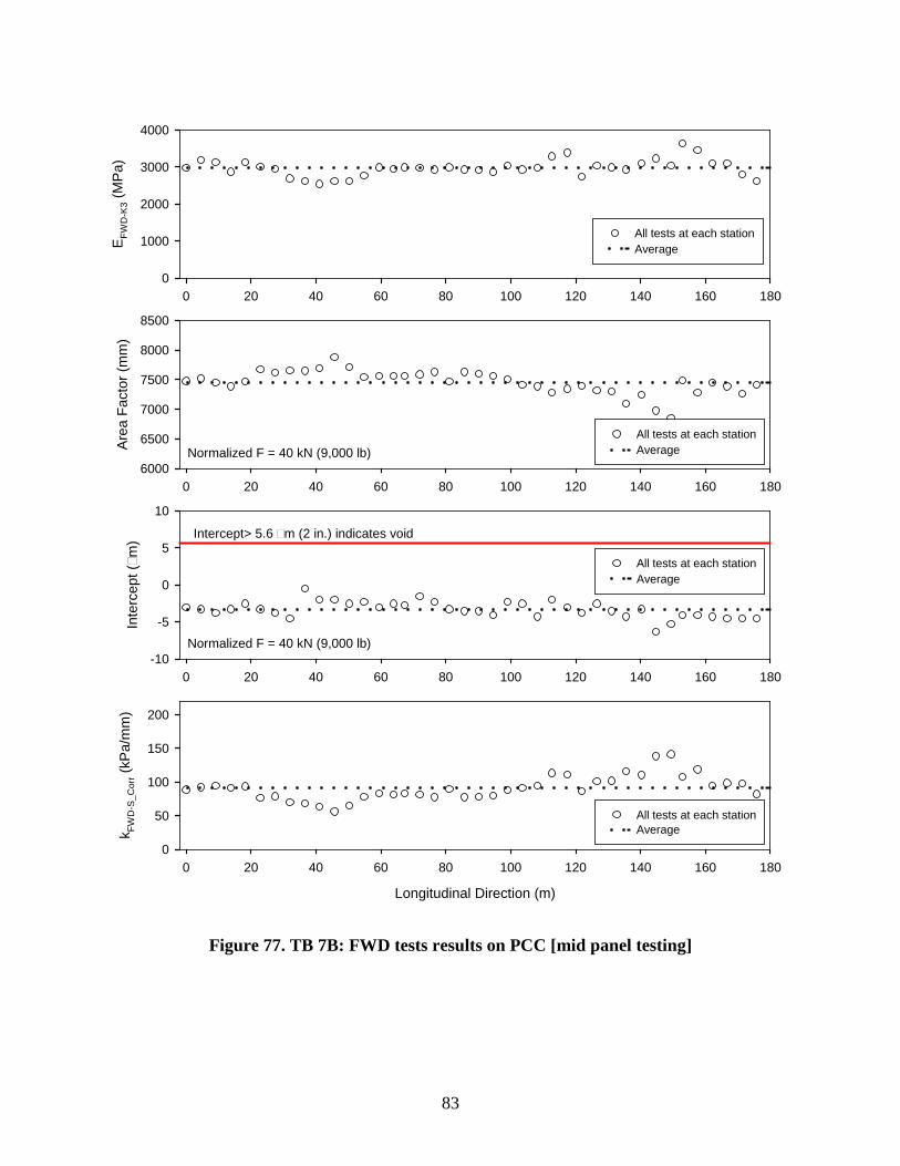
83

Figure 77. TB 7B: FWD tests results on PCC [mid panel testing]

0 20 40 60 80 100 120 140 160 180

EFW

D-K

3 (M

Pa)

0

1000

2000

3000

4000

All tests at each stationAverage

0 20 40 60 80 100 120 140 160 180

Are

a Fa

ctor

(mm

)

6000

6500

7000

7500

8000

8500

All tests at each stationAverageNormalized F = 40 kN (9,000 lb)

Longitudinal Direction (m)

0 20 40 60 80 100 120 140 160 180

k FWD

-S_C

orr (

kPa/

mm

)

0

50

100

150

200

All tests at each stationAverage

0 20 40 60 80 100 120 140 160 180

Inte

rcep

t (m

)

-10

-5

0

5

10

All tests at each stationAverage

Normalized F = 40 kN (9,000 lb)

Intercept> 5.6 m (2 in.) indicates void

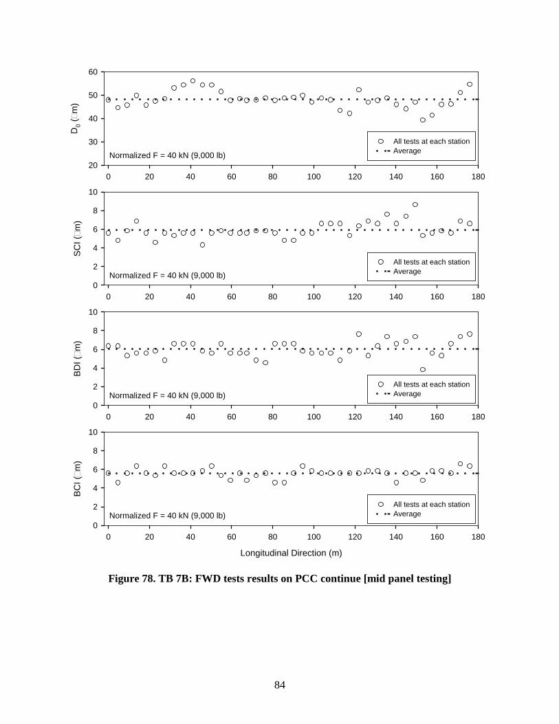
84

Figure 78. TB 7B: FWD tests results on PCC continue [mid panel testing]

0 20 40 60 80 100 120 140 160 180

D0 ( m

)

20

30

40

50

60

All tests at each stationAverageNormalized F = 40 kN (9,000 lb)

0 20 40 60 80 100 120 140 160 180

SCI ( m

)

0

2

4

6

8

10

All tests at each stationAverageNormalized F = 40 kN (9,000 lb)

0 20 40 60 80 100 120 140 160 180

BDI ( m

)

0

2

4

6

8

10

All tests at each stationAverageNormalized F = 40 kN (9,000 lb)

Longitudinal Direction (m)

0 20 40 60 80 100 120 140 160 180

BCI ( m

)

0

2

4

6

8

10

All tests at each stationAverageNormalized F = 40 kN (9,000 lb)

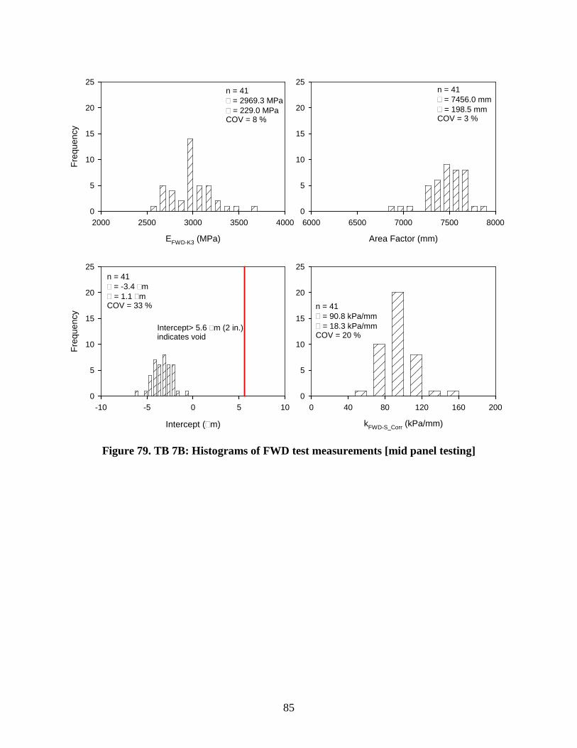
85

Figure 79. TB 7B: Histograms of FWD test measurements [mid panel testing]

EFWD-K3 (MPa)

2000 2500 3000 3500 4000

Freq

uenc

y

0

5

10

15

20

25n = 41 = 2969.3 MPa = 229.0 MPaCOV = 8 %

Area Factor (mm)

6000 6500 7000 7500 80000

5

10

15

20

25n = 41 = 7456.0 mm = 198.5 mmCOV = 3 %

Intercept (m)

-10 -5 0 5 10

Freq

uenc

y

0

5

10

15

20

25n = 41 = -3.4 m = 1.1 mCOV = 33 %

Intercept> 5.6 m (2 in.)indicates void

kFWD-S_Corr (kPa/mm)

0 40 80 120 160 2000

5

10

15

20

25

n = 41 = 90.8 kPa/mm = 18.3 kPa/mmCOV = 20 %

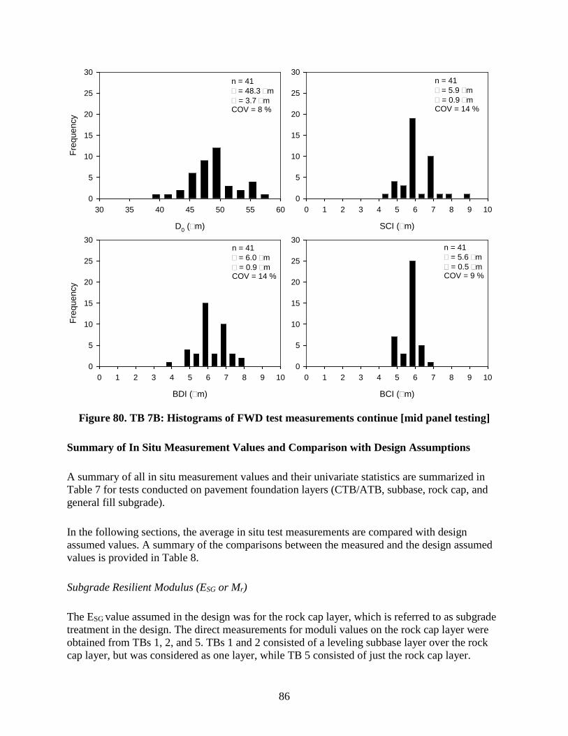
86

Figure 80. TB 7B: Histograms of FWD test measurements continue [mid panel testing]

Summary of In Situ Measurement Values and Comparison with Design Assumptions

A summary of all in situ measurement values and their univariate statistics are summarized in Table 7 for tests conducted on pavement foundation layers (CTB/ATB, subbase, rock cap, and general fill subgrade).

In the following sections, the average in situ test measurements are compared with design assumed values. A summary of the comparisons between the measured and the design assumed values is provided in Table 8.

Subgrade Resilient Modulus (ESG or Mr)

The ESG value assumed in the design was for the rock cap layer, which is referred to as subgrade treatment in the design. The direct measurements for moduli values on the rock cap layer were obtained from TBs 1, 2, and 5. TBs 1 and 2 consisted of a leveling subbase layer over the rock cap layer, but was considered as one layer, while TB 5 consisted of just the rock cap layer.

D0 (m)

30 35 40 45 50 55 60

Freq

uenc

y

0

5

10

15

20

25

30n = 41 = 48.3 m = 3.7 mCOV = 8 %

SCI (m)

0 1 2 3 4 5 6 7 8 9 100

5

10

15

20

25

30n = 41 = 5.9 m = 0.9 mCOV = 14 %

BDI (m)

0 1 2 3 4 5 6 7 8 9 10

Freq

uenc

y

0

5

10

15

20

25

30n = 41 = 6.0 m = 0.9 mCOV = 14 %

BCI (m)

0 1 2 3 4 5 6 7 8 9 100

5

10

15

20

25

30n = 41 = 5.6 m = 0.5 mCOV = 9 %

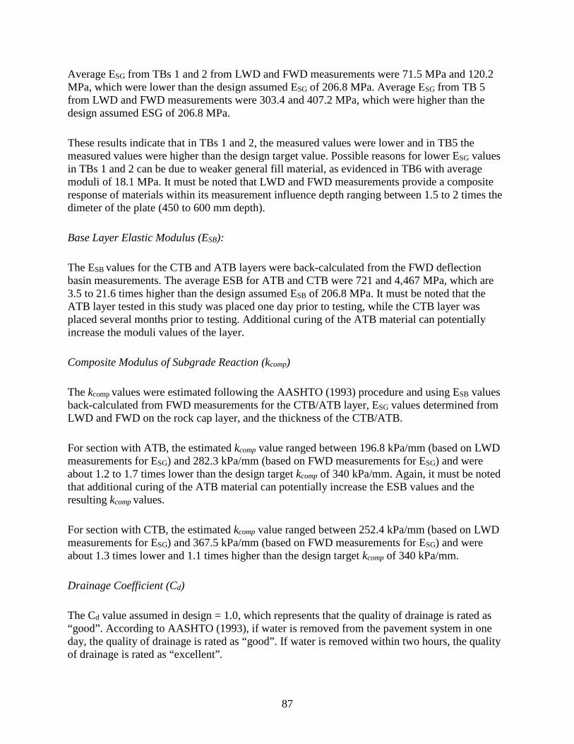
87

Average ESG from TBs 1 and 2 from LWD and FWD measurements were 71.5 MPa and 120.2 MPa, which were lower than the design assumed ESG of 206.8 MPa. Average ESG from TB 5 from LWD and FWD measurements were 303.4 and 407.2 MPa, which were higher than the design assumed ESG of 206.8 MPa.

These results indicate that in TBs 1 and 2, the measured values were lower and in TB5 the measured values were higher than the design target value. Possible reasons for lower ESG values in TBs 1 and 2 can be due to weaker general fill material, as evidenced in TB6 with average moduli of 18.1 MPa. It must be noted that LWD and FWD measurements provide a composite response of materials within its measurement influence depth ranging between 1.5 to 2 times the dimeter of the plate (450 to 600 mm depth).

Base Layer Elastic Modulus (ESB):

The ESB values for the CTB and ATB layers were back-calculated from the FWD deflection basin measurements. The average ESB for ATB and CTB were 721 and 4,467 MPa, which are 3.5 to 21.6 times higher than the design assumed ESB of 206.8 MPa. It must be noted that the ATB layer tested in this study was placed one day prior to testing, while the CTB layer was placed several months prior to testing. Additional curing of the ATB material can potentially increase the moduli values of the layer.

Composite Modulus of Subgrade Reaction (kcomp)

The kcomp values were estimated following the AASHTO (1993) procedure and using ESB values back-calculated from FWD measurements for the CTB/ATB layer, ESG values determined from LWD and FWD on the rock cap layer, and the thickness of the CTB/ATB.

For section with ATB, the estimated kcomp value ranged between 196.8 kPa/mm (based on LWD measurements for ESG) and 282.3 kPa/mm (based on FWD measurements for ESG) and were about 1.2 to 1.7 times lower than the design target kcomp of 340 kPa/mm. Again, it must be noted that additional curing of the ATB material can potentially increase the ESB values and the resulting kcomp values.

For section with CTB, the estimated kcomp value ranged between 252.4 kPa/mm (based on LWD measurements for ESG) and 367.5 kPa/mm (based on FWD measurements for ESG) and were about 1.3 times lower and 1.1 times higher than the design target kcomp of 340 kPa/mm.

Drainage Coefficient (Cd)

The Cd value assumed in design = 1.0, which represents that the quality of drainage is rated as “good”. According to AASHTO (1993), if water is removed from the pavement system in one day, the quality of drainage is rated as “good”. If water is removed within two hours, the quality of drainage is rated as “excellent”.

88

Based on the pavement geometry (i.e., cross slope, width of the pavement, thickness of the base layer), the measured Ksat values from the field, and assuming an effective porosity = 0.3, time for a target 90% of drainage was calculated using “Pavement Drainage Estimator (PDE) Version 1.0),” an Excel-based Visual Basic program developed by Vennapusa (2004). A target of 90% drainage was selected in calculations.

Based on tests conducted on the CTB layer, the time for 90% drainage was estimated as 1.0 day for Ksat = 0.2 cm/s (CTB contaminated with fines) to < 1 hour for Ksat = 7 cm/s (CTB uncontaminated). Based on tests conducted on the ATB layer the time for 90% drainage was estimated < 1 hour for Ksat = 4.6 cm/s. Based on these estimates, the quality of drainage can be rated as “good” to “excellent” and does meet the design requirements.

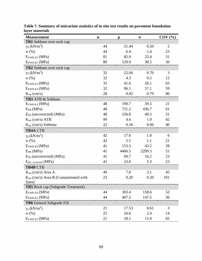
89

Table 7. Summary of univariate statistics of in situ test results on pavement foundation layer materials Measurement n µ σ COV (%) TB1 Subbase over rock cap γd (kN/m3) 44 21.44 0.50 2 w (%) 44 6.4 1.4 23 ELWD-Z3 (MPa) 81 82.9 25.4 31 EFWD-K3 (MPa) 80 129.9 38.5 30 TB2 Subbase over rock cap γd (kN/m3) 32 22.04 0.70 3 w (%) 32 4.3 0.5 12 ELWD-Z3 (MPa) 31 41.6 26.1 63 EFWD-K3 (MPa) 32 96.1 57.1 59 Ksat (cm/s) 28 0.92 0.79 86 TB3 ATB & Subbase EFWD-K3 (MPa) 48 190.7 39.5 21 ESB (MPa) 48 721.2 436.7 61 ESG (uncorrected) (MPa) 48 156.8 49.3 31 Ksat (cm/s) ATB 99 4.6 1.9 42 Ksat (cm/s) Subbase 22 0.16 0.06 40 TB4A CTB γd (kN/m3) 42 17.0 1.0 6 w (%) 42 5.5 1.1 21 EFWD-K3 (MPa) 41 153.3 43.2 28 ESB (MPa) 41 4466.5 2299.3 51 ESG (uncorrected) (MPa) 41 69.7 16.2 23 ESG_corrected (MPa) 41 23.0 5.3 23 TB4B CTB Ksat (cm/s) Area A 49 7.0 3.1 45 Ksat (cm/s) Area B (Contaminated with fines)

23 0.20 0.20 101

TB5 Rock cap (Subgrade Treatment) ELWD-D3 (MPa) 44 303.4 158.6 52 EFWD-K3 (MPa) 44 407.2 147.5 36 TB6 General Subgrade Fill γd (kN/m3) 21 17.53 0.61 3 w (%) 21 16.6 2.4 14 ELWD-Z3 (MPa) 21 18.1 11.8 65

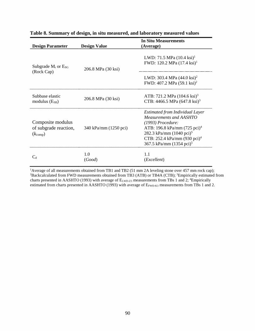
90

Table 8. Summary of design, in situ measured, and laboratory measured values

Design Parameter Design Value In Situ Measurements (Average)

Subgrade Mr or ESG (Rock Cap) 206.8 MPa (30 ksi)

LWD: 71.5 MPa (10.4 ksi)1

FWD: 120.2 MPa (17.4 ksi)1

LWD: 303.4 MPa (44.0 ksi)2

FWD: 407.2 MPa (59.1 ksi)2

Subbase elastic modulus (ESB) 206.8 MPa (30 ksi) ATB: 721.2 MPa (104.6 ksi)3

CTB: 4466.5 MPa (647.8 ksi)3

Composite modulus of subgrade reaction, (kcomp)

340 kPa/mm (1250 pci)

Estimated from Individual Layer Measurements and AASHTO (1993) Procedure: ATB: 196.8 kPa/mm (725 pci)4 282.3 kPa/mm (1040 pci)5 CTB: 252.4 kPa/mm (930 pci)4 367.5 kPa/mm (1354 pci)5

Cd 1.0 (Good)

1.1 (Excellent)

1Average of all measurements obtained from TB1 and TB2 (51 mm 2A leveling stone over 457 mm rock cap); 2Backcalculated from FWD measurements obtained from TB3 (ATB) or TB4A (CTB); 3Empirically estimated from charts presented in AASHTO (1993) with average of ELWD-Z3 measurements from TBs 1 and 2; 4Empirically estimated from charts presented in AASHTO (1993) with average of EFWD-K3 measurements from TBs 1 and 2.

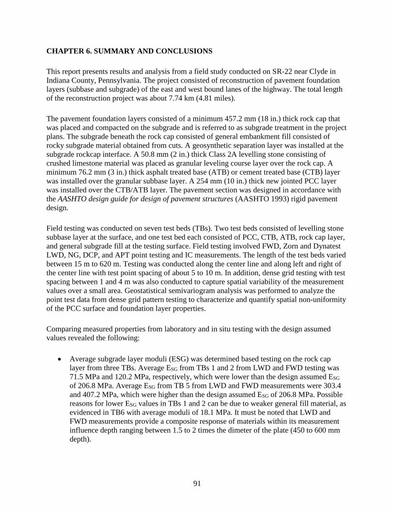
91

CHAPTER 6. SUMMARY AND CONCLUSIONS

This report presents results and analysis from a field study conducted on SR-22 near Clyde in Indiana County, Pennsylvania. The project consisted of reconstruction of pavement foundation layers (subbase and subgrade) of the east and west bound lanes of the highway. The total length of the reconstruction project was about 7.74 km (4.81 miles).

The pavement foundation layers consisted of a minimum 457.2 mm (18 in.) thick rock cap that was placed and compacted on the subgrade and is referred to as subgrade treatment in the project plans. The subgrade beneath the rock cap consisted of general embankment fill consisted of rocky subgrade material obtained from cuts. A geosynthetic separation layer was installed at the subgrade rockcap interface. A 50.8 mm (2 in.) thick Class 2A levelling stone consisting of crushed limestone material was placed as granular leveling course layer over the rock cap. A minimum 76.2 mm (3 in.) thick asphalt treated base (ATB) or cement treated base (CTB) layer was installed over the granular subbase layer. A 254 mm (10 in.) thick new jointed PCC layer was installed over the CTB/ATB layer. The pavement section was designed in accordance with the AASHTO design guide for design of pavement structures (AASHTO 1993) rigid pavement design.

Field testing was conducted on seven test beds (TBs). Two test beds consisted of levelling stone subbase layer at the surface, and one test bed each consisted of PCC, CTB, ATB, rock cap layer, and general subgrade fill at the testing surface. Field testing involved FWD, Zorn and Dynatest LWD, NG, DCP, and APT point testing and IC measurements. The length of the test beds varied between 15 m to 620 m. Testing was conducted along the center line and along left and right of the center line with test point spacing of about 5 to 10 m. In addition, dense grid testing with test spacing between 1 and 4 m was also conducted to capture spatial variability of the measurement values over a small area. Geostatistical semivariogram analysis was performed to analyze the point test data from dense grid pattern testing to characterize and quantify spatial non-uniformity of the PCC surface and foundation layer properties.

Comparing measured properties from laboratory and in situ testing with the design assumed values revealed the following:

• Average subgrade layer moduli (ESG) was determined based testing on the rock cap layer from three TBs. Average ESG from TBs 1 and 2 from LWD and FWD testing was 71.5 MPa and 120.2 MPa, respectively, which were lower than the design assumed ESG of 206.8 MPa. Average ESG from TB 5 from LWD and FWD measurements were 303.4 and 407.2 MPa, which were higher than the design assumed ESG of 206.8 MPa. Possible reasons for lower ESG values in TBs 1 and 2 can be due to weaker general fill material, as evidenced in TB6 with average moduli of 18.1 MPa. It must be noted that LWD and FWD measurements provide a composite response of materials within its measurement influence depth ranging between 1.5 to 2 times the dimeter of the plate (450 to 600 mm depth).

92

• Average subbase layer moduli (ESB) values for the CTB and ATB layers were 721 and 4,467 MPa, which are 3.5 to 21.6 times higher than the design assumed ESB of 206.8 MPa. It must be noted that the ATB layer tested in this study was placed one day prior to testing, while the CTB layer was placed several months prior to testing. Additional curing of the ATB material can potentially increase the moduli values of the layer.

• For section with ATB, the composite modulus of subgrade reaction (kcomp) values ranged between 196.8 kPa/mm (based on LWD measurements for ESG) and 282.3 kPa/mm (based on FWD measurements for ESG) and were about 1.2 to 1.7 times lower than the design target kcomp of 340 kPa/mm. Again, it must be noted that additional curing of the ATB material can potentially increase the ESB values and the resulting kcomp values.

• For section with CTB, the estimated kcomp value ranged between 252.4 kPa/mm (based on LWD measurements for ESG) and 367.5 kPa/mm (based on FWD measurements for ESG) and were about 1.3 times lower and 1.1 times higher than the design target kcomp of 340 kPa/mm.

• The drainage coefficient (Cd) value was assumed in the design as 1.0, which represents that the quality of drainage is rated as “good”. Based on the pavement geometry (i.e., cross slope, width of the pavement, thickness of the base layer), the measured Ksat values from the field, and assuming an effective porosity = 0.3, the time for a target 90% drainage was calculated. Based on APT tests conducted on the CTB layer, the time for 90% drainage was estimated as 1.0 day for Ksat = 0.2 cm/s (CTB contaminated with fines) to < 1 hour for Ksat = 7 cm/s (CTB uncontaminated). Based on tests conducted on the ATB layer the time for 90% drainage was estimated < 1 hour for Ksat = 4.6 cm/s. Based on these estimates, the quality of drainage can be rated as “good” to “excellent” and does meet the design requirements.

93

REFERENCES

AASHTO T-307. (1999). Standard method of test for determining the resilient modulus of soils and aggregate materials, American Association of State Highway and Transportation Officials AASHTO, Washington, DC.

AASHTO. (1993). AASHTO Design Guide for Design of Pavement Structures. American Association of State Highway and Transportation Officials, Washington D.C.

Andrei, D., M. W. Witczak, C. W. Schwartz, and J. Uzan. (2004). Harmonized resilient modulus test method for unbound pavement materials. Transportation Research Record: Journal of the Transportation Research Board No. 1874. Transportation Research Board, Washington, DC, 29-37.

ASTM C39/C39M-12. (2012). Standard test method of compressive strength of cylindrical concrete specimens. ASTM International, West Conshohocken, PA.

ASTM C117-04. (2010). Standard test method for materials finer than 75µm (No. 200) sieve in mineral aggregates by washing. American Standards for Testing Methods (ASTM), West Conshohocken, PA.

ASTM C136-06. (2010). Standard test method for sieve analysis of fine and coarse aggregates. ASTM International, West Conshohocken, PA.

ASTM D422-63. (2010). Standard test method for particle-size analysis of soils. ASTM International, West Conshohocken, PA.

ASTM D559-03. (2010). Wetting and drying compacted soil-cement mixtures. ASTM International, West Conshohocken, PA.

ASTM D560-03. (2010). Freezing and thawing compacted soil-cement mixtures. ASTM International, West Conshohocken, PA.

ASTM D698-07. (2010). Standard test method for laboratory compaction characteristics of soil using standard effort 12,400 ft-lbf/ft3 600 kN-m/m3. ASTM International, West Conshohocken, PA.

ASTM D854-14. (2014). Standard test methods for specific gravity of soil solids by water pycnometer. ASTM International, West Conshohocken, PA.

ASTM D1557-07. (2010). Standard test method for laboratory compaction characteristics of soil using modified effort 56,000 ft-lbf/ft3 2,700 kN-m/m3. ASTM International, West Conshohocken, PA.

ASTM D1883-07. (2010). Standard test method for CBR (California Bearing Ratio) of laboratory-compacted soils. ASTM International, West Conshohocken, PA.

ASTM D2487-10. (2010). Standard test method for classification of soil for engineering purposes unified soil classification system. ASTM International, West Conshohocken, PA.

ASTM D3282-09. (2010). Standard test method for classification of soils and soil-aggregate mixtures for highway construction purposes. ASTM International, West Conshohocken, PA.

ASTM D4253-00. (2010). Standard test methods for maximum index density and unit weight of soils using a vibratory table. ASTM International, West Conshohocken, PA.

ASTM D4254-00. (2010). Standard test methods for minimum index density and unit weight of soils and calculation of relative density. ASTM International, West Conshohocken, PA.

ASTM D4318-10. (2010). Standard test methods for liquid limit, plastic limit, and plasticity index of soils. ASTM International, West Conshohocken, PA.

94

ASTM D4694-09. (2010). Standard test method for deflections with a falling-weight-type impulse load device. American Standards for Testing Methods (ASTM), West Conshohocken, PA.

ASTM D5918-06. (2010). Standard test methods for frost heave and thaw weakening susceptibility of soils. American Standards for Testing Methods (ASTM), West Conshohocken, PA.

ASTM D6951-03. (2010). Standard test method for use of the dynamic cone penetrometer in shallow pavement applications. ASTM International, West Conshohocken, PA.

ASTM D6938-10. Standard test method for in-place density and water content of soil and soil-aggregate by nuclear methods shallow depth. ASTM International, West Conshohocken, PA.

Barenberg, E. J., and Petros, K. A. (1991). Evaluation of Concrete Pavements Using NDT Results, Illinois Highway Research Project IHR-512, University of Illinois and Illinois Department of Transportation, Report No. UILU-ENG-91-2006, IL.

Brandl, H., and D. Adam. (1997). “Sophisticated continuous compaction control of soils and granular materials.” Proceedings of the 14th International Conference of Soil Mechanics and Foundation Engineering. Hamburg, Germany, 1-6.

Clark, I. and W. Harper. 2002. Practical Geostatistics 2000. 3rd reprint, Ecosse North America LLC, Columbus, OH.

Darter, M. I., Hall, K. T., and Kuo, C-M. (1995). Support under Portland Cement Concrete Pavements, NCHRP Report 372. Transportation Research Board, Washington, D.C.

ERES Consultants Inc. (1982). Techniques for Pavement Rehabilitation: A Training Course. U.S. Department of Transportation, FHWA, Washington, D.C.Floss, R., G. Bräu, M. Gahbauer, N. Gruber, and J. Obermayer. 1991). Dynamische Verdichtungsprüfung bei Erd-und Straßenbauten. Prüfamt fur Grundbau, Boden-und Felsmechanik Technische Universität München, Heft 612, München, Germany in German).

Hoffman, M. S., and Thompson, M. R. (1981). Mechanistic Interpretation of Nondestructive Pavement Testing Deflections. Transportation Engineering Series No. 32, Illinois cooperative Highway and Transportation Research Series No. 190. University of Illinois at Urbana-Champaign, Champaign, IL.

Horak, E. (1987). “Aspects of deflection basin parameters used in a mechanistic rehabilitation design procedure for flexible pavements in South Africa.” University of Pretoria, South Africa.

Ioannides, A. M. (1990). “Dimensional analysis in NDT rigid pavement evaluation.” Transportation Engineering Journal, ASCE, Vol. 116, No. TE1.

Isaaks, E. H. and R. M. Srivastava. (1989). An Introduction to Applied Geostatistics. Oxford University Press, New York.

Janssen, D. J., and Snyder, M. B. (2000). “Temperature-moment concept for evaluating pavement temperature data.” Journal of Infrastructure Systems, 6(2), 81–83.

Kilareski, W. P., and Anani, B. A. (1982). “Evaluation of in situ moduli and pavement life from deflection basins.” Presented at the 5th International Conference of Asphalt Pavements, University of Michigan, Ann Arbor, MI.

NCHRP 1-28A. (2002). Recommended standard method for routine resilient modulus testing of unbound granular base/subgrade materials and subgrade soils–NCHRP protocol 1-28A, National Cooperative Highway Research Program.

95

Quintus, V. H. L., and A. L. Simpson. (2002). Backcalculation of Layer Parameters for LTPP Test Sections, Volume II: Layered Elastic Analysis for Flexible and Rigid Pavements, Research Report, Long-Term Pavement Performance Program, Report No. FHWA-RD-01-113, Federal Highway Administration, Washington, DC, October 2002.

Samaras, A. A., R. Lamm, and J. Treiterer. (1991). Application of continuous dynamic compaction control for earthworks in railroad construction. Transportation Research Record: Journal of the Transportation Research Board. No. 1309, Transportation Research Board of the National Academies, Washington, DC, 42-46.

Sandström, Å. (1994). Numerical simulation of a vibratory roller on cohesionless soil. Internal Report, Geodynamik, Stockholm, Sweden.

Sandström Å., and C. B. Pettersson. (2004). Intelligent systems for QA/QC in soil compaction, Proceedings of the TRB 2004 Annual Meeting (CD-ROM), Transportation Research Board, Washington, D.C.

Schmalzer, P. N. (2006). LTPP Manual for Falling Weight Deflectometer Measurements, Version 4.1. Final Report, FHWA-HRT-06-132. Federal Highway Administration.

Smith, K. D., Wade, M. J., Bruinsma, J. E., Chatti, K., Vandenbossche, J. M., Yu, H. T., Hoerner, T. E., Tayabji, S. D. (2007). Using Falling Weight Deflectometer Data with Mechanistic-Empirical Design and Analysis, Draft Interim Report, DTFH61-06-C-0046, Federal Highway Administration, Washington, D.C.

Substad, R. N. (2002). “LTPP data analysis: Feasibility of using FWD deflection data to characterize pavement construction quality.” NCHRP Web Document 52, Project No. 20-50(9), National Cooperative Highway Research Program, Transportation Research Board of the National Academies, Washington, D.C.

Thompson, M., and D. White. (2008). “Estimating compaction of cohesive soils from machine drive power.” Journal of Geotechnical and Geoenvironmental Engineering, ASCE, 134(12), 1771–1777.

Trimble Navigation Ltd. (2013). Trimble S3 Total Station Datasheet. Retrieved December 12, 2013, < http://trl.trimble.com/docushare/dsweb/Get/Document-469042/022543-492A_TrimbleS3_DS_0110_sec.pdf > (Date accessed 8/6/2015).

Ullidtz, P. (1987). Pavement analysis. Developments in civil engineering, 19. 318 p. Elsevier, Amsterdam.

Vandenbossche, J. M. (2005). Effects of slab temperature profiles on the use of falling weight deflectometer data to monitor joint performance and detect voids. Transportation Research Record: Journal of the Transportation Research Board, 2005, Washington, D.C., 75–85.

Vennapusa, P. (2004). Determination of the Optimum Base Characteristics for Pavements. Master’s Thesis, Department of Civil Construction and Environmental Engineering, Iowa State University, Ames, Iowa.

Vennapusa, P., and D. J. White. (2009). Comparison of light weight deflectometer measurements for pavement foundation materials. Geotechnical Testing Journal, ASTM, 323, 239–251.

Vennapusa, P., D. J. White, and M. Morris. (2010). Geostatistical analysis of spatial referenced roller-integrated compaction measurements. Journal of Geotechnical and Geoenvironmental Engineering, ASCE, 1366, 813–822.

96

Vennapusa, P., D. J. White, and H. Gieselman. (2009). Influence of support conditions on roller-integrated machine drive power measurements for granular base. International Foundation Congress and Equipment Exposition 2009 (IFCEE 09). March 15-19, Orlando, FL.

White, D.J., Vennapusa, P. (2014). “Optimizing pavement base, subbase, and subgrade layers for cost and performance of local roads.” Final Field Data Report IHRB Project TR-640, Iowa State University, Ames, Iowa.

White, D. J., and M. Thompson. (2008). Relationships between in situ and roller-integrated compaction measurements for granular soils. Journal of Geotechnical and Geoenvironmental Engineering, ASCE, 134(2), 1763-1770.

White, D., P. Vennapusa, and L. Zhao. (2014). Verification and repeatability analysis of the in situ air permeameter test. Geotechnical Testing Journal, 37(2), DOI: 10.1520/GTJ20130111.

White, D. J., E. Jaselskis, V. Schaefer, and T. Cackler. (2005). Real-time compaction monitoring in cohesive soils from machine response. Transportation Research Record: Journal of the Transportation Research Board No. 1936, Washington DC, 173–180.

Witczak, M. W. and J. Uzan. (1988). The universal airport design system–Report I of IV: Granular material characterization. Department of Civil Engineering, University of Maryland, College Park, MD.

Zorn, G. (2003). Operating Manual: Light Drop-weight Tester ZFG2000, Zorn Stendal, Germany.

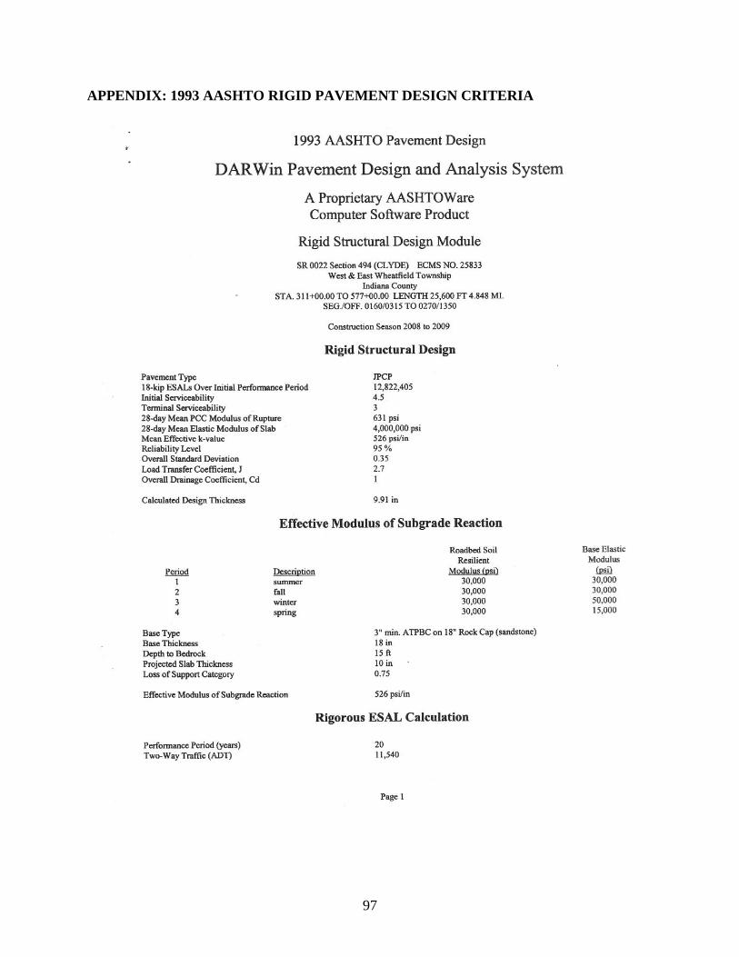
97

APPENDIX: 1993 AASHTO RIGID PAVEMENT DESIGN CRITERIA