Improving Sustainable Safe Transport via Automated Vehicle ...

sustainability

Article

Improving Sustainable Safe Transport via Automated VehicleControl with Closed-Loop Matching

Tamás Hegedus, Dániel Fényes, Balázs Németh and Péter Gáspár *

Citation: Hegedus, T.; Fényes, D.;

Németh, B.; Gáspár, P. Improving

Sustainable Safe Transport via

Automated Vehicle Control with

Closed-Loop Matching. Sustainability

2021, 13, 11264. https://doi.org/

10.3390/su132011264

Academic Editor: Anders Wretstrand

Received: 26 August 2021

Accepted: 6 October 2021

Published: 13 October 2021

Publisher’s Note: MDPI stays neutral

with regard to jurisdictional claims in

published maps and institutional affil-

iations.

Copyright: © 2021 by the authors.

Licensee MDPI, Basel, Switzerland.

This article is an open access article

distributed under the terms and

conditions of the Creative Commons

Attribution (CC BY) license (https://

creativecommons.org/licenses/by/

4.0/).

Institute for Computer Science and Control (SZTAKI), Eötvös Loránd Research Network (ELKH), Kende u. 13-17,H-1111 Budapest, Hungary; [email protected] (T.H.); [email protected] (D.F.);[email protected] (B.N.)* Correspondence: [email protected]

Abstract: The concept of vehicle automation is a promising approach to achieve sustainable transportsystems, especially in an urban context. Automation requires the integration of learning-basedapproaches and methods in control theory. Through the integration, a high amount of information inautomation can be incorporated. Thus, a sustainable operation, i.e., energy-efficient and safe motionwith automated vehicles, can be achieved. Despite the advantages of integration with learning-basedapproaches, enhanced vehicle automation poses crucial safety challenges. In this paper, a novelclosed-loop matching method for control-oriented purposes in the context of vehicle control systemsis presented. The goal of the method is to match the nonlinear vehicle dynamics to the dynamics of alinear system in a predefined structure; thus, a control-oriented model is obtained. The matching isachieved by an additional control input from a neural network, which is designed based on the input–output signals of the nonlinear vehicle system. In this paper, the process of closed-loop matching,i.e., the dataset generation, the training, and the evaluation of the neural network, is proposed. Theevaluation process of the neural network through data-driven reachability analysis and statisticalperformance analysis methods is carried out. The proposed method is applied to achieve the pathfollowing functionality, in which the nonlinearities of the lateral vehicle dynamics are handled. Theeffectiveness of the closed-loop matching and the designed control functionality through high fidelityCarMaker simulations is illustrated.

Keywords: vehicle control; closed-loop matching; control-oriented modeling; neural networks

1. Introduction and Motivation

In recent years, advanced driver-assistance systems have become widespread amongmodern vehicles. These systems are focused on assisting the driver of the vehicle (e.g.,lane-keeping assist system, cruise control). The main role of these systems is to makeeveryday traffic safer and to reduce the accidents caused by human errors. However,many problems cannot be solved using only the mentioned systems. One of the mainissues to be addressed is the loss of time due to driving. An average American workerspends more than an hour a day driving a vehicle [1]. The main problem is that thistime cannot be usefully spent by the driver. In the future, highly automated/autonomousvehicles will take over the burden of driving, which will allow the passengers to spendthe traveling time with other productive activities. Moreover, autonomous vehicles willhave a major impact on society. Self-driving vehicles will increase the living standards ofmany people, and personal freedom can be also increased [2]. Furthermore, maintainingthe same level of mobility will not require owning a car, which will result in a significantreduction in spending.

In addition, traffic jams have a number of negative effects, such as increased traveltime, increasing fuel consumption [3], and emission [4]. These effects can be significantlyreduced with autonomous vehicles [5]. Moreover, other advantages of autonomous vehiclesare the reduction in the safe traveling distance and the higher speed limits, which decrease

Sustainability 2021, 13, 11264. https://doi.org/10.3390/su132011264 https://www.mdpi.com/journal/sustainability

Sustainability 2021, 13, 11264 2 of 20

traffic jams and traveling times. Previously, some problems were presented that arestrongly related to energy usage and emission. Autonomous vehicles play a key role inreducing these effects. Due to the mentioned advantages, many automotive companiesand researchers are dealing with issues related to autonomous vehicles. The main criterionfor the widespread of the fully autonomous vehicle is the safe and reliable operation inany traffic situation. The development of autonomous vehicle technologies has grownsignificantly in the last decade. The system, which is responsible for the operation ofautonomous vehicles, can be divided into several layers [6]. For example, the sensing layeraccurately evaluates the given traffic situation; another layer, the decision-making one, isresponsible for the motion planning of the car. Finally, the control algorithm guaranteesthe accurate trajectory tracking of the vehicle.

In the future era of autonomous vehicles, optimal traffic control algorithms will playa key role (e.g., smart intersections). These algorithms provide reference trajectories forthe vehicles. By tracking these trajectories, an energy optimal traffic flow can be achieved.Therefore, in order to reach this energy optimal traffic flow, the control systems on thevehicle must guarantee accurate tracking performance.

Furthermore, it can be said that a number of problems arise during the control design.One of the main problems is that the system parameters are not known exactly known. Thismeans that the control algorithm may not be satisfying the energy minimum requirement.In this paper, a novel method is presented for the control design, which can improve theperformance of the nominal control system.

One of the most difficult challenges is the modeling process of a system since itmay contain several nonlinearities and uncertain parameters. Moreover, in several cases,nonlinearities are difficult to handle [7]. In recent years, several approaches have beendeveloped to solve this problem. The first group includes methods, which linearize thesystem. The simplest approach is when only one linear system is determined. In othercases, several linear systems are determined in numerous operating points of the nonlinearsystem. Furthermore controllers can be designed for the defined linear systems. Usingthe resulted set of controllers, and based on the actual information of the system, thecontroller parameters can be calculated as an interpolation. This method is called, inthe literature, gain-scheduling control [8]. Although the control design of this methodis simple, the performance of this method may be poor. There can be found polytopicsystem–based algorithms, such as the linear parameter-varying framework (LPV) [9]. Thesecond group consists of algorithms, in which the nonlinearities of the system are takeninto account during the modeling phase. The stability analysis of a polynomial system ispresented in [10]. In [11], a control problem is introduced, using a (sum-of-squares) SOSprogramming method. In these methods, the model contains nonlinearities, which makesthe control design a challenging task. The nonlinearities of the system can be taken intoaccount in several ways, e.g., the nonlinear model predictive control method (NMPC) [12].An advantage of the MPC approach is that it can take into account the bounds of the statesof the system, by which the stability of the controlled plant is guaranteed. These boundscan be determined by computing the reachability sets of the system; see [13].

The third group is the classical methods. A possible approach to deal with the nonlin-earities of the system is the feedback linearization; see [14,15]. The feedback linearizationprocess requires an accurate description of the system. However, in many cases, it is notavailable or cannot be determined since the system may contain high nonlinearities anduncertainties. Moreover, if it is available, the inversion of the system is also a difficult taskto achieve; see [16].

With the increase in the computation capacity of computers, new fields have comeinto view, such as data-driven and machine learning–based approaches. Several methodshave been developed, using a combination of the classical and machine learning–basedapproaches. In [9], a method is presented in which an (LPV) approach is combined withthe results of machine learning–based technique. The reachability sets are computedfor the controlled vehicle, using data-driven analyses and a machine learning algorithm,

Sustainability 2021, 13, 11264 3 of 20

and the results are used in a model predictive approach, which guarantees the trajectorytracking [17]. Furthermore, neural networks can be also used during feedback linearization.In [18], a feedback linearization method is presented for the tracking performance based onneural networks. Moreover, neural network-based feedback linearization is used in manyfields of vehicle control (such as suspension control [19], and longitudinal control [20]).Feedback linearization is made for a nonlinear system with unknown dynamics, using thereinforcement learning technique [21]. Moreover, in [22], an input–output linearizationmethod is presented for robotic applications by reinforcement learning. One of the mainadvantages of the proposed methods is the fact that an accurate system description is notnecessary during the linearization process.

The main advantage of the first three methods is that the stability of the systemcan be guaranteed in the operation range of the system. However, the accurate controldesign requires the exact knowledge of the given system, which is a challenging task inseveral cases. Although the machine learning algorithms can boost the performance of thecontrolled plant, there is no analytical proof to guarantee their stability, which is a majorissue in safety-critical systems. Some papers deal with this problem, e.g., in the workof [23], a method is proposed for computing the reliability of the neural networks.

In this paper, a novel model matching-based control approach is presented, using amachine learning–based algorithm. The control algorithm is beneficial for those systems,which are of high complexity and exposed to parameter uncertainty. A contribution ofthe paper is that the level of control performance through learning-based approachesis improved, and similarly, stable motion of the vehicle through the operation of thecontrol is guaranteed. Thus, one of the main disadvantages of several neural network–based control methods can be avoided, i.e., lack of stability. A further contribution ofthe paper, in contrast to the former methods in the literature, is that the improvementof the performance level through the extension of the simplified design methods basedon the nominal linear system model is carried out. The nominal model of the systemis considered to be known since the dynamics of the original system is adjusted to thenominal model. In this way, the complexity of the control design process is reduced and theperformance of the closed-loop system can be guaranteed without taking into account theuncertainties and the unmodeled dynamics of the system. The presented control strategyis implemented in Matlab/CarMaker environments, and its efficiency is demonstratedthrough a comprehensive simulation example.

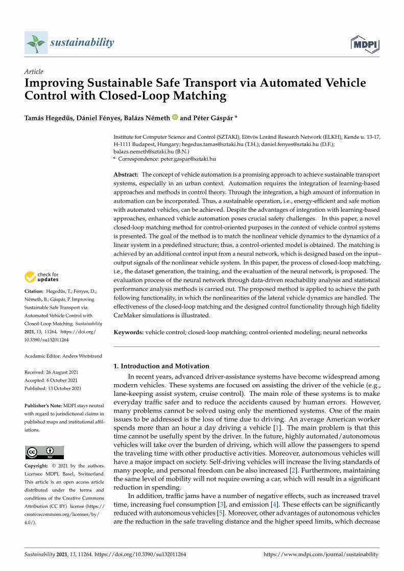
The structure of the proposed algorithm is shown in Figure 1, which can be dividedinto three main parts. The first block contains the steps of the data generation. Firstly,a nominal model is selected, which is the basis of the matching problem. Then, the testscenarios and the simulations are considered. The appropriately selected scenarios areessential in order to ensure that the collected dataset covers the full operating range of thesystem. Using the nominal model and the scenarios, data acquisition is performed. In thesecond part of the algorithm, the reachability sets are computed based on the collected data,and also the machine learning–based method is presented for the additional steering anglecomputation. Then, the reliability estimation for the network is determined. Finally, themain goal of the third part is the control design. The lateral controller is designed, usingsolely the nominal model. Moreover, the last part is the calculation of the reference signal,which takes into account the computed stability sets in order to ensure the stability of thenonlinear system.

Figure 1. Methodological scheme of the control method.

Sustainability 2021, 13, 11264 4 of 20

The paper is structured as follows: In Section 2, the construction of the nominal modelis presented, which is used both in the training process of the neural network and duringthe reference signal generation. Moreover, this section describes the acquisition of thedataset, which is used to train and evaluate the closed-loop matching neural network.Section 3 presents the computation of the stability sets. Moreover, the reliability estimationof the neural network is also presented in this section. The model-based reference signalgeneration is presented in Appendix A. In Section 4, a comprehensive simulation exampleis given to show the efficiency and the operation of the proposed control algorithm. Finally,the paper is concluded in Section 5.

2. Closed-Loop Matching Using a Neural Network-Based Approach

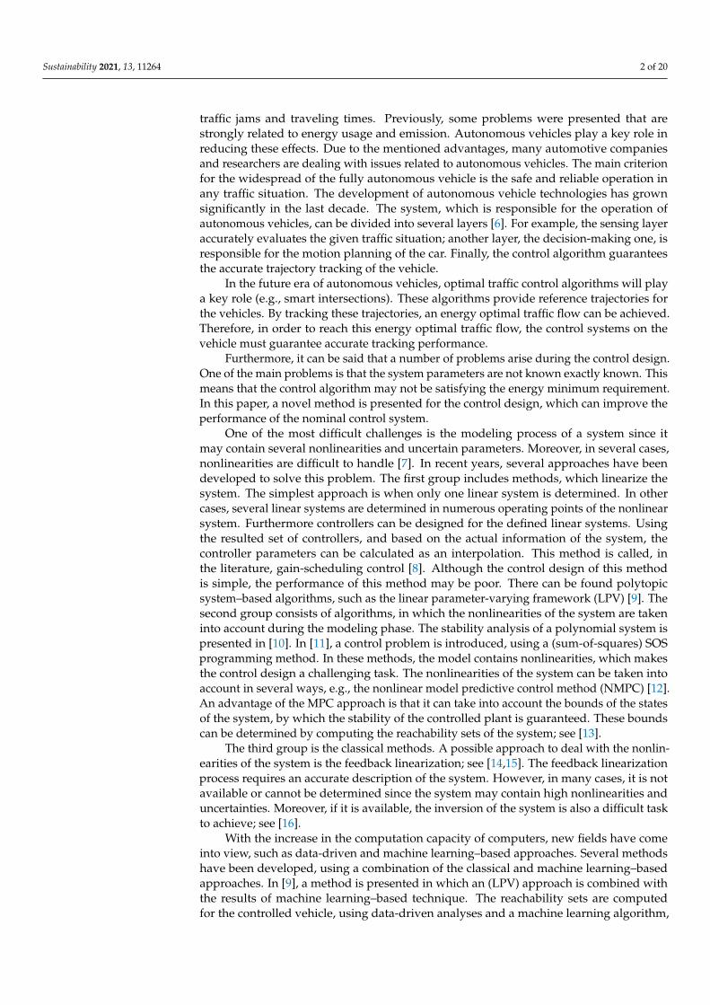
In this paper, the effectiveness of the proposed method is demonstrated through avehicle-oriented problem, in which the model matching process is carried out in termsof the yaw rate of the vehicle. In Figure 2, the scheme of the closed-loop matching ispresented. The goal is to compute an additional input signal ∆u by which the outputsignals (ynom, ymat) become identical. In this case, ∆u means an additional steering angle,and (ynom, ymat) are the yaw rates of the nominal and nonlinear system.

+

Figure 2. Structure of the closed-loop matching.

In the following subsection, the construction of the nominal model is presented, whichserves as a base of the neural network-based closed-loop matching and the model-basedreference generation. The nominal model consists of two main parts: the lateral vehicle,which is based on the two-wheeled bicycle model, and the steering system, which ismodeled by a first-order term.

2.1. Lateral Vehicle Model

The main idea behind this model is to replace the front and rear wheels of the vehicleby one wheel, which is placed on the axis of symmetry of the vehicle. Basically, it consistsof two equations: the first describes the lateral motion of the car, while the second equationdescribes its yaw motion (see [24]):

Izψ = Ff ,y(α f )l f − Fr,y(αr)lr (1)

mvx(ψ + β) = Ff ,y(α f ) + Fr,y(αr) (2)

where m is the mass of the car, l f , fr are geometrical parameters and Iz denotes the yawinertia. Moreover, β is the side-slip angle. The longitudinal velocity of the vehicle is (vx),the road wheel angle is denoted by δr and ψ is the yaw rate. The lateral tire forces can becomputed as follows:

Fi,y = Ciαi, (3)

Sustainability 2021, 13, 11264 5 of 20

where Ci is the cornering stiffness of the tires, and αi represents the side-slip angles ofthe tires. Using (1)–(3), a transfer function (Gdyn(s)) can be determined. The input of thesystem is the steering angle (δ), and the output is the yaw rate (ψ) of the vehicle. Using theLaplace transform of the output (Bdyn(s)) and the Laplace transform of the input Adyn(s),the following transfer function can be formed:

Gdyn(s) =Bdyn(s)Adyn(s)

(4)

Note that during the construction of the nominal model, several parameters of thevehicle are unknown, such as the cornering stiffness and the yaw inertia. The longitudinalvelocity can change during the simulations, but this value is fixed during the constructionof the nominal model. The second part of the nominal model is the steering system. Inautonomous vehicles, the steering system has a significant effect on the lateral dynamics,due to the delays caused by the electric motor and its inertia. This dynamics can be modeledby a simple first-order term [25], as follows:

Gst(s) =Ast

Tst + 1(5)

where Tst is the time delay and Ast provides the steady-state gain of the steering system.

2.2. Computation of the Inverse Model

The nominal linear model consists of the presented two parts: lateral vehicle and thesteering system. This model can be transformed into a transfer function, whose input isthe steering angle (δ) and its output is the yaw rate (ψ) of the vehicle. In the first step, theinverse of the nominal model is calculated [26]:

G−1nom(s) ≈ G−1

st (s)G−1dyn(s). (6)

The computation of the inverse model can be challenging [27]. Furthermore, after theinversion, the system may not be causal. In order to meet this issue, a prefilter is used.

G−1p f ,nom(s) = Gp f (s)G−1

nom(s) (7)

where Gp f (s) gives the prefilter, which is used in order to deal with non-causalities. Thediscretization process is made, using Tustin’s method [28].

zi = esiT ≈ 1 + siT/21− siT/2

(8)

where si denotes the ith pole of the continuous system, while zi represents the discretepoles of the discretized system. Furthermore, T is the discretization time. Finally, thecalculated discretized inverse model is used during the neural network-based matchingprocess, which is presented in the next subsection.

2.3. Data Generation for the Neural Network

In this subsection, the data generation is presented for the neural network, which isresponsible for closed-loop matching. The goal of the matching process is to compute anadditional steering angle (∆δ) by which the closed-loop system matches the behavior (out-put) of the nominal model, which is presented in Section 2.1. Since the system is influencedby high nonlinearities and the parameters are not accurately known, the computation of ∆δis not a straightforward task. In order to compute the additional steering angle, an iterativeprocess is presented, which cannot be applied in real-time application. The main role ofthe neural network is to calculate the additional steering angle for the nonlinear system

Sustainability 2021, 13, 11264 6 of 20

based on the measurable states of the system in real-time application. In the following,more details are given for the data generation process.

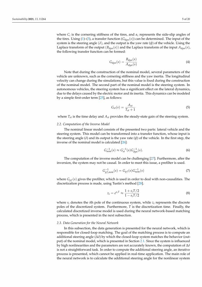
In Figure 3, the data generation process is presented. The basis of the data generationis the deviation between the output (yaw rate) of the nominal model and the measured yawrate of the nonlinear model by which a nominal steering angle sequence (δ) is determined,using the inverse of the nominal model. This error function is computed at each iterationstep. After an iteration step, the resulting additional steering angle (δ) sequence is addedto the previously determined sequence. The training dataset consists of the measurabledata, which are collected directly from the nonlinear system at the last iteration step. In thefollowing, more details are given on the iterative algorithm.

-

+

+ +

Figure 3. Structure of the data generation.

In the first iteration step, the value of the additional steering angle is set to zero and theyaw rate is computed from the nominal model. Then, the error between the yaw rate signalcan be computed, (ψerror). Using the error value and the inverse of the nominal model, theadditional steering angle is computed and saved. In the second iteration step, the input ofthe vehicle is modified as follows: δ = δ + δ2. Note that the yaw rate of the vehicle and thecalculated yaw rate using the nominal model may not match. This phenomenon can beexplained by the fact that (∆δ) is computed using only the nominal model. The iterativeprocess with which the additional steering angle is computed, is formed as follows:

∆δ =n

∑i

δi, (9)

δ = δ + ∆δ, (10)

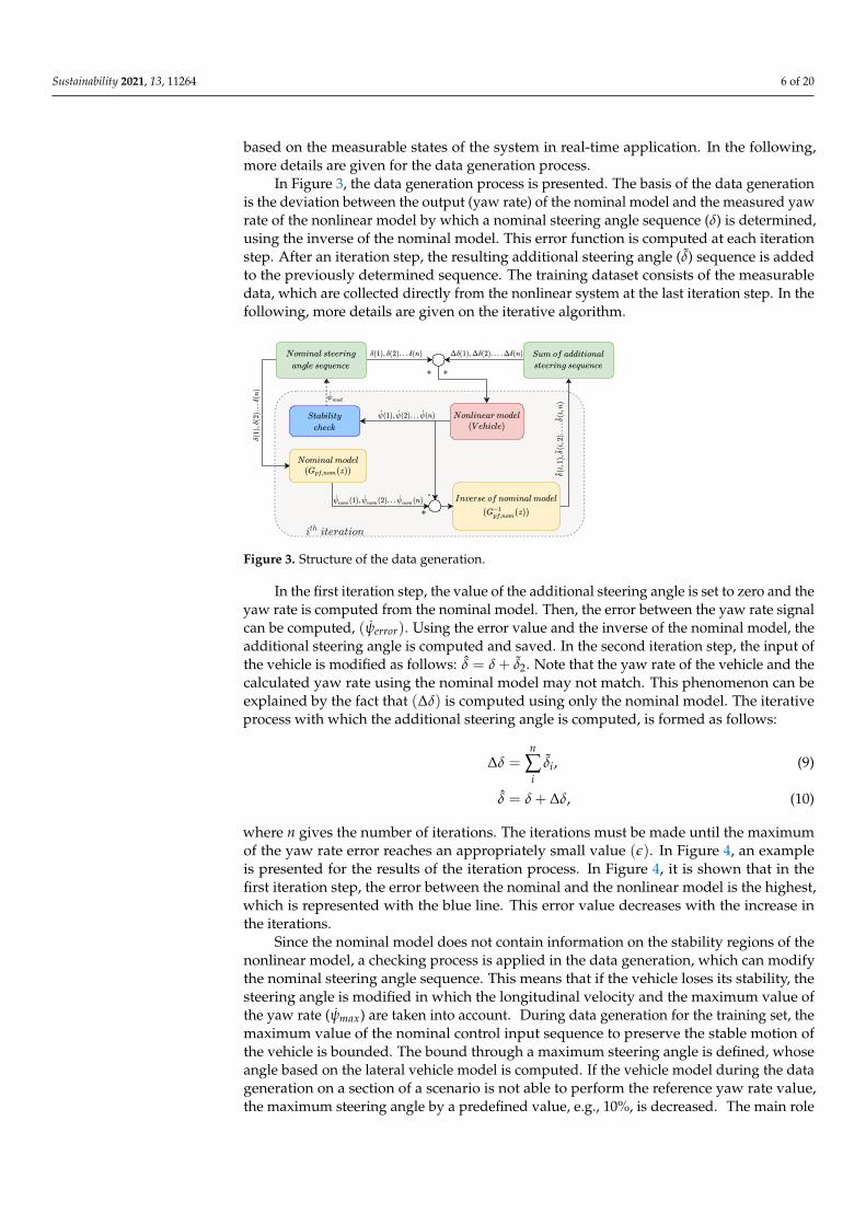
where n gives the number of iterations. The iterations must be made until the maximumof the yaw rate error reaches an appropriately small value (ε). In Figure 4, an exampleis presented for the results of the iteration process. In Figure 4, it is shown that in thefirst iteration step, the error between the nominal and the nonlinear model is the highest,which is represented with the blue line. This error value decreases with the increase inthe iterations.

Since the nominal model does not contain information on the stability regions of thenonlinear model, a checking process is applied in the data generation, which can modifythe nominal steering angle sequence. This means that if the vehicle loses its stability, thesteering angle is modified in which the longitudinal velocity and the maximum value ofthe yaw rate (ψmax) are taken into account. During data generation for the training set, themaximum value of the nominal control input sequence to preserve the stable motion ofthe vehicle is bounded. The bound through a maximum steering angle is defined, whoseangle based on the lateral vehicle model is computed. If the vehicle model during the datageneration on a section of a scenario is not able to perform the reference yaw rate value,the maximum steering angle by a predefined value, e.g., 10%, is decreased. The main role

Sustainability 2021, 13, 11264 7 of 20

of this part is to ensure the stable motion of the vehicle. The following pseudo algorithmpresents the data generation for the nth step.

0 5 10 15 20 25 30 35 40 45 50

Time (s)

-0.15

-0.1

-0.05

0

0.05

0.1

0.151st iteration 2nd iteration

3rd iteration 4th iteration

5th iteration 6th iteration

7th iteration

Figure 4. Results of the iteration processes

The presented iterative process is used in the simulations, which provide the datasetfor the training process of the neural network. The whole iteration process is performeduntil the error between the nominal and the measured yaw rate reaches a predefined smallvalue ε. In the example of this paper, the value of ε is set to 0.01. During the simulations, thelongitudinal velocity of the vehicle varies between vx ∈ 30–110 km/h and the vehicle isdriven along different tracks. Using Algorithm 1, the additional steering angle sequenceis determined and saved. Note that the additional control input has an influence on thestates of the vehicle. This means that the training dataset should contain the effect of theadditional steering angle because the neural network calculates the additional steeringangle, using the measured states. In order to solve this problem, the input of the neuralnetwork is the states of the vehicle, which is saved at the last iteration step. The followingvariables are measured and collected from the simulations:

• Longitudinal velocity (vx).• Acceleration (ax, ay).• Angular velocities (ψ, Θ, Φ).• Steering angle (δ).• Nominal steering angle from the inverse model (δnom).• Additional steering angle (∆δ).

In this way, more than 1 million distinct instances are gathered. Note that only thatthe signals are used, which are available from the onboard sensors. In summary, the valueof the additional steering angle cannot be determined in only one step, due to uncertainparameters and high nonlinearities.

Algorithm 1: Computation of the steering angle.

δ = δ . Initializationwhile max(ψerror) ≥ ε do

Simulating system with δComputing ψerror and δif ψ > ψmax then

Modify δ . Recomputing the nominal sequenceelse

Save ∆δ

δ = δ + ∑ni ∆δi . Calculation of the updated sequence

Sustainability 2021, 13, 11264 8 of 20

2.4. Training of the Neural Network

It is mentioned that the closed-loop matching is achieved through the computation ofan additional steering angle, which is generated using an iterative algorithm. Nevertheless,the iterative algorithm cannot be used in real-time applications. In order to meet this issue,a neural network is used to calculate the additional steering angle, using the measurablestates of the vehicle. The training dataset of the network is created, using the iterativealgorithm, which is detailed in Section 2.3. The inputs of the network are the measurablestates, and the output is the computed additional steering angle. In this subsection, thetraining process is presented.

The neural networks can be divided into three main layers: the input layer, the hiddenlayers, and finally the output layer. Each layer consists of neurons, more precisely, weightsand activation functions. Before the training process, the number of neurons and hiddenlayers must be determined. In this paper, the parameters of the implemented neuralnetwork are determined, using the so-called k-fold cross-validation technique [29]. Thefollowing table shows the parameters of the trained neural network.

In Table 1, the main parameters of the neural network are presented, and during thetraining process, a Levenberg–Marquardt algorithm is used. The training process of the neuralnetwork-based additional control input computation algorithm is performed using MatlabNeural Network Toolbox [30]. Figure 5 illustrates the loss function of the training process.

Table 1. Parameters of the trained neural network.

Parameters of the Neural Network

1st hidden layer 2nd hidden layer

Number of fcn. 20 15

Activation fcn. ReLU log-sigmoid

0 10 20 30 40 50 60

67 Epochs

10-8

10-6

10-4

10-2

Mean

Sq

uare

d E

rro

r (

mse)

Best Validation Performance is 3.6161e-08 at epoch 65

Train

Validation

Test

Best

Figure 5. Loss function of the training process.

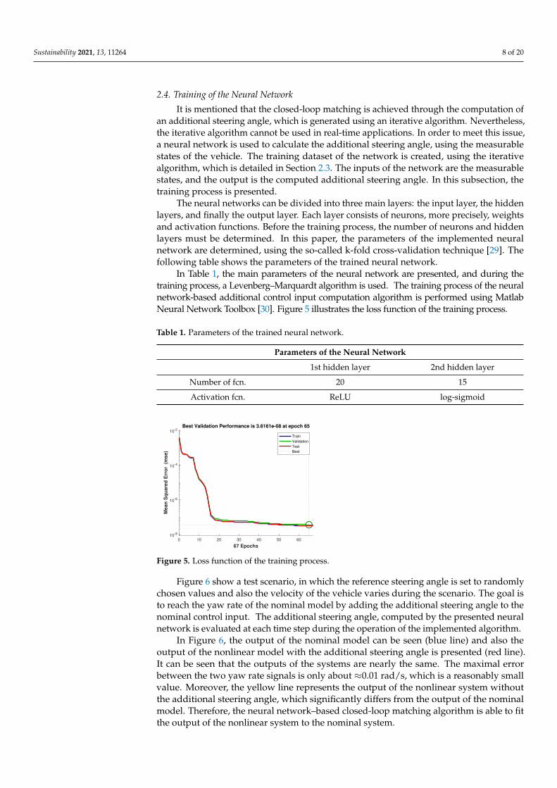
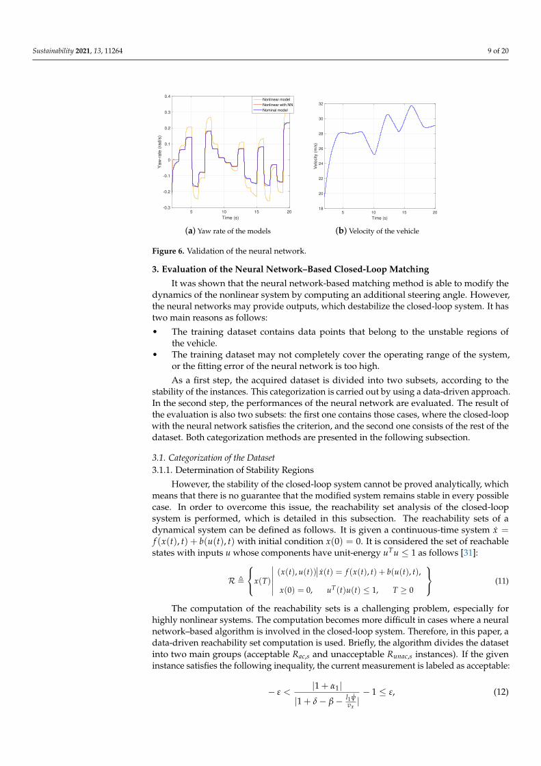
Figure 6 show a test scenario, in which the reference steering angle is set to randomlychosen values and also the velocity of the vehicle varies during the scenario. The goal isto reach the yaw rate of the nominal model by adding the additional steering angle to thenominal control input. The additional steering angle, computed by the presented neuralnetwork is evaluated at each time step during the operation of the implemented algorithm.

In Figure 6, the output of the nominal model can be seen (blue line) and also theoutput of the nonlinear model with the additional steering angle is presented (red line).It can be seen that the outputs of the systems are nearly the same. The maximal errorbetween the two yaw rate signals is only about ≈0.01 rad/s, which is a reasonably smallvalue. Moreover, the yellow line represents the output of the nonlinear system withoutthe additional steering angle, which significantly differs from the output of the nominalmodel. Therefore, the neural network–based closed-loop matching algorithm is able to fitthe output of the nonlinear system to the nominal system.

Sustainability 2021, 13, 11264 9 of 20

5 10 15 20

Time (s)

-0.3

-0.2

-0.1

0

0.1

0.2

0.3

0.4

Ya

w-r

ate

(ra

d/s

)

Nonlinear model

Nonlinear with NN

Nominal model

(a) Yaw rate of the models

5 10 15 20

Time (s)

18

20

22

24

26

28

30

32

Velo

city (

m/s

)

(b) Velocity of the vehicle

Figure 6. Validation of the neural network.

3. Evaluation of the Neural Network–Based Closed-Loop Matching

It was shown that the neural network-based matching method is able to modify thedynamics of the nonlinear system by computing an additional steering angle. However,the neural networks may provide outputs, which destabilize the closed-loop system. It hastwo main reasons as follows:

• The training dataset contains data points that belong to the unstable regions ofthe vehicle.

• The training dataset may not completely cover the operating range of the system,or the fitting error of the neural network is too high.

As a first step, the acquired dataset is divided into two subsets, according to thestability of the instances. This categorization is carried out by using a data-driven approach.In the second step, the performances of the neural network are evaluated. The result ofthe evaluation is also two subsets: the first one contains those cases, where the closed-loopwith the neural network satisfies the criterion, and the second one consists of the rest of thedataset. Both categorization methods are presented in the following subsection.

3.1. Categorization of the Dataset3.1.1. Determination of Stability Regions

However, the stability of the closed-loop system cannot be proved analytically, whichmeans that there is no guarantee that the modified system remains stable in every possiblecase. In order to overcome this issue, the reachability set analysis of the closed-loopsystem is performed, which is detailed in this subsection. The reachability sets of adynamical system can be defined as follows. It is given a continuous-time system x =f (x(t), t) + b(u(t), t) with initial condition x(0) = 0. It is considered the set of reachablestates with inputs u whose components have unit-energy uTu ≤ 1 as follows [31]:

R ,

x(T)(x(t), u(t)) x(t) = f (x(t), t) + b(u(t), t),

x(0) = 0, uT(t)u(t) ≤ 1, T ≥ 0

(11)

The computation of the reachability sets is a challenging problem, especially forhighly nonlinear systems. The computation becomes more difficult in cases where a neuralnetwork–based algorithm is involved in the closed-loop system. Therefore, in this paper, adata-driven reachability set computation is used. Briefly, the algorithm divides the datasetinto two main groups (acceptable Rac,s and unacceptable Runac,s instances). If the giveninstance satisfies the following inequality, the current measurement is labeled as acceptable:

− ε <|1 + α1|

|1 + δ− β− l1ψvx|− 1 ≤ ε, (12)

Sustainability 2021, 13, 11264 10 of 20

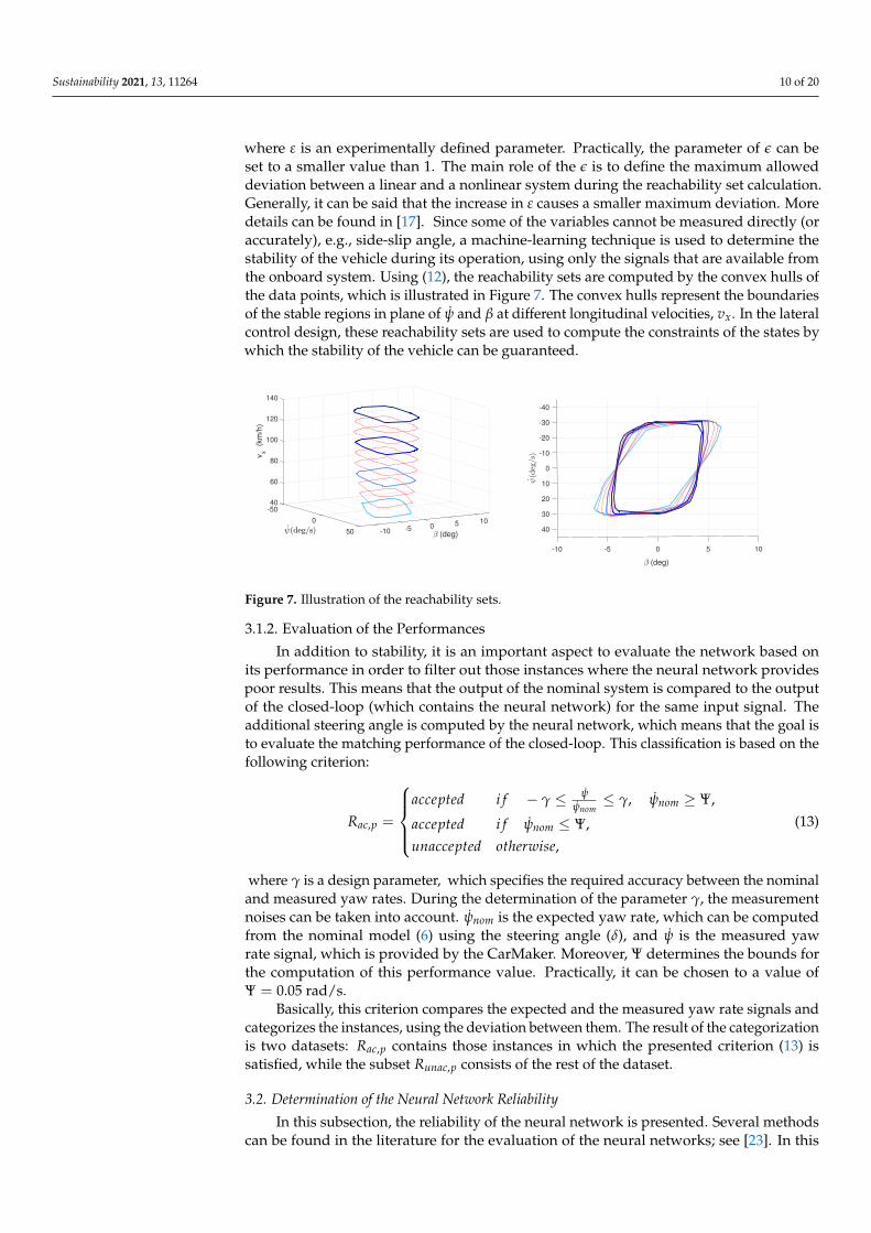
where ε is an experimentally defined parameter. Practically, the parameter of ε can beset to a smaller value than 1. The main role of the ε is to define the maximum alloweddeviation between a linear and a nonlinear system during the reachability set calculation.Generally, it can be said that the increase in ε causes a smaller maximum deviation. Moredetails can be found in [17]. Since some of the variables cannot be measured directly (oraccurately), e.g., side-slip angle, a machine-learning technique is used to determine thestability of the vehicle during its operation, using only the signals that are available fromthe onboard system. Using (12), the reachability sets are computed by the convex hulls ofthe data points, which is illustrated in Figure 7. The convex hulls represent the boundariesof the stable regions in plane of ψ and β at different longitudinal velocities, vx. In the lateralcontrol design, these reachability sets are used to compute the constraints of the states bywhich the stability of the vehicle can be guaranteed.

40

60

-50

80

vx

(km

/h)

100

120

140

(deg)

0 1050-5-1050

(deg)

-10 -5 0 5 10

40

-40

-30

-20

-10

0

10

20

30

Figure 7. Illustration of the reachability sets.

3.1.2. Evaluation of the Performances

In addition to stability, it is an important aspect to evaluate the network based onits performance in order to filter out those instances where the neural network providespoor results. This means that the output of the nominal system is compared to the outputof the closed-loop (which contains the neural network) for the same input signal. Theadditional steering angle is computed by the neural network, which means that the goal isto evaluate the matching performance of the closed-loop. This classification is based on thefollowing criterion:

Rac,p =

accepted i f − γ ≤ ψ

ψnom≤ γ, ψnom ≥ Ψ,

accepted i f ψnom ≤ Ψ,unaccepted otherwise,

(13)

where γ is a design parameter, which specifies the required accuracy between the nominaland measured yaw rates. During the determination of the parameter γ, the measurementnoises can be taken into account. ψnom is the expected yaw rate, which can be computedfrom the nominal model (6) using the steering angle (δ), and ψ is the measured yawrate signal, which is provided by the CarMaker. Moreover, Ψ determines the bounds forthe computation of this performance value. Practically, it can be chosen to a value ofΨ = 0.05 rad/s.

Basically, this criterion compares the expected and the measured yaw rate signals andcategorizes the instances, using the deviation between them. The result of the categorizationis two datasets: Rac,p contains those instances in which the presented criterion (13) issatisfied, while the subset Runac,p consists of the rest of the dataset.

3.2. Determination of the Neural Network Reliability

In this subsection, the reliability of the neural network is presented. Several methodscan be found in the literature for the evaluation of the neural networks; see [23]. In this

Sustainability 2021, 13, 11264 11 of 20

paper, the reliability analysis means that based on the measurable states of the vehicle,it is determined whether the network provides appropriate results or not. In this analysisprocess, the stability regions of the system are also taken into account indirectly.

The analysis is based on the previously calculated dataset, which is sorted into subsets.The goal of the reliability analysis is to examine, in a given operating range of the system,whether the neural network satisfies the requirements for stability and performance or not.Using this information, it is decided whether the additional term (output of the network) isadded to the control input or not. The main role of this process is to increase performancein regions where the network gives appropriate results and avoid the cases where theresults of the network may decrease the performance or stability.

During the reliability analysis of the neural network, all of the measurable data areused, which is detailed in Section 2. Firstly, the whole dataset is divided into two sets interms of stability (Rac,s), using (11) and (12). Secondly, two subsets are created, taking intoaccount the performance of the closed-loop using the neural network (Rac,p). Furthermore,the performance and the stability of the system must be guaranteed at the same time.This means that the given data point is considered to be accepted if it satisfies both of theconditions (stability and performances). Based on the created subsets, the acceptable datacan be determined, using the following expression:

R =

Rac, Rac,s ∧ Rac,p

Runac, otherwise(14)

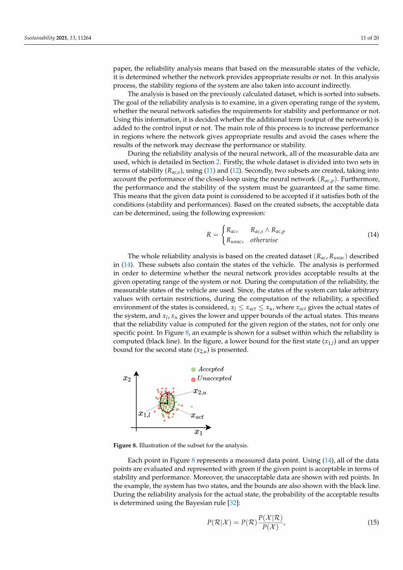
The whole reliability analysis is based on the created dataset (Rac, Runac) describedin (14). These subsets also contain the states of the vehicle. The analysis is performedin order to determine whether the neural network provides acceptable results at thegiven operating range of the system or not. During the computation of the reliability, themeasurable states of the vehicle are used. Since, the states of the system can take arbitraryvalues with certain restrictions, during the computation of the reliability, a specifiedenvironment of the states is considered, xl ≤ xact ≤ xu, where xact gives the actual states ofthe system, and xl , xu gives the lower and upper bounds of the actual states. This meansthat the reliability value is computed for the given region of the states, not for only onespecific point. In Figure 8, an example is shown for a subset within which the reliability iscomputed (black line). In the figure, a lower bound for the first state (x1,l) and an upperbound for the second state (x2,u) is presented.

Figure 8. Illustration of the subset for the analysis.

Each point in Figure 8 represents a measured data point. Using (14), all of the datapoints are evaluated and represented with green if the given point is acceptable in terms ofstability and performance. Moreover, the unacceptable data are shown with red points. Inthe example, the system has two states, and the bounds are also shown with the black line.During the reliability analysis for the actual state, the probability of the acceptable resultsis determined using the Bayesian rule [32]:

P(R|X ) = P(R)P(X |R)P(X )

, (15)

Sustainability 2021, 13, 11264 12 of 20

where P(R|X ) gives the probability of the acceptable results, if the states are X ∈[xact − xl , xact + xu]. The goodness of the neural network can be given by P(R) term,which gives the rate of the acceptable data in the saved dataset. Finally, P(X ) specifies aprobability value that expresses how often the system is within the given operating range.The reliability of the neural network is computed by (15).

However, the determination of the optimal bounds (xl , xu) can be challenging for eachstate. For the determination of the optimal bounds, a clustering algorithm is used. Thegoal is to find the subsets within which the probability value does not change significantly.The subsets are calculated using the k-medoids clustering algorithm [33]. During thedetermination of the sets, the following cost function must be minimized:

J =N

∑i=1

Kj

∑j=1|xj − ci|, (16)

where ci gives the center of the ith set, and xj is the jth point in the ith set. Ki denotes thenumber of the elements in the given set, and N is the number of sets. The number of setsshould be increased until the probabilities of any subset within a given set are nearly equalto the probability values calculated for the given set.

ζ−P(Xi|Ri)

P(Xi)≤

P(Xi,l |Ri,l)

P(Xi,l)≤ ζ+

P(Xi|Ri)

P(Xi), (17)

Xi,l ⊆ Xi ∀i, l,

where (ζ−, ζ+) defines the lower and upper bounds of the maximum deviation. Thecomputation of the probabilities in real-time application cannot be achieved, due to thehigh amount of data. In order to meet this criterion, based on the results of (15), a piecewiselinear function is determined:

fP(x) =

P(Xi |Ri)P(Xi)

, x ∈ Xi

0, otherwise.(18)

where Xi gives the ith subset, created by the clustering algorithm. Practically, this meansthat between two data points, the probability value is calculated, using interpolation.

Based on the proposed algorithm, the reliability of the neural network can be investi-gated. The reliability values contain the following three issues at the same time:

• The result of the network is not used in the range where its reliability is low (perfor-mances and stability).

• The result of the network is not used in the range where no training data are savedduring the data collection process.

• Indirectly, sensor failure or an incorrect measurement sequence can be considered.

In summary, the goal is to determine the reliability of the neural network at the givenoperating point. In the cases when the reliability of the network is low, the additionalsteering angle is considered to be zero in order to avoid the instability and low performanceof the system.

Finally, the whole algorithm is summarized in Figure 9. The additional steering angle(∆δ) is provided by the machine learning–based algorithm, by which the closed-loopmatching is performed. Note that the neural network uses only those signals, which areavailable from the onboard system (see Section 2). Moreover, the checking of the additionalcontrol signal resulting from the machine learning algorithm is an important step to main-tain stability. A data-driven approach is also applied to determine the reachability sets ofthe vehicle (ψmax, βmax), which is detailed in Section 3. During the reference signal genera-tion, these sets are also taken into account. Furthermore, the reference signal is generatedusing only the nominal model of the system, which is detailed in Appendix A. Finally,the lateral controller is designed using only the nominal model of the nonlinear system.

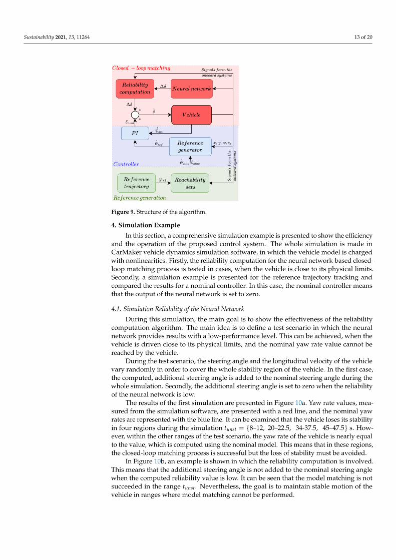
Sustainability 2021, 13, 11264 13 of 20

+

+

Figure 9. Structure of the algorithm.

4. Simulation Example

In this section, a comprehensive simulation example is presented to show the efficiencyand the operation of the proposed control system. The whole simulation is made inCarMaker vehicle dynamics simulation software, in which the vehicle model is chargedwith nonlinearities. Firstly, the reliability computation for the neural network-based closed-loop matching process is tested in cases, when the vehicle is close to its physical limits.Secondly, a simulation example is presented for the reference trajectory tracking andcompared the results for a nominal controller. In this case, the nominal controller meansthat the output of the neural network is set to zero.

4.1. Simulation Reliability of the Neural Network

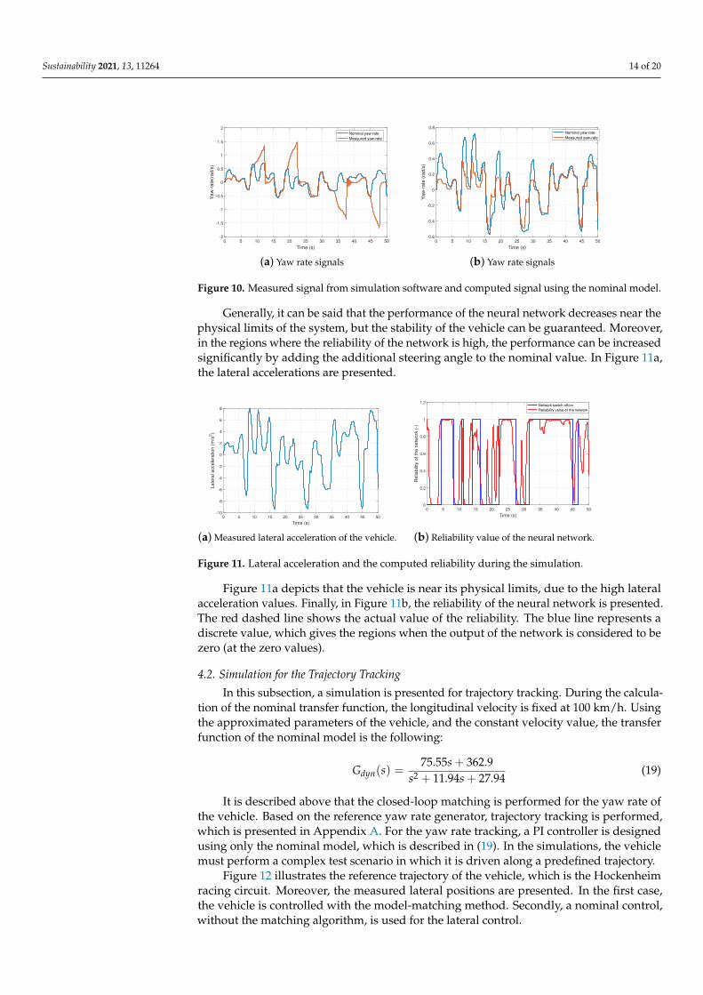
During this simulation, the main goal is to show the effectiveness of the reliabilitycomputation algorithm. The main idea is to define a test scenario in which the neuralnetwork provides results with a low-performance level. This can be achieved, when thevehicle is driven close to its physical limits, and the nominal yaw rate value cannot bereached by the vehicle.

During the test scenario, the steering angle and the longitudinal velocity of the vehiclevary randomly in order to cover the whole stability region of the vehicle. In the first case,the computed, additional steering angle is added to the nominal steering angle during thewhole simulation. Secondly, the additional steering angle is set to zero when the reliabilityof the neural network is low.

The results of the first simulation are presented in Figure 10a. Yaw rate values, mea-sured from the simulation software, are presented with a red line, and the nominal yawrates are represented with the blue line. It can be examined that the vehicle loses its stabilityin four regions during the simulation tunst = 8–12, 20–22.5, 34-37.5, 45–47.5 s. How-ever, within the other ranges of the test scenario, the yaw rate of the vehicle is nearly equalto the value, which is computed using the nominal model. This means that in these regions,the closed-loop matching process is successful but the loss of stability must be avoided.

In Figure 10b, an example is shown in which the reliability computation is involved.This means that the additional steering angle is not added to the nominal steering anglewhen the computed reliability value is low. It can be seen that the model matching is notsucceeded in the range tunst. Nevertheless, the goal is to maintain stable motion of thevehicle in ranges where model matching cannot be performed.

Sustainability 2021, 13, 11264 14 of 20

0 5 10 15 20 25 30 35 40 45 50

Time (s)

-2

-1.5

-1

-0.5

0

0.5

1

1.5

2

Yaw

-rate

(rad/s

)

Nominal yaw-rate

Measured yaw-rate

(a) Yaw rate signals

0 5 10 15 20 25 30 35 40 45 50

Time (s)

-0.6

-0.4

-0.2

0

0.2

0.4

0.6

0.8

Yaw

-rate

(ra

d/s

)

Nominal yaw-rate

Measured yaw-rate

(b) Yaw rate signals

Figure 10. Measured signal from simulation software and computed signal using the nominal model.

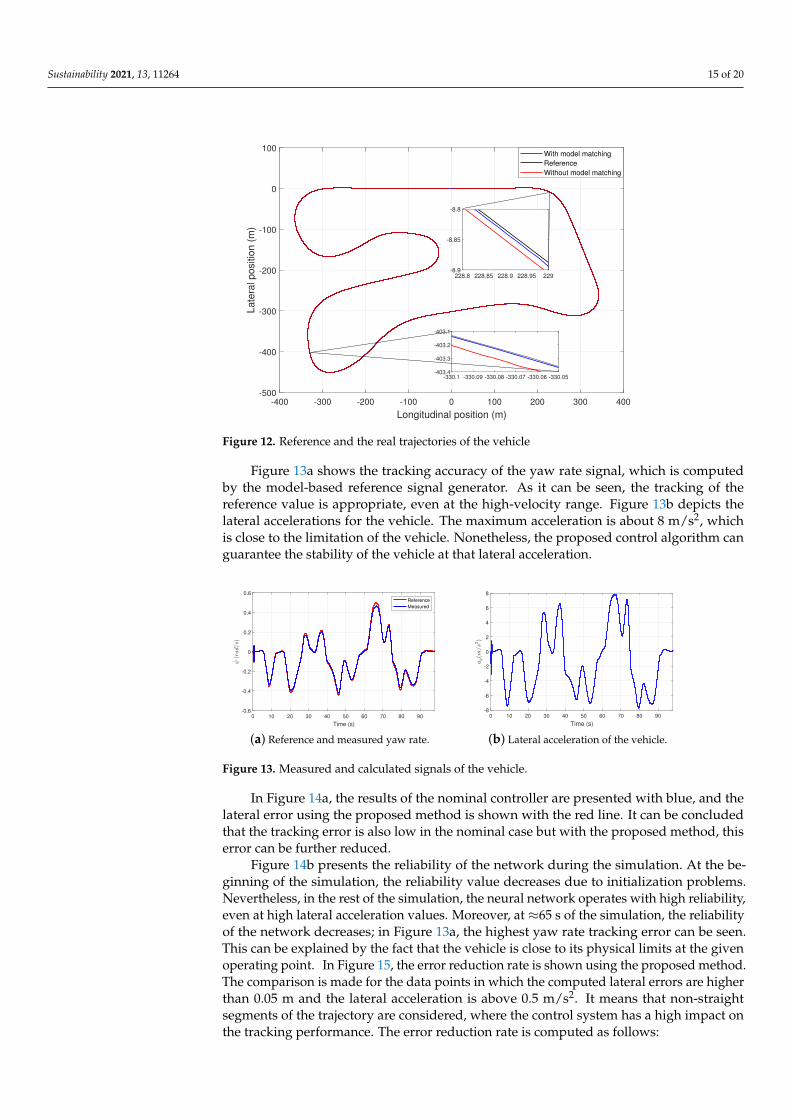
Generally, it can be said that the performance of the neural network decreases near thephysical limits of the system, but the stability of the vehicle can be guaranteed. Moreover,in the regions where the reliability of the network is high, the performance can be increasedsignificantly by adding the additional steering angle to the nominal value. In Figure 11a,the lateral accelerations are presented.

0 5 10 15 20 25 30 35 40 45 50

Time (s)

-10

-8

-6

-4

-2

0

2

4

6

8

Late

ral accele

ration (

m/s

2)

(a) Measured lateral acceleration of the vehicle.

0 5 10 15 20 25 30 35 40 45 50

Time (s)

0

0.2

0.4

0.6

0.8

1

1.2

Re

liab

ility

of

the

ne

two

rk (

-)

Network switch off/on

Reliability value of the network

(b) Reliability value of the neural network.

Figure 11. Lateral acceleration and the computed reliability during the simulation.

Figure 11a depicts that the vehicle is near its physical limits, due to the high lateralacceleration values. Finally, in Figure 11b, the reliability of the neural network is presented.The red dashed line shows the actual value of the reliability. The blue line represents adiscrete value, which gives the regions when the output of the network is considered to bezero (at the zero values).

4.2. Simulation for the Trajectory Tracking

In this subsection, a simulation is presented for trajectory tracking. During the calcula-tion of the nominal transfer function, the longitudinal velocity is fixed at 100 km/h. Usingthe approximated parameters of the vehicle, and the constant velocity value, the transferfunction of the nominal model is the following:

Gdyn(s) =75.55s + 362.9

s2 + 11.94s + 27.94(19)

It is described above that the closed-loop matching is performed for the yaw rate ofthe vehicle. Based on the reference yaw rate generator, trajectory tracking is performed,which is presented in Appendix A. For the yaw rate tracking, a PI controller is designedusing only the nominal model, which is described in (19). In the simulations, the vehiclemust perform a complex test scenario in which it is driven along a predefined trajectory.

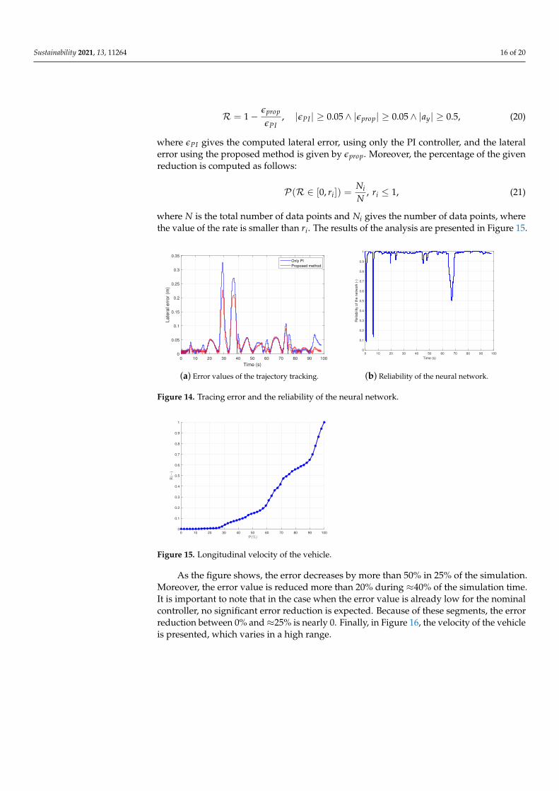
Figure 12 illustrates the reference trajectory of the vehicle, which is the Hockenheimracing circuit. Moreover, the measured lateral positions are presented. In the first case,the vehicle is controlled with the model-matching method. Secondly, a nominal control,without the matching algorithm, is used for the lateral control.

Sustainability 2021, 13, 11264 15 of 20

-400 -300 -200 -100 0 100 200 300 400

Longitudinal position (m)

-500

-400

-300

-200

-100

0

100

Late

ral positio

n (

m)

With model matching

Reference

Without model matching

-330.1 -330.09 -330.08 -330.07 -330.06 -330.05-403.4

-403.3

-403.2

-403.1

228.8 228.85 228.9 228.95 229-8.9

-8.85

-8.8

Figure 12. Reference and the real trajectories of the vehicle

Figure 13a shows the tracking accuracy of the yaw rate signal, which is computedby the model-based reference signal generator. As it can be seen, the tracking of thereference value is appropriate, even at the high-velocity range. Figure 13b depicts thelateral accelerations for the vehicle. The maximum acceleration is about 8 m/s2, whichis close to the limitation of the vehicle. Nonetheless, the proposed control algorithm canguarantee the stability of the vehicle at that lateral acceleration.

0 10 20 30 40 50 60 70 80 90

Time (s)

-0.6

-0.4

-0.2

0

0.2

0.4

0.6

Reference

Measured

(a) Reference and measured yaw rate.

0 10 20 30 40 50 60 70 80 90

Time (s)

-8

-6

-4

-2

0

2

4

6

8

(b) Lateral acceleration of the vehicle.

Figure 13. Measured and calculated signals of the vehicle.

In Figure 14a, the results of the nominal controller are presented with blue, and thelateral error using the proposed method is shown with the red line. It can be concludedthat the tracking error is also low in the nominal case but with the proposed method, thiserror can be further reduced.

Figure 14b presents the reliability of the network during the simulation. At the be-ginning of the simulation, the reliability value decreases due to initialization problems.Nevertheless, in the rest of the simulation, the neural network operates with high reliability,even at high lateral acceleration values. Moreover, at ≈65 s of the simulation, the reliabilityof the network decreases; in Figure 13a, the highest yaw rate tracking error can be seen.This can be explained by the fact that the vehicle is close to its physical limits at the givenoperating point. In Figure 15, the error reduction rate is shown using the proposed method.The comparison is made for the data points in which the computed lateral errors are higherthan 0.05 m and the lateral acceleration is above 0.5 m/s2. It means that non-straightsegments of the trajectory are considered, where the control system has a high impact onthe tracking performance. The error reduction rate is computed as follows:

Sustainability 2021, 13, 11264 16 of 20

R = 1−εprop

εPI, |εPI | ≥ 0.05∧ |εprop| ≥ 0.05∧ |ay| ≥ 0.5, (20)

where εPI gives the computed lateral error, using only the PI controller, and the lateralerror using the proposed method is given by εprop. Moreover, the percentage of the givenreduction is computed as follows:

P(R ∈ [0, ri]) =NiN

, ri ≤ 1, (21)

where N is the total number of data points and Ni gives the number of data points, wherethe value of the rate is smaller than ri. The results of the analysis are presented in Figure 15.

0 10 20 30 40 50 60 70 80 90 100

Time (s)

0

0.05

0.1

0.15

0.2

0.25

0.3

0.35

Late

ral err

or

(m)

Only PI

Proposed method

(a) Error values of the trajectory tracking.

0 10 20 30 40 50 60 70 80 90 100

Time (s)

0

0.1

0.2

0.3

0.4

0.5

0.6

0.7

0.8

0.9

1

Relia

bili

ty o

f th

e n

etw

ork

(-)

(b) Reliability of the neural network.

Figure 14. Tracing error and the reliability of the neural network.

0 10 20 30 40 50 60 70 80 90 100

0

0.1

0.2

0.3

0.4

0.5

0.6

0.7

0.8

0.9

1

Figure 15. Longitudinal velocity of the vehicle.

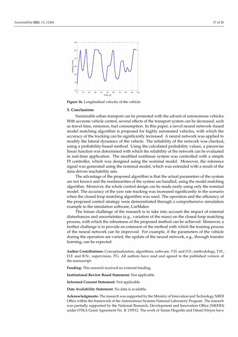
As the figure shows, the error decreases by more than 50% in 25% of the simulation.Moreover, the error value is reduced more than 20% during ≈40% of the simulation time.It is important to note that in the case when the error value is already low for the nominalcontroller, no significant error reduction is expected. Because of these segments, the errorreduction between 0% and≈25% is nearly 0. Finally, in Figure 16, the velocity of the vehicleis presented, which varies in a high range.

Sustainability 2021, 13, 11264 17 of 20

0 10 20 30 40 50 60 70 80 90 100

Time (s)

10

15

20

25

30

35

40

Ve

locity (

m/s

)

Figure 16. Longitudinal velocity of the vehicle.

5. Conclusions

Sustainable urban transport can be promoted with the advent of autonomous vehicles.With accurate vehicle control, several effects of the transport system can be decreased, suchas travel time, emission, fuel consumption. In this paper, a novel neural network–basedmodel matching algorithm is proposed for highly automated vehicles, with which theaccuracy of the tracking can be significantly increased. A neural network was applied tomodify the lateral dynamics of the vehicle. The reliability of the network was checked,using a probability-based method. Using the calculated probability values, a piecewiselinear function was determined with which the reliability of the network can be evaluatedin real-time application. The modified nonlinear system was controlled with a simplePI controller, which was designed using the nominal model. Moreover, the referencesignal was generated using the nominal model, which was extended with a result of thedata-driven reachability sets.

The advantage of the proposed algorithm is that the actual parameters of the systemare not known and the nonlinearities of the system are handled, using the model matchingalgorithm. Moreover, the whole control design can be made easily using only the nominalmodel. The accuracy of the yaw rate tracking was increased significantly in the scenariowhen the closed-loop matching algorithm was used. The operation and the efficiency ofthe proposed control strategy were demonstrated through a comprehensive simulationexample in the simulation software, CarMaker.

The future challenge of the research is to take into account the impact of externaldisturbances and uncertainties (e.g., variation of the mass) on the closed-loop matchingprocess, with which the robustness of the proposed method can be achieved. Moreover, afurther challenge is to provide an extension of the method with which the training processof the neural network can be improved. For example, if the parameters of the vehicleduring the operation are varied, the update of the neural network, e.g., through transferlearning, can be expected.

Author Contributions: Conceptualization, algorithms, software, T.H. and D.F.; methodology, T.H.,D.F. and B.N.; supervision, P.G. All authors have read and agreed to the published version ofthe manuscript.

Funding: This research received no external funding.

Institutional Review Board Statement: Not applicable.

Informed Consent Statement: Not applicable.

Data Availability Statement: No data is available.

Acknowledgments: The research was supported by the Ministry of Innovation and Technology NRDIOffice within the framework of the Autonomous Systems National Laboratory Program. The researchwas partially supported by the National Research, Development and Innovation Office (NKFIH)under OTKA Grant Agreement No. K 135512. The work of Tamás Hegedus and Dániel Fényes have

Sustainability 2021, 13, 11264 18 of 20

been supported by the ÚNKP-21-3 New National Excellence Program of the Ministry for Innovationand Technology from the source of the National Research, Development and Innovation Fund.

Conflicts of Interest: The authors declare no conflict of interest.

Appendix A. Determination of the Reference Signal

In the following, the model-based reference signal generation is presented. In thispaper, the output of nonlinear is matched to the linear one with respect to the yaw rate.However, in many cases, the goal is to follow the predefined path during lateral controlof the vehicle. In this section, the reference signal generation is presented in which thenominal model is taken into account. Using (1) and (2), a state-space representation can bedetermined in the following form:

x = Ax + Bu (A1)

where A and B are matrices, u = δ is the steering angle and the states are x = [vy y ψ ψ]T ,where vy gives the lateral velocity of the vehicle. However, during the reference signalgeneration, a discrete model is needed, which can be formed as follows:

x(k + 1) = φx(k) + Γu(k),

y(k) = Cx(k),(A2)

where φ = eATs and Γ =(k+1)Ts∫

kTs

eA((K+1)Ts−τ)Bdτ, where Ts is a sampling time. The main

role of the model-based reference generation is to compute the reference yaw rate for thevehicle, which is tracked by the vehicle. The vehicle motion can be predicted, and the goalis to guarantee the tracking of the reference trajectory. Using (A2), the lateral position ofthe vehicle is predicted along the predefined time horizon (n):

yp(k, n) =

y(k + 1)y(k + 2)

...y(k + n)

=

CφCφ2

...Cφn

︸ ︷︷ ︸A

x(k)+

+

CΓ 0 · · · 0

CφΓ CΓ · · · 0...

. . . . . ....

Cφn−1Γ CφΓ · · · CΓ

︸ ︷︷ ︸

B

u(k)

u(k + 1)...

u(k + n− 1)

.

(A3)

In this case, the input vector of the system is defined as follows:

U = [u(k), u(k + 1)...u(k− 1 + n)]T = [ω1, ω2...ωn]Tun (A4)

where ωi gives the weight for the ith input signal. Using (A3) and (A4), the reference signalfor the vehicle can be computed as follows:

un = B−1Ω−T(yp(k, n)−Ax(k)) (A5)

where the reference trajectory is defined by the (yp(k, n)) vector and the actual states of thevehicle are given by x(k). Moreover, Ω gives the weights for the given time horizon.

During the computation, the reachability sets can be also taken into account, whichserves the stability of the vehicle. This means that the states can be saturated, using thereachability sets. During the computation of the lateral error, the motion of the vehicle is

Sustainability 2021, 13, 11264 19 of 20

predicted in order to decrease the lateral error during the tracking. Based on the actualstates of the vehicle, the predicted error value can be computed as follows:

xe(t + Tp) = R(xp, yp)− (y(t) + v(t)cos(ψ(t))Tp) (A6)

ye(t + Tp) = R(xp, yp)− (y(t) + v(t)sin(ψ(t))Tp) (A7)

where Tp denotes the length of the prediction and R is the reference position at the givenstate of the vehicle. In this paper, the value of the prediction is set to Tp = 0.2 s. Using thepredicted error and (A5), the goal is to compute a yaw rate sequence with which the lateralerror of the vehicle is zero at the end of the n horizon length.

References1. Das, S.; Sekar, A.; Chen, R.; Kim, H.C.; Wallington, T.J.; Williams, E. Impacts of Autonomous Vehicles on Consumers Time-Use

Patterns. Challenges 2017, 8, 32. [CrossRef]2. Bissell, D.; Birtchnell, T.; Elliott, A.; Hsu, E.L. Autonomous automobilities: The social impacts of driverless vehicles. Curr. Sociol.

2020, 68, 116–134. [CrossRef]3. Treiber, M.; Kesting, A.; Thiemann, C. How Much Does Traffic Congestion Increase Fuel Consumption and Emissions? Applying

Fuel Consumption Model to NGSIM Trajectory Data. In Proceedings of the 87th Annual Meeting of the Transportation ResearchBoard, Washington, DC, USA, 13–17 January 2008.

4. Barth, M.; Boriboonsomsin, K. Real-World Carbon Dioxide Impacts of Traffic Congestion. Transp. Res. Rec. 2008, 2058, 163–171.[CrossRef]

5. Wadud, Z.; MacKenzie, D.; Leiby, P. Help or hindrance? The travel, energy and carbon impacts of highly automated vehicles.Transp. Res. Part Policy Pract. 2016, 86, 1–18. [CrossRef]

6. Fan, R.; Jiao, J.; Ye, H.; Yu, Y.; Pitas, I.; Liu, M. Key Ingredients of Self-Driving Cars. arXiv 2019, arXiv:1906.02939.7. Isidori, A. Nonlinear Control Systems; Springer: Berlin/Heidelberg, Germany, 1995.8. Leith, D.J.; Leithead, W.E. Survey of gain-scheduling analysis and design. Taylor Fr. 2000, 73, 1001–1025. [CrossRef]9. Fenyes, D.; Nemeth, B.; Gaspar, P. LPV-based autonomous vehicle control using the results of big data analysis on lateral

dynamics. In Proceedings of the 2020 American Control Conference (ACC), Denver, CO, USA, 1–3 July 2020; pp. 2250–2255.10. Tan, W.; Packard, A. Stability Region Analysis Using Polynomial and Composite Polynomial Lyapunov Functions and

Sum-of-Squares Programming. IEEE Trans. Autom. Control 2008, 53, 565–571. [CrossRef]11. Jarvis-Wloszek, Z.; Feeley, R.; Tan, W.; Sun, K.; Packard, A. Some controls applications of sum of squares programming.

In Proceedings of the 42nd IEEE International Conference on Decision and Control (IEEE Cat. No.03CH37475), Maui, HI, USA,9–12 December 2003.

12. Allgöwer, F.; Findeisen, R.; Nagy, Z. Nonlinear Model Predictive Control: From Theory to Application. J. Chin. Inst. Chem. Eng.2004, 35, 299–315.

13. Nemeth, B.; Gaspar, P.; Peni, T. Nonlinear analysis of vehicle control actuations based on controlled invariant sets. Int. J. Appl.Math. Comput. Sci. 2016, 26, 31–43. [CrossRef]

14. Khalil, H.K. Nonlinear Systems, 3rd ed.; Prentice Hall: Hoboken, NJ, USA, 1997.15. Voosi, H. Nonlinear control of a quadrotor micro-UAV using feedback-linearization. In Proceedings of the 2009 IEEE Interna-

tional Conference on Mechatronics, Malaga, Spain, 14–17 April 2009; pp. 21–40.16. Pushkov, S.G. Inversion of Linear Systems on the Basis of State Space Realization. J. Comput. Syst. Sci. Int. 2017, 57, 7–17.

[CrossRef]17. Fenyes, D.; Nemeth, B.; Gaspar, P. Impact of big data on the design of MPC control for autonomous vehicles. In Proceedings of

the 2019 18th European Control Conference (ECC), Naples, Italy, 25–28 June 2019; pp. 4154–4159.18. Yesildirek, A.; Lewis, F.L. Feedback linearization using neural networks. Automatica 1995, 31, 1659–1664. [CrossRef]19. Pedro, J.O.; Dangor, M.; A.Dahunsi, O.; Ali, M.M. Dynamic neural network-based feedback linearization control of full-car

suspensions using PSO. Appl. Soft Comput. 2018, 70, 723–736. [CrossRef]20. John, S.; Pedroi, J. Neural Network-Based Adaptive Feedback Linearization Control of Antilock Braking System. Int. J. Artif.

Intell. 2013, 10, 21–40.21. Westenbroek, T.; Fridovich-Keil, D.; Mazumdar, E.; Arora, S.; Prabhu, V.; Sastry, S.S.; Tomlin, C.J. Feedback Linearization for

Unknown Systems via Reinforcement Learning. arXiv 2020, arXiv:1910.13272.22. Castaneda, F.; Wulfman, M.; Agrawal, A.; Westenbroek, T.; Tomlin, C.J.; Sastry, S.S.; Sreenath, K. Improving Input-Output

Linearizing Controllers for Bipedal Robots via Reinforcement Learning. arXiv 2020, arXiv:2004.07276.23. Burton, R.M.; Faris, W.G. Reliable evaluation of neural networks. Neural Netw. 1991, 4, 411–415. [CrossRef]24. Rajamani, R. Vehicle Dynamics and Control; Springer: Berlin/Heidelberg, Germany, 2005.25. Mortazavizadeh, S.A.; Ghaderi, A.; Ebrahimi, M.; Hajian, M. Recent Developments in the Vehicle Steer-by-Wire System.

IEEE Trans. Transp. Electrif. 2020, 6, 1226–1235. [CrossRef]

Sustainability 2021, 13, 11264 20 of 20

26. Shamash, Y. Construction of the inverse of linear time-invariant multivariable systems. Int. J. Syst. Sci. 1975, 6, 733–740.[CrossRef]

27. Devasia, S.; Paden, B. Stable inversion for nonlinear nonminimum-phase time-varying systems. IEEE Trans. Autom. Control1998, 43, 283–288. [CrossRef]

28. Malinen, J. Tustin’s method for final state approximation of conservative dynamical systems. IFAC Proc. Vol. 2011, 44, 4564–4569.[CrossRef]

29. Demut, H.; Hagan, M.; Beale, M. Neural Network Design; PWS Publishing Co.: Boston, MA, USA, 1997.30. The MathWorks Inc. Deep Learning Toolbox; The MathWorks Inc.: Natick, MA, USA, 2018.31. Boyd, S.; Ghaoui, L.E.; Feron, E.; Balakrishnan, V. Linear Matrix Inequalities in System and Control Theory; Society for Industrial

and Applied Mathematics: Philadelphia, PA, USA, 1997.32. Bolstad, W.M. Introduction to Bayesian Statistics; John Wiley and Sons, Ltd.: Hoboken, NJ, USA, 2007.33. Schubert, E.; Rousseeuw, P.J. Faster k-Medoids Clustering: Improving the PAM, CLARA, and CLARANS Algorithms. In Lecture

Notes in Computer Science; Springer: Cham, Germany, 2019; pp. 171–187.