Improvements to A-Priori

1

Improvements to A-Priori

Park-Chen-Yu Algorithm

Multistage Algorithm

Approximate Algorithms

2

PCY Algorithm During Pass 1 of A-priori, most memory is idle. Use that memory to keep counts of buckets into

which the pairs of items are hashed. Just the count, not the pairs themselves.

Gives extra condition that candidate pairs must satisfy on Pass 2.

3

PCY – Pass 1

Hashtable

Item counts

Pass 1

FOR (each basket) {

FOR (each item)

add 1 to item’s count;

FOR (each pair of items) {

hash the pair to a bucket;

add 1 to the count for that bucket

}

}

4

Observations About Buckets1. If a bucket contains a frequent pair, then the bucket is

surely frequent. We cannot use the hash table to eliminate any member

of this bucket.

2. Even without any frequent pair, a bucket can be frequent.

Again, nothing in the bucket can be eliminated.

3. But in the best case, the count for a bucket is less than the support s.

Now, all pairs that hash to this bucket can be eliminated as candidates, even if the pair consists of two frequent items.

5

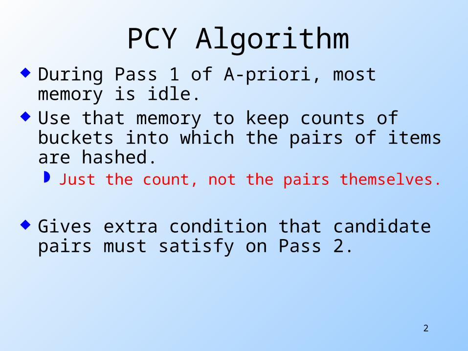
PCY Algorithm – Between Passes

Replace the buckets by a bit-vector: 1 means the bucket

count exceeds the support s (a frequent bucket );

0 means it did not.

4-byte integers are replaced by bits, so the bit-vector requires 1/32 of memory.

Hashtable

Item counts

Bitmap

Pass 1 Pass 2

Frequent items

Counts ofcandidate pairs

6

PCY Algorithm – Pass 2

Count all pairs {i, j } that meet the conditions:1. Both i and j are frequent items.2. The pair {i, j }, hashes to a bucket number

whose bit in the bit vector is 1.

Notice both these conditions are necessary for the pair to have a chance of being frequent.

7

Memory Details

Hash table requires buckets of 2-4 bytes. Number of buckets thus almost 1/4-1/2 of the

number of bytes of main memory.

On second pass, a table of (item, item, count) triples is essential. Thus, hash table must eliminate 2/3 of the

candidate pairs to beat a-priori with triangular matrix for counts.

8

Multistage Algorithm It might happen that even after hashing there are

still too many surviving pairs and the main memory isn't sufficient to hold their counts.

Key idea: After Pass 1 of PCY, rehash only those pairs that qualify for Pass 2 of PCY. Using a different hash function!

On middle pass, fewer pairs contribute to buckets, so fewer false positives –frequent buckets with no frequent pair.

9

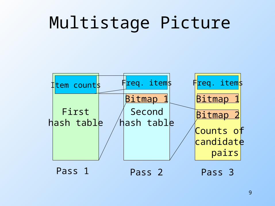
Multistage Picture

Firsthash table

Secondhash table

Item counts

Bitmap 1 Bitmap 1

Bitmap 2

Freq. items Freq. items

Counts ofcandidate pairs

Pass 1 Pass 2 Pass 3

10

Multistage – Pass 3

Count only those pairs {i, j } that satisfy:1. Both i and j are frequent items.2. Using the first hash function, the pair hashes

to a bucket whose bit in the first bit-vector is 1.

3. Using the second hash function, the pair hashes to a bucket whose bit in the second bit-vector is 1.

11

Multihash

Key idea: use several independent hash tables on the first pass.

Risk: halving the number of buckets doubles the average count. We have to be sure most buckets will still not reach count s.

If so, we can get a benefit like multistage, but in only 2 passes.

12

Multihash Picture

First hashtable

Secondhash table

Item counts

Bitmap 1

Bitmap 2

Freq. items

Counts ofcandidate pairs

Pass 1 Pass 2

13

Extensions Either multistage or multihash can use more than

two hash functions.

In multistage, there is a point of diminishing returns, since the bit-vectors eventually consume all of main memory.

For multihash, too many hash functions makes all counts > s.

14

All (Or Most) Frequent Itemsets In < 2 Passes

Simple algorithm. SON (Savasere, Omiecinski, and Navathe). Toivonen.

15

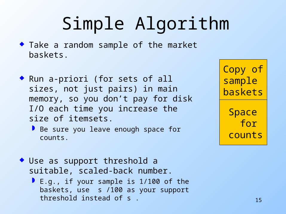
Simple Algorithm Take a random sample of the market

baskets.

Run a-priori (for sets of all sizes, not just pairs) in main memory, so you don’t pay for disk I/O each time you increase the size of itemsets. Be sure you leave enough space for

counts.

Use as support threshold a suitable, scaled-back number. E.g., if your sample is 1/100 of the

baskets, use s /100 as your support threshold instead of s .

Copy ofsamplebaskets

Space forcounts

16

Simple Algorithm – Option

Optionally, verify that your guesses are truly frequent in the entire data set by a second pass.

But you don’t catch sets frequent in the whole but not in the sample.

17

SON Algorithm – (1) Repeatedly read small subsets of the baskets into main

memory and perform the first pass of the simple algorithm on each subset.

An itemset becomes a candidate if it is found to be frequent in any one or more subsets of the baskets.

On a second pass, count all the candidate itemsets and determine which are frequent in the entire set.

Key “monotonicity” idea: an itemset cannot be frequent in the entire set of baskets unless it is frequent in at least one subset.

18

SON Algorithm – Distributed Version

This idea lends itself to distributed data mining.

If baskets are distributed among many nodes, compute frequent itemsets at each node, then distribute the candidates from each node.

Finally, accumulate the counts of all candidates.

19

Toivonen’s Algorithm – (1)

Start as in the simple algorithm, but lower the threshold slightly for the sample.

Example: if the sample is 1% of the baskets, use s /125 as the support threshold rather than s /100.

Goal is to avoid missing any itemset that is frequent in the full set of baskets.

20

Toivonen’s Algorithm – (2) Add to the itemsets that are frequent in the sample the

negative border of these itemsets.

An itemset is in the negative border if it is not deemed frequent in the sample, but all its immediate subsets are.

Example. ABCD is in the negative border if and only if it is not

frequent, but all of ABC, BCD, ACD, and ABD are. Also, a singleton which is not frequent in the sample is

in the negative border.

21

Toivonen’s Algorithm – (3)

In a second pass, count all candidate frequent itemsets from the first pass, and also count their negative border.

If no itemset from the negative border turns out to be frequent, then the candidates found to be frequent in the whole data are exactly the frequent itemsets.

22

Toivonen’s Algorithm – (4)

What if we find that something in the negative border is actually frequent?

We must start over again!

Try to choose the support threshold so the probability of failure is low, while the number of itemsets checked on the second pass fits in main-memory.

23

Theorem:

If there is an itemset that is frequent in the whole, but not frequent in the sample,

then there is a member of the negative border for the sample that is frequent in the whole.

24

Proof: Suppose not; i.e., there is an itemset S frequent in

the whole but Not frequent in the sample, and Not present in the sample’s negative border.

Let T be a smallest subset of S that is not frequent in the sample.

T is frequent in the whole (S is frequent, monotonicity).

T is in the negative border (else not “smallest”).

Remark. In order for the above proof to work, we will require that frequent singletons are first added to any sample.