Hao Zhao Improvements in seismic imaging and migration-velocity model building Thesis submitted for the degree of Philosophiae Doctor Department of Geosciences Faculty of Mathematics and Natural Sciences Group of petroleum geosciences Group of digital signal processing and image analysis (DSB) 2019

Welcome message from author
This document is posted to help you gain knowledge. Please leave a comment to let me know what you think about it! Share it to your friends and learn new things together.
Transcript

Hao Zhao
Improvements in seismic imagingand migration-velocity modelbuilding
Thesis submitted for the degree of Philosophiae Doctor
Department of GeosciencesFaculty of Mathematics and Natural Sciences
Group of petroleum geosciencesGroup of digital signal processing and image analysis (DSB)
2019

© Hao Zhao, 2020 Series of dissertations submitted to the Faculty of Mathematics and Natural Sciences, University of Oslo No. 2218 ISSN 1501-7710 All rights reserved. No part of this publication may be reproduced or transmitted, in any form or by any means, without permission. Cover: Hanne Baadsgaard Utigard. Print production: Reprosentralen, University of Oslo.

PrefaceThis thesis is submitted in partial fulfillment of the requirements for the degreeof Philosophiae Doctor at the University of Oslo. The research presented hereis conducted under the main supervision of Professor Leiv-J Gelius, AssociateProfessor Einar Iversen, and co-supervision of Professor Anne H. Schistad Sol-berg, Doctor Walter Söllner and Doctor Endrias Asgedom. This work is a partof a joint project, improved seismic imaging based on resolution enhancementand pattern recognition, which is cooperated between the Department of Geo-sciences and the Department of Informatics at the University of Oslo. Theproject is funded by the Norwegian Research Council under the Large pro-gram for petroleum research (PETROMAKS2) with the project number 234019.
The thesis is a collection of three papers, presented in chronological order.The common theme to them is in the methods to improve seismic imaging andmigration-velocity model building. The papers are preceded by an introductorychapter that relates them together and provides background information andmotivation for the work. One of the papers, I am the second author for the jointwork. For the remaining papers, I am the first author.
Acknowledgements
I would like to thank my supervisors for their support through my Ph.D. study.I am especially grateful to Prof. Leiv-J Gelius and Assoc. Prof. Einar Iversen fortheir good guidance and advice for my studies and researches. I would also like toextend my gratitude to Prof. Martin Tygel, Prof. Anne H. Schistad Solberg., Dr.Walter Söllner and Dr. Endrias Asgedom for their co-supervision and discussionsregarding my papers. I also specially thank Anders U. Waldeland for his goodcollaboration and valuable discussions in this project. I would also like to thankall the co-authors of the articles appended. During my Ph.D. study, I haveworked at both the Department of Geosciences and the Digital Signal Processingand Image Analysis Group in Department of Informatics, where I have obtainedthe great support for my study and research. I especially thank professor AnnikM Myhre, Professor Valerie Maupin, Michael Heeremans, Hans Peter Verneand Svein Bøe for your kind help of providing me the good environment for mystudy and arranging the necessary computing resource for conducting my work.Finally, I especially thank my parents and families for all the love and supportfor this journey.
Hao ZhaoOslo, December 2019
iii


List of PublicationsThis thesis is based on the following papers, referred to in the text by theirromain numbers(I-III):
Paper I
Fast and robust common-reflection-surface parameter estimation.
Anders U. Waldeland, Hao Zhao, Jorge H. Faccipieri, Anne H. Schistad Solberg,and Leiv-J. Gelius.
Geophysics VOL.83 NO.1 (2018), O1-O13
Paper II
3D Prestack Fourier Mixed-Domain (FMD) depth migration for VTI media withlarge lateral contrasts.
Hao Zhao, Leiv-J. Gelius, Martin Tygel, Espen Harris Nilsen, and AndreasKjelsrud Evensen.
Journal of Applied Geophysics VOL.168 (2019), 118-127
Paper III
Time-migration velocity estimation using Fréchet derivatives based on nonlinearkinematic migration/demigration solvers.
Hao Zhao, Anders U. Waldeland, Dany Rueda Serrano, Martin Tygel, andEinar Iversen.
Studia Geophysica et Geodaetica. Accepted for publication, November 2019
The published papers are reprinted with permission from Hao Zhao. All rightsreserved.
v


Related PublicationsThe following papers are related to the thesis but not included in their full text:
Paper I
A New Generalized Screen Propagator for Wave Equation Depth Migration.
Hao Zhao, Leiv-J. Gelius, and Martin Tygel.
Extended abstract 77th EAGE Conference and Exhibition , Madrid, 2015
Paper II
Time-migration Tomography based on Reflection Slopes in Pre-stack Time-migrated Seismic Data.
Hao Zhao, Anders U. Waldeland, Dany Rueda Serrano, Martin Tygel andEinar Iversen.
Extended abstract 80th EAGE Conference and Exhibition , Copenhagen, 2018
vii


Contents
Preface iii
List of Publications v
Related Publications vii
Contents ix
List of Figures xi
List of Tables xv
1 Introduction 11.1 Motivations . . . . . . . . . . . . . . . . . . . . . . . . . . 21.2 Scope of the thesis . . . . . . . . . . . . . . . . . . . . . . . 31.3 Thesis outline . . . . . . . . . . . . . . . . . . . . . . . . . 6
2 Structure tensor methods for a common reflection-surfacestack 72.1 Common reflection surface stack . . . . . . . . . . . . . . 72.2 Structure tensor methods . . . . . . . . . . . . . . . . . . . 13
3 Depth imaging with wavefield extrapolation migration 193.1 Overview of seismic migration imaging methods . . . . . . 193.2 Depth-migration methods . . . . . . . . . . . . . . . . . . . 223.3 Wavefield extrapolation and imaging condition . . . . . . . 253.4 One-way wave equation migration algorithms . . . . . . . . 273.5 3D prestack Fourier mixed-domain (FMD) depth-migration
method . . . . . . . . . . . . . . . . . . . . . . . . . . . . . 36
4 Migration velocity estimation based on kinematic wave-field attributes 454.1 Overview of migration-velocity estimation methods . . . . 454.2 Time-migration velocity estimation based on nonlinear kine-
matic migration/demigration solvers . . . . . . . . . . . . . 60
5 Summary of publications and discussion of future work 695.1 Paper I . . . . . . . . . . . . . . . . . . . . . . . . . . . . . 695.2 Paper II . . . . . . . . . . . . . . . . . . . . . . . . . . . . 705.3 Paper III . . . . . . . . . . . . . . . . . . . . . . . . . . . . 71
ix

Contents
Bibliography 73
Papers 82
I Fast and robust common-reflection-surface parameter es-timation 83
II 3D Prestack Fourier Mixed-Domain (FMD) depth migra-tion for VTI media with large lateral contrasts 99
III Time-migration velocity estimation using Fréchet deriva-tives based on nonlinear kinematic migration/demigrationsolvers 111
x

List of Figures
1.1 Iterative depth-velocity model-building and depth-imaging work-flow. Those steps marked with yellow represent the content ofthis thesis. . . . . . . . . . . . . . . . . . . . . . . . . . . . . . . 4
2.1 Schematics of CMP geometry . . . . . . . . . . . . . . . . . . . . 82.2 Illustration of the CMP stack. (a) CMP-sorted traces, (b) NMO-
corrected CMP traces, and (c) the stacked trace. . . . . . . . . 92.3 Comparison of the CMP and ZO CRS operators. (a) CMP opera-
tor in the midpoint and half-offset domain . (b) ZO CRS operatorin the midpoint and half-offset domain . The aperture is centredaround the midpoint, and is defined by the green line where thehalf-offset is used and the red line where the midpoint is used. . 9
2.4 CRS semblance calculation window. The grey surface (tCRS)represents the CRS travel-time surface calculated at the referencepoint (x0, h0, t0), and the two light blue surfaces resemble thetime gate used for semblance calculation. . . . . . . . . . . . . . 12
2.5 Schematic representation of the 3D structure tensor. Vectors(v1, v2, v3) are derived from the GST of a local point on a planarsurface. The length of each vector represents the magnitude ofthe eigenvalues (λ1, λ2, λ3). . . . . . . . . . . . . . . . . . . . . . 14
2.6 Schematic view of the local reflector-oriented coordinate system.The vector u is normal to the reflector, while vectors v and w areorthogonal to u, and correspond to the two principal curvatures(κ1, κ2). . . . . . . . . . . . . . . . . . . . . . . . . . . . . . . . . 16
3.1 Illustration of the migration concept in relation to a dippingreflector. (a) Schematics of a ZO seismic acquisition for a dippingreflector. (b) The recorded seismic section. (c) The migrated(true) section. . . . . . . . . . . . . . . . . . . . . . . . . . . . . 19
3.2 Comparison of migration methods. . . . . . . . . . . . . . . . . . 223.3 Kirchhoff prestack depth migration. . . . . . . . . . . . . . . . . 233.4 Wavefield extrapolation migration. The reflector image (A–B)
is constructed by correlating the down-going (red curves) andup-coming (blue curves) wavefields. . . . . . . . . . . . . . . . . 24
3.5 Workflow of the (2D) poststack phase-shift depth migration. . . 273.6 Workflow of the (2D) prestack phase-shift depth migration. . . . 283.7 Schematics of velocity model decomposition . . . . . . . . . . . . 293.8 Workflow of poststack PSPI migration (Gazdag et al., 1984) . . 313.9 Workflow of prestack phase-shift plus interpolation migration. . 32
xi

List of Figures
3.10 Workflow of SSF migration (2D). . . . . . . . . . . . . . . . . . . 333.11 Workflow of prestack SSF migration (2D). . . . . . . . . . . . . 343.12 Sigsbee 2A stratigraphic model. . . . . . . . . . . . . . . . . . . 383.13 Sigsbee 2A ZO synthetic stack. . . . . . . . . . . . . . . . . . . . 393.14 Poststack FMD migration image. . . . . . . . . . . . . . . . . . . 393.15 Single-shot migration profile. (a) First-order dual-velocity FMD
with cross-correlation imaging condition, (b) first-order dual-velocity FMD with deconvolution imaging condition and muteapplied. . . . . . . . . . . . . . . . . . . . . . . . . . . . . . . . . 40
3.16 Prestack FMD migration image. . . . . . . . . . . . . . . . . . . 403.17 CIG from shot profile migration using perturbed velocity field.
Location outside the salt indicated by the red vertical line to theleft in Fig.3.17. . . . . . . . . . . . . . . . . . . . . . . . . . . . . 41
3.18 CIG from shot-profile migration using perturbed velocity field.Location inside the salt, indicated by the red vertical line to theright in Fig.3.17. . . . . . . . . . . . . . . . . . . . . . . . . . . . 42
3.19 Initialisation step employed prior to reflection tomography. Raysare traced from a specific image point (Pi) on an interpretedhorizon in the migrated CIG, and the ray (SiPi) closest to the se-lected source location is picked or interpolated. The correspondingreceiver location (Ri) is now defined by the specular or stationaryray (RiPi), fulfilling Snell’s law; that is, using information aboutthe angle of incidence (α) and the local dip (β) of the reflectioninterface. . . . . . . . . . . . . . . . . . . . . . . . . . . . . . . . 42
4.1 Conventional workflow of time MVA . . . . . . . . . . . . . . . . 464.2 Schematics of Dix conversion . . . . . . . . . . . . . . . . . . . . 494.3 Coherent inversion. . . . . . . . . . . . . . . . . . . . . . . . . . 504.4 Schematics of reflection tomography in the migrated domain. . . 534.5 Schematic workflow of linearized tomography. After the first
model is set up. PSDM is run with this model. CIG gathersare analysed in terms of event flatness. The model is updated insuch a way as to reduce the coset function C(m). The process isiterated until C(m) reaches a minimum value. A PSDM is neededin each iteration. . . . . . . . . . . . . . . . . . . . . . . . . . . 53
4.6 Stereotomography data and model. The dataset consists of a setof shot and receiver positions (s and r), travel times (Tsr) andslopes at both the receiver and shot locations (Pr and Ps), pickedon locally-coherent events. The model is composed of a discretedescription of the velocity field Cm, and a set of diffracting points(x), two scattering angles (φs, φr), and two one-way travel times(Ts, Tr) associated with each picked event (Billette et al., 1998,figure redrawn) . . . . . . . . . . . . . . . . . . . . . . . . . . . . 56
xii

List of Figures
4.7 Definition of data and model components. The data consistof the quadruples (T, M, φ, ξ), while the model consists of thecorresponding triples (x, z, θ) and the velocity field v(x, z) =∑nx
j=1∑nz
k=1 mjkβj(x)βk(z). . . . . . . . . . . . . . . . . . . . . . 584.8 Schematic workflow of nonlinear tomography. . . . . . . . . . . . 594.9 Kinematic time migration (green) and demigration (orange) pro-
cesses for constant offset, with indicated input and output reflection-time parameters. The process estimates the aperture vector anda number of diffraction-time partial derivatives, using the giveninput parameters and the known time-migration velocity model.Small green/orange arrows signify the data flow. Redrawn fromIversen et al. (2012). . . . . . . . . . . . . . . . . . . . . . . . . 60
4.10 Coordinate system used for describing 3D seismic experiments.The source (s), receiver (r), CMP (x) and common-image point(m) are defined in the horizontal measurement plane. The vectorsof the aperture (a), half-offset h, source-offset
(hS)
and receiver-offset
(hR)
are outlined. . . . . . . . . . . . . . . . . . . . . . . . 624.11 Schematic overview of kinematic time migration and demigration
for a 2D prestack seismic dataset. Based on the known diffraction-time function, with its associated derivatives, and a time-migrationvelocity model, the local kinematic parameters (x, T x, px, ph) inthe recording domain can be forward/backward-mapped to/fromthe counterpart (m, T M , ψm, ψh) in the migration domain bykinematic time migration/demigration. . . . . . . . . . . . . . . 65
4.12 Grid cell and local dimensionless coordinate (u, v, w) used fordescribing the 3D time-migration velocity model. . . . . . . . . . 66
4.13 Time-migration velocity estimation workflow . . . . . . . . . . . 68
xiii


List of Tables
2.1 Number of parameters in CRS . . . . . . . . . . . . . . . . . . . 11
4.1 Tomographic types and domains. . . . . . . . . . . . . . . . . . . 52
xv


Chapter 1
Introduction
In reflection seismology, reflected seismic waves are used to image, and estimatethe elastic properties of, the subsurface. This method is widely used in thepetroleum industry for hydrocarbon exploration and reservoir monitoring. Theprinciple of reflection seismology is based on the reflection of acoustic wavesgenerated from a seismic source, and the measurement of the propagation of thosewaves through the medium of the earth. In reflection experiments, the emittedseismic waves propagate down into the earth, and are reflected and refracted ateach litho stratigraphic boundary. Those reflected waves are recorded by sensorsnear the surface within a defined time period, and are subsequently processed inorder to image the subsurface structures, predict the types of rocks encounteredand determine the presence of hydrocarbons (oil and gas).
Seismic migration – the major technique used for imaging Earth’s interior– extrapolates and maps seismic events recorded at the surface to their truesubsurface locations, thereby creating an accurate image of the subsurface.Migration algorithms are classified by time and depth based on the domain ofthe application. Both of these can be performed either after (poststack migration)or before (prestack migration) stacking. The time-migration method generatesthe migrated image in the time domain, which is known to be a fast and robustprocess that has enabled its wide use in the seismic industry for several decades.In comparison, depth migration produces the image in the depth domain, whichcan be directly used in hydrocarbon characterisation. The significant differencebetween time and depth migration is that time migration assumes mild, lateralvelocity variations, while depth migration accommodates large velocity variations,both in vertical and lateral directions, thus deriving more accurate images undervariable circumstances .
Depth-migration algorithms can be further classified into ray-based andwavefield-extrapolation-based methods. The ray-based depth migration meth-ods, which solve the wave equation under the assumption of high-frequencyapproximation, have an advantage in being computationally efficient, but theirweakness being in their limited accuracy in imaging complex structures. Thewavefield-extrapolation-based depth migration methods directly solve the waveequation, and are able to handle more complex cases of seismic imaging. Basedon differences in the way the dispersion relationship of the wave equation issolved, wavefield-extrapolation-based depth migration is divided into one-wayand two-way wave equation migration (OWEM, TWEM). TWEM is representedby reverse-time migration (RTM), which utilises full wave fields in the imagingprocess, making it theoretically capable of handling the most complex casesof depth imaging. However, due to its high demand for computer memoryand the computational costs, RTM use is still limited in large-scale industrial
1

1. Introduction
situations. OWEM, with appropriately-developed algorithms, is able to achievemigrations comparable to those from RTM in moderate to complex geologicalscenarios, but works more efficiently in large-scale situations. Moreover, dueto its superior performance when compared to Kirchhoff-type depth-migrationmethods, OWEM still plays an import role in the industry for seismic depthimaging in complex subsurface areas.
The accuracy of depth imaging relies on the quality and details of thevelocity model. Iterative depth-velocity model building, based on Kirchhoff-based depth-migration and ray-theory reflection tomography, is the most widelyused approach in constructing detailed depth-velocity models. Two limitationsof this approach are the heavy costs associated with the iterations, and it alsousually requires an appropriate initial-velocity model generated by time-domainprocessing. Moreover, the process of velocity model building becomes morechallenging if the subsurface contains complex geological structures, such assalt domes. Time-consuming manual interpretation of the geological bodiesand the iterations are always needed in such circumstances. Reflection-basedtomography methods rely on the quality of the seismic data, and deliver velocitymodels with limited resolution. In the case of data with a low signal-to-noiseratio (SNR), or associated with strong attenuation, these methods fail to providesatisfactory tomographic results. Full-waveform inversion (FWI) attempts toinvert the high-resolution velocity model, using TWEM-based modelling andan inversion scheme for velocity optimisation. FWI calculates the differencebetween the modelled synthetic data and the seismic record, generating thegradient of the cost function for iterative velocity optimisation. Although FWIhas been regarded as one of the best tools for velocity estimation and imaging incomplex geological settings, its application requires preserved low frequencies, aswell as considerably larger offsets, to record the direct/diving/refracted waves inseismic acquisition, which limits its application in conventional seismic reflectionsituations.
1.1 Motivations
With the progress of exploration and production, the petroleum industry hasmoved into exploring fields that have ever more complex geological structures.Examples include salt deposits in the Nordkapp Basin in the Norwegian BarentsSea, carbonate reservoirs in the Middle East and pre-salt discoveries in theSantos Basin in Brazil. Conventional seismic processing and imaging methodsface challenges with resolution, SNR or accuracy of the image in such geologicalscenarios. Thus, there is a strong need to further develop the techniques employedin seismic processing and imaging to better handle these challenges.
The motivation behind this project was to develop improved techniques forhigh-resolution seismic imaging, in combination with the iterative, 3D depth-velocity model-building approach, in order to address velocity modelling anddepth imaging in complex geological scenarios. Based on this motivation, wehave developed three new methods for enhancing seismic images in complex
2

Scope of the thesis
environments. First, in order to improve the SNR in images of complex sub-surface geological environments, we have proposed a fast parameter estimationapproach for a common reflection surface (CRS) technique. Second, to improvethe accuracy of seismic depth-domain imaging in vertical transversely-isotropic(VTI) media with large lateral contrasts and complex structures, we have devel-oped a 3D prestack Fourier mixed-domain (FMD) depth-migration technique.Finally, to develop an accurate time-migration velocity model for time-domainmigration, and an accurate initial model for depth imaging, we have developeda numerical algorithm for time-migration velocity estimation using nonlinearmapping processes based on kinematic time migration and demigration.
1.2 Scope of the thesis
This study constitutes part of the joint project Improved seismic imaging basedon resolution enhancement and pattern recognition, which is a collaborationbetween the Department of Geosciences and the Department of Informatics atthe University of Oslo. An outline of the entire project’s workflow is shown inFig.1.1.
As a first step, we employed the CRS method (e.g. Mann et al., 1999; Jägeret al., 2001) to estimate the kinematic wavefield attributes; that is, the CRSstack parameters. The CRS method is known to be an effective approach forimproving the SNR and the continuity of the reflections in the stack, but iscomputationally expensive in terms of parameter estimation. For this project,we proposed a fast and robust approach for CRS parameter estimation thatcan effectively speed up the process. The conventional poststack CRS approachonly derives a zero offset (ZO) stack. Zhang et al. (2001) generalised the CRSapproach to produce a finite offset stack, thus extending the CRS approach toprestack application. In this project, a fast parameter searching approach wasalso provided in order to estimate the prestack CRS attributes (Waldeland et al.,2019). Based on the derived prestack CRS parameters, the SNR of the prestackdata can be significantly enhanced, and used for subsequent seismic processingand imaging.
Next, in order to derive an accurate depth-velocity model for depth-domainseismic imaging, we started with an estimation of the time-migration velocityusing kinematic wavefield parameters. Unlike formalising the tomography toobtain the depth-velocity model directly (Duveneck, 2004), we simplified theprocess using a more stable approach, including the estimation of time-migrationvelocity using first-order kinematic attributes, and mapped the derived time-migration velocity to the depth domain by image-ray tomography (Cameronet al., 2007; Dell et al., 2014; Gelius et al., 2015). The mapped depth velocitywas then used as the initial velocity model for the following iterative process ofdepth-velocity model-building.
Finally, the conventional iterative depth-velocity modelling approach consistsof prestack Kirchhoff depth migration (Claerbout, 1985; Biondi et al., 1996)and reflection tomography (Trier, 1990; Stork, 1992; Boehm et al., 1996). The
3

1. Introduction
Figure 1.1: Iterative depth-velocity model-building and depth-imaging workflow.Those steps marked with yellow represent the content of this thesis.
4

Scope of the thesis
prestack Kirchhoff method is widely used in the industry due to the attractivenessof its efficiency of computation. However, as a ray-based migration approach, ithas limited accuracy in imaging complex structures with strong velocity variationsand steep dips. We thus proposed an OWEM-based FMD depth-migrationapproach to handle such scenarios. The proposed FMD prestack depth-migration(PSDM) method, which provides greater accuracy than the Kirchhoff methodin imaging complex geological areas, and is more computationally efficienctthan RTM, was more suitable to be used for the iterative velocity estimation incomplex geology. The FMD migration made use of shot gathers, and derivedmigrated shot profiles in the depth and summed depth images.
In order to fine-tune the depth-velocity model, a shot-profile-based depth-velocity update can be applied to derive the updated velocity model (Al-Yahya,1989; Shen et al., 2008). In cases where the studied area also contains strongvelocity anomalies related to salt or volcanic rocks, manual intervention isalways needed to monitor the conventional velocity model-building process. Also,iterations of the manual interpretation of anomalous geological bodies are neededin the velocity modelling. On this join project, We therefore proposed a deep-learning-based (convolutional neural network), semi-automatic interpretationapproach to assist in this process (Waldeland et al., 2018). As proved throughtesting, this automated method derived high-quality salt interpretation, andeffectively reduced the cost of manual picking as part of the velocity modellingiterations. In the last step of velocity updating, the derived anomalies, delineatedusing interpreted contours and a predefined velocity, can be concatenated intothe original velocity model. The FMD depth migration and velocity updating canthen be applied iteratively in order to derive the optimal depth-velocity modeland depth image. In this study, I focused on three topics from the workflowmentioned above (steps marked in yellow):
1. The CRS method is effective in improving the SNR and the continuity ofthe reflections on the stack. However, the conventional semblance-basedCRS parameter search is computationally expensive. In order to speedup the parameter estimation process, we proposed a method based ongradient and quadratic structure tensors (GSTs, QSTs) to extract the CRSparameters (slope and curvature). This topic is described in Paper I.
2. In the iterative process of depth-velocity modelling, 3D prestack Kirchhoffdepth migration is the most widely used algorithm; however, its loss ofaccuracy in imaging complex media with large lateral contrasts is wellknown. OWEM techniques are therefore more suitable, due to their betterperformance in complex media and their computational attractivenesscompared to RTM. Although there are many different methods that canaccomplish one-way wave propagation in VTI media, most of them struggleeither with stability, anisotropic noise or computational cost. In PaperII, we presented a new method based on a mixed space and wavenumberpropagator that overcomes these issues effectively.
5

1. Introduction
3. The initial velocity used for PSDM always originates from a time-to-depth converted time-migration velocity. In conventional time-domainseismic processing, the time-migration velocity is derived from stackingvelocity picking and Dix conversion. As an alternative, we proposed atime-migration velocity estimation method that directly uses the kinematicwavefield parameters, deriving the optimal time-migration velocity throughan iterative linear inversion approach. This topic is described in Paper III.
1.3 Thesis outline
This thesis is organised as follows. In Chapter 2, we describe the basic conceptsof the CRS method and introduce the GST and QST techniques, which were usedin kinematic wavefield parameter extraction in Papers I and III. In Chapter 3, wefirstly discuss the major (ray- and wavefield-based) categories of depth-migrationimaging algorithms, going on to discuss wavefield extrapolation methods andmigration imaging conditions in some detail, then explaining the advantages anddisadvantages of major OWEM methods in the Fourier domain and pointingout the importance of improving those methods by using the proposed FMDmigration (Paper II). In Chapter 4, we focus on the background underpinningPaper III, providing an overview of the approaches used in migration-velocityestimation. We then introduce the specific definition of the kinematic wavefieldattribute, and the kinematic migration and demigration approach for nonlinearkinematic attribute mapping and time-migration velocity estimation. Finally, wesummarise the three papers included in this thesis, present the main contributionsmade, and give suggestions for possible future work.
6

Chapter 2
Structure tensor methods for acommon reflection-surface stack
The Common-Reflection-Surface (CRS) method is an effective approach inenhancing the SNR of a stack. The bottle-neck of CRS is the time-consumingsemblance search to obtain CRS parameters. In order to speed up this parameterestimation process, we introduced a fast method in paper I for extracting theCRS parameters using local kinematic parameters: the slope and the curvature.To further demonstrate the application of local kinematic parameters, in paperIII, we developed a time-migration velocity estimation method by employing thefirst-order local kinematic parameters (slopes). In this chapter, we first presentan overview of the common-midpoint (CMP) method and the CRS method, andintroduce the conventional CRS parameter estimation based on semblance search.Then, we give an introduction to the structure tensor method and demonstratehow this method is used to extract the local slope and curvature sought in theCRS parameter estimation.
2.1 Common reflection surface stack
The CRS stack (Mann et al., 1999; Jäger et al., 2001) was developed to enhancethe SNR of seismic data. Compared to the conventional normal moveout (NMO)stack, the CRS stack provides a strong increase in redundancy and SNR, leadingto clearer sections and more continuous events. The well-known problem withCRS is its expensive computation of the semblance-based parameter searches. Inorder to solve this problem, based on the gradient structure tensor (GST) method,we have introduced an efficient and robust method for the CRS parameter search.In this section, we provide an overview of the CMP method, then we extend thisconcept to the CRS method and introduce the conventional-semblance-search-based CRS parameter estimation.
2.1.1 Common-mid-point method
The CMP stacking method was introduced by Mayne (1962). It is an efficientand widely used method for improving the SNR in seismic imaging. As shown inFig.2.1, the CMP is the central point between the source and receiver pairs at thesurface. The set of traces recorded from different source/receiver pairs that havethe same CMP is called a CMP gather. Under the assumption of a horizontally-layered model for the earth and a small offset spread, the travel time of therays associated with the different source/receiver pairs can be approximatedby a hyperbolic two-way travel-time equation (Eq.2.1),where t0 is the two-way
7

2. Structure tensor methods for a common reflection-surface stack
travel time at ZO, and h and vNMO denote the half offset and NMO velocity,respectively.
Figure 2.1: Schematics of CMP geometry
t2 = t20 +
4h2
v2NMO
(2.1)
Following acquisition, the recorded dataset is sorted into CMP gathers basedon the coordinates of the sources and receivers. Traces in each of the CMPgathers are NMO corrected to remove the moveout effect on the travel times.The NMO-corrected traces are then summed to form a stacked trace. Thesummation of the NMO-corrected CMP traces leads to the enhancement ofthe SNR through the addition of coherent reflections and the stacking out ofincoherent noise. Fig.2.2 shows a schematic of the recorded and sorted traces ina CMP gather, the NMO-corrected CMP traces, and the final stacked trace.
In most cases, CMP stacking is a robust process that will enhance the SNRof the stacked section. However, CMP stacking has limitations in its application.Because it assumes a straightforward stratigraphic earth model and a shortspread in the acquisition, where complex geological structures or structuresassociated with strong lateral velocity variations exist, CMP stacking is lessaccurate and thus degrades the quality of the stack. The CRS stack can beregarded as an extension of the CMP stack. To obtain a stacked trace from agiven midpoint, unlike stacking traces only in a CMP gather, CRS sums thetraces along a common reflection surface that covers the traces from nearbymidpoints. This leads to a significantly higher SNR in the final stack.
2.1.2 2D common reflection surface method
The CRS method (Mann et al., 1999; Jäger et al., 2001) was originally developedas an alternative to conventional stacking approaches, such as the NMO/DMOstack, as a way of enhancing the SNR. The CRS operator can be derived byparaxial ray theory (Schleicher et al., 1993) or by the geometrical approach of
8

Common reflection surface stack
Figure 2.2: Illustration of the CMP stack. (a) CMP-sorted traces, (b) NMO-corrected CMP traces, and (c) the stacked trace.
Höcht et al. (1999). It resembles the polystack (Bazelaire, 1988) and multifocusing(Berkovitch et al.,1998) operators. The CRS method was initially developed forZO CRS, and was then further generalised to handle the common offset (CO)case by Zhang et al. (2001). In this thesis, we focus on the ZO CRS and itsrelated parameter estimation. Fig.2.3 shows a schematic comparison of the CMPand ZO CRS operators in the midpoint and half-offset domain .
Figure 2.3: Comparison of the CMP and ZO CRS operators. (a) CMP operatorin the midpoint and half-offset domain . (b) ZO CRS operator in the midpointand half-offset domain . The aperture is centred around the midpoint, and isdefined by the green line where the half-offset is used and the red line where themidpoint is used.
In the general case, the CO CRS in 2D can be formulated as a second-order
9

2. Structure tensor methods for a common reflection-surface stack
Taylor expansion of the travel-time surface around a central point with thecoordinates x0,h0 (Faccipieri et al., 2016):
t2CRS(x, h) = (t0 + AΔx + DΔh)2 + BΔx2 + CΔh2 + εΔxΔh, (2.2)
where x and h denote the coordinates of the midpoint and half-offset of a selectedpoint in the reflection surface. Δx = x − x0 and Δh = h − h0. A, B, C, D and Eare the CRS model parameters defined in Eq.2.3, which represent the first- andsecond-order derivatives with respect to the reflection surface at the referencepoint.
A =∂t
∂x, B = t0
∂2t
∂x2 , C = t0∂2t
∂h2 , D =∂t
∂h, ε = 2t0
∂2t
∂x∂h|x=x0,h=h0 . (2.3)
According to paraxial ray theory, and because the approximation of the CRSoperator is truncated to the second order in the Taylor expansion, Eq.2.3 is onlyaccurate in the vicinity of the reference midpoint (x0,h0). With respect to theZO CRS case (h0 = 0), the general 2D CRS operator simplifies to:
t2CRS(x, h) = (t0 + AΔx)2 + BΔx2 + Ch2, (2.4)
where A, B and C are the CRS model parameters describing the ZO case. Inthe case of the 3D ZO CRS, these parameters are generalised to vectors andmatrices, as given in Eqs. 2.5-2.7:
A =
[∂t∂x
∂t∂y
]∣∣∣∣∣x=x0, h=0
, (2.5)
B = t0
⎡⎣ ∂2t∂x2
∂2t∂x∂y
∂2t∂x∂y
∂2t∂y2
⎤⎦∣∣∣∣∣∣x=x0, h=0
, (2.6)
C = t0
⎡⎣ ∂2t∂h2
x
∂2t∂hx∂hy
∂2t∂hx∂hy
∂2t∂h2
y
⎤⎦∣∣∣∣∣∣x=x0, h=0
. (2.7)
We can see from Eq. 2.4 that three model parameters must be determinedfor the 2D (ZO) CRS, and eight for the 3D (ZO) CRS because B and C aresymmetric matrices. Once we have derived the CRS parameters, the stack canbe applied by summing all traces within a selected aperture. Bear in mind thata larger stacking aperture will increase the SNR, but may also lead to too muchsmoothing of details in the stack. Thus, the CRS operator in the offset andmidpoint has to be selected carefully to retain both the high resolution and highSNR in the stack image (Faccipieri et al.,2016).
10

Common reflection surface stack
2.1.3 Common reflection surface parameter estimation
As indicated above, CRS parameter estimation is a challenging and expensivecomputational process. With respect to the number of parameters in the CRScalculation (Tab. 2.1), in the case of ZO CRS, there are three parameters in2D and eight in 3D. The number of parameters increases to five for 2D and 13for 3D in the case of CO CRS. Thus, the balance between accurate parameterestimation and feasible computational cost is always the issue with CRS.
2D 3DZO CRS 3 parameters 8 parametersCO CRS 5 parameters 13 parameters
Table 2.1: Number of parameters in CRS
A semblance-based parameter search (Neidell et al., 1971) is the most com-monly used approach in CRS. As defined in Eq.2.8, semblance measures theratio between the coherent energy and the total energy in a defined time window.As shown in Fig.2.4, the window used in the semblance calculation is given as atime gate along the CRS operator. Based on the criteria of the semblance, wecan evaluate all possible CRS parameter combinations at any given point in thestack, and so derive the optimal CRS parameters.
S(tCRS , x0, h0, t0) =
tCRS+Tw∑t=tCRS−Tw
( ∑x, h∈X0
I(x, h, t)
)2
NtCRS+Tw∑
t=tCRS−Tw
∑x, h∈X0
I(x, h, t)2, (2.8)
where I(x, h, t) is the 2D prestack data in the midpoint and offset domain , andN is the total number of traces. tCRS is the CRS travel-time surface, defined atthe reference point (x0, h0, t0). The aperture of the surface is given by X0, andthe time-window used in the semblance calculation is defined along the CRStravel-time surface within the time gate: [tCRS − Tw, tCRS + Tw], where Tw ishalf of the window size.
11

2. Structure tensor methods for a common reflection-surface stack
Figure 2.4: CRS semblance calculation window. The grey surface (tCRS) repre-sents the CRS travel-time surface calculated at the reference point (x0, h0, t0),and the two light blue surfaces resemble the time gate used for semblancecalculation.
The semblance-based global search is computationally expensive. It has tosearch all predefined parameter combinations to obtain the optimal parameters.The computational cost increases significantly from a ZO CRS to CO CRS,and from a 2D (ZO/CO) to 3D (ZO/CO) CRS. To overcome this limitation,alternative approaches have been proposed. The pragmatic searches proposedby Mann et al. (1999) and Jager et al. (2001) suggested finding the threeparameters sequentially. In 2D, this begins with searching for the correlationparameter in the CMP domain, and subsequently by constructing the CMP stackand search for the remaining parameters – emergency angle and curvature. Inthe last step, based on the initial searched parameters, a global parameter opti-misation is applied to further refine the parameters. A further pragmatic searchapproach was proposed by Garabito et al. (2001). Their hybrid method startedwith a simultaneous search for the emergence angle and velocity on prestackdata, followed by a one-parametric semblance search to obtain the curvature,and a global optimisation employed to refine the parameters. In addition tothese pragmatic CRS parameter approaches, other search strategies have beenproposed. Most of them are based on optimisation algorithms that reduce thenumber of searches in the semblance approach. The most popular approach inthis category is the CRS parameter search based on simulated annealing (Müller,2003; Garabito et al., 2001; Minato et al., 2012).
One of the main challenges in CRS parameter estimation is to handle thecase of conflicting dips, since conventional parameter estimation approaches leadto only one set of CRS parameters. This may lead to a problem of conflict in thedips. To solve this problem, Mann (2001) and Müller (2009) proposed deriving
12

Structure tensor methods
multiple CRS parameter sets for conflicting-dip regions that are identified bya threshold of multiple-semblance maxima on the emergence angle. The finalstack is then constructed by merging the multiple sections generated by theseindividual parameter datasets.
2.2 Structure tensor methods
Structure tensor methods use the gradient information from an image to de-termine the orientation information of local structures in that image. Thistechnique has been widely used in image processing and computer vision for pat-tern recognition and feature detection. In the following, we give an introductionto the structure tensor concept, and a demonstration of its application to localslope and curvature extraction from seismic data.
2.2.1 Gradient structure tensor
The structure tensor describes the local structures in an image by calculating thepredominant directions of the gradient in a specified neighbourhood of a point.There are several implementations and applications of the structure tensor inthe literature. Bigun et al. (1987) introduced the GST method to detect theorientation of a local neighbourhood, in both the frequency and space domains.Kass et al. (1988) used the structure tensor derived from first-order derivatives tocalculate the local orientation of 2D images. Knutsson (1989) successfully usedthe structure tensor to estimate the orientation of 3D surfaces. The GST (Bigunet al., 1987), being an efficient and simplified implementation of the structuretensor, was used in the present study for the estimation of slopes and curvaturesfrom the seismic data.
According to Bakker (2002), for a 3D seismic cube, represented by a vectorx (x = [x, y, t]T ), the generalised form of GST can be defined as:
T ≡(
ggT
‖g‖n
), (2.9)
where g is the gradient vector field g = [gx(x), gy(x), gt(x)]T , gT is the trans-posed vector, || g ||n is the normalisation factor, and () represents the localsmooth operation of the tensor.
The gradient vector field g can be derived from the finite difference schemeor the convolution of a gradient filter. The latter scheme is easy to implementand is less sensitive to noise, as shown in Eq.2.10, which derives the gradientfields (gx, gy, gt) by convolving the input seismic image I(x) with the derivativeof a Gaussian function G(x, σg).
gi = I(x) ∗ ∂
∂xiG(x, σg), i = (x, y, t). (2.10)
13

2. Structure tensor methods for a common reflection-surface stack
where ∂∂xi
is the differentiation operator applied to the Gaussian function, andthe parameter σg is the variance that represents the scale of the defined Gaussianfunction.
Once the gradient vector fields are derived, the GST is constructed as Eq.2.11,which corresponds to the co-variance matrix of the gradient vector fields.
T =
⎡⎣ g2x gygx gtgx
gxgy g2y gtgy
gxgt gygt g2t
⎤⎦ , (2.11)
where the elements gx, gy and gz are the gradient vector fields obtained fromEq.2.10. The symbol ¯ represents the additional smoothing operation on thegradients. The purpose of the additional smoothing is to further remove thenoise in order to stabilise the GST in the subsequent matrix decomposition. Thesmoothing operation can be implemented through a normal spatial smoothingfilter on the derived gradient volumes.
2.2.2 Local slope estimation by gradient structure tensor
Because the orientation information of local structures is associated with theeigenvalues and eigenvectors of the above-constructed GST T, the eigen de-composition of the tensor (T) is applied to derive the eigenvalues (λ1, λ2, λ3)and eigenvectors (v1, v2, v3), which are illustrated in Fig.2.5, where those threevectors point in the direction of the eigenvectors, and the length of each vectoron each axis resembles the corresponding magnitude of the eigenvalues.
Figure 2.5: Schematic representation of the 3D structure tensor. Vectors(v1, v2, v3) are derived from the GST of a local point on a planar surface. Thelength of each vector represents the magnitude of the eigenvalues (λ1, λ2, λ3).
14

Structure tensor methods
By analysing the decomposed eigenvalues and eigenvectors, we can obtainorientation information about the local structure in the image. The eigenvectorassociated with the largest eigenvalue corresponds to the dominant orientation ofthe gradient vector field. In the case of the derived eigenvalues (λ1 ≥ λ2 ≥ λ3),the corresponding eigenvector v1 is then the dominant direction of the gradientvector field.
With respect to a seismic planar reflector, the GST-derived eigenvector v1represents the normal vector to the reflector plane. Thus, by considering thecomponents of v1 = [v1x, v1y, v1t], the corresponding slopes along the dominantdirection can then be derived using Eqs. 2.12 and 2.13:
qx =∂t
∂x=
v1x
v1t, (2.12)
qy =∂t
∂y=
v1y
v1t. (2.13)
When the GST method is applied to 3D seismic data, we can obtain theslope and azimuth attributes of the local reflector surfaces, which are directlyrelated to the CRS parameters defined by their kinematic wavefront attributes.
2.2.3 Local curvature estimation using the quadratic gradientstructure tensor
The GST method can be extended from the estimation of first-order derivatives(slope) to second-order derivatives (curvature). This extended method – theQST – was proposed by Weijer et al. (2001) and Bakker (2002).
This method assumes that an arbitrary surface S(x) = 0 can be describedby a second-order polynomial approximation:
S(x) ≈ xT Ax + bx + c = 0, (2.14)
where A is a symmetric 3 × 3 matrix, with at least two non-zero eigenvalues,and b is a unit normal vector to this surface.
Assuming that this quadratic surface is described by two principal curvatures,the approximated second-order polynomial (Eq.2.14) can be expressed as Eq.2.15in the reflector-oriented coordinate system:
S(x) ≈ 12
κ1v +12
κ2w + u, (2.15)
where κ1 and κ2 are the two principal curvatures of the surface, and (u, v, w) arethe vectors describing the local reflector-oriented coordinate system (Fig.2.6).
15

2. Structure tensor methods for a common reflection-surface stack
Figure 2.6: Schematic view of the local reflector-oriented coordinate system. Thevector u is normal to the reflector, while vectors v and w are orthogonal to u,and correspond to the two principal curvatures (κ1, κ2).
As shown in Bakker (2002), this quadratic surface is described by twocurvatures (κ1, κ2) and a local frame, which is oriented along the normalvector and the two vectors that correspond to the principal curvatures. Byemploying a coordinate transform scheme (Bakker, 2002), the quadratic surfacecan be deformed to a plane, and those curvatures can be estimated in thedeformed surface system based on the traditional GST method. The twoprinciple curvatures obtained from the reflector-oriented coordinate systemcan be expressed as:
κ1 =vgugv
v2g2u
, (2.16)
κ2 =wgugw
w2g2u
, (2.17)
where v and w are vectors derived from the traditional GST method, while gu,gv and gw are the gradients along the axes in the reflector-oriented coordinatesystem.
Since the gradients (gu, gv, gw) used in Eqs. 2.16 and 2.17 are computedin the local reflector-oriented coordinate system, this means that the gradientcalculation is spatially variant with respect to different locations in the stack,which leads to a heavy computational cost. To avoid such a problem, Bakker(2002) introduced an approach based on a linear combination of the convolutions,which can be invariantly applied to the full stack, thus increasing the computa-tional efficiency.
16

Structure tensor methods
Finally, in order to obtain the derivatives with respect to x and y, the v andw must be set to be oriented along the x and y axes, in order to obtain thecurvatures along axes x and y. Furthermore, to get the final curvatures in the3D Cartesian coordinate system (x, y, t), the following coordinate rotations mustbe applied:
κx =∂t2
∂2x= κ1
(1 +
(∂t
∂x
)2) 3
2
, (2.18)
κy =∂t2
∂2y= κ2
(1 +
(∂t
∂y
)2) 3
2
. (2.19)
17


Chapter 3
Depth imaging with wavefieldextrapolation migration
In Paper II, we proposed an OWEM depth-migration technique, Fourier Mixed-Domain (FMD) prestack depth migration. This can be regarded as a stableand explicit wavefield extrapolation-based migration algorithm. The FMD is aphase-screen type of migration, implemented both in the space and wavenumberdomains, and valid for a 3D VTI medium with large lateral contrasts in verticalvelocity and anisotropic parameters. In this chapter, we give an overview ofthe most important depth-migration methods and the necessary background forderiving the FMD migration algorithm.
3.1 Overview of seismic migration imaging methods
Seismic migration is a process that builds an image from recorded data byrepositioning the recorded data to its true geological position in the subsurface.Fig.3.1 illustrates the concept of migration in the case of a dipping reflector.As shown in the figure, assuming a ZO seismic experiment was conducted in aconstant-velocity medium (Fig.3.1(a)), the recorded traces are plotted verticallyin time, causing a distorted image in the time domain (Fig.3.1(b)). In order toobtain the correct spatial position of the dipping reflector, migration needs to beapplied to reposition the misplaced recorded data to its true geological position(Fig.3.1(c)).
Figure 3.1: Illustration of the migration concept in relation to a dipping reflector.(a) Schematics of a ZO seismic acquisition for a dipping reflector. (b) Therecorded seismic section. (c) The migrated (true) section.
19

3. Depth imaging with wavefield extrapolation migration
Migration algorithms can be classified by time and depth, both of whichcan be performed either after stacking (poststack migration) or before stacking(prestack migration). Prestack migration applies to prestack data (shot, CMPor CO gather), while poststack migration operates on stacked data. In thefollowing, we give a brief description of the major migration methods and discussthe strengths and weaknesses of these methods in different scenarios.
• Poststack migration versus prestack migration
Poststack migration is a cost-effective process. It assumes that the stackingprocess simulates a ZO section, and the migration performs in the ZO domain.However, with the growth of structural complexity, poststack migration becomesinaccurate because the stack is not able to approximate the ZO section; prestackmigration must be applied in such scenarios.
• Time migration versus depth migration
Time migration builds a migrated image in two-way travel time, while thedepth migration method directly outputs vertical-depth images. Apart fromthe cost efficiency of time migration over depth migration, the major differencebetween them is how they cope with lateral velocity variations. Time migrationassumes that lateral velocities are invariant/homogeneous along a cable lengthand are generally gentle. Conversely, depth migration accommodates lateralvelocity changes and is capable of correctly imaging complex structures associatedwith strong velocity variations. However, in order to get an accurate imagefrom depth migration, accurate depth-velocity parameters (vertical velocity,anisotropic parameters) are required, which are always challenging to obtain.
• Ray-based versus wavefield-extrapolation-based migration
With respect to the implementation of migration algorithms, migration can becategorised into ray-based and wavefield-extrapolation-based methods. These arealso known as integral migration algorithms and differential migration algorithms,respectively. Unlike the wavefield-extrapolation-based methods that solve thewave equation directly, ray-based migration methods are based on high-frequencyapproximations. Thus, seismic waves approximate rays and ray-paths, with theassumption that the scale of the structure is greater than the seismic wavelength.The Kirchhoff integral migration is the classic ray-based migration method, andit has been widely used in industry for both time and depth migrations. However,ray-based migration methods rely on a gently varying smooth velocity field forcalculating travel times, which makes these less accurate than the wavefield-extrapolation-based methods in cases where the subsurface is complex and hasstrong velocity variations. An extension of the Kirchhoff migration method is theray-based Gaussian beam migration (GBM). Compared to traditional Kirchhoofmethods that migrate one trace at a time, the GBM processes a group of traces
20

Overview of seismic migration imaging methods
(a supergather) and maps the supergather collectively into the migration domain.The advantage of the GBM is that it can handle multi-path arrivals, as opposedto the single-path Kirchhoff method, and it can achieve comparable results towavefield-extrapolation-based migration methods, but with less computationalcost in imaging structures with moderate complexity.
• One-way versus two-way wave equation migration
Wavefield-extrapolation-based migration (also known as wave-equation migration(WEM)) models the full wavefield in a propagation so that it can image all theenergy from the surface to the subsurface point in order to generate an accu-rate image in areas where the subsurface is complex. wave-equation migrationcan be classified into one-way wave-equation migration (OWEM) and two-way(full-wave) wave-equation migration (TWEM). Reverse time migration (RTM) isthe best known algorithm based on TWEM, which utilises both down-going andup-coming wavefields. As an advanced WEM method, RTM is able to handlemost of the challenges associated with seismic imaging, including large velocityvariations, steep dips, multiple paths and caustics. However, RTM requires fullwavefield modelling in each migration step, which leads to a heavy computationalcost and large memory requirement. In comparison, OWEM is more cost-effectiveand requires less memory for computation. Moreover, OWEM is superior toray-based migration methods, and is able to achieve comparable results to RTMin imaging complex structures, as well as strong velocity variations. Comparedwith RTM, the disadvantages of OWEM are that it has less accuracy in imag-ing very steep dips, and it does not treat turning waves and prismatic wavesintrinsically. We give a detailed discussion of OWEM methods in the next section.
The above is summarised in Fig.3.2. This demonstrates the appropriatemigration method needed, with respect to the complexity of the subsurfacestructures and of the lateral velocity. As can be seen, with an increase in thecomplexity of geological structures and lateral velocity, more advanced seismicmigration methods, such as Kirchhoff PSDM, beam migration, one-way wavefield-extrapolation-based migration or RTM, must be applied. In this chapter, wefocus our discussion on PSDM.
21

3. Depth imaging with wavefield extrapolation migration
Figure 3.2: Comparison of migration methods.
3.2 Depth-migration methods
Depth migration handles complex subsurface structures with both vertical andlateral velocity variations, and generates an image directly in the depth domain.The quality of depth migration relies on an accurate depth-velocity model andan appropriate algorithm. Depth-migration methods can be categorised intoray-based and wavefield-extrapolation-based methods as already mentioned. Weintroduce these methods in more detail in the following sections.
3.2.1 Ray-based depth-migration methods
Ray-based migration methods, such as Kirchhoff and Gaussian beam migration,are based on solutions of the wave equation, assuming a high-frequency approxi-mation. This assumption is acceptable if the seismic wavelength is much smallerthan the scale of the structure(s) (Etgen et al., 2009; Jones, 2010). The classicmethod is Kirchhoff migration, as introduced by Schneider (1978) and developedfurther by Bleistein (1987), Bancroft et al. (1994) and Etgen et al., (1997).The basic formulation of Kirchhoff migration is given by Eq.3.1 (common-shotmigration):
I(X; Xs) =∫
dXr
∫W
∂Pu(Xr, Xs, t)∂t
δ[t − (ts + tr)]dt, (3.1)
where X is the image point location, Xs and Xr are, respectively, the locationsof the source and receiver, ts and tr are travel times from the source and receiverlocations to the image point, W is a weight function, Pu is the recorded wavefield,and δ is the Dirac function, representing the time shift in the integration.
22

Depth-migration methods
This equation shows that the image point can be constructed by the integra-tion of the combined rays from the source and receiver locations via the imagepoint (as indicated in Fig.3.3). In practice, the Kirchhoff migration processis separated into two steps – the travel time table calculation, using dynamicray tracing, and collection of the associated data samples for the summation.Due to the efficiency in its implementation and computation, Kirchhoff PSDMhas been widely used in industry for depth imaging. However, as most of thecommonly used Kirchhoff migration algorithms assume a single ray path betweenthe source and receiver (although a multi-path Kirchhoff migration has recentlybeen developed ), these methods have limited accuracy in imaging complex struc-tures. To solve this challenge, another type of ray-based migration – Gaussianbeam migration (GBM) (Hill, 1990, 2001) – has been developed. GBM, being adirectional Kirchhoff migration approach, is performed by applying the imagingto decomposed local-slant stacked traces and summing the contributions to formthe migration image. Because this approach adds the contribution of differentrays to the imaging, it naturally overcomes the single-path limitation of Kirchhoffmigration, and thus derives improved image results for complex subsurface struc-tures. However, as ray-based migration approaches, both GBM and Kirchhoffmigration solve the wave equation under high-frequency approximation, whichrelies on a smooth velocity field for the ray path calculations.
Figure 3.3: Kirchhoff prestack depth migration.
23

3. Depth imaging with wavefield extrapolation migration
3.2.2 Wavefield-extrapolation-based depth migration
Wavefield-extrapolation-based depth migration is the most effective way to han-dle complex structures and strong velocity variations. Unlike the ray-based depthmigration method, which uses ray tracing to construct the ray paths, wavefield-extrapolation-based depth migration uses the wave equation to model completewavefronts. It can be classified into OWEM and TWEM, both of which use so-lutions of the (acoustic) scalar wave equation for the wavefield extrapolation. Ingeneral, all wavefield-extrapolation-based depth migration methods are based ontwo key steps: (1) extrapolation of the source wavefield and the receiver (record)wavefield; and (2) construction of the image by applying the imaging condition.Wavefield extrapolation can be implemented either in the time or depth domains.RTM (a TWEM method) employs both the down-going and up-coming wavefields.On the other hand, OWEM methods, such as shot-profile and survey-sinkingmigration, only utilise the one-way wavefield in the depth domain extrapola-tion. As mentioned above, RTM is able to solve most seismic-image challenges,but is characterised by expensive computational costs and significant memorydemands. Thus, OWEM, as a cost-efficient WEM method, is still attractivein industrial application. We focus on discussing OWEM in the following sections.
Figure 3.4: Wavefield extrapolation migration. The reflector image (A–B) isconstructed by correlating the down-going (red curves) and up-coming (bluecurves) wavefields.
Fig.3.4 illustrates the concept of wavefield extrapolation migration proposedby Claerbout (1971), who generalised it into two steps – computation of thedown-going and up-going wavefield and application of an imaging condition toobtain an image of the reflectors. As illustrated in the figure, the down-goingwavefield is derived from the forward propagation of the source field, and the
24

Wavefield extrapolation and imaging condition
up-coming wavefield is derived from the backward propagation of the recordedreceiver field. The reflectors are then imaged when the down-going wavefieldand up-going wavefield coincide in time (imaging condition).
3.3 Wavefield extrapolation and imaging condition
In wavefield-extrapolation-based migration, the wavefield extrapolation can beachieved by either directly solving the two-way wave equation through employingfinite difference schemes, or by implementing the wavefield downward continua-tion, based on the one-way wave equation. We focus our discussion on the latterapproach in this section.
Based on the 3D acoustic wave equation (Eqs. 3.2), we can split the two-waywave equation into two one-way wave equations (Eqs. 3.3 and 3.4) by applyinga 3D Fourier transform with respect to the variables (x, y and t). The derivedequations represent the solution of the down-going and up-going wavefields inthe frequency-wavenumber domain.
∂p2
∂x2 +∂p2
∂y2 +∂p2
∂z2 =1v2
∂p2
∂t2 , (3.2)
where x and y are the spatial coordinates, z is the depth, v is the velocity of themedium and p is the pressure wavefield.
∂d
∂z= −i
√ω2
v2 − (K2x + K2
y) d, (3.3)
∂u
∂z= +i
√ω2
v2 − (K2x + K2
y) u, (3.4)
where Kx and Ky are horizontal wavenumbers, z is the depth, v is the velocityof the medium, ω is the angular frequency. d and u are respectively the 3Dpressure down-going and up-going wavefield following the 3D Fourier transform,with respect to x, y and t.
From the integration of both sides of Eqs. 3.3 and 3.4, between limits z andz+dz, we derive the wavefield extrapolation equations for both the down-going(Eq.3.5) and up-going (Eq.3.6) wavefields in the frequency-wavenumber domain:
d(z + Δz) = d(z) exp−i√
ω2v2 −(k2
x+k2y)Δz, (3.5)
u(z + Δz) = u(z) expi√
ω2v2 −(k2
x+k2y)Δz, (3.6)
where d and u denote the down-going and up-going 3D pressure wavefields inthe frequency-wavenumber domain.
25

3. Depth imaging with wavefield extrapolation migration
Eqs. 3.5 and 3.6 illustrate that wavefield extrapolation is a recursive process,where the wavefield can be extrapolated from one depth to another. In PSDM, thedown-going wavefield is derived by the downward extrapolation of a predefinedsource function at the surface, and the up-going wavefield is the downwardextrapolation from the receiver positions. The imaging condition is usually basedon different versions of the concept: reflectivity = up-going wavefield/down-goingwavefield. The original imaging condition was proposed by Claerbout (1971):
R(x, y, zi) =∫
u(x, y, zi, ω)d(x, y, zi, ω)
dω, (3.7)
where u(x, y, zi, ω) and d(x, y, zi, ω) are the extrapolated up-going and down-going wavefields at depth level zi, and R is the computed reflectivity.
In order to avoid instabilities associated with the division in Eq.3.7, thealternative formulation is used:
R(x, y, zi) =∫
u(x, y, zi, ω)d∗(x, y, zi, ω)d(x, y, zi, ω)d∗(x, y, zi, ω)
dω ≈∫
u(x, y, zi, ω)d∗(x, y, zi, ω)dω,
(3.8)where d∗(x, y, zi, ω) is the complex conjugate of wavefield d(x, y, zi, ω). Thedenominator d(x, y, zi, ω).d∗(x, y, zi, ω) is treated as a negligible weight factor inthe equation.
Eq.3.8 is known as the cross-correlation imaging condition. In practice,different extensions of the original imaging condition have been proposed (Savaet al., 2005; Guitton et al., 2007). In Paper II, we adapted a modified imagingcondition (Eq.3.9), which demonstrated good qualities in numerical examples:
R(x, y, zi) =∫
u(x, y, zi, ω)d∗(x, y, zi, ω)dω⟨∫d(x, y, zi, ω)d∗(x, y, zi, ω)dω
⟩ , (3.9)
where the notation 〈〉 denotes a smoothing operation with a triangular filter.Before applying the smoothing, a threshold can be applied to the illuminationfunction (
∫d(x, y, zi, ω)d∗(x, y, zi, ω)dω) to remove extremely small values. The
imaging condition in Eq.3.9 is a deconvolution type of imaging condition.
26

One-way wave equation migration algorithms
3.4 One-way wave equation migration algorithms
Downward extrapolation/continuation, based on one-way wave equation meth-ods, has been studied for decades. Many OWEM algorithms exist, includingfinite-difference migration, phase-shift migration, frequency-wavenumber domainmigration and Fourier finite-difference (FFD) migration. Among them, thefrequency-wavenumber and FFD techniques have attracted much attention dueto their simplicity of implementation and computational efficiency. We introducethe most classic frequency wavenumber migration algorithms and FFD migrationalgorithms in the following. By following the same concept, the extension to the3D code is straightforward.
3.4.1 Phase-shift migration method
Wave-equation migration by phase shift was proposed by Gazdag (1978). It isbased on the downward extrapolation equation:
Pz+Δz(ω, k) = Pz(ω, k) · eikzΔz, (3.10)
kz =
√ω2
v(z)2 − (kx)2, (3.11)
where Pz and Pz+Δz denote the pressure wavefield in the frequency and wavenum-ber domains at respective depth levels z and z + Δz, ω and k are the angularfrequency and horizontal wavenumber respectively, v(z) is the depth-dependentvelocity, and kz is the vertical wavenumber in a 2D migration; for 3D migration,kz =
√ω2
v(z)2 − (kx)2 − (ky)2.
Based on the phase-shift operator (Eqs. 3.10 and 3.11), the algorithm for the(2D) poststack phase-shift depth migration can be summarised into the workflowshown in Fig.3.5.
Figure 3.5: Workflow of the (2D) poststack phase-shift depth migration.
27

3. Depth imaging with wavefield extrapolation migration
Figure 3.6: Workflow of the (2D) prestack phase-shift depth migration.
The poststack phase-shift migration algorithm can be easily extended to theprestack. As shown in Fig.3.6, the (2D) prestack phase-shift depth migration isbased on the wavefield extrapolation of both the source field and shot records.‘D’ and ‘U’ represent the forward-extrapolated down-going wavefield from thesource and the backward-extrapolated up-going wavefield from the shot record(receivers), respectively. Compared to the backward operator applied to theup-going wavefield, a sign change in the operator has to be applied to forward-propagate the source field. Once the down-going and up-going wavefields havebeen extrapolated separately for each depth level, the prestack imaging conditionis applied to derive the image of each level. By repeating this process, a prestackmigrated section is finally obtained.
As can be seen, the phase-shift migration algorithm has the advantages ofsimple implementation and high computational efficiency. However, this methodhas not been widely used in practice due to its inability to handle laterally-variantvelocity media. For this reason, other OWEM methods, implemented in a mixedfrequency-wavenumber and frequency-space domain, were introduced.
28

One-way wave equation migration algorithms
3.4.2 Mixed frequency-wavenumber and frequency-spacemigration method
In order to improve the limitation of phase-shift migration, mixed frequency-wavenumber and frequency-space migration methods have been proposed. Thephase-shift plus interpolation (PSPI) migration (Gazdag et al., 1984) and thesplit-step Fourier (SSF) migration (Stoffa et al., 1990) are representative methodsof this category.
The main concept of these methods hangs on the decomposition of thelaterally-varying velocity model into constant background and velocity pertur-bations (Fig.3.7) and application of the decomposed wavefield-extrapolationoperators in the frequency-wavenumber and frequency-space domains.
Figure 3.7: Schematics of velocity model decomposition
All of these mixed frequency-wavenumber and frequency-space migrationmethods concentrate on approximating the single-square-root (SSR) equation(3D case shown in Eq.3.12); the accuracy of the approximation is key to theseOWEM methods.
kz = SSR(ω, k) =
√ω2
v2(z,x,y)
− |k|2, (3.12)
where, ω and k denote the angular frequency and horizontal wavenumber vector,v(z,x,y) is the velocity model, with lateral and vertical variations, and kz is thevertical wavenumber.
Various solutions have been proposed over the years to approximate the SSRoperator. The generalised solution can be written symbolically as:
kz = SSR(ω, k) ≈(√
ω2
v2ref
− |k|2)
+(
ω
v(z, x, y)− ω
vref
)+ ε, (3.13)
29

3. Depth imaging with wavefield extrapolation migration
where vref is the reference velocity and ε denotes high-order scattering terms.
Based on Eq.3.13, the vertical wavenumber kz can then be decomposed intothree terms – as indicated in Eq.3.14 – that correspond to the split verticalwavenumber, with respect to the reference velocity, velocity perturbations andhigh-order terms.
kz = SSR(ω, k) ≈ krefz + ksplit−step
z + khigh_orderz
⎧⎪⎨⎪⎩kref
z =√
ω2
v2ref
− |k|2
ksplit−stepz = ω
v(z,x,y) − ωvref
khigh_orderz = ε
(3.14)
, where krefz is the vertical wavenumber, based on the reference velocity, the
thin-lens term is the vertical wavenumber, based on velocity perturbations, andthe high order is the vertical wavenumber, based on the remaining high-orderterms.
With the generalised solution of SSR, we can rewrite the wavefield extrapola-tion equation as:
Pz+Δz(ω, k) = Pz(ω, k) · eikzΔz
≈ Pz(ω, k) · eikrefz Δz · eiksplit−step
z Δz · eikhigh_orderz Δz,
(3.15)
where Pz and Pz+Δz respectively denote the pressure wavefield in the frequencyand wavenumber domain at depth levels z and z + Δz, and Δz is the depthinterval in the migration.
It should be noted that, in the implementation, the three decomposedwavefield-extrapolation operators in the symbolic Eq.3.15 must be applied sep-arately in the frequency-wavenumber and frequency-space domains. We givedetails of the relevant methods in the following. The discussion is limited to the2D case, but further extension to 3D is trivial.
3.4.2.1 Phase-shift plus interpolation method
The PSPI migration method was developed to take into account lateral velocityvariations by interpolating extrapolated wavefields using a phase shift employingtwo or more reference velocities.
The PSPI algorithm only utilises the first two operators in Eq.3.15, and canbe arranged and expressed as Eqs. 3.16 and 3.17. The detailed 2D workflowshows in Fig.3.8.
P ∗z (ω, x) = Pz(ω, x) · ei ω
v Δz, v = v(x, z), (3.16)
30

One-way wave equation migration algorithms
and
Pz+Δz(ω, x) = F−1kx
{Fx {P ∗
z (ω, x)} · ei(kz− ωv′ )Δz
}, kz =
√ω2
v′2 − kx2, (3.17)
where Pz(ω, x) is the input wavefield in the time-space domain, Fx and F−1kx
de-note forward and inverse Fourier transform with respect to x and kx respectively.Moreover, v and v′ are the input velocity and reference velocity.
Figure 3.8: Workflow of poststack PSPI migration (Gazdag et al., 1984)
Following a similar scheme to that shown in Fig.3.6, we can also generate theprestack PSPI migration scheme (Fig.3.9). As can be seen from the workflowof prestack PSPI migration, the source and shot record wavefields have to beextrapolated separately, using multiple reference velocities in the frequency-wavenumber domain, and being interpolated in the frequency-space domain,leading to high computational costs.
31

3. Depth imaging with wavefield extrapolation migration
Figure 3.9: Workflow of prestack phase-shift plus interpolation migration.
PSPI migration is an extension of phase-shift migration, and is capable ofhandling media with lateral velocity variations. However, as the accuracy of themigration depends on the number of reference velocities used in the migration,and the interpolation has to be applied at each depth level, the PSPI migrationperforms less efficiently than other migration approaches.
3.4.2.2 Split-step Fourier method
SSF migration was introduced by Stoffa et al. (1990). This approach separatesthe velocity field into a constant background (reference) velocity field and avarying velocity perturbation field (thin-lens term), and approximates the SSRequation as:
kz = SSR(ω, k) ≈ krefz + ksplit−step
z . (3.18)
The corresponding wavefield extrapolation is then treated as a separateconstant phase-shift operation in the frequency-wavenumber domain, followedby an additional phase correction in the frequency-space domain.
32

One-way wave equation migration algorithms
Pz+Δz(ω, k) = Ft,x {Pz(t, x)} · ei√
ω2v2
ref
−(kx)2Δz
, (3.19)
Pz+Δz(ω, x) = F−1k {Pz+Δz(ω, k)} · e
iω( 1V − 1
Vref ) Δz. (3.20)
As shown in Fig.3.10 (poststack SSF workflow), this method splits the wave-field extrapolation into two steps: (1) operation of the phase-shift extrapolation,using a defined constant reference velocity (Eq.3.19); and (2) application of theadditional thin-lens term correction to handle the velocity perturbation (Eq.3.20).The corresponding prestack SSF workflow is also shown in Fig.3.11.
Figure 3.10: Workflow of SSF migration (2D).
33

3. Depth imaging with wavefield extrapolation migration
Figure 3.11: Workflow of prestack SSF migration (2D).
Compared to the PSPI method, SSF migration has a higher computationalefficiency, since it does not require interpolation due to the use of only onereference velocity during the downward extrapolation. It is also unconditionallystable because the downward continuation only involves phase correction termsin the frequency-wavenumber and frequency-space domains. However, as the SSFoperator assumes moderate lateral variations in velocity, it performs relativelypoorly in cases where the subsurface has large velocity contrasts and structureswith steep dips.
34

One-way wave equation migration algorithms
3.4.3 Fourier finite-difference migration method
SSF migration is unconditionally stable, and is capable of handling steep dips;however, it is inaccurate in cases where large lateral velocity contrasts exist.Another type of one-way wave migration – finite-difference migration (Claerbout,1971, 1985) – is able to handle large velocity variations in both lateral andvertical directions, but has shortcomings in dealing with steeply-dipping events(Claerbout, 1985). Ristow et al. (1994) proposed the FFD migration, whichcombines the advantages of a SSF migration and a finite-difference migration toimprove the migration performance in cases of large velocity contrasts and steepdips.
FFD is a high-order, hybrid algorithm implemented in mixed frequency-spaceand frequency-wavenumber domains. It is formulated by a direct expansion ofthe difference between the SSR equation, evaluated at the real medium velocityand the reference velocity. The (3D) SSR equation is approximated as:
kz = SSR(ω, k) ≈ krefz + ksplit−step
z + khigh_orderz
⎧⎪⎪⎪⎨⎪⎪⎪⎩kref
z =√
ω2
v2ref
− |k|2
ksplit−stepz = ω
v(z,x,y) − ωvref
khigh_orderz =
(ω
v(z,x,y) − ωvref
)(2vrefvX2
4−(v2ref+v2+vrefv)X2
) (3.21)
where, krefz is the vertical wavenumber based on the reference velocity, ksplit−step
z
is the vertical wavenumber based on velocity perturbations, and khigh_orderz is
the vertical wavenumber based on the remaining high-order terms (whereinX = |k|vref /ω).
The downward extrapolation can then be approximated as (B. L. Biondi,2006):
Pz+Δz(ω, k) ≈ Pz(ω, k) · eikrefz Δz · eiksplit−step
z Δz · eikhigh_orderz Δz, (3.22)
where Pz and Pz+Δz denote the pressure wavefield in the frequency and wavenum-ber domain at the respective depth levels z and z + Δz, and Δz is the depthinterval in the migration.
As shown in Eqs. 3.21 and 3.22, FFD migration includes the constant phase-shift term applied in the frequency-wavenumber domain, the split-step (thin-lens) correction term in the frequency-wavenumber domain and the additionalcascading high-order correction term implemented by an implicit finite-differencescheme in the frequency-wavenumber domain.
35

3. Depth imaging with wavefield extrapolation migration
Compared to other OWEM methods, this hybrid FFD migration operatoreffectively improves the accuracy of the depth image in cases of complex structureswith steep dips and large lateral velocity variations. Thus, it has been widely usedin industry for OWEM. However, the FFD migration method has shortcomingsin 3D. Although the FFD approach can be extended to a 3D wave-migrationscheme, employing finite-difference operator splitting (e.g. Li, 1991; Ristow et al.,1997). This splitting process is not straightforward and generates numericalanisotropy. Furthermore, the extension of the FFD technique to the VTI caseis also challenging due to difficulties in selecting appropriate references for theanisotropy parameters.
3.5 3D prestack Fourier mixed-domain (FMD)depth-migration method
As discussed above, although many OWEM methods exist for seismic depthmigration, most of them struggle either with stability, accuracy, anisotropic noiseor computational cost. Thus, in Paper II, we proposed a new OWEM methodbased on a mixed space- and wavenumber-propagator that effectively overcomesthese issues and is feasible in VTI media.
FMD PSDM can be regarded as a high-order extension of the SSF migrationmethod. Unlike the mixed domain depth migration methods (SSF and PSPI),FMD is capable of imaging complex geology with large lateral contrasts, in bothisotropic and anisotropic cases. Furthermore, compared to the FFD migrationmethod, FMD naturally avoids numerical anisotropy in its implementation, andachieves sufficient accuracy for 3D VTI media with large lateral contrasts interms of the velocity and anisotropy parameters.
3.5.1 3D Fourier mixed-domain one-way propagator for a verticaltransversely isotropic medium
For VTI media, the mixed-domain representation of the vertical wavenumber isformulated as (3D case):
kzj(x, k, ω) =
√k2
j (x) − (1 + 2εj(x)) k2T
1 − 2 [εj(x) − δj(x)] k2T /k2
j (x), (3.23)
with:
kj =ω
cj(x), k · k =
√k2
x + k2y = k2
T , (3.24)
where cj(x) is the laterally-varying vertical medium velocity in the j-th layer,and εj(x) and δj(x) are the Thomson parameters.
In FMD migration, the VTI vertical wavenumber can be approximated byEq.3.25, where the vertical wavenumber is decomposed into a background plane-wave term associated with a layered model, a thin-lens term to correct the
36

3D prestack Fourier mixed-domain (FMD) depth-migration method
velocity perturbations and an additional high-order correction term of order N,taking into account the strong lateral velocity variations and higher dip angles.
kzj(x, k, ω) ∼= kz0j(k, ω) + [kj(x) − k0j ] (1 + ξ)
+k0j
[{a0j−
√1+γj(x)Aj(x)
}2
T/k2
0j
{1−b0jk2T
/k20j}
−∑N
n=1
√1+γj(x)Aj(x){Bj(x)−b0j}n(k2
T /k20j)n+1
{1−b0jk2T
/k20j}n+1
],
(3.25)where:
Aj(x) =aj(x)
1 + γj(x), Bj(x) =
bj(x)1 + γj(x)
, (3.26)
and
kj(x) =√
1 + γj(x) · k0j , γj(x) =c2
0j
c2j (x)
− 1, k0j =ω
c0j, (3.27)
with coefficients defined as:ξ = −0.00099915, aj(x) = 0.46258453 (1 + 2δj(x)) ,
bj(x) = 2 (εj(x) − δj(x)) + 0.40961897 (1 + 2δj(x)) ,(3.28)
and
a0j = 0.462584531 (1 + 2δ0j) , b0j = 2 (ε0j − δ0j) + 0.40961897 (1 + 2δ0j) .(3.29)
Based on Eq.3.25, the generalised mixed-domain VTI PSDM scheme can beformulated (after reorganisation and neglecting the high-order cross terms):
P (zj + Δz) =P (zj) · e[ikz0jΔz] · e[i(kj(x)−k0j)(1+ξ)Δz] · {1 + Γj(u, x)} ,(3.30)
where: u = k2T /k2
0j and
Γj(u, x) ={
ik0j
{a0j −
√1 + γj(x)Aj(x)
}Δz
}u
[1 − b0ju]
−N∑
n=1ik0j
√1 + γj(x)Aj(x) [Bj(x) − b0j ]n Δz
un+1
[1 − b0ju]n+1 .
(3.31)
To make the proposed FMD scheme unconditionally stable, a dip filter in thefrequency-wavenumber domain is applied. Moreover, a dual-reference scheme forhighly-complex geological models (with the inclusion of large velocity anomalies,such as salt bodies) is proposed. The corresponding updated scheme can befound in Eqs. (18) and (20) in Paper II.
37

3. Depth imaging with wavefield extrapolation migration
3.5.2 Examples of Fourier mixed-domain migration
We can now demonstrate the potential of the FMD migration, using a controlled-data example based on prestack data from the Sigsbee2A model, made publicby the Subsalt Multiples Attenuation and Reduction Technology Joint Venture(SMAART JV) between 2001 and 2002. As shown in Fig.3.12, this modeldescribes the subsalt geological setting of the Sigsbee Escarpment in the deep-water Gulf of Mexico. Both the upper and lower parts of the Sigsbee2A modelrepresent complex features. The shallow geology has a challenging combination ofstrong lateral variation and steep dip structures, defined by two synclines. Belowthe salt, faulted blocks with fine-layered structures are present, superimposedon a line of point scatterers.
Figure 3.12: Sigsbee 2A stratigraphic model.
To test the poststack version of the FMD migration, a ZO dataset, based onthe exploding reflector model, were generated using a finite-difference programmefrom the CREWES software package. The controlled data (shown in Fig.3.13)were characterised by a spatial sample interval of 7.62 m (25 ft), a temporalsample interval of 8 ms and a total recorded length of 12 s. A Ricker wavelet,with a centre frequency of 20Hz, was used in the modelling.
In poststack FMD migration, a frequency range of between 5 and 20Hzand a depth interval of 7.62 m (25 ft) were employed. The correspondingdepth-migration results are shown in Fig.3.14. On direct comparison with thestratigraphic model, the migrated image demonstrates good quality for boththe salt and most of the sedimentary structures. However, the image showssome dipping noise and degraded structures under the salt body, which wouldbe expected in the poststack depth migration. This can be improved by usingthe prestack FMD migration, as shown in the following.
38

3D prestack Fourier mixed-domain (FMD) depth-migration method
Figure 3.13: Sigsbee 2A ZO synthetic stack.
Figure 3.14: Poststack FMD migration image.
For the prestack FMD migration test, the prestack data consisted of 500source gathers, each containing a total of 348 receivers. During the migration, weemployed a bandwidth of 0–40 Hz, a dual-velocity reference and a second-orderscattering scheme (Eq. (18) in Paper II).
We first give an example of a single-shot migration, employing a cross-correlation imaging condition (IC) (Fig.3.15a). By introducing the denominatorfrom Eq. (23) in Paper II, we obtain the deconvolution IC actually employed,where the denominator can be interpreted as an illumination compensation. Thecorresponding result is given in Fig.3.15b, where it can be seen that the subsaltevents have now been amplified. In addition, an appropriate mute has beenapplied. The final image is constructed by summing all the partial images outputfrom each shot-point migration. The spatial sample interval of the final image is
39

3. Depth imaging with wavefield extrapolation migration
37.5 ft along the horizontal direction and 25 ft along the vertical direction. Ascan be observed from Fig.3.16, most of the subsalt features were well recovered.The deep, flat reflector was also well reconstructed, and the scatterers along thetwo horizontal lines are mostly well focused.
Figure 3.15: Single-shot migration profile. (a) First-order dual-velocity FMDwith cross-correlation imaging condition, (b) first-order dual-velocity FMD withdeconvolution imaging condition and mute applied.
Figure 3.16: Prestack FMD migration image.
40

3D prestack Fourier mixed-domain (FMD) depth-migration method
In Paper II, we further demonstrated the performance of the prestack FMDmethod in both 2D and 3D VTI anisotropic migration cases, which included con-trolled data and 3D field data from the Barents Sea. All the results demonstratedthe good performance of the proposed FMD migration algorithm.
3.5.3 Schematics of iterative Fourier mixed-domaindepth-migration and velocity-building
Besides being a powerful PSDM method in itself, a possible future application ofthe FMD technique might be in velocity model building, as part of an iterativemigration loop. In cases of complex velocity fields associated with embeddedsalt bodies, or other strongly-contrasting inhomogeneities, the conventionalapproach that employs a Kirchhoff PSDM may give poor results in areas belowsuch structures. In iterative Kirchhoff PSDM, typical input data will compriseconstant-offset (or, alternatively, constant-angle) sections. Shifts in depth, pickedin a series of common-image gathers (CIGs), are then used as inputs into areflection-tomography programme to obtain an updated velocity model, followedby a new iterative migration step.
Figure 3.17: CIG from shot profile migration using perturbed velocity field.Location outside the salt indicated by the red vertical line to the left in Fig.3.17.
In the case of the FMD method, which is a shot-point-based PSDM technique,the concept of CIG is still valid, but the offsets are replaced by shot-point indices(or shot-point offsets). Figs. 3.17 and 3.18 illustrate examples of two CIGs fromthe Sigsbee2A model. In both figures, results are shown for a true velocity modeland perturbed models in the range +20% to -20%. The locations of the two CIGsare indicated by the left (corresponding to Fig.3.17 and outside salt) and right(Fig.3.18 and inside salt) red vertical lines in Fig.3.16. In both examples, it canbe seen that these CIGs demonstrate the same sensitivity to velocity errors asthe more conventional CIGs formed from depth-migrated constant-offset sections.
41

3. Depth imaging with wavefield extrapolation migration
Note that the number of traces in each CIG is about 100 for this dataset, whichis actually higher than the fold of 87.
Figure 3.18: CIG from shot-profile migration using perturbed velocity field.Location inside the salt, indicated by the red vertical line to the right in Fig.3.17.
Figure 3.19: Initialisation step employed prior to reflection tomography. Raysare traced from a specific image point (Pi) on an interpreted horizon in themigrated CIG, and the ray (SiPi) closest to the selected source location is pickedor interpolated. The corresponding receiver location (Ri) is now defined by thespecular or stationary ray (RiPi), fulfilling Snell’s law; that is, using informationabout the angle of incidence (α) and the local dip (β) of the reflection interface.
42

3D prestack Fourier mixed-domain (FMD) depth-migration method
Thus, by analogy with the conventional Kirchhoff type of velocity analysisand model building, depth shifts can be (automatically) picked for each imagedtrace in a given CIG. Before these picked data can be input into a reflectiontomography programme, a preprocessing step needs to be carried out; for eachshot-point index associated with an imaged trace in the CIG, the correspondingreceiver location needs to be determined. This procedure is shown schematicallyin Fig.3.19. We assume an initial smooth velocity model and a set of interpretedkey horizons.
In this short discussion, the 2D case is used as an illustration. Extension to3D requires that a sophisticated regularisation technique can be applied to thedata to compensate for the irregular source and receiver distribution.
43


Chapter 4
Migration velocity estimationbased on kinematic wavefieldattributes
In Paper III, we revisited the kinematic time migration and demigration, anddeveloped a detailed numerical scheme for time-migration velocity estimation,using nonlinear mapping. This proposed time-migration velocity method isbased on the input of kinematic attributes (travel times and local slopes), whichare extracted from the prestack seismic dataset in the migration or recordingdomain. Using the derived kinematic attributes, an algorithm based on Fréchetderivatives, employing a nonlinear kinematic time-migration/demigration solver,was developed for the time-migration velocity estimation. This generalised schemeis valid for both 2D and 3D homogeneous and heterogeneous time-migrationvelocity estimation, and is feasible for use in both narrow- and wide-azimuthgeometries. As an alternative to conventional time-migration velocity estimation,it can be used for initial velocity model building in depth-migration velocitymodelling, and is likely to be extendable to direct depth-migration velocityestimation. In this chapter, we first give an overview of migration velocityestimation methods, then provide the key elements of the time-migration velocityestimation based on nonlinear kinematic migration/demigration solvers.
4.1 Overview of migration-velocity estimation methods
In seismic imaging, two main problems need to be addressed: (1) the estimationof the subsurface velocity model; and (2) the choice of an appropriate migrationalgorithm. As discussed in the previous chapter, seismic migration is a process ofplacing recorded data into the correct subsurface position, and it is classified intotime and depth migration based on the domains being migrated. Prestack timemigration (PSTM) (e.g. Claerbout, 1976, 1985; Bancroft et al., 1994; Fowler,1997) uses prestack seismic data and a locally homogeneous time-migrationvelocity model to construct a migrated image in the time domain. The moresophisticated PSDM algorithm (e.g. Gazdag, 1978; Bleistein, 1987; Hill, 1990;Stoffa et al., 1990; Ristow et al., 1994) honours a complex depth-migrationvelocity model and generates a more accurate subsurface image. For both PSTMand PSDM, accurate migration-velocity models are relied on to obtain thecorrect migration image. We introduce the classic time/depth migration-velocityestimation in the following. The content of this section is based on Yilmaz(2001), B. L. Biondi (2006) and Jones (2010).
45

4. Migration velocity estimation based on kinematic wavefield attributes
4.1.1 Time migration-velocity estimation
PSTM is a robust and efficient process that is routinely applied in seismicimaging. It achieves a reasonable accuracy in imaging simple to moderatestructures with a homogeneous velocity background. An accurate time-migrationvelocity determines the image quality of PSTM, and affects the depth-migrationresult, as most depth-migration velocity estimations use this as the initial velocitymodel. In the following, we give an overview of the classic time-migration velocityestimation methods.
4.1.1.1 Migration-velocity analysis
To derive an accurate migration-velocity model, Al-Yahya (1989) proposed amigration-velocity analysis (MVA) based on the analysis of residual moveouts(RMOs) of migrated common-image-gathers (CIGs). Although the proposedscheme is based on the migration of shot gathers, and is used for depth-MVA,this MVA concept has been adapted for time MVA (e.g. Deregowski, 1990; Liuet al., 1995; Schleicher, Tygel, et al., 2007). Among all such analyses, the timeMVA by iterative PSTM and residual MVA is the most used approach in theindustry. As shown in Fig.4.1, this method uses multiple iterations of PSTM andNMO MVA on CIGs to estimate the time-migration velocity (Biondi, 2006). Inthis process, the flatness of events on the CIGs is used as a criterion for optimaltime-migration velocity estimation.
Figure 4.1: Conventional workflow of time MVA
Due to the simplicity of the method, this time-migration velocity-estimationmethod has been used routinely in the industry. However, the limitation of this
46

Overview of migration-velocity estimation methods
method is that it assumes a horizontally-layered model without lateral velocityvariations. Similar to the conventional NMO velocity analysis on CMP gathers,in the case of dipping reflectors or lateral velocity variations, this method isinaccurate in estimating the optimal time-migration velocity. Moreover, thisapproach requires manual NMO-velocity picking in every iteration, and the costincreases greatly as the density of the MVAs increase.
4.1.1.2 Migration velocity estimation by velocity continuation
Another type of time-migration velocity estimation – velocity continuation – wasproposed by Fomel (1994), Hubral et al. (1996) and Schleicher et al. (1997).This migration velocity estimation method is based on the analysis of migratedimages using a series of migration velocities. Applying velocity continuation tomigration analysis includes the following steps (Fomel, 2003):
1. The prestack CO migration to generate the initial data for continuation.
2. Velocity continuation with stacking and semblance analysis across differentoffsets to transform the offset data dimension into the velocity dimension.
3. Picking the optimal velocity and slicing through the migrated data volumeto generate an optimally-focused image.
This method is essentially a process of migration-velocity scanning, which de-termines the time-migration velocity based on searching of the optimal migrationimage. As mentioned above, the first step of this approach is to transform theprestack data into multiple migrated images, using a series of constant velocities,and time-migration velocity picking based on these migrated images.
4.1.1.3 Migration velocity estimation by using local event slopes
Ottolini (1983) proposed an PSTM method based on local event slopes. Fomelet al. (2007) further generalised this approach for time-domain imaging and theestimation of the NMO, interval and migration velocities.
Based on the 2D formulation of Fomel et al. (2007), using the oriented PSTMapproach, the recorded data can be mapped from the prestack data domain (t,h, y) to the time-migrated image domain (τ, x) (Eqs4.1 and 4.2). Furthermore,a time-migration velocity model can be derived from mapping the prestack localevent slopes (Eq.4.3):
τ2 =tph
[(t − hph)2 − h2p2
y
]2
(t − hph)2 [tph + h
(p2
y − p2h
)] , (4.1)
x = y − htpy
tph + h(p2
y − p2h
) , (4.2)
47

4. Migration velocity estimation based on kinematic wavefield attributes
4v2 =
t[tph + h
(p2
y − p2h
)]h (t − hph)
, (4.3)
where t, h and y are the prestack data coordinates, (τ, x) are the time-migratedimage coordinates, phandpy are the prestack local event slopes in the offset andspace direction, h is a half-offset and v is the time-migration velocity.
Based on this formulation, time-migration velocities turn into data attributesassociated with local event slopes, which can be directly extracted from the inputdata. As discussed in the previous chapter, the local slopes in Eqs4.1–4.3 can beextracted from the prestack data based on the local slant stack (Ottolini, 1983),the Hilbert transform (Cooke et al., 2009), plane-wave destruction (Claerbout,1992) and the GST (Bigun et al., 1987) methods.
4.1.2 Depth-migration velocity estimation
In the subsurface imaging of complex structures and laterally-varying velocities,depth migration provides a more accurate subsurface image than time migration.Unlike time migration, which assumes a laterally-invariant velocity model, depthmigration honours the lateral velocity variation in the migration algorithm, andthus is capable of accurately imaging complex structures with strong velocityvariations. In this sense, an accurate depth-velocity model is critical for depth-domain migration. Conventionally, the depth-migration velocity estimation canbe divided into two categories – non-tomographic and tomography-based (Jones,2003). We give an overview of each category in the following.
4.1.2.1 Non-tomographic type depth-velocity estimation
• Dix conversion
Dix conversion (Dix, 1955) was one of the most common non-tomographicvelocity-estimation methods used before the development of tomographic meth-ods. As shown in the schematic (Fig.4.2), the interval velocity in a series of flatlayers can be derived from the associated rms velocities and travel times:
vintn =
√V 2
n tn − V 2n−1tn−1
tn − tn−1, (4.4)
where vintn is the interval velocity in the layer bounded by interfaces n-1 and n,tn−1 and tn are the corresponding ZO two-way travel times, and Vn−1 and Vn
are the corresponding rms velocities, which are approximated by the stackingvelocity obtained from the NMO analysis of the CMP gathers.
Assuming the subsurface is composed of flat layers with homogeneous ve-locities, the Dix formula transforms rms velocities into interval velocities. Theadvantage of the Dix transform is its simple implementation. However, itsfundamental problem is that the Dix conversion does not take into account
48

Overview of migration-velocity estimation methods
Figure 4.2: Schematics of Dix conversion
lateral velocity variations in the layers. As stacking-velocity estimation assumesa flat-layered and homogeneous velocity model in a cable length, where thestructure is associated with lateral velocity variations, the stacking-velocityestimation becomes unfeasible, leading to inaccurate interval velocities.
In order to solve this problem, other non-tomographic velocity-estimationmethods have been proposed, such as normal and image ray map migration(Hubral, 1975), stacking velocity inversion (Thorson et al., 1985), coherencyinversion (Landa et al.,1987), the Deregowski loop (Deregowski, 1990), MVAbased on RMO analysis (Audebert et al., 1997;I. F. Jones et al., 1998), and moreadvanced Dix inversion approaches (Cameron et al., 2007; Iversen et al., 2008).We briefly introduce two classic methods in the following.
• Velocity-estimation techniques based on map migration
Map migration is a mapping technique that has frequently been used in velocity-estimation approaches. It repositions picked time horizons at their ‘true’ depthlocations, given an estimate of the interval velocities between the picked horizons.This technique can be grouped into normal and image ray map migration, andinterval-velocity map migration. As far as the author is aware , for the mapmigration of events in the recording domain, the first reference is Kleyn (1977),whilst Hubral (1977) introduced the image ray. Concerning map migration fromthe time-migration domain, a useful reference is Hubral and Krey (1980). Wegive a short introduction to these methods in the following.
i Normal ray map migration: Using picked time horizons and the associatedinterval velocities, normal ray migration maps non-migrated time horizonsto migrated horizons at depth by applying Snell ray-bending at eachinterface and calculating the positions at depth. This process gives anestimation of the depth horizons, but does not update the velocity betweenthe horizons.
49

4. Migration velocity estimation based on kinematic wavefield attributes
ii Image ray map migration: This maps the migrated horizons in time tothe migrated horizons at depth by employing the known interval velocityand the lateral derivatives of the velocity field. Similarly to normal raymigration, this process does not update the velocity between the horizons.However, this process is more reliable than the normal ray migrationbecause the horizon picking is applied to the migrated data.
iii Interval velocity map migration: This is a tool for velocity sensitivityanalysis. In order to evaluate an effect of velocity perturbations on depthhorizons, interval velocity mapping is applied, consisting of two key steps– a de-map-migration using the original migration velocity, and then are-map-migration using the perturbed migration velocity.
• Coherency velocity inversion
Coherent inversion (shown in Fig.4.3) is an interval-velocity scanning technique.It uses ray tracing through predefined velocity models to compute moveouttrajectories and calculate the coherency (semblance) along the trajectories inCMP gathers. The estimated velocity is the one with the highest semblances.
Figure 4.3: Coherent inversion.
As shown in Fig.4.3, with the perturbation of overburden velocities abovethe reflection point, the calculated trajectories vary. The trajectory calculatedat the optimal velocity will best fit the seismic event and generate the highestsemblance. The advantage of this method is that it employs ray tracing inthe trajectory’s modelling, thus being able to handle non-hyperbolic eventsin the data. However, the main disadvantage of this method is that it is notvery accurate for complex structures, and is susceptible to noise in the seismic
50

Overview of migration-velocity estimation methods
data. Therefore, this method is more commonly used to construct an initialdepth-velocity model.
• Deregowski loop
This approach assumes that the seismic data has been migrated using an ap-propriate depth-migration velocity model to generate flat events on migratedgathers. In its operation, the migrated-depth gathers are scaled to time, andan inverse NMO correction is applied using the rms velocity converted from thedepth-migration velocity. A new rms velocity picking is applied subsequently.Ideally, if the depth-migration velocity is accurate, the newly-derived rms velocitywill be identical to the converted rms velocity. If not, the new rms velocity willbe converted to an interval velocity using Dix, and used to update the existingmigration velocity. The advantage of this method is that it is simple to apply.The disadvantage is that the process is a 1D operation that does not considerlateral variation caused by a velocity update and, also, the picked RMS velocityis used to update the existing depth-migration velocity by Dix transform, whichwill inevitably lead to errors in the velocity updates.
4.1.2.2 Tomography-based depth velocity estimation
The non-tomographic velocity-estimation methods mentioned above can beregarded as local velocity updating schemes. They are generally capable ofhandling moderately-complex structures, but are not suitable for geological sce-narios with complex overburden structures. As global velocity update schemes,variant-tomography-based velocity-estimation approaches have been proposedand applied in the industry for several decades. Most of the tomographic methodswere formulated to solve an inverse problem (Backus et al., 1968; Backus et al.,1970; Tarantola, 1987). With a predefined objective function, the tomographicinversion process measures the difference between the recorded data and theforward-modelled data derived from the existing velocity field, minimising thedifference to obtain the next velocity update.
As shown in Tab.4.1, the tomographic velocity estimation can be categorisedinto ray- and waveform-based tomographies. Based on the domains used in theoperation, they can be further classified into data domain/recording domainand image domain/migration domain tomographies. Ray-based tomographyconsists of reflection (e.g. Bishop et al., 1985), transmission (Brownell, 1984) andrefraction (e.g. Osypov, 1999) tomographies. The waveform-based tomographyrepresented by full waveform inversion (e.g. Pratt et al., 1996; Sirgue et al., 2004)integrates both the velocity estimation and depth migration into an inversionprocess to generate the optimal depth image and the migration velocity model. Inthis thesis, the focus is on a discussion of ray-based tomography in the data andimage domains. We outline some of the main ray-based tomographic methods inthe following.
51

4. Migration velocity estimation based on kinematic wavefield attributes
Data domain Image domain
Ray-basedtomography
Reflection travletime tomography
Transmission tomography
Refraction tomography
PSTM tomography
PSDM tomography
Waveform-basedtomography
Waveform tomography
Full waveform inversion (FWI)
Diffraction tomorgaphy
WEM velocity analysisWavepath tomography
Table 4.1: Tomographic types and domains.
• Reflection tomography
Most of the ray-based tomographic velocity-estimation methods work byconstructing an initial depth velocity model, followed by ray tracing to predictthe travel times in the prestack datasets. The travel time differences are thenminimised by iterative linear inversion to derive the velocity updates (e.g. Akiet al., 1977; Bishop et al., 1985; Williamson, 1986; Farra et al., 1988). Theearly reflection-tomography approaches use prestack datasets for tomographicvelocity estimation, but suffer from the challenge of reflection-horizon picking inthe data domain (i.e. the stacked data in the recording domain). To solve thisproblem, reflection-tomography methods based on depth-migrated data havebeen developed (e.g. Stork, 1992; Whitcombe et al., 1994; Ehinger et al., 1995).Stork, 1992 introduced the tomographic method based on a linear inversion ofRMO on depth-migrated gathers. Due to the robustness of this method, it hasbeen widely used in industrial applications of reflection tomography.
As shown in Fig.4.4, reflection tomography in the migrated domain includesthe following steps: (1) the sorting of prestack data into the CO domain; (2)construction of an initial depth velocity model; (3) application of PSDM toCO sorted data using the velocity model derived from Step 2; (4) sortingthe PSDM-migrated data into CIGs; (5) picking the RMO on the CIGs; (6)applying linearised tomography using the RMO to derive the velocity update;(7) updating the initial velocity model; and (8) repeating Steps 3–7 until theCIGs are flattened.
52

Overview of migration-velocity estimation methods
Figure 4.4: Schematics of reflection tomography in the migrated domain.
Figure 4.5: Schematic workflow of linearized tomography. After the first modelis set up. PSDM is run with this model. CIG gathers are analysed in termsof event flatness. The model is updated in such a way as to reduce the cosetfunction C(m). The process is iterated until C(m) reaches a minimum value. APSDM is needed in each iteration.
53

4. Migration velocity estimation based on kinematic wavefield attributes
The goal of the depth-velocity estimation is to find the depth-velocity modelthat best flattens the CIGs. This is achieved through a tomographic inversionprocess. Tomography can be regarded as an optimisation problem. With adefined cost function, the tomography must find the best velocity-model parame-ters to minimise the cost function. With respect to the reflection tomography, alinearised tomography workflow is formulated, as shown in Fig.4.5. As shown, thecost function of the reflection tomography is mathematically quantified by theRMO on the CIGs and additional constraints (seismic-to-well ties, regularisationand geological constraints, etc.). With the defined cost function, the tomographyis formulated to give a linearised problem, and is solved by an optimisationmethod.
To solve a linearised tomography, the equivalent optimisation problem isto minimise the RMOs (ΔZ) of the events on the CIGs. Assuming a prestackdataset has been migrated using an initial depth-migration velocity mcur, wecan characterise the RMO of the event on the CIGs by comparing the migrateddepth at offset 2h with the depth at the reference (ZO) offset:
ΔZevent (x, y, h, mcur) = Zevent (x, y, h, mcur) − Zevent_ref, (x, y, h = 0, mcur) ,(4.5)
where Zevent is the migrated depth for a given event, Zevent_ref is the migrateddepth at the reference offset, ΔZ is the depth difference representing the RMOof the picked event, x and y are the coordinates of a CIG location, h is thehalf-offset and mcur is the current velocity model.
After quantifying the RMO, we hope to obtain a more accurate velocity model(mfinal = mi + dmi) to flatten the events on the gathers and to remove theRMO. Based on the linearised inversion theory, if the current RMO is small,we can linearise the problem by finding the small velocity perturbation dmi tocorrect the RMO. Thus, by using the first-order Taylor expansion, Eq.4.5 can bewritten as:
ΔZevent (x, y, h, mfinal ) = ΔZevent (x, y, h, mcur ) +∑mi
∂Δz
∂mi· dmi ≡ 0, (4.6)
The quantity ∂Δz∂mi
is the gradient representing perturbations of the RMO Δz,with respect to the small changes in a single velocity-model parameter mi. Eq.4.6can be further rewritten as a matrix notation:
[∂ΔZj/∂mi]i=1,N ;j=1,M ·
⎡⎢⎢⎣...
dmi
...
⎤⎥⎥⎦i=1,N
= −
⎡⎢⎢⎣...
ΔZj
...
⎤⎥⎥⎦j=1,M
, (4.7)
54

Overview of migration-velocity estimation methods
where [∂ΔZj/∂mi] is a Jacobian matrix represented by M x N gradients,[. . .dmi. . .
]T is the N x 1 vector, representing the velocity perturbation to besolved, and
[. . .ΔZj . . .
]T is the M x 1 vector, denoting the RMOs.
Based on the known RMOs, and the necessary gradients (calculated by raytracing), the velocity perturbations are then estimated by solving the linearequations (Eq.4.7). In practice, as the formulated linearised equations mayhave billions of parameters, and need to be repeated for many iterations, somenumerical algorithm-like conjugate gradients can be employed to solve the system.Once the velocity perturbations have been derived from Eq.4.7, the migrationvelocity is updated for the next iteration of the reflection tomography. Afterseveral iterations, we can finally obtain the optimal depth-migration velocitymodel.
• Stereotomography
Stereotomography (another type of reflection-based tomography) was devel-oped by Billette et al., 1998, and is based on the concept of slope tomography,introduced by Rieber, 1936, Riabinkin, 1957 and Sword, 1986. This techniquemakes use of the picked travel times and slopes from the shot and receiver gathers,and constructs a ray-based tomographic system to derive the velocity-modelupdate.
The idea behind this method is to use locally-coherent events in the prestacknon-migration domain, which are characterised by travel times and slopes, toderive information about the velocity model. As shown in Fig.4.6, each locally-coherent event of the tomographic dataset d is described by:
d = (s, r, Tsr, Ps, Pr) , (4.8)
where s and r are the source and receiver positions, respectively, Tsr is the two-way travel time, and Ps and Pr are slopes of the event in the common-receiverand common-shot gathers.
Any locally-coherent event is associated with a pair of model parameters(ray-segment parameters):
(x, φs, φr, Ts, Tr) , (4.9)
where x is the position of the reflector, φs and φr are the ray-shooting anglesfrom x toward s and r, and Ts and Tr are two one-way travel times from xtoward s and from x toward r.
Meanwhile, the stereotomographic model is defined as a combination of thevelocity model, described by a set of velocity parameters (Vm) and a set of pairsof ray segments associated with each picked event:
55

4. Migration velocity estimation based on kinematic wavefield attributes
Figure 4.6: Stereotomography data and model. The dataset consists of a set ofshot and receiver positions (s and r), travel times (Tsr) and slopes at both thereceiver and shot locations (Pr and Ps), picked on locally-coherent events. Themodel is composed of a discrete description of the velocity field Cm, and a setof diffracting points (x), two scattering angles (φs, φr), and two one-way traveltimes (Ts, Tr) associated with each picked event (Billette et al., 1998, figureredrawn)
.
m =[(Vm)M
m=1 , [(x, βs, βr, Ts, Tr)n]Nn=1
], (4.10)
where x is the position of the reflector/diffractor point, βs and βr are the ray-shooting angles from x toward x, and Ts and Tr are two one-way travel timesfrom x toward s and from x toward r.At the modelling stage, assuming the model parameters and associated ray-segment parameters are known, a set of stereotomographic data attributes(Eq.4.11) can be calculated by ray tracing from scatter point X to the surface,using the initial ray-shooting angles φs and φr, and with the travel time lengthscorresponding to Ts and Tr.
dcalc = (s, r, Tsr, Ps, Pr)calc , (4.11)
Once the initially-picked locally-coherent event attributes d and the velocity-model-calculated attributes dcalc have been prepared, a tomographic scheme canbe formulated to minimise the calculated and observed data. The correspondingcost function is defined as:
C(m) =12
(dcalc(m) − dobs)TC−1
D (dcalc(m) − dobs) , (4.12)
56

Overview of migration-velocity estimation methods
where CD denotes a prior covariance matrix for the data parameters (Tarantola,1987).
To solve this optimisation problem, an iterative nonlinear local optimisationscheme, such as a quasi-Newton method, can be used to calculate the velocityupdate, and the Fréchet derivatives of the data d, with respect to model m, canbe derived by paraxial ray tracing (Billette et al., 1998).
As an effective tomographic method, stereotomography has been one of themost popular methods used for depth-velocity estimation. However, because thisapproach requires accurate slope picking on the shot and receiver gathers in therecording domain, the quality and cost of the picking becomes a major limitation.To solve this problem, Chauris et al. (2002a,b) proposed a flatness criterionfor locally-coherent events in the migrated domain for the linear tomographicinversion. It proposed locally-coherent event-picking on the CIGs in the migrateddomain, a demigration process to map the attributes to the recording domain,and a tomographic inversion for the velocity estimation. This approach improvesthe stability of the stereotomographic method because of the more feasiblepicking in the migrated domain. However, the limitation of this method isthat it still needs tedious manual interaction and careful quality control for thelocally-coherent event picking.
• Tomography based on CRS wavefront kinematic attributes
As understood from previous chapters, CRS stacking provides enhanced ZOstack and local kinematic wavefront attributes. These kinematic attributes canalso be used in tomographic inversion to derive velocity information. The conceptof tomography based on (CRS) kinematic wavefront attributes was proposed byDuveneck and Hubral (2002) and Duveneck (2004).
Assuming the CRS stack has been applied to a dataset, and the kinematicwavefront attributes (i.e. the emergence angle φ, the radius of curvature RNIP
of the NIP wave emerging at the surface position ξ, and the two-way-travel timet0) have been generated, the tomographic problem can then be set as: giveninput data (T, M, φ, ξ)i, i = 1, ..., ndata, find velocity model parameters mjk,j = 1, ..., nx, k = 1, ..., nz, and normal ray starting parameters at depth (x, z, θ)i,i = 1, ..., ndata that correctly model the input data (shown in Fig.4.7). Here,M = 1/v0RNIP and T = t0/2 are used in the calculations (V0 is the near-surfacevelocity); M is the second derivative of the travel time, with respect to theray-centre coordinate; x and z are the coordinates of the reflection point; and θis the starting angle of the normal ray (i.e. the reflector dip). Once the dataand model have been parameterised, the tomographic problem can be set up tominimise the misfit between the measured values (T, M, φ, ξ)i and those obtainedby dynamic ray tracing in the model. This nonlinear tomography problem isthen linearised and solved by iterative least squares inversion.
57

4. Migration velocity estimation based on kinematic wavefield attributes
Figure 4.7: Definition of data and model components. The data consist of thequadruples (T, M, φ, ξ), while the model consists of the corresponding triples(x, z, θ) and the velocity field v(x, z) =
∑nx
j=1∑nz
k=1 mjkβj(x)βk(z).
Another tomographic method utilising (CRS) kinematic wavefront attributeswas proposed by Lavaud et al. (2004) – poststack stereotomography. Contrary tothe approach introduced by Duveneck and Hubral (2002) and Duveneck (2004),this method converts CRS wavefront kinematic attributes into stereotomographicparameters, and uses the stereotomography to solve the velocity estimation. Theworkflow of this method is summarised as:
i Calculation of CRS and wavefront parameters for each CMP position andtime sample.
ii Picking locally-coherent events on the CRS stacked section.
iii Prestack travel time and slope calculations using the picked events andthe associated wavefront parameters. For each picked event at (Xcmp, t0),we compute for a given offset h:
a) the source position s = Xcmp − h/2 and the receiver position r =Xcmp + h/2.
b) the associated prestack traveltime t(s, r) = tCRS (Xcmp, h) using theCRS operator.
c) the local slopes in the offset direction ph = ∂tCRS
∂h and in the CMPdirection pm = ∂tCRS
∂xcmp. The local slopes at the source andreceiver are
then given by ps = (pm−ph)2 , pr = (pm+ph)
2 .
Based on these steps, a set of prestack data parameters (s, r, ps, prandtsr) forstereotomographic inversion is prepared. A stereotomographic scheme can thenbe applied to estimate the depth-migration velocity model.
58

Overview of migration-velocity estimation methods
• Non-linear tomography
Most of these depth-velocity estimation methods require a full PSDM at eachiteration of the tomography. Thus, this linear tomography process is expensive,and may converge slowly in complex areas. In order to reduce the cost ofthe tomography, another tomographic approach – nonlinear tomography – wasintroduced by Adler et al. (2008). This method proposed employing nonlinear 3Dtomographic inversion to replace the conventional linear tomographic processes.As shown in Fig.4.8, the nonlinear tomography only applies full PSDM once inthe tomographic process. Unlike linear tomographic methods that pick the eventsin the recording or migrated domain, nonlinear tomography first demigratesa horizon picked on the RMO-corrected stack in the migrated domain to itsZO equivalent horizon in the recording domain, and then uses ray tracing toemulate PSDM by finite-offset map migration, and models synthetic CIGs in themigrated domain. Ultimately, the modelled synthetic gathers are compared withthe PSDM gathers (RMO applied) to derive misfits for velocity tomographicoptimisation.
Figure 4.8: Schematic workflow of nonlinear tomography.
Apart from the method proposed by Adler et al. (2008), Guillaume et al.(2008) addressed the flexibility of using the kinematic invariants (travel timesand slopes in the unmigrated recording domain) for nonlinear depth tomography.Lambaré et al. (2009) also demonstrated the concept of nonlinear tomographyfor time-migration velocity estimation. These proposed nonlinear tomographicapproaches greatly reduce the turnaround time and costs associated with depth-migration velocity estimation by replacing the conventional PSDM and velocityRMO analysis with the kinematic migration/demigration-based internal velocityupdating scheme. Due to the their efficiency and effectiveness, The nonlineartomographic technique has attracted much more attention and development forindustrial application and from academic research in recent years ( Guillaume etal.,2013; Messud et al., 2015).
59

4. Migration velocity estimation based on kinematic wavefield attributes
4.2 Time-migration velocity estimation based on nonlinearkinematic migration/demigration solvers
As discussed in previous sections, nonlinear tomography is an effective andefficient technique for seismic migration velocity estimation. Compared tolinear tomography, nonlinear tomography does not require complete PSDM andRMO picking in each iteration, which greatly reduces project costs. Moreover,nonlinear tomography quantifies the RMO by its kinematic attributes, and usesthose kinematic attributes (travel times and slopes) in the tomographic velocityestimation, which also increases the flexibility and stability of the tomography.
In Paper III, we revisited the nonlinear tomographic technique, introducing atime-migration velocity-estimation technique based on the concept of nonlinearkinematic migration and demigration. In this paper, based on available explicitand analytic expressions that relate kinematic attributes (namely, travel timesand local slopes) of locally-coherent events in the recording (demigration) andmigrated domains, we revisited tomographic methodologies for velocity-modelbuilding with a specific focus on the time domain. We particularly focused onthe ones that made use of local slopes, as well as travel times, as key attributesfor imaging. We adopted a strategy of estimating local inclinations in the time-migrated domain (where there is less noise and better focus), and use demigrationto estimate those inclinations in the recording domain.
Figure 4.9: Kinematic time migration (green) and demigration (orange) processesfor constant offset, with indicated input and output reflection-time parameters.The process estimates the aperture vector and a number of diffraction-time partialderivatives, using the given input parameters and the known time-migrationvelocity model. Small green/orange arrows signify the data flow. Redrawn fromIversen et al. (2012).
60

Time-migration velocity estimation based on nonlinear kinematicmigration/demigration solvers
As shown in the kinematic migration and demigration scheme from Iversenet al. (2012) (Fig.4.9), assuming the time-migration velocity model and adiffraction function with its derivatives are known, the kinematic attributes inthe recording and migration domains can be mapped correspondingly with thekinematic migration/demigration. In Paper III , we revisited this kinematictime-migration and -demigration scheme (Iversen et al., 2012) and develop adetailed numerical scheme for time-migration velocity estimation, employing thekinematic attributes. In the following, we provide an introduction to the basicelements of the proposed method.
4.2.1 Overview of kinematic attributes
Kinematic attributes (kinematic parameters) refer to the local kinematic pa-rameters of a seismic event point, which are represented by the local slopesand curvatures of the individual event point. It is known that such quantitiesprovide the travel time approximation of the seismic event in the vicinity of thatreference event point (e.g, Ursin, 1982; Landa et al., 1999; Hubral, 1999; Jägeret al., 2001; Fomel et al., 2012), and that they are associated with the first- andsecond-order derivatives of the measured travel time (Bortfeld, 1989; Schleicheret al., 1993).
Kinematic attributes have been used for a number of applications in seismicprocessing, imaging and inversion. These include: (1) poststack/prestack dataenhancement (e.g. Baykulov et al., 2009; Faccipieri et al., 2016); (2) diffractionseparation and imaging (e.g., Berkovitch et al., 2009; Klokov et al., 2012); (3)time migration/demigration (e.g. Dell et al., 2011; Iversen et al., 2012); (4) datainterpolation and regularisation (e.g. Hoecht et al., 2009; Coimbra et al. (2016));and (5) attribute-oriented seismic processing (e.g. Zhang et al., 2002; Cookeet al., 2009).
Iversen et al (2012) systematically generalised and extended kinematic timemigration and demigration using kinematic attributes. We follow the conventionfor defining the kinematic attributes, as explained below. We first define thecoordinate system used for the kinematic attributes and the associated kinematicmapping, then we present the analytic diffraction function, which can be usedto derive the derivatives, and ultimately provide the generalised kinematicattributes.
• Coordinate systems for recorded and migrated seismic data
We use a 2D Cartesian coordinate system (ξ1, ξ2) to describe the acquisitiongeometry of 3D seismic experiments. As shown in Fig.4.10, in the horizontalmeasurement plane, we consider a source point, s = (s1, s2), and a receiver point,r = (r1, r2). The midpoint and half-offset coordinates are given as:
61

4. Migration velocity estimation based on kinematic wavefield attributes
x =12
(r + s), h =12
(r − s). (4.13)
We also define the output point of the time migration using the notation m.Then we can derive the aperture vector a as:
a = x − m. (4.14)
and define hS and hR as the source-offset vector and the receiver-offsetvector, respectively.
hS = s − m = a − h,
hR = r − m = a + h. (4.15)
Figure 4.10: Coordinate system used for describing 3D seismic experiments. Thesource (s), receiver (r), CMP (x) and common-image point (m) are defined inthe horizontal measurement plane. The vectors of the aperture (a), half-offset h,source-offset
(hS)
and receiver-offset(hR)
are outlined.
• Diffraction Time Function for Time Migration and Demigration
The analytic diffraction-time function is used to generate the kinematicattribute-related derivatives. The example given here uses one widely-useddiffraction-time function – the double-square-root (DSR) equation – which isbased on the exact travel-time function for both P- and S-wave-propagationhomogeneous isotropic media. The formulation is:
T D = T S + T R, (4.16)
62

Time-migration velocity estimation based on nonlinear kinematicmigration/demigration solvers
T S =√
τ2
4+ (a − h)T SM (m, τ)(a − h)), (4.17)
T R =√
τ2
4+ (a + h)T SM (m, τ)(a + h)), (4.18)
where T S , T RandT D represent the travel time from source to diffraction point,travel time from diffraction point to receiver, and total travel time, respectively.SM (m, τ) is defined as the time-migration velocity model.
• Diffraction-time function partial derivatives
Based on the predefined diffraction-time function, such as the presentedDSR travel time function, we can derive the analytic expression of the partialderivatives used in the kinematic migration and demigration. Those derivativesare the partial derivative of the diffraction time T D, with respect to the half-offset, h, aperture, a, image gather location, m, and migration time, τ , whichare given as:
i First order partial derivatives
u =∂T D
∂τ, qh =
∂T D
∂h, qa =
∂T D
∂a, qm =
∂T D
∂m. (4.19)
ii Second order partial derivatives
uh =∂2T D
∂h∂τ, ua =
∂2T D
∂a∂τ, um =
∂2T D
∂m∂τ
Uhh =∂2T D
∂h∂hT, Uaa =
∂2T D
∂a∂aT, Umm =
∂2T D
∂m∂mT
Uha =∂2T D
∂h∂aT, Uhm =
∂2T D
∂h∂mT, Uam =
∂2T D
∂a∂mT
Uah = UhaT
, Umh = UhmT
, Uma = UamT
(4.20)
where,qh, qa, qm, uh, ua, um are 2x1 diffraction-time partial derivativevectors, and Uhh, Uaa, Umm, Uha, Uhm, Uam, Uah, Umh, Uma are 2x2diffraction-time partial derivative matrices.
63

4. Migration velocity estimation based on kinematic wavefield attributes
• Reflection-time function partial derivatives
For the reflection-time function, we generalise two single-valued reflection-time functions corresponding to symmetrically-reflected waves:
t = T (h, x), τ = τ(h, m), (4.21)
where T and τ are the reflection time function in the recording and time-migrationdomains, respectively.
By obeying the same convention, we can also define the reflection-timeparameters in the recording and time-migration domains:
i First- and second-order partial derivatives in the recording domain
p =∂T
∂x=(
ph
px
), M =
∂2T
∂x∂xT=(
Mhh Mhx
MhxT
Mxx
), (4.22)
where we define the kinematic parameters for a reflection event at a giventrace location in the recording domain thus: reflection time, T X = T (h, x),,slope (first-order derivative) vectors ph = ∂T/∂h, px = ∂T/∂x, andsecond-order derivative matrices Mhh = ∂2T/∂h∂hT , Mhx = ∂2T/∂h∂xT ,Mxx = ∂2T/∂x∂xT .
ii First- and second-order partial derivatives in the migration domain
ψ =∂T∂m
=(
ψh
ψm
), M =
∂2T∂m∂mT
=( Mhh Mhm
MhmT Mmm
), (4.23)
where we also define the kinematic parameters for a reflection event at agiven trace location in the migration domain: migrated reflection time,T M = T (h, m),, slope vectors ψh = ∂T /∂h, ψm = ∂T /∂m, and second-order derivative matrices Mhh = ∂2T /∂h∂hT , Mhm = ∂2T /∂h∂mT , Mmm
= ∂2T /∂m∂mT .
In our method, considering the implementation efficiency and calculationrobustness, we chose the GST method for the first-order kinematic parameter(slope) extraction and the QST for the second-order kinematic parameter (curva-ture) extraction. The numerical GST and QST schemes are described in ChapterI. This operation is applied either to stacked data in the migration domain or tothe NMO stack in the recording domain.
64

Time-migration velocity estimation based on nonlinear kinematicmigration/demigration solvers
4.2.2 Kinematic migration and kinematic demigration
Kinematic migration and its counterpart kinematic demigration have been usedto map kinematic local wavefront attributes (travel times, slopes and curvatures)from/to the recording time domain to/from the migrated time or depth domain(e.g. Hubral et al., 1980; Gjøystdal et al., 1981; Ursin, 1982; Iversen et al., 1996;Iversen, 2004). With respect to the kinematic demigration, Whitcombe et al.(1994) introduced a ZO kinematic time demigration scheme using the constantmigration velocity assumption. Söllner et al. (2004) further investigated ZOkinematic migration and demigration under the framework of ray theory.
A systematic generalisation and extension of kinematic time migration anddemigration was developed by Iversen et al., (2012). The proposed techniqueextends the kinematic time migration and demigration from ZO to finite-offset,includes both the first-order (slope) and second-order (curvature) travel timederivatives during the mapping, and generalises for any type of diffraction-timefunctions. We illustrate the concept of kinematic migration and demigration usingthe 2D prestack schematics in Fig.4.11, which use the diffraction-time functionand time-migration velocity to nonlinearly map the kinematic parameters (traveltime and slope) between the recording and migration domains. In Paper III,we presented a detailed and generalised numerical scheme for kinematic timedemigration and migration.
Figure 4.11: Schematic overview of kinematic time migration and demigra-tion for a 2D prestack seismic dataset. Based on the known diffraction-timefunction, with its associated derivatives, and a time-migration velocity model,the local kinematic parameters (x, T x, px, ph) in the recording domain can beforward/backward-mapped to/from the counterpart (m, T M , ψm, ψh) in themigration domain by kinematic time migration/demigration.
65

4. Migration velocity estimation based on kinematic wavefield attributes
4.2.3 Time-migration velocity model
In this proposed algorithm, we use the grid-based velocity model to describe thetime-migration velocity. The time-migration velocity model is defined on a 3Drectangular grid in the variables ξ1 = m1, ξ2 = m2 and ξ3 = τ , where we add ξ3to describe the velocity model in the time domain. Model parameters relatedto cells or vertices within the grid will be unknowns in the velocity-estimationprocess. The velocity model is described in terms of a multi-component vectorfunction, (Mλ), λ = 1, . . . , Nλ, where each component function Mλ(ξ1, ξ2, ξ3)corresponds to one of the coefficients of the diffraction-time function.
Figure 4.12: Grid cell and local dimensionless coordinate (u, v, w) used fordescribing the 3D time-migration velocity model.
As shown in Fig.4.12, the time-migration model is defined on a 3D rectangulargrid. The model parameters relate to the cells and the corresponding verticeswithin the grid. A rectangular grid cell (i, j, k) is defined in terms of eightvertices. We assume that the value of the function Mλ is known in all relevantgrid vertices Xi,j,k, and these values are denoted as Mλ
i,j,k.
In the tomography, we apply a local function Mλ(u, v, w) that pertains toonly one selected cell. The variables u, v, w are dimensionless, and take valuesin the interval [0, 1] (in this case, Mλ (ξ1, ξ2, ξ3) = Mλ(u, v, w)). The functionMλ is then expressed as values in the grid vertices that are neighbours to thecell. To allow the differentiability of this function up to the second order, we usea local cubic spline function to describe the velocity model (bicubic and tricubicspline functions are used for 2D and 3D grids, respectively).
66

Time-migration velocity estimation based on nonlinear kinematicmigration/demigration solvers
4.2.4 Inversion scheme of time-migration velocity estimation
Based on the formulated kinematic time-migration/-demigration scheme, we setup an inversion scheme to estimate the time-migration velocity. In the following,we first give an overview of a common way of linearising a generally nonlinearinversion problem, then we introduce the approach of iterative linearised inver-sion to estimate the optimal time-migration velocity model.
Assuming we have observed (true) data and predicted data in the migrationdomain, the misfit between these can be expressed as a function Dm(ν), whereν is the model parameter vector with M components:
Dm(ν) = dtruem − dpred
m (ν), m = 1, . . . , M. (4.24)
This equation can be linearised with respect to a reference model ν0, wherethe quantity ∂dpred
m /∂νn is the Fréchet derivative of Dm, with respect to ν.
Dm(ν) = Dm
(ν0)+
∂Dm
∂νn
(ν0) (νn − ν0
n
). (4.25)
Given Dm(ν) = 0 with optimal model parameters, the equation is rearrangedas:
∂Dm
∂νn
(ν0) (νn − ν0
n
)= −Dm
(ν0) . (4.26)
In our time-migration velocity estimation, the observed data represent idealslopes in the offset coordinates of the CIGs, which are zero and correspond toan optimal time-migration velocity model. The predicted data represent thecorresponding slopes of the CIGs migrated using the current time-migrationvelocity model. The Fréchet derivative of Dm, with respect to ν, is now ∂ψh
I
∂νn,
which is a partial derivative of the reflection slope in the offset coordinates ψhI ,
with respect to the parameters νn of the time-migration velocity model.
∂ψhI
∂νn
(ν0) (νn − ν0
n
)= −ψh
I
(ν0) . I = 1, 2. (4.27)
To derive the Fréchet derivative of the above linear system, ∂ψhI
∂νn, we applied
the sensitivity analysis of kinematic time migration, with respect to the time-migration velocity model, and derived the analytic expression of the first-orderchanges of the reflection location, with respect to the time-migration velocitymodel (i.e. the derivatives dmI/dν and dτ /dν), as well as the the first-orderchanges of the reflection slopes (i.e. the derivativesdψh
I /dν).
Based on the above inversion scheme as set up above, and the derivedFréchet derivatives, we are able to estimate the time-migration velocity byusing the kinematic parameters and the nonlinear mapping of the kinematicmigration/demigration.
67

4. Migration velocity estimation based on kinematic wavefield attributes
4.2.5 Workflow of time-migration velocity estimation based onkinematic migration/demigration
Based on the formulated inversion scheme, we can summarise the workflowof the time-migration velocity estimation based on the nonlinear kinematicmigration/demigration solvers as:
i Sort prestack data into common offset planes.
ii Construct an initial time-migration velocity model by smoothing the stack-ing velocities.
iii Apply PSTM with the initial time-migration velocity model to derive themigrated CIGs.
iv Derive the kinematic attributes in the migration domain(
m, τ, ψh, ψm)
by applying the GST methods and picking the locally-coherent events.
v Apply the kinematic demigration to generate the invariant kinematicattributes in the recording domain
(x, T, ph, px
).
vi Apply the internal iterations for time-migration velocity estimation, em-ploying the invariant kinematic attributes in the recording domain. Thisprocess includes kinematic migration and a constrained linear inversionscheme.
vii Apply full PSTM, once the optimal time-migration velocity is obtained.
Figure 4.13: Time-migration velocity estimation workflow
68

Chapter 5
Summary of publications anddiscussion of future work
In this chapter, the contributions of the papers are summarised, and potentialfuture work is proposed.
5.1 Paper I
Fast and robust Common Reflection Surface (CRS) parameter esti-mationAnders U. Waldeland, Hao Zhao, Jorge H. Faccipieri, Anne H. Schistad Solberg,and Leiv-J. GeliusGeophysics, 83, O1-013, January, 2018.
The CRS method is an effective way to enhance the SNR of seismic data.Compared to the conventional NMO stack, the CRS stack provides a strongincrease in redundancy and SNR. Conventionally, CRS parameters are obtainedby semblance-based parameter searches, which require expensive computation. Inorder to solve this problem, we proposed a fast and robust (ZO) CRS parameter-estimation technique in this paper. The proposed method can be generalisedas the following steps: (1) assume that a velocity guide is provided and deriveparameter C based on the velocity field; (2) construct a CMP stack based onthe known velocity; and (3) apply GST and QST methods to derive parametersA and B. In numerical examples, we compared the proposed method with anexisting slope-based CRS parameter-estimation method. Our proposed methoddemonstrated comparable accuracy and considerably improved efficiency overthe conventional semblance search- and slope-based CRS parameter-estimationmethods.
Although the proposed method is robust and efficient for CRS parameterestimation, there are some limitations to its application. First, the proposedapproach assumes that an appropriate initial velocity field is provided for thestack and parameter estimation. If a poor initial velocity field is used in thestacking process, the stacked section will not have consistent reflections, or it willbe contaminated by noise, which will deteriorate the CRS parameter estimation.In such a case, we would suggest applying the proposed method with a limitedaperture size to estimate the initial CRS parameters, and then employ thesemblance-based search to further refine the parameters. Moreover, the proposedapproach has limitations in its application to complex structures or structureswith conflicting dips. This is because the GST and QST methods assume that
69

5. Summary of publications and discussion of future work
there is only one dominant direction for a local structure. To address thischallenge in a future work, we would propose implementing an extended (higher-order) structure tensor method for multi-directional estimation (Barmpoutiset al., 2007; Herberthson et al., 2007; Andersson et al., 2013). Alternatively, thekinematic parameters can also be estimated in the time-migration domain, as weproposed in Paper III, and mapped back to the recording domain via a nonlinearkinematic demigration scheme. As discussed above, the CRS parameters canbe utilised to estimate the time- and depth-migration velocities (Duveneck etal., 2002; Duveneck, 2004; Lavaud et al., 2004; Gelius et al., 2015). In a futurestudy, we would integrate the GST- and QST-based CRS parameter estimationinto those velocity estimation methods to further improve the efficiency of themigration-velocity estimation based on CRS parameters.
5.2 Paper II
3D Prestack Fourier Mixed-Domain (FMD) depth migration for VTImedia with large lateral contrastsHao Zhao, Leiv-J. Gelius, Martin Tygel, Espen Harris Nilsen, and AndreasKjelsrud EvensenJournal of Applied Geophysics, 168C, 118-127, September, 2019.
The superiority of RTM in imaging complex media is well known. How-ever, as a costly and computer-intensive technique, RTM is typically used inprocessing data from complex models. OWEM, as an effective wave-equationdepth-migration approach, is still widely used among the contracting companiesfor 2D and 3D fast-track depth migration. Although many OWEM methodsexist for isotropic depth migration, most of them struggle either with accuracy,stability or computational costs. The problem becomes more complicated whenextending OWEM from 2D isotropic media to 3D anisotropic media. Thus, inthis paper we presented a new method based on a mixed space- and wavenumber-propagator that overcomes these issues very effectively, as demonstrated byprovided examples. The proposed method is a new OWEM algorithm for 2D and3D prestack data that is also valid for VTI media, which can be regarded as ahigher-order version of the split-step Fourier (SSF) method, and is denoted as aFMD migration. We tested the FMD technique in numerical experiments, usingboth the control data generated by the synthetic models (the 3D SEG/EAGE saltmodel and the 2D anisotropic Hess model) and the 3D field dataset, includinganisotropy from the Barents Sea. All the tests demonstrated the superior imageresolution provided by FMD migration.
The current version of the FMD method can handle 3D VTI media. Furtherextension to the more general (Tilted Transverse Isotropy) TTI case is thesubject of ongoing research. In addition to the set of perturbed media parametersinherent in the present formulation, the tilt of the symmetry axis also needsto be included in a computer-efficient manner. Several similar studies have
70

Paper III
indicated the potential for an extension of the phase-screen methods, from 3DVTI to 3D TTI media (Shan et al., 2005; Bale et al., 2007; Shin et al., 2014).Future potential use of the FMD technique, besides it being an efficient PSDMmethod, might include iterative PSDM velocity building as an alternative to theindustry-preferred Kirchhoff method.
5.3 Paper III
Time-migration velocity estimation with Fréchet derivatives based onnonlinear kinematic migration/demigration solversHao Zhao, Anders Ueland Waldeland, Dany Rueda Serrano, Martin Tygel, andEinar IversenStudia Geophysica et Geodaetica, submitted, August 2019
PSTM is a robust and efficient process that is routinely applied in seismic imag-ing. It achieves reasonably accuracy in imaging simple to moderate structureswith a homogeneous velocity background. An accurate time-migration velocitydetermines the image quality of the PSTM and affects the depth-migrationresult, as most depth-migration velocity estimations are highly dependent on asufficiently accurate initial depth-velocity model, derived from the time-migrationvelocity, to guarantee convergence in iterative tomographic schemes. Convention-ally, the most commonly-used approach of time-migration velocity estimation ismigration-velocity-analysis (MVA). This is based on the iterative PSTM andresidual moveout (RMO) analysis of migrated CIGs. Because this approachassumes a horizontally-layered model and invariant lateral velocities in the MVA,it is inaccurate in handling dipping structures and lateral velocity variations.Recently, seismic wavefield kinematic parameters (i.e. travel time, local slopesand local curvatures) have been more widely used in seismic processing, imagingand inversion. Migration-velocity estimation methods employing kinematic at-tributes have also been proposed, and have demonstrated their robustness andefficiency in depth-migration velocity estimation (e.g. Rieber, 1936; Riabinkin,1957; Billette et al., 1998; Chauris et al., 2002a,b; Adler et al., 2008).
In this paper, we revisited nonlinear tomography, and introduced a time-migration velocity-estimation technique based on the concept of nonlinear kine-matic migration and demigration. This approach utilises the kinematic attributes(travel time and local slopes) of locally-coherent events in the recording (demi-gration) and migrated domains, and estimates the time-migration velocity modelvia nonlinear kinematic migration and demigration. In order to derive accuratekinematic parameters, we adopted the gradient structure tensor (GST) methodof estimating local slopes in the time-migrated domain, where we have less noiseand better focus, and used demigration to estimate those slopes in the recordingdomain. We also formulated an iterative linear inversion scheme, and derived theFréchet derivatives for the time-migration velocity estimation. In the numericaltest, we demonstrated proof-of-concept examples, employing both 2D control and
71

5. Summary of publications and discussion of future work
3D field datasets. Based on the proposed approach, the time-migration velocityestimation could be further extended to construct the initial depth-migrationvelocity model in a future study. The nonlinear time- to depth-migration velocitymapping proposed by Cameron et al. (2007) and Iversen et al. (2008) could beemployed for the velocity conversion.
72

Bibliography
Adler, F., Baina, R., Soudani, M. A., Cardon, P., and Richard, J.-B. (2008).“Nonlinear 3D tomographic least-squares inversion of residual moveout inKirchhoff prestack-depth-migration common-image gathers”. In: Geophysicsvol. 73, no. 5, VE13–VE23.
Aki, K., Christoffersson, A., and Husebye, E. S. (1977). “Determination ofthe three-dimensional seismic structure of the lithosphere”. In: Journal ofGeophysical Research vol. 82, no. 2, pp. 277–296.
Andersson, F. and Duchkov, A. A. (2013). “Extended structure tensors formultiple directionality estimation”. In: Geophysical Prospecting vol. 61, no. 6,pp. 1135–1149.
Audebert, F., Diet, J. P., Guillaume, P., Jones, I. F., and Zhang, X. (1997). “CRP-scans: 3D PreSDM velocity analysis via zero-offset tomographic inversion”.In: SEG Technical Program Expanded Abstracts 1997. Society of ExplorationGeophysicists.
Backus, G. and Gilbert, F. (1970). “Uniqueness in the Inversion of InaccurateGross Earth Data”. In: Philosophical Transactions of the Royal Society A:Mathematical, Physical and Engineering Sciences vol. 266, no. 1173, pp. 123–192.
Backus, G. and Gilbert, F. (1968). “The Resolving Power of Gross Earth Data”.In: Geophysical Journal International vol. 16, no. 2, pp. 169–205.
Bakker, P. (2002). “Image structure analysis for seismic interpretation”. PhDthesis. Technische Universiteit Delft.
Bale, R. A., Gray, S. H., and Grech, M. G. K. (2007). “TTI Wave EequationMigration Using Phase-Shift Plus Interpolation”. In: 69th EAGE Conferenceand Exhibition incorporating SPE EUROPEC 2007. EAGE.
Bancroft, J. C. and Geiger, H. D. (1994). “Equivalent offset CRP gathers”. In:SEG Technical Program Expanded Abstracts 1994. Society of ExplorationGeophysicists.
Barmpoutis, A., Vemuri, B. C., and Forder, J. R. (2007). “Registration of highangular resolution diffusion MRI images using 4th order tensors”. In: Inter-national Conference on Medical Image Computing and Computer-AssistedIntervention MICCAI vol. 10, no. Pt 1, pp. 908–15.
Baykulov, M. and Gajewski, D. (2009). “Prestack seismic data enhancementwith partial common-reflection-surface (CRS) stack”. In: Geophysics vol. 74,no. 3, pp. V49–V58.
Bazelaire, E. de (1988). “Normal moveout revisited: Inhomogeneous media andcurved interfaces”. In: Geophysics vol. 53, no. 2, pp. 143–157.
Berkovitch, A., Belfer, I., Hassin, Y., and Landa, E. (2009). “Diffraction imagingby multifocusing”. In: Geophysics vol. 74, no. 6, WCA75–WCA81.
73

Bibliography
Berkovitch, A., Keydar, S., Landa, E., and Trachtman, P. (1998). “Multifocusingin Practice”. In: SEG Technical Program Expanded Abstracts 1998. Societyof Exploration Geophysicists.
Bigun, J. and Granlund, G. H. (1987). “Optimal Orientation Detection of LinearSymmetry”. In: Proceedings of the IEEE First International Conference onComputer Vision vol. 54, pp. 433–438.
Billette, F. and Lambaré, G. (1998). “Velocity macro-model estimation fromseismic reflection data by stereotomography”. In: Geophysical Journal Inter-national vol. 135, no. 2, pp. 671–690.
Biondi, B. L. (2006). 3D seismic imaging. Society of Exploration Geophysicists.Biondi, B. and Palacharla, G. (1996). “3-D prestack migration of common-
azimuth data”. In: Geophysics vol. 61, no. 6, pp. 1822–1832.Bishop, T. N. et al. (1985). “Tomographic determination of velocity and depth
in laterally varying media”. In: Geophysics vol. 50, no. 6, pp. 903–923.Bleistein, N. (1987). “On the imaging of reflectors in the earth”. In: Geophysics
vol. 52, no. 7, pp. 931–942.Boehm, G., Carcione, J., and Vesnaver, A. (1996). “Reflection tomography versus
stacking velocity analysis”. In: Journal of Applied Geophysics vol. 35, no. 1,pp. 1–13.
Bortfeld, R. (1989). “Geometrical ray theory: Rays and traveltimes in seismicsystems (second-order approximations of the traveltimes)”. In: Geophysicsvol. 54, no. 3, pp. 342–349.
Brownell, G. (1984). “Emission and transmission tomography: An overview”.In: Nuclear Instruments and Methods in Physics Research vol. 221, no. 1,pp. 87–92.
Cameron, M. K., Fomel, S. B., and Sethian, J. A. (2007). “Seismic velocityestimation from time migration”. In: Inverse Problems vol. 23, pp. 1329–1369.
Chauris, H., Noble, M. S., Lambaré, G., and Podvin, P. (2002a). “Migrationvelocity analysis from locally coherent events in 2-D laterally heterogeneousmedia, Part I: Theoretical aspects”. In: Geophysics vol. 67, no. 4, pp. 1202–1212.
— (2002b). “Migration velocity analysis from locally coherent events in 2-Dlaterally heterogeneous media, Part II: Applications on synthetic and realdata”. In: Geophysics vol. 67, no. 4, pp. 1213–1224.
Claerbout, J. F. (1971). “Toward a unified theory of reflection mapping”. In:Geophysics vol. 36, no. 3, pp. 467–481.
— (1976). fundamentals of geophysical data processing. McGraw-Hill.— (1985). Imaging the earth interior. Boston: Blackwell Scientific Publications.— (1992). “Earth soundings analysis: processing versus inversion”. In: Boston:
Blackwell Scientific Publications.Coimbra, T. A., Novais, A., and Schleicher, J. (2016). “Offset-continuation
stacking: Theory and proof of concept”. In: Geophysics vol. 81, no. 5, pp. V387–V401.
74

Bibliography
Cooke, D., Bóna, A., and Hansen, B. (2009). “Simultaneous time imaging, velocityestimation, and multiple suppression using local event slopes”. In: Geophysicsvol. 74, no. 6, WCA65–WCA73.
Dell, S., Gajewski, D., and Tygel, M. (2014). “Image-ray Tomography”. In:Geophysical Prospecting vol. 62, no. 3, pp. 413–426.
Dell, S. and Gajewski, D. (2011). “Common-reflection-surface-based workflowfor diffraction imaging”. In: Geophysics vol. 76, no. 5, S187–S195.
Deregowski, S. (1990). “Common-offset migrations and velocity analysis”. In:First Break vol. 8, no. 1232.
Dix, C. H. (1955). “Seismic velocities from surface measurements”. In: Geophysicsvol. 20, no. 1, pp. 68–86.
Duveneck, E. (2004). “3D tomographic velocity model estimation with kinematicwavefield attributes”. In: Geophysical Prospecting vol. 52, no. 6, pp. 535–545.
Duveneck, E. and Hubral, P. (2002). “Tomographic velocity model inversionusing kinematic wavefield attributes”. In: SEG Technical Program ExpandedAbstracts 2002. Society of Exploration Geophysicists.
Ehinger, A. and Lailly, P. (1995). “Velocity model determination by the SMARTmethod, part 1: Theory”. In: SEG Technical Program Expanded Abstracts1995. Society of Exploration Geophysicists.
Etgen, J., Rietveld, W., and Alford, R. (1997). “3D V(z) Prestack Migration -an Alternative to Conventional Processing”. In:
Etgen, J., Gray, S. H., and Zhang, Y. (2009). “An overview of depth imaging inexploration geophysics”. In: Geophysics vol. 74, no. 6, WCA5–WCA17.
Faccipieri, J. H., Coimbra, T. A., Gelius, L. J., and Tygel, M. (2016). “Stackingapertures and estimation strategies for reflection and diffraction enhance-ment”. In: Geophysics vol. 81, no. 4, pp. V271–V282.
Faccipieri, J. H., Coimbra, T. A., Gelius, L.-j., and Tygel, M. (2016). “Stackingapertures and estimation strategies for reflection and diffraction enhance-ment”. In: Geophysics vol. 81, no. 4, pp. V271–V282.
Farra, V. and Madariaga, R. (1988). “Non-Linear Reflection Tomography”. In:Geophysical Journal International vol. 95, no. 1, pp. 135–147.
Fomel, S. (1994). “Kinematically equivalent differential operator for offset con-tinuation of seismic sections: Russian”. In:
— (2003). “Asymptotic pseudounitary stacking operators”. In: Geophysicsvol. 68, no. 3, pp. 1032–1042.
Fomel, S. and Kazinnik, R. (2012). “Non-hyperbolic common reflection surface”.In: Geophysical Prospecting vol. 61, no. 1, pp. 21–27.
Fomel, S., Landa, E., and Taner, M. T. (2007). “Poststack velocity analysis byseparation and imaging of seismic diffractions”. In: Geophysics vol. 72, no. 6,U89–U94.
Fowler, P. J. (1997). “A comparative overview of prestack time migration meth-ods”. In: SEG Technical Program Expanded Abstracts 1997. Society of Explo-ration Geophysicists.
Garabito, G., Cruz, J. C., Hubral, P., and Costa, J. (2001). “Common ReflectionSurface Stack: A new parameter search strategy by global optimization”. In:SEG, Expanded Abstracts. SEG, pp. 2009–2012.
75

Bibliography
Gazdag, J. (1978). “Wave equation migration with the phase-shift method”. In:Geophysics vol. 43, no. 7, pp. 1342–1351.
Gazdag, J. and Sguazzero, P. (1984). “Migration of seismic data by phase shiftplus interpolation”. In: Geophysics vol. 49, no. 2, pp. 124–131.
Gelius, L.-J. and Tygel, M. (2015). “Migration-velocity building in time anddepth from 3D (2D) Common-Reflection-Surface (CRS) stacking - theoreticalframework”. In: Studia Geophysica et Geodaetica vol. 59, no. 2, pp. 253–282.
Gjøystdal, H. and Ursin, B. (1981). “Inversion of reflection times in threedimensions”. In: Geophysics vol. 46, no. 7, pp. 972–983.
Guillaume, P., Lambare, G., et al. (2008). “Kinematic invariants: an efficient andflexible approach for velocity model building”. In: SEG Technical ProgramExpanded Abstracts 2008. Society of Exploration Geophysicists.
Guillaume, P., Reinier, M., Lambaré, G., Cavalié, A., Adamsen, M. I., and Bruun,B. M. (2013). “Dip constrained non-linear slope tomography: an applicationto shallow channels characterization”. In: 13th International Congress of theBrazilian Geophysical Society and EXPOGEF,Rio de Janeiro, Brazil, 26–29August 2013. Society of Exploration Geophysicists and Brazilian GeophysicalSociety.
Guitton, A., Valenciano, A., Bevc, D., and Claerbout, J. (2007). “Smoothingimaging condition for shot-profile migration”. In: GEOPHYSICS vol. 72,no. 3, S149–S154.
Herberthson, M., Brun, A., and Knutsson, H. (2007). “Representing pairs oforientations in the plane”. In: Scandinavian Conference on Image Analysis,pp. 661–670.
Hill, N. R. (1990). “Gaussian beam migration”. In: Geophysics vol. 55, no. 11,pp. 1416–1428.
— (2001). “Prestack Gaussian-beam depth migration”. In: Geophysics vol. 66,no. 4, pp. 1240–1250.
Höcht, G., Bazelaire, E. D., Majer, P., and Hubral, P. (1999). “Seismics andoptics: hyperbolae and curvatures”. In: Geophysical Prospecting vol. 42, no. 3,pp. 261–281.
Hoecht, G., Ricarte, P., Bergler, S., and Landa, E. (2009). “Operator-orientedCRS interpolation”. In: Geophysical Prospecting vol. 57, no. 6, pp. 957–979.
Hubral, P. (1975). “locating a diffractor below plane layers of constant intervalvelocity and varying dip”. In: Geophysical Prospecting vol. 23, no. 2, pp. 313–322.
— (1977). “Time migration - some ray theoretical aspects”. In: GeophysicalProspecting vol. 25, no. 4, pp. 738–745.
— (1999). “Special issue: Macro model independent seismic imaging”. In: Journalof Applied Geophysics vol. 42, no. 3-4.
Hubral, P. and Krey, T. (1980). Interval Velocities from Seismic Reflection TimeMeasurements. Tulsa, USA: Society of Exploration Geophysicists (SEG).
Hubral, P., Schleicher, J., and Tygel, M. (1996). “A unified approach to 3-Dseismic reflection imaging,Part II: Theory”. In: Geophysics vol. 61, no. 3,pp. 759–775.
76

Bibliography
Iversen, E. and Tygel, M. (2008). “Image-ray tracing for joint 3D seismic velocityestimation and time-to-depth conversion”. In: Geophysics vol. 73, no. 3, S99–S114.
Iversen, E. (2004). “The isochron ray in seismic modeling and imaging”. In:Geophysics vol. 69, no. 4, pp. 1053–1070.
Iversen, E. and Gjoystdal, H. (1996). “Event-oriented velocity estimation basedon prestack data in time or depth domain1”. In: Geophysical Prospectingvol. 44, no. 4, pp. 643–686.
Iversen, E., Tygel, M., Ursin, B., and Hoop, M. V. de (2012). “Kinematictime migration and demigration of reflections in pre-stack seismic data”. In:Geophysical Journal International vol. 189, no. 3, pp. 1635–1666.
Jäger, R., Mann, J., Höcht, G., and Hubral, P. (2001). “Common-reflection-surface stack: Image and attributes”. In: Geophysics vol. 66, no. 1, pp. 97–109.
Jones (2003). “A review of 3D preSDM velocity model building techniques”. In:First Break vol. 21, no. 3, pp. 45–58.
— (2010). An introduction to: velocity model building. European Association ofGeoscientists and Engineers.
Jones, I. F., Ibbotson, K., Grimshaw, M., and Plasterie, P. (1998). “3-D prestackdepth migration and velocity model building”. In: The Leading Edge vol. 17,no. 7, pp. 897–906.
Kass, M., Witkin, A., and Terzopoulos, D. (1988). Snakes: Active contour models.Kleyn, A. H. (1977). “On the migration of reflection time contour maps”. In:
Geophysical Prospecting vol. 25, no. 1, pp. 125–140.Klokov, A. and Fomel, S. (2012). “Separation and imaging of seismic diffractions
using migrated dip-angle gathers”. In: Geophysics vol. 77, no. 6, S131–S143.Knutsson, H. (1989). “Representing local structure using tensors”. In: Proceedings
of 6th Scandinavian Conference on Image Analysis, Oulu, Finland. LinköpingUniversity Electronic Press, pp. 244–251.
Lambaré, G., Deladerrière, N., Traonmilin, Y., Touré, J. P., Moigne, J. L.,and Herrmann, P. (2009). “Non-linear Tomography for Time Imaging”. In:71st EAGE Conference and Exhibition incorporating SPE EUROPEC 2009.EAGE.
Landa, E., Shtivelman, V., and Gelchinsky, B. (1987). “A method for detectionof diffracted waves on common-offset sections”. In: Geophysical Prospectingvol. 35, no. 4, pp. 359–373.
Landa, E., Gurevich, B., Keydar, S., and Trachtman, P. (1999). “Applicationof multifocusing method for subsurface imaging”. In: Journal of AppliedGeophysics vol. 42, no. 3-4, pp. 283–300.
Lavaud, B., Baina, R., and Landa, E. (2004). “Automatic robust velocity estima-tion by poststack Stereotomography”. In: SEG Technical Program ExpandedAbstracts 2004. Society of Exploration Geophysicists.
Li, Z. (1991). “Compensating finite-difference errors in 3-D migration and mod-eling”. In: Geophysics vol. 56, no. 10, pp. 1650–1660.
Liu, Z. and Bleistein, N. (1995). “Migration velocity analysis: Theory and aniterative algorithm”. In: Geophysics vol. 60, no. 1, pp. 142–153.
77

Bibliography
Mann, J. (2001). “Common-Reflection-Surface Stack and Conflicting Dips”. In:63rd EAGE Conference & Exhibition.
Mann, J., Jäger, R., Müller, T., Höcht, G., and Hubral, P. (1999). “Common-reflection-surface stack: a real data example”. In: Journal of Applied Geo-physics vol. 42, no. 3-4, pp. 301–318.
Mayne, W. H. (1962). “Common-reflection-point horizontal data stacking tech-niques”. In: Geophysics vol. 27, no. 6, pp. 927–938.
Messud, J., Lambaré, G., Guillaume, P., and Rohel, C. (2015). “Non-linear SlopeTomography for Orthorhombic Pre-stack Time Imaging”. In: 77th EAGEConference and Exhibition 2015. EAGE.
Minato, S., Tsuji, T., Matsuoka, T., Nishizaka, N., and Ikeda, M. (2012). “Globaloptimisation by simulated annealing for common reflection surface stack-ing and its application to low-fold marine data in southwest Japan”. In:Exploration Geophysics vol. 43, no. 2, pp. 59–69.
Müller (2003). “The 3D Common – Reflection – Surface Stack Theory andApplication”. PhD Thesis. Universität Karlsruhe, pp. 1–110.
— (2009). “Treatment of conflicting dips in the 3D common-reflection-surfacestack”. In: Geophysical Prospecting vol. 57, no. 6, pp. 981–995.
Neidell, N. S. and Taner, M. T. (1971). “Semblance and other coherency measuresfor multichannel data”. In: Geophysics vol. 36, no. 3, pp. 482–497.
Osypov, K. (1999). “Refraction tomography without ray tracing”. In: SEG Tech-nical Program Expanded Abstracts 1999. Society of Exploration Geophysicists.
Ottolini, R. (1983). “Velocity independent seismic imaging”. In: SEP-37: StanfordExploration Project.
Pratt, R. G., Song, Z.-M., Williamson, P., and Warner, M. (1996). “Two-dimensional velocity models from wide-angle seismic data by wavefield in-version”. In: Geophysical Journal International vol. 124, no. 2, pp. 323–340.
Riabinkin (1957). “Fundamentals of resolving power of Controlled DirectionalReception (CDR) of seismic waves”. In: vol. 14, pp. 36–60.
Rieber, F. (1936). “Visual presentation of elastic wave patterns under variousstructural conditions”. In: Geophysics vol. 1, no. 2, pp. 196–218.
Ristow, D. and Rühl, T. (1994). “Fourier finite-difference migration”. In: Geo-physics vol. 59, no. 12, pp. 1882–1893.
— (1997). “3-D implicit finite-difference migration by multiway splitting”. In:Geophysics vol. 62, no. 2, pp. 554–567.
Sava, P. C., Biondi, B., and Etgen, J. (2005). “Wave-equation migration velocityanalysis by focusing diffractions and reflections”. In: Geophysics vol. 70, no. 3,U19–U27.
Schleicher, J., Hubral, P., Tygel, M., and Jaya, M. S. (1997). “Minimum aperturesand Fresnel zones in migration and demigration”. In: Geophysics vol. 62,no. 1, pp. 183–194.
Schleicher, J., Tygel, M., and Hubral, P. (1993). “Parabolic and hyperbolicparaxial two-point traveltimes in 3d media”. In: Geophysical Prospecting,no. June 1992, pp. 495–513.
78

Bibliography
Schleicher, J., Tygel, M., and Hubral, P. (2007). Seismic True-Amplitude Imaging.Society of Exploration Geophysicists (SEG).
Schneider, W. A. (1978). “Integral formulation for migration in two and threedimensions”. In: Geophysics vol. 43, no. 1, pp. 49–76.
Shan, G. and Biondi, B. (2005). “3D wavefield extrapolation in laterally-varyingtilted TI media”. In: SEG Technical Program Expanded Abstracts 2005.Society of Exploration Geophysicists.
Shen, P. and Symes, W. W. (2008). “Automatic velocity analysis via shot profilemigration”. In: GEOPHYSICS vol. 73, no. 5, VE49–VE59.
Shin, S.-I., Seol, S. J., and Byun, J. (2014). “Imaging Tilted Transversely IsotropyMedia with a Generalized-Screen Propagator”. In: CPS-SEG Beijing 2014International Geophysical Conference. Society of Exploration Geophysicistsand Chinese Petroleum Society.
Sirgue, L. and Pratt, R. G. (2004). “Efficient waveform inversion and imaging:A strategy for selecting temporal frequencies”. In: Geophysics vol. 69, no. 1,pp. 231–248.
Söllner, W., Andersen, E., and Lima, J. (2004). “Fast time-to-depth mapping byfirst-order ray transformation in a 3-D visualization system”. In: SEG Techni-cal Program Expanded Abstracts 2004. Society of Exploration Geophysicists.
Stoffa, P. L., Fokkema, J. T., Luna Freire, R. M. de, and Kessinger, W. P. (1990).“Split-step Fourier migration”. In: Geophysics vol. 55, no. 4, pp. 410–421.
Stork, C. (1992). “Reflection tomography in the postmigrated domain”. In:Geophysics vol. 57, no. 5, pp. 680–692.
Sword, C. H. (1986). “Tomographic determination of interval velocities frompicked reflection seismic data”. In: SEG Technical Program Expanded Ab-stracts 1986. Society of Exploration Geophysicists.
Tarantola, A. (1987). “Inverse problem theory: Elsevier”. In:Thorson, J. R. and Claerbout, J. F. (1985). “Velocity-stack and slant-stack
stochastic inversion”. In: Geophysics vol. 50, no. 12, pp. 2727–2741.Trier, J. V. (1990). “Reflection tomography after depth migration: Field data
results”. In: SEG Technical Program Expanded Abstracts 1990. Society ofExploration Geophysicists.
Ursin, P. (1982). “Quadratic wavefront and traveltime approximations in inho-mogeneous layered media with curved interfaces”. In: Geophysics vol. 47,no. 7, pp. 1012–1021.
Waldeland, A. U., Coimbra, T. A., Faccipieri, J. H., Solberg, A. H. S., andGelius, L. J. (2019). “Fast estimation of prestack common reflection surfaceparameters”. In: Geophysical Prospecting vol. 67, no. 5, pp. 1163–1183.
Waldeland, A. U., Jensen, A. C., Gelius, L.-J., and Solberg, A. H. S. (2018).“Convolutional neural networks for automated seismic interpretation”. In:The Leading Edge vol. 37, no. 7, pp. 529–537.
Weijer, J. van de, Vliet, L. J. van, Verbeek, P. W., and Ginkel, M. van (2001).“Curvature Estimation in Oriented Patterns Using Curvilinear Models Appliedto Gradient Vector Fields”. In: IEEE Transactions on Pattern Analysis andMachine Intelligence vol. 23, no. 9, pp. 1035–1042.
79

Bibliography
Whitcombe, D. N., Murray, E. H., Aubin, L. A. S., and Carroll, R. J. (1994).“The application of 3-D depth migration to the development of an Alaskanoffshore oil field”. In: Geophysics vol. 59, no. 10, pp. 1551–1560.
Williamson, P. R. (1986). “Tomographic inversion in reflection seismology”. In:Workshop on Inverse Problems. Canberra AUS: Centre for MathematicalAnalysis, The Australian National University, pp. 115–131.
Al-Yahya, K. (1989). “Velocity analysis by iterative profile migration”. In: Geo-physics vol. 54, no. 6, pp. 718–729.
Yilmaz, Ö. (2001). Seismic Data Analysis. Society of Exploration Geophysicists.Zhang, Y., Bergler, S., and Hubral, P. (2001). “Common-reflection-surface (CRS)
stack for common offset”. In: Geophysical Prospecting vol. 49, no. 6, pp. 709–718.
Zhang, Y., Bergler, S., Tygel, M., and Hubral, P. (2002). “Model-independenttravel-time attributes for 2-D, finite-offset multicoverage reflections”. In: Pureand Applied Geophysics vol. 159, pp. 1601–1616.
80

Papers


Paper II
3D Prestack Fourier Mixed-Domain(FMD) depth migration for VTImedia with large lateral contrasts
Hao Zhao, Leiv-J. Gelius, Martin Tygel, Espen Harris Nilsen,Andreas Kjelsrud EvensenPublished in Journal of Applied Geophysics, September 2019, volume 168,issue C, pp.118-127. DOI: 10.1016/j.jappgeo.2019.06.009.
II
99


3D Prestack FourierMixed-Domain (FMD) depthmigration for VTImediawith large lateral contrasts
H. Zhao a,⁎, L.-J. Gelius a, M. Tygel b, E. Harris Nilsen c, A. Kjelsrud Evensen c
a University of Oslo, Department of Geosciences, Sem Sælands vei 1, 0371 Oslo, Norwayb University of Campinas, Center for Petroleum Studies, Rua Cora Coralina, 350 Campinas, SP, Brazilc Lundin Norway AS, Oslo, Norway
a b s t r a c ta r t i c l e i n f o
Article history:Received 14 January 2019Received in revised form 30 May 2019Accepted 10 June 2019Available online 18 June 2019
Although many 3D One-Way Wave-equation Migration (OWEM) methods exist for VTI media, most of themstruggle either with the stability, the anisotropic noise or the computational cost. In this paper we present anew method based on a mixed space- and wavenumber-propagator that overcome these issues very effectivelyas demonstrated by the examples. The pioneering methods of phase-shift (PS) and Stolt migration in thefrequency-wavenumber domain designed for laterally homogeneous media have been followed by several ex-tensions for laterally inhomogeneous media. Referred many times to as phase-screen or generalized phase-screen methods, such extensions include as main examples of the Split-step Fourier (SSF) and the phase-shiftplus interpolation (PSPI). To further refine such phase-screen techniques, we introduce a higher-order extensionto SSF valid for a 3D VTI medium with large lateral contrasts in vertical velocity and anisotropy parameters. Themethod is denoted Fourier Mixed-Domain (FMD) prestack depth migration and can be regarded as a stable ex-plicit algorithm. The FMD technique was tested using the 3D SEG/EAGE salt model and the 2D anisotropic Hessmodelwith good results. Finally, FMDwas appliedwith success to a 3Dfield data set from the Barents Sea includ-ing anisotropy.© 2019 The Authors. Published by Elsevier B.V. This is an open access article under the CC BY-NC-ND license (http://
creativecommons.org/licenses/by-nc-nd/4.0/).
Keywords:Seismic migrationPSDMAnisotropicFourier mixed domain
1. Introduction
In seismic processing and imaging, the terminology seismic migra-tion refers to methods designed to correct the distortions in positionand shape of reflections and diffraction events, in such a way that thetransformed (migrated) data are amenable to geological interpretation.Because of its prominent role in extractingmeaningful information fromseismic data, migration has always been a topic of active research, lead-ing to a large variety of methodologies and applications. A generaloverview of migration methods, in particular their advantages and dis-advantages in theory and practice, can be found in Gray et al. (2001)(see also references therein). Gray and collaborators provide a roughclassification of the migration techniques into four main categories:Kirchhoff migration (performed, e.g., by stacking along diffractioncurves), finite-difference migration (employing one-way wavefieldcontinuation in space-time or space-frequency domain), reverse-timemigration (using finite-differences to solve the full wave equation)and frequency-wavenumber migration (using one-way wavefield con-tinuation in the frequency-wavenumber domain).
As an extension to the latter category, we can define the classof phase-screen propagators that represent a hybrid frequency-wavenumber formulationwhere also parts of the operations are carriedout in the space-domain (a typical example being the thin-lens term).Well-known isotropic algorithms include the Split-Step Fourier (SSF)method (Stoffa et al., 1990) and the Phase Shift Plus Interpolationtechnique (PSPI) (Gazdag and Sguazzero, 1984). However, SSF degradesseverely in accuracy for large velocity contrasts in combination withnon-vertically travellingwaves. The PSPI can handle lateral velocity var-iations by using multiple reference velocities within each depth level.However, the accuracy of the method relies on the number of multiplereference functions employed, which again in combination with neces-sary interpolations unavoidably increases the computational cost. Moreimportantly, an extension of the PSPI method to the anisotropic caserepresents a major challenge with respect to the construction of an op-timized range of reference functions for the anisotropic parameter set.The authors are not aware of any such successful implementation re-ported. Based on these observations, a new 3Dphase-screen propagatorscheme is derived in this paper which can handle large contrasts in theanisotropy parameters and the vertical velocity (both laterally and indepth in a VTI medium). The method is denoted Fourier Mixed-Domain (FMD) prestack depth migration (PSDM), due to its combineduse of both wavenumber- and space-domain calculations. FMD can be
Journal of Applied Geophysics 168 (2019) 118–127
⁎ Corresponding author.E-mail address: [email protected] (H. Zhao).
https://doi.org/10.1016/j.jappgeo.2019.06.0090926-9851/© 2019 The Authors. Published by Elsevier B.V. This is an open access article under the CC BY-NC-ND license (http://creativecommons.org/licenses/by-nc-nd/4.0/).
Contents lists available at ScienceDirect
Journal of Applied Geophysics
j ourna l homepage: www.e lsev ie r .com/ locate / j appgeo
101

regarded as a stable explicit formulation implemented as a phase-screen operator. For completeness, it should be noted that the higher-order correction terms could alternatively be implemented using animplicit finite-difference scheme. This approach is known in the litera-ture as the Fourier Finite-Difference (FFD) method (Ristow and Rühl,1994). However, by avoiding a finite-difference implementation in 3Das in the FMD proposed here, numerical anisotropy will not be anissue to cope with (Collino and Joly, 1995). Note also that the extensionof the FFD technique to the VTI case is more challenging than that of theimplicit FD technique due to difficulties in selecting appropriate refer-ences of anisotropy parameters (Hua et al., 2006 Shan, 2009). Aspointed out byZhang andYao (2012), the choice of the reference anisot-ropy parameters as the minimum of each layer, will imply constructionof a large table of coefficients, whereas the zero-value reference choicewill lead to a simplified table but significant loss of accuracy.
The potential superiority of Reverse-Time Migration (RTM) to One-Way Wave-equation Migration (OWEM) in case of complex media iswell known. However, RTM is still a costly and computer-intensivetechnique which typically will be employed in the late stage of process-ing data from complex models. OWEM is therefore still used as a prag-matic and effective wave-equation depth migration approach and iswidely used among the contracting companies for 2D and 3D fast-track depthmigration. Thus, the proposed 3D FMD-PSDM technique in-troduced here should represent a good alternative to current OWEMtechniques due to its accuracy and computational efficiency. Moreover,in the velocity model building of complex media, 3D prestack Kirchhoffdepth migration is still the ‘working horse’, due to its computationalattractiveness. FMDwill outperform Kirchhoff migration in image qual-ity in case of complex geology, and may also be used as an alternativein the iterative velocity-model building due to its computationalattractiveness.
This paper is organized as follows. In the first section, we derive theFMDone-wayVTI propagator and then introduce the full PSDM scheme.In the section to follow, we discuss the stable implementation of thealgorithm in case of strong contrasts in velocity and anisotropy param-eters. The FMDmethod is then tested on controlled data employing the3DSEG/EAGE saltmodel and the 2Danisotropic Hessmodel. In addition,FMD is applied with success to a 3D field data set from the Barents Sea,including anisotropy where the high-velocity target zone representingPermian carbonate rocks is well imaged.
2. 3D Fourier Mixed-Domain (FMD) one-way propagator for a VTI-medium
With some abuse of notation, we introduce the Fourier transformpairs for a general 3D seismic pressure field p(x,z, t) with x = (x,y)representing a position vector in the horizontal plane
p x; z;ωð Þ ¼ ℑt p x; z; tð Þf g ¼Z ∞
−∞dt exp −iωtð Þp x; z; tð Þ;
p x; z; tð Þ ¼ ℑ−1ω p x; z;ωð Þf g ¼ 1
2π
� �Z ∞
−∞dω exp iωtð Þp x; z;ωð Þ;
ð1Þ
and
p k; z;ωð Þ ¼ ℑx p x; z;ωð Þf g ¼Z ∞
−∞
Z ∞
−∞dx exp −ik � x½ �p x; z;ωð Þ;
p x; z;ωð Þ ¼ ℑ−1k p k; z;ωð Þf g ¼ 1
2π
� �2 Z ∞
−∞
Z ∞
−∞dk exp ik � x½ �p k; z;ωð Þ;
ð2Þ
with k = (kx,ky) representing the wavenumber vector. Our aim is toback-propagate p(x,z,ω) from level zj to zj+1 = zj + Δz by downwardextrapolation in the frequency and dual space-wavenumber domains.In symbols, we assume that p(x,zj,ω) is known and wish to find an ap-proximation of p(x,zj+1,ω).
The starting point is the following ansatz for a mixed-domain repre-sentation of the vertical wavenumber (dispersion relation)
kzj x;k;ωð Þ ¼ffiffiffiffiffiffiffiffiffiffiffiffiffiffiffiffiffiffiffiffiffiffiffiffiffiffiffiffiffiffiffiffiffiffiffiffiffiffiffiffiffiffiffiffiffiffiffiffiffiffiffiffiffiffiffiffiffiffi
k2j xð Þ− 1þ 2ε j xð Þ� �k2T
1−2 ε j xð Þ−δ j xð Þ� �k2T=k
2j xð Þ
vuut ð3Þ
with
kj ¼ ωc j xð Þ ; k � k ¼
ffiffiffiffiffiffiffiffiffiffiffiffiffiffiffiffik2x þ k2y
q¼ k2T ð4Þ
Note that in Eq. (3), the positive sign in front of the square root cor-responds to the backpropagation (migration) case. Correspondingly,forward propagation is obtained by introducing a negative squareroot. In Eq. (4), ω is a fixed angular frequency, εj(x) and δj(x) are theThompson parameters, and cj(x) is the laterally varying vertical me-dium velocity within the j-th layer. We assume that evanescent wavesare removed in Eq. (3), namely that kj2(x) − [1 + 2εj(x)]kT2 ≥ 0.
In case of no anisotropy, Eq. (3) takes the form of themixed-domainrepresentation as proposed by Margrave (1998) and Margrave andFerguson (1999) for the isotropic case within the framework of nonsta-tionary filter theory. In case of a constantmedium, Eq. (3) resembles thedispersion relation introduced by Alkhalifah (1998) for a VTI medium.
Let x′ and x represent position vectors in the horizontal plane atinput level zj and output level zj + Δz, respectively. Based on Eq. (3),the following one-way wavefield extrapolation scheme can be con-structed:
p x; z j þ Δz;ω� � ¼ ℑ−1
k ℑx0 p x0; z j;ω� � � exp ikz j x;k;ωð ÞΔz
h ih ið5Þ
Eq. (5) can be regarded as a generalization of the continuous-velocity PSPI algorithm of Margrave and Ferguson (1999) to the aniso-tropic case. The name continuous-velocity PSPI is given with referenceto the original PSPI-method of Gazdag and Sguazzero (1984).
To achieve efficient implementation of the algorithm in Eq. (5), weseek to factorize the dispersion relation in Eq. (3) in separatewavenum-ber and spatial terms. We begin by introducing the globally optimizedcascaded form of the VTI dispersion relation to second order (Zhangand Yao, 2012)):
kzj x;k;ωð Þ≅kj xð Þ 1þ ξ−aj xð Þk2T=k2j xð Þ
1−bj xð Þk2T=k2j xð Þ
" #ð6Þ
with coefficients defined as
ξ ¼ −0:00099915; ajðxÞ ¼ 0:46258453ð1þ 2δjðxÞÞ; bjðxÞ¼ 2ðεjðxÞ−δjðxÞÞ þ 0:40961897ð1þ 2δjðxÞÞ ð7ÞWe are seeking a solution to Eq. (5) which allows a split into a back-
ground plane-wave term associated with a layered model and addi-tional correction terms taking into account lateral velocity variationsand higher dip angles. This approach is by analogy with the well-known Split-Step Fourier (SSF) method of Stoffa et al. (1990). Thus,we introduce a constant background or reference medium character-ized by the parameters{c0j,ε0j,δ0j} and with a corresponding dispersionrelation:
kz0 j k;ωð Þ ¼ffiffiffiffiffiffiffiffiffiffiffiffiffiffiffiffiffiffiffiffiffiffiffiffiffiffiffiffiffiffiffiffiffiffiffiffiffiffiffiffiffiffiffiffik20 j− 1þ 2ε0 j
� �k2T
1−2 ε0 j−δ0 j� �
k2T=k20 j
vuut ≅ k0 j 1þ ξ−a0 jk
2T=k
20 j
1−b0 jk2T=k
20 j
� ; k0 j ¼ωc0 j
"
ð8Þ
119H. Zhao et al. / Journal of Applied Geophysics 168 (2019) 118–127
102

where
a0 j ¼ 0:462584531 1þ 2δ0 j� �
; b0 j ¼ 2 ε0 j−δ0 j� �þ 0:40961897 1þ 2δ0 j
� � ð9Þ
We also introduce the following useful relation:
kj xð Þ ¼ffiffiffiffiffiffiffiffiffiffiffiffiffiffiffiffiffiffiffiffi1þ γ j xð Þ
q� k0 j; γ j xð Þ ¼ c20 j
c2j xð Þ−1 ð10Þ
with γj being the scattering potential or velocity contrast. By the use ofEq. (10) and a Taylor expansion (finite number of termsN assumed),wecan approximate Eq. (3) as follows:
kzj x;k;ωð Þ≅kj xð Þ 1þ ξ−aj xð Þk2T=k2j xð Þ
1−bj xð Þk2T=k2j xð Þ
" #¼ k0 j
ffiffiffiffiffiffiffiffiffiffiffiffiffiffiffiffiffiffiffiffi1þ γ j xð Þ
q�
1þ ξ−Aj xð Þk2T=k20 j
1−Bj xð Þk2T=k20 j
" #¼ k0 j
ffiffiffiffiffiffiffiffiffiffiffiffiffiffiffiffiffiffiffiffi1þ γ j xð Þ
q�
1þ ξ−Aj xð Þk2T=k20 j
1−b0 jk2T=k
20 j
n o1−
Bj xð Þ−b0 j� �
k2T=k20 j
1−b0 jk2T=k
20 j
h i8<:
9=;
26666664
37777775≅k0 j
ffiffiffiffiffiffiffiffiffiffiffiffiffiffiffiffiffiffiffiffi1þ γ j xð Þ
q�
1þ ξ−∑Nn¼0
Aj xð Þ Bj xð Þ−b0 j� �n k2T=k
20 j
� �nþ1
1−b0 jk2T=k
20 j
n onþ1
264
375
ð11Þ
where
Aj xð Þ ¼ aj xð Þ1þ γ j xð Þ ; Bj xð Þ ¼ bj xð Þ
1þ γ j xð Þ ð12Þ
Next, we introduce the equation
kzj x;k;ωð Þ≅kz0 j k;ωð Þ þ kzj x;k;ωð Þ−kz0 jðk;ωÞ� �approx ð13Þ
where the quantities inside the bracket are calculated employing Eq. (8)and Eq. (11) giving as a final result:
kzj x;k;ωð Þ≅kz0 j k;ωð Þ þ kj xð Þ−k0 j� �
1þ ξð Þ
þ k0 ja0 j−
ffiffiffiffiffiffiffiffiffiffiffiffiffiffiffiffiffiffiffiffi1þ γ j xð Þ
qAj xð Þ
n ok2T=k
20 j
1−b0 jk2T=k
20 j
n o −∑Nn¼1
ffiffiffiffiffiffiffiffiffiffiffiffiffiffiffiffiffiffiffiffi1þ γ j xð Þ
qAj xð Þ Bj xð Þ−b0 j
n k2T=k20 j
� �nþ1
1−b0 jk2T=k
20 j
n onþ1
264
375 ð14Þ
The three terms on the right-hand side of Eq. (14) can now be easilyidentified as the background term, the modified thin-lens term and ahigher-order correction term of order N.
To test the robustness of the approximation given by Eq. (14), wecalculated the relative dispersion error as a function of phase or propa-gation angle (no lateral variation in parameters). We considered two
cases: (i) weak-contrast case withc0c¼ ε0
ε¼ δ0
δ= 4/5 and a (ii)
strong-contrast case withc0c¼ ε0
ε¼ δ0
δ= 1/2. In both simulations, we
let ε = 0.3, δ = 0.1, but the velocity c changed from 2500 m/s to4000 m/s between the two runs. It can be easily seen from Fig. 1 thatthe strong contrast case performs almost as well as the weak-contrastcase and that the 1% phase-error limit is around 55–60 degrees. Dueto the use of an optimized version of the anisotropic dispersion relationto second order, it may happen that for a given combination of anisot-ropy parameters, the weak-contrast case will locally perform slightly
more poorly than the strong-contrast case (e.g. in the current examplefor the largest angles).
Improved accuracy can be obtained if the analytical expressions forthe parameters Aj and Bj are replaced by parameter fitting at higher an-gles formulated as an optimization problem. Such an approach is used byShan (2009) to obtain optimized implicit finite-difference schemes forVTI media. However, because our ultimate goal is to carry out 3Dprestack PSDM in complex geological models, such an optimizationapproach will be a highly time-consuming task, building severalpredefined tables of coefficients. However, such tables are typicallybuilt once for a given dataset and applied to all the shots in the survey.In this paper, we also avoid a finite-difference implementation of theperturbation term in Eq. (14) but introduce a stable explicit propagatorin the Fourier mixed-domain. Accordingly, we denote our method asFourier Mixed-Domain (FMD) PSDM. By avoiding a finite-difference im-plementation in 3D, numerical anisotropy will not be an issue to cope
with (Collino and Joly, 1995) as in Ristow and Rühl (1994). These latterauthors derived an alternative expression for the dispersion relation inEq. 14 with one perturbation term and implemented this term as a cas-cading Fourier finite-difference (FFD) operator (implicit and stablescheme).
Based on Eq. (14), a one-way VTI propagator can now be con-structed:
exp ikzj x;k;ωð ÞΔz� � ¼ exp ikz0 j k;ωð ÞΔz� � � exp i k j xð Þ−k0 j� �
1þ ξð ÞΔz� ��exp
k2T=k20 j
1−b0 jk2T=k
20 j
n o ik0 j a0 j−ffiffiffiffiffiffiffiffiffiffiffiffiffiffiffiffiffiffiffiffi1þ γ j xð Þ
qAj xð Þ
� �Δz
n o24
35�
exp −∑Nn¼1
k2T=k20 j
� �nþ1
1−b0 jk2T=k
20 j
n onþ1 ik0 jffiffiffiffiffiffiffiffiffiffiffiffiffiffiffiffiffiffiffiffi1þ γ j xð Þ
qAj xð Þ Bj xð Þ−b0 j
� �nΔzn o264
375ð15Þ
Fig. 1. Relative dispersion error versus phase angle: weak-contrast case (solid line) andstrong-contrast case (broken line). The 1% dispersion-error line has also beensuperimposed.
120 H. Zhao et al. / Journal of Applied Geophysics 168 (2019) 118–127
103

The two last exponential factors on the right-hand side of Eq. (15)are approximated using a first-order Taylor expansion, an approachwhich leads to the following symbolic version of a mixed-domain VTIPSDM scheme (after reorganization and neglecting high-order cross-terms):
P zj þ Δz� � ¼ exp ikz0 jΔz
� �exp i k j xð Þ−k0 jÞð1þ ξ
� �Δz
� �� 1þ Γ j u; xð Þ
P zj� �
; Γ j u; xð Þ¼ ik0 j a0 j−
ffiffiffiffiffiffiffiffiffiffiffiffiffiffiffiffiffiffiffiffi1þ γ j xð Þ
qAj xð Þ
n oΔz
n o u1−b0 ju� �−∑N
n¼1ik0 jffiffiffiffiffiffiffiffiffiffiffiffiffiffiffiffiffiffiffiffi1þ γ j xð Þ
qAj xð Þ Bj xð Þ−b0 j
� �nΔz unþ1
1−b0 ju� �nþ1 ; u ¼ k2T=k
20 j ð16Þ
To make the explicit formulation in Eq. (16) unconditionally stable,we introduce a dip-filter Ψj(u) defined by the condition.
Ψ j uð Þ ¼ 1max 1þ Γ j u; xð Þ � � ; 0≤u≤1 ð17Þ
To ensure that this dip-filter harms the data as little as possible, ref-erence values of the vertical velocity and the anisotropy parameters arecomputed using the mean values. In the explicit migration of Hale(1991), a stability constraint similar to Eq. 17 is employed but in thespace domain. It should be noted that the conventional FD method isnot stable when the medium velocity has sharp discontinuities(Biondi, 2002). Zhang et al. (2003) also use similar ideas to stabilizean isotropic phase-screen migration scheme.
The final version of the FMD scheme now takes the form:
p x; z j þ Δz;ω� � ¼exp i k j xð Þ−k0 j
� �1þ ξð ÞΔz� �
I−1k exp ikz0 jΔz
� �Ψ j k2T=k
20 j
� �Ix0 pðx0; z j;ω
� �n oþ
ik0 j a0 j−ffiffiffiffiffiffiffiffiffiffiffiffiffiffiffiffiffiffiffiffi1þ γ j xð Þ
qAj xð Þ
n oΔz
n oexp i kj xð Þ−k0 j
� �1þ ξð ÞΔz� ��
I−1k exp ikz0 jΔz
� �Ψ j k2T=k
20 j
� � k2T=k20 j
1−b0 jk2T=k
20 j
h i Ix0 pðx0; z j;ω� �8<:
9=;−
∑Nn¼1ik0 j
ffiffiffiffiffiffiffiffiffiffiffiffiffiffiffiffiffiffiffiffi1þ γ j xð Þ
qAj xð Þ Bj xð Þ−b0 j
� �nΔz exp i k j xð Þ−k0 j� �
1þ ξð ÞΔz� ���
I−1k exp ikz0 jΔz
� �Ψ j k2T=k
20 j
� � k2T=k20 j
� �nþ1
1−b0 jk2T=k
20 j
h inþ1 Ix0 pðx0; z j;ω:� �
8><>:
9>=>;375
ð18Þ
In case of an isotropic medium, the parameters in Eq. (18) take thesimplified forms
a0 j ¼ 0:46258453; b0 j ¼ 0:40961897; Aj
¼ a0 j
1þ γ j xð Þ� � ; Bj ¼
b0 j
1þ γ j xð Þ� � ð19Þ
2.1. Dual-referencemodel
Our overall goal is to develop a reconstruction (migration) schemethat is able to image complex geological models (e.g., with the inclusionof salt diapers), and at the same time being computationally attractive.Due to its formulation, the FMD technique fulfils the last criterion, butinaccuracies in phases are to be expected in case of very strongvertical-velocity contrasts (i.e., velocity jumps of a factor of three andmore) and/or similar large contrasts in the anisotropic parameters. Inorder to handle such more extreme cases, we propose dual-referenceFMD for which the basic idea is as follows:
• if a region exists within a given depth-migration strip where the ve-locity and/or the anisotropy contrasts are larger than a user-definedfactor (e.g. 2.5), backpropagation employing FMD is carried outtwice for that extrapolation depth: first with the mean values as the
references and second with a parameter set chosen as the mean ofthe values of the anomalous region(s);
• for such a migration strip, the two results are finally merged at theoutput level in the space domain.
The above conditions can be mathematically described as
p x; z j þ Δz;ω� � ¼ X2
i¼1
Μi xð Þpi x; z j þ Δz;ω� �
; ð20Þ
where pi (i=1,2) represents the extrapolated field using as a referencevelocity field themean-velocity of the non-anomalous regions (say, i=1) and the anomalous regions (i = 2) respectively. Moreover, as in theequation, Mi denote corresponding mask functions as follows: If i = 1specifies the mean velocity, then M1, as in the equation, takes thevalue 1 at all location points corresponding to the non-anomalous re-gions and 0 otherwise. Correspondingly, the second mask-function M2
represents the complementary case, M2 = 1-M1.
2.2. Comparison with literature of screen-propagators
The attractive features of simplicity and computational efficiency offrequency-wavenumber techniques have motivated a series of worksaiming to generalize the approach to be valid in a more realistic geolog-ical setting. The most popular frequency-wavenumber migrationschemes are Phase Shift (Gazdag, 1978) and Stolt f-k migration (Stolt,1978). Although very quick and inexpensive, both techniques have thedrawback of being limited to velocity media that varies only withdepth. In order to handle lateral velocity variations, Gazdag andSguazzero (1984) introduced PSPI. It can handle lateral velocity varia-tions by using multiple reference velocities within each depth level.However, the accuracy of the method relies on the number of multiplereference functions employed, an approachwhich again in combinationwith necessary interpolation unavoidably increases the computationalcost. An extension of the PSPI method to the anisotropic case representsamajor challenge regarding how to construct an optimized range of ref-erence functions of the anisotropic parameter set. The authors are notaware of any such successful implementation being reported.
If we consider the limit of vertically travelling waves (e.g., kT → 0)and an isotropic case, Eq. (16)will take the formof the Split-Step Fourier(SSF) method introduced by Stoffa et al. (1990). SSF can handle lateralvariations and only requires a single reference velocity for each depthlevel. The SSF operator is unconditionally stable but degrades in accu-racy for large velocity contrasts in combinationwith non-vertically trav-elling waves. Popovici (1996) extended SSF to the prestack caseformulated in the offset-midpoint domain employing the DSR equation.Jin and Wu (1999) extended this latter work to also include higher-order terms. Still, the combination of strong velocities and steep anglesis not treated in an accurate manner. Within an isotropic formulation,other higher-order alternatives to the SSF technique have been pro-posed to copewith larger propagation angles. Huang et al. (1999) intro-duced the Extended Local Born Fourier (ELBF) propagator to includewaves propagating at non-vertical angles and Chen andMa (2006) pro-posed a higher-order version of ELBF. However, despite being able to
121H. Zhao et al. / Journal of Applied Geophysics 168 (2019) 118–127
104

handle larger angles more accurately, this class of screen-propagatorsstill suffers from the underlying Born assumption in case of larger veloc-ity contrasts and the propagators become unstable in use in thefrequency-wavenumber domain. Le Rousseau and de Hoop (2001a) in-troduced an isotropic higher-order scheme which they denoted Gener-alized Screen (GS) propagators. The GS scheme is more robust tovelocity variations than ELBF type of schemes, but all of these tech-niques suffer from a singularity at the evanescent boundary. Le Rous-seau and de Hoop proposed a phase normalization to stabilize thealgorithm, but the accuracy of this normalization degrades with thecomplexity of the model (only exact for a homogeneous model). In anaccompanying work, Le Rousseau and de Hoop (2001b) extended theGS scheme to a VTI type of medium. However, only weak approxima-tions of the anisotropy parameters were introduced, and the demon-stration part was limited to one modeling example (thus, no imagingresults provided).
Note that all techniques discussed above are restricted to a range ofpropagation angles when it comes to accuracy. Thus, they do not per-form better than FMD in terms of this issue in case of an isotropicmedium.
2.3. 3D common-shot implementation of FMD
Applied to each common-shot gather, the FMD migration followsthe classical procedure (see Claerbout, 1971) of computing, as a firststep, the frequency-domain reflectivity function r(x,zj,ω) at all levels z= zj, and next applying the imaging condition of inverse Fouriertransforming that reflectivity to the time domain and evaluating it attime zero.
We now explain the algorithm to extrapolate the reflectivity r(x,zj,ω) at level z = zj (supposedly already known) to the (unknown)reflectivity r(x,zj + Δz,ω) at the new level z = zj + Δz. FollowingClaerbout (1985), an estimate of the reflectivity function r(x,zj+ Δz,ω) can be written in the form
r x; z j þ Δz;ω� � ¼ U x; zj þ Δz;ω
� �D x; z j þ Δz;ω� � ¼ U x; z j þ Δz;ω
� �D� x; z j þ Δz;ω� �
D x; zj þ Δz;ω� �
D� x; z j þ Δz;ω� � :
ð21Þ
Here, U(x,zj + Δz,ω) and D(x,zj + Δz,ω) are upward and downwardpressure wavefields defined as follows. On one hand, U(x,zj + Δz,ω)represents the backward extrapolation of the recorded common-source surface data to level z = zj + Δz. On the other hand, D(x,zj +Δz,ω) represents the forward extrapolation of the common-sourcepoint wavefield from the surface to level z = zj + Δz. We assume thatU(x,zj,ω) and D(x,zj,ω) at level z = zj are already available. Then, theFMD extrapolations to U(x,zj + Δz,ω) and D(x,zj + Δz,ω) can symbol-ically be expressed as
U x; zþ Δz;ωð Þ ¼ ℓFMDU x; z;ωð Þ and D x; zþ Δz;ωð Þ¼ ℓ�
FMDD x; z;ωð Þ; ð22Þ
where ℓFMD represents the backward FMD propagator and ℓFMD∗ the
corresponding FMD forward propagator. Thus, we assume that ourFMD propagator can be well approximated by a pure-phase or plane-wave propagator. In such a case, the forward propagator is readily ob-tained from its backward propagator counterpart by means of a simplecomplex conjugation.
Finally, taking the inverse Fourier Transform over frequency and ap-plying it to t = 0 and an additionally summation over number of shotpoints, provides the sought-for pre-stack FMD depth migration
R x; z j þ Δz� �
≅Xk
Xi
Uk x; z j þ Δz;ωi� �
D�k x; z j þ Δz;ωi� �
Xi
Dk x; z j þ Δz;ωi� �
D�kðx; zj þ Δz;ωiÞ
* + ; ð23Þ
the summations running over all available discrete frequencies (i) andshot points (k). Note that Eq. (23) represents a slightly differentdeconvolution imaging condition (IC) than the classical version ofClaerbout (1985). The summation over frequencies is here carried outseparately for the nominator and denominator in Eq. (23). We foundthat this approach gave an improved image in case of the data investi-gated in this paper. The notation b N in Eq. (23) indicates smoothingwith a triangular filter. Before the smoothing was applied, the spatialaverage value Iav of the illumination function Iðx; zj þ ΔzÞ ¼
Xi
Dkðx; z jþΔz;ωiÞD�
kðx; z j þ Δz;ωiÞ was calculated and the following thresholdintroduced: if I(x,zj + Δz) b 0.2Iav then replace it with that value.
Fig. 2. Slices through final image cube.
122 H. Zhao et al. / Journal of Applied Geophysics 168 (2019) 118–127
105

From experience based on the datasets considered in this study, thescale-factor of 0.2 in this threshold equation seemed to be a good choice.However, in general this scale-factor can be user selected and dependon the data being employed.
3. Controlled data examples
In this section, we demonstrate the ability of the proposed FMDtechnique to provide accurate imaging results in case of complex con-trolled models. The first example involves the 3D isotropic SEG/EAGEmodel, whereas the second study is based on the 2D VTI Hess model.
3.1. 3D isotropic SEG/EAGE model
Data were taken from the SEG/EAGE Salt Model Phase C WA (WideAzimuth) survey (Aminzadeh et al., 1996). For this data set, each shothas eight streamers with a maximum of 68 groups per streamer. The
group interval is 40m, the cable separation is 80m and the shot intervalis 80 m. The sample interval is 8 ms, the recording length is 5 s and thecentre frequency of the source pulse is 20 Hz. The survey consists of 26sail lines separated by 320 m and with 96 shots per line. In order toproperly apply the FK-part of our imaging technique, the original 2D re-ceiver layout corresponding to each shot point was interpolated to afiner and regular grid of 20 m × 20 m. This interpolation was carriedout in the frequency domain employing a 2D spline algorithm. It is likelythat the use of the more sophisticated 5D-type of interpolation algo-rithms would have given even better results. However, the authorsdid not have access to such techniques. A depth increment of 20 mwas used in the FMDmigration scheme. In this example, we employedthe dual-velocity concept and a second-order scattering scheme (corre-sponding to n = 2 in Eq. (18)).
Fig. 2 shows a 3D visualization of the final imaging results based onrepresentative slices through the image cube. The overall quality seems
Fig. 3. (a) Stratigraphic interval velocity model and (b) corresponding FMD image.
123H. Zhao et al. / Journal of Applied Geophysics 168 (2019) 118–127
106

to be quite satisfactory, given the complexity of the model and the im-perfectness in the data generation and acquisition geometry.
To further address the quality of the FMD technique, we selected theinline profile located at X= 7700m. Fig. 3a represents the correspond-ing velocitymodel andwith the associated imaged line shown in Fig. 3b.The obtained reconstruction shown in Fig. 3b can now be comparedwith recently published results in the literature:
• Jang and Kim (2016) gave examples of the implementation under theuse of Parallel 3D PSPImigration. The citedwork is one of the latest ar-ticles of a 3D screen-propagator technique employed to the 3D SEG/EAGE salt model. In this way, it is appropriate to include their resultsin this paper. Their Fig. 6 represents the same inline profile as theone in our Fig. 3b. Direct comparison shows that the 3D FMD resultis superior with respect to resolution and accuracy. The image ob-tained by Jang and Kim (2016) demonstrates the difficulties whengoing from 2D to 3D using Fourier techniques; in particular, theissue of spatial aliasing is a main challenge.
• Li et al. (2015) introduces 3D weak-dispersion RTM using a so-calledStereo-Modeling Operator. They apply the RTM method to the SEG/EAGE Salt Model, and their Fig. 5 gives the image of the same profileas in our Fig. 3b. However, note that Li et al. (2015) employed datafrom Phase A, an approach which implies that each shot has sixstreamers and not eight as in Phase C. More importantly, the coverageof the right part of themodel is larger in Phase A. Thus, themost-rightpart of our image is missing simply because of this lack of coverage.When the relevant parts of the image are compared, ourmethod is su-perior with more reflectors present.
3.2. 2D Hess VTI model
This model was originally built by J. Leveille and F. Qin of AmeradaHess Corp, and is considered to be representative of several explorationareas in the Gulf of Mexico. The overall structural complexity is moder-ate, but it includes a salt body surrounded by sedimentary layers and arelatively steep fault plane. The magnitudes of the coefficients ε and δare in some of the intervals considered to fall between moderate tostrongly anisotropic. In this study, we employ the multiple-free versionof the data generated by SEP at the Stanford University. The data setconsists of a 2D linewith 720 shots separated by 100 ft. andwith offsetsranging from 0 ft. and 26,200 ft. (receiver spacing of 40 ft). The trace
length is 8 s and the temporal sampling interval is 6msec. A depth incre-ment of 20 ft. was used in the imaging stage. Fig. 4 shows thefinal imageobtained using the VTI-FMD technique. In this example, we used thedual-velocity approach and a first-order scattering approximation (i.e.use of n = 1 in Eq. (18)). The reconstruction is well resolved with re-spect to both the fault system, the steep salt flank and the anisotropicanomalous regions.
We can also compare the image in Fig. 4with recent results reportedin the literature:
• Shin and Byun (2013) implemented the VTI version of the GS scheme(Le Rousseau and deHoop, 2001a, 2001b) and tested it using the Hessmodel. Direct comparisonwith their Fig. 7b shows that the FMD tech-nique is superior in quality: better resolved shallow parts and top salt,better-defined faulting system and the ability to image the steep flankof the salt structure. Due to the fact that the VTI-GS scheme is gener-ally regarded as the most optimal one among the phase-screen prop-agators, the result obtained by our FMD technique is therefore ratherencouraging.
• Han et al. (2018) introduced a wavelength-dependent Fresnel-beammigration (FBM) technique valid for VTI media. They applied thewavelength-dependent FBM to the Hess model and obtained the re-sult shown in their Fig. 9c. In addition, a comparison with standardFBM was included (cf. their Fig. 9b). Han et al. (2018) employedGaussian smoothing of themodel parameters in advance of themigra-tion. Direct comparison with the FMD reconstruction in Fig. 4 shows
Table 1Key acquisition parameters.
Number of sources 2Depth of source arrays 6 mShot point interval 18.75 mNumber of streamers 12Active streamer length 7050 mDepth of streamers 18.0–29.0 m ± 2.0 mGroup interval 12.5 mNumber of groups 564 per streamerStreamer separation 75 mNominal near offset 120.9 mSample rate 2 msRecord length 7060 msNominal fold 94
Fig. 4. Image of the Hess model obtained using 2D VTI-FMD.
124 H. Zhao et al. / Journal of Applied Geophysics 168 (2019) 118–127
107

that the two results are very similar in quality, but with FMD recover-ing more structures at the far-most left part of the model. However, aslight variation in amplitude of events to the right of the salt exists inthe FMD result. This is due to a tighter mute applied to the migratedshots closer to the major fault to minimize spurious events.
4. 3D Marine field data example
A 3Dmarine dataset provided by Lundin Norway AS and acquired inthe Barents Sea is used as a benchmark of the full 3D VTI-FMDmethod.The dataset was acquired with 12 streamers separated by 75 m and adual-source configuration. Table 1 provides a summary of the key acqui-sition parameters.
Several challenges were associated with this field data set. Firstly,strong ocean currents forced the seismic survey to be acquired alongthe strike direction of the subsurface geology to increase the operationalefficiency. However, this approach implied increased challenges forboth the 3D seismic processing and imaging due to the increasedamount of out-of-plane contributions. The strong ocean current alsoled to a significant amount of cable feathering. Fig. 5 gives an exampleof cable feathering for one selected shot point, where the feathering isseen to amount to approximately 300 m or more. Finally, the hard seafloor in the Barents Sea also caused strong noise interference in thema-rine data set.
The field data had been pre-processed by a contracting companyprior to being employed in this study. This pre-processing involved nav-igationmerging, debubble, attenuation of swell noise, and seismic inter-ference noise as well as 3D SRME. The authors, to improve data quality
and save computational time, further processed the data set. This addi-tional processing involved the following steps:
• resampling from 2 to 4 ms,• application of a tau-p mute to remove residual linear noise,• bandpass-filtering to keep frequencies between 2 and 80 Hz only,• data regularization employing a 2D spline interpolation in the fre-quency and space domain (12.5m by 12.5m inline and crossline sam-pling after regularization),
• mute in offset keeping only smaller offsets for larger travel times (dueto a large increase in velocity from overburden to target zone), and
• keeping only a recording length of 2 s (sufficient to image the maintarget area).
In case of a real production processing, interpolation using 2Dsplines should be avoided due to possible smearing effects. Thus, moreadvanced 5D interpolation algorithms like Minimum Weighted NormInterpolation (MWNI) (Liu and Sacchi, 2004) or Anti-Leakage FourierTransform (ALFT) reconstruction (Xu et al., 2005) should be the pre-ferred choice.
Before the actual 3D shot-point migration was executed, an appro-priate zero-padding was introduced in space and time to minimizetransform and migration noise. The contracting company had provided3D depth cubes of the vertical velocity, aswell as the anisotropy param-eters ε and δ (cf. Fig. 6). It can be seen from Fig. 6 that a significant jumpin the vertical velocity characterizes the area at larger depths and that
Fig. 7. 3D VTI-FMD depth migration: slices through the image cube. Note that the result isbased on one sail-line only (cross-line sections stretched for ease of visualization).
Fig. 6. Vertical-velocity cube, epsilon cube and delta cube (from left to right).
Fig. 5. Example of strong cable feathering for selected shot point.
125H. Zhao et al. / Journal of Applied Geophysics 168 (2019) 118–127
108

the anisotropy parameters are reflecting the same jump and in generalwith a simple step-like variation.
A depth increment of 4 mwas chosen for the migration. In this fielddata example, we applied a single-velocity approach and a first-orderscattering approximation to lower the computational burden. Fig. 7shows a 3D visualization of the final imaging results based on represen-tative slices through the image cube. The fits between the inline andcrossline sections seem to be overall good. Note that due to the heavycomputational burden associated with 3D VTI type of PSDM using ourprototype-software in Matlab, we limited the 3D demonstration of ouralgorithm to three sail lines in Fig. 7. To investigate further the qualityof the migrated cube, one representative inline section is shown inFig. 8. This reconstruction is formed by employing a depth-dependentaperture that only included one sail-line in the overburden and asmooth transition to the use of three sail lines within the carbonate tar-get zone. The overall image quality is seen to be highly satisfactory. Theoverburden is well imaged with its highly-resolved fault systems. Thehigh-velocity target zone starting at Top Permian reconstructs equallywell both the top structures and the faulted reflector band below.
Because these Permian carbonate rocks represent a major jump in thevelocities, only a smaller band of offsets were employed within thiszone in order to avoid critically refracted events harming the overallimage quality.
To further demonstrate the good performance of our proposedmethod, the corresponding image result obtained by the previouslymentioned contracting company is shown in Fig. 9. The contractingcompany made use of a sophisticated common-angle migration ap-proach implemented in the offset-midpoint domain. Direct comparisonbetween Figs. 8 and 9 support our claim regarding the excellent imagequality provided by the FMD technique. It represents a better-resolvedand less noisy migration except for the left-most part of the image at adepth of approximately 2 km where some dipping noise appears,which is due to the use of a smaller lateral aperture than the contractor.
4.1. Computational issues
In this work, we have followed common practice and developed aresearch prototype of ourmethod employingMatlab. To develop a com-mercial C++ code has been outside the scope of this paper. However,by the use of figures reported from the literature describing typicalspeed improvements when converting a Matlab code to an optimizedC++ version, we can make estimates regarding how well the FMDtechnique will perform after such a conversion.
TheMatlab code ran on a supercomputer consisting of 650+ Super-micro X9DRT computing nodes. All nodes are dual Intel E5–2670 (SandyBridge) running at 2.6 GHz, yielding 16 physical cores. Each node has64 GB of DDR3 memory operating at 1600 MHz, giving 4 GB memoryper physical core at approximately 58 GB/s aggregated bandwidthusing all physical cores. Because this super computer is a shared re-source for several universities, we only had access to a limited part ofits computing capacity (typically not N40–60 nodes). The computationaltime for 100 3D shots, taken from the field data set, distributed on 20nodes (16 cores each) was typically about 20 h, a result which impliesthat on average, five 3D shots per node consumed the same amountof time.
If a program written in a high-level language such as Matlab is con-verted to an optimized C++ code, we can expect a typical improvementin computational speed in the range of 10–100based on the experiencesreported by professional program developers. Andrews (2012) even re-ports an improvement in speed of several hundreds. If we employ theconservative factor of 20, it implies that we can compute five 3D shotsper node using about 60 min (or approximately 12 min per 3D shotper node). From a major contracting company, we have been informedthat for 3D depth migration based on 1-way formulation, the computa-tional cost for an optimized code with the same source-receiver layoutwill be typically around eight minutes per 3D shot per node. However,to obtain such a computational speed, the company also made use of aGPU environment. Thus, based on this industry example as well as ourconservative analysis of possible gain in computational speed within aCPU environment, it is highly likely that a significantly efficient andcompetitive implementation can be achieved for the FMD method ona C++/GPU platform.
5. Conclusion
In this paper, a newmigration technique for 2D and 3D prestack dataalso valid for vertical transverse isotropic media has been presented. Itcan be regarded as a higher-order version of the Split-Step Fourier(SSF) method and is denoted Fourier Mixed-Domain (FMD) migration.By applying an optimized dip filter, the FMD is shown to be stable forstrong variations in anisotropy and velocity parameters despite beingan explicit type of scheme.
In contrast to Fourier FiniteDifferencemigration, the high-order cor-rection terms are implemented as screen-propagator terms, avoidingthe issues of anisotropic noise in 3D finite-difference implementations.
Fig. 9. Same inline section as in Fig. 8, but as provided by the contracting company using3D VTI common-angle migration.
Fig. 8. Inline section taken from the image cube in Fig. 7.
126 H. Zhao et al. / Journal of Applied Geophysics 168 (2019) 118–127
109

The FMD technique was tested using the 3D SEG/EAGE salt modeland the 2D anisotropic Hess model with good results. Finally, FMDwas applied with success to a 3D field data set from the Barents Sea in-cluding anisotropy where the high-velocity target zone representingPermian carbonate rocks was well imaged. Direct comparison with theresult obtained by a contracting company using a sophisticated com-mon-angle migration technique, further demonstrated the superiorimage resolution provided by FMD imaging.
The current version of the FMD method can handle 3D VTI media.Further extension to the more general TTI case is ongoing research. Inaddition to the set of perturbed medium parameters inherent in thepresent formulation, also the tilt of the symmetry axis needs to be in-cluded in a computer efficient manner.
Future potential use of the FMD technique, besides being an efficientprestack depth migration (PSDM) method, could also be in iterativePSDM velocity building as an alternative to the industry-preferredKirchhoff method.
Acknowledgements
H. Z. and L.-J. G. acknowledge support from the Norwegian ResearchCouncil through a PETROMAKS 2 project (NFR/234019).
M. T. acknowledges support from the National Council for Scientificand Technological Development (CNPq-Brazil), the National Institute ofScience and Technology of Petroleum Geophysics (INCT-GP-Brazil) andthe Center for Computational Engineering and Sciences (Fapesp/Cepid# 2013/08293-7-Brazil). He also acknowledges support of the sponsorsof the Wave Inversion Technology (WIT) Consortium and the BrazilianOil Company (Petrobras).
Finally, the authors thank Lundin Norway AS for making the 3D fielddata set available for this study. The authors also thank SEG and HessCorporation for providing the SEG and Hess synthetic data.
References
Alkhalifah, T., 1998. Acoustic approximations for processing in transversely isotropicmedia. Geophysics 63, 623–631.
Aminzadeh, F., Burkhard, N., Long, J., Kunz, T., Duclos, P., 1996. Three dimensional SEG/EAEG models—an update. Lead. Edge 15 (2), 131–134.
Andrews, T., 2012. Computation Time Comparison Between Matlab and C++ UsingLaunch Windows. American Institute of Aeronautics and Astronautics (6 pages).
Biondi, B., 2002. Stable-wide angle Fourier finite difference downward extrapolation of3D wavefields. Geophysics 67 (3), 872–882.
Chen, S.C., Ma, Z.T., 2006. High order generalized screen propagator for wave equationprestack depth migration. Chin. J. Geophys. 49 (5), 1290–1297.
Claerbout, J.F., 1971. Toward a unified theory of reflector mapping. Geophysics 36 (3),467–481.
Claerbout, J., 1985. Imaging the Earth's Interior. Blackwell Scientific Publications, Inc.Collino, F., Joly, P., 1995. Splitting of operators, alternate directions and paraxial approxi-
mations for the three-dimensional wave equation. SIAM J. Sci. Comput. 16,1019–1048.
Gazdag, J., 1978. Wave equation migration with the phase-shift method. Geophysics 43(7), 1342–1351.
Gazdag, J., Sguazzero, P., 1984. Migration of seismic data by phase shift plus interpolation.Geophysics 49 (2), 124–131.
Gray, S.H., Etgen, J., Dellinger, J., Whitmore, D., 2001. Y2K Review Article: Seismic migra-tion problems and solutions. Geophysics 66, 1622–1640.
Hale, D., 1991. 3-D depth migration via McClellan transforms. Geophysics 56, 1778–1785.Han, B., Gu, H., Liu, S., Yan, Z., Tang, Y., Liu, C., 2018. Wavelength-dependent Fresnel beam
propagator and migration in VTI media. J. Appl. Geophys. 155, 176–186.Hua, B.L., Calandra, H., Williamson, P., 2006. 3D common azimuth Fourier finite-difference
depth migration in transversely isotropic media. 76th Annual International Meeting,SEG, Expanded Abstracts, pp. 2387–2391.
Huang, L.-J., Fehler, M.C., Wu, R.-S., 1999. Extended local born Fourier migration method.Geophysics 64 (5), 1524–1534.
Jang, S., Kim, T., 2016. Prestack depth migration by a parallel 3D PSPI. Int. J. Geosci. 7,904–914.
Jin, S., Wu, R.S., 1999. Common-offsetpseudo-screen depth migration. 69th Annual Inter-national Meeting, SEG, Expanded Abstracts, pp. 1516–1519.
Le Rousseau, J.H., de Hoop, M.V., 2001a. Modeling and imaging with the scalargeneralized-screen algorithms in isotropic media. Geophysics 66, 1551–1568.
Le Rousseau, J.H., de Hoop, M.V., 2001b. Scalar generalized-screen algorithms in trans-versely isotropic media with a vertical symmetry axis. Geophysics 66, 1538–1550.
Li, J., Fehler, M., Yang, D., Huang, X., 2015. 3D weak-dispersion reverse time migrationusing a stereo-modeling operator. Geophysics 80, S19–S30.
Liu, B., Sacchi, M.D., 2004. Minimum weighted norm interpolation of seismic records.Geophysics 69, 1560–1568.
Margrave, G.F., 1998. Theory of nonstationary linear filtering in the Fourier domain withapplication to time-variant filtering. Geophysics 63 (1), 244–259.
Margrave, G.F., Ferguson, R.J., 1999. Wavefield extrapolation by nonstationary phase shift.Geophysics 64 (4), 1067–1078.
Popovici, A.M., 1996. Prestack migration by split-step DSR. Geophysics 61, 1412–1416.Ristow, D., Rühl, T., 1994. Fourier Finite difference migration. Geophysics 59 (12),
1882–1893.Shan, G., 2009. Optimized implicit finite-difference and Fourier finite-difference migra-
tion for VTI media. Geophysics 74, WCA189–WCA197.Shin, S., Byun, J., 2013. Development of a prestack generalized-screen migration module
for vertical transversely isotropic media. Jigu-Mulli-wa-Mulli-Tamsa 16, 71–78.Stoffa, P.L., Fokkerna, J.T., Luna Freire, R.M., Kessinger, W.P., 1990. Split-step Fourier mi-
gration. Geophysics 55 (4), 410–421.Stolt, R.H., 1978. Migration by Fourier transform. Geophysics 43 (1), 23–48.Xu, S., Zhang, Y., Pham, D., Lambare, G., 2005. Antileakage Fourier transform for seismic
data regularization. Geophysics 70, V87–V95.Zhang, J.-H., Yao, Z.-X., 2012. Globally optimized finite-difference extrapolator for strongly
VTI media. Geophysics 77, T125–T135.Zhang, Y., Notfors, C., Xie, Y., 2003. Stable xk wavefield extrapolation in a v(x,y,z) me-
dium. SEG 74th Annual Meeting (Expanded Abstracts).
127H. Zhao et al. / Journal of Applied Geophysics 168 (2019) 118–127
110

Paper III
Time-migration velocity estimationusing Fréchet derivatives basedon nonlinear kinematicmigration/demigration solvers
Hao Zhao, Anders Ueland Waldeland, Dany Rueda Serrano,Martin Tygel, Einar IversenAccepted with minor revision, Studia Geophysica et Geodaetica, Novem-ber 2019,
III
111


Manuscript draft
Time-migration velocity estimation
using Frechet derivatives based on nonlinear
kinematic migration/demigration solvers
Hao Zhao1
Anders Ueland Waldeland2
Dany Rueda Serrano3
Martin Tygel3
Einar Iversen4
1 University of Oslo, Department of Geosciences, P.O. Box 1047 Blindern, N-0316 Oslo, Norway,
e-mail: [email protected]
2 University of Oslo, Department of Informatics, P.O. Box 1080 Blindern, N-0316 Oslo, Norway
3 Center for Petroleum Studies, Rua Cora Coralina 350, Cidade Universitaria, Campinas - SP,
13083-896, Brazil
4 University of Bergen, Department of Earth Science, P.O. Box 7803, N-5020 Bergen, Norway
9 September 2019
113

2 H. Zhao et al.
SUMMARY
Advanced seismic imaging and inversion are dependent on a velocity model that
is sufficiently accurate to render reliable and meaningful results. For that reason,
methods for extracting such velocity models from seismic data are always in high
demand and are topics of active investigation. Velocity models can be obtained from
both the time and depth domains. Relying on the former, time migration is an inex-
pensive, quick and robust process. In spite of its limitations, especially in the case of
complex geologies, time migration can, in many instances (e.g. simple to moderate
geological structures), produce image results compatible to the those required for
the project at hand. An accurate time-velocity model can be of great use in the
construction of an initial depth-velocity, from which a high-quality depth image can
be produced. Based on available explicit and analytical expressions that relate the
kinematic attributes (namely, traveltimes and local slopes) of local events in the
recording (demigration) and migrated domains, we revisit tomographic methodolo-
gies for velocity-model building, with a specific focus on the time domain, and on
those that makes use of local slopes, as well as traveltimes, as key attributes for imag-
ing. We also adopt the strategy of estimating local inclinations in the time-migrated
domain (where we have less noise and better focus) and use demigration to esti-
mate those inclinations in the recording domain. On the theoretical side, the main
contributions of this work are twofold: 1) we base the velocity model estimation
on kinematic migration/demigration techniques that are nonlinear (and therefore
more accurate than simplistic linear approaches) and 2) the corresponding Frechet
derivatives take into account that the velocity model is laterally heterogeneous. In
addition to providing the comprehensive mathematical algorithms involved, three
proof-of-concept numerical examples are demonstrated, which confirm the potential
of our methodology.
114

Time-migration velocity estimation 3
INTRODUCTION
In seismic data, wave responses to subsurface structures (e.g. layer interfaces or geological
bodies) manifest themselves in the form of signal alignments, referred to as seismic events.
In the simplest case of a 2D section, such as shot or common-midpoint (CMP) gathers, data
points along an event occupy a traveltime strip around a curve within that section. In the
case of 2D acquisition, with the arbitrary location of sources and receivers, an event aligns
on a strip around a surface in a 3D data volume. For 3D data acquisition, the alignment
occurs in the neighbourhood of a hypersurface within a 5D data volume. Seismic events in
the data set represent the time link for accessing information on depth geological structures.
For complex geologies and noisy environments, however such events, are generally obscured
or hidden within the data, requiring proper processing schemes for their identification and use.
As recognised in the literature, it is advantageous to describe an event alignment by means
of slopes and curvatures that pertain to their individual points. Referred to as local kinematic
parameters of an event point, such quantities are able to provide parametric traveltime ap-
proximations of the seismic event in the vicinity of that original event point (see, e.g., Ursin
1982; Hubral 1999; Landa et al. 1999; Perroud et al. 1999; Jager et al. 2001; Bergler et al.
2002; Hertweck et al. 2007; Landa 2007; Tygel & Santos 2007; Berkovitch et al. 2008; Landa
et al. 2010; Fomel & Kazinnik 2012; Gelius & Tygel 2015; Bloot et al. 2018). In this way, the
search for seismic events is reduced to the search for event points and their corresponding local
kinematic parameters. Each of the traveltimes is associated with specific events (e.g. primary
reflections or diffractions) for which, conceptually, best approximations are expected. As also
documented in the literature, the formulation outlined above allows for the use of coherence
(e.g. semblance) analysis (see, e.g., Neidell & Taner 1971) for the detection of the desired
information (see, e.g., Bonomi et al. 2009; Minato et al. 2012; Barros et al. 2015; Walda &
Gajewski 2017; Garabito et al. 2017; Waldeland et al. 2019). Local kinematic parameters have
shown to be rather instrumental in a number of applications of seismic processing, imaging
and inversion. These include a) poststack/prestack data enhancement (Baykulov & Gajewski
2009; Faccipieri et al. 2016); b) diffraction separation and imaging (Rad et al. 2018; Bauer
et al. 2009; Berkovitch et al. 2009; Faccipieri et al. 2013; Klokov & Fomel 2012); c) time
migration/demigration (Spinner & Mann 2006; Bona 2011; Dell & Gajewski 2011; Iversen
et al. 2012; Coimbra et al. 2013; Dell et al. 2014; Coimbra et al. 2016a); d) data interpolation
and regularisation (Hoecht et al. 2009; Coimbra et al. 2016b); e) attribute-oriented seismic
processing (Fomel 2002; Zhang et al. 2002; Fomel 2007a,b; Cooke et al. 2009; Khoshnavaz
115

4 H. Zhao et al.
et al. 2016a,b; Stovas & Fomel 2015; Khoshnavaz 2017; Vanelle et al. 2018).
In addition to the applications mentioned above, local kinematic parameters have made
a substantial impact on ray-based reflection tomography through the introduction of new al-
gorithms that are able to use slope parameters in addition to the traveltimes normally used
in conventional schemes. In the classic literature, such an approach is referred to as slope
tomography. (Rieber 1936; Riabinkin 1957; Sword 1986). A powerful extension of slope to-
mography was proposed by Billette & Lambare (1998) under the name of stereotomography.
Such an extension takes full advantage of the more recently available theoretical and practical
(computational) advances in inverse-problem solving. To overcome the difficulties of travel-
times and slope picking of local coherent events in the recording time domain, Guillaume
et al. (2001) and Chauris et al. (2002a,b) proposed that the picking should first be done in
the prestack depth migration (PSDM), and then demigrated back to the recorded domain.
Such an approach demonstrates the interest in using kinematic migration and its counterpart
kinematic demigration for velocity-model building. In fact, kinematic migration and kine-
matic demigration also have a history in the seismic literature, having been used to map the
local kinematic parameters (traveltimes, slopes and curvatures) from/to the recording time
domain to/from the migrated time or depth domain (Shah 1973; Kleyn 1977; Hubral & Krey
1980; Gjøystdal & Ursin 1981; Ursin 1982; Iversen & Gjøystdal 1996; Iversen 2004; Douma &
de Hoop 2006; Stolk et al. 2009).
Concerning kinematic demigration, Whitcombe et al. (1994) introduced a zero-offset kine-
matic time demigration scheme using the constant migration velocity assumption. Sollner et al.
(2004); Sollner & Andersen (2005) further investigated zero-offset kinematic migration and
demigration under the framework of ray theory. A more systematic generalisation and ex-
tension of kinematic time migration and demigration was developed by Iversen et al. (2012).
Their proposed technique extends the kinematic time migration and demigration from a zero-
offset to a finite-offset, including both first-order (slope) and second-order (curvature) travel
time derivatives during the mapping, and taking into account the diffraction time functions
of the second order in the common-image gather location, the source-receiver offset and the
migration aperture. To use kinematic migration and demigration in velocity estimation, an-
other type of tomography technique, nonlinear tomography, has been proposed by different
authors. Adler et al. (2008) proposed a technique of nonlinear 3D tomographic inversion to
replace the conventional linear process of PSDM using residual moveout analysis (RMO).
116

Time-migration velocity estimation 5
Guillaume et al. (2008) addressed the flexibility of using the kinematic invariants (traveltimes
and slopes in the unmigrated recording domain) for nonlinear depth tomography. Lambare
et al. (2009) extended this nonlinear inversion concept to time imaging. These proposed non-
linear tomographic approaches greatly reduce the turnaround times and cost of the PSDM
and velocity estimation by replacing the conventional PSDM-plus-velocity-RMO analysis with
the kinematic demigration and migration internal velocity updating scheme. Due to its men-
tioned efficiency and effectiveness, the non-linear tomography technique attracted much more
attention and development through industrial application and academic research in recent
years (Guillaume et al. 2013; Messud et al. 2015).
In this paper, we revisit the kinematic time migration and demigration scheme (Iversen
et al. 2012), developing a detailed numerical scheme for time-migration velocity estimation.
As the authors are aware, a general description of time-migration velocity estimation us-
ing nonlinear mapping processes, based on kinematic time migration and demigration, has
been missing from the geophysical theory. Considering the importance of the generalisation
of time-migration velocity estimation using Frechet derivatives based on nonlinear kinematic
migration and demigration solvers, this paper provides the missing element for event-oriented
seismic velocity estimation. In the following, we first describe the diffraction time function for
time migration, the time-migration velocity model. Thereafter, we review the algorithms for
kinematic time migration and demigration, and derive the Frechet derivatives using sensitivity
analysis of the kinematic time migration with respect to the time-migration velocity model.
Finally, we formulate the linear system for time-migration velocity estimation. Based on the
derived mathematical algorithms, we provide three proof-of-concept examples. First, we ver-
ify the derived formulation for kinematic time migration and the calculation of the Frechet
derivatives based on a constant time-migration velocity model. Next, we present an example of
a time-migration velocity estimation based on a 2D synthetic dataset. In the last - a 3D real-
data example, in which we did not have access to the individual, non-stacked, time-migrated
common-offset panels - we use a workaround by identifying the times and slopes on a stacked
image in the time-migration domain, and verifing the availability of the 3D time-migration
velocity estimation based on the theoretical formulations. The three examples confirm the
potential of our methodology.
117

6 H. Zhao et al.
1 DIFFRACTION TIME FUNCTION FOR TIME MIGRATION
We describe the diffraction time function for time migration and the coordinates and coef-
ficients related to it. The description follows Iversen et al. (2012) but includes an extension
from second to fourth order.
1.1 Coordinates
We use a 2D Cartesian coordinate system (ξ1, ξ2) for describing the acquisition geometry of
3D seismic experiments. As shown in Figure 1, in the horizontal measurement plane, consider
a source point, s = (s1, s2), and a receiver point, r = (r1, r2). The midpoint and half-offset
coordinates are given as
x =1
2(r+ s), h =
1
2(r− s). (1)
For the output point of time migration, i.e., the image-gather location, we use the notation
m. The aperture vector a is defined as
a = x−m. (2)
We will also need the quantities hS and hR,
hS = s−m = a− h,
hR = r−m = a+ h. (3)
referred to, respectively, as the source-offset vector and the receiver-offset vector.
Figure 1: Coordinate system used for describing the 3D seismic experiments. Source(s),
receiver(r), common-mid point(x) and common-image point(m) are defined in the horizontal
measurement plane. The vectors of aperture(a), half-offset(h), source-offset(hS) and receiver-
offset (hR) are outlined.
118
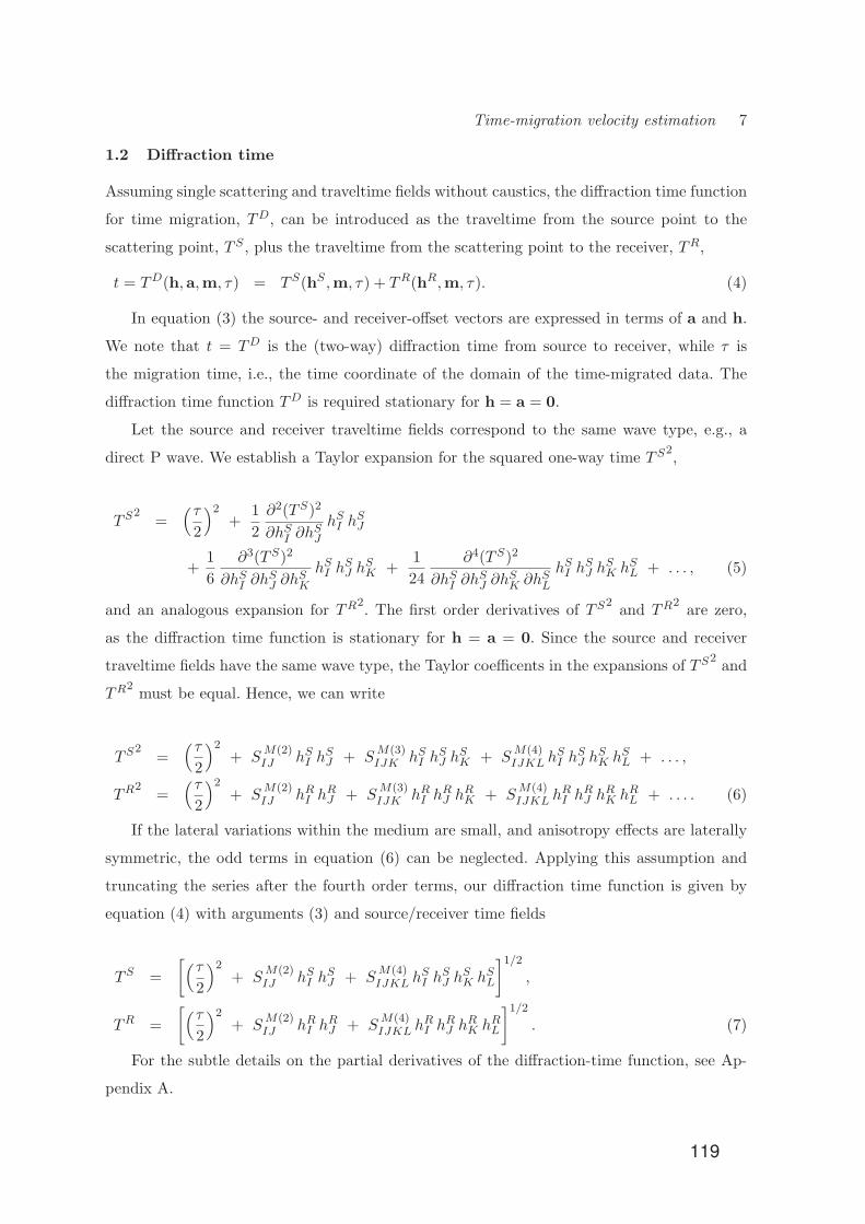
Time-migration velocity estimation 7
1.2 Diffraction time
Assuming single scattering and traveltime fields without caustics, the diffraction time function
for time migration, TD, can be introduced as the traveltime from the source point to the
scattering point, TS , plus the traveltime from the scattering point to the receiver, TR,
t = TD(h,a,m, τ) = TS(hS ,m, τ) + TR(hR,m, τ). (4)
In equation (3) the source- and receiver-offset vectors are expressed in terms of a and h.
We note that t = TD is the (two-way) diffraction time from source to receiver, while τ is
the migration time, i.e., the time coordinate of the domain of the time-migrated data. The
diffraction time function TD is required stationary for h = a = 0.
Let the source and receiver traveltime fields correspond to the same wave type, e.g., a
direct P wave. We establish a Taylor expansion for the squared one-way time TS2,
TS2=
(τ2
)2+
1
2
∂2(TS)2
∂hSI ∂hSJ
hSI hSJ
+1
6
∂3(TS)2
∂hSI ∂hSJ ∂h
SK
hSI hSJ h
SK +
1
24
∂4(TS)2
∂hSI ∂hSJ ∂h
SK ∂hSL
hSI hSJ h
SK hSL + . . . , (5)
and an analogous expansion for TR2. The first order derivatives of TS2
and TR2are zero,
as the diffraction time function is stationary for h = a = 0. Since the source and receiver
traveltime fields have the same wave type, the Taylor coefficents in the expansions of TS2and
TR2must be equal. Hence, we can write
TS2=
(τ2
)2+ S
M(2)IJ hSI h
SJ + S
M(3)IJK hSI h
SJ h
SK + S
M(4)IJKL h
SI h
SJ h
SK hSL + . . . ,
TR2=
(τ2
)2+ S
M(2)IJ hRI h
RJ + S
M(3)IJK hRI h
RJ h
RK + S
M(4)IJKL h
RI h
RJ h
RK hRL + . . . . (6)
If the lateral variations within the medium are small, and anisotropy effects are laterally
symmetric, the odd terms in equation (6) can be neglected. Applying this assumption and
truncating the series after the fourth order terms, our diffraction time function is given by
equation (4) with arguments (3) and source/receiver time fields
TS =
[(τ2
)2+ S
M(2)IJ hSI h
SJ + S
M(4)IJKL h
SI h
SJ h
SK hSL
]1/2,
TR =
[(τ2
)2+ S
M(2)IJ hRI h
RJ + S
M(4)IJKL h
RI h
RJ h
RK hRL
]1/2. (7)
For the subtle details on the partial derivatives of the diffraction-time function, see Ap-
pendix A.
119

8 H. Zhao et al.
1.3 Diffraction time coefficients
The coefficients in equation (7) may be expressed, for example, as
SM(2)IJ = 2τ
∂2TS
∂aI∂aJ, (8)
SM(4)IJKL = 1
12
[2τ
∂4TS
∂aI∂aJ∂aK∂aL
+∂2TS
∂aI∂aJ
∂2TS
∂aK∂aL+
∂2TS
∂aI∂aK
∂2TS
∂aJ∂aL+
∂2TS
∂aI∂aL
∂2TS
∂aJ∂aK
], (9)
where all derivatives are taken for a = h = 0. Observe, however, that the coefficients SM(2)IJ
and SM(4)IJKL are functions of m and τ . We can relate these coefficients to derivatives of the
diffraction time function and its square, as follows,
∂2TD
∂aI∂aJ=
4
τS
M(2)IJ , (10)
∂4TD
∂aI∂aJ∂aK∂aL=
16
τ
[3S
M(4)IJKL − 1
τ2
(S
M(2)IJ S
M(2)KL + S
M(2)IK S
M(2)JL + S
M(2)IL S
M(2)JK
)], (11)
∂2(TD)2
∂aI∂aJ= 8S
M(2)IJ , (12)
∂4(TD)2
∂aI∂aJ∂aK∂aL= 96S
M(4)IJKL. (13)
1.4 A simplified setup of diffraction time coefficients
Equation (7) is formulated to allow for a full coverage of directions and magnitudes of the
source- and receiver-offset vectors. For situations with limited coverage it is however useful to
have a simplified setup for the diffraction time coefficients.
One approach often used is to assume that the diffraction time moveout is rotationally
symmetric. We then write
SM(2)IJ = SM(2) δIJ , S
M(4)IJKL = SM(4) δIJδKL, (14)
where SM(2) and SM(4) are scalar functions of the coordinates (m, τ). Using the relations
(14) in equation (7) yields
TS =
[(τ2
)2+ SM(2) (hS)2 + SM(4) (hS)4
]1/2,
TR =
[(τ2
)2+ SM(2) (hR)2 + SM(4) (hR)4
]1/2. (15)
120

Time-migration velocity estimation 9
Here, the quantities hS and hR denote the magnitudes of the respective source- and receiver
offset vectors, hS and hR.
1.5 Time-migration velocity model
The time-migration velocity model is defined on a three-dimensional rectangular grid in the
variables ξ1 = m1, ξ2 = m2, ξ3 = τ , where we add ξ3 to describe the velocity model in time
domain. Model parameters related to cells or vertices within the grid will be unknowns in a
velocity estimation process.
Our velocity model is described in terms of a multi-component vector function, (Mλ), λ =
1, . . . , Nλ, where each component functionMλ(ξ1, ξ2, ξ3) corresponds to one of the coefficients
of the diffraction time function. For different contexts for these coefficients, see equations (6),
(7), and (15). The vector function (Mλ) is introduced to yield a compact equivalent of the
diffraction time coefficients under consideration. For example, for the simplified situation (15)
we take
M1 = SM(2), M2 = SM(4). (16)
To allow the differentiability up to the second order, we use a local cubic spline function
(see Appendix C) to describe the velocity model. Bicubic and tricubic spline functions are
used for 2D and 3D grids respectively. In Appendix E, we give a detailed description of the
parameterization of the time-migration velocity model.
2 KINEMATIC TIME MIGRATION AND DEMIGRATION
Kinematic time migration maps the local kinematic parameters (traveltimes, slopes and cur-
vatures) from the recording time domain of seismic data to the time-migration domain. The
inverse process, kinematic time demigration, maps the local kinematic parameters in time-
migration domain back to the recording time domain. As illustrated in Figure 2, by using
the diffraction function with its associated partial derivatives, and a known time-migration
velocity model, kinematic time migration and demigration are able to map the local kine-
matic parameters between the recording time domain and the migration time domain. In this
paper, we focus on the utilization of the kinematic parameters up to the first order for time-
migration velocity estimation. For mapping of second order kinematic parameters, see Iversen
et al. (2012).
121

10 H. Zhao et al.
The local kinematic parameters can be extracted from both the recording domain and
the migration domain. Since the time-migrated dataset in general contains less noise and is
more easily interpreted, the kinematic parameters extraction is commonly often applied in the
migration domain, and subsequently demigrated to the recording domain. The time-migrated
dataset is normally generated by pre-stack time migration of the recorded seismic data with
an initial time-migration velocity model. The migrated dataset is not necessarily to be optimal
but is assumed to have a good resolution for the local kinematic parameters picking. Once the
picking process applied in the migration domain, the local kinematic parameters are able to
be mapped to the recording domain by kinematic demigration with the same initial velocity
model. This process needs the computation of the first and second order partial derivatives of
the known diffraction-time function (i.e. equations (4), (7), and (15)), which are then used in
the kinematic demigration and migration for velocity estimation. We give the formulation of
kinematic time demigration and migration in the following context.
Figure 2: Schematic overview of kinematic time migration and demigration for 2D pre-stack
seismic data set. Based on the known diffraction time function with its associated derivatives,
and a time-migration velocity model, the local kinematic parameters (x, T x, px, ph) in record-
ing domain can be forward/backward mapped to/from the counterpart (m, T M , ψm, ψh) in
migration domain by kinematic time migration/kinematic time demigration.
122

Time-migration velocity estimation 11
2.1 Algorithm for kinematic time demigration
Consider equation (43) in Iversen et al. (2012), referred to as the consistency equation,
∂TD
∂aI− ∂TD
∂mI=
∂TD
∂τ
∂T∂mI
, (17)
with I = 1, 2. We can use equation (17) to obtain the aperture vector corresponding to a
kinematic time demigration,
aI = xI −mI . (18)
Under special conditions the vector a = (aI) can be obtained analytically, see equation 78 in
Iversen et al. (2012).
Based on equation (17) we introduce a vector function (fI(a)) so that
fI(a) =∂TD
∂aI− ∂TD
∂mI− ∂TD
∂τ
∂T∂mI
, (19)
where a = a is the sought unknown aperture vector. As a consequence, the system of equations
to be solved has the general form
fI(a) = 0. (20)
One possible approach to obtain a solution is to use the Newton-Raphson iteration method. Let
us assume that the component values of the function fI is known for some starting component
values a = a(0). For these starting values we compute the first-order partial derivatives of fI ,
∂fI∂aJ
(a(0)) =∂2TD
∂aI∂aJ− ∂2TD
∂mI∂aJ− ∂2TD
∂τ∂aJ
∂T∂mI
, (21)
with all the partial derivatives on the right-hand side evaluated for a = a(0). To first order we
can then write
0− fI(a(0)) =
∂fI∂aJ
(a(0))(a(1)J − a
(0)J
). (22)
Defining
WIJ(a(0)) =
∂fI∂aJ
(a(0)), WMN (a(0)) =
{{∂fI∂aJ
(a(0))
}−1}
MN
, (23)
equation (22) yields
a(1)J = a
(0)J − WJL(a
(0)) fL(a(0)), (24)
Equation (24) provides a first-order update of the aperture vector. We can now compute the
components fI(a(1)) and check if these are sufficiently close to zero. Should that be the case,
the Newton-Raphson process is completed and has returned the solution a = a(1). Otherwise,
the process goes on to the next iteration. The process is stopped when both components fI
123

12 H. Zhao et al.
are sufficiently close to zero. It is also stopped if we do not attain convergence to a meaningful
solution.
Equations (19) and (21) contain first- and second-order partial derivatives of the diffraction-
time function, TD. For the calculation of such derivatives, see Appendices C and D in Iversen
et al. (2012).
Now that we know the kinematic demigration aperture vector, a = (aI), it is easy to find
the time TX and the slopes pxI = ∂T/∂xI and phI = ∂T/∂hI resulting from the kinematic
demigration. To compute TX and pxI we simply use the equalities
TX = TD(h, a,m, T M ), pxI =∂TD
∂aI(h, a,m, T M ). (25)
The slope phI is given by equation (45) in Iversen et al. (2012),
phI =∂TD
∂hI(h, a,m, T M ) + ψh
I
∂TD
∂τ(h, a,m, T M ). (26)
2.1.1 Half-offset vector with only one degree of freedom
The coverage of azimuthal directions for the half-offset vector h may be two small to permit
extraction of two slope components ψhI to be input to kinematic time demigration. For this
situation the (two-component) half-offset vector has effectively only one degree of freedom, so
that we can parametrize the components of h by a single scalar, σ. The quantity σ will then
be a distance variable for traces belonging to a common-image gather in the migration-time
domain or a common-midpoint gather in the recording-time domain. The parametrization
reads
hI(σ) = h(σ)nI(σ), (27)
where h is the magnitude of h and n = (nI) is a unit vector. The quantity σ is a distance
variable for traces belonging to a common-image gather in the migration-time domain or a
common-midpoint gather in the recording-time domain. The first derivative of hI with respect
to σ is
dhIdσ
=dh
dσnI + h
dnIdσ
. (28)
The slope mapping in equation (26) can now be restated
pσ =∂TD
∂hI
dhIdσ
+ ψσ ∂TD
∂τ, (29)
where we have introduced new, effective, slopes with respect to offset in the recording-time
and migration-time domains,
pσ =∂T
∂σ, ψσ =
∂T∂σ
. (30)
124

Time-migration velocity estimation 13
2.2 Algorithm for kinematic time migration
In the case of kinematic time demigration we first solved a system of two equations in two
unknowns, i.e., the components of the aperture vector, followed by a straightforward evaluation
of the diffraction-time function to obtain the output time. In the kinematic time migration
situation there will still be three unknowns of the same type, the aperture vector components
plus an output time, but now we will in general need to solve simultaneously a system of three
equations in the three unknowns. The equations under consideration are given as (68) and
(69) in Iversen et al. (2012); we restate them here as
∂T
∂xI(h,x) =
∂TD
∂aI(h, a,x− a, τ), (31)
T (h,x) = TD(h, a,x− a, τ). (32)
To describe the unknowns it is convenient to introduce a three-component vector (ζi) such
that ζI = aI and ζ3 = τ .
We use equations (31)–(32) to formulate a three component vector function (gi(ζ)), as
follows
gI(ζ) =∂TD
∂aI− ∂T
∂xI, (33)
g3(ζ) = TD − T, (34)
where function arguments on the right-hand side have been skipped. Equations (31)–(32) can
then be restated
gi(ζ) = 0. (35)
To solve the system of equations (35) we may proceed in the same way as described for
equation (20). That means, to use a Newton-Raphson approach using derivatives ∂gi/∂ζj .
These derivatives are given explicitly as
∂gI∂ζJ
=∂2TD
∂aI∂aJ− ∂2TD
∂aI∂mJ, (36)
∂gI∂ζ3
=∂2TD
∂aI∂τ, (37)
125

14 H. Zhao et al.
∂g3∂ζJ
=∂TD
∂aJ− ∂TD
∂mJ, (38)
∂g3∂ζ3
=∂TD
∂τ. (39)
To obtain them, we have used that the time T and the slopes ∂T/∂xI in equations (33)–(34)
are invariant in kinematic time migration.
Knowing the output point (h, m, τ) resulting from a kinematic time migration, it means
that any requested partial derivative of the diffraction-time function TD in the variables hI ,
aI , mI , and τI may be computed. The natural next task is to obtain the slopes ψmI and ψh
I
at the point (h, m, τ). For that, we reuse here equation (70) in Iversen et al. (2012),
ψhI =
(∂TD
∂τ
)−1(phI −
∂TD
∂hI
), (40)
ψmI =
(∂TD
∂τ
)−1(pxI −
∂TD
∂mI
). (41)
For a half-offset vector with only one degree of freedom, see equation (27), equation (40)
can be restated
ψσ =
(∂TD
∂τ
)−1(pσ − ∂TD
∂hI
dhIdσ
). (42)
3 SENSITIVITY OF KINEMATIC TIME MIGRATION WITH RESPECT
TO THE TIME-MIGRATION VELOCITY MODEL
Considering one selected parameter ν of the time-migration velocity model, we study how the
kinematic time migration is affected by a perturbation in ν. We investigate the first-order
changes of the reflection location with respect to the time-migration velocity model (i.e. the
derivatives dmI/dν and dτ /dν), as well as the the first-order changes of the reflection slopes
with respect to the time-migration velocity model (i.e. the derivatives dψhI /dν).
In view of the model representation described in Appendix E, we take ν specifically as the
node value
ν = Mλr,s,t. (43)
126

Time-migration velocity estimation 15
3.1 First-order changes of the reflection location with respect the
time-migration velocity model
The location of a reflection in the migration-time domain can be expressed in terms of the
parameter ν as (h, m(h, ν), τ(h, ν)). As shown in Figure 3, we investigate how this location
(m, τ) is affected, to first order, by a perturbation in ν.
Figure 3: Schematic overview (2D) of the first-order changes of the reflection location with
respect to the time-migration velocity model. The symbol hi signify a specific common-offset
section. The figure shows, perturbation of a time-migration velocity model parameter (δν)
leads to the position change (δm, δτ) of the kinematic migration result: the kinematic migrated
output is shifted from red point to green point. These perturbations are described by the
derivatives: dm/dν and dτ/dν. In the figure, the yellow point and the dash black line represent
the input event point and its local slope. The red point and the red dash line represent the
migrated point and its diffraction traveltime curve by using the initial time-migration velocity
of ν0. Correspondingly, the green point and the green dash line represent the migrated point
and its diffraction traveltime curve by using the updated time-migration velocity ν0 + δν.
Equation (35) yields a mapping from a location in the recording-time domain to a location
in the migration-time domain. The relation is valid regardless of which time-migration velocity
model we use. As a consequence, we have
dgidν
= 0. (44)
Also, we note that the time T and the slopes ∂T/∂xI in equations (33)–(34) are insensitive
127

16 H. Zhao et al.
to the value of ν. A differentiation of these equations with respect to ν therefore yields
d
dν
(∂TD
∂aI
)= 0, (45)
dTD
dν= 0. (46)
Equations (45)–(46) contain information to estimate the derivatives dmI/dν and dτ /dν. The
total derivative operator in these equations can be stated as
d
dν=
∂
∂ν+
daJdν
∂
∂aJ+
dmJ
dν
∂
∂mJ+
dτ
dν
∂
∂τ.
Using that the location (xI) is insensitive to the value of ν, the operator appears in the form
d
dν=
∂
∂ν+
dmJ
dν
(∂
∂mJ− ∂
∂aJ
)+
dτ
dν
∂
∂τ. (47)
The specific partial derivatives of the diffraction time with respect to ν are given in Appendix
B.
Applying equation (47) in (45)–(46) yields[dmJ
dν
(∂
∂mJ− ∂
∂aJ
)+
dτ
dν
∂
∂τ
](∂TD
∂aI
)= − ∂2TD
∂ν∂aI,
[dmJ
dν
(∂
∂mJ− ∂
∂aJ
)+
dτ
dν
∂
∂τ
] (TD)
= −∂TD
∂ν,
and hence,(∂2TD
∂aI∂mJ− ∂2TD
∂aI∂aJ
)dmJ
dν+∂2TD
∂aI∂τ
dτ
dν= − ∂2TD
∂ν∂aI, (48)
(∂TD
∂mJ− ∂TD
∂aJ
)dmJ
dν+∂TD
∂τ
dτ
dν= −∂T
D
∂ν. (49)
Equations (48)–(49) can be restated as the matrix equation
Aη = b, (50)
which includes the 3× 1 matrix of unknowns
η =
⎡⎣{dmJdν
}dτdν
⎤⎦ , (51)
and the 3× 3 and 3× 1 coefficient matrices
A =
⎡⎣{ ∂2TD
∂aI∂mJ− ∂2TD
∂aI∂aJ
} {∂2TD
∂aI∂τ
}{
∂TD
∂mJ− ∂TD
∂aJ
}∂TD
∂τ
⎤⎦ , (52)
b = −
⎡⎣{ ∂2TD
∂ν∂aI
}∂TD
∂ν
⎤⎦ . (53)
128

Time-migration velocity estimation 17
Inversion of equation (50),
η = A−1b, (54)
will then yield the sought derivatives dmI/dν and dτ /dν.
3.2 First-order changes of reflection slopes with respect to the time-migration
velocity model
Apart from the investigation of the reflection position changes of a kinematic time migration
output, we also need study the variation of reflection slopes with respect to the perturbation
of time-migration velocity. As presented in the Figure 4, the derivative dψhI /dν describes the
sensitivity of the variation of the reflection slopes with respect to the velocity perturbation.
In the following, we derive an expressions for the first-order derivatives of reflection slopes
in offset, resulting from a kinematic time migration, taken with respect to parameters of the
time-migration velocity model.
Figure 4: Schematic overview (2D) of the first-order changes of the reflection (offset) slopes
with respect to the time-migration velocity model. The symbols hi andmj signify, respectively,
a common-offset section and a common-image gather. The figure shows, with a fixed input
point from the recording domain, the perturbation of time-migration velocity model leads to
the changes of the reflection slopes in the kinematic migration domain. The yellow and red
points represent the initial migrated point, the further migrated point after the velocity update
respectively. The green point resembles the idea time-migration result (ψh = 0 )derived from
the optimal migration velocity.
129

18 H. Zhao et al.
3.2.1 Half-offset vector with two effective degrees of freedom
The most general mapping of reflection slopes ψhI is given by equation (40), for which the
half-offset vector has two degrees of freedom. We differentiate this equation with respect to
the parameter ν, which yields,
d
dν
(∂TD
∂hI+∂TD
∂τψhI
)= 0. (55)
Using the differentiation operator in equation (47), we obtain after some elaboration
dψhI
dν= −
(∂TD
∂τ
)−1{∂2TD
∂ν∂hI+∂2TD
∂ν∂τψhI
+dmJ
dν
[∂2TD
∂mJ∂hI− ∂2TD
∂aJ∂hI+
(∂2TD
∂mJ∂τ− ∂2TD
∂aJ∂τ
)ψhI
]+dτ
dν
[∂2TD
∂τ∂hI+∂2TD
∂τ2ψhI
]}. (56)
3.2.2 Half-offset vector with one effective degree of freedom
When the half-offset vector has effectively only one degree of freedom, we take the mapping
equation (42) as a starting point for obtaining a derivative of the slope along offset, ψσ, with
respect the model parameter, ν. The result is
dψσ
dν= −
(∂TD
∂τ
)−1{∂2TD
∂ν∂hI
dhIdσ
+∂2TD
∂ν∂τψσ
+dmJ
dν
[(∂2TD
∂mJ∂hI− ∂2TD
∂aJ∂hI
)dhIdσ
+
(∂2TD
∂mJ∂τ− ∂2TD
∂aJ∂τ
)ψσ
]+dτ
dν
[∂2TD
∂τ∂hI
dhIdσ
+∂2TD
∂τ2ψσ
]}. (57)
In the calculation of equation (57), the partial derivatives related to the time-migration
velocity model are needed. The detailed description of this calculation is described in Appendix
F.
4 VELOCITY ESTIMATION FORMULATION
Once we formulated the kinematic time migration/demigration scheme and derived the Frechet
derivatives of kinematic time migration with respect to the time-migration velocity model,
we are now able to set up an inversion scheme to estimate the time-migration velocity. In the
following, we first review a common way to linearize a generally non-linear inversion problem,
then we introduce the approach of iterative linearized inversion to estimate the optimal time-
migration velocity model.
130

Time-migration velocity estimation 19
4.1 Linearization of the inversion problem
Consider a parameter vector ν containing N parameters belonging to a general data model
(not necessarily related to seismics) and a vector function D(ν) with M components
Dm(ν) = dtruem − dpredm (ν), m = 1, . . . ,M, (58)
where dpredm is a quantity predicted on the basis of the model parameter vector ν, and dtruem is
the corresponding true (observed or idealized) quantity. Linearization of equation (58) with
respect to a certain reference vector ν0 yields
Dm(ν) = Dm(ν0) +∂Dm
∂νn(ν0) (νn − ν0n). (59)
Furthermore, assume that Dm = 0 for all values of the index m. The first-order update ν of
the model parameter vector ν0 must then satisfy the equation
∂Dm
∂νn(ν0) (νn − ν0n) = −Dm(ν0). (60)
Using the definition of the vector function D in equation (58) we can alternatively write
∂dpredm
∂νn(ν0) (νn − ν0n) = dtruem − dpredm (ν0). (61)
Equation (61) describes a system of M linear equations with N unknown parameters to be
determined. The quantity ∂dpredm /∂νn is commonly referred to as a Frechet derivative.
4.2 Iterative linearized inversion
We use an iterative linearized inversion approach where the objective is to minimize the misfit
between idealized and predicted slopes in the offset coordinates of the common-image gathers.
The idealized slopes are zero and correspond to an optimal time-migration velocity model. It
is remarked that such a model may not exist in practice, because of the limitations of time
migration.
In our situation, the linear equations are obtained by adaption of equation (61), so that
each slope event under consideration will give rise to two equations or a single equation,
depending on the effective degree of freedom for the variation of the half-offset vector. The
resulting equations for these two situations are, respectively,
∂ψhI
∂νn(ν0) (νn − ν0n) = −ψh
I (ν0). I = 1, 2 , (62)
and
∂ψσ
∂νn(ν0) (νn − ν0n) = −ψσ(ν0). (63)
131

20 H. Zhao et al.
The Frechet derivatives of our tomographic approach are partial derivatives of the re-
flection slope in the offset direction, ψhI or ψσ, with respect to the parameters, νn, of the
time-migration velocity model. These derivatives can be obtained using, respectively, equa-
tion (56) or equation (57).
To avoid artificial jumps of the solution in areas with little data coverage, it is important
to include regularization in the system of linear equations. We use Tikhonov regularization of
zeroth, first, and second order (e.g., Aster et al., 2013). The first- and second-order regular-
ization equations are included separately for each coordinate direction under consideration.
5 EXTRACTION OF LOCAL KINEMATIC PARAMETERS
With the above formulation, we are now able to estimate the time-migration velocity model
based on the kinematic time migration and demigration by using the local kinematic pa-
rameters (traveltimes, slopes, and curvatures). In our method, considering the efficiency in
implementation and the robustness in the calculation, we choose the gradient structure ten-
sor (GST) method for the first-order kinematic parameters (slopes) extraction and quadratic
gradient structure tensor (QST) for the second-order kinematic parameters (curvatures) ex-
traction. This operation is applied either on stacked data in the migration domain or the
seismic stack in recording domains. In the following, we review the gradient structure ten-
sor method and GST method for slope extraction. we also give the description of curvature
extraction in Appendix D.
5.1 The Gradient Structure Tensor
Structure tensors provide a description of the local structure in images using a tensor field.
For a 3D image, this yields a 3× 3 tensor matrix for each voxel. Knutsson (1989) showed that
this tensor could be optimally obtained using six spatially oriented quadrature filters. The
gradient structure tensor (GST) (Bigun 1987), is a simplified implementation of the structure
tensor, where the tensor is estimated using three gradient filters.
For a 3D seismic cube, the GST is computed using gradient estimates along the three
image dimensions (x = [x, y, t]T ). The gradient tensor:
T ≡ ggT , (64)
132

Time-migration velocity estimation 21
is the estimated covariance matrix of the gradient vector field:
g(x) =
⎡⎢⎢⎢⎣gx(x)
gy(x)
gt(x)
⎤⎥⎥⎥⎦ . (65)
The gradients (gx, gy, gt) along the three axes (x, y, t) are obtained by convolving the seismic
data cube (I(x)) with the derivative of the 3D Gaussian function G(x, σ):
gi = I(x) ∗ ∂
∂xiG(x, σg). (66)
where σg is the gradient scale. As the GST is sensitive to structures at different scales depend-
ing on σg, when applied to seismic data, we want the GST to be sensitive to reflections. This
can be achieved by setting σg to match half the typical thickness of the reflections. (full width
at half maximum of the Gaussian function). The GST is then computed as the smoothed
outer product of the gradient vector:
T =
⎡⎢⎢⎢⎣g2x gygx gtgx
gxgy g2y gtgy
gxgt gygt g2t
⎤⎥⎥⎥⎦ , (67)
where ¯ is the smoothing operator. The smoothed tensor elements are computed using the
Gaussian window function:
Tij = Tij ∗G(x, σT ), (68)
where σT is the smoothing scale. The parameter σT controls the spatial smoothing. By having
a large σT , the GST becomes more robust against noise. By having a smaller σT , more detailed
information about the structure may be obtained.
5.2 Slope estimation
The local structure in the image can be analyzed by considering the eigenvalues (λ1 ≥ λ2 ≥ λ3)
and corresponding eigenvectors (v1,v2,v3) of T. Since T is the estimated covariance matrix
of the gradient vector field, the eigenvectors span the axes of the covariance ellipsoid. This
means that v1 will have the same direction as the locally dominant direction of the gradient
vector field. It is also possible to derive attributes from the eigenstructure (Randen et al.
2000).
By considering the components of v1 = [v1x, v1y, v1t], the slopes (estimates of the deriva-
tives) are given as:
133

22 H. Zhao et al.
qx =∂t
∂x=v1xv1t
, (69)
qy =∂t
∂y=v1yv1t
. (70)
The eigenvector analysis is carried out for all locations in space, which produces the slope-
fields.
6 NUMERICAL EXAMPLES
In this section, we demonstrate the viability of the proposed time-migration velocity estima-
tion technique using three numerical examples. In the first example, we evaluate the derived
formulation of kinematic time migration and the calculation of the Frechet derivatives based
on a constant time-migration velocity model. In the next, we present an example based on a
2D synthetic dataset. In the last example, we provide an application of time-migration velocity
estimation on real 3D marine data from the Barents Sea.
6.1 Test of the Frechet derivative formula for time-migration velocity
estimation
First, we tested the kinematic migration using single event (point) mapping from the recording
domain to the migration domain. As shown in Figure 5, we used an input event point at CMP
location x = 2.5 km, with travel time TD = 2.2676 s and a half offset of h = 1 km. The
corresponding event slopes were px = 0.6840 s/km and ph = 0.0694 s/km. In the example, a
true time-migration velocity model with SM = 0.16 s2/km2 was known, and a time-migration
velocity model with SM = 0.175 s2/km2 was used in the test. The diffraction traveltime curves
based on the true and test are plotted, represented by the solid black and the broken black
lines, respectively in Figure 5. During the test, we applied the kinematic migration to the
selected input event in the recording domain based on the test and true models, and observed
that the kinematic migration using the test migration velocity misplaced the reflection event
in the migration domain and derived kinematic parameters, m = 0.1889 m, τ = 1.1011 s, ψm
= 1.2692 and ψh = -0.0447 s/km, while the kinematic migration using the true migration
velocity correctly mapped the event back to the known diffraction point location, and derived
the correct kinematic parameters, m = 0 km, τ = 1.0 s, ψm = 1.4009 and ψh = 0 s/km in
the migration domain.
134

Time-migration velocity estimation 23
In the next example, we verified the accuracy of the Frechet derivative approximations
derived in Equations (56) or (57). In the test, we first numerically generated the function ψh(v)
using the input migration velocity quantities v = SM and the reflection slope quantities in
the offset direction ψh, derived from the kinematic migration (Figure 6). Since the Frechet
derivatives of our constrained linear inversion are partial derivatives of the reflection slope
in the offset direction, ψhI or ψσ, with respect to the parameters νn of the time-migration
velocity model, we could then calculate these derivatives by using Equations (56) or (57).
In Figure 6,we plotted the linear approximation of ψh(v) using an explicit formula for the
derivative ∂ψh/∂ν at velocity model coordinate v = SM = 0.175 s2/km2. The derived Frechet
derivative ∂ψh/∂ν = -2.7389 km/s, using the explicit formula in Equation (56), is very close
to the numerically-derived Frechet derivative ∂ψh/∂ν = -2.7390 km/s. However, if we ignore
the movement of the point (m,τ) in Equation (56), the derived linear approximation of ψh(v)
at the selected velocity model coordinate gives the wrong slope approximation.
Figure 5: Kinematic time-migration test using different velocity models. The red dot represents
an input event point in the recording domain. The black dot represents the output event point
of the kinematic migration based on the true velocity model, while the black circle represents
the migrated output based on the test velocity model. The diffraction time functions using the
true and test velocity models are represented by the solid and dashed black lines, respectively.
135

24 H. Zhao et al.
Figure 6: Verification of the Frechet derivative approximations. The green line represents
the numerically-calculated function ψh(v). The solid blue line denotes the calculated Frechet
derivative based on Equation (56) at the velocity model coordinate v = SM = 0.175 s2/km2,
while the dashed blue line is the Frechet derivative calculated for the same velocity-model
coordinate, but ignoring the movement of the point.
6.2 2D time-migration velocity estimation
In the 2D velocity estimation example, we used a 2D synthetic data set to demonstrate the
proposed time-migration velocity estimation workflow (1), shown in Figure 7. This is based
on fully using all common-offset gathers, reflection surface picking and slope extraction in the
migration domain, and iterations of the internal time-migration velocity estimation.
In this example, a 2D depth-velocity model (Figure 8) was generated, consisting of five geo-
logical layers with predefined velocities (1500m/s, 2000m/s, 2500m/s, 3000m/s and 3500m/s),
delineated by four interfaces. A surface with a syncline and anticline is defined on Interface
2, and a dipping surface is defined on Interface 3. The prestack shot-gather dataset was simu-
lated by Kirchhoff modelling in NORSAR using a conventional 2D marine seismic geometry:
shot interval 12.5 m, trace interval 25 m, minimal offset 100 m, maximum offset 3100 m, group
number 121, and total number of shots 953.
136

Time-migration velocity estimation 25
Figure 7: Time-migration velocity estimation workflow (1)
Figure 8: 2D synthetic depth velocity model
Based on the simulated prestack dataset, we applied 2D Kirchhoff prestack time migra-
tion using an initial migration velocity field. To test the feasibility of the velocity estimation
algorithm, we deliberately used a constant water velocity 1500 m/s as an initial migration
velocity model for the Kirchhoff prestack time migration. After the migration, the gradient
structure tensor-based slopes extraction was applied to the migrated volume to derive slopes
volumes, and a semi-automated seed-point-based horizon tracking was applied so as to derive
the reflection traveltime surface in the common image point and offset domain. The corre-
sponding slopes were extracted along the four interpreted surfaces in the migration domain.
137

26 H. Zhao et al.
Based on the derived kinematic parameters in the migration domain - the half-offset h, the
common image point coordinate, m, the migration time τ , and the reflection slopes ψm and
ψh the kinematic demigration was applied to map those kinematic parameters to the record-
ing domain and derive the half-offset h, the common midpoint coordinate x, the reflection
time TD and the reflection slopes px and ph. Based on the kinematic demigration, the reflec-
tion surfaces in the recording domain were recreated. Figure 9 shows the picked surfaces in
the migration domain and the corresponding kinematic demigrated surfaces in the recording
domain, selected from the finite-offset panels.
Figure 9: Input finite surface planes in the migration domain (black), and kinematic demi-
grated finite surface planes in the recording domain (red). The selected offset planes (1, 30,
60 and 90) from the second interface are displayed from top left to bottom right.
Using the input of kinematic parameters in the recording domain, the internal iterations
for the time-migration velocity estimation were applied. Each iteration consisted of a kine-
matic migration with a defined velocity field, and the following constrained linear inversion
for deriving the velocity update in order to minimise the reflection slope ψh in the migra-
tion domain. In this synthetic example, we started the kinematic migration, based on the
water velocity (1500 m/s), and the estimated time-migration velocity, by running three in-
ternal iterations. Figure 10 shows the kinematic migrated reflection surfaces based on the
input/estimated time-migration velocity fields. We projected all the finite-offset surfaces onto
138

Time-migration velocity estimation 27
the zero-offset plane to verify the improvement of the estimated time-migration velocity field.
As mentioned earlier, the best estimated time-migration velocity field is able to flatten all the
common image gathers in the offset direction, which is equivalent to zero for the quantity of
reflection slope ψh in the migration domain. From the reduced residual moveout from Figure
10 a-d, the rapid convergence of the algorithm can be seen.
Figure 10: Kinematically-migrated reflection surfaces based on the estimated time-migration
velocity field. a): Reflection surface derived from initial water velocity. b-d): Reflection surface
derived from velocity estimation’s iterations 1-3. All surfaces in the finite-offset were projected
onto the zero offset plane for this comparison.
The constrained linear inversion estimated time-migration velocity field was compared
with the original depth-model-converted time-migration velocity field for the whole section,
as shown in Figure 11, and for the selected common-image-gather (CIG) locations in Figure
12. The estimated time-migration velocity shows good consistency with the model converted
reference time-migration velocity within the spatial coordinates 0 to 10 km. From 10 km to
the end of the model, the estimated velocity presents a slightly slower velocity trend than the
reference velocity, which might be the result of the sparse sampling between the second and
third horizons at the right end of the original model.
139

28 H. Zhao et al.
Figure 11: Comparison of time-migration velocity (top) and constrained linear inversion de-
rived time-migrated velocity (bottom).
Figure 12: Comparison of derived time-migrated velocity (red) and Dix converted time-
migration velocity (black) at selected CIG locations.
140

Time-migration velocity estimation 29
Figure 13: CIG gathers migrated using derived migration velocity.
Figure 14: Migration stacked image from PSTM with derived time-migration velocity.
In order to verify the quality of the derived time-migration velocity field, we applied
Kirchhoff prestack time migration to the synthetic common-offset gathers using the derived
time-migration velocity field. Figure 13 shows the selected CIG gathers after the migration.
It can be seen that most of the events on the CIG gathers are flat following the migration
using the estimated time-migration velocity. The final migrated stack, shown in Figure 14,
also proves the good quality of the estimated time-migration velocity field.
141

30 H. Zhao et al.
6.3 3D time-migration velocity estimation
In this final example, we employed a 3D marine dataset, acquired in the Barents Sea, to
demonstrate the time-migration velocity estimation in 3D scenarios. The dataset contains
the migrated stacked 3D volume, the interpreted geological horizons, the pre-migration CMP
gathers, and the time-migration velocity field derived from the conventional migration velocity
estimation. As the migrated common image gathers were not available for the study, we
modified the prior workflow (1) of the time-migration velocity estimation demonstrated in
the 2D example, and proposed an alternative version of the workflow (2) (Figure 15) for the
3D time-migration velocity estimation. Instead of the application of an initial prestack time
migration to the input data, and the subsequent picking of each migrated offset volume, the
algorithm uses the interpreted key reflectors from the time-migrated zero-offset volume as
the input and replaces the reflection surface picking and slope extraction in the migration
domain with the reflection surface modelling, fitting and slope extraction in the recording
domain. In the following 3D numerical example, we used the provided migration velocity as
the reference velocity model, and derived the demigrated zero-offset kinematic parameters.
Using the subsequent application of reflection surface modeling, seismic to surface fitting and
slope extraction, we estimated the 3D time-migration velocity based on the internal iteration
of nonlinear constrained 3D velocity inversion. Ultimately, the derived migration velocity
field was compared with the reference velocity model to demonstrate the effectiveness of the
proposed 3D time-migration velocity estimation approach.
Figure 15: time-migration velocity estimation workflow (2)
142

Time-migration velocity estimation 31
The 3D marine dataset was acquired using 12 streamers separated by 75 m and a dual-
source configuration with a shot point interval of 18.75 m. The data on each cable was recorded
using 564 receivers per streamer at interval of 12.5 m. The sorted 3D CMP dataset, a prestack
time-migrated stack volume, the 3D time-migration velocity field and the interpreted horizons
from the operating company were used in this numerical example.
Figure 16: 3D surfaces picked from zero-offset migrated volume, which represent the geological
interfaces of the seabed, top Triassic, intra-Triassic, and top Permian, from top to bottom
respectively.
Based on legacy seismic processing, four horizons (Figure 16) were interpreted based on the
migrated stack volume, which represents the geological interfaces of the seabed, top Triassic,
intra-Triassic and top Permian respectively. The original surfaces covered a 300-km2 area. In
this example , we selected an area of interest of 25 km2 (x = 1.625-6.625 km, y = 0.375-5.375
km) for the time-migration velocity estimation.
In the first step of the algorithm (Figure 15), we proposed applying an initial pre-stack or
post-stack time migration using a raw time-migration velocity field, derived either from stack-
ing velocity analysis or a manually-defined velocity trend, then applying the key reflections
picking and slope extraction based on the migrated zero-offset dataset. In this example, based
on the provided pre-stack time-migration (PSTM) volume and the interpreted key reflection
horizons, we first derived the kinematic attribute slope ψm using the gradient structure ten-
sor method and extracted the slopes along the interpreted surfaces to derive the zero-offset
kinematic parameters (m, τ , ψh = 0, ψm) in the migration domain. Kinematic demigration
143

32 H. Zhao et al.
was applied subsequently to generate the zero-offset kinematic parameters in the recording
domain (x, TD, ph = 0, px) by employing the original prestack time-migration velocity. In
Figure 17, the fourth zero-offset surface in the migration domain, the demigrated surface in
the recording domain and the corresponding slopes of ψm are displayed as an example.
Figure 17: Input and output of zero-offset kinematic demigration, and the derived slopes ψm in
the recording domain. (a) Interpreted fourth surface in the migration domain. (b) Kinematic
demigrated fourth surface in the recording domain. (c) Slopes ψm of the demigrated surface
along the x direction. (d) Slopes ψm of the demigrated surface along the y direction.
Next, in order to obtain the kinematic parameters of the finite-offsets in the recording
domain, we introduced a fast-track approach to reflection-surface modelling and surface-to-
seismic fitting in the recording domain. In this process, referring to the derivation of Iversen
et al. (2012) (Eq. 84), we derived the normal moveout matrices SNMO based on the migration
velocity SM and zero-offset slope px. In Figure 17, we display all four components of the normal
moveout (NMO) matrices derived from the kinematic demigration of the fourth reflection
surface. We then modelled the traveltime surfaces of the finite-offset reflections (Figure 18)
using the CMP approximation. The NMO matrices SNMO, zero-offset reflection surfaces T 0,
and offset vectors h extracted from the CMP gathers were used in this calculation. The
generated finite-offset reflection surfaces in the recording domain are shown in Figure 18.
144

Time-migration velocity estimation 33
Meanwhile, considering that the CMP traveltime equation is under the assumption that the
reflection travel time, as the function of the offset, follows hyperbolic trajectories, which are
not valid in the case of complex overburden structures that give rise to strong lateral variations,
in this case, we assumed the gentle velocity variation within the migration aperture and only
tackled the time-migration velocity estimation for the isotropic medium. Thus, at next step in
traveltime surfaces/curves to seismic fitting is needed to match the derived reflection curves
to the seismic events on the CMP gathers. A semblance-based parameter searching approach
was applied in this fitting process. The fitting was applied to the selected CMP locations using
the defined grid size of 500 x 500 m. Once the traveltime was calculated at the selected offset
and CMP locations, the individual finite-offset surfaces were created using the bi-cubic spline
interpolation based on the local traveltime control points. The original modelled reflection
events and the fitted reflection events were overlaid on the corresponding CMP gather, and
are shown in Figure 19.
Figure 18: Modelled finite-offset reflection surfaces in the recording domain. (a) First finite-
offset reflection surfaces using selected offset planes from the zero offset panel to the maximal
offset panel of 15 with step 5. (b) Second finite-offset reflection surfaces using selected offset
planes from the zero offset panel to the maximal offset panel of 15 with step 5. (c) Third
finite-offset reflection surfaces using selected offset planes from the zero offset panel to the
maximal offset panel of 30 with step 5. (d) Fourth finite-offset reflection surfaces with selected
offset planes from the zero offset panel to the maximal offset panel of 60 with step 5.
145

34 H. Zhao et al.
Figure 19: Modelled reflection events overlain on the CMP gather (left), and fitted reflection
events overlain on the CMP gather (right)
To derive the finite-offset kinematic parameters in the recording domain, polynomial fitting
and slope extraction along the selected directions were applied on each reflection surface. The
second order polynomial and cubic smoothing spline were used to fit and derive the slopes px
and ph, respectively. Figure 20 shows the reflection surfaces and their corresponding extracted
slopes on the selected offset.
Figure 20: Finite-offset reflection surfaces of the fourth surface and the corresponding ex-
tracted slopes on the tenth offset panel. (a) Finite-offset reflection surfaces. (b) Extracted
slope surface px along x direction. (c) Extracted slope surface px along y direction. (d) Ex-
tracted slope surface ph.
146

Time-migration velocity estimation 35
In the next step, based on the derived finite-offset kinematic parameters (h, x, TD, ph,
px ) in the recording domain, we applied the 3D kinematic migration and constrained the
linear inversion in order to estimate the time-migration velocity. As mentioned in the section
on the velocity estimation formulation, the internal time-migration velocity estimation is
formulated as an iteration of the kinematic time migration and the constrained linear inversion.
The kinematic time migration is applied on a defined velocity model to map the kinematic
parameters from the recording domain to the migration domain, while the constrained linear
inversion provides the time-migration velocity perturbation that minimises the misfit between
the idealised slope ph = 0 and the current slope ph in the common-image gathers. In the 3D
time-migration velocity estimation example, we selected a testing area (5 km x 5 km x 2
s) for the velocity field estimation. Unlike using the constant-velocity model in the 2D time-
migration velocity estimation example, we derived an initial 3D velocity model from a previous
2D time-migration velocity estimation using a specified sparse grid sampling (1 km x 1 km x
0.1 s), which was used to constrain and stabilise the 3D linear inversion. The derived initial
velocity field is shown in Figure 21.
Figure 21: Initial 3D velocity field model (5km x 5km x 2s)
In the 3D time-migration velocity estimation, we applied three iterations of velocity in-
version using the setting of variant grid sizes. The grid parameters of the migration velocity
used for each iteration are listed in Table 1. The regularisation condition of the first order
of Tikhonov using an adaptive damping scheme, was applied to all the iterations. The initial
velocity model, and the derived migration velocities of each iteration, are shown in Figure 22
for selected inline location (x = 3.4 km).
147

36 H. Zhao et al.
Table 1. Grid parameter setting for 3D time-migration velocity estimation
X sampling(m) Y sampling(m) Time sampling(m)
Iteration 1 1000 1000 100
Iteration 2 500 500 50
Iteration 3 250 250 25
Figure 22: Time-migration velocity from the 3D velocity estimation (selected location at x
= 3.4 km). (a) Initial time-migration velocity. (b) Time-migration velocity from the first
iteration of the velocity estimation, (c) Time-migration velocity from the second iteration of
the velocity estimation, (d) Time-migration velocity from the third iteration of the velocity
estimation.
148

Time-migration velocity estimation 37
In the last step, for quality controlling the derived 3D time-migration velocity field, we used
the reference time-migration velocity field, which was derived from conventional migration
velocity analysis as a benchmark against which to compare the velocity field derived from our
approach. The two velocity volumes are compared in Figure 23. The selected inline and xline
velocity profiles are compared in Figures 24 and 25 , respectively. These two velocity fields
were also compared at randomly-selected CIG locations, as shown in Figure 26. From these
figures, it can be clearly seen that the inversion-generated velocity field has good consistency
with the velocity derived by the conventional approach, especially within the time range 0-
1.6 s. In the deeper part, from 1.6 s to 2 s, it can be observed that there is a mismatch
between the inversion-derived velocity and the conventional-approach-derived velocity. The
inversion-derived velocity gives a slower velocity than the conventional approach; however,
upon investigation of the locations that were mismatched, we found that uplift of the bottom
horizon and regularisation were the main reasons, and that, potentially, if more deep horizons
were included, the version might better constrain the inversion, giving an even better velocity
estimation at the bottom.
Figure 23: Comparison of 3D time-migration velocity fields derived from the kinematic time
migration and demigration approach (left), and the conventional migration velocity analysis
approach (right).
149

38 H. Zhao et al.
Figure 24: Comparison of the velocity-estimation derived time-migration velocity field (top)
and the conventional migration-velocity-analysis-derived time-migration velocity field (bot-
tom). The plot was selected from location x = 3 km
Figure 25: Comparison of the velocity-estimation derived time-migration velocity field (top)
and conventional migration-velocity-analysis-derived time-migration velocity field (bottom).
The plot was selected along from y = 1.65 km
150

Time-migration velocity estimation 39
Figure 26: Comparison of velocity-estimation derived time-migration velocity field (black line)
and the conventional migration-velocity-analysis- derived time-migration velocity field (red
line) for randomly selected locations.
7 CONCLUSIONS
In this paper, we have presented a technique for time-migration velocity estimation, which
is based on known reflection traveltimes and local slopes. We have generalised the time-
migration velocity estimation using nonlinear mapping processes based on kinematic time
migration and demigration, and derived, to a great detail, the involved Frechet derivatives;
that is, the partial derivatives of the local reflection slopes in the offset direction with respect
to the time-migration velocity model. Ultimately, a system of linear equations was applied
iteratively in order to solve the nonlinear velocity update.
Using the proposed scheme, we have generalised both the 2D and 3D homogeneous and
heterogeneous seismic time-migration velocity estimation approaches based on reflection trav-
eltimes and local slopes. The scheme is applied to both conventional narrow- and wide-azimuth
acquisition geometries. The proposed time-migration velocity estimation approach is, in gen-
151

40 H. Zhao et al.
eral, more accurate than conventional methods because it better honours the spatial variations
of the diffraction time function. Through numerical examples, we have shown that the new
approach is robust. The optimal migration velocity was obtained within the internal velocity
estimation loop, and was subsequently used for final PSTM. Regarding reflection traveltime
picking, we proposed extracting the local reflection slopes using the technique of gradient
structure tensor and semi-automatic reflection horizon picking in the pre-stack migration do-
main in order to utilise the migrated pre-stack data with a higher resolution and signal-to-noise
ratio.
In the numerical experiments, the theoretical formulations were tested using three ex-
amples. In the first example, we verified the Frechet derivatives used for the time-migration
velocity estimation. The presented examples of the comparison between the analytical and
numerical derivatives of both the kinematic migration and Frechet derivatives proved the accu-
racy of the theoretical derivation. In the next example, we demonstrated the time-migration
velocity estimation on a 2D dataset. The experimental dataset was initially generated by
Kirchhoff modelling. In the subsequent velocity estimation, the generated synthetic datasets
were migrated by PSTM using an initial migration velocity model, and then the reflection
traveltime picks and corresponding local slopes were derived. The following applied internal
velocity updates showed a rapid convergence of the linear velocity iterations. The accuracy
of the derived 2D time-migration velocity was also proved by the flatness of the final PSTM-
migrated gather and the reasonable quality of the PSTM-migrated stack image. In the last
numerical example, we demonstrated the feasibility of applying the derived scheme for the es-
timation of time-migration velocity to a 3D marine field dataset. In this example, as we were
short of a PSTM-migrated prestack dataset, only obtaining the migrated stacked dataset,
the corresponding integrated reflection horizons, and legacy PSTM migration-velocity field,
we used a workaround scheme to derive the invariant reflection traveltimes and local slopes
in the recording domain, and applied the velocity estimation using the input from selected
finite-offset planes. Although we understand that the picking in the recording domain may
have included artifacts from the complex geological region, the experiment-derived migration
velocity volume still showed good consistency with the velocity derived from conventional
migration-velocity analysis. This proved the feasibility of the 3D time-migration velocity es-
timation formulation.
In general, considering the initial depth-velocity model is still crucial for most of the depth-
domain tomography algorithms, we believe that the proposed technique of time-migration
velocity estimation, using nonlinear kinematic migration/demigration solvers based on Frechet
152

Time-migration velocity estimation 41
derivatives, will improve the accuracy of velocity model estimation and the resulting final
image in both the time and depth domains.
ACKNOWLEDGMENTS
The authors acknowledge support from the Norwegian Research Council through the Petro-
Maks 2 project (NFR/234019). We thank Lundin Norway AS for making the 3D field dataset
available for this study. We also grateful to NORSAR for providing the software for the syn-
thetic data generation.
153

42 H. Zhao et al.
REFERENCES
Adler, F., Baina, R., Soudani, M. A., Cardon, P., & Richard, J.-B., 2008. Nonlinear 3d tomographic
least-squares inversion of residual moveout in kirchhoff prestack-depth-migration common-image
gathers, Geophysics, 73(5), VE13–VE23.
Aster, R. C., Borchers, B., & Thurber, C. H., 2013. Parameter estimation and inverse problems ,
Academic Press, Waltham, MA, 2nd edn.
Bakker, P., 2002. Image structure analysis for seismic interpretation: Ph.D. thesis, Ph.D. thesis,
Technische Universiteit Delft.
Barros, T., Ferrari, R., Krummenauer, R., & Lopes, R., 2015. Differential evolution-based optimiza-
tion procedure for automatic estimation of the common-reflection surface traveltime parameters,
Geophysics, 80(6), WD189–WD200.
Bartels, R. H., Beatty, J. C., & Barsky, B. A., 1987. An Introduction to Splines for Use in Computer
Graphics and Geometric Modeling., Morgan Kaufmann Publishers.
Bauer, A., Schwarz, B., & Gajewski, D., 2009. Enhancement of prestack diffraction data and attributes
using a traveltime decomposition approach, Studia Geophysica et Geodaetica, 60, 471–486.
Baykulov, M. & Gajewski, D., 2009. Prestack seismic data enhancement with partial common-
reflection-surface (CRS) stack, Geophysics, 74(3), V49–V58.
Bergler, S., Hubral, P., Marchetti, P., Cristini, A., & Cardone, G., 2002. 3D common-reflection-surface
stack and kinematic wavefield attributes, The Leading Edge, 21(10), 1010–1015.
Berkovitch, A., Belfer, I., & Landa, E., 2008. Multifocusing as a method of improving subsurface
imaging, The Leading Edge, 27(2), 250–256.
Berkovitch, A., Belfer, I., Hassin, Y., & Landa, E., 2009. Diffraction imaging by multifocusing,
Geophysics, 74(6), WCA75–WCA81.
Bigun, J., 1987. G.h.: Optimal orientation detection of linear symmetry, in In: Proceedings of the
IEEE First International Conference on Computer Vision, London, Great Britain, pp. 433–438.
Billette, F. & Lambare, G., 1998. Velocity macro-model estimation from seismic reflection data by
stereotomography, Geophysical Journal International , 135(2), 671–690.
Bloot, R., Coimbra, T. A., Faccipieri, J. H., & Tygel, M., 2018. Common-reflection-surface method
in weakly anisotropic vertical transverse isotropic media, Geophysics, 83(3), C99–C113.
Bona, A., 2011. Shot-gather time migration of planar reflectors without velocity model, Geophysics ,
76(2), S93–S101.
Bonomi, E., Cristini, M., Theis, D., & Marchetti, P., 2009. 3D CRS analysis: a data-driven opti-
mization for the simultaneous estimate of the eight parameters, in SEG Houston 2009 International
Exposition and Annual Meeting .
Chauris, H., Noble, M. S., Lambare, G., & Podvin, P., 2002a. Migration velocity analysis from locally
coherent events in 2-d laterally heterogeneous media, part i: Theoretical aspects, Geophysics, 67(4),
1202–1212.
154

Time-migration velocity estimation 43
Chauris, H., Noble, M. S., Lambare, G., & Podvin, P., 2002b. Migration velocity analysis from
locally coherent events in 2-d laterally heterogeneous media, part II: Applications on synthetic and
real data, Geophysics , 67(4), 1213–1224.
Coimbra, T. A., de Figueiredo, J. J. S., Schleicher, J., Novais, A., & Costa, J. C., 2013. Migration
velocity analysis using residual diffraction moveout in the poststack depth domain, Geophysics,
78(3), S125–S135.
Coimbra, T. A., Faccipieri, J. H., Rueda, D. S., & Tygel, M., 2016a. Common-reflection-point time
migration, Studia Geophysica et Geodaetica, 60(3), 500–530.
Coimbra, T. A., Novais, A., & Schleicher, J., 2016b. Offset-continuation stacking: Theory and proof
of concept, Geophysics, 81(5), V387–V401.
Cooke, D., Bona, A., & Hansen, B., 2009. Simultaneous time imaging, velocity estimation, and
multiple suppression using local event slopes, Geophysics, 74(6), WCA65–WCA73.
Dell, S. & Gajewski, D., 2011. Common-reflection-surface-based workflow for diffraction imaging,
Geophysics, 76(5), S187–S195.
Dell, S., Gajewski, D., & Tygel, M., 2014. Image-ray tomography, Geophysical Prospecting , 62(3),
413–426.
Douma, H. & de Hoop, M. V., 2006. Leading-order seismic imaging using curvelets, in SEG Technical
Program Expanded Abstracts 2006 , Society of Exploration Geophysicists.
Faccipieri, J. H., Serrano, D. R., Gelius, L. J., & Tygel, M., 2013. Recovering diffractions in CRS
stacked sections, First Break , 31(1973), 27–31.
Faccipieri, J. H., Coimbra, T. A., Gelius, L. J., & Tygel, M., 2016. Stacking apertures and estimation
strategies for reflection and diffraction enhancement, Geophysics, 81(4), V271–V282.
Fomel, S., 2002. Applications of plane-wave destruction filters, Geophysics, 67(6), 1946–1960.
Fomel, S., 2007a. Velocity-independent time-domain seismic imaging using local event slopes, Geo-
physics, 72(3), S139–S147.
Fomel, S., 2007b. Local seismic attributes, Geophysics, 72(3), A29–A33.
Fomel, S. & Kazinnik, R., 2012. Non-hyperbolic common reflection surface, Geophysical Prospecting ,
61(1), 21–27.
Garabito, G., Cruz, J, C. R., & S’olner, W., 2017. Finite-offset common reflection surface stack using
global optimisation for parameter estimation: a land data example, Geophysical Prospecting , 65(5),
11231137.
Gelius, L.-J. & Tygel, M., 2015. Migration-velocity building in time and depth from 3D (2D) Common-
Reflection-Surface (CRS) stacking - theoretical framework, Studia Geophysica et Geodaetica, 59(2),
253–282.
Gjøystdal, H. & Ursin, B., 1981. Inversion of reflection times in three dimensions, Geophysics, 46(7),
972–983.
Guillaume, P., Audebert, F., Berthet, P., David, B., Herrenschmidt, A., & Zhang, X., 2001. 3d
155

44 H. Zhao et al.
finite-offset tomographic inversion of CRP-scan data, with or without anisotropy, in SEG Technical
Program Expanded Abstracts 2001 , Society of Exploration Geophysicists.
Guillaume, P., Lambare, G., Leblanc, O., Mitouard, P., Moigne, J. L., Montel, J.-P., Prescott, T.,
Siliqi, R., Vidal, N., Zhang, X., & Zimine, S., 2008. Kinematic invariants: an efficient and flexible
approach for velocity model building, in SEG Technical Program Expanded Abstracts 2008 , Society
of Exploration Geophysicists.
Guillaume, P., Reinier, M., Lambare, G., Cavalie, A., Adamsen, M. I., & Bruun, B. M., 2013. Dip
constrained non-linear slope tomography: an application to shallow channels characterization, in
13th International Congress of the Brazilian Geophysical Society and EXPOGEF,Rio de Janeiro,
Brazil, 26–29 August 2013 , Society of Exploration Geophysicists and Brazilian Geophysical Society.
Hertweck, T., Schleicher, J., & Mann, J., 2007. Data stacking beyond CMP, The Leading Edge, 26(7),
818–827.
Hoecht, G., Ricarte, P., Bergler, S., & Landa, E., 2009. Operator-oriented CRS interpolation, Geo-
physical Prospecting , 57(6), 957–979.
Hubral, P., 1999. Special issue: Macro model independent seismic imaging, Journal of Applied Geo-
physics, 42(3-4).
Hubral, P. & Krey, T., 1980. Interval Velocities from Seismic Reflection Time Measurements , Society
of Exploration Geophysicists (SEG), Tulsa, USA.
Iversen, E., 2004. The isochron ray in seismic modeling and imaging, Geophysics, 69(4), 1053–1070.
Iversen, E. & Gjøystdal, H., 1996. Event-oriented velocity estimation based on prestack data in time
or depth domain1, Geophysical Prospecting , 44(4), 643–686.
Iversen, E., Tygel, M., Ursin, B., & Hoop, M. V., 2012. Kinematic time migration and demigration
of reflections in pre-stack seismic data, Geophysical Journal International , 189(3), 1635–1666.
Jager, R., Mann, J., Hocht, G., & Hubral, P., 2001. Common-reflection-surface stack: Image and
attributes, Geophysics, 66(1), 97–109.
Khoshnavaz, M. J., 2017. Oriented time-domain dip moveout correction for planar reflectors in
common-source domain, Geophysics, 82(6), U87–U97.
Khoshnavaz, M. J., Bona, A., Dzunic, A., Ung, K., & Urosevic, M., 2016a. Oriented prestack time mi-
gration using local slopes and predictive painting in the common-source domain for planar reflectors,
Geophysics, 81(6), S409–S418.
Khoshnavaz, M. J., Bona, A., & Urosevic, M., 2016b. Velocity-independent estimation of kinematic at-
tributes in vertical transverse isotropy media using local slopes and predictive painting, Geophysics,
81(5), U73–U85.
Kleyn, A. H., 1977. On the migration of reflection time contour maps, Geophysical Prospecting , 25(1),
125–140.
Klokov, A. & Fomel, S., 2012. Separation and imaging of seismic diffractions using migrated dip-angle
gathers, Geophysics, 77(6), S131–S143.
156

Time-migration velocity estimation 45
Knutsson, H., 1989. Representing local structure using tensors, in Proceedings of 6th Scandinavian
Conference on Image Analysis , pp. 244–251.
Lambare, G., Deladerriere, N., Traonmilin, Y., Toure, J. P., Moigne, J. L., & Herrmann, P., 2009.
Non-linear tomography for time imaging, in 71st EAGE Conference and Exhibition incorporating
SPE EUROPEC 2009 , EAGE Publications BV.
Landa, E., 2007. Beyond Conventional Seismic Imaging , EAGE, The Hague, Netherlands.
Landa, E., Gurevich, B., Keydar, S., & Trachtman, P., 1999. Application of multifocusing method
for subsurface imaging, Journal of Applied Geophysics, 42(3-4), 283–300.
Landa, E., Keydar, S., & Moser, T. J., 2010. Multifocusing revisited - inhomogeneous media and
curved interfaces, Geophysical Prospecting , 58(11), 925–938,.
Messud, J., Lambare, G., Guillaume, P., & Rohel, C., 2015. Non-linear slope tomography for or-
thorhombic pre-stack time imaging, in 77th EAGE Conference and Exhibition 2015 , EAGE Publi-
cations BV.
Minato, S., Tsuji, T., Matsuoka, T., Nishizaka, N., & Ikeda, M., 2012. Global optimisation by
simulated annealing for common reflection surface stacking and its application to low-fold marine
data in southwest japan, Exploration Geophysics , 43(2), 59–69.
Neidell, N. S. & Taner, M. T., 1971. Semblance and other coherency measures for multichannel data,
Geophysics , 36(3), 482–497.
Perroud, M., Hubral, P., & Hocht, G., 1999. Common-reflection-point stacking in laterally inhomo-
geneous media, Geophysical Prospecting , 47, 1–24.
Rad, P. B., Schwarz, B., Gajewski, D., & Vanelle, C., 2018. Common-reflection-surface-based prestack
diffraction separation and imaging, Geophysics, 83(1), S47–S55.
Randen, T., Monsen, E., Signer, C., Abrahamsen, A., Hansen, J. O., Sæter, T., & Schlaf, J., 2000.
Three-dimensional texture attributes for seismic data analysis, in SEG Technical Program Expanded
Abstracts 2000 , Society of Exploration Geophysicists.
Riabinkin, 1957. Fundamentals of resolving power of controlled directional reception (cdr) of seismic
waves, 14, 36–60.
Rieber, F., 1936. Visual presentation of elastic wave patterns under various structural conditions,
Geophysics, 1(2), 196–218.
Shah, P. M., 1973. use of wavefront curvature to relate seismic data with subsurface parameters,
Geophysics, 38(5), 812–825.
Sollner, W. & Andersen, E., 2005. Kinematic time migration and demigration in a 3d visualization
system, Journal of Seismic Exploration, 14(2-3), 255–270.
Sollner, W., Andersen, E., & Lima, J., 2004. Fast time-to-depth mapping by first-order ray transfor-
mation in a 3-d visualization system, in SEG Technical Program Expanded Abstracts 2004 , Society
of Exploration Geophysicists.
Spinner, M. & Mann, J., 2006. True-amplitude based Kirchhoff time migration for AVO/AVA analysis,
157

46 H. Zhao et al.
Geophysics, 15, 133–152.
Stolk, C. C., de Hoop, M. V., & Symes, W. W., 2009. Kinematics of shot-geophone migration,
Geophysics, 74(6), WCA19–WCA34.
Stovas, A. & Fomel, S., 2015. Mapping of moveout attributes using local slopes, Geophysical Prospect-
ing , 64(1), 31–37.
Sword, C. H., 1986. Tomographic determination of interval velocities from picked reflection seismic
data, in SEG Technical Program Expanded Abstracts 1986 , Society of Exploration Geophysicists.
Tygel, M. & Santos, L. T., 2007. Quadratic normal moveouts of symmetric reflections in elastic
media: A quick tutorial, Studia Geophysica et Geodaetica, 51(1), 185–206.
Ursin, P., 1982. Quadratic wavefront and traveltime approximations in inhomogeneous layered media
with curved interfaces, Geophysics, 47(7), 1012–1021.
van de Weijer, J., van Vliet, L., Verbeek, P., & van Ginkel, R., 2001. Curvature estimation in oriented
patterns using curvilinear models applied to gradient vector fields, IEEE Transactions on Pattern
Analysis and Machine Intelligence, 23(9), 1035–1042.
Vanelle, C., Abakumov, I., & Gajewski, D., 2018. Wavefront attributes in anisotropic media, Geo-
physical Journal International , 214(1), 430–443.
Walda, J. & Gajewski, D., 2017. Determination of wavefront attributes by differential evolution in
the presence of conflicting dips, Geophysics, 82(4), V229–V239.
Waldeland, A. U., Coimbra, T. A., Faccipieri, J. H., Solberg, A. H. S., & Gelius, L. J., 2019. Fast
estimation of prestack common reflection surface parameters, Geophysical Prospecting , 67(5), 1163–
1183.
Whitcombe, D. N., Murray, E. H., Aubin, L. A. S., & Carroll, R. J., 1994. The application of 3-d
depth migration to the development of an alaskan offshore oil field, Geophysics, 59(10), 1551–1560.
Zhang, Y., Bergler, S., Tygel, M., & Hubral, P., 2002. Model-independent travel-time attributes for
2-d, finite-offset multicoverage reflections, Pure and Applied Geophysics, 159, 1601–1616.
158

Time-migration velocity estimation 47
APPENDIX A: FIRST- AND SECOND-ORDER DERIVATIVES OF
DIFFRACTION TIME WITH RESPECT TO MIGRATION-TIME
COORDINATES AND APERTURE
The diffraction-time function relies on migration-time coordinates and aperture– totally seven
independent variables. We specify the first- and second-order derivatives in these variables.
To simplify the formulations, define the coordinate vector ξ = (ξi) such that ξ1 = m1,
ξ2 = m2, ξ3 = τ , and the coordinate vector γ = (γr), with γ1 = h1, γ2 = h2, γ3 = a1, γ4 = a2.
We observe that the first-order relations between source- and receiver-offset components (hSI
and hRI ) and the γr-components (hJ and aJ) are given by
∂hSI∂hJ
= −δIJ ,∂hSI∂aJ
= δIJ , (A.1)
and
∂hRI∂hJ
= δIJ ,∂hRI∂aJ
= δIJ . (A.2)
Once we know the derivative of TS and TR with respect to ξi and/or γr, the corresponding
derivative of TD results by simple summation.
A1 Derivatives of one-way time
First, consider the one-way time function TS . Straightforward differentiation of the first sub-
equation in (7) yields the first-order derivatives
∂TS
∂ξm=
1
2TS
[ξ32δ3m +
∂
∂ξm
(S
M(2)IJ
)hSI h
SJ +
∂
∂ξm
(S
M(4)IJKL
)hSI h
SJ h
SK hSL
], (A.3)
∂TS
∂γr=
∂TS
∂hSM
∂hSM∂γr
,∂TS
∂hSM=
1
TS
(S
M(2)IM hSI + 2S
M(4)IJKM hSI h
SJ h
SK
), (A.4)
with ∂hSM/∂γr given by equation (A.1).
For the second-order derivatives we find
∂2TS
∂ξm∂ξn=
1
2TS
[∂2
∂ξm∂ξn
(S
M(2)IJ
)hSI h
SJ +
∂2
∂ξm∂ξn
(S
M(4)IJKL
)hSI h
SJ h
SK hSL
]− 1
TS
∂TS
∂ξm
∂TS
∂ξn, (A.5)
∂2TS
∂γr∂γs=
1
TS
(S
M(2)MN + 6S
M(4)IJMN hSI h
SJ
) ∂hSM∂γr
∂hSN∂γs
− 1
TS
∂TS
∂γr
∂TS
∂γs, (A.6)
∂2TS
∂ξm∂γr=
1
TS
[∂
∂ξm
(S
M(2)IN
)hSI + 2
∂
∂ξm
(S
M(4)IJKN
)hSI h
SJ h
SK
]∂hSN∂γr
− 1
TS
∂TS
∂ξm
∂TS
∂γr. (A.7)
159

48 H. Zhao et al.
To obtain formulas for the corresponding derivatives of the one-way time TR, simply
substitute the superscript label R for S in equations (A.3)–(A.7).
A2 Derivatives of one-way time for rotationally symmetric diffraction moveout
If the diffraction-time moveout is rotationally symmetric, equations (A.3)–(A.7) are recast as
∂TS
∂ξm=
1
2TS
[ξ32δ3m +
∂SM(2)
∂ξm(hS)2 +
∂SM(4)
∂ξm(hS)4
], (A.8)
∂TS
∂γr=
∂TS
∂hSM
∂hSM∂γr
,∂TS
∂hSM=
1
TS
(SM(2) + 2SM(4) (hS)2
)hSM , (A.9)
∂2TS
∂ξm∂ξn=
1
2TS
[∂2SM(2)
∂ξm∂ξn(hS)2 +
∂2SM(4)
∂ξm∂ξn(hS)4
]− 1
TS
∂TS
∂ξm
∂TS
∂ξn, (A.10)
∂2TS
∂γr∂γs=
1
TS
(SM(2) + 6SM(4) (hS)2
) ∂hSM∂γr
∂hSM∂γs
− 1
TS
∂TS
∂γr
∂TS
∂γs, (A.11)
∂2TS
∂ξm∂γr=
1
TS
[∂SM(2)
∂ξm+ 2
∂SM(4)
∂ξm(hS)2
]hSN
∂hSN∂γr
− 1
TS
∂TS
∂ξm
∂TS
∂γr. (A.12)
160

Time-migration velocity estimation 49
APPENDIX B: FIRST-ORDER DERIVATIVES OF DIFFRACTION TIME
WITH RESPECT TO PARAMETERS OF THE TIME-MIGRATION
VELOCITY MODEL
We show how one can calculate first-order derivatives of diffraction time with respect to
parameters of the time-migration velocity model.
The first-order derivative of diffraction time with respect to a parameter ν of the time-
migration velocity model is given by
∂TD
∂ν=
∂TS
∂ν+∂TR
∂ν. (B.1)
Since the derivatives of TS and TR have the same form, we only specify derivatives with
respect to TS in the following.
Consider a model parameter ν = ν(2) associated with the diffraction-time coefficient
SM(2)IJ . For this parameter differentiation of the first sub-equation of (7) yields
∂TS
∂ν(2)=
1
2TS
∂
∂ν(2)
(S
M(2)IJ
)hSI h
SJ . (B.2)
Likewise, for a model parameter ν = ν(4) associated with the diffraction-time coefficient SM(4)IJKL
we obtain
∂TS
∂ν(4)=
1
2TS
∂
∂ν(4)
(S
M(2)IJKL
)hSI h
SJ h
SK hSL. (B.3)
B1 Derivatives of one-way time for rotationally symmetric diffraction moveout
In the special case where the diffraction-time moveout is rotationally symmetric, equations
(B.2)–(B.3) are simplified to
∂TS
∂ν(2)=
1
2TS
∂
∂ν(2)
(SM(2)
)(hS)2, (B.4)
∂TS
∂ν(4)=
1
2TS
∂
∂ν(4)
(SM(2)
)(hS)4. (B.5)
161

50 H. Zhao et al.
APPENDIX C: REPRESENTATION OF A TRIVARIATE LOCAL
FUNCTION IN TERMS OF B-SPLINE BASIS FUNCTIONS
We consider the representation of a trivariate function in terms of ”B-spline” basis functions.
The generality is trivially extended to yield a multicomponent function and a number of
variables higher than three.
C1 A hierarchy of local functions for a grid cell
Without loss of generality, consider the grid cell for which i = j = k = 1. The normalized
coordinates for this grid cell shall be denoted as u, v, and w. Each of these coordinates extends
between 0 and 1 inside the cell. Generalizing the results of Bartels et al. (1987), we write the
approximate value of a function M in a point inside the cell as
M(u, v, w) =
k=kmax∑k=kmin
bk(w)
j=jmax∑j=jmin
bj(v)
i=imax∑i=imin
bi(u)Mi,j,k . (C.1)
Here, M i,j,k is a known value of the global function M(ξ) in the grid point Xi,j,k, and the
functions bi(u), i = imin, ..., imax are referred to as basis functions. Equation (C.1) may be
used for all three local function representations discussed in section 1.5. The basis functions
and/or the limits of the sums in equation (C.1) are however different for a locally constant
function, a local trilinear interpolator, and a local tricubic spline function.
Assume now that an unknown parameter ν to be estimated by the iterative linearized
process is a coefficient of the type M r,s,t included on the right-hand side of equation (C.1). In
order to obtain Frechet derivatives, we may need, as indicated by equation (56), the derivative
∂TD/∂ν and therefore also ∂M/∂ν. Since equation (C.1) is linear in the coefficients M i,j,k,
we obtain
∂M∂M r,s,t
(u, v, w) = bi(u) bj(v) bk(w) δir δjs δkt.
Consequently we have
∂M∂M r,s,t
(u, v, w) =
⎧⎪⎪⎪⎨⎪⎪⎪⎩br(u) bs(v) bt(w)
if r ∈ [imin, imax]; s ∈ [jmin, jmax]; t ∈ [kmin, kmax];
0 otherwise.
(C.2)
Equation (C.2) is interesting in several respects. In particular, equation (C.2) shows that
derivatives of the type ∂Mλ/∂ν are equal for functions Mλ that are evaluated in the same
location and are defined with respect to the same grid. Careful implementation of equation
(C.2) is therefore expected to be very beneficial with respect to the efficiency of the Frechet
derivative calculations.
162

Time-migration velocity estimation 51
C2 Taking the mean value
Taking the summation limits in equation (C.1) as imin = jmin = kmin = 0 and imax = jmax =
kmax = 1, and defining the basis functions as
b0(u) =1
2b1(u) =
1
2, (C.3)
equation (C.1) is reduced to
M(u, v, w) =1
8
i=1∑i=0
j=1∑j=0
k=1∑k=0
M i,j,k . (C.4)
In other words, the constant local function may be obtained by taking the mean value of the
values M i,j,k in the vertices bounding the grid cell. Moreover, equation (C.2) gets the simple
form
∂M∂M r,s,t
(u, v, w) =
⎧⎨⎩ 18 if r ∈ [0, 1]; s ∈ [0, 1]; t ∈ [0, 1];
0 otherwise.(C.5)
C3 Trilinear interpolation
For trilinear interpolation we have the summation limits imin = jmin = kmin = 0 and imax =
jmax = kmax = 1, and the basis functions are given by
b0(u) = 1− u b1(u) = u . (C.6)
Writing out the various terms in equation (C.1) we therefore obtain
M(u, v, w) = b0(u)b0(v)b0(w)M000
+ b1(u)b0(v)b0(w)M100
+ b0(u)b1(v)b0(w)M010
+ b1(u)b1(v)b0(w)M110
+ b0(u)b0(v)b1(w)M001
+ b1(u)b0(v)b1(w)M101
+ b0(u)b1(v)b1(w)M011
+ b1(u)b1(v)b1(w)M111 .
163

52 H. Zhao et al.
(C.7)
C4 Tricubic spline evaluation
Considering tricubic spline evaluation, the summation limits in equation (C.1) become imin =
jmin = kmin = −1 and imax = jmax = kmax = 2, and the basis functions are given by Bartels
et al. (1987),
b−1(u) =1
6(1− 3u+ 3u2 − u3) ,
b0(u) =1
6(4− 6u2 + 3u3) ,
b1(u) =1
6(1 + 3u+ 3u2 − 3u3) ,
b2(u) =1
6u3 .
(C.8)
164

Time-migration velocity estimation 53
APPENDIX D: CURVATURE ESTIMATION BY QUADRATIC GRADIENT
STRUCTURE TENSOR (QST)
The quadratic gradient structure tensor (QST) (van de Weijer et al. 2001; Bakker 2002) is a
method for estimating local curvature. The main assumption behind this method is that we
are considering a locally quadratic surface on the form:
S(x) ≈ xTAx+ bx+ c = 0, (D.1)
where b is the unit normal vector to the surface and A is a symmetric 3× 3 matrix with at
least two non-zero eigenvalues. When observing the surface in the reflector-oriented coordinate
system (u, v, w) (the u-axis is normal to the surface) the surface becomes:
S(x) ≈ 1
2κ1v +
1
2κ2w + u (D.2)
where κ1 and κ2 are the principal curvatures of the surface. Further, it is shown in Bakker
(2002) that these curvatures can be estimated by considering the transform that deforms S into
a plane. This results in the expressions for obtaining the curvatures in the reflector-oriented
coordinate system:
κ1 =vgugv
v2g2u, (D.3)
κ2 =wgugw
w2g2u, (D.4)
where the gu, gv and gw are the gradients along the axes in the reflector-oriented coordinate
system.
In Bakker (2002), the vectors spanning this coordinate system are given by the eigenvectors
of the GST:
u = [xu, yu, tu]T =v1,
v = [xv, yv, tv]T =v2, (D.5)
w = [xw, yw, tw]T =v3.
In that case, the extracted curvatures will be the principal curvatures of the surface. We
are, however, seeking the derivatives with respect to x and y. Therefore, we do not use the
eigenvectors to span this coordinate system but force v and w to be oriented along the x-
and y- axes.
Further more, Bakker (2002) shows that estimates of the second order derivatives are
obtained by accounting for the rotation of the reflector-oriented coordinate system. Assuming
that the two approaches for defining the reflector-oriented coordinate system coincide (that the
165

54 H. Zhao et al.
principal curvature is the same as the derivative with respect to x), the curvatures (estimates
of the second order derivatives) are given as:
κx =∂t2
∂2x= κ1
(1 +
(∂t
∂x
)2) 3
2
, (D.6)
κy =∂t2
∂2y= κ2
(1 +
(∂t
∂y
)2) 3
2
. (D.7)
166

Time-migration velocity estimation 55
APPENDIX E: TIME-MIGRATION VELOCITY MODEL DEFINITION
We define the time-migration model on a 3D rectangular grid. The model parameters related to
the cells and the corresponding vertices within the grid. As shown Figure A1, a rectangular grid
cell (i, j, k) is defined in terms of eight vertices Xi−1,j−1,k−1, Xi,j−1,k−1, Xi−1,j,k−1, Xi,j,k−1,
Xi−1,j−1,k, Xi,j−1,k, Xi−1,j,k, Xi,j,k. We assume that the values of the function Mλ is known
in all relevant grid vertices Xi,j,k, and we denote these values as Mλi,j,k.
Figure A1: Grid cell and local dimensionless coordinates (u,v,w) used for describing the 3D
time-migration velocity model.
As in (depth) tomography, we apply here a local function Mλ(u, v, w) which pertains only
to one selected cell. The variables u, v, w are dimensionless and take values on the interval
[0, 1]. At any point within the cell the global and local functions must yield the same output
value,
Mλ(ξ1, ξ2, ξ3) = Mλ(u, v, w). (E.1)
The evaluation of the function Mλ is based on the values Mλi,j,k in the vertices forming
the cell, and eventually also on values in grid vertices that are neighbors to the cell. In the
following, we consider three ways of representing the local function Mλ in a specific grid cell
(i, j, k).
E1 Constant local function
A common approach in tomography is to assume that the value of the function Mλ is con-
stant within each grid cell. Using this approach, the medium within each cell is treated as
167

56 H. Zhao et al.
homogeneous. Application of constant local functions will give rise to discontinuities in the
function values across grid cell boundaries.
E2 Linear interpolation
Depending on whether the grid is 1D, 2D, or 3D, one may use linear, bilinear, or trilinear in-
terpolation in order to obtain function values inside a grid cell. These interpolation approaches
yield a continuous function value along and across the grid cell boundaries, while the first-
and second-order derivatives with respect to the coordinate xi are generally discontinuous.
The number of grid vertices contributing to linear, bilinear, and trilinear interpolation are,
respectively, two, four, and eight.
E3 Local spline approximation
In order to achieve continuity of zeroth-, first- and second-order derivatives, one may use a local
spline function. For 1D, 2D, and 3D grids the spline function is referred to as cubic, bicubic
and tricubic, respectively. The spline function does not interpolate exactly, meaning that the
function value Mλ in the grid vertex Xi,j,k is not necessarily equal to the input value M i,j,kλ .
However, the local spline function possesses the so-called convex hull property, which prevents
the function from fluctuating drastically between the grid vertices. As approximate coefficients
of the function we take the input values to function generation given in the grid vertices. For
cubic, bicubic, and tricubic spline evaluation, the number of contributing coefficients are,
respectively, 4, 16, and 64.
168

Time-migration velocity estimation 57
APPENDIX F: PARTIAL DERIVATIVES RELATED TO THE
TIME-MIGRATION VELOCITY MODEL
Our time-migration velocity model is described in terms of the vector function (Mλ), λ =
1, . . . , Nλ. Within a given grid cell under consideration, the global function Mλ and the
corresponding local function Mλ for the grid cell must be equal. Using equation (C.1) we can
then write
Mλ(m1,m2, τ) = Mλ(u, v, w) =
k=kmax∑k=kmin
bk(w)
j=jmax∑j=jmin
bj(v)
i=imax∑i=imin
bi(u)Mi,j,kλ . (F.1)
When differentiating the function Mλ with respect to the variables m1, m2, and τ , we
can utilize their one-to-one linear relationship with the corresponding dimensionless grid-cell
variable,
m1 ↔ u; m2 ↔ v; τ ↔ w. (F.2)
For example, differentiation of equation (F.1) with respect to τ yields
∂Mλ
∂τ(m1,m2, τ) =
1
Δτ
k=kmax∑k=kmin
dbkdw
(w)
j=jmax∑j=jmin
bj(v)
i=imax∑i=imin
bi(u)Mi,j,kλ , (F.3)
where Δτ signifies the grid spacing in the τ direction. Likewise, a partial second derivative
in, say, m1 and τ is given by
∂2Mλ
∂m1∂τ(m1,m2, τ) =
1
Δm1Δτ
k=kmax∑k=kmin
dbkdw
(w)
j=jmax∑j=jmin
bj(v)
i=imax∑i=imin
dbidu
(u)M i,j,kλ , (F.4)
Equations (53) and (56) contain partial derivatives of the diffraction time TD with respect
to a given parameter of the time-migration velocity model, ν. Furthermore, the dependence
of TD on ν is channelled through the diffraction time coefficients, Mλ Now, let the parameter
ν be defined as in equation (43). Differentiation of equation (F.1) with respect to ν yields, in
view of equation (C.2),
∂Mλ
∂ν(m1,m2, τ) =
⎧⎪⎪⎪⎨⎪⎪⎪⎩br(u) bs(v) bt(w)
if r ∈ [imin, imax]; s ∈ [jmin, jmax]; t ∈ [kmin, kmax];
0 otherwise.
(F.5)
Equation (56) implies also computation of the second-order mixed partial derivative in
the model parameter ν and the time variable τ . Differentiation of equation (F.5) with respect
169

58 H. Zhao et al.
to τ yields
∂2Mλ
∂ν∂τ(m1,m2, τ) =
⎧⎪⎪⎪⎨⎪⎪⎪⎩1Δτ br(u) bs(v)
dbtdw (w)
if r ∈ [imin, imax]; s ∈ [jmin, jmax]; t ∈ [kmin, kmax];
0 otherwise.
(F.6)
170
Related Documents