Improvements in Macroeconomic Stability: The Role of Wages and

646 John B. Taylor

8py1.0

-0.5

--- 1891-1914-- 1952-1983

8yp~

8yy1\1 \

0.5 1 \ 1.0I \I \

I \I \ 1\

I ~/ \

0 \ /' 0.5

- 1.0

-0.5

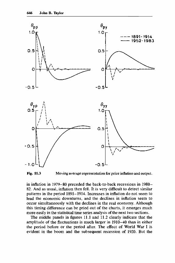
Fig. 11.3 Moving average representation for price inflation and output.

in inflation in 1979-80 preceded the back-to-back recessions in 1980-82. And as usual, inflation then fell. It is very difficult to detect similarpatterns in the period 1891-1914. Increases in inflation do not seem tolead the economic downturns, and the declines in inflation seem tooccur simultaneously with the declines in the real ecanomy. Althoughthis timing difference can be pried out of the charts, it emerges muchmore easily in the statistical time series analysis of the next two sections.

The middle panels in figures 11.1 and 11.2 clearly indicate that theamplitude of the fluctuations is much larger in 1910-40 than in eitherthe period before or the period after. The effect of World War I isevident in the boom and the subsequent recession of 1920. But the

647 Improvements in Macroeconomic Stability

8yw

0.5

-0.5

- 1.0

--- 1891-1914- 1952-1983

0.5

-0.5

0.5

O~~JIL--~~------~

-0.5

Fig. 11.4 Moving average representation for wage inflation and output.

extended boom in the 1920s and the Great Depression dominate thecharts. The wide fluctuations in wages and prices indicate the sametype of flexibility that is evident before World War I. The persistenceof wage and price inflation-a sign of wage and price rigidities used inmacrotheory-definitely seems relatively nc~w.

11.3 Vector Autoregressions

The dynamic properties ofoutput, wages, and prices can be examinedmore systematically by estimating unconstrained vector autoregres-sions. Estimates of bivariate autoregressions for wage inflation and out-

648 John B. Taylor

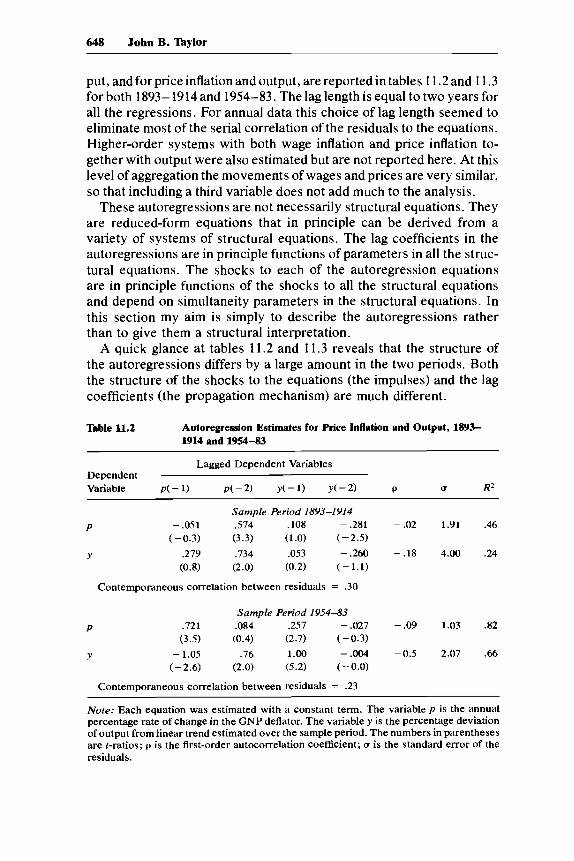
put, and for price inflation and output, are reported in tables 11.2 and 11.3for both 1893-1914 and 1954-83. The lag length is equal to two years forall the regressions. For annual data this choice of lag length seemed toeliminate most of the serial correlation of the residuals to the equations.Higher-order systems with both wage inflation and price inflation to-gether with output were also estimated but are not reported here. At thislevel ofaggregation the movements ofwages and prices are very similar,so that including a third variable does not add much to the analysis.

These autoregressions are not necessarily structural equations. Theyare reduced-form equations that in principle can be derived from avariety of systems of structural equations. The lag coefficients in theautoregressions are in principle functions of parameters in all the struc-tural equations. The shocks to each of the autoregression equationsare in principle functions of the shocks to all the structural equationsand depend on simultaneity parameters in the structural equations. Inthis section my aim is simply to describe the autoregressions ratherthan to give them a structural interpretation.

A quick glance at tables 11.2 and 11.3 reveals that the structure ofthe autoregressions differs by a large amount in the two periods. Boththe structure of the shocks to the equations (the impulses) and the lagcoefficients (the propagation mechanism) are much different.

Contemporaneous correlation between residuals = .30

p

y

Sample Period 1954-83.721 .084 .257 -.027 -.09 1.03 .82(3.5) (0.4) (2.7) ( -0.3)

-1.05 .76 1.00 -.004 -0.5 2.07 .66( -2.6) (2.0) (5.2) ( -0.0)


Note: Each equation was estimated with a constant term. The variable p is the annualpercentage rate ofchange in the GNP deflator. The variable y is the percentage deviationofoutput from linear trend estimated over the sample period. The numbers in parenthesesare t-ratios; p is the first-order autocorrelation coefficient; 0" is the standard error of theresiduals.


Table 11.3 Autoregression Estimates for Wage InBation and Output, 1893-1914 and 1954-83

Lagged Dependent VariablesDependentVariable w( -1) w( -2) y( -1) y(-2) p cr R2

Sample Period 1893-1914w 0.52 .007 .147 - .213 .02 1.66 .30

(0.2) (0.1) (1.3) ( -1.8)y -.358 -0.30 .220 -.063 .05 4.49 .04

( -0.6) (- 0.1) (0.7) ( -0.2)


w

y

Sample Period 1954-83.569 .175 .097 .103 -.03 1.20 .70(2.5) (0.7) (0.8) (0.8)

-.650 .336 1.026 - .181 .04 2.21 .62( -1.6) (0.8) (4.5) ( -0.8)


Note: The variable w is the annual percentage rate of change in average hourly earningsin manufacturing. For the definition of other variables see the note to table 11.2.

11.3.1 The ImpulsesThe variance of the shocks, or the impulses, to the output equation

has decreased sharply from the prewar to the postwar period. To theextent that macroeconomic policy works by changing the dynamics ofthe economy-as it would with feedback policy, the finding that areduction in the size of the shocks explains most of the reduced vari-ability suggests that such feedback policy ,vas not responsible for im-provements in performance. However, part of the change in policycould affect the variance of the shocks by working' 'within the period"to offset exogenous disturbances. This would be more likely for theautomatic stabilizers that react simultaneously, but with annual dataeven a feedback policy that reacts to econoInic disturbances within theyear would affect the variance of the shocks rather than the dynamicsof the system.

The variance of the shocks to the inflation equations is also muchsmaller in the postwar period. Since the overall variance of inflation isabout the same in the two periods, changes in the propagation mech-anism must have had a positive influence on the variance of inflation.The impulses have become weaker. It is perhaps surprising that thevariance of the shocks to inflation has become smaller. According tothese estimates, an increased importance of price shocks in postwarbusiness cycles is not supported by a comparison with the period beforeWorld War I.

650 John B. Taylor

The contemporaneous correlation between the shocks to the equa-tions is positive in both the prewar and the postwar periods. However,the correlation is stronger in the prewar period. More of the actionseems to come within the annual time interval during the prewar period.

11.3.2 The Propagation MechanismThe sum of the coefficients of the lagged inflation rates in the inflation

equations is much smaller in the earlier period. This change is moremarked for wage inflation than for price inflation. This change is con-sistent with the increased persistence of inflation in the postwar periodthat is evident in the time series charts. The sum of the coefficients onlagged output in the output equation is also higher in the postwar period,reflecting a corresponding increase in the persistence of output fluc-tuations.

The difference in the temporal ordering of inflation and output move-ments that seems to emerge from the time series plots is evident in thecross, or off-diagonal, autoregression coefficients. In the prewar periodlagged inflation has either a positive or an insignificant effect on output.In the postwar period the effect of lagged inflation on output is signif-icantly negative. Looking at the other side of the diagonal, in the prewarperiod lagged output has a negative effect on inflation; in the postwarperiod it has a positive effect.

11.4 Moving Average Representations

The moving average representations provide a more convenient wayto look at the propagation mechanisms in the economy. They can bederived directly from the autoregression equations. The vector auto-regressions reported in tables 11.2 and 11.3 can be written in matrixnotation as follows:

(1)

where Zt = (wt,Yt), in the systems with wage inflation and output, andwhere Zt = (Pt,Yt) , in the systems with price inflation and output. Aland A 2 are two-by-two matrixes of lag coefficients. The two-by-onevector et is supposed to be serially uncorrelated. The moving averagerepresentation is then given by(2)

where the 8 1 matrixes are found by successive substitution of laggedzs in equation (1). Alternatively, and perhaps more intuitively, the 8matrixes can be computed by dynamically simulating the effects of unitshocks to each of the equations in (1). The two elements of the firstcolumn of8 1 are given by the effects ofa unit inflation shock on inflation


and output, respectively, in this simulation. The two elements of thesecond column of 8 1 are given by the effects of a unit output shockon inflation and output, respectively, in the simulation.

Denote the elements ofthe first column ofe by Opp and Oyp, and the ele-ments ofthe second column of8 by Opy and Oy)'. These four elements ofthe8;matrixes are tabulated in tables 11.4through 11.7for iequals0 to a valuewhere the coefficients are negligible in size. The coefficients are also plot-ted in figures 11.3 and 11.4 for easy comparison ofthe two time periods.

table 11.4

1.00-.05

.61-.06

.15-.04

.02-.02

.00-.00-.00

Moving Avenge Representation for Price Inflation and Output,1893-1914

Opy Oyp Oyy

.00 .00 1.00

.11 .28 .05-.28 .73 -.23

.04 .10 -.03-.10 .24 -.14

.02 -.01 -.00-.02 .04 -.03

.01 -.02 .01-.00 -.00 .00

.00 -.01 .00

.00 -.00 .00

Note: Derived from the autoregression coeflicients reported in table 11.2.

table 11.5 Moving Avenge Representation for Price Inftation and Output,1954-83

Oyp

1.00.72.33.06

-.12-.23-.28-.29-.27-.24-.20-.16-.12-.08-.05-.03

.00

.26

.41

.48

.48

.44

.38

.31

.24

.18

.12

.08

.04

.01-.00-.02

.00-1.05-1.06-.85-.65-.47-.32-.20-.10-.03

.02

.05

.07

.07

.07

.06

1.001.00.72.47.27.12.02

-.05-.09- .11-.12- .11-.10-.08-.06-.05

Note: Derived from the autoregression coefficients reported in table 11.2.

652 John B. Taylor

Table 11.6

1.00.05

-.04.06.03

-.00-.00

.00

.00

Moving Average Representation for Wage Inflation and Output,1893-1914

6wy 6yw 6yy

.00 .00 1.00

.15 -.35 .22- .17 -.12 -.07-.06 .01 .03

.01 -.01 .04

.00 -.02 .00-.01 -.00 -.00-.00 .00 .00

.00 -.00 .00


Table 11.7 Moving Average Representation for Wage Inflation and Output,1954-83

6yw

1.00.57.44.21.06

-.06-.12- .15-.15- .13-.10-.07-.04-.02-.00

.00

.10

.26

.35

.37

.35

.29

.22

.14

.08

.02-.01-.03-.05-.05

.00-.65-.70-.69-.58-.43-.28- .15-.05

.03

.07

.09

.09

.08

.07

1.001.03

.81

.52

.25

.02- .12-.20-.23-.22-.18- .13-.09-.05-.01


The use of moving average representations in macroeconomics orig-inates with the influential paper by Sims (1980) in which he refers to itas innovation accounting; the approach has since been adopted by manyother researchers. There are many moving average representations of agiven multivariate process depending on what one assumes about thecontemporaneous correlation between the shocks. Sims suggests that aform be chosen so that the covariance matrix of the shocks is diagonal-an orthogonalization ofthe shocks. This requires a transformation of the8 i matrixes. The transformation is a function of the correlation of theshocks and depends on how one wishes to order the way the shocksenter the system. The methodology used here is different from that ofSims in that the 8 i matrixes have not been transformed to yield orthog-


onal shocks. I have found that such a transformation makes it difficultto give a direct structural economic interpretation of the 8 j matrixes.The method used here was also used for very similar purposes in aninternational comparison of economic performance (Taylor 1980).

Figures 11.3 and 11.4 indicate the enormousness of the change thathas taken place in the dynamics of inflation and output since the periodbefore World War I. The charts on the diagonal of figures 11.3 and 11.4show the persistence of inflation 8pp and output 8yy • Both have increased.

The cross effect of the shocks has changed even more. The 6py

coefficients have changed sign; an output shock has a long-delayedeffect on inflation in the more recent period. Before World War I thisdynamic effect was very small. Recall, however, that a positive contemporaneous relation between output and inflation existed before WorldWar I. The 6yp coefficients have changed in the reverse direction.Whereas inflation shocks generated a reduction in output iIi the morerecent period, they generated an increase in output before World WarI. This change, which emerges so clearly from the moving averagerepresentations, is the same change that was barely visible in the timeseries charts: when inflation rises in the r(~cent period, output falls;inflation then subsequently subsides.

11.5 Summary of the Facts

The preceding examination of the facts of inflation and output fluc-tuations in 1891-1914 (the first period) and 1952-83 (the second period)can be summarized as follows:

1. Output fluctuations are smaller in amplitude and more persistentin the second period.

2. Inflation fluctuations are about the same in amplitude in bothperiods but are more persistent in the second.

3. Inflation shocks have a negative, but lagged, effect on output inthe second period; output shocks have a positive, but lagged effect oninflation in the second period. No such timing relation exists in the firstperiod. If there is any intertemporal effect in the first period, it is inthe reverse direction.

4. There is a positive contemporaneous correlation between the in-flation shocks and the output shocks in both periods. This correlationis larger in the first period.

5. The variances of the shocks to inflation and to output are smallerin the later period.

11.6 Structural Interpretations

The vector autoregression can be viewed as a reduced form of astructural model. Unfortunately the mapping from the reduced form

654 John B. Taylor

to the structural form is not one-to-one. The traditional identificationliterature shows formally that there will in principle be many structuralmodels that are consistent with a given reduced form. In practice,however, the situation is not so dismal. There are a relatively smallnumber of theoretically sound or "reasonable" structural models.Moreover, the properties of an estimated reduced form can frequentlynarrow the range of possible structural models.

11.6.1 The Postwar PeriodThe third property of the estimated autoregressions listed at the end

of the previous section is very useful for nailing down a reasonablestructural model. The dynamic interaction between inflation and outputin the postwar period is very strong. Inflation "Granger causes" outputin a negative direction; and output "Granger causes" inflation in apositive direction. This pattern naturally leads to the following inter-pretation for the postwar period.

The Federal Reserve, or the "aggregate demand authorities" in gen-eral, is concerned with stabilizing inflation as well as unemployment.For aggregate demand shocks this joint aim causes no conflict; the bestpolicy for both price and output stabilization is to offset the shocks.When an inflation shock comes, however, there is a conflict. The Fedmust decide how "accommodative" to be. On average during the post-war period the Fed seems to have made a compromise. Policy is de-scribed by a policy rule. When an inflation shock occurs, the Fed neitherfully "accommodates" the shock by increasing the rate of growth ofthe money supply point for point with inflation nor tries to eliminateit immediately by sharply reducing money growth. Instead, it lets moneygrowth increase, but by less than the inflation shock. The result is thedynamic pattern observed in the vector autoregressions. When inflationincreases the Fed lets real money balances-appropriately defined-fall, and the economy slips into a recession. Hence, inflation "Grangercauses" output. The slack demand conditions then gradually work toreduce inflation. Hence, output "Granger causes" inflation.

This structural interpretation is by no means new, and it is graduallybeing incorporated in standard textbooks. For the data used here thefollowing simple algebraic structural model seems to match the reducedform very well:

(3)

(4) Yt = -~tPt-l + ~2Pt-2 + Yt-l + Vt·

The notation for output Yt and inflation Pt is the same as earlier. Theoperator E is the conditional expectation based on information throughperiod t - 1. The shocks U t and V t are assumed to be serially uncorrelated.


The first equation is a simple price adjustment equation. This equa-tion has no simulaneous effects between output and inflation. The sec-ond equation is the policy rule described above. It states that the rateof growth of output relative to trend is reduced if inflation has risen.If this system is to match up with the reduced-form evidence, theparameters should all be positive.

The estimated equations (written with the constants explicit and thet-ratios in parentheses) are:

(J" = 1.0, R2 = .83(5) Pt = .89pt-l + .25EYt + .55 ,(10.1) (3.6) (1.3)

(6) Yt = -1.Olpt_l + .69pt-2 +Yt-l + 1.17, (J" = 2.0, R2 = .67( - 3.5) (2.5) (1.6)

These equations were estimated using the full information maximumlikelihood method. This method takes account of the cross-equationrestrictions that occur when the second equation is used to forecastoutput in the first equation. The output equation is already in re-duced form and is clearly not much different from the estimatedequation in table 11.2. The reduced form for inflation can easily bederived by substituting the expectation of equation (6) into equation(5). It also matches up well with the reduced-form equation intable 11.2.

Equation (6) indicates that there is much less accommodation ofinflation in the short run than in the long run. The short-run reactioncoefficient is about -I, whereas the long-run reaction is about - 0.3.Equation (5) indicates that inflation responds to slack demand with alag. 3 The coefficient on lagged inflation depends on the structure ofcontracts in the economy as well as on expectations of inflation; theparameter would change with a change in the policy rule that changedexpectations, and in this sense it is incorrect to refer to the equationas structural.

The policy rule can be written in the following interesting form:

(7) Yt - Yt-l = - .32pt-l - .69(pt-l - Pt-2) + 1.17.

In other words, the rate of growth of real GNP (relative to potential)is reduced by 32% of the inflation rate in the last period plus 69% ofthe change of the inflation rate. The response of the Fed to high inflationis stronger when inflation is increasing than when it is decreasing. A

3. The data cannot discriminate between the assumptions that Yt or E t appears inequation (5). The contemporaneous correlation is positive and could equally well be dueto the correlation between the structural shocks as to a direct simultaneous effect of Yton Pt.

656 John B. Taylor

nominal GNP rule could be interpreted4 as having an implied coefficient- 1 on the lagged inflation rate, with no adjustment for increasing ordecreasing inflation. The estimated rule is less accommodative than anominal GNP rule in the short run and more accommodative than anominal GNP rule in the long run.

11.6.2 The Prewar PeriodThis model of price adjustment and policy is explicitly oriented to

the postwar period in the United States. The wide differences betweenthe autoregressions in the prewar and the postwar periods indicatethat the same model is unlikely to fit in the prewar period. In fact,the model does very poorly in the prewar period. The coefficient onlagged inflation in the inflation equation (3) is negative though smalland insignificant, whereas the coefficients on lagged prices in theoutput equation (4) are all positive. As the reduced-form results sug-gested, the dynamic relation between inflation and output in the pre-war period is weak and opposite in sign from that for the postwarperiod.

The price adjustment equation without the insignificant lagged infla-tion rate is

(8) Pt = .28Yt + 1.33.(2.5) (2.0)

Hence, although the lagged inflation rate disappears, the adjustmentcoefficient is about the same size as before.

There are two possible implications of this failure of the postwarmodel. 5 First, prices and wages appear to be more flexible in the prewarperiod in that their correlation with output fluctuations is almost entirelycontemporaneous. Adjustments occur within the annual time interval,unlike the postwar period, where the adjustments are drawn out forseveral years. Second, macroeconomic policy appears to be very ac-commodative; inflation shocks seemed to have no prior negative effecton output. Are these implications plausible?

11.6.3 More Flexible Wages and Prices?The reduced importance of the lagged inflation term could be due

to simple expectations effects as well as to changes in the structure of

4. Taken literally, a nominal GNP rule would respond to inflation shocks in the currentperiod. In practice, however, a lag would probably occur.

5. It should be noted that there are fairly strong dynamic feedback effects from outputand prices two years earlier in the price inflation system (see table 11.2). This is puzzlingsince the impact from prices and output one year earlier is weak. This two-year leap isthe reason for the sawtooth moving average representation for this system (see fig. 11.3).


wage and price setting. The inertia effect in the postwar period is acombination of expectations effects and stIucture. Since inflationaryexpectations were probably much lower in the prewar period, the effectof lagged inflation would be smaller. Unfortunately, it is difficult todistinguish these two effects with aggregate data.

The problem has been addressed by Cagan (1979) and Mitchell (1983)using microeconomic data. Although neither author looks at data beforeWorld War I, their findings are probably relevant for the comparisonof this paper. Cagan compares price movemc~nts in the business cyclesof the 1920s with price movements in the business cycles after WorldWar II. Mitchell compares wage adjustments in the 1930s with wageadjustments in the postwar period. Both find that price and wage ad-justments were larger and more frequent in the earlier period. From amicroeconomic perspective wages and prict~s were more flexible.

Two possible reasons for this change have been noted. First, theincreased importance of large business enterprises and large unionscould have centralized price and wage decisions and made them lesssubject to short-run market pressures. In the major labor unions, forexample, the costs of negotiating a large settlement made it economicalto have long three-year contracts in many industries. The overlappingnature of these contracts added to the persistence of wage trends.Second, economic policy changed so as to reduce the severity ofreces-sions and thereby lessen the need to reduce wages and prices quicklyin the face of slack demand conditions. This policy effect is differentfrom the expectation of inflation effect mentioned above.

11.6.4 More Accommodative Policy?Although the United States Treasury took on some central bank

functions in the early 1900s, during most of the period 1891-1914 mon-etary policy was determined solely by the lfnited States commitmentto the gold standard. A gold standard is normally thought to generateaggregate demand "discipline." Policy would automatically be non-accommodative. For example, if there was an inflation shock, then acontractionary policy would be necessary in order to bring the pricelevel back to its relative position with gold. Then why do the datasuggest the opposite, that policy was accommodative?

One explanation comes from the fact that the United States was asmall open economy during this period. Most price shocks probablycame from abroad, much as the price shocks in the 1970s came fromabroad. An increase in external prices with a fixed exchange rate willmake domestically produced goods cheaper. 'This will lead to a balanceof payments surplus until internal prices rise. A balance of paymentssurplus increases the money supply for a country on a gold standard.

658 John B. Taylor

The increase in the money supply will therefore tend to occur just asthe domestic price level rises in response to the rise in world prices.Policy will look very accommodative.

A fixed exchange rate gold standard will be less accommodative toprice shocks that originate at home. A price shock will raise domesticprices relative to external prices. The resulting balance of paymentsdeficit will reduce the domestic money supply, and the economy willtend to fall into a recession. Internal prices will then fall. Either thistype of scenario did not occur in 1891-1914, or it occurred so quicklythat the timing cannot be detected with aggregate annual data. It isinteresting that accommodation under a gold standard seems to bedifferent for external shocks and internal shocks. According to modernexpectations theories this discrimination is appropriate. Internal en-dogenous price and wage shocks are discouraged, whereas externalexogenous price shocks are accommodated. Because the external priceand wage behavior is unlikely to be influenced by the monetary policyin a small open economy, accommodation will not do any long-runharm. But internal price and wage behavior is likely to be adverselyaffected by an accommodative policy.

Another way to describe the prewar policy rule is to say that it wasaccommodative in the short run, permitting much slippage to accom-modate external price shocks, but nonaccommodative in the long run.Prices in the United States could not differ from world prices in thelong run. This is in contrast to the characterization in the previoussection of policy in the postwar period: in the short run policy is muchless accommodative than in the long run.

To summarize, the interpretation that prices and wages adjust quicklyand that policy is very accommodative in the short run is plausiblefrom a microeconomic perspective. Unlike the postwar period, wherelags in the relation between output and inflation permitted one to narrowdown the field of potential models, for the prewar period data are moreambiguous. If all the action occurs within the annual timing interval,it is difficult to distinguish one structural model from another. The lagsare not long enough to identify the structure. In fact, the contempor-aneous relation between prices and output in equation (8) could havebeen generated from a mechanism like the Lucas (1972) supply curve.If prices were as flexible as they appear to be during this earlier period,then the Lucas model itself is more plausible.

11.7 Concluding Remarks

Macroeconomic performance in the United States from 1891 through1914 was much different from the performance after World War II. Thisdifference is apparent in reduced-form autoregressions, in their moving


average representations, in simple structural models, and even in simpletime series charts of the data. The shocks, or impulses, to the economicsystem were smaller in the second period, mainly because of the policyand structural changes that Arthur Burns lnentioned in his 1959 pres-idential address. Deposit insurance, for example, reduced the shocksto aggregate demand that came from financial panics.

But the dynamics, or propagation mechanisms, of the economicsystem are much slower and more drawn out in the postwar period.This tends to translate the smaller shocks into larger and more pro-longed movements in output and inflation than would occur if the pre-war dynamics were applicable in the later period. In other words, thechange in the dynamics of the system offset some of the gains fromthe smaller impulses. These postwar dynamics can be given a structuralinterpretation in terms of the accommodative stance of monetary policyand the speed of wage and price adjustments. These dynamics werenot evident in the prewar period.

One interpretation of these developments is that the change in thedynamics was a direct result of the reduction in the importance of theshocks. For example, prices and wages may have became more rigidbecause of the reduced risks of serious reeessions or because move-ments in the money supply began to do some of the macroeconomicstabilization work that was previously done: by wage and price adjust-ments. The analysis of this paper is not conclusive on this or on theother interpretation that the change in the dynamics was unrelated tothe change in policy. But the possibility that a combination of thesmaller postwar shocks with the shorter prewar dynamics might im-prove macroeconomic performance should be sufficient motivation forfurther study of these historical developments and their alternativeinterpretations.

Comment Phillip Cagan

It has long been noted that prices fluctuate less in post-World War IIbusiness cycles than they used to, though with the higher rates ofinflation in the 1970s the amplitude of fluctuations became larger. Onereason was that business cycles were generally less severe in the post-war period; none matched the severity of 1929-33, 1937-38, 1920-21,or 1907. Yet even for cycles of comparablt:~ severity in terms of realvariables the postwar period appeared to exhibit less price fluctuation.It was generally agreed that prices and wages had become less flexible.

Phillip Cagan is professor of economics at Columbia University.

660 John B. Taylor

In Taylor's annual data, these differences between periods are lessclear. Compared with the interwar cycles 1910-40, the post-World WarII period shows a standard deviation only one-quarter of the earliervalue for price inflation and one-third of the earlier value for wageinflation. But compared with the pre-World War I cycles 1891-1914,the post-World War II cycles had about the same standard deviations-only 8% smaller for price inflation and actually 16% larger for wageinflation, even though the standard deviation of real GNP from its trendwas 25% smaller in the post-World War II period. Inflation rates in thislater period had a greater upward trend until the past few years, how-ever, so that their standard deviations, if measured from trend, wouldbe smaller.

The smaller variation in inflation in the later period becomes clearin the vector autoregression analysis of price and wage inflation andthe real GNP gap. The residuals from these regressions represent unex-plained movements, which Taylor interprets as "shocks" to the system.These shocks are much smaller in the postwar period. Compared withthe pre-World War I period, in the postwar period shocks are reducedby 50% for prices and for the output gap and by 25% for wages.

Taylor uses this comparison of shocks to explain why, if prices andwages are less flexible in the postwar period, the output gap at thesame time shows less rather than more variability. The answer is thatshocks in the postwar period were sufficiently smaller to overcome thetendency of cyclical fluctuations to show up more in output than inprices and wages.

What are these shocks? Some are supply shocks, best illustrated bythe OPEC oil price increases of 1973 and 1979 or by major labor strikes,as in steel in 1953 and automobiles in 1971, but for the most part theseare fairly rare events. Shocks can also appear on the demand side, asin the financial panics of 1893 and 1907, which produced sudden con-tractions in the available money supply. In addition, we should rec-ognize the possibility of mundane but ubiquitous measurement errors,particularly in the earlier period when the data are clearly less accurate.When Simon Kuznets put together his annual GNP data for the pre-1929 period, he was so concerned with the imprecision of the estimatesthat he was unwilling to publish the annual figures and planned torelease only five-year averages. He was subsequently persuaded, Iunderstand, to allow Friedman and Schwartz to use the data in annualform, since the five-year averages would have been useless for cyclicalanalysis. Kuznets obviously knew something about these data that therest of us should not ignore. The GNP series from Historical Statisticsthat Taylor used are not much better.

Finally, Taylor's shocks may reflect variations over time in cyclicalrelationships that cannot be captured by a small number of autoregres-


sion lag terms. Cycles vary in duration and amplitude, and such vari-ations may reflect the internal dynamics of the cyclical process as wellas different dynamics depending on the type of shock, particularlywhether it is viewed as temporary or permanent. I cannot refrain herefrom expressing my uneasiness with the spreading popularity of vectorautoregression analysis. My concern is not with its atheoretical ap-proach, which bothers some critics-that can often be an advantage-but with the fact that relatively simple autoregression and moving av-erage representations do not fit many tirne series adequately, eventhough the residuals may pass tests as white noise. In work that I havedone, an ARIMA fit to Ml growth produces residuals that have a muchsmaller variance in the 1960s than in the 1950s and 1970s. There is nosimple way to model this pronounced change in variance. I also foundthat GNP growth in the 1970s cannot be represented by ARIMA func-tions that fit earlier periods. (Of course, structural econometric modelsmay face the same problem of inadequate fit over different periods.)The NBER used to have a tradition of presenting charts of basic data.I would be less uneasy if the users of vector autoregressions ponderedcharts of their fits and showed them to the reader.

Having raised these red warning flags, I do not wish to dismiss allsuch statistical analyses. In many cases, and in Taylor's analysis ofprices and wages, I find the vector autore:gressions a useful and en-lightening supplement to other modes of analysis.

His autoregressions contain three other pieces of information in ad-dition to the variance of the residuals. The first is the contemporaneouscorrelation of residuals in the paired regressions. These are about thesame for the pre-World War I and post-World War II periods but twiceas large in the wage as in the price regressions. Although Taylor doesnot comment on this information, I interpret it as some evidence againstgreater measurement error in the earlier period. The shocks should becorrelated, since most demand and supply shocks will affect prices andwages as well as output in the span of one year. Measurement errorwould normally be uncorrelated and thus would produce no correlationof residuals.

Another more important piece of information provided by the vectorautoregressions is the coefficients on lagged values of the dependentvariables. These are a measure of persiste~nce-thedegree to whichthe series is a continuation of its previous values. Based on the sizeand statistical significance of these coeffic:ients, the postwar periodshows much more persistence, as we knew it would from previousstudies of the flexibility of prices and wages. Taylor's measure of per-sistence nicely summarizes this development. The pattern of increasingpersistence is broken, however, by a large significant coefficient in theearlier period on the lag of prices two years previous. This coefficient,

662 John B. Taylor

which is positive and characteristic of "sawtooth" movements, has noobvious interpretation. A feedback mechanism such as existed underthe gold standard would produce a negative coefficient. It appears tobe a fluke and lends support to the importance of measurement error.

The cross-coefficients in these regressions, those showing the effectofprice and wage inflation on output, can be interpreted as the responseof the monetary system to inflationary pressures. Positive coefficientsindicate accommodation, zero coefficients no accommodation, and neg-ative coefficients a counter response. Here I am surprised by the re-sults, and apparently Taylor was also. In the postwar period thesecoefficients of prices and wages in the output regressions are negativefor the first lag and positive for the second. This has the interestinginterpretation that policy since World War II has initially opposed in-flationary pressures but then accommodated them, possibly as a re-action to the consequences of the initial anti-inflationary actions or inany event as an inability or unwillingness to carry through with them.Although I am surprised to find this in the autoregressions, it is notimplausible. The time series pattern of inflation since World War II canbe viewed as supporting this interpretation: inflationary movementshave fluctuated but overall have tended to rise from cycle to cycle,except (let us hope!) for the most recent episode, 1979-83.

The indicated degree of such accommodation in the pre-World WarI period is quite different. The response to wage inflation is weaklynegative in the first lag and then zero in the second, indicating eithera partial accommodation over the two years or perhaps an immediatestrong opposition to inflation that is completed within one year and sois absent from the first lagged year. For price inflation, however, theresponse in the pre-World War I period is surprisingly positive, and itis significantly positive in the second lagged year. This implies thatprice movements were more fully accommodated under the gold stan-dard than later under the Federal Reserve System. This may at firstseem counterintuitive, but I believe it correctly depicts the dynamicsof the gold standard. The vaunted monetary discipline of the goldstandard occurred only in the long run. The gold standard took two tothree cycles or more to reverse monetary and price developments ifthey were moderate and not severely out of line with world trends,and it was quite loose in the short run. I and others have pointed outthat United States gold specie flows were much smaller than cyclicalmovements in the foreign trade balance. Most of the cyclical tradeimbalances were financed by capital flows, probably because of a gen-eral expectation that gold would remain convertible at a fixed exchangerate. The distribution of growing world gold stocks to maintain fixedexchange rates worked slowly over long periods, except when con-vertibility was threatened, such as by financial panics or by the United


States silver purchase legislation of the early 1890s. The managed mon-etary regime under the Federal Reserve System, on the other hand,could and usually did act more quickly at first to counter inflationarypressures, but since World War II, unfortunately, inadequately.

The vector autoregression technique allows a description of the pathof the variables when a shock to one of the variables occurs. Taylorshows the paths of the variables for the two periods in his figures 11.3and 11.4 where the contemporaneous cOITelation between the errorterms has been ignored. He suggests that the two periods are bestrepresented by two quite different model interpretations. For the laterperiod he postulates that changes in output depend on the one-yearlagged inflation rate and the change in the inflation rate between thetwo previous years. This is consistent with the results reported for theautoregression equation. It is intended to represent a one-year laggedeffect of monetary policy on output. When fit to the data, this equationsuggests that policy actions reduce output by 30% of the previous year'sinflation rate and by 70% of the change in the inflation rate in theprevious year. This differs from a straightforward rule of keeping nom-inal GNP constant, by which the coefficient for the inflation rate in thisequation on a one-year lag would be - 1. The fitted equation for thelater period thus differs from the GNP rule in that the response is wellunder unity, and stronger if inflation is increasing than if decreasing.

In the other equation for the later period, price inflation is madedependent on the one-year lagged inflation rate and the expected outputgap. This expectation is based on the output equation. The assumptionthat expected rather than actual output belongs in this equation followsthe literature on rational expectations and staggered contracts. Priceinflation is persistent because of contracts but partially responds in anyyear to expected demand, here represented by expected output.

This model for the later period is an interesting and ingenious inter-pretation of the empirical results. It is useful for comparison with theearlier period. My main difficulty is with its extreme abstraction fromthe details of the business cycle. Monetary policy is assumed to respondonly to inflation and not to output or other variables, and all the con-tributions to the business cycle other than policy and price responsesare subsumed in the error terms. It is anyone's guess whether thecyclical process that is approximated by this high degree of abstractionis valid or misleading.

In comparing the later with the earlier period, what in summary canbe said? First of all, prices in the later period lost much of the flexibilitythey displayed earlier. Unions and longer '''age contracts are a majorreason. But I believe the later inflexibility reflects more than this:adjustments have become less flexible on a broader scale than can beattributed to union contracts or their influence on costs. Taylor men-

664 John B. Taylor

tions the growth of large business enterprises centralizing price deci-sions, but inflexibility is just as true of fabricated products supplied bymany small firms. The only broad effect that Taylor or anyone else,including me, has been able to identify that stands up is the lessenedseverity of cyclical fluctuations since World War II and presumably ageneral expectation that government policies will oppose severe pricemovements, thus reducing the likelihood that major price or wagechanges will have to be made. This shows up in the time series asautocorrelation and greater persistence.

The second conclusion is that in the short run the monetary systemdid not accommodate price movements in the later period but did soin the earlier period. Taylor suggests that the earlier period reflectedthe difference between external and internal price shocks. Under thegold standard external price increases from abroad produced tradesurpluses and gold inflows along with direct price increases and thusappeared to accommodate the price shock. On the other hand, domesticprice increases not matched abroad led to gold outflows and a subse-quent contraction. The effect of internal price shocks in the earlierperiod either occurred very quickly and so was invisible in the annualdata or was dominated by the external shocks. The latter is conceivable,but there is no particular reason to believe that external shocks dom-inated. Although the United States was somewhat like a small openeconomy in this period and so ~as subject to influences from abroad,it also generated major internal shocks such as harvest surpluses, bank-ing panics, and the silver agitation.

In any event, I favor Taylor's other explanation, which in my inter-pretation is to view the gold standard as accommodative in the shortrun through variations in the gold reserve and as disciplined to benonaccommodative only in the long run to maintain convertibility.

Finally, although shocks were smaller in the later period, the dy-namics of the system translated the shocks into larger and more pro-longed movements in output and inflation. The change in dynamicsfrom the earlier to the later period would have produced larger cyclesin the later period had the shocks not become smaller.

The lack of conclusiveness of the results here is due to the undefinedcharacter of the shocks. Taylor alludes to stabilizing developmentslisted by Arthur Burns in his 1959 presidential address, which includeddeposit insurance to prevent panics, less fluctuation in dividend pay-ments, automatic fiscal stabilizers, and so on. Most of these are "shocks"only in the sense that they are not directly specified in Taylor's vectorautoregression. Moreover, they may not have been independent of thedynamics. As Taylor suggests, price adjustments may have becomeslower in response to these other developments that reduced the am-plitude of the shocks.

66S Improvements in Macroeconomic Stability

The interpretation of these developments I like is that policy becamemore responsive to output gaps in the later period and that this allowedprices and wages to become less responsive. The effect was both toreduce cyclical fluctuations and to accolnmodate a gradually risinginflation rate. At first sight the autoregressions appear to contradictthis explanation, which implies that the output gap in the later periodshould have a negative coefficient on its lagged value when in fact ithas a positive value. However, the negative coefficient may occur onlyfor contractions in output, not expansions, if policy has been asym-metrical. The vector autoregressions miss such a distinction.

Taylor's analysis forces us to grapple with an apparent change in thedegree of accommodation between the earlier and later periods and areduction in the amplitude of shocks. I find these results generallyplausible. My main reservation is that the: shocks may be misleadingif their large size in the earlier period re:flects an inadequacy of theprice and output lags for explaining the dt~pendent variables. It mightbe that a structural representation of both periods would yield exog-enous shocks of equal amplitude. A comparison of these periods willremain incomplete until we can empirically demonstrate whether struc-tural changes or a decline in shocks account for the reduction in am-plitude of cycles. But my best guess is that mild cycles in both periodswere similar in dynamics and shocks and that the periods differ overallbecause of selected "severe" cycles owing to monetary disturbances,which were a special breed prevalent before World War II.

Comment Stephen R. King

John Taylor has written an elegant paper on interpreting the differencesin the cyclical behavior of output and inflation between the eight busi-ness cycles that preceded World War I and the eight that followed theWorld War II. The central difference he idt~ntifies between the periodsis that the postwar fluctuations in inflation and detrended output displaylower variance, but higher persistence, than those before World WarI. In fact, the mean peak-to-peak period of the postwar output cyclesis 4.2 years, ten months longer than in the prewar period.! To distinguishthe impulses that initiate cycles from the propagation mechanism thatextends them, he examines innovations, or shocks to the system, which

Stephen R. King is assistant professor of economic:s at Stanford University.1. These calculations are computed from a second-order autoregression for the output

gap, using the formula for the mean cyclical period given in Taylor (1980): period = 2'TT/cost- l ( - 0.5(1 - al + a2», where aj are the coeffi<;ients of the ith lags in the auto-regression for output.

666 John B. Taylor

he finds display much lower variance in the second period, and thedegree of serial correlation in the responses of the system to shocks,which he finds increases.

A particular strength ofthe paper is that Taylor interprets thereduced-form evidence gleaned from vector autoregressions (VARs) of de-trended output and inflation in the light of a simple structural model toaccount for the stylized facts that emerge. The transformation of a massof data into a few key parameters is very welcome. The model combines"sticky" price setting (with prices unresponsive to contemporaneousdemand movements) with a reaction function for aggregate demand pol-icy that implies that the monetary and fiscal authorities respond withsome degree of accommodation to output and inflation shocks.

The postwar results, as one might suspect, are quite consistent withthe interpretation offered by Taylor's model. The well-known stickinessof wages and prices, combined with partial demand accommodation,leads to a cyclical response of inflation, recession, and eventual returnto equilibrium in response to a price shock.

The pre-World War I results do not fit easily with such a model. Theshortness of output cycles in the data is consistent with the very lowdegree of serial correlation of prices (lack of stickiness) in this timeperiod. But the fact that price shocks do not lead to output fluctuations,except contemporaneously, suggests full accommodation by the mon-etary authority. This is the puzzle Taylor faces us with, since we usuallythink of policy as being unaccommodative under a gold standard. Theresolution of the puzzle is obtained by noting that under a gold standard,imported (but not domestic) price shocks would be accommodated bygold inflows and hence would not necessarily be followed by adversefluctuations in real output.

Credence is given to this interpretation by adding the growth rate ofmoney to the VAR that Taylor estimates. When this is done, priceinnovations not only are found to be positively correlated with moneyshocks, but are also followed by subsequent accommodating monetarymovements. 2 For the explanation to be convincing, however, it must

2. Exactly the opposite results hold for the postwar period when it appears that positiveoutput shocks leave money unchanged (and are followed by velocity increases), but priceshocks are followed by expansionary monetary growth. These observations, too, are inaccord with Taylor's conjectures. The actual equations (estimated for 1893-1914 and1954-83, with m representing the growth rate of M2 prewar and Ml postwar and t ratiosin parentheses) are:

Prewar: m t = .64Pt-l + .70Pt-2 - .52Yt-l - .33Yt-2 R2 = 0.51

(2.1) (2.4) (2.8) (1.8)

Postwar: m t = - .59pt-l + 1.25pt-2 + .25Yt-l + .02Yt-2 R2 = 0.66

(2.1) (4.6) (1.9) (0.1)


also be argued that the price shocks really did originate overseas. Inview of the desynchronization of the United States cycle from Euro-pean fluctuations that Moore and Zarno\\'itz document for the prewarperiod, this is by no means self-evident. More doubt arises becauseTaylor is using a deflator for domestic prices to measure inflation, notone that includes the prices of imports directly. It is true, of course,that the rapid expansion of world gold production after 1896 is con-sistent with the importation of price rises from abroad. Taylor's otherconjecture from looking at the output/inflation results is that outputshocks were followed by extinguishing monetary fluctuations. The VARmentioned above also confirms this supposition.

For whatever reasons, then, prewar policy does appear to have beenmore accommodating ofprice shocks and l,ess accommodating ofoutputshocks than it was in the postwar period. What does all this have todo with the role of prices and wages in improving macroeconomicstability? Despite the usefulness of Taylor's interpretive model andreduced-form findings, we learn little about the really fundamental dif-ference between the two time periods. Given that wages and prices doappear stickier in the postwar period, is this increase in stickiness aresult of more accommodative demand policy followed since the 1946Employment Act, or was the accommodative policy itself a reactionto an increase in wage and price stickiness? The answer to this questionis absolutely crucial in learning from these two periods.

Many reasons have been advanced for "exogenous" reductions inwage and price flexibility: increased concentration in industry, reduc-tion in the role of primary industries and their replacement by serviceindustry, and increased unionization of the labor force. The growingimportance of explicit and implicit contracts is also cited by some. Butthe increased willingness of the governm(~nt to accommodate fluctua-tions, either by automatic stabilizers, by institutions such as depositinsurance, or through discretionary policy, will also increase the in-centive of private agents to save on costly negotiations by writing long-term contracts.

Since a problem in interpreting the appearance of high coefficientson the lagged dependent variable in an inflation equation as due toinertia is that they may be in part expectational, it might make senseto estimate inflation equations for the two periods with lagged inflationand anticipated nominal GNP growth (in excess of trend real GNPgrowth) as explanatory variables. If the lagged dependent variable inTaylor's inflation equation was capturing expectations of inflation ac-

The prewar and postwar contemporaneous correlation coefficients of output and moneyare .61 and .63 respectively, and the corresponding inflation and money correlations are.29 and .36.

668 John B. Taylor

commodation, then such an approach might remove the significanceof the lags of the dependent variable in the equation. Doing this forthe prewar and postwar samples yields an insignificant sum of coeffi-cients on two lags of inflation of .42 (F(2,19) = 2.81) for the prewarperiod, and a highly significant .67 (F(2,26) = 47.1) for the postwar. 3

It seems, therefore, that this simple technique has not found evidencethat the increased importance of lags represents purely expectationaleffects. Inertia still characterizes the postwar, more than the prewar,data. Just as in Taylor's paper, however, there is some limited evidenceof stickiness in the prewar period at a two-year lag.

One must applaud Taylor's use of the pre-World War I sample. Thisinteresting period deserves study and provides an instructive compar-ison with the postwar period. At the same time, one runs the risk oftreat-ing the prewar period as though it were the "normal" state ofaffairs andcontrasting it with the postwar era with its "exceptional" price sticki-ness. A slightly broader comparison might be made with some evidencefrom an earlier period. David Hume, in his justly famous essay on money,reports that in the last year of Louis XIV (1715) in France, prices roseby only one-third the amount by which money grew. That performanceis comparable to postwar behavior in the United States. Perhaps, then,the period that requires special explanation is not the recent quarter-century but the twenty-four years that preceded World War I.

Taylor provides results for both price and wage inflation. To measurewages, he uses hourly earnings in manufacturing, which may not reflecteconomywide wages, especially in view of the hypothesized changesin relative prices of tradable goods. In his empirical results, he con-sistently finds lower coefficients on wages than on prices, especiallyin the prewar sample. Because of this, the moving average results givethe appearance of a procyclical real wage before the war. Althoughthis may be true, the lower coefficients on nominal wages, and theconsequent cyclical pattern of real wages, may simply be due to mea-surement error in the wage series and hence may be spurious.

A methodological problem with the empirical analysis is the weightput on interpretation of moving average coefficients, whose statisticalsignificance is not given in the paper. The very weak "fit" of the prewarinflation and output equations (for example, none of the coefficients in

3. The actual equations estimated for 1893-1914 and 1954-83 are:

Prewar: Pt = .12pt-1 + .30Pt-2 + .20E(PY)t R2 = .41

(0.6) (1.5) (1.6)

Postwar: Pt = 1.06Pt-1 - .39pt-2 + .27E(PY)t, R2 = .85

(7.0) ( - 2.4) (2.5)

where a constant and two lagged values of inflation and growth of nominal output andthe money supply are used as instruments for contemporaneous nominal output growth.


the prewar wage/output system is individually significant at the .05level) must be hiding some "true" stickiness from the observer. Itwould certainly be surprising if any of the moving average terms fromthat system were significantly different from zero.

Another obstacle to interpreting the moving average coefficients isTaylor's decision to ignore the contemporaneous correlation of theinnovations to the two equations, which in the systems he estimatesare always significantly different from zero (and positive). Althoughthere are, as he says, an infinite number of possible decompositions ofthis correlation, his model specifically implies one. Since prices aremodeled as being unresponsive to contenlporaneous demand shocks,it seems natural to allow price shocks (assuming they represent some-thing more than pure measurement error) to enter the output gap equa-tion contemporaneously. This might upsc~t the interpretation of theoutput equation as a policy reaction function. In fact, it would lead toa model with three equations-one for price adjustment, one for realGNP, and a monetary policy rule. In any event, given the size of thecontemporaneous correlations involved, suc;h an orthogonalization maywell make quite a difference to the results.

In conclusion, John Taylor's paper has Inade a very useful and pro-vocative contribution to the analysis of price/wage interaction in twodisparate periods of United States history. If there are still questionsto be answered about the roles of wages and prices in the behavior ofthe economy between the two periods, then this simply underscoresTaylor's concluding statement in the paper: that the policy implicationsof understanding why the Phillips curve has become flatter with thepassage of time are sufficient motivation for further study of the issues.

Comment J. Bradford DeLong and Lawrence H. Summers

In his contributions to this volume John Taylor reaches exactly theopposite conclusion from that in our papl~r (chap. 12); he finds thatimproved macroeconomic performance has taken place in spite of ratherthan because of the increased rigidity of wages and prices in the postwarperiod. Our explanation has the virtue of parsimony. We attribute themajor change in economic performance to the major change in eco-nomic structure rather than telling a complt~x story involving offsettingeffects. Moreover, Taylor provides no explanation of the forces thathave accounted for the huge decline in thl~ variance of aggregate de-mand shocks he claims took place. As we shall argue below, Taylor's

J. Bradford DeLong is a graduate student in the Department of Economics at HarvardUniversity. Lawrence H. Summers is professor of economics at Harvard University.

670 John B. Taylor

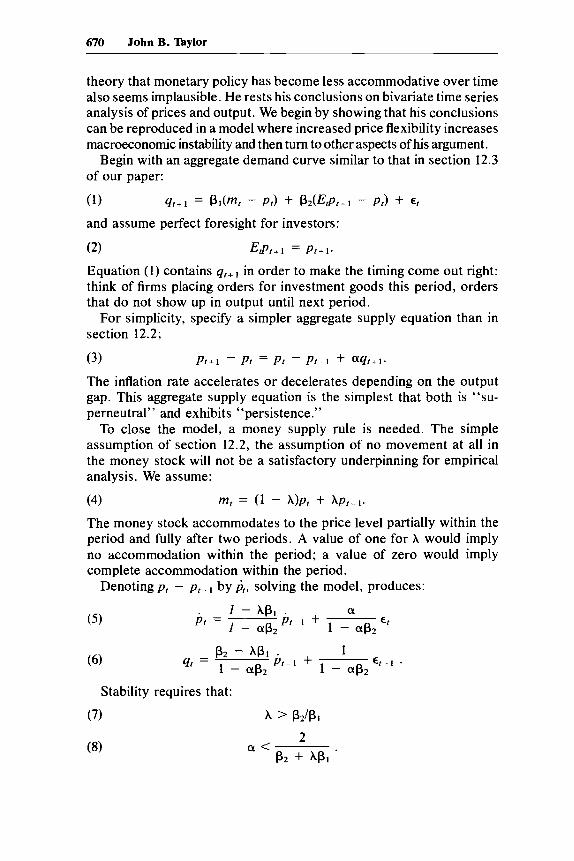
theory that monetary policy has become less accommodative over timealso seems implausible. He rests his conclusions on bivariate time seriesanalysis of prices and output. We begin by showing that his conclusionscan be reproduced in a model where increased price flexibility increasesmacroeconomic instability and then tum to other aspects ofhis argument.

Begin with an aggregate demand curve similar to that in section 12.3of our paper:

(1) qt+1 = ~I(mt - Pt) + ~2(EtPt+1 - Pt) + Et

and assume perfect foresight for investors:

(2) Etpt+1 = Pt+l·

Equation (1) contains qt+ I in order to make the timing come out right:think of firms placing orders for investment goods this period, ordersthat do not show up in output until next period.

For simplicity, specify a simpler aggregate supply equation than insection 12.2;

(3) Pt+1 - Pt = Pt - Pt-I + aqt+l·

(5)

(6)

The inflation rate accelerates or decelerates depending on the outputgap. This aggregate supply equation is the simplest that both is "su-perneutral" and exhibits "persistence."

To close the model, a money supply rule is needed. The simpleassumption of section 12.2, the assumption of no movement at all inthe money stock will not be a satisfactory underpinning for empiricalanalysis. We assume:

(4) m t = (1 - A)Pt + APt-I.

The money stock accommodates to the price level partially within theperiod and fully after two periods. A value of one for A would implyno accommodation within the period; a value of zero would implycomplete accommodation within the period.

Denoting Pt - Pt-I by Pt, solving the model, produces:

. 1 - A~I • aPt = 1 (.l Pt-I + 1 (.l E t- a~2 - a~2

~2 - A~I • 1qt = 1 (.l Pt-l + 1 (.l Et-l •- a~2 - a~2

Stability requires that:

(7)

(8)

A > ~2/~1

2a< .~2 + A~l

(9)


If Et follows a white-noise process with unit variance, then solvingfor the inverse of the variance of output leads to the equation:

J.. _ _ (~ !) (~~ ~1~2A) 2(f~ - 1 2 132 + 2 131/\ (l + 2 + 2 (l •

Therefore further increases in the price flexibility parameter a are des-tabilizing and increase the variance of output, so long as

1 1(10) a < - + ---- .2~2 ~2 + ~~lA

But (7) and (8) imply that a must satisfy (10). In this model, the varianceof output is least when a equals zero, when there is no flexibility at allin the aggregate price level.

And yet empirical analysis of a system generated by (1) through (4)would produce results that might mimic quite closely those Taylorobtained for the postwar period. An economist who knew the timingof the aggregate supply equation might be able to recover it exactly:

(11) Pt = Pt-l + aqt .

And an attempt to estimate a combined aggregate demand/monetaryreaction function equation would yield:

qt - qt-l (- ~131 - :2 - !) Pt-l(12) - a 2 ICl

+ (A~l - ~2 1 - aA~l ) .1 Q. + (1 Q.) Pt-2,- a...,2 a - a...,2

where A~l - ~2' 1 - a~2' and 1 - aA~b are all positive.These coefficients are too large to be taken seriously. However, their

size (but not their sign) is clearly an artifact of the model. The coef-ficients on Pt-l and Pt-2 are highly correlated, and the introduction ofa supply shock or of serial correlation in the demand shock wouldquickly bring them down to more reasonable values-their large sizein (12) is due to the fact that the difference betweenpt_l andpt-2 carrieslots of information about Et-l • It is interesting that (11) and (12) mightbe rewritten as:

(13)

(14)

Pt = Pt-l + aqt

which bear a close resemblance to Taylor's (5) and (7):

(15)

(16)

Pt = .88pt-l + .25qt

qt - qt-l = - 1.03pt-l -1- •73pt-2·

672 John B. Taylor

Therefore we conclude that Taylor's empirical findings are neither evi-dence for nor evidence against the hypothesis that an increase in per-sistence has led to an increase in stability. By assuming that the sizeof the shocks is independent of the structure of the model, he can reachone conclusion. By specifying a different underlying model-one thatstresses the role of variations in the real interest rate in producingvariations in output-the opposite conclusions emerge.!

It is a striking feature of Taylor's structural analysis that in explainingthe changes in cyclical patterns between the pre-World War I periodand the present one, he finds that all the structural parameters in hismodel change. Particularly surprising are his conclusions about mon-etary policy. He finds that it has become less accommodative underthe current fiat money regime than it was under the earlier gold stan-dard. He attributes the looseness of short-run monetary policy underthe gold standard to the effects of foreign price shocks, which shouldhave led to specie inflows. There are at least two important flaws inthis argument. First, it is implausible that, at a time when importsrepresented only about 6% of GNP, foreign price shocks were theprincipal source of inflation shocks, especially using the GNP deflatorto measure prices. Second, analyses of the gold standard surveyed inBordo and Schwartz (1984) have made it clear that short-run specieflows in response to price shocks were negligible during the gold stan-dard period. There thus seems to be little evidence for the monetarypolicy assumptions necessary to drive Taylor's conclusions.

Reply John B. Taylor

In their comments on my paper DeLong and Summers introduce asimple three-equation macromodel to argue their main point. Using thismodel, they show that a decrease in price flexibility-that is, a reduc-tion of the coefficient of demand in the price adjustment equation-leads to a decrease in the variance of real output. They assert that thismodel is roughly consistent with the empirical findings in my paper.Therefore, they argue, my empirical findings support the view that adecrease in price flexibility unambiguously decreases output variance,contrary to my own stated views.

1. Taylor's finding that output is a decreasing function of past inflation is not evidencethat the positive effect-through the real interest rate-of inflation on output is small.Taylor's negative coefficient is for an equation that is itself not structural, that is acombination ofthe aggregate demand equation and the"monetary policy reaction function.


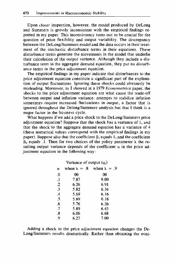
Upon closer inspection, however, the [nodel produced by DeLongand Summers is grossly inconsistent with the empirical findings re-ported in my paper. This inconsistency turns out to be crucial for thequestion of price flexibility and output variability. The discrepancybetween the DeLong/Summers model and the data occurs in their treat-ment of the stochastic disturbance terms in their equations. Thesedisturbance terms generate the movements in the model that underlietheir calculation of the output variance. Although they include a dis-turbance term in the aggregate demand equation, they put no disturb-ance terms in the price adjustment equation.

The empirical findings in my paper indi(=ate that disturbances to theprice adjustment equation constitute a significant part of the explana-tion of output fluctuations. Ignoring these shocks could obviously bemisleading. Moreover, as I showed in a 1979 Econometrica paper, theshocks to the price adjustment equation are what cause the trade-offbetween output and inflation variance: attempts to stabilize inflationsometimes require increased fluctuations in output, a factor that isignored throughout the Delong/Summers analysis but that I think is amajor factor in the business cycle.

What happens if we add a price shock to the DeLong/Summers priceadjustment equation? Suppose that the shock has a variance of 1, andthat the shock"to the aggregate demand equation has a variance of 4(these numerical values correspond with the empirical findings in mypaper). Suppose also that the coefficient ~l equals 1, and the coefficient~2 equals .1. Then for two choices of the policy parameter A the re-sulting output variance depends of the coefficient 0: in the price ad-justment equation in the following way:

Variance of output (qt)

0: when A = .8 when A = .9.0 00 00.1 7.87 9.00.2 6.26 6.91.3 5.82 6.34.4 5.69 6.16.5 5.69 6.16.6 5.76 6.26.7 5.89 6.43.8 6.06 6.68.9 6.27 7.00

Adding a shock to the price adjustment equation changes the De-Long/Summers results dramatically. Rath(~r than obtaining the mini-

674 John B. Taylor

mum value of the output variance when the price adjustment coefficientis zero, we see that the maximum value of the variance (00) is obtained.The rationale is clear. When demand has no effect on inflation, thereis nothing available to stabilize inflation, and the inflation rate takes arandom walk with infinite variance. Since inflation appears in the ag-gregate demand equation, output also has infinite variance. As weincrease the price adjustment parameter the variance of output de-clines, contrary to the DeLong/Summers findings. Only for very largevalues of the price adjustment term does the variance of output beginto increase again. But such large values are not empirically realistic.

The DeLong/Summers model-appropriately augmented to realisti-cally take account of price shocks-therefore does support the viewstated in my paper that an increase in price flexibility would tend toimprove macroeconomic perrormance. In fact their model (with priceshocks) is much like the structural model reported and estimated inmy 1979 Econometrica paper, in which I computed trade-offs betweenoutput and inflation fluctuations. In that paper the expected rate ofinflation appears in the aggregate demand equation (though with aninsignificant negative sign), so that the same possibilities for destabil-izing price flexibility, which DeLong and Summers have emphasized,exist in that model. As in this example, such a possibility does notappear to be borne out empirically in the estimated version of thatmodel.

Some of the other criticisms of my analysis that DeLong and Sum-mers raise are irrelevant, in my view. For example, they argue that myexplanation of the change in economic perrormance is too complicated,involving offsetting effects. What is so complex? More stable aggregatedemand reduced economic fluctuations more than changes in wage-and price-setting behavior increased them. Many people have inves-tigated the reasons for the increased stability of aggregate demand.That was not the subject of my paper, though I found the revisionistanalysis of these issues in the DeLong/Summers paper in this volumefascinating reading. In general, however, how can one defend rejectinga two-step argument that is correct in favor of a one-step argumentthat is wrong?

DeLong and Summers also question the explanations of my empiricalfinding that aggregate demand policy appears to be less accommodativeunder the current fiat money regime than under the gold standard. Asthe numerical example above shows, the degree of accommodation (asmeasured by A) does not change the conclusion that decreased priceflexibility increases output variance over the relevant range of param-eters. The result also holds for a wide range of values of Anot reportedabove. In no way is this observed change in the response of aggregatedemand policy to inflation "necessary to drive Taylor's conclusions,"


as DeLong and Summers argue. I found my empirical result~ on ag-gregate demand policy surprising and offered some possible explana-tions, but these results are unrelated to my view of the relation betweenprice flexibility and output variability.

Discussion Summary

Much of the initial discussion focused on the problems involved withTaylor's structural interpretations of his \i'AR results. Martin N. Bailycommented that it seemed impossible to distinguish between aggregatedemand and aggregate supply shifts when the reduced- form equationsare used. Consequently it was unclear hov{ Taylor's "structure" couldbe differentiated from a Lucas-type supply function in which priceflexibility leads to output fluctuations. Taylor's response was that thedynamics embodied in his VAR results provide evidence for the ag-gregate demand/supply structure rather than a Lucas supply function.These dynamics show that positive price surprises are associated withnegative output movements and hence are identified with aggregatesupply shocks. Also, positive output surprises are found, over a longerhorizon, to be associated with positive price movements, which isconsistent with aggregate demand shocks .. Robert Hall remarked thatin the classic demand/supply curve estimation problem, Taylor's strat-egy was equivalent to identifying every price rise with a shift in thedemand curve and every price decline with a shift in supply.

Blanchard questioned Taylor's use of a two-variable vector auto-regression involving price and output. Since so much of the paper wasconcerned with the accommodative polici(~s of the government, wouldnot a three-variable VAR including a poli,~y variable like money havebeen preferable? Taylor replied that he had decided against using agovernment policy variable for two reasons; first, the problems in find-ing a satisfactory measure of policy-Ml, M2 unborrowed reserves,or such-seemed difficult, and second, the goal of the paper was toplace structure on VAR results. This task is difficult enough in a two-variable system. McCallum then noted that the structure Taylor em-ployed essentially involved collapsing the monetary authority's pricerule into the aggregate demand curve to arrive at equation (7). Mc-Callum thought that an undesirable feature of the resulting equationwas that it implied that the monetary authority could influence thegrowth rate of real output through its choice of the inflation rate. Tayloragreed with McCallum's interpretation but said he felt equation (7) wasjustified by the data. In a world of sticky prices, in which the Fed

676 John B. Taylor

targets nominal GNP growth, its policies can affect real output growthdirectly.

The final point raised in the discussion was methodological and in-volved Taylor's procedure for generating the moving average represen-tations shown in tables 11.4-11.7 and figures 11.3 and 11.4. John Gew-eke declared that VAR techniques can be used for two legitimatepurposes: to generate the response of the system to a shock in a partic-ular variable, and to identify how the shocks in each variable feed backfrom one another over some time period (the "historical decompositionof the series"). Both of these procedures require the researcher to spec-ify how the covariance matrix of the shocks in the system is to be or-thogonalized. In constructing his moving average representations Tay-lor has deliberately avoided specifying such an orthogonalization. Hethus ignores the effect of the correlations between the shocks of the twoequations on the moving average coefficients. The moving average rep-resentations Taylor presents are therefore "partial" in that they ignorethe channels for feedback from the other variable. Taylor agreed withGeweke's statements but argued that for the purposes of this paper the"partial" moving average representations facilitated a behavioral inter-pretation of the results. Transforming the VAR estimates by a samplecovariance matrix would only muddle the structural interpretations thatcould be placed on the resulting moving average representations.

References

Bordo, Michael, and Anna Schwartz, eds. 1984. A retrospective on theclassical gold standard. Chicago: University of Press.

Bums, Arthur F. 1969. Progress towards economic stability. In Thebusiness cycle in a changing world. New York: Columbia UniversityPress.

Cagan, Phillip. 1979. Changes in the cyclical behavior of prices. InPersistent inflation: Historical and policy essays. New York: Colum-bia University Press.

Friedman, Milton, and Anna J. Schwartz. 1963. A monetary historyof the United States, 1867-1960. Princeton: Princeton UniversityPress.

Gordon, Robert J. 1983. A century of evidence on wage and pricestickiness in the United States, the United Kingdom and Japan. InMacroeconomics, prices and quantities, ed. James Tobin. Washing-ton, D.C.: Brookings Institution.


Lucas, Robert E., Jr. 1972. Expectations and the neutrality of money.Journal of Economic Theory 4: 103-24.

Mitchell, Daniel J. B. 1983. Wage flexibility: Then and now. WorkingPaper 65. Institute of Industrial Relations, University of Californiaat Los Angeles.

Sims, C.hristopher A. 1980. Macroeconomics and reality. Econometrica48 (January): 1-48.

Taylor, John B. 1980. Output and price stability: An international com-parison. Journal of Economic Dynamics and Control 2: 109-32.

---. 1982. Policy choice and economic structure. Occasional Paper9, Group of Thirty, New York.

Tobin, James. 1980. Asset accumulation and economic activity: Reflections on contemporary macroeconomic theory. Oxford: BasilBlackwell.

Improvements in Macroeconomic Stability: The Role of Wages and

Documents