MOLECULAR PHYLOGENETIC ANALYSIS, GENETIC MAPPING, AND IMPROVEMENT OF SWITCHGRASS (PANICUM VIRGATUM L.) FOR BIOENERGY AND BIOREMEDIATION TO EXCESS PHOSPHORUS IN THE SOIL by ALI M. MISSAOUI (Under the Direction of Joseph H. Bouton) ABSTRACT Research was conducted to explore the genomic organization of switchgrass (Panicum virgatum L.) and its potential for bioenergy and bioremediation to excess P in the soil. The utility of nrDNA ITS1-5.8S-ITS2 region and chloroplast trnL(UAA) intron in determining relatives of switchgrass in the genus Panicum were evaluated using 42 Panicum taxa. The ITS sequences exhibited higher divergence than trnL(UAA) and provide potential in resolving the classification of this genus. Alignment of trnL(UAA) sequences from 34 switchgrass accessions revealed a 49 nucleotide-deletion (∆350-399) specific to lowland accessions, which can be used for the classification of upland and lowland germplasm. The extent of genetic diversity in 21 upland and lowland switchgrass genotypes was investigated using 85 RFLP probes. Jaccard and Dice distances showed a high genetic diversity between and within ecotypes. The segregation and linkage of 224 single dose restriction fragments (SDRF) generated from 99 RFLP probes in 85 progenies of two tetraploid (2n = 4x = 36) parents (Alamo x Summer) indicated that switchgrass is an autotetraploid with high degree of preferential pairing. The recombinational length of switchgrass genome is 4617 cM. Greenhouse and field investigation of the genetic variation and heritability of P uptake in 30 genotypes under fertilizer rates of 450 mg P and 200 mg N Kg -1 soil showed that switchgrass accumulates high levels of P (0.76 % in the greenhouse and 0.36% in the field). P uptake was correlated more with biomass production (r= 0.65 to 0.90) and less with P concentration (r= 0.10 to 0.42). Expected gain from selection for P concentration is low (1 to 2%). A substantial progress can be achieved through selection for higher biomass. Effectiveness of the honeycomb selection design in identifying superior genotypes for biomass production in switchgrass was evaluated at 1.2 m inter-plant spacing. In four field experiments, yield of half-sib lines derived from polycrossing 15 genotypes selected for high yield was on average higher than the yield of half-sib lines derived from 15 genotypes selected for low yield from

Welcome message from author
This document is posted to help you gain knowledge. Please leave a comment to let me know what you think about it! Share it to your friends and learn new things together.
Transcript

MOLECULAR PHYLOGENETIC ANALYSIS, GENETIC MAPPING, AND
IMPROVEMENT OF SWITCHGRASS (PANICUM VIRGATUM L.) FOR
BIOENERGY AND BIOREMEDIATION TO EXCESS PHOSPHORUS IN THE SOIL
by
ALI M. MISSAOUI
(Under the Direction of Joseph H. Bouton)
ABSTRACT
Research was conducted to explore the genomic organization of switchgrass (Panicum virgatum L.) and its potential for bioenergy and bioremediation to excess P in the soil. The utility of nrDNA ITS1-5.8S-ITS2 region and chloroplast trnL(UAA) intron in determining relatives of switchgrass in the genus Panicum were evaluated using 42 Panicum taxa. The ITS sequences exhibited higher divergence than trnL(UAA) and provide potential in resolving the classification of this genus. Alignment of trnL(UAA) sequences from 34 switchgrass accessions revealed a 49 nucleotide-deletion (∆350-399) specific to lowland accessions, which can be used for the classification of upland and lowland germplasm. The extent of genetic diversity in 21 upland and lowland switchgrass genotypes was investigated using 85 RFLP probes. Jaccard and Dice distances showed a high genetic diversity between and within ecotypes. The segregation and linkage of 224 single dose restriction fragments (SDRF) generated from 99 RFLP probes in 85 progenies of two tetraploid (2n = 4x = 36) parents (Alamo x Summer) indicated that switchgrass is an autotetraploid with high degree of preferential pairing. The recombinational length of switchgrass genome is 4617 cM. Greenhouse and field investigation of the genetic variation and heritability of P uptake in 30 genotypes under fertilizer rates of 450 mg P and 200 mg N Kg-1 soil showed that switchgrass accumulates high levels of P (0.76 % in the greenhouse and 0.36% in the field). P uptake was correlated more with biomass production (r= 0.65 to 0.90) and less with P concentration (r= 0.10 to 0.42). Expected gain from selection for P concentration is low (1 to 2%). A substantial progress can be achieved through selection for higher biomass. Effectiveness of the honeycomb selection design in identifying superior genotypes for biomass production in switchgrass was evaluated at 1.2 m inter-plant spacing. In four field experiments, yield of half-sib lines derived from polycrossing 15 genotypes selected for high yield was on average higher than the yield of half-sib lines derived from 15 genotypes selected for low yield from

Alamo and Kanlow nurseries. This suggests that identifying superior genotypes at 1.2 m spacing using the honeycomb method is possible.
INDEX WORDS: Switchgrass, Panicum virgatum, bioenergy, nrDNA, ITS,
chloroplast, trnL(UAA), phylogeny, SDRF, genetic diversity, genetic mapping, RFLP, polyploid mapping, phosphorus, P uptake, bioremediation, honeycomb design.

MOLECULAR PHYLOGENETIC ANALYSIS, GENETIC MAPPING AND
IMPROVEMENT OF SWITCHGRASS (PANICUM VIRGATUM L.) FOR
BIOENERGY AND BIOREMEDIATION TO EXCESS PHOSPHORUS IN THE SOIL
by
ALI M. MISSAOUI
B.S., Oregon State University, 1986
M.S., Texas Tech University, 1998
A Dissertation Submitted to the Graduate Faculty of The University of Georgia in Partial
Fulfillment of the Requirements for the Degree
DOCTOR OF PHILOSOPHY
ATHENS, GEORGIA
2003

© 2003
Ali M. Missaoui
All Rights Reserved

MOLECULAR PHYLOGENETIC ANALYSIS, GENETIC MAPPING AND
IMPROVEMENT OF SWITCHGRASS (PANICUM VIRGATUM L.) FOR
BIOENERGY AND BIOREMEDIATION TO EXCESS PHOSPHORUS IN THE SOIL
by
ALI M. MISSAOUI
Major Professor: Joseph H. Bouton
Committee: H. Roger Boerma Andrew H. Paterson Peggy Ozias-Akins David E. Kissel
Electronic Version Approved: Maureen Grasso Dean of the Graduate School The University of Georgia August 2003

iv
ACKNOWLEDGEMENTS
I wish to express my sincere gratitude to Dr. Joe Bouton who has provided me
with support throughout this work along with the freedom to choose my research topics.
I am grateful to the members who served on my committee and took the time to
review this lengthy document including Dr. Andrew H. Paterson, Dr. Peggy Ozias-Akins,
Dr. Miguel Cabrera, and Dr. David E. Kissel. Special thanks are given to Dr. Roger
Boerma for his assistance and critical insights into my work.
I also express my deep appreciation to the people who have helped during all
phases of this project.
I remain very grateful to Dr. Glenn Burton and his family for their support
through the “Glenn and Helen Burton Feeding the Hungry Scholarship”, the Department
of Crop and Soil Sciences, and the United States Department of Energy, Environmental
Sciences Division, Oak Ridge National Laboratory for the financial support of this work
Finally, I am deeply indebted to my family and especially my wife Wided for
their constant support, encouragement and love. Their inspiration remains my main
support throughout all my endeavors.

v
TABLE OF CONTENTS
Page
ACKNOWLEDGEMENTS............................................................................................... iv
LIST OF TABLES............................................................................................................. ix
LIST OF FIGURES .......................................................................................................... xii
CHAPTER
1 INTRODUCTION .............................................................................................1
2 GENOME ANALYSIS OF POLYPLOIDS USING MOLECULAR
MARKERS: A LITERATURE REVIEW ....................................................3
Genetic and evolutionary aspects of polyploidy ...........................................3
Molecular markers and their importance in genome analysis .....................12
Linkage mapping.........................................................................................37
Genetic mapping in polyploids....................................................................45
References ...................................................................................................63
3 MOLECULAR PHYLOGENETIC ANALYSIS OF THE COMPLEX
PANICUM (PANICOIDEAE, PANICEAE): UTILITY OF
CHLOROPLAST DNA SEQUENCES AND RIBOSOMAL INTERNAL
TRANSCRIBED SPACERS.....................................................................104
Abstract .....................................................................................................105
Introduction ...............................................................................................105
Materials and methods...............................................................................113

vi
Results .......................................................................................................115
Discussion .................................................................................................119
References .................................................................................................123
4 MOLECULAR INVESTIGATION OF THE GENETIC VARIATION AND
POLYMORPHISM IN SWITCHGRASS (PANICUM VIRGATUM L.)
CULTIVARS AND DEVELOPMENT OF A DNA MARKER FOR THE
CLASSIFICATION OF SWITCHGRASS GERMPLASM .....................137
Abstract .....................................................................................................138
Introduction ...............................................................................................140
Materials and methods...............................................................................144
Results .......................................................................................................149
Discussion .................................................................................................153
References .................................................................................................158
5 GENETIC LINKAGE MAPPING IN SWITCHGRASS (PANICUM
VIRGATUM L.) USING DNA MARKERS ..............................................173
Abstract .....................................................................................................174
Introduction ...............................................................................................175
Materials and methods...............................................................................179
Results .......................................................................................................183
Discussion .................................................................................................191
References .................................................................................................198
6 PHOSPHORUS NUTRITION AND ACCUMULATION IN PLANTS:
A LITERATURE REVIEW ..........................................................................219

vii
Introduction ...............................................................................................219
Phosphorus in the soil................................................................................219
P uptake across the plasma membrane ......................................................222
Destiny of P transported into the cell ........................................................225
Control of P uptake activity.......................................................................227
Phenotypic and genetic differences in P uptake by plants ........................230
Environmental aspects of phosphorus .......................................................233
Potential use of crop species for phytoremediation to excess
phosphorus in the soil................................................................................235
Genetic manipulation to increase P uptake in plants.................................237
References .................................................................................................241
7 GENETIC VARIATION AND HERITABILITY OF PHOSPHORUS
UPTAKE IN SWITCHGRASS (PANICUM VIRGATUM L.) UNDER
EXCESSIVE PHOSPHORUS CONDITIONS.........................................256
Abstract .....................................................................................................257
Introduction ...............................................................................................258
Materials and methods...............................................................................260
Results .......................................................................................................263
Discussion .................................................................................................267
References .................................................................................................271
8 APPLICATION OF THE HONEYCOMB SELECTION METHOD IN
SWITCHGRASS (PANICUM VIRGATUM L.) FOR BIOMASS
PRODUCTION .........................................................................................284

viii
Abstract .....................................................................................................285
Introduction ...............................................................................................287
Materials and methods...............................................................................291
Results .......................................................................................................294
Discussion .................................................................................................299
References .................................................................................................303
9 SUMMARY AND CONCLUSIONS ............................................................312

ix
LIST OF TABLES
Table Page
3.1. List of Panicum and outgroup taxa included in the chloroplast trnL(UAA) and nrDNA-ITS sequence analysis................................................................................131 3.2. Sequence characteristics ........................................................................................133 3.3. Statistics of parsimony analysis of trnL(UAA) and nrDNA-ITS sequences .........134 4.1. Switchgrass accessions used for RFLP and Chloroplast trnL(UAA) analysis ......164 4.2. Number of fragments scored and polymorphic in switchgrass genotypes ............166 4.3. Matrix of pairwise Jaccard distances between 21 switchgrass upland and lowland genotypes based on RFLP markers analysis. ...........................................167 4.4. Matrix of pairwise Dice distances between 21 switchgrass upland and lowland genotypes based on RFLP markers analysis..........................................................168 5.1. Summary of probes surveyed and mapped in the progeny of a cross between lowland Alamo (AP13) and upland Summer (VS16) switchgrass. .......................208 5.2 Single dose restriction fragments that deviated significantly (p<0.05) from the 1:1 segregation ratio expected in AP13...................................................209 5.3 Single dose restriction fragments that deviated significantly (p<0.05) from the 1:1 segregation ratio expected for presence and absence of bands in the pollen parent Summer VS16...............................................................210 5.4 Pairs of markers showing repulsion-phase associations in the female parent Alamo AP13.................................................................................................211 5.5 Pairs of markers showing repulsion-phase associations in the male parent Summer VS16..............................................................................................212

x
5.6 Summary of Chi square tests of simplex to multiplex, and repulsion to coupling ratios observed in switchgrass mapping population compared to expected ratios in autotetraploids and allotetraploids............................................213 5.7. RFLP probes mapped in Alamo AP13 switchgrass and their corresponding locations rice, maize, and sorghum linkage groups.. .............................................214 7.1. Mean P concentration, biomass production, and P uptake combined over 3 harvests of switchgrass grown in the greenhouse at fertilizer rates of 450 mg P and 200 mg N kg-1 soil. .........................................................................275 7.2. Combined analysis of variance over harvests of P concentration, biomass
production, and P uptake in switchgrass grown in the greenhouse and the field under fertilizer rates of 450 mg P and 200 mg N kg-1 soil. ...........................276 7.3 Mean P concentration, biomass production, and P uptake combined over 2 harvests of switchgrass grown in the field at fertilizer rates of 450 mg P and 200 mg N kg-1 soil. .....................................................................277 7.4. Spearman rank correlation coefficients between genotypes for P concentration, biomass production, and P uptake for different harvest dates and locations. ........278 7.5. Analysis of variance and variance component estimates for genotypes and genotype x location interaction, for P concentration, biomass production, and P uptake of 29 switchgrass genotypes grown in two locations (greenhouse and field) under fertilizer rates of 450 mg P and 200 mg N kg-1 soil. ...................279 7.6. P concentration, biomass production, and P uptake of half-sib progenies and their parental genotypes evaluated in one location at fertilizer rates of 450 mg P and 200 mg N kg-1 soil. .........................................................................280 7.7. Mean squares and variance components for P concentration, biomass production, and P uptake in 12 half-sib families of switchgrass grown in one location (Athens) under fertilizer rates of 450 mg P and 200 mg N kg-1 soil........281 7.8. Heritability estimates on individual plants, family means, parent-offspring regression, and parent-offspring correlation and predicted genetic gain from selection on individual plants basis and family selection. .....................................282 7.9. Pearson coefficient of correlation between P concentration, biomass production, and P uptake in switchgrass parental genotypes and half-sib progeny grown under fertilizer rates of 450 mg P and 200 mg N kg-1 soil. ..........283

xi
8.1. Analysis of variance for biomass production of half-sib lines derived from high and low genotype groups selected from Alamo and Kanlow switchgrass using the honeycomb selection method and grown in sward plots at a row spacing of 18 cm .....................................................................................................307 8.2. Dry matter production of half-sib lines of genotypes selected for high and low yield using the honeycomb selection design from Alamo and Kanlow switchgrass evaluated for 3 yr in sward plots spaced by 18 cm. ............................308 8.3. ANOVA of biomass production of half-sib lines derived from high and low genotype groups selected using the honeycomb selection method from Alamo and Kanlow switchgrass and grown at a row spacing of 76 cm. ................309 8.4. Dry matter production of half-sib lines derived from genotypes selected for high and low yield using the honeycomb selection method from Alamo switchgrass and evaluated in two locations for two years in row plots spaced by 76 cm..................................................................................................................310 8.5. Biomass production of half-sib lines of genotypes selected for high and low yield using the honeycomb selection design from Kanlow switchgrass evaluated in one location for two years in row plots spaced by 76 cm...................................311

xii
LIST OF FIGURES Figure Page 3.1. Strict consensus of the 12 most parsimonious trees retained from the heuristic search of PAUP based on ribosomal ITS sequence analysis. .................135 3.2. Strict consensus tree of the 81 most parsimonious trees retained from the heuristic search of PAUP based on chloroplast trnL (UAA) intron. ...............136 4.1. Dendogram derived from the analysis of 21 switchgrass genotypes using RFLP markers based on distances obtained from Jaccard’s dissimilarity index and Ward’s minimum variance cluster analysis.. ...................................................169 4.2. Dendogram derived from the analysis of 21 switchgrass genotypes using RFLP based on distances obtained from Dices’s dissimilarity matrix and Ward’s minimum variance cluster analysis. ...........................................................170 4.3. Multiple alignment of the chloroplast intron trn L DNA sequences obtained from different switchgrass accessions. ...................................................................171 4.4. Dendogram derived from the analysis of 34 switchgrass accessions using chloroplast trnL (UAA) intron ......................................................................172 5.1. Distribution of observed segregation ratios for 118 markers present in the female parent Alamo P13 and 114 markers segregating in the male parent VS16 switchgrass....................................................................................................215 5.2. Combined RFLP linkage map of Alamo AP13 and Summer VS16 switchgrass derived from 85 F1 progenies .................................................................................216

1
CHAPTER 1
INTRODUCTION
The Bioenergy Feedstock Development Program (BFDP) at the U.S. Department
of Energy has chosen switchgrass (Panicum virgatum L.) as a model bioenergy species
from which renewable sources of transportation fuel or biomass-generated electricity
could be derived. Interest in alternatives to fossil fuels was forced mainly because of the
environmental concerns associated with burning of coal and petroleum-based fuels. In the
USA., this interest was heightened because of concerns about the consequences of
dependence on foreign energy sources following the oil embargo of the 1970s. Unlike
fossil fuels, using perennial grasses for biomass energy does not lead to an increase in the
levels of atmospheric CO2 because the carbon dioxide released during the biomass
combustion and conversion is balanced by photosynthesis and CO2 fixation by the
growing crop.
Switchgrass or tall panic grass (Panicum virgatum L.) belongs to the Paniceae
tribe in the subfamily Panicoideae of the Poaceae (Gramineae) family. It is a warm
season, C4 perennial grass that is native to most of North America, and has been widely
grown for summer grazing and soil conservation.
Switchgrass breeding has been based solely on phenotypic selection and most
switchgrass cultivars released are synthetics derived from wild populations. Important to
the improvement of this species is the development of molecular approaches, including

2
gene transfer and marker assisted selection that can be used to supplement conventional
breeding programs.
Information regarding the amount of genetic diversity and polymorphism in
switchgrass is crucial to enhance the effectiveness of breeding programs and germplasm
conservation efforts. This issue has not been fully explored at the genomic level and the
genomic organization of switchgrass has never been studied. Thus, research was begun in
1998 to evaluate the degree of genetic diversity between switchgrass cytotypes,
investigate the genomic organization and chromosomal transmission in switchgrass,
explore the potential of applying DNA markers for an effective characterization and
maintenance of switchgrass germplasm, and develop a linkage map. We also intended to
assess the potential use of switchgrass to remove excess phosphorus in soils continuously
amended with animal waste, and study the effectiveness of the honeycomb selection
design in identifying superior genotypes in switchgrass selection nurseries.

3
CHAPTER 2
GENOME ANALYSIS OF POLYPLOIDS USING MOLECULAR
MARKERS: A LITERATURE REVIEW
Genetic and evolutionary aspects of polyploidy
Polyploidy refers to the presence of more than two genomes per cell. It is a major
process influencing plant evolution. Classical estimates of the frequency of polyploidy in
angiosperm species range from 30 to 35% (Stebbins, 1950) to as high as 80% (Masterson,
1994), but recent molecular studies indicate that probably all the angiosperms have
undergone polyploidization at sometime during their evolution (Simillion et al., 2002;
Bowers et al., 2003a). Some researchers have regarded polyploidy as "the black hole of
evolutionary biology" (Soltis and Soltis, 2000) because it has been relatively under-
investigated and the exploration of these complex phenomena leads often to more
questions than answers.
There are several reasons to expect polyploidy to increase rates of adaptive
evolution since polyploids have a greater chance of bearing new beneficial alleles and
evolving novel functions in duplicated gene families. The role of polyploidy in evolution
remains enigmatic despite the many recent insights. Much remains to be learned about
many aspects of polyploid evolution. Application of molecular genetic approaches to
questions of polyploid genome organization and evolution may provide insights into the

4
processes by which new genotypes are generated and ultimately into how polyploidy
facilitates evolution and adaptation.
Mechanisms of polyploid formation
Several cytological mechanisms are known to induce polyploidy in plants. Harlan
and DeWet (1975) outlined three mechanisms responsible for the formation of new
polyploids. The first involves sexual polyploidization through the fusion of 2n gametes.
The second requires an intermediate step involving a hybrid diploid, which produces 2n
gametes. The third involves diploid hybridization and somatic doubling. Somatic
doubling in meristem tissue of sporophytes has been observed to produce “mixoploid
chimeras” (Jorgensen, 1928). Somatic doubling, which can occur in the zygote or young
embryo, leading to the formation of completely polyploid sporophytes, has been
described from heat shock experiments in which young embryos were exposed for a short
time to high temperature. Randolph (1932) reported that corn (Zea mays) plants exposed
to temperatures of 40 oC for about 24 h after pollination produced 1.8 % tetraploid and
0.8% octoploid seedlings. Polyspermy, the fertilization of an egg by more than one sperm
nucleus, was also recognized as a cause of polyploidy in many plant species (Vigfusson,
1970).
Unreduced gametes are believed to be the major mechanism of polyploid
formation. According to Harlan and De Wet (1975), autopolyploids may occur by
unilateral or bilateral sexual polyploidization. Unilateral polyploidization usually
involves an intermediate triploid cytotype; hence the use of the term “triploid bridge

5
hypothesis”. In the case of direct bilateral sexual polyploidization, there is no
involvement of intermediate chromosome number.
Polyploidization was viewed as a reversible phenomenon. As pointed out by
DeWet (1975), tetraploids may occasionally revert to the diploid state because of
parthenogenetic development of reduced gametes producing progeny with a ploidy level
lower than that of the maternal level. Ramsey and Schemske (1998) suggested that the
formation of allopolyploids might be more common in nature than that of autopolyploids.
The rate of allopolyploid formation depends on the hybridization frequency in the
population and the rate of polyploid formation in interspecific hybrids (Abdel-hameed
and Snow, 1972). The production of later generation polyploids are achieved through
numerous pathways including the mating between polyploids produced independently
that leads to the formation of outcrossing second-generation polyploids (Ramsey and
Schemske, 1998).
Classification of polyploids
Detecting polyploidy can be extremely difficult. It has been suggested that the
most important criterion for classifying polyploids should be the mode of origin.
Polyploids that originated from crosses within or between populations of single species
are designated as “autoploids” and those derived from interspecific hybridization between
different species are “alloploids” (Ramsey and Schemske, 1998). Early reports
emphasized the frequency of meiotic multivalent formation as a criterion for
distinguishing auto and allopolyploids because chromosome behavior was believed to be
a dependable sign of homology between chromosomes (Muntzing, 1936). Soltis and

6
Soltis (2000) argued that multivalent pairing at meiosis are effective only in detecting
recent polyploidization events and cannot be extended to identify ancient ones because
the signals of chromosomal duplication can be erased by time through rearrangements
and scrambling of their gene order.
Genetic control of polyploid formation
Bretagnolle and Thompson (1995) suggested the possibility of existence of
heritable genetic variations in the production of 2n gametes in plant populations. This
variation was illustrated by the rapid response to selection for 2n gamete production
observed in crop cultivars (Parrott and Smith, 1986). The mean frequency for 2n pollen
was increased form 0.04% to 47% in three generations of selection in Trifolium pratense,
giving a realized heritability of 0.50. Based on meiotic analysis of progeny derived form
crosses between plants differing in the level of 2n gamete production, Mok and Peloquin,
(1975) indicated that this phenotype could be under strong genetic control and possibly
determined by a single locus. A possible mechanism suggested by Ramsey and Schemske
(1998) is that the cytological abnormalities leading to non-reduction and production of 2n
gametes are the pleiotropic effects of genes that have other beneficial effects. Another
possible theory is that characters related to sexual reproduction may be under relaxed
selection, resulting in higher frequency of 2n and nonfunctional gametes. A likely support
for this hypothesis comes from the observation that many of the taxa in which 2n gamete
production has been documented are perennials that are vegetatively propagated (Maceira
et al., 1992).

7
Genetic variability in polyploids and effects of polyploidy
The level of genetic diversity and allelic variation in polyploids depends on the
mode of their formation. Allopolyploidy doubles the number of loci, whereas
autopolyploidy results in twice the number of alleles segregating at each locus without
affecting the number of loci. Theoretically, both modes of formation are expected to
result in polyploids having more genetic diversity than closely related diploids. During
their formation, autopolyploid species have equal or less genetic diversity than the
diploid progenitor. However, because of the higher number of alleles segregating at each
locus and polysomic inheritance, these polyploids have larger effective population sizes
than their diploid progenitors. Therefore, loss of heterozygosity is slower than in diploid
populations, and the equilibrium heterozygosity with mutation and random drift is higher
than for diploids (Moody et al., 1993). Alloploids have fixed heterozygosity and the level
of genetic diversity depends of the degree of divergence of the parental genomes (Soltis
and Soltis, 2000).
The effects of polyploidization on gene structure and function have been the
center of a considerable body of theory. After polyploid formation, significant changes in
genome structure and gene expression may occur (Leitch and Bennett, 1997). Recent
studies indicated that genes duplicated by polyploidy can retain their original or similar
function, undergo diversification in protein function or regulation, or one copy may
become silenced through mutational or epigenetic means (Wendel, 2000). Duplicated
genes also may interact through inter-locus recombination, gene conversion, or concerted
evolution (Soltis and Soltis, 1993).

8
The increase in chromosome number through polyploidization may lead to an
increased recombination between loci and influence the success of polyploid lineages.
Grant (1982) suggested that larger chromosome numbers would be "favored by selection
for open recombination systems". On the other hand, Otto and Whitton (2000) argued
that recombination is not always advantageous, and that increased recombination may
lead to a reduction in the fitness of the polyploid, if the co-adapted gene complexes are
dispersed.
Gene expression and regulation may also be affected by changes in the genomic
background as a result polyploidization. As an example, Song et al. (1995) created
polyploid Brassica hybrids and observed extensive genomic rearrangements within five
generations. They suspected these rapid changes are the result of activation in the hybrid
polyploids of some transposable elements that were silent in parental lines. These
elements may contribute to physical changes in the karyotype through translocations,
fusions, fissions, and may increase gene silencing of duplicate gene copies. Other data
from a variety of polyploids suggest that a large fraction of duplicate gene copies is
retained for long periods. In maize, the fraction of genes retained in duplicate has been
estimated as 72% over 11 MYears (Gaut and Doebley, 1997). Otto and Whitton (2000)
suggested that purifying selection is the main factor that preserves duplicated genes in
polyploids for periods of time long enough to generate beneficial mutations and
diversification. Walsh (1995) also estimated that about 99% of duplicate genes would
evolve into pseudogenes by the process of purifying selection. Miller and Venable (2000)
suggested that polyploidy is an important factor in the evolution of gender dimorphism. It
acts through the disruption of self-incompatibility and leads to inbreeding depression.

9
Consequently, male sterile mutants invade and increase because they are unable to
inbreed. They presented evidence for this pathway from 12 genera involving at least 20
independent evolutionary events and showed that gender dimorphism in North American
Lycium (Solanaceae) has evolved in polyploid, self-compatible taxa whose closest
relatives are cosexual, self-incompatible diploids.
Phenotypic effects of polyploidy
The role of polyploidization in producing evolutionary novelties is mediated
through its effects on the phenotype. Therefore, a fundamental question that must be
addressed is whether polyploidization produces phenotypic changes that influence the
adaptive potential of the polyploid species. Levin (1983) stated based on evidence from
flowering plants that “chromosome doubling may propel a population into a new adaptive
sphere” and “bring about abrupt, transgressive, and conspicuous changes in the adaptive
gestalt of populations within micro-evolutionary time”. Among the well known changes
associated with polyploidization are the increase in cell volume and changes in metabolic
processes, which are environment dependent. Polyploid plants frequently produce larger
seeds than related diploids, which leads to more rapid development at the seedling stages
(Villar et al., 1998). This increases the chances of establishment in harsh environments
and results in niche differentiation as a byproduct of polyploidization (Villar et al. 1998).
Polyploidization can also result in changes in the reproductive system and lead to asexual
reproduction mechanisms such as apomixis. Lewis (1980) suggested that polyploidization
often predates apomixis in most flowering plants even though not all polyploids are
apomictic. Recent studies also indicated that the genes for apomixis are only transmitted

10
in unreduced gametes, which is the main mechanism for the formation of polyploids
(Pessino et al., 1999). In addition to shifts to asexual reproduction, other changes in
breeding systems have been noted in plants. For example, Wedderburn and Richard
(1992) reported that genetic self-incompatibility systems might break down in polyploids,
resulting in higher selfing rates in polyploids than in their diploid progenitors.
Furthermore, polyploidization can modify floral traits, including the relative sizes and
spatial relations of floral organs (Brochmann, 1993). These different changes possibly
change the interactions with pollinators leading to a further selection for divergence in
reproductive traits.
Polyploidy and speciation
It is well established that speciation in most organisms occurs because of gradual
establishment of reproductive barriers between populations over many generations
irrespective of selection type. This usually takes thousands to millions of years. Polyploid
formation has often been considered a mechanism of instantaneous speciation that rapidly
provides new genetic combinations to help the new reproductively isolated populations to
adjust to new habitats (Leitch and Bennett, 1997). To assess the evolutionary significance
of polyploidization in plant speciation, Otto and Whitton (2000) estimated the rate of
polyploidization per speciation event in angiosperms based on the distribution of haploid
chromosome numbers. They used published data from different plant families to calculate
the fraction of speciation events associated with a change in chromosome number. They
concluded that at least 987 chromosomal shifts took place in 8884 speciation events,
which corresponds to a rate of change of chromosome number of 11% per speciation

11
event. Multiplying this by the polyploidy index, they estimated that 2 to 4% of speciation
events in angiosperms involve polyploidization.
Evolutionary consequences of poylploidy
It is well established that the rate of evolutionary change in a trait depends on the
intensity of selection and the extent of genetic variability present within a population
(Fisher, 1930). One of the intriguing issues of polyploidy in plants is their widespread
existence and success. Soltis and Soltis (2000) outlined some genetic attributes that
account for the great success of polyploid plants. Among these attributes are the multiple
origin of polyploids and heterozygosity. The recurrent formation of polyploids usually
results in a higher genetic diversity because of the incorporation of genes from different
progenitor populations into the polyploid species. Otto and Whitton (2000) indicated that
deleterious mutation loads decrease with increasing ploidy levels. They also suggested
the masking of deleterious mutations in the gametophyte resulting from the higher copy
number of genes as a possible advantage to sexual polyploids compared to diploids.
Paquin and Adams (1983) suggested, based on a study of the effects of mutation load on
the rate of adaptation of polyploid species, that polyploids have greater chances of
carrying new beneficial mutations because of the high number of alleles implying that the
rate of adaptation is faster for higher-level ploidy as long as beneficial alleles are partially
dominant.
Polyploids are assumed to have broader ecological tolerances compared to their
diploid progenitors (Levin, 1983). Among the explanations for this observation is the idea
that increased heterozygosity can provide metabolic flexibility, which enables the

12
polyploid to adapt to a wider range of conditions. Another possibility is that the polyploid
species that successfully establish have a higher ability to persist and are more likely to
inhabit different niches than their diploid progenitors. Other factors with major
significance in the success of polyploids include outcrossing, asexual reproduction,
perenniality, and predominantly the availability of new ecological niches (Stebbins,
1950).
Plants in their natural habitats experience many of the environmental factors
known to influence 2n gamete production. McHale (1983) suggested that the high
incidence of polyploidy at high latitudes, high altitudes, and glaciated areas might be
related to the tendency of harsh environmental conditions to induce 2n gametes and
polyploid formation. This suggests that natural environmental variation, and major
climate change, could significantly influence the dynamics of polyploid evolution.
Molecular markers and their importance in genome analysis
Molecular markers refer to specific landmarks on a chromosome, which can be
used for genome analysis (Tanksley, 1983). A molecular marker can be derived from any
type of molecular data that provides screenable variation or polymorphism between
individuals (Weising et al., 1998). Traditionally, three types of markers have been used in
the analysis of genetic relations in crop species. These were morphological, protein based
markers, and DNA based markers.

13
Morphological markers
This marker system is based on observable changes in phenotype and was the first
type of genetic markers used for linkage analysis and the construction of linkage maps.
However, the availability of phenotypic markers is limited in most organisms and it is
difficult to analyze several morphological changes in a single cross. The use of
morphological markers has been very limited since their number is usually very limited
and their allelic interaction makes it difficult to distinguish the heterozygous individuals
from homozygous individuals (Kumar, 1999). The genes or gene products underlying
morphological markers are in most cases unknown, which make it difficult to determine
which genes are homologous or orthologous in related taxa and more difficult to
determine the loci and gene families through evolutionary time (Tanksley, 1987). A
further drawback of these markers is their sensitivity to environmental and genetic factors
like epistasis (Staub and Serquen, 1996).
Protein based markers
Protein based markers also known as biochemical markers are proteins produced
as a result of gene expression which can be separated by electrophoresis to identify allelic
variants and explore polymorphisms at the protein level (Tanksley and Orton, 1983). This
marker system is based on the staining of proteins with identical function, but different
electrophoretic mobilities. The amino acids making the enzymes are electrically charged
therefore conferring a net electric charge to the enzyme. Mutations can cause substitution
of amino acids and change the net charge of the protein affecting their migration rate in
an electric field. Allelic variations are detected by gel-electrophoresis and subsequent

14
specific enzymatic staining. The most commonly used protein markers are isozymes and
allozymes. Isozymes refer to enzymes that catalyze the same biochemical reaction but are
encoded by different genes at different loci. The International Union of Biochemistry
(1978) recommended that “the term isoenzyme or isozyme should apply only to those
multiple forms of enzymes arising from genetically determined differences in primary
structure and not to those derived by modification of the same primary sequence”.
Allozymes are distinct forms or allelic variants of the same enzyme encoded by different
alleles at a single locus (Hamrick and Godt, 1990; Parker et al., 1998).
Protein based markers have many properties that make them useful as genetic
markers for studies of plant genetic diversity. They are easy to use and relatively
inexpensive. In addition, these markers reveal differences in the gene sequence and
function as co-dominant markers so that homozygous and heterozygous genotypes can be
distinguished and detailed population genetic analyses conducted (Tanksley and Orton,
1983; Parker et al., 1998).
Protein markers have been applied in many population genetic studies like
assessing levels of genetic relatedness among individuals and populations and revealing
patterns of mating, dispersal, and genetic variation within and among plant populations
(Brown, 1979; Hamrick and Godt, 1990; Parker et al., 1998). Allozymes are believed to
be of particular interest in population investigations because they allow the estimation of
population genetic parameters such as allele and genotype frequencies and heterozygosity
and genetic differentiation (Hamrick and Godt, 1990). Allozymes were used to clarify the
ecotypic differentiation and gene flow in natural cocksfoot (Dactylis glomerata)
populations (Lindner et al., 1999). Allozymes have also been used to measure genetic

15
variation in populations of wild-proso millet (Panicum miliaceum L.) and johnsongrass
(Sorghum halepense L.), (Warwick et al., 1984). The main limitation of allozymes is
their low abundance and low level of polymorphism, which makes them suitable only at
the level of conspecific populations and closely related species (Kephart, 1990; May,
1992).
Isozymes have been used to investigate the genetic structure of potato (Solanum
tuberisum) germplasm collections (Huaman et al., 2000), the analysis of genetic
structure of different Trifolium species (Hickey et al., 1991), and to assess the genetic
variation and structure in nonimproved populations of perennial ryegrass (Lolium
perenne) and Agrostis curtisii (Warren et al., 1998). Iozymes have also been used
extensively in genetic mapping and linkage analysis in several crop species including oat
(Avena sativa), (Hoffman, 1999), rye (Secale cereale), (Benito et al, 1990; Borner and
Korzun, 1998), soybean (Glycine max), (Kiang and Bult, 1991), and faba bean (Vicia
faba) (Satovic et al., 1996). Genes coding for 41 isozymes and subunits of isozymes have
been described in tomato and most of them have been positioned on chromosomes
(Tanksley and Rick, 1980; Tanksley, 1987). Isozyme loci coding nine enzymes were
compared among Eleusine species to determine the second wild ancestor of the
allotetraploid finger millet (Eleusine coracana), (Werth et al., 1994). Isozymes have also
been used as genetic markers to infer the location of genetic factors influencing the
expression of quantitative traits in the maize (Zea mays), (Edwards et al., 1992).
Polymorphism in a phosphoglucoisomerase locus has been linked to variation in growth
habit of fountain grass (Pennisetum alopecuroides) and segregation analysis in three
generations of this species showed a Mendelian inheritance of this isozyme (Meyer and

16
White, 1995). Phosphoglucomutase (PGM) was found to be a useful isozyme marker of
resistance to root-knot nematode (Meloidogyne spp.) in sugarbeet (Beta vulgaris L.) and
derived lines (Yu et al., 2001a).
Despite their many strengths for studies of plant genetic diversity, protein based
markers have some limitations. Their use is restricted due to their limited number in
many crop species and because they are subject to post-translational modifications and
environmental variations (Staub et al., 1996).The genes encoding these markers do not
represent a random sample of the genome and thus may bias some inferences (Karp et al.
1998; Parker et al., 1998). Only nucleotide substitutions that change the net charge, and
therefore the electrophoretic mobility of the enzyme molecules, are detected. Based on
Isozyme studies in tomato, Tanksley (1987) estimated that about 12% of the expressed
genes in this species are duplicated compared to 47% duplications estimated by random
cDNA studies. He argued that isozyme studies do not take into account duplicate genes
that may have been silenced because these studies are usually conducted at the protein
level and therefore estimate only actively expressed genes. Analyses of population
genetic diversity and structure assume that phenotypic differences among protein markers
are selectively neutral. But some studies suggested that allozymes may differ in
metabolic function and as a consequence can be exposed to natural and balancing
selections that lead to overestimation of allelic similarity among populations compared to
neutral loci (Altukov, 1991). A further limitation is that allozyme markers cannot resolve
unambiguously very small genetic differences. Many allelic variants remain undetected
because of redundancy in the genetic code and similar migration distances along a gel

17
(Jasieniuk and Maxwell, 2001). Thus, they are unsuitable for studies of paternity,
variation within closely related lineages, or individual identification.
DNA based markers
DNA markers are based on nucleotide differences at the DNA sequence level.
The polymorphism detected by these markers usually arises through base sequence
changes and genomic rearrangements such as insertions or deletions that lead to the
addition or elimination of restriction sites (Paterson, 1996; Jones et al., 1997), or unequal
crossing over and replication slippage that can create variation in the number of tandem
sequence repeats and cause changes in primer annealing sites for PCR based markers
(Schlotterer and Tautz, 1992). These DNA sequence variations are very often neutral and
do not express themselves at the phenotypic level. Unlike morphological and protein
markers, their variation is not affected by environmental conditions making them very
powerful tools for genomic analysis and studies of genetic variation.
DNA markers have provided valuable tools in genome analyses including
applications ranging from phylogenetic analysis to the positional cloning of genes. They
have also been applied in fingerprinting of genotypes and systematic studies of
germplasm relationships. The progress made in knowledge of nucleic acids and the rapid
development of molecular techniques provided biologists and breeders with a wide array
of diverse technical approaches. Choice of the appropriate technique can sometimes be a
daunting task. Factors such as the extent of genetic polymorphism of the organism being
investigated, the analytical or statistical procedures available for the technique’s

18
application, and the elements of time and costs of materials have been suggested as
guidelines for the choice of the appropriate technique (Parker et al., 1998)
Restriction fragment length polymorphism (RFLP)
DNA restriction fragment length polymorphism (RFLP) is a hybridization-based
technique. It was the first type of DNA markers used in the construction of genetic maps
(Botstein et al., 1980). The technique is based on the analysis of patterns derived from
DNA cutting with a particular restriction endonuclease and resolving of the generated
fragments by electrophoresis. The variation between individuals in recognition sites of
the restriction enzyme and distance between sites of cleavage generates fragments of
variable length referred to as polymorphism. In most plants, RFLP variability is caused
by genome rearrangements rather than changes in the nucleotide sequences (Landry et al.,
1987; Miller and Tanksley, 1990). A radiolabeled or chemically tagged piece of genomic
or cDNA is used as a probe to detect the fragments with sequence homology on a
Southern blot (Feinberg and Vogelstein, 1984; Ishii et al., 1990). The similarity of the
patterns generated can be used to differentiate species and lines from one another. The
value of using RFLP for the construction of linkage maps has been demonstrated in many
important crop species (Paterson et al., 1988; Yu et al., 1991; Xu et al., 1994). Beside the
construction of genetic maps, RFLP can be used for gene tagging, map-based cloning,
assessment of genetic variability (Prince and Tanksley, 1992), and comparative mapping
(Whitkus et al., 1992. Van Deynze et al., 1995; Livingstone et al., 1999).

19
Microsatellites
The advent of the polymerase chain reaction (PCR) (Mullis et al., 1986) has led to
the development of wide array of new marker systems. Microsatellites, also called simple
sequence repeats (SSRs), simple sequence length polymorphisms (SSLP) and short
tandem repeats (STRs), are PCR based markers consisting of tandem repeat units of short
nucleotide motifs of 1 to 6 bp long (Jarne and Lagoda, 1996). The term microsatellites is
preferred for short simple sequence repeat arrays over the alternatives (McDonald and
Potts 1997). Chambers and MacAvoy (2000) suggested a minimum total array size of
eight nucleotides for a microsatellite array and support the retention of a strict definition,
2 to 6 nt, for the size of repeat units contained in them in order to make a clear distinction
between microsatellites and minisatellites since these two evolve by different
mechanisms. Microsatellites occur frequently and randomly throughout the genomes of
plants and animals, and typically show extensive length variation (Tautz, 1989). The
polymorphism revealed is due to the change in the number of repeats (Hearne et al.,
1992). Levinson and Gutman (1987) suggested slipped-strand mispairing in concert with
unequal crossing-over as major factors responsible for the length variation of repeat
motifs.
The most abundant and polymorphic microsatellite motifs reported in plant
species are (AT)n (Staub and Serquen, 1996). Di-nucleotide microsatellites have been
characterized and used as genetic markers in rice (Oryza sativa). Wu and Tanksley
(1993) screened a rice genomic library with poly(GA)-(CT) and poly(GT)-(CA) probes
and indicated that (GA)n repeats occurred, on average, once every 225 kb and (GT)n
repeats once every 480 kb. In the tomato genome, (GA)n and (GT)n sequences were the

20
most frequent and occurred every 1.2 Mb, followed by ATTn and GCCn that occurred
every 1.4 Mb and 1.5 Mb, respectively (Broun and Tanksley, 1996). Characterization of
microsatellites in the polyploid sugarcane (Saccharum officinarum) revealed that the
repeat motif (TG)n/(CA)n was the most common in the genome representing 29.5% of all
microsatellites motifs identified (Cordeiro et al., 2000). Levinson and Gutman (1987)
suggested that the frequency of occurrence of particular tandem repeat motif is most
likely the result of nonrandom patterns of nucleotide substitution. However, a recent
study of Harr et al. (2002) suggested that the genomic distribution of different types of
repeats is affected by a mutational bias in the mismatch repair system that is essential for
correcting mutations caused by replication slippage in tandem repeat DNA. Results of
this study conducted on Drosophila spel1-/- lines suggested that mismatch repair does not
treat all primary mutations equally and consequently introduces a mutation bias. This
theory was supported by the observation of higher efficiency of mismatch repair in
correcting (AT)n mutations compared to (GT)n mutations despite the higher mutation rate
of the (AT)n.
The high rate of variation in the number of repeat units and the high level of
polymorphism combined with the ease of analyzing by means of the polymerase chain
reaction, using specific flanking sequence primers make microsatllites very powerful
markers in several genetic studies (Weber and May, 1989). SSRs have been especially
useful for molecular genetic analysis because of their great abundance, ability to be
"tagged" in the genome, their high level of polymorphism, and their ease of detection via
automated systems (Rafalsky and Tingey, 1993).

21
In plants, application of microsatellite markers ranges from studies of population
dynamics and gene diagnostics (Rongwen et al., 1995; Devos et al., 1995; Yang et al.,
1994) through the assessment of species biodiversity (Maramirolli et al., 1999), marker
assisted selection ( Werner et al., 2000) to their use as tools in fingerprinting and cultivar
identification (Rongwen et al., 1995). Because of their hyper-variability and high allelic
frequency, microsatellite loci are ideal tools for molecular identification of individuals
and DNA profiling that has become frequently applied in forensic investigations (Kumar
et al., 2001). Gilmore et al. (2003) demonstrated the usefulness of microsatellite markers
in forensic investigations of the use of the drug crop Cannabis sativa by providing
information about the agronomic type, geographic origin of drug seizures, and production
of clonally propagated drug crops. Because microsatellites are locus specific, co-
dominant, biparentally inherited, and present at a high level of allelic diversity that allows
for the unambiguous identification of alleles, they are excellent tools for inferring
patterns of relationship between individuals (Chambers and MacAvoy, 2000) and for
crop inter-cultivar breeding applications (Stephenson et al., 1998).
The utility of SSR markers for genetic mapping and for germplasm analysis has
been established in several crops such as rice (Panaud et al., 1996), maize (Taramino and
Tingey, 1996), Banana [Musa acumunata] (Kaemmer et al., 1997), barley (Ramsay and
Macaulay, 2000), common bean (Yu and Park, 2000), and soybean (Cregan and Jarvik,
1999). Maughan et al. (1995) indicated that SSRs are the marker of choice, especially for
species with low levels of variation.
The SSR markers usually detects higher levels of polymorphism and allelic
variation compared to RFLP or other PCR markers, and can be efficiently distributed

22
throughout the world by publication of the sequences of the PCR primers used to amplify
the markers (Gupta et al., 1996).
The main limitation of microsatellite markers is the high input in terms of cost
and labor related to the identification of informative loci and the development of
microsatellites (Weising et al., 1998). Another limitation of these markers is their
transferability. Their potential for cross-species amplification is limited as has been
shown in potato where pairs of primers designed to amplify microsatellites from tomato
failed to reveal variation in potato accessions (Provan et al., 1996). Microsatellites are
therefore considered ideal for studies within species and successful cross-species
amplification of these markers in plants is largely restricted to members of the same
genus or closely related genera (Gupta et al., 1996; Parker et al., 1998). In order to use
microsatellites meaningfully, knowledge of DNA sequence is essential since mutations in
both the SSR region and the flanking region can contribute to variation in allele size
among species (Peakall et al., 1998).
AFLP markers
Amplified fragment length polymorphisms (AFLP) are generated by PCR based
selective amplification of fragments digested with restriction enzymes (Vos et al., 1995).
The technique involves DNA cutting with restriction endonucleases followed by a
ligation of oligonucleotide adapters to the ends of restriction fragments and amplification
with adaptor-homologous primers. To reduce further the number of amplification
products, primer selectivity can be increased by adding additional arbitrary nucleotides to
the 3'-ends of the primers (Zabeau and Vos, 1993). Selective primers will match the

23
adapter except for the 1 to 3 bases at the end. This will result in the selective
amplification of only those fragments in which the primer extensions match the
nucleotides flanking the restriction sites. The amplification products are separated on
denaturing polyacrylamide gels. AFLP differences are detected by autoradiography if the
primers were initially radiolabeled with 32P or detected in an automated DNA sequencer
that scans the gel with a laser if the primers were tagged with fluorescence (Myburg et
al., 2001).
Using this method, a high number of restriction fragments can be visualized
simultaneously without construction of libraries or any prior knowledge of nucleotide
sequences. AFLP markers have the capacity to detect a high number of independent loci
with minimal cost and time since a large number of polymorphic DNA fragments can be
generated using only a few primer combinations. As an example, three hundred AFLP
markers were identified with only 10 primer combinations in rice and were mapped in
two populations (Zhu et al., 1999). The high abundance and efficiency for rapid genome
coverage makes AFLP markers ideal for fingerprinting and study of genetic
polymorphism in plant species (Mueller and Wolfenbarger, 1999; Hongtrakul et al.,
1997; Potokina et al., 2002). The distribution of AFLP markers across the chromosomes
might be affected by factors such as DNA methylation. Castiglioni et al. (1999) explained
the random distribution they observed in PstI AFLP markers on the genetic map of maize
as a reflection of preferential localization of the markers in the hypomethylated telomeric
regions of the chromosomes. Qi et al. (1998) found that AFLP mapping in barley
generated many redundant markers that tended to group into clusters near the centromeric
regions. AFLP has been routinely utilized in assessing genetic diversity in plant systems

24
mainly because it has a high multiplex ratio and does not require any prior sequence
information.
Some theoretical and technical problems relating to the application of these
markers remain to be solved. Unlike RFLP and microsatellite markers, AFLP markers are
not locus specific and therefore present a concern about the transferability of mapped
AFLP markers between species and crosses. This issue arises from the difficulty involved
in the identification of the same DNA fragments in different crosses and on different gels,
and from the possibility that different DNA fragments may have similar electrophoretic
mobility. Qi et al. (1998) could not identify any AFLP markers in common between
barley and the closely related Triticum species suggesting that the application of map
they generated based on these markers should be restricted to barley species. The
transferability of these markers between different crosses of the same species has been
verified in potato (Rouppe van der Voort et al., 1997) and rice (Zhu et al., 1999). Groh et
al, (2001) reported a high reproducibility and consistency of AFLP assays between
laboratories as well as a uniform distribution of markers across the genomes of two
hexaploid oat populations. AFLP primers can be easily distributed among laboratories by
publishing primer sequences. The ability of AFLP markers for efficient and rapid
detection of genetic variations at the species as well as intraspecific level qualifies it as an
efficient tool for estimating genetic similarity in plant species and for effective
management of genetic resources (Negi et al., 2000; D’Ennequin et al., 2000; Mian et al.,
2002).
Amplified fragment length polymorphism (AFLP) were also proposed for gene
mapping in plants even though they are dominant in nature and cannot estimate the levels

25
of heterozygosity. Staub and Serquen (1996) suggested that AFLP can be used as
quantitative marker systems in which the distinction between homozygous and
heterozygous loci should be based on the intensity of the amplified bands. AFLP markers
have been used in the construction and saturation of linkage maps in several crops
including melon [Cucumus melo] (Wang et al., 1997), maize (Vuylsteke et al., 1998),
sugarcane (Hoarau et al., 2001), and ryegrass (Bert et al., 1999). AFLP markers have also
been used successfully in the identification of QTLs associated with important agronomic
traits in several crops species (Spielmeyer et al., 1998; Nandi et al., 1997). Numerous
studies have suggested that the dominant AFLP markers can be converted to co-dominant
polymorphic sequence-tagged-site (STS) markers and provide better tools for high-
throughput genotype scoring as well as for the discovery of SNP and STS (Shan et al.,
1999; Bradeen and Simon, 1998; Meksem et al., 2001).
RAPD markers
Random amplified polymorphic DNA (RAPD) markers are based on the PCR
amplification of random genomic DNA segments using single primers of arbitrary
sequence of an average size of 8 to 10 nucleotides (Williams et al., 1990). The short
random primers used in RAPD analysis usually anneal with multiple sites in different
regions of the genome and thus may amplify several loci. The amplification products can
be separated by electrophoresis, and visualized with ethidium bromide or silver staining.
These arbitrary primed PCR markers present several advantages compared to other DNA
techniques such as speed, simplicity, ability to amplify from small amounts of genomic
DNA, and the capacity to screen the entire genome without prior knowledge of any DNA

26
sequence information (Welsh and McClelland, 1990). Venugopal et al. (1993) suggested
that the mechanism underlying RAPD fingerprinting is possibly the result of a number of
sites in the genome that are flanked by perfect or imperfect invert repeats, which permit
the occurrence of multiple mismatch-annealing between the single primer and the DNA
template and lead to an exponential amplification of the encompassing DNA segments.
Like AFLP, the transferability of these markers at least between different species and
their reproducibility between laboratories is questionable because of the sensitivity to
reaction conditions. Several factors are believed to affect the reproducibility and the
patterns of RAPD bands such as DNA template, Mg, and polymerase concentrations
(Devos and Gale, 1992). Other factors such as olignucleotide primers, between DNA-
variations, and thermal cycler variations have been reported as sources of variation in the
size range of amplified RAPD fragments and reproducibility between different
laboratories (Penner et al., 1993; Meunier and Grimont, 1993; MacPherson et al. 1993;
Chen et al., 1997). Scoring errors were also reported as factors that hamper
reproducibility of RAPD patterns (Skroch and Nieuhuis, 1995).
There is enough evidence to suggest similarity in RAPD bands patterns at the
intraspecific level and less homology between species and genera. Comparison of RAPD
markers among cruciferous species showed that, within species, all co-migrating bands
were homologous (Thormann et al., 1994). Rieseberg (1996) analyzed the homology of
RAPD bands among three sunflower species and found that only 9% of the bands that co-
migrated were not homologous. Similar findings were reported in other crop species.
Intergeneric analyses between Brassica species and Raphanus sativa showed that about
20% of the co-migrating bands were not homologous (Thormann et al., 1994). Williams

27
et al. (1993) found that 10% of co-migration bands were not homologous among several
species of Glycine. Several studies have shown that the repeatability and reproducibility
of RAPD results can be achieved through appropriate optimization of the RAPD protocol
(Blixt et al., 2003). Yamagishi et al. (2002) tested random primers with various lengths
(10-, 12-, 15- and 20-base) twice in randomly amplified polymorphic DNA (RAPD)
reactions with DNA from two cultivars of Asiatic hybrid lily (Lilium sp.) and indicated
that efficiency, reproducibility, and genetic stability of the RAPD markers can be
increased with increasing primer length. RAPD markers are usually described as
dominant-recessive markers because they detect polymorphism based on the presence or
absence of bands (Williams et al., 1990) and therefore they cannot discriminate between
heterozygous individuals and homozygous dominant individuals. Despite this
disadvantage they are believed to be more useful in detecting polymorphism within a
gene pool than RFLPs (Staub and Serquen, 1996).
Despite all limitations, RAPD markers have been extensively used to answer a
wide range of genetic questions. RAPD markers have been suggested as a useful tool in
fingerprinting (Mienie et al., 1995) and detecting genomic alterations during plant
development or under certain stress environments, as long as the factors affecting the
reproducibility of RAPD patterns can be properly controlled (Chen et al., 1997).
Barcaccia et al. (1997) used RAPD markers in Kentucky bluegrass (Poa pratensis L.) to
discriminate between progenies of apomictic and hybrid origin, to assess the genetic
origin of aberrant plants, and to quantify the inheritance of parental genomes. Ortiz et al.
(1997) performed a RAPD fingerprint analysis to characterize an outcrossing population

28
of Paspalum notatum for the purpose of identification of hybrid progenies based on the
presence of specific bands belonging to the male parent.
Their use for genetic mapping has also been demonstrated (Levi et al., 2002;
Loarce et al., 1996; Hernandez et al., 2001). Sobral and Honeycutt (1993) showed that
single-dose arbitrarily primed PCR (AP-PCR) polymorphisms could be used to generate
fingerprints that are useful in constructing genetic linkage maps in polyploids more
efficiently than RFLP since they require less DNA and less time. RAPD markers have
also been used successfully in the identification and mapping of genes associated with
important agronomic traits (Tacconi et al., 2001; Dweikat et al., 2001; Prabhu et al.,
1998). They were also used in the construction of synteny groups as has been
demonstrated with Brassica alboglabra where RAPD markers were used in detection of
chromosome aberrations and distorted transmission under the genetic background of B.
campestris (Nozaki et al., 2000).
Single nucleotide polymorphisms (SNPs)
This marker system is based on single nucleotide differences. A SNP is a
polymorphic site for which the allelic variants differ by a single nucleotide substitution or
insertion deletion (Van Tienderen et al., 2002). They can be found by comparing the
sequences of target fragments from a set of different genotypes (Brookes, 1999).
Detection of single nucleotide polymorphism has been initially based on sequence-
nonspecific approaches like chemical or enzymatic cleavage methods (Mashal et al.,
1995) or electrophoretic mobility change due to mismatches of heteroduplexes formed
between alleles (Orita et al., 1989) or denaturing high-pressure liquid chromatography

29
(Underhill et al., 1997, Ezzeldin et al., 2002; Oefner and Huber, 2002). These methods
are believed to be non-reliable approaches for mutation scanning because of the lack in
sensitivity and specificity such as the case of chemical cleavage of mismatch method
(Taylor and Deeble, 1999) and because of the uncertainty that the inferred genotype is the
true one (Kwok, 2001).
Recent development in sequencing technology led to the introduction of novel
approaches that focus more on sequence-specific detection of heterozygous positions and
thus simplified the task of discovery and genotyping of single nucleotide polymorphisms.
Most of these approaches rely heavily on specialized software (Nickerson et al., 1997;
Marth et al., 1999). Most of the new genotyping approaches are non-gel based and
perform allelic discrimination by mechanisms like allele-specific hybridization, allele-
specific primer extension, allele-specific oligonucleotide ligation and allele-specific
cleavage of flap probes (Gut, 2001; Kwok, 2000; Gupta et al., 2001). Other non-
electrophoretic methods such as DNA pyrosequencing are emerging as popular
alternatives for the analysis of SNPs (Ronaghi et al., 1996; Ahmadian, 2000). This
technology has the advantage of accuracy and flexibility for different applications
(Fakhrai-Rad et al., 2002). Combining these allelic discrimination mechanisms with
fluorescence detection methods or mass spectrometry made possible the development of
reliable high-throughput genotyping methods (Kwok, 2000). Automation of SNP
genotyping was further improved by the integration of DNA-sequence analysis
techniques with the high-throughput feature of oligonucleotide microarray-based
technologies (Tillib and Mirzabekov, 2001; Pastinen et al., 2000). The increasing number
of genes and expressed sequence tag (EST) sequences published in databases has been

30
suggested as an excellent and inexpensive substrate for direct finding of SNPs without de
novo sequencing (Beutow et al., 1999; Neff et al., 2002). Several strategies have been
developed to take advantage of this wealth of sequence information. Marth et al. (1999)
suggested the use of genomic sequences as templates that can be aligned with unmapped
sequence data and to use base quality values to determine true allelic variations from
sequencing errors and the probability that a given site is polymorphic is determined using
specialized software. Picoult-Newberg et al. (1999) used direct assembly of 300,000
distinct sequences from a set of ESTs derived from 19 different cDNA libraries. This
strategy allowed them a quick identification of 850 mismatches or candidate SNPs from
contiguous EST data sets without any input in sequencing. In many crop species, a large
number of ESTs already exists in public databases and these sequences are in many cases
generated from several different inbreds. Given the high level of intraspecific diversity of
nucleotides known in plants, this could be an inexpensive substrate for SNP discovery
(Rafalski, 2002 a). In crop species where no prior knowledge of sequence information is
available, direct sequencing of PCR amplified DNA regions from different individuals is
the most direct way to identify SNP polymorphisms (Shattuck-Eidens et al., 1990;
Bhattramakki et al., 2002).
Several studies have suggested that SNPs are highly abundant in many organisms
and genomic regions. In Arabidopsis thaliana, 25,274 SNPs were identified between the
Landsberg and Columbia strains (The Arabidopsis Genome Initiative, 2000).
Bhattramakki et al. (2002) re-sequenced a set of 502 EST-derived loci (400-500 bp/locus)
from eight diverse elite maize inbreds. They found polymorphism in 86% of the loci. The
overall frequency of SNPs was one in every 48 bp in 3'-UTRs and one in every 130 bp in

31
coding regions. They also found that 43% of the loci analyzed contained
insertion/deletion polymorphisms of at least 1 bp in size suggesting that such indels may
be easily mapped genetically or used for diagnostic purposes by sizing the PCR products.
In another study, sequencing of a common sample of 25 individuals representing
16 exotic landraces and 9 U.S. inbred lines of maize indicated that maize has an average
of one SNP every 104 bp between two randomly sampled sequences (Tenaillon et al.,
2001).
SNPs are Mendelian, co-dominant markers (Gupta, 2001) and unlike most DNA
based markers, which constitute indirect methods of assessment of DNA sequence
differences, they focus directly on the detection and analysis of intraspecific sequence
differences (Rafalski, 2002a). The stability and fidelity of their inheritance is probably
higher than any other marker system (Gray et al., 2000). These markers are biallelic
unlike the poly-allelic nature of microsatellites (Gupta et al., 2001). They provide an
unambiguous designation of alleles and thus a precise estimation of allele frequency in
populations. Their frequency in genomes is much higher than SSRs and any of the other
markers. Unlike other DNA based markers, SNPs may not be neutral and can contribute
directly to a phenotype because they may occur in both in coding and noncoding
sequences (Rafalski, 2002b). Their genotyping is amenable to automation and high
throughput methods like multiplexing and microarray technology (Cho et al., 1999;
Kwok, 2001).
SNPs can be used effectively for any purpose that requires DNA markers
including the construction of linkage maps, fingerprinting, and identification of genetic
factors associated with complex traits. Cho et al., (1999) reported the construction of a

32
biallelic genetic map in A. thaliana with a resolution of 3.5 cM and used it to map the
Eds16 gene associated with resistance to the fungal pathogen Erysiphe orontii. Mapping
of this trait involved the high-throughput generation of meiotic maps of F2 individuals
using high-density oligonucleotide probe array-based genotyping. Genetic mapping using
SNPs was also carried out in maize (Ching and Rafalski, 2002) and barley (Kota et al.,
2001). Applications of SNP analysis has also been extended to map-based positional
cloning (Drenkard et al., 2000; Jander et al., 2002). These results clearly demonstrate that
SNP-based mapping can be practically generalized to any plant species. SNP markers are
transferable at least between related species. This has been demonstrated in members of
the Brassicaceae family. Kuittinen et al. (2002) were able to validate markers for 22
different genes developed, using primers designed from sequences in the Arabidopsis
data base in five species containing 2 to 4 genotypes per species. Primer combinations
worked well in the relatives of A. thaliana (A. lyrata and A. halleri), and sometimes in
Brassica oleracea, with adjustments in PCR conditions.
The major disadvantage of SNPs is the high cost in terms of discovery. Their
successful utilization also requires detailed knowledge of the genetics and polymorphism
of the organism under investigation.
Other PCR based markers
During the past years several PCR based marker systems were developed. Most of
these are either based on modification or combination of the original known markers such
as RAPD, AFLP, and SSR. The strategies employed differ mainly in the number and
length and specificity of primers used to generate the marker, the stringency of the PCR

33
conditions, and the method of fragment separation and detection (Staub and Serquen,
1996; Kumar, 1999). Markers that are generated using single primers include: DNA
amplification fingerprinting (DAF) and arbitrarily primed PCR (AP-PCR). These marker
systems use synthetic oligonucleotides of arbitrary sequence as primers to target specific
but unknown sites in the genome in the same way as RAPD. They are usually dominant,
but can be converted to codominant markers if treated with restriction enzymes (Staub
and Serquen, 1996).
DNA amplification fingerprinting (DAF) markers are generated using very short
primers (5-8 nucleotides), and the amplification products are separated on urea containing
polyester-backed polyacrylamide gels and are detected by silver staining resulting in a 2-
to 3-fold increase in the number of polymorphic and monomorphic fragments (Caetano-
Anolles, 1991; Bassam et al., 1991; Bassam et al., 1995). DAF uses a higher ratio of
primer/template ratio of molar concentration in the amplification reaction (Kumar, 1999).
Arbitrarily primed PCR (AP-PCR) uses primers of lengths comparable with those
of normal PCR primers, usually 18 to 24 bp long, and the amplification products are
detected on agarose gels after staining with ethidium bromide (Welsh and McClelland,
1991). Both DAF and AP-PCR were used extensively in DNA profiling, fingerprinting,
and measuring of the genetic relatedness of crop genotypes (Elliot et al., 1995; Kohler
and Friedt, 1999; Anderson et al., 2001).
Sequence characterized amplified regions (SCARs) markers are generated from
end sequencing of RAPD fragments and the designing of longer primers (24 nt) which
can be used for amplification of specific bands (Staub and Serquen, 1996). SCAR
markers are preferred over RAPD markers because they detect only single loci, their

34
amplification is less sensitive to reaction conditions, and they can be easily converted into
allele-specific markers (Paran and Michelmore, 1993). SCAR markers have been used for
tagging genes in many crops species including barley (Ardiel et al., 2002), pepper
[Capsicum annuum] (Arnedo-Andres et al., 2002), wheat (Myburg et al., 1998), and
Brassica (Barret et al., 1998).
Microsatellite primed PCR . This DNA marker system uses primers based on
mismatch repair mismatch repair simple sequence repeats (SSRs) or microsatellites and
amplifies inter-SSR DNA sequences. It is also called Inter-Simple Sequence Repeat PCR
(ISSR-PCR) or Simple Sequence Repeat (SSR)-Anchored PCR (Godwin et al., 1997).
The technique is based on the use of a terminally (5’ or 3’) anchored primer specific to a
particular repeat sequence such as, (CA)nRG or (AGC)nTY to amplify the DNA
sequences located between two opposed SSRs of the same type (Zietkiewcz et al., 1994).
The ISSR primers are usually radiolabelled with 32P via end-labelling or incorporation of
one of the [32P] labeled dNTPs in the PCR reaction and the PCR products are resolved
on a polyacrylamide sequencing gel and visualized by autoradiography. Polymorphism
occurs whenever one genome is missing one of the SSRs or has a deletion or insertion
that modifies the distance between the repeats. Nagaraju et al. (2002) have recently
showed that informativity, sensitivity, and speed of the ISSR-PCR can be improved
significantly by the incorporation of fluorescent nucleotides in the PCR reaction followed
by resolution of PCR products on an automated sequencer. Unlike SSR where flanking
sequences must be known to design the PCR primers, there is no requirement for
sequence information to develop Inter SSR (ISSR) markers.

35
ISSR yields a multilocus marker system with 20 to100 bands per lane in a typical
reaction depending on the species and primers as has been shown in sorghum and banana
(Godwin et al., 1997). Fluorescent ISSR analysis in chili pepper (Capsicum annum)
revealed a total number of 566 bands using three tri- and one di-nucleotide primers with
an average of 141 bands per primer (Lekha et al., 2001). ISSR markers are inherited and
segregate in a Mendelian fashion as has been demonstrated on a panel of 99 F2 progeny
derived from a cross of two divergent silkworm (Bombyx mori) strains (Nagaraju et al.,
2002).
The level of polymorphism detected by this marker system is usually higher than
that detected with RFLP (Fang et al., 1997) or RAPD analyses (Nagaoka and Ogihara,
1997). But Godwin et al. (1997) suggested that the higher polymorphism detected by this
marker system could be due to technical reasons associated with the detection
methodology used for ISSR analysis rather than the result of a higher genetic differences.
Because of its high reproducibility, this technique has been suggested as a reliable
tool for large scale genotyping, fingerprinting, and screening of cultivars (Fang and
Roose, 1997; Prevost and Wilkinson, 1999; Fernandez et al., 2002) and high throughput
genome mapping (Sankar and Moore, 2001; Levi et al., 2002). The ISSR-PCR technique
has also been suggested a reliable tool for the protection of Plant Breeder's Rights.
Fluorescent ISSR-PCR has been applied in litigation to solve a case of marketing of
spurious seeds of chili, under the brand name of an elite cultivar. Only four primers were
required to distinguish unamibigously between all the four disputed samples (Lekha et
al., 2001).

36
Cleaved amplified polymorphic regions (CAPs). This marker system employs a
combination of PCR and RFLP techniques and sometimes called PCR-RFLP (Parducci
and Szmidt, 1999). PCR amplified fragments are cleaved with a suitable restriction
enzyme to generate a polymorphism that is detected directly (Konieczny and Ausubel,
1993). This requires small amounts of genomic DNA and simple electrophoretic systems
to reveal polymorphism. This marker system combines the benefits of codominance of
RFLP and the speed of PCR. It has a distinct advantage over other markers especially
when they are developed from mapped cDNA clones that represent expressed genes
(Barlaan et al., 2001). The only drawback is that sequence information is needed to tag
the desired DNA fragment. CAP markers have been successfully applied to a number of
crop species (Zheng et al., 1999; Wen et al., 2002).
Selectively amplified microsatellite polymorphic locus (SAMPL). This marker
system is a combination of AFLP and microsatellite methods. The technique is based on
the selective amplification of microsatellite loci using one AFLP primer in combination
with an anchored primer complementary to microsatellite sequences (Vogel and Scolnik,
1998). Since SAMPL primers target the hyper-variable microsatellite loci, they may
detect more polymorphic loci compared to AFLP markers and therefore can be more
suitable for studies where low genetic variation is expected (Singh et al., 2002). SAMPL
analysis of forty-five cultivars of lettuce and five wild species of Lactuca revealed that
SAMPL analysis is more applicable to intraspecific than to interspecific comparisons
(Witsenboer et al., 1997).
Sequence-specific amplification polymorphism (SSAP). The SSAP procedure is a
modification of the AFLP technique where genomic DNA is digested with a restriction

37
enzyme and adapters are ligated to the resulting fragments. A PCR reaction is carried out
using a primer that is based on the sequence of the adapter and a specific primer that is
based on a conserved sequence like the LTR of a retrotransposon (Waugh et al., 1997,
Porceddu et al., 2002). Use of conserved motifs will result in the amplification of
fragments comprising the conserved sequence at one end and a flanking host restriction
site at the other end. The resulting fragments are radiolabeled and separated by gel
electrophoresis, resulting in a multilocus DNA fingerprint. This dominant marker system
detects variation in the presence and length of fragments caused by the presence or
absence of a restriction site near the target sequence (Waugh et al., 1997). An advantage
of the SSAP procedure is that the DNA can be analyzed for specific functional regions in
a relatively short time, without prior knowledge about specific loci and alleles. This
marker system is dominant and it is usually difficult to tell whether different fragments
are allelic or they originate from different loci (van Tienderen et al., 2002). The level of
polymorphism is higher than that revealed by AFLP as has been demonstrated in barley
using a Bare-1-like retrotransposon long terminal repeat (LTR) as a conserved sequence
(Waugh et al., 1997) and in Medicago sativa using LTR of the Tms1 element (Porceddu
et al., 2002).
Linkage mapping
Among the many applications of the information obtained from molecular marker
data is the construction of genetic linkage maps and their use in the detection of
association of markers with genes conditioning traits of importance. A genetic linkage
map can be described as a graphical representation of the arrangement of markers along

38
the chromosomes. Molecular genetic maps are commonly constructed by analyzing the
segregation of the markers in a mapping population of a sexual cross (Jones et al., 1997).
The distance between the markers is usually described in terms of recombination fraction
between the markers and expressed in centimorgans (cM). Because of the non-uniformity
of recombination along the chromosomes it is difficult to establish a direct relationship
between the recombination distance and the physical distance expressed in base-pairs. It
has been reported that markers that appear genetically close on a linkage map may in
reality be several thousands or even millions of base pairs apart from each other due to
the suppression of recombination as has been demonstrated with the physical mapping of
the Tm-2a region of chromosome 9 in tomato (Ganal et al., 1989). Several studies
suggested that recombination is usually minimal if not suppressed in the regions near the
centromeres and crossing over is nearly absent in heterochromatin (Zicker, 1999; Fransz
et al., 2000). Linkage maps also do not allow a clear establishment of relationships
between linkage groups and the actual chromosomes (Jones et al., 1997). Relating
linkage groups to chromosomes can be established through the mapping with various
aneuploid chromosomal stocks and C banding patterns (Delaney et al., 1995; Fox et al.,
2001). In situ-hybridization has been proven useful in determining the physical distances
between markers on plant chromosomes (Jiang et al., 1996; Tor et al., 2002). Given the
wide array of DNA based markers currently available, dense genetic maps can be
constructed for any crop species in a very short time depending on the genome size of the
crop and the total map length. The selection of an adequate marker system to use for
mapping has been related to several criteria among which the population structure, the
genomic diversity of the crop species under investigation, the availability of the marker

39
system, the time required, and the cost per unit information are critical (Walton, 1993;
Staub and Serquen, 1996; Brown, 1996; Parker et al., 1998). Linkage maps have been
constructed for nearly every crop of economic importance and have been used as a direct
method to target genes and chromosomal regions via their linkage to readily detectable
markers.
Application of linkage maps
The linkage map will enable genetic researchers more quickly and cost-
effectively to identify chromosomal regions and monitor their inheritance from one
generation to the next. Among the many useful applications of linkage maps in plant
breeding several will be discussed in detail.
Map based cloning of genes of interest
Map based cloning has been developed for the isolation of genes based on their
phenotype and their position on a linkage map (Wing et al., 1994). The technique consists
of high resolution mapping of the gene of interest in a large segregating population and
construction of a fine linkage map by saturating the genomic region with molecular
markers. A "physical map" of the region encompassing the gene of interest has to be
constructed in order to determine the physical distance separating the two closest markers
bracketing the gene and the ratio between genetic and physical distance. Once the
distance between the flanking markers is known, a large-insert genomic library such as
bacterial artificial chromosomes (BAC) or yeast artificial chromosomes (YAC) is
constructed (Monaco and Larzin, 1994). A “chromosome walk” (Martin et al., 1993) is
then initiated from the closest linked marker and a series of overlapping clones are

40
isolated. The walk continues until another molecular marker known to be situated on the
opposite side of the target gene is reached, or until there is indication that the walk has
gone past the target gene. At the end, the gene of interest has to be identified in the
selected clones through phenotypic complementation in transgenic plants lacking the
gene. To get around the tedious and time consuming “chromosome walking”, Tanksley et
al. (1995) suggested “chromosome landing” as an alternative. In this approach, one or
more DNA markers situated near the gene of interest at a physical distance that is less
than the average insert size of the genomic library being used are isolated. These markers
are then used to screen the library in order to isolate or “land on” the clone containing the
gene, without any need for chromosome walking and the complications associated with
it. The effectiveness of this approach has been demonstrated in the isolation of the BS-4
locus in tomato (Ballvora et al., 2001). Map-based cloning in crop species has been used
successfully in the isolation of single genes with discrete phenotypes and whose
genotypes can be unambiguously inferred by progeny testing such as disease resistance
genes like the Sw-5 tospovirus resistance gene in tomato (Brommonschenkel and
Tanksley, 1997), and the barley Rar1 gene specific to powdery mildew resistance
(Lahaye et al., 1998).
There has been no indication of the application of map-based cloning to isolate
genes underlying quantitative characters. Remington et al. (2001) suggested that map-
based cloning can be used effectively for QTL isolation, provided they can be crossed
into an isogenic background and progeny testing can be used to determine the QTL
genotypes of recombinants. They also argued that the difficulties presumed to be limiting
to QTL isolation such as the difficulty of resolving individual effects of multiple genes

41
affecting the trait and the limitations imposed by the plant itself like not producing
enough offspring to identify recombinants, long generation times, self incompatibility, or
high levels of inbreeding depression are likely to affect map-based cloning of genes with
discrete phenotypes as well as QTLs.
Comparative mapping
Several studies have suggested that the gene order in most higher plants is
conserved to varying degrees as has been shown between Arabidopsis and Brassica
(Kowalski et al. 1994; Lagercrantz et al., 1996), between Arabidopsis (a dicot) and
Sorghum (a monocot) (Paterson et al., 1996), and among grasses (Hulbert et al., 1990;
Ahn et al., 1993; Paterson et al., 1995; Van Deynze et al, 1995; Keller and Feuillet,
2000). These findings indicate that the transfer of genetic information across species and
genera and genomic cross-referencing between well-characterized model plants and crop
species where more agronomic traits have been mapped is highly possible. The main
requirements for comparative mapping are a linkage map for each species and a common
set of DNA markers that can be used to align the maps (Ahn and Tanksley, 1993). The
common markers can be used to simultaneously ‘‘anchor’’ loci on species-specific maps
and serve as a point of departure for the development of increasingly comprehensive
comparative maps and establishing genetic relationships for comparisons among the
species and genera being studied (Ahn and Tanksley, 1993; Van Deynze et al., 1995; Van
Deynze et al., 1998). Comparative mapping analysis between incompatible species has
resulted in synteny maps that are useful in not only predicting genome organization and
evolution, but also have practical application in plant breeding.

42
Tagging genes of economic importance
The development of saturated linkage maps have made possible the dissection and
tagging of several economically important traits in crops (Doganlar et al., 2000; Yadav et
al., 2002; Kandemir et al., 2000; Csanadi et al., 2001; Jiang et al., 2000; Kebede et al.,
2001). The information provided by the genetic linkage map is exploited to correlate
molecular markers with a phenotype in a segregating population. Methods like interval
mapping are used for the assignment of chromosomal positions to individual QTLs and
for determining the types and the magnitude of gene effects of individual QTLs (Lander
and Botstein, 1989). This strategy uses the statistical procedure maximum likelihood for
the estimation of the likelihood (LOD) of the existence of a QTL based on the
recombination rates between the flanking markers. Zeng (1993) argued that the resolution
of interval mapping is low because the genetic background is not controlled and therefore
QTLs linked on the same chromosome cannot be adequately separated. He suggested the
application of multiple regression analysis to locate the position of a QTL in an interval
between a pair of markers and at the same time control the background using other
markers. Other approaches based on mixed linear models have been suggested as means
of dissecting QTL effects and QTL by environment interactions (Wang et al., 1999). In
this method, maximum likelihood is used to estimate the main effects of QTLs including
additive and epistatic and the best-linear-unbiased-prediction (BLUP) is used to predict
QTL by environment interactions. The probability of successful characterization of these
loci depends strongly on density of the markers and the population size (Lander and
Botstein, 1989).

43
Agronomic traits of economic importance such as yield, quality, maturity, and
stress tolerance are usually quantitative traits that are controlled by a large number of loci
with varying effects. The phenotype is determined by the combined effects and
interactions of these loci (Falconer and Mackay, 1996), and subject to environmental
variations. A QTL that is important in one environment may not necessarily be important
in a different environment (Paterson et al., 1991). The genetic complexity of these traits
makes their manipulation very difficult. Because of the polygenic nature of these traits,
the genes involved generally have smaller individual effects on the plant phenotype
therefore the effect of individual regions cannot be easily identified. Since the
methodology of QTL analysis is based on statistical inference, bias in many cases is
difficult to avoid. The exact number of QTLs will be underestimated in most cases
because only the QTLs with major effects are detected by the significance test (Kearsey
and Farquhar, 1998).
Marker assisted selection (MAS)
Marker-assisted selection is based on the idea that it is possible to establish tight
linkage between a molecular marker and a gene of interest, and then monitor the
inheritance of the gene in a breeding program (Ribaut and Hoisington, 1998). Simulation
studies showed that the application of MAS in autogamous crops, with the objective of
obtaining transgressive genotypes, can improve selection results when compared to
conventional selection procedures (Van Berloo and Stam, 1998). Near isogenic lines have
been described as a useful tool for the identification of tight linkage between a gene of
interest and markers since they differ among each other only for the presence or absence

44
of the target gene and a small chromatin region around it (Muehlbauer et al., 1988). Once
chromosomal segments have been correlated to the trait of interest and the alleles at each
locus have been identified in the donor, they can be transferred into elite recipient
cultivars through a series of backcrosses and the offspring with the desired combination
of alleles are selected for further evaluation using marker-assisted selection. Frisch et al.
(1999) suggested that selection for recombinants on the carrier chromosome of the target
allele in early generations would decrease the number of marker data points required for
monitoring the elimination of the undesired genetic background of the donor parent.
Marker-assisted selection has been successfully applied for the transfer and
integration of novel desirable genes from wild species into agronomically important
related crops (Xiao et al., 1996). MAS has been shown as an effective strategy to reduce
linkage drag and optimize population sizes, by selecting against the donor genome
except for the allele(s) to be introduced from the donor in backcross breeding programs
(Hospital et al., 1992). Barone et al. (2001) used RAPD and AFLP markers to monitor
the introgression of Solanum commersonii resistance to tuber soft rot caused by Erwinia
carotovora into the cultivated potato S. tuberosum across three backcross generations. In
order to enhance the recovery of the recurrent parent genome in each backross, they
performed a marker-assisted selection for the recurrent parent’s genome in each
generation. Another area in which the application of MAS has been successfully reported
is in the screening for several different resistance genes at the same time (Kelly et al.,
1995). This was accomplished without need for pathogen inoculation and allowed the
pyramiding of these genes into an elite cultivar to provide durable resistance. Singh et al.
(2001) reported the successful pyramiding of three rice bacterial blight (Xanthomonas

45
oryzae) resistance genes, xa5, xa13 and Xa21, into a widely grown rice cultivar using
MAS. Marker assisted selection has also been proposed as a way to increase gains from
selection for quantitative traits (Tanksley 1993). But, the success in the application of this
breeding strategy to quantitative traits appears to be difficult despite a few reports of
success in the identification and manipulation of chromosomal segments controlling such
traits. Some of the major issues that have been routinely addressed concerning the
efficiency of MAS for quantitative traits is the QTL by environment interactions (Beavis
and Keim, 1996) and the uncertainty in estimated QTL map positions (Van Berloo and
Stam, 1998). Bouchez et al. (2002) reported marker-assisted introgression of favorable
alleles at three quantitative trait loci (QTL) for earliness and grain yield among elite
maize lines and found significant inconsistency in the magnitude and sign of the QTL
effects for yield after introgression compared to those expected from the original QTL
mapping study. They suggested that these discrepancies are stemming from the
significant genotype-by-environment interactions. Results of evaluation of marker
assisted introgression of yield QTL alleles into soybean indicated that the value assigned
to QTL alleles derived from diverse parents with variable genetic value may be difficult
to capture when the alleles are introgressed into populations with different genetic
backgrounds, or when tested in different environments (Reyna and Sneller, 2001).
Genetic mapping in polyploids
The construction of a linkage map is based on the estimation of recombination
frequencies between marker loci and the determination of the linear order of these loci in
linkage groups. Recombination fractions between all pairwise combinations of loci are

46
estimated based on the ratio of recombinant gametes to the total number of gametes using
maximum likelihood methods (Allard, 1956). The distance between markers is expressed
in map units and is calculated using mapping functions such as Kosambi (1944) or
Haldane (1919) functions. These functions employ mathematical procedures for the
conversion of recombination fractions into map distances and have been implemented in
computer programs such as MapMaker (Lander et al., 1987a) and Linkage 1 (Suiter et al.,
1983).
Construction of linkage maps in polyploid species is more complicated than that
in diploids because of the higher number of alleles and the greater number of possible
genotype combinations (Sorrells, 1992). In many species, the genotypes are not always
easy to identify based on their marker phenotypes and for many species, the genomic
constitution of the polyploid is uncertain (Wu et al., 2001).
Linkage analysis in polyploids
In allopolyploid species, such as wheat, meiotic pairing occurs predominantly
between the homologous chromosomes. Thus, their genetics is considered similar to
diploids except for the multiple genomes and linkage mapping in these species applies
the same statistical methods established by Lander and Green (1987b) for estimating
recombination in diploid species. In polyploid species that have not been well
characterized, genetic mapping is complicated by factors such as preferential pairing
between homologous chromosomes and double reduction that lead to distortion of the
segregation ratios needed to estimate recombination fractions.

47
Preferential pairing
It is well established that autopolyploid species are derived from the chromosome
doubling of the same genome and therefore possess only homologous chromosomes,
while allopolyploids originated from the combination of chromosomes of distinct
genomes followed by chromosome doubling and therefore possess two or more sets of
homeologous chromosomes (Soltis and Soltis, 2000). As a consequence, meiotic
behavior and inheritance are expected to be different between the two types of
polyploids. Chromosome pairing at prophase I has been indicated as a strong determinant
of genetic recombination and chromosome distribution in gametes (Zickler, 1999).
Theoretically, we expect pairing in allopolyploids to occur only between the pairs of
homologous choromosomes (autosyndesis) at the exclusion of homeologous pairing
(allosyndesis) (Ramsey and Schemske, 2002). This meiotic configuration results in
bivalent formation and therefore, the alleles of a given locus on the homeologues are
expected to segregate independently as in diploids resulting in a disomic inheritance. In
autopolyploids, the multiple sets of homologous chromosomes are expected to pair at
random forming groups of multivalents and therefore alleles at a given locus on the
homologous chromosomes of autopolyploids should segregate at random resulting in
polysomic inheritance. Recognition of homologous chromosomes during meiotic
prophase has been associated predominantly with the formation of the synaptonemal
complex along the length of the chromosome with telomeres being the preferential
initiation sites for the assembly of the synaptonemal complex (Schmidt et al., 1996).
Sybenga (1999) suggested that protein chains formed on chromosome segments
attach to homologous chains coming from homologous sequences in other chromosomes,

48
and the chains move along each other until the homologous DNA sequences meet.
Pairing control genes are believed to be responsible for the two major types of polyploids
(Jackson, 1982). The Ph1 gene has long been considered the main factor responsible for
the diploid-like meiotic behavior of polyploid wheat. This dominant gene, located on the
long arm of chromosome 5B, suppresses pairing of homoeologous chromosomes in
polyploid wheat and determines the chromosome pairing pattern at metaphase I by
scrutinizing homology across the entire chromosome (Dvorak and Lukaszewski, 2000).
Ozkan and Feldman (2001) found genotypic variation among tetraploid wheats in the
control of homoeologous pairing. In their study of Helianthus ciliaris, Jackson and
Hauber (1994) presented cytological evidence for the possibility that some naturally
occurring allopolyploids may have developed from autoploids through pairing control
mutations. In a recent survey, Ramsey and Schemske (2002) reported that the occurrence
of multivalent pairing is common in allopolyploids with trivalents and quadrivalents
observed in 80% of surveyed allopolyploids, and the mean frequency of multivalent
pairing observed in allopolyploids is 8% compared to 29% in autopolyploids. Several
studies have pointed out considerable preferential pairing in a number of proven
autotetraploid species, such as Dactylis, Lathyrus, and sugarcane (Lenz et al., 1983;
Khawaja et al., 1995; Grivet et al., 1996).
RFLP analysis of the tetraploid (2n=4x=24) Lotus corniculatus suggested support
for chromosomal-type tetrasomic inheritance despite the predominance of bivalent
pairing observed in the two parental lines and their F1 hybrid through cytological analysis
(Fjellstrom et al., 2001). Pairing competition analysis between homologous chromosomes
of rye in different primary trisomics suggested the existence of preferences for pairing

49
between chromosome arms of the trisomes (Diez et al., 2001). Martinez-Reyna et al.
(2001) reported that chromosome pairing was primarily bivalent in all hybrids of
tetraploid crosses between Upland and Lowland switchgrass cytotypes. These differences
in pairing probability have been described by the “preferential pairing factor” (Sybenga,
1994) and assigned values ranging from 0 for extreme autoploids to 2/3 for extreme
alloploids (Wu et al., 2001).
Double reduction in polyploids
Double reduction is a phenomenon associated with multivalent pairing of
homologous chromosomes that leads to two sister chromatids ending up together into the
same gamete (Mather, 1935). At anaphase I, chromatids located on the same
chromosome may migrate either to the same pole (reductional separation) or to different
poles (equational separation) depending on the cross overs between the locus and the
centromere (Ronfort et al., 1998). From a genetic consideration, the occurrence and
frequency of double reduction is expected to affect the pattern of gene segregation in
autopolyploids (Mather, 1935). Double reduction leads to an increase in the frequency
and distribution of homozygous gametes as compared to what is expected under random
chromosome segregation and consequently may change many parameters of population
genetics and influences the evolution of autopolyploid populations (Butruille and
Boiteux, 2000). The quantification of this phenomenon has been very difficult because
double reduction is position-dependent, therefore affected by the tendency of
chromosomes to form multivalents and the position of a locus on the chromosome with
respect to the centromere, which will be higher for loci in distal-proterminal regions and

50
almost nil for loci in the proximity of the centromeres (Welch, 1962). Studies designed at
estimating the frequency of double reduction in autotetraploids have yielded values
ranging from 0 to almost 0.30 (Welch, 1962; Haynes and Douches, 1993).
Early studies suggested that the frequency of double reduction can be assigned
values of 0 under random chromosome segregation model, 1/7 with pure random
chromatid segregation, and 1/6 with complete equational segregation (Muller, 1914;
Mather, 1935).
Linkage phase determination in polyploids
Linkage phase analysis in polyploids has been suggested as a useful tool to
distinguish between allopolyploids and autopolyploids because repulsion-phase linkages
are much more difficult to detect in autopolyploids with polysomic inheritance than
allopolyploids with disomic inheritance (Wu et al., 1992). Ratios of repulsion-phase to
coupling linked single dose markers are expected to be 1:1 for allopolyploids and less
than 0.25:1 for autopolyploids (Da Silva and Sorrells, 1996). Ripol et al. (1999)
concluded that linkage maps in autopolyploids would most likely be based on linkages in
coupling unless thousands of offspring are available because configurations involving
only linkage in coupling are much more informative than those involving linkages in
repulsion. In alloploids with strict disomic inheritance and diploids, recombination
between markers on homologous chromosomes can occur only by crossing over.
Therefore, the number of markers linked in coupling and repulsion-phase should have the
same ratio (1:1) and the genetic distance can be accurately estimated using recombination
fraction between both types of markers. In autopolyploids, recombination in coupling

51
phase is similar to allopolyploids, but recombinant genotypes in repulsion-phase can be
produced by crossing-over between repulsion-phase markers on two paired chromosomes
and by independent assortment, when the chromosomes carrying the repulsion-phase
markers pair with the homologues not carrying the markers bringing the two repulsion-
phase linked markers into one gamete (Qu and Hancock, 2001). This means that the
segregation pattern of repulsion phase linked markers in polyploids is affected by
preferential pairing. Qu and Hancock (2001) suggested that repulsion linkages could only
be placed on a polyploid map if the degree of preferential pairing among chromosomes in
the same homologous group is known, so that the real genetic distance between two
markers linked in repulsion phase can be calculated. They also stressed the importance of
selecting the proper default linkage in this type of analysis because the values are
strongly dependent on ploidy levels. For example, in autotetraploids, the recombination
fraction resulting from independent assortment is 0.3333. Therefore, the default linkage
should be set higher than this number otherwise, it will be impossible to detect any
repulsion-phase linkages no matter how large the population size and the number of
markers used are. The detection of repulsion-phase linkages in polyploids has been
accomplished predominantly through the analysis of combined data sets of original
markers and its inverse as has been reported by Al-Janabi et al. (1993). Qu and Hancock
(2001) argued that accurate detection of repulsion-phase linkage in polyploids with
polysomic inheritance should be based on the analysis of each pair of markers
individually. They stressed the necessity of the individual analysis of marker pairs
because the observed values of repulsion-phase recombination fraction in a polyploid
with preferential pairing exceed those of the real genetic distance between two markers

52
linked in repulsion phase due to independent assortment. Therefore, the placement of
these markers on a map will result in breakage of linkage between coupling phase
markers and wind up left out of the linkage group. Several reports have indicated that the
detection of repulsion-phase linkages in polysomic polyploids requires a population of a
larger size than in disomic polyploids because of the effect of independent assortment on
the recombination fraction (Wu et al., 1992; Qu and Hancock, 2001).
Segregation analysis in polyploids
Several attempts have been made to predict gene segregation in autoploids. Early
methods were predominantly based on mathematical theory and aimed at the
determination of recombination frequencies leading to double reduction. The best
documented models are the chromosome segregation model based on chromosome
segregation with no recombination between the centromere and a marker gene as
proposed by Mueller (1914), and the maximum chromatid segregation model with
crossing over always occurring between the centromere and marker gene (Mather, 1935).
As summarized in Jackson and Jackson (1996), the gametes expected from a chromatid
segregation model is an AAaa sporophyte with quadrivalent pairing will be in the ratio
2aa:5Aa:2AA. The chromosome segregation model would predict 1aa:4Aa:1AA since
crossing over between the A locus and the centromere is not expected. Marsden et al.
(1987) pointed out that tetrasomic inheritance patterns cannot be predicted accurately
without adequate knowledge of crossing-over and bivalent and quadrivalent frequencies.
Jackson and Jackson (1996) presented a method for analyzing tetrasomic inheritance
based on meiotic configuration. The method is based on two chiasmata per bivalent and

53
four per quadrivalent. The theoretically expected numbers of bivalents and chain and
circle quadrivalents are derived first, and then chromosome frequencies from these
configurations are used to determine relative contributions from each configuration to the
gamete genotypes. These methods were proven tedious and unreliable because
homologues of autopolyploids often associate randomly into bivalents rather than
multivalents (Crawford and Smith, 1984; Soltis and Rieseberg, 1986; Qu and Hancock,
1998). Segregation ratios of molecular markers are now thought to be a more-reliable
method of determining segregation types in polyploids, with polysomic ratios indicating
autopolyploidy and disomic ratios signalling allopolyploidy (Soltis and Rieseberg, 1986;
Krebs and Hancock, 1989; Qu and Hancock, 1995).
Recently, two other methods have been proposed to distinguish between
polysomic and disomic inheritance. The first is based on comparing the number of loci
linked in coupling vs repulsion-phase (Sorrells, 1992; Wu et al., 1992), and the second is
based on comparing the proportion of single- to multiple-dose markers (Da Silva et al.,
1993). Low frequencies of multi-dose or repulsion-phase linked markers are thought to
identify polysomic polyploids. These methods have been accepted but there has been
some critical views cautioning against their application because of the problems
associated with the detection of repulsion-phase linkages and their application in
determining polyploid type (Qu and Hancock, 2001).
Predicting parental genotypes
The use of codominant molecular markers for linkage mapping in polyploid
species has been avoided because of the complication arising from determining the

54
parental genotypes at each marker locus required for estimating the recombination
frequency between two markers (Luo et al., 2000). In autoploids, much of the
polymorphism between parental clones is masked by ‘dosage’ that significantly reduces
the number of individual markers that can be scored in a population (Meyer et al., 1998).
Reconstruction of parental genotypes is simple when each of the parents carries four
distinct alleles that appear as four different bands, but in real life, this is unusual. When
each of the parents carries less than four bands, the analysis becomes complicated
because the dosage of each allele has to be determined separately. Manual reconstruction
of the parental genotypes based on the segregation ratios of each allele is a possible
approach but can sometimes be complicated by double reduction and segregation
distortion. This approach can also be tedious and time consuming if the objective is the
construction of a linkage map.
Recently, Luo et al. (2000) developed a computational methodology for the
prediction of parental genotypes based on their phenotypes and the joint segregation
information of their progeny’s phenotypes observed at a marker locus in tetraploid
populations. In this approach, the conditional probabilities of all possible parental
genotypes consistent with their phenotype banding patterns are calculated and maximum-
likelihood is used to estimate the coefficient of double-reduction, and a test of whether
this is significantly different from zero performed. A goodness of fit test indicates loci
where the offspring data do not fit the expected frequencies, and therefore alternative
hypotheses such as multi-locus markers or a mistyped parental banding pattern need to be
investigated. Simulation study revealed that prediction of tetrasomic segregation could be
achieved satisfactorily by using a full-sib progeny size of about 100. The authors

55
cautioned that the inference of parental genotypes using this theory might be affected by
segregation distortion and the errors in data entry leading to impossible configurations
given the true parental genotype. This method also is not suited for the identification of
linkage phase of alleles at different marker loci when two or more markers are considered
simultaneously.
Mapping strategies
Diploid relatives
Diploid relatives have been suggested to address a number of polyploid questions
in order to avoid the complicated polysomic inheritance and linkage relationships of
autoploids (Da Silva et al., 1996). For example, several molecular genetic linkage maps
have been created using closely related diploid species in oat (O’Donoughue et al., 1992),
alfalfa (Brummer et al., 1993; Echt et al., 1994), and potato (Boinierbale et al., 1988;
Medina et al., 2002). Brouwer and Osborn (1999) constructed a linkage map of tetraploid
alfalfa using RFLP probes that have been mapped in diploid populations and compared
the diploid and tetraploid maps. They found a smaller number of marker loci deviating
from Mendelian ratios in the tetraploid compared to what has been reported for inbred
diploid mapping populations (4-9% compared to 18-54%) and explained this by the
greater buffering capacity of autotetraploids against the effects of deleterious recessive
alleles. They also found that the tetraploid map has nearly the same map orders and
distances as those found in diploid alfalfa.
This strategy presents several disadvantages. First, linkage maps constructed in
diploid relatives are expected to bear several differences from those of polyploids

56
because polyploid formation may be accompanied by genome modifications and
extensive rearrangements (Ramsey and Schemske, 2002). In synthetic polyploids of
Brassica, Song et al. (1995) observed several genomic changes involving loss and gain of
parental restriction fragments and appearance of novel fragments leading to variations in
genome composition and phenotypes. These changes were observed in each generation
from F2 to F5, and their frequency was associated with divergence of the diploid parental
genomes. Second, the majority of the polyploids do not have known diploid relatives,
therefore the genomic analysis has to be conducted in the polyploid form. And finally
breeding of a cultivated polyploid crop species is conducted at the polyploid level and not
the diploid. Da Silva et al. (1996) suggested that in order to apply RFLP information
from diploid maps to the polyploid, each species should be represented in survey filters
used to screen DNA clone libraries and only the probes that reveal RFLP for each species
population should be used. Another major requirement is that genomes should have the
same gene order or rearrangements should be well characterized in the diploid and
polyploid.
Single dose restriction fragments (SDRF)
The main difficulty in performing linkage analysis for autopolyploids is caused by
the complexity of polysomic inheritance. With the occurrence of polysomic inheritance,
the recombination fraction alone does not specify the frequencies of gamete genotypes
and their segregation patterns. To simplify linkage analysis in autoploids, Wu et al.
(1992) designed a method for mapping polyploids based on the segregation of single dose
restriction fragments (SDRF) that segregate in a ratio of 1:1 (absence versus presence) in

57
the progeny. These single dose loci are considered equivalent to simplex alleles in
autoploids or to heterozygous alleles in diploid genomes of alloploids.
The first step in the construction of a genetic map using this method is to
determine the dosage of each marker locus from its segregation ratio. The observed
presence: absence ratios are tested for goodness of fit to expected ratios using a chi-
square test. For example in an autotetraploid, simplex markers will segregate in a 1:1
ratio in a simplex by nulliplex cross while double-dose markers may segregate in 5:1 in a
duplex by nulliplex cross. Triple dose markers are not expected to segregate (Hackett et
al., 1998). Marker loci present in single doses are ordered in a framework map for
individual chromosomes while fragments present in higher dosage are used to order the
individual linkage groups into homologous groups and for the indirect detection of SDRF
linked in repulsion (Da Silva and Sorrels, 1996). In a simulation study to investigate
methods for mapping single-dose and double-dose markers in autotetraploids and for the
identification of homology groups, Hackett et al. (1998) indicated that the accuracy of the
estimates is more reliable with simplex-simplex coupling pairs and less reliable for
simplex-simplex repulsion pairs and duplex-duplex pairs in any configuration except
coupling.
The SDRF mapping procedure has been applied successfully in construction of
linkage maps in sugarcane (Da Silva et al., 1993), sour cherry [Prunus cerasus] (Wang et
al., 1998), potato (Li et al., 1998) and alfalfa (Brouwer and Osborn, 1999). One of the
limitations of this approach is the validity of the assumption of strict bivalent pairing
between homologous chromosomes during meiosis intended to help simplify the model

58
derivations. In reality, there are a number of intermediate types between strict bivalent
pairing and multivalent pairing (Fjellstrom et al., 2001).
Theories of linkage analysis
Recent developments in genomic and computational technologies have led to the
development of several genetic models for linkage analysis in polyploids. Most of these
models are aimed at the application of codominant molecular markers in full-sib families
based on the assumptions of bivalent or multivalent pairing or both. Wu et al. (2001a)
presented a maximum-likelihood method to estimate simultaneously the frequency of
double reduction and the recombination fraction between different markers in
autopolyploids with multivalent pairing. They showed mathematically, that the difference
in the frequency of double reduction between two loci is delimited by two times the
recombination fraction in tetraploids based on fully informative codominant markers with
eight different alleles at each marker between the two autotetraploid parents. This model
has been proposed for fully informative codominant markers (eight different alleles)
between the two autotetraploid parents even though in a realistic full-sib mapping
population, other types of markers such as dominant or partially informative, may be
common.
Luo et al. (2001) presented another methodology for the construction of linkage
maps in bivalent autotetraploid species, using either codominant or dominant molecular
markers scored on two parents and their full-sib progeny. The steps of the analysis
involve: i) the identification of parental genotypes from the parental and offspring
phenotypes, ii) testing for independent segregation of markers, iii)partition of markers

59
into linkage groups using cluster analysis, iv) maximum-likelihood estimation of the
phase, recombination frequency, and LOD score for all pairs of markers in the same
linkage group using the EM algorithm, v) ordering the markers and estimating distances
between them, and vi) reconstructing their linkage phases. The information from different
marker configurations about the recombination frequency varied considerably, depending
on the number of different alleles, the number of alleles shared by the parents, and the
phase of the markers. This model has been criticized as being oversimplified because it
does not take into consideration the preferential pairing factor and assumes equal
probability of pairing for each pair of bivalents (Wu et al., 2002).
Wu et al. (2002) developed an alternative method for linkage analysis of
polymorphic markers in bivalent polyploids that takes into account the preferential
pairing factor. A maximum likelihood method implemented with the EM algorithm is
proposed to simultaneously estimate linkage and parental linkage phases over a pair of
markers from any possible marker cross type between two outbred bivalent tetraploid
parents with preferential bivalent pairing. Simulation studies showed that the method can
be used to estimate the recombination fraction between different marker types and the
preferential pairing factor typical of bivalent tetraploids.
Wu et al. (2001b) suggested that from the point of view of linkage analysis,
polyploids should be better described as bivalent polyploids, multivalent polyploids, and
general polyploids, in which bivalent and multivalent formations occur at the same time.
Based on this assumption, they devised a statistical model using maximum-likelihood to
estimate gene segregation from patterns of molecular markers in a full-sib family derived
from an arbitrary polyploid combining meiotic behaviors of both bivalent and multivalent

60
pairings. The model is intended to estimate the preferential pairing factor typical of
allopolyploids and the degree of double reduction in autopolyploids. Simulation studies
showed that this model is well suited to estimate the preferential pairing factor and the
frequency of double reduction at meiosis, which should help to characterize gene
segregation in the progeny of autopolyploids. The authors argued that this method can be
applied for all possible marker types segregating in a family, as opposed to simple
dominant marker systems currently used to construct genetic maps using the SDRF
method. So far there has been no practical application of any of the proposed methods in
mapping of polyploids.
Mapping populations
For the purpose of constructing linkage maps, divergent parents are crossed to
produce a segregating population which could be an F2, backcross, recombinant inbred
lines (RILs) or double haploids (DH). These types of mapping populations have been
extensively used in genetic mapping of diploids and well characterized self-pollinated
alloploids (Kojima et al., 1998; Bommineni et al., 1997; Yaneshita et al., 1999; Campbell
et al., 2001). Most polyploids are open-pollinated. Consequently, selfing and sib mating
in these allogamous species are generally accompanied by inbreeding depression and loss
of fertility (Golmirzaie et al., 1998) that prevents the development of inbred lines.
Further, many of the polyploids possess self-incompatibility systems that prevent self-
fertilization (Heslop-Harrison, 1982; Martinez-Reyna and Vogel, 2002). Mapping
polyploids has therefore been limited to pseudotestcrosses and double haploids.

61
Double pseudotestcross
Double pseudotestcross is produced by a cross between two highly heterozygous
parents. They are considered excellent mapping populations because alleles in these
crosses segregate 1:1 unless both parents are heterozygous, in which case a 3:1, 1:2:1 or
1:1:1:1 ratio is expected (Da Silva et al., 1996)
Doubled haploids
Doubled haploid populations are generated artificially through in vitro culture of
anthers followed by chromosome doubling using chemical reagents like colchicine
(Maheshwari et al., 1982). Doubled haploid lines are preferred over single seed descent
populations for mapping because they contain duplicated genes at each locus (identical
alleles) which eliminates dominance/recessive relationships between alleles (Kumar,
1999). They also have reduced development time and reduced potential for outcrossing
and loss of genotypes that may occur over multiple generations (Sorrells, 1992). Other
benefits of doubled haploid populations as mapping populations is the homozygosity at
each locus which enables the lines to be multiplied indefinitely through self-pollination
and allows the population to be evaluated for multiple seasons under multiple
environments, leading to a more accurate estimate of phenotypic variation on which to
base the mapping (Sharma et al., 2002). Genetic mapping of polyploids using doubled
haploids has been reported in sugarcane (Da Silva et al., 1993). Qu and Hancock (2002)
cautioned against the use of mapping populations derived from backcrossing a doubled
haploid to its parents suggesting that genetic structure of these populations may affect the
accuracy and interpretation of molecular marker analysis. They also suggested that

62
doubled-haploids can be used to construct genetic maps but we have to keep in mind that
fewer repulsion linkages can be detected in their segregating populations, and most
individual chromosomal maps are fractured. In such crosses, we should not assume that
the ratio of single- to multiple-dose markers is an indicator of polyploid type because the
ratio of single-dose to multiple-dose markers is inflated since a multi-dose marker has a
higher likelihood of being present in the doubled-haploid and the increase is larger for
autopolyploids than for allopolyploids. However, repulsion linkage analysis in
backcrosses with a doubled-haploid can be useful in the estimate of crossover numbers
per bivalent.

63
References
Abdel-hameed, F., and R. Snow. 1972. The origin of the allotetraploid Clarkia gracilis.
Evolution. 26:74-83.
Ahmadian, A., B. Gharizadeh, A.C. Gustafsson, F. Sterky, P. Nyrén, M. Uhlén, and J.
Lundeberg. 2000. Single-nucleotide polymorphism analysis by pyrosequencing,
Analyt. Biochem. 280:103-110.
Ahn, S.N., and S.D. Tanksley. 1993. Comparative linkage maps of the rice and maize
genomes. Proc. Natl. Acad. Sci. USA 90:7980–7984.
Ahn, S., J.A. Anderson, M.E. Sorrells, and S.D. Tanksley. 1993. Homoeologous
relationships of rice, wheat and maize chromosomes. Mol. Gen. Genet. 241:483-
490.
Al-Janabi, S.M., R.J. Honeycutt, and B.W.S. Sobral. 1994. Chromosome assortment in
Saccharum. Theor. Appl. Genet. 89:959–963.
Allard, R.W. 1956. Formulas and tables to facilitate the calculation of recombination
values in heredity. Hilgardia 24:235–278.
Altukov, Y.P. 1991. The role of balancing selection and overdominance in maintaining
allozyme polymorphism. Genet. 85:79-90.
Anderson, M.P., C.M. Taliaferro, D. L. Martin, and C. S. Anderson. 2001. Comparative
DNA Profiling of U-3 Turf Bermudagrass Strains. Crop Sci. 41:1184-1189.
Ardiel, G.S., T.S. Grewal, P. Deberdt, B.G. Rossnagel, and G. J. Scoles. 2002.
Inheritance of resistance to covered smut in barley and development of a tightly
linked SCAR marker. Theor. Appl. Genet. 104: 457-464.

64
Arnedo-Andrés, M., R. Gil-Ortega, M. Luis-Arteaga, and J. Hormaza. 2002.
Development of RAPD and SCAR markers linked to the Pvr4 locus for resistance
to PVY in pepper (Capsicum annuum L.). Theor. Appl. Genet. 105:1067-1074.
Ballvora, A., S. Schornack, B. Baker, M. Ganal, U. Bonas, T. Lahaye. 2001.
Chromosome landing at the tomato Bs4 locus. Mol. Genet.Genomics. 266:639-
645.
Barcaccia, G., A. Mazzucato, A. Belardinelli, M. Pezzotti, S. Lucretti, M. Falcinelli.
1997. Inheritance of parental genomes in progenies of Poa pratensis L. from
sexual and apomictic genotypes as assessed by RAPD markers and flow
cytometry. Theor. Appl.Genet. 95:516-524.
Barlaan, E.A., H. Sato, J. Mushika, S. Taketa, and M. Ichii. 2001. Molecular mapping of
the cnx2 locus involved in molybdenum cofactor biosynthesis in rice (Oryza
sativa L.). Theor. Appl. Genet. 102:540-544.
Barone, A., A. Sebastiano, D. Carputo, F. della Rocca, and L. Frusciante. 2001.
Molecular marker-assisted introgression of the wild Solanum commersonii
genome into the cultivated S. tuberosum gene pool. Theor.Appl. Genet. 102:900-
907.
Barret, P., R. Delourme, N. Foisset, and M. Renard. 1998. Development of a SCAR
(sequence characterised amplified region) marker for molecular tagging of the
dwarf BREIZH (Bzh) gene in Brassica napus L.. Theor. Appl. Genet. 97: 828-
833.

65
Bassam, B.J., and S. Bentley. 1995. Electrophoresis of polyester backed polyacrylamide
gels. Biotechniques 19:568–573.
Bassam, B.J., G. Caetano-Anolles, and P.M. Gresshoff. 1991. Fast and sensitive silver
staining of DNA in polyacrylamide gels. Analyt. Biochem. 196:80–83.
Beavis, W.D., and P. Keim. 1996. Identification of quantitative trait loci that are affected
by environment, in Genotype-by-environment Interaction (Kang, M.S. and
Gauch, H.G., eds), pp. 123–149, CRC Press.
Benito, C., J.M. Frade, J. Orellana, and J.M. Carillo. 1990. Linkage and cytogenetic
maps of genes controlling endosperm storage proteins and isozymes in rye
(Secale cereale L.). Theor. Appl. Genet. 79:347-352.
Bert, P.F., G. Charmet, P. Sourdille, M. D. Hayward, and F. Balfourier. 1999. A high-
density molecular map for ryegrass (Lolium perenne) using AFLP markers.
Theor. Appl. Genet. 99:445-452.
Beutow, K.H., M.N. Edmonson and, A.B. Cassidy. 1999. Reliable identification of large
numbers of candidate SNPs from public EST data. Nat. Genet. 21:323–325.
Bhattramakki, D., M. Dolan, M. Hanafey, R. Wineland, D. Vaske, J.C. Register, S.V.
Tingey, and A. Rafalski. 2002. Insertion-deletion polymorphisms in 3' regions of
maize genes occur frequently and can be used as highly informative genetic
markers. Plant Mol. Biol. 48:539-547.
Blixt, Y., R. Knutsson, E. Borch and P. Rådström. 2003. Interlaboratory random
amplified polymorphic DNA typing of Yersinia enterocolitica and Y.
enterocolitica-like bacteria, Int. J. Food Microbiol. 83:15-26.

66
Bonierbale, M.W., R.L. Plaisted, and S.D. Tanksley. 1998. RFLP maps based on a
common set of clones reveal modes of chromosomal evolution in potato and
tomato. Genet. 120:1095-1103.
Bommineni, V.R., P. P. Jauhar, T. S. Peterson, R. N. Chibbar, and A. B. Almouslem.
1997. Analysis of hybrids of durum wheat with Thinopyrum junceiforme using
RAPD markers. Theor. Appl. Genet. 95:757-763.
Borner, A., and V. Korzun. 1998.A consensus linkage map of rye (Secale cereale L.)
including 374 RFLPs, 24 isozymes and 15 gene loci. Theor. Appl. Genet.
97:1279-1288.
Botstein, D., R.L. White, M. Skolnick, and R.W. Davis. 1980. Construction of a genetic
linkage map in man using restriction fragment length polymorphism. Am. J. Hum.
Genet. 32:314-331.
Bouchez, A., F. Hospital, M. Causse, A. Gallais, and A.Charcosset. 2002. Marker-
assisted introgression of favorable alleles at quantitative trait loci between maize
elite lines. Genet. 162: 1945 - 1959.
Bowers, J.E., B.A. Chapman, J. Rong, and A.P. Paterson. 2003a. Unraveling angiosperm
genome evolution by phylogenetic analysis of chromosomal duplication events.
Nature 422:433-438.
Bradeen, J.M., and P.W. Simon. 1998. Conversion of an AFLP fragment linked to the
carrot Y2 locus to a simple codominant PCR-based marker form. Theor. Appl.
Genet. 97:960-967.

67
Bretagnolle, F., and J.D. Thompson. 1995. Tansley review no. 78. Gametes with the
somatic chromosome number: mechanisms of their formation and role in
evolution of autopolyploid plants. New Phytol. 129:1-22.
Brochmann, C. 1993. Reproductive strategies of diploid and polyploid populations of
arctic Draba (Brassicaceae). Plant Syst. Evol. 185:55-83.
Brommonschenkel, S.H., and S. D. Tanksley. 1997. Map-based cloning of the tomato
genomic region that spans the Sw-5 tospovirus resistance gene in tomato. Mol.
Genet. Genomics. 256: 121-126.
Brookes, A.J. 1999.The essence of SNPs. Gene. 234:177–186.
Broun, P., and S. D. Tanksley. 1996. Characterization and genetic mapping of simple
repeat sequences in the tomato genome. Mol. Gen. Genet. 250:39–49.
Brouwer, D.J., and T. C. Osborn. 1999. A molecular marker linkage map of tetraploid
alfalfa (Medicago sativa L.). Theor. Appl. Genet. 99:1194–1200.
Brown, A.H.D. 1979. Enzyme polymorphisms in plant populations. Theor. Pop. Biol. 15:
1-42.
Brown, J.K.M. 1996. The choice of molecular marker methods for population genetic
studies of plant pathogens. New Phytol. 133:183-195.
Brummer E.C, J.H. Bouton, G. Kochert. 1993. Development of an RFLP map in diploid
alfalfa. Theor. Appl. Genet. 86:329–332.
Burt, D.W. 2002. A comprehensive review on the analysis of QTL in animals. Trends
Genet.18: 488-488.

68
Butruille, D. V., and L. S. Boiteux. 2000. Selection-mutation balance in polysomic
tetraploids: impact of double reduction and gametophytic selection on the
frequency and subchromosomal localization of deleterious mutations. Proc. Natl.
Acad. Sci. USA. 97:6608-6613.
Caetano-Anolles, G., B.J. Bassam, and P.M. Gresshoff. 1991. DNA amplification
fingerprinting using very short arbitrary oligonucleotide primers. Bio/Technology
9:553–556.
Campbell, A.W., P. J. Campbell, W. B. Griffin, D. J. Burritt, and A. J. Conner. 2001.
Prediction of sample size to maintain genetic variation in doubled-haploid
populations following marker selection. Theor. Appl. Genet.103:1028-1036.
Castiglioni, P., P. Ajmone-Marsan, R. van Wijk, and M. Motto. 1999. AFLP markers in
a molecular linkage map of maize: codominant scoring and linkage group
ditsribution. Theor Appl. Genet. 99:425-431.
Chambers, G.K., and E.S. MacAvoy. 2000. Microsatellites: consensus and controversy.
Comparative Biochemistry and Physiology Part B: Biochem. Mol. Biol. 126:455-
476.
Chen, L.-F.O., H.-Y. Kuo, M-H. Chen, K.-N. Lai, and S.-C. G. Chen. 1997.
Reproducibility of the differential amplification between leaf and root DNAs in
soybean revealed by RAPD markers. Theor. Appl. Genet. 95: 1033–1043.
Ching, A., and A. Rafalski, 2002. Rapid genetic mapping of ESTs using SNP
pyrosequencing and indel analysis. Cell. Mol. Biol. Lett. 7: 803-810.

69
Cho, R.J., M. Mindrinos, D.R. Richards, R.J. Sapolsky, M. Anderson, E. Drenkard, J.
Dewdney, T.L. Reuber, M. Stammers, N. Federspiel, A. Theologis, W.H. Yang,
E. Hubbell, M. Au, E.Y. Chung, D. Lashkari, B. Lemieux, C. Dean, R.J. Lipshutz,
F.M. Ausubel, R.W. Davis, and P.J. Oefner. 1999. Genome-wide mapping with
biallelic markers in Arabidopsis thaliana. Nat. Genet. 23:203-207.
Cordeiro, G.M., G.O.Taylor, and R.J. Henry. 2000. Characterisation of microsatellite
markers from sugarcane (Saccharum sp.), a highly polyploidy species. Plant Sci.
155:161-168.
Cregan, P.B. and T. Jarvik. 1999. All integrated genetic linkage map of the soybean
genome. Crop Sci. 39:1464-1491.
Csanadi, G., J. Vollmann, G. Stift, and T. Lelley. 2001. Seed quality QTLs identified in a
molecular map of early maturing soybean. Theor. Appl.Genet.103:912-919.
Da Silva, J.A.G., M.E. Sorrells, W.L. Burnquist, and S.D.Tanksley, 1993. RFLP linkage
map and genome analysis of Saccharum spontaneum. Genome. 36:782-91.
Da Silva, J.A.G, and M. E. Sorrels. 1996. Linkage analysis in polyploids using molecular
markers. p. 211-228. In P.P. Jauhar (ed), Methods of genome analysis in plants,
Boca Raton : CRC Press.
De Bustos, A., C. Casanova, C. Soler, and N. Jouve. 1998. RAPD variation in wild
populations of four species of the genus Hordeum (Poaceae). Theor. Appl. Genet.
96:101-111.
Delaney, D.E, S. Nasuda, T.R. Endo, B.S. Gill, S.H. Hulbert. 1995. Cytologically based
physical maps of the group-2 chromosomes of wheat. Theor. Appl. Genet.
91:568-573.

70
D'Ennequin, M.L.T., O. Panaud, B. Toupance, and A. Sarr. 2000. Assessment of genetic
relationships between Setaria italica and its wild relative S. virdis using AFLP
markers. Theor. Appl. Genet. 100:1061–1066.
Devos, K.M., and M.D. Gale. 1992. The use of random amplified polymorphic DNA
markers in wheat. Theor. Appl. Genet. 84:567–572.
Devos, K.M., G.J. Bryan, A.J. Collins, P. Stephenson, and M.D. Gale. 1995. Application
of two microsatellite sequences in wheat storage proteins as molecular markers.
Theor. Appl. Genet. 90 : 247–252.
DeWet, M.J. 1975. Reversible tetraploidy as an evolutionary mechanism. Evol. 25:545-
549.
Diez, M., J.L. Santos, N. Cuñado, and T. Naranjo. 2001. Meiosis in primary trisomics of
rye: considerations for models of chromosome pairing. Chromosome Res. 9:13-
23.
Doganlar, S., S.D. Tanksley, and M.A. Mutschler. 2000. Identification and molecular
mapping of loci controlling fruit ripening time in tomato. Theor. Appl.
Genet.100:249-255.
Drenkard, E., B.G. Richter, S. Rozen, L.M. Stutius, N.A. Angell, M. Mindrinos, R.J.
Cho, P.J. Oefner, R.W. Davis, and F.M. Ausubel. 2000. A simple procedure for
the analysis of single nucleotide polymorphisms facilitates map-based cloning in
Arabidopsis. Plant Physiol. 124:1483-1492.
Dvorak, J., and A.J. Lukaszewski. 2000. Centromere association is an unlikely
mechanism by which the wheat Ph1 locus regulates metaphase I chromosome
pairing between homoeologous chromosomes. Chromosoma. 109:410-414.

71
Dweikat, I., H. Ohm, F. Patterson, and S. Cambron. 1997. Identification of RAPD
markers for 11 Hessian fly resistance genes in wheat. Theor. Appl. Genet. 94:419-
423.
Echt, C.S., K.K. Kidwell, S.J. Knapp, T.C. Osborn, and T.J. McCoy. 1994. Linkage
mapping in diploid alfalfa (Medicago sativa). Genome 37:61–71.
Edwards, M.D., T. Helentjaris, S. Wright, and C.W. Stuber. 1992. Molecular-marker-
facilitated investigations of quantitative trait loci in maize. 4. Analysis based on
genome saturation with isozyme and restriction fragment length polymorphism
markers. Theor. Appl. Genet. 83:765-774.
Elliott, M.L. 1995. DNA amplification fingerprinting analysis of bermudagrass
(Cynodon) genetic relationships between species and interspecific crosses. Theor.
Appl. Genet. 91:228–235.
Ezzeldin, H., Y.Okamoto, M.R. Johnson and R.B. Diasio. 2002. A High-throughput
denaturing high-performance liquid chromatography method for the identification
of variant alleles associated with dihydropyrimidine dehydrogenase deficiency.
Analyt. Biochem. 306:63-73.
Fakhrai-Rad, H., N. Pourmand, and M. Ronaghi. 2002. Pyrosequencing: an accurate
detection platform for single nucleotide polymorphisms. Hum. Mutat. 19:479-85.
Falconer, D.S., and T.F.C. Mackay. 1996. Introduction to quantitative genetics. 4th Ed.
Essex, England : Longman.
Fang, D.Q., and M.L. Roose. 1997. Identification of closely related citrus cultivars with
inter-simple sequence repeat markers. Theor. Appl. Genet. 95:408-417.

72
Fang, D.Q., M.L. Roose, R.R. Krueger, and C.T. Federici. 1997. Fingerprinting
trifoliate orange germplasm accessions with isozymes, RFLPs, and inter-simple
sequence repeat markers. Theor. Appl. Genet. 95:211-219.
Feinberg, A.P. and B. Vogelstein. 1984. A technique for radiolabelling DNA restriction
fragments to a high specific activity. Analyt. Biochem. 132:6-13.
Fernandez, M., A. Figueiras, and C. Benito. 2002. The use of ISSR and RAPD markers
for detecting DNA polymorphism, genotype identification and genetic diversity
among barley cultivars with known origin. Theor. Appl. Genet. 104:845-851.
Fisher, R.A. 1930. The Genetical Theory of Natural Selection. Oxford, UK: Oxford
Univ. Press.
Fjellstrom, R.G., P.R. Beuselinck, and J.J. Steiner. 2001. RFLP marker analysis supports
tetrasomic inheritance in Lotus corniculatus L. Theor. Appl. Genet.102:718-725.
Fox, S.L., E. N. Jellen, S.F. Kianian, H.W. Rines, and R.L. Phillips. 2001.Assignment
of RFLP linkage groups to chromosomes using monosomic F1 analysis in
hexaploid oat. Theor. Appl.Genet. 102:320-326.
Fransz , P.F., S.J. Armstrong, J. Hans de Jong, L.D. Parnell, C. van Drunen, C. Dean, P.
Zabel, T. Bisseling, and G.H. Jones. 2000. Integrated cytogenetic map of
chromosome arm 4S of A. thaliana: structural organisation of the heterochromatic
knob and centromere region. Cell. 100:367–376.
Frisch, M., M. Bohn, and A.E. Melchinger. 1999. Comparison of selection strategies for
marker-assisted backcrossing of a gene. Crop Sci. 39:1295-1301.

73
Ganal, M.W., N.D. Young, and S.D. Tanksley. 1989. Pulsed-field gel electrophoresis and
physical mapping of large DNA fragments in the Tm-2a region of chromosome 9
in tomato. Mol. Gen. Genet. 215:395–400.
Gaut, B.S, and J.F. Doebley. 1997. DNA sequence evidence for the segmental
allotetraploid origin of maize. Proc. Natl. Acad. Sci. USA 94:6809-6814.
Gilmore, S., R. Peakall, and J. Robertson. 2003. Short tandem repeat (STR) DNA
markers are hypervariable and informative in Cannabis sativa: implications for
forensic investigations. Forensic Sci. Int. 3486:1-10.
Godwin, I.D., E.A.B. Aitken and L.W. Smith. 1997. Application of inter simple
sequence repeat (ISSR) markers to plant genetics. Electrophoresis 18:1524–1528.
Golmirzaie, A.M., K. Bretschneider, and R. Ortiz. 1998. Inbreeding and true seed in
tetrasomic potato. II. Selfing and sib-mating in heterogeneous hybrid populations
of Solanum tuberosum. Theor. Appl. Genet. 97:1129-1132.
Grant, V. 1982. Periodicities in the chromosome numbers of the angiosperms. Bot. Gaz.
143-369-389.
Gray, I.C., D.A. Campbell, and N.K. Spurr. 2000. Single nucleotide polymorphisms as
tools in human genetics. Human Mol. Genet. 9:2403-2408.
Groh, S., A. Zacharias, S.F. Kianian, G.A. Penner, J. Chong, H.W. Rines, and R.L.
Phillips. 2001. Comparative AFLP mapping in two hexaploid oat populations.
Theor. Appl. Genet. 102:876-884.
Gupta, P.K., I.S. Balyan, P.C. Sharma, and B. Ramesh. 1996. Microsatellites in plants - a
new class of molecular markers. Current Sci. 70:45–54.

74
Gupta, P.K., J.K. Roy, and M. Prasad. 2001. Single nucleotide polymorphisms: A new
paradigm for molecular marker technology and DNA polymorphism detection
with emphasis on their use in plants. Current Sci. 80:524-535.
Gut, I.G. 2001. Automation in genotyping of single nucleotide polymorphisms. Human
mutation. 17:475-792.
Hackett, C.A. J.E. Bradshaw, R.C. Myer, J.W. McNicol, D. Milbourne, and R. Waugh.
1998. Linkage analysis in tetraploid species: a simulation study. Genet.
Res.71:143-153.
Haldane, J.B.S. 1919. The combination of linkage values and the calculation of distances
between the loci of linked factors. J. Genet. 8:299-309.
Hamrick, J.L., and M.J.W. Godt. 1990. Allozyme diversity in plants. p. 43–63. In A.H.D.
Brown, M. T. Clegg, A. L. Kahler, and B. S. Weir, (eds), Plant Population
Genetics, Breeding, and Genetic Resources. Sunderland, MA, Sinauer.
Harlan, J.R., and J.M.J. De Wet. 1975. On O. Wing and a prayer: the origins of
polyploidy. Bot. Review 41:361-690.
Harr, B., J. Todorova, and C. Schlötterer. 2002. Mismatch repair-driven mutational bias
in D. melanogaster. Mol. Cell. 10:199-205.
Haynes, K.G. and D.S. Douches. 1993. Estimation of the coefficient of double reduction
in the cultivated tetraploid potato. Theor. Appl. Genet. 85:857-862.
Hearne, C.M., S. Ghosh and J.A. Todd. 1992. Microsatellites for linkage analysis of
genetic traits. Trends Genet. 8:288–293.

75
Hernandez, P., G. Dorado, P. Prieto, M. J. Giménez, M. C. Ramírez, D. A. Laurie, J. W.
Snape, and A. Martín. 2001. A core genetic map of Hordeum chilense and
comparisons with maps of barley (Hordeum vulgare) and wheat (Triticum
aestivum). Theor. Appl. Genet. 102:1259-1264.
Heslop-Harrison, J. 1982. Pollen-stigma interaction and cross-incompatibility in the
grasses. Sci. 210:1358–1364.
Hickey, R.J., M.A. Vincent, and S.I. Guttman. 1991. Genetic variation in running buffalo
clover (Trifolium stoloniferum, Fabaceae). Conserv. Biol. 5:309–316.
Hoarau, J.-Y., B. Offmann, A. D'Hont, A.-M. Risterucci, D. Roques, J.-C. Glaszmann,
and L. Grivet. 2001. Genetic dissection of a modern sugarcane cultivar
(Saccharum spp.). I. Genome mapping with AFLP markers. Theor. Appl. Genet.
103:84-97.
Hoffman, D.L. 1999. Inheritance and linkage relationships of morphological and isozyme
loci in As-genome diploid oat (Avena spp.). J. Hered. 90: 446-452.
Hongtrakul, V., G. M. Huestis, and S. J. Knapp. 1997. Amplified fragment length
polymorphisms as a tool for DNA fingerprinting sunflower germplasm: genetic
diversity among oilseed inbred lines. Theor. Appl. Genet. 95: 400-407.
Hospital, F., C. Chevalet, and P. Mulsant. 1992. Using markers in gene introgression
breeding programs. Genet. 132:1199–1210.
Huaman, Z., R. Ortiz, D. Zhang, and F. Rodríguez . 2000. Isozyme Analysis of Entire
and Core Collections of Solanum tuberosum subsp. andigena Potato Cultivars.
Crop Sci. 40: 273-276.

76
Hulbert, S.H., T.E. Richter, J.D. Axtell, and J.L. Bennetzen. 1990. Genetic mapping and
characterization of sorghum and related crops by means of maize DNA probes.
Proc. Nat. Acad. Sci. USA. 87: 4251-4255.
International Union of Biochemistry. Nomenclature Committee. 1978. Enzyme
nomenclature, 1978 : recommendations of the Nomenclature Committee of the
International Union of Biochemistry on the nomenclature and classification of
enzymes. New York: Academic Press, 1979.
Ishii, T., O. Panaud, D.S. Brar, and G.S. Khush. 1990. Use of non-radioactive
digoxigenin-labellec DNA probes for RFLP analysis in rice. Plant Mol. Biol. Rep.
8:167-171.
Jackson, R.C. 1982. Polyploidy and diploidy: new perspectives on chromosome pairing
and its evolutionary implications. Am. J. Bot. 69:1515-1523.
Jackson, R.C., and J.W. Jackson. 1996. Gene segregation in autotetraploids: Prediction
from meiotic configurations. Am. J. Bot. 83:673-678.
Jander, G., S. R. Norris, S. D. Rounsley, D. F. Bush, I. M. Levin, and R. L. Last. 2002.
Arabidopsis Map-Based Cloning in the Post-Genome Era. Plant Physiol. 129:440-
450.
Jarne, P., and P.J.L. Lagoda. 1996. Microsatellites. Trends Ecol. Evol. 11:424–429.
Jasieniuk, M., and B.D. Maxwell, 2001. Plant diversity: new insights from molecular
biology and genomics technologies. Weed Sci. 49:257–265.
Jiang, C., R. J. Wright, S. S. Woo, T. A. DelMonte, and A. H. Paterson. 2000. QTL
analysis of leaf morphology in tetraploid Gossypium (cotton). Theor. Appl.Genet.
100: 409-418.

77
Jiang, J., S. H. Hulbert, B.S. Gill, and D.C. Ward. 1996. Interphase fluorescence in situ
hybridization mapping: a physical mapping strategy for plant species with large
complex genomes. Mol. Gen. Genet. 252:497-502.
Jones, N., H. Ougham, and H. Thomas. 1997. Markers and mapping: we are all
geneticists now. New Phytol. 137:165-177.
Jorgensen, G.A. 1928. The experimental formation of heteroploid plants in the genus
Solanum. J. Genet. 11:133-210.
Kaemmer, D., D. Fischer, R.L. Jarret, F.-C. Baurens, A. Grapin, D. Dambier, J.-L.
Noyer, C. Lanaud, G. Kahl, and P.J.L. Lagoda. 1997. Molecular breeding in the
genus Musa: a strong case for STMS marker technology. Euphyt. 96:49-63.
Kandemir, N., D. A. Kudrna, S. E. Ullrich, and A. Kleinhofs. 2000. Molecular marker
assisted genetic analysis of head shattering in six-rowed barley. Theor. Appl.
Genet. 101:203-210.
Karp, A., P.G. Isaac, and D.S. Ingram. 1998. Molecular Tools for Screening Biodiversity.
London: Chapman and Hall.
Kearsey, M.J., and A.G.L. Farquhar. 1998. QTL analsysis in plants; where are we now?
Heredit. 80:137-142.
Kebede, H., P.K. Subudhi, D.T. Rosenow, and H.T. Nguyen. 2001. Quantitative trait
loci influencing drought tolerance in grain sorghum (Sorghum bicolor L.
Moench). Theor. Appl.Genet. 103:266-276.
Keller, B., and C. Feuillet. 2000. Colinearity and gene density in grass genomes, Trends
Plant Sci. 5:246-251.
78
Kelly, J.D., L. Afanador, and S.D. Haley. 1995. Pyramiding genes for resistance to bean
common mosaic virus. Euphyt. 82:207–212.
Kephart, S.R. 1990. Starch gel electrophoresis of plant isozymes: a comparative analysis
of techniques. Am. J. Bot. 77:693-712.
Khawaja, H.I.T., J.R. Ellis, and J. Sybenga. 1995. Cytogenetics of natural
autohexaploid Lathyrus palustris.. Genome 38:827-831.
Kiang, Y.T., and C.J. Bult. 1991. Genetic and linkage analysis of aconitate hydratase
variants in soybean. Crop Sci. 31:322-325.
Kohler, H., and W. Friedt. 1999. Genetic variability as identified by AP-PCR and
reaction to mid-stem infection of Sclerotinia sclerotiorum among interspecific
sunflower (Helianthus annuus L.) hybrid progenies. Crop Sci. 39:1456-1463.
Kojima, T., T. Nagaoka, K. Noda, and Y. Ogihara. 1998. Genetic linkage map of ISSR
and RAPD markers in Einkorn wheat in relation to that of RFLP markers. Theor.
Appl. Genet. 96:37-45.
Konieczny, A., and F.M. Ausubel. 1993. A procedure for mapping Arabidopsis
mutations using co-dominant ecotype specific PCR-based markers. Plant J.
4:403–410.
Kosambi, D. D. 1944. The estimation of map distance from recombination values. Ann
Eugen 12:172–175.
Kota, R., M. Wolf, W. Michalek, and A. Graner. 2001. Application of denaturing high-
performance liquid chromatography for mapping of single nucleotide
polymorphisms in barley (Hordeum vulgare L.). Genome 44:523-528.

79
Kuittinen H., M. Aguadé, D. Charlesworth, A.D.E. Haan, B. Lauga, T. Mitchell-Olds, S.
Oikarinen, S. Ramos-Onsins, B. Stranger, P.Van Tienderen, and O. Savolainen.
2002. Primers for 22 candidate genes for ecological adaptations in Brassicaceae.
Mol. Ecol. Notes 2:258–262.
Kumar, L.S. 1999. DNA markers in plant improvement: An overview. Biotech. Adv.
17:143-182.
Kwok P-Y. 2000. High-throughput genotyping assay approaches. Pharmacogenomics
1:95–100.
Kwok, P.-Y. 2001. Methods for genotyping single nucleotide polymorphisms. Annu.
Rev. Genom. Human. Genet. 2: 235-258.
Lagercrantz, U., J. Putterill, G. Coupland, and D. Lydiate. 1996. Comparative mapping in
Arabidopsis and Brassica, fine scale genome colinearity and congruence of genes
controlling flowering time. Plant J. 9:13–20.
Lahaye, T., K. Shirasu, and P. Schulze-Lefert. 1998. Chromosome landing at the barley
Rar1 locus. Mol. Genet. Genomics. 260:92-101.
Lander, E.S., P. Green, J. Abrahamson, A. Barlow, M.J. Daly, S.E. Lincoln and L.
Newberg. 1987a. MAPMAKER, an interactive computer package for
constructing primary genetic linkage maps of experimental and natural
populations. Genomics. 1:174–81.
Lander, E.S., and P. Green. 1987b. Construction of multilocus genetic linakge maps in
human. Proc. Natl. Acad. Sci. USA. 84:2363-2367.
Lander, E.S., and D. Botstein. 1989. Mapping Mendelian factors underlying quantitative
traits using RFLP linkage maps. Genet. 121:185–199.

80
Landry, B.S., R. Kessei, H. Leung, and R.W. Michelmore. 1987. Comparison of
endonucleases and sources of probes for their efficiency in detecting restriction
fragment length polymorphisms in lettuce (Lactuca sativea L.). Theor. Appl.
Genet. 74:646-653.
Leitch, I.L., and M.D. Bennett. 1997. Polyploidy in angiosperms. Trends Plant Sci.
2:470-476.
Lekha D. Kumar, M. Kathirvel, G. V. Rao and J. Nagaraju. 2001. DNA profiling of
disputed chilli samples (Capsicum annum) using ISSR-PCR and FISSR-PCR
marker assays. Forensic Sci. Internat. 116: 63-68.
Lenz, E. M., C. F. Grane, D. A. Sleeper, and W. Q. Loegering. 1983. An assessment of
preferential chromosome pairing at meiosis in Dactylis glomerata.. Can. J. Genet.
Cytol. 25:222-232.
Levi, A., C. Thomas, T. Joobeur, X. Zhang, and A. Davis. 2002. A genetic linkage map
for watermelon derived from a testcross population: (Citrullus lanatus var.
citroides x C. lanatus var. lanatus) x Citrullus colocynthis. Theor. Appl. Genet.
105:555-563.
Levin, D.A, 1983. Polyploidy and novelty in flowering plants. Am. Nat. 122:1-25.
Levinson, G. and G.A. Gutman. 1987. Slipped-strand mispairing: a major mechanism for
DNA sequence evolution. Mol. Biol. Evol. 4:203–221.
Lewis, W.H. 1980. Polyploidy: biological Relevance. New York plenum.

81
Li, X., H. J. van Eck, J. N. A. M. Rouppe van der Voort, D.-J. Huigen, P. Stam, and E.
Jacobsen. 1998. Autotetraploids and genetic mapping using common AFLP
markers: the R2 allele conferring resistance to Phytophthora infestans mapped on
potato chromosome 4. Theor. Appl. Genet. 96:1121-1128.
Lindner, R., M. Lema, and A. Garcia.1999. Ecotypic differences and performance of the
genetic resources of cocksfoot (Dactylis glomerata L.) in north-east Spain. Grass
forage Sci. 54: 336-346.
Livingstone, K.D., V.K. Lackney, J.R. Blauth, R. van Wijk and M.K. Jahn. 1999.
Genome mapping in Capsicum and the evolution of genome structure in the
Solanaceae. Genet. 152:1183–1202.
Loarce, Y., G. Hueros, and E. Ferrer. 1996. A molecular linkage map of rye. Theor. Appl.
Genet. 93:1112-1118.
Luo, Z.W., C. A. Hackett, J. E. Bradshaw, J. W. McNicol, and D. Milbourne. 2000.
Predicting parental genotypes and gene segregation for tetrasomic inheritance.
Theor. Appl.Genet. 100:1067-1073.
Luo, Z.W., C. A. Hackett, J. E. Bradshaw, J. W. McNicol, and D. Milbourne. 2001.
Construction of a genetic linkage map in tetraploid species using molecular
markers. Genet.157: 1369-1385.
Maceira, N.O., A.A. DeHann, R. Lumaret, M. Billon, and J. Delay. 1992. Production of
2n gametes in diploid subspecies of Dactylis glomerata L. 1. Occurrence and
frequency of 2n pollen. Ann. Rev. Bot. 69:335-343.

82
MacPherson, J.M., P.E. Eckstein, G.J. Scoles, and A.A. Gajadhar. 1993. Variability of
the random amplified polymorphic DNA assay among thermal cyclers and effects
of primer and DNA concentration. Mol. Cell Probes 7:293–299.
Maheshwari, S.C., A. Rashid, and A. K. Tyagi. 1982. Haploids from pollen grains –
retrospect and prospect. Am. J. Bot. 69:856-879.
Maramirolli, N., E. Maestri, L. Liviero, A. Massari, A. Malcevschi and P. Monciardini.
1999. Application of genomics in assessing biodiversity in wild and cultivated
barley. Mol. Ecol. 8:S95-S106.
Marsden, J.E., J.E. Schwager, and B. May. 1987. Single-locus inheritance in the
tetraploid tree frog Hyla versicolor with an analysis of expected progeny ratios in
tetraploid organisms. Genet. 116:299-311.
Marth, G.T., I. Korf, M.D. Yandell, R.T. Yeh, Z. Gu, H, Zakeri, N.O. Stitziel, L. Hillier,
Kwok, P.Y., and W.R. Gish. 1999. A general approach to single-nucleotide
polymorphism discovery. Nat. Genet. 23:452-456.
Martin, G.B., S.H. Brommonschenkel, J. Chunwongse, A. Frary, M.W. Ganal, R. Spivey,
T. Wu, E.D. Earle and S.D. Tanksley. 1993. Map-based cloning of a protein
kinase gene conferring disease resistance in tomato of outstanding interest. Sci.
262:1432–1436.
Martinez-Reyna, J.M., K. P. Vogel, C. Caha, and D.J. Lee. 2001. Meiotic stability,
chloroplast DNA polymorphisms, and morphological traits of upland x lowland
switchgrass reciprocal hybrids. Crop Sci. 2001 41:1579-1583.
Martinez-Reyna, J.M., and K. P. Vogel. 2002. Incompatibility systems in switchgrass.
Cop. Sci. 42:1800-1805.

83
Mashal, R.D., J. Koontz and J. Sklar. 1995. Detection of mutations by cleavage of DNA
heteroduplexes with bacteriophage resolvases. Nat. Genet. 9:177–183.
Masterson, J. 1994. Stomatal size in fossil plants: evidence for polyploidy in majority of
angiosperms. Sci. 264:421-423.
Mather, K. 1935. Reductional and equational separation of the chromosomes in bivalents
and multivalents. J. Genet. 30:53-78.
Maughan, P.J., M.A. Saghai Maroof, and G.R.Buss.1995. Microsatellite and amplified
sequence length polymorphisms in cultivated and wild soybean. Genome. 38:715-
23.
May, B. 1992. Starch gel electrophoresis of allozymes, pp. 1-27. In A.R. Hoelzel (ed.),
Molecular Genetic Analysis of populations: a practical approach. Oxford
University Press, Oxford.
McDonald, D.B., and W.K. Potts. 1997. DNA microsatellites as genetic markers for
several scales. p. 29–49. In D.P. Mindell (ed.), Avian molecular evolution and
systematics. Academic Press, San Diego.
McHale, N.A. 1983. Environmental induction of high frequency 2n pollen formation in
diploid Solanum. Can. J. Genet. Cytol. 15:609-615.
Medina, T., E. Fogelman, E. Chani, A. Miller, I. Levin, D. Levy, and R. Veilleux. 2002.
Identification of molecular markers associated with leptine in reciprocal
backcross families of diploid potato. Theor. Appl.Genet. 105:1010-1018.
Meksem, M., E. Ruben, D. Hyten, K. Triwitayakorn, and D.A. Lightfoot. 2001.
Conversion of AFLP bands into high-throughput DNA markers. Mol. Genet.
Genom. 265:207-14.

84
Meunier, J.R., and P.A.D. Grimont. 1993. Factors affecting the reproducibility of random
amplified polymorphic DNA fingerprinting. Res. Microbiol. 144:373–379.
Meyer, M.H., and D.B. White. 1995. Inheritance of phosphoglucoisomerase in fountain
grass. J. Am. Soc. Hort. Sci. 3:543-547.
Meyer, R. C., D. Milbourne, C.A. Hackett, J.E. Bradshaw, J. W. McNichol, and R.
Waugh. 1998. Linkage analysis in tetraploid potato and association of markers
with quantitative resistance to late blight (Phytophthora infestans), Mol. Gen.
Genet. 259:150–160.
Mian, M.A.R., A. A. Hopkins, and J.C. Zwonitzer. 2002. Determination of genetic
diversity in tall fescue with AFLP markers. Crop Sci. 42: 944 - 950.
Mienie, C.M.S., M. A. Smit and P. J. Pretorius. 1995. Use of random amplified
polymorphic DNA for identification of South African soybean cultivars. Field
Crops Res. 43: 43-49.
Miller, J.C., and S.D. Tanksley. 1990. Effect of different restriction enzymes, probe
source, and probe length on detecting restricton fragment length polymorphism in
tomato. Theor. Appl. Genet. 80:385-389.
Miller J.S, and D.L.Venable. 2000. Polyploidy and the evolution of gender dimorphism
in plants. Sci. 289:2335-2338.
Mok, D.W.S. and S.J. Peloquin. 1975. The inheritance of three mechanisms of
diplandroid (2n pollen formation in diploid potatoes. Hered.35:295-302.
Monaco, A.P., and Z. Larzin. 1994. YACs, BACs, PACs and MACs: Artificial
chromosomes.Trends Biotechnol. 12:280–286.

85
Moody, M.E., L.D. Mueller, and D.E. Soltis. 1993. Genetic variation and random drift in
autotetraploid populations. Genet. 134:649-657.
Muehlbauer, G.J., J.E. Specht, M.A. Thomas-Compton, P.E. Staswick and R.L. Bernard.
1988. Near-isogenic lines: A potential resource in the integration of conventional
and molecular marker linkage maps. Crop Sci 28:729–735.
Mueller, H.J. 1914. A new mode of segregation in Gregory’s tetraploid Primulas. Am.
Nat. 48:508-512.
Mueller, U.G., and L.L. Wolfenbarger. 1999. AFLP genotyping and fingerprinting.
Trends Cognitive Sci. 14:389-394.
Mullis, K., F. Faloona, S. Scharf, R. Saiki, G. Horn, and H. Erlich. 1986. Specific
enzymatic amplification of DNA in vitro: the polymerase chain reaction. Cold
Spring Harbor Symp. Quant. Biol. 51:263–273.
Muntzing, A. 1936. The evolutionary significance of autopolyploidy. Hereditas 21:263-
378.
Myburg, A.A., M. Cawood, B. D. Wingfield, and A.-M. Botha. 1998. Development of
RAPD and SCAR markers linked to the Russian wheat aphid resistance gene Dn2
in wheat. Theor. Appl. Genet. 96:1162-1169.
Myburg, A.A., D.L. Remington, D.M. O'Malley, R.R. Sederoff, and R.W. Whetten.
2001. High-throughput AFLP analysis using infrared dye-labeled primers and an
automated DNA sequencer. Biotechniques. 30: 348-52, 354, 356-357.
Nagaoka, T., and Y. Ogihara. 1997. Applicability of inter-simple sequence repeat
polymorphisms in wheat for use as DNA markers in comparison to RFLP and
RAPD markers. Theor. Appl. Genet. 94:597-602.

86
Nagaraju, J., M. Kathirvel, E. V. Subbaiah, M. Muthulakshmi and L. D. Kumar. 2002.
FISSR-PCR: a simple and sensitive assay for highthroughput genotyping and
genetic mapping. Mol. Cell. Probes. 16:67-72.
Nandi, S., P. K. Subudhi, D. Senadhira, N. L. Manigbas, S. Sen-Mandi, and N. Huang.
1997. Mapping QTLs for submergence tolerance in rice by AFLP analysis and
selective genotyping. Mol. Genet. Genom. 255:1-8.
Neff, M.M., E. Turk and M. Kalishman. 2002. Web-based primer design for single
nucleotide polymorphism analysis. Trends Genet. 18:613-615.
Negi, M.S., A. Singh and M. Lakshmikumaran. 2000. Genetic variation and relationship
among and within Withania species as revealed by AFLP markers. Genome
43:975–980.
Nickerson, D.A., V.O. Tobe and S.L. Taylor. 1997. PolyPhred: automating the detection
and genotyping of single nucleotide substitutions using fluorescence-based
resequencing. Nucleic Acids Res. 25:2745–2751.
Nozaki, T., K. Mishiba, M. Mii, and T. Koba. 2000. Construction of synteny groups of
Brassica alboglabra by RAPD markers and detection of chromosome aberrations
and distorted transmission under the genetic background of B. campestris. Theor.
Appl. Genet. 101:538–546.
O‘Donoughue, L. S., Z. Wang, M. Roder, B. Kneen, M. Leggett, M.E. Sorrells, and
S.D.Tanksley. 1992. An RFLP-based map of oat on a cross between two
diploid taxa Avena atlantica x A. hirtula. Genome 35, 765–771.
Oefner, P.J., and C.G. Huber 2002. A decade of high-resolution liquid chromatography of
nucleic acids on styrene–divinylbenzene copolymers. J. Chromat.B, 782: 27-55.

87
Orita, M., H. Iwahana, H. Kanazawa, K. Hayashi and T. Sekiya. 1989. Detection of
polymorphisms of human DNA by gel electrophoresis as single-strand
conformation polymorphisms. Proc. Natl. Acad. Sci. USA 86:2766–2770.
Ortiz, J.P.A., S.C. Pessino, O. Leblanc, M.D. Hayward, and C.L. Quarín. 1997. Genetic
fingerprinting for determining the mode of reproduction in Paspalum notatum, a
subtropical apomictic forage grass. Theor. Appl. Genet. 95: 850-856.
Otto, S.P., and J. Whitton. 2000. Polyploid incidence and evolution. Annu. Rev. Genet.
34:401-437.
Ozkan, H., and M. Feldman. 2001. Genotypic variation in tetraploid wheat affecting
homoeologous pairing in hybrids with Aegilops peregrine. Genome 44:1000–
1006.
Panaud, O., X. Chen, S. R. McCouch. 1996. Development of microsatellite markers and
characterization of simple sequence length polymorphism (SSLP) in rice (Oryza
sativa L.). Mol. Gen. Genet. 252:597-607.
Paquin, C. and J.Adams. 1983. Frequency of adaptive mutations is gigher in evolving
diploid than haploid yeast populations. Nature 302:495-500.
Paran, I., and R.W. Michelmore. 1993. Development of reliable PCR-based markers
linked to downy mildew resistance genes in lettuce. Theor. Appl. Genet. 85:985–
993.
Parducci, L., and A. E. Szmidt. 1999. PCR-RFLP analysis of cpDNA in the genus Abies.
Theor.Appl.Genet. 98:802-808.

88
Parker, P.G., A.A. Snow, M.D. Schug, G.C. Bouton, and P.A. Fuerst. 1998, What
molecules can tell us about populations: choosing and using a molecular marker:
Ecol. 79 361–382.
Parrott, W.A, and R.R. Smith, 1986. Recurrent selection for 2n pollen formation in red
clover. Crop Sci. 1132-1135.
Pastinen, T., M. Raitio, K. Lindroos, P. Tainola, L. Peltonen and A.C. Syvanen. 2000. A
system for specific, high-throughput genotyping by allele-specific primer
extension on microarrays. Gen. Res. 10:1031–1042.
Paterson, A.H., E.S. Lander, J.D. Hewitt, S.Peterson, S.E. Lincoln, and S.D. Tanksley.
1988. Resolution of quantitative traits into Mendelian factors by using a complete
linkage map of restriction fragment length polymorphisms. Nature 335:721-726.
Paterson, A.H., S. Damon, J.D. Hewitt, D. Zamir, H.D. Rabinowitch, S.E. Lincoln, E.S.
Lander and S.D. Tanksley. 1991. Mendelian factors underlying quantitative traits
in tomato, comparison across species, generations and environments. Genet.
127:181–197.
Paterson, A.H., Y.-R.Lin, Z.K. Li, K.F. Schertz, J. Doebley, S.R.M. Pinson, S.-C. Liu,
J.W. Stansel, and J.E. Irvine. 1995. Convergent domestication of cereal crops by
independent mutations at corresponding genetic loci. Science 269: 1714-1718.
Paterson, A.H. 1996. Genome mapping in plants. Austin, Tex. R.G. Landes Co. ; San
Diego, Calif. Academic Press, c1996. 330 p.
Paterson, A.H., K.A. Feldmann, and J. F. Wendel. 1996. Toward a unified genetic map of
higher plants, transcending the monocot-dicot divergence of outstanding interest.
Nat. Genet. 14:380–383.

89
Peakall, R., S. Gilmore, W. Keys, M. Morgante and A. Rafalski. 1998. Cross-species
amplification of Soybean (Glycine max) simple sequence repeats (SSRs) within
the genus and other legume genera: implications for the transferability of SSRs in
plants. Mol. Biol. Evol. 15:1275–1287.
Penner, G.A., A. Bush, R. Wise, W. Kim, L. Domier, K. Kasha, A. Laroche, G. Scoles,
S.J. Molnar, and G. Fedak. 1993. Reproducibility of random amplified
polymorphic DNA (RAPD) analysis among laboratories. PCR Methods Appl.
2:341–345.
Pessino, S.C., J.P.A, Ortiz, M.D. Hayward and C.L. Quarin. 1999 The molecular genetics
of gametophytic apomixis. Hereditas 130:1-11.
Picoult-Newberg, L., R. Ideker, M. Pohl, S. Taylor, M.B. Addelston, D.A. Nickerson and
M. Boyce-Jacino. 1999. Mining single nucleotide polymorphisms (SNPs) from
expressed sequence tag (EST) databases. Genome Res. 9:167–174.
Porceddu, A., E. Albertini, G. Barcaccia, G. Marconi, F. Bertoli, and F. Veronesi. 2002.
Development of S-SAP markers based on an LTR-like sequence from Medicago
sativa L. Mol. Genet. Genom. 267:107-114.
Potokina, E., F. Blattner, T. Alexandrova, and K. Bachmann. 2002. AFLP diversity in the
common vetch (Vicia sativa L.) on the world scale. Theor. Appl. Genet. 105:58-
67.
Prabhu, K.V., D.J. Somers, G. Rakow, and R.K. Gugel. 1998. Molecular markers linked
to white rust resistance in mustard Brassica juncea. Theor.Appl.Genet. 97: 865-
870.

90
Prevost, A., and M. J. Wilkinson. 1999. A new system of comparing PCR primers
applied to ISSR fingerprinting of potato cultivars. Theor. Appl. Genet. 98:107-
112.
Provan, J., W. Powell and R. Waugh. 1996. Microsatellite analysis of relationships
within cultivated potato (Solanum tuberosum). Theor. Appl. Gen. 92:1078–1084.
Prince, J.P. and S.D. Tanksley. 1992. Restriction fragment length polymorphisms in plant
breeding and genetics. Proc. R. Soc. Edinb. 99 B (3/4):23-29.
Qi, X., P. Stam, and P. Lindhout. 1998. Use of locus-specific AFLP markers to construct
a high-density molecular map in barley. Theor. Appl. Genet. 96:376-384.
Qu, L., and J.F. Hancock. 1995. Nature of 2n gamete formation and mode of inheritance
in interspecific hybrids of diploid Vaccinium darrowi and tetraploid V.
corymbosum. Theor. Appl. Genet. 91:1309–1315.
Qu, L, and J.F. Hancock. 1998. Evolution in an autopolyploid group displaying
predominantly bivalent pairing at meiosis: genomic similarity of diploid
Vaccinium darrowi and autotetraploid V. corymbosum. Am. J. Bot. 85:698–703.
Qu, L., and Hancock, J.F. 2001. Detecting and mapping repulsion-phase linkage in
polyploids with polysomic inheritance. Theor. Appl. Genet. 103:136–143.
Qu, L., and J. F. Hancock 2002. Pitfalls of genetic analysis using a doubled-haploid
backcrossed to its parent. Theor. Appl. Genet.105:392–396.
Rafalski, J.A. 2002 a. Applications of single nucleotide polymorphisms in crop genetics.
Curr. Opinion Plant Biol. 5: 94-100.
Rafalski, J.A. 2002 b. Novel genetic mapping tools in plants: SNPs and LD-based
approaches. Plant Sci. 162:329-333.

91
Rafalsky J.A., and S.V. Tingey. 1993. Genetic diagnostics in plant breeding, RAPDs,
microsatellites and machines. Trends Genet. 9:275–279.
Rajapakse, S., D. H Byrne, L. Zhang, N. Anderson, K. Arumuganathan, and R. E.
Ballard. 2001. Two genetic linkage maps of tetraploid roses. Theor. Appl. Genet.
103:575–583.
Ramsey, J. and D.W. Schemske. 1998. Pathways, mechanisms, and rates of poylploid
formation in flowering plants. Annu. Rev. Ecol. Syst. 29:467-501.
Ramsay, L., and M. Macaulay. 2000. A Simple Sequence Repeat-Based Linkage Map of
Barley. Genet. 156:1997-2006.
Ramsey, J. and D.W. Schemske. 2002. Neopolyploidy in flowering plants. Annu. Rev.
Ecol. Syst. 2002. 33:589-639.
Randolph, L.F. 1932. Some effects for high temperature on polyploidy and other
variation in maize. Proc. Nat. Acad. Sci. USA 18:222-229.
Remington, D.L., M.C. Ungerer, and M.D. Purugganan. 2001. Map-based cloning of
quantitative trait loci: progress and prospects. Genet. Res. 78:213-218.
Reyna, N., and C. H. Sneller. 2001. Evaluation of marker-assisted introgression of yield
QTL alleles into adapted soybean. Crop Sci. 41: 1317-1321.
Ribaut, J.-M., and D. Hoisington. 1998. Marker-assisted selection: new tools and
strategies, Trends Plant Sci. 3:236-239.
Rieseberg, L.H. 1996. Homology among RAPD fragments in interspecific comparisons.
Mol. Ecol. 5:99–105.

92
Reiter, R.S., J.G.K.,Williams, K.J. Feldmann, J.A. Rafalski, S.C. Tingey, and P.A.
Scolnik, 1992. Global and local genome mapping in Arabidopsis thaliana by
using recombinant inbred lines and random amplified polymorphic DNAs. Proc.
Natl. Acad. Sci. U.S.A. 89: 1477–1488.
Ripol, M.I., G. A. Churchill, J. A. G. da Silva and M. Sorrells. 1999. Statistical aspects of
genetic mapping in autopolyploids. Gene. 235:31-41.
Rodriguez, M., T. Berke, L. Engle, and J. Nienhuis. 1999. Variation among and within
Capsicum species revealed by RAPD markers. Theor. Appl. Genet. 99:147-156.
Ronaghi, M., S. Karamohamed, B. Pettersson, M. Uhlén, and P. Nyrén. 1996. Real-Time
DNA Sequencing Using Detection of pyrophosphate Release. Analyt. Biochem.
242:84-89.
Ronfort, J., E. Jenczewski, T. Bataillon, and F. Rousset. 1998. Analysis of population
structure in autotetraploid species. Genet. 150:921-930.
Rongwen, J., M.S. Akkaya, A.A. Bhagwat, U. Lavi, and B.B. Cregan. 1995. The use of
microsatellite DNA markers for soybean genotype identification. Theor. Appl.
Genet. 90: 43–48.
Rouppe van der Voort, J.N.A.M., H.J. Van Eck, R.T. Folkertsma, P .Van Zandvoort,
R.C.B. Hutten, J. Draaistra, F.J. Gommers, E . Jacobsen, J. Helder, and J. Bakker.
1997. Locus specificity of AFLP markers used to align genetic maps from
di§erent potato genotypes. Mol. Gen. Genet 255:438–447.
Roy, J.K., H.S. Balyan, M. Prasad, and P. K. Gupta. 2002. Use of SAMPL for a study of
DNA polymorphism, genetic diversity and possible gene tagging in bread wheat.
Theor. Appl. Genet. 104:465-472.

93
Sankar, A.A., and G. A. Moore. 2001. Evaluation of inter-simple sequence repeat
analysis for mapping in Citrus and extension of the genetic linkage map. Theor.
Appl. Genet. 102:206-214.
Satovic, Z., A.M. Torres, and J.I. Cubero. 1996. Genetic mapping of new morphological,
isozyme and RAPD markers in Vicia faba L. using trisomics. Theor. Appl.Genet.
93:1130-1138.
Schlotterer, C. and D. Tautz. 1992. Slippage synthesis of simple sequence DNA. Nucl.
Acids Res. 20:211-215.
Schmit, A.C., M.C. Endle, A.M. Lambert. 1996. The perinuclear microtubule-organizing
center and the synaptonemal complex of higher plants share a common antigen:
its putative transfer and role in meiotic chromosomal ordering. Chromosoma
104:405-413.
Shan, X., T.K. Blake, and L.E. Talbert. 1999. Conversion of AFLP markers to sequence-
specific PCR markers in barley and wheat. Theor. Appl. Genet. 98:1072-1078.
Sharma, H.C., J.H. Crouch, K.K. Sharma, N. Seetharama and C.T. Hash. 2002.
Applications of biotechnology for crop improvement: prospects and constraints.
Plant Sci. 163:381-395.
Shattuck-Eidens, D.M., R.N. Bell, S.L. Neuhausen and T. Helentjaris. 1990. DNA
sequence variation within maize and melon: observations from polymerase chain
reaction amplification and direct sequencing. Genet. 126:207–217.
Simillion, C., K. Vandepoele, M.C.E. Van Montagu, M. Zabeau, and Y. Van de Peer.
2002. The hidden duplication past of Arabidopsis thaliana. Proc. Nat. Acad. Sci.
USA. 99:13627-13632.

94
Singh, A., A. Chaudhury, P.S. Srivastava, and M. Lakshmikumaran. 2002. Comparison
of AFLP and SAMPL markers for assessment of intra-population genetic
variation in Azadirachta indica A. (Juss.). Plant Sci.162:17-25.
Singh, S., J.S. Sidhu, N. Huang, Y. Vikal, Z. Li, D.S. Brar, H.S. Dhaliwal, and G.S.
Khush. 2001. Pyramiding three bacterial blight resistance genes (xa-5, xa-13 and
Xa21) using marker-assisted selection into indica rice cultivar PR106. Theor.
Appl. Genet. 102:1011-1015.
Skroch, P.W., and J. Nieuhuis. 1995. Impact of scoring error and reproducibility of
RAPD data on RAPD-based estimates of genetic distance. Theor. Appl. Genet.
91:1086-1091.
Sobral, B.W.S., and R.J. Honeycutt. 1993. High output genetic mapping in polyploids
using PCR-generated markers. Theor. Appl. Genet. 86:105-112.
Soltis, D.E., and L.H. Rieseberg. 1986. Autopolyploidy in Tolmiea menziesii
(Saxifragaceae): genetic insights from enzyme electrophoresis. Am. J. Bot.
73:310–318.
Soltis, P.S. and D.E. Soltis. 1993. Molecular data and the dynamic nature of polyploidy.
Crit. Rev. Plant Sci. 12:243-273.
Soltis, P.S., and D.E. Soltis. 2000. The role of genetic and genomic attributes in the
success of polyploids. Proc. Nat. Acad. Sci. USA. 97: 7051-7057.
Song, K., P. Lu, K. Tang, and T.C. Osborn . 1995. Rapid genome change in synthetic
polyploids of brassica and its implications for polyploid evolution. Proc. Nat.
Acad. Sci. U.S.A. 92:7719-7723.

95
Sorrells, M.E. 1992. Development and application of RFLPs in polyploids. Crop Sci.
32:1086-1091.
Spielmeyer, W., A.G. Green, D. Bittisnich, N. Mendham, and E.S. Lagudah. 1998.
Identification of quantitative trait loci contributing to Fusarium wilt resistance on
an AFLP linkage map of flax (Linum usitatissimum). Theor. Appl. Genet. 97:633-
641.
Staub, J.E., F.C. Serquen, and M. Gupta. 1996. Genetic markers, Map construction, and
their application in plant breeding. Hort. Sci. 31:729-741.
Stebbins, G. L. 1950 Variation and evolution in plants. Columbia Univ. Press, New
York.
Suiter, K.A., J.F. Wendel and J.S. Case. 1983. Linkage-1: A pascal computer program for
the detection and analysis of genetic linkage. J. Hered. 74:203–204.
Sybenga, A., 1994 Preferential pairing estimates from multivalent frequencies in
tetraploids. Genome 37:1045-1055.
Sybenga, J. 1999. What makes homologous chromosomes find each other in meiosis? A
review and a hypothesis. Chromosoma 108:209–219.
Tacconi, G., L. Cattivelli, N. Faccini, N. Pecchioni, A.M. Stanca, and G. Valé. 2001.
Identification and mapping of a new leaf stripe resistance gene in barley
(Hordeum vulgare L.). Theor. Appl. Genet. 102:1286-1291.
Tai, G.C.C. 1982. Estimation of double reduction and genetic parameters of
autotetraploids. Heredity 49:63-70.
Tanksley, S.D. 1983. Molecular markers in plant breeding. Plant Mol. Biol. Rep. 1:3–8.

96
Tanksley, S.D. 1987. Organization of the nuclear genome in tomato and related diploid
species. Am. Nat.130: S46-S61.
Tanksley, S.D. 1993. Mapping polygenes. Annu. Rev. Genet. 27:205-233.
Tanksley, S.D. and C.M. Rick, 1980. Isozymic linkage map of the tomato: applications in
genetics and breeding. Theor. Appl. Genet. 57:161-170.
Tanksley, S.D., and T.J. Orton. 1983. Isozymes in plant genetics and breeding. 2 vols.
Elsevier, Amsterdam.
Tanksley, D., M.W. Ganal, and G.B. Martin. 1995. Chromosome landing, a paradigm for
map-based gene cloning in plants with large genomes. Trends Genet. 11:63–68.
Taramino,G., and S.Tingey. 1996. Simple sequence repeats for germplasm analysis and
mapping in maize. Genome. 39:277-87.
Tautz , D. 1989. Hypervariability of simple sequences as a general source for
polymorphic DNA markers. Nucleic Acids Res. 17:6463–6471.
Taylor, G.R., and J. Deeble. 1999. Enzymatic methods for mutation scanning, Genetic
analysis: Biomol. Eng. 14:181-186.
Tenaillon, M.I., M.C. Sawkins, A.D. Long, R. L. Gaut, J.F. Doebley, and B.S. Gaut.
2001. Patterns of DNA sequence polymorphism along chromosome 1 of maize
(Zea mays ssp. mays L.). Proc. Nat. Acad. Sci. USA. 98: 9161-9166.
The Arabidopsis Genome Initiative. 2000. Analysis of the genome sequence of the
flowering plant Arabidopsis thaliana. Nat. 408:796–815.

97
Thorman, C.E., and T.C. Osborn. 1992. Use of RAPD and RFLP markers for germplasm
evaluation. In Application of RAPD technology to plant breeding. Proceedings of
the Joint Plant Breeding Symposia Series, 1992. Minneapolis, Minnesota. pp. 9-
11.
Thormann, C.E., M.E. Ferrieira, L.E.A. Camargo, J.G. Tivang, and T.C. Osborn. 1994.
Comparison of RFLP and RAPD markers to estimating genetic relationships
within and among cruciferous species. Theor. Appl. Genet. 88:973–980.
Tillib, S.V., and A. D Mirzabekov. 2001. Advances in the analysis of DNA sequence
variations using oligonucleotide microchip technology. Curr. Opinion Biotech.
12:53-58.
Tor, M., K. Manning, G.J. King, A.J. Thompson, G.H. Jones, G.B. Seymour, and S.J.
Armstrong. 2002. Genetic analysis and FISH mapping of the colourless non-
ripening locus of tomato. Theor. Appl. Genet.104:165-170.
Underhill, P.A., L. Jin, A.A. Lin, S.Q. Mehdi, T. Jenkins, D. Vollrath, R.W. Davis, L.L.
Cavalli-Sforza and P.J. Oefner. 1997. Detection of numerous Y chromosome
biallelic polymorphisms by denaturing high-performance liquid chromatography.
Genome Res. 7:996–1005.
Van Berloo, R., and P. Stam. 1998. Marker-assisted selection in autogamous RIL
populations: a simulation study. Theor. Appl. Genet. 96:147-154.
Van Deynze, A.E., J.C. Nelson, E.S. Yglesias, S.E. Harrington, D.P. Braga, S.R.
McCouch, and M.E. Sorrells.1995. Comparative mapping in grasses. Wheat
relationships. Mol. Gen. Genet. 248:744–754.

98
Van Deynze, A.E., M.E. Sorrells, W.D. Park, N.M. Ayres, H. Fu, S.W. Cartinhour, E.
Paul, and S. R. McCouch. 1998. Anchor probes for comparative mapping of grass
genera. Theor. Appl. Genet. 97:356-369.
Van Tienderen, P.H., A. A. de Haan, C. G.van der Linden and B. Vosman. 2002.
Biodiversity assessment using markers for ecologically important traits. Trends
Ecol. Evol. 17:577-582.
Venugopal, G., S. Mohapatra, D. Salo, and S. Mohapatra. 1993. Multiple mismatch
annealing: Basis for random amplified polymorphic DNA Fingerprinting.
Biochem. Biophys. Res. Comm.197:1382-1387.
Vigfusson, E. 1970. On polyspermy in the sunflower. Hereditas. 64:1-52.
Villar, R., E.J. Veneklaas, P. Jordano, and h. Lambers. 1998. Relative growth rate and
biomass allocation in 20 Aegilops (Poaceae) species. New Phytol 140:425-437.
Vogel, J.M., and P.A. Scolnik. 1998. Direct amplification from microsatellites: detection
of simple repeat-based polymorphisms without cloning. p. 133–150.In G.
Caetano-Anolles and P.M. Gresshoff (eds), DNA Markers, Protocols,
Applications, and Overviews, Wiley-Liss, New York.
Vos, P., R. Hogers, M. Bleeker, M. Reijans, T. Van de Lee, M. Hornes, A. Frijters, J.
Pot , J. Peleman, M. Kuiper, and M. Zabeau. 1995. AFLP: A new technique for
DNA fingerprinting. Nucleic Acids Res. 23:4407-4414.
Vuylsteke, M., R. Mank, R. Antonise, E. Bastiaans, M. L. Senior, C. W. Stuber, A. E.
Melchinger, T. Lübberstedt, X. C. Xia, P. Stam, M. Zabeau, and M. Kuiper. 1999.
Two high-density AFLP linkage maps of Zea mays L.: analysis of distribution of
AFLP markers. Theor. Appl. Genet. 99:921-935.

99
Walsh, J.B. 1995. How often do duplicated genes evolve new functions? Genet. 139:421-
428.
Walton, M. 1993. Molecular markers: which ones to use? Seed World. 131: 22-29.
Wang, D., R. Karle, T. S. Brettin, and A. F. Iezzoni. 1998. Genetic linkage map in sour
cherry using RFLP markers. Theor. Appl.Genet. 97:1217-1224.
Wang, Y.H., C.E. Thomas, and R.A. Dean. 1997. A genetic map of melon (Cucumis
melo L.) based on amplified fragment length polymorphism (AFLP) markers.
Theor. Appl. Genet. 95:791-798.
Wang, D.L., J. Zhu, Z. K. L. Li, and A. H. Paterson. 1999. Mapping QTLs with epistatic
effects and QTL X environment interactions by mixed linear model approaches.
Theor. Appl. Genet. 99:1255-1264.
Warren, J.M., A.F. Raybould, T. Ball, A.J.Gray, M.D.Hayward. 1998. Genetic structure
in the perennial grasses Lolium perenne and Agrostis curtisii. Hered. 81:556-562.
Warwick, S.I., B.K. Thompson, and L.D. Black. 1984, Population variation in Sorghum
halepense, Johnson grass, at the northern limits of its range: Can. J. Bot. 62 1781–
1790.
Waugh, R., K. McLean, A.J. Flavell, S.R. Pearce, A. Kumar, B.B.T. Thomas, and W.
Powell. 1997. Genetic distribution of BARE-1 retrotransposable elements in the
barley genome revealed by sequence-specific amplification polymorphisms (S-
SAP). Mol. Gen. Genet. 253:687–694.
Weber, J.E., and P.E. May. 1989. Abundant class of human DNA polymorphisms which
can be typed using the polymerase chain reaction. Am. J. Hum. Genet. 44:388–
396.

100
Wedderburn, RM, and A.J. Richards. 1992. Secondary homostyly in Primula L.: evidence
for the model of the “S” supergene. New Phytol. 121:649-655.
Welch, J. E. 1962. Linkage in autotetraploid maize. Genet. 47:367-396.
Welsh, J. and M. McClelland. 1990. Fingerprinting genomes using PCR with arbitrary
primers. Nucl. Acids Res. 18:7213–7218.
Welsh, J., and M. McClelland. 1991. Fingerprinting genomes using PCR with arbitrary
primers. Nucleic Acids Res. 18:7213–7218.
Wen, L., H.V. Tang, W. Chen, R. Chang, D.R. Pring, P. E. Klein, K.L. Childs, and R.
R. Klein. 2002. Development and mapping of AFLP markers linked to the
sorghum fertility restorer gene rf4. Theor. Appl. Genet. 104:577-585.
Wendel, J. F. 2000. Genome evolution in polyploids. Plant Mol. Biol. 42:225-249.
Werner, K., B. Pellio, F. Ordon, and W. Friedt. 2000. Development of an STS marker
and SSRs suitable for marker-assisted selection for the BaMMV resistance gene
rym9 in barley. Plant Breeding. 119:51-519.
Werth, C.R., K.W. Hilu, and C.A. Langner. 1994. Isozymes of Eleusine (Gramineae) and
the origin of finger millet. Am. J. Bot. 81:1186-1197.
Whitkus, R., J. Doebley, and M. Lee. 1992. Comparative genome mapping of sorghum
and mazie. Genet. 132:119-130.
Williams, J.G.K., A.R. Kubelik. K.J. Livak, J.A. Rafalski, and S.V. Tingey. 1990. DNA
polymorphisms amplified by arbitrary primers are useful as genetic markers.
Nucl. Acids Res. 18:6531–6535.

101
Williams, J.G.K., M.K. Hanafey, J.A. Rafalski, and S.V. Tingey. 1993. Genetic analysis
using random amplified polymorphic DNA markers. Methods Enzymol. 218:704–
740.
Wing, R.A., H.-B. Zhang, and S.D. Tanksley. 1994. Map-based cloning in crop plants.
Tomato as a model system. I. Genetic and physical mapping of jointless. Mol.
Gen. Genet. 242:681–688.
Witsenboer, H., J. Vogel, and R.W. Michelmore. 1997 Identification, genetic
localization, and allelic diversity of selectively amplified microsatellite
polymorphic loci in lettuce and wild relatives (Lactuca spp.). Genome 40: 923-
936.
Wu, K.K., W. Burnquist, M.E. Sorrells, T.L. Tew, P.H. Moore, and S.D. Tanksley. 1992.
The detection and estimation of linkage in polyploids using single-dosage
restriction fragments. Theor. Appl. Genet. 83:294–300.
Wu, K.S., and S.D. Tanksley. 1993. Abundance, polymorphism and genetic mapping of
microsatellites in rice. Mol. Gen. Genet. 241:225-35.
Wu, R., M. Gallo-Meagher, R.C. Littell, and Z.-B. Zeng. 2001. A general polyploid
model for analyzing gene segregation in outcrossing tetraploid species. Genet.
159: 869-882.
Wu, S.S., R. Wu, C.-X. Ma, Z.-B. Zeng, M.C. K. Yang, and G. Casella. 2001. A
multivalent pairing model of linkage analysis in autotetraploids. Genet. 159:
1339-1350.
Wu, R., C.-X. Ma, and G. Casella. 2002. A bivalent polyploid model for linkage analysis
in outcrossing tetraploids. Theor. Pop. Biol. 62:129-151.

102
Xiao, J., S. Grandillo, S.N.K. Ahn, S.R. McCouch, S.D. Tanksley, J. Li and L. Yuan.
1996. Genes from wild rice improve yield. Nat. 384:223–224.
Xu, G.W., C.W. Magill, K.F. Schertz, and G.E. Hart. 1994. A RFLP map of sorghum
bicolor (L.) Moench. Theor. Appl. Genet. 89:139-145.
Yadav, R.S., C.T. Hash, F.R. Bidinger, G.P. Cavan, and C.J. Howarth. 2002.
Quantitative trait loci associated with traits determining grain and stover yield in
pearl millet under terminal drought-stress conditions. Theor.Appl.Genet.104: 67-
83.
Yamagishi, M., H. Abe, M. Nakano and A. Nakatsuka. 2002. PCR-based molecular
markers in Asiatic hybrid lily, Sci. Hort.96: 225-234.
Yaneshita, M., S. Kaneko, and T. Sasakuma. 1999. Allotetraploidy of Zoysia species with
2n=40 based on a RFLP genetic map. Theor. Appl. Genet. 98:751-756.
Yu, Z.H., D.J. Mackill, J.M. Bonman, S.D. Tanksley. 1991. Tagging genes for blast
resistance in rice via linkage to RFLP markers. Theor. Appl. Genet. 81:471-476.
Yu, K., and S.J. Park. 2000. Integration of simple sequence repeat (SSR) markers into a
molecular linkage map of common bean (Phaseolus vulgaris L.). J. Hered.
91:429-435.
Yu, J., A. Mosjidis, K. A. Klingler, and F. M. Woods. 2001. Isozyme Diversity in North
American Cultivated Red Clover. Crop Sci. 41: 1625-1628.
Yu, M.H., L. M. Pakish, and H. Zhou. 2001 a. An Isozyme Marker for Resistance to
Root-Knot Nematode in Sugarbeet. Crop Sci. 41: 1051-1053.
Zabeau, M., and P. Vos. 1993. Selective restriction fragment amplification: A general
method for DNA fingerprinting. European Patent Application. Publ. 0534858A1.

103
Zicker, D. 1999. Meiotic chromosomes: Integrating structure and function. Ann. Rev.
Genet. 33:603-754.
Zeng, Z.-B. 1993. Theoretical basis of separation of multiple linked gene effects on
mapping quantitative trait loci. Proc. Natl. Acad. Sci. USA 90:10972–10976.
Zheng, X.Y., D. W. Wolff, S. Baudracco-Arnas, and M. Pitrat. 1999. Development and
utility of cleaved amplified polymorphic sequences (CAPS) and restriction
fragment length polymorphisms (RFLPs) linked to the Fom-2 fusarium wilt
resistance gene in melon (Cucumis melo L.). Theor. Appl. Genet. 99:453-463.
Zhu, J., M.D. Gale, S. Quarrie, M.T. Jackson, and G.J. Bryan. 1998. AFLP markers for
the study of rice biodiversity. Theor. Appl. Genet. 96:602-611.
Zhu, J.H., P. Stephenson, D. A. Laurie, W. Li, D. Tang, and M.D. Gale. 1999. Towards
rice genome scanning by map-based AFLP fingerprinting. Mol. Gen. Genet.
261:184-195.
Zietkiewcz, E., A. Rafalski and D. Labuda. 1994. Genome, fingerprinting by simple
sequence repeats (SSR) anchored PCR amplification. Genomics 20:176–183.

104
CHAPTER 3
MOLECULAR PHYLOGENETIC ANALYSIS OF THE COMPLEX
PANICUM L. (PANICOIDEAE, POACEAE): UTILITY OF NON-CODING
CHLOROPLAST DNA SEQUENCES AND RIBOSOMAL INTERNAL
TRANSCRIBED SPACERS1
1 Ali M. Missaoui, Nicholas W. Ellison, and Joseph H. Bouton. To be submitted to Theoretical and Applied Genetics

105
Abstract
Delimitation of the genus Panicum is controversial and the traditional
classification has not provided a clear resolution. Phylogenetic relationships among 42
taxa of this complex were explored using DNA sequence data from the nuclear ribosomal
internal transcribed spacer (ITS) region and the chloroplast trnL(UAA) intron. Data from
both sequences indicated that the complex Panicum is polyphyletic and heterogeneous
with three main different assemblages being resolved by the different data sets with high
bootstrap confidence values. Our results suggest that molecular data could provide insight
into resolving the relationship between the different subgenera and groups of the
complex. Within the genus Panicum, the chloroplast trnL (UAA) intron exhibits enough
sequence divergence to provide phylogenetic resolution at the subgenus levels. The
ribosomal transcribed spacers exhibit a much higher sequence divergence between the
different Panicum taxa and provide the potential to resolve the phylogeny of this complex
below the subgenus level (section or group).

106
Introduction
The genus Panicum is the largest genus of the Poaceae family and includes
around 600 species widely distributed throughout the world (Webster 1987). Panicum is
a member of the subfamily Panicoideae, containing the tribes Paniceae and
Andropogoneae (Gould and Shaw 1983). This subfamily represents nearly 1/3 of the U.S.
grasses with 32 genera and 325 species (Gould and Shaw 1983). The Panicum genus is
poorly differentiated. Determining the relationships between Panicum species may
provide an important guide for plant breeders to exploit this huge gene pool and make
useful crosses between related wild and cultivated species.
Several attempts have been made to resolve the taxonomy of this genus. Major
contributions to our understanding of the relationships between Panicum species have
come from studies of a variety of morphological and anatomical characters.
Morphological features such as style base, epidermal pattern of the leaf, and ligule type
have been used as diagnostic features. Hitchcock and Chase (1910) initially classified the
different Panicum species in natural groupings based on the relative uniqueness and
consistency of their spikelet structures. These characters are sometimes difficult to
examine and to use in a convenient key. Hitchcock (1951) listed 170 Panicum species in
the USA. alone that he grouped into three major subgenera namely, Paurochaetium,
Dichanthelium, and Eupanicum. Brown (1977) suggested that physiological differences
in the photosynthetic pathways could be used as an alternative tool to morphological
features. A recent effort to delimit the different American sections of Panicum was
proposed by Zuloaga (1987), which used a combination of available morphological,
physiological, and karyological data in a more comprehensive classification system. He

107
divided the genus Panicum into six subgenera namely, Panicum, Agrostoides,
Megathyrsus, Phanopyrum, Dichanthelium, and Steinchisma. The six subgenera were
further subdivided into 25 sections based on characteristics of their upper anthecium.
There is no firm experimental evidence to enable taxonomists to make a clear,
reliable placement of the taxa. Recent advances in molecular techniques have led to an
improved understanding of the phylogenetic relationships between land plants. The
choice of the genetic tool to be used has been shown to depend on the level of
taxonomical divergence under consideration. Accordingly, the evolutionary dynamics of
a gene such as gene conversion and recombination must be examined prior to its use in
phylogenetic analysis. Systematists have been cautious of using nuclear genes for
phylogenetic analysis because many of these genes are members of multigene families.
The inability to distinguish orthologous and paralogous genes within a multigene family
could undermine the construction of the evolutionary relationship. The plant
mitochondrial genome also did not find much use in plant phylogenetic studies mainly
because of its lower rate of substitution (Avise 1994).
In studies of plant molecular evolution and systematics, the chloroplast genome
has been the major focus because it is fully characterized and complete sequences are
now available from a large number of plant species. Most plastid genomes in
angiosperms range in size from 120 to 160 kb and share similar patterns of gene
distribution and organization. The genome typically comprises four segments consisting
of a large region of single-copy genes (LSC), a small region of single-copy genes (SSC),
and two copies of an inverted repeat (IRA and IRB) that separate the single copy regions.
The inverted repeats contain genes coding for the ribosomal RNAs (rRNA) and several

108
tRNAs (Whitfeld and Bottomley 1983). The genome includes only about 100 single-copy
genes, most of them encoding proteins that are required for photosynthetic functions
(Sugiura and Takeda 2000). The high abundance of chloroplast DNA in the cell and the
small size of its genome together with the extensive characterization of the encoded
genes have combined to facilitate evolutionary investigations and provide valuable
information to support comparative evolutionary research. The mode of inheritance of
chloroplast DNA is a very important feature from the perspective of phylogenetic studies
especially at lower taxonomic levels. It is inherited clonally, through the maternal parent
in most angiosperms and the paternal parent in gymnosperms. In plants where both
parents contribute chloroplasts to their offspring, the chloroplast genomes simply sort out
(Palmer et al. 1988) and their genes do not recombine (Birky 1995). This predominant
uni-parental inheritance has provided unique insights into the origin of hybrid and
polyploid complexes, as has been demonstrated in rice where the genome types of the
maternal parents of the allotetraploid species were inferred from the chloroplast matK
gene phylogeny (Ge et al. 1999).
In angiosperms, coding and noncoding regions of the chloroplast genome were
proven useful in resolving plant phylogenies at various levels (Olmstead and Sweere
1994). The rbcL gene which encodes the large subunit of ribulose-1,5 bisphosphate
caboxylase/oxygenease (RUBISCO) has been the most widely used coding sequence for
inferring plant phylogenies at higher taxonomic levels (Wolfe et al. 1994; Bousquet et al.
1992; Chase et al. 1993; Nozaki et al. 2000; Chaw et al. 2000; Korall and Kenrick, 2002)
and for estimating divergence times between taxa (Wikstrom and Kenrick 2001). The
matK sequence is thought to be appropriate for phylogenetic studies at both inter- and

109
intra-familial levels (Johnson and Soltis 1994; Hilu and Liang 1997). It has been used to
classify species of Crassulaceae sampled from different genera at the subfamily level
(Mort and Soltis 2001). The chloroplast gene ndhF which encodes a subunit of the
nicotinamide dehydrogenase complex has been used successfully to elucidate
phylogenetic relationships at the infraordinal, family, and genus levels (Olmstead et al.
2000 ; Clark et al. 1995; Alverson et al. 1999; Prather et al. 2000). It has been proven
more useful than rbcL and provided more phylogenetic information (Olmstead and
Sweere 1994 ; Kim and Jansen 1995). In grasses, DNA sequence data from the
chloroplast gene ndhF was used to estimate the phylogeny of the subfamily Panicoideae.
This emphasized the tribe Paniceae but did not clearly resolve the relationships among the
different clades (Giussani et al. 2001).
Coding sequences are usually conserved and in most situations, they do not
contain enough information to resolve relationships between closely related taxa. One
proposed alternative solution to the use of coding sequences was to analyze noncoding
regions of chloroplast DNA. Several studies clearly showed that noncoding regions
evolved faster than coding regions and consequently were likely to be more useful at
lower taxonomic levels (Clegg et al. 1994; Curtis and Clegg 1984; Gielly and Taberlet
1994; Wolfe et al. 1987; Zurawski et al. 1986). Some of the widely used noncoding
sequences are the intergenic spacers such as the trnL-trnF region, consisting of an intron
in the transfer-RNA leucine gene trnL (UAA), and the adjacent spacer between trnL and
trnF (GAA) (Taberlet et al.1991). The spacer trnT-trnL , psbA-trnH, and atpB-rbcL
spacer regions have also been used (Renner et al. 2000; Mummenhoff et al. 2001).

110
Introns such as the trnL(UAA) were also proven useful in constructing phylogenies at the
generic level. Gielly and Taberlet (1994) carried out pairwise comparisons among dicots
and monocots for rbcL and two noncoding sequences of cpDNA, the trnL (UAA) intron
and the intergenic spacer between the trnL (UAA) - trnF (GAA) gene. They found that
the latter region evolves on average more than three times faster than rbcL, and that the
trnL intron evolves at the same rate as that of the intergenic spacer.
Few sequences from the nuclear genome have found utility in phylogenetic
studies. However, DNA sequences coding for ribosomal RNA (rRNA or rDNA) have
commonly been used to reconstruct the evolutionary history of many organisms and
deduce phylogenetic relationships at all systematic levels, from basal lineages of life to
relationships among closely related species and populations. The reasons for the
systematic usefulness of rDNA include the high rates of evolution among different
regions of rDNA (Hamby and Zimmer 1992; Hershkovitz and Lewis 1996; Mayer and
Soltis 1999), the presence of many copies of rDNA sequences per genome, and the
pattern of concerted evolution, driven by unequal crossing over and gene conversion that
occurs among repeated copies (Dover 1982).
In plants, rRNA genes are organized as groups of tandem repeat arrays at the
nucleolar organizer regions (NOR) of chromosomes. The copy number of these repeats
may vary between 500 and 40,000 copies per diploid cell. The repeating units, which
range from 7.8 to 185 kb, are composed of rRNA genes of sizes 18S, 5.8S, and 26S that
are highly conserved among various organisms. These genes are separated by spacer
sequences which are highly variable in length and primary structure among organisms
and individuals. The spacer sequences include an external transcribed spacer (ETS)

111
located at the 5’ end of the18S subunit, the internal transcribed spacer I (ITS1) located
between the 18S and the 5.8S subunits and the internal transcribed spacer II (ITS2)
located between the 5.8S and 26S subunits (Ferl and Paul 2000).
The use of 18S rDNA sequences to infer phylogenetic relationships of land plants
have generally found weak support due to a conservative rate of evolution and the low
rate of phylogenetically informative characters to resolve relationships adequately
(Mishler et al. 1994; Kranz et al. 1995). Soltis et al. (1999) suggested that the rate and
pattern of 18S rDNA evolution across land plants might limit the usefulness of this gene
for phylogeny reconstruction at deep levels of plant phylogeny because of the constraints
imposed by the secondary structure of the rRNA, which might affect the phylogenetic
information content of 18S rDNA. They suggested that 18S rDNA sequences be
combined with other data to accommodate these differences in evolutionary patterns,
particularly across deep divergences in the tree of life. The large-subunit rDNA (26S)
was found to evolve 1.6 to 2.2 times as fast as 18S rDNA and provide 3.3 times as many
phylogenetically informative characters in a diverse array of seed plants (Kuzoff et al.
1998).
The two internal transcribed spacers (ITS1 and ITS2) of nuclear ribosomal DNA
have become widely exploited sources of informative variation to diagnose phylogenetic
relationships among angiosperms. Because the rDNA genes are well conserved, but flank
the more variable internal transcribed spacers, universal primers can be used to amplify
the spacer regions using PCR methods (White et al. 1990). The high-copy number, rapid
concerted evolution, small size, and length conservation of the ITS spacer regions make

112
them useful for amplification, sequencing and alignment to detect variation within genera
(Baldwin et al. 1995).
ITS sequence data have already been used successfully in discerning the
phylogenic relationship in a wide array of plants including Fabaceae (Vander et al.
1998), Cucurbitaceae (Jobst et al. 1998), Solanaceae (Marshall et al. 2001), Asteraceae
(Francisco-Ortega et al. 2001), and coffee (Coffea arabica L.) (Lashermes et al. 1996). In
grasses, ITS sequences were shown to be useful for assessing evolutionary relationships
among closely related Bromus species, as well as for clarifying taxonomic problems in
previously controversial cases (Ainouche et al. 1997). A combined analysis of ITS1 was
used to resolve the relationship between 25 sorghum species (Dillon et al. 2001).
Hsiao et al. (1994) evaluated the phylogenetic utility of entire sequences of the internal
transcribed spacers (ITSs) and 5.8S subunit in grass species from subfamilies Pooideae,
Panicoideae and Bambusoideae. They found that 118 of 269 variable sites contained
potential phylogenetic information among the aligned sequences that ranged from 588 to
603 nt in length.
The utility of molecular data in resolving the phylogenetic relationships among
the different Panicum species has not been evaluated. In the present study, we intended to
assess the usefulness of chloroplast noncoding trnL(UAA) intron sequences and entire
sequences of ribosomal DNA spacers including the 5.8S subunit to infer phylogenetic
relationships on a broad scale across the Panicum genus. These two sequences have
already been shown to have a mutation rate that makes them suitable for studies of
intrageneric relationships in rapidly evolving taxa (Gielly and Taberlet 1996; Fineshi et
al. 2002).

113
Materials and methods
Plant Material
Forty-two accessions belonging to 34 Panicum species were used in this study.
Sampling was based on a representation of the major groups as classified by (Zuloaga
1987). Most of the species originated from different geographic distribution areas of the
genus in different parts of the world to represent the broad range of morphological,
biological, and ecogeographical diversity of the complex. The plant material used in this
study is listed in Table 1. Five different accessions of P. virgatum and four accessions of
P. miliaceum were included as internal controls.
To assess the order of divergence of the different species within the complex, two
members of the subfamily Andropogoneae, a sister group of the Paniceae, were included
as outgroup. These were Sorghum bicolor and Zea mays. Their sequences were obtained
from Genbank databases and the accession numbers are listed in Table 3.1.
DNA extraction
Total DNA was extracted directly from seeds following the CTAB protocols of
Lefort and Douglas (1999) with slight modifications. Five to ten seeds were crushed with
a hammer in a folded weighing paper and then transferred to a 1.5-ml microtube
containing 500 µl of extraction buffer (50 mM Tris-HCl pH 8, 20 mM EDTA, 0.7 M
NaCl, 0.4 M LiCl, 1% (w/v) CTAB, 1% (w/v) PVP 40, 2% (w/v) SDS, 1% b-
mercaptoethanol). The samples were incubated for 60 min at 65ºC and then extracted
with an equal volume of chloroform:isoamyl alcohol (24:1). The DNA was precipitated

114
with an equal volume of isopropanol, washed with 75% ethanol, 10 mM ammonium
acetate, and redissolved in 50 µl of H2O.
PCR amplification and sequencing
The region consisting of ITS1, the 5.8s gene, and ITS2 was amplified with
flanking primers EC-1 and EC-2 as described by Williams et al. (2001). The chloroplast
trnL (UAA) intron was amplified with flanking primers “c” and “d” as described by
Taberlet et al. (1991) Amplifications using 2 µl of DNA, were performed in a total
volume of 20 µl, containing 50 mM Tris-HCl pH 8.3, 50 mM KCl, 2.5 mM MgCl2, 0.4
µM of each primer, 200 µM of each dNTP, and 1.0U of Taq polymerase. Cycling
conditions consisted of an initial denaturation step of 94o C for 4min, followed by 40
cycles of 94o C for 30 s, 55o C for 30 s, 72o C for 1 min, and a final extension of 72o C for
7 min. PCR products were electrophoresed on a 1% agarose gel prepared with SeaPlaque
agarose (BMA Bioproducts, Rockland, ME) and subsequently purified from the agarose
gel as described previously (Williams et al. 2001).
Purified PCR products were sequenced in both directions using the individual
primers used for PCR amplification in separate sequencing reactions. Each sequencing
reaction consisted of 2 µl of sequencing mix (BigDye Terminator Cycle Sequencing
Ready Reaction Kit, Applied Biosystems, Foster City, CA), 1.0 µM of each primer, 1%
DMSO, 2 µl of 5x sequencing buffer (400 mM Tris-HCl pH 9, 10 mM MgCl2), and 4 µl
of purified PCR product in a total volume of 10µl. Cycle sequencing conditions were as
recommended by the kit manufacturer except that 99 cycles were used. Sequencing
reactions were purified using the MultiScreen Filtration System (Millipore Corporation,

115
Bedford, MA) using Sephadex G50 Superfine (Sigma-Aldrich, St. Louis, MO) as per the
manufacturer’s protocol, dried down in a SpeedVac, and redissolved in 20 µl of H2O.
Purified sequencing reactions were analyzed on a Perkin Elmer 3700 capillary DNA
Analyzer (Applied Biosystems, Foster City, CA).
Data analysis
Raw sequence chromatogram files of the two DNA strands from each accession
were initially assembled and edited for base calling using Autoassembler 2.1 (Applied
Biosystems, Foster City, CA) and (DNASTAR Inc., Madison, WI). The sequences
included in the study were submitted to GenBank databases and their accession numbers
are listed in Table 3.1.
Sequences were aligned using ClustalX (Higgins et al. 1992) with penalties of 10
and 2 for gap introduction and extension. Some of the ambiguous regions were adjusted
manually to optimize the alignment. Phylogenetic analysis was performed using PAUP
version 4.0b10 for Macintosh (Swofford 2000). Pairwise divergences, pairwise
transition/transversion ratios, and GC content were calculated in PAUP. Analysis of both
chloroplast and ITS data was based on maximum parsimony using two taxa of the
Andropogoneae (Sorghum and Maize) as outgroup. All characters were treated as
unordered with equal weight since the ratio of transition and transversion was near one.
Constant and uninformative characters were excluded and gaps were treated as a fifth
base to take into consideration the informative indels (Sun et al. 1994). Two heuristic
searches with ACCTRAN were conducted for each data set. The first search was
conducted with starting trees obtained via random stepwise addition of taxons (1000

116
replications) using TBR (tree-bisection-reconnection) branch swapping algorithm with
steepest descent and multrees options in effect. Swapping was done on the best trees,
keeping only the most parsimonious tree at each step. Branches were collapsed creating
polytomies whenever the branch length equaled zero. The second search was carried out
in the same way starting from the shortest trees retained from the first search with the
objective of finding shorter trees. Length and fit measures including consistency,
homoplasy, and retention indexes were determined for each retained tree.
Reliability of the groupings (probability that the members of a given clade are
always members of that clade) was estimated statistically by the bootstrap resampling
method (Felsenstein, 1985). Bootstrap confidence values were calculated based on 1000
replications of a heuristic search with simple stepwise sequence addition and TBR branch
swapping retaining only the topology groups with frequency exceeding 50%.
Results
The ITS region in Panicum
Even though the pair of primers (EC1/EC2) used to amplify the ITS region were
designed from a legume species (Vicia faba), they were still able to amplify this region in
the grass Panicum, which shows the high conservation of the ribosomal regions across
the angiosperms. The ITS PCR products of Panicum ranged in size from 585 to 599 bp
with a mean of 589 (Table 3.2). The outgroup sequences were slightly longer with 611 bp
for sorghum and 616 bp for maize. The Panicum sequences are in the range of most of
the sequences published in Genbank databases (500 to 690 bp). The entire ITS region,
including both spacers and the 5.8S subunit, of 33 species of the bambusoideae ranged

117
from 588 bp to 597 bp (Guo et al. 2002). In Spartina, the total length of ITS sequences
was found to be 606 bp for the entire region (Baumel et al. 2002).
The Panicum ITS sequences are slightly GC rich. The mean content of G and C
(all positions included) was 57% with a range between 53 and 60% (Table 3.2). This is
very close to most values reported for members of the Poaceae family (52.7% for
Spartina (Baumel et al. 2002). In 10 grass species of the subfamily Pooideae, The G+C
content ranged from 55 to 66% for ITS1 and from 59 to 67% in ITS2 (Hsiao et al. 1994).
The GC content of individual sequences of the subfamily Calamoideae (Palmae) ranged
from 53 to 70% with a mean of 56.2% (Baker et al. 2000). The outgroup sequences have
on average a higher G+C content compared to the Panicum sequences (65% for sorghum
and 61% for maize).
Pairwise base differences between the different Panicum taxa was on average
12.6% with a range between 1% and 21% (Table 3.2). The average difference between
the ingroup and the outgroup was 18%. Sequence divergence reported within members of
the Bambusoideae was between 0 and 4.45% (Baumel et al. 2002).
The transition to transversion ratio (Ti/Tv) between the aligned Panicum
sequences was on average 1.7 with a range from 0.2 to 4.2 (Table 3.2). This ratio was
smaller when the Panicum sequences were aligned against sorghum and maize. The
Ti/Tv ratio was on average 1.2 and ranged between 0.8 and 1.7. The total number of
aligned positions were 684 for the entire ITS region. A total of 464 positions were
excluded from the analysis because they were either constant (390 characters) or
parsimony uninformative (74 characters). The first heuristic search yielded 140
parsimonious trees using 1,076,326,432 rearrangements. These trees ranged in score from

118
992 to 813 (Table 3.3). A second heuristic search among the 140 previously found trees
retained only the 4 shortest trees using 102,368 rearrangements. The most parsimonious
trees retained have an average length of 1070, an overall consistency index (CI) of 0.40, a
retention index (RI) of 0.66, and a homoplasy index (HI) of 0.60. The strict consensus
tree from the 4 most parsimonious trees (Fig. 3.1) divided the genus Panicum into three
highly supported clades.
Chloroplast trnL(UAA)
Successful double-strand amplifications and complete sequences were obtained
for 41 of the 42 taxa studied. The size of the trnL (UAA) intron was on average 574 bp
and ranged from 526 bp in the low land types of switchgrass (P. virgatum) to 588 bp in
P.milioides (Table 3.2). This size is within the range of most sequences published from
angiosperms. Sorghum and maize sequences were much shorter (483 bp and 492 bp,
respectively). Unlike the ITS sequences, the trnL intron in Panicum is AT rich. The G+C
content was on average 33.64% with a range of 32.5 to 34.80 %. The outgroup sequences
were also AT rich, with a G+C content of 33.13 % in sorghum and 32.86 % in maize.
Pairwise base differences between the different Panicum taxa were on average
2.26% (Table 3.2). The average base difference from the outgroup sequences was 3.14 %.
The transition to transversion ratio with the different Panicum taxa was on average 1.1.
This ratio was comparable between the ingroup and the outgroup grass taxa with a mean
of 0.98, a minimum of 0.45 and a maximum of 2.67. The total number of aligned
positions in the trnL(UAA) intron were 621 characters. Among these, 545 positions were
constant among all taxa. Thirty-two characters were variable but parsimony

119
uninformative. These 577 positions were excluded and only the 44 parsimony
informative positions were included in the analysis.
The first heuristic search found 1186 in 399 islands using 40,070,744
rearrangements. These scores (tree length) varied between 98 and 100 (Table 3.3). The
second heuristic search among the 1186 retained trees from the first search retained the
shortest 81 equally most parsimonious trees using 4,699,408 rearrangements. The sum of
minimum possible lengths for these trees was 79 and the sum of maximum possible
lengths of 350. The most parsimonious trees retained have a mean length of 98, and had
an overall consistency index (CI) of 0.806, a retention index (RI) of 0.930, and a
homoplasy index (HI) of 0.194. Similar to the ITS data set, the strict consensus tree from
the 79 most parsimonious trees produced from the chloroplast trnL intron data grouped
the different panicum taxa in three major clades although with lower bootstrap
confidence values (Fig. 3.2).
Discussion
Phylogenetic analysis
In this study, we performed the analysis of each data set separately following the
recommendation of Miyamoto and Fitch (1995). The independence of the data sets may
provide a higher significance and better support for the phylogenetic analysis and help
avoid noise contribution from the heterogeneity contained in the different DNA
sequences reducing the accuracy of the phylogenetic signals detected (Bull et al. 1993).
The results reported here clearly show that the amount of divergence in ribosomal ITS
sequences among the different Panicum taxa is nearly 5 x higher than the chloroplast

120
intron (12.6% versus 2.3%). This contrasting situation has been observed in many
comparative studies in angiosperms involving these two sequences. In the genus
Gentiana the evolution of pooled ITS1and ITS2 sequences was 2.47 x that of chloroplast
trnL (UAA) intron sequences (Gielly et al. 1996). Comparison of nrDNA ITS and trnL
intron sequences in Sphaerocardamum and other Brassicaceae showed that the number
of informative characters were about 5.5 x higher than in the chloroplast intron (Bailey
and Doyle, 1999).
The phylogenetic resolution based on the trnL intron was clear at the subgenus
level but very weak below that, possibly because of the low number of parsimony
informative characters (44 compared to 220 characters in the ribosomal sequences).
Surprisingly, the chloroplast intron analysis was able to resolve the differences between
the upland and lowland cytotypes of P. virgatum. The lowland types of switchgrass
(Alamo, Kanlow and Cubense) showed a characteristic deletion of 49 nucleotides
between the positions 350 and 399. This issue will be considered in a separate study.
Congruence between trees from different data sets and the phenetic classification
Both trees showed a high degree of congruence at the subgenus level. The
Panicum complex was divided in both trees into three major clades with high bootstrap
support. Both trees have assigned the same species to the same subgenera with two
exceptions. P. decompositum and P. pilosum were assigned to the subgenus Panicum in
the ITS data while the chloroplast dataset assigned them to a group containing
predominantly members of the Phanopyrum group. To test the accuracy of these
topologies, we calculated consistency and homoplasy indices for each tree. The backward

121
and parallel substitutions (homoplasy) are 3 x as high in the ITS data (0.60 versus 0.19 in
the trnL) which makes this tree to some extent less reliable despite the much higher
number of informative sites (Nei and Kumar, 2000). Another area of incongruence was P.
bisculatum, which could not be assigned to any group by the chloroplast data set. P.
antidotale appeared to be not related to any of the three major clades in both datasets.
The separate trees produced by the trnL and ITS sequences rooted with sorghum
and maize both identified a large monophyletic group containing 61% of the Panicum
taxa included in the study. This group corresponds to the Panicum subgenus in the
phenetic classification of Zuloaga (1987). There are several areas of conflicts with
Zuloaga’s classification. For example P. maximum and P. bulbosum were assigned to
different subgenera subsequently Megathyrsus and Agrostoides (bulbosa) while both sets
of our data joined them in one highly supported cluster together with P. natalense (100%
bootstrap for both trnL and ITS). The topology shown by our molecular data is similar to
the classification of Hitchcock (1951) which assigns these two species to the group
Maxima in the subgenus Eupanicum. Several species including P. bisculatum, P.
boliviense, P. decipiens, P. laxum, P. milioides, and P. prionitis were assigned in our data
to a single clade with 97% bootstrap support (in both trnL and ITS) while in the phenetic
classification of Zuloaga (1987), they were assigned to different subgenera namely,
Agrostoides, Phanopyrum, and Steinchisma.
Obviously, the delimitation of the complex Panicum based on morphological and
physiological characteristics alone remains ambiguous. Consequently, to provide a better
resolution, molecular phylogenetics should be explored. Data from both sequences in the
present study indicated that the genus Panicum is polyphyletic and heterogeneous. Three

122
different assemblages were resolved by the different data sets in this complex with high
bootstrap confidence values. These results remain to be confirmed in a more
comprehensive study involving all members of the complex Panicum. Within the genus
Panicum, the chloroplast trnL (UAA) intron exhibits enough sequence divergence to
provide phylogenetic resolution of this complex at the subgenus levels. The ribosomal
transcribed spacers exhibit a much higher sequence divergence between the different
Panicum taxa and provide the potential to resolve the phylogeny of this complex below
the subgenus level (section).

123
References
Ainouche ML, Bayer RJ (1997) On the origins of the tetraploid Bromus species (section
Bromus, Poaceae): insights from internal transcribed spacer sequences of nuclear
ribosomal DNA. Genome 40:730-743
Alverson WS, Whitlock BA, Nyffeler R, Bayer C, Baum DA (1999) Phylogeny of the
core Malvales: evidence from ndhF sequence data. Am J Bot 86: 1474-1486.
Atchison BA, Whitfeld PR, Bottomley W (1976) Comparison of chloroplast DNAs by
specific fragmentation with EcoRI endonuclease. Mol Gen Genet 148:263-269.
Baker WJ, Hedderson T A, Dransfield J (2000) Molecular Phylogenetics of Subfamily
Calamoideae (Palmae) Based on nrDNA ITS and cpDNA rps16 Intron Sequence
Data. Mol. Phylogenet.Evol. 14:195-217.
Bailey CD, Doyle JJ (1999) Potential phylogenetic utility of the low-copy nuclear gene
pistillata in dicotyledonous plants: Comparison to nrDNA ITS and trnL intron in
Sphaerocardamum and other Brassicaceae. Mol Phylogenet Evol 1:20-30
Baumel A, Ainouche L, Bayer RJ, Ainouche AK, Misset MT (2002) Molecular
Phylogeny of Hybridizing Species from the Genus Spartina Schreb (Poaceae).
Mol Phylogenet Evol. 22:303-314
Birky CW Jr (1995) Uniparental Inheritance of Mitochondrial and Chloroplast Genes:
Mechanisms and Evolution. Proc Nat Acad Sci USA 92:11331 11338
Bousquet J, Strauss SH, Doerksen AH, and Price RA (1992) Extensive variation in
evolutionary rate of rbcL gene sequences among seed plants. Proc Nat Acad Sci
USA 89:7844-7848

124
Brown WV (1977). The kranz syndrome and its subtypes in grass systematics. Mem.
Torr. Bot. Club 23: vi-97
Bull JJ, Huelsenbeck, JP, Cunningham W, Swofford DL, Waddell PJ (1993) Partitioning
and Combining Data in Phylogenetic Analysis. Syst. Biol. 42:384-397.
Chase MW, Soltis DE, Olmstead RG, Morgan D, Les DH, Mishler BD, Duvall MR,
Price RA, Hills HG, Qiu YL, Kron KA, Rettig JH, Conti E., Palmer JD, Manhart
JR, Sytsma KJ, Michael HJ, Kress WJ, Karol KG, Clark WD, Hedre´n M, Gaut
BS, Jansen RK, Kim KJ, Wimpee CF, Smith JF, Furnier GR, Strauss SH, Xiang
QY, Plunkett GM, Soltis PS, Swensen SM, Williams SE, Gadek PA, Quinn CJ,
Eguiarte LE, Golenberg E, Learn Jr. GH, Graham SW, Barrett SCH., Dayanandan
S, Albert VA (1993) Phylogenetics of seed plants: an analysis of nucleotide
sequences from the plastid gene rbcL. Ann Missouri Bot Gard 80: 528–580
Chaw SM, Parkinson CL, Cheng Y, Vincent TM, Palmer, J. D. (2000). Seed plant
phylogeny inferred from all three plant genomes: Monophyly of extant
gymnosperms and origin of Gnetales from conifers. Proc Nat Acad Sci USA 97:
4086 4091
Clark LG, Zhang W, Wendel JF (1995) A phylogeny of the grass family (Poaceae) based
on ndhF data. Syst Bot 20: 436–460
Clegg MT, Gaut BS, Learn Jr GH, Morton BR (1994) Rates and patterns of chloroplast
DNA pvolution. Proc Nat Acad Sci USA 91:6795 6801
Curtis SE, Clegg MT (1984) Molecular evolution of chloroplast DNA sequences. Mol
Biol Evol 1:291-301

125
Dillon SL, Lawrence PK, Henry RJ (2001) The use of ribosomal ITS to determine
phylogenetic relationships within Sorghum. Plant Syst Evol 230:97-110
DNASTAR (1994) ‘‘Lasergene, biocomputing software for the Macintosh,’’
Madison,WI.
Dover G (1982). Molecular drive: a cohesive mode of species evolution. Nature
299:111–117.
Felsenstein J (1985) Confidence limits on phylogenies: An approach using bootstrap.
Evolution 39: 783–791
Ferl R, Paul A-L (2000) Genome organization and expression. In: Buchanan BB,
Gruissen W, Jones RL (eds) Biochemistry and molecular biology of plants.
American society of plant physiologists, Rockville, Maryland, pp. 312-355
Fineschi S, Anzidei M, Cafasso D, Cozzolino S, Garfý G, Pastorelli R, Salvini D,
Taurchini D, Vendramin GG (2002) Molecular markers reveal a strong genetic
differentiation between two European relic tree species: Zelkova abelicea (Lam.)
Boissier and Z. sicula Di Pasquale, Garfì & Quézel (Ulmaceae). Conservation
Genet 3:145-153
Francisco-Ortega J, Park SJ, Santos-Guerra A, Benabid A, Jansen RK (2001) Origin and
evolution of the endemic Macaronesian Inuleae (Asteraceae): evidence from the
internal transcribed spacers of nuclear ribosomal DNA. Biol J Linnean Soc
72:77-97
Ge S, Sang T, Lu B-R, Hong De-Y (1999) Phylogeny of rice genomes with emphasis on
origins of allotetraploid species. Proc Nat Acad Sci USA 96: 14400-14405

126
Gielly L, Taberlet P (1994) The use of chloroplast DNA to resolve plant phylogenies:
noncoding versus rbcL sequences. Mol Biol Evol 11:769-77
Gielly L, Yuan YM, Küpfer P, Taberlet P (1996) Phylogenetic se of oncoding regions in
the renus Gentiana L.: Chloroplast trnL(UAA) intron versus nuclear ribosomal
internal transcribed spacer sequences. Mol Phylogenet Evol 5:460-466
Giussani LM, Cota-Sánchez H, Zuloaga FO, Kellogg EA (2001) A molecular phylogeny
of the grass subfamily Panicoideae (Poaceae) shows multiple origins of C4
photosynthesis. Am J Bot 88: 1993-2012
Guo ZH, Chen YY, Li DZ (2002) Phylogenetic Studies on the Thamnocalamus Group
and Its Allies (Gramineae: Bambusoideae) Based on ITS Sequence Data. Mol
Phylogenet Evol 22:20–30
Higgins DG, Fucks R, Blesby A (1992) Clustal: a new multiple sequence alignement
program. Comp Appl Biosci 8:189-191
Hilu KW, Liang H (1997) The matK gene: sequence variation application in plant
systematics. Am J Bot 84:830–839
Hitchcock AS (1951) Manual of the grasses of the United States. 2nd ed. Revised by A.
Chase, United States Department of Agriculture Miscellaneous Publications
200:1-1051
Hsiao C, Chatterton NJ, Asay KH, Jensen KB (1994) Phylogenetic relationships of 10
grass species: an assessment of phylogenetic utility of the internal transcribed
spacer region in nuclear ribosomal DNA in monocots. Genome 37:112-20

127
Jobst J, King K, Hemleben V (1998) Molecular evolution of the internal transcribed
spacers (ITS1 and ITS2) and phylogenetic relationships among species of the
family Cucurbitaceae. Mol Phylogenet Evol 9:204-19
Johnson LA, Soltis DE (1994) matK phylogenetic reconstruction in the Saxifragaceae.
Syst Bot 19:143–156
Kim K, Jansen RK (1995) ndhF Sequence Evolution and the Major Clades in the
Sunflower Family. Proc Nat Acad Sci USA 92:10379 10383
Korall P, Kenrick P (2002) Phylogenetic relationships in Selaginellaceae based on
RBCL sequences. Am J Bot 89:506-517
Kuzoff RK, Sweere JA, Soltis DE, Soltis PS, Zimmer EA (1998) The phylogenetic
potential of entire 26S rDNA sequences in plants. Mol Biol Evol 15:251-263
Lashermes P, Combes P, Trouslot PP, Charrier A (1996) Phylogenetic relationships of
coffee-tree species (Coffea L.) as inferred from ITS sequences of nuclear
ribosomal DNA. Theor Appl Genet 94:947-955.
Lefort P, Douglas GC (1999) An efficient micro method of DNA isolation from mature
leaves of four hardwood tree species Acer, Fraxinus, Prunus and Quercus, Ann
Forest Sci 56:259-263
Marshall JA, Knapp S, Davey MR, Power JB, Cocking EC, Bennett MD and Cox AV
(2001). Molecular systematics of Solanumsection Lycopersicum (Lycopersicon)
using the nuclear ITS rDNA region. Theor Appl Genet 103:1216–1222
Miyamoto MM, Fitch WM (1992) Testing species phylogenies and phylogenetic methods
with congruence. Syst Biol 44:64-76

128
Mort, ME, Soltis DE, Soltis PS, Francisco-Ortega J, Santos-Guerra A (2001)
Phylogenetic relationships and evolution of Crassulaceae inferred from matK
sequence data. Am J Bot 88:76-91
Mummenhoff K, Brüggemann H, Bowman, J. L. (2001). Chloroplast DNA phylogeny
and biogeography of Lepidium (Brassicaceae). Am J Bot 88: 2051-2063
Nei M, Kumar S (2000) Phylogenetic inference: Maximum parsimony methods.
In Molecular evolution and phylogenetics, pp 115-145, Oxford Universtity Press,
Inc
Nozaki H, Misawa K, Kajita T, Kato M, Nohara S, Watanabe M M (2000) Origin and
evolution of the colonial Volvocales (Chlorophyceae) as inferred from multiple,
chloroplast gene sequences. Mol Phylogenet Evol 2:256-268
Olmstead RG Sweere JA (1994) Combining data in phylogenetic systematics: an
empirical approach using three molecular data sets in the Solanaceae. Syst Biol
43: 467–481
Olmstead RG, Kim KJ, Jansen RK Wagstaff SJ (2000). The Phylogeny of the Asteridae
sensu lato based on chloroplast ndhF gene sequences. Mol Phylogenet Evol
16:96-112
Palmer JD, Jansen RK, Michaels HJ, Chase MW, Manhart JR (1988) Chloroplast DNA
variation and plant phylogeny. Ann Missouri Bot Gard 75:1180-1206
Prather LA, Ferguson CJ, Jansen RK (2000) Polemoniaceae phylogeny and classification:
implications of sequence data from the chloroplast gene ndhF. Am J Bot
87:1300-1308

129
Renner SS, Foreman DB, Murray D (2000) Timing ransantarctic disjunctions in the
Atherospermataceae (Laurales): Evidence from coding and noncoding chloroplast
sequences. Syst Biol 49:579-591
Soltis PS, Soltis DE, Wolf G, Nickrent DL, Chaw SM, Chapman RL (1999). The
phylogeny of land plants inferred from 18S rDNA sequences: pushing the limits
of rDNA signal? Mol Biol Evol 16:1774-1784
Sugiura M, Takeda Y (2000) Nucleic acids. In: Buchanan BB, Gruissen W, Jones RL
(eds) Biochemistry and molecular biology of plants. American society of plant
physiologists, Rockville, Maryland, pp. 260-311
Sun Y, Skinner DZ, Liang GH, Hulbert SH (1994) Phylogenetic analysis of sorghum and
related taxa using internal transcribed spacers of nuclear ribosomal DNA. Theor
Appl Genet 89:26-32
Swofford DL (2000) PAUP* 4.0 Beta Version: Phylogenetic analysis using Parsimony
and other methods (software). Sinauer Associates, Sunderland, MA
Taberlet P, Gielly L, Pautou G, Bouvet J (1991) Universal primers for amplification of
three noncoding regions of chloroplast DNA. Plant Mol Biol 17: 1105–1109
Thompson JD, Gibson TJ, Plewniak F, Jeanmougin F, Higgins DG (1997) The
CLUSTAL-X windows interface: Flexible strategies for multiple sequence
alignment aided by quality analysis tools. Nucleic Acids Res 25:15
Vander J, Van S, Gama S, Volckaert G (1998) Sequencing of the internal transcribed
spacer region ITS1 as a molecular tool detecting variation in the Stylosanthes
guianensis species complex. Theor Appl Genet 96: 869-877

130
Whitfeld P, Bottomley W (1983) Organization and structure of chloroplast genes.
Ann Rev Plant Physiol 34:279-326
Wikström N, Kenrick P (2001) Evolution of Lycopodiaceae (Lycopsida): Estimating
divergence times from rbcL gene sequences by use of nonparametric rate
smoothing. Mol Phylogenet Evol 19:177-186
Williams WM, Ansari HA, Ellison NW, Hussain SW (2001) Evidence of three
subspecies in Trifolium nigrescens Viv. Ann Bot 87:683-691
Wolf PG, Soltis PS, Soltis DE (1994) Phylogenetic relationships of dennstaedtioid ferns:
evidence from rbcL sequences. Mol Phylogenet Evol 3:383-92
Zuloaga FO, Soderstrom TR (1985) Classification for the outlying species of New World
Panicum (Poaceae: Paniceae). Smithsonian Contributions to Botany 59:1-63
Zuloaga, F.O. (1988). Systematics of new world Panicum (Poaceae: Paniceae). In
Soderstrom, T.R., K.W.Hilu, S. C. Christopher, and M.E. Barkworth, Eds. Grass
systemstics and evolution: an international symposium held at the Smithsonian
Institution, Washington, D.C., July 27-31, 1986. P. 287-306. Smithsonian
Institution Press, Whashington, D.C
Zurawski GP, Whitfeld R, Bottomley W (1986) Sequence of the gene for the large
subunit of ribulose 1,5-bisphosphate carboxylase from pea chloroplasts. Nucleic
Acids Res 14:3975

131
Table 3.1: List of Panicum and outgroup taxa included in the chloroplast trnL(UAA) and nrDNA-ITS sequence analysis. Presented are taxa, geographic origin, NPGS (National Plant Germplasm System), and GenBank accession numbers. ____________________________________________________________________________________________________________ Taxa Origin NPGS GenBank accession number GenBank accession number accession number (ITS sequences) (trnL (UAA) intron) ------------------------------------------------------------------------------------------------------------------------------------------------------------------ P. prolutum (Homopholus) Morocco PI338658 AY129691 AY142713 P. amarum/amrulum Florida, USA PI476815 AY129693 AY142715 P. anceps Arkansas, USA PI434164 AY129694 AY142716 P. antidotale Argentina PI331180 AY129695 AY142714 P. bergii Brazil PI310019 AY129696 AY142717 P. bisculatum Japan PI194861 AY129697 AY142718 P. boliviense Argentina PI496371 AY129698 AY142719 P. bulbosum Japan PI442123 AY129699 AY142720 P. capillare Afghanistan PI220025 AY129700 AY142721 P. coloratum (Coloratum) South Africa PI185548 AY129701 AY142722 P. coloratum (Makarikariensis) Zimbabwe PI295647 AY129702 AY142723 P. decipiens Brazil PI496374 AY129703 AY142724 P. decompositum Australia PI371932 AY129704 AY142725 P. deustum South Africa PI300044 AY129705 AY142726 P. dichotomiflorum USA PI315726 AY129706 AY142727 P. dregeanum South Africa PI364956 AY129707 AY142728 P. gromosum Argentina PI491557 AY129708 AY142729 P. hallii Texas, USA PI229051 AY129692 AY142730 P. infestum Kenya PI406168 AY129709 AY142731 P. lanipes South Africa PI185560 AY129710 AY142732 P. laxum Brazil PI496378 AY129711 AY142733 P. maximum Tanzania PI153669 AY129712 AY142734 P. miliaceum Australia PI367684 AY129713 AY142735

132
Table 3.1: Continued P. miliaceum Bulgaria PI531399 AY129714 AY142736 P. miliaceum China PI536623 AY129715 AY142737 P. miliaceum Turkey PI170586 AY129716 AY142738 P. milioides Brazil PI310042 AY129717 AY142739 P. natalense South Africa PI 410261 AY129718 AY142740 P. pilosum Argentina PI 496394 AY129719 AY142741 P. prionitis Brazil PI 496395 AY129720 AY142742 P. queenslandicum Australia PI257775 AY129721 - P. repens Morocco PI338659 AY129722 AY142743 P. schinzii Cyprus PI284153 AY129723 AY142744 P. stapfianum South Africa PI145794 AY129724 AY142745 P. subalbidum South Africa PI410233 AY129725 AY142746 P. trichanthum Brazil PI206329 - AY142747 P. virgatum/ cubense Maryland, USA PI315728 AY129726 AY142748 P. virgatum/alamo Texas, USA PI422006 AY129727 AY142749 P. virgatum/ cave in rock Illinois, USA PI469228 AY129728 AY142750 P. virgatum/ kanlow Kansas, USA PI421521 AY129729 AY142751 P. virgatum/ summer USA NSL29896 AY129730 AY142752 P. whitei Australia PI257778 AY129731 AY142753 Sorghum bicolor - - U04789 M13662 Zea mays - - U04796 V001178

133
Table 3.2. Sequence characteristics
Chloroplast trnL (UAA)
Ribosomal ITS Characteristic
Range Mean SD Range Mean SD
Sequence length (bp)
Within ingroup 526-588 574 14.4 585-599 589 2.9
Within outgroup 492-483 - - 611-616 - -
G+C content (%)
Within in-group 32.5-34.8 33.6 0.5 53-60 57 1.5
Within outgroup 32.2-33.2 - - 61-65 - -
Pairwise base Differences (%)
Within Ingroup 0.0-5.0 2.26 1.3 1.0-21.0 12.6 5.2
Ingroup vs Outgroup 2.0-5.0 3.14 0.6 15.0-21.0 18.1 1.4
Transition/Transversion ratio
Within Ingroup 0.14-2.8 1.06 0.6 0.2-4.2 1.7 0.6
Ingroup vs Outgroup 0.45-2. 7 1.0 0.4 0.8-1.7 1.2 0.2

134
Table 3.3. Statistics of parsimony analysis of trnL(UAA) and nrDNA-ITS sequences.
Chloroplast trnL (UAA) Ribosomal ITS
Number of taxa
Ingroup 41 41
Outgroup 2 2
Informative characters 44 220
Number of trees 81 4
Tree length 98 1070
Consistency index (CI) 0.81 0.40
Retention index (RI) 0.93 0.66
Rescaled consistency index (RC) 0.75 0.27
Homoplasy index (HI) 0.19 0.59
G-fit -39.6 -135

135
P. prolutum - - P. decompositum - - P. repens Panicum RepentiaP. whitei - - P. coloratum/ coloratum - -P. stapfianum - -P. dregeanum - -P. coloratum/ Makarikariensis - -P. infestum - - P. Hallii Panicum PanicumP. capillare Panicum Panicum P. amarum/ amarulum Panicum RepentiaP. pilosum Phanopyrum LaxaP. virgatum/ cubense Panicum Repentia P. virgatum/ Alamo Panicum Repentia P. virgatum/ kanlow Panicum Repentia P. virgatum/ cave n’ rock Panicum Repentia P. virgatum/ Summer Panicum Repentia P. dichotomiflorum Panicum Dichotomiflora P. bergii Panicum Panicum P. lanipes - - P. miliaceum/ Australia Panicum Panicum P. miliaceum/ Bulgaria Panicum Panicum P. miliaceum/ China Panicum Panicum P. miliaceum/ Turkey Panicum Panicum P .queenslandicum - - P. schinzii - - P. subalbidum - -P. antidotale - -P. bulbosum Agrostoides Bulbosa P. maximum Megathyrsus -P. natalense - -P. grumosum Phanopyrum LaxaP. deustum - -P. anceps Agrostoides AgrostoideaP. bisculatum - -P. boliviense Phanopyrum LaxaP. decipiens Steinchisma -P. laxum Phanopyrum LaxaP. milioides Steinchisma -P. prionitis Agrostoides PrionitiaZea maysSorghum bicolor
100
98
100
100
100
91 90
65
99
98
67 100
62
85
66 100
66
56 85
10075
97 98 100
10057
Genus/Species Subgenus Section
Figure 3.1: Strict consensus of the 12 most parsimonious trees retained from the heuristic search of PAUP based on ribosomal ITS sequence analysis. The bootstrap confidence values are indicated above the branches. Subgenus and section partitions are based on the classification of Zuloaga et al. (1987).

136
P. prolutum - - P. amarum/ amarulum Panicum Repentia P.virgatum/ cubense Panicum RepentiaP. virgatum/ Alamo Pancicum RepentiaP. virgatum/ kanlow Panicum RepentiaP. virgatum/ cave n’rock Panicum RepentiaP. virgatum/ summer Panicum RepentiaP. bergii Panicum PanicumP. capillare Panicum PanicumP. dichotomiflorum Panicum DichotomifloraP. hallii Panicum PanicumP. miliaceum/ Australia Panicum PanicumP. miliaceum/ Bulgaria Panicum PanicumP. miliaceum/ china Panicum PanicumP. miliaceum/ Turkey Panicum PanicumP. coloratum / coloratum - - P .coloratum/ makarikariensis - - P. dregeanum - - P. infestum - - P. lanipes - - P. repens Panicum Repentia P. schinzii - -P. stapfianum - - P. subalbidum - - P. whitei - - P. antidotale - - P. anceps Agrostoides AgrostoideaP. prionitis Agrostoides PrionitiaP. boliviense Phanopyrum LaxaP. pilosum Phanopyrum LaxaP. decipiens Steinchisma - P. decompositum - - P. laxum Phanopyrum LaxaP. milioides Steinchisma - P. bulbosum Agrostoides BulbosaP. maximum Megathyrsus - P. natalense - - P. grumosum Phanopyrum LaxaP. deustum - - P. bisculatum - - P. trichanthum - - Sorghum bicolor - - Zea mays - -
100
60
64
97 100
56 64
97
99
79
100
70 100
Genus/species Subgenus Section
Figure 3.2: Strict consensus tree of the 81 most parsimonious trees retained from the heuristic search of PAUP based on chloroplast trnL (UAA) intron. The bootstrap confidence values are indicated above the branches. Subgenus and section partitions are based on the classification of Zuloaga et al. (1987).

137
CHAPTER 4
MOLECULAR INVESTIGATION OF THE GENETIC VARIATION AND
POLYMORPHISM IN SWITCHGRASS (PANICUM VIRGATUM L.)
CULTIVARS AND DEVELOPMENT OF A DNA MARKER FOR THE
CLASSIFICATION OF SWITCHGRASS GERMPLASM 1
1Ali M. Missaoui, Andrew H. Paterson, and Joseph H. Bouton. To be submitted to Crop Science.

138
Abstract
In the present study, RFLP probes were used to quantify the polymorphism and
genetic diversity within and between 21 upland and lowland tetraploid accessions of
switchgrass. Three ‘Summer’ genotypes, four ‘Kanlow’, and 14 ‘Alamo’ genotypes were
assayed with 53 rice (RZ), 4 bermudagrass (pCD), and 28 Pennisetum (pPAP) probes in
combination with one of four restriction enzymes (EcoRI, EcoRV, HindIII and XbaI).
Eighty-five loci were compared between the different genotypes. Ninety two percent of
the loci were polymorphic between at least two genotypes from the upland and lowland
ecotypes. Within ecotypes, the upland genotypes showed a higher polymorphism than
lowland genotypes. Kanlow had a lower percent of polymorphic loci than Alamo (52% vs
60%). Similarity analysis between these genotypes using Dice and Jaccard similarity
indices revealed a higher genetic diversity between upland and lowland ecotypes than
between genotypes within each ecotype. Jaccard dissimilarity coefficients were higher
than Dice distances but both indices showed the same trend and the pairwise dissimilarity
values were highly correlated (r= 0.91, p<0.01). Hierarchical cluster analysis using
Ward’s minimum variance and the Jaccard and Dice distances segregated the genotypes
as expected into upland and lowland clusters. The genotypes belonging to the same
populations were grouped together. We also conducted an analysis of chloroplast trnL
(UAA) sequences from six upland cultivars (3 octaploid and 3 tetraploid), two lowland
cultivars, and 26 accessions of unknown affiliation. Alignment of the different sequences
using Clustal X and Megalign generated a dendogram comprised of two major clusters.
One cluster grouped the 6 known upland cultivars and 16 accessions. The other cluster
grouped the two known lowland cultivars and 10 accessions. All 12 accessions grouped

139
in the lowland cluster had a deletion of 49 nucleotides in the region between nucleotides
350 and 399 of the trnL (UAA) sequence. These studies indicate that there is a high level
of DNA polymorphism within and between switchgrass ecotypes. The deletion in
trnL(UAA) sequences appears to be specific to lowland accessions and should be useful
as a DNA marker for the classification of upland and lowland germplasm.

140
Introduction
Switchgrass or tall panic grass (Panicum virgatum L.) belongs to the Paniceae
tribe in the subfamily Panicoideae of the Poaceae (Gramineae) family. It is a warm
season, C4 perennial grass that is native to most of North America (Hitchcock, 1971).
Switchgrass has been widely grown for summer grazing and soil conservation (Vogel et
al., 1985; Jung et al., 1990). The Bioenergy Feedstock Development Program (BFDP) at
the US Department of Energy has chosen switchgrass as a model bioenergy species from
which a renewable sources of transportation fuel and/or biomass-generated electricity
could be derived based on its high biomass production, high nutrient use efficiency, wide
geographic distribution, and environmental benefits (Sanderson and Wolf, 1995;
Sanderson et al., 1996).
Switchgrass is largely cross pollinated and self-incompatible (Talbert, 1983) even
though some plants were found to produce selfed seed when bagged (Newell, 1936). In a
recent investigation of the incompatibility systems in switchgrass, Martinez-Reyna and
Vogel (2002) found proportions of selfing of 0.35% in tetraploid and 1.39 % in octaploid
parents crossed. They observed significant differences in percentage of compatible pollen
as measured by percentage of total seed set between reciprocal matings and suggested
that prefertilization incompatibility in switchgrass is possibly under gametophytic
control, similar to the S-Z incompatibility system found in other members of the Poaceae.
Switchgrass populations have been broadly classified into two main ecotypes,
lowland and upland, based on morphology and natural habitat (Porter, 1966). Lowland
ecotypes grow as tall semi-bunchgrass that can reach up to 3 m in height and have coarse,

141
erect stems and glabrous leaves while Upland ecotypes can reach 0.9 to 1.5 m in height
and have fine stems and pubescense on the upper surface of the leaf blade (Porter, 1966).
Several different chromosome numbers and ploidy levels have been reported for
switchgrass. Nielson (1944) noted the presence of polyploid series ranging from 2n=18,
36, 54, 72, 90, to 108. Church (1940) found somatic chromosome complements of 36 and
72 in accessions originating from Kansas and Oklahoma. Burton (1942) reported somatic
counts of 72 chromosomes in a P. virgatum plant originating from Florida. Meiotic
analysis of switchgrass collections indicated that the cytological differences and variation
in chromosome numbers are associated with ecotypes. Brunken and Estes (1975) reported
that lowland ecotypes were mainly tetraploids, whereas upland ecotypes contained
octaploids and aneuploid variants of octaploids. Recent analyses of the different ecotypes
using laser flow cytometry to quantify nuclear DNA content in relation to chromosome
numbers revealed that lowland accessions are mainly tetraploids (2n=4x=36) and upland
accessions are mainly octaploids (2n=8x=72). Nuclear DNA content of the tetraploids is
on average 3.1 pg whereas the nuclear content of the octaploid populations averaged 5.2
pg (Hopkins et al., 1996). The extent of preferential chromosome pairing in switchgrass
has not yet been established. Evolutionary studies using the nuclear gene encoding plastid
acetyl-CoA carboxylase and the molecular clock determined for the Triticeae tribe,
suggested that the time of the polyploidization events which established various existing
switchgrass lineages was less than 2 million years ago (Huang et al., 2003).
Application of molecular techniques in the classification of switchgrass has
confirmed cytological differences between the two major ecotypes. Hultquist et al. (1996)
surveyed cpDNA polymorphisms in 18 cultivars and experimental strains representing

142
the eco-geographical distribution of the species. They detected one polymorphism that
was associated with the lowland-upland classification. The lowland cultivars have a
restriction site change that was missing in the upland type. The two cytotypes were
named correspondingly as U and L indicating upland and lowland ecotypes. Results of
the survey have shown that this polymorphism is associated only with ecotype variation
but not with nuclear DNA content. Hultquist et al. (1997) suggested that germplasm from
Midwestern prairies should be identified according to DNA content and cytotype before
it is utilized in breeding programs.
Hybridization between the two cytotypes is limited by the ploidy level. Martinez-
Reyna et al. (2001) made reciprocal crosses between a lowland Kanlow (tetraploid) and
upland summer (tetraploid) plants and found that chromosome pairing was normal and
primarily bivalent in all hybrids, indicating a high degree of genome similarity between
upland and lowland. These findings suggest that switchgrass breeders should be able to
effectively use upland and lowland germplasm sources of the same ploidy level in
switchgrass improvement programs. Crosses between cytotypes of different ploidy levels
have been difficult difficult difficult difficult (Taliaferro and Hopkins, 1996) despite a
recent suggestion that homeologous genomes of tetraploid and octaploid switchgrass are
very closely related to each other based on sequence alignment of the nuclear gene
encoding plastid acetyl-CoA carboxylase (Huang et al., 2003). Intermating between
octaploid and tetraploid populations is believed to be prevented by post-fertilization
processes that inhibit normal seed development similar to endosperm incompatibility
caused by the endosperm balance number system found in other species (Martinez-Reyna
and Vogel, 2002).

143
Switchgrass breeding has been based solely on phenotypic selection (Hopkins and
Taliaferro, 1995; Redfearn et al., 1999). Most switchgrass cultivars released are
synthetics derived from wild populations collected at various geographical locations or
from collections at different stages of the breeding process (Henry and Taylor, 1989;
Vogel et al., 1996). Important to the improvement of this species is the development of
molecular approaches, including gene transfer and marker assisted selection that can be
used to supplement conventional breeding programs.
Information regarding the amount of genetic diversity and polymorphism in
switchgrass is necessary to enhance the effectiveness of breeding programs and
germplasm conservation efforts. This issue has not been fully explored at the genomic
level. Most investigations were centered on variation between upland and lowland
cytotypes using chloroplast DNA (Hultquist et al., 1996) or nuclear genes coding for
plastid proteins (Huang et al., 2003). A broad assessment of the genetic relationship
among 14 populations of upland and lowland switchgrass ecotypes has been carried out
by Gunter et al. (1996) using 92 polymorphic RAPD markers. The reliability of RAPD
markers in phylogenetic studies is disputed because of the discrepancies associated with
RAPD pattern inheritance and the sequence identity of RAPD fragments (Reiter et al.,
1992). In some plant species, comigrating RAPD bands were shown to be non-
homologous DNA sequences (Thorman and Osborn, 1992).
The objectives of the present study are: i) the evaluation of the degree of
polymorphism and genetic diversity within and between selected populations of
switchgrass for the purpose of genetic mapping and molecular marker analysis using the
more locus specific RFLP markers, and ii) explore the potential of using a deletion in

144
chloroplast trnL(UAA) intron as a molecular marker to discriminate between switchgrass
upland and lowland cytotypes in effective characterization and maintenance of
switchgrass collections.
Materials and methods
RFLP analysis
Plant material
Twenty one Switchgrass genotypes were evaluated for RFLP polymorphism and
genetic diversity (Table 4.1). The material studied consisted of three upland genotypes
belonging to the cultivar Summer and 18 lowland genotypes. The lowland genotypes
consisted of four ‘Kanlow’ accessions and 14 ‘Alamo’ accessions that showed
phenotypic variation in phosphorus uptake. Fully expanded leaves were collected from
each plant every 6 wk. Leaf samples were freeze-dried and powdered in a Tecator
Cyclotec sample mill and stored frozen at -80o C.
DNA extraction, digestion and southern hybridization
Total genomic DNA was extracted from lyophilized tissue using the CTAB
method (Murray and Thompson, 1982: Kidwell and Osborn, 1992) with slight
modifications. The samples were extracted in a buffer containing 5% CTAB, 0.7 M
NaCl, 10 mM EDTA pH 8.0, 50 mM Tris-HCl pH 8.0, and 0.1% 2-mercaptoethanol and
incubated for 2 h at 65o C with occasional gentle mixing.

145
Southern blotting and hybridization
Survey filters consisted of 21 lanes each containing DNA from a different
genotype. Approximately 10 µg of DNA per genotype were digested with one of four
restriction enzymes (EcoRI, EcoRV, HindIII, and XbaI). The digested product was
electrophoresed on 0.8% agarose gels using 1x NEB (neutral electrophoresis buffer). The
DNA was then transferred to a Hybond N+ nylon membrane (Amersham, Arlington
Heights, Il) in accordance with the technique of Southern (1975). Probes were labeled
using the random primer labeling method (Feinberg and Vogelstein, 1983). DNA filters
were pre-hybridized in hybridization buffer (6x SSPE pH 7.0, 5x Denhardt Solution, and
0.5% SDS) containing 200 mg ml-1 of denatured Herring sperm DNA at 65°C for 4 to 6
h. This was followed by the addition of the labeled probe to the pre-hybridization mix,
and overnight hybridization at 65° C. After hybridization, the filters were washed for 30
min with the following buffers, 2xSSC, 0.1% SDS, 1 xSSC, 0.1% SDS, at 65° C, and
exposed to X-ray film.
DNA Probes
Heterologous grass probes from three sources were used for the detection of
polymorphism between the different switchgrass genotypes. The DNA probes utilized
were 53 rice cDNA probes (prefix RZ), 4 bermuda grass probes (prefix pCD), and 28
Pennisetum probes (prefix pPAP).

146
Data analysis
Electrophoretic data were scored as 1 or 0 for the presence or absence of RFLP
fragments. Only one band per probe was used in the analysis to avoid redundancy
resulting from using bands representing the same locus, therefore biasing the results.
From the resulting matrix of binary data, coefficients of similarity were calculated using
both Jaccard and Dice indices that are commonly used to compare associations, limited to
absence/presence data. Dice, also known as the Czekanowski or Sorensen, is an index in
which joint absences are excluded from consideration, and matches are weighted double
(Dice, 1945; Nei and Li, 1979). The Jaccard coefficient is defined as the number of
variables that are coded as 1 for both states divided by the number of variables that are
coded as 1 for either or both states (Falouss, 1989; Wolda, 1981). Correlation between
corresponding values determined by the two distance matrices obtained with the two
indices was estimated using Pearson correlation coefficient.
The two similarity matrices were converted into dissimilarity matrices by
subtracting from 1(dissimilarity =1-similarity) and used for cluster analysis using Ward’s
minimum-variance criteria. Ward’s method has been viewed as a very efficient
clustering methods because it applies an analysis of variance approach for the evaluation
of distances between clusters and attempts to minimize the sum of squares (SS) of any
two (hypothetical) clusters that can be formed at each step (Ward, 1963). The analysis
was performed using the SAS program version 8.2 (SAS Institute Inc., Cary, NC, USA.).

147
Chloroplast analysis
Plant material
The material analyzed consisted of 34 different accessions of switchgrass seed
obtained from the USDA Plant Genetic Resources Conservation Unit (Griffin, GA).
Sampling was based on a representation of the major origins of the accessions. Most of
the accessions originated from different geographic distribution areas of switchgrass in
the USA and abroad to represent the broad range of morphological, biological, and
ecogeographical diversity of the species. The plant material used in this study is listed in
Table 4.1. Accessions of known ploidy level and ecotype affiliation (upland vs lowland)
were included as reference for the classification.
DNA extraction, amplification and sequencing
Total DNA was extracted directly from seeds following the CTAB protocols of
Lefort and Douglas (1999) with slight modifications. Five to ten seeds were crushed with
a hammer in a folded weighing paper and then transferred to a 1.5-ml microtube
containing 500 µl of extraction buffer (50 mM Tris-HCl pH 8, 20 mM EDTA, 0.7M
NaCl, 0.4 M LiCl, 1% (w/v) CTAB, 1% (w/v) PVP 40, 2% (w/v) SDS, 1% b-
mercaptoethanol). The samples were incubated for 60min at 65ºC and then extracted with
an equal volume of chloroform:isoamyl alcohol (24:1). The DNA was precipitated with
an equal volume of isopropanol, washed with 75% ethanol, 10mM ammonium acetate,
and redissolved in 50 µl of ddH2O.
The region consisting of the chloroplast trnL (UAA) intron was amplified with
flanking primers “c” and “d” as described by Taberlet et al. (1991). Amplifications using

148
2 µl of DNA, were performed in a total volume of 20 µl, containing 50 mM Tris-HCl pH
8.3, 50 mM KCl, 2.5 mM MgCl2, 0.4 µM of each primer, 200 µM of each dNTP, and 1
unit of Taq polymerase. Cycling conditions consisted of an initial denaturation step of
94oC for 4min, followed by 40 cycles of 94oC for 30 s, 55oC for 30 s, 72oC for 1 min, and
a final extension of 72oC for 7 min. PCR products were electrophoresed on a 1% agarose
gel prepared with SeaPlaque agarose (BMA Bioproducts, Rockland, Maine) and
subsequently purified from the agarose gel as described by Williams et al. (2001).
Purified PCR products were sequenced in both directions using the individual
primers used for PCR amplification in separate sequencing reactions. Each sequencing
reaction consisted of 2 µl of sequencing mix (BigDye Terminator Cycle Sequencing
Ready Reaction Kit, Applied Biosystems, Foster City, CA), 1.0 µM of each primer, 1%
DMSO, 2 µl of 5x sequencing buffer (400 mM Tris-HCl pH 9, 10 mM MgCl2), and 4 µl
of purified PCR product in a total volume of 10 µl. Cycle sequencing conditions were as
recommended by the kit manufacturer except that 99 cycles were used. Sequencing
reactions were purified using the MultiScreen Filtration System (Millipore Corporation,
Bedford, MA) using Sephadex G50 Superfine (Sigma-Aldrich, St. Louis, MO) per the
manufacturer’s protocol, dried down in a SpeedVac, and redissolved in 20 µl of H2O.
Purified sequencing reactions were analyzed on a Perkin Elmer 3700 capillary DNA
Analyzer (Applied Biosystems, Foster City, CA).
Data analysis
Raw sequence chromatogram files of the two DNA strands from each accession
were initially assembled and edited for base calling using Autoassembler 2.1 (Applied

149
Biosystems, Foster City, CA) and (DNASTAR Inc., Madison, WI). Confirmation of
identity of the intron was done through comparison with similar sequences in GenBank
using a Blast search. Sequences were aligned and compared using both Clustal X
(Higgins et al., 1992) and the Jotun-Hein algorithm of MegAlign (3.06b) from
DNASTAR (Madison, WI) with penalties of 10 and 2 for gap introduction and extension.
The Jotun Hein algorithm was used because it is effective in the alignment of very
closely related sequences using a mixed algorithm that uses both parsimony and
maximum likelihood and gives a better approximation to the minimal evolutionary
history in terms of a distance function for sequences known to be related by descent. The
distance function is considered as a minimal weighted path length constructed from
substitutions and insertions-deletions of segments of any length (Hein, 1990).
Results
RFLP patterns and polymorphism
In the present paper, we conduct a molecular characterization of 21 genotypes
from the switchgrass cultivars Alamo, Kanlow, and Summer using RFLP analysis. The
analysis of the 85 RFLP probes showed a high allelic richness of these genotypes, a
reflection of their polyploid nature. The number of fragments identified by the 85 probe
for each group of genotypes is shown in table 4.2. One single band randomly chosen
from each probe was compared among the different genotypes yielding a total of 85
bands that were used in the analysis. Between the upland and lowland groups, 78 bands
among the 85 compared were polymorphic (92%). Within the lowland groups, the 85
bands used showed a slightly higher presence in Alamo compared to Kanlow (50 versus

150
48 bands, respectively). In Alamo, 30 bands among the 50 detected were polymorphic
between at least two genotypes (60%). Among the 48 bands detected in Kanlow, 25
bands were polymorphic at least between two genotypes (52%). Within the upland
summer, 55 among the 85 bands compared were present. Among the 50 bands present, 35
were polymorphic at least between two genotypes (64%).
Genetic distance estimates
Two types of genetic distances between the different genotypes were calculated
using the Jaccard index and Dice index based on the presence versus absence of 85 RFLP
fragments. From the similarity matrix obtained with the two indices, intra- and inter-
ecotype distances were calculated as dissimilarity (1 – similarity). Distances of 0
represent totally identical individuals, and values of 1 represent totally different ones
(Table 4.3 and 4.4). Distances were higher between the upland and lowland genotypes.
Jaccard distances ranged from 0.74 to 0.79 between Kanlow and summer
accessions and from 0.70 to 0.82 between Alamo and summer accessions (Table 4.3).
Kanlow genotypes showed a slightly higher mean dissimilarity with summer compared to
Alamo (0.77 versus 0.75, respectively). Within Alamo, Jaccard distances ranged from
0.27 to 0.47 with an average of 0.39. These distances were slightly higher in Kanlow with
an average of 0.42 (0.39 to 0.46). Within the upland genotypes, Jaccard distances were
higher than the lowland genotypes with an average of 0.54 and a range between 0.52 and
0.57.
Dice distances showed a similar trend as the Jaccard distances except that the
values were much lower because of its method of calculation (Table 4.4). Dice

151
dissimilarity between the lowland and upland genotypes ranged from 0.37 to 0.45 (mean
= 0.42) between Kanlow and Summer, and from 0.32 to 0.49 (mean = 0.40) between
Alamo and Summer. Within each ecotype, the dissimilarity values were much lower. In
the upland Summer, dissimilarity values were nearly the same for all genotypes (0.16 to
0.20). In Alamo, these values ranged from 0.04 to 0.15 (mean =0.08). In Kanlow, the
dissimilarity values were very close to Alamo, ranging from 0.08 to 0.12 (mean = 0.10).
Pairwise genetic distances generated by the two indices were highly correlated (r =0.91,
p< 0.01)) indicating a strong agreement between the two methods.
Cluster analysis
Cluster analysis based on dissimilarity values between genotypes generated two
dendograms that represent the phylogenetic relationships among the 21 genotypes under
study. The two dendrograms obtained after cluster analysis using Ward’s minimum-
variance criteria and the Jaccard and Dice distances, showed that the different genotypes
could be divided into two main clusters (Fig. 4.1 and 4.2). One cluster was formed
predominantly by the lowland genotypes and the other cluster was formed by the upland
genotypes. The Jaccard method gave a better resolution of the lowland genotypes than the
Dice method. Kanlow genotypes were grouped together in one cluster, separately from
the majority of Alamo genotypes.
Chloroplast analysis
Successful double-stranded amplifications and complete sequences were obtained
for all of the 34 accessions studied. The size of the trnL (UAA) intron for the individual

152
sequences averaged 557 bp and ranged from 525 bp to 576 bp. This size is within the
range of most sequences published from angiosperms. The trnL intron in switchgrass is
predominantly AT rich. The G+C content averaged 33.84% (SD= 0.23). Pairwise base
differences between the different switchgrass accessions were very low ranging from 0.1
to 0.4 indicating a very high similarity. The total number of aligned positions in the
trnL(UAA) intron were 582 characters. Among these, 512 positions were constant
between all accessions and 70 were variables. The variable positions involved 61
insertion/deletions, 3 transitions, and 6 transversions. The most striking difference was a
deletion of 49 nucleotides in the region between 350 and 399 that was present in 12
accessions including Alamo and Kanlow (Fig. 4.3).
A phylogenetic guide tree was generated from the alignment of the different
sequences using the Megalign program (Fig. 4.4). The different accessions were grouped
into two main clusters. One cluster contained the lowland ecotypes Alamo and Kanlow
and another 10 accessions originating mainly from Kansas, Texas, Maryland, New
Jersey, Arkansas, and North Carolina. The other cluster contained all the accessions
known to be of upland ecotypes. The upland cluster is divided into three main groups.
One small group included Cave in rock and two accessions from Mississippi and North
Carolina. A medium sized cluster included ‘Summer’, ‘Blackwell’, ‘Shawnee’, and sic
accessions originating from Nebraska, New York, Kentucky, New Mexico, Turkey, and
Argentina. The largest clade within the upland cluster included the cultivars, Dacotah,
Caddo, and eight accessions originating from Kansas, Okalahoma, North Dakota,
Colorado, North Carolina, Arkansas, and Belgium. Octaploid and tetraploid accessions
were included together in the same clusters.

153
Discussion
Switchgrass cultivars have long been assumed to be highly heterogeneous due to
the cross-pollinated nature of the species and the breeding system used for the release and
maintenance of these cultivars. Most of the plant material available commercially was
released by the Natural Resources Conservation Service (NRCS) and originated from
collected natural populations (Alderson and Sharp, 1995). To our knowledge there have
been no detailed reports quantifying the extent of genetic polymorphism within
switchgrass populations especially for the purpose of genetic mapping and molecular
marker analysis. A previous assessment of the genetic relationship among 14 populations
of upland and lowland switchgrass ecotypes using 92 polymorphic RAPD markers
showed a genetic similarity based on Dice index of 65% between the ecotypes compared
to 81% within populations (Gunter et al., 1996). In the present study we report estimates
of polymorphism and genetic diversity within and between three widely used synthetic
cultivars, Alamo, Kanlow, and Summer using RFLP analysis. RFLP markers have been
used in studies of genetic diversity in several grasses including rice (Oryza sativa
L.)(Zhang et al., 1992), maize (Gauthier et al., 2002), and pearl millet (Pennisetum
glaucum L.) (Bhattacharjee et al., 2002). Even though they are more tedious and time
consuming compared to RAPD and AFLP markers (Karp et al., 1996), RFLPs are locus
specific and more repeatable. Therefore, they provide a more accurate estimation of
polymorphism.
Distances between the 21 accessions of switchgrass were determined from a
binary matrix including all the loci detected within a genotype. We used two different
genetic similarity coefficients in the present study for a more efficient estimation of the

154
genetic distances. The Dice and Jaccard similarity indices have been used to compare
associations, limited to absence/presence of fragments. The Dice index gives a higher
weight to the bands shared by two accessions compared to bands present in only one
accession. Therefore it is expected to yield similar results to the Jaccard index for
similarity levels below 0.1 or greater than 0.9. The two indices are also expected to yield
very different values at intermediate similarity levels which make the comparison of their
simultaneous analysis useful in this region (Mattioni, 2002). In our study, Dice distances
showed a 42 % genetic divergence between the lowland Kanlow and the upland Summer
and 40 % between the lowland Alamo and the upland Summer. Jaccard distances showed
higher degree of dissimilarity than Dice index between and within ecotypes. Lowland
populations were 77% (Kanlow) and 75 % (Alamo) different from the upland ecotype.
Cluster membership assessed by calculating the total sum of squared deviations from the
mean of a cluster using Ward’s method (Ward, 1963) was similar using both Dice and
Jaccard distances. Mean dissimilarity values within ecotypes were much lower than
between ecotypes.
Even though it has been recently suggested that the homoeologous genomes of
tetraploid and octaploid switchgrass are very closely related to each other among and
between lowland and upland ecotypes based on the assessment of genetic variation in the
nuclear gene encoding plastid acetyl-CoA carboxylase from six switchgrass cultivars
(Huang et al., 2003), our results showed a high degree of polymorphism and genetic
diversity between lowland and upland ecotypes of switchgrass at the genomic level. Of
the 85 RFLP loci compared in these populations, 92 % were different between the two
ecotypes. Within ecotypes, the upland Summer showed a higher degree of genetic

155
variation than the lowland ecotypes. The fraction of polymorphic loci within Summer
genotypes were 64 % compared to 52 % within Kanlow and 60 % within Alamo. Dice
and Jaccard distances also indicated higher genetic variability in Summer compared to
Alamo and Kanlow.
The extensive genetic variation between and within switchgrass ecotypes could be
due to its polyploid nature and to its adaptation to a wide range of geographical and
ecological niches and climatic regimes. Evolutionary studies using the nuclear gene
encoding plastid acetyl-CoA carboxylase and the molecular clock determined for the
Triticeae tribe, suggested that the time of the polyploidization events that produced the
existing switchgrass lineages may have been less than 2 million years ago (Huang et al.,
2003). Analyses of synonymous nucleotide substitution rates for Adh genes in monocots
indicated that replacement substitution rates are variable with time, which may suggest
that adaptive evolution plays an important role in driving divergence following gene
duplication events (Clegg et al., 1997). Similar patterns of genetic variation in other
polyploid grasses have been reported. AFLP analyses of genetic variation within and
among South American hexaploid accessions and taxa of Bromus section Ceratochloa
showed a diversity of 94% among accessions and an average diversity of 47% within
taxonomic groups of hexaploid accessions (Massa et al., 2001). Assessment of genetic
diversity in pearl millet using RFLP revealed 30.9% variability within accessions and
69.1% between accessions (Bhattacharjee et al., 2002).
In a previous investigation of the utility of the chloroplast intron trnL(UAA) in
the phylogenetic analysis of the genus Panicum and positioning switchgrass within this
complex, we discovered that all the lowland ecotypes of switchgrass included in the study

156
showed a characteristic deletion of 49 nucleotides (Chapter 3). In the present work, we
conducted an investigation of trnL DNA sequences in 34 switchgrass accessions among
which 26 have no known affiliation to upland or lowland. Two lowland accessions and
six upland accessions (three octaploid and three tetraploid) were included in the study as
a reference.
A phylogenetic guide tree generated based on the number of nucleotide
differences grouped the different accessions into two major clusters, one containing the
upland accessions and the other containing the lowland accessions. There is no clear
separation of upland accessions based on ploidy level suggesting that these accessions
may have been derived from the same maternal origin since chloroplast inheritance in
switchgrass has been shown to be maternal (Martinez-Reyna et al., 2001). All 10
accessions grouped in the same cluster with Alamo and Kanlow were missing 49
nucleotides in the region between 350 and 399 suggesting that this deletion is associated
with the lowland accessions (Fig. 4.3). In a previous survey of polymorphism in 18
cultivars and experimental strains of switchgrass using sorghum cpDNA probes,
Hultquist et al. (1996) detected one polymorphism that was associated with the lowland-
upland classification. The lowland cultivars have a restriction site change that was
missing in the upland type. Results of the survey have also shown that this polymorphism
is associated only with ecotype variation but not with nuclear DNA content. The authors
suggested that the cpDNA polymorphism found in upland and lowland ecotypes could be
used to trace the mode of inheritance of the cpDNA in switchgrass.
In conclusion, it appears from the RFLP data that genetic polymorphism and
diversity within and between accessions of switchgrass is high and can be useful in
157
devising strategies for genetic manipulation of this crop. The high polymorphism
between upland and lowland tetraploid ecotypes combined with the ease of crossing
between the two ecotypes may constitute a platform for genetic mapping and molecular
investigations in this crop. The difference observed in chloroplast trnL sequences offers a
DNA marker for the classification of upland and lowland germplasm without having to
grow the plants (since the DNA can be extracted directly from seeds). This marker would
save valuable resources for both germplasm conservation and switchgrass breeding
programs.

158
References
Alderson, J., and W.C. Sharp. 1995. Grass varieties in the United States. CRC Lewis
Publishers. Boca Raton, Fla.
Bhattacharjee, R., P. Bramel, C.T. Hash, M. Kolesnikova-Allen, and I. Khairwal. 2002.
Assessment of genetic diversity within and between pearl millet landraces. Theor.
Appl. Genet. 105:666-673.
Brunken, J.N., and J.R. Estes. 1975. Cytological and morphological variation in Panicum
virgatum L. Southwest. Nat. 19:379-385.
Burton, G. W. 1942. A cytological study of some species in the tribe Paniceae. Am. J.
Bot. 29:355-359.
Church, G.L. 1940. Cytotaxonomic studies in the gramineae Spartina, Andropogon, and
Panicum. Am. J. Bot. 27:263-271.
Clegg, M.T., M. P. Cummings, and M.L. Durbin. 1997. The evolution of plant
nuclear genes. Proc. Nat. Acad. Sci. USA. 94:7791-7798.
Dice, L.R. 1945. Measures of the amount of ecological association between speices. Ecol.
26:297-302.
Falouss, A. 1989. Distributional properties of Jaccard's index of similarity. Thesis (M.S.)
University of Georgia, 1989.
Feinberg, A.P., and B.Vogelstein. 1983. A technique for radiolabelling DNA restriction
endonuclease fragments to high specific activity. Anal. Biochem 132 : 6–13.
Gauthier, P., B. Gouesnard, J. Dallard, R. Redaelli, C. Rebourg, A. Charcosset, and A.
Boyat. 2002. RFLP diversity and relationships among traditional European maize
populations. Theor. Appl. Genet. 105:91-99.

159
Gunter, L.E., G.A. Tuskan and S.D. Wullschleger. 1996. Diversity among populations of
switchgrass based on RAPD markers. Crop Sci. 36:1017–1022.
Hein, J. 1990 Unified approach to alignments and phylogenies. Methods Enzymol.
183:625–645.
Henry, D.S., and T.H. Taylor. 1989. Registration of KY 1625 switchgrass germplasm.
Crop Sci. 29:1096.
Higgins, D.G., R. Fucks, and A. Blesby. 1992. Clustal: a new multiple sequence
alignment program. Comp. Appl. Biosci. 8:189-191.
Hitchcock, A.S. 1971. Manual of grasses of the United States. Vol. II. Dover Publications
Inc., New York.
Hopkins, A.A., and C.M. Taliaferro. 1995. A comparison of selection strategies in
switchgrass. Proceedings / Am. Forage Grass. Council. 4:190-192.
Hopkins, A.A., C.M. Taliaferro, C.D. Murphy, and D.Chrisitian, 1996. Chromosome
number and nuclear DNA content of several Switchgrass population. Crop Sci.
36:1192-1195.
Huang, S., X. Su, R. Haselkorn and P. Gornicki. 2003. Evolution of switchgrass
(Panicum virgatum L.) based on sequences of the nuclear gene encoding plastid
acetyl-CoA carboxylase. Plant Sci. 164:43-49.
Hultquist, S.J., K.P. Vogel, D.J. Lee, K. Arumuganathan, and S. Kaeppler. 1996.
Chloroplast DNA and nuclear DNA content variations among cultivars of
switchgrass, Panicum virgatum L. Crop Sci. 36: 1049–1052.

160
Hultquist, S.J., K.P. Vogel, D.J. Lee, K. Arumuganathan and S. Kaeppler. 1997. DNA
content and chloroplast DNA polymorphisms among switchgrasses from remnant
midwestern prairies. Crop Sci. 37:595–598.
Jung, G.A., J.A. Shaffer, W.L Stout, and M.J. Panciera. 1990. Warm season grass
diversity in yield, plant morphology, and nitrogen concentration and removal in
northeastern USA. Agron. J. 82:21-26.
Karp, A., O. Seberg, and M. Buiatti, 1996. Molecular techniques in the assessment of
botanical diversity. Ann. Bot. 78: 143–149.
Kidwell, K.K., and T.C. Osborn. 1992. Simple plant DNA isolation procedures. In J.S.
Beckmann and T.C. Osborn (eds) Plant genomes:Methods for genetic and
physical mapping, 1-13. Kluwer Academic Publishing. Netherlands.
Lefort, P., and G.C. Douglas. 1999. An efficient micro method of DNA isolation from
mature leaves of four hardwood tree species Acer, Fraxinus, Prunus and Quercus,
Ann. Forest. Sci. 56:259-263.
Martinez-Reyna, J.M. and K.P. Vogel. 1998. Controlled Hybridization technique for
Switchgrass. Crop Sci. 38:876-878.
Martinez-Reyna, J.M., K. P. Vogel, C. Caha, and D. J. Lee. 2001. Meiotic stability,
chloroplast DNA polymorphisms, and morphological traits of Upland Lowland
Switchgrass reciprocal hybrids. Crop Sci. 41:1579-1583.
Martinez-Reyna, J.M., and K. P. Vogel. 2002. Incompatibility systems in Switchgrass
Crop Sci. 42: 1800-1805.
Massa, A.N., S. R. Larson, K. B. Jensen, and D. J. Hole. 2001. AFLP Variation in
Bromus Section Ceratochloa Germplasm of Patagonia. Crop Sci. 41:1609 - 1616.

161
Mattioni, C., M. Casasoli, M. Gonzalez, R. Ipinza, and F. Villani. 2002. Comparison of
ISSR and RAPD markers to characterize three Chilean Nothofagus species.
Theor. Appl. Genet. 104:1064-1070.
Murray, M.G., and W.F. Thompson. 1980. Rapid isolation of high molecular weight plant
DNA. Nucleic Acids Res. 8:4321-4325.
Nei, M. and W. Li. 1979. Mathematical model for studying the genetic variation in terms
of restriction endonucleases. Proc. Natl. Acad. Sci. USA. 76:427-434.
Newell, L.C. 1936. Annual report, grass improvement investigations, USDA and the
Nebraska AES, Lincoln, NE.
Nielson, E.L. 1944. Analysis of variation in Panicum virgatum. J. Agric. Res. 69:327-
353.
Porter, C.L. 1966. An analysis of variation between upland and lowland switchgrass
Panicum virgatum L. in central Oklahoma. Ecol. 47:980–992.
Redfearn, D.D., KJ Moore, KP Vogel, SS Waller, and RB Mitchell. 1999. Fiber digestion
dynamics of sward components within switchgrass populations. Crop Sci. 1999
39: 784-789.
Sanderson, M.A., and D.D. Wolf. 1995. Morphological development of switghrass in
diverse environments. Agron. J. 87:908-915.
Sanderson, M.A., R.L. Reed, S.B. McLaughlin, S.D. Wullschleger, B.V. Conger, D.J.
Parrish, D.D. Wolf, C. Taliaferro, A.A. Hopkins, W.R. Osumpaugh, M.A.
Hussey, J.C. Read, and C.R. Tischler. 1996. Switchgrass as a sustainable
bioenergy source. Bioresour. Technol. 56:83–93.

162
Southern, E.M. 1975. Detection of specific sequences among DNA fragments separated
by gel electrophoresis. J. Mol. Biol. 98:503–517.
Taberlet, P., L. Gielly, G. Pautou, and J. Bouvet. 1991. Universal primers for
amplification of three noncoding regions of chloroplast DNA. Plant Mol. Biol.
17:1105–1109.
Talbert, L.E., D.H. Timothy, J.C. Burns, J.O. Rawlings, and R.H. Moll. 1983. Estimates
of genetic parameters in Switchgrass. Crop Sci. 23:725-728.
Taliaferro, C.M., and A.A. Hopkins. 1996. Breeding characteristics and improvement
potential of switchgrass.p. 2–9. In J.S. Cundiff et al. (ed.) Proceedings of the
Third Liquid Fuel Conference, Nashville, TN. 15–17 Sept. 1996. ASAE, St.
Joseph, MI.
Vogel, K.P., C.L. Dewald, H.J Gorz., and F.A. Haskins. 1985. Development of
Switchgrass, indiangrass, and eastern gamagrass: Current status and future. P. 51-
62. In Symposium on range plant improvement in Western North America:
Current status and future. Salt Lake City, UT. 14 Feb. 1985. Soc. Range Manag.,
Denver, CO.
Vogel, K.P., A.A. Hopkins, K.J. Moore, K.D. Johnson, and I.T. Carlson. 1996.
Registration of 'Shawnee' switchgrass. Crop Sci. 36:1713.
Ward, J.H. 1963. Hierarchical grouping to optimize an objective function. Am. Stat.
Assoc. J. 56:236–244.
Wolda, H. 1981. Similarity indices, sample size and diversity. Gecologia. 50:296-302.

163
Zhang, Q., M.A. Saghai-Maroof , T.Y. Lu TY, and B.Z. Shen. 1992. Genetic diversity
and differentiation of indica and japonica rice detected by RFLP analysis. Theor.
Appl. Genet. 83:495–499.

164
Table 4.1. Switchgrass accessions used for RFLP and Chloroplast trnL(UAA) analysis.
Accession Plant name Origin Classification RFLP analysis VK4 Kanlow Univ. of Nebraska Lowland† VK6 Kanlow Univ. of Nebraska Lowland† VK11 Kanlow Univ. of Nebraska Lowland† VK15 Kanlow Univ. of Nebraska Upland† VS12 Summer Univ. of Nebraska Upland† VS16 Summer Univ. of Nebraska Upland† VS23 Summer Univ. of Nebraska Upland† P3 Alamo Commercial Lowland† P6 Alamo Commercial Lowland† P7 Alamo Commercial Lowland† P9 Alamo Commercial Lowland† P10 Alamo Commercial Lowland† P11 Alamo Commercial Lowland† 12 Alamo Commercial Lowland† P13 Alamo Commercial Lowland† P15 Alamo Commercial Lowland† P17 Alamo Commercial Lowland† P18 Alamo Commercial Lowland† P19 Alamo Commercial Lowland† P23 Alamo Commercial Lowland† P29 Alamo Commercial Lowland† Chloroplast trnL (UAA) analysis Alamo Commercial Lowland† Cave in rock Commercial Upland† Kanlow Commercial Lowland† PI 204907 Turkey Upland‡ PI 315723 BN-8358-62 North Carolina Lowland‡ PI 315724 BN-10860-61 Kansas Upland‡ PI 315725 BN-14669-92 Mississipi Upland‡ PI 315727 Cubense North Carolina Lowland‡ PI 315728 Cubense Maryland Lowland‡ PI 337553 196 Argentina Upland‡ PI 414065 BN-14668-65 Arkansas Lowland‡ PI 414066 Greenville New Mexico Upland‡ PI 414067 BN-8624-67 North Carolina Upland‡ PI 414068 BN-18758-67 Kansas Upland‡ PI 414069 BN--309-69 New York Upland‡ PI 414070 BN-12323-69 Kansas Lowland‡

165
Table 4.1. Continued PI 421138 NJ 50 North Carolina Upland‡ PI 421520 Blackwell Oklahoma Upland† PI 421999 AM-314/MS-155 Arkansas Lowland PI 431575 KY 1625 Kentucky Upland‡ PI 442535 156 Belgium Upland‡ PI 476290 T 2086 North Carolina Lowland‡ PI 476291 T 2099 Maryland Lowland‡ PI 476292 T 2100 Arkansas Upland‡ PI 476293 T 2101 New Jersey Lowland‡ PI 476295 T 4614 Colorado Upland‡ PI 476297 Caddo Oklahoma Upland† PI 477003 Nebraska 28 Nebraska Upland‡ PI 478001 Forestburg South Dakota Upland† PI 478002 T 6011 North Dakota Upland‡ PI 537588 Dacotah Oregon Upland† PI 591824 Shawnee Nebraska Upland† PI 607837 TEM-SLC Texas Lowland‡ Summer Commercial Upland†
† indicates known classification. ‡ Indicates classification inferred based on the chloroplast trnL(UAA) intron deletion.

166
Table 4.2. Number of fragments scored and polymorphic in switchgrass genotypes using 85 probes.
pPAP pCD RZ Total
------------------- no.---------------
Number of probes examined 28 4 53 85
Between Upland and Lowland
Loci compared 28 4 53 85
Polymorphic loci 24 4 50 78 Within Kanlow
Loci compared 11 4 33 48
Polymorphic loci 3 3 19 25 Within Summer
Loci compared 22 2 31 55
Polymorphic loci 10 23 35 Within Alamo
Loci compared 14 4 32 50
Polymorphic loci 5 3 22 30
2

167
Table 4.3. Matrix of pairwise Jaccard distances between 21 switchgrass upland and lowland genotypes based on RFLP markers analysis. The distance values were generated based on the dissimilarity (1-similarity) index between the different genotypes.
VK4 VK6 VK11 VK15 VS12 VS16 VS23 P3 P6 P7 P9 P10 P11 P12 P13 P15 P17 P18 P19 P23 P29
VK4
VK6 0.42
VK11 0.39 0.43
VK15 0.39 0.43 0.46
VS12 0.77 0.78 0.78 0.75
VS16 0.78 0.79 0.74 0.74 0.52
VS23 0.74 0.79 0.79 0.74 0.54 0.57
P3 0.42 0.43 0.46 0.48 0.77 0.73 0.74
P6 0.45 0.51 0.51 0.49 0.72 0.69 0.71 0.34
P7 0.47 0.49 0.46 0.41 0.76 0.73 0.74 0.43 0.36
P9 0.39 0.49 0.41 0.46 0.78 0.73 0.71 0.34 0.34 0.31
P10 0.46 0.45 0.47 0.33 0.77 0.74 0.77 0.42 0.42 0.36 0.39
P11 0.40 0.50 0.45 0.45 0.76 0.74 0.72 0.36 0.33 0.36 0.29 0.38
P12 0.43 0.39 0.42 0.39 0.80 0.75 0.78 0.36 0.45 0.36 0.39 0.34 0.34
P13 0.46 0.42 0.47 0.39 0.82 0.78 0.77 0.39 0.47 0.47 0.45 0.41 0.41 0.27 0
P15 0.42 0.51 0.46 0.43 0.78 0.76 0.74 0.38 0.38 0.38 0.38 0.39 0.33 0.42 0.42 0
P17 0.45 0.49 0.46 0.38 0.79 0.76 0.74 0.46 0.43 0.43 0.41 0.33 0.39 0.36 0.36 0.41 0
P18 0.46 0.52 0.45 0.47 0.80 0.77 0.75 0.45 0.45 0.45 0.36 0.46 0.38 0.43 0.43 0.36 0.42 0
P19 0.34 0.47 0.39 0.39 0.76 0.74 0.70 0.39 0.36 0.36 0.29 0.38 0.31 0.41 0.43 0.27 0.39 0.34 0
P23 0.42 0.51 0.41 0.43 0.77 0.73 0.73 0.43 0.43 0.43 0.41 0.42 0.39 0.42 0.39 0.38 0.41 0.39 0.29 0
P29 0.39 0.37 0.38 0.34 0.78 0.75 0.73 0.41 0.46 0.46 0.41 0.39 0.39 0.29 0.33 0.41 0.38 0.39 0.33 0.38 0
0
0
0
0
0
0
0
0
0
0
0
0
0
0

168
Table 4.4. Matrix of pairwise Dice distances between 21 switchgrass upland and lowland genotypes based on RFLP markers analysis. The distance values were generated based on the dissimilarity (1-similarity) index between the different genotypes.
VK4 VK6 VK11 VK15 VS12 VS16 VS23 P3 P6 P7 P9 P10 P11 P12 P13 P15 P17 P18 P19 P23 P29
VK4
VK6 0.10
VK11 0.08 0.10
VK15 0.08 0.10 0.12
VS12 0.43 0.44 0.44 0.39
VS16 0.44 0.45 0.38 0.38 0.16
VS23 0.37 0.45 0.45 0.38 0.17 0.20
P3 0.10 0.10 0.12 0.13 0.42 0.36 0.38
P6 0.11 0.15 0.15 0.13 0.35 0.32 0.33 0.06
P7 0.13 0.13 0.12 0.10 0.42 0.36 0.38 0.10 0.08
P9 0.08 0.13 0.1 0.12 0.44 0.36 0.34 0.06 0.06 0.05
P10 0.12 0.11 0.13 0.06 0.43 0.37 0.42 0.10 0.10 0.07 0.08
P11 0.10 0.14 0.11 0.11 0.4 0.37 0.35 0.07 0.06 0.07 0.04 0.08
P12 0.10 0.08 0.1 0.08 0.48 0.39 0.44 0.07 0.11 0.07 0.08 0.06 0.06
P13 0.12 0.10 0.13 0.08 0.50 0.44 0.42 0.08 0.13 0.11 0.10 0.09 0.09 0.04
P15 0.1 0.15 0.12 0.10 0.44 0.40 0.38 0.08 0.08 0.10 0.08 0.08 0.06 0.10 0.1
P17 0.11 0.13 0.12 0.08 0.47 0.40 0.38 0.12 0.10 0.08 0.09 0.06 0.08 0.07 0.07 0.09 0
P18 0.12 0.16 0.11 0.13 0.49 0.42 0.39 0.11 0.11 0.11 0.07 0.12 0.08 0.10 0.10 0.07 0.10 0
P19 0.06 0.13 0.08 0.08 0.40 0.37 0.33 0.08 0.07 0.08 0.04 0.08 0.05 0.09 0.10 0.04 0.08 0.06 0
P23 0.10 0.15 0.9 0.10 0.42 0.36 0.36 0.10 0.10 0.13 0.09 0.10 0.08 0.10 0.08 0.08 0.09 0.08 0.04 0
P29 0.08 0.08 0.08 0.06 0.44 0.40 0.36 0.09 0.12 0.08 0.09 0.08 0.08 0.04 0.06 0.09 0.08 0.08 0.06 0.08 0
0
0
0
0
0
0
0
0
0
0
0
0
0
0
0
0

169
P10
VK15
P17
P13
P12
P29
VK11
VK4
VK6
P15
P9
P7
P6
P3
P19
P15
P23
P18
VS16
VS12
VS23
0.00 0.05 0.10 0.15 0.20 0.25 0.30 0.35 0.40
Upl
and
Low
land
Figure 4.1: Dendogram derived from the analysis of 21 switchgrass genotypes using RFLP markers based on distances obtained from Jaccard’s dissimilarity index and Ward’s minimum variance cluster analysis. Numbers refer to semi-partial R- squared values. These are equal to the between-cluster sum of squares divided by the corrected total sum of squares and correspond to the decrease in the proportion of variance accounted for as a result of joining the two clusters.

170
VK11
VK4
P19
P15
P18
P23
P11
P9
P7
P6
P3
P13
P12
P29
VK6
P17
P10
VK15
VS16
VS12
VS23
0.0 0.1 0.2 0.3 0.4 0.5 0.6 0.7 0.8
Upl
and
Low
land
Figure 4.2: Dendogram derived from the analysis of 21 switchgrass genotypes using RFLP based on distances obtained from Dices’s dissimilarity matrix and Ward’s minimum variance cluster analysis. Numbers refer to semi-partial R- squared values. These are equal to the between-cluster sum of squares divided by the corrected total sum of squares and correspond to the decrease in the proportion of variance accounted for as a result of joining the two clusters.

171
Figure 4.3. Multiple alignment of the chloroplast intron trnL(UAA) sequences obtained from different switchgrass accessions. The alignment was performed with Clustal X (version 1.81).

172
0
20406080100 120
PI414066NM PI204907TRK PI421520OKSummerPI591824NEPI477003NEPI337553ARGPI431575KYPI414069NYPI476292ARPI414067NCPI476297OKPI414068KSPI478001SDPI537588ORPI442535BPI478002NDPI476295COPI315724KSCave in rockPI421138NCPI315725MSPI315727NCPI476290NCPI476293NJPI414070KSPI476291MDPI315723NC PI607837TXPI421999ARKanlow PI315728MD AlamoPI414065AR
Upland
Low
land
Figure 4.4. Dendogram derived from the analysis of 34 switchgrass accessions using chloroplast trnL (UAA) intron. Multiple sequence alignment was done using the Jotun Hein method of Megalign (DNASTAR Inc., Madison, WI).

173
CHAPTER 5
GENETIC LINKAGE MAPPING OF SWITCHGRASS (PANICUM
VIRGATUM L.) USING DNA MARKERS1
1Ali M. Missaoui, Andrew H. Paterson, and Joseph H. Bouton. To be submitted to Theoretical and Applied Genetics

174
Abstract
We report an early investigation into the genomic organization and chromosomal
transmission in switchgrass, based on RFLP markers. Two linkage maps were
constructed from the segregation of 224 single dose restriction fragments (SDRF) in 85
full-sib progeny of a cross between a lowland ecotype ‘Alamo’ (AP13) and an upland
ecotype ‘Summer’ (VS16). The maternal map AP13 consisted of 11 cosegregation groups
identified by 45 SDRF markers and has a cumulative length of 412.4 cM. The paternal
map VS16 consisted of 57 SDRF markers assigned to 16 cosegregation groups covering a
length of 466.5 cM. SDRF markers identified by the same probes and mapping to
different cosegregation groups were used to combine the two maps and identify
homology groups. Eight homology groups were identified among the total of nine
haploid linkage groups expected in switchgrass. The high incidence of repulsion linkages
detected in the present study indicates that preferential pairing between homologous
chromosomes appears to be predominant in switchgrass. The recombinational length of
switchgrass genome, estimated from marker distribution in the paternal map (VS16)
amounted to an average of 4617 cM indicating that the current maps cover approximately
27% of the genome. In order to link 95% of the genome to a maker at 15 cM distance, a
minimum of 459 markers are required. Using information from the ratio of simplex to
multiplex markers, and the ratio of repulsion to coupling linkages, we infer that
switchgrass is an autotetraploid with a high degree of preferential pairing. This
conclusion requires a confirmation with a higher number of markers. The switchgrass
map presented in this study can be used as a framework for basic and applied genetic
studies. It also establishes a foundation for extending genetic mapping in this crop.

175
Introduction
Switchgrass (Panicum virgatum L.), a warm season, C4 perennial grass that is
native to most of North America (Hitchcock 1971). It has been widely grown for summer
grazing, soil conservation, and was chosen by the Bioenergy Feedstock Development
Program (BFDP) at the U.S. Department of Energy as a model bioenergy species from
which renewable sources of transportation fuel and/or biomass-generated electricity
could be derived (Vogel et al. 1985; Jung et al. 1990; Sanderson and Wolf 1995;
Sanderson et al. 1996). Switchgrass belongs to the Paniceae tribe in the subfamily
Panicoideae of the Poaceae (Gramineae) family and is largely cross pollinated (Talbert
1983) and self-incompatible, possibly under gametophytic control similar to the S-Z
system found in other members of the Poaceae (Martinez-Reyna and Vogel 2002).
Natural populations of switchgrass have been broadly classified into two main
ecotypes, lowland and upland, based on morphology and natural habitat (Porter 1966).
Chloroplast DNA surveys have confirmed cytological differences between the two major
ecotypes and detected one polymorphism that was associated with the lowland-upland
classification (Hultquist et al. 1996). Several different chromosome numbers and ploidy
levels have been reported for switchgrass with polyploid series ranging from 2n=18, 36,
54, 72, 90, to 108 (Church 1940; Burton 1942; Nielson 1944). Meiotic analysis indicated
that the cytological differences and variation in chromosome numbers are associated with
ecotypes, with the lowland ecotypes being mainly tetraploids (2n=4x=36), whereas
upland ecotypes contain octaploids and aneuploid variants of octaploids (Brunken and
Estes 1975). Nuclear DNA quantification in relation to chromosome numbers of
switchgrass using laser flow cytometry revealed that lowland accessions are mainly

176
tetraploids (2n=4x=36) with an average DNA content of 3.1 pg, whereas upland
accessions are mainly octaploids (2n=8x=72) with an average of 5.2 pg of DNA
(Hopkins et al. 1996). Evolutionary studies using the nuclear gene encoding plastid
acetyl-CoA carboxylase and the molecular clock determined for the Triticeae tribe,
suggested that the time of the polyploidization events that established various existing
switchgrass lineages is less than 2 million years ago (Huang et al. 2003). The extent of
preferential chromosome pairing in switchgrass has not yet been established.
Hybridization between the two cytotypes is possible only between plants of similar
ploidy level (Martinez-Reyna et al. 2001). Intermating between octaploid and tetraploid
populations is believed to be prevented by post-fertilization processes that inhibit normal
seed development, similar to endosperm incompatibility caused by the endosperm
balance number system found in other species (Martinez-Reyna and Vogel, 2002).
Switchgrass has not received much attention in genetic research, despite its
agricultural, bioenergetic, and environmental values. The use of molecular markers will
greatly enhance the capability of breeders to modify and improve traits of herbaceous
bioenergy crops. Linkage maps will enable switchgrass breeders more quickly and cost-
effectively to identify chromosomal regions and monitor their inheritance from one
generation to the next. The development of saturated linkage maps have made possible
the dissection and tagging of several economically important traits in crops (Doganlar et
al. 2000; Yadav et al. 2002; Kandemir et al. 2000; Csanadi et al. 2001; Jiang et al. 2000;
Kebede et al. 2001). The information provided by the genetic linkage map is exploited to
correlate molecular markers with a phenotype in a segregating population, presenting a

177
great potential for marker-assisted plant breeding and the deployment of favorable gene
combinations (Ribaut and Hoisington, 1998).
Construction of linkage maps in polyploid species like switchgrass is more
complicated than that in diploids because of the higher number of alleles and the greater
number of possible genotype combinations (Sorrells 1992). In many species, the
genotypes are not always easy to identify based on their phenotypes and the genomic
constitution of the polyploid is uncertain (Wu et al. 2001). In allopolyploid species, such
as wheat (Triticum aestivum), meiotic pairing occurs predominantly between homologous
chromosomes. Thus, their genetics is considered similar to diploids except for the
multiple genomes and linkage mapping in these species applies the same statistical
procedures established by Lander and Green (1987) for estimating recombination in
diploid species. In polyploid species that have not been well characterized, genetic
mapping is further complicated by factors such as preferential pairing between
homologous chromosomes and double reduction that lead to distortion of the segregation
ratios needed to estimate recombination fractions (Wu et al. 2002).
Diploids have been suggested to address linkage relationships of polyploid
relatives in order to avoid the complicated polysomic inheritance (Da Silva et al. 1996).
For example, several molecular genetic linkage maps have been created using closely
related diploid species in oat (Avena sativa) (O’Donoughue et al. 1992), alfalfa
(Medicago sativa) (Brummer et al. 1993; Echt et al. 1994), and potato (Solanum
tuberusum)(Bonierbale et al. 1988; Medina et al. 2002). This strategy presents several
disadvantages. First, because linkage maps constructed in diploid relatives are expected
to bear differences from those of polyploids as polyploid formation may be accompanied

178
by genome modifications and extensive rearrangements (Song et al. 1995; Ramsey and
Schemske 2002). Second, the majority of the polyploids including switchgrass do not
have known diploid relatives; therefore the genomic analysis has to be conducted in the
polyploid form.
Several genetic models for linkage analysis in polyploids have been suggested.
Most of these models are aimed at the application of codominant molecular markers in
full-sib families based on the assumptions of bivalent or multivalent pairing or both (Luo
et al. 2001; Wu et al. 2001; Wu et al. 2002). These models are intended to estimate the
preferential pairing factor typical of allopolyploids and the degree of double reduction in
autopolyploids. So far there has been no practical application of any of the proposed
methods in mapping of polyploids. To simplify linkage analysis in polyploids, Wu et al.
(1992) designed a method for mapping polyploids based on the segregation of single dose
restriction fragments (SDRF) that segregate in a ratio of 1:1 (absence versus presence) in
the progeny. These single dose loci are considered equivalent to simplex alleles in
autoploids or to heterozygous alleles in diploid genomes of alloploids. The first step in
the construction of a genetic map using this method is to determine the dosage of each
marker locus based on its segregation ratio using a Chi-square test. Marker loci present in
single dose are ordered in a framework map for individual chromosomes while fragments
present in higher dosage are used to order the individual linkage groups into homologous
groups and for the indirect detection of SDRF linked in repulsion (Da Silva and Sorrells
1996). The SDRF mapping procedure has been applied successfully in constructing
linkage maps in sugarcane (Saccharum officinarum)(Da Silva et al. 1993), sour cherry

179
(Prunus cerasus)(Wang et al. 1998), potato (Li et al. 1998) and alfalfa (Brouwer and
Osborn 1999).
The purpose of the current study is to investigate the genomic organization and
chromosomal transmission in switchgrass. The genetic inheritance, segregation, and
linkage of heterologous RFLP markers that have been mapped in other grass species, was
examined in two tetraploid (2n = 4x = 36) switchgrass cytotypes and used to develop the
first low density linkage map in switchgrass.
Materials and methods
The mapping population consisted of a full-sib family of 85 individuals derived
from a cross between two outbred parents, specifically an upland tetraploid and a lowland
tetraploid genotype that showed extensive genetic divergence based on an RFLP survey
of 21 accessions (Chapter 4). The lowland ‘Alamo’ (AP13) was used as the seed parent
and the upland ‘Summer’ (VS16) was used as the pollen parent. The hybrid progeny has
an intermediate phenotype between the two parents. The true hybrids have a triangular
patch of hair on the upper side, near the base of the leaves which is absent in the moternal
plant. This phenotype was used to screen against individuals derived from self-
pollination. The hybrid progeny was also tested for accidental selfing using RFLP
markers. Five probe-enzyme combinations showed that none of the 85 progeny selected
from the cross population was a result of self-pollination. Fully expanded leaves were
collected from each individual plant every 6 weeks. Leaf samples were freeze-dried and
powdered in a Tecator cyclotec sample mill and stored frozen at -80 C.

180
DNA extraction and RFLP analysis
Total genomic DNA was extracted from lyophilized tissue using the CTAB
method as described by Murray and Thompson (1982) and Kidwell and Osborn (1992)
with slight modifications. The samples were extracted in a buffer containing 5% CTAB,
0.7 M NaCl, 10 mM EDTA pH 8.0, 50 mM Tris-HCl pH 8.0, and 0.1% 2-
mercaptoethanol and incubated for 2 h at 65o C with occasional gentle mixing.
Approximately 10 µg of DNA from each individual were digested with one of
four restriction enzymes, EcoRI, EcoRV, HindIII, and XbaI that showed polymorphism
between the parents. The digested product was electrophoresed on 0.8% agarose gels
using 1x NEB buffer. The DNA was then transferred by capillarity to a Hybond N+ nylon
membrane (Amersham, Arlington Heights, Il) in accordance with the technique of
Southern (1975). Probes were labeled using the random primer labeling method
(Feinberg and Vogelstein 1983). DNA filters were pre-hybridized in hybridization buffer
(6x SSPE pH 7.0, 5x Denhardt Solution, and 0.5% SDS) containing 200 mg ml-1 of
denatured Herring sperm DNA at 65°C for 4 to 6 h. This was followed by the addition of
the labeled probe into the pre-hybridization mix, and overnight hybridization at 65°C.
After hybridization, the filters were washed for 30 min with the following buffers,
2xSSC, 0.1% SDS, 1 x SSC, 0.1% SDS, at 65°C, and exposed to X-ray film.
A total of 389 heterologous grass probes from four sources were used for the
detection of polymorphism between the parents. The DNA probes mapped were 74 rice
(Oryza sativa) cDNA probes, prefix RZ (Causses et al. 1994), 11 Bermuda grass
(Cynodon dactylon) hypomethylated (PstI) genomic clones (prefix pCD and T574), and 8
cDNA clones from Pennisetum apomictic pistils (prefix pPAP).

181
Linkage analysis and mapping of markers
RFLP phenotypes were scored manually from autoradiographs. The segregation
of each scorable band was treated independently based on its presence or absence in the
progeny. Plants containing alleles from the seed parent were scored as ‘4’ or‘1’, for
presence or absence, respectively. Plants containing alleles from the pollen parent were
scored as 5’ (present) or ‘3’(absent), respectively. Ambiguous bands were designated as
‘0’. Multiple loci detected by the same probe were assigned a letter after the probe
designation. Loci differing between the parents and segregating in the progeny were
tested for goodness-of-fit to the theoretical ratio of 1:1using a Chi-square test. This
segregation pattern is characteristic of a single dose restriction fragment (SDRF) or
simplex marker, that is a fragment present in a single copy in the parent and which
segregates in a single-dose ratio in the progeny of a cross between two outcrossing
parents (Wu et al., 1992). Loci that did not fit a 1:1 ratio were tested for fit to the 5:1 ratio
characteristic of tetrasomic inheritance of double-dose restriction fragments (DDRF).
Loci that did not fit either of these two ratios at p = 0.05 were considered single dose if
the absolute ratio of present to absent was below 2.24:1, which gives equal χ2 for simplex
and duplex ratios (Mather, 1957). Markers present in both parents and segregating in the
progeny were tested for fit to 3:1 (presence:absence) ratio characteristic of a simplex by
simplex cross. Marker loci that were produced by the same probe and displayed the same
segregation pattern were considered to be redundant and only one was retained for
analysis.
The linkage relationships between simplex markers were determined using the
computer program MAPMAKER 3.0 (Lander et al. 1987). A separate map was

182
constructed for each parent and the SDRFs were analyzed as an “F2 backcross”. The
SDRF loci were entered with A for the presence of a fragment, H for the absence of a
fragment, and ‘-‘ for a missing fragment. SDRFs were first assigned to linkage groups
using two-point analysis at a LOD score of 5 and a maximum recombination fraction of
0.25. This high threshold was chosen to minimize false linkages. Linkage was also tested
by reducing the LOD score to 3 to see if more markers will be added to the associated
markers. Orders within each group were determined by the “compare” function of
Mapmaker and the most-likely order selected. The “ripple” command was used to verify
the order. Loci were sorted according to this order, and double-crossover events indicated
by the “error detect on” option were rechecked for scoring errors on the original
autoradiographs. Recombination fractions were converted to centimorgan (cM) distances
using the Kosambi function (Kosambi, 1944).
Cosegregation groups were assigned into homology groups based on common
markers detected by the same probe on two groups. Chromosome pairing behavior was
investigated using repulsion linkage between linked and unlinked simplex markers
detected by the same probe as well as between markers borne on putative homologous
cosegregation groups.
The approximate number of centimorgans in the switchgrass genome was
estimated using the method-of –moment estimator (Hulbert et al. 1988) as modified in
method 3 of Chakravarti et al. (1991).
E(G) = [n(n-1)2d]/2k , Where

183
E(G) = estimated genome length, n = the number of informative markers, d = the largest
observed distance between the locus pairs at a specified LOD score Z, and k = the
number of pairs of markers linked at the specified LOD Z or greater.
The values used for Z in the estimate were 3, 4, and 5. The values of “d” and “k” were
obtained directly from the output list of values generated by the “LOD” function of
MapMaker.
Expected genome coverage E (Cn) was calculated using the method of Bishop et
al. (1983).
E(Cn) = 1 – P1,n ; and
P1,n = (2 R/ n + 1) * [(1 – d/2G)n+1 – (1 – d/G)n+1] + (1 – Rd/G)(1 – d/G)n
Where ‘R’ is the number of chromosomes, ‘d’ is the maximum distance used to detect
linkage at LOD score = 3, and ‘G’ is the estimated genome length in cM. The minimum
number of randomly distributed markers (n) required to cover a proportion (P) of a
genome of size (L) at a maximum distance (2d) between markers was estimated using the
method of Lange and Boehnke (1982) as follows:
n = [log (1 – P)] / log (1 – 2d)
Results
Segregation analysis
A total of 389 probes from different grass sources were screened for
polymorphism between the two parents (Table 5.1). Ninety nine probe-enzyme
combinations generated RFLP markers that segregated in the 85 mapping progeny. A
total of 328 clearly scorable polymorphic loci were generated by the 99 probes. Among

184
these markers, 232 (71%) segregated in the mapping progeny. A total of 96 bands
polymorphic between the parents did not segregate in the progeny suggesting that they
are either triplex or quadruplex. Triplex markers are not expected to segregate in the
progeny of tetraploids unless there was double reduction resulting from random
chromatid segregation. Quadruplex markers are not expected to result in observable
segregation in the offspring of tetraploid crosses. Segregating bands were separated
according to their presence in either one or both parents and their segregation in the
progeny. The observed segregation of markers scored in each of the parents is
summarized in Figure 5.1. The distribution of markers in both parents exhibited a peak in
the class 51-55 % presence indicative of simplex markers. Fifty three markers (22.8%)
present in either one of the parents did not fit the 1:1 ratio expected for simplex markers
or the 5:1 segregation ratio expected for double dose markers at P = 0.05. Applying
Mather’s criterion for differentiating between duplex and simplex markers (see materials
and methods), 49 of these had presence to absence ratios below 2.24:1 and therefore were
retained as single dose markers (Table 5.2 and 5.3). Among these 49 markers, 18 were
skewed toward ratios below 1:1 presence to absence and were marked with a star on the
map. Seven fragments that were present in both parents and segregated in the progeny fit
the 3:1 ratio, which would have resulted from segregation of a SDRF in each parent
(simplex by simplex). The number of duplex markers was very low. Only seven markers
polymorphic between the two parents fit the 5:1 ratio or had a segregation ratio above
2.24:1 (P = 0.05).

185
Map construction
Two linkage maps were generated separately based on simplex markers from each
parent. A total of 116 single dose fragments generated from 81 RFLP probes were
mapped in the maternal parent AP13. A total of 109 single dose fragments generated by
64 probes were mapped in the paternal parent VS16. In the maternal parent (AP13),
grouping with a LOD score of 5 and a maximum distance of 25 cM assigned 45 markers
into 11 cosegregation groups. Decreasing the LOD score to 3 while keeping constant the
maximum distance to 25 cM did not add any new linkages. In the paternal parent (VS16),
grouping with the LOD score of 5 assigned 57 markers into 16 cosegregation groups. The
same linkages remained when the LOD score was decreased to 3. The resulting map of
AP13 consisted of 45 markers assigned to 11 linkage groups covering 412.4 cM. Seventy
simplex markers remained unlinked. The size of the cosegregation groups ranged from
5.8 cM to 126.6 cM and the genetic distance between markers ranged from 1.3 cM to
33.3 cM.
Marker distribution across the genome was 2 to 18 markers per cosegregation
group. The VS16 map consisted of 57 simplex markers assigned to 16 linkage groups
covering 466.5cM. Fifty one simplex markers remained unlinked. The size of the groups
ranged from 2.4 cM to 80.3 cM and the genetic distance between markers ranged from
1.0 cM to 26.7 cM. The marker distribution across the genome ranged from 2 to 8
markers. For both maps, two markers were removed from the data because they were
redundant (identified by the same probe and mapping to the same location). The
cosegregation groups were named Ax for the AP13 map and Sx for the VS16 map and
numbered arbitrarily according to their output in Mapmaker (Fig. 5.2).

186
Homologous groups
Assembly of homology groups is usually based on two or more common loci that
are detected by the same probe and carried on different cosegregation groups. The two
maps were combined based on markers identified by the same probe and mapping to
different cosegregation groups in the two maps (Fig. 5.2). The parents used in this
mapping study are both believed to be tetraploids (2n = 4x = 36), therefore up to four
homologous cosegregation groups from each parent are expected for each linkage group.
Gathering cosegregation groups on the basis of common markers led to the identification
of eight homology groups among the expected nine basic groups in switchgrass. The
homology groups were labeled arbitrarily as LG x (Fig. 2). The largest of the homology
groups (LG1) contained four cosegregation groups from AP13, 2 cosegregation groups
from VS16, and two unlinked markers from AP13 that showed repulsion-phase linkage
with groups A6 and A7. The smallest (LG3) contained only two cosegregation groups
from VS16. Two cosegregation groups from AP13 (A4 and A10), one cosegregation
groups from VS16 (S11), and six markers from AP13 that showed repulsion-phase
linkage were not assigned to any homology groups because they did not contain enough
information. The order of loci among homologues sharing two or more markers was
consistent and no inversions were observed. The generation of a composite map for each
of the different homology groups was not possible because the information provided by
the individual cosegregation groups was not enough.
The assignment of cosegregation groups into homology groups based solely on
common loci identified by the same probe is very sensitive and may be misleading since
homologous regions may not be present only in homologous chromosomes because of the

187
possibility of gene duplication involving non-homologous chromosomes (Pichersky
1990; da Silva et al. 1993). Homologous groups assembled based on common markers
may therefore involve non homologous chromosomes with homologous regions.
Preferential pairing
The study of repulsion linkage between pairs of markers generated by the same
probe or linked on homologous groups permitted investigation of chromosome
assortment and pairing behavior within homology groups. In order to determine repulsion
linkage, a new data set was first generated by inverting the scores of the simplex markers
of the original data set (Al-Janabi et al. 1994; Grivet et al. 1996; Ming et al. 1998). The
two data sets were then combined and analyzed in Mapmaker. Each pair of repulsion-
phase markers were examined individually. We took into account markers involved in
cosegregation groups as well as unlinked simplex markers that could be borne by
undetected homologous chromosomes. A LOD threshold of 3 and a maximum
recombination distance of 0.35 were used to detect the linkages. If switchgrass was an
autotetraploid, setting the default linkage below 0.33 will not lead to detection of
repulsion linkages even in a large population with a large number of markers because the
recombination fraction due to independent assortment of repulsion markers is equal to
0.33 (Qu and Hancock 2001). Pairs of markers linked in repulsion and the statistics
associated with them are listed in Table 5.4 and Table 5.5. In AP13, a total of 17 pairs of
markers were linked in repulsion. Markers on seven out of the 11 linkage groups (64%)
showed evidence of strong preferential pairing with each other or with unlinked markers.
Among the unlinked markers, seven pairs showed preferential pairing among each other

188
(Table 5.4). In VS16, 25 pairs of markers linked in repulsion were detected. Twelve out
of the 16 cosegregation groups (75%) and two pairs of unlinked markers showed
preferential pairing (Table 5.5). The repulsion linkage between pairs of markers that were
assigned to cosegregation groups confirmed the assignment of these linkage groups into
homology groups. Estimation of actual genetic distances and ordering of dominant
simplex markers in repulsion was not feasible. In order to place repulsion phase markers
directly on a genetic map, the degree of preferential pairing in this species must be known
and the distance between markers in repulsion-phase must be expressed in terms of
genetic distance rather than the observed recombination fraction (Qu and Hancock,
2001). Markers showing repulsion-phase linkage were shown on the map as a list rather
than linkage groups (Fig. 5.2). A total of 96 polymorphic markers detected in the parents
showed no segregation in the progeny, presumably indicating that they are
polymorphisms in higher dosage than duplex and that no double reduction has occurred.
This further supports data from repulsion-linkage analysis in suggesting that chromosome
segregation in switchgrass involves preferential pairing. Therefore, no major map
distance distortions are expected in the mapping study of this population (Yu and Pauls
1993; Lu et al. 2002).
Type of polyploidy in switchgrass
In order to distinguish between autopolyploids and allopolyploids using molecular
markers, two methods have been suggested. The first is based on comparison of the
number of marker loci linked in coupling to the number of loci linked in repulsion (Wu et
al., 1992). The second is based on comparing the proportion of single to multiple dose

189
markers (Da Silva et al., 1993). In autotetraploids, multiple dose fragments are duplex,
triplex, and quadriplex. Fragments with three and four doses are expected to be found in
all the gametes. Only double dose fragments are expected to be absent in 1/6 of the
gametes. Therefore the expected proportion of non-SDRF markers in the gametes of an
autotetraploid is 0.17 (1/6 Double dose + 0/6 triple dose). The theoretical proportion of
polymorphic SDRF expected in an autotetraploid is therefore 0.83. The expected ratio of
non-SDRF in an alloploid is 0.25.
In the current switchgrass mapping population, the proportion of single to double
dose markers is significantly different from the expected ratios of both autoploid and
alloploids, but there is a trend toward autoploidy (lower χ2 values) (Table 5.6). The
skewed ratio toward a much higher proportion of SDRF compared to double dose
markers could be influenced by omitting a number of bands that were not clearly
scorable. The observed ratio of detectable SDRF linkages in coupling is expected to be
equal to repulsion linkages (1:1) in allopolyploids (Wu et al., 1992). This ratio is
expected to be 0.25:1 (repulsion: coupling) in autotetraploids and 0:1 in higher ploidy
levels (Wu et al., 1992). In the AP13 map, the observed ratio of detectable SDRF pairs
linked in repulsion and coupling were 0.16:1 and was not significantly different from the
autotetraploid ratio (Table 5.6). In the VS16 map, the ratio of repulsion to coupling
linkage was (0.23:1) and was significantly different from the expected ratio of alloploids
(Table 5.6).

190
Recombination length and marker coverage
The recombination length of switchgrass genome was estimated based on the
paternal map of VS16 only because it has a better random distribution of markers and a
higher number of cosegregation groups compared to the maternal map. A crucial
assumption for recombination length estimation using the method-of moment estimation
is the random distribution of markers and the mutual independence between locus pairs
(Charkravarti et al., 1991). Setting the LOD score to Z= 3, 4, and 5 gave length estimates
of 4688, 4733, and 4431cM respectively leading to an average of 4617 cM.
The expected proportion of the switchgrass genome covered by the 57 single dose
markers was estimated at 27% given an estimated recombination length of 4617 cM, an
expected 36 chromosomes in switchgrass, and a distance of 25 cM between the markers.
In order to cover 95 % of the estimated switchgrass genome at 15 cM distance, suitable
for QTL analysis and marker assisted applications (Beckmann and Soller, 1983), a
minimum of 459 markers should be placed on the map.
Comparative mapping
The linkage relationship of switchgrass compared to rice, maize, and sorghum
was examined using common probes that were mapped in the different species. Thirty
five of the 99 probes (35 %) mapped in switchgrass revealed conserved regions in other
grasses (Table 5.7). In the combined map, Pennisetum clones (pPAP) that mapped to
switchgrass linkage groups LG1(A1, A3), LG3(S1, S2), and LG5(A2, A11) were also
mapped on sorghum linkage groups A, C, G, I, J, and F. A total of 32 rice (RZ) clones
were assigned to seven linkage groups in switchgrass were also mapped on 9 linkage

191
groups in rice, nine linkage groups in maize, and 5 linkage groups in sorghum (Table
5.7). Fourteen of the rice (RZ) clones were assigned to nine cosegregation groups of the
AP13 and 24 were assigned to 15 cosegregation groups of the VS16 parent. One region
of 6.3 cM on switchgrass LG2 (A9) detected by the probes RZ2 and RZ516 corresponded
to a region of 10.1 cM on chromosome 6 of rice. Markers RZ398 and RZ953 detected a
region of 62 cM on group LG1(A1) of switchgrass that corresponded to a region of 48.5
cM on linkage group six of rice. Another two regions of 44.1 cM and 23.6 cM on
cosegregation groups A6 and A5 that were assigned to homology groups LG1 and LG8
of switchgrass corresponded to a region of 27.3 cM on linkage group two and a region of
17.1 cM on linkage group fiveof rice. A total of eight regions in eight cosegregation
groups of the VS16 have corresponding regions in rice linkage groups 1, 3, 5, and 6.
Discussion
We report early investigation into the genomic organization and chromosomal
transmission in switchgrass (Panicum virgatum L.), based on RFLP markers. Switchgrass
has not received much attention in genetic research, despite its agricultural, bioenergetic,
and environmental value. Like in most outcrossing polyploid species with a heterozygous
genome, molecular marker analysis is complex. A major difficulty in applying and
analyzing molecular markers arises from the uncertainty about parental linkage phases
over markers. In polyploid species that have not been well characterized, genetic
mapping is further complicated by factors such preferential pairing between homologous
chromosomes and double reduction that lead to distortion of the segregation ratios needed
to estimate recombination fractions.

192
Segregation distortion in switchgrass
The large number of fragments deviating from the expected ratios (23 %)
indicates that segregation distortion is very common in switchgrass. Segregation
distortion may be due to gametophytic competition or sporophytic selection (Taylor and
Ingvarsson, 2003). The extent of distortion is influenced by sex and by parental
interactions as has been shown in Pennisetum species (Liu et al. 1996). In the present
study, the number of distorted segregation is slightly higher in the male parent than the
female parent (27 vs 22 loci). In many grasses including Aegilops and wheat, preferential
transmission of gametes is affected by genetic factors like the ‘cuckoo’ chromosomes that
make the gametes lacking them in a hetero- or hemizygous condition non-functional, and
therefore favoring the transmission of only the gametes containing the gene (King et al.
1991).
Basic chromosome number in switchgrass
The individual linkage maps reported in this study consist of 11 and 16
cosegregation groups in AP13 and VS16 respectively. Combining the two maps based on
common markers identified by the same probes clearly identified eight homologous
groups out of the nine haploid chromosome sets expected in switchgrass. Chromosome
numbers have been determined for fewer than half the number of the species in the genus
Panicum. Several studies have revealed nine as the basic haploid number, but frequent
deviations were reported (Burton 1942; Church 1929). Zuloaga et al. (1989) studied the
cytology of Panicum validum in order to determine its systematic position within the
genus. They reported chromosome counts of 2n=20 with a basic number (x = 10). They

193
also reported that the karyotype is symmetrical and uniform with metacentric and
submetacentric chromosomes, a characteristic feature in most of the karyotypes of the
poaceae family. Warmke (1951) suggested x=8 as the basic chromosome number for P.
maximum based on the study of two collections with 2n=32 and 2n = 48. Jauhar and Joshi
(1969) investigated the cytological features and evolution of the karyotype in the P.
maximum complex which like switchgrass comprises several forms of different
chromosome numbers. They found collections with chromosome numbers in multiples of
eight even though the majority of the types had chromosome counts in multiples of nine.
They suggested that the (x = 8) could have possibly been derived from forms of x = 9
since the diploid form (2n = 18) was not found in this species.
Ploidy type in switchgrass
The nature of switchgrass ploidy, auto-versus allo-polyploidy, has not yet been
established. Switchgrass is suspected to be an autopolyploid simply based on its high
degree of outcrossing and the presence of multivalents in meiosis even though recent
reports have shown that the presence or the absence of multivalent associations at meiosis
cannot necessarily be treated as an evidence of autoploidy or alloploidy (Ramsey and
Shemske, 2002). Several different chromosome numbers and ploidy levels have been
reported for switchgrass. Nielsen (1944) noted the presence of polyploid series ranging
from 2n=18, 36, 54, 72, 90, to 108. Church (1940) found somatic chromosome
complements of 36 and 72 in accessions originating from Kansas and Oklahoma. Burton
(1942) reported somatic counts of 72 chromosomes in a P. virgatum plant originating
from Florida. Aneuploid somatic complements of 21, 25, 30, and 32 were reported by

194
Brown (1948) who noted that some of the chromosomes appeared to be fragments.
Aneuploid complements of 68, 70, 76, and 78 chromosomes were also reported by
Barnett and Carver (1967). They also observed telophase I bridges in 13 out of 32
octaploid switchgrass plants with an occurrence in over 35% of the cells of one plant.
They did not observe bridges in any of the tetraploids, haxaploids, and aneuploids they
examined. In the present study, combining the information from simplex to multiplex
ratio and repulsion to coupling linkages detected in two maps, we suspect that
switchgrass is more likely to be an autotetraploid with a high degree of preferential
pairing between homologous chromosomes. Soltis and Soltis (1993) argued that bivalent
pairing in tetraploids is a way of enforcing regular chromosome division at meiosis in
autotetraploids and is not an indication of allotetraploidy.
Meiotic analysis of switchgrass collections indicated that the cytological
differences and variation in chromosome numbers are associated with ecotypes.
Brunken and Estes (1975) reported that lowland ecotypes are mainly tetraploids, whereas
upland ecotypes contained octaploids and aneuploid variants of octaploids. Recent
analyses of the different ecotypes using laser flow cytometry to quantify nuclear DNA
content in relation to chromosome numbers revealed that lowland accessions are mainly
tetraploids (2n=4x=36) and upland accessions are mainly octaploids (2n=8x=72).
Tetraploids have an average nuclear DNA content of 3 pg whereas the nuclear content of
the octaploid populations is around 5 pg (Hopkins et al. 1996).

195
Preferential pairing
In diploids and alloploids, each dominant marker has only one recessive homolog;
therefore, the marker image of the dominant simplex fragment can be used to simulate
the homologous recessive allele and used to detect repulsion- phase linkages. In
autotetraploids, each dominant single dose marker has three homologous recessive
alleles, therefore using the marker image of the dominant simplex marker to simulate the
homologous recessive alleles is only an approximation and calculation of repulsion-phase
linkage may not be accurate (Krieger et al. 2000). The high incidence of repulsion
linkages detected in the present study indicates that preferential pairing between
homologous chromosomes appears to be frequent in switchgrass. In reciprocal crosses
between lowland Kanlow (tetraploid) and upland summer (tetraploid) plants, Martinez-
Reyna et al. (2001) found that chromosome pairing was primarily bivalent in all hybrids
indicating a high degree of genome similarity between upland and lowland.
In the current study, not a single double reduction event has been observed,
providing strong support for the suggestion of preferential pairing between chromosomes.
Polymorphic markers present in triple dose in one parent and absent in the other
(homozygous recessive) are useful in detecting double reduction in tetraploid crosses.
Double reduction is a phenomenon associated with multivalent pairing of homologous
chromosomes that leads to two sister chromatids ending up together in the same gamete
(Mather 1935). Double reduction leads to an increase in the frequency and distribution of
homozygous gametes as compared to what is expected under random chromosome
segregation. Early studies suggested that the frequency of double reduction can be
assigned values of 0 under random chromosome segregation model, 1/7 with pure random

196
chromatid segregation, and 1/6 with complete equational segregation (Mueller 1914;
Mather 1935).
Recombinational length of switchgrass genome
The design of an efficient genome mapping study and linkage analysis leading to
a dense map, particularly the determination of the number of markers necessary to cover
a genome depends on the genome size (Bishop et al. 1983). Therefore, a preliminary
estimate of the number of centimorgans in the genome is useful for designing linkage
experiments. The estimated recombinational length of 4617 cM is distributed over 36
chromosomes giving an average chromosome size of 128 cM. The largest linkage group
identified in this mapping study was 126.6 cM in the AP13 map.
Comparative mapping
Comparative mapping provides an important basis for combining genetic
information from different related species in consensus maps that can be useful for cross
referencing of genetic information from distantly related species. The rice genome
provides an excellent basis for comparative mapping in monocots because of its small,
diploid genome (0.45 pg per haploid cell) (Arumuganathan and Earle 1991), well-
characterized classical and molecular maps (Causse et al. 1994; Van Deynze et al. 1998),
and nearly-completed sequence.
The use of heterologous probes to generate RFLP markers in the present study
showed that several genomic regions in switchgrass are composed of clones located on
rice syntenic regions. Nevertheless, more anchor probes need to be placed on most

197
switchgrass linkage groups in order to carry a more comprehensive comparative analysis.
The large number of heterologous common probes between switchgrass (Pancoideae)
and rice (Orizoideae) support the general conclusion of “grasses as a single genetic
system” (Bennetzen and Freeling 1993; Freeling 2001). Comparative maps in members
of the Panicoideae subfamily to which switchgrass belongs have been developed. These
include crops such as maize, sorghum, and sugarcane (Whitkus et al. 1992; Ming et al.
1998). Much homology between the polyploid sugarcane and the diploid sorghum has
been shown based on common probes (Ming et al. 1998).
Several studies have suggested that gene order is well-conserved within higher
plant families such as the crucifers [Arabidopsis and Brassica (Kowalski et al. 1994;
Lagercrantz et al. 1996; Lan and Paterson 2000) and among grasses (Keller and Feuillet
2000). Even across greater taxonomic distances, discernible similarities remain (Paterson
et al. 1996; Bowers et al. 2003b), indicating that the transfer of genetic information
across species and genera and genomic cross-referencing between well-characterized
model plants and crop species where more agronomic traits have been mapped is highly
possible.
The switchgrass map presented in this study can be used as a framework for basic
and applied genetic studies. It also establishes a foundation for extending genetic
mapping in this crop. Adding more markers to this framework map will aid in the
identification of QTLs associated with traits of importance to bioenergy such as biomass
production and cellulose content.

198
References
Arumuganthan K, Earle ED (1991) Nuclear DNA content of some important plant
species. Plant Mol Biol Reporter 9:208-218
Al-Janabi SM, Honeycutt RJ, Sobral BWS (1994) Chromosome assortment in
Saccharum. Theor Appl Genet 89:959-963
Barnett FL, Carver RF (1967) Meiosis and pollen stainability in switchgrass,
Panicum virgatum L. Crop Sci 7:301-304
Bennetzen JL, Freeling M (1998) The unified grass genome: synergy in synteny.
Genome Res 7:301-306
Beckmann JS, Soller M (1983) Restriction fragment length polymorphisms in genetic
improvement: methodologies, mapping and costs. Theor Appl Genet 67:35-43
Bishop DT, Cannings C, Skolnick M, Williamson JA (1983) The number of
polymorphic DNA clones required to map the human genome. In: Wier, B.S (ed)
Statistical analysis of DNA sequence data. Marcel Dekker, New York, pp 181-
200.
Bonierbale MW, Plaisted RL, Tanksley SD (1998) RFLP maps based on a common set of
clones reveal modes of chromosomal evolution in potato and tomato. Genet
120:1095-1103
Bowers JH., Abbey C, Anderson S, Chang C, Draye X, Hope AH, Jessup R, Lemke C,
Lennington J, Li Z, Lin Y-R, Liu S-C, Luo L, Marler BS, Ming R, Mitchell SE,
Qiang D, Reschmann K, Schulze SR, Skinner DN, Wang Y-W, Kresovich S,
Schertz KF, Paterson AH (2003) A high density recombination map of sequence-

199
tagged sites for Sorghum, as a framework for comparative structural and
evolutionary genomics of tropical grains and grasses. Genetics In press.
Brouwer DJ, Osborn TC (1999) A molecular marker linkage map of tetraploid alfalfa
(Medicago sativa L.). Theor Appl Genet 99:1194–1200
Brown WV (1948) A cytological study in the gramineae. Am. J. Bot. 35:382-395.
Brummer E.C, J.H. Bouton, G. Kochert. 1993. Development of an RFLP map in diploid
alfalfa. Theor App. Genet 86:329–332
Brunken JN, Estes JR (1975) Cytological and morphological variation in Panicum
virgatum L. Southwest Nat 19:379-385
Burton GW (1942) A cytological study of some species in the tribe Paniceae. Am J
Bot 29:355-359
Church GL (1929) Meiotic phenomena in certain gramineae. II Paniceae and
Andropogoneae. Bot Gaz 88:63-84
Church GL (1940) Cytotaxonomic studies in the gramineae Spartina, Andropogon, and
Panicum. Am J Bot 27:263-271
Chakravarti A, Lasher LK, Reefer JE (1991) A maximum likelihood method for
estimating genome length using genetic linkage data. Genet 128:175-182
Causse M, Fulton TM, Cho YG, Ahn SN, Chunwongse J, Wu K, Xiao J, Yu Z,
Ronald PC, Harrington SB, Second GA, McCouch SR, Tanksley SD (1994)
Saturated molecular map of the rice genome based on an interspecific backcross
population. Genet 138:1251–1274
Csanadi G, Vollmann J, Stift G, Lelley T (2001) Seed quality QTLs identified in a
molecular map of early maturing soybean. Theor Appl Genet 103:912-919

200
Da Silva JAG, Sorrells ME, Burnquist WL, Tanksley SD (1993) RFLP linkage map and
genome analysis of Succharum spontaneum. Genome 36:182-791
Da Silva JAG, Honeycutt RG, Burnquist W, Al-Janaibi SM, Sorrells ME, Tanksley SD,
Sobral BWS (1995) Saccharum spontaneum L. SES 208’ genetic linkage map
combining RFLP- and PCR-based markers. Mol Breeding 1:179-179
Da Silva JAG, Sorrells ME (1996) Linkage analysis in polyploids using molecular
markers. p. 211-228. In P.P. Jauhar (ed), Methods of genome analysis in plants,
Boca Raton : CRC Press.
Doganlar S, Tanksley SD, Mutschler MA (2000) Identification and molecular mapping of
loci controlling fruit ripening time in tomato. Theor Appl Genet 100:249-255
Echt CS, Kidwell KK, Knapp SJ, Osborn TC, McCoy TJ (1994) Linkage mapping in
diploid alfalfa (Medicago sativa). Genome 37:61–71.
Freeling M (2001) Grasses as single genetic system. Reassessment 2001. Plant Physiol
125:1191-1197
Grivet L, D’Hont A, Roques D, Feldmann P, Lanaud C, Glaszmann JC (1996) RFLP
mapping in cultivated sugarcane (Saccharum spp.): genome organization in a
highly polyploid and aneuploid interspecific hybrid. Genet 142:987–1000
Hackett CA, Bradshaw JE, Myer RC, McNicol JW, Milbourne D, Waugh R (1998)
Linkage analysis in tetraploid species: a simulation study. Genet Res 71:143-153
Hitchcock AS (1971) Manual of grasses of the United States. Vol. II. Dover Publications
Inc., New York

201
Huang S, Su X, Haselkorn R, Gornicki P (2003) Evolution of switchgrass (Panicum
virgatum L.) based on sequences of the nuclear gene encoding plastid acetyl-CoA
carboxylase. Plant Sci 164:43-49
Hulbert S, Ilott T, Legg EJ, Lincoln S, Lander E, Michelmore R (1988) Genetic analysis
of the fungus Bremia Lactucae, using restriction length polymorphism. Genet
120:947-958
Hultquist SJ, Vogel KP, Lee DJ, Arumuganathan K, Kaeppler S (1996) Chloroplast
DNA and nuclear DNA content variations among cultivars of switchgrass,
Panicum virgatum L. Crop Sci 36: 1049–1052
Jiang C, Wright RJ, Woo SS, DelMonte TA, Paterson AH (2000) QTL analysis of leaf
morphology in tetraploid Gossypium (cotton). Theor Appl Genet 100: 409-418
Jung GA, Shaffer JA, Stout WL, Panciera MJ (1990) Warm season grass diversity in
yield, plant morphology, and nitrogen concentration and removal in northeastern
USA. Agron J 82:21-26
Kandemir N, Kudrna DA, Ullrich SE, Kleinhofs A (2000) Molecular marker assisted
genetic analysis of head shattering in six-rowed barley. Theor Appl Genet
101:203-210
Kebede H, Subudhi PK, Rosenow DT, Nguyen HT (2001) Quantitative trait loci
influencing drought tolerance in grain sorghum (Sorghum bicolor L. Moench).
Theor. Appl.Genet. 103:266-276
Keller B, Feuillet C (2000) Colinearity and gene density in grass genomes, Trends Plant
Sci 5:246-251

202
Kidwell KK, Osborn TC (1992) Simple plant DNA isolation procedures. In J.S.
Beckmann and T.C. Osborn (eds) Plant genomes:Methods for genetic and
physical mapping, 1-13. Kluwer Academic Publishing. Netherlands
King IP, Koebner RMD, Reader SM, Miller TE (1991) Induction in the male fertility
gene of the preferentially transmitted Aegilops sharoneneis chromosome 4S and
its application for hybrid wheat production. Euphytica 54:33-39
Kosambi DD (1944) The estimation of map distances from recombination values. Ann
Eugenet 12:172-175
Kowalski SP, Lan TH, Feldman KA, Paterson AH (1994) Comparative mapping of
Arabidopsis thaliana and Brassica oleracea chromosomes reveals islands of
conserved organization. Genet 138:499-510
Krieger A, Cervantes JC, Burg K, Mwanga RO, Zhang DP (2000) A genetic linkage of
sweet potato (Ipomoea batatas (L.) Lam.) based on AFLP markers. CIP Program
Report 1999-2000. p303-313
Lan TH Paterson AH (2000) Comparative mapping of quantitative trait loci sculpting the
curd of Brassica oleracea. Genet 155:1927-1954
Lander ES, Green P, Abrahamson J, Barlow A, Daly MJ, Lincoln SE, Newburg L (1987)
MAPMAKER: an interactive computer package for constructing primary genetic
linkage maps of experimental and natural populations. Genomics 1:174-181
Lange K, Boehnke M (1982) How many polymorphic marker genes will it take to span
the human genome? Am J Hum Genet 34:842-845

203
Li X, van Eck HJ, Rouppe van der Voort JNAM, Huigen D-J, Stam P, Jacobsen E (1998)
Autotetraploids and genetic mapping using common AFLP markers: the R2 allele
conferring resistance to Phytophthora infestans mapped on potato chromosome 4.
Theor Appl Genet 96:1121-1128
Liu CJ, Devos KM, Witcombe JR, Pittaway TS, Gale MD (1996) The effect of genome
and sex on recombination rates in Pennisetum species. Theor Appl Genet 93:902-
908
Lu H, Romero-Severson J, and R. Bernardo. 2002. Chromosomal regions associated with
segregation distortion in maize. Theor Appl Genet. 105:622-628.
Luo S, He P, Zheng X, Zhou P (2002) Inheritance of RAPD markers in an interspecific
F1 hybrid of grape between Vitis quinquangularis and V. vinifera., Sci Hort 93:19-
28
Mather K (1935) Reductional and equational separation of the chromosomes in bivalents
and multivalents. J Genet 30:53-78
Mather K (1957) The measurement of linkage in heredity. Methuen and Co. LTD,
London
Martinez-Reyna JM, Vogel KP, Caha C, Lee DJ (2001) Meiotic stability, chloroplast
DNA polymorphisms, and morphological traits of Upland Lowland Switchgrass
reciprocal hybrids. Crop Sci 41:1579-1583
Martinez-Reyna JM, Vogel KP (2002) Incompatibility systems in switchgrass Crop Sci
42: 1800-1805

204
Medina T, Fogelman E, Chani E, Miller A, Levin I, Levy D, Veilleux R (2002)
Identification of molecular markers associated with leptine in reciprocal
backcross families of diploid potato. Theor Appl Genet 105:1010-1018
Ming R, Liu S-C, Lin Y-R, da Silva JAG, Wilson W, Braga D, van Deynze A, Weslaff
TF (1998) Detailed alignment of Saccharum and Sorghum chromosomes:
Comparative organization of closely related diploid and polyploidy genomes.
Genet 150:1663-1682
Mueller HJ (1914) A new mode of segregation in Gregory’s tetraploid Primulas. Am
Nat 48:508-512
Murray MG, Thompson WF (1980) Rapid isolation of high molecular weight plant
DNA. Nucleic Acids Res 8:4321-4325
Nielso EL (1944) Analysis of variation in Panicum virgatum. J. Agric. Res. 69:327-
353
O’Donoughue LS, Wang Z, Roder M, Kneen B, Legget M, Sorrells ME, Tanksley SD
(1992) An RFLP-based linkage map of oats based on a cross between two diploid
taxa (Avena atlantica x A. hirtula. Genome 35:765-771
Paterson AH, Lander ES, Hewitt JD, Peterson S, Lincoln SE, Tanksley SD (1988)
Resolution of quantitative traits into Mendelian factors by using a complete
linkage map of restriction fragment length polymorphisms. Nature 335:721-726
Paterson AH, Feldmann KA, Wendel JF (1996) Toward a unified genetic map of higher
plants, transcending the monocot-dicot divergence of outstanding interest. Nat
Genet 14:380–383

205
Pichersky E (1990) Nomad DNA- A model and duplication of DNA sequences in plants
genomes. Plant Mol Biol 15:437-448
Porter CL (1966) An analysis of variation between upland and lowland switchgrass
Panicum virgatum L. in central Oklahoma. Ecol 47:980–992
Prince JP, Tanksley SD (1992) Restriction fragment length polymorphisms in plant
breeding and genetics. Proc R Soc Edinb 99 B (3/4):23-29
Qu L, Hancock JF (2001) Detecting and mapping repulsion-phase linkage in polyploids
with polysomic inheritance. Theor Appl Genet 103:136–143
Ramsey J, Schemske DW (2002) Neopolyploidy in flowering plants. Annu Rev Ecol Syst
33:589-639
Ribaut J-M, Hoisington D (1998) Marker-assisted selection: new tools and strategies.
Trends Plant Sci 3:236-239
Sanderson MA, Wolf DD (1995) Morphological development of switghrass in diverse
environments. Agron J 87:908-915
Sanderson MA, Reed RL, McLaughlin SB, Wullschleger SD, Conger BV, Parrish DJ,
Wolf DD, Taliaferro C, Hopkins AA, Osumpaugh WR, Hussey MA, Read JC,
Tischler CR (1996) Switchgrass as a sustainable bioenergy source. Bioresources
Technol 56:83–93
Soltis DE, Soltis PS (1993) Molecular data and the dynamic nature of polyploidy.
Crit Rev Plant Sci 12:243-273
Song K, Lu P, Tang K, Osborn TC (1995) Rapid genome change in synthetic polyploids
of brassica and its implications for polyploid evolution. Proc Nat Acad Sci USA
92:7719-7723

206
Sorrells ME (1992) Development and application of RFLPs in polyploids. Crop Sci
32:1086-1091
Southern EM (19750 Detection of specific sequences among DNA fragments separated
by gel electrophoresis. J Mol Biol 98:503-517
Talbert LE, Timothy DH, Burns JC, Rawlings JO, Moll RH (1983) Estimates of genetic
parameters in Switchgrass. Crop Sci 23:725-728
Taylor DR, Ingvarsson PK (2003) Common features of segregation distortion in plants
and animals. Genetica 117:27-35
Van Deynze AE, Sorrells ME, Park WD, Ayres NM, Fu H, Cartinhour SW, Paul E,
McCouch SR (1998) Anchor probes for comparative mapping of grass genera.
Theor Appl Genet 97:356-369
Vogel KP, Dewald CL, Gorz HJ., Haskins FA (1985) Development of switchgrass,
indiangrass, and eastern gamagrass: Current status and future. P. 51-62. In
Symposium on range plant improvement in Western North America: Current
status and future. Salt Lake City, UT. 14 Feb. 1985. Soc. Range Manag., Denver,
CO.
Wang D, Karle R, Brettin TS, Iezzoni AF (1998) Genetic linkage map in sour cherry
using RFLP markers. Theor Appl Genet 97:1217-1224
Warmke HE (1954 Apomixis in Panicum maximum. Am J Bot 41:5-11
Whitkus R, Doebley J, Lee M (1992) Comparative genome mapping of sorghum
and mazie. Genet 132:119-130

207
Wu KK, Burnquist W, Sorrells ME, Tew TL, Moore PH, Tanksley SD (1992) The
detection and estimation of linkage in polyploids using single-dosage restriction
fragments. Theor Appl Genet 83:294–300
Wu R, Gallo-Meagher M, Littell RC, Zeng Z-B (2001) A general polyploid model for
analyzing gene segregation in outcrossing tetraploid species. Genet. 159: 869-882
Wu R, Ma C-X, Casella G (2002) A bivalent polyploid model for linkage analysis in
outcrossing tetraploids, Theor Pop Biol 62:129-151
Xu GW, Magill CW, Schertz KF, Hart GE (1994) A RFLP map of Sorghum bicolor (L.)
Moench. Theor Appl Genet 89:139-145
Yadav RS, Hash CT, Bidinger FR, Cavan GP, Howarth CJ (2002) Quantitative trait loci
associated with traits determining grain and stover yield in pearl millet under
terminal drought-stress conditions. Theor Appl Genet 104: 67-83
Yu ZH, Mackill DJ, Bonman JM, Tanksley SD (1991) Tagging genes for blast resistance
in rice via linkage to RFLP markers. Theor Appl Genet 81:471-476
Yu KF, Pauls KP (1993) Segregation of random amplified polymorphic DNA
markers and strategies for molecular mapping in tetraploid alfalfa. Genome
36:844-851
Zuloaga F, Monroe O, Dubcovsky J (1989) Exomorphological, anatomical, and
cytological studies in Panicum validum (Poaceae: Panicoideae: Panacea): its
systematic position within the genus. Syst Bot 14:220-230

208
Table 5.1. Summary of probes surveyed and mapped in the progeny of a cross between lowland Alamo (AP13) and upland Summer (VS16) switchgrass.
Origin of probes Probes tested No
signal or non scorable bands
Non polymorphic between parents
No segregation in the
progeny Mapped
Pennisetum cDNA (pPAP) 39 8 18 5 8
Bermuda grass (pCD) 60 45 6 2 7
Bermuda grass (T574) 67 51 3 3 10
Rice cDNA (RZ) 223 129 11 9 74
Total 389 233 38 19 99

209
Table 5.2. Single dose restriction fragments that deviated significantly (p<0.05) from the 1:1 segregation ratio expected in the seed parent AP13.
Marker Cosegregation group Present:Absent χ2
RZ475Ia A1 48:26 6.54* RZ891Xa A1 52:26 8.67** P7H7Ha A2 27:51 7.38** RZ590Va A2 20:38 5.59* RZ590Vb A3 49:31 4.05* RZ386Id A4 53:31 5.76* PCD43Xb A6 31:54 6.22* RZ404Ia A6 29:56 8.58 ** RZ753Id A6 33:52 4.25 * P7H9If UL 57:28 9.89 ** RZ217Ib UL 52:33 4.25 * RZ319Xc UL 56:29 8.58 ** RZ399Id UL 48:27 5.88 * RZ448Va UL 53:32 5.19 * RZ531H UL 52:33 4.25 * RZ672Xa UL 52:32 4.76 * RZ672Xb UL 32:52 4.76 * RZ682Hb UL 33:52 4.25 * RZ717X UL 33:52 4.25 * RZ776Xb UL 52:33 4.25 * RZ900H UL 53:32 5.19 *
RZ915Ia UL 57:28 9.89 ** * Significant at p = 0.05, ** Significant at p = 0.01.

210
Table 5.3. Single dose restriction fragments that deviated significantly (p<0.05) from the 1:1 segregation ratio expected for presence and absence of bands in the pollen parent Summer VS16.
Marker Cosegregation group Present:Absent χ2
P7H9Ia S1 54:30 6.86 ** P7H9Ie S1 54:31 6.22 ** P7H9Ib S2 33:52 4.25 * P7H9Id S2 32:53 5.19 * RZ182X S3 54:31 6.22 * RZ455I S3 53:29 7.02 ** RZ995Vb S4 52:32 4.76 * RZ753Ic S6 33:52 4.25 * RZ730Vc S10 28:49 5.73 * RZ390Ha S11 39:21 5.40 * RZ390Ib S11 53:28 7.72 ** RZ776Xe S12 33:52 4.25 * RZ630Vc S14 56:28 9.33 ** T1A7Ic S16 51:31 4.88 * P2H3Va UL 54:31 6.22 * PCD87Ia UL 19:36 5.25 * RZ103Hc UL 36:19 5.25 * RZ204Xa UL 17:68 48.83 ** RZ213Ib UL 53:32 5.19 * RZ319Xd UL 58:27 11.31 ** RZ386Xa UL 31:54 6.22 * RZ390Ia UL 29:53 7.02 ** RZ399Ic UL 48:26 6.54 ** RZ565Xc UL 56:29 8.58 ** RZ574He UL 52:33 4.25 * RZ787Xc UL 56:29 8.58 ** RZ830Xb UL 26:59 12.81 **
* Significant at p = 0.05, ** Significant at p = 0.01.

211
Table 5.4. Pairs of markers showing repulsion-phase associations in the female parent Alamo AP13.
Pairs of markers Distance LOD Linkage group
RZ337Xa - RZ337Xb 1.2 22.3 UL, UL
RZ166X - RZ319Xb 21.5 6.1 A7, UL
RZ319Xb - RZ319Xa 4.7 18.6 A7, UL
RZ565Xd - RZ565I 8.4 14.8 A10, UL
RZ319Xc - T1A10Ia 19.8 7.7 UL, A6
RZ166Va - P8B4H 9.4 9 A6, A3
RZ386Xb - RZ386Xe 14.5 10.6 A3, A6
RZ488Xc - RZ488Xb 0 25.6 UL, UL
RZ489I - RZ995Vf 9.5 14.1 UL, UL
RZ672Xb - RZ672Xa 0 25.3 UL, UL
P7H7Hc - P7H7Ha 22.1 6.1 A11, A2
RZ590Va - RZ590Vb 3.5 14.9 A2, A11
RZ787Xd - RZ787Xb 19.4 7.5 A11, UL
RZ448Ve - RZ630Vb 20.1 7.5 UL, UL
RZ630Vb - RZ556Xa 10.9 12.9 UL, UL
PCD130Ic - PCD130a 20.1 7.5 UL, A4
P7H8Hb - P7H7Ib 14.1 10.2 UL, UL
UL = Unlinked, see Fig.5.2.

212
Table 5.5. Pairs of markers showing repulsion-phase associations in the male parent Summer VS16. Pairs of markers Distance LOD Linkage group
RZ261Xe - RZ261Xc 3.5 20 S5, S3 RZ217Ia - RZ455I 19.2 7.7 S5, S3 PCD87Ib - PCD87Ia 11.1 8.3 S3, UL RZ261Xc - RZ217Ia 10.8 13.1 S3, S5 P7H9Id - P7H9Ie 1.2 23.2 S2, S1 RZ761Ha - RZ448Vc 10.9 8.6 S13, S14 RZ630Xa - RZ630Va 2.4 21.2 S14, S13 RZ630Xb - RZ556Xb 18 8.2 S13, S14 RZ556Xb - RZ556Xf 11.4 11.9 S14, S13 RZ995Vb - RZ776Xe 14.7 10.3 S4, S12 RZ409V - RZ161X 1.4 18.8 S12, S4 RZ161X - RZ730Vb 7.1 16.2 S4, S12 RZ730Vb - RZ739Va 4.7 18.6 S12, S4 RZ538Xb - RZ538Xa 2.4 21.5 S12, S4 RZ538I - RZ801Xb 21.5 6.9 S4, S12, RX801Xb - RZ801Xa 5.9 17.3 S12, UL RZ801Xa - T5C2Xb 15.8 9.8 UL, S12 RZ739Va - T1A7Ie 3.8 18.5 S4, S12 T8C8Id - RZ556V 14.7 9.5 S10, S9 RZ475Ib - RZ475Ic 18.4 8.4 S9, S10 RZ475Ic - RZ556V 17.1 9.1 S10, S9 RZ2Xc - RZ2Xd 4.7 18.6 S7, S8 RZ516Va - RZ953Xb 17.1 9.1 S8, S7 PCD43Xa - P7E6Ha 17.1 9.1 UL, UL
P7E6Ha - P7E6Hb 8.4 14.8 UL, UL UL = Unlinked, see Fig.2.

213
Table 5.6. Summary of Chi square tests of simplex to multiplex, and repulsion to coupling ratios observed in switchgrass mapping population compared to expected ratios in autotetraploids and allotetraploids.
Autopolyploid
Allopolyploid
Criteria
Observed
Expected χ2 Expected χ2
Simplex to multiplex ratio Alamo P13 Simplex 109 92.13 83.25
Multiplex 2 18.87 18.16 ** 27.75 > 25 **
111 111 111
Summer VS16 Simplex 102 88.81 80.25
Multiplex 5 18.19 11.52 ** 26.75 23.4 **
107 107 107
Repulsion to coupling linkage Alamo P13 Repulsion 17 25 62.5
Coupling 108 100 3.20 ns 62.5 > 25 **
125 125 125
Summer VS16 Repulsion 25 26.4 67
Coupling 107 105.6 0.09 ns 67 > 25 **
132 132 132 * Significant at p = 0.05, ** Significant at p = 0.01. ns non significant.

214
Table 5.7. RFLP probes mapped in Alamo AP13 switchgrass and their corresponding locations rice, maize, and sorghum linkage groups. Marker Switchgrass Rice a,b Maize b Sorghum c,d
pPAP6H9 LG1(A1) G RZ398 LG1(A1) 6 RZ474c LG1(A1) 3 C RZ953a LG1(A1), LG2 (S7) 6 RZ590a LG1(A1), LG5 (A2) 4 2,10 RZ475a LG1(A1, S9, S10) 1 pPAP8B4 LG1(A3) F RZ386b LG1(A3, A6, A7) 2 RZ166 LG1(A6, A7) 2 F RZ319a LG1(A7, S9, S10) 3 RZ730b LG1(S10), LG7(S120 1 RZ2b LG2(A9, S7, S8) 6 5,6,9 RZ516a LG2(A9, S8) 6 9 I pPAP7H9a LG3(S1, S2) C,J RZ244b LG4(A8) 5 A RZ556c LG4(A8) 5 RZ761a LG4(S13) 3 RZ912 LG4(S13) 3 1,5 RZ630a LG4(S13, S14) 3 1,3,4,5 RZ448b LG4(S13, S14, S15) 3 RZ488a LG4(S14, S15) 7 pPAP7H7c LG5 (A2, A11) A,G,I RZ182 LG6(S3) 5 RZ261c LG6(S3) 12 10 RZ455 LG6(S3) 5 6,8 RZ217 LG6(S5) 2 RZ409 LG7(S12 1 RZ776e LG7(S12) 1 A RZ801b LG7(S12) 1 RZ161 LG7(S4) 1 RZ995 LG7(S4) 1 3,8 RZ739a LG7(S4), LG1 (S10) 1 RZ538 LG7(S4, S120 1 3,8 RZ404a LG8(A5) 9 C RZ753b LG8(A5, S6) 7 7 RZ390a S11 5 3,8
a Causse et al. 1994; b Van Deynze et al. 1998 c Ming et al. 1998. d Bowers et al. 2003.

215
igure 5.1. Distribution of observed segregation ratios for 118 markers present in the
0
5
10
15
20
25
30
35
40
16-20 21-25 26-30 31-35 36-40 41-45 46-50 51-55 56-60 61-65 66-70 71-75 76-80
Segregation ratio (%)
Freq
uenc
y of
mar
kers
AP13 VS16
Ffemale parent Alamo P13 and 114 markers segregating in the male parent VS16 switchgrass.
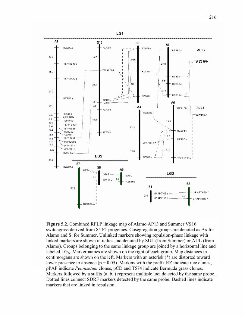
216
Figure 5.2. Combined RFLP linkage map of Alamo AP13 and Summer VS16 switchgrass derived from 85 F1 progenies. Cosegregation groups are denoted as Ax for Alamo and Sx for Summer. Unlinked markers showing repulsion-phase linkage with linked markers are shown in italics and denoted by SUL (from Summer) or AUL (from Alamo). Groups belonging to the same linkage group are joined by a horizontal line andlabeled LGX. Marker names are shown on the right of each group. Map distances in centimorgans are shown on the left. Markers with an asterisk (*) are distorted toward lower presence to absence (p = 0.05). Markers with the prefix RZ indicate rice clones, pPAP indicate Pennisetum clones, pCD and T574 indicate Bermuda grass clones. Markers followed by a suffix (a, b..) represent multiple loci detected by the same probe. Dotted lines connect SDRF markers detected by the same probe. Dashed lines indicate markers that are linked in repulsion.

217
Figure 2. Continued

218
Figure 2. Continued

219
CHAPTER 6
PHOSPHORUS NUTRITION AND ACCUMULATION IN PLANTS:
A LITERATURE REVIEW
Introduction
Phosphorus (P) is an important inorganic macronutrient affecting plant growth
and development. It is a key element in all metabolic processes such as biosynthesis of
macromolecules, signal transduction, photosynthesis, respiration, and energy transfer
(Plaxton and Carswell, 1999). Understanding P metabolism and its regulation in plants
aids in the optimization of crop productivity and prevention of loss of P to aquatic
ecosystems.
P in the soil
Phosphorus is one of the least available of all essential macronutrients in the soil
where P levels are believed to be regulated predominantly through the interaction of P
with organic and inorganic particles. Generally, P is partitioned into several ‘pools’,
including but not limited to, inorganic P sorbed onto soil surfaces, unbound precipitates
deposited by various processes, organic P pools, and dissolved inorganic P (McGechan
and Lewis, 2000). The quantity of P in each pool at a given time is related to the history
of P application. Reddy et al. (1999) evaluated changes in plant-available Olsen P and in
different inorganic and organic P fractions in soil as related to repeated additions of

220
manure and fertilizer P under a soybean-wheat rotation. They found a linear increase in
the level of P through the years with regular application of fertilizer P in both manured
and unmanured plots. The mean P balance required to raise Olsen P by 1 mg kg-1 was
17.9 kg ha-1 of fertilizer P in unmanured plots and 5.6 kg ha-1 of manure plus fertilizer P
in manured plots.
A considerable fraction of soil P can be found in the organic form (20–80%),
which has to be mineralized to the inorganic form before it becomes available for plants
use (Jungk et al., 1993; Richardson, 1994). Available P for plant growth is controlled by
sorption/desorption of P to soil surfaces. The sorbing surfaces consist mainly of iron and
aluminum oxides of the clay components in acid soils, and calcium carbonate in
calcareous soils (McGechan and Lewis, 2002). The mechanism for P sorption onto metal
oxides is based on charge differences of the ions. Sorption onto organic material is
believed to be mediated through a cation bridging mechanism that involves other
substances because negatively charged phosphate anions will not bind to organic colloids
of the same charge. Gerke and Hermann (1992) studied this bridging process in the
adsorption of orthophosphate onto humic-Fe-complexes, observing a large increase in the
extent of sorption in relation to the amount of iron present. As discussed by De Willigen
et al. (1982), manure or slurry added to the soil contains large amounts of both P and
colloidal material on which P is sorbed and such colloids provide additional sorption sites
when distributed by ploughing.
Soil adsorption of P is high in soils with a high proportion of small-size particles
and high specific surface area such as clay (Bowden et al., 1977). Total P concentrations
are generally highest in the clay-sized fractions, compared with the sand- and silt-sized

221
fractions, and always highest in the lowest-density separates, with the highest abundances
occurring in the 2.2 to 2.5 Mg m-3 fractions (Pierzynski et al., 1990). Another important
environmental factor controlling the availability of P is pH (Barrow, 1984).
There appears to be at least two distinct processes of sorption, a fast reversible
sorption onto solid mineral surfaces followed by precipitation reactions that form less
soluble compounds with reduced availability to plants (McGechan and Lewis, 2002).
Addiscott and Thomas (2000) suggested that the processes involved in P sorption and
precipitation reactions should be considered as a continuum since it is difficult to
distinguish between fast and slow physical/chemical reactions.
The term ‘buffering capacity’ is regularly used to indicate the extent of sorption
that affects P precipitation reactions that decrease the availability of P and influence the
amount of P fertilizer required for adequate plant nutrition (Dear et al. 1992 ; Indiati,
2000). Buffering capacity is generally determined from the slope of a P sorption curve
when a range of known P concentrations are added to soil and the amount of P sorbed is
measured after a period of equilibration. Equations that are commonly fitted to the P
sorption data are the Freundlich, Langmuir (single or double surface model), or Tempkin
with the first equation being preferred because its assumption of the exponential decline
in P bonding energy as the amount of sorbed P increases (Barrow, 1978). Buffering
capacity is affected by the type of fertilizer applied. The application of biosolids
decreased buffering capacity and increased the equilibrium P concentration in the soil
resulting in a large increase in the P concentration of the soil solution. The increase of
soluble forms of P in soil solution heavily amended with biosolids could enhance the loss
of P in runoff and P movement below the root zone (Sui and Thompson, 2000)

222
P uptake across the plasma membrane
Phosphorus concentration in plant cells is usually around (5 to 20 mM). This is
much higher than the concentration of available inorganic P in the soil that rarely exceeds
10 µM even in fertile soils (Bieleski, 1973). In order for plants to absorb P against this
steep concentration gradient across their plasma membranes, an energy mediated
transport process must be in effect. Phosphorus uptake systems across the plasma
membrane of plant cells have been extensively investigated and several studies have
established that there are at least two well-documented types of P transporters in the
plasma membrane of plant cells. One is an H+/P symporter, driven by the electrochemical
potential gradient for protons resulting from the operation of the electrogenic H+pump in
the plasma membrane (Ullrich-Eberius et al., 1981; 1984). Another type of P transporter
driven by Na+ is well known in animal cells, including humans, and is responsible for the
transport of P as well as many other metabolites. This type of transporter was also
identified in fungi (Oshima 1997). There is no clear evidence of a Na+-coupled P uptake
system in plant cells even though Mimura et al. (1998) found that a Na+-coupled P
uptake system is induced by P deficiency in internodal cells of the giant alga Chara. Reid
et al. (2000) argued that in order for this uptake system to be driven by the
electrochemical potential for Na+, the stoichiometry would need to be greater than 5 to 6
Na+ for each P. Also, since in most physiological environments the concentration
gradient for Na+ will be directed outward rather than inward, the active component of the
membrane potential produced by the electrogenic plasma membrane H+ pump should still
play a major role.

223
In higher plants, the phosphate/proton co-transport system driven by protons
generated by a plasma membrane H+-ATPase, was proposed as the mechanism of
phosphate uptake by roots and distribution within the different parts of most plants
(Schachtman et al., 1998; Mimura, 1999). Blockage of P uptake through the use of
inhibitors that eliminate the proton gradient across membranes provided most of the
evidence for the role of H+-ATPases in Pi uptake (Daram et al., 1998 ; Leggewie et al.,
1997).
Understanding phosphate transport processes in plants was greatly advanced
through the application of molecular techniques and the molecular identity of a large
number of P transporters has been determined in recent years. Genes encoding phosphate
transporters have been isolated from a number of plant species, such as Arabidopsis
(Muchhal et al., 1996), potato (Solanum tuberosum) (Leggewie et al., 1997), tomato
(Lycopersicon esculentum) (Daram et al. 1998), Medicago truncatula (Burleigh and
Harrison, 1998; Liu et al., 1998a), tobacco (Nicotiana tabacum ) (Kai et al., 2002), and
Hordeun vulgare (Smith et al., 1999).
The peptide transporters encoded by these genes were predicted to contain 12
membrane-spanning domains, related to the major family of facilitator proteins and
function as H+/H2PO4- cotransporters (Smith et al., 2000). Gene expression studies and
functional analysis of protein product from a cloned cDNA (Pht2;1) isolated from
Arabidopsis showed that it encodes a 61-kD protein with a putative topology of 12
transmembrane domains interrupted by a large hydrophilic loop between TM8 and TM9.
Two boxes of eight and nine amino acids, located in the N- and C-terminal domains,

224
respectively, are highly conserved among species across all kingdoms including,
eubacteria, archea, fungi, plants, and animals (Daram et al., 1999).
The P-uptake mechanisms in plants are classified into two groups, high affinity
and low affinity (Mimura, 1999). In Arabidopsis, more than nine different genes for P
transport across the plasma membrane have been identified with their majority associated
with high affinity Pi uptake (Muchhal et al., 1996; Mitsukawa et al., 1997). A low affinity
P transporter in Arabidopsis has also been identified (Daram et al., 1999). The high-
affinity uptake process is usually induced under deficiency conditions, whereas the low-
affinity transport system is believed to be expressed constitutively in plants (Mimura,
1999). The Michalis-Menten constant (Km), the substrate concentration that allows the
reaction to proceed at half its maximum rate, for high-affinity transporters varies from 1.8
to 9.9 µM (Minmura, 1999). The Km for P uptake of two cDNAs, StPT1 and StPT2,
isolated from potato and that showed homology to the phosphate/proton cotransporter
PHO84 from yeast (Saccharomyces cerevisiae) were determined to be 280 and 130 µM
for StPT1 and StPT2 proteins (Leggewie et al., 1997). When expressed in a P-uptake-
deficient yeast mutant, the tomato phosphate transporter 1 (LePT1) protein showed an
apparent Km of 31 µM. The transporter activity was detected even at submicromolar P
concentrations and the highest Pi uptake was at pH 5 (Daram et al., 1998). Functional
analysis of the Arabidopsis Pht2;1 protein in mutant yeast cells indicated that it is a
proton/P symporter dependent on the electrochemical gradient across the plasma
membrane and has a fairly high apparent Km for P of 400 µM (Daram et al., 1999).
Southern analysis of tobacco NtPT1 indicated that phosphate transporter genes have low
copy number and are members of a small multi-gene family (Baek et al., 2001).

225
Expression of the StPT1 gene in potato occurs in roots, tubers, and source leaves
as well as in floral organs while StPT2 expression is detected mainly in plant roots
deprived of P (Leggewie et al., 1997). In tomato, Pi-transporter genes are regulated by P
in a tissue-specific manner. The encoded peptides of the LePT1 and LePT2 genes with
high degree of sequence identity to known high-affinity Pi transporters were both highly
expressed in roots, although there is some expression of LePT1 in leaves. Their
transcripts were primarily localized in root epidermis and their expression is markedly
induced by P starvation (Liu et al., 1998b). In situ transcript localization experiments in
tomato demonstrated that P transporter genes are preferentially expressed in the epidermis
and root hairs (Daram et al., 1998). Mudge et al. (2002) suggested that the root
epidermally expressed gene members of the Pht1 family of phosphate transporters in
Arabidopsis are expressed most strongly in trichoblasts, the primary sites for Pi uptake.
Destiny of P transported into the cell
Phosphate acquired by roots is translocated to the upper part of the plant where it
is utilized and where the phosphate transport in the cell is important in the phosphate
metabolism. The P taken up into the cell has three main destinies: i) it remains in the
cytoplasm as inorganic phosphate, ii) it is incorporated into various metabolites, or iii) it
is stored in the vacuole (Lee and Ratcliffe, 1993; Mimura, 1999).
The distribution of P in plants is believed to require multiple P transport systems
that must function in concert to maintain homeostasis throughout growth and
development. A different class of proteins involved in P transport but structurally
different from the family of H+/P cotransporters was identified in Arabidopsis. The PHO1

226
gene was identified by map-based cloning in an Arabidopsis mutant pho1 deficient in the
transfer of P from root epidermal and cortical cells to the xylem (Hamburger et al., 2002).
Another transporter presumably different in primary structure, affinity for P, and function
from the members of the known plant P transporter family is the Pht2; 1 gene of
Arabidopsis. This gene is predominantly expressed in green tissue and shoots, especially
in leaves, along with a high apparent Km for P (400 µM), suggesting a role for shoot
organs in P loading (Daram et al., 1999). Functional characterization of the transporters
are enabling the characterization of roles of various transporters in the overall P nutrition
of plants. Complementation studies in a yeast high affinity phosphate transporter mutant
strain, NS219, revealed that the expression of a 2059 bp tobacco leaf cDNA clone NtPT1
re-established the transport function in the mutant (Baek et al., 2001). It also promoted
cell growth suggesting that NtPT1 encodes a functional high affinity phosphate
transporter. Analysis of the Arabidopsis null mutant, pht2;1-1 revealed that PHT2;1
activity affects P allocation within the plant and modulates Pi-starvation responses,
including the expression of P-starvation response genes and the translocation of P within
leaves (Versaw and Harrison, 2002). Studies with PHO1 promoter-glucuronidase
constructs revealed predominant expression of the PHO1 promoter in the stellar cells of
the root and the lower part of the hypocotyls and endodermal cells that are adjacent to the
protoxylem vessels (Hamburger et al., 2002). It has also been suggested that the product
of the well characterized pho2 mutant of Arabidopsis may be involved in phloem loading
(Delhaize and Randall, 1995; Dong et al., 1998). Promoter analysis and expression of
chimeric genes of members of the Pht1 family of phosphate transporters in Arabidopsis
grown under high and low Pi concentrations has revealed some members of this family

227
are expressed in a range of shoot tissues and in pollen grains (Mudge et al., 2002).This
suggests that the role of this gene family in phosphate uptake and remobilization
throughout the plant is broad. Karthikeyan et al. (2002) also suggested that members of
the P transporter family may have similar but non-redundant functions in plants.
Control of P uptake activity
Many of the biochemical, physiological, and morphological changes that occur in
plants in response to P status are associated with altered gene expression. Plants increase
their capacity for P uptake during P starvation by synthesis of additional transporter
molecules, which results in increased P uptake when P is re-supplied (Raghothama,
1999). Some researchers have reported that the expression of different P transporters
increases under P deficiency, especially in roots (Leggewie et al., 1997; Daram et al.,
1998). The expression of many of these genes is transcriptionally regulated by signals
that respond to the nutrient status of the plant, mainly the demand and the availability of
precursors needed in the assimilatory pathways (Coruzzi and Bush, 2001; Forde, 2002).
Uptake of P is controlled via the concentration of P in the external medium through
induction or repression of plasma membrane P transporters (Mimura et al., 1998). The
level of expression of the Arabidopsis APT1 and APT2 genes, associated with membrane
transport of phosphate in roots, was shown to be regulated by the P status of the plant,
with their activity being greatly enhanced under deprivation of the plants from
phosphorus (Smith, 1997). Expression of Medicago truncatula Mt4 cDNA was sensitive
to exogenous applications of P fertilizer, with transcripts being abundant in roots
fertilized with nutrient solution lacking P, decreasing when fertilized with 0.02 or

228
0.1 mM P until they became undetectable when the plants were supplied with 1 or 5 mM
of phosphate (Burleigh and Harrison, 1998). Using antibodies specific to one of the
tomato P transporters (encoded by LePT1), Muchhal and Raghothama (1999) found that
transporter protein accumulation levels depend on the P concentration in the medium, and
is reversible upon resupply of P
Changes in gene expression is presumed to be due to interaction of regulatory cis-
element sequences present in the promoters with DNA binding trans-factors as
demonstrated in the P starvation-induced genes AtPT2 and TPSI1 of Arabidopsis and
tomato. Using DNA mobility-shift assays, Mukatira et al. (2001) found that two specific
regions of AtPT2 and TPSI1 promoters interact with nuclear protein factors from P-
sufficient plants. This DNA binding activity disappeared during P starvation, leading to
the hypothesis that P starvation-induced genes is under negative regulation. The presence
of cis-activation sequences in P starvation–induced gene promoters, similar to those
found in yeast genes induced by P starvation, was shown in the Mt4 gene from M.
truncatula whose promoter region contains a conserved 5' flanking sequence of 1133 bp
also found in the promoters of phosphate starvation inducible genes of yeast and tomato
(Burleigh and Harrison, 1998). There is also evidence for increased phosphorylation of
specific peptides under P starvation as shown in Brassica napus cell cultures using an
anti-fungal agent phosphonate (Phi). This led to the hypothesis that a primary site of Phi
action in higher plants is at the level of the signal transduction chain by which plants
perceive and respond to P stress at the molecular level (Carswell et al., 1997).
Immunocytochemical studies of the green alga Chlamydomonas reinhardtii
phosphorus starvation response (Psr1) gene demonstrated this protein is a transcriptional
.

229
activator similar to myb DNA-binding domains (Wykoff et al., 1999). Under both
nutrient-replete and phosphorus-starvation conditions, this protein is nuclear-localized
suggesting vascular plants may have similar homologs responsible in the control of
phosphorus metabolism. Some of the induced genes are also implicated in the direct
enhancement of Pi availability and the promoting of its uptake such as phosphatases
(Raghothama, 2000).
Auxin and cytokinin phytohormones suppressed the expression of both the
reporter genes driven by the AtPT1 promoter and that of the native gene, suggesting
hormones are involved in regulation of the P starvation response pathway (Karthikeyan et
al., 2002). Results of manipulation of the cytoplasmic pH in Chara coralline by weak
acids or ammonium showed Pi influx is controlled by factors other than simple feedback
from cytoplasmic or vacuolar Pi concentrations or thermodynamic driving forces for H -
coupled P uptake (Mimura et al., 1998). At the plant cellular level, Sakano (1990) found
H -coupled P uptake rate was constant over a broad range of pH in the medium and that
the stoichiometry of H / P was not constant during P uptake. Mimura (2001) also
reported P uptake induces cytoplasmic acidification, and that inducing cytoplasmic
acidification causes the cytoplasmic P concentration to decrease which may affect the
+
+
Evidently, there is an initiation of gene expression as a direct and specific
response to P status. There is also genetic control of P acquisition in plants, via the
synthesis of transporters. However, certain phenomena point to a more complex control
of P uptake. Lefebvre and Glass (1982) suggested that P uptake sometimes decreases
within 1 h of P addition to the external medium, which is possibly too fast to be a result
of changes in gene expression.
+

230
operation of the H+ -pump. This suggests a possible mechanism for the physiological
control of P uptake by plant cells. The high number of enzymes and genes identified in
response to P starvation, and the complex pattern of their induction suggests the P
metabolism in plants is highly regulated through a complex molecular network.
Phenotypic and genetic differences in P uptake by plants
The inherent differences in P uptake and utilization by plant species are
demonstrated in a number of investigations. Under low levels of soluble P, Arabidopsis
accessions differing in their P acquisition efficiencies showed significant differences in
root morphology, P uptake kinetics, organic acid release, rhizosphere acidification, and
the ability of roots to penetrate substrates (Narang et al., 2000). In a comparative study of
P efficiencies of seven different species, Fohse et al. (1988) reported that highly efficient
plants had either high influx rates like rape (Brassica napus ) and spinach (Spinacia
oleracea LINN.) or high root-shoot ratios like rye (Secale cereale L.) and wheat
(Triticum aestivum L.) compared to species of low efficiency (onion, tomato, and bean),
which had low influx rates and low root-shoot ratios. Lynch and Beebe (1995) found that
P-efficient bean genotypes possess a highly branched, actively growing root system
compared to those of P-inefficient genotypes, suggesting that root architectural traits
strongly influence Pi acquisition.
A significant difference in P uptake is also attributed to the production of more
root hairs by P-efficient plants in low Pi soil (Fohse et al., 1991). Bates and Lynch,
(1996) reported that P deficiency leads to elongation of root hairs in addition to increased
density of root hairs. Root hairs, because of their small diameter and perpendicular

231
growth to the root axis, provide better soil exploration an enhanced absorptive surface
area. Evidence for the involvement of root hairs in P acquisition was demonstrated in a
study of rye (Secale cereale L.) grown in PVC pipes covered with nylon mesh that was
permeable only to root hairs (Gahoonia and Nielsen, 1998). Results showed 63% of total
Pi uptake by plants was from root hairs.
It is well known that under P deficiency, some plants modify the architecture of
their root system. Formation of proteoid roots as a response to P deficiency was
characterized in white lupins (Lupinus albus) (Gardner et al., 1982). Proteoid roots are
composed of clusters of rootlets like a bottlebrush covered with dense mats of root hairs.
These root structures permit a more efficient synthesis and secretion of organic acids to
the rhizosphere (Yan et al., 2000; Dinkelaker et al., 1995; Keerthisinghe et al., 1998).
Proteoid roots also absorb Pi at a faster rate than non-proteoid roots (Vorster and Jooste,
1986).
Differences in P uptake and utilization were also attributed to a possible active
mechanism of organic acid exudations secreted from roots, which aid in the release of P
from Ca, Fe, and Al phosphate complexes. Increased P acquisition efficiency in Andean
genotypes of common bean (Phaseolus vulgaris) has been related to their higher P-
solubilizing activity attributed to a higher exudation of organic acids, particularly citrate
(Shen et al., 2002). Increase in secretion of organic acids was correlated with an increase
in the activity of a number of enzymes involved in organic acid synthesis, including
phosphoenolpyruvate carboxylase (PEPC), citrate synthase (CS), and malate
dehydrogenase (MDH) (Keerthisinghe et al., 1998). Increase in the production of PEPC
was associated with increased protein and mRNA levels for PEPC in P-deficient proteoid

232
roots suggesting its transcriptional regulation (Johnson et al., 1996). Production of citrate,
malate, and succinate were several folds higher in P starved roots of lupin compared to P
treated (Johnson et al., 1996). Under low-P stress, efficient bean genotypes exuded higher
amounts of citrate, tartrate, and acetate and mobilized more P than the inefficient
genotypes. P-deficient root exudates were composed of 55 and 73% citrates (Shen et al.,
2002). In addition to secretion of organic acids, phosphatase production also increased
nearly 20-fold in lupins under Pi deficiency (Tadano and Sakai, 1991). In a study of the
expression and secretion of acid phosphatase in Indian mustard (Brassica juncea
L. Czern.), Haran et al. (2000) found that phosphorus starvation induced two acid
phosphatases in roots. Under P starvation, the expression of an acid phosphatase
promoter-GUS fusion was initiated in lateral root meristems followed by expression
throughout the root (Haran et al., 2000).
In addition to the production of phosphatases, plants produce other hydrolytic
enzymes that help scavenge P from intracellular and extracellular sources. In tomato,
several RNases induced upon P starvation were characterized, many of which are
localized in the vacuole suggesting a possible function in the release of P from cellular
RNA (Jost et al., 1991 ; Löffler et al., 1992 ; Löffler et al., 1993). Nürnberger et al.
(1990) identified a periplasmic RNase in tomato that was specifically synthesized during
P limitation and presumed to be important for releasing ribonucleotides from RNA in the
soil. RNase genes that are strongly induced under P starvation have also been
characterized in Arabidopsis including genes encoding S-like ribonucleases, like RNS1
and RNS2 (Taylor et al., 1993; Bariola et al., 1994; LeBrasseur et al., 2002). Expression
and mRNA accumulation of RNS1 and RNS2 in Arabidopsis was suppressed up to 90%

233
for RNS1 and 65% for RNS2 by the use of antisense constructs (Bariola et al., 1999). The
transgenic plants with reduced levels of RNases showed increased anthocyanin
accumulation, a typical sign of P stress. Another S-like RNase identical to a tomato
extracellular RNase has been characterized in the styles of a self-incompatible Nicotiana
alata (Dodds et al., 1996). Under low phosphate conditions, this RNase is induced in
roots but not leaves suggesting the likelihood of a role in the response to phosphate
limitation by scavenging phosphate from sources of RNA in the root environment.
Environmental aspects of phosphorus
Animal waste has historically been an important source of plant nutrients for
agricultural land. However, many parts of the world with intensive, animal-based
agricultural systems deal with an increasing threat to the environment as a result of the
excess soluble P in the soil. Continuously amending soils with animal waste increases
phosphorus in the upper soil horizons to levels exceeding crop requirements (Sharpley et
al., 1993). Long-term application of massive quantities of nutrient-rich manure increased
soil total, available, and soluble P levels in both the surface and subsurface horizons,
reduced soil P adsorption capacity, and increased rates of turnover of organic P by
stimulating microbial activity in the soil (Sommers and Sutton, 1980; Mozaffari and
Sims, 1994; Tiessen et al., 1994). These effects are believed to be influenced by several
factors such as the soil type (Pote et al., 1999), the composition of the organic
amendment (Nziguheba et al., 1998), the climate, the rate and method of application, and
the amount of reaction time with soil after application (Reddy et al., 1980; Edwards and
Daniel, 1994).

234
Tiessen et al. (1984) suggested that the relative proportions of available and
stable, as well as organic and inorganic P forms are dependent upon soil type and
chemical properties. In Mollisols, they found that much of the labile P was derived from
inorganic forms in contrast to the more weathered Ultisols where 80% of the variability
in labile P was accounted for by organic P forms.
Eghball et al. (1996) reported that P from manure application moved deeper in the
soil than P from fertilizer at similar P loading rates. Possible explanations are that P from
manure moved in organic forms, or that chemical reactions of P occurred with
compounds in manure, which may have enhanced P solubility.
Application of cattle feedlot waste to irrigated continuous-grain sorghum
(Sorghum bicolor (L.) Moench) over an 8-year period showed that the amounts of P in
the surface soil were highly correlated with the total amount of waste -P applied and time
between applications. The proportion of total P as inorganic P increased with larger waste
applications (Sharpley et al., 1984).
Studies of P transformations in poultry litter-amended soils of the Atlantic Coastal
Plains suggested that soil test P was increased by an average of 167 and 279 mg kg-1
upon the application of 18 and 36 Mg ha-1 (Mozaffari and Sims, 1996). Considerable
attention is usually given to the dissolved organic P because it composes a substantial
part of the total phosphorus in soil solution and leachates. Chardon et al. (1997) showed
that dissolved organic P fraction constitutes the largest part of total P in soil solutions
below a depth of 50 cm. They also found in a manured sandy soil column that more than
90% of P leached was in organic form. In leachates from maize grown in lysimeters,
organic P represented 77% of total P.

235
A combination of excess P and low P-sorption capacity was shown to saturate
soils with P and result in environmentally significant P losses (Sharpley, 1995; Hooda et
al., 2001). The accumulated P in the surface layers from heavy loading of manure is
subject to losses through erosion and run-off especially in area with high rainfall.
Phosphorus leaching to ground waters in excessive concentrations is the most common
cause of eutrophication in lakes, streams, and water reservoirs. Eutrophication is the
overenrichment of waters with mineral nutrients that leads to excessive production of
autotrophs, especially algae and cyanobacteria. The result is an increase in respiration
rates, leading to hypoxia or anoxia. Low dissolved oxygen causes the death of aquatic
animals and release of many materials normally bound to bottom sediments (Correll,
1998).
Potential use of crop species for phytoremediation to excess P in the soil
Phosphorus concentrations in water exceeding 20 µg/L are often considered a
problem (Correl, 1998). Several strategies to reduce P losses to the environment have
been considered. These include the manipulation of dietary P intake by livestock (Mohan
and Hower, 1995), the genetic altering of phytic acid content in grains to improve feeding
efficiencies and the reduction of P content of manure (Verwoerd et al., 1995; Hegeman
and Grabau, 2001), the addition of amendments like alum (aluminum sulfate) to manure
to reduce NH3 volatilization, and P solubility of poultry litter (Moore and Miller, 1994;
Sims and Luka-McCafferty, 2002), and direct elimination with macrophytes (Ahn et al.,
2002).

236
Growing crops with high P uptake may also constitute an economical alternative,
especially those intended for biomass production and transport away from the source of
pollution. Plant requirements for P are generally high and luxury accumulation of this
macronutrient usually occurs without toxicity to the crop. The negative effects of high P
on plants are associated with zinc (Zn) nutrition, and iron (Fe) to some degree, as high P
levels are known to interfere with their normal metabolism. Phosphorus is also known to
promote manganese (Mn) uptake to toxic levels. Toxic P levels are not clearly defined for
most crops. Jones (1998) observed the occurrence of nutritional stress in tomato plants
when the P level in leaves exceeded 1.00% of its dry matter. Mallarino (1996) determined
critical concentrations of 3.4 g P kg-1 for maize plants and 2.4 g P kg-1 for leaves. He also
observed that P concentrations of whole plants and their leaves increased with soil-test P
until a plateau was reached, suggesting that plant tissue may have upper limits for luxury
accumulation of P. It has also been shown that C4 species are inherently less P efficient
than C3 species, but monocots in general are more P efficient than dicots, because of
contrasting P and biomass allocation (Halsted and Lynch, 1996).
Plants play a major role in microbiological P transformation processes and in the
direct elimination of P by binding it to humic substances (Lüderitz and Gerlach , 2002 ).
The importance of plants in bioremediation of P has been demonstrated by several
investigations. Using fescue (Festuca arundinacea Schreb.) in vegetative filter strips
reduced mass transport and losses of ortho-P (PO4-P) and total P in surface runoff up to
94% for PO4-P, and up to 92% of the total P, from plots treated with liquid swine manure
at 200 kg Nha-1 (Chaubey et al., 1994). The use of `Alamo' switchgrass (Panicum
virgatum L.) in a biomass production-filter strip system treated with dairy manure

237
reduced the concentrations of total reactive P in surface runoff water by an average of 47
to 76% after passing through the strip depending on the N level. This suggests that
switchgrass can be used in sequestering excess P and reducing its loss to streams, besides
taking advantage of manure as a substitute for inorganic fertilizers (Sanderson et al.,
2001).
Genetic manipulation to increase P uptake in crops
The development of improved plant cultivars more efficient in P uptake
represents an attractive alternative to reduce the use of P fertilizers and achieve a more
sustainable agriculture. The existence of mutants such as the pho2 mutant of Arabidopsis
that accumulates excessive P concentrations in shoots compared to wild-type plants
(Delhaize and Randall, 1995) suggests possible selection for increased P uptake. Dong et
al. (1998) reported that uptake and translocation of P by pho2 mutant was twofold greater
than wild-type plants under P-sufficient conditions and a greater proportion of the P taken
up was accumulated in shoots of pho2, suggesting that the greater P uptake by the pho2
mutant is due to a greater shoot sink for P.
Phenotypic and genotypic variation for P uptake was found in a number of crop
species such as alfalfa (Medicago sativa) (Hill and Jung, 1975), white clover (Trifolium
repens )(Caradus et al., 1998), and tall fescue (Festuca arundeinacea ) (Sleper et al.,
1977). Furlani et al. (1987) indicated that P absorption, distribution, and efficiency in
sorghum inbred parents and their hybrids were genetically controlled. Based on the better
growth of the male parents, and the transfer of the trait to their hybrids, they suggested
the importance of dominant genes and suspected that genes with additive effects might

238
also be involved in the variability of P uptake and efficiency traits. Barber et al. (1967)
studied the inheritance of P accumulation in maize and confirmed the existence of
genetically controlled variation in P accumulation between inbred lines and indicated the
involvement of at least two genetic factors. Ciarelli et al. (1998) found that most of the
favorable characteristics for P uptake and use efficiency identified in maize parental
genotypes were also found in hybrids indicating that these traits are heritable and under
genetic control. Barber and Thomas (1972) investigated the genetic control of P
accumulation by maize using reciprocal chromosomal translocations. They postulated
that a minimum of six loci are involved in the control of P accumulation. Quantitative
trait loci associated with relative P uptake, content, and relative P utilization efficiency
were also identified in rice (Ming et al., 2001).
Variation between and within species in the concentration to which a plant can
deplete P in the soil has been documented. Krannitz et al. (1991) reported that the
concentration to which a plant can deplete P in the soil (Cmin) varied from 30 to 120 nM
in 25 different ecotypes of Arabidopsis. If this variability is due to genetic differences
like the expression of phosphate transporters, it may be possible to convert a high Cmin to
a low Cmin genotype simply through selection or by over-expressing the right gene. A
linear relationship between relative grain yield and acid phosphatase activity was
reported in 12 wheat genotypes that showed significant variation in the activity of acid
phosphatase exuded by roots under P-deficiency implying that the enzyme activity could
be used as an early indicator to select P-efficient wheat genotypes (Sun and Zhang,
2002). Miller et al. (1987) selected alfalfa plants for increased P uptake and suggested

239
that selection based on individual plants performance is an efficient selection procedure
in terms of progress over time.
The extraction of P from soils also represents one of the most promising areas for
genetic manipulation (Hirsch and Sussman, 1999). With the identification of regulators
such as Psr1 it may become possible to engineer photosynthetic organisms for more
efficient utilization of P and to establish better practices for the management of
agricultural lands and natural ecosystems (Wykoff et al., 1999). Over-expression of the
Arabidopsis gene PHT1 in tobacco-cultured cells increased the rate of P uptake. The
transgenic cells exhibited increased biomass production when the supply of phosphate
was limited, establishing gene engineering of P transport as one approach toward
enhancing plant P uptale (Mitsukawa et al., 1997).
The ability of plants to use insoluble P compounds can be significantly enhanced
by engineering plants to produce more organic acids. Citrate-overproducing plants were
shown to yield more leaf and fruit biomass when grown in alakaline soils with P limiting
conditions (Lopez-Bucio et al., 2000). An increase in the excretion of organic acids,
particularly citrate, was described in rape (Brassica napus L) and radish (Raphanus
sativus L), as a potential mechanism to enhance P uptake. Due to its affinity for divalent
and trivalent cations, citrate can displace P form insoluble complexes, making it more
available (Zhang et al., 1997).
In the soil, a significant amount of total P occurs in organic fractions and is
present as phytates. Plants have a limited ability to obtain P directly from phytates.
Increasing extracellular phytase activity of plant roots is a significant factor in the
utilization of phosphorus from phytates and several studies demonstrated that using gene

240
technology to improve the ability of plants to utilize accumulated forms of soil organic P
exists. Richardson et al. (2001) showed that the growth and P nutrition of Arabidopsis
plants supplied with phytate was improved significantly when the phytase genes (PhyA-1
and PhyA-2) from Aspergillus niger were introduced. Phytase was secreted with the
inclusion of the signal peptide sequence from the carrot extensin (ex) gene.

241
References:
Addiscott, T.M., and D.Thomas. 2000. Tillage, mineralization and leaching: phosphate.
Soil Till. Res. 53:255–273.
Ahn, J., T. Daidou, S. Tsuneda, and A. Hirata. 2002. Transformation of phosphorus and
relevant intracellular compounds by a phosphorus-accumulating enrichment
culture in the presence of both the electron acceptor and electron donor. Biotech.
Bioengineering. 79: 83-93.
Baek, S.H., I.M. Chung, and S.J. Yun . 2001. Molecular cloning and characterization of a
tobacco leaf cDNA encoding a phosphate transporter. Mol. Cells. 11:1-6.
Barber, W.D., and W.I. Thomas. 1972. Evaluation of the genetics of relative phosphorus
accumulation by corn (Zea mays L.) using chromosomal translocations. Crop Sci.
12:755-758.
Barber, W.D., W.I. Thomas, and D.E. Baker. 1967. Inheritance of relative phosphorus
accumulation in corn (Zea mays L.). Crop sci. 7:104-107.
Bariola, P.A, G.C. MacIntosh, and P.J. Green. 1999. Regulation of S-like ribonuclease
levels in Arabidopsis. Antisense inhibition of RNS1 or RNS2 elevates
anthocyanin accumulation. Plant Physiol. 119:331–42
Bariola, P.A., C.J. Howard, C.B. Taylor, M.T. Verburg, V.D. Jaglan, and P.J. Green.
1994. The Arabidopsis ribonuclease gene RNS1 is tightly controlled in response
to phosphate limitation. Plant J. 6:673-85.
Barrow, N.J. 1978. The description of phosphate adsorption curves. Soil Sci. 29:447–462.

242
Barrow, N.J. 1984. Modelling the effects of pH on phosphate sorption by soils. J. Soil
Sci. 35: 283–297.
Bates, T.R., and J.P. Lynch. 1996. Stimulation of root hair elongation in Arabidopsis
thaliana by low phosphorous availability. Plant Cell Environ. 19:529–538.
Bieleski, R.L. 1973. Phosphate pools, phosphate transport, and phosphate availability.
Annu. Rev. Plant Physiol. 24:225–52.
Bowden, J.W., A. Posner and J. Quirk. 1977. Ionic adsorption on variable charge mineral
surfaces. Theoretical-charge developmemnt and titration curves. Aust. J. Soil Res.
15:121–136.
Burleigh, S. H, and M.J. Harrison. 1998. Characterization of the Mt4 gene from
Medicago truncatula. Gene 216:47–53.
Caradus, J.R., L.D. Kennedy, and A. Dunn. 1998. Genetic variation for the ration of
inorganic to total phosphorus in white clover leaves. J. Plant Nutri. 21:2265-2272.
Carswell, M.C, B.R.Grant, and W.C. Plaxton. 1997. Disruption of the phosphate-
starvation response of oilseed rape suspension cells by the fungicide phosphonate.
Planta 203:67–74.
Chardon, W.J., O. Oenema, P. del Castilho, R. Vriesema, J.D. Japenga, and D. Blaauw.
1997. Organic phosphorus in solutions and leachates from soils treated with
animal slurries. J. Environ. Qual. 26:372–378.
Chaubey, I., D.R. Edwards, T.C. Daniel, P.A. Jr. Moore, and D.J. Nichols.1994.
Effectiveness of vegetative filter strips in retaining surface-applied swine manure
constituents. Trans. A.S.A.E. 37:845-850.

243
Ciarelli, D.M., A.M.C. Furlanim A.R.Dechen, and M. Lima. 1998. Genetic variation
among maize genotypes for phosphorus-uptake and phosphorus-use efficiency in
nutrient solution. J. Plant Nutri. 2:2219-2229.
Correll, D.L. 1998. The role of phosphorus in the eutrophication of receiving waters: a
review. J. Environ. Qual. 27:261-266.
Coruzzi, G., and D. R. Bush. 2001. Nitrogen and carbon nutrient and metabolite signaling
in plants. Plant Physiol. 125: 61-64.
Daram, P., S. Brunner, C. Rausch, C. Steiner, N. Amrhein, and M. Bucher. 1999. Pht2;1
encodes a low-affinity phosphate transporter from Arabidopsis. Plant Cell
11:2153-2166.
Daram, P., S. Brunner, B. L. Persson, N. Amrhein, and M. Bucher. 1998. Functional
analysis and cell-specific expression of a phosphate transporter from tomato.
Planta 206:225-233.
De Willigen, P., P.A.C. Raats, and R.G. Gerritse. 1982. Transport and fixation of
phosphate in acid, homogeneous soils, II.Computer simulation. Agri. Environ.
7:161–174.
Dear, B.S., K.R. Helyar, W.J. Muller, and B. Loveland. 1992. The P fertilizer
requirements of subterranean clover, and the soil P status, sorption and buffering
capacities from two P analyses. Aust. J. Soil Res. 30:27-44.
Delhaize E., and P.J. Randall. 1995. Characterization of a phosphate-accumulator mutant
of Arabidopsis thaliana. Plant Physiol. 107:207-213.
Dinkelaker, B., C. Hengeler, and H. Marschner. 1995. Distribution and function of
proteoid roots and other root clusters. Bot. Acta 108:183–200.

244
Dodds, P.N., A. E Clarke, and E. Newbigin. 1996. Molecular characterization of an S-
like RNase of Nicotiana alata that is induced by phosphate starvation. Plant Mol.
Biol. 31: 227-38.
Dong, B., Z. Rengel, and E. Delhaize. 1998. Uptake and translocation of phosphate by
pho2 mutant and wild-type seedlings of Arabidopsis thaliana Source: Planta 205:
251 - 256.
Edwards, D.R., and T.C. Daniel. 1994. Quality of runoff from fescue plots treated with
poultry litter and inorganic fertilizer. J. Environ. Qual. 23:579-584.
Eghball, B., G. Binford, and D.D. Baltensperger. 1996. Phosphorus movement and
adsorption in a soil receiving long-term manure and fertiliser application. J.
Environ. Quality 25:1339-1343.
Fohse, D, N. Claassen, and A. Jungk. 1988. Phosphorus efficiency of plants I. External
and internal P requirement and P uptake efficiency of different plant species.
Plant Soil 110:101–9.
Fohse, D., N. Classen, and A. Jungk A. 1991. Phosphorus efficiency of plants. II.
Significance of root radius, root hairs and cation-anion balance for phosphorus
influx in seven plant species. Plant Soil 132:261–272.
Forde, B.G. 2002. Local and long-range-signaling pathways regulating plant responses to
nitrate. Annu. Rev. Plant Biol. 53: 203-24.
Furlani, A.M.C., R.B. Clark, W.M. Ross, and J. W. Maranville. 1987. Differential
phosphorus uptake, distribution, and efficiency, by sorghum inbred parents and
their hybrids. p. 287-297. In H.W. Gabelman and B.C. Loughman (Eds.), Genetic
aspects of plant mineral nutrition. Maritinus Nijhoff. Boston.

245
Gahoonia, T.S, and N.E. Nielsen. 1998. Direct evidence on participation of root hairs in
phosphorus (32P) uptake from soil. Plant Soil 198:147-152.
Gardner, W.K., D.G. Parberry, and D.A. Barber. 1982. The acquisition of phosphorus by
Lupinus albus L. I. Some characteristics of the soil/root interface. Plant Soil
68:19–32.
Gerke, J., and R. Hermann. 1992. Adsorption of orthophosphate to humic-Fe-complexes
and to amorphous Fe-oxide. J. Plant Nutri. Soil Sci. 155:233–236.
Halsted, M., and J. Lynch. 1996. Phosphorus responses of C3 and C4 species. J. Exp.
Bot. 47:497-505.
Hamburger, D., E. Rezzonico, J. M.C. Petétot, C. Somerville and Y. Poirier . 2002.
Identification and characterization of the Arabidopsis PHO1 gene involved in
phosphate loading to the xylem. Plant Cell. 14:889-902.
Haran, S., S. Logendra, M. Seskar, M. Bratanova, and I. Raskin. 2000. Characterization
of Arabidopsis acid Phosphatase promoter and regulation of acid phosphatase
expression. Plant Physiol. 24: 615-626.
Hegeman, C.E, and E.A. Grabau. 2001. A novel phytase with sequence similarity to
purple acid phosphatases is expressed in cotyledons of germinating soybean
seedlings. Plant Physiol 126:1598–1608.
Hill, R.R., and G.A. Jung. 1975. Genetic variability for chemical composition of alfalfa.
I. Mineral elements. Crop Sci. 15:652-657.
Hirsch, R.E., and M.R. Sussman. 1999. Improving nutrient capture from soil by the
genetic manipulation of crop plants. Trends Biotech. 17:356-361.

246
Hooda, P.S., V.W. Truesdale, A.C. Edwards, P.J.A. Withers, M.N. Aitken, A. Miller
and A.R. Rendell. 2001. Manuring and fertilization effects on phosphorus
accumulation in soils and potential environmental implications. Advances
Environ. Res. 5:13-21.
Indiati, R. 2000. Addition of phosphorus to soils with low to medium phosphorus
retention capacities. I. Effect on soil phosphorus sorption properties. Comm. Soil
Sci. Plant Anal. 31:1179-1194.
Johnson, J.F., D.L.Allan, and C.P. Vance. 1996. Phosphorus deficiency in Lupinus albus.
Altered lateral root development and enhanced expression of
phosphoenolpyruvate carboxylase. Plant Physiol. 112:31–41.
Jones, J.B. Jr. 1998. Phosphorus toxicity in tomato plants: when and how does it occur?
Comm. Soil Sci. Plant Anal. 29:1779-1784.
Jost, W., H. Bak, K. Glund, P. Terpstra, and J.J. Beintema. 1991. Amino acid sequence of
an extracellular, phosphate-starvation-induced ribonuclease from cultured tomato
(Lycopersicon esculentum) cells. Eur. J. Biochem. 198:1-6.
Jungk, A., B. Seeling, and J. Gerke. 1993. Mobilization of different phosphate fractions
in the rhizosphere. Plant Soil 155/156:91–94.
Kai, M., K.Takazumi, H. Adachi, J. Wasaki, T. Shinano and M. Osaki. 2002. Cloning
and characterization of four phosphate transporter cDNAs in tobacco, Plant Sci.
163: 837-846.
Karthikeyan, A.S., D.K. Varadarajan, U.T. Mukatira, M.P. D'Urzo, B. Damsz, and K.G.
Raghothama. 2002. Regulated expression of Arabidopsis phosphate transporters.
Plant Physiol 130:221-33.
247
Keerthisinghe, G., P.J. Hocking, P.R. Ryan, and E. Delhaize. 1998. Effect of phosphorus
supply on the formation and function of proteoid roots of white lupin (Lupinus
albus L.). Plant Cell Environ. 21:467–478.
Krannitz, P.G., L.W. Aarssen, and D.D. Lefebvre. 1991. Relationship between
physiological and morphological attributes related to phosphate uptake in 25
genotypes of Arabidopsis thaliana. Plant Soil. 133:169–175.
LeBrasseur, N.D., G.C. MacIntosh, M.A. Perez-Amador, M. Saitoh, and P.J. Green.
2002. Local and systemic wound-induction of RNase and nuclease activities in
Arabidopsis: RNS1 as a marker for a JA-independent systemic signaling pathway.
Plant J. 29:393-403.
Lee, R. B., and R.G. Ratcliffe. 1993. Subcellular distribution of inorganic phosphate, and
levels of nucleotide triphosphate, in mature maize roots at low external phosphate
concentrations: measurements with 31P-NMR. J. Exp. Bot. 44: 587–598.
Lefebvre, D. D., and A.D.M. Glass. 1982. Regulation of phosphate influx in barley roots:
effects of phosphate deprivation and reduction of influx with provision of
orthophosphate. Physiol. Plant. 54:199–206.
Leggewie, G., L. Willmitzer and J.W. Riesmeier, 1997. Two cDNAs from potato are able
to complement a phosphate uptake-deficient yeast mutant: Identification of
phosphate transporters from higher plants. Plant Cell 9:381¯392.
Liu, C., U.S. Muchhal, U. Mukatira, A.K. Kononowicz, and K.G. Raghothama. 1998 b.
Tomato phosphate transporter genes are differentially regulated in plant tissues by
phosphorus. Plant Physiol. 116:91–99.

248
Liu, H., A.T. Trieu, L.A. Blaylock, and M.J.Harrison. 1998 a. Cloning and
characterization of two phosphate transporters from Medicago truncatula roots:
regulation in response to phosphate and to colonization by arbuscular mycorrhizal
(AM) fungi. Mol. Plant-Microbe Interact. 11:14-22.
Löffler, A., K. Glund K, and M. Irie. 1993. Amino acid sequence of an intracellular,
phosphate-starvation inducible ribonuclease from cultured tomato (Lycopersicon
esculentum) cells. Eur. J. Biochem. 214:627–633.
Löffler, A., S. Abel, W. Jost, and K. Glund. 1992. Phosphate-regulated induction of
intracellular ribonucleases in cultured tomato (Lycopersicon esculentum) cells.
Plant Physiol. 98:1472–1478.
Lopez-Bucio, J., O.M. De la Vega, A. Guevara-Garcia, and L. Herrera-Estrella. 2000.
Enhanced phosphorus uptake in transgenic tobacco plants that overproduce
citrate. Nat. Biotech. 18: 450-453.
Lüderitz, V., and F. Gerlach. 2002. Phosphorus Removal in Different Constructed
Wetlands. Acta Biotechnologica 22: 91-99.
Lynch, J.P., and S.E. Beebe. 1995. Adaptation of beans (Phaseolus vulgaris L.) to low
phosphorus availability. HortSci. 30:1165-71.
Mallarino, A.P. 1996. Evaluation of optimum and above-optimum phosphorus supplies
for corn by analysis of plant parts. Agron. J. 88:376-380.
McGechan, M.B., and D.R. Lewis. 2002. Sorption of Phosphorus by Soil, Part 1:
Principles, Equations and Models. Biosystems Eng. 82:1–24.

249
Miller,D., N. Waissman, B. Melton, C. Currier, and B. McCaslin. 1987. Selection of
increased phosphorus in Alfalfa and effects on other characteristics. Crop Sci.
27:22-26.
Mimura, T., R.J. Reid, and F.A. Smith. 1998. Control of phosphate transport across the
plasma membrane of Chara corallina. J. Exp. Bot. 49:13–19.
Mimura, T. 1999. Regulation of phosphate transport and homeostasis in plant cells.
International Review of Cytology 191:149–200.
Mimura, T. 2001. Physiological control of phosphate uptake and phosphate homeostasis
in plant cells. Australian J. Plant Physiol.(now called Functional Plant Biology),
28:655-660.
Ming, F., X. Zheng, G. Mi, L. Zhu, and F. Zhang . 2001. detection and verification of
quantitative trait loci affecting tolerance to low phosphorus in rice . J. Plant Nutri.
24:1399-1408.
Mitsukawa, N, S. Okumura, Y. Shirano, S. Sato, and T. Kato.1997. Overexpression of an
Arabidopsis thaliana high-affinity phosphate transporter gene in tobacco cultured
cells enhances cell growth under phosphate-limited conditions. Proc. Natl. Acad.
Sci. USA 94:7098-7102.
Moore, P.A., and D.M. Miller. 1994. Decreasing phosphorus solubility in poultry litter
with aluminium calcium and iron amendments. J. Environ. Qual. 23:325-330.
Mozaffari, M., and J.T. Sims. 1994. Phosphorus availability and sorption in an Atlantic
coastal plain watershed dominated by animal-based agriculture. Soil Sci 157:97-
107.

250
Mozaffari, M., and J.T. Sims. 1996. Phosphorus transformations in poultry litter-
amended soils of the Atlantic Coastal plain. J. Environ. Qual. 25:1357-13656.
Muchhal, U.S., J.M. Pardo, and K.G. Ragothama 1996. Phosphate transporters from the
higher plant Arabidopsis thaliana. Proc. Natl. Acad. Sci. USA 93:10519¯10523.
Muchhal, U.S., and K.G. Raghothama. 1999. Transcriptional regulation of plant
phosphate transporters. Proc. Natl. Acad. Sci. U. S. A. 96: 5868-5872.
Mudge, S. R., A.L. Rae, E. Diatloff, and F.W. Smith FW. 2002. Expression analysis
suggests novel roles for members of the Pht1 family of phosphate transporters in
Arabidopsis. Plant J. 31:341-53.
Mukatira, U.T., C. Liu C, D.K. Varadarajan, and K.G. Raghothama. 2001. Negative
regulation of phosphate starvation-induced genes. Plant Physiol 127:1854-62.
Narang, R. A., A. Bruene, and T. Altmann. 2000. Analysis of Phosphate Acquisition
Efficiency in Different Arabidopsis Accessions. Plant Physiol. 124: 1786-1799.
Nürnberger, T., S. Abel, W. Jost, and K. Glund. 1990. Induction of an extracellular
ribonuclease in cultured tomato cells upon phosphate starvation. Plant Physiol.
92:970–976.
Nziguheba, G., C.A. Palm, R.J. Buresh, and P.C. Smithson. 1998. Soil phosphorus
fractions and adsorption as affected by organic and inorganic sources. Plant Soil
198:159-168.
Oshima, Y. 1997. The phosphatase system in Saccharomyces cerevisiae. Genes Genet.
Syst. 72:323–334.

251
Pierzynski, G.M., T.J. Logan, S.J. Traina, and J.M. Bigham. 1990. Phosphorus chemistry
and mineralogy in excessively fertilized soils: quantitative analysis of
phosphorus-rich particles. Soil Sci. Soc. Am. J. 54:1576-1583.
Plaxton, W.C., and M.C. Carswell. 1999. Metabolic aspects of the phosphate starvation
response in plants. In: H.R. Lerner, Editor, Plant Responses to Environmental
Stresses: From Phytohormones to Genome Reorganization, pp. 349¯372. Dekker,
New York
Pote, D.H., T.C. Daniel, D.J. Nichols, A.N. Sharpley, P.A. Moore, D.M. Miller, and D.R.
Edwards. 1999. Relationship between phosphorus levels in three Ultisols and
phosphorus concentrations in runoff. J. Environ. Qual. 28:170-175.
Raghothama, K.G. 1999. Phosphate acquisition. Annu. Rev. Plant Physiol. Plant Mol.
Biol. 50:665-693.
Raghothama, KG . 2000. Phosphate transport and signaling, Curr. Opinion Plant Biol.
3:182-187.
Reddy, D.D., A.S. Rao, and P. N. Takkar. 1999. Effects of repeated manure and fertilizer
phosphorus additions on soil phosphorus dynamics under a soybean-wheat
rotation. Biol. Fertil. Soil. 28: 150-155.
Reddy, K.R., M.R. Overcash, R. Khaleel, and P.W. Westerman. 1980. Phosphorus
adsorption-desorption characteristics of two soils utilized for disposal of animal
wastes. J. Environ. Qual. 9:86-92.
Reid, R.J, T. Mimura, Y. Ohsumi, N.A. Walker, and F.A. Smith. 2000. Phosphate
transport in Chara: membrane transport via Na/Pi cotransport. Plant Cell Environ.
23:223–228.

252
Richardson, A.E. 1994. Soil microorganisms and phosphorus availability. Soil Biota 50-
62.
Richardson, A.E., P.A. Hadobas, and J.E. Hayes. 2001. Extracellular secretion of
Aspergillus phytase from Arabidopsis roots enables plants to obtain phosphorus
from phytate. Plant J. 25:641–649.
Sakano, K. 1990. Proton/phosphate stoichiometry in uptake of inorganic phosphate by
cultured cells of Catharanthus roseus (L.) G. Don. Plant Physiology 93: 479–483.
Sanderson, M.A., R.M. Jones, M.J. McFarland, J. Stroup, R.L. Reed, and J.P. Muir. 2001.
Nutrient movement and removal in a Switchgrass biomass–filter strip system
treated with dairy manure. J. Environ. Qual. 30: 210-216.
Schachtman, D.P., R.J. Reid, and S.M. Ayling, 1998. Phosphorus uptake by plants: from
soil to cell. Plant Physiol 116: 447¯453.
Sharpley, A. N., S.J. Smith, B.A. Stewart, and A.C. Mathers. 1984. Forms of phosphorus
in soil receiving cattle feedlot waste. J. Environ. Qual. 13:211-215.
Sharpley, A.N. 1995. Identifying sites vulnerable to phosphorus loss in agricultural
runoff. J. Environ. Qual. 24:947–51.
Sharpley, A.N., S.J. Smith, and R. Bain. 1993. Nitrogen and phosphorus: Fate from long
term poultry litter application to Oklahoma soil. Soil Sci. Soc. Am. J. 57:1131-
1137.
Shen, H., X. Yan, M. Zhao, S. Zheng, and X.Wang. 2002. Exudation of organic acids
in common bean as related to mobilization of aluminum- and iron-bound
phosphates. Environ. Exp. Bot. 48:1-9.

253
Sims, J.T., and N. J. Luka-McCafferty. 2002. On-farm evaluation of aluminum sulfate
(Alum) as a poultry litter amendment: Effects on litter properties. J. Environ.
Qual. 31: 2066-2073.
Sleper, D.A., G.B. Garner, K.H. Asay, R. Boland, and E.E. Pickett. 1977. Breeding for
Mg, Ca, K, and P content in tall fescue. Crop Sci. 17:433-437.
Smith, F.W, P.M. Ealing, B. Dong, and E. Delhaize. 1997. The cloning of two
Arabidopsis genes belonging to a phosphate transporter family. Plant J. Cell Mol.
Biol. 11:83-92.
Smith, F.W., D. Cybinski and A.L. Rae. 1999. Regulation of expression of genes
encoding phosphate transporters in barley roots. In Gissel-Nielsen G, Jensen A,
eds, Plant Nutrition-Molecular Biology and Genetics: Proceedings of the Sixth
International Symposium on Genetics and Molecular Biology of Plant Nutrition.
Kluwer Academic Publishers, Dordrecht, The Netherlands, pp 145 150.
Smith, F.W., a.L. Rae, and M.J. Hawkesford. 2000. Molecular mechanisms of phosphate
and sulphate transport in plants. Biochimica and Biophysica Acta. 1465:236-45.
Sommers, L.E., and A.L. Sutton. 1980. Use of waste materials as sources of phosphorus.
p. 515-545. In: Khasawneh, F.E., E.C. Sample, and E.J. Kamprath (eds). The role
of phosphorus in agriculture. American Society of Agronomy, Madison, Wis.
Sui , Y., and M.L. Thompson. 2000. Phosphorus Sorption, Desorption, and Buffering
Capacity in a Biosolids-Amended Mollisol. Soil Sci. Soc. Am. J. 64: 164-169.
Sun, H., and F. Zhang. 2002. Effect of phosphorus deficiency on activity of acid
phosphatase exuded by wheat roots. Ying Yong Sheng Tai Xue Bao. 13:379-
381(English abstract).

254
Tadano, T, and H. Sakai. 1991. Secretion of acid phosphatase by the roots of several crop
species under phosphorus-deficient conditions. Soil Sci. Plant Nutr. 37:129–140.
Taylor, C.B., P.A. Bariola, SB. delCardayre, R.T. Raines, and P.J. Green. 1993. RNS2: a
senescence-associated RNase of Arabidopsis that diverged from the S-RNases
before speciation. Proc Natl Acad Sci U S A. 90:5118-22.
Tiessen, H., J.W.B. Stewart, and A. Oberson. 1994. Innovative soil phosphorus
availability indices: assessing organic phosphorus. In: Havlin, J., and J. Jacobsen
(eds) Soil testing: prospects for improving nutrient recommendations. Soil
Science Society of America, Madison, Wis. 40:143-162,
Tiessen, H., J.W.B. Stewart, and C.V. Cole. 1984. Pathways of phosphorus
transformations in soils of differing pedogenesis. Soil. Sci. Soc. Am. J. 48:853-
858.
Ullrich-Eberius, C.I., A. Novacky, E. Fischer, and U. Lüttge. 1981. Relationship
between energy-dependent phosphate uptake and the electrical membrane
potential in Lemna gibba G1. Plant Physiol. 67:797–801.
Ullrich-Eberius, C.I., A. Novacky, and A.J.E. van Bel. 1984. Phosphate uptake in Lemna
gibba G1: energetics and kinetics. Planta 161:46–52.
Versaw , W.K., and M.J. Harrison. 2002. A chloroplast phosphate transporter, PHT2;1,
influences allocation of phosphate within the plant and phosphate-starvation
responses. Plant Cell 14:1751-1766.
Verwoerd, T.C., P.A. van Paridon, A.J.J. van Ooyen, J.W.M. van Lent, A. Hoekema, and
J. Pen. 1995. Stable accumulation of Aspergillus niger phytase in transgenic
tobacco leaves. Plant physiol. 109:1199-1205.

255
Vorster, P.W., and J.H. Jooste. 1986. Potassium and phosphate absorption by excised
ordinary and proteoid roots of the Proteaceae. S. Afric. J. Bot. 52:276–281.
Wykoff, D.D., A.R. Grossman, D.P. Weeks, H. Usuda, and K. Shimogawara. 1999. Psr1,
a nuclear localized protein that regulates phosphorus metabolism in
Chlamydomonas. Proc. Natl. Acad. Sci. USA. 96:15336 15341.
Yan, F., Y. Zhu, C. Muller, C. Zorb, and S. Schubert. 2002. Adaptation of H+-pumping
and plasma membrane H+ ATPase activity in proteoid roots of white lupin under
phosphate deficiency. Plant Physiol. 129: 50-63.
Zhang, F.S., J. Ma, and Y.P. Cao. 1997. Phosphorus deficiency enhances root exudation
of low-molecular weight organic acids and utilization of sparingly soluble
inorganic phosphates by radish (Raghanus sativus L) and rape (Brassica napus
L). Plant Soil 196:261-264.

256
CHAPTER 7
GENETIC VARIATION AND HERITABILITY OF PHOSPHORUS
UPTAKE IN SWITCHGRASS (PANICUM VIRGATUM L.) UNDER
EXCESSIVE SOIL PHOSPHORUS CONCENTRATIONS1
1Ali M. Missaoui and Joseph H. Bouton. To be submitted to Crop Science

257
Abstract
Continuous excessive amendment of soil with animal waste leads to the
accumulation of phosphorus (P) in the surface layers of the soil and its escape to streams
and water reservoirs causing their eutrophication. Developing crop cultivars with high P
uptake may constitute a remedy to such a problem. Therefore, the purpose of this
investigation was to determine the potential of P uptake in switchgrass (Panicum
virgatum L.), an important bioenergy and forage crop, and determine the nature of
genetic variation and heritability of this trait and its components (P concentration and
biomass production) in switchgrass. To accomplish this objective, 30 genotypes were
randomly selected from a population of ‘Alamo’ switchgrass and evaluated in the
greenhouse and the field under fertilizer rates of 450 mg P and 200 mg N kg-1 soil. Half-
sib families were generated from 12 selected genotypes using a polycross mating design
and evaluated in the field for P uptake and its components. Significant genetic variation
was observed among the parental genotypes and the half-sib families for P concentration,
biomass production, and P uptake. Genotype x environment interaction was significant.
Nevertheless, rank correlation of the genotypes between the two locations was high (r =
0.83, p< 0.01) indicating that much of the genotype x location interaction is not
associated with changes in genotype ranking across sites. Narrow sense heritability,
calculated on individual plant basis, family means, and using parent-offspring regression
gave estimates of 2%, 13%, and 16% for P concentration, 60, 69, and 84% for biomass
production, and 67, 73, and 90 % for P uptake. Expected genetic gain estimates based on
individual plant selection and expressed as percentage of the mean of parents were less
than 1%, 51%, and 65% for P concentration, biomass production, and P uptake,
respectively. Expected gain from selection based on half-sib progeny testing was slightly
higher (2, 55, and 68 % for P concentration, biomass, and P uptake). Although no gain
from selection is predicted for P concentration, the range in genetic variability and
magnitude of heritability values for biomass production and P uptake indicate that
substantial genetic progress can be made through breeding for these two traits.

258
Introduction
Phosphorus leaching to ground waters is increasingly becoming a serious
environmental problem in countries with intensive animal production where the waste
generated is applied to the soil as fertilizer. The accumulation of P in the surface layers of
the soil is subject to losses through erosion and run off especially in areas with high
rainfall. Excessive concentrations of P in lakes, streams, and water reservoirs lead to
excessive production of autotrophs, especially algae and cyanobacteria. The result is an
increase in respiration and reduction of dissolved oxygen that causes the loss of aquatic
life and release of many materials normally bound to bottom sediments (Correll, 1998).
In the southeastern USA, the primary producer of broiler chickens (Gallus gallus
domesticus), a large proportion of poultry litter generated is applied to pastures and hay
fields. Studies of P transformations in poultry litter-amended soils of the Atlantic Coastal
Plains showed that soil test P can be increased by an average of 279 mg kg-1 through the
application of 36 Mg ha-1 (Mozaffari and Sims, 1996). Considerable attention is given to
the dissolved organic phosphorus because it makes up to 77% of the total phosphorus in
soil solution and leachates (Chardon et al., 1997). Phosphorus concentrations above 20
µg L-1 of water are often considered a problem (Correl, 1998). Several strategies to
reduce P losses to the environment have been considered. These include the genetic
manipulation of phytic acid content in grains to improve feeding efficiencies and reduce
the P content of subsequent manure (Verwoerd et al., 1995), and addition of amendments
like slaked lime or alum (Aluminum Sulfate) to manure to reduce P solubility (Moore and
Miller, 1994).
Crop production represents an important component of nutrient management.
Growing crops with high P uptake may constitute an economical alternative, especially
those intended for biomass production and transport away from the source of pollution.
By exporting nutrients in the form of biomass from land receiving animal waste, the rate
of nutrient accumulation in the soil and the potential for ground and surface water
contamination may be reduced (Sims and Wolf, 1994). Plant requirements for P are
generally high and luxury accumulation of this macronutrient occurs without detrimental
toxic effect (Mallarino, 1996; Jones, 1998). Reported amounts of P removed annually

259
from soil by grasses vary between 15 kg ha-1 for annual bluegrass (Poa annua L.) and 83
kg ha-1 in johnsongrass [Sorghum halepense (L.) Pers.] (Pierzynsky and Logan, 1993).
Plants also play a major role in microbiological P transformation processes where P is
directly eliminated by binding to humic substances (Lüderitz and Gerlach , 2002 ). Using
tall fescue (Festuca arundinacea Schreb.) in vegetative filter strips reduced mass
transport and losses of ortho-phosphorus (PO4-P) each by 94 % and total P by 67 to 92%
of the incoming P, from plots treated with liquid swine manure at 200 kg N ha-1
(Chaubey et al., 1994).
Phenotypic and genotypic variation for the ability to take up phosphorus has been
found in a number of crop species such as alfalfa [Medicago sativa L. ] (Hill and Jung,
1975), white clover [Trifolium repens] (Caradus et al., 1998), tall fescue [Festuca
arundinacea Schreb] (Sleper et al., 1977), sorghum [Sorghum bicolor (L.) Pers.] (Furlani
et al., 1987), and maize [Zea mays ](Ciarelli et al., 1998). Therefore breeding programs
can exploit this variation in order to develop cultivars with higher P accumulation.
Maximizing nutrient uptake by crops would facilitate nutrient removal from animal
waste-treated soils when the plants are mechanically harvested and removed. Most
studies involving P uptake by plants identified genotypes that grow and produce better at
low P levels. No information is available on the genetic variability in P accumulation in
switchgrass at high P concentrations in the soil.
Switchgrass has been widely grown for summer grazing and soil conservation
(Vogel et al., 1985; Jung et al., 1990). The Bioenergy Feedstock Development Program
(BFDP) at the U.S. Department of Energy chose switchgrass (Panicum virgatum L.) as a
model bioenergy species from which renewable sources of transportation fuel and
biomass-generated electricity are derived based on its high biomass production, nutrient
use efficiency, wide geographic distribution, and environmental benefits (Sanderson and
Wolf, 1995; Sanderson et al., 1996). The use of `Alamo' switchgrass in a biomass
production–filter strip system treated with dairy manure reduced the concentrations of
total reactive P in surface runoff water by an average of 47% to 76% suggesting that
switchgrass can be used effectively in sequestering excess P in the soil preventing its loss
to streams (Sanderson et al., 2001). In the present study, we investigated the extent of
genetic variation for phosphorus uptake and the heritability of this trait in switchgrass

260
grown under high P rates similar to what can be expected in a soil continuously amended
with poultry litter.
Materials and methods
Genetic variability in P uptake
Two experiments were conducted to investigate the extent of variability in P
uptake in switchgrass under high P rates similar to what can be expected in a soil
continuously amended with animal waste. The first experiment was conducted in a
greenhouse. Thirty randomly selected Alamo switchgrass plants were established in pots
in the greenhouse on 7 Dec. 1998. The plants were allowed to grow and develop until
they reached on average 10 tillers. Each plant was cloned vegetatively via rooted tillers
into six replications and transplanted in plastic pots containing 3 kg of Tifton loamy sand
soil (fine, loamy, siliceous thermic family of the Plinthic Paludults). This soil type is
found in Coastal Plain of Georgia and is known to have a low P adsorption capacity. The
soil was amended with magnesium oxide to raise the pH to 6.8. Pots were lined with
plastic to prevent loss of P with irrigation water. Phosphorus was applied as ammonium
phosphate monobasic NH4H2PO4 at the rate of 5 g pot-1, the equivalent of 450 mg of P
and 200 mg of N kg-1 of soil. Once a week, the plants received 50 mL of a Hoagland
nutrient solution without N and P. The pots were arranged in a randomized complete
block design with six replications. Plant biomass was harvested on 2 Oct. 1999, 5 Jan.
2000, and 17 Apr. 2000. Clipping height was about 15 cm. The top growth from each
plant in all six replications was placed separately in a bag, dried for 48 h at 65°C in a
mechanical convection oven, and weighed for dry weight determination. Prior to
chemical analysis, the dried biomass was ground to pass through a 2-mm screen in a
Wiley mill.
A second study including the same entries evaluated in the greenhouse was
conducted in the field. Plants of similar vigor were cloned into six replications and
transplanted on 29 May 2000 at a site on the Univ. of Georgia Plant Sciences Farm near
Watkinsville, GA. The soil was a Wedowee coarse sandy loam (fine, kaolinitic, thermic
family of the Typic Kanhapludults). The experimental design was a randomized

261
complete block design with six replications. The plants were spaced 1 m apart.
Phosphorus was applied as superphoshpate at a rate of 900 kg P ha-1 to simulate a
concentration of 450 mg of P kg-1 soil. Nitrogen was applied as ammonium nitrate at a
rate of 400 kg N ha-1 to provide a level of 200 mg N kg-1 soil at a depth of nearly 20 cm.
Phosphorus uptake was evaluated for each separate entry in a single-cut biomass
production system for 2 yr. Plant biomass was harvested before stem elongation. The first
cut was taken on 29 Sept. 2000. The second cut was taken on 5 July 2001.
To determine P, samples were digested in standard Kjeldahl tubes using
aluminum blocks. Sample weight was 0.2 g, digested in 1 g of mixed salt/catalyst
containing (90% K2SO4, 9% CuSO4.5H2O and 1% Se for 2 h at 375°C using 3 mL of
H2SO4). Phosphorus in the digest was determined using a Perstorp Enviroflow 3500
Segmented Colormetric Analyzer (Perstorp, Sweden). Phosphorus uptake by each
genotype was estimated based on biomass yield and P concentration in the tissue. Results
are presented on a dry weight basis.
Statistical analysis was performed using the SAS program V.8.2 (SAS Institute
Inc., Cary, NC, USA) following the model of Steele and Torrie (1980) for multi-cut
forage experiments. Analysis of variance was conducted separately for each experiment
and for combined replication means of the greenhouse and field locations for P
concentration, biomass production, and P uptake. The harvest date main effects were
considered fixed. The genotypes, replications, and locations were considered random.
The expected mean squares were obtained by the RANDOM statement in PROC GLM of
SAS. Phenotypic correlations (Pearson) among the components of P uptake were
estimated on the basis of genotype means across harvest dates and locations.
The P uptake means of individual genotypes were compared by Fisher's protected
least significant difference (FLSD). The 0.05 level of probability was used to identify
differences. Spearman correlation of the genotype ranks were determined for P uptake
and its components on a genotype mean basis between the greenhouse and field locations.
Components of variance were estimated by equating mean squares with their expected
values and solving for the appropriate component (Schultz, 1955).

262
Estimation of genetic parameters of P uptake
Twelve genotypes were selected from the 30 genotypes evaluated in the
greenhouse and the field and polycrossed in the greenhouse in a randomized complete
block design with 6 replications to create half-sib families. Five plants from each of the
12 half-sib families were raised in pots in the greenhouse and transplanted in the field at
the Univ. of Georgia Plant Sciences Farm on 4 June 2002. The plants were placed on 1-m
centers in single row-plots. Rows were spaced 1 m apart. The experimental design was a
randomized complete block with five replications. The 12 parents were planted in a
randomized complete block design with five replications adjacent to the progeny.
Phosphorus and nitrogen were applied as described above. Plant biomass was harvested
once on 17 Oct. 2002. Each plant was kept separate. Plant biomass was oven-dried and
analyzed for P as described above. Analysis of variance was performed on the single
harvest using SAS V.8.2 (SAS Institute, Inc.). Families were considered random effects.
Replications and plants within families were considered random effects. Variance
component estimates were determined using the appropriate coefficients obtained from
the RANDOM procedure of SAS and the mean squares of ANOVA output. Narrow sense
heritabilities for P uptake and its components were estimated using parent-offspring
regression, parent-offspring rank correlation, and from variance components of the mean
squares according to the following equations:
Individual plant basis
h2 = σ2A /σ2
P
= 4σ2f / σ2
f +σ2 + σ2
w and
HS family-means basis
h2FM = σ2
f / (σ2f +σ2/r + σ2
w/rn)
where,
σ2A = additive genetic variance,
σ2P = phenotypic variance,
σ2f = variance component due to half-sib families,
σ2w = variance component due to plant-to-plant variation within each family,
σ2 = error variance,

263
r = number of replications, and
n = number of plants in a family.
Expected genetic gain from selection for P uptake and its components on single plant and
family basis were estimated according to Nguyen and Sleper (1983) based on a selection
differential of 10% (k = 1.76).
Results
Phenotypic variation in P uptake
In the greenhouse, average P concentration varied from 0.62 % to 1.38 % in the
first harvest, from 0.42 % to 0.94% in the second harvest, and from 0.31 % to 0.68 % in
the third harvest and was different between the 30 genotypes for each of the harvest
dates. This contrasting difference between the harvest dates was due to an increase in
biomass production in the third harvest, which coincided with the active growing period
of the summer grass. The average P concentration over the three harvests ranged from
0.53 % to 0.98 % (Table 7.1).
Biomass production ranged from 1.0 g to 1.9 g per plant in the first harvest, from
0.5 to 3 g in the second harvest, and from 1.3 g to 8.6 g per plant in the third harvest and
was different between the 30 genotypes for each of the harvest dates. After the second
harvest, survival of some genotypes was affected. Combined over the three harvest dates,
biomass production ranged from 0.9 to 3.94 g per plant (Table 7.1). Phosphorus uptake
was calculated as the product of biomass production per plant and P percentage in the
tissue. Phosphorus uptake ranged from 0.63 to 2.5 g in the first harvest, from 0.4 to 1.99
g in the second harvest, and from 0.54 to 5.7 g per plant in the third harvest. Phosphorus
uptake was significantly different between the genotypes in each of the harvest dates.
Average P uptake between the 30 genotypes varied from 0.63 to 2.9 g plant-1over three
harvests (Table 7.1).
Analysis of variance combined over the three harvest dates revealed significant
harvest date effect and a genotype by harvest interaction for P concentration, biomass
production, and P uptake (Table 7.2). Despite the strong interaction, there was an overall
genotype effect and a difference among the genotypes in P concentration, biomass
production, and P uptake. There were moderate spearman rank correlation between the

264
means of P concentration across the three harvest dates (r= 0.25 to 0.57) (Table 4).
Correlation between the genotypic ranks of biomass means (r = 0.02 to 0.19) and P
uptake (r = 0.13 to 0.33) were low and non-significant.
In the field experiment, P concentration in the tissue was much lower compared to
the greenhouse. Average P concentration ranged from 0.32 % to 0.56 % in the first
harvest and was different between the genotypes. In the second harvest, P concentration
declined and ranged from 0.22 % to 0.32 % and was marginally different between the
different genotypes. Over the two harvests, P concentration in the tissue of the different
genotypes ranged from 0.28 to 0.41 % (Table 7.3). Dry matter production in the second
year harvest ranged from 27 g to 415 g plant-1 and was much higher than the yield of the
first year harvest that ranged from 13 to 110 g plant-1. In each of the two harvests,
genotypes were significantly different in biomass production. Over the two harvests,
biomass production ranged from 19 to 257 g plant-1. Phosphorus uptake in the field was
much higher in the second harvest despite the lower concentration of P measured in the
plant tissue of all the genotypes compared to the first harvest. P uptake ranged from 5 g to
47 g plant-1 in the first harvest and from 9 to 105 g plant-1 in the second. At both harvest
dates, P uptake was different among the various genotypes. Over the two harvests, P
uptake ranged from 8 to 76 g plant-1.
Analysis of variance combined over the two harvests in the field showed a large
harvest date effect for P concentration, biomass, and P uptake as well as a significant
genotype x harvest interaction for the three variables (Table 7.2). The effect of the
genotypes was significant and the variance component due to genotypes was nearly twice
that of the interaction genotypes x harvest for P concentration and biomass production,
and three times higher for P uptake (Table 7.2). Spearman rank correlation between the
two harvests was low for P concentration (r = 0.27) and moderate but significant for
biomass production and P uptake (r = 0.41 and r = 0.40, respectively) (Table 7.4).
Combined analysis of variance of the 30-genotype means over the two locations
(greenhouse and field) is summarized in Table 7.5. The separate analysis of the
greenhouse and field data showed large differences in variances and experimental errors
between the two locations for biomass production and P uptake. In order to perform a
combined analysis, the data was transformed on the Log (Y+1) scale for the two variables

265
to remove correlation between variances and means. The magnitude of differences in P
concentration, biomass production, and P uptake between the greenhouse and the field
environments contributed to a significant location effect. The genotype by location
interaction was also significant across the two locations. The variance component due to
genotype effect was much smaller than that of the interaction for P concentration. For
biomass production and P uptake, the variance component associated with the genotypes
was much larger than that of the interaction. Genotype rank correlation between the two
locations was non significant for P concentration (r = 0.13) and significant and relatively
high for biomass production and P uptake (r = 0.84, and 0.83, respectively) indicating
that much of the genotype x location interaction is not associated with changes in
genotype ranking across the two sites (Table 7.4).
Variation in P uptake and heritability in half-sib families
Phosphorus concentration in plant tissue ranged from 0.38 to 0.47 % in the 12
half-sib families. Dry matter production and P uptake ranged from 58 to 107g plant-1 and
from 24 to 55 g plant-1, respectively (Table 7.6). Analysis of variance of the selected half-
sib families evaluated in one location revealed no differences in P concentration between
the families. Biomass production and P uptake were both different between the families
(Table 7.7). Environmental variation was high for all the three variables. Within-plot
variation accounted for 86 %, 63 %, and 66% of the total variation for P concentration,
biomass production, and P uptake (Table 7.7). This large variation is probably due to the
high variability in Athens soil and the non uniformity of field irrigation since summer of
2002 was exceptionally dry at the Plant Sciences Farm. This variation may be reduced by
increasing the number of plants evaluated within each family and the number of
environments.
Narrow sense heritability estimates based on individual plants were very low for P
concentration (0.02) and moderate for both biomass production and P uptake (0.60 and
0.67, respectively) (Table 7.8). When expressed on family means, narrow sense
heritability was slightly higher than the heritability on individual plants but showed the
same trend. The higher estimates are probably due to the elimination of within-family
variation. Heritability estimates on family mean basis were low for P concentration (0.13)

266
and moderate to high for biomass production and P uptake (0.69 and 0.73). Heritability
estimates derived from parent-offspring regression were high compared to the estimates
of family means and individual plants basis. Since the parents were evaluated separately
from the progeny, this could be inflated by the differences in soil conditions and other
environmental variations. Because the covariance between offspring and parent is only
one-half the additive genetic variance, the regression coefficient is multiplied by two to
obtain an estimate of narrow sense heritability.
Expected gain from selection for P concentration was low using all methods of
selection (Table 7.8). Selection gain for biomass production was highest based on half-sib
progeny test followed by individual plant selection (51% and 55% of the mean). Gain
from selection based on half-sib family selection was nearly half the gain from progeny
test and individual plants (27%). Expected gain from selection for P uptake was nearly
the same when selecting for individual plants or using half-sib progeny test (65 % and 68
%). Based on half-sib family selection, gain for P uptake was only 35%.
Phenotypic correlation between P concentration, biomass production and P uptake
Pearson correlation between P concentration and biomass was low and
inconsistent, with a low negative relationship in the greenhouse experiment and a low
positive relationship in the field experiment (Table 7.9). Pearson correlation coefficients
between P concentration in the tissue and biomass production in the greenhouse was (r =
- 0.09, p = 0.201). There is a moderate correlation between P concentration and P uptake
(r = 0.31, p<0.01). Biomass production was highly correlated with P uptake (r = 0.90, p<
0.01).
In the field experiment, phenotypic correlation between the means of P
concentration in the two harvest dates and biomass production was low (r= 0.03, p =
0.671). P concentration was not correlated with P uptake (r = 0.07, p = 0.341). Over the
two harvests, correlation between P uptake and biomass production was high (r = 0.65,
p<0.001). A similar trend in correlation between P concentration, biomass, and P uptake
was observed in the half-sib progeny. Pearson correlation coefficient between biomass
and P concentration was 0.02 (p = 0.731). Correlation between P concentration and P

267
uptake was moderate (r = 0.42, p < 0.01). Phenotypic correlation between biomass
production and P uptake was high (r = 0.89, p< 0.01).
Discussion
Phosphorus accumulation in biomass
The P concentrations in the tissue measured in the controlled greenhouse study
were similar to concentrations reported in wetland plants grown under high P rates. Sharp
dock (Polygonum amphibium L.), and water hyacinth (Eichornia crassipes) grown in
pots and fertilized with a solution containing 1.0 mmol P l-1 water had concentration of
11.3 and 6.5 g P kg-1 plant tissue (Wang et al., 2002). These concentrations are much
higher than values reported in other crops. Forage P concentration among genotypes of
timothy (Phleum pratense L.) grown in pots ranged from 4.1 to 5.1 g P kg-1 DM and
decreased under N stress (Belanger et al., 2002). P concentrations measured in ryegrass
(Lolium multiflorum Lam.) grown in pots and fertilized with monocalcium phosphate and
pig manure were between 2.0 and 4.0 g P kg-1(Tunney and Pommel, 1987). In the field
experiments, P concentrations were also higher than values reported in different crops
grown under non-limiting conditions. Examples are P concentration of 2.11 g kg-1
measured in forage kenaf (Hibiscus cannabinus L.) that received 20 Mg DM ha-1 of dairy
compost (Muir, 2001) and 2.2 to 3.3 g P kg-1 measured in various temperate grasses
fertilized with 9 Mg ha-1 broiler litter (Brink et al., 2001).
We speculate that the soluble form of P fertilizer applied under greenhouse
conditions (ammonium phosphate) led to a greater P availability than under field
conditions leading to a high accumulation of mineral P in plant tissue of greenhouse
grown plants. The markedly high P concentrations under both greenhouse and field
conditions indicate that switchgrass can accumulate excessive amounts of P. Even though
toxic P levels are not clearly defined for most crops, Jones (1998) observed the
occurrence of nutritional stress in tomato plants when the P concentration in leaves
exceeded 1% of its dry matter. Mallarino (1996) determined critical concentrations of 3.4
g P kg-1 for whole maize plants and 2.4 g P kg-1 for leaves suggesting that plant tissues
may have upper limits for luxury accumulation of phosphorus. In the greenhouse

268
experiment, we witnessed a higher mortality in some genotypes that accumulated more
than 10 g P kg-1 dry matter in the first harvest. However, it is not clear whether the
mortality is due to P toxicity or to possible increased salinity in the pots.
Genetic variation in P uptake
The mean squares associated with the variance components showed important
genetic variation between the genotypes for P concentration, biomass production and P
uptake. Despite the fact that harvest date had a great effect on P uptake and its
components, the genetic variance represented 22 and 20 % of the phenotypic variation
observed between the genotypes for P concentration, 28 and 30 % for biomass, and 29 to
27 % for P uptake in the greenhouse and the field. Across the two locations, the
interaction between genotypes and locations was less than the genetic variance despite
the contrasting differences between the two locations for biomass production and P
uptake. The high values of rank correlation coefficients between the two locations
indicate that the magnitude of genotype differences and genetic variance changed without
affecting the ranking of genotypes. This would predict that performance of genotypes
selected for higher biomass and higher P uptake can be maintained beyond the selection
environment (Yamada, 1962). The genetic variation for P concentration in the tissue
across the two locations was very low and so was the rank correlation between the
locations.
Heritability of P concentration estimated by the different methods was very low
compared to findings in other grasses. Reported narrow sense heritability coefficient for
P concentration in the regrowth forage of tall fescue was between 61 and 84% (Nguyen
and Sleper, 1981). It is worth noting that the results of our study apply to excessive P
conditions unlike most of the studies reported. Phosphorus concentration among
genotypes might differ under normal and limiting P conditions. The predicted gains
suggest that P concentration under high P rates cannot be improved through selection.
The range in genetic variability and magnitude of heritability values for biomass
production and P uptake indicate that substantial genetic progress can be made through
selection. Narrow sense heritability estimates suggest that more than 60% of the variation
in P uptake between the different genotypes is due to additive variance suggesting that

269
breeding methods such as phenotypic recurrent selection or simple mass selection can be
expected to improve P uptake (Nguyen and Sleper, 1981).
The importance of additive genetic effects for the inheritance of P accumulation
was reported in tall fescue (Sleper et al., 1979). Choice of the most efficient selection
method requires further investigation of the environmental effect on P uptake. In this
study, variance components and genetic gain from selection are estimated based on a
single environment. Because of the large genotype x environment interaction observed in
parental genotypes, we expect the gain from selection to be smaller than that of the single
environment. Therefore, evaluation should be carried under more environments before
undertaking selection. Results of prediction of cultivar performance based on single
versus multiple year tests in soybean (Glycine max L.) showed that a single-year,
multiple location trial had sufficient power to identify genotypes that would perform well
or poor (Yan and Rajcan, 2003).
Phenotypic correlation between P uptake and its components
Information on the association between P uptake and its components (P
concentration and biomass production) is of interest to the switchgrass breeder. Studies of
P uptake in timothy indicated that forage P concentration decreases with increasing DM
yield during the growth cycle suggesting that genotypes with greater forage P
concentration may have lower DM yield (Bélanger and Richards, 1999, Belanger et al.,
2002). This was not the case in our study with switchgrass. Phosphorus concentration
appears to be uncorrelated with biomass production in the parental genotypes at both
locations and in the half-sib families. Some of the genotypes had both greater P
concentration and biomass yield compared to other genotypes tested in the same
experiment. The phenotypic correlation coefficient of 0.06 between dry matter and P was
reported in perennial rye grass (Lolium perenne L.) (Smith et al., 1999). Low correlation
was also found in tall fescue (Festuca arundinacea shreb) between mineral concentration
(including P) and forage dry matter indicating that forage yield in tall fescue should not
be altered significantly by modifying mineral levels (Nguyen and Sleper, 1981). The low
correlation between P concentration and dry matter suggests that mineral concentration
could be altered without affecting the yield. The high correlation between biomass and P

270
uptake suggests that selection for P uptake can be carried indirectly through yield in
switchgrass. Superior P uptake of ryegrass compared with other species was attributed to
positive association between dry herbage weight and P uptake (Brink et al., 2001).
In couclusion, the markedly high P concentrations under controlled conditions
and the field indicate that switchgrass can accumulate excessive amounts of P without
detrimental effect. We conclude that heritable genetic variation exists among switchgrass
genotypes for P uptake. The results of this experiment suggest that it is possible to make
reasonable progress in increasing P uptake by selection methods that take advantage of
the additive genetic variation. Indirect selection for high yield should also concurrently
increase P uptake. Maximizing nutrient uptake by the bioenergy crop switchgrass would
facilitate excessive P removal from P contaminated soils when the biomass is
mechanically harvested and exported away from the polluted site.

271
References
Bélanger, G., A. Brégard, and R. Michaud. 2002. Phosphorous uptake and concentration
of Timothy genotypes under varying N applications. Crop Sci. 42:2044-2048.
Brink, G.E., G. A. Pederson, K. R. Sistani, and T.E. Fairbrother. 2001. Uptake of selected
nutrients by temperate grasses and legumes. Agron. J. 93:887-890.
Chardon, W.J., O. Oenema, P. del Castilho, R. Vriesema, J.D. Japenga, and D. Blaauw.
1997. Organic phosphorus in solutions and leachates from soils treated with
animal slurries. J. Environ. Qual. 26:372–378.
Caradus, J.R., L.D. Kennedy, and A. Dunn. 1998. Genetic variation for the ration of
inorganic to total phosphorus in white clover leaves. J. Plant Nutri. 21:2265-2272.
Chaubey, I., D.R. Edwards, T.C. Daniel, P.A. Jr. Moore, and D.J. Nichols.1994.
Effectiveness of vegetative filter strips in retaining surface-applied swine manure
constituents. Trans. A.S.A.E. 37:845-850.
Ciarelli, D.M., A.M.C. Furlanim A.R.Dechen, and M. Lima. 1998. Genetic variation
among maize genotypes for phosphorus-uptake and phosphorus-use efficiency in
nutrient solution. J. Plant Nutri. 2:2219-2229.
Correll, D.L. 1998. The role of phosphorus in the eutrophication of receiving waters: a
review. J. Environ. Qual. 27:261-266.
Furlani, A.M.C., R.B. Clark, W.M. Ross, and J. W. Maranville. 1987. Differential
phosphorus uptake, distribution, and efficiency, by sorghum inbred parents and
their hybrids. p. 287-297. In H.W. Gabelman and B.C. Loughman (Eds.), Genetic
aspects of plant mineral nutrition. Maritinus Nijhoff. Boston.

272
Jones, J.B. Jr. 1998. Phosphorus toxicity in tomato plants: when and how does it occur?
Comm. Soil Sci. Plant Anal. 29:1779-1784.
Jung, G.A., J.A. Shaffer, W.L Stout, and M.J. Panciera. 1990. Warm season grass
diversity in yield, plant morphology, and nitrogen concentration and removal in
northeastern USA. Agron. J. 82:21-26.
Lüderitz, V., and F. Gerlach. 2002. Phosphorus Removal in Different Constructed
Wetlands. Acta Biotechnologica 22: 91-99.
Mallarino, A.P. 1996. Evaluation of optimum and above-optimum phosphorus supplies
for corn by analysis of plant parts. Agron. J. 88:376-380.
Moore, P.A., and D.M. Miller. 1994. Decreasing phosphorus solubility in poultry litter
with aluminium calcium and iron amendments. J. Environ. Qual. 23:325-330.
Mozaffari, M., and J.T. Sims. 1994. Phosphorus availability and sorption in an Atlantic
coastal plain watershed dominated by animal-based agriculture. Soil Sci. 157:97-
107.
Muir, J.P. 2001. Dairy compost, variety, and stand age effects on Kenaf forage yield,
nitrogen and phosphorus concentration, and uptake. Agron. J. 93:1169-1173.
Nguyen, H.T., and D.A. Sleper. 1981. Genetic variability of mineral concentrations in
Festuca arundinacea Schreb. Theor. Appl. Genet. 59:57-63.
Pierzynski, G.M., T.J. Logan, S.J. Traina, and J.M. Bigham. 1990. Phosphorus chemistry
and mineralogy in excessively fertilized soils: quantitative analysis of
phosphorus-rich particles. Soil Sci. Soc. Am. J. 54:1576-1583.
Pierzynski, G.M., and T.L. Logan. 1993. Crop, soil, and management effects on
phosphorus soil test levels. J. Prod. Agric. 6:513–520.

273
Sanderson, M.A., and D.D. Wolf. 1996. Switchgrass biomass composition during
morphological in diverse environments. Crop Sci. 35:1432-1438.
Sanderson, M.A., R.L. Reed, S.B. McLaughlin, S.D. Wullschleger, B.V. Conger, D.J.
Parrish, D.D. Wolf, C. Taliaferro, A.A. Hopkins, W.R. Osumpaugh, M.A.
Hussey, J.C. Read, and C.R. Tischler. 1996. Switchgrass as a sustainable
bioenergy source. Bioresour. Technol. 56:83–93.
Sanderson, M.A., R.M. Jones, M.J. McFarland, J. Stroup, R.L. Reed, and J.P. Muir. 2001.
Nutrient movement and removal in a Switchgrass biomass–filter strip system
treated with dairy manure. J. Environ. Qual. 30: 210-216.
Schultz, E.F., Jr. 1955. Rules of thumb for determining expectations of mean squares in
analysis of variance. Biometrics. 11:123-125.
Sims, J.T., and D.C. Wolf. 1994. Poultry waste management: Agricultural and
environmental issues. Adv. Agron. 52:1–83.
Sleper, D.A., G.B. Garner, K.H. Asay, R. Boland, E.F. Pickett. 1979. Breeding for Mg,
Ca, K, and P contents in tall fescue. Crop Sci. 17:433-438.
Smith, K.F., G.J. Rebetzke, H.A. Eagles, M.W. Anderson, and H.S. Easton. 1999.
Genetic control of mineral concentration and yield in perennial ryegrass (Lolium
perenne L.), with special emphasis on minerals related to grass tetany. Aust. J.
Agric. Res. 50:79-86.
Tunney, H., and B. Pommel. 1987. Phosphorus uptake by ryegrass from monocalcium
phosphate and pig manure on two soils in pots. Irrig. J. Agric. Res. 26:189–198.

274
Verwoerd, T.C., P.A. van Paridon, A.J.J. van Ooyen, J.W.M. van Lent, A. Hoekema, and
J. Pen. 1995. Stable accumulation of Aspergillus niger phytase in transgenic
tobacco leaves. Plant physiol. 109:1199-1205.
Vogel, K.P., C.L. Dewald, H.J Gorz., and F.A. Haskins. 1985. Development of
Switchgrass, indiangrass, and eastern gamagrass: Current status and future. P. 51-
62. In Symposium on range plant improvement in western North America:
Current status and future. Salt Lake City, UT. 14 Feb. 1985. Soc. Range Manag.,
Denver, CO.
Wang, Q., Y. Cui, Y. Dong. 2002. Phytoremediation of polluted waters potentials and
prospects of Wetland Plants. Acta Biotechnologica. 22:199-208.
Yamada, Y. 1962. Genotype by environment interaction and genetic correlation of the
same trait under different environments. Japanse J. Genet. 37:498-509.
Yan, W., and I. Rajcan. 2003. Prediction of cultivar performance based on single versus
multiple year tests in soybean. Crop Sci. 43:549-555.

275
Table 7.1. Mean P concentration, biomass production, and P uptake combined over 3 harvests of switchgrass grown in the greenhouse at fertilizer rates of 450 mg P and 200 mg N kg-1 soil.
Entry P concentration DM yield P uptake
---------- % ----------- -----------g plant-1---------- -----------g plant-1-------------
P13 0.98 3.855 2.895
P16 0.80 3.939 2.198
P6 0.83 2.678 2.010
P15 0.69 3.100 1.851
P1 0.91 2.126 1.826
P2 0.90 2.399 1.785
P8 0.86 2.481 1.770
P27 0.82 2.252 1.769
P10 0.73 2.797 1.677
P9 0.96 1.859 1.652
P23 0.66 2.409 1.571
P12 0.65 2.259 1.436
P7 0.62 2.510 1.433
P30 0.75 1.967 1.314
P11 0.78 1.954 1.292
P29 0.77 2.011 1.285
P14 0.68 2.041 1.246
P3 0.83 1.402 1.157
P26 0.66 1.822 1.132
P28 0.72 1.490 1.029
P20 0.91 1.100 1.016
P19 0.91 1.156 0.990
P18 0.77 1.343 0.980
P21 0.97 0.900 0.966
P4 0.73 1.536 0.962
P17 0.61 1.747 0.960
P24 0.65 1.519 0.952
P22 0.81 1.120 0.881
P5 0.53 1.484 0.745
P25 0.57 1.167 0.628
FLSD (0.05) 0.14 0.70 0.51

276
Table 7.2. Combined analysis of variance over harvests of P concentration, biomass production, and P uptake in switchgrass grown in the greenhouse and the field under fertilizer rates of 450 mg P and 200 mg N kg-1 soil. Genotypes and replications are considered random effects while cuts are considered fixed. Greenhouse experiment
Mean squares and variance components † Source of Variation
Degrees of Freedom P (%)2 Dry matter (g)2 P uptake (g)2
Replications 5 0.066 3.24 1.5Genotypes
29 0.172 **
σ2G
= 0.011
6.5 **
σ2G
= 0.43 3.7 **
σ2G
= 0.25 Error a 142 0.044 1.14 0.6
Cut 2 6.852 **
175.76 **
22.77 **
Error b 10 0.053 1.49 1.19Genotypes x Cut
58 0.071 **
σ2
GxC = 0.004
5.77 **
σ2
GxC = 0.48
2.0 **
σ2GxC
= 0.15 Error c 188 0.038 1.42 0.69
Field experiment
Mean squares and variance components Source of Variation
Degrees of Freedom P (%)2 Dry matter (g)2 P uptake (g)2
Replications 5 0.011 4427 419.8Genotypes
28 0.01 **
σ2G
= 0.0007
17099 **
σ2G
= 1334.34
1481.5 **
σ2G
= 122.67 Error a 125 0.003 3717 359.5
Cut 1 1.783 **
1129807 **
35014.6 **
Error b 5 0.002 3031 414.2Genotypes x Cut
28 0.006 *
σ2
GxC = 0.0003
8984 **
σ2
GxC = 499.087
655.4 **
σ2
GxC = 37.787
Error c 118 0.003 2995 202 *= p < 0.05, ** = p < 0.01, ns = non significant. † The coefficients for EMS were adjusted for missing data.

277
Table 7.3. Mean P concentration, biomass production, and P uptake combined over 2 harvests of switchgrass grown in the field at fertilizer rates of 450 mg P and 200 mg N kg-1 soil.
Entry % P DM yield P uptake
------------- % --------------- -----------g plant-1----------- -----------g plant-1----------- P16 0.371 257.240 75.557
P13 0.37 208.133 67.51
P15 0.41 164.872 53.858
P6 0.338 159.75 48.765
P1 0.35 166.222 55.443
P2 0.336 170.433 50.789
P27 0.312 152.244 44.573
P23 0.311 171.767 45.941
P9 0.40 141.008 47.541
P8 0.334 156.991 43.589
P30 0.41 126.167 43.9
P14 0.361 146.108 43.602
P11 0.368 133.958 44.103
P10 0.343 158.641 44.433
P12 0.363 127.400 40.316
P29 0.38 127.517 41.108
P26 0.313 149.825 40.585
P7 0.347 132.392 39.779
P4 0.344 139.983 41.408
P3 0.343 128.933 39.127
P17 0.358 128.850 36.703
P19 0.364 122.458 36.987
P28 0.367 84.263 28.846
P24 0.36 96.933 32.417
P25 0.315 92.9 26.091
P18 0.367 92.142 28.702
P5 0.352 86.425 28.787
P22 0.282 38.483 10.539
P21 0.38 18.867 7.569
FLSD (0.05) 0.04 49.28 15.33

278
Table 7.4. Spearman rank correlation coefficients between genotypes for P concentration, biomass production, and P uptake for different harvest dates and locations. P concentration Biomass P uptake Greenhouse
cut1 vs cut2 0.25 0.02 0.13
cut1 vs cut3 0.36 0.19 0.33
cut2 vs cut3 0.57 ** † 0.03 0.30
Field
cut1 vs cut2 0.27 0.41 ** 0.40 **
Between locations
Greenhouse vs field
0.13
0.84 **
0.83 **
† Significant at P=0.01.

279
Table 7.5. Analysis of variance and variance component estimates for genotypes and genotype x location interaction, for P concentration, biomass production, and P uptake of 29 switchgrass genotypes grown in two locations (greenhouse and field) under fertilizer rates of 450 mg P and 200 mg N kg-1 soil. P concentration
Source of variation Degrees of freedom Mean squares Variance †
Location 1 13.12 ** Replications (location) 10 0.018 Genotypes 28 0.046 ns σ2
G = 0.0024
Genotype x location 28 0.04 ** σ2GxL
= 0.004 Error 262 0.014 Biomass production
Source of variation Degrees of freedom Mean squares Variance†
Location 1 226.1 ** Replications (location) 10 0.03 Genotypes 28 0.202 ** σ2
G = 0.015
Genotypes x locations 28 0.053 ** σ2GxL
= 0.006 Error 266 0.019 P uptake
Source of variation Degrees of freedon Mean squares Variance†
Location 1 114.1 ** Replications (location) 10 0.04 Genotypes 28 0.203 ** σ2
G = 0.015
Genotypes x locations 28 0.042 ** σ2GxL
= 0.004 Error 262 0.021
*= p < 0.05, ** = p < 0.01, ns = non significant. † The coefficients for EMS were adjusted for missing data

280
Figure 7.6. P concentration, biomass production, and P uptake of half-sib progenies and their parental genotypes evaluated in one location at fertilizer rates of 450 mg P and 200 mg N kg-1 soil.
Half-sib progeny Parental genotypes Entries P concentration Dry matter P uptake P concentration Dry matter P uptake
--------% --------- -----g plant-1-------- -----g plant-1-------- --------% --------- -----g plant-1------ -----g plant-1------ P1 0.41 91.5 38.20 0.49 72.6 35.22 P15 0.47 123.08 55.37 0.38 92.5 34.68 P13 0.47 93.61 38.30 0.42 76.7 31.85 P16 0.43 75.85 31.10 0.35 80.2 27.54 P2 0.43 107.37 46.80 0.35 75.8 26.42 P17 0.39 68.072 25.90 0.40 57.3 22.84
P19 0.42 58.30 24.50 0.4 56.0 22.15
P24 0.39 74.20 30.90 0.35 55. 8 19.43
P18 0.41 78.79 31.60 0.4 46.4 19.41
P6 0.38 73.30 29.30 0.27 67.7 18.65
P5 0.38 67.55 24.90 0.26 65.4 16.58
P22 0.4 68.30 28.10 0.3 48.0 15.21 LSD (0.05) 0.05 18.4 9.2 0.09 2.01 9.86

281
Table 7.7. Mean squares and variance components for P concentration, biomass production, and P uptake in 12 half-sib families of switchgrass grown in one location (Athens) under fertilizer rates of 450 mg P and 200 mg N kg-1 soil. P concentration (%)
Source of variation
Degrees of freedom
Mean squares
Variance † components
Replications 4 Families 11 0.015 ns σ2
F = 4.3573 x 10⁻⁵
Rep x Families 44 0.014 σ2 = 0.00124 Plants (within plots) 218 0.0078 σ2
W = 0.0078
Biomass (g)
Source of variation
Degrees of freedom
Mean squares
Variance † components
Replications 4 Families 11 8105.82 ** σ2
F = 235.84
Rep x Families 44 2693.32 σ2 = 341.22
Plants (within plots) 219 987.24 σ2W
= 987.24 P uptake (g)
Source of variation
Degrees of freedom
Mean squares and significance
Variance † components
Replications 4 Families 11 1911.924 ** σ2
F = 61.83
Rep x Families 44 547.238 σ2 = 62.47
Plants (within plots) 218 234.913 σ2W
= 234.91 * Significant at p = 0.05. ** Significant at p=0.01. ns = non significant. † The coefficients for EMS were adjusted for missing data

282
Table 7.8. Heritability estimates on individual plants, family means, parent-offspring regression, and parent-offspring correlation and predicted genetic gain from selection on individual plants basis and family selection. Genetic gain is expressed in percent of the parental mean.
Method P concentration Biomass P uptake
Heritability estimates ------------------------------ % ---------------------------------
Individual plants 2 60 67
Family means 13 69 73
Parent-offspring regression 16 84 90
Parent-offspring correlation 9 57 46
Genetic gain from selection
------------------------------ % ---------------------------------
Individual plants † < 1 51 65
Half-sib family selection † 1 27 35
Half-sib progeny test † 2 55 68
† Standardized selection differential, K= 1.76 for 10 % selection intensity.

283
Table 7.9. Pearson coefficient of correlation between P concentration, biomass production, and P uptake in switchgrass parental genotypes and half-sib progeny grown under fertilizer rates of 450 mg P and 200 mg N kg-1 soil.
P concentration
vs biomass P concentration
vs P uptake Biomass vs P
uptake
Parental genotypes
Greenhouse
-0.09
0.31 **
0.90 **
Field
0.03
0.07
0.65 **
Half-Sib progeny
0.02
0.42 **
0.89 **
** Significant at p=0.01.

284
CHAPTER 8
APPLICATION OF THE HONEYCOMB SELECTION METHOD IN
SWITCHGRASS (PANICUM VIRGATUM L.) IMPROVEMENT FOR
BIOMASS PRODUCTION 1
1 Ali M. Missaoui and Joseph H. Bouton. To be submitted to Crop Science

285
Abstract
The objective of this study was to evaluate the effectiveness of the honeycomb
selection design in identifying superior genotypes for biomass production from
switchgrass nursery with 1.2-m inter-plant spacing; at which some level of competition
may still occur. Traditionally, 1-m center spacing is used in switchgrass selection
nurseries. Four field experiments were conducted. Half-sib lines of 4 of 15 genotypes
selected for high yield and 4 lines from the 15 low groups from Alamo and Kanlow
switchgrass were evaluated in one location for 3 yrs together with commercial checks
from each cultivar and the bulk seed of each group of lines in sward plots with 18-cm
row spacing. In the two other experiments, five half-sib lines from the 15 high and 5 from
the 15 low Alamo polycross progenies were evaluated in two locations for 2 yrs, together
with a check, and the bulk seed of each of the five lines in row plots spaced by 76 cm.
Another five half-sib families from each of high and low group polycross progenies of
Kanlow were evaluated in one location for 2 yrs. On average biomass production of the
lines from the high groups of both Alamo and Kanlow was higher than the average of the
low groups in each of the four experiments. The bulk seed of the high group produced
consistently more biomass than the bulk of the low group in all four experiments. In the
sward plots with narrow spacing, ¾ of the lines from the low group of Alamo and ¼ of
the lines from the low group of Kanlow produced more biomass than at least one of the
high group lines. In the row plots with 76 cm spacing, all the high group lines in Kanlow
outyielded those of the low group. Only two lines from low group produced higher
biomass than at least one of the high group lines in Alamo. The results of these
experiments suggest that it is possible to make reasonable progress in identifying high

286
biomass yielding switchgrass genotypes at a plant spacing of 1.2-m using the honeycomb
selection method. The performance of the half-sib families in polycorss progeny tests was
not consistent over the 18- and 76-cm inter-row spacing, indicating that the genotypes
selected were not density-independent. Four genotypes from the Alamo population and
one genotype from the Kanlow population that were eliminated by the moving average
selection method outperformed some of the superior genotypes, indicating that they were
not accurately assessed during selection. Increasing interplant spacing in switchgrass
selection nurseries above 1.2 m is not practical and because the honeycomb method
requires considerably more effort than conventional mass selection, the progress achieved
with the honeycomb design remains to be compared against the traditional methods
applied in switchgrass breeding.

287
Introduction
Switchgrass or tall panic grass (Panicum virgatum L.) belongs to the Paniceae
tribe in the subfamily Panicoideae of the Poaceae (Gramineae) family. It is a warm
season, C4 perennial grass that is native to most of North America (Hitchcock, 1971).
Switchgrass has been widely grown for summer grazing and soil conservation (Vogel et
al., 1985; Jung et al., 1990). The Bioenergy Feedstock Development Program (BFDP) at
the U.S. Department of Energy has chosen switchgrass as a model bioenergy species
from which renewable sources of transportation fuel and/or biomass-generated electricity
could be derived based on its high biomass production, high nutrient use efficiency, wide
geographic distribution, and environmental benefits (Sanderson and Wolf, 1995;
Sanderson et al., 1996). Unlike fossil fuels, using perennial grasses for biomass energy
does not lead to an increase in the levels of atmospheric CO2 because the carbon dioxide
released during the biomass combustion and conversion is balanced by photosynthesis
and CO2 fixation by the growing crop (Lynd et al., 1991).
Switchgrass is largely cross pollinated and self-incompatible (Talbert, 1983) even
though some plants were found to produce selfed seed when bagged (Newell, 1936). In a
recent investigation of the incompatibility systems in switchgrass, Martinez-Reyna and
Vogel (2002) found proportions of selfing of 0.35% in tetraploids and 1.39 % in
octaploids. They observed significant differences in percentage of compatible pollen as
measured by percentage of total seed set between reciprocal matings and suggested that
prefertilization incompatibility in switchgrass is possibly under gametophytic control,
similar to the S-Z incompatibility system found in other members of the Poaceae.

288
Breeding of cross-pollinated perennial grasses has focused on the development of
synthetic cultivars. In most cases the character of interest for improvement is biomass
production, a quantitative trait highly influenced by environmental variations. The typical
methods of breeding perennial forage grasses involve single plant phenotypic selection or
spaced planting stage, and polycross progeny test selection or sward-plot stage (Casler et
al. 1997). Polycross progeny testing is used to identify genotypes with superior
combining ability, mainly because of the simplicity of the procedure (Aastveit and
Aastveit, 1990). Precision of the estimates depends on adequate sampling of the
population of genotypes and environments used for evaluation. Vogel and Pederson
(1993) argued that half-sib progeny test is less efficient in improving traits such as yield
because it involves among family selection and therefore exploits only ½ of the total
additive genetic variance. Progeny performance may also not reflect the breeding values
of the parents because of differences in heterosis.
The most effective breeding systems for such crops are recurrent selection
methods that take advantage of the ability of vegetative propagation and additive genetic
variation (Vogel and Pederson, 1993). According to Hallauer (1992), recurrent selection
includes all methods of selection that are conducted recurrently including mass selection.
This selection scheme has been implemented in different forms including the recurrent
restricted phenotypic selection (Burton, 1992), recurrent between and within half-sib
family selection, and recurrent multistep family selection (Vogel and Pederson, 1993).
All these breeding systems are initiated from a space planted source nursery that is used
to identify superior phenotypes whose progeny is to be evaluated. Therefore accurate
identification of the superior plants is critical to the success of the subsequent steps.

289
Plants compete for a broad range of resources, including water, mineral nutrients,
and light. Interplant competition often reduces plant performance and results in the
selection of high competing plants instead of the ones with a high yield potential. Forage
yield measured in spaced plant nurseries poorly predicts yield performance in sward-plots
(Hayward and Vivero, 1984, Carpenter and Casler, 1990). Mitchell et al. (1982) noticed a
reduction among yield of durum wheat (Triticum durum Desf.) plants with increased
plant density and suggested that single plant selection would be more effective at higher
interplant spacing. The principal factors interfering with the efficiency of single plant
selection are inter-plant competition that affects full expression of the genetic potential in
closely spaced plantings and soil heterogeneity (Fasoula and Fasoula, 1997).
The spatial, non-genetic competition usually masks the difference among
randomly distributed genotypes (Cannel, 1983). To minimize the impact of interplant
competition on the effectiveness of selecting superior yielding genotypes, the honeycomb
selection design was proposed (Fasoulas and Fasoula, 1995). In this design, entries,
whether hill plots or single plants, are placed equidistantly in the corners of triangles
resulting in a hexagonal arrangement of plots. Each plant grows in the center of an
equilateral hexagon and on the points of the hexagon are six neighboring plants. Each
plot is surrounded by plots occurring in the periphery of concentric circles. This layout
permits an increase in the number of plots per unit area of 15.5% more compared to the
square pattern. The underlying principles of the honeycomb method, selection in
optimum growing conditions in absence of interplant competition to permit full
expression of the genotypic potential and effective sampling of soil heterogeneity, are
accomplished by a large number of moving replicates and each plant’s comparison to its

290
neighbors (Fasoula and Fasoula, 2000).The genotypes to be selected should be superior to
each of their six neighbors. Selection is conducted within moving circular grids where
each plant is compared against the plants enclosed in the circle. The center of the circle is
moved from plant to plant so that all plants are evaluated by the same moving circle and
the intensity of selection is determined by the size of the circle. An effective size of the
moving circle is estimated between 19 and 91 plants which correspond to a selection
pressure of 5.3 and 1.1%. The appropriate size needs to be determined experimentally
depending on the genetic structure and size of the population being sampled and the
degree of soil heterogeneity. Border plants are either ignored or evaluated by a lower
selection pressure. Selection in honeycomb designs and data analysis is enabled by a
QBASIC computer program called HONEY (Batzios and Roupakias, 1997).
Robertson and Frey (1987) tested the effectiveness of the honeycomb design for
grain yield selection among homozygous oat (Avena sativa L.) lines. Their results
suggested that selecting for grain or biomass of plants grown in the absence of
competition identified higher yielding lines. Roupakias et al. (1997) found that lines of
faba bean (Vicia faba L.) selected in early generation of under low plant density had a
significantly higher yield than the material selected under high plant density.
Comparative efficiency of mass honeycomb selection, pedigree honeycomb selection,
and pedigree honeycomb selection using a non-improved population of Dactylis
glomerata and an improved population Agropyron cristatum showed the three methods
were all effective with the mass honeycomb selection being the least effective of the three
(Abraham and Fasoulas, 2001). The effectiveness of honeycomb selection was compared
to panicle-to-row selection in two rice (Oryza sativa L.) populations that were advanced

291
from F2 to the F6 generation by both methods. The honeycomb selection for yield and
quality applied during early generations was more effective than panicle-to-row selection
applied in later generations. (Ntanos and Roupakias, 2001).
The honeycomb selection method has not been exploited in switchgrass
improvement and the literature available on the relative efficiency of this method
compared to traditional methods is non existent. The main condition in honeycomb
selection is the absence of competition between genotypes. Inter-genotypic competition is
usually eliminated by increasing the spacing between plants. In the case of switchgrass,
plant size makes it difficult to avoid spatial competition unless extensive land area is
available. Experimental data on optimum spacing for single plant selection is not
available. From visual observations, inter-plant spacing may have to exceed 2 m in order
to completely eliminate competition in switchgrass. Land requirement for selection,
polycross, and progeny evaluation in multiple locations becomes a limiting factor. One
meter- center spacing has traditionally been used in selection nurseries (Van Esbroek et a.
1998). The objective of this study is to evaluate the effectiveness of the honeycomb
design in identifying superior genotypes for biomass production in switchgrass using 1.2
m inter-plant spacing. At this spacing some level of competition may still occur.
Materials and methods
A selection nursery was established in 7 June 1996 at the Univ. of Georgia Plant
Science Farm near Watkinsville, GA. Single plants from ‘Alamo’ or ‘Kanlow’
switchgrass were planted separately in non replicated Honeycomb designs at a rate of
1000 plants in each nursery, with a spacing of 1.2 m between plants. Fertilizer was

292
applied at the rate of 785 kg ha-1 of 14-7-14 in the beginning of the growing season
(May) and after the first harvest. Herbicide was applied as 2,4-D (Dimethylamine salt of
2-3-Dichlorophenoxy acetic acid) or Banvel (Dimethylamine salt of 3-6-Dichloro-o-
anisic acid) at the rate of 2.3 L ha-1 and 1.2 L ha-1. In both the Alamo and Kanlow 1000
plant nurseries, biomass production was evaluated individually for each plant. For
selection, the center of a moving grid comprising 19 plants in both populations was
moved from plant to plant. A particular plant was selected if its yield exceeded the yield
of its neighbor plants within the grid (5.3% selection pressure) for the high yielding group
and below the neighbor plants for the low yielding groups. Border plants were evaluated
with a lower selection pressure since the moving circle was incomplete. Based on 2-yr
yield data, 15 high yielding (157 to 193 % above the mean; Alamo high and Kanlow
high) and 15 low yielding (38 to 57 % below the mean; Alamo low and Kanlow low)
genotypes were selected from each nursery for polycross and progeny testing.
Selected genotypes from each (Kanlow high, Kanlow low, Alamo high, and
Alamo low) group were planted in separate polycrosses on 15 May 1998. The crossing
blocks were arranged in a randomized complete block design with six replications. The
distance between plants was 76.2 cm. The seed harvested from each individual plant was
kept separate. The four highest seed yielding genotypes and their bulks from the high and
low groups of Alamo and Kanlow were evaluated for biomass yield in replicated sward
trials. The bulks from each groups were obtained from mixing equal amounts of seed
from each line.
The replicated sward trials were established in 10 May 1999 at the Univ. of
Georgia Plant Sciences Farm on a Wedowee coarse sandy loam soil (fine, kaolinitic,

293
thermic family of the Typic Kanhapludults). The seed was drilled at the rate of 8 kg ha-1
pure live seed in plots of 1.5x 4.5m (5x15’). The plots were arranged in a randomized
complete block design with five replications. The rows within each plot were spaced at
18 cm. Commercial seed of Alamo and Kanlow were included in the evaluation trial as
checks. Plots were mechanically harvested from the inner 1 x 3.75 m of each plot on 20
July 2000, 27 Nov. 2000, 3 Aug. 2001; 1 Nov. 2001, 17 July 2002, and 20 Nov. 2002.
The harvested material was weighed in the field and sampled for dry matter (DM)
determination. The yield was determined after drying at 65o C for 48 h.
Seeds from the original Alamo polycross nursery were also harvested again in
Oct. 1999. Five half-sib families from the high yielding group and their bulk and five half
sib-families and their bulk from the low yielding group of Alamo were evaluated in row
plots at two locations for 2 yr. The first location was the Univ. of Georgia Plant Sciences
Farm near Watkinsville, GA on a Cecil coarse sandy loam soil (clayey, kanolinitic,
thermic family of Typic hapludults). The seed was drilled on 24 May 2000 in three-row
plots of 2 m length and 0.76 m spacing. The experimental design was a randomized
complete block design with 5 replications. The inner row of each plot was harvested at an
approximately 12-cm stubble height on 5 July, 2001, 1 Nov. 2001, 16 July 2002, and 21
Nov. 2002. The second location was at the Coastal Plains Experimental Station, Tifton,
GA on a Tifton loamy sand soil (fine, loamy, siliceous thermic family of the the Plinthic
Paludults). The experimental design and conditions were the same as described above.
The seed were planted on 7 May 2000 and the plots were harvested on 16 July 2001, 14
Nov. 2001, 17 July 2002, and 26 Nov. 2002.

294
Seed from the Kanlow polycross nursery were also harvested on October 1999.
Five half-sib families from the high yielding group and their bulk and five half sib-
families from the low yielding group and their their bulk were evaluated in three-row
plots at one location at the Univ. of Georgia Plant Sciences Farm. The experimental
design was randomized complete block with six replications. The experimental
conditions and harvest dates were as described above for the Alamo evaluation trial at the
Univ. of Georgia Plant Sciences Farm.
Yield evaluation data was subjected to statistical analysis using SAS V. 8.2 (SAS
Institute, INC). Data from the sward experiments were analyzed as a randomized
complete block in a split-plot arrangement of genotypes. Analysis of variance was
conducted on genotypes (main plots), harvest dates (subplots), and all possible
interactions using the model outlined by McIntosh (1983). Half-sib lines, replications,
locations, and years were considered random effects. Harvest dates were considered fixed
effects. Main effects and all interactions were considered significant when P < 0.05.
When the F-test was significant (P < 0.05), means were separated using Fisher's protected
LSD (alpha = 0.05). Ranks of the mean yield of the parental genotypes was compared to
the rank of their half-sib progenies using Spearman coefficient of rank correlation (Steele
and Torrie, 1980).
Results
Alamo sward plots
Based on the mean squares determined from analysis of variance across
replications, harvest dates and years, there was a significant difference in biomass

295
production among the various genotypes (Table 8.1). The mean yield of the different
lines combined over 3 yr varied between 8.6 and 10.9 Mg ha-1 (CV= 15.6%). Although
there was no significant year x line interaction over the 3 yr (p>0.05), there was a
significant year effect (p < 0.01). The yield in year 2000 represented nearly 40% of the
biomass yield in 2001 and 36% of the 2002 production (Table 8.2). This is probably due
to the juvenility effect observed repeatedly in newly established switchgrass plantations.
There was a strong harvest date effect (p<0.01) and a significant interaction between
harvest dates and lines (p<0.01)). Biomass production for the summer harvest was on
average 14.6 Mg ha-1 (CV=16.8%). Mean biomass production for November harvest date
was only 5.1 Mg ha-1 (CV= 20.1%).
Comparison of the biomass production between the groups of half-sib lines
selected using the honeycomb method showed that the high group produced on average
3% higher biomass than the low group (Table 8.2). Progenies from three of the low
yielding genotypes produced higher biomass than progenies from some genotypes of the
high yielding group (Table 8.2). The check yield was 6% higher than the average of the
high group and 9% higher than the yield of the progenies from genotypes selected for low
biomass production over the 3 yr evaluation period (Table 8.2). Yield of the bulk seed
from the high group was 12% higher than the bulk of the low group and 9% less than the
check (Table 8.2). The check produced 23% more biomass than the bulk of low group
(Table 8.2). Spearman rank correlation between the biomass production of the parents
and their half-sib progenies was not significantly greater than zero (r = 0.10).

296
Kanlow sward plots
Biomass production was different between the genotypes over the 3 yr of
evaluation (p<0.01) (Table 8.1). There was interaction between years and genotypes
(p<0.01) Average biomass production in the year 2000 ranged from 3.0 to 4.39 Mg ha-1
(CV=18.7%) and was on average 69% lower than the yield in 2001(11 Mg, CV=18%)
and 77% lower than the yield in 2002 (14.6 Mg, CV=17%) (Table 2). The harvest date
effect was very strong (p<0.01) but the interaction between genotypes and harvest dates
was not significant (p>0.05). Mean biomass production in the summer harvest was 5
times higher than November harvest (16.2 vs 3.1 Mg ha-1) over the 3 yr evaluation.
Progenies of the genotypes selected for high yield produced on average 16%
higher biomass than the progenies of those selected for low yield (p<0.01). Over the 3 yr
evaluation, all the lines from the high group out yielded those of the low group with the
exception of H554 that produced 6% less biomass than the best of low group L529 (Table
8.2). The bulk of the high group lines produced 19% higher biomass compared to the
bulk of the low group lines (Table 8.2). Biomass production of the check was 19% lower
than the average of the high group lines (p<0.01) and 24% lower than the yield of the
bulk of the high group lines (Table 8.2). Biomass production of the check was also 10%
lower than that the average of the low group lines (Table 8.2) and 10% lower than that of
the bulk of the low group (p<0.05). Spearman rank correlation between the yield of
polycross progenies and their parents was moderately high and significant (r = 0.74, p =
0.037).

297
Alamo row plots
Across the two locations and the 2 yr evaluation, biomass production between the
various lines was different (p<0.01) (Table 8.3). The average yield ranged from 9.9 to
12.14 Mg ha-1(mean=1.72, CV=30%) for the low group, from 11.12 to 13.4 Mg ha-1
(CV=25%) for the high group and was 7.9 Mg for the check (Table 8.4). There was no
location by year interaction (p>0.05). There was no line x location, line x year or
location x year x line interaction (p>0.05) even though, the portions of mean square error
for the location and year effects are much larger than the mean square error due to
genotype effect (Table 8.3). In the year 2002 biomass production was on average 18%
higher than the yield of 2001 (Table 8.4). There was interaction between years and
harvest dates (p<0.05). All lines generally produced higher biomass in Athens compared
to Tifton (Table 8.4).
Comparison of the mean biomass production between highs and lows showed a
significant difference in favor of the high groups (p<0.05). One half-sib line from the low
group (L467) ranked second highest in biomass production and produced higher biomass
than the all the lines of the high group except H129 (Table 8.4). Line L278 was also
higher than 3 of the high group lines (H204, H180, and H66). On average, lines of the
high group produced 8% higher biomass than those of low group over the two locations
and the two years of evaluation (12.1 vs 11.3 Mg). The bulk of the low group produced
6% lower biomass than the bulk of the high group (Table 8.4) The check mean biomass
production was 30% lower than the average yield of the low group lines(p<0.01) and
35% lower than the average yield of the high group lines (p<0.01) (Table 8.4). Spearman

298
rank correlation between biomass production of the polycross progenies and their parents
was not significantly greater than zero (r =0.52).
Kanlow row plots
Half-sib offspring from the five high and five low genotypes selected from
Kanlow were evaluated in only one location for two years, together with their bulked
seed and one commercial check. All the high group lines produced higher biomass than
those of the low group (Table 8.5). There was a significant interaction between years and
harvest dates (p<0.01), but there was no interaction between years and genotypes
(P>0.05). There was a strong harvest date effect (p<0.01), a significant genotype x
harvest date interaction (p<0.01), but the interaction genotype x cut x year was not
significant (Table 8.3). The year effect was also very strong (p<0.01) (Table 8.3). In the
year 2001, biomass production averaged over all the genotypes was 10.6 Mg ha-1
(CV=24.6%) and was 33 % lower than the average for the year 2002 (15.9 Mg ha-1,
CV=29%) (Table 8.5). Yield of the high group half-sib lines in 2001 ranged from 9.1 to
15.7 Mg ha-1 (mean = 12.4, CV=20%) over the two harvest dates and was higher than the
biomass production of those from the low group that ranged from 6.3 to 9.1 Mg ha-1
(mean = 7.9, CV=13%). Biomass production of the check was 11.5 Mg ha-1 (Table 5). In
the year 2002, biomass production of the high group ranged from 15.1 to 20.4 Mg ha-1
(mean = 17.4, CV = 12%) over the two harvest dates and was 25% higher than biomass
production of the low group which ranged from 11.1 to 15.1 Mg (mean = 13.9, CV =
10%) (Table 8.5).

299
Biomass production combined over the 2 yr was different between the different
lines (p<0.01), (Table 8.5). Biomass production of the high group ranged between 12.1
and 18.0 Mg ha-1 (mean = 14.9, CV = 22%) and was on average 26% higher than that of
the low group which ranged between 8.7 and 11.73 Mg ha-1 (mean = 10.9, CV = 30%).
Comparison of the mean biomass production of each category (high and low)
against the check indicated a difference between the check and the low group (P<0.01).
The check has a biomass production of 14.1 Mg ha-1 over the two years, and was 29%
higher than the average yield of the low group (Table 8.5). The check produced 5% less
biomass compared to the average of the high group lines. The check also produced 20%
less than the bulk of the high group lines and 19% higher biomass than the bulk of the
low group lines. The bulk of the high group produced 33% higher biomass than the bulk
of the low groups (Table 8.5). Spearman rank correlation between the Kanlow polycross
progenies evaluated in row plots and their parent was moderately high and significant (r=
0.74, p= 0.037).
Discussion
An appropriate selection method is mandatory for an efficient breeding program.
The choice of a suitable selection design depends on its effectiveness in handling large
numbers of entries and sampling for spatial heterogeneity. A large number of genotypes
increase the chances of including markedly superior genotypes, and a large number of
replications reduces errors and thereby increases the chances of correctly identifying truly
superior material (Gauch and Zobel, 1996). The major goals of the honeycomb design are
selection of individual plants in absence of competition and the development of density-

300
independent cultivars with stable performance over the target environments (Fasoula and
Fasoula, 2000).
There is evidence from our results in the four experiments that the original
performance of all the selected genotypes was not the same under the different row
spacings. In the row plots were the spacing was 76 cm, all the half-sib lines from the
genotypes selected for high yield consistently performed better than the lines from the
low yielding group in Kanlow. In Alamo, 2/5 of the lines of low group genotypes
produced more biomass than at least one line from the high group. The bulk of the lines
from the high yield group produced 6% higher biomass than the bulk seed from the low
yielding group in Alamo and 33% in Kanlow in the plots of 76 cm row spacing. In the
sward plots with 18 cm row spacing, ¾ of Alamo low group lines ranked higher in
biomass production than at least two lines from the high yielding group. The bulk of the
high group was 12% higher in biomass production than the bulk of the low group. In
Kanlow, ¼ of the low group lines outperformed some of the high group. The bulk of the
high group was 16% higher in biomass production than the bulk of the low group. Rank
correlation between the parents selected using the honeycomb method and their half-sib
progenies were also higher in the experiments were row spacing was higher. Under 76
cm row spacing, the parent-progeny rank correlation was 0.52 (p>0.05) in Alamo and
0.69 (p<0.05) in Kanlow. In the 18 cm row spacing, parent-progeny rank correlation was
only 0.10 (p>0.05) in Alamo and 0.74 (p<0.05) in Kanlow.
In spite of high selection pressure applied, we clearly were not able to select with
high confidence all the superior genotypes. Half-sib lines from some of the low yielding
genotypes that could have been discarded because they were lower than the moving

301
average outperformed lines from some of the best genotypes. This suggests that many
genotypes were not accurately assessed in the original honeycomb nursery. Therefore, it
may be difficult to evaluate when a plant has expressed its full genetic capability in the
absence of competition. From our observations, lowland switchgrass genotypes can grow
up to 2.5 m in height and more than 1.5 m in canopy, therefore we can speculate that
competition cannot be entirely avoided with the 1.2 m single plant spacing that was
applied for honeycomb selection. It may be impractical from the point of land availability
to use plant spacing above 1.2 m.
Of considerable interest though, was the fact that the mean of half-sib lines from
superior genotypes selected with the honeycomb method at the current spacing of 1.2 m
was higher in all four experiments than the mean of the lines from the low group
genotypes and the bulk of the high group was always higher in yield than the bulk of the
low group indicating that on average, high performing genotypes had been selected. It
remains to be seen whether this gain could also have been achieved with the traditional
selection practices such as recurrent restricted phenotypic selection (Burton, 1992).
Evaluation of the effect on interplant distance for five selection cycles in spring
rye (Secale cereale L.), led Bussemakers and Bos (1999) to the conclusion that mass
selection should be applied at the plant density used in commercial practice since the
progeny of plants selected under low density did not yield better than the progeny of
plants selected at high density and the initial plant material from which selection was
made. Mitchell et al. (1982) considered honeycomb selection to be impractical because it
requires considerably more effort than conventional mass selection. Another principle
underlying the honeycomb selection is “enhanced gene fixation” to favor the additive

302
alleles (Fasoula and Fasoula, 2000). In cross-pollinated species this is achieved thorough
means that favor self-fertilization, such as controlled crosses, increased spacing, and
higher selection pressure. Switchgrass is highly self-incompatible (Martinez-Reyna and
Vogel, 2002). In an effort to create a switchgrass genetic mapping progeny by mutual
open pollination using Alamo as the seed parent and Summer as the pollen parent, we
found 19 out of 300 individuals scored resembling the female parent and thus resulted
from selfing (Unpublished data). Therefore heterozygosity in switchgrass cannot be
avoided. This factor complicates further the application of the honeycomb selection
method in switchgrass cultivar development.
In conclusion, the results of these experiments suggest that it is possible to make
reasonable progress identifying high biomass yielding switchgrass genotypes at a plant
spacing of 1.2 m using the honeycomb selection method. The performance of the half-sib
families in polycorss progeny tests was not consistent over the two inter-row spacings of
18 and 76 cm indicating that some of the genotypes selected were not density-
independent. In the sward plots of 18 cm row spacing, ¾ of the low group genotypes in
Alamo and ¼ of the low group genotypes in Kanlow that could have been eliminated by
the moving average selection method outperformed some of the superior genotypes
indicating that these genotypes were possibly not expressing their full genetic potential
during selection. Increasing interplant spacing in switchgrass selection nurseries above
1.2 m is not practical and therefore, progress achieved with the honeycomb design
remains to be compared against the traditional methods applied in switchgrass breeding.

303
References
Aastveit, A.H., and K. Aastveit. 1990. Theory and application of open-pollination and
polycross in forage grass breeding. Theor. Appl. Genet. 79:618–624.
Abraham, E.M., and A. C. Fasoulas. 2001. Comparative efficiency of three selection
methods in Dactylis glomerata L. and Agropyron cristatum L. J. Agri. Sci.
Cambridge 137:173–178.
Batzios, D.P., and D.G. Roupakias. 1997. HONEY: a microcomputer program for plant
selection and analyses of the honeycomb designs. Crop Sci. 37 (3):744-747.
Burton, G.W. 1992. Recurrent restricted phenotypic selection. Plant Breeding Rev.
9:101–113.
Bussemakers, A., and I. Bos. 1999. The effect of interplant distance on the effectiveness
of honeycomb selection in spring rye. III. Accumulated results of five selection
cycles. Euphyt. 105:229-237.
Carpenter, J.A. and M.D. Casler. 1990. Divergent phenotypic selection response in
smooth bromegrass for forage yield and nutritive value. Crop Sc. 30:17–22.
Casler, M.D., I.T. Carlson, C.C. Berg, D.S. Sleper, and R.E. Barker. 1997. Convergent-
divergent selection for seed production and forage traits in Orchardgrass. I. Direct
selection responses. Crop Sci. 37:1047–1053.
Casper, B.B., and R.B. Jackson. 1997. Plant competition underground. Annu. Rev. Ecol.
Syst. 28:545-570.
Fasoulas, A.C., and V.A. Fasoula. 1995. Honeycomb selection designs. Plant breeding
Rev. 13:87-139.

304
Fasoula, D.A., and V.A. Fasoula. 1997. Competitive ability and plant breeding. Plant
Breeding Rev. 14:89-138.
Fasoula, V.A., and D.A. Fasoula. 2000. Honeycomb breeding: Principles and
applications. Plant Breeding Rev. 18:177-251.
Gardner, C.O. 1961. An evaluation of effects of mass selection and seed irradiation with
thermal neutrons on yield of corn. Crop Sci. 1:241-245.
Gauch, H.G. Jr., and R.W. Zobel. 1996. Optimal replication in selection experiments.
Crop sci. 36:838-843.
Hallauer, A.R. 1990. Recurrent selection in maize. Plant Breeding Reviews. 9:115-179.
Hayward, M.S., and J.L. Vivero. 1984. Selection for yield in Lolium perenne. II.
Performance of spaced plant selections under competitive conditions. Euphytica
33:787-800.
Hitchcock, A.S. 1951. Manual of grasses of the United States. Revised by Agnes Chase.
Misc. Pub. 199. 2nd ed. USDA, Washington, DC.
Hitchcock, A.S. 1971. Manual of grasses of the United States. Vol. II. Dover Publications
Inc., New York.
Jung, G.A., J.A. Shaffer, W.L. Stout, and M.J. Panciera. 1990. Warm season grass
diversity in yield, plant morphology, and nitrogen concentration and removal in
northeastern USA. Agron. J. 82:21-26.
Lynd, L.R., J.H. Cushman, R.J. Nichols, and C.E. Wyman. 1991. Fuel ethanol from
cellulosic biomass. Science 251:1318–1323.
Martinez-Reyna, J.M., and K. P. Vogel. 2002. Incompatibility systems in switchgrass.
Crop Sci. 42: 1800-1805.

305
McIntosh, M.S. 1983. Analysis of combined experiments. Agron. J. 75:153-155.
Mitchell, J.W., R.J. Baker, and D.R. Knott. 1982. Evaluation of honeycomb design for
single plant yield in durum wheat. Crop Sci. 22:840-843.
Newell, L.C. 1936. Annual Report, Grass improvement investigations, USDA and the
Nebraska AES, Lincoln, NE.
Ntanos, D.A., and DG. Roupakias. 2001. Comparative efficiency of two breeding
methods for yield and quality in rice. Crop Sci. 2001 41: 345-350.
Robertson, L.D., and K.J. Frey. 1987. Honeycomb design for selection among
homozygous oat lines. Crop Sci 27:1105-1108.
Roupakias, D., A. Zesopoulou, S. Kazolea, G. Dalkalistes, A. Mavromatis, and T.
Lazaridou. 1997. Effectiveness of early generation selection under two plant
densities in faba bean (Vicia faba L.). Euphyt. 93:63-70.
Sanderson, M.A., and D.D. Wolf. 1996. Switchgrass biomass composition during
morphological in diverse environments. Crop Sci. 35:1432-1438.
Sanderson, M.A., R.L. Reed, S.B. McLaughlin, S.D. Wullschleger, B.V. Conger, D.J.
Parrish, D.D. Wolf, C. Taliaferro, A.A. Hopkins, W.R. Osumpaugh, M.A.
Hussey, J.C. Read, and C.R. Tischler. 1996. Switchgrass as a sustainable
bioenergy source. Bioresour. Technol. 56:83–93.
Steele, R.G.D., and J.H. Torrie. 1980. Principles and procedures of statistics: A
biometrical approach. 2nd ed. McGraw-Hill, New York.
Talbert, L.E., D.H. Timothy, J.C. Burns, J.O. Rawlings, and R.H. Moll. 1983. Estimates
of genetic parameters in Switchgrass. Crop Sci. 23:725-728.

306
Van Esbroek, G.A., Hussey, M.A., and Sanderson, M.A. 1998. Selection response and
developmental basis for early and late panicle emergence in Alamo switchgrass.
Crop Sci. 38:342-346.
Vogel, K.P., and J.F. Pederson. 1993. Breeding systems for cross-pollinated perennial
grasses. Plant breeding reviews 11:251-275.
Vogel, K.P., C.L. Dewald, H.J Gorz, and F.A. Haskins. 1985. Development of
switchgrass, indiangrass, and eastern gamagrass: Current status and future. P. 51-
62. In Symposium on range plant improvement in western North America:
Current status and future. Salt Lake City, UT. 14 Feb. 1985. Soc. Range Manag.,
Denver, CO.

307
Table 8.1. Analysis of variance for biomass production of half-sib lines derived from high and low genotype groups selected from Alamo and Kanlow switchgrass using the honeycomb selection method and grown in sward plots at a row spacing of 18 cm
* Significant mean square at the 0.05 probability level. ** Significant mean square at the 0.01 probability level. NS = not significant.
Mean squares Source
Df Alamo Kanlow
Year 2 2142.8 ** 3586 **
Blocks (year) 12 4.13 9.64
Lines 10 13.2 ** 30.16 **
Lines x year 20 4.74 NS 13.9 **
Lines x Blocks (year) 120 4.71 4.7
Cut 1 7098.5 ** 13738.5 **
Cut x year 2 2116.9 ** 3354.4 **
Cut x Blocks (year) 12 5.14 8.6
Lines x cut 10 7.66 * 11.5 NS
Lines x year x cut 20 3.19 NS 17.5 **
Pooled error 120 2.34 3.53
CV (%) 15.65 19.48

308
Table 8.2. Dry matter production of half-sib lines of genotypes selected for high and low yield using the honeycomb selection design from Alamo and Kanlow switchgrass evaluated for 3 yr in sward plots spaced by 18 cm. Yield is the average of two harvests per year. The check represents commercial seed of Alamo and Kanlow.
Lines 2000 2001 2002 Across years
-------------------------------Mg ha-1---------------------------
Alamo H129 4.69 10.29 12.99 9.32 H204 5.30 13.13 11.95 10.13 H246 4.67 12.3 12.87 9.95 H66 4.67 13.02 15.03 10.91 Mean high 4.79 12.10 13.10 10.08 HBulk 4.63 11.76 12.58 9.66 L137 5.15 12.43 13.18 10.25 L460 4.01 10.43 12.43 8.96 L467 4.89 11.93 13.28 10.03 L50 4.40 12.06 12.70 9.72 Mean low 4.58 11.46 12.51 9.52 Lbulk 4.46 10.44 10.97 8.62 Check 4.94 13.28 13.71 10.64 LSD (0.05) 0.84 1.85 2.77 1.12 Kanlow
H146 3.47 12.35 15.65 10.49 H298 3.60 11.80 16.42 10.61 H554 3.88 10.90 13.47 9.42 H690 4.39 11.08 16.82 10.76 Mean high 3.88 12.21 15.38 10.49 HBulk 4.08 14.91 14.59 11.19 L175 2.66 9.07 15.24 8.99 L529 3.02 13.39 13.62 10.01 L613 2.05 9.28 13.31 8.21 L705 3.00 9.78 13.38 8.72 Mean low 3.27 9.91 15.06 9.41 LBulk 3.27 9.91 15.06 9.41 Check 3.14 8.85 13.46 8.49 LSD (0.05) 0.79 1.87 2.76 1.12

309
NS = not significant.
Table 8.3. ANOVA of biomass production of half-sib lines derived from high and low genotype groups selected using the honeycomb selection method from Alamo and Kanlow switchgrass and grown at a row spacing of 76 cm.
Source of variation Df Mean squares
Alamo Location 1 3724.6 ** Year 1 477.8 ** Location*year Blocks (location x year)
1 16
0.27 NS 45.6
Lines 12 85.93 ** Lines x location 12 27.44 NS Lines x year 12 15.21 NS Lines x year x location 12 13.04 NS Genotype x Blocks (location x year) 192 17.20 Cut 1 14976.39 ** Cut x location 1 398.46 ** Cut x year 1 1421.57 ** Cut x location x year 1 741.64 ** Cut x Blocks (location x year) 16 29.52 Lines x cut 12 18.43 NS Lines x cut x location 12 17.04 NS Lines x cut x year 12 20.82 * Lines x cut x location x year 12 16.07 NS Pooled error 191 10.32 CV (%) - 28.0 Kanlow Year 1 2221.21 ** Blocks (year) 10 50.22 Lines 12 177.58 ** Lines x year 12 7.52 NS Lines x Blocks (year) 120 20.18 Cut 1 19088.40 ** Cut x year 1 4921.48 ** Cut x Blocks (year) 10 37.79 Lines x cut 12 69.43 ** Lines x cut x year 12 14.10 NS Pooled error CV (%)
120 -
14.03 28.24
* Significant mean square at the 0.05 probability level. ** Significant mean square at the 0.01 probability level.

310
LSD (0.05) 3.82 4.27 3.16 2.98 1.96 1.89 1.83
Table 8.4. Dry matter production of half-sib lines derived from genotypes selected for high and low yield using the honeycomb selection method from Alamo switchgrass and evaluated in two locations for two years in row plots spaced by 76 cm. Yield is the average of two harvests per year. The check represents commercial seed of Alamo.
Athens
Tifton
Lines 2001 2002 Across years 2001 2002 Across years
Across locations and
years
-------------------- Mg ha-1--------------------- --------------------------- Mg ha-1------------------------------
Check 5.74 10.82 8.28 7.68 8.24 7.46 7.87 H129 14.95 18.21 16.58 9.20 11.05 10.13 13.35 H180 14.11 13.26 13.68 8.80 9.97 9.38 11.53 H204 12.72 14.71 13.74 7.85 10.89 9.37 11.55 H246 15.20 17.90 16.55 9.12 9.59 9.36 12.95 H66 12.04 14.60 13.32 7.38 10.47 8.93 11.12Mean high 13.80 15.74 14.77 8.47 10.39 9.43 12.10HBulk 14.87 16.23 15.55 7.70 11.10 9.40 12.47 L278 16.99 14.09 15.54 8.03 9.47 8.75 12.15 L467 16.44 16.34 16.39 9.07 10.43 9.75 13.07 L50 12.36 14.32 13.34 7.06 9.03 8.05 10.69 L508 10.43 14.37 12.40 6.98 7.71 7.34 9.87 L77 13.39 14.58 13.98 6.12 8.71 7.41 10.70Mean low 13.92 14.74 14.33 7.45 9.07 8.26 11.30LBulk 12.23 16.36 14.30 7.08 10.00 8.54 11.42

311
Table 8.5. Biomass production of half-sib lines of genotypes selected for high and low yield using the honeycomb selection design from Kanlow switchgrass evaluated in one location for two years in row plots spaced by 76 cm. Yield is the average of 2 harvests per year. The check represents commercial seed of Kanlow.
Lines 2001 2002 Across years
--------------------------------- Mg ha-1-------------------------------
Check 11.49 16.76 14.11
H146 9.07 15.05 12.06
H298 11.91 18.16 15.03
H349 15.67 20.39 18.03
H554 12.78 17.80 15.29
H690 12.32 15.75 14.04
Mean high 12.35 17.43 14.89
Hbulk 16.08 19.26 17.67
L338 8.38 15.08 11.73
L529 8.05 14.08 11.07
L577 6.30 11.19 8.74
L613 7.67 14.55 11.11
L733 9.05 14.39 11.72
Mean low 7.89 13.86 10.87
Lbulk 8.96 14.68 11.82
LSD 2.94 4.28 2.57

312
CHAPTER 9
SUMMARY AND CONCLUSIONS
The Bioenergy Feedstock Development Program (BFDP) at the U.S. Department
of Energy has chosen switchgrass (Panicum virgatum L.) as a model bioenergy species
from which renewable sources of transportation fuel or biomass-generated electricity
could be derived. We conducted five studies in order to provide insights into the genomic
organization and the improvement of this species for bioenergy production.
Switchgrass belongs to the genus Panicum, the largest of the Poaceae family with
600 species widely distributed throughout the world. Determining the relationship
between Panicum species may provide an important guide for plant breeders to exploit
this huge gene pool and make useful crosses between related wild and cultivated species.
Major contributions to our understanding of the relationship between Panicum species
have come from studies of a variety of morphological and anatomical characters.
Unfortunately, the delimitation of this complex genus based on morphological and
physiological characteristics alone remains ambiguous. Our results show that using DNA
sequence data such as rDNA internal transcribed spacers in combination with
morphological data will enable taxonomists to make a clear, reliable placement of the
different Panicum taxa.
Information regarding the amount of genetic diversity and polymorphism in
switchgrass is crucial to enhance the effectiveness of breeding programs and germplasm

313
conservation efforts. Our research showed that there is extensive genetic variation and
polymorphism between upland and lowland switchgrass cytotypes as well as within each
cytotypes. Analysis of the sequence alignments of the chloroplast intron trnL(UAA) in 34
switchgrass accessions revealed a deletion of 49 nucleotides (∆350-399) in this intron
that appeared to be specific to lowland accessions. This deletion should be useful as a
DNA marker for the classification of upland and lowland switchgrass germplasm,
especially that DNA can be extracted directly from the seed without having to spend time
and resources on growing plants.
The use of molecular markers will greatly enhance the capability of breeders to
modify and improve traits of herbaceous bioenergy crops. Linkage maps will enable
switchgrass breeders more quickly and cost- effectively to identify chromosomal regions
and monitor their inheritance from one generation to the next. In the current research, we
investigated the genomic organization and chromosomal transmission in switchgrass
through the genetic inheritance, segregation, and linkage of heterologous RFLP markers
that have been mapped in other grass species, in two tetraploid (2n = 4x = 36)
switchgrass cytotypes and used the information to develop the first low density linkage
map in switchgrass. We inferred from our results that segregation distortion is very
common in switchgrass and the genomic constitution of this species is likely to be an
autotetraploid with high degree of preferential pairing between homologous
chromosomes. The switchgrass map presented in this study can be used as a framework
map for basic and applied genetic studies. It also establishes a foundation for extending
genetic mapping in this crop. Adding more markers to this framework map will aid in the
identification of QTLs associated with traits of importance to bioenergy such as biomass

314
production and cellulose content. The use of heterologous probes to generate RFLP
markers in our research showed that several genomic regions in switchgrass are
composed of clones located on rice, maize, and sorghum syntenic regions. This indicates
that the transfer of genetic information across species and genera and genomic cross-
referencing between well-characterized model plants and crop species where useful
agronomic traits have been mapped is highly possible.
Large, confined, animal feeding operations, such as poultry, swine, and beef lots
in association with the application of manure on cropland have raised concern about
nutrient management and the potential for contamination of surface and ground waters
with nutrients. Continuous excessive amendment of soil with animal waste leads to the
accumulation of phosphorus (P) in the surface layers of the soil and its leaching to
streams and water reservoirs causing their eutrophication. Recycling animal waste to
land as fertilizer for crop production offers opportunities for recycling large amounts of
nutrients available for plant growth in place of conventional inorganic fertilizers.
Developing switchgrass cultivars with high P uptake may constitute a remedy to such a
problem. Switchgrass with its suitability for mechanical harvesting and transport outside
the site of P accumulation may offer a potential for P cycling and waste management.
Our research has shown that switchgrass can accumulate excessive amounts of P in the
tissue without detrimental effect. Average P concentration measured in the tissue of 30
switchgrass genotypes was 0.76 % in the greenhouse and 0.36% in the field under
fertilizer rates of 450 mg P and 200 mg N kg-1 soil. Our data also showed that high P
uptake is correlated more with biomass production (0.65 to 0.90) compared to P
concentration (0.10 to 0.42). Expected genetic gain estimates based on individual plant

315
selection and half-sib progeny testing indicated that very low gain from selection can be
expected for P concentration (1 and 2%). A substantial amount of genetic progress in
increasing P uptake in switchgrass can be achieved through breeding for higher biomass
production.
Breeding of cross-pollinated perennial grasses like switchgrass has focused on the
development of synthetic cultivars. The most effective breeding systems for such crops
are recurrent selection methods that take advantage of the ability of vegetative
propagation and additive genetic variation. In this research, we evaluated the
effectiveness of the honeycomb selection design in identifying superior genotypes for
biomass production in switchgrass using 1.2 m inter-plant spacing, at which some level
of competition still occurs. The main condition in honeycomb selection is the absence of
competition between genotypes. Inter-genotypic competition is usually eliminated by
increasing the spacing between plants. The results of our study suggest that it is possible
to make reasonable progress in identifying high biomass yielding switchgrass genotypes
at a plant spacing of 1.2 m using the honeycomb selection method. The performance of
the half-sib families in polycross progeny tests was not consistent over 18 cm and 76 cm
inter-row spacing, indicating that some of genotypes selected were not density-
independent. In the sward plots of 18 cm row spacing, ¾ of the low group genotypes in
Alamo and ¼ of the low group genotypes in Kanlow that could have been eliminated by
the moving average selection method outperformed some of the superior genotypes
indicating that these genotypes were possibly not expressing their full genetic potential
during selection. Increasing interplant spacing in switchgrass selection nurseries above

316
1.2 m is not practical and therefore, progress achieved with the honeycomb design
remains to be compared against the traditional methods applied in switchgrass breeding.
Overall, our results provide a foundation of information for researchers dealing
with switchgrass breeding and genetics. Additionally the information should prove useful
in the classification of switchgrass germplasm and exploiting the large genetic pool of
switchgrass collections. The extensive genetic variation within and between switchgrass
ecotypes can be exploited for the development of elite cultivars with superior traits
important to bioenergy. The important genetic variation and expected gain from selection
to increased P uptake, creates a place for switchgrass in waste management and adds an
important environmental aspect that may increase the market demand for switchgrass
cultivars. Future directions in switchgrass genomic research should focus on improving
the saturation of linkage map we initiated and focus on the detection of QTLs associated
with high P uptake and traits of importance to bioenergy.
Related Documents


