Improved Suter Transform for Pump-Turbine Characteristics

332

International Journal of Fluid Machinery and Systems DOI: 10.5293/IJFMS.2010.3.4.332 Vol. 3, No. 4, October-December 2010 ISSN (Online): 1882-9554 Original Paper (Invited)

Improved Suter Transform for Pump-Turbine Characteristics

Peter K. Dörfler

R&D Department, Andritz Hydro Ltd. P.O. Box 2602, 8021 Zurich, Switzerland, [email protected]

Abstract

Standard dimensionless parameters cannot simultaneously represent all operation modes of a pump-turbine. They either have singularities at E=0 and multiple values in the ‘unstable’ areas, or else get singular at n=0. P. Suter (1966) introduced an alternative set of variables which avoids singularity and always remains unique-valued. This works for non-regulated pumps but not so well for regulated machines. A modification by C.S. Martin avoids distortion at low load. The present paper describes further improvements for the representation of torque, and for closed gate (where Suter’s concept does not work). The possibility to interpolate across all operation modes is likewise useful for representing other mechanical parameters of the machine. Practical application for guide vane torque and pressure pulsation data is demonstrated by examples.

Keywords: Pump turbine, water hammer, characteristics, simulation, pulsation

1. Standard 4-quadrant characteristics The operating characteristics of a turbo-machine are usually described by a set of dimensionless parameters; this implies

dividing some physical variables by others, in order to make the dimensions cancel out [5]. Most frequently, the ‘reference’ parameters are either energy E (operating head H) or speed n (velocity of rotation).

Examples are: nED (or Ku, or n11, or …) = c1⋅D⋅n⋅E-0.5 …………………………………………………... (1a)

or EnD (or ψ … ) = c2⋅D-2⋅E⋅n-2 …………………………………………………………... (1b)

or QnD (or ϕ … ) = c3⋅D-3⋅Q⋅n-3 etc. ……………………………………………………. (1c)

Unfortunately there is not a single operational variable (E, n, Q, α … ) which would never attain a zero value, hence every one of the usual parameters becomes singular (zero or infinite) at least in some condition. Especially the infinite (asymptotic) conditions are causing troubles, inhibiting interpolation in their vicinity. For example, the most popular kind of discharge characteristic Q11 = f(α, n11), or Kcm = f(α, Ku), has asymptotic behavior where E becomes zero, see Fig. 1 (a). Even if E does never become zero in most applications, the division by sqrt(E) is a source of serious distortion in the characteristics.

1.1 Parameters based on E

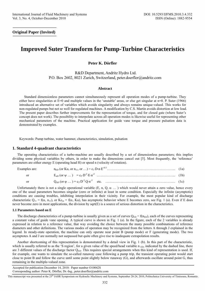
The discharge characteristics of a pump-turbine is usually given as a set of curves QED = f(nED), each of the curves representing a constant value of guide vane opening. A typical curve is shown in Fig. 1 (a). In the figure, each of the 2 variables is already expressed in relation to a reference value, that way avoiding the choice between the many possible combinations of reference diameters and other definitions. The various modes of operation may be recognized from the letters A through J explained in the legend. In steady-state operation, the machine can only operate near point B (pump mode) or F (generating mode). The two asymptotes A and J are normally not surpassed but quite often give rise to inadequate extrapolation results.

Another shortcoming of this representation is demonstrated by a detail view in Fig. 1 (b). In this part of the characteristic, which is usually referred to as the ‘S region’, for a given value of the speed/head variable n ED, indicated by the dashed line, there are 3 different values of the discharge factor QED. This requires special arrangements when this kind of representation is used. If, for example, one wants to simulate the so-called runaway case following a pump trip, the transient operating point would start close to point B and follow the curve until some point slightly below runaway (G), and afterwards oscillate around point G, thus remaining in the multiple-valued zone.

This manuscript was presented at the 25th IAHR Symposium on Hydraulic Machinery and Systems, September 20-24, 2010, Politechnica University of Timisoara, Romania .

Accepted for publication December 14, 2010: Paper number O10042S Corresponding author: Peter K. Dörfler, Dr.-Ing., [email protected]

333

Fig. 1 (a) Example of a 4-quadrant diagram using sqrt(E) as reference (b) Multiple values

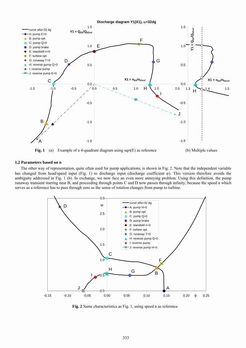
1.2 Parameters based on n The other way of representation, quite often used for pump applications, is shown in Fig. 2. Note that the independent variable

has changed from head/speed input (Fig. 1) to discharge input (discharge coefficient ϕ). This version therefore avoids the ambiguity addressed in Fig. 1 (b). In exchange, we now face an even more annoying problem. Using this definition, the pump runaway transient starting near B, and proceeding through points C and D now passes through infinity, because the speed n which serves as a reference has to pass through zero as the sense of rotation changes from pump to turbine.

0.0

0.5

1.0

1.5

2.0

2.5

3.0

-0.15 -0.10 -0.05 0.00 0.05 0.10 0.15 0.20 0.25φ

ψ curve alfa=32 dgA: pump H=0B: pump optC: pump Q=0D: pump brakeE: standstill n=0F: turbine optG: runaway T=0H: reverse pump Q=0I: reverse pumpJ: reverse pump H=0

Fig. 2 Same characteristics as Fig. 1, using speed n as reference

Discharge diagram Y1(X1), α=32dg

-1.5

-1.0

-0.5

0.0

0.5

1.0

1.5

-1.5 -1.0 -0.5 0.0 0.5 1.0 1.5 2.0

X1 = nED/nEDref

Y1 = QED/QEDrefcurve alfa=32 dgA: pump E=0B: pump optC: pump Q=0D: pump brakeE: standstill n=0F: turbine optG: runaway T=0H: reverse pump Q=0I: reverse pumpJ: reverse pump E=0

-1.5

-1.0

-0.5

0.0

0.5

1.0

1.5

1.3 1.4 1.5

X1 = nED/nEDref

Y1 =

QED

/QED

ref

B

A

C

D

E F

G

HI

J

H

AJ

I H G B

FC

D

334

2. Suter’s artifice The above-described dilemma may be avoided by selecting a more suitable reference variable. Such a definition has been

invented by P. Suter [1] for water hammer computations with non-regulated pumps. Suter’s idea starts from the ψ(ϕ) representation of pump head and replaces the square of speed denominator n2 by a sort of mixed velocity (n2 + Q2) which never becomes zero, because at least one of the variables n and Q is always different from zero. Thus, based on ψ a new variable for head is obtained which is proportional to H/(n2 + Q2). This new variable may become zero together with the head H, but it always remains finite.1

Suter then introduced a second artifice in order to obtain also a better way to represent the discharge Q. He took account of the fact that, in the 4-quadrant diagram Q11(n11), or Kcm(Ku), the discharge coefficient ϕ is basically the tangent of the radius connecting (0,0) to the operation point (Ku, Kcm), the ratio Kcm/Ku being equal to ϕ, hence arctan (ϕ) = arctan (Kcm/Ku) is a suitable measure for discharge because even at the asymptote H=0 where Kcm and Ku become infinite, it has a finite value.

The runner torque variable T, formerly represented by M11 or λ, was treated in a manner similar to the head H, thus the torque vs. discharge characteristics also became well-behaved for both n=0 and H=0.

To eliminate the problem of different dimensions of H, n, Q, T, the original transform already replaced them by ‘per unit’ variables H/Href, Q/Qref, etc., proposing the optimum point for reference.

His set of variable thus became

Θ = arc.tan (ϕ/ϕopt) for discharge, ……………………………………………………………………. (2a)

(H/Hopt)/((n/nopt)2 + (Q/Qopt)2) for head, and ………………………………………………………. (2b)

(T/Topt)/((n/nopt)2 + (Q/Qopt)2) for torque. …………………………………………………..…… (2c)

0.0

0.2

0.4

0.6

0.8

1.0

1.2

1.4

0 1 2 3 4 5 6theta (rad)

WH (p.u.)

curve alfa=32 dgA: pump H=0B: pump optC: pump Q=0D: pump brakeE: standstill n=0F: turbine optG: runaway T=0H: reverse pump Q=0I: reverse pumpJ: reverse pump H=0

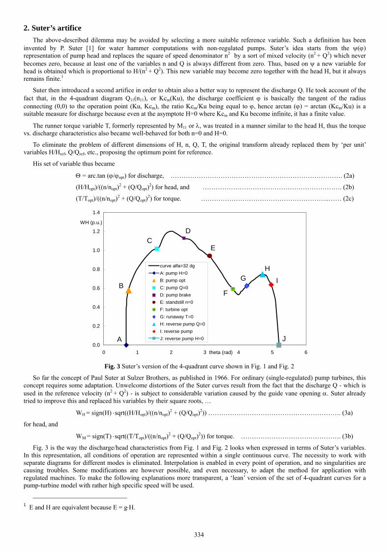
Fig. 3 Suter’s version of the 4-quadrant curve shown in Fig. 1 and Fig. 2

So far the concept of Paul Suter at Sulzer Brothers, as published in 1966. For ordinary (single-regulated) pump turbines, this concept requires some adaptation. Unwelcome distortions of the Suter curves result from the fact that the discharge Q - which is used in the reference velocity (n2 + Q2) - is subject to considerable variation caused by the guide vane opening α. Suter already tried to improve this and replaced his variables by their square roots, …

WH = sign(H) ⋅sqrt((H/Hopt)/((n/nopt)2 + (Q/Qopt)2)) ……………………………………………………. (3a)

for head, and

WM = sign(T) ⋅sqrt((T/Topt)/((n/nopt)2 + (Q/Qopt)2)) for torque. ………………………………………. (3b)

Fig. 3 is the way the discharge/head characteristics from Fig. 1 and Fig. 2 looks when expressed in terms of Suter’s variables. In this representation, all conditions of operation are represented within a single continuous curve. The necessity to work with separate diagrams for different modes is eliminated. Interpolation is enabled in every point of operation, and no singularities are causing troubles. Some modifications are however possible, and even necessary, to adapt the method for application with regulated machines. To make the following explanations more transparent, a ‘lean’ version of the set of 4-quadrant curves for a pump-turbine model with rather high specific speed will be used.

1 E and H are equivalent because E = g⋅H.

J A

B

C D

E

F

GH

I

335

3. First improvements

3.1 Definition of the reference discharge

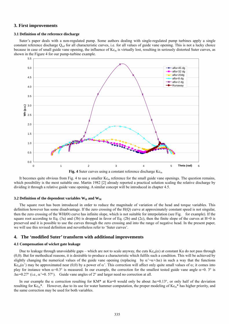
Suter’s paper deals with a non-regulated pump. Some authors dealing with single-regulated pump turbines apply a single constant reference discharge Qref for all characteristic curves, i.e. for all values of guide vane opening. This is not a lucky choice because in case of small guide vane opening, the influence of Kcm is virtually lost, resulting in seriously distorted Suter curves, as shown in the Figure 4 for our pump-turbine example.

0.0

0.5

1.0

1.5

2.0

2.5

3.0

3.5

4.0

4.5

5.0

5.5

0 1 2 3 4 5 6Theta (rad)

Wh

(p.u

.)

alfa=45 dgalfa=32 dgalfa=20dgalfa=8 dgalfa=2 dgRunaway

Fig. 4 Suter curves using a constant reference discharge Kcm

It becomes quite obvious from Fig. 4 to use a smaller Kcm reference for the small guide vane openings. The question remains, which possibility is the most suitable one. Martin 1982 [2] already reported a practical solution scaling the relative discharge by dividing it through a relative guide vane opening. A similar concept will be introduced in chapter 4.5.

3.2 Definition of the dependent variables WH and WM

The square root has been introduced in order to reduce the magnitude of variation of the head and torque variables. This definition however has some disadvantage. If the zero crossing of the H(Q) curve at approximately constant speed is not singular, then the zero crossing of the WH(Θ) curve has infinite slope, which is not suitable for interpolation (see Fig. for example). If the square root according to Eq. (3a) and (3b) is dropped in favor of Eq. (2b) and (2c), then the finite slope of the curves at H=0 is preserved and it is possible to use the curves through the zero crossing and into the range of negative head. In the present paper, we will use this revised definition and nevertheless refer to ‘Suter curves’.

4. The ‘modified Suter’ transform with additional improvements 4.1 Compensation of wicket gate leakage

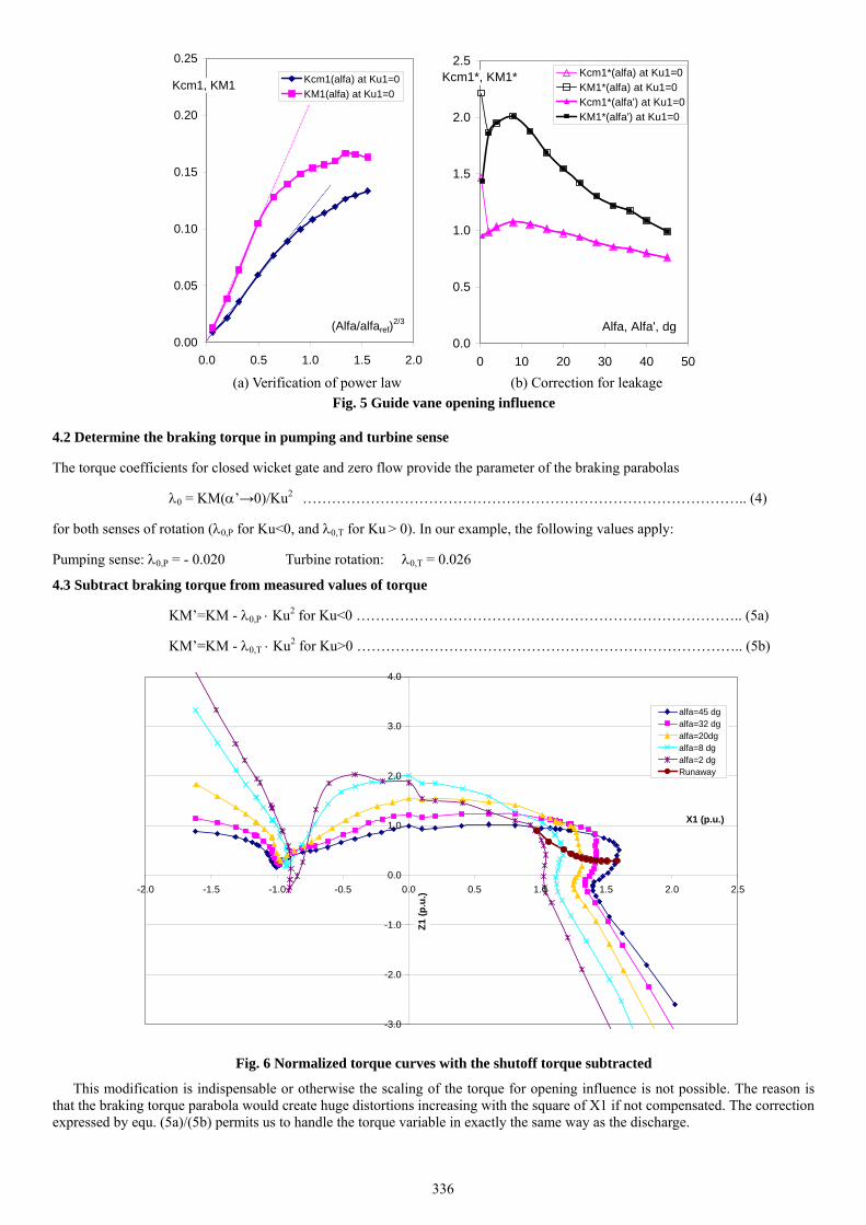
Due to leakage through unavoidable gaps – which are not to scale anyway, the cuts Kcm(α) at constant Ku do not pass through (0,0). But for methodical reasons, it is desirable to produce a characteristic which fulfils such a condition. This will be achieved by slightly changing the numerical values of the guide vane opening (replacing by α’=α+Δα) in such a way that the functions Kcm(α’) may be approximated near (0,0) by a power of α’. This correction will affect only quite small values of α; it comes into play for instance when α=0.3° is measured. In our example, the correction for the smallest tested guide vane angle α=0. 3° is Δα=0.27° (i.e., α’=0. 57°). Guide vane angles of 2° and larger need no correction at all.

In our example the α correction resulting for KM* at Ku=0 would only be about Δα=0.13°, or only half of the deviation resulting for Kcm*. However, due to its use for water hammer computation, the proper modeling of Kcm* has higher priority, and the same correction may be used for both variables.

336

(a) Verification of power law (b) Correction for leakage

Fig. 5 Guide vane opening influence

4.2 Determine the braking torque in pumping and turbine sense

The torque coefficients for closed wicket gate and zero flow provide the parameter of the braking parabolas

λ0 = KM(α’→0)/Ku2 ……………………………………………………………………………….. (4)

for both senses of rotation (λ0,P for Ku<0, and λ0,T for Ku > 0). In our example, the following values apply:

Pumping sense: λ0,P = - 0.020 Turbine rotation: λ0,T = 0.026

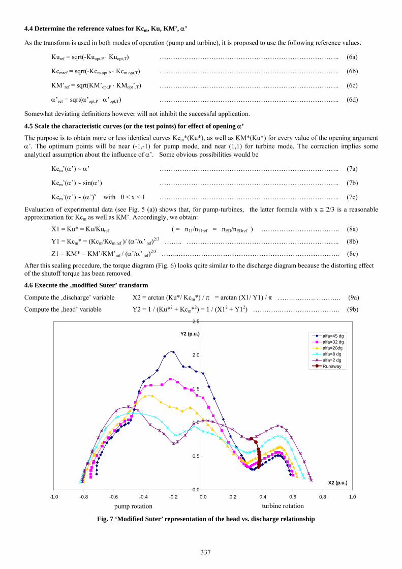
4.3 Subtract braking torque from measured values of torque

KM’=KM - λ0,P ⋅ Ku2 for Ku<0 …………………………………………………………………….. (5a)

KM’=KM - λ0,T ⋅ Ku2 for Ku>0 …………………………………………………………………….. (5b)

Fig. 6 Normalized torque curves with the shutoff torque subtracted

This modification is indispensable or otherwise the scaling of the torque for opening influence is not possible. The reason is that the braking torque parabola would create huge distortions increasing with the square of X1 if not compensated. The correction expressed by equ. (5a)/(5b) permits us to handle the torque variable in exactly the same way as the discharge.

0.0

0.5

1.0

1.5

2.0

2.5

0 10 20 30 40 50

Alfa, Alfa', dg

Kcm1*, KM1* Kcm1*(alfa) at Ku1=0KM1*(alfa) at Ku1=0Kcm1*(alfa') at Ku1=0KM1*(alfa') at Ku1=0

0.00

0.05

0.10

0.15

0.20

0.25

0.0 0.5 1.0 1.5 2.0

(Alfa/alfaref)2/3

Kcm1, KM1 Kcm1(alfa) at Ku1=0KM1(alfa) at Ku1=0

-3.0

-2.0

-1.0

0.0

1.0

2.0

3.0

4.0

-2.0 -1.5 -1.0 -0.5 0.0 0.5 1.0 1.5 2.0 2.5

X1 (p.u.)

Z1 (p

.u.)

alfa=45 dgalfa=32 dgalfa=20dgalfa=8 dgalfa=2 dgRunaway

337

4.4 Determine the reference values for Kcm, Ku, KM’, α’

As the transform is used in both modes of operation (pump and turbine), it is proposed to use the following reference values.

Kuref = sqrt(-Kuopt,P ⋅ Kuopt,T) …………………………………………………………………….. (6a)

Kcmref = sqrt(-Kcm opt,P ⋅ Kcm opt,T) …………………………………………………………………….. (6b)

KM’ref = sqrt(KM’opt,P ⋅ KMopt’,T) …………………………………………………………………….. (6c)

α’ref = sqrt(α’opt,P ⋅ α’opt,T) …………………………………………………………………….. (6d)

Somewhat deviating definitions however will not inhibit the successful application.

4.5 Scale the characteristic curves (or the test points) for effect of opening α’

The purpose is to obtain more or less identical curves Kcm*(Ku*), as well as KM*(Ku*) for every value of the opening argument α’. The optimum points will be near (-1,-1) for pump mode, and near (1,1) for turbine mode. The correction implies some analytical assumption about the influence of α’. Some obvious possibilities would be

Kcm’(α’) ∼ α’ …………………………………………………………………….. (7a)

Kcm’(α’) ∼ sin(α’) …………………………………………………………………….. (7b)

Kcm’(α’) ∼ (α’)x with 0 < x < 1 …………………………………………………………………….. (7c)

Evaluation of experimental data (see Fig. 5 (a)) shows that, for pump-turbines, the latter formula with x ≅ 2/3 is a reasonable approximation for Kcm as well as KM’. Accordingly, we obtain:

X1 = Ku* = Ku/Kuref ( = n11/n11ref = nED/nEDref ) …………………………….. (8a)

Y1 = Kcm* = (Kcm/Kcm ref )/ (α’/α’ ref)2/3 …….. ………………………………………………………….. (8b)

Z1 = KM* = KM’/KM’ref / (α’/α’ ref)2/3 ……..……………….…………………………………………….. (8c)

After this scaling procedure, the torque diagram (Fig. 6) looks quite similar to the discharge diagram because the distorting effect of the shutoff torque has been removed.

4.6 Execute the ‚modified Suter’ transform

Compute the ‚discharge’ variable X2 = arctan (Ku*/ Kcm*) / π = arctan (X1/ Y1) / π …….………. ……….. (9a)

Compute the ‚head’ variable Y2 = 1 / (Ku*2 + Kcm*2) = 1 / (X12 + Y12) ………….…………………….. (9b)

0.0

0.5

1.0

1.5

2.0

2.5

-1.0 -0.8 -0.6 -0.4 -0.2 0.0 0.2 0.4 0.6 0.8 1.0

X2 (p.u.)

Y2 (p.u.) alfa=45 dgalfa=32 dgalfa=20dgalfa=8 dgalfa=2 dgRunaway

Fig. 7 ‘Modified Suter’ representation of the head vs. discharge relationship

pump rotation turbine rotation

338

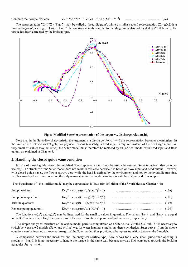
Compute the ‚torque’ variable Z2 = Y2⋅KM* = Y2⋅Z1 = Z1 / (X12 + Y12) ………….……………….. (9c)

The representation Y2=f(X2) (Fig. 7) may be called a ‚head diagram’, while a similar second representation Z2=g(X2) is a ‚torque diagram’, see Fig. 8. Like in Fig. 7, the runaway condition in the torque diagram is also not located at Z2=0 because the torque has been corrected by the brake torque.

-1.0

-0.5

0.0

0.5

1.0

1.5

2.0

-1.0 -0.8 -0.6 -0.4 -0.2 0.0 0.2 0.4 0.6 0.8 1.0

X2 (p.u.)

Z2 (p.u.)alfa=45 dgalfa=32 dgalfa=20dgalfa=8 dgalfa=2 dgRunaway

Fig. 8 ‘Modified Suter’ representation of the torque vs. discharge relationship

Note that, in the Suter-like characteristic, the argument is a discharge. For α’ → 0 this representation becomes meaningless. In the limit case of closed wicket gate, for physical reasons (causality) a head input is required instead of the discharge input. For very small α’ values (say, α’<0.5°), the Suter model must therefore be replaced by an ‚orifice’ model with head input and flow output, as explained in Chapter 5.

5. Handling the closed guide vane condition In case of closed guide vanes, the modified Suter representation cannot be used (the original Suter transform also becomes

useless). The structure of the Suter model does not work in this case because it is based on flow input and head output. However, with closed guide vanes, the flow is always zero while the head is defined by the environment and not by the hydraulic machine. In other words, close to zero opening the only reasonable kind of model structure is with head input and flow output.

The 4 quadrants of the orifice model may be expressed as follows (for definition of the * variables see Chapter 4.4):

Pump quadrant Kcm* = c1⋅sqrt((c2(α’) ⋅Ku*)2 – 1) ………….……………………………. (10a)

Pump brake quadrant: Kcm* = c3⋅sqrt(1 - (c2(α’) ⋅Ku*)2 ) ………….……………………………. (10b)

Turbine quadrant: Kcm* = c3⋅sqrt(1 - (c4(α’) ⋅Ku*)2 ) ………….……………………………. (10c)

Reverse pump quadrant: Kcm* = c5⋅sqrt((c4(α’) ⋅Ku*)2 – 1) ………….……………………………. (10d)

The functions c2(α’) and c4(α’) may be linearized for the small α values in question. The values (1/c2) and (1/c4) are equal to the Ku* values where Kcm* becomes zero in the case of rotation in pump and turbine sense, respectively.

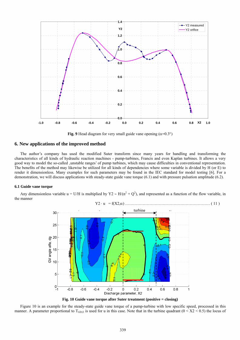
The simple analytical structure of the orifice model permits computation of a Suter curve Y2=f(X2, α’=0). If it is necessary to switch between the 2 models (Suter and orifice) e.g. for water hammer simulation, then a synthetical Suter curve from the above equations can be inserted as lower α’ margin of the Suter model, thus providing a bumpless transition between the 2 models.

A comparison between the measured and the analytical (orifice-type) flow curves for a very small guide vane opening is shown in Fig. 9. It is not necessary to handle the torque in the same way because anyway KM converges towards the braking parabolas for α’ → 0.

339

0.0

0.2

0.4

0.6

0.8

1.0

1.2

1.4

-1.0 -0.8 -0.6 -0.4 -0.2 0.0 0.2 0.4 0.6 0.8 1.0X2

Y2Y2 measuredY2 orifice

Fig. 9 Head diagram for very small guide vane opening (α=0.3°)

6. New applications of the improved method

The author’s company has used the modified Suter transform since many years for handling and transforming the characteristics of all kinds of hydraulic reaction machines - pump-turbines, Francis and even Kaplan turbines. It allows a very good way to model the so-called ‚unstable ranges’ of pump turbines, which may cause difficulties in conventional representation. The benefits of the method may likewise be utilized for all kinds of dependencies where some variable is divided by H (or E) to render it dimensionless. Many examples for such parameters may be found in the IEC standard for model testing [6]. For a demonstration, we will discuss applications with steady-state guide vane torque (6.1) and with pressure pulsation amplitude (6.2).

6.1 Guide vane torque

Any dimensionless variable u = U/H is multiplied by Y2 ∼ H/(n2 + Q2), and represented as a function of the flow variable, in the manner

Y2 ⋅ u = f(X2,α) ……………………………………………………… ( 11 )

Fig. 10 Guide vane torque after Suter treatment (positive = closing)

Figure 10 is an example for the steady-state guide vane torque of a pump-turbine with low specific speed, processed in this manner. A parameter proportional to TGD,E is used for u in this case. Note that in the turbine quadrant (0 < X2 < 0.5) the locus of

turbine

340

zero guide vane torque (bold black curve) would be expected to correspond to constant α values (red lines), however, this only holds in the range of well-developed turbine flow, and not in the turbine brake area – also not in pump brake (-0.5 < X2 < 0).

Other variables like intermediate pressure (between guide vanes and runner), or axial force can be handled in the same way.

6.2 Pressure pulsation

Pressure pulsation amplitudes are often subject to guarantee. In case of transient operation, it is difficult to predict the maximum amplitude because it may depend on many parameters influencing the particular transient. It is possible to apply a transformation of the described kind and connect it to the results of hydraulic transient computations. In case of the amplitude, which by definition never becomes negative, it is convenient to apply a square root to the transformed variable because the amplitudes Δp in normal and transient operation may differ by more than an order of magnitude, and hence

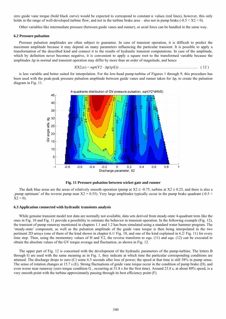
f(X2,α) = sqrt(Y2 ⋅ Δp/(ρE)) …………………………………………………….. ( 12 )

is less variable and better suited for interpolation. For the low-head pump-turbine of Figures 1 through 9, this procedure has been used with the peak-peak pressure pulsation amplitude between guide vanes and runner taken for Δp, to create the pulsation diagram in Fig. 11.

Fig. 11 Pressure pulsation between wicket gate and runner

The dark blue areas are the areas of relatively smooth operation (pump at X2 ≅ -0.75, turbine at X2 ≅ 0.25, and there is also a ‚pump optimum’ of the reverse pump near X2 = 0.55). Very large amplitudes typically occur in the pump brake quadrant (-0.5 < X2 < 0).

6.3 Application connected with hydraulic transients analysis

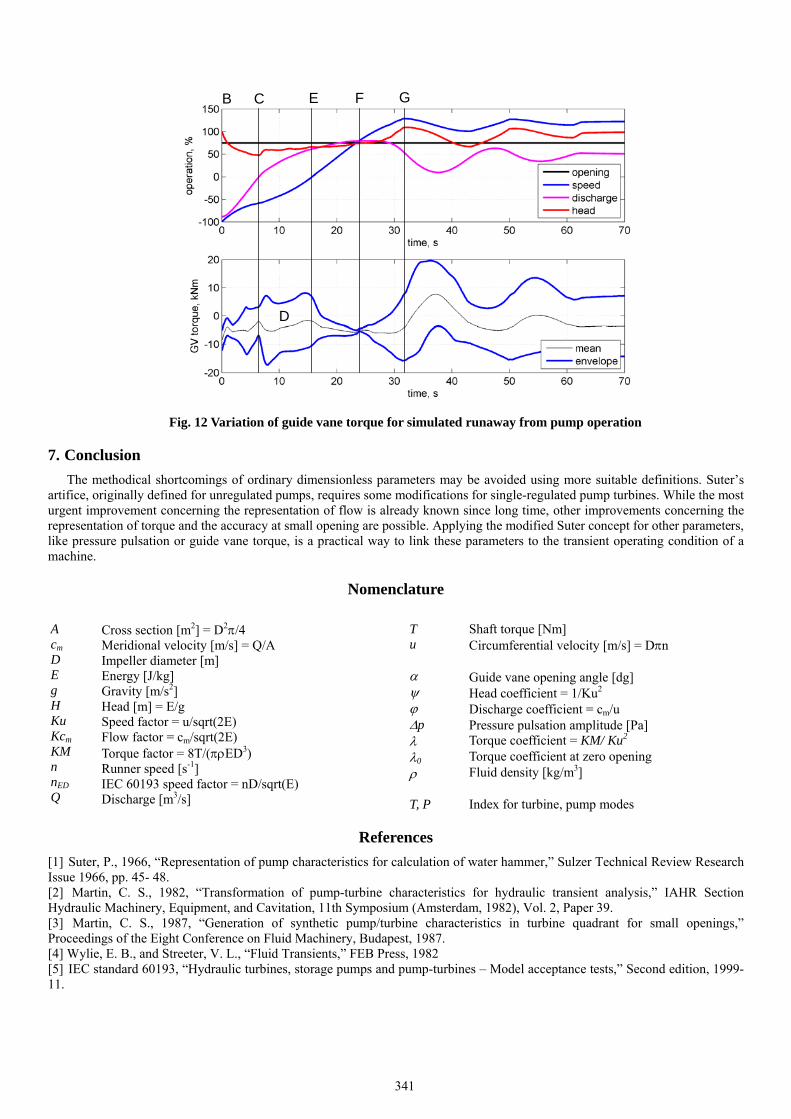
While genuine transient model test data are normally not available, data sets derived from steady-state 4-quadrant tests like the ones in Fig. 10 and Fig. 11 provide a possibility to estimate the behavior in transient operation. In the following example (Fig. 12), the transient of pump runaway mentioned in chapters 1.1 and 1.2 has been simulated using a standard water hammer program. The ‘steady-state’ component, as well as the pulsation amplitude of the guide vane torque is then being interpolated in the two pertinent 2D arrays (one of them of the kind shown in chapter 6.1/ Fig. 10, and one of the kind explained in 6.2/ Fig. 11) for every time step. Then, using the momentary values of H and Y2, the reverse transform to equ. (11) and equ. (12) can be executed to obtain the absolute values of the GV torque average and fluctuation, as shown in Fig. 12.

The upper part of Fig. 12 is concerned with the development of the hydraulic parameters of the pump-turbine. The letters B through G are used with the same meaning as in Fig. 1, they indicate at which time the particular corresponding conditions are attained. The discharge drops to zero (C) some 6.5 seconds after loss of power; the speed at that time is still 58% in pump sense. The sense of rotation changes at 15.7 s (E). Strong fluctuations of guide vane torque occur in the condition of pump brake (D), and even worse near runaway (zero torque condition G , occurring at 31.8 s for the first time). Around 23.8 s, at about 80% speed, is a very smooth point with the turbine approximately passing through its best efficiency point (F).

341

Fig. 12 Variation of guide vane torque for simulated runaway from pump operation

7. Conclusion The methodical shortcomings of ordinary dimensionless parameters may be avoided using more suitable definitions. Suter’s

artifice, originally defined for unregulated pumps, requires some modifications for single-regulated pump turbines. While the most urgent improvement concerning the representation of flow is already known since long time, other improvements concerning the representation of torque and the accuracy at small opening are possible. Applying the modified Suter concept for other parameters, like pressure pulsation or guide vane torque, is a practical way to link these parameters to the transient operating condition of a machine.

Nomenclature A cm D E g H Ku Kcm KM n nED Q

Cross section [m2] = D2π/4 Meridional velocity [m/s] = Q/A Impeller diameter [m] Energy [J/kg] Gravity [m/s2] Head [m] = E/g Speed factor = u/sqrt(2E) Flow factor = cm/sqrt(2E) Torque factor = 8T/(πρED3) Runner speed [s-1] IEC 60193 speed factor = nD/sqrt(E) Discharge [m3/s]

T u α ψ ϕ Δp λ λ0 ρ T, P

Shaft torque [Nm] Circumferential velocity [m/s] = Dπn Guide vane opening angle [dg] Head coefficient = 1/Ku2 Discharge coefficient = cm/u Pressure pulsation amplitude [Pa] Torque coefficient = KM/ Ku2 Torque coefficient at zero opening Fluid density [kg/m3] Index for turbine, pump modes

References [1] Suter, P., 1966, “Representation of pump characteristics for calculation of water hammer,” Sulzer Technical Review Research Issue 1966, pp. 45- 48. [2] Martin, C. S., 1982, “Transformation of pump-turbine characteristics for hydraulic transient analysis,” IAHR Section Hydraulic Machinery, Equipment, and Cavitation, 11th Symposium (Amsterdam, 1982), Vol. 2, Paper 39. [3] Martin, C. S., 1987, “Generation of synthetic pump/turbine characteristics in turbine quadrant for small openings,” Proceedings of the Eight Conference on Fluid Machinery, Budapest, 1987. [4] Wylie, E. B., and Streeter, V. L., “Fluid Transients,” FEB Press, 1982 [5] IEC standard 60193, “Hydraulic turbines, storage pumps and pump-turbines – Model acceptance tests,” Second edition, 1999-11.

F GE C

D

B